is inflation bad for income inequality: the importance of ...ed_emp/documents/publication/... ·...

EMPLOYMENT PAPER 2001/29

Is inflation bad for income inequality:

The importance of the initial rate of inflation

Rossana Galli University of Lugano, Switzerland

and

Rolph van der Hoeven

International Labour Office

Abstract

This paper explores theoretically and empirically the effects of monetary policy and

inflation on income inequality in developed economies. The few empirical studies touching on this issue have given conflicting answers, and the impact on inequality remains puzzling. In an attempt to solve this puzzle we argue that the effects of monetary policy and inflation on inequality depend on the initial rate of inflation. Though in high inflation countries restrictive monetary policy is often beneficial for inequality, reducing inflation in economies with initially low inflation might increase inequality. Empirical investigations for the US and a sample of 15 OECD countries seem to support this hypothesis.

This paper was written while Rossana Galli was visiting ILO. Comments can be sent to [email protected] or to [email protected].

1

1. Introduction

The purpose of this paper is to investigate the effects of monetary policy and inflation on income distribution. As such it forms part of new research activities on the relation between economic policies, economic growth and poverty, which have been the subject of a flurry of recent publications, mainly in relation to developing countries. Although considerable differences exist among researchers, it is generally accepted that economic policies aiming at stimulating growth need to consider effects on poverty and inequality, by emphasising equitable growth policies and by explicit redistributive policies; the relative importance of these policies depending on the initial economic situation and the socio-political structure in the country in question (Dagdeviren, van der Hoeven and Weeks, 2001).

In order to contribute a different angle to this debate we thought it of interest to investigate the situation in developed countries. In order to keep the research focussed we concentrated on one aspect of economic policy, namely monetary policy. This choice was not only dictated by concerns to arrive at a manageable research agenda, but also by the current debate on the use of monetary policy as an active instrument of economic policy. Researchers and policy-makers both in the United States and in the European Union differ as to the appropriateness of monetary policy in broader policy making. The restrictive stance of the European Central Bank on this issue is well known and criticised by many scholars and international policy-makers, who argue for a broader role of monetary policy in terms of stimulating growth and reducing unemployment. However, given the dis-equalising tendencies in most industrialised countries in the 1990s and the beginning of the current decade, we thought it important not only to look at implication of monetary policies on growth (see for example Brown, 2001) but also to take, as in the case of developing countries, the issue of poverty and inequality into account. We follow Blank and Blinder (1986) in their observations that if one is interested in poverty, a case can be made that the share of income received by the lowest 20 per cent of families or another inequality measure like the Gini ratio is at least as good an index of poverty as the official poverty rate, thus avoiding the complications around the definition of an absolute poverty line. Furthermore, we investigate effects on personal income inequality rather than factor income inequality (as in Argitis and Pitelis, 2001) because the latter, although a major determinant of inequality, is less sensitive for poverty indices.

In looking at the effects of monetary policy and inflation on income distribution this paper takes a different route from the recent stream of literature on the relationship between income inequality and growth. A large debate, in fact, has arisen since the article by Persson and Tabellini (1994) on whether initial inequality is beneficial or detrimental to growth. The debate is still open, with authors piling in both positions. Although related to our topic, this literature differs from the present study in that it looks at the opposite causality from inequality to macroeconomic outcomes, and focuses mainly on fiscal outcome and the consequences for growth; it does not deal with monetary outcomes1.

The remainder of this paper is organised as follows. Section 2 discusses what we call “the inflation-inequality” puzzle by reviewing previous empirical literature. Section 3 places these findings in a theoretical context examining both the short-run and long-run effects of

––––––––––––– 1 For recent contributions to this debate see Banerjee and Duflo (2000), Bertola (2000), Forbes (2000) and Galor (2000). Two studies tracing explicitly the causality from inequality to monetary policy or inflation are the articles by Beetsma and Van der Ploeg (1996) and by Al-Marhubi (2000).

2

monetary policy on inequality. Section 4 discusses the outcome of empirical analysis carried out with data we collected from the United States and 15 OECD countries. Section 5 concludes.

2. The inflation-inequality puzzle

The impact of monetary policy and inflation on personal income distribution has been studied in a non-systematic way. A major determinant of the distribution of income in a country is traditionally assumed to be the level of development: as predicted by the so-called Kuznets hypothesis (Kuznets 1955) countries shift from relative equality to inequality and back to greater equality as they move through the development stages. A large number of multi-country empirical studies have shown however that the Kuznets hypothesis explains only a very limited part of the inter-country variation in income distribution (see Bulir and Gulde, 1995, for a review of the literature), and that other policy and structural variables – such as tax and government spending, social transfers, state employment or human capital – improve significantly the explanation of the cross-country differences in income distribution (see among others Milanovic, 1994; Tanzi, 1998; and Chu, Davoodi and Gupta, 2000)2.

Some of these multi-country studies include inflation among the explanatory variables for income inequality or poverty indicators, but do not have a specific interest in studying the relationship between inflation and income distribution or poverty rates. Few studies are concerned specifically with this question, most of them using time-series data for the United States. The results from all these studies are noticeably mixed – some authors find inflation to be a regressive tax, others find it to be a progressive tax, and others find it to be unrelated to income distribution – so that the literature seems to have generated an inflation-inequality puzzle.

In order to help assessing the inflation-inequality puzzle, tables 1A and 1B summarise the empirical findings of studies known to us on the effects of inflation on different measures of inequality and poverty, divided by nature of the sample (time-series studies in panel A and cross-country/panel data studies in panel B). As shown in table 1A, most time series studies find inflation to be either progressive or non-significant, with the most technically advanced papers in this group (such as Jäntti, 1994 or Mocan, 1999) confirming the progressive effect of inflation on income distribution in the United States over the past five decades. Table 1B shows instead that in all cross country and panel data studies inflation is either regressive or non-significant, but in no case it is progressive.

At first glance the inflation-inequality puzzle stands out clearly. But a more cautious observation suggests a simple way of solving the apparent inflation-inequality puzzle. The effect of inflation on income inequality might depend on the initial level of inflation: when initial inflation is high, reducing inflation might decrease inequality; when initial inflation is low, instead, reducing inflation might come at the cost of higher inequality. This would explain why inflation seems progressive only in time series studies, concerning low-inflation countries, while is found regressive in most cross-country and panel data samples including high-inflation developing economies. There are, however, some exceptions. First, among the cross-section studies, Romer and Romer’s (1998) finding of inflation significantly worsening the bottom

––––––––––––– 2 Although originally formulated as a time-series proposition, the Kuznets hypothesis has been assessed mainly in cross-country studies due to the lack of long time-series data on income distribution for a single country.

3

quintile’s average income and inequality in a cross-section of OECD countries in 1988. Given the relatively low level of inflation in the OECD countries in the late 80s, under our hypothesis we would expect inflation to be progressive or at least non-significant. However, Atkinson and Brandolini (1999: p.8) show that Romer and Romer’s results for the OECD countries are not robust, and that using strictly comparable data on income inequality (as opposed to the Deininger and Squire (1996) “accept” data set) the inflation variable ceases to be significantly different from zero3. In addition, two single-country studies contradict our hypothesis: Power’s (1995) finding of United States inflation significantly increasing a consumption-based poverty rate in 1959-89 – but the same author finds inflation not significant with respect to income-based poverty – and Blank and Blinder’s (1986) finding of United States inflation increasing poverty in 1959-83 – but the same authors find inflation to increase significantly the lower quintiles income shares. However, more technically advanced studies on United States inequality (such as Mocan, 1999) confirm the progressive impact inflation had in the United States during the last 5 decades.

In this paper we intend to contribute to the solution of the inflation-inequality puzzle by making the explicit assumption that the effect of inflation on income distribution changes direction depending on the initial rate of inflation. More specifically we investigate the hypothesis that long-run inflation has a non-monotonic impact on income inequality by estimating a model for inequality with a quadratic term in long-run inflation in two samples (the United States from 1966 to 1999, and a panel of 15 OECD countries from 1973 to 1996). We expect the quadratic term to be positive and significant, suggesting that the relationship between inflation and inequality is U-shaped: income inequality decreases as inflation rises from low to moderate rates, and increases again as inflation grows beyond a certain threshold.

To our knowledge, the hypothesis of a non-monotonic relationship between inflation and inequality has not been tested yet in the literature. In fact, the vast majority of empirical studies assume a linear relationship between income distribution and inflation. Only three studies, among those known to us, assume some form of non-linear (but not necessarily non-monotonic) inflation-inequality relationship.

The first is a study by Bulir and Gulde (1995) testing the impact of inflation on income distribution in time series data for Finland, Israel and Russia. The authors compare their results to previous estimates obtained with similar models for a selection of developed countries. Interestingly, they come to the conclusion that whether inflation is a progressive or regressive tax depends on the level of development and the sophistication of the financial structure: in lower income countries with a relatively unsophisticated financial sector higher inflation tends to be associated to higher inequality, while in richer financially sophisticated countries the poor gain from higher inflation. In other words, Bulir and Gulde conclude that the inflation-inequality relationship is non-monotonic but relate the non-monotonicity to the level of development and the sophistication of the financial markets (not to the level of initial inflation as we do) nor they test the non-monotonic relationship in a cross-country sample.

Second, Easterly and Fischer (2001) estimate the relationship between three measures of improvement in well-being for the poor – the change in the poor’s share of national income, the percentage decline in poverty, and the percentage change in real minimum wage – and a non-linear transformation of the inflation rate for a pooled cross-country sample drawn from Deininger and Squire’s (1996) data set. They find the well being of the poor negatively

––––––––––––– 3 Note that the comparability problem affecting the OECD data contained in Deininger and Squire’s “accept” data set affects all estimates based on this data, such as Dollar and Kraay’s (2000).

4

correlated with the inflation transformation, which implies that higher inflation reduces the well being of the poor with a non-linear (but still monotonic) factor.

Third, Bulir (2001) explores the relationship between income inequality and inflation using a cross-section database containing 75 developing and developed countries. Bulir tests the hypothesis of non-linear effects of inflation on income distribution by representing inflation with a set of dummies, each one representing a different range of inflation (hyperinflation above 300 percent annually, high inflation between 41 percent and 300 percent, low inflation between 5 percent and 40 percent, and very low inflation below 5 percent). Bulir finds that reducing inflation from hyperinflation rates significantly lowers income inequality: the Gini coefficient in high and low inflation countries is lower than in hyperinflation countries by 6 and 9 percentage points respectively. Interestingly, Bulir also finds that further reducing inflation toward very low levels allows a reduction by only 6 percentage points in the Gini coefficient with respect to hyperinflation countries. This implies that moving from low to very low inflation causes inequality to rise by 3 percentage points. Even though Bulir does not focus his attention on the latter result, it is of particular interest to us in that it is consistent with our hypothesis that the inflation-inequality relationship is non-monotonic, and that pushing inflation below a certain threshold makes inequality to worsen again.

In sum, the present study is different from the predecessors in that it tests explicitly the hypothesis of a non-monotonic relationship between inflation and inequality, and it does it for the United States as well as a sample covering 15 developed countries. Most cross-country works on income distribution in fact include both developed and developing countries or developing countries only. By selecting only the developed countries we expect to increase the statistical significance, if it exists, of the U-shaped relationship between inflation and income inequality, whose minimum we expect to be at low levels of inflation, so to shed new light on the impact of monetary policy and inflation on income inequality.

3. Monetary policy and income distribution: the channels of transmission

Textbooks predict that restrictive monetary policy in the short run decreases aggregate income and employment. In an open flexible exchange rate economy, the output and employment loss is reinforced by a real appreciation. The contractionary effect on employment in turn implies a downturn in nominal wage growth, and, through this way, a drop in inflation.

In the long run, the lower-than-expected inflation rate induces workers to adjust downwards their inflation expectations and to bargain lower nominal wage rises, so that a slowdown in labour cost pulls down inflation. Once inflation becomes slower than money supply growth, the increase in real money balances reduces interest rate and leads to an expansion in output and aggregate employment. Accordingly, in an open flexible exchange rate economy, a real depreciation contributes to restore output and employment. The expansive effect ends when expected inflation is fulfilled again, and this happens in correspondence to the initial levels of output, unemployment, real interest rate and real exchange rate. As a result, monetary policy is claimed to be neutral in the sense that it has no long-run effect on level and composition of income, the only long-run effect being on inflation (see for instance Blanchard, 2000).

Textbooks do not analyse the effects of monetary policy on income distribution. However, monetary policy does have an impact on income distribution both in the short run – through the cycle in economic activity generated by the policy change – and in the long run

5

through the change in inflation reached at the end of the adjustment period. Major causal linkages are depicted in Figure 1 and discussed below.

3.1 The short run

The cyclical downturn produced by a restrictive monetary policy affects income distribution through a number of channels, depicted in the top panel of Figure 1. First, the halt in economic growth caused by the increase in interest rates and the real appreciation adds to unemployment, and this is likely to affect different workers at various degrees. Given that hiring and firing costs are generally higher for skilled than for unskilled workers, unemployment tends to affect mostly low-skilled workers, making income inequality to rise in the short run4. The degree of worsening in income distribution depends, among other things, on the sensitivity of investment and consumption to higher interest rate and lower expected demand, and on the elasticity of employment to output fluctuations. In periods of low business confidence and in highly flexible labour markets the impact on inequality is likely to be more serious.

The spurt in unemployment can be reinforced by the presence of downward rigidities in nominal wages, making the slowdown in nominal wage rises to lag behind the decline in inflation brought by the monetary restriction. In this case the growth in real wages reinforces the rise in unemployment (Leidy and Tokarick, 1998). Once again, unemployment is likely to hit mainly low-skilled workers, further deteriorating the impact of monetary restrictions on inequality.

Another way in which monetary policy affects income distribution in the short run is through real interest rates. Since expected inflation is constant by definition in the short run, a decrease in money supply growth leads to an increase in both nominal interest rate and real interest rate. The increase in real interest rate, by making the net borrowers worse off and the net lenders better off, augments income inequality because certainly there are more net lenders at the top than at the bottom of income distribution5.

Finally, to the limited extent that inflation slows down in the short run following a monetary restriction, lower inflation slows down the loss in purchasing power of non-indexed nominal fixed incomes, such as pensions and transfers. This would reduce income inequality given that the poor receive a larger fraction of their income from transfers than do the remainder of the population.

In sum, as shown in the top panel of Figure 1, restrictive monetary policy has predominantly worsening effects on inequality in the short run. Benefits in terms of income distribution just come from the slowdown in inflation, that helps protecting the purchasing power of non-indexed transfers. However, since the impact of restrictive monetary policy on inflation is limited in the short run, the net effect of restrictive monetary policy in the short run is likely to be a worsening in income inequality.

––––––––––––– 4 Moreover the real appreciation distributes its effects on employment unevenly among sectors, mostly affecting export industries. The impact on income distribution is a priori uncertain, depending on the relative concentration of low-skilled labour in export industries. In addition the real appreciation, by reducing the relative price of imported goods, affects the purchasing power of residents with an a priori ambiguous impact on income distribution. 5 If financial intermediaries are more prompt to raise loan rates than deposit rates, the worsening effect on inequality is stronger. See Atkinson (1999, p.18) on the role of financial intermediaries in setting interest rates and affecting household welfare.

6

3.2 The long run

The main purpose of restrictive monetary policy is to lower inflation in the long run. Lower inflation, in turn, can have an impact on income inequality through various channels, depicted in the bottom panel of Figure 1.

Lower long-run inflation slows down the erosion of money purchasing power, and this can affect income distribution in at least three ways. First, it is usually argued that the poor are less able to protect their living standards from inflationary shocks than the non-poor. Due to the existence of entry barriers in most markets for non-money financial assets, in fact, the poor hold greater proportion of their wealth in cash than do the non-poor disproportionately exposing them to purchasing power erosion by inflation (Ferreira, Prennushi, Ravallion, 1999). Therefore, by slowing down the erosion of monetary financial assets, restrictive monetary policy tends to improve income distribution. Second, lower inflation slows down the erosion of the real value of non-indexed public transfers, such as unemployment benefits and pensions. Since transfer recipients typically belong to the poorest part of the population, this would reduce inequality. Third, since private debt is usually set in nominal terms, a lower inflation rate slows down the erosion of the real value of private debt. If the poor are net nominal debtors, as it is likely, this tend to increase income inequality.

Under specific circumstances, monetary policy can be non-neutral, i.e. can have real effects in the long run. First, restrictive monetary policy can enhance long-run growth by achieving macroeconomic stability and stimulating investment. Although the relationship between growth and income distribution is far from being theoretically and empirically settled (see, for instance, Aghion et al., 1999 and van der Hoeven, 2000), higher long-run growth is typically assumed to improve income distribution (see, for instance, Romer and Romer, 1998 or Dollar and Kraay, 20006).

However, the positive effect of disinflation on growth concerns only countries with initially high inflation, most commonly hyperinflation. In low and moderate inflation economies, inflation is unlikely to create a degree of macroeconomic instability that discourages investment and dampens long-run growth. This idea is largely supported by the empirical literature: Hess and Morris (1996) acknowledge the weak association between growth and low inflation, and Barro (1996) estimates that if inflation falls from 5 percent a year to zero, the growth rate will increase by a mere 0.1-0.15 percent a year (a statistically not significant effect). Fischer (1993) finds that very high inflation is not consistent with sustained growth whereas low inflation is not necessary for high growth, some countries having succeeded in growing over sustained periods with persistent inflation between 15 and 30 percent, typically with the assistance of extensive indexation. Finally Sarel (1996) examines the possibility of non-linear effects of inflation on economic growth, and finds evidence of a significant structural break around 8 percent: inflation below 8 percent has no effect on growth, or may even have a slightly positive effect.

A second possible real impact of non-neutral monetary policy in the long run is on real interest rate. Under neutrality of money, in fact, monetary policy actions have no impact on real interest rate in the long run (the so-called Fisher effect): while real interest rate goes up in ––––––––––––– 6 Dollar and Kraay (2000, page 5-6) assert “reducing government consumption and stabilizing inflation are examples of policies that are ‘super-pro-poor’. Not only do both of these raise overall incomes, but they appear to have additional positive effect on the distribution of income, further increasing incomes of the poor. In the case of inflation, this additional distributional effect (…) reflects primarily the reduction of inflation from very high levels.”

7

the short run, in the long run nominal interest rate falls with expected inflation and real interest rate goes back to its original value. Therefore, the short-run negative impact on net borrowers is reversed, making the net borrowers better-off and the net lenders worse-off in the long run. On this ground, monetary policy would have no long-run effects on income distribution through real interest rates. However, when initial inflation is very high, a successful disinflation can lead to a reduction in the risk premium. In this case, real interest rates would be lower in the long run, net borrowers would gain from the disinflation, and net lenders would lose, making income distribution more equitable.

Finally, as noted for the short run, the existence of downward rigidities in nominal wages implies that the slowdown in nominal wage rises lags behind the decline in inflation, leading to higher real wages and higher unemployment. If nominal rigidities are persistent – or even if they are temporary, under certain conditions (see Akerlof, Dickens and Perry, 1996) – there may be a permanent trade-off between inflation and unemployment7. Hence, there may also be a permanent trade-off between inflation and income inequality.

The bottom panel of Figure 1 summarises the channels through which restrictive monetary policy affects income inequality in the long run. At first glance, the net impact on inequality seems ambiguous. However, it can be noted that some of these channels (marked with a star in Figure 1) are activated only or mainly in high inflation economies. For obvious reasons, in fact, we can expect the three channels linked to the erosion of money purchasing power (real value of monetary assets, real value of unindexed transfers, and real value of private debt) to have a more important impact on income inequality in high-inflation than in low-inflation economies. Similarly, as already noted, the effects of disinflation on growth and real interest rate occur only when initial inflation is high.

On the contrary, the permanent trade-off between inflation and unemployment is accentuated at very low rates of inflation, since workers are more adverse to actual declines in nominal wages than to reductions in real wages achieved through nominal wage rises smaller than inflation. Akerlof, Dickens and Perry (1996) estimate via simulations that while at 2 percent inflation the long-run equilibrium unemployment rate is 6.1 percent, at 1 percent inflation it rises to 6.5 percent, and at zero inflation (price stability) it is as high as 7.6 percent. Because of the existence of downward rigidities in nominal wage, then, reducing inflation from low to lower levels could be more disruptive for unemployment, hence for income inequality, than the traditional theory predicts. This is confirmed also by Wyplosz (2000), who finds evidence for a selected group of five European countries of a non-linear relationship between inflation and steady state unemployment, with unemployment first rising and then decreasing starting from zero inflation.

Taking all that into account, it becomes clear that the net long-run impact of restrictive monetary policy on income inequality is not ambiguous but depends on the initial rate of inflation. In high-inflation countries successful disinflation can bring benefits in terms of income distribution, thanks to a slower erosion in money purchasing power, higher long-run growth and lower real interest rates. On the contrary, in low-inflation countries the distribution benefits from disinflation are likely to be trivial, whereas there is a higher chance of running into a permanent trade-off between inflation and unemployment, which would permanently worsen income inequality.

––––––––––––– 7 The existence of a permanent trade-off between inflation and unemployment is controversial in the literature. While we do not specifically support it, we acknowledge the possibility that this permanent trade-off exists, and consider its impact on income inequality.

8

4. Data and estimation

In the previous section it was argued that there are theoretical reasons to expect the long-run relationship between inequality and inflation to be non-monotonic. The empirical part of this paper investigates the hypothesised existence of a non-monotonic long-run relationship between inequality and inflation by estimating a quadratic model of the form:

Χ+++= '221 γπβπβαG

where G is the Gini index, π is the long-run inflation rate and X is a vector of other explanatory variables. We expect 1β < 0 and 02 >β meaning that inequality decreases when inflation moves from low to moderate rates, and raises when inflation grows beyond a certain threshold. This hypothesis implies that the inflation elasticity of the Gini coefficient – equal to

πββ 21 2+ – is not constant, but depends on the inflation rate: the elasticity is negative (higher inflation leading to lower inequality) for inflation rates below a threshold )2/(* 21 ββπ −= , and positive above this threshold. We expect the inflation threshold to be low, and for this reason we restrict our analysis to low-inflation countries – namely the United States and a selection of 15 OECD countries – in order to increase the statistical significance of the non-monotonic relationship, if it exists, between inflation and inequality.

4.1 Time-series analysis of income distribution in the United States

The United States are the only country providing continuous data for income distribution over a long time period, and are therefore the natural object of analysis for time series studies on income distribution. We use data on Gini inequality index and specific quintile income shares from 1966 to 1999 provided by the United States Census Bureau8, referring to household money income excluding capital gains before taxes.

A visual inspection of the income distribution series (see Figure 2) reveals that inequality in the United States has been rising throughout the period considered, due to a continuous increase in the income share going to the highest quintile at the expenses of the lowest 80 per cent of the distribution9. In order to test whether inflation has any long run effect on inequality, running through channels different from growth, we first run a set of six static regressions of the form:

gt = φ0 + φ1 πt + φ2 πt2 + φ3 yt + ut (1)

where g is a transformation of the Gini index or of the income share of each quintile10, π is the long run CPI inflation rate, y is the long run real GDP growth rate and u is an error term11.

––––––––––––– 8 Data are available on the internet site www.census.gov (Historical Income Tables). 9 However, in the 60s and 70s the income share of the lowest and the fourth quintiles increased. 10 The transformation (y* = log (y/(1-y)) is applied to all dependent variables to account for the fact that the Gini coefficient and the income shares lie in the unit interval and to constrain the predicted values to fall between 0 and 1. 11 An Augmented Dickey Fuller (ADF) test shows that the null hypothesis of a unit root in the Gini index and in the income shares of all quintiles cannot be rejected. However, Raj and Slottje (1994) show that the time series process of income inequality in the United States has experienced a structural break, which biases the ADF test in favour of a unit-root hypothesis. Therefore for several measures of income inequality a segmented trend model is more appropriate than a stochastic trend model. Moreover, given that the values of the Gini …/…

9

Long-run inflation and growth are obtained through a Hodrick-Prescott filter (with a smoothing parameter 100) from the original series. Estimation is run via ordinary least squares over the sample 1966-1999.

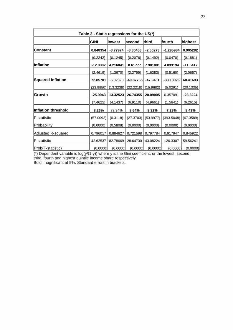
Table 2 presents the estimated coefficients of the static regressions and the implied inflation threshold (the turning point of the U-shaped relationship). In all regressions (except the lowest quintile) the estimated coefficients are highly significant and with the expected signs, and the adjusted R-squared ranges from 0.7 in the second quintile to 0.9 in the fourth quintile. In the Gini regression the coefficient on squared inflation is positive, indicating that starting from zero inflation, the Gini coefficient decreases (higher equality) up to an inflation threshold (estimated around 8 per cent) and increases afterwards. In the quintile income shares regressions the coefficient on squared inflation is negative for the lowest (not significant), second, third and fourth quintiles, and positive for the highest quintile. This indicates that starting from zero inflation, the income share of the lowest 80 per cent of the distribution increases up to an inflation threshold (estimated around 8 per cent) and decreases afterwards. Symmetrically, as inflation rises from zero to about 8 per cent, the income share going to the richest quintile decreases, and rises afterwards. The coefficient on growth is significant in all regressions (except the fourth quintile), positive in the first four quintiles and negative in the Gini and highest quintile regressions, suggesting that growth lowers inequality by increasing the income share of the first 80 per cent of the distribution at the expenses of the richest quintile.

To reduce the finite sample biases in the static regressions we then run an error correction version of the long run relationships given by:

gt = a0 + a1 gt-1 + b0 πt + b1πt-1 + c0 π2t + c1 π2

t-1 + d0 yt + d1 yt-1 + εt (2)

where the implied long-run coefficients of interest can be recovered as φ1=(b0+b1)/(1-a1), φ2=(c0+c1)/(1-a1) and φ3=(d0+d1)/(1-a1).

Table 3 presents the least squares estimation results for the dynamic equations. The dynamic estimates are generally well behaved: the estimated coefficients on inflation and squared inflation are highly significant in all regressions (except the lowest quintile, and for the first lag of both inflation and squared inflation in the fourth quintile) and the adjusted R-squared scores very high (above 0.9 in all equations). The solved long run coefficients on inflation and squared inflation are all highly significant (except for the lowest quintile) with the expected signs, and imply a threshold inflation rate very close to that estimated with the static regressions, i.e. around 8 per cent.

The long run coefficient on growth is not significant in any of the regressions suggesting that growth had no long run effect on income distribution in the United States in the considered period. Although rather surprising, this is in line with other works finding that growth is not a statistically significant determinant of changes in the distribution of income in cross-country samples (e.g. Easterly and Fischer (2001) and Ravallion and Chen (1997)).

To test for robustness of these results we estimate a number of modifications to the benchmark models presented in equations (1) and (2). First we control for fiscal policy by adding both in the static and the dynamic model (all regressions) the log of the GDP share of government non-defence expenditure. Results for the static and the dynamic regressions are presented in table 2B and 3B respectively. We find that the government expenditure share of GDP is not significant in any of the regressions (except for the lowest quintile static regression –––––––––––––––– index and income shares are intrinsically limited in the (0,1) interval, the non-stationarity is conceptually difficult to apply.

10

where it is only marginally significant), does not alter significantly the results on inflation and growth, nor the estimate of the inflation threshold (which is just slightly lower than in the benchmark equations).

We then run the static and dynamic regressions without the term in squared inflation and present the result in tables 2C and 3C. The linear model in inflation suggests that inflation significantly reduces inequality, by increasing the income share of the lowest 80 per cent of the distribution at the expenses of the richest quintile. Similarly to the quadratic model long run real growth is significant in the static but not in the dynamic regressions, but in both cases long run growth reduces inequality by raising the income shares of the lowest 80 per cent of the distribution, at the expenses of the richest quintile. In all static and dynamic regressions the adjusted R-squared is lower than in the quadratic model (except for the lowest quintile), suggesting that the quadratic model fits the data better.

Next, we test the sensitivity of the coefficients to a change in the sample period used for the estimation. Figure 3 shows the estimated coefficient and the ±2 standard error band from the static quadratic model when the sample is reduced from 1967-99 to 1985-99 by one year at a time. As Figure 3 shows the coefficients of inflation and squared inflation, and the implied inflation threshold, are very stable until 1983, when they suddenly change sign and the quadratic term in inflation is no longer significant. So, after 1983 the quadratic relationship between inflation and inequality is no longer observable, and a linear estimation would yield a negative significant coefficient on inflation indicating that lower inflation increases inequality. This is not at all surprising given that the period 1983-99 contains no observations of inflation above the estimated threshold (8 per cent), so looking at the 1983-99 period allows to observe only the left part of the U-shaped inflation-inequality relationship. Interestingly, however, also the estimated coefficient on growth shows a change after 198312, suggesting that year 1983 might mark a structural break in the estimated relationship.

A structural break in the relationship between macroeconomic performance and inequality beginning about 1983 is not new to the literature on inequality in the United States. For instance, Cutler and Katz’s (1991) discuss this structural break and the possible alternative explanations for the changing relationship between macroeconomic activity and the income of the poor. They find that increased family income inequality is largely associated with increased wage inequality, particularly of primary earners, and argue that higher wage inequality is related to factors that have shifted relative labour demand away from less skilled workers.

Hence, we estimate the static quadratic model with a dummy for the post-1983 period, and present the results in table 2D. The 1983-99 dummy is highly significant in all but the fourth quintile regression, and shows that inequality was higher in the post-1983 period due to a sharp increase in the top quintile income share at the expenses of the rest of the distribution. The sign and significance of the other coefficients do not change appreciably with the introduction of the time dummy. However, the estimated inflation threshold is remarkably lower than in the benchmark case going down to around 6 per cent. Given that the adjusted R-squared is higher than in the benchmark model for all regressions (except the fourth quintile), the specification presented in table 3D is considered the preferred specification.

In sum the evidence for the United States favour the hypothesis of a non-monotonic long-run relationship between income inequality and inflation, with inequality decreasing as inflation moves away from zero, reaching a minimum in the neighbourhood of 6 per cent

––––––––––––– 12 The coefficient on growth also shows a change – from negative to positive – in 1971 and then stays positive, indicating that higher growth lead to higher inequality after 1971.

11

inflation, and increasing afterwards. The analysis of the quintile income shares shows that the increase in inequality taking place from zero to 6 per cent inflation is due to the decrease in the income share of the richest quintile, all the other quintiles benefiting from the higher (but still moderate) inflation13.

4.2 Panel data analysis of income distribution in the OECD countries

Panel data studies of income inequality require a careful selection of the observations to be included in the sample, in order to guarantee the comparability of data across countries and time14. We drew our data on income inequality from the World Income Inequality Database (WIID) collected by the World Institute for Development Economics Research (WIDER). The WIID database contains all available information on income inequality over time for developed, developing and transition countries derived from different sources, and classified by income definition (net income, gross income, expenditure or earnings) and reference unit (household, household equivalent, household per capita, family etc.), as well as by area covered (all, rural, urban), population covered (all, employed, taxpayers etc.) and quality ratings (reliable, less reliable).

We first selected all the “reliable” data on the Gini coefficient covering full area (urban and rural) and population for the OECD countries (excluding Mexico, Korea and Hungary who joined the OECD in the 1990s). We then selected the series based on the same reference unit and income definition, in order to have consistent data for cross-country and cross-time comparison. Among all possible combinations (household and gross income, household and net income, household equivalent and gross income etc.), we chose household as the reference unit and net income as the income definition, because this allowed the largest time and country coverage. Since this sub-sample still included overlapping observations from different sources for a single year in some countries, we further selected the data by keeping only the observations from the same source within each country (but different sources across countries). In choosing our preferred source, we looked for the most updated and longest time series15. Finally we excluded countries with only one observation (Austria, Luxembourg, Spain, Switzerland and Turkey). This selection process left us with a panel of 88 observations covering 15 OECD countries over the period 1960-1996, shown in Table 4. The number of observations over time for each country varies from 2 (Denmark, Finland and Portugal) to 22 (Italy). In order to make the panel less unbalanced we truncated the sample in 1973 (the first year in which we have observations on at least four countries) and adjusted the sample by selecting only observations two years apart from each other16. We then estimate the benchmark regressions over the period 1973-96 for the adjusted sample (60 observations), and test for sensitivity of results to sample variations.

––––––––––––– 13 In the case of the lowest quintile, our estimates indicate a monotonic and positive long run relationship with inflation: the income share of the lowest quintile rises with inflation at all levels of inflation. 14 Atkinson and Brandolini (1999) warn about combining in cross-country and time series analysis income inequality data based on different income concepts, sampling, demography etc.. They show that the widely used “accept” sub-sample of Deininger and Squire’s (1996) data set contains inequality data based on different income concepts and reference units, and can therefore lead to misleading conclusions even if dummy variables are introduced to account for the difference in definitions. 15 More precisely for each country we selected, first, the source whose last observation is the most recent, and, when two different sources extended to the same year in time, we selected the longer one. We also excluded all sources providing only one observation over time. Choosing the most updated time series has the side-advantage of maximizing the number of observations on income inequality in years of low inflation. 16 For each couple of adjacent observations, we select the most recent one and exclude the other.

12

Our indicator for inflation is the yearly percentage variation of the consumer price index (all items) contained in the OECD Main Economic Indicators database. The inflation data (see Table 5) show that average inflation in 1973-1996 for the selected OECD countries is 7.4 per cent, ranging from 3.7 per cent in Western Germany to 16 per cent in Portugal. The median observation on inflation is 6.3 per cent, maximum inflation is found in Portugal in 1977 (33 per cent) and minimum deflation in the Netherlands in 1987 (-0.7 per cent). By containing observations on moderate and low inflation only, our sample should allow to pick up any possible upsurge of inequality at low levels of inflation. Growth data are based on real GDP (Laspeyres index, 1985 international prices) provided by the Penn World Tables 5. Table 6 shows the descriptive statistics of growth, reporting an average annual growth rate of 2.6 per cent, ranging from 4.4 per cent in Ireland to 1.54 per cent in Sweden.

Since our objective is to study the relationship between inflation and income inequality in the log-run, we derive a time series for long-run inflation and long-run real GDP by applying the Hodrick-Prescott filter, with a smoothing parameter 100, to the original data on inflation and real GDP of each country. We then estimate via the fixed effect estimator the following regression:

ititititiit yG εγπβπβα ++++= 221

where Git is the Gini index in country i at time t, iα is a country-specific fixed effect, πit is

long-run inflation, yit is long-run real GDP growth, and itε is a standard normal error17. Note

that we choose not to include per capita income and its square among the regressors because the Kuznets hypothesis is supposed to explain the variability of inequality along the development process, whereas the OECD countries in the period considered were largely in the same stage of development. Moreover, the Kuznets hypothesis is not widely supported by the empirical evidence. In addition, note that by including growth among the regressors, the effect of inflation on inequality working through overall growth is captured there. The coefficients on inflation and squared inflation then capture any additional redistributive effect inflation can have other than through growth.

The first column of table 7 shows the estimated coefficients and the White heteroskedasticity-consistent standard errors of the benchmark model. The coefficients on long-run inflation rate and squared rate have the expected sign – negative and positive respectively – and are highly significant. The estimated coefficient on long-run growth is highly significant and positive, which is somewhat surprising indicating that higher growth leads to higher inequality in the considered sample. The fit of the regression is relatively good (the adjusted R-squared is 0.82).

Using the long-run inflation and squared inflation estimated coefficients, 1β)

and 2β)

, the value of the inflation threshold minimising income inequality can be calculated as

)2/(* 21 ββπ))) −= . The estimates of 1β

) and 2β

) reported in the first column of table 7 imply an

inflation threshold just above 12%. In other words, as inflation grows above zero, income inequality decreases, reaches a minimum around 12 per cent inflation, and rises again for higher

––––––––––––– 17 The fixed effects estimator for panel data allows for country-specific intercepts, while assuming common slope coefficients across countries. The model was estimated also for a transformation of the Gini index, namely log (Gini/(1-Gini)), to account for the fact that the Gini coefficient is limited to the (0, 1) interval. Since the results obtained do not differ qualitatively, we present the results obtained with the Gini index as dependent variable, because the estimated coefficients are more readily interpretable as elasticities.

13

inflation rates. The change in income inequality caused by a one percentage point change in inflation is represented by the elasticity of the Gini index with respect to inflation, and could be called the Gini sacrifice ratio analogously to the “sacrifice ratio” referring to the unemployment cost of disinflation. This elasticity, represented by itπββ 21 2

))+ in our model, varies with the

initial rate of inflation and is therefore country and year specific.

Table 8 presents the estimated inflation elasticities of the Gini index for alternative values of initial inflation, ranging from 1 to 20%. As shown, lowering inflation by one percentage point when initial inflation is, say, 3%, would increase income inequality by nearly 0.7 Gini points. The Gini sacrifice ratio would be halved (0.33 Gini points) at 8% initial inflation, and would be null at 12% inflation. The elasticity becomes larger and positive for initial inflation rates above 12%, indicating, for instance, a 0.5 Gini points gain in income equality when inflation is reduced from 20 to 19%.

The estimated values of the Gini sacrifice ratio may appear low, but are quite substantial compared to the average value of the Gini coefficient in the OECD countries. Consider for instance the hypothetical income distribution represented in table 9 (case 1). This distribution is not far from the United Kingdom’s or United States’ distribution of income in the last decade. The corresponding Gini coefficient is 33.2. Transferring income directly from the top to the bottom quintile, so to increase the bottom quintile income share by 10%, would decrease the Gini coefficient by 0.8 (see case 2). This is to show that the apparently low values of the inflation elasticities presented in table 8 may be associated to important changes in the distribution of income.

The stability of estimates of the benchmark model presented in the previous section was tested in a number of different ways.

The second column of table 7 shows the estimates of the benchmark equation without squared inflation. In the linear model the coefficient on inflation is negative (suggesting that higher inflation goes with lower income inequality) but not significant, the coefficient on growth remains positive and significant, and the adjusted R-squared (0.79) is lower than in the quadratic model indicating that the quadratic model fits the data better.

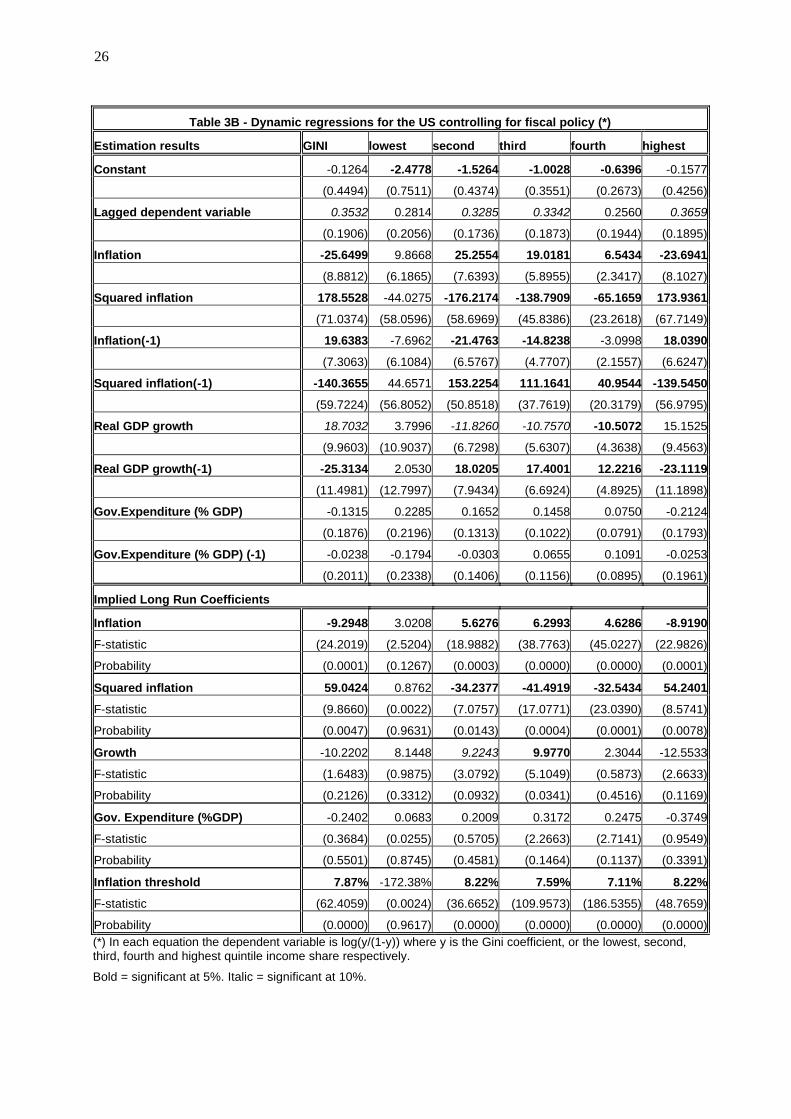
The third column of table 7 reports the estimated coefficients when the GDP share of government expenditure (lagged one year) is added to the benchmark model. The coefficient on fiscal policy is negative – as expected – and significant, leaving the non-monotonic inflation-inequality relationship significant and substantially unchanged (the inflation threshold would be slightly lower than in the benchmark model).

The fourth column of table 7 shows the sensitivity of the benchmark equation to the inclusion of a dummy variable for the high-inflation period 1973-81. The time dummy does not affect the sign or the significance of any of the coefficients of interest, and is positive and significant indicating that in the high-inflation years there was an upsurge of inequality, as predicted by the theory. However, we prefer not to include this dummy in the benchmark model since it picks up the effect of high inflation on inequality, also controlled by squared inflation.

Next, the benchmark model is tested for robustness to variations in the sample. First, each country in turn is excluded from the sample, and table 10 presents the estimated coefficients and inflation thresholds obtained in each case. As shown in the table, the coefficients on inflation and squared inflation are remarkably stable, as it is consequently the implied inflation threshold. Also the coefficient on growth is quite stable, except for the exclusion of Italy and Norway, in which cases the estimate is lower..

14

The benchmark model is then tested for robustness to variations in the sample period. Figure 4 shows that restricting the sample period progressively from 1960-96 to 1980-96 has no relevant effect on the value or the significance of the estimated coefficients on inflation and squared inflation, with the inflation threshold stable around 12 per cent. Further reducing the sample to 1981-96 makes the coefficients on inflation and squared inflation jointly non-significant. Similarly the inflation threshold is stable and significant when years prior to 1980 are included, and becomes non-significant if only post-1980 years are included. This is not surprising because since 1984 long-run inflation has been below the estimated 12 per cent threshold in all considered countries (except Portugal). Naturally, when initial inflation for all observations is below the threshold only the decreasing side of the U-shaped inflation-inequality relationship can be observed. In fact, fitting a linear model in long-run inflation and growth over the period 1981-96 gives a negative and significant coefficient on inflation, suggesting that lower inflation increases inequality. Finally note that the coefficient on growth is always positive, but non-significant when years 77-80 are excluded from the sample. From 1981 onwards it is much lower, positive, and (marginally) significant.

In sum, the evidence presented for the OECD countries supports the hypothesis of a U-shaped long-run relationship between income inequality and inflation. Controlling for long-run growth and for country-specific fixed effects it is found that the lowest inequality is reached around 12 per cent inflation. Pushing inflation below 12 per cent, as well as allowing inflation to go above 12 per cent, makes inequality progressively higher. The 12 per cent inflation threshold found in the OECD countries is higher than that found for the United States, showing a minimum in the Gini coefficient at around 6 per cent inflation. The difference may be partially explained by the lower precision of the estimates obtained from the multi-sources discontinuous OECD panel with respect to the United States time series. However, the result suggests that reducing inflation from moderate (around 12 per cent) to low (around 6 per cent) rates would increase inequality in the OECD (mainly European) countries, whereas it would decrease inequality in the United States.

Recalling that one important theoretical reason for expecting lower inflation to increase inequality in the long run is the presence of downward stickiness of nominal wages (paragraph 3.2), one could argue that the different result for the 15 OECD countries and the United States may be explained by the different degree of downwardly rigidity of nominal wages in Europe and in the United States. Given that nominal wages are downwardly more rigid in Europe than in the United States, when inflation is reduced from moderate to low levels, nominal wage cuts lag behind the decline in inflation and lead to higher real wages, unemployment and inequality more in Europe than in the United States.

We would like to stress that these results can only be indicative, given that the scarcity of comparable data on inequality makes it difficult to test any hypothesis on income inequality in cross-country studies to a high degree of confidence. We are also aware that we are explaining only a minor part of the cross-country variability in income inequality, the major part being explained by the country-specific fixed effects. However, the objective of this paper is not to give an exhaustive explanation of the cross-country variability in income inequality, but rather to shed light on the effects of monetary policy and inflation on income distribution in low inflation countries. Moreover, given that considerable attention was put to include in the OECD panel only directly comparable data, and given that the hypothesis of a non-monotonic inflation-inequality relationship is not rejected in two different samples (the United States and the 15 OECD) overall we think that the U-shaped inflation-inequality relationship emerges as a relatively robust finding.

15

5. Conclusions

This paper is concerned with the effects of monetary policy and inflation on income inequality. As explained in section 2, in the literature the empirical evidence on the relationship between inflation and inequality is mixed, with examples of both positive and negative correlation, producing what we have called the inflation-inequality puzzle. We suggest to solve this puzzle by assuming a non-monotonic relationship between inflation and inequality. Particularly, we suggest the use of a U-shaped relationship between income inequality and inflation, with inequality decreasing as inflation moves from high to low rates, and increasing as inflation is further reduced from low to lower rates.

The theoretical discussion of section 3 has identified a set of possible channels through which monetary policy can affect income inequality in the short and in the long run. The theory suggests that while in the short run restrictive monetary policy can be expected to deteriorate income distribution unambiguously, in the long run the net impact can be different depending on the initial rate of inflation. Particularly, when initial inflation is high the beneficial effects of disinflation on income distribution can be expected to dominate, whereas when initial inflation is low the detrimental effects of disinflation on income distribution may prevail. Therefore the economic theory suggests that the long-run relationship between inequality and inflation is U-shaped.

In section 4 we explored the empirical evidence for the non-monotonic long-run relationship between inequality and inflation in the United States over the period 1967-1999 and in 15 OECD countries using a panel of 60 observations over the period 1973-1996. From both samples we found evidence in favour of a U-shaped long-run relationship between inflation and inequality, with the estimated minimum in inequality around 6 per cent inflation in the United States, and around 12 per cent in the OECD countries. In the case of the United States, where data are available also on the quintiles income shares, the increase in inequality below 6 per cent inflation arises from the richest quintile gaining income share at the expenses of the rest of the distribution.

Unfortunately, the scarcity of cross-country and cross-time comparable data on inequality makes it difficult to estimate any hypothesis about the factors driving income distribution to a high degree of confidence. Hopefully in the future more continuous data will be collected on income distribution for the OECD countries and especially the European Union, so that it will be possible to analyse the topic with higher precision and confidence. We intend to do that in the future, as well as to extend the analysis to relative poverty data. However, even in the absence of extensive data sets, policy makers in the developed countries should take into account the negative permanent effects that restrictive monetary policy could have on income distribution at low inflation rates, and try to minimise them through effective labour and fiscal policies. As a recent contribution of the World Bank (Ferreira et al., 1999) puts it: “macroeconomic policies should aim to achieve stabilisation goals at the least cost to the poor, … and as soon as a sustainable external balance has been reached and inflationary pressures have been contained, macroeconomic policy should be eased (interest rates reduced and efficient public spending restored), to help offset the worst effects of the recession on the poor”. These words are referred to the developing countries: our wish is that they could be heard in the developed countries too.

17

Bibliography

Al-Marhubi, F. 2000. Income inequality and inflation: the cross evidence, Contemporary Economic Policy, vol. 18, no. 4, pp. 428-439.

Aghion, P., Caroli, E. and Garcìa-Penalosa, C. 1999. Inequality and economic growth: the perspective of the new growth theories, Journal of Economic Literature, vol. 37, pp. 1615-1660.

Akerlof, G., Dickens W. and Perry, G. 1996. The macroeconomics of low inflation, Brookings Papers on Economic Activity, no. 1, pp. 1-76.

Argitis, G. and Pitelis, C. 2001. Monetary policy and the distribution of income: evidence for the United States and the United Kingdom, Journal of Post Keynesian Economics, vol. 23, no. 4, pp. 617-638.

Atkinson, A.B. 1999. ‘Macroeconomics and the social dimension’, unpublished manuscript, Nuffield College, Oxford.

Atkinson, A.B. and Brandolini, A. 1999. ‘Promise and pitfalls in the use of “secondary” data-sets: income inequality in OECD countries’, unpublished manuscript, Nuffield College, Oxford.

Banerjee, A.V. and Duflo, E. 2000. ‘Inequality and growth: what can the data say?’, unpublished manuscript, Department of Economics, MIT.

Barro, R. 1996. Inflation and economic growth, Quarterly Review, Federal Reserve Bank of St. Louis, no. 78, pp. 133-169.

Beetsma, R. and van der Ploeg, F. 1996. Does inequality cause inflation? The political economy of inflation taxation and government debt, Public Choice, vol. 87, pp. 143-162.

Bertola, G. 2000. Macroeconomics of distribution and growth, in: Atkinson, A.B. and Bourguignon, F. (eds), Handbook of Income Distribution, Amsterdam, Elsevier.

Blanchard, O. 2000. Macroeconomics, Upper Saddle River, Prentice Hall.

Blank, R. and Blinder, A. 1986. Macroeconomics, income distribution, and poverty, in: Danziger, S. and Weinger, D. (eds), Fighting Poverty: What Works and What Doesn’t, Cambridge, MA, Harvard University Press.

Blinder, A.S. and Esaki, H.Y. 1978. Macroeconomic activity and income distribution in the postwar United States, The Review of Economics and Statistics, vol. 60, pp. 604-609.

Brandolini, A. and Sestito, P. 1994. ‘Cyclical and trend changes in inequality in Italy, 1977-1991’, paper prepared for the 23rd General Conference of the International Association for Research in Income and Wealth.

Brown, G. 2001. The conditions for high and stable growth and employment, Economic Journal, vol. 111, pp. 30-44.

Bulir, A. 2001. The impact of macroeconomic policies on the distribution of income, Annals of Public and Cooperative Economics, vol. 72, no. 2, pp. 253-270.

Bulir, A. 1998. ‘Income inequality: does inflation matter?’, IMF working paper 98/7, Washington, International Monetary Fund.

Bulir, A. and Gulde, A. 1995. ‘Inflation and income distribution: further evidence on empirical links’, IMF working paper 95/86, Washington, International Monetary Fund.

Chu, K., Davoodi, H. and Gupta, S. 2000. ‘Income distribution and tax and government social spending policies in developing countries’, IMF working paper 00/62, Washington, International Monetary Fund.

Cole, J. and Towe, C. 1996. ‘Income distribution and macroeconomic performance in the United States’, IMF working paper 96/97, Washington, International Monetary Fund.

Cutler, D.M. and Katz, L. 1991. Macroeconomic performance and the disadvantaged, Brookings Papers on Economic Activity, no. 2.

Dagdeviren, H., van der Hoeven, R. and Weeks, J. 2001. ‘Redistribution matters: growth for poverty reduction’, Employment paper 2001/10, Geneva, International Labour Organization.

18

Deininger, K. and Squire, L. 1996. A new data set measuring income inequality, World Bank Economic Review, no. 10, pp. 565-591.

Dollar, D. and Kraay, A. 2000. ‘Growth is good for the poor’, working paper, Washington, World Bank.

Easterly, W. and Fischer, S. 2001. Inflation and the poor, Journal of Money, Credit, and Banking, vol. 33, no. 2.

Feldstein, M. 1996. ‘The costs and benefits of going from low inflation to price stability’, NBER working paper 5469, Cambridge, MA, National Bureau of Economic Research.

Ferreira, F., Prennushi, G. and Ravallion, M. 1999. ‘Protecting the poor from macroeconomic shocks: an agenda for action in a crisis and beyond’, World Bank Policy Research working paper 2160, Washington, World Bank.

Fischer, S. 1993. The role of macroeconomic factors in growth, Journal of Monetary Economics, vol. 32, pp. 485-512.

Forbes, K. 2000. A reassessment of the relationship between inequality and growth, American Economic Review, vol. 90, no. 4, pp. 869-887.

Galor, O. 2000. Income distribution and the process of development, European Economic Review, vol. 44, pp. 706-712.

Hess, G. and Morris, C. 1996. The long-run costs of moderate inflation, Economic Review, Federal Reserve Bank of Kansas City, 2nd quarter, pp. 71-88.

Johnson, D.S. and Shipp, S. 1999. Inequality and the business cycle: a consumption viewpoint, Empirical Economics, vol.24, no. 1, pp. 173-180.

Kuznets, S. 1955. Economic growth and income inequality, American Economic Review, vol. 45, pp. 1-28.

Leidy, M. and Tokarick, S. 1998. ‘Considerations in reducing inflation from low to lower levels’, IMF working paper 98/109, Washington, International Monetary Fund.

Milanovic, B. 1994. ‘Determinants of cross-country income inequality: an ‘augmented’ Kuznets’ hypothesis’, World Bank Policy Research working paper 1246, Washington, World Bank.

Mocan, N. H. 1999. Structural unemployment, cyclical unemployment, and income inequality, Review of Economics and Statistics, vol. 81, no. 1, pp. 122-134.

Persson, T. and Tabellini, G. 1994. Is inequality harmful for growth?, American Economic Review, vol. 84, pp. 600-621.

Powers, E.T. 1995. Inflation, unemployment and poverty revisited, Economic Review, Federal Reserve Bank of Cleveland, 3rd quarter, pp. 2-13.

Raj, B. and Slottje, D.J. 1994. The trend behaviour of alternative income inequality measures in the United States from 1947-1990 and the structural break, Journal of Business & Economic Statistics, vol. 12, no. 4, pp. 479-487.

Ravallion, M. and Chen, S. 1997. What can new survey data tell us about recent changes in distribution and poverty?, World Bank Economic Review, vol. 11, no. 2.

Romer, C.D. and Romer, D.H. 1998. ‘Monetary policy and the well-being of the poor’, NBER working paper 6793, Cambridge, MA, National Bureau of Economic Research.

Sarel, M. 1996. Non-linear effects of inflation on economic growth, IMF Staff Papers, vol. 43, no. 1, pp. 199-215.

Sarel, M. 1997. How macroeconomic factors affect income distribution: the cross-country evidence, IMF working paper 97/152, Washington, International Monetary Fund.

Tanzi, V. 1998. Fundamental determinants of inequality and the role of government, IMF working paper 98/178, Washington, International Monetary Fund.

van der Hoeven, R. 2000. Poverty and structural adjustment. Some remarks on tradeoffs between equity and growth, Employment paper 2000/4, Geneva, International Labour Organization.

Wyplosz, C. 2000. ‘Do we know how low should inflation be?’, paper prepared for the First Central Banking Conference on “Why Price Stability?” organized by the European Central Bank on 2 and 3 November 2000.

19

Yoshino, O. 1993. Size distribution of workers’ household income and macroeconomic activities in Japan: 1963-88, Review of Income and Wealth, vol. 39, no. 4, pp. 387-402.

Table 1 A - The inflation-inequality puzzle (single country studies)

Inflation Authors Sample Dependent variable Control variables Regressive Progressive Not sign.

Mocan (1999) US 1948-94 Change in quintile shares of family income

Change in inflation, levels of structural and cyclical unemployment

X

Johnson and Shipp (1999) US 1980-94 (quarterly data)

Gini indexes based on pre-tax cash income and consumption-expenditures

Inflation, unemployment, per capita real transfers, lagged Gini, time trend X

Inflation X Change in poverty rate Inflation, unemployment X

Change in Gini index Inflation, unemployment X

Romer and Romer (1998) US 1969-94

Change in income share of bottom quintile

Inflation, unemployment X

Cole and Towe (1996) US 1947-93 Gini index Inflation, lagged Gini, GDP per capita, unemployment, time trend

X

Change in income poverty rate Change in inflation and unemployment X Powers (1995) US 1959-92 Change in consumption poverty rate Change in inflation and unemployment X

Jäntti (1994) US 1948-89 Quintile shares of family income Inflation (GNP deflator), prime-age male unemployment rate and squared rate, time trend, dummy 1981.

X

Inflation, poverty line/mean or median income, unemployment, post-1983 trend

X US 1959-89 Poverty rate

Also controlling for lagged poverty rate X

Cutler and Katz (1991)

US 1947-89 Quintile income shares Inflation, real per capita GNP, unemployment, post-1983 trend, lagged dep. var.

X

US 1948-83 Quintile shares of family income Inflation, unemployment (male 25-54), time trend, lagged dep. var.

X (significant for second quintile)

Blank and Blinder (1986)

US 1959-83 Poverty rate Inflation, unemployment, transfers/GDP, poverty line/mean income, lagged poverty rate

X

Blinder and Esaki (1978) US 1947-74 Quintile shares of family income Inflation, unemployment, time trend X Other countries

Finland 1977-84 Gini index Inflation, unemployment X Israel 1986-92 Gini index Inflation, unemployment X

Bulii and Gulde (1995)

Russia 1991-94 (quarterly data)

Gini index Inflation, unemployment X

Brandolini and Sestito (1994) Italy 1977-91 Gini index Inflation, unemployment, trend X Yoshino (1993) Japan 1963-88 Decile income shares of worker’s

households Expected and unexpected inflation, ratio of job offers to applicants, terms of trade, lagged dependent variable

X(*)

Regressive (progressive) means inflation increases (decreases) inequality or poverty, or decreases (increases) the lower quintiles income shares. (*) Both expected and unexpected inflation are estimated to be regressive tax. Expected inflation is insignificant for the lowest 20 and 10 percent groups. Unexpected inflation is insignificant for the 80-51 percent group.

22

Table 1 B - The inflation-inequality puzzle (cross-country and panel data studies) Inflation Authors Sample Dependent variable Control variables

Regressive Progressive Not sign. Bulir (2001) Cross section: various years, 75 dev.ed and

dev.ing countries Gini index (Milanovic data) 4 inflation dummies, per capita GDP,

squared per capita GDP, % state employment, transfers/GDP, M2/GDP

non-monotonic (U-shaped)

panel: 110 obs; not specified number of countries; 3 decades

Change in income share of the bottom quintile (DS data set)

Inflation, growth X

Easterly and Fischer (2001)

panel: 64 obs; 42 dev.ing and transition countries; 1981-93.

Change in poverty rate (50 percent of initial mean income) (Ravalllion and Chen, 1997)

Inflation, growth X

Inflation, per capita income X Dollar and Kraay (2000) panel: 232 obs; 80 dev.ed and dev.ing countries; 4 decades

Average income of the bottom quintile (augmented DS high quality data set)

Inflation, per capita income, openness, government consumption, property rights

X

Chu, Davoodi and Gupta (2000)

panel: 10 dev.ing and transition countries in 80s and 90s

Gini index (DS data set) Inflation, ratio of direct to indirect tax, secondary school enrolment and urbanization rates

X

Inflation X Cross section: 1988, 66 dev.ed + dev.ing countries

Average income of bottom quintile (DS high quality) Inflation, demand variability X

Inflation, continent dummies and demand variability

X Cross section: 1988, 76 dev.ed + dev.ing countries

Gini index (DS high quality)

Inflation, demand variability X Average income of bottom quintile (DS high quality)

Inflation, demand variability X(*)

Romer and Romer (1998)

Cross section: 1988, 19 OECD countries

Gini index (DS high quality) Inflation, demand variability X(*) Sarel (1997) Cross-section: various years, 45 dev.ed and

dev.ing countries Change in Gini index Inflation, plus a large number of

macroeconomic and demographic variables

X

Panel: 121 obs; 18 dev.ed and dev.ing countries; 1960-92

Gini index Inflation, per capita GDP, squared per capita GDP, public expenditure/GDP, country-specific dummies

X Bulir and Gulde (1995)

Panel: 55 obs; 18 dev.ed and dev.ing countries; 1960-92

Change in Gini index Change in inflation, per capita GDP and public expenditure; country-specific dummies

X

Regressive (progressive) means inflation increases (decreases) inequality or poverty, or decreases (increases) the lower quintiles income shares. DS data set = Deininger and Squire data set. (*) Atkinson and Brandolini (1999: p.8) show that using strictly comparable data for the same countries, inflation would be non-significant

23

Table 2 - Static regressions for the US(*)

GINI lowest second third fourth highest

Constant 0.848354 -3.77974 -3.30453 -2.50273 -1.295984 0.905282

(0.2242) (0.1245) (0.2076) (0.1492) (0.0470) (0.1881)

Inflation -12.0302 4.216041 8.61777 7.981081 4.833194 -11.5417

(2.4619) (1.3670) (2.2799) (1.6383) (0.5160) (2.0657)

Squared Inflation 72.85701 -6.32323 -49.87765 -47.9431 -33.13026 68.41693

(23.9950) (13.3238) (22.2218) (15.9682) (5.0291) (20.1335)

Growth -25.9043 13.32523 26.74355 20.09005 0.357091 -23.3224

(7.4625) (4.1437) (6.9110) (4.9661) (1.5641) (6.2615)

Inflation threshold 8.26% 33.34% 8.64% 8.32% 7.29% 8.43%

F-statistic (57.0092) (0.3118) (27.3703) (53.9977) (393.5048) (67.3589)

Probability (0.0000) (0.5808) (0.0000) (0.0000) (0.0000) (0.0000)

Adjusted R-squared 0.796017 0.884627 0.721598 0.797784 0.917947 0.845922

F-statistic 42.62537 82.78669 28.64730 43.08224 120.3307 59.56241

Prob(F-statistic) (0.0000) (0.0000) (0.0000) (0.0000) (0.0000) (0.0000)

(*) Dependent variable is log(y/(1-y)) where y is the Gini coefficient, or the lowest, second, third, fourth and highest quintile income share respectively. Bold = significant at 5%. Standard errors in brackets.

24

Table 3 - Dynamic regressions for the US(*)

GINI lowest second third fourth highest

Constant 0.1182 -2.4319 -1.6006 -1.1772 -0.8382 0.2004

(0.1200) (0.6918) (0.4050) (0.3385) (0.2383) (0.1210)

Lagged dependent variable 0.3922 0.3099 0.3816 0.4188 0.3365 0.4315

(0.1751) (0.1925) (0.1611) (0.1755) (0.1884) (0.1733)

Inflation -23.2158 9.7028 22.5294 15.3572 4.7679 -20.0888

(7.6029) (5.3498) (6.6548) (5.1494) (2.0837) (6.8238)

Squared inflation 151.9829 -39.8000 -149.0894 -100.2629 -39.7269 133.5582

(52.9232) (41.3542) (45.3929) (35.3913) (17.3445) (49.0634)

Inflation(-1) 17.6267 -7.2798 -19.0302 -11.8143 -1.8646 15.0989

(6.3035) (5.5013) (5.7573) (4.2031) (2.0433) (5.6874)

Squared inflation(-1) -117.4339 36.8537 128.2437 78.3472 20.7945 -104.5823

(44.9116) (43.4141) (39.6074) (29.3666) (16.2755) (42.2578)

Real GDP growth 16.7772 0.6698 -11.2619 -7.6069 -6.8604 12.5898

(7.9055) (9.1401) (5.4853) (4.5428) (3.5896) (7.5651)

Real GDP growth(-1) -21.2537 3.3788 15.2236 11.3207 6.5459 -17.0550

(7.5396) (8.7260) (5.2923) (4.4390) (3.3763) (7.3084)


F-statistic 139.2771 52.7489 168.3626 185.2753 73.8960 137.8210

Prob(F-statistic) 0.0000 0.0000 0.0000 0.0000 0.0000 0.0000

Implied Long Run Coefficients

Inflation -9.1957 3.5110 5.6583 6.0960 4.3757 -8.7768

F-statistic (24.4916) (3.5427) (18.6226) (29.9495) (33.5275) (20.4632)

Probability (0.0000) (0.0720) (0.0002) (0.0000) (0.0000) (0.0001)


F-statistic (10.2594) (0.0591) (7.2719) (12.4810) (15.6663) (7.5649)

Probability (0.0038) (0.8099) (0.0126) (0.0017) (0.0006) (0.0111)

Growth -7.3652 5.8665 6.4062 6.3901 -0.4740 -7.8540

F-statistic (1.3315) (0.0753) (1.9380) (2.2850) (0.0307) (1.3652)

Probability (0.2599) (0.7861) (0.1767) (0.1437) (0.8624) (0.2541)


F-statistic (69.9032) (0.0753) (41.7680) (78.3583) (118.2540) (43.5665)

Probability (0.0000) (0.7862) (0.0000) (0.0000) (0.0000) (0.0000) (*) Dependent variable is log(y/(1-y)) where y is the Gini coefficient, or the lowest, second, third, fourth and highest quintile income share respectively.

Bold = significant at 5%. Italic = significant at 10%. Standard errors in brackets.

25

Table 2B - Static regressions for the US controlling for fiscal policy (*)

Estimation results GINI lowest second third fourth highest

Constant 0.283176 -3.30057 -2.76164 -2.09633 -1.402949 0.468684

(0.5121) (0.2740) (0.4733) (0.3392) (0.1079) (0.4314)

Inflation -12.4572 4.578069 9.02794 8.288133 4.752379 -11.8716

(2.4656) (1.3193) (2.2788) (1.6334) (0.5193) (2.0773)


(24.3130) (13.0097) (22.4704) (16.1070) (5.1209) (20.4835)

Growth -29.6558 16.50586 30.34716 22.78768 -0.35292 -26.2204

(8.0075) (4.2847) (7.4006) (5.3048) (1.6866) (6.7462)

Gov.Expenditure (% GDP) -0.34536 0.292802 0.33174 0.248338 -0.065362 -0.26679

(0.2819) (0.1508) (0.2605) (0.1868) (0.0594) (0.2375)


F-statistic (71.0534) (1.3916) (38.1288) (69.6478) (311.8994) (79.1373)

Probability (0.0000) (0.2481) (0.0000) (0.0000) (0.0000) (0.0000)

Adjusted R-squared 0.799481 0.894679 0.72744 0.803003 0.918542 0.847301 (*) Dependent variable is log(y/(1-y)) where y is the Gini coefficient, or the lowest, second, third, fourth and highest quintile income share respectively.

Bold = significant at 5%. Italic = significant at 10%. Standard errors in brackets.

26

Table 3B - Dynamic regressions for the US controlling for fiscal policy (*)


Constant -0.1264 -2.4778 -1.5264 -1.0028 -0.6396 -0.1577

(0.4494) (0.7511) (0.4374) (0.3551) (0.2673) (0.4256)


(0.1906) (0.2056) (0.1736) (0.1873) (0.1944) (0.1895)

Inflation -25.6499 9.8668 25.2554 19.0181 6.5434 -23.6941

(8.8812) (6.1865) (7.6393) (5.8955) (2.3417) (8.1027)


(71.0374) (58.0596) (58.6969) (45.8386) (23.2618) (67.7149)

Inflation(-1) 19.6383 -7.6962 -21.4763 -14.8238 -3.0998 18.0390

(7.3063) (6.1084) (6.5767) (4.7707) (2.1557) (6.6247)

Squared inflation(-1) -140.3655 44.6571 153.2254 111.1641 40.9544 -139.5450

(59.7224) (56.8052) (50.8518) (37.7619) (20.3179) (56.9795)

Real GDP growth 18.7032 3.7996 -11.8260 -10.7570 -10.5072 15.1525

(9.9603) (10.9037) (6.7298) (5.6307) (4.3638) (9.4563)

Real GDP growth(-1) -25.3134 2.0530 18.0205 17.4001 12.2216 -23.1119

(11.4981) (12.7997) (7.9434) (6.6924) (4.8925) (11.1898)

Gov.Expenditure (% GDP) -0.1315 0.2285 0.1652 0.1458 0.0750 -0.2124

(0.1876) (0.2196) (0.1313) (0.1022) (0.0791) (0.1793)

Gov.Expenditure (% GDP) (-1) -0.0238 -0.1794 -0.0303 0.0655 0.1091 -0.0253

(0.2011) (0.2338) (0.1406) (0.1156) (0.0895) (0.1961)


Inflation -9.2948 3.0208 5.6276 6.2993 4.6286 -8.9190

F-statistic (24.2019) (2.5204) (18.9882) (38.7763) (45.0227) (22.9826)

Probability (0.0001) (0.1267) (0.0003) (0.0000) (0.0000) (0.0001)

Squared inflation 59.0424 0.8762 -34.2377 -41.4919 -32.5434 54.2401

F-statistic (9.8660) (0.0022) (7.0757) (17.0771) (23.0390) (8.5741)

Probability (0.0047) (0.9631) (0.0143) (0.0004) (0.0001) (0.0078)

Growth -10.2202 8.1448 9.2243 9.9770 2.3044 -12.5533

F-statistic (1.6483) (0.9875) (3.0792) (5.1049) (0.5873) (2.6633)

Probability (0.2126) (0.3312) (0.0932) (0.0341) (0.4516) (0.1169)

Gov. Expenditure (%GDP) -0.2402 0.0683 0.2009 0.3172 0.2475 -0.3749

F-statistic (0.3684) (0.0255) (0.5705) (2.2663) (2.7141) (0.9549)

Probability (0.5501) (0.8745) (0.4581) (0.1464) (0.1137) (0.3391)

Inflation threshold 7.87% -172.38% 8.22% 7.59% 7.11% 8.22%

F-statistic (62.4059) (0.0024) (36.6652) (109.9573) (186.5355) (48.7659)

Probability (0.0000) (0.9617) (0.0000) (0.0000) (0.0000) (0.0000)(*) In each equation the dependent variable is log(y/(1-y)) where y is the Gini coefficient, or the lowest, second, third, fourth and highest quintile income share respectively.

Bold = significant at 5%. Italic = significant at 10%.

27

Table 2C - Static regressions for the US - Linear model(*)


Constant 0.9403 -3.7877 -3.36746 -2.5632 -1.3378 0.9916

(0.2507) (0.1217) (0.2191) (0.1664) (0.0723) (0.2167)

Inflation -4.6701 3.5773 3.57908 3.1378 1.4863 -4.6302

(0.4855) (0.2357) (0.4243) (0.3222) (0.1400) (0.4196)

Real GDP growth -34.1315 14.0393 32.37587 25.5039 4.0983 -31.0482

(7.8481) (3.8107) (6.8590) (5.2087) (2.2639) (6.7827)

Diagnostics


F-statistic 46.5694 127.3565 35.6531 47.4421 65.8019 61.8311

Prob(F-statistic) 0.0000 0.0000 0.0000 0.0000 0.0000 0.0000 (*) Dependent variable is log(y/(1-y)) where y is the Gini coefficient, or the lowest, second, third, fourth and highest quintile income share respectively.


28

Table 3C – Dynamic regressions for the US - Linear model (*)


Constant 0.2224 -2.3076 -0.5774 -0.4057 -0.3607 0.2152

(0.1254) (0.6663) (0.2536) (0.1911) (0.1592) (0.1279)


(0.0926) (0.1814) (0.0826) (0.0812) (0.1124) (0.0955)

Inflation -1.5184 4.7385 0.9766 0.8679 0.2832 -1.6676

(1.4100) (1.4030) (1.1048) (0.8215) (0.5200) (1.2818)

Inflation(-1) 0.5928 -2.6498 -0.3780 -0.3597 0.2002 0.7230

(1.3059) (1.2875) (1.0176) (0.7555) (0.5900) (1.2061)

Real GDP growth 11.5714 0.8371 -9.2678 -4.7667 -4.4288 9.2704

(8.5015) (8.9241) (6.2615) (4.8765) (3.8328) (8.1563)

Real GDP growth(-1) -19.1759 4.8410 14.3156 9.0742 6.2355 -15.7091

(8.2837) (8.4338) (6.0836) (4.7891) (3.6795) (7.9430)


F-statistic 155.0752 76.6021 174.4455 208.8571 83.0500 157.8235

Prob(F-statistic) 0.0000 0.0000 0.0000 0.0000 0.0000 0.0000


Inflation -4.8839 3.2754 3.4116 3.4002 1.9695 -4.9837

F-statistic (16.2940) (88.3424) (13.6957) (13.8100) (18.8112) (18.1193)

Probability (0.0004) (0.0000) (0.0010) (0.0010) (0.0002) (0.0002)

Growth -40.1225 8.9042 28.7684 28.8170 7.3603 -33.9716

F-statistic (3.1241) (2.0915) (2.9886) (3.0787) (1.0853) (2.7347)

Probability (0.0889) (0.1601) (0.0957) (0.0911) (0.3071) (0.1102) (*) Dependent variable is log(y/(1-y)) where y is the Gini coefficient, or the lowest, second, third, fourth and highest quintile income share respectively.


29

Table 2D - Static regressions for the US using the post-1983 dummy (*)


Constant 0.2158028 -3.57378 -2.67293 -2.059717 -1.286791 0.3957129

(0.1707) (0.1354) (0.1362) (0.1035) (0.0575) (0.1519)

Inflation -12.24377 4.285587 8.83105 8.1306755 4.836299 -11.71381

(1.5585) (1.2361) (1.2436) (0.9446) (0.5245) (1.3864)


(15.6605) (12.4211) (12.4961) (9.4914) (5.2699) (13.9315)

Growth -8.91546 7.793679 9.78007 8.1916891 0.110181 -9.636591

(5.3675) (4.2572) (4.2829) (3.2531) (1.8062) (4.7749)

Dummy 1983-99 0.104579 -0.03405 -0.10442 -0.073243 -0.00152 0.0842465

(0.0157) (0.0124) (0.0125) (0.0095) (0.0053) (0.0140)


F-statistic (377.7757) (2.9761) (395.8198) (464.5610) (264.5079) (339.0871)

Probability (0.0000) (0.0955) (0.0000) (0.0000) (0.0000) (0.0000)


F-statistic 90.902561 77.83665 89.62509 112.06653 87.41441 108.30828

Prob(F-statistic) 0.0000 0.0000 0.0000 0.0000 0.0000 0.0000 (*) In each equation the dependent variable is log(y/(1-y)) where y is the Gini coefficient, or the lowest, second, third, fourth and highest quintile income share respectively.


30

Table 4 – Gini coefficients in 15 OECD countries

income net, household, selected by country-specific homogeneous source

Year AUS BEL CAN DNK FIN FRA DEW IRL ITA NLD NOR PRT SWE GBR USA

1960 38.0

1961

1962 37.5

1963

1964 38.0

1965

1966

1967 40.0 36.0

1968 38.7 40.0

1969 40.0 26.3

1970 39.2 38.0

1971 40.0

1972 38.0

1973 37.0 36.7 42.0 37.5

1974 41.0 28.6 34.0

1975 31.4 36.6 39.0

1976 35.0 37.3 33.1

1977 36.0

1978 36.4 36.0

1979 31.7 37.0 31.2 32.6

1980 36.6 36.0 37.0 36.8 32.4

1981 30.5 27.9 32.0 32.5

1982 31.0 30.7

1983 31.9 33.9

1984 33.4 30.6 31.8

1985 26.2 35.2 31.4 31.2

1986 41.0 33.0 33.1 31.7 33.3 35.2

1987 31.2 31.3 26.2 35.2 34.4 31.7

1988 26.6 32.2

1989 33.9 31.3

1990 42.0 36.8 32.5

1991 31.5 26.1 32.5 31.8 33.3 35.2

1992 26.9 30.0 31.7 32.4

1993 36.3 32.0

1994 32.4

1995 44.0 36.2

1996 44.0

obs 60-96 4 3 4 2 2 3 11 3 22 4 9 2 12 3 4 Tot 88

obs 73-96 4 3 4 2 2 3 7 3 16 4 7 2 12 2 4 Tot 75

adjusted* 3 3 4 2 2 3 6 3 10 2 6 2 8 2 4 Tot 60

Observations in shaded cells are excluded from the benchmark sample.

31

Table 5 - Annual CPI inflation (%) in selected OECD countries, 1973-1996

Country Mean Median Maximum Minimum Std. Dev.

AUS 7.87 8.23 15.31 0.99 4.09

BEL 5.18 4.47 12.76 1.16 3.40

CAN 6.07 5.30 12.42 0.16 3.49

DEW(*) 3.68 3.56 7.04 -0.22 2.16

DNK 6.57 5.53 15.29 1.27 4.07

FIN 7.37 6.83 17.84 0.63 4.88

FRA 6.76 6.60 13.66 1.66 4.32

GBR 8.62 6.93 24.21 1.56 5.96

IRL 8.85 6.54 20.63 1.40 6.76

ITA 10.65 9.99 21.08 4.01 5.72

NLD 4.09 3.18 10.22 -0.69 3.02

NOR 6.68 6.94 13.65 1.25 3.51

PRT 15.95 14.26 33.06 3.09 8.18

SWE 7.44 7.69 13.69 0.80 3.40

USA 5.71 4.56 13.54 1.90 3.21

All countries 7.43 6.33 33.06 -0.69 5.43

(*) West Germany: 1973-1990.

Source: OECD Main Economic Indicators

Table 6 - Annual real GDP growth (%) in selected OECD countries, 1973-1996

Country Mean Median Maximum Minimum Std. Dev.

AUS 2.91 2.98 6.60 -2.76 2.33

BEL 2.03 2.17 6.04 -2.49 2.27

CAN 3.01 3.69 7.57 -4.57 2.91

DEW(*) 2.19 2.46 5.56 -1.52 2.24

DNK 1.90 1.69 6.73 -1.70 2.17

FIN 2.14 2.91 7.92 -9.60 3.93

FRA 2.09 2.41 5.56 -1.59 1.74

GBR 2.07 2.46 7.07 -2.64 2.62

IRL 4.33 3.72 10.20 -1.09 2.91

ITA 2.45 2.70 7.49 -4.00 2.63

NLD 2.25 2.48 5.04 -1.45 1.71

NOR 3.46 3.83 6.96 -0.41 2.00

PRT 3.67 2.97 12.39 -2.77 3.66

SWE 1.54 1.92 4.08 -2.30 2.04

USA 2.42 2.84 6.99 -3.02 2.55

All countries 2.57 2.67 12.39 -9.60 2.65

(*) West Germany: 1973-1990.

Source: OECD Main Economic Indicators

32

Table 7 – Alternative model estimates for the OECD countries

Dependent Variable: Gini index

Method: fixed effects estimator

Sample: 1973 1996

Total panel (unbalanced) observations: 60

Number of cross-sections used: 15

White Heteroskedasticity-Consistent Standard Errors & Covariance

Variable Model 1 Model 2 Model 3 Model 4

Inflation -0.8981 -0.1369 -0.845 -1.0874

(0.1997) (0.0932) (0.2429) (0.1989)

Squared inflation 3.5280 3.3970 3.5567

(0.7051) (0.8480) (0.6669)

Real GDP growth 2.0704 1.3636 1.9984 1.8227

(0.5425) (0.5068) (0.5746) (0.4915)

Gov. Exp. (%GDP) -0.6891

(0.2598)

Dummy 73-81 0.0179

(0.0063)

Adjusted R-squared 0.8192 0.7937 0.7984 0.8422

Inflation threshold 12.73% 12.44% 15.29%

F-Statistic 213.3102 175.2571 141.4988

Estimated fixed effects not reported in table for space reasons. Standard errors in parenthesis. Bold = significant at 5%.

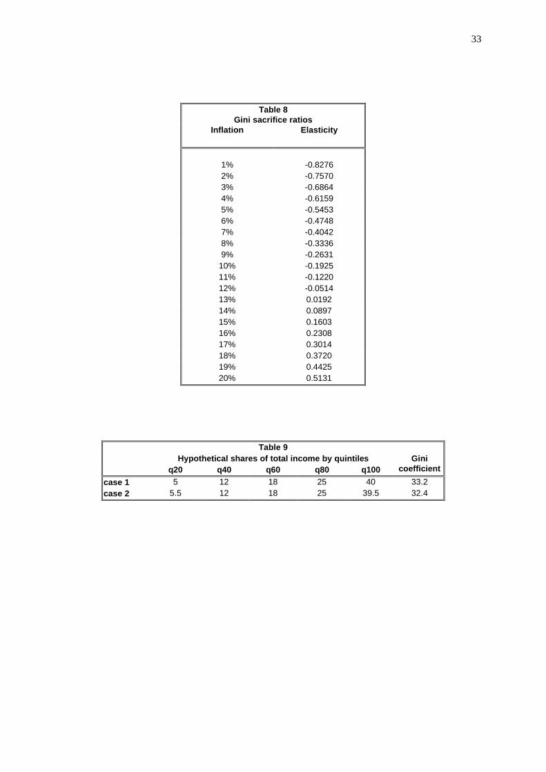
33

Table 8 Gini sacrifice ratios

Inflation Elasticity

1% -0.8276 2% -0.7570 3% -0.6864 4% -0.6159 5% -0.5453 6% -0.4748 7% -0.4042 8% -0.3336 9% -0.2631

10% -0.1925 11% -0.1220 12% -0.0514 13% 0.0192 14% 0.0897 15% 0.1603 16% 0.2308 17% 0.3014 18% 0.3720 19% 0.4425 20% 0.5131

Table 9 Hypothetical shares of total income by quintiles

q20 q40 q60 q80 q100 Gini

coefficient

case 1 5 12 18 25 40 33.2 case 2 5.5 12 18 25 39.5 32.4

34

Table 10 - Sensitivity of estimated coefficients to country exclusion

Excluded country Inflation Squared inflation Growth Inflation threshold

Australia -0.8765 3.4426 2.0527 12.73%

(0.2449) (0.8696) (0.5696)

Belgium -0.9390 3.6928 2.1264 12.71% (0.2129) (0.7542) (0.5585)

Canada -0.8999 3.5315 2.2986 12.74% (0.2105) (0.7375) (0.5906)

West Germany -1.0321 4.0712 2.2324 12.68% (0.2071) (0.7247) (0.5804)

Denmark -0.9738 3.8374 2.1464 12.69% (0.2030) (0.7115) (0.5476)

Finland -0.9053 3.5499 2.1503 12.75% (0.2020) (0.7124) (0.5658)

France -0.8814 3.4725 2.0403 12.69% (0.1996) (0.7045) (0.5435)

Great Britain -0.8306 3.3198 1.9379 12.51% (0.2197) (0.7611) (0.5820)

Ireland -1.0642 4.0027 2.4301 13.29% (0.2015) (0.7496) (0.5585)

Italy -0.7080 2.7898 1.6003 12.69% (0.1828) (0.6835) (0.4861)

Netherlands -0.9004 3.5372 2.0738 12.73% (0.2000) (0.7062) (0.5432)

Norway -0.7654 3.0240 1.6733 12.65% (0.2011) (0.7111) (0.5887)

Portugal -0.8920 3.4893 2.0721 12.78% (0.2137) (1.2638) (0.5695)

Sweden -0.9076 3.5587 2.1391 12.75% (0.2069) (0.7194) (0.5544)

USA -0.8857 3.4817 2.0497 12.72% (0.2339) (0.8251) (0.5730)

All countries -0.8981 3.5280 2.0704 12.73%

(0.1997) (0.7051) (0.5425)

Standard errors in parenthesis. Bold = significant at 5%.

35

Short Run

Interest rate Growth Unemployment

Inequality

Expected inflation

Real interest rate

Real exchange rate appreciation

Real wages (nominal rigidities)

Inflation Inequality

Real value of unindexed transfers

Figure 1 – Short-run and Long-run Effects of Restrictive Monetary Policy on Income Distribution

Inflation Real interest rate(risk premium) *

Inequality

Real value ofprivate debt *

UnemploymentInequality

Long Run

Long run growth*

Real value ofunindexedtransfers *

* Channels activated only or mainly in high inflation economies.

Real value ofmonetary assets*

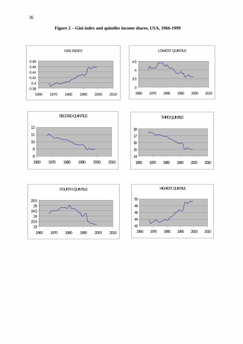
36

GINI INDEX

0.38

0.4

0.42

0.44

0.46

0.48

1960 1970 1980 1990 2000 2010

LOWEST QUINTILE

3

3.5

4

4.5

1960 1970 1980 1990 2000 2010

SECOND QUINTILE

8

9

10

11

12

1960 1970 1980 1990 2000 2010

THIRD QUINTILE

14

15

16

17

18

1960 1970 1980 1990 2000 2010

FOURTH QUINTILE

2323.5

2424.5

2525.5

1960 1970 1980 1990 2000 2010

HIGHEST QUINTILE

42

44

46

48

50

1960 1970 1980 1990 2000 2010

Figure 2 – Gini index and quintiles income shares, USA, 1966-1999

37

Inflation

-20

-15

-10

-5

0

5

10

15

19

67

19

69

19

71

19

73

19

75

19

77

19

79

19

81

19

83

19

85

Inflation squared

-300

-250

-200

-150

-100

-50

0

50

100

150

19

67

19

69

19

71

19

73

19

75

19

77

19

79

19

81

19

83

19

85

Growth

-50-40-30-20-10

01020304050

19

67

19

69

19

71

19

73

19

75

19

77

19

79

19

81

19

83

19

85

Inflation threshold

-0.15

-0.1

-0.05

0

0.05

0.1

0.15

19

67

19

69

19

71

19

73

19

75

19

77

19

79

19

81

19

83

19

85

Figure 3 – Coefficient stability in the Gini static model for the US

38

Inflation

-1.5

-1

-0.5

0

0.5

1

1955 1960 1965 1970 1975 1980 1985

Squared inflation

-15

-10

-5

0

5

10

1955 1960 1965 1970 1975 1980 1985

Growth

-2

-1

0

1

2

3

4

1955 1960 1965 1970 1975 1980 1985

Inflation threshold

-0.4

-0.3

-0.2

-0.1

0

0.1

0.2

1955 1960 1965 1970 1975 1980 1985

Figure 4 – Coefficient stability in the Gini model for the OECD countries

Contents

1. Introduction.................................................................................................................................. 1

2. The inflation-inequality puzzle...................................................................................................... 2

3. Monetary policy and income distribution: the channels of transmission..................................... 4 3.1 The short run....................................................................................................................................... 5 3.2 The long run........................................................................................................................................ 6

4. Data and estimation ..................................................................................................................... 8 4.1 Time-series analysis of income distribution in the US.......................................................................... 8 4.2 Panel data analysis of income distribution in the OECD countries ......................................................11

5. Conclusions .................................................................................................................................15

Bibliography ....................................................................................................................................17

Tables and figures

Table 1 - The inflation-inequality puzzle ................................................................................................ 20

Table 2 - Static regressions for the US ..................................................................................................... 21

Table 3 - Dynamic regressions for the US................................................................................................. 22

Table 2B - Static regressions for the US controlling for fiscal policy ........................................................ 23

Table 3B - Dynamic regressions for the US controlling for fiscal policy ................................................... 24

Table 2C - Static regressions for the US - Linear model ........................................................................... 25

Table 3C - Dynamic regressions for the US - Linear model ..................................................................... 26

Table 2D - Static regressions for the US using the post-1983 dummy ...................................................... 27

Table 4 - Gini coefficients in 15 OECD countries .................................................................................... 28

Table 5 - Annual CPI inflation (%) in selected OECD countries, 1973-1996 ........................................... 29

Table 6 - Annual real GDP growth (%) in selected OECD countries, 1973-1996 ..................................... 29

Table 7 - Alternative model estimates for the OECD countries ................................................................ 30

Table 8 – Gini sacrifice ratios .................................................................................................................. 31

Table 9 – Hypothetical shares of total income by quintiles ....................................................................... 31

Table 10 - Sensitivity of estimated coefficients to country exclusion ......................................................... 32

Figure 1 – Short-run and long-run effects of restrictive monetary policy on income distribution .............. 33

Figure 2 - Gini index and quintiles income shares, USA, 1966-1999 ....................................................... 34

Figure 3 - Coefficient stability in the Gini static model for the US ........................................................... 35

Figure 4 - Coefficient stability in the Gini model for the OECD countries ................................................ 36

is inflation bad for income inequality: the importance of ...ed_emp/documents/publication/... ·...

Documents