is the common good?
TRANSCRIPT

Is the Common Good?A New Perspective Developed in Genetic Algorithms
Stephen ChenSeptember 1999
CMU-RI-TR-99-21
Robotics InstituteCarnegie Mellon University
Pittsburgh, Pennsylvania 15213
Submitted in partial fulfillment of the requirementsfor the degree of Doctor of Philosophy
© by Stephen Chen
Stephen Chen was sponsored in part by the Advanced Research Projects Agency and Rome Laboratory, Air ForceMaterial Command, USAF, under grant numbers F30602-95-1-0018 and F30602-97-C-0227, and the CMU RoboticsInstitute. The views and conclusions contained herein are those of the author and should not be interpreted as neces-sarily representing the official policies or endorsements, either expressed or implied, of the Advanced ResearchProjects Agency and Rome Laboratory or the U.S. Government.

abstract
Similarities are more important than differences. The importance of these common
components is set forth by the commonality hypothesis: schemata common to above-
average solutions are above average. This hypothesis is corroborated by the isolation of
commonality-based selection. It follows that uncommon components should be below
average (relative to their parents).
In genetic algorithms, the traditional advantage of crossover has been attributed to the
recombination of (uncommon) parent components. However, the original analysis
focused on how the schemata of a single parent were affected by crossover. Using an
explicit two-parent perspective, the preservation of common components is emphasized.
The commonality hypothesis suggests that these common schemata are the critical
building blocks manipulated by crossover. Specifically, common components have a
higher expected fitness than uncommon components.
The Commonality-Based Crossover Framework redefines crossover as a two step process:
1) preserve the maximal common schema of two parents, and 2) complete the solution
with a construction heuristic. To demonstrate the utility of this design model, domain-
independent operators, heuristic operators, and hybrid operators have been developed for
benchmark and practical problems with standard and non-standard representations. The
new commonality-based operators have performed consistently better than comparable
operators which emphasize combination.
In heuristic operators (which use problem specific heuristics during crossover), the effects
of commonality-based selection have been isolated in GENIE (a genetic algorithm that
eliminates fitness-based selection of parents). Since the effectiveness of construction
heuristics can be amplified by using only commonality-based restarts, the preservation of
common components has supplied selective pressure at the component (rather than
individual) level. This result corroborates the commonality hypothesis--the preserved
common schemata are above average.
Transferring the concept of commonality-based selection back to standard crossover
operators, beneficial changes should occur more frequently when they are restricted to
uncommon schemata. Since multiple parents are required to identify common compo-
nents, commonality-based selection is an advantage that multi-parent operators (e.g.
crossover) can have over single-parent operators (e.g. mutation). These observations
present a novel perspective on iterative improvement.

i
Chapter 1: Introduction 1
1.1 Motivation 2
1.2 Overview 2
1.3 Outline 4
Chapter 2: Background 7
2.1 The Natural Metaphors 82.1.1 Evolution 82.1.2 Genetics 9
2.2 Genetic Algorithm Basics 11
2.3 The Schema Theorem 132.3.1 The Original Form 132.3.2 The Steady-State Form 15
2.4 Effects of the Schema Theorem 172.4.1 Implicit Parallelism 172.4.2 The Building Block Hypothesis 172.4.3 Combination 18
2.5 Crossover Design Models 182.5.1 Radcliffe’s Design Principles 192.5.2 Convergence Controlled Variation 192.5.3 Path Relinking 19
2.6 Genetic Algorithm Variations 20
2.7 Evolution Strategies 20
2.8 Other General Optimization Methods 212.8.1 Hill Climbing 212.8.2 Simulated Annealing 212.8.3 Tabu Search 222.8.4 A-Teams 232.8.5 Ant Colonies 23
2.9 Benchmark Problems 232.9.1 One Max 242.9.2 The Traveling Salesman Problem 24
2.10 Summary 25

ii
Chapter 3: The Foundation 26
3.1 Overview 27
3.2 The Commonality Hypothesis 28
3.3 Reducing the Concern for Disruption 28
3.4 A Commonality-Based Analysis of the Schema Theorem 30
3.5 The Commonality-Based Crossover Framework 32
3.6 Other Effects on Genetic Algorithms 323.6.1 Crossover Probability in Generational Replacement Schemes 333.6.2 Implicit Parallelism 34
3.7 Effects on Construction Heuristics 343.7.1 An Intuitive Reason to Preserve Common Schemata 353.7.2 Heuristic Amplification 36
3.8 Commonality-Based Selection 39
3.9 The Critical Observation 40
3.10 Summary 41
Chapter 4: Domain-Independent Operators 42
4.1 Overview 43
4.2 A Review of Sequence-Based Crossover Operators 444.2.1 Position-Based Schemata 444.2.2 Edge-Based Schemata 464.2.3 Order-Based Schemata 47
4.3 Preserving Common Components in Sequence-Based Operators 494.3.1 Maximal Sub-Tour Order Crossover 504.3.2 Results: MST-OX vs. OX 50
4.4 Summary 53
Chapter 5: Heuristic Operators: Part One 54
5.1 Overview 55
5.2 Edge-Based Schemata 565.2.1 Greedy Crossover 565.2.2 Common Sub-Tours/Nearest Neighbor 565.2.3 Results: CST/NN vs. GX 57
5.3 Order-Based Schemata 585.3.1 Deconstruction/Reconstruction 595.3.2 Maximum Partial Order/Arbitrary Insertion 605.3.3 Results: MPO/AI vs. Deconstruction/Reconstruction 625.3.4 MPO/AI and the Sequential Ordering Problem 63
5.4 Additional Comments 65
5.5 Summary 66

iii
Chapter 6: Heuristic Operators: Part Two 67
6.1 Overview 68
6.2 GENIE 68
6.3 Heuristic Amplification 696.3.1 One Max 696.3.2 Common Sub-Tours/Nearest Neighbor 706.3.3 Maximum Partial Order/Arbitrary Insertion 726.3.4 Negative Heuristic Amplification 736.3.5 Heuristic Amplification and Fitness-Based Selection 74
6.4 Open-Loop Optimization 756.4.1 One Max 766.4.2 Maximum Partial Order/Arbitrary Insertion 77
6.5 Summary 78
Chapter 7: Hybrid Operators 79
7.1 Overview 80
7.2 Globally Convex Search Spaces 81
7.3 Hybrid Operators for the Traveling Salesman Problem 837.3.1 The Local Optimizer 837.3.2 The Crossover Operators 837.3.3 The Hybrid Operators 847.3.4 Results: CST/NN-2-opt vs. GX-2-opt and RRR-BMM 847.3.5 The Role of Crossover in a Hybrid Operator 86
7.4 Discussion 88
7.5 Additional Comments 88
7.6 Summary 89
Chapter 8: Vehicle Routing 90
8.1 Overview 91
8.2 Problem Formulations 918.2.1 The (Capacitated) Vehicle Routing Problem 928.2.2 The Vehicle Routing Problem with Time Windows 93
8.3 Previous Genetic Algorithms for Vehicle Routing 938.3.1 A Genetic Algorithm with the Petal Method 948.3.2 GIDEON 94
8.4 Common Clusters/Insertion 94
8.5 Results for the Vehicle Routing Problem 96
8.6 Results for the Vehicle Routing Problem with Time Windows 998.6.1 Common Clusters/Insertion vs. GIDEON 998.6.2 Common Clusters/Insertion-Or-opt 99
8.7 Discussion 100
8.8 Summary 101
8.9 Extension 101

iv
Chapter 9: Search Space Reductions(with Applications to Flow Shop Scheduling) 103
9.1 Overview 104
9.2 Flow Shop Scheduling 1049.2.1 Random Flow Shop Problems 1059.2.2 A Building Block Analysis 105
9.3 Sequence-Based Operators (for Flow Shop Scheduling) 1069.3.1 Uniform Order-Based Crossover 1079.3.2 Precedence Preservative Crossover 107
9.4 Results for Unconstrained Search 108
9.5 Search Space Reductions 109
9.6 Results with Search Space Reductions 110
9.7 The Role of Adjacency 1119.7.1 Precedence Preservative Crossover with Edges 1129.7.2 Results for PPXE 112
9.8 Discussion 113
9.9 Summary 114
Chapter 10: A Standard Representation Problem:Feature Subset Selection 115
10.1 Overview 116
10.2 Feature Subset Selection 11710.2.1 The Data Sets 11810.2.2 Training and Testing 11810.2.3 A Building Block Analysis 119
10.3 A New Local Search Operator for Feature Subset Selection 119
10.4 Results for Random Sample Climbing 120
10.5 A Heuristic Operator for Feature Subset Selection 121
10.6 Results for Common Features/Random Sample Climbing 121
10.7 Standard Crossover Operators 12210.7.1 CHC 12310.7.2 Results: CF/RSC vs. CHC 123
10.8 Traditional Feature Selection Techniques 12410.8.1 Forward Selection 12410.8.2 Results: CF/RSC vs. Forward-20 125
10.9 Discussion 12510.9.1 Genetic Algorithms 12610.9.2 Restarts, Local Search, and Hybrid Operators 12610.9.3 Machine Learning 126
10.10 Summary 127

v
Chapter 11: Transmission, Combination, and Heuristic Operators 128
11.1 Overview 129
11.2 Heuristic Operators in Convergence Controlled Variation 129
11.3 The Traveling Salesman Problem 13011.3.1 Matrix Intersection/Arbitrary Insertion 13011.3.2 Results: MPO/AI vs. MI/AI 131
11.4 Feature Subset Selection 13311.4.1 Convergence Controlled Variation/Random Sample Climbing 13311.4.2 Results: CF/RSC vs. CCV/RSC 133
11.5 Discussion 134
11.6 Summary 135
Chapter 12: Conclusions 136
Chapter 13: Extensions and Future Work 139
13.1 Interactive Search Space Reductions 140
13.2 Practical Heuristic Amplification 140
13.3 Theoretical Heuristic Amplification 140
13.4 Open-Loop Optimization 141
13.5 Lamarckian Learning 141
13.6 Commonality-Based Random Hill Climbing 141
13.7 Machine Learning 142
13.8 Case Studies 142
References 143

Chapter 1
Introduction
The commonality hypothesis suggests that common components are more
important than uncommon components. This new perspective motivates a
reexamination of the design influences in genetic algorithms.
Chapter 1: Introduction
page 2
1.1 Motivation
Genetic algorithms (GAs) perform iterative improvement--they use existing candidate
solutions to find better candidate solutions. During this process, good solution parts
should be kept and bad solution parts should be changed. Unfortunately, many iterative
improvement techniques focus only on making changes--the changed parts (of a single
solution) are assumed to be bad. An explicit attempt to identify good solution parts is
often omitted from the search process. To address this omission, crossover in genetic
algorithms can use two solutions to actively identify and preserve the good parts. Since
traditional (combination-based) models of crossover also omit explicit identification of
parent components, the proposed approach to iterative improvement requires a new
model of crossover.
1.2 Overview
The commonality hypothesis suggests that schemata common to above-average solutions
are above average. To exploit these common schemata, the Commonality-Based
Crossover Framework is presented. It defines crossover as a two step process: 1) preserve
the maximal common schema of two parents, and 2) complete the solution with a
construction heuristic.
The commonality hypothesis and the new design model have been implemented in
genetic algorithms. The examined concepts include the Schema Theorem, building
blocks, standard and non-standard representations, and the three major categories of
crossover operators: domain-independent operators, heuristic operators, and hybrid
operators. In theory and in practice, the superior relative fitness of common components
is demonstrated.
The Schema Theorem is the original analysis of genetic algorithms. Its interpretation
suggests that low-order, highly fit schemata are the critical “building blocks” manipulated
by crossover. However, a schemaH that hasm (different) examples in a population is
equivalent to a schemaH that iscommon to m solutions. Switching from differences to
similarities, the analysis used to develop the Schema Theorem can alternatively suggest
that common schemata are the critical building blocks manipulated by crossover.

Chapter 1: Introduction
page 3
Domain-independent crossover operators (e.g. standard crossover) do not use problem
specific knowledge. Although standard crossover operators always preserve common
components, early non-standard operators did not. Experiments show that domain-
independent operators which use only combination perform better after they are modified
to preserve common components.
The definitions of heuristic and hybrid operators have been separated. Heuristic
crossover operators incorporate problem specific heuristics into the crossover process.
The heuristic is used to select offspring components (from the parents). For heuristic
operators, experiments show that transmission and combination can handicap the perfor-
mance of a problem specific heuristic.
In hybrid GAs, the initial crossover solution (heuristic or domain-independent) is post-
processed with a local search technique. A crossover operator-local optimizer pair can be
viewed in the aggregate as a hybrid crossover operator. For the same local optimizer,
experiments show that a commonality-based heuristic operator can lead to a better overall
hybrid operator than other forms of crossover.
The problem domains for the above experiments include vehicle routing, flow shop
scheduling, and feature subset selection. In vehicle routing, the developed hybrid
operator finds best-known solutions to several library instances. In flow shop scheduling,
the performance of the best domain-independent sequencing operator improves when it is
modified to preserve (additional) common components. In feature subset selection, a new
heuristic operator is more effective than the best standard GAs for binary string represen-
tations.
The above experiments also present some general ideas. For example, beneficial search
space reductions have been transparently implemented--representation-level constraints
are maintained by the preservation of common components. It is also shown that
domain-independent design models do not necessarily extend to heuristic operators since
transmission and combination can handicap the performance of a problem specific
heuristic. Further, heuristic amplification and open-loop optimization are introduced.
The last two effects arise because commonality-based restarts will amplify the effec-
tiveness of a construction heuristic. When the common components of (above-average)

Chapter 1: Introduction
page 4
parents are preserved during the first step of the Commonality-Based Crossover
Framework, selective pressure is supplied. This new form of selection acts at the
component/schema level (rather than the level of individuals), and it is called common-
ality-based selection.
Using heuristic operators, commonality-based selection has been isolated in GENIE (a
genetic algorithm without fitness-based selection at the individual level). When fitness-
based “feedback” is removed, this iterative improvement procedure can be viewed as
“open-loop” optimization. The existence of commonality-based selection, heuristic
amplification, and open-loop optimization corroborates the commonality hypothesis--the
schemata common to above-average solutions were above average.
When these above-average (common) components are preserved, beneficial changes
become more likely when they are restricted to the remaining below-average
(uncommon) components of the parents. Since multiple parents are required to find
common components, single-parent operators (e.g. mutation) cannot employ common-
ality-based selection. Commonality-based selection represents an important advantage
that is available to crossover.
1.3 Outline
Chapter 2 provides the necessary background to support the foundation of this thesis. It
includes a brief review of evolution and genetics to establish the perceived importance of
differences and recombination in these fields. The original development and analysis of
genetic algorithms is then introduced.
Chapter 3 is the foundation of this thesis. It focuses on the theoretical effects of the
commonality hypothesis (e.g. the Commonality-Based Crossover Framework, common-
ality-based selection, heuristic amplification, etc). The critical observation is that
beneficial changes should occur more frequently when they are restricted to uncommon
components. Experimental results to support the new theory are presented in chapters 4-
11.
Chapter 4 surveys early domain-independent operators. Since genetic crossover uses no
domain-specific information, the development of crossover operators started with this

Chapter 1: Introduction
page 5
category. It is shown that the preservation of common schemata (which have superior
relative fitness) can improve the performance of domain-independent operators.
Chapter 5 begins the study of heuristic operators--operators which use problem specific
heuristics during the development of the (initial) offspring solution. With its directive to
use construction heuristics, the Commonality-Based Crossover Framework is the first
design model to specifically address this (redefined) category. The developed common-
ality-based heuristic operators perform better than comparable operators based on combi-
nation.
Chapter 6 continues the analysis of heuristic operators. Since these operators are the
primary focus of the Commonality-Based Crossover Framework, the largest differences
between the new and existing models occur in this category. Through this extended
examination, commonality-based selection was first isolated, and heuristic amplification
and open-loop optimization were discovered.
Chapter 7 addresses hybrid operators--operators which use local optimizers to post-
process an initial offspring solution. It is shown that the quality of the initial start
solution (used to seed the local optimizer) can affect the efficiency and effectiveness of
the overall operator. Compared to other forms of crossover, the offspring of common-
ality-based heuristic operators can provide better restart points.
Chapter 8 focuses on vehicle routing problems. Following the Commonality-Based
Crossover Framework, Common Clusters are used as the initial partial solution for two
problem variations. The effectiveness of the resulting operators supports the general
value of common components.
Chapter 9 includes both search space reductions and flow shop scheduling. First, it is
observed that commonality-based crossover operators will preserve matched constraints
at the representation level. These constraints can be used to (transparently) reduce the
search space. When applied to flow shop scheduling problems, Precedence Preservative
Crossover with Edges performs better than Uniform Order-Based Crossover--the best
previous sequencing operator for order-based objectives.

Chapter 1: Introduction
page 6
Chapter 10 examines feature subset selection. Despite the standard representation, an
explicit building block analysis is still necessary. Using the commonality hypothesis to
differentiate the quality of common components, a heuristic operator is designed that
performs better than standard crossover operators.
Chapter 11 analyzes the effects of transmission in heuristic operators. In general, it is
suggested that transmission (and combination) are weak/default heuristics. When the
domain-independent design principles are super-imposed upon the decision-making
process of a problem specific heuristic, the effectiveness of this heuristic can be handi-
capped.
Chapter 12 summarizes the conclusions. When the preservation of common components
supplies selective pressure, the commonality hypothesis must be valid--the schemata
common to above-average solution were above average. With the preservation of these
(above-average) components, beneficial changes occur more frequently when they are
restricted to the (below-average) uncommon components.
Chapter 13 offers a series of possible extensions for the Commonality-Based Crossover
Framework and the commonality hypothesis. These extensions focus on future applica-
tions where the new concepts may lead to improvements.

Chapter 2
Background
The traditional analysis of crossover (in genetics and genetic algorithms)
focuses on recombination--the rearrangement of differences. Single-
parent iterative improvement techniques (e.g. simulated annealing and
tabu search) focus on changes--the creation of differences. The value of
similarities is largely subjugated to the prevailing importance of differ-
ences.

Chapter 2: Background
page 8
2.1 The Natural Metaphors
Genetic algorithms are modeled after processes in evolution and genetics. To understand
GAs at an intuitive level, it is useful to understand the basic concepts of these fields. In
particular, the perceived importance of differences is founded in evolution, and the
primary role of combination is established in genetics.
2.1.1 Evolution
Evolution, or the transmutation of species, is the process by which a population
undergoes sequential changes (and improves) over time. It provides useful metaphors for
the design of iterative improvement techniques--processes by which candidate solutions
change sequentially over time. The two most famous theories of evolution have been
developed by Jean Bapiste de Lamarck and Charles Darwin.
Lamarck presented three assumptions to explain the process of transmutation [BA82]:
1. The ability of organisms to become adapted to their environments over the course of
their own lifetimes.
2. The ability to pass on those acquired adaptations, such as well-developed muscles, to
their offspring.
3. The existence within organisms of a built-in drive toward perfection of adaptations.
The above assumptions were unpopular among naturalists. In addition to being incom-
plete (e.g. they don’t explain speciation), the “drive toward perfection” was seen as
mystical and unnecessary. As a more believable mechanism, Darwin proposed natural
selection. The basic structure of Darwin’s theory of natural selection can be summarized
as a series of four observations and two conclusions [BA82]:
Observation 1: All organisms have a high reproductive capacity. A population of
organisms with an unlimited food supply and not subject to predation could quickly fill
the entire earth with its own kind. Under optimal conditions, all organisms have an
enormous reproductive potential, or capacity for population growth.
Observation 2: The food supply for any population [of] organisms isnot unlimited. The
growth rate of the population tends to outrun the growth rate of the food supply.

Chapter 2: Background
page 9
Conclusion 1: The result must be continual competition among organisms of the same
kind (organisms that have the same food or other resource requirements).
Observation 3: All organisms show heritable variations. No two individuals in a species
are exactly alike.
Observation 4: Some variations are more favorable to existence in a given environment
than others.
Conclusion 2: Those organisms possessing favorable variations for a given environment
will be better able to survive than those that possess unfavorable variations; thus,
organisms with favorable variations will be better able to leave more offspring in the next
generation. As the number and kind of phenotypes change from one generation to the
next, evolution occurs.
Observation 3 and Observation 4 focus on differences. The basis of adaptation is that
certain (random)variations will be more favorable than others. As will be shown, the
development of genetic algorithms extends (implicitly) from the above observations.
thus, a focus on differences has also been inherited.
2.1.2 Genetics
In 1866, Gregor Johann Mendel published an analysis of heredity in peas. This study
focused onphenotype heredity--the inheritance of outward appearances (e.g. plant
height). The inheritance of phenotypes results directly from the inheritance of genes.
Genes are located on chromosomes--the deoxyribonucleic acid (DNA) molecules that
pass from parent to offspring during reproduction.
DNA consists of four nitrogenous bases: adenine (A), guanine (G), cytosine (C), and
thymine (T). These components are arranged on a double helix--a sugar-phosphate
backbone on the outside and the bases on the inside. The bases come in two pairs: A-T
and C-G. For example, every A on one helix must be matched by a T on the other helix.
The following is an example of a DNA string that is 12 base pairs in length:
helix 1: A C C T G A A G C A A T
| | | | | | | | | | | |
helix 2: T G G A C T T C G T T A
Chapter 2: Background
page 10
At the molecular level, the base sequence of DNA represents thegenotype of an
organism--its internal appearance. The various protein molecules that can be synthesized
from the DNA represent the phenotype of an organism. To transform from genotype to
phenotype, the DNA is read as three-letter “words” (of base sequences). Each word
defines an amino acid, and properly composed sequences of amino acids form proteins.
The DNA “source code” for a single protein is often viewed as a singlegene.
Chromosomes consist of linear arrays of genes. For (competing) genes of the sameallele
(chromosome location), the specific gene that an offspring receives depends on how the
parent chromosomescross over during reproduction. In crossover, chromosomes break,
and the broken pieces are exchanged between homologous chromosome pairs. Through
this exchange of genes, the offspring receives arecombination of parental traits
(phenotype expressions).
It is viewed that the “... additional potential for recombining parental traits [during
crossover] is a major advantage of sexual reproduction” [BA82]. Conversely, a more
specific benefit of recombination is shown by Muller’s ratchet [Mul64]. Muller’s ratchet
is the process by which deleterious (bad) mutations accumulate in a population. In highly
evolved organisms, a point mutation (the alteration of a single DNA base pair) will often
be bad. For example, altering a single base pair in the gene for (normal) hemoglobin can
lead to the production of sickle-cell hemoglobin. Since all populations continuously
suffer deleterious mutations, they all suffer decreased fitness as well [Hal37].
In a population that undergoes asexual reproduction, it can be expected thatevery
member of the population will eventually have at least one deleterious mutation. Since
the probability of back-tracking a mutation is negligibly small, the maximum fitness of
the population is irreversibly lowered--the ratchet has clicked. However, with sexual
reproduction, two parents, each with one (different) deleterious mutation, have a 25%
chance to produce a mutation-free offspring1. Thus, the ability to counteract Muller’s
ratchet clearly demonstrates that recombination is a critical advantage of crossover.
1. The offspring has an independent probability of 50% to receive each of the mutated genes.
Therefore, it has a (50%)2 change to receive neither.

Chapter 2: Background
page 11
2.2 Genetic Algorithm Basics
A genetic algorithm performs function optimization by simulating the process of
Darwinian evolution. Its three basic features are a population of solutions, fitness-based
selection, and crossover. In a “classical” genetic algorithm [Hol75], the population is
held at constant size. This population is replaced in “generations”--n offspring solutions
are created fromn parent solutions, and then all of the parent solutions are discarded.
To simulate natural selection, solutions compete for positions in the “mating pool”--the
subset of solutions that are allowed to produce offspring. Competition is based on a
solution’s (phenotype) “fitness”--the value of its objective function. The original method
for fitness-based selection is roulette-wheel/proportionate selection--the proportion that a
parent’s fitness is of the population’s total fitness determines its expected proportion in
the mating pool. Thus, fitter solutions (organisms with favorable variations) should
dominate the mating pool, and they should subsequently propagate more of their genes/
traits onto future generations.
In genetic algorithms, chromosomes (solutions) are represented by binary bit strings--the
“standard representation”. Modeling DNA strings, these bit strings represent the
genotype of a solution. The competing genes for each position (allele) on a string are1
and 0. These bits (genes) are the atomic unit in GAs (rather than DNA bases). An
example of two solutions with lengthl = 9 follows:
A1 = 0 1 1 0 0 1 0 1 1
A2 = 1 1 0 1 1 0 1 1 0
To simulate the recombination of genes during sexual reproduction, genetic algorithms
also use crossover. Crossover creates two offspring solutions from two parents by
exchanging their bits at homologous positions. For example, if one-point crossover is
applied to solutionA1 and solutionA2 with a cut-point after the fourth allele, the resulting
offspring are
= 0 1 1 0 1 0 1 1 0
= 1 1 0 1 0 1 0 1 1
A'1
A'2

Chapter 2: Background
page 12
The transformation from bit strings (genotype) to objective function value (phenotype
fitness) has not been specified. By design, the basic mechanisms of a genetic algorithm
are independent of any specific problem domain. This allows genetic algorithms to be a
general method for function optimization--just like genetic crossover.
Genetic crossover can be applied to any organism that is represented by DNA. Through
the new variations caused by (random) recombination, natural selection at the phenotype
level causes highly adapted DNA strings (organisms) to evolve. By analogy, it should be
possible to optimize any function which can encode its solutions as binary bit strings.
Specifically, select parent solutions with high objective values (phenotype fitness), and
create new offspring solutions by applying crossover to the bit string representations
(genotypes) of the parents. Using fitness-based selection to replace natural selection,
better solutions with higher objective values should “evolve” over time.
This analogy is supported by the Schema Theorem. Before presenting the Schema
Theorem (see section 2.3), the concept ofschemata (plural of schema) is introduced.
Schemata are similarity templates that describe subsets of solutions which are similar at
certain alleles. Using “* ” as a wildcard that allows a1 or a 0 to be substituted, each
allele may be {0,1,* }. Thus, there are39 = 19683 possible schemata in solutions of
length9. Examples of schemata in solutionA1 include:
H1 = 0 * 1 * * * * 1 *
H2 = * * * * * * 0 * 1
H3 = * 1 1 * 0 * * 1 *
These schemata match solutionA1 at all of their non-wildcard genes. Overall, every
solutionA1 is a representative of29 = 512 different schemata--each allele can have the
gene or a wildcard. Thus, a genetic algorithm examines a very large number of schemata
with each complete solution. (See section 2.4.)
To introduce some GA-specific terminology, thedefining length of a schema, ,
represents the number of cut-points that affect the schema (also, the farthest distance
between non-wildcard genes), e.g. = 2. The order of a schema, , is the
number of specified (non-wildcard) genes in the schema, e.g. = 4.
δ H( )
δ H2( ) o H( )
o H3( )

Chapter 2: Background
page 13
Analyzing the previous example of crossover from the perspective of parent solutionA1,
the cut-point affects schemaH1 andH3. SchemaH3 is disrupted, i.e. it appears in neither
offspring, but schemaH1 survives in offspring solution because parent solutionA2
also has a1 for the eighth allele. The cut-point does not affect schemaH2, so it survives
(in offspring solution ).
2.3 The Schema Theorem
Holland’s (initial) genetic algorithm operates as follows: (1) start with an initial
population of n (random) solutions, (2) select a mating pool ofn parents (with
replacement) with a bias towards fitter solutions, (3) create a generation of offspring by
probabilistically applying (one-point) crossover to each parent, and (4) on this new
population, repeat (2) and (3) until a termination condition is met. To follow the effects
of these mechanisms on schemata, the Schema Theorem is introduced.
2.3.1 The Original Form
The original Schema Theorem was developed for the standard (binary string) represen-
tation, a “generational” replacement scheme, roulette-wheel parent selection, and one-
point crossover. For roulette-wheel selection, a solutioni with an objective value
(fitness) has a probability of being selected, where is the summed fitness
of all solutions in the entire population. Visually, spin a roulette wheel with total size
made fromn sectors in size.
If at time t, there arem examples of a particular schemaH in the populationB(t), roulette-
wheel selection will cause an expected
(2.1)
examples of schemaH to be present in the next generation (at time ). In equation
(2.1), is the average fitness of the solutions that contain schemaH in the population
at timet, and is the average fitness of all solutions in the entire population
B(t). Each of then (independent) selections for parents (to form the mating pool) repre-
A'1
A'2
fi fi Σf( )⁄ Σf
Σf
fi
m H t 1+,( ) m H t,( ) f H( )f
----------⋅=
t 1+
f H( )
f Σf( ) n⁄=
Chapter 2: Background
page 14
sents an example of schemaH with probability , i.e. the total
fitness of all solutions with schemaH over the total fitness of the entire population.
Substituting --the proportion of the population that represent
examples of schemaH--for , equation (2.1) becomes
(2.2) .
Although fitness-based selection increases the proportion of above-average schemata in
the mating pool, no search is performed by this process. Crossover is a structured,
randomized method to exchange information among solutions. The purpose of crossover
is to create new solutions with a minimal amount of disruption to the schemata chosen by
fitness-based selection.
Disruption was first observed from a one-parent perspective (e.g. [Gol89]). If one parent
has a schemaH, the expected amount of disruption it will suffer due to crossover is influ-
enced by three factors: the length of the solution, the defining length of the schema, and
the probability of crossover. Of the possible cut-points, represents the
number that affect the schemaH. Thus, an upper bound for the probability of disruption
(if crossover occurs) is . The probability of survival and the probability of
disruption sum to one. Therefore, if the probability of crossover is , then (from the
perspective of the first parent) the probability of survival is
(2.3) .
The inequality arises because the schemaH is not disrupted when the second parent
(selected randomly) has similar genes at the “disrupted” alleles. These alleles always
match when the second parent is also an example of schemaH (i.e. schemaH is common
to both parents). Since disruption can only occur when the first parent mates a second
parent that is not an example of schemaH, the probability of survival is better estimated
by
(2.4) .
m H t,( ) f H( )⋅{ } n f⋅{ }⁄
P H t,( ) m H t,( ) n⁄=
m H t,( )
P H t 1+,( ) P H t,( ) f H( )f
----------⋅=
l 1– δ H( )
δ H( ) l 1–( )⁄
pc
ps 1 p cδ H( )l 1–-----------⋅–≥
ps 1 p cδ H( )l 1–-----------⋅ 1 P H t,( )–[ ]–≥

Chapter 2: Background
page 15
Combining equations (2.2) and (2.4), a schemaH that fills a proportion of
populationB(t) is expected to fill a proportion
(2.5)
of populationB( ) in a genetic algorithm with roulette-wheel parent selection and
(one-point) crossover. Equation (2.5) is Theorem 6.2.3 in Holland’s book [Hol75]. It is
the Schema Theorem, or the Fundamental Theorem of Genetic Algorithms.
2.3.2 The Steady-State Form
Many modifications to the original Schema Theorem exist [GL85][Sch87][Rad91][SJ91]
[NV92]. However, the primary influences (e.g. combination) on crossover design models
still extend from the original version of the Schema Theorem. For the future devel-
opment of a commonality-based Schema Theorem, only the Schema Theorem for a
“steady-state” GA is required. In a steady-state genetic algorithm, solutions are added to
and removed from the population one at a time1.
The steady-state Schema Theorem is shown for GENITOR--a GA in which (both) parents
are selected with a linear rank-based bias and the lowest ranking (least fit) population
member is removed (not necessarily a parent) [WS90]. With this removal policy, the
effect ofelitism is built in--the best solutions always survive. Further, the selection bias
causes the fittest solution to be selected as a parent more often than the median solution
(by the bias amount)2. The likelihood of selecting other solutions varies linearly with
respect to their rank.
The Schema Theorem depends on the actual value of the selection bias. However, to
simplify its development, the effects of fitness-based selection are generically represented
as a fitness ratio, . In roulette-wheel selection, --the “gain” in
1. Previously, crossover created two offspring from two parents. For a steady-state GA, it can beviewed that one of these solutions is added to the population and the other solution is discarded,or that crossover is modified to create only one offspring.
2. With a bias of 2.00, linear rank-based selection is equivalent to 2-tournament.
P H t,( )
P H t 1+,( ) P H t,( ) f H( )f
---------- 1 p cδ H( )l 1–-----------⋅ 1 P H t,( )–[ ]–
⋅≥
t 1+
FR FR f H( ) f⁄=

Chapter 2: Background
page 16
proportion that examples of schemaH should receive in one generation. The terms are
different for linear rank-based selection, but the same notion of gain persists.
The Schema Theorem for a steady-state GA monitors a schemaH with examples
in the populationB(t). This schema can be expected to have
(2.6)
examples after a single solution is created and removed.
In equation (2.6), thelosses occur when an example of schemaH is removed from the
population. If the member to be removed is selected randomly,losses occur with proba-
bility . However, since the least fit member of the population is removed, the
probability of a loss varies inversely with the fitness ratio. Theselosses have been
estimated by
(2.7) .
Thegains from schemaH occur if the first parent has schemaH, , and it is not
disrupted. Disruption occurs if the second parent does not have schemaH,
; and the schemaH is affected by (one-point) crossover, ,
or it survives in the discarded offspring, . Combining the
above terms, thegains from schemaH have been quantified as
(2.8) .
Theother gains occur if two parents, each without schemaH, fortuitously create schema
H through crossover. This event is relatively difficult to quantify, so it has been dropped
as part of the inequality. Substituting equation (2.7) forlosses and equation (2.8) for
gains from schemaH into equation (2.6), the resulting Schema Theorem for GENITOR (a
steady-state genetic algorithm) is
(2.9)
.
m H t,( )
m H t 1+,( ) m H t,( ) losses– gains from schemaH other gains+ +=
P H t,( )
P H t,( ) F⁄ R
FR P⋅ H t,( )
1 FR P⋅ H t,( )– δ H( ) l 1–( )⁄
1 2⁄( ) 1 δ H( ) l 1–( )⁄{ }–[ ]
FR P⋅ H t,( ) 1 1 FR P⋅ H t,( )–{ }– δ H( )l 1–----------- 1
2---+ 1
δ H( )l 1–-----------–
m H t 1+,( ) m H t,( ) P H t,( )FR
-----------------– FR P⋅ H t,( ) 1 1 FR P⋅ H t,( )–{ }–12--- 1
δ H( )l 1–-----------+
+≥

Chapter 2: Background
page 17
(Note: timet represents an entire generation in the original Schema Theorem, but it repre-
sents a single new solution here.)
2.4 Effects of the Schema Theorem
The analysis of genetic algorithms starts with the Schema Theorem. Although its original
intention was to characterize the effects to schemata, its interpretations (e.g. implicit
parallelism, building blocks, and combination) greatly influence the design of crossover
operators. These concepts will be reanalyzed in chapter 3 after the development of a new
Schema Theorem.
2.4.1 Implicit Parallelism
“[The Schema Theorem] provides the first evidence of the [implicit] parallelism of
genetic plans. Each schema represented in the populationB(t) increases or decreases
according to the above formulation [equation (2.5)]independently of what is happening
to other schemata in the population.” [Hol75]
Implicit parallelism provides a computational leverage that is believed to be unique to
genetic algorithms. Specifically, each evaluation provides information (in parallel) on all
2l schemata that are represented in a solution. With duplicates and disruption, it is
estimated that a population ofn solutions usefully processes about O(n3) schemata each
generation [Hol75][Gol89]. This O(n3) of processed schemata is greater than the O(n)
cost of evaluatingn solutions.
2.4.2 The Building Block Hypothesis
The Schema Theorem refers to all schemata independently. However, low-order
schemata are less likely to be disrupted by crossover, so they are more likely to follow the
predicted expectations. Thus, an interpretation of the Schema Theorem suggests that
(above-average) low-order schemata are the critical “building blocks” manipulated by
crossover.
“Just as a child creates magnificent fortresses through the arrangement of simple blocks
of wood, so does a genetic algorithm seek near optimal performance through the juxtapo-
sition of short, low-order, high-performance schemata, or building blocks.” [Gol89]

Chapter 2: Background
page 18
2.4.3 Combination
Implicit parallelism and low-order building blocks support the concept of combination.
Therefore, the interpretation of the Schema Theorem also influences crossover design
models. If genetic algorithms employ a parallel search for good schemata (building
blocks), a necessary function of crossover is combination--theindependently processed
building blocks must be combined into new offspring. For example, if a desirable
schemaH1 exists (in one parent) and another desirable schemaH2 exists (in a second
parent), then crossover should be able to produce an offspring with both of the desirable
schemata.
The concept of combination has received heavy re-emphasis in the literature.
Reinforcing views include Syswerda, “... the next step is to combine [good schemata]
together in one genome. This is, after all, the overt purpose of crossover.” [Sys89],
Radcliffe, “Given instances of two compatible [schemata], it should be possible to cross
them to produce a child which is an instance of both [schemata].” [Rad91], and Davis, “...
the benefits of crossover ... is that crossover acts to combine building blocks of good
solutions from diverse chromosomes.” [Dav91].
2.5 Crossover Design Models
Genetic crossover performs recombination--offspring are created by combining various
genes taken from the parents. A similar role for crossover exists in genetic algorithms--
offspring are created by combining various schemata taken from the parents. With
standard binary string representations, each allele has only two options--take the gene of
the first parent or the second parent. Clearly, a schema common to both parents is taken.
For non-standard representations (e.g. permutation sequences--see section 2.9.2), there
are many choices for the definition of alleles, and many choices for how the resulting
genes can be combined (see section 4.2). To cover general (standard or non-standard)
representations, the concept of combination has been refined by Radcliffe’s design
principles [Rad91] and by Convergence Controlled Variation [EMS96]. In both of these
models, it is suggested that common components should be preserved. Path relinking can
also be considered as a crossover design model.

Chapter 2: Background
page 19
2.5.1 Radcliffe’s Design Principles
A total of seven design principles were presented [Rad91]. Three of the principles
involve the design of solution representations, one of the principles describes mutation
(see section 2.6 for more details), and the last three principles affect the design of
crossover operators. Focusing on these three principles, Radcliffe suggested that
crossover operators should employ “respect”, “proper assortment”, and “strict trans-
mission”.
The principle of respect dictates the preservation of common components--two parents
that have a schemaH in common should produce an offspring that also has the schemaH.
The principle of strict transmission deals with heredity--schemata in the offspring should
be inherited from the parents. The principle of proper assortment is equivalent to combi-
nation--it should be possible for two non-competing schemata, one from each parent, to
both survive in the offspring.
2.5.2 Convergence Controlled Variation
In Convergence Controlled Variation (CCV), the effects of crossover are analyzed from
the perspective of the population. The offspring “variations” that recombination can
produce are constrained by the (current) diversity of the population. Thus, the compo-
sition of genes in the population determines the probability that a given offspring will
receive each of the possible genes. These genes can be sampled from the entire
population (e.g. BSC [Sys93] and PBIL [Bal95]), multiple parents [Müh91], or two
parents. From these alternatives, (two-parent) crossover restricts the offspring to genes
that are represented in only two parents1. Thus, crossover (with fewer parents) promotes
linkage--high-order schemata (of many smaller building blocks) are more likely to be
propagated (because common components are preserved) [EMS96]. However, the
remaining genes are implicitly combined.
2.5.3 Path Relinking
In path relinking [Ree94], a path is traced between two parents, and the best (fittest) point
on this path is returned as the offspring. This process adds local search to the random
1. If the parents have a common gene, the offspring is restricted to taking/preserving it.

Chapter 2: Background
page 20
sampling of recombination. Otherwise, the final offspring of path relinking is consistent
with both of the previous design models.
2.6 Genetic Algorithm Variations
The review of genetic algorithms to this point has focused on crossover, generational
replacement, and steady-state replacement. Beyond these basics (which provide suffi-
cient support for the foundation of this thesis), there are many variations (e.g. messy
GAs, inversion, multiple populations, etc). However, none of the current GA variations
alter the perceived importance of combination in crossover. Nonetheless, mutation is
presented to contrast crossover.
Mutation can be applied to an offspring after crossover. For standard representations,
mutation flips a bit (from a1 to a0, or a0 to a1). For non-standard representations,
mutation should allow any populationB(t) to reach all points in the search space [Rad91].
In general, the purpose of mutation (in genetic algorithms) is to maintain population
diversity. Mutation is the most frequently used “variation” that appears in GA applica-
tions.
2.7 Evolution Strategies
Evolution strategies (ES) are based on asexual reproduction [FOW66][Sch81]. Essen-
tially, offspring are created by making small variations (mutations) to parent solutions.
To simulate the higher reproductive capacity of single-celled (asexually reproducing)
organisms, the population replacement scheme of a (µ+λ) evolution strategy proceeds as
follows: (1) create an initial population of sizeλ, (2) “truncate” the population by
selecting theµ fittest solutions, (3) allow each parent to createλ/µ offspring, and (4) on
the offspring population, repeat (2) and (3) until a termination condition is met.
In general, evolution strategies use continuous (real number) values for genes. However,
ES can also be applied to discrete valued solution representations. In these cases, it has
been argued that evolution strategies can do everything that genetic algorithms can do.
Specifically, from a one-parent perspective, crossover is viewed as a “structured” form of
mutation.

Chapter 2: Background
page 21
2.8 Other General Optimization Methods
Many iterative improvement techniques exist. However, only hill climbing, simulated
annealing, tabu search, A-Teams, and ant colonies are mentioned in future chapters. The
review of general optimization methods is limited to this list.
2.8.1 Hill Climbing
Hill climbing is the basic algorithm for neighborhood search [RK91]. On a given start
solution, apply a series of operators that create a “neighborhood” of new solutions. Take
the best solution1 that improves on the start solution, and continue until the current
solution is better than all of its neighbors. This final solution will be a local optimum.
Since hill climbing routines have no global perspective, they are also known as “local
optimizers”--each solution in a search space is mapped to its nearest locally optimal
solution. However, hill climbing results can be unsatisfactory because no attempt is made
to find the global optimum. The effectiveness of hill climbing can be improved by
restarting the process from several (random) start points.
Hill climbing procedures (and its derivatives) use (one-parent) operators to perform
iterative improvement. Solution parts are changed because changes can lead to improve-
ments. However, the desirability of the unchanged parts is not addressed explicitly. This
oversight may cause hill climbing procedures to terminate in unsatisfactory local optima.
2.8.2 Simulated Annealing
Simulated annealing (SA) is a local search procedure modeled after the physical process
of metal cooling [KGV83]. The fitness of a candidate solution simulates the energy state
of a physical substance (that is being annealed). This substance has a natural tendency to
transition to lower energy states, but it can also transition to higher energy states with a
temperature-dependent probability. At high temperatures, the probability to make
(backward) transitions to higher energy states is also high, so transitions are largely
random. At lower temperatures, there is a strong bias to make only (forward) transitions
1. In random hill climbing, take the first solution.

Chapter 2: Background
page 22
to lower energy states. For a slow enough annealing schedule, the physical substance will
finish in the ideal (lowest energy) state with a high probability.
To mimic physical annealing, simulated annealing starts with random hill climbing. If a
randomly applied operator finds a better solution, that solution is accepted (to become the
new base solution). However, if the operator finds a worse solution, that solution is
accepted with a “temperature” dependent probability. This artificial temperature also
follows a cooling schedule. At high temperatures, worse solutions are accepted with high
probability, and SA acts like a random search. At low temperatures, worse solutions are
rarely accepted, and SA acts like a standard hill climbing procedure. For a slow enough
cooling schedule, simulated annealing will converge with a high probability to the global
optimum.
2.8.3 Tabu Search
Tabu search [Glo89] is a “wander around and keep the best” search strategy that lacks the
romance of a natural metaphor. The rules of tabu search promote wandering. Starting
with the procedure of random hill climbing, the first improving move is taken. If none of
the moves cause an improvement, the next best alternative is taken. At the next step, it is
quite possible that the only improving move will be back into the local optimum. To
avoid becoming trapped in a two-step cycle, inverses of recent moves are made “tabu”.
For example, if the last move was “east”, disallow (make tabu) the “west” move for at
leastn moves (n = 7 is a typical value). By preventing cycles, the “tabu list” (of tabu
moves) promotes exploration.
For similar operators, tabu search should escape from local optima faster than simulated
annealing. If all the moves back into the most recently visited local optimum are tabu,
tabu search can quickly “march out” of the local optimum and towards another region of
the search space. Conversely, simulated annealing can probabilistically “bounce around”
the old search region for a very long time before escaping. Tabu search is not concerned
with the quality of the “final” solution--it is interested in finding the best solution along
the way. Specifically, tabu search concentrates its efforts on exploration (not conver-
gence).

Chapter 2: Background
page 23
2.8.4 A-Teams
A-Teams are a multi-agent (multi-operator) approach based on cooperative strategies
found in certain animal societies (e.g. schools of fish and flocks of birds) [TdS92].
Experiments on A-Teams have shown “scale efficiency”--incorporating more (different)
operators into the system allows better solutions to be found. However, these experi-
ments also show that the most powerful operator has a dominant role in determining the
final solution quality. In fact, the Markov model used to describe A-Teams [dSou93] can
also be interpreted as representing an elaborate restart strategy for the most powerful
operator. Overall, it appears that the cooperative strategies modeled in A-Teams are
better suited to distributed control problems [CT99].
2.8.5 Ant Colonies
Ant colonies are an optimization technique based on the communication processes
employed by foraging ants [DMC96]. Assuming that a solution can be represented as a
path through a graph, the probability that an edge is traversed by an “ant” is influenced by
the amount of “pheromone” deposited on that edge. Typically, only the best solution of
a “generation” is allowed to leave pheromone. Then, with the updated pheromone trails,
a new generation of ants creates a new generation of solutions. The pheromone commu-
nication process allows diversity to be actively controlled.
2.9 Benchmark Problems
There are two benchmark problems that reappear frequently throughout this thesis and
throughout the GA literature in general. They are One Max and the Traveling Salesman
Problem (TSP). These problems have been used as analysis tools (not for application
results). One Max is a GA-specific problem for standard binary string representations.
The TSP is perhaps the most studied of all benchmark combinatorial optimization
problems. It is particularly important to the study of genetic algorithms because the TSP
requires a non-standard representation (i.e. a permutation sequence).

Chapter 2: Background
page 24
2.9.1 One Max
One Max is a simple binary string problem where the fitness of a solution is equal to the
number of1’s that it has. Clearly, the optimal solution is all1’s. The simplicity of this
objective function makes it easy to analyze crossover and its effect on schemata--the
fitness of which are trivially determined.
2.9.2 The Traveling Salesman Problem
The Traveling Salesman Problem is a sequence-based combinatorial optimization
problem. The objective in the TSP is to find the shortest Hamiltonian cycle in a complete
graph ofn nodes with symmetric edge weights, i.e. . Visually, if
a salesman hasn cities to visit, find the “tour” such that the least distance is traveled--
subject to visiting each city once and only once before returning to the start city.
Formally, givenn nodes with edge weights , find a sequenceπ of then
nodes such that the following sum is minimized:
The natural representation for a TSP solution is a permutation sequence (π)--a sequence
where each symbol (city) appears once and only once. On this representation, standard
crossover can create infeasible offspring--some symbols will appear twice, and some
symbols will not appear at all. Thus, constraints must be placed on how the symbols are
manipulated.
The TSP instances used in this thesis have been taken from TSPLIB1. These problems
are the five smallest instances used in Reinelt’s survey study on practical TSP methods
[Rei94]. Each instance represents a real-world (circuit board) application. Reinelt states
that real-world TSP instances are more interesting than random or geometric (e.g.
att532) instances because they contain more “structure”. This structure can cause the
local optima to have larger differences in quality. (See Figure 6.4.)
1. http://www.iwr.uni-heidelberg.de/iwr/comopt/soft/TSPLIB95/TSPLIB.html
d c i c j,( ) d c j c i,( )=
c i d c i c j,( )
min
πd c π k( ) c π k 1+( ),( )
k 1=
n 1–
∑ d c π n( ) c π 0( ),( )+

Chapter 2: Background
page 25
2.10 Summary
Darwinian evolution is based on the existence of differences and genetic crossover
focuses on the recombination of parent differences. Both of these one-parent perspec-
tives were incorporated into the original development of genetic algorithms. One-parent
perspectives are also prevalent in several other iterative improvement techniques.

Chapter 3
The Foundation
A single-parent analysis does not match the defining feature of crossover--
it is a two-parent operator. Using a two-parent perspective, the role of
common components is examined. This analysis leads to the commonality
hypothesis, the Commonality-Based Crossover Framework, heuristic
amplification, and the isolation of commonality-based selection.

Chapter 3: The Foundation
page 27
3.1 Overview
From a two-parent perspective, an offspring receives the common schemata of its parents.
It is important to propagate these common schemata when they are responsible for the
(high) observed fitness of the parent solutions. Thecommonality hypothesis suggests that
the above condition is true: schemata common to above-average solutions are above
average.
The concern for disruption is reduced by the commonality hypothesis--the critical
common schemata can always be preserved. Thus, disruption is not an effect that needs
to be emphasized in the development of the Schema Theorem. A new analysis of the
Schema Theorem demonstrates that common schemata can also receive increasing trials
under the influence of fitness-based selection.
To exploit these common schemata, the Commonality-Based Crossover Framework is
presented as a new design model. It appears that this model is the first to directly address
the category of heuristic operators--operators which use problem specific heuristics to
help select schemataduring the crossover process. In these operators, the effectiveness of
(embedded) construction heuristics can be amplified.
The effect of heuristic amplification demonstrates that the preservation of common
components can supply selective pressure. This form of selection is calledcommonality-
based selection. Acting at the component level, its existence corroborates the common-
ality hypothesis--the common schemata it selected/preserved were above average
(relative to the average fitness of the parents). Commonality-based selection is also
shown to be an advantage of standard crossover operators.
If the (set of) common components are above average, then the (set of) uncommon
components will be below average. If the likelihood of a beneficial change increases
when they are restricted to below-average components, then changes should target
uncommon components. Commonality-based selection provides this focus by ensuring
that common components are preserved.

Chapter 3: The Foundation
page 28
3.2 The Commonality Hypothesis
Neighborhood search assumes that good solutions are clustered in (small) “neighbor-
hoods” around other good solutions. By extension, good solutions should also be
clustered in the neighborhood of two good solutions. The schema (similarity templates)
of a solution define neighborhoods of various size. The schema that most precisely
defines the neighborhood of two (parent) solutions is their maximal common schema.
This schema should be primarily responsible for the high observed fitness of the two
parents.
To generalize the above observation, the commonality hypothesis suggests that schemata
common to above-average solutions are above average. With this explicit attempt to
identify what makes a good solution good, the commonality hypothesis motivates a
review of genetic algorithms. The Schema Theorem and crossover design models are
redeveloped from this vantage.
3.3 Reducing the Concern for Disruption
The original Schema Theorem focuses on the disruptive effects of crossover (see section
2.3). However, these effects are observed from the perspective of a single parent. For
example, the schemaH3 in parent solutionA1 is affected by the cut-point and eventually
disrupted (see section 2.2). Conversely, a two-parent perspective reveals that common
schemata are never disrupted by standard crossover operators1. (See Figure 3.1.) If these
are the critical schemata (as suggested by the commonality hypothesis), then the design
influences derived from the original Schema Theorem may be misled by the disruption-
based terms.
In addition to the above argument, the following experiment further reduces the concern
for disruption. The relationship between disruption andexploratory power is examined.
In particular, crossover operators with greater exploratory power (higher disruption) often
1. Two-point crossover uses two cut-points, and uniform crossover (effectively) uses a randomnumber of cut-points--each allele in the offspring receives its gene from a randomly chosenparent.

Chapter 3: The Foundation
page 29
perform better in elitist (steady-state) GAs [Sys89][Esh91][GS94]. There is less risk to
exploration when the offspring do not replace their parents.
Figure 3.1: Example of standard crossover operators. The offspring solutions areguaranteed to inherit all of the common1’s and0’s from their parents--regardless of thecut-points.
To demonstrate the greater importance of exploratory power, an objective function highly
susceptible to disruption has been designed. In a solution string of 100 bits that is
decomposed into 25 blocks of 4 bits each, the fitness increases by 1 if a block is
complete--all1’s or all 0’s. If there aren adjacent complete blocks of1’s (or 0’s), the
fitness increases byn2. There are two optimal solutions of all1’s or all 0’s (fitness =
625). Crossover causes disruption when it splices a complete block or an adjacent set of
complete blocks.
For this objective function, uniform crossover can disrupt more (complete) blocks than
both one-point and two-point crossover. In general, the offspring of one-point and two-
point crossover were observed to have the same average fitness as their parents.
However, the offspring of uniform crossover had an average fitness that was only 70% of
their parents1.
In a generational replacement scheme (2-tournament selection, ), one-point
and two-point crossover have similar performance, but uniform crossover performs
worse. (See Table 3.1.) Without elitism, disruption can be dangerous. However, when
using a strongly elitist steady-state replacement scheme (2-tournament selection, remove
1. In the steady-state GA, this figure is accurate for only the first few generations. After conver-gence, the offspring also have the same average fitness as their parents.
Parent 1: 1 0 1 1 0 1 1 0 0 0 1Parent 2: 0 0 1 0 0 0 1 1 1 0 1
One-point: 1 0 1 1 0 0 1 1 1 0 1Two-point: 1 0 1 0 0 0 1 0 0 0 1Uniform: 0 0 1 0 0 1 1 1 0 0 1
Common: * 0 1 * 0 * 1 * * 0 1
pc 0.8=

Chapter 3: The Foundation
page 30
worst), uniform crossover performs better than two-point crossover which itself performs
better than one-point crossover. Elitism allows the exploratory power of uniform
crossover to be utilized.
Elitism transforms a highly disruptive crossover operator into a minimally restrictive
search operator. Specifically, if the maximal common schema of two parents hasn wild-
card slots, the exploratory power [ECS89] of one-point crossover includes possible
offspring, two-point crossover can exploren2-n possible offspring, and uniform
crossover can explore2n possible offspring. Since these are supersets, the best possible
offspring for two parents under uniform crossover is at least as good as that under two-
point crossover which is at least as good as that under one-point crossover.
The above relationship matches the relative performance of the three operators in the
elitist GA. With elitist replacement strategies, increased exploratory power is more
important than decreased disruption [Sys89][Esh91][GS94]--even in problems with large
penalties for disruption. Since these results suggest that disruption is not a (practical)
concern, it is removed from the (steady-state) Schema Theorem (see section 2.3.2).
3.4 A Commonality-Based Analysis of the Schema Theorem
Crossover is a two-parent operator. Since crossover is the defining feature of a genetic
algorithm, a two-parent perspective should be used to develop the Schema Theorem.
From this perspective, the effects to common schemata are easy to observe, and the
effects of disruption are easy to ignore. Different design influences extend from the
Schema Theorem when these common schemata are highlighted. In particular, combi-
nation is no longer supported as the primary mechanism of crossover.
Table 3.1: Performance of one-point, two-point, and uniform on anobjective that is highly susceptible to disruption. Results are for theaverage of 100 runs of 100 generations each when using a populationsize of 100 solutions.
Operator Generational GA Steady-State GA
One-point 34.89 54.99
Two-point 37.45 81.34
Uniform 29.06 98.22
2 n⋅

Chapter 3: The Foundation
page 31
Originally, the effects of fitness-based selection and crossover were examined for a
schemaH with m examples in a populationB(t). A schemaH with m examples is equiv-
alent to a schemaH that is common tom solutions. Reexamining the effects of fitness-
based selection and crossover, the development of the Schema Theorem is reanalyzed by
examining a schemaH that is common tom solutions in a populationB(t).
Starting from equation (2.6) for a steady-state GA, the number of solutionsm that have a
common schemaH is approximated by
(3.1) .
If the disruption terms (derived specifically for one-point crossover) are dropped from
equation (2.8), thegains from schemaH become
(3.2) .
Simplifying, it can be seen that thegains from schemaH occur if and only if both parents
have schemaH. Thus, these gains are
(3.3) .
Since only the disruption terms of equation (2.8) were developed with a one-parent
perspective, the gains represented by equation (3.3) implicitly use a two-parent
perspective1. These gains are also independent of the crossover operator (and the repre-
sentation)--any crossover operator that preserves common components will produce these
gains from schemaH.
Filling in the remaining terms, thelosses occur if the removed solution contains schema
H. Since there are many methods by which this solution can be selected (e.g. worst,
tournament, oldest, etc [SV99]), an exact value is less important than an appreciation that
the losses vary with and inversely with . Dropping theother gains to form an
1. These gains are equivalently derived from an explicit (crossover independent) two-parentperspective. (See Figure 3.1.)
m H t 1+,( ) m H t,( ) losses– gains from schemaH other gains+ +≈
FR P⋅ H t,( ) 1 1 FR P⋅ H t,( )–{ }–[ ]
FR P⋅ H t,( )[ ]2
P H t,( ) FR

Chapter 3: The Foundation
page 32
inequality, the Schema Theorem is reduced to
(3.4) .
Although less specific than the original Schema Theorem, it can still be seen that
schemata common to a large number of above-average solutions should still receive the
desired increasing number of trials.
The intended conclusion of the original Schema Theorem is not actively used (e.g. the
exponential allocation of trials is disputed [GB89][Müh97]). However, its influences on
crossover design models remain. The desire to combine components from the parents
(i.e. building blocks) has not diminished to the extent of the Schema Theorem.
The above analysis is independent of crossover and representation. In the subsequent
analysis, the role of combination becomes invisible. However, common components
(given that they are preserved) are uniquely capable ofpersistence--a feature that distin-
guishes “between search like and non-search like processes” [Sha99]. These schemata
become the primary focus of the new design model.
3.5 The Commonality-Based Crossover Framework
The commonality hypothesis suggests that common schemata are responsible for the high
observed fitness of two parents. A (standard) crossover operator preserves these common
schemata and builds an offspring solution from this base (by random recombination). In
this functional model, a problem specific heuristic can be used to complete “construction”
of the offspring solution. To generalize, the Commonality-Based Crossover Framework
defines crossover as a two-step process: 1) preserve the maximal common schema of two
parents, and 2) complete the solution with a construction heuristic.
3.6 Other Effects on Genetic Algorithms
The commonality hypothesis suggests that common schemata are the critical building
blocks manipulated during crossover. An analysis of crossover probability in genera-
tional replacement schemes supports this conclusion. Further, the commonality
m H t 1+,( ) m H t,( ) fP H t,( )
FR-----------------
– FR P⋅ H t,( )[ ]2+≥

Chapter 3: The Foundation
page 33
hypothesis and the Commonality-Based Crossover Framework do not support the original
concept of implicit parallelism.
3.6.1 Crossover Probability in Generational Replacement Schemes
The probability of crossover is less than one ( ) in the original Schema Theorem.
Experimentally, GAs with (non-elitist) generational replacement schemes often perform
better with 1. The positive effects that can have on the preservation/
propagation of common schemata are reconfirmed by the following representation and
crossover independent analysis2.
Recall that a solution with schemaH is selected for the mating pool with a probability
. If crossover always occurs ( ), then schemaH is only
guaranteed to survive when both parents have it,
(3.5) .
However, if , then schemaH also survives when crossover is not applied to its
parent solution,
(3.6) .
Equation (3.6) represents a line between and that is parameterized by . Since
, it follows that . Consequently, equation (3.5) will be less than equation
(3.6) when . The common schemata of a population are more likely to
survive with than with .
Numerically, assume that a schemaH is common to the fittest25% of solutions in a
populationB(t). If parents are chosen by 2-tournament selection, schemaH is expected to
1. For example, the best results for the generational GA presented in section 3.3 occur when
.
2. An equivalent analysis has previously been shown for standard crossover operators [Sch87].
pc 1<
pc 1< pc 1<
pc 0.8=
pm FR P⋅ H t,( )= pc 1=
ps pm2
=
pc 1<
ps pm2
pc⋅ pm 1 p c–( )⋅+=
pm2
pm pc
pm 1≤ pm2
pm≤
0 p c 1<≤
pc 1< pc 1=

Chapter 3: The Foundation
page 34
be in = 7/16 of the parents. For , the probability of survival for schemaH
is represented by equation (3.5):
= (7/16) 2 = 49/256 ≅ 19% .
Since this is less than the original25%, schemaH is not expected to receive increasing
trials. However, if a typical value of is used instead [Gol89], then the proba-
bility of survival for schemaH is represented by equation (3.6):
= (49/256)(0.6)+(7/16)(0.4) = 371/1280 ≅ 29% .
This is greater than the original25%, and it is much greater than the~19% when
. Thus, the probability of crossover has a significant influence on whether or not
the common schemata of above-average solutions will receive an increasing number of
trials. This result lends support to the claim that common schemata are the critical
building blocks manipulated by crossover.
3.6.2 Implicit Parallelism
In the Commonality-Based Crossover Framework, only one schema (the maximal
common schema) is actively manipulated during crossover1. Thus, the new design model
does not promote the (original) concept of implicit parallelism. Instead, crossover is
better viewed as a neighborhood search operator--it exploits the common schemata of two
parents as a base to explore for better solutions.
3.7 Effects on Construction Heuristics
The Commonality-Based Crossover Framework suggests that common schemata should
be preserved during crossover. These common components provide a “confidence
measure” to the embedded construction heuristic. Essentially, it is allowed to “back
track” its uncommon (incorrect) decisions and refocus its search efforts. With these
commonality-based restarts, the effectiveness of construction heuristics can be amplified.
1. Although this schema contains subschemata, they are not used independently during a singleapplication of crossover.
pm pc 1=
ps
pc 0.6=
ps
pc 1=

Chapter 3: The Foundation
page 35
3.7.1 An Intuitive Reason to Preserve Common Schemata
A (greedy) construction heuristic builds a solution one step at a time. At each step, the
heuristic can make a correct decision or an incorrect decision. Assuming that a correct
decision causes correct (fit) schemata to be selected, the quality of the solution will vary
with the number of correct/incorrect decisions1. Thus, increasing the number of correct
decisions should also improve the quality of the final solution.
Assume that a construction heuristic makes correct and incorrect decisions with a
constant ratio. Then, the number of incorrect decisionsmade by the construction
heuristic should decrease if it is started from a partial solution--there are fewer steps
where the heuristic can make an incorrect decision. If the partial start solution has a
higher proportion of correct decisions (fit schemata) than the construction heuristic
normally produces, the final solution should have a higher proportion of fit schemata than
a solution constructed from scratch. Thus, construction heuristics should be more
effective when they are (re)started from partial solutions with high proportions of fit
schemata.
The common schemata of two heuristically constructed solutions can form a partial
solution with high proportions of fit schemata. For example, consider the Nearest
Neighbor construction heuristic for the TSP. This heuristic starts at a random city and
travels to the nearest unvisited city at each step. In this process, Nearest Neighbor starts
by selecting many short (fit) edges. However, after myopically “painting itself into a
corner”, a long (unfit) edge must be selected. Compared to the selection of short edges,
the selection of long edges depends more on the start city. Therefore, two Nearest
Neighbor tours are likely to have the same short edges, but different long edges. (See
Figure 3.2.) The partial solution of common edges should have a higher ratio of short to
long edges (fit to unfit schemata) than a complete Nearest Neighbor (parent) solution.
1. For deceptive functions, the observed fitness may decrease even though the number of correctdecisions is increasing.

Chapter 3: The Foundation
page 36
Figure 3.2: Example of two Nearest Neighbor (parent) solutions constructed fromdifferent start cities. Their common edges tend to be short (nearest neighbor) edges, andtheir uncommon edges tend to be long/crossing edges.
3.7.2 Heuristic Amplification
To analyze the potential increase in effectiveness available from a commonality-based
restart, assume that each (binary) decision of a construction heuristic isindependent
(unlike Nearest Neighbor in which the selection of long edgesdepends on previous
decisions). Further, assume that it makes correct decisions (i.e. selects schemata that are
part of the optimal solution) with probability and incorrect decisions with probability
. If this heuristic is used to generate the initial population, each (parent) solution is
expected to have a proportion of correct decisions, and a proportion of incorrect
decisions. For random parent selection, Table 3.2 shows the expected distribution of
correct/incorrect and common/uncommon decisions for parent pairs taken from the initial
population.
Table 3.2: Expected distribution of decisions for random parent pairsin the initial population.
p 1-p
correct incorrect
p p2 p(1-p)
correct common correct uncommon
1-p p(1-p) (1-p) 2
incorrect uncommon common incorrect
Parent 1 Parent 2
COMMON UNCOMMON
p
1 p–
p 1 p–

Chapter 3: The Foundation
page 37
Among the common decisions, the ratio of correct to incorrect decisions is .
If the construction heuristic makes more correct decisions than incorrect decisions (i.e.
), then and
.
The common-schema partial solutions have a higher ratio of correct to incorrect decisions
than (parent) solutions of the initial population1. When these components are preserved,
a (non-random and productive) form of selection occurs that isnot based on fitness.
Relative to the components generated by the construction heuristic, the subset of compo-
nents identified by commonality are expected to be above average.
Numerically, the proportion of correct decisions in the initial population is , and
the proportion of incorrect decisions is . To extend the analysis, assume that
the above construction heuristic is embedded into a heuristic operator by following the
Commonality-Based Crossover Framework. Specifically, preserve the common compo-
nents of two parents, and complete the offspring solution from this partial solution with
the previous construction heuristic.
Using a GA with random parent selection and generational replacement for the above
operator, the correct decisions in generationi are the common correct decisions from
generation and the correct decisions made by the construction heuristic during
generationi . To simplify the analysis, assume that the construction heuristic generates a
constant proportionp of correct decisions (i.e. the construction heuristic isideal). For
this model, the expected proportion of correct decisions in generationi is
(3.7) .
1. For non-binary decisions, the number of incorrect decisions is usually be greater than the number
of correct decisions. Thus,(1-p) 2 should be a high estimate of the proportion of commonincorrect decisions, and the ratio of correct to incorrect decisions among common componentswill often be even higher.
p2
1 p–( )2⁄
p 0.5> p 1 p–( )⁄ 1.0>
p2
1 p–( )2-------------------- p
1 p–------------->
c 0 p=
c o 1 p–=
i 1–
c i
c i c i 1– c i 1–⋅ p 2 c i 1– c i 1–⋅ ⋅[ ]+=

Chapter 3: The Foundation
page 38
Simplifying,
Representing as , ;
If , then and . The proportion of correct decisions in the
population increases with each generation when . For a commonality-based
restart to be productive, the ratio of correct to incorrect decisions generated by the
construction heuristic needs to be greater than1 (but not necessarily constant).
At convergence, . Substituting into equation (3.7) leads to
(3.8)
The equality in equation (3.8) requires , , or .
For , converges to1 (all solutions in the population are optimal). However,
converges to0 for . (See Figure 3.3.) Therefore, the effectiveness (or
ineffectiveness) of construction heuristics is amplified by commonality-based restarts.
This effect is calledheuristic amplification.
c i c i 1– c i 1– 2p c i 1–⋅+( )⋅=
p 0 1[ , ]∈ 0.5 1 x+( ) x 1– 1[ , ]∈
c i
c i 1–------------- c i 1– 2p c i 1–⋅+=
c i
c i 1–------------- c i 1– 1 x+( ) 1 c i 1––( )⋅+=
c i
c i 1–------------- c i 1– 1 c i 1–– x xc i 1––+ +=
c i
c i 1–------------- 1 x 1 c i 1––( )+=
p 0.5> x 0> c i c i 1–>
p 0.5>
c * c i c i 1–= = c *
c * c *2
p 2 c * 1 c *–( )⋅ ⋅[ ]+=
c * c *2
2pc * 2pc *2
–+=
c * 1 2p–( ) c *2
1 2p–( )=
c * 0= c * 1= p 0.5=
p 0.5> c i
c i p 0.5<

Chapter 3: The Foundation
page 39
Figure 3.3: Expected proportion of correct decisions in generationi for commonality-based crossover operators encapsulating ideal construction heuristics with differentp.
3.8 Commonality-Based Selection
Populations and/or fitness-based selection are used by many iterative improvement
techniques. However, only genetic algorithms use crossover. “[Crossover] is regarded as
the distinguishing feature of [genetic] algorithms ... and as a critical accelerator of the
search process” [Dav91]. Traditionally, the advantage of (genetic) crossover has been
attributed to the mechanism of combination. Thus, crossover operators have been based
on recombination.
The first step of the Commonality-Based Crossover Framework dictates that common
schemata should be preserved. Essentially, they areselected to survive in the offspring.
In heuristic operators, the preservation of common components supplies a selective
pressure that leads to heuristic amplification. To demonstrate that commonality-based
selection is an advantage of standard crossover, its effects are analyzed for One Max1.
A One Max solution with above-average fitness will have more1’s than0’s. If a random
mutation is applied to this solution, it will most likely turn a1 into a0 (rather than the
1. In “decision space”, all binary string problems reduce to One Max--1’s represent correct bits, and0’s represent incorrect bits.
0
0.2
0.4
0.6
0.8
1
0 5 10 15 20
Pro
port
ion
Cor
rect
Generation
"p=0.70""p=0.55""p=0.40""p=0.15"

Chapter 3: The Foundation
page 40
reverse). For randomly selected bits, beneficial mutations are less likely than deleterious
mutations. However, these odds improve if common components are preserved.
Figure 3.4: Example of commonality-based selection. There is a higher ratio of1’s to0’s among the common alleles--the schemata identified by commonality-based selectionare indeed above average. Subsequently, a beneficial mutation is more likely if mutationsare restricted to uncommon schemata only.
Assume that two One Max (parent) solutions each have seven1’s and three0’s (all
randomly distributed). Each allele has a 0.7*0.7 = 49% chance that both parents have
1’s, a 9% chance that both parents have0’s, and a 42% chance that the parents will be
uncommon. (See Table 3.2.) Overall, there should be five alleles with common1’s, one
allele with a common0, and four uncommon alleles--two1’s and two0’s. (See Figure
3.4.)
For a random mutation (to either parent), there is a 70% chance of going backwards
(turning a1 into a0), and only a 30% chance of going forwards. However, if mutation
is restricted to uncommon bits only, then the chance of going forwards is 50%. Specifi-
cally, a beneficial mutation is more likely if mutation is restricted to the uncommon bits.
To identify common schemata, multi-parent operators (e.g. crossover) must be employed.
Therefore, commonality-based selection is an advantage that crossover can have over
one-parent operators. To benefit from this advantage, crossover operators must be
designed to preserve common components.
3.9 The Critical Observation
If the common components are above average (relative to the complete set of components
which represent a parent solution), then the uncommon components will be below
Parent 1: 1 0 1 1 0 1 0 1 1 1Parent 2: 1 1 0 1 0 1 1 1 0 1
Common: 1 1 0 1 1 1
Uncommon 1: 0 1 0 1Uncommon 2: 1 0 1 0

Chapter 3: The Foundation
page 41
average. Since the likelihood of a beneficial change can increase when they are restricted
to below-average components, changes should target uncommon components. Common-
ality-based selection provides this focus by ensuring that common components are
preserved.
3.10 Summary
The commonality hypothesis presents a two-parent perspective for the analysis of
crossover. It suggests that common components are the critical building blocks manipu-
lated by crossover. Following this suggestion, the Commonality-Based Crossover
Framework is introduced. Its directive to preserve common components provides an
additional form of selection. Compared to one-parent operators, crossover can have the
advantage of commonality-based selection.

Chapter 4
Domain-Independent Operators
Standard crossover is a domain-independent operator. Although it
preserves common schemata, several early non-standard operators did not.
The preservation of common schemata (which have superior relative
fitness) can improve the performance of these operators.

Chapter 4: Domain-Independent Operators
page 43
4.1 Overview
The standard crossover operators are domain independent. As the actions of biological
crossover on DNA are independent of the organism, the actions of standard crossover
operators are independent of the objective function. This domain independence allows
genetic algorithms to be a general method for function optimization.
From the original Schema Theorem, fitness-based selection causes the proportion of fit
schemata to increase over time. Since this effect does not require the explicit identifi-
cation of fit schemata, an analysis of the manipulated schemata has often been omitted
from operator design. Asdomain-independent operators, they should be effective
regardless of what the schemata represent!
Crossover operators in genetic algorithms rarely have the same domain independence as
genetic crossover. In general, the relative performance of “domain-independent”
operatorsdepends on the domain. For example, sequencing operators designed for flow
shop scheduling are ineffective on the Traveling Salesman Problem, and vice versa.
Therefore, these operators are more accurately described as “blind” operators--the fitness
of the manipulated schemata cannot be “seen”.
The commonality hypothesis and the new design model do not affect blind operators for
standard representations--they all preserve common schemata. However, several blind
operators that have been designed for the Traveling Salesman Problem (and its permu-
tation sequence representation) do not preserve common schemata. Although operators
that preserve common components have since been developed (e.g. Generalised N-point
Crossover [RS92]), it is still insightful to review the mechanisms of these earlier
operators.
The early sequence-based operators attempt to combine building blocks taken from each
parent. However, due to the nature of the representation, it is possible that the common
components of two parents are taken from neither. Subsequently, these operators cannot
benefit from commonality-based selection.
To examine the effects of commonality-based selection in blind operators, an early
sequence-based operator (Order Crossover [Dav85a][OSH87]) is modified to preserve
common components. The new “commonality-based” operator (Maximal Sub-Tour

Chapter 4: Domain-Independent Operators
page 44
Order Crossover) performs better. Compared to randomly selected schemata (edges),
common schemata have superior relative fitness.
4.2 A Review of Sequence-Based Crossover Operators
The standard crossover operators cannot be directly applied to permutation sequences.
Since each symbol must appear once and only once, the random swapping of parts
between two parents can lead to infeasible offspring. (See Figure 4.1.) To ensure that
feasible offspring are produced, crossover must include a constraint handling mechanism.
Figure 4.1: Example of standard (two-point) crossover on a permutation sequence. Theoffspring is infeasible because the citiesc , b, andj appear twice, and the citiese, f , andg are omitted entirely.
The building blocks that are manipulated by crossover are (implicitly) defined by the
design of the constraint handling mechanism. Specifically, a permutation sequence can
represent position-based schemata, edge-based schemata, or order-based schemata. Blind
operators for the TSP have been designed with each of these interpretations for schemata.
However, the objective for the TSP is primarily edge-based (and secondarily order-
based). Since position-based schemata do not match the “building blocks” of the
objective, they represent an inappropriate choice for the design of TSP operators.
4.2.1 Position-Based Schemata
Position-based schemata interpret a permutation sequence as a series of independent
slots. If the cost (fitness) to assign a city (gene) to a given position (allele) is independent
of the cities assigned to the neighboring positions1, then position-based schemata would
be appropriate. However, the (edge-based) objective of the TSP does not satisfy this
1. For example, bin packing problems and assignment problems can have this independence.
Parent 1: i b d e f g a c h jParent 2: h g a c b j i e d f
Offspring: i b d c b j a c h j
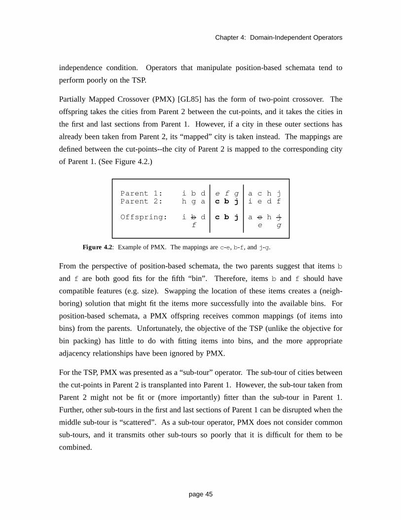
Chapter 4: Domain-Independent Operators
page 45
independence condition. Operators that manipulate position-based schemata tend to
perform poorly on the TSP.
Partially Mapped Crossover (PMX) [GL85] has the form of two-point crossover. The
offspring takes the cities from Parent 2 between the cut-points, and it takes the cities in
the first and last sections from Parent 1. However, if a city in these outer sections has
already been taken from Parent 2, its “mapped” city is taken instead. The mappings are
defined between the cut-points--the city of Parent 2 is mapped to the corresponding city
of Parent 1. (See Figure 4.2.)
Figure 4.2: Example of PMX. The mappings arec -e, b-f , andj -g.
From the perspective of position-based schemata, the two parents suggest that itemsb
and f are both good fits for the fifth “bin”. Therefore, itemsb and f should have
compatible features (e.g. size). Swapping the location of these items creates a (neigh-
boring) solution that might fit the items more successfully into the available bins. For
position-based schemata, a PMX offspring receives common mappings (of items into
bins) from the parents. Unfortunately, the objective of the TSP (unlike the objective for
bin packing) has little to do with fitting items into bins, and the more appropriate
adjacency relationships have been ignored by PMX.
For the TSP, PMX was presented as a “sub-tour” operator. The sub-tour of cities between
the cut-points in Parent 2 is transplanted into Parent 1. However, the sub-tour taken from
Parent 2 might not be fit or (more importantly) fitter than the sub-tour in Parent 1.
Further, other sub-tours in the first and last sections of Parent 1 can be disrupted when the
middle sub-tour is “scattered”. As a sub-tour operator, PMX does not consider common
sub-tours, and it transmits other sub-tours so poorly that it is difficult for them to be
combined.
Parent 1: i b d e f g a c h jParent 2: h g a c b j i e d f
Offspring: i b d c b j a c h jf e g

Chapter 4: Domain-Independent Operators
page 46
Figure 4.3: Example of CX. Subset 1 has the alleles of cycle 1, and subset 2 has thealleles of cycle 2 and cycle 3. The genes from subset 1 are taken from Parent 1, and thegenes of subset 2 are taken from Parent 2.
Cycle Crossover (CX) [OSH87] uses “cycles” to ensure that feasible offspring solutions
are produced. A cycle is a set of positions (alleles) that have the same cities (genes) in
both parents. Unary cycles (common cities) are transferred directly, and the remaining
are split into two subsets. One parent provides the genes for each subset. (See Figure
4.3.) Unfortunately, the building blocks manipulated by Cycle Crossover do not match
the edge-based objective of the TSP.
4.2.2 Edge-Based Schemata
Edge-based schemata interpret a permutation sequence as a series of adjacency relation-
ships. If the permutation sequence represents the order in which cities should be visited,
the salesman will travel the distance between each pair of adjacent cities. Thus, the edges
(between the adjacent cities) make logical building blocks for the TSP. Specifically, fit
solutions should be composed of fit (short/low-weight) edges.
Edge Recombination (ER) [WSF89] uses an intermediate representation to process the
parent sequences into an offspring solution. This “edge map” lists the cities that are
adjacent to a city (preceding or succeeding) in either of the parents. Each city is adjacent
to 2, 3, or 4 other cities. To build the offspring, choose the city (in the current edge map)
that has the fewest remaining options in its edge map. (See Figure 4.4.)
Parent 1: h k c e f d b l a i g jParent 2: a b c d e f g h i j k l
common: ucycle 1: 1 1 1 1 1cycle 2: 2 2 2cycle 3: 3 3 3
subset 1: h l a i jsubset 2: b d e f g k
Offspring: h b c d e f g l a i k j

Chapter 4: Domain-Independent Operators
page 47
Figure 4.4: Example of ER. Start with cityd because its edge map has only tworemaining choices. From these choices, (randomly) pick cityc to visit next. Theupdated edge map for cityc is c : a, b, d. Since citya has only two remaining choices,versus three choices for cityb, city a is chosen. In the final offspring, the common edged-e is disrupted, and the new edgeb-d is added (mutation).
Edge Recombination manipulates edge-based schemata (i.e. edges)--parent edges are
transmitted to the offspring where they are combined. From this original version, ER has
been modified to preserve more common edges (e.g. [SMM91]). With each modification,
more common edges are preserved and the performance of the operator improves. Since
the latest version of ER preserves all common edges [MW92], a commonality-based form
of ER has essentially been developed.
4.2.3 Order-Based Schemata
Order-based schemata interpret a permutation sequence as a series of relative position
relationships (e.g. before and after). Although the objective for the TSP is edge-based,
there is an implicit order-based aspect to this objective when the edge weights represent
physical distances. For example, if there are two clusters of cities, one on the east coast
and one on the west coast, the cities on the east coast should be visitedbefore the cities
on the west cost, or vice-versa. Thus, good order relationships (schemata) can be useful
for geometric TSPs.
Order Crossover (OX) [Dav85a][OSH87] has the form of two-point crossover. The
offspring starts by taking the cities of Parent 2 between the cut-points. Then, starting
from the second cut-point, the offspring takes the cities of Parent 1 (“wrapping around”
from the last segment to the first segment). When a city that has been taken from Parent
Parent 1: a b c d e fParent 2: c d e b f a
Edge Maps: a: b, c, f b: a, c, e, f c: a, b, d d: c, e
f: a, b, e e: b, d, f
Offspring: d c a f e b

Chapter 4: Domain-Independent Operators
page 48
2 is encountered, it is skipped--the remaining cities are appended in theorder they have
in Parent 1. (See Figure 4.5.)
Figure 4.5: Example of OX. Compared to PMX, OX can be less disruptive to sub-tours.For example, the sub-toure-f -g in Parent 1 is now transmitted to the offspring.However, the common sub-tourg-a-c is (still) disrupted.
Order crossover assumes that good solutions consist of good sub-tours and/or good order.
Thus, OX combines a sub-tour taken from Parent 2 with order taken from Parent 1.
Beyond the asymmetry of these actions, common sub-tours and common order are not
considered during the recombination process.
The above operators all use a “natural” (symbolic) representation for sequences.
However, sequences can also be represented by binary matrices. For example, anxn
Boolean matrix represents order-based schemata. Element if cityj follows
city i in the sequence1, otherwise element . A feasible solution requires
three constraints to be satisfied. First, the order must be complete: there are
ones. Second, transitive order is maintained: if element and element
, then element . Third, there are no cycles: element
for all i .
If two feasible matrices are intersected (i.e. only common order relationships are
preserved), a matrix satisfying the last two constraints is created. This under-constrained
“intersection” matrix can be completed by adding random1’s (with an analysis of row/
column sums to ensure feasibility). The result is the Matrix Intersection operator (MI)
[FM91]. (See Figure 4.6.) Due to the matrix representation, MI has an O(n2) time
1. A random city is usually fixed for the first position of all solutions.
Parent 1: i b d e f g a c h jParent 2: h g a c b j i e d f
c b j a c h j i b d e f g
Offspring: e f g c b j a h i d
i j,( ) 1=
i j,( ) 0=
n n 1–( ) 2⁄
i j,( ) 1=
j k,( ) 1= i k,( ) 1= i i,( ) 0=

Chapter 4: Domain-Independent Operators
page 49
complexity--much slower than the O(n) time complexity of the previous operators. In
addition to their intuitive appeal, natural representations often have time and space advan-
tages over binary representations.
Figure 4.6: Example of Matrix Intersection operator.
The Matrix Intersection operator preserves all common order relationships. However,
unlike Order Crossover, MI does not wrap around. Since MI implicitly interprets the
sequence as a “path” (where the start city is not revisited) rather than a “cycle”, it
performs better on Hamiltonian path problems like flow shop scheduling (see chapter 9).
Unfortunately, it performs rather poorly on the TSP.
4.3 Preserving Common Components in Sequence-BasedOperators
If an operator does not preserve common components, it cannot benefit from common-
ality-based selection. To isolate its effects in blind operators, an existing sequence-based
operator has been (minimally) modified to preserve common components. Commonality-
based selection is responsible for the improved performance.
Parent 1: a b c d e f gParent 2: a e f d b c g
Offspring: a b e d f c g
Parent 1: abcdefga 0111111b 0011111c 0001111d 0000111e 0000011f 0000001g 0000000
Parent 2: abcdefga 0111111b 0010001c 0000001d 0110001e 0111011f 0111001g 0000000
Inter- abcdefga 0111111b 0010001c 0000001d 0000001e 0000011f 0000001g 0000000
Offspring: abcdefga 0111111b 001 111 1c 0000001d 00 1 00 1 1e 00 11 011f 00 1 0001g 0000000
sectionMatrix:

Chapter 4: Domain-Independent Operators
page 50
4.3.1 Maximal Sub-Tour Order Crossover
Order Crossover (OX) assumes that good sub-tours can be extracted from the parents and
used to build better offspring. By the commonality hypothesis, an above-average sub-
tour that can be taken is the Maximal Sub-Tour (MST)--the longest (undirected) sub-tour
that is common to both parents. Thus, OX is modified to preserve the MST.
Figure 4.7: Example of MST-OX. The Maximal Sub-Tourg-a-c is now preserved.
After scanning both parents to identify the Maximal Sub-Tour, the first cut-point occurs
to the immediate left of the MST in Parent 2. The second cut-point is then made a
random distance to the right of the MST1. (See Figure 4.7.) Maximal Sub-Tour Order
Crossover (MST-OX) then continues with the regular “appending” procedure of Order
Crossover. Except for the explicit preservation of the MST, the new operator is identical
to OX.
4.3.2 Results: MST-OX vs. OX
The commonality hypothesis suggests that common sub-tours should be shorter than
uncommon sub-tours. To measure the relative fitness of a sub-tour, the average edge
length of the sub-tour can be divided by the average edge length of the entire (parent)
sequence2. This ratio for relative fitness is expected to be 1.00 for random schemata, and
a ratio of less than 1.00 is expected for above-average schemata.
1. For the second cut-point, wrap around is allowed. Virtually, the start position of the MST is“rotated” to become the first position of the sequence.
2. Since the TSP is a minimization problem, this ratio is actually relative cost: (sub-tour length/sub-tour edges) / (total length/n). Relative cost and relative fitness have an inverse relationship.
Parent 1: i b d e f g a c h jParent 2: h g a c b j i e d f
g a c b j i c h ji b d e f g a
Offspring: f g a c b j i h d e

Chapter 4: Domain-Independent Operators
page 51
In OX, the expected ratio of 1.00 is observed for the random sub-tours that are taken from
Parent 2. (See “OX_ratio” in Figure 4.8.) Conversely, the “MST_ratio” tends to be less
than 1.00--this represents the expected higher relative fitness/lower relative cost for the
common components of above-average parents. Although the overall sub-tour taken from
Parent 2 includes additional (random) components, the “MST-OX_ratio” still tends to be
less than 1.00. Therefore, the transplanted sub-tour in MST-OX is above average (relative
to the average fitness of sub-tours in Parent 2).
Figure 4.8: Relative fitness. The graph shows the average relative fitness of various sub-tours for each generation during a single run on thelin318 instance. A lower relative costequates to a higher relative fitness.
From the perspective of sub-tours, the (order-based) appending procedure of Order
Crossover causes (random) “mutations”. These mutations are restricted to the less-fit
(uncommon) sub-tours in MST-OX, so beneficial changes should occur more frequently
(see section 3.9). Specifically, the offspring of MST-OX should be fitter than the
offspring of OX. (See Figure 4.9.) However, the average ratio of offspring length to
parent length is always greater than 1.00 for both operators--the average offspring is less
fit than its parents.
0.85
0.9
0.95
1
1.05
1.1
0 50 100 150 200 250
Rel
ativ
e C
ost
Generation
"MST_ratio""MST-OX_ratio"
"OX_ratio"

Chapter 4: Domain-Independent Operators
page 52
Figure 4.9: Ratio of offspring length to parent length. The graph shows the averagelength of offspring relative to the length of their parents for each generation during asingle run on thelin318 instance. A lower ratio indicates a fitter offspring.
Using an elitist replacement scheme to ensure forward progress, Maximal Sub-Tour
Order Crossover performs better than Order Crossover. (See Table 4.1.) In addition to
elitism and fitness-based selection, the search procedure for MST-OX also benefits from
commonality-based selection. The preservation of common components has improved
the performance of a domain-independent (blind) operator.
Table 4.1: Performance of MST-OX and OX on 5 TSP instances. Results are fora steady-state GA with a population size of 1000 run for 250 generations. Valuesare percent distance from known optimum for average of 5 runs.
TSPInstance Size
AverageRandom
Start Tour
Avg. BestMST-OX Tour
Avg. BestOX Tour
d198 198 + 947 % + 113 % + 85 %
lin318 318 + 1194 % + 301 % + 352 %
fl417 417 + 3723 % + 760 % + 852 %
pcb442 442 +1328 % + 461 % + 485 %
u574 574 + 1627 % + 630 % + 700 %
average + 1764 % + 453 % + 495 %
1
1.01
1.02
1.03
0 50 100 150 200 250
Leng
th R
atio
Generation
"MST-OX""OX"

Chapter 4: Domain-Independent Operators
page 53
4.4 Summary
Crossover operators in genetic algorithms are not completely domain independent. If the
manipulated schemata do not match the “structure” of the objective function, fitness-
based selection will not amass useful building blocks. For properly matched alleles, the
commonality hypothesis helps to identify the most promising building blocks. The
preservation of these (common) components allows fitness-based selection to be
enhanced by commonality-based selection.

Chapter 5
Heuristic Operators:
Part One
Heuristic operators use problem specific heuristics to generate the (initial)
crossover offspring. The Commonality-Based Crossover Framework is
the first design model to specifically address this operator category. It
suggests that problem specific heuristics should replace (not supplement)
the traditional mechanisms of transmission and combination.
Chapter 5: Heuristic Operators: Part One
page 55
5.1 Overview
General methods for function optimization--like genetic algorithms with blind operators-
-are rarely competitive with problem specific methods. For practical applications, the
basic GA mechanisms are often supplemented with problem specific heuristics. If these
heuristics (help) select schemata (genes)during the crossover process, the resulting
procedure is aheuristicoperator.
The Commonality-Based Crossover Framework defines a two step process for crossover:
1) preserve the maximal common schema of two parents, and 2) complete the solution
with a construction heuristic. This design model is the first that specifically addresses
heuristic operators. In particular, it views the traditional mechanisms as weak heuristics.
Specifically, transmission and combination are no longer viewed as the critical features of
crossover.
Random recombination does not guarantee that an offspring solution will receive thebest
components from its parents. If the individual components can be independently
evaluated, the best components could be (heuristically) combined into an offspring.
However, the best components might not be present in the parents. Therefore, the new
design model suggests that problem specific heuristics shouldreplace (not supplement)
combination during the crossover process.
The Commonality-Based Crossover Framework completes a solution with “construction”
heuristics--methods that (incrementally) build complete solutions from partial solutions.
For the Traveling Salesman Problem, edge-based and order-based construction heuristics
are available. With these heuristics, two “commonality-based” heuristic operators have
been developed: Common Sub-Tours/Nearest Neighbor (CST/NN) and Maximum Partial
Order/Arbitrary Insertion (MPO/AI).
Experiments on CST/NN show that transmission and combination can interfere with the
effectiveness of Nearest Neighbor. Experiments on MPO/AI show that an operator’s
effectiveness improves when the basis of the common schemata matches the basis of the
construction heuristic. When these bases are matched, the heuristic operator can handle
constraints with the same basis. For example, MPO/AI has been applied to the
Sequential Ordering Problem.

Chapter 5: Heuristic Operators: Part One
page 56
5.2 Edge-Based Schemata
The Nearest Neighbor (NN) construction heuristic manipulates edge-based schemata.
Starting from a random city, Nearest Neighbor travels to the nearest unvisited city. At
each step, the shortest available edge is added to the (partial) solution. After all the cities
have been visited, Nearest Neighbor returns to the original start city.
Greedy Crossover [GGR85] is an early heuristic operator that uses Nearest Neighbor to
supplement (edge) combination. However, the uncommon edges of two Nearest
Neighbor parent solutions tend to be the (undesirable) long/crossing edges. (See Figure
3.2.) As a corollary to the commonality hypothesis, uncommon schemata are below
average. Therefore, instead of combining these uncommon edges, Nearest Neighbor
should generate new edges altogether. Following this advice, Common Sub-Tours/
Nearest Neighbor is developed as a commonality-based heuristic operator. Experimental
results show that CST/NN performs better than Greedy Crossover.
5.2.1 Greedy Crossover
It has been suggested that crossover should combine the best genesfrom the parents.
With edge-based schemata, this procedure leads to Greedy Crossover (GX). Starting
from a random city, GX takes the shortest edge1 from either parent that connects the
current city to an unvisited city. Since transmission and combination are still the primary
heuristics, Nearest Neighbor is only used when none of the parent edges are feasible.
The parent edges that are taken may be the good edges responsible for the high observed
fitness of the parents, or they may be the poor edges which should be replaced. This lack
of differentiation allows poor components to “hitch hike” their way into the offspring by
tagging along with the good components. Due to this deficiency, the transmission design
principle is a weak (construction) heuristic.
5.2.2 Common Sub-Tours/Nearest Neighbor
The Commonality-Based Crossover Framework suggests that only common edges, which
form the Common Sub-Tours (CST), should be taken (preserved) from the parents. By
1. As an influence from Edge Recombination (see section 4.2.2), undirected edges are used insteadof directed edges.

Chapter 5: Heuristic Operators: Part One
page 57
the commonality hypothesis, these are the good edges responsible for the high observed
fitness of the parents. Treating these common edges/sub-tours as “super nodes”, the
normal procedure of Nearest Neighbor can be used. (See Figure 5.1.) The above process
defines the Common Sub-Tours/Nearest Neighbor heuristic operator.
Figure 5.1: Example of CST/NN. The common (CST) edges are preserved, and theremaining uncommon edges are discarded. As a result, there is no opportunity for combi-nation. Instead, Nearest Neighbor is used to generate new edges to complete theoffspring solution.
Greedy Crossover and CST/NN both use the Nearest Neighbor construction heuristic.
Thus, these experiments isolate the elimination of the transmission design principle from
CST/NN. The uncommon components that transmission attempts to preserve are
expected to be below average. Thus, changes to these components are more likely to be
beneficial--the problem specific heuristic should be more effective than the domain-
independent “heuristic”.
5.2.3 Results: CST/NN vs. GX
The Common Sub-Tours/Nearest Neighbor and Greedy Crossover operators have been
tested experimentally on a series of TSP instances. The initial population is seeded with
Nearest Neighbor started from each city. Since Nearest Neighbor is a deterministic
operator, the population is sized to the problem size (to match the number of available
start tours). In these experiments, CST/NN finds better solutions than GX. (See Table
5.1.)
Parent 1 Parent 2
CST CST/NN

Chapter 5: Heuristic Operators: Part One
page 58
Although GX preserves most of the common edges, it also attempts to maximize trans-
mission. Without transmission, CST/NN can explore a larger solution set than GX, and
the increase in exploratory power (see section 3.3) leads to a more effective operator.
Overall, these experiments suggest that transmission and combination can interfere with
the performance of a problem specific heuristic (see chapter 11).
5.3 Order-Based Schemata
Insertion heuristics manipulate order-based schemata. Starting with a partial order of at
least three (random) cities, cities are “inserted” into the cyclic partial order between two
(currently adjacent) cities. Although this process adds two edges and deletes one edge,
order relationships (1’s in a Boolean matrix) are only added--cityi stays before/after city
j regardless of any additional cities that are inserted between them. At each step, the
insertion point is chosen to minimize the incremental increase in distance.
There are no insertion-based heuristic operators available in genetic algorithms, but a
comparable procedure exists in A-Teams. For the TSP, a “deconstruction/reconstruction”
procedure has used Arbitrary Insertion1 in the “reconstruction” phase [TdS92]. However,
(common) edge-based components are preserved during the “deconstruction” phase, so
the two phases manipulate mismatched components. Preserving common order-based
schemata instead, Maximum Partial Order/Arbitrary Insertion is developed as a common-
1. At each step, a randomly selected city is inserted.
Table 5.1: Performance of CST/NN and GX on 5 TSP instances. Results are for a steady-state GA witha population size equal to problem size, run until 20 generations pass without an improvement. Values arepercent distance from known optimum for average of 5 runs.
TSPInstance
Avg. BestNN Start Tour
Avg. BestCST/NN Tour
Common EdgesFrom Parents
Avg. BestGX Tour
Common EdgesFrom Parents
d198 + 12.42 % + 5.13 % 100.0 % + 10.72 % 99.8 %
lin318 + 17.06 % + 9.16 % 100.0 % + 16.95 % 100.0 %
fl417 + 16.92 % + 13.22 % 100.0 % + 10.66 % 100.0 %
pcb442 + 15.17 % + 9.64 % 100.0 % + 12.11 % 99.0 %
u574 + 19.92 % + 11.36 % 100.0 % + 15.98 % 99.9 %
average + 16.30 % + 9.70 % 100.0 % + 13.28 % 99.7 %

Chapter 5: Heuristic Operators: Part One
page 59
ality-based heuristic operator. Experimental results show that MPO/AI performs better
than the deconstruction/reconstruction procedure.
The MPO/AI operator was originally designed for the TSP. However, it performs better
(in relative terms) on the Sequential Ordering Problem (SOP). The SOP is a precedence
constrained Hamiltonian path problem. Its order-based constraints can be handled “trans-
parently” by the order-based mechanisms in MPO/AI. Experimentally, MPO/AI found
best-known solutions to many SOP instances (although most of these have since been
improved by HAS-SOP [GD97]). The results suggest that “transparent” constraints can
induce a beneficial search space reduction (see chapter 9).
5.3.1 Deconstruction/Reconstruction
As defined in A-Teams[TdS92], the goal of deconstruction is to identify useful compo-
nents (e.g. building blocks) in existing solutions. Ideally, better solutions can be recon-
structed from these components. The following deconstruction mechanism identifies the
common edges of two parents. However, they are not used as edges--they are used to
create a partial order by dropping the remaining cities from Parent 1. (See Figure 5.2.)
Figure 5.2: Example of deconstruction. Although common edges are preserved, theirorientation can be reversed between parents (e.g.a-b andg-h).
Arbitrary Insertion performs reconstruction by rebuilding a complete solution from the
partial order. Unfortunately, the initially preserved common edges can be deleted during
insertion. Since the common parent components (edges) are not always preserved in the
final offspring solution, deconstruction/reconstruction does not necessarily benefit from
commonality-based selection.
Parent 1: a b c d e f g h i j k lParent 2: a c d e k i j f h g l b
commonedges : a-b d-e g-h i-j
partialorder : a b d e g h i j

Chapter 5: Heuristic Operators: Part One
page 60
5.3.2 Maximum Partial Order/Arbitrary Insertion
The neighborhood considered by deconstruction/reconstruction does not always include
both parents. Specifically, if any of the common (undirected) edges have reverse
(directed) orientations, then insertion cannot rebuild Parent 2 from the partial order.
Since a common schema is a partial order that insertion can extend into both parents, the
schemata identified by deconstruction may not be common to both parents. The longest
common partial order is the Maximum Partial Order (MPO). Using Arbitrary Insertion to
complete this partial solution, the overall process defines the Maximum Partial Order/
Arbitrary Insertion heuristic operator.
Figure 5.3: Pseudo-code to find the Maximum Partial Order of two parent sequences.
The pseudo-code for generating the Maximum Partial Order of two parents is listed in
Figure 5.3. To convert the parent sequences into Boolean matrices, all solutions are
assigned the same start city and the same orientation1. Since element when
city i precedes cityj in the sequence, the intersection matrix has element if
and only if cityi precedes cityj in both parents. These1’s represent the common order-
based schemata of two parents.
1. Three evenly spaced convex hull cities (e.g.a, b, c ) define the orientation of all solutions (i.e.a...b...c ...). These cities are the start cities for the three segments that compose the MPO (i.e. theMPO procedure is run three times during MPO/AI).
- Convert parent sequences to Boolean matrices- Intersect matrices- Sum columns to get each city’s predecessors- Build partial order graph - Find city with fewest number of predecessors - Attach city to the predecessor with the most
ordered predecessors- Find longest path in graph
i j,( ) 1=
i j,( ) 1=

Chapter 5: Heuristic Operators: Part One
page 61
Figure 5.4: Example of MPO. Citya is the segment start city, so it has0 ordered prede-cessors at the root of the partial order graph. Cityg is preceded by all of the cities in thegraph, but it can only be attached to citiesc and f because those cities have the mostordered predecessors (2).
In the intersection matrix, the column sums give the number of common predecessors for
each city. Using the segment start city as the root of the partial order graph, cities are
added in increasing order of their predecessors1. Each city is “attached” to the common
predecessor (identified by a1 in its column of the intersection matrix) with the most
“ordered” predecessors. The new city will have one more ordered predecessor than the
city it is attached to--each node represents the longest partial order for that city. When all
cities have been added, the longest path represents the Maximum Partial Order. (See
Figure 5.4.)
1. All ties are broken randomly.
Parent 1: a b c d e f gParent 2: a e f d b c g
Parent 1: abcdefga 0111111b 0011111c 0001111d 0000111e 0000011f 0000001g 0000000
Parent 2: abcdefga 0111111b 0010001c 0000001d 0110001e 0111011f 0111001g 0000000
Intersection abcdefga 0111111b 0010001c 0000001d 0000001e 0000011f 0000001g 0000000
Matrix:
Predecessors: 0121126
Maximum Partial Order: a b c g
g,3
f,2
c,2
e,1
b,1
d,1a,0
PartialOrderGraph:

Chapter 5: Heuristic Operators: Part One
page 62
Figure 5.5: Example of “shape” from the convex hull, the MPO, and deconstruction.
As order-based schemata, partial orders represent “shape” templates. Shape is useful (for
geometric TSPs) because insertion heuristics perform better when they are started from
good “outlines”. For example, if AI is started with the convex hull, it will find solutions
about 1% better than those found with three random cities [Rei94]. The shape of the
MPO is more refined than the convex hull (see Figure 5.5), so AI should perform even
better when it is (re)started from this partial solution.
5.3.3 Results: MPO/AI vs. Deconstruction/Reconstruction
The MPO/AI operator and the deconstruction/reconstruction procedure have been tested
experimentally on a series of TSP instances. The initial population is seeded with 400
Arbitrary Insertion solutions each started from the convex hull. To reduce the rate of
convergence with MPO/AI, one parent is chosen randomly. In these experiments, MPO/
AI performs better than deconstruction/reconstruction. (See Table 5.2.)
Convex Hull MPO Deconstruction
Parent 1 Parent 2

Chapter 5: Heuristic Operators: Part One
page 63
Deconstruction uses the natural (symbolic) representation for TSP solutions, so it is much
faster than finding the MPO--which has an O(n2) time complexity. However, the partial
order of deconstruction is not as useful as the Maximum Partial Order. The outline
produced from (common) edges might not represent the “shape” (defining schema) of
two parent solutions. (See Figure 5.5.)
5.3.4 MPO/AI and the Sequential Ordering Problem
The Sequential Ordering Problem (SOP) is a constrained Hamiltonian path problem.
Specifically, represents a precedence constraint that requires nodej to
precede (not necessarily immediately) nodei in the sequence1. The objective is to find
the shortest Hamiltonian path through the graph ofn nodes subject to satisfying the
precedence constraints. Visually, if a courier hasn clients to visit, and clients with
objects to be “picked up” must be visited before those objects can be “dropped off”, find
a sequence such that travel distance is minimized--subject to visiting each client once and
only once and performing all (paired) pick-ups before their corresponding drop-offs.
Formally, givenn nodes with edge weights , find a sequenceπ of then
nodes such that the following sum is minimized and all precedence constraints are
satisfied:
1. For convenience, problem matrices tend to include “dummy” nodes for the first and last positionsof the (non-cyclic) sequence.
Table 5.2: Performance of MPO/AI and deconstruction/reconstruction on 5 TSP instances. Results are fora steady-state GA with a population of 400 run until 10 generations pass without an improvement. Valuesare percent distance from known optimum for average of 5 runs. Experiment runtimes are given for aSPARC 20.
TSPInstance
Average BestConvex Hull/
AI Start
Average BestMPO/AI
Runtime(min)
Average BestDeconstruction/Reconstruction
Runtime(min)
d198 + 3.05 % + 0.95 % 3 + 1.31 % 1
lin318 + 6.04 % + 0.63 % 13 + 3.38 % 2
fl417 + 1.91 % + 0.57 % 15 + 0.52 % 7
pcb442 + 8.97 % + 1.84 % 37 + 4.20 % 9
u574 + 8.45 % + 2.20 % 74 + 4.01 % 13
average + 5.68 % + 1.24 % + 2.68 %
d c i c j,( ) 1–=
c i d c i c j,( )

Chapter 5: Heuristic Operators: Part One
page 64
if
then
for ,
Although the objective of the SOP is edge-based, its constraints are order-based--
requires nodej to precede nodei , but it does not constrain the number
of (inserted) nodes between them. Therefore, the constraints are transparent to insertion.
Further, the intersection matrix of two feasible parents includes all of their (satisfied)
precedence constraints--each constraint specifies a1 in the Boolean matrix. Subse-
quently, MPO/AI can be applied to the Sequential Ordering Problem with minor modifi-
cations1.
The MPO/AI operator has been tested experimentally on a series of SOP instances2. The
initial population is seeded with 500 Arbitrary Insertion solutions. In these experiments,
MPO/AI finds new best-known solutions for many of the tested SOP instances. Although
MPO/AI is slowed by the O(n2) time complexity associated with matrix representations,
it is still faster than a branch and cut algorithm3 [Asc96]. MPO/AI uses roughly 2% of
the computational effort to reach the (best-known solution) bounds set by the branch and
cut algorithm. (See Table 5.3.)
The order-based mechanisms of MPO/AI match the order-based constraints of the SOP.
This transparently reduces the search space--MPO and AI are oblivious to the existence
of the precedence constraints. In contrast, order-based constraints create “obstacles” in
edge-based search spaces. Thus, edge-based methods (e.g. integer programming) require
additional mechanisms to handle the constraints explicitly. If these mechanisms interfere
with the process of optimization, relative performance can suffer. Although branch and
1. AI is modified to generate only feasible solutions, and MPO is modified to use only one segment.
2. These instances are also taken from TSPLIB (see section 2.9.2).
3. In this study, the branch and cut algorithm was run for 300 minutes on a SPARC 2; 1200 minutesfor the larger “rbg” instances.
min
πd c π k( ) c π k 1+( ),( )
k 1=
n 1–
∑
d c i c j,( ) 1–=
l k<
π l( ) j= π k( ) i=
d c i c j,( ) 1–=

Chapter 5: Heuristic Operators: Part One
page 65
cut algorithms can find optimal solutions on the TSP, they are less effective (than MPO/
AI) on the SOP.
5.4 Additional Comments
As indicated by the lack of asterisks, new best-known solutions have since been found for
many of the presented SOP instances. These solutions were found by HAS-SOP: a
Hybrid Ant System for the Sequential Ordering Problem [GD97]. In HAS-SOP, an initial
solution (of unreported quality) is generated by an ant colony (see section 2.8.5), and it is
locally optimized with a “lexicographic” search operator. Essentially, a hybrid operator
has been compared to a heuristic operator. The new distinction between heuristic and
hybrid operators leads to better (more direct) comparisons among operator instances.
Table 5.3: Performance of MPO/AI on 16 SOP instances taken from TSPLIB. Results are for 5 runs of asteady-state GA with a population of 500 run until 20 generations pass without an improvement. Overallbest MPO/AI solutions in bold improved the previous best-known bounds. (Asterisks indicate that boundis still current.) Times are given for execution on a SPARC Ultra 1 (167 MHz).
SOPInstance Size Con-
straints
AverageBest
AI Start
AverageBest
MPO/AI
Overall BestMPO/AI
Original Branchand Cut Bounds
[Asc96]
Time toBound
(s)
Runtime(s)
ft70.1 71 17 41809 39615 39545 39313 NA 76
ft70.2 71 35 43485 40435 40422 [39739, 41778] 5.4 73
ft70.3 71 68 46731 42558 * 42535 [41305, 44732] 2.8 48
ft70.4 71 86 55982 53583 53562 [52269, 53882] 2.4 47
kro124p.1 101 25 45758 40996 40186 [37722, 42845] 5.4 136
kro124p.2 101 49 49056 42576 41677 [38534, 45848] 5.2 94
kro124p.3 101 97 63768 51085 50876 [40967, 55649] 3.8 103
kro124p.4 101 131 87975 76103 * 76103 [64858, 80753] 2.0 76
rbg323a 325 2412 3466 3161 3157 [3136, 3221] 207.6 1566
rbg341a 343 2542 3184 2603 2597 [2543, 2854] 70.6 2205
rbg358a 360 3239 3165 2636 2599 [2518, 2758] 533.8 4491
rbg378a 380 3069 3420 2843 2833 [2761, 3142] 67.6 5354
ry48p.1 49 11 16602 15813 * 15805 [15220, 15935] 2.4 22
ry48p.2 49 23 18071 16676 * 16666 [15524, 17071] 1.6 32
ry48p.3 49 42 22074 19905 * 19894 [18156, 20051] 7.6 29
ry48p.4 49 58 32591 31446 31446 [29967, 31446] 5.0 19

Chapter 5: Heuristic Operators: Part One
page 66
When the lexicographic operator is added to MPO/AI, the performance improvement
does not match HAS-SOP. The ant colony appears to have two advantages over MPO/AI
for generating initial solutions. First, the ant colony uses a natural representation, so it is
much faster. Second, the ant colony appears to maintain better diversity. The strict
preservation of common components in MPO/AI can cause undesirably strong conver-
gence effects. These advantages are less easily observed when HAS-SOP is compared
directly to MPO/AI.
5.5 Summary
The Commonality-Based Crossover Framework is the first design model to specifically
address the category of heuristic operators. Using the same (traditional) construction
heuristic as previous operators, the superior performance of the new operators isolates the
role of preserving common components. Further, these results suggest two key exten-
sions. First, the results of CST/NN suggest that the transmission design principle can
handicap the effectiveness of a problem specific heuristic (see chapter 11). Second, the
results of MPO/AI suggest that beneficial search space reductions can be developed for
commonality-based operators (see chapter 9).

Chapter 6
Heuristic Operators:
Part Two
As the primary focus of the Commonality-Based Crossover Framework,
heuristic operators deserve a deeper examination. This analysis leads to
commonality-based selection, heuristic amplification, and open-loop
optimization.

Chapter 6: Heuristic Operators: Part Two
page 68
6.1 Overview
The first step in the new design model states, “preserve the maximal common schema of
two parents”. This directive causes common schemata to beselected. To isolate this
commonality-based form of selection, GENIE (a GA without fitness-based selection) is
developed. When heuristic operators are implemented in GENIE, the (additional)
selective pressure supplied through commonality-based restarts can be observed. The
existence of commonality-based selection corroborates the commonality hypothesis--the
preserved common schemata are above average.
The commonality hypothesis provides a “confidence measure” on the performance of
construction heuristics--common decisions should be correct. Thus, heuristic operators
can use commonality-based selection to identify highly-fit partial solutions. With this
accumulated knowledge, restarts can develop better solutions. This effect represents
heuristic amplification.
The Schema Theorem suggests that global payoff information issufficient to perform
optimization. However, the existence of heuristic amplification suggests that it is no
longer necessary. If a standard genetic algorithms performs black box optimization (no
problem model is required), then a heuristic operator in GENIE is analogous to open-loop
optimization (no fitness feedback is required at the level of complete individuals).
6.2 GENIE
In the analysis of ideal construction heuristics (see section 3.7.2), the proportion of
correct schemata was calculated for each generation of a GA with random parent
selection and generational replacement. These features define GENIE--a GA that selects
neither mating parents nor surviving offspring on the basis of their fitness1. With the
elimination of fitness-based selection at the individual, GENIE allows commonality-
based selection to be isolated2.
1. Note: all parents mate twice during each generation to help reduce random biases.
2. For GENIE with finite populations, drift effects are still present.

Chapter 6: Heuristic Operators: Part Two
page 69
6.3 Heuristic Amplification
To amplify the effectiveness of construction heuristics, partial solutions with high propor-
tions of fit schemata are required (see section 3.7). Common schemata (i.e. the schemata
chosen by commonality-based selection) can form these desirable partial solutions.
Therefore, it should be more effective to embed a construction heuristic into a common-
ality-based operator than to use random restarts.
An ideal construction heuristic and a commonality-based heuristic operator have been
developed for One Max. In experiments, it is shown that common schemata are fitter
than random/average schemata (of the parents). Restarts from these partial solutions are
more effective--the (ideal) heuristic operator exhibits heuristic amplification.
The CST/NN and MPO/AI heuristic operators have also been implemented in GENIE.
Experimental results demonstrate that heuristic amplification can occur in practical
operators--even though non-ideal characteristics exist (e.g. “negative” heuristic amplifi-
cation). To combat the effects of negative heuristic amplification, fitness-based selection
(of parents) can be applied.
6.3.1 One Max
The correct gene for each allele is a1. Therefore, a trivial heuristic for One Max is to
select more1’s than0’s. For example, select a1 for each allele with a (constant) proba-
bility of , and a0 with a probability of . This (construction)
heuristic is ideal because the decision at each step has a constant (and independent)
probability of being correct.
The above heuristic has been embedded into a commonality-based heuristic operator and
implemented in GENIE. For a One Max problem of 100 bits, GENIE is run for 20 gener-
ations with a population size of 100. Starting from an initial population that is seeded by
random restarts of the construction heuristic, the optimal solution is always found. (See
Table 6.1.) The superior fitness of the final solutions demonstrates that heuristic amplifi-
cation has occurred.
p 0.6= 1 p– 0.4=

Chapter 6: Heuristic Operators: Part Two
page 70
To measure the effects of commonality-based selection, the average fitness of the partial
solutions has been recorded. The ratio of1’s to 0’s in the common schemata is always
greater than the corresponding ratio for random schemata in the entire population. (See
Figure 6.1.) The commonality hypothesis is valid in this experiment--the average fitness
of the common components was above the average fitness of their parents.
Figure 6.1: Average fitness of common and random components in One Max.
Since common components are above average, the average fitness of the remaining
uncommon components must be below the average fitness of the parents. In particular,
an uncommon allele will have a1 in one parent and a0 in the other. The average fitness
of uncommon components in One Max is always 0.5.
6.3.2 Common Sub-Tours/Nearest Neighbor
A practical construction heuristic (e.g. Nearest Neighbor) is not expected to make correct
decisions with a constant probability. For example, constraints may disallow the correct
decision at any given step. Nonetheless, to study the effects of heuristic amplification for
practical construction heuristics, Common Sub-Tours/Nearest Neighbor has been imple-
mented in GENIE.
Table 6.1: Results for an ideal construction heuristic in GENIE.
Avg. Best Start Avg. Best Overall
One Max 72.1 100.0
0.5
0.6
0.7
0.8
0.9
1
0 5 10 15 20
Ave
rage
Fitn
ess
Generation
"common""random"

Chapter 6: Heuristic Operators: Part Two
page 71
Figure 6.2: Relative cost of common (CST) edges in CST/NN for a single run on thelin318 instance.
The common (CST) edges of two parents should be their short edges. (See Figure 3.2.)
This expectation is confirmed by measuring their relative fitness (relative cost)--the
common edges are much shorter than average. (See Figure 6.2.) However, even with
these promising partial solutions, the results for CST/NN are unimpressive. (See Table
6.2.) Since only 14% of the initial surplus from optimal is reduced from the best start
solutions to the best final solutions, almost no heuristic amplification has occurred.
Table 6.2: Results for CST/NN in GENIE. Population size is equal toproblem size. Initial population is Nearest Neighbor started from eachcity. Values are percent surplus from known optimum for average of 5runs (50 generations each).
TSPLIBInstance
Avg. BestNN Start Tour
Avg. BestCST/NN Tour
d198 + 12.42 % + 8.67 %
lin318 + 17.06 % + 16.30 %
fl417 + 16.92 % + 13.37 %
pcb442 + 15.17 % + 13.30 %
u574 + 19.92 % + 18.40 %
average + 16.30 % + 14.01 %
0.7
0.75
0.8
0.85
0.9
0.95
1
0 5 10 15 20 25 30 35 40 45 50
Rel
ativ
e C
ost
Generation
"CST"

Chapter 6: Heuristic Operators: Part Two
page 72
For the TSP, it is not just the number of correct/incorrect edges that determines solution
quality. The length (relative fitness) of the incorrect edges (schemata) is also important.
Further, starting with a partial solution of short edges does not necessarily reduce the
tendency of Nearest Neighbor to “paint itself into a corner”. These results suggest that
Nearest Neighbor is a poor heuristic (very far from ideal).
6.3.3 Maximum Partial Order/Arbitrary Insertion
Maximum Partial Order/Arbitrary Insertion has also been implemented in GENIE. Since
a partial order represents an exponentially large number of solutions, the fitness of the
MPO cannot be measured directly. Nonetheless, it appears to have a superior relative
fitness--MPO/AI in GENIE reduces the surplus from optimal by 66% from the best start
solutions to the best final solutions. (See Table 6.3.)
The fitness of a partial order can be estimated by a random sample of the solutions that it
represents. For measurement convenience, the average fitness of a population is used to
approximate the fitness of common schemata in mating parents. This average fitness has
been measured for a single run of MPO/AI on thelin318 instance. (See Figure 6.3.)
Table 6.3: Results for MPO/AI in GENIE. Population size is 400, andthe initial population is 400 AI solutions started from the convex hull.Values are percent surplus from known optimum for average of 5 runs(50 generations each).
TSPLIBInstance
Avg. BestConvex Hull/AI
Start Tour
Avg. BestMPO/AI Tour
d198 + 3.05 % + 1.24 %
lin318 + 6.04 % + 1.75 %
fl417 + 1.91 % + 0.58 %
pcb442 + 8.97 % + 3.48 %
u574 + 8.45 % + 2.59 %
average + 5.68 % + 1.93 %

Chapter 6: Heuristic Operators: Part Two
page 73
Figure 6.3: Average population fitness (surplus) for MPO/AI in GENIE and (random)convex hull restarts of Arbitrary Insertion. Fitter populations imply fitter initial schemata.Thus, the MPO is fitter than the convex hull.
In addition to average fitness, the average length of the MPO for mating parents was also
recorded. The size of the partial solution preserved by commonality-based selection
grows consistently through generation 27. Further, the average quality of the MPO/AI
solutions also improves steadily until generation 28. After this phase of convergent
search, a “drift” phase begins which appears to degrade solution quality.
To baseline the MPO/AI results, 50 generations of Arbitrary Insertion restarts from the
convex hull are also plotted. The convex hull (CH) is a static entity, so it does not
accumulate information from previous solutions. Without information accumulation,
there is no “persistence ratchet” [Sha99] to advance search. Compared to the solution
quality of random restart which does not improve over time, these results demonstrate
that commonality-based selection has supplied selective pressure--it has identified and
preserved partial orders of increasing fitness and specificity.
6.3.4 Negative Heuristic Amplification
The effects of heuristic amplification can also be bad. If the probability of making
incorrect decisions is greater than the probability of making correct decisions, then
incorrect schemata will eventually dominate the population. For MPO/AI, its worst
performance occurs on thepcb442 instance. The “structure” of this instance induces
Arbitrary Insertion to make incorrect decisions that are non-random and non-
independent. (See Figure 6.4.)
0
50
100
150
200
250
300
350
0 5 10 15 20 25 30 35 40 45 50
Initi
al L
engt
h of
Par
tial O
rder
Generation
"MPO""CH"
0
2
4
6
8
10
12
0 5 10 15 20 25 30 35 40 45 50
Avg
Sur
plus
(%
)
Generation
"GENIE""restart"

Chapter 6: Heuristic Operators: Part Two
page 74
Figure 6.4: Simplified outlines of severalpcb442 solutions.
The optimal solution for thepcb442 instance includes a “shaft”. To traverse this shaft
correctly, cities must be inserted (in order) from the top. Otherwise, the inserted cities
may be incorrectly attached to the “right” edge. Since the next city is chosen randomly,
there arefewer correct decisions (see pointer 1) than incorrect decisions (see pointer 2).
As systematic errors, these incorrect decisions are likely common to all parents. Negative
heuristic amplification subsequently causes the final solution to be defined by these
incorrect decisions (see pointer 3).
6.3.5 Heuristic Amplification and Fitness-Based Selection
Examining the results for CST/NN (see Table 6.2 and Table 5.1) and the results for MPO/
AI (see Table 6.3 and Table 5.2), the performance of heuristic operators improves when
fitness-based selection is used. Fitness-based selection provides an additional confidence
measure on the performance of a construction heuristic. In particular, fitness-based
selection can help counteract the effects of negative heuristic amplification.
Convex Hull Optimal Solution
Typical AI Typical FinalStart Solution MPO/AI Solution
1
2
3

Chapter 6: Heuristic Operators: Part Two
page 75
For example, the ideal construction heuristic for One Max (see section 6.3.1) has been
redesigned to select1’s with a probability of . Since this heuristic makes
incorrect decisions more often than correct decisions, the resulting heuristic operator is
prone to negative heuristic amplification. This operator has been implemented in GAs
with (GENITOR) and without (GENIE) fitness-based selection. On a problem of 100 bits
with a population size of 100 solutions, GENITOR goes forward while GENIE goes
backward. (See Figure 6.5.)
Figure 6.5: Sample result for GENIE and GENITOR whenp = 0.45 .
Commonality-based selection is weak when the construction heuristic is weak. Since
practical (non-ideal) heuristics will have areas of weakness, fitness-based selection should
still be useful. Although commonality-based selection can enhance fitness-based
selection, it does not replace it.
6.4 Open-Loop Optimization
Closed-loop control is favored over open-loop control. However, feedback is not always
available (or useful). For example, rocket launches are open-loop--by the time the launch
vehicle is observed to be off course, it is too late. Likewise, it appears that fitness-based
selection (used in closed-loop optimization) can always improve the performance of
p 0.45=
0
20
40
60
80
100
0 10 20 30 40 50 60
Bes
t Obj
ectiv
e V
alue
Generation
"GENIE""GENITOR"

Chapter 6: Heuristic Operators: Part Two
page 76
heuristic operators (see section 6.3.5). Nonetheless, open-loop optimization is presented
as an available method.
Open-loop optimization is the reverse of black box optimization. In black box optimi-
zation, the structure of the problem is not modeled, but the fitness must be observable.
Genetic algorithms can then use domain-independent operators and fitness-based
selection at the individual level. Conversely, if the problem structure can be modeled
with enough accuracy, global payoff information may not be necessary. Specifically,
heuristic operators and commonality-based selection can be used instead. For both cases,
the overall objective must be decomposable--good solutions consist of good schemata,
and good schemata form good solutions.
In the experiments with MPO/AI in GENIE (see section 6.3.3), the fittest solutions are
often found in the last generation of the “convergent search” phase (when the average
MPO of mating parents is increasing monotonically). If GENIE is stopped when the
amount of schemata common to mating parents does not increase for the first time, the
best solution should be present in the final population. Further, this solution should be
optimal for an ideal construction heuristic (see section 3.7.2). Since intermediate
solutions do not need to be evaluated, open-loop optimization (non-fitness-based
evolution) can be pursued.
The results for heuristic operators in GENIE (see section 6.3) can be trivially converted
into results for open-loop optimization. Thus, this section focuses on finding optimal
solutions. Although the entire population should converge to the optimal solution for an
ideal construction heuristic, the same is not expected for practical heuristics.
6.4.1 One Max
Using , the ideal heuristic operator for One Max has been implemented in
GENIE. For a problem with 100 bits, a population size of 100 is used. When the
commonality-based stop condition is reached (i.e. when the number of bits common to
mating parents fails to increase), asingle (randomly chosen) member of the final
population is evaluated. In 30 trials, this solution was optimal 25 times. (See Table 6.4.)
p 0.6=

Chapter 6: Heuristic Operators: Part Two
page 77
6.4.2 Maximum Partial Order/Arbitrary Insertion
Since no optimal solutions were found in the previous experiments with MPO/AI (see
section 6.3.3), these experiments use the (easier)kroA100 instance. A population size of
100 is used, and GENIE is initialized with 100 solutions of Arbitrary Insertion started
from the convex hull. The average length of the MPO in mating pairs is recorded for
each generation, and GENIE is stopped when the average MPO does not increase for the
first time. All of the solutions in the final population are then evaluated.
In 30 trials, convergence requires an average of 8 generations, the average length of the
MPO at convergence is 90 cities, and the optimal solution is found 18 times. (See Table
6.5.) For comparison, 1000 random restart (seed) solutions of Convex Hull/Arbitrary
Insertion (CH/AI) are also run. In 30 trials, random restarts never finds the optimal
solution.
The schemata in the convex hull are correct--they are part of the optimal solution [Rei94].
The additional cities in the MPO must also be largely correct since optimal solutions
were found. Therefore, commonality-based selection can identify correct schemata, and
open-loop optimization with non-ideal operators is feasible.
Table 6.4: Ideal construction heuristic in GENIE versus restarts.
Method Optimal Trials Average Best
GENIE 25/30 99.8
3000 Restarts 0/30 77.4
Table 6.5: MPO/AI in GENIE onkroA100 versus 1000 random CH/AI solutions.
OperatorAlgorithm
OptimalTrials
Average Best(% surplus)
MPO/AIGENIE
18/30 + 0.04 %
CH/AI1000 restarts
0/30 + 0.44 %

Chapter 6: Heuristic Operators: Part Two
page 78
6.5 Summary
The GENIE algorithm allows the effects of commonality-based selection to be isolated in
heuristic operators. With the elimination of fitness-based selection, (positive) heuristic
amplification and open-loop optimization depend upon the selective pressure supplied by
commonality-based restarts. Since the preserved common components must be above
average to observe these effects, their existence depends on a satisfied commonality
hypothesis. In the preceding experiments, the common schemata preserved from the
above-average (parent) solutions were indeed above average.

Chapter 7
Hybrid Operators
A hybrid operator uses a local optimizer to post-process an initial start
solution. The quality of this solution affects the efficiency and effec-
tiveness of the overall hybrid operator. Compared to other forms of
crossover, commonality-based heuristic operators may provide better
restart points.

Chapter 7: Hybrid Operators
page 80
7.1 Overview
A crossover operator and a local optimizer form ahybrid operator. Since crossover
operators (heuristic or domain-independent) rarely produce locally optimal solutions, the
offspring can be improved by a local optimizer (i.e. hill climbing procedure). Unlike
heuristic operators which incorporate problem specific knowledge into the crossover
process, hybrid operators apply local search proceduresafter crossover1.
In a “hybrid GA”2, crossover produces start points. However, the goal of finding good
solutions is different from the goal of finding good start points. Therefore, operators that
have been designed as independent entities are unlikely to be effective restart methods.
The crossover operator should be matched to the local optimizer.
Despite the lack of intentional synergy, the two stages of a hybrid operator can still
cooperate. For example, local optimizers provide crossover operators with better building
blocks to combine. Conversely, (fitter) crossover offspring reduce the computational
effort expended by local optimizers to bring random start solutions into the near-optimal
region [UPL91]. In general, hybrid GAs are more effective than random restarts of the
local optimizer.
Although better than a random restart, the behavior of a weak, poorly matched, or
otherwise poorly designed crossover operator may not be significantly different. If
crossover does not consider the neighborhood structure of the local optimizer, the
provided offspring solution can exceed the exploratory horizon (of the parents). When
there is little correlation between the fitness of the parents and offspring, the search
procedure is effectively random. Therefore, crossover design affects the performance of
the overall hybrid operator.
The Commonality-Based Crossover Framework focuses on two aspects. First, if the
initial offspring solution is fitter, the computational efficiency of the local optimizer can
increase. Second, by exploiting common components which match the (neighborhood)
structure of the objective, the final offspring solutions should be less distant from their
1. This distinction between heuristic and hybrid operators is newly introduced. Previously, theseterms have been used interchangeably.
2. These have also been called memetic algorithms [RS94].

Chapter 7: Hybrid Operators
page 81
(above-average) parents. In a globally convex search space (like the TSP), offspring that
are closer to their parents will often be fitter.
7.2 Globally Convex Search Spaces
It has been suggested that hybrid GAs should be analyzed as best-of-k-runs approaches
[JM97]. If the local optimizer is solely responsible for the overall effectiveness of the
hybrid operator, then the perspective of neighborhood search is irrelevant. However,
local optima are often “clustered” in the search space (i.e. local optima have a neigh-
borhood structure). Therefore, neighborhood search is still relevant because good
(locally optimal) solutions can be used to find others.
When local optima are clustered in a “big valley”, the search space isglobally convex.
The existence of this structure causes locally optimal solutions to be closer to (have more
in common with) each other than random solutions [Müh91][Boe96][MBK97].
Conversely, meta-heuristics (e.g. genetic algorithms, tabu search, etc) are not useful
without this structure. Random restart should be equally effective when good solutions
are randomly distributed.
Figure 7.1: Typical distribution of local optima for the TSP.
Scatter plots are the best tool to observe the big valley structure of the TSP. When gener-
ating these graphs, each point represents a random local optima--fitness is on the y-axis
Average distance from other local minima
Cos
t

Chapter 7: Hybrid Operators
page 82
and average distance is on the x-axis1. In a typical scatter plot, the (2500) points fill a
diagonal ellipsoid [Boe96]. (See Figure 7.1.) The best solutions (in the lower left corner)
are closest to the other local optima--they are in the center of the big valley!
Figure 7.2: Simplified outline for Adaptive Multi-Start.
To explore this big valley, an Adaptive Multi-Start (AMS) procedure has been proposed
[Boe96]. (See Figure 7.2.) This procedure is similar to a hybrid GA that uses a multi-
parent, domain-independent operator to generate start points2. (See Figure 7.3.)
Although this construction procedure targets the common components that define the big
valley, it does not explicitly exploit itsstructure.
Figure 7.3: Simplified outline to construct adaptive starting tours for AMS.
The results for Adaptive Multi-Start are not significantly better than random restart3.
Since the analysis of AMS focuses on the population aspects (i.e. selection and
replacement), the role of the (implicit) hybrid operator is less thoroughly examined. The
following experiment on hybrid operators identifies weaknesses in the (domain-
independent) model for adaptive starting tours.
1. For the TSP, the (Hamming) distance represents the number of different edges between two solu-tions.
2. This procedure can be viewed as a multi-parent form of Edge Recombination (see section 4.2.2).
3. See Table 8.2 in [Boe96].
- Generate an initial population of random local optima- Generate new local optima from adaptive starting tours
- Create a set of edges from selected parents- Weight edges based on parent fitness- Add edges to “offspring” solution in order of weights- Add feasible edges as required to complete solution

Chapter 7: Hybrid Operators
page 83
7.3 Hybrid Operators for the Traveling Salesman Problem
Three hybrid operators that use 2-opt as the local optimizer are examined for the
Traveling Salesman Problem. Since the 2-opt local optimizer is held constant, these
experiments isolate the role of crossover. It is shown that offspring solutions with high
individual fitness can (synergistically) reduce the work load of the local optimizer.
Subsequently, the search effort is focused into a small (promising) neighborhood that
surrounds the two parent solutions.
7.3.1 The Local Optimizer
The 2-opt local optimizer is an edge-based hill climbing procedure. In a TSP solution,
each pair of edges can be exchanged for another pair of edges that will feasibly connect
the same four cities. If the alternative edge pair is shorter than the current edge pair, the
exchange is executed1. This procedure uses the smallest possible neighborhood size--it
disrupts the fewest edges.
7.3.2 The Crossover Operators
The three hybrid operators are extended from a commonality-based heuristic operator, a
heuristic operator that uses combination, and a domain-independent operator. Since the
basis of the 2-opt local optimizer is edges, these crossover operators are all based on
edges as well. The operators are Common Sub-Tours/Nearest Neighbors (see section
5.2.2), Greedy Crossover (see section 5.2.1), and Random, Respectful Recombination
[Rad91].
Random, Respectful Recombination (RRR) first preserves the common edges, and then it
selects the remaining edges randomly. In general, RRR is weaker than Edge Recombi-
nation because random edges are less fit than parent edges (which fitness-based selection
has evaluated indirectly). However, hybrid operators with RRR have been previously
reported [Esh91], and RRR is sufficient to demonstrate the weaknesses of the (domain-
independent) adaptive starting tours in AMS.
1. The “random” hill climbing version of 2-opt is used. Whenever an improving exchange is foundduring a sequential scan of all edge pairs, it is taken.

Chapter 7: Hybrid Operators
page 84
7.3.3 The Hybrid Operators
Greedy Crossover solutions often have crossing edges that 2-opt can correct. Thus, 2-opt
has been appended to form the GX-2-opt hybrid operator [SG87]. Since CST/NN
solutions also have crossing edges, 2-opt is again appended to form the CST/NN-2-opt
commonality-based hybrid operator. (See Figure 7.4.) These hybrid operators use the
local optimizer to “repair” the obvious mistakes made by crossover, so the intentional
attempt at cooperation was in only one direction.
Figure 7.4: Example of CST/NN and CST/NN-2-opt. One common edge is lost(disrupted) during 2-opt.
Radcliffe’s design principles (see section 2.5.1) have been expanded to include a domain-
independent mutation operator--Binomial Minimal Mutation (BMM) [RS94]. Using the
BMM to perform local search, a domain-independent model for hybrid operators
emerges1. Since the Binomial Minimal Mutation for the undirected edge representation
is a 2-opt swap, RRR-BMM is equivalent to a 2-opt based hybrid operator2.
7.3.4 Results: CST/NN-2-opt vs. GX-2-opt and RRR-BMM
The CST/NN-2-opt, GX-2-opt, and RRR-BMM operators have been tested experimen-
tally on a series of TSP instances. The initial population is seeded with 400 random 2-opt
1. Hybrid operators of this form are also called “memetic” operators.
2. The allelic hill-climber [RS94] formed from BMM for these experiments is the same as 2-opt(see section 7.1).
Parent 1 Parent 2
CST/NN 2-opt

Chapter 7: Hybrid Operators
page 85
solutions. In these experiments, the CST/NN-2-opt solutions are better than the GX-2-
opt solutions which are better than the RRR-BMM solutions. (See Table 7.1.) Further,
the average time to execute 2-opt is least for restarts from CST/NN, and these times
follow the same progression among the operators.
All of the initial crossover operators are effective at preserving the common edges which
define the big valley structure for the TSP. (See Table 5.1.) However, the initially
preserved common edges can be disrupted during the 2-opt procedure. Despite these
losses, the final CST/NN-2-opt offspring keep over 90% of the common (CST) edges
from their parents. (See Table 7.2.) Conversely, 2.6% more of these common edges are
disrupted in GX-2-opt, and 9.9% more are disrupted in RRR-BMM.
Table 7.1: Comparison of CST/NN-2-opt, GX-2-opt, and RRR-BMM on 5 TSP instances from TSPLIB.Results are for a steady-state GA with a population of 400 run until 10 generations pass without animprovement. Values are percent distance from known optimum for average of 5 runs. Average times for 2-opt are given for a SPARC 20.
TSPInstance
Avg. Best2-opt Start
Avg. BestCST/NN-2-opt
Time(s)
Avg. BestGX-2-opt
Time(s)
Avg. BestRRR-BMM
Time(s)
d198 + 3.06 % + 0.87 % 0.04 + 1.12 % 0.06 + 1.99 % 0.08
lin318 + 5.16 % + 0.31 % 0.13 + 0.77 % 0.21 + 3.04 % 0.27
fl417 + 2.54 % + 1.16 % 0.37 + 1.19 % 0.51 + 1.66 % 0.56
pcb442 + 7.29 % + 1.22 % 0.36 + 2.28 % 0.52 + 5.61 % 0.61
u574 + 8.26 % + 2.68 % 0.83 + 3.66 % 1.00 + 6.75 % 1.14
average + 5.26 % + 1.25 % + 1.80 % + 3.81 %
Table 7.2: Average percentage of common edges in the parents that arekept in the final offspring solution. To avoid convergence effects, data isonly collected during the first generation.
TSPInstance
CST/NN-2-opt GX-2-opt RRR-BMM
d198 89.9 % 87.1 % 80.7 %
lin318 93.5 % 92.1 % 86.8 %
fl417 86.6 % 83.2 % 76.2 %
pcb442 91.1 % 87.9 % 77.8 %
u574 89.7 % 87.5 % 80.0 %
average 90.2 % 87.6 % 80.3 %

Chapter 7: Hybrid Operators
page 86
The number of disrupted common edges is a measure of the distance between the final
offspring and its original parents. Since fitness information from the current parents
might not apply to distant neighbors, a “GA should explore ... new regions [that] are not
too far ... from the currently exploited regions” [MWS91]. Thus, a hybrid operator which
disrupts fewer common edges should also find better solutions. Conversely, a hybrid
operator which disrupts too many common edges is unable to benefit from the above-
average fitness of its parents. (See Table 7.3.)
For the TSP, the number of disrupted common edges is also an implicit measure of the
distance between the initial crossover solution and the big valley of local optima. When
the initial crossover solution is closer to the big valley, the inefficient process of bringing
this start solution into the near optimal region is reduced. In addition to finding better
solutions, the 2-opt local optimizer is also more (time) efficient when it is restarted from
a CST/NN solution. (See Table 7.1.)
7.3.5 The Role of Crossover in a Hybrid Operator
It is argued that a weak, poorly matched, or otherwise poorly designed crossover operator
will act as little more than a random restart method. In the previous hybrid operators, the
2-opt local optimizer repairs the mistakes of crossover. Specifically, crossover has not
been matched to the local optimizer. The following experiment compares hybrid
operators with random restart.
Table 7.3: Average improvement in fitness from the original parents totheir final offspring. To allow comparisons with the edge preservationresults, data is again collected from only the first generation.
TSPInstance
CST/NN-2-opt GX-2-opt RRR-BMM
d198 - 0.04 % - 0.23 % - 0.89 %
lin318 + 0.56 % + 0.19 % - 1.03 %
fl417 - 1.49 % - 1.71 % - 2.52 %
pcb442 + 1.11 % + 1.00 % - 0.79 %
u574 + 0.82 % + 0.52 % - 0.76 %
average + 0.19 % - 0.05 % - 1.20 %

Chapter 7: Hybrid Operators
page 87
In random search, the best solution is found with equal probability at any time. For a
series of random trials, a graph of when the best solution is found should approximate a
uniform distribution. Conversely, the graph for a hybrid operator should be zero while
the search process improves upon the earlier solutions. After this initial phase, the hybrid
GA can either converge, or it can degrade into a random search. The graph for conver-
gence should be a large peak, and the graph for “pseudo-random restart” should again
approximate a flat line.
Figure 7.5: Generation with best solution in 100 independent trials. Bars represent 10generations each. The horizontal line displays the approximate (uniform) distributionthat would be expected for random restart.
This experiment has been conducted on thelin318 instance. Using a steady-state GA
with an initial population of 400 random 2-opt solutions, CST/NN-2-opt, GX-2-opt, and
RRR-BMM are run for 250 generations each. In 100 independent trials, the generation
which contains the best solution is recorded in bar graphs. (See Figure 7.5.)
All of the bar graphs are zero for the first 20 generations. For random search, this event
occurs with a 2.39 x 10⁻⁴ probability. In addition to this initial search phase, CST/NN-2-
opt shows a strong convergence around 80 generations, RRR-BMM is roughly flat after
100 generations, and GX-2-opt is somewhere in between. These results confirm the
ability of CST/NN-2-opt (and the inability of RRR-BMM) to conduct neighborhood
search in the globally convex search space of the TSP.
CST/NN-2-opt GX-2-opt RRR-BMM

Chapter 7: Hybrid Operators
page 88
7.4 Discussion
The CST/NN-2-opt commonality-based hybrid operator finds the best solutions, is the
most time efficient, and has the strongest search convergence. All of these attributes are
derived from CST/NN. Specifically, the higher quality start solutions reduce the work
load (computational time) of the local optimizer. Since the “travel” induced by local
optimization is also reduced, there is more focus (convergence) to the overall search
process. This focus is desirable when good solutions clustered in a big valley.
Conversely, GX and RRR are weaker than CST/NN as independent operators, and they
lead to weaker hybrid operators. The GX-2-opt and RRR-BMM hybrid operators are less
efficient and less effective than CST/NN-2-opt. The distance between parent solutions
and the final offspring may have exceeded the “exploratory horizon beyond which genetic
search degrades to random search” [MWS91] for these operators. A hybrid GA is more
likely to performneighborhood search when it integrates a well-designed, well-matched
crossover operator.
The Adaptive Multi-Start procedure uses the equivalent of a domain-independent
crossover operator to generate its start points. Since domain-independent operators (e.g.
RRR) can lead to relatively weak hybrid operators, the non-heuristically generated
adaptive starting tours may be responsible for the poor overall performance of AMS.
Further, the multi-parent nature of the AMS restart operator creates larger neighborhoods
which can divert the focus of AMS away from the structure of the big valley. By
avoiding these pitfalls, the Commonality-Based Crossover Framework provides a better
design model for restart operators.
7.5 Additional Comments
The results reported for CHC [Esh91] are much better than the observed results for RRR-
BMM. The base crossover operator in CHC is (effectively) RRR, but two-repair (a
modified form of 2-opt that preserves all common edges) is the local optimizer. Two-
repair allows better exploitation of common components, and massive mutation during
(CHC) restarts allows exploration.

Chapter 7: Hybrid Operators
page 89
Exploration can also be achieved by using (single parent) “kick” operators1. Since the
purpose of a kick operator is to escape from the neighborhood of the current local optima,
hybrid operators of this form are clearly intended as best-of-k-runs approaches. As
single-parent operators, these methods cannot explicitly exploit common components.
However, their strong results suggest this doesn’t matter with certain local optimizers
(e.g. Lin-Kernighan [LK73]).
7.6 Summary
It may be possible for hybrid operators to benefit from the new design model. Although
these experiments involved a relatively weak local optimizer (i.e. 2-opt), it was observed
that the fitter initial start solutions of CST/NN were able to reduce the work load of the
local optimizer. Further, the preserved common components were matched to the
structure of the big valley (i.e. edges for the TSP). In CST/NN-2-opt, the search process
focused in the smallest neighborhood around its parent solutions, and it performed best
overall. However, the effectiveness of kick operators contradicts the importance of
common components in restart methods.
1. The “double bridge” (4-opt) kick operator is widely regarded as the best restart method for theTSP [Rei94][JM97].

Chapter 8
Vehicle Routing
The Commonality-Based Crossover Framework has been applied to
vehicle routing problems. Common Clusters are used as the initial partial
solution for two problem variations. The effectiveness of the resulting
operators supports the general value of common components.

Chapter 8: Vehicle Routing
page 91
8.1 Overview
Vehicle routing problems are too complex to solve by exact methods [DDS92]. Thus,
heuristic methods are the primary optimization technique. Since the solution quality for
many of these methods has been reported on the available benchmark problems, vehicle
routing provides an ideal problem domain to examine the practical value of the Common-
ality-Based Crossover Framework.
Vehicle routing problems are derived from the Traveling Salesman Problem--the
“salesman” is replaced by capacity-constrained “vehicles”. Further, depending on the
modeled conditions, additional constraints (e.g. time windows) are often imposed. These
domain specific (non-representation level) constraints compound the (representation
level) constraints inherent to sequences--which best represent routes. Overall, it is
difficult for (random) recombination to develop feasible offspring.
The common schemata of two feasible parents define a search space with at least two
feasible solutions (i.e. the parents). Using a “cluster first, route second” strategy, the
Common Clusters (which consist of customers served by the same vehicle in both
parents) are preserved. This process acts like a dynamic clustering algorithm--parent
fitness updates the clustering criteria. Completing this partial solution by Insertion, the
Common Clusters/Insertion (CC/I) heuristic operator is developed.
The new heuristic operator has been tested on two variations of the vehicle routing
problem. Experiments show that CC/I performs better than previous GA approaches, but
it is not competitive with the best available methods. However, the best methods tend to
be hybrid (restart) techniques. For a better comparison, CC/I has been paired with the
Or-opt local optimizer [Or76]. In preliminary experiments, the Common Clusters/
Insertion-Or-opt hybrid operator has found new best-known solutions on five instances of
the Vehicle Routing Problem with Time Windows.
8.2 Problem Formulations
Vehicle routing problems model the servicing of “customers” by “vehicles”. Examples
include picking up children by school busses, delivering parcels by couriers, and reading
meters by inspectors. In general, these problems involve servicing a set ofN customers

Chapter 8: Vehicle Routing
page 92
from a depot . Each customer has a quantity requirement and a time
requirement , and each vehicle has a maximum capacityQ and a time limitT. Each
vehicle (which must start and finish at the depot) takes time , equal to the (Euclidean)
distance , to travel between customers. Building upon these basic features, the
definitions of the (Capacitated) Vehicle Routing Problem and the Vehicle Routing
Problem with Time Windows follow.
8.2.1 The (Capacitated) Vehicle Routing Problem
Since it is the base form, the Capacitated Vehicle Routing Problem is often referred to as
just the Vehicle Routing Problem (VRP). The assertion of capacity constraints is
redundant because the VRP reverts back to the TSP without them. The most popular
benchmark problems for the VRP have been developed by Christofides [CMT79].
In the VRP, the first objective is to minimize the total number of vehiclesK that are used
to service the customers. The (overhead) cost of adding an extra vehicle is much larger
than the incremental cost of operating an existing vehicle. Therefore, the second
objective is to minimize operating costs. These costs are usually represented by the total
travel distanceD:
(8.1) .
In equation (8.1), represents the distance traveled by vehiclek to sequentially visit
the customers on its route . Specifically, the distance each vehicle travels to visit
its customers is represented by
(8.2) .
The customers that can be included on a route are subject to the vehicle’s capacity
constraint,
(8.3) ,
and time constraint,
c i c 0 qi
t i
t ij
d c i c j,( )
D dk
k 1=
K
∑=
dk
nk πk
dk d c 0 c πk 1( ),( ) d c πk j( ) c πk j 1+( ),( )j 1=
nk 1–
∑ d c πk nk( ) c 0,( )+ +=
πk
Q xik qi⋅i 1=
N
∑≥

Chapter 8: Vehicle Routing
page 93
(8.4) travel time+ service time
(8.5) .
The Boolean variable in equations (8.3) and (8.5) identifies which customers are
serviced by vehiclek on route .
(8.6)
Naturally, all customers must be serviced once and only once.
(8.7)
8.2.2 The Vehicle Routing Problem with Time Windows
The basic VRP does not sufficiently model certain real world conditions. For example,
children cannot be picked up before classes are over, and parcels cannot be delivered after
a customer’s business hours. To handle these additional constraints, the Vehicle Routing
Problem with Time Windows (VRPTW) requires each customer to be serviced within
a time window defined by an earliest service time and a latest service time . If the
vehicle arrives early, it must wait until to begin servicing the customer. Conversely,
if the vehicle arrives late, the solution is infeasible. Otherwise, the VRPTW has the same
objectives and constraints as the VRP. The most popular benchmark problems for the
VRPTW have been developed by Solomon [Sol87].
8.3 Previous Genetic Algorithms for Vehicle Routing
For the VRP, a Genetic Algorithm with the Petal Method [Hjo93] has been tested on the
problems developed by Christofides. For the VRPTW, the GIDEON GA-based system
[Tha93] has been tested on the problems developed by Solomon. Both of these GAs
focus on combination.
T ≥
T dk x ik t i⋅i 1=
N
∑+≥
x ik
πk
x ik
1 i πk∈
0 i πk∉
=
x ik
k 1=
K
∑ 1=
c i
f i l i
f i

Chapter 8: Vehicle Routing
page 94
8.3.1 A Genetic Algorithm with the Petal Method
The Genetic Algorithm with the Petal Method (GAPM) [Hjo93] uses a (blind) “seed
route crossover” (which behaves like Order Crossover--see section 4.2.3) to combine
parent solutions into new cyclic orders (sequences). These cyclic orders are transformed/
decoded into VRP solutions by the Petal Method. When a cyclic order is decoded,
adjacency relationships (edges) are used to form petals. Thus, the building blocks manip-
ulated by the (order-based) seed route crossover operator might not match the structure of
the Petal Method.
8.3.2 GIDEON
The GIDEON system [Tha93] uses a cluster first, route second decomposition. It starts
with a genetic (sectoring) algorithm to cluster customers, it follows with an insertion-
based heuristic to route the customers, and it finishes with aλ-interchange local optimi-
zation process to improve the initial routes. However, GIDEON is not a hybrid operator
as previously defined (see chapter 7) because the genetic algorithm runs to completion
before the local optimizer is invoked. The quality of this initial solution is not reported,
so it is difficult to isolate the effectiveness of the genetic algorithm. Nonetheless,
geometric building blocks (from sectoring) are likely an insufficient basis to support a
highly effective GA--these building blocks do not consider the time and quantity require-
ments of the customers.
8.4 Common Clusters/Insertion
To design a commonality-based crossover operator, it is necessary to select a basis of
commonality. Since the sequencing (routing) problem for each vehicle is defined by the
customers it is assigned, these assignments form the basis of commonality. Customers
that are serviced by the same vehicle in both parent solutions are identified as clusters.
The largest “independent” clusters (of at least 2 customers each) are preserved by
Common Clusters. (See Figure 8.1.)

Chapter 8: Vehicle Routing
page 95
Figure 8.1: Example of Common Clusters. The largest cluster (abcd ) is chosen first.Theef andgik clusters are not independent to it. Ifgik was also chosen, then Parent2 could not be built by Insertion.
An initial route for each of the Common Clusters is developed by Arbitrary Insertion (see
section 5.3). The order to add the remaining customers is determined by selecting three
random customers, and then returning the one farthest away from the depot1. By favoring
the early addition of distant customers, routes with only distant customers are more likely
to be developed. By reducing the number of vehicles that service distant customers, the
total distanceD is often reduced. (See Figure 8.2.)
After choosing which customer will be added next, its vehicle and route location are
determined by Insertion--the customer is inserted in each route location of each vehicle,
and the feasible solution which incurs the least incremental cost is returned. If it is not
feasible to service the customer on any of the current routes, a new vehicle is added.
Overall, this process defines the Common Clusters/Insertion heuristic operator.
1. A randomized insertion order favors diversity--random errors versus systematic errors.
1: a b c d e f 1: d b c g i a k2: g h i j k 2: e f j o t w3: l m n o p q 3: h r l q s4: r s t u 4: m v n u p5: v w
Parent 1 Parent 2
a b c d 1: a b c d e f 2: m n p g i k 3: r s m n p r s
Possible Common Clusters

Chapter 8: Vehicle Routing
page 96
Figure 8.2: Example of VRP solutions. It is usually desirable to service the distantcustomers with fewer vehicles.
8.5 Results for the Vehicle Routing Problem
Common Clusters/Insertion has been tested on the Christofides VRP instances. In these
experiments, the population size is set to 2N, and it is initialized with random Insertion
solutions1. Using a steady-state GA (2-tournament parent selection, remove worst, no
duplicate solutions), the stop condition is 10 generations without an improvement to the
best overall solution.
The results for Common Clusters/Insertion are given as percent distance above the best-
known solutions [Tai93] for the average of 5 runs. The results for GAPM appear to be
for a single run. Since there are no differences in the number of vehiclesK, only results
for the overall distanceD are shown. (See Table 8.1.) The solutions found by CC/I are
better and more consistent than solutions found by GAPM.
1. Using capacity to determine the minimum number of vehicles, a random customer is assigned toeach of these routes. The remaining customers are then added in 3-tournament order by Insertion(see section 8.4).

Chapter 8: Vehicle Routing
page 97
The Petal Method finds the optimal petal solution for a given cyclic order. Thus, it trans-
forms the VRP into the problem of finding the optimal cyclic (seed) order. Essentially,
the Petal Method decodes genotype solutions of cyclic orders into phenotype solutions of
vehicle and route assignments. Fitness-based selection and random recombination are
then used to find better cyclic orders/VRP solutions.
Unfortunately, the performance of blind operators is not domain independent (see section
4.2). The (random) schemata combined during crossover must still match the structure
(building blocks) of the objective function (decoder). Otherwise, the resulting genetic
algorithm may not perform much more than an elaborate random search. Since the
results for GAPM are relatively poor, it appears that the (order-based) seed route
crossover operator may not properly match the genotype search space defined by the
(edge-based) Petal Method.
Table 8.1: Performance of CC/I and GA with the Petal Method on ChristofidesVRP instances. Values are percent distance above best-known solutions.
VRPInstance
Size(N)
Common Clusters/Insertion
GA with thePetal Method
1 50 + 0.45 % + 0.0 %
2 75 + 2.27 % + 4.5 %
3 100 + 1.30 % + 0.7 %
4 150 + 2.57 % + 4.9 %
5 199 + 2.96 % + 6.2 %
1 - 5 + 1.91 % + 3.3 %
6 50 + 0.13 %
7 75 + 1.70 %
8 100 + 0.64 %
9 150 + 3.43 %
10 199 + 2.75 %
11 120 + 3.77 %
12 100 + 0.13 %
13 120 + 2.81 %
14 100 + 0.42 %
1 - 14 + 1.81 %

Chapter 8: Vehicle Routing
page 98
Table 8.2: Performance of CC/I and GIDEON on Solomon VRPTW instances. The better solutions appearin bold.
VRPTWInstance
GIDEON Common Clusters/Insertion VRPTW
Instance
GIDEON Common Clusters/Insertion
Vehicles Distance Vehicles Distance Vehicles Distance Vehicles Distance
R101 20 1700 20 1799.41 R201 4 1478 4 1265.79
R102 17 1549 17 1639.40 R202 4 1279 4 1111.58
R103 13 1319 14 1280.18 R203 3 1167 3 1065.33
R104 10 1090 10 1017.71 R204 3 909 3 768.61
R105 15 1448 14 1466.34 R205 3 1274 3 1247.63
R106 13 1363 13 1247.99 R206 3 1098 3 1021.10
R107 11 1187 11 1122.91 R207 3 1015 3 886.88
R108 10 1048 10 980.84 R208 3 826 2 815.50
R109 12 1345 12 1216.48 R209 3 1159 3 1227.26
R110 11 1234 12 1110.19 R210 3 1269 3 1122.89
R111 11 1238 11 1155.53 R211 3 898 3 811.35
R112 10 1082 10 1180.05
C101 10 833 10 828.94 C201 3 753 3 591.56
C102 10 832 10 828.94 C202 3 756 3 591.56
C103 10 873 10 828.06 C203 3 855 3 591.17
C104 10 904 10 825.54 C204 3 803 3 596.55
C105 10 874 10 828.94 C205 3 667 3 588.88
C106 10 902 10 828.94 C206 3 694 3 588.49
C107 10 926 10 828.94 C207 3 730 3 588.29
C108 10 928 10 828.94 C208 3 735 3 588.32
C109 10 957 10 828.94
RC101 15 1767 16 1681.33 RC201 4 1823 4 1534.95
RC102 14 1569 14 1507.03 RC202 4 1459 4 1245.29
RC103 11 1328 11 1388.67 RC203 3 1323 3 1430.52
RC104 11 1263 10 1186.92 RC204 3 1021 3 836.74
RC105 14 1612 15 1590.66 RC205 4 1594 4 1404.30
RC106 12 1608 13 1447.99 RC206 3 1530 4 1105.78
RC107 12 1396 12 1315.54 RC207 3 1501 4 1034.75
RC108 11 1250 11 1141.88 RC208 3 1038 3 929.67

Chapter 8: Vehicle Routing
page 99
8.6 Results for the Vehicle Routing Problem with Time Windows
With a minor modification, Insertion can be redesigned to handle time window
constraints. The resulting version of Common Clusters/Insertion has been applied to the
Solomon VRPTW instances. This version of CC/I has been extended into a hybrid
operator by pairing it with the Or-opt local optimizer.
8.6.1 Common Clusters/Insertion vs. GIDEON
In GIDEON, five (linked) cycles of the GA andλ-interchange local optimizer are run,
and the best solution is returned. For the CC/I experiments, the same GA parameters
presented in the previous section are used--steady-state replacement, population size 2N1,
random Insertion seed solutions, and a stop condition of 10 generations without an
improvement. Five independent trials are run, and the best result is reported. (See Table
8.2.) The solutions found by CC/I are generally better than those found by GIDEON2,
even though CC/I solutions are not locally optimized.
The initial quality of the GA solutions within GIDEON are not reported. This implies
that the role of crossover (and the overall GA) is to provide coarse start points for theλ-
interchange local optimizer. However, the fitter CC/I solutions should provide better start
points for a local optimizer.
8.6.2 Common Clusters/Insertion-Or-opt
The Or-opt local optimizer uses Or-opt exchanges3 [Or76] to perform a greedy search.
Starting with a complete feasible solution, sequences of three consecutive customers are
moved to other feasible locations within the same route and in other routes. Next,
sequences of two consecutive customers are tried, and then single customers are tried. If
an improving move is found, the procedure is restarted immediately from the new
solution (i.e. random hill climbing). The procedure is repeated until a locally optimal
solution is found.
1. N = 100 for all of Solomon’s VRPTW instances.
2. Results for GIDEON are reported as integral values, not the preferred double-precision floatingpoint.
3. Or-opt exchanges are a subset of 3-opt exchanges.

Chapter 8: Vehicle Routing
page 100
Appending the Or-opt local optimizer to CC/I, the Common Clusters/Insertion-Or-opt
hybrid operator is developed. In preliminary experiments (same parameters with random
Insertion-Or-opt seed solutions), the commonality-based hybrid operator finds new best-
known solutions to five VRPTW instances. (See Table 8.3.) Unfortunately, the time
performance of CC/I-Or-opt is significantly worse than the previous methods. Rather
than claim that the new hybrid operator is competitive with these methods, it is claimed
that CC/I shows promise as a restart method. In particular, Or-opt is much weaker than
the tabu search procedures used by the best VRPTW methods [Tai93][TBG97].
8.7 Discussion
Due to the complex constraints of vehicle routing problems, (random) recombination
rarely produces feasible offspring. The required repair operations and/or decoders can
complicate the identification of building blocks. In particular, certain decoders (e.g.
dispatch rules) cause good solutions to become randomly distributed in the (genotype)
search space [MBK97]. Under these conditions, one good solution cannot be used to
help find other good solutions. Subsequently, neighborhood search is not possible. This
design flaw may have occurred in GAPM and GIDEON--although they incorporate
strong local search techniques, they still perform poorly.
Unlike combination, it is relatively easy to design a commonality-based crossover
operator that will maintain constraints. Specifically, the schemata common to two
feasible parents define a search space with at least two feasible solutions (i.e. the parents).
If the remaining constraints can be satisfied by the construction heuristic1, the overall
Table 8.3: New best-known VRPTW solutions found by CC/I-Or-opt.
VRPTWInstance
Common Clusters/Insertion-Or-opt Previous Best
Vehicles Distance Vehicles Distance Reference
R201 4 1253.23 4 1254.80 [TBG97]
R210 3 961.59 3 967.50 [RT95]
RC204 3 798.73 3 806.75 [RT95]
RC205 4 1309.73 4 1328.21 [TBG97]
RC208 3 832.36 3 833.97 [RT95]

Chapter 8: Vehicle Routing
page 101
search process will stay within the feasible region. This allows decoders and repair
operations to be avoided.
As part of a cluster first, route second procedure, geometric (distance) information is
often used to create clusters [Tai93][Tha93]. However, distance is not the only factor that
determines the compatibility of customers (e.g. time windows and capacity require-
ments). Common Clusters (implicitly) considers all possible factors when it accumulates
information on previous above-average (locally optimized) routes. This information
allows Common Clusters/Insertion to develop new start solutions that are closer to the
(locally optimal) parent solutions. These start solutions should improve the efficiency
and effectiveness of the local optimizers (see section 7.3).
8.8 Summary
The Common Clusters/Insertion heuristic operator is more effective than GAPM and
GIDEON. Since these experiments involve two variations (the VRP and the VRPTW),
they substantiate the general value of common components. An attempt to extend this
value to a novel hybrid operator for the VRPTW is suggested below. The preliminary
work to this extension has already discovered new best-known solutions to five instances.
8.9 Extension
The previous experiments used a simple Insertion heuristic, and the Or-opt local
optimizer is weaker than recently developed tabu search procedures. To improve perfor-
mance, Common Clusters can restart any of Solomon’s insertion variations [Sol87], and
any (or all) of these “new” heuristic operators can be paired with the various local
optimizers that are available. However, these extensions still handle both objectives
(minimizing vehicles and distance) simultaneously. Conversely, a hybrid operator can
pair together two quite different operators (e.g. operators with different objectives).
Specialization could allow the heuristic operator to focus on one objective, and the local
optimizer to focus on the other.
1. It is assumed that feasible solutions are relatively easy to find--that the primary challenge is opti-mization. If feasible solutions are relatively scarce, constraint satisfaction techniques (to findfeasible solutions) may be more appropriate.

Chapter 8: Vehicle Routing
page 102
In the VRPTW experiments with CC/I-Or-opt, vehicle reductions appear difficult to
achieve during the local optimization stage. Since local optimizers seem better suited to
address the distance objective, the heuristic operator should focus strictly on the vehicles
objective. Unfortunately, the distance-based insertion heuristics used by GIDEON,
Common Clusters/Insertion, and the tabu search hybrid system of Taillard et al [TBG97]
have not been designed to optimize a “vehicles-only” objective.
The elimination of distance from the (insertion) objective should make it easier to
construct solutions that use the minimum number of vehicles. Although construction
heuristics that focus strictly on minimizing vehicles do not seem to exist, they should be
relatively easy to develop from operating system principles. Specifically, packing the
time windows of customers onto routes is similar to the allocation of core memory to
CPU processes. As it is desirable to place processes in memory such that the remaining
“holes” are still useful [SPG91], it is equally desirable to assign customers to vehicles
such that the remaining idle times can be productively filled.
With the proper basis of commonality, the above “packing” heuristic can be extended into
a heuristic operator. Since the Common Clusters implicitly consider many aspects (e.g.
capacity and time windows) when determining the compatibility of customers, it should
still identify useful building blocks for a vehicles-only objective. With the implicit
consideration of distance, Common Clusters also prepares the resulting “Common
Clusters/Packing” heuristic operator to be paired with a distance-based local optimizer.
Or-opt is expected to be ineffective as the distance-based local optimizer. When the
initial routes are tightly packed, there is not enough space to accept additional customers
during Or-opt exchanges. Thus,λ-interchanges (which can swap customers between
routes) may be required. Since most tabu search procedures are based onλ-interchanges,
they should be quite effective in post-processing Common Clusters/Packing solutions--
especially if they focus on distance only.

Chapter 9
Search Space Reductions (with
Applications to Flow Shop Scheduling)
Commonality-based crossover operators will preserve matched constraints
at the representation level. These constraints can be used to (transpar-
ently) reduce the search space. When applied to flow shop scheduling
problems with order-based objectives, Precedence Preservative Crossover
with Edges performs better than Uniform Order-Based Crossover--the
previous best sequencing operator for order-based objectives.

Chapter 9: Search Space Reductions (with Applications to Flow Shop Scheduling)
page 104
9.1 Overview
Maximum Partial Order/Arbitrary Insertion performs better (in relative terms) on the
Sequential Ordering Problem than on the Traveling Salesman Problem (see section 5.3).
The precedence constraints in the SOP seem to help the (order-based) MPO/AI operator-
-more constraints increase the relative performance. This observation suggests that
certain constraints can be beneficial to commonality-based operators. These constraints
cause (transparent)search space reductions1--the preservation of common components
will also preserve the satisfied constraints.
When constraints are added heuristically, the optimal solution may be eliminated from
the search space. However, these reductions may still allow a better solution to be found
during a time-limited search. For example, it is a standard textbook proposition that the
sampling of non-delay schedules will be more productive than the sampling of active
schedules--even though the optimal schedule may be active, but not non-delay
[CMM67][Fre82]. In general, problem domains which require computational efficiency
should benefit more from a reduced search space.
Search space reductions have been applied to flow shop scheduling problems. When
single-queue factories (a superset of flow shops) with order-based cost objectives (e.g.
tardiness and earliness) are modeled by simulation, genetic algorithms are the best
optimization technique [RHW96][WHR98]. With search space reductions, the perfor-
mance of blind sequencing operators (and commonality-based operators in particular)
improves further.
9.2 Flow Shop Scheduling
When the factory is modeled by simulation, the “black box” could (interchangeably)
represent a single machine, a flow shop, or a single-queue factory. For computational
simplicity, a two-machine flow shop is used in these experiments. However, since these
problems include sequence dependent set-up times, they are still NP-complete. The
choice of this object (hidden in the black box) has little influence on GA design.
Conversely, the basis of the objectives is critically important--order-based cost penalties
1. Search space reductions have also been developed at the phenotype level [Mat99].

Chapter 9: Search Space Reductions (with Applications to Flow Shop Scheduling)
page 105
require order-based sequencing operators, and order-based constraints should be used to
reduce the search space.
9.2.1 Random Flow Shop Problems
A series of random two-machine flow shop problems has been generated. For these
problems, 500 independent jobs must be processed in the same sequence on both
machines. The jobs have a processing time on each machine, a sequence-dependent set-
up time (based on their immediate predecessor), a transfer time between machines, a due
date, a tardiness cost weight, and an earliness cost weight. The objective is to minimize
the sum of earliness and tardiness costs.
The job parameters are drawn from uniform distributions. The ranges are 25-100 (time
units) for processing times, 5-70 for set-up times, and 5-50 for transfer times. The
tardiness weights have a range of 2-20, and the earliness weights have a range of 1-5.
The due dates are uniformly distributed from time 0 to the average expected makespan
(50,000).
Five problem instances have been generated. Each instance consists of six 500-element
vectors and a 500x500 full matrix for set-up times. To evaluate a sequence, a non-delay
schedule is simulated through the two-machine factory. In this simulation, the first job
has no set-up time (i.e. it starts at time 0). Then, tardiness and earliness costs are calcu-
lated using the completion time of each job on machine 2.
By design, the flow shop model is easy to simulate (two machines) but difficult to
analyze. In particular, the sequence dependent set-up times should cause local search
operations (e.g. swapping two jobs) to have non-localized effects (i.e. chaos--small
changes have large effects). Since these chaotic interactions are an important feature of
real-world factories, the intended complexity of the model allows the results to represent
general environments (e.g. larger flow shops and single queue factories).
9.2.2 A Building Block Analysis
Fitness-based selection is only useful when crossover manipulates the correct building
blocks (see section 4.2). In most scheduling problems, the objectives are based on two
relationships: job adjacency (if jobi immediately precedes jobj , then jobi and jobj

Chapter 9: Search Space Reductions (with Applications to Flow Shop Scheduling)
page 106
are adjacent) and job order. For example, the makespan objective requires (sequence-
dependent) set-up times to be minimized. Since a job’s set-up time depends primarily on
its immediate predecessor, makespan is an adjacency-based objective. Conversely,
tardiness and earliness are order-based objectives--the cost of a job depends more on its
approximate order than on its immediate neighbors.
In the developed flow shop problems, the objective is to minimize tardiness and earliness.
Therefore, crossover should manipulate order-based schemata, and search space reduc-
tions should be implemented with order-based (precedence) constraints. For a prece-
dence constraint which requires jobi to be processed before jobj , two feasible parents
will both process jobi before jobj . Subsequently, a commonality-based operator can
maintain this constraint transparently--as a common order-based schema, it is preserved.
9.3 Sequence-Based Operators (for Flow Shop Scheduling)
The previously presented sequence-based operators (see section 4.2) perform poorly on
flow shop scheduling problems. Due to the order-based objectives, operators which
manipulate position-based and edge-based schemata are inappropriate (e.g. PMX, CX,
and ER). Further, the order-based operators are also ineffective--OX “wraps around”, and
Matrix Intersection has an O(n2) time complexity. Overall, it has been suggested that
Uniform Order-Based Crossover (UX) [Sys91] is the best operator for order-based sched-
uling problems [SWM92].
Uniform Order-Based Crossover combines random (order-based) schemata taken from
the parents, but it does not guarantee that the schemata common to both parents are
preserved. Thus, UX can produce an “infeasible” offspring from two feasible parents.
Conversely, Precedence Preservative Crossover (PPX) [BMK96] is an order-based
operator that maintains all common precedence relationships. For unconstrained search,
PPX is less effective than UX. However, by preserving the added precedence constraints,
PPX should explore a reduced search space better than UX. The UX and PPX operators
are hereby reviewed to highlight their effects on (common) order/precedence schemata.

Chapter 9: Search Space Reductions (with Applications to Flow Shop Scheduling)
page 107
9.3.1 Uniform Order-Based Crossover
Acting directly on permutation sequences, Uniform Order-Based Crossover uses a
uniform crossover mask to select jobs. When the mask has a1, it takes the job of Parent
1 and places it in the offspring at the same site. The remaining jobs are filled into the
empty sites in the order they appear in Parent 2. (See Figure 9.1.) Overall, UX combines
order (and position) information from Parent 1 with order information from Parent 2.
However, if a (common) order relationship is not taken from a single parent, it can be
reversed.
Figure 9.1: Example of UX. Common order for jobse and f is not transferred by asingle parent. Therefore, their order can be reversed in the offspring.
9.3.2 Precedence Preservative Crossover
On a sequence representation, Precedence Preservative Crossover uses a uniform
crossover mask to select the parent from which todraw the next job. The selected parent
is scanned for the first undrawn job, and this job is appended to the offspring. (See Figure
9.2.) This process of “drawing” the jobs guarantees that all common precedence relations
are preserved. Subsequently, PPX will also enforce precedence constraints transparently.
Arguably, PPX is just a natural representation form of Matrix Intersection. Both
operators preserve all of the common precedence relationships that are in the parents--
PPX implicitly during its drawing process and MI explicitly through its Boolean matrix
representation. Further, both operators fill in the remaining precedence relationships
(schemata) randomly. However, by working directly on the permutation sequence repre-
sentation, PPX has an O(n) time complexity versus the O(n2) time complexity of MI.
Parent 1: b a c e f d h j k i g lParent 2: a b c d e f g h i j k lmask: 0 1 1 0 1 0 1 0 1 0 0 1
taken: a c f h k lremaining: b e d j i gorder: b d e g i j
Offspring: b a c d f e h g k i j l

Chapter 9: Search Space Reductions (with Applications to Flow Shop Scheduling)
page 108
Figure 9.2: Example of PPX. Jobe will always be drawn before jobf .
9.4 Results for Unconstrained Search
The UX and PPX operators have been implemented in GENITOR [WS90]. The param-
eters are 1000 for the population size, 200,000 for the number of trials, and 2.00 for the
selection bias (2-tournament selection). The results for ten runs on each of the five flow
shop problems are normalized against the cost of the Earliest Due Date (EDD) dispatch
sequence1. (See Table 9.1)
1. EDD is used because it is independent of the factory. Most of the more advanced dispatch rules(e.g. ATC [VM87]) assume deterministic job processing times (i.e. they ignore factory dependentset-up times).
Table 9.1: Average performance of UX and PPX relative to EDD onrandom two-machine flow shop problems.
Instance UX PPX
1 0.745 7.306
2 1.409 16.550
3 1.106 14.088
4 1.490 22.071
5 0.567 5.538
average 1.063 13.111
Parent 1: b a c e f dParent 2: a b c d e fmask: 0 1 1 0 1 0
From 1: bFrom 2: aFrom 2: a b cFrom 1: b a c eFrom 2: a b c dFrom 1: b a c e f
Offspring: b a c e d f

Chapter 9: Search Space Reductions (with Applications to Flow Shop Scheduling)
page 109
With the allowed computational effort, neither UX nor PPX performs better than EDD.
The randomly initialized genetic search does not perform significantly better than a
simple dispatch technique. These results support the general argument that genetic
algorithms require problem specific heuristics to be competitive with the best available
methods [GGR85][SG87][Dav91].
Between UX and PPX, the results with PPX are about 10 times worse. Although the
commonality hypothesis suggests that schemata common to above-average solutions are
above average, the components that are common to the random solutions of the initial
population are likely to be equally random (i.e. not significantly above average). By
over-exploiting these early building blocks, it appears that PPX converges (prematurely)
in a poor region of the search space.
9.5 Search Space Reductions
To develop beneficial constraints, a promising neighborhood structure (i.e. building
blocks) must be identified. Using the TSP as an example, a standard heuristic is to build
tours with only the ten shortest edges of each city. A random solution in this reduced
search space is much better than a completely random solution, and most of the edges in
the optimal tour are still available [Rei94].
For flow shop scheduling, earliness and tardiness penalties cause jobs to have “V-shaped”
cost functions. Since each job should be processed close to its EDD order, precedence
constraints can be used to restrict jobs to this neighborhood. For example, if jobi is due
x time units after jobj , constrain jobi to be processed before jobj . A series of these
precedence constraints will reduce the search space, and the size of the allowed neigh-
borhood is defined byx .
Precedence constraints have been developed withx equal to 1, 100, 300, 500, 1000,
3000, and 5000 time units. The resulting constraints define neighborhoods with an
average of 0, 2, 6, 10, 20, 60, and 100 non-EDD positions for each job. Since due dates
are an average of 100 time units apart, one additional position (on each side) can be
expected for each such increase inx .

Chapter 9: Search Space Reductions (with Applications to Flow Shop Scheduling)
page 110
9.6 Results with Search Space Reductions
The search space reductions are only enforced for the initial population (of random
solutions). After this initialization, any offspring solution is allowed in the population.
Using the same GA parameters (i.e. GENITOR, 200,000 solutions, ten runs on each
instance, etc), the average performance of UX and PPX has been measured for all values
of x . (See Figure 9.3.)
Whenx is greater than or equal to 300 time units, the results with PPX are about 40%
better than UX. Overall, the cost objective is reduced by over 80% relative to the EDD
sequence and to the performance of unconstrained genetic search1. The added prece-
dence constraints have defined a reduced search space which contains only the most
promising solutions. Since PPX samples this space aggressively, it finds better solutions
than UX in the allotted time. Conversely, UX wanders out of the reduced search space
and wastes time sampling less promising regions of the (overall) search space.
Figure 9.3: Average performance of UX and PPX for different values ofx .
The unconstrained “wandering” of UX causes it to converge slower than PPX. Although
this can be advantageous when the added precedence constraints are too restrictive (e.g.
1. Without bottlenecks, these problems can have very low cost solutions. For problems where theoptimal solution still has a high cost, percentage cost reductions should be measured with respectto the surplus from (the unknown) optimum.
0
0.2
0.4
0.6
0.8
1
0 1000 2000 3000 4000 5000
Cos
t Rel
ativ
e to
ED
D
x
"UX""PPX"

Chapter 9: Search Space Reductions (with Applications to Flow Shop Scheduling)
page 111
whenx is 100), UX still lags PPX. (See Figure 9.4.) For larger values ofx , UX probably
lags PPX by an even greater amount. Thus, depending on the time limit, the performance
difference between PPX and UX may increase or decrease. However, UX should always
catch PPX if it is given enough time.
Figure 9.4: Sample run of UX and PPX on instance1 with x equals 100.
9.7 The Role of Adjacency
Factory scheduling problems can have both adjacency-based and order-based objectives.
In particular, minimizing makespan (maximizing throughput) is often an explicit
objective. Regardless, it is almost always an implicit objective--it directly affects the
completion time of the last job. Therefore, lowering the makespan should improve the
tardiness objective.
Since the (overall) objective can be affected by both order and adjacency relationships,
crossover operators should intentionally manipulate both edge-based and order-based
schemata. Following this suggestion, a new sequencing operator has been developed--
Precedence Preservative Crossover with Edges. This operator adds a local (edge-based)
perspective to the existing global (order-based) perspective of PPX.
0
0.1
0.2
0.3
0.4
0.5
0 20 40 60 80 100
Cos
t Rel
ativ
e to
ED
D
Generation
"UX""PPX"

Chapter 9: Search Space Reductions (with Applications to Flow Shop Scheduling)
page 112
9.7.1 Precedence Preservative Crossover with Edges
Precedence Preservative Crossover can be trivially modified to preserve the common
(directed) edges of the parents. First, scan the parents for common directed edges. Then,
during the normal PPX procedure, each time the first job of a directed edge is drawn, the
second job is also drawn. (See Figure 9.5.) This additional procedure transforms PPX
into Precedence Preservative Crossover with Edges (PPXE).
Figure 9.5: Example of PPXE. The common directed edgee-f is treated like a singleelement.
9.7.2 Results for PPXE
The performance of PPXE has been measured for all values ofx . (See Figure 9.6.)
Compared to PPX, the results for PPXE are consistently better. In addition to addressing
the (implicit) adjacency-based factor within the objective, PPXE will also preserve long
common “sub-tours” (e.g.wxyz )--a specialized order-based relationship. With search
space reductions, the commonality-based Precedence Preservative Crossover with Edges
operator is the best sequencing operator.
Parent 1: b a c e f dParent 2: a b c d e fmask: 0 1 1 0 1 0
From 1: bFrom 2: aFrom 2: a b cFrom 1: b a c efFrom 2: a b c d
Offspring: b a c e f d

Chapter 9: Search Space Reductions (with Applications to Flow Shop Scheduling)
page 113
Figure 9.6: Average performance of PPXE and PPX for different values ofx .
9.8 Discussion
Search space reductions can improve the performance of sequencing operators. Since
these operators have not been changed, heuristic information is incorporated through the
constraints. Specifically, the order-based constraints help the order-based operators find
the best building blocks for the order-based objectives. The matched entities cooperate to
identify and explore the most promising search space.
To benefit from heuristic constraints, they should be preserved. For constraints at the
representation level1, commonality-based operators can preserve the (satisfied)
constraints of two feasible parents. Thus, the preservation of common schemata allows
constraints to be handled and problem specific knowledge to be incorporated--two
recurring challenges of real-world problems. Further, these constraints can be individ-
ually tailored to each problem instance and/or dynamically updated at run time (see
section 13.1).
1. Certain constraints require the solution representation to be processed. For example, the timewindow constraints of the VRPTW (see section 8.2.2) cannot be observed in the representationalone.
0
0.2
0.4
0.6
0.8
1
0 1000 2000 3000 4000 5000
Cos
t Rel
ativ
e to
ED
D
x
"PPXE""PPX"

Chapter 9: Search Space Reductions (with Applications to Flow Shop Scheduling)
page 114
9.9 Summary
Heuristic constraints have been developed for flow shop problems with order-based
objectives. Operators which preserve these constraints benefit more than operators which
do not. With search space reductions, Precedence Preservative Crossover with Edges
performs better than Uniform Order-Based Crossover--the previous best genetic
sequencing operator for black box factories with order-based objectives.

Chapter 10
A Standard Representation Problem:
Feature Subset Selection
The Commonality-Based Crossover Framework has been applied to
feature subset selection. Despite the standard representation, an explicit
building block analysis is still necessary. Using the commonality
hypothesis, a new analysis suggests that only (common) selected features
are critical building blocks. By focusing on these components, the
Common Features/Random Sample Climbing heuristic operator performs
better than standard crossover operators.

Chapter 10: A Standard Representation Problem: Feature Subset Selection
page 116
10.1 Overview
Standard crossover operators always preserve common schemata. Thus, the first step of
the new design model appears to be satisfied by default. However, the commonality
hypothesis provides a new perspective for the analysis of building blocks. Through an
explicit examination, the quality of the common schemata can be differentiated. By
focusing on thesuperior common schemata, heuristic operators can perform better than
standard crossover operators.
Feature subset selection is naturally represented by binary strings. In a solution,1’s
cause features to be used in training (i.e. identify them as relevant), and0’s cause features
to be ignored (as irrelevant). This standard representation “eliminates the need for
designing new genetic operators” [VdJ93]. However, the counter argument is more
compelling--it is “essential ... to incorporate ... local improvement operators” [SG87] to
make genetic algorithms competitive with the best available methods.
A local improvement operator requires the correct building blocks (neighborhood
structure) to be isolated. For feature subset selection, the critical building blocks are the
“relevant” features. The commonality hypothesis, suggests that features selected in two
above-average (parent) solutions (i.e. the common1’s) should be relevant. Conversely, it
also suggests that common0’s (unselected features) are irrelevant. However, this (previ-
ously implicit) hypothesis is inaccurate--these features could also be weakly relevant.
Due to their equal treatment of1’s and0’s, standard crossover operators are poorly suited
to this standard representation problem.
A heuristic operator has been developed for feature subset selection. Since selected
features (1’s) are the critical building blocks, the Common Features (CF) of two parents
should be preserved. To complete this partial solution, Random Sample Climbing (RSC),
a “constructive” local improvement operator based onµ+λ evolution strategies (ES), has
been developed. Overall, this process defines the Common Features/Random Sample
Climbing (CF/RSC) heuristic operator.
Experiments have been conducted on the RSC local improvement operator, the CF/RSC
heuristic operator, a standard crossover operator, and traditional feature selection
techniques. On average, the CF/RSC solutions have the smallest feature subsets, and

Chapter 10: A Standard Representation Problem: Feature Subset Selection
page 117
these subsets lead to the fewest testing errors. The larger subsets may cause the classifier
to over-fit the training data. Further, it appears that (adaptive) commonality-based restarts
can improve the effectiveness of ES-based methods.
10.2 Feature Subset Selection
A classification system predicts the decision class of an object based on its features. In
these experiments, Euclidean Decision Tables (EDT) [GW98] are used as the classifier1.
The feature subset selection (optimization) problem is then isolated by using the
“wrapper” approach [Koh95]. When “wrapped” into the search procedure as the
objective function, an EDT classifier is trained and evaluated for each candidate feature
subset.
In classifier training, the featuresrelevant to prediction accuracy should be used, and the
irrelevant features should be ignored [Koh95]. This increases the “signal-to-noise ratio”
of the data and decreases the training time for the classifier. Implicitly, the objective is to
find the (most) relevant features. However, the explicit fitness function is to minimize the
classification errors during training (with ties broken in favor of smaller subsets). This
objective is used to achieve the overall goal: find the feature subset that minimizes the
number of classification errors duringfinal testing2.
As a method to build classification systems, the merit of the wrapper approach has been
demonstrated using basic search methods like bit climbing [Koh95]. However, most of
the data sets in the original study had small feature spaces (less than 30). Since the effec-
tiveness of search strategies is more apparent on large problems, the LandSat data set (36
features), DNA data set (180 features), and Cloud data set (204 features) are used in these
experiments.
1. Results for other classifiers (including C4.5) appear in [Gue99].
2. The “best” feature subset during training can over-fit the initial training data. Thus, it may not bethe best during final testing.

Chapter 10: A Standard Representation Problem: Feature Subset Selection
page 118
10.2.1 The Data Sets
A data set is a series of vectors which list all of the feature values and the assigned class
for an instance. (See Figure 10.1.) The LandSat data set has 4435 training instances and
2000 testing instances of integer data representing 6 different classes. The DNA data set
has 2000 training instances and 1186 testing instances of binary data representing 3
different classes. Lastly, the Cloud data set has 1633 total instances of real-value data
representing 10 different classes, but no preset definition of training and testing instances
has been made1.
Figure 10.1: Fragment of LandSat training data set.
10.2.2 Training and Testing
For the LandSat and DNA data sets, candidate feature subsets (during search) have classi-
fiers trained on 400 instances and evaluated on 700 instances (both drawn without
replacement from the training instances). The best feature subset (with the fewest
training errors) is then re-evaluated with a final classifier that is trained on all of the
training instances and tested on all of the testing instances. For the Cloud data set, classi-
fiers are trained on 400 instances and evaluated on 500 instances, both drawn without
replacement. Then, the final subset undergoes final testing through 10-fold cross
validation. For each “fold”, 60% of the data set is used for classifier training, and 40% is
used for testing. The average testing errors for 10 random folds are reported.
1. The LandSat and DNA data sets are publicly available from http://www.ncc.up.pt/liacc/ML/statlog/datasets.html. The Cloud data set was provided by Richard Bankert of the NavalResearch Center at Monterey, CA [Ban94].
Instance Feature Class 1 2 3 ... 36 1 92 115 120 87 3 2 84 102 106 79 3 3 84 102 102 79 3 : : 4435 71 91 100 81 4

Chapter 10: A Standard Representation Problem: Feature Subset Selection
page 119
10.2.3 A Building Block Analysis
The offspring of standard crossover operators inherit all of the common1’s and all of the
common0’s from their parents. Applying the commonality hypothesis, the common1’s
should identify relevant features and the common0’s should identify irrelevant features.
However, the common0’s could also be “weakly relevant” features. The only true
building blocks in feature subset selection are the selected features.
Since (common) unselected features can still be weakly relevant, they should not be
eliminated from consideration. Therefore, standard crossover, as described by Conver-
gence Controlled Variation--“allele values that are not present in the two parents cannot
be introduced into the offspring” [EMS96], may be poorly suited for this (standard repre-
sentation) problem. Like sequence-based operators (see section 4.2), blind operators are
not necessarily domain independent--building blocks must still be analyzed.
10.3 A New Local Search Operator for Feature Subset Selection
To determine which weakly relevant features are desirable, “One possibility is to estimate
which features are strongly relevant, and start the search from this subset ...” [Koh95].
Using the commonality hypothesis to identify the strongly relevant features, search
should be (re)started from the common1’s. It has been suggested that bit climbing
should perform this search [Koh95].
Bit climbing is a form of hill climbing, and probabilistic search methods (e.g. simulated
annealing and tabu search) often perform better than hill climbing. Further, the Lin-
Kernighan (variable-depth) heuristic [LK73] is like aµ+λ evolution strategies approach
with µ equal to one. Combining these observations, the Random Sample Climbing local
search operator has been developed for feature subset selection.
As an independent operator, Random Sample Climbing (RSC) is initialized with a seed
solution of all0’s--no features selected. From the seed solution,λ new solutions are
created by mutating up ton bits (these “samples” are selected randomly with
replacement). If the best offspring solution is better than the previous seed solution, it
becomes the new seed solution for the next generation1 (i.e. µ = 1). Overall,k genera-
tions ofλ solutions each are generated.
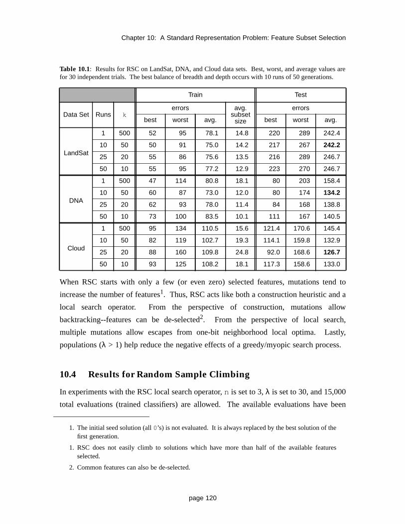
Chapter 10: A Standard Representation Problem: Feature Subset Selection
page 120
When RSC starts with only a few (or even zero) selected features, mutations tend to
increase the number of features1. Thus, RSC acts like both a construction heuristic and a
local search operator. From the perspective of construction, mutations allow
backtracking--features can be de-selected2. From the perspective of local search,
multiple mutations allow escapes from one-bit neighborhood local optima. Lastly,
populations (λ > 1) help reduce the negative effects of a greedy/myopic search process.
10.4 Results for Random Sample Climbing
In experiments with the RSC local search operator,n is set to 3,λ is set to 30, and 15,000
total evaluations (trained classifiers) are allowed. The available evaluations have been
1. The initial seed solution (all0’s) is not evaluated. It is always replaced by the best solution of thefirst generation.
1. RSC does not easily climb to solutions which have more than half of the available featuresselected.
2. Common features can also be de-selected.
Table 10.1: Results for RSC on LandSat, DNA, and Cloud data sets. Best, worst, and average values arefor 30 independent trials. The best balance of breadth and depth occurs with 10 runs of 50 generations.
Train Test
Data Set Runs kerrors avg.
subsetsize
errors
best worst avg. best worst avg.
LandSat
1 500 52 95 78.1 14.8 220 289 242.4
10 50 50 91 75.0 14.2 217 267 242.2
25 20 55 86 75.6 13.5 216 289 246.7
50 10 55 95 77.2 12.9 223 270 246.7
DNA
1 500 47 114 80.8 18.1 80 203 158.4
10 50 60 87 73.0 12.0 80 174 134.2
25 20 62 93 78.0 11.4 84 168 138.8
50 10 73 100 83.5 10.1 111 167 140.5
Cloud
1 500 95 134 110.5 15.6 121.4 170.6 145.4
10 50 82 119 102.7 19.3 114.1 159.8 132.9
25 20 88 160 109.8 24.8 92.0 168.6 126.7
50 10 93 125 108.2 18.1 117.3 158.6 133.0

Chapter 10: A Standard Representation Problem: Feature Subset Selection
page 121
distributed into one run of (k equals) 500 generations, 10 runs of 50 generations, 25 runs
of 20 generations, and 50 runs of 10 generations. These parameters have each been tested
on 30 different pairs of training and evaluation sets. (See Table 10.1.)
The range of results for RSC are highest when only one run of 500 generations is used.
In a single run, RSC can act like a depth-first search. By analogy, more runs of fewer
generations exchange breadth for depth. It appears that more breadth (runs) improve the
worst trial, but that a lack of depth (generations) will negatively affect the best trial.
Overall, the best balance between breadth and depth occurs with 10 runs of 50 genera-
tions each.
10.5 A Heuristic Operator for Feature Subset Selection
As a construction heuristic, the effectiveness of Random Sample Climbing should be
amplified by commonality-based selection (see section 6.3). To transform RSC into a
commonality-based heuristic operator, it is restarted from the Common Features (selected
1’s) of two parents. The overall process defines Common Features/Random Sample
Climbing (CF/RSC)--a heuristic operator for feature subset selection1.
10.6 Results for Common Features/Random Sample Climbing
To allow direct comparisons, the experiments with CF/RSC treatn, λ, and the total
number of evaluations as control variables (set to 3, 30, and 15,000 respectively).
Between RSC and CF/RSC, the first uses random restarts and the second uses common-
ality-based restarts. The number of restarts is parameterized byk : it distributes the 500
available generations.
The value ofk has been set to 20, 10, and 5, so the corresponding GAs are allowed to
generate 25, 50, and 100 total solutions each. Using population sizes of 4, 7, and 10, the
initial populations are seeded with RSC, and the remaining solutions are allocated to CF/
RSC. These GAs are implemented in GENITOR [WS90]--1.00 is used for the selection
bias (random parent selection), and duplicate solutions are disallowed.
1. The Common Features partial solution is not evaluated. This avoids the cost of an evaluation,and it forces RSC to take an initial step of exploration.

Chapter 10: A Standard Representation Problem: Feature Subset Selection
page 122
Compared to RSC alone, the results with CF/RSC are better overall. (See Table 10.2.)
They also appear to be more robust across parameter settings--the average training errors
have a maximum range of 3.4 (Cloud data set) for CF/RSC versus 10.5 (DNA data set)
for RSC. Commonality-based restarts of the ES-based RSC seem to benefit from both
breadth and depth, without sacrificing either. Overall, the best parameter set is (5, 10-
90)--it finds the smallest subsets, and it has the fewest “best test errors”.
10.7 Standard Crossover Operators
For standard crossover operators, Guerra-Salcedo & Whitely [GW98] have shown that
CHC [Esh91] performs better than GENESIS [Gre84]. Comparing CF/RSC to CHC, the
new heuristic operator performs better--even though CHC also incorporates aspects of
local search (e.g. cataclysmic mutation). The constructive nature of CF/RSC and the
explicit identification of strongly relevant features provide advantages over CHC and
standard operators.
Table 10.2: Results for CF/RSC on LandSat, DNA, and Cloud data sets. Best, worst, and average valuesare for 30 independent trials. Performance is robust across parameter settings, but (5, 10-90) leads tosmaller subsets and fewer “best test errors”.
Train Test
Data Set k RSC CF/RSC
errors avg.subset
size
errors
best worst avg. best worst avg.
LandSat
20 4 21 52 92 73.9 13.6 215 315 247.1
10 7 43 53 90 73.8 13.4 215 275 245.2
5 10 90 54 93 75.1 12.8 205 313 247.7
DNA
20 4 21 45 69 54.9 9.5 74 140 98.9
10 7 43 46 68 55.8 9.3 74 126 99.3
5 10 90 45 72 57.4 8.5 74 142 104.1
Cloud
20 4 21 85 115 99.7 18.4 116.2 143.3 130.6
10 7 43 86 118 99.3 18.2 113.5 151.2 128.4
5 10 90 90 119 102.7 14.0 101.9 141.0 124.7

Chapter 10: A Standard Representation Problem: Feature Subset Selection
page 123
10.7.1 CHC
In the CHC algorithm, each pair of mating parents must be different by a minimum
(threshold) number of bits. Essentially, CHC attempts to exploit the differences of
population members, not their similarities. When there are not enough differences to
exploit (i.e. the population has converged), CHC reintroduces variety by cataclysmic
mutation. This form of local search reseeds the population with heavily mutated “clones”
(neighbors) of the best solution.
Since CHC starts with a random population (half1’s and half0’s), it is necessary to bias
the search process towards smaller subsets. Therefore, the objective in CHC is to
minimize the sum of training errors and selected features. Without this “penalty”, CHC
finds much larger subsets with approximately the same training accuracy [GW98].
Naturally, the overall goal is still to minimize the number of classification errors during
final testing.
10.7.2 Results: CF/RSC vs. CHC
Compared to CHC1, the feature subsets found by CF/RSC perform better during final
testing. (See Table 10.3.) The CF/RSC subsets are also smaller than the CHC subsets.
Since the time to train an EDT classifier grows approximately with the square of the
1. The CHC experiments were performed by César Guerra-Salcedo.
Table 10.3: Results for CF/RSC (5, 10-90) and CHC on LandSat, DNA, and Cloud data sets. Best,average, and standard deviation values are for 30 independent trials.
Train Test
Data Set Algorithmaccuracy (% correct) avg.
subsetsize
accuracy (% correct)
best avg. std. dev. best avg. std. dev.
LandSatCF/RSC 92.3 89.3 1.08 12.8 89.8 87.6 1.01
CHC 86.8 85.3 0.81 12.6 88.9 87.6 1.25
DNACF/RSC 93.6 91.8 0.89 8.5 93.8 91.2 1.33
CHC 96.4 95.1 0.51 11.2 92.5 89.4 2.13
CloudCF/RSC 82.0 79.5 1.68 14.0 84.4 80.9 1.67
CHC 84.8 82.2 1.37 42.1 80.8 79.3 1.95

Chapter 10: A Standard Representation Problem: Feature Subset Selection
page 124
number of features, CF/RSC is also faster than CHC. On average, CF/RSC takes 50%
less time than CHC to evaluate 15,000 solutions.
On the DNA and Cloud data sets, the smaller CF/RSC feature subsets perform signifi-
cantly worse during training, but they perform better during testing. (See Table 10.4.)
Since CF/RSC starts with no features and builds up, it stops in local minima with fewer
features. Conversely, CHC starts with many features and works down, so it finds local
minima with more features. Since these additional features are at best weakly relevant,
they likely cause the search process to over-fit the training data.
10.8 Traditional Feature Selection Techniques
Two basic search procedures for feature subset selection are forward selection and
backward elimination. Since backward elimination is computationally impractical for
large feature spaces [Koh95], only forward selection is implemented. Truncating the
search after the expected number of relevant features have been added, forward selection
performs better than CHC on all of the data sets. However, CF/RSC is still slightly better
on the two largest data sets (DNA and Cloud).
10.8.1 Forward Selection
Starting with an initial solution of all0’s, forward selection finds the best subset with a
single feature. At each subsequent step, the best subset which consists of the previous
subset and one additional feature is found. Forward selection terminates when all
features are included in the subset, and it returns the best subset found along the way (i.e.
unlike bit climbing, it does not stop in the first local minimum).
Table 10.4: T-tests -- are the CF/RSC and CHC results different?
Data Set Training Testing
LandSat Yes No
DNA Yes Yes
Cloud Yes No
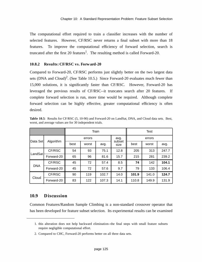
Chapter 10: A Standard Representation Problem: Feature Subset Selection
page 125
The computational effort required to train a classifier increases with the number of
selected features. However, CF/RSC never returns a final subset with more than 18
features. To improve the computational efficiency of forward selection, search is
truncated after the first 20 features1. The resulting method is called Forward-20.
10.8.2 Results: CF/RSC vs. Forward-20
Compared to Forward-20, CF/RSC performs just slightly better on the two largest data
sets (DNA and Cloud)2. (See Table 10.5.) Since Forward-20 evaluates much fewer than
15,000 solutions, it is significantly faster than CF/RSC. However, Forward-20 has
leveraged the previous results of CF/RSC--it truncates search after 20 features. If
complete forward selection is run, more time would be required. Although complete
forward selection can be highly effective, greater computational efficiency is often
desired.
10.9 Discussion
Common Features/Random Sample Climbing is a non-standard crossover operator that
has been developed for feature subset selection. Its experimental results can be examined
1. this alteration does not help backward elimination--the final steps with small feature subsetsrequire negligible computational effort.
2. Compared to CHC, Forward-20 performs better on all three data sets.
Table 10.5: Results for CF/RSC (5, 10-90) and Forward-20 on LandSat, DNA, and Cloud data sets. Best,worst, and average values are for 30 independent trials.
Train Test
Data Set Algorithmerrors avg.
subsetsize
errors
best worst avg. best worst avg.
LandSatCF/RSC 54 93 75.1 12.8 205 313 247.7
Forward-20 65 96 81.6 15.7 215 281 239.2
DNACF/RSC 45 72 57.4 8.5 74 142 104.1
Forward-20 45 72 57.6 9.7 79 133 106.4
CloudCF/RSC 90 119 102.7 14.0 101.9 141.0 124.7
Forward-20 83 122 107.3 14.1 110.8 149.9 131.9

Chapter 10: A Standard Representation Problem: Feature Subset Selection
page 126
with respect to standard GAs, the ES-based RSC operator, and machine learning
concepts. In general, the explicit identification of the strongly relevant features appears
to provide an advantage.
10.9.1 Genetic Algorithms
The utility of the Commonality-Based Crossover Framework is demonstrated on a
standard representation. To develop a commonality-based operator, the critical building
blocks must be explicitly identified--an analysis that has been omitted in previous appli-
cations with standard representations (e.g. [VdJ93]). For feature subset selection, the
selected features are useful building blocks, but the unselected features are not. The
Common Features/Random Sample Climbing heuristic operator focuses on these critical
building blocks better than standard crossover operators.
10.9.2 Restarts, Local Search, and Hybrid Operators
For deterministic hill-climbing procedures (i.e. local optimizers), restarts allow fair time-
based comparisons with other (non-deterministic) methods. In particular, these
techniques have benefited from commonality-based restarts (see chapter 7). Comparing
the results for CF/RSC and RSC alone, it appears that (stochastic/probabilistic) local
search methods (e.g. simulated annealing and tabu search) can also benefit from
commonality-based restarts. These restarts should eliminate the time required to back-
track out of local minima. Although it still takes time to bring a random solution into the
near-optimal region [UPvL91], commonality-based restarts will be more efficient if the
restart solution is already in the near-optimal region (see chapter 7).
10.9.3 Machine Learning
It is desirable to train classifiers with small feature subsets. In addition to speed, intuitive
interpretations of the data are easier [Koh95]. Comparing the results of CF/RSC and
CHC, another advantage is suggested: greater accuracy. The smaller subsets of CF/RSC
perform worse in training, but better in testing. Large feature subsets (like those found by
CHC) may cause the training data to be over-fitted. Specifically, the selection of
additional (weakly relevant) features may induce the classifier to identify subtle charac-
teristics of the training instances.
Chapter 10: A Standard Representation Problem: Feature Subset Selection
page 127
10.10 Summary
A heuristic (non-standard) operator has been developed for feature subset selection--a
standard representation problem. In experiments, Common Features/Random Sample
Climbing performs better than standard GAs (e.g. GENESIS and CHC). The new
operator focuses on the superior common components that have been identified through
an explicit building block analysis. Overall, these results demonstrate that the utility of
the commonality hypothesis and the Commonality-Based Crossover Framework extend to
standard representations.

Chapter 11
Transmission, Combination,
and Heuristic Operators
Transmission is a weak heuristic. If the existing domain-independent
design models are extended to heuristic operators, the effectiveness of the
embedded construction heuristic can be handicapped by transmission.

Chapter 11: Transmission, Combination, and Heuristic Operators
page 129
11.1 Overview
The Commonality-Based Crossover Framework addresses heuristic operators directly--it
is not a domain-independent model that has been extended to this operator category.
From its perspective, the traditional mechanisms of domain-independent operators (i.e.
transmission and combination [Rad91]) are merely default heuristics--they should be
replaced altogether when stronger, problem specific heuristics are available. Unfortu-
nately, through the historical perception that combination is the critical aspect of
crossover, these domain-independent models still influence the design of heuristic
operators1. For example, Greedy Crossover (see section 5.2.1) is a heuristic operator that
places the transmission and combination “heuristics” ahead of the problem specific
Nearest Neighbor heuristic.
The results of Greedy Crossover suggest that transmission and combination are not strong
heuristics. To examine this hypothesis, these mechanisms have been imposed upon two
commonality-based heuristic operators. Specifically, Maximum Partial Order/Arbitrary
Insertion (MPO/AI) and Common Features/Random Sample Climbing (CF/RSC) have
been modified to obey strict transmission. In the converted operators, the offspring
search space is defined by the (feasible) combinations of parent schemata. This
restriction handicaps the effectiveness of the embedded construction heuristic.
The “convergence” in Convergence Controlled Variation is caused by transmission--the
current search space is limited to parent genes. For better or worse, heuristics also apply
implicit limits to their search space (see section 6.3.4). Since the inclusion of both limits
can be redundant, the Commonality-Based Crossover Framework suggests that only the
heuristic should control variation. With the superior performance of these heuristic
operators, the role of transmission and combination in heuristic operators is cast into
doubt.
11.2 Heuristic Operators in Convergence Controlled Variation
In the (domain-independent) model of Convergence Controlled Variation (CCV)
[EMS96], the offspring search space is defined by transmission--offspring must becombi-
1. Before components can be combined, they must be transmitted.

Chapter 11: Transmission, Combination, and Heuristic Operators
page 130
nations of the parent genes (see section 2.5.2). Traditionally, crossover (recombination)
is used to sample this search space randomly. Conversely, this search space can be
explored with problem specific heuristics.
Starting from the maximal common schema, construction heuristics can be incorporated
into Convergence Controlled Variation by following the two-step process of the
Commonality-Based Crossover Framework. If strict transmission is imposed onto the
construction heuristic, the offspring solutions will stay within the search space defined by
CCV. This heuristic model for Convergence Controlled Variation isolates the effects of
transmission.
11.3 The Traveling Salesman Problem
Maximum Partial Order/Arbitrary Insertion is a commonality-based heuristic operator
that has been developed for the Traveling Salesman Problem (see section 5.3.2). When
transmission of all precedence relationships is enforced, it is converted into Matrix Inter-
section/Arbitrary Insertion (MI/AI). Experimental results show that MI/AI performs
worse than MPO/AI. The additional precedence constraints imposed by transmission
handicap the effectiveness of Arbitrary Insertion.
11.3.1 Matrix Intersection/Arbitrary Insertion
To develop the Maximum Partial Order of two parent solutions, their sequences are
converted into Boolean matrices, the matrices are intersected, and a partial order graph is
generated. When the Maximum Partial Order is extracted from the partial order graph,
some arcs are ignored (e.g.e to f --see Figure 5.4). Thus, the Boolean matrix which
represents the MPO specifies fewer precedence relationships than the intersection matrix.
(See Figure 11.1.) Unlike partial orders, the omission of these precedence relationships
violates the principle of transmission for order-based schemata.

Chapter 11: Transmission, Combination, and Heuristic Operators
page 131
Figure 11.1: Comparison of Matrix Intersection and Maximum Partial Order.
The Matrix Intersection (MI) operator (see section 4.2.3) preserves all of the (common)
precedence relationships. Since it follows Radcliffe’s design principles (i.e. respect,
transmission, and assortment [Rad91]), MI is a viable operator for domain-independent
Convergence Controlled Variation. To convert MI into a heuristic operator, Arbitrary
Insertion can explore the offspring search space (i.e. generate the remaining precedence
relationships). Equivalently, the additional precedence constraints of the intersection
matrix can be super-imposed onto MPO/AI. From either perspective, the resulting
heuristic operator is Matrix Intersection/Arbitrary Insertion1.
11.3.2 Results: MPO/AI vs. MI/AI
To allow direct comparisons with MPO/AI, the Matrix Intersection/Arbitrary Insertion
experiments use a population size of 400, and it is seeded with convex hull/Arbitrary
Insertion solutions. From this population, the parents for MI/AI are both selected by 2-
tournament--the additional selection pressure helps Matrix Intersection/Arbitrary
Insertion. Regardless, MPO/AI performs better than MI/AI. (See Table 11.1.)
1. The starting sub-tour is again the Maximum Partial Order. However, Arbitrary Insertion ismodified to preserve the additional precedence constraints in the intersection matrix.
Parent 1: a b c d e f gParent 2: a e f d b c g
Parent 1: abcdefga 0111111b 0011111c 0001111d 0000111e 0000011f 0000001g 0000000
Parent 2: abcdefga 0111111b 0010001c 0000001d 0110001e 0111011f 0111001g 0000000
Inter- abcdefga 0111111b 0010001c 0000001d 0000001e 0000011f 0000001g 0000000
Maximum abcdefga 011 000 1b 0010001c 0000001d 000000 0e 00000 00f 000000 0g 0000000
sectionMatrix:
PartialOrder(abcg):

Chapter 11: Transmission, Combination, and Heuristic Operators
page 132
The MPO/AI and MI/AI operators only differ by the inclusion of strict transmission in
Matrix Intersection/Arbitrary Insertion. The precedence relationships which MPO
ignores in the intersection matrix can be coincidental. (See Figure 11.2.) Subsequently,
their enforcement by transmission may interfere with the performance of AI. Arbitrary
Insertion is a strong, problem specific heuristic which (compared to transmission) can
identify better (order-based) schemata for the TSP.
Figure 11.2: Example of a coincidental precedence relationship. Although cityiprecedes cityj in both parents, the construction heuristic may prefer to place cityjbefore cityi .
Table 11.1: Comparison of MPO/AI and MI/AI on 5 TSP instances. Results are for a steady-state GA witha population of 400 run until 10 generations pass without an improvement. Values are percent distance fromknown optimum for average of 5 runs. Experiment runtimes are given for a SPARC 20.
TSPInstance
Average BestCH/AI Start
Average BestMPO/AI
Runtime(min)
Average BestMI/AI
Runtime(min)
d198 + 3.05 % + 0.95 % 3 + 1.14 % 4
lin318 + 6.04 % + 0.63 % 13 + 1.42 % 15
fl417 + 1.91 % + 0.57 % 15 + 0.61 % 18
pcb442 + 8.97 % + 1.84 % 37 + 3.18 % 47
u574 + 8.45 % + 2.20 % 74 + 2.63 % 73
average + 5.68 % + 1.24 % + 1.80 %
i j i j
i j
Parent 1 Parent 2
DisallowedMPO
i j

Chapter 11: Transmission, Combination, and Heuristic Operators
page 133
11.4 Feature Subset Selection
Common Features/Random Sample Climbing is the commonality-based heuristic
operator that has been developed for feature subset selection (see section 10.5). When
transmission of0’s is imposed upon CF/RSC, the resulting operator is Convergence
Controlled Variation/Random Sample Climbing (CCV/RSC). Experimental results show
that CCV/RSC performs worse than CF/RSC. When it is required that features which are
not selected in either parent (i.e. their common0’s) cannot appear in the offspring, the
effectiveness of Random Sample Climbing is handicapped.
11.4.1 Convergence Controlled Variation/Random Sample Climbing
Feature subset selection is a standard representation problem. Since standard crossover
operators preserve all of the common1’s and all of the common0’s (i.e. they obey strict
transmission), the “variations” available in the offspring search space are due to the
uncommon bits/genes. Convergence Controlled Variation suggests that crossover
operators should be limited to this search space.
To allow direct comparisons with CF/RSC, Random Sample Climbing has been used to
explore the offspring search space defined by Convergence Controlled Variation. Starting
from the partial solution of Common Features, the resulting heuristic operator is Conver-
gence Controlled Variation/Random Sample Climbing. Equivalently, this operator is also
developed by super-imposing the transmission of0’s onto CF/RSC and by disallowing
RSC to back-track common1’s. From either perspective, the search space in CCV/RSC
is limited to the allele positions represented by uncommon bits in the parents.
11.4.2 Results: CF/RSC vs. CCV/RSC
The Convergence Controlled Variation/Random Sample Climbing heuristic operator has
been applied to the LandSat data set, the DNA data set, and the Cloud Data set. In these
experiments,n andλ are again treated as control variables (set to 3 and 30 respectively).
To match the parameters of CF/RSC (5, 10-90),k is set to 5, the population size is set to
10, and 90 offspring solutions (15,000 total evaluations) are allowed. Using the same
GENITOR set-up (i.e. 1.00 selection bias and duplicate solutions disallowed), CCV/RSC
is less effective than CF/RSC. (See Table 11.2.)

Chapter 11: Transmission, Combination, and Heuristic Operators
page 134
The principle of strict transmission handicaps the ability of Random Sample Climbing to
assemble the best weakly relevant features. In particular, a desired feature (1) may be
absent from the entire population (i.e. the population may not have enough diversity).
This situation is partially rectified by increasing the population size to 20, but CF/RSC
still performs better. Overall, transmission has not improved the performance of Random
Sample Climbing.
11.5 Discussion
The domain-independent design principle of transmission has been super-imposed upon
two previously developed heuristic operators. Although combination has been viewed as
a critical feature of crossover (see section 2.4.3), limiting the offspring of heuristic
operators combinations of their parent genes is not always productive. Specifically, MI/
AI performs worse than MPO/AI on the TSP, and CCV/RSC performs worse than CF/
RSC in feature subset selection.
Although the commonality-based heuristic operators perform better than their corre-
sponding versions based on Convergence Controlled Variation, they still have ineffi-
ciencies. For example, MPO/AI suffers from negative heuristic amplification (see Figure
Table 11.2: Results for CF/RSC (5, 10-90) and CCV/RSC on LandSat, DNA, and Cloud data sets. Best,worst, and average values are for 30 independent trials.
Train Test
Data Set k RSC CCV/RSC
errors avg.subset
size
errors
best worst avg. best worst avg.
LandSat
5 10 90 57 97 78.4 11.6 228 282 249.6
5 20 80 55 94 76.4 11.6 230 315 253.9
CF/RSC 54 93 75.1 12.8 205 313 247.7
DNA
5 10 90 55 82 68.2 7.6 93 167 123.4
5 20 80 51 76 61.8 8.2 86 128 107.3
CF/RSC 45 72 57.4 8.5 74 142 104.1
Cloud
5 10 90 95 128 110.4 9.3 120.1 156.4 134.9
5 20 80 94 123 107.1 9.9 117.0 151.4 132.0
CF/RSC 90 119 102.7 14.0 101.9 141.0 124.7

Chapter 11: Transmission, Combination, and Heuristic Operators
page 135
6.4), and CF/RSC will repeatedly reexamine irrelevant features. There is too little
diversity in the search space of MPO/AI, and there is too much diversity in the search
space of CF/RSC.
The ideal balance point between diversity and focus is difficult to estimate. Although
search space reductions (which magnify the convergence effects of transmission) improve
the performance of blind operators (see chapter 9), transmission itself impairs the perfor-
mance of heuristic operators. Conversely, search space reductions (e.g. starting MPO/AI
from the convex hull) have improved the performance of heuristic operators. Each
problem domain must be examined individually.
11.6 Summary
Transmission and combination are traditionally seen as the primary mechanisms of
crossover. However, when these features were imposed upon heuristic operators, they
have handicapped the effectiveness of the embedded construction heuristic. For the
development of heuristic operators, it should be more productive to use the Commonality-
Based Crossover Framework than to extend the existing domain-independent design
models.

Chapter 12
Conclusions

Chapter 12: Conclusions
page 137
For iterative improvement to be more successful than random search, existing candidate
solutions should facilitate the discovery of better candidate solutions. Essentially, good
solutions must share exploitable features. The explicit identification of these common
components leads to an alternative approach for iterative improvement. Instead of
changing (bad) parts in (single) candidate solutions, good parts can be preserved from
two candidate solutions.
Pursuing this alternative approach in genetic algorithms, the commonality hypothesis
suggests that schemata common to above-average solutions are above average. These
common components represent the good parts that should be preserved. Subsequently,
the Commonality-Based Crossover Framework redefines crossover as a two step process:
1) preserve the maximal common schema of two parents, and 2) complete the solution
with a construction heuristic.
To balance the exploitation of common components with the necessary exploration for
new components, diversity is required. The construction heuristic is responsible to
generate diversity (random errors versus systematic errors) and a population of solutions
allows this diversity to be distributed (different parent pairs can have different common
components). Without enough diversity, undesirable components can become common,
and the final solution will be sub-optimal.
The broad utility of the new design model has been demonstrated through the devel-
opment of domain-independent operators, heuristic operators, and hybrid operators for
benchmark and practical problems with standard and non-standard representations.
Although most results are relative, the commonality-based operators consistently perform
better than comparable operators which emphasize combination. Experimental evidence
indicates that components common to above-average parents can have a measurable,
superior relative fitness. In these cases, the uncommon components targeted by combi-
nation will have a below-average fitness relative to their parents.
Selection chooses components for exploitation. Therefore, the preservation of common
components is a form of selection--these components are exploited. This commonality-
based form of selection has been isolated in GENIE (a GA that eliminates fitness-based
selection at the individual level). Since the effectiveness of heuristic operators can be

Chapter 12: Conclusions
page 138
amplified by commonality-based restarts, the productive value of commonality-based
selection corroborates the commonality hypothesis. The common schemata it preserved
were above average.
Although commonality-based selection was first isolated in heuristic operators, its effects
can be transferred back to standard (domain-independent) operators. The preservation of
(above-average) common components restricts changes to the (below-average)
uncommon components of the parents. The probability that these changes are beneficial
should increase with this focus. Since multiple parents are required to identify common
components, commonality-based selection is an advantage that multi-parent operators
(e.g. crossover) can have over single-parent operators (e.g. mutation).

Chapter 13
Extensions and Future Work
A series of extensions and open issues are suggested for the Commonality-
Based Crossover Framework and the commonality hypothesis.

Chapter 13: Extensions and Future Work
page 140
13.1 Interactive Search Space Reductions
Search space reductions can be specified interactively. Although a global parameter was
used for flow shop scheduling (see chapter 9), it does not preclude the addition or
deletion of individual constraints. For example, a graphic user interface (GUI) has been
developed for Common Clusters/Insertion (see section 8.4) to allow the initial customer
clusters to be set manually1. A GUI allows unique and/or ill-defined constraints to be
added as necessary (in real-time). Since real world problems often include similar opera-
tions-level preferences/constraints, interactive search space reductions may be useful in
practical environments.
13.2 Practical Heuristic Amplification
Through the effects of heuristic amplification (see section 6.3), commonality-based
restarts of a good construction heuristic will be more effective than random restarts. To
demonstrate the full value of commonality-based selection and heuristic amplification, a
relevant problem that is currently solved by random restarts is required. Unfortunately,
stand-alone construction heuristics rarely provide the best optimization technique. A
suitable domain has yet to be found.
13.3 Theoretical Heuristic Amplification
A commonality-based heuristic operator that encapsulates an ideal construction heuristic
will converge to the optimal solution. The derivation of the previous statement is
independent of problem size (see section 3.7.2). Therefore, convergence occurs in a
constant number of generations. In the (unlikely) event that a polynomial-time ideal
construction heuristic can be developed, it will solve NP-complete problems in
polynomial time.
1. In this system, interactive results were better than random initial clusters, but they were stillworse than tabu search. However, this study was uncontrolled--the user had knowledge of thebest-known solutions.

Chapter 13: Extensions and Future Work
page 141
13.4 Open-Loop Optimization
The existence of heuristic amplification leads to the concept of open-loop optimization.
Unfortunately, it is difficult to imagine a practical application where open-loop optimi-
zation will be successful. In particular, heuristic amplification is based on construction
heuristics which require local evaluation information. However, open-loop optimization
is only viable when global evaluations are too expensive1. Since global payoff is often a
summation of local cost functions, it may be difficult to resolve this contradiction. A
problem domain with good construction heuristics and an expensive overall evaluation
function is required to test the practical value of open-loop optimization.
13.5 Lamarckian Learning
Open-loop optimization resembles Lamarckian evolution. Fitness-based feedback is not
required because the heuristic provides “a built-in drive toward perfection of adapta-
tions”. Since a learning algorithm acts like a construction heuristic (it builds a world
view incrementally), the Commonality-Based Crossover Framework may be a useful
model for agent-based learning systems.
13.6 Commonality-Based Random Hill Climbing
In random hill climbing (see section 2.8.1), the first improving solution is taken.
Compared to (complete) hill climbing, random hill climbing can be more efficient and
just as effective. However, in problem domains with large operator sets, the improving
moves eventually become scarce, and the relative efficiency will degrade. To increase the
efficiency, it is desirable to identify the improving operators.
Hill climbing operators act on a single solution--just like mutation. However, the proba-
bility of a beneficial mutation is expected to increase when mutation is restricted to
uncommon bits (see section 3.8). By extension, hill climbing operators that target
uncommon components2 may cause improvements more often3. When these operators
1. The removal of evaluations is expected to improve computational efficiency only. For the samenumber of crossover applications, fitness-based selection should still improve solution quality(see section 6.3.5).

Chapter 13: Extensions and Future Work
page 142
are applied first, the resulting procedure becomes “commonality-based random hill
climbing”. This modification can be applied to any point-search method (e.g. simulated
annealing and tabu search).
13.7 Machine Learning
Many techniques in artificial intelligence implicitly seek to identify the common compo-
nents. For example, incremental learning methods (e.g. clustering, neural nets,
reinforcement learning, etc) find the common core by “cancelling out” the differences in
the individual instances. When it is not productive to keep common components (e.g.
common0’s in feature subset selection), these methods may not function properly. The
commonality hypothesis provides an explicit test to examine these implicit actions.
13.8 Case Studies
Case studies (e.g. in business school) are often presented one at a time. The natural
tendency is to look for things that went wrong--things that can be improved. However, it
can be just as useful to know what went right--what should be repeated. If two cases are
studied at the same time, the commonality hypothesis suggests that their common compo-
nents will represent things that should be repeated.
2. An (unspecified) benchmark solution is required to help identify common components.
3. Trivially, if mutation on an-bit binary string is converted inton “mutate-bit” operators, theprevious argument transfers directly see section 3.8).

References

References
page 144
[AL97] E.H.L. Aarts and J.K. Lenstra. (1997)Local Search in Combinatorial Optimi-zation. John Wiley & Sons.
[AN90] E.J. Anderson and J.C. Nyirenda. (1990) “Two New Rules to MinimizeTardiness in a Job Shop.” InInternational Journal of Production Research,28:2277-2292, 1990.
[Asc96] N. Ascheuer. (1996)Hamiltonian Path Problems in the On-line Optimizationof Flexible Manufacturing Systems.ZIB Technical Report TR 96-3.
[BA82] J.J.W. Baker and G.E. Allen. (1982)The Study of Biology, 4th ed. Addison-Wesley.
[Bal95] S. Baluja. (1995)An Empirical Comparison of Seven Iterative and Evolu-tionary Function Optimization Heuristics. Carnegie Mellon Technical ReportCMU-CS-95-193.
[Ban94] R.L. Bankert. (1994) “Cloud Classification of avhrr Imagery in MaritimeRegions using a Probabilistic Neural Network.” InApplied Methodology,33(8):909-918.
[BE95] W. Banzhaf and F.H. Eeckman. (1995)Evolution and Biocomputation:Computational Models of Evolution. Springer.
[Bea90] J.E. Beasley. (1990) “OR-Library: Distributing Test Problems by ElectronicMail.” In Journal of the Operational Research Society, 41:1069-1072, 1990.
[Bea94] J.C. Bean. (1994) “Genetic Algorithms and Random Keys for Sequencingand Optimization.” InORSA Journal on Computing, 6:154-160, 1994.
[Bey95] H.-G. Beyer. (1995) “Toward a Theory of Evolution Strategies: On theBenefits of Sex--the (µ/µ,λ) Theory.” InEvolutionary Computation, 3(1):81-111, 1995.
[Bey97] H.-G. Beyer. (1997) “An Alternative Explanation for the Manner in whichGenetic Algorithms Operate.” InBioSystems, 41:1-15, 1997.

References
page 145
[BL94] J.J. Bernardo and K.-S. Lin. (1994) “An Interactive Procedure for Bi-CriteriaProduction Scheduling.” InComputers and Operations Research, 21:667-688, 1994.
[BMK96] C. Bierwirth, D.C. Mattfeld, and H. Kopfer. (1996) “On Permutation Repre-sentations for Scheduling Problems.” InParallel Problem Solving fromNature IV, H.-M. Voight et al, eds. Springer-Verlag.
[Boe96] K.D. Boese. (1996) Models for Iterative Global Optimization. Ph.D. thesis,University of California at Los Angeles, 1996.
[Boy98] J.A. Boyan. (1976) Learning Evaluation Functions for Global Optimization.Ph.D. thesis, Carnegie Mellon University, 1998.
[BW93] J.L. Blanton Jr. and R.L. Wainwright. (1993) “Multiple Vehicle Routing withTime and Capacity Constraints using Genetic Algorithms.” InProc. FifthInternational Conference on Genetic Algorithms.
[But95] D. Butcher. (1995) “Muller’s Ratchet, Epistasis and Mutation Effects.” InGenetics, 141:431-437, 1995.
[CGS99] S. Chen, C. Guerra-Salcedo, and S.F. Smith. (1999) “Non-StandardCrossover for a Standard Representation -- Commonality-Based FeatureSubset Selection.” InGECCO-99: Proceedings of the Genetic and Evolu-tionary Computation Conference.
[CH93] O. Charalambous and K.S. Hindi. (1993) “A Knowledge Based Job-ShopScheduling System with Controlled Backtracking.” InComputers and Indus-trial Engineering, 24:391-400, 1993.
[Chr85] N. Christofides. (1985) “Vehicle Routing.” InThe Traveling SalesmanProblem, E.L. Lawler, J.K. Lenstra, A.H.G. Rinnooy Kan, and D.B. Shmoys,eds. John Wiley & Sons.
[CMM67] R. Conway, W. Maxwell, and L. Miller. (1967)Theory of Scheduling.Addison-Wesley.

References
page 146
[CMT79] N. Christofides, A. Mingozzi, and P. Toth. (1979) “The Vehicle RoutingProblem.” InCombinatorial Optimization, N. Christofides, A. Mingozzi, P.Toth, and C. Sandi, eds. John Wiley & Sons.
[CS97] C. Cheng and S.F. Smith. (1997) “Applying Constraint SatisfactionTechniques to Job Shop Scheduling.” InAnnals of Operations Research,70:327-357, 1997.
[CS98] S. Chen and S.F. Smith. (1998) “Experiments on Commonality in SequencingOperators.” InGenetic Programming 1998: Proceedings of the Third AnnualConference.
[CS99a] S. Chen and S.F. Smith. (1999) “Putting the “Genetics” back into GeneticAlgorithms (Reconsidering the Role of Crossover in Hybrid Operators).” InFoundations of Genetic Algorithms 5, W. Banzhaf and C. Reeves, eds.Morgan Kaufmann.
[CS99b] S. Chen and S.F. Smith. (1999) “Introducing a New Advantage of Crossover:Commonality-Based Selection.” InGECCO-99: Proceedings of the Geneticand Evolutionary Computation Conference.
[CS99c] S. Chen and S.F. Smith. (1999) “Improving Genetic Algorithms by SearchSpace Reductions (with Applications to Flow Shop Scheduling).” InGECCO-99: Proceedings of the Genetic and Evolutionary ComputationConference.
[CSG99] S. Chen, S.F. Smith, and C. Guerra-Salcedo. (1999) “The GENIE is Out!(Who Needs Fitness to Evolve?).” InCEC99: Proceedings of the Congress onEvolutionary Computation.
[CT99] E. Camponogara and S.N. Talukdar. (1999) “Agent Cooperation: DistributedControl Applications.” InProceedings of the ISAP’99 (The InternationalConference on Intelligent Systems Applications to Power Systems).
[CVA95] C.-L. Chen, V.S. Vempati, and N. Aljaber. (1995) “An Application of GeneticAlgorithms for Flow Shop Problems.” InEuropean Journal of OperationalResearch, 80:389-396, 1995.
References
page 147
[Dav85a] L. Davis. (1985) “Applying Adaptive Algorithms to Epistatic Domains.” InProc. Ninth International Joint Conference on Artificial Intelligence.
[Dav85b] L. Davis. (1985) “Job Shop Scheduling with Genetic Algorithms.” InProc.of an International Conference on Genetic Algorithms and their Applications.
[Dav91] L. Davis. (1991)Handbook of Genetic Algorithms. Van Nostrand Reinhold.
[Daw89] R. Dawkins. (1989)The Selfish Gene. Oxford University Press.
[DDS92] M. Desrochers, J. Desrosiers, and M.M. Solomon. (1992) “A New Optimi-zation Algorithm for the Vehicle Routing Problem with Time Windows.” InOperations Research, 40:342-354, 1992.
[DMC96] M. Dorigo, V. Maniezzo, and A. Colorni. (1991) “The Ant System: Optimi-zation by a Colony of Cooperating Agents.” InIEEE Transactions on Systems,Man, and Cybernetics-Part B, 26, 1, 29-41.
[DS93] C. Dagli and S. Sittsathanchai. (1993) “Genetic Neuro-Scheduler for JobShop Scheduling.” InComputers and Industrial Engineering, 25:267-270,1993.
[dSou93] P.S. de Souza. (1993)Asynchronous Organizations for Multi-AlgorithmsProblems. Ph.D. thesis, Carnegie Mellon University, 1993.
[ECS89] L.J. Eshelman, R.A. Caruana, and J.D. Schaffer. (1989) “Biases in theCrossover Landscape.” InProc. Third International Conference on GeneticAlgorithms.
[EMS96] L.J. Eshelman, K.E. Mathias, and J.D. Schaffer. (1996) “ConvergenceControlled Variation.” InFoundations of Genetic Algorithms 4, R. Belew andM. Vose, eds. Morgan Kaufmann.
[EMS97] L.J. Eshelman, K.E. Mathias, and J.D. Schaffer. (1997) “Crossover OperatorBiases: Exploiting the Population Distribution.” InProc. Seventh Interna-tional Conference on Genetic Algorithms.
[Esc88] L.F. Escudero. (1988) “An Inexact Algorithm for the Sequential OrderingProblem.” InEuropean Journal of Operations Research, 37:236-253, 1988.

References
page 148
[Esh91] L.J. Eshelman. (1991) “The CHC Adaptive Search Algorithm: How to HaveSafe Search When Engaging in Nontraditional Genetic Recombination.” InFoundations of Genetic Algorithms, G. Rawlins, ed. Morgan Kaufmann.
[FB96] D.B. Fogel and H.-G. Beyer. (1996) “A Note on the Empirical Evaluation ofIntermediate Recombination.” InEvolutionary Computation, 3(4):491-495,1996.
[FM91] B. Fox and M.B. McMahon. (1991) “An Analysis of Reordering Operatorsfor Genetic Algorithms.” InFoundations of Genetic Algorithms, G. Rawlins,ed. Morgan Kaufmann.
[FOW66] L.J. Fogel, A.J. Owens, and M.J. Walsh. (1966)Artificial Intelligence throughSimulated Evolution. Wiley.
[Fre82] S. French. (1982)Sequencing and Scheduling--An Introduction to the Mathe-matics of Job Shops. Ellis Horwood Limited.
[GB89] J. Grefenstette and J.E. Baker. (1989) “How Genetic Algorithms Work: ACritical Look at Implicit Parallelism.” InProc. Third InternationalConference on Genetic Algorithms.
[GCW99] C. Guerra-Salcedo, S. Chen, L.D. Whitley, and S.F. Smith. (1999) “Fast andAccurate Feature Selection Using Hybrid Genetic Strategies.” InCEC99:Proceedings of the Congress on Evolutionary Computation.
[GD97] L.M. Gambardella and M. Dorigo. (1997)HAS-SOP: Hybrid And System forthe Sequential Ordering Problem. Technical report IDSIA 11-97.
[GGR85] J. Grefenstette, R. Gopal, B. Rosmaita, and D. Van Gucht. (1985) “GeneticAlgorithms for the Traveling Salesman Problem.” InProc. of an InternationalConference on Genetic Algorithms and their Applications.
[GHL92] M. Gendreau, A. Hertz, and G. Laporte. (1992) “New Insertion and Postopti-mization Procedures for the Traveling Salesman Problem.” InOperationsResearch, 40:1086-1094, 1992.
[GHL94] M. Gendreau, A. Hertz, and G. Laporte. (1994) “A Tabu Search Heuristic forthe Vehicle Routing Problem.” InManagement Science, 40:1276-1290, 1994.

References
page 149
[GJR91] M. Grötschel, M. Jünger, G. Reinelt. (1991) “Optimal Control of Plotting andDrilling Machines: A Case Study.” InZeitschrift für Operations ResearchMethods and Models of Operations Research, 35:61-84, 1991.
[GL85] D. Goldberg and R. Lingle. (1985) “Alleles, loci, and the Traveling SalesmanProblem.” InProc. of an International Conference on Genetic Algorithms andtheir Applications.
[Glo89] F. Glover. (1989) “Tabu Search--Part I.” InORSA Journal on Computing,1:190-206, 1989.
[Gol89] D. Goldberg. (1989) Genetic Algorithms in Search, Optimization, andMachine Learning. Addison-Wesley.
[Gre84] J. Grefenstette. (1984) “GENESIS: A System for Using Genetic SearchProcedures.” InProceedings of a Conference on Intelligent Systems andMachines.
[GS94] D.P. Greene and S.F. Smith. (1994) “Using Coverage as a Model BuildingConstraint in Learning Classifier Systems.” InEvolutionary Computation,2(1):67-91, 1994.
[Gue99] C. Guerra-Salcedo. (1999)Feature Subset Selection: A Genetic SearchPerspective. Ph.D. thesis, Instituto Tecnologico y de Estudios Superiores deMonterrey, 1999.
[GW98] C. Guerra-Salcedo and L.D. Whitley. (1998) “Genetic Search for FeatureSubset Selection: A Comparison Between CHC and GENESIS.” InGeneticProgramming 1998: Proceedings of the Third Annual Conference.
[GW99] C. Guerra-Salcedo and L.D. Whitley. (1999) “Genetic Approach to FeatureSelection for Ensemble Creation.” InGECCO-99: Proceedings of the Geneticand Evolutionary Computation Conference.
[Hal37] J.B.S. Haldane. (1937) “The Effect of Variation on Fitness.” In Am. Nat.71:337-349, 1937.

References
page 150
[HC90] J. Hutchinson and Y.-L. Chang. (1990) “Optimal nondelay job shopschedules.” InInternational Journal of Production Research, 28:245-257,1990.
[HGL93] A. Homaifar, S. Guan and G.E. Liepins. (1993) “A New Approach on theTraveling Salesman Problem by Genetic Algorithms.” InProc. Fifth Interna-tional Conference on Genetic Algorithms.
[Hjo93] C. Hjorring. (1993) “Using Genetic Algorithms and the Petal Method to
Solve Vehicle Routing Problems.” In29th Annual Conference of the Opera-tional Research Society of New Zealand.
[HNN94] N. Hirabayashi, H. Nagasawa, and N. Nishiyama. (1993) “A DecompositionScheduling Method for Operating Flexible Manufacturing Systems.” InInter-national Journal of Production Research, 32:161-178.
[Hol75] J. Holland. (1975) Adaptation in Natural and Artificial Systems. TheUniversity of Michigan Press.
[JM97a] C. Ji and S. Ma. (1997) “Combinations of Weak Classifiers.” InIEEE Trans-actions on Neural Networks, 8:32-42, 1997.
[JM97b] D.S. Johnson and L.A. McGeoch. (1997) “The Traveling Salesman Problem:A Case Study.” InLocal Search in Combinatorial Optimization, E.H.L. Aartsand J.K. Lenstra, eds. John Wiley & Sons.
[JSG89] P. Jog, J.Y. Suh, and D. Van Gucht. (1989) “The Effects of Population Size,Heuristic Crossover and Local Improvement on a Genetic Algorithm for theTraveling Salesman Problem.” InProc. Third International Conference onGenetic Algorithms.
[Koh95] R. Kohavi. (1995) Wrappers for Performance Enhancement and ObliviousDecision Graphs. Ph.D. thesis, Stanford University, 1995.
[KGV83] S. Kirkpatrick, C.D. Gelatt, Jr., and M.P. Vecchi. (1983) “Optimization bySimulated Annealing.” InScience, 220:671-680, 1983.

References
page 151
[vLAL92] P.J.M. van Laarhoven, E.H.L. Aarts, and J.K. Lenstra. (1992) “Job ShopScheduling by Simulated Annealing.” InOperations Research, 40:113-125,1992.
[Lap92] G. Laporte. (1992) “The Vehicle Routing Problem: An overview of exact andapproximate algorithms.” InEuropean Journal of Operational Research,59:345-358, 1992.
[Lew97] B. Lewin. (1997)Genes VI. Oxford.
[LHP87[ G.E. Liepins, M.R. Hillard, M. Palmer, and M. Morrow. (1987) “GreedyGenetics.” InProc. Second International Conference on Genetic Algorithmsand their Applications.
[LK73] S. Lin and B.W. Kernighan. (1973) “An Efficient Heuristic Algorithm for theTraveling Salesman Problem.” InOperations Research, 21:498-516, 1973.
[Lin98] G. Lindhorst. (1998) “Relational Genetic Algorithms: With application toSurface Mount Technology Placement Machines.” InGenetic Programming1998: Proceedings of the Third Annual Conference.
[Mat99] D.C. Mattfeld. (1999) “Scalable Search Spaces for Scheduling Problems.” InGECCO-99: Proceedings of the Genetic and Evolutionary ComputationConference.
[MBK97] D.C. Mattfeld, C. Bierwirth, and H. Kopfer. (1997) “A Search Space Analysisif the Job Shop Scheduling Problem.” To appear inAnnals of OperationsResearch.
[Mit97] T.M. Mitchell. (1997) Machine Learning. WCB/McGraw-Hill.
[ML93] B.L. MacCarthy and J. Liu. (1993) “Addressing the Gap in SchedulingResearch: A Review of optimization and Heuristic Methods in ProductionScheduling.” InInternational Journal of Production Research, 31:59-79,1993.

References
page 152
[MMR93] J. Mittenthal, M. Raghavachari, and A.I. Rana. (1993) “A Hybrid SimulatedAnnealing Approach for Single Machine Scheduling Problems with Non-Regular Penalty Functions.” InComputers and Operations Research, 20:103-111, 1993.
[MP93] T.E. Morton and D.W. Pentico. (1993)Heuristic Scheduling Systems: WithApplications to Production Systems and Project Management. John Wiley &Sons.
[Müh89] H. Mühlenbein. (1989) “Parallel Genetic Algorithms, Population Geneticsand Combinatorial Optimization.” InProc. Third International Conference onGenetic Algorithms.
[Müh91] H. Mühlenbein. (1991) “Evolution in Time and Space--The Parallel GeneticAlgorithm.” In Foundations of Genetic Algorithms, G. Rawlins, ed. MorganKaufmann.
[Müh97] H. Mühlenbein. (1997) “Genetic Algorithms.” InLocal Search in Combina-torial Optimization, E.H.L. Aarts and J.K. Lenstra, eds. John Wiley & Sons.
[Mul64] H.J. Muller. (1964) “The Relation of Recombination to Mutational Advance.”In Mutat. Res., 1:2-9, 1964.
[MW92] K. Mathias and D. Whitley. (1992) “Genetic Operators, the FitnessLandscape and the Traveling Salesman Problem.” InParallel ProblemSolving from Nature-PPSN 2, R. Männer and H.-P. Schwefel, eds. NorthHolland-Elsevier.
[MWS91] B. Manderick, M. de Weger, and P. Spiessens. (1991) “The GeneticAlgorithm and the Structure of the Fitness Landscape.” InProc. Fourth Inter-national Conference on Genetic Algorithms.
[NK97] Y. Nagata and S. Kobayashi. (1997) “Edge Assembly Crossover: A High-power Genetic Algorithm for the Traveling Salesman Problem.” InProc.Seventh International Conference on Genetic Algorithms.
[NV92] A. Nix and M. Vose. (1992) “Modelling genetic algorithms with Markovchains.” InAnnals of Mathematics and Artificial Intelligence, 5:79-88, 1992.

References
page 153
[OS97] A. Oddi and S.F. Smith. (1997) “Stochastic Procedures for GeneratingFeasible Schedules.” InProceedings 14th National Conference on ArtificialIntelligence.
[OSH87] I. Oliver, D. Smith, and J. Holland. (1987) “A Study of PermutationCrossover Operators on the Traveling Salesman Problem.” InProc. SecondInternational Conference on Genetic Algorithms and their Applications.
[Or76] I Or. (1976) Traveling Salesman-Type Combinatorial Problems and theirrelation to the Logistics of Regional Blood Banking. Ph.D. thesis, North-western University, 1976.
[PB96] J.-Y. Potvin and S. Bengio. (1996) “The Vehicle Routing Problem with TimeWindows Part II: Genetic Search.” InINFORMS Journal on Computing,8:165-172, 1996.
[PKG96] J.-Y. Potvin, T. Kervahut, B.-L. Garcia, and J.-M. Rousseau. (1996) “TheVehicle Routing Problem with Time Windows Part I: Tabu Search.” InINFORMS Journal on Computing, 8:158-164, 1996.
[PR93] J.-Y. Potvin and J.-M. Rousseau. (1993) “A parallel route building algorithmfor the vehicle routing and scheduling problem with time windows.” InEuropean Journal of Operational Research, 66:331-340, 1993.
[PT91] W. Pulleyblank and M. Timlin. (1991)Precedence Constrained Routing andHelicopter Scheduling: Heuristic Design. IBM Technical Report RC17154(#76032).
[Rad91] N.J. Radcliffe. (1991) “Forma Analysis and Random respectful Recombi-nation.” InProc. Fourth International Conference on Genetic Algorithms.
[Ree93] C.R. Reeves. (1993) “Improving the Efficiency of Tabu search for MachineSequencing Problems.” InJournal of the Operational Research Society,44:375-382, 1993.
[Ree94] C.R. Reeves. (1994) “Genetic Algorithms and Neighbourhood search.” InEvolutionary Computing: AISB Workshop. T.C. Fogarty, ed. Springer-Verlag.

References
page 154
[Rei94] G. Reinelt. (1994) The Traveling Salesman: Computational Solutions for TSPApplications. Springer-Verlag.
[RHG93] D.M. Ryan, C. Hjorring, and F. Glover. (1993) “Extensions of the PetalMethod for Vehicle Routing.” InJournal of the Operational Research Society,44:289-296, 1993.
[RHW96] S. Rana, A.E. Howe, L.D. Whitley, and K. Mathias. (1996) “ComparingHeuristic, Evolutionary and Local Search Approaches to Scheduling.” InAIPS-96.
[RS94] N.J. Radcliffe and P.D. Surry. (1994) “Formal Memetic Algorithms.” InEvolutionary Computing: AISB Workshop. T.C. Fogarty, ed. Springer-Verlag.
[RS95] N.J. Radcliffe and P.D. Surry. (1995) “Fitness Variance of Formae and Perfor-mance Prediction.” InFoundations of Genetic Algorithms 3, L.D. Whitley andM. Vose, eds. Morgan Kaufmann.
[RT95] Y. Rochat and É. Taillard. (1995) “Probabilistic Diversification and Intensifi-cation in Local Serach.” InJournal of the Operational Research Society,46:1433-1446, 1995.
[RY98] C.R. Reeves and T. Yamada. (1998) “Genetic Algorithms, Path Relinking,and the Flowshop Sequencing Problem.” InEvolutionary Computation,6(1):45-60, 1998.
[Sav90] M.W.P. Savelsbergh. (1990) “An Efficient Implementation of Local SearchAlgorithms for Constrained Routing Problems.” InEuropean Journal ofOperations Research, 47:75-85, 1990.
[SC93] S.F. Smith and C. Cheng. (1993) “Slack-Based Heuristics for ConstraintSatisfaction Scheduling.” InProceedings 11th National Conference onArtificial Intelligence.
[Sch81] H.-P. Schwefel. (1981)Numerical Optimization of Computer Models. Wiley.

References
page 155
[Sch87] J.D. Schaffer. (1987) “Some Effects of Selection Procedures on HyperplaneSampling by Genetic Algorithms.” InGenetic Algorithms and SimulatedAnnealing, L. Davis, ed. Morgan Kaufmann.
[SG87] J.Y. Suh and D. Van Gucht. (1987) “Incorporating Heuristic Information intoGenetic Search.” InProc. Second International Conference on GeneticAlgorithms and their Applications.
[SH87] S.F. Smith and J.E. Hynynen. (1987) “Integrated Decentralization ofProduction Management: An Approach for Factory Scheduling.” InProc.1987 Symposium on Integrated and Intelligent Manufacturing.
[Sha99] O. Sharpe. (1999) “Persistence, Search, and Autopoiesis.” InGECCO-99:Proceedings of the Genetic and Evolutionary Computation Conference.
[SdJ91] W.M. Spears and K.A. de Jong. (1991) “An Analysis of Multi-PointCrossover.” InFoundations of Genetic Algorithms, G. Rawlins, ed. MorganKaufmann.
[SMM91] T. Starkweather, S. McDaniel, K. Mathias, C. Whitley, and L.D. Whitley.(1991) “A Comparison of Genetic Sequencing Operators.” InProc. FourthInternational Conference on Genetic Algorithms.
[SMM92] S.A. Slotnick, J.H. May, and T.E. Morton. (1992) “FURNEX: ModelingExpert Scheduling on the Factory Floor.” InProc. of the Intelligent Sched-uling Systems Symposium.
[Sol87] M.M. Solomon. (1987) “Algorithms for the Vehicle Routing and SchedulingProblems with Time Window Constraints.” InOperations Research, 35:254-265, 1987.
[SPG91] A. Silberschatz, J.L. Peterson, and P.B. Galvin. (1991)Operating SystemConcepts, 3rd ed. Addison=Wesley.
[SV99] J. Smith and F. Vavak. (1999) “Replacement Strategies in Steady StateGenetic Algorithms: Static Environments.” InFoundations of GeneticAlgorithms 5, W. Banzhaf and C.R. Reeves, eds. Morgan Kaufmann.

References
page 156
[SWM92] T. Starkweather, L.D. Whitley, K. Mathias, and S. McDaniel. (1992)“Sequence Scheduling with Genetic Algorithms.” InNew Directions inOperations Research.
[SWV92] R.H. Storer, S.D. Wu, and R. Vaccari. (1992) “New Search Spaces forSequencing Problems with Application to Job Shop Scheduling.” InManagement Science, 38:1495-1509, 1992.
[Sys89] G. Syswerda. (1989) “Uniform Crossover in Genetic Algorithms.” InProc.Third International Conference on Genetic Algorithms.
[Sys91] G. Syswerda. (1991) “Schedule Optimization using Genetic Algorithms.” InHandbook of Genetic Algorithms, L. Davis, ed. Van Nostrand Reinhold.
[Sys93] G. Syswerda. (1993) “Simulated Crossover in Genetic Algorithms.” InFoundations of Genetic Algorithms 2, L.D. Whitley, ed. Morgan Kaufmann.
[Tai93] É. Taillard. (1993) “Parallel Iterative Search Methods for Vehicle RoutingProblems.” InNETWORKS, 23:661-673, 1993.
[TBG97] É. Taillard, P. Badeau, M. Gendreau, F. Guertin, and J.-Y. Potvin. (1997) “ATabu Search Heuristic for the Vehicle Routing Problem with Soft TimeWindows.” InTransportation Science, 31:170-186, 1997.
[Tha93] S.R. Thangiah. (1993)Vehicle Routing with Time Widows Using GeneticAlgorithms. Slippery Rock University Computer Science DepartmentTechnical Report SRU-CpSc-TR-93-23.
[TdS92] S. Talukdar and P. de Souza. (1992) “Scale Efficient Organizations.” InProc.1992 IEEE International Conference on Systems, Man and Cybernetics.
[UPvL91] N.L.J. Ulder, E. Pesch, P.J.M. van Laarhoven, H.-J. Bandelt, E.H.L. Aarts.(1991) “Improving TSP Exchange Heuristics by Population Genetics.” InParallel Problem Solving from Nature, R. Männer and H.-P. Schwefel, eds.Springer-Verlag.
[VdJ93] H. Vafaie and K. de Jong. (1993) “Robust Feature Selection Algorithms.” InProceedings of the International Conference on Tools with AI.

References
page 157
[VI94] H. Vafaie and I. Imam. (1994) “Feature Selection Methods: GeneticAlgorithms vs. Greedy-like Search.” InProceedings of the InternationalConference on Fuzzy and Intelligent Control Systems.
[VM87] A.P.J. Vepsalainen and T.E. Morton. (1987) “Priority Rules for Job Shopswith Weighted Tardiness Costs.” InManagement Science, 33:1035-1047,1987.
[WBG97] L.D. Whitley, J.R. Beveridge, C. Guerra-Salcedo, and C. Graves. (1997)“Messy Genetic Algorithms for Subset Feature Selection.” InProc. SeventhInternational Conference on Genetic Algorithms.
[WC53] J.D. Watson and F.H.C. Crick. (1953) “A structure for Deoxyribose NucleicAcid.” In Nature, 171:737, 1953.
[WHR98] L.D. Whitley, A.E. Howe, S. Rana, J.-P. Watson, and L. Barbulescu. (1998)“Comparing Heuristic Search Methods and Genetic Algorithms forWarehouse Scheduling.” InProc. 1998 IEEE International Conference onSystems, Man and Cybernetics.
[WMS96] B.C. Wallet, D.J. Marchette, J.L. Solka, and E.J. Wegman. (1996) “A GeneticAlgorithm for Best Subset Selection in Linear Regression.” InProceedings ofthe 28th Symposium on the Interface.
[WP99] R.A. Watson and J.B. Pollack. (1999) “Hierarchially Consistent TestProblems for Genetic Algorithms.” InCEC99: Proceedings of the Congresson Evolutionary Computation.
[WPO98] T. White, B. Pagurek, and F. Oppacher. (1998) “ASGA: Improving AntSystem by Integration with Genetic Algorithms.” InGenetic Programming1998: Proceedings of the Third Annual Conference.
[WRE98] J.-P. Watson, C. Ross, V. Eisele, J. Bins, C. Guerra, L.D. Whitley, and A.E.Howe. (1998) “The Traveling Salesrep Problem, Edge Assembly Crossover,and 2-opt.” InParallel Problem Solving from Nature V, A.E. Eiben et al, eds.Springer-Verlag.

References
page 158
[WBH99] J.-P. Watson, L. Barbulesco, A.E. Howe, and L.D. Whitley. (1999)“Algorithm Performance and Problem Structure for Flow-shop Scheduling.”In 16th National Conference on Artificial Intelligence (AAAI-99).
[WS90] L.D. Whitley and T. Starkweather. (1990) “GENITOR II: A distributedGenetic Algorithm.” InJournal of Experimental and Theoretical ArtificialIntelligence, 2:189-214, 1990.
[WSF89] L.D. Whitley, T. Starkweather, and D’A. Fuquay. (1989) “SchedulingProblems and Traveling Salesmen: The Genetic Edge RecombinationOperator.” InProc. Third International Conference on Genetic Algorithms.
[YHC94] T. Yang, Z. He, and K.K. Cho. (1994) “An Effective Heuristic Method forGeneralized Job Shop Scheduling with Due Dates.” InComputers and Indus-trial Engineering, 26:647-660, 1994.