NBER WORKING PAPER SERIES

IS THE MONETARIST ARITHMETIC UNPLEASANT?

Martín Uribe

Working Paper 22866http://www.nber.org/papers/w22866

NATIONAL BUREAU OF ECONOMIC RESEARCH1050 Massachusetts Avenue

Cambridge, MA 02138November 2016

I thank Francisco Ciocchini, Andy Neumeyer, and Stephanie Schmitt-Groh´e for comments and Yoon Joo Jo for excellent research assistance. The views expressed herein are those of the author and do not necessarily reflect the views of the National Bureau of Economic Research.

NBER working papers are circulated for discussion and comment purposes. They have not been peer-reviewed or been subject to the review by the NBER Board of Directors that accompanies official NBER publications.

© 2016 by Martín Uribe. All rights reserved. Short sections of text, not to exceed two paragraphs, may be quoted without explicit permission provided that full credit, including © notice, is given to the source.

Is The Monetarist Arithmetic Unpleasant?Martín UribeNBER Working Paper No. 22866 November 2016, Revised December 2016JEL No. E51,E52,E58,E63

ABSTRACT

The unpleasant monetarist arithmetic of Sargent and Wallace (1981) states that in a fiscally dominant regime tighter money now can cause higher inflation in the future. In spite of the qualifier ‘unpleasant,’ this result is positive in nature, and, therefore, void of normative content. I analyze conditions under which it is optimal in a welfare sense for the central bank to delay inflation by issuing debt to finance part of the fiscal deficit. The analysis is conducted in the context of a model in which the aforementioned monetarist arithmetic holds, in the sense that if the government finds it optimal to delay inflation, it does so knowing that it would result in higher inflation in the future. The central result of the paper is that delaying inflation is optimal when the fiscal deficit is expected to decline over time.

Martín UribeDepartment of EconomicsColumbia UniversityInternational Affairs BuildingNew York, NY 10027and NBERmartin.uribe@columbia.edu

1 Introduction

In “Some Unpleasant Monetarist Arithmetic,” Sargent and Wallace (1981) warned that

‘tighter money now can mean higher inflation eventually.’ They derived this conclusion in

the context of a model with a policy regime characterized by fiscal dominance. Specifically, in

their formulation the fiscal authority sets an exogenous path for real primary deficits, which

must be passively finance by either printing money or issuing debt. In this environment,

tightening current monetary conditions requires increasing the growth of interest-bearing

debt. Because the government must pay its debts eventually, at some point it has to increase

the money supply to pay not only for the primary deficits but also for the increase debt

and accumulated interest, entailing higher inflation than if it had not tightened monetary

conditions.

The fiscally dominant regime studied by Sargent and Wallace is a realistic description of

the restrictions that central banks around the world have faced at different points in history.

A recent case in point is Argentina since the beginning of the Macri administration in late

2015. The government inherited a large fiscal deficit of about 5 percent of GDP and is quite

limited in its ability to either cut spending or raise taxes. As a result, the fiscal authority

has adopted a gradual approach to reducing the deficit, quite independently of the monetary

stance. The central bank has chosen not to fully monetize the fiscal deficit. This approach

has given rise to a burst of central bank debt, known, in the local jargon, as quasi-fiscal

deficits. The rise in central bank debt has been the subject of much criticism by orthodox

economist, who, on precisely the grounds laid out by Sargent and Wallace, warn about its

consequences for future inflation.

I address the question of under what circumstances, if any, postponing inflation by failing

to fully monetize the fiscal deficit can indeed be the optimal policy choice. This question

is relevant not only because, as the above example testifies, we do observe policymakers in

fiscally dominant regimes resorting to debt issuance to finance fiscal deficits, but also because

the term ‘unpleasant’ in the monetarist arithmetic Sargent and Wallace refer to ought not

to be necessarily understood as meaning ‘welfare reducing.’ In fact, Sargent’s and Wallace’s

analysis is purely positive and therefore void of explicit normative predictions. This paper

extends their contribution by placing the choices of their passive monetary authority in a

welfare framework. Specifically, I ask what is the welfare maximizing monetary policy in a

fiscally dominant regime.

To ensure that the present analysis is conducted in a level playing field with that of

Sargent and Wallace, I build a model in which the unpleasant monetarist arithmetic holds.

In particular, in the model, the fiscal authority sets an exogenous path for the primary fiscal

1

deficit, and the central bank is limited to choosing the mix of money creation and debt

issuance. In this model, failing to monetize the fiscal deficit does result in higher inflation

eventually, exactly as dictated by the unpleasant monetarist arithmetic. The key departure

from the analysis of Sargent and Wallace is that the central bank chooses a monetary policy

that maximizes the lifetime utility of the representative household.

The central result of this paper is that whether or not in a fiscally dominant regime

it is optimal to delay inflation by issuing debt depends crucially on the expected path of

fiscal deficits. If fiscal deficits are expected to follow a declining path, or, more generally, are

temporarily high, then it may be optimal for the central bank to fall short of full monetization

of the fiscal deficit. In this case, public debt will initially rise and long-run inflation will be

higher than if the central bank had refrained from initially restricting the pace of monetary

expansion. If fiscal deficits are expected to grow over time, or, more generally, if fiscal deficits

are temporarily low, it may indeed be optimal for the central bank to follow a monetary policy

that is looser than the full monetization of the fiscal deficit would require. In this case, the

long-run rate of inflation is lower than under the policy of monetizing the deficits period by

period. Full monetization of the fiscal deficit emerges as the optimal policy outcome when

the fiscal deficit is expected to be stable over time.

The intuition behind this result is as follows. In virtually all existing monetary models,

inflation represents a distortion. Smoothing this distortion over time can be welfare increas-

ing. In this case, the central bank will tend to set a smooth path of inflation subject to

the restriction that the associated present discounted value of seignorage revenues be large

enough to cover the lifetime liabilities of the government. Thus, the optimal inflation rate

is dictated by the average fiscal deficit, rather than by the current one. As a result, if the

current fiscal deficit is above its average value, seignorage will fall short of the fiscal deficit,

and the government will need to issue debt to close the gap. This expansion in government

liabilities implies higher future inflation than the alternative of printing money today to pay

for the entire current fiscal deficit—the monetarist arithmetic— but is preferable because it

renders a smoother path for the inflation tax.

Section 2 presents an intertemporal model in which a demand for money is motivated by

assuming that real balances produce utility. Section 3 characterizes the Ramsey equilibrium.

Section 4 derives conditions under which it is optimal for the central bank to increase public

debt instead of fully monetizing the fiscal deficit. Section 5 analyzes an economy with long-

run growth. Section 6 provides a numerical example motivated by the recent Argentine

stabilization effort. Section 7 provides concluding remarks.

2

2 The Model

The theoretical environment is an infinite-horizon, flexible-price, endowment economy with

money in the utility function. The fiscal authority runs an exogenous stream of real primary

fiscal deficits and finances them by a combination of debt issuance and money creation.

2.1 Households

Consider an economy populated by a large number of identical households with preferences

for consumption and real money balances described by the following lifetime utility function

∫

∞

0

e−ρt[u(ct) + v(mt)]dt, (1)

where ct denotes consumption of a perishable good, mt denotes real money balances, and

ρ > 0 is a parameter denoting the subjective rate of discount. The subutility functions u(·)

and v(·) are assumed to be strictly increasing and strictly concave.1

Households are endowed with an exogenous and constant stream of goods denoted y > 0

and receive real lump-sum transfers from the government, denoted τt. In addition, house-

holds can hold two types of assets, money, denoted Mt, and interest-bearing nominal bonds,

denoted Bt. Bonds pay the nominal interest rate it, and money bears no interest. The

household’s flow budget constraint is then given by

Ptct + Mt + Bt = Pty + Ptτt + itBt,

where a dot over a variable denotes its time derivative. Dividing through by the price level,

one can write the flow budget constraint as

ct + mt + πtmt + bt + πtbt = y + τt + itbt,

where mt ≡ Mt/Pt denotes real money balances, bt ≡ Bt/Pt denotes real bond holdings, and

πt ≡ Pt/Pt denotes the rate of inflation. Now letting

wt ≡ mt + bt

denote real financial wealth and

rt ≡ it − πt

1The present study is not concerned with dynamics in which the economy falls into liquidity traps, so Ineed not impose weaker assumptions on v(·).

3

denote the real interest rate, one can express the flow budget constraint as

ct + wt = y + τt + rtwt − itmt. (2)

The right-hand side of constraint (2) represents the sources of income, given by the sum of

nonfinancial income, y + τt, and financial income rtwt − itmt. The left-hand side represents

the uses of income, consumption, ct, and savings, wt. Households are also subject to the

following terminal borrowing constraint that prevents them from engaging in Ponzi schemes

limt→∞

e−Rtwt ≥ 0, (3)

where Rt ≡∫ t

0rsds is the compounded interest rate from time 0 to time t.

The household chooses time paths {ct, mt, wt} to maximize the utility function (1), sub-

ject to the flow budget constraint (2) and the no-Ponzi-game constraint (3). Letting λt

denote the multiplier associated with the flow budget constraint (2), the optimality condi-

tions associated with this problem are

u′(ct) = λt, (4)

v′(mt)

u′(ct)= it, (5)

λt

λt= ρ − rt, (6)

ct + wt = y + τt + rtwt − itmt, (7)

and

limt→∞

e−Rtwt = 0. (8)

The first condition says that in the optimal plan the marginal utility of consumption must

equal the shadow value of wealth. The second condition is a demand for money. It says

that the desired level of real money holdings is decreasing in the nominal interest rate and

increasing in consumption. Solving that optimality condition for mt one can write

mt = L(it, ct), (9)

where L(·, ·) is a liquidity preference function with partial derivatives L1 < 0 and L2 > 0. I

assume that iL(i, y) is increasing in i for the ranges of interest rates that are relevant in the

present analysis. This assumption ensures that in equilibrium the government can increase

4

seignorage revenue by raising the nominal interest rate.2 The third optimality condition

is the Euler equation associated with bond holdings. The fourth optimality condition is

the flow budget constraint. And the fifth and last optimality condition is a transversality

condition given by the no-Ponzi-game constraint holding with equality.

2.2 The Government

I assume that the primary fiscal deficit, τt, evolves exogenously over time. An environment

of this type is said to display fiscal dominance. To finance the stream of fiscal deficits, the

government can either print money, Mt > 0, or issue interest-bearing bonds, Bt > 0. The

flow budget constraint of the government is therefore given by

Mt + Bt = Ptτt + itBt.

We can write this constraint in real terms as

wt = τt + rtwt − itmt. (10)

This expression says that the government uses increases in its total liabilities, wt, and seignor-

age, itmt, to pay for the primary deficit, τt, and to meet interest obligations on outstanding

liabilities rtwt.

2.3 Competitive Equilibrium

Combining the flow budget constraints of the household and the central bank (equations (2)

and (10), respectively) yields the resource constraint

ct = y, (11)

which implies that consumption is constant over time. In turn, this result and equation (9)

imply that in equilibrium the demand for money is given by

mt = L(it, y).

Combining (4), (6), and (11) yields

rt = ρ.

2Throughout this paper, I use the term seignorage revenue indistinctly to refer to itmt or to πtmt.

5

This expression says that in the present economy the equilibrium real interest rate is equal

to the subjective discount factor.

Finally, the transversality condition (8) and the flow budget constraint of the government

(10) are equivalent to the following intertemporal restriction

B0 + M0

P0=

∫

∞

0

e−ρt[itL(it, y)− τt]dt, (12)

where we are using the equilibrium conditions ct = y and rt = ρ. Equation (12) says that

the present discounted value of seignorage revenue must be equal to the sum of the present

discounted value of primary deficits and the central bank’s initial real liabilities. We are now

ready to define the competitive equilibrium in this economy.

Definition 1 (Competitive Equilibrium) A competitive equilibrium is an initial price

level P0 and a time path of nominal interest rates {it} satisfying equation (12), given the

initial level of nominal government liabilities B0+M0 and the time path of real primary fiscal

deficits {τt}.

I am interested in economies in which the government is initially a net debtor and in which

the fiscal authority runs a stream of primary deficits that is positive in present discounted

value. Accordingly, we assume that

B0 + M0 > 0 (13)

and∫

∞

0

e−ρtτtdt > 0. (14)

These assumptions ensure that the central bank must generate a stream of seignorage income

that is positive in present discounted value to meet its lifetime financial obligations. The

question is what part of its obligations should it finance with seignorage and what part by

issuing debt at any point in time.

3 Ramsey Optimal Central Bank Policy

I assume that the central bank is benevolent and has the ability to commit to its promises.

This means that among all the interest rate paths and initial price levels that are consistent

with a competitive equilibrium, the monetary authority picks the one that maximizes the

representative household’s lifetime welfare. I refer to such equilibrium as the Ramsey optimal

6

equilibrium. In equilibrium, welfare is given by the following indirect lifetime utility function:

∫

∞

0

e−ρt[u(y) + v(L(it, y))]dt. (15)

Because v(·) is strictly increasing and L(·, ·) is decreasing in its first argument, lifetime

utility is strictly decreasing in the nominal interest rate. It then follows from equations (12)-

(15) that it is optimal for the central bank to implement a policy in which P0 → ∞, that

is, it is optimal to cause a hyperinflation in period 0. By doing this, the central bank

inflates away all of the government’s initial real liabilities, (B0 + M0)/P0 → 0, reducing the

need to generate seignorage revenue through the (distortionary) inflation tax. To avoid this

unrealistic feature of optimal policy, it is typically assumed in the related literature (see, e.g.,

Schmitt-Grohe and Uribe, 2004, and the references therein) that the initial price level, P0,

is given. I follow this tradition. The Ramsey optimal equilibrium is then defined as follows:

Definition 2 (Ramsey Optimal Equilibrium) A Ramsey optimal equilibrium is a path

for the nominal interest rate {it} that maximizes the indirect utility function (15) subject to

the intertemporal constraint (12), given the initial level of real government liabilities (B0 +

M0)/P0 and the path of primary fiscal deficits {τt}.

The optimality conditions associated with the Ramsey problem are equation (12) and

v′(L(it, y))L1(it, y) + η[L(it, y) + itL1(it, y)] = 0, (16)

where η denotes the Lagrange multiplier associated with the constraint (12). The Lagrange

multiplier η is endogenously determined in period 0, but it is constant over time. This

means that the Ramsey optimal nominal interest rate is also time invariant. Let i∗ denote

the Ramsey optimal nominal interest rate. Then we have that in the Ramsey equilibrium

it = i∗,

at all times t ≥ 0. It follows immediately from the intertemporal constraint (12) and from

the assumption that itL(it, y) is increasing in it that i∗ is increasing in both the initial level of

real government liabilities, (M0 + B0)/P0, and the present discounted value of fiscal deficits,∫

∞

0e−ρtτtdt. This implication is intuitive, the larger the present value of all government

liabilities, the larger the amount of seignorage the central bank must generate to meet its

obligations.

Because both the Ramsey optimal nominal interest rate and the equilibrium real interest

rate are constant, we have that the Ramsey optimal inflation rate is also constant. Letting

7

π∗ be the optimal rate of inflation, we have that in the Ramsey equilibrium

πt = π∗ ≡ i∗ − ρ,

for all t ≥ 0. Similarly, in the Ramsey optimal equilibrium real money balances are constant

and satisfy

mt = m∗ ≡ L(i∗, y),

for all t ≥ 0.

4 Optimal Public Debt Dynamics

We are now equipped with the necessary elements to characterize the optimal path of public

debt, bt. Recalling that wt ≡ bt + mt and that mt, it, and πt are constant over time, we can

write the government flow budget constraint given in (10) as

bt = ρbt + τt − π∗m∗, (17)

with the initial condition b0 = (B0 + M0)/P0 − m∗.3 Intuitively, the Ramsey government

uses a combination of debt creation, bt, and seignorage, π∗m∗, to pay the interest on the

outstanding debt, ρbt, and to finance the primary deficit, τt.

The optimal dynamics of public debt depend crucially on the expected future path of

fiscal deficits. To see this, consider first a situation in which the primary fiscal deficit is

expected to fall over time. To fix ideas, assume that the fiscal deficit evolves according to a

first-order autoregressive process of the type

τt = −δτt, (18)

with τ0 > 0 and δ > 0. Then, we can write the equilibrium law of motion of public debt

given in equation (17) as

bt = ρbt + τ0e−δt − π∗m∗, (19)

Because ρ > 0, for arbitrary values of π∗m∗ the differential equation (19) is mathematically

unstable. However, it is economically stable, because the central bank chooses the level

of seignorage π∗m∗ to guarantee the satisfaction of the transversality condition (8), which

implies that wt, and therefore also bt since mt is constant, grows at a rate less than ρ. To

3The implementation of the Ramsey optimal plan, if unanticipated, in general gives rise to a portfoliorecomposition at time 0, because households may change their desired money holdings (and therefore decreasetheir desired bond holdings) in a discrete fashion.

8

see this, solve the difference equation (19) to obtain

bt =

[

b0 +τ0

ρ + δ−

π∗m∗

ρ

]

eρt −τ0

ρ + δe−δt +

π∗m∗

ρ

Using equation (12) one can show that the expression within square brackets is zero,

b0 +τ0

ρ + δ−

π∗m∗

ρ= 0,

which eliminates the unstable branch of the solution. It follows that the optimal equilibrium

dynamics of public debt is given by

bt =π∗m∗

ρ−

τ0

ρ + δe−δt. (20)

Equation (20) delivers the main result of this paper, namely, that if the fiscal deficit is

expected to fall over time, it is optimal for the government to finance it partly by issuing

debt, instead of by money creation alone. This result is quite intuitive. The central bank finds

it optimal to smooth seignorage revenue over time. As a result, if initially the fiscal deficit

exceeds seignorage revenue, the government finances the difference by issuing new debt. Over

time, the primary deficits fall, but interest obligations increase. On net, however, the sum of

these two sources of outlays fall, converging to zero asymptotically. In the limit, the primary

fiscal deficit is nil τt → 0, and interest obligations are exactly equal to seignorage revenue

ρbt → π∗m∗. This means that asymptotically, public debt converges to a constant, given by

the present discounted value of seignorage revenue.

It is straightforward to show that if the primary fiscal deficit is temporarily low or follows

an increasing path over time, as in the autoregressive form

τt = τ − (τ − τ0)e−δt,

with τ > τ0 > 0 and δ > 0, then the optimal path of debt is decreasing. In this case, the

central bank finds it optimal to create more money than is necessary to cover the fiscal deficit,

and it uses the excess seignorage to retire some debt. As time goes by, the primary deficit

increases, and a larger fraction of the constant seignorage revenue is devoted to paying for

it. Finally, in the intermediate case in which the primary deficit is expected to be constant

over time, the government does not resort to debt issuance to finance the primary deficit.

For more general laws of motion of the primary fiscal deficit, one can establish that the

optimal path of public debt depends on the expected trajectory of the present discounted

value of future primary fiscal deficits. To see this, multiply the expression bs = ρbs+τs−π∗m∗

9

(which is equation (17) evaluated at time s) by e−ρs, integrate over the interval (t,∞), and

apply the transversality condition to obtain

bt =π∗L(π∗ + ρ, y)

ρ−

∫

∞

0

e−ρsτt+sds.

This expression says that debt will increase, decrease, or stay constant over time depending

on whether the present discounted value of future primary fiscal deficits is expected to fall,

increase, or stay constant over time, respectively.

5 A Growing Economy

Thus far, I have limited the analysis to a stationary economy. It is of interest to ascertain

how the conditions under which it is optimal to delay inflation change in an environment

with long-run growth. To this end, here I generalize the law of motion of the endowment to

allow for secular growth as follows,

yt = y egt,

where g > 0 is a parameter defining the growth rate of output, and y > 0 is a parameter

defining the detrended level of output. In a balanced growth path, consumption and real

money holdings grow at the same rate as output in the long run. To make this possible, I

assume that the subutility functions u(·) and v(·) are both homogeneous of the same degree,

as in the utility function

u(c) + v(m) =c1−1/α + A1/αm1−1/α

1 − 1/α, (21)

where A, α > 0 are parameters.

Let xt ≡ xte−gt be the detrended version of xt, for xt = ct, mt, τt, wt, bt and let λt ≡ λte

gαt

be the detrended version of λt. We can then write the first-order conditions associated

with the household’s utility maximization problem, given in equations (4)-(8), in terms of

detrended variables as

u′(ct) = λt, (22)

v′(mt)

u′(ct)= it,

˙λt

λt

= ρ +g

α− rt, (23)

ct + ˙wt = y + τt + (rt − g)wt − itmt,

10

and

limt→∞

e−(Rt−gt)wt = 0.

Similarly, after expressing variables in detrended form, the government flow budget con-

straint (10) becomes

˙wt = τt + (rt − g)wt − itmt. (24)

In equilibrium, detrended consumption must equal detrended output

ct = y.

This result together with optimality conditions (4) and (??) implies that the real interest

rate is constant and given by

rt = ρ ≡ ρ +g

α.

According to this expression, the real interest rate is higher in the growing economy. This

is intuitive, because growth makes the marginal utility of consumption fall faster over time,

causing agents to demand higher compensation for sacrificing current consumption in ex-

change for future consumption.

By an analysis similar to that applied in the economy without growth, we can deduce

that a competitive equilibrium in the economy with long-run growth is an initial price level

P0 and a time path of nominal interest rates {it} satisfying the intertemporal constraint

B0 + M0

P0

=

∫

∞

0

e−(ρ−g)t[itL(it, y)− τt]dt, (25)

given the initial level of nominal government liabilities B0 + M0 and the time path of real

detrended primary fiscal deficits {τt}.

With long-run growth, the indirect utility function (15) takes the form

∫

∞

0

e−(ρ−g)t[u(y) + v(L(it, y))]dt. (26)

A Ramsey optimal equilibrium in the growing economy is then a path for the nominal inter-

est rate {it} that maximizes the indirect utility function (26) subject to the intertemporal

constraint (25), given the initial level of real government liabilities (B0 + M0)/P0 and the

path of real detrended primary fiscal deficits {τt}. The first-order condition with respect to

it associated with this optimization problem is identical to its counterpart in the station-

ary economy, namely, equation (16). This implies, in particular, that the Ramsey optimal

nominal interest rate is constant over time in the growing economy.

11

Finally, assume, as we did in the stationary economy, that the primary fiscal deficit obeys

law of motion

˙τt = −δτt,

with τ0 = τ0 > 0 and δ > 0. That is, the primary fiscal deficit as a fraction of output falls

gradually over time. Following the same steps as in the economy without growth, we can

deduce that the Ramsey optimal path of public debt is given by

bt =(π∗ + g)m∗

ρ − g−

τ0

ρ − g + δe−δt,

which says that if the detrended primary fiscal deficit is expected to fall over time, then it

is optimal for the government not to fully monetize the fiscal deficit and instead allow the

public debt to grow over time as a fraction of output. We therefore conclude that the central

result of this paper is robust to allowing for secular growth.

6 A Numerical Illustration: Fiscal Gradualism in Ar-

gentina Since Macri

To illustrate the implications of optimal policy for the dynamics of public debt, consider the

following numerical example, motivated by developments in Argentina since the beginning

of the Macri administration in December of 2015. The time unit is a year. The fiscal

authority inherited a large fiscal deficit of about 5 percentage points of GDP at the end

of 2015. Thus, I set the initial condition τ0 = 0.05 y0. The government is committed to

reducing the fiscal deficit at a gradual pace. Specifically, it has targeted a reduction of the

primary deficit to 1.5 percent of GDP in four years. Assuming that the deficit declines at a

constant rate, this target implies that the parameter δ in the law of motion (18) takes the

value 0.3≈ − ln(0.015/0.05)/4. The resulting path of primary fiscal deficits has a half life

of 2.3 years. With these parameter values, the primary fiscal deficit as a fraction of output

evolves according to the expression

τt = 0.05 e−0.3t.

12

I set the initial total government liabilities equal to 38.9 percent of GDP, or4

w0 ≡M0 + B0

P0= 0.389 y0.

I assume a money demand function of the form

L(i, c) = A c i−α,

where A, α > 0 are parameters. This liquidity preference specification is implied by the

period utility function given in equation (21). I set α = 0.13 using the estimate of the

interest-rate semielasticity of the demand for money in Argentina produced by Kiguel and

Neumeyer (1995).5 This value is in line with estimates for other countries including low-

inflation ones (see, for example, Inagaki, 2009, for the United States and Japan). I calibrate

the scale parameter A to match a monetary-base-to-GDP ratio of about 10 percent of GDP

and an interest rate of 38 percent as observed in Argentina at the beginning of 2016 (see

footnotes 4 and 5). Thus, I set A to satisfy 0.1 = A · 0.38−0.13, or A = 0.0882.

Finally, I set the growth-adjusted subjective discount factor ρ to 4 percent, or ρ =

ln(1.04), and the long-run growth rate of output per capita at 2 percent, or g = ln(1.02).

Table 1 summarizes the calibration of the model.

Under this calibration, the model predicts an optimal inflation rate of 4.8 percent per

year (π∗ = 0.048). The associated optimal nominal interest rate is 8.8 percent (i∗ = 0.088).

The optimal rate of inflation generates seignorage revenue equal to 0.6 percent of GDP

(π∗m∗ = 0.006).

Evaluating equation (20) at the parameter values given in table 1, one can trace out the

4This figure is composed of treasury liabilities with the private sector of 22.9 percent of GDP and centralbank liabilities with the private sector of 16 percent of GDP at the beginning of 2016. I calculate theliabilities of the treasury with the private sector as the difference between the total debt of the treasury of53.6 percent of GDP and the debt of the treasury with other government agencies of 30.7 percent of GDP(Informe Ministerio de Hacienda y Finanzas, first quarter 2016). I measure the liabilities of the centralbank with the private sector by the sum of the monetary base and the stock of Lebac bonds outstanding.These two aggregates stood at 600 billion pesos and 360 billion pesos, respectively, at the beginning of 2016(Informe Diario del BCRA, 2016). At the beginning of 2016, Annual GDP in Argentina was estimated to beabout 400 billion dollars, and the nominal exchange fluctuated around 15 pesos per dollar. Taken together,these figures imply liabilities of the central bank of 16 percent of GDP.

5The interest-rate semielasticity of the demand for money is defined as ∂ lnL(i, y)/∂i. Kiguel andNeumeyer denote this object by a1. They report an average estimate of a1 of -0.041 (arithmetic meanof all the estimates reported in their table 2). To derive the value of α implied by this estimate of a1, onemust apply two transformations. First, in their specification, the opportunity cost of money is measured inpercent per month, so one must rescale a1 by the factor 100/12. Second, to convert the semielasticity a1 intoan elasticity, one must multiply by the opportunity cost of money, i. For this purpose, I apply the interestrate on Lebacs prevailing in Argentina at the beginning of 2016 of 38 percent per year (Informe Diario delBCRA, 2016). This yields α = 0.1298 = 0.041× (100/12)× 0.38.

13

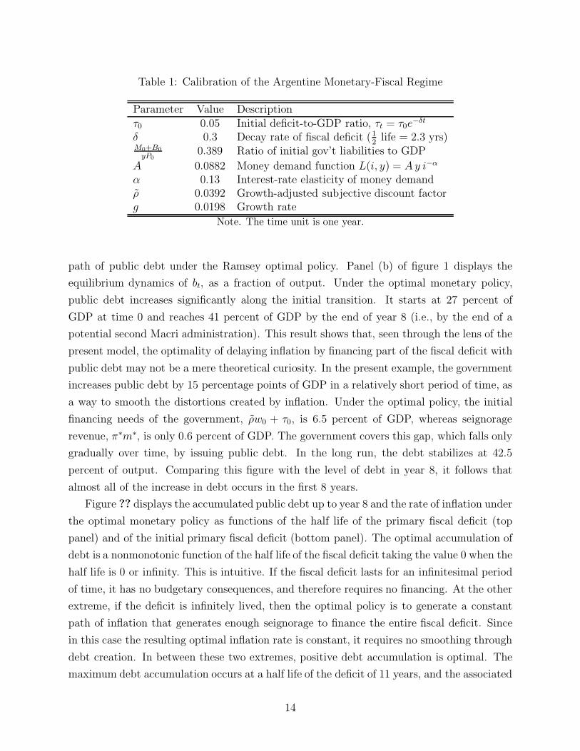
Table 1: Calibration of the Argentine Monetary-Fiscal Regime

Parameter Value Descriptionτ0 0.05 Initial deficit-to-GDP ratio, τt = τ0e

−δt

δ 0.3 Decay rate of fiscal deficit (12

life = 2.3 yrs)M0+B0

yP0

0.389 Ratio of initial gov’t liabilities to GDP

A 0.0882 Money demand function L(i, y) = A y i−α

α 0.13 Interest-rate elasticity of money demandρ 0.0392 Growth-adjusted subjective discount factorg 0.0198 Growth rate

Note. The time unit is one year.

path of public debt under the Ramsey optimal policy. Panel (b) of figure 1 displays the

equilibrium dynamics of bt, as a fraction of output. Under the optimal monetary policy,

public debt increases significantly along the initial transition. It starts at 27 percent of

GDP at time 0 and reaches 41 percent of GDP by the end of year 8 (i.e., by the end of a

potential second Macri administration). This result shows that, seen through the lens of the

present model, the optimality of delaying inflation by financing part of the fiscal deficit with

public debt may not be a mere theoretical curiosity. In the present example, the government

increases public debt by 15 percentage points of GDP in a relatively short period of time, as

a way to smooth the distortions created by inflation. Under the optimal policy, the initial

financing needs of the government, ρw0 + τ0, is 6.5 percent of GDP, whereas seignorage

revenue, π∗m∗, is only 0.6 percent of GDP. The government covers this gap, which falls only

gradually over time, by issuing public debt. In the long run, the debt stabilizes at 42.5

percent of output. Comparing this figure with the level of debt in year 8, it follows that

almost all of the increase in debt occurs in the first 8 years.

Figure ?? displays the accumulated public debt up to year 8 and the rate of inflation under

the optimal monetary policy as functions of the half life of the primary fiscal deficit (top

panel) and of the initial primary fiscal deficit (bottom panel). The optimal accumulation of

debt is a nonmonotonic function of the half life of the fiscal deficit taking the value 0 when the

half life is 0 or infinity. This is intuitive. If the fiscal deficit lasts for an infinitesimal period

of time, it has no budgetary consequences, and therefore requires no financing. At the other

extreme, if the deficit is infinitely lived, then the optimal policy is to generate a constant

path of inflation that generates enough seignorage to finance the entire fiscal deficit. Since

in this case the resulting optimal inflation rate is constant, it requires no smoothing through

debt creation. In between these two extremes, positive debt accumulation is optimal. The

maximum debt accumulation occurs at a half life of the deficit of 11 years, and the associated

14

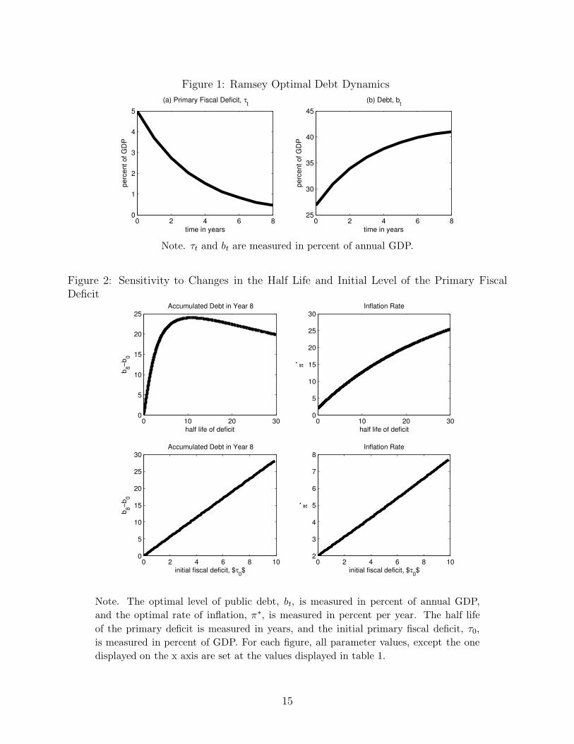
Figure 1: Ramsey Optimal Debt Dynamics

0 2 4 6 80

1

2

3

4

5

(a) Primary Fiscal Deficit, τt

time in years

perc

ent

of

GD

P

0 2 4 6 825

30

35

40

45

(b) Debt, bt

time in years

perc

ent

of

GD

P

Note. τt and bt are measured in percent of annual GDP.

Figure 2: Sensitivity to Changes in the Half Life and Initial Level of the Primary FiscalDeficit

0 10 20 300

5

10

15

20

25

half life of deficit

b8−

b0

Accumulated Debt in Year 8

0 10 20 300

5

10

15

20

25

30

half life of deficit

π*

Inflation Rate

0 2 4 6 8 100

5

10

15

20

25

30

initial fiscal deficit, $τ0$

b8−

b0

Accumulated Debt in Year 8

0 2 4 6 8 102

3

4

5

6

7

8

initial fiscal deficit, $τ0$

π*

Inflation Rate

Note. The optimal level of public debt, bt, is measured in percent of annual GDP,

and the optimal rate of inflation, π∗, is measured in percent per year. The half life

of the primary deficit is measured in years, and the initial primary fiscal deficit, τ0,

is measured in percent of GDP. For each figure, all parameter values, except the one

displayed on the x axis are set at the values displayed in table 1.

15

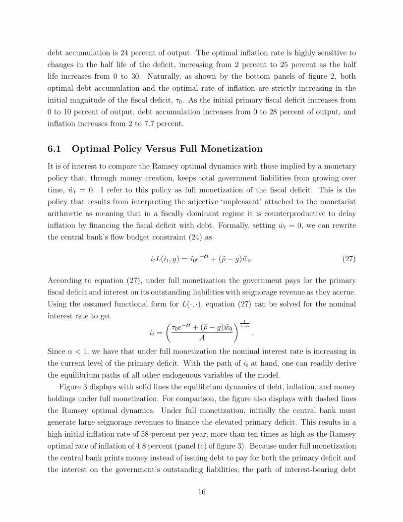
debt accumulation is 24 percent of output. The optimal inflation rate is highly sensitive to

changes in the half life of the deficit, increasing from 2 percent to 25 percent as the half

life increases from 0 to 30. Naturally, as shown by the bottom panels of figure 2, both

optimal debt accumulation and the optimal rate of inflation are strictly increasing in the

initial magnitude of the fiscal deficit, τ0. As the initial primary fiscal deficit increases from

0 to 10 percent of output, debt accumulation increases from 0 to 28 percent of output, and

inflation increases from 2 to 7.7 percent.

6.1 Optimal Policy Versus Full Monetization

It is of interest to compare the Ramsey optimal dynamics with those implied by a monetary

policy that, through money creation, keeps total government liabilities from growing over

time, wt = 0. I refer to this policy as full monetization of the fiscal deficit. This is the

policy that results from interpreting the adjective ‘unpleasant’ attached to the monetarist

arithmetic as meaning that in a fiscally dominant regime it is counterproductive to delay

inflation by financing the fiscal deficit with debt. Formally, setting wt = 0, we can rewrite

the central bank’s flow budget constraint (24) as

itL(it, y) = τ0e−δt + (ρ − g)w0. (27)

According to equation (27), under full monetization the government pays for the primary

fiscal deficit and interest on its outstanding liabilities with seignorage revenue as they accrue.

Using the assumed functional form for L(·, ·), equation (27) can be solved for the nominal

interest rate to get

it =

(

τ0e−δt + (ρ − g)w0

A

)

1

1−α

.

Since α < 1, we have that under full monetization the nominal interest rate is increasing in

the current level of the primary deficit. With the path of it at hand, one can readily derive

the equilibrium paths of all other endogenous variables of the model.

Figure 3 displays with solid lines the equilibrium dynamics of debt, inflation, and money

holdings under full monetization. For comparison, the figure also displays with dashed lines

the Ramsey optimal dynamics. Under full monetization, initially the central bank must

generate large seignorage revenues to finance the elevated primary deficit. This results in a

high initial inflation rate of 58 percent per year, more than ten times as high as the Ramsey

optimal rate of inflation of 4.8 percent (panel (c) of figure 3). Because under full monetization

the central bank prints money instead of issuing debt to pay for both the primary deficit and

the interest on the government’s outstanding liabilities, the path of interest-bearing debt

16

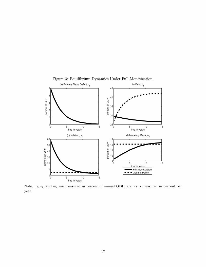
Figure 3: Equilibrium Dynamics Under Full Monetization

0 5 10 150

1

2

3

4

5

(a) Primary Fiscal Deficit, τt

time in years

perc

ent of G

DP

0 5 10 1525

30

35

40

45

(b) Debt, bt

time in years

perc

ent of G

DP

0 5 10 150

10

20

30

40

50

60

(c) Inflation, πt

time in years

perc

ent per

year

0 5 10 159

10

11

12

13

(d) Monetary Base, mt

time in years

perc

ent of G

DP

Full monetizationOptimal Policy

Note. τt, bt, and mt are measured in percent of annual GDP, and πt is measured in percent per

year.

17

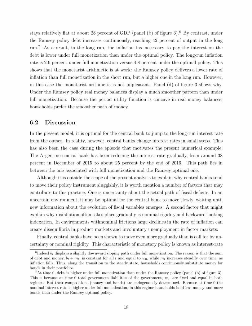
stays relatively flat at about 28 percent of GDP (panel (b) of figure 3).6 By contrast, under

the Ramsey policy debt increases continuously, reaching 42 percent of output in the long

run.7 As a result, in the long run, the inflation tax necessary to pay the interest on the

debt is lower under full monetization than under the optimal policy. The long-run inflation

rate is 2.6 percent under full monetization versus 4.8 percent under the optimal policy. This

shows that the monetarist arithmetic is at work: the Ramsey policy delivers a lower rate of

inflation than full monetization in the short run, but a higher one in the long run. However,

in this case the monetarist arithmetic is not unpleasant. Panel (d) of figure 3 shows why.

Under the Ramsey policy real money balances display a much smoother pattern than under

full monetization. Because the period utility function is concave in real money balances,

households prefer the smoother path of money.

6.2 Discussion

In the present model, it is optimal for the central bank to jump to the long-run interest rate

from the outset. In reality, however, central banks change interest rates in small steps. This

has also been the case during the episode that motivates the present numerical example.

The Argentine central bank has been reducing the interest rate gradually, from around 38

percent in December of 2015 to about 25 percent by the end of 2016. This path lies in

between the one associated with full monetization and the Ramsey optimal one.

Although it is outside the scope of the present analysis to explain why central banks tend

to move their policy instrument sluggishly, it is worth mention a number of factors that may

contribute to this practice. One is uncertainty about the actual path of fiscal deficits. In an

uncertain environment, it may be optimal for the central bank to move slowly, waiting until

new information about the evolution of fiscal variables emerges. A second factor that might

explain why disinflation often takes place gradually is nominal rigidity and backward-looking

indexation. In environments withnominal frictions large declines in the rate of inflation can

create disequilibria in product markets and involuntary unemployment in factor markets.

Finally, central banks have been shown to move even more gradually than is call for by un-

certainty or nominal rigidity. This characteristic of monetary policy is known as interest-rate

6Indeed bt displays a slightly downward sloping path under full monetization. The reason is that the sumof debt and money, bt + mt, is constant for all t and equal to w0, while mt increases steadily over time, asinflation falls. Thus, along the transition to the steady state, households continuously substitute money forbonds in their portfolios.

7At time 0, debt is higher under full monetization than under the Ramsey policy (panel (b) of figure 3).This is because at time 0 total government liabilities of the government, w0, are fixed and equal in bothregimes. But their compositions (money and bonds) are endogenously determined. Because at time 0 thenominal interest rate is higher under full monetization, in this regime households hold less money and morebonds than under the Ramsey optimal policy.

18

smoothing and has been extensively documented in developed countries (see, for example,

Goodfriend, 1991; and Sack, 2000), but is also present in emerging countries, including those

experiencing high inflation (Argentina since late 2015 being an example). Motivated by the

empirical relevance of interest-rate smoothing, a number of studies have introduced this fea-

ture in dynamic models. An early contribution is Barro 1988). Woodford (2003) shows that

when the central bank lacks commitment, adding lagged interest rates to its loss function can

be desirable, as it brings the resulting optimal policy under discretion closer to its counter-

part under commitment. To introduce interest-rate smoothing, consider a modified version

of the indirect utility function (15) of the form∫

∞

0e−ρt[u(y) + v((L(it, y)) − γ(it − zt)

2]dt,

where γ > 0 is a parameter, and zt denotes a weighted average of past interest rates that

obeys the law of motion zt = it − θzt, for θ > 0. The parameter γ measures the degree of

interest-rate smoothing. The model collapses to the baseline specification when γ equals 0.

The parameter θ measures the degree of backward-looking behavior in the central bank’s

monetary conduct. The variable zt is, of course, a state variable. The problem of the central

bank is to choose a path for the nominal interest rate {it} to maximize its modified objective

function subject to the intertemporal constraint (12) and to the law of motion of zt. This

specification of the model is likely to deliver more realistic paths for the nominal interest rate

and inflation—i.e., more gradual disinflation dynamics—while preserving the desirability of

debt creation along the stabilization path.

7 Concluding Remarks

In economies in which the monetary-fiscal regime is fiscally dominant, the central bank

does not control inflation. This is because under this policy regime money creation must

passively finance the present discounted value of fiscal deficits plus the government’s initial

liabilities. The central bank can, however, choose when to create money. The unpleasant

monetarist arithmetic states that tight current monetary conditions imply higher inflation

in the future. This paper does not quarrel with this dictum, but with the conclusion—

implicit in the qualifier ’unpleasant’—that in a fiscally dominant regime tight monetary

policy, understood as financing part of the fiscal deficit by issuing debt, is undesirable.

Arriving at such a conclusion requires a normative analysis. In this paper I attempt to

fill this gap, by characterizing the welfare maximizing path of public debt in a monetary

economy characterized by fiscal dominance.

The main result derived from this analysis is that in a fiscally dominant regime tight

money may not have unpleasant consequences, but, on the contrary, be optimal. This result

obtains when the fiscal deficit is expected to fall over time or is temporarily high. The

19

intuition is simple. Among all the inflation paths that generate enough seignorage revenue

to pay for the present discounted value of the government’s liabilities, the monetary authority

prefers a flat one to smooth out the distortions created by the inflation tax. In turn, a flat

path of inflation induces a flat path of seignorage revenue. This means that in periods in

which fiscal deficits are above average, the central bank will find it optimal to issue debt to

finance part of the fiscal deficit. The central bank prefers to issue debt even though it knows

that it will cause higher inflation in the future than the alternative of financing the entire

current deficit by printing money. In this case, the monetarist arithmetic obtains, but is not

unpleasant.

20

References

Barro, Robert J., “Interest Rate Smoothing,” NBER working paper No. 2581, May 1988.

Goodfriend, Marvin, “Interest Rate Smoothing in the Conduct of Monetary Policy,” Carnegie-

Rochester Conference Series on Public Policy, Spring 1991, 7-30. Inagaki, Kazuyuki/

Estimating the Interest Rate Semi-Elasticity of the Demand for Money in Low Interest

Rate Environments/ Economic Modelling 26/ 2009/ 147-154.

Kiguel, Miguel A., and Pablo Andres Neumeyer, “Seigniorage and Inflation: The Case of

Argentina,” Journal of Money, Credit and Banking 27, August 1995, 672-682.

Sargent, Thomas J., and Neil Wallace, “Some Unpleasant Monetarist Arithmetic,” Federal

Reserve Bank of Minneapolis Quarterly Review, Fall 1981, 1-17.

Sack, Brian, “Does the Fed Act Gradually? A VAR Analysis,” Journal of Monetary Eco-

nomics 46, August 2000, 229-256.

Schmitt-Grohe, Stephanie, and Martın Uribe, “Optimal Fiscal and Monetary Policy Under

Imperfect Competition,” Journal of Macroeconomics 26, June 2004, 183-209.

Woodford, Michael, “Optimal Interest-Rate Smoothing,” Review of Economic Studies 70,

2003, 861-886.

21