ORIGINAL ARTICLE

doi:10.1111/j.1558-5646.2011.01574.x

IS YOUR PHYLOGENY INFORMATIVE?MEASURING THE POWER OF COMPARATIVEMETHODSCarl Boettiger,1,2 Graham Coop3 and Peter Ralph3

1Center for Population Biology, University of California, Davis, California 956162E-mail: cboettig@ucdavis.edu

3Department of Evolution and Ecology, University of California, Davis, California 95616

Received June 14, 2011

Accepted December 13, 2011

Data Archived: Dryad doi:10.5061/dryad.m6r6hc12

Phylogenetic comparative methods may fail to produce meaningful results when either the underlying model is inappropriate or

the data contain insufficient information to inform the inference. The ability to measure the statistical power of these methods

has become crucial to ensure that data quantity keeps pace with growing model complexity. Through simulations, we show that

commonly applied model choice methods based on information criteria can have remarkably high error rates; this can be a problem

because methods to estimate the uncertainty or power are not widely known or applied. Furthermore, the power of comparative

methods can depend significantly on the structure of the data. We describe a Monte Carlo-based method which addresses both

of these challenges, and show how this approach both quantifies and substantially reduces errors relative to information criteria.

The method also produces meaningful confidence intervals for model parameters. We illustrate how the power to distinguish

different models, such as varying levels of selection, varies both with number of taxa and structure of the phylogeny. We provide

an open-source implementation in the pmc (“Phylogenetic Monte Carlo”) package for the R programming language. We hope such

power analysis becomes a routine part of model comparison in comparative methods.

KEY WORDS: Comparative method, information criteria, model choice, parametric bootstrap, phylogenetics.

ARE PHYLOGENIES INFORMATIVE?

Since their introduction into the comparative method over two and

a half decades ago, phylogenetic methods have become increas-

ingly common and increasingly complex. Despite this, concern

persists about the ubiquitous use of these approaches (Price 1997;

Losos 2011). From a statistical perspective, these concerns can

be divided into two categories: (1) Do we have appropriate mod-

els that reflect the biological reality of evolution and represent

meaningful hypotheses? and (2) Do we have adequate data to fit

these models and to choose between them? The models have been

greatly improved since their introduction, and can now account

for stabilizing selection (Hansen and Martins 1996), multiple op-

tima (Butler and King 2004), and differing rates of evolution

across taxa (O’Meara et al. 2006) or through time (Pagel 1999;

Blomberg et al. 2003); but little attention has been given to this

second concern about data adequacy. In this article, we highlight

the importance of these concerns, and illustrate a method for ad-

dressing them.

It can be difficult to accurately interpret the results of com-

parative methods without quantification of uncertainty, model fit,

or power. Most current comparative methods do not attempt to

quantify this uncertainty; consequently it can be easy for in-

adequate power to lead to false biological conclusions. For in-

stance, below we illustrate how estimates of phylogenetic signal

(Gittleman and Kot 1990) using the λ statistic (Pagel 1999; Revell

2010) can reach opposite conclusions (from no signal λ = 0 to

approximately Brownian, λ ≈ 1) when applied to different sim-

ulated realizations of the same process. We also show that model

1C© 2012 The Author(s).Evolution

CARL BOETTIGER ET AL.

selection by information criteria can prefer over-parameterized

models by a wide margin. On the other hand, when a simpler

model is chosen, it may be difficult to determine whether this

merely reflects a lack of power. In both cases, the results can be

correctly interpreted by estimating the uncertainty in parameter

estimates and the statistical power (ability to distinguish between

models) of the model selection procedure.

Here, we provide one solution to these problems using a

parametric bootstrapping approach which easily fits within the

framework used by many comparative methods approaches. As

comparative methods rely on explicit models, this is easily im-

plemented by simulating under the specified models. For the

problem of uncertainty in parameter estimation, the bootstrap

is a well-established and straightforward method (Efron 1987). A

few areas of comparative methods have used a similar approach:

for instance, phylogenetic ANOVA (Garland et al. 1993) calcu-

lates P-values of the test statistic by simulation under Brownian

motion (BM). A similar approach was later introduced in the

Brownie software (O’Meara et al. 2006) to generate the null dis-

tribution of likelihood ratios under BM, and applied in Revell and

Harmon (2008), which showed the distribution can deviate sub-

stantially from χ2, and a similar approach is applied in Revell and

Collar (2009). Unfortunately, such approaches have never be-

come a common in comparative analyses. Here, we describe a

method due to Cox (1962) and used by others (Goldman 1993;

Huelsenbeck and Bull 1996), that can be used in place of informa-

tion criteria for model choice, allowing estimation of power and

false positive rates, and can provide good estimates of confidence

intervals on model parameter estimates. Although simulations are

often performed when a new method is first presented, this prac-

tice rarely becomes routine. By providing a simple R package

(“pmc,” Phylogenetic Monte Carlo) for the method outlined, we

hope Monte Carlo-based model choice and estimates of power

become common in comparative methods.

To set the stage, we will review common phylogenetic models

and describe the Monte Carlo approach to model choice. We then

present the results of our method applied to example data and

discuss its consequences.

COMMON PHYLOGENETIC MODELS

Comparative phylogenetics of continuous traits commonly uses

a collection of simple stochastic models of evolution; we briefly

review these here to fix ideas and notation. All models we con-

sider take as given an ultrametric phylogenetic tree whose branch

lengths represent evolutionary divergence times; extant taxa are

represented by the tips of the tree. We will assume that the tree

is known without error. For convenience, we will in all examples

choose time units so that the tree height is one unit. For each ex-

tant taxon, we have a trait value (say, the species mean) for some

continuous trait such as body size, and represent the collection

of trait values across extant taxa as the vector X . The joint dis-

tribution of these trait values is given by specifying the ancestral

trait value X0 at the root of the tree, by describing the stochastic

process of trait evolution along branches of the tree, and assuming

that evolution on separate branches proceeds independently.

Let Yt be the value of our trait at time t along some branch.

The simplest and most common model for the evolution of the trait

Yt is a scaled BM (Felsenstein 1985), which can be represented

by the stochastic differential equation:

dYt = σd Bt , (1)

in which Bt is standard BM, and σ is the rate parameter. Under

this model, the trait value evolves as a random walk starting

from the ancestral state X0, and upon reaching each node in the

phylogeny, the process bifurcates into two independent Brownian

walks. This BM model is completely defined given a phylogeny

and two parameters: the initial state X0 and the parameter σ, which

is usually interpreted as the rate of increase in variance.

A closely related model introduced in a comparative phy-

logenetics context by Hansen (1997) is the Ornstein-Uhlenbeck

(OU) model, for which trait evolution Yt along each branch fol-

lows the Ornstein-Uhlenbeck process, which is described by the

following stochastic differential equation

dYt = −α(Yt − θ) dt + σd Bt . (2)

Here, BM is modified to have a central tendency toward a

preferred trait value θ, usually interpreted as a optimum trait value

under stabilizing selection. The strength of stabilizing selection

increases linearly with distance from the optimum θ, controlled

by the parameter α. When α = 0, this model reduces to the BM

model. Both evolutionary models are described in more detail

elsewhere, for example, Butler and King (2004).

Many variations of these basic models are also common—

for instance, it may be desirable to allow the diversification rate

parameter σ in the BM model to vary in some way over time

(Pagel 1999; Blomberg et al. 2003; Harmon et al. 2010) or across

the phylogeny (O’Meara et al. 2006). Similar extensions can be

applied to the OU model—we will later consider the example of

Butler and King (2004) which allows the optimum trait value θ to

differ among different branches or clades. One can illustrate which

branches of a phylogeny are permitted to have independently

estimated values of the optimum trait by “painting” them different

colors indicating where the model is allowed to change (Butler

and King 2004).

Another commonly used variation is Pagel’s λ (Pagel 1994;

Freckleton et al. 2002), which was introduced as a test of phylo-

genetic signal—the degree to which correlations in traits reflect

patterns of shared ancestry. The model underlying Pagel’s λ is

the simple BM along the phylogeny as above, except that the

2 EVOLUTION 2012

IS YOUR PHYLOGENY INFORMATIVE?

Figure 1. (A) Empirical distribution of maximum-likelihood estimates of λ for 1000 sets of trait values simulated on the Geospiza

phylogeny with 13 taxa transformed with λ = 0.6, using σ = 0.18. Most such datasets yielded a maximum-likelihood estimate of 0; the

mean estimate is λ = 0.35. (B) As above, but simulating trait values on a much larger phylogenetic tree (a single, simulated Yule tree

with 281 tips), again transformed with λ = 0.6. The estimated values now cluster around the true value, and have mean λ = 0.59. (C) The

data can be more informative about some parameters than others: shown is the empirical distribution of maximum-likelihood estimates

of the diversification rate σ for the same simulations as in (A). The mean of the distribution is σ = 0.18, matching the value used in the

simulations.

phylogeny is modified by shortening all internal edges by a mul-

tiplicative factor of λ, which reduces the resulting correlations

between any pair of taxa by a factor λ, and adjusting terminal

edges so the tree remains ultrametric. The parameter λ can then

be estimated by maximum likelihood. Estimates near unity are

taken to indicate high phylogenetic signal, whereas estimates near

zero indicate that other processes such as natural selection have

erased this “signal” of common descent.

MethodsUNCERTAINTY IN PARAMETER ESTIMATES

To demonstrate the perils of inadequate data without estimates

of uncertainty, we open with an example of a phylogenetic test

using Pagel’s λ statistic that also serves to illustrate the estimation

of uncertainty in parameter estimates (e.g., confidence intervals).

We illustrate that on a small tree, estimates of λ can differ greatly

from the parameter used in the simulations. In practice, the danger

is that an estimate of λ near zero may arise by chance because

the tree is too small, not because the phylogeny is unimportant to

the evolution of the trait. Larger phylogenies, on the other hand,

generally allow greater accuracy.

In Figure 1A, we show the empirical distribution of the

maximum-likelihood estimate of λ for 1000 datasets simulated

under a model with moderate phylogenetic signal, λ = 0.6, and

σ = 0.03. The estimates were performed on the Geospiza data us-

ing functions available in pmc in conjunction with the R package

geiger (Harmon et al. 2008). The phylogeny, data, and script for

the analysis are included in pmc. We see that for datasets coming

from this small phylogeny, the maximum-likelihood statistic λ

is a poor estimator for the true value of λ. The most common

estimate is λ = 0, which is usually interpreted to mean that the

phylogeny contains little information. The next most common es-

timate is λ = 1. Note that this is the upper bound set on λ by the

fitting algorithm. It is clear that we must thus be cautious what

we conclude based on values of λ estimated on this phylogeny.

Repeating this exercise on successively larger datasets makes

it clear that this is a problem of insufficient data. With a simulated

tree of 281 tips, the estimated values are closely centered around

the true value, as shown in Figure 1B.

The amount of data required to be informative will depend

not only on the size and topology of the tree but also on the ques-

tion being asked. For instance, it may be impossible to distinguish

EVOLUTION 2012 3

CARL BOETTIGER ET AL.

Figure 2. Conceptual diagram of the Monte Carlo method for

model choice. First, parameters for both models are estimated

from the original data . Then, n simulated datasets are created

from each model at these parameters, and on each dataset, the

parameters for both models are reestimated and the likelihood ra-

tio statistic is computed. The collection of likelihood ratio statistics

generates the corresponding distribution. This involves a process

of 4n fits by maximum likelihood, instead of only two fits required

for information criteria.

moderately different values of λ, which is very difficult to esti-

mate accurately. However, it may be feasible to estimate other

parameters on smaller phylogenies than this 281 taxa example.

For instance, using the same 13 taxa Geospiza phylogeny, we can

estimate the diversification rate parameter σ much more precisely,

as shown in Figure 1C.

A natural way to report the uncertainty associated with a

parameter estimate is to construct a confidence interval, which

is rarely performed in the literature but can easily be done by

parametric bootstrapping. Given the parameter estimate, a con-

fidence interval can be estimated by simulating a large number

of datasets using the known phylogeny and the estimated param-

eter, and reestimating the parameter on each simulated dataset

(e.g., see Diciccio and Efron 1996). The distribution of the reesti-

mated parameters is used to construct the confidence interval; for

example, the 2.5 to the 97.5 percentile gives a 95% confidence

interval. For the example shown in Figure 1B, our estimate of λ

on the Yule tree with 281 tips, the 95% confidence interval would

be (0.45, 0.69). For the parameter σ, Figure 1C shows that the

confidence interval is (0.007, 0.059). Given the noisy nature of

parameters estimated from phylogenies, we recommend that con-

fidence interval should routinely be reported, and to facilitate this,

have implemented this as pmc::confidenceIntervals.pow. Confi-

dence intervals could also be estimated from the curvature of the

likelihood surface, but these can be unreliable and problematic to

compute.

THE MONTE CARLO APPROACH

Knowing when the data are sufficiently informative is also crucial

when comparing different models. To do this, we introduce a

Monte Carlo-based method, described below. Suppose we have a

dataset X for which we wish to determine which of two models,

model 0 or model 1, is the better description. Each model is

specified by a vector of parameters, �0 and �1, respectively,

which can assume values in the spaces �0 and �1, respectively.

We tend to imagine that model 1 is the more complex model,

though in general they need not be nested. LetL0 be the likelihood

function for model 0, let �0 = arg max�0∈�0(L0(�0|X )) be the

maximum-likelihood estimator for �0 given X , and let L0 =L0(�0|X ); and define L1, �1, L1 similarly for model 1.

The statistic we will use is δ, defined to be twice the difference

in log likelihood of observing the data under the two maximum

likelihood estimate (MLE) models,

δ = −2 (log L0 − log L1) . (3)

For simplicity we will refer to this as the likelihood ratio.

Larger values of δ indicate more support for model 1 relative

to model 0. It is natural to use the difference in log-likelihoods

as a statistic to choose between the models (Neyman and Pear-

son 1933), as do information criteria such as Akaike information

criterion (AIC). To do this, we need to know, for instance, how

large should δ be before we decide that model 1 is much closer

to the truth than is model 0. Many common methods proceed to

approximate the distribution of δ asymptotically. For instance, if

the models are nested in a manner that does not force a parame-

ter to its boundary value, this statistic has asymptotically the χ2

distribution with degrees of freedom equal to the difference in

the number of parameters. These asymptotic approximations for

phylogenetic comparative analyses are often inadequate for phy-

logenetic comparisons. Instead, we can estimate the distribution

of δ under either model directly from Monte Carlo simulation.

This method seems to have been first suggested in the statistical

literature by Cox (1961), 1962) and applied to mixture models by

McLachlan (1987). It has been previously applied to the case of

estimating phylogenies from sequence data by Huelsenbeck and

Bull (1996); see also Goldman (1993).

To estimate the distribution of δ under model 0 and the

estimated parameters (�0), we proceed as follows. First sim-

ulate n datasets X1, . . . , Xn independently from model 0 with

parameters �0. For each 1 ≤ k ≤ n, let �k0 be the maximum-

likelihood estimator of the parameters �0 of model 0 for dataset

Xk , and likewise let �k1 be the MLE under model 1. Then

we compute the likelihood ratio statistic for the kth dataset,

δk = −2(logL0(Xk |�k0) − logL1(Xk |�k

1)), and examine the em-

pirical distribution of δ1, . . . , δn . We can also estimate the distri-

bution of δ under model 1 in the same way.

4 EVOLUTION 2012

IS YOUR PHYLOGENY INFORMATIVE?

There are two things to note about this procedure. First, the

Monte Carlo datasets are simulated at the maximum-likelihood

parameters �0 and �1, which are in turn estimated from the

same dataset X . So if, for instance, the models are nested and

the simpler is correct, then one would expect model 0 at �0 to

be quite similar to model 1 at �1. Second, it is necessary when

computing the Monte Carlo values δk to reestimate the maximum-

likelihood parameters, rather than using the original parame-

ters �0 and �1—simply computing δk = −2(logL0(Xk |�0) −logL0(Xk |�1) would lead to a much less powerful test (Hall

and Wilson 1991). The reason for this is somewhat subtle (see

McLachlan 1987), and is related to the first point. For further

suggestions on obtaining a reliable estimate of the distributions,

see Efron (1987) and Diciccio and Efron (1996).

MODEL SELECTION

If we suppose model 0 is “simpler” than model 1, it is natural to

regard model 0 as the “null” and test the hypothesis that the data

came from model 0. To do this, we would compare where the

observed difference in log likelihoods δ for the original data falls

relative to the distribution under model 0. The proportion of the

simulated values larger than δ provides an approximation to the

P-value for the test, the probability that a difference at least as

large would be seen under model 0. (Because the datasets Xk are

all simulated at the estimated parameters �0, this strictly applies

only for the hypothesis test between the maximum-likelihood

estimated models, and is not the P-value when comparing the

composite hypothesis represented by the original model with un-

specified parameters (see McLachlan 1987). If we choose, say, δ∗so that 95% of the simulated values δ1, . . . , δn fall below δ∗, and

choose to reject model 0 if δ > δ∗, then we have a test of the null

hypothesis that model 0 is true, with a false positive probability

of approximately 0.05 under model 0. If we then want to know

about the statistical power of this test—the probability that we

correctly reject model 0 when the data came from model 1—we

would turn to the distribution of δ under model 1. If we have

chosen δ∗ as above, then the amount of this distribution to the left

of δ∗ approximates the probability of rejecting model 0 when the

data are produced by model 1—the power of the test.

The procedure we have described, illustrated in Figure 2, is

motivated by classical hypothesis testing, but is only one way to

use the information provided by the empirical distributions of δ.

An Example Using Anolis DataTHE ANOLES DATA

To illustrate the concerns about phylogenetic information in com-

parative methods, we shall revisit a classic dataset of mean body

size for 23 species of Anolis lizards from the Lesser Antilles,

which has been used to introduce other comparative phylogenetic

approaches (e.g., Butler and King 2004, familiar to many who

have used the ouch package). The phylogeny reconstruction used

here (Losos 1990) is based upon morphological (Lazell 1972)

and protein-electrophretic (Gorman and Kim 1976) techniques

rather than the more recent phylogenies based on mitochondrial

sequences (Schneider et al. 2001; Stenson et al. 2004), which have

substantial differences. As our purpose is simply to illustrate the

approach, we continue to use older tree familiar to the readers of

earlier work (Losos 1990; Butler and King 2004).

Identification of branches or clades of a phylogenetic tree that

show significantly different evolutionary patterns can illuminate

key elements about the origin and maintenance of biodiversity.

Butler and King (2004) demonstrated how the existence of dif-

ferent adaptive optima in character traits on different parts of a

phylogenetic tree could be detected. They assumed that evolution

of the trait along each branch followed the Ornstein-Uhlenbeck

model, but that different branches could have different optima

(the parameter θ). The branches that must share a common value

of θ are represented by a “painting” of the tree; three possibilities

for the Anolis tree that we later investigate are shown in Figure 3.

Any branch of a given color must have the same optimum trait

value, each of which is estimated by the fitting algorithm. The

remaining parameters α and σ are shared across the entire tree.

To confirm that the proposed pattern of heterogeneity (the

painting) is justified by the data, it is necessary to compare be-

tween possible paintings and possible assignments of model pa-

rameters to each part of the painting. We seek to identify (1) which

model best describes the data and (2) whether we have sufficient

data to resolve that difference?

MODELS FOR THE ANOLIS PHYLOGENY

To illustrate the approach, we consider a total of five models

for the Anolis dataset. The first two models apply the same

model of evolution to the entire tree (i.e., a one-color painting)—

either BM (Edwards and Cavalli-Sforza 1964; Felsenstein 1985),

with two parameters; or the Ornstein-Uhlenbeck process (OU.1)

(Felsenstein 1985; Hansen 1997), with three.

The remaining three models extend these simple cases by in-

troducing heterogeneity in the model, allowing the trait optimum

to vary across the tree as indicated in Figure 3. The OU.3 model

of Figure 3A has three optima, and corresponds to the character

displacement hypothesis (Losos 1990), which predicts three dif-

ferent optimum body sizes—an intermediate optimum on islands

having only one species, and a larger and a smaller optimum for

islands with two species of lizards. The island size determines

to which optimum the tips or extant species are assigned, while

the ancestral states are constructed by parsimony as per Butler

and King (2004). To these three models (BM, OU.1, and OU.3)

EVOLUTION 2012 5

CARL BOETTIGER ET AL.

(A) OU.3 (B) OU.4 (C) OU.15

pogus, St. Maarten

schwartzi, St. Eustatius

schwartzi, St. Christopher

schwartzi, Nevis

wattsi, Barbuda

wattsi, Antigua

bimaculatus, St. Eustatius

bimaculatus, Nevis

bimaculatus, St. Christopher

leachi, Barbuda

leachi, Antigua

nubilus, Redonda

sabanus, Saba

gingivinus, St. Barthelemy

gingivinus, Anguilla

gingivinus, St. Maarten

oculatus, Dominica

ferreus, Marie Galante

lividus, Monserrat

marmoratus, Guadeloupe

marmoratus, Desirade

terraealtae, Illes de Saintes−1

terraealtae, Illes de Saintes−2

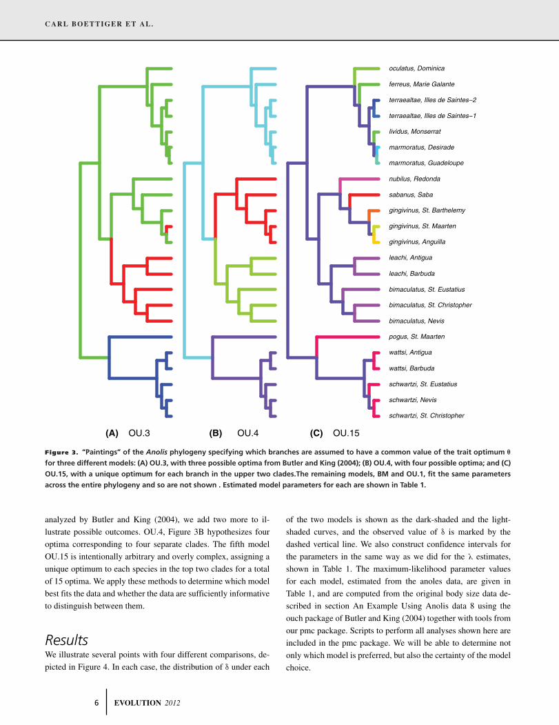
Figure 3. “Paintings” of the Anolis phylogeny specifying which branches are assumed to have a common value of the trait optimum θ

for three different models: (A) OU.3, with three possible optima from Butler and King (2004); (B) OU.4, with four possible optima; and (C)

OU.15, with a unique optimum for each branch in the upper two clades.The remaining models, BM and OU.1, fit the same parameters

across the entire phylogeny and so are not shown . Estimated model parameters for each are shown in Table 1.

analyzed by Butler and King (2004), we add two more to il-

lustrate possible outcomes. OU.4, Figure 3B hypothesizes four

optima corresponding to four separate clades. The fifth model

OU.15 is intentionally arbitrary and overly complex, assigning a

unique optimum to each species in the top two clades for a total

of 15 optima. We apply these methods to determine which model

best fits the data and whether the data are sufficiently informative

to distinguish between them.

ResultsWe illustrate several points with four different comparisons, de-

picted in Figure 4. In each case, the distribution of δ under each

of the two models is shown as the dark-shaded and the light-

shaded curves, and the observed value of δ is marked by the

dashed vertical line. We also construct confidence intervals for

the parameters in the same way as we did for the λ estimates,

shown in Table 1. The maximum-likelihood parameter values

for each model, estimated from the anoles data, are given in

Table 1, and are computed from the original body size data de-

scribed in section An Example Using Anolis data 8 using the

ouch package of Butler and King (2004) together with tools from

our pmc package. Scripts to perform all analyses shown here are

included in the pmc package. We will be able to determine not

only which model is preferred, but also the certainty of the model

choice.

6 EVOLUTION 2012

IS YOUR PHYLOGENY INFORMATIVE?

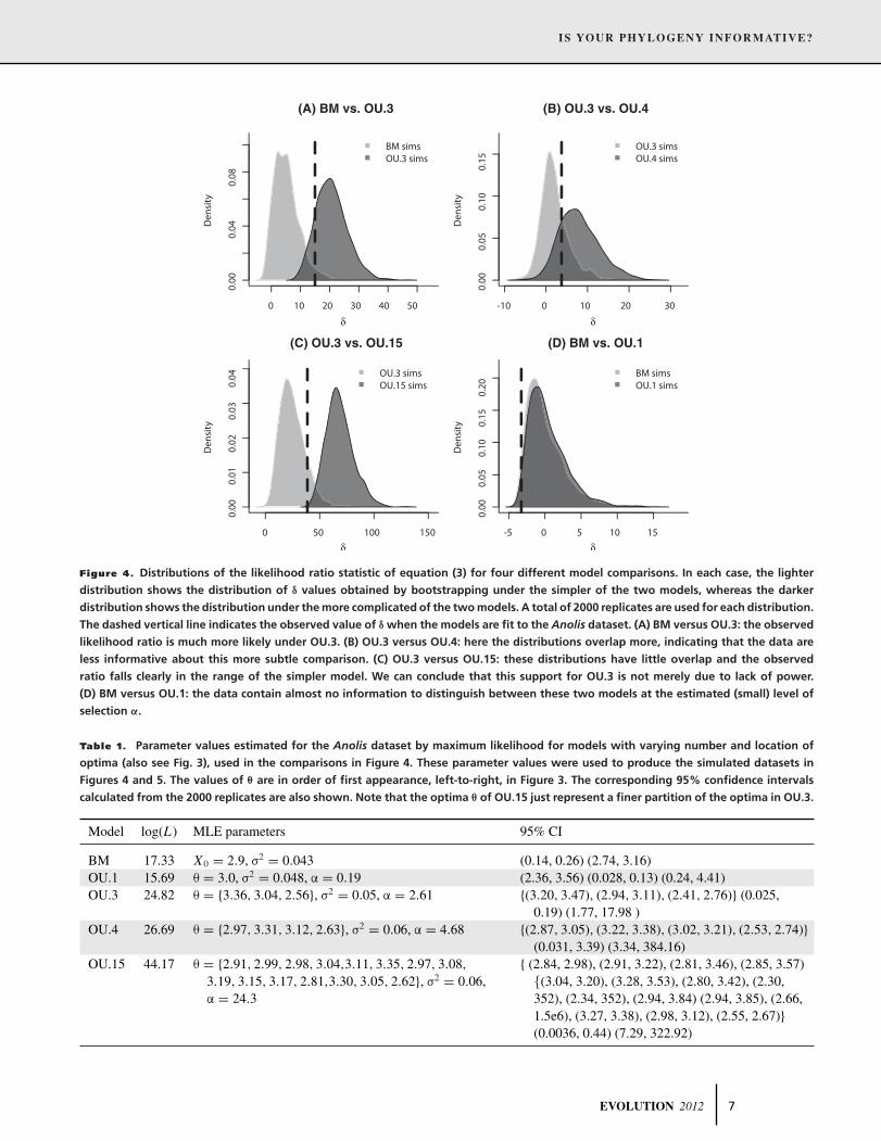
Figure 4. Distributions of the likelihood ratio statistic of equation (3) for four different model comparisons. In each case, the lighter

distribution shows the distribution of δ values obtained by bootstrapping under the simpler of the two models, whereas the darker

distribution shows the distribution under the more complicated of the two models. A total of 2000 replicates are used for each distribution.

The dashed vertical line indicates the observed value of δ when the models are fit to the Anolis dataset. (A) BM versus OU.3: the observed

likelihood ratio is much more likely under OU.3. (B) OU.3 versus OU.4: here the distributions overlap more, indicating that the data are

less informative about this more subtle comparison. (C) OU.3 versus OU.15: these distributions have little overlap and the observed

ratio falls clearly in the range of the simpler model. We can conclude that this support for OU.3 is not merely due to lack of power.

(D) BM versus OU.1: the data contain almost no information to distinguish between these two models at the estimated (small) level of

selection α.

Table 1. Parameter values estimated for the Anolis dataset by maximum likelihood for models with varying number and location of

optima (also see Fig. 3), used in the comparisons in Figure 4. These parameter values were used to produce the simulated datasets in

Figures 4 and 5. The values of θ are in order of first appearance, left-to-right, in Figure 3. The corresponding 95% confidence intervals

calculated from the 2000 replicates are also shown. Note that the optima θ of OU.15 just represent a finer partition of the optima in OU.3.

Model log(L) MLE parameters 95% CI

BM 17.33 X0 = 2.9, σ2 = 0.043 (0.14, 0.26) (2.74, 3.16)OU.1 15.69 θ = 3.0, σ2 = 0.048, α = 0.19 (2.36, 3.56) (0.028, 0.13) (0.24, 4.41)OU.3 24.82 θ = {3.36, 3.04, 2.56}, σ2 = 0.05, α = 2.61 {(3.20, 3.47), (2.94, 3.11), (2.41, 2.76)} (0.025,

0.19) (1.77, 17.98 )OU.4 26.69 θ = {2.97, 3.31, 3.12, 2.63}, σ2 = 0.06, α = 4.68 {(2.87, 3.05), (3.22, 3.38), (3.02, 3.21), (2.53, 2.74)}

(0.031, 3.39) (3.34, 384.16)OU.15 44.17 θ = {2.91, 2.99, 2.98, 3.04,3.11, 3.35, 2.97, 3.08,

3.19, 3.15, 3.17, 2.81,3.30, 3.05, 2.62}, σ2 = 0.06,α = 24.3

{ (2.84, 2.98), (2.91, 3.22), (2.81, 3.46), (2.85, 3.57){(3.04, 3.20), (3.28, 3.53), (2.80, 3.42), (2.30,352), (2.34, 352), (2.94, 3.84) (2.94, 3.85), (2.66,1.5e6), (3.27, 3.38), (2.98, 3.12), (2.55, 2.67)}(0.0036, 0.44) (7.29, 322.92)

EVOLUTION 2012 7

CARL BOETTIGER ET AL.

Table 2. A comparison of error rates across various information criteria. In the comparisons that have high overlap between the

distributions (BM vs. OU.1, OU.3 vs. OU.4, Fig. 4), at least one of the rates will be high for any method. In cases with adequate power

(OU.3 vs. OU.15, BM vs. OU.3), information criteria can still have high error rates. The methods we describe allow the researcher not only

to estimate these rates, but to specify a trade-off between the error types.

AIC errors (%) BIC errors (%) AICc errors (%)

Comparison Type I Type II Type I Type II Type I Type II

BM vs. OU.3 37.00 0.00 15.90 0.45 13.05 1.05OU.3 vs. OU.4 43.75 8.25 29.35 14.5 2.30 73.55OU.3 vs. OU.15 47.75 0.00 13.65 0.00 0.00 100BM vs. OU.1 19.95 76.65 11.95 86.05 8.90 89.7

QUANTIFICATION OF MODEL CHOICE

For a first example, comparing BM to OU.3 (Fig. 4A), we see

that only 2.5% of simulations under BM have a likelihood ratio δ

more extreme than the observed ratio of 15 units seen in the real

data (i.e., P = 0.025). The degree of overlap in the distributions

reflects the extent to which the phylogeny is useful to discriminate

between the two hypotheses at these parameter values; in this case,

the test that rejects the BM model with 5% false positive rate has

a power of 93.6%. Thus, we have a direct estimate of both which

model is a better fit and of our power to choose between the

models. Note that in our framework, we are free to choose the

trade-off between the false positive and false negative rates. For

instance, a 5% cutoff may be too stringent if it is unnatural to treat

either model as a null.

INFORMATION CRITERIA OFTEN FAIL TO CHOOSE

THE CORRECT MODEL

For a second example, we compare OU.3 to the over-

parameterized model OU.15 (Fig. 4C). Table 1 shows that the

maximum-likelihood optimum trait values θ and rate of diver-

gence σ are similar for the two models, but that the strength of

selection α is much larger for OU.15. From the table of esti-

mated values and confidence intervals, it is clear that OU.15 has

simply divided up each of these broader peaks into finer optima

clustered around the original estimates. The higher value of α in

the OU.15 model indicates narrow peaks of strong selection that

result in the much higher likelihood. Despite this, our method

will not select OU.15, because the observed likelihood ratio δ

falls below value of δ seen in 18.8% of simulations under OU.3.

Furthermore, this is a powerful test: 98.8% of simulations under

OU.15 produce a δ that falls beyond the 95% quantile of the OU.3

distribution.

We can compare this method to information criteria (e.g.,

AIC, BIC), which are the standard tools for model comparison

in comparative methods of continuous traits (Butler and King

2004). Because we have generated simulated datasets under both

hypothesized models, it is straightforward to estimate how often

these datasets are misclassified by various information criteria.

The same distributions from Figure 4 are shown with the cutoff

given by AIC for choosing the more complex model in Figure 5.

We see that AIC would assign nearly half (47.7%) of the simula-

tions done under OU.3 incorrectly to the OU.15 model, and that

the observed data would also be assigned to OU.15. If we evaluate

the performance of AIC when comparing two reasonable models,

OU.3 and OU.4, information criteria still prefer the more com-

plicated model (AIC(OU.3) = −39.6; AIC(OU.4) = −41.3, and

BIC(OU.3) = −33.9; BIC(OU.4) = −34.6), but here we know

this may be illusory, because Figure 5 shows that AIC falsely as-

signs 44% of simulations produced under OU.3 as coming from

OU.4. Sample-size correction of AIC (AICc, not shown) can be

similarly misleading. See the online appendix, for example, code

to reproduce this figure under each of the different information

criteria.

APPLIED TO NONNESTED MODELS

The next example compares OU.3 to OU.4, where as mentioned

above, the degree of overlap between the distributions of δ un-

der the two models seen in Figure 4B shows that we have rel-

atively little power to distinguish between the two. Note that

because the painting defining the OU.4 model is not a refine-

ment of the painting defining the OU.3 model, the two mod-

els are not nested. The Monte Carlo approach applies equally

well to nonnested models, unlike the asymptotic derivations

commonly used to justify information criteria. We furthermore

do not have to determine the difference in number of param-

eters, as is required by AIC, which in some situations is not

obvious.

WHEN THE DATA ARE INSUFFICIENT TO

DISTINGUISH BETWEEN MODELS

The fourth comparison is between the simplest models, BM and

OU.1. Figure 4D shows that there is essentially no information to

8 EVOLUTION 2012

IS YOUR PHYLOGENY INFORMATIVE?

Figure 5. Error rates for model choice by AIC based on simulation. Shown are the same distributions of the likelihood ratio statistic δ as

in Figure 4. Also shown is the probability that AIC selects the more complicated model when the simpler is true (“False Positives,” light

shading); and the probability that AIC selects the more simpler model when the more complicated is true (“False Negatives” error, dark

shading).

adequately distinguish between them. This should not be taken as

evidence that BM is a better fit, but rather that given the small se-

lection parameter estimated from the anoles data, we have low

power to distinguish OU.1 from BM on this phylogeny. The

strength of selection in the OU model is represented by α in

equation (2), and is measured in units of inverse time since the

common ancestor (when the tree height has been normalized to

unity). Hence, the maximum-likelihood estimate for this model

with a value of α = 0.2 means that correlations between traits

that diverged at that common ancestor will have decayed to only

e−0.2 = 0.81 of what is expected under BM. The chance we could

detect this level of selection at 95% false positive rate (i.e., the

power) was only 7%.

What is the weakest level of stabilizing selection on a trait

we could reliably detect using this Anolis phylogeny? To answer

this, we repeat the analysis on data simulated using OU.1 mod-

els with progressively larger α and estimate the power for each.

The results are shown as the dashed curve in Figure 6(a). Power

increases with increasing strength of selection α, which we can

visualize by imagining the darker distribution of Figure 4D mov-

ing farther to the right. In the next section, we use this approach of

power simulation to understand what aspects of phylogeny (i.e.,

shape and size) influence its power to detect a given strength of

selection.

Understanding the Role ofPhylogeny Shape and Size onEstimates of SelectionThe shape and size of the phylogeny is key to understanding how

much information about evolutionary processes it is possible to

extract from characters of taxa at the leaves of the tree. As an ap-

plication of the method of obtaining a power curve for the strength

of selection described in section When the Data are Insufficient

to Distinguish between Models, 9 we can compare the power

curves for trees of different shapes. As before, we are comparing

the single-optimum Ornstein-Uhlenbeck (OU.1) model to the BM

model without selection, and computing the power to correctly

choose the OU.1 model at different values of α, if we choose

models based on the 95% quantile of δ under the BM model.

Figure 6A compares trees simulated from a pure-birth process

with increasing number of taxa, scaled to unit height.

Number of taxa is not all that matters; Figure 6B consid-

ers a single (simulated pure-birth) tree of 50 taxa rescaled so

EVOLUTION 2012 9

CARL BOETTIGER ET AL.

Figure 6. Power to identify stabilizing selection α at a given strength on different phylogenies. Shown is the empirical probability that

data generated with a given α on a given tree will favor an OU.1 model over BM, based on a cutoff of the likelihood ratio statistic δ

chosen to have a false positive probability of 5%, based on 1000 simulations with σ = 1. (A) Increasing the number of taxa in the tree

(simulated under a birth–death model) increases the power to detect a given strength of selection. (B) Fixing the number of taxa to 50,

we distort the shape of the simulated tree to one in which most of the branching events occur farther and farther in the past using

Pagel’s λ transformation. On trees that are highly distorted (smaller λ), we have substantially less power to detect any given strength of

selection.

that successively more of the time occurs in the tips and so that

the speciation events occur more distantly in the past. The far-

ther in the past diversification has occurred, the less informa-

tive the tree. This is the rescaling performed by the λ trans-

formation described in section Common Phylogenetic Models.

Covariances introduced by different amounts of shared evolu-

tion are crucial for distinguishing slower character diversification

rates σ from stronger selection α. We see that as the branch-

ing events occur earlier (smaller λ transformations), these cor-

relations are harder to detect, so the phylogeny becomes less

informative.

We note that many simulation studies (e.g., Freckleton et al.

2002) are conducted using trees generated by a pure-birth (Yule)

process, which generates phylogenies with more very shallow

nodes than are generally seen in practice. Perhaps counterintu-

itively, the presence of these highly correlated points makes the

phylogenies particularly informative relative to branching pat-

terns resulting from any density-dependent or niche-filling mod-

els. Early bursts of speciation such as adaptive radiations will

tend to generate phylogenies that are less informative of param-

eters such as the strength of selection, α. These examples show

that the ability to distinguish between models can depend strongly

on the value of the parameters, the number of taxa, and the shape

of the tree. Rather than attempt to draw rules of thumb from such

exercises, we suggest that it is best to perform a power analysis

that is specific to the phylogeny and estimated model parameters

being compared.

DiscussionWe have introduced a general, simulation-based method to choose

between models of character evolution and quantify the power of

such choices on a particular phylogeny. Although the method-

ological underpinnings of this approach are not new, the field

of comparative methods continues to rely almost universally on

information criteria. We have illustrated that the performance of

these methods can be remarkably poor, particularly with insuffi-

ciently large or structured phylogenies. The results can provide a

clear indication of when a phylogenetic tree is either too small or

too unstructured to resolve differences in the proposed models.

Although our analysis selects the same model (OU.3) for the

anoles dataset as does Butler and King (2004), we have shown

that existing approaches such as AIC Butler and King (as used in

2004) would have preferred either of our more complex models

(OU.4 and OU.15). Our models are chosen to illustrate various

possible outcomes: not only can we choose either the simpler or

the more complex model, but through power simulations, we can

determine if choice of simpler model is due to poor fit of the data

by the complex model, or simply due to insufficient data.

Since their introduction in a modeling framework in

Felsenstein (1985), phylogenetic comparative methods have

1 0 EVOLUTION 2012

IS YOUR PHYLOGENY INFORMATIVE?

continued to increase in complexity. We provide a simple method

to reliably indicate if the informativeness of the datasets is keep-

ing pace with this increase in complex models. Through these

methods, we can know when the comparison we are making is

too fine for the resolution of the data, as in the BM versus OU.1

comparison, Figure 4D, and when increased model complexity

is clearly unsupported, as in OU.3 versus OU.15 comparison,

Figure 4C. Model choice plays a similar role in many other mod-

els in comparative phylogenetics, such as deciding between the

various tree transforms such as λ, δ, γ, or ACDC, which can ben-

efit from the same attention to whether the data are adequately

informative.

As shown in section Understanding the Role of Phylogeny

Shape and Size on Estimates of Selection 10, the power to distin-

guish between two models can depend strongly on the parameter

values, which can be a subtle point and pose difficulties for inter-

pretation. For instance, if a power analysis is done by simulating

under a certain set of parameter values, but the test is applied to

datasets consistent with very different parameter values (a situa-

tion found in Harmon et al. 2010), then it remains a possibility

that failure to find evidence for more complex models results from

a lack of power.

Our results cast doubt on the use of AIC for phylogenetic

model selection; however, mathematically our methods are very

similar to information criteria. When applied to a pair of mod-

els, the various information criteria (AIC, BIC, AICc, etc.) give

a cutoff for the likelihood ratio statistic δ that determines which

model to choose. Our method can provide such a cutoff as well,

but also allows choice of such a cutoff based on the power–false

positive trade-off. One use for our methods would be to simply

quantify the resolving power of an AIC-based model choice. A

drawback of our method over AIC is that it does not compare

simultaneously many models, instead relying on a collection of

pairwise comparisons. This is a disadvantage particularly when

AIC is applied to find the best model out of many, and the goal is

to find a parsimonious predictive model of more complex reality.

However, it seems to us that comparative methods are usually con-

cerned with rigorously distinguishing between alternative models,

and so the goal of model choice is to describe underlying process

rather than to provide plausible predictions. See Burnham and

Anderson (2002) for discussion of a philosophy of model selec-

tion using AIC in a predictive framework.

The procedure we describe is grounded in a familiar

maximum-likelihood framework of model comparison, and the

dependence on certain estimated parameter values for each model

poses one of the difficulties for interpretation. A Bayesian ap-

proach might compare models using Bayes factors, thus inte-

grating over all parameter values for each model, and could be

implemented using a reversible jump Markov chain Monte Carlo

scheme (Green 1995). Note, however, that the restriction to fixed

parameter values is not necessarily a limitation, as it allows us to

perform such analyses as identifying the weakest level of selec-

tion detectable on a given phylogeny, as in the power curves of

Figure 6.

Comparative data, while an integral and powerful tool in

evolutionary biology, sometimes holds only limited information

about the evolutionary process. We suggest that the application

of these approaches to specific dataset should routinely be guided

by the use of simulation to assess model choice and power.

A PARALLELIZED PACKAGE FOR THE

COMPUTATIONAL METHODS

To compare models using information criteria, it is only necessary

to fit each model to the observed data once, whereas the Monte

Carlo approach we describe requires 2n model simulations and 4n

model fits, where n is the number of replicates used. Fortunately,

fitting is both fast and easy to parallelize on modern architec-

tures. Our R package pmc integrates parallel computation (from

the snowfall package) with commonly used phylogenetic model

fitting tools provided in the geiger, ape, and ouch packages. The

analyses presented in this article are included as examples, most of

which can be run in minutes when spread over many processors.

GUIDELINES FOR ANALYSIS

We have discussed how to compare models pairwise, and ap-

plied the methods to a series of models for the Anolis dataset.

However, we have not discussed what one is to do when faced

with a multitude of models. Here, as in the situation of choosing

which variables to use in a multiple linear regression, there is no

single best answer. If there are few enough models, by analogy

to stepwise addition for linear regression, one could arrange the

models in rough order of complexity, begin with the simplest,

and compare each to the next more complex, stopping when there

is insufficient support to choose a more complex model. Alterna-

tively, one could do all pairwise comparisons, although the results

may be difficult to interpret if no single model is clearly best. If

there are many models, one option would be to rank all models

according to AIC score, and evaluate uncertainty by comparing

each model to the top-ranking few models by our methods. There

are many methods and philosophies of model choice; it is our

opinion that a good method of evaluating uncertainties behind

model choice can only aid in this process.

ACKNOWLEDGMENTSCB thanks P. Wainwright and the rest of the Wainwright laboratory forvaluable input and inspiration and the generous support of the Compu-tational Sciences Graduate Fellowship from the Department of Energyunder grant number DE-FG02-97ER25308. PR was supported by fundsfrom G. Coop and S. Schreiber, and by an NIH fellowship under grantnumber F32GM096686. GC is supported in part by a Sloan Fellowshipin Computational and Evolutionary Molecular Biology and by Universityof California, Davis start-up funds. We also thank L. Harmon and an

EVOLUTION 2012 1 1

CARL BOETTIGER ET AL.

anonymous reviewer for their insightful comments on an earlier versionof the manuscript.

LITERATURE CITEDBlomberg, S., J. T. Garland, and A. Ives. 2003. Testing for phylo-

genetic signal in comparative data: behavioral traits are more la-bile. Evolution 57:717–745. Available at http://www3.interscience.wiley.com/journal/118867878/abstract

Burnham, K. P., and D. Anderson. 2002. Model selection andmulti-model inference. Springer, New York. Available athttp://www.amazon.com/Selection-Multi-Model Inference-Kenneth-Burnham/dp/0387953647

Butler, M. A., and A. A. King. 2004. Phylogenetic comparative analysis:a modeling approach for adaptive evolution. Am. Nat. 164:683–695.Available at http://www.jstor.org/stable/10.1086/426002

Cox, D. R. 1961. Tests of seperate families of hypotheses. Pp. 105–123 inProceedings of the 4th Berkeley Symposium, Univ. of California Press,Berkeley, CA. No. 2.

———. 1962. Further results on tests of separate families of hypothe-ses. J. R. Stast. Soc. 24:406–424. Available at http://www.jstor.org/stable/2984232

Diciccio, T. J., and B. Efron. 1996. Bootstrap confidence intervals. Stat. Sci.11: 189–212.

Edwards, A. W., and L. L. Cavalli-Sforza. 1964. Reconstruction of evolution-ary trees. Pp. 67–76 in V. H. Heywood and J. McNeill, eds. Phenetic andphylogenetic classification. Systematists Association, London.

Efron, B. 1987. Better bootstrap confidence intervals. J. Am. Stat. Assoc.82:171–185. Available at http://www.jstor.org/stable/2289144

Felsenstein, J. 1985. Phylogenies and the comparative method. Am.Nat. 125:1–15. Available at http://www.journals.uchicago.edu/doi/abs/10.1086/284325

Freckleton, R. P., M. Pagel, and P. H. Harvey. 2002. Phylogenetic analysis andcomparative data: a test and review of evidence. Am. Nat. 160:712–726.Available at http://www.ncbi.nlm.nih.gov/pubmed/18707460

Garland, T., A. W. Dickerman, C. M. Janis, and J. A. Jones.1993. Phylogenetic analysis of covariance by computer simula-tion. Syst. Biol. 42:265–292. Available at http://sysbio.oxfordjournals.org/cgi/doi/10.1093/sysbio/42.3.265

Gittleman, J. L., and M. Kot. 1990. Adaptation: statistics and a null model forestimating phylogenetic effects. Soc. Syst. Biol. 39: 227–241.

Goldman, N. Feb. 1993. Statistical tests of models of DNA substitu-tion. J. Mol. Evol. 36:182–198. Available at http://www.springerlink.com/index/10.1007/BF00166252.

Gorman, G. C., and Y. J. Kim. 1976. Anolis lizards of the Eastern Caribbean:a case study in evolution. II. Genetic relationships and genetic vari-ation of the Bimaculatus group. Syst. Zool. 25:62–77. Available athttp://sysbio.oxfordjournals.org/cgi/content/abstract/25/1/62

Green, P. J. 1995. Reversible jump Markov chain Monte Carlo computationand Bayesian model determination. Biometrika 82:711–732. Availableat http://biomet.oxfordjournals.org/cgi/doi/10.1093/biomet/82.4.711

Hall, P., and S. Wilson. 1991. Two guidelines for bootstrap hypoth-esis testing. Biometrics 47:757–762. Available at http://www.jstor.org/stable/2532163

Hansen, T. F. 1997. Stabilizing selection and the comparative analysisof adaptation. Evolution 51:1341–1351. Available at http://www.jstor.org/stable/2411186

Hansen, T. F., and E. P. Martins. 1996. Translating between microevolution-ary process and macroevolutionary patterns: the correlation structure ofinterspecific data. Evolution 50: 1404–1417.

Harmon, L. J., J. B. Losos, T. Davies, R. Gillespie, J. Gittleman, W.Jennings, K. Kozak, M. McPeek, F. Moreno-Roark, T. Near, et al.2010. Early bursts of body size and shape evolution are rare incomparative data. Evolution 64:2385–2396. Available at http://www3.interscience.wiley.com/journal/123397103/abstract

Harmon, L. J., J. T. Weir, C. D. Brock, R. E. Glor, and W. Challenger. 2008.Geiger: investigating evolutionary radiations. Bioinformatics 24: 129–131.

Huelsenbeck, J. P., and J. J. Bull. 1996. A likelihood ratio test to de-tect conflicting phylogenetic signal. Syst. Biol. 45:92–98. Availableathttp://sysbio.oxfordjournals.org/cgi/content/abstract/4 5/1/92

Lazell, J. D. 1972. The Anoles (Sauria, Iguanidae) of the Lesser Antilles. Bull.Mus. Comp. Zool. Harvard University, Cambridge.

Losos, J. B. 1990. A phylogenetic analysis of character displacement inCaribbean Anolis lizards. Evolution 44: 558–569.

———. 2011. Seeing the forest for the trees: the limitations of phy-logenies in comparative biology (American Society of Naturalistsaddress)*. Am. Nat. 177:709–727. Available at http://www.ncbi.nlm.nih.gov/pubmed/21597249

McLachlan, G. J. 1987. On bootstrapping the likelihood ratio test stastisticfor the number of components in a normal mixture. Appl. Stat. 36:318.Available at http://www.jstor.org/stable/2347790

Neyman, J., and E. Pearson. 1933. On the problem of the most efficienttests of statistical hypotheses. Philos. Trans. R. Soc. Lond., Contain-ing Papers of a Mathematical or Physical Character 231:289–337.Available at http://rsta.royalsocietypublishing.org/content/231/694-706/289.full.pdf

O’Meara, B. C., C. Ane, M. J. Sanderson, and P. C. Wainwright.2006. Testing for different rates of continuous trait evolution us-ing likelihood. Evolution 60:922–933. Available at http://www.ncbi.nlm.nih.gov/pubmed/16817533

Pagel, M.. 1994. Detecting correlated evolution on phylogenies: a generalmethod for the comparative analysis of discrete characters. Proc. R.Soc. Lond. B 255: 37–45.

———. 1999. Inferring the historical patterns of biological evolu-tion. Nature 401:877–884. Available at http://www.ncbi.nlm.nih.gov/pubmed/10553904

Price, T. 1997. Correlated evolution and independent contrasts.Proc. R. Soc. Lond. B 352:519–529. Available at http://www.pubmedcentral.nih.gov/articlerender.fcgi?art id=1691942

Revell, L. J. 2010. Phylogenetic signal and linear regression on speciesdata. Methods Ecol. Evol. 1:319–329. Available at http://blackwell-synergy.com/doi/abs/10.1111/j.2041-210 X.2010.00044.

Revell, L. J., and D. C. Collar. 2009. Phylogenetic analysis of the evolutionarycorrelation using likelihood. Evolution 63: 1090–1100.

Revell, L. J., and L. J. Harmon. 2008. Testing quantitative genetic hy-potheses about the evolutionary rate matrix for continuous characters.Evol. Ecol. Res. 10:311–331. Available at http://anolis.oeb.harvard.edu/liam/pdfs/Revell_and_H armon_2008.EER.pdf

Schneider, C. J., J. B. Losos, K. D. Queiroz, S. Journal, N. Mar, and K.D. E. Queiroz. 2001. Evolutionary relationships of the Anolis bimac-

ulatus group from the northern Lesser Antilles. J. Herpetol. 35:1–12.

Stenson, A. G., R. S. Thorpe, A. Malhotra. 2004. Evolutionary differen-tiation of bimaculatus group anoles based on analyses of mtDNAand microsatellite data. Mol. Phylogenet. Evol. 32:1–10. Available athttp://www.ncbi.nlm.nih.gov/pubmed/15186792

Associate Editor: P. Lindenfors

1 2 EVOLUTION 2012