isaac, bonad (2012) thermo-mechanical characterisation of
TRANSCRIPT

Glasgow Theses Service http://theses.gla.ac.uk/
Isaac, Bonad (2012) Thermo-mechanical characterisation of low density carbon foams and composite materials for the ATLAS upgrade. PhD thesis. http://theses.gla.ac.uk/3341/ Copyright and moral rights for this thesis are retained by the author A copy can be downloaded for personal non-commercial research or study, without prior permission or charge This thesis cannot be reproduced or quoted extensively from without first obtaining permission in writing from the Author The content must not be changed in any way or sold commercially in any format or medium without the formal permission of the Author When referring to this work, full bibliographic details including the author, title, awarding institution and date of the thesis must be given

THERMO-MECHANICAL CHARACTERISATION OFCARBON FOAMS AND COMPOSITE MATERIALS FOR
THE ATLAS UPGRADE
Isaac Bonad
Universityof
Glasgow
September, 2011
Thesis submitted for the degree of Doctor of Philosophyat the University of Glasgow
c© Isaac Bonad 2011

AcknowledgementsI would firstly like to thank my supervisor, Richard Bates for his invaluable help and
guidance over the years of my PhD. I appreciate greatly the friendship that we have devel-oped during the last few years. Craig Buttar, my back up supervisor deserves a big thanksfor his advices. I would also like to acknowledge Calum Torrie and Liam Cunningham whohelped me out at the beginning of my PhD. Liam has been there for me when I needed him,even to the end of the studies.
John Malone, Fiona McEwan, Raymond DiMattia and Frederick Doherty helped me withtheir technical expertise over the years. Their willingness to assist me over the years has beeninvaluable. Cheers to Fiona for being there for me when I was finishing this thing off.
My CASE sponsors Rutherford Appleton Laboratory (RAL) helped support these studiesand for that I am very grateful, especially to Simon Canfer at the Advanced Materials Tech-nology group, Ian Wilmut the ATLAS project engineer and Andy Nichols who supervisedme at RAL. Their help and advice are greatly appreciated. Cyrill Locket was also a greathelp, not only by building mechanical devices but by patiently being with me to make themwork. Thanks to Stephanie Jones who helped me out when I was finishing my work at RAL.
I also like to thank Aaron MacRaighne for his help and guidance. Aaron, together withDima Maneuski and Kenny Wraight, provided much entertainment on the football front.
Thanks to Valerie Flood for helping me with all the travel arrangements, administrationand many other things. Always made sure that things went smoothly, well done.
Cheers to all the guys I had good times with at the department other the years, Nacho,Christina, Michael, big Russell, Andy Blue, Jack, Lars etc. Thanks also to my Pastors andchurch friends, Professor Abraham Ogwu, Abu, Ambakissye, Mugi, Kaifalas, Tulibako, Lu-cas, Francis, Gabriel, Eugene, David-West, Mary Bundu, Blessing, Faith, Judy, Dunnors,Veronica Zuma, Florence kanu etc. for their help and spiritual advices. To all the lads inGlasgow - Silvester, Jean Michel, Christopher, Charlortte, Adelaide, Jose etc.
I would also like to thank of my family - Sahoua Monique nee Bonao, James Amwayi,Rachelle Lund Bonad, Bente Lund Bente, Sarah E. Bonad, Jacob J. Bonad, Rebecca Bonaonee Dion, Rachel Bonao, Gedeon Bonao, Eliezer Bonao, Dion Edmond, Tanoh Guillaume,Marie Claude, Germain Bagou, Sophie Bagou, the late John Cole, Judy Amwayi, AnittaAmwayi, Totto Amwayi, Evelin Amwayi - for the family support over the years. A big thankto my late father who taught me that this was all worthwhile. Biggest thank to VeronicaBonad for supporting, encouraging and being with me over the years.
I cannot forget the source of my strength. ”The joy of the Almighty GOD is my strength”.
Thank you Lord for good health and divine wisdom from above.

Declaration
The research results presented in this thesis are the product of my own work. Appropriatereferences are provided when results of third parties are mentioned. The research presentedhere was not submitted for another degree in any other department or university.
Isaac Bonad

AbstractAs a result of the need to increase the luminosity of the Large Hadron Collider (LHC)
at CERN-Geneva by 2020, the ATLAS detector requires an upgraded inner tracker. Up-grading the ATLAS experiment is essential due to higher radiation levels and high particleoccupancies. The design of this improved inner tracker detector involves development ofsilicon sensors and their support structures. These support structures need to have well un-derstood thermal properties and be dimensionally stable in order to allow efficient coolingof the silicon and accurate track reconstruction. The work presented in this thesis is an in-vestigation which aims to qualitatively characterise the thermal and mechanical propertiesof the materials involved in the design of the inner tracker of the ATLAS upgrade. Thesematerials are silicon carbide foam (SiC foam), low density carbon foams such as PocoFoamand Allcomp foam, Thermal Pyrolytic Graphite (TPG), carbon/carbon and Carbon Fibre Re-inforced Polymer (CFRP). The work involves the design of a steady state in-plane and asteady state transverse thermal conductivity measurement systems and the design of a me-chanical system capable of accurately measuring material stress-strain characteristics. Thein-plane measurement system is used in a vacuum vessel, with a vacuum of approximately10−5 mbar, and over a temperature range from -30C to 20C. The transverse and mechanicalsystems are used at room pressure and temperature. The mechanical system is designed sothat it measures mechanical properties at low stress below 30MPa. The basic concepts usedto design these measurement systems and all the details concerning their operations and im-plementations are described. The thermal measurements were performed at the Physics andAstronomy department of the University of Glasgow while the mechanical measurementswere performed at the Advanced Materials Technology department, at the Rutherford Ap-pleton Laboratory (RAL). Essential considerations about the measurement capabilities andexperimental issues are presented together with experimental results. The values obtainedfor the materials with well understood properties agree well with the values available inthe literature, confirming the reliability of the measurement systems. Additionally, a FiniteElement Analysis (FEA) is performed to predict the thermal and mechanical properties ofPocoFoam. The foam is created by generating spherical bubbles randomly in the computa-tional tool MatLab according to the topology of PocoFoam. The model is transferred to theCAD program Solid works to be extruded and be transformed into PocoFoam. It is later ontransferred to the FEA tool ANSYS to be analysed. Simulations of a specimen of densityequal to 0.60g/cm3 are performed and the results are compared with the values measured fora specimen of density equal to 0.56g/cm3. The simulated results agree within 32% with theexperimental values. The experimental results achieved in the studies undertaken in thesishave made a considerable contribution to the R&D of the stave design by helping to under-stand and optimise the current stave design and explore new design possibilities. The staveis a mechanical support with integrated cooling onto which the silicon sensors are directlyglued.

Contents
1 Introduction 2
1.1 Motivation . . . . . . . . . . . . . . . . . . . . . . . . . . . . . . . . . . . 3
1.2 Stave Design . . . . . . . . . . . . . . . . . . . . . . . . . . . . . . . . . 5
1.3 Stave prototype . . . . . . . . . . . . . . . . . . . . . . . . . . . . . . . . 8
1.4 Thermal Performance . . . . . . . . . . . . . . . . . . . . . . . . . . . . . 9
1.5 FEA Thermal Performance . . . . . . . . . . . . . . . . . . . . . . . . . . 12
1.5.1 Thermal Modeling . . . . . . . . . . . . . . . . . . . . . . . . . . 12
1.5.2 FEA Thermal Model Compared with the Prototype . . . . . . . . . 13
1.5.3 Heating Parameters . . . . . . . . . . . . . . . . . . . . . . . . . . 14
1.5.4 Thermal Results . . . . . . . . . . . . . . . . . . . . . . . . . . . 14
1.6 Mechanical Performance . . . . . . . . . . . . . . . . . . . . . . . . . . . 17
1.7 Aims of the thesis . . . . . . . . . . . . . . . . . . . . . . . . . . . . . . . 18
2 Materials & Manufacturing Process 20
2.1 Foams . . . . . . . . . . . . . . . . . . . . . . . . . . . . . . . . . . . . . 20
2.1.1 Foam structure . . . . . . . . . . . . . . . . . . . . . . . . . . . . 21
2.1.2 Graphite Foam Development . . . . . . . . . . . . . . . . . . . . . 23
2.1.3 ORNL Graphite Foams Production Method . . . . . . . . . . . . . 24
iv

2.1.4 Open Celled Foams Properties . . . . . . . . . . . . . . . . . . . . 26
2.1.4.1 Thermal Conductivity . . . . . . . . . . . . . . . . . . . 27
2.1.4.2 Mechanical Behaviour . . . . . . . . . . . . . . . . . . . 28
2.1.5 Allcomp foam . . . . . . . . . . . . . . . . . . . . . . . . . . . . 31
2.2 Carbon Fibre . . . . . . . . . . . . . . . . . . . . . . . . . . . . . . . . . 31
2.2.1 PAN based Fibre . . . . . . . . . . . . . . . . . . . . . . . . . . . 31
2.2.1.1 PAN Precursor . . . . . . . . . . . . . . . . . . . . . . . 32
2.2.1.2 PAN Homopolymer . . . . . . . . . . . . . . . . . . . . 32
2.2.1.3 Spinning of PAN Fibres . . . . . . . . . . . . . . . . . . 32
2.2.1.4 Oxidation/Stabilization . . . . . . . . . . . . . . . . . . 33
2.2.1.5 Carbonization . . . . . . . . . . . . . . . . . . . . . . . 33
2.2.2 Mesophase pitch based carbon fibre . . . . . . . . . . . . . . . . . 34
2.2.2.1 Heat treatment . . . . . . . . . . . . . . . . . . . . . . . 34
2.2.3 Carbon Fibre Reinforced Polymer . . . . . . . . . . . . . . . . . . 34
2.3 Hysol EA9396, Dow Corning SE4445 and Epolite FH-5313 . . . . . . . . 35
3 In-Plane Thermal Conductivity Measurements 36
3.1 Concept . . . . . . . . . . . . . . . . . . . . . . . . . . . . . . . . . . . . 38
3.2 Measurement System . . . . . . . . . . . . . . . . . . . . . . . . . . . . . 39
3.2.1 Design . . . . . . . . . . . . . . . . . . . . . . . . . . . . . . . . 40
3.2.1.1 Heat sink . . . . . . . . . . . . . . . . . . . . . . . . . . 41
3.2.1.2 Radiation shields . . . . . . . . . . . . . . . . . . . . . 41
3.2.1.3 Temperature Sensors and wires . . . . . . . . . . . . . . 44
3.2.1.4 Thermal compound . . . . . . . . . . . . . . . . . . . . 45

3.2.1.5 Heaters . . . . . . . . . . . . . . . . . . . . . . . . . . . 46
3.3 Measurement Theory . . . . . . . . . . . . . . . . . . . . . . . . . . . . . 46
3.4 Measurement Principles . . . . . . . . . . . . . . . . . . . . . . . . . . . . 47
3.5 Calibration . . . . . . . . . . . . . . . . . . . . . . . . . . . . . . . . . . 49
3.5.1 Calibration of RTDs . . . . . . . . . . . . . . . . . . . . . . . . . 49
3.5.2 Copper measurement . . . . . . . . . . . . . . . . . . . . . . . . . 49
3.6 Uncertainties . . . . . . . . . . . . . . . . . . . . . . . . . . . . . . . . . 51
3.7 Finite Element Analysis (FEA) . . . . . . . . . . . . . . . . . . . . . . . . 53
3.7.1 Analysis Parameters . . . . . . . . . . . . . . . . . . . . . . . . . 53
3.7.2 FEA Results . . . . . . . . . . . . . . . . . . . . . . . . . . . . . 54
3.8 Experimental Results . . . . . . . . . . . . . . . . . . . . . . . . . . . . . 55
3.8.1 PocoFoam . . . . . . . . . . . . . . . . . . . . . . . . . . . . . . 55
3.8.2 Allcomp foam . . . . . . . . . . . . . . . . . . . . . . . . . . . . 56
3.8.3 CSiC Foam and carbon carbon . . . . . . . . . . . . . . . . . . . . 59
3.8.4 CFRP . . . . . . . . . . . . . . . . . . . . . . . . . . . . . . . . . 60
3.8.5 TPG . . . . . . . . . . . . . . . . . . . . . . . . . . . . . . . . . . 61
3.8.6 Diamond . . . . . . . . . . . . . . . . . . . . . . . . . . . . . . . 63
3.9 Summary . . . . . . . . . . . . . . . . . . . . . . . . . . . . . . . . . . . 64
4 Transverse Thermal Conductivity Measurements 65
4.1 Background . . . . . . . . . . . . . . . . . . . . . . . . . . . . . . . . . . 66
4.2 Setup . . . . . . . . . . . . . . . . . . . . . . . . . . . . . . . . . . . . . 69
4.3 Determination of the thermal resistance . . . . . . . . . . . . . . . . . . . 71
4.4 Measurement Optimisation - FEA . . . . . . . . . . . . . . . . . . . . . . 72

4.4.1 Basic Simulation . . . . . . . . . . . . . . . . . . . . . . . . . . . 73
4.4.2 Results and Discussion . . . . . . . . . . . . . . . . . . . . . . . . 73
4.5 Uncertainties . . . . . . . . . . . . . . . . . . . . . . . . . . . . . . . . . 75
4.6 Thermal Properties of Thermal Interface Materials . . . . . . . . . . . . . 76
4.6.1 Methodology of surface area of copper bars at interface (≈ (1cm2) . 76
4.6.2 Dow Corning 340 . . . . . . . . . . . . . . . . . . . . . . . . . . . 78
4.6.3 Araldite 2011 . . . . . . . . . . . . . . . . . . . . . . . . . . . . . 79
4.6.4 Hysol EA9396, Dow Corning SE4445 and Epolite FH-5313 epoxy . 80
4.7 Thermal behaviour of epoxy resin filled with high thermal conductivity mi-cropowders . . . . . . . . . . . . . . . . . . . . . . . . . . . . . . . . . . 82
4.7.1 Different models . . . . . . . . . . . . . . . . . . . . . . . . . . . 83
4.7.1.1 Lewis and Nielsen . . . . . . . . . . . . . . . . . . . . . 83
4.7.1.2 Agari and Uno . . . . . . . . . . . . . . . . . . . . . . . 84
4.7.1.3 Maxwell . . . . . . . . . . . . . . . . . . . . . . . . . . 84
4.7.1.4 Russell . . . . . . . . . . . . . . . . . . . . . . . . . . . 85
4.7.1.5 Cheng and Vachon . . . . . . . . . . . . . . . . . . . . . 85
4.7.1.6 Geometric mean . . . . . . . . . . . . . . . . . . . . . . 86
4.7.2 Hysol EA9396 filled with Boron Nitride (BN) . . . . . . . . . . . . 86
4.7.3 Results and Discussion . . . . . . . . . . . . . . . . . . . . . . . . 86
4.7.4 Araldite and Boron Nitride . . . . . . . . . . . . . . . . . . . . . . 90
4.8 Kapton Bus . . . . . . . . . . . . . . . . . . . . . . . . . . . . . . . . . . 90
4.9 Foams . . . . . . . . . . . . . . . . . . . . . . . . . . . . . . . . . . . . . 91
4.9.1 PocoFoam . . . . . . . . . . . . . . . . . . . . . . . . . . . . . . 93
4.9.2 Allcomp foam . . . . . . . . . . . . . . . . . . . . . . . . . . . . 93

4.10 CFRP . . . . . . . . . . . . . . . . . . . . . . . . . . . . . . . . . . . . . 95
4.11 Summary . . . . . . . . . . . . . . . . . . . . . . . . . . . . . . . . . . . 95
5 Mechanical Measurements 96
5.1 Motivations . . . . . . . . . . . . . . . . . . . . . . . . . . . . . . . . . . 97
5.2 Conventional Measurement of Young’s modulus . . . . . . . . . . . . . . . 99
5.2.1 Hookean Region . . . . . . . . . . . . . . . . . . . . . . . . . . . 101
5.2.2 Yield Strength . . . . . . . . . . . . . . . . . . . . . . . . . . . . 101
5.3 Parasitic effects in the measurement of stress-strain . . . . . . . . . . . . . 102
5.3.1 Misalignment . . . . . . . . . . . . . . . . . . . . . . . . . . . . . 103
5.3.2 Twist . . . . . . . . . . . . . . . . . . . . . . . . . . . . . . . . . 103
5.4 Jig Description . . . . . . . . . . . . . . . . . . . . . . . . . . . . . . . . 104
5.5 Measurement Procedure . . . . . . . . . . . . . . . . . . . . . . . . . . . 105
5.5.1 Video Extensometer . . . . . . . . . . . . . . . . . . . . . . . . . 106
5.5.2 Principles of operation . . . . . . . . . . . . . . . . . . . . . . . . 106
5.6 Calibration . . . . . . . . . . . . . . . . . . . . . . . . . . . . . . . . . . 107
5.7 Young’s Modulus of CFRP and PocoFoam . . . . . . . . . . . . . . . . . . 109
5.7.1 Carbon Fibres . . . . . . . . . . . . . . . . . . . . . . . . . . . . . 109
5.7.1.1 Experimental Results . . . . . . . . . . . . . . . . . . . 110
5.7.2 PocoFoam . . . . . . . . . . . . . . . . . . . . . . . . . . . . . . 111
5.7.2.1 Experimental Results . . . . . . . . . . . . . . . . . . . 112
5.8 Shear Modulus of PocoFoam . . . . . . . . . . . . . . . . . . . . . . . . . 114
5.9 Measurement Technique . . . . . . . . . . . . . . . . . . . . . . . . . . . 116
5.9.1 ISO 11003-2 Shear behaviour of structural adhesives . . . . . . . . 117

5.9.2 ISO 1922 Shear modulus of cellular plastics . . . . . . . . . . . . . 117
5.9.3 ISO 1827:2007 Shear modulus of rubbers . . . . . . . . . . . . . . 117
5.10 Calculation of the Shear Modulus . . . . . . . . . . . . . . . . . . . . . . 118
5.11 Measurements . . . . . . . . . . . . . . . . . . . . . . . . . . . . . . . . . 119
5.11.1 Experimental Results . . . . . . . . . . . . . . . . . . . . . . . . . 119
5.12 Summary . . . . . . . . . . . . . . . . . . . . . . . . . . . . . . . . . . . 121
6 Thermo-Mechanical Measurements 123
6.1 Measurement Principles . . . . . . . . . . . . . . . . . . . . . . . . . . . . 124
6.2 Results . . . . . . . . . . . . . . . . . . . . . . . . . . . . . . . . . . . . . 126
6.2.1 Theoretically Expected Values . . . . . . . . . . . . . . . . . . . . 126
6.2.2 Experimental Values . . . . . . . . . . . . . . . . . . . . . . . . . 127
7 CAD Modeling of Carbon Foam 130
7.1 2D Foam algorithm . . . . . . . . . . . . . . . . . . . . . . . . . . . . . . 131
7.2 3D digital foam algorithm . . . . . . . . . . . . . . . . . . . . . . . . . . 134
7.3 Finite Element Method . . . . . . . . . . . . . . . . . . . . . . . . . . . . 137
7.4 Results and discussion . . . . . . . . . . . . . . . . . . . . . . . . . . . . 138
7.4.1 Thermal conductivity . . . . . . . . . . . . . . . . . . . . . . . . . 139
7.4.2 Young’s modulus . . . . . . . . . . . . . . . . . . . . . . . . . . . 140
8 Conclusions and Summary 141
8.1 In-plane thermal conductivity measurement system . . . . . . . . . . . . . 142
8.2 Transverse thermal conductivity measurement system . . . . . . . . . . . . 142
8.3 Jig for mechanical measurements at low stress . . . . . . . . . . . . . . . . 143
8.4 Post PhD work . . . . . . . . . . . . . . . . . . . . . . . . . . . . . . . . 143

A Detailed view of the in-plane thermal conductivity measurement system 151
B View of the transverse thermal conductivity measurement system 154
C Overview of the jig mounted into a conventional testometer 156

List of Tables
1.1 Measurements of the thermal performance of the retained stave prototypewith 3.3W applied per hybrid . . . . . . . . . . . . . . . . . . . . . . . . . 12
1.2 Baseline properties used in finite element model . . . . . . . . . . . . . . . 13
1.3 Baseline properties used in the finite element model . . . . . . . . . . . . . 16
3.1 Properties of the materials used in the analysis . . . . . . . . . . . . . . . 53
3.2 Summary of the derived thermal conductivity from the simulated temperatures 55
3.3 Results of CSiC and C/C measurements . . . . . . . . . . . . . . . . . . . 60
4.1 Summary of the thermal resistance results measured on different thicknessesof Hysol EA9396 + 23.1% Boron Nitride of cross sectional area equal to 1cm2 78
4.2 Summary of the thermal conductivity results of Epolite FH-5313, HysolEA9396 and Dow corning SE4445 . . . . . . . . . . . . . . . . . . . . . . 82
4.3 Summary of the filler amount in the mixture . . . . . . . . . . . . . . . . . 87
4.4 Summary of the different materials present in the assembly of the kapton bus 90
4.5 Summary of the thermal conductivity results of the kapton bus . . . . . . . 92
4.6 Summary of the In-plane and Transverse thermal conductivity results ofPocoFoam . . . . . . . . . . . . . . . . . . . . . . . . . . . . . . . . . . . 93
4.7 Summary of the Transverse thermal conductivity results for Allcomp foam . 94
4.8 In-plane conductivity of Allcomp foam in the x and y directions measured at20C . . . . . . . . . . . . . . . . . . . . . . . . . . . . . . . . . . . . . . 94
xi

5.1 Young’s modulus values of CFRP -60/60/0/0/60/-60 and 90/0/90. 97MPa(∗)is not taken into consideration in the calculation of the average value becausethis value was measured when the portable table lamp slipped from its position112
5.2 Summary of results of tensile and compressive measurements performed ona PocoFoam specimen of density equal to 0.56g/cm3 . . . . . . . . . . . . 115
5.3 Summary of the PocoFoam shear modulus measurements performed on Poco-Foam of density 0.56g/cm3 . . . . . . . . . . . . . . . . . . . . . . . . . . 122
6.1 Summary of the components used in the design of the sandwich . . . . . . 124
6.2 Summary of the expected resistances of the componenets involved in thesandwich design . . . . . . . . . . . . . . . . . . . . . . . . . . . . . . . . 127
6.3 Summary of the tensile and shear mechanical properties . . . . . . . . . . . 128

List of Figures
1.1 Overview of ATLAS [1] . . . . . . . . . . . . . . . . . . . . . . . . . . . 3
1.2 Structural cut along the ATLAS inner detector [18] . . . . . . . . . . . . . 4
1.3 Proposed all-silicon layout of the inner detector for the ATLAS upgrade [22]] 6
1.4 Illustration of the stave with short-strip silicon detectors. Modules are mountedon both sides of the stave [21] . . . . . . . . . . . . . . . . . . . . . . . . 6
1.5 Overview of a single sided-module [22]. The red component is the siliconand the green component is the hybrid. . . . . . . . . . . . . . . . . . . . . 7
1.6 Cross section view of the stave [21] . . . . . . . . . . . . . . . . . . . . . 8
1.7 The round aluminium tube surrounding by PocoFaom pieces . . . . . . . . 8
1.8 Gluing of honeycomb to facing (left). Gluing of round aluminium tube tofacing (right) . . . . . . . . . . . . . . . . . . . . . . . . . . . . . . . . . 9
1.9 Overview of the mechanical core of the stave . . . . . . . . . . . . . . . . 10
1.10 Overview of stave attached with bus cable, heaters, dummy hybrids anddummy silicon [21] . . . . . . . . . . . . . . . . . . . . . . . . . . . . . . 10
1.11 Overview of stave under thermal test with an IR camera [21] . . . . . . . . 11
1.12 CAD simulation of 1/4 of the module. The x-axis goes through the thicknessof the stave, y-axis runs parallel to the width of the stave and the z-axis runsparallel to the length of the stave [21] . . . . . . . . . . . . . . . . . . . . 12
1.13 Peak detector temperature versus inner wall temperature of cooling tube [21] [22] 15
1.14 Overview of the kapton bus cable . . . . . . . . . . . . . . . . . . . . . . . 17
1.15 Concept for supporting the stave with a thin shell . . . . . . . . . . . . . . 18
xiii

2.1 Planar structure of ABA stacking sequence [26] . . . . . . . . . . . . . . . 21
2.2 Overview of ligaments, cells and nodes inside graphite foam [27] . . . . . . 22
2.3 Optical view of graphite foam ligament structures [27] . . . . . . . . . . . 22
2.4 Scanning Electron Microscopy (SEM) image of reticulated carbon foam [26] 24
2.5 Foam producing diagram; (a) Traditional blowing technique; (b) Process de-veloped at ORNL [32] . . . . . . . . . . . . . . . . . . . . . . . . . . . . 25
2.6 SEM images of mesophase pitch based foams [26] . . . . . . . . . . . . . 26
2.7 Optical micrograph of PocoFoam illustrating high order in the junctions withsignificant porosity in the ligaments and junctions [27] . . . . . . . . . . . 27
2.8 Effect of graphitization rate on thermal conductivity . . . . . . . . . . . . . 28
2.9 Overview of heat paths in different directions . . . . . . . . . . . . . . . . 29
2.10 Illustration of the linear elastic region obtained at low stress [36] . . . . . . 29
2.11 In situ snapshots during damage development in the Recemat specimen. Theimages (a) through (d) correspond to the moments depicted on the stress-strain curve of figure 2.10 [36] . . . . . . . . . . . . . . . . . . . . . . . . 30
2.12 Schematic of the wet spinning process used to produce PAN precursor fi-bres [38] . . . . . . . . . . . . . . . . . . . . . . . . . . . . . . . . . . . . 33
3.1 Material of area (A), thickness (L) and thermal conductivity (k) crossed bya steady state, homogeneous heat flow density ~q normal to its surfaces (Qbeing the total heat flow). . . . . . . . . . . . . . . . . . . . . . . . . . . . 39
3.2 Drawing of the in-plane thermal conductivity measurement system . . . . . 41
3.3 Solid Works model of the apparatus with the specimen surrounded by theradiation shields . . . . . . . . . . . . . . . . . . . . . . . . . . . . . . . . 42
3.4 Solid Works model of the apparatus with the view of the specimen togetherwith the RTDs attached on it . . . . . . . . . . . . . . . . . . . . . . . . . 42
3.5 Temperatures measured at different locations in the apparatus during thethermal conductivity measurement of CFRP at 20C, Q = 0W . . . . . . . . 43
3.6 Diagrammatic layout of the standard technique for measuring thermal con-ductivity . . . . . . . . . . . . . . . . . . . . . . . . . . . . . . . . . . . . 46

3.7 Schematic drawing of the measurement system of in-plane thermal conduc-tivity coefficient kab. Dimensions of specimen: length = 100mm, thicknessup to 5mm and width ∼ 12mm . . . . . . . . . . . . . . . . . . . . . . . . 48
3.8 The temperature along the surface of the copper specimen at Q = 0W and Q= 0.1W . . . . . . . . . . . . . . . . . . . . . . . . . . . . . . . . . . . . 50
3.9 The temperature along the surface of the copper specimen at Q = 0W and Q= 0.2W . . . . . . . . . . . . . . . . . . . . . . . . . . . . . . . . . . . . 50
3.10 Results of in-plane thermal conductivity measurement of copper (99.999%pure) . . . . . . . . . . . . . . . . . . . . . . . . . . . . . . . . . . . . . . 51
3.11 FEA model and boundary conditions . . . . . . . . . . . . . . . . . . . . . 53
3.12 Experimental and predicted temperature values of the RTDs on the specimenat 20C . . . . . . . . . . . . . . . . . . . . . . . . . . . . . . . . . . . . 54
3.13 In-plane thermal conductivity results of PocoFoam 08 and 09 . . . . . . . . 56
3.14 The percentage increase of the thermal conductivity at each temperature be-tween two specimens which have 40% difference in density. . . . . . . . . 57
3.15 In-plane thermal conductivity results of Allcomp with density ρ=0.36g/cm3 58
3.16 Comparison of the thermal conductivity values of poco09 and allcomp foamin the x and y directions . . . . . . . . . . . . . . . . . . . . . . . . . . . 59
3.17 In-plane thermal conductivity results of CFRP in the 0-direction. The errorin the measurements is 5%. . . . . . . . . . . . . . . . . . . . . . . . . . . 61
3.18 View of TPG under investigation with bend placed between PT100 3 andPT100 4 . . . . . . . . . . . . . . . . . . . . . . . . . . . . . . . . . . . . 62
3.19 View of the TPG measurement results together with the values recommendedby Momentive . . . . . . . . . . . . . . . . . . . . . . . . . . . . . . . . . 62
3.20 Results of the thermal conductivity measurements performed on a e2v dia-mond specimen . . . . . . . . . . . . . . . . . . . . . . . . . . . . . . . . 63
4.1 Schematic representation of interface resistance . . . . . . . . . . . . . . . 66
4.2 (a) Heat sink and cooled component roughness, (b) poor heat sink and cooledcomponent flatness [62] . . . . . . . . . . . . . . . . . . . . . . . . . . . . 67

4.3 Exploded view of thermal interface when no TIM is used [62]. R(int) iscomposed only of contact resistance . . . . . . . . . . . . . . . . . . . . . 68
4.4 Exploded view of thermal interface when an ideal TIM is used [62] . . . . . 68
4.5 Exploded view of thermal interface with actual TIM [62] . . . . . . . . . . 69
4.6 Solid Works model of the transverse thermal conductivity measurement system 70
4.7 Overview of the specimens with different cross section areas used the AN-SYS analysis. Qrad and Qconv are the radiative and convective heats trans-ferred between the non sandwiched part of the oversized specimen and theroom temperature. . . . . . . . . . . . . . . . . . . . . . . . . . . . . . . . 72
4.8 Graphical representation of the calculated thermal resistance and thermalconductivity versus the input thermal conductivity. Ro and ko are the resis-tance and conductivity of the oversized specimen; Rtrim and ktrim are theresistance and conductivity of the trimmed specimen . . . . . . . . . . . . 73
4.9 Graphical representation of the calculated thermal conductivities comparedto the expected conductivity. kinput is the expected thermal conductivity, k0
is the thermal conductivity of the oversized specimen and ktrim is the thermalconductivity of the trimmed specimen. . . . . . . . . . . . . . . . . . . . . 74
4.10 Graphical representation of the calculated thermal resistances versus the in-put thermal conductivity . . . . . . . . . . . . . . . . . . . . . . . . . . . 75
4.11 Drawing of the thermal interface measurement system . . . . . . . . . . . . 77
4.12 DC 340 Thermal Interface Resistance vs thickness . . . . . . . . . . . . . 79
4.13 DC 340 Thermal Interface Resistance vs Pressure and Thermal conductivity 80
4.14 Schematic view of the cross-section of the stave with the different glue layersapplied . . . . . . . . . . . . . . . . . . . . . . . . . . . . . . . . . . . . 81
4.15 View of a solid TIM sandwiched between the copper bars . . . . . . . . . . 81
4.16 Thermal conductivity results of Hysol filled with Boron Nitride (Japanese)and compared with different models . . . . . . . . . . . . . . . . . . . . . 88
4.17 Thermal conductivity results of Hysol filled with Boron Nitride (Goodfel-low) and compared with different models . . . . . . . . . . . . . . . . . . 89
4.18 Overview of the kapton bus used for the prototype of the stave . . . . . . . 91
4.19 Overview of a foam specimen under investigation . . . . . . . . . . . . . . 92

5.1 Overview of the bending of the stave along its longitudinal axis, the Poco-Foam is not shown . . . . . . . . . . . . . . . . . . . . . . . . . . . . . . 97
5.2 Detailed view of the forces involved in the bending of the stave shown infigure 5.1 . . . . . . . . . . . . . . . . . . . . . . . . . . . . . . . . . . . 97
5.3 Overview of the stress distribution along the cross section of the stave . . . 98
5.4 Overview of the cooling pipe embedded and glued into the PocoFoam . . . 99
5.5 Schematic illustration of tensile tests . . . . . . . . . . . . . . . . . . . . . 100
5.6 Schematic illustration of common stress-strain of Hooke’s bodies [81] . . . 101
5.7 An example of stress-strain graphs obtained from the two cameras after alow stress tensile test. The test was performed on an aluminium specimenusing a universal testometer . . . . . . . . . . . . . . . . . . . . . . . . . . 102
5.8 Illustration of misalignment between the centre line and the applied force . 103
5.9 View of a specimen used in the jig . . . . . . . . . . . . . . . . . . . . . . 104
5.10 Overview of the jig . . . . . . . . . . . . . . . . . . . . . . . . . . . . . . 105
5.11 Overview of the jig adapted to a conventional testometer . . . . . . . . . . 107
5.12 Stress strain graph for aluminium captured by camera 1. The linear fit tocalculate the Young’s modulus is shown. . . . . . . . . . . . . . . . . . . . 108
5.13 Stress strain graph for aluminium captured by camera 2. The linear fit tocalculate the Young’s modulus is shown. . . . . . . . . . . . . . . . . . . . 109
5.14 Linear-elastic region of carbon fibre specimen (-60/60/0/0/60/-60) calculatedby camera1 . . . . . . . . . . . . . . . . . . . . . . . . . . . . . . . . . . 110
5.15 Linear-elastic region of carbon fibre specimen (-60/60/0/0/60/-60) calculatedby camera2 . . . . . . . . . . . . . . . . . . . . . . . . . . . . . . . . . . 111
5.16 Overview of pocoFoam glued to aluminium ends . . . . . . . . . . . . . . 113
5.17 Stress-strain curve for PocoFoam captured by camera 1. The linear fit tocalculate the Young’s modulus was performed over the blue region of thegraph. . . . . . . . . . . . . . . . . . . . . . . . . . . . . . . . . . . . . . 113
5.18 Stress-strain curve for PocoFoam captured by camera 2. The linear fit tocalculate the Young’s modulus was performed over the blue region of thegraph. . . . . . . . . . . . . . . . . . . . . . . . . . . . . . . . . . . . . . 114

5.19 Schematic illustration of a shear test . . . . . . . . . . . . . . . . . . . . . 116
5.20 Schematic illustration of the test piece arrangement for the measurementof the shear modulus of rubbers. (1) Two external plates, (2) two internalpulling devices and (3) pin and fixture for tensile loading . . . . . . . . . . 118
5.21 Overview of the PocoFoam arrangement for measurement of the shear modulus119
5.22 Overview of the PocoFoam arrangement mounted into a conventional testome-ter . . . . . . . . . . . . . . . . . . . . . . . . . . . . . . . . . . . . . . . 120
5.23 Shear linear-elastic region of PocoFoam captured by camera1. The linear fitused to calculate the Young’s modulus is performed over the region shownby the red data points. . . . . . . . . . . . . . . . . . . . . . . . . . . . . . 120
5.24 Shear linear-elastic region of PocoFoam captured by camera2. The linear fitused to calculate the Young’s modulus is performed over the region shownby the red data points. . . . . . . . . . . . . . . . . . . . . . . . . . . . . . 121
6.1 Solid Works model of the sandwich . . . . . . . . . . . . . . . . . . . . . 124
6.2 Solid Works model of the sandwich placed inside the wooden base . . . . . 125
6.3 Zoomed Solid Works model of the sandwich showing the RTDs on the cop-per bars . . . . . . . . . . . . . . . . . . . . . . . . . . . . . . . . . . . . 125
6.4 Overview of a broken PocoFoam specimen in two parts. As expected theparts are still glued onto the stainless steel and the CFRP . . . . . . . . . . 128
7.1 Scanning electron microscope (SEM) image of PocoFoam [88] . . . . . . 132
7.2 2D view of a PocoFoam specimen [88] . . . . . . . . . . . . . . . . . . . 132
7.3 Placement of the second bubble as a function of the desired pore diameterwhat is randomly chosen. r1 and r2 are the radii of the first and secondcircles, respectively. (x1,y1) and (x2,y2) are the coordinates of the first andsecond circles, respectively . . . . . . . . . . . . . . . . . . . . . . . . . . 133
7.4 Placement of two other bubbles adjacent to the previous intersecting bubbles 134
7.5 placement of third bubble on top of the first two [88] . . . . . . . . . . . . 135
7.6 Four bubbles placed at 90 intervals about an axis [88] . . . . . . . . . . . 135
7.7 overview of 581 bubbles created with the algorithm [88] . . . . . . . . . . 136

7.8 CAD rendering of digital carbon foam with a porosity of 0.65 . . . . . . . . 136
7.9 Overview of the boundary conditions and loads in the thermal analysis . . . 138
7.10 Thermal analysis finite element model showing temperature (C) distribution(A) and heat flux variation in cell walls (B) . . . . . . . . . . . . . . . . . 139
7.11 Stress analysis of the PocoFoam specimen assuming the material propertiesare isotropic . . . . . . . . . . . . . . . . . . . . . . . . . . . . . . . . . . 140
A.1 Overview of the specimen placed inside the measurement system. FourRTDs are placed on the specimen along the heat path. The specimen heaterand the upper shield heater are shown . . . . . . . . . . . . . . . . . . . . 152
A.2 Overview of the measurement system with radiation shields around the spec-imen. The upper heater and a RTD are placed on the upper shield, the wiresanchored on the copper block. The measurement system is ready to be cov-ered inside the copper box . . . . . . . . . . . . . . . . . . . . . . . . . . 152
A.3 Overview of the box containing the measurement system together with thecooling fluid pipes. The box is ready to be placed inside the vacuum chamberfor measurements . . . . . . . . . . . . . . . . . . . . . . . . . . . . . . . 153
A.4 Overview of the inside walls of the vacuum chamber covered with a thinmulti-layer thermo-reflective insulation . . . . . . . . . . . . . . . . . . . 153
B.1 Overview of a specimen placed inside the transverse thermal conductivitymeasurement system. Two RTDs are placed on the copper bars along theheat path. One RTD is placed above the specimen and the other one belowthe specimen. . . . . . . . . . . . . . . . . . . . . . . . . . . . . . . . . . 155
C.1 Overview of the jig mounted into a conventional testometer. The specimenis ready to be measured . . . . . . . . . . . . . . . . . . . . . . . . . . . . 157
1

Chapter 1
Introduction
The Large Hadron Collider (LHC) is the world’s largest and most powerful particle accel-erator and is located at the European Organisation for Nuclear Research (CERN). The LHCconsists of a 27 km ring of superconducting magnets and a number of accelerating structures,which accelerate the particles around the ring. Inside the accelerator, two beams of protonstravel at a speed close to the speed of light before being brought together at four collisionpoints around the ring. The beams travel in opposite directions in separate beam pipes, whichare kept at ultrahigh vacuum. The protons are guided along the accelerator ring with a strongmagnetic field, achieved by the use of superconducting electromagnets. They are built fromcoils of special electrical cable that operate in a superconducting state, efficiently conductingelectricity without resistance or loss of energy. This requires chilling the magnets to around-271C [1]. Many magnets of different varieties and sizes are used to guide the beams alongthe ring. These include magnets of 15 m in length, which are used to bend the beams andquadrupole magnets of 5 to 7 m of length to focus the beams. Prior to the collision points,another set of quadrupole magnets are used to focus the particles to come close to each otherin order to increase the chances of collision.
Six experiments are currently running at the LHC by international collaboration bringingtogether scientists from institutes all over the world. The ToTal Elastic and diffractive crosssection Measurement (TOTEM) [2], [3] and the Large hadron Collider forward (LHCf) [4],[5] are the smallest in size. The LHCf uses forward particles created inside the LHC as asource to simulate cosmic rays in laboratory conditions and TOTEM studies forward parti-cles to focus on physics that is not accessible to general purpose experiments such as thesize of the proton as well as the accurate monitoring of the LHC’s luminosity. The LargeHadron Collider beauty (LHCb) [6] and A Large Ion Collider Experiment (ALICE) [7], [8]are the two medium size experiments. The LHCb experiment focuses in investigating theslight difference between matter and antimatter by studying a type of particle called the“beauty quark” or “b quark”. ALICE collides lead ions to recreate the conditions just afterthe big bang under laboratory conditions. The data obtained should allow physicists to studya state of matter known as quark-gluon plasma. The Compact Muon Solenoid (CMS) [9]and A Toroidal LHC Apparatus (ATLAS) [10] are the largest experiments in CERN. Theyare based on general purpose detectors to investigate a wide range of physics including the
2

CHAPTER 1. INTRODUCTION
Figure 1.1: Overview of ATLAS [1]
search for Higgs bosons. Although they have the same scientific goals, they use differenttechnical solutions and design, which are vital for cross confirmation of any new discoverymade. The ATLAS experiment is the focus of this thesis because the technical solutions anddetector designs considered in this study are only applicable to it. The ATLAS experimentis 44m long, 25m high with a weight of about 7000 tonnes. It comprises an inner detectorsystem immersed in a 2 Tesla solenoidal magnetic field, an electromagnetic and a hadroniccalorimetry, and an outermost muon spectrometer embedded in three superconducting air-core toroids with a typical field of 0.5T in the barrel and 1T in the end-caps [11]. The layoutof ATLAS is illustrated in figure 1.1.
1.1 Motivation
ATLAS is a general purpose detector for the study of proton-proton (p-p) interactions [12].At the centre of ATLAS, inside a solenoid magnet, the inner tracking detector is located. Theinner detector consists of the Transition Radiation Tracker (TRT) [13], the Silicon CentralTracker (SCT) [14] and the innermost part, the Pixel detector [13] [14]. The inner detectoris designed to provide hermetic and robust pattern recognition, excellent momentum resolu-tion and both primary and secondary vertex measurements for charged tracks above a giventhreshold, nominally 0.5GeV [15], [16], [17]. The layout of the inner detector is shown infigure 1.2. The pixel detector provides critical tracking information for pattern recognitionnear the interaction point and contributes significantly to the reconstruction of secondaryvertices. Furthermore, it provides good spatial resolution for the reconstruction of primaryvertices.
3

CHAPTER 1. INTRODUCTION
Figure 1.2: Structural cut along the ATLAS inner detector [18]
The design beam energy of the accelerator is 7 TeV with a luminosity of 1034/cm2s.Radiation from the LHC beam will damage the magnets of the LHC accelerator as the lumi-nosity is accumulated. The quadrupole magnets at the interaction points may end their livesaround an integrated luminosity of 700/fb. With constant design luminosity of 1034/cm2s,this may occur at the end of 2016 [10]. This date was reviewed recently and postponed to2022. Replacement of the quadrupole magnets have been discussed. The upgrading of theaccelerator to the super LHC (SLHC) and the accompanying upgrade of the ATLAS experi-ment are being investigated. The upgrade should provide an opportunity to extend the LHCphysics program by extending the mass reach in the search for new particles predicted bymany theories, or by allowing high-precision measurements including the couplings of theHiggs boson to various other particles. The first stage is to increase the luminosity by a fac-tor 10, to 1035/cm2s resulting in an integrated luminosity of 3000/fb [10]. The increase ofluminosity has two direct consequences in an experiment. The first is the increase of pileupevents per beam crossing, from 20 to 200, and the second is the increase of the total fluenceof particles inside the tracker corresponding to the increase in the integrated luminosity; thatis a factor 4 for a luminosity increase from 700 to 3000/fb [10].
For the ATLAS upgrade the minimal requirement for the beam crossing rate is that thedetector keeps the same readout interval of 25ns, as in the muon and calorimeter systems, en-abling the use of the same electronics. The basic requirements in terms of design is radiationhardness and efficient tracking capabilities with detector occupancies under control [19].
The inner detector system of the ATLAS upgrade has to keep the same performance that itachieved for the current tracker operation. The main challenges are the increased occupancyresulting from the instantaneous increase in event rate and the radiation damage resultingfrom the fluence of particles. Because of high occupancy, the TRT system will cease towork and will be replaced with silicon microstrip sensors. The SCT system has to have finer
4

CHAPTER 1. INTRODUCTION
granularity to keep the occupancy acceptably low. The SCT and the pixel systems need tohave radiation tolerance in their silicon microstrip and pixel sensors, which are a factor tenhigher than that of the LHC operation.
In the light of these LHC upgrade considerations, it is evident that the ATLAS experimentwill be exposed to significant challenges. Its entire tracking system needs to be replaced. Theexpected high radiation level as well as the large increase in occupancy impose very strictrequirements on the inner tracker system. R&D is well advanced and prototypes are beingconstructed and tested in order to take SLHC data around the year 2020. The increasedoccupancy is dealt with by replacing the trackers with higher granularity ones, which im-plies an additional 2-3 times increase in channels. The increased channel number imposesstrict constraints for the power consumption as well as for the material budget. Additionally,very radiation-hard techniques will be needed for the ”hottest” region within 20 cm fromthe beam pipe [20]. Such an environment is demanding fundamental R&D for new detectormaterials and concepts. The efforts of this thesis go towards coping with these challenges.The thesis contributes to an international collaboration, whose objective is to design a me-chanical support with integrated cooling supporting the strip sensors in the tracker detector,which structure is commonly called “stave”. This includes understanding the thermal andmechanical properties of the stave, benchmarking these properties with finite element anal-ysis, understanding the sensitivity of the design to material change and the ways to improveit.
1.2 Stave Design
The design work of the stave is well advanced in the collaboration. In order to examine themagnitude of work already done by the ATLAS upgrade collaboration, this section presentsthe progress of the work done by the American collaborators and reported by M. Gilchriese etal. in [21]. At the present stage, the UK and US collaborators are working on a similar designbut with some difference in the details. The USA collaborators use aluminium for the coolingpipes while the UK collaborators use stainless steel. In this thesis, the US work is presentedbecause considerable advances have been made in this group and documentation is easilyavailable. The design challenges presented here are similar to the other collaboration groups.The proposed layout for the ATLAS inner detector for the SLHC is shown on figure 1.3. Thepixel layers are in green, the short-strips in blue, the long strips in red, and the forward disksin purple.
The objectives of this layout is first to produce a robust design that can withstand tentimes the projected dose of the current detector (the specification for the upgrade trackeris survival to an integrated luminosity of 2x3000/fb, 2 being the safety margin), secondlyto cope with an instantaneous luminosity increase to 1035/cm2s. The requirements on theabsolute value of the stiffness of the stave depends upon the overall stiffness of the staveand the CFRP barrel structure that it is mounted on. In the UK/US design, the silicon stripdetectors will be mounted directly on the stave, which will supply all the necessary servicesand mechanical support. The stave is meant to be mounted on the barrel semiconductor
5

CHAPTER 1. INTRODUCTION
Figure 1.3: Proposed all-silicon layout of the inner detector for the ATLAS upgrade [22]]
Figure 1.4: Illustration of the stave with short-strip silicon detectors. Modules are mountedon both sides of the stave [21]
tracker, shown in figure 1.2. The proposed US stave for the barrel region of the tracker isillustrated in figure 1.4.
The stave consists of [21], [22]:
• A mechanical support with integrated cooling - the mechanical core of the stave
• A bus cable (copper-aluminium-kapton flex-circuit to distribute electrical signals, powerand high voltage). The bus cable is directly glued to the mechanical core (one on eachside of the core)
• Single-sided silicon detector modules glued onto the bus cables. Each single-sidedmodule consists of four rows of 10 read out chips (each of 128 channels) arrangedon two hybrids and glued directly to the sensitive surface of the sensor. A total of 10
6

CHAPTER 1. INTRODUCTION
Figure 1.5: Overview of a single sided-module [22]. The red component is the silicon andthe green component is the hybrid.
modules cover each side of the stave. An exploded view of a single-sided module isshown on figure 1.5.
• an end-of-stave card for stave readout and control (yellow region) in figure1.4.
The mechanical core of the US stave is made of aluminium cooling pipes embeddedinside a sandwich consisting of carbon fibre reinforced polymer, PocoFoam and a carbonfibre honeycomb. A side view of the stave is illustrated on figure 1.6 and shows the differentcomponents inside the mechanical core. These components are mounted as follows:
• Facings (carbon fibre) on both sides of the stave on which the bus cable is glued. Thefacings are to provide stiffness to the stave.
• Core material (honeycomb), between the facings and glued to them to provide stiffnessto the overall structure.
• Aluminium cooling tubes embedded and glued onto PocoFoam. The PocoFoam is alsoglued onto the carbon fibre. The PocoFoam forms a high thermally conductive pathbetween the pipe and the stave facing.
The stave is designed with silicon sensors directly glued on the bus cable. These siliconsensors cover both sides of the stave and are about 10cm x 10cm each in all regions. Thelength of the short strip is set to 1 m, while that of the long strip is set to 2 m. Apart from the
7

CHAPTER 1. INTRODUCTION
Figure 1.6: Cross section view of the stave [21]
Figure 1.7: The round aluminium tube surrounding by PocoFaom pieces
aluminium tubes and adhesives, the design of the mechanical core utilises only carbon basedmaterials.
1.3 Stave prototype
M. Gilchriese et al. prototyped for their studies a series of staves with different shapes ofcooling tubes and different coolants. However, presented in this thesis is only the prototypeconsidered qualified for further study. The reasons for the fabrication of the staves are togain experience with the fabrication techniques of the stave and explore a range of potentialcoolants and measure their thermal performance
The prototype retained for further studies and improvement is the one illustrated via itsfabrication stages, in figure 1.7, figure 1.8 and figure 1.9. PocoFoam pieces are first gluedonto a round (outer diameter equal to 4.8mm) and bent aluminium tube with CGL 7018 fromAI Technology [23]. The PocoFoam was machined to the required thickness and shape. Itoriginates from POCO graphite foam [24] and has a nominal density of about 0.55g/cm3.The carbon fibre facing material is a K13D2U Graphite Toughened Cyanate Ester Unitape,80g/cm2, 6” width and cured at 250 F with EX 1515 resin.
The assembly is then glued directly onto one of the carbon fibre facings with Hysol 9396,figure 1.8 (right). Onto the other carbon fibre facing, the pre-cut honeycomb is glued withthe same adhesive, figure 1.8 (left).
8

CHAPTER 1. INTRODUCTION
Figure 1.8: Gluing of honeycomb to facing (left). Gluing of round aluminium tube to facing(right)
The two half assemblies are glued together and constitute the mechanical core of thestave. The sides are closed with carbon fibre facing material and the ends with aluminiumpieces, see figure 1.9.
1.4 Thermal Performance
To evaluate the thermal performance of the stave, heaters, dummy hybrids and dummy sil-icon detectors were utilised in the following experiment. They were mounted on the buscable which was glued directly onto the facing material as shown in figure 1.10. This ar-rangement was made in order to create the expected operational conditions of the stave inthe SLHC. In this section only the experimental thermal measurements performed on theprototype consisting of the aluminium cooling pipes with outer diameter equal to 4.8mmand entirely surrounded by PocoFoam are shown. One surface of the PocoFoam was bondedto the facing with CGL-7018 adhesive and the other surface with EG76581. The results ofthe measurements will be compared with a thermal FEA analysis in order to assist in thevalidation of the stave modeling process and design improvement.
In normal operation and conditions of the stave in the SLHC, the heat load on the stavewill arise from the electronics glued onto the hybrids, the silicon detector heating (leakagecurrent that varies with the amount of radiation damage and voltage), resistive heating in thebus cable and heat loads from the ambient environment of the stave. The heat arising fromthe electronics contributes significantly more than the other heat sources. Its contribution is
1also from www.aitechnology.com
9

CHAPTER 1. INTRODUCTION
Figure 1.9: Overview of the mechanical core of the stave
Figure 1.10: Overview of stave attached with bus cable, heaters, dummy hybrids and dummysilicon [21]
10

CHAPTER 1. INTRODUCTION
Figure 1.11: Overview of stave under thermal test with an IR camera [21]
estimated to be around 0.3W per chip. The contribution of the other sources is assumed tobe 10% of this. Therefore 3.3W (0.33W x 10 chips) is applied onto the heaters representingthe total heat load transferred from all heat sources onto half a hybrid (10 chips). Figure 1.11shows power connections, connections to water cooling at the bottom of the stave and a typ-ical IR image of the stave. Water at approximately room temperature was used for cooling.
It is worth noting that, during the experiment heat was applied on one surface of the staveonly. The water inlet and outlet temperatures were measured with sensors placed directly inthe water flow and their average measured temperatures were around 20.1C and 20.3Cfor the water inlet and the water outlet, respectively. The experiment was performed witheight heaters powering the side of the stave. An Infra-red (IR) camera was used to measurethe temperature of the surface. The temperature measured when no intentional heat wasapplied was equal to 20.6C. The difference between the inlet water temperature and themeasured temperature on the surface of the stave was, according to M. Gilchriese et al., dueto the calibration of the sensors and the IR camera or from a small heat exchange with theambient environment. The temperature gradient through the stave (between the surface ofthe stave and the cooling water) was determined using the average temperature of the coolingwater (20.2C). The minimum and maximum temperature raises, when no intentional heatis applied were ∆T min=2.3C and ∆T max=5.8C. Heat of 3.3W was applied on the heatersand the maximum and minimum temperatures measured on the surfaces were T max=26.4Cand T min=22.9C. The minimum and maximum temperature gradients were calculated tobe ∆T min=2.7C and ∆T max=6.2C. The results of the measurements are summarised intable 1.1. The measured temperature drops are useful as a comparison to results from asimulation of the stave.
11

CHAPTER 1. INTRODUCTION
Table 1.1: Measurements of the thermal performance of the retained stave prototype with3.3W applied per hybrid
IR reading Relative to Relative to 0W
Ave. water temperature
T min T max T ave ∆T min ∆T max ∆T ave ∆T min ∆T max ∆T ave
PocoFoam with 22.9 26.4 24.61 2.7 6.2 4.4 2.3 5.8 4.0
4.8mm OD tube
Figure 1.12: CAD simulation of 1/4 of the module. The x-axis goes through the thicknessof the stave, y-axis runs parallel to the width of the stave and the z-axis runs parallel to thelength of the stave [21]
1.5 FEA Thermal Performance
This subsection reports a brief description of the FEA thermal model constructed and com-pared with the thermal prototype previously discussed. A detailed explanation of the heatingparameters is given together with an estimation of the stave thermal runaway power.
1.5.1 Thermal Modeling
A 10 cm wide module consists of 10 electronic chips per hybrid with 4 hybrids per module.The total number of chips per module in the US model is then 40. The U-cooling tube runs inthe stave’s axial direction with a symmetrical transverse spacing, see figure 1.8. In this study,an 1/8th size of the module was used where the stave lateral dimension was divided into twoequal transverse thermal zones with respect to the chips, see figure 1.12. The cooling tubewas therefore placed 1/4 of the distance from the outboard stave edge.
The finite element baseline parameters used in this model are summarised in table 1.2.Coordinates are x (normal to stave surface) , y (stave’s long axis) and z (transverse to stave’slong axis), see figure 1.12. The properties of the materials are considered isotropic if nothingelse is mentioned.
12

CHAPTER 1. INTRODUCTION
Table 1.2: Baseline properties used in finite element modelItem Thickness Thermal Conductivity
(mm) (W/mK)x/y/z
Solid Elements
Al tube OD(2.8mm) ID(2.1mm) 200CFRP (K13D2U) 0.21 1.3/294/148
Cable 0.125 0.12Silicon sensor 0.28 148
BeO 0.38 210Hybrid 0.23 5Chip 0.38 148
PocoFoam (0.9 mm min) varies 125/50/50
Adhesives
Foam to Tube (CGL) 0.1 1Foam to CFRP facing (CGL) 0.1 1
CFRP facing to cable (ME7863) 0.05 0.8Cable to silicon sensor (ME7863) 0.05 0.8Silicon sensor to BeO (ME7863) 0.05 0.8
BeO to hybrid (ME7835-RC) 0.05 1.55Hybrid to chip (ME7835-RC) 0.05 1.55
1.5.2 FEA Thermal Model Compared with the Prototype
A Finite Element Analysis was performed in ANSYS on the model and a maximum silicontemperature of 5-6C (depending on different assumptions about thermal conductivity offacing, foam and bus cable) was observed. This calculated value is the temperature gradientestablished between the stave surface and the cooling pipe. The value agrees well withinaround 1 with the maximum gradient temperatures ∆Tmax=6.2C and ∆Tmax=5.8C rel-ative to the average water temperature and relative to the 0W condition, respectively, seetable 1.1. However, the authors point out that the absolute error in the measurements is about1C and also the thermal conductivities of the stave components are not well known in orderto predict temperatures to an accuracy better than 2C. In conclusion, despite the agreementbetween the model and the measurement results, one should bear in mind that uncertaintiesin the range of 1-2C exist.
13

CHAPTER 1. INTRODUCTION
1.5.3 Heating Parameters
On one side of a short strip detector, the total heat load is 120 watts, which is equivalentto 40 (number of chips per module) x 0.3W (each front chip) x 10 (modules per stave). Asmentioned earlier, the heat load on the stave will arise from the electronics glued onto thehybrids, the silicon detector heating, resistive heating in the bus cable and heat loads fromthe ambient environment of the stave. The heat load from the environment is considered neg-ligible and not included. The detector self heating is taken from an integrated luminosity of6000/fb [22]. This luminosity roughly corresponds to six years at an average luminosity of1035/cm2sec with a safety factor of 2. The self heating is numerically equal to 1mW/mm2
at 0C. The power dissipation in the bus cable depends significantly on the details of theimplementation of the module powering scheme. It is assumed that the design of the bus ca-ble makes the power dissipation contribution to be insignificant compared to the electronicspower and is therefore neglected.
1.5.4 Thermal Results
The model was run for different tube inner wall temperatures (-35C to -5C) and the resultsof the peak detector temperature are summarised in figure 1.13. The authors investigated sub-sequent consequences not only at 0.3W per chip but at lower and higher electronics powerssuch as 0.125W and 0.5W with a self heating of 1mW/mm2 at 0C. Additionally, electron-ics power of 0.3W per chip together with self silicon heating of 2mW/mm2 at 0C wasinvestigated. For reference, no silicon self heating was investigated.
Figure 1.13 shows that the baseline design of the stave presented does not have a goodheadroom against thermal runaway when self heating is considered. For 0.3W per chip withself heating at 2mW/mm2 at 0C, thermal runaway begins around -20C while it begins ataround -14C for self heating at 1mW/mm2 at 0C. These temperature values are measuredon the inner wall of the cooling pipe. Driven by the desire to understand the sensitivity ofthe design in order to improve it by reducing mass, increasing runaway headroom and reduc-ing sensitivity to material change, M. Glichriese et al., performed more studies. The studieswere based on the effect of changing the CFRP facing composition, improving thermal per-formance of the bus cable and replacing the honeycomb with low density carbon foam.
CFRP Facing Composition variation
Two specimens of K13D2U of different layup and thicknesses were investigated. Theirthermal conductivity in the three directions (x/y/z) and their thickness (∆L) are K13D2U(1.3/294/148), (0.21mm) and K13D2U (1.3/294/148), (0.42mm) respectively. Carbon fibrereinforced polymer K1100 and carbon/carbon (C/C) with higher thermal conductivities werealso considered. The results are presented in table 1.3. The thermal analysis is performedwith the tube inner wall temperature of 0C providing enough initial thermal gradient be-
14

CHAPTER 1. INTRODUCTION
Figure 1.13: Peak detector temperature versus inner wall temperature of coolingtube [21] [22]
15

CHAPTER 1. INTRODUCTION
tween chip and cooling tube. No detector self heating has been considered. The fibre con-centration in the stave longitudinal direction (z) is chosen to provide higher stave stiffness inthat direction. ’0’ is along the stave longitudinal direction.
Table 1.3: Baseline properties used in the finite element modelFacing conductivity (x/y/z) Thickness Layup Chip peak ∆T Detector peak ∆T
(W/mK) (mm) (C) (C)K13D2U (1.3/294/148) 0.21 0/90/0 8.61 7.96K13D2U (1.3/294/148) 0.42 90/0/0 7.93 7.24
k1100 (2/367/185) 0.21 0/90/0 8.05 7.39C/C (25/367/183) 0.42 90/0/0 6.88 6.19
The use of 0.21 mm thick K1100 as the facing results in 7.71% less in the detectorpeak temperature gradient compared to the use of K13D2U of the same thickness. It isworth noting that, despite this performance of K1100 and its significantly higher thermalconductivity than K13D2U, the authors claim that there is no thermal justification to selectit, particularly since K13D2U’s tensile modulus is within 5% of K1100. The results showthat by doubling the thickness of the K13D2U to 0.42mm, a reduction of the detector peaktemperature gradient from 7.96C to 7.24C can be achieved. This consequently resultsin the doubling of the thermal resistance through the stave. A significant improvement ofthe thermal performance of the stave can been achieved by using 0.42mm thick C/C. Thetemperature gradient across the stave drops from 7.96C to 6.19C by using C/C with atransverse thermal conductivity of 25W/mK.
Bus cable Variations
The kapton bus cable used in the prototype of the stave is largely covered with layers ofcopper and aluminium, as shown in figure 1.14.
In the regions having lamination of copper and aluminium both through thickness andin plane conductivities are increased. The authors estimate the through conductivity to bearound 0.38W/mK and the in plane conductivity to be up to 80W/mK. In order to be conser-vative, they use an isotropic value of 0.12W/mK for the bus cable in the FEA with a cablethickness of 125µm. They claim that changing the thermal conductivity from 0.12W/mK to0.38W/mK results in reducing the temperature drop across the stave of about 1.5C.
Foam versus Honeycomb
The authors also investigate of the possibility of replacing the honeycomb with low densitycarbon foam (k = 15 W/mK). The low density foam (0.1 - 0.2g/cm3) only replaces thehoneycomb and the high density foam remains around the cooling pipe. The addition of
16

CHAPTER 1. INTRODUCTION
Figure 1.14: Overview of the kapton bus cable
the foam gives substantially better thermal performance since it provides an additional heatconduction path to the coolant tube in addition to the PocoFoam. For the heating assumptionsof 0.3W per chip and with self heating at 1mW/mm2 at 0C, the addition of the foamprovides about 8 C more headroom against thermal runaway. It is worth noting that thereplacement of the honeycomb by the low density foam does not increase significantly themass of the stave.
1.6 Mechanical Performance
In this section, the concept for the support of the stave is presented together with a briefsummary of the work of M. Gilchriese et al. on the mechanical performance of the stave.
The arrangement that supports the stave is a shell like structure, where two layers ofstaves are supported by a single shell, see figure 1.15. With this design, the facings of thestave can be significantly thin since the stave is supported at several locations. A detaileddesign of the support of the stave is beyond the scope of this thesis and will not be discussed.After performing an experimental deflection measurement of the stave, M. Gilchriese et al.come to the conclusion that the core shear of the stave is stiff enough and should not bea concern. This high core shear stiffness is due to the honeycomb glued onto the facings,the cooling tube embedded and bonded inside the PocoFoam, which is also glued onto thefacings. Because the deflection of the stave is a result of the CFRP facings bent around theirneutral axis, M. Gilchriese et al. performed tensile tests on the K13D2U (0/90/0) and ob-tained a Young’s modulus of around 379.2GPa. The Young’s modulus is important because itmeasures the resistance of a material to elastic (recoverable) deformation under load. A stiffmaterial has a high Young’s modulus and changes its shape only slightly under elastic loads.
17

CHAPTER 1. INTRODUCTION
Figure 1.15: Concept for supporting the stave with a thin shell
The Young’s modulus value is used in the FEA to mechanically simulate the deflection ofthe stave. The simulated value of the central deflection is 15% less than the experimentallymeasured value. The experimental value was performed by performing a four point bendtest. A central deflection of 0.118mm was observed for 26.59N load applied at the quarterpoints.
1.7 Aims of the thesis
In the work presented, especially in the CAD thermal performance section, M. Gilchriese etal., makes use of materials that they have not measured the properties of. Material propertiessuch as the Young’s modulus and the yield strength. Very often these thermal properties aretaken from the available literature. The authors even remark that the conductivities of thestave components are not well understood enough to predict with accuracy the temperaturesof the stave components. The FEA results obtained are subsequently not reliable and cannotbe trusted for a detailed prediction of the stave’s thermal performance. In the mechanicalstudies, M. Gilchriese et al. make tensile test measurements using the conventional method,which is meant for experiments with high stress and up to failure.
Apart from the aluminium tubes and adhesives, the design of the mechanical core utilisesonly light carbon based materials. The total mass of the stave is estimated to be between 600gto 800g. The stave is mounted into the barrel such that the total load applied to it consistsof its own weight and the force induced by thermal load due to the cooling of the pipe andthe heating of the silicon sensors. The magnitude of the force induced by the thermal loadis not exactly known, however the maximum stress applied on the stave is estimated by theUK collaborators to be around 30MPa. The cooling of the pipe and the heating of the siliconsensors impose a shear force between the PocoFoam and the cooling pipe. It is thereforeessential to understand the mechanical properties of the PocoFoam. The stave will operate at
18

CHAPTER 1. INTRODUCTION
low stress, <30MPa. It is an imperative to know and understand well the stave mechanicalproperties at such low stress.
It is clear that to understand well the thermal and mechanical properties of the stave,accurate values have to be used in the finite element analysis model. Accurate values canonly be obtained by utilising reliable measurement systems capable of obtaining repeatableresults. The aims of this thesis are therefore to design and construct reliable thermal and me-chanical measurement systems and apply them to the measurements of the ATLAS upgradestructures. Basic concepts of a direct in-plane thermal conductivity measurement system arepresented in chapter 3 together with its detailed operation procedure. The measurement sys-tem is used to perform measurements on low density carbon foam, carbon fibre reinforcedpolymer, Thermal Pyrolytic Graphite and Diamond. In chapter 4, concepts of a transversethermal conductivity measurement system are presented together with its mode of operation.The measurement system is used to perform measurements on adhesives and solid materialsup to a few microns thickness. The measurement system is slightly modified and used toperform measurements on low density foams with thickness up to 25mm. The design con-cept of a jig for mechanical measurements at low stress is presented in chapter 5. The jigis adapted to a conventional testometer and used to measure Young’s moduli of low carbonfoams and carbon fibre reinforced polymers. In order to understand the sensitivity of thedesign, a sandwich arrangement of stainless steel, low density carbon foam and carbon fi-bre reinforced polymer is constructed in chapter 6 and thermo-mechanical measurements areperformed on the sandwich under a shear force. Finally, a simulated model of a low densitycarbon foam is studied in chapter 7, in order to understand the relationship between densityand thermal conductivity of low carbon foams.
19

Chapter 2
Materials & Manufacturing Process
Many materials have been investigated for the design of the mechanical core of the stave,among them Silicon Carbide foam (SiC foam), carbon foams including Allcomp foam andPocoFoam to surround the cooling pipe and Carbon fibre reinforced polymer (CFRP), Ther-mal Pyrolytic Graphite (TPG) and carbon/carbon as facings. Only PocoFoam or Allcompfoam and carbon fibre reinforced polymer are important for this thesis because they havebeen selected for the design of the mechanical core of the stave. The selection of PocoFoamand Allcomp foam are motivated by their high thermal performances (high thermal con-ductivity primarily in the z direction), their low density and radiation hardness. PocoFoamhas a vast range of applications including thermal protection systems, thermal managementsystems, solar radiators, industrial heat exchangers, electronics cooling and noise absorption.The selection of carbon fibre reinforced polymer is due to its light weight, high Young’s mod-ulus, high thermal conductivity and radiation hardness. Its application ranges from sportinggoods to aircraft structures. Different glues such as Hysol EA9396, Dow Corning SE4445and Epolite FH-5313 are selected for the assembly of the stave components. The glues areselected for their attractive thermal performance and radiation hardness. In this chapter, car-bon graphite foams and CFRP will be introduced followed by their manufacturing processes.The selected glues will be presented.
2.1 Foams
Foams are cellular materials and are generally classified by material type (metal, ceramic,polymer or natural) and general structure (open or close cells). Open celled foams haveinterconnected cells allowing the passage of gas or fluid through the void space from onecell to the next. Whereas, closed celled foams do not have interconnected cell openings.Gas can be trapped inside the cells. Although foams typically consist of one type of cellularstructure, it is likely to experience foams with both structures inside a specimen.
Depending on its crystallographic structure, carbon can be thermally insulating or con-ducting [25]. Carbon is element 6 of the periodic table and has limited long range or-
20

CHAPTER 2. MATERIALS & MANUFACTURING PROCESS
Figure 2.1: Planar structure of ABA stacking sequence [26]
der. Graphite is an allotropic form of carbon consisting of layers of a hexagonal array ofcarbon atoms which can also exist in a rhombohedral form [25]. In the hexagonal form,graphene layers are arranged parallel to each other in an ABA stacking sequence, see fig-ure 2.1. The layers exhibit long range order which contributes to high thermal conductivityof graphite [26]. The crystallographic nature of graphite makes the thermal conductivity inthe planar directions two orders of magnitude higher than in the perpendicular plane.
2.1.1 Foam structure
Foams are characterised by several elements. The main components are ligaments (alsoreferred to as struts), cells and nodes, as shown in figure 2.2. The size, shape, direction,anisotropy and uniformity of these elements have significant influence on the bulk properties.The ligaments and nodes establish the framework and structural integrity of the foam, whilethe cells contribute largely to the porosity and density of the bulk material.
Ligaments of graphite foams may have a highly aligned graphitic structure, see figure 2.3.Graphene layers are typically oriented parallel to the cell structure and can have extremelyhigh thermal conductivity (up to 2300 W/mK), which contributes to the high bulk thermalconductivity of the foams.
Although foams may contain small fractions of both open or closed cells at the sametime in a general structure, this thesis focuses exclusively on graphite foams with open celledstructures. Cell shapes of graphite foams are typically ellipsoidal or spherical and the cellsizes vary depending primarily on the processing conditions. Because the nodes are the junc-tions where ligaments come together from different directions, graphite planes get disruptedand the nodes tend to be more isotropic compared to ligaments [28].
21

CHAPTER 2. MATERIALS & MANUFACTURING PROCESS
Figure 2.2: Overview of ligaments, cells and nodes inside graphite foam [27]
Figure 2.3: Optical view of graphite foam ligament structures [27]
22

CHAPTER 2. MATERIALS & MANUFACTURING PROCESS
2.1.2 Graphite Foam Development
As Klett James reports well [26], reticulated vitreous carbon foams (a network resemblingglass), also called glassy carbon foam, were developed in the 1960s to obtain a carbon skele-ton but with poor thermal conductivity. Reticulated Vitreous Carbon (RVC) foams are voidof graphitic structure and have large openings and linear ligaments, see figure 2.4. Theywere manufactured by heating a thermosetting organic polymer foam (specially by carbon-ising polyesters, polyurethanes or phenolics). Ligament surface cracks occur during the heattreatment process when molecular weight changes cause shrinkage. M. D. Sarzynski, K.Lafdi and O. O. Ochoa [29] report that microscopic observations of the ligaments indicatethat the surface cracks are filled when the microstructure is coated. They claim that a 10µmcopper coating can significantly increase the thermal conductivity of the carbon foam up tothree orders of magnitude. The commonly used method of coating foams is by chemicalvapour deposition (CVD). Since the open pore cellular materials are used as heat exchang-ers they may also require skins to contain the heat exchange media and/or to contain thepressure within the porous core. Attachment of a skin or skins to foam materials was oftenproblematic because the surface of the foam material is composed of a multitude of discreetpoints or small areas rather than a continuous surface. In order to overcome this challenge,in situ formation of the skins by chemical vapour deposition has been attempted with littlesuccess. The results were that either too much of the “coating” entered into the porous ma-terial, increasing its weight beyond the usable range; or repeated cycles of deposition andmachining were required at great cost. In 2005, Williams et al. [30] invented the thermalspray process to form skins in situ on rigid open and closed-cell materials and claim that theinvention overcomes the difficulties encountered by the CVD based process. In principle, itis possible to thermally spray any material with a stable molten phase. Deposition rates arevery high in comparison to alternative coating technologies. In the application of the inven-tion, the processing parameters such as viscosity are optimised to control penetration of the“coating” into the foam while still achieving substantially complete bonding throughout thesurface of the core of the foam.
A decade after the development of Reticulated Vitreous Carbon foams, production ofcarbon foams from alternative precursors was achieved. One of the major achievements wasproduction of pitch based foams. Pitch is a residue from the pyrolysis, (decomposition of achemical by heat), of an organic material or tar distillation and is essentially hydrocarbonsand hydrocyclic compounds [26]. Pitch is a thixotropic fluid, which is a gel like substanceat rest but fluid when agitated and has high viscosity at its softening point [31]. The firstpitch based foams were developed by Bonzom et al., [26] with petroleum derived pitch andin late 1990s Stiller et al. [26] produced the first coal derived pitch foams at West VirginiaUniversity.
Mesophase pitch has a complex mixture of hydrocarbons and contains anisotropic liquidcrystalline particles [26]. Hager et al. [26] used this precursor to produce graphite foamsin the early 1990s at the Wright Patterson Air Force Base Materials Laboratory. Later in1997, K. James [32] at the Oak Ridge National Laboratory (ORNL) reduced significantlythe production steps of the mesophase pitch based graphite foams, eliminating traditionalblowing and stabilisation steps, see figure 2.5. They reported graphite foams have bulk
23

CHAPTER 2. MATERIALS & MANUFACTURING PROCESS
Figure 2.4: Scanning Electron Microscopy (SEM) image of reticulated carbon foam [26]
thermal conductivities greater than 40 W/mK (conductivities up to 180 W/mK have beenrecently measured).
2.1.3 ORNL Graphite Foams Production Method
Manufacturing of ORNL graphite foam is not complex and is performed following threemajor stages: Foaming, Carbonization and Graphitization heat treatment. The aim of thefoaming is to create the general structure of the foam, whereas the objectives of carbonizationand graphitization are respectively to remove the residual volatile material and increase thestrength of the foam [26].
The foaming process begins with heating a mesophase pitch precursor in an oxygen-freeenvironment to about 50C above its softening point. When the pitch melts, the pressureand temperature are increased in the furnace at a controlled rate. This increased pressure iscalled the “processing pressure”. During the melting process, the pitch evolves low molec-ular weight species. The pitch decomposes and begins to release volatile gas bubbles atnucleation sites on the bottom and sides of the crucible and rise to the top, beginning to ori-ent the mesophase crystal in the vertical direction. These bubbles grow upward and with timea significant amount of the mesophase crystals are oriented vertically. At elevated tempera-tures, the mesophase begins to pyrolyse (polymerise) and creates more volatile species. Thispyrolysis weight loss (dependent of the precursor and very rapid sometimes) is accompanied
24

CHAPTER 2. MATERIALS & MANUFACTURING PROCESS
Figure 2.5: Foam producing diagram; (a) Traditional blowing technique; (b) Process devel-oped at ORNL [32]
by an increase in the molecular weight of the precursor and increases the melt viscosity ofthe liquid mesopahse. With the rapid formation of gases, the increase in viscosity tends tocapture the bubbles, forcing the material to foam in the opened direction (called the z di-rection) of the crucible. The temperature of the furnace is further increased such that theviscosity of the pitch raises until it has enough cross linked ligaments and become infusible(cannot be melted). Typically, the foam presents uniformly shaped bubbles with a normaldistribution, see figure 2.6. Properties such as average pore size, orientation and distributionare determined primarily by the pitch viscosity and processing pressure during foaming. It isworth noting that the cells are not spherical but elongated in the z direction for the mesopahsefoam, with an accompanying anisotropy of properties in the z direction compared to those inthe x-y plane.
After formation of the structure, the foam undergoes at a very slow rate a carbonizationprocess performed normally between 600C and 1000C to yield a relatively pure carbonfoam. Carbonization is the process that increases the carbon content of the foam throughtransforming organic material in an inert atmosphere [26]. The foam is an excellent in-sulator at that stage with a bulk thermal conductivity around 1.2 W/mK with a density of0.5g/cc. With the absence of oxygen during the foaming process, the mesophase crystals ofthe carbonized foam are not inhibited and can grow to very large sizes.
The final stage of foam production is the graphitization heat treatment process to convertthe carbon foam to a highly graphite foam. This operation is normally conducted at tempera-tures above 2800C under an argon purge. The resultant graphite crystals are highly aligned
25

CHAPTER 2. MATERIALS & MANUFACTURING PROCESS
Figure 2.6: SEM images of mesophase pitch based foams [26]
and significantly larger than those found in mesophase derived carbon fibres. Consequently,production of graphite foam with this method yields ligaments which are more thermallyconductive than even the best mesophase pitch based graphite fibres.
Presently, the graphite manufacturing process is licensed to Viatherm, Inc. and PocoGraphite, Inc. (manufactured as PocoFoam).
PocoFoam shows an organised structure throughout the junction regions with little fold-ing and all the microcracks running parallel to the graphite planes. Together with little dis-locations in the ligaments (dislocation can serve as stress concentration points and initiatecracks [32]), this would lead to improved heat transfer in the PocoFoam. However largepores are evident in the ligaments, see figure 2.7. It is clear that the ligaments will be moreconductive than the junctions because of folding, microcracking and dislocations in the junc-tion regions which inhibit heat transfer.
2.1.4 Open Celled Foams Properties
Graphite foams are complex in their structure and difficult to model accurately because ofthe randomness and variety of the cell sizes and configurations; cell size, cells number andshape can vary depending on the analysed location. The bottom portion of graphite foamsare reported to have a slightly lower percent porosity compared to the middle or top portiondue to gravity during the foaming process [33]. With x and y planes being constrained bythe pan (restricting growth), the z direction becomes the foaming direction. The cells appearellipsoidal when viewed in the x and y planes and spherical in the z plane.
26

CHAPTER 2. MATERIALS & MANUFACTURING PROCESS
Figure 2.7: Optical micrograph of PocoFoam illustrating high order in the junctions withsignificant porosity in the ligaments and junctions [27]
2.1.4.1 Thermal Conductivity
The bulk density of graphite foams strongly influence their thermal conductivities. KlettJ. W. et al. [27] report after a series of studies on different foam densities, that thermalconductivity increases with the increase of density. This effect can be explained by thepresence in the foam of more solid graphite with increase of density, which transfers heatmore efficiently than air. Klett J. W. et al. also claim that foam thermal conductivities arevery dependent on the process used. They show on figure 2.8 the effects of graphitizationrate on thermal conductivity for an ORNL graphitic foam, and defend that the results arevalid for all foaming processes.
Thermal conductivities in the x and y directions are considerably lower than in z direc-tion, and are independent of the graphitization rate; whereas the thermal conductivity in zdirection decreases with increasing of graphitization rate. It is reported by B. T. Kelly [34],that the strain energies during the graphitization process can be high and result in micro-cracks, lattice damage and delamination of graphite planes. He claims that graphitizationstresses will tend to reduce the thermal properties in the direction parallel to the planes of thegraphite, because thermal properties in that direction are much higher than those normal tothe planes. However, graphitization will have minimal effect in perpendicular planes wherethere is strain relief. Knowing that the orientation of the graphitic crystals occurs along thez direction, it is predicted that heat treatment affects the z conductivity with little effect inthe x-y directions. J. Mueller [35] explains the difference of thermal conductivities betweenthe z and x-y directions by the fact that thermal conduction along the graphite planes is
27

CHAPTER 2. MATERIALS & MANUFACTURING PROCESS
Figure 2.8: Effect of graphitization rate on thermal conductivity
less complicated due to elongation of the ligaments in the z direction. She claims that thepath of the heat flowing through the graphite ligaments is less tortuous compared to the x-ydirections, see figure 2.9.
2.1.4.2 Mechanical Behaviour
P. R. Onck et al. [36] subjected an open cell nickel-chromium foam to micro-structural char-acterisation and concluded that the failure process of the open cell foam was observed tobe ductile. It is clear that metal foams are different from carbon foams. However, the mi-crostructural characterisation of nickel-chromium foam can be used as an important tool tounderstand the mechanical behaviour of carbon foam. The knowledge acquired through P.R. Onck’s et al. study will be used to explain the mechanical behaviour of ORNL foam inchapter 5.
The Ni-Cr foam analysed is a Recemat foam (manufactured by Recemat InternationalBV, The Netherlands) and has a chromium content between 20 and 40 as a percentage ofweight with a density of 0.60-0.65g/cm3. Two circular notches were machined in the spec-imens to ensure that damage development remains localised between the notches. The di-mensions of the specimens were 10mm wide, 4mm thick, (giving a cross sectional area of40 mm2), 20mm high and with a notch radius of 1.5mm. Tests were performed in situ. P. R.Onck et al. report in figure 2.10 the force displacement curves of two tensile fracture tests.The blue curve illustrates a common stress-strain curve of foams and the red curve (the curvewith the letters a, b, c and d on) displays the response of the Ni-Cr foam to the tensile test,see figure 2.10.
28

CHAPTER 2. MATERIALS & MANUFACTURING PROCESS
Figure 2.9: Overview of heat paths in different directions
Figure 2.10: Illustration of the linear elastic region obtained at low stress [36]
29

CHAPTER 2. MATERIALS & MANUFACTURING PROCESS
Figure 2.11: In situ snapshots during damage development in the Recemat specimen. Theimages (a) through (d) correspond to the moments depicted on the stress-strain curve offigure 2.10 [36]
The curves show an elastic region (less than 5 MPa), a linear hardening regime fol-lowed by failure at a normalised peak load of approximation 9 MPa. These curves evidencethe presence of an Hookean region and the possibility of determining Young’s modulus atvery low stresses. The four snapshots (denoted a - d) along the unloading region of the redcurve (figure 2.10) represents four different stages during the tensile test. (a) shows the mo-ment where the crack begins in a strut (#1) in the vicinity of the right notch, as shown infigure 2.11a. (b) is the moment where the failure in the strut is complete, as shown in fig-ure 2.11b. The gap between the two parts of the strut is increasing till (c), where a secondstrut (#2) fails, as shown in figure 2.11c. At that point a surface crack appears on a third strut(#3) due to a bending moment that is increasing due to the previous failed struts. On fig-ure 2.11d, struts #3 and #4 fail. It is clear that the failure occurs perpendicular to the tensiledirection. One crack forms at the edge and migrates into the foam due to a bending momentimposed by the separation of the parts of the failed strut.
In conclusion, it is worth noting that, it is possible to obtain a linear elastic region for anickel-chromium foam at low stresses and calculate the Young’s modulus. This is supposedto be possible for many types of foams, especially for PocoFoam. Bearing that in mind, inchapter 5 the linear elastic region for PocoFoam will be obtained and the Young’s moduluscalculated.
30

CHAPTER 2. MATERIALS & MANUFACTURING PROCESS
2.1.5 Allcomp foam
Allcomp foam is manufactured by using a reticulated vitreous carbon (RVC) foam and coat-ing it with carbon by chemical vapour deposition (CVD). The material is annealed untilgraphite is obtained. The process time is about 4 to 8 weeks depending on specification.The manufacturer claims that the foam is isotropic with densities ranging from 0.09g/cm3
to 0.40g/cm3 with thermal conductivities between 10W/mK and 75W/mK, at room temper-ature.
2.2 Carbon Fibre
A large number of commercial carbon fibres are manufactured by first converting a carbona-ceous precursor into fibre form. After that, the precursor is crosslinked in order to render itinfusible. In the last process, the crosslinked precursor fibre is heated at temperatures from1200C to approximately 3000C in an inert atmosphere to drive off nearly all of the non-carbon fibre [41]. The carbon fibres final properties are greatly determined by the material,the process and the conditions used to form the precursor. The fibre used in the manufactur-ing of the CFRP facing that is used in the UK design is a coal tar pitch-based carbon fibre(K13C2U)1. The fibre diameter is 10µm with thermal conductivity equal to 620W/mK.
Almost all commercial fibres are produced using one of the three techniques: melt spin-ning, wet spinning or dry spinning. In the melt spinning process, the precursor is melted andforced out through a spinneret containing numerous small capillaries. As the precursor exitsthese capillaries it cools and solidifies into fibre form. The wet spinning process is performedby using a concentrated solution of the precursor and extruding it through a spinneret into acoagulation bath. Because the solvent is more soluble in the coagulation fluid than it is in theprecursor, the precursor is precipitated into fibre form as soon as it comes out of the capillar-ies. In a dry spinning process, a concentrated solution also is forced through a spinneret intoa dry chamber. In this case, the solvent evaporates and the precursor precipitates into fibreform. The melt spinning process has the advantage of converting a pure precursor directlyinto fibre form and does not involve the expense of solvent recycling and recovery. This pro-cess is therefore the preferred fibre formation. However, either wet or dry spinning must beemployed if the precursor degrades at or near its melting temperature. In this section, onlythe process used to form the two dominant classes of carbon fibres, polyacrylonitrile-based(PAN-based) and mesophase pitch-based (pitch-based) are detailed.
2.2.1 PAN based Fibre
A PAN based carbon fibre is produced by oxidative stabilization of a PAN precursor which isfollowed by a two-stage carbonization process with an additional ultra high temperature heat
1www.mitsubishichemical.com
31

CHAPTER 2. MATERIALS & MANUFACTURING PROCESS
treatment stage to manufacture a high modulus carbon fibre. In other words, it is the removalas a gas of all elements other than carbon in the PAN based filaments and carbonizing themto form as much graphitic carbon as desired.
2.2.1.1 PAN Precursor
Among the varieties of precursors used for the production of carbon fibres, PAN is one ofthe most popular. PAN has generally a carbon content of 68% and PAN precursors have acarbon yield of around 55% coupled with the ability to produce high modulus fibres.
2.2.1.2 PAN Homopolymer
The PAN precursor needs to be polymerised for carbon fibre production into PAN homopoly-mer. Homopolymer is a compound produced by polymerisation and it is constructed of iden-tical monomers or macromolecules consisting of a single type of building unit. The PANhomopolymer is a very difficult polymer to process into carbon, since its oxidisation raterises very rapidly with temperature and the oxidative stabilization reaction stage becomesdifficult to control due to sudden and rapid evolution of heat, coupled with a relatively highinitiation temperature. This rapid evolution of heat is undesirable because it can lead to chainbreaking resulting in poor fibre properties. This exothermic reaction is controlled by suitableco-monomers such as itaconic acid (ITA), methacrylate (MA), vinyl esters and more. Theco-monomers lower the glass transition temperature and affect the reactivity of the polymerstructure [37].
2.2.1.3 Spinning of PAN Fibres
The spinning of PAN fibres is made by dissolving PAN copolymer (∼ 95% PAN homopoly-mer) in a solvent such as dimethylformamide, dimethylacetamide, sodium thiocyanate orzinc chloride to form a highly concentrated polymeric solution. The solution is thereafterpumped through a spinneret (consisting of many fine capillary holes) into a coagulation baththat extracts the solvent from the fibre [38]. That phase of the process (extraction of thesolvent) has a large impact on the morphological structure of the filaments and results in fil-aments with circular or dog-bone shaped cross-sections (formed due to rapid and incompletesolvent extraction) and some voids in the filaments. D. D. Edie reports [37] that, because ofthe high concentration of the solvent in the coagulation bath, mass transfer at the fibre/liquidinterface is relatively slow in the wet spinning process. The solvent can therefore diffuseradially through the solidifying fibre quicker than it can diffuse away from the fibre surface.This results in a uniform solvent concentration across the fibre’s cross section during solidifi-cation resulting in uniform shrinking in the radial direction, giving the circular cross sectionthat is characteristic of wetspun PAN. Furthermore, he claims that in case the concentrationof the polymer in the spinning solution is low, a relatively rigid fibre skin can also form inthis process before the centre of the fibre has solidified, yielding a dogbone-shape fibre.
32

CHAPTER 2. MATERIALS & MANUFACTURING PROCESS
Figure 2.12: Schematic of the wet spinning process used to produce PAN precursor fi-bres [38]
The adjustment of parameters such as solution concentration, concentration of the coag-ulation bath, the bath temperature and the rate of extrusion of the filaments control, to anextent, the fibre formation. A wet spinning process is illustrated in figure 2.12.
2.2.1.4 Oxidation/Stabilization
The stabilization process is performed by heating the precursor fibres at low temperature(150C - 300C) in air to convert the precursor to a form that can be further heat-treated [39].The fibres are stabilised mainly to achieve preservation of the molecular structure generatedby the spun fibres. The chemical composition of the filament and it’s diameter are factorsdetermining the heating rate. The heating rates vary from isothermal to step-wise and havedifference consequences. It is worth noting that PAN is a poor conductor of heat and that arun away exotherm is to be avoided during the stabilization process.
2.2.1.5 Carbonization
Tse-Hao, Tzy-Chin Day and Jeng-An Perng [40] report that the carbonization process isperformed at a temperature between 800C and 3000C in an inert atmosphere. The maxi-mum temperature depends upon the type of carbon fibres required. Increasing the final heattreatment temperature increases tensile strength. Fitzer, E. and Frohs, W. [41] report that,the tensile strength increases with the increase of heat treatment temperature but drops sud-denly, when heat treatment temperatures exceed 1600C. Fitzer, E. [42] claims that the dropis related to the release of nitrogen and that the decrease of the strength can be minimised byapplying tension during heat treatment. Despite the drop of the strength, Fitzer, E. and Frohs,W. conclude that the desired orientation within the fibre and thus the modulus of the PANbased carbon fibres increase continually as heat treatment temperature is increased. Becauseof this reason, there are diverse grades of PAN based carbon fibres on the market with a largerange of fibre moduli.
33

CHAPTER 2. MATERIALS & MANUFACTURING PROCESS
2.2.2 Mesophase pitch based carbon fibre
Mustafa Z. Ozel and Keith D. Bartle [43] report that synthetic polyvinyl chloride, polyacry-lonitriles, naphthene, coal tar pitch and petroleum have been used to prepare carbon fibres.However, coal tar and petroleum appear to be the more promising group of carbon precursorsdue to their low cost.
Because of its less expensive material, isotropic pitch has enormous potential for the eco-nomical production of high performance carbon fibre. Coal tar and petroleum pitches havehigh molecular weight carbonaceous materials and are residues, respectively of coal tar andcrude oil distillation. Due to its lower proportions of undesirable and lighter components,petroleum pitch is preferred to coal tar pitch [43]. T. Y. H. Cheung [44] reports that bothpitches have a wide molecular weight distribution with an average ranging from 180 to 600.Basically, these molecules are grouped in four categorises [43]: saturates (low molecularweight aliphatic compounds), naphthene aromatics (made up of low molecular weight aro-matics), polar aromatics (contain higher molecular weights and more heterocyclic rings) andasphaltenes (having the lightest average molecular weight).
The initial stage in mesophase production consists of removing the light molecular weightspecies. This is achieved in conjunction with the free radial reaction of small aromatics toform polyaromatic molecules with molecular weights of around 1200; adequate for the for-mation of mesophase. It is important to get rid of the volatiles because they interfere withthe formation of mesopahse. After the end of this phase, the mesophase reacts well duringthe purification process. Extraction removes the soluble fraction and the insoluble fractionis used to form mesophase.
2.2.2.1 Heat treatment
T. Y. H Cheung claims that heating the pitch in the temperature range of 300C to 500Callows the creation of the polyaromatic mesophase. The processes are the volatilisation oflow molecular mass constituents of the pitch and polymerisation and condensation reactionsof the hydrocarbons. During this thermal treatment, formation of free radicals is introducedby the thermal cracking of the aliphatic side group at the alpha position in the aromaticmolecules. The aromatic free radicals react between each other to give aryl-aryl linkages,building up the polyaromatic molecules to form a carbonaceous mesophase [43].
2.2.3 Carbon Fibre Reinforced Polymer
Carbon fibre reinforced polymer is a strong, light and expensive composite material of carbonfibres and a polymer matrix. The polymer usually used is epoxy (a thermosetting polymerformed from reaction of an epoxide “resin” with polyamine “hardener”) but a polymer suchas nylon is sometimes used. One method of producing a carbon fibre reinforced polymeris by layering sheets of carbon fibre cloth into a mold in the shape of the final product.
34

CHAPTER 2. MATERIALS & MANUFACTURING PROCESS
The alignment and weave of the cloth fibres is intentionally selected in order to optimisethe strength and stiffness of the final material. The mold is then filled with epoxy and isheated or air cured. The resulting material is corrosion resistant, stiff and strong for itsweight. When the material is meant to be used in less critical areas, it can be manufacturedby draping cloth fibres over a mold with epoxy pre-impregnated into the fibres (prepreg).Prepreg consists of thin sheets of evenly distributed uni-or multi-directional carbon fibresuniformly impregnated with an exact proportion of epoxy resin, which has been partiallycured. When the material is expected to have a high performance, the mold is often vacuum-bagged and/or autoclave-cured, because even small air bubbles in the material can reduce itsstrength.
The manufacturing process for the high performance carbon fibre reinforced polymer ispresented as follows: a carbon fibre mold is polished and a release agent is applied. Thefibres and the resin or prepreg are laid down inside the mold and a vacuum is applied. Thisis set aside to allow the composite to cure. There are two ways used to apply the resin onthe carbon fibres in a vacuum mold, the wet layup method and the resin induction system.In the wet layup method, the two-part resin is mixed and applied on the fibres before beinglaid in the mold and placed in the bag. In the resin induction system, the dry fibres and moldare placed inside the bag, while the vacuum pulls the resin through a small tube into the bag,then through a tube with holes to evenly spread the resin on the carbon fibres.
Another method of manufacturing carbon fibre reinforced polymer is known as dry layup.The carbon fibre is already impregnated with resin, as a prepreg, and applied to the mold.The assembly is then placed in a vacuum to cure. The dry layup method has the least amountof resin waste and can achieve lighter carbon fibre reinforced polymer than wet layup. Thisis the method used to produce the CFRP studied in this thesis.
2.3 Hysol EA9396, Dow Corning SE4445 and Epolite FH-5313
Hysol EA9396 is a low viscosity, room temperature curing adhesive system with excellentstrength properties at temperatures from -67F to 350F (-55C to 177C). Hysol EA 9396has a shelf life of one year when stored @ 77F/25C for separate components2. HysolEA9396 consists of two parts, A and B with colours aqua-blue and light amber red-purplerespectively. The mixture has a green to dark purple colour. The mixing ratio by weight is100:30 (part A:part B). Dow corning SE4445 is a high viscosity, room temperature curingadhesive. It is a thermally conductive gel consisting of two parts (A and B). The two partsare a liquid with a white colour for part A and a charcoal colour for part B. The mix ratio is50:50 (A:B) by weight. Epolite FH-5313 is a 100% solid, room-temperature curing, opticallyclear, electrical grade epoxy3. The mixing ratio by weight is 100:15 (A:B).
2www.aerospace.henkel.com3http://www.lot-oriel.com/files/downloads/andover/en/epolite.pdf?
35

Chapter 3
In-Plane Thermal ConductivityMeasurements
The need for the development of advanced materials for design applications requires a moredetailed look at their thermal properties. In general, effective conductivities of materials de-pend on parameters such as density, temperature, moisture content and voids present in theirstructure. There are tabulated values of thermal properties available in the literature. How-ever, the accuracy of these values is sometimes questionable. The reason is that, manufactur-ers and researchers use different techniques to obtain these property values. The reliabilityof a specific method depends on various factors, such as the speed of operation, the requiredaccuracy and execution under various environmental conditions, the physical nature of thematerial under investigation and the size and shape of the available specimen [45].
The thermal conductivity, k, and the thermal diffusivity, α, are heat transport propertiesof a material (unlike a quantity such as the specific heat, c, which is a property of state). Inorder to measure k, or α, the specimen must be subjected to a heat flow whose pattern isknown. The temperature field generated by the heat flow is described by the Fourier heatequation [46]
ρcδT
δt= ∇(k∇T ) (3.1)
with the initial boundary conditions appropriate to the experimental situation, where ρ is thematerial density and ∇T the temperature gradient. The thermal diffusivity, α, is the thermalconductivity divided by the volumetric heat capacity, α = k
ρc.
Thermal techniques are broadly classified under steady state methods and transient meth-ods. D. M. Row [47] reports that, steady state methods provide the most accurate means ofmeasuring thermal conductivity and can be divided into absolute and comparative meth-ods. Absolute methods involve the direct measurement of heat (usually in terms of electricalenergy), which passes through the specimen. This method is employed both at low temper-atures and at high temperatures. At high temperatures it becomes increasingly difficult toallow for radiation heat losses and comparative methods may be more appropriate. In thecomparative methods, the same flow of heat passes through the specimen under test and a
36

CHAPTER 3. IN-PLANE THERMAL CONDUCTIVITY MEASUREMENTS
specimen or specimens of similar thermal conductivity placed in series with it. The flow ofheat is then calculated from the temperature gradient over the standard specimen(s).
• Steady state methods involve time-independent heat flow generated by a heat sourceand a heat sink having the temperatures T1 and T2, respectively. Working understeady state conditions, the partial derivative δT
δtis zero and equation 3.1 is reduced
to Laplace’s equation 3.2 and therefore steady state methods can determine k only.
∇(k∇T ) = 0 (3.2)
Among the steady state methods, the guarded hot plate (GHP) is considered as the mostcommonly used technique for measuring thermal conductivities [48]. This technique worksin principle by establishing a steady temperature gradient over a known thickness of a speci-men while controlling the heat flow from one side to the other. The advantages of steady statemethods are the simplicity of the mathematical processing and the high degree of control ofthe experimental variables which is reflected in a high precision of results [46], with gener-ally less than 5% of error. However, the GHP and other steady state techniques suffer frommajor drawbacks. These drawbacks are the long time required to establish a steady statetemperature gradient across the specimen (up to several hours), and that this temperaturegradient is required to be large. Further, the specimen size also is required to be sufficientlylarge and that the contact resistance between the thermal sensors (used to record tempera-tures) and the specimen surface can be considered a non negligible source of error.
• Transient methods are based on subjecting the specimen to time dependent heat flowand monitoring the temperature at one, or more, points within the specimen or on thesurface of the specimen. Under transient conditions δT
δtis not zero and therefore all the
properties ρ, c and k influence the temperature field. It follows that transient methodscan determine both k and the product ρc and therefore also the thermal diffusivity α.
The transient techniques measure a response as a signal is sent out to create heat inthe specimen. These techniques are therefore distinguished principally by the short timerequired to obtain the desired results. Among these techniques, the laser flash is mainly usedto measure the thermal diffusivity of good conducting solid materials [48].
Other factors associated with the type of property or properties to be measured influencethe choice of the measurement method. Some of the relevant factors are:
1. The requirement to measure k only, α only, k and α simultaneously or even to measureall the properties k, α and c in a single experiment.
2. The required accuracy and precision of measurement, e.g. ≤ 2% for basic researchand ≤ 10% for calculations in engineering design [46].
37

CHAPTER 3. IN-PLANE THERMAL CONDUCTIVITY MEASUREMENTS
This study is based on a steady state method because of the Fourier heat equation whichis reduced to a simple mathematical expression, the high degree of control of experimentalvariables which is reflected in a high precision of results, the requirement of measuringk only, the high degree of accuracy (≤ 2%) due to the purpose of the experiment (basicresearch) and the range of temperatures of interest (-30 C to 20 C). The work presentedin this chapter describes the design and construction of an in-plane thermal conductivitymeasurement system devoted to get reliable thermal parameters for CAD thermal simulationand material characterisation. The basic concepts used to design this measurement systemand all the details concerning its operation and implementation are described. Essentialconsiderations about the measurement capabilities and experimental issues are presentedtogether with experimental results on PocoFoam, Allcomp foam, CSiC foam, carbon fibrereinforced polymer, TPG and diamond.
3.1 Concept
The utilised method is based on the heat conduction phenomena through solids. If the tem-perature field (T) and the heat flux (q[W/m2]) are known, the thermal conductivity can beobtained from the Fourier law of heat conduction
k∇T = −q (3.3)
The flux can be determined from the heat supplied by the source or received by the sink. Insteady state, the scalar quantity thermal resistance is defined as the difference in temperature∆T between two closed isothermal surfaces divided by the heat flowing between them. It isconsidered that all the heat flowing through one surface also flows through the other one andno heat generation occurs between the surfaces. It is worth noting that these surfaces are notphysical solid surfaces but rather imaginary surfaces of constant temperature.
An example with an easy analytical solution of the Fourier’s law is the case of a materialspecimen of area (A), thickness (L) and thermal conductivity (k) being crossed by a steady,homogeneous heat flow density normal to its faces, see figure 3.1
Flat isothermal surfaces are generated parallel to the specimen faces, two of them willcoincide with temperatures T hot and T cold respectively, see figure 3.1. Replacing q by thetotal heat flow expression (Q = Aq), equation 3.3 is simplified to
Q = −kA∇T (3.4)
Knowing that ∇T =∆TL
, equation 3.4 can be rearranged as
Q = −kAT cold − T hot
L= kA
T hot − T cold
L= kA
∆T
L(3.5)
38

CHAPTER 3. IN-PLANE THERMAL CONDUCTIVITY MEASUREMENTS
Figure 3.1: Material of area (A), thickness (L) and thermal conductivity (k) crossed by asteady state, homogeneous heat flow density ~q normal to its surfaces (Q being the total heatflow).
3.2 Measurement System
The conventional method of measuring the thermal conductivity in a given material is thedetermination of a temperature profile along the direction of the energy flow under investiga-tion. There is a possibility that the heat be transferred by convection and/or radiation duringthese measurements. These modes of heat transfer are not accounted for by the Fourier heatequation 3.1 and therefore precautions have to be taken in the methods of measurement tosuppress them. In practice it is almost impossible to ensure that all the heat supplied goesthrough the specimen since heat exchanges occur between the specimen surfaces and its sur-rounding and along sensor wires [49], see figure 3.2. Furthermore, it can be difficult andtime consuming to ensure that measurements are made under equilibrium conditions. Nev-ertheless, equilibrium conditions must be established as they are vital for the measurementsin order to obtain accurate results. G. K. White and S. B. Woods [50] point out that, makingmeasurements under vacuum ensures that any heat losses from the specimen surfaces are ra-diative and at temperatures below about 100 K careful design will ensure that radiative lossesare negligible compared to conduction through the specimen. The same was also emphasisedby G. A. Slack [51]. For temperatures from 100K to room temperature, the radiation lossesbecome significant and must be minimised or taken into account. The use of a heated radi-ation shield around the specimen with a temperature gradient similar to the gradient of thespecimen is effective in reducing radiation losses [52].
In this section, a direct measurement system of heat conduction is designed and con-structed for measurement of in-plane thermal conductivities, kab. C. A. Heusch, H. G. Moser
39

CHAPTER 3. IN-PLANE THERMAL CONDUCTIVITY MEASUREMENTS
and A. Kholodenko measured in-plane thermal conductivities of Thermal Pyrolytic Graphite(TPG) using two sets of boundary conditions with a similar experimental setup [53]. In thefirst setup, they placed the apparatus in a vacuum vessel and in the second they surroundthe apparatus with polystyrene and left it at ambient atmosphere. Measurements with bothsetups were performed without surrounding the sample with radiation shields. The valuesobtained from the two sets are in good agreement, however they disagree with the manu-facturer’s values. Although the results are not in agreement with the recommended values,C. A. Heusch, H. G. Moser and A. Kholodenko claim that the discrepancy in the results isnot caused by thermal radiation. This is an erroneous conclusion as the convective heat lossin the measurement system could simply equal the radiative heat loss compensated by thepolystyrene in the vacuum vessel equipment. The technique used for the direct measurementof in-plane thermal conductivities in this thesis is illustrated on figure 3.2. This techniquemakes two noteworthy contributions
1. The specimen is surrounded by Aluminium thermal shields and the apparatus isplaced in a vacuum with a residual pressure of approximately 10−5 mbar. The inside-wallsof the vacuum vessel are covered with thin multi-layer thermo-reflective insulation withU=0.19W/m2K1. The outside vessel temperature is kept constant at the temperature whichthe specimen is being investigated. The wires from the temperature sensors are anchored tothe heat sink in order to reduce heat loss by conduction.
2. The measurement system is accurately verified. It has been calibrated with a wellunderstood material (copper).
In figure 3.2, Qrad is the heat transferred by radiation, Qconv is the heat transferred by con-vection and Qcond is the heat transferred by conduction. Qcond sen is conduction through thewires connected to the Resistance Temperature Detectors (RTD) on the specimen, Qcond el isconduction through electrical wires connected to the heater on the specimen, Qcond sp is con-duction through the specimen and Qcond per is conduction through the perspex. The perspexthermal conductivity is equal to 0.2W/mK2
3.2.1 Design
The apparatus is designed to achieve one-dimensional heat transfer in the axial direction (xdirection). In order to achieve that, flat and rectangular specimens with significantly largerlength (around 100 mm) compared to the width (around 15 mm) with a very thin thickness(around 500µm) are used. The heat transfer in the radial directions (y and z) are considerednegligible. The apparatus consists of a heat sink, radiation shields (to suppress heat transferby radiation), temperature sensors, thermal compound, long thin wires and heaters. Theapparatus is confined inside a copper box, which is placed inside a vacuum vessel. Thecopper box serves as the first radiation shield to the specimen and reduces the heat transferbetween the vessel’s environment and the environment in the vicinity of the radiation shields.This is achieved by connecting the copper box to the bottom face of the heat sink, hence
1www.insulation-actis.com2www.roymech.co.uk
40

CHAPTER 3. IN-PLANE THERMAL CONDUCTIVITY MEASUREMENTS
Figure 3.2: Drawing of the in-plane thermal conductivity measurement system
forcing the temperature of the copper box to come near the temperature of the radiationshields. The apparatus together with the copper box are placed inside a vacuum vessel witha vacuum of approximately 10−5 mbar in order to suppress any heat transfer by convection.Figure 3.3 shows the apparatus out of the box with the specimen surrounded by the radiationshields. Figure 3.4 shows the apparatus without the upper shield making the specimen underinvestigation visible together with the Resistance Temperature Detectors (RTDs) attached toit. The in-plane thermal conductivty measurement system is shown in detail in Appendix A.
3.2.1.1 Heat sink
A massive heat sink is connected to one end of the specimen in which a coolant circulates.The coolant temperature is regulated by a FP50-MC refrigerated and heating circulator fromJulabo. This circulator has a working temperature between -50 C and 200 C. The coolantcan reduce gradually the heat sink temperature in order to control the heat flow from one sideof the specimen to the other. An anchor is built to the heat sink, where all the sensors wiresare tightly attached. This is done to reduce the temperature difference ∆T over the wires inorder to achieve a very low amount of heat leak by conduction through the wires.
3.2.1.2 Radiation shields
Aluminium plates are used to surround the entire specimen under investigation. These areused as radiation shields to the specimen. These radiation shields place another resistancein the heat flow path by reducing thermal radiation between the specimen and the copperbox environment. The radiation shields are well connected to the heat sink, see figure 3.3and figure 3.4. The shielding function is achieved by applying controlled heat to the alu-minium plates creating a temperature gradient similar to that existing through the specimen.
41

CHAPTER 3. IN-PLANE THERMAL CONDUCTIVITY MEASUREMENTS
Figure 3.3: Solid Works model of the apparatus with the specimen surrounded by the radia-tion shields
Figure 3.4: Solid Works model of the apparatus with the view of the specimen together withthe RTDs attached on it
42

CHAPTER 3. IN-PLANE THERMAL CONDUCTIVITY MEASUREMENTS
Figure 3.5: Temperatures measured at different locations in the apparatus during the thermalconductivity measurement of CFRP at 20C, Q = 0W
It is worth noting that, the measurement apparatus is designed so that the gap between theradiation shields and the specimen is minimal. This is done so that the surfaces of the spec-imen can only exchange radiative heat with the shield surface having the same temperatureand directly facing the specimen. A larger gap can allow an additional heat path along thespecimen.
The contribution of the aluminium radiation shields is vital in reducing the undesired heattransfer by radiation taking place between the specimen surfaces and the walls of the cop-per box. The proof is the significant amount of heat that (in the absence of radiation shields)would be directly transferred between the specimen surfaces and the walls of the copper box.This amount of heat is calculated and compared to the heat transferred between the specimenand its environment when the specimen is surrounded with aluminium shields. The temper-atures used for the calculations are recorded during thermal conductivity measurements ofa CFRP specimen at 20C. The apparatus is placed inside the copper box before insertingit into the vacuum vessel. The power supply is not switched on, so no intentional heat isapplied onto the specimen. Figure 3.5 shows the locations of the RTDs used and the temper-atures measured. The bottom of the copper box is in direct contact with the heat sink and thebox is covered with a flat copper sheet (top).
The expressions used to calculate the radiative heat are
Q(sp/wall) = σA(T 4b − T 4
sp) (3.6)
Q(sp/Al) = σA(T 4Al − T 4
sp) (3.7)
where σ = 5.67x10⁻⁸W/m2K4 is the Stefan-Boltzmann constant, Q(sp/wall) is the amountof heat transferred between the total surface of the specimen and the walls of the copperbox, Q(sp/Al) is the amount of heat transferred between the specimen and the aluminiumradiation shields, T b(K), T Al(K) and T sp(K) are the temperature of the box, the aluminium
43

CHAPTER 3. IN-PLANE THERMAL CONDUCTIVITY MEASUREMENTS
radiation shields and the specimen, respectively. The total surface of the specimen is equalto 10−3m2. In absence of the alumnium radiation shields, 3.49x10⁻³W radiates from thewalls of the copper box towards the specimen, while the specimen loses 1.14x10⁻⁴W withthe use of the aluminium shields. The heats applied intentionally on the specimen are 0.1Wand 0.2W. Q(sp/wall) represents 3.49% and 1.74% of 0.1W and 0.2W, respectively, whileQ(sp/Al) represents 0.11% and 0.06% of 0.1W and 0.2W, respectively. In other words, whenother heat transfer sources are neglected, an effective heat of 0.10349W (in the absence ofthe radiation shields) is flowing through the specimen, while the measurements are thoughtto be performed at 0.1W. This unexpected amount of heat (0.10349W) will cause inaccuracyin the results. An effective heat of 0.99W (with the use of the radiation shields) is flowingthrough the specimen, when the measurements are thought to be performed at 0.1W. It isclear that 0.99W'1W and does not cause any change in the results. In conclusion, the use ofthe radiation shields is vital because it serves to reduce by 96.56% the radiative heat betweenthe walls of the copper box and the specimen.
3.2.1.3 Temperature Sensors and wires
Resistance transducers, commonly known as resistance temperature detectors (RTDs) arewidely used for the measurement of temperature [54]. The common RTDs are based oncopper, nickel and platinum. The resistivity of platinum (∼ 10µ Ω/cm) is six times that ofcopper. Platinum is relatively nonreactive, has a high melting point (1769C) and becauseit has a well-established temperature coefficient of resistance, it is a common choice for theprecise measurement of temperatures between -260C and 1000C [54]. Platinum resistiveelements of thin film type, laid on glass or ceramic, are often used for surface temperaturemeasurements. Their advantages over the wire wound type are their smaller sizes and higherspeed of response [55]. Given the accuracy, stability and linearity of the RTDs, they arechosen as the method for the measurement of temperatures in this study. While the cost isrelatively high, the long term stability of the RTDs makes them the clear winner for accurate,repeatable temperature measurements [56]. Four RTDs of type PT1003 are placed on thesurface of the specimen along the direction of the energy flow under investigation. They areof the international standard IEC 751.
Long and thin manganin wires are used to connect the RTDs to NI USB-9211A dataacquisition modules with integrated signal conditioning that provides plug-and-play connec-tivity via USB for faster setup and measurements4. The USB data acquisition modules aredesigned to operate with 4 channels of 24-bit thermocouple input, which give good accuracy.They are compatible with Microsoft Windows when using NI-DAQmx driver software. EachNI USB data acquisition module includes a copy of NI LabVIEW SignalExpress LE for Win-dows, so that data can be quickly acquired, analysed and presented without programming.The modules are linked to a PC with LabVIEW enabling real time temperature reading.The obtained temperatures are transferred to Microsoft Excel for calculation of their averagevalues. The average temperatures of the four RTDs placed on the specimen are exportedto a data analysis and technical graphics software (ORIGIN), where graphs of temperatures
3www.http://www.omega.co.uk/prodinfo/PT100.html4www.ni.com
44

CHAPTER 3. IN-PLANE THERMAL CONDUCTIVITY MEASUREMENTS
versus position of the RTDs is determined. The ORIGIN inbuilt least square fit function isused to extract the corresponding gradients of temperature as a function of distance. Thesegradients are used to calculate the thermal conductivity coefficients.
The thermal path between the outside environment and the sample is bridged by the wiresconnecting the RTDs to the data acquisition system. The thermal resistance of this path mustbe maximized to reduce parasitic heat sources. The choice of long and thin manganin (φ =0.122 mm) wires is motivated by their high thermal resistance. The sensor wires are wrappedaround an anchor attached to the heat sink which reduces considerably the temperature gra-dient along the wires. Hence the heat leaks trough the RTD wires, since the specimen isdirectly connected to the heat sink and therefore at a similar temperature to the heat sink, seefigure 3.2.
Long (1 m) AWG 28 wires (φ = 0.321 mm) are used to connect the heaters to a QL355 TPpower supply from Thurlby Thandar Instruments (TTi)5. The QL355 TP has two identicaloutputs which are independent and isolated and measures the voltage (V) and the current (I)with four digits precision. The suffix ”P” in QL355 TP indicates that, this ”QL-T” model isincorporated with a full bus interface enabling remote control and read-back via a USB. Afour-wire measurement system is used for the measurements in this thesis. In such a system,separate wires are used for current supply and voltage measurement. The current supplywires have a resistance, so there is a voltage drop across the wires. The voltage sense wiresdo not carry any current, so no voltage drop is present across these wires. This fact makesfour-wires sensing more accurate than two-wire sensing, where the same wires are used forcurrent supply and voltage sensing. The AWG wires are made of copper and consist of twoentangled wires, generally black and white. The maximum temperature difference ∆T max
along the heater wires in this thesis is 13C, because the maximum temperature measuredon the heaters is 33C and the room temperature is considered to be at 20C. The maximumheat leak through the heater wires is determined as follows
Q = kCu4AT heater − T room
L(3.8)
where the thermal conductivity kCu of copper is equal to 380W/mK, A is the cross sec-tion area of the wire, L is the length of the wires and 4 corresponds to the number of wires.The maximum heat leak through the heater wires is calculated to 1.6x10⁻³ W/mK, whichconstitutes 1.6% and 0.8% of the 0.1W and 0.2W intentionally applied power to the speci-men. This amount of heat transferred by conduction through the wires is minimal and willbe negligible in all the measurements.
3.2.1.4 Thermal compound
The thermal compound Dow Corning 3406 is used as the interface thermal material in orderto fill the gap between surfaces and reduce thermal resistances. Its thermal conductivity has
5www.tti-test.com6www.http://www.dowcorning.com
45
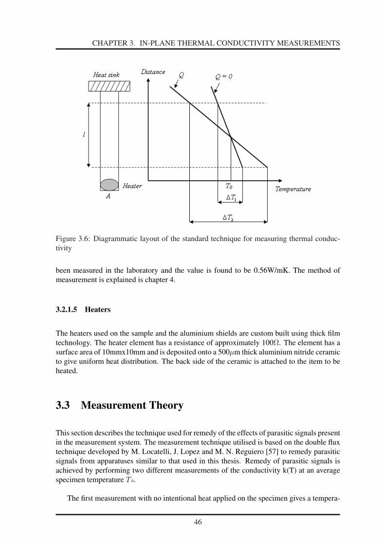
CHAPTER 3. IN-PLANE THERMAL CONDUCTIVITY MEASUREMENTS
Figure 3.6: Diagrammatic layout of the standard technique for measuring thermal conduc-tivity
been measured in the laboratory and the value is found to be 0.56W/mK. The method ofmeasurement is explained is chapter 4.
3.2.1.5 Heaters
The heaters used on the sample and the aluminium shields are custom built using thick filmtechnology. The heater element has a resistance of approximately 100Ω. The element has asurface area of 10mmx10mm and is deposited onto a 500µm thick aluminium nitride ceramicto give uniform heat distribution. The back side of the ceramic is attached to the item to beheated.
3.3 Measurement Theory
This section describes the technique used for remedy of the effects of parasitic signals presentin the measurement system. The measurement technique utilised is based on the double fluxtechnique developed by M. Locatelli, J. Lopez and M. N. Reguiero [57] to remedy parasiticsignals from apparatuses similar to that used in this thesis. Remedy of parasitic signals isachieved by performing two different measurements of the conductivity k(T) at an averagespecimen temperature T 0.
The first measurement with no intentional heat applied on the specimen gives a tempera-
46

CHAPTER 3. IN-PLANE THERMAL CONDUCTIVITY MEASUREMENTS
ture difference ∆T 1 across the specimen whereas the second measurement with applied heatgives a difference ∆T 2. However, the heat sink is cooled so that the average specimen tem-perature remains constant, at T 0. The method considers the parasitic heat current q(T) to beconstant for a given average temperature of the specimen. A is the cross sectional area of thespecimen and the measurements with Q = 0W and Q = QW intentionally applied, give thefollowing thermal gradients
5Q=0 =∆T1
l=
q(T0)
k(T0)
1
A(3.9)
5Q =∆T2
l=
Q + q(T0)
k(T0)
1
A(3.10)
Equation 3.9 is used to determine the amount of heat present in the specimen beforeapplying intentional heat. This parasitic heat can originate from different sources such as theelectrical heater wires, the sensor wires and the radiation of the specimen with the vacuumvessel environment. Equation 3.10 is used to determine the total amount of the heat presentin the specimen after applying intentional heat (the heat applied on the specimen is addedto the heat already present). The expression of the thermal conductivity coefficient can bedetermined as follows
k(T0) =Q
A
1
5Q−5Q=0
(3.11)
where 5Q and 5Q=0 are the temperature gradients along the specimen, when heat dif-ferent from zero and heat equal to zero are intentionally applied.
This expression eliminates the effects of any parasitic heat present in the measurementsystem and prevents the results from being corrupted. The assumption that the parasitic heatload is constant for both measurements has been made. The intentional power is kept low sothe temperature change along the specimen is kept low to reduce the parasitic heat in bothcases. More over the average temperature of the specimen is constant for both cases.
3.4 Measurement Principles
Four PT100 RTDs are placed on the surface of the specimen (labelled PT100 1 to PT100 4)spaced 15mm from each other as shown on figure 3.7. In order to ensure that there is a goodcontact between the RTDs and the surface of the specimen, pressure is applied on the topof the RTDs by sticking pieces of polystyrene in the inner side of the top radiation shield,directly above the RTDs. The polystyrene pieces are square with a cross section area of16 mm2 and a height of 2 mm. The amount of heat flowing through this new created heatpath is calculated and found insignificant for the measurements. The temperature differencebetween the specimen and the shields is measured to 0.05C and the thermal conductivity ofpolystyrene is 0.03W/mK7. The amount of the conductive heat through the polystyrene iscalculated to be 1.13x10⁻⁵W and represents 0.01% and 0.006%, respectively for 0.1W and
7www.engineeringtoolbox.com
47

CHAPTER 3. IN-PLANE THERMAL CONDUCTIVITY MEASUREMENTS
Figure 3.7: Schematic drawing of the measurement system of in-plane thermal conductivitycoefficient kab. Dimensions of specimen: length = 100mm, thickness up to 5mm and width∼ 12mm
0.2W intentionally applied on the specimen. The effect of the polystyrene on the measuredthermal conductivity is minimal and neglected in all the measurements.
An equal amount of heat is applied to each radiation shield and their temperatures arerecorded with a RTD attached to each radiation shield. The RTDs are attached to the ra-diation shields directly above and below the PT100 3, and the three RTDs form a virtualline perpendicular to the specimen. PT100 3 is located at the centre of the specimen and isconsidered to be the average temperature of the specimen, see figure 3.7. It is important thatthe RTDs at the centre of the specimen and those on the shields must be vertically aligned inorder to avoid recording offset temperatures.
The desired experimental temperature of the specimen is reached by regulating the tem-perature of the coolant. Without applying any intentional heat into the system, sufficient timeis allocated to reach thermal equilibrium and the first measurement is performed. Thereafter,heat is applied to both the specimen and the thermal shields until they reach the same tem-perature. The temperature of the coolant is again regulated to bring the temperature of thespecimen and the thermal shields down to the desired experimental temperature. Once againsufficient time is allocated to the system to reach thermal equilibrium and then the measure-ment is performed. It is worth noting that, the intentional heat applied on the specimen can bedifferent from the heat applied on the radiation shields. Several measurements with differentamounts of heat applied on the specimen is necessary to obtain reliable results. The valuesof the conductivities must be equal for a given measurement temperature for each appliedheat load to the specimen.
48

CHAPTER 3. IN-PLANE THERMAL CONDUCTIVITY MEASUREMENTS
3.5 Calibration
In order to validate the measurement method and to demonstrate that the measurement sys-tem operates in accordance with the theory described, a number of measurements of thermalconductivity are performed on a copper specimen, whose thermal conductivity is well under-stood and known. The measurements are performed in the temperature range from -30C to20C. It is known from literature that the thermal conductivity of copper (99.999% pure) isindependent of temperature in that temperature range and the value lies between 370W/mKand 400W/mK. It is important to mention that the calibration of the RTDs is necessary to bedone before the measurement system is utilised. This ensures that the resistance temperaturedetectors operate accurately within the conditions that the measurement system is used.
3.5.1 Calibration of RTDs
Inside the vacuum chamber, the RTDs are placed closely to each other and attached to theheat sink. Dow Corning 340 is used to ensure good surface contact between the RTDs and theheat sink surface and a chamber is evacuated to a pressure of approximately 10−5 mbar. Thecalibration temperature range is taken from -35C to 25C to ensure that all the measurementtemperature range (-30C to 20C) is covered. For a given temperature, enough time isallocated to the process in order to achieve the steady state equilibrium before committingthe temperature. The RTDs were calibrated to be equal with each other and a calibratedtemperature sensor.
3.5.2 Copper measurement
Three sets of measurements are performed on a flat and thin copper specimen, with crosssection area around 6.11 mm2. The first measurement is performed with no intentional heatapplied on the specimen, the second and third measurements are performed with intentionalheat of 0.1W and 0.2W applied on the specimen, respectively.
Plots of average temperature values of the RTDs on the specimen versus distance are pre-sented on figure 3.8 (0.1W intentionally applied) and figure 3.9 (0.2W intentionally applied)together with the obtained gradients. The solid lines represent the linear fits used to extractthe gradient of the temperature as a function of distance along the specimen for a given heatintentionally applied. These average temperature values are obtained from thermal measure-ments of the copper specimen at 0C. The gradient values obtained in this study, when nointentional heat is applied is -0.003K/mm whereas gradients of 0.04K/mm and 0.08K/mmare obtained, when 0.1W and 0.2W are applied respectively. It is clear that the gradientvalue doubles by doubling the amount of heat applied on the specimen and that at an averagetemperature of 0C the parasitic heat load is less than 0.01W.
The calculated thermal conductivity coefficients are presented in figure 3.10. There is
49

CHAPTER 3. IN-PLANE THERMAL CONDUCTIVITY MEASUREMENTS
10 20 30 40 50 60-1.2
-1.0
-0.8
-0.6
-0.4
-0.2
0.0
0.2
0.4
0.6
0.8
1.0
RTD4
RTD3
RTD2
RTD1
Tem
pera
ture
(0 C)
Position of RTDs (mm)
Temp @ 0W; grad=-0.00334 Temp @ 0.1W; grad=0.04013
Figure 3.8: The temperature along the surface of the copper specimen at Q = 0W and Q =0.1W
10 20 30 40 50 60-3.0
-2.5
-2.0
-1.5
-1.0
-0.5
0.0
0.5
1.0
1.5
RTD4
RTD3
RTD2
RTD1
Tem
pera
ture
(0 C)
Position of RTDs (mm)
Temp @ 0W; grad=-0.00334 Temp @ 0.2W; grad=0.08321
Figure 3.9: The temperature along the surface of the copper specimen at Q = 0W and Q =0.2W
50

CHAPTER 3. IN-PLANE THERMAL CONDUCTIVITY MEASUREMENTS
-30 -20 -10 0 10 20376
377
378
379
380
381
382
383
384
385
386
387
388
389
390
Ther
mal
con
duct
ivity
(W/m
K)
Temperature (0C)
Figure 3.10: Results of in-plane thermal conductivity measurement of copper (99.999%pure)
no temperature dependence of the thermal conductivities in the range from -30C to 20C.The values lie between 381W/mK and 383.5W/mK. The results are in good agreement withliterature values and 380W/mK is used in this thesis to be the measured thermal conductivityof the copper specimen. In conclusion, the measurement method together with the theoryare considered suitable and reliable for in-plane thermal conductivity measurements.
3.6 Uncertainties
In this section, a summary of the measuring procedure is addressed together with a study ofthe uncertainty analysis. Suppose that u, ..., z are measured with small uncertainty δu, ..., δz,and the measured values are used to compute q, given by
q =x× y × z
u× v × w, (3.12)
If the uncertainty in u, ..., z are independent, then the fractional uncertainty in q is the sumin quadrature of the original fractional uncertainties,
δq
| q | =
√(δu
u)2 + ... + (
δz
z)2 (3.13)
The uncertainty in the coefficient k results from the errors in the measurement of thetemperature drop ∆T , the heat flow Q and the reading of the dimensions of the specimens
51

CHAPTER 3. IN-PLANE THERMAL CONDUCTIVITY MEASUREMENTS
and positions of the RTDs. The thermal conductivity is calculated with equation 3.11. Usingequation 3.13, its uncertainty can be calculated as
δk
| k | =
√(δU
U)2 + (
δI
I)2 + (
δA
A)2 + (
δgradQ=0
gradQ=0
)2 + (δgradQ
gradQ
)2 (3.14)
where Q = U.I, A = d.h (cross section area of the specimen), U is the voltage, I is thecurrent, d and h are the thickness and width of specimen, respectively. The uncertainty inthe coefficient k is estimated based on the dimensions of the copper specimen used for thecalibration of the measurement system.
The intentional heat applied on the specimen is supplied by QL355TP power supply. Themeter accuracies are δU
U= 1.1% and δI
I= 0.7% for the voltage and the current, respectively.
The specimen thickness and width are measured with a micrometre with a precision of1µm. The dimensions measured are respectively 0.49mm and 12.6mm for the thickness andthe width. The error in the ability of reading the micrometre is found to be around θ=0.12%.The expression of its fractional uncertainty is determined as
δA
A=
√(δd
d)2 + (
δH
H)2 + (θ)2 (3.15)
and the value is deduced at δAA
=√
(0.0000010.00049
)2 + (0.0000010.0126
)2 + (0.0012)2 = 0.237%
The error in the gradient of the temperature as a function of distance along the specimenis determined from the least square fit to the data. The individual data points have errors intheir position and temperature. The distance between two consecutive RTDs is measured as15mm (0.015 m) and this is determined by the use of a vernier calliper with the followingprecision δL = 20µm. The vernier calliper is used to measure several times the distancebetween two RTDs, in order to determine the error in the ability of reading the calliper. Thiserror is found to be around 0.142%. The total fractional uncertainty in the distance between
two consecutive RTDs is δLL
=√
(0.000020.015
)2 + 0.001422 = 0.195%.
Platinum RTDs (HEL-700) are utilised in the measurement system to measure the tem-perature drop along the specimen. The functional behavior of these RTDs is
R(T ) = R(0)(1 + AT + BT 2 − 100CT 3 + CT 4) (3.16)
R(T) = resistance (Ω) at temperature T (C)R(0) = resistance (Ω) at 0 (C)T = temperature in Cwhere A = 3.9083× 10⁻³, B = −5.775× 10⁻⁷, C = −4.183× 10⁻¹² (below 0C), orC = 0 (above 0C). The temperature accuracy is equal to 0.080C.
The gradient accuracies are calculated to be δgradQ=0
gradQ=0= 2.88% and δgradQ
gradQ= 0.6%
The total fractional uncertainty in the coefficient k is determined asδk|k| =
√( 1.1
100)2 + ( 0.7
100)2 + (0.237
100)2 + (2.88
100)2 + ( 0.6
100)2 = 3.22%
52

CHAPTER 3. IN-PLANE THERMAL CONDUCTIVITY MEASUREMENTS
Figure 3.11: FEA model and boundary conditions
3.7 Finite Element Analysis (FEA)
This section presents a detailed methodology for the simulation of the copper specimen, usedin the calibration of the measurement system. The aim of this section is to cross check thevalidity of the measurement method and the physics considerations used. A CAD thermalanalysis software coupled with engineering data is used to create an environment similar tothat of the laboratory. The goal is to determine the temperatures of the resistance temperaturedetectors placed on the specimen and compare them with the temperatures found experimen-tally. The measurement system is first modelled in Solid Works8 and exported to ANSYSWorkbench9 for the finite element analysis. The FEA model and boundary conditions areshown in figure 3.11
3.7.1 Analysis Parameters
The materials used to model the measurement system are aluminium (radiation shields),platinum (RTDs), glass (heaters) and copper 99.999% pure (specimen under investigation).
Table 3.1: Properties of the materials used in the analysisMaterials Density Specific Emissivity Thermal
heat conductivitykg/mm3 J/kg.K W/m.K
Aluminium 2.77×10⁻⁶ 875 0.07 0.235Copper 8.9×10⁻⁶ 385 0.8 0.38
Platinum 2.145×10⁻⁵ 25.86 - 7.16×10⁻²
Glass 2.4×10⁻⁶ 0.6 - 1.05
A steady state thermal analysis is performed. Heat transfer by convection around thespecimen and heat transfer by conduction through all the wires (sensor and heater wires) are
8www.solidworks.com9www.ansys.com
53

CHAPTER 3. IN-PLANE THERMAL CONDUCTIVITY MEASUREMENTS
10 20 30 40 50 60
17
18
19
20
21
22
RTD4RTD3
RTD2RTD1
Tem
pera
ture
(0 C)
RTD position (mm)
exp@0W [email protected] [email protected] ansys@0W [email protected] [email protected]
Figure 3.12: Experimental and predicted temperature values of the RTDs on the specimen at20C
not considered. The measurement system is run at 20C in this analysis. The analysis is firstperformed with no intentional heat applied on the specimen. After that, the analysis is per-formed with intentional heat flows of 0.1W and 0.2W applied on the specimen, respectively.
3.7.2 FEA Results
The experimentally measured temperatures are presented on figure 3.12 and compared to thesimulated temperatures. The dashed lines represent the experimental data and the solid linesthe Ansys derived data. It is worth noting that the heat flows from RTD1 (nearest to the heatsink) to RTD4 (nearest to the heater) when intentional heat is not applied, which is contraryto the heat flow when intentional heat is applied.
The temperatures (experimental and simulated) agree well within 3% when no inten-tional heat is applied on the specimen, as shown in table 3.2. The experimental temperaturesdecrease slightly from 20.18C (RTD1) to 19.92C (RTD4) and the simulated temperaturesfrom 20.13C (RTD1) to 19.97C (RTD4). For a given amount of intentional heat applied tothe specimen there is a good agreement within 3% between the simulated temperatures andthe experimental temperatures. It is worth noting that considerations such as neglecting theheat transfer by convection around the specimen, the heat conduction through the electricalwires and the radiation between the specimen and the shields were made. It is assumed forthe simulation that the specimen is not exposed to any parasitic heat. The simualtion should
54

CHAPTER 3. IN-PLANE THERMAL CONDUCTIVITY MEASUREMENTS
therefore produce values that are considered ideal. The difference observed in the gradientswhen no heat is intentionally applied indicates that some parasites are still present in themeasurement system. The gradients derived from the simulated temperatures differ fromthe experimental gradients by 7.6% and 3.5%, when heat of 0.1 W and 0.2 W is applied,respectively. The thermal conductivities obtained by the simulation are equal to 381W/mK.
Table 3.2: Summary of the derived thermal conductivity from the simulated temperaturesPower Gradient Gradient Conductivity Conductivity
Experimental Simulated Experimental Simulated(W) (K/mm) (K/mm) (W/mK) (W/mK)
0 -0.00334 0.00030.1 0.040013 0.0433 380 3810.2 0.08321 0.0862 380 381
3.8 Experimental Results
In this section, in-plane thermal conductivities of materials (PocoFoam, CFRP) selected inthe design of the stave are presented together with other materials which are Allcomp foam,TPG (candidate materials) and diamond, carbon/carbon (C/C) and carbon silicon carbidefoam (CSiC) (materials of interest). The measurements are performed in the temperaturerange from -30C to 20C.
3.8.1 PocoFoam
Bulk thermal conductivity of two specimens of PocoFoam with different densities are in-vestigated. The specimens are purchased from Poco Graphite SARL10. The densities are0.56g/cm3 (poco08) and 0.40g/cm3 (poco09). The manufacturer claims a similarity in thetwo specimens including the manufacturing process. The delivery date is the sole quoteddifference and the results are presented in figure 3.13.
The measured thermal conductivities agree well with the companies quoted value whichis the range from 25W/mK to 60W/mK for densities between 0.32g/cm3 and 0.68g/cm3. Asmall temperature dependence of the thermal conductivities with temperature is observedfor the y direction. The thermal conductivity of poco08 decreases from 60W/mK at -30C to57.5W/mK at 20C, while that of the poco09 decreases from 57W/mK to 53W/mK. There isno temperature gradient in the x direction. For a given temperature, the thermal conductivityof poco08 is higher than that of poco09 with a maximum difference of 10% (x direction) and11% (y direction) over the measured temperature range. The increase of 40% of the densityof poco09 from 0.40g/cm3 to 0.56g/cm3 results in an increase of the thermal conductivity,however the increase is less than expected and does not increase linearly with density. Of
10Poco Graphite SARL, 1 rue des vergers 69760 Limonest FRANCE, POCOEU [email protected]
55

CHAPTER 3. IN-PLANE THERMAL CONDUCTIVITY MEASUREMENTS
-30 -20 -10 0 10 2046
48
50
52
54
56
58
60
62
64Th
erm
al c
ondu
ctiv
ity (W
/mK
)
Temperature (0C)
x-direction poco08 y-direction poco08 x-direction poco09 y-direction poco09
Figure 3.13: In-plane thermal conductivity results of PocoFoam 08 and 09
course, this single result is not able to establish any relationship between density and ther-mal conductivity. A full understanding of this relationship will be achieved after the study ofseveral PocoFoam densities. Figure 3.14 presents the percentage increase in the conductivitybetween the two specimens in both the x and y directions for each measured temperature.Over the temperature range of -30C to 20C, the average increase of the thermal conductiv-ity in both directions (x and y) is the same and is bout 7%.
3.8.2 Allcomp foam
Bulk thermal conductivities of an Allcomp foam specimen were measured in x and y direc-tions. The specimen was grade K9 foam with a density equal to 0.36g/cm3. A specimenwas cut for the in-plane measurement apparatus with a cross-sectional area of 31mm2. Thefoam was acquired from Allcomp Inc. in USA11. A proper observation of the foam madeit possible to see several broken ligaments on the surface of the specimen. These brokenligaments resulted from the cutting of the specimen and account for the visual total crosssectional area. This meant that the effective cross section area was less than the measuredcross section area that was used to determine the thermal conductivity coefficient. In orderto understand the impact of these broken ligaments on the results, two different thicknessesfor the x direction (2.46mm and 3.76mm) and three different thicknesses for the y direction
11Allcomp Inc., 209 Puente Avenue, vity of industry, CA 91746-2304
56

CHAPTER 3. IN-PLANE THERMAL CONDUCTIVITY MEASUREMENTS
Figure 3.14: The percentage increase of the thermal conductivity at each temperature be-tween two specimens which have 40% difference in density.
specimen (1.47mm, 2.46mm and 3.76mm) were measured. All the measurements results aresummarised on figure 3.15.
A small temperature dependence of the thermal conductivities for the specimens withthickness greater than 1.4mm is observed. For these thicknesses, the conductivity reduceswith increase of temperature for both the x and y directions. The thermal conductivitiesdecrease from 92W/mK to 86W/mK and 79W/mK to 71W/mK in the x and y direction, re-spectively. For a given temperature, the thermal conductivity in the x direction is around 17%higher than the conductivity in the y direction. The foam does not appear totally isotropic andthe results show that the x direction is more thermally conductive than the y direction. Themanufacturer’s measured thermal conductivity for Allcomp foam with density of 0.36g/cm3
is around 70W/mK, at room temperature. The thermal conductivity in the y direction agreeswell with this value, whereas the conductivity in the x direction is 14% above this value. Inorder to understand the difference in the results, Allcomp has been approached. They willperform more studies to understand the disagreement in the results. It is worth noting thatthe manufacturer uses a measurement technique different from that used in this thesis. Themanufacturer measures first the thermal diffusivity using the flash laser method on a 1” thickspecimen and then converts it to a thermal conductivity. The measured thermal conductivityvalues of the two thicknesses in the y direction agree well with each other, though the valuesof the thinner specimen generally lie slightly above those of the thicker specimen.
No temperature dependence is observed for the Allcomp foam for the specimens withthickness equal to 1.4mm. For a given direction, the thermal conductivity value measuredwith such a thin thickness is greater than the value obtained with thicker specimens. At 20C,the thermal conductivity of the thin specimen is 12.79% and 16.9% greater than thicker spec-
57

CHAPTER 3. IN-PLANE THERMAL CONDUCTIVITY MEASUREMENTS
-30 -20 -10 0 10 2070
75
80
85
90
95
100
105
Ther
mal
con
duct
ivity
(W/m
K)
Temperature (0C)
x-direction, thickness=2.422mm x-direction, thickness=1.405mm y-direction, thickness=1.4675mm y-direction, thickness=2.461mm y-direction, thickness=3.7626mm
Figure 3.15: In-plane thermal conductivity results of Allcomp with density ρ=0.36g/cm3
58

CHAPTER 3. IN-PLANE THERMAL CONDUCTIVITY MEASUREMENTS
Figure 3.16: Comparison of the thermal conductivity values of poco09 and allcomp foam inthe x and y directions
imens in the x and y directions, respectively. It is not understood why the thinner specimenshave a higher measured value of thermal conductivity. However, the thin specimens are moreaffected by broken ligaments near the surface compared to the thicker specimens. For thethicker specimens, the broken ligaments constitute a small percentage of the total cross sec-tional area than for the thin specimens. This is confirmed by the similar thermal conductivityvalues in the y direction of the specimens with thicknesses 2.461mm and 3.7626mm. It istherefore concluded that the thermal conductivity values of Allcomp obtained with speci-mens of thickness greater than 1.4mm are considered accurate and reliable.
The thermal conductivity values of the Allcomp foam appear to be more conductive thanthe poco09, from 65.4% to 82.2% in the x direction and from 33.33% to 40.54% in the ydirection. The comparison is preented in figure3.16.
3.8.3 CSiC Foam and carbon carbon
Bulk thermal conductivity measuerements of two carbon silicon carbide foams and car-bon/carbon (C/C) specimens are performed at 20C in this subsection. CSiC foam is fab-ricated by depositing, via the CVD process, silicon onto a carbon matrix. This undergoesthermal treatment to form carbon-silicon carbide. The first foam specimen has a density of
59

CHAPTER 3. IN-PLANE THERMAL CONDUCTIVITY MEASUREMENTS
4% of solid SiC and was cut to have a cross sectional area of around 48mm2 and the secondspecimen of density of 8% of carbon silicon carbide was cut to have a cross sectional area of16mm2. Both foam samples were acquired from ERG12. The manufacturer measured ther-mal conductivity is 5.28W/mK at 250C. The C/C specimen was purchased from Dunlop andcut to a sample with a cross sectional area of 9.984mm2. The results of the measurementsare summarised in table 3.3. The thermal conductivity of pure SiC is 120W/mK13. Thereforethe conductivity of 4% and 8% SiC foam should be as shown in table 3.3.
Table 3.3: Results of CSiC and C/C measurementsMaterial Thermal
Conductivity(W/mK)
CSiC foam 4% 43CSiC foam 8% 52
C/C 300
The results show that the measured value for 8% CSiC foam is ten times higher thanthe recommended value for CSiC at 250C. Though the measurements in this study are per-formed at 20C (a temperature ten times lower than the temperature quoted by the manufac-turer), it is considered that the difference between the measured and recommended valuesis large. In order to understand the causes of the disagreement in the results, meetings withERG were organised. The explanation given by ERG is that a graphite core remains (fromthe fabrication process) in the foam. This graphite core has a higher thermal conductivitythan SiC, which causes this significant increase of the thermal conductivity.
3.8.4 CFRP
Thermal conductivity of a carbon fibre reinforced polymer specimen was also investigated.The carbon fibre used in this study is a 0-90-0 K13D2U from Mitsubishi Dialead in a unidi-rectional preimpregnated (prepreg), and the epoxy is the cyanate ester RS3 from Tencate.The specimen has been autoclave cured at the University of Liverpool at a temperaturearound 177C. The specimen has a thickness about 0.222mm with a cross section area equalto 2.74mm2. The results are presented in figure 3.17.
It is observed that the thermal conductivity decreases with the increase of the tempera-ture in the temperature range from −20C to 20C. At −20C, the thermal conductivity isaround 324W/mK and decreases to 310W/mK at 20C. The thermal conductivity value isabout 315W/mK at −30C. In the temperature range between −30C to 20C, it appearsthat the thermal conductivity of the CFRP increases, reaches a peak and decreases. The re-sults conform with predictions based upon current CAD simulation models analysed withANSYS.
12www.ergaerospace.com13http://accuratus.com/silicar.html
60

CHAPTER 3. IN-PLANE THERMAL CONDUCTIVITY MEASUREMENTS
-30 -20 -10 0 10 20308
310
312
314
316
318
320
322
324
326
328
Ther
mal
con
duct
ivity
(W/m
K)
Temperature (0C)
Figure 3.17: In-plane thermal conductivity results of CFRP in the 0-direction. The error inthe measurements is 5%.
3.8.5 TPG
Thermal conductivity measurements of a thermal pyrolytic graphite specimen were also per-formed. TPG is a unique form of pyrolytic graphite. Pyrolytic graphite can be manufacturedby decomposing a carbonaceous gas which builds up a layer of pyrolytic graphite on a hotpreformed mandrel [58], [59]. It is characterised by a strong anisotropy in its thermal proper-ties. Pyrolytic graphite is a good conductor in its crystallographic direction and less so in theother direction. The pyrolytic graphite used in this study is supplied by Momentive14. Theinvestigated specimen has a thickness of 435µm and a cross section area of 5.032mm2. Thinlayers of TPG are generally difficult to handle because of frequent bends that occur in thespecimens during handling. In order to understand the impact of these bends in the specimenon the thermal performance, an intentional bend is made on the specimen and measurementsare performed. The bend is placed between pt100 3 and pt100 4, see figure 3.18. Figure 3.19summaries the results obtained together with the recommended values by Momentive.
Similarly to the values obtained by Momentive, the thermal conductivity decreases withthe increase of the temperature. The thermal conductivity measured at −30C and 20C are1920W/mK and 1510W/mK, respectively against 1930W/mk and 1565W/mK recommendedby Momentive. The measured thermal conductivity values in this study agree well with therecommended values within 3.5%.
The thermal conductivity measurement of the TPG with a bend is performed at 20Cand it is observed that the thermal conductivity is increased. As unexpected, the introduc-tion of the intentional bend has a contrary effect on the thermal conductivity. The thermalconductivity over the bend, from PT100 4 to PT100 3, is measured to 1641 W/mK. This isan increase of 13.27% over the value of the TPG specimen with no bend. The causes of the
14www.momentive.com
61

CHAPTER 3. IN-PLANE THERMAL CONDUCTIVITY MEASUREMENTS
Figure 3.18: View of TPG under investigation with bend placed between PT100 3 andPT100 4
-30 -20 -10 0 10 20
1500
1600
1700
1800
1900
2000
Ther
mal
con
duct
ivity
(W/m
K)
Temperature (0C)
TPG TPG values from momentive TPG with bend
Figure 3.19: View of the TPG measurement results together with the values recommendedby Momentive
62

CHAPTER 3. IN-PLANE THERMAL CONDUCTIVITY MEASUREMENTS
-30 -20 -10 0 10 20
1000
1002
1004
1006
1008
1010
1012
1014
Ther
mal
con
duct
ivity
(W/m
K)
Temperature (0C)
Figure 3.20: Results of the thermal conductivity measurements performed on a e2v diamondspecimen
increase of the thermal conductivity are unknown and not understood, therefore more studiesare required.
3.8.6 Diamond
Thermal conductivity measurements of a diamond specimen from e2v15 Technologies werealso performed. The specimen has a thickness of 0.282mm with a cross sectional area of2.87mm2. The results are summarised on figure 3.20.
It is observed that the thermal conductivity of e2v diamond is dependent on temperature.The thermal conductivity decreases from 1011W/mK at −30C to 1000W/mK at 20C. Asexpected, the thermal conductivity of diamond is high and more than 2.5 times that of copper.
In conclusion, it is observed that the measured thermal conductivities generally decreasewith the increase of temperature. The thermal conductivity measurements were performed onnon-metal specimens in this chapter. In non-metals, heat conduction occurs mainly by latticevibrations16. Lattice vibration is the phenonmenon taking place in a solid that is heated, andwhere atoms in the hotter region vibrate vigorously and collide with the neighbouring atoms(the colder atoms). Energy is transferred to these colder atoms and also vibrate vigorously.The process is repeated in every part of the solid, resulting in a transfer of heat energy fromthe hotter end to the colder end of the solid. This phenomenon in solids resembles the passageof waves and it is called phonon. In crystals that are free from detects and impurities, lattice
15www.e2v.com16www.http://www.mtm-inc.com/reduce project risk/thermal conductivity at low temperatures part 1 theory/
63

CHAPTER 3. IN-PLANE THERMAL CONDUCTIVITY MEASUREMENTS
vibrations can travel over long distances in solids and effectively transport heat. Latticevibrations scatter in collisions with other lattice vibrations.
The decrease of the thermal conductivities can be explained by the fact that the increaseof the temperature in the specimens increases the number of lattice vibrations, combinedwith the impurities and the defects of the solid hinder the lattice vibrations to travel far. Thisreduces the thermal conductivity.
3.9 Summary
An in-plane thermal conductivity measurement system has been designed and built and re-ported in this chapter. Heat transfer by radiation, convection and conduction have beenconsidered during the design process and solutions to reduce the undesired effects have beenapplied. The measurement system has been calibrated with a 99.999% pure copper speci-men of well known and understood material properties. Measurements of materials such asCRFP, PocoFoam, Allcomp foam, TPG, diamond, CSiC foam and carbon carbon have beenperformed with the system and the measured results agree well with the materials havingdocumented literature values. ANSYS analysis of the measurement system has been per-formed and the heat transfer by convection around the specimen, the conductive heat troughthe electrical wires and the radiation between the surfaces of the specimen and the surfacesof the shield were neglected. At 20C, the measured gradients differ from the gradientsobtained with ANSYS by up to 11%.
64

Chapter 4
Transverse Thermal ConductivityMeasurements
During the use of the upgrade tracker a considerable amount of heat will be generated in thesilicon modules (ASIC and silicon detector) and the electrical cables in the heavily irradiatedsilicon tracker. This heat will establish heat transfer paths through the silicon sensors andtheir support structures towards the cooling fluid. These paths consist of various materialsand the interfaces between them that resist the transport of thermal energy and lead to anincrease temperature throughout the thermal circuit. Efficient dissipation of the heat neces-sitates a reduction of the contact resistances. J. P. Gwinn and R. L. Webb [60] report that forsolids of high thermal conductivity, the contact resistance can be reduced by the followingtwo methods:
(1) Increasing the area of the contact spots. This can be achieved by an increase of thecontact pressure which “flattens” the peaks of the micro-roughness and deflects the matingsurfaces to reduce any non-flatness. The increase of the contact spots can also be achieved byreducing the roughness of the surface before the interface is formed by grinding the surfacesto remove any non-flatness and buffing the surface to reduce any micro-roughness.
(2) Using a Thermal Interface Material (TIM) of high thermal conductivity that can con-form to the imperfect surface features of the mating surfaces.
Load constraints on electronic components make it unfeasible to use high contact pres-sure. Manufacturing of highly finished surfaces is not practical due to the high cost involved.Hence, the best alternative is to use a TIM applied at a moderate contact pressure. The prop-erties of the TIMs need to be well understood in order to achieve a satisfactory heat man-agement inside the design of the stave. The study of TIMs requires a reliable test methodcapable of achieving accurate and repeatable values. In this chapter, the design and con-struction of a transverse thermal conductivity measurement system are performed accordingto the ASTM D-5470 test method. The study is based on 1-D steady state heat conduction atroom temperature. The one dimensional heat flow assumption was investigated by Gwinn J.,Saini M. and Webb R. [61] with models and it was concluded that the 1-D heat flow can be
65

CHAPTER 4. TRANSVERSE THERMAL CONDUCTIVITY MEASUREMENTS
Figure 4.1: Schematic representation of interface resistance
achieved by using long bars, distanced temperature sensing with accurate knowledge of theposition of these sensors.
The ASTM D-5470 test method is a standard method to measure thermal impedance forTIMs such as elastomers, tapes, greases and phase change materials (PCM) [62]. ASTMD-5470 describes a method to measure interface resistance (Rint). The apparatus consistsof two metal bars, across which heat is transferred. The TIM is inserted at the interfacebetween the two bars. The standard test is useful with either homogeneous or compositethermally conductive materials ranging from 0.02mm to 10mm in thickness. Electric heat isapplied at the end of one bar and the end of the other bar is connected to a heat sink. Two ormore temperature sensors are installed on each metal bar. The surface temperature of eachbar is obtained from the temperature gradient in each bar together with the location of thetemperature sensors. This test method will be also be used in this study to measure thin andsolid materials with thickness up to 1mm.
4.1 Background
Thermal interface resistance is a measure of how well heat is transferred across the interfaceof two mating rigid surfaces. A schematic representation of interface resistance is shown infigure 4.1. Referring to figure 4.1, the interface resistance (per unit area) is defined as follows
Rint =T cs − T hs
Q(4.1)
where T(cs) is the cooled surface temperature, T(hs) is the heat sink baseplate tempera-ture and Q is the power per unit area of the heat-emitting component. The R(int) is commonlypresented with units of K/W. It is clear that from equation 4.1, the lowest possible interfaceresistance is reached when the heat sink temperature approaches that of the cooled surface.The junction of the cooled component and the heat sink contains generally a combinationof surface roughness and surface non-flatness as shown on figure 4.2. The micro-roughnessis superimposed on a macroscopic non-planar surface in the form of a concave, convex or
66

CHAPTER 4. TRANSVERSE THERMAL CONDUCTIVITY MEASUREMENTS
Figure 4.2: (a) Heat sink and cooled component roughness, (b) poor heat sink and cooledcomponent flatness [62]
wavy surface which can result in as much as 99% of the interface surface area being by airgaps (see figure 4.3) unless a TIM is used [62].
J.P. Gwinn and R.L. Webb report that, the contacting surfaces will contact each other onlyat discrete points and the number of contact points will increase with the increase of pressureon the interface. Air is a very poor thermal conductor, with kair equal to 0.026W/mK atroom temperature and acts as thermal barrier and hinders efficient heat transfer through theinterface. As seen in figure 4.3, the contact resistance (Rcontact) consists of the conductionresistance at the points where the mating surfaces touch each other and the conduction and/orradiative resistance across the gaps of non-contacting area. Any substance (with thermalconductivity exceeding that of air) that fills the gap will decrease the contact resistance [63],see figure 4.4.
The ideal TIM (figure 4.4) is expected to have high thermal conductivity, be easily de-formed by small contact pressure and have minimal thickness. Further, the TIM should notleak out of the interface, should maintain performance indefinitely and be manufacturingfriendly (easy to apply and remove). To date, no TIM on the market can meet the expec-tation of an ideal TIM. Available TIMs will not completely fill the cavities and small airpockets will remain on both sides of the interface material and the TIM will not have mini-mal thickness, see figure 4.5
As presented in figure 4.5, Rcontact1 is the contact resistance between the TIM and theelectronic component’s surface, Rcond is the conduction across the thickness of the TIM andRcontact2 is the contact resistance between the TIM and the heat sink base plate. The interfaceresistance Rint is the sum of the three resistances and it is expressed as follows
Rint = Rcontact1 + Rcond + Rcontact2 (4.2)
withRcond =
∆L
kTIM
(4.3)
where ∆L and KTIM are the effective thickness of the thermal interface material and itsthermal conductivity, respectively. Rcond is the conductivity of the material.
67

CHAPTER 4. TRANSVERSE THERMAL CONDUCTIVITY MEASUREMENTS
Figure 4.3: Exploded view of thermal interface when no TIM is used [62]. R(int) is com-posed only of contact resistance
Figure 4.4: Exploded view of thermal interface when an ideal TIM is used [62]
68

CHAPTER 4. TRANSVERSE THERMAL CONDUCTIVITY MEASUREMENTS
Figure 4.5: Exploded view of thermal interface with actual TIM [62]
4.2 Setup
Figure 4.6 shows the experimental setup for the measurement of interfacial contact conduc-tance based on 1-D steady state conduction used in this study. The setup consists of a heaterplaced high on the upper copper bar and a liquid-cooled heat sink maintaining a constant heatflux in the test column which consists of two copper bars with the material under investiga-tion sandwiched between. The copper bars have a uniform cross section area of 100mm2.The copper used to machine the bars is heavily oxidised with emissivity equal to 0.8. Theend surfaces of the copper bars are polished to a surface roughness of around Ra∼1µm. Thetemperature distribution is measured along the heat path by RTDs stuck with tape on thecopper bars on each side of the material under investigation. Thermal grease is used as athermal interface material between the RTDs and the copper bar surfaces to ensure goodcontact. The RTDs are placed on two coinciding copper bar surfaces and their positionsform a virtual vertical line equidistant from the vertical edges of the bars. The distance ∆Lfrom the RTDs to the material under investigation is accurately measured with a caliper. Thedistance between the upper RTD and the heater is more than two and half times the lengthof the heater, allowing the heat flow to be well developed and steady. A load cell is used toapply controlled pressure on the material under investigation.
The measurements are performed at room temperature and the average temperature of theRTDs is kept similar to the environment temperature. This is done in order to reduce the heattransfer by radiation between the copper bars and the environment temperature. The amountof heat flowing by conduction through the copper bars is large compared to the radiationloss to the environment because of the large cross sectional area of the bars. Therefore, it
69

CHAPTER 4. TRANSVERSE THERMAL CONDUCTIVITY MEASUREMENTS
Figure 4.6: Solid Works model of the transverse thermal conductivity measurement system
70

CHAPTER 4. TRANSVERSE THERMAL CONDUCTIVITY MEASUREMENTS
is assumed that achievement of satisfactory measured results can be obtained without usingany radiation shield. The measurement system used in the laboratory is shown in appendixB.
The measurements are performed in the laboratory at a location where the air surroundingthe setup is stationary. There are no external means such as fans, pumps and suction devicesswitched on in the vicinity of the measurement system to provoke the flow of the air. Theapplication of heat on the upper copper bar establishes a temperature difference between thesurfaces of the bar and the stationary air. The adjacent air to the upper copper bar will moveupward. This mode of heat transfer is referred to as natural convection. The location of theheater (high up on the upper copper) constrains the bulk of the air to move above the copperbars, reducing considerably the amount of heat transfer by convection along the copper bars.The remaining heat transfer by convection along the copper bars is considered insignificantcompared to the amount of the heat transfer by conduction and is therefore not considered inthis study.
Thermal resistances and conductivities of thermal interface materials such as Dow Corn-ing 340, Dow Corning SE4445, Hysol EA9396, Araldite 2011 and Epolite FH-5313 epoxywere measured in this study. Measurements of solid materials such as CFRP and kaptonfilms was also be performed. The setup was also modified in order to allow measurementsof the thermal properties of blocks of PocoFoams and Allcomp foams.
4.3 Determination of the thermal resistance
Generally, the total contact resistance, per unit area, (Rcontact = Rcontact1 + Rcontact2 ) is deter-mined experimentally by measuring thermal resistance data for a range of TIM thicknessesand plotting Rint, per unit area, versus thickness. The resulting graph exhibits a linear rela-tionship expressed as follows
Rint(∆L) = Rcontact +∆L
kTIM
(4.4)
The slope is equal to the inverse of kTIM and the intercept of the straight line with theRint axis is equal to Rcontact [64]. It is worth noting that the Rcontact1 (surface between theelectronic component and the TIM) and Rcontact2 (surface between heat sink base and theTIM) resistances can be different because each of the two contact surafces may differ inroughness or flatness.
The actual thermal conductivity of the TIM can also be determined by measuring thermalresistance data and plotting Rint versus pressure. It is observed using this method that theresistance decreases with the increase of the pressure until Rint reaches a constant value.This constant value is equal to twice the thermal resistance at the contact between the TIMand sandwishing surface. This method is usually used when the surfaces sandwiching theTIM have similar flatness and roughness. This causes Rcontact1 to be equal to Rcontact2 and
71

CHAPTER 4. TRANSVERSE THERMAL CONDUCTIVITY MEASUREMENTS
Figure 4.7: Overview of the specimens with different cross section areas used the ANSYSanalysis. Qrad and Qconv are the radiative and convective heats transferred between the nonsandwiched part of the oversized specimen and the room temperature.
simplifies the expression of the total resistance to
Rcontact = 2Rcontact1 (4.5)
The two methods mentioned above will be used in this study to determine the thermalconductivity of Dow Corning 3401. However, the method using Rint vs pressure will beutilised for the determination of the transverse thermal conductivity values presented in thisthesis.
4.4 Measurement Optimisation - FEA
A thermal analysis of a solid TIM was performed in ANSYS in order to understand whetherthe dimensions of the cross section area of the specimen sandwiched between the copperbars influences the results. The analysis consists of reproducing a laboratory measurementof two specimens of the same material and of the same thickness (500µm), measuring thethermal conductivities and determining the corresponding thermal resistances. One specimenis trimmed to match the cross sectional area of the copper bars (1cm2) and the other specimenis 50% oversized, as shown figure 4.7.
1www.dowcorning.com
72

CHAPTER 4. TRANSVERSE THERMAL CONDUCTIVITY MEASUREMENTS
0 500 1000 1500 2000-20
0
20
40
60
80
100
120
140
160
k_o K_trim R_o R_trim
kinput
(W/mK)
k outp
ut(W
/mK
)
-20246810121416182022242628303234
Routput (K
/W)
Figure 4.8: Graphical representation of the calculated thermal resistance and thermal con-ductivity versus the input thermal conductivity. Ro and ko are the resistance and conductivityof the oversized specimen; Rtrim and ktrim are the resistance and conductivity of the trimmedspecimen
4.4.1 Basic Simulation
The components of the CAD assembly have the same material properties as the componentsused in the laboratory. A constant heat flow of 5W is applied on the top surface of the uppercopper bar and a fixed temeprature of -10C is applied on the heat sink. Two points areaccurately located on the copper bars, one on each side of the specimen under investigation.These points represent two RTDs with well known distances to the surfaces of the specimen.For a given value of the input thermal conductivity, temperatures are measured at the twopoints and used to calculate the corresponding output thermal conductivity. Heat transfer byradiation and convection are not considered in this analysis.
4.4.2 Results and Discussion
Thermal conductivity values ranging from 0.16W/mK to 2000W/mK are taken as the in-put into ANSYS and the corresponding output thermal conductivities are determined. It isworth noting that the output thermal conductivities are the conductivity values calculatedby using the temperature measured with the RTDs. The results of the whole range of thecalculated conductivities together with the calculated resistances are presented on figure 4.8.The calculated thermal conductivity values of the specimens (oversized and trimmed) in-crease from 0.16W/mK to around 140W/mK when the input conductivity values increase
73

CHAPTER 4. TRANSVERSE THERMAL CONDUCTIVITY MEASUREMENTS
0.0 0.5 1.0 1.5 2.00.0
0.5
1.0
1.5
2.0
k outp
ut(W
/mK
)
kinput
(W/mK)
k0
kinput
ktrim
Figure 4.9: Graphical representation of the calculated thermal conductivities compared tothe expected conductivity. kinput is the expected thermal conductivity, k0 is the thermal con-ductivity of the oversized specimen and ktrim is the thermal conductivity of the trimmedspecimen.
from 0.16W/mK to 2000W/mK. The calculated thermal resistance values of the specimensdecrease rapidly from 33K/W and “flattens” to a constant value of 0.03K/W with the increaseof the input conductivity values from 0.16W/mK to 2000W/mK.
The results of the calculated conductivity values together with the input thermal con-ductivity values are presented on figure 4.9, for the input thermal conductivity values in-creasing from 0.16W/mK to 2W/mK. The calculated conductivity values obtained from thetrimmed specimen are equal to the input values until the input conductivity values reach1W/mK, where they begin to differ progressively. The calculated conductivity is lower thanthe input conductivity for an input value equal or greater than 1W/mK. The calculated con-ductivity values obtained from the oversized specimen differ from the input values over thewhole range of the input thermal conductivity values. However, for a given input valuebetween 0.1W/mK and 2W/mK the thermal conductivity values of the oversized specimenagree within 3%. Within this input value range, the oversized and trimmed specimen valuesagree within 4%, while the thermal conductivity values of the trimmed specimen agree wellwith the input values within 1.5%. The value of the trimmed specimen agrees better with theexpected value for a given input conductivity value less than 2W/mK. It is worth noting thatfor a given input value between 2W/mK and 10W/mK, the calculated conductivity values ofthe oversized and the trimmed specimens differ by up to 6.1%.
For a given input thermal conductivity ranging from 0.16W/mK to 2W/mK, the calcu-lated thermal resistance of the oversized specimen decreases from 30.20K/W to 2.45K/W,see figure 4.10, and of the trimmed specimen from 31.59K/W to 2.53K/W. When the inputthermal conductivity is above 2W/mK, the calculated thermal resistance of the specimens is
74

CHAPTER 4. TRANSVERSE THERMAL CONDUCTIVITY MEASUREMENTS
0.0 0.5 1.0 1.5 2.00
5
10
15
20
25
30
35
Rou
tput(K
/W)
kinput
(W/mK)
Ro
Rtrim
Figure 4.10: Graphical representation of the calculated thermal resistances versus the inputthermal conductivity
less than 2K/W and their values agree well with each other within 0.25%.
In conclusion, it is considered that measurements of solid materials with thickness around500µm and a thermal resistance less than 2K/W are not suitable to measure with the presentmeasurement system. Measurements appear more accurate with specimens with cross sec-tion area matching the cross section area of the copper bars. Specimens larger than the crosssection area of the copper bars cause additional heat paths which contribute to the smalldifference observed from the specimen having the cross section area matching that of thecopper bars.
4.5 Uncertainties
In this section, the error in the thermal conductivity of the specimen under investigation ispresented. This error is due to the experimental uncertainties in the measured data such asthe positions of the RTDs on the copper bars, the thermal conductivity of the copper bar, thetemperature drop and the heat flow along the copper bars, the cross section area of the copperbars and the heat loss along the copper bars.
The total error in the position of the RTDs, including the error in the ability of readingthe calliper was found in chapter 3 to be around 0.195%. The uncertainty in the temperature
75

CHAPTER 4. TRANSVERSE THERMAL CONDUCTIVITY MEASUREMENTS
drop is about 1.8% and is associated with the platinum (HEL-700) type RTD error dataacquisition (0.08C) together with the uncertainty in the position of the RTDs (0.155%).The uncertainty in the heat flow is introduced by the uncertainty of the reading of the voltage(0.1%) and the current (0.2%). The uncertainty in the thermal conductivity of the copper barsis determined by performing conductivity measurements of the copper bars several timesunder the same conditions. The uncertainty in the cross sectional area of the copper barsis due to the ability of reading the micrometer that was used to measure the dimensions ofthe bars. This uncertainty was found to be equal to 0.14%. The uncetainty in the heat lossby radiation along the copper bars is determined by calculating this heat value several timesunder the same conditions. The uncertainty of the heat loss was found to be 0.30%. Basedupon the standard uncertainty analysis technique [65], the uncertainty is found be equal to2.64%.
4.6 Thermal Properties of Thermal Interface Materials
For the stave design materialss of interest, Dow Corning 340, Hysol EA 9396, Epolite andDow Corning SE4445 are selected as thermal interface materials. These substances are in-vestigated for their thermal properties, particularly their resistances and their thermal con-ductivities. Preparations and curing processes of the aforementioned thermal interface ma-terials are presented together with a detailed explanation of the methodology used to mesuretheir thermal properties.
4.6.1 Methodology of surface area of copper bars at interface (≈ (1cm2)
Figure 4.11 shows the terms used in the calculations to determine the thermal resistance andconductivities. T 1
′ and T 2′ are respectively the temperatures at the bottom of the copper and
at the top of the lower copper bars. T 1 and T 2 are the temperatures of RTD1 and RTD2,placed on each side of the TIM on the copper bars. The average temperature of T 1 and T 2
are kept equal to the room temperature constraining the temperature of the TIM to be nearthe room temperature. This is done in order to reduce heat transfer by radiation between theTIM and the environment. T Cu and T heater are placed at the top of the upper copper bar andon the heater respectively. The temperatures of these RTDs are used to determine the heatloss from the heater and the exact amount of heat moving through the upper copper bar fromthe heater.
The heat loss by conduction through the AWG 28 electrical wires (φ = 0.321mm) usedto power the heater was investigated by removing the wire’s electrical insulation and placingtwo RTDs directly on the surface of the copper wire near the heater. By supplying 1W, itwas found that the heat loss by conduction through the wires was 2.05%. The surface areaof the heater is equal to 2.5x10⁻⁵m2. The heat losses by radiation from the heater and thesurfaces of the copper bars depend on the room temperature and they are calculated for eachmeasurement. The total radiative heat loss is typically around 3.60% of the heat applied. The
76

CHAPTER 4. TRANSVERSE THERMAL CONDUCTIVITY MEASUREMENTS
Figure 4.11: Drawing of the thermal interface measurement system
sum of the heat losses by conduction and radiation is considered high and non-negligible,therefore the measurement system is corrected accordingly.
The locations of RTD1 and RTD2 from the edges of the copper bars are accurately knownand denoted (∆L1) and (∆L2). These distances are measured with callipers. The T 1
′ andT 2
′ are the temperatures at these edges and are calculated with the following expressions:
T 1′ = T 1− Q−Qheat −QCu −Q(RTD1−edge)
kCuACu
∆L1 + K0 (4.6)
T 2′ = T 2 +
Q−Qheat −QCu −Q(RTD1−edge)−Q(edge−RTD2)
kCuACu
∆L2 + K0 (4.7)
where Q is the amount of heat intentionally applied by the heater, Qheat is the heat loss byradiation from the heater, QCu is the heat loss by radiation by the portion of the upper copperbar between the top of the bar and RTD1, Q(RTD1−edge) is the heat loss by radiation betweenRTD1 and the bottom of the upper copper bar, Q(edge−RTD2) is the heat loss by radiationbetween the edge of the lower copper bar and RTD2 and K0 = 273.16K. The radiative heatloss by the portion of the copper bar below RTD2 does not influence the results. This heatloss is therefore not considered in the calculations.
In this study, Rcontact1 and Rcontact2 are considered equal by ensuring that the roughness
77

CHAPTER 4. TRANSVERSE THERMAL CONDUCTIVITY MEASUREMENTS
and flatness of the copper bars are similar. Hence, equation 4.2 is simplified in this study as
Rint = Rcond + 2Rcontact1 =T 1
′ − T 2′
Q′ (4.8)
where Q’ = Q - Qheat - QCu - QRTD1−edge is the corrected heat and is considered the exactamount of heat going through the TIM. Finally, the actual resistance of the TIM (Rcond) isdetermined by the following expression
Rcond = Rint − 2Rcontact1 (4.9)
4.6.2 Dow Corning 340
Dow Corning 340 is the thermal grease used in all the measurements in this thesis. It is anodourless white paste that is easy to apply and remove from surfaces. Its thermal resistanceis measured with two different ways in order to cross check the reliability of the methods.
The determination of the thermal interface resistance of Dow Corning 340 is firstlyachieved by performing measurements on different thicknesses of a solid composite con-sisting of Hysol EA9396 and 23.1% Boron Nitride . The preparation of this composite isexplained later in this chapter. The composite is placed inside the copper bars and a thinlayer of Dow Corning 340 is applied between its surfaces and the copper cross section.A pressure of 0.47MPa and a power of 1W are applied on the composite and resistancemeasurements are performed on the composite with following thicknesses: 85µm, 164µm,207µm, 257µm and 438µm. Table 4.1 presents the results of the measured thermal interfaceresistances together with the temperature difference T 1
′-T 2′ .
Table 4.1: Summary of the thermal resistance results measured on different thicknesses ofHysol EA9396 + 23.1% Boron Nitride of cross sectional area equal to 1cm2
Thickness Rint T ′1-T ′
2
(µm) (K/W) (K)
85 1.90 1.79164 3.91 3.62207 4.13 3.91257 5.05 4.68438 8.42 7.65
These results are plotted on figure 4.12 where they exhibit a linear graph intersecting theRint axis. At that intersecting point, Rint = 2RCu/DC340 = 0.55. The resistance at the interfaceof copper/Dow Corning 340 is therefore determined in this study as
RCu/DC340 = 0.27± 0.066K/W (4.10)
78

CHAPTER 4. TRANSVERSE THERMAL CONDUCTIVITY MEASUREMENTS
0.00 0.05 0.10 0.15 0.20 0.25 0.30 0.35 0.40 0.450
1
2
3
4
5
6
7
8
9
2.RCu/DC340
=0.54871
Rin
t(K/W
)
Thickness (mm)
resistance
Figure 4.12: DC 340 Thermal Interface Resistance vs thickness
The second method consists of measuring the interface resistance of DC 340 and plottingRint vs pressure, as shown in figure 4.13. The interface resistance decreases with the increaseof pressure until it reaches a constant value of 0.27K/W from 0.43 MPa. A similar resultis observed when the measurement is performed on a layer of DC 340 sandwiched insidetwo pieces of carbon/carbon of measured thermal conductivity 287W/mK and roughnessRa∼1.5µm. The interface resistance decreases until it reaches a constant value of 0.30K/W.This value differs slightly from 0.27K/W because of the difference in the materials surfaceproperties.
It is clear that the values obtained from the two methods to determine the contact re-sistance agree well. The value of the thermal interface resistance of Dow Corning 340 isconsidered to be 0.27K/W. This value will be used for the calculation of transverse thermalresistances in this thesis. The pressure applied on the interface materials during all of thefollowing measurements is 0.47MPa.
4.6.3 Araldite 2011
Araldite 20112 epoxy adhesive is a multi-purpose, viscous material that is suitable for bond-ing a variety of materials, including metal, ceramic, wood, foams and plastic. Araldite con-sists of two parts A and B, with mixing ratio 1:1. One of the recommended schedule forcuring the epoxy is 10 min @ 100C. It is easy to apply and has a good resistance to staticand dynamic loads. At the beginning of this thesis, araldite 2011 was the epoxy that wasunder investigation to be used for the design of the stave. Thermal conductivity studies havebeen therefore carried out. Other epoxies were later preferred for the stave design and araldite
2www.ebpltd.com
79

CHAPTER 4. TRANSVERSE THERMAL CONDUCTIVITY MEASUREMENTS
0.00 0.05 0.10 0.15 0.20 0.25 0.30 0.35 0.40 0.45 0.50
0.3
0.4
0.5
0.6
0.7
0.8
0.9
1.0
RD
C34
0/co
pper(K
/W)
Pressure (MPa)
Figure 4.13: DC 340 Thermal Interface Resistance vs Pressure and Thermal conductivity
2011 was dropped. The measurements were performed using two copper bars to sandwichthe araldite at room temperature with a power of 1W applied on the copper. The thermalconductivity was measured as 0.22W/mK and agrees well with recommended values.
4.6.4 Hysol EA9396, Dow Corning SE4445 and Epolite FH-5313 epoxy
Hysol EA9396, DC SE4445 and Epolite FH-5313 are proposed for the manufacture of thestave of the ATLAS inner tracker. Figure 4.14 shows a schematic view of the cross sectionof the proposed stave design showing the different glue layers.
The preparation of the glue specimens is performed by mixing thouroughly the two com-ponents according to the defined mixing ratio. The mixture is poured onto a flat teflon sheetbetween two stainless steel shims. These shims define the eventual specimen thickness.Teflon is used due to non-stick property which allows easy specimen removal after the cureprocess.A flat edge pressed hard onto the two shims is drawn over the glue specimen to de-fine the glue thickness. The finished specimens are flat, solid sheets that are easy to cut witha blade, as shown in figure 4.15.
Measurements of these solid specimens were performed by using Dow Corning 340 be-tween the surfaces of the specimens and the copper bars. The meausrements were madeat room temperature with a pressure of 0.47 MPa applied on the specimens. The contactresistance was assumed equal to that found for the two copper bars with DC 340. The tem-
80

CHAPTER 4. TRANSVERSE THERMAL CONDUCTIVITY MEASUREMENTS
Figure 4.14: Schematic view of the cross-section of the stave with the different glue layersapplied
Figure 4.15: View of a solid TIM sandwiched between the copper bars
81

CHAPTER 4. TRANSVERSE THERMAL CONDUCTIVITY MEASUREMENTS
perature difference between the surfaces of the specimens were measured to be 12.71C and12.76C for the epolite and the Hysol specimens, respectively. After the subtraction of thecontact resistances, the epolite specimen with a thickness of 390µm exhibited an actual re-sistance equal to 13.85K/W and the thermal conductivity was found to be 0.28W/mK. TheHysol EA9396, with a thickness of 415µm exhibited an actual resistance equal to 14.02K/Wand the thermal conductivity to be 0.28W/mK. The resistance of the Dow Corning 340 rep-resents 15.51% and 26.68% of the actual resistance of the epolite and the Hysol EA9396,respectively.
The Dow Corning SE4445 is rubber like and cannot be measured using the methodutilised for the epolite or the Hysol. The thickness of the DC SE4445 reduces consider-ably when a pressure of 0.47 MPa is applied. Therefore, another method is used for themeasurement of its thermal conductivity. The method consists of producing the DC SE4445specimen by bonding two copper bars together with the epoxy under modest pressure. Twofishing lines of diameter (500µm) were placed inside the DC SE4445 during the curing pro-cess (overnight at room temperature) to define the thickness of the specimen to equal thatof the fishing lines. Therefore, when a pressure of 0.47 MPa is applied, the fishing lineskeep the thickness of the DC SE4445 at 500µm preventing the DC SE4445 from deform-ing. After the subtraction of the contact resistances, the Dow Corning SE4445 exhibits anactual resistance equal to 8.47K/W, a temperature difference between the surfaces of 8.17Cand a thermal conductivity equal to 2±0.2 W/mK. The resistance of the Dow Corning 340represents 8.97% of the total resistance. Table 4.2 summarises the results.
Table 4.2: Summary of the thermal conductivity results of Epolite FH-5313, Hysol EA9396and Dow corning SE4445
Adhesives Thickness Power applied ∆T Resistance Thermal conductivity(µm) (W) (C) (K/W) (W/mK)
Epolite FH-5313 517 1 15.83 17.41 0.28±0.01Hysol EA9396 415 1 12.76 14.02 0.28±0.01
DC SE4445 214 1 8.17 8.47 2±0.2
4.7 Thermal behaviour of epoxy resin filled with high ther-mal conductivity micropowders
Hysol EA9396 and Araldite 2011 are strong candidates to glue the CFRP facings to the Poco-Foam. Their application in the stave design is limited by their low thermal conductivitiescausing an increase of the thermal resistance between the CFRP facing and the PocoFoamand therefore a temperature rise in the CFRP over the foam temperature. In order to improvethese conductivities, thermally conducting but electrically insulating filler (Boron Nitride) isused to dope the matrices and obtain polymer-based composites. Boron Nitride is attractivebecause it has a low atomic number and therefore a high radiation length. The high thermal
82

CHAPTER 4. TRANSVERSE THERMAL CONDUCTIVITY MEASUREMENTS
conductivity of Boron Nitride in the bulk state can be attributed to the simplicity of the crystalstructure, the low atomic mass, the existence of strong covalent bonding between the atomsand the low disorder within the crystal lattice [66]. The theoretical limit of thermal conduc-tivity for a single crystal of Boron Nitride at room temperature is 1300W/mK. However, theexperimental thermal conductivity of the powder is significantly lower than its crystallinecounterpart (200 to 500W/mK), because of the interface between powder particles [67].
4.7.1 Different models
Berman R. [68] reports that the thermal resistance in a solid is caused by phonon scattering,therefore the phonon scattering has to be minimized in order to increase the thermal con-ductivity. Winco Yung [69] concludes, after his studies on different particle sizes of BoronNitride, that more and larger Boron Nitride particle sizes help to shorten the low thermal con-ductivity path in the epoxy matrix and establish a high thermal conductivity network (BoronNitride) for heat conduction. Larger size means lower surface to volume ratio3, thereby,lower interfacial phonon scattering for a given weight of the filler [70]. In consequence, ahigher percentage and larger particle sizes of Boron Nitride yields a higher thermal conduc-tivity. In this study, the effective thermal conductivity of Hysol filled with Boron Nitrideis determined experimentally as a function of Boron Nitride concentration. The obtainedvalues are compared with existing theoretical and empirical models. The existing theoreticaland empirical models are discussed below followed by the experimental results.
4.7.1.1 Lewis and Nielsen
The Halpin-Tsai theoretical model [71], considered as the best and most versatile to calculatethe elastic moduli of all kinds of composite materials, has been modified by Lewis andNielsen [72] to include the effect of the shape orientation and type of packing of the particlefiller in a two-phase system. The modified equations [73] for the two-phase systems are
kc
km
=1 + ABφ
1−Bφψ(4.11)
A = kE − 1 (4.12)
B =kf
km− 1
kf
km+ A
(4.13)
3The surface to volume ratio and variously denoted SA:V is the amount of surface area per unit volume ofan object. The surface area to volume ratio is measured in units of inverse distance. For a given shape, SA:Vdecreases linearly with increasing volume
83

CHAPTER 4. TRANSVERSE THERMAL CONDUCTIVITY MEASUREMENTS
ψ = 1 + (1− φm
φ2m
)φ (4.14)
The properties kc, kf, km are the thermal conductivities of the composite, filler materialand polymer matrix, respectively and φ is the volume fraction of the filler. The constantA depends primarily upon the shape of the dispersed particles and how they are orientedwith respect to the direction of flow of thermal currents. The constant A is related to thegeneralised Einstein coefficient kE. The factor B is a constant which takes into account therelative conductivity of the two components. The factor ψ is determined by the maximumpacking fraction φm of the dispersed particles. The maximum packing fraction φm is definedas the true volume of the particles divided by the volume they to occupy when packed totheir maximum extent. For fillers which are aggregates of spheres, the constant A is equal to2.5φm
-1 [74]
4.7.1.2 Agari and Uno
Agari and Uno propose a semi-empirical thermal conduction model (fundamentally based onthe generalisation of parallel and series conduction models of a composite) for filled polymerwith particles [75]. The expression governing the thermal conductivity in this model is givenas follows
logkc = φC2logkf + (1− φ)log(C1km) (4.15)
where C1 and C2 are experimentally determined constants of order unity. Dilek Kumlutasand Ismail H. Tavman [76] report that, C1 is a measure of the effect of the particles on thepolymer, like crystallinity and the crystal size of the polymer. C2 (smaller than 1 and largerthan 0) shows how easy the particles can form conductive paths inside the polymer. In otherwords, the easier the particles are gathered to form conductive chains, the more the thermalconductivity of the particles contributes to the thermal conductivity of the composite and C2
tends towards 1. The coefficients C1 and C2 are determined by using the linear regressionequation of the plot of the logarithm of the thermal conductivities of the experimental dataagainst volume contents of the particles.
4.7.1.3 Maxwell
Maxwell [77] uses potential theory and obtains an exact solution for the conductivity ofrandomly distributed and non-interacting homogeneous spheres in a homogeneous medium.The governing equation is expressed as follows
kc = km
kf + 2km + 2φ(kf − km)
kf + 2km − φ(kf − km)(4.16)
84

CHAPTER 4. TRANSVERSE THERMAL CONDUCTIVITY MEASUREMENTS
This Maxwell model is expected to predict the thermal conductivity of composites forlow filler concentrations when filler particles do not touch each other.
4.7.1.4 Russell
With the assumption that the particles are cubic with the same size, Russell [78] proposedthe following model using a series parallel network.
kc = km
φ2/3 + km
kf(1− φ2/3)
φ2/3 − φ + km
kf(1 + φ− φ2/3)
(4.17)
4.7.1.5 Cheng and Vachon
Tsao [79] obtained a model relating the two phase solid mixture thermal conductivity of theindividual components and to two parameters, which describe the spatial distribution of thetwo phases. Assuming a parabolic distribution of the discontinuous phase in the continuousphase, Cheng and Vachon breakthrough and propose a solution to Tsao’s model. The newproposed model does not require knowledge of additional parameters. The determinationof the constants of the parabolic distribution are obtained experimentally and presented as afunction of the discontinuous phase volume fraction. The equivalent thermal conductivity ofthe mixture is derived in terms of the distribution function and the thermal conductivity ofthe constituents. For kf>km, the expression gorverning the model is given as follows
1
kc
=1√
C(kf − km)[km + B(kf − km)]ln
√km + B(kf − km) + B
2
√C(kf − km)√
km + B(kf − km)− B2
√C(kf − km)
+1−B
km
(4.18)where
B =√
3φ2
and C = -4√
23φ
Cheng and Vachon claim that, for two phase materials with the thermal conductivity ofthe continuous phase being much smaller than the thermal conductivity of the discrete phase(km ¿ kf and as long as φ < 0.667), effective thermal conductivity of the composite can beexpressed as follows
kc≈ km
1−B(4.19)
85

CHAPTER 4. TRANSVERSE THERMAL CONDUCTIVITY MEASUREMENTS
4.7.1.6 Geometric mean
In the case of the geometric mean model, the effective thermal conductivity of the compositeis given by [71]
kc = kφf .k1−φ
m (4.20)
4.7.2 Hysol EA9396 filled with Boron Nitride (BN)
The Hysol based composite is prepared by mixing the epoxy resin, hardener and BoronNitride particles and cured at room temperature over a period of three days. Boron Nitrideis non-toxic and transparent to microwaves. Two types of Boron Nitride powders (Japaneseand Goodfellow4) are used to fill the Hysol matrix. The goodfellow Boron Nitride has adensity of 1.9g/cm3 and a maximum particle size of 10µm in diameter. The goodfellowBoron Nitride has a hexagonal structure5 and is sometimes called white graphite, due to itslubricity, anisotropic properties, heat resistance and high thermal conductivity. This latterproperty, combined with a low thermal expansion, leads to excellent resistance to thermalshock. The Japanese Boron Nitride is from the previous ATLAS SCT build.
The Hysol filled with Boron Nitride is prepared with concentrations of 5, 10, 15, 20, 25,30 and 35% by weight. The quantity, by weight, of Hysol used is 2.6g (part A=2g and partB=0.6g). Table 4.3 summarises the filler amount in the composite. The following expressionis used to calculate the volume fraction of the filler for a given weight fraction
φ =W
W + (1−W ) ρf
ρm
(4.21)
where φ is the volume fraction of the filler additives, W is the weight fraction, ρf and ρm arethe densities of the filler (Boron Nitride) and polymer matrix, respectively.
4.7.3 Results and Discussion
Thermal conductivity measurements are performed on Hysol EA9396 filled with Boron Ni-tride of two different origins (Japanese and Goodfellow) up to a volume fraction of 24%.In accordance with litterature values, the addition of the Boron Nitride raises the thermalconductivity of the Hysol with increasing loading. The experimental values of thermal con-ductivity at room temperature are compared to calculated values from Maxwell, Cheng andVachon, Lewis and Nielsen, Russell and the geometric mean models on figure 4.16 and fig-ure 4.17. The density of Hysol is 1.14g/cm36. It is known from literature that Boron Nitridehas a density value between 1.9g/cm3 and 2.2g/cm3. Two similar measuring jars, filled
4www.goodfellow.com5www.azom.com6www.aerospace.henkel.com
86

CHAPTER 4. TRANSVERSE THERMAL CONDUCTIVITY MEASUREMENTS
Table 4.3: Summary of the filler amount in the mixtureBoron Nitride Boron Nitride Hysol EA9396 + BN
weight (%) mass (g) mass (g) %BN by volume
0 0 2.6 04.8 0.13 2.73 0.039.1 0.26 2.86 0.0613 0.39 2.99 0.08
16.7 0.52 3.12 0.1120 0.65 3.25 0.13
23.1 0.78 3.38 0.1525.9 0.91 3.51 0.1729.7 1.1 3.7 0.2035 1.4 4 0.24
with the Japanese and the Goodfellow Boron Nitride were measured with a weight scale.It is observed that the density of the Japanese Boron Nitride is less than the density of theGoodfellow’s. As the exact values of the densities are unknown, 1.9g/cm3 and 2.1g/cm3 areassumed as the densities of the Japanese and the Goodfellow, respectively. The GoodfellowBoron Nitride has a maximum particle size around 10µm. The bulk thermal conductivity ofthe Boron Nitride is unknown, and a lowest value of 200W/mK is used for the calculations.The thermal conductivity of the Hysol EA9396 is experimentally measured and found to beequal 0.28W/mK, see table 4.2. As the maximum packing fraction is unknown, a value ofφm = 0.637 is used is the calculations to determine the thermal conductivity values in theLewis-Nielsen model.
For the Japanese Boron Nitride at low volume content (φ <8%), particles are dispersedin the Hysol EA 9396 matrix and they are not interacting with one other. The equationsof the geometric mean and that of Cheng and Vachon predict the best values for the thermalconductivity of the Hysol EA9396 in this region. The deviation from the experimental data ismaximum 9.5% and 4% for the geometric mean equation and Cheng and Vachon equations,respectively. The Maxwell and both of the Lewis and Nielsen model predictions are lowerthan the experimental results in the whole range. However, at higher Boron Nitride content,as aggregates of particles are formed, Lewis and Nielsen with A = 3 (the particles are ofirregular shapes approximating roughened spheres) and φm = 0.637 gives better predictionthan their model using A = 1.5 (the particles are spherical) and φm = 0.637. For particlecontent greater than 10% by volume, conductive chains of the particles are formed givingrise to a large increase in effective thermal conductivity of the Hysol EA9396. The Russellmodel prediction of thermal conductivity is fairly accurate in that region. With a loadingof 8% Boron Nitride (by volume), the thermal conductivity of the Hysol EA9396 reaches0.51W/mK, which is an increase of 57% compared to pure Hysol EA9396 with a thermalconductivity of 0.28W/mK.
The Hysol EA9396 was filled with 16% and 23% volume of the Goodfellow Boron Ni-tride in this study. The results agree well within 5% with the corresponding thermal conduc-
87

CHAPTER 4. TRANSVERSE THERMAL CONDUCTIVITY MEASUREMENTS
0.00 0.05 0.10 0.15 0.20 0.25
0.2
0.3
0.4
0.5
0.6
0.7
0.8
0.9
1.0
1.1
1.2
1.3
1.4
1.5
Ther
mal
con
duct
ivity
(W/m
K)
%BN by volume
Experimental results Lewis A=3 Lewis A=1.5 Russell Maxwell Cheng and Vachon Geometric
Figure 4.16: Thermal conductivity results of Hysol filled with Boron Nitride (Japanese) andcompared with different models
88

CHAPTER 4. TRANSVERSE THERMAL CONDUCTIVITY MEASUREMENTS
0.00 0.05 0.10 0.15 0.20 0.250.2
0.3
0.4
0.5
0.6
0.7
0.8
0.9
1.0
1.1
1.2
1.3
1.4
Ther
mal
con
duct
ivity
(W/m
K)
%BN by volume
Experimental results Lewis A=3 Lewis A=1.5 Russell Maxwell Cheng and Vachon Geometric
Figure 4.17: Thermal conductivity results of Hysol filled with Boron Nitride (Goodfellow)and compared with different models
89

CHAPTER 4. TRANSVERSE THERMAL CONDUCTIVITY MEASUREMENTS
tivity values derived from the Geometric model. It is observed that none of the other modelsis useful for the prediction of the experimental results. Loading the Hysol EA9396 with theGoodfellow boron Nitride, the thermal conductivity of the Hysol increases from 0.28 W/mKto 0.81 W/mK and 1.3 W/mK for 16% BN and 23%BN, respectively. This is an increaseof the thermal conductivity by 65.4% and 78.5% compared to pure Hysol EA9396 with athermal conductivity of 0.28 W/mK.
4.7.4 Araldite and Boron Nitride
Thermal conductivity measurements of Araldite 2011 filled with the Japanese Boron Nitridewere also performed. The mixture proportion by weight is resin 38.5%, hardener 30.75%and Boron Nitride 30.75%. The curing time at room temperature was three days. The mea-surements are performed at room temperature with a pressure of 0.47MPa and 1W appliedon the composite and Dow Corning 340 grease was used at the copper specimen interfaces.The measured thermal conductivity is found to be 0.77W/mK. This is an increase of 250%compared to the pure Araldite 2011 thermal conductivity value.
4.8 Kapton Bus
The basic function of the kapton bus in the stave is to deliver power and signals to and fromthe front-end electronics. The bus is not uniform but made with layers of different materialsshown in table 4.4. On the surface of the kapton bus, black traces are observable. Thesetraces consist of kapton, aluminium and copper. The copper serves as the conductors todrive the twelve (12) modules mounted on the stave. The aluminium layer serves as a shieldto isolate the modules from noise pick up from the signals in the traces. Figure 4.18 shows aportion of the kapton bus with the black trace.
Table 4.4: Summary of the different materials present in the assembly of the kapton buscomponents thickness manufacturer
µmkapton 25 Shin-Etsu CA333
adhesive 25 Shin-Etsu CA333aluminium shield 25 foil
adhesive 25 DuPont LF0100kapton 25 Shin-Etsu CA333
adhesive 25 Shin-Etsu CA333copper 18 (Espanex) MC 18-25-00kapton 25 (Espanex) MC 18-25-00
In the design of the stave, the kapton bus, also called the bus cable, is mounted betweenthe hybrids and the carbon fibre plate, see figure 4.14. The kapton bus crosses the heat path
90

CHAPTER 4. TRANSVERSE THERMAL CONDUCTIVITY MEASUREMENTS
Figure 4.18: Overview of the kapton bus used for the prototype of the stave
from the silicon sensors to the cooling pipes. Due to its location, there is a need to understandthe thermal properties of the kapton bus in order to understand the thermal performances ofthe stave. This section focuses on the measurement of the transverse thermal conductivitiesof the kapton, assembly of (kapton - glue - aluminium shield) and assembly of (kapton -glue - aluminium shield - glue - copper layer - kapton). It is worth noting that measurementsare not performed on the adhesives alone because this is out of the scope of this study. Themeasurements are performed in the TIM apparatus at room temperature with a pressure of0.47 MPa applied on the copper bars and Dow Corning 340 is used as the thermal greasebetween the copper bars and the specimen.
After substraction of the contact resistances, the kapton has a resistance of 1.31K/Wwith a temperature difference of 1.74C and a resulting thermal conductivity equal to 0.22W/mK. The assembly of the kapton and the aluminium has a resistance of 6.41K/W with atemperature difference between the two surfaces of 14.3C and a resulting thermal conduc-tivity equal to 0.26 W/mK. The assembly of kapton, aluminium, copper and kapton exhibitsa temperature difference of 15.6C between its two surfaces with a resistance of 7.05K/Wand a resulting thermal conductivity equal to 0.24W/mK. Table 4.5 summarises the results.
4.9 Foams
In this section transverse thermal conductivity measurements of PocoFoam and Allcompfoam are performed at room temperature. The technique used for the measurements is shownin figure 4.19; where the foam specimen is placed vertically on a copper bar connected to a
91

CHAPTER 4. TRANSVERSE THERMAL CONDUCTIVITY MEASUREMENTS
Table 4.5: Summary of the thermal conductivity results of the kapton busLayer Thickness Power applied ∆T Resistance Thermal conductivity
(µm) (W) (C) (K/W) (W/mK)
Kapton Shin-Etsu 29.8 1 1.74±0.05 1.31±0.02 0.22±0.01
Assembly(kapton-Al) 170 2 14.30±0.05 6.41±0.02 0.26±0.01
Assembly(kapton-Al-Cu) 189 2 15.60±0.05 7.05±0.02 0.24±0.01
Figure 4.19: Overview of a foam specimen under investigation
heat sink. The foam is 10 mm wide, 10 mm long and 20 mm deep. It is heated at the top bya ceramic heater and cooled at the other end by the heat sink. Two RTD sensors are attachedon the foam for the reading of the temperature through the foam. The distance (∆L) betweenthe sensors is accurately measured with callipers and the heat sink is adjusted so that the av-erage temperature of the sensors is similar to the environment temperature. This is done toensure the temperature of the foam is as near as possible to the environment temperature inorder to reduce heat transfer by radiation between the surfaces of the foam and the environ-ment. When the average temperature is adjusted and equal to the environment temperature,sufficient time is given for the system to reach equilibrium before performing measurements.Convection is considered negligible in this study due to the location of the heater on the topof the foam. As a consequence, only heat conduction is assumed to be important in thisstudy. It is worth noting that the blocks of foam have the following dimensions (250mm x250mm x 30mm), when purchased. These dimensions allows measurements to be performedin all the three directions (x, y and z), where z is the deep direction.
92

CHAPTER 4. TRANSVERSE THERMAL CONDUCTIVITY MEASUREMENTS
4.9.1 PocoFoam
Transverse thermal conductivity measurements of two PocoFoam specimens with differentdensities (ρ=0.40g/cm3 and ρ=0.56g/cm3) are performed. PocoFoam is expected to beanisotropic with conductivity in the z direction (kz) ranging from 50W/mK to 160W/mK.The difference in conductivity values between the x, y and z directions is due to the manu-facturing process. The elongation of pores in the z direction effectively increases the liga-ment length in the z direction. This reduces the number of low conductivity junctions andtherefore increases the overall foam thermal conductivity in the z direction. Table 4.6 showsthe results of the transverse thermal conductivity results together with the PocoFoam valuesmeasured at room temperature with the in-plane measurement system.
Table 4.6: Summary of the In-plane and Transverse thermal conductivity results of Poco-Foam
Density kx ky kz Measurement method(g/cm3) (W/mK) (W/mK) (W/mK)
0.56 - - 135±2 Transverse0.40 43±2 43±2 55±2 Transverse
0.56 54.5±3 57.5±3 - In-plane0.40 51±3 53.5±3 - In-plane
As expected, the conductivities measured are higher in the z direction (135W/mK and55W/mK, for ρ=0.56g/cm3 and ρ=0.40g/cm3, respectively) than the other directions (xand y) and lie in the range quoted by the manufacturer. Transverse measurements forρ=0.40g/cm3 performed in the three directions show that kz is 28% higher than kx/ky.
Comparing the transverse values with the in-plane values, it was observed that for ρ=0.40g/cm3,kz was 7.8% and 2.8% higher than kx and ky, respectively. For ρ=0.56g/cm3, kz is 47.7% and34.8% higher than kx and ky, respectively. Due to the lack of specimens, no measurementwas performed in x and y directions for ρ=0.56g/cm3. However, the results obtained withρ=0.40g/cm3 indicate that there was a considerable difference between the values obtainedby the two methods. The values obtained with the in plane method were higher (18.6% and24.4% for kx and ky, respectively) than the values obtained with the transverse method.
4.9.2 Allcomp foam
Transverse thermal conductivity measurements of two Allccomp foam specimens with dif-ferent densities (ρ=0.22g/cm3 and ρ=0.36g/cm3) were performed. Allcomp foam was ex-pected to be isotropic with conductivities, at room temperature, ranging from 10W/mK to75W/mK for density ranging from 0.09g/cm3 to 0.40g/cm3. The transverse thermal con-
93

CHAPTER 4. TRANSVERSE THERMAL CONDUCTIVITY MEASUREMENTS
ductivity measurements were performed in all the three directions (x, y and z) and the resultswere shown in table 4.7.
Table 4.7: Summary of the Transverse thermal conductivity results for Allcomp foamDensity kx ky kz
(g/cm3) (W/mK) (W/mK) (W/mK)
0.22 33.5±2 38±2 33.5±20.36 61±2 62±2 75±2
Contrary to the expected, the thermal conductivities are not isotropic for a given den-sity. However, the obtained values lie within the thermal conductivity range measured bythe manufacturer. Differences are observed between the measured values of the thermalconductivities. For a specimen with a density of 0.22g/cm3, ky is 13.5% higher than kx =kz = 33.5W/mK. For a specimen with a density of 0.36g/cm3, kz is 23% and 21% higherthan kx and ky, respectively. It is observed that, with an increase of around 64% of density(0.22g/cm3 to 0.36g/cm3), the thermal conductivity increases by more than 100%.
The measured conductivity values of Allcomp foam with density equal to 0.36g/cm3
obtained at 20C in the x and y directions by the use of the in-plane thermal conductivitymeasurement system is shown in table 4.8.
Table 4.8: In-plane conductivity of Allcomp foam in the x and y directions measured at 20CDensity kx ky kz
(g/cm3) (W/mK) (W/mK) (W/mK)
0.36 83±3 72±3 -
Comparing the results obtained from the transverse measurement system and the in-planemeasurement system, it is observed that there is a significant difference between the results ofthe two methods. The values obtained by the in-plane system are higher than those obtainedwith the transverse system as observed for the PocoFoam. kx and ky are 36% and 16.13%higher than the values obtained by the transverse conductivity system at room temperature.
The high values obtained by the in-plane thermal conductivity system compared to thetransverse system can be explained by the presence of radiation shields that add undesiredheat paths to the system and increase the thermal conductivity. It has also been shown thatthermal conductivity measurements performed on PocoFoam specimens thinner than 1.4 mmof PocoFoam result in inaccurate results. Based on these reasons, the transverse thermalconductivity system is considered more accurate and the measured values are consideredreliable.
94

CHAPTER 4. TRANSVERSE THERMAL CONDUCTIVITY MEASUREMENTS
4.10 CFRP
The transverse thermal conductivity of the K13D2U specimen studied in the previous chap-ter, was investigated. The thickness of the specimen was 217µm and a cross section area of1cm2. The measurements were performed at room temperature with a power of 1W appliedon the CFRP. Dow Croning 340 was used as thermal interface material and a pressure of 0.47MPa was applied between the copper bar and the CFRP surfaces.
After the subtraction of the contact resistances, the CFRP exhibits a resistance of 1.78K/Wwith a temperature difference of 2.22C between its surfaces what results in a thermal con-ductivity equal to 1.20±.02W/mK. The filament thermal conductivity of this CFRP is 800W/mK with a density equal to 2.19g/cm3. A prediction based on FEA analysis performedin the collaboration does not conform with the measured value because of unknown factors,such as the transverse thermal conductivity of the filament. The filament transverse conduc-tivity is important to know in order to determine the bulk transverse thermal conductivity ofthe CFRP.
4.11 Summary
A 1-D steady state heat conduction system at room temperature has been designed, builtand reported in this chapter. Heat loss by radiation has been corrected and convection hasbeen neglected. Measurements of epoxies such as Hysol EA9396, Dow Corning SE4445 andEpolite FH-5313 have been performed and the results agree well with literature values. Themeasurement system has been used to measure the thermal resistances and conductivities ofPocoFoam and Allcomp foam. The thermal conductivities obtained by the transverse systemare generally lower than those obtained by the in-plane system at room temperature. Asexpected, the thermal conductivities of PocoFoam are not isotropic for a given temperature.An anisotropy in the thermal conductivities has also been observed for Allcomp foam thatwas expected to be isotropic. A measurement was performed on a K13D2U specimen andthe result was found to be equal to 1.20±0.02 W/mK.
95

Chapter 5
Mechanical Measurements
After investigation of the thermal properties of the silicon module’s support structures, it isimportant to ensure that these structures are dimensionally and structurally stable in order toenable accurate track reconstruction. As seen in figure 4.14, apart from the aluminium cool-ing pipe, (US design), the core of the stave consists of PocoFoam, honeycomb and carbonfibre reinforced polymer. The bulk of the materials used in the stave design are of low massand the total mass of the stave is evaluated to be between 600g and 800g. The mounting ofthe stave inside the barrel is designed in a way that the total load applied on the stave consistsof the stave’s own load coupled with the thermal force created by the cooling of the pipe andthe heating of the silicon sensors. Due to the stave’s low mass combined with the thermalinduced force, it is estimated that the maximum stress applied on the stave is around 30MPa.Furthermore, this maximum stress is expected to occur at the pipe to foam interface.
The CFRP skins provide bending stiffness modules to a face to attach the stave to themacro-support structure of the tracker barrel. The fixture points are attached to “C-channels”which run along the long edge of the stave. The C-channel design is beyond the scope of thisthesis and will not be discussed in this study. The CFRP skins are subject to tension and/orcompression and are largely responsible for the strength of the stave. The function of thehoneycomb is to support the skins so that they do not buckle (deform) and stay fixed relativeto each other. The honeycomb will experience mostly shear stresses (sliding) as well assome degree of vertical tension and compression. There will not be any investigation of thehoneycomb in this thesis. PocoFoam is important because of its good thermal performances,i.e high thermal conductivity. Like the honeycomb, the PocoFoam will experience shearstresses as it is located between the CFRP skins. PocoFoam also suffers large shear stressdue to the differential thermal expansion between the CFRP skins and the cooling pipe, bothof which the foam is glued to.
96

CHAPTER 5. MECHANICAL MEASUREMENTS
Figure 5.1: Overview of the bending of the stave along its longitudinal axis, the PocoFoamis not shown
Figure 5.2: Detailed view of the forces involved in the bending of the stave shown in fig-ure 5.1
5.1 Motivations
The mass of the stave will create a self deflection of the stave resulting several forces in-cluding bending forces at the ends of the stave. The self deflection causes tension and com-pression stresses in the CFRP skins and the creation of shear stress in the honeycomb andPocoFoam, see figure 5.1. The induced thermal force will create an additional shear stressbetween the PocoFoam and the pipe.
The bending forces cause the stave to stretch below the neutral axis and to compressabove the axis as illustrated on figure 5.2. The neutral axis experiences zero stress and strain.As the stave bends, both the core and the skin elongate and shrink linearly from the neutralaxis. The “black” solid line represents the new section of the stave after bending. Becausethe CFRP skins are firmly glued to the honeycomb and the PocoFoam, both the core and theCFRP skins stretch similarly at the glued junction. It is worth noting that, although the CFRPskins and the core stretch equally at the skin/core boundary. The honeycomb, PocoFoam andcarbon fibre reinforced polymer have different physical properties and therefore will reactdifferently to the created elongation.
In engineering terms, the ratio of the elongation (∆L) to the original length (L0) is called
97

CHAPTER 5. MECHANICAL MEASUREMENTS
Figure 5.3: Overview of the stress distribution along the cross section of the stave
“strain”, ε, and expressed as
ε =∆L
L0
(5.1)
Knowing the strain, the stress in both the core and the skins can be determined. Thestress is expressed by equation 5.2, where E is the material’s modulus of elasticity (Young’smodulus). Young’s modulus describes the material’s response to linear strain and it is ameasure of the stiffness1 of a material.
σ = Eε (5.2)
It is known from the available literature that CFRP has larger modulus than the hon-eycomb and the PocoFoam. Therefore, given an equal strain at the glued junction in thedifferent materials, it is clear that a larger stress will be created in the CFRP skins. The dis-continuity of the stress at the skin/core boundary is an indication that the carbon fibre skinsabsorb far more tension and compression than the honeycomb and PocoFoam, see figure 5.3.
A preliminary finite analysis of the UK stave performed with ANSYS shows that the selfdeflection is small and can be neglected when the stave is supported with five points alongone edge and two points on the other edge2. Additionally, the analysis shows that the coolingpipe detaches itself from the PocoFoam due to the induced thermal force. Figure 5.4 showsthe cooling pipe embedded and glued into the PocoFoam. It is worth noting that the materialproperties, such as Young’s Modulus, shear modulus and yield stress, used in the analysis aretaken from the available literature. These values are generally obtained from measurementsat high stress up to failure. In order to understand well and be able to interpret the outcomeof the Finite Element Analysis performed on the stave, it is necessary to use in the simulationthe material properties obtained at the expected low stresses.
The aims of this chapter are to:1Stiffness is the resistance of an elastic body to deflection or deformation by an applied force. It is an
extensive material property.2https://twiki.cern.ch/twiki/bin/view/Sandbox/TrackerExchange?topic=TrackerExchange - 18th August
2008
98

CHAPTER 5. MECHANICAL MEASUREMENTS
Figure 5.4: Overview of the cooling pipe embedded and glued into the PocoFoam
• design and construct a mechanical jig that can be adapted to a conventional testome-ter to achieve accurate measurements of pure mechanical properties, such as Young’smodulus, at low stress. The function of the jig is to reduce significantly the parasiticeffects present in the measurement
• measure pure compressive and tensile Young’s moduli and yield strengths of materialssuch PocoFoam and CFRP
• measure the shear modulus, (G), of PocoFoam
The measurements were performed at room temperature and at low stress, up to 30MPa.The values obtained from the measurements will be compared to text book values and theyield stress will be compared to the stress values simulated for the stave. The stave designwill be concluded dimensional stable only when the stresses applied on the materials of thestave are less than the corresponding yield strength.
In this chapter, the important aspects of stress and linear elastic regions are first intro-duced. This is followed by a detailed explanation of the origin of the parasitic effects presentin the measurement system which are the causes of the non-achievement of the elastic re-gion, when measurements are performed at low stress. Additionally, detailed explanationsof the design of the jig that was used to reduce significantly these parasitic effects are given,together with experimental results of CFRP and PocoFaom. Finally, a method for measuringthe shear modulus of PocoFoam is presented together with experimental results.
5.2 Conventional Measurement of Young’s modulus
Tensile measurement is probably the most important test of a material’s mechanical responseand it is used to determine the Hookean region of elastic bodies3. Tensile and compressive
3In a Hooke body, stress is directly proportional to strain. The relationship is known as the Hooke’s law andthe behaviour is referred to as Hookean behaviour
99

CHAPTER 5. MECHANICAL MEASUREMENTS
Figure 5.5: Schematic illustration of tensile tests
properties indicate how the material reacts to an applied force. Compression tests are rela-tively less complex to perform than tensile measurements. These measurements are carriedout to determine mechanical properties including Young’s modulus and yield strength.
Tensile measurements were performed by placing a carefully prepared specimen insidea conventional testometer. The specimen is thereafter submitted to a force in tension in acontrolled way. The applied force and the elongation of the specimen are recorded simul-taneously. Figure 5.5 presents a simplification of the measurement process and shows thedimensional changes of the specimen. A0 and L0 are the original cross section area and theoriginal length of the specimen, A and L are the actual corresponding dimensions under theforce, F, applied to the specimen and δ is the elongation of the specimen.
The main derivation of a tensile measurement is a force versus elongation curve, which isconverted into a stress versus strain curve. The engineering stress, σ(e), is the applied forceF divided by the original cross section area A0;
σ(e) =F
A0
(5.3)
When true stresses based on the actual cross sectional area of the specimen are used, thestress-strain curve increases continuously until fracture. The stress-strain curve relates theapplied stress to the resulting strain and each material has its own unique stress-strain curve.Figure 5.6 shows a stress-strain curve of a Hooke’s body.
100

CHAPTER 5. MECHANICAL MEASUREMENTS
Figure 5.6: Schematic illustration of common stress-strain of Hooke’s bodies [81]
5.2.1 Hookean Region
The Hookean region is characterised by a linear relationship between the stress and strainindicating that no plastic deformation is occurring. When the applied force is reduced, thespecimen returns to its original shape and dimensions. This region is commonly called thelinear-elastic region.
5.2.2 Yield Strength
If the loading of a test specimen is discontinued below point A, in figure 5.6 and the load isremoved, the stress and strain retraces line OA back to the origin. The proportional limit isthe highest stress at which stress is directly proportional to strain. Above the proportionallimit, both elastic and plastic strains occur as indicated by the curve segment AB. Whenthe point B is reached and the load is gradually removed, the stress and strain now followthe line BE. Once the stress reaches zero, the elastic strain disappears and the plastic strain(OE) remains. The reloading of the specimen now follows the line EBC. In other words,a small amount of plastic strain raises the proportional limit from A to B and is followedby an increase of the yield strength. The yield strength is the smallest stress required toproduce plastic deformation. The yield strength obtained by offsetting the line OA by 0.2%is commonly used for engineering purposes because it avoids the practical difficulties ofmeasuring the proportional limit.
101

CHAPTER 5. MECHANICAL MEASUREMENTS
Figure 5.7: An example of stress-strain graphs obtained from the two cameras after a lowstress tensile test. The test was performed on an aluminium specimen using a universaltestometer
5.3 Parasitic effects in the measurement of stress-strain
At low stress, the determination of the linear-elastic region of Hookean bodies for the cal-culation of Young’s modulus has proven to be difficult to obtain with a universal testometer.In order to understand the factors working against the determination of the linear-elastic re-gion, a video extensometer system4 was used to record strains inside a specimen during themeasurements. The system consists of two cameras positioned to face each surface of thespecimen. A flat specimen is placed inside a universal testometer and a tensile test is per-formed. The data recorded from each camera were used to establish a stress-strain curve foreach surface of the specimen.
It is clear that the stress-strain graphs shown in figure 5.7 are not similar, which explainsthat the specimen surafces behave differently, especially at stress below 10MPa. The surfacefaced by the camera 1 exhibits a tensile behaviour while the other surface exhibits a com-pressive behaviour. Above 10MPa, both surafces display a similar tensile behaviour. TheYoung’s moduli obtained from the two surfaces are 54GPa and 49GPa for surface 1 and 2,respectively. These Young’s moduli are below the well known average value of 70GPa foraluminium available in literature.
The reasons for the different responses of the surfaces in the beginning of the test werefound to be caused by two major factors:
• Misalignment between the force applied and the centre line of the specimen
4Operation procedure is explained in section 5.5
102

CHAPTER 5. MECHANICAL MEASUREMENTS
Figure 5.8: Illustration of misalignment between the centre line and the applied force
• Twisting of the specimen caused by the manner the specimen is gripped by the testome-ter
5.3.1 Misalignment
Tensile measurements during which the applied force is offset from the centre line, as shownin figure 5.8, result in compression of one face of the specimen (A) and tension of the other(B). As a consequence, the values obtained from these tensile measurements do not reflectthe pure “tensile” properties.
5.3.2 Twist
Conventional testometers are designed in a way that the ends of the specimens are clampedtightly in order to position them ready for measurement. These applied forces on the ends ofthe specimens cause considerable twist in the specimens.
It is worth noting that misalignment and twist are insignificant during conventional tensilemeasurements. Conventional measurements, designed to be performed with relatively highstress until failure of the materials occur, use large forces such that the effect of misalignmentand twist are negligible. However, misalignment and twist effect significantly measurements
103

CHAPTER 5. MECHANICAL MEASUREMENTS
Figure 5.9: View of a specimen used in the jig
performed at low stress and appear as parasitics that corrupt the results. There is therefore aneed to get the parasitics remedied. This was achieved by designing a jig and adapting it toa conventional testometer.
5.4 Jig Description
A jig was designed (by me) to correct the misalignment between the applied force and thecentre line of the specimens under investigation. The clamping mechanism to hold the spec-imens ready for measurements was also improved in order to achieve tensile measurementswith no twist in the specimens. The jig was mounted into a conventional testometer andbecomes a vital component of the measurement system. Unlike in conventional techniques,specimens are placed directly inside the jig. Figure 5.9 shows a specimen that will be usedinside the jig together with optical contrast targets used with the video extensometer system.
The jig consists of, see figure 5.10:
• two shafts containing four linear bearings each that constrain the specimens to purevertical movements. Two cylindrical pins are fixed on each shaft in such away thatthey constrain the specimens in the desired vertical position inside the jig. A cylin-drical threaded tube is mounted on each shaft and constrains the applied force to bealigned with the centre line of the specimen. In addition, the cylindrical threaded tubecontributes to obtain the desired vertical position of the specimen by pressing the spec-imen against the inner vertical walls of the jig. The lower shaft is fixed onto the bottomof the jig, whereas the upper shaft moves upward and stretches the specimens whenforce is applied.
104

CHAPTER 5. MECHANICAL MEASUREMENTS
Figure 5.10: Overview of the jig
• four parallel cylindrical bars that constrain the upper shaft to vertical movements.
• top and bottom plates of the jig assure that the four cylindrical bars stand parallel.Additionally, the top plate constrains the applied force to be parallel to the specimen.
5.5 Measurement Procedure
For rigid materials, the strain can be measured by using conventional “clip-on” mechanicalextensometers or foil strain gauges bonded to the specimen. However, these devices are notusually suitable for the measurement of materials such as fibres and foams as their weightand method of attachment can influence the results.
Various non-contacting systems such as mechanical driven optical followers and laserextensometers are available5, but these systems do not possess the necessary resolution forthe accurate determination of material properties at low strain levels. A video Extensome-ter System was used for the strain measurement in this thesis. This system has numerousadvantages including:
5www.sensorland.com
105

CHAPTER 5. MECHANICAL MEASUREMENTS
• No influence on the measured specimen
• Directly measures strain
• Can measure strain up to failure
• Arbitrary choice of gauge length and operating range (Specimens can be any lengthfrom millimetres to metres)
• Allows simultaneous measurement of transverse strain
• Allows measurement of materials such as cables, thin foils, fibres, foams and compos-ites
• No moving parts to wear out
• No errors due to inertia of moving parts
5.5.1 Video Extensometer
The system consists of two cameras that allow the in-built features to be easily adjusted inorder to obtain the best images. The cameras are placed on opposite sides of the specimen atan equal distance from the specimen’s face, see figure 5.11. The cameras are connected to a“frame-grabber” interface card, controlled by PC Windows 9x/2000/NT based software. Thevideo extensometer PC is directly connected to the tensile testing machine’s analogue loadsignal, so that load and strain values are saved simultaneously. In addition, the analogue inputsignal is scaled so that the monitor also provides a real time digital display of applied load.The extensometer can be controlled automatically from the measuring system computer ormanually with the Windows 9x/2000/NT based software using the extensometer PC. In thecase that the operation is done manually, both the start and end measurement load values areinput and the data in between are automatically saved in a tab ASCII format6.
5.5.2 Principles of operation
The jig is mounted into a extensometer together with two load cells. One S type load cell,IP67 tension/compression, indicates the amount of force applied by the testometer. The otherload cell (Universal load cell, Miniature metric, 25 to 35 mm diameter) displays the actualload on the specimen responsible for the strain recorded by the video extensometer system.The load cells require to be well calibrated to each other in order to achieve satisfactoryresults. The cameras are rigidly fixed on a support and focused on a target of high contrast(for example black tape) mounted on the specimen under test, see figure 5.11. It is worthnoting that the distance between each camera and the specimen must remain constant duringthe measurement because any movement will alter the image size. This will erroneously beinterpreted by the software as a change in the specimen size. In the case that the cameras
6https://www.nottingham.ac.uk
106

CHAPTER 5. MECHANICAL MEASUREMENTS
Figure 5.11: Overview of the jig adapted to a conventional testometer
and the surfaces of the specimen are not placed orthogonal, the software will misinterpreteventual angles between the focus and the contrast targets as elongation. The specimen isilluminated on both sides with a constant and similar luminosity lights during the measure-ments and this is achieved by using separate and similar external lights. Self adhesive targetsare placed on the specimen, see figure 5.9. It is important that the targets create a sharp andas great a contrast difference as possible to ensure correct automatic target recognition andtracking. The target position is detected at the edge of a contrast transition. It is thereforenot affected by the changes in target width.
The video extensometer used in this study employs a strain sensitivity of the order of 10−5
and operates by capturing video images. The video system finds the edges of the contrasttransition (gauge marks) and calculates the distance between them before the measurementbegins (original length). During the measurement, a real time processing algorithm runsand calculates the actual distance between the gauge marks. The video system subtracts theoriginal length from the actual distance of the gauge marks to find the elongation. Finally,it calculates the strain by dividing the elongation with the original length. It is worth notingthat the rate of cross-head movement for all the measurements in this study is 0.5mm/minute.Appendix C shows the specimen and the jig mounted into a conventional testometer andready for measurements.
5.6 Calibration
The measurement system described in this study was first used to determine the Hookean re-gion of a specimen made of aluminium to calculate its tensile Young’s modulus. Aluminiumbeing a material with well understood mechanical properties, it serves to demonstrate thatthe measurement system operates well and achieves satisfactory results. The measurementis performed at room temperature and on a specimen with cross section area of 17.73mm2
107

CHAPTER 5. MECHANICAL MEASUREMENTS
Figure 5.12: Stress strain graph for aluminium captured by camera 1. The linear fit to calcu-late the Young’s modulus is shown.
between the optical contrast targets. Schmid E. and Boas W. [82] report that the Young’smodulus of aluminium ranges between 62.7GN/m2 and 75.4GN/m2.
The tensile measurement of aluminium shows a good degree of similarity for resultsobtained by both cameras, see figure 5.12 and figure 5.13. This means that both surfaces ofthe specimen response equally to the tensile force applied on the specimen which implies thatonly pure tensile forces act. This confirms that the jig has removed the bending and twistingforces applied in the specimen during the measurements, which caused a disagreement ofthe first set of results reported by the cameras.
The Young’s moduli calculated from camera 1 and camera 2 are 74±0.25GPa and 71±0.25GPa,respectively. The results obtained from the surfaces of the aluminium specimen agree wellwithin 4% with each other. The average Young’s modulus value measured is 72.5±GPa andagrees well with literature values.
It is worth noting that the lights used during the measurements are two portable tablelamps that can be sometimes difficult to position satisfactorily in order to achieve the sameillumination intensity on both surfaces of the flat specimen. The small change in strainsbetween the two cameras indicates that the lightnings on the surfaces of the specimen are notconstant.
The jig is considered as an accurate and reliable tensile measurement system compo-nent that achieves satisfactory Young’s modulus values at low stress. It will therefore beused in this study to determine the Young’s moduli of carbon fibre reinforced polymer andPocoFoam.
108

CHAPTER 5. MECHANICAL MEASUREMENTS
Figure 5.13: Stress strain graph for aluminium captured by camera 2. The linear fit to calcu-late the Young’s modulus is shown.
5.7 Young’s Modulus of CFRP and PocoFoam
Tensile measurements of PocoFoam and CFRP specimens are performed in this section. ThePocoFoam specimen has a density of 0.56g/cm3 and it is manufactured by Poco Graphitein France. The measurements of the CFRP are performed on two carbon fibre reinforcedpolymers with different fibre orientations. One CFRP specimen is a uni-directional prepregwith a 3 layer lay up structure with fibres running along directions 90/0/90. It uses K13C2Upitch carbon fibres with RS-3C cyanate ester/resin and has 168 grams per square meter arealweight with 32% resin content. The other CFRP is a quasi isotropic skin 0/60/-60 and it wasused in the design of the wing of the current ATLAS SCT end cap support structure.
5.7.1 Carbon Fibres
During the R&D stage for the design of the current ATLAS SCT end cap, tensile measure-ments of the isotropic -60/60/0/0/60/-60 CFRP were performed at the Engineering ResearchLaboratory (MERL)7 and Young’s modulus values between 109GPa and 116GPa were mea-sured. It was reported that these measured values were aligned with the recommended value,which is around 114GPa. Both the recommended Young’s modulus value and the Young’smodulus value measured at the Engineering Research Laboratory were certainly obtainedby performing tensile measurements with conventional testometers, since there was no men-tion of low stress measurements. The current ATLAS SCT End cap was designed with theYoung’s modulus value for CFRP of 114GPa. This Young’s modulus value is acceptable be-cause of the magnitude of stress involved in the current design. Because of the low stress thatthe stave of the ATLAS upgrade will be submitted to, measurements of the Young’s modulusof the CFRP at corresponding low stress values were made. The obtained values, if different
7https://www.usbr.gov/pmts/materials-lab
109

CHAPTER 5. MECHANICAL MEASUREMENTS
Figure 5.14: Linear-elastic region of carbon fibre specimen (-60/60/0/0/60/-60) calculatedby camera1
from the value obtained at high stress, will contribute to a better understanding of the stavemechanical behaviour. In case the values are similar it will be established that there is nodifference between the Young’s moduli of CFRP obtained at low and high stress.
5.7.1.1 Experimental Results
Figure 5.14 and figure 5.15 show the stress-strain curves recorded by the two cameras forthe 0/60/-60 CFRP specimen. The values of the Young’s modulus extracted from a linearfit to the data are 110±1GPa and 108±2GPa for camera 1 and camera 2, respectively. TheCFRP specimens measured in this study have a constant cross section area of 2.737mm2
between the optical contrasts targets. The results of the tensile measurements of CFRP -60/60/0/0/60/-60 and 90/0/90 are presented in table 5.1.
Charles W. Marschall and Robert E. Maringer [?] report also that the elastic modulus ofstructural materials diminishes gradually with the increase of temperature inside the speci-men. This reduction of the elastic modulus is an expected consequence of the small increasein atom spacing associated with the greater atom vibration that accompanies heating. Theyclaim that for elastic strains, tension produces a decrease of temperature and compressionproduces an increase of temperature in the measured specimen. This implies that the com-pressive elastic modulus is less than the tensile elastic modulus for a given material. Theforces applied on the specimen at low stress are so small that the temperature inside thespecimen does not decrease appreciably during the tensile measurements. Based on thisknowledge, elasticity moduli values measured at low stress are expected to be slightly loweror equal to the elasticity moduli obtained with conventional methods.
The Young’s modulus values for -60/60/0/0/60/-60 and 90/0/90 that are used and assumed
110

CHAPTER 5. MECHANICAL MEASUREMENTS
Figure 5.15: Linear-elastic region of carbon fibre specimen (-60/60/0/0/60/-60) calculatedby camera2
correct at the Brookhaven National Laboratory (BNL) in the USA are 114GPa and 125GPa,respectively. These values were obtained at high stress. The corresponding measured valuesare 109GPa and 126GPa, respectively. There is good agreement between these values. Inconclusion, the Young’s modulus value of CFRP at low stress is equal to the Young’s modu-lus value obtained with high stress. In consequence, the CFRP’s Young’s modulus measuredat high stress can be used to undertake precision design of the stave.
5.7.2 PocoFoam
PocoFoam is a low density carbon graphite foam with mechanical properties that are notwell understood. The majority of the research performed on PocoFoam is oriented towardsits thermal properties, which have great performances. There are no documented recom-mended PocoFoam’s mechanical properties that can be used as a reference. However, havingachieved good agreements using the jig between the recommended and the measured valuesof the Young’s moduli of CFRP and aluminium, it is believed that accurate and reliableYoung’s modulus values of PocoFoam can be obtained. The measurements are performedon PocoFoam specimens with a density of 0.56g/cm3.
PocoFoam is fragile and does not require much force applied on it before fracture occurs.It is impossible to measure PocoFoam directly inside the jig by machining and shaping thespecimen as shown in figure 5.9 and obtain accurate results. Another technique is thereforeused to prepare and make the PocoFoam specimen ready for measurements. RectangularPocoFoam specimens were cut according to the direction that was investigated and gluedonto two aluminium pieces, as shown in figure 5.16. Measurements were performed in x, yand z directions. The aluminium pieces have equal dimensions with the ends of the specimenshown in figure 5.9. The thickness of the PocoFoam specimens investigated in this study isaround 4mm and the glue used is Araldite 2011. The PocoFoam specimen is glued onto
111

CHAPTER 5. MECHANICAL MEASUREMENTS
Table 5.1: Young’s modulus values of CFRP -60/60/0/0/60/-60 and 90/0/90. 97MPa(∗) isnot taken into consideration in the calculation of the average value because this value wasmeasured when the portable table lamp slipped from its position
Measured tensile Average BNL Values usedCFRP modulus tensile modulus values in current simulation
(GPa) (GPa) (GPa) (GPa)
0 tensile 110modulus 97(∗) 109 114 1120/60/-60 110
108
0 tensile 124modulus 124 126 12590/0/90 124
132
the aluminium ends and the assembly is put into an oven for 30 minutes at a temperature of100C. The optical contrast targets are placed directly on the PocoFoam away from its ends.This constrains the cameras to capture the displacement occurring only in the PocoFoam andnot in the glued region.
5.7.2.1 Experimental Results
The stress-strain results, shown in figures 5.17 and 5.18 show that the surfaces of the Poco-Foam specimen faced by the cameras do not behave similarly below 0.3MPa. This is not yetunderstood.
It appears that PocoFoam behaves non-elastically in the region up to 0.3MPa. TheYoung’s moduli values obtained by the cameras in this region do not agree with each other.This phenomenon is observed during the tensile measurements of all the three directions ofthe PocoFoam specimen. It can be explained by the spacing out of the highest cell layerthat is directly in contact with the tensile force applied on the specimen. This is followedalmost immediately by the spacing out of the next cell layer and the phenomenon propagatesthrough the specimen to the lowest cell layer. All the successive cell spacings take place untilall the layers are individually spaced out to a certain level. This is achieved with a stress of0.3MPa. Below that stress level, Young’s modulus values of two specimens are not similardue to the random bubble’s creation during the PocoFoam foaming process. From 0.3MPa to0.6MPa, the cells elongate uniformly and together. Measurements of the Young’s modulusof two specimens are similar and repeatable in that stress range. Above the stress of 0.6MPa,the slopes of the curves of two specimens are different, hence different Young’s modulus val-ues. This is an indication that permanent deformation occurs immediately after 0.6MPa. Theultimate yield strength is observed at around 0.8MPa followed shortly by failure at around
112

CHAPTER 5. MECHANICAL MEASUREMENTS
Figure 5.16: Overview of pocoFoam glued to aluminium ends
Figure 5.17: Stress-strain curve for PocoFoam captured by camera 1. The linear fit to calcu-late the Young’s modulus was performed over the blue region of the graph.
113

CHAPTER 5. MECHANICAL MEASUREMENTS
Figure 5.18: Stress-strain curve for PocoFoam captured by camera 2. The linear fit to calcu-late the Young’s modulus was performed over the blue region of the graph.
0.85MPa. Table 5.2 present the results of the tensile and compressive measurement per-formed on PocoFoam specimens. The obtained values agree well with the values reportedby Delsen Testing Laboratory, Inc8. Delsen Inc. is the testing Laboratory that investigatesthe materials involved in the US stave design.
The tensile Young’s modulus value in the z direction appears to be three times higherthan the Young’s moduli value obtained in the x and y directions. The compressive Young’smodulus is twice the value of the modulus measured for the y direction. The considerabledifference between the moduli in the z direction and the other directions were expectedbecause of the elongation of the foam in that direction. As shown in table 4.6, the elongationof the foam in the z direction causes the thermal conductivity to be almost two and half timeshigher than the thermal conductivities in the other directions.
5.8 Shear Modulus of PocoFoam
The shear modulus is a measure of the ability of a material to resist transverse deformations.It describes the material’s response to shearing strains. The shear modulus is the elasticmodulus used in the calculations during deformations caused by an applied force parallel toone surface of an object when the opposite surface is held fixed by another equal force. In thecase where an object of height L, with cross sectional area A, experiences a force F parallelto one surface and is held at the lower surface, the surface subjected to the force F (sheared
8www.delsen.com
114

CHAPTER 5. MECHANICAL MEASUREMENTS
Table 5.2: Summary of results of tensile and compressive measurements performed on aPocoFoam specimen of density equal to 0.56g/cm3
Measured Average Yield Ultimate YM usedTest Direction YM measured YM strength yield strength for modeling
(MPa) (GPa) (MPa) (MPa) (GPa)
11221070
x 1102 1.1±0.27 0.6±0.03 0.8±0.03 11142
1212Tension y 1440 1.3±0.27 0.6±0.03 0.8±0.03 1
41153488
z 4071 3.8±0.27 1±0.03 2±0.03 43470
983991
y 1188 1.07±0.08 - - -Compression 1111
21302140
z 2190 2.15±0.02 - -2140
surface) will move a distance ∆X , see figure 5.19. The created shear stress (τ ) is defined asthe magnitude of the force per unit cross sectional area of the surface being sheared (F/A).τ is applied parallel or tangential to the surface being sheared, as opposed to a normal stresswhich is applied perpendicularly. The created shear strain is defined as ∆X/L.
The shear modulus is mathematically defined as the ratio of the stress to the strain andexpressed as follows
G =shearstress
shearstrain=
F
A
L
∆X(5.4)
It is clear from equation 5.4 that, the bigger the shear modulus the more rigid is thematerial since for the same change in horizontal distance (strain) a bigger force (stress)is needed. That is the reason why the shear modulus is sometimes called the modulus ofrigidity. There is no change in volume of the material during the deformation. The planes ofatoms merely slide sideways over one another. The block is fixed and does not move fromits position at the base. This implies that an equal force F that is not shown on figure 5.19 is
115

CHAPTER 5. MECHANICAL MEASUREMENTS
Figure 5.19: Schematic illustration of a shear test
applied at the lowest surface.
The coolant temperature of the stave during the operation of the inner tracker is around-27C [94]. The considerable amount of heat generated from the silicon modules during theoperation of the ATLAS inner tracker will create a significant temperature gradient betweenthe cooling fluid and the silicon modules. M. Gilchriese et al. reported after an ANSYSanalysis that this temperature difference will affect the stave design by causing the coolingpipe to detach itself from the PocoFoam. The separation is not caused by failure of the gluelayer applied between the PocoFoam and the pipe but by breaking the PocoFoam ligaments.This implies that the thermal induced stress in the PocoFoam is greater than the PocoFoam’sshear modulus. It is worth noting that the shear values used in this analysis are obtainedfrom the available literature. It is therefore necessary to determine the shear moduli of thePocoFoam at low stress and use them as ANSYS input values in order to interpret well theanalysis. Knowledge of the accurate shear modulus of the PocoFoam will also improve thestave design by keeping the thermal induced shear stress lower than the allowable shear stressvalue.
5.9 Measurement Technique
Many shear testing methods exist and can be used for the measurement of shear modulusof different materials. Nevertheless, the shear measurements of PocoFoam exhibit somerestrictions such as thickness and size, therefore a suitable measurement technique must be
116

CHAPTER 5. MECHANICAL MEASUREMENTS
utilised. Methods such as ISO 11003-29, ISO 192210 and ISO 1827:200711 are investigatedin order to use the most suitable one for the measurement of the shear modulus of PocoFoam.These methods are assumed to be the most suitable available.
5.9.1 ISO 11003-2 Shear behaviour of structural adhesives
This method requires that the maximum thickness of the structural adhesive under investiga-tion lies around 0.8 mm. The machining of PocoFoam with a thickness less than 1mm canbe achieved, however concern is raised about the state of the ligaments, hence the stiffnessof the specimen. It is considered that the specimen will be very fragile and it will be easy todamage further the ligaments during the handling of the specimen. Due to this reason, theISO 11003-2 method is considered not suitable for the shear measurement of PocoFoam.
5.9.2 ISO 1922 Shear modulus of cellular plastics
PocoFoam is usually manufactured in the form of sheets with dimensions approximating250mm x 250mm x 25mm. The measurements of the shear modulus can only be performedin the x and y directions and not in z direction. The actual cost of PocoFoam is around3000USD per sheet. This method requires the use of PocoFoam pieces that are 250mmlong. The measurement of one specimen in each of the x and y directions requires thepurchase of at least two sheets. Considering the high cost involved in using this shear testingmethod, the measurement system described in ISO 1922 is considered unsuitable for theshear measurement of PocoFoam.
5.9.3 ISO 1827:2007 Shear modulus of rubbers
This method tolerates no rotation of the rubber pieces under investigation and requires fourelements with dimension around 25mmx25mmx4mm. It is important for the PocoFoampieces under investigations not to rotate in order to achieve pure shear properties. Theavailability of PocoFoam pieces at the dimensions mentioned earlier, makes the test piecearrangement shown on figure 5.20 to be considered suitable for the shear measurement ofPocoFoam.
The technique used to measure the shear modulus of rubbers is utilised in this studyto measure the shear modulus of PocoFoam. The measurements are preceded by carefullypreparing the test specimens. This includes the machining of the PocoFoam pieces accordingto required dimensions, gluing the pieces with Araldite 2011 inside the test arrangement and
9ISO 11003-2:1993, Determination of shear behaviour of structural bonds10ISO 1922:2001, Rigid Cellular plastics - Determination of shear strength11BS ISO 1827:2007, Rubber, vulcanized or thermoplastic - determination of shear modulus and adhesion
to rigid plates, quadruple-shear methods
117

CHAPTER 5. MECHANICAL MEASUREMENTS
Figure 5.20: Schematic illustration of the test piece arrangement for the measurement of theshear modulus of rubbers. (1) Two external plates, (2) two internal pulling devices and (3)pin and fixture for tensile loading
curing the whole arrangement in an oven at 80C for 30 minutes. Figure 5.21 shows a readyPocoFoam arrangement for the measurement of shear modulus.
5.10 Calculation of the Shear Modulus
The determination of the shear modulus is obtained by acquiring the shear strain γ and theshear stress τ . The units are in N/cm2. In this section ISO 1827:2007 is used as referenceto the mathematical expressions.
The shear strain is calculated from the following expression
γ =d
2c(5.5)
where
d is the deformation, in millimetres, of the test piece. c is the thickness, in millimetres,of one PocoFoam element.
The calculation of the shear stress is performed by the following expression
τ =F
2A(5.6)
where
118

CHAPTER 5. MECHANICAL MEASUREMENTS
Figure 5.21: Overview of the PocoFoam arrangement for measurement of the shear modulus
F is the force, in newtons where A is the glued area, in square millimetres, of one faceof one PocoFoam element.
Finally, the value of the shear modulus is calculated by dividing the shear stress by theshear strain,
G =τ
γ(5.7)
5.11 Measurements
The measurement of the shear modulus of PocoFoam is performed by utilising the conven-tional testometer and the video extensometer system mentioned earlier and shown in fig-ure 5.11. The optical contrast targets are attached one each on the two aluminium pullingdevice. This constrains the cameras to measure only the strains appearing in the PocoFoamligaments caused by the upward movement of the upper aluminium pulling device. Mis-alignment between the force applied and the centre line of the PocoFoam arrangement to-gether with twist have been identified and remedied by the design of the arrangement, seefigure 5.22.
5.11.1 Experimental Results
The measurements of the shear modulus were performed on PocoFoam pieces that have adensity of 0.56g/cm3. Measurements were performed at room temperature with a maximumforce of 450N applied to the PocoFoam arrangement. The results obtained for one of the
119

CHAPTER 5. MECHANICAL MEASUREMENTS
Figure 5.22: Overview of the PocoFoam arrangement mounted into a conventional testome-ter
Figure 5.23: Shear linear-elastic region of PocoFoam captured by camera1. The linear fitused to calculate the Young’s modulus is performed over the region shown by the red datapoints.
120

CHAPTER 5. MECHANICAL MEASUREMENTS
Figure 5.24: Shear linear-elastic region of PocoFoam captured by camera2. The linear fitused to calculate the Young’s modulus is performed over the region shown by the red datapoints.
shear measurements of Pocofoam in the y direction is shown in figure 5.23 and figure 5.24.On these figures, it is observed that the shear stress-shear strain curves are not linear at thebeginning of the measurements until the shear stress reaches the value of 0.2MPa. Thisphenomenon is observed during the shear measurements of PocoFoam in the x, y and zdirections. It appears that the shear force applied onto the PocoFoam causes the outer celllayers to slide first. The increase of the shear force increases progressively the number ofsliding cell layers. All the cells get slid sideways to a certain level when the stress appliedon the PocoFoam pieces is around 0.2MPa. Above this stress value, the shear stress and theshear strain exhibit a linear relationship. The measured shear moduli are repeatable for shearstress values between 0.2MPa and 0.45MPa, and agree well with each other within 8%. Asummary of the PocoFoam shear modulus measurements is presented in table 5.3.
5.12 Summary
Young’s modulus measurements of CFRP (0/60/-60) and CFRP (90/0/90) together withPocoFoam have been performed at low stress and at room temperature using a jig designedto remedy the misalignment and twist occurring during the measurements. The jig is adaptedto a conventional testometer and has successfully contributed to the achievement of the elas-tic linear region in the stress-strain curves. The measured Young’s modulus value of CFRP(0/60/-60) agrees well with the previously reported value measured at high stress to within4.6% . However, as expected the value is slightly lower than the manufacturer’s value [89].The results obtained at low stress show that the Young’s modulus value of a given CFRP isconstant and independent of the magnitude of stress applied during the measurements.
121

CHAPTER 5. MECHANICAL MEASUREMENTS
Table 5.3: Summary of the PocoFoam shear modulus measurements performed on Poco-Foam of density 0.56g/cm3
Measured AverageTest Direction modulus modulus
(MPa) (GPa)
1331.1973.07
x 1012.6 1.04±0.16861.73
1261.5Shear 1369.5
y 988.92 1.16±0.161014.3
1840.31817.1
z 1613.5 1.75±0.161724.7
The results obtained from the measurements performed on the PocoFoam specimensshow that PocoFoam is mechanically anisotropic. As already observed in the thermal con-ductivities, this mechanical anisotropy is expected due to the foaming process of PocoFoam.The tensile and compressive Young’s modulus values are around 1.1GPa in the x and y di-rections. In the z direction, the tensile and compressive Young’s modulus values are around3.8GPa and 2.15GPa, respectively.
Shear modulus measurements of PocoFoam have also been performed at low stress andat room temperature. The measurement method normally used to measure rubbers has beenused for the measurement of PocoFoam. The results obtained show that the shear modulusvalues are equal in the x and y directions but differ for the value in the z direction. The valuesobtained in x and y directions are similar to the tensile/compressive values at 1GPa but thevalue in the z direction is around 1.75GPa.
122

Chapter 6
Thermo-Mechanical Measurements
In previous chapters, thermal and mechanical material characterisations have been performed.Pure thermal material properties such as thermal conductivities and thermal resistances havebeen measured. Measurements of pure mechanical material properties such as yield strength,shear and Young’s moduli have also been performed. During the operation of the innertracker, both heat and mechanical forces will act simultaneously on the stave componentswhich effect the stave design. An example of this combination of forces is the cooling ofthe pipe and the heating of the silicon sensors that create a force along the length of the pipeinside the PocoFoam. The thermally induced force can act as a shear force to the PocoFoamand distort its structure including breaking its ligaments. This will result in a change of thePocoFoam thermal properties including an increase of its thermal resistance. The transversethermal response of the stave design can be changed significantly with a change of the actualresistance of the PocoFoam.
The objective of this chapter is to acquire a detailed understanding of the impact that thedamaged PocoFoam ligaments can cause to the thermal performance of the stave. In orderto achieve this objective, measurements of an assembly called a sandwich, is performed.The sandwich is shown on figure 6.1. It is important to reproduce in the laboratory con-ditions similar to that present in the PocoFoam during the use of the inner tracker in orderto achieve accurate understanding of the behaviour of the thermal performance of the stave.The sandwich is therefore designed with stainless steel, PocoFoam and carbon fibre rein-forced polymer in order to reproduce the core materials of the UK stave design. The gluesused in the design of the sandwich such as Hysol EA9396 and Hysol EA9396 + 35%BN arestrong candidates to be used in the stave design.
The sandwich consists of a PocoFoam piece of cross sectional area close to 1cm2 thatis glued with Hysol EA9396 on one side to a stainless steel piece and on the other side toCFRP sheet with Hysol EA9396 + 35%BN. The CFRP is 200µm thick with a 30mmx30mmarea. A 2mm thick piece of Tufnol is attached to the CFRP, see figure 6.1, to aid mechanicalattachment to the measurement apparatus. The thermal measurement system used in chapter4 for the transverse thermal conductivity measurements is used in this study. The sandwichis placed inside a wooden base that is machined in a way that the bottom surface of the sand-
123

CHAPTER 6. THERMO-MECHANICAL MEASUREMENTS
Figure 6.1: Solid Works model of the sandwich
wich (CFRP) is directly in contact to the lower copper bar. The CFRP and stainless steel areglued with Hysol EA9396 on the lower copper bar and the upper copper bar, respectively. Asummary of the components involved in the design of the sandwich is presented in table 6.1.
Table 6.1: Summary of the components used in the design of the sandwichThickness Thermal conductivity
Component (µm) (W/mK)
Solid components
Stainless steel 500 16PocoFoam 2500 54
CFRP 200 1.2Copper 370
Adhesives
Hysol + 35%BN 100 1.24(PocoFoam to CFRP)
Hysol EA9396 20 0.28(Poco to s/s, s/s to Cu, CFRP to Cu)
6.1 Measurement Principles
Resistance Temperature Detectors are used to record the temperature drop along the copperbars. Two RTDs are attached on the copper bars, one on each side of the sandwich. Figures6.2 and 6.3 show the position of the sandwich in the wooden base together with the RTDsattached to the copper bars. The copper bars have the same cross sectional area as the Poco-
124

CHAPTER 6. THERMO-MECHANICAL MEASUREMENTS
Figure 6.2: Solid Works model of the sandwich placed inside the wooden base
Figure 6.3: Zoomed Solid Works model of the sandwich showing the RTDs on the copperbars
125

CHAPTER 6. THERMO-MECHANICAL MEASUREMENTS
Foam specimen, of 1cm2. The PocoFoam specimen is placed in the measurement system ina way that the vertical surfaces of the copper bars coincide with that of the PocoFoam speci-men. This ensures a perfect alignment of the copper bars with the PocoFoam specimen. Themeasurements are performed at room temperature with 1W applied on the heater. A fishingline with a diameter of 500µm and maximum bearing load of 13.6kg is used to create a shearforce acting on the PocoFoam specimen. This is achieved by tying the stainless steel pieceto one end of the fishing line and a mass to the other end. The fishing line slides on a teflonrod in order to hang the mass, see figure 6.2. To prevent the sandwich from being pulled outof the wooden base due to a torque between the force on the fishing line and the reactionbetween the sandwich and the base, the Tufnol was clamped to the base at the opposite sideof the fishing line attachment.
The measurements are performed in situ, meaning that the power is switched on and themass is increased and remains hung on the fishing line during the measurements. Sufficienttime is given to the heat flow to fully develop and reach thermal equilibrium before temper-atures are recorded. The average temperature of the two RTDs is kept as close as possibleto room temperature in order to maintain a sandwich temperature similar to the room. Thisis done in order to minimise heat transfer by radiation between the sandwich and the roomtemperature. As with previous measurements using the transverse measurement system, heattransfer by convection is not considered because of the high position of the heater on the up-per copper bar.
6.2 Results
The resistances presented in this section are calculated and measured from the Hysol EA9396gluing the upper copper bar onto the stainless steel piece to the Hysol EA9396 gluing theCFRP to the lower copper bar.
6.2.1 Theoretically Expected Values
Equations 6.1 and 6.2 are used to calculate the individual resistances and the total resistance,respectively, of the sandwich glued between the copper bars. ∆L is the thickness of thecomponent, k is the thermal conductivity of the component and A is the cross section areaequal to 1cm2. RHysol is the resistance of the Hysol, Rs/s is the resistance of the stainlesssteel, Rpoco is the resistance of the PocoFoam, RHysol+BN is the resistance of the Hysol filledwith 35%BN and RCFRP is the resistance of the CFRP.
Rtotal =∆L
kA(6.1)
Rtotal = RHysol + Rs/s + RHysol + RPoco + RHysol+BN + RCFRP + RHysol (6.2)
126

CHAPTER 6. THERMO-MECHANICAL MEASUREMENTS
A summary of the expected resistances is given in table 6.2 and shows that the resistanceof the Pocofoam constitutes 12.29% of the total resistance of the sandwich.
Table 6.2: Summary of the expected resistances of the componenets involved in the sandwichdesign
Component Expected Resistance(K/W)
Hysol EA9396 0.65(Cu to s/s)
Stainless steel 0.28Hysol EA9396 0.65(s/s to Poco)PocoFoam 0.60
Hysol EA9396+BN 0.56(PocoFoam to CFRP)
CFRP 1.51Hysol EA9396 0.65(CFRP to Cu)
Total Resistance 4.88
Percentage of PocoFoam (%) 12.29
6.2.2 Experimental Values
Measurements are first performed with no pulling force applied to the PocoFoam in orderto measure the resistance across the sandwich and compare it to the theoretical expectedresistance value. After correcting the heat for the radiation loss, the sandwich exhibits a re-sistance equal to 4.90K/W with a ∆T equal to 4.62C. The measured total resistance valueagrees well with the expected value (4.88K/W). Thereafter, the pulling force acting on thePocoFoam is increased progressively by adding more mass to the fishing line. This increasesthe shear stress and further measurements are performed. However, the resistance remainsunchanged until the shear stress reaches 0.5MPa and the sandwich resistance changes to4.97K/W. Theoretically, this means that the resistance of PocoFoam increases by 15%, from0.60K/W to 0.69K/W. Practically, this implies that no PocoFoam ligament breaks below theshear stress value of 0.5MPa. This value is considered the yield shear strength of PocoFoamabove which plastic deformation of ligaments occurs. This yield shear value agrees reason-ably well with the tensile yield strength measured in chapter 5. The yield shear value is16.7% less than the obtained tensile yield strength (0.6MPa).
The resistance remains again unchanged at 4.97K/W with the increase of the mass untilthe shear stress reaches 0.78MPa and the sandwich resistance changes to 5.06K/W. This
127

CHAPTER 6. THERMO-MECHANICAL MEASUREMENTS
Figure 6.4: Overview of a broken PocoFoam specimen in two parts. As expected the partsare still glued onto the stainless steel and the CFRP
implies that the PocoFoam resistance has increased to 0.83K/W which is a 28% increaseabove 0.6K/W. This implies that the broken ligaments has to reach a certain number beforetheir combined contribution can increase the resistance. All the ligaments breaks shortlyafter, at 0.88MPa, implying that after a certain number of broken ligaments, the rate at whichthe remaining ligaments break increase rapidly and failure occurs shortly after. Stressesof 0.78MPa and 0.88MPa are therefore considered as the ultimate shear strength and thebreaking shear strength, respectively. Figure 6.4 shows the PocoFoam as expected broken intwo parts through the ligaments.
The measured shear stress values agree well with the tensile stress measured values.This shows that the tensile yield strength, the ultimate tensile strength and tensile breakingstrength are practically equal to the shear yield strength, the ultimate shear strength andthe breaking shear strength, respectively. A summary of the shear measurement results ispresented in table 6.3 together with the tensile values obtained from figures 5.17 and 5.18
Table 6.3: Summary of the tensile and shear mechanical propertiesMechanical Property Tensile Shear
(MPa) (MPa)
Yield strength 0.6 0.5Ultimate strength 0.8 0.78Breaking strength 0.86 0.88
The error associated with the repeatability of the measurements is about 2%. Thisis obtained by repeating the same measurements several times under similar conditions.
128

CHAPTER 6. THERMO-MECHANICAL MEASUREMENTS
The total resistance of the sandwich increases on average by 3.2% from 4.9±0.02K/W to5.06±0.02K/W shortly before failure occurs. Knowing the error experienced in the repeata-bility of the measurements, it is considered that the sandwich total resistance only increasesby 0.14K/W. This implies that the thermal conductivity of the PocoFoam decreases from54W/mK to 38W/mK, a reduction of around 33%, if only the foam conductivity changes.
An ANSYS simulation1 performed on the full length of the cooling pipe (1200mm) withend closeout piece and constrained at one end shows that the maximum stress in the Poco-Foam is around 0.47MPa. This maximum value is very close to the shear yield stress but farbelow the ultimate shear stress and the breaking shear stress. This implies that small plasticdeformations of the ligaments can occur inside the PocoFoam during the use of the stave.However, failure will not occur in the PocoFoam. In conclusion, the PocoFoam thermal con-ductivity is not expected to be reduced to 38W/mK due to thermally induced shear stress inthe stave.
1https://twiki.cern.ch/twiki/pub/Sandbox/TrackerExchange/thermal effects of a Stave with SS pipes
129

Chapter 7
CAD Modeling of Carbon Foam
In this chapter, a 3D geometry of micro-cellular carbon foam is modelled. Matlab is usedto write a 2D digital foam algorithm and convert it into a 3D model. The solid model istransferred to Solid Works for void creation in order to obtain a micro-cellular carbon foammodel. The primary objective of this model is to develop a predictive capability towardestablishing a process-property relationship of carbon foams. In order to capture the effect ofprocessing parameters that affect the foam micro-structure and hence the foam properties, itis necessary that detailed micro-structural characteristics are included in the model [82]. 3Dmodels of carbon foams can contribute to better understanding and therefore prediction andmanipulation of its mechanical and thermal properties. Models can also reduce significantlythe cost and time associated with experimental measurements. However, 3D modeling ofcarbon foams is complex due to the foam’s heterogeneous and anisotropic structure. Thenon-uniformity of bubble sizes and pore sizes, average porosity and randomness of bubbleplacement are the factors that must be considered.
In 2006, Qijun Yu, Brian E. Thompson and Anthony G. Straatman [83] proposed a CADmodel of carbon foams. The model was based on a unit-cube geometry characterising theinternal foam structure. The model consists of stacked interconnected sphere-centred cubesthat constitute a regularly packed array of spheres. The proposed model predicts well thefoam thermal conductivity as a function of pore size but makes erroneous assumptions suchas single uniform pore diameter of the foam, the centre location inside the unit-cubes of allthe pores and intersection of each pore with six adjacent pores on the six surfaces of theunit-cube. These assumptions do not conform to the real foam topology.
Mesut Kirca et al., [84] developed in early 2007 a CAD based algorithm to generatecarbon foam models. The method consists of computer programs that generate random bub-ble sizes and locations which become an input to a CATIA CAD script that produces a solidfoam model. The only assumption that Mesut Kirca et al., make is that the cells are exactlyspherical. The authors claim that this assumption is mostly valid for mesophase pitch basedcarbon foams that are heated up to 300C during the production process. This assumptionis also made by A.M. Druma, A.K. Alam and C. Druma [85] in their analysis study ofthermal conduction in carbon foams. Moreover, the spherical cell assumption arises from
130

CHAPTER 7. CAD MODELING OF CARBON FOAM
the assumption of spherical bubble growth mechanisms studied in literature [86], [87]. TheYoung’s modulus and Poisson’s ratio obtained with this model agree well with that of theactual subject foam. These results are the proof that physical parameter based modelingtechniques can produce CAD foams which are able to represent real foams in a simulation.
In this thesis, the digital foam algorithm developed by Lamontie James et al., [88] isused to model Poco carbon foams. The model is not complex, easy to understand and seemsaccurate in simulating PocoFoam. Great interest was shown for the model and the authorswere contacted in order to use the algorithm for further studies such as mechanical and ther-mal analysis of PocoFoam. The model is considered the most accurate of the models actuallyavailable because the assumptions made conform to the topology of PocoFoam. Randomnessof cell locations is achieved by randomly distributing the coordinates of the centre points ofthe spheres that represent the bubbles. The porosity value, which indicates the pore vol-ume of the foam model, and properties of microstructural topology such as minimum andmaximum cell diameters and mean pore diameter values are other characterisation parame-ters used as variables in the determination of geometrical data. The cells are assumed to bespherical. The model makes two noteworthy contributions:
• The algorithm is fast. It is written in Matlab and does not require a CAD packagewhose performance can be significantly degraded when rendering large numbers ofbubbles. Creation of bubbles is explained later in this chapter.
• The model’s void fraction is accurately verified using an image processing techniquealso performed without the use of a CAD package.
The reason for generating a PocoFoam model is to import the model to ANSYS and pre-dict the thermal and mechanical properties of the foam. These properties will be comparedto those measured experimentally in the laboratory.
7.1 2D Foam algorithm
Lamontie James et al., report that careful observation of various specimens of Poco carbonfoam reveals a repeated pattern of the way the spherical bubbles intersect. The sizes of thebubbles and pores are not uniform, see figure 7.1. Considering a 2D cross section of thePocoFoam specimen, it appears that each bubble has a circular shape and a pore is created atthe intersection of the bubbles, see figure 7.2. It is clearly seen that the bubbles are not ran-domly positioned since each bubble intersects with another one. Moreover, the intersectionlooks so close so that it allows a particular pore length.
131

CHAPTER 7. CAD MODELING OF CARBON FOAM
Figure 7.1: Scanning electron microscope (SEM) image of PocoFoam [88]
Figure 7.2: 2D view of a PocoFoam specimen [88]
132

CHAPTER 7. CAD MODELING OF CARBON FOAM
Figure 7.3: Placement of the second bubble as a function of the desired pore diameter whatis randomly chosen. r1 and r2 are the radii of the first and second circles, respectively. (x1,y1)and (x2,y2) are the coordinates of the first and second circles, respectively
The 2D digital foam algorithm was developed based on these observations in order for themodel to approximate the real PocoFoam topology. The bubbles are selected randomly froma distribution of diameters equal to that observed for PocoFoam. The position of the firstbubble is fixed at the origin of the algorithm’s inbuilt coordinate system. The position of thesecond bubble relative to the first is chosen in a way that the diameter of their pore is equalto 2p0, see figure 7.3. This value is randomly selected from a data collection of pores with adistribution equal to that measured for a PocoFoam specimen. The algorithm makes sure thatthe centre of the next bubble is not occupied before allocating the position to be the centreof a bubble. The PocoFoam bubble size is between 350µm and 400µm and the pore size isbetween 150µm and 200µm [88].
As seen on the 2D view of the PocoFoam specimen, the intersection of two bubbles offersthe possibility to create two more bubbles. The newly created bubble intersects with theprevious two intersected bubbles. Given a desired radius of the new bubble, Lamontie Jameset al., establish a strong relationship between the position of this bubble and the radii of theprevious two intersecting bubbles, the distance between the centre points of the bubbles andthe pore diameters. In the present example, given the radius r3 of the third bubble its positionis conditioned by the radii r1 and r2, the distance d13 and d23, the pore radii p1 and p2, seefigure 7.4. The mathematical expressions used to calculate the positions are the following
d12 =√
(x2− x1)2 + (y2− y1)2 (7.1)
d13 =√
(r21 − p2
1)1/2 + (r2
3 − p21)
1/2 (7.2)
d23 =√
(r22 − p2
2)1/2 + (r2
3 − p22)
1/2 (7.3)
133

CHAPTER 7. CAD MODELING OF CARBON FOAM
Figure 7.4: Placement of two other bubbles adjacent to the previous intersecting bubbles
φ = ±cos−1(d2
23 − d213 − d2
12
−2d12d13
) (7.4)
(x3, y3) = (x1, y1) + (d13cosφ, d13sinφ) (7.5)
The centre point of the fourth bubble is determined by rotating the centre point of the thirdbubble by 180 using random values of the bubble radius (r4) and pore diameters (p3,p4). Byusing the equations 7.1 to 7.5, the algorithm follows a precise order in generating the bubbles.The algorithm first selects randomly the radius of the new bubble from the radius range,selects the pore diameters from the pore range and calculates the position of the bubble. Thealgorithm verifies that the calculated position is not already occupied and places the bubblethere before finding other possible bubble intersections and processes the same calculations.
7.2 3D digital foam algorithm
After the creation and the positions of the circles in 2D is completed, the algorithm un-dergoes a further step converting the circles into bubbles. The intersection lines betweenbubbles become planes. The algorithm works by creating an intersection plane between twobubbles. The creation of this plane is constrained to contain the centres of the intersectingbubbles. Equations 7.1 to 7.5 are used to position a third bubble on that new created plane,see figure 7.5.
In the 2D digital foam algorithm, the fourth circle is created at that stage by rotating the
134

CHAPTER 7. CAD MODELING OF CARBON FOAM
Figure 7.5: placement of third bubble on top of the first two [88]
Figure 7.6: Four bubbles placed at 90 intervals about an axis [88]
coordinates of the third circle by 180 about an axis passing through the centres of the firsttwo circles. The 3D digital foam algorithm instead places three bubbles at 90 about thataxis creating a total of six bubbles and eight pores, see figure 7.6. Similarly to the 2D digitalfoam algorithm, equations 7.1 to 7.5 are recalculated using a randomly chosen bubble radiusand two randomly chosen pore diameters for each new bubble.
Equations 7.1 to 7.5 are continually used until the circle and bubble creation processis completed with the desired number of bubbles created. An example of a completed 3Dbubble generation algorithm is shown in figure 7.7, with 581 bubbles. This solid 3D modelis exported to a CAD package where it is extruded. In this study, Solid Works1 is the CADpackage used to extrude the created 3D model. This is done by writing a macro in visualbasic that converts the Matlab created bubbles into a solid works model. Figure 7.8 showsthe 3D solid works model ready to be transferred to ANSYS.
The porosity of the foam is an important parameter to know in order to establish a rela-
1www.solidworks.com
135

CHAPTER 7. CAD MODELING OF CARBON FOAM
Figure 7.7: overview of 581 bubbles created with the algorithm [88]
Figure 7.8: CAD rendering of digital carbon foam with a porosity of 0.65
136

CHAPTER 7. CAD MODELING OF CARBON FOAM
tionship between the density and the physical properties of the foam. The porosity, P, or thevoid content of the foam is determined as follows
P = 100V void
V total
(7.6)
where V void is the volume occupied by the pores and V total is the total volume of thefoam.
The relative density (R) is expressed by
R =ρ(b)
ρs
= 1− P
100(7.7)
where ρ(b) is the bulk foam density and ρs is the intrinsic density of the solid in the foam.
7.3 Finite Element Method
In this study, the focus is on developing a finite element model (FEM) of conduction transportin PocoFoam. The effect of convection and radiation within the pores are not considered. TheFEM is used to determine the bulk thermal conductivity of PocoFoam. This is achieved byestablishing a thermal gradient through the PocoFoam specimen.
For the analysis of the thermal field in the PocoFoam specimen, the governing differen-tial equation of steady state heat conduction without internal heat generation in the foam isconsidered. The PocoFoam specimen is sandwiched between two slabs of non-porous solidas shown in figure 7.9. The steady state heat conduction equation applied to the specimen isgiven by:
∇.(k∇T ) = 0 (7.8)
with the boundary conditions:x = 0, power at the top surface of the slabx = L, T = T 2 at the bottom surface of the slabx 6= 0 and x 6= L, no heat transfer through all other surfaces
The heat flux through the specimen is identical to the flux at the top and bottom surfacesbecause there is no internal heat generation in the specimen. The bulk thermal conductivitycan therefore be calculated as follows:
kbulk = q∆L
∆T(7.9)
137

CHAPTER 7. CAD MODELING OF CARBON FOAM
Figure 7.9: Overview of the boundary conditions and loads in the thermal analysis
The 3D PocoFoam geometry shown in figure 7.8 is exported to ANSYS. The softwareprovides an automatic mesh generator that allows surface building and solid meshes that areeither uniform or concentrated around critical regions. The size of the mesh can be specifiedeither as relative to the dimensions of the model (percentage of the smallest characteristicdimension of the model) or as a absolute value (absolute dimension of the edge length). Inthis study, the PocoFoam geometry is meshed with the uniform meshing option. In order forthe PocoFoam geometry to be mesh satisfactorily, the geometry was trimmed to the followingdimensions: 1mm x 1mm x 2mm. The PocoFoam block obtained with these dimensions isconsidered large enough to predict both the thermal and mechanical properties of PocoFoam.
7.4 Results and discussion
In this study, the simulated PocoFoam has a density equal to 0.60g/cm3. The properties ob-tained from the simulation will be compared to the properties of the PocoFoam with densityequals to 0.56g/cm3 presented in chapters 5 and 6. Due to the random process of the bub-ble’s creation, it is sometimes difficult to generate a PocoFoam model with the exact densitythat is desired. This is the reason why the density of the simulated PocoFoam in the presentstudy differs from the density of the PocoFoam compared with. The simulated results willonly be compared to the PocoFoam properties in the x and y directions. This is done be-cause the PocoFoam topology shows spherical bubbles in these two directions [33]. Thestudy is ongoing and aims to establish a relationship between PocoFoam density and thermalconductivity.
138

CHAPTER 7. CAD MODELING OF CARBON FOAM
Figure 7.10: Thermal analysis finite element model showing temperature (C) distribution(A) and heat flux variation in cell walls (B)
7.4.1 Thermal conductivity
The temperature and heat flux distribution of a simulated PocoFoam are presented in fig-ure 7.10A and figure 7.10B, respectively. It is observed that the temperature distribution ismostly one-dimensional in most of the PocoFoam specimen except near the pores. The heatflux varies in the walls of the PocoFoam specimen because greater heat flux occurs in thinnercell walls.
A heat flow of 1W is applied on the top slab and the bottom slab is cooled at 8C in orderto calculate the bulk thermal conductivity of the PocoFoam specimen. The bulk material ofPocoFoam is taken as carbon graphite and is assumed to be isotropic. From the availableliterature, the density is defined as 1.7 g/cm3, the thermal conductivity is 390 W/mK and thespecific heat capacity is 710 J/KgK. The temperature gradient through the specimen is ob-served to be around 36C and the calculated thermal conductivity around 55.49 W/mK. Theconductivities measured with the in-plane system at 20C are 54.5 W/mK and 57.5 W/mK inx and y directions, respectively, see chapter 3. The density of the simulated PocoFoam spec-imen is 7% greater than the density of the measured specimen. However, a corresponding7% increase in the conductivity is not observed. The calculated thermal conductivity agreeswell with the conductivity values measured in the x and y directions. Of course, this singleresult is not able to establish any relationship between density and thermal conductivity. Afull understanding of this relationship will be achieved after the study of several PocoFoamdensities.
139

CHAPTER 7. CAD MODELING OF CARBON FOAM
Figure 7.11: Stress analysis of the PocoFoam specimen assuming the material properties areisotropic
7.4.2 Young’s modulus
The surface contacts between the foam and the slabs are bonded to prevent separation. TheYoung’s modulus and the Poisson’s ratio of the bulk material (graphite) of the PocoFoam aretaken to be 15.61GPa and 0.33 [84].The bottom slab is a fixed support and a pulling force of40N is applied on the top slab. The results of the longitudinal and transverse displacementsare shown in figure 7.11A and figure 7.11B, respectively.
The average longitudinal displacement is simulated to be around 0.81mm and the aver-age transverse displacement is around 0.03mm. The bulk Young’s modulus is calculated tobe 0.98GPa and the Poisson’s ration is 0.04. The experimentally obtained Young’s moduliare 1.1GPa and 1.3GPa in x and y directions, respectively. These experimental values are12% and 33% higher than the calculated value, in the x and y directions, respectively. Unex-pectedly, the calculated Young’s modulus is slightly lower than the measured value. Being7% denser than the measured specimen, the simulated PocoFoam specimen was expected tohave a higher Young’s modulus value, hence stiffer.
140

Chapter 8
Conclusions and Summary
The work described in this thesis centred upon the thermo-mechanical characterisation ofcarbon foams and composite materials for the stave design of the ATLAS inner tracker up-grade. The work focused on the design and construction of measurement systems capable ofaccurately measuring the thermal and mechanical properties of these materials. The thermalmaterial characterisation was performed at the University of Glasgow and the mechanicalmaterial characterisation at the Rutherford Appleton Laboratory (RAL). The results obtainedagree well with the manufacturer measured values for the materials having well understoodproperties and new results were obtained for the other materials. The work undertook con-tributed to understand better the manufacturing process of CSiC foam by discovering thatthe thermal conductivity of the foam, recommended by the manufacturer, was inaccurate.The value measured for the 8% foam is 52 W/mK instead of the 0.52 W/mK published bythe manufacturer. Additionally, this work establishes that the Young’s modulus value of Car-bon fibre reinforced polymer (CFRP) at low stress (<30MPa) is equal to its correspondingvalue at high stress. The work also achieves to determine the mechanical properties of Poco-Foam of 0.56g/cm3 at low stress, which were unknown until now, and concludes a similaritybetween its tensile Young’s modulus and shear modulus values.
The results achieved by the studies undertaken made a considerable contribution to theR&D of the design of the ATLAS inner tracker upgrade. The values measured were usedto understand and optimize the actual inner tracker stave design and explore new designoptions.
Three main measurement systems were designed and used to determine thermal andmechanical material properties in this thesis
• In-Plane thermal conductivity measurement system
• Transverse thermal conductivity measurement system
• Jig for mechanical measurements at low stress
Thermo-mechanical measurements were also performed on a sandwich device composed
141

CHAPTER 8. CONCLUSIONS AND SUMMARY
of stainless steel, PocoFoam and CFRP. The transverse thermal conductivity measurementsystem was used to performed these measurements. Finally, a modelling of PocoFoam ofdensity 0.60 g/cm3 was performed in Solid works and its thermal and mechanical proper-ties were predicted in ANSYS. The simulation work of PocoFoam is ongoing and aims toestablish a relationship between its density and its thermal and mechanical properties.
The conclusions and summaries drawn for each of the above mentioned measurementsand results are discussed in sections 8.1 to 8.3. The immediate Post PhD work plan is detailedin section 8.4.
8.1 In-plane thermal conductivity measurement system
An in-plane thermal conductivity measurement system was designed and reported in this the-sis and used to measure in-plane thermal conductivity values of PocoFoam, Allcomp foamand CFRP which are all materials used in the stave design of the ATLAS inner tracker up-grade. In-plane thermal conductivity values of materials of interest such as TPG, diamond,CSiC foam and carbon carbon were also determined. The method used for these measure-ments is the steady state direct measurement method. The system is designed to measureflat and thin specimens of length equal to 100mm, width approximately equal to 12mm andthickness up to 5mm. The specimen under investigation is heated at one end and cooled atthe other end with a massive heat sink. The specimen is surrounded with aluminium radia-tion shields and all the RTDs wires are anchored on the heat sink. The temperature of theradiation shields are kept equal to the specimen temperature during the measurements. Themeasurements are performed by recording temperatures with RTDs placed on the specimenalong the path of the heat flow. The residual undesired parasitics present in the measure-ment system are remedied by the double flux technique. Measurements are performed inthe temperature range from -30C to 20C inside a vacuum vessel with an air pressure ofapproximately 10−5 mbar. The total fractional uncertainty in the measured thermal conduc-tivity values is around 1.5%. The thermal conductivity values measured for carbon carbon,diamond, CFRP, TPG, Allcomp foam and PocoFoam agree well with the available literaturevalues. However, measurements of thermal conductivity of Allcomp foam specimens withthickness equal to or less than 1.4mm result in inaccurate values. The thermal conductivityvalue of the CSiC foam 8% measured is greater than the expected value. This is likely dueto graphite core which was left from the manufacturing process of the foam.
8.2 Transverse thermal conductivity measurement system
The transverse thermal conductivity measurement system designed in this thesis was usedto measure thermal resistances and thermal conductivities of materials such as Dow Corning340, Dow Corning SE4445, Hysol EA9396, Hysol EA9396 + Boron Nitride, Araldite 2011,Epolite FH-5313 epoxy, CFRP and kapton films. The measurement system was also used toinvestigate PocoFoam and Allcomp foam specimens. The material under investigation was
142

CHAPTER 8. CONCLUSIONS AND SUMMARY
sandwiched between two copper bars. The system was heated by a heater that was placedhigh on the upper copper bar and cooled by a massive heat sink connected to the lower cop-per bar. Two RTDs were placed on the copper bars along the path of the heat flow. OneRTD on each side of the material under investigation. The measurements were performed atroom temperature. The average temperature of the RTDs were kept similar to the environ-ment temperature. Measurements of the thermal conductivity values of Dow Corning 340,Hysol EA9396, Araldite 2011, Epolite FH-5313 epoxy, CFRP and kapton films agree wellwith book values and the measurement of Hysol EA9396 + Boron Nitride was compared totheoretical models of powders in a matrix. The thermal conductivity measurement of DowCorning SE4445 results in 2±0.2W/mK, which is different from the value published by themanufacturer (1.26W/mK1).
Measurements of PocoFoam and Allcomp foam specimens were performed by placingtwo RTDs directly on the specimens. The average temperature of these RTDs average tem-perature was kept similar to the room temperature. The measured transverse thermal conduc-tivity of the PocoFoam specimen with density equal to 0.56g/cm3 agrees very well with theexpected value. The measured value is around three times greater than the values obtained forthe other two directions. This confirms the expected anisotropic conductivity of PocoFoam.The transverse measurement of Allcomp foam with density equal to 0.22g/cm3 results in avalue similar to that found for the other two directions. This confirms the expected isotropicconductivity of Allcomp foam.
8.3 Jig for mechanical measurements at low stress
A jig was designed in this thesis and adapted to a conventional testomer to eliminate twist-ing and bending of the specimen, which appear to influence negatively the results duringtensile measurements at low stress. This mechanical system was used together with a videoextensometer system to measure mechanical properties of CFRP and PocoFoam of density0.56g/cm3. The measurements were performed at room temperature. The results of theYoung’s moduli of the CFRP specimens measured (0/60/-60 and 90/0/90) agree well withthe values obtained at the Engineering Research Laboratory (MERL) for 0/60/-60 and at theBrookhaven National Laboratory for 90/0/90 at higher stress values. The results of the Poco-Foam measurements show that it is possible to determine its elastic region at low stress anddetermine graphically the yield strength and the ultimate tensile strength.
8.4 Post PhD work
The simualtion work of PocoFoam is expected to be completed by establishing a relationshipbetween its density and its thermal and mechanical properties. However, due to the discon-tinuity of the production of PocoFoam, it is more likely that Allcomp foam will be used in
1http://www.ellsworth.com/display/productdetail.html?productid=2491
143

CHAPTER 8. CONCLUSIONS AND SUMMARY
the design of the inner tracker of the ATLAS upgrade. Therefore, the immediate work willbe focused on the simulation of the Allcomp foam.
144

Bibliography
[1] http://www.interactions.org.
[2] M. Bongi et al. Astroparticle physics at LHC: The LHCf experiment ready for datataking. Nucl. Instr. and Meth. A, 612(3):451–454, 2010.
[3] The TOTEM Collaboration. “TOTEM technical design report”. CERN-LHCC-2004-002; addendum CERN-LHCC-2004-020, 612(3), 2004.
[4] L. Bonechi. a LHC detector for astroparticle physics. Nucl. Phys. B, 177(4):263–264,2008.
[5] A. Tricomi et al. The LHCf experiment at the LHC: Physics goals and status. Nucl.Phys. B (Proc. Suppl.), 196(3):30–35, 2009.
[6] A. Augusto Alves Jr. et al. The LHCb collaboration. I. INST, S08005(4), 2008.
[7] The ALICE Collaboration. ALICE technical proposal. CERN/LHCC/95-71, 95(3),1995.
[8] The ALICE Collaboration. ALICE collaboration. J. Phys. G: Nucl. Part., 30(4), 2004.
[9] The CMS Collaboration. CMS collaboration. J. INST, 3(4), 2008.
[10] G. Aad et al. The ATLAS experiment at the CERN large hadron collider. J. INST,3(4):S08003, 2008.
[11] P. Lengo. Status and performance of the ATLAS experiment. Nuc. Phys. (Proc. Suppl.),3(4), 2010.
[12] C. Roda. Jet production in proton-proton collision at s = 49 Tev with the ATLASexperiment. Nucl.Phys. (Proc.Suppl.), 9(4):207–208, 2010.
[13] F. Martin. The ATLAS transition radiation tracker (TRT) from construction to installa-tion. Nucl. Instr. and Meth. A, 581(4):535–537, 2007.
[14] T. Kohiriki et al. Hybrid and module designs for ATLAS silicon tracker upgrade forsuper LHC. Nucl. Phys. Inst., 579(4):806–811, 2007.
[15] P. Sicho. SLHC upgrade plans for the ATLAS pixel detector. Nucl. Instr. and Meth. A,607(4):31–34, 2009.
145

BIBLIOGRAPHY
[16] A. Di Ciaccio. Status and commissioning of the ATLAS experiment at the LHC. Nucl.Instr. and Meth. A, 602(4):682–686, 2009.
[17] The ATLAS Collaboration. The ATLAS inner detector: technical design report. 1,CERN-LHCC-97-016, http://cdsweb.cern.ch/record/331063; ATLAS inner detector:technical design report. 2, CERN-LHCC-97-017, http://cdsweb.cern.ch/record/331064.
[18] The ATLAS Collaboration. ATLAS pixel detector: technical design report, CERN-LHHC-98-013, http:cdsweb.cern.ch/record/381263.
[19] G. Aad et al. ATLAS pixel detector electronics and sensors. J. INST, 3(4):07007, 2008.
[20] Y. Unno. Silicon sensor development for the ATLAS upgrade for SLHC. Nucl. Instr.and Meth. A, 569(1):41–47, 2006.
[21] M. Gilchriese et al. Mechanical and cooling design studies for an integrated staveconcept for silicon strip detectors for the super LHC. ATL-UPGRADE-PUB-2008-001,1(4), 2008.
[22] P. P. Allport et al. The ATLAS collaboration. Nucl. Instr. and Meth. A,DOI:10.1016/j.nima.2010.04.091, 3(4), 2010.
[23] http://www.aitechnology.com.
[24] http://www.poco.com.
[25] H. Marsh. Activated carbon. ISBN 10: 0-08-044463-6, ISBN 13: 978-0-08-044463-5,554, 2006.
[26] K. James. Cellular ceramics: Structure, manufacturing, properties and application.DOI: 10.1002/3527606696.ch2f, 2006.
[27] K.James et al. The role of structure on the thermal properties of graphite foams. JMT-SAS, 39(11):3659–3676, 2004.
[28] K. Alam et al. Thermal transport in graphitic carbon foams. J. Comp. Mat doi:10.1177/0021998304044772, 38(22):1993–2006, 2004.
[29] M. D. Sarzynski et al. Multifunctional hybrid carbon foams: Integrating processingand performance. J. Comp. Mat, DOI: 10.1177/0021998309347805, 44(5), 2010.
[30] Williams et al. United states patent, us 6, 929, 866 b1.
[31] X. Wang et al. The study on the formation of graphite foam.doi:10.1016/j.matlet.2006.05.052, 61(3):741–746, 2007.
[32] N. C. Gallego and K.W. James. Carbon foams for thermal management.DOI:10.1016/S0008-6223(03)00091-5, 41(7):1461–1466, 2003.
[33] A. G. Straatman et al. Thermal characterization of porous carbon foam-convection inparallel flow. JHMT, 49:1991–1996, 2006.
146

BIBLIOGRAPHY
[34] B. T. Kelly. Physics of graphite. JNM, DOI: 10.1016/0022-3115(83)90088-0,114(1):116, 1981.
[35] J. E. Mueller. Determining the role of porosity on the thermal properties of graphitefoam, Thesis at virginia polytechnic institute and state university. 2008.
[36] P. R. Onck et al. Fracture of open and closed cell metal foams. JMS, 40(1):5821–5828,2005.
[37] D. D. Edie. The effect of processing on the structure and properties of carbon fibres.DOI: 10.1016/S0008-6223(97)00185-1, 36(4):345–362, 1998.
[38] G. J. Capone. Wet spinning technology, acrylic fibre technology and applications, Mar-cel Dekker Inc.,. pages 71–78, 1995.
[39] www.harperintl.com/pan-based-carbon fiber.htm.
[40] T. H. Ko et al. The characterization of pan-based carbon fibres developed by two-stage continuous carbonization. DOI:10.1016/0008-6223(93)90013-Z, 31(5):765–771,1993.
[41] W. Frohs E. Fitzer and M. Heine. Optimization of stabilization and carboniza-tion treatment of pan and structural characterization of the resulting carbon fibres.DOI:10.1016/0008-6223(86)90257-5, 24(4):387–395, 1986.
[42] E. Fitzer. Pan-based carbon fibres-present state and trend of the technology from theviewpoint of possibilities and limits to influence and to control the fibre properties bythe process parameters. DOI:10.1016/0008-6223(89)90197-8, 27(5):621–645, 1989.
[43] Z. O. Mustafa. Production of mesophase pitch from coal tar and petroleum pitchesusing supercritical fluid extraction. Turk J Chem, 26(1):417–424, 2001.
[44] T. Y. H. Cheung. PhD thesis, Leeds university, uk, 1993.
[45] A. Franco. An apparatus for the routine measurement of thermal conductiv-ity of materials for building application based on a transient hot-wire method.DOI:10.1016/j.applthermaleng.2007.02.008, 27(14):2495–2504, 2007.
[46] P. Nesvadba. Methods for the measurement of thermal conductivity and diffusivity offoodstuffs. DOI:10.1016/0260-8774(82)90003-6, 1(2):93–113, 1982.
[47] D. M. Rowe and C. M. Bhandari. Preparation and thermal conductivity of doped semi-conductors. DOI:10.1016/0146-3535(86)90028-6, 13(4):233–289, 1986.
[48] S. A. Al-Ajlan. Measurements of thermal properties of insulation materials by us-ing transient plane source technique. DOI:10.1016/j.applthermaleng.2006.04.006,26(3):2184–2191, 2006.
[49] A. I. Vahanyan. A method for the thermal conductivity measurement of semiconduc-tors. DOI:10.1016/j.measurement.2005.11.022, 39(5):447–450, 2006.
[50] G. K. White and S. B. Woods. Electrical and thermal resistivity of the transition ele-ments at low temperatures. DOI:10.1098/rsta.1959.0004, 251(2):273–302, 1959.
147

BIBLIOGRAPHY
[51] G. A. Slack. Effect of isotopes on low temperature thermal conductivity.DOI:10.1103/PhysRev.105.829, 105(2):829–831, 1957.
[52] G. A. Slack. Thermal conductivity of CaF2, MnF2, CoF2 and ZnF2 crystals.DOI:10.1103/PhysRev.122.1451, 122(2):1451–1464, 1961.
[53] C. A. Heusch et al. Direct measurements of the thermal conductivity of various py-rolytic graphite samples (PG, TPG) used as thermal dissipation agents in detector ap-plications. Nucl. Instr. and Meth. A, 480(3):463–469, 2002.
[54] P. R. N. Childs. Resistance temperature detectors, DOI:10.1016/b978-075065080-9/50006-x. pages 145–193, 2001.
[55] S. K. Sen. An improved lead wire compensation technique for conventional two wireresistance temperature detectors (RTDs), DOI:10.1016/j.measurement.2006.01.002.39(5):477–480, 2006.
[56] J. R. Culham et al. Assembly and commissioning of a test apparatus for characterizingthermal interface materials. ITHERM, 45(2):128–134, 2002.
[57] M. Locatelli et al. Thermal radiation effects in thermal conductivity measurements. J.Phys. D:Appl. Phys. DOI:10.1088/0022-3727/16/4/009, 16(4):479, 1983.
[58] J. Pappis and S. L. Blunn. Properties of pyrolytic graphite. DOI:10.1111/j.1151-2916.1961.tb11664.x, 44(12):592–597, 2006.
[59] A. Q. D. Faisal. Preparation of pyrolytic graphite (PG) shell using CVD technique.Eng. Tech. Journal, 27(5):868–879, 2009.
[60] J. P. Gwinn et al. Performance and testing of thermal interface materials.DOI:10.1016/S0026-2692(02)00191-X, 34(3):215–222, 2003.
[61] J. P. Gwinn et al. Apparatus for accurate measurement of interface resistance of highperformance thermal interface materials. 10.1109/ITHERM, 9(3):379–391, 2009.
[62] C. T. Murray et al. Rumination on design and build of an ASTM D-5470 thermalinterface test instrument. THERM, 28(3):309–318, 2006.
[63] F. P. Incropera. Fundamentals of heat and mass transfer. OSTI ID: 6008324, page 832,2008.
[64] C. P. Chu et al. Thermal modeling of grease-type interface material in PPGA applica-tion. 10.1109/STHERM.1997.566783, pages 57–63, 2002.
[65] R. Taylor. An introduction to error analysis. ISBN-10: 093570275X, pages 273–291,1997.
[66] S. L. Shinde. High thermal conductivity materials. ISBN: 0387220216, pages 168–179,2005.
[67] R. Kochetov et al. Thermal conductivity of nano-filled epoxy systems.10.1109/CEIDP.2009.5377801, pages 658–661, 2010.
148

BIBLIOGRAPHY
[68] R. Berman. Some experiments on thermal contact at low temperatures. DOI:10.1063/1.1722369, 27(4):318–323, 1956.
[69] W. Yung. A cost effective advanced thermal material for metal-core printed circuitboard (MCPCB). HKPCA, (24), 2007.
[70] H. Ishida and S. Rimdusit. Very high thermal conductivity obtained by Boron filledpolybenzoxazine. ISSN 0040-6031, 320(2):177–186, 1998.
[71] R. C. Progelhof. Methods for predicting the thermal conductivity of composite systems.DOI: 10.1002/pen.760160905 Polymer Engineering & Science, 16(9):615–625, 2004.
[72] T. B. Lewis and L. E. Nielsen. Dynamic mechanical properties of particulate filledpolymers. DOI: 10.1002/app.1970.070140604 Journal of Applied Polymer Science,14(6):1449–1471, 2003.
[73] The thermal and electrical conductivity of two-phase systems. Ind eng chem fundam.DOI: 10.1002/app.1970.070140604, 13:17–20, 1974.
[74] R. Pal. New models for thermal conductivity of particulate composites. J Reinf PlastCompos, 26:643651, 2007.
[75] Y. Agari and T. Uno. Estimation on thermal conductivities of filled polymers. DOI:10.1002/app.1986.070320702 Journal of Applied Polymer Science, 32(7):5705–5712,2003.
[76] I. H. Tavman and D. Kumlutas. A numerical and experimental study on thermal conduc-tivity of particle filled polymer composites. DOI: 10.1177/0892705706062203 Journalof Thermoplastic Composite Materials, 19(4):441–455, 2006.
[77] J. C. Maxwell. A treatise on electricity and magnetism. ark:/13960/t9s17v886,http://www.archive.org/details/electricandmagne01maxwrich, 2006.
[78] H. W. Russell. Principles of heat flow in porous insulators. DOI: 10.1111/j.1151-2916.1935.tb19340.x Journal of the American Ceramic Society, 18(12):1–5, 2006.
[79] T. N. G. Tsao. Thermal conductivity of two-phase materials. Ind. Engng Chem.,53(5):395 – 397, 1961.
[80] Charles W. Marschall and Robert E. Maringer. Dimensional Instability, an introduction.ISBN 0-08-021305-7, First edition 1977.
[81] E. Schmid and W. Boas. Plasticity of crystals: With special reference to metals. ISBN13: 9780412091308, page 277286, 1968.
[82] S. Sihn and A. K. Roy. Modeling and prediction of bulk properties of open-cell carbonfoam. DOI:10.1016/S0022-5096(03)00072-3 Journal of the Mechanics and Physics ofSolids, 52(1):167191, 2004.
[83] E. B. Thompson Q. Yu and A. G. Straatman. A unit cube-based model for heat trans-fer and fluid flow in porous carbon foam. DOI:10.1115/1.2165203, J. Heat Transfer,128(4):352361, 2006.
149

BIBLIOGRAPHY
[84] M. Kirca et al. Computational modeling of micro-cellular carbon foams.DOI:10.1016/j.finel.2007.08.008 Finite Elements in Analysis and Design, 44(2):4552,2007.
[85] M. K. Alam A. M. Drunna and C. Druma. Analysis of thermal conduction in carbonfoams. DOIdoi:10.1016/j.ijthermalsci.2003.12.004, 43(7):689695, 2004.
[86] K. Lafdi T. Beechem and A. Elgafy. Bubble growth mechanism in carbon foams.DOI:10.1016/j.carbon.2004.11.046, 43(5):10551064, 2005.
[87] G. Rosebrock et al. Study of the growth and motion of graphitic foam bubbles.DOI:10.1016/j.carbon.2005.06.044, 43(15):30753087, 2005.
[88] L. James et al. Modeling the principle physical parameters of graphite carbon foam.DOI:10.1016/j.carbon.2010.02.043, 48(9):24182424, 2010.
150

Appendix A
Detailed view of the in-plane thermalconductivity measurement system
The in-plane thermal conductivity measurements are performed by recording temperatureswith four RTDs placed on the specimen along the path of the heat flow, see figure A.1.The specimen is surrounded with aluminium radiation shields in order to minimise heattransfer by radiation between the specimen and the environment around the measurementsystem, see figure A.2. The measurement system is placed inside a copper box that servesas radiation shield between the vacuum chamber environment and the measurement system,see figure A.3. The entire assembly is placed inside the vacuum chamber whose inside wallsare covered with a thin multi-layer thermo-reflective insulation, see figure A.4.
151

APPENDIX A. DETAILED VIEW OF THE IN-PLANE THERMAL CONDUCTIVITYMEASUREMENT SYSTEM
Figure A.1: Overview of the specimen placed inside the measurement system. Four RTDsare placed on the specimen along the heat path. The specimen heater and the upper shieldheater are shown
Figure A.2: Overview of the measurement system with radiation shields around the speci-men. The upper heater and a RTD are placed on the upper shield, the wires anchored on thecopper block. The measurement system is ready to be covered inside the copper box
152

APPENDIX A. DETAILED VIEW OF THE IN-PLANE THERMAL CONDUCTIVITYMEASUREMENT SYSTEM
Figure A.3: Overview of the box containing the measurement system together with the cool-ing fluid pipes. The box is ready to be placed inside the vacuum chamber for measurements
Figure A.4: Overview of the inside walls of the vacuum chamber covered with a thin multi-layer thermo-reflective insulation
153

Appendix B
View of the transverse thermalconductivity measurement system
The transverse thermal conductivity measurements are performed by recording temperatureswith RTDs placed on the copper bars along the path of the heat flow, see figure B.1. OneRTD is placed at the top of the upper copper bar and another one on the heater. These RTDsare used to calculate the heat loss during the measurements in order to determine the actualheat going through the specimen under investigation. A load cell is used in order to calculatethe pressure applied on the specimen.
154

APPENDIX B. VIEW OF THE TRANSVERSE THERMAL CONDUCTIVITYMEASUREMENT SYSTEM
Figure B.1: Overview of a specimen placed inside the transverse thermal conductivity mea-surement system. Two RTDs are placed on the copper bars along the heat path. One RTD isplaced above the specimen and the other one below the specimen.
155

Appendix C
Overview of the jig mounted into aconventional testometer
156

APPENDIX C. OVERVIEW OF THE JIG MOUNTED INTO A CONVENTIONALTESTOMETER
Figure C.1: Overview of the jig mounted into a conventional testometer. The specimen isready to be measured
157