isabelle tutorial and user's manual
TRANSCRIPT
Isabelle Tutorial and User’s Manual
Lawrence C. Paulson & Tobias NipkowComputer Laboratory
University of Cambridge
Copyright c© 1990 by Lawrence C. Paulson & Tobias Nipkow
15 January 1990
Abstract
This manual describes how to use the theorem prover Isabelle. Forbeginners, it explains how to perform simple single-step proofs in thebuilt-in logics. These include first-order logic, a classical sequent cal-culus, zf set theory, Constructive Type Theory, and higher-order logic.Each of these logics is described. The manual then explains how to de-velop advanced tactics and tacticals and how to derive rules. Finally, itdescribes how to define new logics within Isabelle.
Acknowledgements. Isabelle uses Dave Matthews’s Standard mlcompiler, Poly/ml. Philippe de Groote wrote the first version of thelogic lk. Funding and equipment were provided by SERC/Alvey grantGR/E0355.7 and ESPRIT BRA grant 3245. Thanks also to PhilippeNoel, Brian Monahan, Martin Coen, and Annette Schumann.
Contents
1 Basic Features of Isabelle 5
1.1 Overview of Isabelle . . . . . . . . . . . . . . . . . . . . . . . . . . . 6
1.1.1 The representation of logics . . . . . . . . . . . . . . . . . . . 6
1.1.2 Theorem proving with Isabelle . . . . . . . . . . . . . . . . . . 7
1.1.3 Fundamental concepts . . . . . . . . . . . . . . . . . . . . . . 7
1.1.4 How to get started . . . . . . . . . . . . . . . . . . . . . . . . 8
1.2 Theorems, rules, and theories . . . . . . . . . . . . . . . . . . . . . . 9
1.2.1 Notation for theorems and rules . . . . . . . . . . . . . . . . . 9
1.2.2 The type of theorems and its operations . . . . . . . . . . . . 12
1.2.3 The type of theories . . . . . . . . . . . . . . . . . . . . . . . 12
1.3 The subgoal module . . . . . . . . . . . . . . . . . . . . . . . . . . . 13
1.3.1 Basic commands . . . . . . . . . . . . . . . . . . . . . . . . . 13
1.3.2 More advanced commands . . . . . . . . . . . . . . . . . . . . 14
1.4 Tactics . . . . . . . . . . . . . . . . . . . . . . . . . . . . . . . . . . . 16
1.4.1 A first example . . . . . . . . . . . . . . . . . . . . . . . . . . 18
1.4.2 An example with elimination rules . . . . . . . . . . . . . . . 19
1.4.3 An example of eresolve tac . . . . . . . . . . . . . . . . . . 20
1.5 Proofs involving quantifiers . . . . . . . . . . . . . . . . . . . . . . . 22
1.5.1 A successful quantifier proof . . . . . . . . . . . . . . . . . . . 22
1.5.2 An unsuccessful quantifier proof . . . . . . . . . . . . . . . . . 23
1.5.3 Nested quantifiers . . . . . . . . . . . . . . . . . . . . . . . . . 24
1.6 Priority Grammars . . . . . . . . . . . . . . . . . . . . . . . . . . . . 24
2 Isabelle’s First-Order Logics 27
2.1 First-order logic with natural deduction . . . . . . . . . . . . . . . . . 28
2.1.1 Intuitionistic logic . . . . . . . . . . . . . . . . . . . . . . . . . 28
2.1.2 Classical logic . . . . . . . . . . . . . . . . . . . . . . . . . . . 33
2.1.3 An intuitionistic example . . . . . . . . . . . . . . . . . . . . . 34
2.1.4 A classical example . . . . . . . . . . . . . . . . . . . . . . . . 36
2.2 Classical first-order logic . . . . . . . . . . . . . . . . . . . . . . . . . 38
2.2.1 Syntax and rules of inference . . . . . . . . . . . . . . . . . . . 38
2.2.2 Tactics for the cut rule . . . . . . . . . . . . . . . . . . . . . . 38
2.2.3 Proof procedure . . . . . . . . . . . . . . . . . . . . . . . . . . 41
2.2.4 Sample proofs . . . . . . . . . . . . . . . . . . . . . . . . . . . 43
1
2 Contents
3 Isabelle’s Set and Type Theories 45
3.1 Zermelo-Fraenkel set theory . . . . . . . . . . . . . . . . . . . . . . . 45
3.1.1 Syntax and rules of inference . . . . . . . . . . . . . . . . . . . 45
3.1.2 Derived rules . . . . . . . . . . . . . . . . . . . . . . . . . . . 46
3.1.3 Tactics . . . . . . . . . . . . . . . . . . . . . . . . . . . . . . . 50
3.1.4 Examples . . . . . . . . . . . . . . . . . . . . . . . . . . . . . 51
3.2 Constructive Type Theory . . . . . . . . . . . . . . . . . . . . . . . . 54
3.2.1 Syntax and rules of inference . . . . . . . . . . . . . . . . . . . 55
3.2.2 Tactics . . . . . . . . . . . . . . . . . . . . . . . . . . . . . . . 60
3.2.3 An example of type inference . . . . . . . . . . . . . . . . . . 62
3.2.4 Examples of logical reasoning . . . . . . . . . . . . . . . . . . 64
3.2.5 Arithmetic . . . . . . . . . . . . . . . . . . . . . . . . . . . . . 67
3.3 Higher-order logic . . . . . . . . . . . . . . . . . . . . . . . . . . . . . 69
3.3.1 Tactics . . . . . . . . . . . . . . . . . . . . . . . . . . . . . . . 70
3.3.2 Examples . . . . . . . . . . . . . . . . . . . . . . . . . . . . . 72
4 Developing Tactics, Rules, and Theories 79
4.1 Tacticals . . . . . . . . . . . . . . . . . . . . . . . . . . . . . . . . . . 79
4.1.1 The type of tactics . . . . . . . . . . . . . . . . . . . . . . . . 80
4.1.2 Basic tacticals . . . . . . . . . . . . . . . . . . . . . . . . . . . 80
4.1.3 Derived tacticals . . . . . . . . . . . . . . . . . . . . . . . . . 81
4.1.4 Tacticals for numbered subgoals . . . . . . . . . . . . . . . . . 82
4.2 Examples with tacticals . . . . . . . . . . . . . . . . . . . . . . . . . 83
4.3 A Prolog interpreter . . . . . . . . . . . . . . . . . . . . . . . . . . . 85
4.4 Deriving rules . . . . . . . . . . . . . . . . . . . . . . . . . . . . . . . 90
4.5 Definitions and derived rules . . . . . . . . . . . . . . . . . . . . . . . 94
5 Defining Logics 101
5.1 Types and terms . . . . . . . . . . . . . . . . . . . . . . . . . . . . . 101
5.1.1 The ml type typ . . . . . . . . . . . . . . . . . . . . . . . . . 101
5.1.2 The ml type term . . . . . . . . . . . . . . . . . . . . . . . . 102
5.2 Theories . . . . . . . . . . . . . . . . . . . . . . . . . . . . . . . . . . 103
5.3 The meta-logic . . . . . . . . . . . . . . . . . . . . . . . . . . . . . . 105
5.4 Defining the syntax . . . . . . . . . . . . . . . . . . . . . . . . . . . . 106
5.4.1 Mixfix syntax . . . . . . . . . . . . . . . . . . . . . . . . . . . 106
5.4.2 Lexical conventions . . . . . . . . . . . . . . . . . . . . . . . . 109
5.4.3 Parse translations . . . . . . . . . . . . . . . . . . . . . . . . . 110
5.4.4 Logical types and default syntax . . . . . . . . . . . . . . . . . 111
5.4.5 Printing . . . . . . . . . . . . . . . . . . . . . . . . . . . . . . 112
5.4.6 Miscellaneous . . . . . . . . . . . . . . . . . . . . . . . . . . . 114
5.4.7 Restrictions . . . . . . . . . . . . . . . . . . . . . . . . . . . . 116
5.5 Identifiers, constants, and type inference . . . . . . . . . . . . . . . . 116
5.6 Putting it all together . . . . . . . . . . . . . . . . . . . . . . . . . . 117
Contents 3
A Internals and Obscurities 121A.1 Types and terms . . . . . . . . . . . . . . . . . . . . . . . . . . . . . 121
A.1.1 Basic declarations . . . . . . . . . . . . . . . . . . . . . . . . . 121A.1.2 Operations . . . . . . . . . . . . . . . . . . . . . . . . . . . . . 121A.1.3 The representation of object-rules . . . . . . . . . . . . . . . . 123
A.2 Higher-order unification . . . . . . . . . . . . . . . . . . . . . . . . . 124A.2.1 Sequences . . . . . . . . . . . . . . . . . . . . . . . . . . . . . 124A.2.2 Environments . . . . . . . . . . . . . . . . . . . . . . . . . . . 125A.2.3 The unification functions . . . . . . . . . . . . . . . . . . . . . 126
A.3 Terms valid under a signature . . . . . . . . . . . . . . . . . . . . . . 128A.3.1 The ml type sg . . . . . . . . . . . . . . . . . . . . . . . . . . 129A.3.2 The ml type cterm . . . . . . . . . . . . . . . . . . . . . . . . 129A.3.3 Declarations . . . . . . . . . . . . . . . . . . . . . . . . . . . . 130
A.4 Meta-inference . . . . . . . . . . . . . . . . . . . . . . . . . . . . . . . 131A.4.1 Theorems . . . . . . . . . . . . . . . . . . . . . . . . . . . . . 131A.4.2 Derived meta-rules for backwards proof . . . . . . . . . . . . . 133
A.5 Tactics and tacticals . . . . . . . . . . . . . . . . . . . . . . . . . . . 134A.5.1 Derived rules . . . . . . . . . . . . . . . . . . . . . . . . . . . 135A.5.2 Tactics . . . . . . . . . . . . . . . . . . . . . . . . . . . . . . . 135A.5.3 Filtering of object-rules . . . . . . . . . . . . . . . . . . . . . . 136
Bibliography 139
Index 140
You can only find truth with logicif you have already found truth without it.
G.K. Chesterton, The Man who was Orthodox

Chapter 1
Basic Features of Isabelle
Although the theorem prover Isabelle is still far from finished, there are users enoughto justify writing a manual. The manual describes pure Isabelle and several object-logics — natural deduction first-order logic (constructive and classical versions),Constructive Type Theory, a classical sequent calculus, zf set theory, and higher-order logic — with their syntax, rules, and proof procedures. The theory and ideasbehind Isabelle are described elsewhere [7, 9, 10].
Fortunately, beginners need not understand exactly how Isabelle works. Norneed they know about all the meta-level rules, proof tactics, and interactive proofcommands. This manual starts at an introductory level, and leaves the worst detailsfor the Appendices.
To understand this report you will need some knowledge of the Standard mllanguage (Wikstrom [15] is a simple introduction). When studying advanced mate-rial, you may want to have Isabelle’s sources at hand. Advanced Isabelle theoremproving can involve writing functions in ml.
Isabelle was first distributed in 1986. The 1987 version was the first with ahigher-order meta-logic and
∧-lifting for quantifiers. The 1988 version added limited
polymorphism and =⇒-lifting for natural deduction. The current version includesa pretty printer, an automatic parser generator, and an object-level higher-orderlogic. Isabelle is still under development and will continue to change.
The present syntax is more concise than before — and not upwards-compatiblewith previous versions! Existing Isabelle users can convert their files using a toolprovided on the distribution tape.
The manual is organized around the different ways you can work as you becomemore experienced.
• Chapter 1 introduces Pure Isabelle, the things common to all logics. Theseinclude theories and rules, tactics, and subgoal commands. Several simpleproofs are demonstrated.
• Chapter 2 introduces the versions of first-order logic provided by Isabelle. Theeasiest way to get started with Isabelle is to work in one of these. Each logic hasa large collection of examples, with proofs, that you can try. Some automatictactics are available. As you gain confidence with the standard examples, youcan develop your own proofs and tactics.
5
6 Chapter 1. Basic Features of Isabelle
• Chapter 3 describes Isabelle’s more advanced logics, namely set theory, Con-structive Type Theory, and higher-order logic. It is possible to plunge intothese knowing only about single step proofs, but you might want to skip thischapter on a first reading.
• Chapter 4 describes in detail how tactics work. It also introduces tacticals— the building-blocks for tactics — and describes how to use them to definesearch procedures. The chapter also describes how to make simple extensionsto a logic by defining new constants.
• Chapter 5 (written by Tobias Nipkow) describes how to build an object-logic:syntax definitions, the role of signatures, how theories are combined. Definingyour own object-logic is a major undertaking. You must have a thoroughunderstanding of the logic to have any chance of successfully representing itin Isabelle.
• The Appendices document the internal workings of Isabelle. This informationis for experienced users.
1.1 Overview of Isabelle
Isabelle is a theorem prover that can cope with a large class of logics. You needonly specify the logic’s syntax and rules. To go beyond proof checking, you canimplement search procedures using built-in tools.
1.1.1 The representation of logics
Object-logics are formalized within Isabelle’s meta-logic, which is intuitionistichigher-order logic with implication, universal quantifiers, and equality. The im-plication φ =⇒ ψ means ‘φ implies ψ’, and expresses logical entailment. The quan-tification
∧x .φ means ‘φ is true for all x ’, and expresses generality in rules and
axiom schemes. The equality a ≡ b means ‘a equals b’, and allows new symbols tobe defined as abbreviations. For instance, Isabelle represents the inference rule
P Q
P & Q
by the following axiom in the meta-logic:∧P .
∧Q .P =⇒ (Q =⇒ P & Q)
The structure of rules generalizes Prolog’s Horn clauses; proof procedures canexploit logic programming techniques.
Isabelle borrows ideas from lcf [8]. Formulae are manipulated through themeta-language Standard ML; proofs can be developed in the backwards directionvia tactics and tacticals. The key difference is that lcf represents rules by functions,

1.1. Overview of Isabelle 7
not by axioms. In lcf, the above rule is a function that maps the theorems P andQ to the theorem P & Q .
Higher-order logic uses the typed λ-calculus, including its formalization of quan-tifiers. So ∀x .P can be represented by All(λx .P), where All is a new constant andP is a formula containing x . Viewed semantically, ∀x .F (x ) is represented by All(F ),where the variable F denotes a truth-valued function. Isabelle represents the rule
P
∀x .P
by the axiom ∧F . (
∧x .F (x )) =⇒ All(F )
The introduction rule is subject to the proviso that x is not free in the assumptions.Any use of the axiom involves proving F (x ) for arbitrary x , enforcing the proviso[9]. Similar techniques handle existential quantifiers, the Π and Σ operators ofType Theory, the indexed union operator of set theory, and so forth. Isabelle easilyhandles induction rules and axiom schemes (like set theory’s Axiom of Separation)that involve arbitrary formulae.
1.1.2 Theorem proving with Isabelle
Proof trees are derived rules, and are built by joining rules together. This comprisesboth forwards and backwards proof. Backwards proof works by matching a goalwith the conclusion of a rule; the premises become the subgoals. Forwards proofworks by matching theorems to the premises of a rule, making a new theorem.
Rules are joined by higher-order unification, which involves solving equations inthe typed λ-calculus with respect to α, β, and η-conversion. Unifying f (x ) with theconstant A gives the two unifiers {f = λy .A} and {f = λy .y , x = A}. Multipleunifiers indicate ambiguity: the four unifiers of f (0) with P(0, 0) reflect the fourdifferent ways that P(0, 0) can be regarded as depending upon 0.
To demonstrate the implementation of logics, several examples are provided.Many proofs have been performed in these logics. For first-order logic, an auto-matic procedure can prove many theorems involving quantifiers. Constructive TypeTheory examples include the derivation of a choice principle and simple number the-ory. The set theory examples include properties of union, intersection, and Cartesianproducts.
1.1.3 Fundamental concepts
Isabelle comprises a tree of object-logics. The branching can be deep as well as broad,for one logic can be based on another. The root of the tree, Pure Isabelle, implementsthe meta-logic. Pure Isabelle provides the concepts and operations common to allthe object-logics: types and terms; syntax and signatures; theorems and theories;tactics and proof commands; a functor for building simplifiers.

8 Chapter 1. Basic Features of Isabelle
The types (denoted by Greek letters σ, τ , and υ) include basic types, whichcorrespond to syntactic categories in the object-logic. There are also function typesof the form σ → τ . Types have the ml type typ.
The terms (denoted by a, b, and c) are the usual terms of the typed λ-calculus.They can encode the syntax of object-logics. The encoding of object-formulae intothe meta-logic usually has an obvious semantic reading as well. Isabelle implementsmany operations on terms, of which the most complex is higher-order unification.Terms have the ml type term.
An automatic package (written by Tobias Nipkow) performs parsing and displayof terms. You can specify the syntax of a logic as a collection of mixfix operators,including directives for Isabelle’s pretty printer.
The theorems of the meta-logic have the ml type thm. And since meta-theoremsrepresent the theorems and inference rules of object-logics, those object-theoremsand rules also have type thm. The meta-level inference rules are implemented in lcfstyle: as functions from theorems to theorems.
Theories have the ml type theory. Each object-logic has its own theory. Ex-tending a logic with new constants and axioms creates a new theory. This is a basicstep in developing proofs, and fortunately is much easier than creating an entire newlogic.
Proofs are constructed using tactics. The simplest tactics apply an (object-level) inference rule to a subgoal, producing some new subgoals. Another simpletactic solves a goal by assumption under Isabelle’s framework for natural deduction.Complex tactics typically apply other tactics repeatedly to certain goals, possiblyusing depth-first search or like strategies. Such tactics permit proofs to be performedat a higher level, with fewer top-level steps. The novice does not need to write newtactics, however: deriving new rules can also lead to shorter proofs, and is easierway than writing new tactics. Tactics have the ml type tactic.
1.1.4 How to get started
In order to conduct simple proofs you need to know some details about Isabelle.The following sections introduce theories, theorems, subgoal module commands,and tactics — including ml identifiers with their types. Although these conceptsapply to all the object-logics, they are demonstrated within first-order logic. Ideally,you should have a terminal nearby where you can run Isabelle with this logic. Ifnecessary, see the installation instructions for advice on setting things up.
What about the user interface? Isabelle’s top level is simply the Standard mlsystem. If you are using a workstations that provides a window system, it is easyto make a menu: put common commands in a window where you can pick them upand insert them into an Isabelle session. This may seem uninviting, but once youget started on a serious project, you will see that the main problems are logical.

1.2. Theorems, rules, and theories 9
1.2 Theorems, rules, and theories
The theorems and rules of an object-logic are represented by theorems in the meta-logic. Each logic is defined by a theory. Isabelle provides many operations (as mlfunctions) that involve theorems, and some that involve theories. Chapters 4 and 5present examples of theory construction. For now, we consider built-in theories.
1.2.1 Notation for theorems and rules
The keyboard rendering of the symbols of the meta-logic is summarized below. Theprecise syntax is described in Sections 5.3 and 5.4.4.
a == b a = b meta-equalityφ ==> ψ φ =⇒ ψ meta-implication[| φ1; . . . ; φn |] ==> ψ φ1 =⇒ (· · ·φn =⇒ ψ · · ·) nested implication!xyz.φ
∧xyz .φ meta-quantification
%xyz.φ λxyz .φ meta-abstraction?P ?Q4 ?Ga12 ?P ?Q4 ?Ga12 scheme variables
Meta-abstraction is normally invisible, as in quantification. It comes into play whennew binding operators are introduced: for example, an operator for defining primi-tive recursive functions.
Symbols of object-logics also must be rendered into keyboard characters. Thesetypically are as follows:
P & Q P & Q conjunctionP | Q P ∨Q disjunction˜ P ¬P negationP --> Q P ⊃ Q implicationP <-> Q P ↔ Q bi-implicationALL xyz.P ∀xyz .P for allEX xyz.P ∃xyz .P there exists
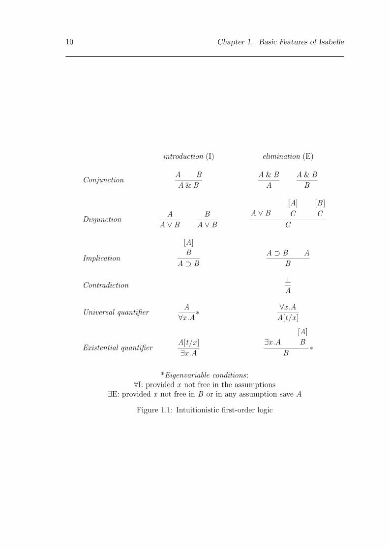
To illustrate this notation, let us consider how first-order logic is formalized.Figure 1.1 presents the natural deduction system for intuitionistic first-order logicas implemented by Isabelle.
The rule &I is expressed by the meta-axiom∧PQ .P =⇒ (Q =⇒ P & Q)
This translates literally into keyboard characters as
!P Q. P ==> (Q ==> P&Q)
Leading universal quantifiers are usually dropped in favour of scheme variables:
?P ==> (?Q ==> ?P & ?Q)
10 Chapter 1. Basic Features of Isabelle
introduction (I) elimination (E)
ConjunctionA B
A & B
A & B
A
A & B
B
DisjunctionA
A ∨ B
B
A ∨ B
A ∨ B
[A]
C
[B ]
C
C
Implication
[A]
B
A ⊃ B
A ⊃ B A
B
Contradiction⊥A
Universal quantifierA
∀x .A∗∀x .A
A[t/x ]
Existential quantifierA[t/x ]
∃x .A∃x .A
[A]
B
B∗
*Eigenvariable conditions :∀I: provided x not free in the assumptions
∃E: provided x not free in B or in any assumption save A
Figure 1.1: Intuitionistic first-order logic
1.2. Theorems, rules, and theories 11
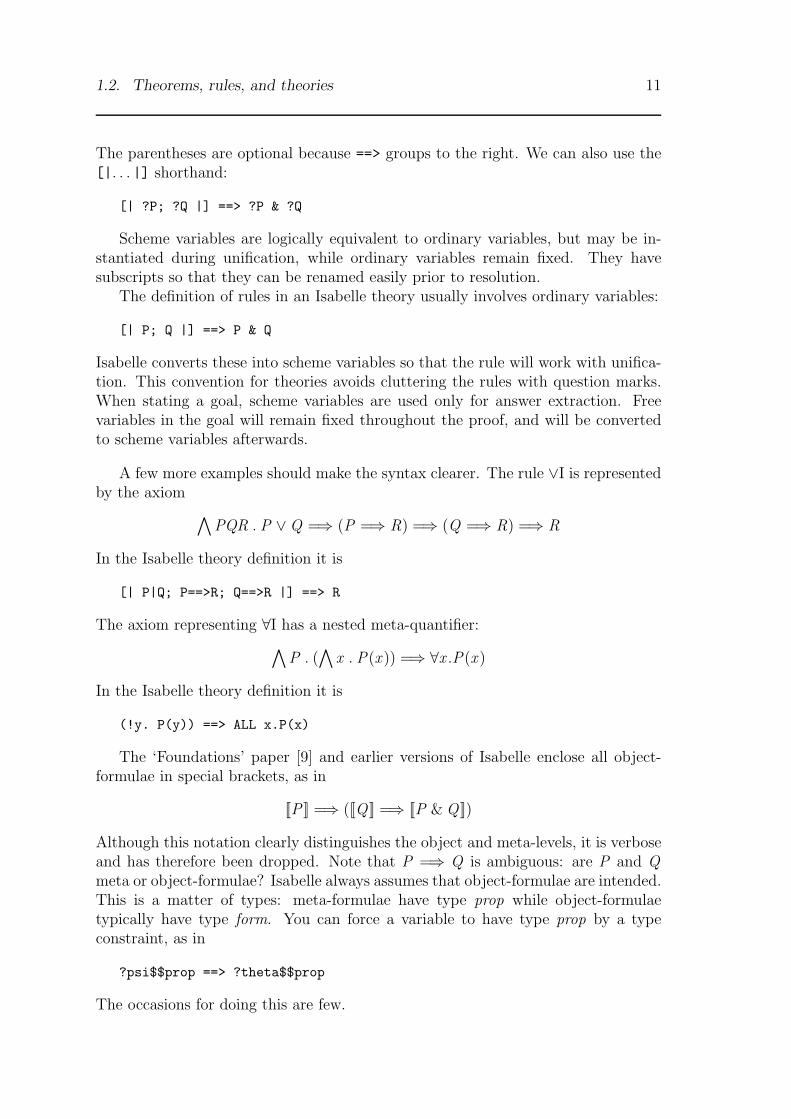
The parentheses are optional because ==> groups to the right. We can also use the[|. . . |] shorthand:
[| ?P; ?Q |] ==> ?P & ?Q
Scheme variables are logically equivalent to ordinary variables, but may be in-stantiated during unification, while ordinary variables remain fixed. They havesubscripts so that they can be renamed easily prior to resolution.
The definition of rules in an Isabelle theory usually involves ordinary variables:
[| P; Q |] ==> P & Q
Isabelle converts these into scheme variables so that the rule will work with unifica-tion. This convention for theories avoids cluttering the rules with question marks.When stating a goal, scheme variables are used only for answer extraction. Freevariables in the goal will remain fixed throughout the proof, and will be convertedto scheme variables afterwards.
A few more examples should make the syntax clearer. The rule ∨I is representedby the axiom ∧
PQR . P ∨Q =⇒ (P =⇒ R) =⇒ (Q =⇒ R) =⇒ R
In the Isabelle theory definition it is
[| P|Q; P==>R; Q==>R |] ==> R
The axiom representing ∀I has a nested meta-quantifier:∧P . (
∧x . P(x )) =⇒ ∀x .P(x )
In the Isabelle theory definition it is
(!y. P(y)) ==> ALL x.P(x)
The ‘Foundations’ paper [9] and earlier versions of Isabelle enclose all object-formulae in special brackets, as in
[[P ]] =⇒ ([[Q ]] =⇒ [[P & Q ]])
Although this notation clearly distinguishes the object and meta-levels, it is verboseand has therefore been dropped. Note that P =⇒ Q is ambiguous: are P and Qmeta or object-formulae? Isabelle always assumes that object-formulae are intended.This is a matter of types: meta-formulae have type prop while object-formulaetypically have type form. You can force a variable to have type prop by a typeconstraint, as in
?psi$$prop ==> ?theta$$prop
The occasions for doing this are few.
12 Chapter 1. Basic Features of Isabelle
1.2.2 The type of theorems and its operations
The inference rules, theorems, and axioms of a logic have type thm. Theorems andaxioms can be regarded as rules with no premises, so let us speak just of rules. Eachproof is constructed by a series of rule applications, usually through subgoal modulecommands.
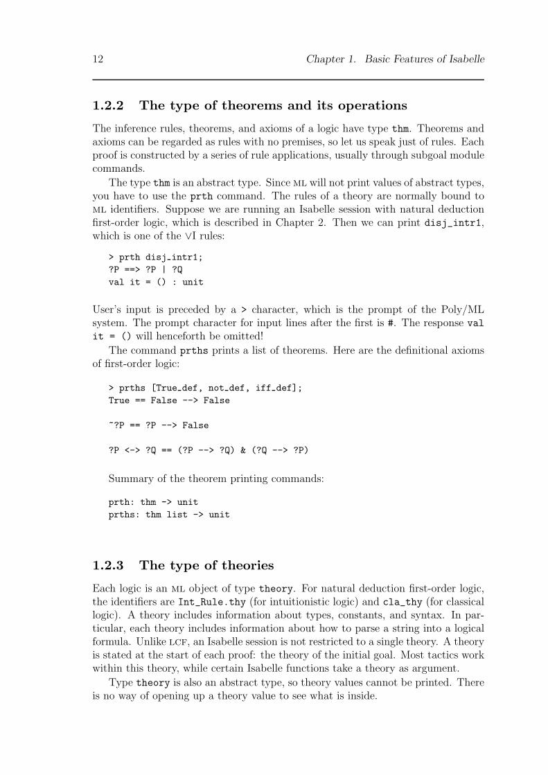
The type thm is an abstract type. Since ml will not print values of abstract types,you have to use the prth command. The rules of a theory are normally bound toml identifiers. Suppose we are running an Isabelle session with natural deductionfirst-order logic, which is described in Chapter 2. Then we can print disj_intr1,which is one of the ∨I rules:
> prth disj intr1;?P ==> ?P | ?Qval it = () : unit
User’s input is preceded by a > character, which is the prompt of the Poly/MLsystem. The prompt character for input lines after the first is #. The response val
it = () will henceforth be omitted!
The command prths prints a list of theorems. Here are the definitional axiomsof first-order logic:
> prths [True def, not def, iff def];True == False --> False
~?P == ?P --> False
?P <-> ?Q == (?P --> ?Q) & (?Q --> ?P)
Summary of the theorem printing commands:
prth: thm -> unitprths: thm list -> unit
1.2.3 The type of theories
Each logic is an ml object of type theory. For natural deduction first-order logic,the identifiers are Int_Rule.thy (for intuitionistic logic) and cla_thy (for classicallogic). A theory includes information about types, constants, and syntax. In par-ticular, each theory includes information about how to parse a string into a logicalformula. Unlike lcf, an Isabelle session is not restricted to a single theory. A theoryis stated at the start of each proof: the theory of the initial goal. Most tactics workwithin this theory, while certain Isabelle functions take a theory as argument.
Type theory is also an abstract type, so theory values cannot be printed. Thereis no way of opening up a theory value to see what is inside.
1.3. The subgoal module 13
1.3 The subgoal module
Most Isabelle proofs are conducted through the subgoal module, which maintainsa proof state and manages the proof construction. Isabelle is largely a functionalprogram, but this kind of interaction is imperative. From the ml top-level you caninvoke commands (which are ml functions, with side effects) to establish a goal,apply a tactic to the proof state, undo a proof step, and finally obtain the theoremthat has been proved.
Tactics, which are operations on proof states, are described in the followingsection. We peek at them here, however, during the demonstration of the subgoalcommands.
1.3.1 Basic commands
To start a new proof, type
goal theory formula ;
where the formula is written as an ml string.To apply a tactic to the proof state, type
by tactic ;
A tactic can do anything to a proof state — even replace it by a completely unrelatedstate — but most tactics apply a rule or rules to a numbered subgoal.
At the end of the proof, call result() to get the theorem you have just proved.If ever you are dissatisfied with a previous step, type undo() to cancel it. The
undo operation can be repeated.
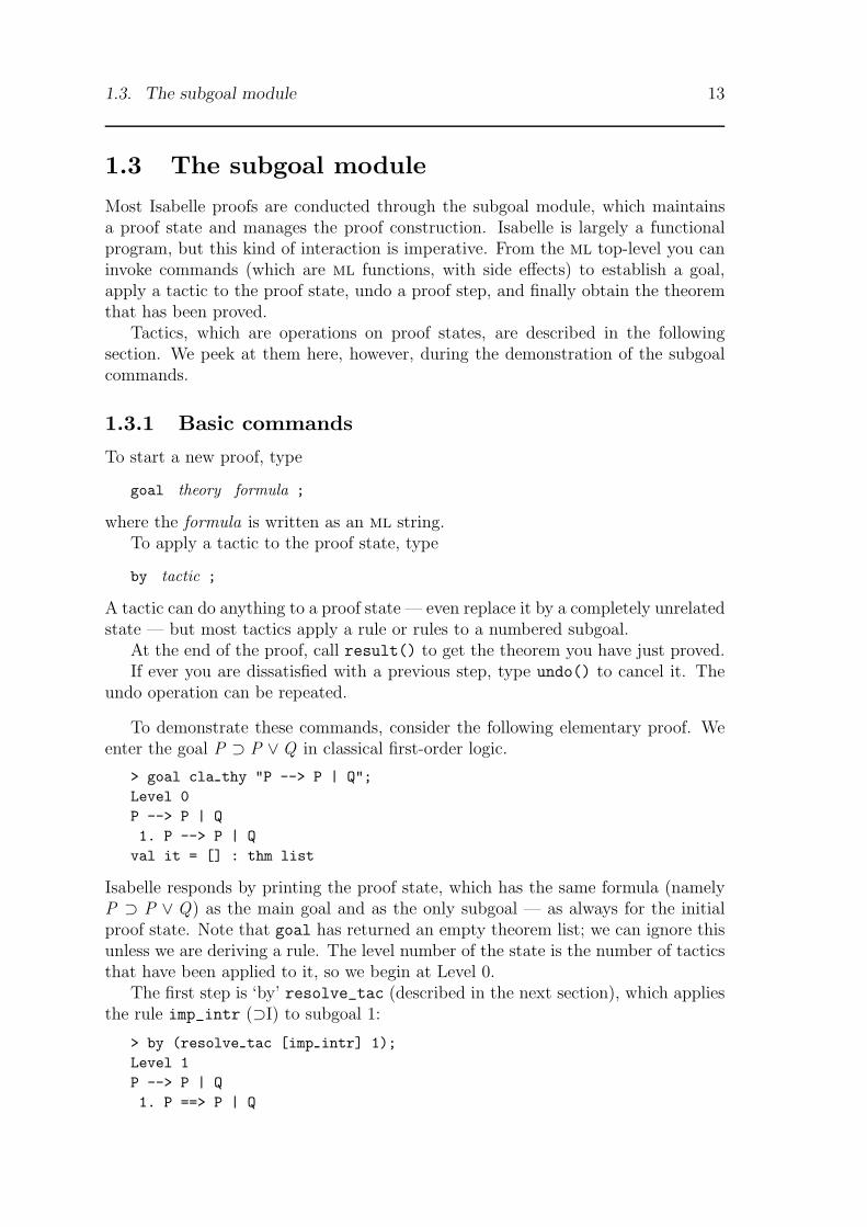
To demonstrate these commands, consider the following elementary proof. Weenter the goal P ⊃ P ∨Q in classical first-order logic.
> goal cla thy "P --> P | Q";Level 0P --> P | Q1. P --> P | Q
val it = [] : thm list
Isabelle responds by printing the proof state, which has the same formula (namelyP ⊃ P ∨ Q) as the main goal and as the only subgoal — as always for the initialproof state. Note that goal has returned an empty theorem list; we can ignore thisunless we are deriving a rule. The level number of the state is the number of tacticsthat have been applied to it, so we begin at Level 0.
The first step is ‘by’ resolve_tac (described in the next section), which appliesthe rule imp_intr (⊃I) to subgoal 1:
> by (resolve tac [imp intr] 1);Level 1P --> P | Q1. P ==> P | Q

14 Chapter 1. Basic Features of Isabelle
In the new proof state, subgoal 1 is P ∨Q under the assumption P . (The meta-implication ==> indicates assumptions.) We now apply the rule disj_intr1 to thatsubgoal:
> by (resolve tac [disj intr1] 1);Level 2P --> P | Q1. P ==> P
At Level 2 the one subgoal is ‘prove P assuming P ’. That is easy, by the tacticassume_tac.
> by (assume tac 1);Level 3P --> P | QNo subgoals!
Isabelle tells us that there are no longer any subgoals: the proof is complete. Oncefinished, call result() to get the theorem you have just proved.
> val mythm = result();val mythm = ? : thm
ml will not print theorems unless we force it to:
> prth mythm;?P --> ?P | ?Q
Note that P and Q have changed from free variables into the scheme variables ?P and?Q. As free variables, they remain fixed throughout the proof; as scheme variables,the theorem mythm can be applied with any formulae in place of P and Q . Here wego back to Level 2:
> undo();Level 2P --> P | Q1. P ==> P
You can undo() and undo() right back to the beginning. But undo() is irreversible.Incidentally, do not omit the parentheses:
> undo;val it = fn : unit -> unit
This is just a function value!
1.3.2 More advanced commands
The following commands are mainly of importance to experienced users, so feel freeto skip this section on the first reading.
1.3. The subgoal module 15
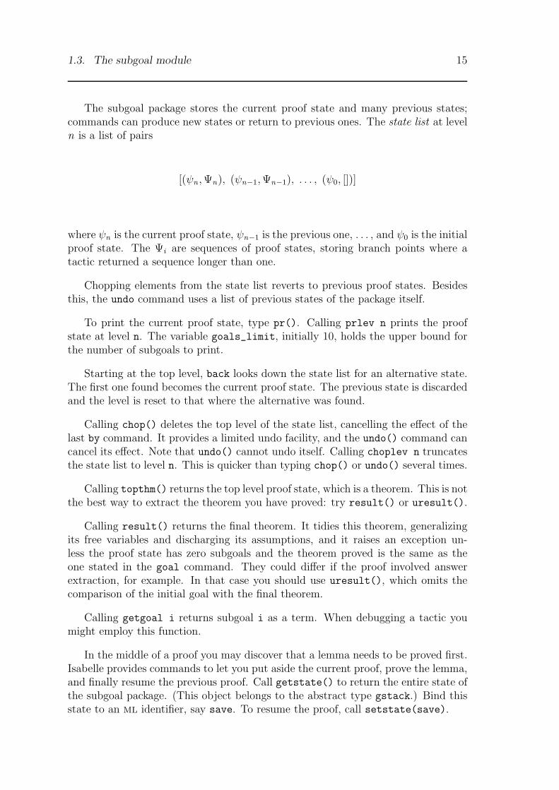
The subgoal package stores the current proof state and many previous states;commands can produce new states or return to previous ones. The state list at leveln is a list of pairs
[(ψn ,Ψn), (ψn−1,Ψn−1), . . . , (ψ0, [])]
where ψn is the current proof state, ψn−1 is the previous one, . . . , and ψ0 is the initialproof state. The Ψi are sequences of proof states, storing branch points where atactic returned a sequence longer than one.
Chopping elements from the state list reverts to previous proof states. Besidesthis, the undo command uses a list of previous states of the package itself.
To print the current proof state, type pr(). Calling prlev n prints the proofstate at level n. The variable goals_limit, initially 10, holds the upper bound forthe number of subgoals to print.
Starting at the top level, back looks down the state list for an alternative state.The first one found becomes the current proof state. The previous state is discardedand the level is reset to that where the alternative was found.
Calling chop() deletes the top level of the state list, cancelling the effect of thelast by command. It provides a limited undo facility, and the undo() command cancancel its effect. Note that undo() cannot undo itself. Calling choplev n truncatesthe state list to level n. This is quicker than typing chop() or undo() several times.
Calling topthm() returns the top level proof state, which is a theorem. This is notthe best way to extract the theorem you have proved: try result() or uresult().
Calling result() returns the final theorem. It tidies this theorem, generalizingits free variables and discharging its assumptions, and it raises an exception un-less the proof state has zero subgoals and the theorem proved is the same as theone stated in the goal command. They could differ if the proof involved answerextraction, for example. In that case you should use uresult(), which omits thecomparison of the initial goal with the final theorem.
Calling getgoal i returns subgoal i as a term. When debugging a tactic youmight employ this function.
In the middle of a proof you may discover that a lemma needs to be proved first.Isabelle provides commands to let you put aside the current proof, prove the lemma,and finally resume the previous proof. Call getstate() to return the entire state ofthe subgoal package. (This object belongs to the abstract type gstack.) Bind thisstate to an ml identifier, say save. To resume the proof, call setstate(save).

16 Chapter 1. Basic Features of Isabelle
Summary of these subgoal module commands:
back: unit -> unitby: tactic -> unitchop: unit -> unitchoplev: int -> unitgetgoal: int -> termgetstate: unit -> gstackgoal: theory -> string -> thm listgoals limit: int refpr: unit -> unitprlev: int -> unitresult: unit -> thmsetstate: gstack -> unittopthm: unit -> thmundo: unit -> unituresult: unit -> thm
1.4 Tactics
Tactics are operations on the proof state, such as, ‘apply the following rules to thesesubgoals’. For the time being, you may want to regard them as part of the syntaxof the by command. They have a separate existence because they can be combined— using operators called tacticals — into more powerful tactics. Those tactics canbe similarly combined, and so on.
Tacticals are not discussed until Chapter 4. Here we consider only the most basictactics. Fancier tactics are provided in the built-in logics, so you should still be ableto do substantial proofs.
Applying a tactic changes the proof state to a new proof state. A tactic mayproduce multiple outcomes, permitting backtracking and search. For now, let uspretend that a tactic can produce at most one next state. When a tactic producesno next state, it is said to fail.
The tactics given below each act on a subgoal designated by a number, startingfrom 1. They fail if the subgoal number is out of range.
To understand tactics, you will need to have read ‘The Foundation of a GenericTheorem Prover’ [9] — particularly the discussion of backwards proof. We shallperform some proofs from that paper in Isabelle.
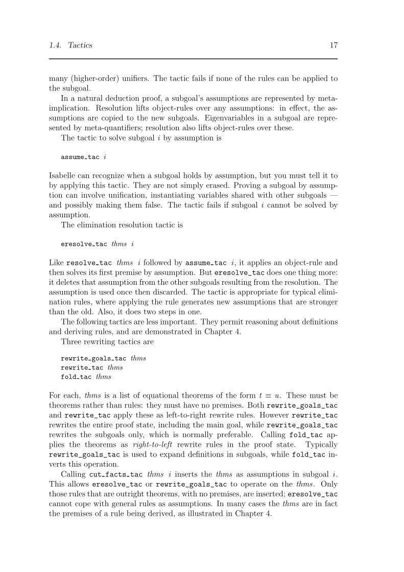
The basic resolution tactic, used for most proof steps, is
resolve tac thms i
The thms represent object-rules. The rules in this list are tried against subgoal i ofthe proof state. For a given rule, resolution can form the next state by unifying theconclusion with the subgoal, replacing it by the instantiated premises. There canbe many outcomes: many of the rules may be unifiable, and for each there can be
1.4. Tactics 17
many (higher-order) unifiers. The tactic fails if none of the rules can be applied tothe subgoal.
In a natural deduction proof, a subgoal’s assumptions are represented by meta-implication. Resolution lifts object-rules over any assumptions: in effect, the as-sumptions are copied to the new subgoals. Eigenvariables in a subgoal are repre-sented by meta-quantifiers; resolution also lifts object-rules over these.
The tactic to solve subgoal i by assumption is
assume tac i
Isabelle can recognize when a subgoal holds by assumption, but you must tell it toby applying this tactic. They are not simply erased. Proving a subgoal by assump-tion can involve unification, instantiating variables shared with other subgoals —and possibly making them false. The tactic fails if subgoal i cannot be solved byassumption.
The elimination resolution tactic is
eresolve tac thms i
Like resolve tac thms i followed by assume tac i , it applies an object-rule andthen solves its first premise by assumption. But eresolve_tac does one thing more:it deletes that assumption from the other subgoals resulting from the resolution. Theassumption is used once then discarded. The tactic is appropriate for typical elimi-nation rules, where applying the rule generates new assumptions that are strongerthan the old. Also, it does two steps in one.
The following tactics are less important. They permit reasoning about definitionsand deriving rules, and are demonstrated in Chapter 4.
Three rewriting tactics are
rewrite goals tac thmsrewrite tac thmsfold tac thms
For each, thms is a list of equational theorems of the form t ≡ u. These must betheorems rather than rules: they must have no premises. Both rewrite_goals_tac
and rewrite_tac apply these as left-to-right rewrite rules. However rewrite_tac
rewrites the entire proof state, including the main goal, while rewrite_goals_tac
rewrites the subgoals only, which is normally preferable. Calling fold_tac ap-plies the theorems as right-to-left rewrite rules in the proof state. Typicallyrewrite_goals_tac is used to expand definitions in subgoals, while fold_tac in-verts this operation.
Calling cut facts tac thms i inserts the thms as assumptions in subgoal i .This allows eresolve_tac or rewrite_goals_tac to operate on the thms . Onlythose rules that are outright theorems, with no premises, are inserted; eresolve_taccannot cope with general rules as assumptions. In many cases the thms are in factthe premises of a rule being derived, as illustrated in Chapter 4.
18 Chapter 1. Basic Features of Isabelle
Summary of these tactics:
assume tac: int -> tacticcut facts tac: thm list -> int -> tacticeresolve tac: thm list -> int -> tacticfold tac: thm list -> tacticresolve tac: thm list -> int -> tacticrewrite goals tac: thm list -> tacticrewrite tac: thm list -> tactic
The tactics resolve_tac, assume_tac, and eresolve_tac suffice for mostsingle-step proofs. The examples below demonstrate how the subgoal commandsand tactics are used in practice. Although eresolve_tac is not strictly necessary,it simplies proofs that involve elimination rules.
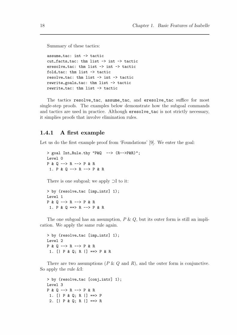
1.4.1 A first example
Let us do the first example proof from ‘Foundations’ [9]. We enter the goal:
> goal Int Rule.thy "P&Q --> (R-->P&R)";Level 0P & Q --> R --> P & R1. P & Q --> R --> P & R
There is one subgoal; we apply ⊃I to it:
> by (resolve tac [imp intr] 1);Level 1P & Q --> R --> P & R1. P & Q ==> R --> P & R
The one subgoal has an assumption, P & Q , but its outer form is still an impli-cation. We apply the same rule again.
> by (resolve tac [imp intr] 1);Level 2P & Q --> R --> P & R1. [| P & Q; R |] ==> P & R
There are two assumptions (P & Q and R), and the outer form is conjunctive.So apply the rule &I:
> by (resolve tac [conj intr] 1);Level 3P & Q --> R --> P & R1. [| P & Q; R |] ==> P2. [| P & Q; R |] ==> R
1.4. Tactics 19
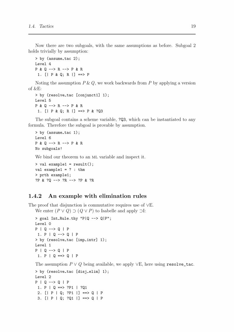
Now there are two subgoals, with the same assumptions as before. Subgoal 2holds trivially by assumption:
> by (assume tac 2);Level 4P & Q --> R --> P & R1. [| P & Q; R |] ==> P
Noting the assumption P & Q , we work backwards from P by applying a versionof &E:
> by (resolve tac [conjunct1] 1);Level 5P & Q --> R --> P & R1. [| P & Q; R |] ==> P & ?Q3
The subgoal contains a scheme variable, ?Q3, which can be instantiated to anyformula. Therefore the subgoal is provable by assumption.
> by (assume tac 1);Level 6P & Q --> R --> P & RNo subgoals!
We bind our theorem to an ml variable and inspect it.
> val example1 = result();val example1 = ? : thm> prth example1;?P & ?Q --> ?R --> ?P & ?R
1.4.2 An example with elimination rules
The proof that disjunction is commutative requires use of ∨E.We enter (P ∨Q) ⊃ (Q ∨ P) to Isabelle and apply ⊃I:
> goal Int Rule.thy "P|Q --> Q|P";Level 0P | Q --> Q | P1. P | Q --> Q | P
> by (resolve tac [imp intr] 1);Level 1P | Q --> Q | P1. P | Q ==> Q | P
The assumption P ∨Q being available, we apply ∨E, here using resolve_tac.
> by (resolve tac [disj elim] 1);Level 2P | Q --> Q | P1. P | Q ==> ?P1 | ?Q12. [| P | Q; ?P1 |] ==> Q | P3. [| P | Q; ?Q1 |] ==> Q | P
20 Chapter 1. Basic Features of Isabelle
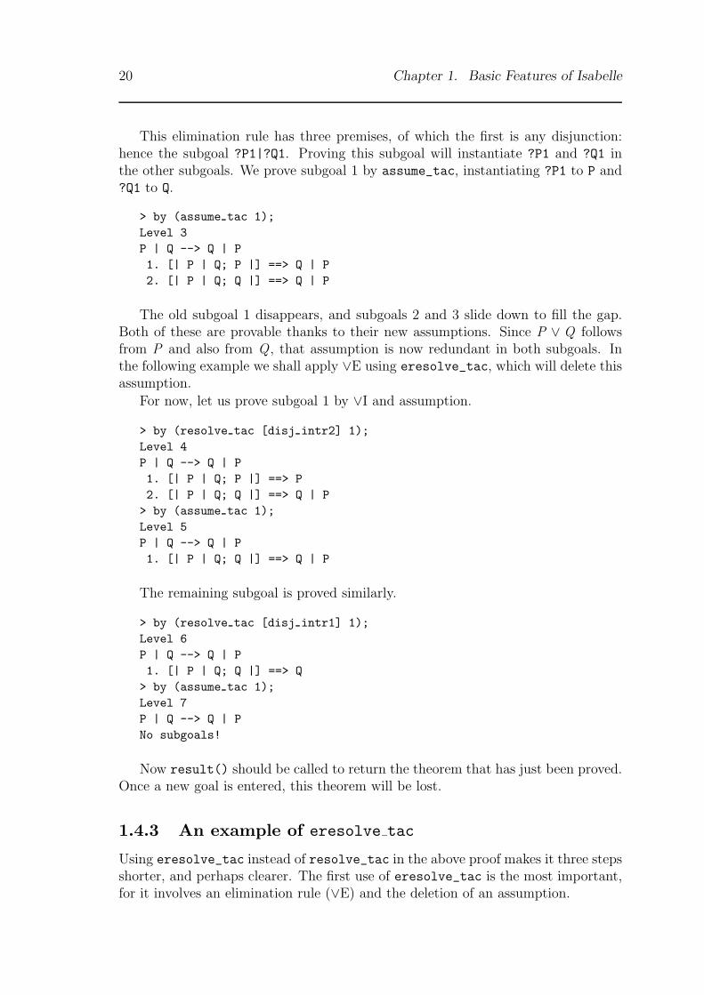
This elimination rule has three premises, of which the first is any disjunction:hence the subgoal ?P1|?Q1. Proving this subgoal will instantiate ?P1 and ?Q1 inthe other subgoals. We prove subgoal 1 by assume_tac, instantiating ?P1 to P and?Q1 to Q.
> by (assume tac 1);Level 3P | Q --> Q | P1. [| P | Q; P |] ==> Q | P2. [| P | Q; Q |] ==> Q | P
The old subgoal 1 disappears, and subgoals 2 and 3 slide down to fill the gap.Both of these are provable thanks to their new assumptions. Since P ∨ Q followsfrom P and also from Q , that assumption is now redundant in both subgoals. Inthe following example we shall apply ∨E using eresolve_tac, which will delete thisassumption.
For now, let us prove subgoal 1 by ∨I and assumption.
> by (resolve tac [disj intr2] 1);Level 4P | Q --> Q | P1. [| P | Q; P |] ==> P2. [| P | Q; Q |] ==> Q | P> by (assume tac 1);Level 5P | Q --> Q | P1. [| P | Q; Q |] ==> Q | P
The remaining subgoal is proved similarly.
> by (resolve tac [disj intr1] 1);Level 6P | Q --> Q | P1. [| P | Q; Q |] ==> Q> by (assume tac 1);Level 7P | Q --> Q | PNo subgoals!
Now result() should be called to return the theorem that has just been proved.Once a new goal is entered, this theorem will be lost.
1.4.3 An example of eresolve tac
Using eresolve_tac instead of resolve_tac in the above proof makes it three stepsshorter, and perhaps clearer. The first use of eresolve_tac is the most important,for it involves an elimination rule (∨E) and the deletion of an assumption.

1.4. Tactics 21
Let us again enter (P ∨ Q) ⊃ (Q ∨ P) and apply ⊃I. (If you have done theprevious example on a terminal, type undo() six times to get back to Level 1.)
> goal Int Rule.thy "P|Q --> Q|P";Level 0P | Q --> Q | P1. P | Q --> Q | P
> by (resolve tac [imp intr] 1);Level 1P | Q --> Q | P1. P | Q ==> Q | P
The first premise of ∨E is the formula being eliminated: the disjunction. Thetactic eresolve_tac searches among the assumptions for one that unifies with thefirst premise, simultaneously unifying the conclusion of this rule with the subgoal.(The conclusion of ∨E unifies with any formula, for it is simply R.) It uses theselected assumption to prove the first premise, and deletes that assumption fromthe resulting subgoals. In short, the assumption is eliminated.
> by (eresolve tac [disj elim] 1);Level 2P | Q --> Q | P1. P ==> Q | P2. Q ==> Q | P
Although subgoals 1 and 2 now have only one assumption (compared with twoin the previous proof), they can be proved exactly as before. But eresolve_tac
simplifies these steps also, for they consist of application of a rule followed by proofby assumption.
> by (eresolve tac [disj intr2] 1);Level 3P | Q --> Q | P1. Q ==> Q | P
The same thing again . . .
> by (eresolve tac [disj intr1] 1);Level 4P | Q --> Q | PNo subgoals!
The importance of eresolve_tac is clearer in larger proofs. It prevents assump-tions from accumulating and getting reused. The eliminated assumption is redun-dant with most elimination rules save ∀E. Their deletion is especially important inautomatic tactics.
22 Chapter 1. Basic Features of Isabelle
1.5 Proofs involving quantifiers
One of the most important aspects of Isabelle is the treatment of quantifier reason-ing. We can illustrate this by comparing a proof of ∀x .∃y .x = y with an attemptedproof of ∃y . ∀x . x = y (which happens to be false). The one proof succeeds andthe other fails because of the scope of quantified variables. These proofs are alsodiscussed in ‘Foundations’ [9].
Unification helps even in these trivial proofs. In ∀x .∃y .x = y the y that ‘exists’is simply x , but we need never say so. This choice is forced by the reflexive law forequality, and it happens automatically. The proof forces the correct instantiationof variables. Of course, if the instantiation is complicated, it may not be found in areasonable amount of time!
1.5.1 A successful quantifier proof
The theorem ∀x . ∃y . x = y is one of the simplest to contain both quantifiers. Itsproof illustrates the use of the introduction rules ∀I and ∃I.
To begin, we enter the goal:
> goal Int Rule.thy "ALL x. EX y. x=y";Level 0ALL x. EX y. x = y1. ALL x. EX y. x = y
The only applicable rule is ∀I:
> by (resolve tac [all intr] 1);Level 1ALL x. EX y. x = y1. !ka. EX y. ka = y
The !ka introduces an eigenvariable in the subgoal. The exclamation mark isthe character for meta-forall (
∧). The subgoal must be proved for all possible values
of ka. Isabelle chooses the names of eigenvariables; they are always ka, kb, kc, . . . ,in that order.
The only applicable rule is ∃I:
> by (resolve tac [exists intr] 1);Level 2ALL x. EX y. x = y1. !ka. ka = ?a1(ka)
Note that the bound variable y has changed into ?a1(ka), where ?a1 is a schemevariable. It is also a function, and is applied to ka. Instantiating ?a1 will change?a1(ka) into a term that may — or may not — contain ka. In particular, if
1.5. Proofs involving quantifiers 23
?a1 is instantiated to the identity function, ?a1(ka) changes into simply ka. Thiscorresponds to proof by the reflexivity of equality.
> by (resolve tac [refl] 1);Level 3ALL x. EX y. x = yNo subgoals!
The proof is finished. Unfortunately we cannot observe the instantiation of ?a1
because it appears nowhere else.
1.5.2 An unsuccessful quantifier proof
The formula ∃y .∀x . x = y is not a theorem. Let us hope that Isabelle cannot proveit!
We enter the goal:
> goal Int Rule.thy "EX y. ALL x. x=y";Level 0EX y. ALL x. x = y1. EX y. ALL x. x = y
The only rule that can be considered is ∃I:> by (resolve tac [exists intr] 1);Level 1EX y. ALL x. x = y1. ALL x. x = ?a
The scheme variable ?a may be replaced by any term to complete the proof.Problem is, no term is equal to all x . We now must apply ∀I:
> by (resolve tac [all intr] 1);Level 2EX y. ALL x. x = y1. !ka. ka = ?a
Compare our position with the previous Level 2. Where before was ?a1(ka)
there is now ?a. In both cases the scheme variable (whether ?a1 or ?a) can onlybe instantiated by a term that is free in the entire proof state. But so doing canchange ?a1(ka) into something that depends upon ka. In our present position wecan do nothing. The reflexivity axiom does not unify with subgoal 1 because ka isa bound variable. Here is what happens if we try:
> by (resolve tac [refl] 1);by: tactic returned no resultsException- ERROR raised
You do not have to think about the β-reduction that changes ?a1(ka) into ka.Instead, regard ?a1(ka) as any term possibly containing ka.
24 Chapter 1. Basic Features of Isabelle
1.5.3 Nested quantifiers
Multiple quantification produces complicated terms. Consider this contrived exam-ple. Without more information about P we cannot prove anything, but observe howthe eigenvariables and scheme variables develop.
> goal Int Rule.thy "EX u.ALL x.EX v.ALL y.EX w. P(u,x,v,y,w)";Level 0EX u. ALL x. EX v. ALL y. EX w. P(u,x,v,y,w)1. EX u. ALL x. EX v. ALL y. EX w. P(u,x,v,y,w)> by (resolve tac [exists intr, all intr] 1);Level 1EX u. ALL x. EX v. ALL y. EX w. P(u,x,v,y,w)1. ALL x. EX v. ALL y. EX w. P(?a,x,v,y,w)
The scheme variable ?a has appeared.Note that resolve_tac, if given a list of rules, will choose a rule that applies.
Here the only rules worth considering are ∀I and ∃I.> by (resolve tac [exists intr, all intr] 1);Level 2EX u. ALL x. EX v. ALL y. EX w. P(u,x,v,y,w)1. !ka. EX v. ALL y. EX w. P(?a,ka,v,y,w)> by (resolve tac [exists intr, all intr] 1);Level 3EX u. ALL x. EX v. ALL y. EX w. P(u,x,v,y,w)1. !ka. ALL y. EX w. P(?a,ka,?a2(ka),y,w)
The bound variable ka and scheme variable ?a2 have appeared. Note that ?a2 isapplied to the bound variables existing at the time of its introduction — but not,of course, to bound variables introduced later.
> by (resolve tac [exists intr, all intr] 1);Level 4EX u. ALL x. EX v. ALL y. EX w. P(u,x,v,y,w)1. !ka kb. EX w. P(?a,ka,?a2(ka),kb,w)> by (resolve tac [exists intr, all intr] 1);Level 5EX u. ALL x. EX v. ALL y. EX w. P(u,x,v,y,w)1. !ka kb. P(?a,ka,?a2(ka),kb,?a4(ka,kb))
In the final state, ?a cannot become any term containing ka or kb, while ?a2(ka)can become a term containing ka, and ?a4(ka,kb) can become a term containingboth bound variables. This example is discussed in ‘Foundations’ [9].
1.6 Priority Grammars
In the remainder of this manual we shall frequently define the precise syntax ofsome logic by means of context-free grammars. These grammars obey the following
1.6. Priority Grammars 25
conventions: identifiers denote nonterminals, typewriter fount denotes terminals,constructs enclosed in {.} can be repeated 0 or more times (Kleene star), and alter-natives are separated by |. The predefined categories of alphanumeric identifiers andof scheme variables are denoted by identifier and variable respectively (see Section5.4.2).
In order to simplify the description of mathematical languages, we introduce anextended format which permits priorities or precedences. This scheme generalizesprecedence declarations in ml and prolog. In this extended grammar format,nonterminals are decorated by integers, their priority. In the sequel, priorities areshown as subscripts. A nonterminal Ap on the right-hand side of a production mayonly be rewritten using a production Aq = γ where q is not less than p.
Formally, a set of context free productions G induces a derivation relation −→G
on strings as follows:
αApβ −→G αγβ iff ∃q ≥ p. (Aq=γ) ∈ G
Any extended grammar of this kind can be translated into a normal context freegrammar. However, this translation may require the introduction of a large numberof new nonterminals and productions.
Example 1.1 The following simple grammar for arithmetic expressions demon-strates how binding power and associativity of operators can be enforced by priori-ties.
A9 = 0
A9 = ( A0 )
A0 = A0 + A1
A2 = A3 * A2
A3 = - A3
The choice of priorities determines that “-” binds tighter than “*” which bindstighter than “+”, and that “+” and “*” associate to the left and right, respectively.
To minimize the number of subscripts, we adopt the following conventions:
• all priorities p must be in the range 0 ≤ p ≤ m for some fixed m.
• priority 0 on the right-hand side and priority m on the left-hand side may beomitted.
In addition, we write the production Ap = α as A = α (p).Using these conventions and assuming m = 9, the grammar in Example 1.1
becomes
A = 0
| ( A )
| A + A1 (0)| A3 * A2 (2)| - A3 (3)
Priority grammars are not just used to describe logics in this manual. They arealso supported by Isabelle’s syntax definition facility (see Chapter 5).

26 Chapter 1. Basic Features of Isabelle
Chapter 2
Isabelle’s First-Order Logics
Although Isabelle has been developed to be a generic theorem prover — one thatyou can customize to your own logics — several logics come with it. They reside invarious subdirectories and can be built using the installation instructions. You canuse Isabelle simply as an implementation of one of these. This chapter describesthe three versions of first-order logic provided with Isabelle. The following chapterdescribes set and type theories.
First-order logic with natural deduction comes in both constructive and classicalversions. First-order logic is also available as the classical sequent calculus LK .Each sequent has the form A1, . . . ,Am |− B1, . . . ,Bn . This formulation is equivalentto deductive tableaux.
Each object-logic comes with simple proof procedures. These are reasonablypowerful (at least for interactive use), though neither complete nor amazingly sci-entific. You can use them as they are or take them as examples of tactical program-ming. You can perform single-step proofs using resolve_tac and assume_tac,referring to the inference rules of the logic by ml identifiers of type thm.
Call a rule safe if when applied to a provable goal the resulting subgoals willalso be provable. If a rule is safe then it can be applied automatically to a goalwithout destroying our chances of finding a proof. For instance, all the rules of theclassical sequent calculus lk are safe. Intuitionistic logic includes some unsafe rules,like disjunction introduction (P ∨ Q can be true when P is false) and existentialintroduction (∃x . P(x ) can be true when P(a) is false for certain a). Universalelimination is unsafe if the formula ∀x .P(x ) is deleted after use, which is necessaryfor termination.
Proof procedures use safe rules whenever possible, delaying the application ofunsafe rules. Those safe rules are preferred that generate the fewest subgoals. Saferules are (by definition) deterministic, while the unsafe rules require search. Thedesign of a suitable set of rules can be as important as the strategy for applyingthem.
Many of the proof procedures use backtracking. Typically they attempt to solvesubgoal i by repeatedly applying a certain tactic to it. This tactic, which is knownas a step tactic, resolves a selection of rules with subgoal i . This may replace onesubgoal by many; but the search persists until there are fewer subgoals in total thanat the start. Backtracking happens when the search reaches a dead end: when thestep tactic fails. Alternative outcomes are then searched by a depth-first or best-first
27
28 Chapter 2. Isabelle’s First-Order Logics
strategy. Techniques for writing such tactics are discussed in the next chapter.Each logic is distributed with many sample proofs, some of which are described
below. Though future Isabelle users will doubtless find better proofs and tacticsthan mine, the examples already show that Isabelle can prove interesting theoremsin various logics.
2.1 First-order logic with natural deduction
The directory FOL contains theories for first-order logic based on Gentzen’s naturaldeduction systems (which he called nj and nk). Intuitionistic logic is first defined,then classical logic is obtained by adding the double negation rule.
Natural deduction typically involves a combination of forwards and backwardsreasoning, particularly with the rules &E, ⊃E, and ∀E. Isabelle’s backwards stylehandles these rules badly, so alternative rules are derived to eliminate conjunctions,implications, and universal quantifiers. The resulting system is similar to a cut-freesequent calculus.
Basic proof procedures are provided. The intuitionistic prover works with derivedrules to simplify uses of implication in the assumptions. Far from complete, it canstill prove many complex theorems automatically. The classical prover works like astraightforward implementation of lk, which is like a deductive tableaux prover. Itis not complete either, though less flagrantly so.
A serious theorem prover for classical logic would exploit sophisticated methodsfor efficiency and completeness. Most known methods, unfortunately, work onlyfor certain fixed inference systems. With Isabelle you often work in an evolvinginference system, deriving rules as you go. Classical resolution theorem provers areextremely powerful, of course, but do not support interactive proof.
The type of expressions is term while the type of formulae is form. The mlnames for these types are Aterm and Aform respectively. The infixes are the equalssign and the connectives. Note that --> has two meanings: in ml it is a constructorof the type typ, while in FOL it is the implication sign. Figure 2.1 gives the syntax,including translations for the quantifiers.
2.1.1 Intuitionistic logic
The intuitionistic theory has the ml identifier Int_Rule.thy. Figure 2.2 shows theinference rules with their ml names. The connective ↔ is defined through & and⊃; introduction and elimination rules are derived for it. Derived rules are shown inFigure 2.3, again with their ml names.
The hardest rule for search is implication elimination (whether expressed by mp
or imp_elim). Given P ⊃ Q we may assume Q provided we can prove P . In classicallogic the proof of P can assume ¬P , but the intuitionistic proof of P may requirerepeated use of P ⊃ Q . If the proof of P fails then the whole branch of the proofmust be abandoned. Thus intuitionistic propositional logic requires backtracking.For an elementary example, consider the intuitionistic proof of Q from P ⊃ Q and

2.1. First-order logic with natural deduction 29
symbol meta-type precedence description= [term, term]→ form Left 50 equality (=)& [form, form]→ form Right 35 conjunction (&)| [form, form]→ form Right 30 disjunction (∨)--> [form, form]→ form Right 25 implication (⊃)<-> [form, form]→ form Right 25 if and only if (↔)
Infixes
symbol meta-type descriptionTrueprop form → prop meta-predicate of truth
~ form → form negation (¬)Forall (term → form)→ form universal quantifier (∀)Exists (term → form)→ form existential quantifier (∃)True form tautologous formula (>)False form absurd formula (⊥)
Constants
external internal standard notationALL x. P Forall(λx .P) ∀x .PEX x. P Exists(λx .P) ∃x .P
Translations
form = ALL identifier { identifier } . form (10)| EX identifier { identifier } . form (10)| ~ form40 (40)| others . . .
Grammar
Figure 2.1: Syntax of FOL
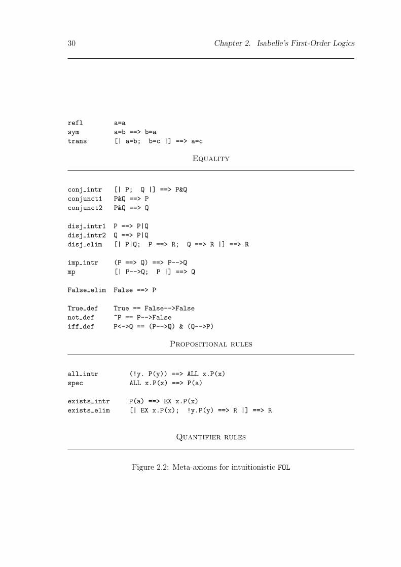
30 Chapter 2. Isabelle’s First-Order Logics
refl a=asym a=b ==> b=atrans [| a=b; b=c |] ==> a=c
Equality
conj intr [| P; Q |] ==> P&Qconjunct1 P&Q ==> Pconjunct2 P&Q ==> Q
disj intr1 P ==> P|Qdisj intr2 Q ==> P|Qdisj elim [| P|Q; P ==> R; Q ==> R |] ==> R
imp intr (P ==> Q) ==> P-->Qmp [| P-->Q; P |] ==> Q
False elim False ==> P
True def True == False-->Falsenot def ~P == P-->Falseiff def P<->Q == (P-->Q) & (Q-->P)
Propositional rules
all intr (!y. P(y)) ==> ALL x.P(x)spec ALL x.P(x) ==> P(a)
exists intr P(a) ==> EX x.P(x)exists elim [| EX x.P(x); !y.P(y) ==> R |] ==> R
Quantifier rules
Figure 2.2: Meta-axioms for intuitionistic FOL
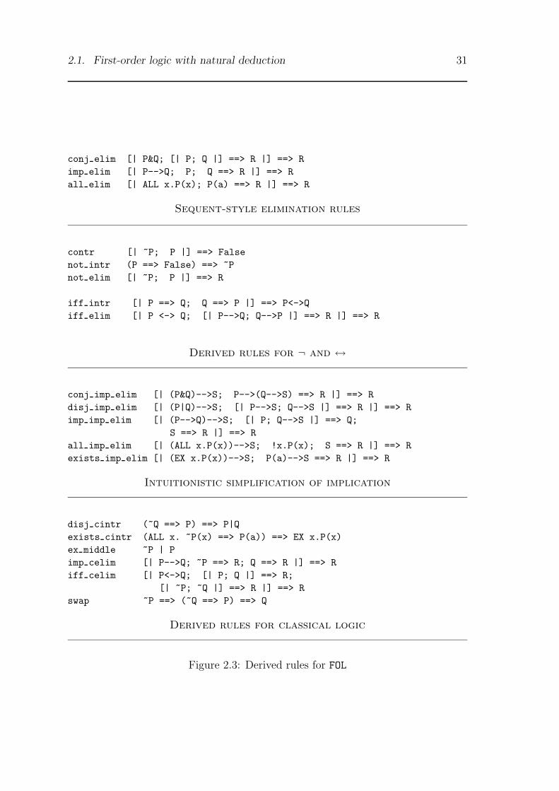
2.1. First-order logic with natural deduction 31
conj elim [| P&Q; [| P; Q |] ==> R |] ==> Rimp elim [| P-->Q; P; Q ==> R |] ==> Rall elim [| ALL x.P(x); P(a) ==> R |] ==> R
Sequent-style elimination rules
contr [| ~P; P |] ==> Falsenot intr (P ==> False) ==> ~Pnot elim [| ~P; P |] ==> R
iff intr [| P ==> Q; Q ==> P |] ==> P<->Qiff elim [| P <-> Q; [| P-->Q; Q-->P |] ==> R |] ==> R
Derived rules for ¬ and ↔
conj imp elim [| (P&Q)-->S; P-->(Q-->S) ==> R |] ==> Rdisj imp elim [| (P|Q)-->S; [| P-->S; Q-->S |] ==> R |] ==> Rimp imp elim [| (P-->Q)-->S; [| P; Q-->S |] ==> Q;
S ==> R |] ==> Rall imp elim [| (ALL x.P(x))-->S; !x.P(x); S ==> R |] ==> Rexists imp elim [| (EX x.P(x))-->S; P(a)-->S ==> R |] ==> R
Intuitionistic simplification of implication
disj cintr (~Q ==> P) ==> P|Qexists cintr (ALL x. ~P(x) ==> P(a)) ==> EX x.P(x)ex middle ~P | Pimp celim [| P-->Q; ~P ==> R; Q ==> R |] ==> Riff celim [| P<->Q; [| P; Q |] ==> R;
[| ~P; ~Q |] ==> R |] ==> Rswap ~P ==> (~Q ==> P) ==> Q
Derived rules for classical logic
Figure 2.3: Derived rules for FOL
32 Chapter 2. Isabelle’s First-Order Logics
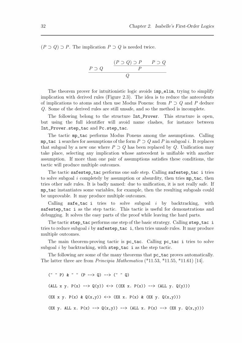
(P ⊃ Q) ⊃ P . The implication P ⊃ Q is needed twice.
P ⊃ Q
(P ⊃ Q) ⊃ P P ⊃ Q
P
Q
The theorem prover for intuitionistic logic avoids imp_elim, trying to simplifyimplication with derived rules (Figure 2.3). The idea is to reduce the antecedentsof implications to atoms and then use Modus Ponens: from P ⊃ Q and P deduceQ . Some of the derived rules are still unsafe, and so the method is incomplete.
The following belong to the structure Int_Prover. This structure is open,but using the full identifier will avoid name clashes, for instance betweenInt_Prover.step_tac and Pc.step_tac.
The tactic mp_tac performs Modus Ponens among the assumptions. Callingmp_tac i searches for assumptions of the form P ⊃ Q and P in subgoal i . It replacesthat subgoal by a new one where P ⊃ Q has been replaced by Q . Unification maytake place, selecting any implication whose antecedent is unifiable with anotherassumption. If more than one pair of assumptions satisfies these conditions, thetactic will produce multiple outcomes.
The tactic safestep_tac performs one safe step. Calling safestep_tac i triesto solve subgoal i completely by assumption or absurdity, then tries mp_tac, thentries other safe rules. It is badly named: due to unification, it is not really safe. Ifmp_tac instantiates some variables, for example, then the resulting subgoals couldbe unprovable. It may produce multiple outcomes.
Calling safe_tac i tries to solve subgoal i by backtracking, withsafestep_tac i as the step tactic. This tactic is useful for demonstrations anddebugging. It solves the easy parts of the proof while leaving the hard parts.
The tactic step_tac performs one step of the basic strategy. Calling step_tac i
tries to reduce subgoal i by safestep_tac i, then tries unsafe rules. It may producemultiple outcomes.
The main theorem-proving tactic is pc_tac. Calling pc_tac i tries to solvesubgoal i by backtracking, with step_tac i as the step tactic.
The following are some of the many theorems that pc_tac proves automatically.The latter three are from Principia Mathematica (*11.53, *11.55, *11.61) [14].
(~ ~ P) & ~ ~ (P --> Q) --> (~ ~ Q)
(ALL x y. P(x) --> Q(y)) <-> ((EX x. P(x)) --> (ALL y. Q(y)))
(EX x y. P(x) & Q(x,y)) <-> (EX x. P(x) & (EX y. Q(x,y)))
(EX y. ALL x. P(x) --> Q(x,y)) --> (ALL x. P(x) --> (EX y. Q(x,y)))
2.1. First-order logic with natural deduction 33
Summary of the tactics (which belong to structure Int_Prover):
mp tac: int -> tacticpc tac: int -> tacticsafestep tac: int -> tacticsafe tac: int -> tacticstep tac: int -> tactic
2.1.2 Classical logic
The classical theory has the ml identifier cla_thy. It consists of intuitionistic logicplus the rule
[¬P ]
P
P
Natural deduction in classical logic is not really all that natural. Derived rulessuch as the following help [8, pages 46–49].
[¬Q ]
P
P ∨Q
P ⊃ Q
[¬P ]
R
[Q ]
R
R
¬P
[¬Q ]
P
Q
The first two exploit the classical equivalence of P ⊃ Q and ¬P ∨ Q . The third,or swap rule, is typically applied to an assumption ¬P . If P is a complex formulathen the resulting subgoal is P , which can be broken up using introduction rules.The classical proof procedures combine the swap rule with each of the introductionrules, so that it is only applied for this purpose. This simulates the sequent calculuslk [13], where a sequent P1, . . . ,Pm |− Q1, . . . ,Qn can have multiple formulae onthe right. In Isabelle, at least, this strange system seems to work better than lkitself.
The functor ProverFun makes theorem-proving tactics for arbitrary collectionsof natural deduction rules. It could be applied, for example, to some introductionand elimination rules for the constants of set theory. At present it is applied onlyonce, to the basic rules of classical logic. The main tactics so defined are fast_tac,best_tac, and comp_tac; they belong to structure Pc.
The tactic onestep_tac performs one safe step. It is the classical counterpartof Int_Prover.safestep_tac.
The tactic step_tac performs one step, something like Int_Prover.step_tac.Calling step_tac thms i tries to reduce subgoal i by safe rules, or else by unsaferules. The rules given as thms are treated like unsafe introduction rules. The tacticmay produce multiple outcomes.
The main theorem-proving tactic is fast_tac. Calling fast_tac thms i triesto solve subgoal i by backtracking, with step_tac thms i as the step tactic.
A slower but more powerful tactic is best_tac. Calling best_tac thms tries tosolve all subgoals by best-first search with step_tac.
34 Chapter 2. Isabelle’s First-Order Logics
A yet slower but ‘almost’ complete tactic is comp_tac. Calling comp_tac thms
tries to solve all subgoals by best-first search. The step tactic is rather judiciousabout expanding quantifiers and so forth.
The following are proved, respectively, by fast_tac, best_tac, and comp_tac.They are all due to Pelletier [11].
(EX y. ALL x. J(y,x) <-> ~J(x,x))--> ~ (ALL x. EX y. ALL z. J(z,y) <-> ~ J(z,x))
(ALL x. P(a) & (P(x)-->P(b))-->P(c)) <->(ALL x. (~P(a) | P(x) | P(c)) & (~P(a) | ~P(b) | P(c)))
(EX x. P-->Q(x)) & (EX x. Q(x)-->P) --> (EX x. P<->Q(x))
Summary of the tactics (which belong to structure Pc):
best tac : thm list -> tacticcomp tac : thm list -> tacticfast tac : thm list -> int -> tacticonestep tac : int -> tacticstep tac : thm list -> int -> tactic
2.1.3 An intuitionistic example
Here is a session similar to one in my book on lcf [8, pages 222–3]. lcf users maywant to compare its treatment of quantifiers with Isabelle’s.
The proof begins by entering the goal in intuitionistic logic, then applying therule ⊃I.
> goal Int Rule.thy"(EX y. ALL x. Q(x,y)) --> (ALL x. EX y. Q(x,y))";
Level 0(EX y. ALL x. Q(x,y)) --> (ALL x. EX y. Q(x,y))1. (EX y. ALL x. Q(x,y)) --> (ALL x. EX y. Q(x,y))> by (resolve tac [imp intr] 1);Level 1(EX y. ALL x. Q(x,y)) --> (ALL x. EX y. Q(x,y))1. EX y. ALL x. Q(x,y) ==> ALL x. EX y. Q(x,y)
In this example we will never have more than one subgoal. Applying ⊃I changed--> into ==>, so ∃y . ∀x . Q(x , y) is now an assumption. We have the choice ofeliminating the ∃x . or introducing the ∀x .. Let us apply ∀I.
> by (resolve tac [all intr] 1);Level 2(EX y. ALL x. Q(x,y)) --> (ALL x. EX y. Q(x,y))1. EX y. ALL x. Q(x,y) ==> (!ka. EX y. Q(ka,y))
2.1. First-order logic with natural deduction 35
Applying ∀I replaced the ALL x by !ka. The universal quantifier changes fromobject (∀) to meta (
∧). The bound variable is renamed ka, and is a parameter of
the subgoal. We now must choose between ∃I and ∃E. What happens if the wrongrule is chosen?
> by (resolve tac [exists intr] 1);Level 3(EX y. ALL x. Q(x,y)) --> (ALL x. EX y. Q(x,y))1. EX y. ALL x. Q(x,y) ==> (!ka. Q(ka,?a2(ka)))
The new subgoal 1 contains the function variable ?a2. Although ka is a boundvariable, instantiating ?a2 can replace ?a2(ka) by a term containing ka. Now wesimplify the assumption ∃y .∀x .Q(x , y) using elimination rules. To apply ∃E to theassumption, call eresolve_tac.
> by (eresolve tac [exists elim] 1);Level 4(EX y. ALL x. Q(x,y)) --> (ALL x. EX y. Q(x,y))1. !ka kb. ALL x. Q(x,kb) ==> Q(ka,?a2(ka))
This step has produced the parameter kb and replaced the assumption by auniversally quantified one. The next step is to eliminate that quantifier. But thesubgoal is unprovable. There is no way to unify ?a2(ka) with the bound variablekb: assigning %(x)kb to ?a2 is illegal.
Using undo we can return to where we went wrong, and correct matters. Thistime we apply ∃E.
...Level 2(EX y. ALL x. Q(x,y)) --> (ALL x. EX y. Q(x,y))1. EX y. ALL x. Q(x,y) ==> (!ka. EX y. Q(ka,y))
> by (eresolve tac [exists elim] 1);Level 3(EX y. ALL x. Q(x,y)) --> (ALL x. EX y. Q(x,y))1. !ka kb. ALL x. Q(x,kb) ==> EX y. Q(ka,y)
We now have two parameters and no scheme variables. Parameters should beproduced early. Applying ∃I and ∀E will produce two scheme variables.
> by (resolve tac [exists intr] 1);Level 4(EX y. ALL x. Q(x,y)) --> (ALL x. EX y. Q(x,y))1. !ka kb. ALL x. Q(x,kb) ==> Q(ka,?a3(ka,kb))
> by (eresolve tac [all elim] 1);Level 5(EX y. ALL x. Q(x,y)) --> (ALL x. EX y. Q(x,y))1. !ka kb. Q(?a4(ka,kb),kb) ==> Q(ka,?a3(ka,kb))

36 Chapter 2. Isabelle’s First-Order Logics
The subgoal has variables ?a3 and ?a4 applied to both parameters. The obviousprojection functions unify ?a4(ka,kb) with ka and ?a3(ka,kb) with kb.
> by (assume tac 1);Level 6(EX y. ALL x. Q(x,y)) --> (ALL x. EX y. Q(x,y))No subgoals!
The theorem was proved in six tactic steps, not counting the abandoned ones.But proof checking is tedious: pc_tac proves the theorem in one step.
Level 0(EX y. ALL x. Q(x,y)) --> (ALL x. EX y. Q(x,y))1. (EX y. ALL x. Q(x,y)) --> (ALL x. EX y. Q(x,y))> by (pc tac 1);Level 1(EX y. ALL x. Q(x,y)) --> (ALL x. EX y. Q(x,y))No subgoals!
2.1.4 A classical example
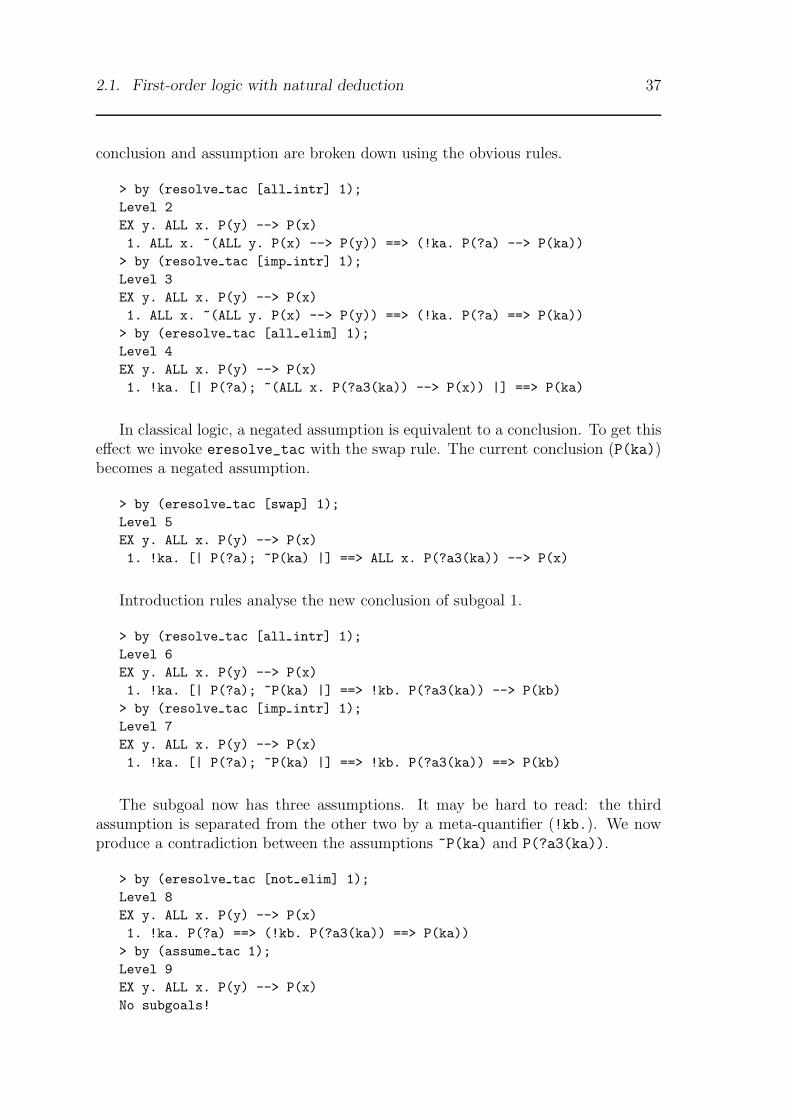
To illustrate classical logic, we shall prove the theorem ∃y . ∀x . P(y) ⊃ P(x ). Thisfails constructively because no y can be exhibited such that ∀x . P(y) ⊃ P(x ).Classically, ∃ does not have this meaning, and the theorem can be proved rather asfollows. If there is any y such that ¬P(y), then chose that y ; otherwise ∀x . P(x )is true. Either way the theorem holds. If this proof seems counterintuitive, thenperhaps you are an intuitionist.
The formal proof does not conform in any obvious way to the sketch above. Thekey step is the very first rule, exists_cintr, which is the classical ∃I rule. Thisestablishes the case analysis.
> goal cla thy "EX y. ALL x. P(y)-->P(x)";Level 0EX y. ALL x. P(y) --> P(x)1. EX y. ALL x. P(y) --> P(x)> by (resolve tac [exists cintr] 1);Level 1EX y. ALL x. P(y) --> P(x)1. ALL x. ~(ALL y. P(x) --> P(y)) ==> ALL x. P(?a) --> P(x)
We now can either exhibit a term ?a to satisfy the conclusion of subgoal 1, orproduce a contradiction from the assumption. The following steps are routine: the
2.1. First-order logic with natural deduction 37
conclusion and assumption are broken down using the obvious rules.
> by (resolve tac [all intr] 1);Level 2EX y. ALL x. P(y) --> P(x)1. ALL x. ~(ALL y. P(x) --> P(y)) ==> (!ka. P(?a) --> P(ka))
> by (resolve tac [imp intr] 1);Level 3EX y. ALL x. P(y) --> P(x)1. ALL x. ~(ALL y. P(x) --> P(y)) ==> (!ka. P(?a) ==> P(ka))
> by (eresolve tac [all elim] 1);Level 4EX y. ALL x. P(y) --> P(x)1. !ka. [| P(?a); ~(ALL x. P(?a3(ka)) --> P(x)) |] ==> P(ka)
In classical logic, a negated assumption is equivalent to a conclusion. To get thiseffect we invoke eresolve_tac with the swap rule. The current conclusion (P(ka))becomes a negated assumption.
> by (eresolve tac [swap] 1);Level 5EX y. ALL x. P(y) --> P(x)1. !ka. [| P(?a); ~P(ka) |] ==> ALL x. P(?a3(ka)) --> P(x)
Introduction rules analyse the new conclusion of subgoal 1.
> by (resolve tac [all intr] 1);Level 6EX y. ALL x. P(y) --> P(x)1. !ka. [| P(?a); ~P(ka) |] ==> !kb. P(?a3(ka)) --> P(kb)
> by (resolve tac [imp intr] 1);Level 7EX y. ALL x. P(y) --> P(x)1. !ka. [| P(?a); ~P(ka) |] ==> !kb. P(?a3(ka)) ==> P(kb)
The subgoal now has three assumptions. It may be hard to read: the thirdassumption is separated from the other two by a meta-quantifier (!kb.). We nowproduce a contradiction between the assumptions ~P(ka) and P(?a3(ka)).
> by (eresolve tac [not elim] 1);Level 8EX y. ALL x. P(y) --> P(x)1. !ka. P(?a) ==> (!kb. P(?a3(ka)) ==> P(ka))
> by (assume tac 1);Level 9EX y. ALL x. P(y) --> P(x)No subgoals!
38 Chapter 2. Isabelle’s First-Order Logics
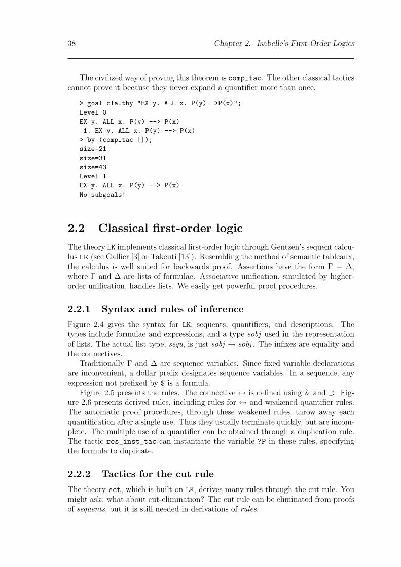
The civilized way of proving this theorem is comp_tac. The other classical tacticscannot prove it because they never expand a quantifier more than once.
> goal cla thy "EX y. ALL x. P(y)-->P(x)";Level 0EX y. ALL x. P(y) --> P(x)1. EX y. ALL x. P(y) --> P(x)> by (comp tac []);size=21size=31size=43Level 1EX y. ALL x. P(y) --> P(x)No subgoals!
2.2 Classical first-order logic
The theory LK implements classical first-order logic through Gentzen’s sequent calcu-lus lk (see Gallier [3] or Takeuti [13]). Resembling the method of semantic tableaux,the calculus is well suited for backwards proof. Assertions have the form Γ |− ∆,where Γ and ∆ are lists of formulae. Associative unification, simulated by higher-order unification, handles lists. We easily get powerful proof procedures.
2.2.1 Syntax and rules of inference
Figure 2.4 gives the syntax for LK: sequents, quantifiers, and descriptions. Thetypes include formulae and expressions, and a type sobj used in the representationof lists. The actual list type, sequ, is just sobj → sobj . The infixes are equality andthe connectives.
Traditionally Γ and ∆ are sequence variables. Since fixed variable declarationsare inconvenient, a dollar prefix designates sequence variables. In a sequence, anyexpression not prefixed by $ is a formula.
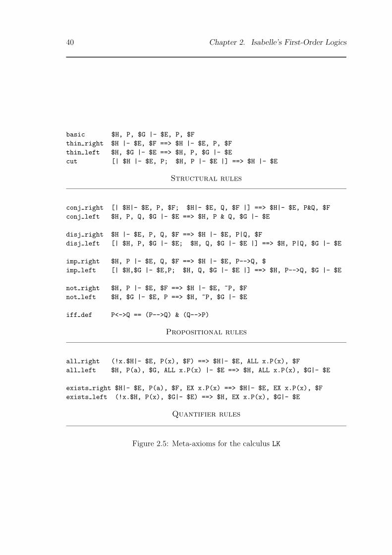
Figure 2.5 presents the rules. The connective ↔ is defined using & and ⊃. Fig-ure 2.6 presents derived rules, including rules for ↔ and weakened quantifier rules.The automatic proof procedures, through these weakened rules, throw away eachquantification after a single use. Thus they usually terminate quickly, but are incom-plete. The multiple use of a quantifier can be obtained through a duplication rule.The tactic res_inst_tac can instantiate the variable ?P in these rules, specifyingthe formula to duplicate.
2.2.2 Tactics for the cut rule
The theory set, which is built on LK, derives many rules through the cut rule. Youmight ask: what about cut-elimination? The cut rule can be eliminated from proofsof sequents, but it is still needed in derivations of rules.

2.2. Classical first-order logic 39
symbol meta-type precedence description= [term, term]→ form Left 50 equality (=)& [form, form]→ form Right 35 conjunction (&)| [form, form]→ form Right 30 disjunction (∨)--> [form, form]→ form Right 25 implication (⊃)<-> [form, form]→ form Right 25 if and only if (↔)
Infixes
symbol meta-type descriptionTrue sequ → sequ → prop meta-predicate of truthSeqof form → sequ singleton formula list~ form → form negation (¬)
Forall (term → form)→ form universal quantifier (∀)Exists (term → form)→ form existential quantifier (∃)The (term → form)→ term description operator (ε)
Constants
external internal standard notationΓ |- ∆ True(Γ, ∆) sequent Γ |− ∆ALL x. P Forall(λx .P) ∀x .PEX x. P Exists(λx .P) ∃x .PTHE x. P The(λx .P) εx .P
Translations
prop = sequence6 |- sequence6 (5)sequence = item{ , item}
| emptyitem = $identifier
| $variable| form
form = ALL identifier { identifier } . form (10)| EX identifier { identifier } . form (10)| ~ form40 (40)| others . . .
Grammar
Figure 2.4: Syntax of LK
40 Chapter 2. Isabelle’s First-Order Logics
basic $H, P, $G |- $E, P, $Fthin right $H |- $E, $F ==> $H |- $E, P, $Fthin left $H, $G |- $E ==> $H, P, $G |- $Ecut [| $H |- $E, P; $H, P |- $E |] ==> $H |- $E
Structural rules
conj right [| $H|- $E, P, $F; $H|- $E, Q, $F |] ==> $H|- $E, P&Q, $Fconj left $H, P, Q, $G |- $E ==> $H, P & Q, $G |- $E
disj right $H |- $E, P, Q, $F ==> $H |- $E, P|Q, $Fdisj left [| $H, P, $G |- $E; $H, Q, $G |- $E |] ==> $H, P|Q, $G |- $E
imp right $H, P |- $E, Q, $F ==> $H |- $E, P-->Q, $imp left [| $H,$G |- $E,P; $H, Q, $G |- $E |] ==> $H, P-->Q, $G |- $E
not right $H, P |- $E, $F ==> $H |- $E, ~P, $Fnot left $H, $G |- $E, P ==> $H, ~P, $G |- $E
iff def P<->Q == (P-->Q) & (Q-->P)
Propositional rules
all right (!x.$H|- $E, P(x), $F) ==> $H|- $E, ALL x.P(x), $Fall left $H, P(a), $G, ALL x.P(x) |- $E ==> $H, ALL x.P(x), $G|- $E
exists right $H|- $E, P(a), $F, EX x.P(x) ==> $H|- $E, EX x.P(x), $Fexists left (!x.$H, P(x), $G|- $E) ==> $H, EX x.P(x), $G|- $E
Quantifier rules
Figure 2.5: Meta-axioms for the calculus LK
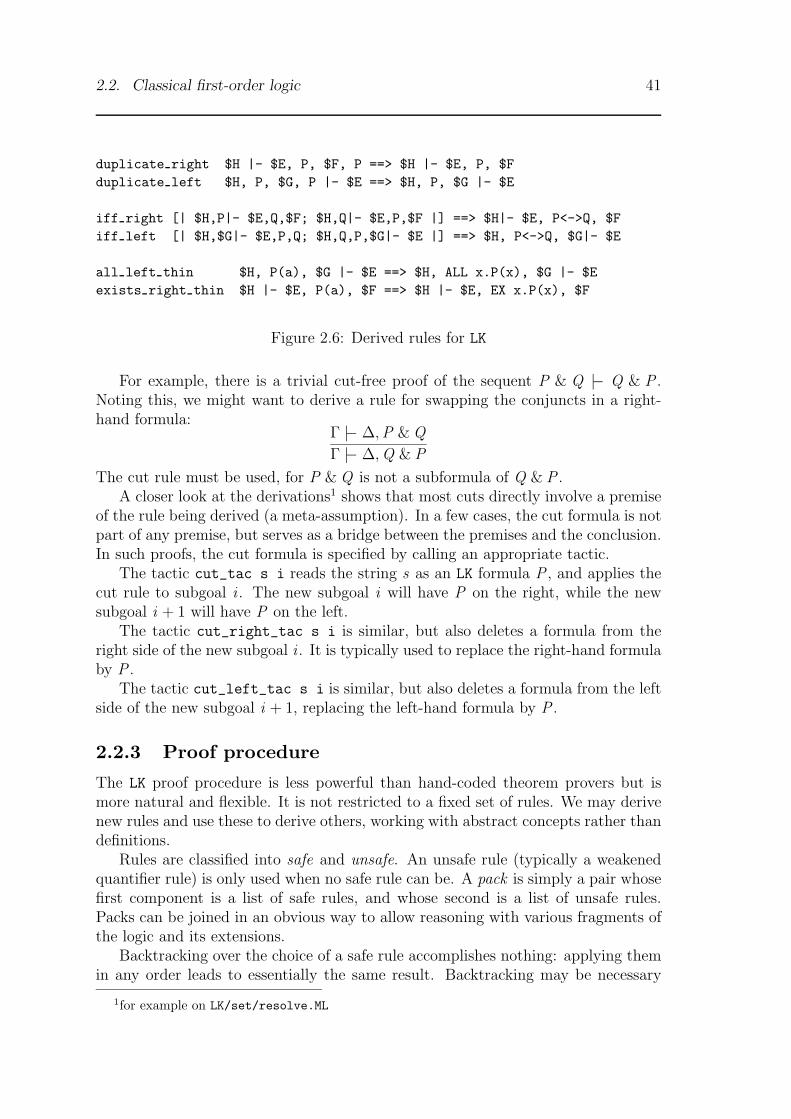
2.2. Classical first-order logic 41
duplicate right $H |- $E, P, $F, P ==> $H |- $E, P, $Fduplicate left $H, P, $G, P |- $E ==> $H, P, $G |- $E
iff right [| $H,P|- $E,Q,$F; $H,Q|- $E,P,$F |] ==> $H|- $E, P<->Q, $Fiff left [| $H,$G|- $E,P,Q; $H,Q,P,$G|- $E |] ==> $H, P<->Q, $G|- $E
all left thin $H, P(a), $G |- $E ==> $H, ALL x.P(x), $G |- $Eexists right thin $H |- $E, P(a), $F ==> $H |- $E, EX x.P(x), $F
Figure 2.6: Derived rules for LK
For example, there is a trivial cut-free proof of the sequent P & Q |− Q & P .Noting this, we might want to derive a rule for swapping the conjuncts in a right-hand formula:
Γ |− ∆,P & Q
Γ |− ∆,Q & P
The cut rule must be used, for P & Q is not a subformula of Q & P .A closer look at the derivations1 shows that most cuts directly involve a premise
of the rule being derived (a meta-assumption). In a few cases, the cut formula is notpart of any premise, but serves as a bridge between the premises and the conclusion.In such proofs, the cut formula is specified by calling an appropriate tactic.
The tactic cut_tac s i reads the string s as an LK formula P , and applies thecut rule to subgoal i . The new subgoal i will have P on the right, while the newsubgoal i + 1 will have P on the left.
The tactic cut_right_tac s i is similar, but also deletes a formula from theright side of the new subgoal i . It is typically used to replace the right-hand formulaby P .
The tactic cut_left_tac s i is similar, but also deletes a formula from the leftside of the new subgoal i + 1, replacing the left-hand formula by P .
2.2.3 Proof procedure
The LK proof procedure is less powerful than hand-coded theorem provers but ismore natural and flexible. It is not restricted to a fixed set of rules. We may derivenew rules and use these to derive others, working with abstract concepts rather thandefinitions.
Rules are classified into safe and unsafe. An unsafe rule (typically a weakenedquantifier rule) is only used when no safe rule can be. A pack is simply a pair whosefirst component is a list of safe rules, and whose second is a list of unsafe rules.Packs can be joined in an obvious way to allow reasoning with various fragments ofthe logic and its extensions.
Backtracking over the choice of a safe rule accomplishes nothing: applying themin any order leads to essentially the same result. Backtracking may be necessary
1for example on LK/set/resolve.ML
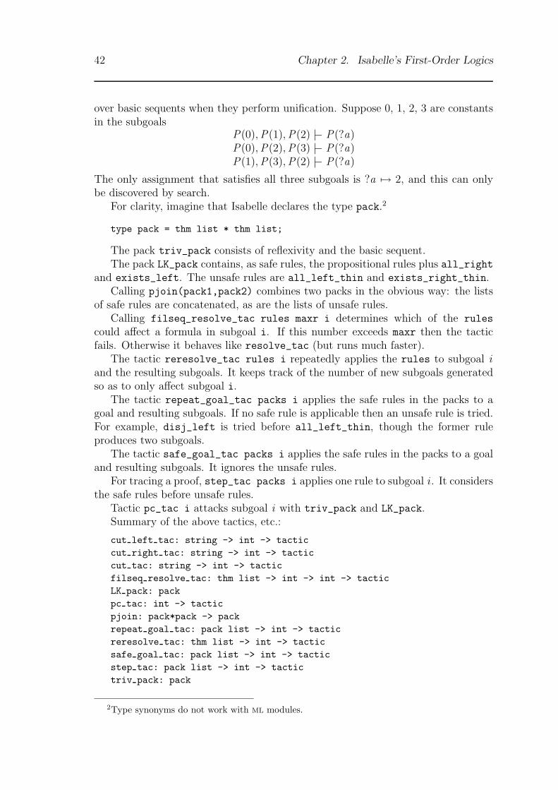
42 Chapter 2. Isabelle’s First-Order Logics
over basic sequents when they perform unification. Suppose 0, 1, 2, 3 are constantsin the subgoals
P(0),P(1),P(2) |− P(?a)P(0),P(2),P(3) |− P(?a)P(1),P(3),P(2) |− P(?a)
The only assignment that satisfies all three subgoals is ?a 7→ 2, and this can onlybe discovered by search.
For clarity, imagine that Isabelle declares the type pack.2
type pack = thm list * thm list;
The pack triv_pack consists of reflexivity and the basic sequent.The pack LK_pack contains, as safe rules, the propositional rules plus all_right
and exists_left. The unsafe rules are all_left_thin and exists_right_thin.Calling pjoin(pack1,pack2) combines two packs in the obvious way: the lists
of safe rules are concatenated, as are the lists of unsafe rules.Calling filseq_resolve_tac rules maxr i determines which of the rules
could affect a formula in subgoal i. If this number exceeds maxr then the tacticfails. Otherwise it behaves like resolve_tac (but runs much faster).
The tactic reresolve_tac rules i repeatedly applies the rules to subgoal iand the resulting subgoals. It keeps track of the number of new subgoals generatedso as to only affect subgoal i.
The tactic repeat_goal_tac packs i applies the safe rules in the packs to agoal and resulting subgoals. If no safe rule is applicable then an unsafe rule is tried.For example, disj_left is tried before all_left_thin, though the former ruleproduces two subgoals.
The tactic safe_goal_tac packs i applies the safe rules in the packs to a goaland resulting subgoals. It ignores the unsafe rules.
For tracing a proof, step_tac packs i applies one rule to subgoal i . It considersthe safe rules before unsafe rules.
Tactic pc_tac i attacks subgoal i with triv_pack and LK_pack.Summary of the above tactics, etc.:
cut left tac: string -> int -> tacticcut right tac: string -> int -> tacticcut tac: string -> int -> tacticfilseq resolve tac: thm list -> int -> int -> tacticLK pack: packpc tac: int -> tacticpjoin: pack*pack -> packrepeat goal tac: pack list -> int -> tacticreresolve tac: thm list -> int -> tacticsafe goal tac: pack list -> int -> tacticstep tac: pack list -> int -> tactictriv pack: pack
2Type synonyms do not work with ml modules.
2.2. Classical first-order logic 43
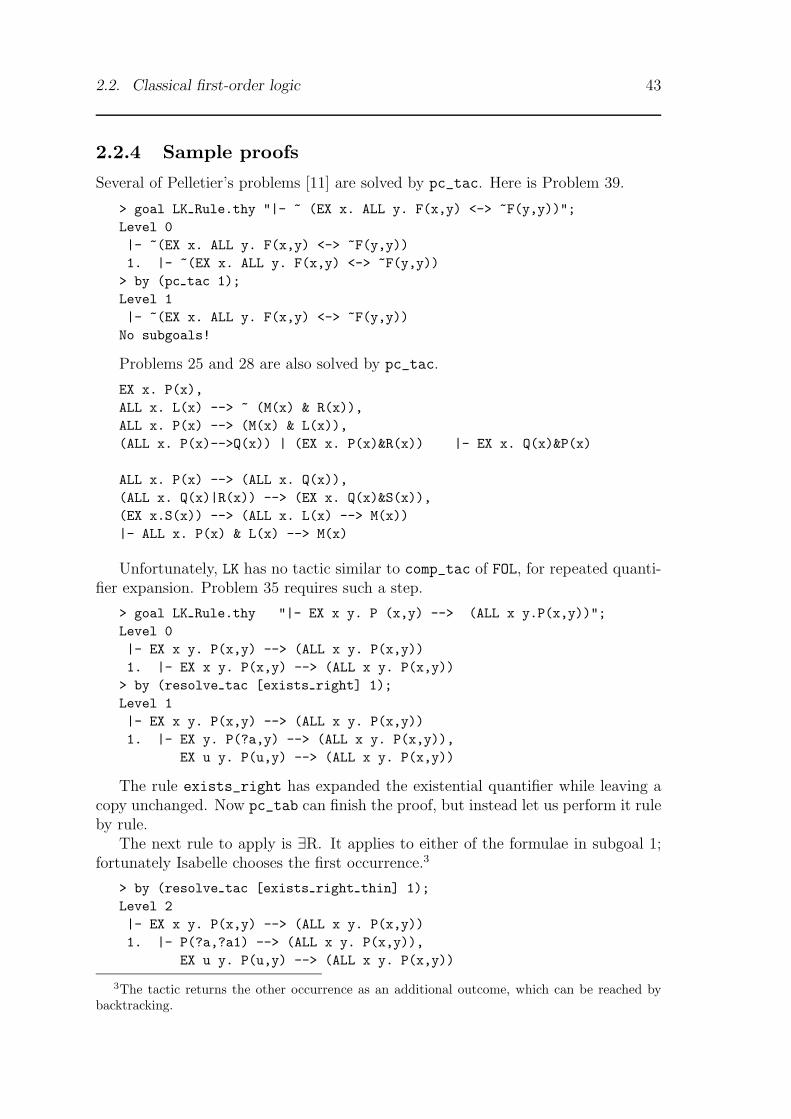
2.2.4 Sample proofs
Several of Pelletier’s problems [11] are solved by pc_tac. Here is Problem 39.
> goal LK Rule.thy "|- ~ (EX x. ALL y. F(x,y) <-> ~F(y,y))";Level 0|- ~(EX x. ALL y. F(x,y) <-> ~F(y,y))1. |- ~(EX x. ALL y. F(x,y) <-> ~F(y,y))
> by (pc tac 1);Level 1|- ~(EX x. ALL y. F(x,y) <-> ~F(y,y))
No subgoals!
Problems 25 and 28 are also solved by pc_tac.
EX x. P(x),ALL x. L(x) --> ~ (M(x) & R(x)),ALL x. P(x) --> (M(x) & L(x)),(ALL x. P(x)-->Q(x)) | (EX x. P(x)&R(x)) |- EX x. Q(x)&P(x)
ALL x. P(x) --> (ALL x. Q(x)),(ALL x. Q(x)|R(x)) --> (EX x. Q(x)&S(x)),(EX x.S(x)) --> (ALL x. L(x) --> M(x))|- ALL x. P(x) & L(x) --> M(x)
Unfortunately, LK has no tactic similar to comp_tac of FOL, for repeated quanti-fier expansion. Problem 35 requires such a step.
> goal LK Rule.thy "|- EX x y. P (x,y) --> (ALL x y.P(x,y))";Level 0|- EX x y. P(x,y) --> (ALL x y. P(x,y))1. |- EX x y. P(x,y) --> (ALL x y. P(x,y))
> by (resolve tac [exists right] 1);Level 1|- EX x y. P(x,y) --> (ALL x y. P(x,y))1. |- EX y. P(?a,y) --> (ALL x y. P(x,y)),
EX u y. P(u,y) --> (ALL x y. P(x,y))
The rule exists_right has expanded the existential quantifier while leaving acopy unchanged. Now pc_tab can finish the proof, but instead let us perform it ruleby rule.
The next rule to apply is ∃R. It applies to either of the formulae in subgoal 1;fortunately Isabelle chooses the first occurrence.3
> by (resolve tac [exists right thin] 1);Level 2|- EX x y. P(x,y) --> (ALL x y. P(x,y))1. |- P(?a,?a1) --> (ALL x y. P(x,y)),
EX u y. P(u,y) --> (ALL x y. P(x,y))
3The tactic returns the other occurrence as an additional outcome, which can be reached bybacktracking.

44 Chapter 2. Isabelle’s First-Order Logics
The next rule is ⊃R. Because LK is a sequent calculus, the formula P(?a,?a1)
does not become an assumption. Instead, it moves to the left of the turnstile (|−).
> by (resolve tac [imp right] 1);Level 3|- EX x y. P(x,y) --> (ALL x y. P(x,y))1. P(?a,?a1) |- ALL x y. P(x,y), EX u y. P(u,y) --> (ALL x y. P(x,y))
Next the universal quantifiers are stripped. Meanwhile, the existential formulalies dormant.
> by (resolve tac [all right] 1);Level 4|- EX x y. P(x,y) --> (ALL x y. P(x,y))1. !ka. P(?a,?a1)
|- ALL y. P(ka,y), EX u y. P(u,y) --> (ALL x y. P(x,y))> by (resolve tac [all right] 1);Level 5|- EX x y. P(x,y) --> (ALL x y. P(x,y))1. !ka kb. P(?a,?a1) |- P(ka,kb), EX u y. P(u,y) --> (ALL x y. P(x,y))
Note that the formulae P(?a,?a1) and P(ka,kb) are not unifiable, so this is nota basic sequent. Instead we strip the existential quantifiers.
> by (resolve tac [exists right thin] 1);Level 6|- EX x y. P(x,y) --> (ALL x y. P(x,y))1. !ka kb. P(?a,?a1)
|- P(ka,kb), EX y. P(?a14(ka,kb),y) --> (ALL x y. P(x,y))> by (resolve tac [exists right thin] 1);Level 7|- EX x y. P(x,y) --> (ALL x y. P(x,y))1. !ka kb. P(?a,?a1)
|- P(ka,kb),P(?Ga18(ka,kb),?a15(ka,kb)) --> (ALL x y. P(x,y))
Applying ⊃R again produces a basic sequent, solving the goal.
> by (resolve tac [imp right] 1);Level 8|- EX x y. P(x,y) --> (ALL x y. P(x,y))1. !ka kb. P(?a,?a1), P(?Ga25(ka,kb),?Ga23(ka,kb))
|- P(ka,kb), ALL x y. P(x,y)> by (resolve tac [basic] 1);Level 9|- EX x y. P(x,y) --> (ALL x y. P(x,y))No subgoals!
Chapter 3
Isabelle’s Set and Type Theories
The discussion of Isabelle’s object-logic continues with its set and type theories.They are all large and complicated, as well as involving subtle mathematical ideas.Each section will only make sense to people who are familiar with the logic inquestion.
The theories are as follows:
• Zermelo-Fraenkel set theory is a subtheory of LK . The Zermelo-Fraenkelaxiom system is an established formulation of set theory.
• Martin-Lof’s Constructive Type Theory is partially implemented. Universesare the main omission.
• Higher-order logic is the largest and most recent of the Isabelle logics. Itis rather more elaborate than Church’s well-known formulation. This is anobject-logic and should not be confused with Isabelle’s meta-logic, which isalso a version of higher-order logic.
Theorem proving in these theories is extremely difficult, as may be imagined,for each encompasses large portions of mathematics. The proof procedures suppliedwith Isabelle must be regarded as first attempts.
3.1 Zermelo-Fraenkel set theory
The Isabelle theory called set implements Zermelo-Fraenkel set theory [12] over theclassical sequent calculus LK. The theory includes a collection of derived rules thatform a sequent calculus of sets. The simplistic sequent calculus proof procedure ofLK works reasonably for set theory.
3.1.1 Syntax and rules of inference
Figure 3.1 gives the syntax for set, which extends LK with finite sets, ordered pairs,and comprehension. The constant :: is a ‘set cons’, for a :: B = {a} ∪ B . Startingfrom the empty set ∅, it constructs finite sets in the obvious way:
{a, b, c, d} = a :: (b :: (c :: (d :: ∅)))
45

46 Chapter 3. Isabelle’s Set and Type Theories
By the separation axiom, the set Collect(A,P) forms the set of all x ∈ A thatsatisfy P(x ). By the replacement axiom, the set Replace(f ,A) forms the set ofall f (x ) for x ∈ A. The syntax of set can express three kinds of comprehension:separation, replacement, and both together.
Infixes include union and intersection (A ∪ B and A ∩ B), and the subset andmembership relations. The ‘big union’ and ‘big intersection’ operators (
⋃C and⋂
C ) form the union or intersection of a set of sets;⋃
C can also be written⋃
A∈C A.Of these operators only ‘big union’ is primitive.
The language of set theory, as studied by logicians, has no constants. The emptyset axiom asserts that some set is empty, not that ∅ is the empty set; and so onfor union, powerset, etc. Since formal proofs in this language would be barbarous,the Isabelle theory declares constants. Some of the constants are primitive (like theempty set), while others are defined (like intersection).
The axioms appear in Figure 3.2. They contain unusual definitions where oneformula is defined to denote another. The extensionality axiom states that A = Bmeans the same thing as A ⊆ B & B ⊆ A. The power set axiom states thatA ∈ Pow(B) means the same thing as A ⊆ B . Such definitions are not conservative.The theory also defines abbreviations for ordered pairs, successor, etc.
The axioms can be expressed in many different ways. For example, the ruleequal_members could be expressed as the formula
∀xyA . (x = y & y ∈ A) ⊃ x ∈ A
But applying this axiom would involve several LK rules. (Most books on set theoryomit this axiom altogether!) The axiom of regularity is expressed in its most usefulform: transfinite induction.
The replacement axiom involves the concept of class function, which is like afunction defined on the entire universe of sets. Examples include the power setoperator and the successor operator succ(x ) = x ∪ {x}. In set theory, a functionis its graph. Since the graph of a class function is ‘too big’ to be a set, it is rep-resented by a 2-place predicate. The theory set assumes that every class functioncan be expressed by some Isabelle term — possibly involving LK’s description op-erator (‘The’). Recent experience gives some evidence in favour of the traditionalformulation of the replacement axiom, however.
3.1.2 Derived rules
The theory derives a sequent calculus from the axioms. Figures 3.3–3.4 present mostof the rules, which refer to the constants of set rather than the logical constants.
A rule named X _thin has been weakened. In a typical weakened rule:
• A formula in the conclusion is omitted in the premises to allow repeated appli-cation of the rule without looping — but this proof procedure is incomplete.
• Some scheme variables appear in the premises but not in the conclusion. Inbackwards proof these rules introduce new variables in the subgoals.

3.1. Zermelo-Fraenkel set theory 47
symbol meta-type precedence description‘ [term, term]→ term Left 65 function applicationInt [term, term]→ term Right 60 intersection (∩)Un [term, term]→ term Right 55 union (∪)- [term, term]→ term Right 55 difference (−):: [term, term]→ term Right 55 inclusion of an element<= [term, term]→ form Right 50 subset (⊆): [term, term]→ form Right 50 membership (∈)
Infixes
0 term empty setINF term infinite setPow term → term powerset operatorUnion term → term ‘big union’ operatorInter term → term ‘big intersection’ operatorPair [term, term]→ term pairing operatorsucc term → term successor operatorChoose term → term choice operatorCollect [term, term → form]→ term separation operatorReplace [term → term, term]→ term replacement operator
Constants
external internal standard notation{ a1, . . ., an } a1::· · ·::(an::0) {a1, . . . , an}[ x || x:A, P ] Collect(A,λx .P) {x ∈ A | P}[ b || x:A ] Replace(λx .b,A) {b | x ∈ A}[ b || x:A,P(x ) ] Replace(λx .b,Collect(A,λx .P)) {b | x ∈ A & P}
Notation
term = < term , term >
| [ identifier || identifier : term , form ]
| [ term || identifier : term ]
| [ term || identifier : term , form ]
| others . . .
Grammar
Figure 3.1: Syntax of set
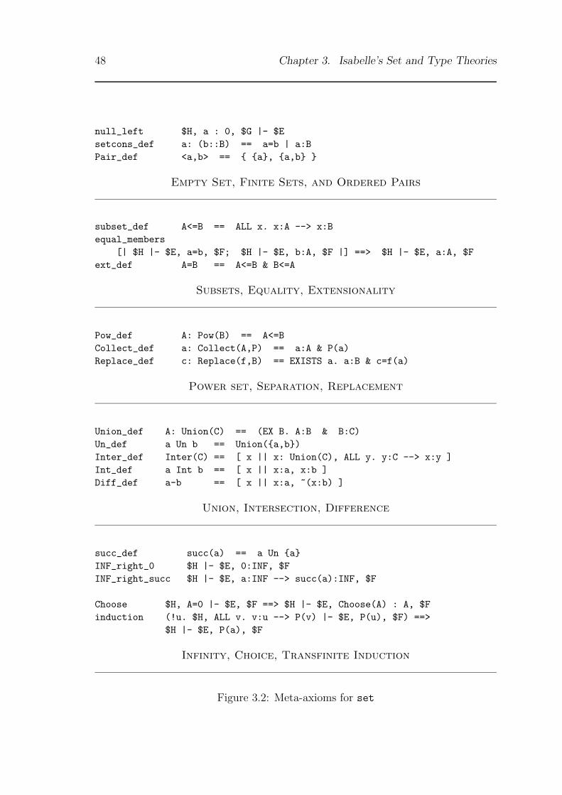
48 Chapter 3. Isabelle’s Set and Type Theories
null_left $H, a : 0, $G |- $Esetcons_def a: (b::B) == a=b | a:BPair_def <a,b> == { {a}, {a,b} }
Empty Set, Finite Sets, and Ordered Pairs
subset_def A<=B == ALL x. x:A --> x:Bequal_members
[| $H |- $E, a=b, $F; $H |- $E, b:A, $F |] ==> $H |- $E, a:A, $Fext_def A=B == A<=B & B<=A
Subsets, Equality, Extensionality
Pow_def A: Pow(B) == A<=BCollect_def a: Collect(A,P) == a:A & P(a)Replace_def c: Replace(f,B) == EXISTS a. a:B & c=f(a)
Power set, Separation, Replacement
Union_def A: Union(C) == (EX B. A:B & B:C)Un_def a Un b == Union({a,b})Inter_def Inter(C) == [ x || x: Union(C), ALL y. y:C --> x:y ]Int_def a Int b == [ x || x:a, x:b ]Diff_def a-b == [ x || x:a, ~(x:b) ]
Union, Intersection, Difference
succ_def succ(a) == a Un {a}INF_right_0 $H |- $E, 0:INF, $FINF_right_succ $H |- $E, a:INF --> succ(a):INF, $F
Choose $H, A=0 |- $E, $F ==> $H |- $E, Choose(A) : A, $Finduction (!u. $H, ALL v. v:u --> P(v) |- $E, P(u), $F) ==>
$H |- $E, P(a), $F
Infinity, Choice, Transfinite Induction
Figure 3.2: Meta-axioms for set

3.1. Zermelo-Fraenkel set theory 49
null_right $H |- $E, $F ==> $H |- $E, a:0, $Fsetcons_right $H |- $E, a=b, a:B, $F ==> $H |- $E, a : (b::B), $Fsetcons_left [| $H, a=b, $G |- $E; $H, a:B, $G |- $E |] ==>
$H, a:(b::B), $G |- $E
subset_right (!x.$H, x:A |- $E, x:B, $F) ==> $H|- $E, A<=B, $Fsubset_left_thin [| $H, $G |- $E, c:A; $H, c:B, $G |- $E |] ==>
$H, A<=B, $G |- $E
equal_right [| $H |- $E, A<=B, $F; $H |- $E, B<=A, $F |] ==>$H |- $E, A=B, $F
equal_left_s $H, A<=B, B<=A, $G |- $E ==> $H, A=B, $G |- $Eeqext_left_thin [| $H,$G|- $E, c:A, c:B; $H, c:B, c:A, $G|- $E |] ==>
$H, A=B, $G |- $eqmem_left_thin [| $H,$G|- $E, a:c, b:c; $H,$G, b:c, a:c |- $E |] ==>
$H, a=b, $G |- $E
Finite Sets, Subsets, Equality, Extensionality
Union_right_thin [| $H |- $E, A:B, $F; $H |- $E, B:C, $F |] ==>$H |- $E, A : Union(C), $F
Union_left (!x.$H, A:x, x:C, $G |- $E) ==> $H, A:Union(C), $G |- $EUn_right $H |- $E, $F, c:A, c:B ==> $H |- $E, c : A Un B, $FUn_left [| $H, c:A, $G|- $E; $H, c:B, $G |- $E |] ==>
$H, c: A Un B, $G|- $E
Inter_right (!x.$H, x:C |- $E, A:x, $F) ==> $H, C<=0 |- $E, $F ==>$H |- $E, A: Inter(C), $F
Inter_left_thin [| $H, A:B, $G |- $E; $H, $G |- $E, B:C |] ==>$H, A: Inter(C), $G |- $E
Int_right [| $H|- $E, c:A, $F; $H|- $E, c:B, $F |] ==>$H|- $E, c: A Int B, $F
Int_left $H, c:A, c:B, $G |- $E ==> $H, c : A Int B, $G |- $E
Diff_right [| $H|- $E, c:A, $F; $H, c:B|- $E,$F |] ==> $H|- $E, c:A-B, $FDiff_left $H, c:A, $G |- $E, c:B ==> $H, c: A-B, $G |- $E
Union, Intersection, Difference
Figure 3.3: The derived sequent calculus for set
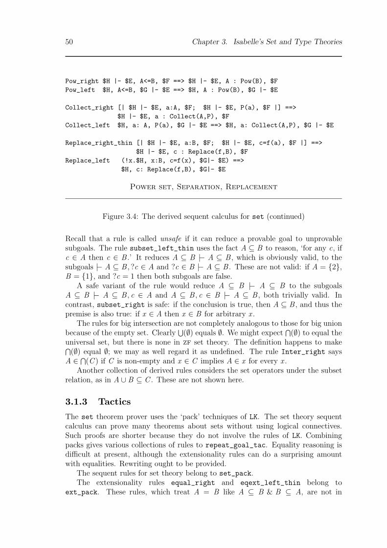
50 Chapter 3. Isabelle’s Set and Type Theories
Pow_right $H |- $E, A<=B, $F ==> $H |- $E, A : Pow(B), $FPow_left $H, A<=B, $G |- $E ==> $H, A : Pow(B), $G |- $E
Collect_right [| $H |- $E, a:A, $F; $H |- $E, P(a), $F |] ==>$H |- $E, a : Collect(A,P), $F
Collect_left $H, a: A, P(a), $G |- $E ==> $H, a: Collect(A,P), $G |- $E
Replace_right_thin [| $H |- $E, a:B, $F; $H |- $E, c=f(a), $F |] ==>$H |- $E, c : Replace(f,B), $F
Replace_left (!x.$H, x:B, c=f(x), $G|- $E) ==>$H, c: Replace(f,B), $G|- $E
Power set, Separation, Replacement
Figure 3.4: The derived sequent calculus for set (continued)
Recall that a rule is called unsafe if it can reduce a provable goal to unprovablesubgoals. The rule subset_left_thin uses the fact A ⊆ B to reason, ‘for any c, ifc ∈ A then c ∈ B .’ It reduces A ⊆ B |− A ⊆ B , which is obviously valid, to thesubgoals |− A ⊆ B , ?c ∈ A and ?c ∈ B |− A ⊆ B . These are not valid: if A = {2},B = {1}, and ?c = 1 then both subgoals are false.
A safe variant of the rule would reduce A ⊆ B |− A ⊆ B to the subgoalsA ⊆ B |− A ⊆ B , c ∈ A and A ⊆ B , c ∈ B |− A ⊆ B , both trivially valid. Incontrast, subset_right is safe: if the conclusion is true, then A ⊆ B , and thus thepremise is also true: if x ∈ A then x ∈ B for arbitrary x .
The rules for big intersection are not completely analogous to those for big unionbecause of the empty set. Clearly
⋃(∅) equals ∅. We might expect
⋂(∅) to equal the
universal set, but there is none in zf set theory. The definition happens to make⋂(∅) equal ∅; we may as well regard it as undefined. The rule Inter_right says
A ∈ ⋂(C ) if C is non-empty and x ∈ C implies A ∈ x for every x .Another collection of derived rules considers the set operators under the subset
relation, as in A ∪ B ⊆ C . These are not shown here.
3.1.3 Tactics
The set theorem prover uses the ‘pack’ techniques of LK. The set theory sequentcalculus can prove many theorems about sets without using logical connectives.Such proofs are shorter because they do not involve the rules of LK. Combiningpacks gives various collections of rules to repeat_goal_tac. Equality reasoning isdifficult at present, although the extensionality rules can do a surprising amountwith equalities. Rewriting ought to be provided.
The sequent rules for set theory belong to set_pack.The extensionality rules equal_right and eqext_left_thin belong to
ext_pack. These rules, which treat A = B like A ⊆ B & B ⊆ A, are not in
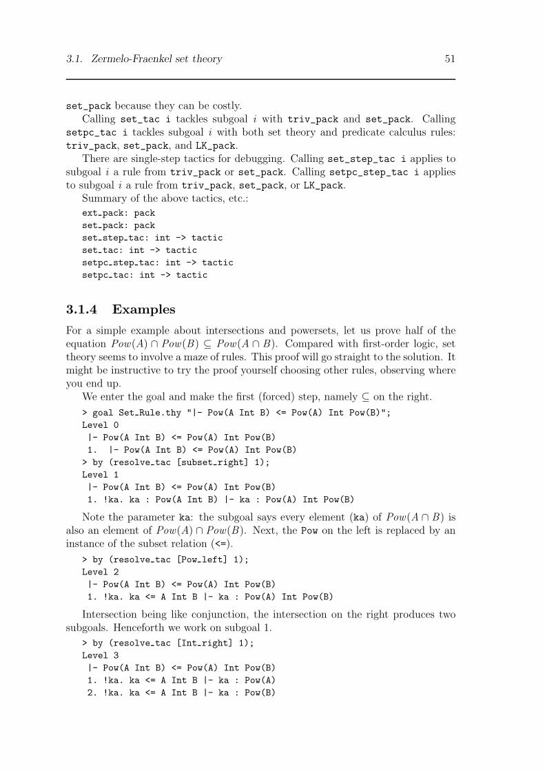
3.1. Zermelo-Fraenkel set theory 51
set_pack because they can be costly.Calling set_tac i tackles subgoal i with triv_pack and set_pack. Calling
setpc_tac i tackles subgoal i with both set theory and predicate calculus rules:triv_pack, set_pack, and LK_pack.
There are single-step tactics for debugging. Calling set_step_tac i applies tosubgoal i a rule from triv_pack or set_pack. Calling setpc_step_tac i appliesto subgoal i a rule from triv_pack, set_pack, or LK_pack.
Summary of the above tactics, etc.:
ext pack: packset pack: packset step tac: int -> tacticset tac: int -> tacticsetpc step tac: int -> tacticsetpc tac: int -> tactic
3.1.4 Examples
For a simple example about intersections and powersets, let us prove half of theequation Pow(A) ∩ Pow(B) ⊆ Pow(A ∩ B). Compared with first-order logic, settheory seems to involve a maze of rules. This proof will go straight to the solution. Itmight be instructive to try the proof yourself choosing other rules, observing whereyou end up.
We enter the goal and make the first (forced) step, namely ⊆ on the right.
> goal Set Rule.thy "|- Pow(A Int B) <= Pow(A) Int Pow(B)";Level 0|- Pow(A Int B) <= Pow(A) Int Pow(B)1. |- Pow(A Int B) <= Pow(A) Int Pow(B)
> by (resolve tac [subset right] 1);Level 1|- Pow(A Int B) <= Pow(A) Int Pow(B)1. !ka. ka : Pow(A Int B) |- ka : Pow(A) Int Pow(B)
Note the parameter ka: the subgoal says every element (ka) of Pow(A ∩ B) isalso an element of Pow(A) ∩ Pow(B). Next, the Pow on the left is replaced by aninstance of the subset relation (<=).
> by (resolve tac [Pow left] 1);Level 2|- Pow(A Int B) <= Pow(A) Int Pow(B)1. !ka. ka <= A Int B |- ka : Pow(A) Int Pow(B)
Intersection being like conjunction, the intersection on the right produces twosubgoals. Henceforth we work on subgoal 1.
> by (resolve tac [Int right] 1);Level 3|- Pow(A Int B) <= Pow(A) Int Pow(B)1. !ka. ka <= A Int B |- ka : Pow(A)2. !ka. ka <= A Int B |- ka : Pow(B)
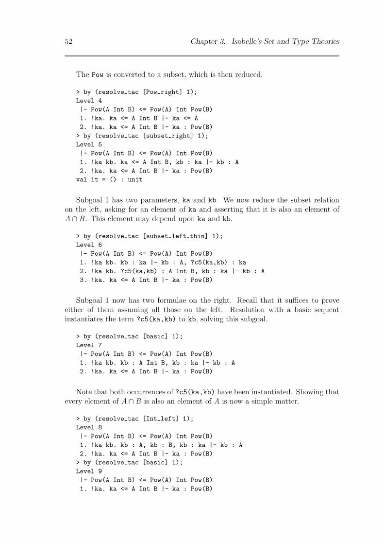
52 Chapter 3. Isabelle’s Set and Type Theories
The Pow is converted to a subset, which is then reduced.
> by (resolve tac [Pow right] 1);Level 4|- Pow(A Int B) <= Pow(A) Int Pow(B)1. !ka. ka <= A Int B |- ka <= A2. !ka. ka <= A Int B |- ka : Pow(B)> by (resolve tac [subset right] 1);Level 5|- Pow(A Int B) <= Pow(A) Int Pow(B)1. !ka kb. ka <= A Int B, kb : ka |- kb : A2. !ka. ka <= A Int B |- ka : Pow(B)val it = () : unit
Subgoal 1 has two parameters, ka and kb. We now reduce the subset relationon the left, asking for an element of ka and asserting that it is also an element ofA ∩ B . This element may depend upon ka and kb.
> by (resolve tac [subset left thin] 1);Level 6|- Pow(A Int B) <= Pow(A) Int Pow(B)1. !ka kb. kb : ka |- kb : A, ?c5(ka,kb) : ka2. !ka kb. ?c5(ka,kb) : A Int B, kb : ka |- kb : A3. !ka. ka <= A Int B |- ka : Pow(B)
Subgoal 1 now has two formulae on the right. Recall that it suffices to proveeither of them assuming all those on the left. Resolution with a basic sequentinstantiates the term ?c5(ka,kb) to kb, solving this subgoal.
> by (resolve tac [basic] 1);Level 7|- Pow(A Int B) <= Pow(A) Int Pow(B)1. !ka kb. kb : A Int B, kb : ka |- kb : A2. !ka. ka <= A Int B |- ka : Pow(B)
Note that both occurrences of ?c5(ka,kb) have been instantiated. Showing thatevery element of A ∩ B is also an element of A is now a simple matter.
> by (resolve tac [Int left] 1);Level 8|- Pow(A Int B) <= Pow(A) Int Pow(B)1. !ka kb. kb : A, kb : B, kb : ka |- kb : A2. !ka. ka <= A Int B |- ka : Pow(B)> by (resolve tac [basic] 1);Level 9|- Pow(A Int B) <= Pow(A) Int Pow(B)1. !ka. ka <= A Int B |- ka : Pow(B)

3.1. Zermelo-Fraenkel set theory 53
The remaining subgoal is like the one we tackled back in Level 3. Instead ofrepeating those steps, let us go for the automatic tactic.
> by (set tac 1);Level 10|- Pow(A Int B) <= Pow(A) Int Pow(B)
No subgoals!
Calling set_tac could have been the first and only step of this proof.
For another example, we prove that big union is monotonic: A ⊆ B implies⋃(A) ⊆ ⋃(B). As above, the first inference reduces the ⊆ on the right.
> goal Set Rule.thy "A<=B |- Union(A) <= Union(B)";Level 0A <= B |- Union(A) <= Union(B)1. A <= B |- Union(A) <= Union(B)
> by (resolve tac [subset right] 1);Level 1A <= B |- Union(A) <= Union(B)1. !ka. A <= B, ka : Union(A) |- ka : Union(B)
Big union is like an existential quantifier, so the occurrence on the left must bereduced before that on the right.
> by (resolve tac [Union left] 1);Level 2A <= B |- Union(A) <= Union(B)1. !ka kb. A <= B, ka : kb, kb : A |- ka : Union(B)
The next two steps infer that since A ⊆ B and kb ∈ A, it follows that kb ∈ B .
> by (resolve tac [subset left thin] 1);Level 3A <= B |- Union(A) <= Union(B)1. !ka kb. ka : kb, kb : A |- ka : Union(B), ?c2(ka,kb) : A2. !ka kb. ?c2(ka,kb) : B, ka : kb, kb : A |- ka : Union(B)> by (resolve tac [basic] 1);Level 4A <= B |- Union(A) <= Union(B)1. !ka kb. kb : B, ka : kb, kb : A |- ka : Union(B)
The only possible step is to reduce the big union operator on the right.
> by (resolve tac [Union right thin] 1);Level 5A <= B |- Union(A) <= Union(B)1. !ka kb. kb : B, ka : kb, kb : A |- ka : ?B5(ka,kb)2. !ka kb. kb : B, ka : kb, kb : A |- ?B5(ka,kb) : B
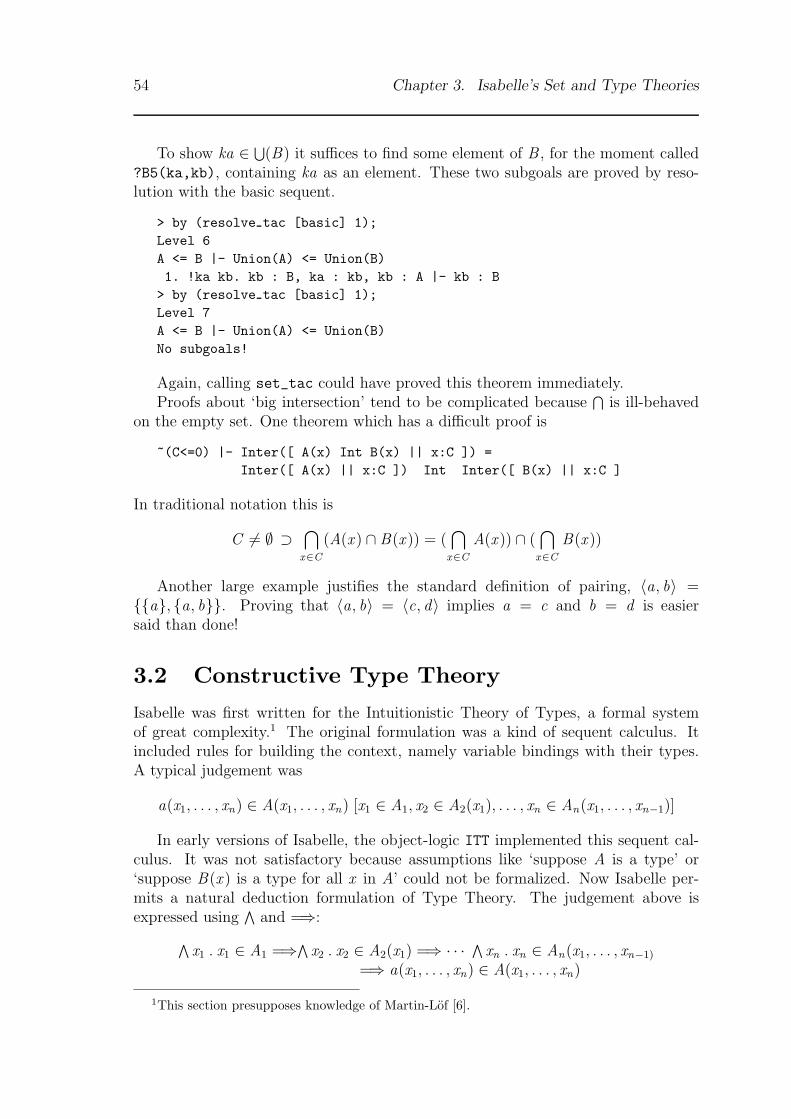
54 Chapter 3. Isabelle’s Set and Type Theories
To show ka ∈ ⋃(B) it suffices to find some element of B , for the moment called?B5(ka,kb), containing ka as an element. These two subgoals are proved by reso-lution with the basic sequent.
> by (resolve tac [basic] 1);Level 6A <= B |- Union(A) <= Union(B)1. !ka kb. kb : B, ka : kb, kb : A |- kb : B> by (resolve tac [basic] 1);Level 7A <= B |- Union(A) <= Union(B)No subgoals!
Again, calling set_tac could have proved this theorem immediately.Proofs about ‘big intersection’ tend to be complicated because
⋂is ill-behaved
on the empty set. One theorem which has a difficult proof is
~(C<=0) |- Inter([ A(x) Int B(x) || x:C ]) =Inter([ A(x) || x:C ]) Int Inter([ B(x) || x:C ]
In traditional notation this is
C 6= ∅ ⊃⋂
x∈C
(A(x ) ∩ B(x )) = (⋂
x∈C
A(x )) ∩ (⋂
x∈C
B(x ))
Another large example justifies the standard definition of pairing, 〈a, b〉 ={{a}, {a, b}}. Proving that 〈a, b〉 = 〈c, d〉 implies a = c and b = d is easiersaid than done!
3.2 Constructive Type Theory
Isabelle was first written for the Intuitionistic Theory of Types, a formal systemof great complexity.1 The original formulation was a kind of sequent calculus. Itincluded rules for building the context, namely variable bindings with their types.A typical judgement was
a(x1, . . . , xn) ∈ A(x1, . . . , xn) [x1 ∈ A1, x2 ∈ A2(x1), . . . , xn ∈ An(x1, . . . , xn−1)]
In early versions of Isabelle, the object-logic ITT implemented this sequent cal-culus. It was not satisfactory because assumptions like ‘suppose A is a type’ or‘suppose B(x ) is a type for all x in A’ could not be formalized. Now Isabelle per-mits a natural deduction formulation of Type Theory. The judgement above isexpressed using
∧and =⇒:∧
x1 . x1 ∈ A1 =⇒∧ x2 . x2 ∈ A2(x1) =⇒ · · · ∧ xn . xn ∈ An(x1, . . . , xn−1)
=⇒ a(x1, . . . , xn) ∈ A(x1, . . . , xn)
1This section presupposes knowledge of Martin-Lof [6].
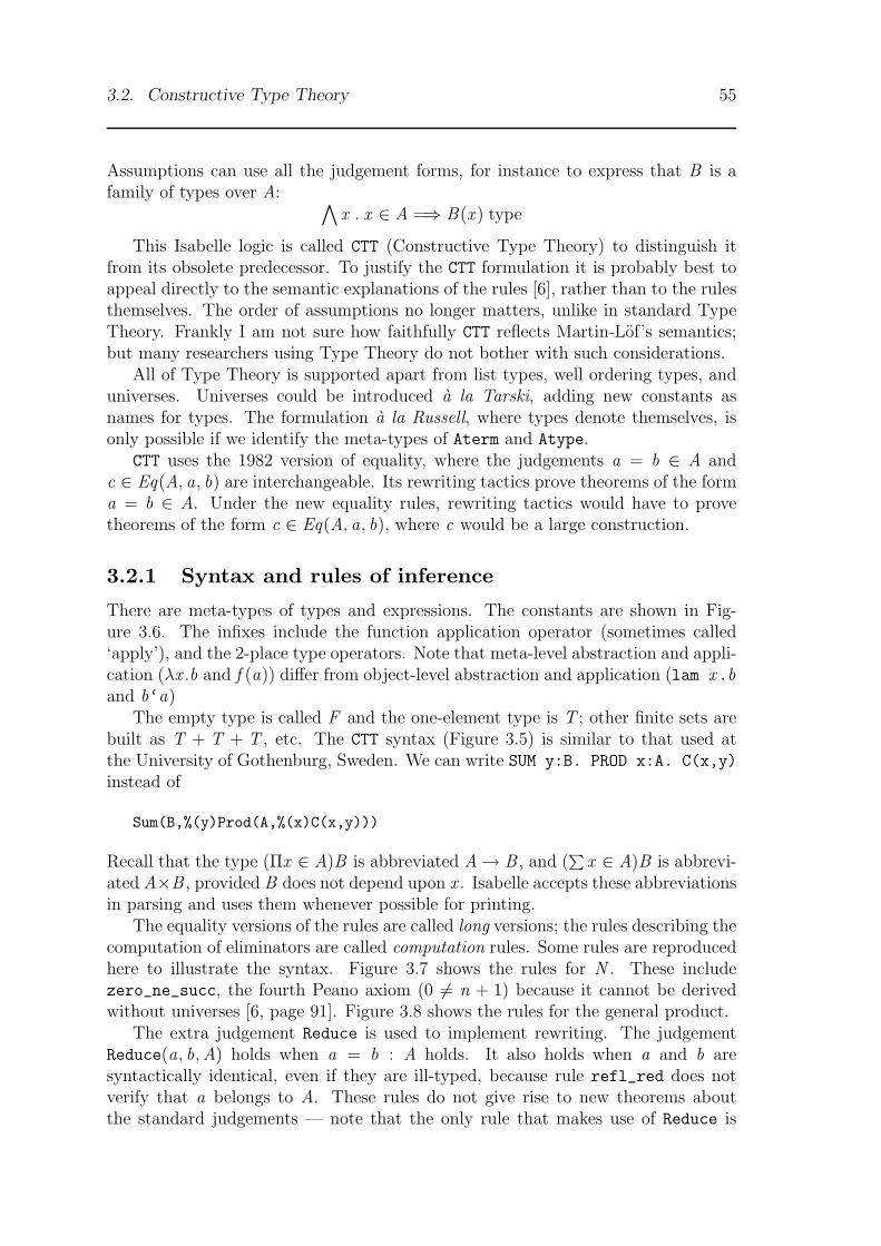
3.2. Constructive Type Theory 55
Assumptions can use all the judgement forms, for instance to express that B is afamily of types over A: ∧
x . x ∈ A =⇒ B(x ) type
This Isabelle logic is called CTT (Constructive Type Theory) to distinguish itfrom its obsolete predecessor. To justify the CTT formulation it is probably best toappeal directly to the semantic explanations of the rules [6], rather than to the rulesthemselves. The order of assumptions no longer matters, unlike in standard TypeTheory. Frankly I am not sure how faithfully CTT reflects Martin-Lof’s semantics;but many researchers using Type Theory do not bother with such considerations.
All of Type Theory is supported apart from list types, well ordering types, anduniverses. Universes could be introduced a la Tarski, adding new constants asnames for types. The formulation a la Russell, where types denote themselves, isonly possible if we identify the meta-types of Aterm and Atype.
CTT uses the 1982 version of equality, where the judgements a = b ∈ A andc ∈ Eq(A, a, b) are interchangeable. Its rewriting tactics prove theorems of the forma = b ∈ A. Under the new equality rules, rewriting tactics would have to provetheorems of the form c ∈ Eq(A, a, b), where c would be a large construction.
3.2.1 Syntax and rules of inference
There are meta-types of types and expressions. The constants are shown in Fig-ure 3.6. The infixes include the function application operator (sometimes called‘apply’), and the 2-place type operators. Note that meta-level abstraction and appli-cation (λx .b and f (a)) differ from object-level abstraction and application (lam x.band b‘a)
The empty type is called F and the one-element type is T ; other finite sets arebuilt as T + T + T , etc. The CTT syntax (Figure 3.5) is similar to that used atthe University of Gothenburg, Sweden. We can write SUM y:B. PROD x:A. C(x,y)
instead of
Sum(B,%(y)Prod(A,%(x)C(x,y)))
Recall that the type (Πx ∈ A)B is abbreviated A→ B , and (∑
x ∈ A)B is abbrevi-ated A×B , provided B does not depend upon x . Isabelle accepts these abbreviationsin parsing and uses them whenever possible for printing.
The equality versions of the rules are called long versions; the rules describing thecomputation of eliminators are called computation rules. Some rules are reproducedhere to illustrate the syntax. Figure 3.7 shows the rules for N . These includezero_ne_succ, the fourth Peano axiom (0 6= n + 1) because it cannot be derivedwithout universes [6, page 91]. Figure 3.8 shows the rules for the general product.
The extra judgement Reduce is used to implement rewriting. The judgementReduce(a, b,A) holds when a = b : A holds. It also holds when a and b aresyntactically identical, even if they are ill-typed, because rule refl_red does notverify that a belongs to A. These rules do not give rise to new theorems aboutthe standard judgements — note that the only rule that makes use of Reduce is
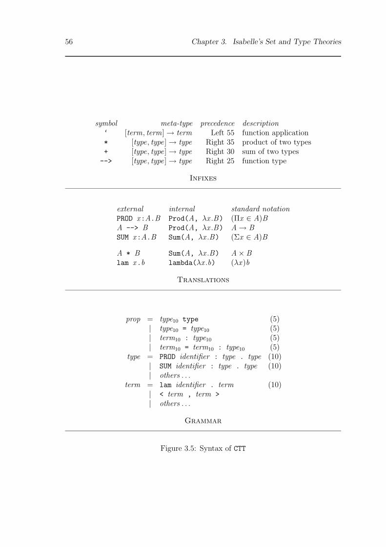
56 Chapter 3. Isabelle’s Set and Type Theories
symbol meta-type precedence description‘ [term, term]→ term Left 55 function application* [type, type]→ type Right 35 product of two types+ [type, type]→ type Right 30 sum of two types--> [type, type]→ type Right 25 function type
Infixes
external internal standard notationPROD x:A.B Prod(A, λx .B) (Πx ∈ A)BA --> B Prod(A, λx .B) A→ BSUM x:A.B Sum(A, λx .B) (Σx ∈ A)B
A * B Sum(A, λx .B) A× Blam x.b lambda(λx .b) (λx )b
Translations
prop = type10 type (5)| type10 = type10 (5)| term10 : type10 (5)| term10 = term10 : type10 (5)
type = PROD identifier : type . type (10)| SUM identifier : type . type (10)| others . . .
term = lam identifier . term (10)| < term , term >
| others . . .
Grammar
Figure 3.5: Syntax of CTT

3.2. Constructive Type Theory 57
symbol meta-type descriptionType type → prop judgement formEqtype [type, type]→ prop judgement formElem [term, type]→ prop judgement formEqelem [term, term, type]→ prop judgement formReduce [term, term, type]→ prop extra judgement form
N type natural numbers type0 term constructor
succ term → term constructorrec [term, term, [term, term]→ term]→ term eliminator
Prod [type, term → type]→ type general product typelambda (term → term)→ term constructor
Sum [type, term → type]→ type general sum typepair [term, term]→ term constructorsplit [term, [term, term]→ term]→ term eliminatorfst snd term → term projections
inl inr term → term constructors for +when [term, term → term, term → term]→ term eliminator for +
Eq [type, term, term]→ type equality typeeq term constructor
F type empty typecontr term → term eliminator
T type singleton typett term constructor
Figure 3.6: The constants of CTT
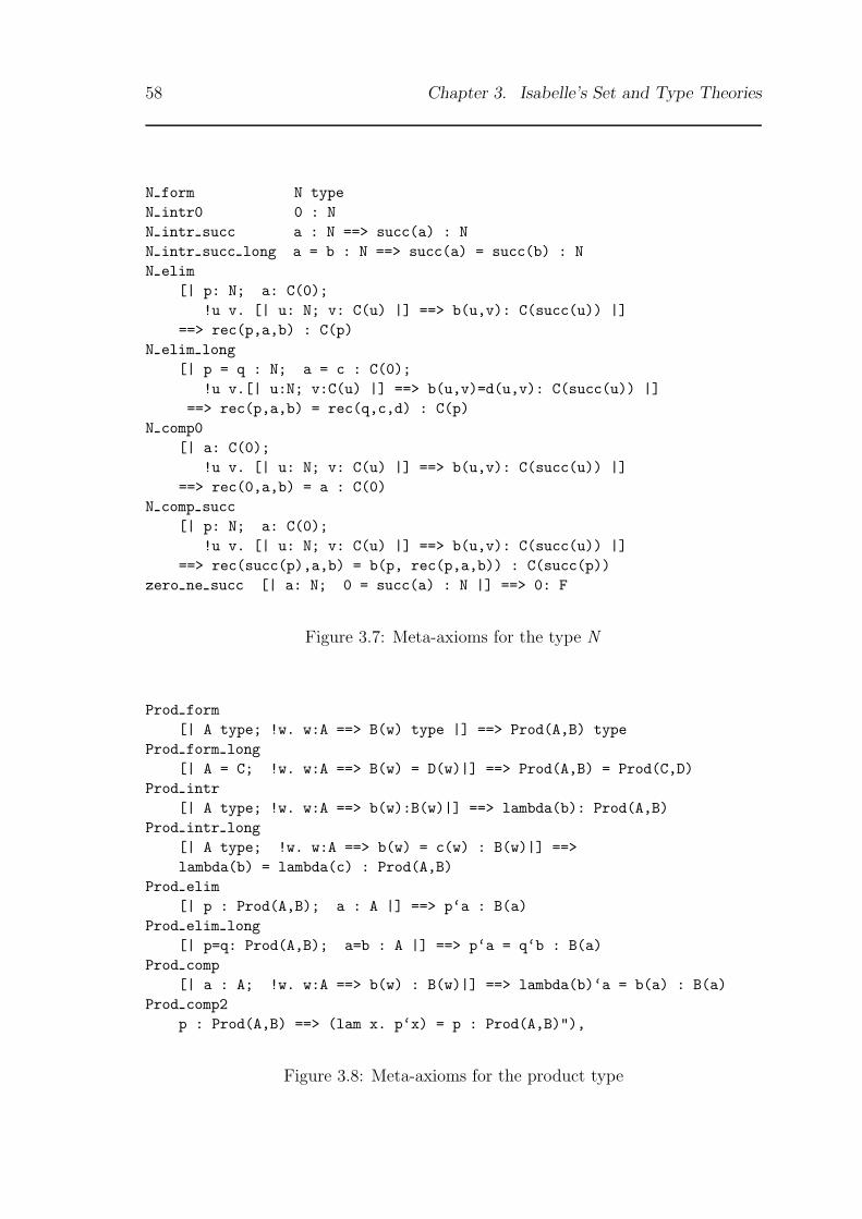
58 Chapter 3. Isabelle’s Set and Type Theories
N form N typeN intr0 0 : NN intr succ a : N ==> succ(a) : NN intr succ long a = b : N ==> succ(a) = succ(b) : NN elim
[| p: N; a: C(0);!u v. [| u: N; v: C(u) |] ==> b(u,v): C(succ(u)) |]
==> rec(p,a,b) : C(p)N elim long
[| p = q : N; a = c : C(0);!u v.[| u:N; v:C(u) |] ==> b(u,v)=d(u,v): C(succ(u)) |]
==> rec(p,a,b) = rec(q,c,d) : C(p)N comp0
[| a: C(0);!u v. [| u: N; v: C(u) |] ==> b(u,v): C(succ(u)) |]
==> rec(0,a,b) = a : C(0)N comp succ
[| p: N; a: C(0);!u v. [| u: N; v: C(u) |] ==> b(u,v): C(succ(u)) |]
==> rec(succ(p),a,b) = b(p, rec(p,a,b)) : C(succ(p))zero ne succ [| a: N; 0 = succ(a) : N |] ==> 0: F
Figure 3.7: Meta-axioms for the type N
Prod form[| A type; !w. w:A ==> B(w) type |] ==> Prod(A,B) type
Prod form long[| A = C; !w. w:A ==> B(w) = D(w)|] ==> Prod(A,B) = Prod(C,D)
Prod intr[| A type; !w. w:A ==> b(w):B(w)|] ==> lambda(b): Prod(A,B)
Prod intr long[| A type; !w. w:A ==> b(w) = c(w) : B(w)|] ==>lambda(b) = lambda(c) : Prod(A,B)
Prod elim[| p : Prod(A,B); a : A |] ==> p‘a : B(a)
Prod elim long[| p=q: Prod(A,B); a=b : A |] ==> p‘a = q‘b : B(a)
Prod comp[| a : A; !w. w:A ==> b(w) : B(w)|] ==> lambda(b)‘a = b(a) : B(a)
Prod comp2p : Prod(A,B) ==> (lam x. p‘x) = p : Prod(A,B)"),
Figure 3.8: Meta-axioms for the product type
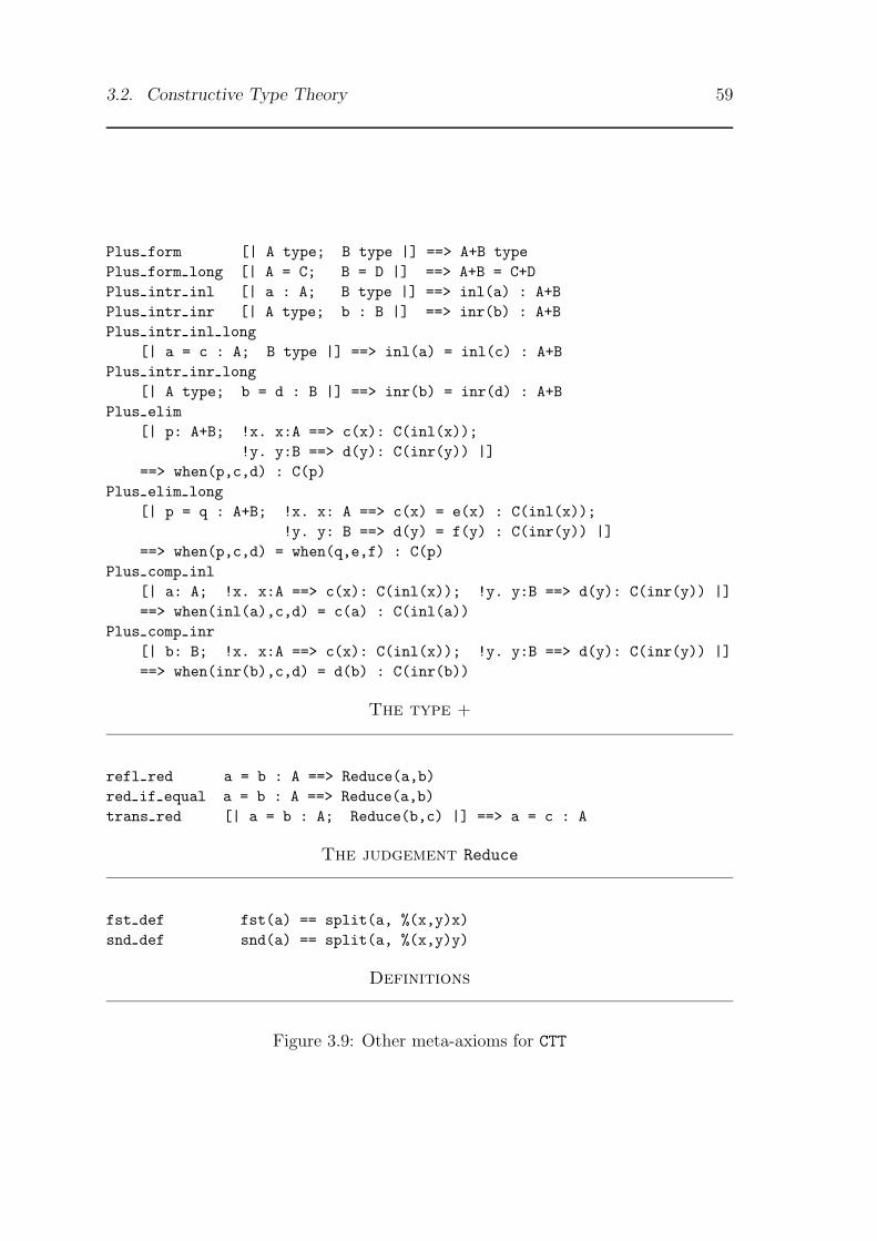
3.2. Constructive Type Theory 59
Plus form [| A type; B type |] ==> A+B typePlus form long [| A = C; B = D |] ==> A+B = C+DPlus intr inl [| a : A; B type |] ==> inl(a) : A+BPlus intr inr [| A type; b : B |] ==> inr(b) : A+BPlus intr inl long
[| a = c : A; B type |] ==> inl(a) = inl(c) : A+BPlus intr inr long
[| A type; b = d : B |] ==> inr(b) = inr(d) : A+BPlus elim
[| p: A+B; !x. x:A ==> c(x): C(inl(x));!y. y:B ==> d(y): C(inr(y)) |]
==> when(p,c,d) : C(p)Plus elim long
[| p = q : A+B; !x. x: A ==> c(x) = e(x) : C(inl(x));!y. y: B ==> d(y) = f(y) : C(inr(y)) |]
==> when(p,c,d) = when(q,e,f) : C(p)Plus comp inl
[| a: A; !x. x:A ==> c(x): C(inl(x)); !y. y:B ==> d(y): C(inr(y)) |]==> when(inl(a),c,d) = c(a) : C(inl(a))
Plus comp inr[| b: B; !x. x:A ==> c(x): C(inl(x)); !y. y:B ==> d(y): C(inr(y)) |]==> when(inr(b),c,d) = d(b) : C(inr(b))
The type +
refl red a = b : A ==> Reduce(a,b)red if equal a = b : A ==> Reduce(a,b)trans red [| a = b : A; Reduce(b,c) |] ==> a = c : A
The judgement Reduce
fst def fst(a) == split(a, %(x,y)x)snd def snd(a) == split(a, %(x,y)y)
Definitions
Figure 3.9: Other meta-axioms for CTT
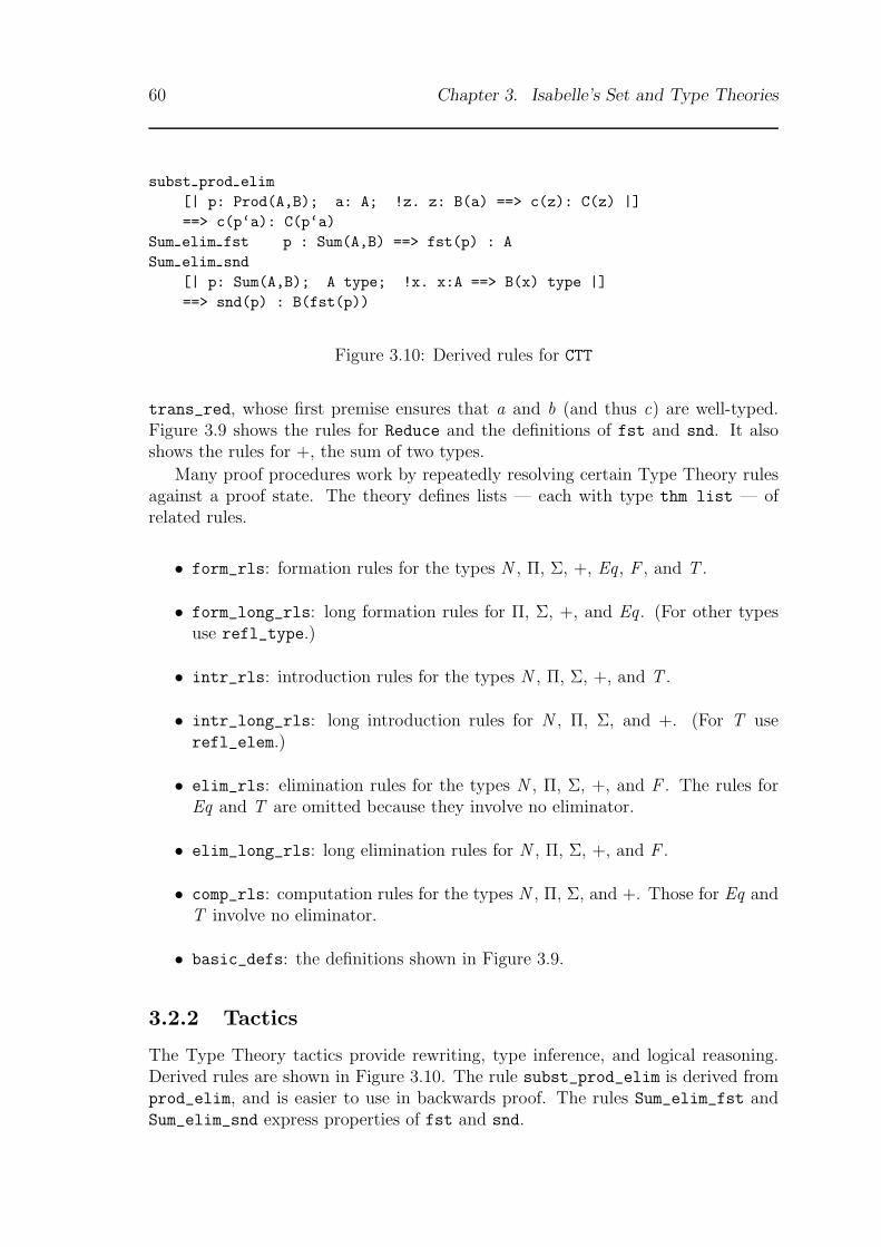
60 Chapter 3. Isabelle’s Set and Type Theories
subst prod elim[| p: Prod(A,B); a: A; !z. z: B(a) ==> c(z): C(z) |]==> c(p‘a): C(p‘a)
Sum elim fst p : Sum(A,B) ==> fst(p) : ASum elim snd
[| p: Sum(A,B); A type; !x. x:A ==> B(x) type |]==> snd(p) : B(fst(p))
Figure 3.10: Derived rules for CTT
trans_red, whose first premise ensures that a and b (and thus c) are well-typed.Figure 3.9 shows the rules for Reduce and the definitions of fst and snd. It alsoshows the rules for +, the sum of two types.
Many proof procedures work by repeatedly resolving certain Type Theory rulesagainst a proof state. The theory defines lists — each with type thm list — ofrelated rules.
• form_rls: formation rules for the types N , Π, Σ, +, Eq , F , and T .
• form_long_rls: long formation rules for Π, Σ, +, and Eq . (For other typesuse refl_type.)
• intr_rls: introduction rules for the types N , Π, Σ, +, and T .
• intr_long_rls: long introduction rules for N , Π, Σ, and +. (For T userefl_elem.)
• elim_rls: elimination rules for the types N , Π, Σ, +, and F . The rules forEq and T are omitted because they involve no eliminator.
• elim_long_rls: long elimination rules for N , Π, Σ, +, and F .
• comp_rls: computation rules for the types N , Π, Σ, and +. Those for Eq andT involve no eliminator.
• basic_defs: the definitions shown in Figure 3.9.
3.2.2 Tactics
The Type Theory tactics provide rewriting, type inference, and logical reasoning.Derived rules are shown in Figure 3.10. The rule subst_prod_elim is derived fromprod_elim, and is easier to use in backwards proof. The rules Sum_elim_fst andSum_elim_snd express properties of fst and snd.
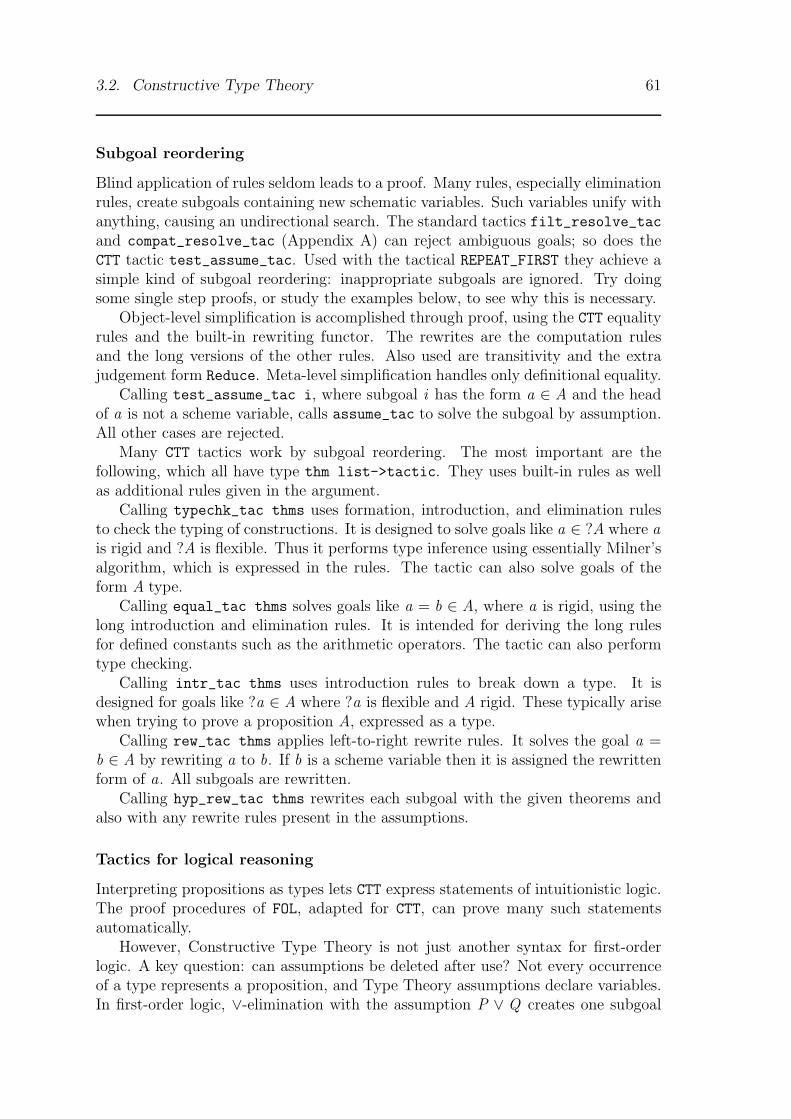
3.2. Constructive Type Theory 61
Subgoal reordering
Blind application of rules seldom leads to a proof. Many rules, especially eliminationrules, create subgoals containing new schematic variables. Such variables unify withanything, causing an undirectional search. The standard tactics filt_resolve_tacand compat_resolve_tac (Appendix A) can reject ambiguous goals; so does theCTT tactic test_assume_tac. Used with the tactical REPEAT_FIRST they achieve asimple kind of subgoal reordering: inappropriate subgoals are ignored. Try doingsome single step proofs, or study the examples below, to see why this is necessary.
Object-level simplification is accomplished through proof, using the CTT equalityrules and the built-in rewriting functor. The rewrites are the computation rulesand the long versions of the other rules. Also used are transitivity and the extrajudgement form Reduce. Meta-level simplification handles only definitional equality.
Calling test_assume_tac i, where subgoal i has the form a ∈ A and the headof a is not a scheme variable, calls assume_tac to solve the subgoal by assumption.All other cases are rejected.
Many CTT tactics work by subgoal reordering. The most important are thefollowing, which all have type thm list->tactic. They uses built-in rules as wellas additional rules given in the argument.
Calling typechk_tac thms uses formation, introduction, and elimination rulesto check the typing of constructions. It is designed to solve goals like a ∈ ?A where ais rigid and ?A is flexible. Thus it performs type inference using essentially Milner’salgorithm, which is expressed in the rules. The tactic can also solve goals of theform A type.
Calling equal_tac thms solves goals like a = b ∈ A, where a is rigid, using thelong introduction and elimination rules. It is intended for deriving the long rulesfor defined constants such as the arithmetic operators. The tactic can also performtype checking.
Calling intr_tac thms uses introduction rules to break down a type. It isdesigned for goals like ?a ∈ A where ?a is flexible and A rigid. These typically arisewhen trying to prove a proposition A, expressed as a type.
Calling rew_tac thms applies left-to-right rewrite rules. It solves the goal a =b ∈ A by rewriting a to b. If b is a scheme variable then it is assigned the rewrittenform of a. All subgoals are rewritten.
Calling hyp_rew_tac thms rewrites each subgoal with the given theorems andalso with any rewrite rules present in the assumptions.
Tactics for logical reasoning
Interpreting propositions as types lets CTT express statements of intuitionistic logic.The proof procedures of FOL, adapted for CTT, can prove many such statementsautomatically.
However, Constructive Type Theory is not just another syntax for first-orderlogic. A key question: can assumptions be deleted after use? Not every occurrenceof a type represents a proposition, and Type Theory assumptions declare variables.In first-order logic, ∨-elimination with the assumption P ∨ Q creates one subgoal

62 Chapter 3. Isabelle’s Set and Type Theories
assuming P and another assuming Q , and P ∨ Q can be deleted. In Type Theory,+-elimination with the assumption z ∈ A + B creates one subgoal assuming x ∈ Aand another assuming y ∈ B (for arbitrary x and y). Deleting z ∈ A + B mayrender the subgoals unprovable if other assumptions refer to z . Some people mightargue that such subgoals are not even meaningful.
The tactic mp_tac performs Modus Ponens among the assumptions. Callingmp_tac i searches for assumptions of the form f ∈ Π(A,B) and a ∈ A in subgoali . It replaces that subgoal by one with a parameter z where f ∈ Π(A,B) has beenreplaced by z ∈ B(a). Unification may take place, selecting any implication whoseantecedent is unifiable with another assumption.
The tactic add_mp_tac is like mp_tac except that the assumption f ∈ Π(A,B)is retained.
Calling safestep_tac thms i attacks subgoal i using formation rules and cer-tain other ‘safe’ rules (F_elim, Prod_intr, Sum_elim, Plus_elim), calling mp_tac
when appropriate. It also uses the theorems thms, which are typically premises ofthe rule being derived.2
Calling safe_tac thms i tries to solve subgoal i by backtracking, withsafestep_tac thms i as the step tactic.
Calling step_tac thms i tries to reduce subgoal i by safestep_tac i, thentries unsafe rules. It may produce multiple outcomes.
Calling pc_tac thms i tries to solve subgoal i by backtracking, withstep_tac thms i as the step tactic. This tactic is for logical reasoning, not typechecking.
Summary of the tactics (which belong to structure CTT_Resolve):
add mp tac: int -> tacticmp tac: int -> tacticpc tac: thm list -> int -> tacticsafestep tac: thm list -> int -> tacticsafe tac: thm list -> int -> tacticstep tac: thm list -> int -> tactic
3.2.3 An example of type inference
Type inference involves proving a goal of the form a ∈?A, where a is a term and ?Ais a scheme variable standing for its type. The type, initially unknown, takes shapein the course of the proof. Our example is the predecessor function on the naturalnumbers.
> goal CTT Rule.thy "lam n. rec(n, 0, %x y.x) : ?A";Level 0lam n. rec(n,0,%x y. x) : ?A1. lam n. rec(n,0,%x y. x) : ?A
2The name, borrowed from FOL, is even less inappropriate for Type Theory. This tactic performsunsafe steps and is therefore incomplete.

3.2. Constructive Type Theory 63
Since the term is a Constructive Type Theory λ-abstraction (not to be confusedwith a meta-level abstraction), the only rule worth considering is Π-introduction.As a result, ?A gets instantiated to a product type, though its domain and rangeare still unknown.
> by (resolve tac [Prod intr] 1);Level 1lam n. rec(n,0,%x y. x) : Prod(?A1,?B1)1. ?A1 type2. !ka. ka : ?A1 ==> rec(ka,0,%x y. x) : ?B1(ka)
Subgoal 1 can be solved in many ways, most of which would invalidate subgoal 2.We therefore tackle the latter subgoal. It asks the type of a term beginning withrec, which can be found by N -elimination.
> by (eresolve tac [N elim] 2);Level 2lam n. rec(n,0,%x y. x) : PROD ka:N. ?C2(ka,ka)1. N type2. !ka. 0 : ?C2(ka,0)3. !ka kb kc. [| kb : N; kc : ?C2(ka,kb) |] ==> kb : ?C2(ka,succ(kb))
We now know that type ?A1 is the natural numbers. However, let us continuewith subgoal 2. What is the type of 0?
> by (resolve tac [N intr0] 2);Level 3lam n. rec(n,0,%x y. x) : N --> N1. N type2. !ka kb kc. [| kb : N; kc : N |] ==> kb : N
The type ?A is now determined: it is (Πka : N )N , which is equivalent to N → N .But we must prove all the subgoals to show that the original term is validly typed.The current subgoal 2 is provable by assumption. The remaining subgoal falls byN -formation.
> by (assume tac 2);Level 4lam n. rec(n,0,%x y. x) : N --> N1. N type
> by (resolve tac [N form] 1);Level 5lam n. rec(n,0,%x y. x) : N --> NNo subgoals!
Calling typechk_tac [] can prove this theorem in one step.
To extract the theorem we must call uresult(), not result(). The latterfunction insists that the theorem be identical to the goal, while here ?A has been
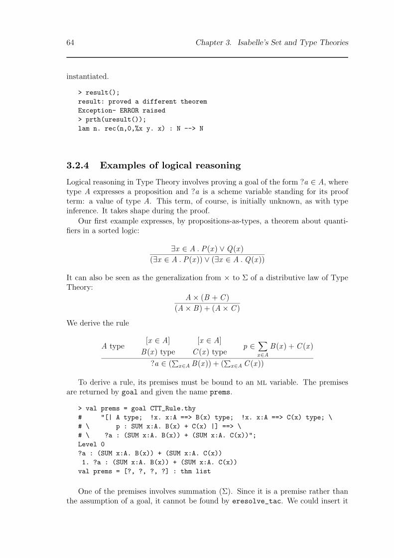
64 Chapter 3. Isabelle’s Set and Type Theories
instantiated.
> result();result: proved a different theoremException- ERROR raised> prth(uresult());lam n. rec(n,0,%x y. x) : N --> N
3.2.4 Examples of logical reasoning
Logical reasoning in Type Theory involves proving a goal of the form ?a ∈ A, wheretype A expresses a proposition and ?a is a scheme variable standing for its proofterm: a value of type A. This term, of course, is initially unknown, as with typeinference. It takes shape during the proof.
Our first example expresses, by propositions-as-types, a theorem about quanti-fiers in a sorted logic:
∃x ∈ A . P(x ) ∨Q(x )
(∃x ∈ A . P(x )) ∨ (∃x ∈ A . Q(x ))
It can also be seen as the generalization from × to Σ of a distributive law of TypeTheory:
A× (B + C )
(A× B) + (A× C )
We derive the rule
A type[x ∈ A]
B(x ) type
[x ∈ A]
C (x ) typep ∈
∑x∈A
B(x ) + C (x )
?a ∈ (∑
x∈A B(x )) + (∑
x∈A C (x ))
To derive a rule, its premises must be bound to an ml variable. The premisesare returned by goal and given the name prems.
> val prems = goal CTT_Rule.thy# "[| A type; !x. x:A ==> B(x) type; !x. x:A ==> C(x) type; \# \ p : SUM x:A. B(x) + C(x) |] ==> \# \ ?a : (SUM x:A. B(x)) + (SUM x:A. C(x))";Level 0?a : (SUM x:A. B(x)) + (SUM x:A. C(x))1. ?a : (SUM x:A. B(x)) + (SUM x:A. C(x))val prems = [?, ?, ?, ?] : thm list
One of the premises involves summation (Σ). Since it is a premise rather thanthe assumption of a goal, it cannot be found by eresolve_tac. We could insert it

3.2. Constructive Type Theory 65
by calling cut_facts_tac prems 1, but instead let us apply the Σ-elimination ruleby calling resolve_tac.
> by (resolve tac [Sum elim] 1);Level 1split(?p1,?c1) : (SUM x:A. B(x)) + (SUM x:A. C(x))1. ?p1 : Sum(?A1,?B1)2. !ka kb. [| ka : ?A1; kb : ?B1(ka) |] ==>
?c1(ka,kb) : (SUM x:A. B(x)) + (SUM x:A. C(x))
Another call to resolve_tac, this time with the premises, solves subgoal 1. Theother subgoal has two new parameters. In the main goal, ?a has been instantiatedwith a split term.
> by (resolve tac prems 1);Level 2split(p,?c1) : (SUM x:A. B(x)) + (SUM x:A. C(x))1. !ka kb. [| ka : A; kb : B(ka) + C(ka) |] ==>
?c1(ka,kb) : (SUM x:A. B(x)) + (SUM x:A. C(x))
The assumption kb ∈ B(ka) + C (ka) is now eliminated, causing a case split anda new parameter. Observe how the main goal appears now.
> by (eresolve tac [Plus elim] 1);Level 3split(p,%ka kb. when(kb,?c2(ka,kb),?d2(ka,kb))): (SUM x:A. B(x)) + (SUM x:A. C(x))1. !ka kb. ka : A ==>
(!kc. kc : B(ka) ==>?c2(ka,kb,kc) : (SUM x:A. B(x)) + (SUM x:A. C(x)))
2. !ka kb. ka : A ==>(!kc. kc : C(ka) ==>
?d2(ka,kb,kc) : (SUM x:A. B(x)) + (SUM x:A. C(x)))
To complete the proof object for the main goal, we need to instantiate the terms?c2(ka,kb,kc) and ?d2(ka,kb,kc). We attack subgoal 1 by introduction of +.Since there are assumptions ka ∈ A and kc ∈ B(ka), we take the left injection(inl).
> by (resolve tac [Plus intr inl] 1);Level 4split(p,%ka kb. when(kb,%kc. inl(?a3(ka,kb,kc)),?d2(ka,kb))): (SUM x:A. B(x)) + (SUM x:A. C(x))1. !ka kb. ka : A ==>
(!kc. kc : B(ka) ==> ?a3(ka,kb,kc) : SUM x:A. B(x))2. !ka kb. ka : A ==> (!kc. kc : B(ka) ==> SUM x:A. C(x) type)3. !ka kb. ka : A ==>
(!kc. kc : C(ka) ==>?d2(ka,kb,kc) : (SUM x:A. B(x)) + (SUM x:A. C(x)))
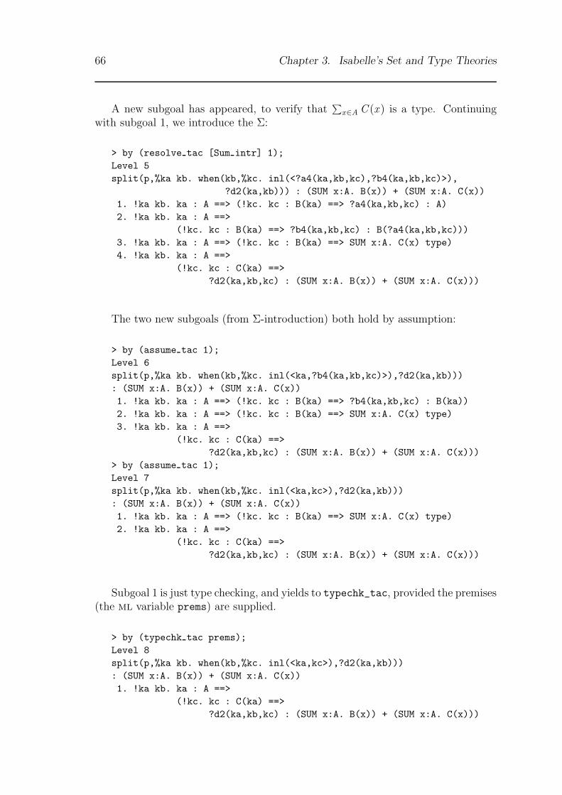
66 Chapter 3. Isabelle’s Set and Type Theories
A new subgoal has appeared, to verify that∑
x∈A C (x ) is a type. Continuingwith subgoal 1, we introduce the Σ:
> by (resolve tac [Sum intr] 1);Level 5split(p,%ka kb. when(kb,%kc. inl(<?a4(ka,kb,kc),?b4(ka,kb,kc)>),
?d2(ka,kb))) : (SUM x:A. B(x)) + (SUM x:A. C(x))1. !ka kb. ka : A ==> (!kc. kc : B(ka) ==> ?a4(ka,kb,kc) : A)2. !ka kb. ka : A ==>
(!kc. kc : B(ka) ==> ?b4(ka,kb,kc) : B(?a4(ka,kb,kc)))3. !ka kb. ka : A ==> (!kc. kc : B(ka) ==> SUM x:A. C(x) type)4. !ka kb. ka : A ==>
(!kc. kc : C(ka) ==>?d2(ka,kb,kc) : (SUM x:A. B(x)) + (SUM x:A. C(x)))
The two new subgoals (from Σ-introduction) both hold by assumption:
> by (assume tac 1);Level 6split(p,%ka kb. when(kb,%kc. inl(<ka,?b4(ka,kb,kc)>),?d2(ka,kb))): (SUM x:A. B(x)) + (SUM x:A. C(x))1. !ka kb. ka : A ==> (!kc. kc : B(ka) ==> ?b4(ka,kb,kc) : B(ka))2. !ka kb. ka : A ==> (!kc. kc : B(ka) ==> SUM x:A. C(x) type)3. !ka kb. ka : A ==>
(!kc. kc : C(ka) ==>?d2(ka,kb,kc) : (SUM x:A. B(x)) + (SUM x:A. C(x)))
> by (assume tac 1);Level 7split(p,%ka kb. when(kb,%kc. inl(<ka,kc>),?d2(ka,kb))): (SUM x:A. B(x)) + (SUM x:A. C(x))1. !ka kb. ka : A ==> (!kc. kc : B(ka) ==> SUM x:A. C(x) type)2. !ka kb. ka : A ==>
(!kc. kc : C(ka) ==>?d2(ka,kb,kc) : (SUM x:A. B(x)) + (SUM x:A. C(x)))
Subgoal 1 is just type checking, and yields to typechk_tac, provided the premises(the ml variable prems) are supplied.
> by (typechk tac prems);Level 8split(p,%ka kb. when(kb,%kc. inl(<ka,kc>),?d2(ka,kb))): (SUM x:A. B(x)) + (SUM x:A. C(x))1. !ka kb. ka : A ==>
(!kc. kc : C(ka) ==>?d2(ka,kb,kc) : (SUM x:A. B(x)) + (SUM x:A. C(x)))
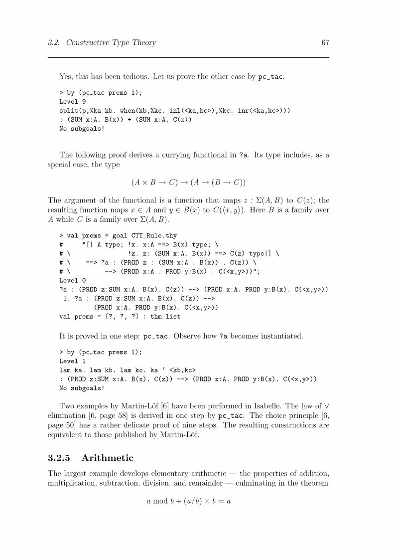
3.2. Constructive Type Theory 67
Yes, this has been tedious. Let us prove the other case by pc_tac.
> by (pc tac prems 1);Level 9split(p,%ka kb. when(kb,%kc. inl(<ka,kc>),%kc. inr(<ka,kc>))): (SUM x:A. B(x)) + (SUM x:A. C(x))No subgoals!
The following proof derives a currying functional in ?a. Its type includes, as aspecial case, the type
(A× B → C )→ (A→ (B → C ))
The argument of the functional is a function that maps z : Σ(A,B) to C (z ); theresulting function maps x ∈ A and y ∈ B(x ) to C (〈x , y〉). Here B is a family overA while C is a family over Σ(A,B).
> val prems = goal CTT_Rule.thy# "[| A type; !x. x:A ==> B(x) type; \# \ !z. z: (SUM x:A. B(x)) ==> C(z) type|] \# \ ==> ?a : (PROD z : (SUM x:A . B(x)) . C(z)) \# \ --> (PROD x:A . PROD y:B(x) . C(<x,y>))";Level 0?a : (PROD z:SUM x:A. B(x). C(z)) --> (PROD x:A. PROD y:B(x). C(<x,y>))1. ?a : (PROD z:SUM x:A. B(x). C(z)) -->
(PROD x:A. PROD y:B(x). C(<x,y>))val prems = [?, ?, ?] : thm list
It is proved in one step: pc_tac. Observe how ?a becomes instantiated.
> by (pc tac prems 1);Level 1lam ka. lam kb. lam kc. ka ‘ <kb,kc>: (PROD z:SUM x:A. B(x). C(z)) --> (PROD x:A. PROD y:B(x). C(<x,y>))No subgoals!
Two examples by Martin-Lof [6] have been performed in Isabelle. The law of ∨elimination [6, page 58] is derived in one step by pc_tac. The choice principle [6,page 50] has a rather delicate proof of nine steps. The resulting constructions areequivalent to those published by Martin-Lof.
3.2.5 Arithmetic
The largest example develops elementary arithmetic — the properties of addition,multiplication, subtraction, division, and remainder — culminating in the theorem
a mod b + (a/b)× b = a

68 Chapter 3. Isabelle’s Set and Type Theories
local open Syntax_Defin val mixfix =
[ Infixr("#+", [Aterm,Aterm]--->Aterm, 25),Infixr("-", [Aterm,Aterm]--->Aterm, 25),Infixr("|-|", [Aterm,Aterm]--->Aterm, 25),Infixr("#*", [Aterm,Aterm]--->Aterm, 35),Infixr("’/’/", [Aterm,Aterm]--->Aterm, 35),Infixr("’/", [Aterm,Aterm]--->Aterm, 35)];
val arith_ext = {logical_types=[],mixfix=mixfix,parse_translation=[],print_translation=[]};
val arith_const_decs = constants mixfix;val arith_syn = Syntax.extend CTT_Syntax.syn arith_ext
end;
val arith_thy = enrich_theory CTT_Rule.thy "arith"([], arith_const_decs, arith_syn)
[ ("add_def", "a#+b == rec(a, b, %u v.succ(v))"),("diff_def", "a-b == rec(b, a, %u v.rec(v, 0, %x y.x))"),("absdiff_def", "a|-|b == (a-b) #+ (b-a)"),("mult_def", "a#*b == rec(a, 0, %u v. b #+ v)"),("mod_def", "a//b == rec(a, 0, %u v. \
\ rec(succ(v) |-| b, 0, %x y.succ(v)))"),("quo_def", "a/b == rec(a, 0, %u v. \
\ rec(succ(u) // b, succ(v), %x y.v))") ];
Figure 3.11: Defining the theory of arithmetic
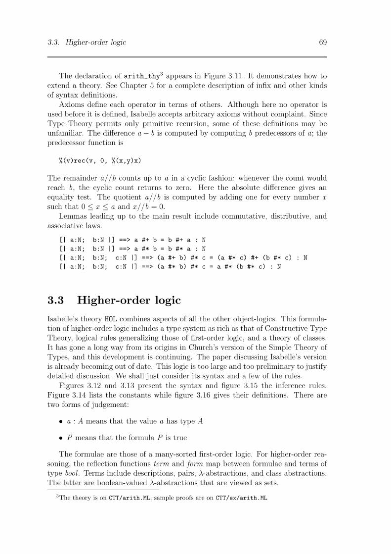
3.3. Higher-order logic 69
The declaration of arith_thy3 appears in Figure 3.11. It demonstrates how toextend a theory. See Chapter 5 for a complete description of infix and other kindsof syntax definitions.
Axioms define each operator in terms of others. Although here no operator isused before it is defined, Isabelle accepts arbitrary axioms without complaint. SinceType Theory permits only primitive recursion, some of these definitions may beunfamiliar. The difference a − b is computed by computing b predecessors of a; thepredecessor function is
%(v)rec(v, 0, %(x,y)x)
The remainder a//b counts up to a in a cyclic fashion: whenever the count wouldreach b, the cyclic count returns to zero. Here the absolute difference gives anequality test. The quotient a//b is computed by adding one for every number xsuch that 0 ≤ x ≤ a and x//b = 0.
Lemmas leading up to the main result include commutative, distributive, andassociative laws.
[| a:N; b:N |] ==> a #+ b = b #+ a : N[| a:N; b:N |] ==> a #* b = b #* a : N[| a:N; b:N; c:N |] ==> (a #+ b) #* c = (a #* c) #+ (b #* c) : N[| a:N; b:N; c:N |] ==> (a #* b) #* c = a #* (b #* c) : N
3.3 Higher-order logic
Isabelle’s theory HOL combines aspects of all the other object-logics. This formula-tion of higher-order logic includes a type system as rich as that of Constructive TypeTheory, logical rules generalizing those of first-order logic, and a theory of classes.It has gone a long way from its origins in Church’s version of the Simple Theory ofTypes, and this development is continuing. The paper discussing Isabelle’s versionis already becoming out of date. This logic is too large and too preliminary to justifydetailed discussion. We shall just consider its syntax and a few of the rules.
Figures 3.12 and 3.13 present the syntax and figure 3.15 the inference rules.Figure 3.14 lists the constants while figure 3.16 gives their definitions. There aretwo forms of judgement:
• a : A means that the value a has type A
• P means that the formula P is true
The formulae are those of a many-sorted first-order logic. For higher-order rea-soning, the reflection functions term and form map between formulae and terms oftype bool . Terms include descriptions, pairs, λ-abstractions, and class abstractions.The latter are boolean-valued λ-abstractions that are viewed as sets.
3The theory is on CTT/arith.ML; sample proofs are on CTT/ex/arith.ML
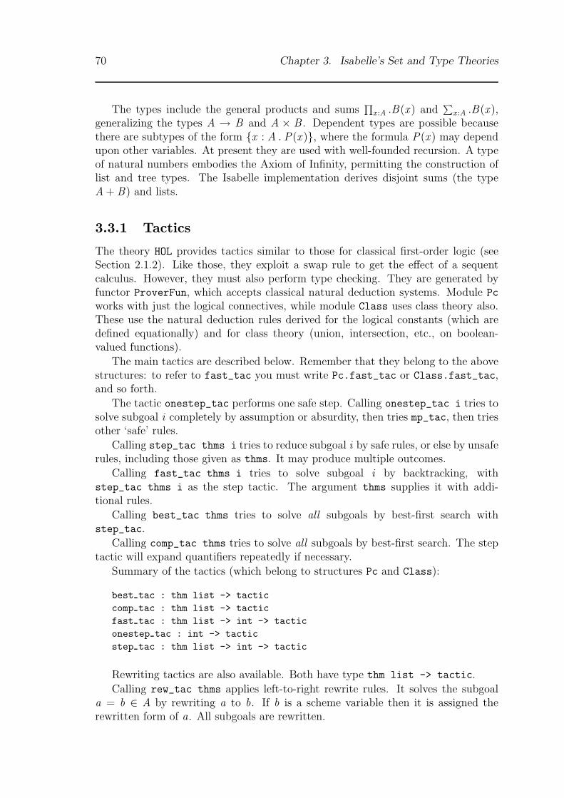
70 Chapter 3. Isabelle’s Set and Type Theories
The types include the general products and sums∏
x :A .B(x ) and∑
x :A .B(x ),generalizing the types A → B and A × B . Dependent types are possible becausethere are subtypes of the form {x : A . P(x )}, where the formula P(x ) may dependupon other variables. At present they are used with well-founded recursion. A typeof natural numbers embodies the Axiom of Infinity, permitting the construction oflist and tree types. The Isabelle implementation derives disjoint sums (the typeA + B) and lists.
3.3.1 Tactics
The theory HOL provides tactics similar to those for classical first-order logic (seeSection 2.1.2). Like those, they exploit a swap rule to get the effect of a sequentcalculus. However, they must also perform type checking. They are generated byfunctor ProverFun, which accepts classical natural deduction systems. Module Pc
works with just the logical connectives, while module Class uses class theory also.These use the natural deduction rules derived for the logical constants (which aredefined equationally) and for class theory (union, intersection, etc., on boolean-valued functions).
The main tactics are described below. Remember that they belong to the abovestructures: to refer to fast_tac you must write Pc.fast_tac or Class.fast_tac,and so forth.
The tactic onestep_tac performs one safe step. Calling onestep_tac i tries tosolve subgoal i completely by assumption or absurdity, then tries mp_tac, then triesother ‘safe’ rules.
Calling step_tac thms i tries to reduce subgoal i by safe rules, or else by unsaferules, including those given as thms. It may produce multiple outcomes.
Calling fast_tac thms i tries to solve subgoal i by backtracking, withstep_tac thms i as the step tactic. The argument thms supplies it with addi-tional rules.
Calling best_tac thms tries to solve all subgoals by best-first search withstep_tac.
Calling comp_tac thms tries to solve all subgoals by best-first search. The steptactic will expand quantifiers repeatedly if necessary.
Summary of the tactics (which belong to structures Pc and Class):
best tac : thm list -> tacticcomp tac : thm list -> tacticfast tac : thm list -> int -> tacticonestep tac : int -> tacticstep tac : thm list -> int -> tactic
Rewriting tactics are also available. Both have type thm list -> tactic.
Calling rew_tac thms applies left-to-right rewrite rules. It solves the subgoala = b ∈ A by rewriting a to b. If b is a scheme variable then it is assigned therewritten form of a. All subgoals are rewritten.
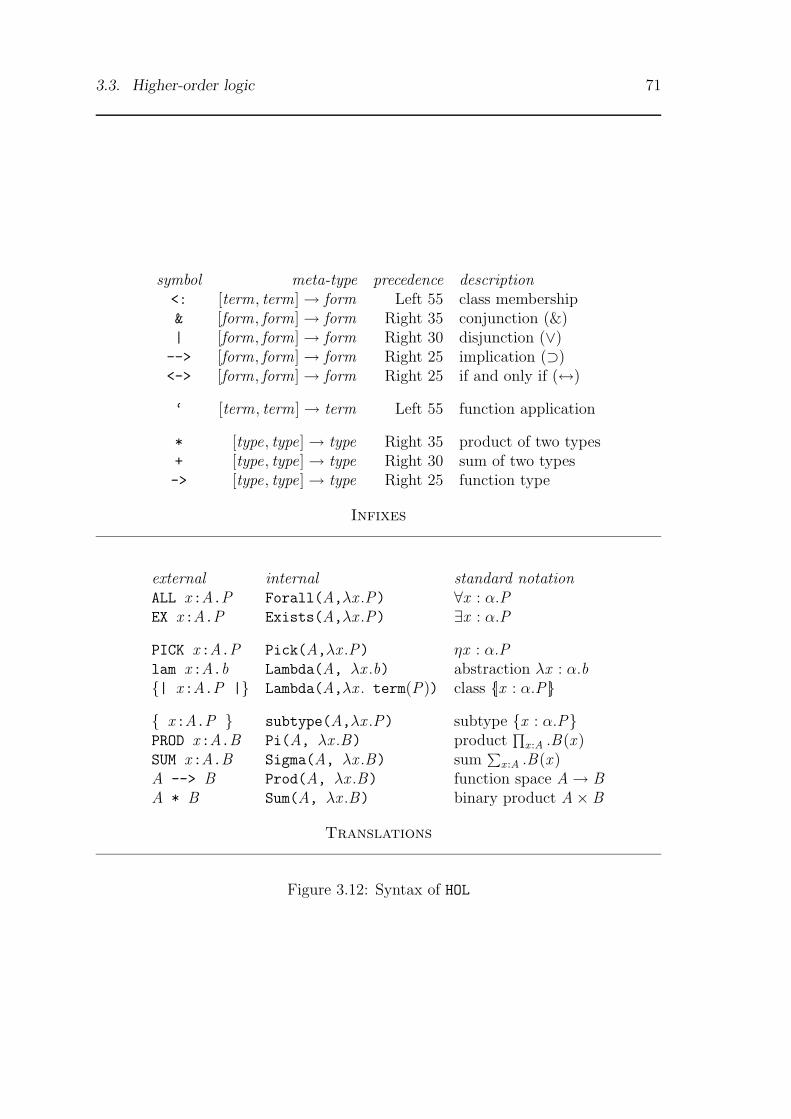
3.3. Higher-order logic 71
symbol meta-type precedence description<: [term, term]→ form Left 55 class membership& [form, form]→ form Right 35 conjunction (&)| [form, form]→ form Right 30 disjunction (∨)--> [form, form]→ form Right 25 implication (⊃)<-> [form, form]→ form Right 25 if and only if (↔)
‘ [term, term]→ term Left 55 function application
* [type, type]→ type Right 35 product of two types+ [type, type]→ type Right 30 sum of two types-> [type, type]→ type Right 25 function type
Infixes
external internal standard notationALL x:A.P Forall(A,λx .P) ∀x : α.PEX x:A.P Exists(A,λx .P) ∃x : α.P
PICK x:A.P Pick(A,λx .P) ηx : α.Plam x:A.b Lambda(A, λx .b) abstraction λx : α.b{| x:A.P |} Lambda(A,λx . term(P)) class {|x : α.P |}
{ x:A.P } subtype(A,λx .P) subtype {x : α.P}PROD x:A.B Pi(A, λx .B) product
∏x :A .B(x )
SUM x:A.B Sigma(A, λx .B) sum∑
x :A .B(x )A --> B Prod(A, λx .B) function space A→ BA * B Sum(A, λx .B) binary product A× B
Translations
Figure 3.12: Syntax of HOL
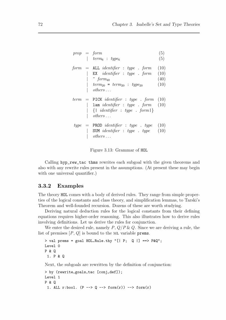
72 Chapter 3. Isabelle’s Set and Type Theories
prop = form (5)| term6 : type6 (5)
form = ALL identifier : type . form (10)| EX identifier : type . form (10)| ~ form40 (40)| term20 = term20 : type20 (10)| others . . .
term = PICK identifier : type . form (10)| lam identifier : type . form (10)| {| identifier : type . form|}| others . . .
type = PROD identifier : type . type (10)| SUM identifier : type . type (10)| others . . .
Figure 3.13: Grammar of HOL
Calling hyp_rew_tac thms rewrites each subgoal with the given theorems andalso with any rewrite rules present in the assumptions. (At present these may beginwith one universal quantifier.)
3.3.2 Examples
The theory HOL comes with a body of derived rules. They range from simple proper-ties of the logical constants and class theory, and simplification lemmas, to Tarski’sTheorem and well-founded recursion. Dozens of these are worth studying.
Deriving natural deduction rules for the logical constants from their definingequations requires higher-order reasoning. This also illustrates how to derive rulesinvolving definitions. Let us derive the rules for conjunction.
We enter the desired rule, namely P ,Q/P & Q . Since we are deriving a rule, thelist of premises [P ,Q ] is bound to the ml variable prems.
> val prems = goal HOL Rule.thy "[| P; Q |] ==> P&Q";Level 0P & Q1. P & Q
Next, the subgoals are rewritten by the definition of conjunction:
> by (rewrite goals tac [conj def]);Level 1P & Q1. ALL r:bool. (P --> Q --> form(r)) --> form(r)
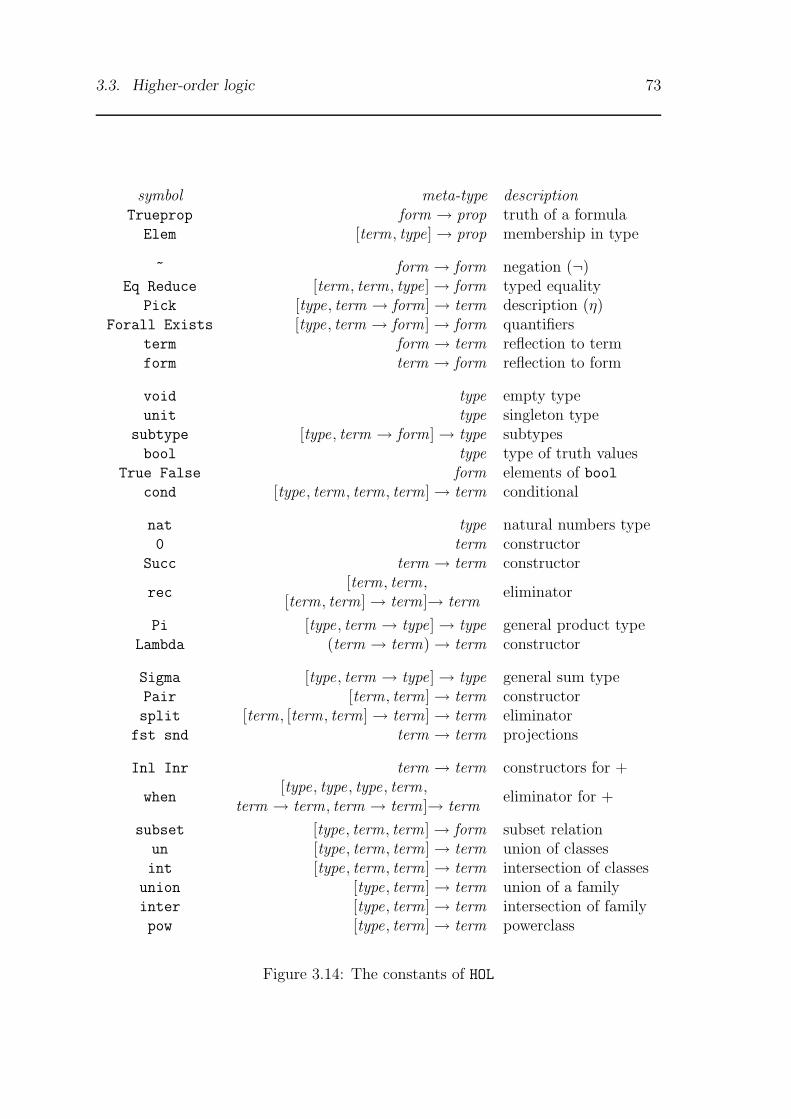
3.3. Higher-order logic 73
symbol meta-type descriptionTrueprop form → prop truth of a formulaElem [term, type]→ prop membership in type
~ form → form negation (¬)Eq Reduce [term, term, type]→ form typed equality
Pick [type, term → form]→ term description (η)Forall Exists [type, term → form]→ form quantifiers
term form → term reflection to termform term → form reflection to form
void type empty typeunit type singleton type
subtype [type, term → form]→ type subtypesbool type type of truth values
True False form elements of boolcond [type, term, term, term]→ term conditional
nat type natural numbers type0 term constructor
Succ term → term constructor
rec[term, term,
[term, term]→ term]→ termeliminator
Pi [type, term → type]→ type general product typeLambda (term → term)→ term constructor
Sigma [type, term → type]→ type general sum typePair [term, term]→ term constructorsplit [term, [term, term]→ term]→ term eliminatorfst snd term → term projections
Inl Inr term → term constructors for +
when[type, type, type, term,
term → term, term → term]→ termeliminator for +
subset [type, term, term]→ form subset relationun [type, term, term]→ term union of classesint [type, term, term]→ term intersection of classesunion [type, term]→ term union of a familyinter [type, term]→ term intersection of familypow [type, term]→ term powerclass
Figure 3.14: The constants of HOL

74 Chapter 3. Isabelle’s Set and Type Theories
pair type [| a: A; b: B(a) |] ==> <a,b> : SUM x:A.B(x)sigma elim [| p: SUM x:A.B(x);
!x y.[| x: A; y: B(x) |] ==> Q(<x,y>) |] ==> Q(p)pair inject [| <a,b> = <c,d> : (SUM x:A.B(x));
[| a = c : A; b = d : B(a) |] ==> R |] ==> R
fst type p: SUM x:A.B(x) ==> fst(p) : Asnd type p: SUM x:A.B(x) ==> snd(p) : B(fst(p))fst conv [| a: A; b: B(a) |] ==> fst(<a,b>) = a: Asnd conv [| a: A; b: B(a) |] ==> snd(<a,b>) = b: B(a)
split def split(p,f) == f(fst(p), snd(p))
The type∑
x :A .B(x )
subtype_intr [| a: A; P(a) |] ==> a : {x:A.P(x)}subtype_elim1 a: {x:A.P(x)} ==> a:Asubtype_elim2 a: {x:A.P(x)} ==> P(a)
Subtypes
term type term(P) : boolterm conv p: bool ==> term(form(p)) = p : boolform intr P ==> form(term(P))form elim form(term(P)) ==> Pterm congr [| P ==> Q; Q ==> P |] ==> term(P) = term(Q) : bool
Reflection
Pick type EX x:A.P(x) ==> (PICK x:A.P(x)) : APick congr [| !x.x: A ==> P(x) <-> Q(x); EX x:A.P(x) |] ==>
(PICK x:A.P(x)) = (PICK x:A.Q(x)) : APick intr EX x:A.P(x) ==> P(PICK x:A.P(x))
Descriptions
Figure 3.15: The rules of HOL
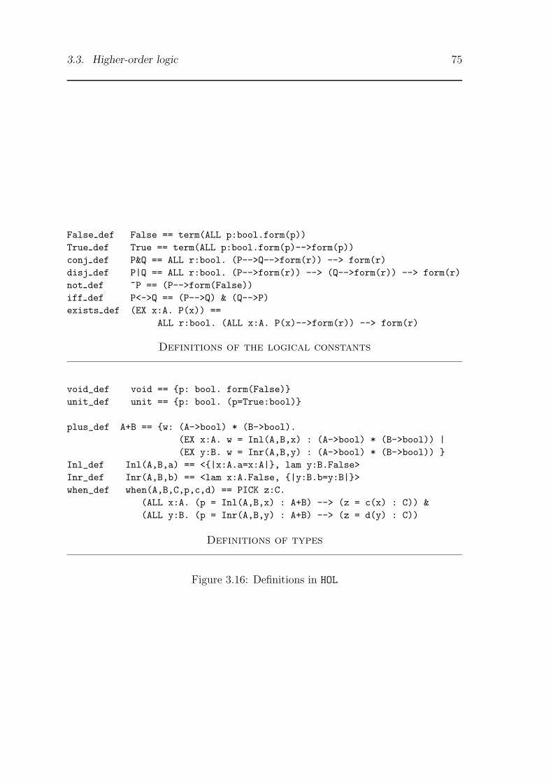
3.3. Higher-order logic 75
False def False == term(ALL p:bool.form(p))True def True == term(ALL p:bool.form(p)-->form(p))conj def P&Q == ALL r:bool. (P-->Q-->form(r)) --> form(r)disj def P|Q == ALL r:bool. (P-->form(r)) --> (Q-->form(r)) --> form(r)not def ~P == (P-->form(False))iff def P<->Q == (P-->Q) & (Q-->P)exists def (EX x:A. P(x)) ==
ALL r:bool. (ALL x:A. P(x)-->form(r)) --> form(r)
Definitions of the logical constants
void_def void == {p: bool. form(False)}unit_def unit == {p: bool. (p=True:bool)}
plus_def A+B == {w: (A->bool) * (B->bool).(EX x:A. w = Inl(A,B,x) : (A->bool) * (B->bool)) |(EX y:B. w = Inr(A,B,y) : (A->bool) * (B->bool)) }
Inl_def Inl(A,B,a) == <{|x:A.a=x:A|}, lam y:B.False>Inr_def Inr(A,B,b) == <lam x:A.False, {|y:B.b=y:B|}>when_def when(A,B,C,p,c,d) == PICK z:C.
(ALL x:A. (p = Inl(A,B,x) : A+B) --> (z = c(x) : C)) &(ALL y:B. (p = Inr(A,B,y) : A+B) --> (z = d(y) : C))
Definitions of types
Figure 3.16: Definitions in HOL

76 Chapter 3. Isabelle’s Set and Type Theories
The rules ∀I and ⊃I are now applied:
> by (resolve tac [all intr] 1);Level 2P & Q1. !ka. ka : bool ==> (P --> Q --> form(ka)) --> form(ka)> by (resolve tac [imp intr] 1);Level 3P & Q1. !ka. [| ka : bool; P --> Q --> form(ka) |] ==> form(ka)
The rule ⊃E is applied twice, to subgoal 1 and then to the resulting subgoal 2,completely decomposing the implication.
> by (eresolve tac [imp elim] 1);Level 4P & Q1. !ka. ka : bool ==> P2. !ka. [| ka : bool; Q --> form(ka) |] ==> form(ka)> by (eresolve tac [imp elim] 2);Level 5P & Q1. !ka. ka : bool ==> P2. !ka. ka : bool ==> Q3. !ka. [| ka : bool; form(ka) |] ==> form(ka)
The first two subgoals are proved using the premises, which are supplied toresolve_tac.
> by (resolve tac prems 1);Level 6P & Q1. !ka. ka : bool ==> Q2. !ka. [| ka : bool; form(ka) |] ==> form(ka)> by (resolve tac prems 1);Level 7P & Q1. !ka. [| ka : bool; form(ka) |] ==> form(ka)
The remaining subgoal holds by assumption. The rule just derived has P and Qas premises.
> by (assume tac 1);Level 8P & QNo subgoals!> prth (result());[| ?P; ?Q |] ==> ?P & ?Q
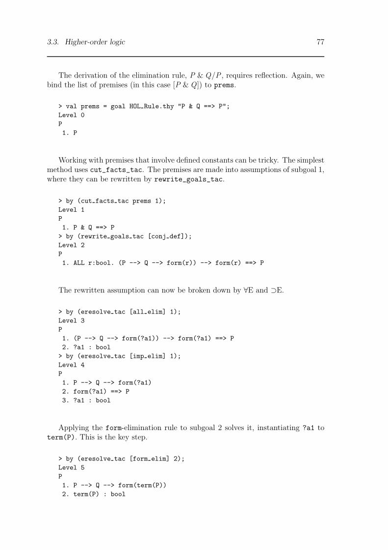
3.3. Higher-order logic 77
The derivation of the elimination rule, P & Q/P , requires reflection. Again, webind the list of premises (in this case [P & Q ]) to prems.
> val prems = goal HOL Rule.thy "P & Q ==> P";Level 0P1. P
Working with premises that involve defined constants can be tricky. The simplestmethod uses cut_facts_tac. The premises are made into assumptions of subgoal 1,where they can be rewritten by rewrite_goals_tac.
> by (cut facts tac prems 1);Level 1P1. P & Q ==> P
> by (rewrite goals tac [conj def]);Level 2P1. ALL r:bool. (P --> Q --> form(r)) --> form(r) ==> P
The rewritten assumption can now be broken down by ∀E and ⊃E.
> by (eresolve tac [all elim] 1);Level 3P1. (P --> Q --> form(?a1)) --> form(?a1) ==> P2. ?a1 : bool
> by (eresolve tac [imp elim] 1);Level 4P1. P --> Q --> form(?a1)2. form(?a1) ==> P3. ?a1 : bool
Applying the form-elimination rule to subgoal 2 solves it, instantiating ?a1 toterm(P). This is the key step.
> by (eresolve tac [form elim] 2);Level 5P1. P --> Q --> form(term(P))2. term(P) : bool
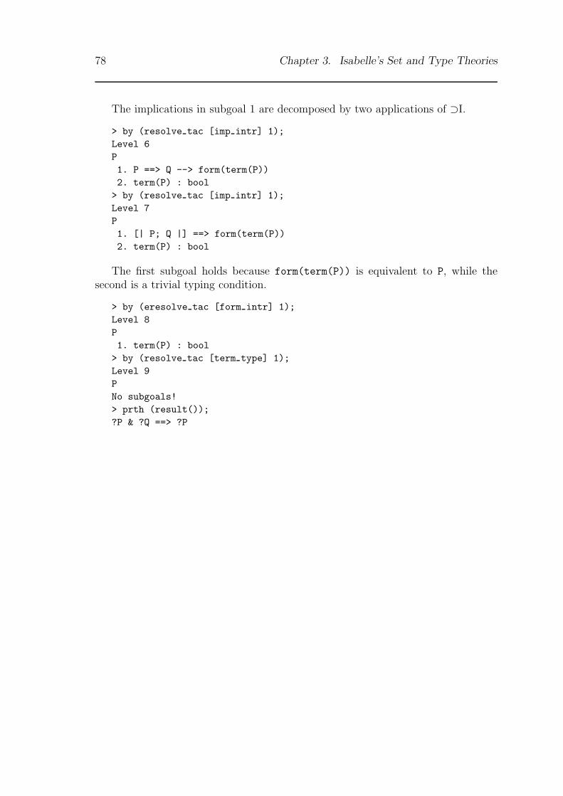
78 Chapter 3. Isabelle’s Set and Type Theories
The implications in subgoal 1 are decomposed by two applications of ⊃I.
> by (resolve tac [imp intr] 1);Level 6P1. P ==> Q --> form(term(P))2. term(P) : bool> by (resolve tac [imp intr] 1);Level 7P1. [| P; Q |] ==> form(term(P))2. term(P) : bool
The first subgoal holds because form(term(P)) is equivalent to P, while thesecond is a trivial typing condition.
> by (eresolve tac [form intr] 1);Level 8P1. term(P) : bool> by (resolve tac [term type] 1);Level 9PNo subgoals!> prth (result());?P & ?Q ==> ?P
Chapter 4
Developing Tactics, Rules, andTheories
The single-step proofs we have studied until now give a gentle introduction to Isabelleand its logics. As you gain experience with these, however, you are likely to realizethat this is not the way to prove anything significant. Single-step proofs are toolong. Isabelle’s basic tactics can be combined to form sophisticated ones usingoperators called tacticals. The resulting tactics can perform hundreds or thousandsof inferences in one invocation. A simple Prolog interpreter is easily expressed.
This chapter also describes how to extend a logic with new constants and axioms,and how to make definitions. Definitions, if viewed as abbreviations, are meta-levelrewrite rules. Expanding abbreviations can lead to gigantic formulae and tediousproofs, however. Deriving rules for the new constants permits shorter proofs.
4.1 Tacticals
Tacticals provide a control structure for tactics, with operators resembling those forregular expressions. The tacticals THEN, ORELSE, and REPEAT form new tactics asfollows:
• The tactic tac1 THEN tac2 performs tac1 followed by tac2: a form of sequenc-ing.
• The tactic tac1 ORELSE tac2 performs tac1, or if that fails then tac2: a formof choice.
• The tactic REPEAT tac performs tac repeatedly until it fails: a form of repeti-tion.
Users of the systems lcf, hol, or Nuprl will recognize these tacticals, and otherpeople may find the above descriptions simple enough. But these descriptions aremere sketches of complex operations involving sequences of proof states. To under-stand this, we must take a closer look at tactics.
79
80 Chapter 4. Developing Tactics, Rules, and Theories
4.1.1 The type of tactics
An Isabelle tactic maps a theorem, representing a proof state, to a possibly infinitesequence of proof states:
datatype tactic = Tactic of thm -> thm Sequence.seq;
Lazy lists are implemented in ml by the type Sequence.seq, which is describedin Appendix A. You need not know the details of this type to use Isabelle’s built-in tacticals, but may find the discussion more comprehensible if you have someprogramming experience with lazy lists.
Higher-order unification can return an infinite sequence of results, and so cantactics that invoke it: especially resolve_tac, eresolve_tac, and assume_tac.Multiple proof states also arise when these tactics are supplied with more than onerule that is unifiable with the subgoal. When the conclusion of a subgoal is unifiablewith more than one of its assumptions, assume_tac returns multiple outcomes.
If the above considerations did not apply, the basic tactics might not requiresequences of proof states. In lcf, a tactic either returns one result or fails. By re-turning a possibly infinite sequence of outcomes, Isabelle tactics can perform back-tracking search. Furthermore, search strategies can be expressed by tacticals: asoperations on tactics.
Chapter 1 describes most of Isabelle’s tactics. Two more, all_tac and no_tac,are of interest because they are identities of tacticals.
The tactic all_tac is the identity element of the tactical THEN. It maps anyproof state φ to the 1-element sequence [φ] containing that state. Thus it succeedsfor all states.
The tactic no_tac is the identity element of the tacticals ORELSE and APPEND. Itmaps any proof state to the empty sequence. Thus it succeeds for no state.
4.1.2 Basic tacticals
Tacticals work by combining sequences of proof states. For each tactic constructedby one of these tacticals, we consider the output sequence that results when it isapplied to the proof state φ.
The tactic tac1 THEN tac2 computes tac1(φ), obtaining a sequence of states[ψ1, ψ2, ψ3, . . .]. It applies tac2 to each of these states. The output sequence isthe concatenation of the sequences tac2(ψ1), tac2(ψ2), tac2(ψ3), . . .. In a commonnotation for lazy lists, the output is
[θ | ψ ∈ tac1(φ), θ ∈ tac2(ψ)]
The tactic tac1 ORELSE tac2 computes tac1(φ). If this sequence is non-emptythen it is returned as the overall result; otherwise tac2(φ) is returned. This is adeterministic choice, a bit like Prolog’s cut directive. If tac1 succeeds then tac2is excluded from consideration.
The tactic tac1 APPEND tac2 returns the concatenation of the sequences tac1(φ)and tac2(φ). This is not a fair interleaving, for if tac1(φ) is infinite then that
4.1. Tacticals 81
sequence is the overall result. A tactical with interleaving could be written, buteven APPEND has few uses, for it causes excessive branching during search.
The tactic DETERM tac truncates the sequence tac(φ) to have at most one ele-ment. Thus the resulting tactic is deterministic. The tactical DETERM is used tolimit the search space.
The tacticals EVERY and FIRST are n-ary versions of THEN and ORELSE. They aregiven a list of tactics. The tactic EVERY [tac1, . . . , tacn ] behaves like
tac 1 THEN . . . THEN tac n
The tactic FIRST [tac1, . . . , tacn ] behaves like
tac 1 ORELSE . . . ORELSE tac n
4.1.3 Derived tacticals
The tacticals given above suffice to describe (and to implement) more sophisticatedones. Recursively defined tacticals perform repetition and search. Again, we describethe output sequence returned when the new tactic is applied to the state φ.
The tactic TRY tac returns tac(φ) if this sequence is non-empty, and returns thesingleton sequence [φ] otherwise. The definition of the tactical in ml is
fun TRY tac = tac ORELSE all tac;
The tactic REPEAT tac computes tac(φ). If this sequence is non-empty then thetactic recursively applies itself to each element, concatenating the results. Otherwiseit returns the singleton sequence [φ]. Its ml definition makes use of the functiontapply, which applies a tactic to a state:
fun REPEAT tac = Tactic (fn state =>tapply((tac THEN REPEAT tac) ORELSE all tac, state));
Recursive tacticals must be coded in this awkward fashion to avoid infiniterecursion.1
If tac can return multiple outcomes then so can REPEAT tac. Since REPEAT usesORELSE and not APPEND, it applies tac as many times as possible in each outcome.A common idiom is
REPEAT (tac1 ORELSE tac2)
This repeatedly applies tac1 or tac2 as many times as possible, giving priority totac1.
The tactic DEPTH_FIRST satpred tac performs a depth-first search for satisfac-tory proof states, which are those for which satpred returns true. If satpred(φ) is true
1This more attractive definition loops:fun REPEAT tac = (tac THEN REPEAT tac) ORELSE all tac;
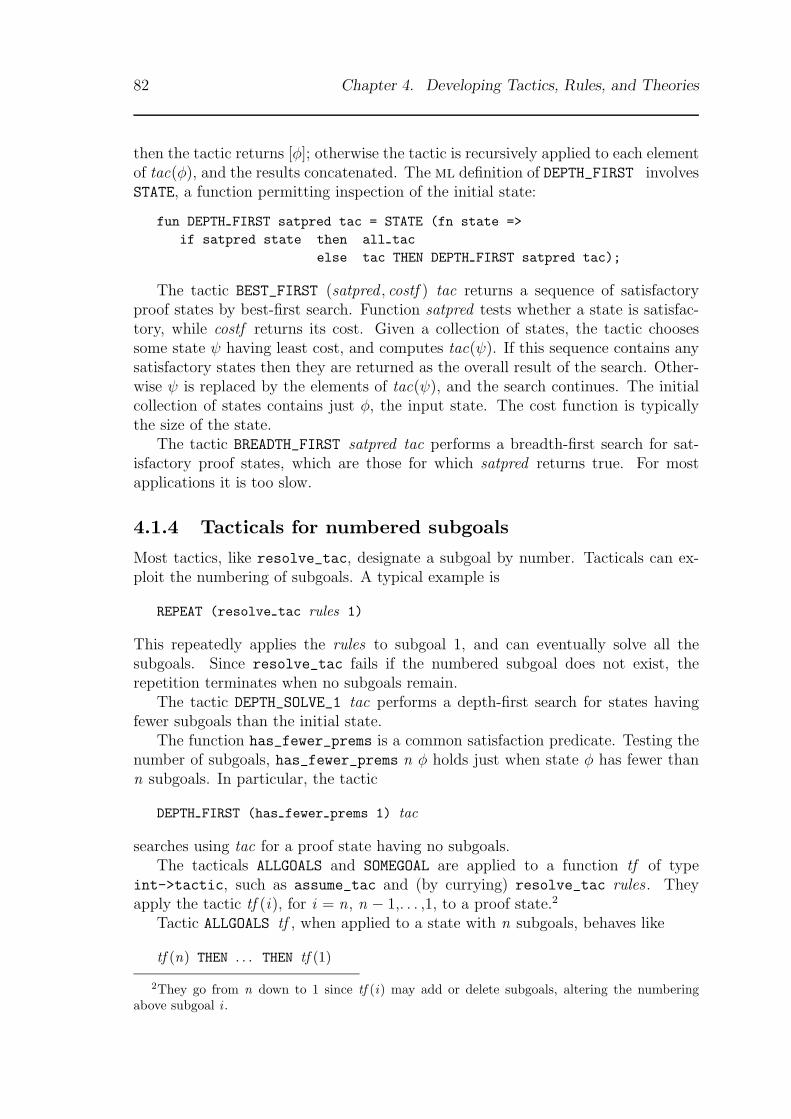
82 Chapter 4. Developing Tactics, Rules, and Theories
then the tactic returns [φ]; otherwise the tactic is recursively applied to each elementof tac(φ), and the results concatenated. The ml definition of DEPTH_FIRST involvesSTATE, a function permitting inspection of the initial state:
fun DEPTH FIRST satpred tac = STATE (fn state =>if satpred state then all tac
else tac THEN DEPTH FIRST satpred tac);
The tactic BEST_FIRST (satpred , costf ) tac returns a sequence of satisfactoryproof states by best-first search. Function satpred tests whether a state is satisfac-tory, while costf returns its cost. Given a collection of states, the tactic choosessome state ψ having least cost, and computes tac(ψ). If this sequence contains anysatisfactory states then they are returned as the overall result of the search. Other-wise ψ is replaced by the elements of tac(ψ), and the search continues. The initialcollection of states contains just φ, the input state. The cost function is typicallythe size of the state.
The tactic BREADTH_FIRST satpred tac performs a breadth-first search for sat-isfactory proof states, which are those for which satpred returns true. For mostapplications it is too slow.
4.1.4 Tacticals for numbered subgoals
Most tactics, like resolve_tac, designate a subgoal by number. Tacticals can ex-ploit the numbering of subgoals. A typical example is
REPEAT (resolve tac rules 1)
This repeatedly applies the rules to subgoal 1, and can eventually solve all thesubgoals. Since resolve_tac fails if the numbered subgoal does not exist, therepetition terminates when no subgoals remain.
The tactic DEPTH_SOLVE_1 tac performs a depth-first search for states havingfewer subgoals than the initial state.
The function has_fewer_prems is a common satisfaction predicate. Testing thenumber of subgoals, has_fewer_prems n φ holds just when state φ has fewer thann subgoals. In particular, the tactic
DEPTH FIRST (has fewer prems 1) tac
searches using tac for a proof state having no subgoals.The tacticals ALLGOALS and SOMEGOAL are applied to a function tf of type
int->tactic, such as assume_tac and (by currying) resolve_tac rules . Theyapply the tactic tf (i), for i = n, n − 1,. . . ,1, to a proof state.2
Tactic ALLGOALS tf , when applied to a state with n subgoals, behaves like
tf (n) THEN . . . THEN tf (1)
2They go from n down to 1 since tf (i) may add or delete subgoals, altering the numberingabove subgoal i .
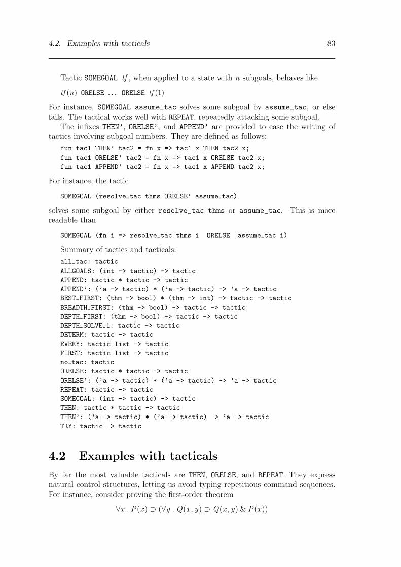
4.2. Examples with tacticals 83
Tactic SOMEGOAL tf , when applied to a state with n subgoals, behaves like
tf (n) ORELSE . . . ORELSE tf (1)
For instance, SOMEGOAL assume_tac solves some subgoal by assume_tac, or elsefails. The tactical works well with REPEAT, repeatedly attacking some subgoal.
The infixes THEN’, ORELSE’, and APPEND’ are provided to ease the writing oftactics involving subgoal numbers. They are defined as follows:
fun tac1 THEN’ tac2 = fn x => tac1 x THEN tac2 x;fun tac1 ORELSE’ tac2 = fn x => tac1 x ORELSE tac2 x;fun tac1 APPEND’ tac2 = fn x => tac1 x APPEND tac2 x;
For instance, the tactic
SOMEGOAL (resolve tac thms ORELSE’ assume tac)
solves some subgoal by either resolve_tac thms or assume_tac. This is morereadable than
SOMEGOAL (fn i => resolve tac thms i ORELSE assume tac i)
Summary of tactics and tacticals:
all tac: tacticALLGOALS: (int -> tactic) -> tacticAPPEND: tactic * tactic -> tacticAPPEND’: (’a -> tactic) * (’a -> tactic) -> ’a -> tacticBEST FIRST: (thm -> bool) * (thm -> int) -> tactic -> tacticBREADTH FIRST: (thm -> bool) -> tactic -> tacticDEPTH FIRST: (thm -> bool) -> tactic -> tacticDEPTH SOLVE 1: tactic -> tacticDETERM: tactic -> tacticEVERY: tactic list -> tacticFIRST: tactic list -> tacticno tac: tacticORELSE: tactic * tactic -> tacticORELSE’: (’a -> tactic) * (’a -> tactic) -> ’a -> tacticREPEAT: tactic -> tacticSOMEGOAL: (int -> tactic) -> tacticTHEN: tactic * tactic -> tacticTHEN’: (’a -> tactic) * (’a -> tactic) -> ’a -> tacticTRY: tactic -> tactic
4.2 Examples with tacticals
By far the most valuable tacticals are THEN, ORELSE, and REPEAT. They expressnatural control structures, letting us avoid typing repetitious command sequences.For instance, consider proving the first-order theorem
∀x . P(x ) ⊃ (∀y . Q(x , y) ⊃ Q(x , y) & P(x ))

84 Chapter 4. Developing Tactics, Rules, and Theories
We could apply the rules ∀I, ⊃I, ∀I, ⊃I, &I in succession (by resolve_tac) andthen apply assume_tac twice: a total of seven commands. You might want to trythis proof now.
With tacticals the proof can be accomplished in two steps, or even one.
> goal Int Rule.thy "ALL x. P(x) --> (ALL y. Q(x,y) --> Q(x,y) & P(x))";Level 0ALL x. P(x) --> (ALL y. Q(x,y) --> Q(x,y) & P(x))1. ALL x. P(x) --> (ALL y. Q(x,y) --> Q(x,y) & P(x))
First we repeatedly apply resolve_tac to subgoal 1. We supply all the rulesthat are needed: ∀I, ⊃I, and &I:
> by (REPEAT (resolve tac [all intr,imp intr,conj intr] 1));Level 1ALL x. P(x) --> (ALL y. Q(x,y) --> Q(x,y) & P(x))1. !ka. P(ka) ==> (!kb. Q(ka,kb) ==> Q(ka,kb))2. !ka. P(ka) ==> (!kb. Q(ka,kb) ==> P(ka))
Those rules have been applied as much as possible. The two subgoals that resultare solved by assumption.
> by (REPEAT (assume tac 1));Level 2ALL x. P(x) --> (ALL y. Q(x,y) --> Q(x,y) & P(x))No subgoals!
A single tactic, combining the repetition of assume_tac and resolve_tac, canprove the theorem in a single command:
REPEAT (assume tac 1 ORELSEresolve tac [all intr,imp intr,conj intr] 1)
Elimination rules can be applied repeatedly through eresolve_tac. This tacticselects an assumption and finally deletes it, to allow termination. A proof of
(∃x . P(f (x ))) ∨ (∃y . P(g(y))) ⊃ (∃z . P(z ))
goes by ⊃I, ∨E, ∃E, ∃E, and ∃I. The order is critical: ∃E must be applied before∃I in each subgoal. We could tackle the proof as follows:
> goal Int Rule.thy "(EX x. P(f(x))) | (EX y. P(g(y))) --> (EX z. P(z))";Level 0(EX x. P(f(x))) | (EX y. P(g(y))) --> (EX z. P(z))1. (EX x. P(f(x))) | (EX y. P(g(y))) --> (EX z. P(z))> by (resolve tac [imp intr] 1);Level 1(EX x. P(f(x))) | (EX y. P(g(y))) --> (EX z. P(z))1. (EX x. P(f(x))) | (EX y. P(g(y))) ==> EX z. P(z)
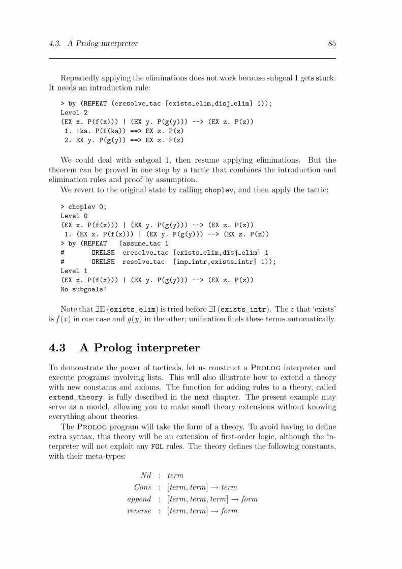
4.3. A Prolog interpreter 85
Repeatedly applying the eliminations does not work because subgoal 1 gets stuck.It needs an introduction rule:
> by (REPEAT (eresolve tac [exists elim,disj elim] 1));Level 2(EX x. P(f(x))) | (EX y. P(g(y))) --> (EX z. P(z))1. !ka. P(f(ka)) ==> EX z. P(z)2. EX y. P(g(y)) ==> EX z. P(z)
We could deal with subgoal 1, then resume applying eliminations. But thetheorem can be proved in one step by a tactic that combines the introduction andelimination rules and proof by assumption.
We revert to the original state by calling choplev, and then apply the tactic:
> choplev 0;Level 0(EX x. P(f(x))) | (EX y. P(g(y))) --> (EX z. P(z))1. (EX x. P(f(x))) | (EX y. P(g(y))) --> (EX z. P(z))
> by (REPEAT (assume tac 1# ORELSE eresolve tac [exists elim,disj elim] 1# ORELSE resolve tac [imp intr,exists intr] 1));Level 1(EX x. P(f(x))) | (EX y. P(g(y))) --> (EX z. P(z))No subgoals!
Note that ∃E (exists_elim) is tried before ∃I (exists_intr). The z that ‘exists’is f (x ) in one case and g(y) in the other; unification finds these terms automatically.
4.3 A Prolog interpreter
To demonstrate the power of tacticals, let us construct a Prolog interpreter andexecute programs involving lists. This will also illustrate how to extend a theorywith new constants and axioms. The function for adding rules to a theory, calledextend_theory, is fully described in the next chapter. The present example mayserve as a model, allowing you to make small theory extensions without knowingeverything about theories.
The Prolog program will take the form of a theory. To avoid having to defineextra syntax, this theory will be an extension of first-order logic, although the in-terpreter will not exploit any FOL rules. The theory defines the following constants,with their meta-types:
Nil : term
Cons : [term, term]→ term
append : [term, term, term]→ form
reverse : [term, term]→ form
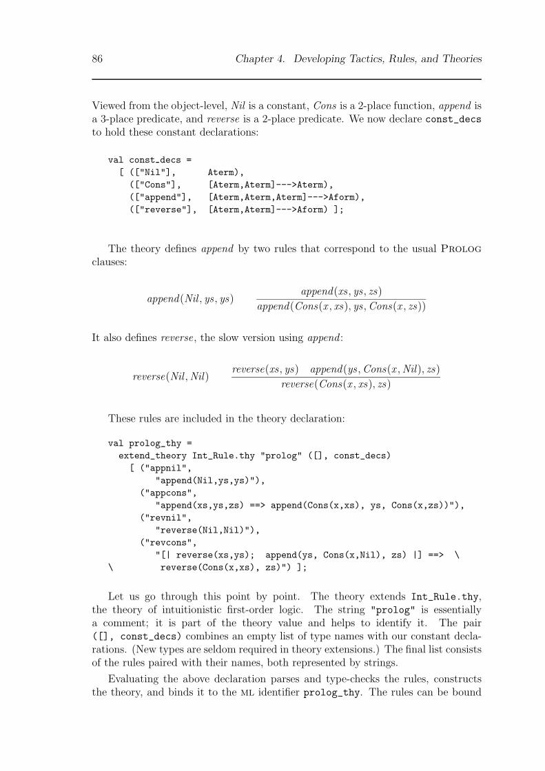
86 Chapter 4. Developing Tactics, Rules, and Theories
Viewed from the object-level, Nil is a constant, Cons is a 2-place function, append isa 3-place predicate, and reverse is a 2-place predicate. We now declare const_decs
to hold these constant declarations:
val const decs =[ (["Nil"], Aterm),
(["Cons"], [Aterm,Aterm]--->Aterm),(["append"], [Aterm,Aterm,Aterm]--->Aform),(["reverse"], [Aterm,Aterm]--->Aform) ];
The theory defines append by two rules that correspond to the usual Prologclauses:
append(Nil , ys , ys)append(xs , ys , zs)
append(Cons(x , xs), ys ,Cons(x , zs))
It also defines reverse, the slow version using append :
reverse(Nil ,Nil)reverse(xs , ys) append(ys ,Cons(x ,Nil), zs)
reverse(Cons(x , xs), zs)
These rules are included in the theory declaration:
val prolog_thy =extend_theory Int_Rule.thy "prolog" ([], const_decs)
[ ("appnil","append(Nil,ys,ys)"),
("appcons","append(xs,ys,zs) ==> append(Cons(x,xs), ys, Cons(x,zs))"),
("revnil","reverse(Nil,Nil)"),
("revcons","[| reverse(xs,ys); append(ys, Cons(x,Nil), zs) |] ==> \
\ reverse(Cons(x,xs), zs)") ];
Let us go through this point by point. The theory extends Int_Rule.thy,the theory of intuitionistic first-order logic. The string "prolog" is essentiallya comment; it is part of the theory value and helps to identify it. The pair([], const_decs) combines an empty list of type names with our constant decla-rations. (New types are seldom required in theory extensions.) The final list consistsof the rules paired with their names, both represented by strings.
Evaluating the above declaration parses and type-checks the rules, constructsthe theory, and binds it to the ml identifier prolog_thy. The rules can be bound
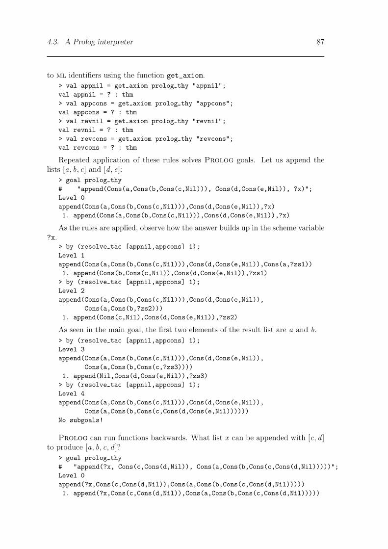
4.3. A Prolog interpreter 87
to ml identifiers using the function get_axiom.
> val appnil = get axiom prolog thy "appnil";val appnil = ? : thm> val appcons = get axiom prolog thy "appcons";val appcons = ? : thm> val revnil = get axiom prolog thy "revnil";val revnil = ? : thm> val revcons = get axiom prolog thy "revcons";val revcons = ? : thm
Repeated application of these rules solves Prolog goals. Let us append thelists [a, b, c] and [d , e]:
> goal prolog thy# "append(Cons(a,Cons(b,Cons(c,Nil))), Cons(d,Cons(e,Nil)), ?x)";Level 0append(Cons(a,Cons(b,Cons(c,Nil))),Cons(d,Cons(e,Nil)),?x)1. append(Cons(a,Cons(b,Cons(c,Nil))),Cons(d,Cons(e,Nil)),?x)
As the rules are applied, observe how the answer builds up in the scheme variable?x.
> by (resolve tac [appnil,appcons] 1);Level 1append(Cons(a,Cons(b,Cons(c,Nil))),Cons(d,Cons(e,Nil)),Cons(a,?zs1))1. append(Cons(b,Cons(c,Nil)),Cons(d,Cons(e,Nil)),?zs1)
> by (resolve tac [appnil,appcons] 1);Level 2append(Cons(a,Cons(b,Cons(c,Nil))),Cons(d,Cons(e,Nil)),
Cons(a,Cons(b,?zs2)))1. append(Cons(c,Nil),Cons(d,Cons(e,Nil)),?zs2)
As seen in the main goal, the first two elements of the result list are a and b.
> by (resolve tac [appnil,appcons] 1);Level 3append(Cons(a,Cons(b,Cons(c,Nil))),Cons(d,Cons(e,Nil)),
Cons(a,Cons(b,Cons(c,?zs3))))1. append(Nil,Cons(d,Cons(e,Nil)),?zs3)
> by (resolve tac [appnil,appcons] 1);Level 4append(Cons(a,Cons(b,Cons(c,Nil))),Cons(d,Cons(e,Nil)),
Cons(a,Cons(b,Cons(c,Cons(d,Cons(e,Nil))))))No subgoals!
Prolog can run functions backwards. What list x can be appended with [c, d ]to produce [a, b, c, d ]?
> goal prolog thy# "append(?x, Cons(c,Cons(d,Nil)), Cons(a,Cons(b,Cons(c,Cons(d,Nil)))))";Level 0append(?x,Cons(c,Cons(d,Nil)),Cons(a,Cons(b,Cons(c,Cons(d,Nil)))))1. append(?x,Cons(c,Cons(d,Nil)),Cons(a,Cons(b,Cons(c,Cons(d,Nil)))))
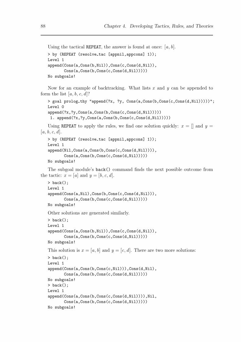
88 Chapter 4. Developing Tactics, Rules, and Theories
Using the tactical REPEAT, the answer is found at once: [a, b].
> by (REPEAT (resolve tac [appnil,appcons] 1));Level 1append(Cons(a,Cons(b,Nil)),Cons(c,Cons(d,Nil)),
Cons(a,Cons(b,Cons(c,Cons(d,Nil)))))No subgoals!
Now for an example of backtracking. What lists x and y can be appended toform the list [a, b, c, d ]?
> goal prolog thy "append(?x, ?y, Cons(a,Cons(b,Cons(c,Cons(d,Nil)))))";Level 0append(?x,?y,Cons(a,Cons(b,Cons(c,Cons(d,Nil)))))1. append(?x,?y,Cons(a,Cons(b,Cons(c,Cons(d,Nil)))))
Using REPEAT to apply the rules, we find one solution quickly: x = [] and y =[a, b, c, d ].
> by (REPEAT (resolve tac [appnil,appcons] 1));Level 1append(Nil,Cons(a,Cons(b,Cons(c,Cons(d,Nil)))),
Cons(a,Cons(b,Cons(c,Cons(d,Nil)))))No subgoals!
The subgoal module’s back() command finds the next possible outcome fromthe tactic: x = [a] and y = [b, c, d ].
> back();Level 1append(Cons(a,Nil),Cons(b,Cons(c,Cons(d,Nil))),
Cons(a,Cons(b,Cons(c,Cons(d,Nil)))))No subgoals!
Other solutions are generated similarly.
> back();Level 1append(Cons(a,Cons(b,Nil)),Cons(c,Cons(d,Nil)),
Cons(a,Cons(b,Cons(c,Cons(d,Nil)))))No subgoals!
This solution is x = [a, b] and y = [c, d ]. There are two more solutions:
> back();Level 1append(Cons(a,Cons(b,Cons(c,Nil))),Cons(d,Nil),
Cons(a,Cons(b,Cons(c,Cons(d,Nil)))))No subgoals!> back();Level 1append(Cons(a,Cons(b,Cons(c,Cons(d,Nil)))),Nil,
Cons(a,Cons(b,Cons(c,Cons(d,Nil)))))No subgoals!
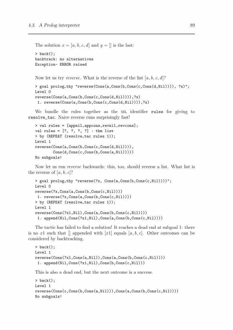
4.3. A Prolog interpreter 89
The solution x = [a, b, c, d ] and y = [] is the last:
> back();backtrack: no alternativesException- ERROR raised
Now let us try reverse. What is the reverse of the list [a, b, c, d ]?
> goal prolog thy "reverse(Cons(a,Cons(b,Cons(c,Cons(d,Nil)))), ?x)";Level 0reverse(Cons(a,Cons(b,Cons(c,Cons(d,Nil)))),?x)1. reverse(Cons(a,Cons(b,Cons(c,Cons(d,Nil)))),?x)
We bundle the rules together as the ml identifier rules for giving toresolve_tac. Naive reverse runs surprisingly fast!
> val rules = [appnil,appcons,revnil,revcons];val rules = [?, ?, ?, ?] : thm list> by (REPEAT (resolve tac rules 1));Level 1reverse(Cons(a,Cons(b,Cons(c,Cons(d,Nil)))),
Cons(d,Cons(c,Cons(b,Cons(a,Nil)))))No subgoals!
Now let us run reverse backwards: this, too, should reverse a list. What list isthe reverse of [a, b, c]?
> goal prolog thy "reverse(?x, Cons(a,Cons(b,Cons(c,Nil))))";Level 0reverse(?x,Cons(a,Cons(b,Cons(c,Nil))))1. reverse(?x,Cons(a,Cons(b,Cons(c,Nil))))
> by (REPEAT (resolve tac rules 1));Level 1reverse(Cons(?x1,Nil),Cons(a,Cons(b,Cons(c,Nil))))1. append(Nil,Cons(?x1,Nil),Cons(a,Cons(b,Cons(c,Nil))))
The tactic has failed to find a solution! It reaches a dead end at subgoal 1: thereis no x1 such that [] appended with [x1] equals [a, b, c]. Other outcomes can beconsidered by backtracking.
> back();Level 1reverse(Cons(?x1,Cons(a,Nil)),Cons(a,Cons(b,Cons(c,Nil))))1. append(Nil,Cons(?x1,Nil),Cons(b,Cons(c,Nil)))
This is also a dead end, but the next outcome is a success.
> back();Level 1reverse(Cons(c,Cons(b,Cons(a,Nil))),Cons(a,Cons(b,Cons(c,Nil))))No subgoals!
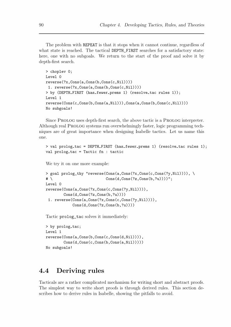
90 Chapter 4. Developing Tactics, Rules, and Theories
The problem with REPEAT is that it stops when it cannot continue, regardless ofwhat state is reached. The tactical DEPTH_FIRST searches for a satisfactory state:here, one with no subgoals. We return to the start of the proof and solve it bydepth-first search.
> choplev 0;Level 0reverse(?x,Cons(a,Cons(b,Cons(c,Nil))))1. reverse(?x,Cons(a,Cons(b,Cons(c,Nil))))> by (DEPTH FIRST (has fewer prems 1) (resolve tac rules 1));Level 1reverse(Cons(c,Cons(b,Cons(a,Nil))),Cons(a,Cons(b,Cons(c,Nil))))No subgoals!
Since Prolog uses depth-first search, the above tactic is a Prolog interpreter.Although real Prolog systems run overwhelmingly faster, logic programming tech-niques are of great importance when designing Isabelle tactics. Let us name thisone.
> val prolog tac = DEPTH FIRST (has fewer prems 1) (resolve tac rules 1);val prolog tac = Tactic fn : tactic
We try it on one more example:
> goal prolog_thy "reverse(Cons(a,Cons(?x,Cons(c,Cons(?y,Nil)))), \# \ Cons(d,Cons(?z,Cons(b,?u))))";Level 0reverse(Cons(a,Cons(?x,Cons(c,Cons(?y,Nil)))),
Cons(d,Cons(?z,Cons(b,?u))))1. reverse(Cons(a,Cons(?x,Cons(c,Cons(?y,Nil)))),
Cons(d,Cons(?z,Cons(b,?u))))
Tactic prolog_tac solves it immediately:
> by prolog tac;Level 1reverse(Cons(a,Cons(b,Cons(c,Cons(d,Nil)))),
Cons(d,Cons(c,Cons(b,Cons(a,Nil)))))No subgoals!
4.4 Deriving rules
Tacticals are a rather complicated mechanism for writing short and abstract proofs.The simplest way to write short proofs is through derived rules. This section de-scribes how to derive rules in Isabelle, showing the pitfalls to avoid.

4.4. Deriving rules 91
Suppose your style of proof involves replacing P & Q by Q & P frequently. Youmight want to derive the rule P & Q/Q & P . Its logical derivation is simple:
P & Q
Q
P & Q
P
Q & P
The wrong way to derive a rule in Isabelle is to make its conclusion your goaland try to reduce it to the subgoals. Let us try this, stating the goal and applying&I. At first things seem to be working:
> goal Int Rule.thy "?Q & ?P";Level 0?Q & ?P1. ?Q & ?P
> by (resolve tac [conj intr] 1);Level 1?Q & ?P1. ?Q2. ?P
Now we intend to apply the conjunction elimination rules to these subgoals,reducing both to ?P&?Q.
> by (resolve tac [conjunct2] 1);Level 2?Q & ?P1. ?P2 & ?Q2. ?P
Subgoal 1 refers not to ?P but to the new variable ?P2. And things get worse,especially if we make a mistake.
> by (resolve tac [conj intr] 2);Level 3?Q & ?P3 & ?Q31. ?P2 & ?Q2. ?P33. ?Q3
The rule conjunct1 should have been applied. But conj_intr is accepted,modifying the main goal. In other words, the conclusion of our intended rule has
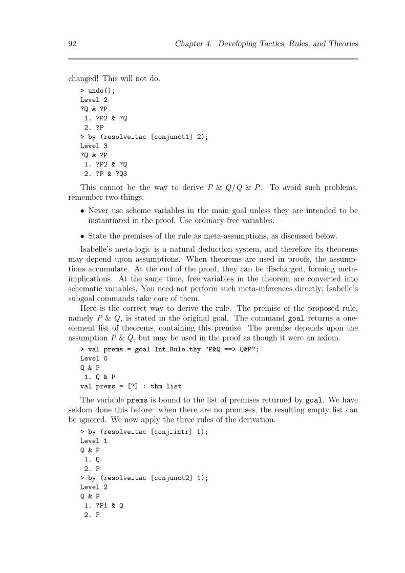
92 Chapter 4. Developing Tactics, Rules, and Theories
changed! This will not do.
> undo();Level 2?Q & ?P1. ?P2 & ?Q2. ?P> by (resolve tac [conjunct1] 2);Level 3?Q & ?P1. ?P2 & ?Q2. ?P & ?Q3
This cannot be the way to derive P & Q/Q & P . To avoid such problems,remember two things:
• Never use scheme variables in the main goal unless they are intended to beinstantiated in the proof. Use ordinary free variables.
• State the premises of the rule as meta-assumptions, as discussed below.
Isabelle’s meta-logic is a natural deduction system, and therefore its theoremsmay depend upon assumptions. When theorems are used in proofs, the assump-tions accumulate. At the end of the proof, they can be discharged, forming meta-implications. At the same time, free variables in the theorem are converted intoschematic variables. You need not perform such meta-inferences directly; Isabelle’ssubgoal commands take care of them.
Here is the correct way to derive the rule. The premise of the proposed rule,namely P & Q , is stated in the original goal. The command goal returns a one-element list of theorems, containing this premise. The premise depends upon theassumption P & Q , but may be used in the proof as though it were an axiom.
> val prems = goal Int Rule.thy "P&Q ==> Q&P";Level 0Q & P1. Q & Pval prems = [?] : thm list
The variable prems is bound to the list of premises returned by goal. We haveseldom done this before: when there are no premises, the resulting empty list canbe ignored. We now apply the three rules of the derivation.
> by (resolve tac [conj intr] 1);Level 1Q & P1. Q2. P> by (resolve tac [conjunct2] 1);Level 2Q & P1. ?P1 & Q2. P
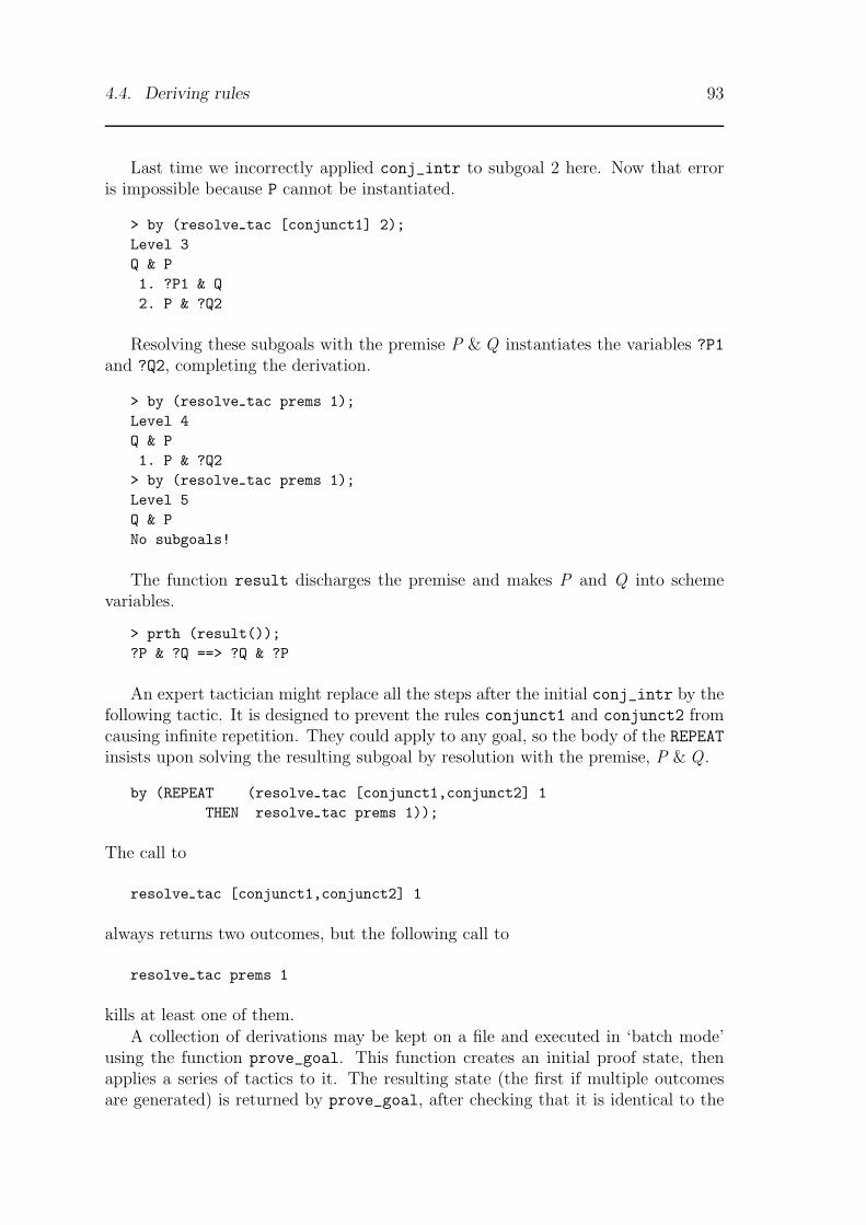
4.4. Deriving rules 93
Last time we incorrectly applied conj_intr to subgoal 2 here. Now that erroris impossible because P cannot be instantiated.
> by (resolve tac [conjunct1] 2);Level 3Q & P1. ?P1 & Q2. P & ?Q2
Resolving these subgoals with the premise P & Q instantiates the variables ?P1and ?Q2, completing the derivation.
> by (resolve tac prems 1);Level 4Q & P1. P & ?Q2
> by (resolve tac prems 1);Level 5Q & PNo subgoals!
The function result discharges the premise and makes P and Q into schemevariables.
> prth (result());?P & ?Q ==> ?Q & ?P
An expert tactician might replace all the steps after the initial conj_intr by thefollowing tactic. It is designed to prevent the rules conjunct1 and conjunct2 fromcausing infinite repetition. They could apply to any goal, so the body of the REPEATinsists upon solving the resulting subgoal by resolution with the premise, P & Q .
by (REPEAT (resolve tac [conjunct1,conjunct2] 1THEN resolve tac prems 1));
The call to
resolve tac [conjunct1,conjunct2] 1
always returns two outcomes, but the following call to
resolve tac prems 1
kills at least one of them.A collection of derivations may be kept on a file and executed in ‘batch mode’
using the function prove_goal. This function creates an initial proof state, thenapplies a series of tactics to it. The resulting state (the first if multiple outcomesare generated) is returned by prove_goal, after checking that it is identical to the
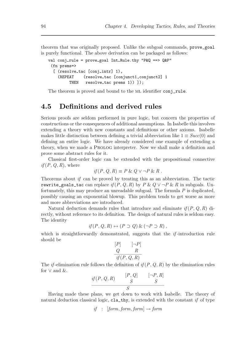
94 Chapter 4. Developing Tactics, Rules, and Theories
theorem that was originally proposed. Unlike the subgoal commands, prove_goalis purely functional. The above derivation can be packaged as follows:
val conj rule = prove goal Int Rule.thy "P&Q ==> Q&P"(fn prems=>[ (resolve tac [conj intr] 1),(REPEAT (resolve tac [conjunct1,conjunct2] 1
THEN resolve tac prems 1)) ]);
The theorem is proved and bound to the ml identifier conj_rule.
4.5 Definitions and derived rules
Serious proofs are seldom performed in pure logic, but concern the properties ofconstructions or the consequences of additional assumptions. In Isabelle this involvesextending a theory with new constants and definitions or other axioms. Isabellemakes little distinction between defining a trivial abbreviation like 1 ≡ Succ(0) anddefining an entire logic. We have already considered one example of extending atheory, when we made a Prolog interpreter. Now we shall make a definition andprove some abstract rules for it.
Classical first-order logic can be extended with the propositional connectiveif (P ,Q ,R), where
if (P ,Q ,R) ≡ P & Q ∨ ¬P & R .
Theorems about if can be proved by treating this as an abbreviation. The tacticrewrite_goals_tac can replace if (P ,Q ,R) by P & Q ∨ ¬P & R in subgoals. Un-fortunately, this may produce an unreadable subgoal. The formula P is duplicated,possibly causing an exponential blowup. This problem tends to get worse as moreand more abbreviations are introduced.
Natural deduction demands rules that introduce and eliminate if (P ,Q ,R) di-rectly, without reference to its definition. The design of natural rules is seldom easy.The identity
if (P ,Q ,R)↔ (P ⊃ Q) & (¬P ⊃ R) ,
which is straightforwardly demonstrated, suggests that the if -introduction ruleshould be
[P ]
Q
[¬P ]
R
if (P ,Q ,R)
The if -elimination rule follows the definition of if (P ,Q ,R) by the elimination rulesfor ∨ and &.
if (P ,Q ,R)[P ,Q ]
S
[¬P ,R]
S
SHaving made these plans, we get down to work with Isabelle. The theory of
natural deduction classical logic, cla_thy, is extended with the constant if of type
if : [form, form, form]→ form

4.5. Definitions and derived rules 95
The axiom if_def equates if (P ,Q ,R) with P & Q ∨ ¬P & R.
> val if thy =# extend theory cla thy "if"# ([], [ (["if"], [Aform,Aform,Aform]--->Aform) ])# [ ("if def", "if(P,Q,R) == P&Q | ~P & R") ];val if thy = ? : theory> val if def = get axiom if thy "if def";val if def = ? : thm
The derivations of the introduction and elimination rules demonstrate the meth-ods for rewriting with definitions. Complicated classical reasoning is involved, butthe tactic Pc.fast_tac is able to cope.
First, the introduction rule. We state it, with its premises P =⇒ Q and ¬P =⇒R, and the goal if (P ,Q ,R). Calling rewrite_goals_tac rewrites occurrences of ifin the subgoals, while leaving the main goal unchanged.
> val prems = goal if thy "[| P ==> Q; ~P ==> R |] ==> if(P,Q,R)";Level 0if(P,Q,R)1. if(P,Q,R)
val prems = [?, ?] : thm list> by (rewrite goals tac [if def]);Level 1if(P,Q,R)1. P & Q | ~P & R
The premises (in the variable prems) are passed to Pc.fast_tac, which usesthem in proving the goal.
> by (Pc.fast tac prems 1);Level 2if(P,Q,R)No subgoals!> val if intr = result();val if intr = ? : thm
Next, we state the elimination rule. It has three premises, two of which arethemselves rules. The conclusion is simply S .
> val prems = goal if thy"[| if(P,Q,R); [| P; Q |] ==> S; [| ~P; R |] ==> S |] ==> S";
# Level 0S1. S
val prems = [?, ?, ?] : thm list
How can we rewrite the occurrences of if in the premises? One way is to incor-porate the premises into the subgoal so that rewrite_goals_tac will work. The
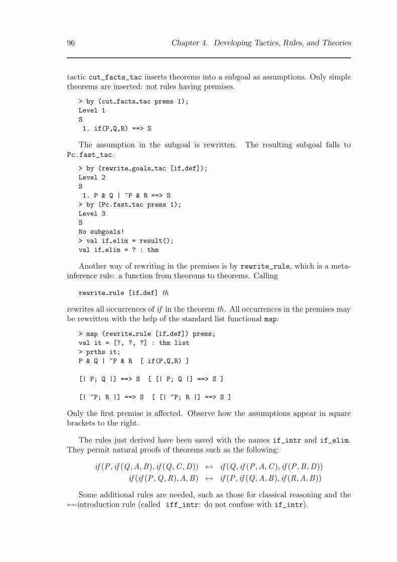
96 Chapter 4. Developing Tactics, Rules, and Theories
tactic cut_facts_tac inserts theorems into a subgoal as assumptions. Only simpletheorems are inserted: not rules having premises.
> by (cut facts tac prems 1);Level 1S1. if(P,Q,R) ==> S
The assumption in the subgoal is rewritten. The resulting subgoal falls toPc.fast_tac.
> by (rewrite goals tac [if def]);Level 2S1. P & Q | ~P & R ==> S> by (Pc.fast tac prems 1);Level 3SNo subgoals!> val if elim = result();val if elim = ? : thm
Another way of rewriting in the premises is by rewrite_rule, which is a meta-inference rule: a function from theorems to theorems. Calling
rewrite rule [if def] th
rewrites all occurrences of if in the theorem th. All occurrences in the premises maybe rewritten with the help of the standard list functional map:
> map (rewrite rule [if def]) prems;val it = [?, ?, ?] : thm list> prths it;P & Q | ~P & R [ if(P,Q,R) ]
[| P; Q |] ==> S [ [| P; Q |] ==> S ]
[| ~P; R |] ==> S [ [| ~P; R |] ==> S ]
Only the first premise is affected. Observe how the assumptions appear in squarebrackets to the right.
The rules just derived have been saved with the names if_intr and if_elim.They permit natural proofs of theorems such as the following:
if (P , if (Q ,A,B), if (Q ,C ,D)) ↔ if (Q , if (P ,A,C ), if (P ,B ,D))
if (if (P ,Q ,R),A,B) ↔ if (P , if (Q ,A,B), if (R,A,B))
Some additional rules are needed, such as those for classical reasoning and the↔-introduction rule (called iff_intr: do not confuse with if_intr).
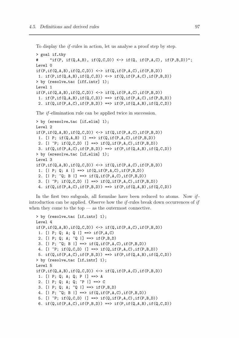
4.5. Definitions and derived rules 97
To display the if -rules in action, let us analyse a proof step by step.
> goal if thy# "if(P, if(Q,A,B), if(Q,C,D)) <-> if(Q, if(P,A,C), if(P,B,D))";Level 0if(P,if(Q,A,B),if(Q,C,D)) <-> if(Q,if(P,A,C),if(P,B,D))1. if(P,if(Q,A,B),if(Q,C,D)) <-> if(Q,if(P,A,C),if(P,B,D))
> by (resolve tac [iff intr] 1);Level 1if(P,if(Q,A,B),if(Q,C,D)) <-> if(Q,if(P,A,C),if(P,B,D))1. if(P,if(Q,A,B),if(Q,C,D)) ==> if(Q,if(P,A,C),if(P,B,D))2. if(Q,if(P,A,C),if(P,B,D)) ==> if(P,if(Q,A,B),if(Q,C,D))
The if -elimination rule can be applied twice in succession.
> by (eresolve tac [if elim] 1);Level 2if(P,if(Q,A,B),if(Q,C,D)) <-> if(Q,if(P,A,C),if(P,B,D))1. [| P; if(Q,A,B) |] ==> if(Q,if(P,A,C),if(P,B,D))2. [| ~P; if(Q,C,D) |] ==> if(Q,if(P,A,C),if(P,B,D))3. if(Q,if(P,A,C),if(P,B,D)) ==> if(P,if(Q,A,B),if(Q,C,D))
> by (eresolve tac [if elim] 1);Level 3if(P,if(Q,A,B),if(Q,C,D)) <-> if(Q,if(P,A,C),if(P,B,D))1. [| P; Q; A |] ==> if(Q,if(P,A,C),if(P,B,D))2. [| P; ~Q; B |] ==> if(Q,if(P,A,C),if(P,B,D))3. [| ~P; if(Q,C,D) |] ==> if(Q,if(P,A,C),if(P,B,D))4. if(Q,if(P,A,C),if(P,B,D)) ==> if(P,if(Q,A,B),if(Q,C,D))
In the first two subgoals, all formulae have been reduced to atoms. Now if -introduction can be applied. Observe how the if -rules break down occurrences of ifwhen they come to the top — as the outermost connective.
> by (resolve tac [if intr] 1);Level 4if(P,if(Q,A,B),if(Q,C,D)) <-> if(Q,if(P,A,C),if(P,B,D))1. [| P; Q; A; Q |] ==> if(P,A,C)2. [| P; Q; A; ~Q |] ==> if(P,B,D)3. [| P; ~Q; B |] ==> if(Q,if(P,A,C),if(P,B,D))4. [| ~P; if(Q,C,D) |] ==> if(Q,if(P,A,C),if(P,B,D))5. if(Q,if(P,A,C),if(P,B,D)) ==> if(P,if(Q,A,B),if(Q,C,D))
> by (resolve tac [if intr] 1);Level 5if(P,if(Q,A,B),if(Q,C,D)) <-> if(Q,if(P,A,C),if(P,B,D))1. [| P; Q; A; Q; P |] ==> A2. [| P; Q; A; Q; ~P |] ==> C3. [| P; Q; A; ~Q |] ==> if(P,B,D)4. [| P; ~Q; B |] ==> if(Q,if(P,A,C),if(P,B,D))5. [| ~P; if(Q,C,D) |] ==> if(Q,if(P,A,C),if(P,B,D))6. if(Q,if(P,A,C),if(P,B,D)) ==> if(P,if(Q,A,B),if(Q,C,D))
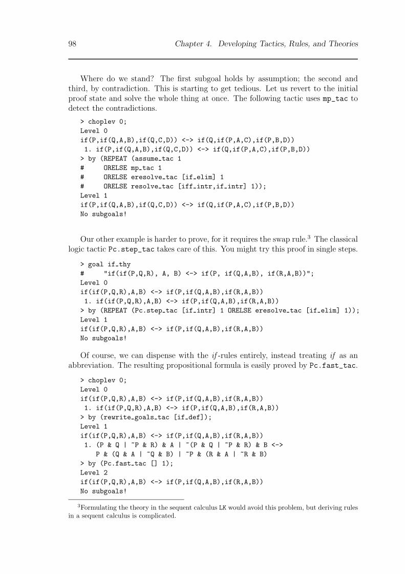
98 Chapter 4. Developing Tactics, Rules, and Theories
Where do we stand? The first subgoal holds by assumption; the second andthird, by contradiction. This is starting to get tedious. Let us revert to the initialproof state and solve the whole thing at once. The following tactic uses mp_tac todetect the contradictions.
> choplev 0;Level 0if(P,if(Q,A,B),if(Q,C,D)) <-> if(Q,if(P,A,C),if(P,B,D))1. if(P,if(Q,A,B),if(Q,C,D)) <-> if(Q,if(P,A,C),if(P,B,D))> by (REPEAT (assume tac 1# ORELSE mp tac 1# ORELSE eresolve tac [if elim] 1# ORELSE resolve tac [iff intr,if intr] 1));Level 1if(P,if(Q,A,B),if(Q,C,D)) <-> if(Q,if(P,A,C),if(P,B,D))No subgoals!
Our other example is harder to prove, for it requires the swap rule.3 The classicallogic tactic Pc.step_tac takes care of this. You might try this proof in single steps.
> goal if thy# "if(if(P,Q,R), A, B) <-> if(P, if(Q,A,B), if(R,A,B))";Level 0if(if(P,Q,R),A,B) <-> if(P,if(Q,A,B),if(R,A,B))1. if(if(P,Q,R),A,B) <-> if(P,if(Q,A,B),if(R,A,B))> by (REPEAT (Pc.step tac [if intr] 1 ORELSE eresolve tac [if elim] 1));Level 1if(if(P,Q,R),A,B) <-> if(P,if(Q,A,B),if(R,A,B))No subgoals!
Of course, we can dispense with the if -rules entirely, instead treating if as anabbreviation. The resulting propositional formula is easily proved by Pc.fast_tac.
> choplev 0;Level 0if(if(P,Q,R),A,B) <-> if(P,if(Q,A,B),if(R,A,B))1. if(if(P,Q,R),A,B) <-> if(P,if(Q,A,B),if(R,A,B))> by (rewrite goals tac [if def]);Level 1if(if(P,Q,R),A,B) <-> if(P,if(Q,A,B),if(R,A,B))1. (P & Q | ~P & R) & A | ~(P & Q | ~P & R) & B <->
P & (Q & A | ~Q & B) | ~P & (R & A | ~R & B)> by (Pc.fast tac [] 1);Level 2if(if(P,Q,R),A,B) <-> if(P,if(Q,A,B),if(R,A,B))No subgoals!
3Formulating the theory in the sequent calculus LK would avoid this problem, but deriving rulesin a sequent calculus is complicated.
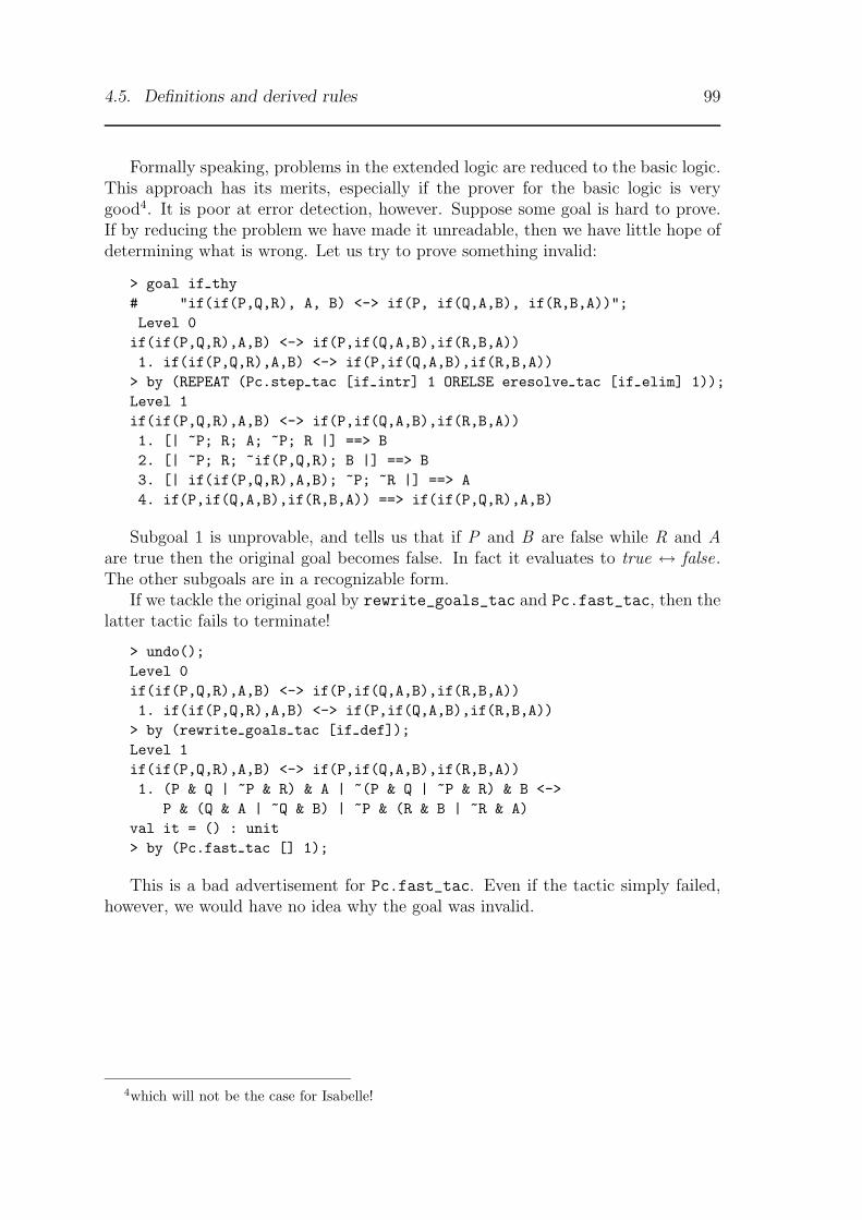
4.5. Definitions and derived rules 99
Formally speaking, problems in the extended logic are reduced to the basic logic.This approach has its merits, especially if the prover for the basic logic is verygood4. It is poor at error detection, however. Suppose some goal is hard to prove.If by reducing the problem we have made it unreadable, then we have little hope ofdetermining what is wrong. Let us try to prove something invalid:
> goal if thy# "if(if(P,Q,R), A, B) <-> if(P, if(Q,A,B), if(R,B,A))";Level 0
if(if(P,Q,R),A,B) <-> if(P,if(Q,A,B),if(R,B,A))1. if(if(P,Q,R),A,B) <-> if(P,if(Q,A,B),if(R,B,A))
> by (REPEAT (Pc.step tac [if intr] 1 ORELSE eresolve tac [if elim] 1));Level 1if(if(P,Q,R),A,B) <-> if(P,if(Q,A,B),if(R,B,A))1. [| ~P; R; A; ~P; R |] ==> B2. [| ~P; R; ~if(P,Q,R); B |] ==> B3. [| if(if(P,Q,R),A,B); ~P; ~R |] ==> A4. if(P,if(Q,A,B),if(R,B,A)) ==> if(if(P,Q,R),A,B)
Subgoal 1 is unprovable, and tells us that if P and B are false while R and Aare true then the original goal becomes false. In fact it evaluates to true ↔ false.The other subgoals are in a recognizable form.
If we tackle the original goal by rewrite_goals_tac and Pc.fast_tac, then thelatter tactic fails to terminate!
> undo();Level 0if(if(P,Q,R),A,B) <-> if(P,if(Q,A,B),if(R,B,A))1. if(if(P,Q,R),A,B) <-> if(P,if(Q,A,B),if(R,B,A))
> by (rewrite goals tac [if def]);Level 1if(if(P,Q,R),A,B) <-> if(P,if(Q,A,B),if(R,B,A))1. (P & Q | ~P & R) & A | ~(P & Q | ~P & R) & B <->
P & (Q & A | ~Q & B) | ~P & (R & B | ~R & A)val it = () : unit> by (Pc.fast tac [] 1);
This is a bad advertisement for Pc.fast_tac. Even if the tactic simply failed,however, we would have no idea why the goal was invalid.
4which will not be the case for Isabelle!

100 Chapter 4. Developing Tactics, Rules, and Theories

Chapter 5
Defining Logics
This chapter is for Isabelle experts only. It explains how to define new logicalsystems, Isabelle’s raison d’etre. In doing so, Isabelle’s internals have to be discussedin a certain amount of detail. Section 5.1 describes the internal representations oftypes and terms, a prerequisite for understanding the rest of the chapter. This isfollowed by sections on how to define hierarchical theories, on the precise definitionof the meta-logic’s syntax, and on how to specify a concrete syntax and a prettyprinter for some new object-logic. Section 5.6 shows how all this fits together bygiving some simple examples of complete logic definitions.
5.1 Types and terms
Isabelle is based on the idea that proofs in many logics can be naturally representedin intuitionistic higher-order logic [9], henceforth called the meta-logic. In Isabelle,like in higher-order logic, the terms are those of the typed λ-calculus. Types andterms are represented by the ml types typ and term.
5.1.1 The ml type typ
Every term has a type. The type typ is defined as follows:
infixr 5 -->;datatype typ = Ground of string
| Poly of string| op --> of typ * typ;
A ground type has a name, represented by a string, as does a polymorphic type(or type variable). A function type has the form S-->T. Two types are equal if theyhave identical structure: ml’s equality test is correct for types.
A term of type S-->T denotes a function: if applied to a term of type S, theresulting term has type T. A term should obey the type-checking rules of the typedλ-calculus. It is possible to construct ill-typed terms, but the meta-rules ensure thatall terms in theorems are well-typed.
Functions of several arguments are expressed by currying. The operator -->
associates to the right, so
101

102 Chapter 5. Defining Logics
S1-->(S2-->(S3-->T))
can be written S1-->S2-->S3-->T. There is an ml operator ---> for writing thisas [S1,S2,S3]--->T.
Example: suppose that f has type S-->T-->S, where S and T are distinct types, ahas type S, and b has type T. Then f(a) has type T-->S and f(a,b) has type S, whilef(b), f(a,a), and f(a,b,a) are ill-typed. Note that f(a,b) means (f(a))(b).
Type variables (Poly) permit ml-style type inference (see Section 5.5). Theyare used only internally and may not appear in theorems. A typed object-logic canbe represented by making the object-level typing rules explicit. See the section onConstructive Type Theory, which is the ultimate example of a typed logic.
5.1.2 The ml type term
There are six kinds of term.
type indexname = string * int;
infix 9 $;datatype term = Const of string * typ
| Free of string * typ| Var of indexname * typ| Bound of int| Abs of string * typ * term| op $ of term * term;
A constant has a name and a type. Constants include connectives like ∧ and∀ (logical constants), as well as constants like 0 and succ. Other constants may berequired to define the concrete syntax of a logic.
A free variable (or Free) has a name and a type.A scheme variable (or Var) has an indexname and a type, where an indexname
is a string paired with a non-negative index. A Var is logically the same as afree variable. It stands for a variable that may be instantiated during unification.The Vars in a term can be systematically renamed by incrementing the indices. InProlog jargon these are ‘logical variables’ and they may be ‘standardized apart’.
A bound variable has no name, only a number: de Bruijn’s representation [1]. Thenumber counts the number of lambdas, starting from zero, between an occurrenceof the variable and the lambda that binds it. The representation prevents captureof bound variables, allowing a simple and quick substitution function. The type ofa bound variable is stored with its binding lambda (an Abs node). For more infor-mation see de Bruijn [1] or look at the functions incr_boundvars, subst_bounds,aconv.
An abstraction stores the name and type of its bound variable, and its body.The name is used only for parsing and printing; it has no logical significance.
An application consists of a term applied to another term. The constructor isthe infix $, so the ml expression t$u constructs the application of t to u.

5.2. Theories 103
5.2 Theories
Isabelle logics are hierarchies of theories. Each theory consists of a signature andinference rules. Signatures describe the syntax of a logic, both abstract and concrete.The definition of the concrete syntax is described in great detail in Section 5.4. Forthis section let us assume the following ml type abbreviations:
type sorts = string list;type ops = (string list * typ) list;type rules = (string * string) list;
The types sorts and ops describe the abstract syntax and corresponds to a signaturein universal algebra: sorts is the list of all type names, ops the list of all typedconstants that are declared in a theory.
Example 5.1 The abstract syntax defined by isorts and iops introduces the twotype names "int" and "form", two binary operations "+" and "-" on "int", anda binary function "=" from "int" to "form".
val Tint = Ground "int";val Tform = Ground "form";val isorts = ["int", "form"];val iops = [(["+", "-"], [Tint,Tint] ---> Tint),
(["="], [Tint,Tint] ---> Tform)];
The Isabelle equivalent of abstract syntax trees is the type term. An abstract syntaxdetermines which terms are valid and which are not: all constants and ground typesmust have been declared and the whole term must be type correct. In the contextof the above example,
Const("+",[Tint,Tint] ---> Tint) $ Free("x",Tint)
is a valid term of typ Tint --> Tint.The names and types of the constants "+", "-", and "=" suggest they represent
addition, subtraction, and equality respectively. However, we could have used ar-bitrary strings since there is no a priori connection between abstract and concretesyntax, with one exception: if the name of a constant is an identifier (as opposed toan arbitrary string), any occurrence of that identifier in an input string is treatedas that constant; no special concrete syntax is necessary. The parser does not evenknow about these identifiers and their types. For that reason, it ignores type in-formation completely: the dummy typ Adummy is used by the parser in all terms itgenerates. The real types are inferred at a later stage (see Section 5.5).
Many Isabelle users will never need to know about internal concepts like typesand constants because they think in terms of the external representation determinedby the concrete syntax associated with a theory.
The ml type rules is a list of pairs of rule names and rules, for example
val irls = [("+-comm", "x+y = y+x"), ("?" "x-x = x")];
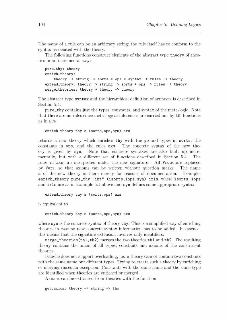
104 Chapter 5. Defining Logics
The name of a rule can be an arbitrary string; the rule itself has to conform to thesyntax associated with the theory.
The following functions construct elements of the abstract type theory of theo-ries in an incremental way:
pure thy: theoryenrich theory:
theory -> string -> sorts * ops * syntax -> rules -> theoryextend theory: theory -> string -> sorts * ops -> rules -> theorymerge theories: theory * theory -> theory
The abstract type syntax and the hierarchical definition of syntaxes is described inSection 5.4.
pure_thy contains just the types, constants, and syntax of the meta-logic. Notethat there are no rules since meta-logical inferences are carried out by ml functionsas in lcf.
enrich theory thy s (sorts,ops,syn) axs
returns a new theory which enriches thy with the ground types in sorts, theconstants in ops, and the rules axs. The concrete syntax of the new the-ory is given by syn. Note that concrete syntaxes are also built up incre-mentally, but with a different set of functions described in Section 5.4. Therules in axs are interpreted under the new signature. All Frees are replacedby Vars, so that axioms can be written without question marks. The names of the new theory is there merely for reasons of documentation. Example:enrich_theory pure_thy "int" (isorts,iops,syn) irls, where isorts, iopsand irls are as in Example 5.1 above and syn defines some appropriate syntax.
extend theory thy s (sorts,ops) axs
is equivalent to
enrich theory thy s (sorts,ops,syn) axs
where syn is the concrete syntax of theory thy. This is a simplified way of enrichingtheories in case no new concrete syntax information has to be added. In essence,this means that the signature extension involves only identifiers.
merge_theories(th1,th2) merges the two theories th1 and th2. The resultingtheory contains the union of all types, constants and axioms of the constituenttheories.
Isabelle does not support overloading, i.e. a theory cannot contain two constantswith the same name but different types. Trying to create such a theory by enrichingor merging raises an exception. Constants with the same name and the same typeare identified when theories are enriched or merged.
Axioms can be extracted from theories with the function
get axiom: theory -> string -> thm
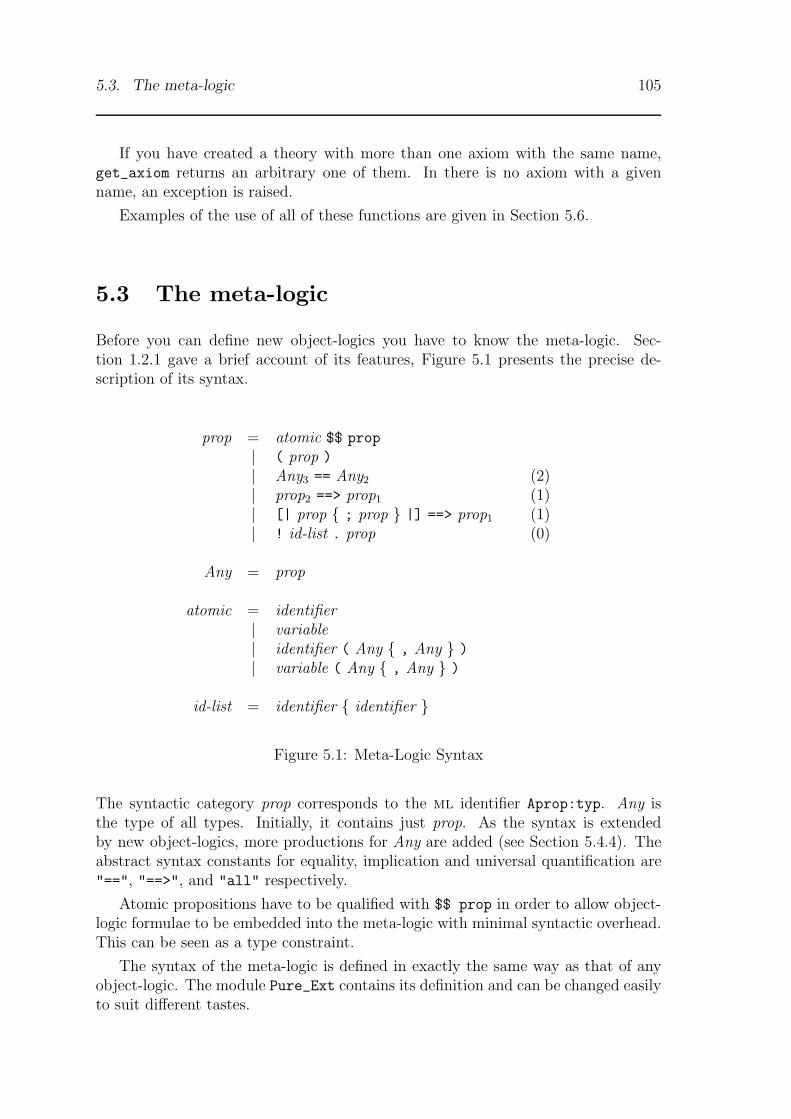
5.3. The meta-logic 105
If you have created a theory with more than one axiom with the same name,get_axiom returns an arbitrary one of them. In there is no axiom with a givenname, an exception is raised.
Examples of the use of all of these functions are given in Section 5.6.
5.3 The meta-logic
Before you can define new object-logics you have to know the meta-logic. Sec-tion 1.2.1 gave a brief account of its features, Figure 5.1 presents the precise de-scription of its syntax.
prop = atomic $$ prop
| ( prop )
| Any3 == Any2 (2)| prop2 ==> prop1 (1)| [| prop { ; prop } |] ==> prop1 (1)| ! id-list . prop (0)
Any = prop
atomic = identifier| variable| identifier ( Any { , Any } )| variable ( Any { , Any } )
id-list = identifier { identifier }
Figure 5.1: Meta-Logic Syntax
The syntactic category prop corresponds to the ml identifier Aprop:typ. Any isthe type of all types. Initially, it contains just prop. As the syntax is extendedby new object-logics, more productions for Any are added (see Section 5.4.4). Theabstract syntax constants for equality, implication and universal quantification are"==", "==>", and "all" respectively.
Atomic propositions have to be qualified with $$ prop in order to allow object-logic formulae to be embedded into the meta-logic with minimal syntactic overhead.This can be seen as a type constraint.
The syntax of the meta-logic is defined in exactly the same way as that of anyobject-logic. The module Pure_Ext contains its definition and can be changed easilyto suit different tastes.
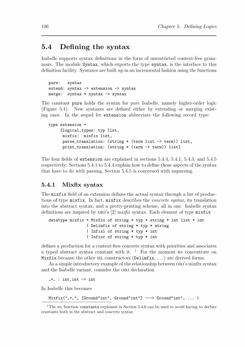
106 Chapter 5. Defining Logics
5.4 Defining the syntax
Isabelle supports syntax definitions in the form of unrestricted context-free gram-mars. The module Syntax, which exports the type syntax, is the interface to thisdefinition facility. Syntaxes are built up in an incremental fashion using the functions
pure: syntaxextend: syntax -> extension -> syntaxmerge: syntax * syntax -> syntax
The constant pure holds the syntax for pure Isabelle, namely higher-order logic(Figure 5.1). New syntaxes are defined either by extending or merging exist-ing ones. In the sequel let extension abbreviate the following record type:
type extension ={logical_types: typ list,mixfix: mixfix list,parse_translation: (string * (term list -> term)) list,print_translation: (string * (term -> term)) list}
The four fields of extension are explained in sections 5.4.4, 5.4.1, 5.4.3, and 5.4.5respectively. Sections 5.4.1 to 5.4.4 explain how to define those aspects of the syntaxthat have to do with parsing, Section 5.4.5 is concerned with unparsing.
5.4.1 Mixfix syntax
The mixfix field of an extension defines the actual syntax through a list of produc-tions of type mixfix. In fact, mixfix describes the concrete syntax, its translationinto the abstract syntax, and a pretty-printing scheme, all in one. Isabelle syntaxdefinitions are inspired by obj’s [2] mixfix syntax. Each element of type mixfix
datatype mixfix = Mixfix of string * typ * string * int list * int| Delimfix of string * typ * string| Infixl of string * typ * int| Infixr of string * typ * int
defines a production for a context-free concrete syntax with priorities and associatesa typed abstract syntax constant with it. 1 For the moment we concentrate onMixfix because the other ml constructors (Delimfix, . . . ) are derived forms.
As a simple introductory example of the relationship between obj’s mixfix syntaxand the Isabelle variant, consider the obj declaration
+ : int,int -> int
In Isabelle this becomes
Mixfix(" + ", [Ground"int", Ground"int"] ---> Ground"int", ... )
1The ml function constants explained in Section 5.4.6 can be used to avoid having to declareconstants both in the abstract and concrete syntax
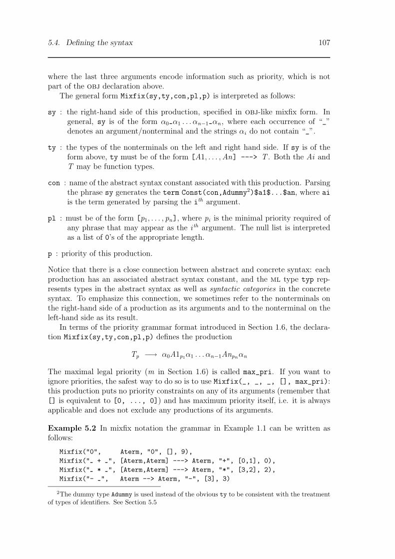
5.4. Defining the syntax 107
where the last three arguments encode information such as priority, which is notpart of the obj declaration above.
The general form Mixfix(sy,ty,con,pl,p) is interpreted as follows:
sy : the right-hand side of this production, specified in obj-like mixfix form. Ingeneral, sy is of the form α0 α1 . . . αn−1 αn , where each occurrence of “_”denotes an argument/nonterminal and the strings αi do not contain “_”.
ty : the types of the nonterminals on the left and right hand side. If sy is of theform above, ty must be of the form [A1, . . . ,An] ---> T . Both the Ai andT may be function types.
con : name of the abstract syntax constant associated with this production. Parsingthe phrase sy generates the term Const(con,Adummy2)$a1$...$an, where ai
is the term generated by parsing the ith argument.
pl : must be of the form [p1, . . . , pn], where pi is the minimal priority required ofany phrase that may appear as the i th argument. The null list is interpretedas a list of 0’s of the appropriate length.
p : priority of this production.
Notice that there is a close connection between abstract and concrete syntax: eachproduction has an associated abstract syntax constant, and the ml type typ rep-resents types in the abstract syntax as well as syntactic categories in the concretesyntax. To emphasize this connection, we sometimes refer to the nonterminals onthe right-hand side of a production as its arguments and to the nonterminal on theleft-hand side as its result.
In terms of the priority grammar format introduced in Section 1.6, the declara-tion Mixfix(sy,ty,con,pl,p) defines the production
Tp −→ α0A1p1α1 . . . αn−1Anpnαn
The maximal legal priority (m in Section 1.6) is called max_pri. If you want toignore priorities, the safest way to do so is to use Mixfix(_, _, _, [], max_pri):this production puts no priority constraints on any of its arguments (remember that[] is equivalent to [0, ..., 0]) and has maximum priority itself, i.e. it is alwaysapplicable and does not exclude any productions of its arguments.
Example 5.2 In mixfix notation the grammar in Example 1.1 can be written asfollows:
Mixfix("0", Aterm, "0", [], 9),Mixfix(" + ", [Aterm,Aterm] ---> Aterm, "+", [0,1], 0),Mixfix(" * ", [Aterm,Aterm] ---> Aterm, "*", [3,2], 2),Mixfix("- ", Aterm --> Aterm, "-", [3], 3)
2The dummy type Adummy is used instead of the obvious ty to be consistent with the treatmentof types of identifiers. See Section 5.5
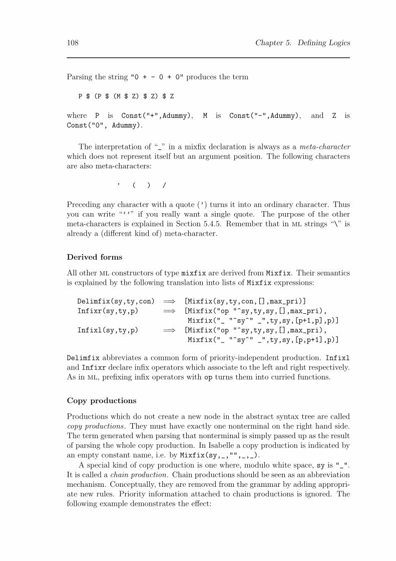
108 Chapter 5. Defining Logics
Parsing the string "0 + - 0 + 0" produces the term
P $ (P $ (M $ Z) $ Z) $ Z
where P is Const("+",Adummy), M is Const("-",Adummy), and Z isConst("0", Adummy).
The interpretation of “_” in a mixfix declaration is always as a meta-characterwhich does not represent itself but an argument position. The following charactersare also meta-characters:
’ ( ) /
Preceding any character with a quote (’) turns it into an ordinary character. Thusyou can write “’’” if you really want a single quote. The purpose of the othermeta-characters is explained in Section 5.4.5. Remember that in ml strings “\” isalready a (different kind of) meta-character.
Derived forms
All other ml constructors of type mixfix are derived from Mixfix. Their semanticsis explained by the following translation into lists of Mixfix expressions:
Delimfix(sy,ty,con) =⇒ [Mixfix(sy,ty,con,[],max_pri)]
Infixr(sy,ty,p) =⇒ [Mixfix("op "^sy,ty,sy,[],max_pri),
Mixfix("_ "^sy^" _",ty,sy,[p+1,p],p)]
Infixl(sy,ty,p) =⇒ [Mixfix("op "^sy,ty,sy,[],max_pri),
Mixfix("_ "^sy^" _",ty,sy,[p,p+1],p)]
Delimfix abbreviates a common form of priority-independent production. Infixl
and Infixr declare infix operators which associate to the left and right respectively.As in ml, prefixing infix operators with op turns them into curried functions.
Copy productions
Productions which do not create a new node in the abstract syntax tree are calledcopy productions . They must have exactly one nonterminal on the right hand side.The term generated when parsing that nonterminal is simply passed up as the resultof parsing the whole copy production. In Isabelle a copy production is indicated byan empty constant name, i.e. by Mixfix(sy,_,"",_,_).
A special kind of copy production is one where, modulo white space, sy is "_".It is called a chain production. Chain productions should be seen as an abbreviationmechanism. Conceptually, they are removed from the grammar by adding appropri-ate new rules. Priority information attached to chain productions is ignored. Thefollowing example demonstrates the effect:
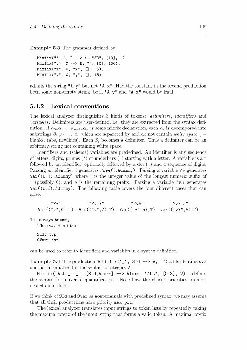
5.4. Defining the syntax 109
Example 5.3 The grammar defined by
Mixfix("A ", B --> A, "AB", [10], ),Mixfix(" ", C --> B, "", [0], 100),Mixfix("x", C, "x", [], 5),Mixfix("y", C, "y", [], 15)
admits the string "A y" but not "A x". Had the constant in the second productionbeen some non-empty string, both "A y" and "A x" would be legal.
5.4.2 Lexical conventions
The lexical analyzer distinguishes 3 kinds of tokens: delimiters , identifiers andvariables . Delimiters are user-defined, i.e. they are extracted from the syntax defi-nition. If α0 α1 . . . αn−1 αn is some mixfix declaration, each αi is decomposed intosubstrings β1 β2 . . . βk which are separated by and do not contain white space ( =blanks, tabs, newlines). Each βj becomes a delimiter. Thus a delimiter can be anarbitrary string not containing white space.
Identifiers and (scheme) variables are predefined. An identifier is any sequenceof letters, digits, primes (’) or underbars (_) starting with a letter. A variable is a ?
followed by an identifier, optionally followed by a dot (.) and a sequence of digits.Parsing an identifier i generates Free(i,Adummy). Parsing a variable ?v generatesVar((u,i),Adummy) where i is the integer value of the longest numeric suffix ofv (possibly 0), and u is the remaining prefix. Parsing a variable ?v .i generatesVar((v,i),Adummy). The following table covers the four different cases that canarise:
"?v" "?v.7" "?v5" "?v7.5"
Var(("v",0),T) Var(("v",7),T) Var(("v",5),T) Var(("v7",5),T)
T is always Adummy.The two identifiers
SId: typSVar: typ
can be used to refer to identifiers and variables in a syntax definition.
Example 5.4 The production Delimfix("_", SId --> A, "") adds identifiers asanother alternative for the syntactic category A.
Mixfix("ALL _. _", [SId,Aform] --> Aform, "ALL", [0,3], 2) definesthe syntax for universal quantification. Note how the chosen priorities prohibitnested quantifiers.
If we think of SId and SVar as nonterminals with predefined syntax, we may assumethat all their productions have priority max_pri.
The lexical analyzer translates input strings to token lists by repeatedly takingthe maximal prefix of the input string that forms a valid token. A maximal prefix

110 Chapter 5. Defining Logics
that is both a delimiter and an identifier or variable (like "ALL") is treated as adelimiter. White spaces are separators.
An important consequence of this translation scheme is that delimiters need notbe separated by white space to be recognized as separate. If "-" is a delimiter but"--" is not, the string "--" is treated as two consecutive occurrences of "-". Thisis in contrast to ml which would treat "--" as a single (undeclared) identifier. Theconsequence of Isabelle’s more liberal scheme is that the same string may be parsedin a different way after extending the syntax: after adding "--" as a delimiter, theinput "--" is treated as a single occurrence of "--".
5.4.3 Parse translations
So far we have pretended that there is a close enough relationship between concreteand abstract syntax to allow an automatic translation from one to the other usingthe constant names supplied with each production. In many cases this scheme isnot powerful enough, especially for constructs involving variable bindings. Thereforeeach extension can associate a user-defined translation function with a constantname via the parse_translation field of type
(string * (term list -> term)) list
After the input string has been translated into a term according to the syntax defini-tion, there is a second phase in which the term is translated using the user-suppliedfunctions. Given a list tab of the above type, a term t is translated as follows. If t isnot of the form Const(s,T)$t1$...$tn, then t is returned unchanged. Otherwiseall ti are translated into ti’. Let t’ = Const(s,T)$t1’$...$tn’. If there is nopair (s,f) in tab, return t’. Otherwise apply f to [t1’,...,tn’]. If that raisesan exception, return t’, otherwise return the result.
Example 5.5 Isabelle represents the phrase ∀x .P(x ) internally by ∀(λx .P(x )),where ∀ is a constant of type (term → form) → form. Assuming that term andform are represented by the typs Aterm and Aform, the concrete syntax can be givenas
Mixfix("ALL . ", ALLt, "ALL", , )
where ALLt is [SId,Aform] ---> Aform. Parsing "ALL x. ..." according tothis syntax yields the term Const("ALL",Adummy)$Free("x",Adummy)$t, wheret is the body of the quantified formula. What we need is the termConst("All",Adummy)$Abs("x",Adummy,t’), where "All" is an abstract syntaxconstant of type (Aterm --> Aform) --> Aform and t’ is some “abstracted” ver-sion of t. Therefore we define a function
fun ALLtr[Free(s,T), t] = Const("All", Adummy) $Abs(s, T, abstract over(Free(s,T), t));
and associate it with "ALL" in this fragment of syntax extension:
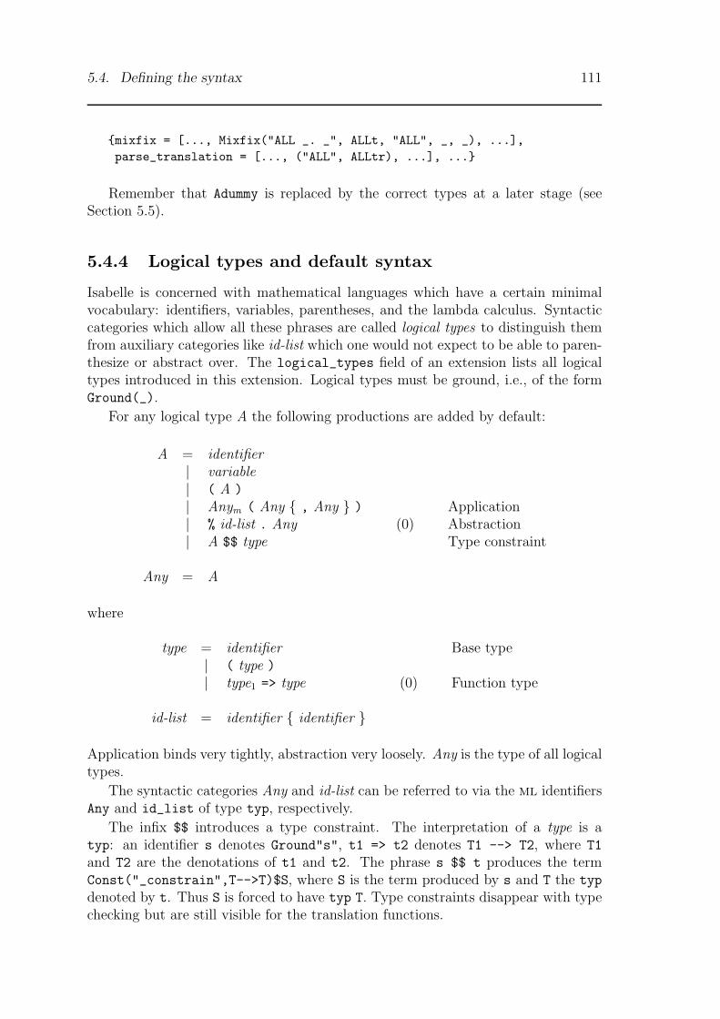
5.4. Defining the syntax 111
{mixfix = [..., Mixfix("ALL _. _", ALLt, "ALL", _, _), ...],parse_translation = [..., ("ALL", ALLtr), ...], ...}
Remember that Adummy is replaced by the correct types at a later stage (seeSection 5.5).
5.4.4 Logical types and default syntax
Isabelle is concerned with mathematical languages which have a certain minimalvocabulary: identifiers, variables, parentheses, and the lambda calculus. Syntacticcategories which allow all these phrases are called logical types to distinguish themfrom auxiliary categories like id-list which one would not expect to be able to paren-thesize or abstract over. The logical_types field of an extension lists all logicaltypes introduced in this extension. Logical types must be ground, i.e., of the formGround(_).
For any logical type A the following productions are added by default:
A = identifier| variable| ( A )
| Anym ( Any { , Any } ) Application| % id-list . Any (0) Abstraction| A $$ type Type constraint
Any = A
where
type = identifier Base type| ( type )
| type1 => type (0) Function type
id-list = identifier { identifier }
Application binds very tightly, abstraction very loosely. Any is the type of all logicaltypes.
The syntactic categories Any and id-list can be referred to via the ml identifiersAny and id_list of type typ, respectively.
The infix $$ introduces a type constraint. The interpretation of a type is atyp: an identifier s denotes Ground"s", t1 => t2 denotes T1 --> T2, where T1
and T2 are the denotations of t1 and t2. The phrase s $$ t produces the termConst("_constrain",T-->T)$S, where S is the term produced by s and T the typ
denoted by t. Thus S is forced to have typ T. Type constraints disappear with typechecking but are still visible for the translation functions.

112 Chapter 5. Defining Logics
5.4.5 Printing
Syntax definitions provide printing information in three distinct ways: through
• the syntax of the language (as used for parsing),
• pretty printing information, and
• print translation functions.
The bare mixfix declarations enable Isabelle to print terms, but the result will notnecessarily be pretty and may look different from what you expected. To produce apleasing layout, you need to read the following sections.
Printing with mixfix declarations
Let t = Const(s,_)$t1$...$tn be a term and M = Mixfix(sy,_,s,_,_) be amixfix declaration where sy is of the form α0 α1 . . . αn−1 αn . Printing t accordingto M means printing the string α0β1α1 . . . αn−1βnαn , where βi is the result of printingti.
Note that the system does not insert blanks. They should be part of the mixfixsyntax if they are required to separate tokens or achieve a certain layout.
Pretty printing
In order to format the output, it is possible to include pretty printing directions aspart of the mixfix syntax definition. Of course these directions are ignored duringparsing and affect only printing. The characters “(”, “)”, and “/” are interpretedas meta-characters when found in a mixfix definition. Their meaning is
( Open a block. A sequence of digits following it is interpreted as the indentationof this block. It causes the output to be indented by n positions if a line breakoccurs within the block. If “(” is not followed by a digit, the indentationdefaults to 0.
) Close a block.
/ Allow a line break. White spaces immediately following “/” are not printed ifthe line is broken at this point.
Print translations
Since terms can be subject to a translation after parsing (see Section 5.4.3), thereis a similar mechanism to translate them back before printing. Therefore eachextension can associate a user-defined translation function with a constant namevia its print_translation field of type
(string * (term -> term)) list
Including a pair (s,f) results in f being applied to any term with head Const(s,_)
before printing it.
5.4. Defining the syntax 113
Example 5.6 In Example 5.5 we showed how to translate the concrete syntax foruniversal quantification into the proper internal form. The string "ALL x. ..."
now parses as Const("All", _)$Abs("x", _, _). If, however, the latter term isprinted without translating it back, it would result in "All(%x. ...)". Thereforethe abstraction has to be turned back into a term that matches the concrete mixfixsyntax:
fun Alltr( $ Abs(id,T,P)) =let val (id’,P’) = variant abs(id,T,P)in Const("ALL",ALLt) $ Free(id’,T) $ P’ end;
The function variant_abs, a basic term manipulation function, replaces the boundvariable id by a Free variable id’ having a unique name. A term produced byAlltr can now be printed according to the concrete syntax
Mixfix("ALL . ", ALLt, "ALL", , ).
Notice that the application of Alltr fails if the second component of the argu-ment is not an abstraction, but for example just a Free variable. This is intentionalbecause it signals to the caller that the intended translation is inapplicable.
The syntax extension, including concrete syntax and both translation functions,would have the following form:
{mixfix = [..., Mixfix("ALL _. _", ALLt, "ALL", _, _), ...],parse_translation = [..., ("ALL", ALLtr), ...],print_translation = [..., ("All", Alltr), ...], ...}
As during the parse translation process, the types attached to variables or con-stants during print translation are immaterial because printing is insensitive to types.This means that in the definition of function Alltr above, we could have writtenConst("ALL",Adummy) $ Free(id’,Adummy).
Printing a term
Let G be the set of all Mixfix declarations and T the set of all string-function pairsof print translations in the current syntax.
Terms are printed recursively.
• Free(s,_) is printed as s.
• Var((s,i),_) is printed as s, if i = 0 and s does not end with a digit, as s
followed by i, if i 6= 0 and s does not end with a digit, and as s.i, if s endswith a digit. Thus the following cases can arise:
Var(("v",0),_) Var(("v",7),_) Var(("v5",0),_)
"?v" "?v7" "?v5.0"
• Abs(x,_,Abs(y,_,...Abs(z,_,b)...), where b is not an abstraction, isprinted as %u v ... w. t, where t is the result of printing b, and x, y and z
are replaced by u, v and w. The latter are new unique names.
114 Chapter 5. Defining Logics
• Bound(i) is printed as B.i 3 .
• The application t = Const(s,_)$t1$...$tn (where n may be 0!) is printedas follows:
If there is a pair (s,f) in T , print f(t). If this application raises an ex-ception or there is no pair (s,f) in T , let S be the set of sy such thatMixfix(sy,_,s,_,_) is in G . If S is empty, t is printed as an application.Otherwise let sy’ ∈ S be a mixfix declaration with the maximal number ofnonterminals, n. If sy’ has n arguments, print t according to sy’, otherwiseprint it as an application.
All other applications are printed as applications.
Printing a term c$t1$...$tn as an application means printing it as s(s1,...,sn),where si is the result of printing ti. If c is a Const, s is its first argument. Otherterms c are printed as described above.
The printer also inserts parentheses where they are necessary for reasons ofpriority.
5.4.6 Miscellaneous
In addition to the ml identifiers introduced so far, the syntax module provides thefollowing functions:
read: syntax -> typ -> string -> term
Calling read sy t s parses s as a term of type t according to syntax sy. Validtypes are Aprop, Any, all logical types (see Section 5.4.4), and all function types. Ifthe input does not conform to the syntax, an error message is printed and exceptionERROR is raised.
prin: syntax -> term -> unitprint top level: syntax -> term -> unit
Calling prin sy tm performs the inverse translation: it prints the term tm accordingto syntax sy. print_top_level is like prin, except that the output is written on aseparate line.
print syntax: syntax -> unit
prints a syntax in some readable format.
constants: mixfix list -> (string list * typ) list
Calling constants(ml) builds a list of all pairs ([s],T) such thatMixfix(_,T,s,_,_), Delimfix(_,T,s), Infixl(s,T), or Infixr(s,T) is in ml.
3The occurrence of such “loose” bound variables indicates that either you are trying to print asubterm of an abstraction, or there is something wrong with your print translations.
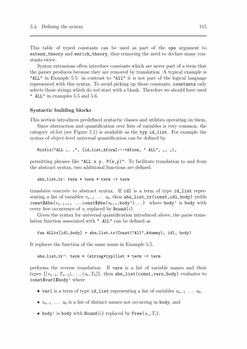
5.4. Defining the syntax 115
This table of typed constants can be used as part of the ops argument toextend_theory and enrich_theory, thus removing the need to declare many con-stants twice.
Syntax extensions often introduce constants which are never part of a term thatthe parser produces because they are removed by translation. A typical example is"ALL" in Example 5.5: in contrast to "All" it is not part of the logical languagerepresented with this syntax. To avoid picking up those constants, constants onlyselects those strings which do not start with a blank. Therefore we should have used" ALL" in examples 5.5 and 5.6.
Syntactic building blocks
This section introduces predefined syntactic classes and utilities operating on them.Since abstraction and quantification over lists of variables is very common, the
category id-list (see Figure 5.1) is available as the typ id_list. For example thesyntax of object-level universal quantification can be defined by
Mixfix("ALL . ", [id list,Aform]--->Aform, " ALL", , ),
permitting phrases like "ALL x y. P(x,y)". To facilitate translation to and fromthe abstract syntax, two additional functions are defined.
abs list tr: term * term * term -> term
translates concrete to abstract syntax. If idl is a term of type id_list repre-senting a list of variables vn−1 . . . v0, then abs_list_tr(const,idl,body) yieldsconst$Abs(vn−1, , ...const$Abs(v0, ,body’)...) where body’ is body withevery free occurrence of vi replaced by Bound(i).
Given the syntax for universal quantification introduced above, the parse trans-lation function associated with " ALL" can be defined as
fun ALLtr[idl,body] = abs list tr(Const("All",Adummy), idl, body)
It replaces the function of the same name in Example 5.5.
abs list tr’: term * (string*typ)list * term -> term
performs the reverse translation. If vars is a list of variable names and theirtypes [(vn−1,Tn−1), . . . , (v0,T0)], then abs_list(const,vars,body) evaluates toconst$varl$body’ where
• varl is a term of type id_list representing a list of variables un−1 . . . u0,
• un−1 . . . u0 is a list of distinct names not occurring in body, and
• body’ is body with Bound(i) replaced by Free(ui,Ti).
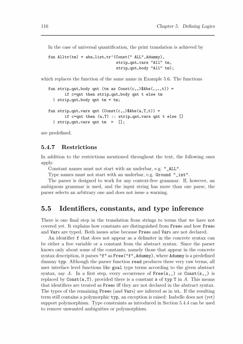
116 Chapter 5. Defining Logics
In the case of universal quantification, the print translation is achieved by
fun Alltr(tm) = abs list tr’(Const(" ALL",Adummy),strip qnt vars "All" tm,strip qnt body "All" tm);
which replaces the function of the same name in Example 5.6. The functions
fun strip qnt body qnt (tm as Const(c, )$Abs( , ,t)) =if c=qnt then strip qnt body qnt t else tm
| strip qnt body qnt tm = tm;
fun strip qnt vars qnt (Const(c, )$Abs(a,T,t)) =if c=qnt then (a,T) :: strip qnt vars qnt t else []
| strip qnt vars qnt tm = [];
are predefined.
5.4.7 Restrictions
In addition to the restrictions mentioned throughout the text, the following onesapply.
Constant names must not start with an underbar, e.g. "_ALL".Type names must not start with an underbar, e.g. Ground "_int".The parser is designed to work for any context-free grammar. If, however, an
ambiguous grammar is used, and the input string has more than one parse, theparser selects an arbitrary one and does not issue a warning.
5.5 Identifiers, constants, and type inference
There is one final step in the translation from strings to terms that we have notcovered yet. It explains how constants are distinguished from Frees and how Freesand Vars are typed. Both issues arise because Frees and Vars are not declared.
An identifier f that does not appear as a delimiter in the concrete syntax canbe either a free variable or a constant from the abstract syntax. Since the parserknows only about some of the constants, namely those that appear in the concretesyntax description, it parses "f" as Free("f",Adummy), where Adummy is a predefineddummy typ. Although the parser function read produces these very raw terms, alluser interface level functions like goal type terms according to the given abstractsyntax, say A. In a first step, every occurrence of Free(s,_) or Const(s,_) isreplaced by Const(s,T), provided there is a constant s of typ T in A. This meansthat identifiers are treated as Frees iff they are not declared in the abstract syntax.The types of the remaining Frees (and Vars) are inferred as in ml. If the resultingterm still contains a polymorphic typ, an exception is raised: Isabelle does not (yet)support polymorphism. Type constraints as introduced in Section 5.4.4 can be usedto remove unwanted ambiguities or polymorphism.

5.6. Putting it all together 117
One peculiarity of the current type inference algorithm is that variables with thesame name must have the same type, irrespective of whether they are free or bound.For example, take the first-order formula f (x ) = x ∧ (∀f . f = f ) where the constants= and ∀ have type term → term → form and (term → form) → form. The firstconjunct forces x : term and f : term → term, the second one f : term. Althoughthe two f ’s are distinct, they are required to have the same type, thus leading to atype clash in the above formula.
5.6 Putting it all together
Having discussed the individual building blocks of a logic definition, it remains to beshown how they fit together. In particular we need to say how an object-logic syntaxis hooked up to the meta-logic. Since all theorems must conform to the syntax forprop (see Figure 5.1), that syntax has to be extended with the object-level syntax.Assume that the syntax of your object-logic defines a category form of formulae.These formulae can now appear in axioms and theorems wherever prop does if youadd the production
prop = form.
More precisely, you need a coercion from formulae to propositions:
Mixfix(" ", Aform --> Aprop, "Prop", [0], 5)
The constant "Prop" (the name is arbitrary) acts as an invisible coercion function.
One of the simplest nontrivial logics is minimal logic of implication. Its definitionin Isabelle needs no advanced features but illustrates the overall mechanism quitenicely:
val Aform = Ground "form";val mixfix = [Mixfix("_", Aform --> Aprop, "Prop", [], 5),
Infixr("-->", [Aform,Aform]--->Aform, 10)];val impl_syn = extend pure {logical_types=[Aform], mixfix=mixfix,
parse_translation=[], print_translation=[]};val impl_thy = enrich_theory pure_thy "Impl"
(["form"], constants mixfix, impl_syn)[("K", "P --> Q --> P"),("S", "(P --> Q --> R) --> (P --> Q) --> P --> R"),("MP", "[| P --> Q; P |] ==> Q")];
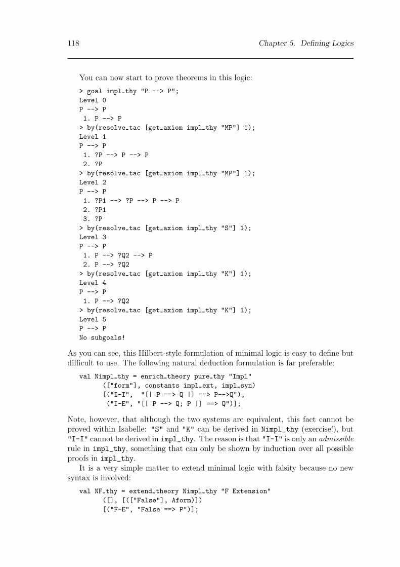
118 Chapter 5. Defining Logics
You can now start to prove theorems in this logic:
> goal impl thy "P --> P";Level 0P --> P1. P --> P> by(resolve tac [get axiom impl thy "MP"] 1);Level 1P --> P1. ?P --> P --> P2. ?P> by(resolve tac [get axiom impl thy "MP"] 1);Level 2P --> P1. ?P1 --> ?P --> P --> P2. ?P13. ?P> by(resolve tac [get axiom impl thy "S"] 1);Level 3P --> P1. P --> ?Q2 --> P2. P --> ?Q2> by(resolve tac [get axiom impl thy "K"] 1);Level 4P --> P1. P --> ?Q2> by(resolve tac [get axiom impl thy "K"] 1);Level 5P --> PNo subgoals!
As you can see, this Hilbert-style formulation of minimal logic is easy to define butdifficult to use. The following natural deduction formulation is far preferable:
val Nimpl thy = enrich theory pure thy "Impl"(["form"], constants impl ext, impl syn)[("I-I", "[| P ==> Q |] ==> P-->Q"),("I-E", "[| P --> Q; P |] ==> Q")];
Note, however, that although the two systems are equivalent, this fact cannot beproved within Isabelle: "S" and "K" can be derived in Nimpl_thy (exercise!), but"I-I" cannot be derived in impl_thy. The reason is that "I-I" is only an admissiblerule in impl_thy, something that can only be shown by induction over all possibleproofs in impl_thy.
It is a very simple matter to extend minimal logic with falsity because no newsyntax is involved:
val NF thy = extend theory Nimpl thy "F Extension"([], [(["False"], Aform)])[("F-E", "False ==> P")];
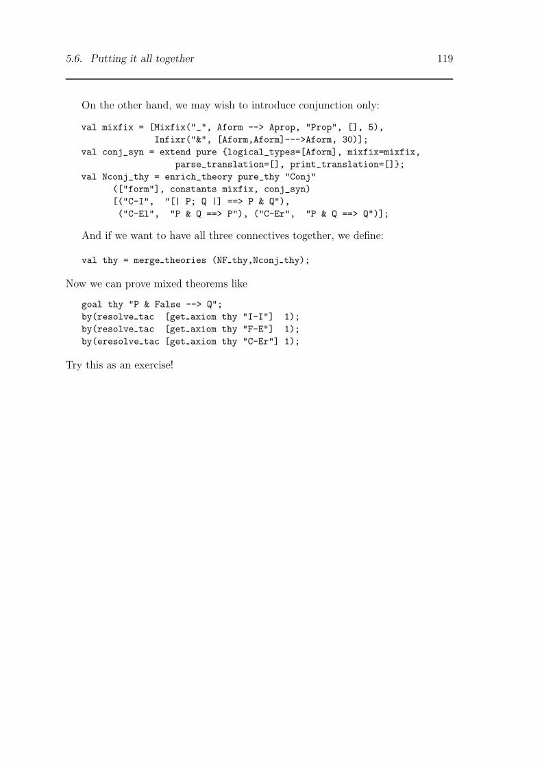
5.6. Putting it all together 119
On the other hand, we may wish to introduce conjunction only:
val mixfix = [Mixfix("_", Aform --> Aprop, "Prop", [], 5),Infixr("&", [Aform,Aform]--->Aform, 30)];
val conj_syn = extend pure {logical_types=[Aform], mixfix=mixfix,parse_translation=[], print_translation=[]};
val Nconj_thy = enrich_theory pure_thy "Conj"(["form"], constants mixfix, conj_syn)[("C-I", "[| P; Q |] ==> P & Q"),("C-El", "P & Q ==> P"), ("C-Er", "P & Q ==> Q")];
And if we want to have all three connectives together, we define:
val thy = merge theories (NF thy,Nconj thy);
Now we can prove mixed theorems like
goal thy "P & False --> Q";by(resolve tac [get axiom thy "I-I"] 1);by(resolve tac [get axiom thy "F-E"] 1);by(eresolve tac [get axiom thy "C-Er"] 1);
Try this as an exercise!

120 Chapter 5. Defining Logics
Appendix A
Internals and Obscurities
This Appendix is a tour through the Isabelle sources themselves, listing functions(and other identifiers) with their types and purpose.
A.1 Types and terms
Isabelle types and terms are those of the typed λ-calculus.
A.1.1 Basic declarations
Exceptions in Isabelle are mainly used to signal errors. An exception includes astring (the error message) and other data to identify the error.
exception TYPE of string * typ list * term list
Signals errors involving types and terms.
exception TERM ERROR of string * term list
Signals errors involving terms.The following ml identifiers denote the symbols of the meta-logic.The type of propositions is Aprop.The implication symbol is implies.The term all T is the universal quantifier for type T.The term equals T is the equality predicate for type T.
A.1.2 Operations
There are a number of basic functions on terms and types.
op ---> : typ list * typ -> typ
Given types [τ1, . . . , τn ] and τ , it forms the type τ1 → · · · → (τn → τ).
loose bnos: term -> int list
121

122 Appendix A. Internals and Obscurities
Calling loose_bnos t returns the list of all ’loose’ bound variable references. Inparticular, Bound 0 is loose unless it is enclosed in an abstraction. Similarly Bound 1
is loose unless it is enclosed in at least two abstractions; if enclosed in just one, thelist will contain the number 0. A well-formed term does not contain any loosevariables.
Calling type of t computes the type of the term t . Raises exception TYPE unlessapplications are well-typed.
op aconv: term*term -> bool
Calling t aconv u tests whether terms t and u are α-convertible: identical up torenaming of bound variables.
• Two constants, Frees, or Vars are α-convertible just when their names andtypes are equal. (Variables having the same name but different types are thusdistinct. This confusing situation should be avoided!)
• Two bound variables are α-convertible just when they have the same number.
• Two abstractions are α-convertible just when their bodies are, and their boundvariables have the same type.
• Two applications are α-convertible just when the corresponding subterms are.
incr boundvars: int -> term -> term
This increments a term’s ‘loose’ bound variables by a given offset, required whenmoving a subterm into a context where it is enclosed by a different number oflambdas.
abstract over: term*term -> term
For abstracting a term over a subterm v : replaces every occurrence of v by a Bound
variable with the correct index.Calling subst_bounds([un−1, . . . , u0], t) substitutes the ui for loose bound vari-
ables in t . This achieves β-reduction of un−1 · · · u0 into t , replacing Bound i withui . For (λxy .t)(u, v), the bound variable indices in t are x : 1 and y : 0. The appro-priate call is subst_bounds([v,u],t). Loose bound variables ≥ n are reduced byn to compensate for the disappearance of n lambdas.
subst term: (term*term)list -> term -> term
Simultaneous substitution for atomic terms in a term. An atomic term is a constantor any kind of variable.
maxidx of term: term -> int
A.1. Types and terms 123
Computes the maximum index of all the Vars in a term. If there are no Vars, theresult is −1.
term match: (term*term)list * term*term -> (term*term)list
Calling term_match(vts,t,u) instantiates Vars in t to match it with u. The re-sulting list of variable/term pairs extends vts, which is typically empty. First-orderpattern matching is used to implement meta-level rewriting.
A.1.3 The representation of object-rules
The module Logic contains operations concerned with inference — especially, forconstructing and destructing terms that represent object-rules.
op occs: term*term -> bool
Does one term occur in the other? (This is a reflexive relation.)
add term vars: term*term list -> term list
Accumulates the Vars in the term, suppressing duplicates. The second argumentshould be the list of Vars found so far.
add term frees: term*term list -> term list
Accumulates the Frees in the term, suppressing duplicates. The second argumentshould be the list of Frees found so far.
mk equals: term*term -> term
Given t and u makes the term t ≡ u.
dest equals: term -> term*term
Given t ≡ u returns the pair (t , u).
list implies: term list * term -> term
Given the pair ([φ1, . . . , φm ], φ) makes the term [φ1; . . . ;φm ] =⇒ φ.
strip imp prems: term -> term list
Given [φ1; . . . ;φm ] =⇒ φ returns the list [φ1, . . . , φm ].
strip imp concl: term -> term
Given [φ1; . . . ;φm ] =⇒ φ returns the term φ.
list equals: (term*term)list * term -> term

124 Appendix A. Internals and Obscurities
For adding flex-flex constraints to an object-rule. Given ([(t1, u1), . . . , (tk , uk)], φ),makes the term [t1 ≡ u1; . . . ; tk ≡ uk ] =⇒ φ.
strip equals: term -> (term*term) list * term
Given [t1 ≡ u1; . . . ; tk ≡ uk ] =⇒ φ, returns ([(t1, u1), . . . , (tk , uk)], φ).
rule of: (term*term)list * term list * term -> term
Makes an object-rule: given the triple
([(t1, u1), . . . , (tk , uk)], [φ1, . . . , φm ], φ)
returns the term [t1 ≡ u1; . . . ; tk ≡ uk ;φ1; . . . ;φm ] =⇒ φ
strip horn: term -> (term*term)list * term list * term
Breaks an object-rule into its parts: given
[t1 ≡ u1; . . . ; tk ≡ uk ;φ1; . . . ;φm ] =⇒ φ
returns the triple ([(tk , uk), . . . , (t1, u1)], [φ1, . . . , φm ], φ).
strip assums: term -> (term*int) list * (string*typ) list * term
Strips premises of a rule allowing a more general form, where∧
and =⇒ may beintermixed. This is typical of assumptions of a subgoal in natural deduction. Returnsadditional information about the number, names, and types of quantified variables.For more discussion of assumptions, see Section A.4.2.
strip prems: int * term list * term -> term list * term
For finding premise (or subgoal) i : given the triple (i , [], φ1; . . . φi =⇒ φ) it re-turns another triple, (φi , [φi−1, . . . , φ1], φ), where φ need not be atomic. Raises anexception if i is out of range.
A.2 Higher-order unification
Unification is used in the resolution of object-rules. Since logics are formalized inthe typed λ-calculus, Isabelle uses Huet’s higher-order unification algorithm [4].
A.2.1 Sequences
The module Sequence declares a type of unbounded sequences by the usual closureidea [8, page 118]. Sequences are defined in terms of the type option, declared inIsabelle’s basic library, which handles the possible presence of a value.
datatype ’a option = None | Some of ’a;

A.2. Higher-order unification 125
Operations on the type ’a seq include conversion between lists and sequences(with truncation), concatenation, and mapping a function over a sequence. Se-quences are used in unification and tactics. The module Sequence, which is normallyclosed, declares the following.
type ’a seq
The type of (possibly unbounded) sequences of type ’a.
seqof: (unit -> (’a * ’a seq) option) -> ’a seq
Calling seqof (fn()=> Some(x,s)) constructs the sequence with head x and tails, neither of which is evaluated.
null: ’a seq
This is seqof (fn()=> None), the empty sequence.
single: ’a -> ’a seq
This is seqof (fn()=> Some(x,null)); makes a 1-element sequence.
pull: ’a seq -> (’a * ’a seq) option
Calling pull s returns None if the sequence is empty and Some(x,s’) if the sequencehas head x and tail s’. Only now is x evaluated. (Calling pull s again willrecompute this value! It is not stored!)
append: ’a seq * ’a seq -> ’a seq
Concatenates two sequences.
flats: ’a seq seq -> ’a seq
Concatenates a sequence of sequences.
maps: (’a -> ’b) -> ’a seq -> ’b seq
Applies a function to every element of a sequence, producing a new sequence.
A.2.2 Environments
The module Envir (which is normally closed) declares a type of environments. Anenvironment holds variable assignments and the next index to use when generatinga variable.
datatype env = Envir of {asol: term xolist, maxidx: int}
The operations of lookup, update, and generation of variables are used during uni-fication.
empty: int->env
126 Appendix A. Internals and Obscurities
Creates the environment with no assignments and the given index.
lookup: env * indexname -> term option
Looks up a variable, specified by its indexname, and returns None or Some as appro-priate.
update: (indexname * term) * env -> env
Given a variable, term, and environment, produces a new environment where thevariable has been updated. This has no side effect on the given environment.
genvar: env * typ -> env * term
Generates a variable of the given type and returns it, paired with a new environment(with incremented maxidx field).
alist of: env -> (indexname * term) list
Converts an environment into an association list containing the assignments.
norm term: env -> term -> term
Copies a term, following assignments in the environment, and performing allpossible β-reductions.
rewrite: (env * (term*term)list) -> term -> term
Rewrites a term using the given term pairs as rewrite rules. Assignments are ignored;the environment is used only with genvar, to generate unique Vars as placeholdersfor bound variables.
A.2.3 The unification functions
The module Unify implements unification itself. It uses depth-first search with adepth limit that can be set. You can also switch tracing on and off, and specify aprint function for tracing.
search bound: int ref
Default 20, holds the depth limit for the unification search. The message
***Unification bound exceeded
appears whenever the search is cut off. This usually means the search wouldotherwise run forever, but a few proofs require increasing the default value ofsearch_bound.
printer: (term->unit) ref
A.2. Higher-order unification 127
This function is used to print terms during tracing. It should be set to an object-logic’s function prin. The default is a dummy that prints nothing.
trace bound: int ref
Default 10, tracing information is printed whenever the search depth exceeds thisbound.
trace simp: bool ref
Default false, controls whether tracing information should include the simpl phaseof unification. Otherwise only match is traced.
unifiers: env * ((term*term)list) -> (env * (term*term)list) seq
This is the main unification function. Given an environment and a list of disagree-ment pairs, it returns a sequence of outcomes. Each outcome consists of an updatedenvironment and a list of flex-flex pairs (these are discussed below).
smash unifiers: env * (term*term)list -> env seq
This unification function maps an environment and a list of disagreement pairs toa sequence of updated environments. The function obliterates flex-flex pairs bychoosing the obvious unifier. It may be used to tidy up any flex-flex pairs remainingat the end of a proof.
Flexible-flexible disagreement pairs
A flexible-flexible disagreement pair is one where the heads of both terms are vari-ables. Every set of flex-flex pairs has an obvious unifier and usually many others.The function unifiers returns the flex-flex pairs to constrain later unifications;smash_unifiers uses the obvious unifier to eliminate flex-flex pairs.
For example, the many unifiers of ?f (0) ≡ ?g(0) include ?f 7→ λx .?g(0) and{?f 7→ λx .x , ?g 7→ λx .0}. The trivial unifier, which introduces a new variable ?a, is{?f 7→ λx .?a, ?g 7→ λx .?a}. Of these three unifiers, none is an instance of another.
Flex-flex pairs are simplified to eliminate redundant bound variables, as shownin the following example:
λxy .?f (k(y), l(x )) ≡ λxy .?g(y)
The bound variable x is not used in the right-hand term. Any unifier of theseterms must delete all occurrences of x on the left. Choosing a new variable ?h, theassignment ?f 7→ λuv .?h(u) reduces the disagreement pair to
λxy .?h(k(y)) ≡ λxy .?g(y)
without losing any unifiers. Now x can be dropped on both sides (adjusting boundvariable indices) to leave
λy .?h(k(y)) ≡ λy .?g(y)
Assigning ?g 7→ λy .?h(k(y)) eliminates ?g and unifies both terms to λy .?h(k(y)).

128 Appendix A. Internals and Obscurities
Multiple unifiers
Higher-order unification can generate an unbounded sequence of unifiers. Multipleunifiers indicate ambiguity; usually the source of the ambiguity is obvious. Someunifiers are more natural than others. In solving ?f (a) ≡ a + b − a, the solution?f 7→ λx .x +b−x is better than ?f 7→ λx .a +b−a because it reveals the dependenceof a + b − a on a. There are four unifiers in this case. Isabelle generates the betterones first by preferring projection over imitation.
The unification procedure performs Huet’s match operation [4] in big steps. Itsolves ?f (t1, . . . , tp) ≡ u for ?f by finding all ways of copying u, first trying projectionon the arguments ti . It never copies below any variable in u; instead it returns anew variable, resulting in a flex-flex disagreement pair. If it encounters ?f in u,it allows projection only. This prevents looping in some obvious cases, but can befooled by cycles involving several disagreement pairs. It is also incomplete.
Associative unification
Associative unification comes for free: encoded through function composition, anassociative operation [5, page 37]. To represent lists, let C be a new constant. Theempty list is λx .x , while the list [t1, t2, . . . , tn ] is represented by the term
λx .C (t1,C (t2, . . . ,C (tn , x )))
The unifiers of this with λx .?f (?g(x )) give all the ways of expressing [t1, t2, . . . , tn ]as the concatenation of two lists.
Unlike standard associative unification, this technique can represent certain in-finite sets of unifiers as finite sets containing flex-flex disagreement pairs. Butλx .C (t , ?a) does not represent any list. Such garbage terms may appear in flex-flex pairs and accumulate dramatically.
Associative unification handles sequent calculus rules, where the comma is theassociative operator:
Γ,A,B ,∆ |− Θ
Γ,A & B ,∆ |− Θ
Multiple unifiers occur whenever this is resolved against a goal containing more thanone conjunction on the left. Note that we do not really need associative unification,only associative matching.
A.3 Terms valid under a signature
The module Sign declares the abstract types of signatures and checked terms. Asignature contains the syntactic information needed for building a theory. A checkedterm is simply a term that has been checked to conform with a given signature, andis packaged together with its type, etc.
A.3. Terms valid under a signature 129
A.3.1 The ml type sg
A signature lists all ground types that may appear in terms in the theory. Thelexical symbol table declares each constant, infix, variable, and keyword. The syntaxcontains the theory’s notation in some internal format; this concerns users but hasno logical meaning.
type sg ={gnd_types: string list, (*ground types*)const_tab: typ Symtab.table, (*types of constants*)ident_tab: typ Symtab.table, (*default types of identifiers*)syn: Syntax.syntax, (*Parsing and printing operations*)stamps: string ref list (*unique theory identifier*) };
The stamps identify the theory. Each primitive theory has a single stamp. Whenthe union of theories is taken, the lists of stamps are merged. References are usedas the unique identifiers. The references are compared, not their contents.
Two signatures can be combined into a new one provided their constants arecompatible. If an identifier is used as a constant in both signatures, it must be thesame kind of symbol and have the same type in both signatures. This union opera-tion should be idempotent, commutative, and associative. You can build signaturesthat ought to be the same but have different syntax functions, since functions cannotbe compared.
A.3.2 The ml type cterm
A term t is valid under a signature provided every type in t is declared in thesignature and every constant in t is declared as a constant or infix of the same typein the signature. It must be well-typed and monomorphic and must not have loosebound variables. Note that a subterm of a valid term need not be valid: it maycontain loose bound variables. Even if λx .x is valid, its subterm x is a loose boundvariable.
A checked term is stored with its signature, type, and maximum index of itsVars. This information is computed during the checks.
datatype cterm = Cterm of {sign: sg,t: term,T: typ,maxidx: int};
The inference rules maintain that the terms that make up a theorem are validunder the theorem’s signature. Rules (like specialization) that operate on termstake them as cterms rather than taking raw terms and checking them. It is possibleto obtain cterms from theorems, saving the effort of checking the terms again.
130 Appendix A. Internals and Obscurities
A.3.3 Declarations
Here are the most important declarations of the module Sign. (This module isnormally closed.)
type sg
The type of signatures, this is an abstract type: the constructor is not exported. Asignature can only be created by calling new, typically via a call to prim_theory.
type cterm
The abstract type of checked terms. A cterm can be created by calling cterm_of orread_cterm.
rep sg: sg -> {gnd types: string list, lextab: lexsy table...}
The representation function for type sg, this returns the underlying record.
new: string -> ... -> sg
Calling new signame (gnd_types,lextab,parser,printer) creates a new signa-ture named signame from the given type names, lexical table, parser, and printingfunctions.
rep cterm: cterm -> {T: typ, maxidx: int, sign: sg, t: term}
The representation function for type cterm.
term of: cterm -> term
Maps a cterm to the underlying term.
cterm of: sg -> term -> cterm
Given a signature and term, checks that the term is valid in the signature andproduces the corresponding cterm. Raises exception TERM_ERROR with the message‘type error in term’ or ‘term not in signature’ if appropriate.
read cterm: sg -> string*typ -> cterm
Reads a string as a term using the parsing information in the signature. It checksthat this term is valid to produce a cterm. Note that a type must be supplied: thisaids type inference considerably. Intended for interactive use, read_cterm catchesthe various exceptions that could arise and prints error messages. Commands likegoal call read_cterm.
print cterm: cterm -> unit
A.4. Meta-inference 131
Prints the cterm using the printing function in its signature.
print term: sg -> term -> unit
Prints the term using the printing function in the given signature.
type assign: cterm -> cterm
Produces a cterm by updating the signature of its argument to include all vari-able/type assignments. Type inference under the resulting signature will assumethe same type assignments as in the argument. This is used in the goal package togive persistence to type assignments within each proof. (Contrast with lcf’s stickytypes [8, page 148].)
A.4 Meta-inference
Theorems and theories are mutually recursive. Each theorem is associated with atheory; each theory contains axioms, which are theorems. To avoid circularity, atheorem contains a signature rather than a theory.
The module Thm declares theorems, theories, and all meta-rules. Together withSign this module is critical to Isabelle’s correctness: all other modules call on themto construct valid terms and theorems.
A.4.1 Theorems
The natural deduction system for the meta-logic [9] is represented by the obvioussequent calculus. Theorems have the form Φ |− ψ, where Φ is the set of hypothesesand ψ is a proposition. Each meta-theorem has a signature and stores the maximumindex of all the Vars in ψ.
datatype thm = Thm of{sign: Sign.sg,maxidx: int,hyps: term list,prop: term};
The proof state with subgoals φ1, . . . , φm and main goal φ is represented by theobject-rule φ1 . . . φm/φ, which in turn is represented by the meta-theorem
Φ |− [t1 ≡ u1; . . . ; tk ≡ uk ;φ1; . . . ;φm ] =⇒ φ (A.1)
The field hyps holds Φ, the set of meta-level assumptions. The field prop holdsthe entire proposition, [t1 ≡ u1; . . . ;φm ] =⇒ φ, which can be further broken down.The function tpairs_of returns the (t , u) pairs, while prems_of returns the φi andconcl_of returns φ.
exception THM of string * int * thm list

132 Appendix A. Internals and Obscurities
Signals incorrect arguments to meta-rules. The tuple consists of a message, a premisenumber, and the premises.
rep thm: thm -> {prop: term, hyps: term list, . . . }
This function returns the representation of a theorem, the underlying record.
tpairs of: thm -> (term*term)list
Maps the theorem (A.1) to the list of flex-flex constraints, [(t1, u1), . . . , (tk , uk)].
prems of: thm -> term list
Maps the theorem (A.1) to the premises, [φ1, . . . , φm ].
concl of: thm -> term
Maps the theorem (A.1) to the conclusion, φ.
Meta-rules
All of the meta-rules are implemented (though not all are used). They raise excep-tion THM to signal malformed premises, incompatible signatures and similar errors.
assume: Sign.cterm -> thm
Makes the sequent ψ |− ψ, checking that ψ contains no Vars. Recall that Vars areonly allowed in the conclusion.
implies intr: Sign.cterm -> thm -> thm
This is =⇒-introduction.
implies elim: thm -> thm -> thm
This is =⇒-elimination.
forall intr: Sign.cterm -> thm -> thm
The∧
-introduction rule generalizes over a variable, either Free or Var. The variablemust not be free in the hypotheses; if it is a Var then there is nothing to check.
forall elim: Sign.cterm -> thm -> thm
This is∧
-elimination.
reflexive: Sign.cterm -> thm
Reflexivity of equality.
symmetric: thm -> thm
Symmetry of equality.
transitive: thm -> thm -> thm
Transitivity of equality.
instantiate: (Sign.cterm*Sign.cterm) list -> thm -> thm
Simultaneous substitution of terms for distinct Vars. The result is not normalized.
A.4. Meta-inference 133
Definitions
An axiom of the form C ≡ t defines the constant C as the term t . Rewriting withthe axiom C ≡ t unfolds the constant C : replaces C by t . Rewriting with thetheorem t ≡ C (obtained by the rule symmetric) folds the constant C : replaces tby C . Several rules are concerned with definitions.
rewrite rule: thm list -> thm -> thm
This uses a list of equality theorems to rewrite another theorem. Rewriting is left-to-right and continues until no rewrites are applicable to any subterm.
rewrite goals rule: thm list -> thm -> thm
This uses a list of equality theorems to rewrite just the antecedents of anothertheorem — typically a proof state. This unfolds definitions in the subgoals but notin the main goal.
Unfolding should only be needed for proving basic theorems about a definedsymbol. Later proofs should treat the symbol as a primitive. For example, in first-order logic, bi-implication is defined in terms of implication and conjunction:
P<->Q == (P-->Q) & (Q-->P)
After deriving basic rules for this connective, we can forget its definition.This treatment of definitions should be contrasted with many other theorem
provers, where defined symbols are automatically unfolded.
A.4.2 Derived meta-rules for backwards proof
The following rules, coded directly in ml for efficiency, handle backwards proof.They typically involve a proof state
[ψ1; . . . ;ψi ; . . . ;ψn ] =⇒ ψ
Subgoal i , namely ψi , might have the form∧x1.θ1 =⇒ · · · (
∧xk .θk =⇒ θ)
Each θj may be preceded by zero or more quantifiers, whose scope extends to θ.The θj represent the assumptions of the subgoal; the xj represent the parameters.
The object-rule [φ1; . . . ;φm ] =⇒ φ is lifted over the assumptions and parametersof the subgoal and renumbered [9]; write the lifted object-rule as
[φ1; . . . ; φm ] =⇒ φ
Recall that, for example, φ has the form∧x1.θ1; . . . ; (
∧xk .θk =⇒ φ′)
134 Appendix A. Internals and Obscurities
where φ′ is obtained from φ by replacing its free variables by certain terms.Each rule raises exception THM if subgoal i does not exist.
resolution: thm * int * thm list -> thm Sequence.seq
Calling resolution(state,i,rules) performs higher-order resolution of a theoremin rules, typically an object-rule, with subgoal i of the proof state held in thetheorem state. The sequence of theorems contains the result of each successfulunification of φ ≡ ψi , replacing ψi by φ1, . . . , φm and instantiating variables instate. The rules are used in order.
assumption: thm * int -> thm Sequence.seq
Calling assumption(state,i) attempts to solve subgoal i by assumption in naturaldeduction. The call tries each unification of the form θj ≡ θ for j = 1, . . . , k . Thesequence of theorems contains the outcome of each successful unification, where ψi
has been deleted and variables may have been instantiated elsewhere in the state.
biresolution: thm * int * (bool*thm)list -> thm Sequence.seq
Calling biresolution(state,i,brules) is like calling resolution, except thatpairs of the form (true,rule) involve an implicit call of assumption. This permitsusing natural deduction object-rules in a sequent style, where the ‘principal formula’is deleted after use. Write the lifted object-rule as
[φ1; φ2; . . . ; φm ] =⇒ φ
The rule is interpreted as an elimination rule with φ1 as the major premise, andbiresolution will insist on finding φ1 among the assumptions of subgoal i . Thecall tries each unification of the form {φ′1 ≡ θj , φ ≡ ψi} for j = 1, . . . , k . Thesequence of theorems contains the result of each successful unification, replacing ψi
by the m−1 subgoals φ2, . . . , φm and instantiating variables in state. The relevantassumption is deleted in the subgoals: if unification involved θj , then the occurrence
of θj is deleted in each of φ2, . . . , φm .Pairs of the form (false,rule) are treated exactly as in resolution. The
pairs are used in order.
trivial: Sign.cterm -> thm
Makes the theorem ψ =⇒ ψ, used as the initial state in a backwards proof. Theproposition ψ may contain Vars.
A.5 Tactics and tacticals
Here are some of the more obscure tactics, tacticals, derived meta-rules, and otheritems that are available.
A.5. Tactics and tacticals 135
A.5.1 Derived rules
The following derived rules are implemented using primitive rules.
forall intr frees: thm -> thm
Generalizes a meta-theorem over all Free variables not free in hypotheses.
forall elim vars: int -> thm -> thm
Replaces all outermost quantified variables by Vars of a given index.
zero var indexes: thm -> thm
Replaces all Vars by Vars having index 0, preserving distinctness by renaming whennecessary.
standard: thm -> thm
Puts a meta-theorem into standard form: no hypotheses, Free variables, or outerquantifiers. All generality is expressed by Vars having index 0.
resolve: thm * int * thm list -> thm
Calling resolve (rlb,i,rules) tries each of the rules, in turn, resolving themwith premise i of rlb. Raises exception THM unless resolution produces exactly oneresult. This function can be used to paste object-rules together, making simplederived rules.
op RES: thm * thm -> thm
Calling (rule2 RES rule1) is equivalent to resolve(rule2,1,[rule1]); it re-solves the conclusion of rule1 with premise 1 in rule2. Raises exception THM unlessthere is exactly one unifier.
A.5.2 Tactics
The following tactics are mainly intended for use in proof procedures that processlots of rules. However, res_inst_tac can be used even in single-step proofs to keepcontrol over unification.
biresolve tac: (bool*thm) list -> int -> tactic
This is analogous to resolve_tac but calls biresolution. It is thus suitable for amixture of introduction rules (which should be paired with false) and eliminationrules (which should be paired with true).
res inst tac: (string*string*typ)list -> thm -> int -> tactic
136 Appendix A. Internals and Obscurities
For selective instantiation of variables, res_inst_tac [(v,t,T)] rule i reads thestrings v and t, obtaining a variable ?v and term t of the given type T. The termmay refer to parameters of subgoal i , for the tactic modifies ?v and t to compensatefor the parameters, and lifts the rule over the assumptions of the subgoal. Thetactic replaces ?v by t in the rule and finally resolves it against the subgoal.
smash all ff tac: tactic
Eliminates all flex-flex constraints from the proof state by applying the trivial higher-order unifier.
A.5.3 Filtering of object-rules
Higher-order resolution involving a long list of rules is slow. Filtering techniquescan shorten the list of rules given to resolution. A second use of filtering is to detectwhether resolving against a given subgoal would cause excessive branching. If toomany rules are applicable then another subgoal might be selected.
The module Stringtree implements a data structure for fast selection of rules.A term is classified by its head string : the string of symbols obtained by followingthe first argument in function calls until a Var is encountered. For instance, theConstructive Type Theory judgement
rec(succ(?d),0,?b): N
has the head string ["Elem","rec","succ"] where the constant Elem representsthe elementhood judgement form a ∈ A.
Two head strings are compatible if they are equal or if one is a prefix of the other.If two terms have incompatible head strings, then they are clearly not unifiable. Atheorem is classified by the head string of its conclusion, indicating which goals itcould resolve with. This method is fast, easy to implement, and powerful.
Head strings can only discriminate terms according to their first arguments.Type Theory introduction rules have conclusions like 0:N and inl(?a):?A+?B. Be-cause the type is the second argument, the head string does not discriminate bytypes.
could unify: term*term->bool
This function quickly detects nonunifiable terms. It assumes all variables are dis-tinct, reporting that ?a=?a may unify with 0=1.
filt resolve tac: thm list -> int -> int -> tactic
Calling filt_resolve_tac rules maxr i uses could_resolve to discover whichof the rules are applicable to subgoal i. If this number exceeds maxr then the tacticfails (returning the null sequence). Otherwise it behaves like resolve_tac.
compat resolve tac: thm list -> int -> int -> tactic
A.5. Tactics and tacticals 137
Calling compat_resolve_tac rules maxr i builds a stringtree from the rules
to discover which of them are applicable to subgoal i. If this number exceedsmaxr then the tactic fails (returning the null sequence). Otherwise it behaveslike resolve_tac. (To avoid repeated construction of the same stringtree, applycompat_resolve_tac to a list of rules and bind the result to an identifier.)

138 Appendix A. Internals and Obscurities
Bibliography
[1] N. G. de Bruijn, Lambda calculus notation with nameless dummies, a tool forautomatic formula manipulation, with application to the Church-Rosser Theorem,Indagationes Mathematicae 34 (1972), pages 381–392.
[2] K. Futatsugi, J.A. Goguen, J.-P. Jouannaud, J. Meseguer, Principles of OBJ2, 12thACM Symposium on Principles of Programming Languages (1985), pages 52–66.
[3] J. H. Gallier, Logic for Computer Science: Foundations of Automatic TheoremProving (Harper & Row, 1986).
[4] G. P. Huet, A unification algorithm for typed λ-calculus, Theoretical ComputerScience 1 (1975), pages 27–57.
[5] G. P. Huet, B. Lang, Proving and applying program transformations expressed withsecond-order patterns, Acta Informatica 11 (1978), pages 31–55.
[6] P. Martin-Lof, Intuitionistic Type Theory (Bibliopolis, 1984).
[7] L. C. Paulson, Natural deduction as higher-order resolution, Journal of LogicProgramming 3 (1986), pages 237–258.
[8] L. C. Paulson, Logic and Computation: Interactive Proof with Cambridge LCF(Cambridge University Press, 1987).
[9] L. C. Paulson, The foundation of a generic theorem prover, Journal of AutomatedReasoning 5 (1989), 363–397.
[10] L. C. Paulson, Isabelle: The next 700 theorem provers, In: P. Odifreddi (editor),Logic and Computer Science (Academic Press, 1990, in press), 361–385.
[11] F. J. Pelletier, Seventy-five problems for testing automatic theorem provers, Journalof Automated Reasoning 2 (1986), pages 191–216.
[12] P. Suppes, Axiomatic Set Theory (Dover Publications, 1972).
[13] G. Takeuti, Proof Theory (2nd Edition) (North Holland, 1987).
[14] A. N. Whitehead and B. Russell, Principia Mathematica (Paperback edition to *56,Cambridge University Press, 1962).
[15] A. Wikstrom, Functional Programming Using Standard ML (Prentice-Hall, 1987).
139
Index
! 9, 105$ 102$$ 111$$ prop 11, 105% 9, 111’ 108( 112) 112--> 101---> 102, 121/ 112== 9, 105==> 9, 105=> 111? 9, 109[| 9, 105|] 9, 105_ 107_constrain 111
Abs 102, 113abs_list_tr 115abs_list_tr’ 115abstract_over 110, 122aconv 122add_term_frees 123add_term_vars 123Adummy 103, 107, 109, 113, 116all 105ALLGOALS 82, 83all_tac 80, 83Any 111Any 105, 111APPEND 81, 83append 125APPEND’ 83Aprop 105assume 132assume_tac 17, 18
assumption 134
B. 114back 15, 16, 88BEST_FIRST 82, 83biresolution 134biresolve_tac 135Bound 102, 114BREADTH_FIRST 82, 83by 13, 16
chop 15, 16choplev 15, 16compat_resolve_tac 136concl_of 132Const 102constants 114could_unify 136cut_facts_tac 17, 18, 77
Delimfix 106, 108DEPTH_FIRST 81, 83DEPTH_SOLVE_1 82, 83dest_equals 123DETERM 81, 83
enrich_theory 104eresolve_tac 17, 18, 20EVERY 81, 83extend 106extend_theory 104extension 106
filt_resolve_tac 136FIRST 81, 83flats 125fold_tac 17, 18forall_elim 132forall_elim_vars 135forall_intr 132forall_intr_frees 135
140
Index 141
Free 102, 109, 113
get_axiom 104getgoal 15, 16getstate 15, 16goal 13, 16, 64, 92goals_limit 15Ground 101gstack 15
has_fewer_prems 82
identifier 109id_list 111, 115implies_elim 132implies_intr 132incr_boundvars 122Infixl 106, 108Infixr 106, 108instantiate 132
list_equals 123list_implies: 123logical_types 106, 111loose_bnos 121
maps 125max_pri 107maxidx_of_term 122merge 106merge_theories 104Mixfix 106mixfix 106mk_equals 123
no_tac 80, 83None 124null 125
occs 123op 108option 124ORELSE 79, 80, 83ORELSE’ 83
parse_translation 106, 110Poly 101pr 15, 16
prems_of 132prin 114print_syntax 114print_top_level 114print_translation 106, 112printer 126prlev 15, 16prop 105prove_goal 93prth 12prths 12pull 125pure 106pure_thy 104
read 114reflexive 132rep_thm 132REPEAT 79, 81, 83RES 135res_inst_tac 135resolution 134resolve 135resolve_tac 16, 18result 13, 15, 16, 63rewrite_goals_rule 133rewrite_goals_tac 17, 18, 77rewrite_rule 96, 133rewrite_tac 17, 18rule_of 124
search_bound 126seq 125seqof 125setstate 15, 16SId 109single 125smash_all_ff_tac 136Some 124SOMEGOAL 82, 83standard 135strip_assums 124strip_equals 124strip_horn 124strip_imp_concl 123strip_imp_prems 123
142 Index
strip_prems 124subst_bounds 123subst_term 123SVar 109symmetric 132
Tactic 80tactic 8, 80tapply 81term 8, 102term_match 123THEN 79, 80, 83THEN’ 83theory 8, 12, 104thm 8, 11, 131topthm 15, 16tpairs_of 132trace_bound 127trace_simp 127transitive 133trivial 134TRY 81, 83typ 8, 101type_of 122
undo 13, 16uresult 15, 16, 63
Var 102, 109, 113variable 109variant_abs 113
zero_var_indexes 135