isbatch: a batch-processing platform for data analysis and

iSBatch: a batch-processing platform for data analysis and

exploration of live-cell single-molecule microscopy images and other hierarchical datasets

Journal: Molecular BioSystems

Manuscript ID: MB-MET-05-2015-000321.R1

Article Type: Method

Date Submitted by the Author: 10-Jul-2015

Complete List of Authors: Armini Caldas, Victor Emanoel; University of Groningen , Zernike Institute

for Advanced Materials Punter, Christiaan; University of Groningen, Zernike Institute for Advanced Materials Ghodke, Harshad; University of Groningen, Zernike Institute for Advanced Materials Robinson, Andrew; University of Groningen, Zernike Institute for Advanced Materials van Oijen, Antoine; University of Groningen, Zernike Institute for Advanced Materials

Molecular BioSystems

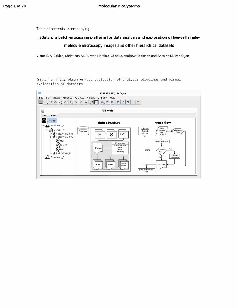
Table of contents accompanying

iSBatch: a batch-processing platform for data analysis and exploration of live-cell single-

molecule microscopy images and other hierarchical datasets

Victor E. A. Caldas, Christiaan M. Punter, Harshad Ghodke, Andrew Robinson and Antoine M. van Oijen

iSBatch: an ImageJ plugin for fast evaluation of analysis pipelines and visual

exploration of datasets.

Page 1 of 28 Molecular BioSystems

of 27 Molecular Biosystems

iSBatch: a batch-processing platform for data analysis and exploration of live-cell single-1

molecule microscopy images and other hierarchical datasets 2

Victor E. A. Caldas1, Christiaan M. Punter1, Harshad Ghodke1, Andrew Robinson1 and 3

Antoine M. van Oijen1* 4

5

6

1Zernike Institute for Advanced Materials, Centre for Synthetic Biology, University 7

of Groningen, The Netherlands 8

*Corresponding author. Current address: School of Chemistry, University of Wollongong, 9

Wollongong NSW 2522, Australia. 10

Phone: +61-(2)4221 4780. Fax: +61-(2)4221 4287. Email: [email protected] 11

12

Running title: Batch processing tool for single-molecule single-cell images 13

14

15

Key words: single-molecule microscopy, live-cell imaging, fluorescence, batch processing 16

17

Page 2 of 28Molecular BioSystems


Abstract 18

Recent technical advances have made it possible to visualize single molecules inside live cells. 19

Microscopes with single-molecule sensitivity enable the imaging of low-abundance proteins, 20

allowing for a quantitative characterization of molecular properties. Such data sets contain 21

information on a wide spectrum of important molecular properties, with different aspects 22

highlighted in different imaging strategies. The time-lapsed acquisition of images provides 23

information on protein dynamics over long time scales, giving insight into expression dynamics 24

and localization properties. Rapid burst imaging reveals properties of individual molecules in real-25

time, informing on their diffusion characteristics, binding dynamics and stoichiometries within 26

complexes. This richness of information, however, adds significant complexity to analysis 27

protocols. In general, large datasets of images must be collected and processed in order to 28

produce statistically robust results and identify rare events. More importantly, as live-cell single-29

molecule measurements remain on the cutting edge of imaging, few protocols for analysis have 30

been established and thus analysis strategies often need to be explored for each individual 31

scenario. Existing analysis packages are geared towards either single-cell imaging data or in vitro 32

single-molecule data and typically operate with highly specific algorithms developed for particular 33

situations. Our tool, iSBatch, instead allows users to exploit the inherent flexibility of the popular 34

open-source package ImageJ, providing a hierarchical framework in which existing plugins or 35

custom macros may be executed over entire datasets or portions thereof. This strategy affords 36

users freedom to explore new analysis protocols within large imaging datasets, while maintaining 37

hierarchical relationships between experiments, samples, fields of view, cells, and individual 38

molecules. 39

40

41

42

43

44



Introduction 45

46

Fluorescence microscopy has played an enormously important role in our understanding of biology. 47

By tagging molecules of interest with fluorescent proteins, the dynamics of many cellular systems 48

have been observed within live cells. However, many important cellular processes are carried out by 49

proteins that are expressed at very low levels and are therefore undetectable using standard 50

fluorescence microscopes1,2

. Proteins that replicate and repair chromosomes in bacteria, for 51

example, are often expressed at a level of less than 100 molecules per cell3. The recent development 52

of fluorescence microscopes with single-molecule sensitivity is allowing us to peer into this world for 53

the first time. 54

In addition to extending the sensitivity of established wide-field microscopy techniques, single-55

molecule microscopes allow rapid image sequences to be recorded that reveal the movements of 56

individual molecules. Single-molecule microscopes can be used to record wide-field video-rate 57

movies, with exposure times of 10–100 ms for individual images. On this timescale, fluorescent 58

signals from molecules that diffuse freely within the cytosol of a bacterial cell or within the 59

organelles of eukaryotic cells, blur out over the accessible volume in the cell or organelle due to 60

rapid diffusion rates (D ~ 1–10 μm2/s 4–6). On the other hand, molecules that bind relatively static 61

structures, such as chromosomal DNA, exhibit a much smaller diffusion constant and thus present as 62

static foci of diffraction-limited size (~ 300 nm). Similarly, molecules that diffuse slowly, such as 63

proteins associated with cell membranes, present discrete foci that move along the cell periphery. 64

Movements of such single-molecule foci can be tracked in order to observe events that lead to a 65

change in diffusion rate, for example, binding of molecules to DNA or other large structures. At the 66

same time, intensities of foci in conjunction with photobleaching can be tracked in order to measure 67

the number of fluorescent molecules giving rise to each focus, allowing the compositions of 68

molecular complexes to be determined7. 69

70



These extra layers of information provide fresh insight into the behaviors of molecules within cells, 71

but also pose a problem for the scientists who study them: in order to obtain sufficient statistics to 72

generalize observations, data must be recorded for many molecules, within many cells. Single-73

molecule imaging requires the use of high-magnification, high-numerical aperture objectives6, 74

limiting the size of the field-of-view and thus the number of cells that can be observed 75

simultaneously. Typically, to discern statistically significant outcomes, hundreds of images must be 76

recorded for a particular a live-cell single-molecule sample. That sample may contain hundreds of 77

fields, potentially containing hundreds of time-points, up to thousands of cells of which each contain 78

a handful of foci. Furthermore, it is often desirable to collect images in two or more fluorescence 79

colors in order to correlate the behaviors of multiple types of molecules, as well as bright-field or 80

phase-contrast images to define cell boundaries. These data are highly hierarchical in nature and 81

efficient analysis is only possible when the hierarchical relationships between the different levels in 82

the data are maintained during analysis. 83

A software package for single-molecule analysis in live-cells should meet four basic conditions. 84

Firstly, it should allow for hierarchical classification of images and regions-of-interest (ROIs): samples 85

contain fields of view (images), fields of view contain ROIs that capture individual cells (cell ROIs), 86

and cells contain ROIs that define single-molecule foci (focus ROIs). Secondly, it should allow for 87

analysis over both long and short time scales, resulting in the generation of different data structures: 88

in time-lapse datasets there is one cell ROI per time point, whereas in rapid-imaging mode each cell 89

ROI is typically used to analyze fluorescence signals over many time-points (Fig. 1). Thirdly, and most 90

importantly, a package for live-cell single-molecule analysis should be highly flexible and allow for 91

exploration of new analysis techniques. Finally, the source code used in the package be made 92

available to users so that researchers can fully understand the algorithms they use8. 93

Sophisticated packages for both cell analysis and single-molecule analysis are currently available, 94

however none meet all of the requirements listed above9. Commercial packages typically offer out-95



of-the-box solutions to a particular set of problems, often involve high licensing fees and utilize 96

undisclosed source code, limiting the users’ ability to adapt the software or to add their own 97

customized code. CellProfiler10 (and its extension CellProfiler Analyst11) is a free open-source package 98

with a robust set of algorithms for analysis of 2D images. CellProfiler excels at automated assignment 99

of cellular phenotypes, as well as identification of sub-cellular particles. However, with its focus on 100

high-throughput screening data, the package provides little support for time-resolved studies. 101

MicrobeTracker12 allows users to conveniently assign outlines for microbial cells within time-lapse 102

datasets and provides some support for characterization of foci. It is, however, not suitable for 103

analysis of rapid-imaging data and is not geared towards exploration of new analysis methods. In 104

addition, while MicrobeTracker itself is free, it runs within an environment that requires a paid 105

licence (Matlab). Single-molecule packages such as the Mosaic Suite13

, as well as plugin collections, 106

such as GDSC ImageJ Plugins14 offer a myriad of analysis methods for single-molecule image 107

processing, but are intended for in vitro analysis and thus lack the hierarchical classification systems 108

that are required for the analysis of data derived from cellular systems. A significant advantage of 109

these packages, however, is that they are extensions of the popular image-analysis platform 110

ImageJ15,16, which is extremely flexible, supported by a strong user community and a wealth of user-111

written extensions. Unfortunately, ImageJ is geared towards working with individual files, making 112

hierarchical analysis strategies difficult to implement. 113

Flexible software that links analysis routines used in single-molecule imaging with those used in live-114

cell imaging is required for researchers to keep up with the rapid development of new imaging 115

techniques. Ideally, one would be able to utilize ImageJ to develop code for new analysis routines, 116

whilst being able to easily accommodate data structures that are large, hierarchical and multi-117

dimensional. 118

We present a free open-source ImageJ plugin, iSBatch, which allows users to use batch processing to 119

treat files within hierarchical datasets in a straightforward manner. Routines built into ImageJ15

, 120



downloadable plugins and even user-written macros can be executed across any level of the dataset 121

hierarchy. This strategy dramatically simplifies the often cumbersome tasks of scripting and data 122

management, allowing users to run scripts over their entire datasets or portions thereof. Our tool 123

complements existing single-cell and single-molecule analysis packages by allowing cell and focus 124

ROIs generated in single-cell packages to be applied across hierarchical time-lapse and rapid-imaging 125

datasets, with complete flexibility in choice of analysis methods. 126

Results and Discussion 127

iSBatch is straightforward to use, platform independent, and requires only ImageJ and Java Virtual 128

Machine, which are freely available. iSBatch provides an interface to explore data in hierarchical 129

datasets. Its graphical user interface (GUI) provides an intuitive means for controlling the operations 130

and manipulating datasets of any size. iSBatch incorporates a powerful adapter for the ImageJ macro 131

interpreter, allowing users to implement existing or newly written macros within the data hierarchy. 132

Data is stored in an SQL database and displayed in a tree format for manipulation (Fig. 2a). The 133

database format assists in managing the transfer and back-up of large imaging datasets, which may 134

contain hundreds or even thousands of images and can be prone to errors when handled manually 135

17. A file named ‘iSBatch.zip‘, which contains the plugin, its source code and user manual, is included 136

in the online Supplementary Material. To help to illustrate the concepts in the following sections of 137

this report, we also include an example dataset containing three Experiments in the Supplementary 138

Material. 139

Data Structure and Graphical User Interface (GUI) 140

The fundamental unit of iSBatch is the image itself. Each image belongs to a Field of View, 141

representing the region of the sample that was imaged by the microscope. A collection of Fields of 142

View is called a Sample, and a collection of Samples is called an Experiment. This hierarchy is 143

assigned to each image by placing hierarchy parameters alongside the image within an image object. 144

Image objects may contain an unlimited number of additional parameters. Within iSBatch, image 145



objects contain information on the nature of the image, for example identifiers for color channels, 146

metadata generated during operations, such as peak tables and image projections, as well as ROIs 147

that designate the positions of cells and foci. A dedicated dialog guides the import of imaging data 148

and assures compatibility with iSBatch. There is no specific requirement for file name structure, 149

however we suggest the inclusion of a useful identifier for the imaging channel (e.g. 514.tif, BF.tif, 150

GFP.tif). 151

The general workflow within iSBatch is straightforward (Fig. 2b). In short, the user selects which 152

subset needs to be processed, chooses the operation to be performed and indicates either to save 153

results and images to disc or keep it in the database. The graphic user interface is divided into 154

subpanels containing the navigation tree, file lists, buttons to run built-in functions or custom 155

macros and a log panel (Fig. 2c). The GUI also has buttons to add images to the data structure, as 156

well as cell ROIs generated in ImageJ or in MicrobeTracker18. 157

We have included several operations commonly used in single-molecule analysis within iSBatch, such 158

as functions to correct images for uneven illumination, find and fit peaks inside or outside of cells, 159

and basic peak table operations. These operations will be explored in detail in the form of case 160

studies in the sections below. 161

Case studies 162

To demonstrate the applicability of our iSBatch software we present here a case in which the custom 163

macro interpreter was applied to a dataset, as well as two detailed case studies based on the most 164

common types of data generated by single-molecule single-cell measurements: rapid-acquisition 165

movies and time-lapse series. We imaged Escherichia coli cells in which two different subunits of the 166

replisome were tagged with fluorescent proteins at their carboxy-termini; the ϵ subunit (DnaQ gene) 167

is tagged with red mKate2 (DnaQ-mKate2) and the τ subunit (DnaX gene) is tagged with yellow YPet 168

(DnaX-YPet). The E. coli replisomes contain ten different proteins, each at different copy numbers, 169

including up to three molecules of τ (a component of the clamp loader complex) and three 170



molecules of ϵ (proof-reading exonuclease)3. Replisome proteins are of particular interest for single-171

molecule studies3,19 both because of their biological role of importance (replisomes duplicate the 172

genome prior to cell division)20 and because the replisomal proteins are present at extremely low 173

levels within cells. A single E. coli cell produces only about 100 molecules of τ per cell and ~250 174

molecules of ϵ3. 175

The example data is comprised of a single database containing three experiments, labeled RA_DnaX-176

YPet, RA_DnaQ-mKate2 and TimeLapse). RA_DnaX-YPet and RA_DnaQ-mKate2 are Rapid Acquisition 177

(RA) experiments (500 times 34 ms) that each contain three samples recorded at different excitation 178

laser powers. Each of these samples contains 10 fields of view. TimeLapse contains just one sample 179

and 10 fields of view (50 ms every 20 min, repeated for 400 minutes). RA_DnaX-YPet includes 134 180

cell selections, RA_DnaQ-mKate2 contains 107 and TimeLapse contains 10 fully tracked cells. iSBatch 181

assumes that, if no cell ROIs are provided, the entire image is selected. This scenario is applicable to 182

analyses that do not rely on cell outlines, such as reconstruction of super-resolution images by PALM 183

21,22 or STORM 23, or even to the analysis of in vitro single-molecule data. 184

When loaded into iSBatch, our datasets appear in the operation panel (Fig 2c). Selecting a node 185

within one of the datasets allows image-processing operations to be executed across all images 186

falling under that node. For example, when the user selects the node RA_DnaQ in the tree and the 187

operation flatten, iSBatch guides the user through the steps required for image flattening and 188

correction for the unevenness of the beam profile (more details found in the User Manual – 189

Supplementary Materials) within selected images in the RA_DnaQ experiment. Next, iSBatch 190

assumes that operations will be performed on the resulting flattened images as will be shown in the 191

following sections. 192

Custom macro interpreter 193

The ImageJ support to macros is a powerful tool to execute a sequence of operations in an image. 194

Traditionally, in order to apply basic ImageJ functions across portions of a dataset, the user has to 195



write sequences of steps and functions to navigate through the folders, to identity the required files, 196

and to save the results. Even small changes in the folder or file structure prevent the code from 197

running properly and troubleshooting becomes a daunting task. iSBatch, via its custom macro 198

interpreter, provides the necessary tools to automatize these steps (Fig. 3). 199

Within our rapid acquisition data, for instance, stacks exported from the microscope contain dark 200

frames at the beginning of the image series, resulting from a small delay before the opening of the 201

laser shutter. The custom macro interpreter can be easily used to trim stacks in order to remove 202

these frames. There are two possibilities of implementation: an experienced user may just write a 203

macro to trim one image and them use it within the custom macro interpreter; or could take 204

advantage of ImageJ Macro Recorder – a panel that stores all commands performed by the user 205

while processing an image– and then simply paste the sequence of steps into the iSBatch custom 206

macro interpreter. The user then can analyse the images further in a statistical package, like R24. 207

Rapid-Acquisition Analysis 208

Rapid-Acquisition experiments usually result in a stack of fluorescence images, containing hundreds 209

or thousands of individual frames, acquired at rapid frame rates (typically continuous series of 210

frames, 10-100 ms duration each, with a total duration of seconds), as well as a bright-field image 211

enabling the identification of cell boundaries in cases of low fluorescence signals. This type of 212

imaging allows the behaviors of individual molecules to be monitored in real time. It is typically used 213

to count molecules within foci, to count the total number of molecules in cells, to measure diffusive 214

behavior and to observe binding kinetics1,3,7

. 215

In our datasets, DnaX-YPet and DnaQ-mKate2 frequently are associated with DNA-bound replisomes, 216

and as a result form immobile foci on the imaging timescale (34 ms). We used iSBatch to detect foci 217

and measure their integrated intensities using the peak fitter operation in a selected node (Fig. 4a). 218

The built-in peak fitter fits each peak to a Gaussian profile using least-squares fitting. It takes into 219

account sources of noise, such as general background noise, and uses a non-symmetric 2D Gaussian, 220



so peaks can be later filtered based on their symmetry25

. The properties of foci in single-molecule 221

single-cell measurements can vary between experiments, depending on the brightness of the 222

fluorophore and the amount of background fluorescence arising from cellular auto fluorescence. It is 223

therefore desirable to be able to explore parameters such as peak-detection thresholds for 224

individual samples. iSBatch automatically stores peak tables generated from the peak fitter module, 225

appending the results with the values of key parameters used. In this way, the user can explore 226

different parameters and plot the resulting peaks lists in an external plotting or statistical analysis 227

package, for example GNU Octave26

or R24

. In our example data, we see that for both fluorescent 228

species the intensities of peaks increase with higher excitation power, as expected (Fig. 4b). 229

Foci containing fewer than about 10 molecules show step-wise photobleaching behavior that can be 230

used to quantify the number of fluorescent molecules within each focus 5,27

. Using iSBatch, 231

trajectories of intensity versus time can be generated for foci using the traces module. This can be 232

done in two different ways. One option is to produce an average projection of each image stack, 233

assign focus ROIs in the projected image using peak finder and measure the integrated intensity 234

under each ROI for each frame of the stack. The second option is to use peak fitter to measure foci 235

throughout the entire stack of a ‘Field of View’ and then use track to identify foci falling within a 236

small, user-defined search radius of a focus that appeared in the first frame and produce a time-237

ordered list of their intensities. As expected, traces for DnaQ-mKate2 show step-wise 238

photobleaching behavior (Fig. 5). Intensity levels within traces can be automatically assigned using 239

the changepoint analysis (Fig. 5c, red lines). This algorithm estimates the time point at which the 240

statistical properties of a sequence change, e.g. photobleaching causing a discrete jump in intensity 241

followed by a period of constant intensity28,29

. 242

As well as quantifying the number of molecules in each focus, the single-molecule intensity 243

determined within the change-point module can be used to determine the total number of 244

molecules in each cell. For this, it is necessary to have ROIs defining the cell boundaries. These can 245



be generated in ImageJ or imported from MicrobeTracker using the module MicrobeTracker I/O. In 246

iSBatch, the total fluorescence signal originating from a cell as it photobleaches can be measured by 247

applying the cell intensity operation to a batch (Fig. 6). Comparing the three DnaQ-mKate2 samples 248

within the RA_DnaQ experiment (Fig 6a), we observe that DnaQ-mKate2 photobleaches faster at 249

higher laser excitation intensities, as expected (Fig. 6b). Comparing the OD1 samples between the 250

RA_DnaX and RA_DnaQ experiments (Fig. 6c), we observed that YPet photobleaches faster than 251

mKate2 (Fig. 6d), as expected 30,31. Using the cellular concentration operation, the amplitudes of 252

these decays (representing the total fluorescence of the cell) is divided by the intensity of a single 253

molecule in order to obtain the number of molecules in that cell and the cellular concentration. For 254

DnaX-YPet and DnaQ-mKate2 we measure 110 ± 35 and 95 ± 22 molecules per cell respectively. 255

Based on the mean volume of cells as measured from bright field images (4.6 ± 0.9 fL), these values 256

correspond to concentrations of approximately 23 and 20 nM for DnaX-YPet and DnaQ-mKate2 257

respectively. 258

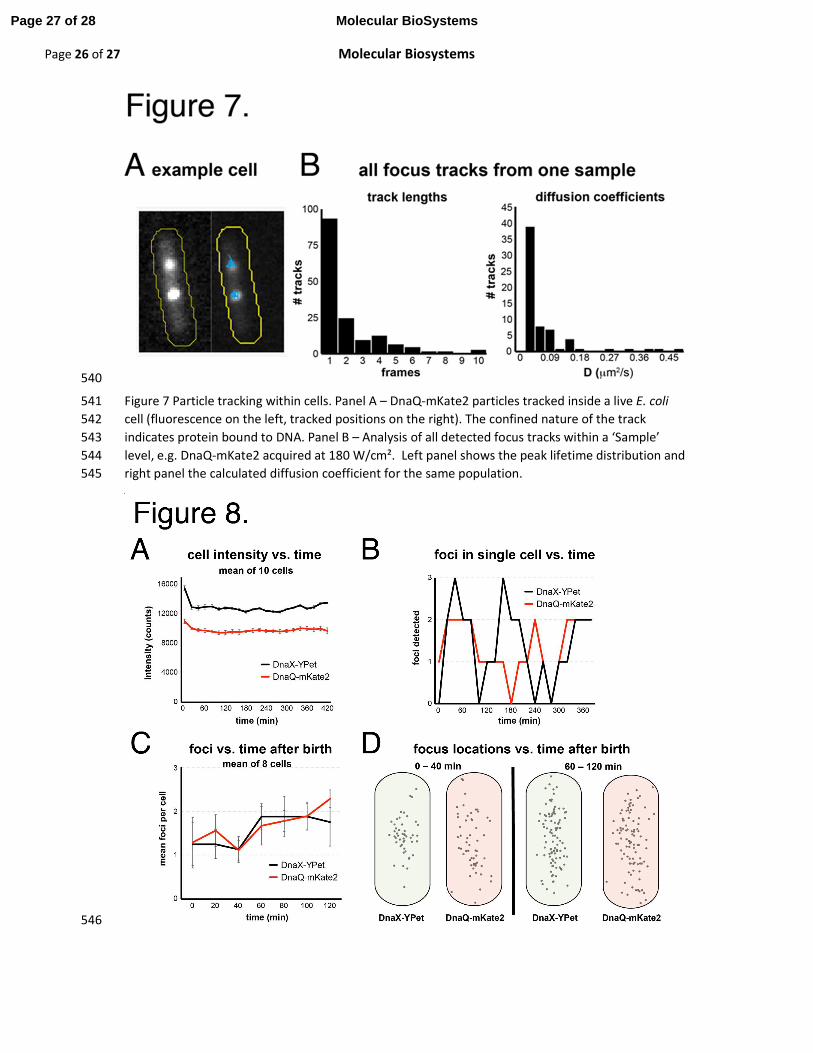
Rapid-acquisition imaging can also be used to measure the movements of molecules. Single-particle 259

tracking can be used to measure the diffusional motions of molecules. In iSBatch this operation is 260

implemented in the tracking module. Here foci within the tables generated by peak fitter are 261

assigned to trajectories if they fall within a set distance on consecutive frames and, optionally, are 262

within the same cell ROI (Fig. 7a). These trajectories can be used to build step-size distributions or 263

mean-square displacement plots that allow for measurement of properties such as diffusion 264

coefficients. For DnaQ-mKate2, which present long-lived trackable foci, we observe two populations: 265

one with low diffusion coefficients corresponding to molecules bound to DNA, and one with higher 266

diffusion coefficients corresponding to freely-diffusing molecules5 (Fig. 7b). 267

Time-Lapse Analysis 268

Time-lapse datasets consist of image stacks containing equal numbers of bright-field images and 269

fluorescence images, with individual frames corresponding to measurements at periodically sampled 270



time-points. Time-lapse measurements can be used to monitor temporal changes in the expression 271

level of a protein, the number of foci within cells, or the localization of proteins within cells. With the 272

availability of automated microscopes, we can monitor hundreds cells in several fields of view over a 273

period of minutes to days32

. 274

Our example dataset, TimeLapse, contains images of cells expressing DnaX-YPet and DnaQ-mKate2 275

recorded over 400 minutes. Using the module cell intensity, we measured the levels of each 276

fluorescent protein for ten cells over time. The levels of DnaX and DnaQ remain relatively constant 277

throughout the measurement (Fig. 8a). Using the number of foci detected by peak finder or peak 278

fitter, we quantified the number of DnaX-YPet and DnaQ-mKate2 foci observed over time. As 279

expected, cells periodically changed between zero, one, two and occasionally three foci (Fig. 8b). 280

Because we imaged in time-lapse mode, movie sequences of individual cells could be synchronized 281

to the beginning of the cell cycle. This analysis shows that after division, daughter cells contain one 282

foci on average, then the increases to two foci later in the cell cycle (Fig. 8c). If cell ROIs have been 283

imported from MicrobeTracker, it is possible to produce maps of focus locations within cells using 284

the location maps module. MicrobeTracker ROIs consist of high-resolution meshes, allowing the 285

relative positions of foci to be mapped to their relative cellular coordinates. For DnaX-YPet and 286

DnaQ-mKate2 cells, one focus was present from 0 to 40 min after birth (Fig. 8c). This focus was 287

located close to the mid-cell position (Fig. 8d). In contrast, 60 to 120 min after division, cells 288

exhibited two foci (Fig 8c). These foci were more evenly distributed through the entire cell (Figure 289

8d). 290

Materials and Methods 291

Implementation 292

Software 293



iSBatch is a Java 1.6-based plugin for ImageJ15

(version 1.49d) or its distribution Fiji33

. iSBatch is 294

designed for quick evaluation of analysis pipelines and visual exploration of datasets. It is distributed 295

under an open open-source34 license (GNU General Public License, version 3). iSBatch handles the 296

data in a hierarchical fashion based on a source folder containing all data and little guidance 297

provided by the user. Due to memory limitations when handling large datasets, iSBatch alleviates 298

memory overload by loading only the minimum set of images required for a process. Garbage 299

collection is done after each cycle so effective memory limitations are imposed by the amount of 300

memory available in the system and not by the size of the database. 301

The software is designed for rapid exploration of large datasets and it includes an internal SQLite 302

database (http://sqljet.com/) for convenience. All files related to the iSBatch platform, including 303

source codes and API for developers can be accessed directly from the plugin website 304

(https://github.com/SingleMolecule/iSBatch). 305

306

General workflow 307

308

In the following subsections, we describe the general workflow and how to use the plugin for 309

accessing basic cellular information. iSBatch guides the user in the initial configuration steps to 310

proper categorization of the input data. 311

Processing and Exploring Data - Custom functions 312

313

iSBatch couples its hierarchical data structure management to an extended version of ImageJ’s 314

macro interpreter. The user can record the executed operations, e.g. using ImageJ’s built in macro 315

recorder, and simply copy and paste the code in iSBatch interpreter. After selecting the desired 316

parameters, the results are displayed, allowing the user to quickly check the results. 317

Built-in functions 318



319

Data preprocessing involves image operations as well. Image Flattening is available and follows the 320

equation 321

�� =�� − �� − ��

�� − ��∗ ��

were ImageRange depends on the image type (8-, 16- or 32-bit), the CameraDarkCount can be 322

provided either as a constant or an image; BackgroundImage, if not available, can be generated from 323

all images acquired. Generating the Background image may lead to biased correction if saturated 324

peaks or high intensity regions are found for long time in the movies. A Gaussian filter with a default 325

value of four pixels is applied to reduce the influence of bright spots. 326

Ideally, the background should be an image taken in the same conditions of the experiment prior to 327

have the sample in the Field Of View. 328

To allow for fast and accurate detection of peaks, we implemented the fluoroBancrof algorithm35

. 329

This algorithm localizes peaks with sub-diffraction limit accuracy without the need of numerical 330

fitting36

. All the results will be available in human-readable format like comma-separated-values 331

(csv). 332

Acquiring peak tables from the images configures a starting point of a whole new section of analysis 333

of single molecule data. Change point analysis is used to assign steps to single-molecule traces and 334

infer stoichiometry of molecules. Cellular ROIS can be either added manually or imported from 335

MicrobeTracker. In the later, a detailed subdivision of each cell with meshes is available. Therefore, 336

is possible to localize every peak in relation to the mesh and assign relative positions. With the 337

cellular parameters, such as cell length, width, area, can be obtained from the imported ROIs and an 338

artificial cell is created for the peaks to be inserted. 339

Image Acquisition 340

Cell Culture 341



Derivatives of E. coli K12 MG1655 carrying a chromosomal C-terminal fusions37

containing DnaX-YPet 342

and DnaQ-mKate2 were grown overnight in M9 Minimal medium supplemented with Glycerol 2% 343

and 10mM thiamine hydrochloride; Cell cultures were diluted to 1:100 and grown from 4 hours at 344

37oC at 1100 rpm prior to the start of the imaging experiment. 345

Image Acquisition 346

The images were taken on a home-built single-molecule fluorescence microscope consisting of a 347

fully-automated inverted microscope body (Olympus IX-81) with excitation light provided by 514 nm 348

and 568 nm Sapphire lasers (Coherent) and equipped with a 1.49 NA 100x objective and a 512 × 349

512 pixel EM-CCD camera (C9100-13, Hamamatsu). For imaging we used flow cells derivatized with 350

3-aminopropyl triethoxy silane (APTES, Sigma) and kept the flow at 10 µl/min. 351

The datasets are described as follows: 1) Rapid acquisition of DnaX-YPet and DnaQ-mKate2 each 352

containing 10 Fields of View. A Field of View comprises a reference bright field image and a 353

fluorescence movie (500 frames each with 34ms interval between acquisitions under different laser 354

intensities); 2) Time Lapse acquisition of DnaX-YPet and DnaQ-mKate2 containing 10 fields of View 355

containing a bright field and two fluorescent images of 50 ms for each fluorescent protein. The cycle 356

time is 20 minutes and the experiment was carried out for 400 minutes. Datasets are available as 357

supplementary materials S1 and S2; 358

Conclusion 359

We present here a fully open-source and community-driven ImageJ plugin for single-molecule 360

analysis focused on hierarchical data obtained from live-cell single-molecule experiments. The plugin 361

facilitates data exploration and bookkeeping of datasets with large number of images in multiple 362

colour channels, including basic pipelines and support for custom macros. We present case studies 363

that illustrate the ability to carry out analysis in a structured way, minimizing the burden of code 364

development. With this in mind, we envision that the user will be able to place a larger focus on 365



exploration of biological phenomena and new analysis routines. The development of open-source 366

analysis tools such as the ones presented here allows for a community-based sharing and 367

development38 of the platforms required to analyse experiments that increasingly grow in complexity 368

and data richness. Software documentation is included within the Supplementary Material. The 369

source code is available for download at https://github.com/SingleMolecule/iSBatch. 370

Acknowledgements 371

We would like to thank M. Cox and E.A. Wood for providing the E. coli strain used in this work. The 372

authors would like to acknowledge funding from the Netherlands Organization for Scientific 373

Research (NWO; Vici 680-47-607) and the European Research Council (ERC Starting 281098). The 374

authors alone are responsible for the content and writing of the paper. 375

Conflict of interest 376

The authors declare that they have no conflicts of interest concerning this article. 377

References 378

1. Xia, T., Li, N. & Fang, X. Single-molecule fluorescence imaging in living cells. Annu. Rev. Phys. 379

Chem. 64, 459–80 (2013). 380

2. Rigler, R. Fluorescence and single molecule analysis in cell biology. Biochem. Biophys. Res. 381

Commun. 396, 170–175 (2010). 382

3. Reyes-Lamothe, R., Sherratt, D. J. & Leake, M. C. Stoichiometry and architecture of active 383

DNA replication machinery in Escherichia coli. Science 328, 498–501 (2010). 384

4. Mashanov, G. I. Single molecule dynamics in a virtual cell: a three-dimensional model that 385

produces simulated fluorescence video-imaging data. J. R. Soc. Interface 11, (2014). 386

5. Yu, J., Xiao, J., Ren, X., Lao, K. & Xie, X. S. Probing gene expression in live cells, one protein 387

molecule at a time. Science 311, 1600–1603 (2006). 388

6. Haas, B. L., Matson, J. S., DiRita, V. J. & Biteen, J. S. Imaging Live Cells at the Nanometer-Scale 389

with Single-Molecule Microscopy: Obstacles and Achievements in Experiment Optimization 390

for Microbiology. Molecules 19, 12116–12149 (2014). 391

7. Lenn, T. & Leake, M. C. Experimental approaches for addressing fundamental biological 392

questions in living, functioning cells with single molecule precision. Open Biol. 2, 120090 393

(2012). 394



8. Cardona, A. & Tomancak, P. Current challenges in open-source bioimage informatics. Nat. 395

Methods 9, 661–5 (2012). 396

9. Eliceiri, K. W. et al. Biological imaging software tools. Nat. Methods 9, 697–710 (2012). 397

10. Kamentsky, L. et al. Improved structure, function and compatibility for cellprofiler: Modular 398

high-throughput image analysis software. Bioinformatics 27, 1179–1180 (2011). 399

11. Jones, T. R. et al. CellProfiler Analyst: data exploration and analysis software for complex 400

image-based screens. BMC Bioinformatics 9, 482 (2008). 401

12. Sliusarenko, O., Heinritz, J., Emonet, T. & Jacobs-Wagner, C. High-throughput, subpixel 402

precision analysis of bacterial morphogenesis and intracellular spatio-temporal dynamics. 403

Mol. Microbiol. 80, 612–27 (2011). 404

13. Shivanandan, A., Radenovic, A. & Sbalzarini, I. F. MosaicIA: an ImageJ/Fiji plugin for spatial 405

pattern and interaction analysis. BMC Bioinformatics 14, 349 (2013). 406

14. Herbert, A. D., Carr, A. M. & Hoffmann, E. FindFoci: A Focus Detection Algorithm with 407

Automated Parameter Training That Closely Matches Human Assignments, Reduces Human 408

Inconsistencies and Increases Speed of Analysis. PLoS One 9, e114749 (2014). 409

15. Abràmoff, M. D., Magalhães, P. J. & Ram, S. J. Image processing with ImageJ Part II. 410

Biophotonics Int. 11, 36–43 (2005). 411

16. Schneider, C. a, Rasband, W. S. & Eliceiri, K. W. NIH Image to ImageJ: 25 years of image 412

analysis. Nat. Methods 9, 671–675 (2012). 413

17. Wollman, R. & Stuurman, N. High throughput microscopy: from raw images to discoveries. J. 414

Cell Sci. 120, 3715–22 (2007). 415

18. Sliusarenko. Microbetracker software. Mol. Microbiol. 80, 612–627 (2012). 416

19. Stratmann, S. a & van Oijen, a M. DNA replication at the single-molecule level. Chem. Soc. 417

Rev. 43, 1201–20 (2014). 418

20. Robinson, A. & van Oijen, A. M. Bacterial replication, transcription and translation: 419

mechanistic insights from single-molecule biochemical studies. Nat. Rev. Microbiol. 11, 303–420

15 (2013). 421

21. Betzig, E. et al. Imaging intracellular fluorescent proteins at nanometer resolution. Science 422

313, 1642–5 (2006). 423

22. Henriques, R., Griffiths, C., Hesper Rego, E. & Mhlanga, M. M. PALM and STORM: unlocking 424

live-cell super-resolution. Biopolymers 95, 322–31 (2011). 425

23. Zhu, L., Zhang, W., Elnatan, D. & Huang, B. Faster STORM using compressed sensing. Nat. 426

Methods 9, 721–3 (2012). 427

24. Team R Core Development. R: a language and environment for statistical computing | 428

GBIF.ORG. R Foundation for Statistical Computing (2013). at <http://www.r-project.org/> 429



25. Thompson, R. E., Larson, D. R. & Webb, W. W. Precise nanometer localization analysis for 430

individual fluorescent probes. Biophys. J. 82, 2775–83 (2002). 431

26. Hauberg, J. W. E. and D. B. and S. GNU Octave version 3.0.1 manual: a high-level interactive 432

language for numerical computations. (CreateSpace Independent Publishing Platform, 2009). 433

at <http://www.gnu.org/software/octave/doc/interpreter> 434

27. Leake, M. C. et al. Stoichiometry and turnover in single, functioning membrane protein 435

complexes. Nature 443, 355–8 (2006). 436

28. Eckley, R. K. and I. A. changepoint: An R Package for Changepoint Analysiso Title. J. Stat. 437

Softw. 58, (2014). 438

29. Watkins, L. P. & Yang, H. Detection of intensity change points in time-resolved single-439

molecule measurements. J. Phys. Chem. B 109, 617–28 (2005). 440

30. Shcherbo, D. et al. Far-red fluorescent tags for protein imaging in living tissues. Biochem. J. 441

418, 567–574 (2009). 442

31. Shaner, N. C., Steinbach, P. A. & Tsien, R. Y. A guide to choosing fluorescent proteins. Nat. 443

Methods 2, 905–909 (2005). 444

32. Muzzey, D. & van Oudenaarden, A. Quantitative time-lapse fluorescence microscopy in single 445

cells. Annu. Rev. Cell Dev. Biol. 25, 301–27 (2009). 446

33. Schindelin, J. et al. Fiji: an open-source platform for biological-image analysis. Nat. Methods 447

9, 676–82 (2012). 448

34. Prlić, A. & Procter, J. B. Ten Simple Rules for the Open Development of Scientific Software. 449

PLoS Comput. Biol. 8, 8–10 (2012). 450

35. Hedde, P. N., Fuchs, J., Oswald, F., Wiedenmann, J. & Nienhaus, G. U. Online image analysis 451

software for photoactivation localization microscopy. Nat. Methods 6, 689–690 (2009). 452

36. Andersson, S. B. Localization of a fluorescent source without numerical fitting. Opt. Express 453

16, 18714–18724 (2008). 454

37. Datsenko, K. A. & Wanner, B. L. One-step inactivation of chromosomal genes in Escherichia 455

coli K-12 using PCR products. Proc. Natl. Acad. Sci. U. S. A. 97, 6640–5 (2000). 456

38. Carpenter, A. E., Kamentsky, L. & Eliceiri, K. W. A call for bioimaging software usability. 457

Nature Methods 9, 666–670 (2012). 458

459

Figure Captions 460

Figure 1 Schematic design of a single-cell, single-molecule experiment. Panel A – Structure of a 461

time-lapse experiment. Each time point shows a bright-field (BF) image and its corresponding 462



fluorescence channel (in this example 568-nm excitation). The intervals are on the time scale of 463

minutes. Panel B – Monitoring of cell fluorescence intensity and its relation to total observable 464

protein concentration and protein number per cell throughout the experiment. Panel C – Structure 465

of a rapid-acquisition experiment. A single bright-field image is taken prior to subsequent rapid 466

image acquisition in the fluorescence channel (in this case 568-nm excitation). Panel D – Simulated 467

data of binding dynamics of a molecule. 468

Figure 2 iSBatch Structure. Panel A – Schematic representation of data structure (Experiment – E, 469

Sample – S, Field of View – FoV) and its connections. Panel B – Logic structure of the algorithm; 470

Panel C – User interface including ImageJ main panel (upper part) and iSBatch interface with the 471

main commands. 472

Figure 3 Custom Macro runner. iSBatch contains a custom macro runner that support syntax-473

highlighting for creating, running and editing existing ImageJ macros and plugin commands from the 474

MacroRecorder. 475

Figure 4 Built-in Peak Fitting Operation. Panel A – Selected node highlighting the ‘Experiment’ level. 476

Panel B – Distribution of detected peak intensities within different ‘Samples’ in the same selected 477

‘Experiment’ node for DnaQ-mKate2. 478

Figure 5 Step-wise photobleaching. Panel A – Selected node highlighting a ‘Field of View’ level. 479

Panel B – Selected cell within a ‘Field of View’ with the boundaries assigned in yellow and a selection 480

box in red. Panel C – Representative photobleaching trace of a detected focus. Red traces represent 481

the detected steps by change-point analysis algorithm. 482

Figure 6 Cellular fluorescence obtained by Rapid Acquisition. Panel A – Selected node highlighting a 483

‘Experiment’ level Panel B – Cellular fluorescence photobleaching dependent on laser intensity for 484

DnaQ-mKate2. Panel C – Selected node highlighting two ‘Samples’ selected within different 485

experiments. Panel D – Comparison of photobleaching properties of YPet and mKate2 when excited 486

with same laser intensity (180 W/cm²). 487

Figure 7 Particle tracking within cells. Panel A – DnaQ-mKate2t particles tracked inside a live E. coli 488

cell. Blue: Confined track indicating protein bound to DNA. Panel B – Analysis of all detected focus 489

tracks within a ‘Sample’ level, e.g. DnaQ-mKate2 acquired at 180 W/cm². Left panel shows the peak 490

lifetime distribution and right panel the calculated diffusion coefficient for the same population. 491

Figure 8 Built-in Time-Lapse analysis. Panel A – Fluorescence cell intensity over time for DnaX-YPet 492

and DnaQ-mKate2. Panel B – Number of long-lived immobile peaks per cell, i.e. foci. Panel C – Data 493

synchronization considering cell division times. Time zero is the first frame after cell division; cell 494

division time is 100 – 120 min. Panel D – Location maps. A projection of detected peaks in an 495

artificial, normalized cell. Left: projected cells with one detected focus, distributed towards the 496

centre of the cell; Right: projected cells with two detected foci, distributed towards the ¼ and ¾ of 497

the cell. 498

499



500

501



502

Figure 31 Schematic design of a single-cell, single-molecule experiment. Panel A – Structure of a 503

time-lapse experiment. Each time point shows a bright-field (BF) image and its corresponding 504

fluorescence channel (in this example 568-nm excitation). The intervals are on the time scale of 505

minutes. Panel B – Exemplified cell fluorescence intensity and its relation to total observable protein 506

concentration and protein number per cell throughout the experiment. Panel C – Structure of a 507

rapid-acquisition experiment. A single bright-field image is taken prior to subsequent rapid image 508

acquisition in the fluorescence channel (in this case 568-nm excitation). Panel D – Simulated data of 509

binding dynamics of a molecule. 510



511

Figure 42 iSBatch Structure. Panel A – Schematic representation of data structure (Experiment – E, 512

Sample – S, Field of View – FoV) and its connections. Panel B – Logic structure of the algorithm; 513

Panel C – User interface including ImageJ main panel (upper part) and iSBatch interface with the 514

main commands. 515



516

Figure 3 Custom Macro runner. iSBatch contains a custom macro runner that support syntax-517

highlighting for creating, running and editing existing ImageJ macros and plugin commands from the 518

MacroRecorder. 519

520

521



522 Figure 4 Built-in Peak Fitting Operation. Panel A – Selected node highlighting the ‘Experiment’ level. 523

Panel B – Distribution of detected peak intensities within different ‘Samples’ in the same selected 524

‘Experiment’ node for DnaQ-mKate2. 525

526

527

Figure 5 Step-wise photobleaching. Panel A – Selected node highlighting a ‘Field of View’ level. Panel 528

B – Selected cell within a ‘Field of View’ with the boundaries assigned in yellow and a selection box 529

in red. Panel C – Representative photobleaching trace of a detected focus. Red traces represent the 530

detected steps by change-point analysis algorithm. 531

532



533

534

Figure 6 Cellular fluorescence obtained by Rapid Acquisition. Panel A – Selected node highlighting a 535

‘Experiment’ level Panel B – Dependence of cellular fluorescence photobleaching on laser intensity 536

for DnaQ-mKate2. Panel C – Selected node highlighting two ‘Samples’ selected within different 537

experiments. Panel D – Comparison of photobleaching properties of YPet and mKate2 when excited 538

with same laser intensity (180 W/cm²). 539



540

Figure 7 Particle tracking within cells. Panel A – DnaQ-mKate2 particles tracked inside a live E. coli 541

cell (fluorescence on the left, tracked positions on the right). The confined nature of the track 542

indicates protein bound to DNA. Panel B – Analysis of all detected focus tracks within a ‘Sample’ 543

level, e.g. DnaQ-mKate2 acquired at 180 W/cm². Left panel shows the peak lifetime distribution and 544

right panel the calculated diffusion coefficient for the same population. 545

546



Figure 8 Built-in Time-Lapse analysis. Panel A – Fluorescence cell intensity over time for DnaX-YPet 547

and DnaQ-mKate2. Panel B – Number of long-lived immobile peaks per cell, i.e. foci. Panel C – Data 548

synchronization considering cell division times. Time zero is the first frame after cell division; cell 549

division time is 100 – 120 min. Panel D – Location maps. A projection of detected peaks in an 550

artificial, normalized cell. Left: projected cells with one detected focus, distributed towards the 551

centre of the cell; Right: projected cells with two detected foci, distributed more towards the ¼ and 552

¾ positions in the cell. 553

554


isbatch: a batch-processing platform for data analysis and

Documents