isobaric tag based ms quantification algorithms … · 0 isobaric tag based ms quantification...
TRANSCRIPT
0
Isobaric Tag based MS Quantification Algorithms
Analysis and Implementation Master’s degree in Proteomics and Bioinformatics
Written by Sankar Martial
Supervisors: Nicolas Budin1, Pierre-Alain Binz1
Academic year 2007/2008
This thesis was submitted as part of the requirements for the Master’s degree in Proteomics and Bioinformatics
from the University of Geneva.
1Geneva Bioinformatics (GeneBio) SA
25 avenue de Champel 1206 Geneva – Switzerland
1
Contents
Abstract ................................................................................................................................................... 2
Acknowledgements ................................................................................................................................. 3
1. Introduction ..................................................................................................................................... 4
1.1. GeneBio SA .............................................................................................................................. 4
1.2. Organisation ............................................................................................................................ 4
1.3. Biological Context .................................................................................................................... 5
2. Quantitative Proteomics ................................................................................................................. 6
2.1. Global View .............................................................................................................................. 6
2.2. Isobaric Tagging ....................................................................................................................... 9
2.3. Experimental Application ...................................................................................................... 12
2.4. Experimental Design: Principle of Replicate Analysis ............................................................ 13
3. Methods: Study Quantification Workflow .................................................................................... 14
3.1. Introduction ........................................................................................................................... 14
3.2. Experimental samples ........................................................................................................... 15
3.3. Tested Software Presentation ............................................................................................... 16
3.4. Software comparison ............................................................................................................ 26
3.5. Discussion .............................................................................................................................. 29
4. Establish Quantification WF .......................................................................................................... 30
4.1. Introduction ........................................................................................................................... 30
4.2. Description ............................................................................................................................ 31
4.3. Validation of the algorithms .................................................................................................. 42
4.4. Discussion .............................................................................................................................. 45
5. Application of the Quantification Workflows................................................................................ 46
5.1. Alireza collaboration: Peptides Ratios-based Quantification Approach applied to
Characterize Daptomycin Resistance in Staphylococcus aureus. ..................................................... 46
5.2. Loic Dayon Collaboration ...................................................................................................... 51
5.2.1. CSF Analysis by TMT 6-plex ........................................................................................... 51
5.2.2. CSF micro-dialysis .......................................................................................................... 66
6. Conclusion ..................................................................................................................................... 71
7. Reference ...................................................................................................................................... 72
2
Abstract
One single gene gives rise to several proteins. This well-known sentence illustrates all of the complexity of the proteome compared to the genome and the transcriptome. As does genomics, proteomics provides a large toolbox of experimental methods to achieve the quantification of proteins. In contrast, the analytical means to obtain a reliable and trusted value of protein relative abundances are less developed. Although more and more tools are released to assess protein ratios, a quick review of proteomics papers reveals that quantitative data analysis is still performed manually.
For this purpose, three algorithms for isobaric tag-based quantitative analysis were implemented. They were successfully applied on experimental datasets provided by the Biomedical Proteomics Research Group (BPRG) and the Clinical Proteomics Research Group (CPRG) of the University of Geneva. Finally, these algorithms were implemented in the quantification module of the Phenyx software.

3
Acknowledgements
It was an immense privilege to be guided and to be under the tutelage of my supervisors Nicolas Budin and Pierre-Alain Binz.
I am very grateful to Alexandre Masselot for having given me the opportunity to do this training course at GeneBio, for his availability and his advice.
I would like to thank Nasri Nahas for having permitted me to carry out this training under the optimal conditions.
Many thanks are due to Olivier Evalet, Yann Mauron, Roman Mylonas and Ivan Topolsky for their support and their good mood.
I am very thankful to Alireza Vaezzadeh and Loic Dayon for their collaboration,
I thank very much David Bouyssié who did an essential previous work on the reporter ion peaks extraction.
Finally, I would like to thank all the members of GeneBio for having welcoming me during one year.
4
1. Introduction
1.1. GeneBio SA
Geneva Bioinformatics (GeneBio) SA is a bioinformatics company founded in November 1997. It was created quasi simultaneously with the Swiss Institute of Bioinformatics (SIB). One of the main activities of GeneBio is to act as the privileged commercial arm of the SIB, and therefore bring to market developments done at the SIB in order to provide back revenues to help further developments. Its first product line started in 1998 with the Swiss-Prot database. Swiss-2DPAGE (a 2D gel database), Prosite (a database of protein domains, families and functional sites) and Melanie (a 2D gel analysis software) soon followed. GeneBio also develops and commercialises proper specialized and innovative databases and software on biological molecules. These include Phenyx, a renowned software platform for the identification and characterization of proteins and peptides from mass spectrometry data. Another example is SmileMS, the latest GeneBio software and also developed in collaboration with the SIB. It is a unique platform for the identification and analysis of small molecules by mass spectrometry. Located in Geneva, a centre of excellence in the field of proteomics, GeneBio now has between 15 and 20 employees, including a majority of biologists and computer scientists.
1.2. Organisation
My training course was achieved within the Phenyx development team. It's a bioinformatics training involving a binomial supervision. Dr Pierre-Alain-Binz has taken the responsibility of the scientific aspects of my project, giving me advice and orientation in proteomics and data analysis. Dr Nicolas Budin directed the informatics part of the project. He has managed the whole development side of the project, initiating me into R language, Java language, and to reliable methods of software development.
The mass-spectrometric-based quantification universe is wide. From the beginning, it was decided that only iTRAQ quantification would be covered in my work.
To deepen my knowledge of the master courses about Mass-Spectrometric-based quantification in proteomics, I started the training by reading papers on iTRAQ reagents and principles of quantification. Later, in order to familiarize with MS-identification and quantification, I focused on testing some of the available quantification tools. These steps permitted me to handle biological data, to see and understand the basis of large amounts of data analysis and to feel the span of the perspectives that the mass-spectrometric-based quantitative analysis offers. Subsequently, I have developed my own tools. Using the R Language, I have replicated the workflow of some of the studied software. Finally, the time came to offer quantification mean to the Phenyx users. The implementation was done in Java with the inclusion of calls to a few crucial statistical steps.
5
In order to obtain real users’ feedback, to collect what was needed in quantification, to see how the data was analysed, to obtain quantification materials and to have an idea of how the developed tools should behave when faced with real data, a collaboration was carried out with the Biochemical Proteomics Research Group and the Clinical Proteomics Group of the Geneva University.
1.3. Biological Context
Proteomics analysis proposes a large toolbox of analytical methods, instruments and algorithms to identify and characterize proteins. The majority of the published proteomics studies are limited to the identification of the proteins expressed in a biological system. However, this is not sufficient to answer to most biological questions. Does a protein behave significantly different between two samples? Does a protein exhibit time-dependent change? Which proteins behave similarly in the experiment? Thus, quantitative answers are more and more required and populate an increasing number of publications.
Initially, quantitative and comparative proteome analysis was performed with 2D-PAGE. Due to some limitations (low dynamic range, bias against membrane and soluble proteins), “gel-free” methods have complemented and are gradually supplanting “gel-based” quantitative proteomics. Specific techniques are used to address this issue. One solution is based on the employment of stable isotopes. Isotope label can be incorporated to the process in three ways: metabolically (during cell growth), enzymatically, and chemically.
Chemical incorporation of the stable isotope has produced the most of the quantitative proteome data mainly due to its chemical versatility and because it allows the analysis of any biological sample (in contrast to metabolic).
Due to the high amount of data, manual analysis is laborious but remains persistent in the scientific community. Thus, many software tools are made available to support data analysis. Several are open-source, with their own assets and caveats. Most of them are able to handle identification results from one or more different search engine (Mascot, Phenyx, SEQUEST, X!Tandem...). Recently, Mascot (a major player in the identification market) proposed its own quantification module. Phenyx need to meet the concurrent demands of quantitative high throughput MS data by proposing its own quantification module. Following the six month’s work of the Master Student David Bouyssié in 2006 on the quantitative data extraction module for mainly SILAC and iTRAQ, my main objective was to add the missing downstream analyses pieces of the puzzle and provide a complete quantification pipeline for iTRAQ methodology.
6
2. Quantitative Proteomics
2.1. Global View
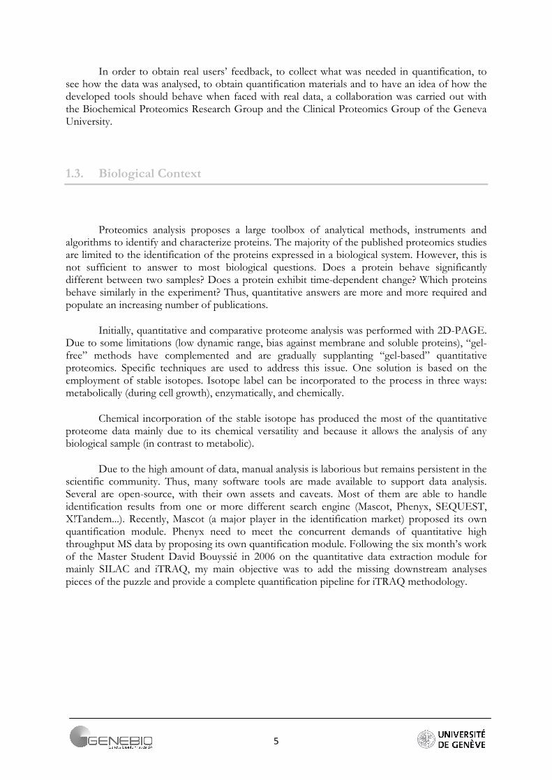
Several methods exist to assess the protein abundance in a sample. Classical methods such as western blotting, fluorophores and radioactivity are widely used due to their sensitivity and dynamic range. However, these methods are not generally appropriate due to some constraints for large scale screening, and particularly for biomarker discovery (non-targetted experiments). Wu et al. has compared MS-based stable isotope labelling methods (iTRAQ, cICAT) and DIGE (Differential Gel Electrophoresis) and has shown that these problems can be overcomed by MS-based approaches [32]. MS-based strategy coupled with separation methods (2DE or LC) is currently the more efficient mean to perform the identification of a complex mixture of protein. However, due to the fact that protolytic peptides exhibit a wide range of physico-chemical properties (size, charge, hydrophocity...), the relationship between the amount of proteins and the signal intensities is complex. Therefore mass spectrometry is not inherently quantitative, when seen as a tool for absolute quantitation. Therefore, relative quantitation is preferred, where peptides are compared between experiments data points. This can be achieved in a numbers of ways. Thus, high throughput assessment of change in protein expression is usually performed by stable isotope labelling of peptides and proteins either metabolically, enzymatically (160, 180 incorporation by proteolysis) or chemically using external reagents (Figure 1).
7
Figure 1. Overview of quantification in Proteomics, [41]
Metabolic Labelling involves in-vivo incorporation of the stable isotope during cell growth and division. One of the most widely used approaches is the SILAC (Stable Isotope Labelling Amino acid in Cell culture) approach, which was introduced by Mann and co-workers in 2002 [33]. In these methods, the heavy amino acid is incorporated during the protein synthesis. The main advantage is that no multiple steps in the labelling protocol are needed and the experimental error does not affect the ratio [34] as shown in However, this approach is almost exclusively applicable to cell
An other approach is chemical labelling. For example, several papers studied fluids basing on isobaric tag, iTRAQ [4] or TMT [7]. The principle of chemical tagging rests on the reactivity of the N-ter and side chains of lysine (iTRAQ, TMT) and cysteine (ICAT).
ICAT (Isotope Coded Affinity Tag) is the most known of the Cys tagging strategies. Chemical tags were designed to simultaneously allow the enrichment of a subfration (Cys peptides) from a complex mixture of proteins and the quantification of the selected peptides at the precursor ions level. Gygi et al. [35] developed this approach in which cysteine residues are specifically derivatized with a reagent containing either zero or eight deuterium atoms as well as a biotin group for affinity purification of cysteine-derivatized peptides and subsequent MS analysis. Modified versions of ICAT are emerged to solve problems of elution (cICAT) and fragment loss (VICAT...). Wu et al. highlighted drawbacks and weaknesses of ICAT methods compared with other chemical tagging approaches [32]. Although ICAT analysis yields to good results when performed on simple or moderately complex sample, the cysteine-specificity leads to a loss of sensitivity when analyzing a complex protein mixture.
8
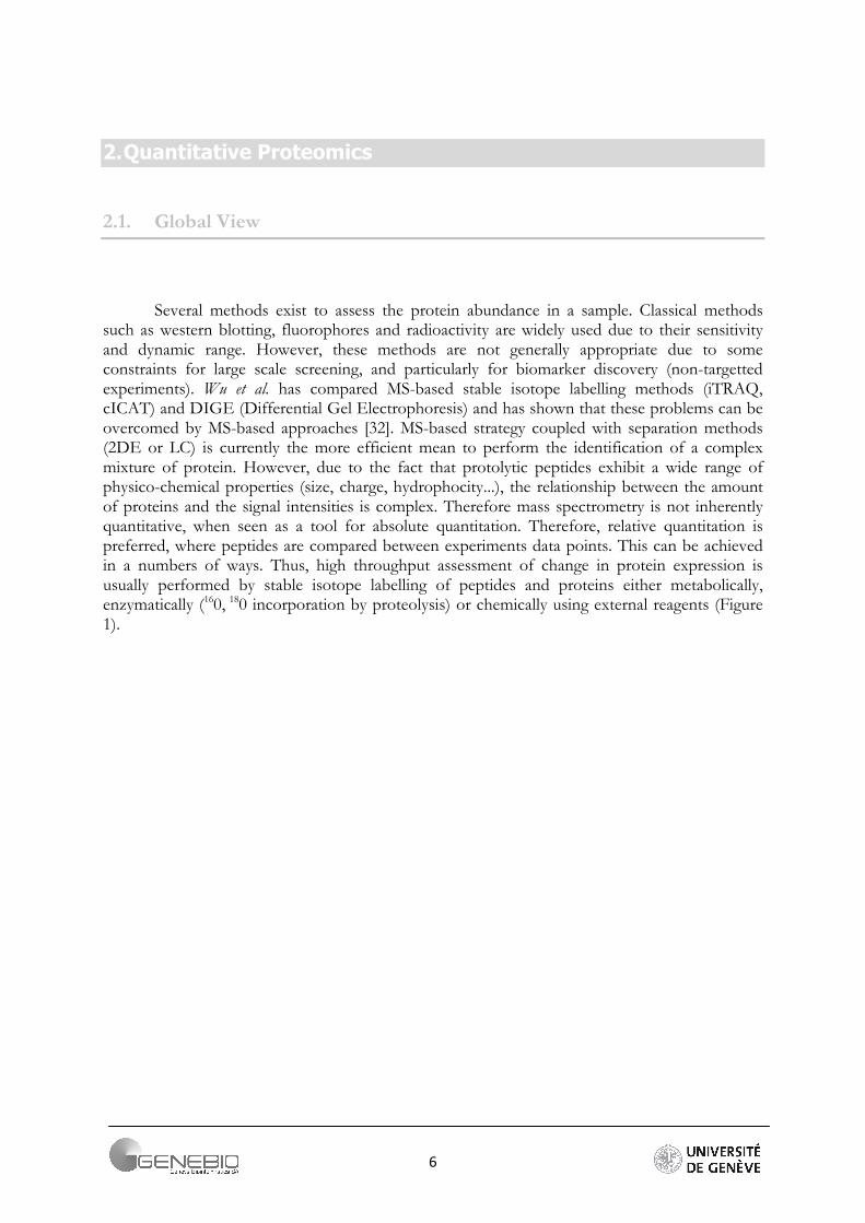
Figure 2. Common quantitative mass spectrometry workflows, Boxes in blue and yellow represent two experimental conditions. Horizontal lines indicate when samples are combined. Dashed lines indicate points at which experimental variation and thus quantification errors can occur [30].
Group of labelling reagents which targets the peptide N-terminus and the epsilon-amino group of lysine residues are the most sensitive. Most of the time, this is realized via the very specific N-hydroxysuccinimide (NHS) chemistry or other active esters and acid anhydride as in, e.g., the isotope coded protein label (ICPL), isotope tags for relative and absolute quantification (iTRAQ) [19], tandem mass tags (TMT) [8], ...
ICPL, ICAT methods and most of the aforementioned chemical modification techniques, relative quantification is achieved by integration of MS signal over ‘heavy’ and ’light’ labels. TMT and iTRAQ introduce the concept of the isobaric tag. Isobaric tags labelled peptides co-migrate in liquid chromatography separations. The different tag can be distinguished by the mass spectrometer only upon peptide fragmentation. This permits the simultaneous determination of both identity and relative abundance of peptide in tandem-mass spectra. ITRAQ and TMT are described more in details below and some examples of application are provided and summarised (Figure 5).
9
2.2. Isobaric Tagging
iTRAQ
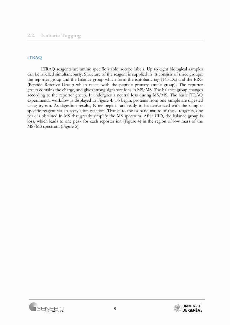
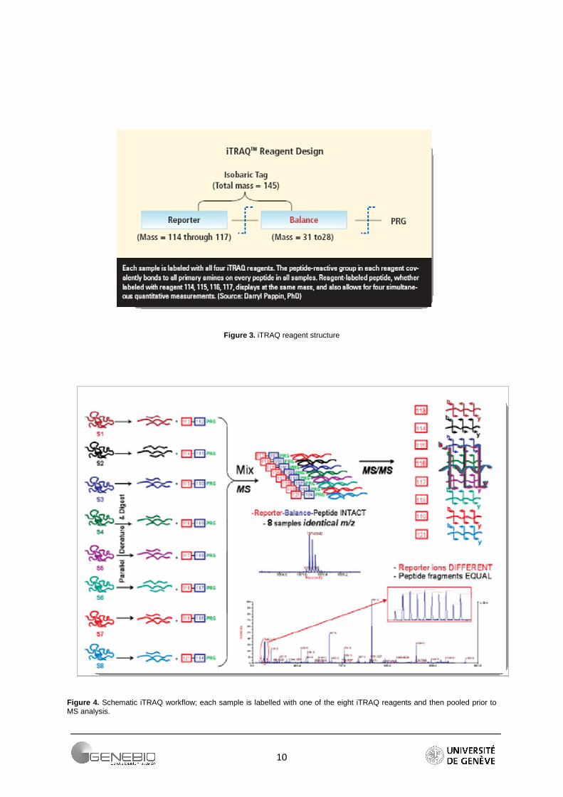
ITRAQ reagents are amine specific stable isotope labels. Up to eight biological samples can be labelled simultaneously. Structure of the reagent is supplied in It consists of three groups: the reporter group and the balance group which form the isotobaric tag (145 Da) and the PRG (Peptide Reactive Group which reacts with the peptide primary amine group). The reporter group contains the charge, and gives strong signature ions in MS/MS. The balance group changes according to the reporter group. It undergoes a neutral loss during MS/MS. The basic iTRAQ experimental workflow is displayed in Figure 4. To begin, proteins from one sample are digested using trypsin. As digestion results, N-ter pepides are ready to be derivatized with the sample-specific reagent via an acetylation reaction. Thanks to the isobaric nature of these reagents, one peak is obtained in MS that greatly simplify the MS spectrum. After CID, the balance group is loss, which leads to one peak for each reporter ion (Figure 4) in the region of low mass of the MS/MS spectrum (Figure 5).
10
Figure 3. iTRAQ reagent structure
Figure 4. Schematic iTRAQ workflow; each sample is labelled with one of the eight iTRAQ reagents and then pooled prior to MS analysis.
11
iTRAQ reagents allow multiplexed quantification of up to eight samples (cell, tissue, serum). Moreover, it permits PTM analysis. Aggarwal et al. show that the reagent does not interfere negatively with the fragmentation to the extent that peptides length and amino acid content are similar to those obtained using other MS approaches [36]. Furthermore, iTRAQ is a highly sensitive approach. Wu et al. demonstrated that iTRAQ covers a large part of the E.coli proteomes. It helps to identify proteins across extreme pI and MW, it detects a great number of fragment peptides per protein and low abundance proteins are more often discerned. This high sensitivity can be explained by two factors. First, iTRAQ is a global tagging reagent on all primary amine, contrary to ICAT (labels only cysteine). The second one is related the reactivity of lysine which leads to a stronger signal in MALDI-MS. Quantification relies on daughter ions generated during CID. However, a potential pitfall inherent to the Timed Ion Selector (TIS) resolution of the MALDI-TOF/TOF may affect quantification accuracy. Quantification relies on daughter ions generated during CID. TIS allows precursor ion and his fragment to pass through a gate in order to reach the detector and contribute in this way to the quantification ratio [32].A second limitation is that experimental variations can occur during tryptic digestion. In iTRAQ workflow (Figure 4), digestion is prior to the labelling and the mix, contrary to ICAT where the labelling is prior to mix and digestion. This may introduce a potential source of error, especially in sample handling and variable degrees of tryptic digestion between two or more samples [32].
Table 1. Advantages/Disadvantage of iTRAQ reagents
Advantages Disadvantage
– Parallel proteomics: 8-plexing.
– Analyze proteins from cell, tissues or
serum.
– PTM analysis.
– iTRAQ reagent don't interfere negatively
with fragmentation.
– High sensitivity.
– Mass spectrometer interference could
hinder iTRAQ reliability.
– iTRAQ labelling after the tryptic digestion.
TMT
Tandem Mass Tag uses exactly the same approach as iTRAQ. TMT tags are however heavier (TMT 6-plex: 126 to 131 Da).
12
2.3. Experimental Application
The isobaric labelling approaches have been successfully applied to a variety of experiments and to various samples (prokaryotic and eukaryotic samples including Escherichia coli, yeast, human saliva, human fibroblasts and mammary epithelial cells...) [34,36].
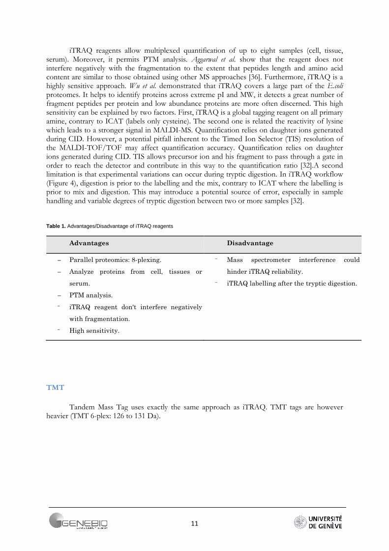
The iTRAQ approach can be applied for various purposes. For example, most of time when searching to characterize proteins from a specific signalling pathway, parallel proteomics approaches such as iTRAQ 4-plex or TMT 6-plex are commonly used in order to obtain time courses profiles. Schmelzle et al. used iTRAQ to label 4 samples of adipocytes stimulated for insulin at different time. Then, time course profiles have been plotted and proteins displaying the same behaviour in the same fashion are clustered. Unknown protein Glu-4 functionality was discovered in this manner [20]. Another study carried out by Zhang et al. used iTRAQ for the same purpose. Profiles were made and clustered using Spotfiretm and the methods of SOM matrix [27]. Biomarkers can also be discovered using isobaric tags. Dayon et al and Choe et al analyzed CSF samples, using respectively TMT 6-plex [5] and iTRAQ 4-plex [7]. Moreover, Desouza et al. identified five potential markers for endometrial cancer with iTRAQ reagents and a set of four proteins using ICAT [9]. Cong et al. compared proteomes of human fibroblasts in four different biological states: replicatively senescent (under permanent growth arrest), stress-induced prematurely senescent, quiescent and young replicating, to identify the signature proteins of each biological state [6]. Figure 5 summarizes the purpose of quantitative proteomics using the isobaric tags.
Figure 5 . Common application of isobaric tags in proteomics and related analysis workflows.
13
2.4. Experimental Design: Principle of Replicate Analysis
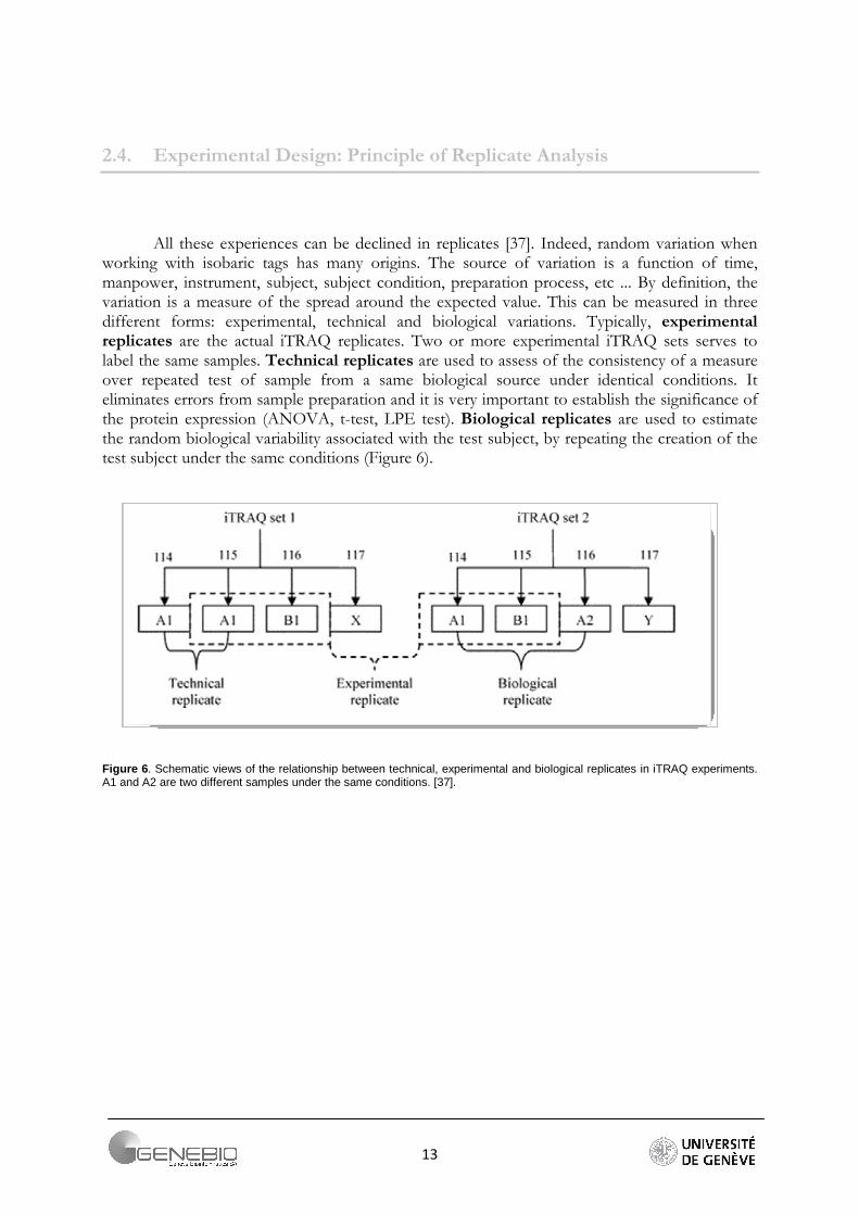
All these experiences can be declined in replicates [37]. Indeed, random variation when working with isobaric tags has many origins. The source of variation is a function of time, manpower, instrument, subject, subject condition, preparation process, etc ... By definition, the variation is a measure of the spread around the expected value. This can be measured in three different forms: experimental, technical and biological variations. Typically, experimental replicates are the actual iTRAQ replicates. Two or more experimental iTRAQ sets serves to label the same samples. Technical replicates are used to assess of the consistency of a measure over repeated test of sample from a same biological source under identical conditions. It eliminates errors from sample preparation and it is very important to establish the significance of the protein expression (ANOVA, t-test, LPE test). Biological replicates are used to estimate the random biological variability associated with the test subject, by repeating the creation of the test subject under the same conditions (Figure 6).
Figure 6 . Schematic views of the relationship between technical, experimental and biological replicates in iTRAQ experiments. A1 and A2 are two different samples under the same conditions. [37].
14
3. Methods: Study Quantification Workflow
3.1. Introduction
An important part of my training course was a prospective work. How is the quantification performed in proteomics? What are the tools? What are the best existing tools? What is the difference between them?
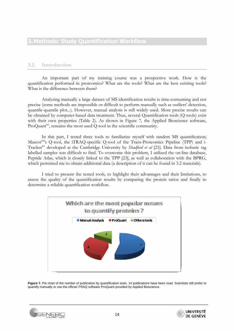
Analysing manually a large dataset of MS identification results is time-consuming and not precise (some methods are impossible or difficult to perform manually such as outliers’ detection, quantile-quantile plot...). However, manual analysis is still widely used. More precise results can be obtained by computer-based data treatment. Thus, several Quantification tools (Q-tools) exist with their own properties (Table 2). As shown in Figure 7, the Applied Bioscience software, ProQuanttm, remains the most used Q-tool in the scientific community.
In this part, I tested three tools to familiarize myself with tandem MS quantification; Mascottm's Q-tool, the iTRAQ-specific Q-tool of the Trans-Proteomics Pipeline (TPP) and i-Trackertm developed at the Cambridge University by Shadford et al [21]. Data from isobaric tag labelled samples was difficult to find. To overcome this problem, I utilized the on-line database, Peptide Atlas, which is closely linked to the TPP [23], as well as collaboration with the BPRG, which permitted me to obtain additional data (a description of it can be found in 3.2 materials).
I tried to present the tested tools, to highlight their advantages and their limitations, to assess the quality of the quantification results by comparing the protein ratios and finally to determine a reliable quantification workflow.
Figure 7. Pie chart of the number of publication by quantification tools. 14 publications have been read. Scientists still prefer to quantify manually or use the official iTRAQ software ProQuant provided by Applied Bioscience.
15
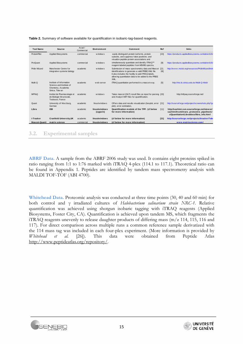
Table 2. Summary of software available for quantification in isobaric-tag-based reagents.
Source Comment links
commercial [23]
commercial [9]
[5]
[20]
Quant [21]
ISB [11]
[21]
commercial
Tool NameAcad /
CommercialEnvironment Ref
ProteinPilot Applied Biosystems w indow s easily distinguish protein isoforms, protein subsets, and suppress false positives; and visualize peptide-protein associations and
https://products.appliedbiosystems.com/ab/en/US/adirect/ab?cmd=catNavigate2&catID=600908
ProQuant Applied Biosystems w indow s simultaneously quantitate and identify iTRAQ™ reagent-labeled peptides from MS/MS spectra.
https://products.appliedbiosystems.com/ab/en/US/adirect/ab?cmd=catNavigate2&catID=600908
Pride Wizard Manchester Centre for integrative systems biology
academic w indow s Submission of mass spectrometry data and Mascot identifications to generate a valid PRIDE XML f ile. It also includes the facility to add iTRAQ labels, allow ing quantitation data to be added to the PRIDE XML.
[22,28]
http://w w w .mcisb.org/resources/PrideWizard/index.html
Multi-Q Institute of Information Science and Institute of Chemistry, Academia Sinica, Taiw an
academic w eb server iTRAQ quantitation performed in a mascot w ay. http://ms.iis.sinica.edu.tw /Multi-Q-Web/
MFPaQ Institut de Pharmacologie et de Biologie Structurale, Toulouse, France
academic w indow s Takes mascot (DAT) result f iles as input for parsing and Analyst Wiff f iles for quantif ication.
http://mfpaq.sourceforge.net/
University of Wurzburg, German
academic linux/w indow s Offers data and results visualization (boxplot, error plot), error estimation,
http://sourceforge.net/project/screenshots.php?group_id=109078
Libra academic linux/w indows (cygw in)
Quantification module of the TPP. (cf below for more information)
http://sashimi.svn.sourceforge.net/viewvc/sashimi/trunk/trans_proteomic_pipeline/sr
c/Quantitation/Libra/docs/libra_info.html
i-Tracker Cranfield University,UK academic linux/w indows (cf below for more information) http://sourceforge.net/projects/itracker/?abmode=1
Mascot-Quanti matrix science linux/w indows (cf below f or more information) www.matrixscience.com/
3.2. Experimental samples
ABRF Data. A sample from the ABRF 2006 study was used. It contains eight proteins spiked in ratio ranging from 1:1 to 1:76 marked with iTRAQ 4-plex (114.1 to 117.1). Theoretical ratio can be found in Appendix 1. Peptides are identified by tandem mass spectrometry analysis with MALDI TOF-TOF (ABI 4700).
Whitehead Data. Proteomic analysis was conducted at three time points (30, 40 and 60 min) for both control and γ irradiated cultures of Halobacterium salinarium strain NRC-1. Relative quantification was achieved using shotgun isobaric tagging with iTRAQ reagents (Applied Biosystems, Foster City, CA). Quantification is achieved upon tandem MS, which fragments the iTRAQ reagents unevenly to release daughter products of differing mass (m/z 114, 115, 116 and 117). For direct comparison across multiple runs a common reference sample derivatized with the 114 mass tag was included in each four-plex experiment. (More information is provided by Whitehead et al. [26]). This data were obtained from Peptide Atlas http://www.peptideatlas.org/repository/.
16
3.3. Tested Software Presentation
I-Tracker
Three tools were compared; i-Tracker developed by Shadford & al.[21], the iTRAQ quantification tools packaged with the TTP pipeline [22], Libra and the quantification module of the 2.2 version of the Mascot sofware.
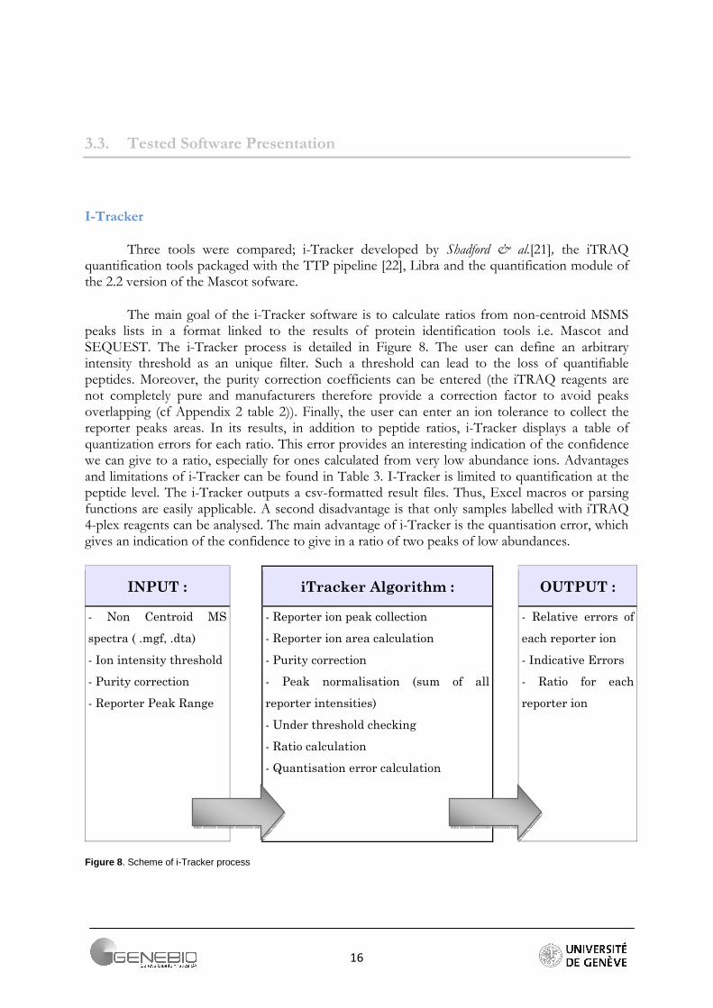
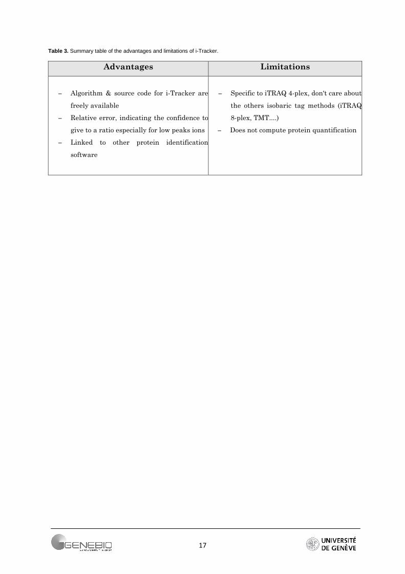
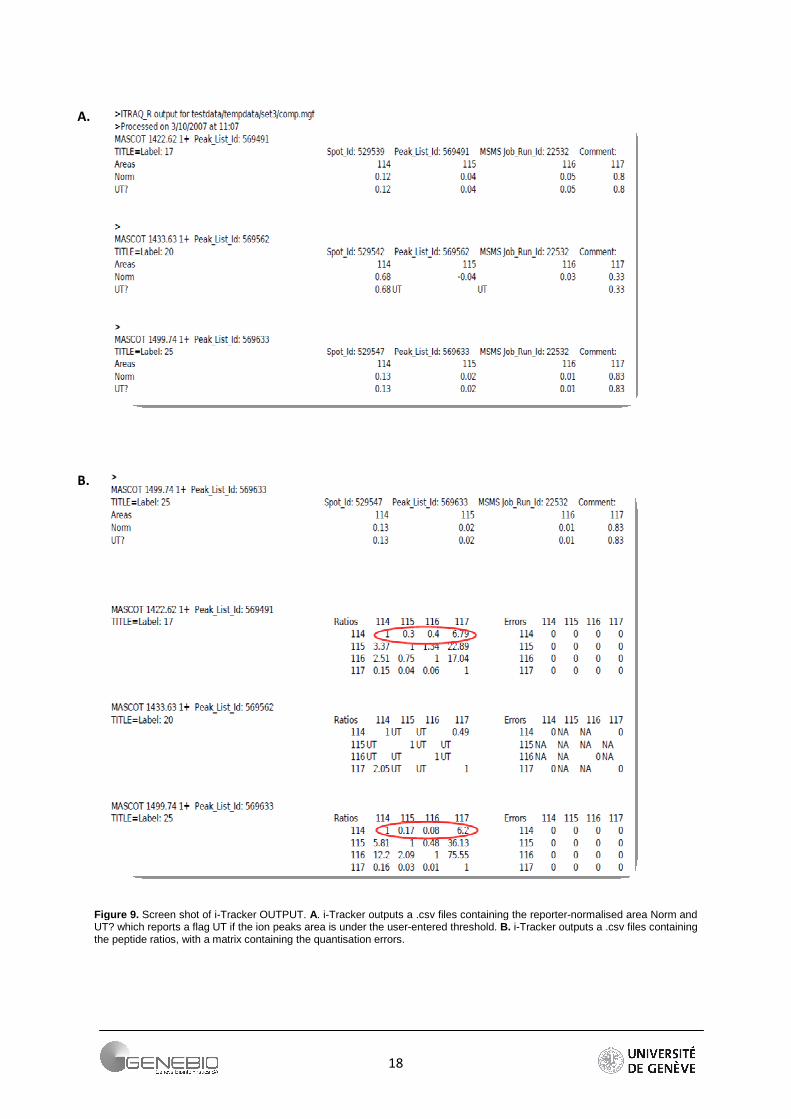
The main goal of the i-Tracker software is to calculate ratios from non-centroid MSMS peaks lists in a format linked to the results of protein identification tools i.e. Mascot and SEQUEST. The i-Tracker process is detailed in Figure 8. The user can define an arbitrary intensity threshold as an unique filter. Such a threshold can lead to the loss of quantifiable peptides. Moreover, the purity correction coefficients can be entered (the iTRAQ reagents are not completely pure and manufacturers therefore provide a correction factor to avoid peaks overlapping (cf Appendix 2 table 2)). Finally, the user can enter an ion tolerance to collect the reporter peaks areas. In its results, in addition to peptide ratios, i-Tracker displays a table of quantization errors for each ratio. This error provides an interesting indication of the confidence we can give to a ratio, especially for ones calculated from very low abundance ions. Advantages and limitations of i-Tracker can be found in Table 3. I-Tracker is limited to quantification at the peptide level. The i-Tracker outputs a csv-formatted result files. Thus, Excel macros or parsing functions are easily applicable. A second disadvantage is that only samples labelled with iTRAQ 4-plex reagents can be analysed. The main advantage of i-Tracker is the quantisation error, which gives an indication of the confidence to give in a ratio of two peaks of low abundances.
INPUT :
iTracker Algorithm :
OUTPUT :
- Non Centroid MS
spectra ( .mgf, .dta)
- Ion intensity threshold
- Purity correction
- Reporter Peak Range
- Reporter ion peak collection
- Reporter ion area calculation
- Purity correction
- Peak normalisation (sum of all
reporter intensities)
- Under threshold checking
- Ratio calculation
- Quantisation error calculation
- Relative errors of
each reporter ion
- Indicative Errors
- Ratio for each
reporter ion
Figure 8 . Scheme of i-Tracker process
17
Table 3. Summary table of the advantages and limitations of i-Tracker.
Advantages Limitations
– Algorithm & source code for i-Tracker are
freely available
– Relative error, indicating the confidence to
give to a ratio especially for low peaks ions
– Linked to other protein identification
software
– Specific to iTRAQ 4-plex, don't care about
the others isobaric tag methods (iTRAQ
8-plex, TMT....)
– Does not compute protein quantification
18
Figure 9. Screen shot of i-Tracker OUTPUT. A. i-Tracker outputs a .csv files containing the reporter-normalised area Norm and UT? which reports a flag UT if the ion peaks area is under the user-entered threshold. B. i-Tracker outputs a .csv files containing the peptide ratios, with a matrix containing the quantisation errors.
A.
B.
19
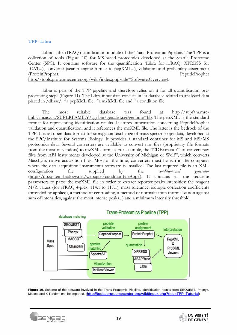
TPP- Libra
Libra is the iTRAQ quantification module of the Trans-Proteomic Pipeline. The TPP is a collection of tools (Figure 10) for MS-based proteomics developed at the Seattle Proteome Center (SPC). It contains software for the quantification (Libra for iTRAQ, XPRESS for ICAT...), converter (search engine format to pepXML...), validation and probability assignment (ProteinProphet, PeptideProphet http://tools.proteomecenter.org/wiki/index.php?title=Software:Overview).
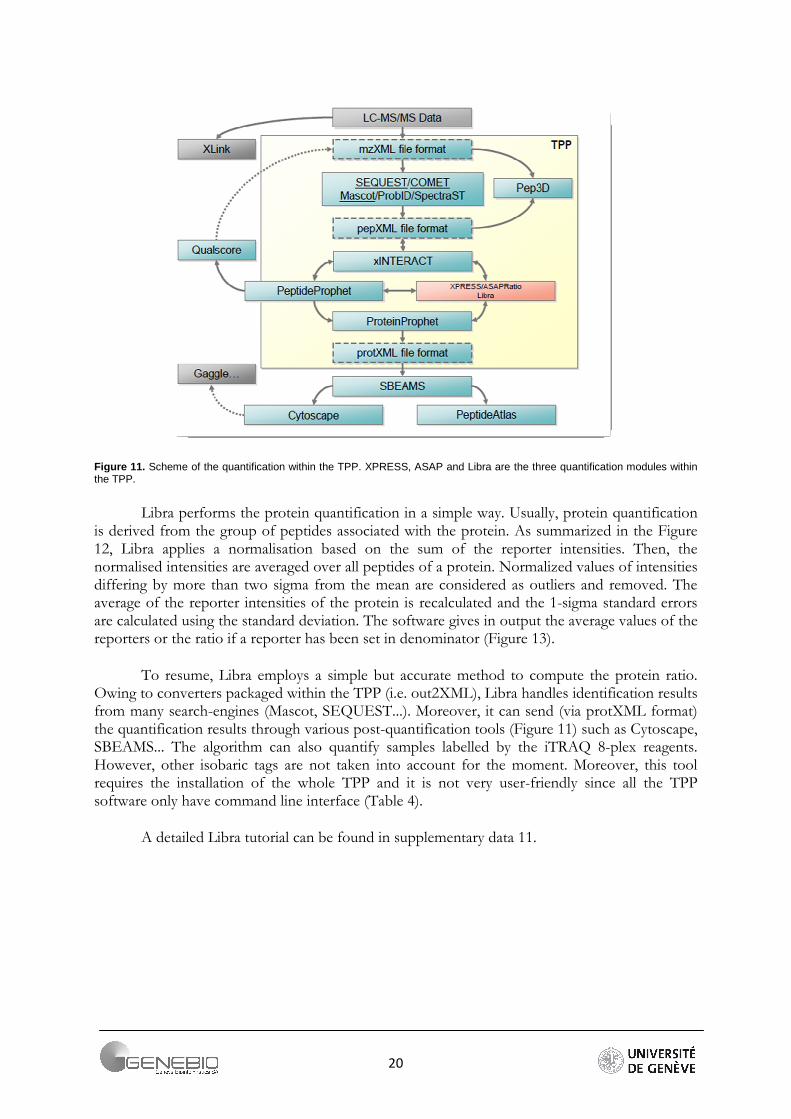
Libra is part of the TPP pipeline and therefore relies on it for all quantification pre-processing steps (Figure 11). The Libra input data consists in (1)a database related to analyzed data placed in /dbase/, (2)a pepXML file, (3)a mzXML file and (4)a condition file.
The most suitable database was found at http://supfam.mrc-lmb.cam.ac.uk/SUPERFAMILY/cgi-bin/gen_list.cgi?genome=hb. The pepXML is the standard format for representing identification results. It stores information concerning PeptideProphet validation and quantification, and it references the mzXML file. The latter is the bedrock of the TPP. It is an open data format for storage and exchange of mass spectroscopy data, developed at the SPC/Institute for Systems Biology. It provides a standard container for MS and MS/MS proteomics data. Several converters are available to convert raw files (proprietary file formats from the most of vendors) to mzXML format. For example, the T2DExtractortm to convert raw files from ABI instruments developed at the University of Michigan or Wolftm, which converts MassLynx native acquisition files. Most of the time, converters must be run in the computer where the data acquisition instrument's software is installed. The last required file is an XML configuration file supplied by the condition.xml generator (http://db.systemsbiology.net/webapps/conditionFileApp/). It contains all the requisite parameters to parse the mzXML file in order to extract reporter peaks intensities: the reagent M/Z values (for iTRAQ 4-plex: 114.1 to 117.1), mass tolerance, isotopic correction coefficients (provided by applied), a method of centroiding, a method of normalization (normalization against sum of intensities, against the most intense peaks...) and a minimum intensity threshold.
Figure 10. Scheme of the software involved in the Trans-Proteomic Pipeline. Identification results from SEQUEST, Phenyx, Mascot and X!Tandem can be imported. (http://tools.proteomecenter.org/wiki/index.php?titl e=TPP_Tutorial )
20
Figure 11. Scheme of the quantification within the TPP. XPRESS, ASAP and Libra are the three quantification modules within the TPP.
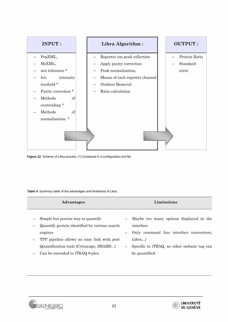
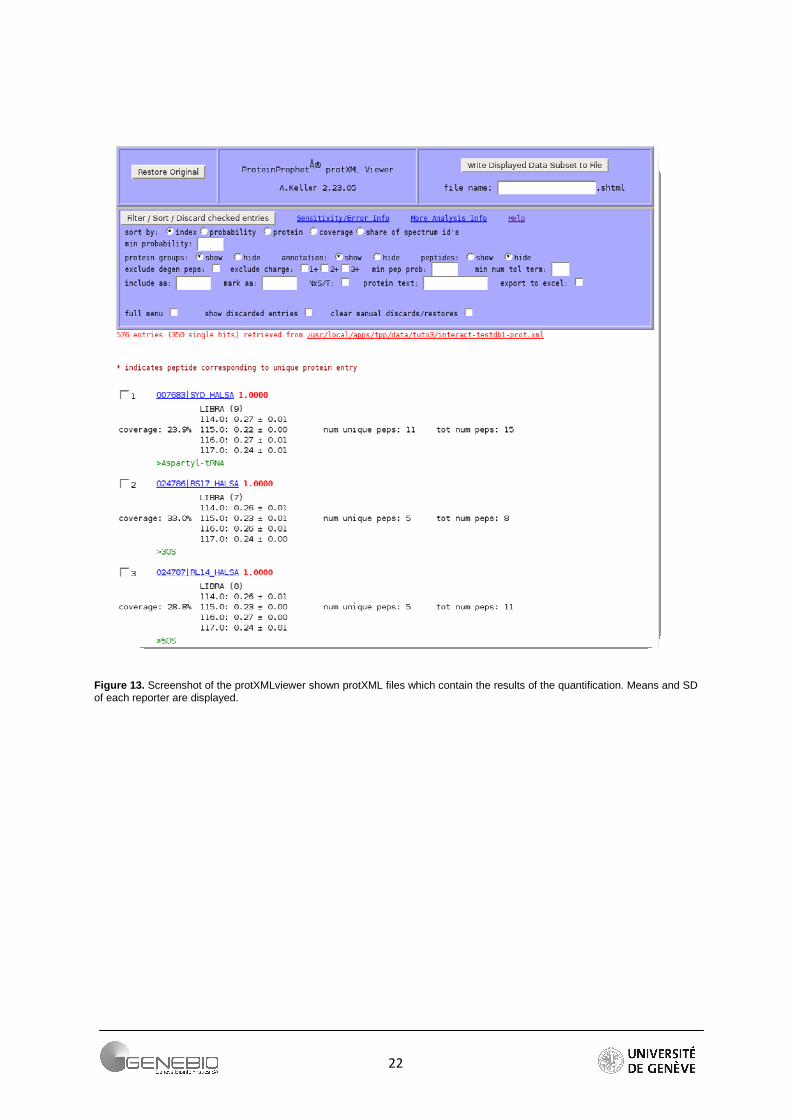
Libra performs the protein quantification in a simple way. Usually, protein quantification is derived from the group of peptides associated with the protein. As summarized in the Figure 12, Libra applies a normalisation based on the sum of the reporter intensities. Then, the normalised intensities are averaged over all peptides of a protein. Normalized values of intensities differing by more than two sigma from the mean are considered as outliers and removed. The average of the reporter intensities of the protein is recalculated and the 1-sigma standard errors are calculated using the standard deviation. The software gives in output the average values of the reporters or the ratio if a reporter has been set in denominator (Figure 13).
To resume, Libra employs a simple but accurate method to compute the protein ratio. Owing to converters packaged within the TPP (i.e. out2XML), Libra handles identification results from many search-engines (Mascot, SEQUEST...). Moreover, it can send (via protXML format) the quantification results through various post-quantification tools (Figure 11) such as Cytoscape, SBEAMS... The algorithm can also quantify samples labelled by the iTRAQ 8-plex reagents. However, other isobaric tags are not taken into account for the moment. Moreover, this tool requires the installation of the whole TPP and it is not very user-friendly since all the TPP software only have command line interface (Table 4).
A detailed Libra tutorial can be found in supplementary data 11.
21
INPUT :
Libra Algorithm :
OUTPUT :
– PepXML,
– MzXML,
– m/z tolerance *
– Ion intensity
treshold *
– Purity correction *
– Methods of
centroiding *
– Methods of
normalisation. *
– Reporter ion peak collection
– Apply purity correction
– Peak normalisation,
– Means of each reporter channel
– Outliers Removal
– Ratio calculation
– Protein Ratio
– Standard
error
Figure 12 . Scheme of Libra process. (*) Contained in a configuration.xml file.
Table 4. Summary table of the advantages and limitations of Libra.
Advantages Limitations
– Simple but precise way to quantify
– Quantify protein identified by various search
engines
– TPP pipeline allows an easy link with post
Quantification tools (Cytoscape, SBAMS...)
– Can be extended to iTRAQ 8-plex
– Maybe too many options displayed in the
interface
– Only command line interface (converters,
Libra...)
– Specific to iTRAQ, no other isobaric tag can
be quantified
22
Figure 13. Screenshot of the protXMLviewer shown protXML files which contain the results of the quantification. Means and SD of each reporter are displayed.
23
Mascot quantification module
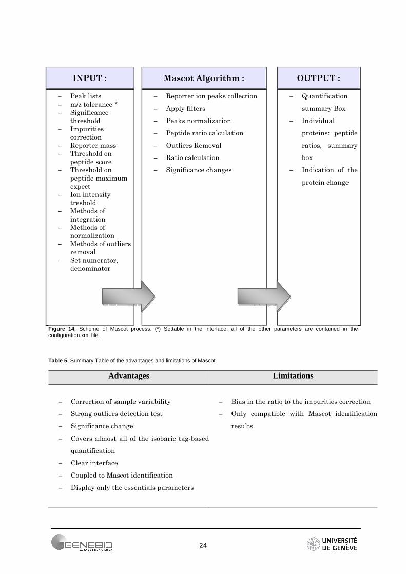
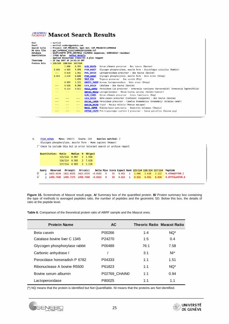
Mascot 2.2 includes a quantification module that computes ratios of identified proteins. This module covers most of the quantification methods i.e. reporter-based (iTRAQ, TMT), precursor-based (ICAT, SILAC, Absolute Quantification...) and Label Free. All these methods are classified in protocols. Reporter protocol takes into account samples labelled with the most of the isobaric tag (iTRAQ, TMT, ExacTag) except the AMT. All of the information required for the isobaric quantification is contained in the peak list, which is needed in input. Reagents and the MS/MS tolerance can be set in the interface. All the other parameters are set in the XML configuration file. The configuration.xml file encapsulates all users’ parameters. There are many different parameters, split into groups. For example, the group Methods contains the methods used to calculate the ratio and the significance level used for the statistical test (default 0.05). The group Component contains the information concerning each reporter (average and mono-isotopic mass, values of impurities correction...). In Ratio users can define each ratio they want to display (numerator, denominator). The group Quality contains the filter parameters, on intensity, on score, on expect value. Outlier and Normalization include specific methods. Mascot implements Grubbs, Rosner, Dixon detection methods, and three types of are available; summing intensities, median and geometric mean. Finally, Mascot performs the quantification following protein identification. It displays a summary box containing all the protein ratios (Figure 15A). A detailed view is also provided for each protein (Figure 15B). Each peptide ratio is given and the protein ratio value is displayed in a box coupled with a measure of spread, generally a geometric standard deviation (Figure 15B). Figure 14 summarizes the Mascot Process.
Table 6 shows a comparison between the theoretical ratios of the proteins of the ABRF dataset and the ratios found in Mascot. Parameters are summarised in the Figure 1 of Appendix 3. Mascot fails to quantify three proteins. Carbonic anhydrase was not identified whereas beta-casein and ribonuclease was identified but not quantified. The quantification cannot be performed due to the outlier’s removal option. When the option is set to none, these two proteins become quantifiable.
Due to its number of parameters and its very user-friendly interface, Mascot seems to be a very complete tool for quantification (Table 5). However, importing identification results from other search-engine is impossible.
24
INPUT :
Mascot Algorithm :
OUTPUT :
– Peak lists – m/z tolerance * – Significance
threshold – Impurities
correction – Reporter mass – Threshold on
peptide score – Threshold on
peptide maximum
expect – Ion intensity
treshold – Methods of
integration – Methods of
normalization – Methods of outliers
removal – Set numerator,
denominator
– Reporter ion peaks collection
– Apply filters
– Peaks normalization
– Peptide ratio calculation
– Outliers Removal
– Ratio calculation
– Significance changes
– Quantification
summary Box
– Individual
proteins: peptide
ratios, summary
box
– Indication of the
protein change
Figure 14. Scheme of Mascot process. (*) Settable in the interface, all of the other parameters are contained in the configuration.xml file.
Table 5. Summary Table of the advantages and limitations of Mascot.
Advantages Limitations
– Correction of sample variability
– Strong outliers detection test
– Significance change
– Covers almost all of the isobaric tag-based
quantification
– Clear interface
– Coupled to Mascot identification
– Display only the essentials parameters
– Bias in the ratio to the impurities correction
– Only compatible with Mascot identification
results
25
Figure 15. Screenshots of Mascot result page, A/ Summary box of the quantified protein. B/ Protein summary box containing the type of methods to averaged peptides ratio, the number of peptides and the geometric SD. Below this box, the details of ratio at the peptide level.
Table 6. Comparison of the theoretical protein ratio of ABRF sample and the Mascot ones.
Protein Name AC Mascot Ratio
Beta casein P00266 1:4 NQ*
P24270 1:5 0.4
P00489 76:1 7.58
/ 3:1 NI*
Peroxidase horseradish P 6782 P04333 1:1 1.51
P61823 1:1 NQ*
Bovine serum albumin P02769_CHAIN0 1:1 0.94
P80025 1:1 1.1
Theoric Ratio
Catalase bovine liver C 1345
Glycogen phosphorylase rabbit
Carbonic anhydrase I
Ribonuclease A bovine R5500
Lactoperoxidase
(*) NQ means that the protein is identified but Not Quantifiable. NI means that the proteins are Not Identified.
26
3.4. Software comparison
Comparison of the different tools can be made at several levels; at the level of the quantification results and at the level of the algorithm.
Comparison of the Quantification Results
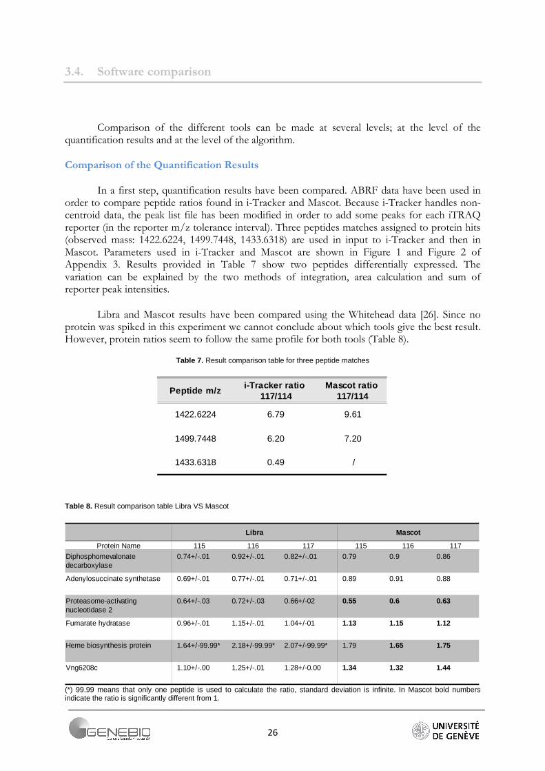
In a first step, quantification results have been compared. ABRF data have been used in order to compare peptide ratios found in i-Tracker and Mascot. Because i-Tracker handles non-centroid data, the peak list file has been modified in order to add some peaks for each iTRAQ reporter (in the reporter m/z tolerance interval). Three peptides matches assigned to protein hits (observed mass: 1422.6224, 1499.7448, 1433.6318) are used in input to i-Tracker and then in Mascot. Parameters used in i-Tracker and Mascot are shown in Figure 1 and Figure 2 of Appendix 3. Results provided in Table 7 show two peptides differentially expressed. The variation can be explained by the two methods of integration, area calculation and sum of reporter peak intensities.
Libra and Mascot results have been compared using the Whitehead data [26]. Since no protein was spiked in this experiment we cannot conclude about which tools give the best result. However, protein ratios seem to follow the same profile for both tools (Table 8).
Table 7. Result comparison table for three peptide matches
1422.6224 6.79 9.61
1499.7448 6.20 7.20
1433.6318 0.49 /
Peptide m/zi-Tracker ratio
117/114Mascot ratio
117/114
Table 8. Result comparison table Libra VS Mascot
Libra Mascot
Protein Name 115 116 117 115 116 117
0.74+/-.01 0.92+/-.01 0.82+/-.01 0.79 0.9 0.86
0.69+/-.01 0.77+/-.01 0.71+/-.01 0.89 0.91 0.88
0.64+/-.03 0.72+/-.03 0.66+/-02 0.55 0.6 0.63
0.96+/-.01 1.15+/-.01 1.04+/-01 1.13 1.15 1.12
1.64+/-99.99* 2.18+/-99.99* 2.07+/-99.99* 1.79 1.65 1.75
Vng6208c 1.10+/-.00 1.25+/-.01 1.28+/-0.00 1.34 1.32 1.44
Diphosphomevalonate decarboxylase
Adenylosuccinate synthetase
Proteasome-activating nucleotidase 2
Fumarate hydratase
Heme biosynthesis protein
(*) 99.99 means that only one peptide is used to calculate the ratio, standard deviation is infinite. In Mascot bold numbers indicate the ratio is significantly different from 1.
27
A quantitative analysis can be subdivided in 5 cardinal steps. A pre-processing step in other words by which methods of integration the reporters are extracted (summing intensities of the profile or calculating the area under the profile curves) is performed. This is followed by a filtering step. We can imagine various filters; the most observed ones are a threshold on intensities, on score, and on p-value (“expect”). The normalization step is generally applied to correct systematic biases or to avoid giving too much weight to one reporter. This step is followed by the outliers removal step. Finally, the protein ratio can be estimated. The quantification workflow of each tool is compared for each of these steps.
The three tested tools have their own ways to achieve the quantification. The i-Tracker makes the quantification at the peptide level. The user must therefore manually calculate protein ratios.
INPUT/OUTPUT
First, we compare the INPUT file formats. Mascot quantification is clearly paired with the Mascot identification, in the extent that quantification of proteins which are identified using other identification software are impossible. On the contrary, i-Tracker permits the importing of SEQUEST and Mascot results, and Libra can handle many types of identification tools results (Figure 10) due to the availability of tools such as Out2XML and Mascot2XML, which convert, respectively, .out file format from SEQUEST and .dat file format from Mascot in pepXML format. In addition to pepXML file, Libra inputs RAW files converted to mzXML format (for the conversion of raw to mzXML, converters need access to the computer where the instrument-specific software for data acquisition is installed). In OUTPUT, Mascot releases a .dat file. Libra encapsulates its results in a protXML format file, which is read with the protXML viewer tool and exported to post-quantification tools (Cystoscape, SpotFire etc…). I-Tracker chooses to produce two types of .csv file. Output style 1 is designed to be human-readable when imported into programs such as MS Excel as a comma-separated variable file. It is strictly ordered so automated parsing is also straightforward. Output style 2 is designed to allow very easy basic analysis within programs such as MS Excel. All information is outputted on a one row per spectrum basis and thus all human-readability is lost, but to the gain of being able to run functions and macros more easily.
Reporter Peaks Collection
There are two ways to collect peaks. Mascot allows the choice between both via the configuration editor. Libra employs the sum of intensities of the peaks profiles whereas i-Tracker used the trapezoid approximation for calculating the area under a curve.
Filters
After reporter ion peaks collection comes the filtering process. Many filters can be applied. All of them may involve data loss, especially when choosing a threshold on intensity, since peptides that present weak intensity are removed.
28
Type of Quantification Workflow
We can now talk about the quantification workflow of each tool. Libra and Mascot have two ways to compute the protein ratio. Mascot computes an average of peptides ratios whereas Libra computes a ratio of averaged peptide reporter intensities.
Outliers Removal
In a quantification workflow, outliers’ removal (as normalisation) is a crucial step that is always in the quantification workflow although their implementation varies among the Q-tools. Mascot implements three methods for outlier removal. Dixon's r11 test, also referred to as N9, is used to detect and remove a single outlier at a time from either the upper or lower extreme of the range [27, 28]. It is applicable to values between 4 and 100. For a greater number of values, Rosner's test is applied [24]. Grubbs detection is applicable for values between 3 and 100 [26, 25]. Libra decides that a value of intensity is an outlier if it is outside of the range:
]µ - 2 * σ, µ + 2 * σ, [ (1)
Where µ is the means and σ is the standard deviation.
Care must be taken when outliers are blindly removed. A rigorous analysis would be to compare data with or without outliers to see to what extend the conclusions are qualitatively different.
Normalisation
A second important thing when working with large biological dataset is normalisation. Normalisation always takes place at peptide level. To remove variability of the sample incorporated during the experimental procedure, and based on the assumption that differential proteins in a biological sample are in a minority, Mascot proposes two methods to normalise the data so as to make the average of the whole population ratios across the entire data set equal to one. This can be done via the median or the geometric mean. Another method is the sum; totals intensities for each reporter across the entire data set are made equal. In contrast, for Libra and i-Tracker, no variability correction is implemented. However, in order to not give too much confidence in one reporter, both tools normalise on the sum of all reporter intensities.
Determination of protein abundance and measure of spread
Libra implements a simple ratio of the reporter means and displays a standard error calculated from the numerator standard deviation. Due to the fact that Mascot treats the peptide ratios, it allows several methods for averaging them; median, geometric mean, and weighted mean associated with a geometric standard deviation. I-Tracker does not provide the ratio at the protein level.
29
Bonus
Several functionalities are software specific. I-Tracker for example is the only tool that displays a quantisation error. This value can serve as warning against placing too high confidence on reported ratios when these have been based on peaks with low ion counts [21].
Err(1,2) = (100 * ((0.5 / Peak1Max) + (0.5 / Peak2Max)) (2)
Mascot provides an interesting and robust indication of the relative protein fold change. It employs a one-sample t-test. The null hypothesis H0 is that the estimation of the ratios x is equal to one. If H0 is rejected, x is significantly different from 1. The protein ratio is reported in bold.
3.5. Discussion
Software comparison reveals that some steps are always found. Filters, outliers removal and estimation of the ratio are essentials in a quantitative analysis.
Each tool has its own way to estimate the ratio. Although they display a good estimation of the relative protein abundance, some of them are not user-friendly (i-Tracker, Libra). Moreover, they don’t take into account the experimental design of the experiment (i.e. replicates analysis, time course...). Finally, no mean to visualize the protein expression is implemented.
A complete summary of the tools that I tested can be found in table 1 of Appendix 4.
30
4. Establish Quantification WF
4.1. Introduction
Based on the previous study, three methods of quantification were implemented using the R language. This programming language is very well appropriate when analysing large amount of data for quantification to the extent that it offers an environment for statistical programming and In fact, descriptive statistics methods and inference tests are all ready when installing R. There are many additional packages that are easy to use and well documented. Moreover, R is able to output graphs and charts and provides therefore an attractive way to represent quantitative results.
Librus, an intensity-based method similar to Libra, and Mascat, a peptide ratio based method that resembles Mascot were first implemented. Furthermore, a novel quantification algorithm, named QI (Quantification Isobaric), was developed.
QI workflow is a least-square regression-based workflow. According to Bantscheff et al. [30], linear regression could be a good alternative to the filter on intensity and the inherent data loss that such a filter involves. In fact, making the difference between (1) a weak intensity from a low abundance peptide and (2) a weak intensity from the background noise is difficult. A least-square regression line is a straight line that passes through the data so that the sum of the square of the vertical distance data points from the line is as small as possible. So, the advantages are double. First of all, we avoid useless loss of peptide matches by applying an arbitrary threshold on intensity, and secondly, we obtain an easy method in order to visualise the protein quantification. The idea of this method is to create a linear model and coerce the regression line to pass through the origin. The slope of the line is an estimation of the protein ratio. The R-squared gives an indication of the data spread (Figure 20). Then, strong methods of outliers and influential detection are used. These methods are part of regression diagnostics.
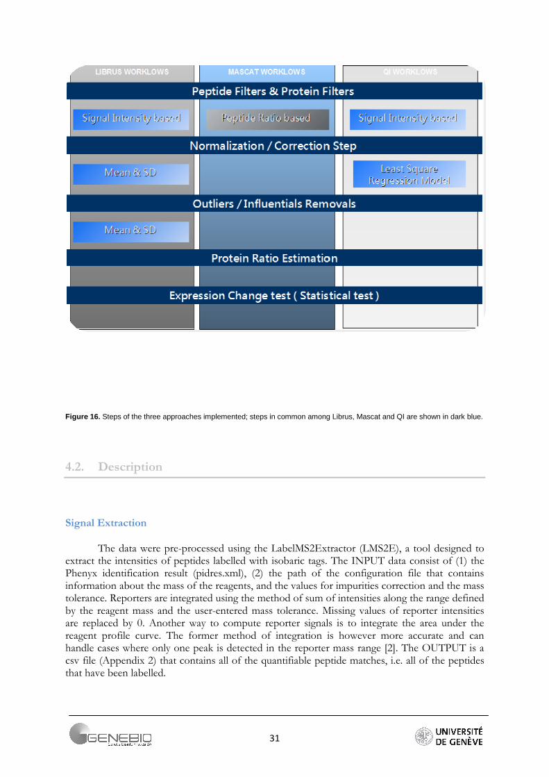
As highlighted in part 3.5, several statistical steps are common to all quantification approaches. These steps are shown in dark blue in the Figure 16 and detailed in the next part.
The validation of the algorithms was effected by using two sets of spiked proteins. The ratios of the proteins contained in the ABRF sample (described in 3.2) were compared between the three methods. Then a dataset (provided by Loïc Dayon) obtained from samples containing 4 spiked proteins [7] was used to measure the root mean square deviation (RMSD) between the expected theoretical ratio and the obtained ratios for each quantification algorithm.
31
Figure 16. Steps of the three approaches implemented; steps in common among Librus, Mascat and QI are shown in dark blue.
4.2. Description
Signal Extraction
The data were pre-processed using the LabelMS2Extractor (LMS2E), a tool designed to extract the intensities of peptides labelled with isobaric tags. The INPUT data consist of (1) the Phenyx identification result (pidres.xml), (2) the path of the configuration file that contains information about the mass of the reagents, and the values for impurities correction and the mass tolerance. Reporters are integrated using the method of sum of intensities along the range defined by the reagent mass and the user-entered mass tolerance. Missing values of reporter intensities are replaced by 0. Another way to compute reporter signals is to integrate the area under the reagent profile curve. The former method of integration is however more accurate and can handle cases where only one peak is detected in the reporter mass range [2]. The OUTPUT is a csv file (Appendix 2) that contains all of the quantifiable peptide matches, i.e. all of the peptides that have been labelled.
32
Filters
In all implemented quantification methods, the first step consists of the filtering of the LMS2E results table. Filters can act at peptide level or at protein level. Various filters can be imagined. At protein level, a threshold on the number of peptide matches is implemented. The greater the number of peptides per proteins, the more accurate is the ratio. At peptides level, several filters are implemented; a threshold on the minimum intensity value, on the minimum score, the maximum p-value, and a filter on proteotypic peptides i.e. when a peptide matches for several proteins, the peptide is removed. Thus, only unique peptides are taken into consideration when performing the protein quantification.
Normalisation/Correction step
The second crucial step is the normalisation of the dataset. Librus implements the normalisation of the peptide intensity, as Libra does. Mascat implements the three normalisation methods of the Mascot quantification module. In fact, the Librus normalisation permits one to not give too much confidence to one reporter whereas the Mascat normalisation corrects the systematic bias that occurs during the sample preparation.
Outliers removal
In Librus, if a normalized value of intensity is more than 2σ from the mean of the signals of one reporter, it is considered as an outlier and removed. Mascot uses specific outliers detection tests (Grubbs, Rosner, Dixon). (For more details see part 3.4). QI bases its workflow on strong regression diagnostic methods.
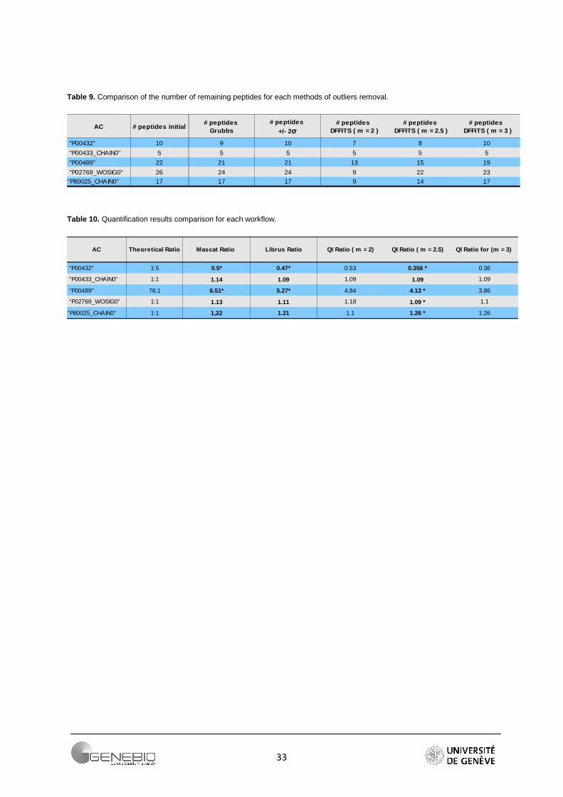
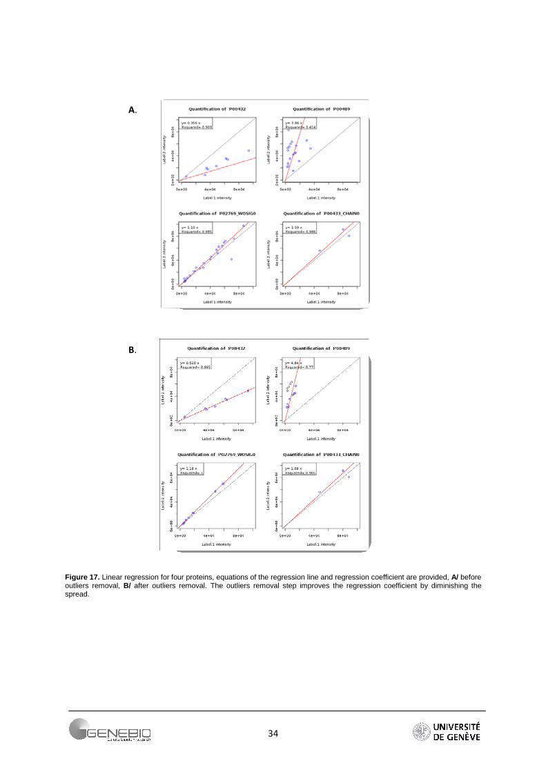
The DFFITS and studentized residuals are important techniques to the detection of outliers and influential points in a regression analysis. The DFFITS of an observation is a measure of the influence of this observation on its own predicted value. The studentized (standardized) residuals are adjusted by dividing them by an estimate of their standard deviation. The Table 9 shows the number of peptides remaining after outliers removal. Due to its tolerance to a large range of values, the Grubbs detection test has been chosen for Mascot. For Libra, the methods described above are used. For QI, if a DFFITS value is farther than m* standard deviation σ from the average of the DFFITS, the peptide is considered as an outlier and removed. We use the factor m equal to 2, 2.5 and 3. Authors recommend 2 [31] but the number of lost peptides becomes important (Table 9). As a reliable alternative, I propose a factor m equal to 2.5. The number of peptides per protein is greater. Moreover, the resulting ratios are closer to the theoretical ratios (Table 10). The Figure 17 shows the effect of such a method. Regression lines have been plotted before and after outliers removal (m = 2).
33
Table 9. Comparison of the number of remaining peptides for each methods of outliers removal.
AC # peptides initial
"P00432" 10 9 10 7 8 10
"P00433_CHAIN0" 5 5 5 5 5 5
"P00489" 22 21 21 13 15 19
"P02769_WOSIG0" 26 24 24 9 22 23
"P80025_CHAIN0" 17 17 17 9 14 17
# peptides Grubbs
# peptides +/- 2σ
# peptides DFFITS ( m = 2 )
# peptides DFFITS ( m = 2.5 )
# peptides DFFITS ( m = 3 )
Table 10. Quantification results comparison for each workflow.
AC Theoretical Ratio
"P00432" 1:5 0.5* 0.47* 0.53 0.356 * 0.36
"P00433_CHAIN0" 1:1 1.14 1.09 1.09 1.09 1.09
"P00489" 76:1 6.51* 5.27* 4.84 4.13 * 3.86
“P02769_WOSIG0” 1:1 1.13 1.11 1.18 1.09 * 1.1
"P80025_CHAIN0" 1:1 1,22 1.21 1.1 1.26 * 1.26
Mascat Ratio Librus Ratio QI Ratio ( m = 2) QI Ratio ( m = 2.5) QI Ratio for (m = 3)
34
Figure 17. Linear regression for four proteins, equations of the regression line and regression coefficient are provided, A/ before outliers removal, B/ after outliers removal. The outliers removal step improves the regression coefficient by diminishing the spread.
A.
B.
35
Protein ratio calculation and measure of spread
Libra performs a ratio of averaged intensities and gives a standard error. Mascat averages the peptide ratios by some descriptive statistics methods (median and MAD, geometric mean and geometric SD, weighted mean and weighted SD…). Being based on a regression model, QI gives the ratio by least square estimation.
OUTPUT and Visualization
The three implemented approaches provide csv sheets and graphs to visualize the quantification. Each workflow has its own presentation of the results and specific graphs.
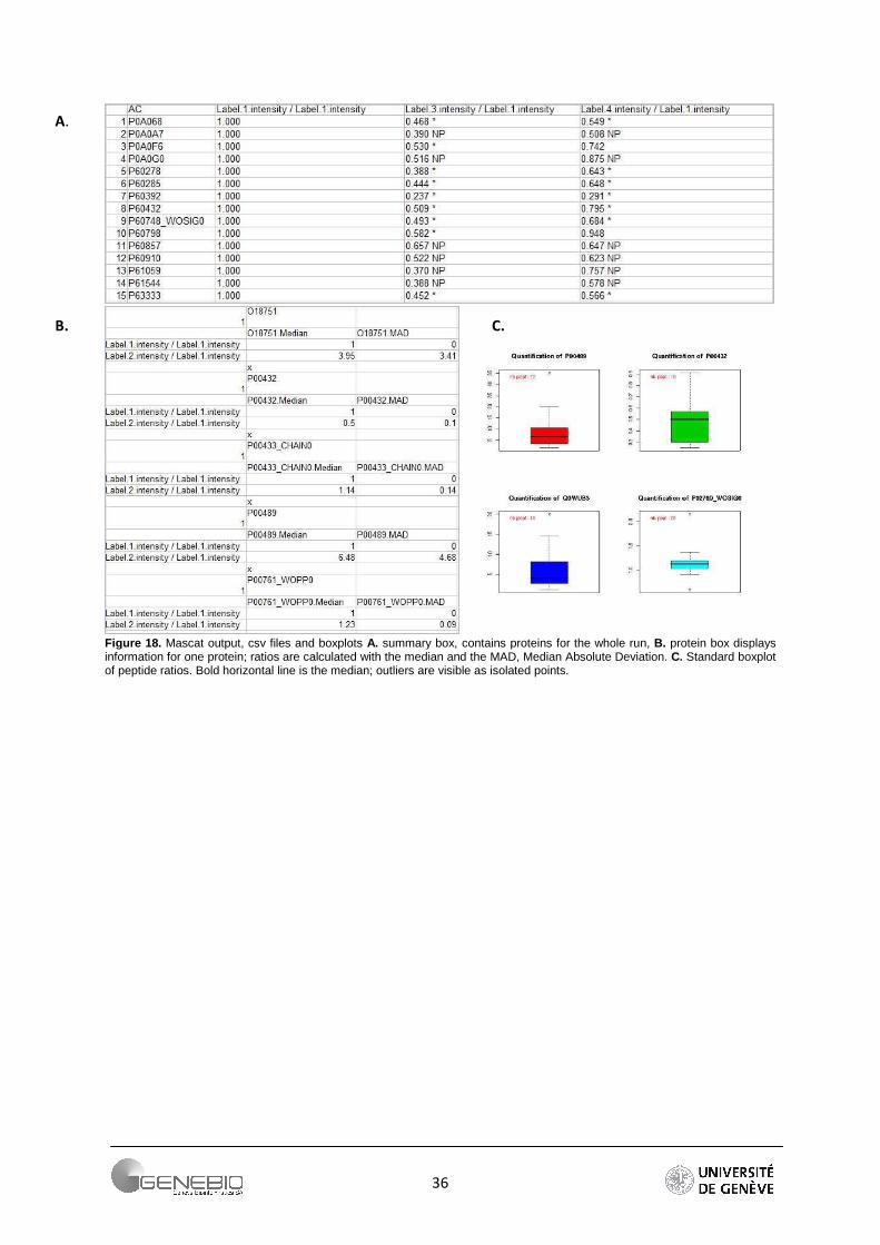
Thus, Mascat displays a summary table containing the ratio and an indication of the protein fold change (Figure 18A), and a protein box containing all quantitative information of one protein is provided by the R package (Figure 18B). In addition to histogram and density distribution of the peptides ratio, boxplots are used to display the peptide ratio distribution for each quantified protein (Figure 18C). A boxplot is a graph of statistical summary, with the outliers plotted individually. The quartiles are spammed by the central box (first and third quartiles) and the median is displayed by the central line (bold). Observations plotted outside of the range 1.5*IQR are suspected as possible outliers and the whiskers show the largest and smallest peptide ratios that are not considered as outliers.
Librus provides a matrix of result (Figure 19A), and a protein summary box that contains all information relative to one protein (Figure 19B).
36
Figure 18. Mascat output, csv files and boxplots A. summary box, contains proteins for the whole run, B. protein box displays information for one protein; ratios are calculated with the median and the MAD, Median Absolute Deviation. C. Standard boxplot of peptide ratios. Bold horizontal line is the median; outliers are visible as isolated points.
A.
B. C.
37
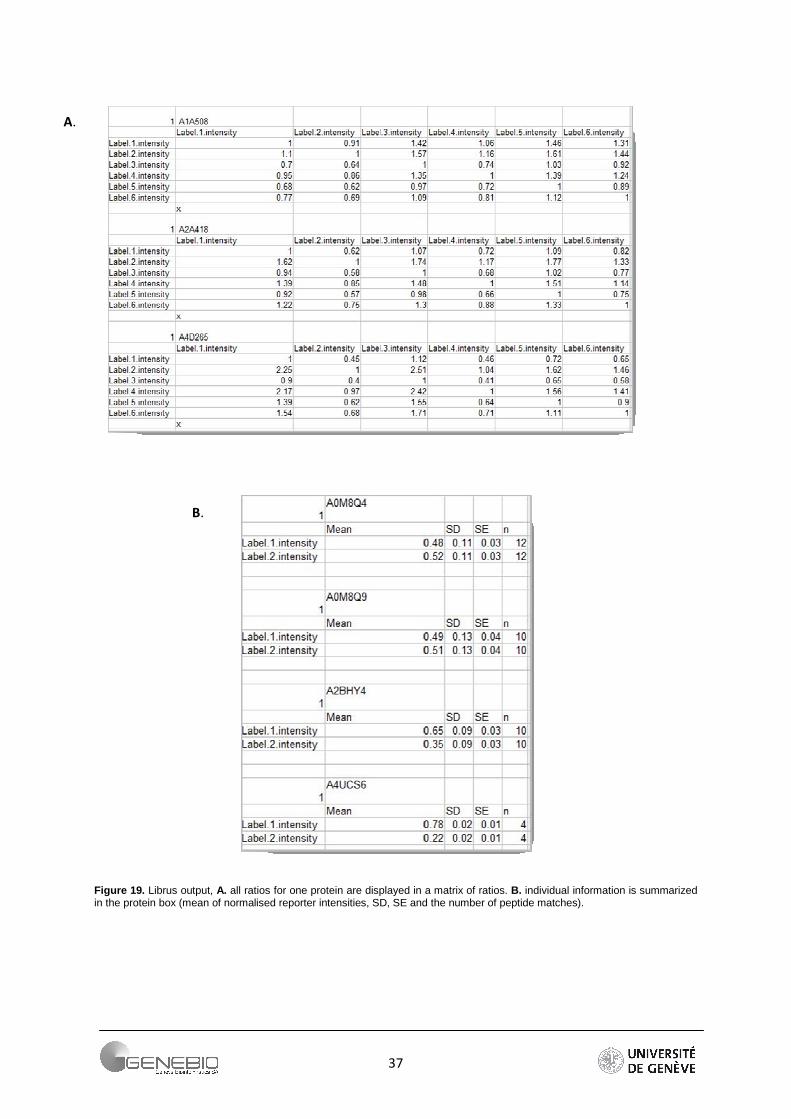
Figure 19. Librus output, A. all ratios for one protein are displayed in a matrix of ratios. B. individual information is summarized in the protein box (mean of normalised reporter intensities, SD, SE and the number of peptide matches).
A.
B.
38
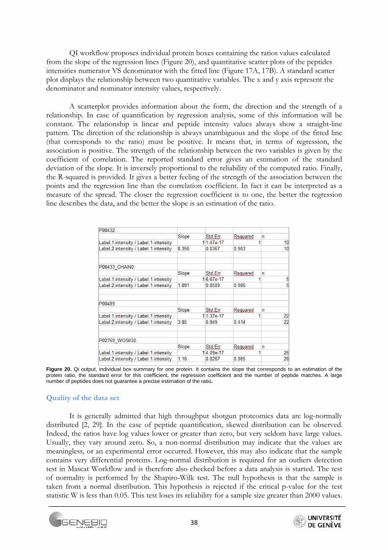
QI workflow proposes individual protein boxes containing the ratios values calculated from the slope of the regression lines (Figure 20), and quantitative scatter plots of the peptides intensities numerator VS denominator with the fitted line (Figure 17A, 17B). A standard scatter plot displays the relationship between two quantitative variables. The x and y axis represent the denominator and nominator intensity values, respectively.
A scatterplot provides information about the form, the direction and the strength of a relationship. In case of quantification by regression analysis, some of this information will be constant. The relationship is linear and peptide intensity values always show a straight-line pattern. The direction of the relationship is always unambiguous and the slope of the fitted line (that corresponds to the ratio) must be positive. It means that, in terms of regression, the association is positive. The strength of the relationship between the two variables is given by the coefficient of correlation. The reported standard error gives an estimation of the standard deviation of the slope. It is inversely proportional to the reliability of the computed ratio. Finally, the R-squared is provided. It gives a better feeling of the strength of the association between the points and the regression line than the correlation coefficient. In fact it can be interpreted as a measure of the spread. The closer the regression coefficient is to one, the better the regression line describes the data, and the better the slope is an estimation of the ratio.
Figure 20. Qi output, individual box summary for one protein. It contains the slope that corresponds to an estimation of the protein ratio, the standard error for this coefficient, the regression coefficient and the number of peptide matches. A large number of peptides does not guarantee a precise estimation of the ratio.
Quality of the data set
It is generally admitted that high throughput shotgun proteomics data are log-normally distributed [2, 29]. In the case of peptide quantification, skewed distribution can be observed. Indeed, the ratios have log values lower or greater than zero, but very seldom have large values. Usually, they vary around zero. So, a non-normal distribution may indicate that the values are meaningless, or an experimental error occurred. However, this may also indicate that the sample contains very differential proteins. Log-normal distribution is required for an outliers detection test in Mascat Workflow and is therefore also checked before a data analysis is started. The test of normality is performed by the Shapiro-Wilk test. The null hypothesis is that the sample is taken from a normal distribution. This hypothesis is rejected if the critical p-value for the test statistic W is less than 0.05. This test loses its reliability for a sample size greater than 2000 values.
39
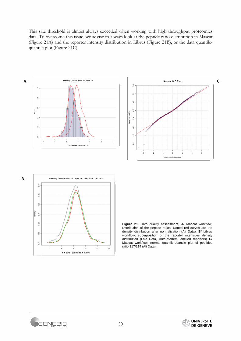
This size threshold is almost always exceeded when working with high throughput proteomics data. To overcome this issue, we advise to always look at the peptide ratio distribution in Mascat (Figure 21A) and the reporter intensity distribution in Librus (Figure 21B), or the data quantile-quantile plot (Figure 21C).
Figure 21. Data quality assessment, A/ Mascat workflow, Distribution of the peptide ratios. Dotted red curves are the density distribution after normalisation (Ali Data). B/ Librus workflow, superposition of the reporter intensities density distribution (Loic Data, Ante-Mortem labelled reporters) C/ Mascat workflow, normal quantile-quantile plot of peptides ratio 117/114 (Ali Data).
B.
C. A.
40
Implementation
The implementation was done using R version 2.6.0. The program files, documentation and example script are contained in supplementary data 1.
Reporter peaks were collected using the LMS2E that performed the integration by sum of intensities and corrected the reporter impurities.
Librus workflow can be applied using the script librus.R. It executes the wrapper function librus that performs the quantification. It calls the function of normalisaton, firstnorm, the outliers removal function outlier; getRatio calculated the ratio and the standard error.
Mascat workflow is called by the wrapper mascat found in the module Mascatfunc.R. This workflow is devised in four modules. The wrapper calls the script Mascat_norm.R which contains normalisation function, the script Mascat_outliers.R which contains the outliers detection test (this script needs the installation of an additional library), outliers which clusters a collection of some tests commonly used for identifying outliers and Mascat_changes.R which contains statistical test for significance change. The script Mascat_displays.R performs the export of the quantification results and charts.
The last workflow, QI, is designed as a single module Qifunc.R. It implements a wrapper qi, which calls slopeRatio, a subroutine that creates the linear regression model and displays the regression summary. The summary contains the regression statistics of the model, the slope, the standard error, and the regression coefficient. Moreover the wrapper calls regression diagnostic methods by the function diagnRM. No additional libraries are needed for dffits and studentized residues. R default distribution contains all regression diagnostic functions.
41
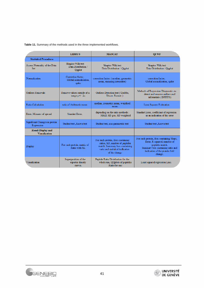
Table 11. Summary of the methods used in the three implemented workflows.
42
4.3. Validation of the algorithms
The ratios for the five spiked proteins of the ABRF data are compared in the table 10. It shows that ratios resulting from Mascat, Librus and QI are closed to the expected theoretical values. This therefore validates our three quantification algorithms.
A more precise study was performed to determine which quantification workflow provides the more accurate ratios. For this purpose, we used a data set supplied by Loic Dayon that contains a mixture of albumin (ALBU) from bovine serum, myoglobin (MYO) from horse heart, -lactoglobulin (LACB) from bovine milk, and lysozyme (LYS) from hen egg in equal weight. This dataset was originally used to determine the coefficient for impurities correction for the TMT reagents, Dayon et Al. for more information [7].
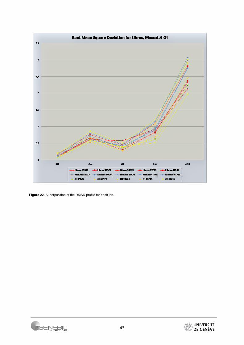
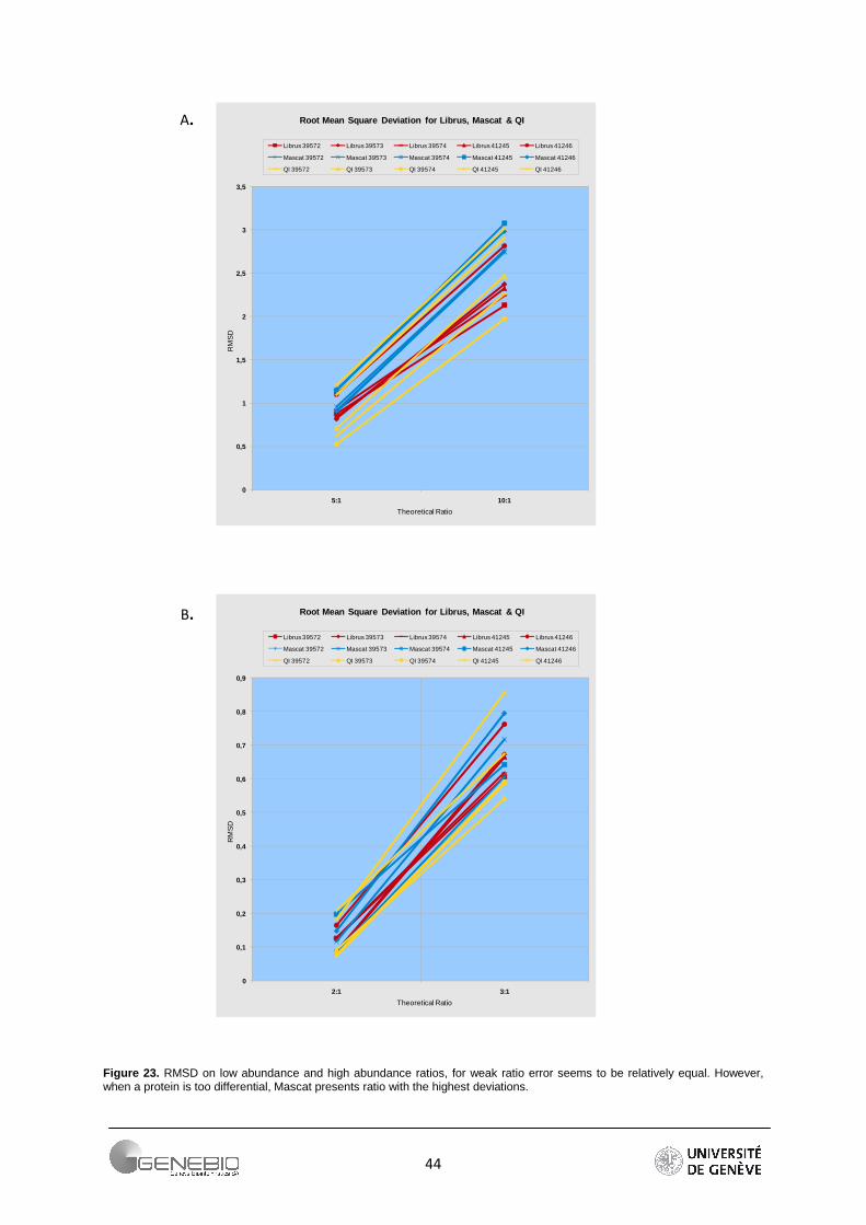
Due to its robustness, root mean square deviation was chosen to calculate the deviation from expected theoretical ratio of 1:2:3:3:5:10. As summarized in Figure 22, RMSD for each expected ratios are combined for all the experiments. The profiles clearly show that the higher a ratio, the greater is its error. To obtain a better indication of the relative accuracy of a quantitative approach, a zoom is performed on the array of low (2:1, 3:1) and high (5:1, 10:1) theoretical ratio (Figure 23). This shows that for a relatively weak ratio, the approaches seem to behave equally (Figure 23A). However for ratios higher than 3:1, the workflow based on peptide ratio, Mascat presents the largest error in the extent that its errors calculated from all the jobs are higher than a RMSD value of 2.5 (Figure 23B). On the contrary, only one job presents a big deviation for the intensity-based workflow - Librus. Moreover except for this latter, Librus' error profiles are closely clustered whatever the expected ratios. The regression-based approach generally gives low error but the job profiles are more dispersed, almost parallel. More information is found in supplementary data 7. Detailed profiles per job can be seeing in Appendix 5.
43
Figure 22. Superposition of the RMSD profile for each job.
44
0
0,5
1
1,5
2
2,5
3
3,5
5:1 10:1
RM
SD
Theoretical Ratio
Root Mean Square Deviation for Librus, Mascat & QI
Librus 39572 Librus 39573 Librus 39574 Librus 41245 Librus 41246
Mascat 39572 Mascat 39573 Mascat 39574 Mascat 41245 Mascat 41246
QI 39572 QI 39573 QI 39574 QI 41245 QI 41246
0
0,1
0,2
0,3
0,4
0,5
0,6
0,7
0,8
0,9
2:1 3:1
RM
SD
Theoretical Ratio
Root Mean Square Deviation for Librus, Mascat & QI
Librus 39572 Librus 39573 Librus 39574 Librus 41245 Librus 41246
Mascat 39572 Mascat 39573 Mascat 39574 Mascat 41245 Mascat 41246
QI 39572 QI 39573 QI 39574 QI 41245 QI 41246
Figure 23. RMSD on low abundance and high abundance ratios, for weak ratio error seems to be relatively equal. However, when a protein is too differential, Mascat presents ratio with the highest deviations.
B.
A.
45
4.4. Discussion
Three algorithms were developed and validated using the R language Each of them proposes their own statistical procedure (Appendix 6).
By measuring the RMSD between the expected theoretical ratios and the estimated ratios from the different algorithms, we conclude that Librus or to a less extent, QI give the more accurate ratios. This corroborates the observations of Carillo et al. [39].
However, care must be taken by giving too much confidence to this conclusion. Indeed, the two analysed datasets are from samples containing only spiked proteins; the normality assumption is therefore not respected. This assumption is important especially in Mascat where the outliers detection test requires that the peptide ratios of the whole dataset are normally distributed. This could explain the fact that Mascat shows the biggest variations from the expected ratios. Consequently, to say that one of these algorithms gives the more accurate ratios, a study should be done on a dataset from real biological samples where some spiked proteins would be incorporated.
The next studies show the application of the algorithms into real biological contexts.
46
5. Application of the Quantification Workflows
5.1. Alireza collaboration: Peptides Ratios-based Quantification Approach applied to Characterize Daptomycin Resistance in Staphylococcus aureus.
A two-month work with Alireza Vaezzadeh, a PHD student from the Biomedical Proteomics Research Group (BPRG), has been carried out. My part of the job consisted of an analysis of MS/MS Data obtained from quantitative MS based proteomic experiments on Staphylococcus S.aureus.
5.1.1. Introduction
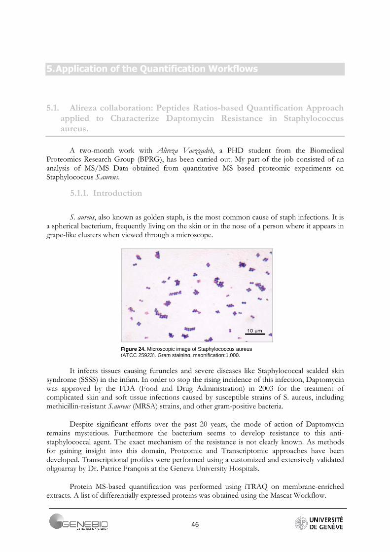
S. aureus, also known as golden staph, is the most common cause of staph infections. It is a spherical bacterium, frequently living on the skin or in the nose of a person where it appears in grape-like clusters when viewed through a microscope.
It infects tissues causing furuncles and severe diseases like Staphylococcal scalded skin syndrome (SSSS) in the infant. In order to stop the rising incidence of this infection, Daptomycin was approved by the FDA (Food and Drug Administration) in 2003 for the treatment of complicated skin and soft tissue infections caused by susceptible strains of S. aureus, including methicillin-resistant S.aureus (MRSA) strains, and other gram-positive bacteria.
Despite significant efforts over the past 20 years, the mode of action of Daptomycin remains mysterious. Furthermore the bacterium seems to develop resistance to this anti-staphylococcal agent. The exact mechanism of the resistance is not clearly known. As methods for gaining insight into this domain, Proteomic and Transcriptomic approaches have been developed. Transcriptional profiles were performed using a customized and extensively validated oligoarray by Dr. Patrice François at the Geneva University Hospitals.
Protein MS-based quantification was performed using iTRAQ on membrane-enriched extracts. A list of differentially expressed proteins was obtained using the Mascat Workflow.
Figure 24. Microscopic image of Staphylococcus aureus (ATCC 25923). Gram staining, magnification:1,000.
47
5.1.2. Materials
Experimental Workflow. Three strains were analysed in this study: 616 (initial patient isolate), 629 (first isolate breaking through Daptomycin therapy and demonstrating decreased Daptomycin susceptibility but still within the susceptible range, termed the “transitional strain”), and 701 (subsequently isolated during Daptomycin therapy and non-susceptible to Daptomycin). Quantitative-MS based proteomic experiments were performed in practical triplicates. Samples were prepared according to manufacturer’s protocol (Applied Biosystems, Framingham MA). More details concerning the Experiments can be found in Supplementary Data 2.
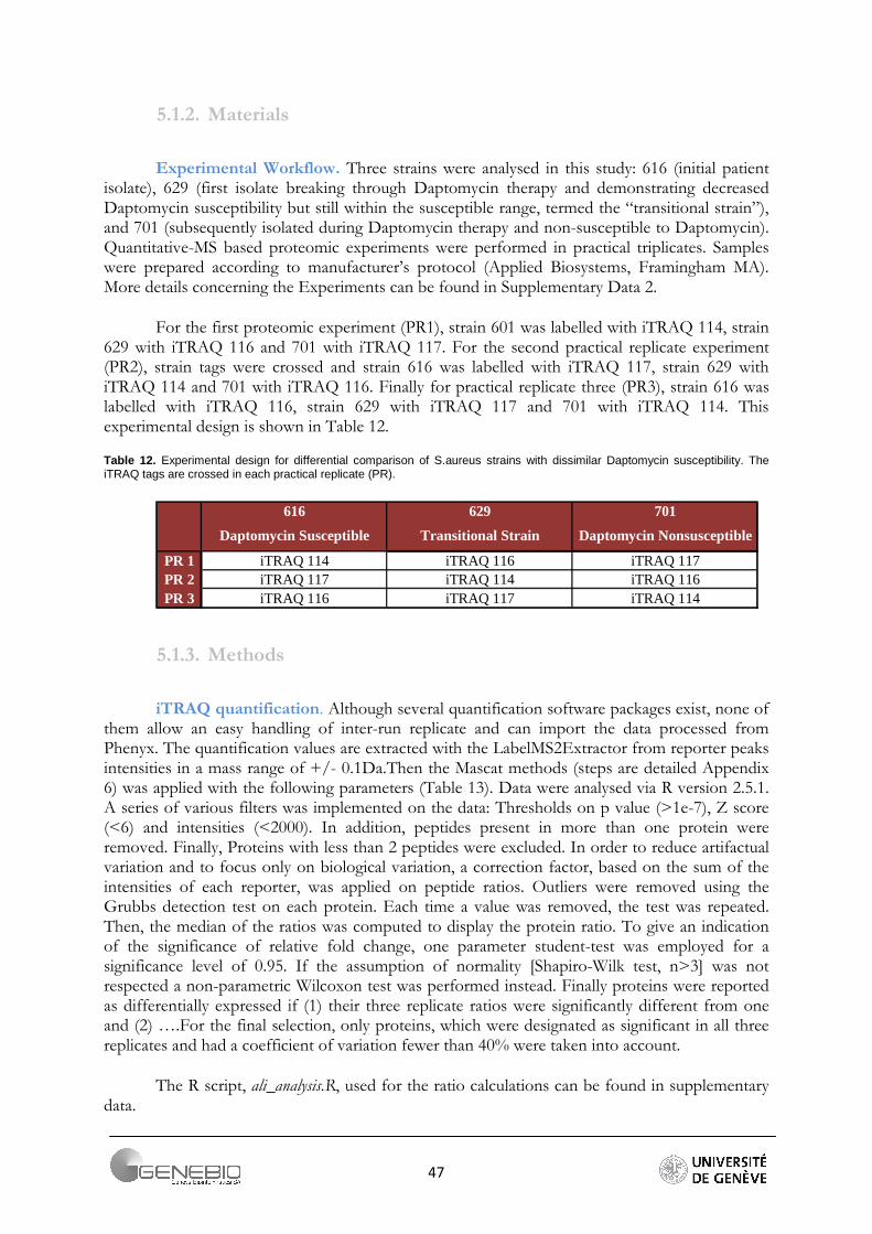
For the first proteomic experiment (PR1), strain 601 was labelled with iTRAQ 114, strain 629 with iTRAQ 116 and 701 with iTRAQ 117. For the second practical replicate experiment (PR2), strain tags were crossed and strain 616 was labelled with iTRAQ 117, strain 629 with iTRAQ 114 and 701 with iTRAQ 116. Finally for practical replicate three (PR3), strain 616 was labelled with iTRAQ 116, strain 629 with iTRAQ 117 and 701 with iTRAQ 114. This experimental design is shown in Table 12.
Table 12. Experimental design for differential comparison of S.aureus strains with dissimilar Daptomycin susceptibility. The iTRAQ tags are crossed in each practical replicate (PR).
616 629 701
PR 1 iTRAQ 114 iTRAQ 116 iTRAQ 117PR 2 iTRAQ 117 iTRAQ 114 iTRAQ 116PR 3 iTRAQ 116 iTRAQ 117 iTRAQ 114
Daptomycin Susceptible Transitional Strain Daptomycin Nonsusceptible
5.1.3. Methods
iTRAQ quantification. Although several quantification software packages exist, none of them allow an easy handling of inter-run replicate and can import the data processed from Phenyx. The quantification values are extracted with the LabelMS2Extractor from reporter peaks intensities in a mass range of +/- 0.1Da.Then the Mascat methods (steps are detailed Appendix 6) was applied with the following parameters (Table 13). Data were analysed via R version 2.5.1. A series of various filters was implemented on the data: Thresholds on p value (>1e-7), Z score (<6) and intensities (<2000). In addition, peptides present in more than one protein were removed. Finally, Proteins with less than 2 peptides were excluded. In order to reduce artifactual variation and to focus only on biological variation, a correction factor, based on the sum of the intensities of each reporter, was applied on peptide ratios. Outliers were removed using the Grubbs detection test on each protein. Each time a value was removed, the test was repeated. Then, the median of the ratios was computed to display the protein ratio. To give an indication of the significance of relative fold change, one parameter student-test was employed for a significance level of 0.95. If the assumption of normality [Shapiro-Wilk test, n>3] was not respected a non-parametric Wilcoxon test was performed instead. Finally proteins were reported as differentially expressed if (1) their three replicate ratios were significantly different from one and (2) ….For the final selection, only proteins, which were designated as significant in all three replicates and had a coefficient of variation fewer than 40% were taken into account.
The R script, ali_analysis.R, used for the ratio calculations can be found in supplementary data.
48
Table 13. Quantification parameters
Reporter extraction moz tolerance 0.1 Da
Impurities Correction No
Quantification Workflow Mascat
Filters * Intensities < 50
* z-score < 6
* p-value >10^-7 Normalisation Sum of intensities
Outliers Grubbs
Ratio calculation Median
5.1.4. Results
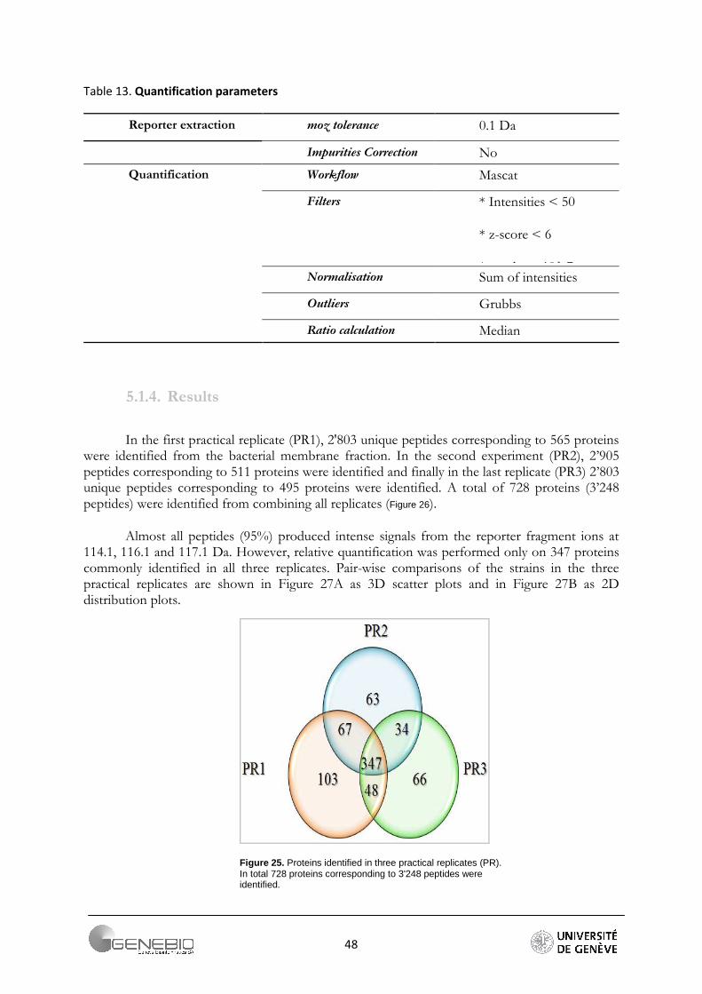
In the first practical replicate (PR1), 2'803 unique peptides corresponding to 565 proteins were identified from the bacterial membrane fraction. In the second experiment (PR2), 2’905 peptides corresponding to 511 proteins were identified and finally in the last replicate (PR3) 2’803 unique peptides corresponding to 495 proteins were identified. A total of 728 proteins (3’248 peptides) were identified from combining all replicates (Figure 26).
Almost all peptides (95%) produced intense signals from the reporter fragment ions at 114.1, 116.1 and 117.1 Da. However, relative quantification was performed only on 347 proteins commonly identified in all three replicates. Pair-wise comparisons of the strains in the three practical replicates are shown in Figure 27A as 3D scatter plots and in Figure 27B as 2D distribution plots.
Figure 25. Proteins identified in three practical replicates (PR). In total 728 proteins corresponding to 3'248 peptides were identified.
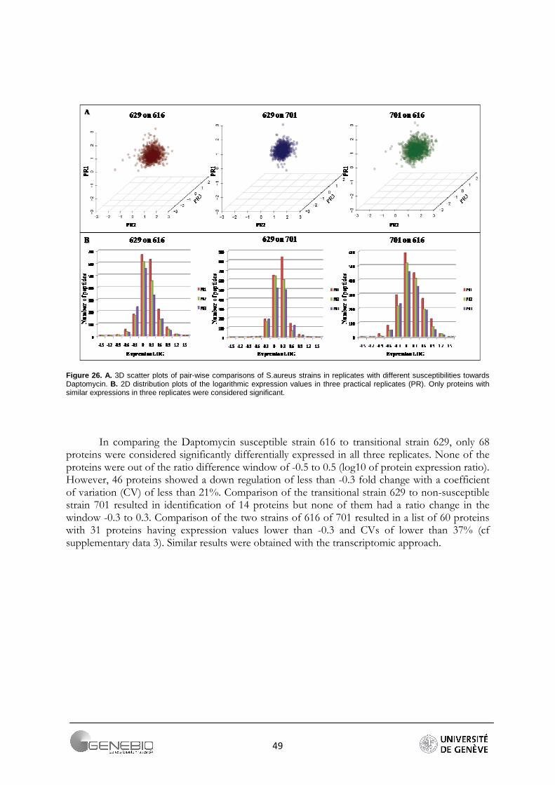
49
Figure 26. A. 3D scatter plots of pair-wise comparisons of S.aureus strains in replicates with different susceptibilities towards Daptomycin. B. 2D distribution plots of the logarithmic expression values in three practical replicates (PR). Only proteins with similar expressions in three replicates were considered significant.
In comparing the Daptomycin susceptible strain 616 to transitional strain 629, only 68 proteins were considered significantly differentially expressed in all three replicates. None of the proteins were out of the ratio difference window of -0.5 to 0.5 (log10 of protein expression ratio). However, 46 proteins showed a down regulation of less than -0.3 fold change with a coefficient of variation (CV) of less than 21%. Comparison of the transitional strain 629 to non-susceptible strain 701 resulted in identification of 14 proteins but none of them had a ratio change in the window -0.3 to 0.3. Comparison of the two strains of 616 of 701 resulted in a list of 60 proteins with 31 proteins having expression values lower than -0.3 and CVs of lower than 37% (cf supplementary data 3). Similar results were obtained with the transcriptomic approach.
50
5.1.5. Discussion
A number of interesting observations emanated from our study. From a biological point of view, we can notice that most of the identified under-expressed proteins between the susceptible and transitional strains were similar to those observed with a down-regulation from the susceptible to the non-susceptible strains. The majority of these proteins were involved in metabolism or were ribosomal or transcriptional factors. Two proteins (Q99UV7, Q7A869) involved in the ion transportation were also identified and showed a reduction in expression. L.Cui & all observed a correlation between membranes thickness and Daptomycin susceptibility. The identification and quantification of proteins that contribute to the synthesis or the metabolism of the cell membrane like Q99V41, Q7A7A5, Q7A5K8, Q7A619, Q7A5D5, Q7A6K0 and P64003 tend to confirm this observation.
Moreover, this study highlights several critical points in a quantification analysis. First, an automated, computer-based analysis for quantization of large amount of proteins is more reliable than manual. Indeed, another analysis that was manually carried out was not in agreement with transcriptomic results. Owing to the filtering and outlier removal steps, the correction of experimental variation is provided during the normalization step. Secondly, Mascat provides an indication of change that directly gives an indication of the protein expression (cf Supplementary Data 4). Third, this collaboration brought to our attention complex experimental designs involving inter-run replicates (experimental replicates) and lead to their implementation and support in the quantification workflows.
Combined proteomic and transcriptomic analyses allowed for obtaining a global view of complex processes involving differentially regulated factors contributing to antibiotic resistance. This combined information is essential for the global integration of the data. Several potential proteins implicated in Daptomycin resistance were identified. However, their implication has to be confirmed by targeted investigation with conventional molecular biology techniques. In view of the results found in the literature and additional information obtained in this study, we showed that our data appeared particularly relevant and that multiple mechanisms are mobilized by Staphylococcus aureus to produce resistance towards antibiotics.
51
5.2. Loic Dayon Collaboration
5.2.1. CSF Analysis by TMT 6-plex
5.2.1.1. Introduction
A second collaboration has been carried out on a TMT 6-plex dataset, generously provided by Loic Dayon. This study consisted of the quantitative analysis of proteins obtained by shotgun proteomic approach on Cerebrospinal fluid samples using TMT. The CSF is a clear fluid found in the brain chambers (ventricles), spinal canal, and spinal cord. It is secreted by the choroids plexus, a vascular part in the ventricles of the brain. It acts as a shock absorber to protect the brain against injury. It contains electrolytes, glucose, and low proteins concentration. Chemical labelling seems to Aggarwal et al show that isobaric tags are highly sensitive and can identify low abundant proteins.
In this study, relative quantification on ante-mortem and post-mortem CSF was done [7]. Due to the disruption of the Blood-Brain Barrier (BBB) a few hours after death, post-mortem CSF and ante-mortem CSF are very different in composition.
In a first step, I performed a quantification analysis using Librus (a quantification workflow based on the TPP-Libra) and compared the results with the published ratio values [7]. However, I found sometimes-dissimilar protein ratios. In order to address this issue, an investigation was carried out on two possible sources of bias in the protein ratio: missing values of intensities and impurities correction. Generally, missing values are due to problems in the detection of weak signal from low abundance peptides. Instruments sometimes fail to detect the signal and even if the detection is successful, the peaks intensity may be too low to be distinguished from the background noise [38]. When looking at the Phenyx job, we can notice that a lot of peptides contain missing events for one specific reporter. Thus, I tried to assess the influence of these “missing” events in the quantification results by running our three quantification approaches on the data. Results showed that an approach based on linear regression is a relatively good alternative to overcome this issue. A last study has been performed on the impurity correction. In fact, TMT or iTRAQ reagents differ in the isotopic compositions of nitrogen, carbon and oxygen but have identical masses. Due to isotopic contamination in tags, peak overlapping occurs, i.e. the peak area for each reporter ion has some contribution from other reporter ions. To correct this bias, the manufacturer ABI (iTRAQ)) provides a datasheet which indicates the percentages of each reporter ion reagent that differs by -2, -1, +1, +2 Da from the quoted mass. I-Tracker, proQuant and most of the quantification software implement this correction. Purity correction may however lead to biased estimation of the protein fold change, especially when low abundance peptides are detected.

52
5.2.1.2. Materials
CSF Collection. Post-Mortem (PM) CSF samples from different patients (n = 4) were collected by ventricular puncture at autopsy, 6 h after death on average. Control Ante-Mortem (AM) CSF samples were collected by routine diagnostic lumbar puncture from living healthy patients (n = 4). Clinical data of deceased and living patients have been previously reported. Each patient or patient’s relatives gave informed consent prior to enrolment. The local institutional ethical committee board approved the clinical protocol.
Experimental Workflow. After immunoaffinity depletion, triplicates of AM and PM CSF pooled samples were reduced, alkylated, digested by trypsin, and labelled, respectively, with the six isobaric variants of the TMT (with reporter ions from m/z ) 126.1 to 131.1 Th). The samples were pooled and fractionated by SCX chromatography. After RP-LC separation, peptides were identified and quantified by MS/MS analysis with MALDI TOF/TOF and ESI-Q-TOF.
Spiking of Protein. β-lactoglobulin (LACB) from bovine milk (90%) was purchased from Sigma (St. Louis, MO).
(cf Dayon & al. [7] For more details about the Experimental Procedure).
53
5.2.1.3. Data analysis
Protein Quantification
Reporter peaks are extracted using the LabelMS/MSExtractor. They are collected with a m/z tolerance of 0.15. No isotopic correction is applied due to the bias generated on the low peaks intensities. Protein quantification was performed using the Librus method. (Appendix 6). Peptides are filtered according to the signal intensity (< 50), sum of intensity (< 300), and the quality of the labelling. The protein is removed if a protein does not contain at least two peptides. A parameters summary can be found in table 14. The R script CSF6plex_analysis.R can be found in supplementary data 6.
Table 14. Quantification parameters
Reporter extraction moz tolerance 0.15 Da
Impurities correction No
Quantification Workflow Librus
Filters * intensities < 50
* quality of the labelling
* sum of reporter per peptides <500
* min number of peptides : 2
Normalisation Sum of peptides reporter intensities
Outliers µ+/-2*σ
Ratio calculation Σ PM CSF reporter mean / Σ AM CSF reporter mean
Error Estimation
To obtain a more reliable comparison with Loic's published result, no filter on intensity is applied; the only filter applied is the one that assesses the quality of the labelling. Proteins are removed if a protein does not contain at least 2 peptides. The Librus quantification method has been used and the ratio of the mean label 131 m/z on 126 m/z reported. A confidence interval on the estimated ratio was then obtained. An average value for the noise was first estimated. According to Loic’s opinion and a brief glance at the peak list, the background noise was estimated to 50 counts. This value was then used to determine the maximum and minimum values of each reporter intensity (Table 15). Finally, the following crossing pairs of ratio were used to compute the interval [Label6MAX/Label1MIN, Label6MIN/Label1MAX] (Figure 27).
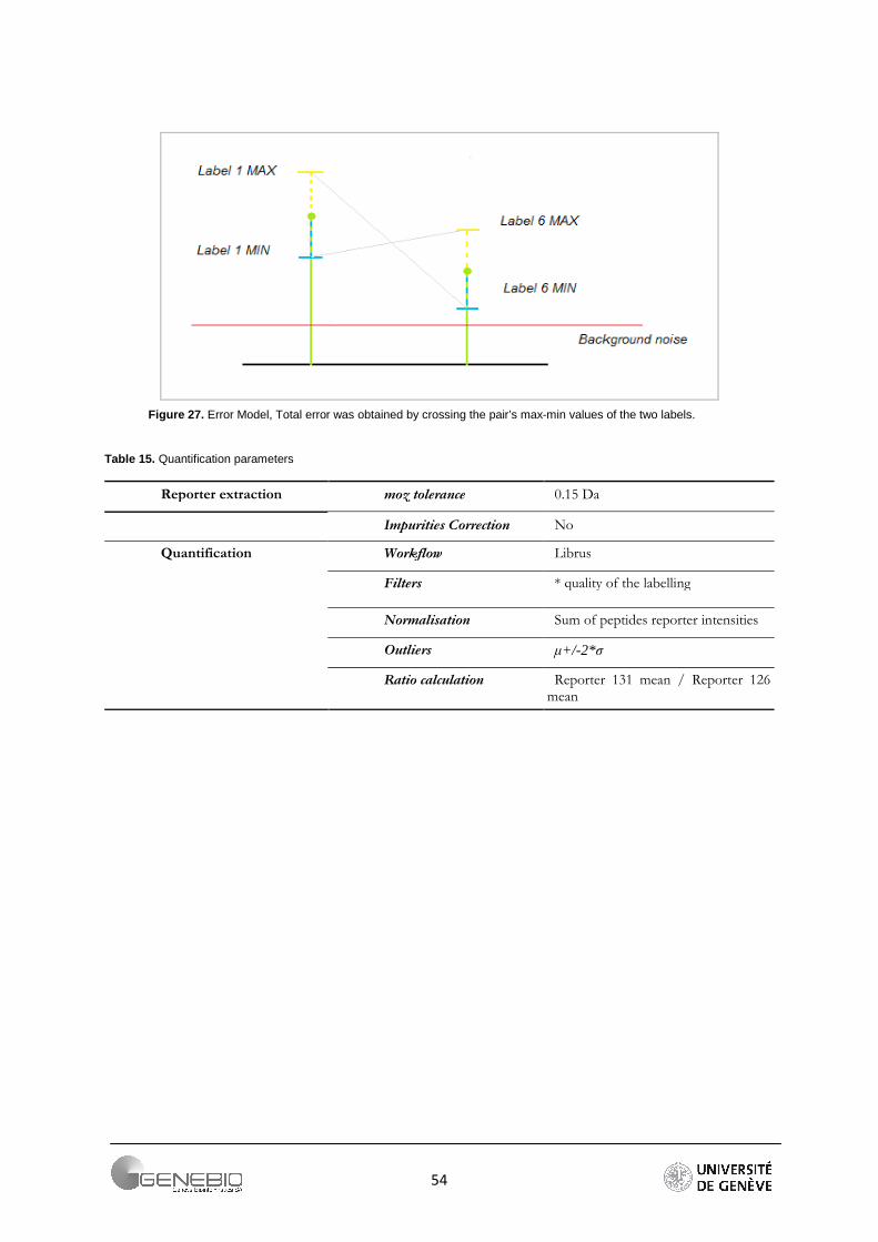
54
Table 15. Quantification parameters
Reporter extraction moz tolerance 0.15 Da
Impurities Correction No
Quantification Workflow Librus
Filters * quality of the labelling
Normalisation Sum of peptides reporter intensities
Outliers µ+/-2* σ
Ratio calculation Reporter 131 mean / Reporter 126 mean
Figure 27. Error Model, Total error was obtained by crossing the pair’s max-min values of the two labels.
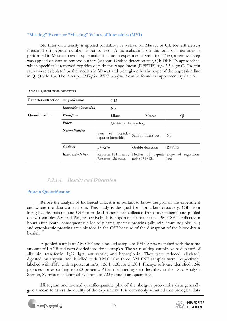
55
“Missing” Events or “Missing” Values of Intensities (MVI)
No filter on intensity is applied for Librus as well as for Mascat or QI. Nevertheless, a threshold on peptide number is set to two. A normalisation on the sum of intensities is performed in Mascat to avoid systematic bias due to experimental variation. Then, a removal step was applied on data to remove outliers (Mascat: Grubbs detection test, QI: DFFITS approaches, which specifically removed peptides outside the range [mean (DFFTIS) +/- 2.5 sigma]). Protein ratios were calculated by the median in Mascat and were given by the slope of the regression line in QI (Table 16). The R script CSF6plex_MVI_analysis.R can be found in supplementary data 6.
Table 16. Quantification parameters
Reporter extraction moz tolerance 0.15
Impurities Correction No
Quantification Workflow Librus Mascat QI
Filters Quality of the labelling
Normalisation Sum of peptides reporter intensities
Sum of intensities No
Outliers µ+/-2* σ Grubbs detection DFFITS
Ratio calculation Reporter 131 mean / Reporter 126 mean
Median of peptide ratios 131/126
Slope of regression line
5.2.1.4. Results and Discussion
Protein Quantification
Before the analysis of biological data, it is important to know the goal of the experiment and where the data comes from. This study is designed for biomarkers discovery. CSF from living healthy patients and CSF from dead patients are collected from four patients and pooled on two samples AM and PM, respectively. It is important to notice that PM CSF is collected 6 hours after death; consequently a lot of plasma specific proteins (albumin, immunoglobulin...) and cytoplasmic proteins are unloaded in the CSF because of the disruption of the blood-brain barrier.
A pooled sample of AM CSF and a pooled sample of PM CSF were spiked with the same amount of LACB and each divided into three samples. The six resulting samples were depleted of albumin, transferrin, IgG, IgA, antitrypsin, and haptoglobin. They were reduced, alkylated, digested by trypsin, and labelled with TMT. The three AM CSF samples were, respectively, labelled with TMT with reporter at m/z) 126.1, 128.1,and 130.1. Phenyx software identified 1246 peptides corresponding to 220 proteins. After the filtering step describes in the Data Analysis Section, 89 proteins identified by a total of 722 peptides are quantified.
Histogram and normal quantile-quantile plot of the shotgun proteomics data generally give a mean to assess the quality of the experiment. It is commonly admitted that biological data
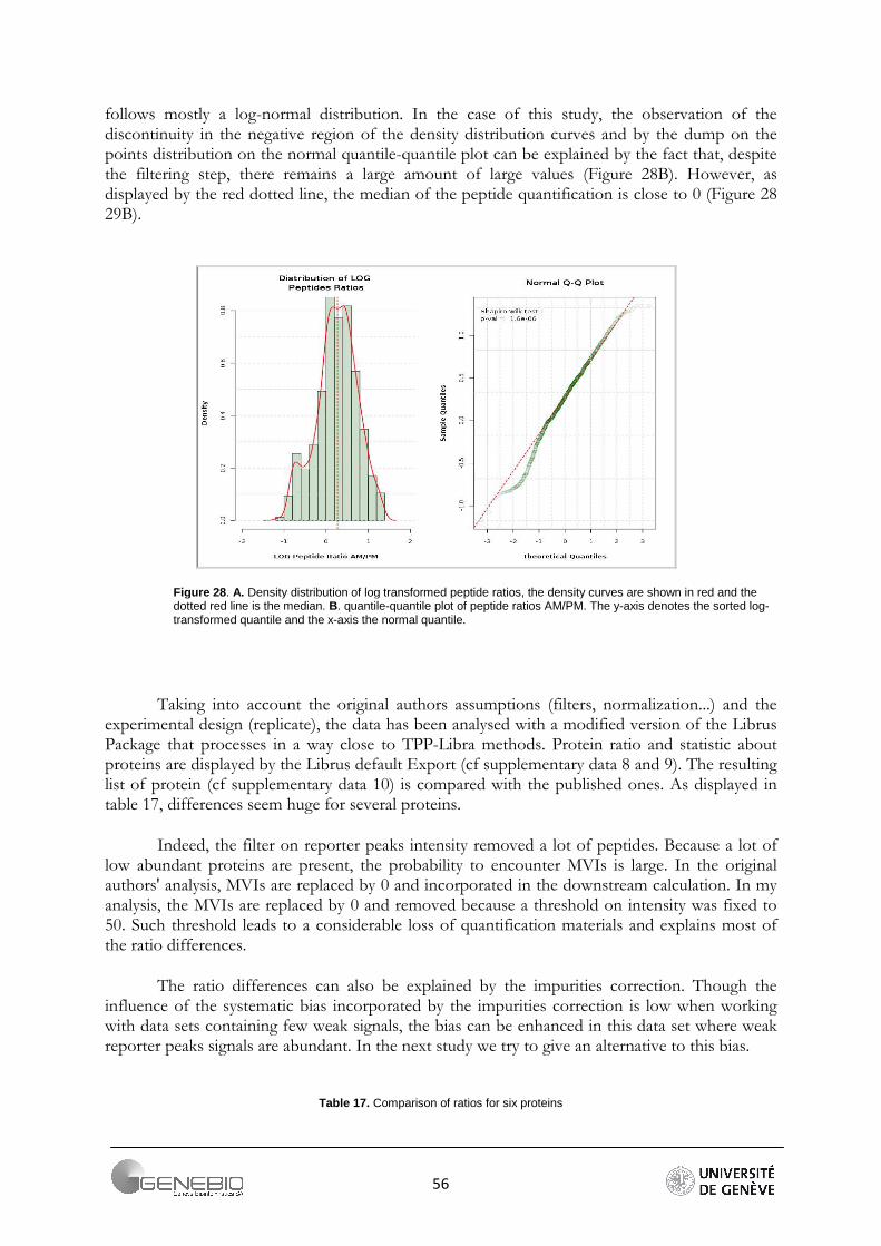
56
follows mostly a log-normal distribution. In the case of this study, the observation of the discontinuity in the negative region of the density distribution curves and by the dump on the points distribution on the normal quantile-quantile plot can be explained by the fact that, despite the filtering step, there remains a large amount of large values (Figure 28B). However, as displayed by the red dotted line, the median of the peptide quantification is close to 0 (Figure 28 29B).
Taking into account the original authors assumptions (filters, normalization...) and the experimental design (replicate), the data has been analysed with a modified version of the Librus Package that processes in a way close to TPP-Libra methods. Protein ratio and statistic about proteins are displayed by the Librus default Export (cf supplementary data 8 and 9). The resulting list of protein (cf supplementary data 10) is compared with the published ones. As displayed in table 17, differences seem huge for several proteins.
Indeed, the filter on reporter peaks intensity removed a lot of peptides. Because a lot of low abundant proteins are present, the probability to encounter MVIs is large. In the original authors' analysis, MVIs are replaced by 0 and incorporated in the downstream calculation. In my analysis, the MVIs are replaced by 0 and removed because a threshold on intensity was fixed to 50. Such threshold leads to a considerable loss of quantification materials and explains most of the ratio differences.
The ratio differences can also be explained by the impurities correction. Though the influence of the systematic bias incorporated by the impurities correction is low when working with data sets containing few weak signals, the bias can be enhanced in this data set where weak reporter peaks signals are abundant. In the next study we try to give an alternative to this bias.
Table 17. Comparison of ratios for six proteins
Figure 28 . A. Density distribution of log transformed peptide ratios, the density curves are shown in red and the dotted red line is the median. B. quantile-quantile plot of peptide ratios AM/PM. The y-axis denotes the sorted log-transformed quantile and the x-axis the normal quantile.
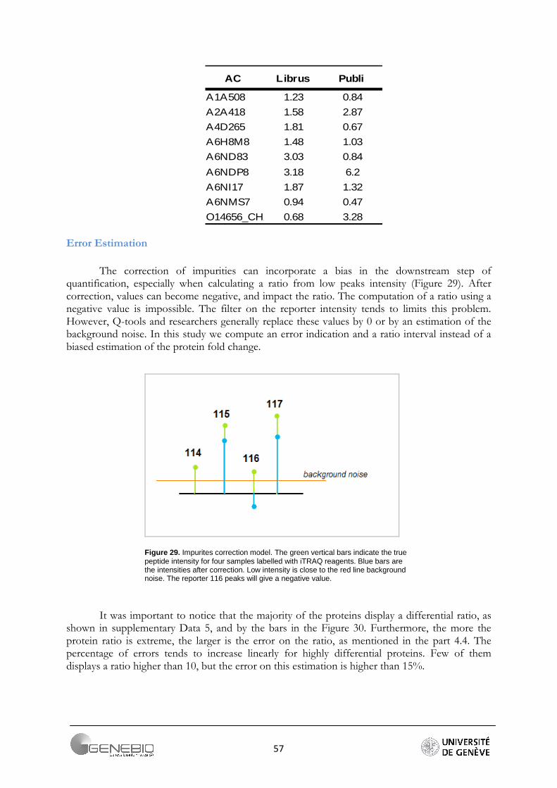
57
AC Librus Publi
A1A508 1.23 0.84
A2A418 1.58 2.87
A4D265 1.81 0.67
A6H8M8 1.48 1.03
A6ND83 3.03 0.84
A6NDP8 3.18 6.2
A6NI17 1.87 1.32
A6NMS7 0.94 0.47
O14656_CHAIN_0 0.68 3.28
Error Estimation
The correction of impurities can incorporate a bias in the downstream step of quantification, especially when calculating a ratio from low peaks intensity (Figure 29). After correction, values can become negative, and impact the ratio. The computation of a ratio using a negative value is impossible. The filter on the reporter intensity tends to limits this problem. However, Q-tools and researchers generally replace these values by 0 or by an estimation of the background noise. In this study we compute an error indication and a ratio interval instead of a biased estimation of the protein fold change.
It was important to notice that the majority of the proteins display a differential ratio, as shown in supplementary Data 5, and by the bars in the Figure 30. Furthermore, the more the protein ratio is extreme, the larger is the error on the ratio, as mentioned in the part 4.4. The percentage of errors tends to increase linearly for highly differential proteins. Few of them displays a ratio higher than 10, but the error on this estimation is higher than 15%.
Figure 29. Impurites correction model. The green vertical bars indicate the true peptide intensity for four samples labelled with iTRAQ reagents. Blue bars are the intensities after correction. Low intensity is close to the red line background noise. The reporter 116 peaks will give a negative value.
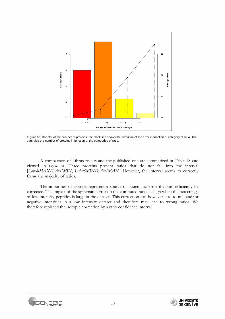
58
Figure 30. Bar plot of the number of proteins. the black line shows the evolution of the error in function of category of ratio. The bars give the number of proteins in function of the categories of ratio.
A comparison of Librus results and the published one are summarized in Table 18 and viewed in Figure 31. Three proteins present ratios that do not fall into the interval [Label6MAX/Label1MIN, Label6MIN/Label1MAX]. However, the interval seems to correctly frame the majority of ratios.
The impurities of isotope represent a source of systematic error that can efficiently be corrected. The impact of the systematic error on the computed ratios is high when the percentage of low intensity peptides is large in the dataset. This correction can however lead to null and/or negative intensities in a low intensity dataset and therefore may lead to wrong ratios. We therefore replaced the isotopic correction by a ratio confidence interval.
<
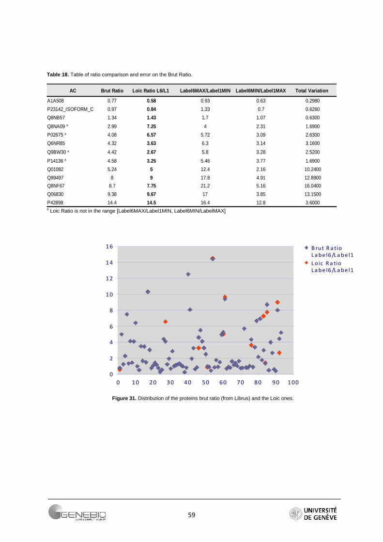
59
0 10 20 30 40 50 60 70 80 90 100
0
2
4
6
8
10
12
14
16
Figure 31. Distribution of the proteins brut ratio (from Librus) and the Loic ones.
B rut R a tio
L a be l6/L a be l1
L oic R a tio
L a be l6/L a be l1
Table 18. Table of ratio comparison and error on the Brut Ratio.
AC Brut Ratio Loïc Ratio L6/L1 Label6MAX/Label1MIN Lab el6MIN/Label1MAX Total Variation
A1A508 0.77 0.58 0.93 0.63 0.2980
P23142_ISOFORM_C 0.97 0.84 1.33 0.7 0.6260
Q8NB57 1.34 1.43 1.7 1.07 0.6300
2.99 7.25 4 2.31 1.6900
4.08 6.57 5.72 3.09 2.6300
Q6NR85 4.32 3.63 6.3 3.14 3.1600
4.42 2.67 5.8 3.28 2.5200
4.58 3.25 5.46 3.77 1.6900
Q01082 5.24 5 12.4 2.16 10.2400
Q99497 8 9 17.8 4.91 12.8900
Q8NF67 8.7 7.75 21.2 5.16 16.0400
Q06830 9.38 9.67 17 3.85 13.1500
P42898 14.4 14.5 16.4 12.8 3.6000
Q8NA09 a
P02675 a
Q9BW30 a
P14136 a
a Loic Ratio is not in the range [Label6MAX/Label1MIN, Label6MIN/LabelMAX]
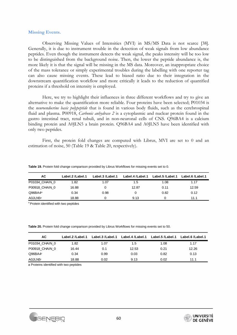
60
Missing Events.
Observing Missing Values of Intensities (MVI) in MS/MS Data is not scarce [38]. Generally, it is due to instrument trouble in the detection of weak signals from low abundance peptides. Even though the instrument detects the weak signal, the peaks intensity will be too low to be distinguished from the background noise. Then, the lower the peptide abundance is, the more likely it is that the signal will be missing in the MS data. Moreover, an inappropriate choice of the mass tolerance or simply experimental troubles during the labelling with one reporter tag can also cause missing events. These lead to biased ratio due to their integration in the downstream quantification workflow and more critically it leads to the reduction of quantified proteins if a threshold on intensity is employed.
Here, we try to highlight their influences in three different workflows and try to give an alternative to make the quantification more reliable. Four proteins have been selected; P01034 is the neuroendocrine basic polypeptide that is found in various body fluids, such as the cerebrospinal fluid and plasma. P00918, Carbonic anhydrase 2 is a cytoplasmic and nuclear protein found in the gastro intestinal tract, renal tubuli, and in non-neuronal cells of CNS. Q96BA4 is a calcium binding protein and A0JLN5 a brain protein. Q96BA4 and A0JLN5 have been identified with only two peptides.
First, the protein fold changes are computed with Librus, MVI are set to 0 and an estimation of noise, 50 (Table 19 & Table 20, respectively).
Table 20. Protein fold change comparison provided by Librus Workflows for missing events set to 50.
AC Label.2 /Label.1 Label.3 /Label.1 Label.4 /Label.1 L abel.5 /Label.1 Label.6 /Label.1
P01034_CHAIN_0 1.82 1.07 1.5 1.08 1.17
P00918_CHAIN_0 16.44 0.1 12.53 0.21 12.26
0.34 0.99 0.03 0.82 0.13
18.88 0.02 9.13 0.02 11.1
Q96BA4a
A0JLN5a
a Proteins identified with two peptides
Table 19. Protein fold change comparison provided by Librus Workflows for missing events set to 0.
AC Label.2 /Label.1 Label.3 /Label.1 Label.4 /Label.1 L abel.5 /Label.1 Label.6 /Label.1
P01034_CHAIN_0 1.82 1.07 1.5 1.08 1.17
P00918_CHAIN_0 16.88 0 12.87 0.11 12.59
0.34 0.98 0 0.82 0.12
18.88 0 9.13 0 11.1
Q96BA4a
A0JLN5a
a Protein identified with two peptides
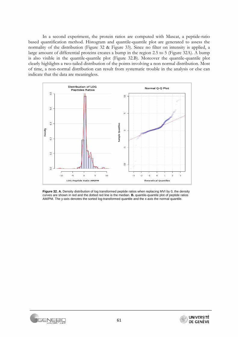
61
In a second experiment, the protein ratios are computed with Mascat, a peptide-ratio based quantification method. Histogram and quantile-quantile plot are generated to assess the normality of the distribution (Figure 32 & Figure 33). Since no filter on intensity is applied, a large amount of differential proteins creates a bump in the region 2.5 to 5 (Figure 32A). A bump is also visible in the quantile-quantile plot (Figure 32.B). Moreover the quantile-quantile plot clearly highlights a two-tailed distribution of the points involving a non normal distribution. Most of time, a non-normal distribution can result from systematic trouble in the analysis or else can indicate that the data are meaningless.
Figure 32. A. Density distribution of log transformed peptide ratios when replacing MVI by 0, the density curves are shown in red and the dotted red line is the median. B. quantile-quantile plot of peptide ratios AM/PM. The y-axis denotes the sorted log-transformed quantile and the x-axis the normal quantile.
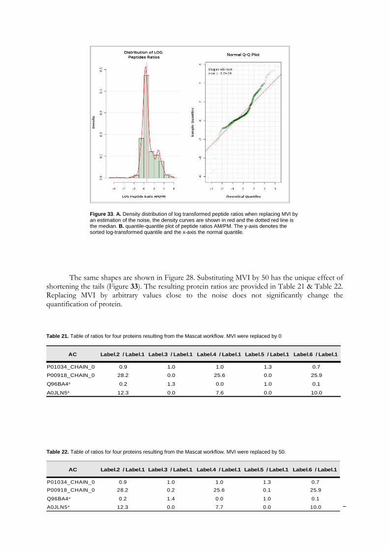
62
The same shapes are shown in Figure 28. Substituting MVI by 50 has the unique effect of shortening the tails (Figure 33). The resulting protein ratios are provided in Table 21 & Table 22. Replacing MVI by arbitrary values close to the noise does not significantly change the quantification of protein.
Table 22. Table of ratios for four proteins resulting from the Mascat workflow. MVI were replaced by 50.
AC Label.2 / Label.1 Label.3 / Label.1 Label.4 / Label.1 Label.5 / Label.1 Label.6 / Label.1
P01034_CHAIN_0 0.9 1.0 1.0 1.3 0.7
P00918_CHAIN_0 28.2 0.2 25.6 0.1 25.9
0.2 1.4 0.0 1.0 0.1
12.3 0.0 7.7 0.0 10.0
Q96BA4a
A0JLN5a
Table 21. Table of ratios for four proteins resulting from the Mascat workflow. MVI were replaced by 0
AC Label.2 / Label.1 Label.3 / Label.1 Label.4 / Label.1 Label.5 / Label.1 Label.6 / Label.1
P01034_CHAIN_0 0.9 1.0 1.0 1.3 0.7
P00918_CHAIN_0 28.2 0.0 25.6 0.0 25.9
0.2 1.3 0.0 1.0 0.1
12.3 0.0 7.6 0.0 10.0
Q96BA4a
A0JLN5a
Figure 33 . A. Density distribution of log transformed peptide ratios when replacing MVI by an estimation of the noise, the density curves are shown in red and the dotted red line is the median. B. quantile-quantile plot of peptide ratios AM/PM. The y-axis denotes the sorted log-transformed quantile and the x-axis the normal quantile.
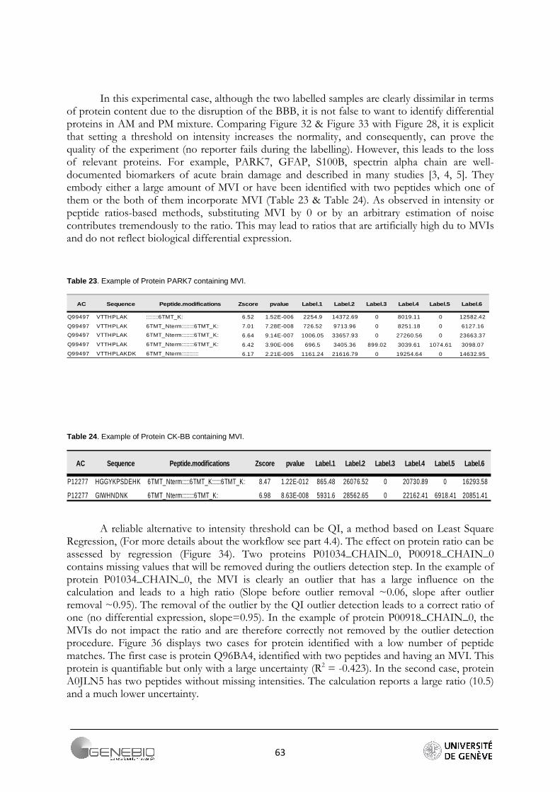
63
In this experimental case, although the two labelled samples are clearly dissimilar in terms of protein content due to the disruption of the BBB, it is not false to want to identify differential proteins in AM and PM mixture. Comparing Figure 32 & Figure 33 with Figure 28, it is explicit that setting a threshold on intensity increases the normality, and consequently, can prove the quality of the experiment (no reporter fails during the labelling). However, this leads to the loss of relevant proteins. For example, PARK7, GFAP, S100B, spectrin alpha chain are well-documented biomarkers of acute brain damage and described in many studies [3, 4, 5]. They embody either a large amount of MVI or have been identified with two peptides which one of them or the both of them incorporate MVI (Table 23 & Table 24). As observed in intensity or peptide ratios-based methods, substituting MVI by 0 or by an arbitrary estimation of noise contributes tremendously to the ratio. This may lead to ratios that are artificially high du to MVIs and do not reflect biological differential expression.
A reliable alternative to intensity threshold can be QI, a method based on Least Square Regression, (For more details about the workflow see part 4.4). The effect on protein ratio can be assessed by regression (Figure 34). Two proteins P01034_CHAIN_0, P00918_CHAIN_0 contains missing values that will be removed during the outliers detection step. In the example of protein P01034_CHAIN_0, the MVI is clearly an outlier that has a large influence on the calculation and leads to a high ratio (Slope before outlier removal ~0.06, slope after outlier removal ~0.95). The removal of the outlier by the QI outlier detection leads to a correct ratio of one (no differential expression, slope=0.95). In the example of protein P00918_CHAIN_0, the MVIs do not impact the ratio and are therefore correctly not removed by the outlier detection procedure. Figure 36 displays two cases for protein identified with a low number of peptide matches. The first case is protein Q96BA4, identified with two peptides and having an MVI. This protein is quantifiable but only with a large uncertainty (R2 = -0.423). In the second case, protein A0JLN5 has two peptides without missing intensities. The calculation reports a large ratio (10.5) and a much lower uncertainty.
Table 23. Example of Protein PARK7 containing MVI.
AC Sequence Peptide.modifications Zscore pvalue Label.1 Label.2 Label.3 Label.4 Label.5 Label.6
Q99497 VTTHPLAK ::::::::6TMT_K: 6.52 1.52E-006 2254.9 14372.69 0 8019.11 0 12582.42
Q99497 VTTHPLAK 6TMT_Nterm::::::::6TMT_K: 7.01 7.28E-008 726.52 9713.96 0 8251.18 0 6127.16
Q99497 VTTHPLAK 6TMT_Nterm::::::::6TMT_K: 6.64 9.14E-007 1006.05 33657.93 0 27260.56 0 23663.37
Q99497 VTTHPLAK 6TMT_Nterm::::::::6TMT_K: 6.42 3.90E-006 696.5 3405.36 899.02 3039.61 1074.61 3098.07
Q99497 VTTHPLAKDK 6TMT_Nterm::::::::::: 6.17 2.21E-005 1161.24 21616.79 0 19254.64 0 14632.95
Table 24. Example of Protein CK-BB containing MVI.
AC Sequence Peptide.modifications Zscore pvalue Label.1 Label.2 Label.3 Label.4 Label.5 Label.6
P12277 HGGYKPSDEHK 6TMT_Nterm:::::6TMT_K::::::6TMT_K: 8.47 1.22E-012 865.48 26076.52 0 20730.89 0 16293.58
P12277 GIWHNDNK 6TMT_Nterm::::::::6TMT_K: 6.98 8.63E-008 5931.6 28562.65 0 22162.41 6918.41 20851.41
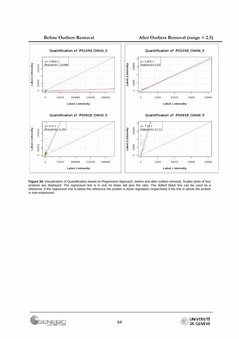
64
Before Outliers Removal After Outliers Removal (range = 2.5)
Figure 34. Visualization of Quantification based on Regression Approach, before and after outliers removal. Scatter plots of four proteins are displayed. The regression line is in red; its slope will give the ratio. The dotted black line can be used as a reference; if the regression line is below the reference the protein is down regulated, respectively if the line is above the protein is over-expressed.
65
Two peptides matched-protein quantification
5.2.1.5. Conclusion
This second collaboration with Loic Dayon allowed us to validate the Librus workflow and to underline two problems; (1) The loss of quantifiable data when applying a threshold on intensity and (2) the bias incorporated by the correction of impurities when low abundance peptides were analysed.
The problem of data loss can be overcome by the QI workflow since weak intensities are removed in an appropriate way (.outliers) by the regression diagnostics methods. However, this algorithm cannot quantify proteins identified with one peptide match. Wang et al. propose a Bayesian probability model to investigate the intensity dependent missing events and provides possible substitutions for the MVI [38]. In a next study, I will try to reproduce and validate this probability model in R and integrates this approach in our quantification algorithms.
Figure 35. Visualization of two peptides contained-protein Quantitation based on Regression Approach, Scatter plots of two proteins are displayed. The regression line is in red; its slope will give the ratio. The dotted black line can be used as a reference; if the regression line is below the reference the protein is down regulated, respectively if the line is above the protein is over-expressed.
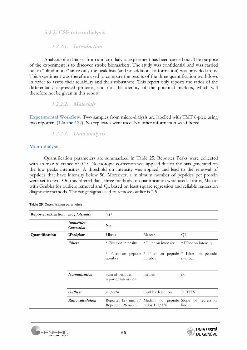
66
5.2.2. CSF micro-dialysis
5.2.2.1. Introduction
Analysis of a data set from a micro-dialysis experiment has been carried out. The purpose of the experiment is to discover stroke biomarkers. The study was confidential and was carried out in “blind mode” since only the peak lists (and no additional information) was provided to us. This experiment was therefore used to compare the results of the three quantification workflows in order to assess their reliability and their robustness. This report only reports the ratios of the differentially expressed proteins, and not the identity of the potential markers, which will therefore not be given in this report.
5.2.2.2. Materials
Experimental Workflow. Two samples from micro-dialysis are labelled with TMT 6-plex using two reporters (126 and 127). No replicates were used. No other information was filtered.
5.2.2.3. Data analysis
Micro-dialysis.
Quantification parameters are summarized in Table 25. Reporter Peaks were collected with an m/z tolerance of 0.15. No isotopic correction was applied due to the bias generated on the low peaks intensities. A threshold on intensity was applied, and lead to the removal of peptides that have intensity below 50. Moreover, a minimum number of peptides per protein were set to two. On this filtered data, three methods of quantification were used. Librus, Mascat with Grubbs for outliers removal and Qi, based on least square regression and reliable regression diagnostic methods. The range sigma used to remove outlier is 2.5.
Table 25. Quantification parameters.
Reporter extraction moz tolerance 0.15
Impurities
Correction No
Quantification Workflow Librus Mascat QI
Filters * Filter on intensity
* Filter on peptide number
* Filter on intensity
* Filter on peptide number
* Filter on intensity
* Filter on peptide number
Normalisation Sum of peptides reporter intensities
median no
Outliers µ+/-2*σ Grubbs detection DFFITS
Ratio calculation Reporter 127 mean / Reporter 126 mean
Median of peptide ratios 127/126
Slope of regression line
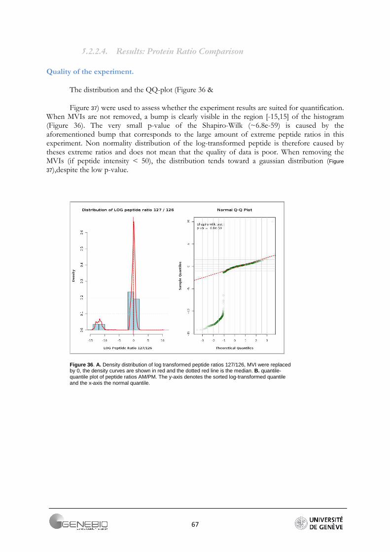
67
5.2.2.4. Results: Protein Ratio Comparison
Quality of the experiment.
The distribution and the QQ-plot (Figure 36 &
Figure 37) were used to assess whether the experiment results are suited for quantification. When MVIs are not removed, a bump is clearly visible in the region [-15,15] of the histogram (Figure 36). The very small p-value of the Shapiro-Wilk (~6.8e-59) is caused by the aforementioned bump that corresponds to the large amount of extreme peptide ratios in this experiment. Non normality distribution of the log-transformed peptide is therefore caused by theses extreme ratios and does not mean that the quality of data is poor. When removing the MVIs (if peptide intensity < 50), the distribution tends toward a gaussian distribution (Figure
37),despite the low p-value.
Figure 36 . A. Density distribution of log transformed peptide ratios 127/126, MVI were replaced by 0, the density curves are shown in red and the dotted red line is the median. B. quantile-quantile plot of peptide ratios AM/PM. The y-axis denotes the sorted log-transformed quantile and the x-axis the normal quantile.
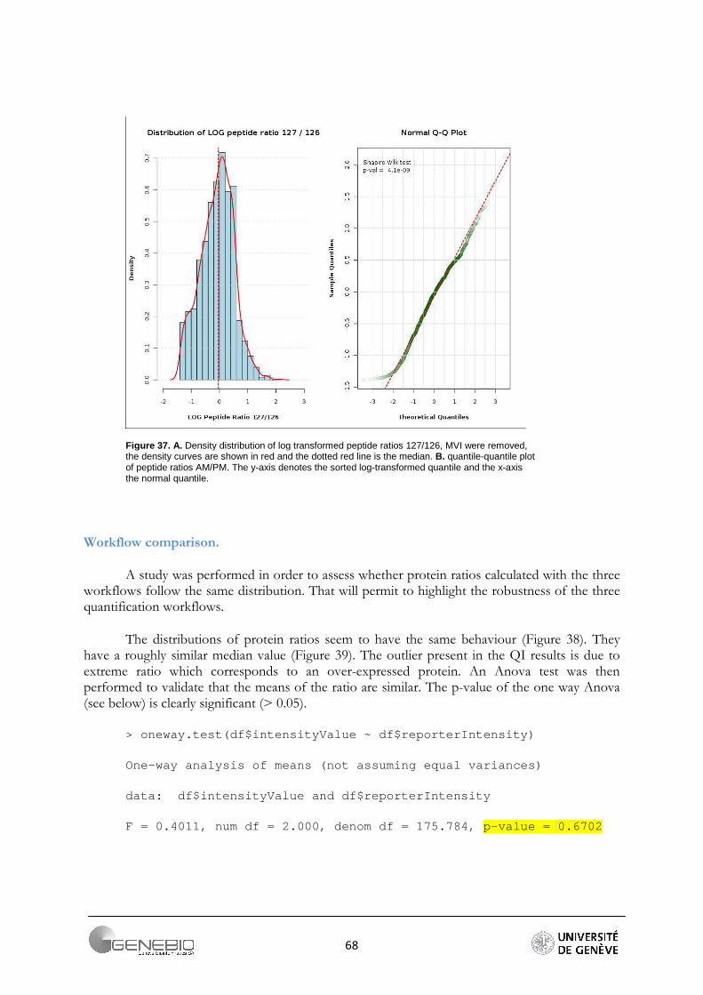
68
Workflow comparison.
A study was performed in order to assess whether protein ratios calculated with the three workflows follow the same distribution. That will permit to highlight the robustness of the three quantification workflows.
The distributions of protein ratios seem to have the same behaviour (Figure 38). They have a roughly similar median value (Figure 39). The outlier present in the QI results is due to extreme ratio which corresponds to an over-expressed protein. An Anova test was then performed to validate that the means of the ratio are similar. The p-value of the one way Anova (see below) is clearly significant (> 0.05).
> oneway.test(df$intensityValue ~ df$reporterIntens ity)
One-way analysis of means (not assuming equal varia nces)
data: df$intensityValue and df$reporterIntensity
F = 0.4011, num df = 2.000, denom df = 175.784, p-v alue = 0.6702
Figure 37. A. Density distribution of log transformed peptide ratios 127/126, MVI were removed, the density curves are shown in red and the dotted red line is the median. B. quantile-quantile plot of peptide ratios AM/PM. The y-axis denotes the sorted log-transformed quantile and the x-axis the normal quantile.
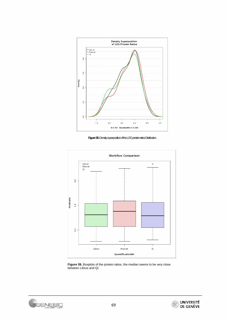
69
Figure 39. Boxplots of the protein ratios, the median seems to be very close between Librus and QI.
Figure 38. Density superposition of the LOG protein ratios Distribution.

70
5.2.2.5. Discussion
Protein ratios resulting from specific workflow follows the same distribution, proving the reliability and the robustness of the ratios and the quantification workflows. However, applying the workflows to data from a biological sample containing several spiked proteins would allow one to assess the precision of the calculated ratios. Furthermore, the analysis and comparison of ratio values obtained without filters on intensity and/or on the number of peptides would give us an indication of the sensitivity of the three methods.
71
6. Conclusion
This one year diploma thesis allowed me to deepen my knowledge in proteomics and IT. I was integrated in the Phenyx development team and physically located in the developer room. I learned the Java programming language and contributed to the development of commercial software. I learned central IT tools and frameworks like CVS, Junit (the testing framework), and the Eclipe Integrated Development Environment (IDE). Moreover, I learned R (a statistical programming language), and deepened my knowledge in statistics and data-analysis.
Although there were constraints inherent to commercial software development, I was free to make my own investigations and statistical researches. Thus, I could develop a novel quantification algorithm based on linear regression and regression diagnostics, which turns out to more robust than existing algorithms. It will be incorporated in the next version of the Phenyx quantification module.
The main objectives of my diploma thesis were achieved. The end of my training corresponds to the release of the first version of the Phenyx quantification module.
Nevertheless, the quantification algorithms are still not perfect, i.e. the estimation of the relative protein abundance can still be enhanced by implementing additional normalisation methods such as those recently published by Callister et al. which successfully applied microarray-based methods to MS data [40]. Implementing a probability model to estimate the noise could also be useful to avoid the loss of important quantifiable proteins [38].
72
7. Reference
1. Aggarwal K, Choe LH, Lee KH Quantitative analysis of protein expression using amine-specific isobaric tags in Escherichia coli cells expressing rhsA elements. Proteomics. 2005 Jun;5(9):2297-308.
2. Boehm AM, Pütz S, Altenhöfer D, Sickmann A, Falk M Precise protein quantification based on peptide quantification using iTRAQ. BMC Bioinformatics. 2007 Jun 21;8:214.
3. Borner GH, Harbour M, Hester S, Lilley KS, Robinson MS Comparative proteomics of clathrin-coated vesicles. J Cell Biol. 2006 Nov 20;175(4):571-8.
4. Choe L, D'Ascenzo M, Relkin NR, Pappin D, Ross P, Williamson B, Guertin S, Pribil P, Lee KH 8-plex quantitation of changes in cerebrospinal fluid protein expression in subjects undergoing intravenous immunoglobulin treatment for Alzheimer's disease. Proteomics. 2007 Oct;7(20):3651-60.
5. Chuan-Yih Yu, Yin-Hao Tsui, Yi-Hwa Yian, Ting-Yi Sung and Wen-Lian Hsu The Multi-Q web server for multiplexed protein quantitation. Nucleic Acids Research 2007 Jul;35(Web Server issue):W707-12
6. Cong YS, Fan E, Wang E Simultaneous proteomic profiling of four different growth states of human fibroblasts, using amine-reactive isobaric tagging reagents and tandem mass spectrometry. Mech
Ageing Dev. 2006 Apr;127(4):332-43.
7. Dayon L, Hainard A, Licker V, Turck N, Kuhn K, Hochstrasser DF, Burkhard PR, Sanchez JC Relative quantification of proteins in human cerebrospinal fluids by MS/MS using 6-plex isobaric tags. Anal Chem. 2008 Apr 15;80(8):2921-31.
8. Desiere F, Deutsch EW, Nesvizhskii AI, Mallick P, King NL, Eng JK, Aderem A, Boyle R, Brunner E, Donohoe S, Fausto N, Hafen E, Hood L, Katze MG, Kennedy KA, Kregenow F, Lee H, Lin B, Martin D, Ranish JA, Rawlings DJ, Samelson LE, Shiio Y, Watts JD, Wollscheid B, Wright ME, Yan W, Yang L, Yi EC, Zhang H, Aebersold R Integration with the human genome of peptide sequences obtained by high-throughput mass spectrometry. Genome Biol. 2005 ;6(1):R9. Epub 2004 Dec 10.
9. DeSouza L, Diehl G, Rodrigues MJ, Guo J, Romaschin AD, Colgan TJ, Siu KW Search for Cancer Markers from Endometrial Tissues Using Differentially Labeled Tags iTRAQ and cICAT with Multidimensional Liquid Chromatography and Tandem Mass Spectrometry. J. Proteome Res. 2005 Mar-Apr;4(2):377-86.
10. Dixon WJ Processing Data for Outliers. Biometrics 1953 9 74-89
11. Bouyssié D, Gonzalez de Peredo A, Mouton E, Albigot R, Roussel L, Ortega N, Cayrol C, Burlet-Schiltz O, Girard JP, Monsarrat B. Mascot file parsing and quantification (MFPaQ), a new software to parse, validate, and quantify proteomics data generated by ICAT and SILAC mass spectrometric analyses: application to the proteomics study of membrane proteins from primary human endothelial cells. Mol
Cell Proteomics. 2007 Sep;6(9):1621-37. Epub 2007 May 28.
12. Gagné JP, Ethier C, Gagné P, Mercier G, Bonicalzi ME, Mes-Masson AM, Droit A, Winstall E, Isabelle M, Poirier GG Comparative proteome analysis of human epithelial ovarian cancer. Proteome Sci. 2007 Sep 24;5:16.
13. Doc Technical, experimental, and biological variations in isobaric tags for relative and absolute quantitation (iTRAQ). J Proteome Res. 2007 Feb;6(2):821-7.
14. Grubbs FE Procedures for Detecting Outlying Observations in Samples. Technometrics 1969 11-020-21
15. Karp NA, Spencer M, Lindsay H, O'Dell K, Lilley KS Impact of replicate types on proteomic expression analysis. J Proteome Res. 2005 Sep-Oct;4(5):1867-71.
73
16. Keshamouni VG, Michailidis G, Grasso CS, Anthwal S, Strahler JR, Walker A, Arenberg DA, Reddy RC, Akulapalli S, Thannickal VJ, Standiford TJ, Andrews PC, Omenn GS Differential protein expression profiling by iTRAQ-2DLC-MS/MS of lung cancer cells undergoing epithelial-mesenchymal transition reveals a migratory/invasive phenotype. J Proteome Res. 2006 May;5(5):1143-54.
17. Panchaud A, Affolter M, Moreillon P, Kussmann M Experimental and computational approaches to quantitative proteomics: status quo and outlook. J Proteomics. 2007 Apr 30;71(1):19-33.
18. Rosner B Percentage Points for a Generalized ESD Many-Outlier Procedure. Technometrics 1983 25 165-172
19. Ross PL, Huang YN, Marchese JN, Williamson B, Parker K, Hattan S, Khainovski N, Pillai S, Dey S, Daniels S, Purkayastha S, Juhasz P, Martin S, Bartlet-Jones M, He F, Jacobson A, Pappin DJ Multiplexed protein quantitation in Saccharomyces cerevisiae using amine-reactive isobaric tagging reagents. Mol Cell
Proteomics. 2004 :1154-69
20. Schmelzle K, Kane S, Gridley S, Lienhard GE, White FM Temporal dynamics of tyrosine phosphorylation in insulin signaling. Diabetes. 2006 Aug;55(8):2171-9.
21. Shadforth IP, Dunkley TP, Lilley KS, Bessant C i-Tracker: For quantitative proteomics using iTRAQTM. BMC Genomics. 2005 Oct 20;6:145.
22. Siepen JA, Swainston N, Jones AR, Hart SR, Hermjakob H, Jones P, Hubbard SJ An informatic pipeline for the data capture and submission of quantitative proteomic data using iTRAQ. Proteome Sci. 2007 Feb 1;5:4.
23. Technical note ProteinPilotTM Software for Protein Identification and Expression Analysis. Technical note 2006
24. Verma SP, Quiroz-Ruiz A Critical values for 22 discordancy test variants for outliers in normal samples up to sizes 100, and applications in science and engineering. Revista Mexicana de Ciencias Geol 2006 Gicas, 23 302-319
25. Verma SP, Quiroz-Ruiz A Critical values for six Dixon tests for outliers in normal samples up to sizes 100, and applications in science and engineering. Revista Mexicana de Ciencias Geol 2006 Gicas, 23 133-161
26. Whitehead K, Kish A, Pan M, Kaur A, Reiss DJ, King N, Hohmann L, DiRuggiero J, Baliga NS An integrated systems approach for understanding cellular responses to gamma radiation. Mol Syst Biol. 2006 12 Septt
27. Zhang Y, Wolf-Yadlin A, Ross PL, Pappin DJ, Rush J, Lauffenburger DA, White FM Time-resolved mass spectrometry of tyrosine phosphorylation sites in the epidermal growth factor receptor signaling network reveals dynamic modules. Mol Cell Proteomics. 2005 Sep;4(9):1240-50.
28. Siepen JA, Swainston N, Jones AR, Hart SR, Hermjakob H, Jones P, Hubbard SJ Pride Wizard: generation of standards compliant quantitative proteomics data. BMC Bioinformatics. 2007 1(Suppl 1):P27doi:10.1186/1752-0509-1-S1-P27
29. Bensmail H, Golek J, Moody MM, Semmes JO, Haoudi A A novel approach for clustering proteomics data using Bayesian fast Fourier transform. Bioinformatics. 2005 May 15;21(10):2210-24.
30. Bantscheff M, Schirle M, Sweetman G, Rick J, Kuster B Quantitative mass spectrometry in proteomics: a critical review. Anal Bioanal Chem. 2007 Oct;389(4):1017-31. Epub 2007 Aug 1.
31. Belsley, David A, Edwin Kuh, Roy E Welsch Regression diagnostics : identifying influential data and sources of collinearity. Wiley series in probability and mathematical statistics. 1980 New York: John Wiley & Sons.
74
32. Wu WW, Wang G, Baek SJ, Shen RF Comparative study of three proteomic quantitative methods, DIGE, cICAT, and iTRAQ, using 2D gel- or LC-MALDI TOF/TOF. J Proteome Res. 2005 2006 Mar;5 (3):651-8.
33. Ong SE, Blagoev B, Kratchmarova I, Kristensen DB, Steen H, Pandey A, Mann M Stable isotope labeling by amino acids in cell culture, SILAC, as a simple and accurate approach to expression proteomics. Mol Cell Proteomics. 2002 May;1(5):376-86.
34. Ong SE, Mann M Mass spectrometry-based proteomics turns quantitative. Nat Chem Biol. 2005 Oct;1(5):252-62.
35. Gygi SP, Rist B, Gerber SA, Turecek F, Gelb MH, Aebersold R Quantitative analysis of complex protein mixtures using isotope-coded affinity tags. 1999 Oct;17(10):994-9.
36. Aggarwal K, Choe LH, Lee KH Shotgun proteomics using the iTRAQ isobaric tags. Brief Funct Genomic Proteomic. 2006 Jun;5(2):112-20. Epub 2006 May 10.
37. Gan CS, Chong PK, Pham TK, Wright PC Technical, experimental, and biological variations in isobaric tags for relative and absolute quantitation (iTRAQ). J Proteome Res. 2007 Feb;6(2):821-7.
38. Wang P, Tang H, Zhang H, Whiteaker J, Paulovich AG, Mcintosh M Normalization regarding non-random missing values in high-throughput mass spectrometry data. Pac Symp Biocomput. 2006 :315-26.
39. Carrillo B, Yanofsky C, Boismenu D, Latterich M, Kearney RE Statistical limits of isotopic/isobaric quantification in counting detectors. Proceedings of the American Society for Mass Spectrometry 174 2006.
40. Callister SJ, Barry RC, Adkins JN, Johnson ET, Qian WJ, Webb-Robertson BJ, Smith RD, Lipton MS Normalization approaches for removing systematic biases associated with mass spectrometry and label-free proteomics. J Proteome Res. 2006 Feb;5(2):277-86.
41. Yan W, Chen SS. Mass spectrometry-based quantitative proteomic profiling. Brief Funct Genomic
Proteomic. 2005 May;4(1):27-38. Review.
Books:
Moore DS, McCabe GP, Introduction to the practice of statistics. New-York: Freeman and
Company.1999.
Dalgaard P, Introductory statistics with R. New-York: Springer. 2002.
Niemeyer P, Knudsen J, Learning Java. Paris: O’Reilly. 2006.
Delannoy C., Programmer en Java. Paris: Eyrolles 2007.
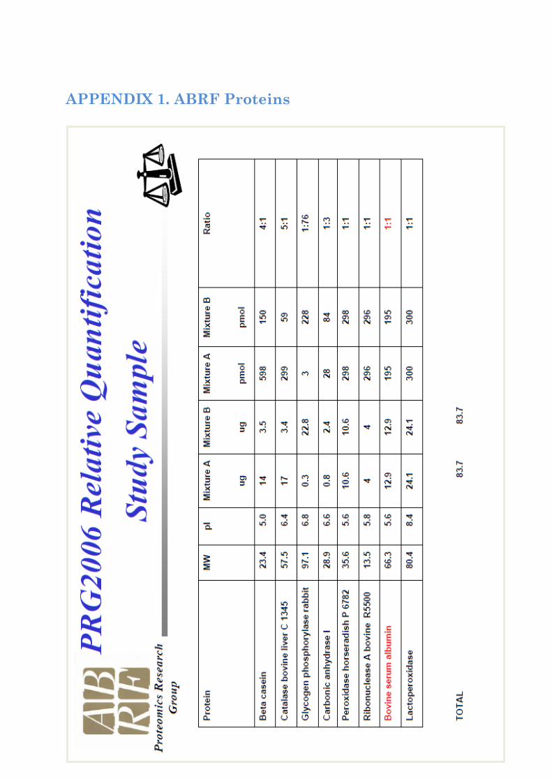
75
APPENDIX 1. ABRF Proteins
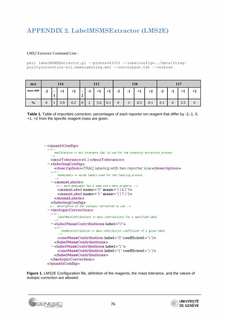
76
APPENDIX 2. LabelMSMSExtractor (LMS2E)
LMS2 Extractor Command Line :
perl labelMSMSExtractor.pl --pidres=43351 --labelco nfig=../data/itraq-puritycorrection-ali.msmslabeling.xml --out=output. txt --verbose
m/z 114 115 116 117 mass shift -2 -
1 +1 +2 -
2 -1 +1 +2 -2 -1 +1 +2 -2 -1 +1 +2
% 0 1 5.9 0.2 0 2 5.6 0.1 0 3 4.5 0.1 0.1 4 3.5 0
Table 1. Table of impurities correction, percentages of each reporter ion reagent that differ by -2,-1, 0, +1, +2 from the specific reagent mass are given.
Figure 1. LMS2E Configuration file, definition of the reagents, the mass tolerance, and the values of isotopic correction are allowed.
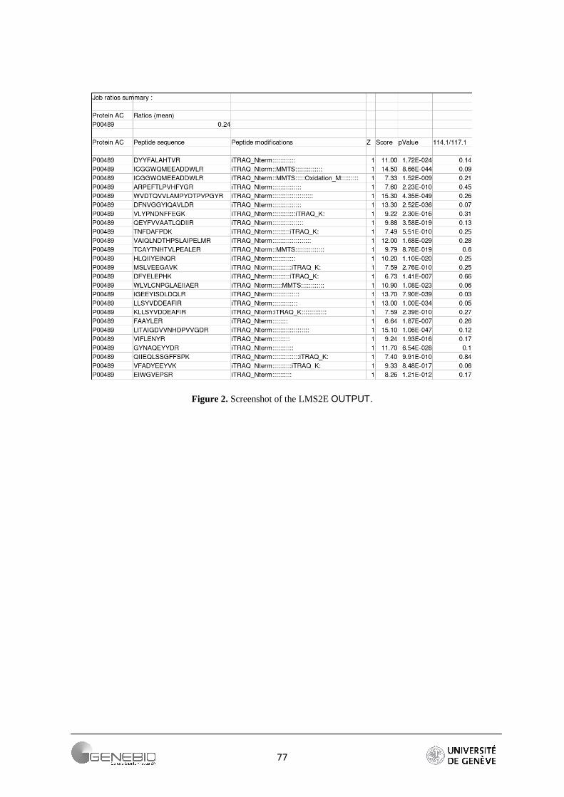
77
Figure 2. Screenshot of the LMS2E OUTPUT.
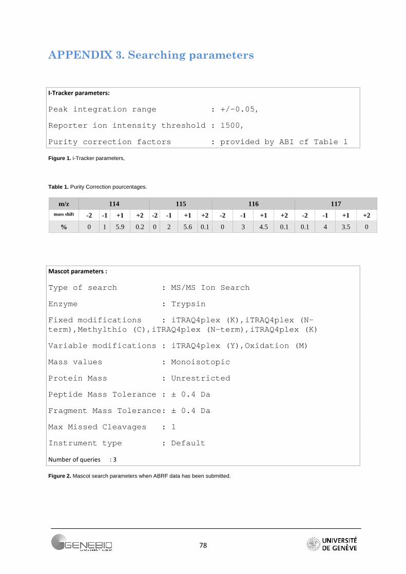
78
APPENDIX 3. Searching parameters
I-Tracker parameters:
Peak integration range : +/-0.05,
Reporter ion intensity threshold : 1500,
Purity correction factors : provided by ABI cf Table 1
Figure 1. i-Tracker parameters,
Table 1. Purity Correction pourcentages.
m/z 114 115 116 117 mass shift -2 -1 +1 +2 -2 -1 +1 +2 -2 -1 +1 +2 -2 -1 +1 +2
% 0 1 5.9 0.2 0 2 5.6 0.1 0 3 4.5 0.1 0.1 4 3.5 0
Mascot parameters :
Type of search : MS/MS Ion Search
Enzyme : Trypsin
Fixed modifications : iTRAQ4plex (K),iTRAQ4plex (N-term),Methylthio (C),iTRAQ4plex (N-term),iTRAQ4plex (K)
Variable modifications : iTRAQ4plex (Y),Oxidation ( M)
Mass values : Monoisotopic
Protein Mass : Unrestricted
Peptide Mass Tolerance : ± 0.4 Da
Fragment Mass Tolerance: ± 0.4 Da
Max Missed Cleavages : 1
Instrument type : Default
Number of queries : 3
Figure 2. Mascot search parameters when ABRF data has been submitted.
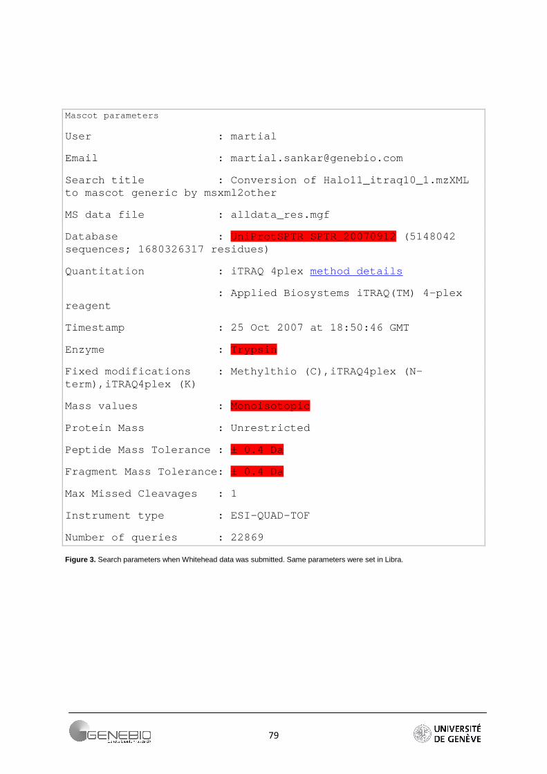
79
Mascot parameters
User : martial
Email : [email protected]
Search title : Conversion of Halo11_itraq 10_1.mzXML to mascot generic by msxml2other
MS data file : alldata_res.mgf
Database : UniProtSPTR SPTR_20070912 (5148042 sequences; 1680326317 residues)
Quantitation : iTRAQ 4plex method details
: Applied Biosystems iTRAQ(T M) 4-plex reagent
Timestamp : 25 Oct 2007 at 18:50:46 GM T
Enzyme : Trypsin
Fixed modifications : Methylthio (C),iTRAQ4plex (N-term),iTRAQ4plex (K)
Mass values : Monoisotopic
Protein Mass : Unrestricted
Peptide Mass Tolerance : ± 0.4 Da
Fragment Mass Tolerance: ± 0.4 Da
Max Missed Cleavages : 1
Instrument type : ESI-QUAD-TOF
Number of queries : 22869
Figure 3. Search parameters when Whitehead data was submitted. Same parameters were set in Libra.

80
APPENDIX 4. Software comparison
Ma
sco
t Q
ua
nti
TP
P-L
ibra
iTra
cke
rQ
ua
nt
INP
UT
/ O
UT
PU
T/
DIS
PLA
YIN
PU
T f
orm
at
mg
f p
ep
XM
L, m
zXM
Lm
gf
or
dta
d
taO
UT
PU
T f
orm
at
.da
tp
rotX
ML
form
at
two
typ
es
of
.csv
.xls
Ra
tio
Vis
ua
lisa
tio
n
--
-
Da
ta p
re-p
roce
ssin
gM
S/M
S I
DY
Y-
-P
ea
k i
nte
gra
tio
nR
ep
ort
er
ion
pe
ak
are
a
Y-
YY
m/z
to
lera
nce
YY
YY
Su
mm
ing
in
ten
siti
es
YY
-Y
Filt
ers
Filt
er
on
in
ten
sity
YY
YY
Filt
er
on
pva
lue
Y-
--
Filt
er
on
sco
reY
--
-
filt
er
on
pro
teo
typ
ic p
ep
tid
e-
--
YQ
ua
nti
tati
on
Wo
rkfl
ow
Qu
an
tita
tio
n t
ype
pe
pti
de
ra
tio
-ba
sed
Inte
nsi
ty-b
ase
dIn
ten
sity
-ba
sed
pe
pti
de
ra
tio
ba
sed
Pro
tein
Ra
tio
me
dia
n
Y-
-Y
Ari
thm
eti
c m
ea
n-
Y-
-G
eo
me
tric
me
an
Y-
--
we
igh
ted
me
an
Y-
--
Lea
st S
qu
are
Est
ima
tio
n-
--
YO
utl
iers
Ou
tlie
r R
em
ova
l ca
lcu
late
th
e r
an
ge
me
an
+/-
2S
D-
-
No
rma
lisa
tio
nM
ed
ian
co
rre
ctio
n f
act
or
Y-
--
Y-
--
Su
mm
ing
in
ten
siti
es
Y-
--
Err
or
Ca
lcu
lati
on
M
ea
sure
of
Sp
rea
dG
eo
me
tric
Sta
nd
art
SD
Sta
nd
art
err
or
-R
MS
Qu
an
tiz
ati
on
err
ors
-
-Y
-
Oth
ers
--
Ge
ne
rals
La
ng
ag
eP
erl
Pe
rlP
erl
MA
TLA
BS
ou
rce
Ma
trix
sci
en
ceIS
BC
ran
field
un
ive
rsit
yU
niv
ers
ity
of
wu
rzb
urg
Aca
d/co
mm
erc
ial
com
me
rcia
lO
pe
n-S
ou
rce
Op
en
-So
urc
eO
pe
n-S
ou
rce
we
b/lo
cal
CG
I in
terf
ace
loca
l in
sta
llati
on
/ C
GI i
nte
rfa
celo
cal
loca
l
No
t te
ste
d
bo
xplo
t a
nd
err
or
plo
tst
ore
d in
file
s.
no
ne
, a
uto
, d
ixo
ns,
gru
bb
s, a
nd
ro
sne
r
Ge
om
etr
ic M
ea
n c
orr
ect
ion
fa
cto
r
Bo
ld v
alu
es
ind
ica
te a
ra
tio
si
gn
ifica
nte
ly d
iffe
ren
t fr
om
1
Co
mm
en
ts
- ve
ry c
om
ple
te in
op
tio
ns
- n
ice
inte
rfa
ce,
ea
sy
rea
da
ble
, e
sse
nti
al
info
rma
tio
n
- ve
ry c
om
ple
te in
op
tio
ns
- m
ayb
e t
oo
,,,
to
o m
uch
in
form
ati
on
s d
isp
laye
d-
Inst
alla
tio
n a
nd
ru
n in
Co
mm
an
d
Lin
e n
ot
con
fort
ab
lel u
sers
- Q
ua
nti
fica
tio
n a
t p
ep
tid
e le
vel
- Q
ua
nti
zati
on
err
or
Tab
le 1
. S
umm
ary
of to
ols
com
paris
on.
Pea
ks li
sts
in m
any
form
at
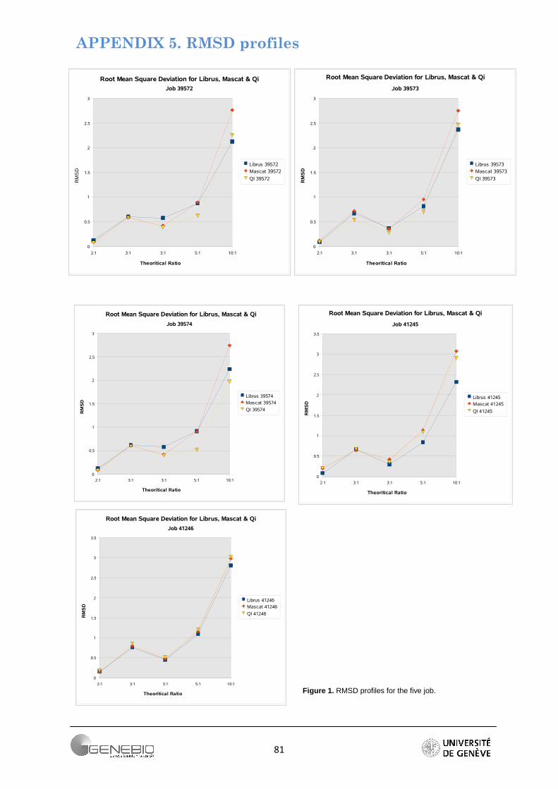
81
2:1 3:1 3:1 5:1 10:1
0
0.5
1
1.5
2
2.5
3
Root Mean Square Deviation for Librus, Mascat & Qi
Job 39572
Librus 39572
Mascat 39572
QI 39572
Theoritical Ratio
RMSD
2:1 3:1 3:1 5:1 10:1
0
0.5
1
1.5
2
2.5
3
Root Mean Square Deviation for Librus, Mascat & Qi
Job 39574
Librus 39574
Mascat 39574
QI 39574
Theoritical Ratio
RM
SD
2:1 3:1 3:1 5:1 10:1
0
0.5
1
1.5
2
2.5
3
Root Mean Square Deviation for Librus, Mascat & Qi
Job 39573
Librus 39573
Mascat 39573
QI 39573
Theoritical Ratio
RM
SD
2:1 3:1 3:1 5:1 10:1
0
0.5
1
1.5
2
2.5
3
3.5
Root Mean Square Deviation for Librus, Mascat & Qi
Job 41245
Librus 41245
Mascat 41245
QI 41245
Theoritical Ratio
RM
SD
2:1 3:1 3:1 5:1 10:1
0
0.5
1
1.5
2
2.5
3
3.5
Root Mean Square Deviation for Librus, Mascat & Qi
Job 41246
Librus 41246
Mascat 41246
QI 41246
Theoritical Ratio
RM
SD
APPENDIX 5. RMSD profiles
Figure 1. RMSD profiles for the five job.
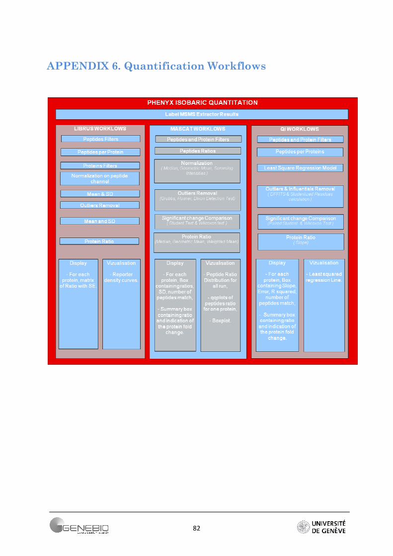
82
APPENDIX 6. Quantification Workflows
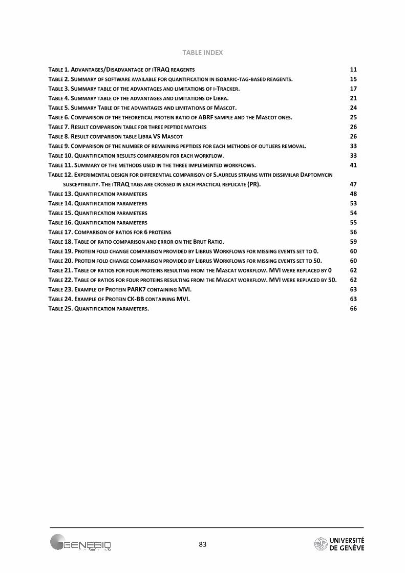
83
TABLE INDEX
TABLE 1. ADVANTAGES/DISADVANTAGE OF ITRAQ REAGENTS 11
TABLE 2. SUMMARY OF SOFTWARE AVAILABLE FOR QUANTIFICATION IN ISOBARIC-TAG-BASED REAGENTS. 15
TABLE 3. SUMMARY TABLE OF THE ADVANTAGES AND LIMITATIONS OF I-TRACKER. 17
TABLE 4. SUMMARY TABLE OF THE ADVANTAGES AND LIMITATIONS OF LIBRA. 21
TABLE 5. SUMMARY TABLE OF THE ADVANTAGES AND LIMITATIONS OF MASCOT. 24
TABLE 6. COMPARISON OF THE THEORETICAL PROTEIN RATIO OF ABRF SAMPLE AND THE MASCOT ONES. 25
TABLE 7. RESULT COMPARISON TABLE FOR THREE PEPTIDE MATCHES 26
TABLE 8. RESULT COMPARISON TABLE LIBRA VS MASCOT 26
TABLE 9. COMPARISON OF THE NUMBER OF REMAINING PEPTIDES FOR EACH METHODS OF OUTLIERS REMOVAL. 33
TABLE 10. QUANTIFICATION RESULTS COMPARISON FOR EACH WORKFLOW. 33
TABLE 11. SUMMARY OF THE METHODS USED IN THE THREE IMPLEMENTED WORKFLOWS. 41
TABLE 12. EXPERIMENTAL DESIGN FOR DIFFERENTIAL COMPARISON OF S.AUREUS STRAINS WITH DISSIMILAR DAPTOMYCIN
SUSCEPTIBILITY. THE ITRAQ TAGS ARE CROSSED IN EACH PRACTICAL REPLICATE (PR). 47
TABLE 13. QUANTIFICATION PARAMETERS 48
TABLE 14. QUANTIFICATION PARAMETERS 53
TABLE 15. QUANTIFICATION PARAMETERS 54
TABLE 16. QUANTIFICATION PARAMETERS 55
TABLE 17. COMPARISON OF RATIOS FOR 6 PROTEINS 56
TABLE 18. TABLE OF RATIO COMPARISON AND ERROR ON THE BRUT RATIO. 59
TABLE 19. PROTEIN FOLD CHANGE COMPARISON PROVIDED BY LIBRUS WORKFLOWS FOR MISSING EVENTS SET TO 0. 60
TABLE 20. PROTEIN FOLD CHANGE COMPARISON PROVIDED BY LIBRUS WORKFLOWS FOR MISSING EVENTS SET TO 50. 60
TABLE 21. TABLE OF RATIOS FOR FOUR PROTEINS RESULTING FROM THE MASCAT WORKFLOW. MVI WERE REPLACED BY 0 62
TABLE 22. TABLE OF RATIOS FOR FOUR PROTEINS RESULTING FROM THE MASCAT WORKFLOW. MVI WERE REPLACED BY 50. 62
TABLE 23. EXAMPLE OF PROTEIN PARK7 CONTAINING MVI. 63
TABLE 24. EXAMPLE OF PROTEIN CK-BB CONTAINING MVI. 63
TABLE 25. QUANTIFICATION PARAMETERS. 66