isolated capital cities, accountability, and corruption ... · isolated capital cities,...
TRANSCRIPT
American Economic Review 2014, 104(8): 2456–2481 http://dx.doi.org/10.1257/aer.104.8.2456
2456
Isolated Capital Cities, Accountability, and Corruption: Evidence from US States †
By Filipe R. Campante and Quoc-Anh Do *
We show that isolated capital cities are robustly associated with greater levels of corruption across US states, in line with the view that this isolation reduces accountability. We then provide direct evidence that the spatial distribution of population relative to the capital affects different accountability mechanisms: newspapers cover state politics more when readers are closer to the capital, voters who live far from the capital are less knowledgeable and interested in state politics, and they turn out less in state elections. We also find that isolated capitals are associated with more money in state-level campaigns, and worse public good provision. (JEL D72, D73, H41, H83, K42, R23)
Corruption is widely seen as a major problem, in developing and developed coun-tries alike, and much has been written on its determinants and correlates. This paper pursues the first systematic investigation of a hitherto underappreciated element in this story: the spatial distribution of the population in a given polity of interest, rela-tive to the seat of political power.
This spatial distribution might affect the incentives and opportunities for public officials to misuse their office for private gain. In particular, it may affect the degree of accountability, as has long been noted in the particular context of US state poli-tics. For instance, Wilson’s (1966) seminal contribution argued that state-level politics were particularly prone to corruption because state capitals are often far from the major metropolitan centers, and thus face a lower level of scrutiny by citizens and by the media: these isolated capitals have “small-city newspapers, few (and weak)
* Campante: Harvard Kennedy School, 79 JFK Street, Cambridge, MA 02138, and NBER (e-mail: [email protected]); Do: Department of Economics and LIEPP, Sciences Po Paris, 28 rue des Saints-Pères, 75007 Paris, France (e-mail: [email protected]). We are grateful to three anonymous referees for many helpful suggestions. We also thank Alberto Alesina, Jim Alt, Dave Bakke, Francesco Caselli, Davin Chor, Thomas Cole, Alan Ehrenhalt, Claudio Ferraz, Jeff Frieden, Ed Glaeser, Josh Goodman, Rema Hanna, David Lauter, David Luberoff, Kieu-Trang Nguyen, Andrei Shleifer, Rodrigo Soares, Enrico Spolaore, Ernesto Stein, David Yanagizawa-Drott, and Katia Zhuravskaya for useful conversations, as well as numerous seminar partici-pants. Ed Glaeser, Sue Long, Kieu-Trang Nguyen, Nguyen Phu Binh, Raven Saks, Kristina Tobio, and espe-cially C. Scott Walker gave us invaluable help with the data collection, and Siaw Kiat Hau provided excellent research assistance. Access to TRAC data used in this research was secured as a result of our appointment as TRAC Fellows at the Transactional Records Access Clearinghouse (TRAC) at Syracuse University. Campante thanks the Taubman Center for State and Local Government for generous financial support, and the Economics Department at PUC-Rio for its outstanding hospitality for much of the period of work on this research. Do thanks Singapore Management University and its Lee Foundation Research Award for generous support over an impor-tant portion of the work on this research. The authors declare that they have no relevant or material financial interests that relate to the research described in this paper.
† Go to http://dx.doi.org/10.1257/aer.104.8.2456 to visit the article page for additional materials and author disclosure statement(s).

2457campante and do: Isolated capItal cItIes and corruptIonVol. 104 no. 8
civic associations, and relatively few attentive citizens with high and vocal standards of public morality” (Wilson, p. 596). As a result, “it is no accident that state officials in Annapolis, Jefferson City, Trenton, and Springfield have national reputations for political corruption” (Maxwell and Winters 2005, p. 3).
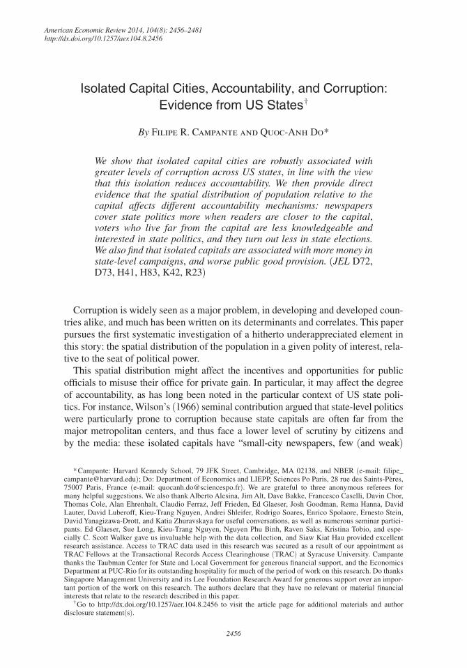
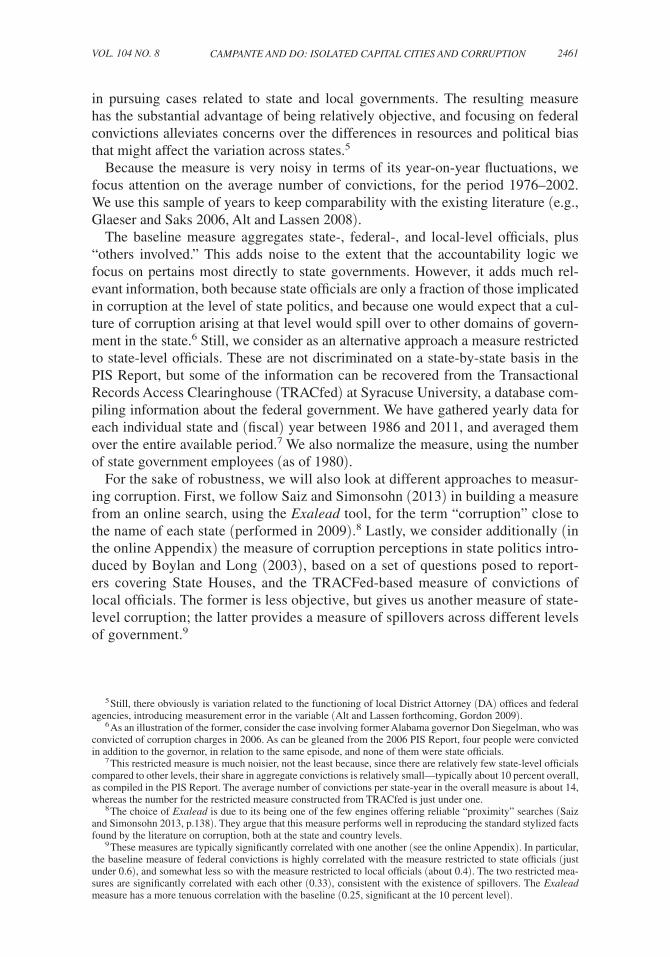
Our first contribution is to establish a basic stylized fact that is very much in line with this “accountability view”: isolated US state capital cities are associ-ated with higher levels of corruption. A simple depiction of that can be seen in Figure 1, where our baseline measure of corruption is plotted against our baseline measure of the isolation of a state’s capital city. We show that this connection is very robust, despite the inherently small sample size, and consistently meaningful from a quantitative perspective.
Quite importantly, we are also able to address the issue of endogeneity, which is evidently present since the location of the capital city is an institutional choice, and since it might itself affect the distribution of population. Fortunately, the his-torical record documenting the designation of state capitals gives us a plausible source of exogenous variation: the location of the geographical centroid of each state. We develop instrumental variables based on that location, and find that the effect of an isolated capital city on corruption is again significant when estimated using this strategy.
Our second contribution is to provide direct evidence that isolated capital cities are associated with lower accountability. We investigate two different realms of accountability, certainly among the most important: the roles of the media and of the electoral process. We find that they are indeed affected by the spatial distri-bution of population.
When it comes to the media, we show that newspapers give more coverage to state politics when their readership is more concentrated around the state capital city. This is matched by individual-level patterns: individuals who live farther from
0.6
0.5
0.4
0.3
0.2
0.1
0.4 0.5 0.6 0.7 0.8
Average log distance
Corruption Fitted values
• RI • MA• CT
• DE
• CO• UT• NH• VT
• MD• NJ
• IN• ME
• MN
• AR
• NE
• MI • KS
• NC• AZ
• WA• OR
• WI
• WV• VA • KY• OH
• GA• SC• OK
• PA• AL
• TN
• LA
• MS
• ND• MT• NY• IL• SD
• FL
• NM
• MO
• ID • WY• NV• TX• CA
Figure 1
Note: Corruption = Federal convictions of public officials for corruption-related crime (average 1976–2002); independent variable: AvgLogDistancenot (average 1920–1970).
2458 THE AMERICAN ECONOMIC REVIEW AugusT 2014
the state capital are less informed and display less interest in state politics, but not in politics in general.
When it comes to elections, we find that voter turnout in state elections is greater in counties that are closer to the state capital. In addition, we also show that iso-lated capital cities are associated with a greater role for money in state-level elec-tions, as measured by campaign contributions, and that, in states with a relatively isolated capital, firms and individuals who are closer to it contribute dispropor-tionately more. These are novel empirical regularities, all of which likely further distort accountability.
Finally, we provide some evidence on whether this pattern of low accountability affects the ultimate provision of public goods: states with isolated capital cities also seem to spend relatively less, and get worse outcomes, on things like education, public welfare, and health care. This suggests that low accountability and corrup-tion induced by isolation do have an impact in terms of government performance and priorities.
The substantial quantitative literature looking at corruption across US states (e.g., Meier and Holbrook 1992; Fisman and Gatti 2002; Alt and Lassen 2003; Glaeser and Saks 2006), has pointed at factors ranging from education to historical and cultural factors to the degree of openness of a state’s political system, but it has essentially not tested the idea that the isolation of the capital city is related to corruption.1 We also relate to the literature on media and accountability, particularly in the United States, such as Snyder and Strömberg (2010), and Lim, Snyder, and Strömberg (2014). Our evidence is very much consistent with their finding that a disconnect between media markets and political jurisdictions weakens accountability.
Most directly, our paper belongs in the intersection between urban economics and economic geography, on one side, and political economy—such as Ades and Glaeser (1995); Davis and Henderson (2003); Campante and Do (2010); Galiani and Kim (2011); and Campante, Do, and Guimaraes (2013). A recent literature in political science has also dealt with the political implications of spatial distributions, as surveyed for instance by Rodden (2010). We add the idea that some places (e.g., capital cities) are distinctive.
The paper is organized as follows: Section I presents the data, Section II discusses the empirical strategy to deal with endogeneity issues, Section III showcases the results, and Section IV discusses them. Section V concludes.
I. Data
We start by describing our data, focusing on the main variables of interest. Our choices for instrumental variables will be discussed later, within the context of our empirical strategy. All variables (including control variables), sources, and descrip-tive statistics are documented in the online Appendix.
1 Some studies have found that population size is positively correlated with corruption (Meier and Holbrook 1992, Maxwell and Winters 2005), although this relationship is not especially robust (Meier and Schlesinger 2002, Glaeser and Saks 2006). As for the spatial distribution of population, most effort has been devoted to looking at urbanization, under the assumption that corruption thrives in cities (Alt and Lassen 2003). There is some evidence for that assertion, but it is not robust (Glaeser and Saks 2006).
2459campante and do: Isolated capItal cItIes and corruptIonVol. 104 no. 8
A. Isolation of the Capital
We get information on the spatial distribution of population for the 48 continental states with county-level data from the US Census, for all census years between 1920 and 2000. We attribute the location of each county’s population to the geographical position of the centroid of the county, and then calculate its distance to the State House or Assembly.2 From that we compute measures of isolation averaged over time, both because the effects of changes in the distribution of population would likely be felt over a relatively long period, and because, while autocorrelation turns out to be very high, there is nontrivial variation over time in a number of states.3
Our preferred measure of isolation is the average of the log of the distance of the state’s population to the capital city, AvgLogDistance for shorthand. Campante and Do (2010) show that this measure (uniquely) has a number of desirable properties. (See details and a brief discussion of properties in the online Appendix.)
It is also rather easy to interpret. To fix ideas, consider an intuitive measure of isolation of a state’s capital, namely the distance between the capital and that state’s largest city. AvgLogDistance takes this intuition and applies it in a more comprehen-sive and systematic fashion. First, instead of looking at the largest city only, it takes into account the entire state without arbitrarily discarding information. Second, it does so by weighing each place according to its population. Last but not least, the log transformation ensures that the measure is unbiased with respect to the measure-ment error introduced by not having the exact location of individuals, and thus hav-ing to approximate the actual spatial distribution (Campante and Do 2010).
To further facilitate interpretation, we normalize the measure so that zero rep-resents a situation of minimum isolation, in which all individuals live arbitrarily close to the State House. Conversely, we set at one the situation where the capital is maximally isolated, with all individuals living as far from it as possible in the context of interest.
Given this basic framework, different choices can yield specific versions that highlight distinct aspects of isolation. We choose to adopt a relatively agnostic view and experiment with a few options.
The first choice has to do with normalization and what it means to have “maxi-mal” isolation. To fix ideas, consider that the salience of what happens in the state capital, for a given citizen, decreases with her distance from it. One possibility is that salience falls at the same rate across different states, so that distances are weighted in the same way in states large and small. In this case, we set maximum isolation as benchmarked by the highest possible level across all states: a measure of one would correspond to a situation where the entire population of the state is as far from its
2 While finer geographical subdivisions such as census tract and block are available, the focus on counties enables us to compute the measures for the years before the population data became consistently available at those more detailed levels for the entire United States in 1980. We start in 1920 because that is when detailed county data first becomes available. Alaska and Hawaii are left out as the data for them do not go as far back in time.
3 We will use different averages depending on the relevant period of analysis but, quite importantly, our results are essentially unaltered if we use time-specific measures instead (see the online Appendix). Also importantly, we will leave aside the time variation in our estimation, because the very high autocorrelation in the isolation measures and the fluctuations over time in the baseline corruption variable, as we will note, make that variation very noisy, entailing severe econometric problems with standard methods and thus rendering its use unwarranted.
2460 THE AMERICAN ECONOMIC REVIEW AugusT 2014
capital as it is possible to be far from Austin while remaining in Texas. We denote this “unadjusted” measure by AvgLogDistanc e not .
Another possibility is that this salience falls to zero beyond the state’s borders. In this case, we would want to set the level of maximum isolation in each state to be a situation where the entire population lives as far from the capital as it is pos-sible to be in that specific state. This would correspond to an “adjusted” version of our measure, AvgLogDistanc e adj , which automatically adjusts for the size of each state.
An important point coming out of this distinction is that AvgLogDistanc e not is in practice highly correlated with the geographical size of the state. At the same time, we want to distinguish the impact of the distribution of population from a possible unrelated correlation with geographical size per se. We will do that by controlling for the size and shape of each state in all AvgLogDistanc e not specifications, by including (the log of) the state’s area and (the log of) the maximum distance from county cen-troids to state capital (i.e., the measure that benchmarks AvgLogDistanc e adj ). This will allow us to consider the hypothetical of comparing states with similar sizes but different degrees of isolation, which seems to be the relevant experiment.
A second choice has to do with functional form. While AvgLogDistance has the notable advantage of unbiasedness, its concavity entails a view of accountability that gives disproportional weight to citizens living relatively close to the capital. For instance, in the limit, one could imagine a model in which all that matters is the population that lives within a certain range of the capital; concavity gives us a way to approximate this without attributing arbitrary limits. An alternative view would have individual weights decline linearly with distance, and to allow for this possibility we will consider AvgDistance, without the log transformation, as a robustness check.4
We will also consider a couple of well-known (inverse) measures of isolation: the share of population living in the state capital (as of 2010), CapitalShare, and a dummy for whether the capital is the largest city in the state, CapitalLargest. These are very coarse and rather unsatisfactory measures, relying on arbitrary definitions of what counts as the capital city and discarding all the spatial information beyond those arbitrary limits, but we will check them for the sake of completeness.
B. Corruption
Our baseline measure of corruption across US states is the oft-used number of federal convictions for corruption-related crime (relative to the size of the popula-tion). (A detailed description of this measure can be found in Glaeser and Saks 2006.) These refer to cases, typically prosecuted by US Attorneys all over the coun-try, against public officials and others involved in public corruption, as surveyed and compiled by the Public Integrity Section (PIS) at the US Department of Justice in their “Report to Congress.” Federal authorities can claim jurisdiction, for instance, over corruption-related crime that “affects interstate commerce,” or in entities that receive more than $10,000 in federal funds—which yields them a lot of leeway
4 This measure has all of the other main properties of AvgLogDistance, as noted in the online Appendix. The correlation between the two in our sample is around 0.8.
2461campante and do: Isolated capItal cItIes and corruptIonVol. 104 no. 8
in pursuing cases related to state and local governments. The resulting measure has the substantial advantage of being relatively objective, and focusing on federal convictions alleviates concerns over the differences in resources and political bias that might affect the variation across states.5
Because the measure is very noisy in terms of its year-on-year fluctuations, we focus attention on the average number of convictions, for the period 1976–2002. We use this sample of years to keep comparability with the existing literature (e.g., Glaeser and Saks 2006, Alt and Lassen 2008).
The baseline measure aggregates state-, federal-, and local-level officials, plus “others involved.” This adds noise to the extent that the accountability logic we focus on pertains most directly to state governments. However, it adds much rel-evant information, both because state officials are only a fraction of those implicated in corruption at the level of state politics, and because one would expect that a cul-ture of corruption arising at that level would spill over to other domains of govern-ment in the state.6 Still, we consider as an alternative approach a measure restricted to state-level officials. These are not discriminated on a state-by-state basis in the PIS Report, but some of the information can be recovered from the Transactional Records Access Clearinghouse (TRACfed) at Syracuse University, a database com-piling information about the federal government. We have gathered yearly data for each individual state and (fiscal) year between 1986 and 2011, and averaged them over the entire available period.7 We also normalize the measure, using the number of state government employees (as of 1980).
For the sake of robustness, we will also look at different approaches to measur-ing corruption. First, we follow Saiz and Simonsohn (2013) in building a measure from an online search, using the Exalead tool, for the term “corruption” close to the name of each state (performed in 2009).8 Lastly, we consider additionally (in the online Appendix) the measure of corruption perceptions in state politics intro-duced by Boylan and Long (2003), based on a set of questions posed to report-ers covering State Houses, and the TRACFed-based measure of convictions of local officials. The former is less objective, but gives us another measure of state-level corruption; the latter provides a measure of spillovers across different levels of government.9
5 Still, there obviously is variation related to the functioning of local District Attorney (DA) offices and federal agencies, introducing measurement error in the variable (Alt and Lassen forthcoming, Gordon 2009).
6 As an illustration of the former, consider the case involving former Alabama governor Don Siegelman, who was convicted of corruption charges in 2006. As can be gleaned from the 2006 PIS Report, four people were convicted in addition to the governor, in relation to the same episode, and none of them were state officials.
7 This restricted measure is much noisier, not the least because, since there are relatively few state-level officials compared to other levels, their share in aggregate convictions is relatively small—typically about 10 percent overall, as compiled in the PIS Report. The average number of convictions per state-year in the overall measure is about 14, whereas the number for the restricted measure constructed from TRACfed is just under one.
8 The choice of Exalead is due to its being one of the few engines offering reliable “proximity” searches (Saiz and Simonsohn 2013, p.138). They argue that this measure performs well in reproducing the standard stylized facts found by the literature on corruption, both at the state and country levels.
9 These measures are typically significantly correlated with one another (see the online Appendix). In particular, the baseline measure of federal convictions is highly correlated with the measure restricted to state officials (just under 0.6), and somewhat less so with the measure restricted to local officials (about 0.4). The two restricted mea-sures are significantly correlated with each other (0.33), consistent with the existence of spillovers. The Exalead measure has a more tenuous correlation with the baseline (0.25, significant at the 10 percent level).
2462 THE AMERICAN ECONOMIC REVIEW AugusT 2014
C. “Placebo” Variables
We consider other features of the spatial distribution of population, beyond the role of the capital city, by looking at the isolation of the state’s largest city (again measured by AvgLogDistance). We also check for outcome variables related to crime and federal prosecutorial efforts, apart from corruption. Here we resort to a measure of criminal cases brought by prosecutors to federal courts in each state (as of 2011) in relation to drug offenses, which are by far the most numerous type among the federal cases.
D. Accountability
Newspaper Coverage.—When it comes to the media as a source of accountability, we focus on state-level political coverage by newspapers, since they tend to provide far greater coverage of state politics in the United States than competing media such as TV (e.g., Vinson 2003, Druckman 2005).
We look at newspapers whose print edition content is available online and search-able at the website NewsLibrary.com—covering nearly four thousand outlets all over the United States. We search for the names of each state’s then-current gover-nors—as well as, alternatively, for terms such as “state government,” “state budget,” or “state elections,” where “state” refers to the name of each state.10 We only con-sider mentions to the state in which each newspaper is based.11
We also compute a state-level measure of political coverage. We take the first principal component of the four search terms for each newspaper (adjusted by size), and perform a weighted sum of this measure over all newspapers.12 We use two alternative sets of weights: the circulation of each newspaper in the state, which for its simplicity is our preferred option, and that circulation weighted by its geographi-cal concentration, as captured by the ReaderConcentr variable described below. The latter would put more weight on circulation closer to the capital, allowing for the possibility that newspapers whose audience is more concentrated around the capital city might have a disproportionate effect on the behavior of state politicians.
Concentration of Readership around the Capital.—We use circulation data bro-ken down by county, provided by the Audit Bureau of Circulations (ABC). We com-pute the AvgLogDistance to the capital analogously to what we described before, only using newspaper readership instead of population.13 We then define the mea-sure of readership concentration, ReaderConcentr, as 1 − AvgLogDistance: a larger
10 Similar procedures using NewsLibrary.com have been used, for instance, by Snyder and Strömberg (2010) and Lim, Snyder, and Strömberg (2012). We look for terms that are not necessarily related to corruption scan-dals—though it can certainly be the case (and actually is, for some states) that governors are involved in a few of those—to guard against reverse causality—namely, the possibility that there is a lot of media coverage because of the existence of such scandals.
11 We also run a search for a “neutral” term (“Monday”), following Gentzkow, Glaeser, and Goldin (2006), to control for newspaper size.
12 This aggregate measure introduces a source of measurement error, due to the fact that the data do not cover the totality of a state’s newspaper industry. There is no particular reason to believe that this measurement error is correlated with the underlying value of the variable we want to measure.
13 We use the unadjusted version of AvgLogDistance, but normalization is immaterial here, because our estima-tion will use state fixed effects.

2463campante and do: Isolated capItal cItIes and corruptIonVol. 104 no. 8
measure of ReaderConcentr implies that a given newspaper’s audience is more concentrated around its home state’s capital. The number of newspapers with ABC data available is considerably smaller than what NewsLibrary.com covers, so we end up with a total of 436 newspapers in our sample. We leave aside the circula-tion of a newspaper outside of its home state, since we are focusing on coverage of home-state politics.
Citizens’ Information.—We use data from the American National Election Studies (ANES). In the 1998 pre-election survey, a random sample of voting-age citizens were interviewed, in California, Georgia, and Illinois. As usual for the ANES up until 2000, the 1998 survey includes information about the county of each interview, which we use to compute distance (from the county centroid) to the state capital. Most interestingly and uniquely, it asks questions that directly measure knowledge of state politics and interest in news coverage related to state politics.
We code a dummy for Knowledge that captures whether the individual respon-dents are able to provide the correct name of at least one candidate in the upcoming gubernatorial elections. We also code a dummy for Interest in state political news: whether the respondent reports to care about newspaper articles about the guberna-torial campaign, conditional on her reading newspapers, so as to focus on potential consumers of print media. Finally, we create a GeneralInterest dummy based on whether respondents follow public affairs in general, unconstrained to the state level.
Voter Turnout.—We look at turnout in all gubernatorial elections between 1990 and 2012, at the county level, again attributing for simplicity the county’s popula-tion to its centroid, and computing the distance between each county’s centroid and the state capital.
Money in State Politics.—We look at data on total contributions to electoral cam-paigns, comprising all types of state-level office and aggregated at the state level. We focus on the period 2001–2010, as the state coverage of the data for previous elec-toral cycles is somewhat inconsistent. In addition to total contributions, we also focus on county-level contributions coming from a specific industry, namely real estate, which we choose because it tends not to be spatially concentrated, and because it is one of the industries that contributes the most to state-level campaigns.14 This will let us look into whether distance from the capital affects contribution patterns within states.
E. Public Good Provision
We start with data on the pattern of expenditures by US states (in 2009). Most of state government expenditures that might be directly ascribed to public good provision fall under four categories: “Education,” “Public Welfare,” “Health,” and “Hospitals.” We take the share of these categories in total spending as a proxy for resources devoted to public good provision. We also compute the share devoted to
14 Out of the classification provided by our source, the National Institute on Money in State Politics, real estate falls behind only public sector unions and lawyers/lobbyists, which tend to be more naturally concentrated.
2464 THE AMERICAN ECONOMIC REVIEW AugusT 2014
“Government Administration,” “Interest on General Debt,” and “Other” as a proxy for what is not directly related to public good provision.
These measures do not speak to how effectively resources are spent, so we check proxies for the ultimate provision of public goods. These are affected by many fac-tors other than state-level policy, but should still provide useful information. We use three measures that capture aspects of what should be affected by the type of pub-lic good expenditure we have defined: the “Smartest State” index (Morgan Quitno Corporation 2005), which aggregates different measures of educational inputs and outcomes, the percentage of the population that has health insurance, and the log of the number of hospital beds per capita.
II. Empirical Strategy
Our analysis sits on three pillars. First, we will look at the correlation patterns linking isolated capital cities and corruption; on the other hand, we will look at direct evidence on whether isolation relates to different accountability mechanisms. The third pillar is about addressing endogeneity concerns regarding those correla-tion patterns, related to the facts that the location of the capital city is an institu-tional decision and that it affects the spatial distribution of population. Both of these could be correlated with omitted variables that are also associated with corruption. For instance, corruption and the location of the capital city could be jointly deter-mined—say, with relatively corrupt states choosing to isolate their capital cities. Alternatively, it could be the case that corruption affects the population flows that determine how isolated the capital city will ultimately be—say, by pushing eco-nomic activity and population away from the capital. We now turn to the empirical strategy we use to address these confounding factors.
A. Source of Exogenous Variation
In the absence of something like a natural experiment on the location of capital cities, a source of exogenous variation in the isolation of the capital comes from a specific point of interest: each state’s centroid. Defined as the average coordinate of the state, the centroid does not depend on the spatial distribution of population, but only on the state’s geographical shape.
The first crucial point is that the centroid is an essentially arbitrary location and should not affect any relevant outcomes in and of itself. This should be true at least once the territorial limits of each state are set.15 Because of that, we will eventually control, in all of our specifications, for the geographical size of the state, to guard against the possibility that a correlation between omitted variables and the expan-sion or rearrangement of state borders might affect the results.
The second crucial point is that there is a connection between the location of the centroid and the location of the capital city, which is obviously a necessary condi-tion for the variation in the former to generate meaningful variation in the latter. As it turns out, the history of the designation of state (and federal) capitals in the United
15 State borders have been generally stable after establishment. For a history of those borders, see Stein (2008).
2465campante and do: Isolated capItal cItIes and corruptIonVol. 104 no. 8
States strongly suggests exactly such a link. This is because concerns with equal representation led to strong pressures to locate the capital in a relatively central posi-tion, particularly as state capital cities were typically chosen at a time when trans-portation and communication costs were substantial (Zagarri 1987; Shelley 1996; Engstrom, Hammond, and Scott 2013). Consistent with that, a quick inspection of any map of the United States displaying all state capitals makes it immediately apparent that many of them are actually in relatively central locations.
B. Instrumental Variables
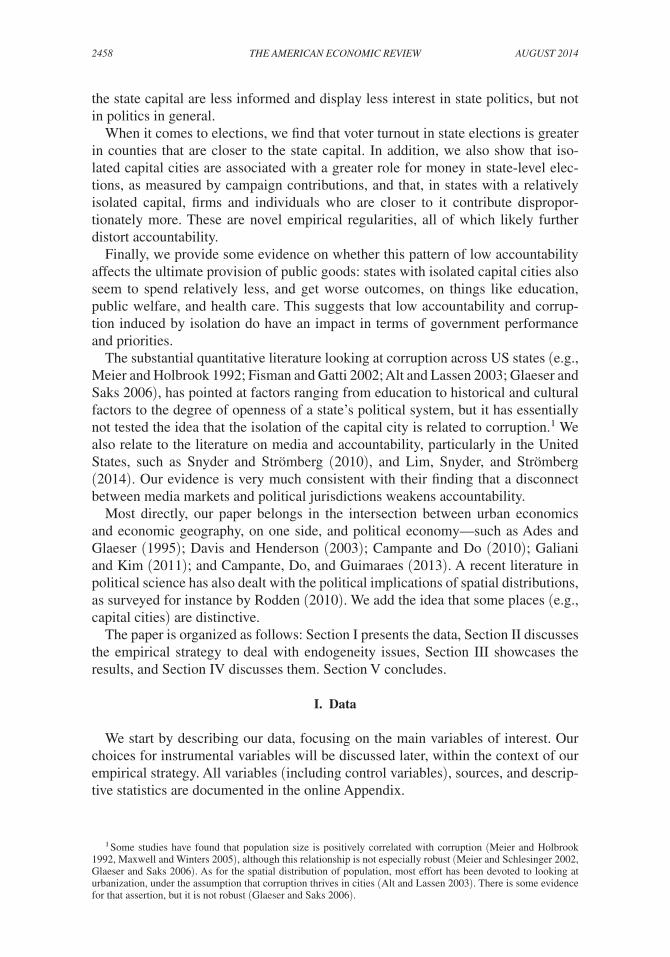
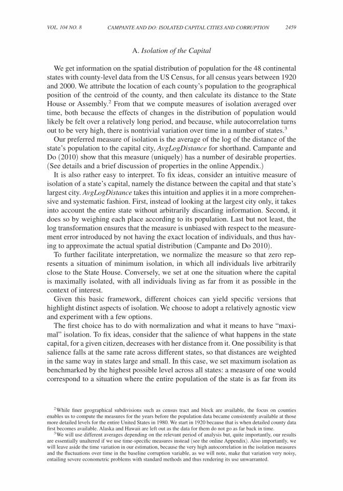
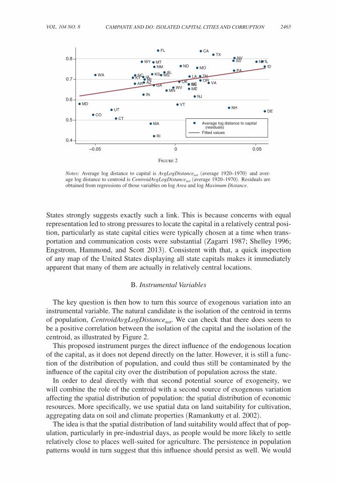
The key question is then how to turn this source of exogenous variation into an instrumental variable. The natural candidate is the isolation of the centroid in terms of population, CentroidAvgLogDistanc e not . We can check that there does seem to be a positive correlation between the isolation of the capital and the isolation of the centroid, as illustrated by Figure 2.
This proposed instrument purges the direct influence of the endogenous location of the capital, as it does not depend directly on the latter. However, it is still a func-tion of the distribution of population, and could thus still be contaminated by the influence of the capital city over the distribution of population across the state.
In order to deal directly with that second potential source of exogeneity, we will combine the role of the centroid with a second source of exogenous variation affecting the spatial distribution of population: the spatial distribution of economic resources. More specifically, we use spatial data on land suitability for cultivation, aggregating data on soil and climate properties (Ramankutty et al. 2002).
The idea is that the spatial distribution of land suitability would affect that of pop-ulation, particularly in pre-industrial days, as people would be more likely to settle relatively close to places well-suited for agriculture. The persistence in population patterns would in turn suggest that this influence should persist as well. We would
0.8
0.7
0.6
0.5
0.4
AL
AZAR
CA
COCT
DE
FL
GA
IDIL
IN
IAKS
KY LA
ME
MD
MA
MI
MN
MS
MOMT
NE
NV
NH
NJ
NMNY
NC
ND
OHOK
PA
RI
SC
SD
TN
TX
UTVT
VA
WA
WV
WI
WY
–0.05 0 0.05
• RI
• MA• CT
• DE• CO
• UT • NH• VT
• NJ• IN• ME• MN
• AR • NE• MI
• KS• NC
• AZ • OR
• WV• VA
• KY
• GA • OK
• PA• AL• TN• LA• MS
• ND• MT • NY• IL• SD
• FL
• NM • MO • ID• WY
• NV
Average log distance to capital (residuals) Fitted values
•
• CA
• WA • IA
• MD
• TX
• SC
Figure 2
Notes: Average log distance to capital is AvgLogDistancenot (average 1920–1970) and aver-age log distance to centroid is CentroidAvgLogDistancenot (average 1920–1970). Residuals are obtained from regressions of those variables on log Area and log Maximum Distance.
2466 THE AMERICAN ECONOMIC REVIEW AugusT 2014
thus expect that, in case the most suitable land is relatively far from the centroid, population would tend to be too—and the capital city would be more isolated, to the extent that it tends to be located close to the centroid. Crucially, it is eminently plau-sible that spatial patterns in terms of climate and soil, relative to the state’s centroid, would neither be meaningfully affected by current population patterns that could be correlated with corruption, nor likely to affect corruption through any means other than their impact on the isolation of the capital.
We thus compute SuitCentroidAvgLogDistanc e not for the 48 states in the conti-nental United States, and use it as an alternative instrumental variable. Its main drawback is that, quite naturally, it has a more tenuous correlation with our variable of interest, namely the isolation of the capital.
C. Validation
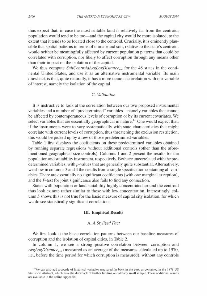
It is instructive to look at the correlation between our two proposed instrumental variables and a number of “predetermined” variables—namely variables that cannot be affected by contemporaneous levels of corruption or by its current covariates. We select variables that are essentially geographical in nature.16 One would expect that, if the instruments were to vary systematically with state characteristics that might correlate with current levels of corruption, thus threatening the exclusion restriction, this would be picked up by a few of those predetermined variables.
Table 1 first displays the coefficients on these predetermined variables obtained by running separate regressions without additional controls (other than the afore-mentioned geographical size controls). Columns 1 and 2 present the results for the population and suitability instrument, respectively. Both are uncorrelated with the pre-determined variables, with p-values that are generally quite substantial. Alternatively, we show in columns 3 and 4 the results from a single specification containing all vari-ables. There are essentially no significant coefficients (with one marginal exception), and the F-test for joint significance also fails to find any connection.
States with population or land suitability highly concentrated around the centroid thus look ex ante rather similar to those with low concentration. Interestingly, col-umn 5 shows this is not true for the basic measure of capital city isolation, for which we do see statistically significant correlations.
III. Empirical Results
A. A Stylized Fact
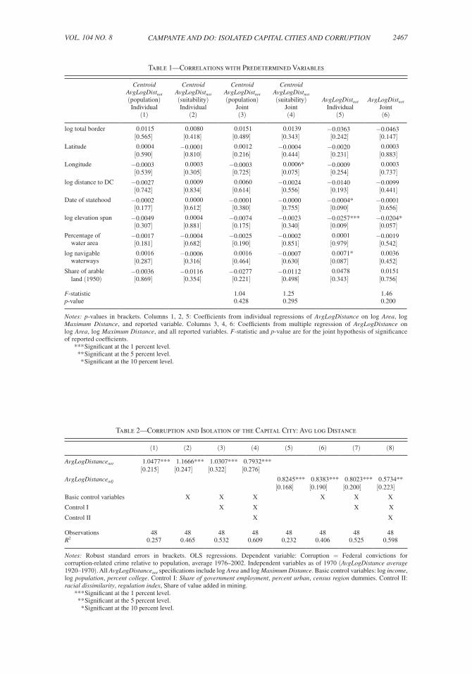
We first look at the basic correlation patterns between our baseline measures of corruption and the isolation of capital cities, in Table 2.
In column 1, we see a strong positive correlation between corruption and AvgLogDistanc e not (measured as an average of the measures calculated up to 1970, i.e., before the time period for which corruption is measured), without any controls
16 We can also add a couple of historical variables measured far back in the past, as contained in the 1878 US Statistical Abstract, which have the drawback of further limiting our already small sample. These additional results are available in the online Appendix.
2467campante and do: Isolated capItal cItIes and corruptIonVol. 104 no. 8
Table 2—Corruption and Isolation of the Capital City: Avg log Distance
(1) (2) (3) (4) (5) (6) (7) (8)
AvgLogDistancenot 1.0477*** 1.1666*** 1.0307*** 0.7932***[0.215] [0.247] [0.322] [0.276]
AvgLogDistanceadj 0.8245*** 0.8383*** 0.8023*** 0.5734**[0.168] [0.190] [0.200] [0.223]
Basic control variables X X X X X X
Control I X X X X
Control II X X
Observations 48 48 48 48 48 48 48 48R2 0.257 0.465 0.532 0.609 0.232 0.406 0.525 0.598
Notes: Robust standard errors in brackets. OLS regressions. Dependent variable: Corruption = Federal convictions for corruption-related crime relative to population, average 1976–2002. Independent variables as of 1970 (AvgLogDistance average 1920–1970). All AvgLogDistancenot specifications include log Area and log Maximum Distance. Basic control variables: log income, log population, percent college. Control I: Share of government employment, percent urban, census region dummies. Control II: racial dissimilarity, regulation index, Share of value added in mining.
*** Significant at the 1 percent level. ** Significant at the 5 percent level. * Significant at the 10 percent level.
Table 1—Correlations with Predetermined Variables
Centroid AvgLogDistnot (population) Individual
(1)
Centroid AvgLogDistnot (suitability) Individual
(2)
Centroid AvgLogDistnot (population)
Joint (3)
Centroid AvgLogDistnot (suitability)
Joint (4)
AvgLogDistnot
Individual (5)
AvgLogDistnot Joint(6)
log total border 0.0115 0.0080 0.0151 0.0139 −0.0363 −0.0463[0.565] [0.418] [0.489] [0.343] [0.242] [0.147]
Latitude 0.0004 −0.0001 0.0012 −0.0004 −0.0020 0.0003[0.590] [0.810] [0.216] [0.444] [0.231] [0.883]
Longitude −0.0003 0.0003 −0.0003 0.0006* −0.0009 0.0003[0.539] [0.305] [0.725] [0.075] [0.254] [0.737]
log distance to DC −0.0027 0.0009 0.0060 −0.0024 −0.0140 −0.0099[0.742] [0.834] [0.614] [0.556] [0.193] [0.441]
Date of statehood −0.0002 0.0000 −0.0001 −0.0000 −0.0004* −0.0001[0.177] [0.612] [0.380] [0.755] [0.090] [0.656]
log elevation span −0.0049 0.0004 −0.0074 −0.0023 −0.0257*** −0.0204*[0.307] [0.881] [0.175] [0.340] [0.009] [0.057]
Percentage of −0.0017 −0.0004 −0.0025 −0.0002 0.0001 −0.0019 water area [0.181] [0.682] [0.190] [0.851] [0.979] [0.542]log navigable 0.0016 −0.0006 0.0016 −0.0007 0.0071* 0.0036 waterways [0.287] [0.316] [0.464] [0.630] [0.087] [0.452]Share of arable −0.0036 −0.0116 −0.0277 −0.0112 0.0478 0.0151 land (1950) [0.869] [0.354] [0.221] [0.498] [0.343] [0.756]
F-statistic 1.04 1.25 1.46p-value 0.428 0.295 0.200
Notes: p-values in brackets. Columns 1, 2, 5: Coefficients from individual regressions of AvgLogDistance on log Area, log Maximum Distance, and reported variable. Columns 3, 4, 6: Coefficients from multiple regression of AvgLogDistance on log Area, log Maximum Distance, and all reported variables. F-statistic and p-value are for the joint hypothesis of significance of reported coefficients.
*** Significant at the 1 percent level. ** Significant at the 5 percent level. * Significant at the 10 percent level.
2468 THE AMERICAN ECONOMIC REVIEW AugusT 2014
other than geographical size.17 Column 2 then introduces a basic set of controls, as of 1970. The coefficient of interest is highly significant, and fairly stable in size. Columns 3 and 4 add as controls other correlates of corruption that are established in the literature, and our preferred specification is that of column 3, which essentially reproduces the basic specification in Glaeser and Saks (2006). While in column 4 the size of the coefficient is slightly reduced, it is robustly statistically significant at the 1 percent level, quite remarkably in light of the small sample size.18 The same pat-tern is also present for our first alternative measure of isolation, AvgLogDistanc e adj , as shown by columns 5–8 reproducing the four specifications.19
The effect is also meaningful quantitatively. Our preferred specification’s coeffi-cient (1.03) implies that an increase of one standard deviation in the isolation of the capital city (around 0.09, or roughly the increase experienced by Carson City, NV between 1920 and 2000), would yield a corresponding increase in corruption (0.10) of around 0.75 standard deviation.20
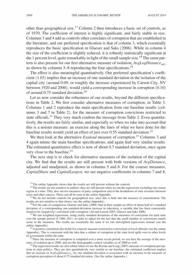
Let us now consider the robustness of our results, beyond the different specifica-tions in Table 2. We first consider alternative measures of corruption, in Table 3. Columns 1 and 2 reproduce the main specification from our baseline results (col-umns 3 and 7 in Table 2), for the measure of corruption convictions restricted to state officials.21 They very much confirm the message from Table 2. Even quantita-tively, the results are fairly similar, and especially so when we take into account that this is a noisier measure: an exercise along the lines of what we have done for the baseline results would yield an effect of just over 0.55 standard deviation.22
We then look at the alternative Exalead measure of corruption.23 Columns 3 and 4 again mimic the main baseline specifications, and again find very similar results. The estimated quantitative effect is now of about 0.7 standard deviation, once again very close to the baseline.24
The next step is to check for alternative measures of the isolation of the capital city. We find that the results are still present with both versions of AvgDistance, adjusted and unadjusted, as shown in columns 5 and 6. For the coarser measures, CapitalShare and CapitalLargest, we see negative coefficients in columns 7 and 8,
17 The online Appendix shows that the results are still present without the controls.18 The results are not sensitive to outliers: they are still present when we run the regressions excluding one census
region at a time. They also survive measures of party competition and of the breakdown of state revenues between taxes and other sources. These can all be seen in the online Appendix.
19 We do not include controls for geographical size, since this is built into the measure of concentration. The results are not sensitive to that choice (see the online Appendix).
20 For the sake of comparison, Glaeser and Saks (2006) find in their sample an effect of about half of a standard deviation of a corresponding one-standard-deviation increase in education, a variable that has been consistently found to be (negatively) correlated with corruption (Alt and Lassen 2003, Glaeser and Saks 2006).
21 We run weighted regressions, using yearly standard deviations of the measures of convictions for each state over the sample period of 1986–2011, in order to adjust for the fact that the small number of convictions entails noise in the measures. The results are essentially the same if we run unweighted regressions instead (see the online Appendix).
22 A positive correlation also holds for a narrow measure restricted to convictions of local officials (see the online Appendix). This is consistent with the idea that a culture of corruption at the state level spills over to other levels of government within the state.
23 Since the measure of corruption is computed over a more recent period, we use here the average of the mea-sures of isolation up to 2000, and use the demographic control variables as of 2000 as well.
24 The regression results are also robust when we use the Boylan and Long (2003) measure of corruption percep-tions in state politics. They are also quantitatively very similar to our baseline: the estimated coefficient implies that an increase in AvgLogDistanc e not by one standard deviation is associated with an increase in the measure of corruption perception of about 0.75 standard deviation. (See the online Appendix.)
2469campante and do: Isolated capItal cItIes and corruptIonVol. 104 no. 8
consistent with the baseline results. The quantitative implications, however, suggest in both cases a smaller effect, of about one-third of a standard deviation. This is consistent with a substantial measurement error being introduced by the use of these coarse measures.25
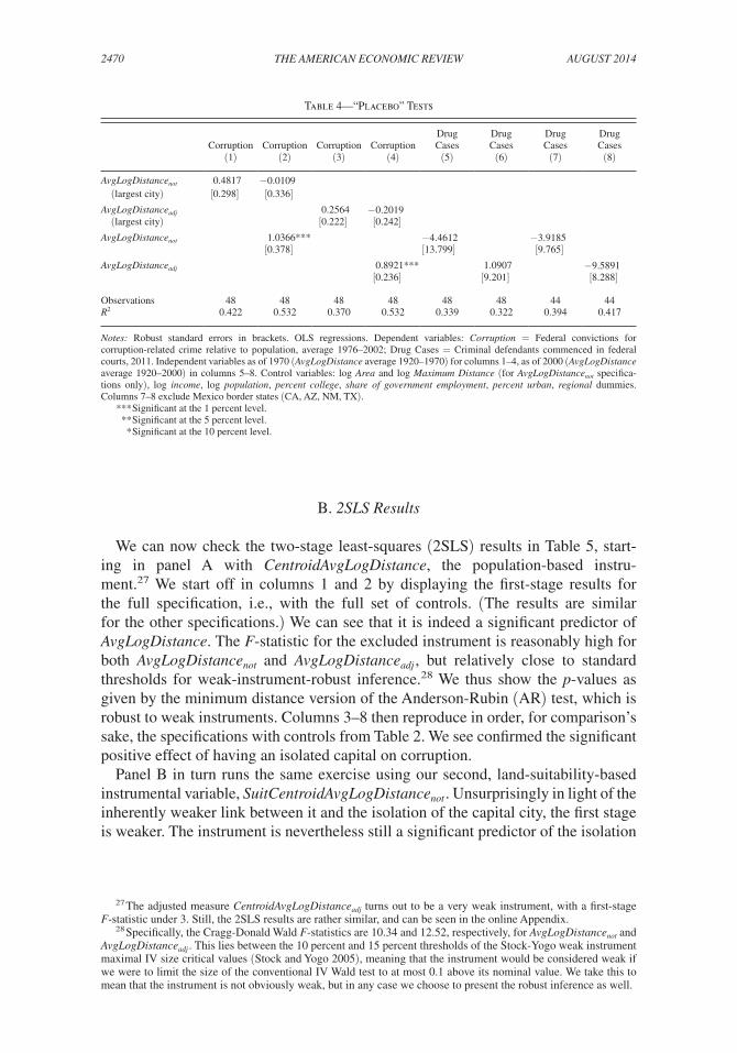
We then probe the results with a few “placebo” regressions, meant to check whether the patterns we find in the data are actually related to the isolation of capi-tal cities and its conjectured link with corruption and accountability. Columns 1– 4 in Table 4 use the isolation of the largest city—since the latter is also the capital city in 17 out of 50 states, one might wonder whether the measure of isolation of the capital could be in fact proxying for that. It has no independent effect, and its inclusion does not affect the significance or size of the coefficient on the isolation of the capital.
From our basic hypothesis about accountability, one would not expect any par-ticular connection between the isolation of the capital city and the prevalence of (or federal prosecutorial efforts in pursuing) other types of crime that are presumably unrelated to state politics. We see in columns 5–8 that indeed there is no connection between the number of drug cases and the isolation of the capital.26
25 Note that we use the “Exalead” measure of corruption, in light of the time period for which we have the popu-lation data at the city level. The coefficients are negative, but statistically insignificant, when we use the baseline measure of convictions, again consistent with substantial measurement error (see the online Appendix).
26 To check that this is not driven by outliers, we also dropped the states on the Mexico border—which tend to have a disproportionate number of drug-related cases (especially Arizona and New Mexico). Columns 7 and 8 show the same pattern holds in that case.
Table 3—Corruption and Isolation of the Capital City: Robustness
State officials
Stateofficials
Corruption (Exalead)
Corruption (Exalead) Corruption Corruption
Corruption (Exalead)
Corruption (Exalead)
(1) (2) (3) (4) (5) (6) (7) (8)
AvgLogDistancenot 0.1311** 0.0020** [0.064] [0.001]
AvgLogDistanceadj 0.0741* 0.0018** [0.043] [0.001]
AvgDistancenot 0.7733*** [0.284]
AvgDistanceadj 0.4710*** [0.091]
Capital share −0.0011** [0.0005]
Capital largest −0.0001* [0.0001]
Observations 48 48 48 48 48 48 50 50 R2 0.591 0.551 0.395 0.398 0.485 0.553 0.340 0.328
Notes: Robust standard errors in brackets. OLS regressions; Columns 1–2: Weighted OLS regressions (Weight = 0.0000001 + stan-dard deviation of conviction sample). Dependent variables: State Officials = Federal convictions of state public officials for cor-ruption-related crime per 100 state government employees, average 1986–2011. Corruption (Exalead) = Number of search hits for “corruption” close to state name divided by number of search hits for state name, using Exalead search tool (in 2009). Corruption = Federal convictions for corruption-related crime relative to population, average 1976–2002. Independent variables as of 1970 (AvgLogDistance average 1920–1970) in columns 1–2 and 5–6, as of 2000 (AvgLogDistance average 1920–2000) in columns 3–4 and 7–8. Control variables: log Area and log Maximum Distance (for AvgLogDistancenot specifications only), log income, log popu-lation, percent college, share of government employment, percent urban, census region dummies.
*** Significant at the 1 percent level. ** Significant at the 5 percent level. * Significant at the 10 percent level.
2470 THE AMERICAN ECONOMIC REVIEW AugusT 2014
B. 2SLS Results
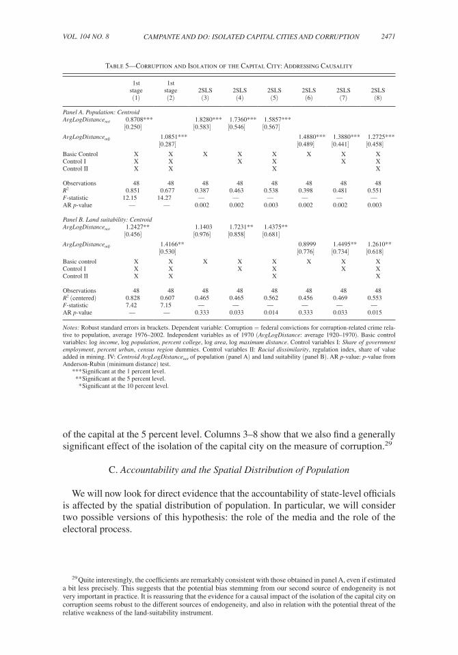
We can now check the two-stage least-squares (2SLS) results in Table 5, start-ing in panel A with CentroidAvgLogDistance, the population-based instru-ment.27 We start off in columns 1 and 2 by displaying the first-stage results for the full specification, i.e., with the full set of controls. (The results are similar for the other specifications.) We can see that it is indeed a significant predictor of AvgLogDistance. The F-statistic for the excluded instrument is reasonably high for both AvgLogDistanc e not and AvgLogDistanc e adj , but relatively close to standard thresholds for weak-instrument-robust inference.28 We thus show the p-values as given by the minimum distance version of the Anderson-Rubin (AR) test, which is robust to weak instruments. Columns 3–8 then reproduce in order, for comparison’s sake, the specifications with controls from Table 2. We see confirmed the significant positive effect of having an isolated capital on corruption.
Panel B in turn runs the same exercise using our second, land-suitability-based instrumental variable, SuitCentroidAvgLogDistanc e not . Unsurprisingly in light of the inherently weaker link between it and the isolation of the capital city, the first stage is weaker. The instrument is nevertheless still a significant predictor of the isolation
27 The adjusted measure CentroidAvgLogDistanc e adj turns out to be a very weak instrument, with a first-stage F-statistic under 3. Still, the 2SLS results are rather similar, and can be seen in the online Appendix.
28 Specifically, the Cragg-Donald Wald F-statistics are 10.34 and 12.52, respectively, for AvgLogDistanc e not and AvgLogDistanc e adj . This lies between the 10 percent and 15 percent thresholds of the Stock-Yogo weak instrument maximal IV size critical values (Stock and Yogo 2005), meaning that the instrument would be considered weak if we were to limit the size of the conventional IV Wald test to at most 0.1 above its nominal value. We take this to mean that the instrument is not obviously weak, but in any case we choose to present the robust inference as well.
Table 4—“Placebo” Tests
Corruption Corruption Corruption Corruption Drug Cases
Drug Cases
Drug Cases
Drug Cases
(1) (2) (3) (4) (5) (6) (7) (8)
AvgLogDistancenot 0.4817 −0.0109 (largest city) [0.298] [0.336]
AvgLogDistanceadj 0.2564 −0.2019 (largest city) [0.222] [0.242]
AvgLogDistancenot 1.0366*** −4.4612 −3.9185 [0.378] [13.799] [9.765]
AvgLogDistanceadj 0.8921*** 1.0907 −9.5891 [0.236] [9.201] [8.288]
Observations 48 48 48 48 48 48 44 44 R2 0.422 0.532 0.370 0.532 0.339 0.322 0.394 0.417
Notes: Robust standard errors in brackets. OLS regressions. Dependent variables: Corruption = Federal convictions for corruption-related crime relative to population, average 1976–2002; Drug Cases = Criminal defendants commenced in federal courts, 2011. Independent variables as of 1970 (AvgLogDistance average 1920–1970) for columns 1–4, as of 2000 (AvgLogDistance average 1920–2000) in columns 5–8. Control variables: log Area and log Maximum Distance (for AvgLogDistancenot specifica-tions only), log income, log population, percent college, share of government employment, percent urban, regional dummies. Columns 7–8 exclude Mexico border states (CA, AZ, NM, TX).
*** Significant at the 1 percent level. ** Significant at the 5 percent level. * Significant at the 10 percent level.
2471campante and do: Isolated capItal cItIes and corruptIonVol. 104 no. 8
of the capital at the 5 percent level. Columns 3–8 show that we also find a generally significant effect of the isolation of the capital city on the measure of corruption.29
C. Accountability and the Spatial Distribution of Population
We will now look for direct evidence that the accountability of state-level officials is affected by the spatial distribution of population. In particular, we will consider two possible versions of this hypothesis: the role of the media and the role of the electoral process.
29 Quite interestingly, the coefficients are remarkably consistent with those obtained in panel A, even if estimated a bit less precisely. This suggests that the potential bias stemming from our second source of endogeneity is not very important in practice. It is reassuring that the evidence for a causal impact of the isolation of the capital city on corruption seems robust to the different sources of endogeneity, and also in relation with the potential threat of the relative weakness of the land-suitability instrument.
Table 5—Corruption and Isolation of the Capital City: Addressing Causality
1st stage
1st stage 2SLS 2SLS 2SLS 2SLS 2SLS 2SLS
(1) (2) (3) (4) (5) (6) (7) (8)
Panel A. Population: Centroid AvgLogDistancenot 0.8708*** 1.8280*** 1.7360*** 1.5857*** [0.250] [0.583] [0.546] [0.567]
AvgLogDistanceadj 1.0851*** 1.4880*** 1.3880*** 1.2725*** [0.287] [0.489] [0.441] [0.458] Basic Control X X X X X X X X Control I X X X X X X Control II X X X X
Observations 48 48 48 48 48 48 48 48 R 2 0.851 0.677 0.387 0.463 0.538 0.398 0.481 0.551 F-statistic 12.15 14.27 — — — — — —AR p-value — — 0.002 0.002 0.003 0.002 0.002 0.003
Panel B. Land suitability: Centroid AvgLogDistancenot 1.2427** 1.1403 1.7231** 1.4375**
[0.456] [0.976] [0.858] [0.681] AvgLogDistanceadj 1.4166** 0.8999 1.4495** 1.2610**
[0.530] [0.776] [0.734] [0.618] Basic control X X X X X X X X Control I X X X X X X Control II X X X X
Observations 48 48 48 48 48 48 48 48 R2 (centered) 0.828 0.607 0.465 0.465 0.562 0.456 0.469 0.553 F-statistic 7.42 7.15 — — — — — —AR p-value — — 0.333 0.033 0.014 0.333 0.033 0.015
Notes: Robust standard errors in brackets. Dependent variable: Corruption = federal convictions for corruption-related crime rela-tive to population, average 1976–2002. Independent variables as of 1970 (AvgLogDistance: average 1920–1970). Basic control variables: log income, log population, percent college, log area, log maximum distance. Control variables I: Share of government employment, percent urban, census region dummies. Control variables II: Racial dissimilarity, regulation index, share of value added in mining. IV: Centroid AvgLogDistancenot of population (panel A) and land suitability (panel B). AR p-value: p-value from Anderson-Rubin (minimum distance) test.
*** Significant at the 1 percent level. ** Significant at the 5 percent level. * Significant at the 10 percent level.
2472 THE AMERICAN ECONOMIC REVIEW AugusT 2014
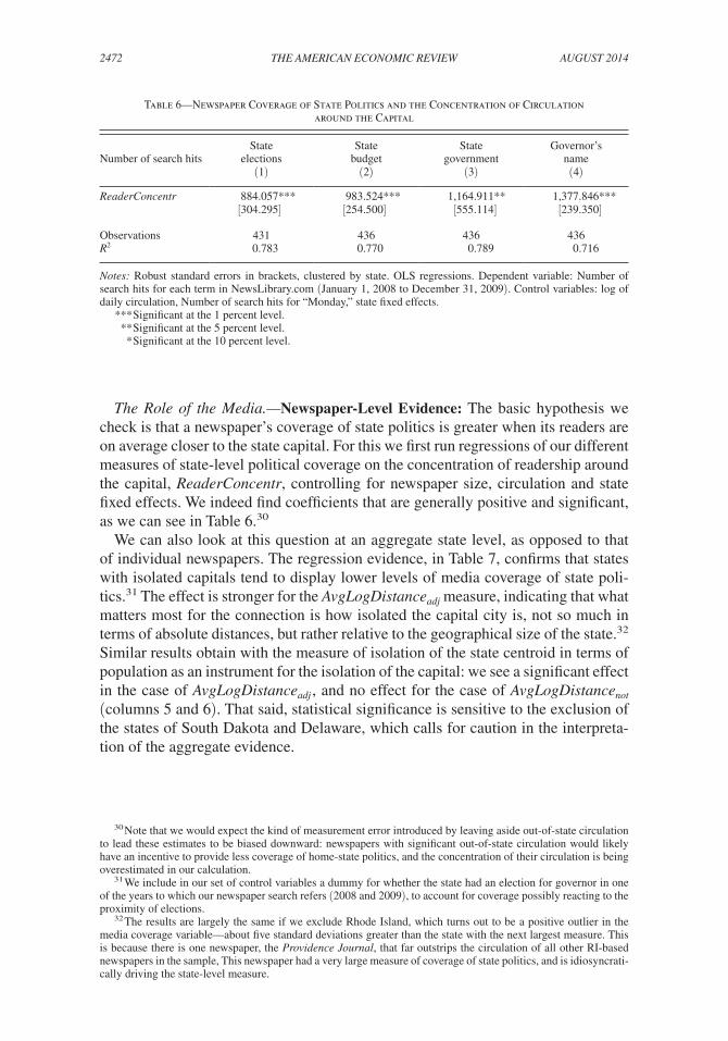
The Role of the Media.—Newspaper-Level Evidence: The basic hypothesis we check is that a newspaper’s coverage of state politics is greater when its readers are on average closer to the state capital. For this we first run regressions of our different measures of state-level political coverage on the concentration of readership around the capital, ReaderConcentr, controlling for newspaper size, circulation and state fixed effects. We indeed find coefficients that are generally positive and significant, as we can see in Table 6.30
We can also look at this question at an aggregate state level, as opposed to that of individual newspapers. The regression evidence, in Table 7, confirms that states with isolated capitals tend to display lower levels of media coverage of state poli-tics.31 The effect is stronger for the AvgLogDistanc e adj measure, indicating that what matters most for the connection is how isolated the capital city is, not so much in terms of absolute distances, but rather relative to the geographical size of the state.32 Similar results obtain with the measure of isolation of the state centroid in terms of population as an instrument for the isolation of the capital: we see a significant effect in the case of AvgLogDistanc e adj , and no effect for the case of AvgLogDistanc e not (columns 5 and 6). That said, statistical significance is sensitive to the exclusion of the states of South Dakota and Delaware, which calls for caution in the interpreta-tion of the aggregate evidence.
30 Note that we would expect the kind of measurement error introduced by leaving aside out-of-state circulation to lead these estimates to be biased downward: newspapers with significant out-of-state circulation would likely have an incentive to provide less coverage of home-state politics, and the concentration of their circulation is being overestimated in our calculation.
31 We include in our set of control variables a dummy for whether the state had an election for governor in one of the years to which our newspaper search refers (2008 and 2009), to account for coverage possibly reacting to the proximity of elections.
32 The results are largely the same if we exclude Rhode Island, which turns out to be a positive outlier in the media coverage variable—about five standard deviations greater than the state with the next largest measure. This is because there is one newspaper, the Providence Journal, that far outstrips the circulation of all other RI-based newspapers in the sample, This newspaper had a very large measure of coverage of state politics, and is idiosyncrati-cally driving the state-level measure.
Table 6—Newspaper Coverage of State Politics and the Concentration of Circulation around the Capital
Number of search hits State
elections State
budget State
government Governor’s
name (1) (2) (3) (4)
ReaderConcentr 884.057*** 983.524*** 1,164.911** 1,377.846*** [304.295] [254.500] [555.114] [239.350]
Observations 431 436 436 436 R2 0.783 0.770 0.789 0.716
Notes: Robust standard errors in brackets, clustered by state. OLS regressions. Dependent variable: Number of search hits for each term in NewsLibrary.com (January 1, 2008 to December 31, 2009). Control variables: log of daily circulation, Number of search hits for “Monday,” state fixed effects.
*** Significant at the 1 percent level. ** Significant at the 5 percent level. * Significant at the 10 percent level.

2473campante and do: Isolated capItal cItIes and corruptIonVol. 104 no. 8
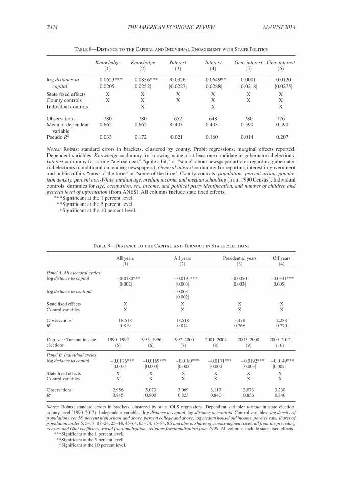
Individual-Level Evidence: We now look at whether individuals display lower levels of interest and information regarding state politics when they are farther away from the state capital. Table 8 shows the results of probit specifications, with our sur-vey dummy variables for Knowledge and Interest as dependent variables, and (the log of) distance to the state capital being the main independent variable of interest.33
Columns 1 and 2 show a robust, significant pattern: individuals who are farther from the state capital are substantially less likely to be informed about state politics. Columns 3 and 4 show the same goes for the level of interest in state campaign news, within the subset of newspaper readers. Quantitatively, our preferred speci-fications with all individual- and county-level controls imply substantial marginal decreases of about 8 percentage points (from a mean probability around 66 per-cent), and 6 percentage points (off a 40 percent mean probability), respectively. Finally, columns 5 and 6 display a placebo test: the correlation with distance is distinctly absent when it comes to the level of GeneralInterest in government and public affairs.
The Role of Voters.—We now check whether citizens who are farther away from the capital are also less likely to vote in state elections. Table 9 (panel A) runs county-level regressions, with data from all gubernatorial elections between 1990 and 2012, controlling for county demographics (in the preceding census, for each year), and with state-year fixed effects so as to focus on within-state and within-election variation.
33 For all dependent variables, we first show the specification with county-level controls only, and then include individual-level controls. In all specifications we cluster the standard errors at the county level and include state fixed effects, and marginal effects are reported. We also control for the surveyor’s assessment of the respondent’s general level of information about politics and public affairs, so that we look at the effect of distance conditional on the respondents’ level of information beyond the confines of state politics.
Table 7—Media Coverage and Isolation of the Capital City
Media coverage Circ.
weighted AvgLogDistance
weighted Circ.
weighted AvgLogDistance
weighted
Circ. weighted2SLS
population
Circ. weighted2SLS
population (1) (2) (3) (4) (5) (6)
AvgLogDistancenot −2.3921 −2.1841 −4.4325 [3.379] [3.285] [2.730]
AvgLogDistanceadj −4.7810* −5.2566** −3.6317* [2.529] [2.589] [2.169]
Observations 47 47 47 47 46 46 AR p-value — — — — 0.115 0.115 R2 0.460 0.451 0.246 0.237 0.554 0.570
Notes: Robust standard errors in brackets. OLS regressions except where noted. Dependent variable: First principal component of weighted search hits for each of the terms in Table 7 (weighted by newspaper circulation or AvgLogDistance-weighted newspaper circulation, as indicated), divided by hits for “Monday.” Independent variables as of 2000 (AvgLogDistance average 1920–2000). Control variables: log Area and log Maximum Distance (for AvgLogDistancenot specifications), log income, log population, per-cent college, share of government employment, regional dummies, dummy for election in 2008–2009. Columns 5–6 exclude Rhode Island. The state of Montana is missing from the media coverage sample. Instrument: centroid AvgLogDistancenot of population. AR p-value: p-value from Anderson-Rubin (minimum distance) test.
*** Significant at the 1 percent level. ** Significant at the 5 percent level. * Significant at the 10 percent level.
2474 THE AMERICAN ECONOMIC REVIEW AugusT 2014
Table 8—Distance to the Capital and Individual Engagement with State Politics
Knowledge Knowledge Interest Interest Gen. interest Gen. interest (1) (2) (3) (4) (5) (6)
log distance to −0.0623*** −0.0836*** −0.0326 −0.0649** −0.0001 −0.0120 capital [0.0205] [0.0252] [0.0227] [0.0288] [0.0218] [0.0275] State fixed effects X X X X X X County controls X X X X X X Individual controls X X X
Observations 780 780 652 648 780 776 Mean of dependent variable
0.662 0.662 0.403 0.403 0.590 0.590
Pseudo R2 0.033 0.172 0.021 0.160 0.014 0.207
Notes: Robust standard errors in brackets, clustered by county. Probit regressions, marginal effects reported. Dependent variables: Knowledge = dummy for knowing name of at least one candidate in gubernatorial elections; Interest = dummy for caring “a great deal,” “quite a bit,” or “some” about newspaper articles regarding gubernato-rial elections (conditional on reading newspapers); General interest = dummy for reporting interest in government and public affairs “most of the time” or “some of the time.” County controls: population, percent urban, popula-tion density, percent non-White, median age, median income, and median schooling (from 1990 Census); Individual controls: dummies for age, occupation, sex, income, and political party identification, and number of children and general level of information (from ANES). All columns include state fixed effects.
*** Significant at the 1 percent level. ** Significant at the 5 percent level. * Significant at the 10 percent level.
Table 9—Distance to the Capital and Turnout in State Elections
All years All years Presidential years Off years(1) (2) (3) (4)
Panel A. All electoral cycleslog distance to capital −0.0180*** −0.0191*** −0.0053 −0.0341***
[0.002] [0.003] [0.003] [0.005]log distance to centroid −0.0031
[0.002]State fixed effects X X X XControl variables X X X X
Observations 18,518 18,518 3,471 2,288R2 0.819 0.814 0.768 0.770
Dep. var.: Turnout in state 1990–1992 1993–1996 1997–2000 2001–2004 2005–2008 2009–2012 elections (5) (6) (7) (8) (9) (10)
Panel B. Individual cycles log distance to capital −0.0176*** −0.0169*** −0.0180*** −0.0171*** −0.0192*** −0.0149***
[0.003] [0.003] [0.003] [0.002] [0.003] [0.002]State fixed effects X X X X X X Control variables X X X X X X
Observations 2,956 3,073 3,069 3,117 3,073 3,230R2 0.845 0.800 0.823 0.840 0.836 0.846
Notes: Robust standard errors in brackets, clustered by state. OLS regressions. Dependent variable: turnout in state election, county-level (1990–2012). Independent variables: log distance to capital, log distance to centroid. Control variables: log density of population over 18, percent high school and above, percent college and above, log median household income, poverty rate, shares of population under 5, 5–17, 18–24, 25–44, 45–64, 65–74, 75–84, 85 and above, shares of census-defined races, all from the preceding census, and Gini coefficient, racial fractionalization, religious fractionalization from 1990. All columns include state fixed effects.
*** Significant at the 1 percent level. ** Significant at the 5 percent level. * Significant at the 10 percent level.
2475campante and do: Isolated capItal cItIes and corruptIonVol. 104 no. 8
We see a negative effect of distance to the capital on turnout in column 1 that is statistically significant and quantitatively nontrivial: doubling the distance from the capital would reduce turnout by around 1.5 percentage points (or one-sixth of the within-state standard deviation), from a mean around 45 percent. Column 2 further shows that the result is related to the special role of the capital: a placebo variable (distance to state centroid) is insignificant and barely affects the main coefficient.
Interestingly, column 3 shows the effect is much weaker, and statistically insig-nificant, for state elections that coincided with presidential elections. In contrast, the same regression restricted to the sample of “off ”-years where no federal election took place yields a coefficient that is three times as large (column 4)—we can reject the equality of coefficients at the 1 percent level.
Panel B (columns 5–10) then shows that the result is unaltered if we consider each of the separate six election cycles covered by our data separately: the coefficient is remarkably consistent, although it gets smaller in the most recent cycle.34
D. Money in Politics
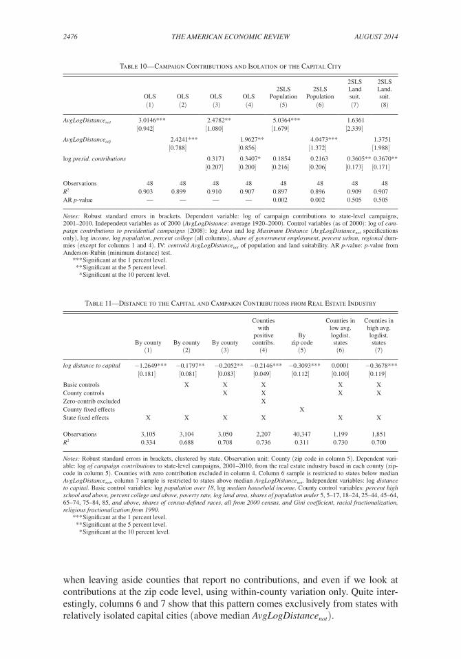
We now ask whether there is a link between the spatial distribution of population around the state capital and the amount of campaign money in state-level politics. Table 10 shows a robust positive relationship, at the aggregate state level, between the isolation of the capital and campaign contributions (controlling for population and income).
Columns 1 and 2 show that the result holds for the basic OLS specifications, which reproduce our preferred specifications for corruption, but with campaign contributions as our dependent variable. It is also substantial quantitatively: a one-standard-deviation increase in the isolation of the capital would be associated with a 30 percent increase in contributions. Columns 3 and 4 then show the result survives unscathed when we control for presidential campaign contributions (in the 2008 election cycle), which helps capture other factors leading to a high general propen-sity to engage in this form of political activity (the raw correlation is 0.87). Finally, columns 5–8 show similar results when we again instrument for AvgLogDistance using the isolation of the centroid with respect to population, although the same is not true with the alternative instrument.
In light of this aggregate pattern, we then ask whether, within states, individuals or firms who are located closer to the capital have a different propensity to contrib-ute money to state politics. We look at this question by focusing on one specific industry whose location is not particularly concentrated spatially, namely real estate.
We see in columns 1 and 2 in Table 11 that individuals and firms located in counties that are farther from the capital spend less in campaign contributions, both in abso-lute terms and controlling for income per capita. Columns 3–5 show that the results stay remarkably consistent when controlling for additional county demographics,
34 Note that assuming that the relationship that emerges from the county-level data would necessarily aggregate up to a link between state-level turnout and the isolation of the state capital would be incurring in the well-known ecological fallacy. As it turns out, there is a weak negative link between turnout and the isolation of the capital, that is borderline statistically significant (at the 10 percent level) once states with presidential-year elections are excluded from the sample. (See the online Appendix.) The difference between presidential and off-years is also true for every election cycle taken in isolation (see the online Appendix).
2476 THE AMERICAN ECONOMIC REVIEW AugusT 2014
when leaving aside counties that report no contributions, and even if we look at contributions at the zip code level, using within-county variation only. Quite inter-estingly, columns 6 and 7 show that this pattern comes exclusively from states with relatively isolated capital cities (above median AvgLogDistanc e not ).
Table 10 — Campaign Contributions and Isolation of the Capital City
OLS OLS OLS OLS 2SLS
Population 2SLS
Population
2SLSLand suit.
2SLSLand. suit.
(1) (2) (3) (4) (5) (6) (7) (8)
AvgLogDistancenot 3.0146*** 2.4782** 5.0364*** 1.6361 [0.942] [1.080] [1.679] [2.339]
AvgLogDistanceadj 2.4241*** 1.9627** 4.0473*** 1.3751 [0.788] [0.856] [1.372] [1.988] log presid. contributions 0.3171 0.3407* 0.1854 0.2163 0.3605** 0.3670**
[0.207] [0.200] [0.216] [0.206] [0.173] [0.171]
Observations 48 48 48 48 48 48 48 48 R2 0.903 0.899 0.910 0.907 0.897 0.896 0.909 0.907 AR p-value — — — — 0.002 0.002 0.505 0.505
Notes: Robust standard errors in brackets. Dependent variable: log of campaign contributions to state-level campaigns, 2001–2010. Independent variables as of 2000 (AvgLogDistance: average 1920–2000). Control variables (as of 2000): log of cam-paign contributions to presidential campaigns (2008): log Area and log Maximum Distance (AvgLogDistancenot specifications only), log income, log population, percent college (all columns), share of government employment, percent urban, regional dum-mies (except for columns 1 and 4). IV: centroid AvgLogDistancenot of population and land suitability. AR p-value: p-value from Anderson-Rubin (minimum distance) test.
*** Significant at the 1 percent level. ** Significant at the 5 percent level. * Significant at the 10 percent level.
Table 11—Distance to the Capital and Campaign Contributions from Real Estate Industry
By county By county By county
Counties with
positive contribs.
By zip code
Counties inlow avg. logdist. states
Counties inhigh avg. logdist.states
(1) (2) (3) (4) (5) (6) (7)
log distance to capital −1.2649*** −0.1797** −0.2052** −0.2146*** −0.3093*** 0.0001 −0.3678***[0.181] [0.081] [0.083] [0.049] [0.112] [0.100] [0.119]
Basic controls X X X X XCounty controls X X X XZero-contrib excluded X County fixed effects XState fixed effects X X X X X X
Observations 3,105 3,104 3,050 2,207 40,347 1,199 1,851R2 0.334 0.688 0.708 0.736 0.311 0.730 0.700
Notes: Robust standard errors in brackets, clustered by state. Observation unit: County (zip code in column 5). Dependent vari-able: log of campaign contributions to state-level campaigns, 2001–2010, from the real estate industry based in each county (zip-code in column 5). Counties with zero contribution excluded in column 4. Column 6 sample is restricted to states below median AvgLogDistancenot, column 7 sample is restricted to states above median AvgLogDistancenot. Independent variables: log distance to capital. Basic control variables: log population over 18, log median household income. County control variables: percent high school and above, percent college and above, poverty rate, log land area, shares of population under 5, 5–17, 18–24, 25–44, 45–64, 65–74, 75–84, 85, and above, shares of census-defined races, all from 2000 census, and Gini coefficient, racial fractionalization, religious fractionalization from 1990.
*** Significant at the 1 percent level. ** Significant at the 5 percent level. * Significant at the 10 percent level.
2477campante and do: Isolated capItal cItIes and corruptIonVol. 104 no. 8
E. Isolated Capital Cities and the Provision of Public Goods
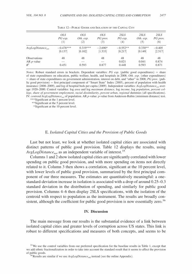
Last but not least, we look at whether isolated capital cities are associated with distinct patterns of public good provision. Table 12 displays the results, using AvgLogDistanc e not as an independent variable of interest.35
Columns 1 and 2 show isolated capital cities are significantly correlated with lower spending on public good provision, and with more spending on items not directly related to it. Column 3 then shows a correlation, significant at the 10 percent level, with lower levels of public good provision, summarized by the first principal com-ponent of our three measures. The estimates are quantitatively meaningful: a one-standard-deviation increase in isolation is associated with a drop of around 0.25–0.3 standard deviation in the distribution of spending, and similarly for public good provision. Columns 4–6 then display 2SLS specifications, with the isolation of the centroid with respect to population as the instrument. The results are broadly con-sistent, although the coefficient for public good provision is now essentially zero.36
IV. Discussion
The main message from our results is the substantial evidence of a link between isolated capital cities and greater levels of corruption across US states. This link is robust to different specifications and measures of both concepts, and seems to be
35 We use the control variables from our preferred specification for the baseline results in Table 1, except that we add ethnic fractionalization in order to take into account the standard result that it seems to affect the provision of public goods.
36 Results are similar if we use AvgLogDistanc e adj instead (see the online Appendix).
Table 12—Public Goods and Isolation of the Capital City
OLS OLS OLS 2SLS 2SLS 2SLS PG exp. Oth. exp. PG prov. PG exp. Oth. exp. PG prov.
(1) (2) (3) (4) (5) (6)
AvgLogDistancenot −0.478*** 0.319*** −2.690* −0.552** 0.330** −0.405 [0.137] [0.102] [1.533] [0.217] [0.149] [2.517]
Observations 48 48 48 48 48 48 AR p-value — — — 0.021 0.041 0.874 R2 0.451 0.593 0.877 0.448 0.593 0.871
Notes: Robust standard errors in brackets. Dependent variables: PG exp. (public good expenditures) = share of state expenditures on education, public welfare, health, and hospitals in 2008; Oth. exp. (other expenditures) = share of state expenditures on government administration, interest on debt, and “other” in 2008; PG prov. (pub-lic good provision) = first principal component of “Smart State” Index (2005), percent of population with health insurance (2008–2009), and log of hospital beds per capita (2009). Independent variables: AvgLogDistancenot aver-age 1920–2000. Control variables: log area and log maximum distance, log income, log population, percent col-lege, share of government employment, racial dissimilarity, percent urban, regional dummies (all specifications). IV: centroid AvgLogDistancenot of population. AR p-value: p-value from Anderson-Rubin (minimum distance) test.
*** Significant at the 1 percent level. ** Significant at the 5 percent level. * Significant at the 10 percent level.
2478 THE AMERICAN ECONOMIC REVIEW AugusT 2014
specific about corruption, and about the role of the capital city.37 In addition, while we are short of a true natural experiment where state capitals would have been ran-domly assigned, plausible sources of exogenous variation indicate that our stylized fact is not driven by confounding factors related to the endogeneity of that choice and its impact on the spatial distribution of population.
This is very much in line with what we have termed the accountability view: the idea that isolated capitals may see corruption fester because of reduced accountabil-ity. We have also found direct evidence for that view, as different mechanisms are related to the spatial distribution of population.38
First, we saw that newspapers whose audience is on average farther from the state capital provide less coverage of state politics. Such a pattern could be expected, to the extent that media outlets are at least partly trying to provide content that inter-ests their audience (e.g., Mullainathan and Shleifer 2005, Gentzkow and Shapiro 2010), and to the extent that media consumers are at least somewhat more interested (ceteris paribus) in what happens close to where they live. We also found some evidence that states with more isolated capitals have less intense media coverage of state politics.
This lower level of media scrutiny could very well lead to, and be reinforced by, a less informed and less engaged citizenry. Consistent with that, we find that living farther from the capital substantially decreases the level of interest in state cam-paigns among individuals with comparable demographic characteristics and with a comparable level of information about policy in general. In contrast, it does not affect the level of interest in public affairs in general. Put together, these pieces suggest that where individuals are located matters substantively for media account-ability at the state level.
It is thus natural to conjecture that other forms of holding state officials account-able could also be linked to the spatial distribution of population. In particular, one might expect that disengagement to be reflected in lower voter turnout, and hence less accountability via the electoral process. We find that turnout in state elections is indeed lower farther from the state capital—an empirical regularity that is novel, to the best of our knowledge, in the US context.39 Notably, the logic of our hypothesis would predict a weaker link between turnout and distance to the state capital for presidential-year elections, where presumably turnout would be more affected by forces unrelated to state politics. This is exactly what we find.
Still in the realm of the electoral process, we find a strong positive relationship between the isolation of the state capital and the amount of money in state-level campaigns. We can thus speculate that, with lower media scrutiny and reduced involvement by voters, an isolated capital opens the way for a stronger role of money in shaping political outcomes.
37 In particular, that the results do not extend to other types of federal crime helps alleviate the concern that they might be driven by differences in the ability, zeal, or resources available to federal prosecutors—at least to the extent that these differences apply across different types of cases.
38 We also find that politicians earn higher salaries in states with more isolated capitals, as proxied by governor compensation (as a share of per capita income and controlling for the relative desirability of living in the capital, as captured by relative housing prices). This is consistent lower accountability, in that one would expect politicians to be able to extract rents both legally as well as illegally (see the online Appendix).
39 Similar effects have been detected elsewhere (Hearl, Budge, and Pearson 1996).
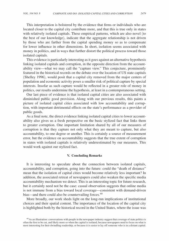
2479campante and do: Isolated capItal cItIes and corruptIonVol. 104 no. 8
This interpretation is bolstered by the evidence that firms or individuals who are located closer to the capital city contribute more, and that this is true only in states with relatively isolated capitals. These empirical patterns, which are also novel (to the best of our knowledge), indicate that the aggregate relationship is not driven by those who are farther from the capital spending money so as to compensate for lower influence in other dimensions. In short, isolation seems associated with money in politics, and in ways that further distort the political process toward those isolated capitals.
This evidence is particularly interesting as it goes against an alternative hypothesis linking isolated capitals and corruption, in the opposite direction from the account-ability view—what we may call the “capture view.” This conjecture, prominently featured in the historical records on the debate over the location of US state capitals (Shelley 1996), would posit that a capital city removed from the major centers of population and economic activity poses a smaller risk of political capture by special interests. Insofar as such capture would be reflected in a greater role of money in politics, our results undermine the hypothesis, at least in a contemporaneous setting.
Our last piece of evidence is that isolated capital cities are also associated with diminished public good provision. Along with our previous results, this paints a picture of isolated capital cities associated with low accountability and corrup-tion, with important detrimental effects on the state’s performance as a provider of public goods.
As a final note, the direct evidence linking isolated capital cities to lower account-ability also gives us a fresh perspective on the basic stylized fact that links them to greater corruption. One important limitation shared by all of our measures of corruption is that they capture not only what they are meant to capture, but also accountability, to one degree or another. This is certainly a source of measurement error, but the evidence on accountability suggests that the true extent of corruption in states with isolated capitals is relatively underestimated by our measures. This would work against our stylized fact.
V. Concluding Remarks
It is interesting to speculate about the connection between isolated capitals, accountability, and corruption, going into the future: could the “death of distance” mean that the isolation of capital cities would become relatively less important? In addition, the associated retreat of newspapers could also weaken the specific media accountability mechanism we detect. This is an interesting topic for future research, but it certainly need not be the case: casual observation suggests that online media is not immune from a bias toward local coverage—consistent with demand-driven bias—and there could also be countervailing forces.40
More broadly, our work sheds light on the long-run implications of institutional choices and their spatial content. The importance of the location of the capital city is highlighted both by the historical record in the United States, where the issue was
40 As an illustration: conversations with people in the newspaper industry suggest that coverage of state politics is often the first to be cut, and likely more so when the capital is isolated, because newspapers need to focus on what is most interesting for their dwindling readership, or because it is easier to lay off someone who is in a distant capital.
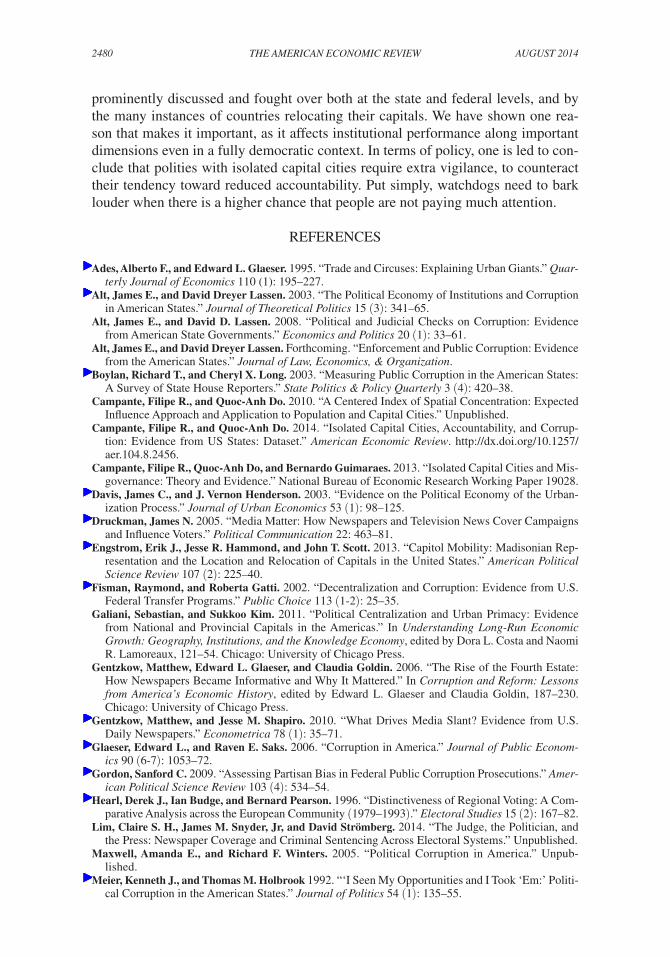
2480 THE AMERICAN ECONOMIC REVIEW AugusT 2014
prominently discussed and fought over both at the state and federal levels, and by the many instances of countries relocating their capitals. We have shown one rea-son that makes it important, as it affects institutional performance along important dimensions even in a fully democratic context. In terms of policy, one is led to con-clude that polities with isolated capital cities require extra vigilance, to counteract their tendency toward reduced accountability. Put simply, watchdogs need to bark louder when there is a higher chance that people are not paying much attention.
REFERENCES
Ades, Alberto F., and Edward L. Glaeser. 1995. “Trade and Circuses: Explaining Urban Giants.” Quar-terly Journal of Economics 110 (1): 195–227.
Alt, James E., and David Dreyer Lassen. 2003. “The Political Economy of Institutions and Corruption in American States.” Journal of Theoretical Politics 15 (3): 341–65.
Alt, James E., and David D. Lassen. 2008. “Political and Judicial Checks on Corruption: Evidence from American State Governments.” Economics and Politics 20 (1): 33–61.
Alt, James E., and David Dreyer Lassen. Forthcoming. “Enforcement and Public Corruption: Evidence from the American States.” Journal of Law, Economics, & Organization.
Boylan, Richard T., and Cheryl X. Long. 2003. “Measuring Public Corruption in the American States: A Survey of State House Reporters.” State Politics & Policy Quarterly 3 (4): 420–38.
Campante, Filipe R., and Quoc-Anh Do. 2010. “A Centered Index of Spatial Concentration: Expected Influence Approach and Application to Population and Capital Cities.” Unpublished.
Campante, Filipe R., and Quoc-Anh Do. 2014. “Isolated Capital Cities, Accountability, and Corrup-tion: Evidence from US States: Dataset.” American Economic Review. http://dx.doi.org/10.1257/aer.104.8.2456.
Campante, Filipe R., Quoc-Anh Do, and Bernardo Guimaraes. 2013. “Isolated Capital Cities and Mis-governance: Theory and Evidence.” National Bureau of Economic Research Working Paper 19028.
Davis, James C., and J. Vernon Henderson. 2003. “Evidence on the Political Economy of the Urban-ization Process.” Journal of Urban Economics 53 (1): 98–125.
Druckman, James N. 2005. “Media Matter: How Newspapers and Television News Cover Campaigns and Influence Voters.” Political Communication 22: 463–81.
Engstrom, Erik J., Jesse R. Hammond, and John T. Scott. 2013. “Capitol Mobility: Madisonian Rep-resentation and the Location and Relocation of Capitals in the United States.” American Political Science Review 107 (2): 225–40.
Fisman, Raymond, and Roberta Gatti. 2002. “Decentralization and Corruption: Evidence from U.S. Federal Transfer Programs.” Public Choice 113 (1-2): 25–35.
Galiani, Sebastian, and Sukkoo Kim. 2011. “Political Centralization and Urban Primacy: Evidence from National and Provincial Capitals in the Americas.” In Understanding Long-Run Economic Growth: Geography, Institutions, and the Knowledge Economy, edited by Dora L. Costa and Naomi R. Lamoreaux, 121–54. Chicago: University of Chicago Press.
Gentzkow, Matthew, Edward L. Glaeser, and Claudia Goldin. 2006. “The Rise of the Fourth Estate: How Newspapers Became Informative and Why It Mattered.” In Corruption and Reform: Lessons from America’s Economic History, edited by Edward L. Glaeser and Claudia Goldin, 187–230. Chicago: University of Chicago Press.
Gentzkow, Matthew, and Jesse M. Shapiro. 2010. “What Drives Media Slant? Evidence from U.S. Daily Newspapers.” Econometrica 78 (1): 35–71.
Glaeser, Edward L., and Raven E. Saks. 2006. “Corruption in America.” Journal of Public Econom-ics 90 (6-7): 1053–72.
Gordon, Sanford C. 2009. “Assessing Partisan Bias in Federal Public Corruption Prosecutions.” Amer-ican Political Science Review 103 (4): 534–54.
Hearl, Derek J., Ian Budge, and Bernard Pearson. 1996. “Distinctiveness of Regional Voting: A Com-parative Analysis across the European Community (1979–1993).” Electoral Studies 15 (2): 167–82.
Lim, Claire S. H., James M. Snyder, Jr, and David Strömberg. 2014. “The Judge, the Politician, and the Press: Newspaper Coverage and Criminal Sentencing Across Electoral Systems.” Unpublished.
Maxwell, Amanda E., and Richard F. Winters. 2005. “Political Corruption in America.” Unpub-lished.
Meier, Kenneth J., and Thomas M. Holbrook 1992. “‘I Seen My Opportunities and I Took ‘Em:’ Politi-cal Corruption in the American States.” Journal of Politics 54 (1): 135–55.
2481campante and do: Isolated capItal cItIes and corruptIonVol. 104 no. 8
Meier, Kenneth J., and Thomas Schlesinger. 2002. “Variations in Corruption among the American States.” In Political Corruption: Concepts and Contexts, edited by Arnold J. Heidenheimer and Michael Johnson, 627–44. New Brunswick, NJ: Transaction Publishers.
Morgan Quitno Corporation. 2005. Education State Rankings: 2005–2006. Lawrence, KS: Morgan Quitno Press.
Mullainathan, Sendhil, and Andrei Shleifer. 2005. “The Market for News.” American Economic Review 95 (4): 1031–53.
Ramankutty, Navin, Jonathan A. Foley, John Norman, and Kevin McSweeney. 2002. “The Global Distribution of Cultivable Lands: Current Patterns and Sensitivity to Possible Climate Change.” Global Ecology and Biogeography 11 (5): 377–92.
Rodden, Jonathan. 2010. “The Geographic Distribution of Political Preferences.” Annual Review of Political Science 13: 321–40.
Saiz, Albert, and Uri Simonsohn. 2013. “Proxying for Unobservable Variables with Internet Docu-ment-Frequency.” Journal of the European Economic Association 11 (1): 137–65.
Shelley, Fred M. 1996. Political Geography of the United States. New York, NY: Guilford Press.Snyder, James M., Jr., and David Strömberg. 2010. “Press Coverage and Political Accountability.”
Journal of Political Economy 118 (2): 355–408.Stein, Mark. 2008. How the States Got Their Shapes. New York: HarperCollins.Stock, James H., and Motohiro Yogo. 2005. “Testing for Weak Instruments in Linear IV Regression.”
In Identification and Inference for Econometric Models: Essays in Honor of Thomas Rothenberg, edited by Donald W. K. Andrews and James H. Stock, 80–108. Cambridge, UK: Cambridge Uni-versity Press.
Vinson, C. Danielle. 2003. Local Media Coverage of Congress and Its Members: Through Local Eyes. Cresskill, NJ: Hampton Press.
Wilson, James Q. 1966. “Corruption: The Shame of the States.” Public Interest 2: 28–38.Zagarri, Rosemarie. 1987. The Politics of Size: Representation in the United States, 1776–1850.
Ithaca, NY: Cornell University Press.