isolation of single muscle fibers in preparation for

Isolation of Single Muscle Fibers in Preparation for

Loading into Microfluidic Devices

Summary

Modeling and simulation of microfluidic devices to capture single muscle fibers has led

to several design possibilities. Before testing the fabricated devices, however, a procedure for

the isolation of single muscle fibers from muscle tissue must be developed. The aim is to

optimize a collagenase treatment that can yield consistent fibers of large quantity and

dimensions that correspond to device tapering regions. Optimization of collagenase

concentration and trituration showed that a 0.6% (w/v) solution produced the most fibers and

the wide bore pipette tip method of trituration produced the longest fibers. Further analysis of

centrifugation reinforced the theory of fiber separation and clean up based upon length. Future

work includes testing of a larger sample size of muscle tissue/type, testing fiber functionality,

preparing new methods of collagenase preparation and treatment, and seeing fiber

response/analysis in the fabricated devices.

Figure 1 - Muscle Fiber Diagram1

Introduction

Skeletal muscle in organisms, under the control of the somatic nervous system, provides

the external skeleton and body the ability to generate force and movement. The force output

depends upon the molecular mechanism of muscle contraction. Skeletal muscle is made up of

large bundles of muscle cells or fibers surrounded by connective tissue. Each fiber lies parallel

with each other in the bundle and contains contractile elements called myofibrils. Figure 1

shows the basic diagram of a muscle fiber.

The myofibrils have similar repeating patterns due

to the end to end connection of the contractile

elements of sarcomeres. These sarcomeres are

made up on thick and thin myosin and actin

filaments and bounded by Z-lines. Skeletal muscle

contraction occurs through the cross bridge cycle, which is activated through the energy

consumption of ATP (Figure 2). First, ADP binds at the cross bridge section of the myosin

filament, which is opened up by the binding of calcium to troponin and the movement of

tropomyosin to block the cross bridge. ADP binding causes the myosin cross bridge segment to

attach to actin and cause a sliding movement. The detachment of the actin bound to the

myosin is triggered by binding of ATP to the cross bridge section of the myosin. Hydrolysis of

the ATP reenergizes the cross bridge to cause ADP binding the contraction to ensue yet again.3

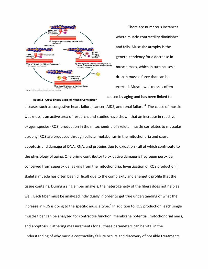
Figure 2 - Cross-Bridge Cycle of Muscle Contraction2

There are numerous instances

where muscle contractility diminishes

and fails. Muscular atrophy is the

general tendency for a decrease in

muscle mass, which in turn causes a

drop in muscle force that can be

exerted. Muscle weakness is often

caused by aging and has been linked to

diseases such as congestive heart failure, cancer, AIDS, and renal failure.4 The cause of muscle

weakness is an active area of research, and studies have shown that an increase in reactive

oxygen species (ROS) production in the mitochondria of skeletal muscle correlates to muscular

atrophy. ROS are produced through cellular metabolism in the mitochondria and cause

apoptosis and damage of DNA, RNA, and proteins due to oxidation - all of which contribute to

the physiology of aging. One prime contributor to oxidative damage is hydrogen peroxide

conceived from superoxide leaking from the mitochondria. Investigation of ROS production in

skeletal muscle has often been difficult due to the complexity and energetic profile that the

tissue contains. During a single fiber analysis, the heterogeneity of the fibers does not help as

well. Each fiber must be analyzed individually in order to get true understanding of what the

increase in ROS is doing to the specific muscle type.4 In addition to ROS production, each single

muscle fiber can be analyzed for contractile function, membrane potential, mitochondrial mass,

and apoptosis. Gathering measurements for all these parameters can be vital in the

understanding of why muscle contractility failure occurs and discovery of possible treatments.

Figure 4 - CAD Drawing of Initial 2-Channel Device

Figure 3 - Schematic of Design of first Model

One type of single muscle fiber analysis that has been in development within this lab

involves microfluidics. Microfluidic devices typically consist of one or more channels and are

able to precisely manipulate fluid flows within the micrometer range of length scales.

Microfluidic devices rely on fundamental principles of fluid mechanics in order to function

properly. The flow characteristics usually consist of a steady state, incompressible, laminar flow

with a low Reynolds number.5 An initial, simple two channel device was first developed based

on preliminary rat and mouse muscle fiber length and diameter data collected by Dr. Vrata

Kostal. Figure 3 shows a schematic initial drawing of the device and Figure 4 shows a CAD

model made before undergoing simulations. The basis of the design was to load fibers through

the inlet, using a pressure difference, and then capture the fibers at a particular clamping or

tapering region farther down the channels. At this region, most of the analysis of the fiber

through drug treatment and image could take place. Similar technology was developed for

capturing of C. elegans in the Whiteside Lab.

y

x

Microfluidics can encompass a large range of systems to drive the flow. In the device

we designed, flow was driven by application of a pressure gradient between the inlet and

outlet. After sketching out the design, Ansys Workbench software (CFX) was used to create a 3D

model, mesh, and simulation of the flow through the device with set parameters identified as

steady state and laminar. Various optimizations in device design were required to ensure the

flow through the device carried out properly and did not hit the sides or bifurcations of the

device. Streamline and contour plots of the flow were analyzed intensively for this optimization.

Figure 5a shows a full body contour plot of flow and Figure 5b shows inlet streamline of flow

(indicative of proper flow splitting at bifurcation) obtained during multiple trials of simulations.

After a two channel device was successfully simulated and designed, additional

simulations were conducted to model a pseudo-fiber trapped in the tapered region of one

channel of the device, where the fiber would essentially be analyzed and delivered reagents to.

The modeled pseudo-fiber was based upon the average length and diameter of mouse muscle

fibers cultured previously in the Arriaga lab. A trapped fiber will reduce fluid flow to that

Figure 5a. Full body Contour Plot of Flow through 2 Ch. Device Figure 5a. Full body Contour Plot of Flow through 2 Ch. Device Figure 5a. Full body Contour Plot of Flow through 2 Ch. Device Figure 5b. Streamline Plot of Flow through inlet bifurcation of 2 Ch. Device

channel and increase flow to the open channel –

leaving both flows to converge nicely in the outlet.

Figure 6a shows a close-up of the fiber trapped in the

tapering region of the device and flow streamlines

around the fiber and Figure 6b shows the flow

difference obtained when the fiber was trapped in

the bottom channel. All in all, the 2-channel device

was successfully modeled and simulated. Figure 5a

shows that the flow of the devices converges nicely

in the outlet region and the tapering region induces

max flow. Figure 5b shows the bifurcation of the

device was successfully modeled in that the flow

does not converge into the middle nor hit the sides

of the device. Figures 6a and 6b demonstrate that if a

fiber was captured, flow would occur around the fiber and more-so in the open channel. This

last summer, work was done to create and simulate extended channel devices that hopefully

mimic the same flow data as the 2-Channel devices. Figures 7 and 8 shows streamline flow plots

of a 4-channel device and 8-channel device. CAD drawings of 54 different devices (as can be

seen in Figure 9) that vary in channel number (2,4, and 8), tapering length, and tapering width

were prepared for fabrication of this device for wet-lab testing. Table 1 lists the tapering

Figure 6a. Close-up of Trapped Fiber and Flow Around

Figure 6b. Streamline Flow Difference Between Trapped Fiber Channel and Open Channel

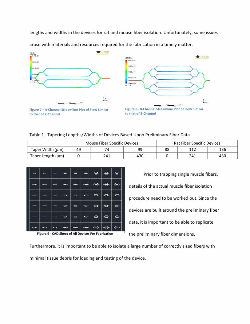
lengths and widths in the devices for rat and mouse fiber isolation. Unfortunately, some issues

arose with materials and resources required for the fabrication in a timely matter.

Table 1. Tapering Lengths/Widths of Devices Based Upon Preliminary Fiber Data

Prior to trapping single muscle fibers,

details of the actual muscle fiber isolation

procedure need to be worked out. Since the

devices are built around the preliminary fiber

data, it is important to be able to replicate

the preliminary fiber dimensions.

Furthermore, it is important to be able to isolate a large number of correctly sized fibers with

minimal tissue debris for loading and testing of the device.

Mouse Fiber Specific Devices Rat Fiber Specific Devices

Taper Width (μm) 49 74 99 88 112 136

Taper Length (μm) 0 241 430 0 241 430

Figure 9 - CAD Sheet of All Devices For Fabrication

Figure 7 – 4-Channel Streamline Plot of Flow Similar to that of 2-Channel

Figure 8– 8-Channel Streamline Plot of Flow Similar to that of 2-Channel

One way to obtain muscle fibers from a muscle tissue sample involves the use of

collagenase. Collagen is a fibrous structural protein whose role is to provide support and

structure to tissues. In fact, it makes up a large percentage of the extracellular matrix of

cells/tissue. In muscle tissue, collagen fibers form fibrous connective tissue around single

muscle fibers and help hold them together by providing tensile strength. Collagenase is a type

of endopeptidase that attacks the structure of collagen and digests it. Typically for muscle, Type

II collagenase is the enzyme used for digestion of connective tissue and isolation of muscle

fibers. Due to the complicated enzymatic activity of collagenase, there is no single procedure

for isolation of muscle fibers. Factors such as collagenase concentration, incubation time, and

trituration method in disruption of fibers vary between experimental methods.

The main objective of this paper is to describe some of the different collagenase

treatments I have performed to isolate single skeletal muscle fibers. After optimization of the

concentration of collagenase acceptable for treatments, different trituration methods were

assessed for tissue disruption. Each trituration method was compared by the number of fibers

and average dimensions yielded, with the goal of determining which method can yield

consistent fiber data that corresponds to device specifications. After knowing this, more fibers

can be isolated to be used for loading into the fabricated devices and running tests.

Materials and Methods

Muscle Tissue Isolation

The muscle tissue used in experiments were cut and donated from Dr. LaDora

Thompson’s lab, in the Program of Physical Therapy at the University of Minnesota. All tissue

used came from C57BL/6 strain mice with variable ages. The types of muscle tissue used include

foot adductors, thigh muscle, gracilis/SM, and hamstring – all of various size. After isolation

from mice, individual types of muscle were stored on ice in Kreb solution (118 mM NaCl, 4.7

mM KCl, 1.2 mM KH2PO4, 1.2 mM MgSO4, 4.2 mM NaHCO3, 2 mM CaCl2, 10 mM glucose, 200

mM sulphinpyrazone and 10 mM Hepes, pH 7.4). All muscle tissue was used within one hour of

isolation. Before collagenase treatment, the tissue was cut so that multiple treatment

conditions could be used on a single muscle type. Size of tissue pieces varied, but all were cut in

such a way that the incisions were made parallel to the muscle fibers. This was done with use of

a scalpel, tweezers, and microscope.

Preparation of Tissue Isolation Buffer and Collagenase Solutions

Type II collagenase was prepared in tissue isolation buffer prepared in our lab. The

buffer consisted of 185 mM Sucrose, 100 mM KCl, 5 mM CaCl2, 1 mM KH2PO4, 50 mM tris-HCl,

0.2% BSA (w/v), and 500 mL sterile H20. A large quantity of this buffer was prepared, titrated to

a pH of 7.4, purified to 0.2 μm by filtration under a sterile hood, and kept in a 4°C refrigerator.

Different concentrations of collagenase solutions were made by dissolving Type II Collagenase

(Sigma Aldrich) in the tissue isolation buffer and vortexing at low speed. 0.4% (w/v), 0.6% (w/v),

1.0% (w/v), and 1.4% (w/v) solutions were made and tested.

Determination of Optimum Collagenase Concentration and First Trituration Method – Normal

Pipette

After preparation of the collagenase solutions, the optimum concentration was

evaluated on samples of mouse muscle tissue. First, the cut muscle was placed into

microcentrifuge tubes. Approximately 400 μL of the specific concentration of collagenase

solution was added to the tube with the cut muscle. Samples were incubated for 5 minutes at

37 °C in a Thermomixer set at a gyration of 300 rpm. After incubation, the collagenase is

replaced with an equivalent volume of isolation buffer and trituration, or pulling and pushing of

the mixture slowly through a simple 1000 μL pipette tip, is done five times to disrupt the bundle

of fibers and release them. The fibers, in suspension of the buffer, are then washed two times

in a centrifuge set at 600 g for 30 seconds to remove any residual collagenase. At this point, the

suspension of fibers can be transferred to microscope slides for imaging.

Second Trituration Method – Wide Bore Pipette

Using the optimum collagenase concentration (0.6% (w/v)), the same treatment as

above was done, but a different trituration releasing step of the fibers was induced. Instead of

using the normal length of the pipette tip, we made a wider bore pipette tip by cutting it 23.8

mm from the end and creating a larger 3.5 mm diameter opening. After the treatment and

washing steps, the fibers in suspension were transferred to slides for image analysis

Third Trituration Method – Centrifugation

The third trituration method consisted of the use of centrifugation. Contrary to placing

the cut isolated muscle tissue into microcentrifuge tubes to start treatment, the muscle was

placed into centrifugal filtration tubes, which contain small lipped insert/membranes stationed

in deeper tubes. It was important to make sure that the muscle was gently placed all the way

down to the membrane. A 400 μL aliquot of 0.6% (w/v) collagenase solution was added to the

tubes of various muscle types. The centrifuge was set to run for 5 minutes at 37°C. Initially

deciding on a set speed, however, was difficult. It was decided to start at 500g and work our

way down. The proper speed of centrifugation was determined by observing different spinning

speeds and seeing which did not let the collagenase solution simply pass all the way through

the membrane to the bottom. Eventually, 300g was the optimum speed chosen, as the solution

was trapped above the membrane and engulfed the muscle tissue. Three cycles were done, at

different speeds, for a final duration of 15 minutes. After centrifugation with the collagenase,

the solution was washed from the muscle by spinning at 600g for 2 minutes. Then, a wash step

was done with replacement of the collagenase solution with buffer and spinning down at 300g

for 5 minutes. Fiber suspensions were transferred to slides for analysis.

Differential Centrifugation – Separation of Fibers

To further test the capabilities of the centrifugation technique, another test was done

solely on one muscle type, the SM/gracilis. This test was done to verify if differential

centrifugation can be utilized to separate out long muscle fibers from short fiber/debris. This

separation can occur by performing the original technique of centrifugation as described above,

but after washing, small samples of the fiber suspensions should be transferred with created

wide bore pipette tips to new eppendorfs. In our test, a total of 4 trials were done with

different speeds to test the differential centrifugation theory. At a spin time set at 5 minutes,

100g, 200g, 300g, and 400g speeds were tested with approximately 100 μL of fiber suspension

sample in each tube. Supernatants (top fluid) and pellets fractions from the tubes were

analyzed by microscopy after centrifugation. Numbers of large fibers and small fibers were

determined in both portions with Image J. The prediction was that the pellet should have a

large fiber to small fiber ratio of greater than 50% and that the supernatant should contain

virtually no large fibers.

Imaging and Analysis

All slides with suspensions of fibers were analyzed with an Olympus IX81 microscope.

The camera attachment was a Nikon KX85 and a program named MiroCCd was used to capture

images. Analysis of fiber dimensions and quantity was performed by taking the captured images

and importing into ImageJ software.

Results

After compiling all of the captured images taken with the different collagenase

treatments, Image J was utilized to adjust image quality/contrast and obtain measurements

based off of microscope scale. Table 2 shows the average number of fibers per captured image

for each collagenase concentration. This was the initial test run to see what concentration

would be used for the rest of the trituration techniques. As can be seen, 0.6% (w/v) yielded the

most fibers, and was thus used for the rest of the experiments. Table 3 shows a summary of the

results acquired for the normal pipette tip trituration (control), the wide bore pipette tip

trituration, and centrifugation. Average fiber width, length, and quantity were recorded for

each set of images for different muscle types. The results for length varied quite a bit, but the

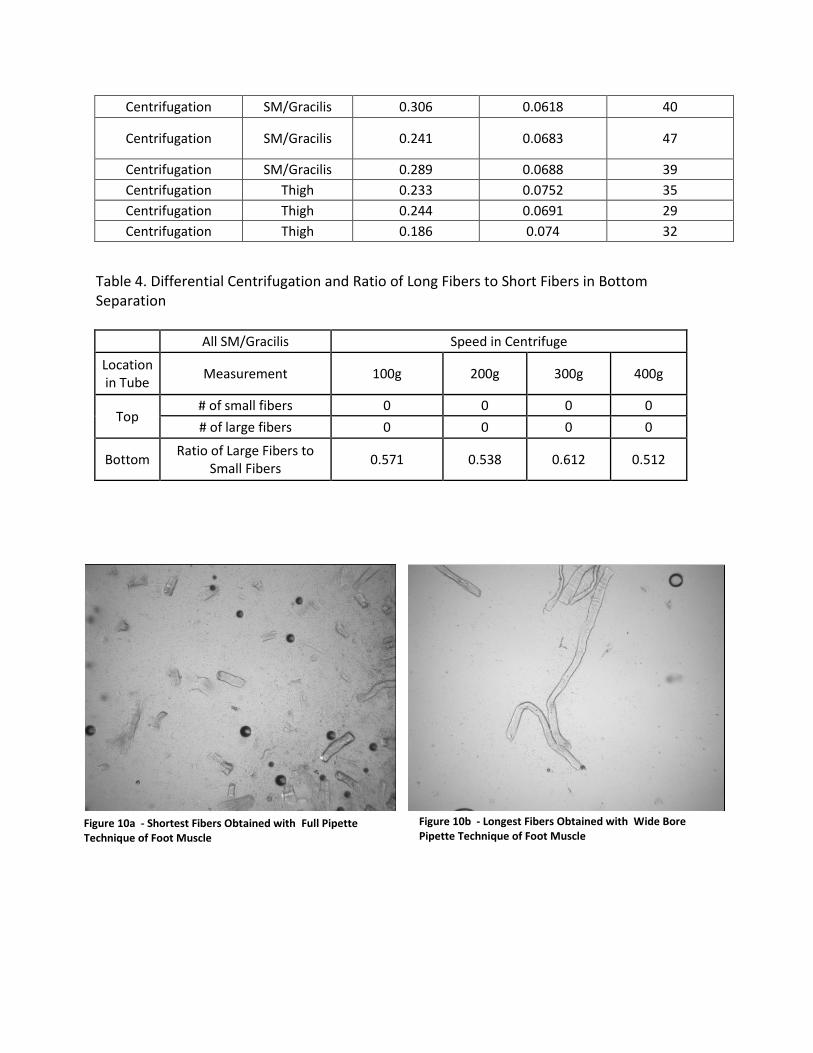
widths were fairly consistent. Comparison of the images for the shortest and longest fibers is

displayed in Figure 10a and 10b. Going a step farther into the centrifugation technique of the

collagenase treatment, results from differential centrifugation of long and short fibers/debris

can be seen in Table 4. The differential centrifugation can indeed act as one method to clean up

the fiber samples. All trials, with the same muscle type, showed that long fibers dominated the

bottom separation of the tubes. Figures 11a and 11b show the supernatant and bottom of the

300g trial.

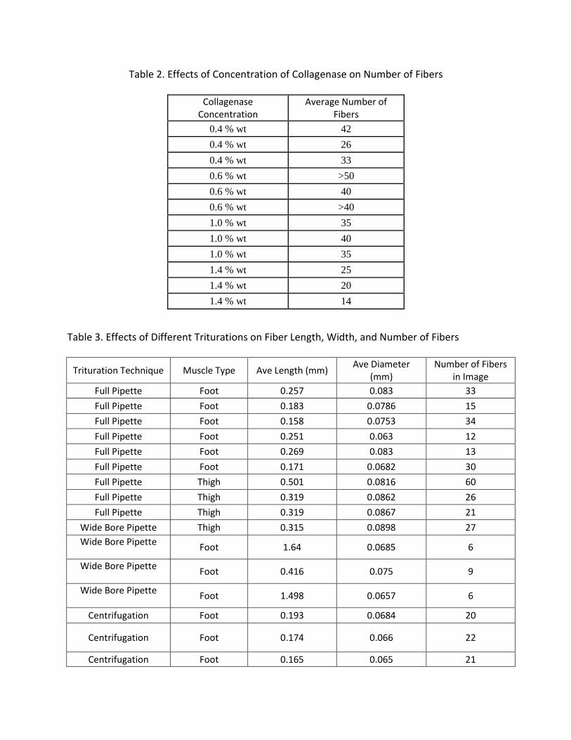
Table 2. Effects of Concentration of Collagenase on Number of Fibers

Collagenase Concentration

Average Number of Fibers

0.4 % wt 42

0.4 % wt 26

0.4 % wt 33

0.6 % wt >50

0.6 % wt 40

0.6 % wt >40

1.0 % wt 35

1.0 % wt 40

1.0 % wt 35

1.4 % wt 25

1.4 % wt 20

1.4 % wt 14

Table 3. Effects of Different Triturations on Fiber Length, Width, and Number of Fibers

Trituration Technique Muscle Type Ave Length (mm) Ave Diameter

(mm) Number of Fibers

in Image

Full Pipette Foot 0.257 0.083 33






Full Pipette Thigh 0.501 0.0816 60



Wide Bore Pipette Thigh 0.315 0.0898 27

Wide Bore Pipette Foot 1.64 0.0685 6



Centrifugation Foot 0.193 0.0684 20



Centrifugation SM/Gracilis 0.306 0.0618 40



Centrifugation Thigh 0.233 0.0752 35



Table 4. Differential Centrifugation and Ratio of Long Fibers to Short Fibers in Bottom Separation

All SM/Gracilis Speed in Centrifuge

Location in Tube

Measurement 100g 200g 300g 400g

Top # of small fibers 0 0 0 0

# of large fibers 0 0 0 0

Bottom Ratio of Large Fibers to

Small Fibers 0.571 0.538 0.612 0.512

Figure 10a - Shortest Fibers Obtained with Full Pipette Technique of Foot Muscle

Figure 10b - Longest Fibers Obtained with Wide Bore Pipette Technique of Foot Muscle

Discussion

Analysis of the results of the different collagenase treatments yields some valuable

information about muscle fiber isolation techniques. For the muscle tissue used, 0.6% (w/v)

concentration of collagenase yielded the greatest number of fibers in treatment, but that does

not necessarily mean that this is the ideal concentration for future isolations. There are a lot of

factors to consider when determining fiber quantity and dimensions, including muscle tissue

type, age, gender, and initial dimensions. Thus, in future experiments, a collagenase

concentration assay, such as the one done in our experiment with same procedures/trituration

technique, must be done in order to determine optimum concentration for each treatment and

muscle tissue used.

When comparing the results of Table 3, it seems that almost all the trituration

techniques meet the criteria for the tapering lengths/widths of the devices. The width is

consistent across all trituration trials, but length varies quite a bit. The wide bore pipette tip

Figure 11a – Top (Supernatant) of Centrifugation of Fibers at 300g

Figure 11b – Bottom of Centrifugation of Fibers at 300g

technique produced much larger fibers than the centrifugation and normal pipette trituration.

In theory, the longer the fibers, the better, as we want to keep the fiber physiologically sound

and preserve them to their original state within the muscle tissue. The lengths within trituration

trials still vary too much to determine average lengths with confidence and really decide on

what technique worked best. The full pipette and centrifugation techniques of trituration may

not be getting long fibers due to the large amounts of shear force that are breaking the fibers

apart. When trying to reduce the force by testing out a wide bore pipette tip, the fibers were

indeed longer, but the quantity was low.

Further experimentation with differential centrifugation provided results as hoped.

Centrifugation aided in the separation of long and short fibers, with over 50% of the bottom

consisting of long fibers. In fact, the supernatant of all the speeds tested showed very small

amounts of fibers and debris. Again, the sample size of muscle tissue quantity/type does not aid

in statistical significance, but it can help in the future with isolation. After treatment with

whichever trituration technique/collagenase concentration chosen, differential centrifugation

can be performed to gather only the long fibers for loading into the devices. 300g seemed to

work the best in our case for the centrifugation speed, but again like the collagenase

concentration, this value would need to be optimized during treatments.

As mentioned previously, variation is indeed present within the length/quantity of fibers

across treatments and can be solved by testing more muscle tissue/types. However, the

statistical variation/insignificance can also be due to methodological errors. One of these errors

lies within the muscle tissue preparation and cutting. Muscle tissue type and physiology do play

roles in fiber isolation, but so does tissue length and structure. When cutting the tissue,

sometimes it was hard to make sure the cut was parallel to the muscle fibers according to

microscopy. Furthermore, it was undecided on what was the proper length/width of tissues

samples to be put into the tubes for treatment. Most studies that use fiber isolation state that

because of the variability of muscle, fiber length should not be a parameter to analyze alone.

Instead, fiber-length-to-muscle-length ratios are often compared to known literature values.7

This means that before treatments, we should have measured the length of the muscle tissue

cut and then determined these ratios for comparison. Another means of improvement for

methods also includes using fresh preparations of collagenase solutions each experiment. To

save time and material, large batches of both were made and preserved in fridge/freezer units.

Loss of collagenase activity could occur and cause treatment to deviate from normal results.

Future

Along with improvement of statistical and methodological errors, improvement can be

made by introducing new possible collagenase treatments. One treatment that was attempted

in this study, but yielded poor results, was a treatment involving magnetic fixation. After muscle

tissue preparation, the tissue was attached to a small dissection pin and stabilized. The muscle

on the pin was then placed into a small piece of tubing and held in place with a strong magnet.

The goal was deliver the collagenase solution directly to the stationary muscle so that the

muscle fibers were not gently peeled away with the delivery of the wash buffer. Issues did arise

from the muscle being so degraded after treatments that it easily slipped from the pin. If we

could figure out a better way to keep the muscle stationary, this treatment could relay valuable

results. Another possibility in changing up the treatment involves different preparation and use

of collagenase solution. Some research and studies use different dissolving buffers for the

collagenase and different incubation conditions for degradation of the muscle tissue. For

example, Dr. Starkey, of the University of Connecticut, prepared muscle fibers in a study on

satellite cells using DMEM as the dissolving buffer, performing a 90 minute incubation period

with the muscle/collagnease solution mixture, and triturating with fire-polished Pasteur

pipettes. Perhaps the change in the buffer/incubation alters the contraction of the fibers.8

Since the trituration of the fibers during the collagenase treatment induces fiber

fragments and damage, it is also important to make sure that the fibers are still functional after

treatment. The easiest way to do this would be to check membrane sealing. Like most cells,

when the membrane is disrupted or damaged, the cell acts quickly in repair and reformation.

Membrane sealing of the disrupted fibers can be tracked after trituration by using propidium

iodide as a dye within the cells and using fluorescent microscopy to track changes in membrane

formation.

Once the devices are fabricated, the next step in measuring how well fibers are isolated

would be to try to trap them within devices. Methods on how to load the fibers would need to

be experimented with, but after loading, the pressure gradient can be monitored/optimized to

ensure proper flow of the fibers within devices. The flow and capture of the fibers will be

analyzed through the use of bright field and fluorescent microscopy. After fibers are trapped,

physiological properties of the fibers, such as ROS and mitochondrial mass, can be evaluated

with florescent microscopy.

Conclusion

Multiple collagenase treatments were performed to yield fibers that fit the criteria of

the tapered regions of the microfluidic devices. The 0.6% (w/v) collagenase concentration

yielded the largest number of fibers, the wide bore pipette tip method of trituration had the

longest fibers in length, and centrifugation can be used to separate lengths of strands. In all

tests, however, results vary and statistical significance is lacking. Use of a larger sample size of

muscle tissue quantity/type and adjustments to methodology ae required. Future work includes

preparation of a new approach to applying collagenase more directly and not disrupting fibers,

changing preparation/incubation of collagenase solution, researching more about intact

satellite cells on isolated fibers, checking fiber functionality with membrane sealing, and

eventually testing out isolated fiber response in the future fabricated devices.

Acknowledgements

I would like to thank Dr. Arriaga, Dr. Donoghue, and the rest of the Arriaga Organelle

Research Group for all of the mentoring and support they have given me during this extensive

project. Also, special thanks should be given to Dr. Thompson and her lab for donating muscle

for testing.

References

1 Muscle Fiber. (2011). Retrieved December 21, 2011, from:

http://www.nvo.com/jin/nss-folder/scrapbookanatomy/muscle1fiber.jpg.

2 Cross-Bridge Cycle. (2011) Retrieved December 21, 2011, from:

http://faculty.irsc.edu/

FACULTY/TFischer/AP1/cross%20bridge%20cycle.jpg

3 Widmaier, Eric, et al. Vander’s Human Physiology, Twelfth Edition. McGraw-Hill,

2011.

4 Alberts, Bruce, et al. Essential Cell Biology. Second Edition. New York, NY: Garland

Science, 2004.

5 Brown, Andrew et al. "Microfluidics," California Engineer 86(1), Aug 2007: 20-24.

6 Whitsides, George M. et al. “A Microfabricated Array of Clamps for Immobilization

and Imaging C. elegans,” Lab Chip 7, May 2007: 1515-23.

7 Burkholder, Thomas J, et al. “Relationship Between Muscle Fiber Types and Sizes and

Muscle Architectural Properties in the Mouse Hindlimb,” Journal of Morphology 221,

1994: 177-90.

8 Starkey, Jessica D, et al. “Skeletal Muscle Satellite Cells Are Committed to Myogenesis

and Do Not Spontaneously Adopt Nonmyogenic Fates,” Journal of Histochemistry &

Cytochemistry 59(1), February 2011: 33-46.

isolation of single muscle fibers in preparation for

Documents