ispa / scea 2008 joint international conference huis ter ...menzies.us/pdf/08ispa.pdf · ispa /...

ISPA / SCEA 2008 Joint International Conference

Huis ter Duin, Noordwijk, The Netherlands, 12 – 14 May 2008

2CEE, A TWENTY FIRST CENTURY EFFORT ESTIMATION METHODOLOGY

Jairus Hihn

Karen Lum

Jet Propulsion Laboratory/

California Institute of Technology

[email protected]

[email protected]

Tim Menzies

Dan Baker

Omid Jalali

Lane Dept. CSEE

West Virginia University

[email protected]

[email protected] [email protected]

Abstract1

There exists an extensive academic literature on software cost estimation that explores techniques such as boot

strapping, assorted analogy methods such as nearest neighbor, and even highly non-linear ‘models’ such as

decision trees. However, industry “best practice” virtually ignores the academic literature and continues to

rely upon standard regression-based algorithms and most often local calibration. Local calibration only

calibrates or tunes the main intercept and slope in a log-linear regression. Over the past three years our

research has been investigating the behavior and performance of these various models and calibration/tuning

techniques using machine learning methods. A summary of our preliminary findings was presented in 2006 at

the 28th Annual Conference of the International Society of Parametric Analysts. While all of the analysis has

been performed on NASA software project COCOMO data, the results should easily extend to systems and size

estimation models.

Our work cautions that current approaches to model specification and calibration can often produce sub-

optimal models, which are likely to be a significant contributor to the cost growth exhibited by most software

projects. This paper will provide an overview of the systemic cost estimation issues that have been identified,

and a description of the best performing tuning techniques. While we have found that COCOMO is a very robust

model, our results also indicate that local calibration using boot strapping over standard regression, combined

with variable reduction (column pruning) and stratification (row pruning using nearest neighbor) is in the vast

majority of experiments the most efficient and effective tuning method.

Our research findings are captured in what we call the 21st Century Effort Estimation Methodology (2cee).

2cee has been encoded in a Windows based tool that can be used to both generate an estimate and allow the

model developer to calibrate and develop models using these techniques.

I. INTRODUCTION

In the 21st century, software managers have access to many different estimation tools. So how does one

determine what is the right model to use over varying domains and organizations? How does one determine the

best way to calibrate or tune their models to a local environment? Different commercial vendors recommend

different methods. Whose method is better? Are they all equally valid? This is a more serious problem than

generally recognized because of the underlying large variance problem that is typically found in cost and effort

data sets [1]. The variance problem causes model brittleness and makes it difficult to distinguish performance

across various models. This is a pressing problem since effort estimates are often inaccurate. Early lifecycle

effort estimates can be inaccurate by up to 400% [2, p310]. In 2001, the Standish group reported that, 53% of

U.S. software projects ran over 189% of the original estimate [3]. In a study of NASA software development

projects, the most frequently identified cause (71%) of cost overrun with the largest impact (35% contribution to

observed cost growth) was basic failures in planning, estimation & control [4]. So the question becomes, how

can we stop project managers and sometimes cost estimators from using the wrong (i.e. sometimes the worst)

method just because it is convenient?

Clearly, better software estimation techniques are needed. It became quickly apparent in the early stages of our

research task that there was a major disconnect between the techniques used by estimation practitioners and the

numerous ideas being addressed in the research community as has been demonstrated by the wide variety of

estimation techniques that have been proposed in the academic literature including clustering [5], neural

1 The research described in this abstract was carried out at the Jet Propulsion Laboratory, California Institute of

Technology, under a contract with the National Aeronautics and Space Administration. Reference herein to any

specific commercial product, process, or service by trade name, trademark, manufacturer, or otherwise, does not

constitute or imply its endorsement by the United States Government.



2

networks [6], and case-based reasoning [7]. However, in industry, the most commonly-used formal techniques

are parametric model and regression-based techniques such as those used in COCOMO 81 [2], COCOMO II [8],

SEER-SEM [9], PRICE-S [10], and SLIM [11].

Unfortunately, there are very few published studies that empirically compare this diverse set of techniques.

Those that have, such as Briand et al. [12], Smith and Mason [13], Finnie et al. [14], Gray and MacDonnell[15],

Mair et al. [6], and Shepperd and Kadoda [16] are limited in scope. In addition, the commonly found studies are

more narrowly focused, such as those conducted by Kemerer [17], Lum et al. [1], and Ferens and Christensen

[18] that test linear regression models in different environments. Given the need, why aren’t there more studies

comparing software effort models?

It also became clear that many fundamental estimation questions were not being addressed:

• What is a model’s real estimation uncertainty?

• How many records are required to calibrate?

o Answers have varied from 1-20 just for the intercept

o If we do not have enough data what is the impact on model uncertainty

• Data is expensive to collect and maintain so minimizing the number of cost drivers and effort

multipliers is important

o But what are the right ones to keep?

o When should we build domain specific models?

• What are the best functional forms?

• What are the best ways to tune/calibrate a model?

Data mining techniques provide the rigorous toolset required to explore the many dimensions of the estimation

model calibration problem in a repeatable manner by supporting the following analysis capabilities:

• Different calibration and validation datasets

• Analysis of both standard and non-standard models

• Exhaustive searches over all parameters and records in order to guide data pruning

o Pruning rows (stratification)

o Pruning columns (variable reduction)

• Multiple measures for evaluating model performance

o We have even been able to determine what performance measures are best

This article reports on a five-year study using data mining techniques to identify the best performing models and

best calibration techniques with an introduction to the estimation tool (2cee) we developed to incorporate what

we identified as best practice2. This paper consists of the following sections:

• Data

• The Conclusion Instability Problem and the Need for Non-Parametric Based Tests

• Overview of Experiments and Results,

• Overview of 2cee

• Conclusion and Summary

II. DATA

The data used in the analysis is from the original 63 records in the COCOMO 81 dataset (Coc81) and a

historical NASA dataset we refer to as Nasa93 as it has 93 flight and ground records form multiple NASA

Centers that completed from the late 1970’s through the late 1980’s. The Nasa93 data has been in the public

domain for many years but few have been aware of it. It can now be found at the PROMISE (Predictor Models

in Software Engineering) web site.3 PROMISE is an organization of software engineers working to organize

datasets that can be used to verify existing studies and to make data available for future research. To participate

in a PROMISE workshop one must promise to make their data available to the PROMISE repository.

In this study, we used a data mining techniques to build and validate effort estimation models based on the

COCOMO model parameters. Over 150 model variations were studied using all or some part of two COCOMO

81 data sets (Nasa93 and Coc81). Each part selected some subset of the total records. The parts and data sets are

described in more detail in Figure 1 See [19] for a more extensive write up on the data sets.

2 The research task was funded by the NASA Office of Safety and Mission Assurance Software Assurance

Research Program operated by the NASA Independent Verification & Validation Facility. 3 http://promise.site.uottawa.ca/SERepository/



3

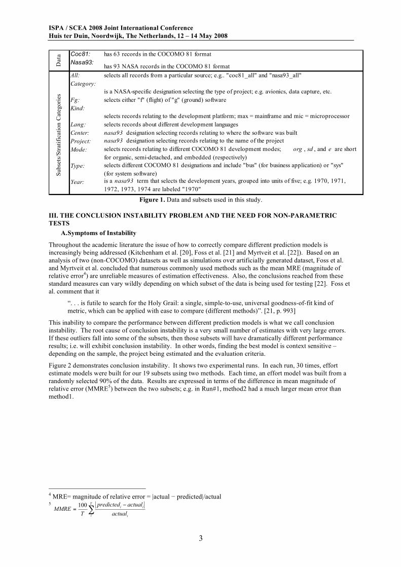
Coc81: has 63 records in the COCOMO 81 format

Nasa93:has 93 NASA records in the COCOMO 81 format

All: selects all records from a particular source; e.g.. "coc81_all" and "nasa93_all"

Category:

is a NASA-specific designation selecting the type of project; e.g. avionics, data capture, etc.

Fg: selects either "f" (flight) of "g" (ground) software

Kind:

selects records relating to the development platform; max = mainframe and mic = microprocessor

Lang: selects records about different development languages

Center: nasa93 designation selecting records relating to where the software was built

Project: nasa93 designation selecting records relating to the name of the project

Mode: selects records relating to different COCOMO 81 development modes; org , sd , and e are short

for organic, semi-detached, and embedded (respectively)

Type: selects different COCOMO 81 designations and include "bus" (for business application) or "sys"

(for system software)

Year: is a nasa93 term that selects the development years, grouped into units of five; e.g. 1970, 1971,

1972, 1973, 1974 are labeled "1970"

Data

Su

bse

ts/S

trat

ific

atio

n C

ateg

ori

es

Figure 1. Data and subsets used in this study.

III. THE CONCLUSION INSTABILITY PROBLEM AND THE NEED FOR NON-PARAMETRIC

TESTS

A. Symptoms of Instability

Throughout the academic literature the issue of how to correctly compare different prediction models is

increasingly being addressed (Kitchenham et al. [20], Foss et al. [21] and Myrtveit et al. [22]). Based on an

analysis of two (non-COCOMO) datasets as well as simulations over artificially generated dataset, Foss et al.

and Myrtveit et al. concluded that numerous commonly used methods such as the mean MRE (magnitude of

relative error4) are unreliable measures of estimation effectiveness. Also, the conclusions reached from these

standard measures can vary wildly depending on which subset of the data is being used for testing [22]. Foss et

al. comment that it

“. . . is futile to search for the Holy Grail: a single, simple-to-use, universal goodness-of-fit kind of

metric, which can be applied with ease to compare (different methods)”. [21, p. 993]

This inability to compare the performance between different prediction models is what we call conclusion

instability. The root cause of conclusion instability is a very small number of estimates with very large errors.

If these outliers fall into some of the subsets, then those subsets will have dramatically different performance

results; i.e. will exhibit conclusion instability. In other words, finding the best model is context sensitive –

depending on the sample, the project being estimated and the evaluation criteria.

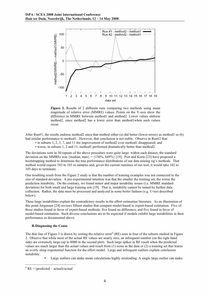
Figure 2 demonstrates conclusion instability. It shows two experimental runs. In each run, 30 times, effort

estimate models were built for our 19 subsets using two methods. Each time, an effort model was built from a

randomly selected 90% of the data. Results are expressed in terms of the difference in mean magnitude of

relative error (MMRE5) between the two subsets; e.g. in Run#1, method2 had a much larger mean error than

method1.

4 MRE= magnitude of relative error = |actual ! predicted|/actual

5 !

"=

T

i i

ii

actual

actualpredicted

TMMRE

100



4

Figure 2. Results of 2 different runs comparing two methods using mean

magnitude of relative error (MMRE) values. Points on the Y-axis show the

difference in MMRE between method1 and method2. Lower values endorse

method2, since method2 has a lower error than method1when such values

occur.

After Run#1, the results endorse method2 since that method either (a) did better (lower errors) as method1 or (b)

had similar performance to method1. However, that conclusion is not stable. Observe in Run#2 that:

• in subsets 1, 2, 3, 7, and 11 the improvement of method2 over method1 disappeared; and

• worse, in subsets 1, 2 and 11, method1 performed dramatically better than method2.

The deviations seen in 30 repeats of the above procedure were quite large: within each dataset, the standard

deviation on the MMREs was {median, max} = {150%, 649%} [19]. Port and Korte [23] have proposed a

bootstrapping method to determine the true performance distributions of our data mining rig’s methods. That

method would require 102 to 103 re-samples and, given the current runtimes of our tool, it would take 102 to

103 days to terminate.

One troubling result from the Figure 2 study is that the number of training examples was not connected to the

size of standard deviation. A pre-experimental intuition was that the smaller the training set, the worse the

prediction instability. On the contrary, we found minor and major instability issues (i.e. MMRE standard

deviation) for both small and large training sets [19]. That is, instability cannot be tamed by further data

collection. Rather, the data must be processed and analyzed in some better fashion (e.g. U-test described

below).

These large instabilities explain the contradictory results in the effort estimation literature. As an illustration of

this point Jorgensen [24] reviews fifteen studies that compare model-based to expert-based estimation. Five of

those studies found in favor of expert-based methods; five found no difference; and five found in favor of

model-based estimation. Such diverse conclusions are to be expected if models exhibit large instabilities in their

performance as documented above.

B. Diagnosing the Cause

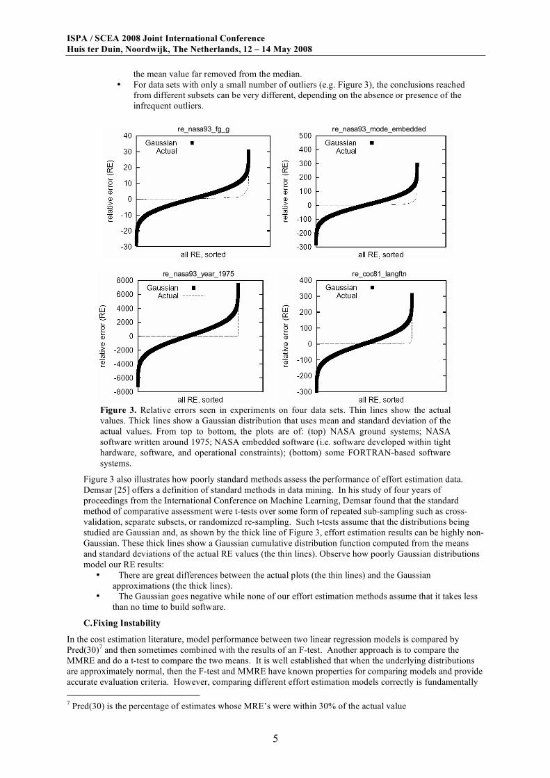
The thin line of Figure 3 is drawn by sorting the relative error6 (RE) seen in four of the subsets studied in Figure

2. Observe that while most of the actual RE values are nearly zero, an infrequent number (on the right hand

side) are extremely large (up to 8000 in the second plot). Such large spikes in RE result when the predicted

values are much larger than the actual values and result from (1) noise in the data or (2) a training set that learns

an overly steep exponential function for the effort model. Large and infrequent outliers explain conclusion

instability:

• Large outliers can make mean calculations highly misleading. A single large outlier can make

6 RE = (predicted ! actual)/actual



5

the mean value far removed from the median.

• For data sets with only a small number of outliers (e.g. Figure 3), the conclusions reached

from different subsets can be very different, depending on the absence or presence of the

infrequent outliers.

re_coc81_langftn re_nasa93_year_1975

re_nasa93_fg_g re_nasa93_mode_embedded

Figure 3. Relative errors seen in experiments on four data sets. Thin lines show the actual

values. Thick lines show a Gaussian distribution that uses mean and standard deviation of the

actual values. From top to bottom, the plots are of: (top) NASA ground systems; NASA

software written around 1975; NASA embedded software (i.e. software developed within tight

hardware, software, and operational constraints); (bottom) some FORTRAN-based software

systems.

Figure 3 also illustrates how poorly standard methods assess the performance of effort estimation data.

Demsar [25] offers a definition of standard methods in data mining. In his study of four years of

proceedings from the International Conference on Machine Learning, Demsar found that the standard

method of comparative assessment were t-tests over some form of repeated sub-sampling such as cross-

validation, separate subsets, or randomized re-sampling. Such t-tests assume that the distributions being

studied are Gaussian and, as shown by the thick line of Figure 3, effort estimation results can be highly non-

Gaussian. These thick lines show a Gaussian cumulative distribution function computed from the means

and standard deviations of the actual RE values (the thin lines). Observe how poorly Gaussian distributions

model our RE results:

• There are great differences between the actual plots (the thin lines) and the Gaussian

approximations (the thick lines).

• The Gaussian goes negative while none of our effort estimation methods assume that it takes less

than no time to build software.

C. Fixing Instability

In the cost estimation literature, model performance between two linear regression models is compared by

Pred(30)7 and then sometimes combined with the results of an F-test. Another approach is to compare the

MMRE and do a t-test to compare the two means. It is well established that when the underlying distributions

are approximately normal, then the F-test and MMRE have known properties for comparing models and provide

accurate evaluation criteria. However, comparing different effort estimation models correctly is fundamentally

7 Pred(30) is the percentage of estimates whose MRE’s were within 30% of the actual value



6

difficult because the underlying distributions have very large variances and tend to be heavily skewed. We

typically deal with this by assuming our models are multiplicative and working with the natural logarithms (ln)

of the variables, which will make the normality assumptions more tenable. However, how often do we really

test our assumptions? If the underlying assumptions are violated, then the standard statistical tests are

invalidated. The problem becomes significantly worse if we want to compare non-linear models or compare

very different types of models such as nearest neighbor with a regression-based prediction model. Pred(30)

which can be viewed as a variant of a rank order statistic is intuitively attractive and it is easy to compute but it

has no known properties. The unanswered question is how do we know if a Pred(30) of 50% is significantly

better then a Pred(30) of 60%? We currently do not. The textbook response from the statistics literature is that

non-parametric tests need to be used because non-parametric tests make no assumptions about the population or

sample distributions. Non-parametric tests are typically derived from computing statistics from the rank order

of the data. A median (fiftieth percentile) is an example of a non-parametric statistic, where the mean is not.

Mann and Whitney’s 1947 modification [26] to the Wilcoxon rank-sum test (proposed along with his signed-

rank test) is the test we prefer because:

• The Mann-Whitney U-test does not require that the sample sizes be the same. So, in a single U-test,

learner L1 can be compared to all its rivals.

• The U-test does not require any post-processing (such as the Friedman test) to conclude if the median

rank of one population (say, the L1 results) is greater than, equal to, or less than the median rank of

another (say, the L2, L3, .., Lx results).

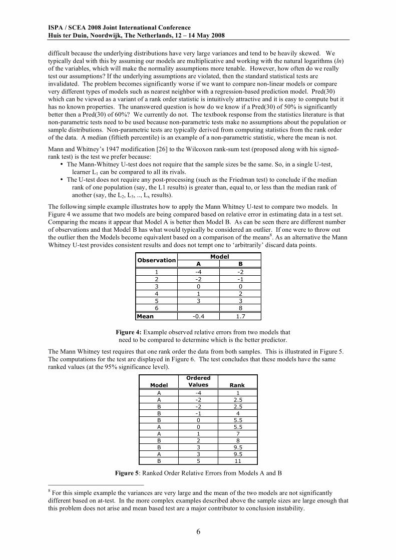
The following simple example illustrates how to apply the Mann Whitney U-test to compare two models. In

Figure 4 we assume that two models are being compared based on relative error in estimating data in a test set.

Comparing the means it appear that Model A is better then Model B. As can be seen there are different number

of observations and that Model B has what would typically be considered an outlier. If one were to throw out

the outlier then the Models become equivalent based on a comparison of the means8. As an alternative the Mann

Whitney U-test provides consistent results and does not tempt one to ‘arbitrarily’ discard data points.

A B

1 -4 -2

2 -2 -1

3 0 0

4 1 2

5 3 3

6 8

Mean -0.4 1.7

ObservationModel

Figure 4: Example observed relative errors from two models that

need to be compared to determine which is the better predictor.

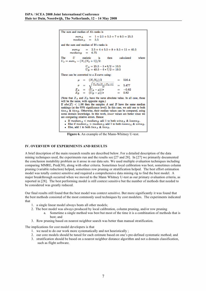
The Mann Whitney test requires that one rank order the data from both samples. This is illustrated in Figure 5.

The computations for the test are displayed in Figure 6. The test concludes that these models have the same

ranked values (at the 95% significance level).

Model

Ordered

Values Rank

A -4 1

A -2 2.5

B -2 2.5

B -1 4

B 0 5.5

A 0 5.5

A 1 7

B 2 8

B 3 9.5

A 3 9.5

B 5 11

Figure 5: Ranked Order Relative Errors from Models A and B

8 For this simple example the variances are very large and the mean of the two models are not significantly

different based on at-test. In the more complex examples described above the sample sizes are large enough that

this problem does not arise and mean based test are a major contributor to conclusion instability.



7

Figure 6. An example of the Mann-Whitney U-test.

IV. OVERVIEW OF EXPERIMENTS AND RESULTS

A brief description of the main research results are described below. For a detailed description of the data

mining techniques used, the experiments run and the results see [27 and 28]. In [27] we primarily documented

the conclusion instability problem as it arose in our data sets. We used multiple evaluation techniques including

comparing MMRE, Pred(30), along with other criteria. Sometimes local calibration was best, sometimes column

pruning (variable reduction) helped, sometimes row pruning or stratification helped. The best effort estimation

model was totally context sensitive and required a comprehensive data mining rig to find the best model. A

major breakthrough occurred when we moved to the Mann Whitney U-test as our primary evaluation criteria, as

reported in [28]. The best performing model is still context sensitive but the number of methods that needed to

be considered was greatly reduced.

Our final results still found that the best model was context sensitive. But more significantly it was found that

the best methods consisted of the most commonly used techniques by cost modelers. The experiments indicated

that

1. a single linear model always beats all other models;

2. The best model was always produced by local calibration, column pruning, and/or row pruning

a. Sometime a single method was best but most of the time it is a combination of methods that is

best; and

3. Row pruning based on nearest neighbor search was better than manual stratification.

The implications for cost model developers is that

1. we need to do our work more systematically and not heuristically ;

2. our core models should be tuned for each estimate based on one’s pre-defined systematic method; and

3. stratification should be based on a nearest neighbor distance algorithm and not a domain classification,

such as flight software.



8

V. OVERVIEW OF 2CEE

All of the methods described in this paper have been implemented in the software estimation tool 2cee9 (21

st

Century Effort Estimation Methodology). 2cee has been encoded in a Windows based tool that can be used to

both generate an estimate and allow the model developer to calibrate and develop models using these techniques

for COCOMO II data sets.

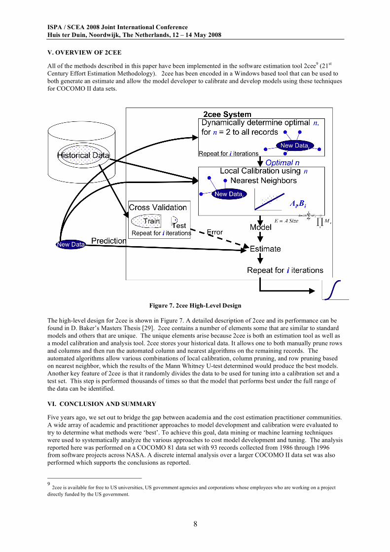
Figure 7. 2cee High-Level Design

The high-level design for 2cee is shown in Figure 7. A detailed description of 2cee and its performance can be

found in D. Baker’s Masters Thesis [29]. 2cee contains a number of elements some that are similar to standard

models and others that are unique. The unique elements arise because 2cee is both an estimation tool as well as

a model calibration and analysis tool. 2cee stores your historical data. It allows one to both manually prune rows

and columns and then run the automated column and nearest algorithms on the remaining records. The

automated algorithms allow various combinations of local calibration, column pruning, and row pruning based

on nearest neighbor, which the results of the Mann Whitney U-test determined would produce the best models.

Another key feature of 2cee is that it randomly divides the data to be used for tuning into a calibration set and a

test set. This step is performed thousands of times so that the model that performs best under the full range of

the data can be identified.

VI. CONCLUSION AND SUMMARY

Five years ago, we set out to bridge the gap between academia and the cost estimation practitioner communities.

A wide array of academic and practitioner approaches to model development and calibration were evaluated to

try to determine what methods were ‘best’. To achieve this goal, data mining or machine learning techniques

were used to systematically analyze the various approaches to cost model development and tuning. The analysis

reported here was performed on a COCOMO 81 data set with 93 records collected from 1986 through 1996

from software projects across NASA. A discrete internal analysis over a larger COCOMO II data set was also

performed which supports the conclusions as reported.

9 2cee is available for free to US universities, US government agencies and corporations whose employees who are working on a project

directly funded by the US government.



9

Traditional approaches to model development and tuning is to develop a simple regression model for internal

use or to use a commercial tool that can estimate across a large number of domains. The result in the latter case

is models with a large number of inputs. Typically tuning to local data is done very infrequently and consists of

adjusting some combination of the intercept, slope and range of possible values for a model input. When using

these models, estimators tend to provide values for all inputs even when they are not really relevant to one’s

local domain. From a research perspective, the existing general purpose models do provide a parameter set that

fully spans the possible space of parameters that one should consider.

Academics derive whole new models from their data and try to compare very different models, such as analogy

models versus regression models. Because they approach the estimation problem from a much broader

perspective they have run into a different set of problems – some of which are red herrings but some would

improve the state of practice in the cost estimation community.

The most important results with respect to how we as estimation practitioners do business are

Use non-parametric tests more often

From the academic literature we learned that there were difficulties determining what model is best

because of the existence of large outliers as well as kurtosis in the underlying population distributions.

We also ended up rediscovering that non-parametric tests, like the Mann Whitney U-test, are the more

robust tests under these conditions. The implication is that in industry we are misusing standard Gaussian

based tests, such as the t-test.

Tune or calibrate our models more frequently and with a larger set of methods

We find what is the best tuning for a model is context sensitive so that every time one estimates, a local

tuning should be performed, but one need only consider a small number of basic methods. These basic

methods are a simple extension of the heuristic techniques we commonly use: local calibration,

stratification, and column pruning. Stratification is most effective by accounting for similarities in the

model parameter values, not just assuming that all software projects fall in a common type (e.g. flight or

ground data systems).



10

REFERENCES

[1] K. Lum, J. Powell, and J. Hihn, “Validation of spacecraft cost estimation models for flight and ground systems,” in

ISPA Conference Proceedings, Software Modeling Track, May 2002.

[2] B. Boehm, Software Engineering Economics. Prentice Hall, 1981.

[3] “The Standish Group Report: Chaos 2001,” 2001, available from http: //standishgroup.com/sample

research/PDFpages/extreme chaos.pdf.

[4] J. Hihn and H. Habib-agahi, “Identification and measurement of the sources of flight software cost growth,” in

Proceedings of the 22nd Annual Conference of the International Society of Parametric Analysts (ISPA), Noordwijk,

Netherlands, 8-10 May 2000.

[5] M. Garre, M. S. J.J. Cuadrado-Gallego, M. Charro, and D. Rodriguez, “Segmented parametric software estimation

models: Using the em algorithm with the isbsg 8 database,” in 27th International Conference on Information

Technology Interfaces. ITI 2005, Dubrovnik, Croatia, 2005.

[6] C. Mair, G. Kadoda, M. Lefley, K. Phalp, C. Schofield, M. Shepperd, and S. Webster, “An investigation of machine

learning based prediction systems,” The Journal of Systems and Software, vol. 53, no. 1, pp. 23–29, 2000. [Online].

Available: citeseer.ist.psu.edu/mair99investigation.html

[7] M. Shepperd and C. Schofield, “Estimating software project effort using analogies,” IEEE Transactions on Software

Engineering, vol. 23, no. 12, November 1997, available from http://www.utdallas.edu/~rbanker/SE XII.pdf.

[8] B. Boehm, E. Horowitz, R. Madachy, D. Reifer, B. K. Clark, B. Steece, A. W. Brown, S. Chulani, and C. Abts,

Software Cost Estimation with Cocomo II. Prentice Hall, 2000.

[9] R. Park, “The central equations of the price software cost model,” in 4th COCOMO Users Group Meeting,

November 1988.

[10] R. Jensen, “An improved macrolevel software development resource estimation model,” in 5th ISPA Conference,

April 1983, pp. 88–92.

[11] L. Putnam and W. Myers, Measures for Excellence. Yourdon Press Computing Series, 1992.

[12] L. Briand, T. Langley, and I. Wieczorek, “A replicated assessment and comparison of common software cost

modeling techniques,” in Proceedings of the 22nd International Conference on Software Engineering, Limerick,

Ireland, 2000, pp. 377–386.

[13] A. Smith and A. Mason, “Cost estimation predictive modeling: Regression versus neural network,” The Engineering

Economist, vol. 42, no. 2, pp. 137–161, 1997.

[14] G. Finnie, G. Wittig, and J. Desharnais, “A comparison of software effort estimation techniques: Using function

points with neural networks, case-based reasoning and regression models,” Journal of Systems and Software, vol. 39,

no. 3, pp. 281–289, 1997.

[15] A. Gray and S. MacDonnell, “A comparison of techniques for developing predictive models of software metrics,”

Information and Software Technology, vol. 39, 1997.

[16] M. Shepperd and G. Kadoda, “Comparing software prediction techniques using simulation,” IEEE Transactions on

Software Engineering, vol. 27, no. 11, Nov. 2001.

[17] C. Kemerer, “An empirical validation of software cost estimation models,” Communications of the ACM, vol. 30, no.

5, pp. 416–429, May 1987.

[18] D. Ferens and D. Christensen, “Calibrating software cost models to Department of Defense Database: A review of

ten studies,” Journal of Parametrics, vol. 18, no. 1, pp. 55–74, November 1998.

[19] T. Menzies, Z. Chen, J. Hihn, and K. Lum, “Selecting best practices for effort estimation,” IEEE Transactions on

Software Engineering, November 2006, available from http://menzies.us/pdf/06coseekmo.pdf.

[20] B. A. Kitchenham, E. Mendes, and G. H. Travassos, “Cross- vs. within-company cost estimation studies: A systematic

review,” IEEE Transactions on Software Engineering, pp. 316–329, May 2007.

[21] T. Foss, E. Stensrud, B. Kitchenham, and I. Myrtveit, “A simulation study of the model evaluation criterion MMRE,”

IEEE Transactions on Software Engineering, vol. 29, no. 11, pp. 985 – 995, November 2003.

[22] I. Myrtveit, E. Stensrud, and M. Shepperd, “Reliability and validity in comparative studies of software prediction

models,” IEEE Transactions on Software Engineering, vol. 31, no. 5, pp. 380–391, May 2005.

[23] D. Port and M. Korte, “Comparative studies of the model evaluation criterions MMRE and Pred in software cost

estimation research,” Proceedings of the Predictor Models in Software Engineering Workshop, 2008.

[24] M. Jorgensen, “A review of studies on expert estimation of software development effort,” Journal of Systems and

Software, vol. 70, no. 1-2, pp. 37–60, 2004.

[25] J. Demsar, “Statistical comparisons of classifiers over multiple data sets,” Journal of Machine Learning

Research, vol. 7, pp. 1–30, 2006, available from http://jmlr.csail.mit.edu/papers/v7/demsar06a.html.

[26] H. B. Mann and D. R. Whitney, “On a test of whether one of two random variables is stochastically larger

than the other,” Ann. Math. Statist., vol. 18, no. 1, pp. 50–60, 1947, available online at

http://projecteuclid.org/DPubS?service=

[27] K. Lum, J. Hihn, and T. Menzies, “Studies in software cost model behavior: do we really understand cost

model performance,” ISPA 2006 Conference Proceedings, Seattle, WA, May 2006.

[28] T. Menzies, O. Jalali, J. Hihn, D. Baker, and K. Lum, Identifying the “Best” Software Prediction Models

Requires a Combination of Methods, Transactions on Software Engineering (in review), 2008.

[29] D.R. Baker, A Hybrid Approach to Expert and Model based Effort Estimation, Masters Thesis, West

Virginia University, 2007.



11

Jairus Hihn is a Principal Member of the Engineering staff at NASA’s Jet Propulsion

Laboratory and is currently the manager for the Software Quality Improvement Projects Measurement

Estimation and Analysis Element, which is establishing a laboratory wide software metrics and software

estimation program at JPL. M&E’s objective is to enable the emergence of a quantitative software management

culture at JPL. He has a Ph.D. in Economics from the University of Maryland. He has been developing

estimation models and providing software and mission level cost estimation support to JPL’s Deep Space

Network and flight projects since 1988. He has extensive experience in simulation and Monte Carlo methods

with applications in the areas of decision analysis, institutional change, R&D project selection cost modeling,

and process models. email [email protected]

Karen Lum is a senior member of the technical staff at the Jet Propulsion Laboratory,

involved in the collection of software metrics, and the development of software cost estimating relationships.

She is currently pursuing her PhD in Information Systems from Claremont Graduate University. She has a

MBA in Business Economics and a Certificate in Advanced Information Systems from the California State

University, Los Angeles. She has a BA in Economics and Psychology from the University of California at

Berkeley. She is one of the main authors of the JPL Software Cost Estimation Handbook. Publications include

Best Conference Paper for ISPA 2002: Validation of Spacecraft Software Cost Estimation Models for Flight and

Ground Systems. email: [email protected]

Tim Menzies is an associate professor at the Lane Department of Computer Science at the

University of West Virginia (USA), and has been working with NASA on software quality issues since 1998.

He has a CS degree and a PhD from the University of New South Wales. His recent research concerns modeling

and learning with a particular focus on light weight modeling methods. His doctoral research aimed at

improving the validation of, possibly inconsistent, knowledge-based systems in the QMOD specification

language. He also has worked as an object-oriented consultant in industry and has authored over 150

publications and served on numerous conference and workshop programs and well as guest editor of journal

special issues. email [email protected]

Daniel R. Baker is a software developer for Epic Systems in Madison, WI, USA. He was completing his

masters in computer science at West Virginia University when this research was conducted. He spent the

summer of 2007 at NASA’s Jet Propulsion Laboratory to wrap up- the development of 2cee. e-mail:

[email protected].

Omid Jalali is a master's student in computer science in West Virginia University. He is currently working

under the supervision of Dr. Tim Menzies. His current research focuses on the evaluation bias present in

comparing effort estimation methods.

ispa / scea 2008 joint international conference huis ter ...menzies.us/pdf/08ispa.pdf · ispa /...

Documents