isr technical report 2010-11 stochastic average consensus filter
TRANSCRIPT

The InsTITuTe for sysTems research
Isr develops, applies and teaches advanced methodologies of design and analysis to solve complex, hierarchical, heterogeneous and dynamic prob-lems of engineering technology and systems for industry and government.
Isr is a permanent institute of the university of maryland, within the a. James clark school of engineering. It is a graduated national science
foundation engineering research center.
www.isr.umd.edu
Stochastic Average Consensus Filter for Distributed HMM Filtering: Almost Sure Convergence
Nader GhasemiSubhrakanti Dey John S. Baras
Isr TechnIcal rePorT 2010-11
Stochastic Average Consensus Filter for Distributed HMM Filtering:Almost Sure Convergence
Nader Ghasemi, Student Member, IEEE, Subhrakanti Dey, Senior Member, IEEE,and John S. Baras, Fellow, IEEE
Abstract—This paper studies almost sure convergence of adynamic average consensus algorithm which allows distributedcomputation of the product of n time-varying conditional prob-ability density functions. These conditional probability densityfunctions (often called as “belief functions”) correspond to theconditional probability of observations given the state of anunderlying Markov chain, which is observed by n different nodeswithin a sensor network. The network topology is modeled asan undirected graph. The average consensus algorithm is usedto obtain a distributed state estimation scheme for a hiddenMarkov model (HMM), where each sensor node computes aconditional probability estimate of the state of the Markov chainbased on its own observations and the messages received from itsimmediate neighbors. We use the ordinary differential equation(ODE) technique to analyze the convergence of a stochasticapproximation type algorithm for achieving average consensuswith a constant step size. This allows each node to track thetime varying average of the logarithm of conditional observationprobabilities available at the individual nodes in the network. Itis shown that, for a connected graph, under mild assumptionson the first and second moments of the observation probabilitydensities and a geometric ergodicity condition on an extendedMarkov chain, the consensus filter state of each individual sensorconverges P–a.s. to the true average of the logarithm of theconditional observation probability density functions of all thesensors. Convergence is proved by using a perturbed stochasticLyapunov function technique. Numerical results suggest thatthe distributed Markov chain state estimates obtained at theindividual sensor nodes based on this consensus algorithm trackthe centralized state estimate (computed on the basis of havingaccess to observations of all the nodes) quite well, while formalresults on convergence of the distributed HMM filter to thecentralized one are currently under investigation.
I. INTRODUCTION
The study of distributed estimation algorithms in a networkof spatially distributed sensor nodes has been the subjectof extensive research. A fundamental problem in distributedestimation is to design scalable estimation algorithms formulti-sensor networked systems where the data of a sensornode is communicated only to its immediate neighbor nodes.This is in contrast to the centralized estimation where thedata from all the sensors are transmitted to a central unit,known as the fusion center, where the task of data fusion
This research was supported in part by the Australian Research Council(ARC) under Grant ARC DP 0985397. This work was performed while N.Ghasemi was a visiting scholar at the University of Maryland, College Park.
N. Ghasemi and S. Dey are with the Department of Electrical andElectronic Engineering, The University of Melbourne, Parkville, Mel-bourne, VIC 3010, Australia. [email protected],[email protected]
J. S. Baras is with the Institute for Systems Research and the Department ofElectrical and Computer Engineering, University of Maryland, College Park,MD 20742, USA. [email protected]
is performed. The centralized scheme, clearly, is not energy-efficient in terms of message exchange. Also, this approachmakes the estimation algorithms susceptible to single pointfailure. Moreover, for a large scale network, performing acentralized estimation algorithm at the fusion center may notbe computationally feasible. As such, the centralized approachis not robust and also not efficient in terms of both computationand communication.
Recently, designing distributed estimation algorithms usingconsensus schemes has attracted significant surge of interest.For this, consensus filters are used to combine the individ-ual node data in a way that every node can compute anapproximation to a quantity, which is based on data fromall the nodes, by using input data only from its nearestneighbors. Then, by decomposing the centralized algorithminto some subalgorithms where each subalgorithm can beimplemented using a consensus algorithm, each node can runa distributed algorithm which relies only on the data fromits neighboring nodes. The problem, then, is to study howclose the distributed estimate is to the estimate obtained bythe centralized algorithm.
Some pioneering works in distributed estimation were doneby [1] and [2]. Recently, there has been many studies on theuse of consensus algorithms in distributed estimation, see, e.g.,distributed Kalman filtering in [3], [4], [5], [6], approximateKalman filter in [7], linear least square estimator in [8], anddistributed information filtering in [9].
This paper will focus on analyzing asymptotic properties ofa stochastic approximation type algorithm for dynamic averageconsensus introduced in [4]. Using the dynamic average con-sensus algorithm, we compute the product of n time-varyingconditional probability density functions, known as beliefs,corresponding to n different nodes within a sensor network.The stochastic approximation algorithm uses a constant stepsize to track the time-varying average of the logarithm ofthe belief functions. We use the ordinary differential equation(ODE) technique1 in stochastic approximation to study almostsure convergence of the consensus algorithm. In order to proveconvergence, we use a stochastic stability method where weintroduce a perturbed stochastic Lyapunov function to showthat the error between the consensus filter state at each nodeand the true average enters some compact set infinitely oftenP–w.p.1. Then, using this result and stability of the mean ODEit is shown that the error process is bounded P–w.p.1. Thisis then used towards proving almost sure convergence of theconsensus algorithm.
1see [10] and [11].
The outline of the paper is as follows. In Section II, wepresent the model for distributed HMM filtering and introducethe stochastic approximation algorithm for average consensus.Section III introduces required assumptions for convergenceand provides convergence analysis of the consensus algorithm.Numerical results are presented in Section IV. Details of theproofs are given in the Appendix.
II. PROBLEM STATEMENT
Notations: In this paper, R denotes the set of real numbersand N and Z+ represent the sets of positive and nonneg-ative integers, respectively. We denote by Cn the class ofn-times continuously differentiable functions. Let (Ω,F) bea measurable space consisting of a sample space Ω and thecorresponding σ-algebra F of subsets of Ω. The symbol ωdenotes the canonical point in Ω. Let P represent probabilitydistribution with respect to some σ-finite measure and Edenote the expectation with respect to the probability measureP. By 1n, and 0n we denote n-dimensional2 vectors with allelements equal to one, and zero respectively. Let I denotethe identity matrix of proper dimension. For readability of themanuscript, matrix/vector symbols are in bold face with theirelements presented within brackets [ ], uppercase letters denoterandom variables and lowercase is used for a realization of arandom variable. Let ‖.‖p denote the p-norm on a Euclideanspace. In this paper, vector means a column vector, and ′
denotes the transpose notation.
A. Distributed Filtering Model: Preliminaries & Notations
Let a stochastic process Xk, k ∈ Z+, defined on theprobability space (Ω,F ,P), represent a discrete time ho-mogeneous Markov chain with transition probability matrixX = [xij ] and finite state space S = 1, · · · , s, s ∈ N,where xij = P(Xk = j | Xk−1 = i) for i, j ∈ S . Assumethat s > 1 is fixed and known. Note that X is a stochasticmatrix, that is, xij ≥ 0,
∑j xij = 1, ∀i ∈ S . The initial
probability distribution of Xk is denoted by π = [πi]i∈S ,where πi = P(X0 = i).
The Markov process Xk is assumed to be hidden andobserved indirectly through noisy measurements obtained by aset of sensor nodes. Consider a network of spatially distributedsensor nodes, observing the Markov process Xk, where thenetwork topology is represented by a graph G = (N , E),with N = 1, · · · , n, n ∈ N denoting the set of vertices(nodes) and E ⊂ N ×N representing the set of edges. Anedge between node i and j is denoted by an unordered pair(i, j) ∈ E . In this paper, all graphs are assumed undirectedand simple (with no self-loop), i.e., for every edge (i, j) ∈ E ,i 6= j. The set of neighbors of node j is denoted byNj = i ∈ N | (i, j) ∈ E. A k-regular graph is definedas a graph in which every vertex has k neighbors. A k-regulargraph on m = k + 1 vertices is called a complete graph and isdenoted by Km. For convenience, in the following, the names,sensor and node will be used interchangeably. For brevity, anundirected graph will be simply referred to as a graph.
2for convenience, the dimension subscript n may be omitted when it isclear from the context.
For each node m ∈ N , the sequence of observations isdenoted by Y m
k , k ∈ Z+, which is a sequence of con-ditionally independent random variables given a realiza-tion xk of Xk. The conditional probability distribu-tion of the observed data Y m
k , taking values in Rq , giventhe Markov chain state Xk = `, ` ∈ S is assumed to beabsolutely continuous with respect to a nonnegative andσ-finite measure % on Rq , with the density function fm
` (.),where P(Y m
k ∈ dy | Xk = `) = fm` (y)%(dy), ` ∈ S . Let Ym
k ,adapted to Ym
k , denote the sequence of observed data at nodem ∈ N up to time instant k, where Ym
k = σ(Y ml , 0 ≤ l ≤ k)
is the σ-algebra generated by the corresponding random ob-servations. Define also Yk, measurable on Yk, as the randomvector of the observations obtained by all n number of sensorsat time k, where Yk = σ(Y m
k , 1 ≤ m ≤ n) is the correspond-ing σ-algebra. We introduce the following assumption:
A-1: The observations Yk = [Y mk ]m∈N are mutually con-
ditionally independent with respect to the node index m giventhe Markov chain state Xk = `, ` ∈ S .
We specify an HMM corresponding to the observation se-quence Yk, k ∈ Z+ by H 4
= (X,S, π,Ψ), where we definethe matrix Ψ(y) = diag[ψi(y)]i∈S , with i-th diagonal elementψi(y) called state-to-observation probability density functionfor the Markov chain state Xk = i.
B. Distributed Information State Equations
For k ∈ Z+, define the centralized information state vectoror normalized filter vk = [vk(j)]j∈S , as the conditional prob-ability mass function of the Markov chain state Xk given theobserved data from all n number of nodes up to time k, thatis, vk(j)
4= P(Xk = j | Y1
k , · · · ,Ynk ) for each j ∈ S .
Clearly, in the centralized estimation scenario, where eachnode transmits its observations to a (remote) fusion center,vk can be computed at the fusion center using the receivedmeasurements from all the sensors. However, in the distributedscenario, in order to compute the centralized filter vk ateach node, G must be a Kn graph which may not be apractical assumption for most (large scale) sensor networks.A practical approach is to express the filter equation in termsof summations of the individual node observations or somefunction of the observations, as shown in the following lemma.Each node, then, can approximate those summations usingdynamic average consensus filters by exchanging appropriatemessages only with its immediate neighbors. In this way,the communication costs for each sensor are largely reducedwhich leads to a longer life time of the overall network. It isclear, however, that without the knowledge of all the sensors’measurements and distribution models, each node may onlybe able to find an approximation to the centralized filter vk.The following lemma presents the equivalent distributed formof the centralized filter equations.
Lemma 2.1: Assume A-1. For a given sequence of thesensors’ observations yk, where yk = [y1
k, · · · , ynk ]′ ∈ Yk
and for any ` ∈ S , the centralized filter vk(`) satisfies thefollowing recursion:w`
k(yk) = n−1〈1n, z`k(yk)〉, k ∈ Z+,
v0(`) = e−nw`0π` ,
vk(`) = e−nw`k∑s
i=1 xi`vk−1(i), k ∈ N,vk(`) = 〈1s,vk〉−1vk(`), k ∈ Z+,where vk = [vk(`)]`∈S is the unnormalized centralized fil-ter, z`
k = [z`k(j)]j∈N
4= [−logf1
` (y1k), · · · ,−logfn
` (ynk )]′ is the
vector of sensors’ contributions.For any ` ∈ S , the random sequence w`
k, k ∈ Z+ is, infact, the arithmetic mean of the individual sensor contribu-tions. From Lemma 2.1, assuming the knowledge of HMMparameters (X,S, π) at each node, the centralized filter vk(`)may be computed exactly with no error if the average quantityw`
k is known exactly at each node. It is clear, however, that ina distributed scenario, this average could be calculated with noerror only for a complete graph with all-to-all communicationtopology. In practice, for other network topologies, each nodemay only be able to compute an approximation to w`
k byexchanging appropriate messages only with its neighboringnodes. A possible approach to approximate w`
k at each nodeis to run a dynamic average consensus filter for every ` ∈ S . Inthe following section, we introduce a stochastic approximationtype algorithm for achieving consensus with respect to theaverage of time-varying (dynamical) inputs z`
k. Next, we focuson studying the asymptotic properties of the dynamic averageconsensus algorithm which is used in computing a distributedHMM filter as an approximation to the centralized filter. Inparticular, we study almost sure convergence of the averagecomputed by using the consensus algorithm to the true averagew`
k.
C. Stochastic Approximation Algorithm for Consensus Filter
In the following, we present a stochastic approximationalgorithm for estimating centralized quantity w`
k ∈ R+ asthe average of the vector elements z`
k(j), j ∈ N defined inLemma 2.1. Since the same algorithm is performed for everyMarkov chain state ` ∈ S , to simplify the notation, hence-forth we omit the superscript dependence on the Markovchain state, e.g., w`
k, z`k = [z`
k(j)] will be simply denoted bywk, zk = [zk(j)] respectively.
Let the consensus filter state for node i ∈ N at time k ∈ Z+
be denoted by wik which is, in fact, the node’s estimate of the
centralized (or true) average wk. Let wk = [wik]i∈N denote
the vector of all the nodes’ estimates. Each node i employs astochastic approximation algorithm to estimate wk using theinput messages zk(j) and consensus filter states wj
k only fromits immediate neighbors, that is, j ∈ Ni ∪ i. The state ofeach node i ∈ N is updated using the following algorithm(see [4]):
wik = (1 + ρqii)wi
k−1 + ρ(Aiwk−1 + Aizk + zk(i)), k ∈ Z+
(1)
where ρ is a fixed small scalar gain called step size, Ai isi-th row of the matrix A = [aij ]i,j∈N which specifies theinterconnection topology3 of the network, and the parameterqii is defined by qii
4= −(1 + 2Ai1). Precise conditions on
the step size ρ will be introduced later. For further details onthe consensus algorithm (1) the reader is referred to [4].
3in this paper, it is assumed that aij > 0 for j ∈ Ni and is zero otherwise.
Definition 1: Strong Average Consensus : Consider astochastic process Zk, k ∈ Z+ with a given realizationzk = Zk(ω), ω ∈ Ω, where zk = [zk(i)]i∈N is the vec-tor of random data assigned to the set N of nodes attime k. It is said that all the nodes have reached strongconsensus with respect to the average of the input vectorzk if for random variable w∗k
4= n−1〈1, zk〉, the condition
limk→∞ (wik − w∗k) = 0 P–a.s. is satisfied uniformly in
i ∈ N .We may write (1) in the form
wk = ΠH [wk−1 + ρ(Λwk−1 + Γzk)], k ∈ Z+ (2)
where ΠH is the projection onto a constraint setH, the matricesΛ,Γ are defined by Λ
4= diag[qii]i∈N + A and Γ
4= I + A,
and the initial condition w−1 may be chosen as an arbitraryvector w−1
4= c1, for some c ∈ R+. It is noted that the iterates
wk are confined to a proper subset H of the Euclidean spaceRn, such that if an iterate ever escapes the constraint set, it isprojected back to the closest point in the constraint set. Theconstraint set H is assumed to be compact and its elementsare admissible vectors satisfying the required constraints.
III. CONVERGENCE ANALYSIS OF THE CONSENSUSALGORITHM
In this section, we study the convergence of the averageconsensus algorithm (2) introduced in the previous section. Inwhat follows, we use the ordinary differential equation (ODE4)approach to prove P w.p.1 convergence of the consensus filterstate wk to the centralized average quantity w∗
k
4= n−111′zk.
In the ODE method, the asymptotic behavior of the discretetime iterates wk is studied by analyzing asymptotic stabilityof a continuous time mean ODE, see [10] for further detail.
A. Preliminary Assumptions
We introduce the following assumptions:A-2: For any ` ∈ S , and k ∈ Z+, the conditional probabil-
ity distribution of the observed data Yk given the Markovchain state Xk = ` is absolutely continuous with respectto a nonnegative and σ-finite measure % on appropriateEuclidean space, with %-a.e. positive density ψ`(.), whereP(Yk ∈ dy | Xk = `) = ψ`(y)%(dy).
A-3: The transition probability matrix X = [xij ] of theMarkov chain Xk, k ∈ Z+ is primitive5 with index of prim-itivity r.
Remark 1: Under A-2, A-3, the extended Markov chain(Xk,Yk), k ∈ Z+ is geometrically ergodic (see [12])with a unique invariant measure ν = [ν`
]`∈S on S × Rnq ,ν`(dy) = γ`
ψ`(y)%(dy) for any ` ∈ S , where γ = [γ`]`∈S
defined on S is the unique stationary probability distributionof the Markov chain6 Xk, k ∈ Z+.
Define the stochastic process ηk, k ∈ Z+, where theerror ηk = [ηi
k]i∈N , defined as ηk4= wk − w∗
k, is the error
4for relevant literature on ODE approach, the reader is referred to [11], [10],and references therein.
5equivalently, the Markov chain is irreducible and aperiodic.6note that under A-3, the Markov chain Xk is also geometrically ergodic.

between the consensus filter state and average of the nodes’data w∗
k
4= w∗k1 at time k. For notational convenience, let
ξk4= (zk, zk−1) adapted to Ok denote the extended data at
time k, where Ok is the σ-algebra generated by (Yk,Yk−1)for k ∈ Z+.
Lemma 3.1: For a given sequence zk(yk), whereyk ∈ Yk, the error vector ηk evolves according to the fol-lowing stochastic approximation algorithm
ηk+1 = ηk + ρQ(ηk, ξk+1), k ∈ Z+ (3)
where Q(.) is a measurable function7, which determines howthe error is updated as a function of new input zk+1, definedby
Q(ηk, ξk+1)4=Ληk + Γ(zk+1 − n−111′zk)
− (nρ)−111′(zk+1 − zk) (4)
Remark 2: The argument may be verified by using thealgorithm (2) and the equality8 Λ1 = −Γ1 for the undirectedgraph G.
B. Mean ODE
In the following, we define, for t ∈ R, a continuous timeinterpolation η•(t) of the sequence ηk in terms of the stepsize ρ. Let t0 = 0 and tk = kρ. Define the map α(t) = k,for t ≥ 0, tk ≤ t < tk+1, and α(t) = 0 for t < 0. Definethe piecewise constant interpolation η•(t) on t ∈ (−∞,∞)with interpolation interval ρ as follows: η•(t) = ηk, fort ≥ 0, tk ≤ t < tk+1 and η•(t) = η0 for t ≤ 0. Define alsothe sequence of shifted processes ηk
•(t) = η•(tk + t) fort ∈ (−∞,∞).
Define mean vector field Q(η) as the limit average of thefunction Q(.) by
Q(η)4= lim
k→∞Eη Q(η, ξk) (5)
where Eη denotes the expectation with respect to the distri-bution of ξk for a fixed η. In order to analyze the asymptoticproperties of the error iterates ηk in (3), we define the ODEdetermined by the mean dynamics as
η• = Q(η•), η•(0) = η0 (6)
where η0 is the initial condition. Here, we present a stronglaw of large numbers to specify the mean vector field Q(.).
Define χ(ι)4= [χι(i)]i∈N , where
χι(i)4= max
j∈S
∫ [max`∈S
| log f i`(y
i) | ]ιf i
j(yi)%(dyi)
∆(ι)4= max
j∈S
∫ [max`∈S
| log ψ`(y) | ]ιψj(y)%(dy)
and the average
Qk(η)4= (k + 1)−1
k∑
l=0
Q(η, ξl) (7)
7note that for each (z, z), Q(., z, z) is a C0-function in η on Rn.8note that for the undirected graph G, the matrix −(Λ + Γ) is positive-
semidefinite with 1 as an eigenvector corresponding to the trivial eigenvalueλ0 = 0.
Proposition 3.2: Assume conditions A-2 and A-3. If ∆(1)
is finite, then there exists a finite Q(η) such that
limk→∞
Qk(η) = Q(η) P–a.s.
is satisfied uniformly in η, where
Q(η) = Λη + Γ(z − n−111′z) (8)
and z = [z(i)]i∈N , in which we have
z(i) =∫
| log f i`(y
i) |µi(dyi), ` ∈ S (9)
with µi denoting the marginal density of the invariant measure
ν for node i ∈ N defined on Rq .In the following, we establish the global asymptotic
ε-stability of the mean ODE (6) in sense of the followingdefinition.
Definition 2: A set E∗ is said to be asymptotically ε-stablefor the ODE (6) if for each ε1 > 0 there exists an ε2 > 0such that all trajectories η(t) of the ODE (6) with initialcondition η•(0) in an ε2-neighborhood of E∗ will remainin an ε1-neighborhood of E∗ and ultimately converge to anε-neighborhood of E∗. If this holds for the set of all initialconditions, then E∗ is globally asymptotically ε-stable.We introduce the assumptions.
A-4: There exists a real-valued C1-function V (.) : Rn 7→ Rof η• such that V (0) = 0, V (η•) > 0 for η• 6= 0 andV (η•) →∞ as ‖η•‖ → ∞.
A-5: For any trajectory η•(.) solving the ODE (6) forwhich the initial condition η•(0) lies in Rn \Ωc, where Ωc isa compact level set defined by Ωc
4= η• : V (η•(t)) ≤ c, for
some 0 < c < ∞, the derivative V (η•(t)) is strictly negative.
Proposition 3.3: Consider the ODE (6). Assume A-4. Inparticular, consider the Lyapunov function V (η•) = 1
2η′•η•.Also, assume A-5 holds for some compact set Ωc , wherec = 1
2ε2 for some ε > 0. Then, the origin is globally asymp-totically ε-stable for the mean ODE (6), with ε given by
ε = 2ν√
n(1 + dmax)| λmax(Λ) |−1 (10)
where ν4= maxi∈N z(i).
Proof: See Appendix A.
C. Stochastic Stability of the Consensus Error Iterates
Since the error iterates ηk in (3) are not known tobe bounded a priori and not confined to a compact con-straint set, in this section, we use a stochastic stabilitymethod to prove that the sequence ηk is recurrent, whichmeans that the error process ηk visits some compact setΩc
4= η : V (η(t)) ≤ c, 0 < c < ∞ infinitely often P–w.p.1.
Then, in the next section, using this result and the ODEmethod it is shown that ηk is bounded P–w.p.1 andconverges P–w.p.1 to the largest bounded invariant set ofthe mean ODE (6) contained in Ωc. In order to prove thatsome compact set Ωc is recurrent, we introduce a perturbedstochastic Lyapunov function in which the Lyapunov functionof the mean ODE is slightly perturbed in a way that the

resulting stochastic Lyapunov function has the supermartingaleproperty. The Doob’s martingale convergence theorem is thenused to show that the compact set Ωc is reached again P–w.p.1after each time the error process ηk exits Ωc. As the nextstep, using this result and the stability hypothesis on the meanODE, it is shown that the error sequence ηk is boundedP–w.p.1.
Define the filtration Fk, k ∈ Z+ as a sequence of nonde-creasing sub-σ-algebras of F defined as Fk
4= [F i
k]i∈N suchthat for each i ∈ N , F i
k ⊂ F ik+1 is satisfied for all k ∈ Z+,
and F ik measures at least σ(ηi
0,Yjk, j ∈ Ni ∪ i). Let Ek
denote the conditional expectation given Fk. For i ≥ k, definethe discount factor βi
k by βik
4= (1− ρ)i−k+1 and the empty
product βik
4= 1 for i < k.
Define the discounted perturbation δϑk(η) : Rn 7→ Rn asfollows:
δϑk(η) =∞∑
i=k
ρβik+1Ek[Q(η, ξi+1)− Q(η)] (11)
In view of the fact that supk
∑∞i=k ρβi
k+1 < ∞, the sum inthe discounted perturbation (11) is well defined and we have9
Ekδϑk+1(η) =∞∑
i=k+1
ρβik+2Ek[Q(η, ξi+1)− Q(η)] P–w.p.1
(12)
Define the perturbed stochastic Lyapunov function
Vk(ηk)4= V (ηk) +∇ηk
V (η) δϑk(ηk) (13)
where ∇ηkV (η) = ∇V (η) |η=ηk
, with ∇V (η) denoting thegradient of V (.). Note that Vk(ηk) is Fk-measurable.
We introduce the assumptions.A-6: Let there be positive numbers bi, i ∈ N and define
b4= [b−2
i ]i∈N such that bn →∞ for large n. In particular, letbn = n. Let the following series
〈b, χ(2)〉 − 〈b,χ2(1)〉 (14)
converge for sufficiently large n.A-7: The step size ρ is strictly positive10 satisfying the
condition ρ < 2(1 + 3dmax)−1.The following theorem establishes a sufficient condition forrecurrence of the error iterates ηk.
Theorem 3.4: Consider the unconstrained stochastic ap-proximation algorithm (3). Assume conditions A-1, A-2, A-3,and A-6 hold. Let the real-valued Lyapunov function V (.)of the mean ODE (6) have bounded second mixed partialderivatives and satisfy condition A-4. Also, assume ∆(1) and∆(2) are finite and let the step size ρ satisfy condition A-7. Then, the perturbed stochastic Lyapunov function Vk(ηk)is an Fk–supermartingale for the stopped process ηk whenηk first visits some compact set Ωc
4= η : V (η(t)) ≤ c, for
c ∈ (0,∞).Proof: See Appendix B.
9cf. [11, Chapter 6, Section 6.3.2]10note that ρ must be kept strictly away from zero in order to allow wi
k totrack the time varying true average wk , see [11] for further detail.
The following theorem establishes the recurrence of the erroriterates ηk.
Theorem 3.5: Consider the perturbed stochastic Lyapunovfunction Vk(ηk) defined in (13). Let Vk(ηk) be a real-valuedsupermartingale with respect to the filtration Fk. Assumethat EV (η0) is bounded. Then, for any δ ∈ (0, 1], there isa compact set Lδ such that the iterates ηk enter Lδ infinitelyoften with probability at least δ.
Proof: See Appendix C.
D. Almost Sure Convergence of the Consensus Algorithm
Recall the main result of the previous section, where astochastic stability method based on a perturbed stochasticLyapunov function is used to show that the error iterates ηk
return to some compact set Ωc infinitely often P–w.p.1. Inthis section, we use this recurrence result in combination withan ODE-type method to prove almost sure convergence of theerror sequence ηk under rather weak conditions11. The ODEmethod shows that asymptotically the stochastic process ηk,starting at the recurrence times when ηk enters the compactrecurrence set Ωc, converges to the largest bounded invariantset of the mean ODE (6) contained in Ωc. Therefore, if theorigin is globally asymptotically ε-stable for the mean ODE (6)with some invariant level set Ωc , where c < c, then ηkconverges to an ε-neighborhood of the origin P–w.p.1.
The following lemma establishes a nonuniform regularitycondition on the function Q(., ξ) in η required for the proofof convergence.
Lemma 3.6: There exist nonnegative measurable functionsh1(.) and hk2(.) of η and ξ, respectively, such that h1(.) isbounded on each bounded η-set and
‖Q(η, ξ)−Q(η, ξ)‖ ≤ h1(η − η)hk2(ξ) (15)
where h1(η) → 0 as η → 0 and hk2 satisfies
P[lim sup
l
α(tl+τ)∑
k=l
ρhk2(ξk) < ∞]= 1, (16)
for some τ > 0.Proof: By applying Gersgorin theorem to the neg-
ative definite matrix Λ, it is shown that its mini-mum eigenvalue satisfies λmin(Λ) ≥ −(1 + 3dmax), wheredmax
4= max
i∈N∑
j∈Niaij . Thus, from (4) we have
‖Λ(η − η)‖ ≤ (1 + 3dmax)‖η − η‖where choosing hk2 as hk2(ξ) = (1 + 3dmax) satisfies con-dition (16) for any finite τ > 0. Moreover, the functionh1(η) = ‖η‖p is bounded on each bounded η-set and tendsto 0 as η → 0. This completes the proof of the lemma.
We introduce the assumption.A-8: For each η, let the rate of change of
Qη(t)4=
α(t)−1∑
i=0
ρ[Q(η, ξi+1)− Q(η)]
11for example, the square summability condition on the step size ρ is notneeded.
12
4
3
5
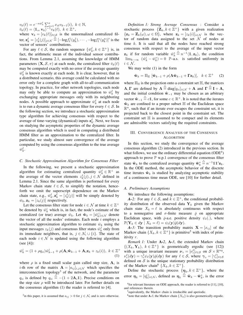
6
Fig. 1. Network topology G
go to zero P–w.p.1 as t →∞. This means the asymptotic rateof change condition12
limk
supj≥k
max0≤t≤T
| Qη(jT + t)−Qη(jT ) | = 0 P–w.p.1
(17)
is satisfied uniformly in η for every T > 0.In the main theorem of this section, by assuming that some
compact set Ωc is recurrent and the mean ODE (6) is stable,it is stated that the error process ηk is bounded P–w.p.1and converges to a bounded invariant set in Ωc.
Theorem 3.7: Consider the unconstrained stochastic ap-proximation algorithm (3). For any δ ∈ (0, 1], let there be acompact set Lδ such that the iterates ηk return to Lδ infinitelyoften with probability at least δ. Assume conditions A-4and A-5. Then, ηk is bounded P–w.p.1 , that is,
lim supk
‖ηk‖ < ∞ P–w.p.1
Assume condition A-8. Also, assume that the function Q(., ξ)satisfies the nonuniform regularity condition in η establishedin Lemma 3.6. Then, there exists a null set f such that forω 6∈ f, the set of functions ηk
•(ω, .), k < ∞ is equicon-tinuous. Let η(ω, .) denote the limit of some convergentsubsequence ηk′
• (ω, .). Then, for P–almost all ω ∈ Ω, thelimits η(ω, .) are trajectories of the mean ODE (6) in somebounded invariant set and the error iterates ηk converge tothis invariant set. Moreover, let the origin be globally13 asymp-totically ε-stable14 for the mean ODE (6) with some invariantlevel set Ωc , where Ωc ⊂ L1. Then, ηk converges to theε-neighborhood of the origin P–w.p.1 as k →∞.
Proof: The proof follows from [11, Theorem 7.1 andTheorem 1.1, Chapter 6] and for brevity the details are omittedhere.
IV. NUMERICAL RESULTS
In this section, we numerically evaluate the performanceof the distributed HMM filter computed using the average
12see Section 5.3 and 6.1, [11] for further detail.13note that in case of local asymptotic stability, convergence result holds if
Lδ is in the domain of attraction of the ODE equilibrium.14this is shown in Proposition 3.3.
0 20 40 60 80 100−8
−6
−4
−2
0
2
4
6
Time (k)
Sta
te E
stim
ate
Node 1Node 2Node 3Node 4Node 5Node 6Fusion Center
Fig. 2. Distributed and centralized state estimates
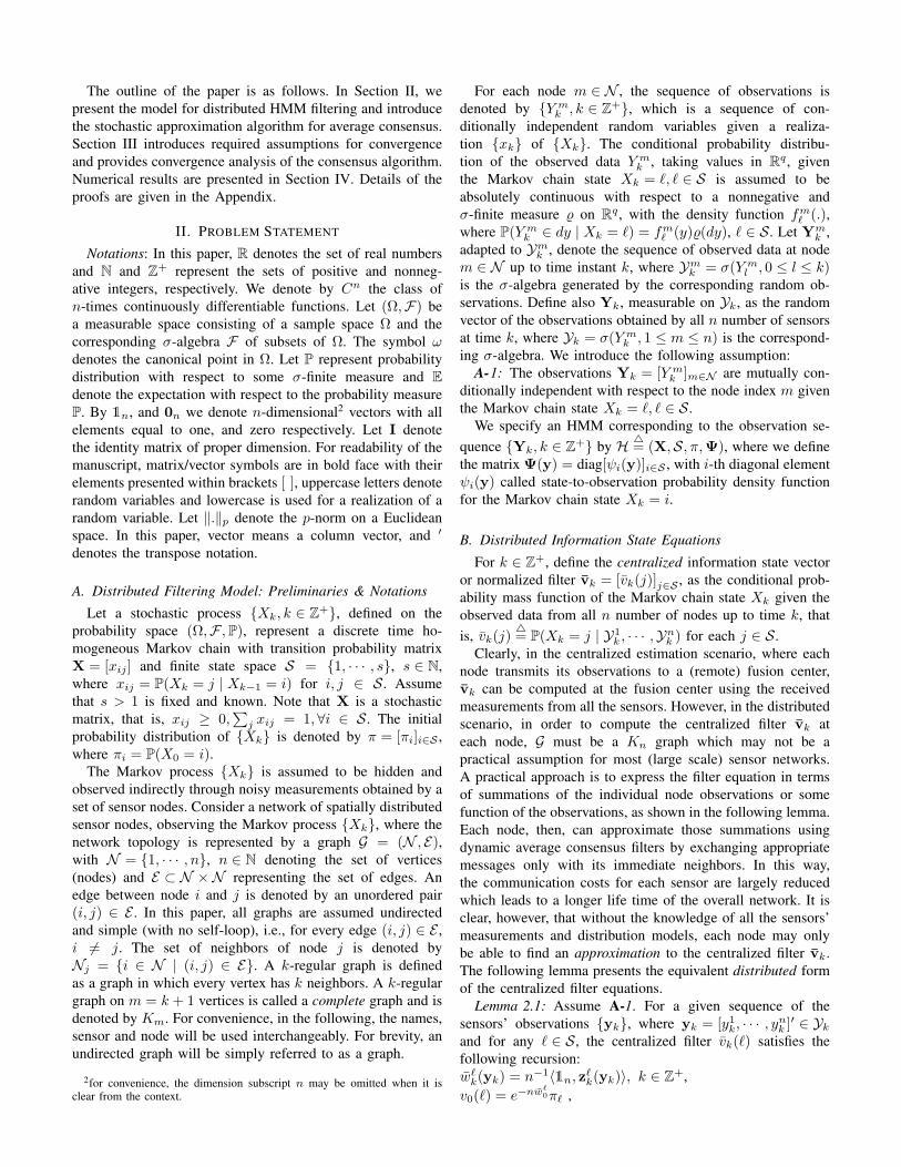
consensus algorithm (1), and study its average behavior rel-ative to the centralized filter. To this end, we present somenumerical results for distributed estimation over a sensornetwork with the irregular topology G depicted in Fig. 1. Weconsider a dynamical system whose state evolves accordingto a four-state Markov chain Xk, k ∈ Z+ with state spaceS = −7.3,−1.2, 2.1, 4.9 and transition kernel
X =
0.80 0.10 0 0.100.05 0.90 0.05 00 0.10 0.85 0.05
0.05 0 0.10 0.85
The initial distribution of Xk is chosen as an arbitraryvector π = [0.20, 0.15, 0.30, 0.35]. The Markov process Xkis observed by every node j according to Y j
k = Xk + ujk,
where the measurement noises uk = [ujk]j∈N , k ∈ Z+ are
assumed to be zero-mean white Gaussian noise processeswith the noise variance vector [0.29 + 0.01j]j∈N . The initialcondition w−1 is chosen w−1 = c1, with c = 3.
Fig. 2 shows the distributed (or local) estimateXj
k
4= Ej [Xk | Fk] of the Markov chain state Xk at
each node j ∈ N , where the expectation Ej is with respect todistributed filter vj
k = [vjk(`)]
`∈S computed using the averageconsensus filter (1). Although node 5 and 2 have direct accessto only one and two nodes’ observations respectively, theymaintain an estimate of Xk but with some time delay. Thereason is because these two nodes receive the observations ofother nodes in the network indirectly through the consensusalgorithm which incur some delay. Nevertheless, every nodefollows the state transition of the Markov process Xk ateach time k.
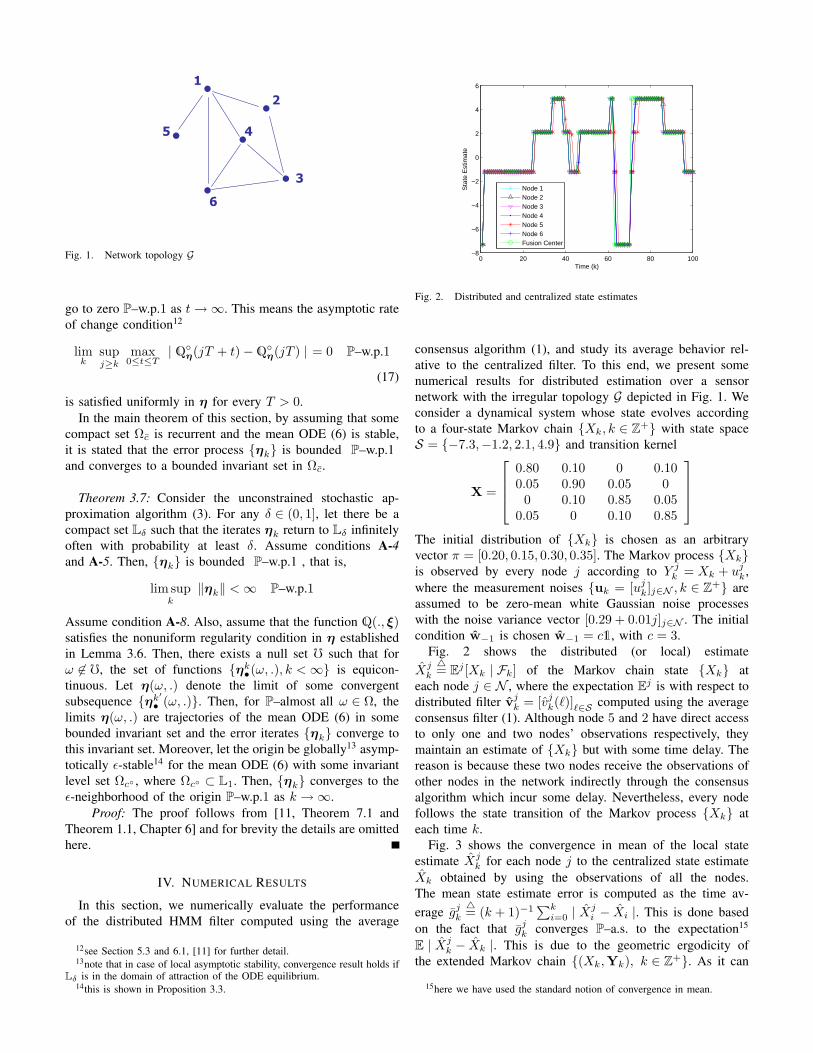
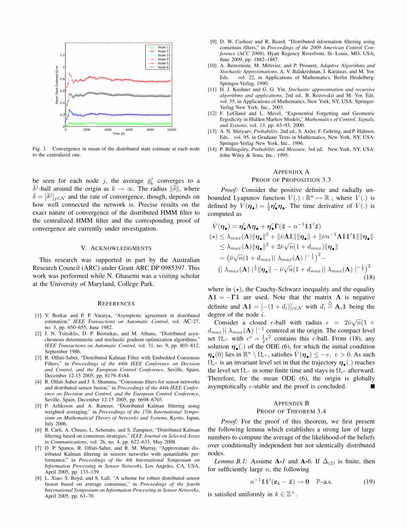
Fig. 3 shows the convergence in mean of the local stateestimate Xj
k for each node j to the centralized state estimateXk obtained by using the observations of all the nodes.The mean state estimate error is computed as the time av-erage gj
k
4= (k + 1)−1
∑ki=0 | Xj
i − Xi |. This is done basedon the fact that gj
k converges P–a.s. to the expectation15
E | Xjk − Xk |. This is due to the geometric ergodicity of
the extended Markov chain (Xk,Yk), k ∈ Z+. As it can
15here we have used the standard notion of convergence in mean.
0 2000 4000 6000 8000 100000
0.2
0.4
0.6
0.8
1
1.2
Time (k)
Mea
n S
tate
Est
imat
e E
rror
Node 1Node 2Node 3Node 4Node 5Node 6
Fig. 3. Convergence in mean of the distributed state estimate at each nodeto the centralized one.
be seen for each node j, the average gjk converges to a
δj-ball around the origin as k → ∞. The radius ‖δ‖, whereδ = [δj ]j∈N and the rate of convergence, though, depends onhow well connected the network is. Precise results on theexact nature of convergence of the distributed HMM filter tothe centralized HMM filter and the corresponding proof ofconvergence are currently under investigation.
V. ACKNOWLEDGMENTS
This research was supported in part by the AustralianResearch Council (ARC) under Grant ARC DP 0985397. Thiswork was performed while N. Ghasemi was a visiting scholarat the University of Maryland, College Park.
REFERENCES
[1] V. Borkar and P. P. Varaiya, “Asymptotic agreement in distributedestimation,” IEEE Transactions on Automatic Control, vol. AC-27,no. 3, pp. 650–655, June 1982.
[2] J. N. Tsitsiklis, D. P. Bertsekas, and M. Athans, “Distributed asyn-chronous deterministic and stochastic gradient optimization algorithms,”IEEE Transactions on Automatic Control, vol. 31, no. 9, pp. 803–812,September 1986.
[3] R. Olfati-Saber, “Distributed Kalman Filter with Embedded ConsensusFilters,” in Proceedings of the 44th IEEE Conference on Decisionand Control, and the European Control Conference, Seville, Spain,December 12-15 2005, pp. 8179–8184.
[4] R. Olfati-Saber and J. S. Shamma, “Consensus filters for sensor networksand distributed sensor fusion,” in Proceedings of the 44th IEEE Confer-ence on Decision and Control, and the European Control Conference,Seville, Spain, December 12-15 2005, pp. 6698–6703.
[5] P. Arliksson and A. Rantzer, “Distributed Kalman filtering usingweighted averaging,” in Proceedings of the 17th International Sympo-sium on Mathematical Theory of Networks and Systems, Kyoto, Japan,July 2006.
[6] R. Carli, A. Chiuso, L. Schenato, and S. Zampieri, “Distributed Kalmanfiltering based on consensus strategies,” IEEE Journal on Selected Areasin Communications, vol. 26, no. 4, pp. 622–633, May 2008.
[7] D. P. Spanos, R. Olfati-Saber, and R. M. Murray, “Approximate dis-tributed Kalman filtering in sensors networks with qunatifiable per-formance,” in Proceedings of the 4th International Symposium onInformation Processing in Sensor Networks, Los Angeles, CA, USA,April 2005, pp. 133–139.
[8] L. Xiao, S. Boyd, and S. Lall, “A scheme for robust distributed sensorfusion based on average consensus,” in Proceedings of the fourthInternational Symposium on Information Processing in Sensor Networks,April 2005, pp. 63–70.
[9] D. W. Casbeer and R. Beard, “Distributed information filtering usingconsensus filters,” in Proceedings of the 2009 American Control Con-ference (ACC 2009), Hyatt Regency Riverfront, St. Louis, MO, USA,June 2009, pp. 1882–1887.
[10] A. Benveniste, M. Metivier, and P. Priouret, Adaptive Algorithms andStochastic Approximations, A. V. Balakrishnan, I. Karatzas, and M. Yor,Eds. vol. 22, in Applications of Mathematics, Berlin Heidelberg:Springer-Verlag, 1990.
[11] H. J. Kushner and G. G. Yin, Stochastic approximation and recursivealgorithms and applications, 2nd ed., B. Rozovskii and M. Yor, Eds.vol. 35, in Applications of Mathematics, New York, NY, USA: Springer-Verlag New York, Inc., 2003.
[12] F. LeGland and L. Mevel, “Exponential Forgetting and GeometricErgodicity in Hidden Markov Models,” Mathematics of Control, Signals,and Systems, vol. 13, pp. 63–93, 2000.
[13] A. N. Shiryaev, Probability, 2nd ed., S. Axler, F. Gehring, and P. Halmos,Eds. vol. 95, in Graduate Texts in Mathematics, New York, NY, USA:Springer-Verlag New York, Inc., 1996.
[14] P. Billingsley, Probability and Measure, 3rd ed. New York, NY, USA:John Wiley & Sons, Inc., 1995.
APPENDIX APROOF OF PROPOSITION 3.3
Proof: Consider the positive definite and radially un-bounded Lyapunov function V (.) : Rn 7→ R , where V (.) isdefined by V (η•) = 1
2η′•η•. The time derivative of V (.) iscomputed as
V (η•) = η′•Λη• + η′•Γ(z − n−111′z)
(?) ≤ λmax(Λ)‖η•‖2 + ‖νΛ1‖‖η•‖+ ‖νn−1Λ11′1‖‖η•‖≤ λmax(Λ)‖η•‖2 + 2ν
√n(1 + dmax)‖η•‖
=(ν√
n(1 + dmax)| λmax(Λ) |− 12)2−
(| λmax(Λ) | 12 ‖η•‖ − ν√
n(1 + dmax)| λmax(Λ) |− 12)2
(18)
where in (?), the Cauchy-Schwarz inequality and the equalityΛ1 = −Γ1 are used. Note that the matrix Λ is negativedefinite and Λ1 = [−(1 + di)]i∈N with di
4= Ai1 being the
degree of the node i.Consider a closed ε-ball with radius ε = 2ν
√n(1 +
dmax)| λmax(Λ) |−1 centered at the origin. The compact levelset Ωc with c = 1
2ε2 contains this ε-ball. From (18), anysolution η•(.) of the ODE (6), for which the initial conditionη•(0) lies in Rn \ Ωc , satisfies V (η•) ≤ −v, v > 0. As suchΩc is an invariant level set in that the trajectory η•(.) reachesthe level set Ωc in some finite time and stays in Ωc afterward.Therefore, for the mean ODE (6), the origin is globallyasymptotically ε-stable and the proof is concluded.
APPENDIX BPROOF OF THEOREM 3.4
Proof: For the proof of this theorem, we first presentthe following lemma which establishes a strong law of largenumbers to compute the average of the likelihood of the beliefsover conditionally independent but not identically distributednodes.
Lemma B.1: Assume A-1 and A-6. If ∆(2) is finite, thenfor sufficiently large n, the following
n−111′(zk − z) → 0 P–a.s. (19)
is satisfied uniformly in k ∈ Z+.
Remark 3: For the proof see [13, Theorem 2, §3, ChapterIV].
Proof of Theorem 3.4: From the definition (13) we have
Ek
[Vk+1(ηk+1)− Vk(ηk)
]= Ek
[V (ηk+1)− V (ηk)
]
+ Ek
[η′k+1δϑk+1(ηk+1)− η′kδϑk(ηk)
](20)
Taylor series expansion of the Lyapunov function V (η) =12‖η‖2 in a neighborhood of ηk yields
EkV (ηk+1)− V (ηk) =
ρη′kΛηk + ρη′kEkG(zk+1, zk) +12ρ2‖Ληk‖2 +
ρ2η′kΛEkG(zk+1, zk) +12ρ2Ek‖G(zk+1, zk)‖2 (21)
where we define
G(zk+1, zk)4= Γ(zk+1 − n−111′zk)− (nρ)−111′(zk+1 − zk)
Define also
G4= Γ(z − n−111′z)
From (11), we write
Ekη′kδϑk(ηk) = η′kEk
∞∑
i=k
ρβik+1Ek[Q(ηk, ξi+1)− Q(ηk)]
= ρη′kEk[Q(ηk, ξk+1)− Q(ηk)] +
(1− ρ)η′k∞∑
i=k+1
ρβik+2Ek[Q(ηk, ξi+1)− Q(ηk)]
= ρη′kEkG(zk+1, zk)− ρη′kG+
(1− ρ)η′k∞∑
i=k+1
ρβik+2EkG(zi+1, zi)− (1− ρ)η′kG
= ρη′kEkG(zk+1, zk)− η′kG +
(1− ρ)η′k∞∑
i=k+1
ρβik+2EkG(zi+1, zi) (22)
Also, from (11) and (12), we write
Ekη′k+1δϑk+1(ηk+1)
= Ekη′k+1
∞∑
i=k+1
ρβik+2Ek+1[Q(ηk+1, ξi+1)− Q(ηk+1)]
= −Ekη′k+1G+ Ekη′k+1
∞∑
i=k+1
ρβik+2Ek+1G(zi+1, zi)
= −Ek
[η′k + ρη′kΛ + ρG′(zk+1, zk)
]G
+ Ek
[[η′k + ρη′kΛ + ρG′(zk+1, zk)
]
∞∑
i=k+1
ρβik+2Ek+1G(zi+1, zi)
]
= −η′kG− ρη′kΛG− ρEkG′(zk+1, zk)G +
η′k
∞∑
i=k+1
ρβik+2EkG(zi+1, zi) +
ρη′kΛ∞∑
i=k+1
ρβik+2EkG(zi+1, zi) +
ρEk
[G′(zk+1, zk)
∞∑
i=k+1
ρβik+2Ek+1G(zi+1, zi)
](23)
For k ∈ Z+, define the distributed prediction filter at nodej ∈ N by pj
k = [pjk(`)]
`∈S , where
pjk(`)
4= P(Xk = ` | F j
k−1)
for each ` ∈ S . The conditional expected value Ekzi for eachi ≥ k + 1 may be written as
Ekzi = [f j ′Xi
k+1
′pj
k+1]j∈N (24)
where we define for ` ∈ Sf
j =[f j
x
]x∈S
4=
[ ∫| log f j
` (yj) |f jx(yj)%(dyj)
]x∈S
and Xik
′ 4=
i−k∏κ=1
X′, where for i = k the empty product is
defined by Xkk
′ 4= I. Define also
f (ι)max
4= max
j∈Nmaxx∈S
∫| log f j
` (yj) |ιf jx(yj)%(dyj) (25)
Since ∆(1) and ∆(2) are finite, f(ι)max for both ι = 1, 2 are
finite. Substituting (21), (22), and (23) in (20) gives
Ek
[Vk+1(ηk+1)− Vk(ηk)
]=
ρη′k(I +12ρΛ)Ληk + ρ2η′kΛEkG(zk+1, zk) +
12ρ2Ek‖G(zk+1, zk)‖22 + ρη′k
∞∑
i=k+1
ρβik+2EkG(zi+1, zi)
+ ρη′kΛ( ∞∑
i=k+1
ρβik+2EkG(zi+1, zi)− G
)
+ ρEk
[G′(zk+1, zk) (
∞∑
i=k+1
ρβik+2Ek+1G(zi+1, zi)− G)
]
(26)

Using Lemma B.1 and (24), we write
ρ2η′kΛEkG(zk+1, zk)
= ρ2η′kΛΓ(Ekzk+1 − n−111′z)
≤ ( ‖ρ2ΛΓ[f j ′pj
k+1]j∈N ‖+ ‖n−1ρ2ΛΓ11′z‖ ) ‖ηk‖≤ ρ2λmax(Λ)
( ‖f (1)maxΛ1‖+ ‖n−1f (1)
maxΛ11′1‖ ) ‖ηk‖
≤ 2√
nρ2f (1)maxλmax(Λ)(1 + dmax) ‖ηk‖ (27)
Also, we have
‖G(zk+1, zk)‖2≤ ‖Γzk+1‖2 + ‖n−1Γ11′z‖2≤ ‖Γzk+1‖1 + ‖n−1f (1)
maxΓ11′1‖2
= (Γ1)′zk+1 + f (1)max‖Λ1‖2
≤ ‖Λ1‖2‖zk+1‖2 +√
nf (1)max(1 + dmax)
≤ √n(1 + dmax)(‖zk+1‖2 + f (1)
max)
and then under A-1 we may write12ρ2Ek‖G(zk+1, zk)‖22≤ 1
2nρ2(1 + dmax)2
(Ek‖zk+1‖22 + 2f (1)
maxEk‖zk+1‖2+ (f (1)
max)2)
=12nρ2(1 + dmax)2
( ∥∥[EFj
kz2k+1(j)
]j∈N
∥∥1
+ 2f (1)maxEk‖zk+1‖2 + (f (1)
max)2)
≤ 12nρ2(1 + dmax)2
(∥∥f (2)max1
∥∥1
+ 2f (1)maxEk‖zk+1‖1
+ (f (1)max)2
)
=12nρ2(1 + dmax)2
(nf (2)
max + 2f (1)max‖Ekzk+1‖1
+ (f (1)max)2
)
≤ 12nρ2(1 + dmax)2
(nf (2)
max + 2f (1)max‖f (1)
max1‖1+ (f (1)
max)2)
=12nρ2(1 + dmax)2
(nf (2)
max + (2n + 1)(f (1)max)2
) 4= ρϕ2
2
(28)
As∑∞
i=k+1 ρβik+2 = 1, using Lemma B.1 and (24) we write
ρη′k
∞∑
i=k+1
ρβik+2EkG(zi+1, zi)
= ρη′kΓ( ∞∑
i=k+1
ρβik+2Ekzi+1 − n−111′z
)
≤ ρ(∥∥Γ[f j ′
X′k,i pj
k+1]j∈N∥∥ + ‖n−1Γ11′z‖) ‖ηk‖
where we define X′k,i
4=
∑∞i=k+1 ρβi
k+2Xik′. It is clear that
Xk,i is a stochastic matrix and, thus, we have
ρη′k
∞∑
i=k+1
ρβik+2EkG(zi+1, zi)
≤ ρ(‖f (1)
maxΛ1‖+ ‖n−1f (1)maxΛ11
′1‖) ‖ηk‖≤ 2
√nρf (1)
max(1 + dmax)‖ηk‖ (29)
Similarly, we have
ρη′kΛ( ∞∑
i=k+1
ρβik+2EkG(zi+1, zi)− G
)
= ρη′kΛΓ
( ∞∑
i=k+1
ρβik+2Ekzi+1 − n−111′z − z + n−111′z
)
≤ ρ(∥∥ΛΓ[f j ′
X′k,i pj
k+1]j∈N∥∥ + ‖ΛΓz‖) ‖ηk‖
≤ ρ(‖f (1)
maxΛΓ1‖+ ‖f (1)maxΛΓ1‖) ‖ηk‖
≤ 2ρf (1)maxλmax(Λ)‖Λ1‖ ‖ηk‖
≤ 2√
nρf (1)maxλmax(Λ)(1 + dmax)‖ηk‖ (30)
Using Lemma B.1, we write∞∑
i=k+1
ρβik+2Ek+1G(zi+1, zi)− G
= Γ(∞∑
i=k+1
ρβik+2Ek+1zi+1 − z)
and thus we have
G′(zk+1, zk) (∞∑
i=k+1
ρβik+2Ek+1G(zi+1, zi)− G)
≤ ‖Γ(zk+1 − n−111′z)‖2
‖Γ(∞∑
i=k+1
ρβik+2Ek+1zi+1 − z)‖2
≤ (‖Γzk+1‖2 + ‖n−1Γ11′z‖2)
.(‖Γ[f j ′
X′k+1,i pj
k+1]j∈N ‖2 + ‖Γz‖2)
As before, the matrix X′k+1,i =
∑∞i=k+1 ρβi
k+2Xik+1
′ is leftstochastic and we write
G′(zk+1, zk) (∞∑
i=k+1
ρβik+2Ek+1G(zi+1, zi)− G)
≤ (‖Γzk+1‖1 + ‖n−1f (1)maxΓ11
′1‖2)
.(‖f (1)maxΓ1‖2 + ‖f (1)
maxΓ1‖2)
= 2f (1)max‖Λ1‖2
((Γ1)′zk+1 + f (1)
max‖Λ1‖2)
≤ 2f (1)max‖Λ1‖2
(‖Λ1‖2‖zk+1‖2 + f (1)max‖Λ1‖2
)
≤ 2f (1)max‖Λ1‖22
(‖zk+1‖1 + f (1)max
)(31)
thus we have
ρEk
[G′(zk+1, zk) (
∞∑
i=k+1
ρβik+2Ek+1G(zi+1, zi)− G)
]
≤ 2nρf (1)max(1 + dmax)2
(Ek‖zk+1‖1 + f (1)
max
)
≤ 2nρf (1)max(1 + dmax)2
(‖Ekzk+1‖1 + f (1)max
)
= 2nρf (1)max(1 + dmax)2
(‖[f j ′pj
k+1]j∈N ‖1 + f (1)max
)
≤ 2nρf (1)max(1 + dmax)2
(‖f (1)max1‖1 + f (1)
max
)
= 2n(n + 1)ρ(1 + dmax)2(f (1)max)2
(32)
By applying Gersgorin theorem to the matrix I + 12ρΛ, it
is shown that under Assumption A-7 all the eigenvalues arestrictly positive and as such the matrix Q
4= (I + 1
2ρΛ)Λ isnegative definite. Substituting (27)- (32) in (26) yields
Ek
[Vk+1(ηk+1)− Vk(ηk)
]
≤ ρλmax(Q)‖ηk‖2 + ϕ‖ηk‖+ ϕ2
= ϕ2 +14ϕ2 | ρλmax(Q) |−1
− ( | ρλmax(Q) | 12 ‖ηk‖ −12ϕ | ρλmax(Q) |− 1
2)2
where ϕ4= | 2√nρf
(1)max(1 + dmax)(1 + (1 + ρ)λmax(Λ)) |
and ϕ2 4= nρ(1 + dmax)2
(12nρf
(2)max + ( 1
2ρ(2n + 1) + 2(n +1))(f (1)
max)2).
Now if the iterate ηk lies outside the interior Ωcof a compact level set Ωc, where Ωc is defined asΩc
4= η : V (η) ≤ c, with c = 1
2 c2, where c > 0 is givenby c = | ρλmax(Q) |− 1
2 | ϕ | + ϕ| ρλmax(Q) |−1, then thereexists an α > 0 such that
‖ηk‖ ≥ c : ηk ∈Rn \ Ωc ⇒Ek
[Vk+1(ηk+1)−Vk(ηk)
]
≤ −ϕ| ρλmax(Q) |− 12 | ϕ | 4= −α < 0
Thus, EkVk+1(ηk+1) < Vk(ηk) P–w.p.1 for V (ηk) ≥ c.Define a random variable τ with values in [0,∞] as anFk–stopping time with respect to the error process ηkwhen ηk first enters Ωc, that is, τ is finite P–a.s. and theevent τ < k is measurable with respect to Fk for eachfinite k ∈ Z+. Define τ ∧ k
4= minτ, k. Hence, Vτ∧k(ητ∧k)
is an Fk–supermartingale for the stopped process ηk withthe Fk–stopping time τ . This completes the proof of thetheorem.
APPENDIX CPROOF OF THEOREM 3.5
Proof: In order to show that some compact set Lδ
is recurrent for the error process ηk with probability atleast δ ∈ (0, 1], we use the Doob’s martingale conver-gence theorem. The sufficient condition for the Doob’stheorem is for the Fk–supermartingale Vk(ηk) to satisfysupk EV −
k (ηk) < ∞ , where V −k
4= max(−Vk, 0) is defined
as the negative part of the random variable Vk(.). From (13),since Vk(ηk) is a summation of two terms (possibly with dif-ferent signs), we need to show that E | Vk(ηk) | is boundedabove16 for every k ∈ Z+. A sufficient condition for this is toshow that
supk
E V (ηk) < ∞sup
kE | η′kδϑk(ηk) | < ∞
For the proof, we use induction on k. Assume EV (η0)is bounded. For the induction hypothesis, suppose thatEV (ηk) < ∞ for some k ∈ N. Then, we show that
16note that | Vk(ηk) |= V +k
(ηk) + V −k
(ηk), where V +k
4= max(Vk, 0)
is defined as the positive part of Vk(.).
EV (ηk+1) < ∞.Using Lemma B.1 and (24), we write
ρ | η′kEkG(zk+1, zk) |= ρ | η′kΓ(Ekzk+1 − n−111′z) |≤ ρ
( ‖Γ[f j ′pj
k+1]j∈N ‖+ ‖n−1Γ11′z‖ ) ‖ηk‖≤ ρ
( ‖f (1)maxΛ1‖+ ‖n−1f (1)
maxΛ11′1‖ ) ‖ηk‖
≤ 2√
nρf (1)max(1 + dmax) ‖ηk‖ (33)
By writing the Taylor series expansion of the Lyapunovfunction V (η) in a neighborhood of ηk, we have
EkV (ηk+1)− V (ηk)
≤ ρλmax(Q)‖ηk‖2 + ρ | η′kEkG(zk+1, zk) |+ ρ2 | η′kΛEkG(zk+1, zk) | +1
2ρ2Ek‖G(zk+1, zk)‖2
(34)
Substituting (27), (28), and (33) in (34) yields
EkV (ηk+1)− V (ηk)
≤ ρλmax(Q)‖ηk‖2 + ρϕ1‖ηk‖+ ρϕ22
where ϕ14= 2
√nf
(1)max(1 + dmax)(1 + ρλmax(Λ)). If the er-
ror iterate ηk lies outside the unit sphere17, then there existsa real ϕ3
4= 2(ϕ1 + λmax(Q)) such that
EkV (ηk+1) ≤ (ρϕ3 + 1)V (ηk) + ρϕ22 P–w.p.1 (35)
where the marginal density of (η0,Yjk, j ∈ Ni ∪ i) and
the above inequality together with the induction hypothesisimplies that E V (ηk+1) < ∞.
Next, we show that under the induction hypothesisEV (ηk) < ∞, we have E | η′kδϑk(ηk) | < ∞ for somek ∈ Z+ and then it is shown that the following
E | η′k+1δϑk+1(ηk+1) | < ∞also holds.
Since∑∞
i=k ρβik+1 = 1, from Lemma B.1, (11), and (24)
we write
| η′kδϑk(ηk) |
≤∥∥∞∑
i=k
ρβik+1Ek[Q(ηk, ξi+1)− Q(ηk)]
∥∥ ∥∥ηk
∥∥
≤ (‖Γ∞∑
i=k
ρβik+1Ekzi+1‖+ ‖Γz‖)‖ηk‖
≤ (‖Γ[f j ′X′
k,i pjk+1]j∈N ‖+ ‖f (1)
maxΓ1‖)‖ηk‖
where the matrix X′k,i
4=
∑∞i=k ρβi
k+1Xik′ is left stochastic
and we have
| η′kδϑk(ηk) | ≤ 2f (1)max‖Λ1‖‖ηk‖
≤ 2√
n(1 + dmax)f (1)max‖ηk‖
17note that in opposite case when ‖ηk‖ ≤ 1, we get a uniform boundin (35) and the proof follows in a straightforward way.
and for ηk outside the unit sphere, there is a real ϕ44=
4√
n(1 + dmax)f (1)max such that by the induction hypothesis
we have
E | η′kδϑk(ηk) | ≤ ϕ4EV (ηk) < ∞Now, we show that E | η′k+1δϑk+1(ηk+1) | < ∞.
From (11), we write
| η′k+1δϑk+1(ηk+1) |
=∣∣η′k+1
∞∑
i=k+1
ρβik+2Ek+1[Q(ηk+1, ξi+1)− Q(ηk+1)]
∣∣
≤∣∣η′k
∞∑
i=k+1
ρβik+2Ek+1[G(zi+1, zi)− G]
∣∣
(?) + ρ∣∣η′kΛ
∞∑
i=k+1
ρβik+2Ek+1[G(zi+1, zi)− G]
∣∣
+ ρ∣∣G′(zk+1, zk)
∞∑
i=k+1
ρβik+2Ek+1[G(zi+1, zi)− G]
∣∣
(36)
We may compute∞∑
i=k+1
ρβik+2Ek+1zi+1 = [f j ′
X′k+1,i pj
k+1]j∈N
where X′k+1,i
4=
∑∞i=k+1 ρβi
k+2Xik+1
′ is also a left stochasticmatrix. As such, for the term (?) in (36) by replacing Ek withEk+1 in (30), the final upper bound will remain unchanged.Similar to (30), using Lemma B.1 we write
∣∣η′k∞∑
i=k+1
ρβik+2Ek+1[G(zi+1, zi)− G]
∣∣
=∣∣η′kΓ
( ∞∑
i=k+1
ρβik+2Ek+1zi+1 − z
)∣∣
≤ (∥∥Γ[f j ′X′
k+1,i pjk+1]j∈N
∥∥ + ‖Γz‖) ‖ηk‖≤ (‖f (1)
maxΓ1‖+ ‖f (1)maxΓ1‖
) ‖ηk‖≤ 2f (1)
max‖Λ1‖ ‖ηk‖≤ 2
√nf (1)
max(1 + dmax)‖ηk‖ (37)
Substituting (37), (30), and (31) in (36) we write forϕ5
4= 4
√nf
(1)max(1 + dmax)(1 + ρλmax(Λ))
| η′k+1δϑk+1(ηk+1) |≤ 1
2ϕ5‖ηk‖+ 2ρf (1)
max‖Λ1‖22(‖zk+1‖1 + f (1)
max
)
where again for ηk outside the unit sphere we have
E | η′k+1δϑk+1(ηk+1) |≤ ϕ5EV (ηk) + 2ρf (1)
max‖Λ1‖22(E‖zk+1‖1 + f (1)
max
)
≤ ϕ5EV (ηk) + 2nρf (1)max(1 + dmax)2
(‖Ezk+1‖1 + f (1)max
)
The expected value Ezk+1 can be computed as
Ezk+1 = [f j ′Xk+1
0
′π]j∈N (38)
Note that for every k ∈ Z+, Xk0′ 4=
∏kκ=1 X′ is a left stochas-
tic matrix. Thus, by the induction hypothesis we have
E | η′k+1δϑk+1(ηk+1) |≤ ϕ5EV (ηk) + 2nρf (1)
max(1 + dmax)2(‖[f j ′
Xk+10
′π]j∈N ‖1 + f (1)
max
)
≤ ϕ5EV (ηk) + 2nρf (1)max(1 + dmax)2
(‖f (1)max1‖1 + f (1)
max
)
= ϕ5EV (ηk) + 2n(n + 1)ρ(1 + dmax)2(f (1)max)2 < ∞
Therefore by induction, we have shown thatE | Vk(ηk) | < ∞ for all k ∈ Z+ and thussupk EV −
k (ηk) ≤ M < ∞.Now, from the martingale convergence theorem18, due
to Doob, there exists a random variable U satisfyingE | U | ≤ M such that the pointwise limit
limk→∞
Vk(ηk(ω)) = U(ω) (39)
exists for P–almost all ω ∈ Ω. Hence, Vk(ηk) → U P–a.s.as k →∞. From this and Theorem 7.3 [11, Chapter 6], thecompact set Ωc is again reached P–w.p.1 after each time itis exited. This means that ηk returns to Ωc infinitely oftenP–w.p.1. Also, from Theorem 7.3 [11, Chapter 6] we havethat the sequence ηk is bounded in probability, that is,
limE→∞
supkP[‖ηk‖ ≥ E ] = 0
and thus using Theorem 7.2 [11, Chapter 6] given anyδ ∈ (0, 1], there is a compact set Lδ such that the iteratesηk enter Lδ infinitely often with probability at least δ. Inparticular, we may choose Lδ = Ωc for all δ ∈ (0, 1]. Theproof of the theorem is concluded.
18the proof of the Doob’s theorem can be found in most classic books onprobability theory, see, e.g., [14, Theorem 35.5.].