issue #1, ma determination of the reactions in rimtuoradea.ro/auo.fmte/files-2013-v1/popa dinel...

DETERMINATION OF THE REACTIONS IN LINKAGES WITH AUTOLISP FUNCTIONS

Dinel POPA1, Nicolae-Doru STĂNESCU

2, Claudia-Mari POPA

3

1University of Piteşti, Romania, [email protected] 2University of Piteşti, Romania, [email protected]

3Armand Călinescu College, Piteşti, Romania, [email protected]

Abstract—The present paper completes a previous paper in which were determined the positions, velocities and accelerations of a jointed quadrilateral mechanism with the aid of some certain AutoLisp functions. The completion consists in the realization of two AutoLisp functions which determine the reactions in the RRR dyad, at the active element and the animation of the vector polygonals or the animation of a wished reaction. The AutoLisp functions are easy to write, the relation that stay at the base of the thinking are vector relations used in the graph-analytical analysis. In the end are shown, as diagrams, the obtained numerical results. Keywords—animation, AutoCAD, AutoLisp, reactions, mechanism

I. INTRODUCTION N the design activity a remarkable aid is due to AutoLisp. This is a programming language that permits to the user the realization of mathematic calculation

and the work with objects in AutoCAD. In this paper we have the goal to solve the problem of

kineto-static analysis with AutoLisp functions. First of all we have to perform the kinematic analysis.

In references [7], [8] we presented modalities of solving the problems of kinematic analysis with the aid of certain AutoLisp functions.

These are easy to be written, the used relations are the vector ones used in the graph-analytical analysis.

One obtains numerical results with the same precision of the assisted analytical methods.

To complete the reference [8] with the determination of the reactions in the kinematic joints of an articulated quadrilateral mechanism, we will write two AutoLisp functions.

The first one will determine the reactions in RRR dyad, while the second one determines the reactions at the active element.

The relations that stay at the base of thinking for the two functions are vector relations.

Finally, we will present the way of animation of the vector polygonals of forces.

II. DETERMINATION OF THE REACTIONS BY CLASSICAL GRAPH-ANALYTICAL METHOD

Dyads enter the category of the passive modular groups. These are statically determined and for this reason the kineto-static analysis of a mechanism starts

from the last modular element, which is in reverse sense comparing to the kinematic analysis.

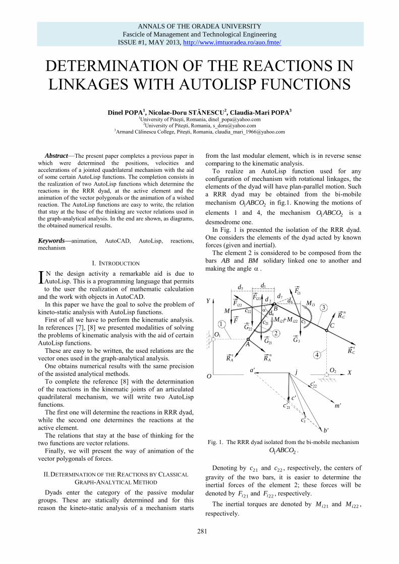
To realize an AutoLisp function used for any configuration of mechanism with rotational linkages, the elements of the dyad will have plan-parallel motion. Such a RRR dyad may be obtained from the bi-mobile mechanism 21ABCOO in fig.1. Knowing the motions of elements 1 and 4, the mechanism 21ABCOO is a desmodrome one.

In Fig. 1 is presented the isolation of the RRR dyad. One considers the elements of the dyad acted by known forces (given and inertial).

The element 2 is considered to be composed from the bars AB and BM solidary linked one to another and making the angle .

O

A

B

C

O X

Y

O

a' j

c'

b'

c'

c'

RC

t

RC

n

Rn

ARt

A

c

Fi3

F d d

M +Mi21

M

m'

c'

F

d

G

c

G

d

G

d

i22F

di22

i21

M

ci3

Fig. 1. The RRR dyad isolated from the bi-mobile mechanism

21ABCOO .

Denoting by 21c and 22c , respectively, the centers of gravity of the two bars, it is easier to determine the inertial forces of the element 2; these forces will be denoted by

21iF and 22iF , respectively.

The inertial torques are denoted by 21iM and 22iM , respectively.

I

ANNALS OF THE ORADEA UNIVERSITY Fascicle of Management and Technological Engineering

ISSUE #1, JULY 2013, http://www.imtuoradea.ro/auo.fmte/

281

ANNALS OF THE ORADEA UNIVERSITY

Fascicle of Management and Technological Engineering

ISSUE #1, MAY 2013, http://www.imtuoradea.ro/auo.fmte/

On the element 2 acts also the force F , with the expression ([5]):

]360,280[for 0

]280,80[for N50

)80,0[for 0

F . (1)

The bars AB and BM are also acted by the weight

forces 21G , and 22G (the masses of the elements kg 125.021 m , and kg 125.022 m are known).

The element 3 has the center of gravity denoted by 3c , the mass 3m ( kg 125.03 m ) and the weight 3G . The inertial force was denoted by 3iF , while the inertial torque was denoted by 3iM .

We considered that the bars are homogeneous; hence the centers of gravity are situated at the middle of the bars.

The torsor of the inertial forces is given by the relations:

icii amF , ici i

JM , (2)

where i takes the values 21, 22 and 3.

In figure the inertial forces ( iF ) were drawn in opposite sense to the accelerations of the elements, while

iM were represented in opposite direction to the angular accelerations.

That is why in the bottom part of Fig. 1 we represented the acceleration polygonals at which we added the accelerations of the gravity centers of the elements.

To determine the reactions in the kinematic joints A , B and C , one isolates the elements, and decomposes the reactions in A and C into the normal components n

AR , nCR , and into the components along the bars t

AR , tCR .

From the equations of moments relative to the point B , one determines the components n

AR and nCR . Thus, for

the dyad in Fig. 1 it results

, 22215

422322221121

ABMMFd

dFdGdFdGR

ii

iinA

(3)

BC

MdFdGR iin

C37363

(4)

where the distances 1d , …, 7d correspond to the forces marked in Fig. 1.

Further on, writing the equilibrium of the forces for the all dyad,

,03

322222121

AB

R

BC

RRF

GFFGFGR

tA

tC

nCi

iinA

(5)

result the components t

CR and tAR ; hence the reactions at

A and C were completely determined,

tA

nAA RRR , t

CnCC RRR . (6)

From the equilibrium of forces which act upon the

element 2,

022222121 BiiA RFFGFGR , (7)

one determines the reaction BR .

The active element 1 has the mass 1m ( kg 05.01 m ) and it is acted by: the weight 1G , the torsor of the inertial forces calculated relative to the rotational axis, and the reaction AR (equal and of opposite direction to that calculated at the RRR dyad).

Because the active element has constant angular speed, the torsor of the inertial forces reduces at the inertial force 11 ci amF , where 1c marks the center of gravity for the element 1.

Since OA is a homogeneous bar, 1c is at the middle of the element.

To determine the reactions of the active element, one isolates the element 1 (Fig. 2).

RA

Fi1

O1

RO

c

A

Me

1

G1

d8

d9

1

Fig. 2. Isolation of the active element.

From the addition of forces

011 BiA RGFR , (8)

results the reaction BR , while from the sum of moments relative to 1O one obtains the moment of equilibration

1eM ,

9811 dRdGM Ae . (9)



282




III. AUTOLISP FUNCTION TO DETERMINE THE REACTIONS OF THE RRR DYAD

Based on the relations (1) – (7) we wrote the AutoLisp function named "Reacţiuni_RRR", the content of which is as follows: (Defun Reactiuni_RRR ()

(Setq m21 0.125

m22 0.125

m3 0.125

G21(* m21 9.8)

G22(* m22 9.8)

G3(* m3 9.8)

J21(/ (* m21 lAB lAB) 12)

J22(/ (* m22 lBM lBM) 12)

J3(/ (* lBC lBC) 12) fmic(List 50 50))

(Setq pctC21(Polar aprim (Angle aprim

bprim) (/ (Distance aprim bprim) 2))

pctC22(Polar bprim (Angle bprim

pctmprim) (/ (Distance bprim pctmprim) 2))

pctC3(Polar bprim (Angle bprim

cprim) (/ (Distance bprim cprim) 2))

acc21(Distance jmic pctC21)

acc22(Distance jmic pctC22)

acc3(Distance jmic pctC3))

(Setq fFi21(* m21 acc21)

fFi22(* m22 acc22)

fFi3(* m3 acc3)

Mi21(* J21 eps2 semnEps2)



Fmare 0.0)

(If (> fi1 70) (Setq Fmare 50))

(If (> fi1 280) (Setq Fmare 0))

(Setq aG21(- (/ pi 2) fi2)

aFi21(- (Angle pctC21 jmic) fi2)

aG22(- alfaRad fi2 (/ pi 2))

aFi22(- (Angle pctC22 jmic) (+ fi2 pi

(* -1 alfaRad)))

aG3(- fi3 (* Pi 1.5))

aF3(- fi3 (Angle pctC3 jmic))

d1(* (/ lAB 2) (Sin aG21))

d2(* (/ lAB 2) (Sin aFi21))

d3(* (/ lBM 2) (Sin aG22))

d4(* (/ lBM 2) (Sin aFi22))

d5(* lBM (Sin aG22))

d6(* (/ lBC 2) (Sin aG3))

d7(* (/ lBC 2) (Sin aF3)))

(Setq RAn(/ (+ (* G21 d1 -1) (* fFi21 d2)

(* G22 d3 -1) (* fFi22 d4) (* Fmare d5 -1)

(* (+ Mi21 Mi22) -1)) lAB)

RCn(/ (+ (* G3 d6) (* fFi3 d7 -1) (* Mi3

-1)) lBC))

(Setq aRAn(+ fi2 (* pi 1.5))

aRCn(- fi3 (* pi 1.5))

pRAn(Polar fmic aRAn RAn)

pG21(Polar pRAn (* pi 1.5) G21)

pFi21(Polar pG21 (Angle pctC21 jmic)

fFi21)

pG22(Polar pFi21 (* pi 1.5) G22)

pFi22(Polar pG22 (Angle pctC22 jmic)

fFi22)

pFmare(Polar pFi22 (* pi 1.5) Fmare)

pG3(Polar pFmare (* pi 1.5) G3)

pFi3(Polar pG3 (Angle pctC3 jmic) fFi3)

pRCn(Polar pFi3 aRCn RCN)

pfRCt(Polar pRCn fi3 10)

pfRAt(Polar fmic fi2 10)

int(Inters pRCn pfRCt fmic pfRAt Nil)

RAt(Distance fmic int)

RCt(Distance pRCn int)

RA(Distance int pRAn)

RC(Distance pFi3 int)

RB(Distance pFmare int))

(Command "Line" fmic pRAn pG21 pFi21 pG22

pFmare pG3 pFi3 pRCn int "C")

(setq l(/ RA 40) g(/ l 0.353))

(Sageti pRAn fmic)

(Sageti pG21 pRAn)

(Sageti pFi21 pG21)

(Sageti pG22 pFi21)

(Sageti pFmare pG22)

(Sageti pG3 pFmare)

(Sageti pFi3 pG3)

(Sageti pRCn pFi3)

(Sageti int pRCn)

(Sageti fmic int)

)

The AutoLisp function starts by assigning values

(Setq) to the masses of elements, continues with the calculation of gravity forces and inertial moments. It also assigns to the forces pole the coordinates )50,50(f .

To determine the accelerations of the gravity centers 21ca , 22ca and 3ca , one firstly determine the coordinates

of the middles of segments ba , cb and mj , respectively, from the accelerations polygonal presented in [5] with the AutoLisp function Polar.

The polygonal uses the accelerations determined with the AutoLisp function "Acceleratii" and presented in [5], and the names of the points in the accelerations plan. In the AutoLisp function the points were denoted by pctC21, pctC22 pctC3, the accelerations being the distances between these points (Distance) and the pole j of the accelerations.

The notations for these accelerations are acc21, acc22 and acc3, respectively.

The inertial forces given by (2) were denoted by fFi21, fFi21, fFi3, and the inertial torques by Mi21, Mi22, Mi3. Due to the fact that on the elements the inertial forces draw in the opposite sense to accelerations, and the inertial moments in the opposite sense of the angular accelerations, we have to solve the problem of the sense of angular acceleration. The theory states that the geometric figure in the accelerations plan is similar to that in the position plan and rotated by the angle

2

arctan

(10)

in the sense of the angular acceleration. To do this, one writes an AutoLisp function which compares the two angles from the accelerations and positions plans, respectively, the angle being measured from the end of the element in trigonometric sense. If the difference is equal to , then semn takes the value 1, otherwise it takes the value –1.



283




To define the force F given by (1), one used two interrogations IF.

The determination of the distances jd from a point jB

to the support straight line of the force jF (Fig. 3) is performed with the aid of the relation )sin( jFjjj BCd . (11)

We denoted by F the angle made by the force jF

with the horizontal, and by j the angle made by the

orientated segment jjBC with the horizontal.

Fj

dj

B j j

F

C j

Fig. 3. The distance from a point to a straight line.

In the AutoLisp function, the distances were denoted

by d1, …, d7, they being determinate according to the representation in Fig. 3. Further on, were determined the components n

AR and nCR with the algebraic relations

(3) and (4). To obtain the vector contour given by (5) one started

Polar from the pole of forces f with the angle 2/32 and the distance n

AR . One obtained the point pRAn. Further on, again with

the function Polar, one obtains, one after another, the points pG21, pfi21, PG22, pFi22, pF, pG3, pFi3, pRCn, keeping into account the forces and their magnitudes, according to the vector polygonal [5].

To obtain the intersection between the parallel to BC and passing through pRCn, and the parallel to AB and passing through the pole f , one constructs two points pfRCt and pFRAt situated on the two straight lines at an arbitrary distance (10).

With the function Inters one analyzes the four point pRCn, pfRCT, fmic and pfRAt and if there exists point of intersection (Nil), then it is denoted by int.

We thus obtain the components: tAR as distance

(Distance) between the points fmic and int, and tCR as distance (Distance) between the points pRcn

and int. AR , according to (6), is the distance between the points int and pRAn, while CR is the distance between the points pFi3 and int.

The reaction BR , according to the vector relation (7), is obtained from the same contour as distance (Distance) between the points pF and int.

We thus obtained the magnitudes of the reactions in the joints of RRR dyad, with no representation of the vector contour.

One may also draw the vector contour of the polygonal using the AutoCAD command LINE.

This vector contour completes with arrows with the AutoLisp function "Sageti" described in [8] (Fig. 4).

pRCnpG21

pG22

pFi21

pFi3

int

RAt

RCt

pF

pG3

pRAn

pFi22fmic

RB

Fig. 4. The RRR dyad – the forces polygonal.

IV. AUTOLISP FUNCTION TO DETERMINE THE REACTIONS

AT THE ACTIVE ELEMENT

To obtain the components at the active element we write a new AutoLisp function named "React_Motor". It calls the function "Reactiuni" or from the main function "R_3R" presented in [8]. Its construction follows the algorithm given by (8) and (9). (Defun React_Motor ()

(Setq m1 0.05

G1(* m1 9.8))

(Setq pctC1(Polar jmic (Angle jmic aprim)

(/ (Distance jmic aprim) 2))

acC1(Distance jmic pctC1)

fFi1(* m1 acC1))

(Setq pF1(Polar int (Angle jmic pctC1)

Fi1Rad)

pG1(POlar pF1 (* pi 1.5) G1)

RO(Distance pG1 pRAn))

(Setq aRA(- (Angle pRAn int) (+ fi1RAD (/

pi 2)))

d8(* (/ lOA 2) (Sin Fi1RAD))

d9(* lOA (Sin aRA))

Me1(- (* G1 d8) (* RA d9))

)

)

After the determination of the inertial force, one

obtains OR using the previous vector contour. One uses a new pole of forces, the point pRAN. The force AR is at the point int. We continue from this point with the force

1iF (it results the point pFi1) and with the force 1G (it results the point pG1). One thus obtained the reaction OR as distance (Distance) between the points pG1 and pRAn (fig. 5).



284




int pRAnRA

pG1

pFi1

RO

Fig. 5. Active element – the forces polygonal.

The moment of equilibration is determined with the aid

of (9), after we previously determined the distances 8d and 9d with (11). In this mode, we completely determined the reactions at the active element. V. ANIMATION OF THE VECTOR POLYGONALS OF FORCES

The functions presented above are called from the

function "R_3R" presented in [5]. The function "R_3R" was though to also realize files of values in which will be written the reactions in the mechanism joints. The function "R_3R" was performing the animation of the mechanism, velocities and accelerations polygonals. With the aid of the described functions one also obtains the animation of the polygonals of reactions or, separately, the reactions of interest.

The visualization of the animation is made in proper windows, the angle at the active element varying from 0 to 2 . To do this, one uses the AutoCAD command ZOOM. One establishes a point of visualization (the option Center of the command) and a magnification factor. For instance, if one wishes to visualize only the animation of the reaction CR , then one chooses as central point the point pFi3 and draws only the segment between the points pFi3 and int with the command LINE. One may also draw with the function "Sageti" the arrow with the peak at the point int. In this window of visualization, when the angle of the active element varies, we will observe the rotation about the chosen point of the reaction. If one wishes, then one may superimposes the 360 components of the reactions, obtaining thus a diagram with partially or totally blacked zones.

VI. CONCLUSIONS

The way of approaching of the kineto-static analysis in the paper hast at its basis the graphic methods which were forgotten a period of time because their low precision in obtaining the results.

With the apparition of the CAD soft, the notion of imprecision for the graphical methods disappeared. The results obtained with these softs have the same precision to that of the assisted analytical methods.

The vector mode in which works AutoCAD creates a strong closing to the vector methods used in mechanics and in the kinematic and kineto-static analysis of the mechanisms.

The present paper wishes, first of all, to prove this statement and to re-bring in nowadays the old graphic methods which are also intuitive.

When one produces an imagine of the mechanism or its animation, the obtained results give a distinct note to the work comparing to the tables of the values obtained with the aid of the analytical methods.

With the aid of the AutoLisp functions, one obtains numerical results from vector equations, without any representation of the vector polygonal. But it is very useful and easy to give a representation of it.

To realize the animation, in fact one establishes the parameters of interest and how must be realized the representation. In the AutoLisp functions presented in the paper are determined all the parameters; the only thing we have to establish is what we wish visualize.

The application was realized for a jointed Chebyshev type quadrilateral mechanism for 360 positions of the active element. In reference [8] were presented the all six AutoLisp functions that realize the kinematic analysis of the mechanism. From the main function presented there, one calls the two functions presented in this paper, the first determines the reactions in the RRR dyad, and the second one the reactions at the active element.

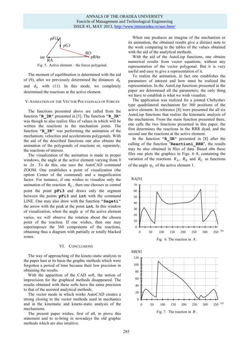
In the function "R_3R" presented in [8] after the calling of the function "Reactiuni_RRR", the results may be also obtained in files of data. Based o0n these files one plots the graphics in Figs. 6–8, containing the variation of the reactions AR , BR and CR as functions of the angle 1 of the active element 1.

RA[N]

0

10

20

30

40

50

60

70

0 50 100 150 200 250 300 350[0]

Fig. 6. The reaction in A .

RB[N]

0

20

40

60

80

100

120

0 50 100 150 200 250 300 350 [0]

Fig. 7. The reaction in B .



285




RC[N]

0

20

40

60

80

100

120

0 50 100 150 200 250 300 350 [0]

Fig. 8. The reaction in C .

In similar way for the active element, after the calling

of the function "React_Motor" one obtains the graphic in Fig. 9 for the reaction OR and the graphic in Fig. 10 for 1eM .

RO[N]

0

10

20

30

40

50

60

70

0 50 100 150 200 250 300 350[0]

Fig. 9. The reaction in the joint O .

Me1[Nm]

-3

-2

-1

0

1

2

3

0 50 100 150 200 250 300 350

[0]

Fig. 10. The moment of equilibration.

In the 360 layers one obtained the position of the

mechanism, the velocities, accelerations and forces polygonals. The polygonals are accompanied by letters at the vectors’ arrows; in the case of the animation the

letters move simultaneously with the vector. It is thus obtained a better clarity of the representation.

One can combine the results obtained in the kinematic analysis with those from the kineto-static analysis.

For instance, one can realize the animation only for shaft 2 in Fig. 1, accompanied by the representation of the reactions AR and BR in the joints in A and B . For this one must write the following lines of program: (Command "Line" Amare Bmare "")

(Setq pFAmare(Polar Amare (Angle int pRAn)

(* RA kf)))

(Command "Line" Amare pFAmare "")

(Setq pFBmare(Polar Bmare (Angle pF int) (*

RB kf)))

(Command "Line" Bmare pFBmare "")

The following things were realized:

- the drawing of the segment AB with the command Line, - the determination of the point pFAmare starting from the point A , Polar with the angle of the force AR and a length fAkR , where by fk was denoted the scale of representation of the force in the forces polygonal, - the drawing of the force AR at the point A with the command, - the determination and the drawing of the force BR at the point B in a similar mode.

Further on, one chooses a window of visualization that is kept constant when the element 1 takes the 360 positions. One can proceed in an analogous way for any other element or vector which accompany the representation in a certain animation.

REFERENCES [1] I. Artobolevski, Theory of Mechanisms and Machines (Théorie

des mécanismes et des machines), Ed. MIR, Moskow, 1977. [2] Fl. Dudiţă, Mechanisms (Mecanisme), Universitatea din Braşov,

1977. [3] Fl. Dudiţă, D. Diaconescu, Structural Optimisation of Mechanisms

(Optimizarea structurală a mecanismelor), Ed. Tehnică,

Bucureşti, 1987. [4] V. Handra Luca, I. A. Stoica, Introduction to the Theory of

Mechanisms (Introducere în teoria mecanismelor), Ed. Dacia, Cluj-Napoca, 1983.

[5] Chr. Pelecudi, D. Maroş, V. Merticaru, N. Pandrea, I. Simionescu, Mechanisms (Mecanisme), Ed. Didactică şi Pedagogică, Bucureşti,

1985. [6] N. Manolescu, Fr. Kovacs, A. Orănescu, Theory of Mechanisms

and Machines (Teoria mecanismelor şi maşinilor), Editura Didactică şi Pedagogică, Bucureşti, 1972.

[7] D. Popa, M. Stan, C. Popa, “AutoLisp Procedures Used in Kinematic Analysis of Mechanisms”, The XXVII-th National

Conference on Solids Mechanics, Târgovişte 2004, pp. 132 – 136. [8] D. Popa, N.-D. Stănescu, C.-M. Popa, “Animation of the Vector

Relations by Autolisp Functions”, Annual Session of Scientific

Papers IMT, Oradea, 2013. [9] N. Pandrea, E. Bărăscu, Mechanisms (Mecanisme), Universitatea

din Piteşti, 1990. [10] R. Voinea, D. Voiculescu, V. Ceauşu, Mechanics (Mecanica), Ed.

Didactică şi Pedagogică, Bucureşti, 1988. [11] D. Manolea, Programming in AutoLisp under AutoCAD

(Programarea în AutoLisp sub AutoCAD), Editura Albastră, Cluj-Napoca, 1996.



286




issue #1, ma determination of the reactions in rimtuoradea.ro/auo.fmte/files-2013-v1/popa dinel...

Documents