istituto di matematica applicata e tecnologie...
TRANSCRIPT

Consiglio Nazionale delle Ricerche
Istituto di
Matematica Applicata e Tecnologie Informatiche ldquoEnrico Magenesrdquo
PUBBLICAZIONI
MS Pauletti M Martinelli N Cavallini P Antoliacuten IGATOOLS AN ISOGEOMETRIC ANALYSIS LIBRARY
3PV1410
CNR - Istituto di Matematica Applicata e Tecnologie Informatiche ldquoEnrico Magenesrdquo
Sede di Pavia Via Ferrata 1 - 27100 PAVIA (Italy) Tel +39 0382 548211 Fax +39 0382 548300 Sezione di Genova Via De Marini 6 (Torre di Francia) - 16149 GENOVA (Italy) Tel +39 010 6475671 Fax +39 010 6475660 Sezione di Milano Via E Bassini 15 - 20133 MILANO (Italy) Tel +39 02 23699521 Fax +39 02 23699538
URL httpwwwimaticnrit
IGATOOLS AN ISOGEOMETRIC ANALYSIS LIBRARY
M SEBASTIAN PAULETTIlowast MASSIMILIANO MARTINELLIdagger NICOLA CAVALLINIDagger AND PABLO ANTOLINsect
Abstract We present a novel mathematically faithful object oriented design for a general purpose isogeometric libraryand introduce a high quality open source implementation of it igatools (httpcodegooglecompigatools) The libraryuses advanced programming techniques and supports dimension independent programming It includes support for manifoldsand isogeometric elements of the h-div and h-curl type To illustrate the flexibility and power of the library we present someexample applications including surfaces fluid and elasticity
Key words isogeometric analysis software library open source object oriented generic programming dimensionindependent B-splines NURBS h div h curl CAD integration
AMS subject classifications 65N30 97N80 97N40 68N19 65D07
1 Introduction Inspired by the desire to unify the fields of computer aided geometrical design(CAGD) and the finite element method (FEM) the visionary work [30] introduced a technique for thediscretization of partial differential equations dubbed isogeometric analysis (IGA) In this work any nu-merical method fitting the isogeometric analysis framework will be referred to as an isogeometric method(IgM) The mainly advertised feature of an IgM has been the ability to describe exactly CAGD type ge-ometries This is so because the method proposes to use the same type of spaces to represent the geometryand the shape functions (mostly non uniform rational B-splines) But in addition to exact representa-tion of CAGD geometries the use of B-spline functions allows global smoothness beyond the classical C0
continuity of standard finite elements this permits the design of novel numerical schemes that would beextremely difficult to obtain with standard finite elements Isogeometric methods have been summarizedin a recent book [19] and studied in [16 17] They have been successfully used in applications such as fluid[6 7 24] structural mechanics [44 33 20]
After a decade of research in the area with many successes some issues (that require further research)and many promising ideas it is time ndashat least in the research communityndash to have an open source modernlydesigned isogeometric software library Which should be capable of dealing with the current understand-ing of an IgM while providing the flexibility to adapt to the future evolution of the IgM And not lessimportant to justify the time invested in its learning it should follow high quality standards in designand development Unfortunately we did not find an isogeometric library with the features and qualitystandards of our expectations This need and the scientific environment at Pavia provided the supportingframework for us to undertake the first step toward the creation of such software Pavia enjoined the earlystages on the development of the isogeometric concept Several scientists in mathematics and engineeringcontributed with their work to the theoretical and computational development of isogeometric analysisFor several years GeoPDEs [21] (an easy to use MATLAB toolkit) has ldquopropelledrdquo the dissemination of theconcept in its early stages partially paving the road for our work
The main purpose of this work is to present an object oriented design for an isogeometric softwarelibrary and introduce a high quality implementation of it igatools igatools is a general purpose opensource library to solve partial differential equations using isogeometric type spaces Unlike most academic
lowastInstituto de Matematica Aplicada del Litoral (IMAL) Consejo Nacional de Investigaciones cientıficas y tecnicas (CON-ICET) Santa Fe Argentina Partially supported by European Research Council through the FP7 Ideas Starting Grant205004 GeoPDEs and Agencia Nacional de Promocion Cientıfica y Tecnologica through grant PICT-2008-0622 (Argentina)daggerIstituto di Matematica Applicata e Tecnologie Informatiche (IMATI) Consiglio Nazionale delle Ricerche (CNR)
Pavia Italy Partially supported by Hutchinson-Total under contract TOTAL DSndash2753 and FIRB ldquoFuturo in RicercardquoRBFR08CZ0SDaggerDipartimento di Matematica ldquoF Casoratirdquo Universita degli Studi di Pavia Via Ferrata 1 27100 Pavia Italy Pavia
Italy Supported by the TERRIFIC project European Communitys Seventh Framework Programme Grant Agreement284981 Call FP7-2011-NMP-ICT-FoFsectDipartimento di Ingegneria Civile ed Architettura Universita degli Studi di Pavia Via Ferrata 3 27100 Pavia Italy
Partially supported by Hutchinson-Total under contract TOTAL DSndash2753 and by European Research Council through theFP7 Ideas Starting Grant 259229 ISOBIO
1
2
software that start as a tool to solve the specific applications of a small research group igatools wasconceived from the beginning to provide useful tools to aid in the approximation to a wide range of possibleapplications
The design of igatools encapsulates the mathematical concepts of an isogeometric method intoobjects and map their relations into interaction between these objects We tried hard to attain thesimplest possible design that is faithful to the mathematics behind Figure 31 shows a blueprint of thebasic design As a guiding rule to validate the design we use the following ldquoif an awkward code is neededto perform a task consistent with the mathematics of the problem then there is a problem with the designof the libraryrdquo Desirable consequences of such a design are improved maintainability as it produces acode that reads closer to the human conception of the problem and flexibility for extensions as adding anew feature coming from the mathematics of the problem should face no major restrictions
A good design is paramount for a software library to transcend the original group of developers Butit is also necessary to carefully plan and execute the structure and documentation of the code as wellas the infrastructure to support its development In igatools we have considered all these principlesThe library is implemented in C++11 [32 9] its design is object oriented with extensive use of genericprogramming techniques that allows among other advantages to obtain code that is dimension independentwhile suppressing the overhead of virtual functions The development environment follows the high qualitystandards of today software engineering we use a platform independent configuration system (CMake) anautomatic test suite (CTestCDash) a version control system (git) a bug tracking system (Trac) anin-source documentation system (Doxygen) a user discussion forum and an on-line tutorial On top ofthe novel object oriented design that it implements igatools provides practical useful features such asthe possibility of floating-point types of different precision integration with CAGD modelers and parallelsupport for shared (multi-threading) and distributed (MPI) memory systems
The IgM is closely related to the well known FEM they are both Galerkin methods that provide anspecific way of constructing the basis functions of the discrete approximating spaces Some finite elementspaces can be generated with the IgM (Lagrange elements on quadrilaterals for example) In a loose sensean IgM can be interpreted as a generalized FEM where the basis functions are more regular But thisinterpretation starts to diverge as a closer look is taken onto the details for example even though theLagrange spaces are the same the basis functions generated using the FEM are different from the ones ofthe IgM It is our view that even though a finite element code could be adapted to accept an isogeometricplugin [13] this approach presents some shortcoming The popular well-maintained modernly designedand stable FE libraries are so tailored for the FEM that using them for and IgM makes some forcedinterpretation of a few concepts In fact we would need to define an isogeometric counterpart for the finiteelement triple or the unstructured triangulation It is our opinion that forcing IgM concepts to fit intoa FEM design without existing a true matching between concepts will lead to a shady design affectingclarity maintainability efficiency and extensibility of the code Still we should not forget the similaritiesthese methods share Our IgM design is inspired by these similarities as well as these differences toproduce a software that suites an easy implementation of state of the art method and original techniquesIn particular we have absorbed many applicable concepts from an open source finite element library thatseems to have survived the test of time namely the dealII library [2 3]
This work is neither a manual nor a user guide for igatools In fact there are online documentation(more than hundreds of pages if printed) and a tutorial dedicated for these purposes The main purpose isto present and explain a novel object oriented design for isogeometric analysis faithful to the mathematicsof the IgM and introduce a high quality software implementation of it igatools
The outline for this work follows the ideal approach for designing a computer program (see [42]) inthree stages analysis design and programming In the analysis we need to gain a clear understandingof the problem in our case the IgM this is what we do in sect2 where we describe the method from theviewpoint of designing a software library for it The design is presented in sect3 where the key concepts ofthe IgM and their relations are identified and mapped into objects Here we also detail the main classesimplemented in igatools (the programming stage) Finally in sect6 we present some common applicationsthat our library can easily accommodate including the Poisson problem Laplace-Beltrami on surfaces a
3
fluid application and an elasticity problem
2 Isogeometric spaces In order to design an isogeometric library it is crucial first to achieve aclear understanding of what an isogeometric method is Since its introduction what we call isogeometricmethod (IgM) has evolved to incorporate new concepts and ideas The original emphasis when IGA wasintroduced was on the exact representation of the geometry and the requirement of the isoparametricparadigm to be satisfied On one hand new reference spaces beside NURBS has been introduced (T-splines [5 23 15 39] locally refined splines [22] and hierarchical splines [26 27 43]) On the otherhand the isoparametric constraint has been lately relaxed [18 17 16] to include mappings that are notnecessarily in the reference space We also support the relaxation of the exact domain geometry constraintFrom the mathematical point of view is not mandatory to have an exact representation of the domain(what is needed is an approximation of the geometry that leads to an error of the same order of the onethat is due to the approximation order of the discrete space) but from an engineering point of view it isextremely useful to have an exact representation of the geometry indeed with an exact representation thegeometry (and the grid built upon it) can be easily modifiedmanipulated (for instance in optimizationloops) without the needs of re-meshing procedures For the approximation of some vector-valued problemsto be stable it is known [11 35] that the approximating spaces must satisfy some properties Particularexamples are the Raviar-Thomas and the edge elements A more general mathematical framework in thelanguage of differential forms and de Rham cohomology has been studied in [1] and applied in the contextof isogeometric methods in [18 17] Our design supports this spaces through the use of a transformationtype and the concept of an associated push-forward operator
Thus in our design we conceive an isogeometric method to be a method that incorporates most existingflavors of isogeometric techniques such as the ones described in the previous paragraph But moreoverbased on the fact that the design strives to be conceptually faithful to the mathematics we expect thesoftware to be flexible enough to adapt to and encourage the creation of new methods that are unknownat the moment
In this section we give a brief overview of the isogeometric method B-splines and NURBS whileintroducing the notation used in this work Details can be found in the standard bibliography for example[38 36 19]
21 The isogeometric method An IgM is a type of Galerkin method to approximate the solutionof boundary value problems To make the discussion more concrete let us consider a differential equationin a d-dimensional domain Ω sub Rs being s the dimension of the embedding euclidean space and s minus dthe codimension of the domain More precisely let V be a Sobolev space (infinite dimensional) on ΩA V rarr V prime a differential operator and f isin V prime a linear functional The variational problem is to findu isin V such that Au = f The Galerkin procedure approximates the solution u by solving a similar problemin finite dimensional subspaces The IgM (as well as the FEM) provides a recipe to construct these discretespaces More specifically we define an IgM as one providing
1 A reference space Given a d-dimensional rectangle Ω sub Rd that we call the reference domainprovides a specific way to construct a reference space V(Ω) of the B-spline type (see definition 21)
2 A deformation Provides a smooth deformation F Ω rarr Rs (with smooth inverse) We referto F as the mapping and to Ω = F (Ω) as the physical domain
3 A transformation type This is a rule that specifies how to use the deformation to transformthe functions in the reference space into the ones in the physical space Some example besides directcomposition are divergence and curl preserving transformations (cf Table 21)
The mapping together with the transformation type define a push-forward operator1 P and this op-erator acts on the reference space to give the physical space V(Ω) (see Figure 21) as V(Ω) = φ =
P (φ) with φ isin V(Ω) We say that V(Ω) is an isogeometric space and a function u isin V(Ω) is generallyreferred to as a field
1In the context of differential geometry P would be called the pullback (as there is no distinction between reference andphysical) for our setting it is more natural and clear to refer to P as the push-forward of reference functions to physicalfunctions
4
h_grad h_curl h_div l_2
φ = φ Fminus1 u = DFminusT (u Fminus1) v =DF
detDF(v Fminus1) ϕ =
ϕ Fminus1
detDFTable 21
Examples of different transformation types to obtain a physical discrete space V from a reference spline or NURBSspace V and a mapping F The table shows the transformation name given in the library and the formula that defines itspush-forward operator
Ω
xy
z
ΩF
xy
zϕ
xy
z
ϕP
Fig 21 The isogeometric method delivers a recipe to construct a discrete space by providing a reference space of theB-Spline type a deformation F and a transformation type The transformation type indicates how to use the deformationto define the push-forward operator P The physical space V(Ω) is obtained as the image of the reference space V(Ω) throughP
22 B-splines and NURBS
221 Univariate B-spline Given a non negative number p a spline of degree p on the interval [a b]is a real valued piecewise polynomial function of degree at most p on each subinterval of [a b] determinedby the partition a = ζ1 lt middot middot middot lt ζm = b The ζirsquos are called the knots and they form the knot vectorζ = (ζ1 ζm) At each knot the spline function is allowed to have a regularity that ranges fromdiscontinuous (Cminus1) to Cpminus1 this is usually indicated using the so called regularity vector α = (α1 αm)where αi isin Z and minus1 le αi le pminus 1 It is sometimes convenient to encode both knot and regularity vectorsinto a single vector of repeated knots ξ = (ζ1 ζ1︸ ︷︷ ︸
r1 times
ζ2 ζ2︸ ︷︷ ︸r2 times
ζm ζm︸ ︷︷ ︸rm times
) where ri = p minus αi and
r = (r1 rm) is called the multiplicity vector When the multiplicity of the first and last knots is p+ 1we call ξ an open knot vector
We define Spξ to be the space of spline functions of degree p subordinated to the knot vector with
repetition ξ It is a well known result that the dimensionality of this space is n =summi=1 ri minus p minus 1 The
classical Cox-de Boor recursive algorithm [36] allows to construct a basis for Spξ known as the B-splinebasis We denote these basis functions by Bi (see Figure 22) Some important properties of B-spline basisfunctions are
(i) Non-negativity each Bi(x) ge 0 for all x isin [a b](ii) Small support each Bi is non-zero only in [ζi ζi+j) with 1 le j le p + 1 and on each interval
[ζi ζi+1) (with i = 1 mminus 1) only p+ 1 basis functions have non-zero values(iii) Partition of unity the set of basis functions B1 Bn satisfies that
sumni=1Bi(x) = 1 for all
x isin [a b] if ξ is an open knot vectorRemark 1 (Univariate B-spline evaluation) A convenient method to compute values and derivatives
of univariate B-spline functions can be achieved using the so called Bezier extraction operator techniqueThis method was introduced by Borden et al [13] as a local adaptation of the global Bezier decompositionalgorithm [36 A56] More precisely as a B-spline function of degree p restricted to the k-th intervalIk = [ζk ζk+1) is a polynomial of degree p we can write this polynomial as a linear combination of thep+ 1 Bernstein polynomial basis functions bjp of degree p as
(21) Bi(x)∣∣∣[ζkζk+1)
= Bki(x) =
p+1sumj=1
c(k)ij bjp
( xminus ζkζk+1 minus ζk
) i = 1 p+ 1
5
ζminus3 ζminus2 ζminus1 ζ0 ζ1 ζ2 ζ3 ζ4 ζ5 ζ6
1
0
Natural definition domain
B-23 B-13 B03 B13 B23 B33
sum3i=minus2 Bi3
Fig 22 One dimensional B-spline basis functions of degree 3 for a maximum regularity knot vector As it can be seenall the functions are non-negative they span over four knot intervals (small support) on each interval only four functionhave non-zero values and they form a partition of unity on the interval [ζ0 ζ3]
with bjp(t) =(pjminus1
)tjminus1(1minus t)pminusj+1 for 0 le t le 1 and j = 1 p+ 1 The coefficients c
(k)ij define the k-th
interval matrix C(k) = (c(k)ij ) referred to as the k-th Bezier extraction operator A simple consequence of
equation (21) is that the m-th derivative of a B-spline function can be written as linear combination of
the m-th derivatives of the Bernstein polynomials with the same coefficients c(k)ij as the function More
precisely
(22) B(m)ki (x) =
p+1sumj=1
c(k)ij
dmbjpdζm
( xminus ζkζk+1 minus ζk
)=
1
(ζk+1 minus ζk)m
p+1sumj=1
c(k)ij b
(m)jp (t)
with t = xminusζkζk+1minusζk This property leads to an efficient method to compute values and derivatives of univari-
ate B-splines More precisely assume we have a spline space with N intervals and we want to computethe values and derivatives of the B-spline functions using the same quadrature scheme on each interval
According to equation (22) we need to compute the matrices C(k) (N times) and b(m)jp at the unit quadra-
ture points (one time independent of N) With this information pre-computed we can compute all therequired values and derivatives of the B-spline functions over all the intervals Thus making this evaluationmethod efficient and convenient in the context of an IgM
222 Multivariate B-splines The univariate spline spaces can be used to generate multidi-mensional spline spaces through tensor product multiplication More precisely given a positive inte-ger d we consider the spline spaces Spiξi ([ai bi]) for i = 1 d and define the multivariate spline space
Sp1pdξ1ξd(Ω) = Sp1ξ1 ([a1 b1]) otimes otimes Spdξd ([ad bd]) where Ω is the hyper-rectangle [a1 b1] times middot middot middot times [ad bd] In
this case the multivariate B-Spline basis functions are
(23) Bi1id(x1 xd) = B1i1(x1) Bdid(xd)
with Bij isin Spiξi for j = 1 ni being the B-spline basis of the univariate spaces The dimension of the
space is n =proddi=1 ni
To simplify the notation in the multidimensional setting we define p = (p1 pd) to be the vector of
degrees andminusrarrξ = (ξ1 ξd) the vector of knot vectors with repetition Then we can write Spminusrarr
ξ(Ω) instead
of Sp1pdξ1ξd(Ω) Similarly we consider a vector index like i = (i1 id) for tensor product structures
such as basis functions or elements or m = (m1 md) as a derivative multi-index Thus we can
write DmBi(x) as a short notation forpartmBi1idpartxm11 partx
mdd
(x1 xd) with m = |m| Associated to a vector
of knot vectors ζ we define the grid (or mesh or cartesian grid) Q = Qi1id = [ζ1i1 ζ1i1+1] times middot middot middot times
[ζdid ζdid+1] with 1 le ij le mj and 1 le j le d and its members Qi are called the elements
6
One way igatools exploits the computational benefits of tensor products and B-splines is stated inthe following remark
Remark 2 (Uniform computation of any order derivatives) The tensor product structure of a multi-variate B-spline together with the Bezier extraction technique provide the foundation to an algorithm thattranslates to a single piece of code capable of computing any order of derivatives for multivariate B-splinefunctions To see this consider the multi-index m and differentiate (23) from where it follows that
DmBi(x) =proddj=1(Bjij )
(mj)(xj) This formula can be implemented with a single code for any size of m
(whether 1 or 50) If the univariate derivatives (Bjij )(mj) required by the formula can be easily precom-
puted this provides a uniform and efficient code that can compute multivariate B-splines derivatives ofany order And this is the case as we have shown in Remark 1 This level of computational simplicity andefficiency is proper of B-splines and cannot be achieved with NURBS functions
223 Non uniform rational B-splines (NURBS) NURBS functions are quotients of splinefunctions thus a subspace of the rational functions A NURBS space is constructed from a spline spaceSpminusrarrξ
(Ω) and a given strictly positive weight function ω isin Spminusrarrξ
(Ω) as follows
Npminusrarrξ
(Ω) = Np1pdξ1ξd
(Ω) = φω
φ isin Spminusrarrξ
(Ω)
NURBS are a fundamental tool in computer graphics In the original isogeometric method the physicaldomain (cf sect21) is always a NURBS deformation Without disregarding its ubiquitous use in the CAGDcommunity (for their exact representation of conics) and the historical role in the spread of IGA intoa broader community it is important to remark that the approximation properties of a NURBS spaceNpminusrarrξ
(Ω) is not better than the one of its associated spline space Spminusrarrξ
(Ω) With the addition that spline
spaces enjoy important theoretical and computational properties that NURBS spaces do not (for examplea spline space is closed under the differentiation operation while a NURBS space is not)
224 Tensor-valued multivariate B-splines Most interesting problems in applications involvevector or tensor valued quantities or even systems of them A tensor-valued spline space is one where eachcomponent function belongs to a scalar-valued multivariate spline space as described in sect222 Given theintegers s gt 0 and k ge 0 let T k(Rs) be the space of rank k tensors over the vector space Rs Given sk
scalar-valued spline spaces Si = Spiminusrarrξi
(Ω) where i = (i1 ik) is a tensor index with 1 le ij le s we define
the tensor valued spline space Ssk to be the set of all tensor valued functions φ Ωrarr T k(Rs) such thatφi1ik isin Si1ik(Ω) In particular we get scalar vector and tensor valued spaces if k equals 0 1 or 2respectively We can similarly define a tensor valued NURBS space
Definition 21 (B-spline type spaces) We use the term B-spline type space to refer to either aspline or NURBS space And in general to refer to any space that can be generated by some operationinvolving B-spline basis functions
23 Multipatch So far we have considered a physical domain Ω that is the smooth deformation ofa hyper-rectangle Ω For some geometries this is enough but in some cases even for simple geometriessuch as the one in Figure 23 this is not possible The natural solution used in CAGD is to construct thephysical domain as a gluing of the box-like domains (the patches) Proceeding in a similar way one wouldglue together the physical spaces over each patch to obtain a physical space in the physical geometry
The library allows conforming C0 gluing of patches and we are currently conducting the research workon gluing with higher regularity The latter being an open issue that goes beyond the scope of this paper
3 IgM software design The main theoretical contribution of this work is a novel (the first oneas far as we know) object oriented software design for the IgM The main practical contribution is ahigh quality implementation of this design in the open source library igatools Figure 31 shows a toplevel blueprint of this design that will be described in this section Starting by a global overview in sect31we continue to emphasize two important considerations that contributed to the design a discussion onthe similarities and differences with the FEM and a generic programming model for dimension and rank
7
Ω1
Ω2
Ω3
Ω4
Ω1
Ω2
Ω3
Ω4
Fig 23 Simple geometry that requires more than a single patch to be represented
independent code Then we give a detailed description of the main objects generally accompanied withsnippet of code to illustrate its use finishing with a simple code to assemble a local operator in Listing 13that integrates some of the main classes
31 Design overview Following sect21 an IgM is a special case of a Galerkin method where the basisfunctions in the reference domain are of B-spline type (NURBS T-spline etc) and the basis functions in thephysical domain are their push-forwards (see Table 21) The regularity of the mapping must be compatiblewith the one of the reference basis and the transformation type In this conception of an isogeometricmethod the main mathematical concepts are the reference domain Ω the reference space V(Ω) the physicaldomain Ω the mapping F Ω rarr Ω the transformation type that together with the mapping gives thepush-forward operator P and the physical space V(Ω) These concepts and their relations are depictedon the left column of Figure 31 In the physical space we are interested in handling quantities such asthe differential operators A V(Ω) rarr V(Ω)prime source operators f isin V(Ω)prime and fields u isin V(Ω) (see lowerpart of Figure 31) We need access to these quantities both on the global level (where the system issolved and solution plotted) as well as on the local level (where the operators are assembled) Under theobject oriented paradigm a good software design for an IgM library is one that remains faithful to themathematics of isogeometric analysis The right column of Figure 31 sketches the design of igatools
emphasizing the relation between the main concepts in an IgM (left column) in synchronization with theclasses used to represent these concepts in the library
32 Similarities and differences with the FEM For the creation of our design it was importantto identify the similarities and differences between the IgM and the FEM One approach that has beenproposed ([10 13]) to implement isogeometric codes is to add an isogeometric plugin on existing FEMsoftware packages This idea only exploits the similarities and could make sense for specific engineeringapplications where decades of FEM coding has been invested Another approach which is the one wefollow is to take advantages not only of the similarities but also of the differences Thus we use thesuccessfully proven finite element design ideas that also apply to an IgM but we do not include uselessFE design ideas Instead we create new concepts to produce a design naturally suitable for an IgM Thesimilarities come from both being Galerkin methods with basis functions of small support which makesconvenient to perform the assembling by adding local contributions Also the handling of the globalsystem is similar but this is not even the ground of the FEM itself but of a linear algebra system Asfar as the differences we should start by saying that there are concepts in each of the methods that donot make sense for the other For example in an IgM we have no master element or finite element tripleor degrees of freedom associated with geometric objects of the triangulation but we have concepts suchas a reference space a push-forward and a physical space which on the ground of implementation havenot made a lot of sense for a FEM code design Having a design with native support for these conceptsmakes the whole approach to the IgM more natural and comprehensible not only for a user but more sofor new programmers that want to develop in the isogeometric concept without having to produce a forcedtranslation to finite elements Figure 32 pictorially compares the different concepts used in a FEM andan IgM to generate the physical space
33 Dimension independent code Besides the implementation of a new design a very interestingfeature of igatools is the capability of writing dimension and range independent code All classes are
8
V
P V
FType of
transformation
V on localelements
OperatorsA V rarr Vprime
f isin Vprime
Fieldsu isin V
Isogeometric Method Concepts igatools Classes
PhysicalSpace(sect35)
PushForward(sect352) ReferenceSpace
(sect34)
Mapping(sect351)TransformationType
(sect352)
ElementIterator
(sect35)Matrix A
Vector F
PhysicalSpace
(sect37)
Vector U
PhysicalSpace
(sect37)
Fig 31 The conceptual diagram sketches the IgM object oriented design advocated in this work and implemented inigatools on the left column there are the mathematical concepts found in isogeometric analysis and on the right columnthe corresponding realization of such concepts through the main classes in igatools Both location and color are used toemphasis the synchronization of concepts-classes and their interaction Under the object oriented paradigm a good softwaredesign for an IgM library is one that remains faithful to the mathematics of isogeometric analysis The classes include areference to the paper section where they are described
V(Ω)
xy
z
x y
z
V(Ω)
P
V(Ω)
xy
z
(K P Σ
)
+
Th
Fig 32 Both the FEM and the IgM are particular cases of the Galerkin method They provide a specific wayof constructing a sequence of discrete approximating spaces Both share the properties of having basis function with smallsupport but the way to generate the spaces is essentially different as illustrated in the picture In the FEM the approximatingspace V(Ω) is constructed from the finite element triple (K PΣ) and the triangulation Th In the IgM the physical space isgenerated from a global reference space and a push-forward operator
designed in such a way that the space dimension co-dimension and the tensorial range are selected astemplate parameters The use of templates is very convenient for scientific computing they allow to havea single code that is resolved at compile time generating optimized code as if it was written for each instance
9
of the dimension and with no run-time checks that would affect performance This approach allows us towrite an application code that is independent of dimension and range (provided that the mathematicalproblem can so be formulated) For example letrsquos say that a user writes the code for a 2D problem thatcan be mathematically formulated in any dimension (for ex Poissonrsquos equation) If this code is writtenwith some minimal care then the same code will run for the problem with the physical domain being 1D3D or a 2D manifold embedded in R4 and for the solution being scalar- vector- or tensor-valued (cf sect61)Table 31 shows an example of how the template technique for dimension independent code appears to theuser in the case of the class BSplineSpace (sect34) The dimension independent approach can be discoveredin any piece of code shown in this work
V(Ω) is a spline space and φ isin V(Ω) igatools realization of V(Ω)
φ R2 rarr R BSplineSpacelt211gt v_hat()
φ R3 rarr R3 BSplineSpacelt331gt v_hat()
φ R2 rarr R3times3 BSplineSpacelt232gt v_hat()
φ Rd rarr T k(Rs) BSplineSpaceltdskgt v_hat()
Table 31The library uses template parameters to attain dimension and range independent code the table shows an example on
how the code looks when constructing an object of the BSplineSpace type The left column shows the domain and range of aspline function for a given spline space and the right column the how igatools uses template parameters to define a splinespace for that domain and range combination The last row shows the generic format of this class The second and thirdarguments can be omitted in which case the library assumes some default values
34 Reference space (BSplineSpace and NURBSSpace) Currently the library provides two classes
or types for the reference space V(Ω) These are BSplineSpace and NURBSSpace realizations of the spacesSpminusrarrξ
(Ω) and Npminusrarrξ
(Ω) described in sect22 (including their tensor-valued counterparts of sect224) These classes
can have different degrees and multiplicities in each coordinate direction and different scalar spaces foreach range component The last type of spaces are necessary for example in the context of fluid [25 17]We will use the generic class ReferenceSpace to refer to either BSplineSpace or NURBSSpace In orderto construct a reference space it is necessary to provide the reference domain Ω the vector of knot vectorsminusrarrξ = (ξ1 ξd) the degrees p = (p1 pd) and in the case of a NURBS space the weight functionω In igatools the class CartesianGrid provides a realization for the vector of knot vectors withoutrepetition as well as for the reference domain (a hyper-rectangle) Listing 1 shows example of creatingCartesianGrids
1 2-dim unit grid with 4 uniformly distributed knots in each coordinate direction
2 auto grid_2d = CartesianGrid lt2gt create (4)
34 3-dim unit grid with 2 4 and 3 knots in each coordinate direction
5 auto grid_3d = CartesianGrid lt3gt create (2 4 3)
Listing 1Creating CartesianGrids in igatools some details are explained in the Listing as comments The code also shows the
use of the create idiom implemented in igatools for simple handling of smart pointers (cf sect43)
The vector with repetitionminusrarrξ is obtained from a CartesianGrid and a corresponding knot multiplic-
ities (Multiplicity) The NURBS space weight function is passed through its coefficients In Listing 2we show some examples of constructing reference spaces
35 Physical space (PhysicalSpace) The physical space V(Ω) in igatools is realized by the classPhysicalSpace this class needs to be provided with a RefereceSpace and a PushForward The lattercontains the geometry and transformation type
10
1 Scalar B-spline space over [0 1]^2 of degree 2 with maximum regularity
2 auto space1 = BSplineSpace lt2gt create(grid_2d 2)
34 Idem to space1 but providing the multiplicities
5 auto space2 = BSplineSpace lt2gt create(grid_2d 2 31133213)
67 Vector -valued B-spline space over [0 1]^2 of
8 degree 2 and 1 in each component and maximum regularity
9 auto space3 = BSplineSpace lt2 2gt create(grid_2d 2 1)
1011 Vector -valued B-spline space over [0 1]^3 of degree 2
12 auto space4 = BSplineSpace lt3 3gt create(grid_3d 2)
1314 Scalar NURBS space of degree 2 with given weight coefficients
15 auto space5 = NURBSSpace lt2gt create(grid_2d 2 weight )
Listing 2Creating reference spaces Examples of constructing B-spline type spaces in igatools some details are explained in the
listing as comments The code is referring to the grids created in Listing 1
351 Geometry (Mapping) The geometry or physical domain is described by the deformation Fof the reference domain in igatools the deformation is realized by the Mapping class It is basically afunction from Rd to Rs with the added feature of being element aware in the sense of sect36 so that itsvalues can be handled with the grid-like iterators for uniformity and efficiency Listing 3 shows examplesof creating mappings In particular we remark that the encapsulation of the geometry in the Mappings
1 Creating a Mapping object from the provided library of maps
2 auto map = SphericalMap create(grid)
34 Creating a Mapping object from a space and a vector of control points
5 auto bs_map = IgMapping create(bspace control_points )
67 Importing a Mapping object from a file
8 IgReader ltdim gt reader(pipexml)
9 auto nurbs_map = readerget_map ()
Listing 3Code examples showing how to create some geometries (Mappings) The library allows the use of different types of
deformations including analytic functions and isogeometric mapping
class allows to cleanly integrate a geometric modeler (or a CAD system) by implementing a Mapping
specialization (see sect52)
352 Push-forward operator (PushForward) The other ingredient besides a reference spacerequired to construct a physical space is a push-forward operator In igatools it is realized by thePushForward class which is constructed from a Mapping and a Transformation Currently igatoolsprovides support for h_grad h_div h_curl and l2 transformation types (see Table 21) Listing 4 showsan example for creating a push-forward operator and a physical space
36 Element level access (ElementIterator) The ReferenceSpace class can be thought of asa container of basis functions The latter are supported only on a small number of elements whichmakes it convenient to access them through the elements Q of the grid Q We refer to it as the local orelement level access to quantities and it is provided using an element iterator in the spirit of the standardtemplate library (STL) [41] Simply speaking given an object collection (the container) an iterator maybe thought of as a type of pointer that has two primary operations referencing one particular element inthe container (called element access) and modifying itself so it points to the next element (called elementtraversal) The primary purpose of an iterator is to allow a user to process every element of a container
11
1 using PushFw = PushForward ltTransformation h_grad dim gt
2 using Space = PhysicalSpace ltRefSpace PushFw gt
34 auto push_fw = PushFw create(map)
5 auto space = Space create(ref_space push_fw )
Listing 4Creating a physical space The physical space is created from a reference space and a push-forward operator The
push-forward operator is defined from the map using the h_grad transformation type The variables ref_space and map areassumed to have been defined as shown in Listings 2 and 3 respectively Also notice the use of the using keyword to simplifylong type names (see sect43)
while isolating the user from the internal structure of the container This allows the container to storeelements in any manner it wishes while allowing the user to treat it as if it were a simple sequence or listAn iterator class is designed in tight coordination with the corresponding container class In igatools wesee the classes CartesianGrid BSplineSpace NURBSSpace Mapping PushForward and PhysicalSpace
as containers of elements that we collectively call grid-like containers The containers provide the methodsfor creating the iterators and thus a consistent way to iterate on the different data structures In this waythe code is more readable reusable and less sensitive to changes in the data structure (for example if weadd support for local refinement) In particular it fits perfectly in the dimension independent paradigmadvocated by our design Listing 5 shows a typical use of element iterators in igatools comparing thecases of a CartesianGrid ReferenceSpace and PhysicalSpace In particular notice the consistency inthe treatment despite the different data stored in each class
1 for(auto elem grid)
2
3 cout ltlt elemvertex (0)
4
56 for(auto elem ref_space)
7
8 int n_basis = elemget_num_basis ()
9 for (int i = 0 i lt n_basis ++i)
10
11 do something with the reference basis
12
13 auto loc_dofs = elemget_local_to_global ()
14
1516 for(auto elem phys_space)
17
18 int n_basis = elemget_num_basis ()
19 for (int i = 0 i lt n_basis ++i)
20
21 do something with the physical basis
22
23
Listing 5Uses of element iterators on igatools containers We iterate on the elements of a CartesianGrid a ReferenceSpace
and a PhysicalSpace Notice the consistent treatment that iterators allow to access different data We assume that gridref_space and phys_space were defined as shown in listings 1 2 and 4 respectively
A general purpose library like igatools cannot (and should not try to) guess what equation or problemthe user will want to solve Instead it should provide a flexible and intuitive way to access the quantities thatseem to be common to all typical problems Most operators require access to basis functions (values andderivatives of any order) and to geometric quantities (values and derivatives of the mapping determinantsand curvatures) Given the small support (in number of elements) of the basis functions the assembling of
12
the global quantities is conveniently performed by adding the local contributions The ElementIterator
is the mechanism that igatools provides to compute and access these values In addition to the consistentinterface to the different grid-like containers a second task that is handled by the element iterator is themanagement of an element values cache A cache is a smart piece of memory that depending on the desiredquantities to be computed stores commonly used computations to increase efficiency Most optimizationtechniques tend to interfere with a clean code and it is common to have a trade off between efficiencyand clean design In order to partially counteract this effect we use the element iterator to implement anabstraction layer that is designed to be invisible from the neighbor layers This provides the efficiencyrequired but still keep an organized design for the caches For using the cache mechanism the cleaninterface of the range based for loop shown in Listing 5 needs to be slightly modified Listing 6 show theactual code for the assembling of the stiffness matrix (using the efficient cache mechanism) for a Poissonrsquosproblem Obviously in the art of software design there is no technique to show that our design is the right
1 void PoissonProblem assemble_matrix ()
2
3 ValueFlags flag = ValueFlags gradient | ValueFlags w_measure
45 auto elem = space -gtbegin ()
6 auto end = space -gtend ()
7 elem -gtinit_values(flag quad)
8 for( elem = end ++elem)
9
10 elem -gtfill_values ()
11 loc_matrix = 0
12 auto w_meas = elem -gtget_w_measures ()
13 for (int i = 0 i lt n_basis ++i)
14
15 auto grd_phi_i = elem -gtget_basis_gradients(i)
16 for (int j = 0 j lt n_basis ++j)
17
18 auto grd_phi_j = elem -gtget_basis_gradients(j)
19 for (int qp = 0 qp lt n_qp ++qp)
20
21 loc_matrix(i j) +=
22 scalar_product(grd_phi_i[qp] grd_phi_j[qp]) w_meas[qp]
23
24
25
26 auto loc_dofs = elem -gtget_local_to_global ()
27 matrix -gtadd(loc_dofs loc_dofs loc_matrix )
28
29
Listing 6Code for the assembling of the stiffness matrix for the Poisson problem (cf sect61 In order to use the efficient cache
mechanism the range based for loops of Listing 5 needs to be modified by adding the lines 5 6 7 and 10 Notice thatinit_values() is execute one time and fill_values() for each element
one but we find encouraging that the assembly function looks simple and plain enough also to non-codingexperts without sacrificing efficiency
37 Global quantities fields operators and the linear algebra We have discussed the localhandling of basis functions to assemble the local contribution of operators The global quantities such asfields and global operators are stored in containers of the linear algebra system (eg global vectors andmatrices) They are assembled from the local element contributions through the bookkeeping mechanismkept by the space For each element the non-zero basis functions have a local index for which space knowsthe corresponding global index The query for this information is obtained through the element iteratorthrough the get_local_to_global() function Listing 6 line 26) Almost any of the many excellent linear
13
algebra systems could be easily plugged into the proposed design From a bias preference of the originaldevelopers (and for the sake of selecting one) in igatools we have used the linear (and non-linear) algebraprovided by some packages of the Trilinos library [29] Trilinos among other things provides stateof the art storage for distributed vectors and matrices as well as a complete collection of linear and nonlinear solvers In order to have a consistent style with the other pieces of the library igatools providessimplified wrappers to basic Trilinos vectors matrices and linear solvers At the same time we do notrestrict the more advanced and powerful use that can be obtained by dealing directly with the Trilinos
object
4 igatools implementation standards The effort in igatools has been directed to develop ahigh quality implementation of the isogeometric software design presented in sect3 To partially justify thestatement in this section we briefly describe some of the software engineering tools and development modelwe have adopted
41 Development infrastructure The development of igatools is supported by todayrsquos standardsofware engineering tools for that purpose We use the distributed version control system and sourcecode management git2 and the bug tracking system Trac3 For managing the build process we useCMake4 allowing the software compilation process using a simple platform and compiler independentconfiguration files Most importantly we strive for high standards for documentation and user supportThe documentation can be divided in three level this paper that describes the design concepts and howthey work together the tutorial examples provided with the source to give a hand-on introduction to usethe library and a reference manual generated by processing the in-source documentation with Doxygen5For community support we have a user group6 for discussion between the igatools developers and usersand a development group7 where the igatools developers discuss about new features library designimplentation details discovered bugs and possible remedies We also mantain a wiki page 8 working asthe webpage to the world of the library
42 Development model (testing and debugging) igatools has hundreds of unit tests (smallprograms) that are run automatically using CDashCTest9 to verify that new changes are not breakingworking features
We use and advocate the use of the test driven development model [8] This basically means thatwe write a unit test for the feature we want to implement or fix the test initially fails then we writecode until the test passes from that moment on the test is executed automatically Now we can refactorthe code (clean remove any duplication rename variables and methods optimize etc) being confidentthat the new code is not damaging any existing functionality In addition to the unit tests igatools hasautomatic integration and validation tests (more cpu-time expensive than unit tests) in order to verifythat the different modules interact correctly
The libray makes use defensive programming techniques to detect and easily find bugs at runtimethrough the exception handling mechanism We adopt two levels of checks One more expensive in termsof running time but only active when igatools is compiled in Debug mode We perform this kind ofchecks wherever there may be a chance of error eg out-of-bound index for accessing to vectors elementsuninitialized objects invalid object states mismatching dimensions etc The second level of checks isalways active (both in Debug and in Release mode) and it is used for checking anomalies that may beintroduced by the input data
The typical workflow for a user of igatools would be to first write his code and test it with the library
2httpwwwgit-scmcom3httptracedgewallorg4httpwwwcmakeorg5httpwwwdoxygenorg6httpsgroupsgooglecomforumforumigatools-users7httpsgroupsgooglecomforumforumigatools-development8httpcodegooglecompigatoolswlist9httpwwwcdashorg
14
in Debug mode on a small-size problem When this is working as expected and (virtually) bug-free linkthe code with igatools in Release mode on a real-size problem
43 Programming language The main language used in the development of igatools is C++11[32]It includes many additions to the previous standard C++03[31] mostly aimed to produce a code that iscleaner safer more efficient and easier to maintain In particular igatools makes heavy use of some ofthe language features somehow defining certain aspects of its programming style as for example
(i) Smart pointers and create facility Objects in igatools can have big sizes and can beshared by different other objects This sharing mechanism is handled through the use of smart pointersThey provide automatic memory management ensuring that the resource they control is automaticallydestroyed when its last (or only) owner is destroyed Moreover the igatools classes intended to be usedthrough smart pointers provide a create facility for this purpose For each constructor of the class thereis a static function (called create) with the same arguments of the constructor that returns an instanceof the class wrapped by a shared pointer A code example showing the implementation and use of thetechnique is shown in Listing 7
1 class MyClass
2
3 public
4 MyClass constructor using arg1 of type T1 and arg2 of type T2
5 MyClass(T1 arg1 T2 arg2)
67 The static function create () uses the constructor
8 MyClass(T1 arg1 T2 arg2) to build a MyClass
9 instance wrapped by a std shared_ptr
10 static stdshared_ptr ltMyClass gt create(T1 arg1 T2 arg2)
11
12 return std make_shared ltMyClass gt( MyClass(arg1 arg2) )
13
14
1516 void foo(T1 a T2 b)
17
18 Create an instance of MyClass wrapped by a std shared_ptr
19 stdshared_ptr ltMyClass gt my_obj = MyClass create(a b)
20
Listing 7Create facility For each class that is intended to be used through a smart pointer igatools provides a create facility
The static function create returns an instance of the class wrapped by a stdshared_ptr The function foo shows how thepointer is created
(ii) Template types (using and auto) C++11 provides better management of templates thanC++03 and igatools extensively uses templates in order to attain efficiency and the dimension indepen-dent paradigm One drawback of using templates is the fact that the template arguments may becomeinhumanly difficult to express We solve this problem with the C++11 using alias facility that allows tocreate human readable aliases for the necessary types Related is the automatic type inference facilityauto that deduces the type of an explicit initialization An appropriate combination of using create andauto results in a much more simple and human comprehensible syntax as shown in Listing 8 creating acertain style to code with igatools
5 igatools practical features Besides implementing the novel object oriented design presented inthis work with high quality standards igatools provides useful features that make it useful and attractivefor practical applications
51 Inputoutput facilities It is important for the library to use NURBS geometries generated byother software At the present stage there is no scientific computing dedicated format for isogeometric typeof spaces The developers of igatools and GeoPDEs in a joint effort defined an xml format to describe such
15
1 void brute_force_syntax ()
2
3 stdshared_ptr ltCartesianGrid ltdim gtgt grid =
4 std make_shared ltCartesianGrid ltdim gtgt(CartesianGrid ltdim gt(4))
5 stdshared_ptr ltMapping ltdim gtgt map =
6 std make_shared ltBallMapping ltdim gtgt(BallMapping ltdim gt(grid ))
7 stdshared_ptr ltBSplineSpace ltdim 11gtgt ref_space =
8 std make_shared ltBSplineSpace ltdim 11gtgt(BSplineSpace ltdim 11gt(grid 3))
9 stdshared_ptr ltPushForward ltTransformation h_grad dim gtgt push_fw =
10 std make_shared ltPushForward ltTransformation h_grad dim gtgt(
11 PushForward ltTransformation h_grad dim gt(map))
12 stdshared_ptr ltPhysicalSpace ltBSplineSpace ltdim 11gt
13 PushForward ltTransformation h_grad dim gtgtgt space =
14 std make_shared ltPhysicalSpace ltBSplineSpace ltdim 11gt
15 PushForward ltTransformation h_grad dim gtgtgt(
16 PhysicalSpace ltBSplineSpace ltdim 11gt
17 PushForward ltTransformation h_grad dim gtgt(ref_space push_fw ))
18
1920 void human_syntax ()
21
22 using Grid = CartesianGrid ltdim gt
23 using Map = Mapping ltdim gt
24 using RefSpace = BSplineSpace ltdim 1 1gt
25 using PushFw = PushForward ltTransformation h_grad dim gt
26 using Space = PhysicalSpace ltRefSpace PushFw gt
2728 auto grid = Grid create (4)
29 auto map = BallMapping ltdim gt create(grid)
30 auto ref_space = RefSpace create(grid 3)
31 auto push_fw = PushFw create(map)
32 auto space = Space create(ref_space push_fw )
33
Listing 8Library facilities using auto and create The two functions perform the same operations but the second one uses
the combination of the using auto and create facilities advocated by the igatools programming style resulting in a morehuman readable syntax than the brute force counterpart
geometries Thus igatools through it IgReader class (see Listing 3 lines 8 and 9) supports importinggeometries in this data format which is completely specified in the library documentation xml is anextremely flexible format that is supported by wide number of libraries and applications igatools sourceis distributed with contributed scripts to convert geometries generated with the MATLAB NURBS toolbox10
to the xml formatSimilarly important for the library is to provide a useful mechanism to analise and visualize the com-
putational results igatools generates output for this purpose through its Writer class (see Listing 15)So far the writer provides output in vtk format [37] which can be visually processed (among other things)with Paraview [40]
52 Interaction with CAGD software The main selling point when isogeometric analysis wasintroduced was the possibility to integrate the geometry with the analysis In the context of igatools
this can be cleanly achieved by implementing a Mapping specialization (see sect351) that internally use allgeometric features of a modern CAD system provides a clear interface to the user without him worryingabout the implementation details Now after a decade from the introduction of IGA there is no dedicatedCAD software that directly generates a 3D analysis suitable geometry this being one of the limiting issuesin the use of the IgM in the industrial community One reason is that most CAD software when dealingwith a 3D geometries only model the boundary surfaces of the represented domain An exception is the
10httpwwwariauklinuxnetnurbsphp3
16
geometric modeler IRIT 11 developed by G Elber at Technion that natively handles trivariate volumesWe have tested the integration of igatools with this particular geometric modeler by implementing aMapping specialization (MappingIRIT) that internally uses the IRITrsquos routines and data structures forthe evaluation of the geometric quantities required by Mapping This MappingIRIT class is used for thegeometry in the non-linear elasticity example presented in sect64
53 Parallel support Computationally demanding applications require igatools to take advan-tage of parallel computing technologies The Trilinos and Intel TBB12 libraries used in cooperation withigatools provides this service using a distributed and shared memory model respectively The container-iterator model separates data from operations In fact the iterators are designed in such a way they do notmodify their container In this way we can obtain parallel iterators where each thread points to differentgrid elements We have successfully tested the use of Intel TBB in igatools following very closely theimplementation of the dealII classes for the threads management In particular a correct managementof threadsiterators for the parallel assembly routines has been checked A distributed memory modelusing MPI have been succesfully applied to igatools application code by using the Trilinos facilities fora distributed assembling and parallel solving of the global system
6 Examples In this section we illustrate the library flexibility to naturally handle and adapt todifferent situations We do this by showing its use to solve typical application problems We start witha rather detailed description for the implementation of a simple Poisson equation This is the de factoprototype example in any Galerkin numerical method that we also employ to describe the basic buildingblocks typical to the use of the library and to which we refer to in the subsequent examples We con-tinue with a tiny adaptation to the Poisson problem code that solves the Laplace-Beltrami problem on amanifold Then we illustrate the handling of vector-valued and many spaces problems by discussing theimplementation of the Stokes equation Finally we present a non-linear elasticity problem showing theflexibility of the library to cleanly interact with other software packages
Notice that in the snippets of code listed in the section some non-relevant pieces are omitted (or moreprecisely replaced by a comment of the form ldquordquo) to help with the understanding of the main piecesAlso as we move on in the examples less details are provided as we assume they can be translated fromthe previous examples
61 Poisson Equation The Poisson problem consists in finding u Ω sub Rd rarr R such that
(61) minus∆u = f in Ω u = g on partΩ
It can be rewritten in weak form as find u = u0 + ug with u0 isin H10 (Ω) and ug the lift of g such that
Au(v) = F (v) for all v isin H10 (Ω) where Au(v) =
intΩnablau middot nablav and F (v) =
intΩfv The IgM for this problem
(cf sect21) requires the definition of the isogeometric space V(Ω) the assembling of the stiffness matrix Kand right hand side F by adding the element contributions and the solving of the linear system KU = F
Below we describe a possible approach for the implementation of this problem with igatools Thefull running code for this problem is part of the tutorial distributed with the library To be concrete wechoose the physical domain Ω to be a d-dimensional spherical sector for d = 1 2 and 3 a homogeneousboundary condition and a constant source of 5 The code would look practically the same if we decide touse a CAD geometry for the domain a non-homogeneous boundary function andor a non-constant sourceterm
In order to undertake this problem a class for it (see Listing 9) is defined its public interface providestwo members the constructor PoissonProblem and the run() function Within the private membersone can identify the declaration of objects for the space and the linear algebra We can also see theusing keyword to create short alias for the usually long templated types and the use of smart pointers(shared_ptr) both common techniques within the programming style of igatools (cf sect43) For theactual solving of the problem we define objects of PoissonProblem type in the programrsquos main() (see
11httpwwwcstechnionacil~irit12httpswwwthreadingbuildingblocksorg
17
1 template ltint dim gt
2 class PoissonProblem
3
4 public
5 PoissonProblem(TensorSize ltdim gt ampn_knots int deg)
6 void run ()
78 private
9 void assemble ()
10 void solve ()
11 void output ()
1213 private
14 using RefSpace = BSplineSpace ltdim gt
15 using PushFw = PushForward ltTransformation h_grad dim gt
16 using Space = PhysicalSpace ltRefSpace PushFw gt
1718 shared_ptr ltCartesianGrid ltdim gtgt grid
19 shared_ptr ltRefSpace gt ref_space
20 shared_ptr ltMapping ltdim gtgt map
21 shared_ptr ltSpace gt space
2223 quadratures defined
2425 ConstantFunction ltdim gt f
26 ConstantFunction ltdim gt g
2728 shared_ptr ltMatrix gt matrix
29 shared_ptr ltVector gt rhs
30 shared_ptr ltVector gt solution
31
Listing 9Class to approximate the solution of a Poisson problem The public interface provides the constructor that prepares the
object and the function run() that computes and plots the solution In the private members we can find objects to handlethe space and the linear algebra
Listing 10) Here we can see how the dimension independent template technique (cf sect33) is put to
1 int main()
2
3 n_knots and deg defined
4 PoissonProblem lt1gt poisson_1d ( n_knots deg)
5 poisson_1drun()
67 PoissonProblem lt2gt poisson_2d (n_knots n_knots deg)
8 poisson_2drun()
910 PoissonProblem lt3gt poisson_3d (n_knots n_knots n_knots deg)
11 poisson_3drun()
12
13
Listing 10Main routine to solve the Poisson problem for different domain dimensions For each dimension 1 2 and 3 we construct
the problem and then assemble solve and output the result by calling the function run()
use We are solving the Poisson problem in 1 2 and 3 dimensions with the same templated code As amatter of fact with the same code we could solve this problem in 4 dimensions if we wish to Each objectdefinition (lines 4 7 and 10) calls the constructor that prepares the object to be ready to use and thenwe call the object member function run() that computes the solution The function run() (see Listing
18
1 void PoissonProblem ltdim gt run()
2
3 assemble ()
4 solve ()
5 output ()
6
Listing 11The run function is the public interface that solves the Poisson problem by assembling and solving the discrete linear
system and saving the solution in graphical format
11) is just a high level interface that calls the private members assemble() solve() and output() thatwill do the actual computational work and are explained later on After executing this program graphicaloutput files (in vtk format) for the different dimensions with the problem solution are saved Figure 61shows these files
Fig 61 Plot of the solutions to the Poisson problem with homogeneous boundary conditions and constant source termon a spherical sector in 1 2 and 3 dimensions Notice that the three plots were generate with the same code by only changingthe dimension template argument
Now we explain the implementation of the different member functions of the PoissonProblem classThe constructor (see Listing 12) is in charge of making the object ready to be used So it creates a physicalspace space by first creating a grid a reference space ref_space a mapping map and a push forward
The assemble() routine assembles the global stiffness matrix matrix and global right hand side rhs
by adding the element contributions In igatools we use the element iterator (sect36) for this purposeWe have already seen in Listing 6 the assemble of the global matrix here in Listing 13 we include theassembling of the right hand side and the treatment of the boundary conditions In this case we proceedin two steps (lines 27 and 28) first we project the boundary function g onto the trace space and then weenforce into the linear system these values for the Dirichlet degrees of freedom Notice that a projectionis necessary as splines are not interpolatory in general
As discussed in sect37 igatools relies on external algebra packages for solving the global system Thefunction solve() in Listing 14 defines a Solver object which is a wrapper class provided by igatools
for basic use of Trilinos solvers The solution of the system is returned in solution The lines in thislisting look simple enough to be self-explanatory
To manage the graphical output (sect51) igatools provides a Writer class that can be used to handle
19
1 PoissonProblem(TensorSize ltdim gt ampn_knots int deg)
2
3 initilize elem_quad and face_quad
4 f(5) g(0)
5
6 define box a bounding box for the grid
78 grid = CartesianGrid ltdim gt create(box n_knots )
9 ref_space = RefSpace create(grid deg)
10 map = BallMapping ltdim gt create(grid)
11 space = Space create(ref_space PushFw create(map))
1213 initialize matrix rhs and solution
14
Listing 12Poissonrsquos problem constructor It construct the physical space for which it needs to construct a reference space and
a push-forward which in turn requires the construction of a map and a cartesian grid It also initializes the quadratureschemes the linear algebra and the source and boundary functions
1 void PoissonProblem ltdim gt assemble ()
2
3 same code as listing 6 we are only adding
4 the pieces for the right hand side
56 for ( elem = elem_end ++elem)
7
8 loc_rhs = 0
9 auto points = elem -gtget_points ()
10 auto phi = elem -gtget_basis_values ()
11 auto f_values = fevaluate(points )
1213 for (int i = 0 i lt n_basis ++i)
14
15 matrix assembling (Listing 6)
1617 auto phi_i = phiget_function(i)
18 for (int qp = 0 qp lt n_qp ++qp)
19 loc_rhs(i) +=
20 scalar_product(phi_i[qp] f_values[qp]) w_meas[qp]
21
22
23 rhs -gtadd(loc_dofs loc_rhs )
24
2526 Apply dirichlet boundary condition
27 project_boundary_values(g space face_quad dirichlet_id dof_values )
28 apply_boundary_values(dof_values matrix rhs solution )
29
Listing 13Assembling of the global system for Poisson problem The matrix assembling was already shown in Listing 6 here we
only show the additional code required to assemble the right hand side and take care of the dirichlet boundary constraints
geometries and fields that are to be saved in a graphical output format (for now a vtk file) In Listing 15a Writer object associated with the geometry of map is defined (line 4) then the solution field is added toit (line 5) and finally writer is asked to save the geometry and the solution field to disk (line 6)
62 A surface example The code of sect61 can be trivially modified to solve a partial differentialequation on a surface igatools can naturally handle manifold domains such as surfaces or curves
Let Γ be a d-dimensional manifold and consider the Laplace-Beltrami equation find u Γrarr R such
20
1 void PoissonProblem ltdim gt solve ()
2
3 Solver solver(SolverType CG)
4 solversolve(matrix rhs solution )
5
Listing 14Solver for the Poisson problem We use the simple wrapper igatools provides to the Trilinos solvers
1 void PoissonProblem ltdim gt output ()
2
3 define filename
4 Writer ltdim gt writer(map)
5 writeradd_field (space solution Temperature)
6 writersave(filename )
7
Listing 15Saving the solution of Poisson problem in a graphical output
that
(62) minus∆Γu = f in Γ u = g on partΓ
which can be rewritten in weak form as find u = u0 + ug with u0 isin H10 (Γ) and ug the lift of g such that
Au(v) = F (v) for all v isin H10 (Γ) where Au(v) =
intΓnablaΓu middot nablaΓv and F (v) =
intΓfv Except for the fact that
the differential operators are surface operators one can see the similarity of this problem with equation(61) The library understands manifolds thus when the physical space has codimension different from 0igatools understand that gradients refers to surface gradients In this way minor modifications to thePoisson problem code of sect61 allow to solve the Laplace-Beltrami problem
More precisely without loss of generality let assume we want to solve equation (62) on a d-dimensionalspherical piece of codimension 1 It only requires minor changes on a few lines in the problem class firstthe definitions of codim and space
static const int codim = 1
static const int spacedim = dim + codim
and then some small changes in lines 15 20 25 and 26 of Listing 9 by the following four lines in the givenorder
using PushFw = PushForward ltTransformation h_grad dim codim gt
shared_ptr ltMapping ltdim codim gtgt map
ConstantFunction ltspacedim gt f
ConstantFunction ltspacedim gt g
The only change required in the constructor is to replace line 10 of Listing 12 by
map = SphereMapping ltdim gt create(grid)
In Figure 62 we plot the isogeometic approximate solution to the Laplace-Beltrami problem over a sphericalpiece given by a spherical coordinate map
63 Navier-Stokes Equations An incompressible viscous fluid flowing in with a laminar motionis modeled by the Navier-Stokes equations
ρ (parttu + (nablau)u)minus micro∆u +nablap = f and div u = 0 in Ωtimes (0 T )
supplied with appropriate initial and boundary conditions Here u is the fluid velocity field and p itspressure A distinctive attribute of these equations is the combination of hyperbolic and parabolic terms[28] The key to the application of the Galerkin method to the weak form of these equations lays into
21
Fig 62 Plot of the solution to the Laplace-Beltrami problem with homogenous boundary condition and constant sourceterm on a piece of a d-sphere for d = 1 2
its parabolic term with the incompressibility constraint leading to a saddle point problem In particularthe spaces for velocity and pressure have to satisfy the well-known inf-sup condition [11] We assume thatV sub H1(Ω)d and Q sub L2(Ω) is a pair of spaces for the velocity and pressure that satisfy this conditionexactly what subspaces are taken depends on the type of boundary conditions The discrete problem isobtained by considering discrete spaces Vh sub V and Qh sub Q for the velocity and pressure respectivelyand can be written in matrix form as
(63)
(A Bt
B 0
)(UP
)=
(F0
)
where the submatrix A corresponds to the terms involving the fluid velocity and B corresponds to themixed term For the discretization of this problem we use two spaces one scalar-valued (for the pressure)and the other vector-valued (for the velocity) Most importantly they should form a stable pair (iesatisfy a discrete inf-sup condition)
Below we illustrate the use of igatools to treat the two coupled spaces by listing the relevant piecesof code for a Stokes type of problem Listing 16 shows part of the StokesProblem class declaration Inparticular notice the scalar-valued space type PreSpace being similar to the space of section 61 while forthe VelSpace type the addition of the second template parameter renders it into a vector-valued space
For the purpose of this example we consider the Taylor-Hood type of spaces adapted to the isogeometricsetting [4 14] In which the pressure and velocity spaces share the same global regularity and the velocitydegree is one more that of the pressure These spaces are constructed in the StokesProblem constructor(see Listing 17) Here given the degree for the pressure space and the global regularity as arguments theconstructor builds the multiplicity vectors pre_mult and vel_mult and the degrees pre_deg and vel_deg
for both spaces which are created in lines 17 and 18 Recall that to have a global regularity r in a splinespace of degree d the multiplicity of the interior knots must be dminus r and the end knots to be interpolatoryrequire a multiplicity d+ 1
An interaction between the velocity and pressure spaces is required for example in the assembling ofthe mixed term Bt This involves the simultaneous access to basis functions from both spaces over thesame element and quadrature points Listing 18 illustrates how this is attained in igatools using twoelement iterators We use the iterators pre_el and vel_el one for the pressure and one for the velocityspace in a common for loop with a simultaneous increment This works because both spaces are definedon the same CartesianGrid so the increment operator ensures that both iterators traverse the elementsin synchronization
22
1 class StokesProblem
2
3 public
4 StokesProblem(int deg int n_knots int reg)
5 void run ()
67 private
8 void assemble_Bt ()
9
10 private
11 using PreSpace = BSplineSpace ltdim gt
12 using VelSpace = BSplineSpace ltdim dim gt
1314 shared_ptr ltPreSpace gt pre_space
15 shared_ptr ltVelSpace gt vel_space
16
17 shared_ptr ltMatrix gt Bt
18
Listing 16Sketch of a class to solve the Stokes problem Observe the declaration of two spaces one vector-valued for the velocity
and one scalar-valued for the pressure
1 StokesProblem(int deg_p int n_knots int reg)
2
3 define pre_mult vel_mult pre_deg and vel_deg
4 int deg_v = deg_p + 1
5 vector ltint gt mult_p(n_knots deg_p - reg)
6 vector ltint gt mult_v(n_knots deg_v - reg)
7 mult_p [0] = mult_p[n_knots -1] = deg_p +1
8 mult_v [0] = mult_v[n_knots -1] = deg_v +1
910 pre_multfill(mult_p )
11 vel_multfill(mult_v )
12 pre_degfill(deg)
1314 vel_degfill(deg +1)
1516 auto grid = CartesianGrid ltdim gt create(n_knots )
17 pre_space = PreSpace create(grid pre_mult pre_deg )
18 vel_space = VelSpace create(grid vel_mult vel_deg )
1920 Bt = Matrix create (vel_space pre_space )
21
Listing 17Constructor for Stokes class The scalar and vector-valued spaces for the isogeometric version of the Taylor-Hood
elements are created The pressure and velocity spaces share the same global regularity and the velocity degree is one morethat of the pressure
In Figure 64 we show a simulation run with igatools to solve a time dependent Navier-Stokesequations on a domain given by a quintic B-spline map The time integration is performed using a firstorder operator splitting technique see [28] as a reference The geometry is sketched in Figure 63 it isinspired in vascular valves leaflets but there is no claim to model anything Our main motivation is usingour software in a non-trivial geometry The geometry size is a 1 by 5 box The leaflet tip is modeled withthree control points separated by a distance of 10minus3 The geometry mapping as well as the Taylor-Hoodspaces have a C4 global regularity with degree 5 and 6 for the pressure and velocity respectively Figure 64shows the resulting pressure and streamlines at different time frames Boundary conditions are no-slip atthe bottom side unitary horizontal velocity at the inlet symmetry on top and no stress at the outlet The
23
1 void StokesProblem ltdim gt assemble_Bt ()
2
3 define vel_n_basis pre_n_basis vel_loc_dofs pre_loc_dofs
4 DenseMatrix loc_mat(vel_n_basis pre_n_basis )
5 auto vel_el = vel_space -gtbegin ()
6 auto pre_el = pre_space -gtbegin ()
7 auto end_el = vel_space -gtend ()
89 ValueFlags vel_flag = ValueFlags divergence|ValueFlags w_measure
10 ValueFlags pre_flag = ValueFlags value
11 vel_el -gtinit_values(vel_flag elem_quad )
12 pre_el -gtinit_values(pre_flag elem_quad )
1314 for ( vel_el = end_el ++vel_el ++ pre_el)
15
16 loc_mat = 0
17 vel_el -gtfill_values ()
18 pre_el -gtfill_values ()
1920 auto q = pre_el -gtget_basis_values ()
21 auto div_v = vel_el -gtget_basis_divergences ()
22 auto w_meas = vel_el -gtget_w_measures ()
2324 for (int i = 0 i lt vel_n_basis ++i)
25
26 auto div_i = div_vget_function(i)
27 for (int j = 0 j lt pre_n_basis ++j)
28
29 auto q_j = qget_function(j)
30 for (int qp = 0 qp lt n_qp ++qp)
31 loc_mat(i j) -= scalar_product(div_i[qp] q_j[qp]) w_meas[qp]
32
33
34 vel_loc_dofs = vel_el -gtget_local_to_global ()
35 pre_loc_dofs = pre_el -gtget_local_to_global ()
36 Bt-gtadd(vel_loc_dofs pre_loc_dofs loc_mat )
37
38
Listing 18Assembling Bt involves simultaneous access to the basis functions of both the pressure and velocity spaces igatools
approach is the use of two element iterators that are incremented simultaneously
Fig 63 Domain given by a quintic spline deformation of the unit square inspired in a vascular leaflet
main vortex originates as expected from the leaflet tip As time evolves a secondary vortex originatesfrom the bottom of the leaflet
24
(a) t = 01 (b) t = 03
(c) t = 09 (d) t = 15
Fig 64 A time dependent Navier-Stokes simulation for the rigid leaflet geometry of Figure 63 For illustrative reasonswe decided to reproduce the shape of a vascular leaflet without any particular modelling motivation we were interested inthe vortex shedding by this geometry In particular we notice the main vortex started at the tip of the leaflet and a secondone downstream at the bottom of the leaflet The colormap represents the pressure
64 Non-linear elasticity The library design provides a flexible access to the isogeometric spacesThis flexibility and encapsulation permit easy integration not only with different algebra systems but alsowith other scientific packages for specific purposes This section presents an example in which we haveintegrated igatools with FEBio [34] a non-linear finite element software for biomechanics
The behavior of an elastic body is characterized by the equations
(64) divσ + f = 0 in Ω σn = t on Γσ u = u on Γu
where σ is the Cauchy stress tensor f and u are the body force and displacement vectors respectively nis the outter surface normal and t is the surface traction vector For this example we assume a non-linearconstitutive relation between σ and u that leads to a non-linear problem
The variational form of the equation (64) can be written as
δW (ϕ δv) =
intΩ
σ nablaδvdΩminusint
Ω
f middot δvdΩminusint
Γσ
t middot δvdΓ = 0
being ϕ the map such that the current (deformed) configuration is expressed as Ω = ϕ(Ω) At the discretelevel this equation can be expressed in a vector form as δW (ϕ δv) = δvTR = 0 where R is the residualvector Due to the fact that R depends non-linearly on the unknowns vector u it is needed to perform alinearization of this equation The matrix form of the linearization is K(ϕk)∆uk = minusR(ϕk) being K thestiffness matrix (further details can be found in [12]) They are referred to as the deformed configurationof the body Ωk = ϕk(Ω) An iterative procedure in k is applied for achieving an equilibrium configurationϕe such as R(ϕe) asymp 0 for a given tolerance
igatools has been integrated with FEBio in a minimally invasive way only the inputoutput andthe computation of the element right-hand side vector and stiffness matrix have been modified meanwhilelinear algebra degrees of freedom material level computations etc are still managed by FEBio TheIGAElasticDomain class (Listing 19) materializes this integration being derived from the FEBiorsquos classFEBioElasticDomain it adds the isogeometric components such as the physical space As it can be seena NURBSpace is used for the displacement The final integration occurs in the functions for assemblingthe global stiffness matrix K and residual vector R by iterating over the elements and computing localcontributions For example Listing 20 shows the assembling of K by computing the local matrices Ke
given by
(65) Keij =
intΩe
nablaBi C nablaBjdΩ +
intΩe
nablaBi middot σnablaBjdΩ
25
1 class IGAElasticDomain public FEBioElasticDomain
2
3 public
4 public functions and members
5 using Space = PhysicalSpace ltRefSpace PForward gt
67 private
8 private functions and members
9 Space space
10 void stiffness_matrix(FESolidSolver psolver )
11 void residual(FESolidSolver psolver )
12
Listing 19Class for the solution of the non-linear elascity problem by means of the IgM integrated into FEBio The spaces and
push forward types are shown as well as the public functions for assemblying the residual vector and the stiffness matrix
to be then added in line 29 into a global FEBio matrix
1 void
2 IGAElasticDomain stiffness_matrix(FESolidSolver psolver)
3
4 define loc_mat elem elem_end init elem values with quadrature
56 for( elem= elem_end ++elem)
7
8 Elasticity and Cauchy stress tensors evaluated by FEBio
9 auto sigma = this -gtget_stress_tensor(elem)
10 auto c = this -gtget_elasticity_tensor(elem)
1112 loc_mat = 0
13 auto w_meas = elem -gtget_w_measures ()
14 for (int i = 0 i lt n_basis ++i)
15
16 auto Dphi_i = elem -gtget_basis_gradients(i)
17 for (int j = 0 j lt n_basis ++j)
18
19 auto Dphi_j = elem -gtget_basis_gradients(j)
20 for (int qp = 0 qp lt n_points ++qp)
21 loc_mat += Compute formula (65) using
22 Dphi_i[qp] Dphi_j[qp] c[qp] sigma[qp] w_meas[qp]
23
24
25 auto loc_to_global = this -gtget_local_to_global(elem)
26 auto nodal_connectivity = this -gtget_nodal_connectivity(elem)
2728 Add element contribution into global FEBio stiffness matrix
29 psolver -gtAssembleStiffness(nodal_connectivity
30 loc_to_global loc_mat )
31
32
Listing 20Implementation of the stiffness matrix for the nonlinear elasticity case The local element matrices are assembled into
the FEBio expected structure
Finally Figure 65 shows a simulation for the torsion of a curved tube with an open section Thegeometry is given by a three dimensional single NURBS patch of degree two and its material modeled bya Neo-Hookean formulation
Acknowledgements We would like to thank A Buffa and G Sangalli for feedback and suggestions
26
(a) The geometry map (b) t = 03 (c) t = 05 (d) t = 10
Fig 65 A non-linear elasticity simulation for an open tube is shown The map is a second order deformation of asquare 65(a) In this simulation a rotation around the axis of the tube is prescribed in one of the ends of tube whereas theother is fixed Finite deformations are considered for an hyperelastic material formulation Colormap represents von Misesstress
and to the beta testers of igatools for their patience and feedback in particular to A Bressan E Brivadisand R Vazquez
REFERENCES
[1] D N Arnold R S Falk and R Winther Finite element exterior calculus from Hodge theory to numericalstability Bull Amer Math Soc (NS) 47 (2010) pp 281ndash354
[2] W Bangerth R Hartmann and G Kanschat dealII ndash a general purpose object oriented finite element libraryACM Trans Math Softw 33 (2007) pp 241ndash2427
[3] W Bangerth T Heister and G Kanschat dealII Differential Equations Analysis Library Technical Referencehttpwwwdealiiorg
[4] Y Bazilevs L Beirao da Veiga J A Cottrell T J R Hughes and G Sangalli Isogeometric analysisApproximation stability and error estimates for h-refined meshes Math Mod Meth Appl S 16 (2006) pp 1031ndash1090
[5] Y Bazilevs V M Calo J A Cottrell J A Evans T J R Hughes S Lipton M A Scott and T WSederberg Isogeometric analysis using T-splines Comput Methods Appl Mech Engrg 199 (2010) pp 229ndash263
[6] Y Bazilevs C Michler V M Calo and T J R Hughes Isogeometric variational multiscale modeling of wall-bounded turbulent flows with weakly enforced boundary conditions on unstretched meshes Comput Methods ApplMech Engrg 199 (2010) pp 780ndash790
[7] Y Bazilevs C Michler V M Calo and T J R Hughes Isogeometric variational multiscale modeling of wall-bounded turbulent flows with weakly enforced boundary conditions on unstretched meshes Comput Methods ApplMech Engrg 199 (2010) pp 780ndash790
[8] K Beck Test Driven Development By Example Addison-Wesley Longman 2002[9] P Becker Working draft standard for programming language C++ Tech Report N3242=11-0012 ISOIEC JTC 1
Information Technology Subcommittee SC 22 Programming Language C++ Feb 2011[10] D J Benson Y Bazilevs E De Luycker M-C Hsu M Scott T J R Hughes and T Belytschko A
generalized finite element formulation for arbitrary basis functions From isogeometric analysis to XFEM Int JNumer Meth Eng 83 (2010) pp 765ndash785
[11] D Boffi F Brezzi and M Fortin Mixed Finite Element Methods and Applications Springer Series in Computa-tional Mathematics Springer London Limited 2013
[12] J Bonet and R D Wood Nonlinear Continuum Mechanics for Finite Element Analysis Cambridge UniversityPress New York NY USA 2 ed 2008
[13] M J Borden M A Scott J A Evans and T J R Hughes Isogeometric finite element data structures basedon Bezier extraction of NURBS Int J Numer Meth Eng 87 (2011) pp 15ndash47
[14] A Bressan and G Sangalli Isogeometric discretizations of the Stokes problem stability analysis by the macroelementtechnique IMA J Numer Anal (2012)
[15] A Buffa D Cho and G Sangalli Linear independence of the T-spline blending functions associated with someparticular T-meshes Comput Methods Appl Mech Engrg 199 (2010) pp 1437ndash1445
[16] A Buffa C de Falco and G Sangalli IsoGeometric Analysis stable elements for the 2D Stokes equation Int JNumer Meth Fl 65 (2011) pp 1407ndash1422
[17] A Buffa J Rivas G Sangalli and R Vazquez Isogeometric discrete differential forms in three dimensionsSIAM J Numer Anal 49 (2011) pp 818ndash844
[18] A Buffa G Sangalli and R Vazquez Isogeometric analysis in electromagnetics B-splines approximation Com-
27
put Methods Appl Mech Engrg 199 (2010) pp 1143ndash1152[19] J A Cottrell T J R Hughes and Y Bazilevs Isogeometric Analysis Toward Integration of CAD and FEA
Wiley 2009[20] J A Cottrell A Reali Y Bazilevs and T J R Hughes Isogeometric analysis of structural vibrations Comput
Methods Appl Mech Engrg 195 (2006) pp 5257ndash5296[21] C de Falco A Reali and R Vazquez GeoPDEs A research tool for isogeometric analysis of PDEs Adv Eng
Softw 42 (2011) pp 1020 ndash 1034[22] T Dokken T Lyche and K F Pettersen Locally refinable splines over box-partitions tech report SINTEF
February 2012[23] M Dorfel B Juttler and B Simeon Adaptive isogeometric analysis by local h-refinement with T-splines Comput
Methods Appl Mech Engrg 199 (2009) pp 264ndash275[24] J A Evans and T J R Hughes Isogeometric divergence-conforming B-spline for the steady NavierndashStokes equations
Math Mod Meth Appl S 23 (2013) pp 1421ndash1478[25] Isogeometric divergence-conforming B-splines for the unsteady NavierndashStokes equations J Comput Phys 241
(2013) pp 141ndash167[26] D R Forsey and R H Bartels Hierarchical B-spline refinement in SIGGRAPH rsquo88 Proceedings of the 15th annual
conference on Computer graphics and interactive techniques 1988 pp 205ndash212[27] C Giannelli B Juttler and H Speleers THBndashsplines The truncated basis for hierarchical splines Compute
Aided Geometric D 29 (2012) pp 485ndash498[28] R Glowinski P G Ciarlet and J L Lions Numerical Methods for Fluids vol 3 of Handbook of numerical
analysis Elsevier 2002[29] M Heroux R Bartlett V E Howle R Hoekstra J Hu T Kolda R Lehoucq K Long R Pawlowski
E Phipps A Salinger H Thornquist R Tuminaro J Willenbring and A Williams An Overview ofTrilinos Tech Report SAND2003-2927 Sandia National Laboratories 2003
[30] T J R Hughes J A Cottrell and Y Bazilevs Isogeometric analysis CAD finite elements NURBS exactgeometry and mesh refinement Comput Methods Appl Mech Engrg 194 (2005) pp 4135ndash4195
[31] ISOIEC 148822003 ndash Programming languages ndash C++ 2003[32] ISOIEC 148822011 ndash Information technology ndash programming languages ndash C++ 2011[33] J Kiendl Y Bazilevs M-C Hsu R Wuchner and K-U Bletzinger Kirchhoff-Love shell structures comprised
of multiple patches Comput Methods Appl Mech Engrg 199 (2010) pp 2403ndash2416[34] S A Maas B J Ellis G A Ateshian and J A Weiss FEBio Finite elements for biomechanics J Biomed
Eng 134 (2012)[35] P Monk Finite element methods for Maxwellrsquos equations Numerical Mathematics and Scientific Computation Oxford
University Press New York 2003[36] L A Piegl and W Tiller The NURBs Book Monographs in Visual Communication Series Springer-Verlag GmbH
1997[37] W Schroeder K Martin and B Lorensen The Visualization Toolkit An Object-oriented Approach to 3D Graph-
ics Kitware 2006[38] L L Schumaker Spline functions basic theory Cambridge Mathematical Library Cambridge University Press
Cambridge third ed 2007[39] M A Scott X Li T W Sederberg and T J R Hughes Local refinement of analysis-suitable T-splines Comput
Methods Appl Mech Engrg 213ndash216 (2012) pp 206 ndash 222[40] A H Squillacote The ParaView Guide Kitware 2007[41] A Stepanov and M Lee The standard template library tech report WG21N0482 ISO Programming Language
C++ Project 1994[42] B Stroustrup The C++ Programming Language Addison-Wesley 2000[43] A-V Vuong C Giannelli B Juttler and B Simeon A hierarchical approach to adaptive local refinement in
isogeometric analysis Comput Methods Appl Mech Engrg 200 (2011 Dec) pp 3554ndash3567[44] O Weeger U Wever and B Simeon Isogeometric analysis of nonlinear Euler Bernoulli beam vibrations Nonlinear
Dynam 72 (2013) pp 813ndash835

2
software that start as a tool to solve the specific applications of a small research group igatools wasconceived from the beginning to provide useful tools to aid in the approximation to a wide range of possibleapplications
The design of igatools encapsulates the mathematical concepts of an isogeometric method intoobjects and map their relations into interaction between these objects We tried hard to attain thesimplest possible design that is faithful to the mathematics behind Figure 31 shows a blueprint of thebasic design As a guiding rule to validate the design we use the following ldquoif an awkward code is neededto perform a task consistent with the mathematics of the problem then there is a problem with the designof the libraryrdquo Desirable consequences of such a design are improved maintainability as it produces acode that reads closer to the human conception of the problem and flexibility for extensions as adding anew feature coming from the mathematics of the problem should face no major restrictions
A good design is paramount for a software library to transcend the original group of developers Butit is also necessary to carefully plan and execute the structure and documentation of the code as wellas the infrastructure to support its development In igatools we have considered all these principlesThe library is implemented in C++11 [32 9] its design is object oriented with extensive use of genericprogramming techniques that allows among other advantages to obtain code that is dimension independentwhile suppressing the overhead of virtual functions The development environment follows the high qualitystandards of today software engineering we use a platform independent configuration system (CMake) anautomatic test suite (CTestCDash) a version control system (git) a bug tracking system (Trac) anin-source documentation system (Doxygen) a user discussion forum and an on-line tutorial On top ofthe novel object oriented design that it implements igatools provides practical useful features such asthe possibility of floating-point types of different precision integration with CAGD modelers and parallelsupport for shared (multi-threading) and distributed (MPI) memory systems
The IgM is closely related to the well known FEM they are both Galerkin methods that provide anspecific way of constructing the basis functions of the discrete approximating spaces Some finite elementspaces can be generated with the IgM (Lagrange elements on quadrilaterals for example) In a loose sensean IgM can be interpreted as a generalized FEM where the basis functions are more regular But thisinterpretation starts to diverge as a closer look is taken onto the details for example even though theLagrange spaces are the same the basis functions generated using the FEM are different from the ones ofthe IgM It is our view that even though a finite element code could be adapted to accept an isogeometricplugin [13] this approach presents some shortcoming The popular well-maintained modernly designedand stable FE libraries are so tailored for the FEM that using them for and IgM makes some forcedinterpretation of a few concepts In fact we would need to define an isogeometric counterpart for the finiteelement triple or the unstructured triangulation It is our opinion that forcing IgM concepts to fit intoa FEM design without existing a true matching between concepts will lead to a shady design affectingclarity maintainability efficiency and extensibility of the code Still we should not forget the similaritiesthese methods share Our IgM design is inspired by these similarities as well as these differences toproduce a software that suites an easy implementation of state of the art method and original techniquesIn particular we have absorbed many applicable concepts from an open source finite element library thatseems to have survived the test of time namely the dealII library [2 3]
This work is neither a manual nor a user guide for igatools In fact there are online documentation(more than hundreds of pages if printed) and a tutorial dedicated for these purposes The main purpose isto present and explain a novel object oriented design for isogeometric analysis faithful to the mathematicsof the IgM and introduce a high quality software implementation of it igatools
The outline for this work follows the ideal approach for designing a computer program (see [42]) inthree stages analysis design and programming In the analysis we need to gain a clear understandingof the problem in our case the IgM this is what we do in sect2 where we describe the method from theviewpoint of designing a software library for it The design is presented in sect3 where the key concepts ofthe IgM and their relations are identified and mapped into objects Here we also detail the main classesimplemented in igatools (the programming stage) Finally in sect6 we present some common applicationsthat our library can easily accommodate including the Poisson problem Laplace-Beltrami on surfaces a
3
fluid application and an elasticity problem
2 Isogeometric spaces In order to design an isogeometric library it is crucial first to achieve aclear understanding of what an isogeometric method is Since its introduction what we call isogeometricmethod (IgM) has evolved to incorporate new concepts and ideas The original emphasis when IGA wasintroduced was on the exact representation of the geometry and the requirement of the isoparametricparadigm to be satisfied On one hand new reference spaces beside NURBS has been introduced (T-splines [5 23 15 39] locally refined splines [22] and hierarchical splines [26 27 43]) On the otherhand the isoparametric constraint has been lately relaxed [18 17 16] to include mappings that are notnecessarily in the reference space We also support the relaxation of the exact domain geometry constraintFrom the mathematical point of view is not mandatory to have an exact representation of the domain(what is needed is an approximation of the geometry that leads to an error of the same order of the onethat is due to the approximation order of the discrete space) but from an engineering point of view it isextremely useful to have an exact representation of the geometry indeed with an exact representation thegeometry (and the grid built upon it) can be easily modifiedmanipulated (for instance in optimizationloops) without the needs of re-meshing procedures For the approximation of some vector-valued problemsto be stable it is known [11 35] that the approximating spaces must satisfy some properties Particularexamples are the Raviar-Thomas and the edge elements A more general mathematical framework in thelanguage of differential forms and de Rham cohomology has been studied in [1] and applied in the contextof isogeometric methods in [18 17] Our design supports this spaces through the use of a transformationtype and the concept of an associated push-forward operator
Thus in our design we conceive an isogeometric method to be a method that incorporates most existingflavors of isogeometric techniques such as the ones described in the previous paragraph But moreoverbased on the fact that the design strives to be conceptually faithful to the mathematics we expect thesoftware to be flexible enough to adapt to and encourage the creation of new methods that are unknownat the moment
In this section we give a brief overview of the isogeometric method B-splines and NURBS whileintroducing the notation used in this work Details can be found in the standard bibliography for example[38 36 19]
21 The isogeometric method An IgM is a type of Galerkin method to approximate the solutionof boundary value problems To make the discussion more concrete let us consider a differential equationin a d-dimensional domain Ω sub Rs being s the dimension of the embedding euclidean space and s minus dthe codimension of the domain More precisely let V be a Sobolev space (infinite dimensional) on ΩA V rarr V prime a differential operator and f isin V prime a linear functional The variational problem is to findu isin V such that Au = f The Galerkin procedure approximates the solution u by solving a similar problemin finite dimensional subspaces The IgM (as well as the FEM) provides a recipe to construct these discretespaces More specifically we define an IgM as one providing
1 A reference space Given a d-dimensional rectangle Ω sub Rd that we call the reference domainprovides a specific way to construct a reference space V(Ω) of the B-spline type (see definition 21)
2 A deformation Provides a smooth deformation F Ω rarr Rs (with smooth inverse) We referto F as the mapping and to Ω = F (Ω) as the physical domain
3 A transformation type This is a rule that specifies how to use the deformation to transformthe functions in the reference space into the ones in the physical space Some example besides directcomposition are divergence and curl preserving transformations (cf Table 21)
The mapping together with the transformation type define a push-forward operator1 P and this op-erator acts on the reference space to give the physical space V(Ω) (see Figure 21) as V(Ω) = φ =
P (φ) with φ isin V(Ω) We say that V(Ω) is an isogeometric space and a function u isin V(Ω) is generallyreferred to as a field
1In the context of differential geometry P would be called the pullback (as there is no distinction between reference andphysical) for our setting it is more natural and clear to refer to P as the push-forward of reference functions to physicalfunctions
4
h_grad h_curl h_div l_2
φ = φ Fminus1 u = DFminusT (u Fminus1) v =DF
detDF(v Fminus1) ϕ =
ϕ Fminus1
detDFTable 21
Examples of different transformation types to obtain a physical discrete space V from a reference spline or NURBSspace V and a mapping F The table shows the transformation name given in the library and the formula that defines itspush-forward operator
Ω
xy
z
ΩF
xy
zϕ
xy
z
ϕP
Fig 21 The isogeometric method delivers a recipe to construct a discrete space by providing a reference space of theB-Spline type a deformation F and a transformation type The transformation type indicates how to use the deformationto define the push-forward operator P The physical space V(Ω) is obtained as the image of the reference space V(Ω) throughP
22 B-splines and NURBS
221 Univariate B-spline Given a non negative number p a spline of degree p on the interval [a b]is a real valued piecewise polynomial function of degree at most p on each subinterval of [a b] determinedby the partition a = ζ1 lt middot middot middot lt ζm = b The ζirsquos are called the knots and they form the knot vectorζ = (ζ1 ζm) At each knot the spline function is allowed to have a regularity that ranges fromdiscontinuous (Cminus1) to Cpminus1 this is usually indicated using the so called regularity vector α = (α1 αm)where αi isin Z and minus1 le αi le pminus 1 It is sometimes convenient to encode both knot and regularity vectorsinto a single vector of repeated knots ξ = (ζ1 ζ1︸ ︷︷ ︸
r1 times
ζ2 ζ2︸ ︷︷ ︸r2 times
ζm ζm︸ ︷︷ ︸rm times
) where ri = p minus αi and
r = (r1 rm) is called the multiplicity vector When the multiplicity of the first and last knots is p+ 1we call ξ an open knot vector
We define Spξ to be the space of spline functions of degree p subordinated to the knot vector with
repetition ξ It is a well known result that the dimensionality of this space is n =summi=1 ri minus p minus 1 The
classical Cox-de Boor recursive algorithm [36] allows to construct a basis for Spξ known as the B-splinebasis We denote these basis functions by Bi (see Figure 22) Some important properties of B-spline basisfunctions are
(i) Non-negativity each Bi(x) ge 0 for all x isin [a b](ii) Small support each Bi is non-zero only in [ζi ζi+j) with 1 le j le p + 1 and on each interval
[ζi ζi+1) (with i = 1 mminus 1) only p+ 1 basis functions have non-zero values(iii) Partition of unity the set of basis functions B1 Bn satisfies that
sumni=1Bi(x) = 1 for all
x isin [a b] if ξ is an open knot vectorRemark 1 (Univariate B-spline evaluation) A convenient method to compute values and derivatives
of univariate B-spline functions can be achieved using the so called Bezier extraction operator techniqueThis method was introduced by Borden et al [13] as a local adaptation of the global Bezier decompositionalgorithm [36 A56] More precisely as a B-spline function of degree p restricted to the k-th intervalIk = [ζk ζk+1) is a polynomial of degree p we can write this polynomial as a linear combination of thep+ 1 Bernstein polynomial basis functions bjp of degree p as
(21) Bi(x)∣∣∣[ζkζk+1)
= Bki(x) =
p+1sumj=1
c(k)ij bjp
( xminus ζkζk+1 minus ζk
) i = 1 p+ 1
5
ζminus3 ζminus2 ζminus1 ζ0 ζ1 ζ2 ζ3 ζ4 ζ5 ζ6
1
0
Natural definition domain
B-23 B-13 B03 B13 B23 B33
sum3i=minus2 Bi3
Fig 22 One dimensional B-spline basis functions of degree 3 for a maximum regularity knot vector As it can be seenall the functions are non-negative they span over four knot intervals (small support) on each interval only four functionhave non-zero values and they form a partition of unity on the interval [ζ0 ζ3]
with bjp(t) =(pjminus1
)tjminus1(1minus t)pminusj+1 for 0 le t le 1 and j = 1 p+ 1 The coefficients c
(k)ij define the k-th
interval matrix C(k) = (c(k)ij ) referred to as the k-th Bezier extraction operator A simple consequence of
equation (21) is that the m-th derivative of a B-spline function can be written as linear combination of
the m-th derivatives of the Bernstein polynomials with the same coefficients c(k)ij as the function More
precisely
(22) B(m)ki (x) =
p+1sumj=1
c(k)ij
dmbjpdζm
( xminus ζkζk+1 minus ζk
)=
1
(ζk+1 minus ζk)m
p+1sumj=1
c(k)ij b
(m)jp (t)
with t = xminusζkζk+1minusζk This property leads to an efficient method to compute values and derivatives of univari-
ate B-splines More precisely assume we have a spline space with N intervals and we want to computethe values and derivatives of the B-spline functions using the same quadrature scheme on each interval
According to equation (22) we need to compute the matrices C(k) (N times) and b(m)jp at the unit quadra-
ture points (one time independent of N) With this information pre-computed we can compute all therequired values and derivatives of the B-spline functions over all the intervals Thus making this evaluationmethod efficient and convenient in the context of an IgM
222 Multivariate B-splines The univariate spline spaces can be used to generate multidi-mensional spline spaces through tensor product multiplication More precisely given a positive inte-ger d we consider the spline spaces Spiξi ([ai bi]) for i = 1 d and define the multivariate spline space
Sp1pdξ1ξd(Ω) = Sp1ξ1 ([a1 b1]) otimes otimes Spdξd ([ad bd]) where Ω is the hyper-rectangle [a1 b1] times middot middot middot times [ad bd] In
this case the multivariate B-Spline basis functions are
(23) Bi1id(x1 xd) = B1i1(x1) Bdid(xd)
with Bij isin Spiξi for j = 1 ni being the B-spline basis of the univariate spaces The dimension of the
space is n =proddi=1 ni
To simplify the notation in the multidimensional setting we define p = (p1 pd) to be the vector of
degrees andminusrarrξ = (ξ1 ξd) the vector of knot vectors with repetition Then we can write Spminusrarr
ξ(Ω) instead
of Sp1pdξ1ξd(Ω) Similarly we consider a vector index like i = (i1 id) for tensor product structures
such as basis functions or elements or m = (m1 md) as a derivative multi-index Thus we can
write DmBi(x) as a short notation forpartmBi1idpartxm11 partx
mdd
(x1 xd) with m = |m| Associated to a vector
of knot vectors ζ we define the grid (or mesh or cartesian grid) Q = Qi1id = [ζ1i1 ζ1i1+1] times middot middot middot times
[ζdid ζdid+1] with 1 le ij le mj and 1 le j le d and its members Qi are called the elements
6
One way igatools exploits the computational benefits of tensor products and B-splines is stated inthe following remark
Remark 2 (Uniform computation of any order derivatives) The tensor product structure of a multi-variate B-spline together with the Bezier extraction technique provide the foundation to an algorithm thattranslates to a single piece of code capable of computing any order of derivatives for multivariate B-splinefunctions To see this consider the multi-index m and differentiate (23) from where it follows that
DmBi(x) =proddj=1(Bjij )
(mj)(xj) This formula can be implemented with a single code for any size of m
(whether 1 or 50) If the univariate derivatives (Bjij )(mj) required by the formula can be easily precom-
puted this provides a uniform and efficient code that can compute multivariate B-splines derivatives ofany order And this is the case as we have shown in Remark 1 This level of computational simplicity andefficiency is proper of B-splines and cannot be achieved with NURBS functions
223 Non uniform rational B-splines (NURBS) NURBS functions are quotients of splinefunctions thus a subspace of the rational functions A NURBS space is constructed from a spline spaceSpminusrarrξ
(Ω) and a given strictly positive weight function ω isin Spminusrarrξ
(Ω) as follows
Npminusrarrξ
(Ω) = Np1pdξ1ξd
(Ω) = φω
φ isin Spminusrarrξ
(Ω)
NURBS are a fundamental tool in computer graphics In the original isogeometric method the physicaldomain (cf sect21) is always a NURBS deformation Without disregarding its ubiquitous use in the CAGDcommunity (for their exact representation of conics) and the historical role in the spread of IGA intoa broader community it is important to remark that the approximation properties of a NURBS spaceNpminusrarrξ
(Ω) is not better than the one of its associated spline space Spminusrarrξ
(Ω) With the addition that spline
spaces enjoy important theoretical and computational properties that NURBS spaces do not (for examplea spline space is closed under the differentiation operation while a NURBS space is not)
224 Tensor-valued multivariate B-splines Most interesting problems in applications involvevector or tensor valued quantities or even systems of them A tensor-valued spline space is one where eachcomponent function belongs to a scalar-valued multivariate spline space as described in sect222 Given theintegers s gt 0 and k ge 0 let T k(Rs) be the space of rank k tensors over the vector space Rs Given sk
scalar-valued spline spaces Si = Spiminusrarrξi
(Ω) where i = (i1 ik) is a tensor index with 1 le ij le s we define
the tensor valued spline space Ssk to be the set of all tensor valued functions φ Ωrarr T k(Rs) such thatφi1ik isin Si1ik(Ω) In particular we get scalar vector and tensor valued spaces if k equals 0 1 or 2respectively We can similarly define a tensor valued NURBS space
Definition 21 (B-spline type spaces) We use the term B-spline type space to refer to either aspline or NURBS space And in general to refer to any space that can be generated by some operationinvolving B-spline basis functions
23 Multipatch So far we have considered a physical domain Ω that is the smooth deformation ofa hyper-rectangle Ω For some geometries this is enough but in some cases even for simple geometriessuch as the one in Figure 23 this is not possible The natural solution used in CAGD is to construct thephysical domain as a gluing of the box-like domains (the patches) Proceeding in a similar way one wouldglue together the physical spaces over each patch to obtain a physical space in the physical geometry
The library allows conforming C0 gluing of patches and we are currently conducting the research workon gluing with higher regularity The latter being an open issue that goes beyond the scope of this paper
3 IgM software design The main theoretical contribution of this work is a novel (the first oneas far as we know) object oriented software design for the IgM The main practical contribution is ahigh quality implementation of this design in the open source library igatools Figure 31 shows a toplevel blueprint of this design that will be described in this section Starting by a global overview in sect31we continue to emphasize two important considerations that contributed to the design a discussion onthe similarities and differences with the FEM and a generic programming model for dimension and rank
7
Ω1
Ω2
Ω3
Ω4
Ω1
Ω2
Ω3
Ω4
Fig 23 Simple geometry that requires more than a single patch to be represented
independent code Then we give a detailed description of the main objects generally accompanied withsnippet of code to illustrate its use finishing with a simple code to assemble a local operator in Listing 13that integrates some of the main classes
31 Design overview Following sect21 an IgM is a special case of a Galerkin method where the basisfunctions in the reference domain are of B-spline type (NURBS T-spline etc) and the basis functions in thephysical domain are their push-forwards (see Table 21) The regularity of the mapping must be compatiblewith the one of the reference basis and the transformation type In this conception of an isogeometricmethod the main mathematical concepts are the reference domain Ω the reference space V(Ω) the physicaldomain Ω the mapping F Ω rarr Ω the transformation type that together with the mapping gives thepush-forward operator P and the physical space V(Ω) These concepts and their relations are depictedon the left column of Figure 31 In the physical space we are interested in handling quantities such asthe differential operators A V(Ω) rarr V(Ω)prime source operators f isin V(Ω)prime and fields u isin V(Ω) (see lowerpart of Figure 31) We need access to these quantities both on the global level (where the system issolved and solution plotted) as well as on the local level (where the operators are assembled) Under theobject oriented paradigm a good software design for an IgM library is one that remains faithful to themathematics of isogeometric analysis The right column of Figure 31 sketches the design of igatools
emphasizing the relation between the main concepts in an IgM (left column) in synchronization with theclasses used to represent these concepts in the library
32 Similarities and differences with the FEM For the creation of our design it was importantto identify the similarities and differences between the IgM and the FEM One approach that has beenproposed ([10 13]) to implement isogeometric codes is to add an isogeometric plugin on existing FEMsoftware packages This idea only exploits the similarities and could make sense for specific engineeringapplications where decades of FEM coding has been invested Another approach which is the one wefollow is to take advantages not only of the similarities but also of the differences Thus we use thesuccessfully proven finite element design ideas that also apply to an IgM but we do not include uselessFE design ideas Instead we create new concepts to produce a design naturally suitable for an IgM Thesimilarities come from both being Galerkin methods with basis functions of small support which makesconvenient to perform the assembling by adding local contributions Also the handling of the globalsystem is similar but this is not even the ground of the FEM itself but of a linear algebra system Asfar as the differences we should start by saying that there are concepts in each of the methods that donot make sense for the other For example in an IgM we have no master element or finite element tripleor degrees of freedom associated with geometric objects of the triangulation but we have concepts suchas a reference space a push-forward and a physical space which on the ground of implementation havenot made a lot of sense for a FEM code design Having a design with native support for these conceptsmakes the whole approach to the IgM more natural and comprehensible not only for a user but more sofor new programmers that want to develop in the isogeometric concept without having to produce a forcedtranslation to finite elements Figure 32 pictorially compares the different concepts used in a FEM andan IgM to generate the physical space
33 Dimension independent code Besides the implementation of a new design a very interestingfeature of igatools is the capability of writing dimension and range independent code All classes are
8
V
P V
FType of
transformation
V on localelements
OperatorsA V rarr Vprime
f isin Vprime
Fieldsu isin V
Isogeometric Method Concepts igatools Classes
PhysicalSpace(sect35)
PushForward(sect352) ReferenceSpace
(sect34)
Mapping(sect351)TransformationType
(sect352)
ElementIterator
(sect35)Matrix A
Vector F
PhysicalSpace
(sect37)
Vector U
PhysicalSpace
(sect37)
Fig 31 The conceptual diagram sketches the IgM object oriented design advocated in this work and implemented inigatools on the left column there are the mathematical concepts found in isogeometric analysis and on the right columnthe corresponding realization of such concepts through the main classes in igatools Both location and color are used toemphasis the synchronization of concepts-classes and their interaction Under the object oriented paradigm a good softwaredesign for an IgM library is one that remains faithful to the mathematics of isogeometric analysis The classes include areference to the paper section where they are described
V(Ω)
xy
z
x y
z
V(Ω)
P
V(Ω)
xy
z
(K P Σ
)
+
Th
Fig 32 Both the FEM and the IgM are particular cases of the Galerkin method They provide a specific wayof constructing a sequence of discrete approximating spaces Both share the properties of having basis function with smallsupport but the way to generate the spaces is essentially different as illustrated in the picture In the FEM the approximatingspace V(Ω) is constructed from the finite element triple (K PΣ) and the triangulation Th In the IgM the physical space isgenerated from a global reference space and a push-forward operator
designed in such a way that the space dimension co-dimension and the tensorial range are selected astemplate parameters The use of templates is very convenient for scientific computing they allow to havea single code that is resolved at compile time generating optimized code as if it was written for each instance
9
of the dimension and with no run-time checks that would affect performance This approach allows us towrite an application code that is independent of dimension and range (provided that the mathematicalproblem can so be formulated) For example letrsquos say that a user writes the code for a 2D problem thatcan be mathematically formulated in any dimension (for ex Poissonrsquos equation) If this code is writtenwith some minimal care then the same code will run for the problem with the physical domain being 1D3D or a 2D manifold embedded in R4 and for the solution being scalar- vector- or tensor-valued (cf sect61)Table 31 shows an example of how the template technique for dimension independent code appears to theuser in the case of the class BSplineSpace (sect34) The dimension independent approach can be discoveredin any piece of code shown in this work
V(Ω) is a spline space and φ isin V(Ω) igatools realization of V(Ω)
φ R2 rarr R BSplineSpacelt211gt v_hat()
φ R3 rarr R3 BSplineSpacelt331gt v_hat()
φ R2 rarr R3times3 BSplineSpacelt232gt v_hat()
φ Rd rarr T k(Rs) BSplineSpaceltdskgt v_hat()
Table 31The library uses template parameters to attain dimension and range independent code the table shows an example on
how the code looks when constructing an object of the BSplineSpace type The left column shows the domain and range of aspline function for a given spline space and the right column the how igatools uses template parameters to define a splinespace for that domain and range combination The last row shows the generic format of this class The second and thirdarguments can be omitted in which case the library assumes some default values
34 Reference space (BSplineSpace and NURBSSpace) Currently the library provides two classes
or types for the reference space V(Ω) These are BSplineSpace and NURBSSpace realizations of the spacesSpminusrarrξ
(Ω) and Npminusrarrξ
(Ω) described in sect22 (including their tensor-valued counterparts of sect224) These classes
can have different degrees and multiplicities in each coordinate direction and different scalar spaces foreach range component The last type of spaces are necessary for example in the context of fluid [25 17]We will use the generic class ReferenceSpace to refer to either BSplineSpace or NURBSSpace In orderto construct a reference space it is necessary to provide the reference domain Ω the vector of knot vectorsminusrarrξ = (ξ1 ξd) the degrees p = (p1 pd) and in the case of a NURBS space the weight functionω In igatools the class CartesianGrid provides a realization for the vector of knot vectors withoutrepetition as well as for the reference domain (a hyper-rectangle) Listing 1 shows example of creatingCartesianGrids
1 2-dim unit grid with 4 uniformly distributed knots in each coordinate direction
2 auto grid_2d = CartesianGrid lt2gt create (4)
34 3-dim unit grid with 2 4 and 3 knots in each coordinate direction
5 auto grid_3d = CartesianGrid lt3gt create (2 4 3)
Listing 1Creating CartesianGrids in igatools some details are explained in the Listing as comments The code also shows the
use of the create idiom implemented in igatools for simple handling of smart pointers (cf sect43)
The vector with repetitionminusrarrξ is obtained from a CartesianGrid and a corresponding knot multiplic-
ities (Multiplicity) The NURBS space weight function is passed through its coefficients In Listing 2we show some examples of constructing reference spaces
35 Physical space (PhysicalSpace) The physical space V(Ω) in igatools is realized by the classPhysicalSpace this class needs to be provided with a RefereceSpace and a PushForward The lattercontains the geometry and transformation type
10
1 Scalar B-spline space over [0 1]^2 of degree 2 with maximum regularity
2 auto space1 = BSplineSpace lt2gt create(grid_2d 2)
34 Idem to space1 but providing the multiplicities
5 auto space2 = BSplineSpace lt2gt create(grid_2d 2 31133213)
67 Vector -valued B-spline space over [0 1]^2 of
8 degree 2 and 1 in each component and maximum regularity
9 auto space3 = BSplineSpace lt2 2gt create(grid_2d 2 1)
1011 Vector -valued B-spline space over [0 1]^3 of degree 2
12 auto space4 = BSplineSpace lt3 3gt create(grid_3d 2)
1314 Scalar NURBS space of degree 2 with given weight coefficients
15 auto space5 = NURBSSpace lt2gt create(grid_2d 2 weight )
Listing 2Creating reference spaces Examples of constructing B-spline type spaces in igatools some details are explained in the
listing as comments The code is referring to the grids created in Listing 1
351 Geometry (Mapping) The geometry or physical domain is described by the deformation Fof the reference domain in igatools the deformation is realized by the Mapping class It is basically afunction from Rd to Rs with the added feature of being element aware in the sense of sect36 so that itsvalues can be handled with the grid-like iterators for uniformity and efficiency Listing 3 shows examplesof creating mappings In particular we remark that the encapsulation of the geometry in the Mappings
1 Creating a Mapping object from the provided library of maps
2 auto map = SphericalMap create(grid)
34 Creating a Mapping object from a space and a vector of control points
5 auto bs_map = IgMapping create(bspace control_points )
67 Importing a Mapping object from a file
8 IgReader ltdim gt reader(pipexml)
9 auto nurbs_map = readerget_map ()
Listing 3Code examples showing how to create some geometries (Mappings) The library allows the use of different types of
deformations including analytic functions and isogeometric mapping
class allows to cleanly integrate a geometric modeler (or a CAD system) by implementing a Mapping
specialization (see sect52)
352 Push-forward operator (PushForward) The other ingredient besides a reference spacerequired to construct a physical space is a push-forward operator In igatools it is realized by thePushForward class which is constructed from a Mapping and a Transformation Currently igatoolsprovides support for h_grad h_div h_curl and l2 transformation types (see Table 21) Listing 4 showsan example for creating a push-forward operator and a physical space
36 Element level access (ElementIterator) The ReferenceSpace class can be thought of asa container of basis functions The latter are supported only on a small number of elements whichmakes it convenient to access them through the elements Q of the grid Q We refer to it as the local orelement level access to quantities and it is provided using an element iterator in the spirit of the standardtemplate library (STL) [41] Simply speaking given an object collection (the container) an iterator maybe thought of as a type of pointer that has two primary operations referencing one particular element inthe container (called element access) and modifying itself so it points to the next element (called elementtraversal) The primary purpose of an iterator is to allow a user to process every element of a container
11
1 using PushFw = PushForward ltTransformation h_grad dim gt
2 using Space = PhysicalSpace ltRefSpace PushFw gt
34 auto push_fw = PushFw create(map)
5 auto space = Space create(ref_space push_fw )
Listing 4Creating a physical space The physical space is created from a reference space and a push-forward operator The
push-forward operator is defined from the map using the h_grad transformation type The variables ref_space and map areassumed to have been defined as shown in Listings 2 and 3 respectively Also notice the use of the using keyword to simplifylong type names (see sect43)
while isolating the user from the internal structure of the container This allows the container to storeelements in any manner it wishes while allowing the user to treat it as if it were a simple sequence or listAn iterator class is designed in tight coordination with the corresponding container class In igatools wesee the classes CartesianGrid BSplineSpace NURBSSpace Mapping PushForward and PhysicalSpace
as containers of elements that we collectively call grid-like containers The containers provide the methodsfor creating the iterators and thus a consistent way to iterate on the different data structures In this waythe code is more readable reusable and less sensitive to changes in the data structure (for example if weadd support for local refinement) In particular it fits perfectly in the dimension independent paradigmadvocated by our design Listing 5 shows a typical use of element iterators in igatools comparing thecases of a CartesianGrid ReferenceSpace and PhysicalSpace In particular notice the consistency inthe treatment despite the different data stored in each class
1 for(auto elem grid)
2
3 cout ltlt elemvertex (0)
4
56 for(auto elem ref_space)
7
8 int n_basis = elemget_num_basis ()
9 for (int i = 0 i lt n_basis ++i)
10
11 do something with the reference basis
12
13 auto loc_dofs = elemget_local_to_global ()
14
1516 for(auto elem phys_space)
17
18 int n_basis = elemget_num_basis ()
19 for (int i = 0 i lt n_basis ++i)
20
21 do something with the physical basis
22
23
Listing 5Uses of element iterators on igatools containers We iterate on the elements of a CartesianGrid a ReferenceSpace
and a PhysicalSpace Notice the consistent treatment that iterators allow to access different data We assume that gridref_space and phys_space were defined as shown in listings 1 2 and 4 respectively
A general purpose library like igatools cannot (and should not try to) guess what equation or problemthe user will want to solve Instead it should provide a flexible and intuitive way to access the quantities thatseem to be common to all typical problems Most operators require access to basis functions (values andderivatives of any order) and to geometric quantities (values and derivatives of the mapping determinantsand curvatures) Given the small support (in number of elements) of the basis functions the assembling of
12
the global quantities is conveniently performed by adding the local contributions The ElementIterator
is the mechanism that igatools provides to compute and access these values In addition to the consistentinterface to the different grid-like containers a second task that is handled by the element iterator is themanagement of an element values cache A cache is a smart piece of memory that depending on the desiredquantities to be computed stores commonly used computations to increase efficiency Most optimizationtechniques tend to interfere with a clean code and it is common to have a trade off between efficiencyand clean design In order to partially counteract this effect we use the element iterator to implement anabstraction layer that is designed to be invisible from the neighbor layers This provides the efficiencyrequired but still keep an organized design for the caches For using the cache mechanism the cleaninterface of the range based for loop shown in Listing 5 needs to be slightly modified Listing 6 show theactual code for the assembling of the stiffness matrix (using the efficient cache mechanism) for a Poissonrsquosproblem Obviously in the art of software design there is no technique to show that our design is the right
1 void PoissonProblem assemble_matrix ()
2
3 ValueFlags flag = ValueFlags gradient | ValueFlags w_measure
45 auto elem = space -gtbegin ()
6 auto end = space -gtend ()
7 elem -gtinit_values(flag quad)
8 for( elem = end ++elem)
9
10 elem -gtfill_values ()
11 loc_matrix = 0
12 auto w_meas = elem -gtget_w_measures ()
13 for (int i = 0 i lt n_basis ++i)
14
15 auto grd_phi_i = elem -gtget_basis_gradients(i)
16 for (int j = 0 j lt n_basis ++j)
17
18 auto grd_phi_j = elem -gtget_basis_gradients(j)
19 for (int qp = 0 qp lt n_qp ++qp)
20
21 loc_matrix(i j) +=
22 scalar_product(grd_phi_i[qp] grd_phi_j[qp]) w_meas[qp]
23
24
25
26 auto loc_dofs = elem -gtget_local_to_global ()
27 matrix -gtadd(loc_dofs loc_dofs loc_matrix )
28
29
Listing 6Code for the assembling of the stiffness matrix for the Poisson problem (cf sect61 In order to use the efficient cache
mechanism the range based for loops of Listing 5 needs to be modified by adding the lines 5 6 7 and 10 Notice thatinit_values() is execute one time and fill_values() for each element
one but we find encouraging that the assembly function looks simple and plain enough also to non-codingexperts without sacrificing efficiency
37 Global quantities fields operators and the linear algebra We have discussed the localhandling of basis functions to assemble the local contribution of operators The global quantities such asfields and global operators are stored in containers of the linear algebra system (eg global vectors andmatrices) They are assembled from the local element contributions through the bookkeeping mechanismkept by the space For each element the non-zero basis functions have a local index for which space knowsthe corresponding global index The query for this information is obtained through the element iteratorthrough the get_local_to_global() function Listing 6 line 26) Almost any of the many excellent linear
13
algebra systems could be easily plugged into the proposed design From a bias preference of the originaldevelopers (and for the sake of selecting one) in igatools we have used the linear (and non-linear) algebraprovided by some packages of the Trilinos library [29] Trilinos among other things provides stateof the art storage for distributed vectors and matrices as well as a complete collection of linear and nonlinear solvers In order to have a consistent style with the other pieces of the library igatools providessimplified wrappers to basic Trilinos vectors matrices and linear solvers At the same time we do notrestrict the more advanced and powerful use that can be obtained by dealing directly with the Trilinos
object
4 igatools implementation standards The effort in igatools has been directed to develop ahigh quality implementation of the isogeometric software design presented in sect3 To partially justify thestatement in this section we briefly describe some of the software engineering tools and development modelwe have adopted
41 Development infrastructure The development of igatools is supported by todayrsquos standardsofware engineering tools for that purpose We use the distributed version control system and sourcecode management git2 and the bug tracking system Trac3 For managing the build process we useCMake4 allowing the software compilation process using a simple platform and compiler independentconfiguration files Most importantly we strive for high standards for documentation and user supportThe documentation can be divided in three level this paper that describes the design concepts and howthey work together the tutorial examples provided with the source to give a hand-on introduction to usethe library and a reference manual generated by processing the in-source documentation with Doxygen5For community support we have a user group6 for discussion between the igatools developers and usersand a development group7 where the igatools developers discuss about new features library designimplentation details discovered bugs and possible remedies We also mantain a wiki page 8 working asthe webpage to the world of the library
42 Development model (testing and debugging) igatools has hundreds of unit tests (smallprograms) that are run automatically using CDashCTest9 to verify that new changes are not breakingworking features
We use and advocate the use of the test driven development model [8] This basically means thatwe write a unit test for the feature we want to implement or fix the test initially fails then we writecode until the test passes from that moment on the test is executed automatically Now we can refactorthe code (clean remove any duplication rename variables and methods optimize etc) being confidentthat the new code is not damaging any existing functionality In addition to the unit tests igatools hasautomatic integration and validation tests (more cpu-time expensive than unit tests) in order to verifythat the different modules interact correctly
The libray makes use defensive programming techniques to detect and easily find bugs at runtimethrough the exception handling mechanism We adopt two levels of checks One more expensive in termsof running time but only active when igatools is compiled in Debug mode We perform this kind ofchecks wherever there may be a chance of error eg out-of-bound index for accessing to vectors elementsuninitialized objects invalid object states mismatching dimensions etc The second level of checks isalways active (both in Debug and in Release mode) and it is used for checking anomalies that may beintroduced by the input data
The typical workflow for a user of igatools would be to first write his code and test it with the library
2httpwwwgit-scmcom3httptracedgewallorg4httpwwwcmakeorg5httpwwwdoxygenorg6httpsgroupsgooglecomforumforumigatools-users7httpsgroupsgooglecomforumforumigatools-development8httpcodegooglecompigatoolswlist9httpwwwcdashorg
14
in Debug mode on a small-size problem When this is working as expected and (virtually) bug-free linkthe code with igatools in Release mode on a real-size problem
43 Programming language The main language used in the development of igatools is C++11[32]It includes many additions to the previous standard C++03[31] mostly aimed to produce a code that iscleaner safer more efficient and easier to maintain In particular igatools makes heavy use of some ofthe language features somehow defining certain aspects of its programming style as for example
(i) Smart pointers and create facility Objects in igatools can have big sizes and can beshared by different other objects This sharing mechanism is handled through the use of smart pointersThey provide automatic memory management ensuring that the resource they control is automaticallydestroyed when its last (or only) owner is destroyed Moreover the igatools classes intended to be usedthrough smart pointers provide a create facility for this purpose For each constructor of the class thereis a static function (called create) with the same arguments of the constructor that returns an instanceof the class wrapped by a shared pointer A code example showing the implementation and use of thetechnique is shown in Listing 7
1 class MyClass
2
3 public
4 MyClass constructor using arg1 of type T1 and arg2 of type T2
5 MyClass(T1 arg1 T2 arg2)
67 The static function create () uses the constructor
8 MyClass(T1 arg1 T2 arg2) to build a MyClass
9 instance wrapped by a std shared_ptr
10 static stdshared_ptr ltMyClass gt create(T1 arg1 T2 arg2)
11
12 return std make_shared ltMyClass gt( MyClass(arg1 arg2) )
13
14
1516 void foo(T1 a T2 b)
17
18 Create an instance of MyClass wrapped by a std shared_ptr
19 stdshared_ptr ltMyClass gt my_obj = MyClass create(a b)
20
Listing 7Create facility For each class that is intended to be used through a smart pointer igatools provides a create facility
The static function create returns an instance of the class wrapped by a stdshared_ptr The function foo shows how thepointer is created
(ii) Template types (using and auto) C++11 provides better management of templates thanC++03 and igatools extensively uses templates in order to attain efficiency and the dimension indepen-dent paradigm One drawback of using templates is the fact that the template arguments may becomeinhumanly difficult to express We solve this problem with the C++11 using alias facility that allows tocreate human readable aliases for the necessary types Related is the automatic type inference facilityauto that deduces the type of an explicit initialization An appropriate combination of using create andauto results in a much more simple and human comprehensible syntax as shown in Listing 8 creating acertain style to code with igatools
5 igatools practical features Besides implementing the novel object oriented design presented inthis work with high quality standards igatools provides useful features that make it useful and attractivefor practical applications
51 Inputoutput facilities It is important for the library to use NURBS geometries generated byother software At the present stage there is no scientific computing dedicated format for isogeometric typeof spaces The developers of igatools and GeoPDEs in a joint effort defined an xml format to describe such
15
1 void brute_force_syntax ()
2
3 stdshared_ptr ltCartesianGrid ltdim gtgt grid =
4 std make_shared ltCartesianGrid ltdim gtgt(CartesianGrid ltdim gt(4))
5 stdshared_ptr ltMapping ltdim gtgt map =
6 std make_shared ltBallMapping ltdim gtgt(BallMapping ltdim gt(grid ))
7 stdshared_ptr ltBSplineSpace ltdim 11gtgt ref_space =
8 std make_shared ltBSplineSpace ltdim 11gtgt(BSplineSpace ltdim 11gt(grid 3))
9 stdshared_ptr ltPushForward ltTransformation h_grad dim gtgt push_fw =
10 std make_shared ltPushForward ltTransformation h_grad dim gtgt(
11 PushForward ltTransformation h_grad dim gt(map))
12 stdshared_ptr ltPhysicalSpace ltBSplineSpace ltdim 11gt
13 PushForward ltTransformation h_grad dim gtgtgt space =
14 std make_shared ltPhysicalSpace ltBSplineSpace ltdim 11gt
15 PushForward ltTransformation h_grad dim gtgtgt(
16 PhysicalSpace ltBSplineSpace ltdim 11gt
17 PushForward ltTransformation h_grad dim gtgt(ref_space push_fw ))
18
1920 void human_syntax ()
21
22 using Grid = CartesianGrid ltdim gt
23 using Map = Mapping ltdim gt
24 using RefSpace = BSplineSpace ltdim 1 1gt
25 using PushFw = PushForward ltTransformation h_grad dim gt
26 using Space = PhysicalSpace ltRefSpace PushFw gt
2728 auto grid = Grid create (4)
29 auto map = BallMapping ltdim gt create(grid)
30 auto ref_space = RefSpace create(grid 3)
31 auto push_fw = PushFw create(map)
32 auto space = Space create(ref_space push_fw )
33
Listing 8Library facilities using auto and create The two functions perform the same operations but the second one uses
the combination of the using auto and create facilities advocated by the igatools programming style resulting in a morehuman readable syntax than the brute force counterpart
geometries Thus igatools through it IgReader class (see Listing 3 lines 8 and 9) supports importinggeometries in this data format which is completely specified in the library documentation xml is anextremely flexible format that is supported by wide number of libraries and applications igatools sourceis distributed with contributed scripts to convert geometries generated with the MATLAB NURBS toolbox10
to the xml formatSimilarly important for the library is to provide a useful mechanism to analise and visualize the com-
putational results igatools generates output for this purpose through its Writer class (see Listing 15)So far the writer provides output in vtk format [37] which can be visually processed (among other things)with Paraview [40]
52 Interaction with CAGD software The main selling point when isogeometric analysis wasintroduced was the possibility to integrate the geometry with the analysis In the context of igatools
this can be cleanly achieved by implementing a Mapping specialization (see sect351) that internally use allgeometric features of a modern CAD system provides a clear interface to the user without him worryingabout the implementation details Now after a decade from the introduction of IGA there is no dedicatedCAD software that directly generates a 3D analysis suitable geometry this being one of the limiting issuesin the use of the IgM in the industrial community One reason is that most CAD software when dealingwith a 3D geometries only model the boundary surfaces of the represented domain An exception is the
10httpwwwariauklinuxnetnurbsphp3
16
geometric modeler IRIT 11 developed by G Elber at Technion that natively handles trivariate volumesWe have tested the integration of igatools with this particular geometric modeler by implementing aMapping specialization (MappingIRIT) that internally uses the IRITrsquos routines and data structures forthe evaluation of the geometric quantities required by Mapping This MappingIRIT class is used for thegeometry in the non-linear elasticity example presented in sect64
53 Parallel support Computationally demanding applications require igatools to take advan-tage of parallel computing technologies The Trilinos and Intel TBB12 libraries used in cooperation withigatools provides this service using a distributed and shared memory model respectively The container-iterator model separates data from operations In fact the iterators are designed in such a way they do notmodify their container In this way we can obtain parallel iterators where each thread points to differentgrid elements We have successfully tested the use of Intel TBB in igatools following very closely theimplementation of the dealII classes for the threads management In particular a correct managementof threadsiterators for the parallel assembly routines has been checked A distributed memory modelusing MPI have been succesfully applied to igatools application code by using the Trilinos facilities fora distributed assembling and parallel solving of the global system
6 Examples In this section we illustrate the library flexibility to naturally handle and adapt todifferent situations We do this by showing its use to solve typical application problems We start witha rather detailed description for the implementation of a simple Poisson equation This is the de factoprototype example in any Galerkin numerical method that we also employ to describe the basic buildingblocks typical to the use of the library and to which we refer to in the subsequent examples We con-tinue with a tiny adaptation to the Poisson problem code that solves the Laplace-Beltrami problem on amanifold Then we illustrate the handling of vector-valued and many spaces problems by discussing theimplementation of the Stokes equation Finally we present a non-linear elasticity problem showing theflexibility of the library to cleanly interact with other software packages
Notice that in the snippets of code listed in the section some non-relevant pieces are omitted (or moreprecisely replaced by a comment of the form ldquordquo) to help with the understanding of the main piecesAlso as we move on in the examples less details are provided as we assume they can be translated fromthe previous examples
61 Poisson Equation The Poisson problem consists in finding u Ω sub Rd rarr R such that
(61) minus∆u = f in Ω u = g on partΩ
It can be rewritten in weak form as find u = u0 + ug with u0 isin H10 (Ω) and ug the lift of g such that
Au(v) = F (v) for all v isin H10 (Ω) where Au(v) =
intΩnablau middot nablav and F (v) =
intΩfv The IgM for this problem
(cf sect21) requires the definition of the isogeometric space V(Ω) the assembling of the stiffness matrix Kand right hand side F by adding the element contributions and the solving of the linear system KU = F
Below we describe a possible approach for the implementation of this problem with igatools Thefull running code for this problem is part of the tutorial distributed with the library To be concrete wechoose the physical domain Ω to be a d-dimensional spherical sector for d = 1 2 and 3 a homogeneousboundary condition and a constant source of 5 The code would look practically the same if we decide touse a CAD geometry for the domain a non-homogeneous boundary function andor a non-constant sourceterm
In order to undertake this problem a class for it (see Listing 9) is defined its public interface providestwo members the constructor PoissonProblem and the run() function Within the private membersone can identify the declaration of objects for the space and the linear algebra We can also see theusing keyword to create short alias for the usually long templated types and the use of smart pointers(shared_ptr) both common techniques within the programming style of igatools (cf sect43) For theactual solving of the problem we define objects of PoissonProblem type in the programrsquos main() (see
11httpwwwcstechnionacil~irit12httpswwwthreadingbuildingblocksorg
17
1 template ltint dim gt
2 class PoissonProblem
3
4 public
5 PoissonProblem(TensorSize ltdim gt ampn_knots int deg)
6 void run ()
78 private
9 void assemble ()
10 void solve ()
11 void output ()
1213 private
14 using RefSpace = BSplineSpace ltdim gt
15 using PushFw = PushForward ltTransformation h_grad dim gt
16 using Space = PhysicalSpace ltRefSpace PushFw gt
1718 shared_ptr ltCartesianGrid ltdim gtgt grid
19 shared_ptr ltRefSpace gt ref_space
20 shared_ptr ltMapping ltdim gtgt map
21 shared_ptr ltSpace gt space
2223 quadratures defined
2425 ConstantFunction ltdim gt f
26 ConstantFunction ltdim gt g
2728 shared_ptr ltMatrix gt matrix
29 shared_ptr ltVector gt rhs
30 shared_ptr ltVector gt solution
31
Listing 9Class to approximate the solution of a Poisson problem The public interface provides the constructor that prepares the
object and the function run() that computes and plots the solution In the private members we can find objects to handlethe space and the linear algebra
Listing 10) Here we can see how the dimension independent template technique (cf sect33) is put to
1 int main()
2
3 n_knots and deg defined
4 PoissonProblem lt1gt poisson_1d ( n_knots deg)
5 poisson_1drun()
67 PoissonProblem lt2gt poisson_2d (n_knots n_knots deg)
8 poisson_2drun()
910 PoissonProblem lt3gt poisson_3d (n_knots n_knots n_knots deg)
11 poisson_3drun()
12
13
Listing 10Main routine to solve the Poisson problem for different domain dimensions For each dimension 1 2 and 3 we construct
the problem and then assemble solve and output the result by calling the function run()
use We are solving the Poisson problem in 1 2 and 3 dimensions with the same templated code As amatter of fact with the same code we could solve this problem in 4 dimensions if we wish to Each objectdefinition (lines 4 7 and 10) calls the constructor that prepares the object to be ready to use and thenwe call the object member function run() that computes the solution The function run() (see Listing
18
1 void PoissonProblem ltdim gt run()
2
3 assemble ()
4 solve ()
5 output ()
6
Listing 11The run function is the public interface that solves the Poisson problem by assembling and solving the discrete linear
system and saving the solution in graphical format
11) is just a high level interface that calls the private members assemble() solve() and output() thatwill do the actual computational work and are explained later on After executing this program graphicaloutput files (in vtk format) for the different dimensions with the problem solution are saved Figure 61shows these files
Fig 61 Plot of the solutions to the Poisson problem with homogeneous boundary conditions and constant source termon a spherical sector in 1 2 and 3 dimensions Notice that the three plots were generate with the same code by only changingthe dimension template argument
Now we explain the implementation of the different member functions of the PoissonProblem classThe constructor (see Listing 12) is in charge of making the object ready to be used So it creates a physicalspace space by first creating a grid a reference space ref_space a mapping map and a push forward
The assemble() routine assembles the global stiffness matrix matrix and global right hand side rhs
by adding the element contributions In igatools we use the element iterator (sect36) for this purposeWe have already seen in Listing 6 the assemble of the global matrix here in Listing 13 we include theassembling of the right hand side and the treatment of the boundary conditions In this case we proceedin two steps (lines 27 and 28) first we project the boundary function g onto the trace space and then weenforce into the linear system these values for the Dirichlet degrees of freedom Notice that a projectionis necessary as splines are not interpolatory in general
As discussed in sect37 igatools relies on external algebra packages for solving the global system Thefunction solve() in Listing 14 defines a Solver object which is a wrapper class provided by igatools
for basic use of Trilinos solvers The solution of the system is returned in solution The lines in thislisting look simple enough to be self-explanatory
To manage the graphical output (sect51) igatools provides a Writer class that can be used to handle
19
1 PoissonProblem(TensorSize ltdim gt ampn_knots int deg)
2
3 initilize elem_quad and face_quad
4 f(5) g(0)
5
6 define box a bounding box for the grid
78 grid = CartesianGrid ltdim gt create(box n_knots )
9 ref_space = RefSpace create(grid deg)
10 map = BallMapping ltdim gt create(grid)
11 space = Space create(ref_space PushFw create(map))
1213 initialize matrix rhs and solution
14
Listing 12Poissonrsquos problem constructor It construct the physical space for which it needs to construct a reference space and
a push-forward which in turn requires the construction of a map and a cartesian grid It also initializes the quadratureschemes the linear algebra and the source and boundary functions
1 void PoissonProblem ltdim gt assemble ()
2
3 same code as listing 6 we are only adding
4 the pieces for the right hand side
56 for ( elem = elem_end ++elem)
7
8 loc_rhs = 0
9 auto points = elem -gtget_points ()
10 auto phi = elem -gtget_basis_values ()
11 auto f_values = fevaluate(points )
1213 for (int i = 0 i lt n_basis ++i)
14
15 matrix assembling (Listing 6)
1617 auto phi_i = phiget_function(i)
18 for (int qp = 0 qp lt n_qp ++qp)
19 loc_rhs(i) +=
20 scalar_product(phi_i[qp] f_values[qp]) w_meas[qp]
21
22
23 rhs -gtadd(loc_dofs loc_rhs )
24
2526 Apply dirichlet boundary condition
27 project_boundary_values(g space face_quad dirichlet_id dof_values )
28 apply_boundary_values(dof_values matrix rhs solution )
29
Listing 13Assembling of the global system for Poisson problem The matrix assembling was already shown in Listing 6 here we
only show the additional code required to assemble the right hand side and take care of the dirichlet boundary constraints
geometries and fields that are to be saved in a graphical output format (for now a vtk file) In Listing 15a Writer object associated with the geometry of map is defined (line 4) then the solution field is added toit (line 5) and finally writer is asked to save the geometry and the solution field to disk (line 6)
62 A surface example The code of sect61 can be trivially modified to solve a partial differentialequation on a surface igatools can naturally handle manifold domains such as surfaces or curves
Let Γ be a d-dimensional manifold and consider the Laplace-Beltrami equation find u Γrarr R such
20
1 void PoissonProblem ltdim gt solve ()
2
3 Solver solver(SolverType CG)
4 solversolve(matrix rhs solution )
5
Listing 14Solver for the Poisson problem We use the simple wrapper igatools provides to the Trilinos solvers
1 void PoissonProblem ltdim gt output ()
2
3 define filename
4 Writer ltdim gt writer(map)
5 writeradd_field (space solution Temperature)
6 writersave(filename )
7
Listing 15Saving the solution of Poisson problem in a graphical output
that
(62) minus∆Γu = f in Γ u = g on partΓ
which can be rewritten in weak form as find u = u0 + ug with u0 isin H10 (Γ) and ug the lift of g such that
Au(v) = F (v) for all v isin H10 (Γ) where Au(v) =
intΓnablaΓu middot nablaΓv and F (v) =
intΓfv Except for the fact that
the differential operators are surface operators one can see the similarity of this problem with equation(61) The library understands manifolds thus when the physical space has codimension different from 0igatools understand that gradients refers to surface gradients In this way minor modifications to thePoisson problem code of sect61 allow to solve the Laplace-Beltrami problem
More precisely without loss of generality let assume we want to solve equation (62) on a d-dimensionalspherical piece of codimension 1 It only requires minor changes on a few lines in the problem class firstthe definitions of codim and space
static const int codim = 1
static const int spacedim = dim + codim
and then some small changes in lines 15 20 25 and 26 of Listing 9 by the following four lines in the givenorder
using PushFw = PushForward ltTransformation h_grad dim codim gt
shared_ptr ltMapping ltdim codim gtgt map
ConstantFunction ltspacedim gt f
ConstantFunction ltspacedim gt g
The only change required in the constructor is to replace line 10 of Listing 12 by
map = SphereMapping ltdim gt create(grid)
In Figure 62 we plot the isogeometic approximate solution to the Laplace-Beltrami problem over a sphericalpiece given by a spherical coordinate map
63 Navier-Stokes Equations An incompressible viscous fluid flowing in with a laminar motionis modeled by the Navier-Stokes equations
ρ (parttu + (nablau)u)minus micro∆u +nablap = f and div u = 0 in Ωtimes (0 T )
supplied with appropriate initial and boundary conditions Here u is the fluid velocity field and p itspressure A distinctive attribute of these equations is the combination of hyperbolic and parabolic terms[28] The key to the application of the Galerkin method to the weak form of these equations lays into
21
Fig 62 Plot of the solution to the Laplace-Beltrami problem with homogenous boundary condition and constant sourceterm on a piece of a d-sphere for d = 1 2
its parabolic term with the incompressibility constraint leading to a saddle point problem In particularthe spaces for velocity and pressure have to satisfy the well-known inf-sup condition [11] We assume thatV sub H1(Ω)d and Q sub L2(Ω) is a pair of spaces for the velocity and pressure that satisfy this conditionexactly what subspaces are taken depends on the type of boundary conditions The discrete problem isobtained by considering discrete spaces Vh sub V and Qh sub Q for the velocity and pressure respectivelyand can be written in matrix form as
(63)
(A Bt
B 0
)(UP
)=
(F0
)
where the submatrix A corresponds to the terms involving the fluid velocity and B corresponds to themixed term For the discretization of this problem we use two spaces one scalar-valued (for the pressure)and the other vector-valued (for the velocity) Most importantly they should form a stable pair (iesatisfy a discrete inf-sup condition)
Below we illustrate the use of igatools to treat the two coupled spaces by listing the relevant piecesof code for a Stokes type of problem Listing 16 shows part of the StokesProblem class declaration Inparticular notice the scalar-valued space type PreSpace being similar to the space of section 61 while forthe VelSpace type the addition of the second template parameter renders it into a vector-valued space
For the purpose of this example we consider the Taylor-Hood type of spaces adapted to the isogeometricsetting [4 14] In which the pressure and velocity spaces share the same global regularity and the velocitydegree is one more that of the pressure These spaces are constructed in the StokesProblem constructor(see Listing 17) Here given the degree for the pressure space and the global regularity as arguments theconstructor builds the multiplicity vectors pre_mult and vel_mult and the degrees pre_deg and vel_deg
for both spaces which are created in lines 17 and 18 Recall that to have a global regularity r in a splinespace of degree d the multiplicity of the interior knots must be dminus r and the end knots to be interpolatoryrequire a multiplicity d+ 1
An interaction between the velocity and pressure spaces is required for example in the assembling ofthe mixed term Bt This involves the simultaneous access to basis functions from both spaces over thesame element and quadrature points Listing 18 illustrates how this is attained in igatools using twoelement iterators We use the iterators pre_el and vel_el one for the pressure and one for the velocityspace in a common for loop with a simultaneous increment This works because both spaces are definedon the same CartesianGrid so the increment operator ensures that both iterators traverse the elementsin synchronization
22
1 class StokesProblem
2
3 public
4 StokesProblem(int deg int n_knots int reg)
5 void run ()
67 private
8 void assemble_Bt ()
9
10 private
11 using PreSpace = BSplineSpace ltdim gt
12 using VelSpace = BSplineSpace ltdim dim gt
1314 shared_ptr ltPreSpace gt pre_space
15 shared_ptr ltVelSpace gt vel_space
16
17 shared_ptr ltMatrix gt Bt
18
Listing 16Sketch of a class to solve the Stokes problem Observe the declaration of two spaces one vector-valued for the velocity
and one scalar-valued for the pressure
1 StokesProblem(int deg_p int n_knots int reg)
2
3 define pre_mult vel_mult pre_deg and vel_deg
4 int deg_v = deg_p + 1
5 vector ltint gt mult_p(n_knots deg_p - reg)
6 vector ltint gt mult_v(n_knots deg_v - reg)
7 mult_p [0] = mult_p[n_knots -1] = deg_p +1
8 mult_v [0] = mult_v[n_knots -1] = deg_v +1
910 pre_multfill(mult_p )
11 vel_multfill(mult_v )
12 pre_degfill(deg)
1314 vel_degfill(deg +1)
1516 auto grid = CartesianGrid ltdim gt create(n_knots )
17 pre_space = PreSpace create(grid pre_mult pre_deg )
18 vel_space = VelSpace create(grid vel_mult vel_deg )
1920 Bt = Matrix create (vel_space pre_space )
21
Listing 17Constructor for Stokes class The scalar and vector-valued spaces for the isogeometric version of the Taylor-Hood
elements are created The pressure and velocity spaces share the same global regularity and the velocity degree is one morethat of the pressure
In Figure 64 we show a simulation run with igatools to solve a time dependent Navier-Stokesequations on a domain given by a quintic B-spline map The time integration is performed using a firstorder operator splitting technique see [28] as a reference The geometry is sketched in Figure 63 it isinspired in vascular valves leaflets but there is no claim to model anything Our main motivation is usingour software in a non-trivial geometry The geometry size is a 1 by 5 box The leaflet tip is modeled withthree control points separated by a distance of 10minus3 The geometry mapping as well as the Taylor-Hoodspaces have a C4 global regularity with degree 5 and 6 for the pressure and velocity respectively Figure 64shows the resulting pressure and streamlines at different time frames Boundary conditions are no-slip atthe bottom side unitary horizontal velocity at the inlet symmetry on top and no stress at the outlet The
23
1 void StokesProblem ltdim gt assemble_Bt ()
2
3 define vel_n_basis pre_n_basis vel_loc_dofs pre_loc_dofs
4 DenseMatrix loc_mat(vel_n_basis pre_n_basis )
5 auto vel_el = vel_space -gtbegin ()
6 auto pre_el = pre_space -gtbegin ()
7 auto end_el = vel_space -gtend ()
89 ValueFlags vel_flag = ValueFlags divergence|ValueFlags w_measure
10 ValueFlags pre_flag = ValueFlags value
11 vel_el -gtinit_values(vel_flag elem_quad )
12 pre_el -gtinit_values(pre_flag elem_quad )
1314 for ( vel_el = end_el ++vel_el ++ pre_el)
15
16 loc_mat = 0
17 vel_el -gtfill_values ()
18 pre_el -gtfill_values ()
1920 auto q = pre_el -gtget_basis_values ()
21 auto div_v = vel_el -gtget_basis_divergences ()
22 auto w_meas = vel_el -gtget_w_measures ()
2324 for (int i = 0 i lt vel_n_basis ++i)
25
26 auto div_i = div_vget_function(i)
27 for (int j = 0 j lt pre_n_basis ++j)
28
29 auto q_j = qget_function(j)
30 for (int qp = 0 qp lt n_qp ++qp)
31 loc_mat(i j) -= scalar_product(div_i[qp] q_j[qp]) w_meas[qp]
32
33
34 vel_loc_dofs = vel_el -gtget_local_to_global ()
35 pre_loc_dofs = pre_el -gtget_local_to_global ()
36 Bt-gtadd(vel_loc_dofs pre_loc_dofs loc_mat )
37
38
Listing 18Assembling Bt involves simultaneous access to the basis functions of both the pressure and velocity spaces igatools
approach is the use of two element iterators that are incremented simultaneously
Fig 63 Domain given by a quintic spline deformation of the unit square inspired in a vascular leaflet
main vortex originates as expected from the leaflet tip As time evolves a secondary vortex originatesfrom the bottom of the leaflet
24
(a) t = 01 (b) t = 03
(c) t = 09 (d) t = 15
Fig 64 A time dependent Navier-Stokes simulation for the rigid leaflet geometry of Figure 63 For illustrative reasonswe decided to reproduce the shape of a vascular leaflet without any particular modelling motivation we were interested inthe vortex shedding by this geometry In particular we notice the main vortex started at the tip of the leaflet and a secondone downstream at the bottom of the leaflet The colormap represents the pressure
64 Non-linear elasticity The library design provides a flexible access to the isogeometric spacesThis flexibility and encapsulation permit easy integration not only with different algebra systems but alsowith other scientific packages for specific purposes This section presents an example in which we haveintegrated igatools with FEBio [34] a non-linear finite element software for biomechanics
The behavior of an elastic body is characterized by the equations
(64) divσ + f = 0 in Ω σn = t on Γσ u = u on Γu
where σ is the Cauchy stress tensor f and u are the body force and displacement vectors respectively nis the outter surface normal and t is the surface traction vector For this example we assume a non-linearconstitutive relation between σ and u that leads to a non-linear problem
The variational form of the equation (64) can be written as
δW (ϕ δv) =
intΩ
σ nablaδvdΩminusint
Ω
f middot δvdΩminusint
Γσ
t middot δvdΓ = 0
being ϕ the map such that the current (deformed) configuration is expressed as Ω = ϕ(Ω) At the discretelevel this equation can be expressed in a vector form as δW (ϕ δv) = δvTR = 0 where R is the residualvector Due to the fact that R depends non-linearly on the unknowns vector u it is needed to perform alinearization of this equation The matrix form of the linearization is K(ϕk)∆uk = minusR(ϕk) being K thestiffness matrix (further details can be found in [12]) They are referred to as the deformed configurationof the body Ωk = ϕk(Ω) An iterative procedure in k is applied for achieving an equilibrium configurationϕe such as R(ϕe) asymp 0 for a given tolerance
igatools has been integrated with FEBio in a minimally invasive way only the inputoutput andthe computation of the element right-hand side vector and stiffness matrix have been modified meanwhilelinear algebra degrees of freedom material level computations etc are still managed by FEBio TheIGAElasticDomain class (Listing 19) materializes this integration being derived from the FEBiorsquos classFEBioElasticDomain it adds the isogeometric components such as the physical space As it can be seena NURBSpace is used for the displacement The final integration occurs in the functions for assemblingthe global stiffness matrix K and residual vector R by iterating over the elements and computing localcontributions For example Listing 20 shows the assembling of K by computing the local matrices Ke
given by
(65) Keij =
intΩe
nablaBi C nablaBjdΩ +
intΩe
nablaBi middot σnablaBjdΩ
25
1 class IGAElasticDomain public FEBioElasticDomain
2
3 public
4 public functions and members
5 using Space = PhysicalSpace ltRefSpace PForward gt
67 private
8 private functions and members
9 Space space
10 void stiffness_matrix(FESolidSolver psolver )
11 void residual(FESolidSolver psolver )
12
Listing 19Class for the solution of the non-linear elascity problem by means of the IgM integrated into FEBio The spaces and
push forward types are shown as well as the public functions for assemblying the residual vector and the stiffness matrix
to be then added in line 29 into a global FEBio matrix
1 void
2 IGAElasticDomain stiffness_matrix(FESolidSolver psolver)
3
4 define loc_mat elem elem_end init elem values with quadrature
56 for( elem= elem_end ++elem)
7
8 Elasticity and Cauchy stress tensors evaluated by FEBio
9 auto sigma = this -gtget_stress_tensor(elem)
10 auto c = this -gtget_elasticity_tensor(elem)
1112 loc_mat = 0
13 auto w_meas = elem -gtget_w_measures ()
14 for (int i = 0 i lt n_basis ++i)
15
16 auto Dphi_i = elem -gtget_basis_gradients(i)
17 for (int j = 0 j lt n_basis ++j)
18
19 auto Dphi_j = elem -gtget_basis_gradients(j)
20 for (int qp = 0 qp lt n_points ++qp)
21 loc_mat += Compute formula (65) using
22 Dphi_i[qp] Dphi_j[qp] c[qp] sigma[qp] w_meas[qp]
23
24
25 auto loc_to_global = this -gtget_local_to_global(elem)
26 auto nodal_connectivity = this -gtget_nodal_connectivity(elem)
2728 Add element contribution into global FEBio stiffness matrix
29 psolver -gtAssembleStiffness(nodal_connectivity
30 loc_to_global loc_mat )
31
32
Listing 20Implementation of the stiffness matrix for the nonlinear elasticity case The local element matrices are assembled into
the FEBio expected structure
Finally Figure 65 shows a simulation for the torsion of a curved tube with an open section Thegeometry is given by a three dimensional single NURBS patch of degree two and its material modeled bya Neo-Hookean formulation
Acknowledgements We would like to thank A Buffa and G Sangalli for feedback and suggestions
26
(a) The geometry map (b) t = 03 (c) t = 05 (d) t = 10
Fig 65 A non-linear elasticity simulation for an open tube is shown The map is a second order deformation of asquare 65(a) In this simulation a rotation around the axis of the tube is prescribed in one of the ends of tube whereas theother is fixed Finite deformations are considered for an hyperelastic material formulation Colormap represents von Misesstress
and to the beta testers of igatools for their patience and feedback in particular to A Bressan E Brivadisand R Vazquez
REFERENCES
[1] D N Arnold R S Falk and R Winther Finite element exterior calculus from Hodge theory to numericalstability Bull Amer Math Soc (NS) 47 (2010) pp 281ndash354
[2] W Bangerth R Hartmann and G Kanschat dealII ndash a general purpose object oriented finite element libraryACM Trans Math Softw 33 (2007) pp 241ndash2427
[3] W Bangerth T Heister and G Kanschat dealII Differential Equations Analysis Library Technical Referencehttpwwwdealiiorg
[4] Y Bazilevs L Beirao da Veiga J A Cottrell T J R Hughes and G Sangalli Isogeometric analysisApproximation stability and error estimates for h-refined meshes Math Mod Meth Appl S 16 (2006) pp 1031ndash1090
[5] Y Bazilevs V M Calo J A Cottrell J A Evans T J R Hughes S Lipton M A Scott and T WSederberg Isogeometric analysis using T-splines Comput Methods Appl Mech Engrg 199 (2010) pp 229ndash263
[6] Y Bazilevs C Michler V M Calo and T J R Hughes Isogeometric variational multiscale modeling of wall-bounded turbulent flows with weakly enforced boundary conditions on unstretched meshes Comput Methods ApplMech Engrg 199 (2010) pp 780ndash790
[7] Y Bazilevs C Michler V M Calo and T J R Hughes Isogeometric variational multiscale modeling of wall-bounded turbulent flows with weakly enforced boundary conditions on unstretched meshes Comput Methods ApplMech Engrg 199 (2010) pp 780ndash790
[8] K Beck Test Driven Development By Example Addison-Wesley Longman 2002[9] P Becker Working draft standard for programming language C++ Tech Report N3242=11-0012 ISOIEC JTC 1
Information Technology Subcommittee SC 22 Programming Language C++ Feb 2011[10] D J Benson Y Bazilevs E De Luycker M-C Hsu M Scott T J R Hughes and T Belytschko A
generalized finite element formulation for arbitrary basis functions From isogeometric analysis to XFEM Int JNumer Meth Eng 83 (2010) pp 765ndash785
[11] D Boffi F Brezzi and M Fortin Mixed Finite Element Methods and Applications Springer Series in Computa-tional Mathematics Springer London Limited 2013
[12] J Bonet and R D Wood Nonlinear Continuum Mechanics for Finite Element Analysis Cambridge UniversityPress New York NY USA 2 ed 2008
[13] M J Borden M A Scott J A Evans and T J R Hughes Isogeometric finite element data structures basedon Bezier extraction of NURBS Int J Numer Meth Eng 87 (2011) pp 15ndash47
[14] A Bressan and G Sangalli Isogeometric discretizations of the Stokes problem stability analysis by the macroelementtechnique IMA J Numer Anal (2012)
[15] A Buffa D Cho and G Sangalli Linear independence of the T-spline blending functions associated with someparticular T-meshes Comput Methods Appl Mech Engrg 199 (2010) pp 1437ndash1445
[16] A Buffa C de Falco and G Sangalli IsoGeometric Analysis stable elements for the 2D Stokes equation Int JNumer Meth Fl 65 (2011) pp 1407ndash1422
[17] A Buffa J Rivas G Sangalli and R Vazquez Isogeometric discrete differential forms in three dimensionsSIAM J Numer Anal 49 (2011) pp 818ndash844
[18] A Buffa G Sangalli and R Vazquez Isogeometric analysis in electromagnetics B-splines approximation Com-
27
put Methods Appl Mech Engrg 199 (2010) pp 1143ndash1152[19] J A Cottrell T J R Hughes and Y Bazilevs Isogeometric Analysis Toward Integration of CAD and FEA
Wiley 2009[20] J A Cottrell A Reali Y Bazilevs and T J R Hughes Isogeometric analysis of structural vibrations Comput
Methods Appl Mech Engrg 195 (2006) pp 5257ndash5296[21] C de Falco A Reali and R Vazquez GeoPDEs A research tool for isogeometric analysis of PDEs Adv Eng
Softw 42 (2011) pp 1020 ndash 1034[22] T Dokken T Lyche and K F Pettersen Locally refinable splines over box-partitions tech report SINTEF
February 2012[23] M Dorfel B Juttler and B Simeon Adaptive isogeometric analysis by local h-refinement with T-splines Comput
Methods Appl Mech Engrg 199 (2009) pp 264ndash275[24] J A Evans and T J R Hughes Isogeometric divergence-conforming B-spline for the steady NavierndashStokes equations
Math Mod Meth Appl S 23 (2013) pp 1421ndash1478[25] Isogeometric divergence-conforming B-splines for the unsteady NavierndashStokes equations J Comput Phys 241
(2013) pp 141ndash167[26] D R Forsey and R H Bartels Hierarchical B-spline refinement in SIGGRAPH rsquo88 Proceedings of the 15th annual
conference on Computer graphics and interactive techniques 1988 pp 205ndash212[27] C Giannelli B Juttler and H Speleers THBndashsplines The truncated basis for hierarchical splines Compute
Aided Geometric D 29 (2012) pp 485ndash498[28] R Glowinski P G Ciarlet and J L Lions Numerical Methods for Fluids vol 3 of Handbook of numerical
analysis Elsevier 2002[29] M Heroux R Bartlett V E Howle R Hoekstra J Hu T Kolda R Lehoucq K Long R Pawlowski
E Phipps A Salinger H Thornquist R Tuminaro J Willenbring and A Williams An Overview ofTrilinos Tech Report SAND2003-2927 Sandia National Laboratories 2003
[30] T J R Hughes J A Cottrell and Y Bazilevs Isogeometric analysis CAD finite elements NURBS exactgeometry and mesh refinement Comput Methods Appl Mech Engrg 194 (2005) pp 4135ndash4195
[31] ISOIEC 148822003 ndash Programming languages ndash C++ 2003[32] ISOIEC 148822011 ndash Information technology ndash programming languages ndash C++ 2011[33] J Kiendl Y Bazilevs M-C Hsu R Wuchner and K-U Bletzinger Kirchhoff-Love shell structures comprised
of multiple patches Comput Methods Appl Mech Engrg 199 (2010) pp 2403ndash2416[34] S A Maas B J Ellis G A Ateshian and J A Weiss FEBio Finite elements for biomechanics J Biomed
Eng 134 (2012)[35] P Monk Finite element methods for Maxwellrsquos equations Numerical Mathematics and Scientific Computation Oxford
University Press New York 2003[36] L A Piegl and W Tiller The NURBs Book Monographs in Visual Communication Series Springer-Verlag GmbH
1997[37] W Schroeder K Martin and B Lorensen The Visualization Toolkit An Object-oriented Approach to 3D Graph-
ics Kitware 2006[38] L L Schumaker Spline functions basic theory Cambridge Mathematical Library Cambridge University Press
Cambridge third ed 2007[39] M A Scott X Li T W Sederberg and T J R Hughes Local refinement of analysis-suitable T-splines Comput
Methods Appl Mech Engrg 213ndash216 (2012) pp 206 ndash 222[40] A H Squillacote The ParaView Guide Kitware 2007[41] A Stepanov and M Lee The standard template library tech report WG21N0482 ISO Programming Language
C++ Project 1994[42] B Stroustrup The C++ Programming Language Addison-Wesley 2000[43] A-V Vuong C Giannelli B Juttler and B Simeon A hierarchical approach to adaptive local refinement in
isogeometric analysis Comput Methods Appl Mech Engrg 200 (2011 Dec) pp 3554ndash3567[44] O Weeger U Wever and B Simeon Isogeometric analysis of nonlinear Euler Bernoulli beam vibrations Nonlinear
Dynam 72 (2013) pp 813ndash835

3
fluid application and an elasticity problem
2 Isogeometric spaces In order to design an isogeometric library it is crucial first to achieve aclear understanding of what an isogeometric method is Since its introduction what we call isogeometricmethod (IgM) has evolved to incorporate new concepts and ideas The original emphasis when IGA wasintroduced was on the exact representation of the geometry and the requirement of the isoparametricparadigm to be satisfied On one hand new reference spaces beside NURBS has been introduced (T-splines [5 23 15 39] locally refined splines [22] and hierarchical splines [26 27 43]) On the otherhand the isoparametric constraint has been lately relaxed [18 17 16] to include mappings that are notnecessarily in the reference space We also support the relaxation of the exact domain geometry constraintFrom the mathematical point of view is not mandatory to have an exact representation of the domain(what is needed is an approximation of the geometry that leads to an error of the same order of the onethat is due to the approximation order of the discrete space) but from an engineering point of view it isextremely useful to have an exact representation of the geometry indeed with an exact representation thegeometry (and the grid built upon it) can be easily modifiedmanipulated (for instance in optimizationloops) without the needs of re-meshing procedures For the approximation of some vector-valued problemsto be stable it is known [11 35] that the approximating spaces must satisfy some properties Particularexamples are the Raviar-Thomas and the edge elements A more general mathematical framework in thelanguage of differential forms and de Rham cohomology has been studied in [1] and applied in the contextof isogeometric methods in [18 17] Our design supports this spaces through the use of a transformationtype and the concept of an associated push-forward operator
Thus in our design we conceive an isogeometric method to be a method that incorporates most existingflavors of isogeometric techniques such as the ones described in the previous paragraph But moreoverbased on the fact that the design strives to be conceptually faithful to the mathematics we expect thesoftware to be flexible enough to adapt to and encourage the creation of new methods that are unknownat the moment
In this section we give a brief overview of the isogeometric method B-splines and NURBS whileintroducing the notation used in this work Details can be found in the standard bibliography for example[38 36 19]
21 The isogeometric method An IgM is a type of Galerkin method to approximate the solutionof boundary value problems To make the discussion more concrete let us consider a differential equationin a d-dimensional domain Ω sub Rs being s the dimension of the embedding euclidean space and s minus dthe codimension of the domain More precisely let V be a Sobolev space (infinite dimensional) on ΩA V rarr V prime a differential operator and f isin V prime a linear functional The variational problem is to findu isin V such that Au = f The Galerkin procedure approximates the solution u by solving a similar problemin finite dimensional subspaces The IgM (as well as the FEM) provides a recipe to construct these discretespaces More specifically we define an IgM as one providing
1 A reference space Given a d-dimensional rectangle Ω sub Rd that we call the reference domainprovides a specific way to construct a reference space V(Ω) of the B-spline type (see definition 21)
2 A deformation Provides a smooth deformation F Ω rarr Rs (with smooth inverse) We referto F as the mapping and to Ω = F (Ω) as the physical domain
3 A transformation type This is a rule that specifies how to use the deformation to transformthe functions in the reference space into the ones in the physical space Some example besides directcomposition are divergence and curl preserving transformations (cf Table 21)
The mapping together with the transformation type define a push-forward operator1 P and this op-erator acts on the reference space to give the physical space V(Ω) (see Figure 21) as V(Ω) = φ =
P (φ) with φ isin V(Ω) We say that V(Ω) is an isogeometric space and a function u isin V(Ω) is generallyreferred to as a field
1In the context of differential geometry P would be called the pullback (as there is no distinction between reference andphysical) for our setting it is more natural and clear to refer to P as the push-forward of reference functions to physicalfunctions
4
h_grad h_curl h_div l_2
φ = φ Fminus1 u = DFminusT (u Fminus1) v =DF
detDF(v Fminus1) ϕ =
ϕ Fminus1
detDFTable 21
Examples of different transformation types to obtain a physical discrete space V from a reference spline or NURBSspace V and a mapping F The table shows the transformation name given in the library and the formula that defines itspush-forward operator
Ω
xy
z
ΩF
xy
zϕ
xy
z
ϕP
Fig 21 The isogeometric method delivers a recipe to construct a discrete space by providing a reference space of theB-Spline type a deformation F and a transformation type The transformation type indicates how to use the deformationto define the push-forward operator P The physical space V(Ω) is obtained as the image of the reference space V(Ω) throughP
22 B-splines and NURBS
221 Univariate B-spline Given a non negative number p a spline of degree p on the interval [a b]is a real valued piecewise polynomial function of degree at most p on each subinterval of [a b] determinedby the partition a = ζ1 lt middot middot middot lt ζm = b The ζirsquos are called the knots and they form the knot vectorζ = (ζ1 ζm) At each knot the spline function is allowed to have a regularity that ranges fromdiscontinuous (Cminus1) to Cpminus1 this is usually indicated using the so called regularity vector α = (α1 αm)where αi isin Z and minus1 le αi le pminus 1 It is sometimes convenient to encode both knot and regularity vectorsinto a single vector of repeated knots ξ = (ζ1 ζ1︸ ︷︷ ︸
r1 times
ζ2 ζ2︸ ︷︷ ︸r2 times
ζm ζm︸ ︷︷ ︸rm times
) where ri = p minus αi and
r = (r1 rm) is called the multiplicity vector When the multiplicity of the first and last knots is p+ 1we call ξ an open knot vector
We define Spξ to be the space of spline functions of degree p subordinated to the knot vector with
repetition ξ It is a well known result that the dimensionality of this space is n =summi=1 ri minus p minus 1 The
classical Cox-de Boor recursive algorithm [36] allows to construct a basis for Spξ known as the B-splinebasis We denote these basis functions by Bi (see Figure 22) Some important properties of B-spline basisfunctions are
(i) Non-negativity each Bi(x) ge 0 for all x isin [a b](ii) Small support each Bi is non-zero only in [ζi ζi+j) with 1 le j le p + 1 and on each interval
[ζi ζi+1) (with i = 1 mminus 1) only p+ 1 basis functions have non-zero values(iii) Partition of unity the set of basis functions B1 Bn satisfies that
sumni=1Bi(x) = 1 for all
x isin [a b] if ξ is an open knot vectorRemark 1 (Univariate B-spline evaluation) A convenient method to compute values and derivatives
of univariate B-spline functions can be achieved using the so called Bezier extraction operator techniqueThis method was introduced by Borden et al [13] as a local adaptation of the global Bezier decompositionalgorithm [36 A56] More precisely as a B-spline function of degree p restricted to the k-th intervalIk = [ζk ζk+1) is a polynomial of degree p we can write this polynomial as a linear combination of thep+ 1 Bernstein polynomial basis functions bjp of degree p as
(21) Bi(x)∣∣∣[ζkζk+1)
= Bki(x) =
p+1sumj=1
c(k)ij bjp
( xminus ζkζk+1 minus ζk
) i = 1 p+ 1
5
ζminus3 ζminus2 ζminus1 ζ0 ζ1 ζ2 ζ3 ζ4 ζ5 ζ6
1
0
Natural definition domain
B-23 B-13 B03 B13 B23 B33
sum3i=minus2 Bi3
Fig 22 One dimensional B-spline basis functions of degree 3 for a maximum regularity knot vector As it can be seenall the functions are non-negative they span over four knot intervals (small support) on each interval only four functionhave non-zero values and they form a partition of unity on the interval [ζ0 ζ3]
with bjp(t) =(pjminus1
)tjminus1(1minus t)pminusj+1 for 0 le t le 1 and j = 1 p+ 1 The coefficients c
(k)ij define the k-th
interval matrix C(k) = (c(k)ij ) referred to as the k-th Bezier extraction operator A simple consequence of
equation (21) is that the m-th derivative of a B-spline function can be written as linear combination of
the m-th derivatives of the Bernstein polynomials with the same coefficients c(k)ij as the function More
precisely
(22) B(m)ki (x) =
p+1sumj=1
c(k)ij
dmbjpdζm
( xminus ζkζk+1 minus ζk
)=
1
(ζk+1 minus ζk)m
p+1sumj=1
c(k)ij b
(m)jp (t)
with t = xminusζkζk+1minusζk This property leads to an efficient method to compute values and derivatives of univari-
ate B-splines More precisely assume we have a spline space with N intervals and we want to computethe values and derivatives of the B-spline functions using the same quadrature scheme on each interval
According to equation (22) we need to compute the matrices C(k) (N times) and b(m)jp at the unit quadra-
ture points (one time independent of N) With this information pre-computed we can compute all therequired values and derivatives of the B-spline functions over all the intervals Thus making this evaluationmethod efficient and convenient in the context of an IgM
222 Multivariate B-splines The univariate spline spaces can be used to generate multidi-mensional spline spaces through tensor product multiplication More precisely given a positive inte-ger d we consider the spline spaces Spiξi ([ai bi]) for i = 1 d and define the multivariate spline space
Sp1pdξ1ξd(Ω) = Sp1ξ1 ([a1 b1]) otimes otimes Spdξd ([ad bd]) where Ω is the hyper-rectangle [a1 b1] times middot middot middot times [ad bd] In
this case the multivariate B-Spline basis functions are
(23) Bi1id(x1 xd) = B1i1(x1) Bdid(xd)
with Bij isin Spiξi for j = 1 ni being the B-spline basis of the univariate spaces The dimension of the
space is n =proddi=1 ni
To simplify the notation in the multidimensional setting we define p = (p1 pd) to be the vector of
degrees andminusrarrξ = (ξ1 ξd) the vector of knot vectors with repetition Then we can write Spminusrarr
ξ(Ω) instead
of Sp1pdξ1ξd(Ω) Similarly we consider a vector index like i = (i1 id) for tensor product structures
such as basis functions or elements or m = (m1 md) as a derivative multi-index Thus we can
write DmBi(x) as a short notation forpartmBi1idpartxm11 partx
mdd
(x1 xd) with m = |m| Associated to a vector
of knot vectors ζ we define the grid (or mesh or cartesian grid) Q = Qi1id = [ζ1i1 ζ1i1+1] times middot middot middot times
[ζdid ζdid+1] with 1 le ij le mj and 1 le j le d and its members Qi are called the elements
6
One way igatools exploits the computational benefits of tensor products and B-splines is stated inthe following remark
Remark 2 (Uniform computation of any order derivatives) The tensor product structure of a multi-variate B-spline together with the Bezier extraction technique provide the foundation to an algorithm thattranslates to a single piece of code capable of computing any order of derivatives for multivariate B-splinefunctions To see this consider the multi-index m and differentiate (23) from where it follows that
DmBi(x) =proddj=1(Bjij )
(mj)(xj) This formula can be implemented with a single code for any size of m
(whether 1 or 50) If the univariate derivatives (Bjij )(mj) required by the formula can be easily precom-
puted this provides a uniform and efficient code that can compute multivariate B-splines derivatives ofany order And this is the case as we have shown in Remark 1 This level of computational simplicity andefficiency is proper of B-splines and cannot be achieved with NURBS functions
223 Non uniform rational B-splines (NURBS) NURBS functions are quotients of splinefunctions thus a subspace of the rational functions A NURBS space is constructed from a spline spaceSpminusrarrξ
(Ω) and a given strictly positive weight function ω isin Spminusrarrξ
(Ω) as follows
Npminusrarrξ
(Ω) = Np1pdξ1ξd
(Ω) = φω
φ isin Spminusrarrξ
(Ω)
NURBS are a fundamental tool in computer graphics In the original isogeometric method the physicaldomain (cf sect21) is always a NURBS deformation Without disregarding its ubiquitous use in the CAGDcommunity (for their exact representation of conics) and the historical role in the spread of IGA intoa broader community it is important to remark that the approximation properties of a NURBS spaceNpminusrarrξ
(Ω) is not better than the one of its associated spline space Spminusrarrξ
(Ω) With the addition that spline
spaces enjoy important theoretical and computational properties that NURBS spaces do not (for examplea spline space is closed under the differentiation operation while a NURBS space is not)
224 Tensor-valued multivariate B-splines Most interesting problems in applications involvevector or tensor valued quantities or even systems of them A tensor-valued spline space is one where eachcomponent function belongs to a scalar-valued multivariate spline space as described in sect222 Given theintegers s gt 0 and k ge 0 let T k(Rs) be the space of rank k tensors over the vector space Rs Given sk
scalar-valued spline spaces Si = Spiminusrarrξi
(Ω) where i = (i1 ik) is a tensor index with 1 le ij le s we define
the tensor valued spline space Ssk to be the set of all tensor valued functions φ Ωrarr T k(Rs) such thatφi1ik isin Si1ik(Ω) In particular we get scalar vector and tensor valued spaces if k equals 0 1 or 2respectively We can similarly define a tensor valued NURBS space
Definition 21 (B-spline type spaces) We use the term B-spline type space to refer to either aspline or NURBS space And in general to refer to any space that can be generated by some operationinvolving B-spline basis functions
23 Multipatch So far we have considered a physical domain Ω that is the smooth deformation ofa hyper-rectangle Ω For some geometries this is enough but in some cases even for simple geometriessuch as the one in Figure 23 this is not possible The natural solution used in CAGD is to construct thephysical domain as a gluing of the box-like domains (the patches) Proceeding in a similar way one wouldglue together the physical spaces over each patch to obtain a physical space in the physical geometry
The library allows conforming C0 gluing of patches and we are currently conducting the research workon gluing with higher regularity The latter being an open issue that goes beyond the scope of this paper
3 IgM software design The main theoretical contribution of this work is a novel (the first oneas far as we know) object oriented software design for the IgM The main practical contribution is ahigh quality implementation of this design in the open source library igatools Figure 31 shows a toplevel blueprint of this design that will be described in this section Starting by a global overview in sect31we continue to emphasize two important considerations that contributed to the design a discussion onthe similarities and differences with the FEM and a generic programming model for dimension and rank
7
Ω1
Ω2
Ω3
Ω4
Ω1
Ω2
Ω3
Ω4
Fig 23 Simple geometry that requires more than a single patch to be represented
independent code Then we give a detailed description of the main objects generally accompanied withsnippet of code to illustrate its use finishing with a simple code to assemble a local operator in Listing 13that integrates some of the main classes
31 Design overview Following sect21 an IgM is a special case of a Galerkin method where the basisfunctions in the reference domain are of B-spline type (NURBS T-spline etc) and the basis functions in thephysical domain are their push-forwards (see Table 21) The regularity of the mapping must be compatiblewith the one of the reference basis and the transformation type In this conception of an isogeometricmethod the main mathematical concepts are the reference domain Ω the reference space V(Ω) the physicaldomain Ω the mapping F Ω rarr Ω the transformation type that together with the mapping gives thepush-forward operator P and the physical space V(Ω) These concepts and their relations are depictedon the left column of Figure 31 In the physical space we are interested in handling quantities such asthe differential operators A V(Ω) rarr V(Ω)prime source operators f isin V(Ω)prime and fields u isin V(Ω) (see lowerpart of Figure 31) We need access to these quantities both on the global level (where the system issolved and solution plotted) as well as on the local level (where the operators are assembled) Under theobject oriented paradigm a good software design for an IgM library is one that remains faithful to themathematics of isogeometric analysis The right column of Figure 31 sketches the design of igatools
emphasizing the relation between the main concepts in an IgM (left column) in synchronization with theclasses used to represent these concepts in the library
32 Similarities and differences with the FEM For the creation of our design it was importantto identify the similarities and differences between the IgM and the FEM One approach that has beenproposed ([10 13]) to implement isogeometric codes is to add an isogeometric plugin on existing FEMsoftware packages This idea only exploits the similarities and could make sense for specific engineeringapplications where decades of FEM coding has been invested Another approach which is the one wefollow is to take advantages not only of the similarities but also of the differences Thus we use thesuccessfully proven finite element design ideas that also apply to an IgM but we do not include uselessFE design ideas Instead we create new concepts to produce a design naturally suitable for an IgM Thesimilarities come from both being Galerkin methods with basis functions of small support which makesconvenient to perform the assembling by adding local contributions Also the handling of the globalsystem is similar but this is not even the ground of the FEM itself but of a linear algebra system Asfar as the differences we should start by saying that there are concepts in each of the methods that donot make sense for the other For example in an IgM we have no master element or finite element tripleor degrees of freedom associated with geometric objects of the triangulation but we have concepts suchas a reference space a push-forward and a physical space which on the ground of implementation havenot made a lot of sense for a FEM code design Having a design with native support for these conceptsmakes the whole approach to the IgM more natural and comprehensible not only for a user but more sofor new programmers that want to develop in the isogeometric concept without having to produce a forcedtranslation to finite elements Figure 32 pictorially compares the different concepts used in a FEM andan IgM to generate the physical space
33 Dimension independent code Besides the implementation of a new design a very interestingfeature of igatools is the capability of writing dimension and range independent code All classes are
8
V
P V
FType of
transformation
V on localelements
OperatorsA V rarr Vprime
f isin Vprime
Fieldsu isin V
Isogeometric Method Concepts igatools Classes
PhysicalSpace(sect35)
PushForward(sect352) ReferenceSpace
(sect34)
Mapping(sect351)TransformationType
(sect352)
ElementIterator
(sect35)Matrix A
Vector F
PhysicalSpace
(sect37)
Vector U
PhysicalSpace
(sect37)
Fig 31 The conceptual diagram sketches the IgM object oriented design advocated in this work and implemented inigatools on the left column there are the mathematical concepts found in isogeometric analysis and on the right columnthe corresponding realization of such concepts through the main classes in igatools Both location and color are used toemphasis the synchronization of concepts-classes and their interaction Under the object oriented paradigm a good softwaredesign for an IgM library is one that remains faithful to the mathematics of isogeometric analysis The classes include areference to the paper section where they are described
V(Ω)
xy
z
x y
z
V(Ω)
P
V(Ω)
xy
z
(K P Σ
)
+
Th
Fig 32 Both the FEM and the IgM are particular cases of the Galerkin method They provide a specific wayof constructing a sequence of discrete approximating spaces Both share the properties of having basis function with smallsupport but the way to generate the spaces is essentially different as illustrated in the picture In the FEM the approximatingspace V(Ω) is constructed from the finite element triple (K PΣ) and the triangulation Th In the IgM the physical space isgenerated from a global reference space and a push-forward operator
designed in such a way that the space dimension co-dimension and the tensorial range are selected astemplate parameters The use of templates is very convenient for scientific computing they allow to havea single code that is resolved at compile time generating optimized code as if it was written for each instance
9
of the dimension and with no run-time checks that would affect performance This approach allows us towrite an application code that is independent of dimension and range (provided that the mathematicalproblem can so be formulated) For example letrsquos say that a user writes the code for a 2D problem thatcan be mathematically formulated in any dimension (for ex Poissonrsquos equation) If this code is writtenwith some minimal care then the same code will run for the problem with the physical domain being 1D3D or a 2D manifold embedded in R4 and for the solution being scalar- vector- or tensor-valued (cf sect61)Table 31 shows an example of how the template technique for dimension independent code appears to theuser in the case of the class BSplineSpace (sect34) The dimension independent approach can be discoveredin any piece of code shown in this work
V(Ω) is a spline space and φ isin V(Ω) igatools realization of V(Ω)
φ R2 rarr R BSplineSpacelt211gt v_hat()
φ R3 rarr R3 BSplineSpacelt331gt v_hat()
φ R2 rarr R3times3 BSplineSpacelt232gt v_hat()
φ Rd rarr T k(Rs) BSplineSpaceltdskgt v_hat()
Table 31The library uses template parameters to attain dimension and range independent code the table shows an example on
how the code looks when constructing an object of the BSplineSpace type The left column shows the domain and range of aspline function for a given spline space and the right column the how igatools uses template parameters to define a splinespace for that domain and range combination The last row shows the generic format of this class The second and thirdarguments can be omitted in which case the library assumes some default values
34 Reference space (BSplineSpace and NURBSSpace) Currently the library provides two classes
or types for the reference space V(Ω) These are BSplineSpace and NURBSSpace realizations of the spacesSpminusrarrξ
(Ω) and Npminusrarrξ
(Ω) described in sect22 (including their tensor-valued counterparts of sect224) These classes
can have different degrees and multiplicities in each coordinate direction and different scalar spaces foreach range component The last type of spaces are necessary for example in the context of fluid [25 17]We will use the generic class ReferenceSpace to refer to either BSplineSpace or NURBSSpace In orderto construct a reference space it is necessary to provide the reference domain Ω the vector of knot vectorsminusrarrξ = (ξ1 ξd) the degrees p = (p1 pd) and in the case of a NURBS space the weight functionω In igatools the class CartesianGrid provides a realization for the vector of knot vectors withoutrepetition as well as for the reference domain (a hyper-rectangle) Listing 1 shows example of creatingCartesianGrids
1 2-dim unit grid with 4 uniformly distributed knots in each coordinate direction
2 auto grid_2d = CartesianGrid lt2gt create (4)
34 3-dim unit grid with 2 4 and 3 knots in each coordinate direction
5 auto grid_3d = CartesianGrid lt3gt create (2 4 3)
Listing 1Creating CartesianGrids in igatools some details are explained in the Listing as comments The code also shows the
use of the create idiom implemented in igatools for simple handling of smart pointers (cf sect43)
The vector with repetitionminusrarrξ is obtained from a CartesianGrid and a corresponding knot multiplic-
ities (Multiplicity) The NURBS space weight function is passed through its coefficients In Listing 2we show some examples of constructing reference spaces
35 Physical space (PhysicalSpace) The physical space V(Ω) in igatools is realized by the classPhysicalSpace this class needs to be provided with a RefereceSpace and a PushForward The lattercontains the geometry and transformation type
10
1 Scalar B-spline space over [0 1]^2 of degree 2 with maximum regularity
2 auto space1 = BSplineSpace lt2gt create(grid_2d 2)
34 Idem to space1 but providing the multiplicities
5 auto space2 = BSplineSpace lt2gt create(grid_2d 2 31133213)
67 Vector -valued B-spline space over [0 1]^2 of
8 degree 2 and 1 in each component and maximum regularity
9 auto space3 = BSplineSpace lt2 2gt create(grid_2d 2 1)
1011 Vector -valued B-spline space over [0 1]^3 of degree 2
12 auto space4 = BSplineSpace lt3 3gt create(grid_3d 2)
1314 Scalar NURBS space of degree 2 with given weight coefficients
15 auto space5 = NURBSSpace lt2gt create(grid_2d 2 weight )
Listing 2Creating reference spaces Examples of constructing B-spline type spaces in igatools some details are explained in the
listing as comments The code is referring to the grids created in Listing 1
351 Geometry (Mapping) The geometry or physical domain is described by the deformation Fof the reference domain in igatools the deformation is realized by the Mapping class It is basically afunction from Rd to Rs with the added feature of being element aware in the sense of sect36 so that itsvalues can be handled with the grid-like iterators for uniformity and efficiency Listing 3 shows examplesof creating mappings In particular we remark that the encapsulation of the geometry in the Mappings
1 Creating a Mapping object from the provided library of maps
2 auto map = SphericalMap create(grid)
34 Creating a Mapping object from a space and a vector of control points
5 auto bs_map = IgMapping create(bspace control_points )
67 Importing a Mapping object from a file
8 IgReader ltdim gt reader(pipexml)
9 auto nurbs_map = readerget_map ()
Listing 3Code examples showing how to create some geometries (Mappings) The library allows the use of different types of
deformations including analytic functions and isogeometric mapping
class allows to cleanly integrate a geometric modeler (or a CAD system) by implementing a Mapping
specialization (see sect52)
352 Push-forward operator (PushForward) The other ingredient besides a reference spacerequired to construct a physical space is a push-forward operator In igatools it is realized by thePushForward class which is constructed from a Mapping and a Transformation Currently igatoolsprovides support for h_grad h_div h_curl and l2 transformation types (see Table 21) Listing 4 showsan example for creating a push-forward operator and a physical space
36 Element level access (ElementIterator) The ReferenceSpace class can be thought of asa container of basis functions The latter are supported only on a small number of elements whichmakes it convenient to access them through the elements Q of the grid Q We refer to it as the local orelement level access to quantities and it is provided using an element iterator in the spirit of the standardtemplate library (STL) [41] Simply speaking given an object collection (the container) an iterator maybe thought of as a type of pointer that has two primary operations referencing one particular element inthe container (called element access) and modifying itself so it points to the next element (called elementtraversal) The primary purpose of an iterator is to allow a user to process every element of a container
11
1 using PushFw = PushForward ltTransformation h_grad dim gt
2 using Space = PhysicalSpace ltRefSpace PushFw gt
34 auto push_fw = PushFw create(map)
5 auto space = Space create(ref_space push_fw )
Listing 4Creating a physical space The physical space is created from a reference space and a push-forward operator The
push-forward operator is defined from the map using the h_grad transformation type The variables ref_space and map areassumed to have been defined as shown in Listings 2 and 3 respectively Also notice the use of the using keyword to simplifylong type names (see sect43)
while isolating the user from the internal structure of the container This allows the container to storeelements in any manner it wishes while allowing the user to treat it as if it were a simple sequence or listAn iterator class is designed in tight coordination with the corresponding container class In igatools wesee the classes CartesianGrid BSplineSpace NURBSSpace Mapping PushForward and PhysicalSpace
as containers of elements that we collectively call grid-like containers The containers provide the methodsfor creating the iterators and thus a consistent way to iterate on the different data structures In this waythe code is more readable reusable and less sensitive to changes in the data structure (for example if weadd support for local refinement) In particular it fits perfectly in the dimension independent paradigmadvocated by our design Listing 5 shows a typical use of element iterators in igatools comparing thecases of a CartesianGrid ReferenceSpace and PhysicalSpace In particular notice the consistency inthe treatment despite the different data stored in each class
1 for(auto elem grid)
2
3 cout ltlt elemvertex (0)
4
56 for(auto elem ref_space)
7
8 int n_basis = elemget_num_basis ()
9 for (int i = 0 i lt n_basis ++i)
10
11 do something with the reference basis
12
13 auto loc_dofs = elemget_local_to_global ()
14
1516 for(auto elem phys_space)
17
18 int n_basis = elemget_num_basis ()
19 for (int i = 0 i lt n_basis ++i)
20
21 do something with the physical basis
22
23
Listing 5Uses of element iterators on igatools containers We iterate on the elements of a CartesianGrid a ReferenceSpace
and a PhysicalSpace Notice the consistent treatment that iterators allow to access different data We assume that gridref_space and phys_space were defined as shown in listings 1 2 and 4 respectively
A general purpose library like igatools cannot (and should not try to) guess what equation or problemthe user will want to solve Instead it should provide a flexible and intuitive way to access the quantities thatseem to be common to all typical problems Most operators require access to basis functions (values andderivatives of any order) and to geometric quantities (values and derivatives of the mapping determinantsand curvatures) Given the small support (in number of elements) of the basis functions the assembling of
12
the global quantities is conveniently performed by adding the local contributions The ElementIterator
is the mechanism that igatools provides to compute and access these values In addition to the consistentinterface to the different grid-like containers a second task that is handled by the element iterator is themanagement of an element values cache A cache is a smart piece of memory that depending on the desiredquantities to be computed stores commonly used computations to increase efficiency Most optimizationtechniques tend to interfere with a clean code and it is common to have a trade off between efficiencyand clean design In order to partially counteract this effect we use the element iterator to implement anabstraction layer that is designed to be invisible from the neighbor layers This provides the efficiencyrequired but still keep an organized design for the caches For using the cache mechanism the cleaninterface of the range based for loop shown in Listing 5 needs to be slightly modified Listing 6 show theactual code for the assembling of the stiffness matrix (using the efficient cache mechanism) for a Poissonrsquosproblem Obviously in the art of software design there is no technique to show that our design is the right
1 void PoissonProblem assemble_matrix ()
2
3 ValueFlags flag = ValueFlags gradient | ValueFlags w_measure
45 auto elem = space -gtbegin ()
6 auto end = space -gtend ()
7 elem -gtinit_values(flag quad)
8 for( elem = end ++elem)
9
10 elem -gtfill_values ()
11 loc_matrix = 0
12 auto w_meas = elem -gtget_w_measures ()
13 for (int i = 0 i lt n_basis ++i)
14
15 auto grd_phi_i = elem -gtget_basis_gradients(i)
16 for (int j = 0 j lt n_basis ++j)
17
18 auto grd_phi_j = elem -gtget_basis_gradients(j)
19 for (int qp = 0 qp lt n_qp ++qp)
20
21 loc_matrix(i j) +=
22 scalar_product(grd_phi_i[qp] grd_phi_j[qp]) w_meas[qp]
23
24
25
26 auto loc_dofs = elem -gtget_local_to_global ()
27 matrix -gtadd(loc_dofs loc_dofs loc_matrix )
28
29
Listing 6Code for the assembling of the stiffness matrix for the Poisson problem (cf sect61 In order to use the efficient cache
mechanism the range based for loops of Listing 5 needs to be modified by adding the lines 5 6 7 and 10 Notice thatinit_values() is execute one time and fill_values() for each element
one but we find encouraging that the assembly function looks simple and plain enough also to non-codingexperts without sacrificing efficiency
37 Global quantities fields operators and the linear algebra We have discussed the localhandling of basis functions to assemble the local contribution of operators The global quantities such asfields and global operators are stored in containers of the linear algebra system (eg global vectors andmatrices) They are assembled from the local element contributions through the bookkeeping mechanismkept by the space For each element the non-zero basis functions have a local index for which space knowsthe corresponding global index The query for this information is obtained through the element iteratorthrough the get_local_to_global() function Listing 6 line 26) Almost any of the many excellent linear
13
algebra systems could be easily plugged into the proposed design From a bias preference of the originaldevelopers (and for the sake of selecting one) in igatools we have used the linear (and non-linear) algebraprovided by some packages of the Trilinos library [29] Trilinos among other things provides stateof the art storage for distributed vectors and matrices as well as a complete collection of linear and nonlinear solvers In order to have a consistent style with the other pieces of the library igatools providessimplified wrappers to basic Trilinos vectors matrices and linear solvers At the same time we do notrestrict the more advanced and powerful use that can be obtained by dealing directly with the Trilinos
object
4 igatools implementation standards The effort in igatools has been directed to develop ahigh quality implementation of the isogeometric software design presented in sect3 To partially justify thestatement in this section we briefly describe some of the software engineering tools and development modelwe have adopted
41 Development infrastructure The development of igatools is supported by todayrsquos standardsofware engineering tools for that purpose We use the distributed version control system and sourcecode management git2 and the bug tracking system Trac3 For managing the build process we useCMake4 allowing the software compilation process using a simple platform and compiler independentconfiguration files Most importantly we strive for high standards for documentation and user supportThe documentation can be divided in three level this paper that describes the design concepts and howthey work together the tutorial examples provided with the source to give a hand-on introduction to usethe library and a reference manual generated by processing the in-source documentation with Doxygen5For community support we have a user group6 for discussion between the igatools developers and usersand a development group7 where the igatools developers discuss about new features library designimplentation details discovered bugs and possible remedies We also mantain a wiki page 8 working asthe webpage to the world of the library
42 Development model (testing and debugging) igatools has hundreds of unit tests (smallprograms) that are run automatically using CDashCTest9 to verify that new changes are not breakingworking features
We use and advocate the use of the test driven development model [8] This basically means thatwe write a unit test for the feature we want to implement or fix the test initially fails then we writecode until the test passes from that moment on the test is executed automatically Now we can refactorthe code (clean remove any duplication rename variables and methods optimize etc) being confidentthat the new code is not damaging any existing functionality In addition to the unit tests igatools hasautomatic integration and validation tests (more cpu-time expensive than unit tests) in order to verifythat the different modules interact correctly
The libray makes use defensive programming techniques to detect and easily find bugs at runtimethrough the exception handling mechanism We adopt two levels of checks One more expensive in termsof running time but only active when igatools is compiled in Debug mode We perform this kind ofchecks wherever there may be a chance of error eg out-of-bound index for accessing to vectors elementsuninitialized objects invalid object states mismatching dimensions etc The second level of checks isalways active (both in Debug and in Release mode) and it is used for checking anomalies that may beintroduced by the input data
The typical workflow for a user of igatools would be to first write his code and test it with the library
2httpwwwgit-scmcom3httptracedgewallorg4httpwwwcmakeorg5httpwwwdoxygenorg6httpsgroupsgooglecomforumforumigatools-users7httpsgroupsgooglecomforumforumigatools-development8httpcodegooglecompigatoolswlist9httpwwwcdashorg
14
in Debug mode on a small-size problem When this is working as expected and (virtually) bug-free linkthe code with igatools in Release mode on a real-size problem
43 Programming language The main language used in the development of igatools is C++11[32]It includes many additions to the previous standard C++03[31] mostly aimed to produce a code that iscleaner safer more efficient and easier to maintain In particular igatools makes heavy use of some ofthe language features somehow defining certain aspects of its programming style as for example
(i) Smart pointers and create facility Objects in igatools can have big sizes and can beshared by different other objects This sharing mechanism is handled through the use of smart pointersThey provide automatic memory management ensuring that the resource they control is automaticallydestroyed when its last (or only) owner is destroyed Moreover the igatools classes intended to be usedthrough smart pointers provide a create facility for this purpose For each constructor of the class thereis a static function (called create) with the same arguments of the constructor that returns an instanceof the class wrapped by a shared pointer A code example showing the implementation and use of thetechnique is shown in Listing 7
1 class MyClass
2
3 public
4 MyClass constructor using arg1 of type T1 and arg2 of type T2
5 MyClass(T1 arg1 T2 arg2)
67 The static function create () uses the constructor
8 MyClass(T1 arg1 T2 arg2) to build a MyClass
9 instance wrapped by a std shared_ptr
10 static stdshared_ptr ltMyClass gt create(T1 arg1 T2 arg2)
11
12 return std make_shared ltMyClass gt( MyClass(arg1 arg2) )
13
14
1516 void foo(T1 a T2 b)
17
18 Create an instance of MyClass wrapped by a std shared_ptr
19 stdshared_ptr ltMyClass gt my_obj = MyClass create(a b)
20
Listing 7Create facility For each class that is intended to be used through a smart pointer igatools provides a create facility
The static function create returns an instance of the class wrapped by a stdshared_ptr The function foo shows how thepointer is created
(ii) Template types (using and auto) C++11 provides better management of templates thanC++03 and igatools extensively uses templates in order to attain efficiency and the dimension indepen-dent paradigm One drawback of using templates is the fact that the template arguments may becomeinhumanly difficult to express We solve this problem with the C++11 using alias facility that allows tocreate human readable aliases for the necessary types Related is the automatic type inference facilityauto that deduces the type of an explicit initialization An appropriate combination of using create andauto results in a much more simple and human comprehensible syntax as shown in Listing 8 creating acertain style to code with igatools
5 igatools practical features Besides implementing the novel object oriented design presented inthis work with high quality standards igatools provides useful features that make it useful and attractivefor practical applications
51 Inputoutput facilities It is important for the library to use NURBS geometries generated byother software At the present stage there is no scientific computing dedicated format for isogeometric typeof spaces The developers of igatools and GeoPDEs in a joint effort defined an xml format to describe such
15
1 void brute_force_syntax ()
2
3 stdshared_ptr ltCartesianGrid ltdim gtgt grid =
4 std make_shared ltCartesianGrid ltdim gtgt(CartesianGrid ltdim gt(4))
5 stdshared_ptr ltMapping ltdim gtgt map =
6 std make_shared ltBallMapping ltdim gtgt(BallMapping ltdim gt(grid ))
7 stdshared_ptr ltBSplineSpace ltdim 11gtgt ref_space =
8 std make_shared ltBSplineSpace ltdim 11gtgt(BSplineSpace ltdim 11gt(grid 3))
9 stdshared_ptr ltPushForward ltTransformation h_grad dim gtgt push_fw =
10 std make_shared ltPushForward ltTransformation h_grad dim gtgt(
11 PushForward ltTransformation h_grad dim gt(map))
12 stdshared_ptr ltPhysicalSpace ltBSplineSpace ltdim 11gt
13 PushForward ltTransformation h_grad dim gtgtgt space =
14 std make_shared ltPhysicalSpace ltBSplineSpace ltdim 11gt
15 PushForward ltTransformation h_grad dim gtgtgt(
16 PhysicalSpace ltBSplineSpace ltdim 11gt
17 PushForward ltTransformation h_grad dim gtgt(ref_space push_fw ))
18
1920 void human_syntax ()
21
22 using Grid = CartesianGrid ltdim gt
23 using Map = Mapping ltdim gt
24 using RefSpace = BSplineSpace ltdim 1 1gt
25 using PushFw = PushForward ltTransformation h_grad dim gt
26 using Space = PhysicalSpace ltRefSpace PushFw gt
2728 auto grid = Grid create (4)
29 auto map = BallMapping ltdim gt create(grid)
30 auto ref_space = RefSpace create(grid 3)
31 auto push_fw = PushFw create(map)
32 auto space = Space create(ref_space push_fw )
33
Listing 8Library facilities using auto and create The two functions perform the same operations but the second one uses
the combination of the using auto and create facilities advocated by the igatools programming style resulting in a morehuman readable syntax than the brute force counterpart
geometries Thus igatools through it IgReader class (see Listing 3 lines 8 and 9) supports importinggeometries in this data format which is completely specified in the library documentation xml is anextremely flexible format that is supported by wide number of libraries and applications igatools sourceis distributed with contributed scripts to convert geometries generated with the MATLAB NURBS toolbox10
to the xml formatSimilarly important for the library is to provide a useful mechanism to analise and visualize the com-
putational results igatools generates output for this purpose through its Writer class (see Listing 15)So far the writer provides output in vtk format [37] which can be visually processed (among other things)with Paraview [40]
52 Interaction with CAGD software The main selling point when isogeometric analysis wasintroduced was the possibility to integrate the geometry with the analysis In the context of igatools
this can be cleanly achieved by implementing a Mapping specialization (see sect351) that internally use allgeometric features of a modern CAD system provides a clear interface to the user without him worryingabout the implementation details Now after a decade from the introduction of IGA there is no dedicatedCAD software that directly generates a 3D analysis suitable geometry this being one of the limiting issuesin the use of the IgM in the industrial community One reason is that most CAD software when dealingwith a 3D geometries only model the boundary surfaces of the represented domain An exception is the
10httpwwwariauklinuxnetnurbsphp3
16
geometric modeler IRIT 11 developed by G Elber at Technion that natively handles trivariate volumesWe have tested the integration of igatools with this particular geometric modeler by implementing aMapping specialization (MappingIRIT) that internally uses the IRITrsquos routines and data structures forthe evaluation of the geometric quantities required by Mapping This MappingIRIT class is used for thegeometry in the non-linear elasticity example presented in sect64
53 Parallel support Computationally demanding applications require igatools to take advan-tage of parallel computing technologies The Trilinos and Intel TBB12 libraries used in cooperation withigatools provides this service using a distributed and shared memory model respectively The container-iterator model separates data from operations In fact the iterators are designed in such a way they do notmodify their container In this way we can obtain parallel iterators where each thread points to differentgrid elements We have successfully tested the use of Intel TBB in igatools following very closely theimplementation of the dealII classes for the threads management In particular a correct managementof threadsiterators for the parallel assembly routines has been checked A distributed memory modelusing MPI have been succesfully applied to igatools application code by using the Trilinos facilities fora distributed assembling and parallel solving of the global system
6 Examples In this section we illustrate the library flexibility to naturally handle and adapt todifferent situations We do this by showing its use to solve typical application problems We start witha rather detailed description for the implementation of a simple Poisson equation This is the de factoprototype example in any Galerkin numerical method that we also employ to describe the basic buildingblocks typical to the use of the library and to which we refer to in the subsequent examples We con-tinue with a tiny adaptation to the Poisson problem code that solves the Laplace-Beltrami problem on amanifold Then we illustrate the handling of vector-valued and many spaces problems by discussing theimplementation of the Stokes equation Finally we present a non-linear elasticity problem showing theflexibility of the library to cleanly interact with other software packages
Notice that in the snippets of code listed in the section some non-relevant pieces are omitted (or moreprecisely replaced by a comment of the form ldquordquo) to help with the understanding of the main piecesAlso as we move on in the examples less details are provided as we assume they can be translated fromthe previous examples
61 Poisson Equation The Poisson problem consists in finding u Ω sub Rd rarr R such that
(61) minus∆u = f in Ω u = g on partΩ
It can be rewritten in weak form as find u = u0 + ug with u0 isin H10 (Ω) and ug the lift of g such that
Au(v) = F (v) for all v isin H10 (Ω) where Au(v) =
intΩnablau middot nablav and F (v) =
intΩfv The IgM for this problem
(cf sect21) requires the definition of the isogeometric space V(Ω) the assembling of the stiffness matrix Kand right hand side F by adding the element contributions and the solving of the linear system KU = F
Below we describe a possible approach for the implementation of this problem with igatools Thefull running code for this problem is part of the tutorial distributed with the library To be concrete wechoose the physical domain Ω to be a d-dimensional spherical sector for d = 1 2 and 3 a homogeneousboundary condition and a constant source of 5 The code would look practically the same if we decide touse a CAD geometry for the domain a non-homogeneous boundary function andor a non-constant sourceterm
In order to undertake this problem a class for it (see Listing 9) is defined its public interface providestwo members the constructor PoissonProblem and the run() function Within the private membersone can identify the declaration of objects for the space and the linear algebra We can also see theusing keyword to create short alias for the usually long templated types and the use of smart pointers(shared_ptr) both common techniques within the programming style of igatools (cf sect43) For theactual solving of the problem we define objects of PoissonProblem type in the programrsquos main() (see
11httpwwwcstechnionacil~irit12httpswwwthreadingbuildingblocksorg
17
1 template ltint dim gt
2 class PoissonProblem
3
4 public
5 PoissonProblem(TensorSize ltdim gt ampn_knots int deg)
6 void run ()
78 private
9 void assemble ()
10 void solve ()
11 void output ()
1213 private
14 using RefSpace = BSplineSpace ltdim gt
15 using PushFw = PushForward ltTransformation h_grad dim gt
16 using Space = PhysicalSpace ltRefSpace PushFw gt
1718 shared_ptr ltCartesianGrid ltdim gtgt grid
19 shared_ptr ltRefSpace gt ref_space
20 shared_ptr ltMapping ltdim gtgt map
21 shared_ptr ltSpace gt space
2223 quadratures defined
2425 ConstantFunction ltdim gt f
26 ConstantFunction ltdim gt g
2728 shared_ptr ltMatrix gt matrix
29 shared_ptr ltVector gt rhs
30 shared_ptr ltVector gt solution
31
Listing 9Class to approximate the solution of a Poisson problem The public interface provides the constructor that prepares the
object and the function run() that computes and plots the solution In the private members we can find objects to handlethe space and the linear algebra
Listing 10) Here we can see how the dimension independent template technique (cf sect33) is put to
1 int main()
2
3 n_knots and deg defined
4 PoissonProblem lt1gt poisson_1d ( n_knots deg)
5 poisson_1drun()
67 PoissonProblem lt2gt poisson_2d (n_knots n_knots deg)
8 poisson_2drun()
910 PoissonProblem lt3gt poisson_3d (n_knots n_knots n_knots deg)
11 poisson_3drun()
12
13
Listing 10Main routine to solve the Poisson problem for different domain dimensions For each dimension 1 2 and 3 we construct
the problem and then assemble solve and output the result by calling the function run()
use We are solving the Poisson problem in 1 2 and 3 dimensions with the same templated code As amatter of fact with the same code we could solve this problem in 4 dimensions if we wish to Each objectdefinition (lines 4 7 and 10) calls the constructor that prepares the object to be ready to use and thenwe call the object member function run() that computes the solution The function run() (see Listing
18
1 void PoissonProblem ltdim gt run()
2
3 assemble ()
4 solve ()
5 output ()
6
Listing 11The run function is the public interface that solves the Poisson problem by assembling and solving the discrete linear
system and saving the solution in graphical format
11) is just a high level interface that calls the private members assemble() solve() and output() thatwill do the actual computational work and are explained later on After executing this program graphicaloutput files (in vtk format) for the different dimensions with the problem solution are saved Figure 61shows these files
Fig 61 Plot of the solutions to the Poisson problem with homogeneous boundary conditions and constant source termon a spherical sector in 1 2 and 3 dimensions Notice that the three plots were generate with the same code by only changingthe dimension template argument
Now we explain the implementation of the different member functions of the PoissonProblem classThe constructor (see Listing 12) is in charge of making the object ready to be used So it creates a physicalspace space by first creating a grid a reference space ref_space a mapping map and a push forward
The assemble() routine assembles the global stiffness matrix matrix and global right hand side rhs
by adding the element contributions In igatools we use the element iterator (sect36) for this purposeWe have already seen in Listing 6 the assemble of the global matrix here in Listing 13 we include theassembling of the right hand side and the treatment of the boundary conditions In this case we proceedin two steps (lines 27 and 28) first we project the boundary function g onto the trace space and then weenforce into the linear system these values for the Dirichlet degrees of freedom Notice that a projectionis necessary as splines are not interpolatory in general
As discussed in sect37 igatools relies on external algebra packages for solving the global system Thefunction solve() in Listing 14 defines a Solver object which is a wrapper class provided by igatools
for basic use of Trilinos solvers The solution of the system is returned in solution The lines in thislisting look simple enough to be self-explanatory
To manage the graphical output (sect51) igatools provides a Writer class that can be used to handle
19
1 PoissonProblem(TensorSize ltdim gt ampn_knots int deg)
2
3 initilize elem_quad and face_quad
4 f(5) g(0)
5
6 define box a bounding box for the grid
78 grid = CartesianGrid ltdim gt create(box n_knots )
9 ref_space = RefSpace create(grid deg)
10 map = BallMapping ltdim gt create(grid)
11 space = Space create(ref_space PushFw create(map))
1213 initialize matrix rhs and solution
14
Listing 12Poissonrsquos problem constructor It construct the physical space for which it needs to construct a reference space and
a push-forward which in turn requires the construction of a map and a cartesian grid It also initializes the quadratureschemes the linear algebra and the source and boundary functions
1 void PoissonProblem ltdim gt assemble ()
2
3 same code as listing 6 we are only adding
4 the pieces for the right hand side
56 for ( elem = elem_end ++elem)
7
8 loc_rhs = 0
9 auto points = elem -gtget_points ()
10 auto phi = elem -gtget_basis_values ()
11 auto f_values = fevaluate(points )
1213 for (int i = 0 i lt n_basis ++i)
14
15 matrix assembling (Listing 6)
1617 auto phi_i = phiget_function(i)
18 for (int qp = 0 qp lt n_qp ++qp)
19 loc_rhs(i) +=
20 scalar_product(phi_i[qp] f_values[qp]) w_meas[qp]
21
22
23 rhs -gtadd(loc_dofs loc_rhs )
24
2526 Apply dirichlet boundary condition
27 project_boundary_values(g space face_quad dirichlet_id dof_values )
28 apply_boundary_values(dof_values matrix rhs solution )
29
Listing 13Assembling of the global system for Poisson problem The matrix assembling was already shown in Listing 6 here we
only show the additional code required to assemble the right hand side and take care of the dirichlet boundary constraints
geometries and fields that are to be saved in a graphical output format (for now a vtk file) In Listing 15a Writer object associated with the geometry of map is defined (line 4) then the solution field is added toit (line 5) and finally writer is asked to save the geometry and the solution field to disk (line 6)
62 A surface example The code of sect61 can be trivially modified to solve a partial differentialequation on a surface igatools can naturally handle manifold domains such as surfaces or curves
Let Γ be a d-dimensional manifold and consider the Laplace-Beltrami equation find u Γrarr R such
20
1 void PoissonProblem ltdim gt solve ()
2
3 Solver solver(SolverType CG)
4 solversolve(matrix rhs solution )
5
Listing 14Solver for the Poisson problem We use the simple wrapper igatools provides to the Trilinos solvers
1 void PoissonProblem ltdim gt output ()
2
3 define filename
4 Writer ltdim gt writer(map)
5 writeradd_field (space solution Temperature)
6 writersave(filename )
7
Listing 15Saving the solution of Poisson problem in a graphical output
that
(62) minus∆Γu = f in Γ u = g on partΓ
which can be rewritten in weak form as find u = u0 + ug with u0 isin H10 (Γ) and ug the lift of g such that
Au(v) = F (v) for all v isin H10 (Γ) where Au(v) =
intΓnablaΓu middot nablaΓv and F (v) =
intΓfv Except for the fact that
the differential operators are surface operators one can see the similarity of this problem with equation(61) The library understands manifolds thus when the physical space has codimension different from 0igatools understand that gradients refers to surface gradients In this way minor modifications to thePoisson problem code of sect61 allow to solve the Laplace-Beltrami problem
More precisely without loss of generality let assume we want to solve equation (62) on a d-dimensionalspherical piece of codimension 1 It only requires minor changes on a few lines in the problem class firstthe definitions of codim and space
static const int codim = 1
static const int spacedim = dim + codim
and then some small changes in lines 15 20 25 and 26 of Listing 9 by the following four lines in the givenorder
using PushFw = PushForward ltTransformation h_grad dim codim gt
shared_ptr ltMapping ltdim codim gtgt map
ConstantFunction ltspacedim gt f
ConstantFunction ltspacedim gt g
The only change required in the constructor is to replace line 10 of Listing 12 by
map = SphereMapping ltdim gt create(grid)
In Figure 62 we plot the isogeometic approximate solution to the Laplace-Beltrami problem over a sphericalpiece given by a spherical coordinate map
63 Navier-Stokes Equations An incompressible viscous fluid flowing in with a laminar motionis modeled by the Navier-Stokes equations
ρ (parttu + (nablau)u)minus micro∆u +nablap = f and div u = 0 in Ωtimes (0 T )
supplied with appropriate initial and boundary conditions Here u is the fluid velocity field and p itspressure A distinctive attribute of these equations is the combination of hyperbolic and parabolic terms[28] The key to the application of the Galerkin method to the weak form of these equations lays into
21
Fig 62 Plot of the solution to the Laplace-Beltrami problem with homogenous boundary condition and constant sourceterm on a piece of a d-sphere for d = 1 2
its parabolic term with the incompressibility constraint leading to a saddle point problem In particularthe spaces for velocity and pressure have to satisfy the well-known inf-sup condition [11] We assume thatV sub H1(Ω)d and Q sub L2(Ω) is a pair of spaces for the velocity and pressure that satisfy this conditionexactly what subspaces are taken depends on the type of boundary conditions The discrete problem isobtained by considering discrete spaces Vh sub V and Qh sub Q for the velocity and pressure respectivelyand can be written in matrix form as
(63)
(A Bt
B 0
)(UP
)=
(F0
)
where the submatrix A corresponds to the terms involving the fluid velocity and B corresponds to themixed term For the discretization of this problem we use two spaces one scalar-valued (for the pressure)and the other vector-valued (for the velocity) Most importantly they should form a stable pair (iesatisfy a discrete inf-sup condition)
Below we illustrate the use of igatools to treat the two coupled spaces by listing the relevant piecesof code for a Stokes type of problem Listing 16 shows part of the StokesProblem class declaration Inparticular notice the scalar-valued space type PreSpace being similar to the space of section 61 while forthe VelSpace type the addition of the second template parameter renders it into a vector-valued space
For the purpose of this example we consider the Taylor-Hood type of spaces adapted to the isogeometricsetting [4 14] In which the pressure and velocity spaces share the same global regularity and the velocitydegree is one more that of the pressure These spaces are constructed in the StokesProblem constructor(see Listing 17) Here given the degree for the pressure space and the global regularity as arguments theconstructor builds the multiplicity vectors pre_mult and vel_mult and the degrees pre_deg and vel_deg
for both spaces which are created in lines 17 and 18 Recall that to have a global regularity r in a splinespace of degree d the multiplicity of the interior knots must be dminus r and the end knots to be interpolatoryrequire a multiplicity d+ 1
An interaction between the velocity and pressure spaces is required for example in the assembling ofthe mixed term Bt This involves the simultaneous access to basis functions from both spaces over thesame element and quadrature points Listing 18 illustrates how this is attained in igatools using twoelement iterators We use the iterators pre_el and vel_el one for the pressure and one for the velocityspace in a common for loop with a simultaneous increment This works because both spaces are definedon the same CartesianGrid so the increment operator ensures that both iterators traverse the elementsin synchronization
22
1 class StokesProblem
2
3 public
4 StokesProblem(int deg int n_knots int reg)
5 void run ()
67 private
8 void assemble_Bt ()
9
10 private
11 using PreSpace = BSplineSpace ltdim gt
12 using VelSpace = BSplineSpace ltdim dim gt
1314 shared_ptr ltPreSpace gt pre_space
15 shared_ptr ltVelSpace gt vel_space
16
17 shared_ptr ltMatrix gt Bt
18
Listing 16Sketch of a class to solve the Stokes problem Observe the declaration of two spaces one vector-valued for the velocity
and one scalar-valued for the pressure
1 StokesProblem(int deg_p int n_knots int reg)
2
3 define pre_mult vel_mult pre_deg and vel_deg
4 int deg_v = deg_p + 1
5 vector ltint gt mult_p(n_knots deg_p - reg)
6 vector ltint gt mult_v(n_knots deg_v - reg)
7 mult_p [0] = mult_p[n_knots -1] = deg_p +1
8 mult_v [0] = mult_v[n_knots -1] = deg_v +1
910 pre_multfill(mult_p )
11 vel_multfill(mult_v )
12 pre_degfill(deg)
1314 vel_degfill(deg +1)
1516 auto grid = CartesianGrid ltdim gt create(n_knots )
17 pre_space = PreSpace create(grid pre_mult pre_deg )
18 vel_space = VelSpace create(grid vel_mult vel_deg )
1920 Bt = Matrix create (vel_space pre_space )
21
Listing 17Constructor for Stokes class The scalar and vector-valued spaces for the isogeometric version of the Taylor-Hood
elements are created The pressure and velocity spaces share the same global regularity and the velocity degree is one morethat of the pressure
In Figure 64 we show a simulation run with igatools to solve a time dependent Navier-Stokesequations on a domain given by a quintic B-spline map The time integration is performed using a firstorder operator splitting technique see [28] as a reference The geometry is sketched in Figure 63 it isinspired in vascular valves leaflets but there is no claim to model anything Our main motivation is usingour software in a non-trivial geometry The geometry size is a 1 by 5 box The leaflet tip is modeled withthree control points separated by a distance of 10minus3 The geometry mapping as well as the Taylor-Hoodspaces have a C4 global regularity with degree 5 and 6 for the pressure and velocity respectively Figure 64shows the resulting pressure and streamlines at different time frames Boundary conditions are no-slip atthe bottom side unitary horizontal velocity at the inlet symmetry on top and no stress at the outlet The
23
1 void StokesProblem ltdim gt assemble_Bt ()
2
3 define vel_n_basis pre_n_basis vel_loc_dofs pre_loc_dofs
4 DenseMatrix loc_mat(vel_n_basis pre_n_basis )
5 auto vel_el = vel_space -gtbegin ()
6 auto pre_el = pre_space -gtbegin ()
7 auto end_el = vel_space -gtend ()
89 ValueFlags vel_flag = ValueFlags divergence|ValueFlags w_measure
10 ValueFlags pre_flag = ValueFlags value
11 vel_el -gtinit_values(vel_flag elem_quad )
12 pre_el -gtinit_values(pre_flag elem_quad )
1314 for ( vel_el = end_el ++vel_el ++ pre_el)
15
16 loc_mat = 0
17 vel_el -gtfill_values ()
18 pre_el -gtfill_values ()
1920 auto q = pre_el -gtget_basis_values ()
21 auto div_v = vel_el -gtget_basis_divergences ()
22 auto w_meas = vel_el -gtget_w_measures ()
2324 for (int i = 0 i lt vel_n_basis ++i)
25
26 auto div_i = div_vget_function(i)
27 for (int j = 0 j lt pre_n_basis ++j)
28
29 auto q_j = qget_function(j)
30 for (int qp = 0 qp lt n_qp ++qp)
31 loc_mat(i j) -= scalar_product(div_i[qp] q_j[qp]) w_meas[qp]
32
33
34 vel_loc_dofs = vel_el -gtget_local_to_global ()
35 pre_loc_dofs = pre_el -gtget_local_to_global ()
36 Bt-gtadd(vel_loc_dofs pre_loc_dofs loc_mat )
37
38
Listing 18Assembling Bt involves simultaneous access to the basis functions of both the pressure and velocity spaces igatools
approach is the use of two element iterators that are incremented simultaneously
Fig 63 Domain given by a quintic spline deformation of the unit square inspired in a vascular leaflet
main vortex originates as expected from the leaflet tip As time evolves a secondary vortex originatesfrom the bottom of the leaflet
24
(a) t = 01 (b) t = 03
(c) t = 09 (d) t = 15
Fig 64 A time dependent Navier-Stokes simulation for the rigid leaflet geometry of Figure 63 For illustrative reasonswe decided to reproduce the shape of a vascular leaflet without any particular modelling motivation we were interested inthe vortex shedding by this geometry In particular we notice the main vortex started at the tip of the leaflet and a secondone downstream at the bottom of the leaflet The colormap represents the pressure
64 Non-linear elasticity The library design provides a flexible access to the isogeometric spacesThis flexibility and encapsulation permit easy integration not only with different algebra systems but alsowith other scientific packages for specific purposes This section presents an example in which we haveintegrated igatools with FEBio [34] a non-linear finite element software for biomechanics
The behavior of an elastic body is characterized by the equations
(64) divσ + f = 0 in Ω σn = t on Γσ u = u on Γu
where σ is the Cauchy stress tensor f and u are the body force and displacement vectors respectively nis the outter surface normal and t is the surface traction vector For this example we assume a non-linearconstitutive relation between σ and u that leads to a non-linear problem
The variational form of the equation (64) can be written as
δW (ϕ δv) =
intΩ
σ nablaδvdΩminusint
Ω
f middot δvdΩminusint
Γσ
t middot δvdΓ = 0
being ϕ the map such that the current (deformed) configuration is expressed as Ω = ϕ(Ω) At the discretelevel this equation can be expressed in a vector form as δW (ϕ δv) = δvTR = 0 where R is the residualvector Due to the fact that R depends non-linearly on the unknowns vector u it is needed to perform alinearization of this equation The matrix form of the linearization is K(ϕk)∆uk = minusR(ϕk) being K thestiffness matrix (further details can be found in [12]) They are referred to as the deformed configurationof the body Ωk = ϕk(Ω) An iterative procedure in k is applied for achieving an equilibrium configurationϕe such as R(ϕe) asymp 0 for a given tolerance
igatools has been integrated with FEBio in a minimally invasive way only the inputoutput andthe computation of the element right-hand side vector and stiffness matrix have been modified meanwhilelinear algebra degrees of freedom material level computations etc are still managed by FEBio TheIGAElasticDomain class (Listing 19) materializes this integration being derived from the FEBiorsquos classFEBioElasticDomain it adds the isogeometric components such as the physical space As it can be seena NURBSpace is used for the displacement The final integration occurs in the functions for assemblingthe global stiffness matrix K and residual vector R by iterating over the elements and computing localcontributions For example Listing 20 shows the assembling of K by computing the local matrices Ke
given by
(65) Keij =
intΩe
nablaBi C nablaBjdΩ +
intΩe
nablaBi middot σnablaBjdΩ
25
1 class IGAElasticDomain public FEBioElasticDomain
2
3 public
4 public functions and members
5 using Space = PhysicalSpace ltRefSpace PForward gt
67 private
8 private functions and members
9 Space space
10 void stiffness_matrix(FESolidSolver psolver )
11 void residual(FESolidSolver psolver )
12
Listing 19Class for the solution of the non-linear elascity problem by means of the IgM integrated into FEBio The spaces and
push forward types are shown as well as the public functions for assemblying the residual vector and the stiffness matrix
to be then added in line 29 into a global FEBio matrix
1 void
2 IGAElasticDomain stiffness_matrix(FESolidSolver psolver)
3
4 define loc_mat elem elem_end init elem values with quadrature
56 for( elem= elem_end ++elem)
7
8 Elasticity and Cauchy stress tensors evaluated by FEBio
9 auto sigma = this -gtget_stress_tensor(elem)
10 auto c = this -gtget_elasticity_tensor(elem)
1112 loc_mat = 0
13 auto w_meas = elem -gtget_w_measures ()
14 for (int i = 0 i lt n_basis ++i)
15
16 auto Dphi_i = elem -gtget_basis_gradients(i)
17 for (int j = 0 j lt n_basis ++j)
18
19 auto Dphi_j = elem -gtget_basis_gradients(j)
20 for (int qp = 0 qp lt n_points ++qp)
21 loc_mat += Compute formula (65) using
22 Dphi_i[qp] Dphi_j[qp] c[qp] sigma[qp] w_meas[qp]
23
24
25 auto loc_to_global = this -gtget_local_to_global(elem)
26 auto nodal_connectivity = this -gtget_nodal_connectivity(elem)
2728 Add element contribution into global FEBio stiffness matrix
29 psolver -gtAssembleStiffness(nodal_connectivity
30 loc_to_global loc_mat )
31
32
Listing 20Implementation of the stiffness matrix for the nonlinear elasticity case The local element matrices are assembled into
the FEBio expected structure
Finally Figure 65 shows a simulation for the torsion of a curved tube with an open section Thegeometry is given by a three dimensional single NURBS patch of degree two and its material modeled bya Neo-Hookean formulation
Acknowledgements We would like to thank A Buffa and G Sangalli for feedback and suggestions
26
(a) The geometry map (b) t = 03 (c) t = 05 (d) t = 10
Fig 65 A non-linear elasticity simulation for an open tube is shown The map is a second order deformation of asquare 65(a) In this simulation a rotation around the axis of the tube is prescribed in one of the ends of tube whereas theother is fixed Finite deformations are considered for an hyperelastic material formulation Colormap represents von Misesstress
and to the beta testers of igatools for their patience and feedback in particular to A Bressan E Brivadisand R Vazquez
REFERENCES
[1] D N Arnold R S Falk and R Winther Finite element exterior calculus from Hodge theory to numericalstability Bull Amer Math Soc (NS) 47 (2010) pp 281ndash354
[2] W Bangerth R Hartmann and G Kanschat dealII ndash a general purpose object oriented finite element libraryACM Trans Math Softw 33 (2007) pp 241ndash2427
[3] W Bangerth T Heister and G Kanschat dealII Differential Equations Analysis Library Technical Referencehttpwwwdealiiorg
[4] Y Bazilevs L Beirao da Veiga J A Cottrell T J R Hughes and G Sangalli Isogeometric analysisApproximation stability and error estimates for h-refined meshes Math Mod Meth Appl S 16 (2006) pp 1031ndash1090
[5] Y Bazilevs V M Calo J A Cottrell J A Evans T J R Hughes S Lipton M A Scott and T WSederberg Isogeometric analysis using T-splines Comput Methods Appl Mech Engrg 199 (2010) pp 229ndash263
[6] Y Bazilevs C Michler V M Calo and T J R Hughes Isogeometric variational multiscale modeling of wall-bounded turbulent flows with weakly enforced boundary conditions on unstretched meshes Comput Methods ApplMech Engrg 199 (2010) pp 780ndash790
[7] Y Bazilevs C Michler V M Calo and T J R Hughes Isogeometric variational multiscale modeling of wall-bounded turbulent flows with weakly enforced boundary conditions on unstretched meshes Comput Methods ApplMech Engrg 199 (2010) pp 780ndash790
[8] K Beck Test Driven Development By Example Addison-Wesley Longman 2002[9] P Becker Working draft standard for programming language C++ Tech Report N3242=11-0012 ISOIEC JTC 1
Information Technology Subcommittee SC 22 Programming Language C++ Feb 2011[10] D J Benson Y Bazilevs E De Luycker M-C Hsu M Scott T J R Hughes and T Belytschko A
generalized finite element formulation for arbitrary basis functions From isogeometric analysis to XFEM Int JNumer Meth Eng 83 (2010) pp 765ndash785
[11] D Boffi F Brezzi and M Fortin Mixed Finite Element Methods and Applications Springer Series in Computa-tional Mathematics Springer London Limited 2013
[12] J Bonet and R D Wood Nonlinear Continuum Mechanics for Finite Element Analysis Cambridge UniversityPress New York NY USA 2 ed 2008
[13] M J Borden M A Scott J A Evans and T J R Hughes Isogeometric finite element data structures basedon Bezier extraction of NURBS Int J Numer Meth Eng 87 (2011) pp 15ndash47
[14] A Bressan and G Sangalli Isogeometric discretizations of the Stokes problem stability analysis by the macroelementtechnique IMA J Numer Anal (2012)
[15] A Buffa D Cho and G Sangalli Linear independence of the T-spline blending functions associated with someparticular T-meshes Comput Methods Appl Mech Engrg 199 (2010) pp 1437ndash1445
[16] A Buffa C de Falco and G Sangalli IsoGeometric Analysis stable elements for the 2D Stokes equation Int JNumer Meth Fl 65 (2011) pp 1407ndash1422
[17] A Buffa J Rivas G Sangalli and R Vazquez Isogeometric discrete differential forms in three dimensionsSIAM J Numer Anal 49 (2011) pp 818ndash844
[18] A Buffa G Sangalli and R Vazquez Isogeometric analysis in electromagnetics B-splines approximation Com-
27
put Methods Appl Mech Engrg 199 (2010) pp 1143ndash1152[19] J A Cottrell T J R Hughes and Y Bazilevs Isogeometric Analysis Toward Integration of CAD and FEA
Wiley 2009[20] J A Cottrell A Reali Y Bazilevs and T J R Hughes Isogeometric analysis of structural vibrations Comput
Methods Appl Mech Engrg 195 (2006) pp 5257ndash5296[21] C de Falco A Reali and R Vazquez GeoPDEs A research tool for isogeometric analysis of PDEs Adv Eng
Softw 42 (2011) pp 1020 ndash 1034[22] T Dokken T Lyche and K F Pettersen Locally refinable splines over box-partitions tech report SINTEF
February 2012[23] M Dorfel B Juttler and B Simeon Adaptive isogeometric analysis by local h-refinement with T-splines Comput
Methods Appl Mech Engrg 199 (2009) pp 264ndash275[24] J A Evans and T J R Hughes Isogeometric divergence-conforming B-spline for the steady NavierndashStokes equations
Math Mod Meth Appl S 23 (2013) pp 1421ndash1478[25] Isogeometric divergence-conforming B-splines for the unsteady NavierndashStokes equations J Comput Phys 241
(2013) pp 141ndash167[26] D R Forsey and R H Bartels Hierarchical B-spline refinement in SIGGRAPH rsquo88 Proceedings of the 15th annual
conference on Computer graphics and interactive techniques 1988 pp 205ndash212[27] C Giannelli B Juttler and H Speleers THBndashsplines The truncated basis for hierarchical splines Compute
Aided Geometric D 29 (2012) pp 485ndash498[28] R Glowinski P G Ciarlet and J L Lions Numerical Methods for Fluids vol 3 of Handbook of numerical
analysis Elsevier 2002[29] M Heroux R Bartlett V E Howle R Hoekstra J Hu T Kolda R Lehoucq K Long R Pawlowski
E Phipps A Salinger H Thornquist R Tuminaro J Willenbring and A Williams An Overview ofTrilinos Tech Report SAND2003-2927 Sandia National Laboratories 2003
[30] T J R Hughes J A Cottrell and Y Bazilevs Isogeometric analysis CAD finite elements NURBS exactgeometry and mesh refinement Comput Methods Appl Mech Engrg 194 (2005) pp 4135ndash4195
[31] ISOIEC 148822003 ndash Programming languages ndash C++ 2003[32] ISOIEC 148822011 ndash Information technology ndash programming languages ndash C++ 2011[33] J Kiendl Y Bazilevs M-C Hsu R Wuchner and K-U Bletzinger Kirchhoff-Love shell structures comprised
of multiple patches Comput Methods Appl Mech Engrg 199 (2010) pp 2403ndash2416[34] S A Maas B J Ellis G A Ateshian and J A Weiss FEBio Finite elements for biomechanics J Biomed
Eng 134 (2012)[35] P Monk Finite element methods for Maxwellrsquos equations Numerical Mathematics and Scientific Computation Oxford
University Press New York 2003[36] L A Piegl and W Tiller The NURBs Book Monographs in Visual Communication Series Springer-Verlag GmbH
1997[37] W Schroeder K Martin and B Lorensen The Visualization Toolkit An Object-oriented Approach to 3D Graph-
ics Kitware 2006[38] L L Schumaker Spline functions basic theory Cambridge Mathematical Library Cambridge University Press
Cambridge third ed 2007[39] M A Scott X Li T W Sederberg and T J R Hughes Local refinement of analysis-suitable T-splines Comput
Methods Appl Mech Engrg 213ndash216 (2012) pp 206 ndash 222[40] A H Squillacote The ParaView Guide Kitware 2007[41] A Stepanov and M Lee The standard template library tech report WG21N0482 ISO Programming Language
C++ Project 1994[42] B Stroustrup The C++ Programming Language Addison-Wesley 2000[43] A-V Vuong C Giannelli B Juttler and B Simeon A hierarchical approach to adaptive local refinement in
isogeometric analysis Comput Methods Appl Mech Engrg 200 (2011 Dec) pp 3554ndash3567[44] O Weeger U Wever and B Simeon Isogeometric analysis of nonlinear Euler Bernoulli beam vibrations Nonlinear
Dynam 72 (2013) pp 813ndash835

4
h_grad h_curl h_div l_2
φ = φ Fminus1 u = DFminusT (u Fminus1) v =DF
detDF(v Fminus1) ϕ =
ϕ Fminus1
detDFTable 21
Examples of different transformation types to obtain a physical discrete space V from a reference spline or NURBSspace V and a mapping F The table shows the transformation name given in the library and the formula that defines itspush-forward operator
Ω
xy
z
ΩF
xy
zϕ
xy
z
ϕP
Fig 21 The isogeometric method delivers a recipe to construct a discrete space by providing a reference space of theB-Spline type a deformation F and a transformation type The transformation type indicates how to use the deformationto define the push-forward operator P The physical space V(Ω) is obtained as the image of the reference space V(Ω) throughP
22 B-splines and NURBS
221 Univariate B-spline Given a non negative number p a spline of degree p on the interval [a b]is a real valued piecewise polynomial function of degree at most p on each subinterval of [a b] determinedby the partition a = ζ1 lt middot middot middot lt ζm = b The ζirsquos are called the knots and they form the knot vectorζ = (ζ1 ζm) At each knot the spline function is allowed to have a regularity that ranges fromdiscontinuous (Cminus1) to Cpminus1 this is usually indicated using the so called regularity vector α = (α1 αm)where αi isin Z and minus1 le αi le pminus 1 It is sometimes convenient to encode both knot and regularity vectorsinto a single vector of repeated knots ξ = (ζ1 ζ1︸ ︷︷ ︸
r1 times
ζ2 ζ2︸ ︷︷ ︸r2 times
ζm ζm︸ ︷︷ ︸rm times
) where ri = p minus αi and
r = (r1 rm) is called the multiplicity vector When the multiplicity of the first and last knots is p+ 1we call ξ an open knot vector
We define Spξ to be the space of spline functions of degree p subordinated to the knot vector with
repetition ξ It is a well known result that the dimensionality of this space is n =summi=1 ri minus p minus 1 The
classical Cox-de Boor recursive algorithm [36] allows to construct a basis for Spξ known as the B-splinebasis We denote these basis functions by Bi (see Figure 22) Some important properties of B-spline basisfunctions are
(i) Non-negativity each Bi(x) ge 0 for all x isin [a b](ii) Small support each Bi is non-zero only in [ζi ζi+j) with 1 le j le p + 1 and on each interval
[ζi ζi+1) (with i = 1 mminus 1) only p+ 1 basis functions have non-zero values(iii) Partition of unity the set of basis functions B1 Bn satisfies that
sumni=1Bi(x) = 1 for all
x isin [a b] if ξ is an open knot vectorRemark 1 (Univariate B-spline evaluation) A convenient method to compute values and derivatives
of univariate B-spline functions can be achieved using the so called Bezier extraction operator techniqueThis method was introduced by Borden et al [13] as a local adaptation of the global Bezier decompositionalgorithm [36 A56] More precisely as a B-spline function of degree p restricted to the k-th intervalIk = [ζk ζk+1) is a polynomial of degree p we can write this polynomial as a linear combination of thep+ 1 Bernstein polynomial basis functions bjp of degree p as
(21) Bi(x)∣∣∣[ζkζk+1)
= Bki(x) =
p+1sumj=1
c(k)ij bjp
( xminus ζkζk+1 minus ζk
) i = 1 p+ 1
5
ζminus3 ζminus2 ζminus1 ζ0 ζ1 ζ2 ζ3 ζ4 ζ5 ζ6
1
0
Natural definition domain
B-23 B-13 B03 B13 B23 B33
sum3i=minus2 Bi3
Fig 22 One dimensional B-spline basis functions of degree 3 for a maximum regularity knot vector As it can be seenall the functions are non-negative they span over four knot intervals (small support) on each interval only four functionhave non-zero values and they form a partition of unity on the interval [ζ0 ζ3]
with bjp(t) =(pjminus1
)tjminus1(1minus t)pminusj+1 for 0 le t le 1 and j = 1 p+ 1 The coefficients c
(k)ij define the k-th
interval matrix C(k) = (c(k)ij ) referred to as the k-th Bezier extraction operator A simple consequence of
equation (21) is that the m-th derivative of a B-spline function can be written as linear combination of
the m-th derivatives of the Bernstein polynomials with the same coefficients c(k)ij as the function More
precisely
(22) B(m)ki (x) =
p+1sumj=1
c(k)ij
dmbjpdζm
( xminus ζkζk+1 minus ζk
)=
1
(ζk+1 minus ζk)m
p+1sumj=1
c(k)ij b
(m)jp (t)
with t = xminusζkζk+1minusζk This property leads to an efficient method to compute values and derivatives of univari-
ate B-splines More precisely assume we have a spline space with N intervals and we want to computethe values and derivatives of the B-spline functions using the same quadrature scheme on each interval
According to equation (22) we need to compute the matrices C(k) (N times) and b(m)jp at the unit quadra-
ture points (one time independent of N) With this information pre-computed we can compute all therequired values and derivatives of the B-spline functions over all the intervals Thus making this evaluationmethod efficient and convenient in the context of an IgM
222 Multivariate B-splines The univariate spline spaces can be used to generate multidi-mensional spline spaces through tensor product multiplication More precisely given a positive inte-ger d we consider the spline spaces Spiξi ([ai bi]) for i = 1 d and define the multivariate spline space
Sp1pdξ1ξd(Ω) = Sp1ξ1 ([a1 b1]) otimes otimes Spdξd ([ad bd]) where Ω is the hyper-rectangle [a1 b1] times middot middot middot times [ad bd] In
this case the multivariate B-Spline basis functions are
(23) Bi1id(x1 xd) = B1i1(x1) Bdid(xd)
with Bij isin Spiξi for j = 1 ni being the B-spline basis of the univariate spaces The dimension of the
space is n =proddi=1 ni
To simplify the notation in the multidimensional setting we define p = (p1 pd) to be the vector of
degrees andminusrarrξ = (ξ1 ξd) the vector of knot vectors with repetition Then we can write Spminusrarr
ξ(Ω) instead
of Sp1pdξ1ξd(Ω) Similarly we consider a vector index like i = (i1 id) for tensor product structures
such as basis functions or elements or m = (m1 md) as a derivative multi-index Thus we can
write DmBi(x) as a short notation forpartmBi1idpartxm11 partx
mdd
(x1 xd) with m = |m| Associated to a vector
of knot vectors ζ we define the grid (or mesh or cartesian grid) Q = Qi1id = [ζ1i1 ζ1i1+1] times middot middot middot times
[ζdid ζdid+1] with 1 le ij le mj and 1 le j le d and its members Qi are called the elements
6
One way igatools exploits the computational benefits of tensor products and B-splines is stated inthe following remark
Remark 2 (Uniform computation of any order derivatives) The tensor product structure of a multi-variate B-spline together with the Bezier extraction technique provide the foundation to an algorithm thattranslates to a single piece of code capable of computing any order of derivatives for multivariate B-splinefunctions To see this consider the multi-index m and differentiate (23) from where it follows that
DmBi(x) =proddj=1(Bjij )
(mj)(xj) This formula can be implemented with a single code for any size of m
(whether 1 or 50) If the univariate derivatives (Bjij )(mj) required by the formula can be easily precom-
puted this provides a uniform and efficient code that can compute multivariate B-splines derivatives ofany order And this is the case as we have shown in Remark 1 This level of computational simplicity andefficiency is proper of B-splines and cannot be achieved with NURBS functions
223 Non uniform rational B-splines (NURBS) NURBS functions are quotients of splinefunctions thus a subspace of the rational functions A NURBS space is constructed from a spline spaceSpminusrarrξ
(Ω) and a given strictly positive weight function ω isin Spminusrarrξ
(Ω) as follows
Npminusrarrξ
(Ω) = Np1pdξ1ξd
(Ω) = φω
φ isin Spminusrarrξ
(Ω)
NURBS are a fundamental tool in computer graphics In the original isogeometric method the physicaldomain (cf sect21) is always a NURBS deformation Without disregarding its ubiquitous use in the CAGDcommunity (for their exact representation of conics) and the historical role in the spread of IGA intoa broader community it is important to remark that the approximation properties of a NURBS spaceNpminusrarrξ
(Ω) is not better than the one of its associated spline space Spminusrarrξ
(Ω) With the addition that spline
spaces enjoy important theoretical and computational properties that NURBS spaces do not (for examplea spline space is closed under the differentiation operation while a NURBS space is not)
224 Tensor-valued multivariate B-splines Most interesting problems in applications involvevector or tensor valued quantities or even systems of them A tensor-valued spline space is one where eachcomponent function belongs to a scalar-valued multivariate spline space as described in sect222 Given theintegers s gt 0 and k ge 0 let T k(Rs) be the space of rank k tensors over the vector space Rs Given sk
scalar-valued spline spaces Si = Spiminusrarrξi
(Ω) where i = (i1 ik) is a tensor index with 1 le ij le s we define
the tensor valued spline space Ssk to be the set of all tensor valued functions φ Ωrarr T k(Rs) such thatφi1ik isin Si1ik(Ω) In particular we get scalar vector and tensor valued spaces if k equals 0 1 or 2respectively We can similarly define a tensor valued NURBS space
Definition 21 (B-spline type spaces) We use the term B-spline type space to refer to either aspline or NURBS space And in general to refer to any space that can be generated by some operationinvolving B-spline basis functions
23 Multipatch So far we have considered a physical domain Ω that is the smooth deformation ofa hyper-rectangle Ω For some geometries this is enough but in some cases even for simple geometriessuch as the one in Figure 23 this is not possible The natural solution used in CAGD is to construct thephysical domain as a gluing of the box-like domains (the patches) Proceeding in a similar way one wouldglue together the physical spaces over each patch to obtain a physical space in the physical geometry
The library allows conforming C0 gluing of patches and we are currently conducting the research workon gluing with higher regularity The latter being an open issue that goes beyond the scope of this paper
3 IgM software design The main theoretical contribution of this work is a novel (the first oneas far as we know) object oriented software design for the IgM The main practical contribution is ahigh quality implementation of this design in the open source library igatools Figure 31 shows a toplevel blueprint of this design that will be described in this section Starting by a global overview in sect31we continue to emphasize two important considerations that contributed to the design a discussion onthe similarities and differences with the FEM and a generic programming model for dimension and rank
7
Ω1
Ω2
Ω3
Ω4
Ω1
Ω2
Ω3
Ω4
Fig 23 Simple geometry that requires more than a single patch to be represented
independent code Then we give a detailed description of the main objects generally accompanied withsnippet of code to illustrate its use finishing with a simple code to assemble a local operator in Listing 13that integrates some of the main classes
31 Design overview Following sect21 an IgM is a special case of a Galerkin method where the basisfunctions in the reference domain are of B-spline type (NURBS T-spline etc) and the basis functions in thephysical domain are their push-forwards (see Table 21) The regularity of the mapping must be compatiblewith the one of the reference basis and the transformation type In this conception of an isogeometricmethod the main mathematical concepts are the reference domain Ω the reference space V(Ω) the physicaldomain Ω the mapping F Ω rarr Ω the transformation type that together with the mapping gives thepush-forward operator P and the physical space V(Ω) These concepts and their relations are depictedon the left column of Figure 31 In the physical space we are interested in handling quantities such asthe differential operators A V(Ω) rarr V(Ω)prime source operators f isin V(Ω)prime and fields u isin V(Ω) (see lowerpart of Figure 31) We need access to these quantities both on the global level (where the system issolved and solution plotted) as well as on the local level (where the operators are assembled) Under theobject oriented paradigm a good software design for an IgM library is one that remains faithful to themathematics of isogeometric analysis The right column of Figure 31 sketches the design of igatools
emphasizing the relation between the main concepts in an IgM (left column) in synchronization with theclasses used to represent these concepts in the library
32 Similarities and differences with the FEM For the creation of our design it was importantto identify the similarities and differences between the IgM and the FEM One approach that has beenproposed ([10 13]) to implement isogeometric codes is to add an isogeometric plugin on existing FEMsoftware packages This idea only exploits the similarities and could make sense for specific engineeringapplications where decades of FEM coding has been invested Another approach which is the one wefollow is to take advantages not only of the similarities but also of the differences Thus we use thesuccessfully proven finite element design ideas that also apply to an IgM but we do not include uselessFE design ideas Instead we create new concepts to produce a design naturally suitable for an IgM Thesimilarities come from both being Galerkin methods with basis functions of small support which makesconvenient to perform the assembling by adding local contributions Also the handling of the globalsystem is similar but this is not even the ground of the FEM itself but of a linear algebra system Asfar as the differences we should start by saying that there are concepts in each of the methods that donot make sense for the other For example in an IgM we have no master element or finite element tripleor degrees of freedom associated with geometric objects of the triangulation but we have concepts suchas a reference space a push-forward and a physical space which on the ground of implementation havenot made a lot of sense for a FEM code design Having a design with native support for these conceptsmakes the whole approach to the IgM more natural and comprehensible not only for a user but more sofor new programmers that want to develop in the isogeometric concept without having to produce a forcedtranslation to finite elements Figure 32 pictorially compares the different concepts used in a FEM andan IgM to generate the physical space
33 Dimension independent code Besides the implementation of a new design a very interestingfeature of igatools is the capability of writing dimension and range independent code All classes are
8
V
P V
FType of
transformation
V on localelements
OperatorsA V rarr Vprime
f isin Vprime
Fieldsu isin V
Isogeometric Method Concepts igatools Classes
PhysicalSpace(sect35)
PushForward(sect352) ReferenceSpace
(sect34)
Mapping(sect351)TransformationType
(sect352)
ElementIterator
(sect35)Matrix A
Vector F
PhysicalSpace
(sect37)
Vector U
PhysicalSpace
(sect37)
Fig 31 The conceptual diagram sketches the IgM object oriented design advocated in this work and implemented inigatools on the left column there are the mathematical concepts found in isogeometric analysis and on the right columnthe corresponding realization of such concepts through the main classes in igatools Both location and color are used toemphasis the synchronization of concepts-classes and their interaction Under the object oriented paradigm a good softwaredesign for an IgM library is one that remains faithful to the mathematics of isogeometric analysis The classes include areference to the paper section where they are described
V(Ω)
xy
z
x y
z
V(Ω)
P
V(Ω)
xy
z
(K P Σ
)
+
Th
Fig 32 Both the FEM and the IgM are particular cases of the Galerkin method They provide a specific wayof constructing a sequence of discrete approximating spaces Both share the properties of having basis function with smallsupport but the way to generate the spaces is essentially different as illustrated in the picture In the FEM the approximatingspace V(Ω) is constructed from the finite element triple (K PΣ) and the triangulation Th In the IgM the physical space isgenerated from a global reference space and a push-forward operator
designed in such a way that the space dimension co-dimension and the tensorial range are selected astemplate parameters The use of templates is very convenient for scientific computing they allow to havea single code that is resolved at compile time generating optimized code as if it was written for each instance
9
of the dimension and with no run-time checks that would affect performance This approach allows us towrite an application code that is independent of dimension and range (provided that the mathematicalproblem can so be formulated) For example letrsquos say that a user writes the code for a 2D problem thatcan be mathematically formulated in any dimension (for ex Poissonrsquos equation) If this code is writtenwith some minimal care then the same code will run for the problem with the physical domain being 1D3D or a 2D manifold embedded in R4 and for the solution being scalar- vector- or tensor-valued (cf sect61)Table 31 shows an example of how the template technique for dimension independent code appears to theuser in the case of the class BSplineSpace (sect34) The dimension independent approach can be discoveredin any piece of code shown in this work
V(Ω) is a spline space and φ isin V(Ω) igatools realization of V(Ω)
φ R2 rarr R BSplineSpacelt211gt v_hat()
φ R3 rarr R3 BSplineSpacelt331gt v_hat()
φ R2 rarr R3times3 BSplineSpacelt232gt v_hat()
φ Rd rarr T k(Rs) BSplineSpaceltdskgt v_hat()
Table 31The library uses template parameters to attain dimension and range independent code the table shows an example on
how the code looks when constructing an object of the BSplineSpace type The left column shows the domain and range of aspline function for a given spline space and the right column the how igatools uses template parameters to define a splinespace for that domain and range combination The last row shows the generic format of this class The second and thirdarguments can be omitted in which case the library assumes some default values
34 Reference space (BSplineSpace and NURBSSpace) Currently the library provides two classes
or types for the reference space V(Ω) These are BSplineSpace and NURBSSpace realizations of the spacesSpminusrarrξ
(Ω) and Npminusrarrξ
(Ω) described in sect22 (including their tensor-valued counterparts of sect224) These classes
can have different degrees and multiplicities in each coordinate direction and different scalar spaces foreach range component The last type of spaces are necessary for example in the context of fluid [25 17]We will use the generic class ReferenceSpace to refer to either BSplineSpace or NURBSSpace In orderto construct a reference space it is necessary to provide the reference domain Ω the vector of knot vectorsminusrarrξ = (ξ1 ξd) the degrees p = (p1 pd) and in the case of a NURBS space the weight functionω In igatools the class CartesianGrid provides a realization for the vector of knot vectors withoutrepetition as well as for the reference domain (a hyper-rectangle) Listing 1 shows example of creatingCartesianGrids
1 2-dim unit grid with 4 uniformly distributed knots in each coordinate direction
2 auto grid_2d = CartesianGrid lt2gt create (4)
34 3-dim unit grid with 2 4 and 3 knots in each coordinate direction
5 auto grid_3d = CartesianGrid lt3gt create (2 4 3)
Listing 1Creating CartesianGrids in igatools some details are explained in the Listing as comments The code also shows the
use of the create idiom implemented in igatools for simple handling of smart pointers (cf sect43)
The vector with repetitionminusrarrξ is obtained from a CartesianGrid and a corresponding knot multiplic-
ities (Multiplicity) The NURBS space weight function is passed through its coefficients In Listing 2we show some examples of constructing reference spaces
35 Physical space (PhysicalSpace) The physical space V(Ω) in igatools is realized by the classPhysicalSpace this class needs to be provided with a RefereceSpace and a PushForward The lattercontains the geometry and transformation type
10
1 Scalar B-spline space over [0 1]^2 of degree 2 with maximum regularity
2 auto space1 = BSplineSpace lt2gt create(grid_2d 2)
34 Idem to space1 but providing the multiplicities
5 auto space2 = BSplineSpace lt2gt create(grid_2d 2 31133213)
67 Vector -valued B-spline space over [0 1]^2 of
8 degree 2 and 1 in each component and maximum regularity
9 auto space3 = BSplineSpace lt2 2gt create(grid_2d 2 1)
1011 Vector -valued B-spline space over [0 1]^3 of degree 2
12 auto space4 = BSplineSpace lt3 3gt create(grid_3d 2)
1314 Scalar NURBS space of degree 2 with given weight coefficients
15 auto space5 = NURBSSpace lt2gt create(grid_2d 2 weight )
Listing 2Creating reference spaces Examples of constructing B-spline type spaces in igatools some details are explained in the
listing as comments The code is referring to the grids created in Listing 1
351 Geometry (Mapping) The geometry or physical domain is described by the deformation Fof the reference domain in igatools the deformation is realized by the Mapping class It is basically afunction from Rd to Rs with the added feature of being element aware in the sense of sect36 so that itsvalues can be handled with the grid-like iterators for uniformity and efficiency Listing 3 shows examplesof creating mappings In particular we remark that the encapsulation of the geometry in the Mappings
1 Creating a Mapping object from the provided library of maps
2 auto map = SphericalMap create(grid)
34 Creating a Mapping object from a space and a vector of control points
5 auto bs_map = IgMapping create(bspace control_points )
67 Importing a Mapping object from a file
8 IgReader ltdim gt reader(pipexml)
9 auto nurbs_map = readerget_map ()
Listing 3Code examples showing how to create some geometries (Mappings) The library allows the use of different types of
deformations including analytic functions and isogeometric mapping
class allows to cleanly integrate a geometric modeler (or a CAD system) by implementing a Mapping
specialization (see sect52)
352 Push-forward operator (PushForward) The other ingredient besides a reference spacerequired to construct a physical space is a push-forward operator In igatools it is realized by thePushForward class which is constructed from a Mapping and a Transformation Currently igatoolsprovides support for h_grad h_div h_curl and l2 transformation types (see Table 21) Listing 4 showsan example for creating a push-forward operator and a physical space
36 Element level access (ElementIterator) The ReferenceSpace class can be thought of asa container of basis functions The latter are supported only on a small number of elements whichmakes it convenient to access them through the elements Q of the grid Q We refer to it as the local orelement level access to quantities and it is provided using an element iterator in the spirit of the standardtemplate library (STL) [41] Simply speaking given an object collection (the container) an iterator maybe thought of as a type of pointer that has two primary operations referencing one particular element inthe container (called element access) and modifying itself so it points to the next element (called elementtraversal) The primary purpose of an iterator is to allow a user to process every element of a container
11
1 using PushFw = PushForward ltTransformation h_grad dim gt
2 using Space = PhysicalSpace ltRefSpace PushFw gt
34 auto push_fw = PushFw create(map)
5 auto space = Space create(ref_space push_fw )
Listing 4Creating a physical space The physical space is created from a reference space and a push-forward operator The
push-forward operator is defined from the map using the h_grad transformation type The variables ref_space and map areassumed to have been defined as shown in Listings 2 and 3 respectively Also notice the use of the using keyword to simplifylong type names (see sect43)
while isolating the user from the internal structure of the container This allows the container to storeelements in any manner it wishes while allowing the user to treat it as if it were a simple sequence or listAn iterator class is designed in tight coordination with the corresponding container class In igatools wesee the classes CartesianGrid BSplineSpace NURBSSpace Mapping PushForward and PhysicalSpace
as containers of elements that we collectively call grid-like containers The containers provide the methodsfor creating the iterators and thus a consistent way to iterate on the different data structures In this waythe code is more readable reusable and less sensitive to changes in the data structure (for example if weadd support for local refinement) In particular it fits perfectly in the dimension independent paradigmadvocated by our design Listing 5 shows a typical use of element iterators in igatools comparing thecases of a CartesianGrid ReferenceSpace and PhysicalSpace In particular notice the consistency inthe treatment despite the different data stored in each class
1 for(auto elem grid)
2
3 cout ltlt elemvertex (0)
4
56 for(auto elem ref_space)
7
8 int n_basis = elemget_num_basis ()
9 for (int i = 0 i lt n_basis ++i)
10
11 do something with the reference basis
12
13 auto loc_dofs = elemget_local_to_global ()
14
1516 for(auto elem phys_space)
17
18 int n_basis = elemget_num_basis ()
19 for (int i = 0 i lt n_basis ++i)
20
21 do something with the physical basis
22
23
Listing 5Uses of element iterators on igatools containers We iterate on the elements of a CartesianGrid a ReferenceSpace
and a PhysicalSpace Notice the consistent treatment that iterators allow to access different data We assume that gridref_space and phys_space were defined as shown in listings 1 2 and 4 respectively
A general purpose library like igatools cannot (and should not try to) guess what equation or problemthe user will want to solve Instead it should provide a flexible and intuitive way to access the quantities thatseem to be common to all typical problems Most operators require access to basis functions (values andderivatives of any order) and to geometric quantities (values and derivatives of the mapping determinantsand curvatures) Given the small support (in number of elements) of the basis functions the assembling of
12
the global quantities is conveniently performed by adding the local contributions The ElementIterator
is the mechanism that igatools provides to compute and access these values In addition to the consistentinterface to the different grid-like containers a second task that is handled by the element iterator is themanagement of an element values cache A cache is a smart piece of memory that depending on the desiredquantities to be computed stores commonly used computations to increase efficiency Most optimizationtechniques tend to interfere with a clean code and it is common to have a trade off between efficiencyand clean design In order to partially counteract this effect we use the element iterator to implement anabstraction layer that is designed to be invisible from the neighbor layers This provides the efficiencyrequired but still keep an organized design for the caches For using the cache mechanism the cleaninterface of the range based for loop shown in Listing 5 needs to be slightly modified Listing 6 show theactual code for the assembling of the stiffness matrix (using the efficient cache mechanism) for a Poissonrsquosproblem Obviously in the art of software design there is no technique to show that our design is the right
1 void PoissonProblem assemble_matrix ()
2
3 ValueFlags flag = ValueFlags gradient | ValueFlags w_measure
45 auto elem = space -gtbegin ()
6 auto end = space -gtend ()
7 elem -gtinit_values(flag quad)
8 for( elem = end ++elem)
9
10 elem -gtfill_values ()
11 loc_matrix = 0
12 auto w_meas = elem -gtget_w_measures ()
13 for (int i = 0 i lt n_basis ++i)
14
15 auto grd_phi_i = elem -gtget_basis_gradients(i)
16 for (int j = 0 j lt n_basis ++j)
17
18 auto grd_phi_j = elem -gtget_basis_gradients(j)
19 for (int qp = 0 qp lt n_qp ++qp)
20
21 loc_matrix(i j) +=
22 scalar_product(grd_phi_i[qp] grd_phi_j[qp]) w_meas[qp]
23
24
25
26 auto loc_dofs = elem -gtget_local_to_global ()
27 matrix -gtadd(loc_dofs loc_dofs loc_matrix )
28
29
Listing 6Code for the assembling of the stiffness matrix for the Poisson problem (cf sect61 In order to use the efficient cache
mechanism the range based for loops of Listing 5 needs to be modified by adding the lines 5 6 7 and 10 Notice thatinit_values() is execute one time and fill_values() for each element
one but we find encouraging that the assembly function looks simple and plain enough also to non-codingexperts without sacrificing efficiency
37 Global quantities fields operators and the linear algebra We have discussed the localhandling of basis functions to assemble the local contribution of operators The global quantities such asfields and global operators are stored in containers of the linear algebra system (eg global vectors andmatrices) They are assembled from the local element contributions through the bookkeeping mechanismkept by the space For each element the non-zero basis functions have a local index for which space knowsthe corresponding global index The query for this information is obtained through the element iteratorthrough the get_local_to_global() function Listing 6 line 26) Almost any of the many excellent linear
13
algebra systems could be easily plugged into the proposed design From a bias preference of the originaldevelopers (and for the sake of selecting one) in igatools we have used the linear (and non-linear) algebraprovided by some packages of the Trilinos library [29] Trilinos among other things provides stateof the art storage for distributed vectors and matrices as well as a complete collection of linear and nonlinear solvers In order to have a consistent style with the other pieces of the library igatools providessimplified wrappers to basic Trilinos vectors matrices and linear solvers At the same time we do notrestrict the more advanced and powerful use that can be obtained by dealing directly with the Trilinos
object
4 igatools implementation standards The effort in igatools has been directed to develop ahigh quality implementation of the isogeometric software design presented in sect3 To partially justify thestatement in this section we briefly describe some of the software engineering tools and development modelwe have adopted
41 Development infrastructure The development of igatools is supported by todayrsquos standardsofware engineering tools for that purpose We use the distributed version control system and sourcecode management git2 and the bug tracking system Trac3 For managing the build process we useCMake4 allowing the software compilation process using a simple platform and compiler independentconfiguration files Most importantly we strive for high standards for documentation and user supportThe documentation can be divided in three level this paper that describes the design concepts and howthey work together the tutorial examples provided with the source to give a hand-on introduction to usethe library and a reference manual generated by processing the in-source documentation with Doxygen5For community support we have a user group6 for discussion between the igatools developers and usersand a development group7 where the igatools developers discuss about new features library designimplentation details discovered bugs and possible remedies We also mantain a wiki page 8 working asthe webpage to the world of the library
42 Development model (testing and debugging) igatools has hundreds of unit tests (smallprograms) that are run automatically using CDashCTest9 to verify that new changes are not breakingworking features
We use and advocate the use of the test driven development model [8] This basically means thatwe write a unit test for the feature we want to implement or fix the test initially fails then we writecode until the test passes from that moment on the test is executed automatically Now we can refactorthe code (clean remove any duplication rename variables and methods optimize etc) being confidentthat the new code is not damaging any existing functionality In addition to the unit tests igatools hasautomatic integration and validation tests (more cpu-time expensive than unit tests) in order to verifythat the different modules interact correctly
The libray makes use defensive programming techniques to detect and easily find bugs at runtimethrough the exception handling mechanism We adopt two levels of checks One more expensive in termsof running time but only active when igatools is compiled in Debug mode We perform this kind ofchecks wherever there may be a chance of error eg out-of-bound index for accessing to vectors elementsuninitialized objects invalid object states mismatching dimensions etc The second level of checks isalways active (both in Debug and in Release mode) and it is used for checking anomalies that may beintroduced by the input data
The typical workflow for a user of igatools would be to first write his code and test it with the library
2httpwwwgit-scmcom3httptracedgewallorg4httpwwwcmakeorg5httpwwwdoxygenorg6httpsgroupsgooglecomforumforumigatools-users7httpsgroupsgooglecomforumforumigatools-development8httpcodegooglecompigatoolswlist9httpwwwcdashorg
14
in Debug mode on a small-size problem When this is working as expected and (virtually) bug-free linkthe code with igatools in Release mode on a real-size problem
43 Programming language The main language used in the development of igatools is C++11[32]It includes many additions to the previous standard C++03[31] mostly aimed to produce a code that iscleaner safer more efficient and easier to maintain In particular igatools makes heavy use of some ofthe language features somehow defining certain aspects of its programming style as for example
(i) Smart pointers and create facility Objects in igatools can have big sizes and can beshared by different other objects This sharing mechanism is handled through the use of smart pointersThey provide automatic memory management ensuring that the resource they control is automaticallydestroyed when its last (or only) owner is destroyed Moreover the igatools classes intended to be usedthrough smart pointers provide a create facility for this purpose For each constructor of the class thereis a static function (called create) with the same arguments of the constructor that returns an instanceof the class wrapped by a shared pointer A code example showing the implementation and use of thetechnique is shown in Listing 7
1 class MyClass
2
3 public
4 MyClass constructor using arg1 of type T1 and arg2 of type T2
5 MyClass(T1 arg1 T2 arg2)
67 The static function create () uses the constructor
8 MyClass(T1 arg1 T2 arg2) to build a MyClass
9 instance wrapped by a std shared_ptr
10 static stdshared_ptr ltMyClass gt create(T1 arg1 T2 arg2)
11
12 return std make_shared ltMyClass gt( MyClass(arg1 arg2) )
13
14
1516 void foo(T1 a T2 b)
17
18 Create an instance of MyClass wrapped by a std shared_ptr
19 stdshared_ptr ltMyClass gt my_obj = MyClass create(a b)
20
Listing 7Create facility For each class that is intended to be used through a smart pointer igatools provides a create facility
The static function create returns an instance of the class wrapped by a stdshared_ptr The function foo shows how thepointer is created
(ii) Template types (using and auto) C++11 provides better management of templates thanC++03 and igatools extensively uses templates in order to attain efficiency and the dimension indepen-dent paradigm One drawback of using templates is the fact that the template arguments may becomeinhumanly difficult to express We solve this problem with the C++11 using alias facility that allows tocreate human readable aliases for the necessary types Related is the automatic type inference facilityauto that deduces the type of an explicit initialization An appropriate combination of using create andauto results in a much more simple and human comprehensible syntax as shown in Listing 8 creating acertain style to code with igatools
5 igatools practical features Besides implementing the novel object oriented design presented inthis work with high quality standards igatools provides useful features that make it useful and attractivefor practical applications
51 Inputoutput facilities It is important for the library to use NURBS geometries generated byother software At the present stage there is no scientific computing dedicated format for isogeometric typeof spaces The developers of igatools and GeoPDEs in a joint effort defined an xml format to describe such
15
1 void brute_force_syntax ()
2
3 stdshared_ptr ltCartesianGrid ltdim gtgt grid =
4 std make_shared ltCartesianGrid ltdim gtgt(CartesianGrid ltdim gt(4))
5 stdshared_ptr ltMapping ltdim gtgt map =
6 std make_shared ltBallMapping ltdim gtgt(BallMapping ltdim gt(grid ))
7 stdshared_ptr ltBSplineSpace ltdim 11gtgt ref_space =
8 std make_shared ltBSplineSpace ltdim 11gtgt(BSplineSpace ltdim 11gt(grid 3))
9 stdshared_ptr ltPushForward ltTransformation h_grad dim gtgt push_fw =
10 std make_shared ltPushForward ltTransformation h_grad dim gtgt(
11 PushForward ltTransformation h_grad dim gt(map))
12 stdshared_ptr ltPhysicalSpace ltBSplineSpace ltdim 11gt
13 PushForward ltTransformation h_grad dim gtgtgt space =
14 std make_shared ltPhysicalSpace ltBSplineSpace ltdim 11gt
15 PushForward ltTransformation h_grad dim gtgtgt(
16 PhysicalSpace ltBSplineSpace ltdim 11gt
17 PushForward ltTransformation h_grad dim gtgt(ref_space push_fw ))
18
1920 void human_syntax ()
21
22 using Grid = CartesianGrid ltdim gt
23 using Map = Mapping ltdim gt
24 using RefSpace = BSplineSpace ltdim 1 1gt
25 using PushFw = PushForward ltTransformation h_grad dim gt
26 using Space = PhysicalSpace ltRefSpace PushFw gt
2728 auto grid = Grid create (4)
29 auto map = BallMapping ltdim gt create(grid)
30 auto ref_space = RefSpace create(grid 3)
31 auto push_fw = PushFw create(map)
32 auto space = Space create(ref_space push_fw )
33
Listing 8Library facilities using auto and create The two functions perform the same operations but the second one uses
the combination of the using auto and create facilities advocated by the igatools programming style resulting in a morehuman readable syntax than the brute force counterpart
geometries Thus igatools through it IgReader class (see Listing 3 lines 8 and 9) supports importinggeometries in this data format which is completely specified in the library documentation xml is anextremely flexible format that is supported by wide number of libraries and applications igatools sourceis distributed with contributed scripts to convert geometries generated with the MATLAB NURBS toolbox10
to the xml formatSimilarly important for the library is to provide a useful mechanism to analise and visualize the com-
putational results igatools generates output for this purpose through its Writer class (see Listing 15)So far the writer provides output in vtk format [37] which can be visually processed (among other things)with Paraview [40]
52 Interaction with CAGD software The main selling point when isogeometric analysis wasintroduced was the possibility to integrate the geometry with the analysis In the context of igatools
this can be cleanly achieved by implementing a Mapping specialization (see sect351) that internally use allgeometric features of a modern CAD system provides a clear interface to the user without him worryingabout the implementation details Now after a decade from the introduction of IGA there is no dedicatedCAD software that directly generates a 3D analysis suitable geometry this being one of the limiting issuesin the use of the IgM in the industrial community One reason is that most CAD software when dealingwith a 3D geometries only model the boundary surfaces of the represented domain An exception is the
10httpwwwariauklinuxnetnurbsphp3
16
geometric modeler IRIT 11 developed by G Elber at Technion that natively handles trivariate volumesWe have tested the integration of igatools with this particular geometric modeler by implementing aMapping specialization (MappingIRIT) that internally uses the IRITrsquos routines and data structures forthe evaluation of the geometric quantities required by Mapping This MappingIRIT class is used for thegeometry in the non-linear elasticity example presented in sect64
53 Parallel support Computationally demanding applications require igatools to take advan-tage of parallel computing technologies The Trilinos and Intel TBB12 libraries used in cooperation withigatools provides this service using a distributed and shared memory model respectively The container-iterator model separates data from operations In fact the iterators are designed in such a way they do notmodify their container In this way we can obtain parallel iterators where each thread points to differentgrid elements We have successfully tested the use of Intel TBB in igatools following very closely theimplementation of the dealII classes for the threads management In particular a correct managementof threadsiterators for the parallel assembly routines has been checked A distributed memory modelusing MPI have been succesfully applied to igatools application code by using the Trilinos facilities fora distributed assembling and parallel solving of the global system
6 Examples In this section we illustrate the library flexibility to naturally handle and adapt todifferent situations We do this by showing its use to solve typical application problems We start witha rather detailed description for the implementation of a simple Poisson equation This is the de factoprototype example in any Galerkin numerical method that we also employ to describe the basic buildingblocks typical to the use of the library and to which we refer to in the subsequent examples We con-tinue with a tiny adaptation to the Poisson problem code that solves the Laplace-Beltrami problem on amanifold Then we illustrate the handling of vector-valued and many spaces problems by discussing theimplementation of the Stokes equation Finally we present a non-linear elasticity problem showing theflexibility of the library to cleanly interact with other software packages
Notice that in the snippets of code listed in the section some non-relevant pieces are omitted (or moreprecisely replaced by a comment of the form ldquordquo) to help with the understanding of the main piecesAlso as we move on in the examples less details are provided as we assume they can be translated fromthe previous examples
61 Poisson Equation The Poisson problem consists in finding u Ω sub Rd rarr R such that
(61) minus∆u = f in Ω u = g on partΩ
It can be rewritten in weak form as find u = u0 + ug with u0 isin H10 (Ω) and ug the lift of g such that
Au(v) = F (v) for all v isin H10 (Ω) where Au(v) =
intΩnablau middot nablav and F (v) =
intΩfv The IgM for this problem
(cf sect21) requires the definition of the isogeometric space V(Ω) the assembling of the stiffness matrix Kand right hand side F by adding the element contributions and the solving of the linear system KU = F
Below we describe a possible approach for the implementation of this problem with igatools Thefull running code for this problem is part of the tutorial distributed with the library To be concrete wechoose the physical domain Ω to be a d-dimensional spherical sector for d = 1 2 and 3 a homogeneousboundary condition and a constant source of 5 The code would look practically the same if we decide touse a CAD geometry for the domain a non-homogeneous boundary function andor a non-constant sourceterm
In order to undertake this problem a class for it (see Listing 9) is defined its public interface providestwo members the constructor PoissonProblem and the run() function Within the private membersone can identify the declaration of objects for the space and the linear algebra We can also see theusing keyword to create short alias for the usually long templated types and the use of smart pointers(shared_ptr) both common techniques within the programming style of igatools (cf sect43) For theactual solving of the problem we define objects of PoissonProblem type in the programrsquos main() (see
11httpwwwcstechnionacil~irit12httpswwwthreadingbuildingblocksorg
17
1 template ltint dim gt
2 class PoissonProblem
3
4 public
5 PoissonProblem(TensorSize ltdim gt ampn_knots int deg)
6 void run ()
78 private
9 void assemble ()
10 void solve ()
11 void output ()
1213 private
14 using RefSpace = BSplineSpace ltdim gt
15 using PushFw = PushForward ltTransformation h_grad dim gt
16 using Space = PhysicalSpace ltRefSpace PushFw gt
1718 shared_ptr ltCartesianGrid ltdim gtgt grid
19 shared_ptr ltRefSpace gt ref_space
20 shared_ptr ltMapping ltdim gtgt map
21 shared_ptr ltSpace gt space
2223 quadratures defined
2425 ConstantFunction ltdim gt f
26 ConstantFunction ltdim gt g
2728 shared_ptr ltMatrix gt matrix
29 shared_ptr ltVector gt rhs
30 shared_ptr ltVector gt solution
31
Listing 9Class to approximate the solution of a Poisson problem The public interface provides the constructor that prepares the
object and the function run() that computes and plots the solution In the private members we can find objects to handlethe space and the linear algebra
Listing 10) Here we can see how the dimension independent template technique (cf sect33) is put to
1 int main()
2
3 n_knots and deg defined
4 PoissonProblem lt1gt poisson_1d ( n_knots deg)
5 poisson_1drun()
67 PoissonProblem lt2gt poisson_2d (n_knots n_knots deg)
8 poisson_2drun()
910 PoissonProblem lt3gt poisson_3d (n_knots n_knots n_knots deg)
11 poisson_3drun()
12
13
Listing 10Main routine to solve the Poisson problem for different domain dimensions For each dimension 1 2 and 3 we construct
the problem and then assemble solve and output the result by calling the function run()
use We are solving the Poisson problem in 1 2 and 3 dimensions with the same templated code As amatter of fact with the same code we could solve this problem in 4 dimensions if we wish to Each objectdefinition (lines 4 7 and 10) calls the constructor that prepares the object to be ready to use and thenwe call the object member function run() that computes the solution The function run() (see Listing
18
1 void PoissonProblem ltdim gt run()
2
3 assemble ()
4 solve ()
5 output ()
6
Listing 11The run function is the public interface that solves the Poisson problem by assembling and solving the discrete linear
system and saving the solution in graphical format
11) is just a high level interface that calls the private members assemble() solve() and output() thatwill do the actual computational work and are explained later on After executing this program graphicaloutput files (in vtk format) for the different dimensions with the problem solution are saved Figure 61shows these files
Fig 61 Plot of the solutions to the Poisson problem with homogeneous boundary conditions and constant source termon a spherical sector in 1 2 and 3 dimensions Notice that the three plots were generate with the same code by only changingthe dimension template argument
Now we explain the implementation of the different member functions of the PoissonProblem classThe constructor (see Listing 12) is in charge of making the object ready to be used So it creates a physicalspace space by first creating a grid a reference space ref_space a mapping map and a push forward
The assemble() routine assembles the global stiffness matrix matrix and global right hand side rhs
by adding the element contributions In igatools we use the element iterator (sect36) for this purposeWe have already seen in Listing 6 the assemble of the global matrix here in Listing 13 we include theassembling of the right hand side and the treatment of the boundary conditions In this case we proceedin two steps (lines 27 and 28) first we project the boundary function g onto the trace space and then weenforce into the linear system these values for the Dirichlet degrees of freedom Notice that a projectionis necessary as splines are not interpolatory in general
As discussed in sect37 igatools relies on external algebra packages for solving the global system Thefunction solve() in Listing 14 defines a Solver object which is a wrapper class provided by igatools
for basic use of Trilinos solvers The solution of the system is returned in solution The lines in thislisting look simple enough to be self-explanatory
To manage the graphical output (sect51) igatools provides a Writer class that can be used to handle
19
1 PoissonProblem(TensorSize ltdim gt ampn_knots int deg)
2
3 initilize elem_quad and face_quad
4 f(5) g(0)
5
6 define box a bounding box for the grid
78 grid = CartesianGrid ltdim gt create(box n_knots )
9 ref_space = RefSpace create(grid deg)
10 map = BallMapping ltdim gt create(grid)
11 space = Space create(ref_space PushFw create(map))
1213 initialize matrix rhs and solution
14
Listing 12Poissonrsquos problem constructor It construct the physical space for which it needs to construct a reference space and
a push-forward which in turn requires the construction of a map and a cartesian grid It also initializes the quadratureschemes the linear algebra and the source and boundary functions
1 void PoissonProblem ltdim gt assemble ()
2
3 same code as listing 6 we are only adding
4 the pieces for the right hand side
56 for ( elem = elem_end ++elem)
7
8 loc_rhs = 0
9 auto points = elem -gtget_points ()
10 auto phi = elem -gtget_basis_values ()
11 auto f_values = fevaluate(points )
1213 for (int i = 0 i lt n_basis ++i)
14
15 matrix assembling (Listing 6)
1617 auto phi_i = phiget_function(i)
18 for (int qp = 0 qp lt n_qp ++qp)
19 loc_rhs(i) +=
20 scalar_product(phi_i[qp] f_values[qp]) w_meas[qp]
21
22
23 rhs -gtadd(loc_dofs loc_rhs )
24
2526 Apply dirichlet boundary condition
27 project_boundary_values(g space face_quad dirichlet_id dof_values )
28 apply_boundary_values(dof_values matrix rhs solution )
29
Listing 13Assembling of the global system for Poisson problem The matrix assembling was already shown in Listing 6 here we
only show the additional code required to assemble the right hand side and take care of the dirichlet boundary constraints
geometries and fields that are to be saved in a graphical output format (for now a vtk file) In Listing 15a Writer object associated with the geometry of map is defined (line 4) then the solution field is added toit (line 5) and finally writer is asked to save the geometry and the solution field to disk (line 6)
62 A surface example The code of sect61 can be trivially modified to solve a partial differentialequation on a surface igatools can naturally handle manifold domains such as surfaces or curves
Let Γ be a d-dimensional manifold and consider the Laplace-Beltrami equation find u Γrarr R such
20
1 void PoissonProblem ltdim gt solve ()
2
3 Solver solver(SolverType CG)
4 solversolve(matrix rhs solution )
5
Listing 14Solver for the Poisson problem We use the simple wrapper igatools provides to the Trilinos solvers
1 void PoissonProblem ltdim gt output ()
2
3 define filename
4 Writer ltdim gt writer(map)
5 writeradd_field (space solution Temperature)
6 writersave(filename )
7
Listing 15Saving the solution of Poisson problem in a graphical output
that
(62) minus∆Γu = f in Γ u = g on partΓ
which can be rewritten in weak form as find u = u0 + ug with u0 isin H10 (Γ) and ug the lift of g such that
Au(v) = F (v) for all v isin H10 (Γ) where Au(v) =
intΓnablaΓu middot nablaΓv and F (v) =
intΓfv Except for the fact that
the differential operators are surface operators one can see the similarity of this problem with equation(61) The library understands manifolds thus when the physical space has codimension different from 0igatools understand that gradients refers to surface gradients In this way minor modifications to thePoisson problem code of sect61 allow to solve the Laplace-Beltrami problem
More precisely without loss of generality let assume we want to solve equation (62) on a d-dimensionalspherical piece of codimension 1 It only requires minor changes on a few lines in the problem class firstthe definitions of codim and space
static const int codim = 1
static const int spacedim = dim + codim
and then some small changes in lines 15 20 25 and 26 of Listing 9 by the following four lines in the givenorder
using PushFw = PushForward ltTransformation h_grad dim codim gt
shared_ptr ltMapping ltdim codim gtgt map
ConstantFunction ltspacedim gt f
ConstantFunction ltspacedim gt g
The only change required in the constructor is to replace line 10 of Listing 12 by
map = SphereMapping ltdim gt create(grid)
In Figure 62 we plot the isogeometic approximate solution to the Laplace-Beltrami problem over a sphericalpiece given by a spherical coordinate map
63 Navier-Stokes Equations An incompressible viscous fluid flowing in with a laminar motionis modeled by the Navier-Stokes equations
ρ (parttu + (nablau)u)minus micro∆u +nablap = f and div u = 0 in Ωtimes (0 T )
supplied with appropriate initial and boundary conditions Here u is the fluid velocity field and p itspressure A distinctive attribute of these equations is the combination of hyperbolic and parabolic terms[28] The key to the application of the Galerkin method to the weak form of these equations lays into
21
Fig 62 Plot of the solution to the Laplace-Beltrami problem with homogenous boundary condition and constant sourceterm on a piece of a d-sphere for d = 1 2
its parabolic term with the incompressibility constraint leading to a saddle point problem In particularthe spaces for velocity and pressure have to satisfy the well-known inf-sup condition [11] We assume thatV sub H1(Ω)d and Q sub L2(Ω) is a pair of spaces for the velocity and pressure that satisfy this conditionexactly what subspaces are taken depends on the type of boundary conditions The discrete problem isobtained by considering discrete spaces Vh sub V and Qh sub Q for the velocity and pressure respectivelyand can be written in matrix form as
(63)
(A Bt
B 0
)(UP
)=
(F0
)
where the submatrix A corresponds to the terms involving the fluid velocity and B corresponds to themixed term For the discretization of this problem we use two spaces one scalar-valued (for the pressure)and the other vector-valued (for the velocity) Most importantly they should form a stable pair (iesatisfy a discrete inf-sup condition)
Below we illustrate the use of igatools to treat the two coupled spaces by listing the relevant piecesof code for a Stokes type of problem Listing 16 shows part of the StokesProblem class declaration Inparticular notice the scalar-valued space type PreSpace being similar to the space of section 61 while forthe VelSpace type the addition of the second template parameter renders it into a vector-valued space
For the purpose of this example we consider the Taylor-Hood type of spaces adapted to the isogeometricsetting [4 14] In which the pressure and velocity spaces share the same global regularity and the velocitydegree is one more that of the pressure These spaces are constructed in the StokesProblem constructor(see Listing 17) Here given the degree for the pressure space and the global regularity as arguments theconstructor builds the multiplicity vectors pre_mult and vel_mult and the degrees pre_deg and vel_deg
for both spaces which are created in lines 17 and 18 Recall that to have a global regularity r in a splinespace of degree d the multiplicity of the interior knots must be dminus r and the end knots to be interpolatoryrequire a multiplicity d+ 1
An interaction between the velocity and pressure spaces is required for example in the assembling ofthe mixed term Bt This involves the simultaneous access to basis functions from both spaces over thesame element and quadrature points Listing 18 illustrates how this is attained in igatools using twoelement iterators We use the iterators pre_el and vel_el one for the pressure and one for the velocityspace in a common for loop with a simultaneous increment This works because both spaces are definedon the same CartesianGrid so the increment operator ensures that both iterators traverse the elementsin synchronization
22
1 class StokesProblem
2
3 public
4 StokesProblem(int deg int n_knots int reg)
5 void run ()
67 private
8 void assemble_Bt ()
9
10 private
11 using PreSpace = BSplineSpace ltdim gt
12 using VelSpace = BSplineSpace ltdim dim gt
1314 shared_ptr ltPreSpace gt pre_space
15 shared_ptr ltVelSpace gt vel_space
16
17 shared_ptr ltMatrix gt Bt
18
Listing 16Sketch of a class to solve the Stokes problem Observe the declaration of two spaces one vector-valued for the velocity
and one scalar-valued for the pressure
1 StokesProblem(int deg_p int n_knots int reg)
2
3 define pre_mult vel_mult pre_deg and vel_deg
4 int deg_v = deg_p + 1
5 vector ltint gt mult_p(n_knots deg_p - reg)
6 vector ltint gt mult_v(n_knots deg_v - reg)
7 mult_p [0] = mult_p[n_knots -1] = deg_p +1
8 mult_v [0] = mult_v[n_knots -1] = deg_v +1
910 pre_multfill(mult_p )
11 vel_multfill(mult_v )
12 pre_degfill(deg)
1314 vel_degfill(deg +1)
1516 auto grid = CartesianGrid ltdim gt create(n_knots )
17 pre_space = PreSpace create(grid pre_mult pre_deg )
18 vel_space = VelSpace create(grid vel_mult vel_deg )
1920 Bt = Matrix create (vel_space pre_space )
21
Listing 17Constructor for Stokes class The scalar and vector-valued spaces for the isogeometric version of the Taylor-Hood
elements are created The pressure and velocity spaces share the same global regularity and the velocity degree is one morethat of the pressure
In Figure 64 we show a simulation run with igatools to solve a time dependent Navier-Stokesequations on a domain given by a quintic B-spline map The time integration is performed using a firstorder operator splitting technique see [28] as a reference The geometry is sketched in Figure 63 it isinspired in vascular valves leaflets but there is no claim to model anything Our main motivation is usingour software in a non-trivial geometry The geometry size is a 1 by 5 box The leaflet tip is modeled withthree control points separated by a distance of 10minus3 The geometry mapping as well as the Taylor-Hoodspaces have a C4 global regularity with degree 5 and 6 for the pressure and velocity respectively Figure 64shows the resulting pressure and streamlines at different time frames Boundary conditions are no-slip atthe bottom side unitary horizontal velocity at the inlet symmetry on top and no stress at the outlet The
23
1 void StokesProblem ltdim gt assemble_Bt ()
2
3 define vel_n_basis pre_n_basis vel_loc_dofs pre_loc_dofs
4 DenseMatrix loc_mat(vel_n_basis pre_n_basis )
5 auto vel_el = vel_space -gtbegin ()
6 auto pre_el = pre_space -gtbegin ()
7 auto end_el = vel_space -gtend ()
89 ValueFlags vel_flag = ValueFlags divergence|ValueFlags w_measure
10 ValueFlags pre_flag = ValueFlags value
11 vel_el -gtinit_values(vel_flag elem_quad )
12 pre_el -gtinit_values(pre_flag elem_quad )
1314 for ( vel_el = end_el ++vel_el ++ pre_el)
15
16 loc_mat = 0
17 vel_el -gtfill_values ()
18 pre_el -gtfill_values ()
1920 auto q = pre_el -gtget_basis_values ()
21 auto div_v = vel_el -gtget_basis_divergences ()
22 auto w_meas = vel_el -gtget_w_measures ()
2324 for (int i = 0 i lt vel_n_basis ++i)
25
26 auto div_i = div_vget_function(i)
27 for (int j = 0 j lt pre_n_basis ++j)
28
29 auto q_j = qget_function(j)
30 for (int qp = 0 qp lt n_qp ++qp)
31 loc_mat(i j) -= scalar_product(div_i[qp] q_j[qp]) w_meas[qp]
32
33
34 vel_loc_dofs = vel_el -gtget_local_to_global ()
35 pre_loc_dofs = pre_el -gtget_local_to_global ()
36 Bt-gtadd(vel_loc_dofs pre_loc_dofs loc_mat )
37
38
Listing 18Assembling Bt involves simultaneous access to the basis functions of both the pressure and velocity spaces igatools
approach is the use of two element iterators that are incremented simultaneously
Fig 63 Domain given by a quintic spline deformation of the unit square inspired in a vascular leaflet
main vortex originates as expected from the leaflet tip As time evolves a secondary vortex originatesfrom the bottom of the leaflet
24
(a) t = 01 (b) t = 03
(c) t = 09 (d) t = 15
Fig 64 A time dependent Navier-Stokes simulation for the rigid leaflet geometry of Figure 63 For illustrative reasonswe decided to reproduce the shape of a vascular leaflet without any particular modelling motivation we were interested inthe vortex shedding by this geometry In particular we notice the main vortex started at the tip of the leaflet and a secondone downstream at the bottom of the leaflet The colormap represents the pressure
64 Non-linear elasticity The library design provides a flexible access to the isogeometric spacesThis flexibility and encapsulation permit easy integration not only with different algebra systems but alsowith other scientific packages for specific purposes This section presents an example in which we haveintegrated igatools with FEBio [34] a non-linear finite element software for biomechanics
The behavior of an elastic body is characterized by the equations
(64) divσ + f = 0 in Ω σn = t on Γσ u = u on Γu
where σ is the Cauchy stress tensor f and u are the body force and displacement vectors respectively nis the outter surface normal and t is the surface traction vector For this example we assume a non-linearconstitutive relation between σ and u that leads to a non-linear problem
The variational form of the equation (64) can be written as
δW (ϕ δv) =
intΩ
σ nablaδvdΩminusint
Ω
f middot δvdΩminusint
Γσ
t middot δvdΓ = 0
being ϕ the map such that the current (deformed) configuration is expressed as Ω = ϕ(Ω) At the discretelevel this equation can be expressed in a vector form as δW (ϕ δv) = δvTR = 0 where R is the residualvector Due to the fact that R depends non-linearly on the unknowns vector u it is needed to perform alinearization of this equation The matrix form of the linearization is K(ϕk)∆uk = minusR(ϕk) being K thestiffness matrix (further details can be found in [12]) They are referred to as the deformed configurationof the body Ωk = ϕk(Ω) An iterative procedure in k is applied for achieving an equilibrium configurationϕe such as R(ϕe) asymp 0 for a given tolerance
igatools has been integrated with FEBio in a minimally invasive way only the inputoutput andthe computation of the element right-hand side vector and stiffness matrix have been modified meanwhilelinear algebra degrees of freedom material level computations etc are still managed by FEBio TheIGAElasticDomain class (Listing 19) materializes this integration being derived from the FEBiorsquos classFEBioElasticDomain it adds the isogeometric components such as the physical space As it can be seena NURBSpace is used for the displacement The final integration occurs in the functions for assemblingthe global stiffness matrix K and residual vector R by iterating over the elements and computing localcontributions For example Listing 20 shows the assembling of K by computing the local matrices Ke
given by
(65) Keij =
intΩe
nablaBi C nablaBjdΩ +
intΩe
nablaBi middot σnablaBjdΩ
25
1 class IGAElasticDomain public FEBioElasticDomain
2
3 public
4 public functions and members
5 using Space = PhysicalSpace ltRefSpace PForward gt
67 private
8 private functions and members
9 Space space
10 void stiffness_matrix(FESolidSolver psolver )
11 void residual(FESolidSolver psolver )
12
Listing 19Class for the solution of the non-linear elascity problem by means of the IgM integrated into FEBio The spaces and
push forward types are shown as well as the public functions for assemblying the residual vector and the stiffness matrix
to be then added in line 29 into a global FEBio matrix
1 void
2 IGAElasticDomain stiffness_matrix(FESolidSolver psolver)
3
4 define loc_mat elem elem_end init elem values with quadrature
56 for( elem= elem_end ++elem)
7
8 Elasticity and Cauchy stress tensors evaluated by FEBio
9 auto sigma = this -gtget_stress_tensor(elem)
10 auto c = this -gtget_elasticity_tensor(elem)
1112 loc_mat = 0
13 auto w_meas = elem -gtget_w_measures ()
14 for (int i = 0 i lt n_basis ++i)
15
16 auto Dphi_i = elem -gtget_basis_gradients(i)
17 for (int j = 0 j lt n_basis ++j)
18
19 auto Dphi_j = elem -gtget_basis_gradients(j)
20 for (int qp = 0 qp lt n_points ++qp)
21 loc_mat += Compute formula (65) using
22 Dphi_i[qp] Dphi_j[qp] c[qp] sigma[qp] w_meas[qp]
23
24
25 auto loc_to_global = this -gtget_local_to_global(elem)
26 auto nodal_connectivity = this -gtget_nodal_connectivity(elem)
2728 Add element contribution into global FEBio stiffness matrix
29 psolver -gtAssembleStiffness(nodal_connectivity
30 loc_to_global loc_mat )
31
32
Listing 20Implementation of the stiffness matrix for the nonlinear elasticity case The local element matrices are assembled into
the FEBio expected structure
Finally Figure 65 shows a simulation for the torsion of a curved tube with an open section Thegeometry is given by a three dimensional single NURBS patch of degree two and its material modeled bya Neo-Hookean formulation
Acknowledgements We would like to thank A Buffa and G Sangalli for feedback and suggestions
26
(a) The geometry map (b) t = 03 (c) t = 05 (d) t = 10
Fig 65 A non-linear elasticity simulation for an open tube is shown The map is a second order deformation of asquare 65(a) In this simulation a rotation around the axis of the tube is prescribed in one of the ends of tube whereas theother is fixed Finite deformations are considered for an hyperelastic material formulation Colormap represents von Misesstress
and to the beta testers of igatools for their patience and feedback in particular to A Bressan E Brivadisand R Vazquez
REFERENCES
[1] D N Arnold R S Falk and R Winther Finite element exterior calculus from Hodge theory to numericalstability Bull Amer Math Soc (NS) 47 (2010) pp 281ndash354
[2] W Bangerth R Hartmann and G Kanschat dealII ndash a general purpose object oriented finite element libraryACM Trans Math Softw 33 (2007) pp 241ndash2427
[3] W Bangerth T Heister and G Kanschat dealII Differential Equations Analysis Library Technical Referencehttpwwwdealiiorg
[4] Y Bazilevs L Beirao da Veiga J A Cottrell T J R Hughes and G Sangalli Isogeometric analysisApproximation stability and error estimates for h-refined meshes Math Mod Meth Appl S 16 (2006) pp 1031ndash1090
[5] Y Bazilevs V M Calo J A Cottrell J A Evans T J R Hughes S Lipton M A Scott and T WSederberg Isogeometric analysis using T-splines Comput Methods Appl Mech Engrg 199 (2010) pp 229ndash263
[6] Y Bazilevs C Michler V M Calo and T J R Hughes Isogeometric variational multiscale modeling of wall-bounded turbulent flows with weakly enforced boundary conditions on unstretched meshes Comput Methods ApplMech Engrg 199 (2010) pp 780ndash790
[7] Y Bazilevs C Michler V M Calo and T J R Hughes Isogeometric variational multiscale modeling of wall-bounded turbulent flows with weakly enforced boundary conditions on unstretched meshes Comput Methods ApplMech Engrg 199 (2010) pp 780ndash790
[8] K Beck Test Driven Development By Example Addison-Wesley Longman 2002[9] P Becker Working draft standard for programming language C++ Tech Report N3242=11-0012 ISOIEC JTC 1
Information Technology Subcommittee SC 22 Programming Language C++ Feb 2011[10] D J Benson Y Bazilevs E De Luycker M-C Hsu M Scott T J R Hughes and T Belytschko A
generalized finite element formulation for arbitrary basis functions From isogeometric analysis to XFEM Int JNumer Meth Eng 83 (2010) pp 765ndash785
[11] D Boffi F Brezzi and M Fortin Mixed Finite Element Methods and Applications Springer Series in Computa-tional Mathematics Springer London Limited 2013
[12] J Bonet and R D Wood Nonlinear Continuum Mechanics for Finite Element Analysis Cambridge UniversityPress New York NY USA 2 ed 2008
[13] M J Borden M A Scott J A Evans and T J R Hughes Isogeometric finite element data structures basedon Bezier extraction of NURBS Int J Numer Meth Eng 87 (2011) pp 15ndash47
[14] A Bressan and G Sangalli Isogeometric discretizations of the Stokes problem stability analysis by the macroelementtechnique IMA J Numer Anal (2012)
[15] A Buffa D Cho and G Sangalli Linear independence of the T-spline blending functions associated with someparticular T-meshes Comput Methods Appl Mech Engrg 199 (2010) pp 1437ndash1445
[16] A Buffa C de Falco and G Sangalli IsoGeometric Analysis stable elements for the 2D Stokes equation Int JNumer Meth Fl 65 (2011) pp 1407ndash1422
[17] A Buffa J Rivas G Sangalli and R Vazquez Isogeometric discrete differential forms in three dimensionsSIAM J Numer Anal 49 (2011) pp 818ndash844
[18] A Buffa G Sangalli and R Vazquez Isogeometric analysis in electromagnetics B-splines approximation Com-
27
put Methods Appl Mech Engrg 199 (2010) pp 1143ndash1152[19] J A Cottrell T J R Hughes and Y Bazilevs Isogeometric Analysis Toward Integration of CAD and FEA
Wiley 2009[20] J A Cottrell A Reali Y Bazilevs and T J R Hughes Isogeometric analysis of structural vibrations Comput
Methods Appl Mech Engrg 195 (2006) pp 5257ndash5296[21] C de Falco A Reali and R Vazquez GeoPDEs A research tool for isogeometric analysis of PDEs Adv Eng
Softw 42 (2011) pp 1020 ndash 1034[22] T Dokken T Lyche and K F Pettersen Locally refinable splines over box-partitions tech report SINTEF
February 2012[23] M Dorfel B Juttler and B Simeon Adaptive isogeometric analysis by local h-refinement with T-splines Comput
Methods Appl Mech Engrg 199 (2009) pp 264ndash275[24] J A Evans and T J R Hughes Isogeometric divergence-conforming B-spline for the steady NavierndashStokes equations
Math Mod Meth Appl S 23 (2013) pp 1421ndash1478[25] Isogeometric divergence-conforming B-splines for the unsteady NavierndashStokes equations J Comput Phys 241
(2013) pp 141ndash167[26] D R Forsey and R H Bartels Hierarchical B-spline refinement in SIGGRAPH rsquo88 Proceedings of the 15th annual
conference on Computer graphics and interactive techniques 1988 pp 205ndash212[27] C Giannelli B Juttler and H Speleers THBndashsplines The truncated basis for hierarchical splines Compute
Aided Geometric D 29 (2012) pp 485ndash498[28] R Glowinski P G Ciarlet and J L Lions Numerical Methods for Fluids vol 3 of Handbook of numerical
analysis Elsevier 2002[29] M Heroux R Bartlett V E Howle R Hoekstra J Hu T Kolda R Lehoucq K Long R Pawlowski
E Phipps A Salinger H Thornquist R Tuminaro J Willenbring and A Williams An Overview ofTrilinos Tech Report SAND2003-2927 Sandia National Laboratories 2003
[30] T J R Hughes J A Cottrell and Y Bazilevs Isogeometric analysis CAD finite elements NURBS exactgeometry and mesh refinement Comput Methods Appl Mech Engrg 194 (2005) pp 4135ndash4195
[31] ISOIEC 148822003 ndash Programming languages ndash C++ 2003[32] ISOIEC 148822011 ndash Information technology ndash programming languages ndash C++ 2011[33] J Kiendl Y Bazilevs M-C Hsu R Wuchner and K-U Bletzinger Kirchhoff-Love shell structures comprised
of multiple patches Comput Methods Appl Mech Engrg 199 (2010) pp 2403ndash2416[34] S A Maas B J Ellis G A Ateshian and J A Weiss FEBio Finite elements for biomechanics J Biomed
Eng 134 (2012)[35] P Monk Finite element methods for Maxwellrsquos equations Numerical Mathematics and Scientific Computation Oxford
University Press New York 2003[36] L A Piegl and W Tiller The NURBs Book Monographs in Visual Communication Series Springer-Verlag GmbH
1997[37] W Schroeder K Martin and B Lorensen The Visualization Toolkit An Object-oriented Approach to 3D Graph-
ics Kitware 2006[38] L L Schumaker Spline functions basic theory Cambridge Mathematical Library Cambridge University Press
Cambridge third ed 2007[39] M A Scott X Li T W Sederberg and T J R Hughes Local refinement of analysis-suitable T-splines Comput
Methods Appl Mech Engrg 213ndash216 (2012) pp 206 ndash 222[40] A H Squillacote The ParaView Guide Kitware 2007[41] A Stepanov and M Lee The standard template library tech report WG21N0482 ISO Programming Language
C++ Project 1994[42] B Stroustrup The C++ Programming Language Addison-Wesley 2000[43] A-V Vuong C Giannelli B Juttler and B Simeon A hierarchical approach to adaptive local refinement in
isogeometric analysis Comput Methods Appl Mech Engrg 200 (2011 Dec) pp 3554ndash3567[44] O Weeger U Wever and B Simeon Isogeometric analysis of nonlinear Euler Bernoulli beam vibrations Nonlinear
Dynam 72 (2013) pp 813ndash835

5
ζminus3 ζminus2 ζminus1 ζ0 ζ1 ζ2 ζ3 ζ4 ζ5 ζ6
1
0
Natural definition domain
B-23 B-13 B03 B13 B23 B33
sum3i=minus2 Bi3
Fig 22 One dimensional B-spline basis functions of degree 3 for a maximum regularity knot vector As it can be seenall the functions are non-negative they span over four knot intervals (small support) on each interval only four functionhave non-zero values and they form a partition of unity on the interval [ζ0 ζ3]
with bjp(t) =(pjminus1
)tjminus1(1minus t)pminusj+1 for 0 le t le 1 and j = 1 p+ 1 The coefficients c
(k)ij define the k-th
interval matrix C(k) = (c(k)ij ) referred to as the k-th Bezier extraction operator A simple consequence of
equation (21) is that the m-th derivative of a B-spline function can be written as linear combination of
the m-th derivatives of the Bernstein polynomials with the same coefficients c(k)ij as the function More
precisely
(22) B(m)ki (x) =
p+1sumj=1
c(k)ij
dmbjpdζm
( xminus ζkζk+1 minus ζk
)=
1
(ζk+1 minus ζk)m
p+1sumj=1
c(k)ij b
(m)jp (t)
with t = xminusζkζk+1minusζk This property leads to an efficient method to compute values and derivatives of univari-
ate B-splines More precisely assume we have a spline space with N intervals and we want to computethe values and derivatives of the B-spline functions using the same quadrature scheme on each interval
According to equation (22) we need to compute the matrices C(k) (N times) and b(m)jp at the unit quadra-
ture points (one time independent of N) With this information pre-computed we can compute all therequired values and derivatives of the B-spline functions over all the intervals Thus making this evaluationmethod efficient and convenient in the context of an IgM
222 Multivariate B-splines The univariate spline spaces can be used to generate multidi-mensional spline spaces through tensor product multiplication More precisely given a positive inte-ger d we consider the spline spaces Spiξi ([ai bi]) for i = 1 d and define the multivariate spline space
Sp1pdξ1ξd(Ω) = Sp1ξ1 ([a1 b1]) otimes otimes Spdξd ([ad bd]) where Ω is the hyper-rectangle [a1 b1] times middot middot middot times [ad bd] In
this case the multivariate B-Spline basis functions are
(23) Bi1id(x1 xd) = B1i1(x1) Bdid(xd)
with Bij isin Spiξi for j = 1 ni being the B-spline basis of the univariate spaces The dimension of the
space is n =proddi=1 ni
To simplify the notation in the multidimensional setting we define p = (p1 pd) to be the vector of
degrees andminusrarrξ = (ξ1 ξd) the vector of knot vectors with repetition Then we can write Spminusrarr
ξ(Ω) instead
of Sp1pdξ1ξd(Ω) Similarly we consider a vector index like i = (i1 id) for tensor product structures
such as basis functions or elements or m = (m1 md) as a derivative multi-index Thus we can
write DmBi(x) as a short notation forpartmBi1idpartxm11 partx
mdd
(x1 xd) with m = |m| Associated to a vector
of knot vectors ζ we define the grid (or mesh or cartesian grid) Q = Qi1id = [ζ1i1 ζ1i1+1] times middot middot middot times
[ζdid ζdid+1] with 1 le ij le mj and 1 le j le d and its members Qi are called the elements
6
One way igatools exploits the computational benefits of tensor products and B-splines is stated inthe following remark
Remark 2 (Uniform computation of any order derivatives) The tensor product structure of a multi-variate B-spline together with the Bezier extraction technique provide the foundation to an algorithm thattranslates to a single piece of code capable of computing any order of derivatives for multivariate B-splinefunctions To see this consider the multi-index m and differentiate (23) from where it follows that
DmBi(x) =proddj=1(Bjij )
(mj)(xj) This formula can be implemented with a single code for any size of m
(whether 1 or 50) If the univariate derivatives (Bjij )(mj) required by the formula can be easily precom-
puted this provides a uniform and efficient code that can compute multivariate B-splines derivatives ofany order And this is the case as we have shown in Remark 1 This level of computational simplicity andefficiency is proper of B-splines and cannot be achieved with NURBS functions
223 Non uniform rational B-splines (NURBS) NURBS functions are quotients of splinefunctions thus a subspace of the rational functions A NURBS space is constructed from a spline spaceSpminusrarrξ
(Ω) and a given strictly positive weight function ω isin Spminusrarrξ
(Ω) as follows
Npminusrarrξ
(Ω) = Np1pdξ1ξd
(Ω) = φω
φ isin Spminusrarrξ
(Ω)
NURBS are a fundamental tool in computer graphics In the original isogeometric method the physicaldomain (cf sect21) is always a NURBS deformation Without disregarding its ubiquitous use in the CAGDcommunity (for their exact representation of conics) and the historical role in the spread of IGA intoa broader community it is important to remark that the approximation properties of a NURBS spaceNpminusrarrξ
(Ω) is not better than the one of its associated spline space Spminusrarrξ
(Ω) With the addition that spline
spaces enjoy important theoretical and computational properties that NURBS spaces do not (for examplea spline space is closed under the differentiation operation while a NURBS space is not)
224 Tensor-valued multivariate B-splines Most interesting problems in applications involvevector or tensor valued quantities or even systems of them A tensor-valued spline space is one where eachcomponent function belongs to a scalar-valued multivariate spline space as described in sect222 Given theintegers s gt 0 and k ge 0 let T k(Rs) be the space of rank k tensors over the vector space Rs Given sk
scalar-valued spline spaces Si = Spiminusrarrξi
(Ω) where i = (i1 ik) is a tensor index with 1 le ij le s we define
the tensor valued spline space Ssk to be the set of all tensor valued functions φ Ωrarr T k(Rs) such thatφi1ik isin Si1ik(Ω) In particular we get scalar vector and tensor valued spaces if k equals 0 1 or 2respectively We can similarly define a tensor valued NURBS space
Definition 21 (B-spline type spaces) We use the term B-spline type space to refer to either aspline or NURBS space And in general to refer to any space that can be generated by some operationinvolving B-spline basis functions
23 Multipatch So far we have considered a physical domain Ω that is the smooth deformation ofa hyper-rectangle Ω For some geometries this is enough but in some cases even for simple geometriessuch as the one in Figure 23 this is not possible The natural solution used in CAGD is to construct thephysical domain as a gluing of the box-like domains (the patches) Proceeding in a similar way one wouldglue together the physical spaces over each patch to obtain a physical space in the physical geometry
The library allows conforming C0 gluing of patches and we are currently conducting the research workon gluing with higher regularity The latter being an open issue that goes beyond the scope of this paper
3 IgM software design The main theoretical contribution of this work is a novel (the first oneas far as we know) object oriented software design for the IgM The main practical contribution is ahigh quality implementation of this design in the open source library igatools Figure 31 shows a toplevel blueprint of this design that will be described in this section Starting by a global overview in sect31we continue to emphasize two important considerations that contributed to the design a discussion onthe similarities and differences with the FEM and a generic programming model for dimension and rank
7
Ω1
Ω2
Ω3
Ω4
Ω1
Ω2
Ω3
Ω4
Fig 23 Simple geometry that requires more than a single patch to be represented
independent code Then we give a detailed description of the main objects generally accompanied withsnippet of code to illustrate its use finishing with a simple code to assemble a local operator in Listing 13that integrates some of the main classes
31 Design overview Following sect21 an IgM is a special case of a Galerkin method where the basisfunctions in the reference domain are of B-spline type (NURBS T-spline etc) and the basis functions in thephysical domain are their push-forwards (see Table 21) The regularity of the mapping must be compatiblewith the one of the reference basis and the transformation type In this conception of an isogeometricmethod the main mathematical concepts are the reference domain Ω the reference space V(Ω) the physicaldomain Ω the mapping F Ω rarr Ω the transformation type that together with the mapping gives thepush-forward operator P and the physical space V(Ω) These concepts and their relations are depictedon the left column of Figure 31 In the physical space we are interested in handling quantities such asthe differential operators A V(Ω) rarr V(Ω)prime source operators f isin V(Ω)prime and fields u isin V(Ω) (see lowerpart of Figure 31) We need access to these quantities both on the global level (where the system issolved and solution plotted) as well as on the local level (where the operators are assembled) Under theobject oriented paradigm a good software design for an IgM library is one that remains faithful to themathematics of isogeometric analysis The right column of Figure 31 sketches the design of igatools
emphasizing the relation between the main concepts in an IgM (left column) in synchronization with theclasses used to represent these concepts in the library
32 Similarities and differences with the FEM For the creation of our design it was importantto identify the similarities and differences between the IgM and the FEM One approach that has beenproposed ([10 13]) to implement isogeometric codes is to add an isogeometric plugin on existing FEMsoftware packages This idea only exploits the similarities and could make sense for specific engineeringapplications where decades of FEM coding has been invested Another approach which is the one wefollow is to take advantages not only of the similarities but also of the differences Thus we use thesuccessfully proven finite element design ideas that also apply to an IgM but we do not include uselessFE design ideas Instead we create new concepts to produce a design naturally suitable for an IgM Thesimilarities come from both being Galerkin methods with basis functions of small support which makesconvenient to perform the assembling by adding local contributions Also the handling of the globalsystem is similar but this is not even the ground of the FEM itself but of a linear algebra system Asfar as the differences we should start by saying that there are concepts in each of the methods that donot make sense for the other For example in an IgM we have no master element or finite element tripleor degrees of freedom associated with geometric objects of the triangulation but we have concepts suchas a reference space a push-forward and a physical space which on the ground of implementation havenot made a lot of sense for a FEM code design Having a design with native support for these conceptsmakes the whole approach to the IgM more natural and comprehensible not only for a user but more sofor new programmers that want to develop in the isogeometric concept without having to produce a forcedtranslation to finite elements Figure 32 pictorially compares the different concepts used in a FEM andan IgM to generate the physical space
33 Dimension independent code Besides the implementation of a new design a very interestingfeature of igatools is the capability of writing dimension and range independent code All classes are
8
V
P V
FType of
transformation
V on localelements
OperatorsA V rarr Vprime
f isin Vprime
Fieldsu isin V
Isogeometric Method Concepts igatools Classes
PhysicalSpace(sect35)
PushForward(sect352) ReferenceSpace
(sect34)
Mapping(sect351)TransformationType
(sect352)
ElementIterator
(sect35)Matrix A
Vector F
PhysicalSpace
(sect37)
Vector U
PhysicalSpace
(sect37)
Fig 31 The conceptual diagram sketches the IgM object oriented design advocated in this work and implemented inigatools on the left column there are the mathematical concepts found in isogeometric analysis and on the right columnthe corresponding realization of such concepts through the main classes in igatools Both location and color are used toemphasis the synchronization of concepts-classes and their interaction Under the object oriented paradigm a good softwaredesign for an IgM library is one that remains faithful to the mathematics of isogeometric analysis The classes include areference to the paper section where they are described
V(Ω)
xy
z
x y
z
V(Ω)
P
V(Ω)
xy
z
(K P Σ
)
+
Th
Fig 32 Both the FEM and the IgM are particular cases of the Galerkin method They provide a specific wayof constructing a sequence of discrete approximating spaces Both share the properties of having basis function with smallsupport but the way to generate the spaces is essentially different as illustrated in the picture In the FEM the approximatingspace V(Ω) is constructed from the finite element triple (K PΣ) and the triangulation Th In the IgM the physical space isgenerated from a global reference space and a push-forward operator
designed in such a way that the space dimension co-dimension and the tensorial range are selected astemplate parameters The use of templates is very convenient for scientific computing they allow to havea single code that is resolved at compile time generating optimized code as if it was written for each instance
9
of the dimension and with no run-time checks that would affect performance This approach allows us towrite an application code that is independent of dimension and range (provided that the mathematicalproblem can so be formulated) For example letrsquos say that a user writes the code for a 2D problem thatcan be mathematically formulated in any dimension (for ex Poissonrsquos equation) If this code is writtenwith some minimal care then the same code will run for the problem with the physical domain being 1D3D or a 2D manifold embedded in R4 and for the solution being scalar- vector- or tensor-valued (cf sect61)Table 31 shows an example of how the template technique for dimension independent code appears to theuser in the case of the class BSplineSpace (sect34) The dimension independent approach can be discoveredin any piece of code shown in this work
V(Ω) is a spline space and φ isin V(Ω) igatools realization of V(Ω)
φ R2 rarr R BSplineSpacelt211gt v_hat()
φ R3 rarr R3 BSplineSpacelt331gt v_hat()
φ R2 rarr R3times3 BSplineSpacelt232gt v_hat()
φ Rd rarr T k(Rs) BSplineSpaceltdskgt v_hat()
Table 31The library uses template parameters to attain dimension and range independent code the table shows an example on
how the code looks when constructing an object of the BSplineSpace type The left column shows the domain and range of aspline function for a given spline space and the right column the how igatools uses template parameters to define a splinespace for that domain and range combination The last row shows the generic format of this class The second and thirdarguments can be omitted in which case the library assumes some default values
34 Reference space (BSplineSpace and NURBSSpace) Currently the library provides two classes
or types for the reference space V(Ω) These are BSplineSpace and NURBSSpace realizations of the spacesSpminusrarrξ
(Ω) and Npminusrarrξ
(Ω) described in sect22 (including their tensor-valued counterparts of sect224) These classes
can have different degrees and multiplicities in each coordinate direction and different scalar spaces foreach range component The last type of spaces are necessary for example in the context of fluid [25 17]We will use the generic class ReferenceSpace to refer to either BSplineSpace or NURBSSpace In orderto construct a reference space it is necessary to provide the reference domain Ω the vector of knot vectorsminusrarrξ = (ξ1 ξd) the degrees p = (p1 pd) and in the case of a NURBS space the weight functionω In igatools the class CartesianGrid provides a realization for the vector of knot vectors withoutrepetition as well as for the reference domain (a hyper-rectangle) Listing 1 shows example of creatingCartesianGrids
1 2-dim unit grid with 4 uniformly distributed knots in each coordinate direction
2 auto grid_2d = CartesianGrid lt2gt create (4)
34 3-dim unit grid with 2 4 and 3 knots in each coordinate direction
5 auto grid_3d = CartesianGrid lt3gt create (2 4 3)
Listing 1Creating CartesianGrids in igatools some details are explained in the Listing as comments The code also shows the
use of the create idiom implemented in igatools for simple handling of smart pointers (cf sect43)
The vector with repetitionminusrarrξ is obtained from a CartesianGrid and a corresponding knot multiplic-
ities (Multiplicity) The NURBS space weight function is passed through its coefficients In Listing 2we show some examples of constructing reference spaces
35 Physical space (PhysicalSpace) The physical space V(Ω) in igatools is realized by the classPhysicalSpace this class needs to be provided with a RefereceSpace and a PushForward The lattercontains the geometry and transformation type
10
1 Scalar B-spline space over [0 1]^2 of degree 2 with maximum regularity
2 auto space1 = BSplineSpace lt2gt create(grid_2d 2)
34 Idem to space1 but providing the multiplicities
5 auto space2 = BSplineSpace lt2gt create(grid_2d 2 31133213)
67 Vector -valued B-spline space over [0 1]^2 of
8 degree 2 and 1 in each component and maximum regularity
9 auto space3 = BSplineSpace lt2 2gt create(grid_2d 2 1)
1011 Vector -valued B-spline space over [0 1]^3 of degree 2
12 auto space4 = BSplineSpace lt3 3gt create(grid_3d 2)
1314 Scalar NURBS space of degree 2 with given weight coefficients
15 auto space5 = NURBSSpace lt2gt create(grid_2d 2 weight )
Listing 2Creating reference spaces Examples of constructing B-spline type spaces in igatools some details are explained in the
listing as comments The code is referring to the grids created in Listing 1
351 Geometry (Mapping) The geometry or physical domain is described by the deformation Fof the reference domain in igatools the deformation is realized by the Mapping class It is basically afunction from Rd to Rs with the added feature of being element aware in the sense of sect36 so that itsvalues can be handled with the grid-like iterators for uniformity and efficiency Listing 3 shows examplesof creating mappings In particular we remark that the encapsulation of the geometry in the Mappings
1 Creating a Mapping object from the provided library of maps
2 auto map = SphericalMap create(grid)
34 Creating a Mapping object from a space and a vector of control points
5 auto bs_map = IgMapping create(bspace control_points )
67 Importing a Mapping object from a file
8 IgReader ltdim gt reader(pipexml)
9 auto nurbs_map = readerget_map ()
Listing 3Code examples showing how to create some geometries (Mappings) The library allows the use of different types of
deformations including analytic functions and isogeometric mapping
class allows to cleanly integrate a geometric modeler (or a CAD system) by implementing a Mapping
specialization (see sect52)
352 Push-forward operator (PushForward) The other ingredient besides a reference spacerequired to construct a physical space is a push-forward operator In igatools it is realized by thePushForward class which is constructed from a Mapping and a Transformation Currently igatoolsprovides support for h_grad h_div h_curl and l2 transformation types (see Table 21) Listing 4 showsan example for creating a push-forward operator and a physical space
36 Element level access (ElementIterator) The ReferenceSpace class can be thought of asa container of basis functions The latter are supported only on a small number of elements whichmakes it convenient to access them through the elements Q of the grid Q We refer to it as the local orelement level access to quantities and it is provided using an element iterator in the spirit of the standardtemplate library (STL) [41] Simply speaking given an object collection (the container) an iterator maybe thought of as a type of pointer that has two primary operations referencing one particular element inthe container (called element access) and modifying itself so it points to the next element (called elementtraversal) The primary purpose of an iterator is to allow a user to process every element of a container
11
1 using PushFw = PushForward ltTransformation h_grad dim gt
2 using Space = PhysicalSpace ltRefSpace PushFw gt
34 auto push_fw = PushFw create(map)
5 auto space = Space create(ref_space push_fw )
Listing 4Creating a physical space The physical space is created from a reference space and a push-forward operator The
push-forward operator is defined from the map using the h_grad transformation type The variables ref_space and map areassumed to have been defined as shown in Listings 2 and 3 respectively Also notice the use of the using keyword to simplifylong type names (see sect43)
while isolating the user from the internal structure of the container This allows the container to storeelements in any manner it wishes while allowing the user to treat it as if it were a simple sequence or listAn iterator class is designed in tight coordination with the corresponding container class In igatools wesee the classes CartesianGrid BSplineSpace NURBSSpace Mapping PushForward and PhysicalSpace
as containers of elements that we collectively call grid-like containers The containers provide the methodsfor creating the iterators and thus a consistent way to iterate on the different data structures In this waythe code is more readable reusable and less sensitive to changes in the data structure (for example if weadd support for local refinement) In particular it fits perfectly in the dimension independent paradigmadvocated by our design Listing 5 shows a typical use of element iterators in igatools comparing thecases of a CartesianGrid ReferenceSpace and PhysicalSpace In particular notice the consistency inthe treatment despite the different data stored in each class
1 for(auto elem grid)
2
3 cout ltlt elemvertex (0)
4
56 for(auto elem ref_space)
7
8 int n_basis = elemget_num_basis ()
9 for (int i = 0 i lt n_basis ++i)
10
11 do something with the reference basis
12
13 auto loc_dofs = elemget_local_to_global ()
14
1516 for(auto elem phys_space)
17
18 int n_basis = elemget_num_basis ()
19 for (int i = 0 i lt n_basis ++i)
20
21 do something with the physical basis
22
23
Listing 5Uses of element iterators on igatools containers We iterate on the elements of a CartesianGrid a ReferenceSpace
and a PhysicalSpace Notice the consistent treatment that iterators allow to access different data We assume that gridref_space and phys_space were defined as shown in listings 1 2 and 4 respectively
A general purpose library like igatools cannot (and should not try to) guess what equation or problemthe user will want to solve Instead it should provide a flexible and intuitive way to access the quantities thatseem to be common to all typical problems Most operators require access to basis functions (values andderivatives of any order) and to geometric quantities (values and derivatives of the mapping determinantsand curvatures) Given the small support (in number of elements) of the basis functions the assembling of
12
the global quantities is conveniently performed by adding the local contributions The ElementIterator
is the mechanism that igatools provides to compute and access these values In addition to the consistentinterface to the different grid-like containers a second task that is handled by the element iterator is themanagement of an element values cache A cache is a smart piece of memory that depending on the desiredquantities to be computed stores commonly used computations to increase efficiency Most optimizationtechniques tend to interfere with a clean code and it is common to have a trade off between efficiencyand clean design In order to partially counteract this effect we use the element iterator to implement anabstraction layer that is designed to be invisible from the neighbor layers This provides the efficiencyrequired but still keep an organized design for the caches For using the cache mechanism the cleaninterface of the range based for loop shown in Listing 5 needs to be slightly modified Listing 6 show theactual code for the assembling of the stiffness matrix (using the efficient cache mechanism) for a Poissonrsquosproblem Obviously in the art of software design there is no technique to show that our design is the right
1 void PoissonProblem assemble_matrix ()
2
3 ValueFlags flag = ValueFlags gradient | ValueFlags w_measure
45 auto elem = space -gtbegin ()
6 auto end = space -gtend ()
7 elem -gtinit_values(flag quad)
8 for( elem = end ++elem)
9
10 elem -gtfill_values ()
11 loc_matrix = 0
12 auto w_meas = elem -gtget_w_measures ()
13 for (int i = 0 i lt n_basis ++i)
14
15 auto grd_phi_i = elem -gtget_basis_gradients(i)
16 for (int j = 0 j lt n_basis ++j)
17
18 auto grd_phi_j = elem -gtget_basis_gradients(j)
19 for (int qp = 0 qp lt n_qp ++qp)
20
21 loc_matrix(i j) +=
22 scalar_product(grd_phi_i[qp] grd_phi_j[qp]) w_meas[qp]
23
24
25
26 auto loc_dofs = elem -gtget_local_to_global ()
27 matrix -gtadd(loc_dofs loc_dofs loc_matrix )
28
29
Listing 6Code for the assembling of the stiffness matrix for the Poisson problem (cf sect61 In order to use the efficient cache
mechanism the range based for loops of Listing 5 needs to be modified by adding the lines 5 6 7 and 10 Notice thatinit_values() is execute one time and fill_values() for each element
one but we find encouraging that the assembly function looks simple and plain enough also to non-codingexperts without sacrificing efficiency
37 Global quantities fields operators and the linear algebra We have discussed the localhandling of basis functions to assemble the local contribution of operators The global quantities such asfields and global operators are stored in containers of the linear algebra system (eg global vectors andmatrices) They are assembled from the local element contributions through the bookkeeping mechanismkept by the space For each element the non-zero basis functions have a local index for which space knowsthe corresponding global index The query for this information is obtained through the element iteratorthrough the get_local_to_global() function Listing 6 line 26) Almost any of the many excellent linear
13
algebra systems could be easily plugged into the proposed design From a bias preference of the originaldevelopers (and for the sake of selecting one) in igatools we have used the linear (and non-linear) algebraprovided by some packages of the Trilinos library [29] Trilinos among other things provides stateof the art storage for distributed vectors and matrices as well as a complete collection of linear and nonlinear solvers In order to have a consistent style with the other pieces of the library igatools providessimplified wrappers to basic Trilinos vectors matrices and linear solvers At the same time we do notrestrict the more advanced and powerful use that can be obtained by dealing directly with the Trilinos
object
4 igatools implementation standards The effort in igatools has been directed to develop ahigh quality implementation of the isogeometric software design presented in sect3 To partially justify thestatement in this section we briefly describe some of the software engineering tools and development modelwe have adopted
41 Development infrastructure The development of igatools is supported by todayrsquos standardsofware engineering tools for that purpose We use the distributed version control system and sourcecode management git2 and the bug tracking system Trac3 For managing the build process we useCMake4 allowing the software compilation process using a simple platform and compiler independentconfiguration files Most importantly we strive for high standards for documentation and user supportThe documentation can be divided in three level this paper that describes the design concepts and howthey work together the tutorial examples provided with the source to give a hand-on introduction to usethe library and a reference manual generated by processing the in-source documentation with Doxygen5For community support we have a user group6 for discussion between the igatools developers and usersand a development group7 where the igatools developers discuss about new features library designimplentation details discovered bugs and possible remedies We also mantain a wiki page 8 working asthe webpage to the world of the library
42 Development model (testing and debugging) igatools has hundreds of unit tests (smallprograms) that are run automatically using CDashCTest9 to verify that new changes are not breakingworking features
We use and advocate the use of the test driven development model [8] This basically means thatwe write a unit test for the feature we want to implement or fix the test initially fails then we writecode until the test passes from that moment on the test is executed automatically Now we can refactorthe code (clean remove any duplication rename variables and methods optimize etc) being confidentthat the new code is not damaging any existing functionality In addition to the unit tests igatools hasautomatic integration and validation tests (more cpu-time expensive than unit tests) in order to verifythat the different modules interact correctly
The libray makes use defensive programming techniques to detect and easily find bugs at runtimethrough the exception handling mechanism We adopt two levels of checks One more expensive in termsof running time but only active when igatools is compiled in Debug mode We perform this kind ofchecks wherever there may be a chance of error eg out-of-bound index for accessing to vectors elementsuninitialized objects invalid object states mismatching dimensions etc The second level of checks isalways active (both in Debug and in Release mode) and it is used for checking anomalies that may beintroduced by the input data
The typical workflow for a user of igatools would be to first write his code and test it with the library
2httpwwwgit-scmcom3httptracedgewallorg4httpwwwcmakeorg5httpwwwdoxygenorg6httpsgroupsgooglecomforumforumigatools-users7httpsgroupsgooglecomforumforumigatools-development8httpcodegooglecompigatoolswlist9httpwwwcdashorg
14
in Debug mode on a small-size problem When this is working as expected and (virtually) bug-free linkthe code with igatools in Release mode on a real-size problem
43 Programming language The main language used in the development of igatools is C++11[32]It includes many additions to the previous standard C++03[31] mostly aimed to produce a code that iscleaner safer more efficient and easier to maintain In particular igatools makes heavy use of some ofthe language features somehow defining certain aspects of its programming style as for example
(i) Smart pointers and create facility Objects in igatools can have big sizes and can beshared by different other objects This sharing mechanism is handled through the use of smart pointersThey provide automatic memory management ensuring that the resource they control is automaticallydestroyed when its last (or only) owner is destroyed Moreover the igatools classes intended to be usedthrough smart pointers provide a create facility for this purpose For each constructor of the class thereis a static function (called create) with the same arguments of the constructor that returns an instanceof the class wrapped by a shared pointer A code example showing the implementation and use of thetechnique is shown in Listing 7
1 class MyClass
2
3 public
4 MyClass constructor using arg1 of type T1 and arg2 of type T2
5 MyClass(T1 arg1 T2 arg2)
67 The static function create () uses the constructor
8 MyClass(T1 arg1 T2 arg2) to build a MyClass
9 instance wrapped by a std shared_ptr
10 static stdshared_ptr ltMyClass gt create(T1 arg1 T2 arg2)
11
12 return std make_shared ltMyClass gt( MyClass(arg1 arg2) )
13
14
1516 void foo(T1 a T2 b)
17
18 Create an instance of MyClass wrapped by a std shared_ptr
19 stdshared_ptr ltMyClass gt my_obj = MyClass create(a b)
20
Listing 7Create facility For each class that is intended to be used through a smart pointer igatools provides a create facility
The static function create returns an instance of the class wrapped by a stdshared_ptr The function foo shows how thepointer is created
(ii) Template types (using and auto) C++11 provides better management of templates thanC++03 and igatools extensively uses templates in order to attain efficiency and the dimension indepen-dent paradigm One drawback of using templates is the fact that the template arguments may becomeinhumanly difficult to express We solve this problem with the C++11 using alias facility that allows tocreate human readable aliases for the necessary types Related is the automatic type inference facilityauto that deduces the type of an explicit initialization An appropriate combination of using create andauto results in a much more simple and human comprehensible syntax as shown in Listing 8 creating acertain style to code with igatools
5 igatools practical features Besides implementing the novel object oriented design presented inthis work with high quality standards igatools provides useful features that make it useful and attractivefor practical applications
51 Inputoutput facilities It is important for the library to use NURBS geometries generated byother software At the present stage there is no scientific computing dedicated format for isogeometric typeof spaces The developers of igatools and GeoPDEs in a joint effort defined an xml format to describe such
15
1 void brute_force_syntax ()
2
3 stdshared_ptr ltCartesianGrid ltdim gtgt grid =
4 std make_shared ltCartesianGrid ltdim gtgt(CartesianGrid ltdim gt(4))
5 stdshared_ptr ltMapping ltdim gtgt map =
6 std make_shared ltBallMapping ltdim gtgt(BallMapping ltdim gt(grid ))
7 stdshared_ptr ltBSplineSpace ltdim 11gtgt ref_space =
8 std make_shared ltBSplineSpace ltdim 11gtgt(BSplineSpace ltdim 11gt(grid 3))
9 stdshared_ptr ltPushForward ltTransformation h_grad dim gtgt push_fw =
10 std make_shared ltPushForward ltTransformation h_grad dim gtgt(
11 PushForward ltTransformation h_grad dim gt(map))
12 stdshared_ptr ltPhysicalSpace ltBSplineSpace ltdim 11gt
13 PushForward ltTransformation h_grad dim gtgtgt space =
14 std make_shared ltPhysicalSpace ltBSplineSpace ltdim 11gt
15 PushForward ltTransformation h_grad dim gtgtgt(
16 PhysicalSpace ltBSplineSpace ltdim 11gt
17 PushForward ltTransformation h_grad dim gtgt(ref_space push_fw ))
18
1920 void human_syntax ()
21
22 using Grid = CartesianGrid ltdim gt
23 using Map = Mapping ltdim gt
24 using RefSpace = BSplineSpace ltdim 1 1gt
25 using PushFw = PushForward ltTransformation h_grad dim gt
26 using Space = PhysicalSpace ltRefSpace PushFw gt
2728 auto grid = Grid create (4)
29 auto map = BallMapping ltdim gt create(grid)
30 auto ref_space = RefSpace create(grid 3)
31 auto push_fw = PushFw create(map)
32 auto space = Space create(ref_space push_fw )
33
Listing 8Library facilities using auto and create The two functions perform the same operations but the second one uses
the combination of the using auto and create facilities advocated by the igatools programming style resulting in a morehuman readable syntax than the brute force counterpart
geometries Thus igatools through it IgReader class (see Listing 3 lines 8 and 9) supports importinggeometries in this data format which is completely specified in the library documentation xml is anextremely flexible format that is supported by wide number of libraries and applications igatools sourceis distributed with contributed scripts to convert geometries generated with the MATLAB NURBS toolbox10
to the xml formatSimilarly important for the library is to provide a useful mechanism to analise and visualize the com-
putational results igatools generates output for this purpose through its Writer class (see Listing 15)So far the writer provides output in vtk format [37] which can be visually processed (among other things)with Paraview [40]
52 Interaction with CAGD software The main selling point when isogeometric analysis wasintroduced was the possibility to integrate the geometry with the analysis In the context of igatools
this can be cleanly achieved by implementing a Mapping specialization (see sect351) that internally use allgeometric features of a modern CAD system provides a clear interface to the user without him worryingabout the implementation details Now after a decade from the introduction of IGA there is no dedicatedCAD software that directly generates a 3D analysis suitable geometry this being one of the limiting issuesin the use of the IgM in the industrial community One reason is that most CAD software when dealingwith a 3D geometries only model the boundary surfaces of the represented domain An exception is the
10httpwwwariauklinuxnetnurbsphp3
16
geometric modeler IRIT 11 developed by G Elber at Technion that natively handles trivariate volumesWe have tested the integration of igatools with this particular geometric modeler by implementing aMapping specialization (MappingIRIT) that internally uses the IRITrsquos routines and data structures forthe evaluation of the geometric quantities required by Mapping This MappingIRIT class is used for thegeometry in the non-linear elasticity example presented in sect64
53 Parallel support Computationally demanding applications require igatools to take advan-tage of parallel computing technologies The Trilinos and Intel TBB12 libraries used in cooperation withigatools provides this service using a distributed and shared memory model respectively The container-iterator model separates data from operations In fact the iterators are designed in such a way they do notmodify their container In this way we can obtain parallel iterators where each thread points to differentgrid elements We have successfully tested the use of Intel TBB in igatools following very closely theimplementation of the dealII classes for the threads management In particular a correct managementof threadsiterators for the parallel assembly routines has been checked A distributed memory modelusing MPI have been succesfully applied to igatools application code by using the Trilinos facilities fora distributed assembling and parallel solving of the global system
6 Examples In this section we illustrate the library flexibility to naturally handle and adapt todifferent situations We do this by showing its use to solve typical application problems We start witha rather detailed description for the implementation of a simple Poisson equation This is the de factoprototype example in any Galerkin numerical method that we also employ to describe the basic buildingblocks typical to the use of the library and to which we refer to in the subsequent examples We con-tinue with a tiny adaptation to the Poisson problem code that solves the Laplace-Beltrami problem on amanifold Then we illustrate the handling of vector-valued and many spaces problems by discussing theimplementation of the Stokes equation Finally we present a non-linear elasticity problem showing theflexibility of the library to cleanly interact with other software packages
Notice that in the snippets of code listed in the section some non-relevant pieces are omitted (or moreprecisely replaced by a comment of the form ldquordquo) to help with the understanding of the main piecesAlso as we move on in the examples less details are provided as we assume they can be translated fromthe previous examples
61 Poisson Equation The Poisson problem consists in finding u Ω sub Rd rarr R such that
(61) minus∆u = f in Ω u = g on partΩ
It can be rewritten in weak form as find u = u0 + ug with u0 isin H10 (Ω) and ug the lift of g such that
Au(v) = F (v) for all v isin H10 (Ω) where Au(v) =
intΩnablau middot nablav and F (v) =
intΩfv The IgM for this problem
(cf sect21) requires the definition of the isogeometric space V(Ω) the assembling of the stiffness matrix Kand right hand side F by adding the element contributions and the solving of the linear system KU = F
Below we describe a possible approach for the implementation of this problem with igatools Thefull running code for this problem is part of the tutorial distributed with the library To be concrete wechoose the physical domain Ω to be a d-dimensional spherical sector for d = 1 2 and 3 a homogeneousboundary condition and a constant source of 5 The code would look practically the same if we decide touse a CAD geometry for the domain a non-homogeneous boundary function andor a non-constant sourceterm
In order to undertake this problem a class for it (see Listing 9) is defined its public interface providestwo members the constructor PoissonProblem and the run() function Within the private membersone can identify the declaration of objects for the space and the linear algebra We can also see theusing keyword to create short alias for the usually long templated types and the use of smart pointers(shared_ptr) both common techniques within the programming style of igatools (cf sect43) For theactual solving of the problem we define objects of PoissonProblem type in the programrsquos main() (see
11httpwwwcstechnionacil~irit12httpswwwthreadingbuildingblocksorg
17
1 template ltint dim gt
2 class PoissonProblem
3
4 public
5 PoissonProblem(TensorSize ltdim gt ampn_knots int deg)
6 void run ()
78 private
9 void assemble ()
10 void solve ()
11 void output ()
1213 private
14 using RefSpace = BSplineSpace ltdim gt
15 using PushFw = PushForward ltTransformation h_grad dim gt
16 using Space = PhysicalSpace ltRefSpace PushFw gt
1718 shared_ptr ltCartesianGrid ltdim gtgt grid
19 shared_ptr ltRefSpace gt ref_space
20 shared_ptr ltMapping ltdim gtgt map
21 shared_ptr ltSpace gt space
2223 quadratures defined
2425 ConstantFunction ltdim gt f
26 ConstantFunction ltdim gt g
2728 shared_ptr ltMatrix gt matrix
29 shared_ptr ltVector gt rhs
30 shared_ptr ltVector gt solution
31
Listing 9Class to approximate the solution of a Poisson problem The public interface provides the constructor that prepares the
object and the function run() that computes and plots the solution In the private members we can find objects to handlethe space and the linear algebra
Listing 10) Here we can see how the dimension independent template technique (cf sect33) is put to
1 int main()
2
3 n_knots and deg defined
4 PoissonProblem lt1gt poisson_1d ( n_knots deg)
5 poisson_1drun()
67 PoissonProblem lt2gt poisson_2d (n_knots n_knots deg)
8 poisson_2drun()
910 PoissonProblem lt3gt poisson_3d (n_knots n_knots n_knots deg)
11 poisson_3drun()
12
13
Listing 10Main routine to solve the Poisson problem for different domain dimensions For each dimension 1 2 and 3 we construct
the problem and then assemble solve and output the result by calling the function run()
use We are solving the Poisson problem in 1 2 and 3 dimensions with the same templated code As amatter of fact with the same code we could solve this problem in 4 dimensions if we wish to Each objectdefinition (lines 4 7 and 10) calls the constructor that prepares the object to be ready to use and thenwe call the object member function run() that computes the solution The function run() (see Listing
18
1 void PoissonProblem ltdim gt run()
2
3 assemble ()
4 solve ()
5 output ()
6
Listing 11The run function is the public interface that solves the Poisson problem by assembling and solving the discrete linear
system and saving the solution in graphical format
11) is just a high level interface that calls the private members assemble() solve() and output() thatwill do the actual computational work and are explained later on After executing this program graphicaloutput files (in vtk format) for the different dimensions with the problem solution are saved Figure 61shows these files
Fig 61 Plot of the solutions to the Poisson problem with homogeneous boundary conditions and constant source termon a spherical sector in 1 2 and 3 dimensions Notice that the three plots were generate with the same code by only changingthe dimension template argument
Now we explain the implementation of the different member functions of the PoissonProblem classThe constructor (see Listing 12) is in charge of making the object ready to be used So it creates a physicalspace space by first creating a grid a reference space ref_space a mapping map and a push forward
The assemble() routine assembles the global stiffness matrix matrix and global right hand side rhs
by adding the element contributions In igatools we use the element iterator (sect36) for this purposeWe have already seen in Listing 6 the assemble of the global matrix here in Listing 13 we include theassembling of the right hand side and the treatment of the boundary conditions In this case we proceedin two steps (lines 27 and 28) first we project the boundary function g onto the trace space and then weenforce into the linear system these values for the Dirichlet degrees of freedom Notice that a projectionis necessary as splines are not interpolatory in general
As discussed in sect37 igatools relies on external algebra packages for solving the global system Thefunction solve() in Listing 14 defines a Solver object which is a wrapper class provided by igatools
for basic use of Trilinos solvers The solution of the system is returned in solution The lines in thislisting look simple enough to be self-explanatory
To manage the graphical output (sect51) igatools provides a Writer class that can be used to handle
19
1 PoissonProblem(TensorSize ltdim gt ampn_knots int deg)
2
3 initilize elem_quad and face_quad
4 f(5) g(0)
5
6 define box a bounding box for the grid
78 grid = CartesianGrid ltdim gt create(box n_knots )
9 ref_space = RefSpace create(grid deg)
10 map = BallMapping ltdim gt create(grid)
11 space = Space create(ref_space PushFw create(map))
1213 initialize matrix rhs and solution
14
Listing 12Poissonrsquos problem constructor It construct the physical space for which it needs to construct a reference space and
a push-forward which in turn requires the construction of a map and a cartesian grid It also initializes the quadratureschemes the linear algebra and the source and boundary functions
1 void PoissonProblem ltdim gt assemble ()
2
3 same code as listing 6 we are only adding
4 the pieces for the right hand side
56 for ( elem = elem_end ++elem)
7
8 loc_rhs = 0
9 auto points = elem -gtget_points ()
10 auto phi = elem -gtget_basis_values ()
11 auto f_values = fevaluate(points )
1213 for (int i = 0 i lt n_basis ++i)
14
15 matrix assembling (Listing 6)
1617 auto phi_i = phiget_function(i)
18 for (int qp = 0 qp lt n_qp ++qp)
19 loc_rhs(i) +=
20 scalar_product(phi_i[qp] f_values[qp]) w_meas[qp]
21
22
23 rhs -gtadd(loc_dofs loc_rhs )
24
2526 Apply dirichlet boundary condition
27 project_boundary_values(g space face_quad dirichlet_id dof_values )
28 apply_boundary_values(dof_values matrix rhs solution )
29
Listing 13Assembling of the global system for Poisson problem The matrix assembling was already shown in Listing 6 here we
only show the additional code required to assemble the right hand side and take care of the dirichlet boundary constraints
geometries and fields that are to be saved in a graphical output format (for now a vtk file) In Listing 15a Writer object associated with the geometry of map is defined (line 4) then the solution field is added toit (line 5) and finally writer is asked to save the geometry and the solution field to disk (line 6)
62 A surface example The code of sect61 can be trivially modified to solve a partial differentialequation on a surface igatools can naturally handle manifold domains such as surfaces or curves
Let Γ be a d-dimensional manifold and consider the Laplace-Beltrami equation find u Γrarr R such
20
1 void PoissonProblem ltdim gt solve ()
2
3 Solver solver(SolverType CG)
4 solversolve(matrix rhs solution )
5
Listing 14Solver for the Poisson problem We use the simple wrapper igatools provides to the Trilinos solvers
1 void PoissonProblem ltdim gt output ()
2
3 define filename
4 Writer ltdim gt writer(map)
5 writeradd_field (space solution Temperature)
6 writersave(filename )
7
Listing 15Saving the solution of Poisson problem in a graphical output
that
(62) minus∆Γu = f in Γ u = g on partΓ
which can be rewritten in weak form as find u = u0 + ug with u0 isin H10 (Γ) and ug the lift of g such that
Au(v) = F (v) for all v isin H10 (Γ) where Au(v) =
intΓnablaΓu middot nablaΓv and F (v) =
intΓfv Except for the fact that
the differential operators are surface operators one can see the similarity of this problem with equation(61) The library understands manifolds thus when the physical space has codimension different from 0igatools understand that gradients refers to surface gradients In this way minor modifications to thePoisson problem code of sect61 allow to solve the Laplace-Beltrami problem
More precisely without loss of generality let assume we want to solve equation (62) on a d-dimensionalspherical piece of codimension 1 It only requires minor changes on a few lines in the problem class firstthe definitions of codim and space
static const int codim = 1
static const int spacedim = dim + codim
and then some small changes in lines 15 20 25 and 26 of Listing 9 by the following four lines in the givenorder
using PushFw = PushForward ltTransformation h_grad dim codim gt
shared_ptr ltMapping ltdim codim gtgt map
ConstantFunction ltspacedim gt f
ConstantFunction ltspacedim gt g
The only change required in the constructor is to replace line 10 of Listing 12 by
map = SphereMapping ltdim gt create(grid)
In Figure 62 we plot the isogeometic approximate solution to the Laplace-Beltrami problem over a sphericalpiece given by a spherical coordinate map
63 Navier-Stokes Equations An incompressible viscous fluid flowing in with a laminar motionis modeled by the Navier-Stokes equations
ρ (parttu + (nablau)u)minus micro∆u +nablap = f and div u = 0 in Ωtimes (0 T )
supplied with appropriate initial and boundary conditions Here u is the fluid velocity field and p itspressure A distinctive attribute of these equations is the combination of hyperbolic and parabolic terms[28] The key to the application of the Galerkin method to the weak form of these equations lays into
21
Fig 62 Plot of the solution to the Laplace-Beltrami problem with homogenous boundary condition and constant sourceterm on a piece of a d-sphere for d = 1 2
its parabolic term with the incompressibility constraint leading to a saddle point problem In particularthe spaces for velocity and pressure have to satisfy the well-known inf-sup condition [11] We assume thatV sub H1(Ω)d and Q sub L2(Ω) is a pair of spaces for the velocity and pressure that satisfy this conditionexactly what subspaces are taken depends on the type of boundary conditions The discrete problem isobtained by considering discrete spaces Vh sub V and Qh sub Q for the velocity and pressure respectivelyand can be written in matrix form as
(63)
(A Bt
B 0
)(UP
)=
(F0
)
where the submatrix A corresponds to the terms involving the fluid velocity and B corresponds to themixed term For the discretization of this problem we use two spaces one scalar-valued (for the pressure)and the other vector-valued (for the velocity) Most importantly they should form a stable pair (iesatisfy a discrete inf-sup condition)
Below we illustrate the use of igatools to treat the two coupled spaces by listing the relevant piecesof code for a Stokes type of problem Listing 16 shows part of the StokesProblem class declaration Inparticular notice the scalar-valued space type PreSpace being similar to the space of section 61 while forthe VelSpace type the addition of the second template parameter renders it into a vector-valued space
For the purpose of this example we consider the Taylor-Hood type of spaces adapted to the isogeometricsetting [4 14] In which the pressure and velocity spaces share the same global regularity and the velocitydegree is one more that of the pressure These spaces are constructed in the StokesProblem constructor(see Listing 17) Here given the degree for the pressure space and the global regularity as arguments theconstructor builds the multiplicity vectors pre_mult and vel_mult and the degrees pre_deg and vel_deg
for both spaces which are created in lines 17 and 18 Recall that to have a global regularity r in a splinespace of degree d the multiplicity of the interior knots must be dminus r and the end knots to be interpolatoryrequire a multiplicity d+ 1
An interaction between the velocity and pressure spaces is required for example in the assembling ofthe mixed term Bt This involves the simultaneous access to basis functions from both spaces over thesame element and quadrature points Listing 18 illustrates how this is attained in igatools using twoelement iterators We use the iterators pre_el and vel_el one for the pressure and one for the velocityspace in a common for loop with a simultaneous increment This works because both spaces are definedon the same CartesianGrid so the increment operator ensures that both iterators traverse the elementsin synchronization
22
1 class StokesProblem
2
3 public
4 StokesProblem(int deg int n_knots int reg)
5 void run ()
67 private
8 void assemble_Bt ()
9
10 private
11 using PreSpace = BSplineSpace ltdim gt
12 using VelSpace = BSplineSpace ltdim dim gt
1314 shared_ptr ltPreSpace gt pre_space
15 shared_ptr ltVelSpace gt vel_space
16
17 shared_ptr ltMatrix gt Bt
18
Listing 16Sketch of a class to solve the Stokes problem Observe the declaration of two spaces one vector-valued for the velocity
and one scalar-valued for the pressure
1 StokesProblem(int deg_p int n_knots int reg)
2
3 define pre_mult vel_mult pre_deg and vel_deg
4 int deg_v = deg_p + 1
5 vector ltint gt mult_p(n_knots deg_p - reg)
6 vector ltint gt mult_v(n_knots deg_v - reg)
7 mult_p [0] = mult_p[n_knots -1] = deg_p +1
8 mult_v [0] = mult_v[n_knots -1] = deg_v +1
910 pre_multfill(mult_p )
11 vel_multfill(mult_v )
12 pre_degfill(deg)
1314 vel_degfill(deg +1)
1516 auto grid = CartesianGrid ltdim gt create(n_knots )
17 pre_space = PreSpace create(grid pre_mult pre_deg )
18 vel_space = VelSpace create(grid vel_mult vel_deg )
1920 Bt = Matrix create (vel_space pre_space )
21
Listing 17Constructor for Stokes class The scalar and vector-valued spaces for the isogeometric version of the Taylor-Hood
elements are created The pressure and velocity spaces share the same global regularity and the velocity degree is one morethat of the pressure
In Figure 64 we show a simulation run with igatools to solve a time dependent Navier-Stokesequations on a domain given by a quintic B-spline map The time integration is performed using a firstorder operator splitting technique see [28] as a reference The geometry is sketched in Figure 63 it isinspired in vascular valves leaflets but there is no claim to model anything Our main motivation is usingour software in a non-trivial geometry The geometry size is a 1 by 5 box The leaflet tip is modeled withthree control points separated by a distance of 10minus3 The geometry mapping as well as the Taylor-Hoodspaces have a C4 global regularity with degree 5 and 6 for the pressure and velocity respectively Figure 64shows the resulting pressure and streamlines at different time frames Boundary conditions are no-slip atthe bottom side unitary horizontal velocity at the inlet symmetry on top and no stress at the outlet The
23
1 void StokesProblem ltdim gt assemble_Bt ()
2
3 define vel_n_basis pre_n_basis vel_loc_dofs pre_loc_dofs
4 DenseMatrix loc_mat(vel_n_basis pre_n_basis )
5 auto vel_el = vel_space -gtbegin ()
6 auto pre_el = pre_space -gtbegin ()
7 auto end_el = vel_space -gtend ()
89 ValueFlags vel_flag = ValueFlags divergence|ValueFlags w_measure
10 ValueFlags pre_flag = ValueFlags value
11 vel_el -gtinit_values(vel_flag elem_quad )
12 pre_el -gtinit_values(pre_flag elem_quad )
1314 for ( vel_el = end_el ++vel_el ++ pre_el)
15
16 loc_mat = 0
17 vel_el -gtfill_values ()
18 pre_el -gtfill_values ()
1920 auto q = pre_el -gtget_basis_values ()
21 auto div_v = vel_el -gtget_basis_divergences ()
22 auto w_meas = vel_el -gtget_w_measures ()
2324 for (int i = 0 i lt vel_n_basis ++i)
25
26 auto div_i = div_vget_function(i)
27 for (int j = 0 j lt pre_n_basis ++j)
28
29 auto q_j = qget_function(j)
30 for (int qp = 0 qp lt n_qp ++qp)
31 loc_mat(i j) -= scalar_product(div_i[qp] q_j[qp]) w_meas[qp]
32
33
34 vel_loc_dofs = vel_el -gtget_local_to_global ()
35 pre_loc_dofs = pre_el -gtget_local_to_global ()
36 Bt-gtadd(vel_loc_dofs pre_loc_dofs loc_mat )
37
38
Listing 18Assembling Bt involves simultaneous access to the basis functions of both the pressure and velocity spaces igatools
approach is the use of two element iterators that are incremented simultaneously
Fig 63 Domain given by a quintic spline deformation of the unit square inspired in a vascular leaflet
main vortex originates as expected from the leaflet tip As time evolves a secondary vortex originatesfrom the bottom of the leaflet
24
(a) t = 01 (b) t = 03
(c) t = 09 (d) t = 15
Fig 64 A time dependent Navier-Stokes simulation for the rigid leaflet geometry of Figure 63 For illustrative reasonswe decided to reproduce the shape of a vascular leaflet without any particular modelling motivation we were interested inthe vortex shedding by this geometry In particular we notice the main vortex started at the tip of the leaflet and a secondone downstream at the bottom of the leaflet The colormap represents the pressure
64 Non-linear elasticity The library design provides a flexible access to the isogeometric spacesThis flexibility and encapsulation permit easy integration not only with different algebra systems but alsowith other scientific packages for specific purposes This section presents an example in which we haveintegrated igatools with FEBio [34] a non-linear finite element software for biomechanics
The behavior of an elastic body is characterized by the equations
(64) divσ + f = 0 in Ω σn = t on Γσ u = u on Γu
where σ is the Cauchy stress tensor f and u are the body force and displacement vectors respectively nis the outter surface normal and t is the surface traction vector For this example we assume a non-linearconstitutive relation between σ and u that leads to a non-linear problem
The variational form of the equation (64) can be written as
δW (ϕ δv) =
intΩ
σ nablaδvdΩminusint
Ω
f middot δvdΩminusint
Γσ
t middot δvdΓ = 0
being ϕ the map such that the current (deformed) configuration is expressed as Ω = ϕ(Ω) At the discretelevel this equation can be expressed in a vector form as δW (ϕ δv) = δvTR = 0 where R is the residualvector Due to the fact that R depends non-linearly on the unknowns vector u it is needed to perform alinearization of this equation The matrix form of the linearization is K(ϕk)∆uk = minusR(ϕk) being K thestiffness matrix (further details can be found in [12]) They are referred to as the deformed configurationof the body Ωk = ϕk(Ω) An iterative procedure in k is applied for achieving an equilibrium configurationϕe such as R(ϕe) asymp 0 for a given tolerance
igatools has been integrated with FEBio in a minimally invasive way only the inputoutput andthe computation of the element right-hand side vector and stiffness matrix have been modified meanwhilelinear algebra degrees of freedom material level computations etc are still managed by FEBio TheIGAElasticDomain class (Listing 19) materializes this integration being derived from the FEBiorsquos classFEBioElasticDomain it adds the isogeometric components such as the physical space As it can be seena NURBSpace is used for the displacement The final integration occurs in the functions for assemblingthe global stiffness matrix K and residual vector R by iterating over the elements and computing localcontributions For example Listing 20 shows the assembling of K by computing the local matrices Ke
given by
(65) Keij =
intΩe
nablaBi C nablaBjdΩ +
intΩe
nablaBi middot σnablaBjdΩ
25
1 class IGAElasticDomain public FEBioElasticDomain
2
3 public
4 public functions and members
5 using Space = PhysicalSpace ltRefSpace PForward gt
67 private
8 private functions and members
9 Space space
10 void stiffness_matrix(FESolidSolver psolver )
11 void residual(FESolidSolver psolver )
12
Listing 19Class for the solution of the non-linear elascity problem by means of the IgM integrated into FEBio The spaces and
push forward types are shown as well as the public functions for assemblying the residual vector and the stiffness matrix
to be then added in line 29 into a global FEBio matrix
1 void
2 IGAElasticDomain stiffness_matrix(FESolidSolver psolver)
3
4 define loc_mat elem elem_end init elem values with quadrature
56 for( elem= elem_end ++elem)
7
8 Elasticity and Cauchy stress tensors evaluated by FEBio
9 auto sigma = this -gtget_stress_tensor(elem)
10 auto c = this -gtget_elasticity_tensor(elem)
1112 loc_mat = 0
13 auto w_meas = elem -gtget_w_measures ()
14 for (int i = 0 i lt n_basis ++i)
15
16 auto Dphi_i = elem -gtget_basis_gradients(i)
17 for (int j = 0 j lt n_basis ++j)
18
19 auto Dphi_j = elem -gtget_basis_gradients(j)
20 for (int qp = 0 qp lt n_points ++qp)
21 loc_mat += Compute formula (65) using
22 Dphi_i[qp] Dphi_j[qp] c[qp] sigma[qp] w_meas[qp]
23
24
25 auto loc_to_global = this -gtget_local_to_global(elem)
26 auto nodal_connectivity = this -gtget_nodal_connectivity(elem)
2728 Add element contribution into global FEBio stiffness matrix
29 psolver -gtAssembleStiffness(nodal_connectivity
30 loc_to_global loc_mat )
31
32
Listing 20Implementation of the stiffness matrix for the nonlinear elasticity case The local element matrices are assembled into
the FEBio expected structure
Finally Figure 65 shows a simulation for the torsion of a curved tube with an open section Thegeometry is given by a three dimensional single NURBS patch of degree two and its material modeled bya Neo-Hookean formulation
Acknowledgements We would like to thank A Buffa and G Sangalli for feedback and suggestions
26
(a) The geometry map (b) t = 03 (c) t = 05 (d) t = 10
Fig 65 A non-linear elasticity simulation for an open tube is shown The map is a second order deformation of asquare 65(a) In this simulation a rotation around the axis of the tube is prescribed in one of the ends of tube whereas theother is fixed Finite deformations are considered for an hyperelastic material formulation Colormap represents von Misesstress
and to the beta testers of igatools for their patience and feedback in particular to A Bressan E Brivadisand R Vazquez
REFERENCES
[1] D N Arnold R S Falk and R Winther Finite element exterior calculus from Hodge theory to numericalstability Bull Amer Math Soc (NS) 47 (2010) pp 281ndash354
[2] W Bangerth R Hartmann and G Kanschat dealII ndash a general purpose object oriented finite element libraryACM Trans Math Softw 33 (2007) pp 241ndash2427
[3] W Bangerth T Heister and G Kanschat dealII Differential Equations Analysis Library Technical Referencehttpwwwdealiiorg
[4] Y Bazilevs L Beirao da Veiga J A Cottrell T J R Hughes and G Sangalli Isogeometric analysisApproximation stability and error estimates for h-refined meshes Math Mod Meth Appl S 16 (2006) pp 1031ndash1090
[5] Y Bazilevs V M Calo J A Cottrell J A Evans T J R Hughes S Lipton M A Scott and T WSederberg Isogeometric analysis using T-splines Comput Methods Appl Mech Engrg 199 (2010) pp 229ndash263
[6] Y Bazilevs C Michler V M Calo and T J R Hughes Isogeometric variational multiscale modeling of wall-bounded turbulent flows with weakly enforced boundary conditions on unstretched meshes Comput Methods ApplMech Engrg 199 (2010) pp 780ndash790
[7] Y Bazilevs C Michler V M Calo and T J R Hughes Isogeometric variational multiscale modeling of wall-bounded turbulent flows with weakly enforced boundary conditions on unstretched meshes Comput Methods ApplMech Engrg 199 (2010) pp 780ndash790
[8] K Beck Test Driven Development By Example Addison-Wesley Longman 2002[9] P Becker Working draft standard for programming language C++ Tech Report N3242=11-0012 ISOIEC JTC 1
Information Technology Subcommittee SC 22 Programming Language C++ Feb 2011[10] D J Benson Y Bazilevs E De Luycker M-C Hsu M Scott T J R Hughes and T Belytschko A
generalized finite element formulation for arbitrary basis functions From isogeometric analysis to XFEM Int JNumer Meth Eng 83 (2010) pp 765ndash785
[11] D Boffi F Brezzi and M Fortin Mixed Finite Element Methods and Applications Springer Series in Computa-tional Mathematics Springer London Limited 2013
[12] J Bonet and R D Wood Nonlinear Continuum Mechanics for Finite Element Analysis Cambridge UniversityPress New York NY USA 2 ed 2008
[13] M J Borden M A Scott J A Evans and T J R Hughes Isogeometric finite element data structures basedon Bezier extraction of NURBS Int J Numer Meth Eng 87 (2011) pp 15ndash47
[14] A Bressan and G Sangalli Isogeometric discretizations of the Stokes problem stability analysis by the macroelementtechnique IMA J Numer Anal (2012)
[15] A Buffa D Cho and G Sangalli Linear independence of the T-spline blending functions associated with someparticular T-meshes Comput Methods Appl Mech Engrg 199 (2010) pp 1437ndash1445
[16] A Buffa C de Falco and G Sangalli IsoGeometric Analysis stable elements for the 2D Stokes equation Int JNumer Meth Fl 65 (2011) pp 1407ndash1422
[17] A Buffa J Rivas G Sangalli and R Vazquez Isogeometric discrete differential forms in three dimensionsSIAM J Numer Anal 49 (2011) pp 818ndash844
[18] A Buffa G Sangalli and R Vazquez Isogeometric analysis in electromagnetics B-splines approximation Com-
27
put Methods Appl Mech Engrg 199 (2010) pp 1143ndash1152[19] J A Cottrell T J R Hughes and Y Bazilevs Isogeometric Analysis Toward Integration of CAD and FEA
Wiley 2009[20] J A Cottrell A Reali Y Bazilevs and T J R Hughes Isogeometric analysis of structural vibrations Comput
Methods Appl Mech Engrg 195 (2006) pp 5257ndash5296[21] C de Falco A Reali and R Vazquez GeoPDEs A research tool for isogeometric analysis of PDEs Adv Eng
Softw 42 (2011) pp 1020 ndash 1034[22] T Dokken T Lyche and K F Pettersen Locally refinable splines over box-partitions tech report SINTEF
February 2012[23] M Dorfel B Juttler and B Simeon Adaptive isogeometric analysis by local h-refinement with T-splines Comput
Methods Appl Mech Engrg 199 (2009) pp 264ndash275[24] J A Evans and T J R Hughes Isogeometric divergence-conforming B-spline for the steady NavierndashStokes equations
Math Mod Meth Appl S 23 (2013) pp 1421ndash1478[25] Isogeometric divergence-conforming B-splines for the unsteady NavierndashStokes equations J Comput Phys 241
(2013) pp 141ndash167[26] D R Forsey and R H Bartels Hierarchical B-spline refinement in SIGGRAPH rsquo88 Proceedings of the 15th annual
conference on Computer graphics and interactive techniques 1988 pp 205ndash212[27] C Giannelli B Juttler and H Speleers THBndashsplines The truncated basis for hierarchical splines Compute
Aided Geometric D 29 (2012) pp 485ndash498[28] R Glowinski P G Ciarlet and J L Lions Numerical Methods for Fluids vol 3 of Handbook of numerical
analysis Elsevier 2002[29] M Heroux R Bartlett V E Howle R Hoekstra J Hu T Kolda R Lehoucq K Long R Pawlowski
E Phipps A Salinger H Thornquist R Tuminaro J Willenbring and A Williams An Overview ofTrilinos Tech Report SAND2003-2927 Sandia National Laboratories 2003
[30] T J R Hughes J A Cottrell and Y Bazilevs Isogeometric analysis CAD finite elements NURBS exactgeometry and mesh refinement Comput Methods Appl Mech Engrg 194 (2005) pp 4135ndash4195
[31] ISOIEC 148822003 ndash Programming languages ndash C++ 2003[32] ISOIEC 148822011 ndash Information technology ndash programming languages ndash C++ 2011[33] J Kiendl Y Bazilevs M-C Hsu R Wuchner and K-U Bletzinger Kirchhoff-Love shell structures comprised
of multiple patches Comput Methods Appl Mech Engrg 199 (2010) pp 2403ndash2416[34] S A Maas B J Ellis G A Ateshian and J A Weiss FEBio Finite elements for biomechanics J Biomed
Eng 134 (2012)[35] P Monk Finite element methods for Maxwellrsquos equations Numerical Mathematics and Scientific Computation Oxford
University Press New York 2003[36] L A Piegl and W Tiller The NURBs Book Monographs in Visual Communication Series Springer-Verlag GmbH
1997[37] W Schroeder K Martin and B Lorensen The Visualization Toolkit An Object-oriented Approach to 3D Graph-
ics Kitware 2006[38] L L Schumaker Spline functions basic theory Cambridge Mathematical Library Cambridge University Press
Cambridge third ed 2007[39] M A Scott X Li T W Sederberg and T J R Hughes Local refinement of analysis-suitable T-splines Comput
Methods Appl Mech Engrg 213ndash216 (2012) pp 206 ndash 222[40] A H Squillacote The ParaView Guide Kitware 2007[41] A Stepanov and M Lee The standard template library tech report WG21N0482 ISO Programming Language
C++ Project 1994[42] B Stroustrup The C++ Programming Language Addison-Wesley 2000[43] A-V Vuong C Giannelli B Juttler and B Simeon A hierarchical approach to adaptive local refinement in
isogeometric analysis Comput Methods Appl Mech Engrg 200 (2011 Dec) pp 3554ndash3567[44] O Weeger U Wever and B Simeon Isogeometric analysis of nonlinear Euler Bernoulli beam vibrations Nonlinear
Dynam 72 (2013) pp 813ndash835
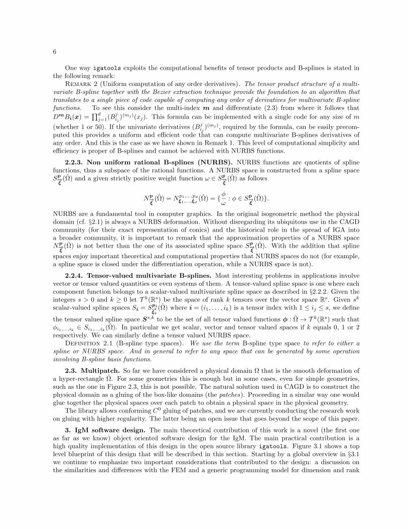
6
One way igatools exploits the computational benefits of tensor products and B-splines is stated inthe following remark
Remark 2 (Uniform computation of any order derivatives) The tensor product structure of a multi-variate B-spline together with the Bezier extraction technique provide the foundation to an algorithm thattranslates to a single piece of code capable of computing any order of derivatives for multivariate B-splinefunctions To see this consider the multi-index m and differentiate (23) from where it follows that
DmBi(x) =proddj=1(Bjij )
(mj)(xj) This formula can be implemented with a single code for any size of m
(whether 1 or 50) If the univariate derivatives (Bjij )(mj) required by the formula can be easily precom-
puted this provides a uniform and efficient code that can compute multivariate B-splines derivatives ofany order And this is the case as we have shown in Remark 1 This level of computational simplicity andefficiency is proper of B-splines and cannot be achieved with NURBS functions
223 Non uniform rational B-splines (NURBS) NURBS functions are quotients of splinefunctions thus a subspace of the rational functions A NURBS space is constructed from a spline spaceSpminusrarrξ
(Ω) and a given strictly positive weight function ω isin Spminusrarrξ
(Ω) as follows
Npminusrarrξ
(Ω) = Np1pdξ1ξd
(Ω) = φω
φ isin Spminusrarrξ
(Ω)
NURBS are a fundamental tool in computer graphics In the original isogeometric method the physicaldomain (cf sect21) is always a NURBS deformation Without disregarding its ubiquitous use in the CAGDcommunity (for their exact representation of conics) and the historical role in the spread of IGA intoa broader community it is important to remark that the approximation properties of a NURBS spaceNpminusrarrξ
(Ω) is not better than the one of its associated spline space Spminusrarrξ
(Ω) With the addition that spline
spaces enjoy important theoretical and computational properties that NURBS spaces do not (for examplea spline space is closed under the differentiation operation while a NURBS space is not)
224 Tensor-valued multivariate B-splines Most interesting problems in applications involvevector or tensor valued quantities or even systems of them A tensor-valued spline space is one where eachcomponent function belongs to a scalar-valued multivariate spline space as described in sect222 Given theintegers s gt 0 and k ge 0 let T k(Rs) be the space of rank k tensors over the vector space Rs Given sk
scalar-valued spline spaces Si = Spiminusrarrξi
(Ω) where i = (i1 ik) is a tensor index with 1 le ij le s we define
the tensor valued spline space Ssk to be the set of all tensor valued functions φ Ωrarr T k(Rs) such thatφi1ik isin Si1ik(Ω) In particular we get scalar vector and tensor valued spaces if k equals 0 1 or 2respectively We can similarly define a tensor valued NURBS space
Definition 21 (B-spline type spaces) We use the term B-spline type space to refer to either aspline or NURBS space And in general to refer to any space that can be generated by some operationinvolving B-spline basis functions
23 Multipatch So far we have considered a physical domain Ω that is the smooth deformation ofa hyper-rectangle Ω For some geometries this is enough but in some cases even for simple geometriessuch as the one in Figure 23 this is not possible The natural solution used in CAGD is to construct thephysical domain as a gluing of the box-like domains (the patches) Proceeding in a similar way one wouldglue together the physical spaces over each patch to obtain a physical space in the physical geometry
The library allows conforming C0 gluing of patches and we are currently conducting the research workon gluing with higher regularity The latter being an open issue that goes beyond the scope of this paper
3 IgM software design The main theoretical contribution of this work is a novel (the first oneas far as we know) object oriented software design for the IgM The main practical contribution is ahigh quality implementation of this design in the open source library igatools Figure 31 shows a toplevel blueprint of this design that will be described in this section Starting by a global overview in sect31we continue to emphasize two important considerations that contributed to the design a discussion onthe similarities and differences with the FEM and a generic programming model for dimension and rank
7
Ω1
Ω2
Ω3
Ω4
Ω1
Ω2
Ω3
Ω4
Fig 23 Simple geometry that requires more than a single patch to be represented
independent code Then we give a detailed description of the main objects generally accompanied withsnippet of code to illustrate its use finishing with a simple code to assemble a local operator in Listing 13that integrates some of the main classes
31 Design overview Following sect21 an IgM is a special case of a Galerkin method where the basisfunctions in the reference domain are of B-spline type (NURBS T-spline etc) and the basis functions in thephysical domain are their push-forwards (see Table 21) The regularity of the mapping must be compatiblewith the one of the reference basis and the transformation type In this conception of an isogeometricmethod the main mathematical concepts are the reference domain Ω the reference space V(Ω) the physicaldomain Ω the mapping F Ω rarr Ω the transformation type that together with the mapping gives thepush-forward operator P and the physical space V(Ω) These concepts and their relations are depictedon the left column of Figure 31 In the physical space we are interested in handling quantities such asthe differential operators A V(Ω) rarr V(Ω)prime source operators f isin V(Ω)prime and fields u isin V(Ω) (see lowerpart of Figure 31) We need access to these quantities both on the global level (where the system issolved and solution plotted) as well as on the local level (where the operators are assembled) Under theobject oriented paradigm a good software design for an IgM library is one that remains faithful to themathematics of isogeometric analysis The right column of Figure 31 sketches the design of igatools
emphasizing the relation between the main concepts in an IgM (left column) in synchronization with theclasses used to represent these concepts in the library
32 Similarities and differences with the FEM For the creation of our design it was importantto identify the similarities and differences between the IgM and the FEM One approach that has beenproposed ([10 13]) to implement isogeometric codes is to add an isogeometric plugin on existing FEMsoftware packages This idea only exploits the similarities and could make sense for specific engineeringapplications where decades of FEM coding has been invested Another approach which is the one wefollow is to take advantages not only of the similarities but also of the differences Thus we use thesuccessfully proven finite element design ideas that also apply to an IgM but we do not include uselessFE design ideas Instead we create new concepts to produce a design naturally suitable for an IgM Thesimilarities come from both being Galerkin methods with basis functions of small support which makesconvenient to perform the assembling by adding local contributions Also the handling of the globalsystem is similar but this is not even the ground of the FEM itself but of a linear algebra system Asfar as the differences we should start by saying that there are concepts in each of the methods that donot make sense for the other For example in an IgM we have no master element or finite element tripleor degrees of freedom associated with geometric objects of the triangulation but we have concepts suchas a reference space a push-forward and a physical space which on the ground of implementation havenot made a lot of sense for a FEM code design Having a design with native support for these conceptsmakes the whole approach to the IgM more natural and comprehensible not only for a user but more sofor new programmers that want to develop in the isogeometric concept without having to produce a forcedtranslation to finite elements Figure 32 pictorially compares the different concepts used in a FEM andan IgM to generate the physical space
33 Dimension independent code Besides the implementation of a new design a very interestingfeature of igatools is the capability of writing dimension and range independent code All classes are
8
V
P V
FType of
transformation
V on localelements
OperatorsA V rarr Vprime
f isin Vprime
Fieldsu isin V
Isogeometric Method Concepts igatools Classes
PhysicalSpace(sect35)
PushForward(sect352) ReferenceSpace
(sect34)
Mapping(sect351)TransformationType
(sect352)
ElementIterator
(sect35)Matrix A
Vector F
PhysicalSpace
(sect37)
Vector U
PhysicalSpace
(sect37)
Fig 31 The conceptual diagram sketches the IgM object oriented design advocated in this work and implemented inigatools on the left column there are the mathematical concepts found in isogeometric analysis and on the right columnthe corresponding realization of such concepts through the main classes in igatools Both location and color are used toemphasis the synchronization of concepts-classes and their interaction Under the object oriented paradigm a good softwaredesign for an IgM library is one that remains faithful to the mathematics of isogeometric analysis The classes include areference to the paper section where they are described
V(Ω)
xy
z
x y
z
V(Ω)
P
V(Ω)
xy
z
(K P Σ
)
+
Th
Fig 32 Both the FEM and the IgM are particular cases of the Galerkin method They provide a specific wayof constructing a sequence of discrete approximating spaces Both share the properties of having basis function with smallsupport but the way to generate the spaces is essentially different as illustrated in the picture In the FEM the approximatingspace V(Ω) is constructed from the finite element triple (K PΣ) and the triangulation Th In the IgM the physical space isgenerated from a global reference space and a push-forward operator
designed in such a way that the space dimension co-dimension and the tensorial range are selected astemplate parameters The use of templates is very convenient for scientific computing they allow to havea single code that is resolved at compile time generating optimized code as if it was written for each instance
9
of the dimension and with no run-time checks that would affect performance This approach allows us towrite an application code that is independent of dimension and range (provided that the mathematicalproblem can so be formulated) For example letrsquos say that a user writes the code for a 2D problem thatcan be mathematically formulated in any dimension (for ex Poissonrsquos equation) If this code is writtenwith some minimal care then the same code will run for the problem with the physical domain being 1D3D or a 2D manifold embedded in R4 and for the solution being scalar- vector- or tensor-valued (cf sect61)Table 31 shows an example of how the template technique for dimension independent code appears to theuser in the case of the class BSplineSpace (sect34) The dimension independent approach can be discoveredin any piece of code shown in this work
V(Ω) is a spline space and φ isin V(Ω) igatools realization of V(Ω)
φ R2 rarr R BSplineSpacelt211gt v_hat()
φ R3 rarr R3 BSplineSpacelt331gt v_hat()
φ R2 rarr R3times3 BSplineSpacelt232gt v_hat()
φ Rd rarr T k(Rs) BSplineSpaceltdskgt v_hat()
Table 31The library uses template parameters to attain dimension and range independent code the table shows an example on
how the code looks when constructing an object of the BSplineSpace type The left column shows the domain and range of aspline function for a given spline space and the right column the how igatools uses template parameters to define a splinespace for that domain and range combination The last row shows the generic format of this class The second and thirdarguments can be omitted in which case the library assumes some default values
34 Reference space (BSplineSpace and NURBSSpace) Currently the library provides two classes
or types for the reference space V(Ω) These are BSplineSpace and NURBSSpace realizations of the spacesSpminusrarrξ
(Ω) and Npminusrarrξ
(Ω) described in sect22 (including their tensor-valued counterparts of sect224) These classes
can have different degrees and multiplicities in each coordinate direction and different scalar spaces foreach range component The last type of spaces are necessary for example in the context of fluid [25 17]We will use the generic class ReferenceSpace to refer to either BSplineSpace or NURBSSpace In orderto construct a reference space it is necessary to provide the reference domain Ω the vector of knot vectorsminusrarrξ = (ξ1 ξd) the degrees p = (p1 pd) and in the case of a NURBS space the weight functionω In igatools the class CartesianGrid provides a realization for the vector of knot vectors withoutrepetition as well as for the reference domain (a hyper-rectangle) Listing 1 shows example of creatingCartesianGrids
1 2-dim unit grid with 4 uniformly distributed knots in each coordinate direction
2 auto grid_2d = CartesianGrid lt2gt create (4)
34 3-dim unit grid with 2 4 and 3 knots in each coordinate direction
5 auto grid_3d = CartesianGrid lt3gt create (2 4 3)
Listing 1Creating CartesianGrids in igatools some details are explained in the Listing as comments The code also shows the
use of the create idiom implemented in igatools for simple handling of smart pointers (cf sect43)
The vector with repetitionminusrarrξ is obtained from a CartesianGrid and a corresponding knot multiplic-
ities (Multiplicity) The NURBS space weight function is passed through its coefficients In Listing 2we show some examples of constructing reference spaces
35 Physical space (PhysicalSpace) The physical space V(Ω) in igatools is realized by the classPhysicalSpace this class needs to be provided with a RefereceSpace and a PushForward The lattercontains the geometry and transformation type
10
1 Scalar B-spline space over [0 1]^2 of degree 2 with maximum regularity
2 auto space1 = BSplineSpace lt2gt create(grid_2d 2)
34 Idem to space1 but providing the multiplicities
5 auto space2 = BSplineSpace lt2gt create(grid_2d 2 31133213)
67 Vector -valued B-spline space over [0 1]^2 of
8 degree 2 and 1 in each component and maximum regularity
9 auto space3 = BSplineSpace lt2 2gt create(grid_2d 2 1)
1011 Vector -valued B-spline space over [0 1]^3 of degree 2
12 auto space4 = BSplineSpace lt3 3gt create(grid_3d 2)
1314 Scalar NURBS space of degree 2 with given weight coefficients
15 auto space5 = NURBSSpace lt2gt create(grid_2d 2 weight )
Listing 2Creating reference spaces Examples of constructing B-spline type spaces in igatools some details are explained in the
listing as comments The code is referring to the grids created in Listing 1
351 Geometry (Mapping) The geometry or physical domain is described by the deformation Fof the reference domain in igatools the deformation is realized by the Mapping class It is basically afunction from Rd to Rs with the added feature of being element aware in the sense of sect36 so that itsvalues can be handled with the grid-like iterators for uniformity and efficiency Listing 3 shows examplesof creating mappings In particular we remark that the encapsulation of the geometry in the Mappings
1 Creating a Mapping object from the provided library of maps
2 auto map = SphericalMap create(grid)
34 Creating a Mapping object from a space and a vector of control points
5 auto bs_map = IgMapping create(bspace control_points )
67 Importing a Mapping object from a file
8 IgReader ltdim gt reader(pipexml)
9 auto nurbs_map = readerget_map ()
Listing 3Code examples showing how to create some geometries (Mappings) The library allows the use of different types of
deformations including analytic functions and isogeometric mapping
class allows to cleanly integrate a geometric modeler (or a CAD system) by implementing a Mapping
specialization (see sect52)
352 Push-forward operator (PushForward) The other ingredient besides a reference spacerequired to construct a physical space is a push-forward operator In igatools it is realized by thePushForward class which is constructed from a Mapping and a Transformation Currently igatoolsprovides support for h_grad h_div h_curl and l2 transformation types (see Table 21) Listing 4 showsan example for creating a push-forward operator and a physical space
36 Element level access (ElementIterator) The ReferenceSpace class can be thought of asa container of basis functions The latter are supported only on a small number of elements whichmakes it convenient to access them through the elements Q of the grid Q We refer to it as the local orelement level access to quantities and it is provided using an element iterator in the spirit of the standardtemplate library (STL) [41] Simply speaking given an object collection (the container) an iterator maybe thought of as a type of pointer that has two primary operations referencing one particular element inthe container (called element access) and modifying itself so it points to the next element (called elementtraversal) The primary purpose of an iterator is to allow a user to process every element of a container
11
1 using PushFw = PushForward ltTransformation h_grad dim gt
2 using Space = PhysicalSpace ltRefSpace PushFw gt
34 auto push_fw = PushFw create(map)
5 auto space = Space create(ref_space push_fw )
Listing 4Creating a physical space The physical space is created from a reference space and a push-forward operator The
push-forward operator is defined from the map using the h_grad transformation type The variables ref_space and map areassumed to have been defined as shown in Listings 2 and 3 respectively Also notice the use of the using keyword to simplifylong type names (see sect43)
while isolating the user from the internal structure of the container This allows the container to storeelements in any manner it wishes while allowing the user to treat it as if it were a simple sequence or listAn iterator class is designed in tight coordination with the corresponding container class In igatools wesee the classes CartesianGrid BSplineSpace NURBSSpace Mapping PushForward and PhysicalSpace
as containers of elements that we collectively call grid-like containers The containers provide the methodsfor creating the iterators and thus a consistent way to iterate on the different data structures In this waythe code is more readable reusable and less sensitive to changes in the data structure (for example if weadd support for local refinement) In particular it fits perfectly in the dimension independent paradigmadvocated by our design Listing 5 shows a typical use of element iterators in igatools comparing thecases of a CartesianGrid ReferenceSpace and PhysicalSpace In particular notice the consistency inthe treatment despite the different data stored in each class
1 for(auto elem grid)
2
3 cout ltlt elemvertex (0)
4
56 for(auto elem ref_space)
7
8 int n_basis = elemget_num_basis ()
9 for (int i = 0 i lt n_basis ++i)
10
11 do something with the reference basis
12
13 auto loc_dofs = elemget_local_to_global ()
14
1516 for(auto elem phys_space)
17
18 int n_basis = elemget_num_basis ()
19 for (int i = 0 i lt n_basis ++i)
20
21 do something with the physical basis
22
23
Listing 5Uses of element iterators on igatools containers We iterate on the elements of a CartesianGrid a ReferenceSpace
and a PhysicalSpace Notice the consistent treatment that iterators allow to access different data We assume that gridref_space and phys_space were defined as shown in listings 1 2 and 4 respectively
A general purpose library like igatools cannot (and should not try to) guess what equation or problemthe user will want to solve Instead it should provide a flexible and intuitive way to access the quantities thatseem to be common to all typical problems Most operators require access to basis functions (values andderivatives of any order) and to geometric quantities (values and derivatives of the mapping determinantsand curvatures) Given the small support (in number of elements) of the basis functions the assembling of
12
the global quantities is conveniently performed by adding the local contributions The ElementIterator
is the mechanism that igatools provides to compute and access these values In addition to the consistentinterface to the different grid-like containers a second task that is handled by the element iterator is themanagement of an element values cache A cache is a smart piece of memory that depending on the desiredquantities to be computed stores commonly used computations to increase efficiency Most optimizationtechniques tend to interfere with a clean code and it is common to have a trade off between efficiencyand clean design In order to partially counteract this effect we use the element iterator to implement anabstraction layer that is designed to be invisible from the neighbor layers This provides the efficiencyrequired but still keep an organized design for the caches For using the cache mechanism the cleaninterface of the range based for loop shown in Listing 5 needs to be slightly modified Listing 6 show theactual code for the assembling of the stiffness matrix (using the efficient cache mechanism) for a Poissonrsquosproblem Obviously in the art of software design there is no technique to show that our design is the right
1 void PoissonProblem assemble_matrix ()
2
3 ValueFlags flag = ValueFlags gradient | ValueFlags w_measure
45 auto elem = space -gtbegin ()
6 auto end = space -gtend ()
7 elem -gtinit_values(flag quad)
8 for( elem = end ++elem)
9
10 elem -gtfill_values ()
11 loc_matrix = 0
12 auto w_meas = elem -gtget_w_measures ()
13 for (int i = 0 i lt n_basis ++i)
14
15 auto grd_phi_i = elem -gtget_basis_gradients(i)
16 for (int j = 0 j lt n_basis ++j)
17
18 auto grd_phi_j = elem -gtget_basis_gradients(j)
19 for (int qp = 0 qp lt n_qp ++qp)
20
21 loc_matrix(i j) +=
22 scalar_product(grd_phi_i[qp] grd_phi_j[qp]) w_meas[qp]
23
24
25
26 auto loc_dofs = elem -gtget_local_to_global ()
27 matrix -gtadd(loc_dofs loc_dofs loc_matrix )
28
29
Listing 6Code for the assembling of the stiffness matrix for the Poisson problem (cf sect61 In order to use the efficient cache
mechanism the range based for loops of Listing 5 needs to be modified by adding the lines 5 6 7 and 10 Notice thatinit_values() is execute one time and fill_values() for each element
one but we find encouraging that the assembly function looks simple and plain enough also to non-codingexperts without sacrificing efficiency
37 Global quantities fields operators and the linear algebra We have discussed the localhandling of basis functions to assemble the local contribution of operators The global quantities such asfields and global operators are stored in containers of the linear algebra system (eg global vectors andmatrices) They are assembled from the local element contributions through the bookkeeping mechanismkept by the space For each element the non-zero basis functions have a local index for which space knowsthe corresponding global index The query for this information is obtained through the element iteratorthrough the get_local_to_global() function Listing 6 line 26) Almost any of the many excellent linear
13
algebra systems could be easily plugged into the proposed design From a bias preference of the originaldevelopers (and for the sake of selecting one) in igatools we have used the linear (and non-linear) algebraprovided by some packages of the Trilinos library [29] Trilinos among other things provides stateof the art storage for distributed vectors and matrices as well as a complete collection of linear and nonlinear solvers In order to have a consistent style with the other pieces of the library igatools providessimplified wrappers to basic Trilinos vectors matrices and linear solvers At the same time we do notrestrict the more advanced and powerful use that can be obtained by dealing directly with the Trilinos
object
4 igatools implementation standards The effort in igatools has been directed to develop ahigh quality implementation of the isogeometric software design presented in sect3 To partially justify thestatement in this section we briefly describe some of the software engineering tools and development modelwe have adopted
41 Development infrastructure The development of igatools is supported by todayrsquos standardsofware engineering tools for that purpose We use the distributed version control system and sourcecode management git2 and the bug tracking system Trac3 For managing the build process we useCMake4 allowing the software compilation process using a simple platform and compiler independentconfiguration files Most importantly we strive for high standards for documentation and user supportThe documentation can be divided in three level this paper that describes the design concepts and howthey work together the tutorial examples provided with the source to give a hand-on introduction to usethe library and a reference manual generated by processing the in-source documentation with Doxygen5For community support we have a user group6 for discussion between the igatools developers and usersand a development group7 where the igatools developers discuss about new features library designimplentation details discovered bugs and possible remedies We also mantain a wiki page 8 working asthe webpage to the world of the library
42 Development model (testing and debugging) igatools has hundreds of unit tests (smallprograms) that are run automatically using CDashCTest9 to verify that new changes are not breakingworking features
We use and advocate the use of the test driven development model [8] This basically means thatwe write a unit test for the feature we want to implement or fix the test initially fails then we writecode until the test passes from that moment on the test is executed automatically Now we can refactorthe code (clean remove any duplication rename variables and methods optimize etc) being confidentthat the new code is not damaging any existing functionality In addition to the unit tests igatools hasautomatic integration and validation tests (more cpu-time expensive than unit tests) in order to verifythat the different modules interact correctly
The libray makes use defensive programming techniques to detect and easily find bugs at runtimethrough the exception handling mechanism We adopt two levels of checks One more expensive in termsof running time but only active when igatools is compiled in Debug mode We perform this kind ofchecks wherever there may be a chance of error eg out-of-bound index for accessing to vectors elementsuninitialized objects invalid object states mismatching dimensions etc The second level of checks isalways active (both in Debug and in Release mode) and it is used for checking anomalies that may beintroduced by the input data
The typical workflow for a user of igatools would be to first write his code and test it with the library
2httpwwwgit-scmcom3httptracedgewallorg4httpwwwcmakeorg5httpwwwdoxygenorg6httpsgroupsgooglecomforumforumigatools-users7httpsgroupsgooglecomforumforumigatools-development8httpcodegooglecompigatoolswlist9httpwwwcdashorg
14
in Debug mode on a small-size problem When this is working as expected and (virtually) bug-free linkthe code with igatools in Release mode on a real-size problem
43 Programming language The main language used in the development of igatools is C++11[32]It includes many additions to the previous standard C++03[31] mostly aimed to produce a code that iscleaner safer more efficient and easier to maintain In particular igatools makes heavy use of some ofthe language features somehow defining certain aspects of its programming style as for example
(i) Smart pointers and create facility Objects in igatools can have big sizes and can beshared by different other objects This sharing mechanism is handled through the use of smart pointersThey provide automatic memory management ensuring that the resource they control is automaticallydestroyed when its last (or only) owner is destroyed Moreover the igatools classes intended to be usedthrough smart pointers provide a create facility for this purpose For each constructor of the class thereis a static function (called create) with the same arguments of the constructor that returns an instanceof the class wrapped by a shared pointer A code example showing the implementation and use of thetechnique is shown in Listing 7
1 class MyClass
2
3 public
4 MyClass constructor using arg1 of type T1 and arg2 of type T2
5 MyClass(T1 arg1 T2 arg2)
67 The static function create () uses the constructor
8 MyClass(T1 arg1 T2 arg2) to build a MyClass
9 instance wrapped by a std shared_ptr
10 static stdshared_ptr ltMyClass gt create(T1 arg1 T2 arg2)
11
12 return std make_shared ltMyClass gt( MyClass(arg1 arg2) )
13
14
1516 void foo(T1 a T2 b)
17
18 Create an instance of MyClass wrapped by a std shared_ptr
19 stdshared_ptr ltMyClass gt my_obj = MyClass create(a b)
20
Listing 7Create facility For each class that is intended to be used through a smart pointer igatools provides a create facility
The static function create returns an instance of the class wrapped by a stdshared_ptr The function foo shows how thepointer is created
(ii) Template types (using and auto) C++11 provides better management of templates thanC++03 and igatools extensively uses templates in order to attain efficiency and the dimension indepen-dent paradigm One drawback of using templates is the fact that the template arguments may becomeinhumanly difficult to express We solve this problem with the C++11 using alias facility that allows tocreate human readable aliases for the necessary types Related is the automatic type inference facilityauto that deduces the type of an explicit initialization An appropriate combination of using create andauto results in a much more simple and human comprehensible syntax as shown in Listing 8 creating acertain style to code with igatools
5 igatools practical features Besides implementing the novel object oriented design presented inthis work with high quality standards igatools provides useful features that make it useful and attractivefor practical applications
51 Inputoutput facilities It is important for the library to use NURBS geometries generated byother software At the present stage there is no scientific computing dedicated format for isogeometric typeof spaces The developers of igatools and GeoPDEs in a joint effort defined an xml format to describe such
15
1 void brute_force_syntax ()
2
3 stdshared_ptr ltCartesianGrid ltdim gtgt grid =
4 std make_shared ltCartesianGrid ltdim gtgt(CartesianGrid ltdim gt(4))
5 stdshared_ptr ltMapping ltdim gtgt map =
6 std make_shared ltBallMapping ltdim gtgt(BallMapping ltdim gt(grid ))
7 stdshared_ptr ltBSplineSpace ltdim 11gtgt ref_space =
8 std make_shared ltBSplineSpace ltdim 11gtgt(BSplineSpace ltdim 11gt(grid 3))
9 stdshared_ptr ltPushForward ltTransformation h_grad dim gtgt push_fw =
10 std make_shared ltPushForward ltTransformation h_grad dim gtgt(
11 PushForward ltTransformation h_grad dim gt(map))
12 stdshared_ptr ltPhysicalSpace ltBSplineSpace ltdim 11gt
13 PushForward ltTransformation h_grad dim gtgtgt space =
14 std make_shared ltPhysicalSpace ltBSplineSpace ltdim 11gt
15 PushForward ltTransformation h_grad dim gtgtgt(
16 PhysicalSpace ltBSplineSpace ltdim 11gt
17 PushForward ltTransformation h_grad dim gtgt(ref_space push_fw ))
18
1920 void human_syntax ()
21
22 using Grid = CartesianGrid ltdim gt
23 using Map = Mapping ltdim gt
24 using RefSpace = BSplineSpace ltdim 1 1gt
25 using PushFw = PushForward ltTransformation h_grad dim gt
26 using Space = PhysicalSpace ltRefSpace PushFw gt
2728 auto grid = Grid create (4)
29 auto map = BallMapping ltdim gt create(grid)
30 auto ref_space = RefSpace create(grid 3)
31 auto push_fw = PushFw create(map)
32 auto space = Space create(ref_space push_fw )
33
Listing 8Library facilities using auto and create The two functions perform the same operations but the second one uses
the combination of the using auto and create facilities advocated by the igatools programming style resulting in a morehuman readable syntax than the brute force counterpart
geometries Thus igatools through it IgReader class (see Listing 3 lines 8 and 9) supports importinggeometries in this data format which is completely specified in the library documentation xml is anextremely flexible format that is supported by wide number of libraries and applications igatools sourceis distributed with contributed scripts to convert geometries generated with the MATLAB NURBS toolbox10
to the xml formatSimilarly important for the library is to provide a useful mechanism to analise and visualize the com-
putational results igatools generates output for this purpose through its Writer class (see Listing 15)So far the writer provides output in vtk format [37] which can be visually processed (among other things)with Paraview [40]
52 Interaction with CAGD software The main selling point when isogeometric analysis wasintroduced was the possibility to integrate the geometry with the analysis In the context of igatools
this can be cleanly achieved by implementing a Mapping specialization (see sect351) that internally use allgeometric features of a modern CAD system provides a clear interface to the user without him worryingabout the implementation details Now after a decade from the introduction of IGA there is no dedicatedCAD software that directly generates a 3D analysis suitable geometry this being one of the limiting issuesin the use of the IgM in the industrial community One reason is that most CAD software when dealingwith a 3D geometries only model the boundary surfaces of the represented domain An exception is the
10httpwwwariauklinuxnetnurbsphp3
16
geometric modeler IRIT 11 developed by G Elber at Technion that natively handles trivariate volumesWe have tested the integration of igatools with this particular geometric modeler by implementing aMapping specialization (MappingIRIT) that internally uses the IRITrsquos routines and data structures forthe evaluation of the geometric quantities required by Mapping This MappingIRIT class is used for thegeometry in the non-linear elasticity example presented in sect64
53 Parallel support Computationally demanding applications require igatools to take advan-tage of parallel computing technologies The Trilinos and Intel TBB12 libraries used in cooperation withigatools provides this service using a distributed and shared memory model respectively The container-iterator model separates data from operations In fact the iterators are designed in such a way they do notmodify their container In this way we can obtain parallel iterators where each thread points to differentgrid elements We have successfully tested the use of Intel TBB in igatools following very closely theimplementation of the dealII classes for the threads management In particular a correct managementof threadsiterators for the parallel assembly routines has been checked A distributed memory modelusing MPI have been succesfully applied to igatools application code by using the Trilinos facilities fora distributed assembling and parallel solving of the global system
6 Examples In this section we illustrate the library flexibility to naturally handle and adapt todifferent situations We do this by showing its use to solve typical application problems We start witha rather detailed description for the implementation of a simple Poisson equation This is the de factoprototype example in any Galerkin numerical method that we also employ to describe the basic buildingblocks typical to the use of the library and to which we refer to in the subsequent examples We con-tinue with a tiny adaptation to the Poisson problem code that solves the Laplace-Beltrami problem on amanifold Then we illustrate the handling of vector-valued and many spaces problems by discussing theimplementation of the Stokes equation Finally we present a non-linear elasticity problem showing theflexibility of the library to cleanly interact with other software packages
Notice that in the snippets of code listed in the section some non-relevant pieces are omitted (or moreprecisely replaced by a comment of the form ldquordquo) to help with the understanding of the main piecesAlso as we move on in the examples less details are provided as we assume they can be translated fromthe previous examples
61 Poisson Equation The Poisson problem consists in finding u Ω sub Rd rarr R such that
(61) minus∆u = f in Ω u = g on partΩ
It can be rewritten in weak form as find u = u0 + ug with u0 isin H10 (Ω) and ug the lift of g such that
Au(v) = F (v) for all v isin H10 (Ω) where Au(v) =
intΩnablau middot nablav and F (v) =
intΩfv The IgM for this problem
(cf sect21) requires the definition of the isogeometric space V(Ω) the assembling of the stiffness matrix Kand right hand side F by adding the element contributions and the solving of the linear system KU = F
Below we describe a possible approach for the implementation of this problem with igatools Thefull running code for this problem is part of the tutorial distributed with the library To be concrete wechoose the physical domain Ω to be a d-dimensional spherical sector for d = 1 2 and 3 a homogeneousboundary condition and a constant source of 5 The code would look practically the same if we decide touse a CAD geometry for the domain a non-homogeneous boundary function andor a non-constant sourceterm
In order to undertake this problem a class for it (see Listing 9) is defined its public interface providestwo members the constructor PoissonProblem and the run() function Within the private membersone can identify the declaration of objects for the space and the linear algebra We can also see theusing keyword to create short alias for the usually long templated types and the use of smart pointers(shared_ptr) both common techniques within the programming style of igatools (cf sect43) For theactual solving of the problem we define objects of PoissonProblem type in the programrsquos main() (see
11httpwwwcstechnionacil~irit12httpswwwthreadingbuildingblocksorg
17
1 template ltint dim gt
2 class PoissonProblem
3
4 public
5 PoissonProblem(TensorSize ltdim gt ampn_knots int deg)
6 void run ()
78 private
9 void assemble ()
10 void solve ()
11 void output ()
1213 private
14 using RefSpace = BSplineSpace ltdim gt
15 using PushFw = PushForward ltTransformation h_grad dim gt
16 using Space = PhysicalSpace ltRefSpace PushFw gt
1718 shared_ptr ltCartesianGrid ltdim gtgt grid
19 shared_ptr ltRefSpace gt ref_space
20 shared_ptr ltMapping ltdim gtgt map
21 shared_ptr ltSpace gt space
2223 quadratures defined
2425 ConstantFunction ltdim gt f
26 ConstantFunction ltdim gt g
2728 shared_ptr ltMatrix gt matrix
29 shared_ptr ltVector gt rhs
30 shared_ptr ltVector gt solution
31
Listing 9Class to approximate the solution of a Poisson problem The public interface provides the constructor that prepares the
object and the function run() that computes and plots the solution In the private members we can find objects to handlethe space and the linear algebra
Listing 10) Here we can see how the dimension independent template technique (cf sect33) is put to
1 int main()
2
3 n_knots and deg defined
4 PoissonProblem lt1gt poisson_1d ( n_knots deg)
5 poisson_1drun()
67 PoissonProblem lt2gt poisson_2d (n_knots n_knots deg)
8 poisson_2drun()
910 PoissonProblem lt3gt poisson_3d (n_knots n_knots n_knots deg)
11 poisson_3drun()
12
13
Listing 10Main routine to solve the Poisson problem for different domain dimensions For each dimension 1 2 and 3 we construct
the problem and then assemble solve and output the result by calling the function run()
use We are solving the Poisson problem in 1 2 and 3 dimensions with the same templated code As amatter of fact with the same code we could solve this problem in 4 dimensions if we wish to Each objectdefinition (lines 4 7 and 10) calls the constructor that prepares the object to be ready to use and thenwe call the object member function run() that computes the solution The function run() (see Listing
18
1 void PoissonProblem ltdim gt run()
2
3 assemble ()
4 solve ()
5 output ()
6
Listing 11The run function is the public interface that solves the Poisson problem by assembling and solving the discrete linear
system and saving the solution in graphical format
11) is just a high level interface that calls the private members assemble() solve() and output() thatwill do the actual computational work and are explained later on After executing this program graphicaloutput files (in vtk format) for the different dimensions with the problem solution are saved Figure 61shows these files
Fig 61 Plot of the solutions to the Poisson problem with homogeneous boundary conditions and constant source termon a spherical sector in 1 2 and 3 dimensions Notice that the three plots were generate with the same code by only changingthe dimension template argument
Now we explain the implementation of the different member functions of the PoissonProblem classThe constructor (see Listing 12) is in charge of making the object ready to be used So it creates a physicalspace space by first creating a grid a reference space ref_space a mapping map and a push forward
The assemble() routine assembles the global stiffness matrix matrix and global right hand side rhs
by adding the element contributions In igatools we use the element iterator (sect36) for this purposeWe have already seen in Listing 6 the assemble of the global matrix here in Listing 13 we include theassembling of the right hand side and the treatment of the boundary conditions In this case we proceedin two steps (lines 27 and 28) first we project the boundary function g onto the trace space and then weenforce into the linear system these values for the Dirichlet degrees of freedom Notice that a projectionis necessary as splines are not interpolatory in general
As discussed in sect37 igatools relies on external algebra packages for solving the global system Thefunction solve() in Listing 14 defines a Solver object which is a wrapper class provided by igatools
for basic use of Trilinos solvers The solution of the system is returned in solution The lines in thislisting look simple enough to be self-explanatory
To manage the graphical output (sect51) igatools provides a Writer class that can be used to handle
19
1 PoissonProblem(TensorSize ltdim gt ampn_knots int deg)
2
3 initilize elem_quad and face_quad
4 f(5) g(0)
5
6 define box a bounding box for the grid
78 grid = CartesianGrid ltdim gt create(box n_knots )
9 ref_space = RefSpace create(grid deg)
10 map = BallMapping ltdim gt create(grid)
11 space = Space create(ref_space PushFw create(map))
1213 initialize matrix rhs and solution
14
Listing 12Poissonrsquos problem constructor It construct the physical space for which it needs to construct a reference space and
a push-forward which in turn requires the construction of a map and a cartesian grid It also initializes the quadratureschemes the linear algebra and the source and boundary functions
1 void PoissonProblem ltdim gt assemble ()
2
3 same code as listing 6 we are only adding
4 the pieces for the right hand side
56 for ( elem = elem_end ++elem)
7
8 loc_rhs = 0
9 auto points = elem -gtget_points ()
10 auto phi = elem -gtget_basis_values ()
11 auto f_values = fevaluate(points )
1213 for (int i = 0 i lt n_basis ++i)
14
15 matrix assembling (Listing 6)
1617 auto phi_i = phiget_function(i)
18 for (int qp = 0 qp lt n_qp ++qp)
19 loc_rhs(i) +=
20 scalar_product(phi_i[qp] f_values[qp]) w_meas[qp]
21
22
23 rhs -gtadd(loc_dofs loc_rhs )
24
2526 Apply dirichlet boundary condition
27 project_boundary_values(g space face_quad dirichlet_id dof_values )
28 apply_boundary_values(dof_values matrix rhs solution )
29
Listing 13Assembling of the global system for Poisson problem The matrix assembling was already shown in Listing 6 here we
only show the additional code required to assemble the right hand side and take care of the dirichlet boundary constraints
geometries and fields that are to be saved in a graphical output format (for now a vtk file) In Listing 15a Writer object associated with the geometry of map is defined (line 4) then the solution field is added toit (line 5) and finally writer is asked to save the geometry and the solution field to disk (line 6)
62 A surface example The code of sect61 can be trivially modified to solve a partial differentialequation on a surface igatools can naturally handle manifold domains such as surfaces or curves
Let Γ be a d-dimensional manifold and consider the Laplace-Beltrami equation find u Γrarr R such
20
1 void PoissonProblem ltdim gt solve ()
2
3 Solver solver(SolverType CG)
4 solversolve(matrix rhs solution )
5
Listing 14Solver for the Poisson problem We use the simple wrapper igatools provides to the Trilinos solvers
1 void PoissonProblem ltdim gt output ()
2
3 define filename
4 Writer ltdim gt writer(map)
5 writeradd_field (space solution Temperature)
6 writersave(filename )
7
Listing 15Saving the solution of Poisson problem in a graphical output
that
(62) minus∆Γu = f in Γ u = g on partΓ
which can be rewritten in weak form as find u = u0 + ug with u0 isin H10 (Γ) and ug the lift of g such that
Au(v) = F (v) for all v isin H10 (Γ) where Au(v) =
intΓnablaΓu middot nablaΓv and F (v) =
intΓfv Except for the fact that
the differential operators are surface operators one can see the similarity of this problem with equation(61) The library understands manifolds thus when the physical space has codimension different from 0igatools understand that gradients refers to surface gradients In this way minor modifications to thePoisson problem code of sect61 allow to solve the Laplace-Beltrami problem
More precisely without loss of generality let assume we want to solve equation (62) on a d-dimensionalspherical piece of codimension 1 It only requires minor changes on a few lines in the problem class firstthe definitions of codim and space
static const int codim = 1
static const int spacedim = dim + codim
and then some small changes in lines 15 20 25 and 26 of Listing 9 by the following four lines in the givenorder
using PushFw = PushForward ltTransformation h_grad dim codim gt
shared_ptr ltMapping ltdim codim gtgt map
ConstantFunction ltspacedim gt f
ConstantFunction ltspacedim gt g
The only change required in the constructor is to replace line 10 of Listing 12 by
map = SphereMapping ltdim gt create(grid)
In Figure 62 we plot the isogeometic approximate solution to the Laplace-Beltrami problem over a sphericalpiece given by a spherical coordinate map
63 Navier-Stokes Equations An incompressible viscous fluid flowing in with a laminar motionis modeled by the Navier-Stokes equations
ρ (parttu + (nablau)u)minus micro∆u +nablap = f and div u = 0 in Ωtimes (0 T )
supplied with appropriate initial and boundary conditions Here u is the fluid velocity field and p itspressure A distinctive attribute of these equations is the combination of hyperbolic and parabolic terms[28] The key to the application of the Galerkin method to the weak form of these equations lays into
21
Fig 62 Plot of the solution to the Laplace-Beltrami problem with homogenous boundary condition and constant sourceterm on a piece of a d-sphere for d = 1 2
its parabolic term with the incompressibility constraint leading to a saddle point problem In particularthe spaces for velocity and pressure have to satisfy the well-known inf-sup condition [11] We assume thatV sub H1(Ω)d and Q sub L2(Ω) is a pair of spaces for the velocity and pressure that satisfy this conditionexactly what subspaces are taken depends on the type of boundary conditions The discrete problem isobtained by considering discrete spaces Vh sub V and Qh sub Q for the velocity and pressure respectivelyand can be written in matrix form as
(63)
(A Bt
B 0
)(UP
)=
(F0
)
where the submatrix A corresponds to the terms involving the fluid velocity and B corresponds to themixed term For the discretization of this problem we use two spaces one scalar-valued (for the pressure)and the other vector-valued (for the velocity) Most importantly they should form a stable pair (iesatisfy a discrete inf-sup condition)
Below we illustrate the use of igatools to treat the two coupled spaces by listing the relevant piecesof code for a Stokes type of problem Listing 16 shows part of the StokesProblem class declaration Inparticular notice the scalar-valued space type PreSpace being similar to the space of section 61 while forthe VelSpace type the addition of the second template parameter renders it into a vector-valued space
For the purpose of this example we consider the Taylor-Hood type of spaces adapted to the isogeometricsetting [4 14] In which the pressure and velocity spaces share the same global regularity and the velocitydegree is one more that of the pressure These spaces are constructed in the StokesProblem constructor(see Listing 17) Here given the degree for the pressure space and the global regularity as arguments theconstructor builds the multiplicity vectors pre_mult and vel_mult and the degrees pre_deg and vel_deg
for both spaces which are created in lines 17 and 18 Recall that to have a global regularity r in a splinespace of degree d the multiplicity of the interior knots must be dminus r and the end knots to be interpolatoryrequire a multiplicity d+ 1
An interaction between the velocity and pressure spaces is required for example in the assembling ofthe mixed term Bt This involves the simultaneous access to basis functions from both spaces over thesame element and quadrature points Listing 18 illustrates how this is attained in igatools using twoelement iterators We use the iterators pre_el and vel_el one for the pressure and one for the velocityspace in a common for loop with a simultaneous increment This works because both spaces are definedon the same CartesianGrid so the increment operator ensures that both iterators traverse the elementsin synchronization
22
1 class StokesProblem
2
3 public
4 StokesProblem(int deg int n_knots int reg)
5 void run ()
67 private
8 void assemble_Bt ()
9
10 private
11 using PreSpace = BSplineSpace ltdim gt
12 using VelSpace = BSplineSpace ltdim dim gt
1314 shared_ptr ltPreSpace gt pre_space
15 shared_ptr ltVelSpace gt vel_space
16
17 shared_ptr ltMatrix gt Bt
18
Listing 16Sketch of a class to solve the Stokes problem Observe the declaration of two spaces one vector-valued for the velocity
and one scalar-valued for the pressure
1 StokesProblem(int deg_p int n_knots int reg)
2
3 define pre_mult vel_mult pre_deg and vel_deg
4 int deg_v = deg_p + 1
5 vector ltint gt mult_p(n_knots deg_p - reg)
6 vector ltint gt mult_v(n_knots deg_v - reg)
7 mult_p [0] = mult_p[n_knots -1] = deg_p +1
8 mult_v [0] = mult_v[n_knots -1] = deg_v +1
910 pre_multfill(mult_p )
11 vel_multfill(mult_v )
12 pre_degfill(deg)
1314 vel_degfill(deg +1)
1516 auto grid = CartesianGrid ltdim gt create(n_knots )
17 pre_space = PreSpace create(grid pre_mult pre_deg )
18 vel_space = VelSpace create(grid vel_mult vel_deg )
1920 Bt = Matrix create (vel_space pre_space )
21
Listing 17Constructor for Stokes class The scalar and vector-valued spaces for the isogeometric version of the Taylor-Hood
elements are created The pressure and velocity spaces share the same global regularity and the velocity degree is one morethat of the pressure
In Figure 64 we show a simulation run with igatools to solve a time dependent Navier-Stokesequations on a domain given by a quintic B-spline map The time integration is performed using a firstorder operator splitting technique see [28] as a reference The geometry is sketched in Figure 63 it isinspired in vascular valves leaflets but there is no claim to model anything Our main motivation is usingour software in a non-trivial geometry The geometry size is a 1 by 5 box The leaflet tip is modeled withthree control points separated by a distance of 10minus3 The geometry mapping as well as the Taylor-Hoodspaces have a C4 global regularity with degree 5 and 6 for the pressure and velocity respectively Figure 64shows the resulting pressure and streamlines at different time frames Boundary conditions are no-slip atthe bottom side unitary horizontal velocity at the inlet symmetry on top and no stress at the outlet The
23
1 void StokesProblem ltdim gt assemble_Bt ()
2
3 define vel_n_basis pre_n_basis vel_loc_dofs pre_loc_dofs
4 DenseMatrix loc_mat(vel_n_basis pre_n_basis )
5 auto vel_el = vel_space -gtbegin ()
6 auto pre_el = pre_space -gtbegin ()
7 auto end_el = vel_space -gtend ()
89 ValueFlags vel_flag = ValueFlags divergence|ValueFlags w_measure
10 ValueFlags pre_flag = ValueFlags value
11 vel_el -gtinit_values(vel_flag elem_quad )
12 pre_el -gtinit_values(pre_flag elem_quad )
1314 for ( vel_el = end_el ++vel_el ++ pre_el)
15
16 loc_mat = 0
17 vel_el -gtfill_values ()
18 pre_el -gtfill_values ()
1920 auto q = pre_el -gtget_basis_values ()
21 auto div_v = vel_el -gtget_basis_divergences ()
22 auto w_meas = vel_el -gtget_w_measures ()
2324 for (int i = 0 i lt vel_n_basis ++i)
25
26 auto div_i = div_vget_function(i)
27 for (int j = 0 j lt pre_n_basis ++j)
28
29 auto q_j = qget_function(j)
30 for (int qp = 0 qp lt n_qp ++qp)
31 loc_mat(i j) -= scalar_product(div_i[qp] q_j[qp]) w_meas[qp]
32
33
34 vel_loc_dofs = vel_el -gtget_local_to_global ()
35 pre_loc_dofs = pre_el -gtget_local_to_global ()
36 Bt-gtadd(vel_loc_dofs pre_loc_dofs loc_mat )
37
38
Listing 18Assembling Bt involves simultaneous access to the basis functions of both the pressure and velocity spaces igatools
approach is the use of two element iterators that are incremented simultaneously
Fig 63 Domain given by a quintic spline deformation of the unit square inspired in a vascular leaflet
main vortex originates as expected from the leaflet tip As time evolves a secondary vortex originatesfrom the bottom of the leaflet
24
(a) t = 01 (b) t = 03
(c) t = 09 (d) t = 15
Fig 64 A time dependent Navier-Stokes simulation for the rigid leaflet geometry of Figure 63 For illustrative reasonswe decided to reproduce the shape of a vascular leaflet without any particular modelling motivation we were interested inthe vortex shedding by this geometry In particular we notice the main vortex started at the tip of the leaflet and a secondone downstream at the bottom of the leaflet The colormap represents the pressure
64 Non-linear elasticity The library design provides a flexible access to the isogeometric spacesThis flexibility and encapsulation permit easy integration not only with different algebra systems but alsowith other scientific packages for specific purposes This section presents an example in which we haveintegrated igatools with FEBio [34] a non-linear finite element software for biomechanics
The behavior of an elastic body is characterized by the equations
(64) divσ + f = 0 in Ω σn = t on Γσ u = u on Γu
where σ is the Cauchy stress tensor f and u are the body force and displacement vectors respectively nis the outter surface normal and t is the surface traction vector For this example we assume a non-linearconstitutive relation between σ and u that leads to a non-linear problem
The variational form of the equation (64) can be written as
δW (ϕ δv) =
intΩ
σ nablaδvdΩminusint
Ω
f middot δvdΩminusint
Γσ
t middot δvdΓ = 0
being ϕ the map such that the current (deformed) configuration is expressed as Ω = ϕ(Ω) At the discretelevel this equation can be expressed in a vector form as δW (ϕ δv) = δvTR = 0 where R is the residualvector Due to the fact that R depends non-linearly on the unknowns vector u it is needed to perform alinearization of this equation The matrix form of the linearization is K(ϕk)∆uk = minusR(ϕk) being K thestiffness matrix (further details can be found in [12]) They are referred to as the deformed configurationof the body Ωk = ϕk(Ω) An iterative procedure in k is applied for achieving an equilibrium configurationϕe such as R(ϕe) asymp 0 for a given tolerance
igatools has been integrated with FEBio in a minimally invasive way only the inputoutput andthe computation of the element right-hand side vector and stiffness matrix have been modified meanwhilelinear algebra degrees of freedom material level computations etc are still managed by FEBio TheIGAElasticDomain class (Listing 19) materializes this integration being derived from the FEBiorsquos classFEBioElasticDomain it adds the isogeometric components such as the physical space As it can be seena NURBSpace is used for the displacement The final integration occurs in the functions for assemblingthe global stiffness matrix K and residual vector R by iterating over the elements and computing localcontributions For example Listing 20 shows the assembling of K by computing the local matrices Ke
given by
(65) Keij =
intΩe
nablaBi C nablaBjdΩ +
intΩe
nablaBi middot σnablaBjdΩ
25
1 class IGAElasticDomain public FEBioElasticDomain
2
3 public
4 public functions and members
5 using Space = PhysicalSpace ltRefSpace PForward gt
67 private
8 private functions and members
9 Space space
10 void stiffness_matrix(FESolidSolver psolver )
11 void residual(FESolidSolver psolver )
12
Listing 19Class for the solution of the non-linear elascity problem by means of the IgM integrated into FEBio The spaces and
push forward types are shown as well as the public functions for assemblying the residual vector and the stiffness matrix
to be then added in line 29 into a global FEBio matrix
1 void
2 IGAElasticDomain stiffness_matrix(FESolidSolver psolver)
3
4 define loc_mat elem elem_end init elem values with quadrature
56 for( elem= elem_end ++elem)
7
8 Elasticity and Cauchy stress tensors evaluated by FEBio
9 auto sigma = this -gtget_stress_tensor(elem)
10 auto c = this -gtget_elasticity_tensor(elem)
1112 loc_mat = 0
13 auto w_meas = elem -gtget_w_measures ()
14 for (int i = 0 i lt n_basis ++i)
15
16 auto Dphi_i = elem -gtget_basis_gradients(i)
17 for (int j = 0 j lt n_basis ++j)
18
19 auto Dphi_j = elem -gtget_basis_gradients(j)
20 for (int qp = 0 qp lt n_points ++qp)
21 loc_mat += Compute formula (65) using
22 Dphi_i[qp] Dphi_j[qp] c[qp] sigma[qp] w_meas[qp]
23
24
25 auto loc_to_global = this -gtget_local_to_global(elem)
26 auto nodal_connectivity = this -gtget_nodal_connectivity(elem)
2728 Add element contribution into global FEBio stiffness matrix
29 psolver -gtAssembleStiffness(nodal_connectivity
30 loc_to_global loc_mat )
31
32
Listing 20Implementation of the stiffness matrix for the nonlinear elasticity case The local element matrices are assembled into
the FEBio expected structure
Finally Figure 65 shows a simulation for the torsion of a curved tube with an open section Thegeometry is given by a three dimensional single NURBS patch of degree two and its material modeled bya Neo-Hookean formulation
Acknowledgements We would like to thank A Buffa and G Sangalli for feedback and suggestions
26
(a) The geometry map (b) t = 03 (c) t = 05 (d) t = 10
Fig 65 A non-linear elasticity simulation for an open tube is shown The map is a second order deformation of asquare 65(a) In this simulation a rotation around the axis of the tube is prescribed in one of the ends of tube whereas theother is fixed Finite deformations are considered for an hyperelastic material formulation Colormap represents von Misesstress
and to the beta testers of igatools for their patience and feedback in particular to A Bressan E Brivadisand R Vazquez
REFERENCES
[1] D N Arnold R S Falk and R Winther Finite element exterior calculus from Hodge theory to numericalstability Bull Amer Math Soc (NS) 47 (2010) pp 281ndash354
[2] W Bangerth R Hartmann and G Kanschat dealII ndash a general purpose object oriented finite element libraryACM Trans Math Softw 33 (2007) pp 241ndash2427
[3] W Bangerth T Heister and G Kanschat dealII Differential Equations Analysis Library Technical Referencehttpwwwdealiiorg
[4] Y Bazilevs L Beirao da Veiga J A Cottrell T J R Hughes and G Sangalli Isogeometric analysisApproximation stability and error estimates for h-refined meshes Math Mod Meth Appl S 16 (2006) pp 1031ndash1090
[5] Y Bazilevs V M Calo J A Cottrell J A Evans T J R Hughes S Lipton M A Scott and T WSederberg Isogeometric analysis using T-splines Comput Methods Appl Mech Engrg 199 (2010) pp 229ndash263
[6] Y Bazilevs C Michler V M Calo and T J R Hughes Isogeometric variational multiscale modeling of wall-bounded turbulent flows with weakly enforced boundary conditions on unstretched meshes Comput Methods ApplMech Engrg 199 (2010) pp 780ndash790
[7] Y Bazilevs C Michler V M Calo and T J R Hughes Isogeometric variational multiscale modeling of wall-bounded turbulent flows with weakly enforced boundary conditions on unstretched meshes Comput Methods ApplMech Engrg 199 (2010) pp 780ndash790
[8] K Beck Test Driven Development By Example Addison-Wesley Longman 2002[9] P Becker Working draft standard for programming language C++ Tech Report N3242=11-0012 ISOIEC JTC 1
Information Technology Subcommittee SC 22 Programming Language C++ Feb 2011[10] D J Benson Y Bazilevs E De Luycker M-C Hsu M Scott T J R Hughes and T Belytschko A
generalized finite element formulation for arbitrary basis functions From isogeometric analysis to XFEM Int JNumer Meth Eng 83 (2010) pp 765ndash785
[11] D Boffi F Brezzi and M Fortin Mixed Finite Element Methods and Applications Springer Series in Computa-tional Mathematics Springer London Limited 2013
[12] J Bonet and R D Wood Nonlinear Continuum Mechanics for Finite Element Analysis Cambridge UniversityPress New York NY USA 2 ed 2008
[13] M J Borden M A Scott J A Evans and T J R Hughes Isogeometric finite element data structures basedon Bezier extraction of NURBS Int J Numer Meth Eng 87 (2011) pp 15ndash47
[14] A Bressan and G Sangalli Isogeometric discretizations of the Stokes problem stability analysis by the macroelementtechnique IMA J Numer Anal (2012)
[15] A Buffa D Cho and G Sangalli Linear independence of the T-spline blending functions associated with someparticular T-meshes Comput Methods Appl Mech Engrg 199 (2010) pp 1437ndash1445
[16] A Buffa C de Falco and G Sangalli IsoGeometric Analysis stable elements for the 2D Stokes equation Int JNumer Meth Fl 65 (2011) pp 1407ndash1422
[17] A Buffa J Rivas G Sangalli and R Vazquez Isogeometric discrete differential forms in three dimensionsSIAM J Numer Anal 49 (2011) pp 818ndash844
[18] A Buffa G Sangalli and R Vazquez Isogeometric analysis in electromagnetics B-splines approximation Com-
27
put Methods Appl Mech Engrg 199 (2010) pp 1143ndash1152[19] J A Cottrell T J R Hughes and Y Bazilevs Isogeometric Analysis Toward Integration of CAD and FEA
Wiley 2009[20] J A Cottrell A Reali Y Bazilevs and T J R Hughes Isogeometric analysis of structural vibrations Comput
Methods Appl Mech Engrg 195 (2006) pp 5257ndash5296[21] C de Falco A Reali and R Vazquez GeoPDEs A research tool for isogeometric analysis of PDEs Adv Eng
Softw 42 (2011) pp 1020 ndash 1034[22] T Dokken T Lyche and K F Pettersen Locally refinable splines over box-partitions tech report SINTEF
February 2012[23] M Dorfel B Juttler and B Simeon Adaptive isogeometric analysis by local h-refinement with T-splines Comput
Methods Appl Mech Engrg 199 (2009) pp 264ndash275[24] J A Evans and T J R Hughes Isogeometric divergence-conforming B-spline for the steady NavierndashStokes equations
Math Mod Meth Appl S 23 (2013) pp 1421ndash1478[25] Isogeometric divergence-conforming B-splines for the unsteady NavierndashStokes equations J Comput Phys 241
(2013) pp 141ndash167[26] D R Forsey and R H Bartels Hierarchical B-spline refinement in SIGGRAPH rsquo88 Proceedings of the 15th annual
conference on Computer graphics and interactive techniques 1988 pp 205ndash212[27] C Giannelli B Juttler and H Speleers THBndashsplines The truncated basis for hierarchical splines Compute
Aided Geometric D 29 (2012) pp 485ndash498[28] R Glowinski P G Ciarlet and J L Lions Numerical Methods for Fluids vol 3 of Handbook of numerical
analysis Elsevier 2002[29] M Heroux R Bartlett V E Howle R Hoekstra J Hu T Kolda R Lehoucq K Long R Pawlowski
E Phipps A Salinger H Thornquist R Tuminaro J Willenbring and A Williams An Overview ofTrilinos Tech Report SAND2003-2927 Sandia National Laboratories 2003
[30] T J R Hughes J A Cottrell and Y Bazilevs Isogeometric analysis CAD finite elements NURBS exactgeometry and mesh refinement Comput Methods Appl Mech Engrg 194 (2005) pp 4135ndash4195
[31] ISOIEC 148822003 ndash Programming languages ndash C++ 2003[32] ISOIEC 148822011 ndash Information technology ndash programming languages ndash C++ 2011[33] J Kiendl Y Bazilevs M-C Hsu R Wuchner and K-U Bletzinger Kirchhoff-Love shell structures comprised
of multiple patches Comput Methods Appl Mech Engrg 199 (2010) pp 2403ndash2416[34] S A Maas B J Ellis G A Ateshian and J A Weiss FEBio Finite elements for biomechanics J Biomed
Eng 134 (2012)[35] P Monk Finite element methods for Maxwellrsquos equations Numerical Mathematics and Scientific Computation Oxford
University Press New York 2003[36] L A Piegl and W Tiller The NURBs Book Monographs in Visual Communication Series Springer-Verlag GmbH
1997[37] W Schroeder K Martin and B Lorensen The Visualization Toolkit An Object-oriented Approach to 3D Graph-
ics Kitware 2006[38] L L Schumaker Spline functions basic theory Cambridge Mathematical Library Cambridge University Press
Cambridge third ed 2007[39] M A Scott X Li T W Sederberg and T J R Hughes Local refinement of analysis-suitable T-splines Comput
Methods Appl Mech Engrg 213ndash216 (2012) pp 206 ndash 222[40] A H Squillacote The ParaView Guide Kitware 2007[41] A Stepanov and M Lee The standard template library tech report WG21N0482 ISO Programming Language
C++ Project 1994[42] B Stroustrup The C++ Programming Language Addison-Wesley 2000[43] A-V Vuong C Giannelli B Juttler and B Simeon A hierarchical approach to adaptive local refinement in
isogeometric analysis Comput Methods Appl Mech Engrg 200 (2011 Dec) pp 3554ndash3567[44] O Weeger U Wever and B Simeon Isogeometric analysis of nonlinear Euler Bernoulli beam vibrations Nonlinear
Dynam 72 (2013) pp 813ndash835
7
Ω1
Ω2
Ω3
Ω4
Ω1
Ω2
Ω3
Ω4
Fig 23 Simple geometry that requires more than a single patch to be represented
independent code Then we give a detailed description of the main objects generally accompanied withsnippet of code to illustrate its use finishing with a simple code to assemble a local operator in Listing 13that integrates some of the main classes
31 Design overview Following sect21 an IgM is a special case of a Galerkin method where the basisfunctions in the reference domain are of B-spline type (NURBS T-spline etc) and the basis functions in thephysical domain are their push-forwards (see Table 21) The regularity of the mapping must be compatiblewith the one of the reference basis and the transformation type In this conception of an isogeometricmethod the main mathematical concepts are the reference domain Ω the reference space V(Ω) the physicaldomain Ω the mapping F Ω rarr Ω the transformation type that together with the mapping gives thepush-forward operator P and the physical space V(Ω) These concepts and their relations are depictedon the left column of Figure 31 In the physical space we are interested in handling quantities such asthe differential operators A V(Ω) rarr V(Ω)prime source operators f isin V(Ω)prime and fields u isin V(Ω) (see lowerpart of Figure 31) We need access to these quantities both on the global level (where the system issolved and solution plotted) as well as on the local level (where the operators are assembled) Under theobject oriented paradigm a good software design for an IgM library is one that remains faithful to themathematics of isogeometric analysis The right column of Figure 31 sketches the design of igatools
emphasizing the relation between the main concepts in an IgM (left column) in synchronization with theclasses used to represent these concepts in the library
32 Similarities and differences with the FEM For the creation of our design it was importantto identify the similarities and differences between the IgM and the FEM One approach that has beenproposed ([10 13]) to implement isogeometric codes is to add an isogeometric plugin on existing FEMsoftware packages This idea only exploits the similarities and could make sense for specific engineeringapplications where decades of FEM coding has been invested Another approach which is the one wefollow is to take advantages not only of the similarities but also of the differences Thus we use thesuccessfully proven finite element design ideas that also apply to an IgM but we do not include uselessFE design ideas Instead we create new concepts to produce a design naturally suitable for an IgM Thesimilarities come from both being Galerkin methods with basis functions of small support which makesconvenient to perform the assembling by adding local contributions Also the handling of the globalsystem is similar but this is not even the ground of the FEM itself but of a linear algebra system Asfar as the differences we should start by saying that there are concepts in each of the methods that donot make sense for the other For example in an IgM we have no master element or finite element tripleor degrees of freedom associated with geometric objects of the triangulation but we have concepts suchas a reference space a push-forward and a physical space which on the ground of implementation havenot made a lot of sense for a FEM code design Having a design with native support for these conceptsmakes the whole approach to the IgM more natural and comprehensible not only for a user but more sofor new programmers that want to develop in the isogeometric concept without having to produce a forcedtranslation to finite elements Figure 32 pictorially compares the different concepts used in a FEM andan IgM to generate the physical space
33 Dimension independent code Besides the implementation of a new design a very interestingfeature of igatools is the capability of writing dimension and range independent code All classes are
8
V
P V
FType of
transformation
V on localelements
OperatorsA V rarr Vprime
f isin Vprime
Fieldsu isin V
Isogeometric Method Concepts igatools Classes
PhysicalSpace(sect35)
PushForward(sect352) ReferenceSpace
(sect34)
Mapping(sect351)TransformationType
(sect352)
ElementIterator
(sect35)Matrix A
Vector F
PhysicalSpace
(sect37)
Vector U
PhysicalSpace
(sect37)
Fig 31 The conceptual diagram sketches the IgM object oriented design advocated in this work and implemented inigatools on the left column there are the mathematical concepts found in isogeometric analysis and on the right columnthe corresponding realization of such concepts through the main classes in igatools Both location and color are used toemphasis the synchronization of concepts-classes and their interaction Under the object oriented paradigm a good softwaredesign for an IgM library is one that remains faithful to the mathematics of isogeometric analysis The classes include areference to the paper section where they are described
V(Ω)
xy
z
x y
z
V(Ω)
P
V(Ω)
xy
z
(K P Σ
)
+
Th
Fig 32 Both the FEM and the IgM are particular cases of the Galerkin method They provide a specific wayof constructing a sequence of discrete approximating spaces Both share the properties of having basis function with smallsupport but the way to generate the spaces is essentially different as illustrated in the picture In the FEM the approximatingspace V(Ω) is constructed from the finite element triple (K PΣ) and the triangulation Th In the IgM the physical space isgenerated from a global reference space and a push-forward operator
designed in such a way that the space dimension co-dimension and the tensorial range are selected astemplate parameters The use of templates is very convenient for scientific computing they allow to havea single code that is resolved at compile time generating optimized code as if it was written for each instance
9
of the dimension and with no run-time checks that would affect performance This approach allows us towrite an application code that is independent of dimension and range (provided that the mathematicalproblem can so be formulated) For example letrsquos say that a user writes the code for a 2D problem thatcan be mathematically formulated in any dimension (for ex Poissonrsquos equation) If this code is writtenwith some minimal care then the same code will run for the problem with the physical domain being 1D3D or a 2D manifold embedded in R4 and for the solution being scalar- vector- or tensor-valued (cf sect61)Table 31 shows an example of how the template technique for dimension independent code appears to theuser in the case of the class BSplineSpace (sect34) The dimension independent approach can be discoveredin any piece of code shown in this work
V(Ω) is a spline space and φ isin V(Ω) igatools realization of V(Ω)
φ R2 rarr R BSplineSpacelt211gt v_hat()
φ R3 rarr R3 BSplineSpacelt331gt v_hat()
φ R2 rarr R3times3 BSplineSpacelt232gt v_hat()
φ Rd rarr T k(Rs) BSplineSpaceltdskgt v_hat()
Table 31The library uses template parameters to attain dimension and range independent code the table shows an example on
how the code looks when constructing an object of the BSplineSpace type The left column shows the domain and range of aspline function for a given spline space and the right column the how igatools uses template parameters to define a splinespace for that domain and range combination The last row shows the generic format of this class The second and thirdarguments can be omitted in which case the library assumes some default values
34 Reference space (BSplineSpace and NURBSSpace) Currently the library provides two classes
or types for the reference space V(Ω) These are BSplineSpace and NURBSSpace realizations of the spacesSpminusrarrξ
(Ω) and Npminusrarrξ
(Ω) described in sect22 (including their tensor-valued counterparts of sect224) These classes
can have different degrees and multiplicities in each coordinate direction and different scalar spaces foreach range component The last type of spaces are necessary for example in the context of fluid [25 17]We will use the generic class ReferenceSpace to refer to either BSplineSpace or NURBSSpace In orderto construct a reference space it is necessary to provide the reference domain Ω the vector of knot vectorsminusrarrξ = (ξ1 ξd) the degrees p = (p1 pd) and in the case of a NURBS space the weight functionω In igatools the class CartesianGrid provides a realization for the vector of knot vectors withoutrepetition as well as for the reference domain (a hyper-rectangle) Listing 1 shows example of creatingCartesianGrids
1 2-dim unit grid with 4 uniformly distributed knots in each coordinate direction
2 auto grid_2d = CartesianGrid lt2gt create (4)
34 3-dim unit grid with 2 4 and 3 knots in each coordinate direction
5 auto grid_3d = CartesianGrid lt3gt create (2 4 3)
Listing 1Creating CartesianGrids in igatools some details are explained in the Listing as comments The code also shows the
use of the create idiom implemented in igatools for simple handling of smart pointers (cf sect43)
The vector with repetitionminusrarrξ is obtained from a CartesianGrid and a corresponding knot multiplic-
ities (Multiplicity) The NURBS space weight function is passed through its coefficients In Listing 2we show some examples of constructing reference spaces
35 Physical space (PhysicalSpace) The physical space V(Ω) in igatools is realized by the classPhysicalSpace this class needs to be provided with a RefereceSpace and a PushForward The lattercontains the geometry and transformation type
10
1 Scalar B-spline space over [0 1]^2 of degree 2 with maximum regularity
2 auto space1 = BSplineSpace lt2gt create(grid_2d 2)
34 Idem to space1 but providing the multiplicities
5 auto space2 = BSplineSpace lt2gt create(grid_2d 2 31133213)
67 Vector -valued B-spline space over [0 1]^2 of
8 degree 2 and 1 in each component and maximum regularity
9 auto space3 = BSplineSpace lt2 2gt create(grid_2d 2 1)
1011 Vector -valued B-spline space over [0 1]^3 of degree 2
12 auto space4 = BSplineSpace lt3 3gt create(grid_3d 2)
1314 Scalar NURBS space of degree 2 with given weight coefficients
15 auto space5 = NURBSSpace lt2gt create(grid_2d 2 weight )
Listing 2Creating reference spaces Examples of constructing B-spline type spaces in igatools some details are explained in the
listing as comments The code is referring to the grids created in Listing 1
351 Geometry (Mapping) The geometry or physical domain is described by the deformation Fof the reference domain in igatools the deformation is realized by the Mapping class It is basically afunction from Rd to Rs with the added feature of being element aware in the sense of sect36 so that itsvalues can be handled with the grid-like iterators for uniformity and efficiency Listing 3 shows examplesof creating mappings In particular we remark that the encapsulation of the geometry in the Mappings
1 Creating a Mapping object from the provided library of maps
2 auto map = SphericalMap create(grid)
34 Creating a Mapping object from a space and a vector of control points
5 auto bs_map = IgMapping create(bspace control_points )
67 Importing a Mapping object from a file
8 IgReader ltdim gt reader(pipexml)
9 auto nurbs_map = readerget_map ()
Listing 3Code examples showing how to create some geometries (Mappings) The library allows the use of different types of
deformations including analytic functions and isogeometric mapping
class allows to cleanly integrate a geometric modeler (or a CAD system) by implementing a Mapping
specialization (see sect52)
352 Push-forward operator (PushForward) The other ingredient besides a reference spacerequired to construct a physical space is a push-forward operator In igatools it is realized by thePushForward class which is constructed from a Mapping and a Transformation Currently igatoolsprovides support for h_grad h_div h_curl and l2 transformation types (see Table 21) Listing 4 showsan example for creating a push-forward operator and a physical space
36 Element level access (ElementIterator) The ReferenceSpace class can be thought of asa container of basis functions The latter are supported only on a small number of elements whichmakes it convenient to access them through the elements Q of the grid Q We refer to it as the local orelement level access to quantities and it is provided using an element iterator in the spirit of the standardtemplate library (STL) [41] Simply speaking given an object collection (the container) an iterator maybe thought of as a type of pointer that has two primary operations referencing one particular element inthe container (called element access) and modifying itself so it points to the next element (called elementtraversal) The primary purpose of an iterator is to allow a user to process every element of a container
11
1 using PushFw = PushForward ltTransformation h_grad dim gt
2 using Space = PhysicalSpace ltRefSpace PushFw gt
34 auto push_fw = PushFw create(map)
5 auto space = Space create(ref_space push_fw )
Listing 4Creating a physical space The physical space is created from a reference space and a push-forward operator The
push-forward operator is defined from the map using the h_grad transformation type The variables ref_space and map areassumed to have been defined as shown in Listings 2 and 3 respectively Also notice the use of the using keyword to simplifylong type names (see sect43)
while isolating the user from the internal structure of the container This allows the container to storeelements in any manner it wishes while allowing the user to treat it as if it were a simple sequence or listAn iterator class is designed in tight coordination with the corresponding container class In igatools wesee the classes CartesianGrid BSplineSpace NURBSSpace Mapping PushForward and PhysicalSpace
as containers of elements that we collectively call grid-like containers The containers provide the methodsfor creating the iterators and thus a consistent way to iterate on the different data structures In this waythe code is more readable reusable and less sensitive to changes in the data structure (for example if weadd support for local refinement) In particular it fits perfectly in the dimension independent paradigmadvocated by our design Listing 5 shows a typical use of element iterators in igatools comparing thecases of a CartesianGrid ReferenceSpace and PhysicalSpace In particular notice the consistency inthe treatment despite the different data stored in each class
1 for(auto elem grid)
2
3 cout ltlt elemvertex (0)
4
56 for(auto elem ref_space)
7
8 int n_basis = elemget_num_basis ()
9 for (int i = 0 i lt n_basis ++i)
10
11 do something with the reference basis
12
13 auto loc_dofs = elemget_local_to_global ()
14
1516 for(auto elem phys_space)
17
18 int n_basis = elemget_num_basis ()
19 for (int i = 0 i lt n_basis ++i)
20
21 do something with the physical basis
22
23
Listing 5Uses of element iterators on igatools containers We iterate on the elements of a CartesianGrid a ReferenceSpace
and a PhysicalSpace Notice the consistent treatment that iterators allow to access different data We assume that gridref_space and phys_space were defined as shown in listings 1 2 and 4 respectively
A general purpose library like igatools cannot (and should not try to) guess what equation or problemthe user will want to solve Instead it should provide a flexible and intuitive way to access the quantities thatseem to be common to all typical problems Most operators require access to basis functions (values andderivatives of any order) and to geometric quantities (values and derivatives of the mapping determinantsand curvatures) Given the small support (in number of elements) of the basis functions the assembling of
12
the global quantities is conveniently performed by adding the local contributions The ElementIterator
is the mechanism that igatools provides to compute and access these values In addition to the consistentinterface to the different grid-like containers a second task that is handled by the element iterator is themanagement of an element values cache A cache is a smart piece of memory that depending on the desiredquantities to be computed stores commonly used computations to increase efficiency Most optimizationtechniques tend to interfere with a clean code and it is common to have a trade off between efficiencyand clean design In order to partially counteract this effect we use the element iterator to implement anabstraction layer that is designed to be invisible from the neighbor layers This provides the efficiencyrequired but still keep an organized design for the caches For using the cache mechanism the cleaninterface of the range based for loop shown in Listing 5 needs to be slightly modified Listing 6 show theactual code for the assembling of the stiffness matrix (using the efficient cache mechanism) for a Poissonrsquosproblem Obviously in the art of software design there is no technique to show that our design is the right
1 void PoissonProblem assemble_matrix ()
2
3 ValueFlags flag = ValueFlags gradient | ValueFlags w_measure
45 auto elem = space -gtbegin ()
6 auto end = space -gtend ()
7 elem -gtinit_values(flag quad)
8 for( elem = end ++elem)
9
10 elem -gtfill_values ()
11 loc_matrix = 0
12 auto w_meas = elem -gtget_w_measures ()
13 for (int i = 0 i lt n_basis ++i)
14
15 auto grd_phi_i = elem -gtget_basis_gradients(i)
16 for (int j = 0 j lt n_basis ++j)
17
18 auto grd_phi_j = elem -gtget_basis_gradients(j)
19 for (int qp = 0 qp lt n_qp ++qp)
20
21 loc_matrix(i j) +=
22 scalar_product(grd_phi_i[qp] grd_phi_j[qp]) w_meas[qp]
23
24
25
26 auto loc_dofs = elem -gtget_local_to_global ()
27 matrix -gtadd(loc_dofs loc_dofs loc_matrix )
28
29
Listing 6Code for the assembling of the stiffness matrix for the Poisson problem (cf sect61 In order to use the efficient cache
mechanism the range based for loops of Listing 5 needs to be modified by adding the lines 5 6 7 and 10 Notice thatinit_values() is execute one time and fill_values() for each element
one but we find encouraging that the assembly function looks simple and plain enough also to non-codingexperts without sacrificing efficiency
37 Global quantities fields operators and the linear algebra We have discussed the localhandling of basis functions to assemble the local contribution of operators The global quantities such asfields and global operators are stored in containers of the linear algebra system (eg global vectors andmatrices) They are assembled from the local element contributions through the bookkeeping mechanismkept by the space For each element the non-zero basis functions have a local index for which space knowsthe corresponding global index The query for this information is obtained through the element iteratorthrough the get_local_to_global() function Listing 6 line 26) Almost any of the many excellent linear
13
algebra systems could be easily plugged into the proposed design From a bias preference of the originaldevelopers (and for the sake of selecting one) in igatools we have used the linear (and non-linear) algebraprovided by some packages of the Trilinos library [29] Trilinos among other things provides stateof the art storage for distributed vectors and matrices as well as a complete collection of linear and nonlinear solvers In order to have a consistent style with the other pieces of the library igatools providessimplified wrappers to basic Trilinos vectors matrices and linear solvers At the same time we do notrestrict the more advanced and powerful use that can be obtained by dealing directly with the Trilinos
object
4 igatools implementation standards The effort in igatools has been directed to develop ahigh quality implementation of the isogeometric software design presented in sect3 To partially justify thestatement in this section we briefly describe some of the software engineering tools and development modelwe have adopted
41 Development infrastructure The development of igatools is supported by todayrsquos standardsofware engineering tools for that purpose We use the distributed version control system and sourcecode management git2 and the bug tracking system Trac3 For managing the build process we useCMake4 allowing the software compilation process using a simple platform and compiler independentconfiguration files Most importantly we strive for high standards for documentation and user supportThe documentation can be divided in three level this paper that describes the design concepts and howthey work together the tutorial examples provided with the source to give a hand-on introduction to usethe library and a reference manual generated by processing the in-source documentation with Doxygen5For community support we have a user group6 for discussion between the igatools developers and usersand a development group7 where the igatools developers discuss about new features library designimplentation details discovered bugs and possible remedies We also mantain a wiki page 8 working asthe webpage to the world of the library
42 Development model (testing and debugging) igatools has hundreds of unit tests (smallprograms) that are run automatically using CDashCTest9 to verify that new changes are not breakingworking features
We use and advocate the use of the test driven development model [8] This basically means thatwe write a unit test for the feature we want to implement or fix the test initially fails then we writecode until the test passes from that moment on the test is executed automatically Now we can refactorthe code (clean remove any duplication rename variables and methods optimize etc) being confidentthat the new code is not damaging any existing functionality In addition to the unit tests igatools hasautomatic integration and validation tests (more cpu-time expensive than unit tests) in order to verifythat the different modules interact correctly
The libray makes use defensive programming techniques to detect and easily find bugs at runtimethrough the exception handling mechanism We adopt two levels of checks One more expensive in termsof running time but only active when igatools is compiled in Debug mode We perform this kind ofchecks wherever there may be a chance of error eg out-of-bound index for accessing to vectors elementsuninitialized objects invalid object states mismatching dimensions etc The second level of checks isalways active (both in Debug and in Release mode) and it is used for checking anomalies that may beintroduced by the input data
The typical workflow for a user of igatools would be to first write his code and test it with the library
2httpwwwgit-scmcom3httptracedgewallorg4httpwwwcmakeorg5httpwwwdoxygenorg6httpsgroupsgooglecomforumforumigatools-users7httpsgroupsgooglecomforumforumigatools-development8httpcodegooglecompigatoolswlist9httpwwwcdashorg
14
in Debug mode on a small-size problem When this is working as expected and (virtually) bug-free linkthe code with igatools in Release mode on a real-size problem
43 Programming language The main language used in the development of igatools is C++11[32]It includes many additions to the previous standard C++03[31] mostly aimed to produce a code that iscleaner safer more efficient and easier to maintain In particular igatools makes heavy use of some ofthe language features somehow defining certain aspects of its programming style as for example
(i) Smart pointers and create facility Objects in igatools can have big sizes and can beshared by different other objects This sharing mechanism is handled through the use of smart pointersThey provide automatic memory management ensuring that the resource they control is automaticallydestroyed when its last (or only) owner is destroyed Moreover the igatools classes intended to be usedthrough smart pointers provide a create facility for this purpose For each constructor of the class thereis a static function (called create) with the same arguments of the constructor that returns an instanceof the class wrapped by a shared pointer A code example showing the implementation and use of thetechnique is shown in Listing 7
1 class MyClass
2
3 public
4 MyClass constructor using arg1 of type T1 and arg2 of type T2
5 MyClass(T1 arg1 T2 arg2)
67 The static function create () uses the constructor
8 MyClass(T1 arg1 T2 arg2) to build a MyClass
9 instance wrapped by a std shared_ptr
10 static stdshared_ptr ltMyClass gt create(T1 arg1 T2 arg2)
11
12 return std make_shared ltMyClass gt( MyClass(arg1 arg2) )
13
14
1516 void foo(T1 a T2 b)
17
18 Create an instance of MyClass wrapped by a std shared_ptr
19 stdshared_ptr ltMyClass gt my_obj = MyClass create(a b)
20
Listing 7Create facility For each class that is intended to be used through a smart pointer igatools provides a create facility
The static function create returns an instance of the class wrapped by a stdshared_ptr The function foo shows how thepointer is created
(ii) Template types (using and auto) C++11 provides better management of templates thanC++03 and igatools extensively uses templates in order to attain efficiency and the dimension indepen-dent paradigm One drawback of using templates is the fact that the template arguments may becomeinhumanly difficult to express We solve this problem with the C++11 using alias facility that allows tocreate human readable aliases for the necessary types Related is the automatic type inference facilityauto that deduces the type of an explicit initialization An appropriate combination of using create andauto results in a much more simple and human comprehensible syntax as shown in Listing 8 creating acertain style to code with igatools
5 igatools practical features Besides implementing the novel object oriented design presented inthis work with high quality standards igatools provides useful features that make it useful and attractivefor practical applications
51 Inputoutput facilities It is important for the library to use NURBS geometries generated byother software At the present stage there is no scientific computing dedicated format for isogeometric typeof spaces The developers of igatools and GeoPDEs in a joint effort defined an xml format to describe such
15
1 void brute_force_syntax ()
2
3 stdshared_ptr ltCartesianGrid ltdim gtgt grid =
4 std make_shared ltCartesianGrid ltdim gtgt(CartesianGrid ltdim gt(4))
5 stdshared_ptr ltMapping ltdim gtgt map =
6 std make_shared ltBallMapping ltdim gtgt(BallMapping ltdim gt(grid ))
7 stdshared_ptr ltBSplineSpace ltdim 11gtgt ref_space =
8 std make_shared ltBSplineSpace ltdim 11gtgt(BSplineSpace ltdim 11gt(grid 3))
9 stdshared_ptr ltPushForward ltTransformation h_grad dim gtgt push_fw =
10 std make_shared ltPushForward ltTransformation h_grad dim gtgt(
11 PushForward ltTransformation h_grad dim gt(map))
12 stdshared_ptr ltPhysicalSpace ltBSplineSpace ltdim 11gt
13 PushForward ltTransformation h_grad dim gtgtgt space =
14 std make_shared ltPhysicalSpace ltBSplineSpace ltdim 11gt
15 PushForward ltTransformation h_grad dim gtgtgt(
16 PhysicalSpace ltBSplineSpace ltdim 11gt
17 PushForward ltTransformation h_grad dim gtgt(ref_space push_fw ))
18
1920 void human_syntax ()
21
22 using Grid = CartesianGrid ltdim gt
23 using Map = Mapping ltdim gt
24 using RefSpace = BSplineSpace ltdim 1 1gt
25 using PushFw = PushForward ltTransformation h_grad dim gt
26 using Space = PhysicalSpace ltRefSpace PushFw gt
2728 auto grid = Grid create (4)
29 auto map = BallMapping ltdim gt create(grid)
30 auto ref_space = RefSpace create(grid 3)
31 auto push_fw = PushFw create(map)
32 auto space = Space create(ref_space push_fw )
33
Listing 8Library facilities using auto and create The two functions perform the same operations but the second one uses
the combination of the using auto and create facilities advocated by the igatools programming style resulting in a morehuman readable syntax than the brute force counterpart
geometries Thus igatools through it IgReader class (see Listing 3 lines 8 and 9) supports importinggeometries in this data format which is completely specified in the library documentation xml is anextremely flexible format that is supported by wide number of libraries and applications igatools sourceis distributed with contributed scripts to convert geometries generated with the MATLAB NURBS toolbox10
to the xml formatSimilarly important for the library is to provide a useful mechanism to analise and visualize the com-
putational results igatools generates output for this purpose through its Writer class (see Listing 15)So far the writer provides output in vtk format [37] which can be visually processed (among other things)with Paraview [40]
52 Interaction with CAGD software The main selling point when isogeometric analysis wasintroduced was the possibility to integrate the geometry with the analysis In the context of igatools
this can be cleanly achieved by implementing a Mapping specialization (see sect351) that internally use allgeometric features of a modern CAD system provides a clear interface to the user without him worryingabout the implementation details Now after a decade from the introduction of IGA there is no dedicatedCAD software that directly generates a 3D analysis suitable geometry this being one of the limiting issuesin the use of the IgM in the industrial community One reason is that most CAD software when dealingwith a 3D geometries only model the boundary surfaces of the represented domain An exception is the
10httpwwwariauklinuxnetnurbsphp3
16
geometric modeler IRIT 11 developed by G Elber at Technion that natively handles trivariate volumesWe have tested the integration of igatools with this particular geometric modeler by implementing aMapping specialization (MappingIRIT) that internally uses the IRITrsquos routines and data structures forthe evaluation of the geometric quantities required by Mapping This MappingIRIT class is used for thegeometry in the non-linear elasticity example presented in sect64
53 Parallel support Computationally demanding applications require igatools to take advan-tage of parallel computing technologies The Trilinos and Intel TBB12 libraries used in cooperation withigatools provides this service using a distributed and shared memory model respectively The container-iterator model separates data from operations In fact the iterators are designed in such a way they do notmodify their container In this way we can obtain parallel iterators where each thread points to differentgrid elements We have successfully tested the use of Intel TBB in igatools following very closely theimplementation of the dealII classes for the threads management In particular a correct managementof threadsiterators for the parallel assembly routines has been checked A distributed memory modelusing MPI have been succesfully applied to igatools application code by using the Trilinos facilities fora distributed assembling and parallel solving of the global system
6 Examples In this section we illustrate the library flexibility to naturally handle and adapt todifferent situations We do this by showing its use to solve typical application problems We start witha rather detailed description for the implementation of a simple Poisson equation This is the de factoprototype example in any Galerkin numerical method that we also employ to describe the basic buildingblocks typical to the use of the library and to which we refer to in the subsequent examples We con-tinue with a tiny adaptation to the Poisson problem code that solves the Laplace-Beltrami problem on amanifold Then we illustrate the handling of vector-valued and many spaces problems by discussing theimplementation of the Stokes equation Finally we present a non-linear elasticity problem showing theflexibility of the library to cleanly interact with other software packages
Notice that in the snippets of code listed in the section some non-relevant pieces are omitted (or moreprecisely replaced by a comment of the form ldquordquo) to help with the understanding of the main piecesAlso as we move on in the examples less details are provided as we assume they can be translated fromthe previous examples
61 Poisson Equation The Poisson problem consists in finding u Ω sub Rd rarr R such that
(61) minus∆u = f in Ω u = g on partΩ
It can be rewritten in weak form as find u = u0 + ug with u0 isin H10 (Ω) and ug the lift of g such that
Au(v) = F (v) for all v isin H10 (Ω) where Au(v) =
intΩnablau middot nablav and F (v) =
intΩfv The IgM for this problem
(cf sect21) requires the definition of the isogeometric space V(Ω) the assembling of the stiffness matrix Kand right hand side F by adding the element contributions and the solving of the linear system KU = F
Below we describe a possible approach for the implementation of this problem with igatools Thefull running code for this problem is part of the tutorial distributed with the library To be concrete wechoose the physical domain Ω to be a d-dimensional spherical sector for d = 1 2 and 3 a homogeneousboundary condition and a constant source of 5 The code would look practically the same if we decide touse a CAD geometry for the domain a non-homogeneous boundary function andor a non-constant sourceterm
In order to undertake this problem a class for it (see Listing 9) is defined its public interface providestwo members the constructor PoissonProblem and the run() function Within the private membersone can identify the declaration of objects for the space and the linear algebra We can also see theusing keyword to create short alias for the usually long templated types and the use of smart pointers(shared_ptr) both common techniques within the programming style of igatools (cf sect43) For theactual solving of the problem we define objects of PoissonProblem type in the programrsquos main() (see
11httpwwwcstechnionacil~irit12httpswwwthreadingbuildingblocksorg
17
1 template ltint dim gt
2 class PoissonProblem
3
4 public
5 PoissonProblem(TensorSize ltdim gt ampn_knots int deg)
6 void run ()
78 private
9 void assemble ()
10 void solve ()
11 void output ()
1213 private
14 using RefSpace = BSplineSpace ltdim gt
15 using PushFw = PushForward ltTransformation h_grad dim gt
16 using Space = PhysicalSpace ltRefSpace PushFw gt
1718 shared_ptr ltCartesianGrid ltdim gtgt grid
19 shared_ptr ltRefSpace gt ref_space
20 shared_ptr ltMapping ltdim gtgt map
21 shared_ptr ltSpace gt space
2223 quadratures defined
2425 ConstantFunction ltdim gt f
26 ConstantFunction ltdim gt g
2728 shared_ptr ltMatrix gt matrix
29 shared_ptr ltVector gt rhs
30 shared_ptr ltVector gt solution
31
Listing 9Class to approximate the solution of a Poisson problem The public interface provides the constructor that prepares the
object and the function run() that computes and plots the solution In the private members we can find objects to handlethe space and the linear algebra
Listing 10) Here we can see how the dimension independent template technique (cf sect33) is put to
1 int main()
2
3 n_knots and deg defined
4 PoissonProblem lt1gt poisson_1d ( n_knots deg)
5 poisson_1drun()
67 PoissonProblem lt2gt poisson_2d (n_knots n_knots deg)
8 poisson_2drun()
910 PoissonProblem lt3gt poisson_3d (n_knots n_knots n_knots deg)
11 poisson_3drun()
12
13
Listing 10Main routine to solve the Poisson problem for different domain dimensions For each dimension 1 2 and 3 we construct
the problem and then assemble solve and output the result by calling the function run()
use We are solving the Poisson problem in 1 2 and 3 dimensions with the same templated code As amatter of fact with the same code we could solve this problem in 4 dimensions if we wish to Each objectdefinition (lines 4 7 and 10) calls the constructor that prepares the object to be ready to use and thenwe call the object member function run() that computes the solution The function run() (see Listing
18
1 void PoissonProblem ltdim gt run()
2
3 assemble ()
4 solve ()
5 output ()
6
Listing 11The run function is the public interface that solves the Poisson problem by assembling and solving the discrete linear
system and saving the solution in graphical format
11) is just a high level interface that calls the private members assemble() solve() and output() thatwill do the actual computational work and are explained later on After executing this program graphicaloutput files (in vtk format) for the different dimensions with the problem solution are saved Figure 61shows these files
Fig 61 Plot of the solutions to the Poisson problem with homogeneous boundary conditions and constant source termon a spherical sector in 1 2 and 3 dimensions Notice that the three plots were generate with the same code by only changingthe dimension template argument
Now we explain the implementation of the different member functions of the PoissonProblem classThe constructor (see Listing 12) is in charge of making the object ready to be used So it creates a physicalspace space by first creating a grid a reference space ref_space a mapping map and a push forward
The assemble() routine assembles the global stiffness matrix matrix and global right hand side rhs
by adding the element contributions In igatools we use the element iterator (sect36) for this purposeWe have already seen in Listing 6 the assemble of the global matrix here in Listing 13 we include theassembling of the right hand side and the treatment of the boundary conditions In this case we proceedin two steps (lines 27 and 28) first we project the boundary function g onto the trace space and then weenforce into the linear system these values for the Dirichlet degrees of freedom Notice that a projectionis necessary as splines are not interpolatory in general
As discussed in sect37 igatools relies on external algebra packages for solving the global system Thefunction solve() in Listing 14 defines a Solver object which is a wrapper class provided by igatools
for basic use of Trilinos solvers The solution of the system is returned in solution The lines in thislisting look simple enough to be self-explanatory
To manage the graphical output (sect51) igatools provides a Writer class that can be used to handle
19
1 PoissonProblem(TensorSize ltdim gt ampn_knots int deg)
2
3 initilize elem_quad and face_quad
4 f(5) g(0)
5
6 define box a bounding box for the grid
78 grid = CartesianGrid ltdim gt create(box n_knots )
9 ref_space = RefSpace create(grid deg)
10 map = BallMapping ltdim gt create(grid)
11 space = Space create(ref_space PushFw create(map))
1213 initialize matrix rhs and solution
14
Listing 12Poissonrsquos problem constructor It construct the physical space for which it needs to construct a reference space and
a push-forward which in turn requires the construction of a map and a cartesian grid It also initializes the quadratureschemes the linear algebra and the source and boundary functions
1 void PoissonProblem ltdim gt assemble ()
2
3 same code as listing 6 we are only adding
4 the pieces for the right hand side
56 for ( elem = elem_end ++elem)
7
8 loc_rhs = 0
9 auto points = elem -gtget_points ()
10 auto phi = elem -gtget_basis_values ()
11 auto f_values = fevaluate(points )
1213 for (int i = 0 i lt n_basis ++i)
14
15 matrix assembling (Listing 6)
1617 auto phi_i = phiget_function(i)
18 for (int qp = 0 qp lt n_qp ++qp)
19 loc_rhs(i) +=
20 scalar_product(phi_i[qp] f_values[qp]) w_meas[qp]
21
22
23 rhs -gtadd(loc_dofs loc_rhs )
24
2526 Apply dirichlet boundary condition
27 project_boundary_values(g space face_quad dirichlet_id dof_values )
28 apply_boundary_values(dof_values matrix rhs solution )
29
Listing 13Assembling of the global system for Poisson problem The matrix assembling was already shown in Listing 6 here we
only show the additional code required to assemble the right hand side and take care of the dirichlet boundary constraints
geometries and fields that are to be saved in a graphical output format (for now a vtk file) In Listing 15a Writer object associated with the geometry of map is defined (line 4) then the solution field is added toit (line 5) and finally writer is asked to save the geometry and the solution field to disk (line 6)
62 A surface example The code of sect61 can be trivially modified to solve a partial differentialequation on a surface igatools can naturally handle manifold domains such as surfaces or curves
Let Γ be a d-dimensional manifold and consider the Laplace-Beltrami equation find u Γrarr R such
20
1 void PoissonProblem ltdim gt solve ()
2
3 Solver solver(SolverType CG)
4 solversolve(matrix rhs solution )
5
Listing 14Solver for the Poisson problem We use the simple wrapper igatools provides to the Trilinos solvers
1 void PoissonProblem ltdim gt output ()
2
3 define filename
4 Writer ltdim gt writer(map)
5 writeradd_field (space solution Temperature)
6 writersave(filename )
7
Listing 15Saving the solution of Poisson problem in a graphical output
that
(62) minus∆Γu = f in Γ u = g on partΓ
which can be rewritten in weak form as find u = u0 + ug with u0 isin H10 (Γ) and ug the lift of g such that
Au(v) = F (v) for all v isin H10 (Γ) where Au(v) =
intΓnablaΓu middot nablaΓv and F (v) =
intΓfv Except for the fact that
the differential operators are surface operators one can see the similarity of this problem with equation(61) The library understands manifolds thus when the physical space has codimension different from 0igatools understand that gradients refers to surface gradients In this way minor modifications to thePoisson problem code of sect61 allow to solve the Laplace-Beltrami problem
More precisely without loss of generality let assume we want to solve equation (62) on a d-dimensionalspherical piece of codimension 1 It only requires minor changes on a few lines in the problem class firstthe definitions of codim and space
static const int codim = 1
static const int spacedim = dim + codim
and then some small changes in lines 15 20 25 and 26 of Listing 9 by the following four lines in the givenorder
using PushFw = PushForward ltTransformation h_grad dim codim gt
shared_ptr ltMapping ltdim codim gtgt map
ConstantFunction ltspacedim gt f
ConstantFunction ltspacedim gt g
The only change required in the constructor is to replace line 10 of Listing 12 by
map = SphereMapping ltdim gt create(grid)
In Figure 62 we plot the isogeometic approximate solution to the Laplace-Beltrami problem over a sphericalpiece given by a spherical coordinate map
63 Navier-Stokes Equations An incompressible viscous fluid flowing in with a laminar motionis modeled by the Navier-Stokes equations
ρ (parttu + (nablau)u)minus micro∆u +nablap = f and div u = 0 in Ωtimes (0 T )
supplied with appropriate initial and boundary conditions Here u is the fluid velocity field and p itspressure A distinctive attribute of these equations is the combination of hyperbolic and parabolic terms[28] The key to the application of the Galerkin method to the weak form of these equations lays into
21
Fig 62 Plot of the solution to the Laplace-Beltrami problem with homogenous boundary condition and constant sourceterm on a piece of a d-sphere for d = 1 2
its parabolic term with the incompressibility constraint leading to a saddle point problem In particularthe spaces for velocity and pressure have to satisfy the well-known inf-sup condition [11] We assume thatV sub H1(Ω)d and Q sub L2(Ω) is a pair of spaces for the velocity and pressure that satisfy this conditionexactly what subspaces are taken depends on the type of boundary conditions The discrete problem isobtained by considering discrete spaces Vh sub V and Qh sub Q for the velocity and pressure respectivelyand can be written in matrix form as
(63)
(A Bt
B 0
)(UP
)=
(F0
)
where the submatrix A corresponds to the terms involving the fluid velocity and B corresponds to themixed term For the discretization of this problem we use two spaces one scalar-valued (for the pressure)and the other vector-valued (for the velocity) Most importantly they should form a stable pair (iesatisfy a discrete inf-sup condition)
Below we illustrate the use of igatools to treat the two coupled spaces by listing the relevant piecesof code for a Stokes type of problem Listing 16 shows part of the StokesProblem class declaration Inparticular notice the scalar-valued space type PreSpace being similar to the space of section 61 while forthe VelSpace type the addition of the second template parameter renders it into a vector-valued space
For the purpose of this example we consider the Taylor-Hood type of spaces adapted to the isogeometricsetting [4 14] In which the pressure and velocity spaces share the same global regularity and the velocitydegree is one more that of the pressure These spaces are constructed in the StokesProblem constructor(see Listing 17) Here given the degree for the pressure space and the global regularity as arguments theconstructor builds the multiplicity vectors pre_mult and vel_mult and the degrees pre_deg and vel_deg
for both spaces which are created in lines 17 and 18 Recall that to have a global regularity r in a splinespace of degree d the multiplicity of the interior knots must be dminus r and the end knots to be interpolatoryrequire a multiplicity d+ 1
An interaction between the velocity and pressure spaces is required for example in the assembling ofthe mixed term Bt This involves the simultaneous access to basis functions from both spaces over thesame element and quadrature points Listing 18 illustrates how this is attained in igatools using twoelement iterators We use the iterators pre_el and vel_el one for the pressure and one for the velocityspace in a common for loop with a simultaneous increment This works because both spaces are definedon the same CartesianGrid so the increment operator ensures that both iterators traverse the elementsin synchronization
22
1 class StokesProblem
2
3 public
4 StokesProblem(int deg int n_knots int reg)
5 void run ()
67 private
8 void assemble_Bt ()
9
10 private
11 using PreSpace = BSplineSpace ltdim gt
12 using VelSpace = BSplineSpace ltdim dim gt
1314 shared_ptr ltPreSpace gt pre_space
15 shared_ptr ltVelSpace gt vel_space
16
17 shared_ptr ltMatrix gt Bt
18
Listing 16Sketch of a class to solve the Stokes problem Observe the declaration of two spaces one vector-valued for the velocity
and one scalar-valued for the pressure
1 StokesProblem(int deg_p int n_knots int reg)
2
3 define pre_mult vel_mult pre_deg and vel_deg
4 int deg_v = deg_p + 1
5 vector ltint gt mult_p(n_knots deg_p - reg)
6 vector ltint gt mult_v(n_knots deg_v - reg)
7 mult_p [0] = mult_p[n_knots -1] = deg_p +1
8 mult_v [0] = mult_v[n_knots -1] = deg_v +1
910 pre_multfill(mult_p )
11 vel_multfill(mult_v )
12 pre_degfill(deg)
1314 vel_degfill(deg +1)
1516 auto grid = CartesianGrid ltdim gt create(n_knots )
17 pre_space = PreSpace create(grid pre_mult pre_deg )
18 vel_space = VelSpace create(grid vel_mult vel_deg )
1920 Bt = Matrix create (vel_space pre_space )
21
Listing 17Constructor for Stokes class The scalar and vector-valued spaces for the isogeometric version of the Taylor-Hood
elements are created The pressure and velocity spaces share the same global regularity and the velocity degree is one morethat of the pressure
In Figure 64 we show a simulation run with igatools to solve a time dependent Navier-Stokesequations on a domain given by a quintic B-spline map The time integration is performed using a firstorder operator splitting technique see [28] as a reference The geometry is sketched in Figure 63 it isinspired in vascular valves leaflets but there is no claim to model anything Our main motivation is usingour software in a non-trivial geometry The geometry size is a 1 by 5 box The leaflet tip is modeled withthree control points separated by a distance of 10minus3 The geometry mapping as well as the Taylor-Hoodspaces have a C4 global regularity with degree 5 and 6 for the pressure and velocity respectively Figure 64shows the resulting pressure and streamlines at different time frames Boundary conditions are no-slip atthe bottom side unitary horizontal velocity at the inlet symmetry on top and no stress at the outlet The
23
1 void StokesProblem ltdim gt assemble_Bt ()
2
3 define vel_n_basis pre_n_basis vel_loc_dofs pre_loc_dofs
4 DenseMatrix loc_mat(vel_n_basis pre_n_basis )
5 auto vel_el = vel_space -gtbegin ()
6 auto pre_el = pre_space -gtbegin ()
7 auto end_el = vel_space -gtend ()
89 ValueFlags vel_flag = ValueFlags divergence|ValueFlags w_measure
10 ValueFlags pre_flag = ValueFlags value
11 vel_el -gtinit_values(vel_flag elem_quad )
12 pre_el -gtinit_values(pre_flag elem_quad )
1314 for ( vel_el = end_el ++vel_el ++ pre_el)
15
16 loc_mat = 0
17 vel_el -gtfill_values ()
18 pre_el -gtfill_values ()
1920 auto q = pre_el -gtget_basis_values ()
21 auto div_v = vel_el -gtget_basis_divergences ()
22 auto w_meas = vel_el -gtget_w_measures ()
2324 for (int i = 0 i lt vel_n_basis ++i)
25
26 auto div_i = div_vget_function(i)
27 for (int j = 0 j lt pre_n_basis ++j)
28
29 auto q_j = qget_function(j)
30 for (int qp = 0 qp lt n_qp ++qp)
31 loc_mat(i j) -= scalar_product(div_i[qp] q_j[qp]) w_meas[qp]
32
33
34 vel_loc_dofs = vel_el -gtget_local_to_global ()
35 pre_loc_dofs = pre_el -gtget_local_to_global ()
36 Bt-gtadd(vel_loc_dofs pre_loc_dofs loc_mat )
37
38
Listing 18Assembling Bt involves simultaneous access to the basis functions of both the pressure and velocity spaces igatools
approach is the use of two element iterators that are incremented simultaneously
Fig 63 Domain given by a quintic spline deformation of the unit square inspired in a vascular leaflet
main vortex originates as expected from the leaflet tip As time evolves a secondary vortex originatesfrom the bottom of the leaflet
24
(a) t = 01 (b) t = 03
(c) t = 09 (d) t = 15
Fig 64 A time dependent Navier-Stokes simulation for the rigid leaflet geometry of Figure 63 For illustrative reasonswe decided to reproduce the shape of a vascular leaflet without any particular modelling motivation we were interested inthe vortex shedding by this geometry In particular we notice the main vortex started at the tip of the leaflet and a secondone downstream at the bottom of the leaflet The colormap represents the pressure
64 Non-linear elasticity The library design provides a flexible access to the isogeometric spacesThis flexibility and encapsulation permit easy integration not only with different algebra systems but alsowith other scientific packages for specific purposes This section presents an example in which we haveintegrated igatools with FEBio [34] a non-linear finite element software for biomechanics
The behavior of an elastic body is characterized by the equations
(64) divσ + f = 0 in Ω σn = t on Γσ u = u on Γu
where σ is the Cauchy stress tensor f and u are the body force and displacement vectors respectively nis the outter surface normal and t is the surface traction vector For this example we assume a non-linearconstitutive relation between σ and u that leads to a non-linear problem
The variational form of the equation (64) can be written as
δW (ϕ δv) =
intΩ
σ nablaδvdΩminusint
Ω
f middot δvdΩminusint
Γσ
t middot δvdΓ = 0
being ϕ the map such that the current (deformed) configuration is expressed as Ω = ϕ(Ω) At the discretelevel this equation can be expressed in a vector form as δW (ϕ δv) = δvTR = 0 where R is the residualvector Due to the fact that R depends non-linearly on the unknowns vector u it is needed to perform alinearization of this equation The matrix form of the linearization is K(ϕk)∆uk = minusR(ϕk) being K thestiffness matrix (further details can be found in [12]) They are referred to as the deformed configurationof the body Ωk = ϕk(Ω) An iterative procedure in k is applied for achieving an equilibrium configurationϕe such as R(ϕe) asymp 0 for a given tolerance
igatools has been integrated with FEBio in a minimally invasive way only the inputoutput andthe computation of the element right-hand side vector and stiffness matrix have been modified meanwhilelinear algebra degrees of freedom material level computations etc are still managed by FEBio TheIGAElasticDomain class (Listing 19) materializes this integration being derived from the FEBiorsquos classFEBioElasticDomain it adds the isogeometric components such as the physical space As it can be seena NURBSpace is used for the displacement The final integration occurs in the functions for assemblingthe global stiffness matrix K and residual vector R by iterating over the elements and computing localcontributions For example Listing 20 shows the assembling of K by computing the local matrices Ke
given by
(65) Keij =
intΩe
nablaBi C nablaBjdΩ +
intΩe
nablaBi middot σnablaBjdΩ
25
1 class IGAElasticDomain public FEBioElasticDomain
2
3 public
4 public functions and members
5 using Space = PhysicalSpace ltRefSpace PForward gt
67 private
8 private functions and members
9 Space space
10 void stiffness_matrix(FESolidSolver psolver )
11 void residual(FESolidSolver psolver )
12
Listing 19Class for the solution of the non-linear elascity problem by means of the IgM integrated into FEBio The spaces and
push forward types are shown as well as the public functions for assemblying the residual vector and the stiffness matrix
to be then added in line 29 into a global FEBio matrix
1 void
2 IGAElasticDomain stiffness_matrix(FESolidSolver psolver)
3
4 define loc_mat elem elem_end init elem values with quadrature
56 for( elem= elem_end ++elem)
7
8 Elasticity and Cauchy stress tensors evaluated by FEBio
9 auto sigma = this -gtget_stress_tensor(elem)
10 auto c = this -gtget_elasticity_tensor(elem)
1112 loc_mat = 0
13 auto w_meas = elem -gtget_w_measures ()
14 for (int i = 0 i lt n_basis ++i)
15
16 auto Dphi_i = elem -gtget_basis_gradients(i)
17 for (int j = 0 j lt n_basis ++j)
18
19 auto Dphi_j = elem -gtget_basis_gradients(j)
20 for (int qp = 0 qp lt n_points ++qp)
21 loc_mat += Compute formula (65) using
22 Dphi_i[qp] Dphi_j[qp] c[qp] sigma[qp] w_meas[qp]
23
24
25 auto loc_to_global = this -gtget_local_to_global(elem)
26 auto nodal_connectivity = this -gtget_nodal_connectivity(elem)
2728 Add element contribution into global FEBio stiffness matrix
29 psolver -gtAssembleStiffness(nodal_connectivity
30 loc_to_global loc_mat )
31
32
Listing 20Implementation of the stiffness matrix for the nonlinear elasticity case The local element matrices are assembled into
the FEBio expected structure
Finally Figure 65 shows a simulation for the torsion of a curved tube with an open section Thegeometry is given by a three dimensional single NURBS patch of degree two and its material modeled bya Neo-Hookean formulation
Acknowledgements We would like to thank A Buffa and G Sangalli for feedback and suggestions
26
(a) The geometry map (b) t = 03 (c) t = 05 (d) t = 10
Fig 65 A non-linear elasticity simulation for an open tube is shown The map is a second order deformation of asquare 65(a) In this simulation a rotation around the axis of the tube is prescribed in one of the ends of tube whereas theother is fixed Finite deformations are considered for an hyperelastic material formulation Colormap represents von Misesstress
and to the beta testers of igatools for their patience and feedback in particular to A Bressan E Brivadisand R Vazquez
REFERENCES
[1] D N Arnold R S Falk and R Winther Finite element exterior calculus from Hodge theory to numericalstability Bull Amer Math Soc (NS) 47 (2010) pp 281ndash354
[2] W Bangerth R Hartmann and G Kanschat dealII ndash a general purpose object oriented finite element libraryACM Trans Math Softw 33 (2007) pp 241ndash2427
[3] W Bangerth T Heister and G Kanschat dealII Differential Equations Analysis Library Technical Referencehttpwwwdealiiorg
[4] Y Bazilevs L Beirao da Veiga J A Cottrell T J R Hughes and G Sangalli Isogeometric analysisApproximation stability and error estimates for h-refined meshes Math Mod Meth Appl S 16 (2006) pp 1031ndash1090
[5] Y Bazilevs V M Calo J A Cottrell J A Evans T J R Hughes S Lipton M A Scott and T WSederberg Isogeometric analysis using T-splines Comput Methods Appl Mech Engrg 199 (2010) pp 229ndash263
[6] Y Bazilevs C Michler V M Calo and T J R Hughes Isogeometric variational multiscale modeling of wall-bounded turbulent flows with weakly enforced boundary conditions on unstretched meshes Comput Methods ApplMech Engrg 199 (2010) pp 780ndash790
[7] Y Bazilevs C Michler V M Calo and T J R Hughes Isogeometric variational multiscale modeling of wall-bounded turbulent flows with weakly enforced boundary conditions on unstretched meshes Comput Methods ApplMech Engrg 199 (2010) pp 780ndash790
[8] K Beck Test Driven Development By Example Addison-Wesley Longman 2002[9] P Becker Working draft standard for programming language C++ Tech Report N3242=11-0012 ISOIEC JTC 1
Information Technology Subcommittee SC 22 Programming Language C++ Feb 2011[10] D J Benson Y Bazilevs E De Luycker M-C Hsu M Scott T J R Hughes and T Belytschko A
generalized finite element formulation for arbitrary basis functions From isogeometric analysis to XFEM Int JNumer Meth Eng 83 (2010) pp 765ndash785
[11] D Boffi F Brezzi and M Fortin Mixed Finite Element Methods and Applications Springer Series in Computa-tional Mathematics Springer London Limited 2013
[12] J Bonet and R D Wood Nonlinear Continuum Mechanics for Finite Element Analysis Cambridge UniversityPress New York NY USA 2 ed 2008
[13] M J Borden M A Scott J A Evans and T J R Hughes Isogeometric finite element data structures basedon Bezier extraction of NURBS Int J Numer Meth Eng 87 (2011) pp 15ndash47
[14] A Bressan and G Sangalli Isogeometric discretizations of the Stokes problem stability analysis by the macroelementtechnique IMA J Numer Anal (2012)
[15] A Buffa D Cho and G Sangalli Linear independence of the T-spline blending functions associated with someparticular T-meshes Comput Methods Appl Mech Engrg 199 (2010) pp 1437ndash1445
[16] A Buffa C de Falco and G Sangalli IsoGeometric Analysis stable elements for the 2D Stokes equation Int JNumer Meth Fl 65 (2011) pp 1407ndash1422
[17] A Buffa J Rivas G Sangalli and R Vazquez Isogeometric discrete differential forms in three dimensionsSIAM J Numer Anal 49 (2011) pp 818ndash844
[18] A Buffa G Sangalli and R Vazquez Isogeometric analysis in electromagnetics B-splines approximation Com-
27
put Methods Appl Mech Engrg 199 (2010) pp 1143ndash1152[19] J A Cottrell T J R Hughes and Y Bazilevs Isogeometric Analysis Toward Integration of CAD and FEA
Wiley 2009[20] J A Cottrell A Reali Y Bazilevs and T J R Hughes Isogeometric analysis of structural vibrations Comput
Methods Appl Mech Engrg 195 (2006) pp 5257ndash5296[21] C de Falco A Reali and R Vazquez GeoPDEs A research tool for isogeometric analysis of PDEs Adv Eng
Softw 42 (2011) pp 1020 ndash 1034[22] T Dokken T Lyche and K F Pettersen Locally refinable splines over box-partitions tech report SINTEF
February 2012[23] M Dorfel B Juttler and B Simeon Adaptive isogeometric analysis by local h-refinement with T-splines Comput
Methods Appl Mech Engrg 199 (2009) pp 264ndash275[24] J A Evans and T J R Hughes Isogeometric divergence-conforming B-spline for the steady NavierndashStokes equations
Math Mod Meth Appl S 23 (2013) pp 1421ndash1478[25] Isogeometric divergence-conforming B-splines for the unsteady NavierndashStokes equations J Comput Phys 241
(2013) pp 141ndash167[26] D R Forsey and R H Bartels Hierarchical B-spline refinement in SIGGRAPH rsquo88 Proceedings of the 15th annual
conference on Computer graphics and interactive techniques 1988 pp 205ndash212[27] C Giannelli B Juttler and H Speleers THBndashsplines The truncated basis for hierarchical splines Compute
Aided Geometric D 29 (2012) pp 485ndash498[28] R Glowinski P G Ciarlet and J L Lions Numerical Methods for Fluids vol 3 of Handbook of numerical
analysis Elsevier 2002[29] M Heroux R Bartlett V E Howle R Hoekstra J Hu T Kolda R Lehoucq K Long R Pawlowski
E Phipps A Salinger H Thornquist R Tuminaro J Willenbring and A Williams An Overview ofTrilinos Tech Report SAND2003-2927 Sandia National Laboratories 2003
[30] T J R Hughes J A Cottrell and Y Bazilevs Isogeometric analysis CAD finite elements NURBS exactgeometry and mesh refinement Comput Methods Appl Mech Engrg 194 (2005) pp 4135ndash4195
[31] ISOIEC 148822003 ndash Programming languages ndash C++ 2003[32] ISOIEC 148822011 ndash Information technology ndash programming languages ndash C++ 2011[33] J Kiendl Y Bazilevs M-C Hsu R Wuchner and K-U Bletzinger Kirchhoff-Love shell structures comprised
of multiple patches Comput Methods Appl Mech Engrg 199 (2010) pp 2403ndash2416[34] S A Maas B J Ellis G A Ateshian and J A Weiss FEBio Finite elements for biomechanics J Biomed
Eng 134 (2012)[35] P Monk Finite element methods for Maxwellrsquos equations Numerical Mathematics and Scientific Computation Oxford
University Press New York 2003[36] L A Piegl and W Tiller The NURBs Book Monographs in Visual Communication Series Springer-Verlag GmbH
1997[37] W Schroeder K Martin and B Lorensen The Visualization Toolkit An Object-oriented Approach to 3D Graph-
ics Kitware 2006[38] L L Schumaker Spline functions basic theory Cambridge Mathematical Library Cambridge University Press
Cambridge third ed 2007[39] M A Scott X Li T W Sederberg and T J R Hughes Local refinement of analysis-suitable T-splines Comput
Methods Appl Mech Engrg 213ndash216 (2012) pp 206 ndash 222[40] A H Squillacote The ParaView Guide Kitware 2007[41] A Stepanov and M Lee The standard template library tech report WG21N0482 ISO Programming Language
C++ Project 1994[42] B Stroustrup The C++ Programming Language Addison-Wesley 2000[43] A-V Vuong C Giannelli B Juttler and B Simeon A hierarchical approach to adaptive local refinement in
isogeometric analysis Comput Methods Appl Mech Engrg 200 (2011 Dec) pp 3554ndash3567[44] O Weeger U Wever and B Simeon Isogeometric analysis of nonlinear Euler Bernoulli beam vibrations Nonlinear
Dynam 72 (2013) pp 813ndash835
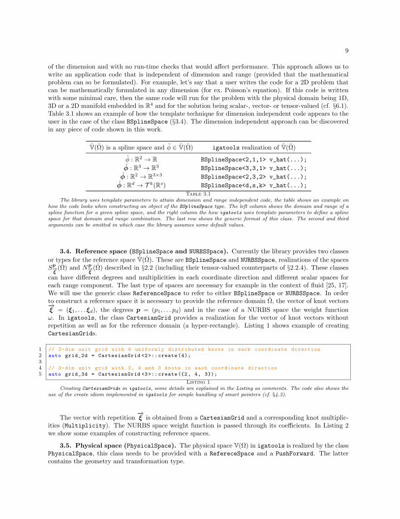
9
of the dimension and with no run-time checks that would affect performance This approach allows us towrite an application code that is independent of dimension and range (provided that the mathematicalproblem can so be formulated) For example letrsquos say that a user writes the code for a 2D problem thatcan be mathematically formulated in any dimension (for ex Poissonrsquos equation) If this code is writtenwith some minimal care then the same code will run for the problem with the physical domain being 1D3D or a 2D manifold embedded in R4 and for the solution being scalar- vector- or tensor-valued (cf sect61)Table 31 shows an example of how the template technique for dimension independent code appears to theuser in the case of the class BSplineSpace (sect34) The dimension independent approach can be discoveredin any piece of code shown in this work
V(Ω) is a spline space and φ isin V(Ω) igatools realization of V(Ω)
φ R2 rarr R BSplineSpacelt211gt v_hat()
φ R3 rarr R3 BSplineSpacelt331gt v_hat()
φ R2 rarr R3times3 BSplineSpacelt232gt v_hat()
φ Rd rarr T k(Rs) BSplineSpaceltdskgt v_hat()
Table 31The library uses template parameters to attain dimension and range independent code the table shows an example on
how the code looks when constructing an object of the BSplineSpace type The left column shows the domain and range of aspline function for a given spline space and the right column the how igatools uses template parameters to define a splinespace for that domain and range combination The last row shows the generic format of this class The second and thirdarguments can be omitted in which case the library assumes some default values
34 Reference space (BSplineSpace and NURBSSpace) Currently the library provides two classes
or types for the reference space V(Ω) These are BSplineSpace and NURBSSpace realizations of the spacesSpminusrarrξ
(Ω) and Npminusrarrξ
(Ω) described in sect22 (including their tensor-valued counterparts of sect224) These classes
can have different degrees and multiplicities in each coordinate direction and different scalar spaces foreach range component The last type of spaces are necessary for example in the context of fluid [25 17]We will use the generic class ReferenceSpace to refer to either BSplineSpace or NURBSSpace In orderto construct a reference space it is necessary to provide the reference domain Ω the vector of knot vectorsminusrarrξ = (ξ1 ξd) the degrees p = (p1 pd) and in the case of a NURBS space the weight functionω In igatools the class CartesianGrid provides a realization for the vector of knot vectors withoutrepetition as well as for the reference domain (a hyper-rectangle) Listing 1 shows example of creatingCartesianGrids
1 2-dim unit grid with 4 uniformly distributed knots in each coordinate direction
2 auto grid_2d = CartesianGrid lt2gt create (4)
34 3-dim unit grid with 2 4 and 3 knots in each coordinate direction
5 auto grid_3d = CartesianGrid lt3gt create (2 4 3)
Listing 1Creating CartesianGrids in igatools some details are explained in the Listing as comments The code also shows the
use of the create idiom implemented in igatools for simple handling of smart pointers (cf sect43)
The vector with repetitionminusrarrξ is obtained from a CartesianGrid and a corresponding knot multiplic-
ities (Multiplicity) The NURBS space weight function is passed through its coefficients In Listing 2we show some examples of constructing reference spaces
35 Physical space (PhysicalSpace) The physical space V(Ω) in igatools is realized by the classPhysicalSpace this class needs to be provided with a RefereceSpace and a PushForward The lattercontains the geometry and transformation type
10
1 Scalar B-spline space over [0 1]^2 of degree 2 with maximum regularity
2 auto space1 = BSplineSpace lt2gt create(grid_2d 2)
34 Idem to space1 but providing the multiplicities
5 auto space2 = BSplineSpace lt2gt create(grid_2d 2 31133213)
67 Vector -valued B-spline space over [0 1]^2 of
8 degree 2 and 1 in each component and maximum regularity
9 auto space3 = BSplineSpace lt2 2gt create(grid_2d 2 1)
1011 Vector -valued B-spline space over [0 1]^3 of degree 2
12 auto space4 = BSplineSpace lt3 3gt create(grid_3d 2)
1314 Scalar NURBS space of degree 2 with given weight coefficients
15 auto space5 = NURBSSpace lt2gt create(grid_2d 2 weight )
Listing 2Creating reference spaces Examples of constructing B-spline type spaces in igatools some details are explained in the
listing as comments The code is referring to the grids created in Listing 1
351 Geometry (Mapping) The geometry or physical domain is described by the deformation Fof the reference domain in igatools the deformation is realized by the Mapping class It is basically afunction from Rd to Rs with the added feature of being element aware in the sense of sect36 so that itsvalues can be handled with the grid-like iterators for uniformity and efficiency Listing 3 shows examplesof creating mappings In particular we remark that the encapsulation of the geometry in the Mappings
1 Creating a Mapping object from the provided library of maps
2 auto map = SphericalMap create(grid)
34 Creating a Mapping object from a space and a vector of control points
5 auto bs_map = IgMapping create(bspace control_points )
67 Importing a Mapping object from a file
8 IgReader ltdim gt reader(pipexml)
9 auto nurbs_map = readerget_map ()
Listing 3Code examples showing how to create some geometries (Mappings) The library allows the use of different types of
deformations including analytic functions and isogeometric mapping
class allows to cleanly integrate a geometric modeler (or a CAD system) by implementing a Mapping
specialization (see sect52)
352 Push-forward operator (PushForward) The other ingredient besides a reference spacerequired to construct a physical space is a push-forward operator In igatools it is realized by thePushForward class which is constructed from a Mapping and a Transformation Currently igatoolsprovides support for h_grad h_div h_curl and l2 transformation types (see Table 21) Listing 4 showsan example for creating a push-forward operator and a physical space
36 Element level access (ElementIterator) The ReferenceSpace class can be thought of asa container of basis functions The latter are supported only on a small number of elements whichmakes it convenient to access them through the elements Q of the grid Q We refer to it as the local orelement level access to quantities and it is provided using an element iterator in the spirit of the standardtemplate library (STL) [41] Simply speaking given an object collection (the container) an iterator maybe thought of as a type of pointer that has two primary operations referencing one particular element inthe container (called element access) and modifying itself so it points to the next element (called elementtraversal) The primary purpose of an iterator is to allow a user to process every element of a container
11
1 using PushFw = PushForward ltTransformation h_grad dim gt
2 using Space = PhysicalSpace ltRefSpace PushFw gt
34 auto push_fw = PushFw create(map)
5 auto space = Space create(ref_space push_fw )
Listing 4Creating a physical space The physical space is created from a reference space and a push-forward operator The
push-forward operator is defined from the map using the h_grad transformation type The variables ref_space and map areassumed to have been defined as shown in Listings 2 and 3 respectively Also notice the use of the using keyword to simplifylong type names (see sect43)
while isolating the user from the internal structure of the container This allows the container to storeelements in any manner it wishes while allowing the user to treat it as if it were a simple sequence or listAn iterator class is designed in tight coordination with the corresponding container class In igatools wesee the classes CartesianGrid BSplineSpace NURBSSpace Mapping PushForward and PhysicalSpace
as containers of elements that we collectively call grid-like containers The containers provide the methodsfor creating the iterators and thus a consistent way to iterate on the different data structures In this waythe code is more readable reusable and less sensitive to changes in the data structure (for example if weadd support for local refinement) In particular it fits perfectly in the dimension independent paradigmadvocated by our design Listing 5 shows a typical use of element iterators in igatools comparing thecases of a CartesianGrid ReferenceSpace and PhysicalSpace In particular notice the consistency inthe treatment despite the different data stored in each class
1 for(auto elem grid)
2
3 cout ltlt elemvertex (0)
4
56 for(auto elem ref_space)
7
8 int n_basis = elemget_num_basis ()
9 for (int i = 0 i lt n_basis ++i)
10
11 do something with the reference basis
12
13 auto loc_dofs = elemget_local_to_global ()
14
1516 for(auto elem phys_space)
17
18 int n_basis = elemget_num_basis ()
19 for (int i = 0 i lt n_basis ++i)
20
21 do something with the physical basis
22
23
Listing 5Uses of element iterators on igatools containers We iterate on the elements of a CartesianGrid a ReferenceSpace
and a PhysicalSpace Notice the consistent treatment that iterators allow to access different data We assume that gridref_space and phys_space were defined as shown in listings 1 2 and 4 respectively
A general purpose library like igatools cannot (and should not try to) guess what equation or problemthe user will want to solve Instead it should provide a flexible and intuitive way to access the quantities thatseem to be common to all typical problems Most operators require access to basis functions (values andderivatives of any order) and to geometric quantities (values and derivatives of the mapping determinantsand curvatures) Given the small support (in number of elements) of the basis functions the assembling of
12
the global quantities is conveniently performed by adding the local contributions The ElementIterator
is the mechanism that igatools provides to compute and access these values In addition to the consistentinterface to the different grid-like containers a second task that is handled by the element iterator is themanagement of an element values cache A cache is a smart piece of memory that depending on the desiredquantities to be computed stores commonly used computations to increase efficiency Most optimizationtechniques tend to interfere with a clean code and it is common to have a trade off between efficiencyand clean design In order to partially counteract this effect we use the element iterator to implement anabstraction layer that is designed to be invisible from the neighbor layers This provides the efficiencyrequired but still keep an organized design for the caches For using the cache mechanism the cleaninterface of the range based for loop shown in Listing 5 needs to be slightly modified Listing 6 show theactual code for the assembling of the stiffness matrix (using the efficient cache mechanism) for a Poissonrsquosproblem Obviously in the art of software design there is no technique to show that our design is the right
1 void PoissonProblem assemble_matrix ()
2
3 ValueFlags flag = ValueFlags gradient | ValueFlags w_measure
45 auto elem = space -gtbegin ()
6 auto end = space -gtend ()
7 elem -gtinit_values(flag quad)
8 for( elem = end ++elem)
9
10 elem -gtfill_values ()
11 loc_matrix = 0
12 auto w_meas = elem -gtget_w_measures ()
13 for (int i = 0 i lt n_basis ++i)
14
15 auto grd_phi_i = elem -gtget_basis_gradients(i)
16 for (int j = 0 j lt n_basis ++j)
17
18 auto grd_phi_j = elem -gtget_basis_gradients(j)
19 for (int qp = 0 qp lt n_qp ++qp)
20
21 loc_matrix(i j) +=
22 scalar_product(grd_phi_i[qp] grd_phi_j[qp]) w_meas[qp]
23
24
25
26 auto loc_dofs = elem -gtget_local_to_global ()
27 matrix -gtadd(loc_dofs loc_dofs loc_matrix )
28
29
Listing 6Code for the assembling of the stiffness matrix for the Poisson problem (cf sect61 In order to use the efficient cache
mechanism the range based for loops of Listing 5 needs to be modified by adding the lines 5 6 7 and 10 Notice thatinit_values() is execute one time and fill_values() for each element
one but we find encouraging that the assembly function looks simple and plain enough also to non-codingexperts without sacrificing efficiency
37 Global quantities fields operators and the linear algebra We have discussed the localhandling of basis functions to assemble the local contribution of operators The global quantities such asfields and global operators are stored in containers of the linear algebra system (eg global vectors andmatrices) They are assembled from the local element contributions through the bookkeeping mechanismkept by the space For each element the non-zero basis functions have a local index for which space knowsthe corresponding global index The query for this information is obtained through the element iteratorthrough the get_local_to_global() function Listing 6 line 26) Almost any of the many excellent linear
13
algebra systems could be easily plugged into the proposed design From a bias preference of the originaldevelopers (and for the sake of selecting one) in igatools we have used the linear (and non-linear) algebraprovided by some packages of the Trilinos library [29] Trilinos among other things provides stateof the art storage for distributed vectors and matrices as well as a complete collection of linear and nonlinear solvers In order to have a consistent style with the other pieces of the library igatools providessimplified wrappers to basic Trilinos vectors matrices and linear solvers At the same time we do notrestrict the more advanced and powerful use that can be obtained by dealing directly with the Trilinos
object
4 igatools implementation standards The effort in igatools has been directed to develop ahigh quality implementation of the isogeometric software design presented in sect3 To partially justify thestatement in this section we briefly describe some of the software engineering tools and development modelwe have adopted
41 Development infrastructure The development of igatools is supported by todayrsquos standardsofware engineering tools for that purpose We use the distributed version control system and sourcecode management git2 and the bug tracking system Trac3 For managing the build process we useCMake4 allowing the software compilation process using a simple platform and compiler independentconfiguration files Most importantly we strive for high standards for documentation and user supportThe documentation can be divided in three level this paper that describes the design concepts and howthey work together the tutorial examples provided with the source to give a hand-on introduction to usethe library and a reference manual generated by processing the in-source documentation with Doxygen5For community support we have a user group6 for discussion between the igatools developers and usersand a development group7 where the igatools developers discuss about new features library designimplentation details discovered bugs and possible remedies We also mantain a wiki page 8 working asthe webpage to the world of the library
42 Development model (testing and debugging) igatools has hundreds of unit tests (smallprograms) that are run automatically using CDashCTest9 to verify that new changes are not breakingworking features
We use and advocate the use of the test driven development model [8] This basically means thatwe write a unit test for the feature we want to implement or fix the test initially fails then we writecode until the test passes from that moment on the test is executed automatically Now we can refactorthe code (clean remove any duplication rename variables and methods optimize etc) being confidentthat the new code is not damaging any existing functionality In addition to the unit tests igatools hasautomatic integration and validation tests (more cpu-time expensive than unit tests) in order to verifythat the different modules interact correctly
The libray makes use defensive programming techniques to detect and easily find bugs at runtimethrough the exception handling mechanism We adopt two levels of checks One more expensive in termsof running time but only active when igatools is compiled in Debug mode We perform this kind ofchecks wherever there may be a chance of error eg out-of-bound index for accessing to vectors elementsuninitialized objects invalid object states mismatching dimensions etc The second level of checks isalways active (both in Debug and in Release mode) and it is used for checking anomalies that may beintroduced by the input data
The typical workflow for a user of igatools would be to first write his code and test it with the library
2httpwwwgit-scmcom3httptracedgewallorg4httpwwwcmakeorg5httpwwwdoxygenorg6httpsgroupsgooglecomforumforumigatools-users7httpsgroupsgooglecomforumforumigatools-development8httpcodegooglecompigatoolswlist9httpwwwcdashorg
14
in Debug mode on a small-size problem When this is working as expected and (virtually) bug-free linkthe code with igatools in Release mode on a real-size problem
43 Programming language The main language used in the development of igatools is C++11[32]It includes many additions to the previous standard C++03[31] mostly aimed to produce a code that iscleaner safer more efficient and easier to maintain In particular igatools makes heavy use of some ofthe language features somehow defining certain aspects of its programming style as for example
(i) Smart pointers and create facility Objects in igatools can have big sizes and can beshared by different other objects This sharing mechanism is handled through the use of smart pointersThey provide automatic memory management ensuring that the resource they control is automaticallydestroyed when its last (or only) owner is destroyed Moreover the igatools classes intended to be usedthrough smart pointers provide a create facility for this purpose For each constructor of the class thereis a static function (called create) with the same arguments of the constructor that returns an instanceof the class wrapped by a shared pointer A code example showing the implementation and use of thetechnique is shown in Listing 7
1 class MyClass
2
3 public
4 MyClass constructor using arg1 of type T1 and arg2 of type T2
5 MyClass(T1 arg1 T2 arg2)
67 The static function create () uses the constructor
8 MyClass(T1 arg1 T2 arg2) to build a MyClass
9 instance wrapped by a std shared_ptr
10 static stdshared_ptr ltMyClass gt create(T1 arg1 T2 arg2)
11
12 return std make_shared ltMyClass gt( MyClass(arg1 arg2) )
13
14
1516 void foo(T1 a T2 b)
17
18 Create an instance of MyClass wrapped by a std shared_ptr
19 stdshared_ptr ltMyClass gt my_obj = MyClass create(a b)
20
Listing 7Create facility For each class that is intended to be used through a smart pointer igatools provides a create facility
The static function create returns an instance of the class wrapped by a stdshared_ptr The function foo shows how thepointer is created
(ii) Template types (using and auto) C++11 provides better management of templates thanC++03 and igatools extensively uses templates in order to attain efficiency and the dimension indepen-dent paradigm One drawback of using templates is the fact that the template arguments may becomeinhumanly difficult to express We solve this problem with the C++11 using alias facility that allows tocreate human readable aliases for the necessary types Related is the automatic type inference facilityauto that deduces the type of an explicit initialization An appropriate combination of using create andauto results in a much more simple and human comprehensible syntax as shown in Listing 8 creating acertain style to code with igatools
5 igatools practical features Besides implementing the novel object oriented design presented inthis work with high quality standards igatools provides useful features that make it useful and attractivefor practical applications
51 Inputoutput facilities It is important for the library to use NURBS geometries generated byother software At the present stage there is no scientific computing dedicated format for isogeometric typeof spaces The developers of igatools and GeoPDEs in a joint effort defined an xml format to describe such
15
1 void brute_force_syntax ()
2
3 stdshared_ptr ltCartesianGrid ltdim gtgt grid =
4 std make_shared ltCartesianGrid ltdim gtgt(CartesianGrid ltdim gt(4))
5 stdshared_ptr ltMapping ltdim gtgt map =
6 std make_shared ltBallMapping ltdim gtgt(BallMapping ltdim gt(grid ))
7 stdshared_ptr ltBSplineSpace ltdim 11gtgt ref_space =
8 std make_shared ltBSplineSpace ltdim 11gtgt(BSplineSpace ltdim 11gt(grid 3))
9 stdshared_ptr ltPushForward ltTransformation h_grad dim gtgt push_fw =
10 std make_shared ltPushForward ltTransformation h_grad dim gtgt(
11 PushForward ltTransformation h_grad dim gt(map))
12 stdshared_ptr ltPhysicalSpace ltBSplineSpace ltdim 11gt
13 PushForward ltTransformation h_grad dim gtgtgt space =
14 std make_shared ltPhysicalSpace ltBSplineSpace ltdim 11gt
15 PushForward ltTransformation h_grad dim gtgtgt(
16 PhysicalSpace ltBSplineSpace ltdim 11gt
17 PushForward ltTransformation h_grad dim gtgt(ref_space push_fw ))
18
1920 void human_syntax ()
21
22 using Grid = CartesianGrid ltdim gt
23 using Map = Mapping ltdim gt
24 using RefSpace = BSplineSpace ltdim 1 1gt
25 using PushFw = PushForward ltTransformation h_grad dim gt
26 using Space = PhysicalSpace ltRefSpace PushFw gt
2728 auto grid = Grid create (4)
29 auto map = BallMapping ltdim gt create(grid)
30 auto ref_space = RefSpace create(grid 3)
31 auto push_fw = PushFw create(map)
32 auto space = Space create(ref_space push_fw )
33
Listing 8Library facilities using auto and create The two functions perform the same operations but the second one uses
the combination of the using auto and create facilities advocated by the igatools programming style resulting in a morehuman readable syntax than the brute force counterpart
geometries Thus igatools through it IgReader class (see Listing 3 lines 8 and 9) supports importinggeometries in this data format which is completely specified in the library documentation xml is anextremely flexible format that is supported by wide number of libraries and applications igatools sourceis distributed with contributed scripts to convert geometries generated with the MATLAB NURBS toolbox10
to the xml formatSimilarly important for the library is to provide a useful mechanism to analise and visualize the com-
putational results igatools generates output for this purpose through its Writer class (see Listing 15)So far the writer provides output in vtk format [37] which can be visually processed (among other things)with Paraview [40]
52 Interaction with CAGD software The main selling point when isogeometric analysis wasintroduced was the possibility to integrate the geometry with the analysis In the context of igatools
this can be cleanly achieved by implementing a Mapping specialization (see sect351) that internally use allgeometric features of a modern CAD system provides a clear interface to the user without him worryingabout the implementation details Now after a decade from the introduction of IGA there is no dedicatedCAD software that directly generates a 3D analysis suitable geometry this being one of the limiting issuesin the use of the IgM in the industrial community One reason is that most CAD software when dealingwith a 3D geometries only model the boundary surfaces of the represented domain An exception is the
10httpwwwariauklinuxnetnurbsphp3
16
geometric modeler IRIT 11 developed by G Elber at Technion that natively handles trivariate volumesWe have tested the integration of igatools with this particular geometric modeler by implementing aMapping specialization (MappingIRIT) that internally uses the IRITrsquos routines and data structures forthe evaluation of the geometric quantities required by Mapping This MappingIRIT class is used for thegeometry in the non-linear elasticity example presented in sect64
53 Parallel support Computationally demanding applications require igatools to take advan-tage of parallel computing technologies The Trilinos and Intel TBB12 libraries used in cooperation withigatools provides this service using a distributed and shared memory model respectively The container-iterator model separates data from operations In fact the iterators are designed in such a way they do notmodify their container In this way we can obtain parallel iterators where each thread points to differentgrid elements We have successfully tested the use of Intel TBB in igatools following very closely theimplementation of the dealII classes for the threads management In particular a correct managementof threadsiterators for the parallel assembly routines has been checked A distributed memory modelusing MPI have been succesfully applied to igatools application code by using the Trilinos facilities fora distributed assembling and parallel solving of the global system
6 Examples In this section we illustrate the library flexibility to naturally handle and adapt todifferent situations We do this by showing its use to solve typical application problems We start witha rather detailed description for the implementation of a simple Poisson equation This is the de factoprototype example in any Galerkin numerical method that we also employ to describe the basic buildingblocks typical to the use of the library and to which we refer to in the subsequent examples We con-tinue with a tiny adaptation to the Poisson problem code that solves the Laplace-Beltrami problem on amanifold Then we illustrate the handling of vector-valued and many spaces problems by discussing theimplementation of the Stokes equation Finally we present a non-linear elasticity problem showing theflexibility of the library to cleanly interact with other software packages
Notice that in the snippets of code listed in the section some non-relevant pieces are omitted (or moreprecisely replaced by a comment of the form ldquordquo) to help with the understanding of the main piecesAlso as we move on in the examples less details are provided as we assume they can be translated fromthe previous examples
61 Poisson Equation The Poisson problem consists in finding u Ω sub Rd rarr R such that
(61) minus∆u = f in Ω u = g on partΩ
It can be rewritten in weak form as find u = u0 + ug with u0 isin H10 (Ω) and ug the lift of g such that
Au(v) = F (v) for all v isin H10 (Ω) where Au(v) =
intΩnablau middot nablav and F (v) =
intΩfv The IgM for this problem
(cf sect21) requires the definition of the isogeometric space V(Ω) the assembling of the stiffness matrix Kand right hand side F by adding the element contributions and the solving of the linear system KU = F
Below we describe a possible approach for the implementation of this problem with igatools Thefull running code for this problem is part of the tutorial distributed with the library To be concrete wechoose the physical domain Ω to be a d-dimensional spherical sector for d = 1 2 and 3 a homogeneousboundary condition and a constant source of 5 The code would look practically the same if we decide touse a CAD geometry for the domain a non-homogeneous boundary function andor a non-constant sourceterm
In order to undertake this problem a class for it (see Listing 9) is defined its public interface providestwo members the constructor PoissonProblem and the run() function Within the private membersone can identify the declaration of objects for the space and the linear algebra We can also see theusing keyword to create short alias for the usually long templated types and the use of smart pointers(shared_ptr) both common techniques within the programming style of igatools (cf sect43) For theactual solving of the problem we define objects of PoissonProblem type in the programrsquos main() (see
11httpwwwcstechnionacil~irit12httpswwwthreadingbuildingblocksorg
17
1 template ltint dim gt
2 class PoissonProblem
3
4 public
5 PoissonProblem(TensorSize ltdim gt ampn_knots int deg)
6 void run ()
78 private
9 void assemble ()
10 void solve ()
11 void output ()
1213 private
14 using RefSpace = BSplineSpace ltdim gt
15 using PushFw = PushForward ltTransformation h_grad dim gt
16 using Space = PhysicalSpace ltRefSpace PushFw gt
1718 shared_ptr ltCartesianGrid ltdim gtgt grid
19 shared_ptr ltRefSpace gt ref_space
20 shared_ptr ltMapping ltdim gtgt map
21 shared_ptr ltSpace gt space
2223 quadratures defined
2425 ConstantFunction ltdim gt f
26 ConstantFunction ltdim gt g
2728 shared_ptr ltMatrix gt matrix
29 shared_ptr ltVector gt rhs
30 shared_ptr ltVector gt solution
31
Listing 9Class to approximate the solution of a Poisson problem The public interface provides the constructor that prepares the
object and the function run() that computes and plots the solution In the private members we can find objects to handlethe space and the linear algebra
Listing 10) Here we can see how the dimension independent template technique (cf sect33) is put to
1 int main()
2
3 n_knots and deg defined
4 PoissonProblem lt1gt poisson_1d ( n_knots deg)
5 poisson_1drun()
67 PoissonProblem lt2gt poisson_2d (n_knots n_knots deg)
8 poisson_2drun()
910 PoissonProblem lt3gt poisson_3d (n_knots n_knots n_knots deg)
11 poisson_3drun()
12
13
Listing 10Main routine to solve the Poisson problem for different domain dimensions For each dimension 1 2 and 3 we construct
the problem and then assemble solve and output the result by calling the function run()
use We are solving the Poisson problem in 1 2 and 3 dimensions with the same templated code As amatter of fact with the same code we could solve this problem in 4 dimensions if we wish to Each objectdefinition (lines 4 7 and 10) calls the constructor that prepares the object to be ready to use and thenwe call the object member function run() that computes the solution The function run() (see Listing
18
1 void PoissonProblem ltdim gt run()
2
3 assemble ()
4 solve ()
5 output ()
6
Listing 11The run function is the public interface that solves the Poisson problem by assembling and solving the discrete linear
system and saving the solution in graphical format
11) is just a high level interface that calls the private members assemble() solve() and output() thatwill do the actual computational work and are explained later on After executing this program graphicaloutput files (in vtk format) for the different dimensions with the problem solution are saved Figure 61shows these files
Fig 61 Plot of the solutions to the Poisson problem with homogeneous boundary conditions and constant source termon a spherical sector in 1 2 and 3 dimensions Notice that the three plots were generate with the same code by only changingthe dimension template argument
Now we explain the implementation of the different member functions of the PoissonProblem classThe constructor (see Listing 12) is in charge of making the object ready to be used So it creates a physicalspace space by first creating a grid a reference space ref_space a mapping map and a push forward
The assemble() routine assembles the global stiffness matrix matrix and global right hand side rhs
by adding the element contributions In igatools we use the element iterator (sect36) for this purposeWe have already seen in Listing 6 the assemble of the global matrix here in Listing 13 we include theassembling of the right hand side and the treatment of the boundary conditions In this case we proceedin two steps (lines 27 and 28) first we project the boundary function g onto the trace space and then weenforce into the linear system these values for the Dirichlet degrees of freedom Notice that a projectionis necessary as splines are not interpolatory in general
As discussed in sect37 igatools relies on external algebra packages for solving the global system Thefunction solve() in Listing 14 defines a Solver object which is a wrapper class provided by igatools
for basic use of Trilinos solvers The solution of the system is returned in solution The lines in thislisting look simple enough to be self-explanatory
To manage the graphical output (sect51) igatools provides a Writer class that can be used to handle
19
1 PoissonProblem(TensorSize ltdim gt ampn_knots int deg)
2
3 initilize elem_quad and face_quad
4 f(5) g(0)
5
6 define box a bounding box for the grid
78 grid = CartesianGrid ltdim gt create(box n_knots )
9 ref_space = RefSpace create(grid deg)
10 map = BallMapping ltdim gt create(grid)
11 space = Space create(ref_space PushFw create(map))
1213 initialize matrix rhs and solution
14
Listing 12Poissonrsquos problem constructor It construct the physical space for which it needs to construct a reference space and
a push-forward which in turn requires the construction of a map and a cartesian grid It also initializes the quadratureschemes the linear algebra and the source and boundary functions
1 void PoissonProblem ltdim gt assemble ()
2
3 same code as listing 6 we are only adding
4 the pieces for the right hand side
56 for ( elem = elem_end ++elem)
7
8 loc_rhs = 0
9 auto points = elem -gtget_points ()
10 auto phi = elem -gtget_basis_values ()
11 auto f_values = fevaluate(points )
1213 for (int i = 0 i lt n_basis ++i)
14
15 matrix assembling (Listing 6)
1617 auto phi_i = phiget_function(i)
18 for (int qp = 0 qp lt n_qp ++qp)
19 loc_rhs(i) +=
20 scalar_product(phi_i[qp] f_values[qp]) w_meas[qp]
21
22
23 rhs -gtadd(loc_dofs loc_rhs )
24
2526 Apply dirichlet boundary condition
27 project_boundary_values(g space face_quad dirichlet_id dof_values )
28 apply_boundary_values(dof_values matrix rhs solution )
29
Listing 13Assembling of the global system for Poisson problem The matrix assembling was already shown in Listing 6 here we
only show the additional code required to assemble the right hand side and take care of the dirichlet boundary constraints
geometries and fields that are to be saved in a graphical output format (for now a vtk file) In Listing 15a Writer object associated with the geometry of map is defined (line 4) then the solution field is added toit (line 5) and finally writer is asked to save the geometry and the solution field to disk (line 6)
62 A surface example The code of sect61 can be trivially modified to solve a partial differentialequation on a surface igatools can naturally handle manifold domains such as surfaces or curves
Let Γ be a d-dimensional manifold and consider the Laplace-Beltrami equation find u Γrarr R such
20
1 void PoissonProblem ltdim gt solve ()
2
3 Solver solver(SolverType CG)
4 solversolve(matrix rhs solution )
5
Listing 14Solver for the Poisson problem We use the simple wrapper igatools provides to the Trilinos solvers
1 void PoissonProblem ltdim gt output ()
2
3 define filename
4 Writer ltdim gt writer(map)
5 writeradd_field (space solution Temperature)
6 writersave(filename )
7
Listing 15Saving the solution of Poisson problem in a graphical output
that
(62) minus∆Γu = f in Γ u = g on partΓ
which can be rewritten in weak form as find u = u0 + ug with u0 isin H10 (Γ) and ug the lift of g such that
Au(v) = F (v) for all v isin H10 (Γ) where Au(v) =
intΓnablaΓu middot nablaΓv and F (v) =
intΓfv Except for the fact that
the differential operators are surface operators one can see the similarity of this problem with equation(61) The library understands manifolds thus when the physical space has codimension different from 0igatools understand that gradients refers to surface gradients In this way minor modifications to thePoisson problem code of sect61 allow to solve the Laplace-Beltrami problem
More precisely without loss of generality let assume we want to solve equation (62) on a d-dimensionalspherical piece of codimension 1 It only requires minor changes on a few lines in the problem class firstthe definitions of codim and space
static const int codim = 1
static const int spacedim = dim + codim
and then some small changes in lines 15 20 25 and 26 of Listing 9 by the following four lines in the givenorder
using PushFw = PushForward ltTransformation h_grad dim codim gt
shared_ptr ltMapping ltdim codim gtgt map
ConstantFunction ltspacedim gt f
ConstantFunction ltspacedim gt g
The only change required in the constructor is to replace line 10 of Listing 12 by
map = SphereMapping ltdim gt create(grid)
In Figure 62 we plot the isogeometic approximate solution to the Laplace-Beltrami problem over a sphericalpiece given by a spherical coordinate map
63 Navier-Stokes Equations An incompressible viscous fluid flowing in with a laminar motionis modeled by the Navier-Stokes equations
ρ (parttu + (nablau)u)minus micro∆u +nablap = f and div u = 0 in Ωtimes (0 T )
supplied with appropriate initial and boundary conditions Here u is the fluid velocity field and p itspressure A distinctive attribute of these equations is the combination of hyperbolic and parabolic terms[28] The key to the application of the Galerkin method to the weak form of these equations lays into
21
Fig 62 Plot of the solution to the Laplace-Beltrami problem with homogenous boundary condition and constant sourceterm on a piece of a d-sphere for d = 1 2
its parabolic term with the incompressibility constraint leading to a saddle point problem In particularthe spaces for velocity and pressure have to satisfy the well-known inf-sup condition [11] We assume thatV sub H1(Ω)d and Q sub L2(Ω) is a pair of spaces for the velocity and pressure that satisfy this conditionexactly what subspaces are taken depends on the type of boundary conditions The discrete problem isobtained by considering discrete spaces Vh sub V and Qh sub Q for the velocity and pressure respectivelyand can be written in matrix form as
(63)
(A Bt
B 0
)(UP
)=
(F0
)
where the submatrix A corresponds to the terms involving the fluid velocity and B corresponds to themixed term For the discretization of this problem we use two spaces one scalar-valued (for the pressure)and the other vector-valued (for the velocity) Most importantly they should form a stable pair (iesatisfy a discrete inf-sup condition)
Below we illustrate the use of igatools to treat the two coupled spaces by listing the relevant piecesof code for a Stokes type of problem Listing 16 shows part of the StokesProblem class declaration Inparticular notice the scalar-valued space type PreSpace being similar to the space of section 61 while forthe VelSpace type the addition of the second template parameter renders it into a vector-valued space
For the purpose of this example we consider the Taylor-Hood type of spaces adapted to the isogeometricsetting [4 14] In which the pressure and velocity spaces share the same global regularity and the velocitydegree is one more that of the pressure These spaces are constructed in the StokesProblem constructor(see Listing 17) Here given the degree for the pressure space and the global regularity as arguments theconstructor builds the multiplicity vectors pre_mult and vel_mult and the degrees pre_deg and vel_deg
for both spaces which are created in lines 17 and 18 Recall that to have a global regularity r in a splinespace of degree d the multiplicity of the interior knots must be dminus r and the end knots to be interpolatoryrequire a multiplicity d+ 1
An interaction between the velocity and pressure spaces is required for example in the assembling ofthe mixed term Bt This involves the simultaneous access to basis functions from both spaces over thesame element and quadrature points Listing 18 illustrates how this is attained in igatools using twoelement iterators We use the iterators pre_el and vel_el one for the pressure and one for the velocityspace in a common for loop with a simultaneous increment This works because both spaces are definedon the same CartesianGrid so the increment operator ensures that both iterators traverse the elementsin synchronization
22
1 class StokesProblem
2
3 public
4 StokesProblem(int deg int n_knots int reg)
5 void run ()
67 private
8 void assemble_Bt ()
9
10 private
11 using PreSpace = BSplineSpace ltdim gt
12 using VelSpace = BSplineSpace ltdim dim gt
1314 shared_ptr ltPreSpace gt pre_space
15 shared_ptr ltVelSpace gt vel_space
16
17 shared_ptr ltMatrix gt Bt
18
Listing 16Sketch of a class to solve the Stokes problem Observe the declaration of two spaces one vector-valued for the velocity
and one scalar-valued for the pressure
1 StokesProblem(int deg_p int n_knots int reg)
2
3 define pre_mult vel_mult pre_deg and vel_deg
4 int deg_v = deg_p + 1
5 vector ltint gt mult_p(n_knots deg_p - reg)
6 vector ltint gt mult_v(n_knots deg_v - reg)
7 mult_p [0] = mult_p[n_knots -1] = deg_p +1
8 mult_v [0] = mult_v[n_knots -1] = deg_v +1
910 pre_multfill(mult_p )
11 vel_multfill(mult_v )
12 pre_degfill(deg)
1314 vel_degfill(deg +1)
1516 auto grid = CartesianGrid ltdim gt create(n_knots )
17 pre_space = PreSpace create(grid pre_mult pre_deg )
18 vel_space = VelSpace create(grid vel_mult vel_deg )
1920 Bt = Matrix create (vel_space pre_space )
21
Listing 17Constructor for Stokes class The scalar and vector-valued spaces for the isogeometric version of the Taylor-Hood
elements are created The pressure and velocity spaces share the same global regularity and the velocity degree is one morethat of the pressure
In Figure 64 we show a simulation run with igatools to solve a time dependent Navier-Stokesequations on a domain given by a quintic B-spline map The time integration is performed using a firstorder operator splitting technique see [28] as a reference The geometry is sketched in Figure 63 it isinspired in vascular valves leaflets but there is no claim to model anything Our main motivation is usingour software in a non-trivial geometry The geometry size is a 1 by 5 box The leaflet tip is modeled withthree control points separated by a distance of 10minus3 The geometry mapping as well as the Taylor-Hoodspaces have a C4 global regularity with degree 5 and 6 for the pressure and velocity respectively Figure 64shows the resulting pressure and streamlines at different time frames Boundary conditions are no-slip atthe bottom side unitary horizontal velocity at the inlet symmetry on top and no stress at the outlet The
23
1 void StokesProblem ltdim gt assemble_Bt ()
2
3 define vel_n_basis pre_n_basis vel_loc_dofs pre_loc_dofs
4 DenseMatrix loc_mat(vel_n_basis pre_n_basis )
5 auto vel_el = vel_space -gtbegin ()
6 auto pre_el = pre_space -gtbegin ()
7 auto end_el = vel_space -gtend ()
89 ValueFlags vel_flag = ValueFlags divergence|ValueFlags w_measure
10 ValueFlags pre_flag = ValueFlags value
11 vel_el -gtinit_values(vel_flag elem_quad )
12 pre_el -gtinit_values(pre_flag elem_quad )
1314 for ( vel_el = end_el ++vel_el ++ pre_el)
15
16 loc_mat = 0
17 vel_el -gtfill_values ()
18 pre_el -gtfill_values ()
1920 auto q = pre_el -gtget_basis_values ()
21 auto div_v = vel_el -gtget_basis_divergences ()
22 auto w_meas = vel_el -gtget_w_measures ()
2324 for (int i = 0 i lt vel_n_basis ++i)
25
26 auto div_i = div_vget_function(i)
27 for (int j = 0 j lt pre_n_basis ++j)
28
29 auto q_j = qget_function(j)
30 for (int qp = 0 qp lt n_qp ++qp)
31 loc_mat(i j) -= scalar_product(div_i[qp] q_j[qp]) w_meas[qp]
32
33
34 vel_loc_dofs = vel_el -gtget_local_to_global ()
35 pre_loc_dofs = pre_el -gtget_local_to_global ()
36 Bt-gtadd(vel_loc_dofs pre_loc_dofs loc_mat )
37
38
Listing 18Assembling Bt involves simultaneous access to the basis functions of both the pressure and velocity spaces igatools
approach is the use of two element iterators that are incremented simultaneously
Fig 63 Domain given by a quintic spline deformation of the unit square inspired in a vascular leaflet
main vortex originates as expected from the leaflet tip As time evolves a secondary vortex originatesfrom the bottom of the leaflet
24
(a) t = 01 (b) t = 03
(c) t = 09 (d) t = 15
Fig 64 A time dependent Navier-Stokes simulation for the rigid leaflet geometry of Figure 63 For illustrative reasonswe decided to reproduce the shape of a vascular leaflet without any particular modelling motivation we were interested inthe vortex shedding by this geometry In particular we notice the main vortex started at the tip of the leaflet and a secondone downstream at the bottom of the leaflet The colormap represents the pressure
64 Non-linear elasticity The library design provides a flexible access to the isogeometric spacesThis flexibility and encapsulation permit easy integration not only with different algebra systems but alsowith other scientific packages for specific purposes This section presents an example in which we haveintegrated igatools with FEBio [34] a non-linear finite element software for biomechanics
The behavior of an elastic body is characterized by the equations
(64) divσ + f = 0 in Ω σn = t on Γσ u = u on Γu
where σ is the Cauchy stress tensor f and u are the body force and displacement vectors respectively nis the outter surface normal and t is the surface traction vector For this example we assume a non-linearconstitutive relation between σ and u that leads to a non-linear problem
The variational form of the equation (64) can be written as
δW (ϕ δv) =
intΩ
σ nablaδvdΩminusint
Ω
f middot δvdΩminusint
Γσ
t middot δvdΓ = 0
being ϕ the map such that the current (deformed) configuration is expressed as Ω = ϕ(Ω) At the discretelevel this equation can be expressed in a vector form as δW (ϕ δv) = δvTR = 0 where R is the residualvector Due to the fact that R depends non-linearly on the unknowns vector u it is needed to perform alinearization of this equation The matrix form of the linearization is K(ϕk)∆uk = minusR(ϕk) being K thestiffness matrix (further details can be found in [12]) They are referred to as the deformed configurationof the body Ωk = ϕk(Ω) An iterative procedure in k is applied for achieving an equilibrium configurationϕe such as R(ϕe) asymp 0 for a given tolerance
igatools has been integrated with FEBio in a minimally invasive way only the inputoutput andthe computation of the element right-hand side vector and stiffness matrix have been modified meanwhilelinear algebra degrees of freedom material level computations etc are still managed by FEBio TheIGAElasticDomain class (Listing 19) materializes this integration being derived from the FEBiorsquos classFEBioElasticDomain it adds the isogeometric components such as the physical space As it can be seena NURBSpace is used for the displacement The final integration occurs in the functions for assemblingthe global stiffness matrix K and residual vector R by iterating over the elements and computing localcontributions For example Listing 20 shows the assembling of K by computing the local matrices Ke
given by
(65) Keij =
intΩe
nablaBi C nablaBjdΩ +
intΩe
nablaBi middot σnablaBjdΩ
25
1 class IGAElasticDomain public FEBioElasticDomain
2
3 public
4 public functions and members
5 using Space = PhysicalSpace ltRefSpace PForward gt
67 private
8 private functions and members
9 Space space
10 void stiffness_matrix(FESolidSolver psolver )
11 void residual(FESolidSolver psolver )
12
Listing 19Class for the solution of the non-linear elascity problem by means of the IgM integrated into FEBio The spaces and
push forward types are shown as well as the public functions for assemblying the residual vector and the stiffness matrix
to be then added in line 29 into a global FEBio matrix
1 void
2 IGAElasticDomain stiffness_matrix(FESolidSolver psolver)
3
4 define loc_mat elem elem_end init elem values with quadrature
56 for( elem= elem_end ++elem)
7
8 Elasticity and Cauchy stress tensors evaluated by FEBio
9 auto sigma = this -gtget_stress_tensor(elem)
10 auto c = this -gtget_elasticity_tensor(elem)
1112 loc_mat = 0
13 auto w_meas = elem -gtget_w_measures ()
14 for (int i = 0 i lt n_basis ++i)
15
16 auto Dphi_i = elem -gtget_basis_gradients(i)
17 for (int j = 0 j lt n_basis ++j)
18
19 auto Dphi_j = elem -gtget_basis_gradients(j)
20 for (int qp = 0 qp lt n_points ++qp)
21 loc_mat += Compute formula (65) using
22 Dphi_i[qp] Dphi_j[qp] c[qp] sigma[qp] w_meas[qp]
23
24
25 auto loc_to_global = this -gtget_local_to_global(elem)
26 auto nodal_connectivity = this -gtget_nodal_connectivity(elem)
2728 Add element contribution into global FEBio stiffness matrix
29 psolver -gtAssembleStiffness(nodal_connectivity
30 loc_to_global loc_mat )
31
32
Listing 20Implementation of the stiffness matrix for the nonlinear elasticity case The local element matrices are assembled into
the FEBio expected structure
Finally Figure 65 shows a simulation for the torsion of a curved tube with an open section Thegeometry is given by a three dimensional single NURBS patch of degree two and its material modeled bya Neo-Hookean formulation
Acknowledgements We would like to thank A Buffa and G Sangalli for feedback and suggestions
26
(a) The geometry map (b) t = 03 (c) t = 05 (d) t = 10
Fig 65 A non-linear elasticity simulation for an open tube is shown The map is a second order deformation of asquare 65(a) In this simulation a rotation around the axis of the tube is prescribed in one of the ends of tube whereas theother is fixed Finite deformations are considered for an hyperelastic material formulation Colormap represents von Misesstress
and to the beta testers of igatools for their patience and feedback in particular to A Bressan E Brivadisand R Vazquez
REFERENCES
[1] D N Arnold R S Falk and R Winther Finite element exterior calculus from Hodge theory to numericalstability Bull Amer Math Soc (NS) 47 (2010) pp 281ndash354
[2] W Bangerth R Hartmann and G Kanschat dealII ndash a general purpose object oriented finite element libraryACM Trans Math Softw 33 (2007) pp 241ndash2427
[3] W Bangerth T Heister and G Kanschat dealII Differential Equations Analysis Library Technical Referencehttpwwwdealiiorg
[4] Y Bazilevs L Beirao da Veiga J A Cottrell T J R Hughes and G Sangalli Isogeometric analysisApproximation stability and error estimates for h-refined meshes Math Mod Meth Appl S 16 (2006) pp 1031ndash1090
[5] Y Bazilevs V M Calo J A Cottrell J A Evans T J R Hughes S Lipton M A Scott and T WSederberg Isogeometric analysis using T-splines Comput Methods Appl Mech Engrg 199 (2010) pp 229ndash263
[6] Y Bazilevs C Michler V M Calo and T J R Hughes Isogeometric variational multiscale modeling of wall-bounded turbulent flows with weakly enforced boundary conditions on unstretched meshes Comput Methods ApplMech Engrg 199 (2010) pp 780ndash790
[7] Y Bazilevs C Michler V M Calo and T J R Hughes Isogeometric variational multiscale modeling of wall-bounded turbulent flows with weakly enforced boundary conditions on unstretched meshes Comput Methods ApplMech Engrg 199 (2010) pp 780ndash790
[8] K Beck Test Driven Development By Example Addison-Wesley Longman 2002[9] P Becker Working draft standard for programming language C++ Tech Report N3242=11-0012 ISOIEC JTC 1
Information Technology Subcommittee SC 22 Programming Language C++ Feb 2011[10] D J Benson Y Bazilevs E De Luycker M-C Hsu M Scott T J R Hughes and T Belytschko A
generalized finite element formulation for arbitrary basis functions From isogeometric analysis to XFEM Int JNumer Meth Eng 83 (2010) pp 765ndash785
[11] D Boffi F Brezzi and M Fortin Mixed Finite Element Methods and Applications Springer Series in Computa-tional Mathematics Springer London Limited 2013
[12] J Bonet and R D Wood Nonlinear Continuum Mechanics for Finite Element Analysis Cambridge UniversityPress New York NY USA 2 ed 2008
[13] M J Borden M A Scott J A Evans and T J R Hughes Isogeometric finite element data structures basedon Bezier extraction of NURBS Int J Numer Meth Eng 87 (2011) pp 15ndash47
[14] A Bressan and G Sangalli Isogeometric discretizations of the Stokes problem stability analysis by the macroelementtechnique IMA J Numer Anal (2012)
[15] A Buffa D Cho and G Sangalli Linear independence of the T-spline blending functions associated with someparticular T-meshes Comput Methods Appl Mech Engrg 199 (2010) pp 1437ndash1445
[16] A Buffa C de Falco and G Sangalli IsoGeometric Analysis stable elements for the 2D Stokes equation Int JNumer Meth Fl 65 (2011) pp 1407ndash1422
[17] A Buffa J Rivas G Sangalli and R Vazquez Isogeometric discrete differential forms in three dimensionsSIAM J Numer Anal 49 (2011) pp 818ndash844
[18] A Buffa G Sangalli and R Vazquez Isogeometric analysis in electromagnetics B-splines approximation Com-
27
put Methods Appl Mech Engrg 199 (2010) pp 1143ndash1152[19] J A Cottrell T J R Hughes and Y Bazilevs Isogeometric Analysis Toward Integration of CAD and FEA
Wiley 2009[20] J A Cottrell A Reali Y Bazilevs and T J R Hughes Isogeometric analysis of structural vibrations Comput
Methods Appl Mech Engrg 195 (2006) pp 5257ndash5296[21] C de Falco A Reali and R Vazquez GeoPDEs A research tool for isogeometric analysis of PDEs Adv Eng
Softw 42 (2011) pp 1020 ndash 1034[22] T Dokken T Lyche and K F Pettersen Locally refinable splines over box-partitions tech report SINTEF
February 2012[23] M Dorfel B Juttler and B Simeon Adaptive isogeometric analysis by local h-refinement with T-splines Comput
Methods Appl Mech Engrg 199 (2009) pp 264ndash275[24] J A Evans and T J R Hughes Isogeometric divergence-conforming B-spline for the steady NavierndashStokes equations
Math Mod Meth Appl S 23 (2013) pp 1421ndash1478[25] Isogeometric divergence-conforming B-splines for the unsteady NavierndashStokes equations J Comput Phys 241
(2013) pp 141ndash167[26] D R Forsey and R H Bartels Hierarchical B-spline refinement in SIGGRAPH rsquo88 Proceedings of the 15th annual
conference on Computer graphics and interactive techniques 1988 pp 205ndash212[27] C Giannelli B Juttler and H Speleers THBndashsplines The truncated basis for hierarchical splines Compute
Aided Geometric D 29 (2012) pp 485ndash498[28] R Glowinski P G Ciarlet and J L Lions Numerical Methods for Fluids vol 3 of Handbook of numerical
analysis Elsevier 2002[29] M Heroux R Bartlett V E Howle R Hoekstra J Hu T Kolda R Lehoucq K Long R Pawlowski
E Phipps A Salinger H Thornquist R Tuminaro J Willenbring and A Williams An Overview ofTrilinos Tech Report SAND2003-2927 Sandia National Laboratories 2003
[30] T J R Hughes J A Cottrell and Y Bazilevs Isogeometric analysis CAD finite elements NURBS exactgeometry and mesh refinement Comput Methods Appl Mech Engrg 194 (2005) pp 4135ndash4195
[31] ISOIEC 148822003 ndash Programming languages ndash C++ 2003[32] ISOIEC 148822011 ndash Information technology ndash programming languages ndash C++ 2011[33] J Kiendl Y Bazilevs M-C Hsu R Wuchner and K-U Bletzinger Kirchhoff-Love shell structures comprised
of multiple patches Comput Methods Appl Mech Engrg 199 (2010) pp 2403ndash2416[34] S A Maas B J Ellis G A Ateshian and J A Weiss FEBio Finite elements for biomechanics J Biomed
Eng 134 (2012)[35] P Monk Finite element methods for Maxwellrsquos equations Numerical Mathematics and Scientific Computation Oxford
University Press New York 2003[36] L A Piegl and W Tiller The NURBs Book Monographs in Visual Communication Series Springer-Verlag GmbH
1997[37] W Schroeder K Martin and B Lorensen The Visualization Toolkit An Object-oriented Approach to 3D Graph-
ics Kitware 2006[38] L L Schumaker Spline functions basic theory Cambridge Mathematical Library Cambridge University Press
Cambridge third ed 2007[39] M A Scott X Li T W Sederberg and T J R Hughes Local refinement of analysis-suitable T-splines Comput
Methods Appl Mech Engrg 213ndash216 (2012) pp 206 ndash 222[40] A H Squillacote The ParaView Guide Kitware 2007[41] A Stepanov and M Lee The standard template library tech report WG21N0482 ISO Programming Language
C++ Project 1994[42] B Stroustrup The C++ Programming Language Addison-Wesley 2000[43] A-V Vuong C Giannelli B Juttler and B Simeon A hierarchical approach to adaptive local refinement in
isogeometric analysis Comput Methods Appl Mech Engrg 200 (2011 Dec) pp 3554ndash3567[44] O Weeger U Wever and B Simeon Isogeometric analysis of nonlinear Euler Bernoulli beam vibrations Nonlinear
Dynam 72 (2013) pp 813ndash835

10
1 Scalar B-spline space over [0 1]^2 of degree 2 with maximum regularity
2 auto space1 = BSplineSpace lt2gt create(grid_2d 2)
34 Idem to space1 but providing the multiplicities
5 auto space2 = BSplineSpace lt2gt create(grid_2d 2 31133213)
67 Vector -valued B-spline space over [0 1]^2 of
8 degree 2 and 1 in each component and maximum regularity
9 auto space3 = BSplineSpace lt2 2gt create(grid_2d 2 1)
1011 Vector -valued B-spline space over [0 1]^3 of degree 2
12 auto space4 = BSplineSpace lt3 3gt create(grid_3d 2)
1314 Scalar NURBS space of degree 2 with given weight coefficients
15 auto space5 = NURBSSpace lt2gt create(grid_2d 2 weight )
Listing 2Creating reference spaces Examples of constructing B-spline type spaces in igatools some details are explained in the
listing as comments The code is referring to the grids created in Listing 1
351 Geometry (Mapping) The geometry or physical domain is described by the deformation Fof the reference domain in igatools the deformation is realized by the Mapping class It is basically afunction from Rd to Rs with the added feature of being element aware in the sense of sect36 so that itsvalues can be handled with the grid-like iterators for uniformity and efficiency Listing 3 shows examplesof creating mappings In particular we remark that the encapsulation of the geometry in the Mappings
1 Creating a Mapping object from the provided library of maps
2 auto map = SphericalMap create(grid)
34 Creating a Mapping object from a space and a vector of control points
5 auto bs_map = IgMapping create(bspace control_points )
67 Importing a Mapping object from a file
8 IgReader ltdim gt reader(pipexml)
9 auto nurbs_map = readerget_map ()
Listing 3Code examples showing how to create some geometries (Mappings) The library allows the use of different types of
deformations including analytic functions and isogeometric mapping
class allows to cleanly integrate a geometric modeler (or a CAD system) by implementing a Mapping
specialization (see sect52)
352 Push-forward operator (PushForward) The other ingredient besides a reference spacerequired to construct a physical space is a push-forward operator In igatools it is realized by thePushForward class which is constructed from a Mapping and a Transformation Currently igatoolsprovides support for h_grad h_div h_curl and l2 transformation types (see Table 21) Listing 4 showsan example for creating a push-forward operator and a physical space
36 Element level access (ElementIterator) The ReferenceSpace class can be thought of asa container of basis functions The latter are supported only on a small number of elements whichmakes it convenient to access them through the elements Q of the grid Q We refer to it as the local orelement level access to quantities and it is provided using an element iterator in the spirit of the standardtemplate library (STL) [41] Simply speaking given an object collection (the container) an iterator maybe thought of as a type of pointer that has two primary operations referencing one particular element inthe container (called element access) and modifying itself so it points to the next element (called elementtraversal) The primary purpose of an iterator is to allow a user to process every element of a container
11
1 using PushFw = PushForward ltTransformation h_grad dim gt
2 using Space = PhysicalSpace ltRefSpace PushFw gt
34 auto push_fw = PushFw create(map)
5 auto space = Space create(ref_space push_fw )
Listing 4Creating a physical space The physical space is created from a reference space and a push-forward operator The
push-forward operator is defined from the map using the h_grad transformation type The variables ref_space and map areassumed to have been defined as shown in Listings 2 and 3 respectively Also notice the use of the using keyword to simplifylong type names (see sect43)
while isolating the user from the internal structure of the container This allows the container to storeelements in any manner it wishes while allowing the user to treat it as if it were a simple sequence or listAn iterator class is designed in tight coordination with the corresponding container class In igatools wesee the classes CartesianGrid BSplineSpace NURBSSpace Mapping PushForward and PhysicalSpace
as containers of elements that we collectively call grid-like containers The containers provide the methodsfor creating the iterators and thus a consistent way to iterate on the different data structures In this waythe code is more readable reusable and less sensitive to changes in the data structure (for example if weadd support for local refinement) In particular it fits perfectly in the dimension independent paradigmadvocated by our design Listing 5 shows a typical use of element iterators in igatools comparing thecases of a CartesianGrid ReferenceSpace and PhysicalSpace In particular notice the consistency inthe treatment despite the different data stored in each class
1 for(auto elem grid)
2
3 cout ltlt elemvertex (0)
4
56 for(auto elem ref_space)
7
8 int n_basis = elemget_num_basis ()
9 for (int i = 0 i lt n_basis ++i)
10
11 do something with the reference basis
12
13 auto loc_dofs = elemget_local_to_global ()
14
1516 for(auto elem phys_space)
17
18 int n_basis = elemget_num_basis ()
19 for (int i = 0 i lt n_basis ++i)
20
21 do something with the physical basis
22
23
Listing 5Uses of element iterators on igatools containers We iterate on the elements of a CartesianGrid a ReferenceSpace
and a PhysicalSpace Notice the consistent treatment that iterators allow to access different data We assume that gridref_space and phys_space were defined as shown in listings 1 2 and 4 respectively
A general purpose library like igatools cannot (and should not try to) guess what equation or problemthe user will want to solve Instead it should provide a flexible and intuitive way to access the quantities thatseem to be common to all typical problems Most operators require access to basis functions (values andderivatives of any order) and to geometric quantities (values and derivatives of the mapping determinantsand curvatures) Given the small support (in number of elements) of the basis functions the assembling of
12
the global quantities is conveniently performed by adding the local contributions The ElementIterator
is the mechanism that igatools provides to compute and access these values In addition to the consistentinterface to the different grid-like containers a second task that is handled by the element iterator is themanagement of an element values cache A cache is a smart piece of memory that depending on the desiredquantities to be computed stores commonly used computations to increase efficiency Most optimizationtechniques tend to interfere with a clean code and it is common to have a trade off between efficiencyand clean design In order to partially counteract this effect we use the element iterator to implement anabstraction layer that is designed to be invisible from the neighbor layers This provides the efficiencyrequired but still keep an organized design for the caches For using the cache mechanism the cleaninterface of the range based for loop shown in Listing 5 needs to be slightly modified Listing 6 show theactual code for the assembling of the stiffness matrix (using the efficient cache mechanism) for a Poissonrsquosproblem Obviously in the art of software design there is no technique to show that our design is the right
1 void PoissonProblem assemble_matrix ()
2
3 ValueFlags flag = ValueFlags gradient | ValueFlags w_measure
45 auto elem = space -gtbegin ()
6 auto end = space -gtend ()
7 elem -gtinit_values(flag quad)
8 for( elem = end ++elem)
9
10 elem -gtfill_values ()
11 loc_matrix = 0
12 auto w_meas = elem -gtget_w_measures ()
13 for (int i = 0 i lt n_basis ++i)
14
15 auto grd_phi_i = elem -gtget_basis_gradients(i)
16 for (int j = 0 j lt n_basis ++j)
17
18 auto grd_phi_j = elem -gtget_basis_gradients(j)
19 for (int qp = 0 qp lt n_qp ++qp)
20
21 loc_matrix(i j) +=
22 scalar_product(grd_phi_i[qp] grd_phi_j[qp]) w_meas[qp]
23
24
25
26 auto loc_dofs = elem -gtget_local_to_global ()
27 matrix -gtadd(loc_dofs loc_dofs loc_matrix )
28
29
Listing 6Code for the assembling of the stiffness matrix for the Poisson problem (cf sect61 In order to use the efficient cache
mechanism the range based for loops of Listing 5 needs to be modified by adding the lines 5 6 7 and 10 Notice thatinit_values() is execute one time and fill_values() for each element
one but we find encouraging that the assembly function looks simple and plain enough also to non-codingexperts without sacrificing efficiency
37 Global quantities fields operators and the linear algebra We have discussed the localhandling of basis functions to assemble the local contribution of operators The global quantities such asfields and global operators are stored in containers of the linear algebra system (eg global vectors andmatrices) They are assembled from the local element contributions through the bookkeeping mechanismkept by the space For each element the non-zero basis functions have a local index for which space knowsthe corresponding global index The query for this information is obtained through the element iteratorthrough the get_local_to_global() function Listing 6 line 26) Almost any of the many excellent linear
13
algebra systems could be easily plugged into the proposed design From a bias preference of the originaldevelopers (and for the sake of selecting one) in igatools we have used the linear (and non-linear) algebraprovided by some packages of the Trilinos library [29] Trilinos among other things provides stateof the art storage for distributed vectors and matrices as well as a complete collection of linear and nonlinear solvers In order to have a consistent style with the other pieces of the library igatools providessimplified wrappers to basic Trilinos vectors matrices and linear solvers At the same time we do notrestrict the more advanced and powerful use that can be obtained by dealing directly with the Trilinos
object
4 igatools implementation standards The effort in igatools has been directed to develop ahigh quality implementation of the isogeometric software design presented in sect3 To partially justify thestatement in this section we briefly describe some of the software engineering tools and development modelwe have adopted
41 Development infrastructure The development of igatools is supported by todayrsquos standardsofware engineering tools for that purpose We use the distributed version control system and sourcecode management git2 and the bug tracking system Trac3 For managing the build process we useCMake4 allowing the software compilation process using a simple platform and compiler independentconfiguration files Most importantly we strive for high standards for documentation and user supportThe documentation can be divided in three level this paper that describes the design concepts and howthey work together the tutorial examples provided with the source to give a hand-on introduction to usethe library and a reference manual generated by processing the in-source documentation with Doxygen5For community support we have a user group6 for discussion between the igatools developers and usersand a development group7 where the igatools developers discuss about new features library designimplentation details discovered bugs and possible remedies We also mantain a wiki page 8 working asthe webpage to the world of the library
42 Development model (testing and debugging) igatools has hundreds of unit tests (smallprograms) that are run automatically using CDashCTest9 to verify that new changes are not breakingworking features
We use and advocate the use of the test driven development model [8] This basically means thatwe write a unit test for the feature we want to implement or fix the test initially fails then we writecode until the test passes from that moment on the test is executed automatically Now we can refactorthe code (clean remove any duplication rename variables and methods optimize etc) being confidentthat the new code is not damaging any existing functionality In addition to the unit tests igatools hasautomatic integration and validation tests (more cpu-time expensive than unit tests) in order to verifythat the different modules interact correctly
The libray makes use defensive programming techniques to detect and easily find bugs at runtimethrough the exception handling mechanism We adopt two levels of checks One more expensive in termsof running time but only active when igatools is compiled in Debug mode We perform this kind ofchecks wherever there may be a chance of error eg out-of-bound index for accessing to vectors elementsuninitialized objects invalid object states mismatching dimensions etc The second level of checks isalways active (both in Debug and in Release mode) and it is used for checking anomalies that may beintroduced by the input data
The typical workflow for a user of igatools would be to first write his code and test it with the library
2httpwwwgit-scmcom3httptracedgewallorg4httpwwwcmakeorg5httpwwwdoxygenorg6httpsgroupsgooglecomforumforumigatools-users7httpsgroupsgooglecomforumforumigatools-development8httpcodegooglecompigatoolswlist9httpwwwcdashorg
14
in Debug mode on a small-size problem When this is working as expected and (virtually) bug-free linkthe code with igatools in Release mode on a real-size problem
43 Programming language The main language used in the development of igatools is C++11[32]It includes many additions to the previous standard C++03[31] mostly aimed to produce a code that iscleaner safer more efficient and easier to maintain In particular igatools makes heavy use of some ofthe language features somehow defining certain aspects of its programming style as for example
(i) Smart pointers and create facility Objects in igatools can have big sizes and can beshared by different other objects This sharing mechanism is handled through the use of smart pointersThey provide automatic memory management ensuring that the resource they control is automaticallydestroyed when its last (or only) owner is destroyed Moreover the igatools classes intended to be usedthrough smart pointers provide a create facility for this purpose For each constructor of the class thereis a static function (called create) with the same arguments of the constructor that returns an instanceof the class wrapped by a shared pointer A code example showing the implementation and use of thetechnique is shown in Listing 7
1 class MyClass
2
3 public
4 MyClass constructor using arg1 of type T1 and arg2 of type T2
5 MyClass(T1 arg1 T2 arg2)
67 The static function create () uses the constructor
8 MyClass(T1 arg1 T2 arg2) to build a MyClass
9 instance wrapped by a std shared_ptr
10 static stdshared_ptr ltMyClass gt create(T1 arg1 T2 arg2)
11
12 return std make_shared ltMyClass gt( MyClass(arg1 arg2) )
13
14
1516 void foo(T1 a T2 b)
17
18 Create an instance of MyClass wrapped by a std shared_ptr
19 stdshared_ptr ltMyClass gt my_obj = MyClass create(a b)
20
Listing 7Create facility For each class that is intended to be used through a smart pointer igatools provides a create facility
The static function create returns an instance of the class wrapped by a stdshared_ptr The function foo shows how thepointer is created
(ii) Template types (using and auto) C++11 provides better management of templates thanC++03 and igatools extensively uses templates in order to attain efficiency and the dimension indepen-dent paradigm One drawback of using templates is the fact that the template arguments may becomeinhumanly difficult to express We solve this problem with the C++11 using alias facility that allows tocreate human readable aliases for the necessary types Related is the automatic type inference facilityauto that deduces the type of an explicit initialization An appropriate combination of using create andauto results in a much more simple and human comprehensible syntax as shown in Listing 8 creating acertain style to code with igatools
5 igatools practical features Besides implementing the novel object oriented design presented inthis work with high quality standards igatools provides useful features that make it useful and attractivefor practical applications
51 Inputoutput facilities It is important for the library to use NURBS geometries generated byother software At the present stage there is no scientific computing dedicated format for isogeometric typeof spaces The developers of igatools and GeoPDEs in a joint effort defined an xml format to describe such
15
1 void brute_force_syntax ()
2
3 stdshared_ptr ltCartesianGrid ltdim gtgt grid =
4 std make_shared ltCartesianGrid ltdim gtgt(CartesianGrid ltdim gt(4))
5 stdshared_ptr ltMapping ltdim gtgt map =
6 std make_shared ltBallMapping ltdim gtgt(BallMapping ltdim gt(grid ))
7 stdshared_ptr ltBSplineSpace ltdim 11gtgt ref_space =
8 std make_shared ltBSplineSpace ltdim 11gtgt(BSplineSpace ltdim 11gt(grid 3))
9 stdshared_ptr ltPushForward ltTransformation h_grad dim gtgt push_fw =
10 std make_shared ltPushForward ltTransformation h_grad dim gtgt(
11 PushForward ltTransformation h_grad dim gt(map))
12 stdshared_ptr ltPhysicalSpace ltBSplineSpace ltdim 11gt
13 PushForward ltTransformation h_grad dim gtgtgt space =
14 std make_shared ltPhysicalSpace ltBSplineSpace ltdim 11gt
15 PushForward ltTransformation h_grad dim gtgtgt(
16 PhysicalSpace ltBSplineSpace ltdim 11gt
17 PushForward ltTransformation h_grad dim gtgt(ref_space push_fw ))
18
1920 void human_syntax ()
21
22 using Grid = CartesianGrid ltdim gt
23 using Map = Mapping ltdim gt
24 using RefSpace = BSplineSpace ltdim 1 1gt
25 using PushFw = PushForward ltTransformation h_grad dim gt
26 using Space = PhysicalSpace ltRefSpace PushFw gt
2728 auto grid = Grid create (4)
29 auto map = BallMapping ltdim gt create(grid)
30 auto ref_space = RefSpace create(grid 3)
31 auto push_fw = PushFw create(map)
32 auto space = Space create(ref_space push_fw )
33
Listing 8Library facilities using auto and create The two functions perform the same operations but the second one uses
the combination of the using auto and create facilities advocated by the igatools programming style resulting in a morehuman readable syntax than the brute force counterpart
geometries Thus igatools through it IgReader class (see Listing 3 lines 8 and 9) supports importinggeometries in this data format which is completely specified in the library documentation xml is anextremely flexible format that is supported by wide number of libraries and applications igatools sourceis distributed with contributed scripts to convert geometries generated with the MATLAB NURBS toolbox10
to the xml formatSimilarly important for the library is to provide a useful mechanism to analise and visualize the com-
putational results igatools generates output for this purpose through its Writer class (see Listing 15)So far the writer provides output in vtk format [37] which can be visually processed (among other things)with Paraview [40]
52 Interaction with CAGD software The main selling point when isogeometric analysis wasintroduced was the possibility to integrate the geometry with the analysis In the context of igatools
this can be cleanly achieved by implementing a Mapping specialization (see sect351) that internally use allgeometric features of a modern CAD system provides a clear interface to the user without him worryingabout the implementation details Now after a decade from the introduction of IGA there is no dedicatedCAD software that directly generates a 3D analysis suitable geometry this being one of the limiting issuesin the use of the IgM in the industrial community One reason is that most CAD software when dealingwith a 3D geometries only model the boundary surfaces of the represented domain An exception is the
10httpwwwariauklinuxnetnurbsphp3
16
geometric modeler IRIT 11 developed by G Elber at Technion that natively handles trivariate volumesWe have tested the integration of igatools with this particular geometric modeler by implementing aMapping specialization (MappingIRIT) that internally uses the IRITrsquos routines and data structures forthe evaluation of the geometric quantities required by Mapping This MappingIRIT class is used for thegeometry in the non-linear elasticity example presented in sect64
53 Parallel support Computationally demanding applications require igatools to take advan-tage of parallel computing technologies The Trilinos and Intel TBB12 libraries used in cooperation withigatools provides this service using a distributed and shared memory model respectively The container-iterator model separates data from operations In fact the iterators are designed in such a way they do notmodify their container In this way we can obtain parallel iterators where each thread points to differentgrid elements We have successfully tested the use of Intel TBB in igatools following very closely theimplementation of the dealII classes for the threads management In particular a correct managementof threadsiterators for the parallel assembly routines has been checked A distributed memory modelusing MPI have been succesfully applied to igatools application code by using the Trilinos facilities fora distributed assembling and parallel solving of the global system
6 Examples In this section we illustrate the library flexibility to naturally handle and adapt todifferent situations We do this by showing its use to solve typical application problems We start witha rather detailed description for the implementation of a simple Poisson equation This is the de factoprototype example in any Galerkin numerical method that we also employ to describe the basic buildingblocks typical to the use of the library and to which we refer to in the subsequent examples We con-tinue with a tiny adaptation to the Poisson problem code that solves the Laplace-Beltrami problem on amanifold Then we illustrate the handling of vector-valued and many spaces problems by discussing theimplementation of the Stokes equation Finally we present a non-linear elasticity problem showing theflexibility of the library to cleanly interact with other software packages
Notice that in the snippets of code listed in the section some non-relevant pieces are omitted (or moreprecisely replaced by a comment of the form ldquordquo) to help with the understanding of the main piecesAlso as we move on in the examples less details are provided as we assume they can be translated fromthe previous examples
61 Poisson Equation The Poisson problem consists in finding u Ω sub Rd rarr R such that
(61) minus∆u = f in Ω u = g on partΩ
It can be rewritten in weak form as find u = u0 + ug with u0 isin H10 (Ω) and ug the lift of g such that
Au(v) = F (v) for all v isin H10 (Ω) where Au(v) =
intΩnablau middot nablav and F (v) =
intΩfv The IgM for this problem
(cf sect21) requires the definition of the isogeometric space V(Ω) the assembling of the stiffness matrix Kand right hand side F by adding the element contributions and the solving of the linear system KU = F
Below we describe a possible approach for the implementation of this problem with igatools Thefull running code for this problem is part of the tutorial distributed with the library To be concrete wechoose the physical domain Ω to be a d-dimensional spherical sector for d = 1 2 and 3 a homogeneousboundary condition and a constant source of 5 The code would look practically the same if we decide touse a CAD geometry for the domain a non-homogeneous boundary function andor a non-constant sourceterm
In order to undertake this problem a class for it (see Listing 9) is defined its public interface providestwo members the constructor PoissonProblem and the run() function Within the private membersone can identify the declaration of objects for the space and the linear algebra We can also see theusing keyword to create short alias for the usually long templated types and the use of smart pointers(shared_ptr) both common techniques within the programming style of igatools (cf sect43) For theactual solving of the problem we define objects of PoissonProblem type in the programrsquos main() (see
11httpwwwcstechnionacil~irit12httpswwwthreadingbuildingblocksorg
17
1 template ltint dim gt
2 class PoissonProblem
3
4 public
5 PoissonProblem(TensorSize ltdim gt ampn_knots int deg)
6 void run ()
78 private
9 void assemble ()
10 void solve ()
11 void output ()
1213 private
14 using RefSpace = BSplineSpace ltdim gt
15 using PushFw = PushForward ltTransformation h_grad dim gt
16 using Space = PhysicalSpace ltRefSpace PushFw gt
1718 shared_ptr ltCartesianGrid ltdim gtgt grid
19 shared_ptr ltRefSpace gt ref_space
20 shared_ptr ltMapping ltdim gtgt map
21 shared_ptr ltSpace gt space
2223 quadratures defined
2425 ConstantFunction ltdim gt f
26 ConstantFunction ltdim gt g
2728 shared_ptr ltMatrix gt matrix
29 shared_ptr ltVector gt rhs
30 shared_ptr ltVector gt solution
31
Listing 9Class to approximate the solution of a Poisson problem The public interface provides the constructor that prepares the
object and the function run() that computes and plots the solution In the private members we can find objects to handlethe space and the linear algebra
Listing 10) Here we can see how the dimension independent template technique (cf sect33) is put to
1 int main()
2
3 n_knots and deg defined
4 PoissonProblem lt1gt poisson_1d ( n_knots deg)
5 poisson_1drun()
67 PoissonProblem lt2gt poisson_2d (n_knots n_knots deg)
8 poisson_2drun()
910 PoissonProblem lt3gt poisson_3d (n_knots n_knots n_knots deg)
11 poisson_3drun()
12
13
Listing 10Main routine to solve the Poisson problem for different domain dimensions For each dimension 1 2 and 3 we construct
the problem and then assemble solve and output the result by calling the function run()
use We are solving the Poisson problem in 1 2 and 3 dimensions with the same templated code As amatter of fact with the same code we could solve this problem in 4 dimensions if we wish to Each objectdefinition (lines 4 7 and 10) calls the constructor that prepares the object to be ready to use and thenwe call the object member function run() that computes the solution The function run() (see Listing
18
1 void PoissonProblem ltdim gt run()
2
3 assemble ()
4 solve ()
5 output ()
6
Listing 11The run function is the public interface that solves the Poisson problem by assembling and solving the discrete linear
system and saving the solution in graphical format
11) is just a high level interface that calls the private members assemble() solve() and output() thatwill do the actual computational work and are explained later on After executing this program graphicaloutput files (in vtk format) for the different dimensions with the problem solution are saved Figure 61shows these files
Fig 61 Plot of the solutions to the Poisson problem with homogeneous boundary conditions and constant source termon a spherical sector in 1 2 and 3 dimensions Notice that the three plots were generate with the same code by only changingthe dimension template argument
Now we explain the implementation of the different member functions of the PoissonProblem classThe constructor (see Listing 12) is in charge of making the object ready to be used So it creates a physicalspace space by first creating a grid a reference space ref_space a mapping map and a push forward
The assemble() routine assembles the global stiffness matrix matrix and global right hand side rhs
by adding the element contributions In igatools we use the element iterator (sect36) for this purposeWe have already seen in Listing 6 the assemble of the global matrix here in Listing 13 we include theassembling of the right hand side and the treatment of the boundary conditions In this case we proceedin two steps (lines 27 and 28) first we project the boundary function g onto the trace space and then weenforce into the linear system these values for the Dirichlet degrees of freedom Notice that a projectionis necessary as splines are not interpolatory in general
As discussed in sect37 igatools relies on external algebra packages for solving the global system Thefunction solve() in Listing 14 defines a Solver object which is a wrapper class provided by igatools
for basic use of Trilinos solvers The solution of the system is returned in solution The lines in thislisting look simple enough to be self-explanatory
To manage the graphical output (sect51) igatools provides a Writer class that can be used to handle
19
1 PoissonProblem(TensorSize ltdim gt ampn_knots int deg)
2
3 initilize elem_quad and face_quad
4 f(5) g(0)
5
6 define box a bounding box for the grid
78 grid = CartesianGrid ltdim gt create(box n_knots )
9 ref_space = RefSpace create(grid deg)
10 map = BallMapping ltdim gt create(grid)
11 space = Space create(ref_space PushFw create(map))
1213 initialize matrix rhs and solution
14
Listing 12Poissonrsquos problem constructor It construct the physical space for which it needs to construct a reference space and
a push-forward which in turn requires the construction of a map and a cartesian grid It also initializes the quadratureschemes the linear algebra and the source and boundary functions
1 void PoissonProblem ltdim gt assemble ()
2
3 same code as listing 6 we are only adding
4 the pieces for the right hand side
56 for ( elem = elem_end ++elem)
7
8 loc_rhs = 0
9 auto points = elem -gtget_points ()
10 auto phi = elem -gtget_basis_values ()
11 auto f_values = fevaluate(points )
1213 for (int i = 0 i lt n_basis ++i)
14
15 matrix assembling (Listing 6)
1617 auto phi_i = phiget_function(i)
18 for (int qp = 0 qp lt n_qp ++qp)
19 loc_rhs(i) +=
20 scalar_product(phi_i[qp] f_values[qp]) w_meas[qp]
21
22
23 rhs -gtadd(loc_dofs loc_rhs )
24
2526 Apply dirichlet boundary condition
27 project_boundary_values(g space face_quad dirichlet_id dof_values )
28 apply_boundary_values(dof_values matrix rhs solution )
29
Listing 13Assembling of the global system for Poisson problem The matrix assembling was already shown in Listing 6 here we
only show the additional code required to assemble the right hand side and take care of the dirichlet boundary constraints
geometries and fields that are to be saved in a graphical output format (for now a vtk file) In Listing 15a Writer object associated with the geometry of map is defined (line 4) then the solution field is added toit (line 5) and finally writer is asked to save the geometry and the solution field to disk (line 6)
62 A surface example The code of sect61 can be trivially modified to solve a partial differentialequation on a surface igatools can naturally handle manifold domains such as surfaces or curves
Let Γ be a d-dimensional manifold and consider the Laplace-Beltrami equation find u Γrarr R such
20
1 void PoissonProblem ltdim gt solve ()
2
3 Solver solver(SolverType CG)
4 solversolve(matrix rhs solution )
5
Listing 14Solver for the Poisson problem We use the simple wrapper igatools provides to the Trilinos solvers
1 void PoissonProblem ltdim gt output ()
2
3 define filename
4 Writer ltdim gt writer(map)
5 writeradd_field (space solution Temperature)
6 writersave(filename )
7
Listing 15Saving the solution of Poisson problem in a graphical output
that
(62) minus∆Γu = f in Γ u = g on partΓ
which can be rewritten in weak form as find u = u0 + ug with u0 isin H10 (Γ) and ug the lift of g such that
Au(v) = F (v) for all v isin H10 (Γ) where Au(v) =
intΓnablaΓu middot nablaΓv and F (v) =
intΓfv Except for the fact that
the differential operators are surface operators one can see the similarity of this problem with equation(61) The library understands manifolds thus when the physical space has codimension different from 0igatools understand that gradients refers to surface gradients In this way minor modifications to thePoisson problem code of sect61 allow to solve the Laplace-Beltrami problem
More precisely without loss of generality let assume we want to solve equation (62) on a d-dimensionalspherical piece of codimension 1 It only requires minor changes on a few lines in the problem class firstthe definitions of codim and space
static const int codim = 1
static const int spacedim = dim + codim
and then some small changes in lines 15 20 25 and 26 of Listing 9 by the following four lines in the givenorder
using PushFw = PushForward ltTransformation h_grad dim codim gt
shared_ptr ltMapping ltdim codim gtgt map
ConstantFunction ltspacedim gt f
ConstantFunction ltspacedim gt g
The only change required in the constructor is to replace line 10 of Listing 12 by
map = SphereMapping ltdim gt create(grid)
In Figure 62 we plot the isogeometic approximate solution to the Laplace-Beltrami problem over a sphericalpiece given by a spherical coordinate map
63 Navier-Stokes Equations An incompressible viscous fluid flowing in with a laminar motionis modeled by the Navier-Stokes equations
ρ (parttu + (nablau)u)minus micro∆u +nablap = f and div u = 0 in Ωtimes (0 T )
supplied with appropriate initial and boundary conditions Here u is the fluid velocity field and p itspressure A distinctive attribute of these equations is the combination of hyperbolic and parabolic terms[28] The key to the application of the Galerkin method to the weak form of these equations lays into
21
Fig 62 Plot of the solution to the Laplace-Beltrami problem with homogenous boundary condition and constant sourceterm on a piece of a d-sphere for d = 1 2
its parabolic term with the incompressibility constraint leading to a saddle point problem In particularthe spaces for velocity and pressure have to satisfy the well-known inf-sup condition [11] We assume thatV sub H1(Ω)d and Q sub L2(Ω) is a pair of spaces for the velocity and pressure that satisfy this conditionexactly what subspaces are taken depends on the type of boundary conditions The discrete problem isobtained by considering discrete spaces Vh sub V and Qh sub Q for the velocity and pressure respectivelyand can be written in matrix form as
(63)
(A Bt
B 0
)(UP
)=
(F0
)
where the submatrix A corresponds to the terms involving the fluid velocity and B corresponds to themixed term For the discretization of this problem we use two spaces one scalar-valued (for the pressure)and the other vector-valued (for the velocity) Most importantly they should form a stable pair (iesatisfy a discrete inf-sup condition)
Below we illustrate the use of igatools to treat the two coupled spaces by listing the relevant piecesof code for a Stokes type of problem Listing 16 shows part of the StokesProblem class declaration Inparticular notice the scalar-valued space type PreSpace being similar to the space of section 61 while forthe VelSpace type the addition of the second template parameter renders it into a vector-valued space
For the purpose of this example we consider the Taylor-Hood type of spaces adapted to the isogeometricsetting [4 14] In which the pressure and velocity spaces share the same global regularity and the velocitydegree is one more that of the pressure These spaces are constructed in the StokesProblem constructor(see Listing 17) Here given the degree for the pressure space and the global regularity as arguments theconstructor builds the multiplicity vectors pre_mult and vel_mult and the degrees pre_deg and vel_deg
for both spaces which are created in lines 17 and 18 Recall that to have a global regularity r in a splinespace of degree d the multiplicity of the interior knots must be dminus r and the end knots to be interpolatoryrequire a multiplicity d+ 1
An interaction between the velocity and pressure spaces is required for example in the assembling ofthe mixed term Bt This involves the simultaneous access to basis functions from both spaces over thesame element and quadrature points Listing 18 illustrates how this is attained in igatools using twoelement iterators We use the iterators pre_el and vel_el one for the pressure and one for the velocityspace in a common for loop with a simultaneous increment This works because both spaces are definedon the same CartesianGrid so the increment operator ensures that both iterators traverse the elementsin synchronization
22
1 class StokesProblem
2
3 public
4 StokesProblem(int deg int n_knots int reg)
5 void run ()
67 private
8 void assemble_Bt ()
9
10 private
11 using PreSpace = BSplineSpace ltdim gt
12 using VelSpace = BSplineSpace ltdim dim gt
1314 shared_ptr ltPreSpace gt pre_space
15 shared_ptr ltVelSpace gt vel_space
16
17 shared_ptr ltMatrix gt Bt
18
Listing 16Sketch of a class to solve the Stokes problem Observe the declaration of two spaces one vector-valued for the velocity
and one scalar-valued for the pressure
1 StokesProblem(int deg_p int n_knots int reg)
2
3 define pre_mult vel_mult pre_deg and vel_deg
4 int deg_v = deg_p + 1
5 vector ltint gt mult_p(n_knots deg_p - reg)
6 vector ltint gt mult_v(n_knots deg_v - reg)
7 mult_p [0] = mult_p[n_knots -1] = deg_p +1
8 mult_v [0] = mult_v[n_knots -1] = deg_v +1
910 pre_multfill(mult_p )
11 vel_multfill(mult_v )
12 pre_degfill(deg)
1314 vel_degfill(deg +1)
1516 auto grid = CartesianGrid ltdim gt create(n_knots )
17 pre_space = PreSpace create(grid pre_mult pre_deg )
18 vel_space = VelSpace create(grid vel_mult vel_deg )
1920 Bt = Matrix create (vel_space pre_space )
21
Listing 17Constructor for Stokes class The scalar and vector-valued spaces for the isogeometric version of the Taylor-Hood
elements are created The pressure and velocity spaces share the same global regularity and the velocity degree is one morethat of the pressure
In Figure 64 we show a simulation run with igatools to solve a time dependent Navier-Stokesequations on a domain given by a quintic B-spline map The time integration is performed using a firstorder operator splitting technique see [28] as a reference The geometry is sketched in Figure 63 it isinspired in vascular valves leaflets but there is no claim to model anything Our main motivation is usingour software in a non-trivial geometry The geometry size is a 1 by 5 box The leaflet tip is modeled withthree control points separated by a distance of 10minus3 The geometry mapping as well as the Taylor-Hoodspaces have a C4 global regularity with degree 5 and 6 for the pressure and velocity respectively Figure 64shows the resulting pressure and streamlines at different time frames Boundary conditions are no-slip atthe bottom side unitary horizontal velocity at the inlet symmetry on top and no stress at the outlet The
23
1 void StokesProblem ltdim gt assemble_Bt ()
2
3 define vel_n_basis pre_n_basis vel_loc_dofs pre_loc_dofs
4 DenseMatrix loc_mat(vel_n_basis pre_n_basis )
5 auto vel_el = vel_space -gtbegin ()
6 auto pre_el = pre_space -gtbegin ()
7 auto end_el = vel_space -gtend ()
89 ValueFlags vel_flag = ValueFlags divergence|ValueFlags w_measure
10 ValueFlags pre_flag = ValueFlags value
11 vel_el -gtinit_values(vel_flag elem_quad )
12 pre_el -gtinit_values(pre_flag elem_quad )
1314 for ( vel_el = end_el ++vel_el ++ pre_el)
15
16 loc_mat = 0
17 vel_el -gtfill_values ()
18 pre_el -gtfill_values ()
1920 auto q = pre_el -gtget_basis_values ()
21 auto div_v = vel_el -gtget_basis_divergences ()
22 auto w_meas = vel_el -gtget_w_measures ()
2324 for (int i = 0 i lt vel_n_basis ++i)
25
26 auto div_i = div_vget_function(i)
27 for (int j = 0 j lt pre_n_basis ++j)
28
29 auto q_j = qget_function(j)
30 for (int qp = 0 qp lt n_qp ++qp)
31 loc_mat(i j) -= scalar_product(div_i[qp] q_j[qp]) w_meas[qp]
32
33
34 vel_loc_dofs = vel_el -gtget_local_to_global ()
35 pre_loc_dofs = pre_el -gtget_local_to_global ()
36 Bt-gtadd(vel_loc_dofs pre_loc_dofs loc_mat )
37
38
Listing 18Assembling Bt involves simultaneous access to the basis functions of both the pressure and velocity spaces igatools
approach is the use of two element iterators that are incremented simultaneously
Fig 63 Domain given by a quintic spline deformation of the unit square inspired in a vascular leaflet
main vortex originates as expected from the leaflet tip As time evolves a secondary vortex originatesfrom the bottom of the leaflet
24
(a) t = 01 (b) t = 03
(c) t = 09 (d) t = 15
Fig 64 A time dependent Navier-Stokes simulation for the rigid leaflet geometry of Figure 63 For illustrative reasonswe decided to reproduce the shape of a vascular leaflet without any particular modelling motivation we were interested inthe vortex shedding by this geometry In particular we notice the main vortex started at the tip of the leaflet and a secondone downstream at the bottom of the leaflet The colormap represents the pressure
64 Non-linear elasticity The library design provides a flexible access to the isogeometric spacesThis flexibility and encapsulation permit easy integration not only with different algebra systems but alsowith other scientific packages for specific purposes This section presents an example in which we haveintegrated igatools with FEBio [34] a non-linear finite element software for biomechanics
The behavior of an elastic body is characterized by the equations
(64) divσ + f = 0 in Ω σn = t on Γσ u = u on Γu
where σ is the Cauchy stress tensor f and u are the body force and displacement vectors respectively nis the outter surface normal and t is the surface traction vector For this example we assume a non-linearconstitutive relation between σ and u that leads to a non-linear problem
The variational form of the equation (64) can be written as
δW (ϕ δv) =
intΩ
σ nablaδvdΩminusint
Ω
f middot δvdΩminusint
Γσ
t middot δvdΓ = 0
being ϕ the map such that the current (deformed) configuration is expressed as Ω = ϕ(Ω) At the discretelevel this equation can be expressed in a vector form as δW (ϕ δv) = δvTR = 0 where R is the residualvector Due to the fact that R depends non-linearly on the unknowns vector u it is needed to perform alinearization of this equation The matrix form of the linearization is K(ϕk)∆uk = minusR(ϕk) being K thestiffness matrix (further details can be found in [12]) They are referred to as the deformed configurationof the body Ωk = ϕk(Ω) An iterative procedure in k is applied for achieving an equilibrium configurationϕe such as R(ϕe) asymp 0 for a given tolerance
igatools has been integrated with FEBio in a minimally invasive way only the inputoutput andthe computation of the element right-hand side vector and stiffness matrix have been modified meanwhilelinear algebra degrees of freedom material level computations etc are still managed by FEBio TheIGAElasticDomain class (Listing 19) materializes this integration being derived from the FEBiorsquos classFEBioElasticDomain it adds the isogeometric components such as the physical space As it can be seena NURBSpace is used for the displacement The final integration occurs in the functions for assemblingthe global stiffness matrix K and residual vector R by iterating over the elements and computing localcontributions For example Listing 20 shows the assembling of K by computing the local matrices Ke
given by
(65) Keij =
intΩe
nablaBi C nablaBjdΩ +
intΩe
nablaBi middot σnablaBjdΩ
25
1 class IGAElasticDomain public FEBioElasticDomain
2
3 public
4 public functions and members
5 using Space = PhysicalSpace ltRefSpace PForward gt
67 private
8 private functions and members
9 Space space
10 void stiffness_matrix(FESolidSolver psolver )
11 void residual(FESolidSolver psolver )
12
Listing 19Class for the solution of the non-linear elascity problem by means of the IgM integrated into FEBio The spaces and
push forward types are shown as well as the public functions for assemblying the residual vector and the stiffness matrix
to be then added in line 29 into a global FEBio matrix
1 void
2 IGAElasticDomain stiffness_matrix(FESolidSolver psolver)
3
4 define loc_mat elem elem_end init elem values with quadrature
56 for( elem= elem_end ++elem)
7
8 Elasticity and Cauchy stress tensors evaluated by FEBio
9 auto sigma = this -gtget_stress_tensor(elem)
10 auto c = this -gtget_elasticity_tensor(elem)
1112 loc_mat = 0
13 auto w_meas = elem -gtget_w_measures ()
14 for (int i = 0 i lt n_basis ++i)
15
16 auto Dphi_i = elem -gtget_basis_gradients(i)
17 for (int j = 0 j lt n_basis ++j)
18
19 auto Dphi_j = elem -gtget_basis_gradients(j)
20 for (int qp = 0 qp lt n_points ++qp)
21 loc_mat += Compute formula (65) using
22 Dphi_i[qp] Dphi_j[qp] c[qp] sigma[qp] w_meas[qp]
23
24
25 auto loc_to_global = this -gtget_local_to_global(elem)
26 auto nodal_connectivity = this -gtget_nodal_connectivity(elem)
2728 Add element contribution into global FEBio stiffness matrix
29 psolver -gtAssembleStiffness(nodal_connectivity
30 loc_to_global loc_mat )
31
32
Listing 20Implementation of the stiffness matrix for the nonlinear elasticity case The local element matrices are assembled into
the FEBio expected structure
Finally Figure 65 shows a simulation for the torsion of a curved tube with an open section Thegeometry is given by a three dimensional single NURBS patch of degree two and its material modeled bya Neo-Hookean formulation
Acknowledgements We would like to thank A Buffa and G Sangalli for feedback and suggestions
26
(a) The geometry map (b) t = 03 (c) t = 05 (d) t = 10
Fig 65 A non-linear elasticity simulation for an open tube is shown The map is a second order deformation of asquare 65(a) In this simulation a rotation around the axis of the tube is prescribed in one of the ends of tube whereas theother is fixed Finite deformations are considered for an hyperelastic material formulation Colormap represents von Misesstress
and to the beta testers of igatools for their patience and feedback in particular to A Bressan E Brivadisand R Vazquez
REFERENCES
[1] D N Arnold R S Falk and R Winther Finite element exterior calculus from Hodge theory to numericalstability Bull Amer Math Soc (NS) 47 (2010) pp 281ndash354
[2] W Bangerth R Hartmann and G Kanschat dealII ndash a general purpose object oriented finite element libraryACM Trans Math Softw 33 (2007) pp 241ndash2427
[3] W Bangerth T Heister and G Kanschat dealII Differential Equations Analysis Library Technical Referencehttpwwwdealiiorg
[4] Y Bazilevs L Beirao da Veiga J A Cottrell T J R Hughes and G Sangalli Isogeometric analysisApproximation stability and error estimates for h-refined meshes Math Mod Meth Appl S 16 (2006) pp 1031ndash1090
[5] Y Bazilevs V M Calo J A Cottrell J A Evans T J R Hughes S Lipton M A Scott and T WSederberg Isogeometric analysis using T-splines Comput Methods Appl Mech Engrg 199 (2010) pp 229ndash263
[6] Y Bazilevs C Michler V M Calo and T J R Hughes Isogeometric variational multiscale modeling of wall-bounded turbulent flows with weakly enforced boundary conditions on unstretched meshes Comput Methods ApplMech Engrg 199 (2010) pp 780ndash790
[7] Y Bazilevs C Michler V M Calo and T J R Hughes Isogeometric variational multiscale modeling of wall-bounded turbulent flows with weakly enforced boundary conditions on unstretched meshes Comput Methods ApplMech Engrg 199 (2010) pp 780ndash790
[8] K Beck Test Driven Development By Example Addison-Wesley Longman 2002[9] P Becker Working draft standard for programming language C++ Tech Report N3242=11-0012 ISOIEC JTC 1
Information Technology Subcommittee SC 22 Programming Language C++ Feb 2011[10] D J Benson Y Bazilevs E De Luycker M-C Hsu M Scott T J R Hughes and T Belytschko A
generalized finite element formulation for arbitrary basis functions From isogeometric analysis to XFEM Int JNumer Meth Eng 83 (2010) pp 765ndash785
[11] D Boffi F Brezzi and M Fortin Mixed Finite Element Methods and Applications Springer Series in Computa-tional Mathematics Springer London Limited 2013
[12] J Bonet and R D Wood Nonlinear Continuum Mechanics for Finite Element Analysis Cambridge UniversityPress New York NY USA 2 ed 2008
[13] M J Borden M A Scott J A Evans and T J R Hughes Isogeometric finite element data structures basedon Bezier extraction of NURBS Int J Numer Meth Eng 87 (2011) pp 15ndash47
[14] A Bressan and G Sangalli Isogeometric discretizations of the Stokes problem stability analysis by the macroelementtechnique IMA J Numer Anal (2012)
[15] A Buffa D Cho and G Sangalli Linear independence of the T-spline blending functions associated with someparticular T-meshes Comput Methods Appl Mech Engrg 199 (2010) pp 1437ndash1445
[16] A Buffa C de Falco and G Sangalli IsoGeometric Analysis stable elements for the 2D Stokes equation Int JNumer Meth Fl 65 (2011) pp 1407ndash1422
[17] A Buffa J Rivas G Sangalli and R Vazquez Isogeometric discrete differential forms in three dimensionsSIAM J Numer Anal 49 (2011) pp 818ndash844
[18] A Buffa G Sangalli and R Vazquez Isogeometric analysis in electromagnetics B-splines approximation Com-
27
put Methods Appl Mech Engrg 199 (2010) pp 1143ndash1152[19] J A Cottrell T J R Hughes and Y Bazilevs Isogeometric Analysis Toward Integration of CAD and FEA
Wiley 2009[20] J A Cottrell A Reali Y Bazilevs and T J R Hughes Isogeometric analysis of structural vibrations Comput
Methods Appl Mech Engrg 195 (2006) pp 5257ndash5296[21] C de Falco A Reali and R Vazquez GeoPDEs A research tool for isogeometric analysis of PDEs Adv Eng
Softw 42 (2011) pp 1020 ndash 1034[22] T Dokken T Lyche and K F Pettersen Locally refinable splines over box-partitions tech report SINTEF
February 2012[23] M Dorfel B Juttler and B Simeon Adaptive isogeometric analysis by local h-refinement with T-splines Comput
Methods Appl Mech Engrg 199 (2009) pp 264ndash275[24] J A Evans and T J R Hughes Isogeometric divergence-conforming B-spline for the steady NavierndashStokes equations
Math Mod Meth Appl S 23 (2013) pp 1421ndash1478[25] Isogeometric divergence-conforming B-splines for the unsteady NavierndashStokes equations J Comput Phys 241
(2013) pp 141ndash167[26] D R Forsey and R H Bartels Hierarchical B-spline refinement in SIGGRAPH rsquo88 Proceedings of the 15th annual
conference on Computer graphics and interactive techniques 1988 pp 205ndash212[27] C Giannelli B Juttler and H Speleers THBndashsplines The truncated basis for hierarchical splines Compute
Aided Geometric D 29 (2012) pp 485ndash498[28] R Glowinski P G Ciarlet and J L Lions Numerical Methods for Fluids vol 3 of Handbook of numerical
analysis Elsevier 2002[29] M Heroux R Bartlett V E Howle R Hoekstra J Hu T Kolda R Lehoucq K Long R Pawlowski
E Phipps A Salinger H Thornquist R Tuminaro J Willenbring and A Williams An Overview ofTrilinos Tech Report SAND2003-2927 Sandia National Laboratories 2003
[30] T J R Hughes J A Cottrell and Y Bazilevs Isogeometric analysis CAD finite elements NURBS exactgeometry and mesh refinement Comput Methods Appl Mech Engrg 194 (2005) pp 4135ndash4195
[31] ISOIEC 148822003 ndash Programming languages ndash C++ 2003[32] ISOIEC 148822011 ndash Information technology ndash programming languages ndash C++ 2011[33] J Kiendl Y Bazilevs M-C Hsu R Wuchner and K-U Bletzinger Kirchhoff-Love shell structures comprised
of multiple patches Comput Methods Appl Mech Engrg 199 (2010) pp 2403ndash2416[34] S A Maas B J Ellis G A Ateshian and J A Weiss FEBio Finite elements for biomechanics J Biomed
Eng 134 (2012)[35] P Monk Finite element methods for Maxwellrsquos equations Numerical Mathematics and Scientific Computation Oxford
University Press New York 2003[36] L A Piegl and W Tiller The NURBs Book Monographs in Visual Communication Series Springer-Verlag GmbH
1997[37] W Schroeder K Martin and B Lorensen The Visualization Toolkit An Object-oriented Approach to 3D Graph-
ics Kitware 2006[38] L L Schumaker Spline functions basic theory Cambridge Mathematical Library Cambridge University Press
Cambridge third ed 2007[39] M A Scott X Li T W Sederberg and T J R Hughes Local refinement of analysis-suitable T-splines Comput
Methods Appl Mech Engrg 213ndash216 (2012) pp 206 ndash 222[40] A H Squillacote The ParaView Guide Kitware 2007[41] A Stepanov and M Lee The standard template library tech report WG21N0482 ISO Programming Language
C++ Project 1994[42] B Stroustrup The C++ Programming Language Addison-Wesley 2000[43] A-V Vuong C Giannelli B Juttler and B Simeon A hierarchical approach to adaptive local refinement in
isogeometric analysis Comput Methods Appl Mech Engrg 200 (2011 Dec) pp 3554ndash3567[44] O Weeger U Wever and B Simeon Isogeometric analysis of nonlinear Euler Bernoulli beam vibrations Nonlinear
Dynam 72 (2013) pp 813ndash835

11
1 using PushFw = PushForward ltTransformation h_grad dim gt
2 using Space = PhysicalSpace ltRefSpace PushFw gt
34 auto push_fw = PushFw create(map)
5 auto space = Space create(ref_space push_fw )
Listing 4Creating a physical space The physical space is created from a reference space and a push-forward operator The
push-forward operator is defined from the map using the h_grad transformation type The variables ref_space and map areassumed to have been defined as shown in Listings 2 and 3 respectively Also notice the use of the using keyword to simplifylong type names (see sect43)
while isolating the user from the internal structure of the container This allows the container to storeelements in any manner it wishes while allowing the user to treat it as if it were a simple sequence or listAn iterator class is designed in tight coordination with the corresponding container class In igatools wesee the classes CartesianGrid BSplineSpace NURBSSpace Mapping PushForward and PhysicalSpace
as containers of elements that we collectively call grid-like containers The containers provide the methodsfor creating the iterators and thus a consistent way to iterate on the different data structures In this waythe code is more readable reusable and less sensitive to changes in the data structure (for example if weadd support for local refinement) In particular it fits perfectly in the dimension independent paradigmadvocated by our design Listing 5 shows a typical use of element iterators in igatools comparing thecases of a CartesianGrid ReferenceSpace and PhysicalSpace In particular notice the consistency inthe treatment despite the different data stored in each class
1 for(auto elem grid)
2
3 cout ltlt elemvertex (0)
4
56 for(auto elem ref_space)
7
8 int n_basis = elemget_num_basis ()
9 for (int i = 0 i lt n_basis ++i)
10
11 do something with the reference basis
12
13 auto loc_dofs = elemget_local_to_global ()
14
1516 for(auto elem phys_space)
17
18 int n_basis = elemget_num_basis ()
19 for (int i = 0 i lt n_basis ++i)
20
21 do something with the physical basis
22
23
Listing 5Uses of element iterators on igatools containers We iterate on the elements of a CartesianGrid a ReferenceSpace
and a PhysicalSpace Notice the consistent treatment that iterators allow to access different data We assume that gridref_space and phys_space were defined as shown in listings 1 2 and 4 respectively
A general purpose library like igatools cannot (and should not try to) guess what equation or problemthe user will want to solve Instead it should provide a flexible and intuitive way to access the quantities thatseem to be common to all typical problems Most operators require access to basis functions (values andderivatives of any order) and to geometric quantities (values and derivatives of the mapping determinantsand curvatures) Given the small support (in number of elements) of the basis functions the assembling of
12
the global quantities is conveniently performed by adding the local contributions The ElementIterator
is the mechanism that igatools provides to compute and access these values In addition to the consistentinterface to the different grid-like containers a second task that is handled by the element iterator is themanagement of an element values cache A cache is a smart piece of memory that depending on the desiredquantities to be computed stores commonly used computations to increase efficiency Most optimizationtechniques tend to interfere with a clean code and it is common to have a trade off between efficiencyand clean design In order to partially counteract this effect we use the element iterator to implement anabstraction layer that is designed to be invisible from the neighbor layers This provides the efficiencyrequired but still keep an organized design for the caches For using the cache mechanism the cleaninterface of the range based for loop shown in Listing 5 needs to be slightly modified Listing 6 show theactual code for the assembling of the stiffness matrix (using the efficient cache mechanism) for a Poissonrsquosproblem Obviously in the art of software design there is no technique to show that our design is the right
1 void PoissonProblem assemble_matrix ()
2
3 ValueFlags flag = ValueFlags gradient | ValueFlags w_measure
45 auto elem = space -gtbegin ()
6 auto end = space -gtend ()
7 elem -gtinit_values(flag quad)
8 for( elem = end ++elem)
9
10 elem -gtfill_values ()
11 loc_matrix = 0
12 auto w_meas = elem -gtget_w_measures ()
13 for (int i = 0 i lt n_basis ++i)
14
15 auto grd_phi_i = elem -gtget_basis_gradients(i)
16 for (int j = 0 j lt n_basis ++j)
17
18 auto grd_phi_j = elem -gtget_basis_gradients(j)
19 for (int qp = 0 qp lt n_qp ++qp)
20
21 loc_matrix(i j) +=
22 scalar_product(grd_phi_i[qp] grd_phi_j[qp]) w_meas[qp]
23
24
25
26 auto loc_dofs = elem -gtget_local_to_global ()
27 matrix -gtadd(loc_dofs loc_dofs loc_matrix )
28
29
Listing 6Code for the assembling of the stiffness matrix for the Poisson problem (cf sect61 In order to use the efficient cache
mechanism the range based for loops of Listing 5 needs to be modified by adding the lines 5 6 7 and 10 Notice thatinit_values() is execute one time and fill_values() for each element
one but we find encouraging that the assembly function looks simple and plain enough also to non-codingexperts without sacrificing efficiency
37 Global quantities fields operators and the linear algebra We have discussed the localhandling of basis functions to assemble the local contribution of operators The global quantities such asfields and global operators are stored in containers of the linear algebra system (eg global vectors andmatrices) They are assembled from the local element contributions through the bookkeeping mechanismkept by the space For each element the non-zero basis functions have a local index for which space knowsthe corresponding global index The query for this information is obtained through the element iteratorthrough the get_local_to_global() function Listing 6 line 26) Almost any of the many excellent linear
13
algebra systems could be easily plugged into the proposed design From a bias preference of the originaldevelopers (and for the sake of selecting one) in igatools we have used the linear (and non-linear) algebraprovided by some packages of the Trilinos library [29] Trilinos among other things provides stateof the art storage for distributed vectors and matrices as well as a complete collection of linear and nonlinear solvers In order to have a consistent style with the other pieces of the library igatools providessimplified wrappers to basic Trilinos vectors matrices and linear solvers At the same time we do notrestrict the more advanced and powerful use that can be obtained by dealing directly with the Trilinos
object
4 igatools implementation standards The effort in igatools has been directed to develop ahigh quality implementation of the isogeometric software design presented in sect3 To partially justify thestatement in this section we briefly describe some of the software engineering tools and development modelwe have adopted
41 Development infrastructure The development of igatools is supported by todayrsquos standardsofware engineering tools for that purpose We use the distributed version control system and sourcecode management git2 and the bug tracking system Trac3 For managing the build process we useCMake4 allowing the software compilation process using a simple platform and compiler independentconfiguration files Most importantly we strive for high standards for documentation and user supportThe documentation can be divided in three level this paper that describes the design concepts and howthey work together the tutorial examples provided with the source to give a hand-on introduction to usethe library and a reference manual generated by processing the in-source documentation with Doxygen5For community support we have a user group6 for discussion between the igatools developers and usersand a development group7 where the igatools developers discuss about new features library designimplentation details discovered bugs and possible remedies We also mantain a wiki page 8 working asthe webpage to the world of the library
42 Development model (testing and debugging) igatools has hundreds of unit tests (smallprograms) that are run automatically using CDashCTest9 to verify that new changes are not breakingworking features
We use and advocate the use of the test driven development model [8] This basically means thatwe write a unit test for the feature we want to implement or fix the test initially fails then we writecode until the test passes from that moment on the test is executed automatically Now we can refactorthe code (clean remove any duplication rename variables and methods optimize etc) being confidentthat the new code is not damaging any existing functionality In addition to the unit tests igatools hasautomatic integration and validation tests (more cpu-time expensive than unit tests) in order to verifythat the different modules interact correctly
The libray makes use defensive programming techniques to detect and easily find bugs at runtimethrough the exception handling mechanism We adopt two levels of checks One more expensive in termsof running time but only active when igatools is compiled in Debug mode We perform this kind ofchecks wherever there may be a chance of error eg out-of-bound index for accessing to vectors elementsuninitialized objects invalid object states mismatching dimensions etc The second level of checks isalways active (both in Debug and in Release mode) and it is used for checking anomalies that may beintroduced by the input data
The typical workflow for a user of igatools would be to first write his code and test it with the library
2httpwwwgit-scmcom3httptracedgewallorg4httpwwwcmakeorg5httpwwwdoxygenorg6httpsgroupsgooglecomforumforumigatools-users7httpsgroupsgooglecomforumforumigatools-development8httpcodegooglecompigatoolswlist9httpwwwcdashorg
14
in Debug mode on a small-size problem When this is working as expected and (virtually) bug-free linkthe code with igatools in Release mode on a real-size problem
43 Programming language The main language used in the development of igatools is C++11[32]It includes many additions to the previous standard C++03[31] mostly aimed to produce a code that iscleaner safer more efficient and easier to maintain In particular igatools makes heavy use of some ofthe language features somehow defining certain aspects of its programming style as for example
(i) Smart pointers and create facility Objects in igatools can have big sizes and can beshared by different other objects This sharing mechanism is handled through the use of smart pointersThey provide automatic memory management ensuring that the resource they control is automaticallydestroyed when its last (or only) owner is destroyed Moreover the igatools classes intended to be usedthrough smart pointers provide a create facility for this purpose For each constructor of the class thereis a static function (called create) with the same arguments of the constructor that returns an instanceof the class wrapped by a shared pointer A code example showing the implementation and use of thetechnique is shown in Listing 7
1 class MyClass
2
3 public
4 MyClass constructor using arg1 of type T1 and arg2 of type T2
5 MyClass(T1 arg1 T2 arg2)
67 The static function create () uses the constructor
8 MyClass(T1 arg1 T2 arg2) to build a MyClass
9 instance wrapped by a std shared_ptr
10 static stdshared_ptr ltMyClass gt create(T1 arg1 T2 arg2)
11
12 return std make_shared ltMyClass gt( MyClass(arg1 arg2) )
13
14
1516 void foo(T1 a T2 b)
17
18 Create an instance of MyClass wrapped by a std shared_ptr
19 stdshared_ptr ltMyClass gt my_obj = MyClass create(a b)
20
Listing 7Create facility For each class that is intended to be used through a smart pointer igatools provides a create facility
The static function create returns an instance of the class wrapped by a stdshared_ptr The function foo shows how thepointer is created
(ii) Template types (using and auto) C++11 provides better management of templates thanC++03 and igatools extensively uses templates in order to attain efficiency and the dimension indepen-dent paradigm One drawback of using templates is the fact that the template arguments may becomeinhumanly difficult to express We solve this problem with the C++11 using alias facility that allows tocreate human readable aliases for the necessary types Related is the automatic type inference facilityauto that deduces the type of an explicit initialization An appropriate combination of using create andauto results in a much more simple and human comprehensible syntax as shown in Listing 8 creating acertain style to code with igatools
5 igatools practical features Besides implementing the novel object oriented design presented inthis work with high quality standards igatools provides useful features that make it useful and attractivefor practical applications
51 Inputoutput facilities It is important for the library to use NURBS geometries generated byother software At the present stage there is no scientific computing dedicated format for isogeometric typeof spaces The developers of igatools and GeoPDEs in a joint effort defined an xml format to describe such
15
1 void brute_force_syntax ()
2
3 stdshared_ptr ltCartesianGrid ltdim gtgt grid =
4 std make_shared ltCartesianGrid ltdim gtgt(CartesianGrid ltdim gt(4))
5 stdshared_ptr ltMapping ltdim gtgt map =
6 std make_shared ltBallMapping ltdim gtgt(BallMapping ltdim gt(grid ))
7 stdshared_ptr ltBSplineSpace ltdim 11gtgt ref_space =
8 std make_shared ltBSplineSpace ltdim 11gtgt(BSplineSpace ltdim 11gt(grid 3))
9 stdshared_ptr ltPushForward ltTransformation h_grad dim gtgt push_fw =
10 std make_shared ltPushForward ltTransformation h_grad dim gtgt(
11 PushForward ltTransformation h_grad dim gt(map))
12 stdshared_ptr ltPhysicalSpace ltBSplineSpace ltdim 11gt
13 PushForward ltTransformation h_grad dim gtgtgt space =
14 std make_shared ltPhysicalSpace ltBSplineSpace ltdim 11gt
15 PushForward ltTransformation h_grad dim gtgtgt(
16 PhysicalSpace ltBSplineSpace ltdim 11gt
17 PushForward ltTransformation h_grad dim gtgt(ref_space push_fw ))
18
1920 void human_syntax ()
21
22 using Grid = CartesianGrid ltdim gt
23 using Map = Mapping ltdim gt
24 using RefSpace = BSplineSpace ltdim 1 1gt
25 using PushFw = PushForward ltTransformation h_grad dim gt
26 using Space = PhysicalSpace ltRefSpace PushFw gt
2728 auto grid = Grid create (4)
29 auto map = BallMapping ltdim gt create(grid)
30 auto ref_space = RefSpace create(grid 3)
31 auto push_fw = PushFw create(map)
32 auto space = Space create(ref_space push_fw )
33
Listing 8Library facilities using auto and create The two functions perform the same operations but the second one uses
the combination of the using auto and create facilities advocated by the igatools programming style resulting in a morehuman readable syntax than the brute force counterpart
geometries Thus igatools through it IgReader class (see Listing 3 lines 8 and 9) supports importinggeometries in this data format which is completely specified in the library documentation xml is anextremely flexible format that is supported by wide number of libraries and applications igatools sourceis distributed with contributed scripts to convert geometries generated with the MATLAB NURBS toolbox10
to the xml formatSimilarly important for the library is to provide a useful mechanism to analise and visualize the com-
putational results igatools generates output for this purpose through its Writer class (see Listing 15)So far the writer provides output in vtk format [37] which can be visually processed (among other things)with Paraview [40]
52 Interaction with CAGD software The main selling point when isogeometric analysis wasintroduced was the possibility to integrate the geometry with the analysis In the context of igatools
this can be cleanly achieved by implementing a Mapping specialization (see sect351) that internally use allgeometric features of a modern CAD system provides a clear interface to the user without him worryingabout the implementation details Now after a decade from the introduction of IGA there is no dedicatedCAD software that directly generates a 3D analysis suitable geometry this being one of the limiting issuesin the use of the IgM in the industrial community One reason is that most CAD software when dealingwith a 3D geometries only model the boundary surfaces of the represented domain An exception is the
10httpwwwariauklinuxnetnurbsphp3
16
geometric modeler IRIT 11 developed by G Elber at Technion that natively handles trivariate volumesWe have tested the integration of igatools with this particular geometric modeler by implementing aMapping specialization (MappingIRIT) that internally uses the IRITrsquos routines and data structures forthe evaluation of the geometric quantities required by Mapping This MappingIRIT class is used for thegeometry in the non-linear elasticity example presented in sect64
53 Parallel support Computationally demanding applications require igatools to take advan-tage of parallel computing technologies The Trilinos and Intel TBB12 libraries used in cooperation withigatools provides this service using a distributed and shared memory model respectively The container-iterator model separates data from operations In fact the iterators are designed in such a way they do notmodify their container In this way we can obtain parallel iterators where each thread points to differentgrid elements We have successfully tested the use of Intel TBB in igatools following very closely theimplementation of the dealII classes for the threads management In particular a correct managementof threadsiterators for the parallel assembly routines has been checked A distributed memory modelusing MPI have been succesfully applied to igatools application code by using the Trilinos facilities fora distributed assembling and parallel solving of the global system
6 Examples In this section we illustrate the library flexibility to naturally handle and adapt todifferent situations We do this by showing its use to solve typical application problems We start witha rather detailed description for the implementation of a simple Poisson equation This is the de factoprototype example in any Galerkin numerical method that we also employ to describe the basic buildingblocks typical to the use of the library and to which we refer to in the subsequent examples We con-tinue with a tiny adaptation to the Poisson problem code that solves the Laplace-Beltrami problem on amanifold Then we illustrate the handling of vector-valued and many spaces problems by discussing theimplementation of the Stokes equation Finally we present a non-linear elasticity problem showing theflexibility of the library to cleanly interact with other software packages
Notice that in the snippets of code listed in the section some non-relevant pieces are omitted (or moreprecisely replaced by a comment of the form ldquordquo) to help with the understanding of the main piecesAlso as we move on in the examples less details are provided as we assume they can be translated fromthe previous examples
61 Poisson Equation The Poisson problem consists in finding u Ω sub Rd rarr R such that
(61) minus∆u = f in Ω u = g on partΩ
It can be rewritten in weak form as find u = u0 + ug with u0 isin H10 (Ω) and ug the lift of g such that
Au(v) = F (v) for all v isin H10 (Ω) where Au(v) =
intΩnablau middot nablav and F (v) =
intΩfv The IgM for this problem
(cf sect21) requires the definition of the isogeometric space V(Ω) the assembling of the stiffness matrix Kand right hand side F by adding the element contributions and the solving of the linear system KU = F
Below we describe a possible approach for the implementation of this problem with igatools Thefull running code for this problem is part of the tutorial distributed with the library To be concrete wechoose the physical domain Ω to be a d-dimensional spherical sector for d = 1 2 and 3 a homogeneousboundary condition and a constant source of 5 The code would look practically the same if we decide touse a CAD geometry for the domain a non-homogeneous boundary function andor a non-constant sourceterm
In order to undertake this problem a class for it (see Listing 9) is defined its public interface providestwo members the constructor PoissonProblem and the run() function Within the private membersone can identify the declaration of objects for the space and the linear algebra We can also see theusing keyword to create short alias for the usually long templated types and the use of smart pointers(shared_ptr) both common techniques within the programming style of igatools (cf sect43) For theactual solving of the problem we define objects of PoissonProblem type in the programrsquos main() (see
11httpwwwcstechnionacil~irit12httpswwwthreadingbuildingblocksorg
17
1 template ltint dim gt
2 class PoissonProblem
3
4 public
5 PoissonProblem(TensorSize ltdim gt ampn_knots int deg)
6 void run ()
78 private
9 void assemble ()
10 void solve ()
11 void output ()
1213 private
14 using RefSpace = BSplineSpace ltdim gt
15 using PushFw = PushForward ltTransformation h_grad dim gt
16 using Space = PhysicalSpace ltRefSpace PushFw gt
1718 shared_ptr ltCartesianGrid ltdim gtgt grid
19 shared_ptr ltRefSpace gt ref_space
20 shared_ptr ltMapping ltdim gtgt map
21 shared_ptr ltSpace gt space
2223 quadratures defined
2425 ConstantFunction ltdim gt f
26 ConstantFunction ltdim gt g
2728 shared_ptr ltMatrix gt matrix
29 shared_ptr ltVector gt rhs
30 shared_ptr ltVector gt solution
31
Listing 9Class to approximate the solution of a Poisson problem The public interface provides the constructor that prepares the
object and the function run() that computes and plots the solution In the private members we can find objects to handlethe space and the linear algebra
Listing 10) Here we can see how the dimension independent template technique (cf sect33) is put to
1 int main()
2
3 n_knots and deg defined
4 PoissonProblem lt1gt poisson_1d ( n_knots deg)
5 poisson_1drun()
67 PoissonProblem lt2gt poisson_2d (n_knots n_knots deg)
8 poisson_2drun()
910 PoissonProblem lt3gt poisson_3d (n_knots n_knots n_knots deg)
11 poisson_3drun()
12
13
Listing 10Main routine to solve the Poisson problem for different domain dimensions For each dimension 1 2 and 3 we construct
the problem and then assemble solve and output the result by calling the function run()
use We are solving the Poisson problem in 1 2 and 3 dimensions with the same templated code As amatter of fact with the same code we could solve this problem in 4 dimensions if we wish to Each objectdefinition (lines 4 7 and 10) calls the constructor that prepares the object to be ready to use and thenwe call the object member function run() that computes the solution The function run() (see Listing
18
1 void PoissonProblem ltdim gt run()
2
3 assemble ()
4 solve ()
5 output ()
6
Listing 11The run function is the public interface that solves the Poisson problem by assembling and solving the discrete linear
system and saving the solution in graphical format
11) is just a high level interface that calls the private members assemble() solve() and output() thatwill do the actual computational work and are explained later on After executing this program graphicaloutput files (in vtk format) for the different dimensions with the problem solution are saved Figure 61shows these files
Fig 61 Plot of the solutions to the Poisson problem with homogeneous boundary conditions and constant source termon a spherical sector in 1 2 and 3 dimensions Notice that the three plots were generate with the same code by only changingthe dimension template argument
Now we explain the implementation of the different member functions of the PoissonProblem classThe constructor (see Listing 12) is in charge of making the object ready to be used So it creates a physicalspace space by first creating a grid a reference space ref_space a mapping map and a push forward
The assemble() routine assembles the global stiffness matrix matrix and global right hand side rhs
by adding the element contributions In igatools we use the element iterator (sect36) for this purposeWe have already seen in Listing 6 the assemble of the global matrix here in Listing 13 we include theassembling of the right hand side and the treatment of the boundary conditions In this case we proceedin two steps (lines 27 and 28) first we project the boundary function g onto the trace space and then weenforce into the linear system these values for the Dirichlet degrees of freedom Notice that a projectionis necessary as splines are not interpolatory in general
As discussed in sect37 igatools relies on external algebra packages for solving the global system Thefunction solve() in Listing 14 defines a Solver object which is a wrapper class provided by igatools
for basic use of Trilinos solvers The solution of the system is returned in solution The lines in thislisting look simple enough to be self-explanatory
To manage the graphical output (sect51) igatools provides a Writer class that can be used to handle
19
1 PoissonProblem(TensorSize ltdim gt ampn_knots int deg)
2
3 initilize elem_quad and face_quad
4 f(5) g(0)
5
6 define box a bounding box for the grid
78 grid = CartesianGrid ltdim gt create(box n_knots )
9 ref_space = RefSpace create(grid deg)
10 map = BallMapping ltdim gt create(grid)
11 space = Space create(ref_space PushFw create(map))
1213 initialize matrix rhs and solution
14
Listing 12Poissonrsquos problem constructor It construct the physical space for which it needs to construct a reference space and
a push-forward which in turn requires the construction of a map and a cartesian grid It also initializes the quadratureschemes the linear algebra and the source and boundary functions
1 void PoissonProblem ltdim gt assemble ()
2
3 same code as listing 6 we are only adding
4 the pieces for the right hand side
56 for ( elem = elem_end ++elem)
7
8 loc_rhs = 0
9 auto points = elem -gtget_points ()
10 auto phi = elem -gtget_basis_values ()
11 auto f_values = fevaluate(points )
1213 for (int i = 0 i lt n_basis ++i)
14
15 matrix assembling (Listing 6)
1617 auto phi_i = phiget_function(i)
18 for (int qp = 0 qp lt n_qp ++qp)
19 loc_rhs(i) +=
20 scalar_product(phi_i[qp] f_values[qp]) w_meas[qp]
21
22
23 rhs -gtadd(loc_dofs loc_rhs )
24
2526 Apply dirichlet boundary condition
27 project_boundary_values(g space face_quad dirichlet_id dof_values )
28 apply_boundary_values(dof_values matrix rhs solution )
29
Listing 13Assembling of the global system for Poisson problem The matrix assembling was already shown in Listing 6 here we
only show the additional code required to assemble the right hand side and take care of the dirichlet boundary constraints
geometries and fields that are to be saved in a graphical output format (for now a vtk file) In Listing 15a Writer object associated with the geometry of map is defined (line 4) then the solution field is added toit (line 5) and finally writer is asked to save the geometry and the solution field to disk (line 6)
62 A surface example The code of sect61 can be trivially modified to solve a partial differentialequation on a surface igatools can naturally handle manifold domains such as surfaces or curves
Let Γ be a d-dimensional manifold and consider the Laplace-Beltrami equation find u Γrarr R such
20
1 void PoissonProblem ltdim gt solve ()
2
3 Solver solver(SolverType CG)
4 solversolve(matrix rhs solution )
5
Listing 14Solver for the Poisson problem We use the simple wrapper igatools provides to the Trilinos solvers
1 void PoissonProblem ltdim gt output ()
2
3 define filename
4 Writer ltdim gt writer(map)
5 writeradd_field (space solution Temperature)
6 writersave(filename )
7
Listing 15Saving the solution of Poisson problem in a graphical output
that
(62) minus∆Γu = f in Γ u = g on partΓ
which can be rewritten in weak form as find u = u0 + ug with u0 isin H10 (Γ) and ug the lift of g such that
Au(v) = F (v) for all v isin H10 (Γ) where Au(v) =
intΓnablaΓu middot nablaΓv and F (v) =
intΓfv Except for the fact that
the differential operators are surface operators one can see the similarity of this problem with equation(61) The library understands manifolds thus when the physical space has codimension different from 0igatools understand that gradients refers to surface gradients In this way minor modifications to thePoisson problem code of sect61 allow to solve the Laplace-Beltrami problem
More precisely without loss of generality let assume we want to solve equation (62) on a d-dimensionalspherical piece of codimension 1 It only requires minor changes on a few lines in the problem class firstthe definitions of codim and space
static const int codim = 1
static const int spacedim = dim + codim
and then some small changes in lines 15 20 25 and 26 of Listing 9 by the following four lines in the givenorder
using PushFw = PushForward ltTransformation h_grad dim codim gt
shared_ptr ltMapping ltdim codim gtgt map
ConstantFunction ltspacedim gt f
ConstantFunction ltspacedim gt g
The only change required in the constructor is to replace line 10 of Listing 12 by
map = SphereMapping ltdim gt create(grid)
In Figure 62 we plot the isogeometic approximate solution to the Laplace-Beltrami problem over a sphericalpiece given by a spherical coordinate map
63 Navier-Stokes Equations An incompressible viscous fluid flowing in with a laminar motionis modeled by the Navier-Stokes equations
ρ (parttu + (nablau)u)minus micro∆u +nablap = f and div u = 0 in Ωtimes (0 T )
supplied with appropriate initial and boundary conditions Here u is the fluid velocity field and p itspressure A distinctive attribute of these equations is the combination of hyperbolic and parabolic terms[28] The key to the application of the Galerkin method to the weak form of these equations lays into
21
Fig 62 Plot of the solution to the Laplace-Beltrami problem with homogenous boundary condition and constant sourceterm on a piece of a d-sphere for d = 1 2
its parabolic term with the incompressibility constraint leading to a saddle point problem In particularthe spaces for velocity and pressure have to satisfy the well-known inf-sup condition [11] We assume thatV sub H1(Ω)d and Q sub L2(Ω) is a pair of spaces for the velocity and pressure that satisfy this conditionexactly what subspaces are taken depends on the type of boundary conditions The discrete problem isobtained by considering discrete spaces Vh sub V and Qh sub Q for the velocity and pressure respectivelyand can be written in matrix form as
(63)
(A Bt
B 0
)(UP
)=
(F0
)
where the submatrix A corresponds to the terms involving the fluid velocity and B corresponds to themixed term For the discretization of this problem we use two spaces one scalar-valued (for the pressure)and the other vector-valued (for the velocity) Most importantly they should form a stable pair (iesatisfy a discrete inf-sup condition)
Below we illustrate the use of igatools to treat the two coupled spaces by listing the relevant piecesof code for a Stokes type of problem Listing 16 shows part of the StokesProblem class declaration Inparticular notice the scalar-valued space type PreSpace being similar to the space of section 61 while forthe VelSpace type the addition of the second template parameter renders it into a vector-valued space
For the purpose of this example we consider the Taylor-Hood type of spaces adapted to the isogeometricsetting [4 14] In which the pressure and velocity spaces share the same global regularity and the velocitydegree is one more that of the pressure These spaces are constructed in the StokesProblem constructor(see Listing 17) Here given the degree for the pressure space and the global regularity as arguments theconstructor builds the multiplicity vectors pre_mult and vel_mult and the degrees pre_deg and vel_deg
for both spaces which are created in lines 17 and 18 Recall that to have a global regularity r in a splinespace of degree d the multiplicity of the interior knots must be dminus r and the end knots to be interpolatoryrequire a multiplicity d+ 1
An interaction between the velocity and pressure spaces is required for example in the assembling ofthe mixed term Bt This involves the simultaneous access to basis functions from both spaces over thesame element and quadrature points Listing 18 illustrates how this is attained in igatools using twoelement iterators We use the iterators pre_el and vel_el one for the pressure and one for the velocityspace in a common for loop with a simultaneous increment This works because both spaces are definedon the same CartesianGrid so the increment operator ensures that both iterators traverse the elementsin synchronization
22
1 class StokesProblem
2
3 public
4 StokesProblem(int deg int n_knots int reg)
5 void run ()
67 private
8 void assemble_Bt ()
9
10 private
11 using PreSpace = BSplineSpace ltdim gt
12 using VelSpace = BSplineSpace ltdim dim gt
1314 shared_ptr ltPreSpace gt pre_space
15 shared_ptr ltVelSpace gt vel_space
16
17 shared_ptr ltMatrix gt Bt
18
Listing 16Sketch of a class to solve the Stokes problem Observe the declaration of two spaces one vector-valued for the velocity
and one scalar-valued for the pressure
1 StokesProblem(int deg_p int n_knots int reg)
2
3 define pre_mult vel_mult pre_deg and vel_deg
4 int deg_v = deg_p + 1
5 vector ltint gt mult_p(n_knots deg_p - reg)
6 vector ltint gt mult_v(n_knots deg_v - reg)
7 mult_p [0] = mult_p[n_knots -1] = deg_p +1
8 mult_v [0] = mult_v[n_knots -1] = deg_v +1
910 pre_multfill(mult_p )
11 vel_multfill(mult_v )
12 pre_degfill(deg)
1314 vel_degfill(deg +1)
1516 auto grid = CartesianGrid ltdim gt create(n_knots )
17 pre_space = PreSpace create(grid pre_mult pre_deg )
18 vel_space = VelSpace create(grid vel_mult vel_deg )
1920 Bt = Matrix create (vel_space pre_space )
21
Listing 17Constructor for Stokes class The scalar and vector-valued spaces for the isogeometric version of the Taylor-Hood
elements are created The pressure and velocity spaces share the same global regularity and the velocity degree is one morethat of the pressure
In Figure 64 we show a simulation run with igatools to solve a time dependent Navier-Stokesequations on a domain given by a quintic B-spline map The time integration is performed using a firstorder operator splitting technique see [28] as a reference The geometry is sketched in Figure 63 it isinspired in vascular valves leaflets but there is no claim to model anything Our main motivation is usingour software in a non-trivial geometry The geometry size is a 1 by 5 box The leaflet tip is modeled withthree control points separated by a distance of 10minus3 The geometry mapping as well as the Taylor-Hoodspaces have a C4 global regularity with degree 5 and 6 for the pressure and velocity respectively Figure 64shows the resulting pressure and streamlines at different time frames Boundary conditions are no-slip atthe bottom side unitary horizontal velocity at the inlet symmetry on top and no stress at the outlet The
23
1 void StokesProblem ltdim gt assemble_Bt ()
2
3 define vel_n_basis pre_n_basis vel_loc_dofs pre_loc_dofs
4 DenseMatrix loc_mat(vel_n_basis pre_n_basis )
5 auto vel_el = vel_space -gtbegin ()
6 auto pre_el = pre_space -gtbegin ()
7 auto end_el = vel_space -gtend ()
89 ValueFlags vel_flag = ValueFlags divergence|ValueFlags w_measure
10 ValueFlags pre_flag = ValueFlags value
11 vel_el -gtinit_values(vel_flag elem_quad )
12 pre_el -gtinit_values(pre_flag elem_quad )
1314 for ( vel_el = end_el ++vel_el ++ pre_el)
15
16 loc_mat = 0
17 vel_el -gtfill_values ()
18 pre_el -gtfill_values ()
1920 auto q = pre_el -gtget_basis_values ()
21 auto div_v = vel_el -gtget_basis_divergences ()
22 auto w_meas = vel_el -gtget_w_measures ()
2324 for (int i = 0 i lt vel_n_basis ++i)
25
26 auto div_i = div_vget_function(i)
27 for (int j = 0 j lt pre_n_basis ++j)
28
29 auto q_j = qget_function(j)
30 for (int qp = 0 qp lt n_qp ++qp)
31 loc_mat(i j) -= scalar_product(div_i[qp] q_j[qp]) w_meas[qp]
32
33
34 vel_loc_dofs = vel_el -gtget_local_to_global ()
35 pre_loc_dofs = pre_el -gtget_local_to_global ()
36 Bt-gtadd(vel_loc_dofs pre_loc_dofs loc_mat )
37
38
Listing 18Assembling Bt involves simultaneous access to the basis functions of both the pressure and velocity spaces igatools
approach is the use of two element iterators that are incremented simultaneously
Fig 63 Domain given by a quintic spline deformation of the unit square inspired in a vascular leaflet
main vortex originates as expected from the leaflet tip As time evolves a secondary vortex originatesfrom the bottom of the leaflet
24
(a) t = 01 (b) t = 03
(c) t = 09 (d) t = 15
Fig 64 A time dependent Navier-Stokes simulation for the rigid leaflet geometry of Figure 63 For illustrative reasonswe decided to reproduce the shape of a vascular leaflet without any particular modelling motivation we were interested inthe vortex shedding by this geometry In particular we notice the main vortex started at the tip of the leaflet and a secondone downstream at the bottom of the leaflet The colormap represents the pressure
64 Non-linear elasticity The library design provides a flexible access to the isogeometric spacesThis flexibility and encapsulation permit easy integration not only with different algebra systems but alsowith other scientific packages for specific purposes This section presents an example in which we haveintegrated igatools with FEBio [34] a non-linear finite element software for biomechanics
The behavior of an elastic body is characterized by the equations
(64) divσ + f = 0 in Ω σn = t on Γσ u = u on Γu
where σ is the Cauchy stress tensor f and u are the body force and displacement vectors respectively nis the outter surface normal and t is the surface traction vector For this example we assume a non-linearconstitutive relation between σ and u that leads to a non-linear problem
The variational form of the equation (64) can be written as
δW (ϕ δv) =
intΩ
σ nablaδvdΩminusint
Ω
f middot δvdΩminusint
Γσ
t middot δvdΓ = 0
being ϕ the map such that the current (deformed) configuration is expressed as Ω = ϕ(Ω) At the discretelevel this equation can be expressed in a vector form as δW (ϕ δv) = δvTR = 0 where R is the residualvector Due to the fact that R depends non-linearly on the unknowns vector u it is needed to perform alinearization of this equation The matrix form of the linearization is K(ϕk)∆uk = minusR(ϕk) being K thestiffness matrix (further details can be found in [12]) They are referred to as the deformed configurationof the body Ωk = ϕk(Ω) An iterative procedure in k is applied for achieving an equilibrium configurationϕe such as R(ϕe) asymp 0 for a given tolerance
igatools has been integrated with FEBio in a minimally invasive way only the inputoutput andthe computation of the element right-hand side vector and stiffness matrix have been modified meanwhilelinear algebra degrees of freedom material level computations etc are still managed by FEBio TheIGAElasticDomain class (Listing 19) materializes this integration being derived from the FEBiorsquos classFEBioElasticDomain it adds the isogeometric components such as the physical space As it can be seena NURBSpace is used for the displacement The final integration occurs in the functions for assemblingthe global stiffness matrix K and residual vector R by iterating over the elements and computing localcontributions For example Listing 20 shows the assembling of K by computing the local matrices Ke
given by
(65) Keij =
intΩe
nablaBi C nablaBjdΩ +
intΩe
nablaBi middot σnablaBjdΩ
25
1 class IGAElasticDomain public FEBioElasticDomain
2
3 public
4 public functions and members
5 using Space = PhysicalSpace ltRefSpace PForward gt
67 private
8 private functions and members
9 Space space
10 void stiffness_matrix(FESolidSolver psolver )
11 void residual(FESolidSolver psolver )
12
Listing 19Class for the solution of the non-linear elascity problem by means of the IgM integrated into FEBio The spaces and
push forward types are shown as well as the public functions for assemblying the residual vector and the stiffness matrix
to be then added in line 29 into a global FEBio matrix
1 void
2 IGAElasticDomain stiffness_matrix(FESolidSolver psolver)
3
4 define loc_mat elem elem_end init elem values with quadrature
56 for( elem= elem_end ++elem)
7
8 Elasticity and Cauchy stress tensors evaluated by FEBio
9 auto sigma = this -gtget_stress_tensor(elem)
10 auto c = this -gtget_elasticity_tensor(elem)
1112 loc_mat = 0
13 auto w_meas = elem -gtget_w_measures ()
14 for (int i = 0 i lt n_basis ++i)
15
16 auto Dphi_i = elem -gtget_basis_gradients(i)
17 for (int j = 0 j lt n_basis ++j)
18
19 auto Dphi_j = elem -gtget_basis_gradients(j)
20 for (int qp = 0 qp lt n_points ++qp)
21 loc_mat += Compute formula (65) using
22 Dphi_i[qp] Dphi_j[qp] c[qp] sigma[qp] w_meas[qp]
23
24
25 auto loc_to_global = this -gtget_local_to_global(elem)
26 auto nodal_connectivity = this -gtget_nodal_connectivity(elem)
2728 Add element contribution into global FEBio stiffness matrix
29 psolver -gtAssembleStiffness(nodal_connectivity
30 loc_to_global loc_mat )
31
32
Listing 20Implementation of the stiffness matrix for the nonlinear elasticity case The local element matrices are assembled into
the FEBio expected structure
Finally Figure 65 shows a simulation for the torsion of a curved tube with an open section Thegeometry is given by a three dimensional single NURBS patch of degree two and its material modeled bya Neo-Hookean formulation
Acknowledgements We would like to thank A Buffa and G Sangalli for feedback and suggestions
26
(a) The geometry map (b) t = 03 (c) t = 05 (d) t = 10
Fig 65 A non-linear elasticity simulation for an open tube is shown The map is a second order deformation of asquare 65(a) In this simulation a rotation around the axis of the tube is prescribed in one of the ends of tube whereas theother is fixed Finite deformations are considered for an hyperelastic material formulation Colormap represents von Misesstress
and to the beta testers of igatools for their patience and feedback in particular to A Bressan E Brivadisand R Vazquez
REFERENCES
[1] D N Arnold R S Falk and R Winther Finite element exterior calculus from Hodge theory to numericalstability Bull Amer Math Soc (NS) 47 (2010) pp 281ndash354
[2] W Bangerth R Hartmann and G Kanschat dealII ndash a general purpose object oriented finite element libraryACM Trans Math Softw 33 (2007) pp 241ndash2427
[3] W Bangerth T Heister and G Kanschat dealII Differential Equations Analysis Library Technical Referencehttpwwwdealiiorg
[4] Y Bazilevs L Beirao da Veiga J A Cottrell T J R Hughes and G Sangalli Isogeometric analysisApproximation stability and error estimates for h-refined meshes Math Mod Meth Appl S 16 (2006) pp 1031ndash1090
[5] Y Bazilevs V M Calo J A Cottrell J A Evans T J R Hughes S Lipton M A Scott and T WSederberg Isogeometric analysis using T-splines Comput Methods Appl Mech Engrg 199 (2010) pp 229ndash263
[6] Y Bazilevs C Michler V M Calo and T J R Hughes Isogeometric variational multiscale modeling of wall-bounded turbulent flows with weakly enforced boundary conditions on unstretched meshes Comput Methods ApplMech Engrg 199 (2010) pp 780ndash790
[7] Y Bazilevs C Michler V M Calo and T J R Hughes Isogeometric variational multiscale modeling of wall-bounded turbulent flows with weakly enforced boundary conditions on unstretched meshes Comput Methods ApplMech Engrg 199 (2010) pp 780ndash790
[8] K Beck Test Driven Development By Example Addison-Wesley Longman 2002[9] P Becker Working draft standard for programming language C++ Tech Report N3242=11-0012 ISOIEC JTC 1
Information Technology Subcommittee SC 22 Programming Language C++ Feb 2011[10] D J Benson Y Bazilevs E De Luycker M-C Hsu M Scott T J R Hughes and T Belytschko A
generalized finite element formulation for arbitrary basis functions From isogeometric analysis to XFEM Int JNumer Meth Eng 83 (2010) pp 765ndash785
[11] D Boffi F Brezzi and M Fortin Mixed Finite Element Methods and Applications Springer Series in Computa-tional Mathematics Springer London Limited 2013
[12] J Bonet and R D Wood Nonlinear Continuum Mechanics for Finite Element Analysis Cambridge UniversityPress New York NY USA 2 ed 2008
[13] M J Borden M A Scott J A Evans and T J R Hughes Isogeometric finite element data structures basedon Bezier extraction of NURBS Int J Numer Meth Eng 87 (2011) pp 15ndash47
[14] A Bressan and G Sangalli Isogeometric discretizations of the Stokes problem stability analysis by the macroelementtechnique IMA J Numer Anal (2012)
[15] A Buffa D Cho and G Sangalli Linear independence of the T-spline blending functions associated with someparticular T-meshes Comput Methods Appl Mech Engrg 199 (2010) pp 1437ndash1445
[16] A Buffa C de Falco and G Sangalli IsoGeometric Analysis stable elements for the 2D Stokes equation Int JNumer Meth Fl 65 (2011) pp 1407ndash1422
[17] A Buffa J Rivas G Sangalli and R Vazquez Isogeometric discrete differential forms in three dimensionsSIAM J Numer Anal 49 (2011) pp 818ndash844
[18] A Buffa G Sangalli and R Vazquez Isogeometric analysis in electromagnetics B-splines approximation Com-
27
put Methods Appl Mech Engrg 199 (2010) pp 1143ndash1152[19] J A Cottrell T J R Hughes and Y Bazilevs Isogeometric Analysis Toward Integration of CAD and FEA
Wiley 2009[20] J A Cottrell A Reali Y Bazilevs and T J R Hughes Isogeometric analysis of structural vibrations Comput
Methods Appl Mech Engrg 195 (2006) pp 5257ndash5296[21] C de Falco A Reali and R Vazquez GeoPDEs A research tool for isogeometric analysis of PDEs Adv Eng
Softw 42 (2011) pp 1020 ndash 1034[22] T Dokken T Lyche and K F Pettersen Locally refinable splines over box-partitions tech report SINTEF
February 2012[23] M Dorfel B Juttler and B Simeon Adaptive isogeometric analysis by local h-refinement with T-splines Comput
Methods Appl Mech Engrg 199 (2009) pp 264ndash275[24] J A Evans and T J R Hughes Isogeometric divergence-conforming B-spline for the steady NavierndashStokes equations
Math Mod Meth Appl S 23 (2013) pp 1421ndash1478[25] Isogeometric divergence-conforming B-splines for the unsteady NavierndashStokes equations J Comput Phys 241
(2013) pp 141ndash167[26] D R Forsey and R H Bartels Hierarchical B-spline refinement in SIGGRAPH rsquo88 Proceedings of the 15th annual
conference on Computer graphics and interactive techniques 1988 pp 205ndash212[27] C Giannelli B Juttler and H Speleers THBndashsplines The truncated basis for hierarchical splines Compute
Aided Geometric D 29 (2012) pp 485ndash498[28] R Glowinski P G Ciarlet and J L Lions Numerical Methods for Fluids vol 3 of Handbook of numerical
analysis Elsevier 2002[29] M Heroux R Bartlett V E Howle R Hoekstra J Hu T Kolda R Lehoucq K Long R Pawlowski
E Phipps A Salinger H Thornquist R Tuminaro J Willenbring and A Williams An Overview ofTrilinos Tech Report SAND2003-2927 Sandia National Laboratories 2003
[30] T J R Hughes J A Cottrell and Y Bazilevs Isogeometric analysis CAD finite elements NURBS exactgeometry and mesh refinement Comput Methods Appl Mech Engrg 194 (2005) pp 4135ndash4195
[31] ISOIEC 148822003 ndash Programming languages ndash C++ 2003[32] ISOIEC 148822011 ndash Information technology ndash programming languages ndash C++ 2011[33] J Kiendl Y Bazilevs M-C Hsu R Wuchner and K-U Bletzinger Kirchhoff-Love shell structures comprised
of multiple patches Comput Methods Appl Mech Engrg 199 (2010) pp 2403ndash2416[34] S A Maas B J Ellis G A Ateshian and J A Weiss FEBio Finite elements for biomechanics J Biomed
Eng 134 (2012)[35] P Monk Finite element methods for Maxwellrsquos equations Numerical Mathematics and Scientific Computation Oxford
University Press New York 2003[36] L A Piegl and W Tiller The NURBs Book Monographs in Visual Communication Series Springer-Verlag GmbH
1997[37] W Schroeder K Martin and B Lorensen The Visualization Toolkit An Object-oriented Approach to 3D Graph-
ics Kitware 2006[38] L L Schumaker Spline functions basic theory Cambridge Mathematical Library Cambridge University Press
Cambridge third ed 2007[39] M A Scott X Li T W Sederberg and T J R Hughes Local refinement of analysis-suitable T-splines Comput
Methods Appl Mech Engrg 213ndash216 (2012) pp 206 ndash 222[40] A H Squillacote The ParaView Guide Kitware 2007[41] A Stepanov and M Lee The standard template library tech report WG21N0482 ISO Programming Language
C++ Project 1994[42] B Stroustrup The C++ Programming Language Addison-Wesley 2000[43] A-V Vuong C Giannelli B Juttler and B Simeon A hierarchical approach to adaptive local refinement in
isogeometric analysis Comput Methods Appl Mech Engrg 200 (2011 Dec) pp 3554ndash3567[44] O Weeger U Wever and B Simeon Isogeometric analysis of nonlinear Euler Bernoulli beam vibrations Nonlinear
Dynam 72 (2013) pp 813ndash835

12
the global quantities is conveniently performed by adding the local contributions The ElementIterator
is the mechanism that igatools provides to compute and access these values In addition to the consistentinterface to the different grid-like containers a second task that is handled by the element iterator is themanagement of an element values cache A cache is a smart piece of memory that depending on the desiredquantities to be computed stores commonly used computations to increase efficiency Most optimizationtechniques tend to interfere with a clean code and it is common to have a trade off between efficiencyand clean design In order to partially counteract this effect we use the element iterator to implement anabstraction layer that is designed to be invisible from the neighbor layers This provides the efficiencyrequired but still keep an organized design for the caches For using the cache mechanism the cleaninterface of the range based for loop shown in Listing 5 needs to be slightly modified Listing 6 show theactual code for the assembling of the stiffness matrix (using the efficient cache mechanism) for a Poissonrsquosproblem Obviously in the art of software design there is no technique to show that our design is the right
1 void PoissonProblem assemble_matrix ()
2
3 ValueFlags flag = ValueFlags gradient | ValueFlags w_measure
45 auto elem = space -gtbegin ()
6 auto end = space -gtend ()
7 elem -gtinit_values(flag quad)
8 for( elem = end ++elem)
9
10 elem -gtfill_values ()
11 loc_matrix = 0
12 auto w_meas = elem -gtget_w_measures ()
13 for (int i = 0 i lt n_basis ++i)
14
15 auto grd_phi_i = elem -gtget_basis_gradients(i)
16 for (int j = 0 j lt n_basis ++j)
17
18 auto grd_phi_j = elem -gtget_basis_gradients(j)
19 for (int qp = 0 qp lt n_qp ++qp)
20
21 loc_matrix(i j) +=
22 scalar_product(grd_phi_i[qp] grd_phi_j[qp]) w_meas[qp]
23
24
25
26 auto loc_dofs = elem -gtget_local_to_global ()
27 matrix -gtadd(loc_dofs loc_dofs loc_matrix )
28
29
Listing 6Code for the assembling of the stiffness matrix for the Poisson problem (cf sect61 In order to use the efficient cache
mechanism the range based for loops of Listing 5 needs to be modified by adding the lines 5 6 7 and 10 Notice thatinit_values() is execute one time and fill_values() for each element
one but we find encouraging that the assembly function looks simple and plain enough also to non-codingexperts without sacrificing efficiency
37 Global quantities fields operators and the linear algebra We have discussed the localhandling of basis functions to assemble the local contribution of operators The global quantities such asfields and global operators are stored in containers of the linear algebra system (eg global vectors andmatrices) They are assembled from the local element contributions through the bookkeeping mechanismkept by the space For each element the non-zero basis functions have a local index for which space knowsthe corresponding global index The query for this information is obtained through the element iteratorthrough the get_local_to_global() function Listing 6 line 26) Almost any of the many excellent linear
13
algebra systems could be easily plugged into the proposed design From a bias preference of the originaldevelopers (and for the sake of selecting one) in igatools we have used the linear (and non-linear) algebraprovided by some packages of the Trilinos library [29] Trilinos among other things provides stateof the art storage for distributed vectors and matrices as well as a complete collection of linear and nonlinear solvers In order to have a consistent style with the other pieces of the library igatools providessimplified wrappers to basic Trilinos vectors matrices and linear solvers At the same time we do notrestrict the more advanced and powerful use that can be obtained by dealing directly with the Trilinos
object
4 igatools implementation standards The effort in igatools has been directed to develop ahigh quality implementation of the isogeometric software design presented in sect3 To partially justify thestatement in this section we briefly describe some of the software engineering tools and development modelwe have adopted
41 Development infrastructure The development of igatools is supported by todayrsquos standardsofware engineering tools for that purpose We use the distributed version control system and sourcecode management git2 and the bug tracking system Trac3 For managing the build process we useCMake4 allowing the software compilation process using a simple platform and compiler independentconfiguration files Most importantly we strive for high standards for documentation and user supportThe documentation can be divided in three level this paper that describes the design concepts and howthey work together the tutorial examples provided with the source to give a hand-on introduction to usethe library and a reference manual generated by processing the in-source documentation with Doxygen5For community support we have a user group6 for discussion between the igatools developers and usersand a development group7 where the igatools developers discuss about new features library designimplentation details discovered bugs and possible remedies We also mantain a wiki page 8 working asthe webpage to the world of the library
42 Development model (testing and debugging) igatools has hundreds of unit tests (smallprograms) that are run automatically using CDashCTest9 to verify that new changes are not breakingworking features
We use and advocate the use of the test driven development model [8] This basically means thatwe write a unit test for the feature we want to implement or fix the test initially fails then we writecode until the test passes from that moment on the test is executed automatically Now we can refactorthe code (clean remove any duplication rename variables and methods optimize etc) being confidentthat the new code is not damaging any existing functionality In addition to the unit tests igatools hasautomatic integration and validation tests (more cpu-time expensive than unit tests) in order to verifythat the different modules interact correctly
The libray makes use defensive programming techniques to detect and easily find bugs at runtimethrough the exception handling mechanism We adopt two levels of checks One more expensive in termsof running time but only active when igatools is compiled in Debug mode We perform this kind ofchecks wherever there may be a chance of error eg out-of-bound index for accessing to vectors elementsuninitialized objects invalid object states mismatching dimensions etc The second level of checks isalways active (both in Debug and in Release mode) and it is used for checking anomalies that may beintroduced by the input data
The typical workflow for a user of igatools would be to first write his code and test it with the library
2httpwwwgit-scmcom3httptracedgewallorg4httpwwwcmakeorg5httpwwwdoxygenorg6httpsgroupsgooglecomforumforumigatools-users7httpsgroupsgooglecomforumforumigatools-development8httpcodegooglecompigatoolswlist9httpwwwcdashorg
14
in Debug mode on a small-size problem When this is working as expected and (virtually) bug-free linkthe code with igatools in Release mode on a real-size problem
43 Programming language The main language used in the development of igatools is C++11[32]It includes many additions to the previous standard C++03[31] mostly aimed to produce a code that iscleaner safer more efficient and easier to maintain In particular igatools makes heavy use of some ofthe language features somehow defining certain aspects of its programming style as for example
(i) Smart pointers and create facility Objects in igatools can have big sizes and can beshared by different other objects This sharing mechanism is handled through the use of smart pointersThey provide automatic memory management ensuring that the resource they control is automaticallydestroyed when its last (or only) owner is destroyed Moreover the igatools classes intended to be usedthrough smart pointers provide a create facility for this purpose For each constructor of the class thereis a static function (called create) with the same arguments of the constructor that returns an instanceof the class wrapped by a shared pointer A code example showing the implementation and use of thetechnique is shown in Listing 7
1 class MyClass
2
3 public
4 MyClass constructor using arg1 of type T1 and arg2 of type T2
5 MyClass(T1 arg1 T2 arg2)
67 The static function create () uses the constructor
8 MyClass(T1 arg1 T2 arg2) to build a MyClass
9 instance wrapped by a std shared_ptr
10 static stdshared_ptr ltMyClass gt create(T1 arg1 T2 arg2)
11
12 return std make_shared ltMyClass gt( MyClass(arg1 arg2) )
13
14
1516 void foo(T1 a T2 b)
17
18 Create an instance of MyClass wrapped by a std shared_ptr
19 stdshared_ptr ltMyClass gt my_obj = MyClass create(a b)
20
Listing 7Create facility For each class that is intended to be used through a smart pointer igatools provides a create facility
The static function create returns an instance of the class wrapped by a stdshared_ptr The function foo shows how thepointer is created
(ii) Template types (using and auto) C++11 provides better management of templates thanC++03 and igatools extensively uses templates in order to attain efficiency and the dimension indepen-dent paradigm One drawback of using templates is the fact that the template arguments may becomeinhumanly difficult to express We solve this problem with the C++11 using alias facility that allows tocreate human readable aliases for the necessary types Related is the automatic type inference facilityauto that deduces the type of an explicit initialization An appropriate combination of using create andauto results in a much more simple and human comprehensible syntax as shown in Listing 8 creating acertain style to code with igatools
5 igatools practical features Besides implementing the novel object oriented design presented inthis work with high quality standards igatools provides useful features that make it useful and attractivefor practical applications
51 Inputoutput facilities It is important for the library to use NURBS geometries generated byother software At the present stage there is no scientific computing dedicated format for isogeometric typeof spaces The developers of igatools and GeoPDEs in a joint effort defined an xml format to describe such
15
1 void brute_force_syntax ()
2
3 stdshared_ptr ltCartesianGrid ltdim gtgt grid =
4 std make_shared ltCartesianGrid ltdim gtgt(CartesianGrid ltdim gt(4))
5 stdshared_ptr ltMapping ltdim gtgt map =
6 std make_shared ltBallMapping ltdim gtgt(BallMapping ltdim gt(grid ))
7 stdshared_ptr ltBSplineSpace ltdim 11gtgt ref_space =
8 std make_shared ltBSplineSpace ltdim 11gtgt(BSplineSpace ltdim 11gt(grid 3))
9 stdshared_ptr ltPushForward ltTransformation h_grad dim gtgt push_fw =
10 std make_shared ltPushForward ltTransformation h_grad dim gtgt(
11 PushForward ltTransformation h_grad dim gt(map))
12 stdshared_ptr ltPhysicalSpace ltBSplineSpace ltdim 11gt
13 PushForward ltTransformation h_grad dim gtgtgt space =
14 std make_shared ltPhysicalSpace ltBSplineSpace ltdim 11gt
15 PushForward ltTransformation h_grad dim gtgtgt(
16 PhysicalSpace ltBSplineSpace ltdim 11gt
17 PushForward ltTransformation h_grad dim gtgt(ref_space push_fw ))
18
1920 void human_syntax ()
21
22 using Grid = CartesianGrid ltdim gt
23 using Map = Mapping ltdim gt
24 using RefSpace = BSplineSpace ltdim 1 1gt
25 using PushFw = PushForward ltTransformation h_grad dim gt
26 using Space = PhysicalSpace ltRefSpace PushFw gt
2728 auto grid = Grid create (4)
29 auto map = BallMapping ltdim gt create(grid)
30 auto ref_space = RefSpace create(grid 3)
31 auto push_fw = PushFw create(map)
32 auto space = Space create(ref_space push_fw )
33
Listing 8Library facilities using auto and create The two functions perform the same operations but the second one uses
the combination of the using auto and create facilities advocated by the igatools programming style resulting in a morehuman readable syntax than the brute force counterpart
geometries Thus igatools through it IgReader class (see Listing 3 lines 8 and 9) supports importinggeometries in this data format which is completely specified in the library documentation xml is anextremely flexible format that is supported by wide number of libraries and applications igatools sourceis distributed with contributed scripts to convert geometries generated with the MATLAB NURBS toolbox10
to the xml formatSimilarly important for the library is to provide a useful mechanism to analise and visualize the com-
putational results igatools generates output for this purpose through its Writer class (see Listing 15)So far the writer provides output in vtk format [37] which can be visually processed (among other things)with Paraview [40]
52 Interaction with CAGD software The main selling point when isogeometric analysis wasintroduced was the possibility to integrate the geometry with the analysis In the context of igatools
this can be cleanly achieved by implementing a Mapping specialization (see sect351) that internally use allgeometric features of a modern CAD system provides a clear interface to the user without him worryingabout the implementation details Now after a decade from the introduction of IGA there is no dedicatedCAD software that directly generates a 3D analysis suitable geometry this being one of the limiting issuesin the use of the IgM in the industrial community One reason is that most CAD software when dealingwith a 3D geometries only model the boundary surfaces of the represented domain An exception is the
10httpwwwariauklinuxnetnurbsphp3
16
geometric modeler IRIT 11 developed by G Elber at Technion that natively handles trivariate volumesWe have tested the integration of igatools with this particular geometric modeler by implementing aMapping specialization (MappingIRIT) that internally uses the IRITrsquos routines and data structures forthe evaluation of the geometric quantities required by Mapping This MappingIRIT class is used for thegeometry in the non-linear elasticity example presented in sect64
53 Parallel support Computationally demanding applications require igatools to take advan-tage of parallel computing technologies The Trilinos and Intel TBB12 libraries used in cooperation withigatools provides this service using a distributed and shared memory model respectively The container-iterator model separates data from operations In fact the iterators are designed in such a way they do notmodify their container In this way we can obtain parallel iterators where each thread points to differentgrid elements We have successfully tested the use of Intel TBB in igatools following very closely theimplementation of the dealII classes for the threads management In particular a correct managementof threadsiterators for the parallel assembly routines has been checked A distributed memory modelusing MPI have been succesfully applied to igatools application code by using the Trilinos facilities fora distributed assembling and parallel solving of the global system
6 Examples In this section we illustrate the library flexibility to naturally handle and adapt todifferent situations We do this by showing its use to solve typical application problems We start witha rather detailed description for the implementation of a simple Poisson equation This is the de factoprototype example in any Galerkin numerical method that we also employ to describe the basic buildingblocks typical to the use of the library and to which we refer to in the subsequent examples We con-tinue with a tiny adaptation to the Poisson problem code that solves the Laplace-Beltrami problem on amanifold Then we illustrate the handling of vector-valued and many spaces problems by discussing theimplementation of the Stokes equation Finally we present a non-linear elasticity problem showing theflexibility of the library to cleanly interact with other software packages
Notice that in the snippets of code listed in the section some non-relevant pieces are omitted (or moreprecisely replaced by a comment of the form ldquordquo) to help with the understanding of the main piecesAlso as we move on in the examples less details are provided as we assume they can be translated fromthe previous examples
61 Poisson Equation The Poisson problem consists in finding u Ω sub Rd rarr R such that
(61) minus∆u = f in Ω u = g on partΩ
It can be rewritten in weak form as find u = u0 + ug with u0 isin H10 (Ω) and ug the lift of g such that
Au(v) = F (v) for all v isin H10 (Ω) where Au(v) =
intΩnablau middot nablav and F (v) =
intΩfv The IgM for this problem
(cf sect21) requires the definition of the isogeometric space V(Ω) the assembling of the stiffness matrix Kand right hand side F by adding the element contributions and the solving of the linear system KU = F
Below we describe a possible approach for the implementation of this problem with igatools Thefull running code for this problem is part of the tutorial distributed with the library To be concrete wechoose the physical domain Ω to be a d-dimensional spherical sector for d = 1 2 and 3 a homogeneousboundary condition and a constant source of 5 The code would look practically the same if we decide touse a CAD geometry for the domain a non-homogeneous boundary function andor a non-constant sourceterm
In order to undertake this problem a class for it (see Listing 9) is defined its public interface providestwo members the constructor PoissonProblem and the run() function Within the private membersone can identify the declaration of objects for the space and the linear algebra We can also see theusing keyword to create short alias for the usually long templated types and the use of smart pointers(shared_ptr) both common techniques within the programming style of igatools (cf sect43) For theactual solving of the problem we define objects of PoissonProblem type in the programrsquos main() (see
11httpwwwcstechnionacil~irit12httpswwwthreadingbuildingblocksorg
17
1 template ltint dim gt
2 class PoissonProblem
3
4 public
5 PoissonProblem(TensorSize ltdim gt ampn_knots int deg)
6 void run ()
78 private
9 void assemble ()
10 void solve ()
11 void output ()
1213 private
14 using RefSpace = BSplineSpace ltdim gt
15 using PushFw = PushForward ltTransformation h_grad dim gt
16 using Space = PhysicalSpace ltRefSpace PushFw gt
1718 shared_ptr ltCartesianGrid ltdim gtgt grid
19 shared_ptr ltRefSpace gt ref_space
20 shared_ptr ltMapping ltdim gtgt map
21 shared_ptr ltSpace gt space
2223 quadratures defined
2425 ConstantFunction ltdim gt f
26 ConstantFunction ltdim gt g
2728 shared_ptr ltMatrix gt matrix
29 shared_ptr ltVector gt rhs
30 shared_ptr ltVector gt solution
31
Listing 9Class to approximate the solution of a Poisson problem The public interface provides the constructor that prepares the
object and the function run() that computes and plots the solution In the private members we can find objects to handlethe space and the linear algebra
Listing 10) Here we can see how the dimension independent template technique (cf sect33) is put to
1 int main()
2
3 n_knots and deg defined
4 PoissonProblem lt1gt poisson_1d ( n_knots deg)
5 poisson_1drun()
67 PoissonProblem lt2gt poisson_2d (n_knots n_knots deg)
8 poisson_2drun()
910 PoissonProblem lt3gt poisson_3d (n_knots n_knots n_knots deg)
11 poisson_3drun()
12
13
Listing 10Main routine to solve the Poisson problem for different domain dimensions For each dimension 1 2 and 3 we construct
the problem and then assemble solve and output the result by calling the function run()
use We are solving the Poisson problem in 1 2 and 3 dimensions with the same templated code As amatter of fact with the same code we could solve this problem in 4 dimensions if we wish to Each objectdefinition (lines 4 7 and 10) calls the constructor that prepares the object to be ready to use and thenwe call the object member function run() that computes the solution The function run() (see Listing
18
1 void PoissonProblem ltdim gt run()
2
3 assemble ()
4 solve ()
5 output ()
6
Listing 11The run function is the public interface that solves the Poisson problem by assembling and solving the discrete linear
system and saving the solution in graphical format
11) is just a high level interface that calls the private members assemble() solve() and output() thatwill do the actual computational work and are explained later on After executing this program graphicaloutput files (in vtk format) for the different dimensions with the problem solution are saved Figure 61shows these files
Fig 61 Plot of the solutions to the Poisson problem with homogeneous boundary conditions and constant source termon a spherical sector in 1 2 and 3 dimensions Notice that the three plots were generate with the same code by only changingthe dimension template argument
Now we explain the implementation of the different member functions of the PoissonProblem classThe constructor (see Listing 12) is in charge of making the object ready to be used So it creates a physicalspace space by first creating a grid a reference space ref_space a mapping map and a push forward
The assemble() routine assembles the global stiffness matrix matrix and global right hand side rhs
by adding the element contributions In igatools we use the element iterator (sect36) for this purposeWe have already seen in Listing 6 the assemble of the global matrix here in Listing 13 we include theassembling of the right hand side and the treatment of the boundary conditions In this case we proceedin two steps (lines 27 and 28) first we project the boundary function g onto the trace space and then weenforce into the linear system these values for the Dirichlet degrees of freedom Notice that a projectionis necessary as splines are not interpolatory in general
As discussed in sect37 igatools relies on external algebra packages for solving the global system Thefunction solve() in Listing 14 defines a Solver object which is a wrapper class provided by igatools
for basic use of Trilinos solvers The solution of the system is returned in solution The lines in thislisting look simple enough to be self-explanatory
To manage the graphical output (sect51) igatools provides a Writer class that can be used to handle
19
1 PoissonProblem(TensorSize ltdim gt ampn_knots int deg)
2
3 initilize elem_quad and face_quad
4 f(5) g(0)
5
6 define box a bounding box for the grid
78 grid = CartesianGrid ltdim gt create(box n_knots )
9 ref_space = RefSpace create(grid deg)
10 map = BallMapping ltdim gt create(grid)
11 space = Space create(ref_space PushFw create(map))
1213 initialize matrix rhs and solution
14
Listing 12Poissonrsquos problem constructor It construct the physical space for which it needs to construct a reference space and
a push-forward which in turn requires the construction of a map and a cartesian grid It also initializes the quadratureschemes the linear algebra and the source and boundary functions
1 void PoissonProblem ltdim gt assemble ()
2
3 same code as listing 6 we are only adding
4 the pieces for the right hand side
56 for ( elem = elem_end ++elem)
7
8 loc_rhs = 0
9 auto points = elem -gtget_points ()
10 auto phi = elem -gtget_basis_values ()
11 auto f_values = fevaluate(points )
1213 for (int i = 0 i lt n_basis ++i)
14
15 matrix assembling (Listing 6)
1617 auto phi_i = phiget_function(i)
18 for (int qp = 0 qp lt n_qp ++qp)
19 loc_rhs(i) +=
20 scalar_product(phi_i[qp] f_values[qp]) w_meas[qp]
21
22
23 rhs -gtadd(loc_dofs loc_rhs )
24
2526 Apply dirichlet boundary condition
27 project_boundary_values(g space face_quad dirichlet_id dof_values )
28 apply_boundary_values(dof_values matrix rhs solution )
29
Listing 13Assembling of the global system for Poisson problem The matrix assembling was already shown in Listing 6 here we
only show the additional code required to assemble the right hand side and take care of the dirichlet boundary constraints
geometries and fields that are to be saved in a graphical output format (for now a vtk file) In Listing 15a Writer object associated with the geometry of map is defined (line 4) then the solution field is added toit (line 5) and finally writer is asked to save the geometry and the solution field to disk (line 6)
62 A surface example The code of sect61 can be trivially modified to solve a partial differentialequation on a surface igatools can naturally handle manifold domains such as surfaces or curves
Let Γ be a d-dimensional manifold and consider the Laplace-Beltrami equation find u Γrarr R such
20
1 void PoissonProblem ltdim gt solve ()
2
3 Solver solver(SolverType CG)
4 solversolve(matrix rhs solution )
5
Listing 14Solver for the Poisson problem We use the simple wrapper igatools provides to the Trilinos solvers
1 void PoissonProblem ltdim gt output ()
2
3 define filename
4 Writer ltdim gt writer(map)
5 writeradd_field (space solution Temperature)
6 writersave(filename )
7
Listing 15Saving the solution of Poisson problem in a graphical output
that
(62) minus∆Γu = f in Γ u = g on partΓ
which can be rewritten in weak form as find u = u0 + ug with u0 isin H10 (Γ) and ug the lift of g such that
Au(v) = F (v) for all v isin H10 (Γ) where Au(v) =
intΓnablaΓu middot nablaΓv and F (v) =
intΓfv Except for the fact that
the differential operators are surface operators one can see the similarity of this problem with equation(61) The library understands manifolds thus when the physical space has codimension different from 0igatools understand that gradients refers to surface gradients In this way minor modifications to thePoisson problem code of sect61 allow to solve the Laplace-Beltrami problem
More precisely without loss of generality let assume we want to solve equation (62) on a d-dimensionalspherical piece of codimension 1 It only requires minor changes on a few lines in the problem class firstthe definitions of codim and space
static const int codim = 1
static const int spacedim = dim + codim
and then some small changes in lines 15 20 25 and 26 of Listing 9 by the following four lines in the givenorder
using PushFw = PushForward ltTransformation h_grad dim codim gt
shared_ptr ltMapping ltdim codim gtgt map
ConstantFunction ltspacedim gt f
ConstantFunction ltspacedim gt g
The only change required in the constructor is to replace line 10 of Listing 12 by
map = SphereMapping ltdim gt create(grid)
In Figure 62 we plot the isogeometic approximate solution to the Laplace-Beltrami problem over a sphericalpiece given by a spherical coordinate map
63 Navier-Stokes Equations An incompressible viscous fluid flowing in with a laminar motionis modeled by the Navier-Stokes equations
ρ (parttu + (nablau)u)minus micro∆u +nablap = f and div u = 0 in Ωtimes (0 T )
supplied with appropriate initial and boundary conditions Here u is the fluid velocity field and p itspressure A distinctive attribute of these equations is the combination of hyperbolic and parabolic terms[28] The key to the application of the Galerkin method to the weak form of these equations lays into
21
Fig 62 Plot of the solution to the Laplace-Beltrami problem with homogenous boundary condition and constant sourceterm on a piece of a d-sphere for d = 1 2
its parabolic term with the incompressibility constraint leading to a saddle point problem In particularthe spaces for velocity and pressure have to satisfy the well-known inf-sup condition [11] We assume thatV sub H1(Ω)d and Q sub L2(Ω) is a pair of spaces for the velocity and pressure that satisfy this conditionexactly what subspaces are taken depends on the type of boundary conditions The discrete problem isobtained by considering discrete spaces Vh sub V and Qh sub Q for the velocity and pressure respectivelyand can be written in matrix form as
(63)
(A Bt
B 0
)(UP
)=
(F0
)
where the submatrix A corresponds to the terms involving the fluid velocity and B corresponds to themixed term For the discretization of this problem we use two spaces one scalar-valued (for the pressure)and the other vector-valued (for the velocity) Most importantly they should form a stable pair (iesatisfy a discrete inf-sup condition)
Below we illustrate the use of igatools to treat the two coupled spaces by listing the relevant piecesof code for a Stokes type of problem Listing 16 shows part of the StokesProblem class declaration Inparticular notice the scalar-valued space type PreSpace being similar to the space of section 61 while forthe VelSpace type the addition of the second template parameter renders it into a vector-valued space
For the purpose of this example we consider the Taylor-Hood type of spaces adapted to the isogeometricsetting [4 14] In which the pressure and velocity spaces share the same global regularity and the velocitydegree is one more that of the pressure These spaces are constructed in the StokesProblem constructor(see Listing 17) Here given the degree for the pressure space and the global regularity as arguments theconstructor builds the multiplicity vectors pre_mult and vel_mult and the degrees pre_deg and vel_deg
for both spaces which are created in lines 17 and 18 Recall that to have a global regularity r in a splinespace of degree d the multiplicity of the interior knots must be dminus r and the end knots to be interpolatoryrequire a multiplicity d+ 1
An interaction between the velocity and pressure spaces is required for example in the assembling ofthe mixed term Bt This involves the simultaneous access to basis functions from both spaces over thesame element and quadrature points Listing 18 illustrates how this is attained in igatools using twoelement iterators We use the iterators pre_el and vel_el one for the pressure and one for the velocityspace in a common for loop with a simultaneous increment This works because both spaces are definedon the same CartesianGrid so the increment operator ensures that both iterators traverse the elementsin synchronization
22
1 class StokesProblem
2
3 public
4 StokesProblem(int deg int n_knots int reg)
5 void run ()
67 private
8 void assemble_Bt ()
9
10 private
11 using PreSpace = BSplineSpace ltdim gt
12 using VelSpace = BSplineSpace ltdim dim gt
1314 shared_ptr ltPreSpace gt pre_space
15 shared_ptr ltVelSpace gt vel_space
16
17 shared_ptr ltMatrix gt Bt
18
Listing 16Sketch of a class to solve the Stokes problem Observe the declaration of two spaces one vector-valued for the velocity
and one scalar-valued for the pressure
1 StokesProblem(int deg_p int n_knots int reg)
2
3 define pre_mult vel_mult pre_deg and vel_deg
4 int deg_v = deg_p + 1
5 vector ltint gt mult_p(n_knots deg_p - reg)
6 vector ltint gt mult_v(n_knots deg_v - reg)
7 mult_p [0] = mult_p[n_knots -1] = deg_p +1
8 mult_v [0] = mult_v[n_knots -1] = deg_v +1
910 pre_multfill(mult_p )
11 vel_multfill(mult_v )
12 pre_degfill(deg)
1314 vel_degfill(deg +1)
1516 auto grid = CartesianGrid ltdim gt create(n_knots )
17 pre_space = PreSpace create(grid pre_mult pre_deg )
18 vel_space = VelSpace create(grid vel_mult vel_deg )
1920 Bt = Matrix create (vel_space pre_space )
21
Listing 17Constructor for Stokes class The scalar and vector-valued spaces for the isogeometric version of the Taylor-Hood
elements are created The pressure and velocity spaces share the same global regularity and the velocity degree is one morethat of the pressure
In Figure 64 we show a simulation run with igatools to solve a time dependent Navier-Stokesequations on a domain given by a quintic B-spline map The time integration is performed using a firstorder operator splitting technique see [28] as a reference The geometry is sketched in Figure 63 it isinspired in vascular valves leaflets but there is no claim to model anything Our main motivation is usingour software in a non-trivial geometry The geometry size is a 1 by 5 box The leaflet tip is modeled withthree control points separated by a distance of 10minus3 The geometry mapping as well as the Taylor-Hoodspaces have a C4 global regularity with degree 5 and 6 for the pressure and velocity respectively Figure 64shows the resulting pressure and streamlines at different time frames Boundary conditions are no-slip atthe bottom side unitary horizontal velocity at the inlet symmetry on top and no stress at the outlet The
23
1 void StokesProblem ltdim gt assemble_Bt ()
2
3 define vel_n_basis pre_n_basis vel_loc_dofs pre_loc_dofs
4 DenseMatrix loc_mat(vel_n_basis pre_n_basis )
5 auto vel_el = vel_space -gtbegin ()
6 auto pre_el = pre_space -gtbegin ()
7 auto end_el = vel_space -gtend ()
89 ValueFlags vel_flag = ValueFlags divergence|ValueFlags w_measure
10 ValueFlags pre_flag = ValueFlags value
11 vel_el -gtinit_values(vel_flag elem_quad )
12 pre_el -gtinit_values(pre_flag elem_quad )
1314 for ( vel_el = end_el ++vel_el ++ pre_el)
15
16 loc_mat = 0
17 vel_el -gtfill_values ()
18 pre_el -gtfill_values ()
1920 auto q = pre_el -gtget_basis_values ()
21 auto div_v = vel_el -gtget_basis_divergences ()
22 auto w_meas = vel_el -gtget_w_measures ()
2324 for (int i = 0 i lt vel_n_basis ++i)
25
26 auto div_i = div_vget_function(i)
27 for (int j = 0 j lt pre_n_basis ++j)
28
29 auto q_j = qget_function(j)
30 for (int qp = 0 qp lt n_qp ++qp)
31 loc_mat(i j) -= scalar_product(div_i[qp] q_j[qp]) w_meas[qp]
32
33
34 vel_loc_dofs = vel_el -gtget_local_to_global ()
35 pre_loc_dofs = pre_el -gtget_local_to_global ()
36 Bt-gtadd(vel_loc_dofs pre_loc_dofs loc_mat )
37
38
Listing 18Assembling Bt involves simultaneous access to the basis functions of both the pressure and velocity spaces igatools
approach is the use of two element iterators that are incremented simultaneously
Fig 63 Domain given by a quintic spline deformation of the unit square inspired in a vascular leaflet
main vortex originates as expected from the leaflet tip As time evolves a secondary vortex originatesfrom the bottom of the leaflet
24
(a) t = 01 (b) t = 03
(c) t = 09 (d) t = 15
Fig 64 A time dependent Navier-Stokes simulation for the rigid leaflet geometry of Figure 63 For illustrative reasonswe decided to reproduce the shape of a vascular leaflet without any particular modelling motivation we were interested inthe vortex shedding by this geometry In particular we notice the main vortex started at the tip of the leaflet and a secondone downstream at the bottom of the leaflet The colormap represents the pressure
64 Non-linear elasticity The library design provides a flexible access to the isogeometric spacesThis flexibility and encapsulation permit easy integration not only with different algebra systems but alsowith other scientific packages for specific purposes This section presents an example in which we haveintegrated igatools with FEBio [34] a non-linear finite element software for biomechanics
The behavior of an elastic body is characterized by the equations
(64) divσ + f = 0 in Ω σn = t on Γσ u = u on Γu
where σ is the Cauchy stress tensor f and u are the body force and displacement vectors respectively nis the outter surface normal and t is the surface traction vector For this example we assume a non-linearconstitutive relation between σ and u that leads to a non-linear problem
The variational form of the equation (64) can be written as
δW (ϕ δv) =
intΩ
σ nablaδvdΩminusint
Ω
f middot δvdΩminusint
Γσ
t middot δvdΓ = 0
being ϕ the map such that the current (deformed) configuration is expressed as Ω = ϕ(Ω) At the discretelevel this equation can be expressed in a vector form as δW (ϕ δv) = δvTR = 0 where R is the residualvector Due to the fact that R depends non-linearly on the unknowns vector u it is needed to perform alinearization of this equation The matrix form of the linearization is K(ϕk)∆uk = minusR(ϕk) being K thestiffness matrix (further details can be found in [12]) They are referred to as the deformed configurationof the body Ωk = ϕk(Ω) An iterative procedure in k is applied for achieving an equilibrium configurationϕe such as R(ϕe) asymp 0 for a given tolerance
igatools has been integrated with FEBio in a minimally invasive way only the inputoutput andthe computation of the element right-hand side vector and stiffness matrix have been modified meanwhilelinear algebra degrees of freedom material level computations etc are still managed by FEBio TheIGAElasticDomain class (Listing 19) materializes this integration being derived from the FEBiorsquos classFEBioElasticDomain it adds the isogeometric components such as the physical space As it can be seena NURBSpace is used for the displacement The final integration occurs in the functions for assemblingthe global stiffness matrix K and residual vector R by iterating over the elements and computing localcontributions For example Listing 20 shows the assembling of K by computing the local matrices Ke
given by
(65) Keij =
intΩe
nablaBi C nablaBjdΩ +
intΩe
nablaBi middot σnablaBjdΩ
25
1 class IGAElasticDomain public FEBioElasticDomain
2
3 public
4 public functions and members
5 using Space = PhysicalSpace ltRefSpace PForward gt
67 private
8 private functions and members
9 Space space
10 void stiffness_matrix(FESolidSolver psolver )
11 void residual(FESolidSolver psolver )
12
Listing 19Class for the solution of the non-linear elascity problem by means of the IgM integrated into FEBio The spaces and
push forward types are shown as well as the public functions for assemblying the residual vector and the stiffness matrix
to be then added in line 29 into a global FEBio matrix
1 void
2 IGAElasticDomain stiffness_matrix(FESolidSolver psolver)
3
4 define loc_mat elem elem_end init elem values with quadrature
56 for( elem= elem_end ++elem)
7
8 Elasticity and Cauchy stress tensors evaluated by FEBio
9 auto sigma = this -gtget_stress_tensor(elem)
10 auto c = this -gtget_elasticity_tensor(elem)
1112 loc_mat = 0
13 auto w_meas = elem -gtget_w_measures ()
14 for (int i = 0 i lt n_basis ++i)
15
16 auto Dphi_i = elem -gtget_basis_gradients(i)
17 for (int j = 0 j lt n_basis ++j)
18
19 auto Dphi_j = elem -gtget_basis_gradients(j)
20 for (int qp = 0 qp lt n_points ++qp)
21 loc_mat += Compute formula (65) using
22 Dphi_i[qp] Dphi_j[qp] c[qp] sigma[qp] w_meas[qp]
23
24
25 auto loc_to_global = this -gtget_local_to_global(elem)
26 auto nodal_connectivity = this -gtget_nodal_connectivity(elem)
2728 Add element contribution into global FEBio stiffness matrix
29 psolver -gtAssembleStiffness(nodal_connectivity
30 loc_to_global loc_mat )
31
32
Listing 20Implementation of the stiffness matrix for the nonlinear elasticity case The local element matrices are assembled into
the FEBio expected structure
Finally Figure 65 shows a simulation for the torsion of a curved tube with an open section Thegeometry is given by a three dimensional single NURBS patch of degree two and its material modeled bya Neo-Hookean formulation
Acknowledgements We would like to thank A Buffa and G Sangalli for feedback and suggestions
26
(a) The geometry map (b) t = 03 (c) t = 05 (d) t = 10
Fig 65 A non-linear elasticity simulation for an open tube is shown The map is a second order deformation of asquare 65(a) In this simulation a rotation around the axis of the tube is prescribed in one of the ends of tube whereas theother is fixed Finite deformations are considered for an hyperelastic material formulation Colormap represents von Misesstress
and to the beta testers of igatools for their patience and feedback in particular to A Bressan E Brivadisand R Vazquez
REFERENCES
[1] D N Arnold R S Falk and R Winther Finite element exterior calculus from Hodge theory to numericalstability Bull Amer Math Soc (NS) 47 (2010) pp 281ndash354
[2] W Bangerth R Hartmann and G Kanschat dealII ndash a general purpose object oriented finite element libraryACM Trans Math Softw 33 (2007) pp 241ndash2427
[3] W Bangerth T Heister and G Kanschat dealII Differential Equations Analysis Library Technical Referencehttpwwwdealiiorg
[4] Y Bazilevs L Beirao da Veiga J A Cottrell T J R Hughes and G Sangalli Isogeometric analysisApproximation stability and error estimates for h-refined meshes Math Mod Meth Appl S 16 (2006) pp 1031ndash1090
[5] Y Bazilevs V M Calo J A Cottrell J A Evans T J R Hughes S Lipton M A Scott and T WSederberg Isogeometric analysis using T-splines Comput Methods Appl Mech Engrg 199 (2010) pp 229ndash263
[6] Y Bazilevs C Michler V M Calo and T J R Hughes Isogeometric variational multiscale modeling of wall-bounded turbulent flows with weakly enforced boundary conditions on unstretched meshes Comput Methods ApplMech Engrg 199 (2010) pp 780ndash790
[7] Y Bazilevs C Michler V M Calo and T J R Hughes Isogeometric variational multiscale modeling of wall-bounded turbulent flows with weakly enforced boundary conditions on unstretched meshes Comput Methods ApplMech Engrg 199 (2010) pp 780ndash790
[8] K Beck Test Driven Development By Example Addison-Wesley Longman 2002[9] P Becker Working draft standard for programming language C++ Tech Report N3242=11-0012 ISOIEC JTC 1
Information Technology Subcommittee SC 22 Programming Language C++ Feb 2011[10] D J Benson Y Bazilevs E De Luycker M-C Hsu M Scott T J R Hughes and T Belytschko A
generalized finite element formulation for arbitrary basis functions From isogeometric analysis to XFEM Int JNumer Meth Eng 83 (2010) pp 765ndash785
[11] D Boffi F Brezzi and M Fortin Mixed Finite Element Methods and Applications Springer Series in Computa-tional Mathematics Springer London Limited 2013
[12] J Bonet and R D Wood Nonlinear Continuum Mechanics for Finite Element Analysis Cambridge UniversityPress New York NY USA 2 ed 2008
[13] M J Borden M A Scott J A Evans and T J R Hughes Isogeometric finite element data structures basedon Bezier extraction of NURBS Int J Numer Meth Eng 87 (2011) pp 15ndash47
[14] A Bressan and G Sangalli Isogeometric discretizations of the Stokes problem stability analysis by the macroelementtechnique IMA J Numer Anal (2012)
[15] A Buffa D Cho and G Sangalli Linear independence of the T-spline blending functions associated with someparticular T-meshes Comput Methods Appl Mech Engrg 199 (2010) pp 1437ndash1445
[16] A Buffa C de Falco and G Sangalli IsoGeometric Analysis stable elements for the 2D Stokes equation Int JNumer Meth Fl 65 (2011) pp 1407ndash1422
[17] A Buffa J Rivas G Sangalli and R Vazquez Isogeometric discrete differential forms in three dimensionsSIAM J Numer Anal 49 (2011) pp 818ndash844
[18] A Buffa G Sangalli and R Vazquez Isogeometric analysis in electromagnetics B-splines approximation Com-
27
put Methods Appl Mech Engrg 199 (2010) pp 1143ndash1152[19] J A Cottrell T J R Hughes and Y Bazilevs Isogeometric Analysis Toward Integration of CAD and FEA
Wiley 2009[20] J A Cottrell A Reali Y Bazilevs and T J R Hughes Isogeometric analysis of structural vibrations Comput
Methods Appl Mech Engrg 195 (2006) pp 5257ndash5296[21] C de Falco A Reali and R Vazquez GeoPDEs A research tool for isogeometric analysis of PDEs Adv Eng
Softw 42 (2011) pp 1020 ndash 1034[22] T Dokken T Lyche and K F Pettersen Locally refinable splines over box-partitions tech report SINTEF
February 2012[23] M Dorfel B Juttler and B Simeon Adaptive isogeometric analysis by local h-refinement with T-splines Comput
Methods Appl Mech Engrg 199 (2009) pp 264ndash275[24] J A Evans and T J R Hughes Isogeometric divergence-conforming B-spline for the steady NavierndashStokes equations
Math Mod Meth Appl S 23 (2013) pp 1421ndash1478[25] Isogeometric divergence-conforming B-splines for the unsteady NavierndashStokes equations J Comput Phys 241
(2013) pp 141ndash167[26] D R Forsey and R H Bartels Hierarchical B-spline refinement in SIGGRAPH rsquo88 Proceedings of the 15th annual
conference on Computer graphics and interactive techniques 1988 pp 205ndash212[27] C Giannelli B Juttler and H Speleers THBndashsplines The truncated basis for hierarchical splines Compute
Aided Geometric D 29 (2012) pp 485ndash498[28] R Glowinski P G Ciarlet and J L Lions Numerical Methods for Fluids vol 3 of Handbook of numerical
analysis Elsevier 2002[29] M Heroux R Bartlett V E Howle R Hoekstra J Hu T Kolda R Lehoucq K Long R Pawlowski
E Phipps A Salinger H Thornquist R Tuminaro J Willenbring and A Williams An Overview ofTrilinos Tech Report SAND2003-2927 Sandia National Laboratories 2003
[30] T J R Hughes J A Cottrell and Y Bazilevs Isogeometric analysis CAD finite elements NURBS exactgeometry and mesh refinement Comput Methods Appl Mech Engrg 194 (2005) pp 4135ndash4195
[31] ISOIEC 148822003 ndash Programming languages ndash C++ 2003[32] ISOIEC 148822011 ndash Information technology ndash programming languages ndash C++ 2011[33] J Kiendl Y Bazilevs M-C Hsu R Wuchner and K-U Bletzinger Kirchhoff-Love shell structures comprised
of multiple patches Comput Methods Appl Mech Engrg 199 (2010) pp 2403ndash2416[34] S A Maas B J Ellis G A Ateshian and J A Weiss FEBio Finite elements for biomechanics J Biomed
Eng 134 (2012)[35] P Monk Finite element methods for Maxwellrsquos equations Numerical Mathematics and Scientific Computation Oxford
University Press New York 2003[36] L A Piegl and W Tiller The NURBs Book Monographs in Visual Communication Series Springer-Verlag GmbH
1997[37] W Schroeder K Martin and B Lorensen The Visualization Toolkit An Object-oriented Approach to 3D Graph-
ics Kitware 2006[38] L L Schumaker Spline functions basic theory Cambridge Mathematical Library Cambridge University Press
Cambridge third ed 2007[39] M A Scott X Li T W Sederberg and T J R Hughes Local refinement of analysis-suitable T-splines Comput
Methods Appl Mech Engrg 213ndash216 (2012) pp 206 ndash 222[40] A H Squillacote The ParaView Guide Kitware 2007[41] A Stepanov and M Lee The standard template library tech report WG21N0482 ISO Programming Language
C++ Project 1994[42] B Stroustrup The C++ Programming Language Addison-Wesley 2000[43] A-V Vuong C Giannelli B Juttler and B Simeon A hierarchical approach to adaptive local refinement in
isogeometric analysis Comput Methods Appl Mech Engrg 200 (2011 Dec) pp 3554ndash3567[44] O Weeger U Wever and B Simeon Isogeometric analysis of nonlinear Euler Bernoulli beam vibrations Nonlinear
Dynam 72 (2013) pp 813ndash835

13
algebra systems could be easily plugged into the proposed design From a bias preference of the originaldevelopers (and for the sake of selecting one) in igatools we have used the linear (and non-linear) algebraprovided by some packages of the Trilinos library [29] Trilinos among other things provides stateof the art storage for distributed vectors and matrices as well as a complete collection of linear and nonlinear solvers In order to have a consistent style with the other pieces of the library igatools providessimplified wrappers to basic Trilinos vectors matrices and linear solvers At the same time we do notrestrict the more advanced and powerful use that can be obtained by dealing directly with the Trilinos
object
4 igatools implementation standards The effort in igatools has been directed to develop ahigh quality implementation of the isogeometric software design presented in sect3 To partially justify thestatement in this section we briefly describe some of the software engineering tools and development modelwe have adopted
41 Development infrastructure The development of igatools is supported by todayrsquos standardsofware engineering tools for that purpose We use the distributed version control system and sourcecode management git2 and the bug tracking system Trac3 For managing the build process we useCMake4 allowing the software compilation process using a simple platform and compiler independentconfiguration files Most importantly we strive for high standards for documentation and user supportThe documentation can be divided in three level this paper that describes the design concepts and howthey work together the tutorial examples provided with the source to give a hand-on introduction to usethe library and a reference manual generated by processing the in-source documentation with Doxygen5For community support we have a user group6 for discussion between the igatools developers and usersand a development group7 where the igatools developers discuss about new features library designimplentation details discovered bugs and possible remedies We also mantain a wiki page 8 working asthe webpage to the world of the library
42 Development model (testing and debugging) igatools has hundreds of unit tests (smallprograms) that are run automatically using CDashCTest9 to verify that new changes are not breakingworking features
We use and advocate the use of the test driven development model [8] This basically means thatwe write a unit test for the feature we want to implement or fix the test initially fails then we writecode until the test passes from that moment on the test is executed automatically Now we can refactorthe code (clean remove any duplication rename variables and methods optimize etc) being confidentthat the new code is not damaging any existing functionality In addition to the unit tests igatools hasautomatic integration and validation tests (more cpu-time expensive than unit tests) in order to verifythat the different modules interact correctly
The libray makes use defensive programming techniques to detect and easily find bugs at runtimethrough the exception handling mechanism We adopt two levels of checks One more expensive in termsof running time but only active when igatools is compiled in Debug mode We perform this kind ofchecks wherever there may be a chance of error eg out-of-bound index for accessing to vectors elementsuninitialized objects invalid object states mismatching dimensions etc The second level of checks isalways active (both in Debug and in Release mode) and it is used for checking anomalies that may beintroduced by the input data
The typical workflow for a user of igatools would be to first write his code and test it with the library
2httpwwwgit-scmcom3httptracedgewallorg4httpwwwcmakeorg5httpwwwdoxygenorg6httpsgroupsgooglecomforumforumigatools-users7httpsgroupsgooglecomforumforumigatools-development8httpcodegooglecompigatoolswlist9httpwwwcdashorg
14
in Debug mode on a small-size problem When this is working as expected and (virtually) bug-free linkthe code with igatools in Release mode on a real-size problem
43 Programming language The main language used in the development of igatools is C++11[32]It includes many additions to the previous standard C++03[31] mostly aimed to produce a code that iscleaner safer more efficient and easier to maintain In particular igatools makes heavy use of some ofthe language features somehow defining certain aspects of its programming style as for example
(i) Smart pointers and create facility Objects in igatools can have big sizes and can beshared by different other objects This sharing mechanism is handled through the use of smart pointersThey provide automatic memory management ensuring that the resource they control is automaticallydestroyed when its last (or only) owner is destroyed Moreover the igatools classes intended to be usedthrough smart pointers provide a create facility for this purpose For each constructor of the class thereis a static function (called create) with the same arguments of the constructor that returns an instanceof the class wrapped by a shared pointer A code example showing the implementation and use of thetechnique is shown in Listing 7
1 class MyClass
2
3 public
4 MyClass constructor using arg1 of type T1 and arg2 of type T2
5 MyClass(T1 arg1 T2 arg2)
67 The static function create () uses the constructor
8 MyClass(T1 arg1 T2 arg2) to build a MyClass
9 instance wrapped by a std shared_ptr
10 static stdshared_ptr ltMyClass gt create(T1 arg1 T2 arg2)
11
12 return std make_shared ltMyClass gt( MyClass(arg1 arg2) )
13
14
1516 void foo(T1 a T2 b)
17
18 Create an instance of MyClass wrapped by a std shared_ptr
19 stdshared_ptr ltMyClass gt my_obj = MyClass create(a b)
20
Listing 7Create facility For each class that is intended to be used through a smart pointer igatools provides a create facility
The static function create returns an instance of the class wrapped by a stdshared_ptr The function foo shows how thepointer is created
(ii) Template types (using and auto) C++11 provides better management of templates thanC++03 and igatools extensively uses templates in order to attain efficiency and the dimension indepen-dent paradigm One drawback of using templates is the fact that the template arguments may becomeinhumanly difficult to express We solve this problem with the C++11 using alias facility that allows tocreate human readable aliases for the necessary types Related is the automatic type inference facilityauto that deduces the type of an explicit initialization An appropriate combination of using create andauto results in a much more simple and human comprehensible syntax as shown in Listing 8 creating acertain style to code with igatools
5 igatools practical features Besides implementing the novel object oriented design presented inthis work with high quality standards igatools provides useful features that make it useful and attractivefor practical applications
51 Inputoutput facilities It is important for the library to use NURBS geometries generated byother software At the present stage there is no scientific computing dedicated format for isogeometric typeof spaces The developers of igatools and GeoPDEs in a joint effort defined an xml format to describe such
15
1 void brute_force_syntax ()
2
3 stdshared_ptr ltCartesianGrid ltdim gtgt grid =
4 std make_shared ltCartesianGrid ltdim gtgt(CartesianGrid ltdim gt(4))
5 stdshared_ptr ltMapping ltdim gtgt map =
6 std make_shared ltBallMapping ltdim gtgt(BallMapping ltdim gt(grid ))
7 stdshared_ptr ltBSplineSpace ltdim 11gtgt ref_space =
8 std make_shared ltBSplineSpace ltdim 11gtgt(BSplineSpace ltdim 11gt(grid 3))
9 stdshared_ptr ltPushForward ltTransformation h_grad dim gtgt push_fw =
10 std make_shared ltPushForward ltTransformation h_grad dim gtgt(
11 PushForward ltTransformation h_grad dim gt(map))
12 stdshared_ptr ltPhysicalSpace ltBSplineSpace ltdim 11gt
13 PushForward ltTransformation h_grad dim gtgtgt space =
14 std make_shared ltPhysicalSpace ltBSplineSpace ltdim 11gt
15 PushForward ltTransformation h_grad dim gtgtgt(
16 PhysicalSpace ltBSplineSpace ltdim 11gt
17 PushForward ltTransformation h_grad dim gtgt(ref_space push_fw ))
18
1920 void human_syntax ()
21
22 using Grid = CartesianGrid ltdim gt
23 using Map = Mapping ltdim gt
24 using RefSpace = BSplineSpace ltdim 1 1gt
25 using PushFw = PushForward ltTransformation h_grad dim gt
26 using Space = PhysicalSpace ltRefSpace PushFw gt
2728 auto grid = Grid create (4)
29 auto map = BallMapping ltdim gt create(grid)
30 auto ref_space = RefSpace create(grid 3)
31 auto push_fw = PushFw create(map)
32 auto space = Space create(ref_space push_fw )
33
Listing 8Library facilities using auto and create The two functions perform the same operations but the second one uses
the combination of the using auto and create facilities advocated by the igatools programming style resulting in a morehuman readable syntax than the brute force counterpart
geometries Thus igatools through it IgReader class (see Listing 3 lines 8 and 9) supports importinggeometries in this data format which is completely specified in the library documentation xml is anextremely flexible format that is supported by wide number of libraries and applications igatools sourceis distributed with contributed scripts to convert geometries generated with the MATLAB NURBS toolbox10
to the xml formatSimilarly important for the library is to provide a useful mechanism to analise and visualize the com-
putational results igatools generates output for this purpose through its Writer class (see Listing 15)So far the writer provides output in vtk format [37] which can be visually processed (among other things)with Paraview [40]
52 Interaction with CAGD software The main selling point when isogeometric analysis wasintroduced was the possibility to integrate the geometry with the analysis In the context of igatools
this can be cleanly achieved by implementing a Mapping specialization (see sect351) that internally use allgeometric features of a modern CAD system provides a clear interface to the user without him worryingabout the implementation details Now after a decade from the introduction of IGA there is no dedicatedCAD software that directly generates a 3D analysis suitable geometry this being one of the limiting issuesin the use of the IgM in the industrial community One reason is that most CAD software when dealingwith a 3D geometries only model the boundary surfaces of the represented domain An exception is the
10httpwwwariauklinuxnetnurbsphp3
16
geometric modeler IRIT 11 developed by G Elber at Technion that natively handles trivariate volumesWe have tested the integration of igatools with this particular geometric modeler by implementing aMapping specialization (MappingIRIT) that internally uses the IRITrsquos routines and data structures forthe evaluation of the geometric quantities required by Mapping This MappingIRIT class is used for thegeometry in the non-linear elasticity example presented in sect64
53 Parallel support Computationally demanding applications require igatools to take advan-tage of parallel computing technologies The Trilinos and Intel TBB12 libraries used in cooperation withigatools provides this service using a distributed and shared memory model respectively The container-iterator model separates data from operations In fact the iterators are designed in such a way they do notmodify their container In this way we can obtain parallel iterators where each thread points to differentgrid elements We have successfully tested the use of Intel TBB in igatools following very closely theimplementation of the dealII classes for the threads management In particular a correct managementof threadsiterators for the parallel assembly routines has been checked A distributed memory modelusing MPI have been succesfully applied to igatools application code by using the Trilinos facilities fora distributed assembling and parallel solving of the global system
6 Examples In this section we illustrate the library flexibility to naturally handle and adapt todifferent situations We do this by showing its use to solve typical application problems We start witha rather detailed description for the implementation of a simple Poisson equation This is the de factoprototype example in any Galerkin numerical method that we also employ to describe the basic buildingblocks typical to the use of the library and to which we refer to in the subsequent examples We con-tinue with a tiny adaptation to the Poisson problem code that solves the Laplace-Beltrami problem on amanifold Then we illustrate the handling of vector-valued and many spaces problems by discussing theimplementation of the Stokes equation Finally we present a non-linear elasticity problem showing theflexibility of the library to cleanly interact with other software packages
Notice that in the snippets of code listed in the section some non-relevant pieces are omitted (or moreprecisely replaced by a comment of the form ldquordquo) to help with the understanding of the main piecesAlso as we move on in the examples less details are provided as we assume they can be translated fromthe previous examples
61 Poisson Equation The Poisson problem consists in finding u Ω sub Rd rarr R such that
(61) minus∆u = f in Ω u = g on partΩ
It can be rewritten in weak form as find u = u0 + ug with u0 isin H10 (Ω) and ug the lift of g such that
Au(v) = F (v) for all v isin H10 (Ω) where Au(v) =
intΩnablau middot nablav and F (v) =
intΩfv The IgM for this problem
(cf sect21) requires the definition of the isogeometric space V(Ω) the assembling of the stiffness matrix Kand right hand side F by adding the element contributions and the solving of the linear system KU = F
Below we describe a possible approach for the implementation of this problem with igatools Thefull running code for this problem is part of the tutorial distributed with the library To be concrete wechoose the physical domain Ω to be a d-dimensional spherical sector for d = 1 2 and 3 a homogeneousboundary condition and a constant source of 5 The code would look practically the same if we decide touse a CAD geometry for the domain a non-homogeneous boundary function andor a non-constant sourceterm
In order to undertake this problem a class for it (see Listing 9) is defined its public interface providestwo members the constructor PoissonProblem and the run() function Within the private membersone can identify the declaration of objects for the space and the linear algebra We can also see theusing keyword to create short alias for the usually long templated types and the use of smart pointers(shared_ptr) both common techniques within the programming style of igatools (cf sect43) For theactual solving of the problem we define objects of PoissonProblem type in the programrsquos main() (see
11httpwwwcstechnionacil~irit12httpswwwthreadingbuildingblocksorg
17
1 template ltint dim gt
2 class PoissonProblem
3
4 public
5 PoissonProblem(TensorSize ltdim gt ampn_knots int deg)
6 void run ()
78 private
9 void assemble ()
10 void solve ()
11 void output ()
1213 private
14 using RefSpace = BSplineSpace ltdim gt
15 using PushFw = PushForward ltTransformation h_grad dim gt
16 using Space = PhysicalSpace ltRefSpace PushFw gt
1718 shared_ptr ltCartesianGrid ltdim gtgt grid
19 shared_ptr ltRefSpace gt ref_space
20 shared_ptr ltMapping ltdim gtgt map
21 shared_ptr ltSpace gt space
2223 quadratures defined
2425 ConstantFunction ltdim gt f
26 ConstantFunction ltdim gt g
2728 shared_ptr ltMatrix gt matrix
29 shared_ptr ltVector gt rhs
30 shared_ptr ltVector gt solution
31
Listing 9Class to approximate the solution of a Poisson problem The public interface provides the constructor that prepares the
object and the function run() that computes and plots the solution In the private members we can find objects to handlethe space and the linear algebra
Listing 10) Here we can see how the dimension independent template technique (cf sect33) is put to
1 int main()
2
3 n_knots and deg defined
4 PoissonProblem lt1gt poisson_1d ( n_knots deg)
5 poisson_1drun()
67 PoissonProblem lt2gt poisson_2d (n_knots n_knots deg)
8 poisson_2drun()
910 PoissonProblem lt3gt poisson_3d (n_knots n_knots n_knots deg)
11 poisson_3drun()
12
13
Listing 10Main routine to solve the Poisson problem for different domain dimensions For each dimension 1 2 and 3 we construct
the problem and then assemble solve and output the result by calling the function run()
use We are solving the Poisson problem in 1 2 and 3 dimensions with the same templated code As amatter of fact with the same code we could solve this problem in 4 dimensions if we wish to Each objectdefinition (lines 4 7 and 10) calls the constructor that prepares the object to be ready to use and thenwe call the object member function run() that computes the solution The function run() (see Listing
18
1 void PoissonProblem ltdim gt run()
2
3 assemble ()
4 solve ()
5 output ()
6
Listing 11The run function is the public interface that solves the Poisson problem by assembling and solving the discrete linear
system and saving the solution in graphical format
11) is just a high level interface that calls the private members assemble() solve() and output() thatwill do the actual computational work and are explained later on After executing this program graphicaloutput files (in vtk format) for the different dimensions with the problem solution are saved Figure 61shows these files
Fig 61 Plot of the solutions to the Poisson problem with homogeneous boundary conditions and constant source termon a spherical sector in 1 2 and 3 dimensions Notice that the three plots were generate with the same code by only changingthe dimension template argument
Now we explain the implementation of the different member functions of the PoissonProblem classThe constructor (see Listing 12) is in charge of making the object ready to be used So it creates a physicalspace space by first creating a grid a reference space ref_space a mapping map and a push forward
The assemble() routine assembles the global stiffness matrix matrix and global right hand side rhs
by adding the element contributions In igatools we use the element iterator (sect36) for this purposeWe have already seen in Listing 6 the assemble of the global matrix here in Listing 13 we include theassembling of the right hand side and the treatment of the boundary conditions In this case we proceedin two steps (lines 27 and 28) first we project the boundary function g onto the trace space and then weenforce into the linear system these values for the Dirichlet degrees of freedom Notice that a projectionis necessary as splines are not interpolatory in general
As discussed in sect37 igatools relies on external algebra packages for solving the global system Thefunction solve() in Listing 14 defines a Solver object which is a wrapper class provided by igatools
for basic use of Trilinos solvers The solution of the system is returned in solution The lines in thislisting look simple enough to be self-explanatory
To manage the graphical output (sect51) igatools provides a Writer class that can be used to handle
19
1 PoissonProblem(TensorSize ltdim gt ampn_knots int deg)
2
3 initilize elem_quad and face_quad
4 f(5) g(0)
5
6 define box a bounding box for the grid
78 grid = CartesianGrid ltdim gt create(box n_knots )
9 ref_space = RefSpace create(grid deg)
10 map = BallMapping ltdim gt create(grid)
11 space = Space create(ref_space PushFw create(map))
1213 initialize matrix rhs and solution
14
Listing 12Poissonrsquos problem constructor It construct the physical space for which it needs to construct a reference space and
a push-forward which in turn requires the construction of a map and a cartesian grid It also initializes the quadratureschemes the linear algebra and the source and boundary functions
1 void PoissonProblem ltdim gt assemble ()
2
3 same code as listing 6 we are only adding
4 the pieces for the right hand side
56 for ( elem = elem_end ++elem)
7
8 loc_rhs = 0
9 auto points = elem -gtget_points ()
10 auto phi = elem -gtget_basis_values ()
11 auto f_values = fevaluate(points )
1213 for (int i = 0 i lt n_basis ++i)
14
15 matrix assembling (Listing 6)
1617 auto phi_i = phiget_function(i)
18 for (int qp = 0 qp lt n_qp ++qp)
19 loc_rhs(i) +=
20 scalar_product(phi_i[qp] f_values[qp]) w_meas[qp]
21
22
23 rhs -gtadd(loc_dofs loc_rhs )
24
2526 Apply dirichlet boundary condition
27 project_boundary_values(g space face_quad dirichlet_id dof_values )
28 apply_boundary_values(dof_values matrix rhs solution )
29
Listing 13Assembling of the global system for Poisson problem The matrix assembling was already shown in Listing 6 here we
only show the additional code required to assemble the right hand side and take care of the dirichlet boundary constraints
geometries and fields that are to be saved in a graphical output format (for now a vtk file) In Listing 15a Writer object associated with the geometry of map is defined (line 4) then the solution field is added toit (line 5) and finally writer is asked to save the geometry and the solution field to disk (line 6)
62 A surface example The code of sect61 can be trivially modified to solve a partial differentialequation on a surface igatools can naturally handle manifold domains such as surfaces or curves
Let Γ be a d-dimensional manifold and consider the Laplace-Beltrami equation find u Γrarr R such
20
1 void PoissonProblem ltdim gt solve ()
2
3 Solver solver(SolverType CG)
4 solversolve(matrix rhs solution )
5
Listing 14Solver for the Poisson problem We use the simple wrapper igatools provides to the Trilinos solvers
1 void PoissonProblem ltdim gt output ()
2
3 define filename
4 Writer ltdim gt writer(map)
5 writeradd_field (space solution Temperature)
6 writersave(filename )
7
Listing 15Saving the solution of Poisson problem in a graphical output
that
(62) minus∆Γu = f in Γ u = g on partΓ
which can be rewritten in weak form as find u = u0 + ug with u0 isin H10 (Γ) and ug the lift of g such that
Au(v) = F (v) for all v isin H10 (Γ) where Au(v) =
intΓnablaΓu middot nablaΓv and F (v) =
intΓfv Except for the fact that
the differential operators are surface operators one can see the similarity of this problem with equation(61) The library understands manifolds thus when the physical space has codimension different from 0igatools understand that gradients refers to surface gradients In this way minor modifications to thePoisson problem code of sect61 allow to solve the Laplace-Beltrami problem
More precisely without loss of generality let assume we want to solve equation (62) on a d-dimensionalspherical piece of codimension 1 It only requires minor changes on a few lines in the problem class firstthe definitions of codim and space
static const int codim = 1
static const int spacedim = dim + codim
and then some small changes in lines 15 20 25 and 26 of Listing 9 by the following four lines in the givenorder
using PushFw = PushForward ltTransformation h_grad dim codim gt
shared_ptr ltMapping ltdim codim gtgt map
ConstantFunction ltspacedim gt f
ConstantFunction ltspacedim gt g
The only change required in the constructor is to replace line 10 of Listing 12 by
map = SphereMapping ltdim gt create(grid)
In Figure 62 we plot the isogeometic approximate solution to the Laplace-Beltrami problem over a sphericalpiece given by a spherical coordinate map
63 Navier-Stokes Equations An incompressible viscous fluid flowing in with a laminar motionis modeled by the Navier-Stokes equations
ρ (parttu + (nablau)u)minus micro∆u +nablap = f and div u = 0 in Ωtimes (0 T )
supplied with appropriate initial and boundary conditions Here u is the fluid velocity field and p itspressure A distinctive attribute of these equations is the combination of hyperbolic and parabolic terms[28] The key to the application of the Galerkin method to the weak form of these equations lays into
21
Fig 62 Plot of the solution to the Laplace-Beltrami problem with homogenous boundary condition and constant sourceterm on a piece of a d-sphere for d = 1 2
its parabolic term with the incompressibility constraint leading to a saddle point problem In particularthe spaces for velocity and pressure have to satisfy the well-known inf-sup condition [11] We assume thatV sub H1(Ω)d and Q sub L2(Ω) is a pair of spaces for the velocity and pressure that satisfy this conditionexactly what subspaces are taken depends on the type of boundary conditions The discrete problem isobtained by considering discrete spaces Vh sub V and Qh sub Q for the velocity and pressure respectivelyand can be written in matrix form as
(63)
(A Bt
B 0
)(UP
)=
(F0
)
where the submatrix A corresponds to the terms involving the fluid velocity and B corresponds to themixed term For the discretization of this problem we use two spaces one scalar-valued (for the pressure)and the other vector-valued (for the velocity) Most importantly they should form a stable pair (iesatisfy a discrete inf-sup condition)
Below we illustrate the use of igatools to treat the two coupled spaces by listing the relevant piecesof code for a Stokes type of problem Listing 16 shows part of the StokesProblem class declaration Inparticular notice the scalar-valued space type PreSpace being similar to the space of section 61 while forthe VelSpace type the addition of the second template parameter renders it into a vector-valued space
For the purpose of this example we consider the Taylor-Hood type of spaces adapted to the isogeometricsetting [4 14] In which the pressure and velocity spaces share the same global regularity and the velocitydegree is one more that of the pressure These spaces are constructed in the StokesProblem constructor(see Listing 17) Here given the degree for the pressure space and the global regularity as arguments theconstructor builds the multiplicity vectors pre_mult and vel_mult and the degrees pre_deg and vel_deg
for both spaces which are created in lines 17 and 18 Recall that to have a global regularity r in a splinespace of degree d the multiplicity of the interior knots must be dminus r and the end knots to be interpolatoryrequire a multiplicity d+ 1
An interaction between the velocity and pressure spaces is required for example in the assembling ofthe mixed term Bt This involves the simultaneous access to basis functions from both spaces over thesame element and quadrature points Listing 18 illustrates how this is attained in igatools using twoelement iterators We use the iterators pre_el and vel_el one for the pressure and one for the velocityspace in a common for loop with a simultaneous increment This works because both spaces are definedon the same CartesianGrid so the increment operator ensures that both iterators traverse the elementsin synchronization
22
1 class StokesProblem
2
3 public
4 StokesProblem(int deg int n_knots int reg)
5 void run ()
67 private
8 void assemble_Bt ()
9
10 private
11 using PreSpace = BSplineSpace ltdim gt
12 using VelSpace = BSplineSpace ltdim dim gt
1314 shared_ptr ltPreSpace gt pre_space
15 shared_ptr ltVelSpace gt vel_space
16
17 shared_ptr ltMatrix gt Bt
18
Listing 16Sketch of a class to solve the Stokes problem Observe the declaration of two spaces one vector-valued for the velocity
and one scalar-valued for the pressure
1 StokesProblem(int deg_p int n_knots int reg)
2
3 define pre_mult vel_mult pre_deg and vel_deg
4 int deg_v = deg_p + 1
5 vector ltint gt mult_p(n_knots deg_p - reg)
6 vector ltint gt mult_v(n_knots deg_v - reg)
7 mult_p [0] = mult_p[n_knots -1] = deg_p +1
8 mult_v [0] = mult_v[n_knots -1] = deg_v +1
910 pre_multfill(mult_p )
11 vel_multfill(mult_v )
12 pre_degfill(deg)
1314 vel_degfill(deg +1)
1516 auto grid = CartesianGrid ltdim gt create(n_knots )
17 pre_space = PreSpace create(grid pre_mult pre_deg )
18 vel_space = VelSpace create(grid vel_mult vel_deg )
1920 Bt = Matrix create (vel_space pre_space )
21
Listing 17Constructor for Stokes class The scalar and vector-valued spaces for the isogeometric version of the Taylor-Hood
elements are created The pressure and velocity spaces share the same global regularity and the velocity degree is one morethat of the pressure
In Figure 64 we show a simulation run with igatools to solve a time dependent Navier-Stokesequations on a domain given by a quintic B-spline map The time integration is performed using a firstorder operator splitting technique see [28] as a reference The geometry is sketched in Figure 63 it isinspired in vascular valves leaflets but there is no claim to model anything Our main motivation is usingour software in a non-trivial geometry The geometry size is a 1 by 5 box The leaflet tip is modeled withthree control points separated by a distance of 10minus3 The geometry mapping as well as the Taylor-Hoodspaces have a C4 global regularity with degree 5 and 6 for the pressure and velocity respectively Figure 64shows the resulting pressure and streamlines at different time frames Boundary conditions are no-slip atthe bottom side unitary horizontal velocity at the inlet symmetry on top and no stress at the outlet The
23
1 void StokesProblem ltdim gt assemble_Bt ()
2
3 define vel_n_basis pre_n_basis vel_loc_dofs pre_loc_dofs
4 DenseMatrix loc_mat(vel_n_basis pre_n_basis )
5 auto vel_el = vel_space -gtbegin ()
6 auto pre_el = pre_space -gtbegin ()
7 auto end_el = vel_space -gtend ()
89 ValueFlags vel_flag = ValueFlags divergence|ValueFlags w_measure
10 ValueFlags pre_flag = ValueFlags value
11 vel_el -gtinit_values(vel_flag elem_quad )
12 pre_el -gtinit_values(pre_flag elem_quad )
1314 for ( vel_el = end_el ++vel_el ++ pre_el)
15
16 loc_mat = 0
17 vel_el -gtfill_values ()
18 pre_el -gtfill_values ()
1920 auto q = pre_el -gtget_basis_values ()
21 auto div_v = vel_el -gtget_basis_divergences ()
22 auto w_meas = vel_el -gtget_w_measures ()
2324 for (int i = 0 i lt vel_n_basis ++i)
25
26 auto div_i = div_vget_function(i)
27 for (int j = 0 j lt pre_n_basis ++j)
28
29 auto q_j = qget_function(j)
30 for (int qp = 0 qp lt n_qp ++qp)
31 loc_mat(i j) -= scalar_product(div_i[qp] q_j[qp]) w_meas[qp]
32
33
34 vel_loc_dofs = vel_el -gtget_local_to_global ()
35 pre_loc_dofs = pre_el -gtget_local_to_global ()
36 Bt-gtadd(vel_loc_dofs pre_loc_dofs loc_mat )
37
38
Listing 18Assembling Bt involves simultaneous access to the basis functions of both the pressure and velocity spaces igatools
approach is the use of two element iterators that are incremented simultaneously
Fig 63 Domain given by a quintic spline deformation of the unit square inspired in a vascular leaflet
main vortex originates as expected from the leaflet tip As time evolves a secondary vortex originatesfrom the bottom of the leaflet
24
(a) t = 01 (b) t = 03
(c) t = 09 (d) t = 15
Fig 64 A time dependent Navier-Stokes simulation for the rigid leaflet geometry of Figure 63 For illustrative reasonswe decided to reproduce the shape of a vascular leaflet without any particular modelling motivation we were interested inthe vortex shedding by this geometry In particular we notice the main vortex started at the tip of the leaflet and a secondone downstream at the bottom of the leaflet The colormap represents the pressure
64 Non-linear elasticity The library design provides a flexible access to the isogeometric spacesThis flexibility and encapsulation permit easy integration not only with different algebra systems but alsowith other scientific packages for specific purposes This section presents an example in which we haveintegrated igatools with FEBio [34] a non-linear finite element software for biomechanics
The behavior of an elastic body is characterized by the equations
(64) divσ + f = 0 in Ω σn = t on Γσ u = u on Γu
where σ is the Cauchy stress tensor f and u are the body force and displacement vectors respectively nis the outter surface normal and t is the surface traction vector For this example we assume a non-linearconstitutive relation between σ and u that leads to a non-linear problem
The variational form of the equation (64) can be written as
δW (ϕ δv) =
intΩ
σ nablaδvdΩminusint
Ω
f middot δvdΩminusint
Γσ
t middot δvdΓ = 0
being ϕ the map such that the current (deformed) configuration is expressed as Ω = ϕ(Ω) At the discretelevel this equation can be expressed in a vector form as δW (ϕ δv) = δvTR = 0 where R is the residualvector Due to the fact that R depends non-linearly on the unknowns vector u it is needed to perform alinearization of this equation The matrix form of the linearization is K(ϕk)∆uk = minusR(ϕk) being K thestiffness matrix (further details can be found in [12]) They are referred to as the deformed configurationof the body Ωk = ϕk(Ω) An iterative procedure in k is applied for achieving an equilibrium configurationϕe such as R(ϕe) asymp 0 for a given tolerance
igatools has been integrated with FEBio in a minimally invasive way only the inputoutput andthe computation of the element right-hand side vector and stiffness matrix have been modified meanwhilelinear algebra degrees of freedom material level computations etc are still managed by FEBio TheIGAElasticDomain class (Listing 19) materializes this integration being derived from the FEBiorsquos classFEBioElasticDomain it adds the isogeometric components such as the physical space As it can be seena NURBSpace is used for the displacement The final integration occurs in the functions for assemblingthe global stiffness matrix K and residual vector R by iterating over the elements and computing localcontributions For example Listing 20 shows the assembling of K by computing the local matrices Ke
given by
(65) Keij =
intΩe
nablaBi C nablaBjdΩ +
intΩe
nablaBi middot σnablaBjdΩ
25
1 class IGAElasticDomain public FEBioElasticDomain
2
3 public
4 public functions and members
5 using Space = PhysicalSpace ltRefSpace PForward gt
67 private
8 private functions and members
9 Space space
10 void stiffness_matrix(FESolidSolver psolver )
11 void residual(FESolidSolver psolver )
12
Listing 19Class for the solution of the non-linear elascity problem by means of the IgM integrated into FEBio The spaces and
push forward types are shown as well as the public functions for assemblying the residual vector and the stiffness matrix
to be then added in line 29 into a global FEBio matrix
1 void
2 IGAElasticDomain stiffness_matrix(FESolidSolver psolver)
3
4 define loc_mat elem elem_end init elem values with quadrature
56 for( elem= elem_end ++elem)
7
8 Elasticity and Cauchy stress tensors evaluated by FEBio
9 auto sigma = this -gtget_stress_tensor(elem)
10 auto c = this -gtget_elasticity_tensor(elem)
1112 loc_mat = 0
13 auto w_meas = elem -gtget_w_measures ()
14 for (int i = 0 i lt n_basis ++i)
15
16 auto Dphi_i = elem -gtget_basis_gradients(i)
17 for (int j = 0 j lt n_basis ++j)
18
19 auto Dphi_j = elem -gtget_basis_gradients(j)
20 for (int qp = 0 qp lt n_points ++qp)
21 loc_mat += Compute formula (65) using
22 Dphi_i[qp] Dphi_j[qp] c[qp] sigma[qp] w_meas[qp]
23
24
25 auto loc_to_global = this -gtget_local_to_global(elem)
26 auto nodal_connectivity = this -gtget_nodal_connectivity(elem)
2728 Add element contribution into global FEBio stiffness matrix
29 psolver -gtAssembleStiffness(nodal_connectivity
30 loc_to_global loc_mat )
31
32
Listing 20Implementation of the stiffness matrix for the nonlinear elasticity case The local element matrices are assembled into
the FEBio expected structure
Finally Figure 65 shows a simulation for the torsion of a curved tube with an open section Thegeometry is given by a three dimensional single NURBS patch of degree two and its material modeled bya Neo-Hookean formulation
Acknowledgements We would like to thank A Buffa and G Sangalli for feedback and suggestions
26
(a) The geometry map (b) t = 03 (c) t = 05 (d) t = 10
Fig 65 A non-linear elasticity simulation for an open tube is shown The map is a second order deformation of asquare 65(a) In this simulation a rotation around the axis of the tube is prescribed in one of the ends of tube whereas theother is fixed Finite deformations are considered for an hyperelastic material formulation Colormap represents von Misesstress
and to the beta testers of igatools for their patience and feedback in particular to A Bressan E Brivadisand R Vazquez
REFERENCES
[1] D N Arnold R S Falk and R Winther Finite element exterior calculus from Hodge theory to numericalstability Bull Amer Math Soc (NS) 47 (2010) pp 281ndash354
[2] W Bangerth R Hartmann and G Kanschat dealII ndash a general purpose object oriented finite element libraryACM Trans Math Softw 33 (2007) pp 241ndash2427
[3] W Bangerth T Heister and G Kanschat dealII Differential Equations Analysis Library Technical Referencehttpwwwdealiiorg
[4] Y Bazilevs L Beirao da Veiga J A Cottrell T J R Hughes and G Sangalli Isogeometric analysisApproximation stability and error estimates for h-refined meshes Math Mod Meth Appl S 16 (2006) pp 1031ndash1090
[5] Y Bazilevs V M Calo J A Cottrell J A Evans T J R Hughes S Lipton M A Scott and T WSederberg Isogeometric analysis using T-splines Comput Methods Appl Mech Engrg 199 (2010) pp 229ndash263
[6] Y Bazilevs C Michler V M Calo and T J R Hughes Isogeometric variational multiscale modeling of wall-bounded turbulent flows with weakly enforced boundary conditions on unstretched meshes Comput Methods ApplMech Engrg 199 (2010) pp 780ndash790
[7] Y Bazilevs C Michler V M Calo and T J R Hughes Isogeometric variational multiscale modeling of wall-bounded turbulent flows with weakly enforced boundary conditions on unstretched meshes Comput Methods ApplMech Engrg 199 (2010) pp 780ndash790
[8] K Beck Test Driven Development By Example Addison-Wesley Longman 2002[9] P Becker Working draft standard for programming language C++ Tech Report N3242=11-0012 ISOIEC JTC 1
Information Technology Subcommittee SC 22 Programming Language C++ Feb 2011[10] D J Benson Y Bazilevs E De Luycker M-C Hsu M Scott T J R Hughes and T Belytschko A
generalized finite element formulation for arbitrary basis functions From isogeometric analysis to XFEM Int JNumer Meth Eng 83 (2010) pp 765ndash785
[11] D Boffi F Brezzi and M Fortin Mixed Finite Element Methods and Applications Springer Series in Computa-tional Mathematics Springer London Limited 2013
[12] J Bonet and R D Wood Nonlinear Continuum Mechanics for Finite Element Analysis Cambridge UniversityPress New York NY USA 2 ed 2008
[13] M J Borden M A Scott J A Evans and T J R Hughes Isogeometric finite element data structures basedon Bezier extraction of NURBS Int J Numer Meth Eng 87 (2011) pp 15ndash47
[14] A Bressan and G Sangalli Isogeometric discretizations of the Stokes problem stability analysis by the macroelementtechnique IMA J Numer Anal (2012)
[15] A Buffa D Cho and G Sangalli Linear independence of the T-spline blending functions associated with someparticular T-meshes Comput Methods Appl Mech Engrg 199 (2010) pp 1437ndash1445
[16] A Buffa C de Falco and G Sangalli IsoGeometric Analysis stable elements for the 2D Stokes equation Int JNumer Meth Fl 65 (2011) pp 1407ndash1422
[17] A Buffa J Rivas G Sangalli and R Vazquez Isogeometric discrete differential forms in three dimensionsSIAM J Numer Anal 49 (2011) pp 818ndash844
[18] A Buffa G Sangalli and R Vazquez Isogeometric analysis in electromagnetics B-splines approximation Com-
27
put Methods Appl Mech Engrg 199 (2010) pp 1143ndash1152[19] J A Cottrell T J R Hughes and Y Bazilevs Isogeometric Analysis Toward Integration of CAD and FEA
Wiley 2009[20] J A Cottrell A Reali Y Bazilevs and T J R Hughes Isogeometric analysis of structural vibrations Comput
Methods Appl Mech Engrg 195 (2006) pp 5257ndash5296[21] C de Falco A Reali and R Vazquez GeoPDEs A research tool for isogeometric analysis of PDEs Adv Eng
Softw 42 (2011) pp 1020 ndash 1034[22] T Dokken T Lyche and K F Pettersen Locally refinable splines over box-partitions tech report SINTEF
February 2012[23] M Dorfel B Juttler and B Simeon Adaptive isogeometric analysis by local h-refinement with T-splines Comput
Methods Appl Mech Engrg 199 (2009) pp 264ndash275[24] J A Evans and T J R Hughes Isogeometric divergence-conforming B-spline for the steady NavierndashStokes equations
Math Mod Meth Appl S 23 (2013) pp 1421ndash1478[25] Isogeometric divergence-conforming B-splines for the unsteady NavierndashStokes equations J Comput Phys 241
(2013) pp 141ndash167[26] D R Forsey and R H Bartels Hierarchical B-spline refinement in SIGGRAPH rsquo88 Proceedings of the 15th annual
conference on Computer graphics and interactive techniques 1988 pp 205ndash212[27] C Giannelli B Juttler and H Speleers THBndashsplines The truncated basis for hierarchical splines Compute
Aided Geometric D 29 (2012) pp 485ndash498[28] R Glowinski P G Ciarlet and J L Lions Numerical Methods for Fluids vol 3 of Handbook of numerical
analysis Elsevier 2002[29] M Heroux R Bartlett V E Howle R Hoekstra J Hu T Kolda R Lehoucq K Long R Pawlowski
E Phipps A Salinger H Thornquist R Tuminaro J Willenbring and A Williams An Overview ofTrilinos Tech Report SAND2003-2927 Sandia National Laboratories 2003
[30] T J R Hughes J A Cottrell and Y Bazilevs Isogeometric analysis CAD finite elements NURBS exactgeometry and mesh refinement Comput Methods Appl Mech Engrg 194 (2005) pp 4135ndash4195
[31] ISOIEC 148822003 ndash Programming languages ndash C++ 2003[32] ISOIEC 148822011 ndash Information technology ndash programming languages ndash C++ 2011[33] J Kiendl Y Bazilevs M-C Hsu R Wuchner and K-U Bletzinger Kirchhoff-Love shell structures comprised
of multiple patches Comput Methods Appl Mech Engrg 199 (2010) pp 2403ndash2416[34] S A Maas B J Ellis G A Ateshian and J A Weiss FEBio Finite elements for biomechanics J Biomed
Eng 134 (2012)[35] P Monk Finite element methods for Maxwellrsquos equations Numerical Mathematics and Scientific Computation Oxford
University Press New York 2003[36] L A Piegl and W Tiller The NURBs Book Monographs in Visual Communication Series Springer-Verlag GmbH
1997[37] W Schroeder K Martin and B Lorensen The Visualization Toolkit An Object-oriented Approach to 3D Graph-
ics Kitware 2006[38] L L Schumaker Spline functions basic theory Cambridge Mathematical Library Cambridge University Press
Cambridge third ed 2007[39] M A Scott X Li T W Sederberg and T J R Hughes Local refinement of analysis-suitable T-splines Comput
Methods Appl Mech Engrg 213ndash216 (2012) pp 206 ndash 222[40] A H Squillacote The ParaView Guide Kitware 2007[41] A Stepanov and M Lee The standard template library tech report WG21N0482 ISO Programming Language
C++ Project 1994[42] B Stroustrup The C++ Programming Language Addison-Wesley 2000[43] A-V Vuong C Giannelli B Juttler and B Simeon A hierarchical approach to adaptive local refinement in
isogeometric analysis Comput Methods Appl Mech Engrg 200 (2011 Dec) pp 3554ndash3567[44] O Weeger U Wever and B Simeon Isogeometric analysis of nonlinear Euler Bernoulli beam vibrations Nonlinear
Dynam 72 (2013) pp 813ndash835

14
in Debug mode on a small-size problem When this is working as expected and (virtually) bug-free linkthe code with igatools in Release mode on a real-size problem
43 Programming language The main language used in the development of igatools is C++11[32]It includes many additions to the previous standard C++03[31] mostly aimed to produce a code that iscleaner safer more efficient and easier to maintain In particular igatools makes heavy use of some ofthe language features somehow defining certain aspects of its programming style as for example
(i) Smart pointers and create facility Objects in igatools can have big sizes and can beshared by different other objects This sharing mechanism is handled through the use of smart pointersThey provide automatic memory management ensuring that the resource they control is automaticallydestroyed when its last (or only) owner is destroyed Moreover the igatools classes intended to be usedthrough smart pointers provide a create facility for this purpose For each constructor of the class thereis a static function (called create) with the same arguments of the constructor that returns an instanceof the class wrapped by a shared pointer A code example showing the implementation and use of thetechnique is shown in Listing 7
1 class MyClass
2
3 public
4 MyClass constructor using arg1 of type T1 and arg2 of type T2
5 MyClass(T1 arg1 T2 arg2)
67 The static function create () uses the constructor
8 MyClass(T1 arg1 T2 arg2) to build a MyClass
9 instance wrapped by a std shared_ptr
10 static stdshared_ptr ltMyClass gt create(T1 arg1 T2 arg2)
11
12 return std make_shared ltMyClass gt( MyClass(arg1 arg2) )
13
14
1516 void foo(T1 a T2 b)
17
18 Create an instance of MyClass wrapped by a std shared_ptr
19 stdshared_ptr ltMyClass gt my_obj = MyClass create(a b)
20
Listing 7Create facility For each class that is intended to be used through a smart pointer igatools provides a create facility
The static function create returns an instance of the class wrapped by a stdshared_ptr The function foo shows how thepointer is created
(ii) Template types (using and auto) C++11 provides better management of templates thanC++03 and igatools extensively uses templates in order to attain efficiency and the dimension indepen-dent paradigm One drawback of using templates is the fact that the template arguments may becomeinhumanly difficult to express We solve this problem with the C++11 using alias facility that allows tocreate human readable aliases for the necessary types Related is the automatic type inference facilityauto that deduces the type of an explicit initialization An appropriate combination of using create andauto results in a much more simple and human comprehensible syntax as shown in Listing 8 creating acertain style to code with igatools
5 igatools practical features Besides implementing the novel object oriented design presented inthis work with high quality standards igatools provides useful features that make it useful and attractivefor practical applications
51 Inputoutput facilities It is important for the library to use NURBS geometries generated byother software At the present stage there is no scientific computing dedicated format for isogeometric typeof spaces The developers of igatools and GeoPDEs in a joint effort defined an xml format to describe such
15
1 void brute_force_syntax ()
2
3 stdshared_ptr ltCartesianGrid ltdim gtgt grid =
4 std make_shared ltCartesianGrid ltdim gtgt(CartesianGrid ltdim gt(4))
5 stdshared_ptr ltMapping ltdim gtgt map =
6 std make_shared ltBallMapping ltdim gtgt(BallMapping ltdim gt(grid ))
7 stdshared_ptr ltBSplineSpace ltdim 11gtgt ref_space =
8 std make_shared ltBSplineSpace ltdim 11gtgt(BSplineSpace ltdim 11gt(grid 3))
9 stdshared_ptr ltPushForward ltTransformation h_grad dim gtgt push_fw =
10 std make_shared ltPushForward ltTransformation h_grad dim gtgt(
11 PushForward ltTransformation h_grad dim gt(map))
12 stdshared_ptr ltPhysicalSpace ltBSplineSpace ltdim 11gt
13 PushForward ltTransformation h_grad dim gtgtgt space =
14 std make_shared ltPhysicalSpace ltBSplineSpace ltdim 11gt
15 PushForward ltTransformation h_grad dim gtgtgt(
16 PhysicalSpace ltBSplineSpace ltdim 11gt
17 PushForward ltTransformation h_grad dim gtgt(ref_space push_fw ))
18
1920 void human_syntax ()
21
22 using Grid = CartesianGrid ltdim gt
23 using Map = Mapping ltdim gt
24 using RefSpace = BSplineSpace ltdim 1 1gt
25 using PushFw = PushForward ltTransformation h_grad dim gt
26 using Space = PhysicalSpace ltRefSpace PushFw gt
2728 auto grid = Grid create (4)
29 auto map = BallMapping ltdim gt create(grid)
30 auto ref_space = RefSpace create(grid 3)
31 auto push_fw = PushFw create(map)
32 auto space = Space create(ref_space push_fw )
33
Listing 8Library facilities using auto and create The two functions perform the same operations but the second one uses
the combination of the using auto and create facilities advocated by the igatools programming style resulting in a morehuman readable syntax than the brute force counterpart
geometries Thus igatools through it IgReader class (see Listing 3 lines 8 and 9) supports importinggeometries in this data format which is completely specified in the library documentation xml is anextremely flexible format that is supported by wide number of libraries and applications igatools sourceis distributed with contributed scripts to convert geometries generated with the MATLAB NURBS toolbox10
to the xml formatSimilarly important for the library is to provide a useful mechanism to analise and visualize the com-
putational results igatools generates output for this purpose through its Writer class (see Listing 15)So far the writer provides output in vtk format [37] which can be visually processed (among other things)with Paraview [40]
52 Interaction with CAGD software The main selling point when isogeometric analysis wasintroduced was the possibility to integrate the geometry with the analysis In the context of igatools
this can be cleanly achieved by implementing a Mapping specialization (see sect351) that internally use allgeometric features of a modern CAD system provides a clear interface to the user without him worryingabout the implementation details Now after a decade from the introduction of IGA there is no dedicatedCAD software that directly generates a 3D analysis suitable geometry this being one of the limiting issuesin the use of the IgM in the industrial community One reason is that most CAD software when dealingwith a 3D geometries only model the boundary surfaces of the represented domain An exception is the
10httpwwwariauklinuxnetnurbsphp3
16
geometric modeler IRIT 11 developed by G Elber at Technion that natively handles trivariate volumesWe have tested the integration of igatools with this particular geometric modeler by implementing aMapping specialization (MappingIRIT) that internally uses the IRITrsquos routines and data structures forthe evaluation of the geometric quantities required by Mapping This MappingIRIT class is used for thegeometry in the non-linear elasticity example presented in sect64
53 Parallel support Computationally demanding applications require igatools to take advan-tage of parallel computing technologies The Trilinos and Intel TBB12 libraries used in cooperation withigatools provides this service using a distributed and shared memory model respectively The container-iterator model separates data from operations In fact the iterators are designed in such a way they do notmodify their container In this way we can obtain parallel iterators where each thread points to differentgrid elements We have successfully tested the use of Intel TBB in igatools following very closely theimplementation of the dealII classes for the threads management In particular a correct managementof threadsiterators for the parallel assembly routines has been checked A distributed memory modelusing MPI have been succesfully applied to igatools application code by using the Trilinos facilities fora distributed assembling and parallel solving of the global system
6 Examples In this section we illustrate the library flexibility to naturally handle and adapt todifferent situations We do this by showing its use to solve typical application problems We start witha rather detailed description for the implementation of a simple Poisson equation This is the de factoprototype example in any Galerkin numerical method that we also employ to describe the basic buildingblocks typical to the use of the library and to which we refer to in the subsequent examples We con-tinue with a tiny adaptation to the Poisson problem code that solves the Laplace-Beltrami problem on amanifold Then we illustrate the handling of vector-valued and many spaces problems by discussing theimplementation of the Stokes equation Finally we present a non-linear elasticity problem showing theflexibility of the library to cleanly interact with other software packages
Notice that in the snippets of code listed in the section some non-relevant pieces are omitted (or moreprecisely replaced by a comment of the form ldquordquo) to help with the understanding of the main piecesAlso as we move on in the examples less details are provided as we assume they can be translated fromthe previous examples
61 Poisson Equation The Poisson problem consists in finding u Ω sub Rd rarr R such that
(61) minus∆u = f in Ω u = g on partΩ
It can be rewritten in weak form as find u = u0 + ug with u0 isin H10 (Ω) and ug the lift of g such that
Au(v) = F (v) for all v isin H10 (Ω) where Au(v) =
intΩnablau middot nablav and F (v) =
intΩfv The IgM for this problem
(cf sect21) requires the definition of the isogeometric space V(Ω) the assembling of the stiffness matrix Kand right hand side F by adding the element contributions and the solving of the linear system KU = F
Below we describe a possible approach for the implementation of this problem with igatools Thefull running code for this problem is part of the tutorial distributed with the library To be concrete wechoose the physical domain Ω to be a d-dimensional spherical sector for d = 1 2 and 3 a homogeneousboundary condition and a constant source of 5 The code would look practically the same if we decide touse a CAD geometry for the domain a non-homogeneous boundary function andor a non-constant sourceterm
In order to undertake this problem a class for it (see Listing 9) is defined its public interface providestwo members the constructor PoissonProblem and the run() function Within the private membersone can identify the declaration of objects for the space and the linear algebra We can also see theusing keyword to create short alias for the usually long templated types and the use of smart pointers(shared_ptr) both common techniques within the programming style of igatools (cf sect43) For theactual solving of the problem we define objects of PoissonProblem type in the programrsquos main() (see
11httpwwwcstechnionacil~irit12httpswwwthreadingbuildingblocksorg
17
1 template ltint dim gt
2 class PoissonProblem
3
4 public
5 PoissonProblem(TensorSize ltdim gt ampn_knots int deg)
6 void run ()
78 private
9 void assemble ()
10 void solve ()
11 void output ()
1213 private
14 using RefSpace = BSplineSpace ltdim gt
15 using PushFw = PushForward ltTransformation h_grad dim gt
16 using Space = PhysicalSpace ltRefSpace PushFw gt
1718 shared_ptr ltCartesianGrid ltdim gtgt grid
19 shared_ptr ltRefSpace gt ref_space
20 shared_ptr ltMapping ltdim gtgt map
21 shared_ptr ltSpace gt space
2223 quadratures defined
2425 ConstantFunction ltdim gt f
26 ConstantFunction ltdim gt g
2728 shared_ptr ltMatrix gt matrix
29 shared_ptr ltVector gt rhs
30 shared_ptr ltVector gt solution
31
Listing 9Class to approximate the solution of a Poisson problem The public interface provides the constructor that prepares the
object and the function run() that computes and plots the solution In the private members we can find objects to handlethe space and the linear algebra
Listing 10) Here we can see how the dimension independent template technique (cf sect33) is put to
1 int main()
2
3 n_knots and deg defined
4 PoissonProblem lt1gt poisson_1d ( n_knots deg)
5 poisson_1drun()
67 PoissonProblem lt2gt poisson_2d (n_knots n_knots deg)
8 poisson_2drun()
910 PoissonProblem lt3gt poisson_3d (n_knots n_knots n_knots deg)
11 poisson_3drun()
12
13
Listing 10Main routine to solve the Poisson problem for different domain dimensions For each dimension 1 2 and 3 we construct
the problem and then assemble solve and output the result by calling the function run()
use We are solving the Poisson problem in 1 2 and 3 dimensions with the same templated code As amatter of fact with the same code we could solve this problem in 4 dimensions if we wish to Each objectdefinition (lines 4 7 and 10) calls the constructor that prepares the object to be ready to use and thenwe call the object member function run() that computes the solution The function run() (see Listing
18
1 void PoissonProblem ltdim gt run()
2
3 assemble ()
4 solve ()
5 output ()
6
Listing 11The run function is the public interface that solves the Poisson problem by assembling and solving the discrete linear
system and saving the solution in graphical format
11) is just a high level interface that calls the private members assemble() solve() and output() thatwill do the actual computational work and are explained later on After executing this program graphicaloutput files (in vtk format) for the different dimensions with the problem solution are saved Figure 61shows these files
Fig 61 Plot of the solutions to the Poisson problem with homogeneous boundary conditions and constant source termon a spherical sector in 1 2 and 3 dimensions Notice that the three plots were generate with the same code by only changingthe dimension template argument
Now we explain the implementation of the different member functions of the PoissonProblem classThe constructor (see Listing 12) is in charge of making the object ready to be used So it creates a physicalspace space by first creating a grid a reference space ref_space a mapping map and a push forward
The assemble() routine assembles the global stiffness matrix matrix and global right hand side rhs
by adding the element contributions In igatools we use the element iterator (sect36) for this purposeWe have already seen in Listing 6 the assemble of the global matrix here in Listing 13 we include theassembling of the right hand side and the treatment of the boundary conditions In this case we proceedin two steps (lines 27 and 28) first we project the boundary function g onto the trace space and then weenforce into the linear system these values for the Dirichlet degrees of freedom Notice that a projectionis necessary as splines are not interpolatory in general
As discussed in sect37 igatools relies on external algebra packages for solving the global system Thefunction solve() in Listing 14 defines a Solver object which is a wrapper class provided by igatools
for basic use of Trilinos solvers The solution of the system is returned in solution The lines in thislisting look simple enough to be self-explanatory
To manage the graphical output (sect51) igatools provides a Writer class that can be used to handle
19
1 PoissonProblem(TensorSize ltdim gt ampn_knots int deg)
2
3 initilize elem_quad and face_quad
4 f(5) g(0)
5
6 define box a bounding box for the grid
78 grid = CartesianGrid ltdim gt create(box n_knots )
9 ref_space = RefSpace create(grid deg)
10 map = BallMapping ltdim gt create(grid)
11 space = Space create(ref_space PushFw create(map))
1213 initialize matrix rhs and solution
14
Listing 12Poissonrsquos problem constructor It construct the physical space for which it needs to construct a reference space and
a push-forward which in turn requires the construction of a map and a cartesian grid It also initializes the quadratureschemes the linear algebra and the source and boundary functions
1 void PoissonProblem ltdim gt assemble ()
2
3 same code as listing 6 we are only adding
4 the pieces for the right hand side
56 for ( elem = elem_end ++elem)
7
8 loc_rhs = 0
9 auto points = elem -gtget_points ()
10 auto phi = elem -gtget_basis_values ()
11 auto f_values = fevaluate(points )
1213 for (int i = 0 i lt n_basis ++i)
14
15 matrix assembling (Listing 6)
1617 auto phi_i = phiget_function(i)
18 for (int qp = 0 qp lt n_qp ++qp)
19 loc_rhs(i) +=
20 scalar_product(phi_i[qp] f_values[qp]) w_meas[qp]
21
22
23 rhs -gtadd(loc_dofs loc_rhs )
24
2526 Apply dirichlet boundary condition
27 project_boundary_values(g space face_quad dirichlet_id dof_values )
28 apply_boundary_values(dof_values matrix rhs solution )
29
Listing 13Assembling of the global system for Poisson problem The matrix assembling was already shown in Listing 6 here we
only show the additional code required to assemble the right hand side and take care of the dirichlet boundary constraints
geometries and fields that are to be saved in a graphical output format (for now a vtk file) In Listing 15a Writer object associated with the geometry of map is defined (line 4) then the solution field is added toit (line 5) and finally writer is asked to save the geometry and the solution field to disk (line 6)
62 A surface example The code of sect61 can be trivially modified to solve a partial differentialequation on a surface igatools can naturally handle manifold domains such as surfaces or curves
Let Γ be a d-dimensional manifold and consider the Laplace-Beltrami equation find u Γrarr R such
20
1 void PoissonProblem ltdim gt solve ()
2
3 Solver solver(SolverType CG)
4 solversolve(matrix rhs solution )
5
Listing 14Solver for the Poisson problem We use the simple wrapper igatools provides to the Trilinos solvers
1 void PoissonProblem ltdim gt output ()
2
3 define filename
4 Writer ltdim gt writer(map)
5 writeradd_field (space solution Temperature)
6 writersave(filename )
7
Listing 15Saving the solution of Poisson problem in a graphical output
that
(62) minus∆Γu = f in Γ u = g on partΓ
which can be rewritten in weak form as find u = u0 + ug with u0 isin H10 (Γ) and ug the lift of g such that
Au(v) = F (v) for all v isin H10 (Γ) where Au(v) =
intΓnablaΓu middot nablaΓv and F (v) =
intΓfv Except for the fact that
the differential operators are surface operators one can see the similarity of this problem with equation(61) The library understands manifolds thus when the physical space has codimension different from 0igatools understand that gradients refers to surface gradients In this way minor modifications to thePoisson problem code of sect61 allow to solve the Laplace-Beltrami problem
More precisely without loss of generality let assume we want to solve equation (62) on a d-dimensionalspherical piece of codimension 1 It only requires minor changes on a few lines in the problem class firstthe definitions of codim and space
static const int codim = 1
static const int spacedim = dim + codim
and then some small changes in lines 15 20 25 and 26 of Listing 9 by the following four lines in the givenorder
using PushFw = PushForward ltTransformation h_grad dim codim gt
shared_ptr ltMapping ltdim codim gtgt map
ConstantFunction ltspacedim gt f
ConstantFunction ltspacedim gt g
The only change required in the constructor is to replace line 10 of Listing 12 by
map = SphereMapping ltdim gt create(grid)
In Figure 62 we plot the isogeometic approximate solution to the Laplace-Beltrami problem over a sphericalpiece given by a spherical coordinate map
63 Navier-Stokes Equations An incompressible viscous fluid flowing in with a laminar motionis modeled by the Navier-Stokes equations
ρ (parttu + (nablau)u)minus micro∆u +nablap = f and div u = 0 in Ωtimes (0 T )
supplied with appropriate initial and boundary conditions Here u is the fluid velocity field and p itspressure A distinctive attribute of these equations is the combination of hyperbolic and parabolic terms[28] The key to the application of the Galerkin method to the weak form of these equations lays into
21
Fig 62 Plot of the solution to the Laplace-Beltrami problem with homogenous boundary condition and constant sourceterm on a piece of a d-sphere for d = 1 2
its parabolic term with the incompressibility constraint leading to a saddle point problem In particularthe spaces for velocity and pressure have to satisfy the well-known inf-sup condition [11] We assume thatV sub H1(Ω)d and Q sub L2(Ω) is a pair of spaces for the velocity and pressure that satisfy this conditionexactly what subspaces are taken depends on the type of boundary conditions The discrete problem isobtained by considering discrete spaces Vh sub V and Qh sub Q for the velocity and pressure respectivelyand can be written in matrix form as
(63)
(A Bt
B 0
)(UP
)=
(F0
)
where the submatrix A corresponds to the terms involving the fluid velocity and B corresponds to themixed term For the discretization of this problem we use two spaces one scalar-valued (for the pressure)and the other vector-valued (for the velocity) Most importantly they should form a stable pair (iesatisfy a discrete inf-sup condition)
Below we illustrate the use of igatools to treat the two coupled spaces by listing the relevant piecesof code for a Stokes type of problem Listing 16 shows part of the StokesProblem class declaration Inparticular notice the scalar-valued space type PreSpace being similar to the space of section 61 while forthe VelSpace type the addition of the second template parameter renders it into a vector-valued space
For the purpose of this example we consider the Taylor-Hood type of spaces adapted to the isogeometricsetting [4 14] In which the pressure and velocity spaces share the same global regularity and the velocitydegree is one more that of the pressure These spaces are constructed in the StokesProblem constructor(see Listing 17) Here given the degree for the pressure space and the global regularity as arguments theconstructor builds the multiplicity vectors pre_mult and vel_mult and the degrees pre_deg and vel_deg
for both spaces which are created in lines 17 and 18 Recall that to have a global regularity r in a splinespace of degree d the multiplicity of the interior knots must be dminus r and the end knots to be interpolatoryrequire a multiplicity d+ 1
An interaction between the velocity and pressure spaces is required for example in the assembling ofthe mixed term Bt This involves the simultaneous access to basis functions from both spaces over thesame element and quadrature points Listing 18 illustrates how this is attained in igatools using twoelement iterators We use the iterators pre_el and vel_el one for the pressure and one for the velocityspace in a common for loop with a simultaneous increment This works because both spaces are definedon the same CartesianGrid so the increment operator ensures that both iterators traverse the elementsin synchronization
22
1 class StokesProblem
2
3 public
4 StokesProblem(int deg int n_knots int reg)
5 void run ()
67 private
8 void assemble_Bt ()
9
10 private
11 using PreSpace = BSplineSpace ltdim gt
12 using VelSpace = BSplineSpace ltdim dim gt
1314 shared_ptr ltPreSpace gt pre_space
15 shared_ptr ltVelSpace gt vel_space
16
17 shared_ptr ltMatrix gt Bt
18
Listing 16Sketch of a class to solve the Stokes problem Observe the declaration of two spaces one vector-valued for the velocity
and one scalar-valued for the pressure
1 StokesProblem(int deg_p int n_knots int reg)
2
3 define pre_mult vel_mult pre_deg and vel_deg
4 int deg_v = deg_p + 1
5 vector ltint gt mult_p(n_knots deg_p - reg)
6 vector ltint gt mult_v(n_knots deg_v - reg)
7 mult_p [0] = mult_p[n_knots -1] = deg_p +1
8 mult_v [0] = mult_v[n_knots -1] = deg_v +1
910 pre_multfill(mult_p )
11 vel_multfill(mult_v )
12 pre_degfill(deg)
1314 vel_degfill(deg +1)
1516 auto grid = CartesianGrid ltdim gt create(n_knots )
17 pre_space = PreSpace create(grid pre_mult pre_deg )
18 vel_space = VelSpace create(grid vel_mult vel_deg )
1920 Bt = Matrix create (vel_space pre_space )
21
Listing 17Constructor for Stokes class The scalar and vector-valued spaces for the isogeometric version of the Taylor-Hood
elements are created The pressure and velocity spaces share the same global regularity and the velocity degree is one morethat of the pressure
In Figure 64 we show a simulation run with igatools to solve a time dependent Navier-Stokesequations on a domain given by a quintic B-spline map The time integration is performed using a firstorder operator splitting technique see [28] as a reference The geometry is sketched in Figure 63 it isinspired in vascular valves leaflets but there is no claim to model anything Our main motivation is usingour software in a non-trivial geometry The geometry size is a 1 by 5 box The leaflet tip is modeled withthree control points separated by a distance of 10minus3 The geometry mapping as well as the Taylor-Hoodspaces have a C4 global regularity with degree 5 and 6 for the pressure and velocity respectively Figure 64shows the resulting pressure and streamlines at different time frames Boundary conditions are no-slip atthe bottom side unitary horizontal velocity at the inlet symmetry on top and no stress at the outlet The
23
1 void StokesProblem ltdim gt assemble_Bt ()
2
3 define vel_n_basis pre_n_basis vel_loc_dofs pre_loc_dofs
4 DenseMatrix loc_mat(vel_n_basis pre_n_basis )
5 auto vel_el = vel_space -gtbegin ()
6 auto pre_el = pre_space -gtbegin ()
7 auto end_el = vel_space -gtend ()
89 ValueFlags vel_flag = ValueFlags divergence|ValueFlags w_measure
10 ValueFlags pre_flag = ValueFlags value
11 vel_el -gtinit_values(vel_flag elem_quad )
12 pre_el -gtinit_values(pre_flag elem_quad )
1314 for ( vel_el = end_el ++vel_el ++ pre_el)
15
16 loc_mat = 0
17 vel_el -gtfill_values ()
18 pre_el -gtfill_values ()
1920 auto q = pre_el -gtget_basis_values ()
21 auto div_v = vel_el -gtget_basis_divergences ()
22 auto w_meas = vel_el -gtget_w_measures ()
2324 for (int i = 0 i lt vel_n_basis ++i)
25
26 auto div_i = div_vget_function(i)
27 for (int j = 0 j lt pre_n_basis ++j)
28
29 auto q_j = qget_function(j)
30 for (int qp = 0 qp lt n_qp ++qp)
31 loc_mat(i j) -= scalar_product(div_i[qp] q_j[qp]) w_meas[qp]
32
33
34 vel_loc_dofs = vel_el -gtget_local_to_global ()
35 pre_loc_dofs = pre_el -gtget_local_to_global ()
36 Bt-gtadd(vel_loc_dofs pre_loc_dofs loc_mat )
37
38
Listing 18Assembling Bt involves simultaneous access to the basis functions of both the pressure and velocity spaces igatools
approach is the use of two element iterators that are incremented simultaneously
Fig 63 Domain given by a quintic spline deformation of the unit square inspired in a vascular leaflet
main vortex originates as expected from the leaflet tip As time evolves a secondary vortex originatesfrom the bottom of the leaflet
24
(a) t = 01 (b) t = 03
(c) t = 09 (d) t = 15
Fig 64 A time dependent Navier-Stokes simulation for the rigid leaflet geometry of Figure 63 For illustrative reasonswe decided to reproduce the shape of a vascular leaflet without any particular modelling motivation we were interested inthe vortex shedding by this geometry In particular we notice the main vortex started at the tip of the leaflet and a secondone downstream at the bottom of the leaflet The colormap represents the pressure
64 Non-linear elasticity The library design provides a flexible access to the isogeometric spacesThis flexibility and encapsulation permit easy integration not only with different algebra systems but alsowith other scientific packages for specific purposes This section presents an example in which we haveintegrated igatools with FEBio [34] a non-linear finite element software for biomechanics
The behavior of an elastic body is characterized by the equations
(64) divσ + f = 0 in Ω σn = t on Γσ u = u on Γu
where σ is the Cauchy stress tensor f and u are the body force and displacement vectors respectively nis the outter surface normal and t is the surface traction vector For this example we assume a non-linearconstitutive relation between σ and u that leads to a non-linear problem
The variational form of the equation (64) can be written as
δW (ϕ δv) =
intΩ
σ nablaδvdΩminusint
Ω
f middot δvdΩminusint
Γσ
t middot δvdΓ = 0
being ϕ the map such that the current (deformed) configuration is expressed as Ω = ϕ(Ω) At the discretelevel this equation can be expressed in a vector form as δW (ϕ δv) = δvTR = 0 where R is the residualvector Due to the fact that R depends non-linearly on the unknowns vector u it is needed to perform alinearization of this equation The matrix form of the linearization is K(ϕk)∆uk = minusR(ϕk) being K thestiffness matrix (further details can be found in [12]) They are referred to as the deformed configurationof the body Ωk = ϕk(Ω) An iterative procedure in k is applied for achieving an equilibrium configurationϕe such as R(ϕe) asymp 0 for a given tolerance
igatools has been integrated with FEBio in a minimally invasive way only the inputoutput andthe computation of the element right-hand side vector and stiffness matrix have been modified meanwhilelinear algebra degrees of freedom material level computations etc are still managed by FEBio TheIGAElasticDomain class (Listing 19) materializes this integration being derived from the FEBiorsquos classFEBioElasticDomain it adds the isogeometric components such as the physical space As it can be seena NURBSpace is used for the displacement The final integration occurs in the functions for assemblingthe global stiffness matrix K and residual vector R by iterating over the elements and computing localcontributions For example Listing 20 shows the assembling of K by computing the local matrices Ke
given by
(65) Keij =
intΩe
nablaBi C nablaBjdΩ +
intΩe
nablaBi middot σnablaBjdΩ
25
1 class IGAElasticDomain public FEBioElasticDomain
2
3 public
4 public functions and members
5 using Space = PhysicalSpace ltRefSpace PForward gt
67 private
8 private functions and members
9 Space space
10 void stiffness_matrix(FESolidSolver psolver )
11 void residual(FESolidSolver psolver )
12
Listing 19Class for the solution of the non-linear elascity problem by means of the IgM integrated into FEBio The spaces and
push forward types are shown as well as the public functions for assemblying the residual vector and the stiffness matrix
to be then added in line 29 into a global FEBio matrix
1 void
2 IGAElasticDomain stiffness_matrix(FESolidSolver psolver)
3
4 define loc_mat elem elem_end init elem values with quadrature
56 for( elem= elem_end ++elem)
7
8 Elasticity and Cauchy stress tensors evaluated by FEBio
9 auto sigma = this -gtget_stress_tensor(elem)
10 auto c = this -gtget_elasticity_tensor(elem)
1112 loc_mat = 0
13 auto w_meas = elem -gtget_w_measures ()
14 for (int i = 0 i lt n_basis ++i)
15
16 auto Dphi_i = elem -gtget_basis_gradients(i)
17 for (int j = 0 j lt n_basis ++j)
18
19 auto Dphi_j = elem -gtget_basis_gradients(j)
20 for (int qp = 0 qp lt n_points ++qp)
21 loc_mat += Compute formula (65) using
22 Dphi_i[qp] Dphi_j[qp] c[qp] sigma[qp] w_meas[qp]
23
24
25 auto loc_to_global = this -gtget_local_to_global(elem)
26 auto nodal_connectivity = this -gtget_nodal_connectivity(elem)
2728 Add element contribution into global FEBio stiffness matrix
29 psolver -gtAssembleStiffness(nodal_connectivity
30 loc_to_global loc_mat )
31
32
Listing 20Implementation of the stiffness matrix for the nonlinear elasticity case The local element matrices are assembled into
the FEBio expected structure
Finally Figure 65 shows a simulation for the torsion of a curved tube with an open section Thegeometry is given by a three dimensional single NURBS patch of degree two and its material modeled bya Neo-Hookean formulation
Acknowledgements We would like to thank A Buffa and G Sangalli for feedback and suggestions
26
(a) The geometry map (b) t = 03 (c) t = 05 (d) t = 10
Fig 65 A non-linear elasticity simulation for an open tube is shown The map is a second order deformation of asquare 65(a) In this simulation a rotation around the axis of the tube is prescribed in one of the ends of tube whereas theother is fixed Finite deformations are considered for an hyperelastic material formulation Colormap represents von Misesstress
and to the beta testers of igatools for their patience and feedback in particular to A Bressan E Brivadisand R Vazquez
REFERENCES
[1] D N Arnold R S Falk and R Winther Finite element exterior calculus from Hodge theory to numericalstability Bull Amer Math Soc (NS) 47 (2010) pp 281ndash354
[2] W Bangerth R Hartmann and G Kanschat dealII ndash a general purpose object oriented finite element libraryACM Trans Math Softw 33 (2007) pp 241ndash2427
[3] W Bangerth T Heister and G Kanschat dealII Differential Equations Analysis Library Technical Referencehttpwwwdealiiorg
[4] Y Bazilevs L Beirao da Veiga J A Cottrell T J R Hughes and G Sangalli Isogeometric analysisApproximation stability and error estimates for h-refined meshes Math Mod Meth Appl S 16 (2006) pp 1031ndash1090
[5] Y Bazilevs V M Calo J A Cottrell J A Evans T J R Hughes S Lipton M A Scott and T WSederberg Isogeometric analysis using T-splines Comput Methods Appl Mech Engrg 199 (2010) pp 229ndash263
[6] Y Bazilevs C Michler V M Calo and T J R Hughes Isogeometric variational multiscale modeling of wall-bounded turbulent flows with weakly enforced boundary conditions on unstretched meshes Comput Methods ApplMech Engrg 199 (2010) pp 780ndash790
[7] Y Bazilevs C Michler V M Calo and T J R Hughes Isogeometric variational multiscale modeling of wall-bounded turbulent flows with weakly enforced boundary conditions on unstretched meshes Comput Methods ApplMech Engrg 199 (2010) pp 780ndash790
[8] K Beck Test Driven Development By Example Addison-Wesley Longman 2002[9] P Becker Working draft standard for programming language C++ Tech Report N3242=11-0012 ISOIEC JTC 1
Information Technology Subcommittee SC 22 Programming Language C++ Feb 2011[10] D J Benson Y Bazilevs E De Luycker M-C Hsu M Scott T J R Hughes and T Belytschko A
generalized finite element formulation for arbitrary basis functions From isogeometric analysis to XFEM Int JNumer Meth Eng 83 (2010) pp 765ndash785
[11] D Boffi F Brezzi and M Fortin Mixed Finite Element Methods and Applications Springer Series in Computa-tional Mathematics Springer London Limited 2013
[12] J Bonet and R D Wood Nonlinear Continuum Mechanics for Finite Element Analysis Cambridge UniversityPress New York NY USA 2 ed 2008
[13] M J Borden M A Scott J A Evans and T J R Hughes Isogeometric finite element data structures basedon Bezier extraction of NURBS Int J Numer Meth Eng 87 (2011) pp 15ndash47
[14] A Bressan and G Sangalli Isogeometric discretizations of the Stokes problem stability analysis by the macroelementtechnique IMA J Numer Anal (2012)
[15] A Buffa D Cho and G Sangalli Linear independence of the T-spline blending functions associated with someparticular T-meshes Comput Methods Appl Mech Engrg 199 (2010) pp 1437ndash1445
[16] A Buffa C de Falco and G Sangalli IsoGeometric Analysis stable elements for the 2D Stokes equation Int JNumer Meth Fl 65 (2011) pp 1407ndash1422
[17] A Buffa J Rivas G Sangalli and R Vazquez Isogeometric discrete differential forms in three dimensionsSIAM J Numer Anal 49 (2011) pp 818ndash844
[18] A Buffa G Sangalli and R Vazquez Isogeometric analysis in electromagnetics B-splines approximation Com-
27
put Methods Appl Mech Engrg 199 (2010) pp 1143ndash1152[19] J A Cottrell T J R Hughes and Y Bazilevs Isogeometric Analysis Toward Integration of CAD and FEA
Wiley 2009[20] J A Cottrell A Reali Y Bazilevs and T J R Hughes Isogeometric analysis of structural vibrations Comput
Methods Appl Mech Engrg 195 (2006) pp 5257ndash5296[21] C de Falco A Reali and R Vazquez GeoPDEs A research tool for isogeometric analysis of PDEs Adv Eng
Softw 42 (2011) pp 1020 ndash 1034[22] T Dokken T Lyche and K F Pettersen Locally refinable splines over box-partitions tech report SINTEF
February 2012[23] M Dorfel B Juttler and B Simeon Adaptive isogeometric analysis by local h-refinement with T-splines Comput
Methods Appl Mech Engrg 199 (2009) pp 264ndash275[24] J A Evans and T J R Hughes Isogeometric divergence-conforming B-spline for the steady NavierndashStokes equations
Math Mod Meth Appl S 23 (2013) pp 1421ndash1478[25] Isogeometric divergence-conforming B-splines for the unsteady NavierndashStokes equations J Comput Phys 241
(2013) pp 141ndash167[26] D R Forsey and R H Bartels Hierarchical B-spline refinement in SIGGRAPH rsquo88 Proceedings of the 15th annual
conference on Computer graphics and interactive techniques 1988 pp 205ndash212[27] C Giannelli B Juttler and H Speleers THBndashsplines The truncated basis for hierarchical splines Compute
Aided Geometric D 29 (2012) pp 485ndash498[28] R Glowinski P G Ciarlet and J L Lions Numerical Methods for Fluids vol 3 of Handbook of numerical
analysis Elsevier 2002[29] M Heroux R Bartlett V E Howle R Hoekstra J Hu T Kolda R Lehoucq K Long R Pawlowski
E Phipps A Salinger H Thornquist R Tuminaro J Willenbring and A Williams An Overview ofTrilinos Tech Report SAND2003-2927 Sandia National Laboratories 2003
[30] T J R Hughes J A Cottrell and Y Bazilevs Isogeometric analysis CAD finite elements NURBS exactgeometry and mesh refinement Comput Methods Appl Mech Engrg 194 (2005) pp 4135ndash4195
[31] ISOIEC 148822003 ndash Programming languages ndash C++ 2003[32] ISOIEC 148822011 ndash Information technology ndash programming languages ndash C++ 2011[33] J Kiendl Y Bazilevs M-C Hsu R Wuchner and K-U Bletzinger Kirchhoff-Love shell structures comprised
of multiple patches Comput Methods Appl Mech Engrg 199 (2010) pp 2403ndash2416[34] S A Maas B J Ellis G A Ateshian and J A Weiss FEBio Finite elements for biomechanics J Biomed
Eng 134 (2012)[35] P Monk Finite element methods for Maxwellrsquos equations Numerical Mathematics and Scientific Computation Oxford
University Press New York 2003[36] L A Piegl and W Tiller The NURBs Book Monographs in Visual Communication Series Springer-Verlag GmbH
1997[37] W Schroeder K Martin and B Lorensen The Visualization Toolkit An Object-oriented Approach to 3D Graph-
ics Kitware 2006[38] L L Schumaker Spline functions basic theory Cambridge Mathematical Library Cambridge University Press
Cambridge third ed 2007[39] M A Scott X Li T W Sederberg and T J R Hughes Local refinement of analysis-suitable T-splines Comput
Methods Appl Mech Engrg 213ndash216 (2012) pp 206 ndash 222[40] A H Squillacote The ParaView Guide Kitware 2007[41] A Stepanov and M Lee The standard template library tech report WG21N0482 ISO Programming Language
C++ Project 1994[42] B Stroustrup The C++ Programming Language Addison-Wesley 2000[43] A-V Vuong C Giannelli B Juttler and B Simeon A hierarchical approach to adaptive local refinement in
isogeometric analysis Comput Methods Appl Mech Engrg 200 (2011 Dec) pp 3554ndash3567[44] O Weeger U Wever and B Simeon Isogeometric analysis of nonlinear Euler Bernoulli beam vibrations Nonlinear
Dynam 72 (2013) pp 813ndash835

15
1 void brute_force_syntax ()
2
3 stdshared_ptr ltCartesianGrid ltdim gtgt grid =
4 std make_shared ltCartesianGrid ltdim gtgt(CartesianGrid ltdim gt(4))
5 stdshared_ptr ltMapping ltdim gtgt map =
6 std make_shared ltBallMapping ltdim gtgt(BallMapping ltdim gt(grid ))
7 stdshared_ptr ltBSplineSpace ltdim 11gtgt ref_space =
8 std make_shared ltBSplineSpace ltdim 11gtgt(BSplineSpace ltdim 11gt(grid 3))
9 stdshared_ptr ltPushForward ltTransformation h_grad dim gtgt push_fw =
10 std make_shared ltPushForward ltTransformation h_grad dim gtgt(
11 PushForward ltTransformation h_grad dim gt(map))
12 stdshared_ptr ltPhysicalSpace ltBSplineSpace ltdim 11gt
13 PushForward ltTransformation h_grad dim gtgtgt space =
14 std make_shared ltPhysicalSpace ltBSplineSpace ltdim 11gt
15 PushForward ltTransformation h_grad dim gtgtgt(
16 PhysicalSpace ltBSplineSpace ltdim 11gt
17 PushForward ltTransformation h_grad dim gtgt(ref_space push_fw ))
18
1920 void human_syntax ()
21
22 using Grid = CartesianGrid ltdim gt
23 using Map = Mapping ltdim gt
24 using RefSpace = BSplineSpace ltdim 1 1gt
25 using PushFw = PushForward ltTransformation h_grad dim gt
26 using Space = PhysicalSpace ltRefSpace PushFw gt
2728 auto grid = Grid create (4)
29 auto map = BallMapping ltdim gt create(grid)
30 auto ref_space = RefSpace create(grid 3)
31 auto push_fw = PushFw create(map)
32 auto space = Space create(ref_space push_fw )
33
Listing 8Library facilities using auto and create The two functions perform the same operations but the second one uses
the combination of the using auto and create facilities advocated by the igatools programming style resulting in a morehuman readable syntax than the brute force counterpart
geometries Thus igatools through it IgReader class (see Listing 3 lines 8 and 9) supports importinggeometries in this data format which is completely specified in the library documentation xml is anextremely flexible format that is supported by wide number of libraries and applications igatools sourceis distributed with contributed scripts to convert geometries generated with the MATLAB NURBS toolbox10
to the xml formatSimilarly important for the library is to provide a useful mechanism to analise and visualize the com-
putational results igatools generates output for this purpose through its Writer class (see Listing 15)So far the writer provides output in vtk format [37] which can be visually processed (among other things)with Paraview [40]
52 Interaction with CAGD software The main selling point when isogeometric analysis wasintroduced was the possibility to integrate the geometry with the analysis In the context of igatools
this can be cleanly achieved by implementing a Mapping specialization (see sect351) that internally use allgeometric features of a modern CAD system provides a clear interface to the user without him worryingabout the implementation details Now after a decade from the introduction of IGA there is no dedicatedCAD software that directly generates a 3D analysis suitable geometry this being one of the limiting issuesin the use of the IgM in the industrial community One reason is that most CAD software when dealingwith a 3D geometries only model the boundary surfaces of the represented domain An exception is the
10httpwwwariauklinuxnetnurbsphp3
16
geometric modeler IRIT 11 developed by G Elber at Technion that natively handles trivariate volumesWe have tested the integration of igatools with this particular geometric modeler by implementing aMapping specialization (MappingIRIT) that internally uses the IRITrsquos routines and data structures forthe evaluation of the geometric quantities required by Mapping This MappingIRIT class is used for thegeometry in the non-linear elasticity example presented in sect64
53 Parallel support Computationally demanding applications require igatools to take advan-tage of parallel computing technologies The Trilinos and Intel TBB12 libraries used in cooperation withigatools provides this service using a distributed and shared memory model respectively The container-iterator model separates data from operations In fact the iterators are designed in such a way they do notmodify their container In this way we can obtain parallel iterators where each thread points to differentgrid elements We have successfully tested the use of Intel TBB in igatools following very closely theimplementation of the dealII classes for the threads management In particular a correct managementof threadsiterators for the parallel assembly routines has been checked A distributed memory modelusing MPI have been succesfully applied to igatools application code by using the Trilinos facilities fora distributed assembling and parallel solving of the global system
6 Examples In this section we illustrate the library flexibility to naturally handle and adapt todifferent situations We do this by showing its use to solve typical application problems We start witha rather detailed description for the implementation of a simple Poisson equation This is the de factoprototype example in any Galerkin numerical method that we also employ to describe the basic buildingblocks typical to the use of the library and to which we refer to in the subsequent examples We con-tinue with a tiny adaptation to the Poisson problem code that solves the Laplace-Beltrami problem on amanifold Then we illustrate the handling of vector-valued and many spaces problems by discussing theimplementation of the Stokes equation Finally we present a non-linear elasticity problem showing theflexibility of the library to cleanly interact with other software packages
Notice that in the snippets of code listed in the section some non-relevant pieces are omitted (or moreprecisely replaced by a comment of the form ldquordquo) to help with the understanding of the main piecesAlso as we move on in the examples less details are provided as we assume they can be translated fromthe previous examples
61 Poisson Equation The Poisson problem consists in finding u Ω sub Rd rarr R such that
(61) minus∆u = f in Ω u = g on partΩ
It can be rewritten in weak form as find u = u0 + ug with u0 isin H10 (Ω) and ug the lift of g such that
Au(v) = F (v) for all v isin H10 (Ω) where Au(v) =
intΩnablau middot nablav and F (v) =
intΩfv The IgM for this problem
(cf sect21) requires the definition of the isogeometric space V(Ω) the assembling of the stiffness matrix Kand right hand side F by adding the element contributions and the solving of the linear system KU = F
Below we describe a possible approach for the implementation of this problem with igatools Thefull running code for this problem is part of the tutorial distributed with the library To be concrete wechoose the physical domain Ω to be a d-dimensional spherical sector for d = 1 2 and 3 a homogeneousboundary condition and a constant source of 5 The code would look practically the same if we decide touse a CAD geometry for the domain a non-homogeneous boundary function andor a non-constant sourceterm
In order to undertake this problem a class for it (see Listing 9) is defined its public interface providestwo members the constructor PoissonProblem and the run() function Within the private membersone can identify the declaration of objects for the space and the linear algebra We can also see theusing keyword to create short alias for the usually long templated types and the use of smart pointers(shared_ptr) both common techniques within the programming style of igatools (cf sect43) For theactual solving of the problem we define objects of PoissonProblem type in the programrsquos main() (see
11httpwwwcstechnionacil~irit12httpswwwthreadingbuildingblocksorg
17
1 template ltint dim gt
2 class PoissonProblem
3
4 public
5 PoissonProblem(TensorSize ltdim gt ampn_knots int deg)
6 void run ()
78 private
9 void assemble ()
10 void solve ()
11 void output ()
1213 private
14 using RefSpace = BSplineSpace ltdim gt
15 using PushFw = PushForward ltTransformation h_grad dim gt
16 using Space = PhysicalSpace ltRefSpace PushFw gt
1718 shared_ptr ltCartesianGrid ltdim gtgt grid
19 shared_ptr ltRefSpace gt ref_space
20 shared_ptr ltMapping ltdim gtgt map
21 shared_ptr ltSpace gt space
2223 quadratures defined
2425 ConstantFunction ltdim gt f
26 ConstantFunction ltdim gt g
2728 shared_ptr ltMatrix gt matrix
29 shared_ptr ltVector gt rhs
30 shared_ptr ltVector gt solution
31
Listing 9Class to approximate the solution of a Poisson problem The public interface provides the constructor that prepares the
object and the function run() that computes and plots the solution In the private members we can find objects to handlethe space and the linear algebra
Listing 10) Here we can see how the dimension independent template technique (cf sect33) is put to
1 int main()
2
3 n_knots and deg defined
4 PoissonProblem lt1gt poisson_1d ( n_knots deg)
5 poisson_1drun()
67 PoissonProblem lt2gt poisson_2d (n_knots n_knots deg)
8 poisson_2drun()
910 PoissonProblem lt3gt poisson_3d (n_knots n_knots n_knots deg)
11 poisson_3drun()
12
13
Listing 10Main routine to solve the Poisson problem for different domain dimensions For each dimension 1 2 and 3 we construct
the problem and then assemble solve and output the result by calling the function run()
use We are solving the Poisson problem in 1 2 and 3 dimensions with the same templated code As amatter of fact with the same code we could solve this problem in 4 dimensions if we wish to Each objectdefinition (lines 4 7 and 10) calls the constructor that prepares the object to be ready to use and thenwe call the object member function run() that computes the solution The function run() (see Listing
18
1 void PoissonProblem ltdim gt run()
2
3 assemble ()
4 solve ()
5 output ()
6
Listing 11The run function is the public interface that solves the Poisson problem by assembling and solving the discrete linear
system and saving the solution in graphical format
11) is just a high level interface that calls the private members assemble() solve() and output() thatwill do the actual computational work and are explained later on After executing this program graphicaloutput files (in vtk format) for the different dimensions with the problem solution are saved Figure 61shows these files
Fig 61 Plot of the solutions to the Poisson problem with homogeneous boundary conditions and constant source termon a spherical sector in 1 2 and 3 dimensions Notice that the three plots were generate with the same code by only changingthe dimension template argument
Now we explain the implementation of the different member functions of the PoissonProblem classThe constructor (see Listing 12) is in charge of making the object ready to be used So it creates a physicalspace space by first creating a grid a reference space ref_space a mapping map and a push forward
The assemble() routine assembles the global stiffness matrix matrix and global right hand side rhs
by adding the element contributions In igatools we use the element iterator (sect36) for this purposeWe have already seen in Listing 6 the assemble of the global matrix here in Listing 13 we include theassembling of the right hand side and the treatment of the boundary conditions In this case we proceedin two steps (lines 27 and 28) first we project the boundary function g onto the trace space and then weenforce into the linear system these values for the Dirichlet degrees of freedom Notice that a projectionis necessary as splines are not interpolatory in general
As discussed in sect37 igatools relies on external algebra packages for solving the global system Thefunction solve() in Listing 14 defines a Solver object which is a wrapper class provided by igatools
for basic use of Trilinos solvers The solution of the system is returned in solution The lines in thislisting look simple enough to be self-explanatory
To manage the graphical output (sect51) igatools provides a Writer class that can be used to handle
19
1 PoissonProblem(TensorSize ltdim gt ampn_knots int deg)
2
3 initilize elem_quad and face_quad
4 f(5) g(0)
5
6 define box a bounding box for the grid
78 grid = CartesianGrid ltdim gt create(box n_knots )
9 ref_space = RefSpace create(grid deg)
10 map = BallMapping ltdim gt create(grid)
11 space = Space create(ref_space PushFw create(map))
1213 initialize matrix rhs and solution
14
Listing 12Poissonrsquos problem constructor It construct the physical space for which it needs to construct a reference space and
a push-forward which in turn requires the construction of a map and a cartesian grid It also initializes the quadratureschemes the linear algebra and the source and boundary functions
1 void PoissonProblem ltdim gt assemble ()
2
3 same code as listing 6 we are only adding
4 the pieces for the right hand side
56 for ( elem = elem_end ++elem)
7
8 loc_rhs = 0
9 auto points = elem -gtget_points ()
10 auto phi = elem -gtget_basis_values ()
11 auto f_values = fevaluate(points )
1213 for (int i = 0 i lt n_basis ++i)
14
15 matrix assembling (Listing 6)
1617 auto phi_i = phiget_function(i)
18 for (int qp = 0 qp lt n_qp ++qp)
19 loc_rhs(i) +=
20 scalar_product(phi_i[qp] f_values[qp]) w_meas[qp]
21
22
23 rhs -gtadd(loc_dofs loc_rhs )
24
2526 Apply dirichlet boundary condition
27 project_boundary_values(g space face_quad dirichlet_id dof_values )
28 apply_boundary_values(dof_values matrix rhs solution )
29
Listing 13Assembling of the global system for Poisson problem The matrix assembling was already shown in Listing 6 here we
only show the additional code required to assemble the right hand side and take care of the dirichlet boundary constraints
geometries and fields that are to be saved in a graphical output format (for now a vtk file) In Listing 15a Writer object associated with the geometry of map is defined (line 4) then the solution field is added toit (line 5) and finally writer is asked to save the geometry and the solution field to disk (line 6)
62 A surface example The code of sect61 can be trivially modified to solve a partial differentialequation on a surface igatools can naturally handle manifold domains such as surfaces or curves
Let Γ be a d-dimensional manifold and consider the Laplace-Beltrami equation find u Γrarr R such
20
1 void PoissonProblem ltdim gt solve ()
2
3 Solver solver(SolverType CG)
4 solversolve(matrix rhs solution )
5
Listing 14Solver for the Poisson problem We use the simple wrapper igatools provides to the Trilinos solvers
1 void PoissonProblem ltdim gt output ()
2
3 define filename
4 Writer ltdim gt writer(map)
5 writeradd_field (space solution Temperature)
6 writersave(filename )
7
Listing 15Saving the solution of Poisson problem in a graphical output
that
(62) minus∆Γu = f in Γ u = g on partΓ
which can be rewritten in weak form as find u = u0 + ug with u0 isin H10 (Γ) and ug the lift of g such that
Au(v) = F (v) for all v isin H10 (Γ) where Au(v) =
intΓnablaΓu middot nablaΓv and F (v) =
intΓfv Except for the fact that
the differential operators are surface operators one can see the similarity of this problem with equation(61) The library understands manifolds thus when the physical space has codimension different from 0igatools understand that gradients refers to surface gradients In this way minor modifications to thePoisson problem code of sect61 allow to solve the Laplace-Beltrami problem
More precisely without loss of generality let assume we want to solve equation (62) on a d-dimensionalspherical piece of codimension 1 It only requires minor changes on a few lines in the problem class firstthe definitions of codim and space
static const int codim = 1
static const int spacedim = dim + codim
and then some small changes in lines 15 20 25 and 26 of Listing 9 by the following four lines in the givenorder
using PushFw = PushForward ltTransformation h_grad dim codim gt
shared_ptr ltMapping ltdim codim gtgt map
ConstantFunction ltspacedim gt f
ConstantFunction ltspacedim gt g
The only change required in the constructor is to replace line 10 of Listing 12 by
map = SphereMapping ltdim gt create(grid)
In Figure 62 we plot the isogeometic approximate solution to the Laplace-Beltrami problem over a sphericalpiece given by a spherical coordinate map
63 Navier-Stokes Equations An incompressible viscous fluid flowing in with a laminar motionis modeled by the Navier-Stokes equations
ρ (parttu + (nablau)u)minus micro∆u +nablap = f and div u = 0 in Ωtimes (0 T )
supplied with appropriate initial and boundary conditions Here u is the fluid velocity field and p itspressure A distinctive attribute of these equations is the combination of hyperbolic and parabolic terms[28] The key to the application of the Galerkin method to the weak form of these equations lays into
21
Fig 62 Plot of the solution to the Laplace-Beltrami problem with homogenous boundary condition and constant sourceterm on a piece of a d-sphere for d = 1 2
its parabolic term with the incompressibility constraint leading to a saddle point problem In particularthe spaces for velocity and pressure have to satisfy the well-known inf-sup condition [11] We assume thatV sub H1(Ω)d and Q sub L2(Ω) is a pair of spaces for the velocity and pressure that satisfy this conditionexactly what subspaces are taken depends on the type of boundary conditions The discrete problem isobtained by considering discrete spaces Vh sub V and Qh sub Q for the velocity and pressure respectivelyand can be written in matrix form as
(63)
(A Bt
B 0
)(UP
)=
(F0
)
where the submatrix A corresponds to the terms involving the fluid velocity and B corresponds to themixed term For the discretization of this problem we use two spaces one scalar-valued (for the pressure)and the other vector-valued (for the velocity) Most importantly they should form a stable pair (iesatisfy a discrete inf-sup condition)
Below we illustrate the use of igatools to treat the two coupled spaces by listing the relevant piecesof code for a Stokes type of problem Listing 16 shows part of the StokesProblem class declaration Inparticular notice the scalar-valued space type PreSpace being similar to the space of section 61 while forthe VelSpace type the addition of the second template parameter renders it into a vector-valued space
For the purpose of this example we consider the Taylor-Hood type of spaces adapted to the isogeometricsetting [4 14] In which the pressure and velocity spaces share the same global regularity and the velocitydegree is one more that of the pressure These spaces are constructed in the StokesProblem constructor(see Listing 17) Here given the degree for the pressure space and the global regularity as arguments theconstructor builds the multiplicity vectors pre_mult and vel_mult and the degrees pre_deg and vel_deg
for both spaces which are created in lines 17 and 18 Recall that to have a global regularity r in a splinespace of degree d the multiplicity of the interior knots must be dminus r and the end knots to be interpolatoryrequire a multiplicity d+ 1
An interaction between the velocity and pressure spaces is required for example in the assembling ofthe mixed term Bt This involves the simultaneous access to basis functions from both spaces over thesame element and quadrature points Listing 18 illustrates how this is attained in igatools using twoelement iterators We use the iterators pre_el and vel_el one for the pressure and one for the velocityspace in a common for loop with a simultaneous increment This works because both spaces are definedon the same CartesianGrid so the increment operator ensures that both iterators traverse the elementsin synchronization
22
1 class StokesProblem
2
3 public
4 StokesProblem(int deg int n_knots int reg)
5 void run ()
67 private
8 void assemble_Bt ()
9
10 private
11 using PreSpace = BSplineSpace ltdim gt
12 using VelSpace = BSplineSpace ltdim dim gt
1314 shared_ptr ltPreSpace gt pre_space
15 shared_ptr ltVelSpace gt vel_space
16
17 shared_ptr ltMatrix gt Bt
18
Listing 16Sketch of a class to solve the Stokes problem Observe the declaration of two spaces one vector-valued for the velocity
and one scalar-valued for the pressure
1 StokesProblem(int deg_p int n_knots int reg)
2
3 define pre_mult vel_mult pre_deg and vel_deg
4 int deg_v = deg_p + 1
5 vector ltint gt mult_p(n_knots deg_p - reg)
6 vector ltint gt mult_v(n_knots deg_v - reg)
7 mult_p [0] = mult_p[n_knots -1] = deg_p +1
8 mult_v [0] = mult_v[n_knots -1] = deg_v +1
910 pre_multfill(mult_p )
11 vel_multfill(mult_v )
12 pre_degfill(deg)
1314 vel_degfill(deg +1)
1516 auto grid = CartesianGrid ltdim gt create(n_knots )
17 pre_space = PreSpace create(grid pre_mult pre_deg )
18 vel_space = VelSpace create(grid vel_mult vel_deg )
1920 Bt = Matrix create (vel_space pre_space )
21
Listing 17Constructor for Stokes class The scalar and vector-valued spaces for the isogeometric version of the Taylor-Hood
elements are created The pressure and velocity spaces share the same global regularity and the velocity degree is one morethat of the pressure
In Figure 64 we show a simulation run with igatools to solve a time dependent Navier-Stokesequations on a domain given by a quintic B-spline map The time integration is performed using a firstorder operator splitting technique see [28] as a reference The geometry is sketched in Figure 63 it isinspired in vascular valves leaflets but there is no claim to model anything Our main motivation is usingour software in a non-trivial geometry The geometry size is a 1 by 5 box The leaflet tip is modeled withthree control points separated by a distance of 10minus3 The geometry mapping as well as the Taylor-Hoodspaces have a C4 global regularity with degree 5 and 6 for the pressure and velocity respectively Figure 64shows the resulting pressure and streamlines at different time frames Boundary conditions are no-slip atthe bottom side unitary horizontal velocity at the inlet symmetry on top and no stress at the outlet The
23
1 void StokesProblem ltdim gt assemble_Bt ()
2
3 define vel_n_basis pre_n_basis vel_loc_dofs pre_loc_dofs
4 DenseMatrix loc_mat(vel_n_basis pre_n_basis )
5 auto vel_el = vel_space -gtbegin ()
6 auto pre_el = pre_space -gtbegin ()
7 auto end_el = vel_space -gtend ()
89 ValueFlags vel_flag = ValueFlags divergence|ValueFlags w_measure
10 ValueFlags pre_flag = ValueFlags value
11 vel_el -gtinit_values(vel_flag elem_quad )
12 pre_el -gtinit_values(pre_flag elem_quad )
1314 for ( vel_el = end_el ++vel_el ++ pre_el)
15
16 loc_mat = 0
17 vel_el -gtfill_values ()
18 pre_el -gtfill_values ()
1920 auto q = pre_el -gtget_basis_values ()
21 auto div_v = vel_el -gtget_basis_divergences ()
22 auto w_meas = vel_el -gtget_w_measures ()
2324 for (int i = 0 i lt vel_n_basis ++i)
25
26 auto div_i = div_vget_function(i)
27 for (int j = 0 j lt pre_n_basis ++j)
28
29 auto q_j = qget_function(j)
30 for (int qp = 0 qp lt n_qp ++qp)
31 loc_mat(i j) -= scalar_product(div_i[qp] q_j[qp]) w_meas[qp]
32
33
34 vel_loc_dofs = vel_el -gtget_local_to_global ()
35 pre_loc_dofs = pre_el -gtget_local_to_global ()
36 Bt-gtadd(vel_loc_dofs pre_loc_dofs loc_mat )
37
38
Listing 18Assembling Bt involves simultaneous access to the basis functions of both the pressure and velocity spaces igatools
approach is the use of two element iterators that are incremented simultaneously
Fig 63 Domain given by a quintic spline deformation of the unit square inspired in a vascular leaflet
main vortex originates as expected from the leaflet tip As time evolves a secondary vortex originatesfrom the bottom of the leaflet
24
(a) t = 01 (b) t = 03
(c) t = 09 (d) t = 15
Fig 64 A time dependent Navier-Stokes simulation for the rigid leaflet geometry of Figure 63 For illustrative reasonswe decided to reproduce the shape of a vascular leaflet without any particular modelling motivation we were interested inthe vortex shedding by this geometry In particular we notice the main vortex started at the tip of the leaflet and a secondone downstream at the bottom of the leaflet The colormap represents the pressure
64 Non-linear elasticity The library design provides a flexible access to the isogeometric spacesThis flexibility and encapsulation permit easy integration not only with different algebra systems but alsowith other scientific packages for specific purposes This section presents an example in which we haveintegrated igatools with FEBio [34] a non-linear finite element software for biomechanics
The behavior of an elastic body is characterized by the equations
(64) divσ + f = 0 in Ω σn = t on Γσ u = u on Γu
where σ is the Cauchy stress tensor f and u are the body force and displacement vectors respectively nis the outter surface normal and t is the surface traction vector For this example we assume a non-linearconstitutive relation between σ and u that leads to a non-linear problem
The variational form of the equation (64) can be written as
δW (ϕ δv) =
intΩ
σ nablaδvdΩminusint
Ω
f middot δvdΩminusint
Γσ
t middot δvdΓ = 0
being ϕ the map such that the current (deformed) configuration is expressed as Ω = ϕ(Ω) At the discretelevel this equation can be expressed in a vector form as δW (ϕ δv) = δvTR = 0 where R is the residualvector Due to the fact that R depends non-linearly on the unknowns vector u it is needed to perform alinearization of this equation The matrix form of the linearization is K(ϕk)∆uk = minusR(ϕk) being K thestiffness matrix (further details can be found in [12]) They are referred to as the deformed configurationof the body Ωk = ϕk(Ω) An iterative procedure in k is applied for achieving an equilibrium configurationϕe such as R(ϕe) asymp 0 for a given tolerance
igatools has been integrated with FEBio in a minimally invasive way only the inputoutput andthe computation of the element right-hand side vector and stiffness matrix have been modified meanwhilelinear algebra degrees of freedom material level computations etc are still managed by FEBio TheIGAElasticDomain class (Listing 19) materializes this integration being derived from the FEBiorsquos classFEBioElasticDomain it adds the isogeometric components such as the physical space As it can be seena NURBSpace is used for the displacement The final integration occurs in the functions for assemblingthe global stiffness matrix K and residual vector R by iterating over the elements and computing localcontributions For example Listing 20 shows the assembling of K by computing the local matrices Ke
given by
(65) Keij =
intΩe
nablaBi C nablaBjdΩ +
intΩe
nablaBi middot σnablaBjdΩ
25
1 class IGAElasticDomain public FEBioElasticDomain
2
3 public
4 public functions and members
5 using Space = PhysicalSpace ltRefSpace PForward gt
67 private
8 private functions and members
9 Space space
10 void stiffness_matrix(FESolidSolver psolver )
11 void residual(FESolidSolver psolver )
12
Listing 19Class for the solution of the non-linear elascity problem by means of the IgM integrated into FEBio The spaces and
push forward types are shown as well as the public functions for assemblying the residual vector and the stiffness matrix
to be then added in line 29 into a global FEBio matrix
1 void
2 IGAElasticDomain stiffness_matrix(FESolidSolver psolver)
3
4 define loc_mat elem elem_end init elem values with quadrature
56 for( elem= elem_end ++elem)
7
8 Elasticity and Cauchy stress tensors evaluated by FEBio
9 auto sigma = this -gtget_stress_tensor(elem)
10 auto c = this -gtget_elasticity_tensor(elem)
1112 loc_mat = 0
13 auto w_meas = elem -gtget_w_measures ()
14 for (int i = 0 i lt n_basis ++i)
15
16 auto Dphi_i = elem -gtget_basis_gradients(i)
17 for (int j = 0 j lt n_basis ++j)
18
19 auto Dphi_j = elem -gtget_basis_gradients(j)
20 for (int qp = 0 qp lt n_points ++qp)
21 loc_mat += Compute formula (65) using
22 Dphi_i[qp] Dphi_j[qp] c[qp] sigma[qp] w_meas[qp]
23
24
25 auto loc_to_global = this -gtget_local_to_global(elem)
26 auto nodal_connectivity = this -gtget_nodal_connectivity(elem)
2728 Add element contribution into global FEBio stiffness matrix
29 psolver -gtAssembleStiffness(nodal_connectivity
30 loc_to_global loc_mat )
31
32
Listing 20Implementation of the stiffness matrix for the nonlinear elasticity case The local element matrices are assembled into
the FEBio expected structure
Finally Figure 65 shows a simulation for the torsion of a curved tube with an open section Thegeometry is given by a three dimensional single NURBS patch of degree two and its material modeled bya Neo-Hookean formulation
Acknowledgements We would like to thank A Buffa and G Sangalli for feedback and suggestions
26
(a) The geometry map (b) t = 03 (c) t = 05 (d) t = 10
Fig 65 A non-linear elasticity simulation for an open tube is shown The map is a second order deformation of asquare 65(a) In this simulation a rotation around the axis of the tube is prescribed in one of the ends of tube whereas theother is fixed Finite deformations are considered for an hyperelastic material formulation Colormap represents von Misesstress
and to the beta testers of igatools for their patience and feedback in particular to A Bressan E Brivadisand R Vazquez
REFERENCES
[1] D N Arnold R S Falk and R Winther Finite element exterior calculus from Hodge theory to numericalstability Bull Amer Math Soc (NS) 47 (2010) pp 281ndash354
[2] W Bangerth R Hartmann and G Kanschat dealII ndash a general purpose object oriented finite element libraryACM Trans Math Softw 33 (2007) pp 241ndash2427
[3] W Bangerth T Heister and G Kanschat dealII Differential Equations Analysis Library Technical Referencehttpwwwdealiiorg
[4] Y Bazilevs L Beirao da Veiga J A Cottrell T J R Hughes and G Sangalli Isogeometric analysisApproximation stability and error estimates for h-refined meshes Math Mod Meth Appl S 16 (2006) pp 1031ndash1090
[5] Y Bazilevs V M Calo J A Cottrell J A Evans T J R Hughes S Lipton M A Scott and T WSederberg Isogeometric analysis using T-splines Comput Methods Appl Mech Engrg 199 (2010) pp 229ndash263
[6] Y Bazilevs C Michler V M Calo and T J R Hughes Isogeometric variational multiscale modeling of wall-bounded turbulent flows with weakly enforced boundary conditions on unstretched meshes Comput Methods ApplMech Engrg 199 (2010) pp 780ndash790
[7] Y Bazilevs C Michler V M Calo and T J R Hughes Isogeometric variational multiscale modeling of wall-bounded turbulent flows with weakly enforced boundary conditions on unstretched meshes Comput Methods ApplMech Engrg 199 (2010) pp 780ndash790
[8] K Beck Test Driven Development By Example Addison-Wesley Longman 2002[9] P Becker Working draft standard for programming language C++ Tech Report N3242=11-0012 ISOIEC JTC 1
Information Technology Subcommittee SC 22 Programming Language C++ Feb 2011[10] D J Benson Y Bazilevs E De Luycker M-C Hsu M Scott T J R Hughes and T Belytschko A
generalized finite element formulation for arbitrary basis functions From isogeometric analysis to XFEM Int JNumer Meth Eng 83 (2010) pp 765ndash785
[11] D Boffi F Brezzi and M Fortin Mixed Finite Element Methods and Applications Springer Series in Computa-tional Mathematics Springer London Limited 2013
[12] J Bonet and R D Wood Nonlinear Continuum Mechanics for Finite Element Analysis Cambridge UniversityPress New York NY USA 2 ed 2008
[13] M J Borden M A Scott J A Evans and T J R Hughes Isogeometric finite element data structures basedon Bezier extraction of NURBS Int J Numer Meth Eng 87 (2011) pp 15ndash47
[14] A Bressan and G Sangalli Isogeometric discretizations of the Stokes problem stability analysis by the macroelementtechnique IMA J Numer Anal (2012)
[15] A Buffa D Cho and G Sangalli Linear independence of the T-spline blending functions associated with someparticular T-meshes Comput Methods Appl Mech Engrg 199 (2010) pp 1437ndash1445
[16] A Buffa C de Falco and G Sangalli IsoGeometric Analysis stable elements for the 2D Stokes equation Int JNumer Meth Fl 65 (2011) pp 1407ndash1422
[17] A Buffa J Rivas G Sangalli and R Vazquez Isogeometric discrete differential forms in three dimensionsSIAM J Numer Anal 49 (2011) pp 818ndash844
[18] A Buffa G Sangalli and R Vazquez Isogeometric analysis in electromagnetics B-splines approximation Com-
27
put Methods Appl Mech Engrg 199 (2010) pp 1143ndash1152[19] J A Cottrell T J R Hughes and Y Bazilevs Isogeometric Analysis Toward Integration of CAD and FEA
Wiley 2009[20] J A Cottrell A Reali Y Bazilevs and T J R Hughes Isogeometric analysis of structural vibrations Comput
Methods Appl Mech Engrg 195 (2006) pp 5257ndash5296[21] C de Falco A Reali and R Vazquez GeoPDEs A research tool for isogeometric analysis of PDEs Adv Eng
Softw 42 (2011) pp 1020 ndash 1034[22] T Dokken T Lyche and K F Pettersen Locally refinable splines over box-partitions tech report SINTEF
February 2012[23] M Dorfel B Juttler and B Simeon Adaptive isogeometric analysis by local h-refinement with T-splines Comput
Methods Appl Mech Engrg 199 (2009) pp 264ndash275[24] J A Evans and T J R Hughes Isogeometric divergence-conforming B-spline for the steady NavierndashStokes equations
Math Mod Meth Appl S 23 (2013) pp 1421ndash1478[25] Isogeometric divergence-conforming B-splines for the unsteady NavierndashStokes equations J Comput Phys 241
(2013) pp 141ndash167[26] D R Forsey and R H Bartels Hierarchical B-spline refinement in SIGGRAPH rsquo88 Proceedings of the 15th annual
conference on Computer graphics and interactive techniques 1988 pp 205ndash212[27] C Giannelli B Juttler and H Speleers THBndashsplines The truncated basis for hierarchical splines Compute
Aided Geometric D 29 (2012) pp 485ndash498[28] R Glowinski P G Ciarlet and J L Lions Numerical Methods for Fluids vol 3 of Handbook of numerical
analysis Elsevier 2002[29] M Heroux R Bartlett V E Howle R Hoekstra J Hu T Kolda R Lehoucq K Long R Pawlowski
E Phipps A Salinger H Thornquist R Tuminaro J Willenbring and A Williams An Overview ofTrilinos Tech Report SAND2003-2927 Sandia National Laboratories 2003
[30] T J R Hughes J A Cottrell and Y Bazilevs Isogeometric analysis CAD finite elements NURBS exactgeometry and mesh refinement Comput Methods Appl Mech Engrg 194 (2005) pp 4135ndash4195
[31] ISOIEC 148822003 ndash Programming languages ndash C++ 2003[32] ISOIEC 148822011 ndash Information technology ndash programming languages ndash C++ 2011[33] J Kiendl Y Bazilevs M-C Hsu R Wuchner and K-U Bletzinger Kirchhoff-Love shell structures comprised
of multiple patches Comput Methods Appl Mech Engrg 199 (2010) pp 2403ndash2416[34] S A Maas B J Ellis G A Ateshian and J A Weiss FEBio Finite elements for biomechanics J Biomed
Eng 134 (2012)[35] P Monk Finite element methods for Maxwellrsquos equations Numerical Mathematics and Scientific Computation Oxford
University Press New York 2003[36] L A Piegl and W Tiller The NURBs Book Monographs in Visual Communication Series Springer-Verlag GmbH
1997[37] W Schroeder K Martin and B Lorensen The Visualization Toolkit An Object-oriented Approach to 3D Graph-
ics Kitware 2006[38] L L Schumaker Spline functions basic theory Cambridge Mathematical Library Cambridge University Press
Cambridge third ed 2007[39] M A Scott X Li T W Sederberg and T J R Hughes Local refinement of analysis-suitable T-splines Comput
Methods Appl Mech Engrg 213ndash216 (2012) pp 206 ndash 222[40] A H Squillacote The ParaView Guide Kitware 2007[41] A Stepanov and M Lee The standard template library tech report WG21N0482 ISO Programming Language
C++ Project 1994[42] B Stroustrup The C++ Programming Language Addison-Wesley 2000[43] A-V Vuong C Giannelli B Juttler and B Simeon A hierarchical approach to adaptive local refinement in
isogeometric analysis Comput Methods Appl Mech Engrg 200 (2011 Dec) pp 3554ndash3567[44] O Weeger U Wever and B Simeon Isogeometric analysis of nonlinear Euler Bernoulli beam vibrations Nonlinear
Dynam 72 (2013) pp 813ndash835
16
geometric modeler IRIT 11 developed by G Elber at Technion that natively handles trivariate volumesWe have tested the integration of igatools with this particular geometric modeler by implementing aMapping specialization (MappingIRIT) that internally uses the IRITrsquos routines and data structures forthe evaluation of the geometric quantities required by Mapping This MappingIRIT class is used for thegeometry in the non-linear elasticity example presented in sect64
53 Parallel support Computationally demanding applications require igatools to take advan-tage of parallel computing technologies The Trilinos and Intel TBB12 libraries used in cooperation withigatools provides this service using a distributed and shared memory model respectively The container-iterator model separates data from operations In fact the iterators are designed in such a way they do notmodify their container In this way we can obtain parallel iterators where each thread points to differentgrid elements We have successfully tested the use of Intel TBB in igatools following very closely theimplementation of the dealII classes for the threads management In particular a correct managementof threadsiterators for the parallel assembly routines has been checked A distributed memory modelusing MPI have been succesfully applied to igatools application code by using the Trilinos facilities fora distributed assembling and parallel solving of the global system
6 Examples In this section we illustrate the library flexibility to naturally handle and adapt todifferent situations We do this by showing its use to solve typical application problems We start witha rather detailed description for the implementation of a simple Poisson equation This is the de factoprototype example in any Galerkin numerical method that we also employ to describe the basic buildingblocks typical to the use of the library and to which we refer to in the subsequent examples We con-tinue with a tiny adaptation to the Poisson problem code that solves the Laplace-Beltrami problem on amanifold Then we illustrate the handling of vector-valued and many spaces problems by discussing theimplementation of the Stokes equation Finally we present a non-linear elasticity problem showing theflexibility of the library to cleanly interact with other software packages
Notice that in the snippets of code listed in the section some non-relevant pieces are omitted (or moreprecisely replaced by a comment of the form ldquordquo) to help with the understanding of the main piecesAlso as we move on in the examples less details are provided as we assume they can be translated fromthe previous examples
61 Poisson Equation The Poisson problem consists in finding u Ω sub Rd rarr R such that
(61) minus∆u = f in Ω u = g on partΩ
It can be rewritten in weak form as find u = u0 + ug with u0 isin H10 (Ω) and ug the lift of g such that
Au(v) = F (v) for all v isin H10 (Ω) where Au(v) =
intΩnablau middot nablav and F (v) =
intΩfv The IgM for this problem
(cf sect21) requires the definition of the isogeometric space V(Ω) the assembling of the stiffness matrix Kand right hand side F by adding the element contributions and the solving of the linear system KU = F
Below we describe a possible approach for the implementation of this problem with igatools Thefull running code for this problem is part of the tutorial distributed with the library To be concrete wechoose the physical domain Ω to be a d-dimensional spherical sector for d = 1 2 and 3 a homogeneousboundary condition and a constant source of 5 The code would look practically the same if we decide touse a CAD geometry for the domain a non-homogeneous boundary function andor a non-constant sourceterm
In order to undertake this problem a class for it (see Listing 9) is defined its public interface providestwo members the constructor PoissonProblem and the run() function Within the private membersone can identify the declaration of objects for the space and the linear algebra We can also see theusing keyword to create short alias for the usually long templated types and the use of smart pointers(shared_ptr) both common techniques within the programming style of igatools (cf sect43) For theactual solving of the problem we define objects of PoissonProblem type in the programrsquos main() (see
11httpwwwcstechnionacil~irit12httpswwwthreadingbuildingblocksorg
17
1 template ltint dim gt
2 class PoissonProblem
3
4 public
5 PoissonProblem(TensorSize ltdim gt ampn_knots int deg)
6 void run ()
78 private
9 void assemble ()
10 void solve ()
11 void output ()
1213 private
14 using RefSpace = BSplineSpace ltdim gt
15 using PushFw = PushForward ltTransformation h_grad dim gt
16 using Space = PhysicalSpace ltRefSpace PushFw gt
1718 shared_ptr ltCartesianGrid ltdim gtgt grid
19 shared_ptr ltRefSpace gt ref_space
20 shared_ptr ltMapping ltdim gtgt map
21 shared_ptr ltSpace gt space
2223 quadratures defined
2425 ConstantFunction ltdim gt f
26 ConstantFunction ltdim gt g
2728 shared_ptr ltMatrix gt matrix
29 shared_ptr ltVector gt rhs
30 shared_ptr ltVector gt solution
31
Listing 9Class to approximate the solution of a Poisson problem The public interface provides the constructor that prepares the
object and the function run() that computes and plots the solution In the private members we can find objects to handlethe space and the linear algebra
Listing 10) Here we can see how the dimension independent template technique (cf sect33) is put to
1 int main()
2
3 n_knots and deg defined
4 PoissonProblem lt1gt poisson_1d ( n_knots deg)
5 poisson_1drun()
67 PoissonProblem lt2gt poisson_2d (n_knots n_knots deg)
8 poisson_2drun()
910 PoissonProblem lt3gt poisson_3d (n_knots n_knots n_knots deg)
11 poisson_3drun()
12
13
Listing 10Main routine to solve the Poisson problem for different domain dimensions For each dimension 1 2 and 3 we construct
the problem and then assemble solve and output the result by calling the function run()
use We are solving the Poisson problem in 1 2 and 3 dimensions with the same templated code As amatter of fact with the same code we could solve this problem in 4 dimensions if we wish to Each objectdefinition (lines 4 7 and 10) calls the constructor that prepares the object to be ready to use and thenwe call the object member function run() that computes the solution The function run() (see Listing
18
1 void PoissonProblem ltdim gt run()
2
3 assemble ()
4 solve ()
5 output ()
6
Listing 11The run function is the public interface that solves the Poisson problem by assembling and solving the discrete linear
system and saving the solution in graphical format
11) is just a high level interface that calls the private members assemble() solve() and output() thatwill do the actual computational work and are explained later on After executing this program graphicaloutput files (in vtk format) for the different dimensions with the problem solution are saved Figure 61shows these files
Fig 61 Plot of the solutions to the Poisson problem with homogeneous boundary conditions and constant source termon a spherical sector in 1 2 and 3 dimensions Notice that the three plots were generate with the same code by only changingthe dimension template argument
Now we explain the implementation of the different member functions of the PoissonProblem classThe constructor (see Listing 12) is in charge of making the object ready to be used So it creates a physicalspace space by first creating a grid a reference space ref_space a mapping map and a push forward
The assemble() routine assembles the global stiffness matrix matrix and global right hand side rhs
by adding the element contributions In igatools we use the element iterator (sect36) for this purposeWe have already seen in Listing 6 the assemble of the global matrix here in Listing 13 we include theassembling of the right hand side and the treatment of the boundary conditions In this case we proceedin two steps (lines 27 and 28) first we project the boundary function g onto the trace space and then weenforce into the linear system these values for the Dirichlet degrees of freedom Notice that a projectionis necessary as splines are not interpolatory in general
As discussed in sect37 igatools relies on external algebra packages for solving the global system Thefunction solve() in Listing 14 defines a Solver object which is a wrapper class provided by igatools
for basic use of Trilinos solvers The solution of the system is returned in solution The lines in thislisting look simple enough to be self-explanatory
To manage the graphical output (sect51) igatools provides a Writer class that can be used to handle
19
1 PoissonProblem(TensorSize ltdim gt ampn_knots int deg)
2
3 initilize elem_quad and face_quad
4 f(5) g(0)
5
6 define box a bounding box for the grid
78 grid = CartesianGrid ltdim gt create(box n_knots )
9 ref_space = RefSpace create(grid deg)
10 map = BallMapping ltdim gt create(grid)
11 space = Space create(ref_space PushFw create(map))
1213 initialize matrix rhs and solution
14
Listing 12Poissonrsquos problem constructor It construct the physical space for which it needs to construct a reference space and
a push-forward which in turn requires the construction of a map and a cartesian grid It also initializes the quadratureschemes the linear algebra and the source and boundary functions
1 void PoissonProblem ltdim gt assemble ()
2
3 same code as listing 6 we are only adding
4 the pieces for the right hand side
56 for ( elem = elem_end ++elem)
7
8 loc_rhs = 0
9 auto points = elem -gtget_points ()
10 auto phi = elem -gtget_basis_values ()
11 auto f_values = fevaluate(points )
1213 for (int i = 0 i lt n_basis ++i)
14
15 matrix assembling (Listing 6)
1617 auto phi_i = phiget_function(i)
18 for (int qp = 0 qp lt n_qp ++qp)
19 loc_rhs(i) +=
20 scalar_product(phi_i[qp] f_values[qp]) w_meas[qp]
21
22
23 rhs -gtadd(loc_dofs loc_rhs )
24
2526 Apply dirichlet boundary condition
27 project_boundary_values(g space face_quad dirichlet_id dof_values )
28 apply_boundary_values(dof_values matrix rhs solution )
29
Listing 13Assembling of the global system for Poisson problem The matrix assembling was already shown in Listing 6 here we
only show the additional code required to assemble the right hand side and take care of the dirichlet boundary constraints
geometries and fields that are to be saved in a graphical output format (for now a vtk file) In Listing 15a Writer object associated with the geometry of map is defined (line 4) then the solution field is added toit (line 5) and finally writer is asked to save the geometry and the solution field to disk (line 6)
62 A surface example The code of sect61 can be trivially modified to solve a partial differentialequation on a surface igatools can naturally handle manifold domains such as surfaces or curves
Let Γ be a d-dimensional manifold and consider the Laplace-Beltrami equation find u Γrarr R such
20
1 void PoissonProblem ltdim gt solve ()
2
3 Solver solver(SolverType CG)
4 solversolve(matrix rhs solution )
5
Listing 14Solver for the Poisson problem We use the simple wrapper igatools provides to the Trilinos solvers
1 void PoissonProblem ltdim gt output ()
2
3 define filename
4 Writer ltdim gt writer(map)
5 writeradd_field (space solution Temperature)
6 writersave(filename )
7
Listing 15Saving the solution of Poisson problem in a graphical output
that
(62) minus∆Γu = f in Γ u = g on partΓ
which can be rewritten in weak form as find u = u0 + ug with u0 isin H10 (Γ) and ug the lift of g such that
Au(v) = F (v) for all v isin H10 (Γ) where Au(v) =
intΓnablaΓu middot nablaΓv and F (v) =
intΓfv Except for the fact that
the differential operators are surface operators one can see the similarity of this problem with equation(61) The library understands manifolds thus when the physical space has codimension different from 0igatools understand that gradients refers to surface gradients In this way minor modifications to thePoisson problem code of sect61 allow to solve the Laplace-Beltrami problem
More precisely without loss of generality let assume we want to solve equation (62) on a d-dimensionalspherical piece of codimension 1 It only requires minor changes on a few lines in the problem class firstthe definitions of codim and space
static const int codim = 1
static const int spacedim = dim + codim
and then some small changes in lines 15 20 25 and 26 of Listing 9 by the following four lines in the givenorder
using PushFw = PushForward ltTransformation h_grad dim codim gt
shared_ptr ltMapping ltdim codim gtgt map
ConstantFunction ltspacedim gt f
ConstantFunction ltspacedim gt g
The only change required in the constructor is to replace line 10 of Listing 12 by
map = SphereMapping ltdim gt create(grid)
In Figure 62 we plot the isogeometic approximate solution to the Laplace-Beltrami problem over a sphericalpiece given by a spherical coordinate map
63 Navier-Stokes Equations An incompressible viscous fluid flowing in with a laminar motionis modeled by the Navier-Stokes equations
ρ (parttu + (nablau)u)minus micro∆u +nablap = f and div u = 0 in Ωtimes (0 T )
supplied with appropriate initial and boundary conditions Here u is the fluid velocity field and p itspressure A distinctive attribute of these equations is the combination of hyperbolic and parabolic terms[28] The key to the application of the Galerkin method to the weak form of these equations lays into
21
Fig 62 Plot of the solution to the Laplace-Beltrami problem with homogenous boundary condition and constant sourceterm on a piece of a d-sphere for d = 1 2
its parabolic term with the incompressibility constraint leading to a saddle point problem In particularthe spaces for velocity and pressure have to satisfy the well-known inf-sup condition [11] We assume thatV sub H1(Ω)d and Q sub L2(Ω) is a pair of spaces for the velocity and pressure that satisfy this conditionexactly what subspaces are taken depends on the type of boundary conditions The discrete problem isobtained by considering discrete spaces Vh sub V and Qh sub Q for the velocity and pressure respectivelyand can be written in matrix form as
(63)
(A Bt
B 0
)(UP
)=
(F0
)
where the submatrix A corresponds to the terms involving the fluid velocity and B corresponds to themixed term For the discretization of this problem we use two spaces one scalar-valued (for the pressure)and the other vector-valued (for the velocity) Most importantly they should form a stable pair (iesatisfy a discrete inf-sup condition)
Below we illustrate the use of igatools to treat the two coupled spaces by listing the relevant piecesof code for a Stokes type of problem Listing 16 shows part of the StokesProblem class declaration Inparticular notice the scalar-valued space type PreSpace being similar to the space of section 61 while forthe VelSpace type the addition of the second template parameter renders it into a vector-valued space
For the purpose of this example we consider the Taylor-Hood type of spaces adapted to the isogeometricsetting [4 14] In which the pressure and velocity spaces share the same global regularity and the velocitydegree is one more that of the pressure These spaces are constructed in the StokesProblem constructor(see Listing 17) Here given the degree for the pressure space and the global regularity as arguments theconstructor builds the multiplicity vectors pre_mult and vel_mult and the degrees pre_deg and vel_deg
for both spaces which are created in lines 17 and 18 Recall that to have a global regularity r in a splinespace of degree d the multiplicity of the interior knots must be dminus r and the end knots to be interpolatoryrequire a multiplicity d+ 1
An interaction between the velocity and pressure spaces is required for example in the assembling ofthe mixed term Bt This involves the simultaneous access to basis functions from both spaces over thesame element and quadrature points Listing 18 illustrates how this is attained in igatools using twoelement iterators We use the iterators pre_el and vel_el one for the pressure and one for the velocityspace in a common for loop with a simultaneous increment This works because both spaces are definedon the same CartesianGrid so the increment operator ensures that both iterators traverse the elementsin synchronization
22
1 class StokesProblem
2
3 public
4 StokesProblem(int deg int n_knots int reg)
5 void run ()
67 private
8 void assemble_Bt ()
9
10 private
11 using PreSpace = BSplineSpace ltdim gt
12 using VelSpace = BSplineSpace ltdim dim gt
1314 shared_ptr ltPreSpace gt pre_space
15 shared_ptr ltVelSpace gt vel_space
16
17 shared_ptr ltMatrix gt Bt
18
Listing 16Sketch of a class to solve the Stokes problem Observe the declaration of two spaces one vector-valued for the velocity
and one scalar-valued for the pressure
1 StokesProblem(int deg_p int n_knots int reg)
2
3 define pre_mult vel_mult pre_deg and vel_deg
4 int deg_v = deg_p + 1
5 vector ltint gt mult_p(n_knots deg_p - reg)
6 vector ltint gt mult_v(n_knots deg_v - reg)
7 mult_p [0] = mult_p[n_knots -1] = deg_p +1
8 mult_v [0] = mult_v[n_knots -1] = deg_v +1
910 pre_multfill(mult_p )
11 vel_multfill(mult_v )
12 pre_degfill(deg)
1314 vel_degfill(deg +1)
1516 auto grid = CartesianGrid ltdim gt create(n_knots )
17 pre_space = PreSpace create(grid pre_mult pre_deg )
18 vel_space = VelSpace create(grid vel_mult vel_deg )
1920 Bt = Matrix create (vel_space pre_space )
21
Listing 17Constructor for Stokes class The scalar and vector-valued spaces for the isogeometric version of the Taylor-Hood
elements are created The pressure and velocity spaces share the same global regularity and the velocity degree is one morethat of the pressure
In Figure 64 we show a simulation run with igatools to solve a time dependent Navier-Stokesequations on a domain given by a quintic B-spline map The time integration is performed using a firstorder operator splitting technique see [28] as a reference The geometry is sketched in Figure 63 it isinspired in vascular valves leaflets but there is no claim to model anything Our main motivation is usingour software in a non-trivial geometry The geometry size is a 1 by 5 box The leaflet tip is modeled withthree control points separated by a distance of 10minus3 The geometry mapping as well as the Taylor-Hoodspaces have a C4 global regularity with degree 5 and 6 for the pressure and velocity respectively Figure 64shows the resulting pressure and streamlines at different time frames Boundary conditions are no-slip atthe bottom side unitary horizontal velocity at the inlet symmetry on top and no stress at the outlet The
23
1 void StokesProblem ltdim gt assemble_Bt ()
2
3 define vel_n_basis pre_n_basis vel_loc_dofs pre_loc_dofs
4 DenseMatrix loc_mat(vel_n_basis pre_n_basis )
5 auto vel_el = vel_space -gtbegin ()
6 auto pre_el = pre_space -gtbegin ()
7 auto end_el = vel_space -gtend ()
89 ValueFlags vel_flag = ValueFlags divergence|ValueFlags w_measure
10 ValueFlags pre_flag = ValueFlags value
11 vel_el -gtinit_values(vel_flag elem_quad )
12 pre_el -gtinit_values(pre_flag elem_quad )
1314 for ( vel_el = end_el ++vel_el ++ pre_el)
15
16 loc_mat = 0
17 vel_el -gtfill_values ()
18 pre_el -gtfill_values ()
1920 auto q = pre_el -gtget_basis_values ()
21 auto div_v = vel_el -gtget_basis_divergences ()
22 auto w_meas = vel_el -gtget_w_measures ()
2324 for (int i = 0 i lt vel_n_basis ++i)
25
26 auto div_i = div_vget_function(i)
27 for (int j = 0 j lt pre_n_basis ++j)
28
29 auto q_j = qget_function(j)
30 for (int qp = 0 qp lt n_qp ++qp)
31 loc_mat(i j) -= scalar_product(div_i[qp] q_j[qp]) w_meas[qp]
32
33
34 vel_loc_dofs = vel_el -gtget_local_to_global ()
35 pre_loc_dofs = pre_el -gtget_local_to_global ()
36 Bt-gtadd(vel_loc_dofs pre_loc_dofs loc_mat )
37
38
Listing 18Assembling Bt involves simultaneous access to the basis functions of both the pressure and velocity spaces igatools
approach is the use of two element iterators that are incremented simultaneously
Fig 63 Domain given by a quintic spline deformation of the unit square inspired in a vascular leaflet
main vortex originates as expected from the leaflet tip As time evolves a secondary vortex originatesfrom the bottom of the leaflet
24
(a) t = 01 (b) t = 03
(c) t = 09 (d) t = 15
Fig 64 A time dependent Navier-Stokes simulation for the rigid leaflet geometry of Figure 63 For illustrative reasonswe decided to reproduce the shape of a vascular leaflet without any particular modelling motivation we were interested inthe vortex shedding by this geometry In particular we notice the main vortex started at the tip of the leaflet and a secondone downstream at the bottom of the leaflet The colormap represents the pressure
64 Non-linear elasticity The library design provides a flexible access to the isogeometric spacesThis flexibility and encapsulation permit easy integration not only with different algebra systems but alsowith other scientific packages for specific purposes This section presents an example in which we haveintegrated igatools with FEBio [34] a non-linear finite element software for biomechanics
The behavior of an elastic body is characterized by the equations
(64) divσ + f = 0 in Ω σn = t on Γσ u = u on Γu
where σ is the Cauchy stress tensor f and u are the body force and displacement vectors respectively nis the outter surface normal and t is the surface traction vector For this example we assume a non-linearconstitutive relation between σ and u that leads to a non-linear problem
The variational form of the equation (64) can be written as
δW (ϕ δv) =
intΩ
σ nablaδvdΩminusint
Ω
f middot δvdΩminusint
Γσ
t middot δvdΓ = 0
being ϕ the map such that the current (deformed) configuration is expressed as Ω = ϕ(Ω) At the discretelevel this equation can be expressed in a vector form as δW (ϕ δv) = δvTR = 0 where R is the residualvector Due to the fact that R depends non-linearly on the unknowns vector u it is needed to perform alinearization of this equation The matrix form of the linearization is K(ϕk)∆uk = minusR(ϕk) being K thestiffness matrix (further details can be found in [12]) They are referred to as the deformed configurationof the body Ωk = ϕk(Ω) An iterative procedure in k is applied for achieving an equilibrium configurationϕe such as R(ϕe) asymp 0 for a given tolerance
igatools has been integrated with FEBio in a minimally invasive way only the inputoutput andthe computation of the element right-hand side vector and stiffness matrix have been modified meanwhilelinear algebra degrees of freedom material level computations etc are still managed by FEBio TheIGAElasticDomain class (Listing 19) materializes this integration being derived from the FEBiorsquos classFEBioElasticDomain it adds the isogeometric components such as the physical space As it can be seena NURBSpace is used for the displacement The final integration occurs in the functions for assemblingthe global stiffness matrix K and residual vector R by iterating over the elements and computing localcontributions For example Listing 20 shows the assembling of K by computing the local matrices Ke
given by
(65) Keij =
intΩe
nablaBi C nablaBjdΩ +
intΩe
nablaBi middot σnablaBjdΩ
25
1 class IGAElasticDomain public FEBioElasticDomain
2
3 public
4 public functions and members
5 using Space = PhysicalSpace ltRefSpace PForward gt
67 private
8 private functions and members
9 Space space
10 void stiffness_matrix(FESolidSolver psolver )
11 void residual(FESolidSolver psolver )
12
Listing 19Class for the solution of the non-linear elascity problem by means of the IgM integrated into FEBio The spaces and
push forward types are shown as well as the public functions for assemblying the residual vector and the stiffness matrix
to be then added in line 29 into a global FEBio matrix
1 void
2 IGAElasticDomain stiffness_matrix(FESolidSolver psolver)
3
4 define loc_mat elem elem_end init elem values with quadrature
56 for( elem= elem_end ++elem)
7
8 Elasticity and Cauchy stress tensors evaluated by FEBio
9 auto sigma = this -gtget_stress_tensor(elem)
10 auto c = this -gtget_elasticity_tensor(elem)
1112 loc_mat = 0
13 auto w_meas = elem -gtget_w_measures ()
14 for (int i = 0 i lt n_basis ++i)
15
16 auto Dphi_i = elem -gtget_basis_gradients(i)
17 for (int j = 0 j lt n_basis ++j)
18
19 auto Dphi_j = elem -gtget_basis_gradients(j)
20 for (int qp = 0 qp lt n_points ++qp)
21 loc_mat += Compute formula (65) using
22 Dphi_i[qp] Dphi_j[qp] c[qp] sigma[qp] w_meas[qp]
23
24
25 auto loc_to_global = this -gtget_local_to_global(elem)
26 auto nodal_connectivity = this -gtget_nodal_connectivity(elem)
2728 Add element contribution into global FEBio stiffness matrix
29 psolver -gtAssembleStiffness(nodal_connectivity
30 loc_to_global loc_mat )
31
32
Listing 20Implementation of the stiffness matrix for the nonlinear elasticity case The local element matrices are assembled into
the FEBio expected structure
Finally Figure 65 shows a simulation for the torsion of a curved tube with an open section Thegeometry is given by a three dimensional single NURBS patch of degree two and its material modeled bya Neo-Hookean formulation
Acknowledgements We would like to thank A Buffa and G Sangalli for feedback and suggestions
26
(a) The geometry map (b) t = 03 (c) t = 05 (d) t = 10
Fig 65 A non-linear elasticity simulation for an open tube is shown The map is a second order deformation of asquare 65(a) In this simulation a rotation around the axis of the tube is prescribed in one of the ends of tube whereas theother is fixed Finite deformations are considered for an hyperelastic material formulation Colormap represents von Misesstress
and to the beta testers of igatools for their patience and feedback in particular to A Bressan E Brivadisand R Vazquez
REFERENCES
[1] D N Arnold R S Falk and R Winther Finite element exterior calculus from Hodge theory to numericalstability Bull Amer Math Soc (NS) 47 (2010) pp 281ndash354
[2] W Bangerth R Hartmann and G Kanschat dealII ndash a general purpose object oriented finite element libraryACM Trans Math Softw 33 (2007) pp 241ndash2427
[3] W Bangerth T Heister and G Kanschat dealII Differential Equations Analysis Library Technical Referencehttpwwwdealiiorg
[4] Y Bazilevs L Beirao da Veiga J A Cottrell T J R Hughes and G Sangalli Isogeometric analysisApproximation stability and error estimates for h-refined meshes Math Mod Meth Appl S 16 (2006) pp 1031ndash1090
[5] Y Bazilevs V M Calo J A Cottrell J A Evans T J R Hughes S Lipton M A Scott and T WSederberg Isogeometric analysis using T-splines Comput Methods Appl Mech Engrg 199 (2010) pp 229ndash263
[6] Y Bazilevs C Michler V M Calo and T J R Hughes Isogeometric variational multiscale modeling of wall-bounded turbulent flows with weakly enforced boundary conditions on unstretched meshes Comput Methods ApplMech Engrg 199 (2010) pp 780ndash790
[7] Y Bazilevs C Michler V M Calo and T J R Hughes Isogeometric variational multiscale modeling of wall-bounded turbulent flows with weakly enforced boundary conditions on unstretched meshes Comput Methods ApplMech Engrg 199 (2010) pp 780ndash790
[8] K Beck Test Driven Development By Example Addison-Wesley Longman 2002[9] P Becker Working draft standard for programming language C++ Tech Report N3242=11-0012 ISOIEC JTC 1
Information Technology Subcommittee SC 22 Programming Language C++ Feb 2011[10] D J Benson Y Bazilevs E De Luycker M-C Hsu M Scott T J R Hughes and T Belytschko A
generalized finite element formulation for arbitrary basis functions From isogeometric analysis to XFEM Int JNumer Meth Eng 83 (2010) pp 765ndash785
[11] D Boffi F Brezzi and M Fortin Mixed Finite Element Methods and Applications Springer Series in Computa-tional Mathematics Springer London Limited 2013
[12] J Bonet and R D Wood Nonlinear Continuum Mechanics for Finite Element Analysis Cambridge UniversityPress New York NY USA 2 ed 2008
[13] M J Borden M A Scott J A Evans and T J R Hughes Isogeometric finite element data structures basedon Bezier extraction of NURBS Int J Numer Meth Eng 87 (2011) pp 15ndash47
[14] A Bressan and G Sangalli Isogeometric discretizations of the Stokes problem stability analysis by the macroelementtechnique IMA J Numer Anal (2012)
[15] A Buffa D Cho and G Sangalli Linear independence of the T-spline blending functions associated with someparticular T-meshes Comput Methods Appl Mech Engrg 199 (2010) pp 1437ndash1445
[16] A Buffa C de Falco and G Sangalli IsoGeometric Analysis stable elements for the 2D Stokes equation Int JNumer Meth Fl 65 (2011) pp 1407ndash1422
[17] A Buffa J Rivas G Sangalli and R Vazquez Isogeometric discrete differential forms in three dimensionsSIAM J Numer Anal 49 (2011) pp 818ndash844
[18] A Buffa G Sangalli and R Vazquez Isogeometric analysis in electromagnetics B-splines approximation Com-
27
put Methods Appl Mech Engrg 199 (2010) pp 1143ndash1152[19] J A Cottrell T J R Hughes and Y Bazilevs Isogeometric Analysis Toward Integration of CAD and FEA
Wiley 2009[20] J A Cottrell A Reali Y Bazilevs and T J R Hughes Isogeometric analysis of structural vibrations Comput
Methods Appl Mech Engrg 195 (2006) pp 5257ndash5296[21] C de Falco A Reali and R Vazquez GeoPDEs A research tool for isogeometric analysis of PDEs Adv Eng
Softw 42 (2011) pp 1020 ndash 1034[22] T Dokken T Lyche and K F Pettersen Locally refinable splines over box-partitions tech report SINTEF
February 2012[23] M Dorfel B Juttler and B Simeon Adaptive isogeometric analysis by local h-refinement with T-splines Comput
Methods Appl Mech Engrg 199 (2009) pp 264ndash275[24] J A Evans and T J R Hughes Isogeometric divergence-conforming B-spline for the steady NavierndashStokes equations
Math Mod Meth Appl S 23 (2013) pp 1421ndash1478[25] Isogeometric divergence-conforming B-splines for the unsteady NavierndashStokes equations J Comput Phys 241
(2013) pp 141ndash167[26] D R Forsey and R H Bartels Hierarchical B-spline refinement in SIGGRAPH rsquo88 Proceedings of the 15th annual
conference on Computer graphics and interactive techniques 1988 pp 205ndash212[27] C Giannelli B Juttler and H Speleers THBndashsplines The truncated basis for hierarchical splines Compute
Aided Geometric D 29 (2012) pp 485ndash498[28] R Glowinski P G Ciarlet and J L Lions Numerical Methods for Fluids vol 3 of Handbook of numerical
analysis Elsevier 2002[29] M Heroux R Bartlett V E Howle R Hoekstra J Hu T Kolda R Lehoucq K Long R Pawlowski
E Phipps A Salinger H Thornquist R Tuminaro J Willenbring and A Williams An Overview ofTrilinos Tech Report SAND2003-2927 Sandia National Laboratories 2003
[30] T J R Hughes J A Cottrell and Y Bazilevs Isogeometric analysis CAD finite elements NURBS exactgeometry and mesh refinement Comput Methods Appl Mech Engrg 194 (2005) pp 4135ndash4195
[31] ISOIEC 148822003 ndash Programming languages ndash C++ 2003[32] ISOIEC 148822011 ndash Information technology ndash programming languages ndash C++ 2011[33] J Kiendl Y Bazilevs M-C Hsu R Wuchner and K-U Bletzinger Kirchhoff-Love shell structures comprised
of multiple patches Comput Methods Appl Mech Engrg 199 (2010) pp 2403ndash2416[34] S A Maas B J Ellis G A Ateshian and J A Weiss FEBio Finite elements for biomechanics J Biomed
Eng 134 (2012)[35] P Monk Finite element methods for Maxwellrsquos equations Numerical Mathematics and Scientific Computation Oxford
University Press New York 2003[36] L A Piegl and W Tiller The NURBs Book Monographs in Visual Communication Series Springer-Verlag GmbH
1997[37] W Schroeder K Martin and B Lorensen The Visualization Toolkit An Object-oriented Approach to 3D Graph-
ics Kitware 2006[38] L L Schumaker Spline functions basic theory Cambridge Mathematical Library Cambridge University Press
Cambridge third ed 2007[39] M A Scott X Li T W Sederberg and T J R Hughes Local refinement of analysis-suitable T-splines Comput
Methods Appl Mech Engrg 213ndash216 (2012) pp 206 ndash 222[40] A H Squillacote The ParaView Guide Kitware 2007[41] A Stepanov and M Lee The standard template library tech report WG21N0482 ISO Programming Language
C++ Project 1994[42] B Stroustrup The C++ Programming Language Addison-Wesley 2000[43] A-V Vuong C Giannelli B Juttler and B Simeon A hierarchical approach to adaptive local refinement in
isogeometric analysis Comput Methods Appl Mech Engrg 200 (2011 Dec) pp 3554ndash3567[44] O Weeger U Wever and B Simeon Isogeometric analysis of nonlinear Euler Bernoulli beam vibrations Nonlinear
Dynam 72 (2013) pp 813ndash835

18
1 void PoissonProblem ltdim gt run()
2
3 assemble ()
4 solve ()
5 output ()
6
Listing 11The run function is the public interface that solves the Poisson problem by assembling and solving the discrete linear
system and saving the solution in graphical format
11) is just a high level interface that calls the private members assemble() solve() and output() thatwill do the actual computational work and are explained later on After executing this program graphicaloutput files (in vtk format) for the different dimensions with the problem solution are saved Figure 61shows these files
Fig 61 Plot of the solutions to the Poisson problem with homogeneous boundary conditions and constant source termon a spherical sector in 1 2 and 3 dimensions Notice that the three plots were generate with the same code by only changingthe dimension template argument
Now we explain the implementation of the different member functions of the PoissonProblem classThe constructor (see Listing 12) is in charge of making the object ready to be used So it creates a physicalspace space by first creating a grid a reference space ref_space a mapping map and a push forward
The assemble() routine assembles the global stiffness matrix matrix and global right hand side rhs
by adding the element contributions In igatools we use the element iterator (sect36) for this purposeWe have already seen in Listing 6 the assemble of the global matrix here in Listing 13 we include theassembling of the right hand side and the treatment of the boundary conditions In this case we proceedin two steps (lines 27 and 28) first we project the boundary function g onto the trace space and then weenforce into the linear system these values for the Dirichlet degrees of freedom Notice that a projectionis necessary as splines are not interpolatory in general
As discussed in sect37 igatools relies on external algebra packages for solving the global system Thefunction solve() in Listing 14 defines a Solver object which is a wrapper class provided by igatools
for basic use of Trilinos solvers The solution of the system is returned in solution The lines in thislisting look simple enough to be self-explanatory
To manage the graphical output (sect51) igatools provides a Writer class that can be used to handle
19
1 PoissonProblem(TensorSize ltdim gt ampn_knots int deg)
2
3 initilize elem_quad and face_quad
4 f(5) g(0)
5
6 define box a bounding box for the grid
78 grid = CartesianGrid ltdim gt create(box n_knots )
9 ref_space = RefSpace create(grid deg)
10 map = BallMapping ltdim gt create(grid)
11 space = Space create(ref_space PushFw create(map))
1213 initialize matrix rhs and solution
14
Listing 12Poissonrsquos problem constructor It construct the physical space for which it needs to construct a reference space and
a push-forward which in turn requires the construction of a map and a cartesian grid It also initializes the quadratureschemes the linear algebra and the source and boundary functions
1 void PoissonProblem ltdim gt assemble ()
2
3 same code as listing 6 we are only adding
4 the pieces for the right hand side
56 for ( elem = elem_end ++elem)
7
8 loc_rhs = 0
9 auto points = elem -gtget_points ()
10 auto phi = elem -gtget_basis_values ()
11 auto f_values = fevaluate(points )
1213 for (int i = 0 i lt n_basis ++i)
14
15 matrix assembling (Listing 6)
1617 auto phi_i = phiget_function(i)
18 for (int qp = 0 qp lt n_qp ++qp)
19 loc_rhs(i) +=
20 scalar_product(phi_i[qp] f_values[qp]) w_meas[qp]
21
22
23 rhs -gtadd(loc_dofs loc_rhs )
24
2526 Apply dirichlet boundary condition
27 project_boundary_values(g space face_quad dirichlet_id dof_values )
28 apply_boundary_values(dof_values matrix rhs solution )
29
Listing 13Assembling of the global system for Poisson problem The matrix assembling was already shown in Listing 6 here we
only show the additional code required to assemble the right hand side and take care of the dirichlet boundary constraints
geometries and fields that are to be saved in a graphical output format (for now a vtk file) In Listing 15a Writer object associated with the geometry of map is defined (line 4) then the solution field is added toit (line 5) and finally writer is asked to save the geometry and the solution field to disk (line 6)
62 A surface example The code of sect61 can be trivially modified to solve a partial differentialequation on a surface igatools can naturally handle manifold domains such as surfaces or curves
Let Γ be a d-dimensional manifold and consider the Laplace-Beltrami equation find u Γrarr R such
20
1 void PoissonProblem ltdim gt solve ()
2
3 Solver solver(SolverType CG)
4 solversolve(matrix rhs solution )
5
Listing 14Solver for the Poisson problem We use the simple wrapper igatools provides to the Trilinos solvers
1 void PoissonProblem ltdim gt output ()
2
3 define filename
4 Writer ltdim gt writer(map)
5 writeradd_field (space solution Temperature)
6 writersave(filename )
7
Listing 15Saving the solution of Poisson problem in a graphical output
that
(62) minus∆Γu = f in Γ u = g on partΓ
which can be rewritten in weak form as find u = u0 + ug with u0 isin H10 (Γ) and ug the lift of g such that
Au(v) = F (v) for all v isin H10 (Γ) where Au(v) =
intΓnablaΓu middot nablaΓv and F (v) =
intΓfv Except for the fact that
the differential operators are surface operators one can see the similarity of this problem with equation(61) The library understands manifolds thus when the physical space has codimension different from 0igatools understand that gradients refers to surface gradients In this way minor modifications to thePoisson problem code of sect61 allow to solve the Laplace-Beltrami problem
More precisely without loss of generality let assume we want to solve equation (62) on a d-dimensionalspherical piece of codimension 1 It only requires minor changes on a few lines in the problem class firstthe definitions of codim and space
static const int codim = 1
static const int spacedim = dim + codim
and then some small changes in lines 15 20 25 and 26 of Listing 9 by the following four lines in the givenorder
using PushFw = PushForward ltTransformation h_grad dim codim gt
shared_ptr ltMapping ltdim codim gtgt map
ConstantFunction ltspacedim gt f
ConstantFunction ltspacedim gt g
The only change required in the constructor is to replace line 10 of Listing 12 by
map = SphereMapping ltdim gt create(grid)
In Figure 62 we plot the isogeometic approximate solution to the Laplace-Beltrami problem over a sphericalpiece given by a spherical coordinate map
63 Navier-Stokes Equations An incompressible viscous fluid flowing in with a laminar motionis modeled by the Navier-Stokes equations
ρ (parttu + (nablau)u)minus micro∆u +nablap = f and div u = 0 in Ωtimes (0 T )
supplied with appropriate initial and boundary conditions Here u is the fluid velocity field and p itspressure A distinctive attribute of these equations is the combination of hyperbolic and parabolic terms[28] The key to the application of the Galerkin method to the weak form of these equations lays into
21
Fig 62 Plot of the solution to the Laplace-Beltrami problem with homogenous boundary condition and constant sourceterm on a piece of a d-sphere for d = 1 2
its parabolic term with the incompressibility constraint leading to a saddle point problem In particularthe spaces for velocity and pressure have to satisfy the well-known inf-sup condition [11] We assume thatV sub H1(Ω)d and Q sub L2(Ω) is a pair of spaces for the velocity and pressure that satisfy this conditionexactly what subspaces are taken depends on the type of boundary conditions The discrete problem isobtained by considering discrete spaces Vh sub V and Qh sub Q for the velocity and pressure respectivelyand can be written in matrix form as
(63)
(A Bt
B 0
)(UP
)=
(F0
)
where the submatrix A corresponds to the terms involving the fluid velocity and B corresponds to themixed term For the discretization of this problem we use two spaces one scalar-valued (for the pressure)and the other vector-valued (for the velocity) Most importantly they should form a stable pair (iesatisfy a discrete inf-sup condition)
Below we illustrate the use of igatools to treat the two coupled spaces by listing the relevant piecesof code for a Stokes type of problem Listing 16 shows part of the StokesProblem class declaration Inparticular notice the scalar-valued space type PreSpace being similar to the space of section 61 while forthe VelSpace type the addition of the second template parameter renders it into a vector-valued space
For the purpose of this example we consider the Taylor-Hood type of spaces adapted to the isogeometricsetting [4 14] In which the pressure and velocity spaces share the same global regularity and the velocitydegree is one more that of the pressure These spaces are constructed in the StokesProblem constructor(see Listing 17) Here given the degree for the pressure space and the global regularity as arguments theconstructor builds the multiplicity vectors pre_mult and vel_mult and the degrees pre_deg and vel_deg
for both spaces which are created in lines 17 and 18 Recall that to have a global regularity r in a splinespace of degree d the multiplicity of the interior knots must be dminus r and the end knots to be interpolatoryrequire a multiplicity d+ 1
An interaction between the velocity and pressure spaces is required for example in the assembling ofthe mixed term Bt This involves the simultaneous access to basis functions from both spaces over thesame element and quadrature points Listing 18 illustrates how this is attained in igatools using twoelement iterators We use the iterators pre_el and vel_el one for the pressure and one for the velocityspace in a common for loop with a simultaneous increment This works because both spaces are definedon the same CartesianGrid so the increment operator ensures that both iterators traverse the elementsin synchronization
22
1 class StokesProblem
2
3 public
4 StokesProblem(int deg int n_knots int reg)
5 void run ()
67 private
8 void assemble_Bt ()
9
10 private
11 using PreSpace = BSplineSpace ltdim gt
12 using VelSpace = BSplineSpace ltdim dim gt
1314 shared_ptr ltPreSpace gt pre_space
15 shared_ptr ltVelSpace gt vel_space
16
17 shared_ptr ltMatrix gt Bt
18
Listing 16Sketch of a class to solve the Stokes problem Observe the declaration of two spaces one vector-valued for the velocity
and one scalar-valued for the pressure
1 StokesProblem(int deg_p int n_knots int reg)
2
3 define pre_mult vel_mult pre_deg and vel_deg
4 int deg_v = deg_p + 1
5 vector ltint gt mult_p(n_knots deg_p - reg)
6 vector ltint gt mult_v(n_knots deg_v - reg)
7 mult_p [0] = mult_p[n_knots -1] = deg_p +1
8 mult_v [0] = mult_v[n_knots -1] = deg_v +1
910 pre_multfill(mult_p )
11 vel_multfill(mult_v )
12 pre_degfill(deg)
1314 vel_degfill(deg +1)
1516 auto grid = CartesianGrid ltdim gt create(n_knots )
17 pre_space = PreSpace create(grid pre_mult pre_deg )
18 vel_space = VelSpace create(grid vel_mult vel_deg )
1920 Bt = Matrix create (vel_space pre_space )
21
Listing 17Constructor for Stokes class The scalar and vector-valued spaces for the isogeometric version of the Taylor-Hood
elements are created The pressure and velocity spaces share the same global regularity and the velocity degree is one morethat of the pressure
In Figure 64 we show a simulation run with igatools to solve a time dependent Navier-Stokesequations on a domain given by a quintic B-spline map The time integration is performed using a firstorder operator splitting technique see [28] as a reference The geometry is sketched in Figure 63 it isinspired in vascular valves leaflets but there is no claim to model anything Our main motivation is usingour software in a non-trivial geometry The geometry size is a 1 by 5 box The leaflet tip is modeled withthree control points separated by a distance of 10minus3 The geometry mapping as well as the Taylor-Hoodspaces have a C4 global regularity with degree 5 and 6 for the pressure and velocity respectively Figure 64shows the resulting pressure and streamlines at different time frames Boundary conditions are no-slip atthe bottom side unitary horizontal velocity at the inlet symmetry on top and no stress at the outlet The
23
1 void StokesProblem ltdim gt assemble_Bt ()
2
3 define vel_n_basis pre_n_basis vel_loc_dofs pre_loc_dofs
4 DenseMatrix loc_mat(vel_n_basis pre_n_basis )
5 auto vel_el = vel_space -gtbegin ()
6 auto pre_el = pre_space -gtbegin ()
7 auto end_el = vel_space -gtend ()
89 ValueFlags vel_flag = ValueFlags divergence|ValueFlags w_measure
10 ValueFlags pre_flag = ValueFlags value
11 vel_el -gtinit_values(vel_flag elem_quad )
12 pre_el -gtinit_values(pre_flag elem_quad )
1314 for ( vel_el = end_el ++vel_el ++ pre_el)
15
16 loc_mat = 0
17 vel_el -gtfill_values ()
18 pre_el -gtfill_values ()
1920 auto q = pre_el -gtget_basis_values ()
21 auto div_v = vel_el -gtget_basis_divergences ()
22 auto w_meas = vel_el -gtget_w_measures ()
2324 for (int i = 0 i lt vel_n_basis ++i)
25
26 auto div_i = div_vget_function(i)
27 for (int j = 0 j lt pre_n_basis ++j)
28
29 auto q_j = qget_function(j)
30 for (int qp = 0 qp lt n_qp ++qp)
31 loc_mat(i j) -= scalar_product(div_i[qp] q_j[qp]) w_meas[qp]
32
33
34 vel_loc_dofs = vel_el -gtget_local_to_global ()
35 pre_loc_dofs = pre_el -gtget_local_to_global ()
36 Bt-gtadd(vel_loc_dofs pre_loc_dofs loc_mat )
37
38
Listing 18Assembling Bt involves simultaneous access to the basis functions of both the pressure and velocity spaces igatools
approach is the use of two element iterators that are incremented simultaneously
Fig 63 Domain given by a quintic spline deformation of the unit square inspired in a vascular leaflet
main vortex originates as expected from the leaflet tip As time evolves a secondary vortex originatesfrom the bottom of the leaflet
24
(a) t = 01 (b) t = 03
(c) t = 09 (d) t = 15
Fig 64 A time dependent Navier-Stokes simulation for the rigid leaflet geometry of Figure 63 For illustrative reasonswe decided to reproduce the shape of a vascular leaflet without any particular modelling motivation we were interested inthe vortex shedding by this geometry In particular we notice the main vortex started at the tip of the leaflet and a secondone downstream at the bottom of the leaflet The colormap represents the pressure
64 Non-linear elasticity The library design provides a flexible access to the isogeometric spacesThis flexibility and encapsulation permit easy integration not only with different algebra systems but alsowith other scientific packages for specific purposes This section presents an example in which we haveintegrated igatools with FEBio [34] a non-linear finite element software for biomechanics
The behavior of an elastic body is characterized by the equations
(64) divσ + f = 0 in Ω σn = t on Γσ u = u on Γu
where σ is the Cauchy stress tensor f and u are the body force and displacement vectors respectively nis the outter surface normal and t is the surface traction vector For this example we assume a non-linearconstitutive relation between σ and u that leads to a non-linear problem
The variational form of the equation (64) can be written as
δW (ϕ δv) =
intΩ
σ nablaδvdΩminusint
Ω
f middot δvdΩminusint
Γσ
t middot δvdΓ = 0
being ϕ the map such that the current (deformed) configuration is expressed as Ω = ϕ(Ω) At the discretelevel this equation can be expressed in a vector form as δW (ϕ δv) = δvTR = 0 where R is the residualvector Due to the fact that R depends non-linearly on the unknowns vector u it is needed to perform alinearization of this equation The matrix form of the linearization is K(ϕk)∆uk = minusR(ϕk) being K thestiffness matrix (further details can be found in [12]) They are referred to as the deformed configurationof the body Ωk = ϕk(Ω) An iterative procedure in k is applied for achieving an equilibrium configurationϕe such as R(ϕe) asymp 0 for a given tolerance
igatools has been integrated with FEBio in a minimally invasive way only the inputoutput andthe computation of the element right-hand side vector and stiffness matrix have been modified meanwhilelinear algebra degrees of freedom material level computations etc are still managed by FEBio TheIGAElasticDomain class (Listing 19) materializes this integration being derived from the FEBiorsquos classFEBioElasticDomain it adds the isogeometric components such as the physical space As it can be seena NURBSpace is used for the displacement The final integration occurs in the functions for assemblingthe global stiffness matrix K and residual vector R by iterating over the elements and computing localcontributions For example Listing 20 shows the assembling of K by computing the local matrices Ke
given by
(65) Keij =
intΩe
nablaBi C nablaBjdΩ +
intΩe
nablaBi middot σnablaBjdΩ
25
1 class IGAElasticDomain public FEBioElasticDomain
2
3 public
4 public functions and members
5 using Space = PhysicalSpace ltRefSpace PForward gt
67 private
8 private functions and members
9 Space space
10 void stiffness_matrix(FESolidSolver psolver )
11 void residual(FESolidSolver psolver )
12
Listing 19Class for the solution of the non-linear elascity problem by means of the IgM integrated into FEBio The spaces and
push forward types are shown as well as the public functions for assemblying the residual vector and the stiffness matrix
to be then added in line 29 into a global FEBio matrix
1 void
2 IGAElasticDomain stiffness_matrix(FESolidSolver psolver)
3
4 define loc_mat elem elem_end init elem values with quadrature
56 for( elem= elem_end ++elem)
7
8 Elasticity and Cauchy stress tensors evaluated by FEBio
9 auto sigma = this -gtget_stress_tensor(elem)
10 auto c = this -gtget_elasticity_tensor(elem)
1112 loc_mat = 0
13 auto w_meas = elem -gtget_w_measures ()
14 for (int i = 0 i lt n_basis ++i)
15
16 auto Dphi_i = elem -gtget_basis_gradients(i)
17 for (int j = 0 j lt n_basis ++j)
18
19 auto Dphi_j = elem -gtget_basis_gradients(j)
20 for (int qp = 0 qp lt n_points ++qp)
21 loc_mat += Compute formula (65) using
22 Dphi_i[qp] Dphi_j[qp] c[qp] sigma[qp] w_meas[qp]
23
24
25 auto loc_to_global = this -gtget_local_to_global(elem)
26 auto nodal_connectivity = this -gtget_nodal_connectivity(elem)
2728 Add element contribution into global FEBio stiffness matrix
29 psolver -gtAssembleStiffness(nodal_connectivity
30 loc_to_global loc_mat )
31
32
Listing 20Implementation of the stiffness matrix for the nonlinear elasticity case The local element matrices are assembled into
the FEBio expected structure
Finally Figure 65 shows a simulation for the torsion of a curved tube with an open section Thegeometry is given by a three dimensional single NURBS patch of degree two and its material modeled bya Neo-Hookean formulation
Acknowledgements We would like to thank A Buffa and G Sangalli for feedback and suggestions
26
(a) The geometry map (b) t = 03 (c) t = 05 (d) t = 10
Fig 65 A non-linear elasticity simulation for an open tube is shown The map is a second order deformation of asquare 65(a) In this simulation a rotation around the axis of the tube is prescribed in one of the ends of tube whereas theother is fixed Finite deformations are considered for an hyperelastic material formulation Colormap represents von Misesstress
and to the beta testers of igatools for their patience and feedback in particular to A Bressan E Brivadisand R Vazquez
REFERENCES
[1] D N Arnold R S Falk and R Winther Finite element exterior calculus from Hodge theory to numericalstability Bull Amer Math Soc (NS) 47 (2010) pp 281ndash354
[2] W Bangerth R Hartmann and G Kanschat dealII ndash a general purpose object oriented finite element libraryACM Trans Math Softw 33 (2007) pp 241ndash2427
[3] W Bangerth T Heister and G Kanschat dealII Differential Equations Analysis Library Technical Referencehttpwwwdealiiorg
[4] Y Bazilevs L Beirao da Veiga J A Cottrell T J R Hughes and G Sangalli Isogeometric analysisApproximation stability and error estimates for h-refined meshes Math Mod Meth Appl S 16 (2006) pp 1031ndash1090
[5] Y Bazilevs V M Calo J A Cottrell J A Evans T J R Hughes S Lipton M A Scott and T WSederberg Isogeometric analysis using T-splines Comput Methods Appl Mech Engrg 199 (2010) pp 229ndash263
[6] Y Bazilevs C Michler V M Calo and T J R Hughes Isogeometric variational multiscale modeling of wall-bounded turbulent flows with weakly enforced boundary conditions on unstretched meshes Comput Methods ApplMech Engrg 199 (2010) pp 780ndash790
[7] Y Bazilevs C Michler V M Calo and T J R Hughes Isogeometric variational multiscale modeling of wall-bounded turbulent flows with weakly enforced boundary conditions on unstretched meshes Comput Methods ApplMech Engrg 199 (2010) pp 780ndash790
[8] K Beck Test Driven Development By Example Addison-Wesley Longman 2002[9] P Becker Working draft standard for programming language C++ Tech Report N3242=11-0012 ISOIEC JTC 1
Information Technology Subcommittee SC 22 Programming Language C++ Feb 2011[10] D J Benson Y Bazilevs E De Luycker M-C Hsu M Scott T J R Hughes and T Belytschko A
generalized finite element formulation for arbitrary basis functions From isogeometric analysis to XFEM Int JNumer Meth Eng 83 (2010) pp 765ndash785
[11] D Boffi F Brezzi and M Fortin Mixed Finite Element Methods and Applications Springer Series in Computa-tional Mathematics Springer London Limited 2013
[12] J Bonet and R D Wood Nonlinear Continuum Mechanics for Finite Element Analysis Cambridge UniversityPress New York NY USA 2 ed 2008
[13] M J Borden M A Scott J A Evans and T J R Hughes Isogeometric finite element data structures basedon Bezier extraction of NURBS Int J Numer Meth Eng 87 (2011) pp 15ndash47
[14] A Bressan and G Sangalli Isogeometric discretizations of the Stokes problem stability analysis by the macroelementtechnique IMA J Numer Anal (2012)
[15] A Buffa D Cho and G Sangalli Linear independence of the T-spline blending functions associated with someparticular T-meshes Comput Methods Appl Mech Engrg 199 (2010) pp 1437ndash1445
[16] A Buffa C de Falco and G Sangalli IsoGeometric Analysis stable elements for the 2D Stokes equation Int JNumer Meth Fl 65 (2011) pp 1407ndash1422
[17] A Buffa J Rivas G Sangalli and R Vazquez Isogeometric discrete differential forms in three dimensionsSIAM J Numer Anal 49 (2011) pp 818ndash844
[18] A Buffa G Sangalli and R Vazquez Isogeometric analysis in electromagnetics B-splines approximation Com-
27
put Methods Appl Mech Engrg 199 (2010) pp 1143ndash1152[19] J A Cottrell T J R Hughes and Y Bazilevs Isogeometric Analysis Toward Integration of CAD and FEA
Wiley 2009[20] J A Cottrell A Reali Y Bazilevs and T J R Hughes Isogeometric analysis of structural vibrations Comput
Methods Appl Mech Engrg 195 (2006) pp 5257ndash5296[21] C de Falco A Reali and R Vazquez GeoPDEs A research tool for isogeometric analysis of PDEs Adv Eng
Softw 42 (2011) pp 1020 ndash 1034[22] T Dokken T Lyche and K F Pettersen Locally refinable splines over box-partitions tech report SINTEF
February 2012[23] M Dorfel B Juttler and B Simeon Adaptive isogeometric analysis by local h-refinement with T-splines Comput
Methods Appl Mech Engrg 199 (2009) pp 264ndash275[24] J A Evans and T J R Hughes Isogeometric divergence-conforming B-spline for the steady NavierndashStokes equations
Math Mod Meth Appl S 23 (2013) pp 1421ndash1478[25] Isogeometric divergence-conforming B-splines for the unsteady NavierndashStokes equations J Comput Phys 241
(2013) pp 141ndash167[26] D R Forsey and R H Bartels Hierarchical B-spline refinement in SIGGRAPH rsquo88 Proceedings of the 15th annual
conference on Computer graphics and interactive techniques 1988 pp 205ndash212[27] C Giannelli B Juttler and H Speleers THBndashsplines The truncated basis for hierarchical splines Compute
Aided Geometric D 29 (2012) pp 485ndash498[28] R Glowinski P G Ciarlet and J L Lions Numerical Methods for Fluids vol 3 of Handbook of numerical
analysis Elsevier 2002[29] M Heroux R Bartlett V E Howle R Hoekstra J Hu T Kolda R Lehoucq K Long R Pawlowski
E Phipps A Salinger H Thornquist R Tuminaro J Willenbring and A Williams An Overview ofTrilinos Tech Report SAND2003-2927 Sandia National Laboratories 2003
[30] T J R Hughes J A Cottrell and Y Bazilevs Isogeometric analysis CAD finite elements NURBS exactgeometry and mesh refinement Comput Methods Appl Mech Engrg 194 (2005) pp 4135ndash4195
[31] ISOIEC 148822003 ndash Programming languages ndash C++ 2003[32] ISOIEC 148822011 ndash Information technology ndash programming languages ndash C++ 2011[33] J Kiendl Y Bazilevs M-C Hsu R Wuchner and K-U Bletzinger Kirchhoff-Love shell structures comprised
of multiple patches Comput Methods Appl Mech Engrg 199 (2010) pp 2403ndash2416[34] S A Maas B J Ellis G A Ateshian and J A Weiss FEBio Finite elements for biomechanics J Biomed
Eng 134 (2012)[35] P Monk Finite element methods for Maxwellrsquos equations Numerical Mathematics and Scientific Computation Oxford
University Press New York 2003[36] L A Piegl and W Tiller The NURBs Book Monographs in Visual Communication Series Springer-Verlag GmbH
1997[37] W Schroeder K Martin and B Lorensen The Visualization Toolkit An Object-oriented Approach to 3D Graph-
ics Kitware 2006[38] L L Schumaker Spline functions basic theory Cambridge Mathematical Library Cambridge University Press
Cambridge third ed 2007[39] M A Scott X Li T W Sederberg and T J R Hughes Local refinement of analysis-suitable T-splines Comput
Methods Appl Mech Engrg 213ndash216 (2012) pp 206 ndash 222[40] A H Squillacote The ParaView Guide Kitware 2007[41] A Stepanov and M Lee The standard template library tech report WG21N0482 ISO Programming Language
C++ Project 1994[42] B Stroustrup The C++ Programming Language Addison-Wesley 2000[43] A-V Vuong C Giannelli B Juttler and B Simeon A hierarchical approach to adaptive local refinement in
isogeometric analysis Comput Methods Appl Mech Engrg 200 (2011 Dec) pp 3554ndash3567[44] O Weeger U Wever and B Simeon Isogeometric analysis of nonlinear Euler Bernoulli beam vibrations Nonlinear
Dynam 72 (2013) pp 813ndash835

21
Fig 62 Plot of the solution to the Laplace-Beltrami problem with homogenous boundary condition and constant sourceterm on a piece of a d-sphere for d = 1 2
its parabolic term with the incompressibility constraint leading to a saddle point problem In particularthe spaces for velocity and pressure have to satisfy the well-known inf-sup condition [11] We assume thatV sub H1(Ω)d and Q sub L2(Ω) is a pair of spaces for the velocity and pressure that satisfy this conditionexactly what subspaces are taken depends on the type of boundary conditions The discrete problem isobtained by considering discrete spaces Vh sub V and Qh sub Q for the velocity and pressure respectivelyand can be written in matrix form as
(63)
(A Bt
B 0
)(UP
)=
(F0
)
where the submatrix A corresponds to the terms involving the fluid velocity and B corresponds to themixed term For the discretization of this problem we use two spaces one scalar-valued (for the pressure)and the other vector-valued (for the velocity) Most importantly they should form a stable pair (iesatisfy a discrete inf-sup condition)
Below we illustrate the use of igatools to treat the two coupled spaces by listing the relevant piecesof code for a Stokes type of problem Listing 16 shows part of the StokesProblem class declaration Inparticular notice the scalar-valued space type PreSpace being similar to the space of section 61 while forthe VelSpace type the addition of the second template parameter renders it into a vector-valued space
For the purpose of this example we consider the Taylor-Hood type of spaces adapted to the isogeometricsetting [4 14] In which the pressure and velocity spaces share the same global regularity and the velocitydegree is one more that of the pressure These spaces are constructed in the StokesProblem constructor(see Listing 17) Here given the degree for the pressure space and the global regularity as arguments theconstructor builds the multiplicity vectors pre_mult and vel_mult and the degrees pre_deg and vel_deg
for both spaces which are created in lines 17 and 18 Recall that to have a global regularity r in a splinespace of degree d the multiplicity of the interior knots must be dminus r and the end knots to be interpolatoryrequire a multiplicity d+ 1
An interaction between the velocity and pressure spaces is required for example in the assembling ofthe mixed term Bt This involves the simultaneous access to basis functions from both spaces over thesame element and quadrature points Listing 18 illustrates how this is attained in igatools using twoelement iterators We use the iterators pre_el and vel_el one for the pressure and one for the velocityspace in a common for loop with a simultaneous increment This works because both spaces are definedon the same CartesianGrid so the increment operator ensures that both iterators traverse the elementsin synchronization
22
1 class StokesProblem
2
3 public
4 StokesProblem(int deg int n_knots int reg)
5 void run ()
67 private
8 void assemble_Bt ()
9
10 private
11 using PreSpace = BSplineSpace ltdim gt
12 using VelSpace = BSplineSpace ltdim dim gt
1314 shared_ptr ltPreSpace gt pre_space
15 shared_ptr ltVelSpace gt vel_space
16
17 shared_ptr ltMatrix gt Bt
18
Listing 16Sketch of a class to solve the Stokes problem Observe the declaration of two spaces one vector-valued for the velocity
and one scalar-valued for the pressure
1 StokesProblem(int deg_p int n_knots int reg)
2
3 define pre_mult vel_mult pre_deg and vel_deg
4 int deg_v = deg_p + 1
5 vector ltint gt mult_p(n_knots deg_p - reg)
6 vector ltint gt mult_v(n_knots deg_v - reg)
7 mult_p [0] = mult_p[n_knots -1] = deg_p +1
8 mult_v [0] = mult_v[n_knots -1] = deg_v +1
910 pre_multfill(mult_p )
11 vel_multfill(mult_v )
12 pre_degfill(deg)
1314 vel_degfill(deg +1)
1516 auto grid = CartesianGrid ltdim gt create(n_knots )
17 pre_space = PreSpace create(grid pre_mult pre_deg )
18 vel_space = VelSpace create(grid vel_mult vel_deg )
1920 Bt = Matrix create (vel_space pre_space )
21
Listing 17Constructor for Stokes class The scalar and vector-valued spaces for the isogeometric version of the Taylor-Hood
elements are created The pressure and velocity spaces share the same global regularity and the velocity degree is one morethat of the pressure
In Figure 64 we show a simulation run with igatools to solve a time dependent Navier-Stokesequations on a domain given by a quintic B-spline map The time integration is performed using a firstorder operator splitting technique see [28] as a reference The geometry is sketched in Figure 63 it isinspired in vascular valves leaflets but there is no claim to model anything Our main motivation is usingour software in a non-trivial geometry The geometry size is a 1 by 5 box The leaflet tip is modeled withthree control points separated by a distance of 10minus3 The geometry mapping as well as the Taylor-Hoodspaces have a C4 global regularity with degree 5 and 6 for the pressure and velocity respectively Figure 64shows the resulting pressure and streamlines at different time frames Boundary conditions are no-slip atthe bottom side unitary horizontal velocity at the inlet symmetry on top and no stress at the outlet The
23
1 void StokesProblem ltdim gt assemble_Bt ()
2
3 define vel_n_basis pre_n_basis vel_loc_dofs pre_loc_dofs
4 DenseMatrix loc_mat(vel_n_basis pre_n_basis )
5 auto vel_el = vel_space -gtbegin ()
6 auto pre_el = pre_space -gtbegin ()
7 auto end_el = vel_space -gtend ()
89 ValueFlags vel_flag = ValueFlags divergence|ValueFlags w_measure
10 ValueFlags pre_flag = ValueFlags value
11 vel_el -gtinit_values(vel_flag elem_quad )
12 pre_el -gtinit_values(pre_flag elem_quad )
1314 for ( vel_el = end_el ++vel_el ++ pre_el)
15
16 loc_mat = 0
17 vel_el -gtfill_values ()
18 pre_el -gtfill_values ()
1920 auto q = pre_el -gtget_basis_values ()
21 auto div_v = vel_el -gtget_basis_divergences ()
22 auto w_meas = vel_el -gtget_w_measures ()
2324 for (int i = 0 i lt vel_n_basis ++i)
25
26 auto div_i = div_vget_function(i)
27 for (int j = 0 j lt pre_n_basis ++j)
28
29 auto q_j = qget_function(j)
30 for (int qp = 0 qp lt n_qp ++qp)
31 loc_mat(i j) -= scalar_product(div_i[qp] q_j[qp]) w_meas[qp]
32
33
34 vel_loc_dofs = vel_el -gtget_local_to_global ()
35 pre_loc_dofs = pre_el -gtget_local_to_global ()
36 Bt-gtadd(vel_loc_dofs pre_loc_dofs loc_mat )
37
38
Listing 18Assembling Bt involves simultaneous access to the basis functions of both the pressure and velocity spaces igatools
approach is the use of two element iterators that are incremented simultaneously
Fig 63 Domain given by a quintic spline deformation of the unit square inspired in a vascular leaflet
main vortex originates as expected from the leaflet tip As time evolves a secondary vortex originatesfrom the bottom of the leaflet
24
(a) t = 01 (b) t = 03
(c) t = 09 (d) t = 15
Fig 64 A time dependent Navier-Stokes simulation for the rigid leaflet geometry of Figure 63 For illustrative reasonswe decided to reproduce the shape of a vascular leaflet without any particular modelling motivation we were interested inthe vortex shedding by this geometry In particular we notice the main vortex started at the tip of the leaflet and a secondone downstream at the bottom of the leaflet The colormap represents the pressure
64 Non-linear elasticity The library design provides a flexible access to the isogeometric spacesThis flexibility and encapsulation permit easy integration not only with different algebra systems but alsowith other scientific packages for specific purposes This section presents an example in which we haveintegrated igatools with FEBio [34] a non-linear finite element software for biomechanics
The behavior of an elastic body is characterized by the equations
(64) divσ + f = 0 in Ω σn = t on Γσ u = u on Γu
where σ is the Cauchy stress tensor f and u are the body force and displacement vectors respectively nis the outter surface normal and t is the surface traction vector For this example we assume a non-linearconstitutive relation between σ and u that leads to a non-linear problem
The variational form of the equation (64) can be written as
δW (ϕ δv) =
intΩ
σ nablaδvdΩminusint
Ω
f middot δvdΩminusint
Γσ
t middot δvdΓ = 0
being ϕ the map such that the current (deformed) configuration is expressed as Ω = ϕ(Ω) At the discretelevel this equation can be expressed in a vector form as δW (ϕ δv) = δvTR = 0 where R is the residualvector Due to the fact that R depends non-linearly on the unknowns vector u it is needed to perform alinearization of this equation The matrix form of the linearization is K(ϕk)∆uk = minusR(ϕk) being K thestiffness matrix (further details can be found in [12]) They are referred to as the deformed configurationof the body Ωk = ϕk(Ω) An iterative procedure in k is applied for achieving an equilibrium configurationϕe such as R(ϕe) asymp 0 for a given tolerance
igatools has been integrated with FEBio in a minimally invasive way only the inputoutput andthe computation of the element right-hand side vector and stiffness matrix have been modified meanwhilelinear algebra degrees of freedom material level computations etc are still managed by FEBio TheIGAElasticDomain class (Listing 19) materializes this integration being derived from the FEBiorsquos classFEBioElasticDomain it adds the isogeometric components such as the physical space As it can be seena NURBSpace is used for the displacement The final integration occurs in the functions for assemblingthe global stiffness matrix K and residual vector R by iterating over the elements and computing localcontributions For example Listing 20 shows the assembling of K by computing the local matrices Ke
given by
(65) Keij =
intΩe
nablaBi C nablaBjdΩ +
intΩe
nablaBi middot σnablaBjdΩ
25
1 class IGAElasticDomain public FEBioElasticDomain
2
3 public
4 public functions and members
5 using Space = PhysicalSpace ltRefSpace PForward gt
67 private
8 private functions and members
9 Space space
10 void stiffness_matrix(FESolidSolver psolver )
11 void residual(FESolidSolver psolver )
12
Listing 19Class for the solution of the non-linear elascity problem by means of the IgM integrated into FEBio The spaces and
push forward types are shown as well as the public functions for assemblying the residual vector and the stiffness matrix
to be then added in line 29 into a global FEBio matrix
1 void
2 IGAElasticDomain stiffness_matrix(FESolidSolver psolver)
3
4 define loc_mat elem elem_end init elem values with quadrature
56 for( elem= elem_end ++elem)
7
8 Elasticity and Cauchy stress tensors evaluated by FEBio
9 auto sigma = this -gtget_stress_tensor(elem)
10 auto c = this -gtget_elasticity_tensor(elem)
1112 loc_mat = 0
13 auto w_meas = elem -gtget_w_measures ()
14 for (int i = 0 i lt n_basis ++i)
15
16 auto Dphi_i = elem -gtget_basis_gradients(i)
17 for (int j = 0 j lt n_basis ++j)
18
19 auto Dphi_j = elem -gtget_basis_gradients(j)
20 for (int qp = 0 qp lt n_points ++qp)
21 loc_mat += Compute formula (65) using
22 Dphi_i[qp] Dphi_j[qp] c[qp] sigma[qp] w_meas[qp]
23
24
25 auto loc_to_global = this -gtget_local_to_global(elem)
26 auto nodal_connectivity = this -gtget_nodal_connectivity(elem)
2728 Add element contribution into global FEBio stiffness matrix
29 psolver -gtAssembleStiffness(nodal_connectivity
30 loc_to_global loc_mat )
31
32
Listing 20Implementation of the stiffness matrix for the nonlinear elasticity case The local element matrices are assembled into
the FEBio expected structure
Finally Figure 65 shows a simulation for the torsion of a curved tube with an open section Thegeometry is given by a three dimensional single NURBS patch of degree two and its material modeled bya Neo-Hookean formulation
Acknowledgements We would like to thank A Buffa and G Sangalli for feedback and suggestions
26
(a) The geometry map (b) t = 03 (c) t = 05 (d) t = 10
Fig 65 A non-linear elasticity simulation for an open tube is shown The map is a second order deformation of asquare 65(a) In this simulation a rotation around the axis of the tube is prescribed in one of the ends of tube whereas theother is fixed Finite deformations are considered for an hyperelastic material formulation Colormap represents von Misesstress
and to the beta testers of igatools for their patience and feedback in particular to A Bressan E Brivadisand R Vazquez
REFERENCES
[1] D N Arnold R S Falk and R Winther Finite element exterior calculus from Hodge theory to numericalstability Bull Amer Math Soc (NS) 47 (2010) pp 281ndash354
[2] W Bangerth R Hartmann and G Kanschat dealII ndash a general purpose object oriented finite element libraryACM Trans Math Softw 33 (2007) pp 241ndash2427
[3] W Bangerth T Heister and G Kanschat dealII Differential Equations Analysis Library Technical Referencehttpwwwdealiiorg
[4] Y Bazilevs L Beirao da Veiga J A Cottrell T J R Hughes and G Sangalli Isogeometric analysisApproximation stability and error estimates for h-refined meshes Math Mod Meth Appl S 16 (2006) pp 1031ndash1090
[5] Y Bazilevs V M Calo J A Cottrell J A Evans T J R Hughes S Lipton M A Scott and T WSederberg Isogeometric analysis using T-splines Comput Methods Appl Mech Engrg 199 (2010) pp 229ndash263
[6] Y Bazilevs C Michler V M Calo and T J R Hughes Isogeometric variational multiscale modeling of wall-bounded turbulent flows with weakly enforced boundary conditions on unstretched meshes Comput Methods ApplMech Engrg 199 (2010) pp 780ndash790
[7] Y Bazilevs C Michler V M Calo and T J R Hughes Isogeometric variational multiscale modeling of wall-bounded turbulent flows with weakly enforced boundary conditions on unstretched meshes Comput Methods ApplMech Engrg 199 (2010) pp 780ndash790
[8] K Beck Test Driven Development By Example Addison-Wesley Longman 2002[9] P Becker Working draft standard for programming language C++ Tech Report N3242=11-0012 ISOIEC JTC 1
Information Technology Subcommittee SC 22 Programming Language C++ Feb 2011[10] D J Benson Y Bazilevs E De Luycker M-C Hsu M Scott T J R Hughes and T Belytschko A
generalized finite element formulation for arbitrary basis functions From isogeometric analysis to XFEM Int JNumer Meth Eng 83 (2010) pp 765ndash785
[11] D Boffi F Brezzi and M Fortin Mixed Finite Element Methods and Applications Springer Series in Computa-tional Mathematics Springer London Limited 2013
[12] J Bonet and R D Wood Nonlinear Continuum Mechanics for Finite Element Analysis Cambridge UniversityPress New York NY USA 2 ed 2008
[13] M J Borden M A Scott J A Evans and T J R Hughes Isogeometric finite element data structures basedon Bezier extraction of NURBS Int J Numer Meth Eng 87 (2011) pp 15ndash47
[14] A Bressan and G Sangalli Isogeometric discretizations of the Stokes problem stability analysis by the macroelementtechnique IMA J Numer Anal (2012)
[15] A Buffa D Cho and G Sangalli Linear independence of the T-spline blending functions associated with someparticular T-meshes Comput Methods Appl Mech Engrg 199 (2010) pp 1437ndash1445
[16] A Buffa C de Falco and G Sangalli IsoGeometric Analysis stable elements for the 2D Stokes equation Int JNumer Meth Fl 65 (2011) pp 1407ndash1422
[17] A Buffa J Rivas G Sangalli and R Vazquez Isogeometric discrete differential forms in three dimensionsSIAM J Numer Anal 49 (2011) pp 818ndash844
[18] A Buffa G Sangalli and R Vazquez Isogeometric analysis in electromagnetics B-splines approximation Com-
27
put Methods Appl Mech Engrg 199 (2010) pp 1143ndash1152[19] J A Cottrell T J R Hughes and Y Bazilevs Isogeometric Analysis Toward Integration of CAD and FEA
Wiley 2009[20] J A Cottrell A Reali Y Bazilevs and T J R Hughes Isogeometric analysis of structural vibrations Comput
Methods Appl Mech Engrg 195 (2006) pp 5257ndash5296[21] C de Falco A Reali and R Vazquez GeoPDEs A research tool for isogeometric analysis of PDEs Adv Eng
Softw 42 (2011) pp 1020 ndash 1034[22] T Dokken T Lyche and K F Pettersen Locally refinable splines over box-partitions tech report SINTEF
February 2012[23] M Dorfel B Juttler and B Simeon Adaptive isogeometric analysis by local h-refinement with T-splines Comput
Methods Appl Mech Engrg 199 (2009) pp 264ndash275[24] J A Evans and T J R Hughes Isogeometric divergence-conforming B-spline for the steady NavierndashStokes equations
Math Mod Meth Appl S 23 (2013) pp 1421ndash1478[25] Isogeometric divergence-conforming B-splines for the unsteady NavierndashStokes equations J Comput Phys 241
(2013) pp 141ndash167[26] D R Forsey and R H Bartels Hierarchical B-spline refinement in SIGGRAPH rsquo88 Proceedings of the 15th annual
conference on Computer graphics and interactive techniques 1988 pp 205ndash212[27] C Giannelli B Juttler and H Speleers THBndashsplines The truncated basis for hierarchical splines Compute
Aided Geometric D 29 (2012) pp 485ndash498[28] R Glowinski P G Ciarlet and J L Lions Numerical Methods for Fluids vol 3 of Handbook of numerical
analysis Elsevier 2002[29] M Heroux R Bartlett V E Howle R Hoekstra J Hu T Kolda R Lehoucq K Long R Pawlowski
E Phipps A Salinger H Thornquist R Tuminaro J Willenbring and A Williams An Overview ofTrilinos Tech Report SAND2003-2927 Sandia National Laboratories 2003
[30] T J R Hughes J A Cottrell and Y Bazilevs Isogeometric analysis CAD finite elements NURBS exactgeometry and mesh refinement Comput Methods Appl Mech Engrg 194 (2005) pp 4135ndash4195
[31] ISOIEC 148822003 ndash Programming languages ndash C++ 2003[32] ISOIEC 148822011 ndash Information technology ndash programming languages ndash C++ 2011[33] J Kiendl Y Bazilevs M-C Hsu R Wuchner and K-U Bletzinger Kirchhoff-Love shell structures comprised
of multiple patches Comput Methods Appl Mech Engrg 199 (2010) pp 2403ndash2416[34] S A Maas B J Ellis G A Ateshian and J A Weiss FEBio Finite elements for biomechanics J Biomed
Eng 134 (2012)[35] P Monk Finite element methods for Maxwellrsquos equations Numerical Mathematics and Scientific Computation Oxford
University Press New York 2003[36] L A Piegl and W Tiller The NURBs Book Monographs in Visual Communication Series Springer-Verlag GmbH
1997[37] W Schroeder K Martin and B Lorensen The Visualization Toolkit An Object-oriented Approach to 3D Graph-
ics Kitware 2006[38] L L Schumaker Spline functions basic theory Cambridge Mathematical Library Cambridge University Press
Cambridge third ed 2007[39] M A Scott X Li T W Sederberg and T J R Hughes Local refinement of analysis-suitable T-splines Comput
Methods Appl Mech Engrg 213ndash216 (2012) pp 206 ndash 222[40] A H Squillacote The ParaView Guide Kitware 2007[41] A Stepanov and M Lee The standard template library tech report WG21N0482 ISO Programming Language
C++ Project 1994[42] B Stroustrup The C++ Programming Language Addison-Wesley 2000[43] A-V Vuong C Giannelli B Juttler and B Simeon A hierarchical approach to adaptive local refinement in
isogeometric analysis Comput Methods Appl Mech Engrg 200 (2011 Dec) pp 3554ndash3567[44] O Weeger U Wever and B Simeon Isogeometric analysis of nonlinear Euler Bernoulli beam vibrations Nonlinear
Dynam 72 (2013) pp 813ndash835

23
1 void StokesProblem ltdim gt assemble_Bt ()
2
3 define vel_n_basis pre_n_basis vel_loc_dofs pre_loc_dofs
4 DenseMatrix loc_mat(vel_n_basis pre_n_basis )
5 auto vel_el = vel_space -gtbegin ()
6 auto pre_el = pre_space -gtbegin ()
7 auto end_el = vel_space -gtend ()
89 ValueFlags vel_flag = ValueFlags divergence|ValueFlags w_measure
10 ValueFlags pre_flag = ValueFlags value
11 vel_el -gtinit_values(vel_flag elem_quad )
12 pre_el -gtinit_values(pre_flag elem_quad )
1314 for ( vel_el = end_el ++vel_el ++ pre_el)
15
16 loc_mat = 0
17 vel_el -gtfill_values ()
18 pre_el -gtfill_values ()
1920 auto q = pre_el -gtget_basis_values ()
21 auto div_v = vel_el -gtget_basis_divergences ()
22 auto w_meas = vel_el -gtget_w_measures ()
2324 for (int i = 0 i lt vel_n_basis ++i)
25
26 auto div_i = div_vget_function(i)
27 for (int j = 0 j lt pre_n_basis ++j)
28
29 auto q_j = qget_function(j)
30 for (int qp = 0 qp lt n_qp ++qp)
31 loc_mat(i j) -= scalar_product(div_i[qp] q_j[qp]) w_meas[qp]
32
33
34 vel_loc_dofs = vel_el -gtget_local_to_global ()
35 pre_loc_dofs = pre_el -gtget_local_to_global ()
36 Bt-gtadd(vel_loc_dofs pre_loc_dofs loc_mat )
37
38
Listing 18Assembling Bt involves simultaneous access to the basis functions of both the pressure and velocity spaces igatools
approach is the use of two element iterators that are incremented simultaneously
Fig 63 Domain given by a quintic spline deformation of the unit square inspired in a vascular leaflet
main vortex originates as expected from the leaflet tip As time evolves a secondary vortex originatesfrom the bottom of the leaflet
24
(a) t = 01 (b) t = 03
(c) t = 09 (d) t = 15
Fig 64 A time dependent Navier-Stokes simulation for the rigid leaflet geometry of Figure 63 For illustrative reasonswe decided to reproduce the shape of a vascular leaflet without any particular modelling motivation we were interested inthe vortex shedding by this geometry In particular we notice the main vortex started at the tip of the leaflet and a secondone downstream at the bottom of the leaflet The colormap represents the pressure
64 Non-linear elasticity The library design provides a flexible access to the isogeometric spacesThis flexibility and encapsulation permit easy integration not only with different algebra systems but alsowith other scientific packages for specific purposes This section presents an example in which we haveintegrated igatools with FEBio [34] a non-linear finite element software for biomechanics
The behavior of an elastic body is characterized by the equations
(64) divσ + f = 0 in Ω σn = t on Γσ u = u on Γu
where σ is the Cauchy stress tensor f and u are the body force and displacement vectors respectively nis the outter surface normal and t is the surface traction vector For this example we assume a non-linearconstitutive relation between σ and u that leads to a non-linear problem
The variational form of the equation (64) can be written as
δW (ϕ δv) =
intΩ
σ nablaδvdΩminusint
Ω
f middot δvdΩminusint
Γσ
t middot δvdΓ = 0
being ϕ the map such that the current (deformed) configuration is expressed as Ω = ϕ(Ω) At the discretelevel this equation can be expressed in a vector form as δW (ϕ δv) = δvTR = 0 where R is the residualvector Due to the fact that R depends non-linearly on the unknowns vector u it is needed to perform alinearization of this equation The matrix form of the linearization is K(ϕk)∆uk = minusR(ϕk) being K thestiffness matrix (further details can be found in [12]) They are referred to as the deformed configurationof the body Ωk = ϕk(Ω) An iterative procedure in k is applied for achieving an equilibrium configurationϕe such as R(ϕe) asymp 0 for a given tolerance
igatools has been integrated with FEBio in a minimally invasive way only the inputoutput andthe computation of the element right-hand side vector and stiffness matrix have been modified meanwhilelinear algebra degrees of freedom material level computations etc are still managed by FEBio TheIGAElasticDomain class (Listing 19) materializes this integration being derived from the FEBiorsquos classFEBioElasticDomain it adds the isogeometric components such as the physical space As it can be seena NURBSpace is used for the displacement The final integration occurs in the functions for assemblingthe global stiffness matrix K and residual vector R by iterating over the elements and computing localcontributions For example Listing 20 shows the assembling of K by computing the local matrices Ke
given by
(65) Keij =
intΩe
nablaBi C nablaBjdΩ +
intΩe
nablaBi middot σnablaBjdΩ
25
1 class IGAElasticDomain public FEBioElasticDomain
2
3 public
4 public functions and members
5 using Space = PhysicalSpace ltRefSpace PForward gt
67 private
8 private functions and members
9 Space space
10 void stiffness_matrix(FESolidSolver psolver )
11 void residual(FESolidSolver psolver )
12
Listing 19Class for the solution of the non-linear elascity problem by means of the IgM integrated into FEBio The spaces and
push forward types are shown as well as the public functions for assemblying the residual vector and the stiffness matrix
to be then added in line 29 into a global FEBio matrix
1 void
2 IGAElasticDomain stiffness_matrix(FESolidSolver psolver)
3
4 define loc_mat elem elem_end init elem values with quadrature
56 for( elem= elem_end ++elem)
7
8 Elasticity and Cauchy stress tensors evaluated by FEBio
9 auto sigma = this -gtget_stress_tensor(elem)
10 auto c = this -gtget_elasticity_tensor(elem)
1112 loc_mat = 0
13 auto w_meas = elem -gtget_w_measures ()
14 for (int i = 0 i lt n_basis ++i)
15
16 auto Dphi_i = elem -gtget_basis_gradients(i)
17 for (int j = 0 j lt n_basis ++j)
18
19 auto Dphi_j = elem -gtget_basis_gradients(j)
20 for (int qp = 0 qp lt n_points ++qp)
21 loc_mat += Compute formula (65) using
22 Dphi_i[qp] Dphi_j[qp] c[qp] sigma[qp] w_meas[qp]
23
24
25 auto loc_to_global = this -gtget_local_to_global(elem)
26 auto nodal_connectivity = this -gtget_nodal_connectivity(elem)
2728 Add element contribution into global FEBio stiffness matrix
29 psolver -gtAssembleStiffness(nodal_connectivity
30 loc_to_global loc_mat )
31
32
Listing 20Implementation of the stiffness matrix for the nonlinear elasticity case The local element matrices are assembled into
the FEBio expected structure
Finally Figure 65 shows a simulation for the torsion of a curved tube with an open section Thegeometry is given by a three dimensional single NURBS patch of degree two and its material modeled bya Neo-Hookean formulation
Acknowledgements We would like to thank A Buffa and G Sangalli for feedback and suggestions
26
(a) The geometry map (b) t = 03 (c) t = 05 (d) t = 10
Fig 65 A non-linear elasticity simulation for an open tube is shown The map is a second order deformation of asquare 65(a) In this simulation a rotation around the axis of the tube is prescribed in one of the ends of tube whereas theother is fixed Finite deformations are considered for an hyperelastic material formulation Colormap represents von Misesstress
and to the beta testers of igatools for their patience and feedback in particular to A Bressan E Brivadisand R Vazquez
REFERENCES
[1] D N Arnold R S Falk and R Winther Finite element exterior calculus from Hodge theory to numericalstability Bull Amer Math Soc (NS) 47 (2010) pp 281ndash354
[2] W Bangerth R Hartmann and G Kanschat dealII ndash a general purpose object oriented finite element libraryACM Trans Math Softw 33 (2007) pp 241ndash2427
[3] W Bangerth T Heister and G Kanschat dealII Differential Equations Analysis Library Technical Referencehttpwwwdealiiorg
[4] Y Bazilevs L Beirao da Veiga J A Cottrell T J R Hughes and G Sangalli Isogeometric analysisApproximation stability and error estimates for h-refined meshes Math Mod Meth Appl S 16 (2006) pp 1031ndash1090
[5] Y Bazilevs V M Calo J A Cottrell J A Evans T J R Hughes S Lipton M A Scott and T WSederberg Isogeometric analysis using T-splines Comput Methods Appl Mech Engrg 199 (2010) pp 229ndash263
[6] Y Bazilevs C Michler V M Calo and T J R Hughes Isogeometric variational multiscale modeling of wall-bounded turbulent flows with weakly enforced boundary conditions on unstretched meshes Comput Methods ApplMech Engrg 199 (2010) pp 780ndash790
[7] Y Bazilevs C Michler V M Calo and T J R Hughes Isogeometric variational multiscale modeling of wall-bounded turbulent flows with weakly enforced boundary conditions on unstretched meshes Comput Methods ApplMech Engrg 199 (2010) pp 780ndash790
[8] K Beck Test Driven Development By Example Addison-Wesley Longman 2002[9] P Becker Working draft standard for programming language C++ Tech Report N3242=11-0012 ISOIEC JTC 1
Information Technology Subcommittee SC 22 Programming Language C++ Feb 2011[10] D J Benson Y Bazilevs E De Luycker M-C Hsu M Scott T J R Hughes and T Belytschko A
generalized finite element formulation for arbitrary basis functions From isogeometric analysis to XFEM Int JNumer Meth Eng 83 (2010) pp 765ndash785
[11] D Boffi F Brezzi and M Fortin Mixed Finite Element Methods and Applications Springer Series in Computa-tional Mathematics Springer London Limited 2013
[12] J Bonet and R D Wood Nonlinear Continuum Mechanics for Finite Element Analysis Cambridge UniversityPress New York NY USA 2 ed 2008
[13] M J Borden M A Scott J A Evans and T J R Hughes Isogeometric finite element data structures basedon Bezier extraction of NURBS Int J Numer Meth Eng 87 (2011) pp 15ndash47
[14] A Bressan and G Sangalli Isogeometric discretizations of the Stokes problem stability analysis by the macroelementtechnique IMA J Numer Anal (2012)
[15] A Buffa D Cho and G Sangalli Linear independence of the T-spline blending functions associated with someparticular T-meshes Comput Methods Appl Mech Engrg 199 (2010) pp 1437ndash1445
[16] A Buffa C de Falco and G Sangalli IsoGeometric Analysis stable elements for the 2D Stokes equation Int JNumer Meth Fl 65 (2011) pp 1407ndash1422
[17] A Buffa J Rivas G Sangalli and R Vazquez Isogeometric discrete differential forms in three dimensionsSIAM J Numer Anal 49 (2011) pp 818ndash844
[18] A Buffa G Sangalli and R Vazquez Isogeometric analysis in electromagnetics B-splines approximation Com-
27
put Methods Appl Mech Engrg 199 (2010) pp 1143ndash1152[19] J A Cottrell T J R Hughes and Y Bazilevs Isogeometric Analysis Toward Integration of CAD and FEA
Wiley 2009[20] J A Cottrell A Reali Y Bazilevs and T J R Hughes Isogeometric analysis of structural vibrations Comput
Methods Appl Mech Engrg 195 (2006) pp 5257ndash5296[21] C de Falco A Reali and R Vazquez GeoPDEs A research tool for isogeometric analysis of PDEs Adv Eng
Softw 42 (2011) pp 1020 ndash 1034[22] T Dokken T Lyche and K F Pettersen Locally refinable splines over box-partitions tech report SINTEF
February 2012[23] M Dorfel B Juttler and B Simeon Adaptive isogeometric analysis by local h-refinement with T-splines Comput
Methods Appl Mech Engrg 199 (2009) pp 264ndash275[24] J A Evans and T J R Hughes Isogeometric divergence-conforming B-spline for the steady NavierndashStokes equations
Math Mod Meth Appl S 23 (2013) pp 1421ndash1478[25] Isogeometric divergence-conforming B-splines for the unsteady NavierndashStokes equations J Comput Phys 241
(2013) pp 141ndash167[26] D R Forsey and R H Bartels Hierarchical B-spline refinement in SIGGRAPH rsquo88 Proceedings of the 15th annual
conference on Computer graphics and interactive techniques 1988 pp 205ndash212[27] C Giannelli B Juttler and H Speleers THBndashsplines The truncated basis for hierarchical splines Compute
Aided Geometric D 29 (2012) pp 485ndash498[28] R Glowinski P G Ciarlet and J L Lions Numerical Methods for Fluids vol 3 of Handbook of numerical
analysis Elsevier 2002[29] M Heroux R Bartlett V E Howle R Hoekstra J Hu T Kolda R Lehoucq K Long R Pawlowski
E Phipps A Salinger H Thornquist R Tuminaro J Willenbring and A Williams An Overview ofTrilinos Tech Report SAND2003-2927 Sandia National Laboratories 2003
[30] T J R Hughes J A Cottrell and Y Bazilevs Isogeometric analysis CAD finite elements NURBS exactgeometry and mesh refinement Comput Methods Appl Mech Engrg 194 (2005) pp 4135ndash4195
[31] ISOIEC 148822003 ndash Programming languages ndash C++ 2003[32] ISOIEC 148822011 ndash Information technology ndash programming languages ndash C++ 2011[33] J Kiendl Y Bazilevs M-C Hsu R Wuchner and K-U Bletzinger Kirchhoff-Love shell structures comprised
of multiple patches Comput Methods Appl Mech Engrg 199 (2010) pp 2403ndash2416[34] S A Maas B J Ellis G A Ateshian and J A Weiss FEBio Finite elements for biomechanics J Biomed
Eng 134 (2012)[35] P Monk Finite element methods for Maxwellrsquos equations Numerical Mathematics and Scientific Computation Oxford
University Press New York 2003[36] L A Piegl and W Tiller The NURBs Book Monographs in Visual Communication Series Springer-Verlag GmbH
1997[37] W Schroeder K Martin and B Lorensen The Visualization Toolkit An Object-oriented Approach to 3D Graph-
ics Kitware 2006[38] L L Schumaker Spline functions basic theory Cambridge Mathematical Library Cambridge University Press
Cambridge third ed 2007[39] M A Scott X Li T W Sederberg and T J R Hughes Local refinement of analysis-suitable T-splines Comput
Methods Appl Mech Engrg 213ndash216 (2012) pp 206 ndash 222[40] A H Squillacote The ParaView Guide Kitware 2007[41] A Stepanov and M Lee The standard template library tech report WG21N0482 ISO Programming Language
C++ Project 1994[42] B Stroustrup The C++ Programming Language Addison-Wesley 2000[43] A-V Vuong C Giannelli B Juttler and B Simeon A hierarchical approach to adaptive local refinement in
isogeometric analysis Comput Methods Appl Mech Engrg 200 (2011 Dec) pp 3554ndash3567[44] O Weeger U Wever and B Simeon Isogeometric analysis of nonlinear Euler Bernoulli beam vibrations Nonlinear
Dynam 72 (2013) pp 813ndash835
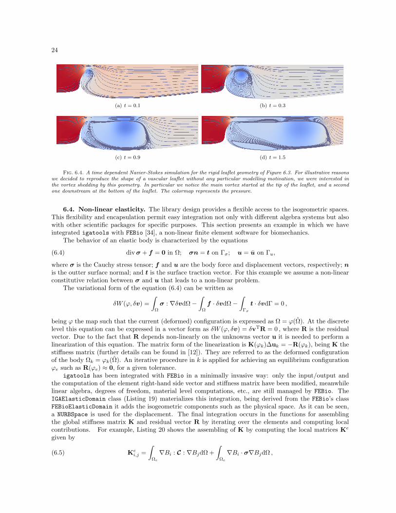
24
(a) t = 01 (b) t = 03
(c) t = 09 (d) t = 15
Fig 64 A time dependent Navier-Stokes simulation for the rigid leaflet geometry of Figure 63 For illustrative reasonswe decided to reproduce the shape of a vascular leaflet without any particular modelling motivation we were interested inthe vortex shedding by this geometry In particular we notice the main vortex started at the tip of the leaflet and a secondone downstream at the bottom of the leaflet The colormap represents the pressure
64 Non-linear elasticity The library design provides a flexible access to the isogeometric spacesThis flexibility and encapsulation permit easy integration not only with different algebra systems but alsowith other scientific packages for specific purposes This section presents an example in which we haveintegrated igatools with FEBio [34] a non-linear finite element software for biomechanics
The behavior of an elastic body is characterized by the equations
(64) divσ + f = 0 in Ω σn = t on Γσ u = u on Γu
where σ is the Cauchy stress tensor f and u are the body force and displacement vectors respectively nis the outter surface normal and t is the surface traction vector For this example we assume a non-linearconstitutive relation between σ and u that leads to a non-linear problem
The variational form of the equation (64) can be written as
δW (ϕ δv) =
intΩ
σ nablaδvdΩminusint
Ω
f middot δvdΩminusint
Γσ
t middot δvdΓ = 0
being ϕ the map such that the current (deformed) configuration is expressed as Ω = ϕ(Ω) At the discretelevel this equation can be expressed in a vector form as δW (ϕ δv) = δvTR = 0 where R is the residualvector Due to the fact that R depends non-linearly on the unknowns vector u it is needed to perform alinearization of this equation The matrix form of the linearization is K(ϕk)∆uk = minusR(ϕk) being K thestiffness matrix (further details can be found in [12]) They are referred to as the deformed configurationof the body Ωk = ϕk(Ω) An iterative procedure in k is applied for achieving an equilibrium configurationϕe such as R(ϕe) asymp 0 for a given tolerance
igatools has been integrated with FEBio in a minimally invasive way only the inputoutput andthe computation of the element right-hand side vector and stiffness matrix have been modified meanwhilelinear algebra degrees of freedom material level computations etc are still managed by FEBio TheIGAElasticDomain class (Listing 19) materializes this integration being derived from the FEBiorsquos classFEBioElasticDomain it adds the isogeometric components such as the physical space As it can be seena NURBSpace is used for the displacement The final integration occurs in the functions for assemblingthe global stiffness matrix K and residual vector R by iterating over the elements and computing localcontributions For example Listing 20 shows the assembling of K by computing the local matrices Ke
given by
(65) Keij =
intΩe
nablaBi C nablaBjdΩ +
intΩe
nablaBi middot σnablaBjdΩ
25
1 class IGAElasticDomain public FEBioElasticDomain
2
3 public
4 public functions and members
5 using Space = PhysicalSpace ltRefSpace PForward gt
67 private
8 private functions and members
9 Space space
10 void stiffness_matrix(FESolidSolver psolver )
11 void residual(FESolidSolver psolver )
12
Listing 19Class for the solution of the non-linear elascity problem by means of the IgM integrated into FEBio The spaces and
push forward types are shown as well as the public functions for assemblying the residual vector and the stiffness matrix
to be then added in line 29 into a global FEBio matrix
1 void
2 IGAElasticDomain stiffness_matrix(FESolidSolver psolver)
3
4 define loc_mat elem elem_end init elem values with quadrature
56 for( elem= elem_end ++elem)
7
8 Elasticity and Cauchy stress tensors evaluated by FEBio
9 auto sigma = this -gtget_stress_tensor(elem)
10 auto c = this -gtget_elasticity_tensor(elem)
1112 loc_mat = 0
13 auto w_meas = elem -gtget_w_measures ()
14 for (int i = 0 i lt n_basis ++i)
15
16 auto Dphi_i = elem -gtget_basis_gradients(i)
17 for (int j = 0 j lt n_basis ++j)
18
19 auto Dphi_j = elem -gtget_basis_gradients(j)
20 for (int qp = 0 qp lt n_points ++qp)
21 loc_mat += Compute formula (65) using
22 Dphi_i[qp] Dphi_j[qp] c[qp] sigma[qp] w_meas[qp]
23
24
25 auto loc_to_global = this -gtget_local_to_global(elem)
26 auto nodal_connectivity = this -gtget_nodal_connectivity(elem)
2728 Add element contribution into global FEBio stiffness matrix
29 psolver -gtAssembleStiffness(nodal_connectivity
30 loc_to_global loc_mat )
31
32
Listing 20Implementation of the stiffness matrix for the nonlinear elasticity case The local element matrices are assembled into
the FEBio expected structure
Finally Figure 65 shows a simulation for the torsion of a curved tube with an open section Thegeometry is given by a three dimensional single NURBS patch of degree two and its material modeled bya Neo-Hookean formulation
Acknowledgements We would like to thank A Buffa and G Sangalli for feedback and suggestions
26
(a) The geometry map (b) t = 03 (c) t = 05 (d) t = 10
Fig 65 A non-linear elasticity simulation for an open tube is shown The map is a second order deformation of asquare 65(a) In this simulation a rotation around the axis of the tube is prescribed in one of the ends of tube whereas theother is fixed Finite deformations are considered for an hyperelastic material formulation Colormap represents von Misesstress
and to the beta testers of igatools for their patience and feedback in particular to A Bressan E Brivadisand R Vazquez
REFERENCES
[1] D N Arnold R S Falk and R Winther Finite element exterior calculus from Hodge theory to numericalstability Bull Amer Math Soc (NS) 47 (2010) pp 281ndash354
[2] W Bangerth R Hartmann and G Kanschat dealII ndash a general purpose object oriented finite element libraryACM Trans Math Softw 33 (2007) pp 241ndash2427
[3] W Bangerth T Heister and G Kanschat dealII Differential Equations Analysis Library Technical Referencehttpwwwdealiiorg
[4] Y Bazilevs L Beirao da Veiga J A Cottrell T J R Hughes and G Sangalli Isogeometric analysisApproximation stability and error estimates for h-refined meshes Math Mod Meth Appl S 16 (2006) pp 1031ndash1090
[5] Y Bazilevs V M Calo J A Cottrell J A Evans T J R Hughes S Lipton M A Scott and T WSederberg Isogeometric analysis using T-splines Comput Methods Appl Mech Engrg 199 (2010) pp 229ndash263
[6] Y Bazilevs C Michler V M Calo and T J R Hughes Isogeometric variational multiscale modeling of wall-bounded turbulent flows with weakly enforced boundary conditions on unstretched meshes Comput Methods ApplMech Engrg 199 (2010) pp 780ndash790
[7] Y Bazilevs C Michler V M Calo and T J R Hughes Isogeometric variational multiscale modeling of wall-bounded turbulent flows with weakly enforced boundary conditions on unstretched meshes Comput Methods ApplMech Engrg 199 (2010) pp 780ndash790
[8] K Beck Test Driven Development By Example Addison-Wesley Longman 2002[9] P Becker Working draft standard for programming language C++ Tech Report N3242=11-0012 ISOIEC JTC 1
Information Technology Subcommittee SC 22 Programming Language C++ Feb 2011[10] D J Benson Y Bazilevs E De Luycker M-C Hsu M Scott T J R Hughes and T Belytschko A
generalized finite element formulation for arbitrary basis functions From isogeometric analysis to XFEM Int JNumer Meth Eng 83 (2010) pp 765ndash785
[11] D Boffi F Brezzi and M Fortin Mixed Finite Element Methods and Applications Springer Series in Computa-tional Mathematics Springer London Limited 2013
[12] J Bonet and R D Wood Nonlinear Continuum Mechanics for Finite Element Analysis Cambridge UniversityPress New York NY USA 2 ed 2008
[13] M J Borden M A Scott J A Evans and T J R Hughes Isogeometric finite element data structures basedon Bezier extraction of NURBS Int J Numer Meth Eng 87 (2011) pp 15ndash47
[14] A Bressan and G Sangalli Isogeometric discretizations of the Stokes problem stability analysis by the macroelementtechnique IMA J Numer Anal (2012)
[15] A Buffa D Cho and G Sangalli Linear independence of the T-spline blending functions associated with someparticular T-meshes Comput Methods Appl Mech Engrg 199 (2010) pp 1437ndash1445
[16] A Buffa C de Falco and G Sangalli IsoGeometric Analysis stable elements for the 2D Stokes equation Int JNumer Meth Fl 65 (2011) pp 1407ndash1422
[17] A Buffa J Rivas G Sangalli and R Vazquez Isogeometric discrete differential forms in three dimensionsSIAM J Numer Anal 49 (2011) pp 818ndash844
[18] A Buffa G Sangalli and R Vazquez Isogeometric analysis in electromagnetics B-splines approximation Com-
27
put Methods Appl Mech Engrg 199 (2010) pp 1143ndash1152[19] J A Cottrell T J R Hughes and Y Bazilevs Isogeometric Analysis Toward Integration of CAD and FEA
Wiley 2009[20] J A Cottrell A Reali Y Bazilevs and T J R Hughes Isogeometric analysis of structural vibrations Comput
Methods Appl Mech Engrg 195 (2006) pp 5257ndash5296[21] C de Falco A Reali and R Vazquez GeoPDEs A research tool for isogeometric analysis of PDEs Adv Eng
Softw 42 (2011) pp 1020 ndash 1034[22] T Dokken T Lyche and K F Pettersen Locally refinable splines over box-partitions tech report SINTEF
February 2012[23] M Dorfel B Juttler and B Simeon Adaptive isogeometric analysis by local h-refinement with T-splines Comput
Methods Appl Mech Engrg 199 (2009) pp 264ndash275[24] J A Evans and T J R Hughes Isogeometric divergence-conforming B-spline for the steady NavierndashStokes equations
Math Mod Meth Appl S 23 (2013) pp 1421ndash1478[25] Isogeometric divergence-conforming B-splines for the unsteady NavierndashStokes equations J Comput Phys 241
(2013) pp 141ndash167[26] D R Forsey and R H Bartels Hierarchical B-spline refinement in SIGGRAPH rsquo88 Proceedings of the 15th annual
conference on Computer graphics and interactive techniques 1988 pp 205ndash212[27] C Giannelli B Juttler and H Speleers THBndashsplines The truncated basis for hierarchical splines Compute
Aided Geometric D 29 (2012) pp 485ndash498[28] R Glowinski P G Ciarlet and J L Lions Numerical Methods for Fluids vol 3 of Handbook of numerical
analysis Elsevier 2002[29] M Heroux R Bartlett V E Howle R Hoekstra J Hu T Kolda R Lehoucq K Long R Pawlowski
E Phipps A Salinger H Thornquist R Tuminaro J Willenbring and A Williams An Overview ofTrilinos Tech Report SAND2003-2927 Sandia National Laboratories 2003
[30] T J R Hughes J A Cottrell and Y Bazilevs Isogeometric analysis CAD finite elements NURBS exactgeometry and mesh refinement Comput Methods Appl Mech Engrg 194 (2005) pp 4135ndash4195
[31] ISOIEC 148822003 ndash Programming languages ndash C++ 2003[32] ISOIEC 148822011 ndash Information technology ndash programming languages ndash C++ 2011[33] J Kiendl Y Bazilevs M-C Hsu R Wuchner and K-U Bletzinger Kirchhoff-Love shell structures comprised
of multiple patches Comput Methods Appl Mech Engrg 199 (2010) pp 2403ndash2416[34] S A Maas B J Ellis G A Ateshian and J A Weiss FEBio Finite elements for biomechanics J Biomed
Eng 134 (2012)[35] P Monk Finite element methods for Maxwellrsquos equations Numerical Mathematics and Scientific Computation Oxford
University Press New York 2003[36] L A Piegl and W Tiller The NURBs Book Monographs in Visual Communication Series Springer-Verlag GmbH
1997[37] W Schroeder K Martin and B Lorensen The Visualization Toolkit An Object-oriented Approach to 3D Graph-
ics Kitware 2006[38] L L Schumaker Spline functions basic theory Cambridge Mathematical Library Cambridge University Press
Cambridge third ed 2007[39] M A Scott X Li T W Sederberg and T J R Hughes Local refinement of analysis-suitable T-splines Comput
Methods Appl Mech Engrg 213ndash216 (2012) pp 206 ndash 222[40] A H Squillacote The ParaView Guide Kitware 2007[41] A Stepanov and M Lee The standard template library tech report WG21N0482 ISO Programming Language
C++ Project 1994[42] B Stroustrup The C++ Programming Language Addison-Wesley 2000[43] A-V Vuong C Giannelli B Juttler and B Simeon A hierarchical approach to adaptive local refinement in
isogeometric analysis Comput Methods Appl Mech Engrg 200 (2011 Dec) pp 3554ndash3567[44] O Weeger U Wever and B Simeon Isogeometric analysis of nonlinear Euler Bernoulli beam vibrations Nonlinear
Dynam 72 (2013) pp 813ndash835
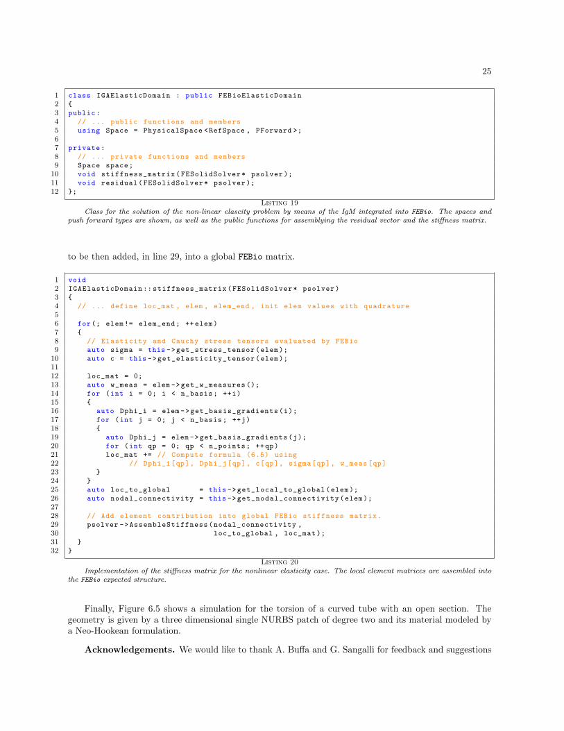
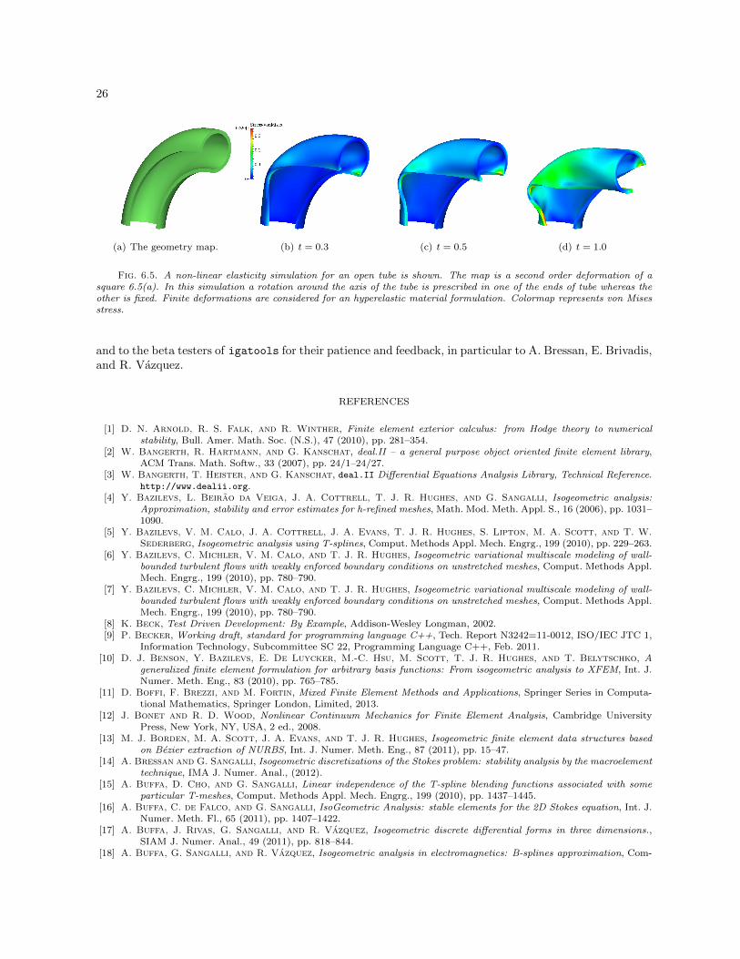