item response theory using the package · item response theory using the ltm package dimitris...

Item Response Theory Using the ltm Package

Dimitris RizopoulosBiostatistical Centre, Catholic University of Leuven, Belgium

[email protected]

The R User Conference 2008Technische Universitat Dortmund

August 14th, 2008

1 Let’s Start with An Example

• Situation:

. A teacher offers a course on Calculus

• Question:

. How can she find out which students have sufficiently understood the material?

• Solution:

. Exams – Students need to take a test with questions on Calculus

useR! 2008, Dortmund 1/21

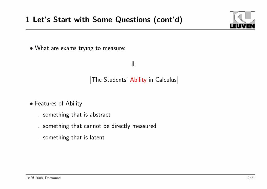
1 Let’s Start with Some Questions (cont’d)

• What are exams trying to measure:

⇓

The Students’ Ability in Calculus

• Features of Ability

. something that is abstract

. something that cannot be directly measured

. something that is latent


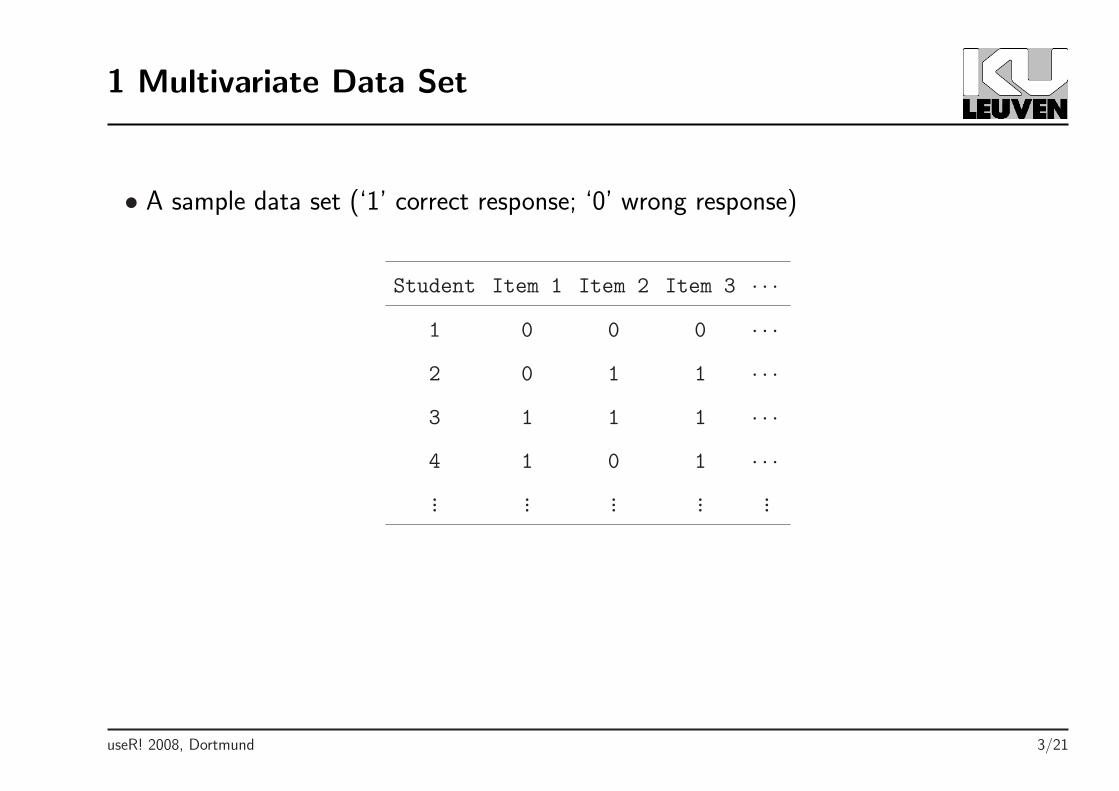
1 Multivariate Data Set

• A sample data set (‘1’ correct response; ‘0’ wrong response)

Student Item 1 Item 2 Item 3 · · ·1 0 0 0 · · ·2 0 1 1 · · ·3 1 1 1 · · ·4 1 0 1 · · ·... ... ... ... ...


2 Item Characteristic Curve

• A pool of items measuring a single latent trait

• Basic components

. θ ∈ (−∞,∞): latent ability

. Pi ∈ (0, 1): probability of responding correctly in item i

Item Characteristic Curve: functional relationship between θ and Pi


2 Item Characteristic Curve (cont’d)

−3 −2 −1 0 1 2 3

0.0

0.2

0.4

0.6

0.8

1.0

θ

Pro

babi

lity

of C

orre

ct R

espo

nse

Item Characteristic Curve


2 Item Characteristic Curve & IRT Models

−3 −2 −1 0 1 2 3

0.0

0.2

0.4

0.6

0.8

1.0

θ

Pro

babi

lity

of C

orre

ct R

espo

nse

P(θ) = exp{ f(θ) }1 + exp{ f(θ) }


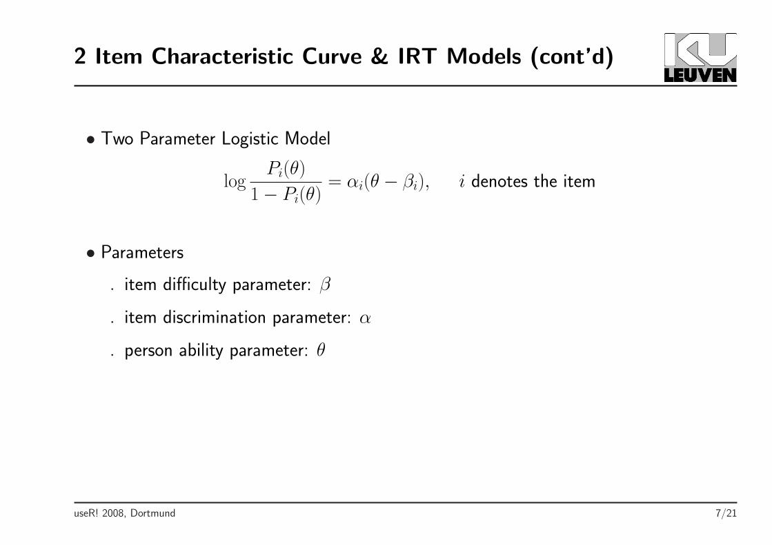
2 Item Characteristic Curve & IRT Models (cont’d)

• Two Parameter Logistic Model

logPi(θ)

1− Pi(θ)= αi(θ − βi), i denotes the item

• Parameters

. item difficulty parameter: β

. item discrimination parameter: α

. person ability parameter: θ


2 Special Case: The Rasch Model

• proposed by Georg Rasch (Danish mathematician) in 1960

logPi(θ)

1− Pi(θ)= θ − βi, i denotes the item

• Properties and Features

. closed-form sufficient statistics

. restrictive ⇒ αi = 1 for all i

. widely used


3 IRT Using the ltm Package

• ltm package has been designed for user-friendly IRT analyses

• Functions for:

. descriptive analyses

. fitting common IRT models

. post-processing of the fitted models

. extra features


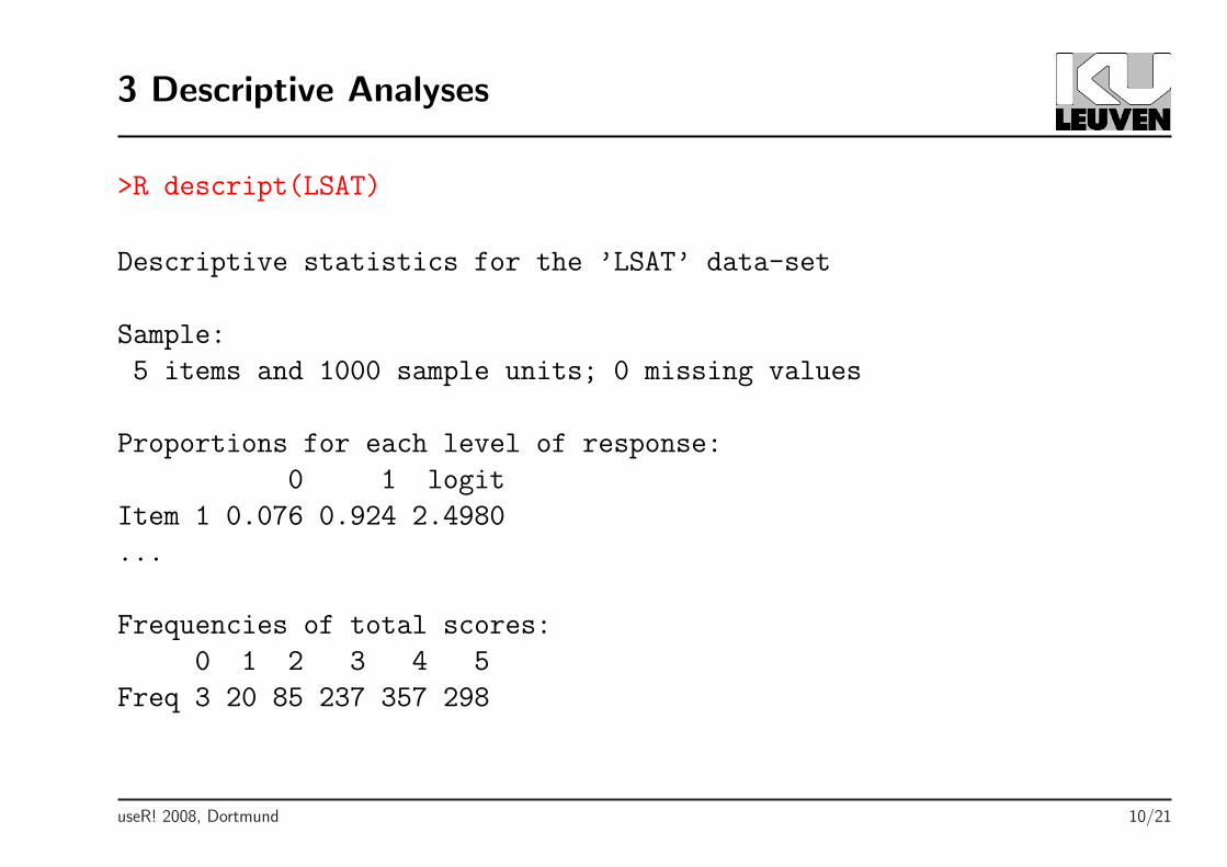
3 Descriptive Analyses

>R descript(LSAT)

Descriptive statistics for the ’LSAT’ data-set

Sample:

5 items and 1000 sample units; 0 missing values

Proportions for each level of response:

0 1 logit

Item 1 0.076 0.924 2.4980

...

Frequencies of total scores:

0 1 2 3 4 5

Freq 3 20 85 237 357 298


Biserial correlation with Total Score:

Included Excluded

Item 1 0.3618 0.1128

...

Cronbach’s alpha:

value

All Items 0.2950

Excluding Item 1 0.2754

...

Pairwise Associations:

Item i Item j p.value

1 1 5 0.565

...


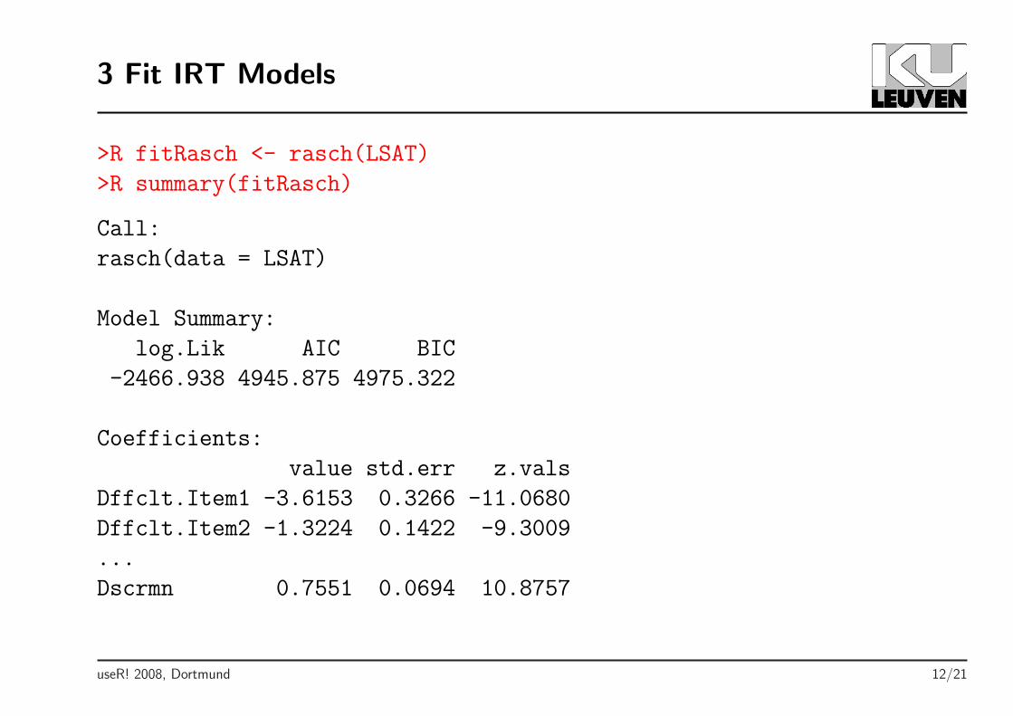
3 Fit IRT Models

>R fitRasch <- rasch(LSAT)

>R summary(fitRasch)

Call:

rasch(data = LSAT)

Model Summary:

log.Lik AIC BIC

-2466.938 4945.875 4975.322

Coefficients:

value std.err z.vals

Dffclt.Item1 -3.6153 0.3266 -11.0680

Dffclt.Item2 -1.3224 0.1422 -9.3009

...

Dscrmn 0.7551 0.0694 10.8757


Integration:

method: Gauss-Hermite

quadrature points: 21

Optimization:

Convergence: 0

max(|grad|): 2.9e-05

quasi-Newton: BFGS


3 Fit IRT Models (cont’d)

>R fit2PL <- ltm(LSAT ∼ z1)

>R summary(fit2PL)

Call:

ltm(formula = LSAT ~ z1)

Model Summary:

log.Lik AIC BIC

-2466.653 4953.307 5002.384

Coefficients:

value std.err z.vals

Dffclt.Item1 -3.3597 0.8669 -3.8754

...

Dscrmn.Item1 0.8254 0.2581 3.1983

...


Integration:

method: Gauss-Hermite

quadrature points: 21

Optimization:

Convergence: 0

max(|grad|): 0.024

quasi-Newton: BFGS


3 Compare Fits with an LRT

>R anova(fitRasch, fit2PL)

Likelihood Ratio Table

AIC BIC log.Lik LRT df p.value

fit1 4945.88 4975.32 -2466.94

fit2 4953.31 5002.38 -2466.65 0.57 4 0.967


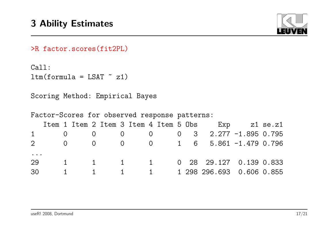
3 Ability Estimates

>R factor.scores(fit2PL)

Call:

ltm(formula = LSAT ~ z1)

Scoring Method: Empirical Bayes

Factor-Scores for observed response patterns:

Item 1 Item 2 Item 3 Item 4 Item 5 Obs Exp z1 se.z1

1 0 0 0 0 0 3 2.277 -1.895 0.795

2 0 0 0 0 1 6 5.861 -1.479 0.796

...

29 1 1 1 1 0 28 29.127 0.139 0.833

30 1 1 1 1 1 298 296.693 0.606 0.855


3 Plot ICCs

>R plot(fit2PL, legend = TRUE, cx = "bottomright")

−4 −2 0 2 4

0.0

0.2

0.4

0.6

0.8

1.0

Item Characteristic Curves

Item 1Item 2Item 3Item 4Item 5

θ

Pro

babi

lity

of C

orre

ct R

espo

nse


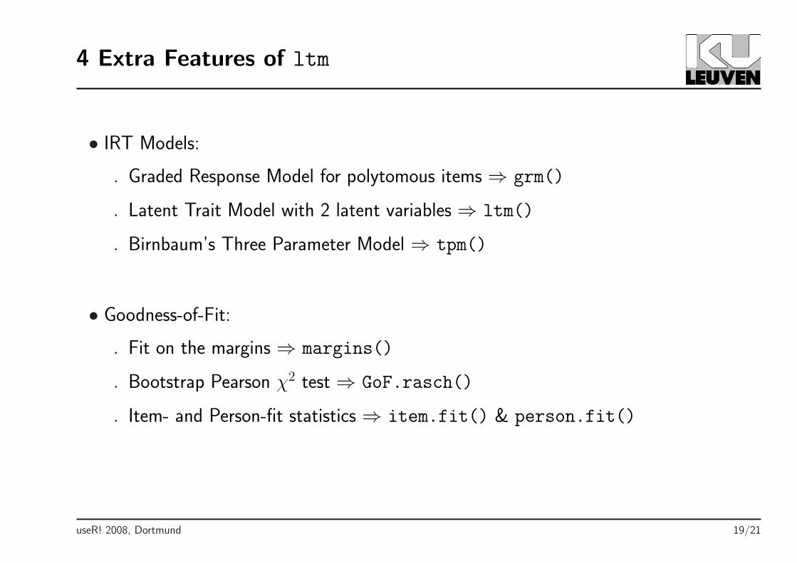
4 Extra Features of ltm

• IRT Models:

. Graded Response Model for polytomous items ⇒ grm()

. Latent Trait Model with 2 latent variables ⇒ ltm()

. Birnbaum’s Three Parameter Model ⇒ tpm()

• Goodness-of-Fit:

. Fit on the margins ⇒ margins()

. Bootstrap Pearson χ2 test ⇒ GoF.rasch()

. Item- and Person-fit statistics ⇒ item.fit() & person.fit()


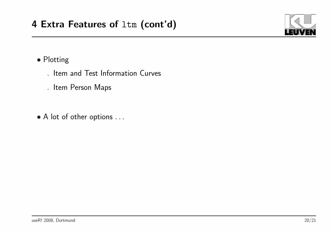
4 Extra Features of ltm (cont’d)

• Plotting

. Item and Test Information Curves

. Item Person Maps

• A lot of other options . . .


Thank you for your attention!

More Information for ltm is available at:

http://wiki.r-project.org/rwiki/doku.php?id=packages:cran:ltm


item response theory using the package · item response theory using the ltm package dimitris...

Documents