itf transport outlook 2017 - ttm.nlitf transport outlook 2017 itf transport outlook 2017 the itf...
TRANSCRIPT
ITF Transport Outlook 2017
ITF Transport Outlook 2017The ITF Transport Outlook provides an overview of recent trends and near-term prospects for the transport sector at a global level. It also presents long-term projections for transport demand to 2050 for freight (maritime, air and surface) and passenger transport (car, rail and air) as well as related CO2 emissions, under different policy scenarios.
This edition specifically looks at how the main policy, economic and technological changes since 2015, along with other international developments such as the UN Sustainable Development Goals, are shaping the future of mobility. A special focus on accessibility in cities highlights the role of policies in shaping sustainable transport systems which provide equal access to all.
Contents
Part I. Global Outlook for transport
Chapter 1. The transport sector today
Chapter 2. Transport demand and CO2 emissions to 2050
Part II. Sectorial Outlook
Chapter 3. International freight
Chapter 4. International passenger aviation
Chapter 5. Mobility in cities
ISbn 978-92-82-10799-774 2017 01 1 P
Consult this publication on line at http://dx.doi.org/10.1787/9789282108000-en.
This work is published on the OECD iLibrary, which gathers all OECD books, periodicals and statistical databases. Visit www.oecd-ilibrary.org for more information.
9HSTCSC*bahjjh+
ITF Tran
spo
rt Ou
tloo
k 2017

ITF Transport Outlook 2017
This work is published on the responsibility of the Secretary-General of the OECD. The
opinions expressed and arguments employed herein do not necessarily reflect the official
views of the OECD member countries.
This document and any map included herein are without prejudice to the status of or
sovereignty over any territory, to the delimitation of international frontiers and boundaries
and to the name of any territory, city or area.
ISBN 978-92-82-10799-7 (print) ISBN 978-92-82-10800-0 (PDF)
The statistical data for Israel are supplied by and under the responsibility of the relevant Israeli authorities. The use of such data by the OECD is without prejudice to the status of the Golan Heights, East Jerusalem and Israeli settlements in the West Bank under the terms of international law.
Photo credits: © iStockphoto.com/visualgo.
Corrigenda to OECD publications may be found on line at: www.oecd.org/publishing/corrigenda.
© OECD/ITF 2017
You can copy, download or print OECD content for your own use, and you can include excerpts from OECD publications, databases and
multimedia products in your own documents, presentations, blogs, websites and teaching materials, provided that suitable
acknowledgement of OECD as source and copyright owner is given. All requests for public or commercial use and translation rights should
be submitted to [email protected]. Requests for permission to photocopy portions of this material for public or commercial use shall be
addressed directly to the Copyright Clearance Center (CCC) at [email protected] or the Centre français d’exploitation du droit de copie (CFC)
Please cite this publication as:OECD/ITF (2017), ITF Transport Outlook 2017, OECD Publishing, Paris.http://dx.doi.org/10.1787/9789282108000-en
EDITORIAL
Editorial
For the first time, the ITF Transport Outlook assembles scenarios for future transport
demand and related CO2 emissions from all sectors and modes of transport. Starting from
long-term projections produced by the OECD as well as non-OECD bodies, it analyses how
socio-economic changes will affect the demand for transport under different policy
scenarios. Several key trends emerge from these, such as the intensifying shift in transport
activity towards developing economies, with Asian countries representing an ever
increasing share of total transport demand for both freight and passengers.
The level of uncertainty in all areas of transport is also striking. Uncertainties related
to the pace of economic and trade development, the price of oil, technology and
innovations all render the future of the transport world difficult to fathom. The different
outcomes of the scenarios should not be read as forecasts for the coming 35 years. Rather,
they describe several possible futures. Whether future reality comes closer to one or the
other will depend on the actions policy-makers take. At a time when the international
commitments, such as the Paris agreement on climate change, need to be transformed into
actions, the scenarios of the ITF Transport Outlook show that an efficient decarbonisation of
the transport sector can only occur if a wide range of measures come into force for both
freight and passengers. All policy levers, Avoid (unnecessary transport demand), Shift (to
sustainable transport options) and Improve (efficiency), must be put into action.
Building the comprehensive scenarios in this Outlook is only the very first step of a
larger enterprise undertaken by the International Transport Forum to understand how the
transport sector can play its part in decarbonising the economy. ITF’s Decarbonising
Transport project aims to build a catalogue of efficient mitigation measures and assess
them under a coherent framework, in order to help countries transform their ambitions
into actions, by building a commonly accepted framework for climate policy assessment,
and by helping countries to develop sustainable transport solutions.
At the same time, the efforts towards greener transport need to be balanced with the
role transport plays as an enabler of sustainable development. There is a growing
recognition that better transport is not about increased mobility and tonne-kilometres but
about providing equitable access to jobs, opportunities, social interactions and markets,
contributing to healthy and fulfilled lives. Transport policies should focus on accessibility,
not only time savings. This Outlook showcases how to analyse policies in terms of access in
two areas, urban and international air travel.
Providing efficient, equitable access while respecting the pledge to decarbonise
transport will prove challenging. Policy-makers need to act now to ensure a sustainable
future for transport, but with a strategic long-term vision. They must avoid the trap of
short-term energy savings which will prove inefficient in the long-term, especially those
involving large investment, for instance in infrastructure.
ITF TRANSPORT OUTLOOK 2017 © OECD/ITF 2017 3
EDITORIAL
Policy makers should also be ready to tap into the potential of innovative technologies
in terms of access and green transport. The impact of digitalisation is already felt strongly
across much of transport. The next transport revolution is underway, based on real-time data
that make it easier and more efficient to match supply and demand. The coming decades
will witness the arrival of more disruptive technologies, vehicle automation and on-demand
transport first and foremost. Car-sharing has the potential to increase accessibility in a
sustainable way. Such solutions need to be promoted and accompanied by sound policies.
Without these, vehicle automation could lead to more cars onto the roads, with all the
associated problems of air pollution, CO2 emissions, congestion, inequitable transport…
Sustainable transport enables sustainable development. It is fundamental for meeting
the needs of people in their personal lives and economic activities while safeguarding the
ability of future generations to meet their own needs. Providing sustainable transport will
be a challenge and will require sound governance from all stakeholders. In this respect, I
hope that this Outlook can enhance the knowledge about the issues at stake and become
the basis for enlightened discussions about solutions.
José Viegas
Secretary-General
International Transport Forum
ITF TRANSPORT OUTLOOK 2017 © OECD/ITF 20174
FOREWORD
Foreword
The 2017 Edition of the ITF Transport Outlook builds and expands on the previous editions to
give a comprehensive overview of the future transport demand and related carbon dioxide (CO2)
emissions up to 2050. The scenarios in this Outlook are built with the International Transport
Forum’s (ITF) in-house modelling tools, developed over the course of several years. Contrary to most
transport-energy modelling framework, the ITF models start by analysing transport demand,
estimating what are the mobility needs and the freight demand coming from the future population,
economic and trade projections (Annex 2.A). Mode choice, energy use and CO2 emissions only come
at a later stage.
Rather than attempting to establish a likely central forecast for the evolution of transport
volumes, the ITF Transport Outlook focuses on scenarios to illustrate the potential impact of
policies on transport demand and related CO2 emissions. This edition covers all modes and combines
them into coherent scenarios. In particular, it gives a low-carbon scenario, which results from the
combination of the most optimistic scenario from all modes and points to a lower bound for CO2
emissions for 2050 with currently foreseen technology and mode choice trajectories.
Compared to the 2015 edition, this publication adds several new elements. Most noteworthy are
the chapter dedicated to international aviation (Chapter 4), as well as the expansion of our analysis
of urban mobility to all the cities of the world (Chapter 5). This Outlook also brings into focus the
issue of accessibility, both for air transport and in cities. Accessibility has become a key angle from
which to analyse transport policies and the Outlook gives some insights into the long-term trends
for accessibility, and how they relate to policy packages.
ITF TRANSPORT OUTLOOK 2017 © OECD/ITF 2017 5
ACKNOWLEDGEMENTS
Acknowledgements
The ITF Transport Outlook was prepared by the ITF Statistics and Modelling Unit, with the
support from numerous persons and partner organisations. The publication was coordinated
by Vincent Benezech, under the supervision of Jari Kauppila (Head of Statistics and
Modelling). The main authors for each chapter are the following:
Statistical and research assistance was provided by Claire Alanoix, Mario Barreto, Ryan
Hunter and Rachele Poggi. Cecilia Paymon, Janine Treves and Margaret Simmons supported
the publication process. Suzanne Parandian copy-edited the manuscript.
The Outlook was reviewed by the Joint Transport Research Centre Committee and the
Outlook team is very grateful for their commnents and contribution. The authors are also
grateful for the help of other ITF staff, in particular, Jagoda Egeland, Seiya Ishikawa, Alain
Lumbroso, Olaf Merk, Stephen Perkins and Daniel Veyrard. The ITF also benefited from the
help provided by the following bodies of the OECD: the Ship Building Unit, the Environment
Directorate and the International Energy Agency.
Several partners have been valuable in developing the methodologies and providing
data: The International Council for Clean Transportation (ICCT) for the work on local
pollutant emissions; The Energy and Resources Institute India, (TERI), China Academy of
Transportation Sciences (CATS), Japan International Cooperation Agency (JICA),
Transportation Planning Research Institute China and the Asian Development Bank (ADB)
for their help with data in Asian cities; Economic Commission for Latin America (ECLAC) and
Development Bank of Latin America (CAF) for data on Latin American cities and trade; the
Road Freight Lab of World Business Council on Sustainable Development (WBCSD) with
whom we worked on the freight optimisation; the International Civil Aviation Organisation
(ICAO) and the Airport Council International Europe (ACI Europe) for their help with aviation
forecasts and emissions; SkyScanner for generously providing a database on fares from the
aviation sector.
Finally, the ITF Secretariat is grateful for contributions provided by several individuals,
including Dr Tristan Smith (University College London), Sainarayan Ananthanarayan and
Antonin Combes (ICAO), Lloyd Wright, Melissa Cardenas and Alvin Mejia (ADB), Dr Cristiano
Façanha (ICCT), Pierpaolo Cazzola (IEA), Jean Chateau and Karin Strodel (OECD) and Sudhir
Gota (Clean Air Asia).
Chapter 1. The transport sector today Vincent Benezech, Christian Pollok, Jari Kauppila
Chapter 2. Overview of long-term Outlook Vincent Benezech, Guineng Chen, Jari Kauppila
Chapter 3. International freight Ronald Halim, Jari Kauppila, Luis Martinez, Olaf Merk
Chapter 4. International aviation Vincent Benezech
Chapter 5. Mobility in cities Guineng Chen (global mobility model), Nicolas Wagner, Olga Petrik and Christian Pollok (accessibility), Wei-Shiuen Ng (Asian cities)
ITF TRANSPORT OUTLOOK 2017 © OECD/ITF 20176
TABLE OF CONTENTS
Table of contents
Executive summary . . . . . . . . . . . . . . . . . . . . . . . . . . . . . . . . . . . . . . . . . . . . . . . . . . . . . . . . . 13
Part I
Global outlook for transport
Chapter 1. The transport sector today . . . . . . . . . . . . . . . . . . . . . . . . . . . . . . . . . . . . . . . . . . 19
Transport and the economic environment . . . . . . . . . . . . . . . . . . . . . . . . . . . . . . . . . . 22
Freight . . . . . . . . . . . . . . . . . . . . . . . . . . . . . . . . . . . . . . . . . . . . . . . . . . . . . . . . . . . . . . . . 27
Passenger transport . . . . . . . . . . . . . . . . . . . . . . . . . . . . . . . . . . . . . . . . . . . . . . . . . . . . . 33
CO2 emissions from transport . . . . . . . . . . . . . . . . . . . . . . . . . . . . . . . . . . . . . . . . . . . . 38
Spending on inland transport infrastructure . . . . . . . . . . . . . . . . . . . . . . . . . . . . . . . . 40
References . . . . . . . . . . . . . . . . . . . . . . . . . . . . . . . . . . . . . . . . . . . . . . . . . . . . . . . . . . . . . 44
Chapter 2. Transport demand and CO2 emissions to 2050 . . . . . . . . . . . . . . . . . . . . . . . . 47
Passenger transport . . . . . . . . . . . . . . . . . . . . . . . . . . . . . . . . . . . . . . . . . . . . . . . . . . . . . 48
Freight transport . . . . . . . . . . . . . . . . . . . . . . . . . . . . . . . . . . . . . . . . . . . . . . . . . . . . . . . . 56
CO2 emissions . . . . . . . . . . . . . . . . . . . . . . . . . . . . . . . . . . . . . . . . . . . . . . . . . . . . . . . . . . 60
References . . . . . . . . . . . . . . . . . . . . . . . . . . . . . . . . . . . . . . . . . . . . . . . . . . . . . . . . . . . . . 63
Annex 2.A. The ITF modelling framework . . . . . . . . . . . . . . . . . . . . . . . . . . . . . . . . . . . 64
Part II
Sectoral outlook
Chapter 3. International freight . . . . . . . . . . . . . . . . . . . . . . . . . . . . . . . . . . . . . . . . . . . . . . . 69
Underlying trade projections . . . . . . . . . . . . . . . . . . . . . . . . . . . . . . . . . . . . . . . . . . . . . 70
International freight transport to 2050 . . . . . . . . . . . . . . . . . . . . . . . . . . . . . . . . . . . . . 73
CO2 emissions from international freight. . . . . . . . . . . . . . . . . . . . . . . . . . . . . . . . . . . 75
Challenges in container shipping. . . . . . . . . . . . . . . . . . . . . . . . . . . . . . . . . . . . . . . . . . 82
Challenges of hinterland transport . . . . . . . . . . . . . . . . . . . . . . . . . . . . . . . . . . . . . . . . 86
Decision making under uncertainty . . . . . . . . . . . . . . . . . . . . . . . . . . . . . . . . . . . . . . . 90
References . . . . . . . . . . . . . . . . . . . . . . . . . . . . . . . . . . . . . . . . . . . . . . . . . . . . . . . . . . . . . 92
Annex 3.A. ITF International Freight Model. . . . . . . . . . . . . . . . . . . . . . . . . . . . . . . . . . 94
Chapter 4. International passenger aviation . . . . . . . . . . . . . . . . . . . . . . . . . . . . . . . . . . . . 101
Modelling global passenger demand . . . . . . . . . . . . . . . . . . . . . . . . . . . . . . . . . . . . . . . 102
Passenger demand for air transport until 2050 . . . . . . . . . . . . . . . . . . . . . . . . . . . . . . 107
Impact of entry restrictions. . . . . . . . . . . . . . . . . . . . . . . . . . . . . . . . . . . . . . . . . . . . . . . 110
ITF TRANSPORT OUTLOOK 2017 © OECD/ITF 2017 7
TABLE OF CONTENTS
CO2 emissions from international aviation . . . . . . . . . . . . . . . . . . . . . . . . . . . . . . . . . 112
Accessibility by air . . . . . . . . . . . . . . . . . . . . . . . . . . . . . . . . . . . . . . . . . . . . . . . . . . . . . . 117
References . . . . . . . . . . . . . . . . . . . . . . . . . . . . . . . . . . . . . . . . . . . . . . . . . . . . . . . . . . . . . 121
Annex 4.A. Modelling framework for international aviation (passenger) . . . . . . . . . 123
Chapter 5. Mobility in cities. . . . . . . . . . . . . . . . . . . . . . . . . . . . . . . . . . . . . . . . . . . . . . . . . . . 127
Modelling passenger transport demand in cities. . . . . . . . . . . . . . . . . . . . . . . . . . . . . 128
Transport policy scenarios . . . . . . . . . . . . . . . . . . . . . . . . . . . . . . . . . . . . . . . . . . . . . . . 131
Passenger mobility in cities up to 2050 . . . . . . . . . . . . . . . . . . . . . . . . . . . . . . . . . . . . . 134
Emissions from mobility in cities up to 2050 . . . . . . . . . . . . . . . . . . . . . . . . . . . . . . . . 136
Accessibility. . . . . . . . . . . . . . . . . . . . . . . . . . . . . . . . . . . . . . . . . . . . . . . . . . . . . . . . . . . . 143
Passenger transport in Asian cities . . . . . . . . . . . . . . . . . . . . . . . . . . . . . . . . . . . . . . . . 157
References . . . . . . . . . . . . . . . . . . . . . . . . . . . . . . . . . . . . . . . . . . . . . . . . . . . . . . . . . . . . . 164
Annex 5.A1. Data sources . . . . . . . . . . . . . . . . . . . . . . . . . . . . . . . . . . . . . . . . . . . . . . . . . 169
Annex 5.A2. Methodology for the global urban passenger model . . . . . . . . . . . . . . . 171
Annex 5.A3. Detailed results for transport speed and densities. . . . . . . . . . . . . . . . . 176
Annex 5.A4. Scenario assumptions for Asian cities . . . . . . . . . . . . . . . . . . . . . . . . . . . 178
Statistical annex. . . . . . . . . . . . . . . . . . . . . . . . . . . . . . . . . . . . . . . . . . . . . . . . . . . . . . . . . . . . 181
Glossary . . . . . . . . . . . . . . . . . . . . . . . . . . . . . . . . . . . . . . . . . . . . . . . . . . . . . . . . . . . . . . . . . . . 215
Tables
1.1. Transport related targets in the UN Sustainable Development Goals . . . . . . . . 21
1.2. GDP growth, percentage change over previous year. . . . . . . . . . . . . . . . . . . . . . . 23
1.3. Annual GDP growth . . . . . . . . . . . . . . . . . . . . . . . . . . . . . . . . . . . . . . . . . . . . . . . . . . 23
1.4. World merchandise trade, 2012-17 . . . . . . . . . . . . . . . . . . . . . . . . . . . . . . . . . . . . . 24
2.1. Growth in GDP and domestic transport demand . . . . . . . . . . . . . . . . . . . . . . . . . 50
2.2. Urban transport by mode compared to economic growth. . . . . . . . . . . . . . . . . . 53
2.3. Annual growth rate for freight transport demand, compared to GDP . . . . . . . . 56
2.4. Freight intensity as a function of GDP per capita . . . . . . . . . . . . . . . . . . . . . . . . . 59
2.5. Per capita emissions from transport . . . . . . . . . . . . . . . . . . . . . . . . . . . . . . . . . . . . 61
3.1. Comparison of the alternative trade scenarios for the 2015-50 period . . . . . . . 72
3.2. Alternative scenarios for CO2 emissions . . . . . . . . . . . . . . . . . . . . . . . . . . . . . . . . 76
3.3. Container traffic by sea area in 2030 and 2050 and planned capacity 2030 . . . 84
3.4. Capacity needs for surface freight by continent . . . . . . . . . . . . . . . . . . . . . . . . . . 89
3.5. Capacity needs for surface freight by continent within 50 km of centroids and ports . . . . . . . . . . . . . . . . . . . . . . . . . . . . . . . . . . . . . . . . . . . . . . . . . . . . . . . . . . . 89
3.A1. Statistical and capacity characterisation of road network . . . . . . . . . . . . . . . . . 99
3.A2. Rail line engineering capacity . . . . . . . . . . . . . . . . . . . . . . . . . . . . . . . . . . . . . . . . . 100
3.A3. Rail infrastructure classification and freight capacity estimation . . . . . . . . . . . 100
4.1. International connectivity for selected countries . . . . . . . . . . . . . . . . . . . . . . . . . 111
4.2. Breakdown of CO2 emissions from aviation . . . . . . . . . . . . . . . . . . . . . . . . . . . . . 115
4.A1. Data sources . . . . . . . . . . . . . . . . . . . . . . . . . . . . . . . . . . . . . . . . . . . . . . . . . . . . . . . . 125
5.1. Specification of the three policy scenarios for city passenger transport. . . . . . 134
5.2. Share of car and public transport by region. . . . . . . . . . . . . . . . . . . . . . . . . . . . . . 136
5.3. Total mobility by world region . . . . . . . . . . . . . . . . . . . . . . . . . . . . . . . . . . . . . . . . . 138
ITF TRANSPORT OUTLOOK 2017 © OECD/ITF 20178
TABLE OF CONTENTS
5.4. Total CO2 emissions in cities by region. . . . . . . . . . . . . . . . . . . . . . . . . . . . . . . . . . 142
5.5. Results of the estimation of the congestion model . . . . . . . . . . . . . . . . . . . . . . . 149
5.6. Changes in some city characteristics between 2015 and 2050 in the baseline scenario . . . . . . . . . . . . . . . . . . . . . . . . . . . . . . . . . . . . . . . . . . . . . . 157
5.7. Changes in some city characteristics between 2015 and 2050 in the LUT scenario . . . . . . . . . . . . . . . . . . . . . . . . . . . . . . . . . . . . . . . . . . . . . . . . . . . . . . . . . . . . 157
5.8. Transport characteristics of selected Asian cities in 2010 . . . . . . . . . . . . . . . . . . 159
5.A1.1. Data Sources . . . . . . . . . . . . . . . . . . . . . . . . . . . . . . . . . . . . . . . . . . . . . . . . . . . . . . . . 169
5.A3.1. Road speeds and density in cities . . . . . . . . . . . . . . . . . . . . . . . . . . . . . . . . . . . . . . 176
5.A3.2. Public transport speeds and provision in cities. . . . . . . . . . . . . . . . . . . . . . . . . . . 177
5.A4.1. Chinese cities . . . . . . . . . . . . . . . . . . . . . . . . . . . . . . . . . . . . . . . . . . . . . . . . . . . . . . . 178
5.A4.2. Indian Cities . . . . . . . . . . . . . . . . . . . . . . . . . . . . . . . . . . . . . . . . . . . . . . . . . . . . . . . . 179
5.A4.3. Southeast Asian Cities . . . . . . . . . . . . . . . . . . . . . . . . . . . . . . . . . . . . . . . . . . . . . . . 179
Figures
1.1. Monthly index of world trade, advanced and emerging economies . . . . . . . . . 25
1.2. Elasticity of global trade to GDP. . . . . . . . . . . . . . . . . . . . . . . . . . . . . . . . . . . . . . . . 25
1.3. Primary commodity price indices, 2011-17 . . . . . . . . . . . . . . . . . . . . . . . . . . . . . . 27
1.4. World seaborne trade . . . . . . . . . . . . . . . . . . . . . . . . . . . . . . . . . . . . . . . . . . . . . . . . 28
1.5. World seaborne trade by type of cargo and country group . . . . . . . . . . . . . . . . . 29
1.6. World container throughput . . . . . . . . . . . . . . . . . . . . . . . . . . . . . . . . . . . . . . . . . . 29
1.7. World air freight traffic 2008-15. . . . . . . . . . . . . . . . . . . . . . . . . . . . . . . . . . . . . . . . 30
1.8. Surface freight volumes by mode of transport . . . . . . . . . . . . . . . . . . . . . . . . . . . 32
1.9. Passenger-kilometres by private car . . . . . . . . . . . . . . . . . . . . . . . . . . . . . . . . . . . . 33
1.10. Motorisation rates in selected developing countries . . . . . . . . . . . . . . . . . . . . . . 34
1.11. Road fatalities per 1 000 inhabitants. . . . . . . . . . . . . . . . . . . . . . . . . . . . . . . . . . . . 35
1.12. Rail passenger traffic . . . . . . . . . . . . . . . . . . . . . . . . . . . . . . . . . . . . . . . . . . . . . . . . . 36
1.13. World air passenger traffic, international and domestic . . . . . . . . . . . . . . . . . . . 37
1.14. Top 10 busiest airports in 2015 and evolution from 2000. . . . . . . . . . . . . . . . . . . 38
1.15. CO2 emissions by sector . . . . . . . . . . . . . . . . . . . . . . . . . . . . . . . . . . . . . . . . . . . . . . 39
1.16. Investment in inland transport infrastructure by region 1998-2014 . . . . . . . . . 41
1.17. Volume of investment in inland transport infrastructure by region 1995-2014. . . . . . . . . . . . . . . . . . . . . . . . . . . . . . . . . . . . . . . . . . . . . . . . . . . . . . . . . . . 42
1.18. Distribution of infrastructure investment across rail, road and inland waterways . . . . . . . . . . . . . . . . . . . . . . . . . . . . . . . . . . . . . . . . . . . . . . . . . . . . . . . . . . 43
1.19. Share of public road maintenance in total road expenditure . . . . . . . . . . . . . . . 43
2.1. Demand for passenger transport by mode. . . . . . . . . . . . . . . . . . . . . . . . . . . . . . . 49
2.2. Domestic aviation by region. . . . . . . . . . . . . . . . . . . . . . . . . . . . . . . . . . . . . . . . . . . 50
2.3. Passenger car ownership by region . . . . . . . . . . . . . . . . . . . . . . . . . . . . . . . . . . . . . 51
2.4. Length of high-speed rail network in selected countries or regions . . . . . . . . . 52
2.5. Urban transport demand by mode . . . . . . . . . . . . . . . . . . . . . . . . . . . . . . . . . . . . . 53
2.6. International air transport demand by region. . . . . . . . . . . . . . . . . . . . . . . . . . . . 55
2.7. Freight transport demand by mode. . . . . . . . . . . . . . . . . . . . . . . . . . . . . . . . . . . . . 56
2.8. Surface freight tonne-kilometres by region . . . . . . . . . . . . . . . . . . . . . . . . . . . . . . 58
2.9. Road freight activity by sector . . . . . . . . . . . . . . . . . . . . . . . . . . . . . . . . . . . . . . . . . 60
2.10. CO2 emissions by sector . . . . . . . . . . . . . . . . . . . . . . . . . . . . . . . . . . . . . . . . . . . . . . 61
2.11. CO2 emissions by sector and scenario . . . . . . . . . . . . . . . . . . . . . . . . . . . . . . . . . . 62
ITF TRANSPORT OUTLOOK 2017 © OECD/ITF 2017 9
TABLE OF CONTENTS
2.A1. The ITF modelling framework . . . . . . . . . . . . . . . . . . . . . . . . . . . . . . . . . . . . . . . . . 65
3.1. Value of trade by region . . . . . . . . . . . . . . . . . . . . . . . . . . . . . . . . . . . . . . . . . . . . . . 72
3.2. Value of trade by commodity . . . . . . . . . . . . . . . . . . . . . . . . . . . . . . . . . . . . . . . . . . 73
3.3. Freight transport demand in alternative trade elasticity scenarios . . . . . . . . . . 74
3.4. International freight volume by mode . . . . . . . . . . . . . . . . . . . . . . . . . . . . . . . . . . 75
3.5. International freight and related CO2 emissions by corridor . . . . . . . . . . . . . . . 75
3.6. CO2 emissions from international freight by mode . . . . . . . . . . . . . . . . . . . . . . . 78
3.7. CO2 emissions from maritime transport by commodity . . . . . . . . . . . . . . . . . . . 78
3.8. Road freight CO2 intensity by region in the 4 degree scenario of the IEA Mobility Model . . . . . . . . . . . . . . . . . . . . . . . . . . . . . . . . . . . . . . . . . . . . . . . . . . . . . . 79
3.9. The impact of policy measures on emissions . . . . . . . . . . . . . . . . . . . . . . . . . . . . 80
3.10. Impact of trade liberalisation on tonne-kilometres and CO2 emissions . . . . . . 80
3.11. Expansion plans compared with traffic projections by sea area . . . . . . . . . . . . 83
3.12. Ship size development of various ship types 1996-2015 . . . . . . . . . . . . . . . . . . . 85
3.13. Market concentration of container shipping lines 2000-16 . . . . . . . . . . . . . . . . . 85
3.14. Container ship capacity on Far East-Mediterranean route by alliance and by port (2015). . . . . . . . . . . . . . . . . . . . . . . . . . . . . . . . . . . . . . . . . . . . . . . . . . . . 86
3.15. Global merchant fleet and seaborne trade, 1995-2015 . . . . . . . . . . . . . . . . . . . . . 87
3.A1. Schematic description of the ITF international freight model . . . . . . . . . . . . . . 96
3.A2. Freight transport networks. . . . . . . . . . . . . . . . . . . . . . . . . . . . . . . . . . . . . . . . . . . . 98
4.1. Competition in international aviation . . . . . . . . . . . . . . . . . . . . . . . . . . . . . . . . . . 105
4.2. Relationship between distance, GDP and air connections. . . . . . . . . . . . . . . . . . 106
4.3. Share of low-cost carriers in regional, international flights . . . . . . . . . . . . . . . . 107
4.4. Demand for passenger aviation by region . . . . . . . . . . . . . . . . . . . . . . . . . . . . . . . 108
4.5. Regional breakdown of passenger-kilometres. . . . . . . . . . . . . . . . . . . . . . . . . . . . 110
4.6. Annual growth of the size of the air network, by origin region . . . . . . . . . . . . . 112
4.7. CO2 emissions from airports participating in the Airport Carbon Accreditation program . . . . . . . . . . . . . . . . . . . . . . . . . . . . . . . . . . . . . . . . . . . . . . . 114
4.8. CO2 emissions from international aviation . . . . . . . . . . . . . . . . . . . . . . . . . . . . . . 116
4.9. Average travel time to the alpha-cities . . . . . . . . . . . . . . . . . . . . . . . . . . . . . . . . . . 119
4.10. Average travel time to the alpha-cities by region, 2004-15 . . . . . . . . . . . . . . . . . 120
4.11. Average number of alpha-cities reachable in less than 24 hours . . . . . . . . . . . . 121
4.A1. Schematic description of the ITF international aviation model . . . . . . . . . . . . . 124
4.A2. Geographical distribution of cities and alpha-cities . . . . . . . . . . . . . . . . . . . . . . . 125
5.1. Total population of cities over 300 000 inhabitants . . . . . . . . . . . . . . . . . . . . . . . 129
5.2. GDP per capita in cities and countries by region. . . . . . . . . . . . . . . . . . . . . . . . . . 129
5.3. Car share in cities by region . . . . . . . . . . . . . . . . . . . . . . . . . . . . . . . . . . . . . . . . . . . 135
5.4. Mobility by mode of transport, Asia and North America . . . . . . . . . . . . . . . . . . . 136
5.5. CO2 emissions in cities by mode of transport . . . . . . . . . . . . . . . . . . . . . . . . . . . . 140
5.6. Mitigation potential by type of measure . . . . . . . . . . . . . . . . . . . . . . . . . . . . . . . . 140
5.7. Stock of electric cars by region, 2015 to 2040 . . . . . . . . . . . . . . . . . . . . . . . . . . . . . 141
5.8. NOx, SO4 and PM2.5 emissions by region . . . . . . . . . . . . . . . . . . . . . . . . . . . . . . . . 143
5.9. Vehicle activity by mode . . . . . . . . . . . . . . . . . . . . . . . . . . . . . . . . . . . . . . . . . . . . . . 144
5.10. Coverage of cities by OpenStreetMap (OSM) . . . . . . . . . . . . . . . . . . . . . . . . . . . . . 147
5.11. Road accessibility in cities by region and city size . . . . . . . . . . . . . . . . . . . . . . . . 148
5.12. Congestion in cities as a function of GDP per capita . . . . . . . . . . . . . . . . . . . . . . 149
5.13. Public transport coverage in selected cities . . . . . . . . . . . . . . . . . . . . . . . . . . . . . . 150
ITF TRANSPORT OUTLOOK 2017 © OECD/ITF 201710
TABLE OF CONTENTS
5.14. Public transport coverage in cities by region . . . . . . . . . . . . . . . . . . . . . . . . . . . . . 151
5.15. Accessibility by public transport in 23 cities . . . . . . . . . . . . . . . . . . . . . . . . . . . . . 152
5.16. Public transport accessibility in cities. . . . . . . . . . . . . . . . . . . . . . . . . . . . . . . . . . . 153
5.17. Accessibility to jobs in Lisbon before (left) and after (right) the introduction of shared mobility solutions. . . . . . . . . . . . . . . . . . . . . . . . . . . . . . . . . . . . . . . . . . . 155
5.18. Total CO2 emissions in the selected Asian cities. . . . . . . . . . . . . . . . . . . . . . . . . . 162
5.A2.1. Modelling framework for the ITF global model for mobility in cities. . . . . . . . . 172
Look for the StatLinks2at the bottom of the tables or graphs in this book. To download the matching Excel® spreadsheet, just type the link into your Internet browser, starting with the http://dx.doi.org prefix, or click on the link from the e-book edition.
Follow OECD Publications on:
This book has... StatLinks2A service that delivers Excel files from the printed page! ®
http://twitter.com/OECD_Pubs
http://www.facebook.com/OECDPublications
http://www.linkedin.com/groups/OECD-Publications-4645871
http://www.youtube.com/oecdilibrary
http://www.oecd.org/oecddirect/ OECD
Alerts
ITF TRANSPORT OUTLOOK 2017 © OECD/ITF 2017 11

ITF Transport Outlook 2017 © OECD/ITF 2017
Executive summary
BackgroundThe ITF Transport Outlook provides an overview of recent trends and near-term
prospects for the transport sector at a global level. It also presents long-term projections for
transport demand to 2050 for freight (maritime, air and surface) and passenger transport
(car, rail and air) as well as related CO2 emissions, under different policy scenarios.
It specifically looks at how the main policy, economic and technological changes since
2015, along with other international developments such as the establishment of the UN
Sustainable Development Goals, are shaping the future of mobility. A special focus on
accessibility in cities highlights the role of policies in creating sustainable transport
systems which provide equal access to all.
FindingsCO2 emissions from transport could increase 60% by 2050, despite the significant
technology progress already assumed in the Outlook’s baseline scenario. If no additional
measures are taken, CO2 emissions from global freight alone could increase by 160%, as
international freight volumes grow threefold in the baseline scenario, which builds on OECD
trade projections. This is largely due to increased use of road transport, especially for short
distances and in regions that lack rail links, such as South-East Asia. Optimising routes or
sharing trucks and warehouses between companies would allow higher load factors and
fewer empty trips. Such efficiency gains could reduce truck CO2 emissions by up to one third.
Air passenger numbers will continue to grow strongly as cities around the world
become more accessible by air. Over the next 15 years, passenger air traffic could grow
between 3% and 6% annually, with intra-Asian routes growing fastest at almost 10%. CO2
emissions from international aviation could grow around 56% between 2015 and 2030, even
with much improved fuel efficiency. Liberal air service agreements and more low-cost
intra-regional flights will enable the network to expand and prices to fall, thus driving
growth. Cities around the world will become more accessible as travel times shorten.
Strong regional discrepancies in accessibility by air remain, but investment in regional
airports and better surface links between airports and cities can address this.
Motorised mobility in cities is set to double between 2015 and 2050, rising 41% to 2030
and 94% by 2050 in the Outlook’s baseline scenario. The share of private cars will continue
to increase strongly in developing regions and fall only slightly in developed economies. In
the alternative policy scenarios where public transport is incentivised, motorised
passenger-kilometres reach similar levels, but with buses and mass transit covering more
than 50% of the total demand.
13
EXECUTIVE SUMMARY
Policy insights
The 2016 Paris climate agreement must be translated into concrete actions for the transport sector.
A wide range of policies and measures will need to be implemented to maintain
transport CO2 emissions at their 2015 levels. All policy levers will need to be pulled: avoid
unnecessary transport demand, shift to sustainable transport options and improve efficiency.
Market-based mechanisms, such as the offsetting scheme for international aviation decided
by the International Civil Aviation Organisation, will also be needed. It is still possible to limit
global warming to 2 degrees Celsius above pre-industrial levels with such measures,
according to the assumptions of the International Energy Agency on the mitigation efforts by
sector, but not to the 1.5 degrees aspired to by the Paris agreement.
Policy will need to embrace and respond to disruptive innovation in transport.
Technological innovations such as electric mobility, autonomous vehicles or new
shared mobility solutions are likely to change mobility patterns radically, notably in cities.
Some of these innovations provide opportunities to significantly reduce the CO2 footprint
of transport and improve inclusive and equitable access. In the freight sector, autonomous
trucks could dramatically shift the competitive advantage among the different modes
towards road freight. Policy and planning need to account for these changes to avoid
building expensive infrastructure soon to become obsolete, or locking in carbon-intensive
or inequitable development pathways.
Reducing CO2 from urban mobility needs more than better vehicle and fuel technology.
Technological progress alone will not achieve a reduction of CO2 emissions in cities.
Behaviour-changing policies such as fuel taxes, low transit fares or land-use policies that
limit urban sprawl are needed to generate the additional CO2 mitigation required. Lower CO2
emissions from urban mobility can also come as positive side effects of policies targeting
local air pollutants and congestion, which are the most pressing transport challenges in
many cities.
Targeted land-use policies can reduce the transport infrastructure needed to provide more equitable access in cities.
Providing equitable access to jobs and services is one of the targets of the United Nations
Sustainable Development Goals. In many cities, the flexibility offered by private cars means
that they provide better accessibility (as measured by the number of opportunities reachable
in a given amount of time) than public transport, even when taking congestion into account.
Yet, public transport has the ability to provide inclusive access to opportunities where it is
itself accessible to all travellers and its coverage is properly planned. As dense cities make
public transport systems more efficient, targeted land-use policies can contribute to
improving access.
Governments need to develop planning tools to adapt to uncertainties created by changing patterns of consumption, production and distribution.
Agile planning procedures grounded in a long-term, strategic vision help to adapt to
uncertainties associated with shifting patterns in global demand, production and shipping
ITF TRANSPORT OUTLOOK 2017 © OECD/ITF 201714

EXECUTIVE SUMMARY
routes. Timing is crucial for good infrastructure planning and the phasing-in of capacity to
smoothen the lumpiness of infrastructure investment, for instance in ports. Such plans
should set the direction for future development, prioritise investments and identify
potential future bottlenecks. They can also form the basis for the reservation of land, for
instance for future port and corridor development.
ITF TRANSPORT OUTLOOK 2017 © OECD/ITF 2017 15

PART I
Global outlook for transport
ITF TRANSPORT OUTLOOK 2017 © OECD/ITF 2017

ITF Transport Outlook 2017 © OECD/ITF 2017
PART I
Chapter 1
The transport sector today
This chapter provides an overview of recent trends and near-term prospects for the transport sector at a global level. It starts by reviewing the main policy, economic and technological changes since 2015, along with other international developments that will shape the future of mobility. It outlines the impact of three current macroeconomic trends on transport: GDP growth, international trade and oil prices. The chapter then focuses on recent trends and the near-term outlook for freight (maritime, air and surface), passenger transport (car, rail and air), CO2 emissions and investment in inland infrastructure, providing the basis for the scenarios and long-term projections developed in the following chapters.
19
I.1. THE TRANSPORT SECTOR TODAY
The last two years have seen a series of major international developments that will help
define a pathway for transforming the world’s mobility in the coming decades. In
December 2015, at the 21st Conference of Parties (COP21) of the United Nations Framework
Convention on Climate Change (UNFCCC), 193 governments adopted the Paris Agreement
on Climate Change, the first step towards a long-lasting and legally binding treaty against
the adverse effects of climate change. In addition, 162 countries submitted Nationally
Determined Contributions (NDCs) reinforcing the strength of the process by quantifying
the mitigation efforts of each country and publicly outlining the policies they intend to
adopt to reach their goals. Around three-quarters of the NDCs mention transport explicitly
as a potential mitigation source with 10% of the agreements including transport-specific
mitigation targets (SLoCaT, 2015). The Paris Agreement, with its five-year review process,
has created momentum for the transport sector to develop a roadmap towards carbon
neutrality. Some of the world’s largest economies, including the People’s Republic of China
(hereafter “China”) and the United States, have already ratified the treaty, sending a strong
signal to the world.
The commitments of the Paris agreement now need to be transformed into actions.
Emissions from the transport sector are growing rapidly and represented, in 2015, around
18% of all man-made CO2 emissions. With even developed economies struggling to curb
emissions from the transport sector, the challenge is huge. However, tackling this issue will
bring large co-benefits to the sector, reducing both congestion and the health impacts of
local pollutants. It also provides an opportunity for economic growth. Congestion and
unreliability impose real costs on individual users and have significant impacts on
productivity and growth (ITF, 2010). The economic cost of air pollution from road transport
in OECD countries is estimated at close to USD 1 trillion per year, measured in terms of the
value of lives lost and ill health (OECD, 2014).
Another important recent development was adoption of the Agenda for Sustainable
Development by the United Nations General Assembly in 2016, which highlights the role of
transport in economic development (see Box 1.1). The 2030 Agenda is composed of
17 Sustainable Development Goals (SDGs) which are supported by 169 targets. Sustainable
transport is implicit in seven of the 17 goals and is covered directly by five targets and
indirectly by seven. The targets are wide reaching and cover, among other issues, road
safety (Target 3.6), enhancing the visibility, urgency and ambition of global road safety
policy. This is essential as today over 1.2 million people die in road crashes every year, with
millions more injured.
Another target (11.2) highlights a profound change likely to transform urban
passenger transport. Aiming to “provide access to safe, affordable, accessible and
sustainable transport systems for all” by 2030, this targets touches upon road safety,
infrastructure development and the need to pay special attention to people in vulnerable
situations, such as women, children, persons with disabilities and older persons. It
underlines the need to shift the focus of policies and investment from time savings and
ITF TRANSPORT OUTLOOK 2017 © OECD/ITF 201720
I.1. THE TRANSPORT SECTOR TODAY
transport demand to accessibility. Under this new paradigm, equal access for all to jobs,
services and other opportunities takes precedence over small changes in travel times or
passenger-kilometre numbers. This new approach deeply modifies the perceived role of
transport infrastructure and services, as well as the policy appraisal process.
Along with these major events in the international transport agenda, the past two years
have also seen the emergence of several technological innovations. Electric vehicles have
developed into an increasingly mainstream alternative to fossil-fuel powered vehicles, with
more than 1.3 million electric cars on the road worldwide in 2015. Autonomous vehicles too
no longer appear to belong to a distant future. In addition, new forms of mobility, such as
car-sharing and carpooling, are emerging that increasingly separate mobility from car
ownership. There is much hope that digital innovation will pave the way for mobility as a
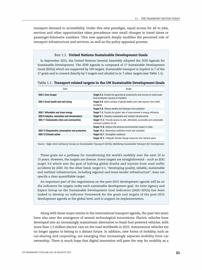
Box 1.1. United Nations Sustainable Development Goals
In September 2015, the United Nations General Assembly adopted the 2030 Agenda for Sustainable Development. The 2030 Agenda is composed of 17 Sustainable Development Goals (SDGs) which are supported by 169 targets. Sustainable transport is implicit in 7 of the 17 goals and is covered directly by 5 targets and alluded to in 7 other targets (see Table 1.1).
These goals set a pathway for transforming the world’s mobility over the next 10 to 15 years. However, the targets are diverse. Some targets are straightforward – such as SDG target 3.6 which sets the goal of halving global deaths and injuries from road traffic accidents by 2020. On the other hand, target 9.1, “developing quality, reliable, sustainable and resilient infrastructure, including regional and trans-border infrastructure”, does not specify a clear quantifiable target.
An important part of the negotiations on the post-2015 development agenda will be on the indicators for targets under each sustainable development goal. An Inter-Agency and Expert Group on the Sustainable Development Goal Indicators (IAEG-SDGs) has been tasked to develop an indicator framework for the goals and targets of the post-2015 development agenda at the global level, and to support its implementation.
Table 1.1. Transport related targets in the UN Sustainable Development Goals
Goal Target
SDG 2 Zero hunger Target 2.3. Double the agricultural productivity and income of small scale food producers (access to markets)
SDG 3 Good health and well-being Target 3.6. Halve number of global deaths and road injuries from traffic accidents
Target 3.9. Reduce deaths and illnesses from pollution
SDG 7 Affordable and clean energy Target 7.3. Double the global rate of improvement in energy efficiency
SDG 9 Industry, innovation and infrastructure Target 9.1. Develop sustainable and resilient infrastructure
SDG 11 Sustainable cities and communities Target 11.2. Provide access to safe, affordable, accessible and sustainable transport systems for all
Target 11.6. Reduce the adverse environmental impact of cities
SDG 12 Responsible consumption and production Target 12.c. Rationalise inefficient fossil-fuel subsidies
SDG 13 Climate action Target 13.1. Strengthen resilience
Target 13.2. Integrate climate change measures into national plans
Source: High-level Advisory Group on Sustainable Transport (2016), Mobilizing Sustainable Transport for Development.
ITF TRANSPORT OUTLOOK 2017 © OECD/ITF 2017 21
I.1. THE TRANSPORT SECTOR TODAY
service, where the traveller is provided with time-responsive, multi-modal information on
the best way to make their trip, including planning and payment (see also Chapter 5 for a
discussion on shared mobility). Private and public transport modes, including ride and
vehicle-sharing services, are increasingly joining forces to transport people in an efficient
and sustainable way. Several countries have already started exploring the potential of this
paradigm shift. This has implications for road infrastructure development as assets that are
built today could be obsolete in 10-20 years.
Transport and the economic environmentDespite political will and technological progress, demand for transport still primarily
responds to the economic environment. Historically, there has been a close statistical
correlation between the growth of Gross Domestic Product (GDP) and growth in transport,
both passenger and freight (Bannister and Stead, 2002). Growth in per-capita income levels
has had a positive effect on the ownership and use of private vehicles, tending to increase
reliance on private vehicles to meet mobility demand, particularly in emerging economies.
The period since the last edition of the ITF Transport Outlook (ITF, 2015a) has been
characterised by three main macroeconomic trends, each with a major impact on the
transport sector. Economic growth remains lower than expected and is subject to continued
downside risks and uncertainties. International trade is now growing at the same rate as GDP
whereas prior to the 2008 economic crisis trade grew twice as fast as GDP. Oil prices have also
sunk to levels unseen since the beginning of the previous decade. Weak trade has
particularly impacted the shipping sector which has been pushed into a serious crisis.
Shipping suffers from overcapacity, partly driven by use of larger ships. This is causing ripple
effects to the whole supply chain as many countries have overinvested in ports, partly
unsuited to the largest vessels, while hinterland connections increasingly suffer from
congestion.
Economic activity and trade are the main drivers of transport demand. Low oil prices
have sustained passenger mobility, yet the freight sector has suffered heavily from the
below-par economic environment. Maritime transport, the back-bone of worldwide trade,
continued to grow at a much slower rate than expected in 2015 (KPMG, 2016). The
increasing number and size of container ships is adding to the problem of overcapacity and
decreasing container freight rates. Air freight, too, slowed considerably in 2015, when
compared to the previous year. In contrast, world air passenger traffic grew strongly at 6.8%
in 2015, supported by the decline of oil and jet fuel prices.
Gross Domestic Product
Eight years after the financial crisis, the world economy is still struggling to find a
durable recovery. Global GDP slowed to around 3% in 2015 and is expected to remain largely
unchanged in 2016 (OECD, 2016). Projections up to 2020 by the OECD, World Bank and
International Monetary Fund (IMF) have been revised down, suggesting that global GDP
growth will only modestly improve with expectations between 3.3% and 3.6% in 2017
(Table 1.2).
Advanced economies are forecast to expand by less than 2% on average for 2016-17.
Supportive macroeconomic policies and continued low commodity prices might lead to a
modest recovery in advanced economies but this assumes that wages and business
investment will increase and financial markets stabilise (OECD, 2016). The marked slowdown
in emerging economies masks significant divergences among countries. China is
ITF TRANSPORT OUTLOOK 2017 © OECD/ITF 201722
I.1. THE TRANSPORT SECTOR TODAY
rebalancing with a slightly stronger outlook than previously forecast due to resilient
domestic consumption and robust growth in services (IMF, 2016). The economic downturn in
Brazil was more severe than anticipated, while Russia has been in recession since 2015 with
negative spill-overs to other transition economies.
Any global economic recovery in the near term is likely to be slow and gradual. The main
risk factors are a sharper slowdown in emerging markets and further slowing of activity in
advanced economies, the increase of the volatility of the financial market, geopolitical
tensions and decreasing trust in policies to stimulate economic growth (World Bank, 2016).
The de-facto exit of the United Kingdom from the European Union (Brexit), following the
referendum held on 23 June 2016, could result in considerable additional volatility in
financial markets and an extended period of uncertainty, with negative consequences for the
United Kingdom, the European Union and the rest of the world (OECD, 2016).
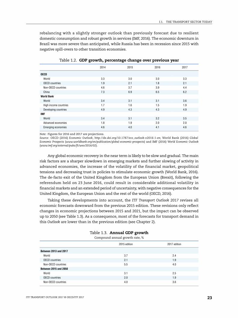
Taking these developments into account, the ITF Transport Outlook 2017 revises all
economic forecasts downward from the previous 2015 edition. These revisions only reflect
changes in economic projections between 2015 and 2021, but the impact can be observed
up to 2050 (see Table 1.3). As a consequence, most of the forecasts for transport demand in
this Outlook are lower than in the previous edition (see Chapter 2).
Table 1.2. GDP growth, percentage change over previous year
2014 2015 2016 2017
OECD
World 3.3 3.0 3.0 3.3
OECD countries 1.9 2.1 1.8 2.1
Non-OECD countries 4.6 3.7 3.9 4.4
China 7.3 6.9 6.5 6.2
World Bank
World 3.4 3.1 3.1 3.6
High income countries 1.7 1.6 1.5 1.9
Developing countries 4.9 4.3 4.3 4.9
IMF
World 3.4 3.1 3.2 3.5
Advanced economies 1.8 1.9 2.0 2.0
Emerging economies 4.6 4.0 4.1 4.6
Note: Figures for 2016 and 2017 are projections.Source: OECD (2016) Economic Outlook, http://dx.doi.org/10.1787/eco_outlook-v2016-1-en; World Bank (2016) Global Economic Prospects (www.worldbank.org/en/publication/global-economic-prospects) and IMF (2016) World Economic Outlook(www.imf.org/external/pubs/ft/weo/2016/02).
Table 1.3. Annual GDP growthCompound annual growth rate, %
2015 edition 2017 edition
Between 2013 and 2017
World 3.7 2.4
OECD countries 2.1 1.9
Non-OECD countries 5.5 4.0
Between 2015 and 2050
World 3.1 2.5
OECD countries 2.0 1.9
Non-OECD countries 4.0 3.6
ITF TRANSPORT OUTLOOK 2017 © OECD/ITF 2017 23
I.1. THE TRANSPORT SECTOR TODAY
International trade
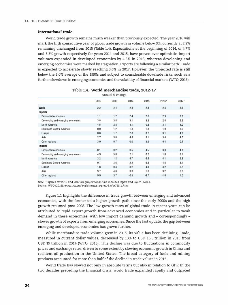
World trade growth remains much weaker than previously expected. The year 2016 will
mark the fifth consecutive year of global trade growth in volume below 3%, currently at 2.8%
remaining unchanged from 2015 (Table 1.4). Expectations at the beginning of 2014, of 4.7%
and 5.3% growth respectively for years 2014 and 2015, have proven over-optimistic. Import
volumes expanded in developed economies by 4.5% in 2015, whereas developing and
emerging economies were marked by stagnation. Exports are following a similar path. Trade
is expected to accelerate slowly reaching 3.6% in 2017. However, the projected rate is still
below the 5.0% average of the 1990s and subject to considerable downside risks, such as a
further slowdown in emerging economies and the volatility of financial markets (WTO, 2016).
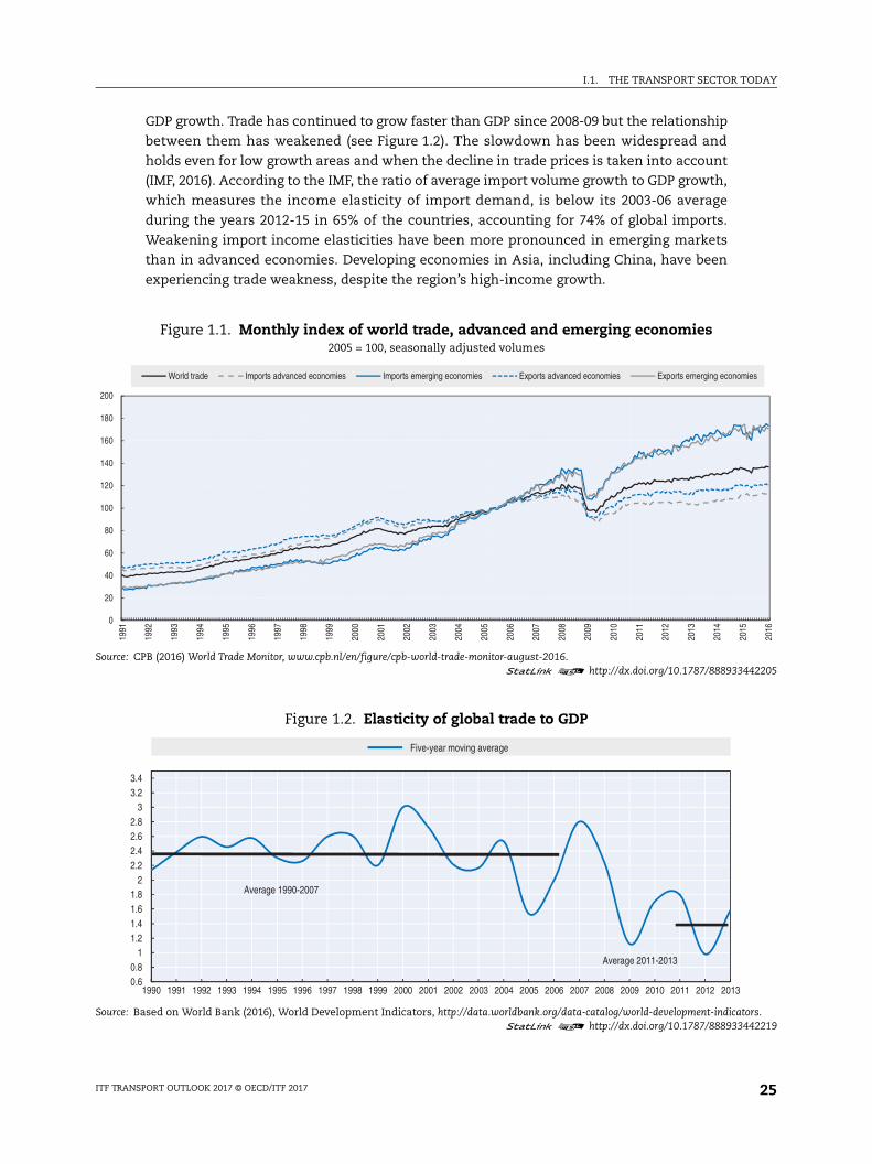
Figure 1.1 highlights the difference in trade growth between emerging and advanced
economies, with the former on a higher growth path since the early 2000s and the high
growth resumed post-2008. The low growth rates of global trade in recent years can be
attributed to tepid export growth from advanced economies and in particular to weak
demand in these economies, with low import demand growth and – correspondingly –
slower growth of exports from emerging economies. Since the last update, the gap between
emerging and developed economies has grown further.
While merchandise trade volume grew in 2015, its value has been declining. Trade,
measured in current dollar values, decreased by 13% to USD 16.5 trillion in 2015 from
USD 19 trillion in 2014 (WTO, 2016). This decline was due to fluctuations in commodity
prices and exchange rates, driven to some extent by slowing economic growth in China and
resilient oil production in the United States. The broad category of fuels and mining
products accounted for more than half of the decline in trade values in 2015.
World trade has slowed not only in absolute terms but also in relation to GDP. In the
two decades preceding the financial crisis, world trade expanded rapidly and outpaced
Table 1.4. World merchandise trade, 2012-17Annual % change
2012 2013 2014 2015 2016* 2017*
World 2.2 2.4 2.8 2.8 2.8 3.6
Exports
Developed economies 1.1 1.7 2.4 2.6 2.9 3.8
Developing and emerging economies 3.8 3.8 3.1 3.3 2.8 3.3
North America 4.5 2.8 4.1 0.8 3.1 4.0
South and Central America 0.9 1.2 -1.8 1.3 1.9 1.9
Europe 0.8 1.7 2.0 3.7 3.1 4.1
Asia 2.7 5.0 4.8 3.1 3.4 4.0
Other regions 3.9 0.7 0.0 3.9 0.4 0.4
Imports
Developed economies -0.1 -0.2 3.5 4.5 3.3 4.1
Developing and emerging economies 4.9 5.0 2.1 0.2 1.8 3.1
North America 3.2 1.2 4.7 6.5 4.1 5.3
South and Central America 0.7 3.6 -2.2 -5.8 -4.5 5.1
Europe -1.8 -0.3 3.2 4.3 3.2 3.7
Asia 3.7 4.8 3.3 1.8 3.2 3.3
Other regions 9.9 3.7 -0.5 -3.7 -1.0 1.0
Note: *Figures for 2016 and 2017 are projections; Asia includes Japan and South-Korea.Source: WTO (2016), www.wto.org/english/news_e/pres16_e/pr768_e.htm.
ITF TRANSPORT OUTLOOK 2017 © OECD/ITF 201724
I.1. THE TRANSPORT SECTOR TODAY
442205
tors.442219
2015
2016
mies
GDP growth. Trade has continued to grow faster than GDP since 2008-09 but the relationship
between them has weakened (see Figure 1.2). The slowdown has been widespread and
holds even for low growth areas and when the decline in trade prices is taken into account
(IMF, 2016). According to the IMF, the ratio of average import volume growth to GDP growth,
which measures the income elasticity of import demand, is below its 2003-06 average
during the years 2012-15 in 65% of the countries, accounting for 74% of global imports.
Weakening import income elasticities have been more pronounced in emerging markets
than in advanced economies. Developing economies in Asia, including China, have been
experiencing trade weakness, despite the region’s high-income growth.
Figure 1.1. Monthly index of world trade, advanced and emerging economies2005 = 100, seasonally adjusted volumes
Source: CPB (2016) World Trade Monitor, www.cpb.nl/en/figure/cpb-world-trade-monitor-august-2016.1 2 http://dx.doi.org/10.1787/888933
Figure 1.2. Elasticity of global trade to GDP
Source: Based on World Bank (2016), World Development Indicators, http://data.worldbank.org/data-catalog/world-development-indica1 2 http://dx.doi.org/10.1787/888933
0
20
40
60
80
100
120
140
160
180
200
1991
1992
1993
1994
1995
1996
1997
1998
1999
2000
2001
2002
2003
2004
2005
2006
2007
2008
2009
2010
2011
2012
2013
2014
World trade Imports advanced economies Imports emerging economies Exports advanced economies Exports emerging econo
0.60.8
11.21.41.61.8
22.22.42.62.8
33.23.4
1990 1991 1992 1993 1994 1995 1996 1997 1998 1999 2000 2001 2002 2003 2004 2005 2006 2007 2008 2009 2010 2011 2012 2013
Average 2011-2013
Five-year moving average
Average 1990-2007
ITF TRANSPORT OUTLOOK 2017 © OECD/ITF 2017 25
I.1. THE TRANSPORT SECTOR TODAY
The changing relationship between trade and income growth in recent years has
caused much debate about the underlying factors and the implications for the near and
longer term. To some extent, trade weakness can be explained by cyclical factors, notably
the low volumes of trade-intensive demand components such as business investment,
since the financial crisis (ECB, 2014). From a historical perspective, however, it may be that
the unusually strong elasticity observed during the 1990-2007 period is attributable to pro-
trade structural factors that that are no longer present. For instance, decreasing transport
costs, reduction of trade barriers, and declining relative prices of traded commodities and
services that boosted trade prior to 2000 had already levelled off by the mid-1990s, so it may
be a natural consequence that current trade volumes are no longer as responsive to a given
level of income growth.
A more recent structural factor accounting for the trade slowdown has been the slower
rate of expansion of global supply chains (Constantinescu et al., 2015). Greater fragmentation
of production, especially by the United States (USA) and China, contributed to the higher
trade elasticity in the 1990s, but this trend has moderated since the middle of the 2000s. The
effect of rising global value chains can be shown by comparing the gap between gross and
value-added trade. As trade flows are measured in gross terms, outsourcing of production
might lead to double counting of tradable items, whenever an international border is
crossed. The gap increased from 33% in 1995 to 51% by the time of the financial crisis,
suggesting that global value chains added 0.2% to the elasticity of global trade during this
time (ECB, 2014).
Chapter 3 discusses this issue in more detail and assesses the long-term implications
of the change of relationship between economic growth and trade for the freight sector.
Oil prices
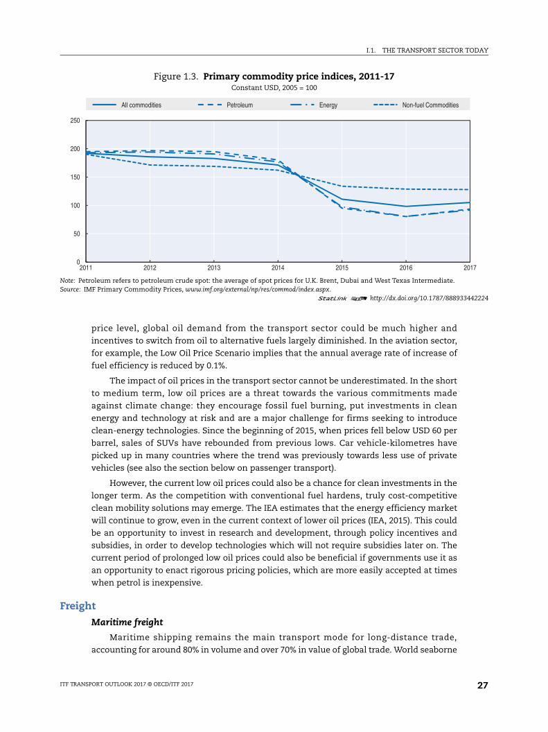
The decline in crude oil prices was particularly sharp in 2014 and 2015, due to a
combination of increasing oil supply and weaker global demand, in part resulting from
improved energy efficiency. Crude oil prices, averaging U.K Brent, Dubai and West Texas
Intermediate, decreased by 47% in 2015 over the previous year (Figure 1.3). It is expected to
decline by a further 16% in 2016. While average crude oil prices are projected to rebound by
16% in 2017, it is not expected that they will reach anywhere near their historical high levels
any time soon. The IMF forecasts the cost of a barrel at only USD 35 in 2016 and USD 41 in 2017,
less than half the 2000-17 average (IMF, 2016). Whether a supply driven decline in oil prices
might have positive effects on the world economy remains debatable. A previous scenario by
the IMF implied that a positive oil supply shock could be beneficiary to global economic
activity, due to a higher marginal propensity to consume in countries benefitting from oil in
contrast to exporting countries. While this scenario could increase global GDP by 1% by 2021,
weakening global demand would more than offset the net positive effect. Moreover, assuming
fiscal and financial stress in major oil-exporting countries could lead to lower public
consumption and investment to absorb negative shocks by lower prices (IMF, 2016).
While short-term projections suggest a slow but gradual recovery of oil prices for 2017,
uncertainty remains for when and at what price level a new equilibrium might be reached.
Increasing demand and slowing supply are expected to lead to a rebalancing of oil prices in
the near to medium term. The New Policy Scenario by the International Energy Agency
(IEA) assumes that a new equilibrium for oil price will be reached at USD 80 per barrel by
2020 (IEA, 2015). In contrast, according to an alternative Low Oil Price Scenario a low price
level ranging between USD 50 and USD 60 per barrel could persist into the 2020s. At this
ITF TRANSPORT OUTLOOK 2017 © OECD/ITF 201726
I.1. THE TRANSPORT SECTOR TODAY
442224
017
price level, global oil demand from the transport sector could be much higher and
incentives to switch from oil to alternative fuels largely diminished. In the aviation sector,
for example, the Low Oil Price Scenario implies that the annual average rate of increase of
fuel efficiency is reduced by 0.1%.
The impact of oil prices in the transport sector cannot be underestimated. In the short
to medium term, low oil prices are a threat towards the various commitments made
against climate change: they encourage fossil fuel burning, put investments in clean
energy and technology at risk and are a major challenge for firms seeking to introduce
clean-energy technologies. Since the beginning of 2015, when prices fell below USD 60 per
barrel, sales of SUVs have rebounded from previous lows. Car vehicle-kilometres have
picked up in many countries where the trend was previously towards less use of private
vehicles (see also the section below on passenger transport).
However, the current low oil prices could also be a chance for clean investments in the
longer term. As the competition with conventional fuel hardens, truly cost-competitive
clean mobility solutions may emerge. The IEA estimates that the energy efficiency market
will continue to grow, even in the current context of lower oil prices (IEA, 2015). This could
be an opportunity to invest in research and development, through policy incentives and
subsidies, in order to develop technologies which will not require subsidies later on. The
current period of prolonged low oil prices could also be beneficial if governments use it as
an opportunity to enact rigorous pricing policies, which are more easily accepted at times
when petrol is inexpensive.
Freight
Maritime freight
Maritime shipping remains the main transport mode for long-distance trade,
accounting for around 80% in volume and over 70% in value of global trade. World seaborne
Figure 1.3. Primary commodity price indices, 2011-17Constant USD, 2005 = 100
Note: Petroleum refers to petroleum crude spot: the average of spot prices for U.K. Brent, Dubai and West Texas Intermediate.Source: IMF Primary Commodity Prices, www.imf.org/external/np/res/commod/index.aspx.
1 2 http://dx.doi.org/10.1787/888933
0
50
100
150
200
250
2011 2012 2013 2014 2015 2016 2
All commodities Petroleum Energy Non-fuel Commodities
ITF TRANSPORT OUTLOOK 2017 © OECD/ITF 2017 27
I.1. THE TRANSPORT SECTOR TODAY
442234
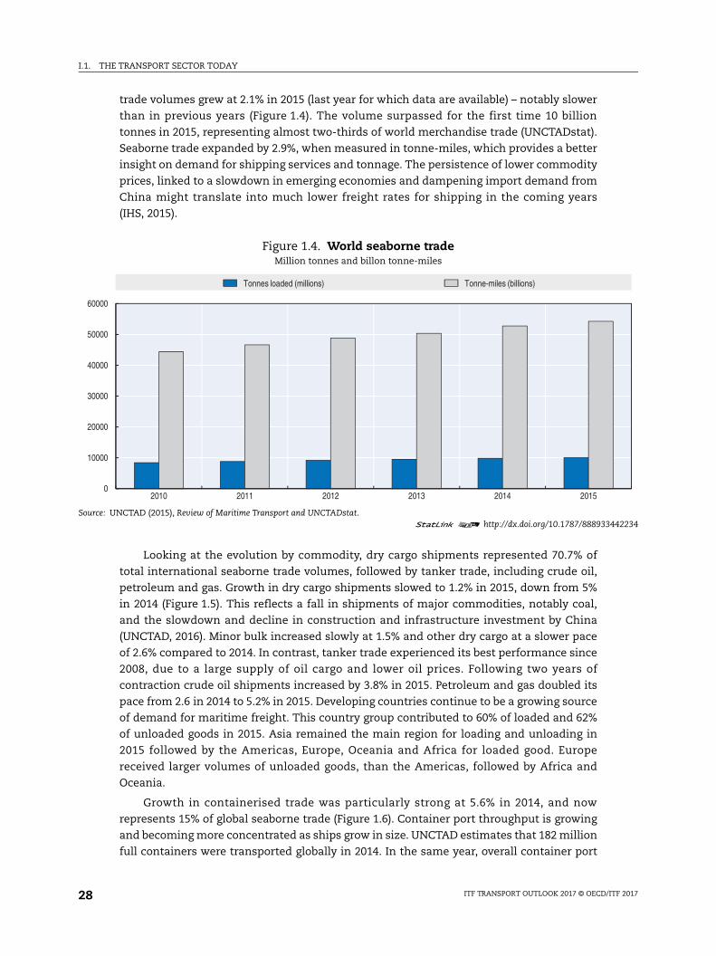
trade volumes grew at 2.1% in 2015 (last year for which data are available) – notably slower
than in previous years (Figure 1.4). The volume surpassed for the first time 10 billion
tonnes in 2015, representing almost two-thirds of world merchandise trade (UNCTADstat).
Seaborne trade expanded by 2.9%, when measured in tonne-miles, which provides a better
insight on demand for shipping services and tonnage. The persistence of lower commodity
prices, linked to a slowdown in emerging economies and dampening import demand from
China might translate into much lower freight rates for shipping in the coming years
(IHS, 2015).
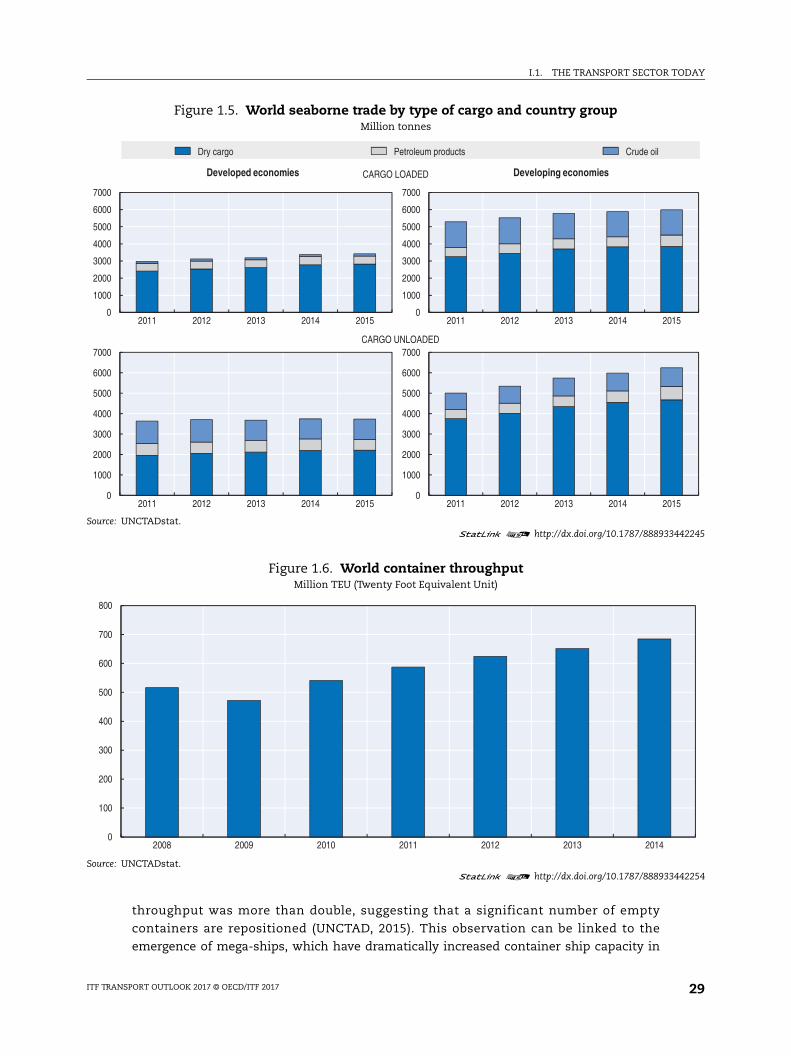
Looking at the evolution by commodity, dry cargo shipments represented 70.7% of
total international seaborne trade volumes, followed by tanker trade, including crude oil,
petroleum and gas. Growth in dry cargo shipments slowed to 1.2% in 2015, down from 5%
in 2014 (Figure 1.5). This reflects a fall in shipments of major commodities, notably coal,
and the slowdown and decline in construction and infrastructure investment by China
(UNCTAD, 2016). Minor bulk increased slowly at 1.5% and other dry cargo at a slower pace
of 2.6% compared to 2014. In contrast, tanker trade experienced its best performance since
2008, due to a large supply of oil cargo and lower oil prices. Following two years of
contraction crude oil shipments increased by 3.8% in 2015. Petroleum and gas doubled its
pace from 2.6 in 2014 to 5.2% in 2015. Developing countries continue to be a growing source
of demand for maritime freight. This country group contributed to 60% of loaded and 62%
of unloaded goods in 2015. Asia remained the main region for loading and unloading in
2015 followed by the Americas, Europe, Oceania and Africa for loaded good. Europe
received larger volumes of unloaded goods, than the Americas, followed by Africa and
Oceania.
Growth in containerised trade was particularly strong at 5.6% in 2014, and now
represents 15% of global seaborne trade (Figure 1.6). Container port throughput is growing
and becoming more concentrated as ships grow in size. UNCTAD estimates that 182 million
full containers were transported globally in 2014. In the same year, overall container port
Figure 1.4. World seaborne tradeMillion tonnes and billon tonne-miles
Source: UNCTAD (2015), Review of Maritime Transport and UNCTADstat.1 2 http://dx.doi.org/10.1787/888933
0
10000
20000
30000
40000
50000
60000
2010 2011 2012 2013 2014 2015
Tonnes loaded (millions) Tonne-miles (billions)
ITF TRANSPORT OUTLOOK 2017 © OECD/ITF 201728
I.1. THE TRANSPORT SECTOR TODAY
442245
442254
15
15
throughput was more than double, suggesting that a significant number of empty
containers are repositioned (UNCTAD, 2015). This observation can be linked to the
emergence of mega-ships, which have dramatically increased container ship capacity in
Figure 1.5. World seaborne trade by type of cargo and country groupMillion tonnes
Source: UNCTADstat.1 2 http://dx.doi.org/10.1787/888933
Figure 1.6. World container throughputMillion TEU (Twenty Foot Equivalent Unit)
Source: UNCTADstat.1 2 http://dx.doi.org/10.1787/888933
0
1000
2000
3000
4000
5000
6000
7000
2011 2012 2013 2014 2015
Developed economies
0
1000
2000
3000
4000
5000
6000
7000
2011 2012 2013 2014 20
Developing economies
0
1000
2000
3000
4000
5000
6000
7000
2011 2012 2013 2014 20150
1000
2000
3000
4000
5000
6000
7000
2011 2012 2013 2014 20
CARGO LOADED
CARGO UNLOADED
Dry cargo Petroleum products Crude oil
0
100
200
300
400
500
600
700
800
2008 2009 2010 2011 2012 2013 2014
ITF TRANSPORT OUTLOOK 2017 © OECD/ITF 2017 29
I.1. THE TRANSPORT SECTOR TODAY
nalysis
442266
recent years (ITF, 2015b). Since 2000, container ships have doubled slot capacity every seven
years and are estimated to reach a capacity over 21 million TEUs by 2017 (Reuters, 2015).
While previous waves of containerisation facilitated global trade by reducing maritime
transport costs, the current round of mega-ships is seen to contribute to overcapacity,
since new capacity is unlikely to be absorbed in the current context of low and stagnant
growth. An increasing gap between supply and demand might lead to lower freight rates
(see also Box 3.1 in Chapter 3), fewer profits for the shipping industry and a challenge for
ports and hinterland transport capacity, especially when handling larger peaks (ITF, 2015b).
Air freight
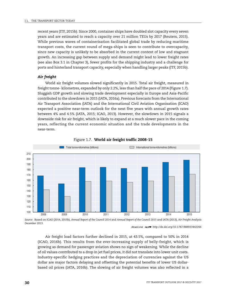
World air freight volumes slowed significantly in 2015. Total air freight, measured in
freight tonne- kilometres, expanded by only 2.2%, less than half the pace of 2014 (Figure 1.7).
Sluggish GDP growth and slowing trade development especially in Europe and Asia-Pacific
contributed to the slowdown in 2015 (IATA, 2016a). Previous forecasts from the International
Air Transport Association (IATA) and the International Civil Aviation Organisation (ICAO)
expected a positive near-term outlook for the next five years with annual growth rates
between 4% and 4.5% (IATA, 2015; ICAO, 2013). However, the slowdown in 2015 signals a
downside risk for air freight, which is likely to expand at a much slower pace in the coming
years, reflecting the current economic situation and the trade developments in the
near-term.
Air freight load factors further declined in 2015, at 43.5%, compared to 50% in 2014
(ICAO, 2016b). This results from the ever-increasing supply of belly-freight, which is
growing as demand for passenger aviation shows no sign of weakening. While the decline
of oil values contributed to a drop in jet fuel prices, it did not translate into lower unit costs.
Industry-specific hedging practices and the depreciation of currencies against the US
dollar are major factors delaying and offsetting the potential benefits of lower US dollar-
based oil prices (IATA, 2016b). The slowing of air freight volumes was also reflected in a
Figure 1.7. World air freight traffic 2008-15
Source: Based on ICAO (2014, 2015b), Annual Report of the Council 2014 and Annual Report of the Council 2015 and IATA (2013), Air Freight ADecember 2013.
1 2 http://dx.doi.org/10.1787/888933
100
110
120
130
140
150
160
170
180
190
200
210
2008 2009 2010 2011 2012 2013 2014 2015
Total tonne-kilometres (billions) International tonne-kilometres (billions)
ITF TRANSPORT OUTLOOK 2017 © OECD/ITF 201730
I.1. THE TRANSPORT SECTOR TODAY
drop in revenues, which were down by 10.7% in 2015 since the peak of USD 67 billion in
2011 (IATA, 2016a).
Among regions, Middle Eastern carriers registered the highest growth rate with 11.3%
in 2015. Network expansion into emerging markets and supportive local economic
conditions suggest a robust growth path for 2016 despite uncertainties stemming from
political instability and the drop in oil prices. Airlines from the Asia-Pacific region, which
account for 39% of world air freight traffic, expanded moderately by 2.3%. With the reform
of the Chinese economy to focus increasingly on services and domestic consumption,
decreasing export orders for Chinese manufacturing contributed to the weakened freight
growth in the Asia-Pacific region. Air carriers in Latin America registered an air traffic
decline of 6.0% in 2015, partly due to the uncertain political situation and deteriorating
economic conditions in Brazil (IATA, 2016a).
Surface freight
Surface freight volumes strongly correlate to the economic environment. It is well
established that surface freight (road and rail) volumes grow with GDP (Garcia et al., 2008;
Meersman and Van de Voorde, 2005; Bennathan et al., 1992). Freight transport is directly
tied to the supply chain (both finished and intermediate goods) and the transport of goods
reflects growth in sales or activity in the manufacturing sector. As a consequence, surface
freight volumes were deeply affected by the economic crisis. Overall, they have been
growing since, reaching their pre-crisis levels in 2011 or 2012, but this hides contrasting
situations depending on the mode and the region (see Figure 1.8).
Recent studies also suggest that the relationship between GDP and tonne-kilometres
may not be as enduring as supposed, resulting, for example, in revisions of road traffic
forecasts in some countries (McKinnon, 2007; Tapio, 2005). There is also strong evidence
that the elasticity of freight tonne-kilometres to GDP decreases as per capita incomes grow
(see also Chapter 2). However, whether the decoupling of economic growth and freight
demand has already occurred in some countries is debated.
In Europe, road and rail freight volumes have remained more or less constant since
2010 but this is happening in a depressed economic environment. In previous decades,
characterised by an expansion of the European Union which led businesses to diversify the
locations of their suppliers, warehouses and plants, increase in freight demand was driven
by longer average distances. Now that the expansion phase is over, freight demand is not
forecast to increase significantly in the near future.
In developing countries, however, freight demand has been increasing steadily since
2009 and is forecast to continue growing in the coming years. As the countries move
towards higher value goods, it is expected that the freight intensity of these economies
may decrease but the date at which this may happen is very uncertain (see also Chapter 2).
While road and rail are both expected to increase, higher value goods tend to be
transported by road, rather than rail.
The modal shares of road and rail are, to a large extent, determined by the type of
commodities transported, and the distance over which they move. As rail is still used
predominantly within countries, due to inter-operability issues, the transport of bulk
commodities in large countries represents most of the world rail freight demand. At the global
level, the performance of the sector is predominantly shaped by three countries: the United
States, China and Russia, which account for nearly 80% of total estimated global rail freight
ITF TRANSPORT OUTLOOK 2017 © OECD/ITF 2017 31
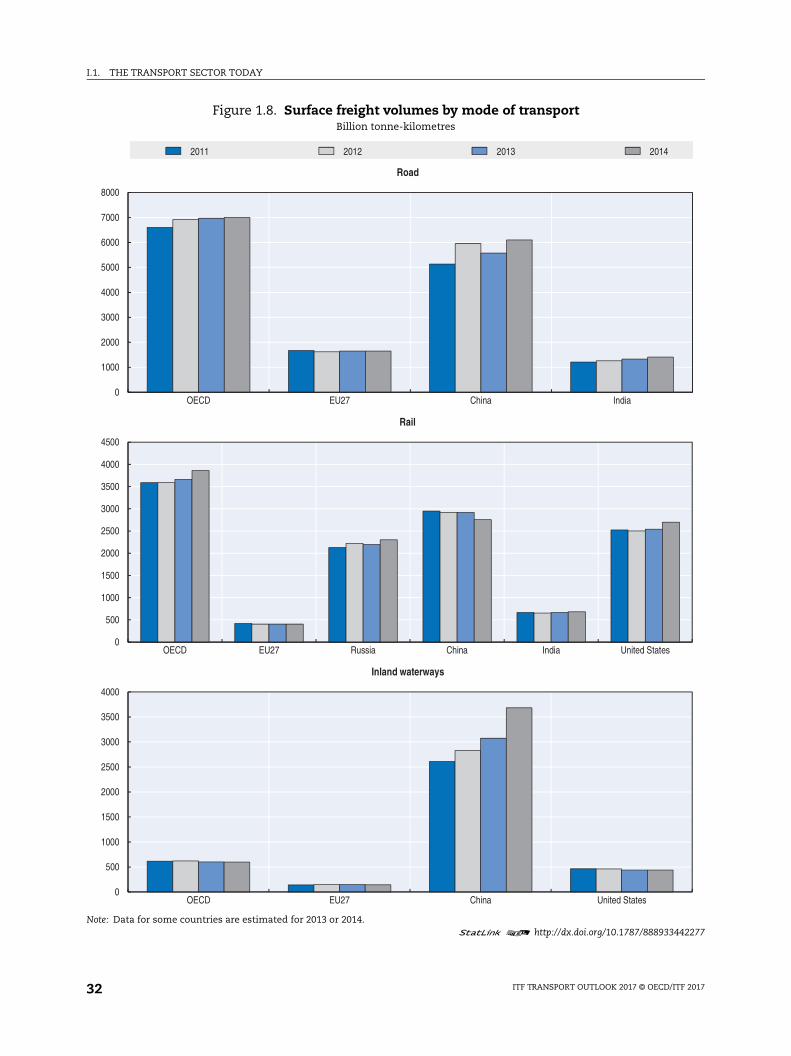
I.1. THE TRANSPORT SECTOR TODAY
442277
Figure 1.8. Surface freight volumes by mode of transportBillion tonne-kilometres
Note: Data for some countries are estimated for 2013 or 2014.1 2 http://dx.doi.org/10.1787/888933
0
1000
2000
3000
4000
5000
6000
7000
8000
OECD EU27 China India
Road
0
500
1000
1500
2000
2500
3000
3500
4000
4500
OECD EU27 Russia China India United States
Rail
0
500
1000
1500
2000
2500
3000
3500
4000
OECD EU27 China United States
Inland waterways
2011 2012 2013 2014
ITF TRANSPORT OUTLOOK 2017 © OECD/ITF 201732
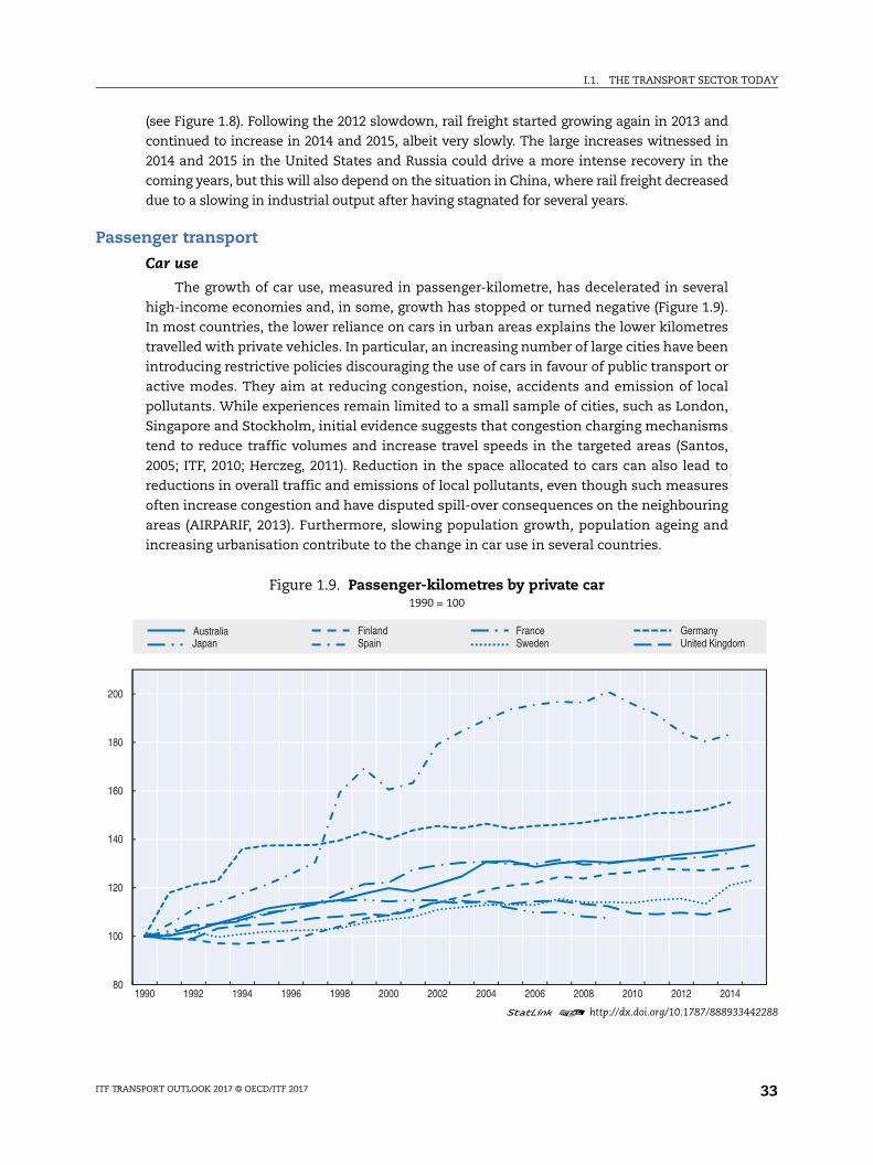
I.1. THE TRANSPORT SECTOR TODAY
442288
(see Figure 1.8). Following the 2012 slowdown, rail freight started growing again in 2013 and
continued to increase in 2014 and 2015, albeit very slowly. The large increases witnessed in
2014 and 2015 in the United States and Russia could drive a more intense recovery in the
coming years, but this will also depend on the situation in China, where rail freight decreased
due to a slowing in industrial output after having stagnated for several years.
Passenger transport
Car use
The growth of car use, measured in passenger-kilometre, has decelerated in several
high-income economies and, in some, growth has stopped or turned negative (Figure 1.9).
In most countries, the lower reliance on cars in urban areas explains the lower kilometres
travelled with private vehicles. In particular, an increasing number of large cities have been
introducing restrictive policies discouraging the use of cars in favour of public transport or
active modes. They aim at reducing congestion, noise, accidents and emission of local
pollutants. While experiences remain limited to a small sample of cities, such as London,
Singapore and Stockholm, initial evidence suggests that congestion charging mechanisms
tend to reduce traffic volumes and increase travel speeds in the targeted areas (Santos,
2005; ITF, 2010; Herczeg, 2011). Reduction in the space allocated to cars can also lead to
reductions in overall traffic and emissions of local pollutants, even though such measures
often increase congestion and have disputed spill-over consequences on the neighbouring
areas (AIRPARIF, 2013). Furthermore, slowing population growth, population ageing and
increasing urbanisation contribute to the change in car use in several countries.
Figure 1.9. Passenger-kilometres by private car1990 = 100
1 2 http://dx.doi.org/10.1787/888933
80
100
120
140
160
180
200
1990 1992 1994 1996 1998 2000 2002 2004 2006 2008 2010 2012 2014
Australia Finland France GermanyJapan Spain Sweden United Kingdom
ITF TRANSPORT OUTLOOK 2017 © OECD/ITF 2017 33
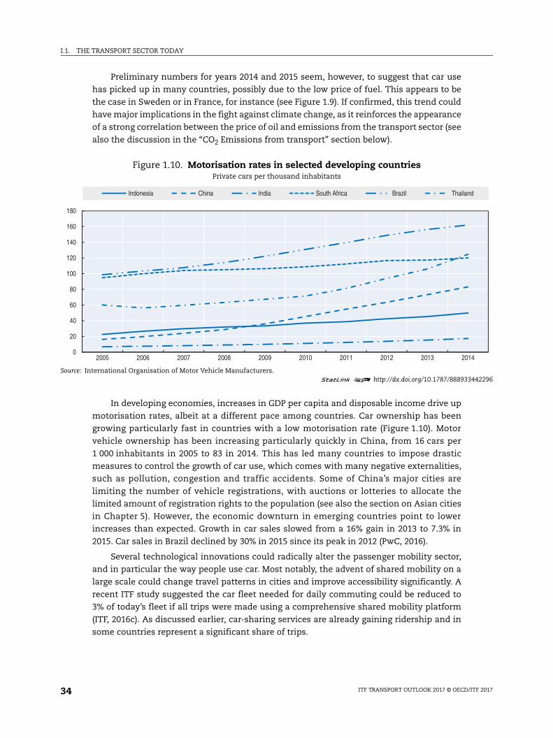
I.1. THE TRANSPORT SECTOR TODAY
442296
4
d
Preliminary numbers for years 2014 and 2015 seem, however, to suggest that car use
has picked up in many countries, possibly due to the low price of fuel. This appears to be
the case in Sweden or in France, for instance (see Figure 1.9). If confirmed, this trend could
have major implications in the fight against climate change, as it reinforces the appearance
of a strong correlation between the price of oil and emissions from the transport sector (see
also the discussion in the “CO2 Emissions from transport” section below).
In developing economies, increases in GDP per capita and disposable income drive up
motorisation rates, albeit at a different pace among countries. Car ownership has been
growing particularly fast in countries with a low motorisation rate (Figure 1.10). Motor
vehicle ownership has been increasing particularly quickly in China, from 16 cars per
1 000 inhabitants in 2005 to 83 in 2014. This has led many countries to impose drastic
measures to control the growth of car use, which comes with many negative externalities,
such as pollution, congestion and traffic accidents. Some of China’s major cities are
limiting the number of vehicle registrations, with auctions or lotteries to allocate the
limited amount of registration rights to the population (see also the section on Asian cities
in Chapter 5). However, the economic downturn in emerging countries point to lower
increases than expected. Growth in car sales slowed from a 16% gain in 2013 to 7.3% in
2015. Car sales in Brazil declined by 30% in 2015 since its peak in 2012 (PwC, 2016).
Several technological innovations could radically alter the passenger mobility sector,
and in particular the way people use car. Most notably, the advent of shared mobility on a
large scale could change travel patterns in cities and improve accessibility significantly. A
recent ITF study suggested the car fleet needed for daily commuting could be reduced to
3% of today’s fleet if all trips were made using a comprehensive shared mobility platform
(ITF, 2016c). As discussed earlier, car-sharing services are already gaining ridership and in
some countries represent a significant share of trips.
Figure 1.10. Motorisation rates in selected developing countriesPrivate cars per thousand inhabitants
Source: International Organisation of Motor Vehicle Manufacturers.1 2 http://dx.doi.org/10.1787/888933
0
20
40
60
80
100
120
140
160
180
2005 2006 2007 2008 2009 2010 2011 2012 2013 201
Indonesia China India South Africa Brazil Thailan
ITF TRANSPORT OUTLOOK 2017 © OECD/ITF 201734
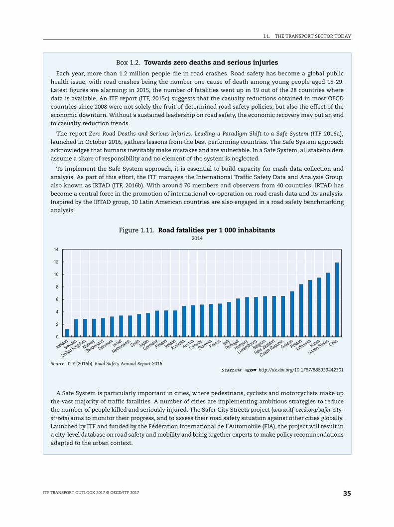
I.1. THE TRANSPORT SECTOR TODAY
lic 29. ere CD the nd
a), ch
ers
nd up, as
sis. ing
up ce
ity-
lly. in ns
301
Box 1.2. Towards zero deaths and serious injuries
Each year, more than 1.2 million people die in road crashes. Road safety has become a global pubhealth issue, with road crashes being the number one cause of death among young people aged 15-Latest figures are alarming: in 2015, the number of fatalities went up in 19 out of the 28 countries whdata is available. An ITF report (ITF, 2015c) suggests that the casualty reductions obtained in most OEcountries since 2008 were not solely the fruit of determined road safety policies, but also the effect of economic downturn. Without a sustained leadership on road safety, the economic recovery may put an eto casualty reduction trends.
The report Zero Road Deaths and Serious Injuries: Leading a Paradigm Shift to a Safe System (ITF 2016launched in October 2016, gathers lessons from the best performing countries. The Safe System approaacknowledges that humans inevitably make mistakes and are vulnerable. In a Safe System, all stakeholdassume a share of responsibility and no element of the system is neglected.
To implement the Safe System approach, it is essential to build capacity for crash data collection aanalysis. As part of this effort, the ITF manages the International Traffic Safety Data and Analysis Groalso known as IRTAD (ITF, 2016b). With around 70 members and observers from 40 countries, IRTAD hbecome a central force in the promotion of international co-operation on road crash data and its analyInspired by the IRTAD group, 10 Latin American countries are also engaged in a road safety benchmarkanalysis.
A Safe System is particularly important in cities, where pedestrians, cyclists and motorcyclists makethe vast majority of traffic fatalities. A number of cities are implementing ambitious strategies to reduthe number of people killed and seriously injured. The Safer City Streets project (www.itf-oecd.org/safer-c
streets) aims to monitor their progress, and to assess their road safety situation against other cities globaLaunched by ITF and funded by the Fédération International de l’Automobile (FIA), the project will resulta city-level database on road safety and mobility and bring together experts to make policy recommendatioadapted to the urban context.
Figure 1.11. Road fatalities per 1 000 inhabitants2014
Source: ITF (2016b), Road Safety Annual Report 2016.1 2 http://dx.doi.org/10.1787/888933442
0
2
4
6
8
10
12
14
ITF TRANSPORT OUTLOOK 2017 © OECD/ITF 2017 35
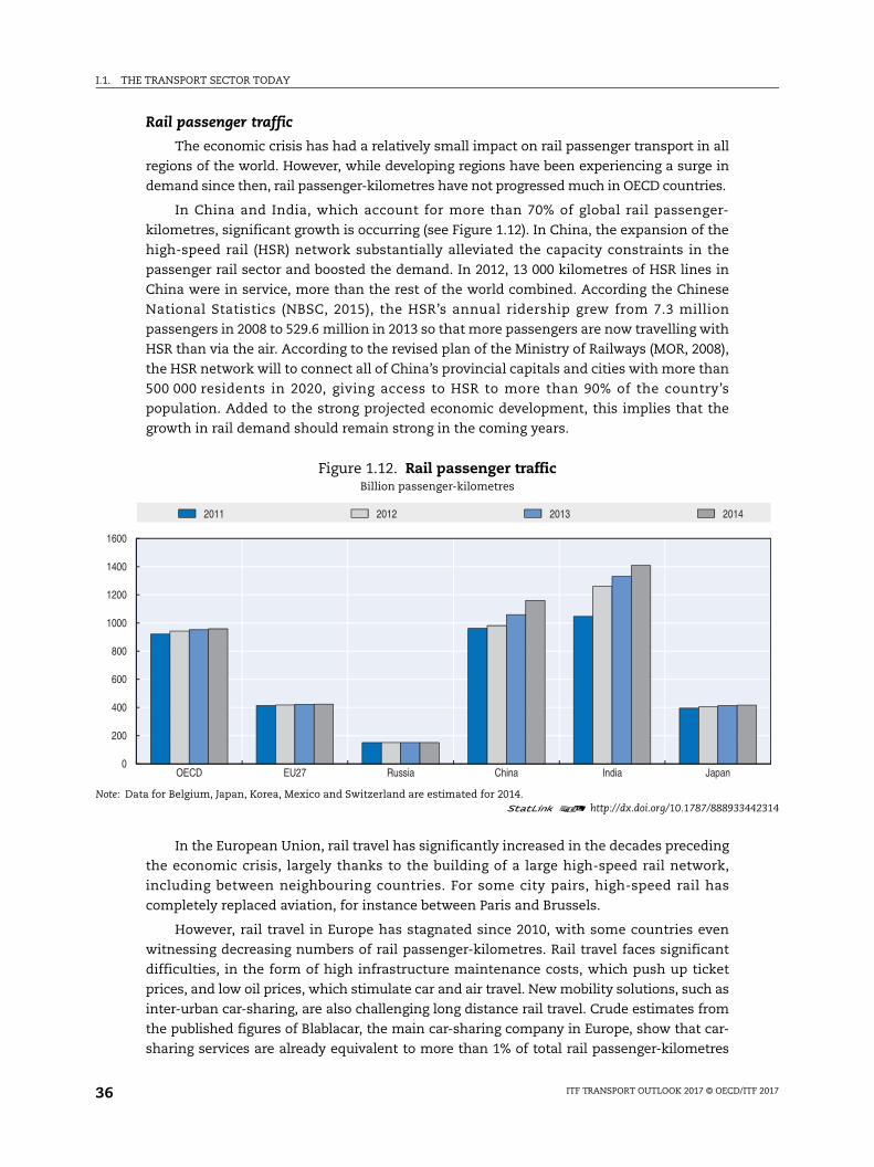
I.1. THE TRANSPORT SECTOR TODAY
442314
Rail passenger traffic
The economic crisis has had a relatively small impact on rail passenger transport in all
regions of the world. However, while developing regions have been experiencing a surge in
demand since then, rail passenger-kilometres have not progressed much in OECD countries.
In China and India, which account for more than 70% of global rail passenger-
kilometres, significant growth is occurring (see Figure 1.12). In China, the expansion of the
high-speed rail (HSR) network substantially alleviated the capacity constraints in the
passenger rail sector and boosted the demand. In 2012, 13 000 kilometres of HSR lines in
China were in service, more than the rest of the world combined. According the Chinese
National Statistics (NBSC, 2015), the HSR’s annual ridership grew from 7.3 million
passengers in 2008 to 529.6 million in 2013 so that more passengers are now travelling with
HSR than via the air. According to the revised plan of the Ministry of Railways (MOR, 2008),
the HSR network will to connect all of China’s provincial capitals and cities with more than
500 000 residents in 2020, giving access to HSR to more than 90% of the country’s
population. Added to the strong projected economic development, this implies that the
growth in rail demand should remain strong in the coming years.
In the European Union, rail travel has significantly increased in the decades preceding
the economic crisis, largely thanks to the building of a large high-speed rail network,
including between neighbouring countries. For some city pairs, high-speed rail has
completely replaced aviation, for instance between Paris and Brussels.
However, rail travel in Europe has stagnated since 2010, with some countries even
witnessing decreasing numbers of rail passenger-kilometres. Rail travel faces significant
difficulties, in the form of high infrastructure maintenance costs, which push up ticket
prices, and low oil prices, which stimulate car and air travel. New mobility solutions, such as
inter-urban car-sharing, are also challenging long distance rail travel. Crude estimates from
the published figures of Blablacar, the main car-sharing company in Europe, show that car-
sharing services are already equivalent to more than 1% of total rail passenger-kilometres
Figure 1.12. Rail passenger trafficBillion passenger-kilometres
Note: Data for Belgium, Japan, Korea, Mexico and Switzerland are estimated for 2014.1 2 http://dx.doi.org/10.1787/888933
0
200
400
600
800
1000
1200
1400
1600
OECD EU27 Russia China India Japan
2011 2012 2013 2014
ITF TRANSPORT OUTLOOK 2017 © OECD/ITF 201736
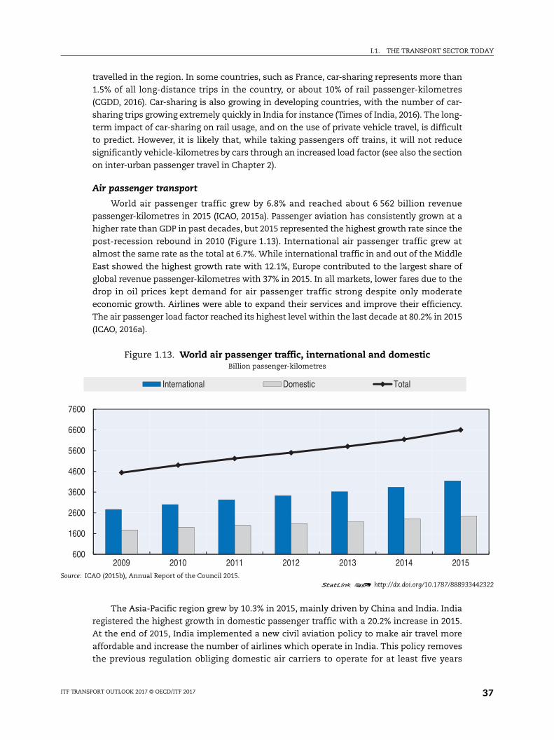
I.1. THE TRANSPORT SECTOR TODAY
442322
travelled in the region. In some countries, such as France, car-sharing represents more than
1.5% of all long-distance trips in the country, or about 10% of rail passenger-kilometres
(CGDD, 2016). Car-sharing is also growing in developing countries, with the number of car-
sharing trips growing extremely quickly in India for instance (Times of India, 2016). The long-
term impact of car-sharing on rail usage, and on the use of private vehicle travel, is difficult
to predict. However, it is likely that, while taking passengers off trains, it will not reduce
significantly vehicle-kilometres by cars through an increased load factor (see also the section
on inter-urban passenger travel in Chapter 2).
Air passenger transport
World air passenger traffic grew by 6.8% and reached about 6 562 billion revenue
passenger-kilometres in 2015 (ICAO, 2015a). Passenger aviation has consistently grown at a
higher rate than GDP in past decades, but 2015 represented the highest growth rate since the
post-recession rebound in 2010 (Figure 1.13). International air passenger traffic grew at
almost the same rate as the total at 6.7%. While international traffic in and out of the Middle
East showed the highest growth rate with 12.1%, Europe contributed to the largest share of
global revenue passenger-kilometres with 37% in 2015. In all markets, lower fares due to the
drop in oil prices kept demand for air passenger traffic strong despite only moderate
economic growth. Airlines were able to expand their services and improve their efficiency.
The air passenger load factor reached its highest level within the last decade at 80.2% in 2015
(ICAO, 2016a).
The Asia-Pacific region grew by 10.3% in 2015, mainly driven by China and India. India
registered the highest growth in domestic passenger traffic with a 20.2% increase in 2015.
At the end of 2015, India implemented a new civil aviation policy to make air travel more
affordable and increase the number of airlines which operate in India. This policy removes
the previous regulation obliging domestic air carriers to operate for at least five years
Figure 1.13. World air passenger traffic, international and domesticBillion passenger-kilometres
Source: ICAO (2015b), Annual Report of the Council 2015. 1 2 http://dx.doi.org/10.1787/888933
600
1600
2600
3600
4600
5600
6600
7600
2009 2010 2011 2012 2013 2014 2015
International Domestic Total
ITF TRANSPORT OUTLOOK 2017 © OECD/ITF 2017 37
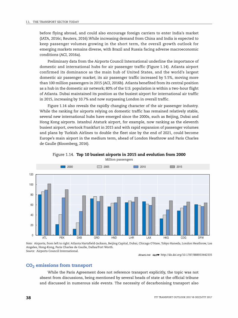
I.1. THE TRANSPORT SECTOR TODAY
ow, Los
442335
before flying abroad, and could also encourage foreign carriers to enter India’s market
(IATA, 2016c; Reuters, 2016).While increasing demand from China and India is expected to
keep passenger volumes growing in the short term, the overall growth outlook for
emerging markets remains diverse, with Brazil and Russia facing adverse macroeconomic
conditions (ACI, 2016a).
Preliminary data from the Airports Council International underline the importance of
domestic and international hubs for air passenger traffic (Figure 1.14). Atlanta airport
confirmed its dominance as the main hub of United States, and the world’s largest
domestic air passenger market; its air passenger traffic increased by 5.5%, moving more
than 100 million passengers in 2015 (ACI, 2016b). Atlanta benefited from its central position
as a hub in the domestic air network; 80% of the U.S. population is within a two-hour flight
of Atlanta. Dubai maintained its position as the busiest airport for international air traffic
in 2015, increasing by 10.7% and now surpassing London in overall traffic.
Figure 1.14 also reveals the rapidly changing character of the air passenger industry.
While the ranking for airports relying on domestic traffic has remained relatively stable,
several new international hubs have emerged since the 2000s, such as Beijing, Dubai and
Hong Kong airports. Istanbul Ataturk airport, for example, now ranking as the eleventh
busiest airport, overtook Frankfurt in 2015 and with rapid expansion of passenger volumes
and plans by Turkish Airlines to double the fleet size by the end of 2021, could become
Europe’s main airport in the medium term, ahead of London Heathrow and Paris Charles
de Gaulle (Bloomberg, 2016).
CO2 emissions from transportWhile the Paris Agreement does not reference transport explicitly, the topic was not
absent from discussions, being mentioned by several heads of state at the official tribune
and discussed in numerous side events. The necessity of decarbonising transport also
Figure 1.14. Top 10 busiest airports in 2015 and evolution from 2000Million passengers
Note: Airports, from left to right: Atlanta Hartsfield-Jackson, Beijing Capital, Dubai, Chicago O’Hare, Tokyo Haneda, London HeathrAngeles, Hong-Kong, Paris Charles de Gaulle, Dallas/Fort Worth.Source: Airports Council International.
1 2 http://dx.doi.org/10.1787/888933
0
20
40
60
80
100
120
ATL PEK DXB ORD HND LHR LAX HKG CDG DFW
2000 2005 2010 2015
ITF TRANSPORT OUTLOOK 2017 © OECD/ITF 201738
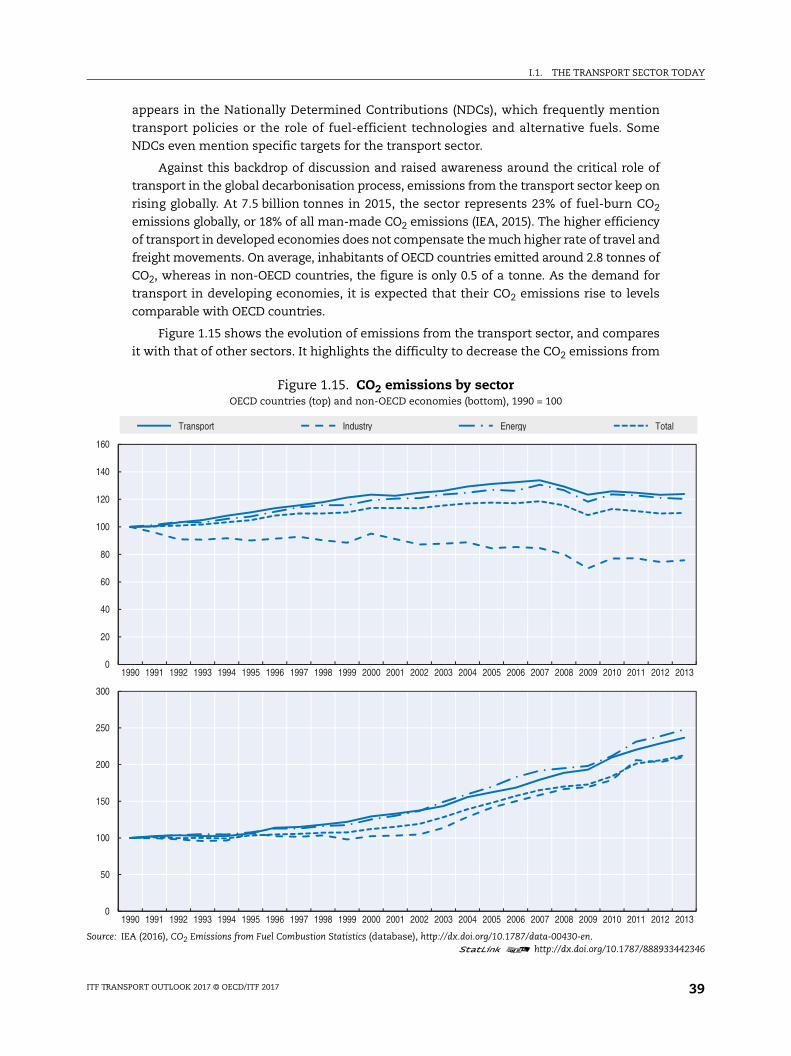
I.1. THE TRANSPORT SECTOR TODAY
442346
2013
2013
l
appears in the Nationally Determined Contributions (NDCs), which frequently mention
transport policies or the role of fuel-efficient technologies and alternative fuels. Some
NDCs even mention specific targets for the transport sector.
Against this backdrop of discussion and raised awareness around the critical role of
transport in the global decarbonisation process, emissions from the transport sector keep on
rising globally. At 7.5 billion tonnes in 2015, the sector represents 23% of fuel-burn CO2
emissions globally, or 18% of all man-made CO2 emissions (IEA, 2015). The higher efficiency
of transport in developed economies does not compensate the much higher rate of travel and
freight movements. On average, inhabitants of OECD countries emitted around 2.8 tonnes of
CO2, whereas in non-OECD countries, the figure is only 0.5 of a tonne. As the demand for
transport in developing economies, it is expected that their CO2 emissions rise to levels
comparable with OECD countries.
Figure 1.15 shows the evolution of emissions from the transport sector, and compares
it with that of other sectors. It highlights the difficulty to decrease the CO2 emissions from
Figure 1.15. CO2 emissions by sectorOECD countries (top) and non-OECD economies (bottom), 1990 = 100
Source: IEA (2016), CO2 Emissions from Fuel Combustion Statistics (database), http://dx.doi.org/10.1787/data-00430-en.1 2 http://dx.doi.org/10.1787/888933
0
20
40
60
80
100
120
140
160
1990 1991 1992 1993 1994 1995 1996 1997 1998 1999 2000 2001 2002 2003 2004 2005 2006 2007 2008 2009 2010 2011 2012
0
50
100
150
200
250
300
1990 1991 1992 1993 1994 1995 1996 1997 1998 1999 2000 2001 2002 2003 2004 2005 2006 2007 2008 2009 2010 2011 2012
Transport Industry Energy Tota
ITF TRANSPORT OUTLOOK 2017 © OECD/ITF 2017 39
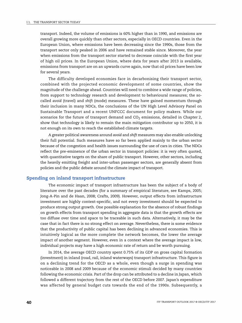
I.1. THE TRANSPORT SECTOR TODAY
transport. Indeed, the volume of emissions is 60% higher than in 1990, and emissions are
overall growing more quickly than other sectors, especially in OECD countries. Even in the
European Union, where emissions have been decreasing since the 1990s, those from the
transport sector only peaked in 2006 and have remained stable since. Moreover, the year
when emissions from the transport sector started to decrease coincide with the first year
of high oil prices. In the European Union, where data for years after 2013 is available,
emissions from transport are on an upwards curve again, now that oil prices have been low
for several years.
The difficulty developed economies face in decarbonising their transport sector,
combined with the projected economic development of some countries, show the
magnitude of the challenge ahead. Countries will need to combine a wide range of policies,
from support to technology research and development to behavioural measures; the so-
called avoid (travel) and shift (mode) measures. These have gained momentum through
their inclusion in many NDCs, the conclusions of the UN High Level Advisory Panel on
Sustainable Transport and a recent UNFCCC document for policy makers. While our
scenarios for the future of transport demand and CO2 emissions, detailed in Chapter 2,
show that technology is likely to remain the main mitigation contributor up to 2050, it is
not enough on its own to reach the established climate targets.
A greater political awareness around avoid and shift measures may also enable unlocking
their full potential. Such measures have so far been applied mainly to the urban sector
because of the congestion and health issues surrounding the use of cars in cities. The NDCs
reflect the pre-eminence of the urban sector in transport policies: it is very often quoted,
with quantitative targets on the share of public transport. However, other sectors, including
the heavily emitting freight and inter-urban passenger sectors, are generally absent from
policies and the public debate around the climate impact of transport.
Spending on inland transport infrastructureThe economic impact of transport infrastructure has been the subject of a body of
literature over the past decades (for a summary of empirical literature, see Kamps, 2005;
Jong-A-Pin and de Haan, 2008; Crafts, 2009). However, output effects from infrastructure
investment are highly context-specific, and not every investment should be expected to
produce strong output growth. One possible explanation for the absence of robust findings
on growth effects from transport spending in aggregate data is that the growth effects are
too diffuse over time and space to be traceable in such data. Alternatively, it may be the
case that in fact there is no strong effect on average. Nevertheless, there is some evidence
that the productivity of public capital has been declining in advanced economies. This is
intuitively logical as the more complete the network becomes, the lower the average
impact of another segment. However, even in a context where the average impact is low,
individual projects may have a high economic rate of return and be worth pursuing.
In 2014, the average OECD country spent 0.75% of its GDP on gross capital formation
(investment) in inland (road, rail, inland waterways) transport infrastructure. This figure is
on a declining trend for the OECD as a whole, even though a surge in spending was
noticeable in 2008 and 2009 because of the economic stimuli decided by many countries
following the economic crisis. Part of the drop can be attributed to a decline in Japan, which
followed a different trajectory from the rest of the OECD before 2007. Japan’s expenditure
was affected by general budget cuts towards the end of the 1990s. Subsequently, a
ITF TRANSPORT OUTLOOK 2017 © OECD/ITF 201740
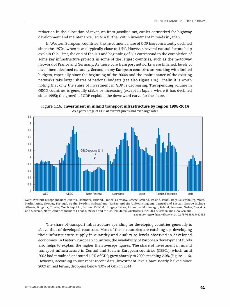
I.1. THE TRANSPORT SECTOR TODAY
Malta, nclude lovakia
442352
reduction in the allocation of revenues from gasoline tax, earlier earmarked for highway
development and maintenance, led to a further cut in investment in roads in Japan.
In Western European countries, the investment share of GDP has consistently declined
since the 1970s, when it was typically close to 1.5%. However, several natural factors help
explain this. First, the end of the 70s and beginning of 80s correspond to the completion of
some key infrastructure projects in some of the largest countries, such as the motorway
network of France and Germany. As these core transport networks were finished, levels of
investment declined naturally. Second, many European countries are working with limited
budgets, especially since the beginning of the 2000s and the maintenance of the existing
networks take larger shares of national budgets (see also Figure 1.16). Finally, it is worth
noting that only the share of investment in GDP is decreasing. The spending volume in
OECD countries is generally stable or increasing (except in Japan, where it has declined
since 1995); the growth of GDP explains the downward curve for the share.
The share of transport infrastructure spending for developing countries generally is
above that of developed countries. Most of these countries are catching up, developing
their infrastructure supply in quantity and quality to levels observed in developed
economies. In Eastern European countries, the availability of European development funds
also helps to explain the higher than average figures. The share of investment in inland
transport infrastructure in Central and Eastern European countries (CEECs), which until
2002 had remained at around 1.0% of GDP, grew sharply to 2009, reaching 2.0% (Figure 1.16).
However, according to our most recent data, investment levels have nearly halved since
2009 in real terms, dropping below 1.0% of GDP in 2014.
Figure 1.16. Investment in inland transport infrastructure by region 1998-2014As a percentage of GDP, at current prices and exchange rates
Note: Western Europe includes Austria, Denmark, Finland, France, Germany, Greece, Iceland, Ireland, Israel, Italy, Luxembourg,Netherlands, Norway, Portugal, Spain, Sweden, Switzerland, Turkey and the United Kingdom. Central and Eastern Europe iAlbania, Bulgaria, Croatia, Czech Republic, Estonia, FYROM, Hungary, Latvia, Lithuania, Montenegro, Poland, Romania, Serbia, Sand Slovenia. North America includes Canada, Mexico and the United States. Australasia includes Australia and New Zealand.
1 2 http://dx.doi.org/10.1787/888933
0
0.2
0.4
0.6
0.8
1
1.2
1.4
1.6
1.8
2
2.2
WEC CEEC North America Australasia Japan Russian Federation India
OECD average 2014
ITF TRANSPORT OUTLOOK 2017 © OECD/ITF 2017 41
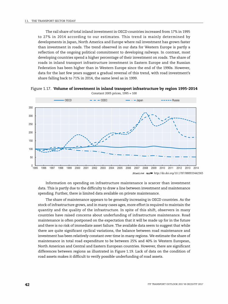
I.1. THE TRANSPORT SECTOR TODAY
4
442365
014
The rail share of total inland investment in OECD countries increased from 17% in 1995
to 27% in 2014 according to our estimates. This trend is mainly determined by
developments in Japan, North America and Europe where rail investment has grown faster
than investment in roads. The trend observed in our data for Western Europe is partly a
reflection of the ongoing political commitment to developing railways. In contrast, most
developing countries spend a higher percentage of their investment on roads. The share of
roads in inland transport infrastructure investment in Eastern Europe and the Russian
Federation has been higher than in Western Europe since the end of the 1990s. However,
data for the last few years suggest a gradual reversal of this trend, with road investment’s
share falling back to 71% in 2014, the same level as in 1999.
Information on spending on infrastructure maintenance is scarcer than investment
data. This is partly due to the difficulty to draw a line between investment and maintenance
spending. Further, there is limited data available on private maintenance.
The share of maintenance appears to be generally increasing in OECD countries. As the
stock of infrastructure grows, and in many cases ages, more effort is required to maintain the
quantity and the quality of the infrastructure. In spite of this shift, observers in many
countries have raised concerns about underfunding of infrastructure maintenance. Road
maintenance is often postponed on the expectation that it will be made up for in the future
and there is no risk of immediate asset failure. The available data seem to suggest that while
there are quite significant cyclical variations, the balance between road maintenance and
investment has been relatively constant over time in many regions. We estimate the share of
maintenance in total road expenditure to be between 25% and 40% in Western European,
North American and Central and Eastern European countries. However, there are significant
differences between regions as illustrated in Figure 1.19. Lack of data on the condition of
road assets makes it difficult to verify possible underfunding of road assets.
Figure 1.17. Volume of investment in inland transport infrastructure by region 1995-201Constant 2005 prices, 1995 = 100
1 2 http://dx.doi.org/10.1787/888933
0
50
100
150
200
250
300
350
1995 1996 1997 1998 1999 2000 2001 2002 2003 2004 2005 2006 2007 2008 2009 2010 2011 2012 2013 2
OECD CEEC Japan Russia
ITF TRANSPORT OUTLOOK 2017 © OECD/ITF 201742
I.1. THE TRANSPORT SECTOR TODAY
ays
442372
Japan, Central
442383
014
Figure 1.18. Distribution of infrastructure investment across rail, road and inland waterwPercentages computed from current prices, current exchange rates
1 2 http://dx.doi.org/10.1787/888933
Figure 1.19. Share of public road maintenance in total road expenditureCurrent prices, current exchange rates (%)
Note: OECD 23 include Austria, Belgium, Canada, Czech Republic, Denmark, Estonia, Finland, France, Hungary, Iceland, Italy,Luxembourg, Mexico, Norway, Poland, Portugal, Slovakia, Slovenia, Sweden, Turkey, the United Kingdom and the United States. CEEC (and Eastern European Countries) include Croatia, Czech Republic, Estonia, Hungary, Latvia, Lithuania, Poland, Slovakia and Slovenia.
1 2 http://dx.doi.org/10.1787/888933
0
10
20
30
40
50
60
70
80
90
100
Western European countries
0
10
20
30
40
50
60
70
80
90
100
Central and Eastern European countries
Road Rail Inland Waterways
20
22
24
26
28
30
32
34
36
38
40
1995 1996 1997 1998 1999 2000 2001 2002 2003 2004 2005 2006 2007 2008 2009 2010 2011 2012 2013 2
OECD 23 CEEC
ITF TRANSPORT OUTLOOK 2017 © OECD/ITF 2017 43
I.1. THE TRANSPORT SECTOR TODAY
References
ACI (2016a), “Airports Council International releases 2015 World Airport Traffic Report. The busiest become busier; the year of the international hub airport”, ACI Media Releases, 9th September 2016, www.aci.aero/News/Releases/Most-Recent/2016/09/09/Airports-Council-International-releases-2015-World-Airport-Traffic-Report-The-busiest-become-busier-the-year-of-the-international-hub-airport.
ACI (2016b), “ACI releases preliminary world airport traffic rankings”, Airports Council International, Press release, 4 April 2016, www.aci.aero/News/Releases/Most-Recent/2016/04/04/ACI-releases-preliminary-world-airport-traffic-rankings-.
Airparif (2013), Évolution de la qualité de l’air à Paris entre 2002 et 2012, Airparif : Surveillance de la qualité de l’air en Ile de France, Juillet 2013, www.airparif.asso.fr/_pdf/publications/rapport-pdp-130703.pdf.
Bennathan, E., J. Frase, L. Thompson (1992), “What Determines Demand for Freight Transport?” World Bank Policy Research Working Paper.
Bloomberg (2016), “Istanbul Ataturk beats Frankfurt to climb Europe’s airport rank”, 1 May 2015, www.bloomberg.com/news/articles/2016-01-15/istanbul-ataturk-beats-frankfurt-to-climb-europe-s-airport-ranks.
CGDD (2016), “Covoiturage longue distance : état des lieux et potentiel de croissance”, Collection « Etudes et documents » du SEEIDD, Mai 2016, www.developpement-durable.gouv.fr/IMG/pdf/ED146.pdf.
Constantinescu, C. et al. (2015), “The Global Trade Slowdown: Cyclical or Structural?”, IMF Working Paper, WP/15/6, www.imf.org/external/pubs/ft/wp/2015/wp1506.pdf.
CPB (2016), World Trade Monitor, Netherlands Bureau for Economic Policy Analysis.
Crafts, N. (2009), “Transport Infrastructure Investment: Implications for Growth and Productivity”, Oxford Review of Economic Policy, 25, pp. 327-343.
ECB (2014), Understanding Gobal Trade Elasticities: What has changed?, Monthly Bulletin, ECB, www.ecb.europa.eu/pub/pdf/other/mb201407_focus01.en.pdf.
Garcia, C. et al. (2008), “Correlation between Transport Intensity and GDP in European Regions: A new Approach”, 8th Swiss Transport Research Conference, Monte Verità/Ascona, October 15-17, 2008.
Herczeg, Marton (2011), Experience with congestion charges, Copenhagen Resource Institute. www.scp-knowledge.eu/sites/default/files/Herzog%202011%20Experience%20with%20congestion%20charges%20.pdf.
High-level Advisory Group on Sustainable Transport (2016), Mobilizing Sustainable Transport for Development, https://sustainabledevelopment.un.org/content/documents/2375Mobilizing%20Sustainable %20Transport.pdf.
IATA (2016a), “Air Freight Growth Slowed to 2.2% in 2015”, Press Release No. 3, 3 February 2016, www.iata.org/pressroom/pr/Pages/2016-02-03-01.aspx.
IATA (2016b), Annual Review 2016, www.iata.org/publications/Documents/iata-annual-review-2016.pdf.
IATA (2016c), India’s aviation policy could relaunch the industry, IATA Airlines International, 25th April 2016, http://airlines.iata.org/analysis/indias-aviation-policy-could-relaunch-the-industry.
IATA (2015), IATA Cargo Strategy, August 2015, www.iata.org/whatwedo/cargo/Documents/cargo-strategy.pdf.
ICAO (2016a), 2015: Air Transport Yearly Monitor (Preliminary), www.icao.int/sustainability/Documents/Yearly %20Monitor/yearly_monitor_2015.pdf.
ICAO (2016b), May 2016: Air Transport Monthly Monitor, www.icao.int/sustainability/Documents/Monthly%20 Monitor_Latest/MonthlyMonitor_latest.pdf.
ICAO (2015a), Continuing Traffic Growth and Record Airline Profits Highlight 2015 Air Transport Results, Press release 22 December 2015, www.icao.int/Newsroom/Pages/Continuing-Traffic-Growth-and-Record-Airline-Profits-Highlight-2015-Air-Transport-Results.aspx.
ICAO (2015b), Annual Report of the Council: 2015, International Civil Aviation Organization. Appendix 1, Tables relating to the world of air transport in 2015, www.icao.int/annual-report-2015/Documents/Appendix_1_en.pdf.
ICAO (2014), Annual Report of the Council: 2014, International Civil Aviation Organization. Appendix 1, Tables relating to the world of air transport in 2015, www.icao.int/annual-report-2014/Documents/Appendix_1_en.pdf.
ICAO (2013), Forecasts of Scheduled Passenger and Freight Traffic. Medium-Term Passenger and Freight Traffic Forecasts, www.icao.int/sustainability/pages/eap_fp_forecastmed.aspx.
ITF TRANSPORT OUTLOOK 2017 © OECD/ITF 201744
I.1. THE TRANSPORT SECTOR TODAY
IEA (2016), CO2 emissions by product and flow, IEA CO2 Emissions from Fuel Combustion Statistics (database), http://dx.doi.org/10.1787/data-00430-en (accessed on 19 October 2016).
IEA (2015), World Energy Outlook 2015, OECD Publishing, Paris, http://dx.doi.org/10.1787/weo-2015-en.
IHS (2015), Five trends shaping the global maritime industry, www.ihs.com/pdf/Global-Trends-Impacting-the-Maritime-Industry_235788110915583632.pdf.
IMF (2016), World Economic Outlook, April 2016, International Monetary Fund, Washington, DC, www.imf.org/external/pubs/ft/weo/2016/01/.
IMF (2015), World Economic Outlook, April 2015, International Monetary Fund, Washington, DC, www.imf.org/external/pubs/ft/weo/2015/01/.
ITF (2016a), Zero Road Deaths and Serious Injuries: Leading a Paradigm Shift to a Safe System, OECD Publishing, Paris, http://dx.doi.org/10.1787/9789282108055-en.
ITF (2016b), Road Safety Annual Report 2016, OECD Publishing, Paris, http://dx.doi.org/10.1787/irtad-2016-en.
ITF (2016c), “Shared Mobility: Innovation for Liveable Cities”, International Transport Forum Policy Papers, No. 21, OECD Publishing, Paris, http://dx.doi.org/10.1787/5jlwvz8bd4mx-en.
ITF (2015a), ITF Transport Outlook 2015, OECD Publishing, Paris, http://dx.doi.org/10.1787/9789282107782-en.
ITF (2015b), “The Impact of Mega-Ships”, International Transport Forum Policy Papers, No. 10, OECD Publishing, Paris, http://dx.doi.org/10.1787/5jlwvzcm3j9v-en.
ITF (2015c), Road Safety Annual Report 2015, OECD Publishing, Paris, http://dx.doi.org/10.1787/irtad-2015-en.
ITF (2010), Implementing Congestion Charges, OECD Publishing, Paris, http://dx.doi.org/10.1787/9789282102855-en.
Jong-A-Pin, R. and J. de Haan (2008), “Time-varying impact of public capital on output: New evidence based on VARs for OECD countries”, EIB Papers, Vol. 13, No. 1, pp. 56-81.
Kamps, C. (2005), “Is there lack of public capital in the European Union?”, EIB Papers, Vol. 10, No. 1, pp. 72-93.
KPMG (2016), KPMG Transport Tracker. Global transport market trends and views.
McKinnon, A. (2007), “The Decoupling of Road Freight Transport and Economic Growth Trends in the UK: An Exploratory Analysis”, Transport Reviews, Volume 207, Issue 1, 2007, pp. 37-64.
Meersman, H. and E. Van de Voorde (2005), “Decoupling of Freight Transport and Economic Activity: Realism or Utopia?” 16th International Symposium on Theory and Practice in Transport Economics: 50 Years of Transport Research: Experience Gained and Major Challenges Ahead, Budapest 29-31 October, ECMT, Paris.
MOR, China’s Ministry of Railway (2008), Mid-to-Long Term Railway Network Plan, www.china-mor.gov.cn/tljs/tlgh/201012/t20101228_731.html (accessed 11.21.10) (in Chinese).
NBSC (2015), China Statistical Yearbook 2015, China Statistics Press, Beijing.
OECD (2016), OECD Economic Outlook, Volume 2016 Issue 1, OECD Publishing, Paris, http://dx.doi.org/10.1787/eco_outlook-v2016-1-en.
OECD (2014), The Cost of Air Pollution, Health Impacts of Road Transport, OECD Publishing, Paris, http://dx.doi.org/10.1787/9789264210448-en.
PwC (2016), Industry perspectives, 2016 Auto Industry Trends, PwC Strategy.
Reuters (2015), Mega-ships are worsening overcapacity in the container market, 23rd September 2015, www.reuters.com/article/us-shipping-mega-ships-kemp-idUSKCN0RM2AS20150923.
Reuters (2016), India overhauls aviation rules to boost air travel, 15th June 2016, http://in.reuters.com/article/india-airlines-aviation-policy-idINKCN0Z10QC.
Santos, G. (2005), “Urban Congestion Charging: A Comparison between London and Singapore“, Transport Reviews, Vol. 25/5, pp. 511-534.
SLoCaT (2015), SLoCaT Preliminary Analysis of NDCs Sees Potential for Ambitious Action on Climate Change in the Transport Sector, available at www.slocat.net/news/1589.
Tapio, P. (2005), “Towards a theory of decoupling: Degrees of decoupling in the EU and the case of road traffic Finland between 1970 and 2001”, Transport Policy, 12, pp. 137-151.
Times of India (2016), “BlaBlaCar: India could soon be our biggest market”, Times of India, 18 April 2016, http://timesofindia.indiatimes.com/tech/tech-news/BlaBlaCar-India-could-soon-be-our-biggest-market/articleshow/51873962.cms.
ITF TRANSPORT OUTLOOK 2017 © OECD/ITF 2017 45

I.1. THE TRANSPORT SECTOR TODAY
UNCTAD (2015), Review of Maritime Transport 2015, United Nations Conference on Trade and Development, http://unctad.org/en/PublicationsLibrary/rmt2015_en.pdf.
World Bank (2016), Global Economic Prospects, June 2016, World Bank, Washington, DC, http://pubdocs.worldbank.org/pubdocs/publicdoc/2016/5/842861463605615468/Global-Economic-Prospects-June-2016-Divergences-and-risks.pdf.
WTO (2016), “Trade growth to remain subdued in 2016 as uncertainties weigh on global demand”, Press Release, 7th April 2016, www.wto.org/english/news_e/pres16_e/pr768_e.htm.
ITF TRANSPORT OUTLOOK 2017 © OECD/ITF 201746
ITF Transport Outlook 2017 © OECD/ITF 2017
PART I
Chapter 2
Transport demand and CO2 emissions to 2050
This chapter provides an overview of the long-term prospects for transport demand. Based on projections from the International Transport Forum’s (ITF) suite of models, it presents the baseline trajectory for transport demand to 2050 and outlines its projections for CO2 emissions from the sector. The chapter starts with the baseline scenario projections for passenger transport demand, broken down by mode, for both urban and non-urban areas, between 2015 and 2050. It then focuses on the outlook for freight for the same period, looking at surface freight (rail and road), maritime and air. The chapter concludes with the projections for the CO2 emissions from transport to 2050, by sector, and a brief review of the ITF’s contribution to the Paris Agreement with its Decarbonising Transport project.
47
I.2. TRANSPORT DEMAND AND CO2 EMISSIONS TO 2050
The International Transport Forum (ITF) has developed a suite of models to build
scenarios for the future of transport demand and related CO2 emissions up to 2050. The
scenarios for passenger demand result from the combination of several sub-models,
distinguishing between mobility in cities, domestic intercity travel and international
passenger aviation. The ITF’s International Freight Model (see Chapter 3) derives the
footprint of global trade on the freight transport network, all modes combined. While each
model focuses on a different mode or type of mobility, they collectively form a coherent
framework for the analysis of long-term global trends. Annex 2.A explains this framework
and how it can yield cross-sectorial results.
This chapter takes advantage of the compatible nature of the different models to give an
overview of the future of transport demand and CO2 emissions for all modes, both passenger
and freight. It analyses the relative importance of the different sectors and compares their
probable evolution. The figures in this chapter result from the baseline scenario for transport
demand, which is a projection of current trends and includes current policies and policy
developments. The low-carbon scenario, discussed at the end of the chapter, corresponds to
the aggregation of the least CO2-intensive pathways for each sector. A more in-depth
discussion of alternative scenarios for international freight and aviation, as well as for
mobility in cities, can be found in the three chapters of Part 2 of this publication.
Passenger transportAccording to our projections, global passenger demand will more than double between
2015 and 2050, from 50 000 to 120 000 billion passenger-kilometres (Figure 2.1). It increases in
all regions and for all modes, but the growth is not uniformly distributed. Most of the growth
occurs in Asia, which will represent around a third of all passenger transport demand in
2050. In contrast, the low growth rates observed in all OECD countries mean that these
countries will only represent 25% of travel demand in 2050, compared to 45% in 2015.
Similarly, all modes do not grow at the same speed. Global average growth rates range from
less than 2% annually for inter-urban rail to almost 5% for international passenger aviation.
Economic development is the main driving force behind the expected modifications of
the passenger mobility landscape. The global increase in Gross Domestic Product (GDP)
projected in this Outlook, albeit slower than estimated in the previous edition (see also
Table 1.2), still induces large-scale changes, both quantitative and qualitative. However, it
only constitutes a medium scenario in an uncertain economic environment. Similarly, future
oil prices are a major unknown in the equation. This Outlook considers several pathways for
oil and fuel prices. The baseline scenario considers a moderate increase of oil prices, in line
with the current projections of the International Energy Agency’s (IEA) 4DS scenario (see
Glossary).
The advent of new transport solutions or radically different technology could also
overhaul current mobility systems. In the urban sector, for instance, making ride-sharing
the norm rather than the exception would completely change the role of cars in urban
ITF TRANSPORT OUTLOOK 2017 © OECD/ITF 201748
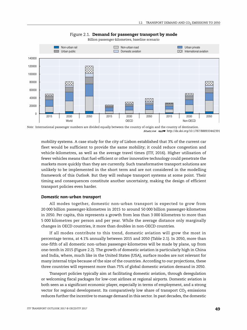
I.2. TRANSPORT DEMAND AND CO2 EMISSIONS TO 2050
442391
0
mobility systems. A case study for the city of Lisbon established that 3% of the current car
fleet would be sufficient to provide the same mobility; it could reduce congestion and
vehicle-kilometres, as well as the average travel times (ITF, 2016). Higher utilisation of
fewer vehicles means that fuel-efficient or other innovative technology could penetrate the
markets more quickly than they are currently. Such transformative transport solutions are
unlikely to be implemented in the short term and are not considered in the modelling
framework of this Outlook. But they will reshape transport systems at some point. Their
timing and consequences constitute another uncertainty, making the design of efficient
transport policies even harder.
Domestic non-urban transport
All modes together, domestic non-urban transport is expected to grow from
20 000 billion passenger-kilometres in 2015 to around 50 000 billion passenger-kilometres
in 2050. Per capita, this represents a growth from less than 3 000 kilometres to more than
5 000 kilometres per person and per year. While the average distance only marginally
changes in OECD countries, it more than doubles in non-OECD countries.
If all modes contribute to this trend, domestic aviation will grow the most in
percentage terms, at 4.1% annually between 2015 and 2050 (Table 2.1). In 2050, more than
one-fifth of all domestic non-urban passenger-kilometres will be made by plane, up from
one-tenth in 2015 (Figure 2.2). The growth of domestic aviation is particularly high in China
and India, where, much like in the United States (USA), surface modes are not relevant for
many internal trips because of the size of the countries. According to our projections, these
three countries will represent more than 75% of global domestic aviation demand in 2050.
Transport policies typically aim at facilitating domestic aviation, through deregulation
or welcoming fiscal packages for low-cost airlines at regional airports. Domestic aviation is
both seen as a significant economic player, especially in terms of employment, and a strong
vector for regional development. Its comparatively low share of transport CO2 emissions
reduces further the incentive to manage demand in this sector. In past decades, the domestic
Figure 2.1. Demand for passenger transport by modeBillion passenger-kilometres, baseline scenario
Note: International passenger numbers are divided equally between the country of origin and the country of destination.1 2 http://dx.doi.org/10.1787/888933
0
20000
40000
60000
80000
100000
120000
140000
2015 2030 2050 2015 2030 2050 2015 2030 205World OECD Non-OECD
Non-urban rail Non-urban road Urban private Urban public Domestic aviation International aviation
ITF TRANSPORT OUTLOOK 2017 © OECD/ITF 2017 49
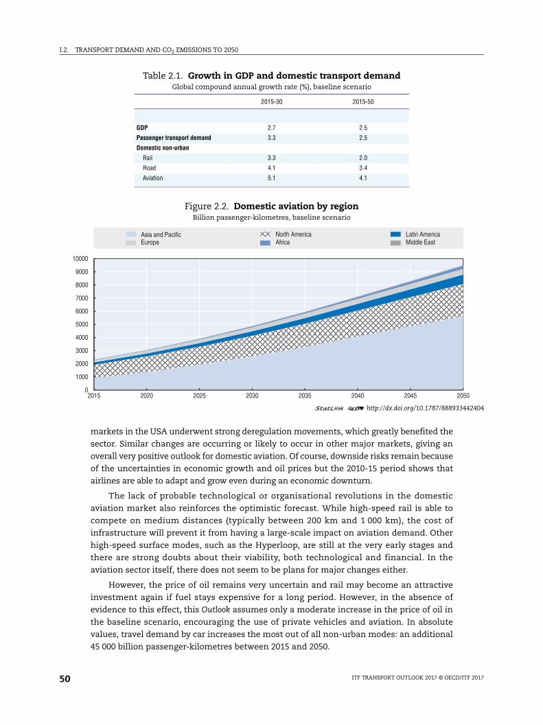
I.2. TRANSPORT DEMAND AND CO2 EMISSIONS TO 2050
442404
50
markets in the USA underwent strong deregulation movements, which greatly benefited the
sector. Similar changes are occurring or likely to occur in other major markets, giving an
overall very positive outlook for domestic aviation. Of course, downside risks remain because
of the uncertainties in economic growth and oil prices but the 2010-15 period shows that
airlines are able to adapt and grow even during an economic downturn.
The lack of probable technological or organisational revolutions in the domestic
aviation market also reinforces the optimistic forecast. While high-speed rail is able to
compete on medium distances (typically between 200 km and 1 000 km), the cost of
infrastructure will prevent it from having a large-scale impact on aviation demand. Other
high-speed surface modes, such as the Hyperloop, are still at the very early stages and
there are strong doubts about their viability, both technological and financial. In the
aviation sector itself, there does not seem to be plans for major changes either.
However, the price of oil remains very uncertain and rail may become an attractive
investment again if fuel stays expensive for a long period. However, in the absence of
evidence to this effect, this Outlook assumes only a moderate increase in the price of oil in
the baseline scenario, encouraging the use of private vehicles and aviation. In absolute
values, travel demand by car increases the most out of all non-urban modes: an additional
45 000 billion passenger-kilometres between 2015 and 2050.
Table 2.1. Growth in GDP and domestic transport demandGlobal compound annual growth rate (%), baseline scenario
2015-30 2015-50
GDP 2.7 2.5
Passenger transport demand 3.3 2.5
Domestic non-urban
Rail 3.3 2.0
Road 4.1 3.4
Aviation 5.1 4.1
Figure 2.2. Domestic aviation by regionBillion passenger-kilometres, baseline scenario
1 2 http://dx.doi.org/10.1787/888933
0
1000
2000
3000
4000
5000
6000
7000
8000
9000
10000
2015 2020 2025 2030 2035 2040 2045 20
Asia and Pacific North America Latin AmericaEurope Africa Middle East
ITF TRANSPORT OUTLOOK 2017 © OECD/ITF 201750
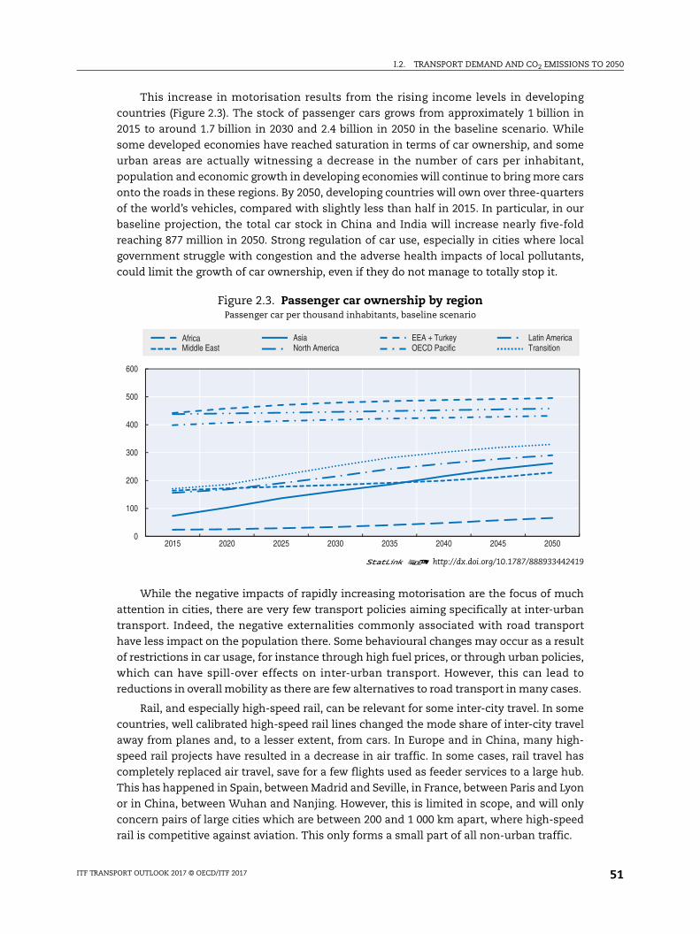
I.2. TRANSPORT DEMAND AND CO2 EMISSIONS TO 2050
This increase in motorisation results from the rising income levels in developing
countries (Figure 2.3). The stock of passenger cars grows from approximately 1 billion in
2015 to around 1.7 billion in 2030 and 2.4 billion in 2050 in the baseline scenario. While
some developed economies have reached saturation in terms of car ownership, and some
urban areas are actually witnessing a decrease in the number of cars per inhabitant,
population and economic growth in developing economies will continue to bring more cars
onto the roads in these regions. By 2050, developing countries will own over three-quarters
of the world’s vehicles, compared with slightly less than half in 2015. In particular, in our
baseline projection, the total car stock in China and India will increase nearly five-fold
reaching 877 million in 2050. Strong regulation of car use, especially in cities where local
government struggle with congestion and the adverse health impacts of local pollutants,
could limit the growth of car ownership, even if they do not manage to totally stop it.
While the negative impacts of rapidly increasing motorisation are the focus of much
attention in cities, there are very few transport policies aiming specifically at inter-urban
transport. Indeed, the negative externalities commonly associated with road transport
have less impact on the population there. Some behavioural changes may occur as a result
of restrictions in car usage, for instance through high fuel prices, or through urban policies,
which can have spill-over effects on inter-urban transport. However, this can lead to
reductions in overall mobility as there are few alternatives to road transport in many cases.
Rail, and especially high-speed rail, can be relevant for some inter-city travel. In some
countries, well calibrated high-speed rail lines changed the mode share of inter-city travel
away from planes and, to a lesser extent, from cars. In Europe and in China, many high-
speed rail projects have resulted in a decrease in air traffic. In some cases, rail travel has
completely replaced air travel, save for a few flights used as feeder services to a large hub.
This has happened in Spain, between Madrid and Seville, in France, between Paris and Lyon
or in China, between Wuhan and Nanjing. However, this is limited in scope, and will only
concern pairs of large cities which are between 200 and 1 000 km apart, where high-speed
rail is competitive against aviation. This only forms a small part of all non-urban traffic.
Figure 2.3. Passenger car ownership by regionPassenger car per thousand inhabitants, baseline scenario
1 2 http://dx.doi.org/10.1787/888933442419
0
100
200
300
400
500
600
2015 2020 2025 2030 2035 2040 2045 2050
Africa Asia EEA + Turkey Latin AmericaMiddle East North America OECD Pacific Transition
ITF TRANSPORT OUTLOOK 2017 © OECD/ITF 2017 51
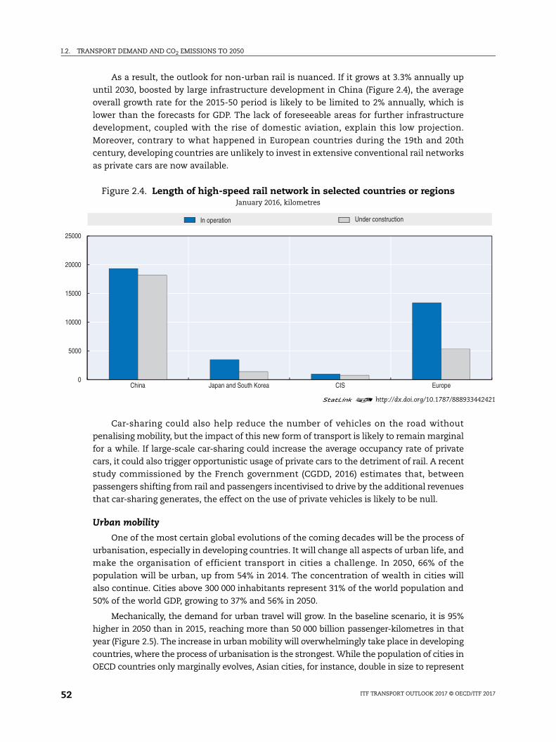
I.2. TRANSPORT DEMAND AND CO2 EMISSIONS TO 2050
442421
As a result, the outlook for non-urban rail is nuanced. If it grows at 3.3% annually up
until 2030, boosted by large infrastructure development in China (Figure 2.4), the average
overall growth rate for the 2015-50 period is likely to be limited to 2% annually, which is
lower than the forecasts for GDP. The lack of foreseeable areas for further infrastructure
development, coupled with the rise of domestic aviation, explain this low projection.
Moreover, contrary to what happened in European countries during the 19th and 20th
century, developing countries are unlikely to invest in extensive conventional rail networks
as private cars are now available.
Car-sharing could also help reduce the number of vehicles on the road without
penalising mobility, but the impact of this new form of transport is likely to remain marginal
for a while. If large-scale car-sharing could increase the average occupancy rate of private
cars, it could also trigger opportunistic usage of private cars to the detriment of rail. A recent
study commissioned by the French government (CGDD, 2016) estimates that, between
passengers shifting from rail and passengers incentivised to drive by the additional revenues
that car-sharing generates, the effect on the use of private vehicles is likely to be null.
Urban mobility
One of the most certain global evolutions of the coming decades will be the process of
urbanisation, especially in developing countries. It will change all aspects of urban life, and
make the organisation of efficient transport in cities a challenge. In 2050, 66% of the
population will be urban, up from 54% in 2014. The concentration of wealth in cities will
also continue. Cities above 300 000 inhabitants represent 31% of the world population and
50% of the world GDP, growing to 37% and 56% in 2050.
Mechanically, the demand for urban travel will grow. In the baseline scenario, it is 95%
higher in 2050 than in 2015, reaching more than 50 000 billion passenger-kilometres in that
year (Figure 2.5). The increase in urban mobility will overwhelmingly take place in developing
countries, where the process of urbanisation is the strongest. While the population of cities in
OECD countries only marginally evolves, Asian cities, for instance, double in size to represent
Figure 2.4. Length of high-speed rail network in selected countries or regionsJanuary 2016, kilometres
1 2 http://dx.doi.org/10.1787/888933
0
5000
10000
15000
20000
25000
China Japan and South Korea CIS Europe
In operation Under construction
ITF TRANSPORT OUTLOOK 2017 © OECD/ITF 201752
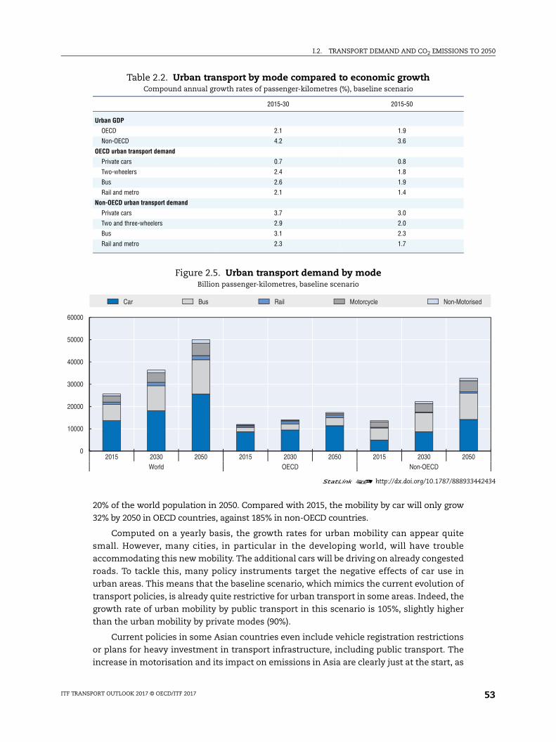
I.2. TRANSPORT DEMAND AND CO2 EMISSIONS TO 2050
442434
sed
20% of the world population in 2050. Compared with 2015, the mobility by car will only grow
32% by 2050 in OECD countries, against 185% in non-OECD countries.
Computed on a yearly basis, the growth rates for urban mobility can appear quite
small. However, many cities, in particular in the developing world, will have trouble
accommodating this new mobility. The additional cars will be driving on already congested
roads. To tackle this, many policy instruments target the negative effects of car use in
urban areas. This means that the baseline scenario, which mimics the current evolution of
transport policies, is already quite restrictive for urban transport in some areas. Indeed, the
growth rate of urban mobility by public transport in this scenario is 105%, slightly higher
than the urban mobility by private modes (90%).
Current policies in some Asian countries even include vehicle registration restrictions
or plans for heavy investment in transport infrastructure, including public transport. The
increase in motorisation and its impact on emissions in Asia are clearly just at the start, as
Table 2.2. Urban transport by mode compared to economic growthCompound annual growth rates of passenger-kilometres (%), baseline scenario
2015-30 2015-50
Urban GDP
OECD 2.1 1.9
Non-OECD 4.2 3.6
OECD urban transport demand
Private cars 0.7 0.8
Two-wheelers 2.4 1.8
Bus 2.6 1.9
Rail and metro 2.1 1.4
Non-OECD urban transport demand
Private cars 3.7 3.0
Two and three-wheelers 2.9 2.0
Bus 3.1 2.3
Rail and metro 2.3 1.7
Figure 2.5. Urban transport demand by modeBillion passenger-kilometres, baseline scenario
1 2 http://dx.doi.org/10.1787/888933
0
10000
20000
30000
40000
50000
60000
2015 2030 2050 2015 2030 2050 2015 2030 2050World OECD Non-OECD
Car Bus Rail Motorcycle Non-Motori
ITF TRANSPORT OUTLOOK 2017 © OECD/ITF 2017 53
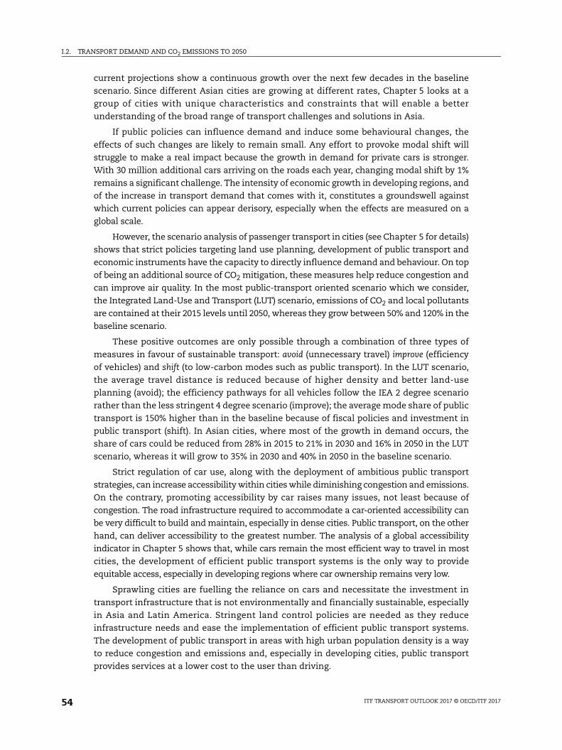
I.2. TRANSPORT DEMAND AND CO2 EMISSIONS TO 2050
current projections show a continuous growth over the next few decades in the baseline
scenario. Since different Asian cities are growing at different rates, Chapter 5 looks at a
group of cities with unique characteristics and constraints that will enable a better
understanding of the broad range of transport challenges and solutions in Asia.
If public policies can influence demand and induce some behavioural changes, the
effects of such changes are likely to remain small. Any effort to provoke modal shift will
struggle to make a real impact because the growth in demand for private cars is stronger.
With 30 million additional cars arriving on the roads each year, changing modal shift by 1%
remains a significant challenge. The intensity of economic growth in developing regions, and
of the increase in transport demand that comes with it, constitutes a groundswell against
which current policies can appear derisory, especially when the effects are measured on a
global scale.
However, the scenario analysis of passenger transport in cities (see Chapter 5 for details)
shows that strict policies targeting land use planning, development of public transport and
economic instruments have the capacity to directly influence demand and behaviour. On top
of being an additional source of CO2 mitigation, these measures help reduce congestion and
can improve air quality. In the most public-transport oriented scenario which we consider,
the Integrated Land-Use and Transport (LUT) scenario, emissions of CO2 and local pollutants
are contained at their 2015 levels until 2050, whereas they grow between 50% and 120% in the
baseline scenario.
These positive outcomes are only possible through a combination of three types of
measures in favour of sustainable transport: avoid (unnecessary travel) improve (efficiency
of vehicles) and shift (to low-carbon modes such as public transport). In the LUT scenario,
the average travel distance is reduced because of higher density and better land-use
planning (avoid); the efficiency pathways for all vehicles follow the IEA 2 degree scenario
rather than the less stringent 4 degree scenario (improve); the average mode share of public
transport is 150% higher than in the baseline because of fiscal policies and investment in
public transport (shift). In Asian cities, where most of the growth in demand occurs, the
share of cars could be reduced from 28% in 2015 to 21% in 2030 and 16% in 2050 in the LUT
scenario, whereas it will grow to 35% in 2030 and 40% in 2050 in the baseline scenario.
Strict regulation of car use, along with the deployment of ambitious public transport
strategies, can increase accessibility within cities while diminishing congestion and emissions.
On the contrary, promoting accessibility by car raises many issues, not least because of
congestion. The road infrastructure required to accommodate a car-oriented accessibility can
be very difficult to build and maintain, especially in dense cities. Public transport, on the other
hand, can deliver accessibility to the greatest number. The analysis of a global accessibility
indicator in Chapter 5 shows that, while cars remain the most efficient way to travel in most
cities, the development of efficient public transport systems is the only way to provide
equitable access, especially in developing regions where car ownership remains very low.
Sprawling cities are fuelling the reliance on cars and necessitate the investment in
transport infrastructure that is not environmentally and financially sustainable, especially
in Asia and Latin America. Stringent land control policies are needed as they reduce
infrastructure needs and ease the implementation of efficient public transport systems.
The development of public transport in areas with high urban population density is a way
to reduce congestion and emissions and, especially in developing cities, public transport
provides services at a lower cost to the user than driving.
ITF TRANSPORT OUTLOOK 2017 © OECD/ITF 201754
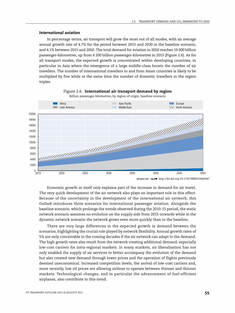
I.2. TRANSPORT DEMAND AND CO2 EMISSIONS TO 2050
442447
2050
International aviation
In percentage terms, air transport will grow the most out of all modes, with an average
annual growth rate of 4.7% for the period between 2015 and 2030 in the baseline scenario,
and 4.1% between 2015 and 2050. The total demand for aviation in 2050 reaches 19 000 billion
passenger-kilometres, up from 4 200 billion passenger-kilometres in 2015 (Figure 2.6). As for
all transport modes, the expected growth is concentrated within developing countries, in
particular in Asia where the emergence of a large middle-class boosts the number of air
travellers. The number of international travellers to and from Asian countries is likely to be
multiplied by five while at the same time the number of domestic travellers in the region
triples.
Economic growth in itself only explains part of the increase in demand for air travel.
The very quick development of the air network also plays an important role in this effect.
Because of the uncertainty in the development of the international air network, this
Outlook introduces three scenarios for international passenger aviation. Alongside the
baseline scenario, which prolongs the trends observed during the 2010-15 period, the static
network scenario assumes no evolution on the supply side from 2015 onwards while in the
dynamic network scenario the network grows even more quickly than in the baseline.
There are very large differences in the expected growth in demand between the
scenarios, highlighting the crucial role played by network flexibility. Annual growth rates of
5% are only conceivable in the coming decades if the air network can adapt to the demand.
The high growth rates also result from the network creating additional demand, especially
low-cost carriers for intra-regional markets. In many markets, air liberalisation has not
only enabled the supply of air services to better accompany the evolution of the demand
but also created new demand through lower prices and the operation of flights previously
deemed uneconomical. Increased competition levels, the arrival of low-cost carriers and,
more recently, low oil prices are allowing airlines to operate between thinner and thinner
markets. Technological changes, and in particular the advancement of fuel-efficient
airplanes, also contribute to this trend.
Figure 2.6. International air transport demand by regionBillion passenger-kilometres, by region of origin, baseline scenario
1 2 http://dx.doi.org/10.1787/888933
0
2000
4000
6000
8000
10000
12000
14000
16000
18000
20000
2015 2020 2025 2030 2035 2040 2045
Africa Asia Pacific EuropeLatin America Middle East North America
ITF TRANSPORT OUTLOOK 2017 © OECD/ITF 2017 55
I.2. TRANSPORT DEMAND AND CO2 EMISSIONS TO 2050
442458
Freight transportIn the baseline scenario, total freight demand (domestic and international) triples
from 112 000 to 329 000 billion tonne-kilometres (Figure 2.7). Demand for freight transport
is still primarily driven by economic growth. We find that GDP and surface freight intensity
are highly correlated. The average long-term elasticity in the panel of countries we have
studied is 0.98 (ITF/OECD, 2015).
The global freight transport demand grows at 3.3% annually prior to 2030, while for the
2015-50 period the average growth rate is slightly lower, affected by lower growth in the
underlying economic projections. Air freight volumes grow faster than other modes, at 5%
annually. This growth is driven by changes in the underlying composition of trade with an
increasing share of higher value goods making up the total. Maritime transport accounts
for the largest share of tonne-kilometres. In our baseline scenario this grows from 71% in
2015 to 75% by 2050. Road and rail account for the remaining shares while air freight,
measured in tonne-kilometres, only represents a marginal proportion.
These projections are clouded with much uncertainty and hinge on various
assumptions which may not hold. Economic growth remains lower than expected and is
subject to increased downside risks and uncertainties. International trade is now growing
Figure 2.7. Freight transport demand by modeBaseline scenario, billion tonne-kilometres
1 2 http://dx.doi.org/10.1787/888933
0
50000
100000
150000
200000
250000
300000
350000
2015 2030 2050
Rail Road Sea Air
Table 2.3. Annual growth rate for freight transport demand, compared to GDPGlobal compound annual growth rate (%), baseline scenario
2015-30 2015-50
GDP 2.7 2.5
Freight transport demand 3.3 3.1
Rail 3.0 2.6
Road 3.2 2.8
Aviation 5.6 5.4
Sea 3.4 3.3
ITF TRANSPORT OUTLOOK 2017 © OECD/ITF 201756
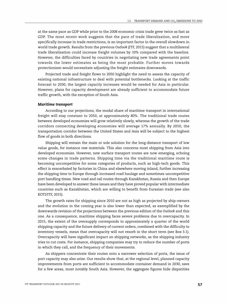
I.2. TRANSPORT DEMAND AND CO2 EMISSIONS TO 2050
at the same pace as GDP while prior to the 2008 economic crisis trade grew twice as fast as
GDP. The most recent work suggests that the pace of trade liberalisation, and more
specifically increase in trade restrictions, is an important factor in the overall slowdown in
world trade growth. Results from the previous Outlook (ITF, 2015) suggest that a multilateral
trade liberalisation could increase freight volumes by 10% compared with the baseline.
However, the difficulties faced by countries in negotiating new trade agreements point
towards the lower estimates as being the most probable. Further moves towards
protectionism would necessitate adjusting the freight estimates downwards.
Projected trade and freight flows to 2050 highlight the need to assess the capacity of
existing national infrastructure to deal with potential bottlenecks. Looking at the traffic
forecast to 2030, the largest capacity increases would be needed for Asia in particular.
However, plans for capacity development are already sufficient to accommodate future
traffic growth, with the exception of South Asia.
Maritime transport
According to our projections, the modal share of maritime transport in international
freight will stay constant to 2050, at approximately 80%. The traditional trade routes
between developed economies will grow relatively slowly, whereas the growth of the trade
corridors connecting developing economies will average 17% annually. By 2050, the
transportation corridor between the United States and Asia will be subject to the highest
flow of goods in both directions.
Shipping will remain the main or sole solution for the long-distance transport of low
value goods, for instance raw materials. This also concerns most shipping from Asia into
developed economies. However, new surface transport routes are now emerging, echoing
some changes in trade patterns. Shipping time via the traditional maritime route is
becoming uncompetitive for some categories of products, such as high-tech goods. This
effect is exacerbated by factories in China and elsewhere moving inland, further increasing
the shipping time to Europe through increased road haulage and sometimes uncompetitive
port handling times. New road and rail routes through Kazakhstan, Russia and then Europe
have been developed to answer these issues and they have proved popular with intermediate
countries such as Kazakhstan, which are willing to benefit from Eurasian trade (see also
KOTI/ITF, 2015).
The growth rates for shipping since 2010 are not as high as projected by ship-owners
and the evolution in the coming year is also lower than expected, as exemplified by the
downwards revision of the projections between the previous edition of the Outlook and this
one. As a consequence, maritime shipping faces severe problems due to overcapacity. In
2015, the extent of the oversupply corresponds to approximately a quarter of the world
shipping capacity and the future delivery of current orders, combined with the difficulty to
inventory vessels, mean that overcapacity will not resorb in the short term (see Box 3.1).
Overcapacity will have significant impact on shipping networks, as the shipping industry
tries to cut costs. For instance, shipping companies may try to reduce the number of ports
in which they call, and the frequency of their movements.
As shippers concentrate their routes onto a narrower selection of ports, the issue of
port capacity may also arise. Our results show that, at the regional level, planned capacity
improvements from ports are sufficient to accommodate container demand in 2030, save
for a few areas, most notably South Asia. However, the aggregate figures hide disparities
ITF TRANSPORT OUTLOOK 2017 © OECD/ITF 2017 57
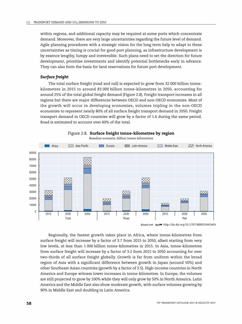
I.2. TRANSPORT DEMAND AND CO2 EMISSIONS TO 2050
442464
erica
within regions, and additional capacity may be required at some ports which concentrate
demand. Moreover, there are very large uncertainties regarding the future level of demand.
Agile planning procedures with a strategic vision for the long term help to adapt to these
uncertainties as timing is crucial for good port planning, as infrastructure development is
by essence lengthy, lumpy and irreversible. Such plans need to set the direction for future
development, prioritise investments and identify potential bottlenecks early in advance.
They can also form the basis for land reservations for future port development.
Surface freight
The total surface freight (road and rail) is expected to grow from 32 000 billion tonne-
kilometres in 2015 to around 83 000 billion tonne-kilometres in 2050, accounting for
around 25% of the total global freight demand (Figure 2.8). Freight transport increases in all
regions but there are major differences between OECD and non-OECD economies. Most of
the growth will occur in developing economies, volumes tripling in the non-OECD
economies to represent nearly 80% of all surface freight transport demand in 2050. Freight
transport demand in OECD countries will grow by a factor of 1.6 during the same period.
Road is estimated to account over 60% of the total.
Regionally, the fastest growth takes place in Africa, where tonne-kilometres from
surface freight will increase by a factor of 3.7 from 2015 to 2050, albeit starting from very
low levels, at less than 1 000 billion tonne-kilometres in 2015. In Asia, tonne-kilometres
from surface freight will increase by a factor of 3.2 from 2015 to 2050 accounting for over
two-thirds of all surface freight globally. Growth is far from uniform within the broad
region of Asia with a significant difference between growth in Japan (around 50%) and
other Southeast Asian countries (growth by a factor of 3.5). High-income countries in North
America and Europe witness lower increases in tonne-kilometres. In Europe, the volumes
are still projected to grow by 100% while they will only grow by 50% in North America. Latin
America and the Middle East also show moderate growth, with surface volumes growing by
90% in Middle East and doubling in Latin America.
Figure 2.8. Surface freight tonne-kilometres by regionBaseline scenario, billion tonne-kilometres
1 2 http://dx.doi.org/10.1787/888933
0
10000
20000
30000
40000
50000
60000
70000
80000
90000
2015 2030 2050 2015 2030 2050 2015 2030 2050Total Road Rail
Africa Asia Pacific Europe Latin America Middle East North Am
ITF TRANSPORT OUTLOOK 2017 © OECD/ITF 201758
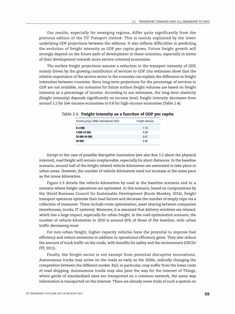
I.2. TRANSPORT DEMAND AND CO2 EMISSIONS TO 2050
Our results, especially for emerging regions, differ quite significantly from the
previous edition of the ITF Transport Outlook. This is mainly explained by the lower
underlying GDP projections between the editions. It also reflects difficulties in predicting
the evolution of freight intensity as GDP per capita grows. Future freight growth will
strongly depend on the future path of development in these countries, especially in terms
of their development towards more service-oriented economies.
The surface freight projections assume a reduction in the transport intensity of GDP,
mainly driven by the growing contribution of services to GDP. Our estimates show that the
relative importance of the service sector in the economy can explain the difference in freight
intensities between countries. Since long-term projections for the percentage of services in
GDP are not available, our scenarios for future surface freight volumes are based on freight
intensity as a percentage of income. According to our estimates, the long-term elasticity
(freight intensity) depends significantly on income level; freight intensity decreases from
around 1.2 for low-income economies to 0.8 for high-income economies (Table 2.4).
Except in the case of possible disruptive innovation (see also Box 3.2 about the physical
internet), road freight will remain irreplaceable, especially for short distances. In the baseline
scenario, around half of the freight-related vehicle-kilometres are estimated to take place in
urban areas. However, the number of vehicle-kilometres need not increase at the same pace
as the tonne-kilometres.
Figure 2.9 details the vehicle-kilometres by road in the baseline scenario and in a
scenario where freight operations are optimised. In this scenario, based on computations by
the World Business Council for Sustainable Development (Route Monkey, 2016), freight
transport operators optimise their load factors and decrease the number of empty trips via a
collection of measures. These include route optimisation, asset sharing between companies
(warehouses, trucks, IT systems). Moreover, it is assumed that delivery windows are relaxed,
which has a large impact, especially for urban freight. In the road optimisation scenario, the
number of vehicle-kilometres in 2050 is around 60% of those of the baseline, with urban
traffic decreasing most.
For non-urban freight, higher capacity vehicles have the potential to improve fuel
efficiency and reduce emissions in addition to operational efficiency gains. They also reduce
the amount of truck traffic on the roads, with benefits for safety and the environment (OECD/
ITF, 2011).
Finally, the freight sector is not exempt from potential disruptive innovations.
Autonomous trucks may arrive on the roads as early as the 2020s, radically changing the
competition between the different modes. Rail, in particular, may suffer from the lower costs
of road shipping. Autonomous trucks may also pave the way for the Internet of Things,
where goods of standardised sizes are transported on a common network, the same way
information is transported on the Internet. There are already some trials of such a system on
Table 2.4. Freight intensity as a function of GDP per capita
Income group (2005 International USD) Freight intensity
0-4 000 1.18
4 000-20 000 0.98
20 000-40 000 0.87
40 000- 0.82
ITF TRANSPORT OUTLOOK 2017 © OECD/ITF 2017 59
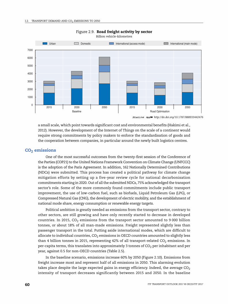
I.2. TRANSPORT DEMAND AND CO2 EMISSIONS TO 2050
442476
de)
a small scale, which point towards significant cost and environmental benefits (Hakimi et al.,
2012). However, the development of the Internet of Things on the scale of a continent would
require strong commitments by policy makers to enforce the standardisation of goods and
the cooperation between companies, in particular around the newly built logistics centres.
CO2 emissionsOne of the most successful outcomes from the twenty-first session of the Conference of
the Parties (COP21) to the United Nations Framework Convention on Climate Change (UNFCCC)
is the adoption of the Paris Agreement. In addition, 162 Nationally Determined Contributions
(NDCs) were submitted. This process has created a political pathway for climate change
mitigation efforts by setting up a five-year review cycle for national decarbonisation
commitments starting in 2020. Out of all the submitted NDCs, 75% acknowledged the transport
sector’s role. Some of the more commonly found commitments include public transport
improvement, the use of low-carbon fuel, such as biofuels, Liquid Petroleum Gas (LPG), or
Compressed Natural Gas (CNG), the development of electric mobility, and the establishment of
national mode share, energy consumption or renewable energy targets.
Political ambition is greatly needed as emissions from the transport sector, contrary to
other sectors, are still growing and have only recently started to decrease in developed
countries. In 2015, CO2 emissions from the transport sector amounted to 9 000 billion
tonnes, or about 18% of all man-made emissions. Freight represented slightly less than
passenger transport in the total. Putting aside international modes, which are difficult to
allocate to individual countries, CO2 emissions in OECD countries amounted to slightly less
than 4 billion tonnes in 2015, representing 42% of all transport-related CO2 emissions. In
per-capita terms, this translates into approximately 3 tonnes of CO2 per inhabitant and per
year, against 0.5 for non-OECD countries (Table 2.5).
In the baseline scenario, emissions increase 60% by 2050 (Figure 2.10). Emissions from
freight increase most and represent half of all emissions in 2050. This alarming evolution
takes place despite the large expected gains in energy efficiency. Indeed, the average CO2
intensity of transport decreases significantly between 2015 and 2050. In the baseline
Figure 2.9. Road freight activity by sectorBillion vehicle-kilometres
1 2 http://dx.doi.org/10.1787/888933
0
1000
2000
3000
4000
5000
6000
7000
2015 2030 2050 2015 2030 2050Baseline Road Optimisation
Urban Domestic International (access mode) International (main mo
ITF TRANSPORT OUTLOOK 2017 © OECD/ITF 201760
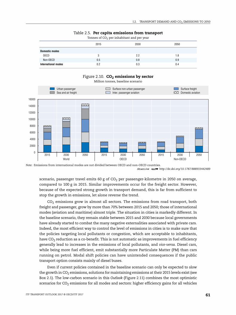
I.2. TRANSPORT DEMAND AND CO2 EMISSIONS TO 2050
442489
scenario, passenger travel emits 60 g of CO2 per passenger-kilometre in 2050 on average,
compared to 100 g in 2015. Similar improvements occur for the freight sector. However,
because of the expected strong growth in transport demand, this is far from sufficient to
stop the growth in emissions, let alone reverse the trend.
CO2 emissions grow in almost all sectors. The emissions from road transport, both
freight and passenger, grow by more than 70% between 2015 and 2050; those of international
modes (aviation and maritime) almost triple. The situation in cities is markedly different. In
the baseline scenario, they remain stable between 2015 and 2030 because local governments
have already started to combat the many negative externalities associated with private cars.
Indeed, the most efficient way to control the level of emissions in cities is to make sure that
the policies targeting local pollutants or congestion, which are acceptable to inhabitants,
have CO2 reduction as a co-benefit. This is not automatic as improvements in fuel efficiency
generally lead to increases in the emissions of local pollutants, and vice-versa. Diesel cars,
while being more fuel efficient, emit substantially more Particulate Matter (PM) than cars
running on petrol. Modal shift policies can have unintended consequences if the public
transport option consists mainly of diesel buses.
Even if current policies contained in the baseline scenario can only be expected to slow
the growth in CO2 emissions, solutions for maintaining emissions at their 2015 levels exist (see
Box 2.1). The low-carbon scenario in this Outlook (Figure 2.11) combines the most optimistic
scenarios for CO2 emissions for all modes and sectors: higher efficiency gains for all vehicles
Table 2.5. Per capita emissions from transportTonnes of CO2 per inhabitant and per year
2015 2030 2050
Domestic modes
OECD 3 2.2 1.8
Non-OECD 0.5 0.8 0.9
International modes 0.2 0.3 0.4
Figure 2.10. CO2 emissions by sectorMillion tonnes, baseline scenario
Note: Emissions from international modes are not divided between OECD and non-OECD countries.1 2 http://dx.doi.org/10.1787/888933
0
2000
4000
6000
8000
10000
12000
14000
16000
2015 2030 2050 2015 2030 2050 2015 2030 2050World OECD Non-OECD
Urban passenger Surface non-urban passenger Surface freightSea and air freight Inter. passenger aviation Domestic aviation
ITF TRANSPORT OUTLOOK 2017 © OECD/ITF 2017 61
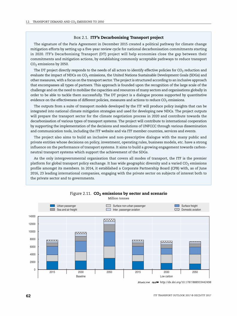
I.2. TRANSPORT DEMAND AND CO2 EMISSIONS TO 2050
ge ing eir ort
nd nd ch
the in ive
be uts the ion ion
nd ng n-
ier ns ne to
442498
Box 2.1. ITF’s Decarbonising Transport project
The signature of the Paris Agreement in December 2015 created a political pathway for climate chanmitigation efforts by setting up a five-year review cycle for national decarbonisation commitments startin 2020. ITF’s Decarbonising Transport (DT) project will help economies close the gap between thcommitments and mitigation actions, by establishing commonly acceptable pathways to reduce transpCO2 emissions by 2050.
The DT project directly responds to the needs of all actors to identify effective policies for CO2 reduction aevaluate the impact of NDCs on CO2 emissions, the United Nations Sustainable Development Goals (SDGs) aother measures, with a focus on the transport sector. The project is structured according to an inclusive approathat encompasses all types of partners. This approach is founded upon the recognition of the large scale of challenge and on the need to mobilise the capacities and resources of many sectors and organisations globallyorder to be able to tackle them successfully. The DT project is a dialogue process supported by quantitatevidence on the effectiveness of different policies, measures and actions to reduce CO2 emissions.
The outputs from a suite of transport models developed by the ITF will produce policy insights that canintegrated into national climate mitigation strategies and used for developing new NDCs. The project outpwill prepare the transport sector for the climate negotiation process in 2020 and contribute towards decarbonisation of various types of transport systems. The project will contribute to international cooperatby supporting the implementation of the decisions and resolutions of UNFCCC through various disseminatand communication tools, including the ITF website and via ITF member countries, services and events.
The project also aims to build an inclusive and non-prescriptive dialogue with the many public aprivate entities whose decisions on policy, investment, operating rules, business models, etc. have a stroinfluence on the performance of transport systems. It aims to build a growing engagement towards carboneutral transport systems which support the achievement of the SDGs.
As the only intergovernmental organisation that covers all modes of transport, the ITF is the premplatform for global transport policy exchange. It has wide geographic diversity and a varied CO2 emissioprofile amongst its members. In 2014, it established a Corporate Partnership Board (CPB) with, as of Ju2016, 23 leading international companies, engaging with the private sector on subjects of interest boththe private sector and to governments.
Figure 2.11. CO2 emissions by sector and scenarioMillion tonnes
1 2 http://dx.doi.org/10.1787/888933
0
2000
4000
6000
8000
10000
12000
14000
2015 2030 2050 2015 2030 2050Baseline Low carbon
Urban passenger Surface non-urban passenger Surface freightSea and air freight Inter. passenger aviation Domestic aviation
ITF TRANSPORT OUTLOOK 2017 © OECD/ITF 201762
I.2. TRANSPORT DEMAND AND CO2 EMISSIONS TO 2050
(including alternative fuels for ships), higher fuel taxes, full benefits of vehicle optimisation for
road freight and land use and public transport planning in the urban sector. In this scenario,
emissions in 2050 amount to 7 370 million tonnes compared to 13 600 in the baseline.
Accounting for surface transport only, the total emissions in 2050 amount to 5 900 million
tonnes, which is slightly above the 2DS target proposed by the IEA. However, it is still far from
the 2 000 million tonnes proposed as a target for the 1.5 degree scenario (Gota, forthcoming).
The mitigation efforts in the low-carbon scenario come from two main areas: road and
maritime transport. In the road sector, efficient technology, combined with modal shift
strategies in cities and optimisation and sharing measures for freight fleets have a
mitigation potential of almost 2 billion tonnes of CO2 per year by 2030. In the maritime, it
is the more optimistic efficiency gains for ships which deliver close to 800 million tonnes
of avoided CO2 emissions by the same year. The three chapters of Part 2 of this publication
detail the mitigation potential in each sector.
For passenger travel, technology brings most of the CO2 emission savings. It represents
between 60% and 80% of the mitigation effort in the urban scenarios, close to 100% in the
inter-urban. However, strong uncertainties remain as to the pace of penetration of fuel-
efficient technologies and alternative fuels. Except in the case of electric vehicles, current
technology is already lagging behind the 2DS scenario, from which emissions are derived in
the low-carbon scenarios of this Outlook (IEA, 2016). This makes the evolution of technology in
the coming decades hard to fathom. The uncertainties in technology directly come from the
uncertainties regarding the future price of fuels and economic growth. Low oil prices strongly
disincentivise the acquisition of more fuel efficient vehicles by individuals and companies.
Likewise, they are likely to delay the development of industrial solutions for the production of
biofuels, which are currently much more expensive than conventional fuels (see also the
emission section of Chapter 4 on aviation). Additionally, low economic growth puts a high risk
on investment, which includes investment in clean technology or alternative-fuel facilities.
References
CGDD (2016), “Covoiturage longue distance : état des lieux et potentiel de croissance”, Collection « Etudes et documents » du SEEIDD, Mai 2016, www.developpement-durable.gouv.fr/IMG/pdf/ED146.pdf.
Gota (forthcoming), Implications of 2DS and 1.5DS for Transport Sector Emissions in 2050.
Hakimi, D. et al. (2012), “Simulating a physical internet enabled mobility web: The case of mass distribution in France (p. 10 p.)”, the 9th International Conference on Modeling, Optimization & SIMulation – MOSIM’12, retrieved from https://hal.archives-ouvertes.fr/hal-00728584/document.
IEA (2016), “Tracking Clean Energy Progress 2016” in Energy Technology Perspectives 2016, OECD Publishing, Paris, http://dx.doi.org/10.1787/energy_tech-2016-en.
ITF (2016), “Shared Mobility: Innovation for Liveable Cities”, International Transport Forum Policy Papers, No. 21, OECD Publishing, Paris, http://dx.doi.org/10.1787/5jlwvz8bd4mx-en.
ITF (2015) ITF Transport Outlook 2015, OECD Publishing, Paris, http://dx.doi.org/10.1787/9789282107782-en.
KOTI/ITF (2015), Transport and Trade: Connecting Continents, Summary of the KOTI-ITF seminar, Seoul, 24 March 2015.
OECD/ITF (2011), Moving Freight with Better Trucks: Improving Safety, Productivity and Sustainability, OECD Publishing, Paris, http://dx.doi.org/10.1787/9789282102961-en.
Route Monkey (2016), Demonstrating the GHG reduction potential of asset sharing, asset optimization and other measures, Report of the Road Freight Lab, prepared on behalf of WBCSD members in the Low Carbon Technology Partnership initiative.
SLoCaT (2015), SLoCaT Preliminary Analysis of NDCs Sees Potential for Ambitious Action on Climate Change in the Transport Sector, available at www.slocat.net/news/1589.
ITF TRANSPORT OUTLOOK 2017 © OECD/ITF 2017 63
I.2. TRANSPORT DEMAND AND CO2 EMISSIONS TO 2050
ANNEX 2.A
The ITF modelling framework
The ITF Transport Outlook presents long-run scenarios, up to 2050, on the development
of global passenger mobility and freight volumes. Scenarios on both passenger and freight
activity are constructed using ITF modelling tools, which have been revised and extended
compared to earlier editions of the Outlook. The ITF tools are unified under single
framework where both input and output data are consistent.
As described in Figure 2.A1, the framework allows modelling a disaggregated,
exhaustive and global description of current and future transport volumes. Domestic, and
urban, non-urban domestic and international are forecasted in separate sub-models with
consistent scope to avoid any double counting. Population and gross domestic product (GDP)
are key drivers of a scenario. Population scenarios are based on world population projections
by the United Nations. GDP scenarios are based on long-term projections developed by the
OECD Environment Directorate. Moreover the ITF framework can assess the effect of a large
range of policies and exogenous impacts. In particular urban policies, such transit
infrastructure provision, parking or land use strategies can have significant impacts on
simulated modal distribution in cities.
Urban transport is estimated via a model based on the 1 667 cities with 300 000
inhabitants or more and results are extrapolated to all urban areas of the world. The model
simulates the evolution of variables that shape transport demand in cities – such as
population growth, economic activity, fuel prices, land use, availability of roads, quantity and
quality of public transport. The model derives levels of transport activity and modal shares
that would result under different scenarios, e.g. for policies that favour public transport or for
declining fuel prices. It is calibrated on a dataset resulting from an extensive collection from
various institutions and covering all the main regions of the world.
International transport is simulated by two distinct network models. The international
freight model projects transport activity in tonnes-km and related CO2 emissions up to 2050
based on alternative trade liberalisation scenarios. It takes as input the value flows from the
ENV Linkage model, the general equilibrium model of Environment directorate of the OECD
that are split into according modes and then converted into tonnes using a weight to value
module. Finally flows are divided between routes using a capacity constrained assignment
procedure. The model takes in account flows of 19 commodities on a zoning system of
333 regions.
The ITF air passenger model is a forecasting tool to study aviation policies. The model
derives the evolution of international passenger volumes (number of passengers and
revenue passenger-kilometres) up to 2050 according to different policy scenarios. The
ITF TRANSPORT OUTLOOK 2017 © OECD/ITF 201764
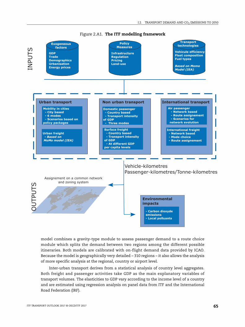
I.2. TRANSPORT DEMAND AND CO2 EMISSIONS TO 2050
tres
model combines a gravity-type module to assess passenger demand to a route choice
module which splits the demand between two regions among the different possible
itineraries. Both models are calibrated with on-flight demand data provided by ICAO.
Because the model is geographically very detailed – 310 regions – it also allows the analysis
of more specific analysis at the regional, country or airport level.
Inter-urban transport derives from a statistical analysis of country level aggregates.
Both freight and passenger activities take GDP as the main explanatory variables of
transport volumes. The elasticities to GDP vary according to the income level of a country
and are estimated using regression analysis on panel data from ITF and the International
Road Federation (IRF).
Figure 2.A1. The ITF modelling framework
GDPTradeDemographics Urbanisation Energy prices
Exogeneous factors
Infrastructure RegulationPricingLand-use
Policy Measures
Vehicule efficiencyFleet composition Fuel types
Based on MomoModel (IEA)
Transporttechnologies
Vehicle-kilometresPassenger-kilometres/Tonne-kilome
Assignement on a common network and zoning system
- Carbon dioxydeemissions- Local polluants
Environmentalimpacts
INPU
TSO
UTP
UTS
Urban transport International transportNon urban transport
Surface freight - Country based - Transport intensity of GDP - At different GDP per capita levels
Domestic passenger - Country based - Transport intensity of GDP - Three modes
Air passenger - Network based - Route assignement - Scenarios for network evolution
Mobility in cities - City based - 6 modes - Scenarios based onpolicy packages
Urban freight - Based on MoMo model (IEA)
International freight - Network based - Mode choice - Route assignement
ITF TRANSPORT OUTLOOK 2017 © OECD/ITF 2017 65


PART II
Sectoral outlook
ITF TRANSPORT OUTLOOK 2017 © OECD/ITF 2017

ITF Transport Outlook 2017 © OECD/ITF 2017
PART II
Chapter 3
International freight
This chapter presents results from the International Transport Forum’s (ITF) International Freight Model with projections for international trade-related freight flows and CO2 emissions up to 2050. The chapter highlights uncertainties in future trade projections and discusses their implications for freight movements. It then presents alternative scenarios for future CO2 emissions from international freight. The chapter also discusses the impacts of growing transport demand on capacity needs in ports and hinterland connections. It addresses the challenges of hinterland transport and finally provides guidelines for decision makers when planning for the future of international freight.
69
II.3. INTERNATIONAL FREIGHT
World trade growth remains weak and the volume of international trade-related freight
movement is growing at a significantly slower pace than prior to 2008. The drop in global
trade demand and increased protectionism, combined with aggressive ordering of
additional and larger ships over recent years, has pushed the shipping sector further into
a crisis. Overcapacity in shipping has reduced ocean freight rates to very low levels. This
decrease in the cost of maritime transport has not resulted in significantly more trade, but
rather has driven the shipping industry into unsustainable debt, resulting in bankruptcy
for several shipping companies. In container shipping, increasing ship size has intensified
consolidation of the sector and increased cooperation via alliances.
This crisis has ripple-effects for the whole global supply chain. Many countries have
overinvested in ports, having used the same optimistic demand projections as shipping
companies. As a result, ports suffer from overcapacity and the financial performance of the
terminal sector is under pressure. In container shipping, the cargo concentration due to
mega-ships and alliances has resulted in less frequent port calls and rationalisation of
shipping services, leaving an increasing number of ports and terminals with less or no
cargo to handle. At the same time, this concentration of container port throughput has
resulted in increased congestion for hinterland transport in some regions.
In the medium and long term, trade growth will likely pick up, but projections are
clouded with much uncertainty. Our projections show that by 2050 international trade-
related freight could still triple, but this hinges on various assumptions that may not hold.
The carbon emissions from international trade-related freight transport could grow by
120% by 2050 if no additional actions are taken. Because of the international nature of
shipping and aviation, their emissions are not part of the current negotiations under the
aegis of the United Nations Framework Climate Change Convention (UNFCCC). Instead,
they are dealt with in the context of the International Maritime Organisation (IMO) and
International Civil Aviation Organisation (ICAO), both specialised agencies of the United
Nations. The challenge will be to reduce the carbon intensity of freight transport. Although
this might be feasible using optimisation of networks and more stringent technologies,
new policy measures and alternative fuels would be needed to reach such a pathway.
Investment needs in ports and trade-related surface transport networks are also
significant but planning is difficult due to this current uncertain climate. Evidence suggests
that estimated capacity improvements currently announced are sufficient while several
regions actually have over planned these needs.
Transport actors will need to find ways to adapt to these uncertainties. Rather than
considering the future as an extrapolation of the past, freight transport companies and
policy makers will need to plan for uncertainties and divergent possible scenarios for the
future. In particular for long-term transport planning, both in the private and public sector,
knowledge and understanding the possible implications of the evolving trends outlined
above will be essential.
ITF TRANSPORT OUTLOOK 2017 © OECD/ITF 201770
II.3. INTERNATIONAL FREIGHT
Underlying trade projectionsThe conditions for global trade have worsened since the International Transport
Forum’s (ITF) 2015 Transport Outlook. In 2016, global trade growth retracted and the short term
outlook has not improved. Recent years have seen an increase in trade restrictions and rising
challenges to finalise negotiations on trade agreements, such as the Trans-Pacific
Partnership (TTP) and Transatlantic Trade and Investment Partnership (TTIP). Moreover, we
seem to have reached the limits of a global outsourcing model: the proliferation of global
value chains has halted and manufacturing has become more regionalised.
As discussed in Chapter 1, world trade has slowed not only in absolute terms but also in
relation to Gross Domestic Product (GDP) in recent years. In the two decades preceding the
financial crisis, world trade expanded rapidly and outpaced GDP growth. This relationship
has declined since 2008-09 (Figure 1.2 in Chapter 1). In our underlying economic projections,
growth in trade is still expected to outpace GDP growth over the next 40 years, although at a
lower scale than during the pre-crisis decades. World trade is estimated to grow at around
3.5% annually (compared with 6.9% over the period 1990-2007), implying a permanently
lower elasticity of trade to GDP.
Several reasons, both cyclical and structural, have been put forward to explain the
changes in trade elasticity (for discussion on trade elasticities, see OECD, 2016; Constantinescu
et al., 2015; ECB, 2014). The cyclical reasons take root in the state of the global economy
following the global crisis. The crisis hit advanced economies, and especially the EU, hardest
and their contribution to trade elasticity fell sharply during the crisis. Investment, the most
trade-intensive component of domestic demand, also suffered during the crisis. However,
these are more the manifestation of a decline in the overall global activity rather than of
changes in trade elasticity.
Other longer-term structural changes can explain the observed shift in elasticity.
Emerging economies are moving up in the value chain resulting in an increase in the
domestic value-added component of exports. The main contributors to world growth over
the next half century will rely less on export-led growth than in the past decades. It also
reflects that the intensity of fragmentation of global value chains is slowing down as there
are likely physical limits on how much a product and tasks can be fragmented (Fontagné
and Fouré, 2013). Indeed, there is evidence of consolidation of global supply chains since
2008, rather than fragmentation as previously observed.
The most recent work by the Organisation for Economic Co-operation and Development
(OECD) suggests that the pace of trade liberalisation is an important factor in the slowdown
of world trade growth (OECD, 2016). This would seem to support the notion that there is some
evidence of increasing protectionism since the start of the economic crisis. This study also
finds evidence that the consolidation of global value chains has played a role in the
slowdown of word trade.
The results further suggest that growth and income convergence consistent with our
underlying GDP projections will generate a trade to GDP ratio of 1.1, which could be
considered as the lower limit provided GDP per capita continues to grow and protectionism
does not increase further. Assuming full trade liberalisation would result, on the basis of the
OECD’s long-term baseline projections in a trade to GDP ratio of 1.4. This constitutes the
upper bound for the long-term ratio (OECD, 2016).
To capture interdependencies between global trade patterns and freight flows, we
present two alternative trade scenarios: Low elasticity and High elasticity, corresponding to
ITF TRANSPORT OUTLOOK 2017 © OECD/ITF 2017 71
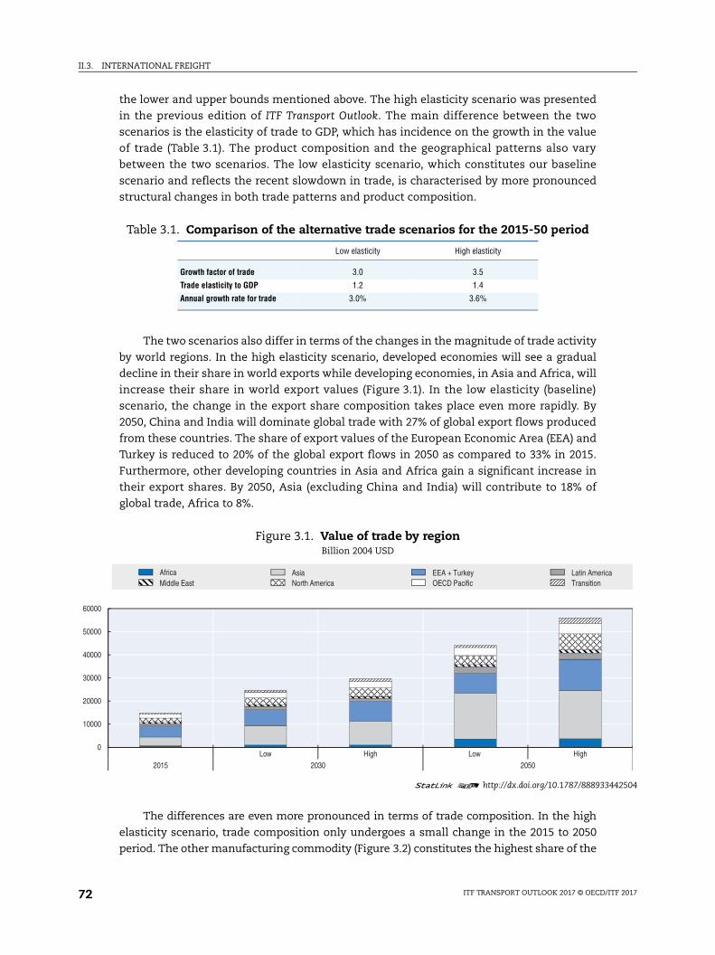
II.3. INTERNATIONAL FREIGHT
442504
a
the lower and upper bounds mentioned above. The high elasticity scenario was presented
in the previous edition of ITF Transport Outlook. The main difference between the two
scenarios is the elasticity of trade to GDP, which has incidence on the growth in the value
of trade (Table 3.1). The product composition and the geographical patterns also vary
between the two scenarios. The low elasticity scenario, which constitutes our baseline
scenario and reflects the recent slowdown in trade, is characterised by more pronounced
structural changes in both trade patterns and product composition.
The two scenarios also differ in terms of the changes in the magnitude of trade activity
by world regions. In the high elasticity scenario, developed economies will see a gradual
decline in their share in world exports while developing economies, in Asia and Africa, will
increase their share in world export values (Figure 3.1). In the low elasticity (baseline)
scenario, the change in the export share composition takes place even more rapidly. By
2050, China and India will dominate global trade with 27% of global export flows produced
from these countries. The share of export values of the European Economic Area (EEA) and
Turkey is reduced to 20% of the global export flows in 2050 as compared to 33% in 2015.
Furthermore, other developing countries in Asia and Africa gain a significant increase in
their export shares. By 2050, Asia (excluding China and India) will contribute to 18% of
global trade, Africa to 8%.
The differences are even more pronounced in terms of trade composition. In the high
elasticity scenario, trade composition only undergoes a small change in the 2015 to 2050
period. The other manufacturing commodity (Figure 3.2) constitutes the highest share of the
Table 3.1. Comparison of the alternative trade scenarios for the 2015-50 period
Low elasticity High elasticity
Growth factor of trade 3.0 3.5
Trade elasticity to GDP 1.2 1.4
Annual growth rate for trade 3.0% 3.6%
Figure 3.1. Value of trade by regionBillion 2004 USD
1 2 http://dx.doi.org/10.1787/888933
0
10000
20000
30000
40000
50000
60000
Low High Low High2015 2030 2050
Africa Asia EEA + Turkey Latin AmericMiddle East North America OECD Pacific Transition
ITF TRANSPORT OUTLOOK 2017 © OECD/ITF 201772
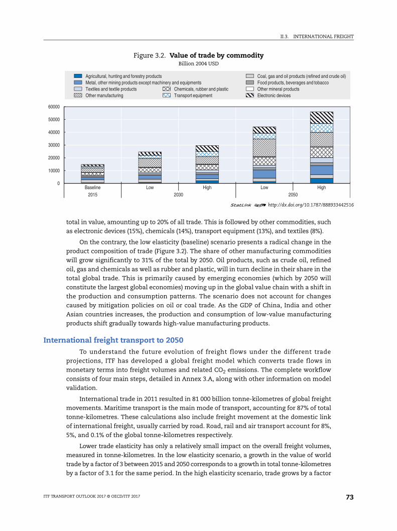
II.3. INTERNATIONAL FREIGHT
442516
e oil)
total in value, amounting up to 20% of all trade. This is followed by other commodities, such
as electronic devices (15%), chemicals (14%), transport equipment (13%), and textiles (8%).
On the contrary, the low elasticity (baseline) scenario presents a radical change in the
product composition of trade (Figure 3.2). The share of other manufacturing commodities
will grow significantly to 31% of the total by 2050. Oil products, such as crude oil, refined
oil, gas and chemicals as well as rubber and plastic, will in turn decline in their share in the
total global trade. This is primarily caused by emerging economies (which by 2050 will
constitute the largest global economies) moving up in the global value chain with a shift in
the production and consumption patterns. The scenario does not account for changes
caused by mitigation policies on oil or coal trade. As the GDP of China, India and other
Asian countries increases, the production and consumption of low-value manufacturing
products shift gradually towards high-value manufacturing products.
International freight transport to 2050To understand the future evolution of freight flows under the different trade
projections, ITF has developed a global freight model which converts trade flows in
monetary terms into freight volumes and related CO2 emissions. The complete workflow
consists of four main steps, detailed in Annex 3.A, along with other information on model
validation.
International trade in 2011 resulted in 81 000 billion tonne-kilometres of global freight
movements. Maritime transport is the main mode of transport, accounting for 87% of total
tonne-kilometres. These calculations also include freight movement at the domestic link
of international freight, usually carried by road. Road, rail and air transport account for 8%,
5%, and 0.1% of the global tonne-kilometres respectively.
Lower trade elasticity has only a relatively small impact on the overall freight volumes,
measured in tonne-kilometres. In the low elasticity scenario, a growth in the value of world
trade by a factor of 3 between 2015 and 2050 corresponds to a growth in total tonne-kilometres
by a factor of 3.1 for the same period. In the high elasticity scenario, trade grows by a factor
Figure 3.2. Value of trade by commodityBillion 2004 USD
1 2 http://dx.doi.org/10.1787/888933
0
10000
20000
30000
40000
50000
60000
Baseline Low High Low High2015 2030 2050
Agricultural, hunting and forestry products Coal, gas and oil products (refined and crudMetal, other mining products except machinery and equipments Food products, beverages and tobaccoTextiles and textile products Chemicals, rubber and plastic Other mineral productsOther manufacturing Transport equipment Electronic devices
ITF TRANSPORT OUTLOOK 2017 © OECD/ITF 2017 73
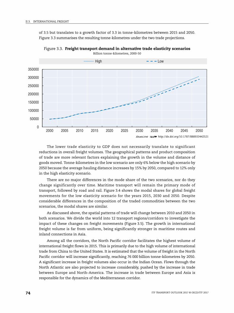
II.3. INTERNATIONAL FREIGHT
442521
50
of 3.5 but translates to a growth factor of 3.3 in tonne-kilometres between 2015 and 2050.
Figure 3.3 summarises the resulting tonne-kilometres under the two trade projections.
The lower trade elasticity to GDP does not necessarily translate to significant
reductions in overall freight volumes. The geographical patterns and product composition
of trade are more relevant factors explaining the growth in the volume and distance of
goods moved. Tonne-kilometres in the low scenario are only 6% below the high scenario by
2050 because the average hauling distance increases by 15% by 2050, compared to 12% only
in the high elasticity scenario.
There are no major differences in the mode share of the two scenarios, nor do they
change significantly over time. Maritime transport will remain the primary mode of
transport, followed by road and rail. Figure 3.4 shows the modal shares for global freight
movements for the low elasticity scenario for the years 2015, 2030 and 2050. Despite
considerable differences in the composition of the traded commodities between the two
scenarios, the modal shares are similar.
As discussed above, the spatial patterns of trade will change between 2010 and 2050 in
both scenarios. We divide the world into 12 transport regions/corridors to investigate the
impact of these changes on freight movements (Figure 3.5). The growth in international
freight volume is far from uniform, being significantly stronger in maritime routes and
inland connections in Asia.
Among all the corridors, the North Pacific corridor facilitates the highest volume of
international freight flows in 2015. This is primarily due to the high volume of international
trade from China to the United States. It is estimated that the volume of freight in the North
Pacific corridor will increase significantly, reaching 76 000 billion tonne-kilometres by 2050.
A significant increase in freight volumes also occur in the Indian Ocean. Flows through the
North Atlantic are also projected to increase considerably, pushed by the increase in trade
between Europe and North-America. The increase in trade between Europe and Asia is
responsible for the dynamics of the Mediterranean corridor.
Figure 3.3. Freight transport demand in alternative trade elasticity scenariosBillion tonne-kilometres, 2000-50
1 2 http://dx.doi.org/10.1787/888933
0
50000
100000
150000
200000
250000
300000
350000
2000 2005 2010 2015 2020 2025 2030 2035 2040 2045 20
High Low
ITF TRANSPORT OUTLOOK 2017 © OECD/ITF 201774
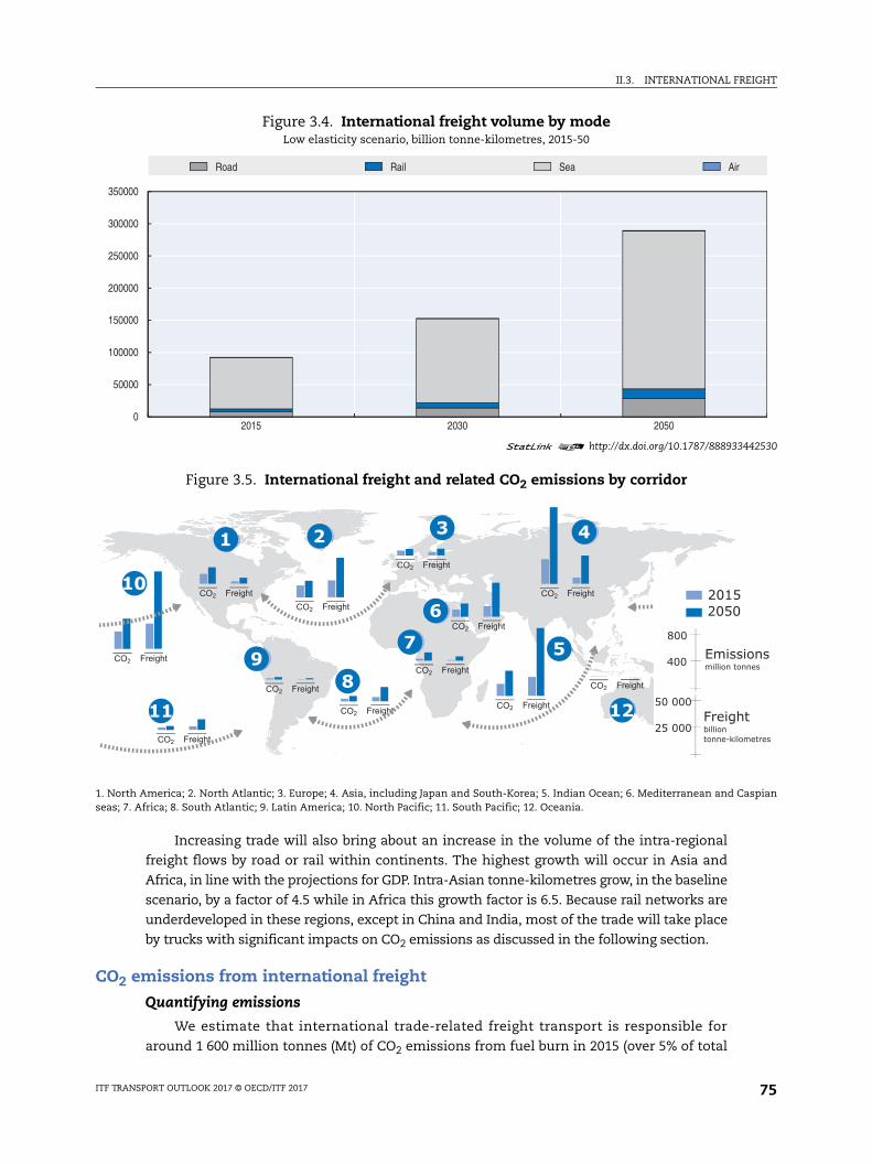
II.3. INTERNATIONAL FREIGHT
442530
aspian
ionsnnes
tmetres
Increasing trade will also bring about an increase in the volume of the intra-regional
freight flows by road or rail within continents. The highest growth will occur in Asia and
Africa, in line with the projections for GDP. Intra-Asian tonne-kilometres grow, in the baseline
scenario, by a factor of 4.5 while in Africa this growth factor is 6.5. Because rail networks are
underdeveloped in these regions, except in China and India, most of the trade will take place
by trucks with significant impacts on CO2 emissions as discussed in the following section.
CO2 emissions from international freight
Quantifying emissions
We estimate that international trade-related freight transport is responsible for
around 1 600 million tonnes (Mt) of CO2 emissions from fuel burn in 2015 (over 5% of total
Figure 3.4. International freight volume by modeLow elasticity scenario, billion tonne-kilometres, 2015-50
1 2 http://dx.doi.org/10.1787/888933
Figure 3.5. International freight and related CO2 emissions by corridor
1. North America; 2. North Atlantic; 3. Europe; 4. Asia, including Japan and South-Korea; 5. Indian Ocean; 6. Mediterranean and Cseas; 7. Africa; 8. South Atlantic; 9. Latin America; 10. North Pacific; 11. South Pacific; 12. Oceania.
0
50000
100000
150000
200000
250000
300000
350000
2015 2030 2050
Road Rail Sea Air
CO2 Freight
CO2 Freight
CO2 Freight
CO2 Freight
CO2 Freight
CO2 Freight
CO2 Freight
CO2 Freight
CO2 Freight
CO2 Freight
CO2 Freight
CO2 Freight
Emissmillion to400
800
Freighbilliontonne-kilo
25 000
50 000
20152050
321 3 4
5
6
7
811
10
9
12
ITF TRANSPORT OUTLOOK 2017 © OECD/ITF 2017 75
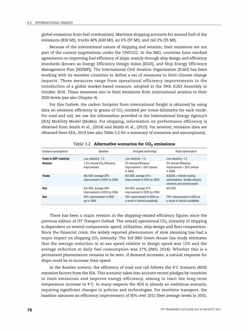
II.3. INTERNATIONAL FREIGHT
global emissions from fuel combustion). Maritime shipping accounts for around half of the
emissions (830 Mt), trucks 40% (630 Mt), air 6% (97 Mt), and rail 2% (35 Mt).
Because of the international nature of shipping and aviation, their emissions are not
part of the current negotiations under the UNFCCC. In the IMO, countries have reached
agreements on improving fuel efficiency of ships, mainly through ship design and efficiency
standards (known as Energy Efficiency Design Index [EEDI], and Ship Energy Efficiency
Management Plan [SEEMP]). The International Civil Aviation Organization (ICAO) has been
working with its member countries to define a set of measures to limit climate change
impacts. These measures range from operational efficiency improvements to the
introduction of a global market-based measure, adopted at the 39th ICAO Assembly in
October 2016. These measures aim to limit emissions from international aviation to their
2020 levels (see also Chapter 4).
For this Outlook, the carbon footprint from international freight is obtained by using
data on emission efficiency in grams of CO2 emitted per tonne-kilometre for each mode.
For road and rail, we use the information provided in the International Energy Agency’s
(IEA) Mobility Model (MoMo). For shipping, information on performance efficiency is
obtained from Smith et al., (2014) and Smith et al., (2015). For aviation, emission data are
obtained from EEA, 2014 (see also Table 3.2 for a summary of scenarios and assumptions).
There has been a major revision in the shipping-related efficiency figures since the
previous edition of ITF Transport Outlook. The overall operational CO2 intensity of shipping
is dependent on several components: speed, utilisation, ship design and fleet composition.
Since the financial crisis, the widely reported phenomenon of slow steaming has had a
major impact on shipping CO2 intensity. The 3rd IMO Green House Gas study estimates
that the average reduction in at-sea speed relative to design speed was 12% and the
average reduction in daily fuel consumption was 27% (IMO, 2014). Whether this is a
permanent phenomenon remains to be seen. If demand increases, a natural response for
ships could be to increase their speed.
In the Baseline scenario, the efficiency of road and rail follows the 4°C Scenario (4DS)
emission factors from the IEA. This scenario takes into account recent pledges by countries
to limit emissions and improve energy efficiency, aiming to limit the long-term
temperature increase to 4°C. In many respects the 4DS is already an ambitious scenario,
requiring significant changes in policies and technologies. For maritime transport, the
baseline assumes an efficiency improvement of 50% over 2012 fleet average levels in 2050,
Table 3.2. Alternative scenarios for CO2 emissions
Scenario assumptions Baseline Stringent technology Road optimisation
Trade to GDP elasticity Low elasticity: 1.2 Low elasticity: 1.2 Low elasticity: 1.2
Aviation 1.5% Annual CO2 Efficiency Improvement
2% Annual Efficiency Improvement + 50% biofuel in 2050
2% Annual Efficiency Improvement + 50% biofuel in 2050
Trucks IEA 4DS: average 20% improvement in EEOI by 2050
IEA 2DS: average 35% improvement in EEOI by 2050
IEA2DS + Vehicle routing optimisations, flexible delivery windows and shared assets
Rail IEA 4DS: average 39% improvement in EEOI by 2050
IEA 2DS: average 47% improvement in EEOI by 2050
IEA 2DS
Sea 50% improvement in EEOI up to 2050
70% improvement in EEOI as a result of biofuel availability
70% improvement in EEOI as a result of biofuel availability
ITF TRANSPORT OUTLOOK 2017 © OECD/ITF 201776
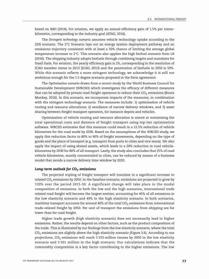
II.3. INTERNATIONAL FREIGHT
based on IMO (2014). For aviation, we apply an annual efficiency gain of 1.5% per tonne-
kilometre, corresponding to the industry goal (ATAG, 2016).
The Stringent technology scenario assumes vehicle technology uptake according to the
2DS scenario. The 2°C Scenario lays out an energy system deployment pathway and an
emissions trajectory consistent with at least a 50% chance of limiting the average global
temperature increase to 2°C. This scenario also applies the high biofuel scenario from LR
(2016). The shipping industry adopts biofuels through combining targets and mandates for
fossil fuels. For aviation, the yearly efficiency gain is 2%, corresponding to the resolution of
ICAO member states in 2013 (ICAO, 2013) and the penetration of biofuels in 2050 is 50%.
While this scenario reflects a more stringent technology, we acknowledge it is still not
ambitious enough for the 1.5 degree scenario proposed in the Paris agreement.
The Optimisation scenario draws from a recent study by the World Business Council for
Sustainable Development (WBCSD) which investigates the efficacy of different measures
that can be adopted by private road freight operators to reduce their CO2 emissions (Route
Monkey, 2016). In this scenario, we incorporate impacts of the measures, in combination
with the stringent technology scenario. The measures include: 1) optimisation of vehicle
routing and resource allocations; 2) avoidance of narrow delivery windows, and 3) asset
sharing between freight transport operators, for instance depots and vehicles.
Optimisation of vehicle routing and resource allocation is aimed at minimising the
total operational costs and distance of freight transport using top-tier optimisation
software. WBCSD estimates that this measure could result in a 12.5% reduction of vehicle
kilometres for the road mode by 2030. Based on the assumptions of the WBCSD study, we
apply this reduction factor to 80% to 90% of freight movements, depending on the type of
goods and the place of transport (e.g. transport from ports to cities and vice versa). We also
apply the impact of using shared assets, which leads to a 20% reduction in road vehicle-
kilometres by 2030 for 80% of all transport. Lastly, the study also concludes that 25% of road
vehicle-kilometres, mostly concentrated in cities, can be reduced by means of a business
model that avoids a narrow delivery time window by 2020.
Long-term outlook for CO2 emissions
The projected tripling of freight transport will translate to a significant increase in
related CO2 emissions by 2050. In the baseline scenario, emissions are projected to grow by
120% over the period 2015-50. A significant change will take place in the modal
composition of emissions. In both the low and the high scenarios, international trade
related road freight will become the largest emitter, accounting for 45% of all emissions in
the low elasticity scenario and 49% in the high elasticity scenario. In both scenarios,
maritime transport accounts for around 40% of the total CO2 emissions from international
trade-related freight by 2050. Per unit of transport the emissions from shipping are far
lower than for road freight.
Higher trade growth (high elasticity scenario) does not necessarily lead to higher
emissions. Rather, the results depend on other factors, such as the product composition of
the trade. This is illustrated by our findings from the low elasticity scenario, where the total
CO2 emissions are slightly above the high elasticity scenario (Figure 3.6). According to our
projections, CO2 emissions will reach 3 533 million tonnes by 2050 in the low elasticity
scenario and 3 501 million in the high scenario. Our calculations indicate that the
commodity composition is a key factor contributing to the higher emissions. The low
ITF TRANSPORT OUTLOOK 2017 © OECD/ITF 2017 77
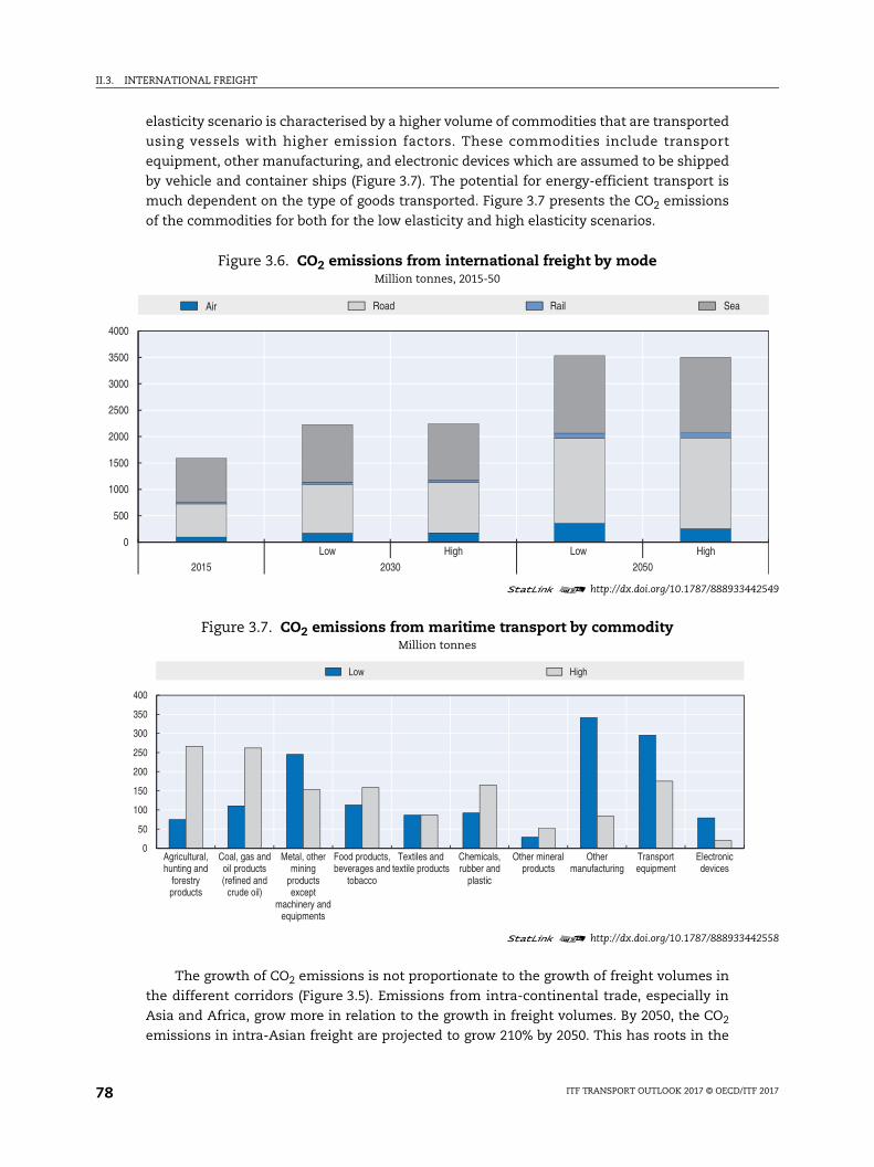
II.3. INTERNATIONAL FREIGHT
442549
442558
elasticity scenario is characterised by a higher volume of commodities that are transported
using vessels with higher emission factors. These commodities include transport
equipment, other manufacturing, and electronic devices which are assumed to be shipped
by vehicle and container ships (Figure 3.7). The potential for energy-efficient transport is
much dependent on the type of goods transported. Figure 3.7 presents the CO2 emissions
of the commodities for both for the low elasticity and high elasticity scenarios.
The growth of CO2 emissions is not proportionate to the growth of freight volumes in
the different corridors (Figure 3.5). Emissions from intra-continental trade, especially in
Asia and Africa, grow more in relation to the growth in freight volumes. By 2050, the CO2
emissions in intra-Asian freight are projected to grow 210% by 2050. This has roots in the
Figure 3.6. CO2 emissions from international freight by modeMillion tonnes, 2015-50
1 2 http://dx.doi.org/10.1787/888933
Figure 3.7. CO2 emissions from maritime transport by commodityMillion tonnes
1 2 http://dx.doi.org/10.1787/888933
0
500
1000
1500
2000
2500
3000
3500
4000
Low High Low High2015 2030 2050
Air Road Rail Sea
0
50
100
150
200
250
300
350
400
Agricultural,hunting and
forestryproducts
Coal, gas andoil products(refined and
crude oil)
Metal, othermining
productsexcept
machinery andequipments
Food products,beverages and
tobacco
Textiles andtextile products
Chemicals,rubber and
plastic
Other mineralproducts
Othermanufacturing
Transportequipment
Electronicdevices
Low High
ITF TRANSPORT OUTLOOK 2017 © OECD/ITF 201778
II.3. INTERNATIONAL FREIGHT
442569
lack of alternative, more environmentally-friendly modes for trucks for the movement of
goods in these regions, except in China and India. Another factor contributing to this trend
includes the slower adoption of more environmentally friendly fuel technologies.
Figure 3.8 shows the rate of reduction of CO2 emission intensity for different regions in the
world in our baseline scenario, based on the IEA’s Mobility Model.
As a result, CO2 emissions across intra-regional corridors are generally higher per unit
of transport compared with other corridors. This is seen for example in the case of the North
Pacific and Indian Ocean corridors where the total tonne-kilometres are among the highest
but their CO2 emissions are below what is produced in the intra-Asia corridor (Figure 3.5).
Alternative pathways
While trade composition is a significant driver of related transport CO2 emissions,
policies and operational measures have a major effect on future emissions.
Figure 3.9 presents the comparison of the impact of different measures on CO2
emissions, by mode, for the years 2030 and 2050. With the Stringent technology scenario,
total emissions would still grow by nearly 40% from 2015. This is driven by still increasing
emissions from the road freight where technology improvements comparable to the 2DS
scenario are not sufficient to curb the growth in emissions. However, combined with
operational improvements in the road sector, the emissions would remain almost at their
2015 levels.
The stringent technology scenario results in a significant reduction in total CO2
emissions, compared with the baseline scenario. This reduction is driven by reduction in
the use of fossil fuel. By 2030, the mid-range market penetration of biofuels, other energy
efficiency measures and availability of hydrogen for the shipping industry will lead to a
27% reduction in CO2 emissions from international shipping compared with the baseline.
By 2050, this reduction is even more significant, reaching up to 50% of the baseline. As a
Figure 3.8. Road freight CO2 intensity by region in the 4 degree scenario of the IEA Mobility Model
Tonne of CO2 per vehicle-kilometre
1 2 http://dx.doi.org/10.1787/888933
0.0005
0.0006
0.0007
0.0008
0.0009
0.001
0.0011
0.0012
0.0013
0.0014
2015 2020 2025 2030 2035 2040 2045 2050
China India Middle East Latin AmericaAfrica World EU27
ITF TRANSPORT OUTLOOK 2017 © OECD/ITF 2017 79
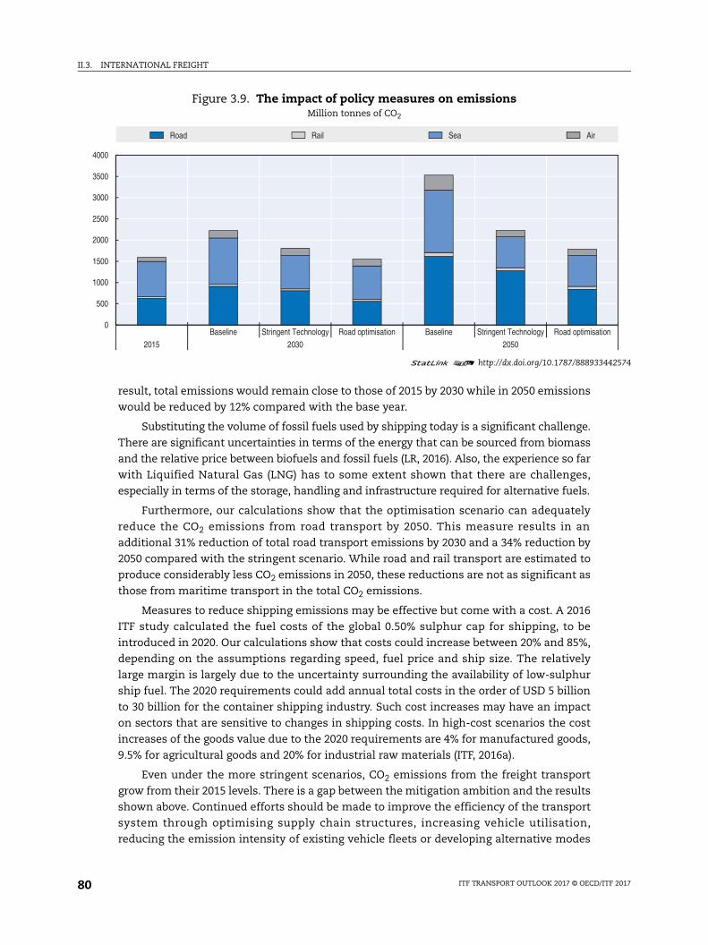
II.3. INTERNATIONAL FREIGHT
442574
ion
result, total emissions would remain close to those of 2015 by 2030 while in 2050 emissions
would be reduced by 12% compared with the base year.
Substituting the volume of fossil fuels used by shipping today is a significant challenge.
There are significant uncertainties in terms of the energy that can be sourced from biomass
and the relative price between biofuels and fossil fuels (LR, 2016). Also, the experience so far
with Liquified Natural Gas (LNG) has to some extent shown that there are challenges,
especially in terms of the storage, handling and infrastructure required for alternative fuels.
Furthermore, our calculations show that the optimisation scenario can adequately
reduce the CO2 emissions from road transport by 2050. This measure results in an
additional 31% reduction of total road transport emissions by 2030 and a 34% reduction by
2050 compared with the stringent scenario. While road and rail transport are estimated to
produce considerably less CO2 emissions in 2050, these reductions are not as significant as
those from maritime transport in the total CO2 emissions.
Measures to reduce shipping emissions may be effective but come with a cost. A 2016
ITF study calculated the fuel costs of the global 0.50% sulphur cap for shipping, to be
introduced in 2020. Our calculations show that costs could increase between 20% and 85%,
depending on the assumptions regarding speed, fuel price and ship size. The relatively
large margin is largely due to the uncertainty surrounding the availability of low-sulphur
ship fuel. The 2020 requirements could add annual total costs in the order of USD 5 billion
to 30 billion for the container shipping industry. Such cost increases may have an impact
on sectors that are sensitive to changes in shipping costs. In high-cost scenarios the cost
increases of the goods value due to the 2020 requirements are 4% for manufactured goods,
9.5% for agricultural goods and 20% for industrial raw materials (ITF, 2016a).
Even under the more stringent scenarios, CO2 emissions from the freight transport
grow from their 2015 levels. There is a gap between the mitigation ambition and the results
shown above. Continued efforts should be made to improve the efficiency of the transport
system through optimising supply chain structures, increasing vehicle utilisation,
reducing the emission intensity of existing vehicle fleets or developing alternative modes
Figure 3.9. The impact of policy measures on emissionsMillion tonnes of CO2
1 2 http://dx.doi.org/10.1787/888933
0
500
1000
1500
2000
2500
3000
3500
4000
Baseline Stringent Technology Road optimisation Baseline Stringent Technology Road optimisat2015 2030 2050
Road Rail Sea Air
ITF TRANSPORT OUTLOOK 2017 © OECD/ITF 201780

II.3. INTERNATIONAL FREIGHT
of transport especially for hinterland connectivity. Fuel economy standards for trucks are
currently limited to four countries (United States, China, Japan and Canada) but they are
gaining momentum. According to the ICCT (Muncrief, 2014), countries considering the
introduction of efficiency regulations concern 80% of all trucks. An integrated approach to
improving the efficiency of new trucks combine three policy elements: information
measures (such as fuel economy or CO2 emissions labelling); standard setting for vehicle
fuel economy and CO2 emissions; and fiscal measures (such as vehicle taxes/tax incentives
and fuel taxes).
CO2 reduction strategies focus typically on vehicle technology, and technological
improvements can do much to de-carbonise transport. Yet there are many other
contributing measures the sector can implement, including vehicle maintenance, driver
training, vehicle loading, routing and scheduling. Higher capacity vehicles have a
potential to improve fuel efficiency and reduce emissions. Improving the efficiency of
operations can have a significant contribution to emission reduction while making
business more profitable. Better route planning, for example, can deliver significant
efficiency gains for companies through reduced fuel costs, while contributing at the same
time to emission reduction. Making more use of shared transport options and
opportunities can results in reductions of both cost and CO2 by creating logistics synergies
and limiting empty runs.
To meet climate mitigation goals, it is important to align policies across supply chains
to decarbonise transport. In addition to international agreements, national policies are
needed for reducing CO2 emissions. Economic measures, regulation, infrastructure and
land-use policies at the national level need to be aligned with industry actions to improve
vehicle design and utilisation, shared loading or use of alternative fuels. Improving
logistics and optimising supply chains can have a significant impact on reducing CO2
emissions form international trade related freight transport.
Impact of trade liberalisation
Trade is an important engine of growth. The related expansion of global value chains,
together with trade, boost economic growth through increased productivity by improving
resource allocation, increasing scale and specialisation, encouraging innovative activities,
facilitating knowledge transfer, fostering the expansion of more productive firms and the
exit of least productive ones. Impact of trade liberalisation on trade and growth is studied
extensively in the literature and empirical literature suggest that trade liberalisation
continuing at the same pace as during the 1990s could boost world trade growth by 1-2%
per year.
However, the objective of trade growth might contradict the objectives for more
sustainable transport. The research on the impact of trade liberalisation on international
freight volumes, the geographical composition of that freight and related CO2 emissions is
limited. The 2015 edition of the Transport Outlook assessed the impact of two alternative
trade liberalisation scenarios on freight volumes and related CO2 emissions (ITF, 2015a).
In the Bilateral liberalisation scenario, a free-trade agreement is established in 2012
between the North American Free Trade Area (NAFTA), the European Free Trade Area (EFTA),
Australia, New Zealand, Japan and Korea. Tariffs and transaction costs (such as handling at
customs) are progressively phased out in this region. Tariffs on goods are abolished by 2060
and transaction costs for goods are reduced by 25% more than in the baseline by 2060. In
ITF TRANSPORT OUTLOOK 2017 © OECD/ITF 2017 81
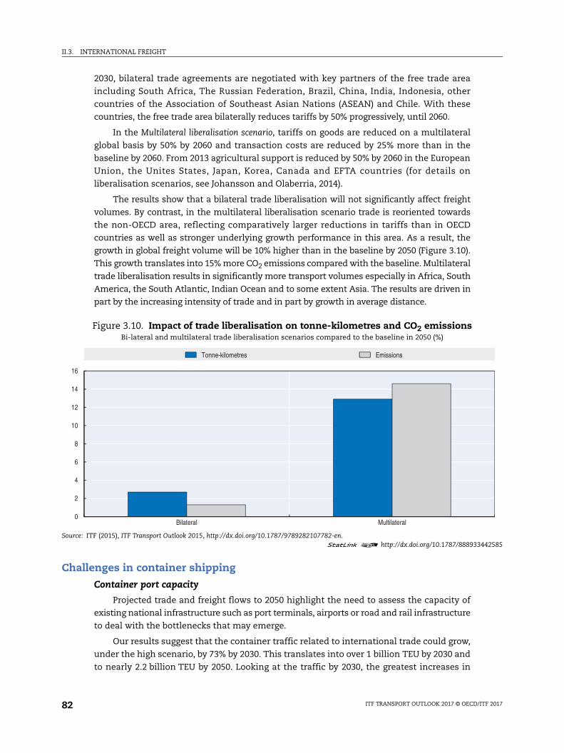
II.3. INTERNATIONAL FREIGHT
442585
2030, bilateral trade agreements are negotiated with key partners of the free trade area
including South Africa, The Russian Federation, Brazil, China, India, Indonesia, other
countries of the Association of Southeast Asian Nations (ASEAN) and Chile. With these
countries, the free trade area bilaterally reduces tariffs by 50% progressively, until 2060.
In the Multilateral liberalisation scenario, tariffs on goods are reduced on a multilateral
global basis by 50% by 2060 and transaction costs are reduced by 25% more than in the
baseline by 2060. From 2013 agricultural support is reduced by 50% by 2060 in the European
Union, the Unites States, Japan, Korea, Canada and EFTA countries (for details on
liberalisation scenarios, see Johansson and Olaberria, 2014).
The results show that a bilateral trade liberalisation will not significantly affect freight
volumes. By contrast, in the multilateral liberalisation scenario trade is reoriented towards
the non-OECD area, reflecting comparatively larger reductions in tariffs than in OECD
countries as well as stronger underlying growth performance in this area. As a result, the
growth in global freight volume will be 10% higher than in the baseline by 2050 (Figure 3.10).
This growth translates into 15% more CO2 emissions compared with the baseline. Multilateral
trade liberalisation results in significantly more transport volumes especially in Africa, South
America, the South Atlantic, Indian Ocean and to some extent Asia. The results are driven in
part by the increasing intensity of trade and in part by growth in average distance.
Challenges in container shipping
Container port capacity
Projected trade and freight flows to 2050 highlight the need to assess the capacity of
existing national infrastructure such as port terminals, airports or road and rail infrastructure
to deal with the bottlenecks that may emerge.
Our results suggest that the container traffic related to international trade could grow,
under the high scenario, by 73% by 2030. This translates into over 1 billion TEU by 2030 and
to nearly 2.2 billion TEU by 2050. Looking at the traffic by 2030, the greatest increases in
Figure 3.10. Impact of trade liberalisation on tonne-kilometres and CO2 emissionsBi-lateral and multilateral trade liberalisation scenarios compared to the baseline in 2050 (%)
Source: ITF (2015), ITF Transport Outlook 2015, http://dx.doi.org/10.1787/9789282107782-en.1 2 http://dx.doi.org/10.1787/888933
0
2
4
6
8
10
12
14
16
Bilateral Multilateral
Tonne-kilometres Emissions
ITF TRANSPORT OUTLOOK 2017 © OECD/ITF 201782
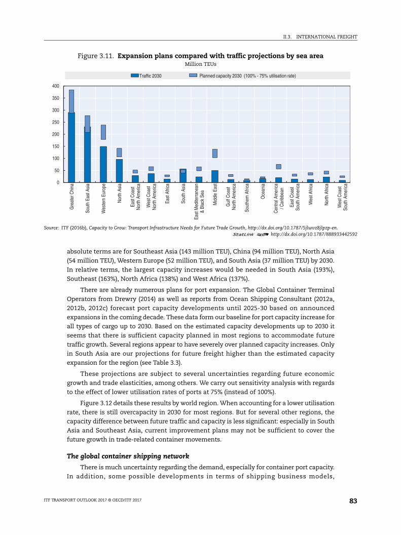
II.3. INTERNATIONAL FREIGHT
442592
Wes
t Coa
stSo
uth
Amer
ica
absolute terms are for Southeast Asia (143 million TEU), China (94 million TEU), North Asia
(54 million TEU), Western Europe (52 million TEU), and South Asia (37 million TEU) by 2030.
In relative terms, the largest capacity increases would be needed in South Asia (193%),
Southeast (163%), North Africa (138%) and West Africa (137%).
There are already numerous plans for port expansion. The Global Container Terminal
Operators from Drewry (2014) as well as reports from Ocean Shipping Consultant (2012a,
2012b, 2012c) forecast port capacity developments until 2025-30 based on announced
expansions in the coming decade. These data form our baseline for port capacity increase for
all types of cargo up to 2030. Based on the estimated capacity developments up to 2030 it
seems that there is sufficient capacity planned in most regions to accommodate future
traffic growth. Several regions appear to have severely over planned capacity increases. Only
in South Asia are our projections for future freight higher than the estimated capacity
expansion for the region (see Table 3.3).
These projections are subject to several uncertainties regarding future economic
growth and trade elasticities, among others. We carry out sensitivity analysis with regards
to the effect of lower utilisation rates of ports at 75% (instead of 100%).
Figure 3.12 details these results by world region. When accounting for a lower utilisation
rate, there is still overcapacity in 2030 for most regions. But for several other regions, the
capacity difference between future traffic and capacity is less significant: especially in South
Asia and Southeast Asia, current improvement plans may not be sufficient to cover the
future growth in trade-related container movements.
The global container shipping network
There is much uncertainty regarding the demand, especially for container port capacity.
In addition, some possible developments in terms of shipping business models,
Figure 3.11. Expansion plans compared with traffic projections by sea areaMillion TEUs
Source: ITF (2016b), Capacity to Grow: Transport Infrastructure Needs for Future Trade Growth, http://dx.doi.org/10.1787/5jlwvz8jlpzp-en.1 2 http://dx.doi.org/10.1787/888933
0
50
100
150
200
250
300
350
400
Gre
ater
Chi
na
Sout
h Ea
st A
sia
Wes
tern
Eur
ope
Nor
th A
sia
East
Coa
stN
orth
Am
eric
a
Wes
t Coa
stN
orth
Am
eric
a
East
Afri
ca
Sout
h As
ia
East
Med
iterra
nean
& Bl
ack
Sea
Mid
dle
East
Gul
f Coa
stN
orth
Am
eric
a
Sout
hern
Afri
ca
Oce
ania
Cen
tral A
mer
ica
/ Car
ibbe
an
East
Coa
stSo
uth
Amer
ica
Wes
t Afri
ca
Nor
th A
frica
Traffic 2030 Planned capacity 2030 (100% - 75% utilisation rate)
ITF TRANSPORT OUTLOOK 2017 © OECD/ITF 2017 83
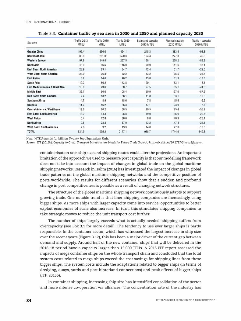
II.3. INTERNATIONAL FREIGHT
acity EU
containerisation rate, ship size and shipping routes could alter the projections. An important
limitation of the approach we used to measure port capacity is that our modelling framework
does not take into account the impact of changes in global trade on the global maritime
shipping networks. Research in Halim (2016) has investigated the impact of changes in global
trade patterns on the global maritime shipping networks and the competitive position of
ports worldwide. The results for different scenarios show that a sudden and profound
change in port competitiveness is possible as a result of changing network structures.
The structure of the global maritime shipping network continuously adapts to support
growing trade. One notable trend is that liner shipping companies are increasingly using
bigger ships. As more ships with larger capacity come into service, opportunities to better
exploit economies of scale also increase. In turn, this stimulates shipping companies to
take strategic moves to reduce the unit transport cost further.
The number of ships largely exceeds what is actually needed: shipping suffers from
overcapacity (see Box 3.1 for more detail). The tendency to use ever larger ships is partly
responsible. In the container sector, which has witnessed the largest increase in ship size
over the recent years (Figure 3.12), this has been a major driver of the current gap between
demand and supply. Around half of the new container ships that will be delivered in the
2016-18 period have a capacity larger than 13 000 TEUs. A 2015 ITF report assessed the
impacts of mega container ships on the whole transport chain and concluded that the total
system costs related to mega-ships exceed the cost savings for shipping lines from these
bigger ships. The system costs include the adaptations related to bigger ships (in terms of
dredging, quays, yards and port hinterland connections) and peak effects of bigger ships
(ITF, 2015b).
In container shipping, increasing ship size has intensified consolidation of the sector
and more intense co-operation via alliances. The concentration rate of the industry has
Table 3.3. Container traffic by sea area in 2030 and 2050 and planned capacity 2030
Sea areaTraffic 2013
MTEUTraffic 2030
MTEUTraffic 2050
MTEUEstimated capacity
2013 MTEUPlanned capacity
2030 MTEUTraffic – cap
2030 MT
Greater China 196.4 290.0 494.1 248.3 383.8 -93.8
Southeast Asia 88.0 231.0 520.3 124.4 277.3 -46.3
Western Europe 97.8 149.4 257.5 168.1 238.2 -88.8
North Asia 43.0 96.5 146.0 70.9 141.6 -45.1
East Coast North America 23.9 29.1 34.7 42.4 51.7 -22.6
West Coast North America 24.9 36.8 32.2 43.2 65.5 -28.7
East Africa 8.2 14.6 46.2 13.0 31.9 -17.3
South Asia 19.2 56.2 143.8 29.1 53.1 3.1
East Mediterranean & Black Sea 16.8 23.6 50.7 27.5 65.1 -41.5
Middle East 36.7 50.0 108.4 50.9 137.6 -87.6
Gulf Coast North America 7.4 13.2 58.1 11.8 33.1 -19.9
Southern Africa 4.7 8.9 18.6 7.8 15.5 -6.6
Oceania 11.2 16.2 36.3 17.1 23.9 -7.7
Central America / Caribbean 19.6 20.2 58.5 29.5 75.4 -55.2
East Coast South America 13.2 14.3 28.8 19.0 35.0 -20.7
West Africa 5.4 12.8 36.6 8.8 40.9 -28.1
North Africa 9.8 23.3 87.0 13.2 47.4 -24.1
West Coast South America 7.9 9.2 19.3 14.0 27.8 -18.6
TOTAL 634.3 1095.2 2177.1 938.7 1744.9 -649.5
Note: MTEU stands for Million Twenty Foot Equivalent Unit. Source: ITF (2016b), Capacity to Grow: Transport Infrastructure Needs for Future Trade Growth, http://dx.doi.org/10.1787/5jlwvz8jlpzp-en.
ITF TRANSPORT OUTLOOK 2017 © OECD/ITF 201784
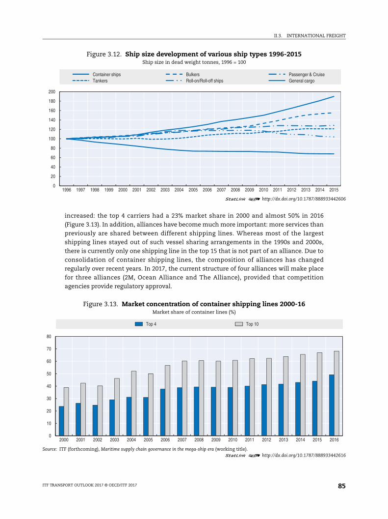
II.3. INTERNATIONAL FREIGHT
442606
2015
442616
2016
increased: the top 4 carriers had a 23% market share in 2000 and almost 50% in 2016
(Figure 3.13). In addition, alliances have become much more important: more services than
previously are shared between different shipping lines. Whereas most of the largest
shipping lines stayed out of such vessel sharing arrangements in the 1990s and 2000s,
there is currently only one shipping line in the top 15 that is not part of an alliance. Due to
consolidation of container shipping lines, the composition of alliances has changed
regularly over recent years. In 2017, the current structure of four alliances will make place
for three alliances (2M, Ocean Alliance and The Alliance), provided that competition
agencies provide regulatory approval.
Figure 3.12. Ship size development of various ship types 1996-2015Ship size in dead weight tonnes, 1996 = 100
1 2 http://dx.doi.org/10.1787/888933
0
20
40
60
80
100
120
140
160
180
200
1996 1997 1998 1999 2000 2001 2002 2003 2004 2005 2006 2007 2008 2009 2010 2011 2012 2013 2014
Container ships Bulkers Passenger & CruiseTankers Roll-on/Roll-off ships General cargo
Figure 3.13. Market concentration of container shipping lines 2000-16Market share of container lines (%)
Source: ITF (forthcoming), Maritime supply chain governance in the mega-ship era (working title).1 2 http://dx.doi.org/10.1787/888933
0
10
20
30
40
50
60
70
80
2000 2001 2002 2003 2004 2005 2006 2007 2008 2009 2010 2011 2012 2013 2014 2015
Top 4 Top 10
ITF TRANSPORT OUTLOOK 2017 © OECD/ITF 2017 85
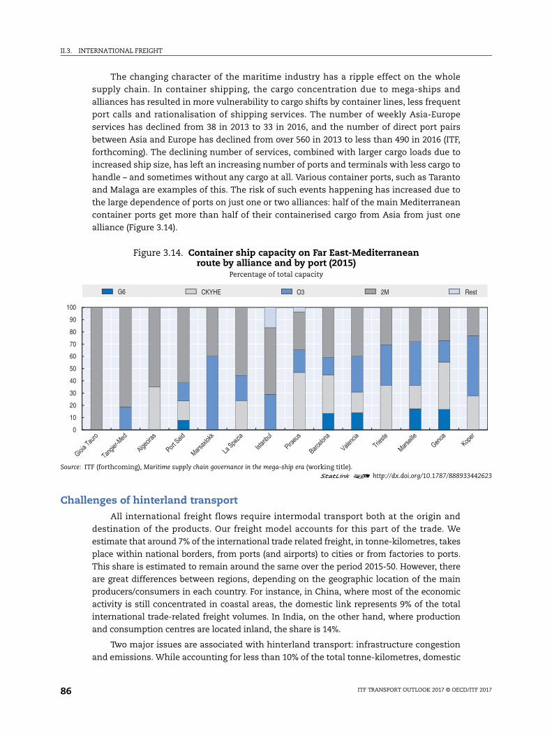
II.3. INTERNATIONAL FREIGHT
442623
est
The changing character of the maritime industry has a ripple effect on the whole
supply chain. In container shipping, the cargo concentration due to mega-ships and
alliances has resulted in more vulnerability to cargo shifts by container lines, less frequent
port calls and rationalisation of shipping services. The number of weekly Asia-Europe
services has declined from 38 in 2013 to 33 in 2016, and the number of direct port pairs
between Asia and Europe has declined from over 560 in 2013 to less than 490 in 2016 (ITF,
forthcoming). The declining number of services, combined with larger cargo loads due to
increased ship size, has left an increasing number of ports and terminals with less cargo to
handle – and sometimes without any cargo at all. Various container ports, such as Taranto
and Malaga are examples of this. The risk of such events happening has increased due to
the large dependence of ports on just one or two alliances: half of the main Mediterranean
container ports get more than half of their containerised cargo from Asia from just one
alliance (Figure 3.14).
Challenges of hinterland transportAll international freight flows require intermodal transport both at the origin and
destination of the products. Our freight model accounts for this part of the trade. We
estimate that around 7% of the international trade related freight, in tonne-kilometres, takes
place within national borders, from ports (and airports) to cities or from factories to ports.
This share is estimated to remain around the same over the period 2015-50. However, there
are great differences between regions, depending on the geographic location of the main
producers/consumers in each country. For instance, in China, where most of the economic
activity is still concentrated in coastal areas, the domestic link represents 9% of the total
international trade-related freight volumes. In India, on the other hand, where production
and consumption centres are located inland, the share is 14%.
Two major issues are associated with hinterland transport: infrastructure congestion
and emissions. While accounting for less than 10% of the total tonne-kilometres, domestic
Figure 3.14. Container ship capacity on Far East-Mediterranean route by alliance and by port (2015)
Percentage of total capacity
Source: ITF (forthcoming), Maritime supply chain governance in the mega-ship era (working title).1 2 http://dx.doi.org/10.1787/888933
0
10
20
30
40
50
60
70
80
90
100
G6 CKYHE O3 2M R
ITF TRANSPORT OUTLOOK 2017 © OECD/ITF 201786
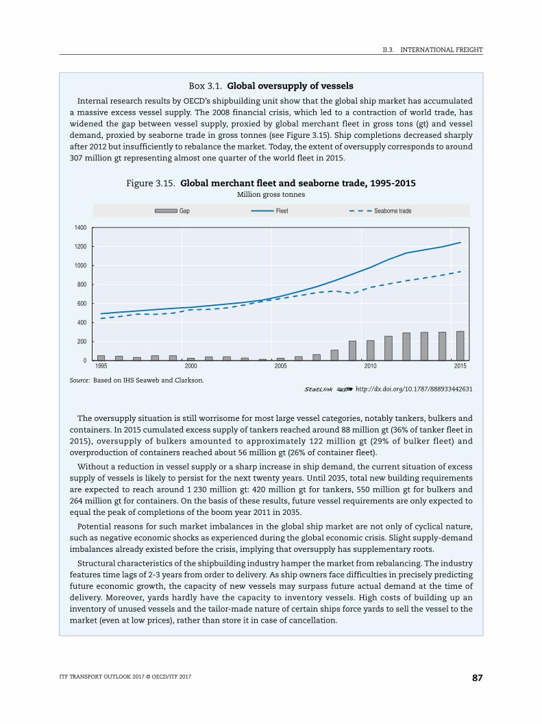
II.3. INTERNATIONAL FREIGHT
ted as
sel ply nd
nd in nd
ess nts nd to
re, nd
try ing of an
the
631
15
Box 3.1. Global oversupply of vessels
Internal research results by OECD’s shipbuilding unit show that the global ship market has accumulaa massive excess vessel supply. The 2008 financial crisis, which led to a contraction of world trade, hwidened the gap between vessel supply, proxied by global merchant fleet in gross tons (gt) and vesdemand, proxied by seaborne trade in gross tonnes (see Figure 3.15). Ship completions decreased sharafter 2012 but insufficiently to rebalance the market. Today, the extent of oversupply corresponds to arou307 million gt representing almost one quarter of the world fleet in 2015.
The oversupply situation is still worrisome for most large vessel categories, notably tankers, bulkers acontainers. In 2015 cumulated excess supply of tankers reached around 88 million gt (36% of tanker fleet2015), oversupply of bulkers amounted to approximately 122 million gt (29% of bulker fleet) aoverproduction of containers reached about 56 million gt (26% of container fleet).
Without a reduction in vessel supply or a sharp increase in ship demand, the current situation of excsupply of vessels is likely to persist for the next twenty years. Until 2035, total new building requiremeare expected to reach around 1 230 million gt: 420 million gt for tankers, 550 million gt for bulkers a264 million gt for containers. On the basis of these results, future vessel requirements are only expectedequal the peak of completions of the boom year 2011 in 2035.
Potential reasons for such market imbalances in the global ship market are not only of cyclical natusuch as negative economic shocks as experienced during the global economic crisis. Slight supply-demaimbalances already existed before the crisis, implying that oversupply has supplementary roots.
Structural characteristics of the shipbuilding industry hamper the market from rebalancing. The indusfeatures time lags of 2-3 years from order to delivery. As ship owners face difficulties in precisely predictfuture economic growth, the capacity of new vessels may surpass future actual demand at the timedelivery. Moreover, yards hardly have the capacity to inventory vessels. High costs of building up inventory of unused vessels and the tailor-made nature of certain ships force yards to sell the vessel to market (even at low prices), rather than store it in case of cancellation.
Figure 3.15. Global merchant fleet and seaborne trade, 1995-2015Million gross tonnes
Source: Based on IHS Seaweb and Clarkson.1 2 http://dx.doi.org/10.1787/888933442
0
200
400
600
800
1000
1200
1400
1995 2000 2005 2010 20
Gap Fleet Seaborne trade
ITF TRANSPORT OUTLOOK 2017 © OECD/ITF 2017 87
II.3. INTERNATIONAL FREIGHT
es, try in try ly,
freight transport related to international trade accounts for 80% of the total transport costs
(Rodridgue and Noteboom, 2012) and nearly 30% of the total trade-related CO2 emissions.
Because most of the transport of goods from ports to consumption centres is by road, the
CO2 intensity of this freight is significantly higher than for other corridors. These
emissions in the domestic link of international trade are further amplified by shipping
emissions at ports. Shipping related CO2 emissions in ports represent only about 2% of
total international shipping CO2 emissions. Locally, shipping emissions have important
health impacts. Local emissions are projected to grow significantly, especially for CH4, CO,
CO2 and NOx emissions, which could grow even four-fold by 2050 if no additional measures
are taken (ITF, 2015a).
Some bottlenecks may also emerge. Existing national infrastructure already faces
issues of insufficient capacity in some regions of the world, especially in port cities.
Projected trade flows to 2050 and the growing freight volumes highlight the need to assess
the capacity of existing national infrastructure, in particular hinterland road and rail
infrastructure, to deal with potential bottlenecks that may emerge.
Capacity requirements (for hinterland connections) are first measured against the
total capacity available by region (measured in lane-km and track-km for road and rail
respectively), even if not located along the main freight corridors. However, congestion
occurs near ports and the main production and consumption centres, where cargo has to
be handled and distributed. Congestion also often concentrates on small distances and it
may not significantly impact the overall performance of the freight network. So, we also
compare surface freight traffic to freight activity, but only in areas less than 50 km away
from ports, consumption and production centres.
Comparing freight volumes to overall capacity by region does not seem to imply large
infrastructure needs, except in Asia and Africa (Table 3.4), which are also the regions where
intra-regional freight increases most. In these regions, the lack of infrastructure may
become an impediment to trade, especially in the longer term.
The results for congestion around ports, consumption and production centres are in
Table 3.5. Capacity needs now appear more clearly for all regions. In 2050, infrastructure in
Asia and Africa around ports, production centres and cities will almost need to triple to go
back to the performance levels of 2010. Overall capacity requirements need not be very
high but spatially focused.
While the pressure on hinterland connections is a challenge, it can also be an
opportunity. In comparison with, for example, maritime transport which is regulated by
international agreements and policy decisions require international agreements, the
domestic component of the international trade and supply chains is an area where national
policies can make a significant difference in the environmental and economic sustainability.
Box 3.1. Global oversupply of vessels (cont.)
Non-market related factors also contribute to oversupply, for instance restrictive trade policipreferential treatment for national firms or direct and indirect subsidies. The global shipbuilding indusfaces historically low capacity utilisation rates of yards of about 57% in 2015 down from its peak of 85%2008. Subsidies help governments to keep their strategically important, national shipbuilding induscompetitive and maintain employment. Such government support, however, stimulates vessel suppexacerbating the oversupply situation further.
ITF TRANSPORT OUTLOOK 2017 © OECD/ITF 201788
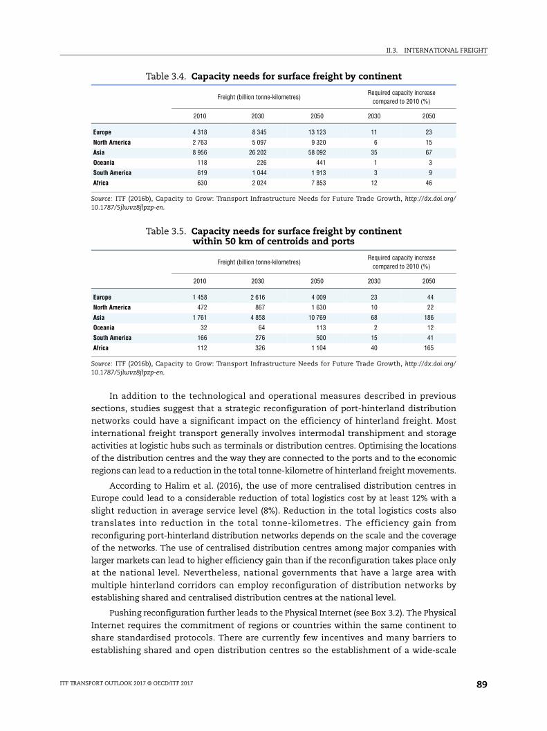
II.3. INTERNATIONAL FREIGHT
In addition to the technological and operational measures described in previous
sections, studies suggest that a strategic reconfiguration of port-hinterland distribution
networks could have a significant impact on the efficiency of hinterland freight. Most
international freight transport generally involves intermodal transhipment and storage
activities at logistic hubs such as terminals or distribution centres. Optimising the locations
of the distribution centres and the way they are connected to the ports and to the economic
regions can lead to a reduction in the total tonne-kilometre of hinterland freight movements.
According to Halim et al. (2016), the use of more centralised distribution centres in
Europe could lead to a considerable reduction of total logistics cost by at least 12% with a
slight reduction in average service level (8%). Reduction in the total logistics costs also
translates into reduction in the total tonne-kilometres. The efficiency gain from
reconfiguring port-hinterland distribution networks depends on the scale and the coverage
of the networks. The use of centralised distribution centres among major companies with
larger markets can lead to higher efficiency gain than if the reconfiguration takes place only
at the national level. Nevertheless, national governments that have a large area with
multiple hinterland corridors can employ reconfiguration of distribution networks by
establishing shared and centralised distribution centres at the national level.
Pushing reconfiguration further leads to the Physical Internet (see Box 3.2). The Physical
Internet requires the commitment of regions or countries within the same continent to
share standardised protocols. There are currently few incentives and many barriers to
establishing shared and open distribution centres so the establishment of a wide-scale
Table 3.4. Capacity needs for surface freight by continent
Freight (billion tonne-kilometres)Required capacity increase
compared to 2010 (%)
2010 2030 2050 2030 2050
Europe 4 318 8 345 13 123 11 23
North America 2 763 5 097 9 320 6 15
Asia 8 956 26 202 58 092 35 67
Oceania 118 226 441 1 3
South America 619 1 044 1 913 3 9
Africa 630 2 024 7 853 12 46
Source: ITF (2016b), Capacity to Grow: Transport Infrastructure Needs for Future Trade Growth, http://dx.doi.org/10.1787/5jlwvz8jlpzp-en.
Table 3.5. Capacity needs for surface freight by continent within 50 km of centroids and ports
Freight (billion tonne-kilometres)Required capacity increase
compared to 2010 (%)
2010 2030 2050 2030 2050
Europe 1 458 2 616 4 009 23 44
North America 472 867 1 630 10 22
Asia 1 761 4 858 10 769 68 186
Oceania 32 64 113 2 12
South America 166 276 500 15 41
Africa 112 326 1 104 40 165
Source: ITF (2016b), Capacity to Grow: Transport Infrastructure Needs for Future Trade Growth, http://dx.doi.org/10.1787/5jlwvz8jlpzp-en.
ITF TRANSPORT OUTLOOK 2017 © OECD/ITF 2017 89

II.3. INTERNATIONAL FREIGHT
physical internet network seems out of reach, at least in the medium term. In the longer
term, however, the establishment of global standardised protocols for the transfer of goods
has a very large potential to reduce the number of vehicle-kilometres travelled.
Decision making under uncertaintyVarious observers speculate that trends are continuing to shift which would result in
less trade than the above projections have indicated. Their argument is based on the premise
that fundamental changes are taking place in consumption, production and energy sources.
For example, an element of consumption has now become virtual, immaterial and shared. A
share of production has become more local, facilitated by innovations such as 3D-printing
and tendencies towards a more circular economy. Energy production has also become more
localised, focused on renewable energy sources; and many countries have adopted the vision
of a zero-carbon future which requires a more stringent move away from fossil fuels. All
these developments could change the volume and composition of global trade flows in a way
that no model has been able to fully account for as yet.
Consumption patterns
Behaviour of consumers is changing in various ways, expressed in the emergence of
more local consumption, more virtual consumption and more shared consumption. An
example of localised consumption relates to food. Local food markets have gained
momentum in the US and elsewhere, leading to increased consumption of local food
products. E.g. two-thirds of the French population consume more local food products than
five years ago. Consumption has also become increasingly virtual with the development of
Box 3.2. The Physical Internet
Recent areas of research have proposed a new vision and solution for tackling sustainability challenges in logistics – the Physical Internet (Montreuil, 2011). The Physical Internet is an open logistic system founded on exchange protocols that allow goods to be transported on a common network, the same way information is transported on the Internet. The physical internet relies on standardisation, of the size of parcels and of the information attached to it, so that goods can freely move, using the different transport modes, regardless of the sender or recipient. The information contained on the goods allow them to be directed when inter-connection is necessary. In the end, large efficiency gains can be expected.
The implementation of open and shared distribution networks could result in a significant reduction in both total logistics costs and CO2 emissions of freight transport activities. Preliminary evidence for the efficacy of such measures at national levels can be found in (Hakimi et al., 2012). The successful reductions of freight tonne-kilometre as indicated by these studies show that higher scale application at a larger geographical level is a promising research avenue.
Within the context of improving port-hinterland connectivity, the Physical Internet concept can be translated into an open, connected, and shared port-hinterland mobility network which may significantly improve hinterland transport efficiency and sustainability. In practice, the open mobility network of Physical Internet could be implemented by the use of shared and centralised distribution centres for different freight transport providers at larger geographical scale such as at a continental or regional scale.
ITF TRANSPORT OUTLOOK 2017 © OECD/ITF 201790
II.3. INTERNATIONAL FREIGHT
all kinds of electronic goods, such as e-books, online music and newspapers that have to
some extent replaced the physical goods: in 2015 e-books generated similar sales revenues
as physical books. Finally, a considerable share of consumption is about shared services,
such as car-sharing. The number of car share users in Europe is predicted to reach
15 million by 2020. All these developments have an effect on the demand for traded goods.
In the examples given here, there is less need for trade and the transport of food, paper
pulp, cars and various other consumer goods. If these trends continue and intensify, they
could have a substantial impact on cargo transport. Another reason to believe that this
could be the case is that many of these trends, such as the shared economy, are
predominantly urban phenomena – and the share of the world population living in cities is
expected to rise to 70% by 2050, according to UN-Habitat.
Production patterns
There are also sufficient reasons for believing that production and manufacturing will
become increasingly localised. As mentioned earlier, the limits of the global value chain
model seem to have been reached (OECD, 2016). This aligns with expectations of business
executives: 54% of US executives are considering re-shoring some of their activities by 2020.
Such re-shoring would be facilitated by technologies such as 3D-printing that promises
production closer to major consumption centres. According to a PwC study (2015), 37% of
ocean container shipments might be threatened by 3D-printing. A considerable share of the
commodities needed for local production could be sourced locally if a more circular
economic model takes off. In such a circular economy scenario, the need of primary material
consumption in 2050 could be half of the current level (McKinsey, 2016).
Energy production
A large share of current global trade flows are from coal and oil. More and more
countries have committed to zero-carbon strategies and reoriented their energy mix
towards more renewable energy sources. E.g. coal consumption in the United Kingdom and
in France is 70% lower than in the 1970s. According to the IEA, renewable energy could
make up half of the global energy mix by 2050. Most of this renewable energy could be
locally sourced via wind or solar energy, so a strict global zero-carbon scenario could result
in a substantial decrease of maritime transport.
Alternative shipping routes
The projections in this Outlook assume that current shipping routes will continue to be
used. Various projects in discussion may change these routes. The Kra Canal could provide a
supplement to the flows currently going through the Malacca Straits; the Nicaragua Canal
could provide an alternative to the Panama Canal and would be better able to accommodate
the biggest container ships. Various proposed land bridges in Latin America could also
provide new options to connect the Atlantic and Pacific Oceans.
The Northern Sea route might also be able to accommodate more shipping, even if the
prospects for regular liner services seem limited. Long-range rail corridors might also at
some point become an alternative for certain maritime trade routes. This is currently not
the case, considering that ocean shipping is so much cheaper and that most of the goods
are fairly time insensitive. Long-distance freight rail has so far been more in competition
with air cargo but the equation could change considering the increased costs that maritime
transport could have to face, such as the low sulphur regulations.
ITF TRANSPORT OUTLOOK 2017 © OECD/ITF 2017 91
II.3. INTERNATIONAL FREIGHT
In short, any study of capacity constraints cannot forego the analysis of potential
sources of uncertainty, some of which have been discussed above. For all key actors in the
transport sector, in particular those responsible for long-term transport planning, both in
the private and public sector, knowledge and the ability to understand the trends outlined
above as they are unfolding will be vital. This will require more flexibility especially in
infrastructure planning and delivery. Port and hinterland infrastructures will need to be
designed in a way that is more closely linked to actual cargo flow and that which can
reasonably be expected in the near future, while leaving enough room for adaptation
should new developments require.
The projections presented above should therefore be interpreted with caution. Indeed,
there is much uncertainty related to consumption and production patterns, energy
production and shipping routes, which make decision making difficult.
References
ATAG (2016), Aviation benefits beyond borders, Air Transport Action Group.
Cambridge Systematics (1998), Transmode Consultants, National Cooperative Highway Research Program, American Association of State Highway and Transportation Officials, Multimodal corridor and capacity analysis manual (No. 399), Transportation Research Board, Washington, DC, USA.
Constantinescu, C., A. Mattoo and M. Ruta, (2015), “The Global Trade Slowdown: Cyclical or Structural?” IMF Working Paper, International Monetary Fund, January 2015.
Drewry Shipping Consultants (2014), Annual Review of Global Container Terminal Operators 2013, London.
ECB (2014), “Understanding global trade elasticties: What has changed?”, ECB Monthly Bulletin, European Central Bank, July 2014.
FHWA (2009), Estimation of 2007 VIUS Variable, Office of Freight Management and Operations, 15 October 2009.
Fontagné, L. and J. Fouré (2013), “Opening a Pandora’s Box: Modelling World Trade Patterns at the 2035 Horizon”, CEPII Working Papers, No. 22. CEPII Research Center, Paris.
Hakimi, D. et al. (2012), “Simulating a physical internet enabled mobility web: the case of mass distribution in France (p. 10 p.)”, the 9th International Conference on Modeling, Optimization & SIMulation – MOSIM’12, Retrieved from https://hal.archives-ouvertes.fr/hal-00728584/document.
Halim, R.A. et al. (2016), “A Strategic Model of Port-Hinterland Freight Distribution Networks”, Transportation Research Part E: Logistics and Transportation Review.
Halim, R.A. (2016), Strategic Modeling of global container transport networks, PhD thesis, Delft University of Technology, the Netherlands.
HCM (2010), Highway Capacity Manual 2010, Transportation Research Board, National Research Council, Washinton, DC, USA.
ICAO (2013), “Consolidated statement of continuing ICAO policies and practices related to environmental protection – Climate change”, ICAO resolution No. A37-19.
IEA (2014), The IEA Mobility Model, IEA, Paris, www.iea.org/media/transport/IEA_MoMo_Presentation.pdf.
International Maritime Organisation (IMO) (2009), Second IMO GHG Study 2009, International Maritime Organization, London, UK.
International Maritime Organisation (IMO) (2014), Third IMO GHG Study 2014,International Maritime Organization, London, UK.
ITF (forthcoming), Maritime supply chain governance in the mega-ship era (working title).
ITF (2016a), The Carbon Footprint of Global Trade, Tackling Emissions from International Freight Transport, www.itf-oecd.org/sites/default/files/docs/cop-pdf-06.pdf.
ITF (2016b), “Capacity to Grow: Transport Infrastructure Needs for Future Trade Growth”, International Transport Forum Policy Papers, No. 19, OECD Publishing, Paris, http://dx.doi.org/10.1787/5jlwvz8jlpzp-en.
ITF TRANSPORT OUTLOOK 2017 © OECD/ITF 201792
II.3. INTERNATIONAL FREIGHT
ITF (2015a), ITF Transport Outlook 2015, OECD Publishing, Paris, http://dx.doi.org/10.1787/9789282107782-en.
ITF (2015b), “The Impact of Mega-Ships”, International Transport Forum Policy Papers, No. 10, OECD Publishing, Paris, http://dx.doi.org/10.1787/5jlwvzcm3j9v-en.
Johansson, Å. and E. Olaberria (2014), “Long-term patterns of trade and specialisation”, OECD Economics Department Working Papers, No. 1136, OECD Publishing, Paris, http://dx.doi.org/10.1787/5jz158tbddbr-en .
LR (2016), Low carbon pathways 2050, Lloyd’s Register, www.lr.org/lcp2050.
Martinez, L.M., J. Kauppila and M. Castaing (2015), “International Freight and Related Carbon Dioxide Emissions by 2050:New Modeling Tool”, Transportation Research Record: Journal of the Transportation Research Board, No. 2477, pp. 58-67.
McKinsey (2016), The circular economy: Moving from theory to practice, McKinsey & Company, USA.
Montreuil, B. (2011), “Toward a Physical Internet: meeting the global logistics sustainability grand challenge”, Logistics Research, 3(2-3), 71-87, https://doi.org/10.1007/s12159-011-0045-x.
Muncrief, R. (2014), Truck efficiency standards and the potential for Latin America, Overview of the Global Green Freight Action Plan, presented at the CCAP MAIN-Latin American Regional Dialogue Mitigation Action Implementation Network, Washington, DC, October 28, 2014.
Ocean Shipping Consultants (2012a), North European Containerport Markets to 2025.
Ocean Shipping Consultants (2012b), East Asian Containerport Markets to 2025.
Ocean Shipping Consultants (2012c), Middle East Containerport Markets to 2025.
OECD (2016), “Cardiac Arrest of Dizzy Spell: Why is World Trade so Weak and What Can Policy Do About It?”, OECD Economic Policy Paper, September 2016, No. 18, http://dx.doi.org/10.1787/5jlr2h45q532-en.
PwC (2015), 2015 Commercial Transportation Trends, Industry perspectives, www.strategyand.pwc.com/perspectives/2015-commercial-transportation-trends.
Rodrigue, J.-P. and T. Notteboom (2012), “Dry ports in European and North American intermodal rail systems: Two of a kind?”, Res. Transp. Bus. Manage., Vol. 5, pp. 4-15.
Route Monkey (2016), Demonstrating the GHG reduction potential of asset sharing, asset optimization and other measures, Report of the Road Freight Lab, prepared on behalf of WBCSD members in the Low Carbon Technology Partnership initiative.
Smith, T.W.P. et al. (2015), The Existing Shipping Fleet’s CO2 Efficiency, International Maritime Organisation, London, UK, March, 2015.
Smith et al. (2014), Low Carbon Shipping – A Systems Approach, Final Report, University College London.
ITF TRANSPORT OUTLOOK 2017 © OECD/ITF 2017 93
II.3. INTERNATIONAL FREIGHT
ANNEX 3.A
ITF International Freight Model
The International Transport Forum’s (ITF) International Freight Model projects
international freight transport activity and related CO2 emissions up to 2050 based on
global trade projections. The model includes six main components, each feeding into the
subsequent calculation:
● A general equilibrium model for international trade, covering 26 world regions and
25 commodities of which 19 require transport
● A global freight transport network model based on 2010 data
● Global production/consumption centroids
● An international freight mode choice model calibrated using Eurostat and ECLAC data
● A weight/value model to convert trade in value into weight, calibrated for each commodity
and transport mode, and
● CO2 intensities and technology pathway by mode.
The final outputs of the model are freight tonne-kilometres by transport corridor by
mode and related CO2 emissions. Each of the model components are described in more
detail below.
Transport network modelThe model consolidates and integrates all freight transport networks based on open
GIS data for different transport modes. Seaports and airports are physically connected to
road and rail networks with data on intermodal dwelling times. Travel times by type of
infrastructure and dwelling times between transport modes are estimated using average
speeds based on available information by region. The model then computes the shortest
paths between each production/consumption centroid for each transport mode (for the
modes available for each link), generating two main inputs:
● The average travel time and distance by mode for each origin destination pair. For
countries with multiple centroids, a weighted average of all centroid pairs is used
● The shortest path between each centroid for each transport mode.
CentroidsThe underlying trade projections are done with a regional aggregation of 26 zones.
This introduces significant uncertainties from a transport perspective as it does not allow
ITF TRANSPORT OUTLOOK 2017 © OECD/ITF 201794
II.3. INTERNATIONAL FREIGHT
a proper discretisation of the travel path used for different types of product. Therefore, we
disaggregate the regional origin-destination (OD) trade flows into a larger number of
production/consumption centroids. The centroids were identified using an adapted
p-median procedure for all the cities around the world classified by the United Nations in
2010 relative to their population (2 539 cities). The objective function for this aggregation is
based on the minimisation of a distance function which includes two components: GDP
density and geographical distance. The selection was also constrained by allowing one
centroid within a 500 km radius in a country. This resulted in 294 centroids globally, with
spatially balanced results for all continents.
Freight mode choice modelThe mode share model (in value) for international freight flows assigns the transport
mode used for trade between any origin-destination pair of centroids. The mode attributed
to each trade connection represents the longest transport section. All freight will require
intermodal transport both in the origin and destination. This domestic component of
international freight is usually not accounted in the literature, but is included in our model.
The model is calibrated using a standard multinomial logit estimator including a
commodity type panel term, variables on travel times and distances taken from the
network model while two geographical and economic context binary variables are added,
one describing if the OD pair has a trade agreement and the other for the existence of a land
border between trading partners.
Weight/value modelWe used a Poisson regression model to estimate the rate of conversion of value units
(dollars) into weight units of cargo (tonnes) by mode, calibrated using Eurostat and Latin
American data on value/weight ratios for different commodities. We use the natural
logarithm of the trade value in millions of dollars as an offset variable, a panel terms by
commodity, travel time and distances, and geographical and cultural variables: the binary
variables for trade agreements and land borders used above and a binary variable identifying
if two countries have the same official language. Moreover, economic profile variables were
included to describe the trade relation between countries with different types of production
sophistication and scale of trade intensity. The resulting dataset was then divided according
to each transport mode, leading to different calibrations by mode.
Generation of the model outputsThe model components result with the value, weight and distance travelled (with path
specification) between 2010 and 2050, for each centroid pair, mode, type of commodity and
year, stemming from international trade. The tonne-kilometres are then combined with
information on related CO2 intensities and technology pathways by mode, obtained from
the International Energy Agency’s MoMo model (IEA, 2014) and the International Maritime
Organisation (IMO, 2009). In case of road and rail, these coefficients and pathways are
geographically dependent, while the maritime and air CO2 efficiencies are considered to be
uniform worldwide.
For technical details of the model, as well as some validation results, see Martinez,
Kauppila, Castaing (2014).
ITF TRANSPORT OUTLOOK 2017 © OECD/ITF 2017 95
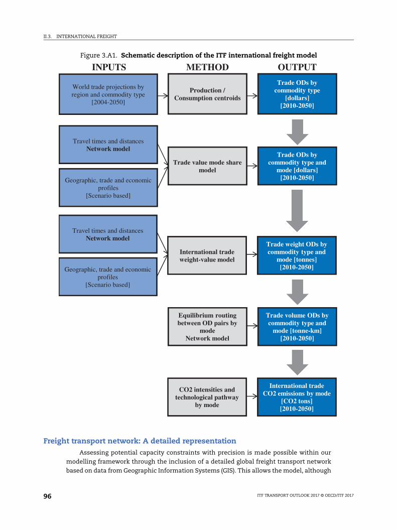
II.3. INTERNATIONAL FREIGHT
Freight transport network: A detailed representationAssessing potential capacity constraints with precision is made possible within our
modelling framework through the inclusion of a detailed global freight transport network
based on data from Geographic Information Systems (GIS). This allows the model, although
Figure 3.A1. Schematic description of the ITF international freight model
Trade value mode share model
Trade ODs by commodity type and
mode [dollars][2010-2050]
Travel times and distancesNetwork model
Geographic, trade and economic profiles
[Scenario based]
Travel times and distancesNetwork model
Geographic, trade and economic profiles
[Scenario based]
International trade weight-value model
Trade weight ODs by commodity type and
mode [tonnes][2010-2050]
Equilibrium routing between OD pairs by
modeNetwork model
Trade volume ODs by commodity type and
mode [tonne-km][2010-2050]
World trade projections by region and commodity type
[2004-2050]
Production / Consumption centroids
Trade ODs by commodity type
[dollars][2010-2050]
CO2 intensities and technological pathway
by mode
International trade CO2 emissions by mode
[CO2 tons][2010-2050]
INPUTS METHOD OUTPUT
ITF TRANSPORT OUTLOOK 2017 © OECD/ITF 201796

II.3. INTERNATIONAL FREIGHT
global, to describe network conditions at a detailed scale. Our main contribution is the
consolidation and integration of all different modal networks into a single, routable freight
network, and the association of capacity constraints to links and nodes.
The freight network comprises links and nodes for all four main modes: a global road
network, containing the primary and secondary road networks (i.e. motorways, main roads
and trunk roads); a rail network; an air network, including all commercial air links between
international airports; a maritime network; and a global inland waterways system with
navigable rivers (see Figure 3.A2). In order to estimate travel times for the different types of
infrastructure, as well as dwelling times between transport modes, we use average speeds
based on available information by region.
GIS data for the global network model are available online:
● The road network information integrates two main sources: Global Roads Open Access
Data Set (gROADS) (http://sedac.ciesin.columbia.edu/data/set/groads-global-roads-open-
access-v1) and OpenStreetMap (www.openstreetmap.org).
● The rail network was collected from the Digital Chart of the World (DCW) (http://
statisk.umb.no/ikf/gis/dcw/) project, integrated and updated with the OpenStreetMap data
on rail lines and rail stations as intermodal points of connection between road and rail.
● The actual maritime routes are taken from the Global Shipping Lane Network data of
Oak Ridge National Labs CTA Transportation Network Group (www-cta.ornl.gov/transnet/
Intermodal_Network.html), which generates a routable network with actual travel times
for different sea segments. We connect this network to ports, based on data from the
latest World Port Index Database of the National Geospatial-Intelligence Agency (http://
msi.nga.mil/NGAPortal/MSI.portal).
● The commercial air links between international airports were integrated using data from
OpenFlights.org database on airports, commercial air links and airline companies
(www.OpenFlights.org).
● The inland waterways network was obtained from the CIA World DataBank II
(www.evl.uic.edu/pape/data/WDB/), and combined with information on the navigability
for each river.
The different networks are consolidated into a single, routable network, and connected
to the centroids using the road network and rail stations. The Annex presents statistics
related to the number of links and the network length for each mode (see Table 3.A1).
Port capacityTo assess future port infrastructure needs, the ITF built a detailed database of current port
capacity, along with planned capacity increases. The data come from the combination of
several sources: Drewry (2014), OSC (2012a, 2012b, 2012c) and Clarkson port database. These
publications are complemented with data from national port authorities for the United States,
Australia, New-Zealand and Brazil, as well as data from Eurostat for European ports.
For each port, we differentiate five types of cargo: containarised cargo, liquid bulk, dry
bulk, break bulk and Ro/Ro. Each commodity is associated to one cargo type. The capacity
figures introduced in the model are in TEU for containerised goods and in tonnes for non-
containerised goods. The data collection focuses mainly on large ports (above 500 MTEU)
for which data is freely available. The global coverage is 75% in terms of TEU, with numbers
ranging from 53% in Scandinavia, where small and medium ports make the bulk of port
ITF TRANSPORT OUTLOOK 2017 © OECD/ITF 2017 97
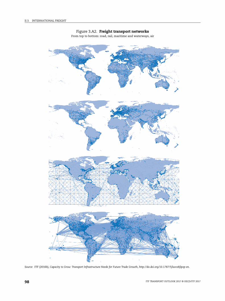
II.3. INTERNATIONAL FREIGHT
Figure 3.A2. Freight transport networksFrom top to bottom: road, rail, maritime and waterways, air
Source: ITF (2016b), Capacity to Grow: Transport Infrastructure Needs for Future Trade Growth, http://dx.doi.org/10.1787/5jlwvz8jlpzp-en.
ITF TRANSPORT OUTLOOK 2017 © OECD/ITF 201798
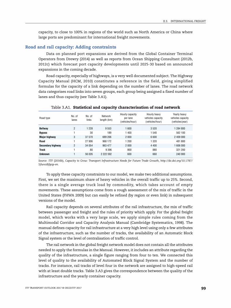
II.3. INTERNATIONAL FREIGHT
capacity, to close to 100% in regions of the world such as North America or China where
large ports are predominant for international freight movements.
Road and rail capacity: Adding constraintsData on planned port expansions are derived from the Global Container Terminal
Operators from Drewry (2014) as well as reports from Ocean Shipping Consultant (2012b,
2012c) which forecast port capacity developments until 2025-30 based on announced
expansions in the coming decade.
Road capacity, especially of highways, is a very well documented subject. The Highway
Capacity Manual (HCM, 2010) constitutes a reference in the field, giving simplified
formulas for the capacity of a link depending on the number of lanes. The road network
data categorises road links into seven groups, each group being assigned a fixed number of
lanes and thus capacity (see Table 3.A1).
To apply these capacity constraints to our model, we make two additional assumptions.
First, we set the maximum share of heavy vehicles in the overall traffic up to 25%. Second,
there is a single average truck load by commodity, which takes account of empty
movements. These assumptions come from a rough assessment of the mix of traffic in the
United States (FHWA 2009) but can easily be refined (by region or even link) in subsequent
versions of the model.
Rail capacity depends on several attributes of the rail infrastructure, the mix of traffic
between passenger and freight and the rules of priority which apply. For the global freight
model, which works with a very large scale, we apply simple rules coming from the
Multimodal Corridor and Capacity Analysis Manual (Cambridge Systematics, 1998). The
manual defines capacity for rail infrastructure at a very high level using only a few attributes
of the infrastructure, such as the number of tracks, the availability of an Automatic Block
Signal system or the level of centralisation of traffic control.
The rail network in the global freight network model does not contain all the attributes
needed to apply the formulas in the Manual. However, it includes an attribute regarding the
quality of the infrastructure, a single figure ranging from four to ten. We connected this
level of quality to the availability of Automated Block Signal System and the number of
tracks. For instance, rail tracks of level four in the network are assigned to high-speed rail
with at least double tracks. Table 3.A3 gives the correspondence between the quality of the
infrastructure and the yearly container capacity.
Table 3.A1. Statistical and capacity characterisation of road network
Road typeNo. of lanes
No. of links
Network length (km)
Hourly capacity per lane
(vehicles/hour)
Hourly heavy vehicles capacity (vehicles/hour)
Yearly heavy vehicles capacity (vehicles/year)
Beltway 2 1 228 9 553 1 600 3 520 1 284 800
Bypass 1 30 189 1 400 1 540 562 100
Major highway 3 37 570 689 206 2 000 6 600 2 409 000
Road 1 27 906 968 172 1 200 1 320 481 800
Secondary highway 2 34 054 963 477 2 000 4 400 1 606 000
Track 1 80 9 396 800 880 321 200
Unknown 1 56 026 2 222 592 600 660 240 900
Source: ITF (2016b), Capacity to Grow: Transport Infrastructure Needs for Future Trade Growth, http://dx.doi.org/10.1787/5jlwvz8jlpzp-en.
ITF TRANSPORT OUTLOOK 2017 © OECD/ITF 2017 99
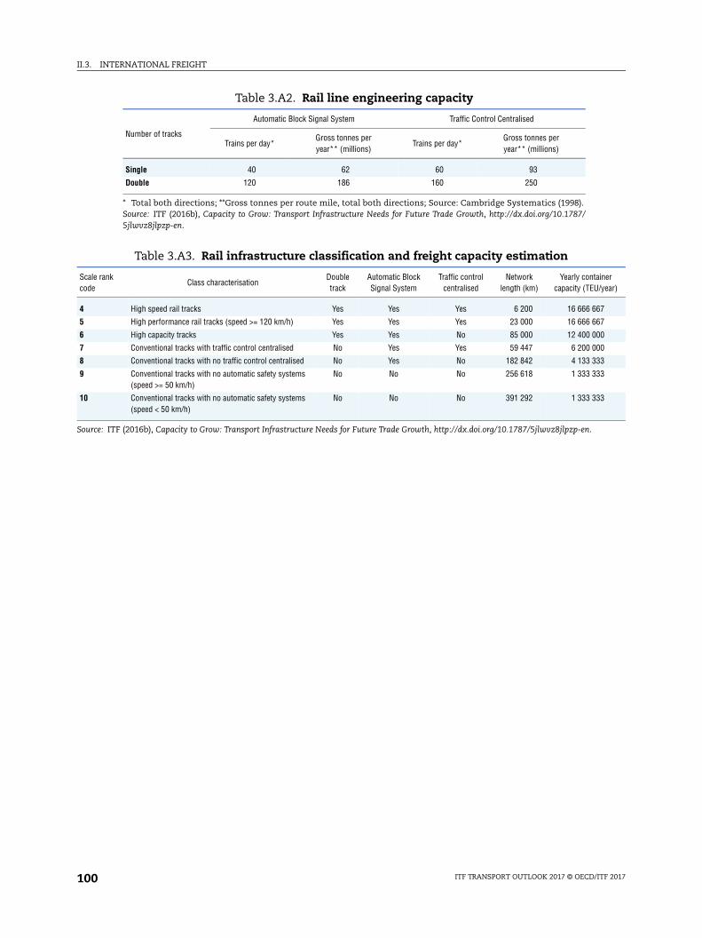
II.3. INTERNATIONAL FREIGHT
iner /year)
67
67
00
00
33
33
33
Table 3.A2. Rail line engineering capacity
Number of tracks
Automatic Block Signal System Traffic Control Centralised
Trains per day*Gross tonnes per year** (millions)
Trains per day*Gross tonnes per year** (millions)
Single 40 62 60 93
Double 120 186 160 250
* Total both directions; **Gross tonnes per route mile, total both directions; Source: Cambridge Systematics (1998).Source: ITF (2016b), Capacity to Grow: Transport Infrastructure Needs for Future Trade Growth, http://dx.doi.org/10.1787/5jlwvz8jlpzp-en.
Table 3.A3. Rail infrastructure classification and freight capacity estimation
Scale rank code
Class characterisationDouble track
Automatic Block Signal System
Traffic control centralised
Network length (km)
Yearly contacapacity (TEU
4 High speed rail tracks Yes Yes Yes 6 200 16 666 6
5 High performance rail tracks (speed >= 120 km/h) Yes Yes Yes 23 000 16 666 6
6 High capacity tracks Yes Yes No 85 000 12 400 0
7 Conventional tracks with traffic control centralised No Yes Yes 59 447 6 200 0
8 Conventional tracks with no traffic control centralised No Yes No 182 842 4 133 3
9 Conventional tracks with no automatic safety systems (speed >= 50 km/h)
No No No 256 618 1 333 3
10 Conventional tracks with no automatic safety systems (speed < 50 km/h)
No No No 391 292 1 333 3
Source: ITF (2016b), Capacity to Grow: Transport Infrastructure Needs for Future Trade Growth, http://dx.doi.org/10.1787/5jlwvz8jlpzp-en.
ITF TRANSPORT OUTLOOK 2017 © OECD/ITF 2017100
ITF Transport Outlook 2017 © OECD/ITF 2017
PART II
Chapter 4
International passenger aviation
International aviation continues to expand, contributing positively to the economy, but bringing with it challenges for the environment. This chapter starts by describing the process for modelling future global passenger demand and then presents three scenarios for the evolution of this demand and the related CO2 emissions. The three scenarios correspond to different mechanisms for the evolution of the air network and combine assumptions on the rules governing the geographical expansion of the network and on future competition levels. The chapter continues by considering projections for CO2 emissions from international passenger aviation up to 2030 as well as an overview of the longer-term prospects. The final section starts with an analysis of the current level of air accessibility, finishing with a global outlook for accessibility by air to 2030.
101
II.4. INTERNATIONAL PASSENGER AVIATION
The number of passengers carried on international flights has more than doubled in the
past two decades, benefitting from economic growth and an ever-growing network. Air
transport has also benefited from a large liberalisation movement in the past four decades,
increasing the economic activity of the sector and bringing significant advantages to
consumers in the form of lower prices and extended possibilities of travel. In the absence
of any significant constraints on the network, such as stalled liberalisation of air services
agreements, similar growth rates could materialise in the twenty years to come.
The rapid development of international aviation brings a significant climate challenge.
In 2015, international aviation represented about 2% of all CO2 emissions from fuel-burn
and, if unchecked, this figure could rise to 22% by 2050 under the IEA 2DS scenario
(European Parliament, 2015; see Glossary for details on 2DS). However, there is a strong
commitment by the industry and countries to limit emissions to their 2020 levels, through
a basket of measures, from CO2 efficiency standards for new aircrafts to a global market-
based measure agreed on at the General Assembly of the International Civil Aviation
Organisation (ICAO) in October 2016.
International aviation benefits from strong support from policy makers. Airport and
airport-related sectors directly generate output and employment in their neighbourhoods,
and indirectly through attracting other businesses, which local policy makers appreciate.
Aviation is valued for the connectivity it provides, creating workplaces that on average are
much more productive than in other areas of the economy. Aviation also facilitates the
movements of goods and services, workers and tourists, investment and ideas. Analysis
carried out for this Outlook (see the last section in this chapter) shows that, thanks to the
development of the air network, accessibility by air is improving in all regions, but still
remains very unequal.
Modelling global passenger demandAt the global level, several long-term aviation forecasts are produced by stakeholders,
most notably aircraft manufacturers. The two main ones, the Boeing Current Market Outlook
(Boeing, 2016) and the Airbus Global Market Forecast (Airbus, 2016) both foresee a large
increase in demand in the coming decades, resulting in an equally large demand for aircrafts.
ICAO (2016) and the International Air Transport Association also produce projections. All the
above forecasts share the view that the average yearly growth in global Revenue Passenger
Kilometres (RPKs) in the two coming decades will be around 5%, continuing the trend of the
years 2010-15. Despite the 6.5% growth recorded in the year 2015, these forecasts have been
revised down each year, most notably due to lower economic projections.
Most, if not all, available global forecasts use a time-series approach. The model in this
Outlook adopts a more structural approach, inferring the role of different socio-economic or
industry drivers by comparing the demand between the different regions of the world in a
single year. It also focuses on the role of the air network in creating demand, through the
application of different network evolution scenarios.
ITF TRANSPORT OUTLOOK 2017 © OECD/ITF 2017102
II.4. INTERNATIONAL PASSENGER AVIATION
In this new modelling framework (see also the methodological Annex 4.1), passenger
demand results from the combination of two sub-models: a gravity-type model for the
prediction of origin-destination passenger volumes and a route-choice model for the
assignment of the latter onto the air transport network. The models apply to a world
divided into 333 regions, each region corresponding to a main centre of economic activity
and having no more than one major airport. Aggregating the air network to these regions
forms a synthetic network on which the model is based. The gravitational model expresses
passenger demand between two regions as a function of socio-economic variables, such as
GDP, population, trade, cultural relationships (language sharing, emigration volumes, etc.)
and the generalised cost of travelling between the two regions. The generalised cost of
travel is itself a function of minimum travel time, minimum number of transfers and some
proxies for price. The model then divides demand between all possible itineraries by
comparing their quality of service, defined as a combination of travel time, number of
transfers, frequency and price.
Supply variables enter the demand prediction models (minimum travel time, price,
etc.). As a consequence, forecasting future passenger demand levels requires a detailed
knowledge of the future state of the network. However, the evolution of the air network is
dependent on phenomena that are difficult to forecast, such as the extent of future
liberalisation and its impacts on traffic rights and price setting, or the emergence of new
business models based on different airline economics or new aeroplanes.
This Outlook forecasts future passenger demand according to three network evolution
scenarios, with different assumptions regarding the future levels of competition and the
expansion of the air network. The following sections take a look at some historical trends
and derive modelling rules for competition and network expansion, useful in defining the
assumptions of the three network evolution scenarios, which are then described. The
section ends with a discussion of access restrictions and the impact they may have on the
scenarios.
Competition
Lower prices naturally lead to more demand for passenger transport, as they make
flying available to people with less purchasing power. The sensitivity of travel demand to
fares is well documented (see IATA, 2008 for instance). The strong growth in passenger
transport resulting from the arrival of low-cost airlines in North-America and Europe bears
testimony to this phenomenon. However, acquiring a comprehensive and coherent set of
ticket prices is a difficult task, due to the high volatility and business sensitivity of airline
fares. An online travel agent comparator, SkyScanner, provided a database of prices for the
year 2014. While this data was sufficient to assess the role of the different drivers behind
airline fares, it could not form the basis of a globally consistent fare model for forecasting.
Instead, the model includes two proxies for the price of airlines. The first is an
indicator of competition, the so-called h-index (see Box 4.1); the second is the presence or
absence of a low-cost carrier on the route. Available literature suggests that both indicators
impact prices negatively (e.g. Fu et al., 2010). In the SkyScanner fare data, both variables are
significant in explaining fares. For instance, for direct flights, there is a GBP 0.02 difference
in the average kilometric price between region pairs, depending on the value of the h-index
between 0 and 1, when the average kilometric price in the sample stands at GBP 0.15. The
presence of a low-cost carrier on a route writes off one-third of the ticket price on average
(see also Benezech et al., 2016).
ITF TRANSPORT OUTLOOK 2017 © OECD/ITF 2017 103
II.4. INTERNATIONAL PASSENGER AVIATION
If h-indices and the penetration of low-cost carriers do not capture all the effects related
to competition, they still explain much of the differences in kilometric prices between origin-
destination pairs. They can also be directly related to passenger demand. The explanatory
power of the related coefficients in the demand model is significant and their evolution in
the past decade has been particularly strong in regions where demand also surged. Figure 4.1
presents the evolution of an aggregate competition indicator in some regions or countries.
This indicator has been growing significantly in Asia, especially in India, where demand also
spiked. In this region, it is now on par with Europe, where competition is notably strong.
Similar trends can be observed for the penetration of low-cost carriers (see also Figure 4.3).
Box 4.1. Quantifying competition in the air market
Competition drives efficiency and the removing of restrictions on market entry, for example by liberalising air service agreements or expanding congested airports, and is indicated where existing agreements are restrictive. At the same time, competition in aviation takes several forms and markets are to some extent segmented. Hub airlines have arisen as a result of network economies whereby feeder traffic from short-haul routes helps fill intercontinental flights, permitting a wider range of profitable long-haul flights and greater frequencies of service on these routes. Other airlines, many of them following a low-cost business model, focus on point to point services, competing for long-haul traffic in some cases but more often on the short haul routes in competition with each other and the hub airline feeder services. Hub airlines have responded on price and quality and maintained most of their services but at a certain point the erosion of margins means routes have to be abandoned. This is not a linear process because of the interdependency of routes in the network. The anti-trust immunity accorded alliances of hub carriers when air service agreements are opened to more entry also complicates the overall scope for and impact of competition. Relieving capacity constraints at congested airports could have a more straightforward effect in enabling competition by reducing scarcity rents (usually accruing to incumbent airlines) and bringing down prices.
In practical terms, there is much debate about the best way to measure competition in the aviation market, relating to what constitutes a market and which airlines actually compete on each market segment.
The question of actual competition versus potential competition has arisen because of the emergence of global alliances and the development of code-sharing. Here, the constraint lies in the data available. The Innovata flight database indicates the operating airline but does not give full information about code-shares. We compute competition at the level of the alliance, or that of the airline for airlines outside of alliances, with a single indicator: the Herfindahl-Hirschman Index (HHI), or h-index. The h-index varies between 0 and 1, with 0 corresponding to atomistic competition and 1 to a monopolistic situation.
To take into account indirect routes, an h-index weighted for quality of service is used. This idea was first introduced by Veldhuis (Veldhuis, 1997) and is widely used in competition assessment (Lieshout and Matsumoto, 2012; Burghouwt et al., 2015). Using such weights, longer flights, or flights necessitating long layovers, are given less weight in the formula for the h-index.
Another crucial question lies in the way we define markets. Looking at airport or city pairs ignores competition between parallel routes, especially when low-cost carriers serve secondary airports (De Wit et al., 2009). Competition here is computed at the regional level, taking secondary airports into account.
ITF TRANSPORT OUTLOOK 2017 © OECD/ITF 2017104

II.4. INTERNATIONAL PASSENGER AVIATION
ee also
442645
4
Network expansion
The second lever within the network evolution scenarios is the geographical extent of
the network and the connectivity it offers. The ability of airlines to operate new flights
easily when they think it may be commercially viable is a key enabler of the growth of air
transport demand. Contrary to rail, the expansion of the air network does not always
necessitate much investment in infrastructure.
The reasons for which an airline may choose to operate a new route depend on a
myriad of factors related to expected costs and revenues, the integration of the route in the
overall network and existing competition levels. Bilateral or multilateral agreements may
also restrain the access of airlines or limit the number of seats they can offer. The network
evolution scenarios do not intend to reciprocate such an intricate process. Rather, it looks
at the evolution of the global air network from a very aggregate viewpoint, allowing several
key trends to emerge.
An analysis of the distribution of direct connections in the global air network shows
that there is a clear relationship between the presence of a direct link and the economic
activity of the origin and the destination. The economic mass of the link (product of the
GDP of the origin and that of the destination) captures the potential for travel at both ends
of the link. However, the threshold from which a link becomes viable and airlines start
operating flights depend on many other factors, several of them relating to operating costs.
More competitive environments lead to lower operating costs and the easier creation
of direct links. This trend appears when modelling the relationship between the probability
of existence of a direct connection and competition. Figure 4.2 shows the economic mass
which corresponds to a 0.5 probability of existence as a function of distance, in differing
environments. Competition has a significant impact on this threshold, reflecting at an
aggregate level the impact of more competition on operating costs. As a result, airlines are
able to operate between regions with lower economic power.
Figure 4.1. Competition in international aviationShare of international city-pairs with h- index lower than 0.5, %
Note: The h-index is an indicator of competition, with values between 0 and 1. Lower values indicate higher competition levels (sBox 4.1).
1 2 http://dx.doi.org/10.1787/888933
0
5
10
15
20
25
30
35
2004 2005 2006 2007 2008 2009 2010 2011 2012 2013 201
Asia Africa Europe North America India
ITF TRANSPORT OUTLOOK 2017 © OECD/ITF 2017 105
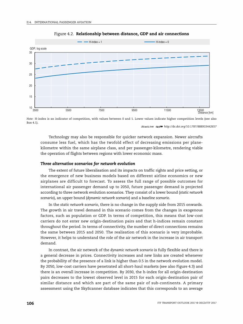
II.4. INTERNATIONAL PASSENGER AVIATION
ee also
442657
e [km]
Technology may also be responsible for quicker network expansion. Newer aircrafts
consume less fuel, which has the twofold effect of decreasing emissions per plane-
kilometre within the same airplane class, and per passenger-kilometre, rendering viable
the operation of flights between regions with lower economic mass.
Three alternative scenarios for network evolution
The extent of future liberalisation and its impacts on traffic rights and price setting, or
the emergence of new business models based on different airline economics or new
airplanes are difficult to forecast. To assess the full range of possible outcomes for
international air passenger demand up to 2050, future passenger demand is projected
according to three network evolution scenarios. They consist of a lower bound (static network
scenario), an upper bound (dynamic network scenario) and a baseline scenario.
In the static network scenario, there is no change in the supply side from 2015 onwards.
The growth in air travel demand in this scenario comes from the changes in exogenous
factors, such as population or GDP. In terms of competition, this means that low-cost
carriers do not enter new origin-destination pairs and that h-indices remain constant
throughout the period. In terms of connectivity, the number of direct connections remains
the same between 2015 and 2050. The realisation of this scenario is very improbable.
However, it helps to understand the role of the air network in the increase in air transport
demand.
In contrast, the air network of the dynamic network scenario is fully flexible and there is
a general decrease in prices. Connectivity increases and new links are created whenever
the probability of the presence of a link is higher than 0.5 in the network evolution model.
By 2050, low-cost carriers have penetrated all short-haul markets (see also Figure 4.3) and
there is an overall increase in competition. By 2030, the h-index for all origin-destination
pairs decreases to the lowest observed level in 2015 for each origin-destination pair of
similar distance and which are part of the same pair of sub-continents. A primary
assessment using the SkyScanner database indicates that this corresponds to an average
Figure 4.2. Relationship between distance, GDP and air connections
Note: H-index is an indicator of competition, with values between 0 and 1. Lower values indicate higher competition levels (sBox 4.1).
1 2 http://dx.doi.org/10.1787/888933
10
15
20
25
30
35
3500 5500 7500 9500 11500 13500
GDP, log scale
Distanc
H-index = 1 H-index = 0
ITF TRANSPORT OUTLOOK 2017 © OECD/ITF 2017106
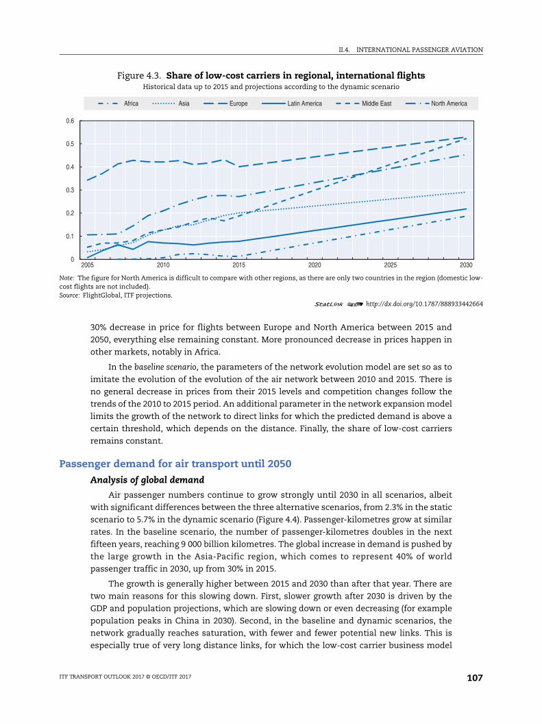
II.4. INTERNATIONAL PASSENGER AVIATION
ic low-
442664
030
ca
30% decrease in price for flights between Europe and North America between 2015 and
2050, everything else remaining constant. More pronounced decrease in prices happen in
other markets, notably in Africa.
In the baseline scenario, the parameters of the network evolution model are set so as to
imitate the evolution of the evolution of the air network between 2010 and 2015. There is
no general decrease in prices from their 2015 levels and competition changes follow the
trends of the 2010 to 2015 period. An additional parameter in the network expansion model
limits the growth of the network to direct links for which the predicted demand is above a
certain threshold, which depends on the distance. Finally, the share of low-cost carriers
remains constant.
Passenger demand for air transport until 2050
Analysis of global demand
Air passenger numbers continue to grow strongly until 2030 in all scenarios, albeit
with significant differences between the three alternative scenarios, from 2.3% in the static
scenario to 5.7% in the dynamic scenario (Figure 4.4). Passenger-kilometres grow at similar
rates. In the baseline scenario, the number of passenger-kilometres doubles in the next
fifteen years, reaching 9 000 billion kilometres. The global increase in demand is pushed by
the large growth in the Asia-Pacific region, which comes to represent 40% of world
passenger traffic in 2030, up from 30% in 2015.
The growth is generally higher between 2015 and 2030 than after that year. There are
two main reasons for this slowing down. First, slower growth after 2030 is driven by the
GDP and population projections, which are slowing down or even decreasing (for example
population peaks in China in 2030). Second, in the baseline and dynamic scenarios, the
network gradually reaches saturation, with fewer and fewer potential new links. This is
especially true of very long distance links, for which the low-cost carrier business model
Figure 4.3. Share of low-cost carriers in regional, international flightsHistorical data up to 2015 and projections according to the dynamic scenario
Note: The figure for North America is difficult to compare with other regions, as there are only two countries in the region (domestcost flights are not included). Source: FlightGlobal, ITF projections.
1 2 http://dx.doi.org/10.1787/888933
0
0.1
0.2
0.3
0.4
0.5
0.6
2005 2010 2015 2020 2025 2
Africa Asia Europe Latin America Middle East North Ameri
ITF TRANSPORT OUTLOOK 2017 © OECD/ITF 2017 107
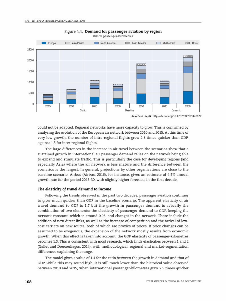
II.4. INTERNATIONAL PASSENGER AVIATION
442672
frica
could not be adapted. Regional networks have more capacity to grow. This is confirmed by
analysing the evolution of the European air network between 2010 and 2015. At this time of
very low growth, the number of intra-regional flights grew 2.5 times quicker than GDP,
against 1.5 for inter-regional flights.
The large differences in the increase in air travel between the scenarios show that a
sustained growth in international air passenger demand relies on the network being able
to expand and stimulate traffic. This is particularly the case for developing regions (and
especially Asia) where the air network is less mature and the difference between the
scenarios is the largest. In general, projections by other organisations are close to the
baseline scenario. Airbus (Airbus, 2016), for instance, gives an estimate of 4.5% annual
growth rate for the period 2015-30, with slightly higher forecasts in the first decade.
The elasticity of travel demand to income
Following the trends observed in the past two decades, passenger aviation continues
to grow much quicker than GDP in the baseline scenario. The apparent elasticity of air
travel demand to GDP is 1.7 but the growth in passenger demand is actually the
combination of two elements: the elasticity of passenger demand to GDP, keeping the
network constant, which is around 0.95, and changes in the network. These include the
addition of new direct links, as well as the increase of competition and the arrival of low-
cost carriers on new routes, both of which are proxies of prices. If price changes can be
assumed to be exogenous, the expansion of the network mostly results from economic
growth. When this effect is taken into account, the GDP elasticity of passenger-kilometres
becomes 1.3. This is consistent with most research, which finds elasticities between 1 and 2
(Gallet and Doucouliagos, 2014), with methodological, regional and market-segmentation
differences explaining the range.
The model gives a value of 1.4 for the ratio between the growth in demand and that of
GDP. While this may sound high, it is still much lower than the historical value observed
between 2010 and 2015, when international passenger-kilometres grew 2.5 times quicker
Figure 4.4. Demand for passenger aviation by regionBillion passenger-kilometres
1 2 http://dx.doi.org/10.1787/888933
0
5000
10000
15000
20000
25000
2015 2030 2050 2030 2050 2030 2050Static Baseline Dynamic
Europe Asia Pacific North America Latin America Middle East A
ITF TRANSPORT OUTLOOK 2017 © OECD/ITF 2017108
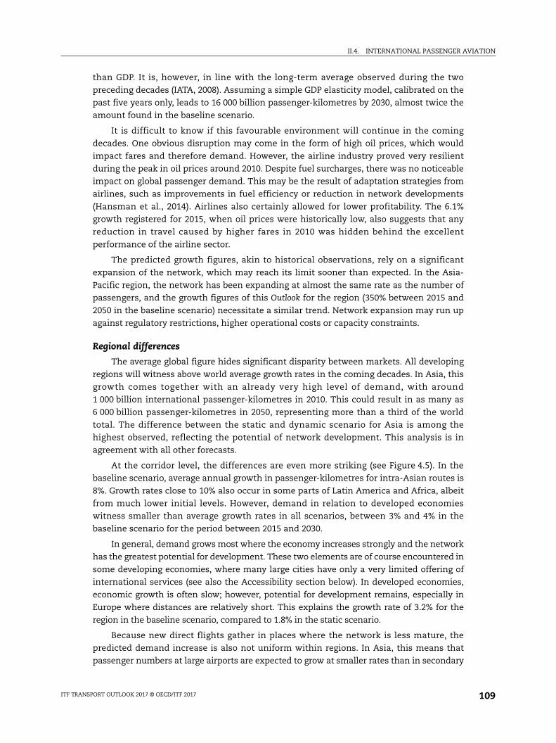
II.4. INTERNATIONAL PASSENGER AVIATION
than GDP. It is, however, in line with the long-term average observed during the two
preceding decades (IATA, 2008). Assuming a simple GDP elasticity model, calibrated on the
past five years only, leads to 16 000 billion passenger-kilometres by 2030, almost twice the
amount found in the baseline scenario.
It is difficult to know if this favourable environment will continue in the coming
decades. One obvious disruption may come in the form of high oil prices, which would
impact fares and therefore demand. However, the airline industry proved very resilient
during the peak in oil prices around 2010. Despite fuel surcharges, there was no noticeable
impact on global passenger demand. This may be the result of adaptation strategies from
airlines, such as improvements in fuel efficiency or reduction in network developments
(Hansman et al., 2014). Airlines also certainly allowed for lower profitability. The 6.1%
growth registered for 2015, when oil prices were historically low, also suggests that any
reduction in travel caused by higher fares in 2010 was hidden behind the excellent
performance of the airline sector.
The predicted growth figures, akin to historical observations, rely on a significant
expansion of the network, which may reach its limit sooner than expected. In the Asia-
Pacific region, the network has been expanding at almost the same rate as the number of
passengers, and the growth figures of this Outlook for the region (350% between 2015 and
2050 in the baseline scenario) necessitate a similar trend. Network expansion may run up
against regulatory restrictions, higher operational costs or capacity constraints.
Regional differences
The average global figure hides significant disparity between markets. All developing
regions will witness above world average growth rates in the coming decades. In Asia, this
growth comes together with an already very high level of demand, with around
1 000 billion international passenger-kilometres in 2010. This could result in as many as
6 000 billion passenger-kilometres in 2050, representing more than a third of the world
total. The difference between the static and dynamic scenario for Asia is among the
highest observed, reflecting the potential of network development. This analysis is in
agreement with all other forecasts.
At the corridor level, the differences are even more striking (see Figure 4.5). In the
baseline scenario, average annual growth in passenger-kilometres for intra-Asian routes is
8%. Growth rates close to 10% also occur in some parts of Latin America and Africa, albeit
from much lower initial levels. However, demand in relation to developed economies
witness smaller than average growth rates in all scenarios, between 3% and 4% in the
baseline scenario for the period between 2015 and 2030.
In general, demand grows most where the economy increases strongly and the network
has the greatest potential for development. These two elements are of course encountered in
some developing economies, where many large cities have only a very limited offering of
international services (see also the Accessibility section below). In developed economies,
economic growth is often slow; however, potential for development remains, especially in
Europe where distances are relatively short. This explains the growth rate of 3.2% for the
region in the baseline scenario, compared to 1.8% in the static scenario.
Because new direct flights gather in places where the network is less mature, the
predicted demand increase is also not uniform within regions. In Asia, this means that
passenger numbers at large airports are expected to grow at smaller rates than in secondary
ITF TRANSPORT OUTLOOK 2017 © OECD/ITF 2017 109
II.4. INTERNATIONAL PASSENGER AVIATION
erica;
airports. These airports, many of them still largely dependent on domestic traffic in 2015,
only recently started to accommodate international traffic. The growth is made possible by
the arrival of regional flights, in particular from low-cost carriers. For instance, the number
of international flights at Chongqing airport multiplied by five between 2010 and 2015, and
passenger demand is expected to increase at a yearly rate of more than 15% in the region
over the next two decades. This contrasts with the Beijing or Shanghai regions, where growth
is already slowing down (less than 5% increase in international passenger numbers in the
past years) and is expected to remain below the 5% limit in the future.
Low-cost intra-regional flights are an important motor of the growth of secondary
airports. As shown in Figure 4.3, the share of low-cost carriers in regional, non-domestic
flights has been growing in the past two decades in all world regions, albeit at different
paces. While this share is now almost stagnating in Europe, it is still growing quickly in
Asia, Latin America and the Middle-East. If their expansion is not hindered by legislation,
the proportion of low-cost carriers in these regions could quickly reach or exceed the levels
observed in Europe.
The situation in Africa is different, where many countries’ primary airports were still
not well connected to the global air network in 2015. The absence of a dynamic regional
market and of powerful low-cost carriers, hinder the potential for development of secondary
airports. In the baseline scenario, primary airports continue to attract most of the demand
and to concentrate the bulk of network development for the region, at least until 2030.
Impact of entry restrictionsEven if the three scenarios differ in the rules governing the evolution of the network,
none of them takes into account potential restrictions to the establishment of a new route.
When restrictive air service agreements (ASAs) are in place between two countries, the
total number of flights and/or seats between these countries may be bounded and foreign
airlines can be restricted in the airports from which they can operate. Another limiting
Figure 4.5. Regional breakdown of passenger-kilometres
1. Asia – North America; 2. Europe – North America; 3. Intra-Europe; 4. Europe – Asia; 5. Intra-Asia; 6. Latin America – North Am7. Intra-Africa; 8. Africa – Asia; 9. Intra Latin-America. Asia includes Japan and Korea in this map.
2015 2030 2050
2015 2030 2050
2015 2030 2050
2015 2030 2050
2015 2030 2050
2015 2030 2050
2015 2030 2050
2015 2030 2050
2015 2030 2050
1000
2000
3000StaticBaseline
Billionpassenger-kilometres
Dynamic
2
1
3 45
6
7
8
9
10
ITF TRANSPORT OUTLOOK 2017 © OECD/ITF 2017110
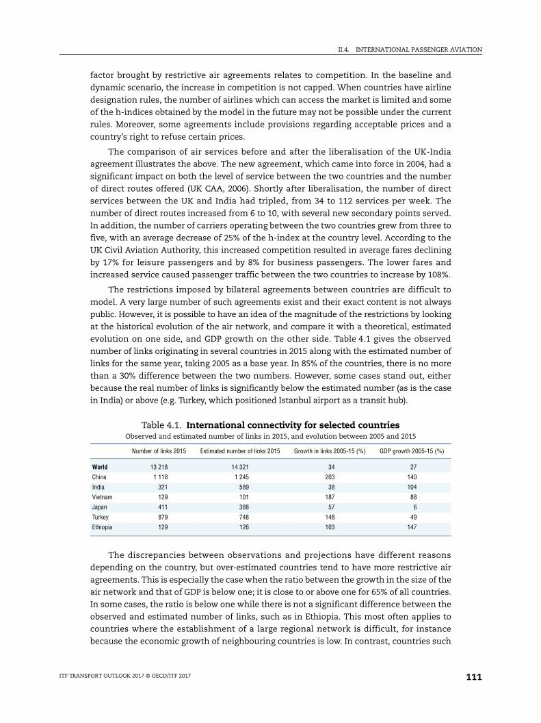
II.4. INTERNATIONAL PASSENGER AVIATION
factor brought by restrictive air agreements relates to competition. In the baseline and
dynamic scenario, the increase in competition is not capped. When countries have airline
designation rules, the number of airlines which can access the market is limited and some
of the h-indices obtained by the model in the future may not be possible under the current
rules. Moreover, some agreements include provisions regarding acceptable prices and a
country’s right to refuse certain prices.
The comparison of air services before and after the liberalisation of the UK-India
agreement illustrates the above. The new agreement, which came into force in 2004, had a
significant impact on both the level of service between the two countries and the number
of direct routes offered (UK CAA, 2006). Shortly after liberalisation, the number of direct
services between the UK and India had tripled, from 34 to 112 services per week. The
number of direct routes increased from 6 to 10, with several new secondary points served.
In addition, the number of carriers operating between the two countries grew from three to
five, with an average decrease of 25% of the h-index at the country level. According to the
UK Civil Aviation Authority, this increased competition resulted in average fares declining
by 17% for leisure passengers and by 8% for business passengers. The lower fares and
increased service caused passenger traffic between the two countries to increase by 108%.
The restrictions imposed by bilateral agreements between countries are difficult to
model. A very large number of such agreements exist and their exact content is not always
public. However, it is possible to have an idea of the magnitude of the restrictions by looking
at the historical evolution of the air network, and compare it with a theoretical, estimated
evolution on one side, and GDP growth on the other side. Table 4.1 gives the observed
number of links originating in several countries in 2015 along with the estimated number of
links for the same year, taking 2005 as a base year. In 85% of the countries, there is no more
than a 30% difference between the two numbers. However, some cases stand out, either
because the real number of links is significantly below the estimated number (as is the case
in India) or above (e.g. Turkey, which positioned Istanbul airport as a transit hub).
The discrepancies between observations and projections have different reasons
depending on the country, but over-estimated countries tend to have more restrictive air
agreements. This is especially the case when the ratio between the growth in the size of the
air network and that of GDP is below one; it is close to or above one for 65% of all countries.
In some cases, the ratio is below one while there is not a significant difference between the
observed and estimated number of links, such as in Ethiopia. This most often applies to
countries where the establishment of a large regional network is difficult, for instance
because the economic growth of neighbouring countries is low. In contrast, countries such
Table 4.1. International connectivity for selected countriesObserved and estimated number of links in 2015, and evolution between 2005 and 2015
Number of links 2015 Estimated number of links 2015 Growth in links 2005-15 (%) GDP growth 2005-15 (%)
World 13 218 14 321 34 27
China 1 118 1 245 203 140
India 321 589 38 104
Vietnam 129 101 187 88
Japan 411 388 57 6
Turkey 879 748 148 49
Ethiopia 129 126 103 147
ITF TRANSPORT OUTLOOK 2017 © OECD/ITF 2017 111
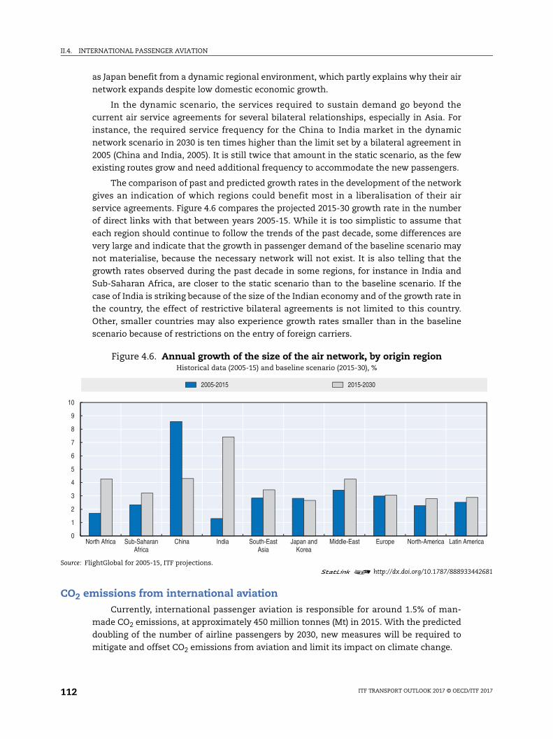
II.4. INTERNATIONAL PASSENGER AVIATION
442681
erica
as Japan benefit from a dynamic regional environment, which partly explains why their air
network expands despite low domestic economic growth.
In the dynamic scenario, the services required to sustain demand go beyond the
current air service agreements for several bilateral relationships, especially in Asia. For
instance, the required service frequency for the China to India market in the dynamic
network scenario in 2030 is ten times higher than the limit set by a bilateral agreement in
2005 (China and India, 2005). It is still twice that amount in the static scenario, as the few
existing routes grow and need additional frequency to accommodate the new passengers.
The comparison of past and predicted growth rates in the development of the network
gives an indication of which regions could benefit most in a liberalisation of their air
service agreements. Figure 4.6 compares the projected 2015-30 growth rate in the number
of direct links with that between years 2005-15. While it is too simplistic to assume that
each region should continue to follow the trends of the past decade, some differences are
very large and indicate that the growth in passenger demand of the baseline scenario may
not materialise, because the necessary network will not exist. It is also telling that the
growth rates observed during the past decade in some regions, for instance in India and
Sub-Saharan Africa, are closer to the static scenario than to the baseline scenario. If the
case of India is striking because of the size of the Indian economy and of the growth rate in
the country, the effect of restrictive bilateral agreements is not limited to this country.
Other, smaller countries may also experience growth rates smaller than in the baseline
scenario because of restrictions on the entry of foreign carriers.
CO2 emissions from international aviationCurrently, international passenger aviation is responsible for around 1.5% of man-
made CO2 emissions, at approximately 450 million tonnes (Mt) in 2015. With the predicted
doubling of the number of airline passengers by 2030, new measures will be required to
mitigate and offset CO2 emissions from aviation and limit its impact on climate change.
Figure 4.6. Annual growth of the size of the air network, by origin regionHistorical data (2005-15) and baseline scenario (2015-30), %
Source: FlightGlobal for 2005-15, ITF projections.1 2 http://dx.doi.org/10.1787/888933
0
1
2
3
4
5
6
7
8
9
10
North Africa Sub-SaharanAfrica
China India South-EastAsia
Japan andKorea
Middle-East Europe North-America Latin Am
2005-2015 2015-2030
ITF TRANSPORT OUTLOOK 2017 © OECD/ITF 2017112
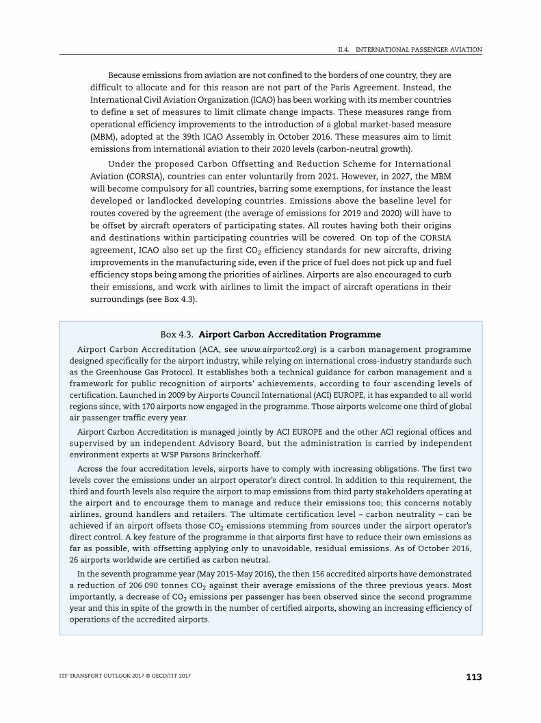
II.4. INTERNATIONAL PASSENGER AVIATION
e ch
d a of rld bal
nd nt
wo the at bly be r’s as 16,
ted ost me of
Because emissions from aviation are not confined to the borders of one country, they are
difficult to allocate and for this reason are not part of the Paris Agreement. Instead, the
International Civil Aviation Organization (ICAO) has been working with its member countries
to define a set of measures to limit climate change impacts. These measures range from
operational efficiency improvements to the introduction of a global market-based measure
(MBM), adopted at the 39th ICAO Assembly in October 2016. These measures aim to limit
emissions from international aviation to their 2020 levels (carbon-neutral growth).
Under the proposed Carbon Offsetting and Reduction Scheme for International
Aviation (CORSIA), countries can enter voluntarily from 2021. However, in 2027, the MBM
will become compulsory for all countries, barring some exemptions, for instance the least
developed or landlocked developing countries. Emissions above the baseline level for
routes covered by the agreement (the average of emissions for 2019 and 2020) will have to
be offset by aircraft operators of participating states. All routes having both their origins
and destinations within participating countries will be covered. On top of the CORSIA
agreement, ICAO also set up the first CO2 efficiency standards for new aircrafts, driving
improvements in the manufacturing side, even if the price of fuel does not pick up and fuel
efficiency stops being among the priorities of airlines. Airports are also encouraged to curb
their emissions, and work with airlines to limit the impact of aircraft operations in their
surroundings (see Box 4.3).
Box 4.3. Airport Carbon Accreditation Programme
Airport Carbon Accreditation (ACA, see www.airportco2.org) is a carbon management programmdesigned specifically for the airport industry, while relying on international cross-industry standards suas the Greenhouse Gas Protocol. It establishes both a technical guidance for carbon management anframework for public recognition of airports’ achievements, according to four ascending levelscertification. Launched in 2009 by Airports Council International (ACI) EUROPE, it has expanded to all woregions since, with 170 airports now engaged in the programme. Those airports welcome one third of gloair passenger traffic every year.
Airport Carbon Accreditation is managed jointly by ACI EUROPE and the other ACI regional offices asupervised by an independent Advisory Board, but the administration is carried by independeenvironment experts at WSP Parsons Brinckerhoff.
Across the four accreditation levels, airports have to comply with increasing obligations. The first tlevels cover the emissions under an airport operator’s direct control. In addition to this requirement, third and fourth levels also require the airport to map emissions from third party stakeholders operatingthe airport and to encourage them to manage and reduce their emissions too; this concerns notaairlines, ground handlers and retailers. The ultimate certification level – carbon neutrality – canachieved if an airport offsets those CO2 emissions stemming from sources under the airport operatodirect control. A key feature of the programme is that airports first have to reduce their own emissionsfar as possible, with offsetting applying only to unavoidable, residual emissions. As of October 2026 airports worldwide are certified as carbon neutral.
In the seventh programme year (May 2015-May 2016), the then 156 accredited airports have demonstraa reduction of 206 090 tonnes CO2 against their average emissions of the three previous years. Mimportantly, a decrease of CO2 emissions per passenger has been observed since the second programyear and this in spite of the growth in the number of certified airports, showing an increasing efficiencyoperations of the accredited airports.
ITF TRANSPORT OUTLOOK 2017 © OECD/ITF 2017 113
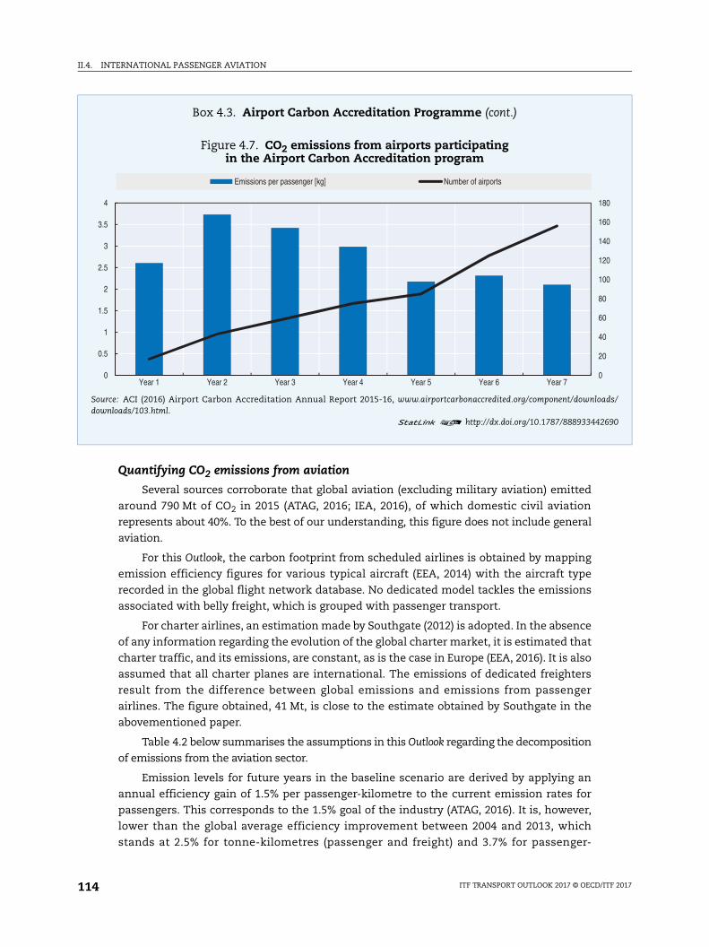
II.4. INTERNATIONAL PASSENGER AVIATION
ds/
690
0
0
0
0
00
20
40
60
80
Quantifying CO2 emissions from aviation
Several sources corroborate that global aviation (excluding military aviation) emitted
around 790 Mt of CO2 in 2015 (ATAG, 2016; IEA, 2016), of which domestic civil aviation
represents about 40%. To the best of our understanding, this figure does not include general
aviation.
For this Outlook, the carbon footprint from scheduled airlines is obtained by mapping
emission efficiency figures for various typical aircraft (EEA, 2014) with the aircraft type
recorded in the global flight network database. No dedicated model tackles the emissions
associated with belly freight, which is grouped with passenger transport.
For charter airlines, an estimation made by Southgate (2012) is adopted. In the absence
of any information regarding the evolution of the global charter market, it is estimated that
charter traffic, and its emissions, are constant, as is the case in Europe (EEA, 2016). It is also
assumed that all charter planes are international. The emissions of dedicated freighters
result from the difference between global emissions and emissions from passenger
airlines. The figure obtained, 41 Mt, is close to the estimate obtained by Southgate in the
abovementioned paper.
Table 4.2 below summarises the assumptions in this Outlook regarding the decomposition
of emissions from the aviation sector.
Emission levels for future years in the baseline scenario are derived by applying an
annual efficiency gain of 1.5% per passenger-kilometre to the current emission rates for
passengers. This corresponds to the 1.5% goal of the industry (ATAG, 2016). It is, however,
lower than the global average efficiency improvement between 2004 and 2013, which
stands at 2.5% for tonne-kilometres (passenger and freight) and 3.7% for passenger-
Box 4.3. Airport Carbon Accreditation Programme (cont.)
Figure 4.7. CO2 emissions from airports participating in the Airport Carbon Accreditation program
Source: ACI (2016) Airport Carbon Accreditation Annual Report 2015-16, www.airportcarbonaccredited.org/component/downloadownloads/103.html.
1 2 http://dx.doi.org/10.1787/888933442
0
2
4
6
8
1
1
1
1
1
0
0.5
1
1.5
2
2.5
3
3.5
4
Year 1 Year 2 Year 3 Year 4 Year 5 Year 6 Year 7
Emissions per passenger [kg] Number of airports
ITF TRANSPORT OUTLOOK 2017 © OECD/ITF 2017114
II.4. INTERNATIONAL PASSENGER AVIATION
kilometres. The lower figure of 1.5% is preferred in a baseline scenario because most of the
efficiency gains from the past decade correspond to a single year, 2010, the other years
seeing efficiency gains closer to 1.5%. Moreover, as passenger demand grows more quickly
than freight, the share of belly freight in the total tonne-kilometres decreases, which
mechanically decreases the efficiency gains for passengers.
Emissions are also computed in a low-carbon scenario, where the yearly efficiency
gain is 2%, corresponding to the resolution of ICAO member States in 2013 (ICAO, 2013). In
this scenario, we assume that the penetration of biofuel in 2050 is 50%. This percentage is
slightly higher than the 40% indicated as a target in the European Union White Paper for
transport (European Commission, 2011) and indicates a strong commitment to the use of
sustainable low-carbon fuels in aviation.
In all scenarios, emissions from charter airlines are assumed to remain constant. Emissions
from dedicated freighters grow according to the demand volumes estimated in Chapter 3,
adjusted by the same 1.5% or 2% efficiency improvement per tonne-kilometre per year.
CO2 emissions from passenger international aviation up to 2030
In the baseline scenario, emissions from international aviation go up 56% by 2030, to
710 Mt (Figure 4.8), excluding dedicated freighters. Mirroring the evolution of passenger
demand, the growth in emissions is concentrated in developing countries. In 2030, the
Asia-Pacific region will represent around 35% of global CO2 emissions from international
scheduled flights, up from 27% in 2015. Higher efficiency gains allow savings of 50 Mt
annually, as shown by the low-carbon scenario.
While emissions in the static scenario are almost constant due to the efficiency gains
being close to the rate of increase in demand, the additional passenger-kilometres in the
dynamic scenario result in the addition of 110 Mt of emissions compared to the baseline
scenario. However, it is likely that the efficiency gains would be higher if the dynamic
scenario materialises, as it will necessitate the quicker introduction of new airplanes.
Achieving carbon-neutral growth for passenger international aviation from 2020 in the
baseline scenario will require 1 000 Mt of cumulated carbon offsets during the decade
between 2020 and 2030. In the year 2030 alone, the offsets required reache 200 Mt, or 220 Mt
when including dedicated freighters. This is lower than suggested by work undertaken by
the ICAO Committee on Aviation Environmental Protection (ICAO/CAEP, 2016), which gives
figures between 288 and 376 Mt for the number of offsets required in 2030. There are two
main underlying reasons. First, the average growth rate of the ITF scenario (4.7%) is lower
than that of the study (around 5%). In the dynamic network scenario, the overall
requirement for offsets to achieve carbon-neutral growth would be around 1 400 Mt of CO2
with 270 Mt for the year 2030 alone. The second reason for the low offset requirement lies
Table 4.2. Breakdown of CO2 emissions from aviation
Sector Emissions (Mt) % of total emissions
Domestic 300 38
Scheduled passenger 293 37
Dedicated freighters 7 1
International 490 62
Scheduled passenger 418 53
Charters 38 5
Dedicated freighters 34 4
ITF TRANSPORT OUTLOOK 2017 © OECD/ITF 2017 115
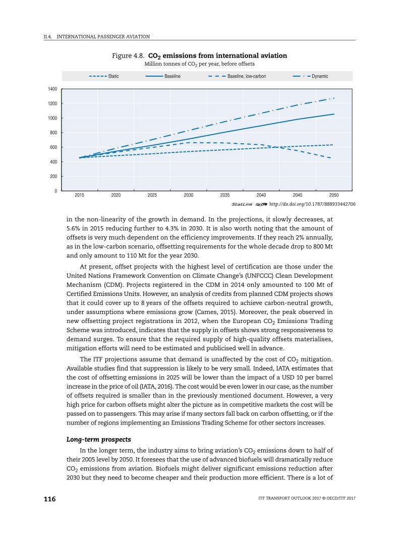
II.4. INTERNATIONAL PASSENGER AVIATION
442706
in the non-linearity of the growth in demand. In the projections, it slowly decreases, at
5.6% in 2015 reducing further to 4.3% in 2030. It is also worth noting that the amount of
offsets is very much dependent on the efficiency improvements. If they reach 2% annually,
as in the low-carbon scenario, offsetting requirements for the whole decade drop to 800 Mt
and only amount to 110 Mt for the year 2030.
At present, offset projects with the highest level of certification are those under the
United Nations Framework Convention on Climate Change’s (UNFCCC) Clean Development
Mechanism (CDM). Projects registered in the CDM in 2014 only amounted to 100 Mt of
Certified Emissions Units. However, an analysis of credits from planned CDM projects shows
that it could cover up to 8 years of the offsets required to achieve carbon-neutral growth,
under assumptions where emissions grow (Cames, 2015). Moreover, the peak observed in
new offsetting project registrations in 2012, when the European CO2 Emissions Trading
Scheme was introduced, indicates that the supply in offsets shows strong responsiveness to
demand surges. To ensure that the required supply of high-quality offsets materialises,
mitigation efforts will need to be estimated and publicised well in advance.
The ITF projections assume that demand is unaffected by the cost of CO2 mitigation.
Available studies find that suppression is likely to be very small. Indeed, IATA estimates that
the cost of offsetting emissions in 2025 will be lower than the impact of a USD 10 per barrel
increase in the price of oil (IATA, 2016). The cost would be even lower in our case, as the number
of offsets required is smaller than in the previously mentioned document. However, a very
high price for carbon offsets might alter the picture as in competitive markets the cost will be
passed on to passengers. This may arise if many sectors fall back on carbon offsetting, or if the
number of regions implementing an Emissions Trading Scheme for other sectors increases.
Long-term prospects
In the longer term, the industry aims to bring aviation’s CO2 emissions down to half of
their 2005 level by 2050. It foresees that the use of advanced biofuels will dramatically reduce
CO2 emissions from aviation. Biofuels might deliver significant emissions reduction after
2030 but they need to become cheaper and their production more efficient. There is a lot of
Figure 4.8. CO2 emissions from international aviationMillion tonnes of CO2 per year, before offsets
1 2 http://dx.doi.org/10.1787/888933
0
200
400
600
800
1000
1200
1400
2015 2020 2025 2030 2035 2040 2045 2050
Static Baseline Baseline, low-carbon Dynamic
ITF TRANSPORT OUTLOOK 2017 © OECD/ITF 2017116
II.4. INTERNATIONAL PASSENGER AVIATION
uncertainty regarding the speed at which sufficient quantities of suitable biofuels can be
phased in. There may also be competition from other modes, in particular from the freight
sector (see also the section on emissions in Chapter 3).
Assuming biofuels have the same energy content as conventional fossil fuels, biofuels
will need to represent around 80% of aviation fuels by 2050 and this share will only suffice
if net CO2 emissions of aviation biofuels are zero. Deane et al (2015) found a similar figure
for Europe (77%), to reach the same target. If the carbon savings compared to conventional
jet fuel were only 70% (a typical figure for current aviation biofuels) the industry target will
require that biofuels power all international flights.
There are very large uncertainties around the potential for the development of
commercially viable biofuels. An 80% share for biofuels in aviation is ambitious, considering
its current marginal relevance and the planning assumptions of some government bodies.
The previously mentioned article (Deane et al., 2015) estimates that the production of
biofuels will have to triple in ten years between 2040 and 2050 to reach such numbers.
Advanced second-generation aviation biofuels are produced from algae or non-food parts of
crops, so do not compete with food production or necessitate the destruction of carbon sinks
such as forests. However, this makes the production process significantly more complex and
such biofuels cost up to twice as much as conventional kerosene. Cost is currently the biggest
barrier to the broad introduction of biofuels in aviation. In the current context of low oil
prices, airlines have little or no economic incentive to invest in alternative fuel technologies.
Accessibility by airAviation brings many benefits to the countries it serves and is not easily replaced with
another, less polluting mode, especially for international flights. For businesses operating
across borders there is often no real alternative to aviation as a mode of transport. It
generates economic activity, through airlines, aircraft manufacturers and airports. A recent
report (ATAG, 2016) estimates that the air transport industry generates around 10 million
jobs. The same report estimates the GDP attributable to the aviation sector at 1 425 billion USD,
or 2% of world GDP in 2015.
The aviation industry is also a key enabler of trade and of many other industries, the
first of which is tourism. In 2015, more than half of international tourists arrived by air
(UNWTO, 2015). This is especially important for developing countries, which are generally
quite far from the countries where their tourists originate. Other research (Oxford
Economic Forecasting, 2006) has suggested that air connectivity, by providing access to
large markets and improving the links between businesses, can boost productivity. Air
connectivity can also influence the choice of location for foreign direct investments or help
attract the most talented individuals (Oxford Economic Forecasting, 2006).
If most of the studies above relate to developed economies, there seems to be a
positive relationship between air connectivity and productivity for all countries (IATA,
2007). This relationship is even stronger for low-income countries. Considering the
economic importance of aviation, there has been a general effort to define an indicator
which best reflects the role of air travel in the economy.
Global indicator of accessibility by air
While air connectivity is the general term in usage, many indicators refer to accessibility
by air. Within the general category of connectivity indicators, there is indeed a clear distinction
ITF TRANSPORT OUTLOOK 2017 © OECD/ITF 2017 117
II.4. INTERNATIONAL PASSENGER AVIATION
between centrality indicators and accessibility indicators (Burghouwt and Redondi, 2013). The
former, which describe the integration of an airport in the global air network, rely on
topological indicators and can be of theoretical importance and help analyse the behaviour of
transfer passengers. However, it is with the latter that one can measure the attractiveness of
an airport, or the cities attached to it. Accessibility indicators measure how easily the world
can be reached from an airport, for instance through the number of destinations accessible in
less than a given number of hours, or the number of direct connections. They answer the
question: How accessible are world markets from a given airport or country?
Because the wider economic impacts of aviation come from the links they provide to
businesses, enabling them to access larger markets and to connect to other businesses,
accessibility indicators provide a better insight into the potential role which aviation has
on the economy. In addition, because the economic activity which aviation facilitates is
more likely to be situated in urban centres than in rural areas or right next to airports, this
Outlook proposes computing an accessibility indicator which measures how cities are
connected to the air network, and not airports.
The accessibility indicator in this Outlook measures the travel time from the centre of
urban agglomerations to a basket of cities around the world, the alpha-cities, as defined by
the Globalization and World Cities Research Network (GaWCR, 2014). These cities are
representative of the current main global economic centres of activity. The travel time is
computed from the centre of urban agglomerations and includes both the time to access
airports, measured on the road network, and the time in the air, including layovers when
necessary (see also the methodological Annex 4.2).
The proposed indicator answers the need for a simple measure, expressed in a real-
world unit (hours). It enables comparisons between cities of different regions of the world.
For this Outlook, the indicator is derived for all cities above 300 000 inhabitants, the same
sample of cities which is used in Chapter 5, in the section on urban mobility.
The methodology is flexible and can be adapted to different regional contexts, but
these 61 alpha-cities, scattered over the five continents, are useful as destinations for
having a globally coherent measure (see the map in Figure 4.A2 in Annex).
Air accessibility today
In 2015, the average time to reach an alpha-city ranged from 12 to 72 hours and, on
average over all the urban agglomerations above 300 000 inhabitants, 32 alpha-cities were
accessible in less than a day.
As expected from the geographical distribution of alpha-cities, developed countries
concentrate most of the cities which have the best access to the main global economic centres
(Figure 4.9). However, geography does not explain everything. The size of the accessibility gap
between the most connected cities, which are mostly situated in developed countries, and the
least connected ones in Africa can be explained by a combination of three factors.
The first factor is the time spent on the roads to access an airport with relevant services.
It is much greater in developing economies than in developed ones due to the scarcity of
airports, especially international airports, and to the lower quality of the road network. In
2015, the airport-access factor explained 40-50% of the difference in accessibility between
developing countries and Europe. The second factor, accounting for around 35% of the same
difference, is the lower quality of the air network serving the developing regions. Because
airports in these regions have few direct connections, travellers need to make large detours
ITF TRANSPORT OUTLOOK 2017 © OECD/ITF 2017118
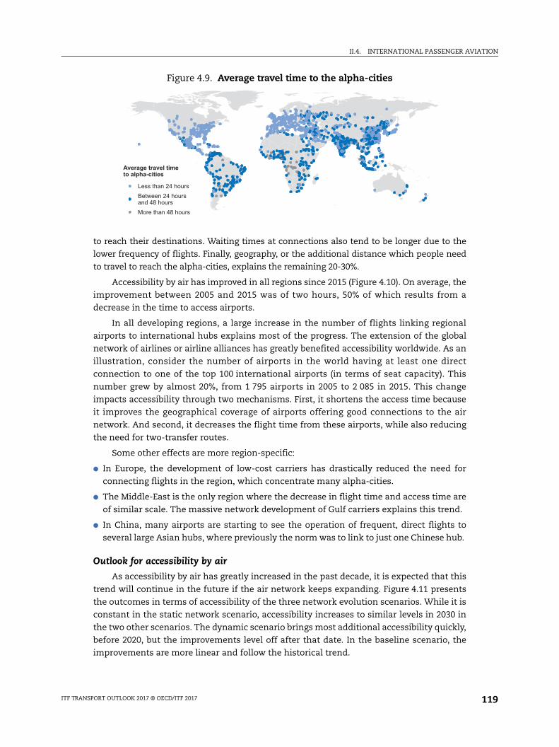
II.4. INTERNATIONAL PASSENGER AVIATION
to reach their destinations. Waiting times at connections also tend to be longer due to the
lower frequency of flights. Finally, geography, or the additional distance which people need
to travel to reach the alpha-cities, explains the remaining 20-30%.
Accessibility by air has improved in all regions since 2015 (Figure 4.10). On average, the
improvement between 2005 and 2015 was of two hours, 50% of which results from a
decrease in the time to access airports.
In all developing regions, a large increase in the number of flights linking regional
airports to international hubs explains most of the progress. The extension of the global
network of airlines or airline alliances has greatly benefited accessibility worldwide. As an
illustration, consider the number of airports in the world having at least one direct
connection to one of the top 100 international airports (in terms of seat capacity). This
number grew by almost 20%, from 1 795 airports in 2005 to 2 085 in 2015. This change
impacts accessibility through two mechanisms. First, it shortens the access time because
it improves the geographical coverage of airports offering good connections to the air
network. And second, it decreases the flight time from these airports, while also reducing
the need for two-transfer routes.
Some other effects are more region-specific:
● In Europe, the development of low-cost carriers has drastically reduced the need for
connecting flights in the region, which concentrate many alpha-cities.
● The Middle-East is the only region where the decrease in flight time and access time are
of similar scale. The massive network development of Gulf carriers explains this trend.
● In China, many airports are starting to see the operation of frequent, direct flights to
several large Asian hubs, where previously the norm was to link to just one Chinese hub.
Outlook for accessibility by air
As accessibility by air has greatly increased in the past decade, it is expected that this
trend will continue in the future if the air network keeps expanding. Figure 4.11 presents
the outcomes in terms of accessibility of the three network evolution scenarios. While it is
constant in the static network scenario, accessibility increases to similar levels in 2030 in
the two other scenarios. The dynamic scenario brings most additional accessibility quickly,
before 2020, but the improvements level off after that date. In the baseline scenario, the
improvements are more linear and follow the historical trend.
Figure 4.9. Average travel time to the alpha-cities
Average travel timeto alpha-cities
Less than 24 hoursBetween 24 hoursand 48 hoursMore than 48 hours
ITF TRANSPORT OUTLOOK 2017 © OECD/ITF 2017 119
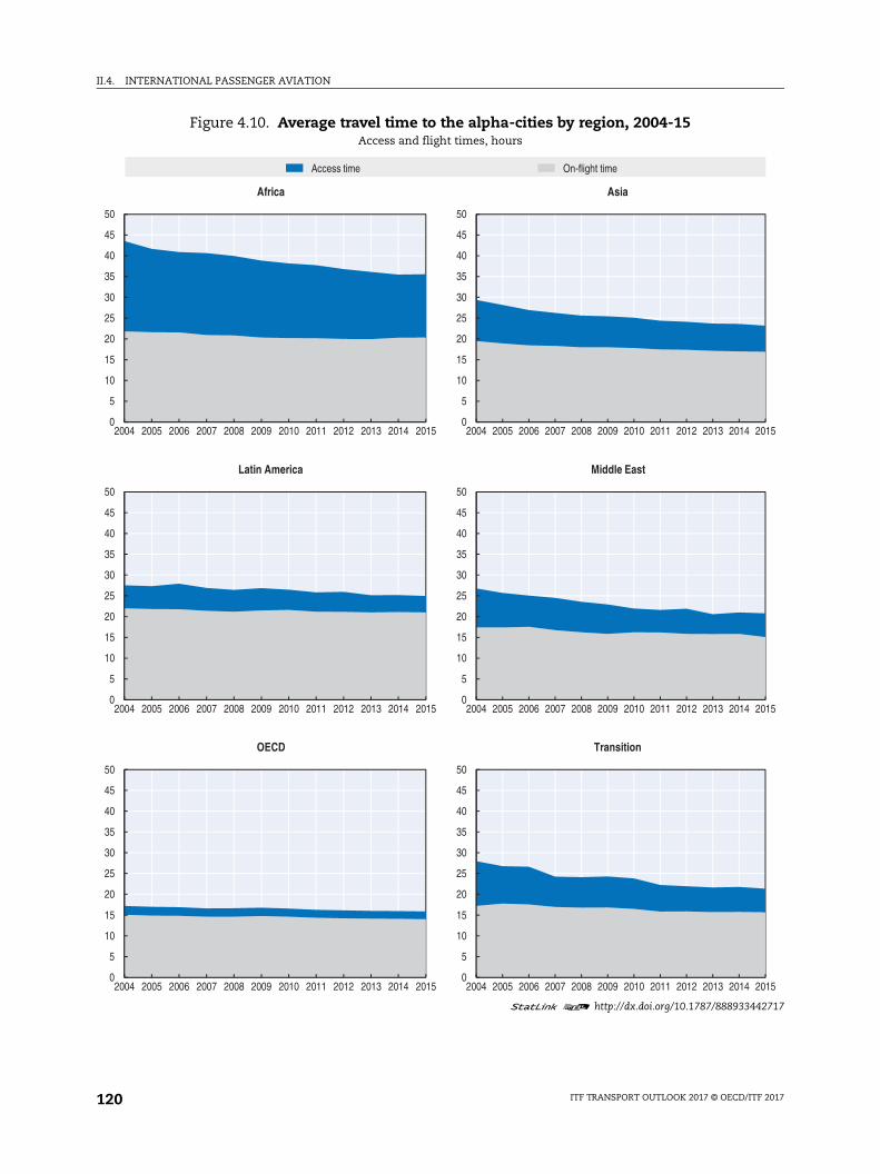
II.4. INTERNATIONAL PASSENGER AVIATION
442717
2015
2015
2015
Figure 4.10. Average travel time to the alpha-cities by region, 2004-15Access and flight times, hours
1 2 http://dx.doi.org/10.1787/888933
0
5
10
15
20
25
30
35
40
45
50
2004 2005 2006 2007 2008 2009 2010 2011 2012 2013 2014 2015
Africa
0
5
10
15
20
25
30
35
40
45
50
2004 2005 2006 2007 2008 2009 2010 2011 2012 2013 2014
Asia
0
5
10
15
20
25
30
35
40
45
50
2004 2005 2006 2007 2008 2009 2010 2011 2012 2013 2014 2015
Latin America
0
5
10
15
20
25
30
35
40
45
50
2004 2005 2006 2007 2008 2009 2010 2011 2012 2013 2014
Middle East
0
5
10
15
20
25
30
35
40
45
50
2004 2005 2006 2007 2008 2009 2010 2011 2012 2013 2014 2015
OECD
0
5
10
15
20
25
30
35
40
45
50
2004 2005 2006 2007 2008 2009 2010 2011 2012 2013 2014
Transition
Access time On-flight time
ITF TRANSPORT OUTLOOK 2017 © OECD/ITF 2017120
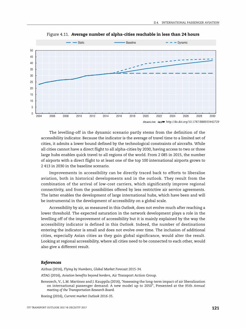
II.4. INTERNATIONAL PASSENGER AVIATION
442729
2030
The levelling-off in the dynamic scenario partly stems from the definition of the
accessibility indicator. Because the indicator is the average of travel time to a limited set of
cities, it admits a lower bound defined by the technological constraints of aircrafts. While
all cities cannot have a direct flight to all alpha-cities by 2030, having access to two or three
large hubs enables quick travel to all regions of the world. From 2 085 in 2015, the number
of airports with a direct flight to at least one of the top 100 international airports grows to
2 413 in 2030 in the baseline scenario.
Improvements in accessibility can be directly traced back to efforts to liberalise
aviation, both in historical developments and in the outlook. They result from the
combination of the arrival of low-cost carriers, which significantly improve regional
connectivity, and from the possibilities offered by less restrictive air service agreements.
The latter enables the development of large international hubs, which have been and will
be instrumental in the development of accessibility on a global scale.
Accessibility by air, as measured in this Outlook, does not evolve much after reaching a
lower threshold. The expected saturation in the network development plays a role in the
levelling off of the improvement of accessibility but it is mainly explained by the way the
accessibility indicator is defined in this Outlook. Indeed, the number of destinations
entering the indicator is small and does not evolve over time. The inclusion of additional
cities, especially Asian cities as they gain global significance, would alter the result.
Looking at regional accessibility, where all cities need to be connected to each other, would
also give a different result.
References
Airbus (2016), Flying by Numbers, Global Market Forecast 2015-34.
ATAG (2016), Aviation benefits beyond borders, Air Transport Action Group.
Benezech, V., L.M. Martinez and J. Kauppila (2016), “Assessing the long-term impact of air liberalization on international passenger demand: A new model up to 2050”, Presented at the 95th Annual meeting of the Transportation Research Board.
Boeing (2016), Current market Outlook 2016-35.
Figure 4.11. Average number of alpha-cities reachable in less than 24 hours
1 2 http://dx.doi.org/10.1787/888933
0
5
10
15
20
25
30
35
40
45
50
2004 2006 2008 2010 2012 2014 2016 2018 2020 2022 2024 2026 2028
Static Baseline Dynamic
ITF TRANSPORT OUTLOOK 2017 © OECD/ITF 2017 121
II.4. INTERNATIONAL PASSENGER AVIATION
Burghouwt, G. and R. Redondi (2013), “Connectivity in air transport networks: an assessment of models and applications”, Journal of Transport Economic and Policy, Vol. 47, pp. 35-53.
Burghouwt, G., P. Mendes De Leon and J. De Wit (2015), “EU Transport Liberalisation Process, Impacts and Future Considerations”, International Transport Forum Discussion Papers, No. 2015/04, OECD Publishing, Paris, http://dx.doi.org/10.1787/5jrw13t57flq-en.
China and India (2005), Memorandum of Understanding on Civil Aviation between India and China.
Cames, M. (2015), “Availability of offsets for a global market-based mechanism for international aviation”, Oko-Instititut briefing paper.
Deane, P., R.O Shea and B.O Gallachoir (2015), “Biofuels for aviation”, Rapid Response Energy Brief, INSIGHT_E.
De Wit, J., J. Veldhuis, G. Burghouwt and H. Matsumoto (2009), “Competitive position of primary airports in the Asia-Pacific rim”, Pacific Economic Review, Vol. 14/5, pp. 639-650.
EEA (2014), EMEP/EEA air pollutant emission inventory guidebook 2013, update July 2014 – Civil and military aviation, European Environmental Agency.
European Commission (2011), EU White Paper, Roadmap to a Single European Transport Area – Towards a competitive and resource efficient transport system.
European Parliament (2015), Emission Reduction Targets for International Aviation and Shipping, Study for the ENVI Committee.
Fu, X., T.H. Oum and A. Zhang (2010), “Air Transport Liberalization and Its Impacts on Airline Competition and Air Passenger Traffic”, Transportation Journal, Vol. 49/4, pp. 24-41.
Gallet, A.G. and H. Doucouliagos (2014), “The income elasticity of air travel: A meta-analysis”, Annals of Tourism Research, Vol. 49, pp. 141-155.
GaWC (2014), The World According to GaWC 2012, list of cities accessible on the web at www.lboro.ac.uk/gawc/world2012t.html.
Hansman et al. (2014), The Impact of Oil Prices on the Air Transportation Industry, Report of the National Center of Excellence for Aviation Operations Research.
ICAO (2013), “Consolidated statement of continuing ICAO policies and practices related to environmental protection – Climate change”, ICAO resolution No. A37-19.
ICAO/CAEP (2016), Results of Technical Analyses by CAEP, presented at the ICAO Environment Advisory Group Meeting (EAG/15), January 2016.
ICAO (2016), ICAO Long-Term Traffic Forecasts, Passenger and Cargo, ICAO, July 2016.
IATA (2007), “Aviation Economic Benefits”, IATA Economics Briefing No. 8.
IATA (2008), “Air Travel Demand”, IATA Economics Briefing No. 9.
IATA (2016), Comments on the cost-impact of the proposed global market-based measure (GMBM), submitted to the High-level meeting on a global market-based measure scheme, ICAO Working paper.
IEA (2016), IEA CO2 Emissions from Fuel Combustion Statistics, Database, http://dx.doi.org/10.1787/co2-data-en.
ITF (2014), “Air Service Agreement Liberalisation and Airline Alliances”, International Transport Forum Policy Papers, No. 4, OECD Publishing, Paris, http://dx.doi.org/10.1787/5jlwvzf1vg41-en.
Lieshout, R. and H. Matsumoto (2012), “New international services and the competitiveness of Tokyo International Airport”, Journal of Transport Geography, Vol. 22, pp. 53-64.
Southgate, D. (2013), Aviation Carbon Footprint: Global Scheduled International Passenger Flights – 2012, published by the author.
Oxford Economic Forecasting (2006), The Economic Contribution of the Aviation Industry to the UK.
Oxford Economics and York Aviation (2013), The Economic Value of International Connectivity, report prepared for Transport for London.
UK CAA (2006), UK-India Air Services: A Case Study in Liberalisation.
UNWTO (2015), Tourism highlights.
Veldhuis, J. (1997), “The competitive position of airline networks”, Journal of Air Transport Management,Vol. 3/4, pp. 181-188.
ITF TRANSPORT OUTLOOK 2017 © OECD/ITF 2017122
II.4. INTERNATIONAL PASSENGER AVIATION
ANNEX 4.A
Modelling framework for international aviation (passenger)
Passenger demand projections: modelling frameworkThe international air passenger model projects international passenger volumes up to
2050 based on alternative network evolution scenarios. The model is structure around
three main components: a gravitational model for the estimation of origin-destination
demand; route choice model; and a network evolution model. An additional module
assesses CO2 emissions. Figure 4.A1 describes the functioning of the model.
The gravitational model estimates origin-destination passenger demand by looking at
the different drivers of air travel. It expresses passenger demand between two regions as a
function of socio-economic variables, such as GDP, population or trade, cultural relationships
(language sharing, emigration volumes…) and the generalized cost of travelling between the
two regions. The generalized cost of travel is itself a function of minimum travel time,
minimum number of transfer and competition levels, which act as a proxy for fares.
The route choice model assigns this demand onto the network by analysing the
different possible routes between each origin and destination. It consists of two steps. First,
origin-destination passenger numbers are divided between direct and indirect passengers,
according to a logit model looking at the quality of service of the different types of routes:
travel time, frequency, competition levels and so on. This gives passenger numbers for
each origin-destination pair and each possible number of transfers (0, 1 or 2), which are
then divided between all the possible paths using another logit model. This time, only
travel time and frequency enter the model.
The network expansion model relates the probability of a presence of a direct link
between two regions to the economic strengths of the regions and the existing competition
environment. It is a binomial model with the presence/absence of a direct link as
dependent variable and GDP, competition levels and distance as explanatory variables. The
network expansion model is combined with several assumptions related to competition,
evolution of the low-cost carrier.
CO2 emissionsCO2 emissions from scheduled airlines are computed using a bottom-up approach, by
mapping scheduled traffic in 2015 with typical aircrafts as categorised in the database of
the European Environment Agency. The database contains the average fuel-burn for each
aircraft type and by distance band, which can be transformed into CO2 emissions.
ITF TRANSPORT OUTLOOK 2017 © OECD/ITF 2017 123
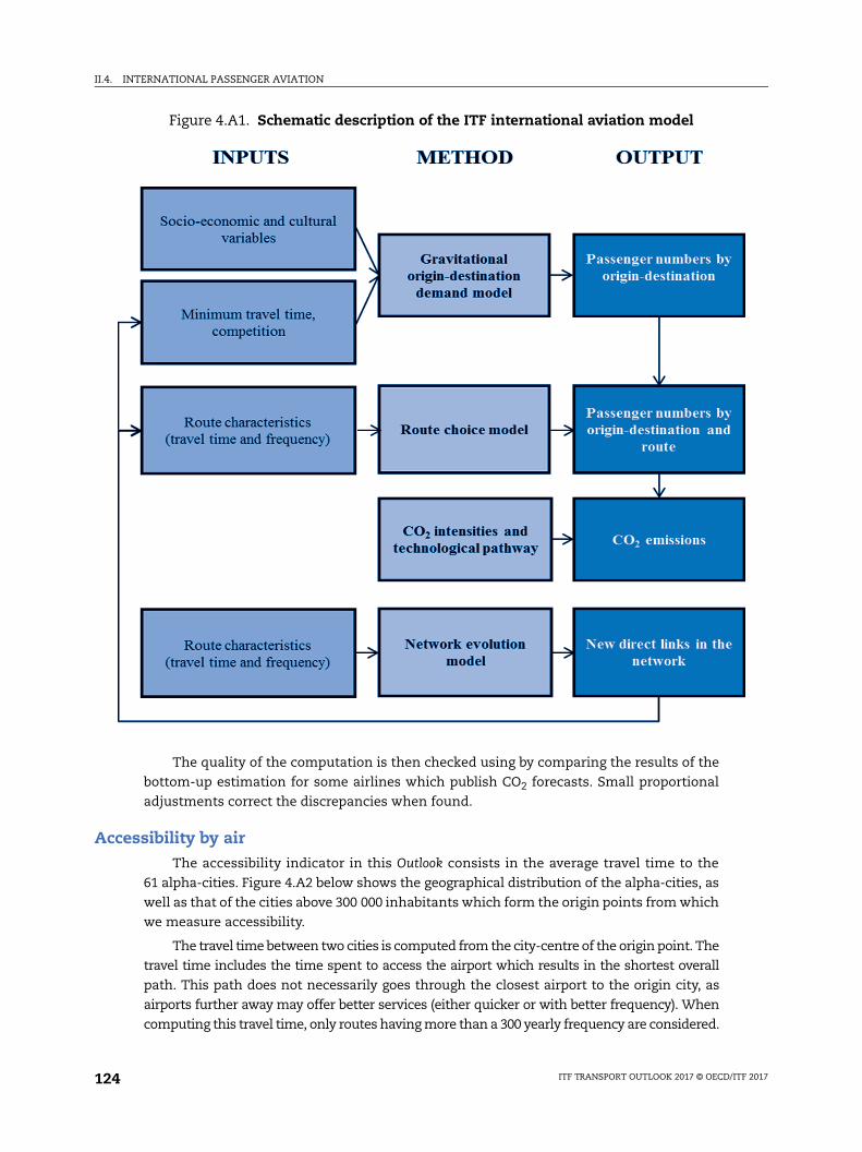
II.4. INTERNATIONAL PASSENGER AVIATION
The quality of the computation is then checked using by comparing the results of the
bottom-up estimation for some airlines which publish CO2 forecasts. Small proportional
adjustments correct the discrepancies when found.
Accessibility by airThe accessibility indicator in this Outlook consists in the average travel time to the
61 alpha-cities. Figure 4.A2 below shows the geographical distribution of the alpha-cities, as
well as that of the cities above 300 000 inhabitants which form the origin points from which
we measure accessibility.
The travel time between two cities is computed from the city-centre of the origin point. The
travel time includes the time spent to access the airport which results in the shortest overall
path. This path does not necessarily goes through the closest airport to the origin city, as
airports further away may offer better services (either quicker or with better frequency). When
computing this travel time, only routes having more than a 300 yearly frequency are considered.
Figure 4.A1. Schematic description of the ITF international aviation model
ITF TRANSPORT OUTLOOK 2017 © OECD/ITF 2017124
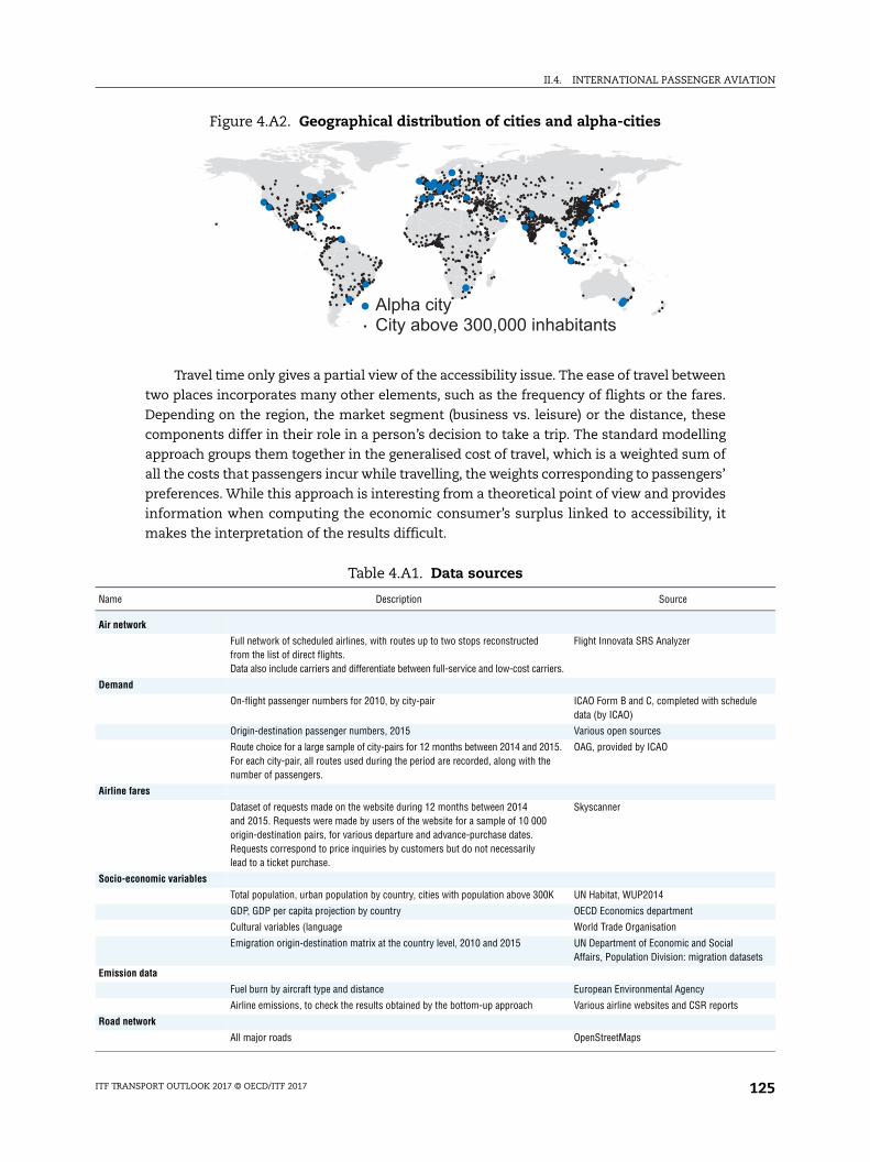
II.4. INTERNATIONAL PASSENGER AVIATION
dule
tasets
Travel time only gives a partial view of the accessibility issue. The ease of travel between
two places incorporates many other elements, such as the frequency of flights or the fares.
Depending on the region, the market segment (business vs. leisure) or the distance, these
components differ in their role in a person’s decision to take a trip. The standard modelling
approach groups them together in the generalised cost of travel, which is a weighted sum of
all the costs that passengers incur while travelling, the weights corresponding to passengers’
preferences. While this approach is interesting from a theoretical point of view and provides
information when computing the economic consumer’s surplus linked to accessibility, it
makes the interpretation of the results difficult.
Figure 4.A2. Geographical distribution of cities and alpha-cities
Alpha cityCity above 300,000 inhabitants
Table 4.A1. Data sources
Name Description Source
Air network
Full network of scheduled airlines, with routes up to two stops reconstructed from the list of direct flights.Data also include carriers and differentiate between full-service and low-cost carriers.
Flight Innovata SRS Analyzer
Demand
On-flight passenger numbers for 2010, by city-pair ICAO Form B and C, completed with schedata (by ICAO)
Origin-destination passenger numbers, 2015 Various open sources
Route choice for a large sample of city-pairs for 12 months between 2014 and 2015.For each city-pair, all routes used during the period are recorded, along with the number of passengers.
OAG, provided by ICAO
Airline fares
Dataset of requests made on the website during 12 months between 2014 and 2015. Requests were made by users of the website for a sample of 10 000 origin-destination pairs, for various departure and advance-purchase dates.Requests correspond to price inquiries by customers but do not necessarily lead to a ticket purchase.
Skyscanner
Socio-economic variables
Total population, urban population by country, cities with population above 300K UN Habitat, WUP2014
GDP, GDP per capita projection by country OECD Economics department
Cultural variables (language World Trade Organisation
Emigration origin-destination matrix at the country level, 2010 and 2015 UN Department of Economic and Social Affairs, Population Division: migration da
Emission data
Fuel burn by aircraft type and distance European Environmental Agency
Airline emissions, to check the results obtained by the bottom-up approach Various airline websites and CSR reports
Road network
All major roads OpenStreetMaps
ITF TRANSPORT OUTLOOK 2017 © OECD/ITF 2017 125

ITF Transport Outlook 2017 © OECD/ITF 2017
PART II
Chapter 5
Mobility in cities
This chapter presents long-term scenarios on the development of passenger mobility in cities and the related emissions up to 2050. The results, based on the new model for mobility in cities of the International Transport Forum (ITF), comprise modal shares, mobility levels and emissions of both CO2 and local pollutants. The first section looks at the development of the modelling framework and analyses the impacts of different transport, environment and technology substitution measures on mobility. The long-term implications of the three policy scenarios in terms of accessibility are then analysed, using a new methodology to compute accessibility in cities. The chapter concludes with a case study on certain cities in Asia, applying the same policy scenarios on a subset of cities from China, India and Southeast Asia.
127
II.5. MOBILITY IN CITIES
By 2050, there will be 2.4 billion additional urban dwellers compared to 2015, when
4 billion persons lived in urban areas. This rapid urbanisation process will create substantial
new demand for mobility in cities, making the provision of efficient, sustainable and
equitable transport even more of a challenge. The combined effects of rapid urbanisation,
income growth and rising private vehicle ownership will result in a surge in emissions,
congestion and public health issues. Under a business-as-usual scenario where no
additional policies are implemented, CO2 emissions are projected to grow by more than 26%
between 2015 and 2050. This creates pressure to pursue energy savings and vehicular
emission reductions, especially in developing countries, where 94% of the new urban
dwellers will live.
At the same time, the increasing rate of urbanisation and the growing size of cities mean
urban transport systems are unable to deliver the benefits they are expected to. Cities face
strong pressure to maintain and expand transport systems to ensure good access to
opportunities for their population, while keeping negative externalities such as congestion
and pollution to a minimum. At a time when private cars and two-wheelers still provide the
quickest way to move around in most urban areas, policy makers are facing a difficult choice
between short-term economic efficiency and the long-term liveability of their cities.
This chapter presents a global snapshot and the outlook for mobility, accessibility and
emissions in cities. It introduces three policy scenarios, describing three different
pathways for urban mobility, from a baseline scenario where private cars remain the
dominant source of mobility in cities to a scenario where all policies, from land-use and
transport planning to fiscal instruments, align to deliver a low-carbon future.
Modelling passenger transport demand in citiesPopulation, urbanisation and economic development are the key drivers of passenger
mobility demand, particularly at an aggregated level and in the long run. Population and
urbanisation trends indicate that the additional mobility demand will be concentrated in
urban agglomerations of developing economies. According to UN projections (United
Nations, 2014), by 2050, the world population will reach 9.55 billion, of which 66%, or
6.34 billion, will be urban. Urban areas will have to accommodate 2.4 billion additional
inhabitants and 94% of them will be moving to cities in developing regions.
This Outlook considers all cities above 300 000 inhabitants in 2014, for which individual
population projections are available (Figure 5.1). The total population of these cities
amounts to 2.2 billion in 2015, making up 31% of the total world population and 57% of the
world’s urban population. This figure will reach 3.6 billion by 2050, representing more than
37% of the world population and remaining a stable share of 56% of the urban population.
The share of population represented by these cities analysed in this chapter is stable across
regions.
While amounting to less than a third of the world population, the total Gross Domestic
Product (GDP) of all the cities in this study represents more than 50% of world GDP in 2015
ITF TRANSPORT OUTLOOK 2017 © OECD/ITF 2017128
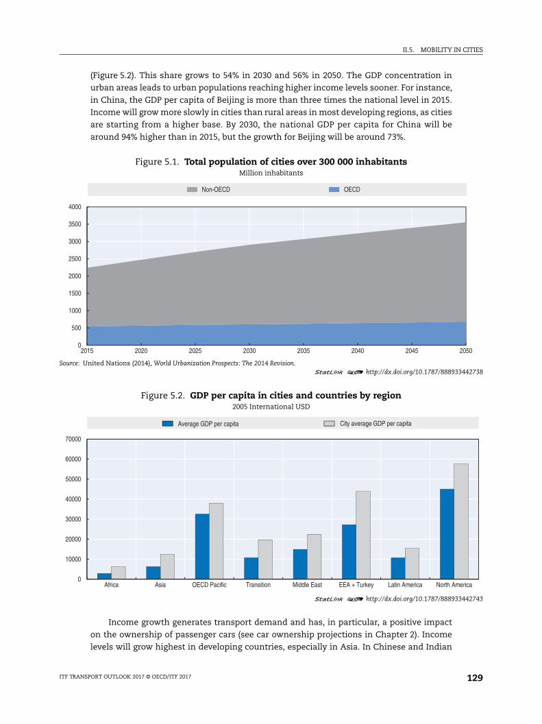
II.5. MOBILITY IN CITIES
442738
442743
050
rica
(Figure 5.2). This share grows to 54% in 2030 and 56% in 2050. The GDP concentration in
urban areas leads to urban populations reaching higher income levels sooner. For instance,
in China, the GDP per capita of Beijing is more than three times the national level in 2015.
Income will grow more slowly in cities than rural areas in most developing regions, as cities
are starting from a higher base. By 2030, the national GDP per capita for China will be
around 94% higher than in 2015, but the growth for Beijing will be around 73%.
Income growth generates transport demand and has, in particular, a positive impact
on the ownership of passenger cars (see car ownership projections in Chapter 2). Income
levels will grow highest in developing countries, especially in Asia. In Chinese and Indian
Figure 5.1. Total population of cities over 300 000 inhabitantsMillion inhabitants
Source: United Nations (2014), World Urbanization Prospects: The 2014 Revision.1 2 http://dx.doi.org/10.1787/888933
Figure 5.2. GDP per capita in cities and countries by region2005 International USD
1 2 http://dx.doi.org/10.1787/888933
0
500
1000
1500
2000
2500
3000
3500
4000
2015 2020 2025 2030 2035 2040 2045 2
Non-OECD OECD
0
10000
20000
30000
40000
50000
60000
70000
Africa Asia OECD Pacific Transition Middle East EEA + Turkey Latin America North Ame
Average GDP per capita City average GDP per capita
ITF TRANSPORT OUTLOOK 2017 © OECD/ITF 2017 129
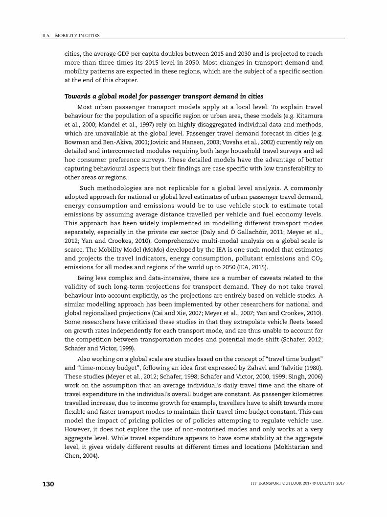
II.5. MOBILITY IN CITIES
cities, the average GDP per capita doubles between 2015 and 2030 and is projected to reach
more than three times its 2015 level in 2050. Most changes in transport demand and
mobility patterns are expected in these regions, which are the subject of a specific section
at the end of this chapter.
Towards a global model for passenger transport demand in cities
Most urban passenger transport models apply at a local level. To explain travel
behaviour for the population of a specific region or urban area, these models (e.g. Kitamura
et al., 2000; Mandel et al., 1997) rely on highly disaggregated individual data and methods,
which are unavailable at the global level. Passenger travel demand forecast in cities (e.g.
Bowman and Ben-Akiva, 2001; Jovicic and Hansen, 2003; Vovsha et al., 2002) currently rely on
detailed and interconnected modules requiring both large household travel surveys and ad
hoc consumer preference surveys. These detailed models have the advantage of better
capturing behavioural aspects but their findings are case specific with low transferability to
other areas or regions.
Such methodologies are not replicable for a global level analysis. A commonly
adopted approach for national or global level estimates of urban passenger travel demand,
energy consumption and emissions would be to use vehicle stock to estimate total
emissions by assuming average distance travelled per vehicle and fuel economy levels.
This approach has been widely implemented in modelling different transport modes
separately, especially in the private car sector (Daly and Ó Gallachóir, 2011; Meyer et al.,
2012; Yan and Crookes, 2010). Comprehensive multi-modal analysis on a global scale is
scarce. The Mobility Model (MoMo) developed by the IEA is one such model that estimates
and projects the travel indicators, energy consumption, pollutant emissions and CO2
emissions for all modes and regions of the world up to 2050 (IEA, 2015).
Being less complex and data-intensive, there are a number of caveats related to the
validity of such long-term projections for transport demand. They do not take travel
behaviour into account explicitly, as the projections are entirely based on vehicle stocks. A
similar modelling approach has been implemented by other researchers for national and
global regionalised projections (Cai and Xie, 2007; Meyer et al., 2007; Yan and Crookes, 2010).
Some researchers have criticised these studies in that they extrapolate vehicle fleets based
on growth rates independently for each transport mode, and are thus unable to account for
the competition between transportation modes and potential mode shift (Schafer, 2012;
Schafer and Victor, 1999).
Also working on a global scale are studies based on the concept of “travel time budget”
and “time-money budget”, following an idea first expressed by Zahavi and Talvitie (1980).
These studies (Meyer et al., 2012; Schafer, 1998; Schafer and Victor, 2000, 1999; Singh, 2006)
work on the assumption that an average individual’s daily travel time and the share of
travel expenditure in the individual’s overall budget are constant. As passenger kilometres
travelled increase, due to income growth for example, travellers have to shift towards more
flexible and faster transport modes to maintain their travel time budget constant. This can
model the impact of pricing policies or of policies attempting to regulate vehicle use.
However, it does not explore the use of non-motorised modes and only works at a very
aggregate level. While travel expenditure appears to have some stability at the aggregate
level, it gives widely different results at different times and locations (Mokhtarian and
Chen, 2004).
ITF TRANSPORT OUTLOOK 2017 © OECD/ITF 2017130
II.5. MOBILITY IN CITIES
The ITF model is a new tool developed to evaluate the impacts of transport,
environment and technology substitution policies through projections of travel demand,
CO2 emissions and accessibility in cities up to 2050. Annex 5.B details the methodology of
the model (see also Chen and Kauppila, 2017).
The model differs from existing models in two main areas. Firstly, it has a global
perspective, extending the geographical reach of the 2015 edition of the ITF Transport
Outlook. It considers each city above 300 000 inhabitants in 2014, and combines data from
various sources to form one of the most extensive databases on mobility in cities (Box 5.1).
It analyses five transport modes: private cars, public transport, motorcycles, walking and
cycling. Secondly, it represents travel behaviour explicitly, modelling the aggregate
behaviour for a segment of travellers as a function of the characteristics of the alternative
modes and the socio-demographic attributes of the group (Koppelman and Bhat, 2006). The
mode share module describes the interactions between the different modes, in a way that
existing models, which analyse the evolution of each mode separately, are unable to do.
Transport policy scenariosThis Outlook assesses the impacts of combinations of policy measures with three
alternative scenarios for future urban passenger transport: a baseline scenario, the Robust
Governance scenario (ROG), and the Integrated Land Use and Transport Planning scenario
Box 5.1. City Mobility database
The database used for the modelling contains the 1 692 cities listed in the United Nations (2014) report, World Urbanization Prospects: The 2014 Revision. After merging cities belonging to the same urban agglomeration (for instance Pretoria and Johannesburg), 1 557 entries remain. The urban boundary for each selected city is provided by the Global Built-up Reference Layer (BUREF, 2010; Pesaresi and Carneiro Freire Sergio, 2014), complemented by the space-based land remote sensing data LANDSAT for the year 2010. Other GIS data sources, such as road and public transport supply, come from the intersection of this global urban boundary layer with the open-source OpenStreetMap layer.
The dataset contains the main socio-economic indicator for each city, such as GDP, population or area size. GDP at city level is estimated by redistributing the national GDP volume into the urban areas according to the GDP distribution map obtained from LANDSAT 2010, which provides GDP information for each cell of a grid with one square kilometre resolution. Future GDP in cities come from the application of an S-shaped curve to the growth of the national GDP projections, using the estimated relation between the concentration of population and the concentration of GDP shown by urban agglomerations in each country. When urban agglomerations are small, the elasticity between GDP and population concentration is low, which will then rise as population grows. Finally, when agglomerations become very large, the marginal benefit of increasing the concentration of population begins to decrease.
To enable the analysis of transport demand, demand related indicators are added for a large group of cities: transit fare, parking cost, average vehicle occupancy, mode share, average travel distance, trip rates, and so on. This information is collected through the analysis of multiple data sources, including individual city household surveys where available (see Table 5.A1.1 in Annex 5.A). The resulting dataset is an integrated cross-sectional dataset from multiple sources for the 1 557 urban agglomerations for the year 2010.
ITF TRANSPORT OUTLOOK 2017 © OECD/ITF 2017 131
II.5. MOBILITY IN CITIES
(LUT). The measures concern all areas of urban life and include land-use planning, public
transport development, economic instruments and governmental regulations. Exogenous
drivers, such as urbanisation, population and income growth, do not change between
scenarios.
Baseline
In the baseline scenario, no additional measure aiming at influencing travel demand
and reducing CO2 emissions is implemented during the 2015-50 period. This scenario
constitutes a business-as-usual reference for travel demand and CO2 emissions in the
urban transport sector against which to measure the efficiency of additional policies and
compare alternative scenarios. It assumes that the future trends of car ownership, road
supply, public transport supply, pricing structure and urban area growth will follow the
trajectories of the past, as calibrated in each of the sub-models. For instance, public
transport provision continues to grow with population and GDP per capita as observed in
the historical data. For more details on these relationships, see Annex 5.B.
Advanced vehicle technology and alternative fuels penetrate the market at a relatively
low rate, as in the latest 4°C Scenario (4DS) of the Mobility Model developed by the
International Energy Agency (IEA). The 4°C Scenario (4DS) takes into account recent pledges
by countries to limit emissions and improve energy efficiency, which help limit the long-
term temperature increase to 4°C. In many respects the 4DS is already an ambitious scenario,
requiring significant changes in policy and technologies. For example, this corresponds to a
global average on-road fuel efficiency of passenger cars of 6.4 litres gasoline equivalent per
100 kilometres in 2050 compared to 10.3 litres gasoline equivalent per 100 kilometres in 2015.
ROG Scenario
The Robust Governance (ROG) scenario assumes that local governments play an active
role and adopt pricing and regulatory policies to slow down the ownership and use of
personal vehicles from 2020 onwards. Existing literature has proved the effectiveness of
rigorous pricing strategies. For example, Meyer (1999) studied the effectiveness of various
transportation demand management actions, and concludes that the actions which tend
to increase the generalised cost of travel for personal vehicle use are most effective. A
cross-country study by Greening (2004) indicates that fuel prices and strong government
policies related to vehicle and fuel taxes play a significant role in shifting travel demand
from private cars towards modes with lower carbon intensity. Studies on the demand for
public transport show that playing on transit fares, parking pricing and car ownership is
the most efficient way to encourage transit use (Litman, 2004; Paulley et al., 2006).
Following these findings, every city in the world implements pricing policies on fuel
prices, fuel taxes, vehicle taxes and fees, parking fees, and transit fares in the ROG
scenario. Each policy measure is specified as follows:
● The public transport pricing sub-model estimates the elasticity of the price of a single
transit ticket with respect to GDP per capita for each country group. In this scenario, the
price of a ticket grows according to the lowest regional elasticity.
● In 2030, fuel prices in each country correspond to a fictive oil price of USD 120 (real USD
per barrel, 2005). Such prices can result from higher taxation, high oil prices, or a
combination of both. The growth rates of oil prices between 2030 and 2050 are assumed
to be the same as that in the baseline.
ITF TRANSPORT OUTLOOK 2017 © OECD/ITF 2017132
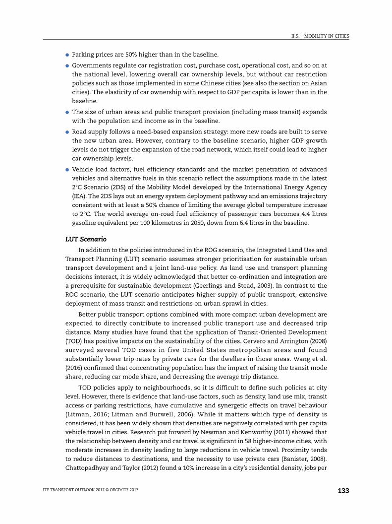
II.5. MOBILITY IN CITIES
● Parking prices are 50% higher than in the baseline.
● Governments regulate car registration cost, purchase cost, operational cost, and so on at
the national level, lowering overall car ownership levels, but without car restriction
policies such as those implemented in some Chinese cities (see also the section on Asian
cities). The elasticity of car ownership with respect to GDP per capita is lower than in the
baseline.
● The size of urban areas and public transport provision (including mass transit) expands
with the population and income as in the baseline.
● Road supply follows a need-based expansion strategy: more new roads are built to serve
the new urban area. However, contrary to the baseline scenario, higher GDP growth
levels do not trigger the expansion of the road network, which itself could lead to higher
car ownership levels.
● Vehicle load factors, fuel efficiency standards and the market penetration of advanced
vehicles and alternative fuels in this scenario reflect the assumptions made in the latest
2°C Scenario (2DS) of the Mobility Model developed by the International Energy Agency
(IEA). The 2DS lays out an energy system deployment pathway and an emissions trajectory
consistent with at least a 50% chance of limiting the average global temperature increase
to 2°C. The world average on-road fuel efficiency of passenger cars becomes 4.4 litres
gasoline equivalent per 100 kilometres in 2050, down from 6.4 litres in the baseline.
LUT Scenario
In addition to the policies introduced in the ROG scenario, the Integrated Land Use and
Transport Planning (LUT) scenario assumes stronger prioritisation for sustainable urban
transport development and a joint land-use policy. As land use and transport planning
decisions interact, it is widely acknowledged that better co-ordination and integration are
a prerequisite for sustainable development (Geerlings and Stead, 2003). In contrast to the
ROG scenario, the LUT scenario anticipates higher supply of public transport, extensive
deployment of mass transit and restrictions on urban sprawl in cities.
Better public transport options combined with more compact urban development are
expected to directly contribute to increased public transport use and decreased trip
distance. Many studies have found that the application of Transit-Oriented Development
(TOD) has positive impacts on the sustainability of the cities. Cervero and Arrington (2008)
surveyed several TOD cases in five United States metropolitan areas and found
substantially lower trip rates by private cars for the dwellers in those areas. Wang et al.
(2016) confirmed that concentrating population has the impact of raising the transit mode
share, reducing car mode share, and decreasing the average trip distance.
TOD policies apply to neighbourhoods, so it is difficult to define such policies at city
level. However, there is evidence that land-use factors, such as density, land use mix, transit
access or parking restrictions, have cumulative and synergetic effects on travel behaviour
(Litman, 2016; Litman and Burwell, 2006). While it matters which type of density is
considered, it has been widely shown that densities are negatively correlated with per capita
vehicle travel in cities. Research put forward by Newman and Kenworthy (2011) showed that
the relationship between density and car travel is significant in 58 higher-income cities, with
moderate increases in density leading to large reductions in vehicle travel. Proximity tends
to reduce distances to destinations, and the necessity to use private cars (Banister, 2008).
Chattopadhyay and Taylor (2012) found a 10% increase in a city’s residential density, jobs per
ITF TRANSPORT OUTLOOK 2017 © OECD/ITF 2017 133
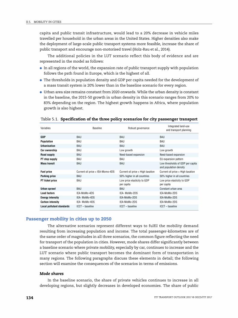
II.5. MOBILITY IN CITIES
capita and public transit infrastructure, would lead to a 20% decrease in vehicle miles
travelled per household in the urban areas in the United States. Higher densities also make
the deployment of large-scale public transport systems more feasible, increase the share of
public transport and encourage non-motorised travel (Holz-Rau et al., 2014).
The additional policies in the LUT scenario reflect this body of evidence and are
represented in the model as follows:
● In all regions of the world, the expansion rate of public transport supply with population
follows the path found in Europe, which is the highest of all.
● The thresholds in population density and GDP per capita needed for the development of
a mass transit system is 20% lower than in the baseline scenario for every region.
● Urban area size remains constant from 2020 onwards. While the urban density is constant
in the baseline, the 2015-50 growth in urban density in this scenario ranges from 20% to
83% depending on the region. The highest growth happens in Africa, where population
growth is also highest.
Passenger mobility in cities up to 2050The alternative scenarios represent different ways to fulfil the mobility demand
resulting from increasing population and income. The total passenger-kilometres are of
the same order of magnitudes in all three scenarios, the common figure reflecting the need
for transport of the population in cities. However, mode shares differ significantly between
a baseline scenario where private mobility, especially by car, continues to increase and the
LUT scenario where public transport becomes the dominant form of transportation in
many regions. The following paragraphs discuss these elements in detail; the following
section will examine the consequences of the scenarios in terms of emissions.
Mode shares
In the baseline scenario, the share of private vehicles continues to increase in all
developing regions, but slightly decreases in developed economies. The share of public
Table 5.1. Specification of the three policy scenarios for city passenger transport
Variables Baseline Robust governanceIntegrated land-use
and transport planning
GDP BAU BAU BAU
Population BAU BAU BAU
Urbanisation BAU BAU BAU
Car ownership BAU Low growth Low growth
Road supply BAU Need-based expansion Need-based expansion
PT stop supply BAU BAU EU expansion pattern
Mass transit BAU BAU Low thresholds of GDP per capita and population density
Fuel price Current oil price + IEA-Momo-4DS Current oil price + High taxation Current oil price + High taxation
Parking price BAU 50% higher in all countries 50% higher in all countries
PT ticket price BAU Low price elasticity to GDP per capita
Low price elasticity to GDP per capita
Urban sprawl BAU BAU Constant urban area
Load factors IEA-MoMo-4DS IEA- MoMo-2DS IEA-MoMo-2DS
Energy intensity IEA- MoMo-4DS IEA-MoMo-2DS IEA-MoMo-2DS
Carbon intensity IEA- MoMo-4DS IEA-MoMo-2DS IEA-MoMo-2DS
Local pollutant standards ICCT – baseline ICCT – baseline ICCT – baseline
ITF TRANSPORT OUTLOOK 2017 © OECD/ITF 2017134
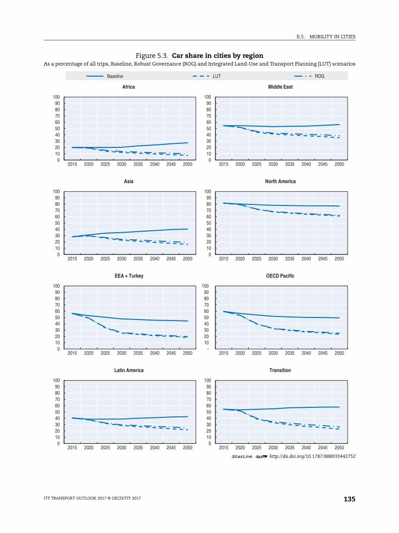
II.5. MOBILITY IN CITIES
narios
442752
50
50
50
50
Figure 5.3. Car share in cities by regionAs a percentage of all trips, Baseline, Robust Governance (ROG) and Integrated Land-Use and Transport Planning (LUT) sce
1 2 http://dx.doi.org/10.1787/888933
0102030405060708090
100
2015 2020 2025 2030 2035 2040 2045 2050
Africa
0102030405060708090
100
2015 2020 2025 2030 2035 2040 2045 2050
Asia
0102030405060708090
100
2015 2020 2025 2030 2035 2040 2045 20
North America
0102030405060708090
100
2015 2020 2025 2030 2035 2040 2045 2050
EEA + Turkey
- 10 20 30 40 50 60 70 80 90
100
2015 2020 2025 2030 2035 2040 2045 20
OECD Pacific
0102030405060708090
100
2015 2020 2025 2030 2035 2040 2045 2050
Latin America
0102030405060708090
100
2015 2020 2025 2030 2035 2040 2045 20
Transition
0102030405060708090
100
2015 2020 2025 2030 2035 2040 2045 20
Middle East
Baseline LUT ROG
ITF TRANSPORT OUTLOOK 2017 © OECD/ITF 2017 135
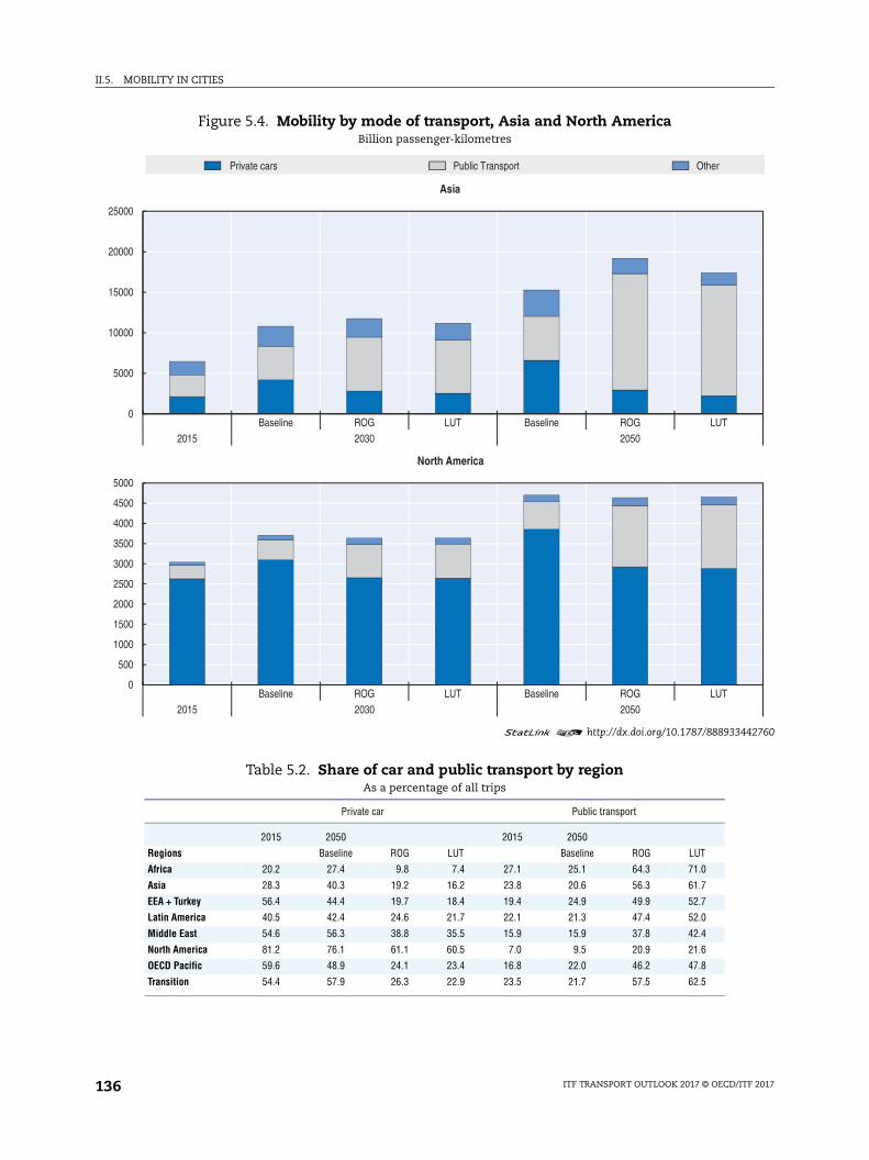
II.5. MOBILITY IN CITIES
442760
Figure 5.4. Mobility by mode of transport, Asia and North AmericaBillion passenger-kilometres
1 2 http://dx.doi.org/10.1787/888933
Table 5.2. Share of car and public transport by regionAs a percentage of all trips
Private car Public transport
2015 2050 2015 2050
Regions Baseline ROG LUT Baseline ROG LUT
Africa 20.2 27.4 9.8 7.4 27.1 25.1 64.3 71.0
Asia 28.3 40.3 19.2 16.2 23.8 20.6 56.3 61.7
EEA + Turkey 56.4 44.4 19.7 18.4 19.4 24.9 49.9 52.7
Latin America 40.5 42.4 24.6 21.7 22.1 21.3 47.4 52.0
Middle East 54.6 56.3 38.8 35.5 15.9 15.9 37.8 42.4
North America 81.2 76.1 61.1 60.5 7.0 9.5 20.9 21.6
OECD Pacific 59.6 48.9 24.1 23.4 16.8 22.0 46.2 47.8
Transition 54.4 57.9 26.3 22.9 23.5 21.7 57.5 62.5
0
5000
10000
15000
20000
25000
Baseline ROG LUT Baseline ROG LUT2015 2030 2050
Asia
0
500
1000
1500
2000
2500
3000
3500
4000
4500
5000
Baseline ROG LUT Baseline ROG LUT2015 2030 2050
North America
Private cars Public Transport Other
ITF TRANSPORT OUTLOOK 2017 © OECD/ITF 2017136
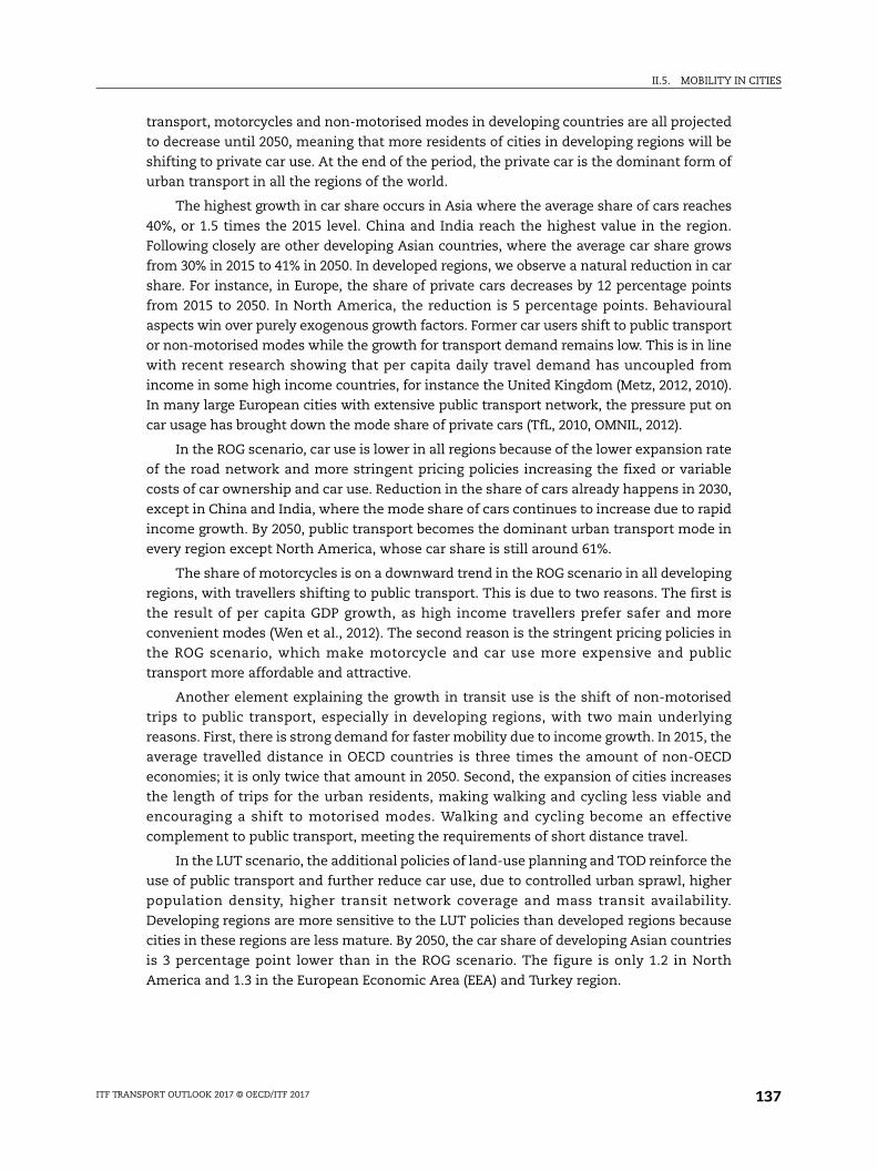
II.5. MOBILITY IN CITIES
transport, motorcycles and non-motorised modes in developing countries are all projected
to decrease until 2050, meaning that more residents of cities in developing regions will be
shifting to private car use. At the end of the period, the private car is the dominant form of
urban transport in all the regions of the world.
The highest growth in car share occurs in Asia where the average share of cars reaches
40%, or 1.5 times the 2015 level. China and India reach the highest value in the region.
Following closely are other developing Asian countries, where the average car share grows
from 30% in 2015 to 41% in 2050. In developed regions, we observe a natural reduction in car
share. For instance, in Europe, the share of private cars decreases by 12 percentage points
from 2015 to 2050. In North America, the reduction is 5 percentage points. Behavioural
aspects win over purely exogenous growth factors. Former car users shift to public transport
or non-motorised modes while the growth for transport demand remains low. This is in line
with recent research showing that per capita daily travel demand has uncoupled from
income in some high income countries, for instance the United Kingdom (Metz, 2012, 2010).
In many large European cities with extensive public transport network, the pressure put on
car usage has brought down the mode share of private cars (TfL, 2010, OMNIL, 2012).
In the ROG scenario, car use is lower in all regions because of the lower expansion rate
of the road network and more stringent pricing policies increasing the fixed or variable
costs of car ownership and car use. Reduction in the share of cars already happens in 2030,
except in China and India, where the mode share of cars continues to increase due to rapid
income growth. By 2050, public transport becomes the dominant urban transport mode in
every region except North America, whose car share is still around 61%.
The share of motorcycles is on a downward trend in the ROG scenario in all developing
regions, with travellers shifting to public transport. This is due to two reasons. The first is
the result of per capita GDP growth, as high income travellers prefer safer and more
convenient modes (Wen et al., 2012). The second reason is the stringent pricing policies in
the ROG scenario, which make motorcycle and car use more expensive and public
transport more affordable and attractive.
Another element explaining the growth in transit use is the shift of non-motorised
trips to public transport, especially in developing regions, with two main underlying
reasons. First, there is strong demand for faster mobility due to income growth. In 2015, the
average travelled distance in OECD countries is three times the amount of non-OECD
economies; it is only twice that amount in 2050. Second, the expansion of cities increases
the length of trips for the urban residents, making walking and cycling less viable and
encouraging a shift to motorised modes. Walking and cycling become an effective
complement to public transport, meeting the requirements of short distance travel.
In the LUT scenario, the additional policies of land-use planning and TOD reinforce the
use of public transport and further reduce car use, due to controlled urban sprawl, higher
population density, higher transit network coverage and mass transit availability.
Developing regions are more sensitive to the LUT policies than developed regions because
cities in these regions are less mature. By 2050, the car share of developing Asian countries
is 3 percentage point lower than in the ROG scenario. The figure is only 1.2 in North
America and 1.3 in the European Economic Area (EEA) and Turkey region.
ITF TRANSPORT OUTLOOK 2017 © OECD/ITF 2017 137
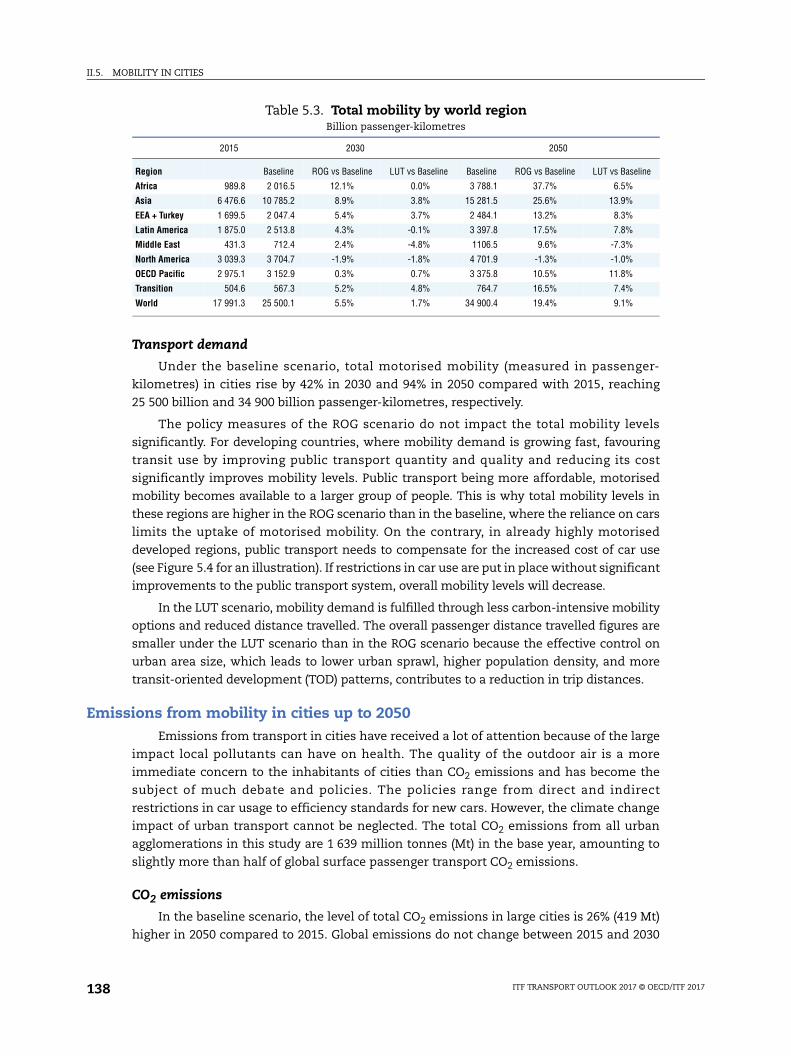
II.5. MOBILITY IN CITIES
Transport demand
Under the baseline scenario, total motorised mobility (measured in passenger-
kilometres) in cities rise by 42% in 2030 and 94% in 2050 compared with 2015, reaching
25 500 billion and 34 900 billion passenger-kilometres, respectively.
The policy measures of the ROG scenario do not impact the total mobility levels
significantly. For developing countries, where mobility demand is growing fast, favouring
transit use by improving public transport quantity and quality and reducing its cost
significantly improves mobility levels. Public transport being more affordable, motorised
mobility becomes available to a larger group of people. This is why total mobility levels in
these regions are higher in the ROG scenario than in the baseline, where the reliance on cars
limits the uptake of motorised mobility. On the contrary, in already highly motorised
developed regions, public transport needs to compensate for the increased cost of car use
(see Figure 5.4 for an illustration). If restrictions in car use are put in place without significant
improvements to the public transport system, overall mobility levels will decrease.
In the LUT scenario, mobility demand is fulfilled through less carbon-intensive mobility
options and reduced distance travelled. The overall passenger distance travelled figures are
smaller under the LUT scenario than in the ROG scenario because the effective control on
urban area size, which leads to lower urban sprawl, higher population density, and more
transit-oriented development (TOD) patterns, contributes to a reduction in trip distances.
Emissions from mobility in cities up to 2050Emissions from transport in cities have received a lot of attention because of the large
impact local pollutants can have on health. The quality of the outdoor air is a more
immediate concern to the inhabitants of cities than CO2 emissions and has become the
subject of much debate and policies. The policies range from direct and indirect
restrictions in car usage to efficiency standards for new cars. However, the climate change
impact of urban transport cannot be neglected. The total CO2 emissions from all urban
agglomerations in this study are 1 639 million tonnes (Mt) in the base year, amounting to
slightly more than half of global surface passenger transport CO2 emissions.
CO2 emissions
In the baseline scenario, the level of total CO2 emissions in large cities is 26% (419 Mt)
higher in 2050 compared to 2015. Global emissions do not change between 2015 and 2030
Table 5.3. Total mobility by world regionBillion passenger-kilometres
2015 2030 2050
Region Baseline ROG vs Baseline LUT vs Baseline Baseline ROG vs Baseline LUT vs Baseline
Africa 989.8 2 016.5 12.1% 0.0% 3 788.1 37.7% 6.5%
Asia 6 476.6 10 785.2 8.9% 3.8% 15 281.5 25.6% 13.9%
EEA + Turkey 1 699.5 2 047.4 5.4% 3.7% 2 484.1 13.2% 8.3%
Latin America 1 875.0 2 513.8 4.3% -0.1% 3 397.8 17.5% 7.8%
Middle East 431.3 712.4 2.4% -4.8% 1106.5 9.6% -7.3%
North America 3 039.3 3 704.7 -1.9% -1.8% 4 701.9 -1.3% -1.0%
OECD Pacific 2 975.1 3 152.9 0.3% 0.7% 3 375.8 10.5% 11.8%
Transition 504.6 567.3 5.2% 4.8% 764.7 16.5% 7.4%
World 17 991.3 25 500.1 5.5% 1.7% 34 900.4 19.4% 9.1%
ITF TRANSPORT OUTLOOK 2017 © OECD/ITF 2017138
II.5. MOBILITY IN CITIES
due to the large fuel efficiency gains expected during the decade to come, and the low
economic growth for the years up to 2020 (see also Chapter 1 for details on the short-term
macroeconomic projections). However, emissions grow again from 2030 onwards based on
the assumptions related to vehicle technology and fuel efficiency in the 4DS scenario of the
IEA’s Mobility Model. The world average fuel efficiency for on-road passenger light duty
vehicles improves by 29% from 2015 to 2030 but only 14% from 2030 to 2050. This pace of
technology improvement is not enough to offset the growing mobility demand between
2030 and 2050.
Policy interventions, especially rigorous car pricing policies, lower transit fares and
higher vehicle technology improvements introduced in the ROG scenario could intensely
mitigate CO2 emissions from the urban passenger transportation sector. With solely the
policy measures from ROG, the avoided CO2 emission could reach 397 Mt in 2030 and 886 Mt
in 2050 compared with the baseline. The additional policies introduced in LUT scenario
would further reduce the CO2 emissions by 48 Mt in 2030 and 104 Mt in 2050. Under the
most effective policy scenario LUT, the global CO2 emissions level from the urban transport
sector would be 26% lower in 2030 and 35% lower in 2050 compared with 2015 levels.
Private cars are the main contributor of CO2 emissions in cities, representing around
82% of all emissions in 2015 and around 75% in 2030 and 2050. With the implementation of
the policy measures of the ROG and LUT scenario, the contribution of cars decreases to 40%
in 2050.
Bus and motorcycle emissions represent 11% and 7% respectively of all emissions in
cities in the base year, going up to 15% and 10% in 2030 and remaining stable until 2050, in
the baseline scenario. In the ROG and LUT scenarios, the contribution of buses in total
emissions increase both because of the additional public transport supply in these
scenarios and because of the lower level of emissions from cars. Buses emit as much as
cars in the ROG scenario in 2050; in the LUT scenario, buses even become the main
contributor of CO2 emissions in 2050. CO2 emissions from urban rail are null in this model,
as only tank-to-wheel CO2 emissions are taken into account and urban rail is assumed to
be fully electrical. A life-cycle analysis would increase the CO2 emissions from urban rail,
especially in India and Africa where the IEA projects that electricity production will remain
carbon intensive through 2050.
The technology aspect of the ROG and LUT scenarios contribute most significantly to
the CO2 mitigation potential of these two scenarios. Figure 5.6 presents the avoided CO2
emissions for the two scenarios, broken down by type of measure in 2030 and 2050.
Technology improvements alone reduce global CO2 emissions in cities by 15% in 2030 and
22% in 2050, compared to 2015.
Behavioural changes of the scale discussed in this Outlook have an impact on emissions
(e.g. 11% less CO2 emissions in the LUT scenario in 2050 compared to the base year) and they
are essential in combatting congestion or health issues. However, emphasising behavioural
changes in the fight against climate change does not take into account the surge in mobility
which will result from the economic development of lower income countries. Even in the LUT
scenario, despite the strict policies in place, car mobility increases in almost all developing
regions. A complete decarbonisation of the transport sector in cities would require extreme
changes in mobility patterns, on a scale out of proportion with the efforts currently deployed
around the world. Such changes could take the form of much higher taxation of car mobility
in cities or higher penetration of alternative fuels. The necessary penetration of electric
ITF TRANSPORT OUTLOOK 2017 © OECD/ITF 2017 139
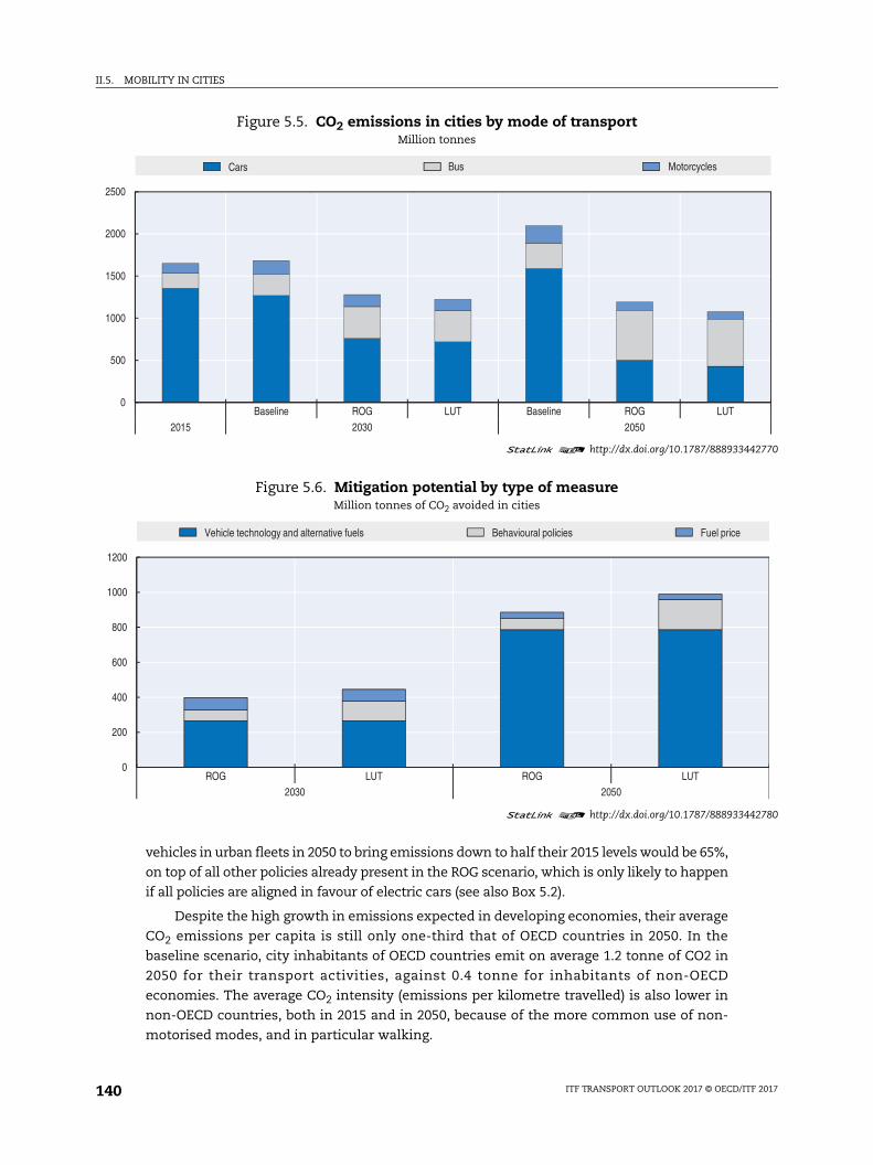
II.5. MOBILITY IN CITIES
442770
442780
vehicles in urban fleets in 2050 to bring emissions down to half their 2015 levels would be 65%,
on top of all other policies already present in the ROG scenario, which is only likely to happen
if all policies are aligned in favour of electric cars (see also Box 5.2).
Despite the high growth in emissions expected in developing economies, their average
CO2 emissions per capita is still only one-third that of OECD countries in 2050. In the
baseline scenario, city inhabitants of OECD countries emit on average 1.2 tonne of CO2 in
2050 for their transport activities, against 0.4 tonne for inhabitants of non-OECD
economies. The average CO2 intensity (emissions per kilometre travelled) is also lower in
non-OECD countries, both in 2015 and in 2050, because of the more common use of non-
motorised modes, and in particular walking.
Figure 5.5. CO2 emissions in cities by mode of transportMillion tonnes
1 2 http://dx.doi.org/10.1787/888933
Figure 5.6. Mitigation potential by type of measureMillion tonnes of CO2 avoided in cities
1 2 http://dx.doi.org/10.1787/888933
0
500
1000
1500
2000
2500
Baseline ROG LUT Baseline ROG LUT2015 2030 2050
Cars Bus Motorcycles
0
200
400
600
800
1000
1200
ROG LUT ROG LUT2030 2050
Vehicle technology and alternative fuels Behavioural policies Fuel price
ITF TRANSPORT OUTLOOK 2017 © OECD/ITF 2017140
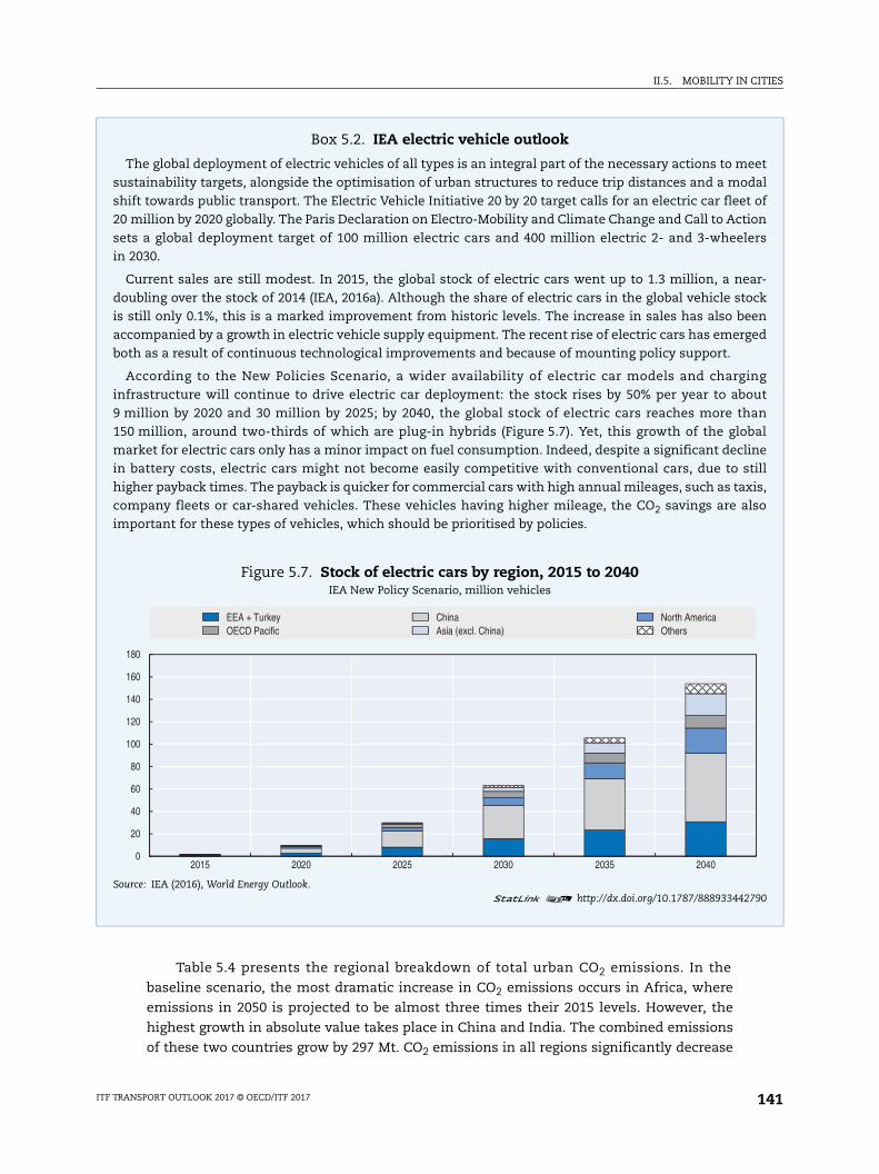
II.5. MOBILITY IN CITIES
eet dal of
ion ers
ar-ck en ed
ng ut an
bal ine till is,
lso
790
Table 5.4 presents the regional breakdown of total urban CO2 emissions. In the
baseline scenario, the most dramatic increase in CO2 emissions occurs in Africa, where
emissions in 2050 is projected to be almost three times their 2015 levels. However, the
highest growth in absolute value takes place in China and India. The combined emissions
of these two countries grow by 297 Mt. CO2 emissions in all regions significantly decrease
Box 5.2. IEA electric vehicle outlook
The global deployment of electric vehicles of all types is an integral part of the necessary actions to msustainability targets, alongside the optimisation of urban structures to reduce trip distances and a moshift towards public transport. The Electric Vehicle Initiative 20 by 20 target calls for an electric car fleet20 million by 2020 globally. The Paris Declaration on Electro-Mobility and Climate Change and Call to Actsets a global deployment target of 100 million electric cars and 400 million electric 2- and 3-wheelin 2030.
Current sales are still modest. In 2015, the global stock of electric cars went up to 1.3 million, a nedoubling over the stock of 2014 (IEA, 2016a). Although the share of electric cars in the global vehicle stois still only 0.1%, this is a marked improvement from historic levels. The increase in sales has also beaccompanied by a growth in electric vehicle supply equipment. The recent rise of electric cars has emergboth as a result of continuous technological improvements and because of mounting policy support.
According to the New Policies Scenario, a wider availability of electric car models and chargiinfrastructure will continue to drive electric car deployment: the stock rises by 50% per year to abo9 million by 2020 and 30 million by 2025; by 2040, the global stock of electric cars reaches more th150 million, around two-thirds of which are plug-in hybrids (Figure 5.7). Yet, this growth of the glomarket for electric cars only has a minor impact on fuel consumption. Indeed, despite a significant declin battery costs, electric cars might not become easily competitive with conventional cars, due to shigher payback times. The payback is quicker for commercial cars with high annual mileages, such as taxcompany fleets or car-shared vehicles. These vehicles having higher mileage, the CO2 savings are aimportant for these types of vehicles, which should be prioritised by policies.
Figure 5.7. Stock of electric cars by region, 2015 to 2040IEA New Policy Scenario, million vehicles
Source: IEA (2016), World Energy Outlook.1 2 http://dx.doi.org/10.1787/888933442
0
20
40
60
80
100
120
140
160
180
2015 2020 2025 2030 2035 2040
EEA + Turkey China North AmericaOECD Pacific Asia (excl. China) Others
ITF TRANSPORT OUTLOOK 2017 © OECD/ITF 2017 141
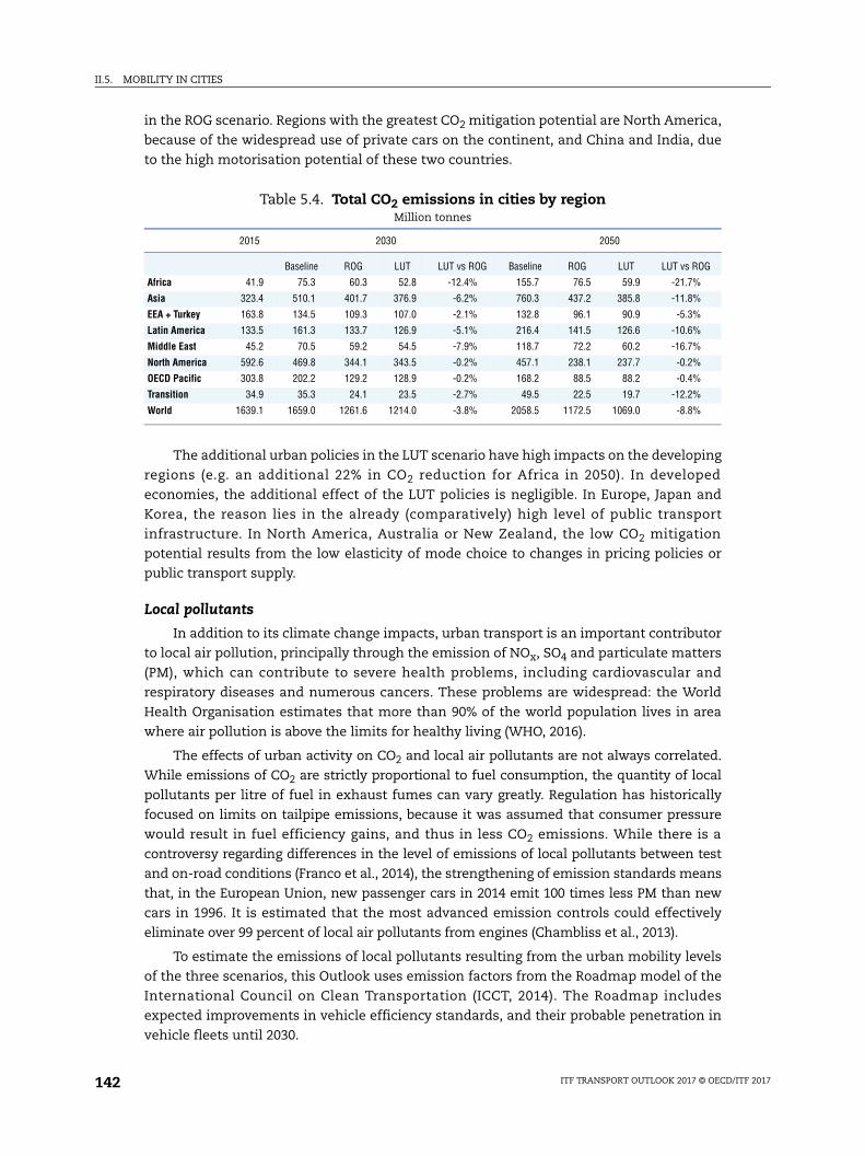
II.5. MOBILITY IN CITIES
in the ROG scenario. Regions with the greatest CO2 mitigation potential are North America,
because of the widespread use of private cars on the continent, and China and India, due
to the high motorisation potential of these two countries.
The additional urban policies in the LUT scenario have high impacts on the developing
regions (e.g. an additional 22% in CO2 reduction for Africa in 2050). In developed
economies, the additional effect of the LUT policies is negligible. In Europe, Japan and
Korea, the reason lies in the already (comparatively) high level of public transport
infrastructure. In North America, Australia or New Zealand, the low CO2 mitigation
potential results from the low elasticity of mode choice to changes in pricing policies or
public transport supply.
Local pollutants
In addition to its climate change impacts, urban transport is an important contributor
to local air pollution, principally through the emission of NOx, SO4 and particulate matters
(PM), which can contribute to severe health problems, including cardiovascular and
respiratory diseases and numerous cancers. These problems are widespread: the World
Health Organisation estimates that more than 90% of the world population lives in area
where air pollution is above the limits for healthy living (WHO, 2016).
The effects of urban activity on CO2 and local air pollutants are not always correlated.
While emissions of CO2 are strictly proportional to fuel consumption, the quantity of local
pollutants per litre of fuel in exhaust fumes can vary greatly. Regulation has historically
focused on limits on tailpipe emissions, because it was assumed that consumer pressure
would result in fuel efficiency gains, and thus in less CO2 emissions. While there is a
controversy regarding differences in the level of emissions of local pollutants between test
and on-road conditions (Franco et al., 2014), the strengthening of emission standards means
that, in the European Union, new passenger cars in 2014 emit 100 times less PM than new
cars in 1996. It is estimated that the most advanced emission controls could effectively
eliminate over 99 percent of local air pollutants from engines (Chambliss et al., 2013).
To estimate the emissions of local pollutants resulting from the urban mobility levels
of the three scenarios, this Outlook uses emission factors from the Roadmap model of the
International Council on Clean Transportation (ICCT, 2014). The Roadmap includes
expected improvements in vehicle efficiency standards, and their probable penetration in
vehicle fleets until 2030.
Table 5.4. Total CO2 emissions in cities by regionMillion tonnes
2015 2030 2050
Baseline ROG LUT LUT vs ROG Baseline ROG LUT LUT vs ROG
Africa 41.9 75.3 60.3 52.8 -12.4% 155.7 76.5 59.9 -21.7%
Asia 323.4 510.1 401.7 376.9 -6.2% 760.3 437.2 385.8 -11.8%
EEA + Turkey 163.8 134.5 109.3 107.0 -2.1% 132.8 96.1 90.9 -5.3%
Latin America 133.5 161.3 133.7 126.9 -5.1% 216.4 141.5 126.6 -10.6%
Middle East 45.2 70.5 59.2 54.5 -7.9% 118.7 72.2 60.2 -16.7%
North America 592.6 469.8 344.1 343.5 -0.2% 457.1 238.1 237.7 -0.2%
OECD Pacific 303.8 202.2 129.2 128.9 -0.2% 168.2 88.5 88.2 -0.4%
Transition 34.9 35.3 24.1 23.5 -2.7% 49.5 22.5 19.7 -12.2%
World 1639.1 1659.0 1261.6 1214.0 -3.8% 2058.5 1172.5 1069.0 -8.8%
ITF TRANSPORT OUTLOOK 2017 © OECD/ITF 2017142
II.5. MOBILITY IN CITIES
442803
Figure 5.8. NOx, SO4 and PM2.5 emissions by regionThousand tonnes
1 2 http://dx.doi.org/10.1787/888933
0
1000000
2000000
3000000
4000000
5000000
6000000
7000000
Baseline ROG LUT2015 2030
NOx
0
10000
20000
30000
40000
50000
60000
70000
Baseline ROG LUT2015 2030
SO4
0
20000
40000
60000
80000
100000
120000
140000
160000
180000
Baseline ROG LUT2015 2030
PM2.5
Africa Asia Pacific EEA + TurkeyLatin America North America Others
ITF TRANSPORT OUTLOOK 2017 © OECD/ITF 2017 143

II.5. MOBILITY IN CITIES
442815
Figure 5.8 shows the evolution of the emissions of local pollutants between 2015 and
2030 by region. In the baseline scenario, emissions of SO4 and NOx moderately increase, and
those of PM2.5 even decrease. Car mobility, which increases most in this scenario, becomes
much cleaner. In the more public transport-oriented scenarios, all local pollutants grow more
because of the development of bus travel necessary to replace car mobility (Figure 5.9). Diesel
buses, which form most of the bus fleet in many countries, have higher emission factors
than cars and will not become much cleaner, especially in developing countries. For instance,
diesel buses in China emit on average 7.7 g of NOx per kilometre in 2015 and 5.7 g in 2030
when emissions from gasoline cars go down from 0.1 g per kilometre in 2015 to 0.03 g in 2030.
It is difficult to predict the health impacts of these scenarios, as transport is only one
contributor of local pollutants. Several other factors, such as the topography and climate of
cities, as well as the presence of industry, also enter the equation. In regions with heavily
polluting industries, such as coal plants, its share can be as low as one-third (Beijing
Municipal Environmental Protection Bureau, 2014). However, our projections show that most
of the increase will take place in developing countries, where many cities are already choking
on local pollution. Any additional emission is likely to bring significant health issues. Extra
effort will be required to develop clean public transportation systems, especially in medium
cities where rail investment is not an option, for instance through the phasing in of buses
powered by alternative fuels or through the development of coherent planning policies. In
the LUT scenario, the decrease in the average distance travel causes some reduction in the
emissions of local pollutants.
AccessibilityPolicy packages that are well co-ordinated and address externalities from increasing
motorised mobility in cities make a significant difference for sustainable urban futures.
The policy scenarios introduced earlier in this chapter (Robust Governance and Land-Use
Transport Planning) do not merely influence mobility patterns in cities. They also affect the
way in which people, jobs and other urban functions can be accessed in cities.
Figure 5.9. Vehicle activity by modeBillion vehicle-kilometres
1 2 http://dx.doi.org/10.1787/888933
0
2000
4000
6000
8000
10000
12000
Baseline ROG LUT2015 2030
Car Bus Motorcycle
ITF TRANSPORT OUTLOOK 2017 © OECD/ITF 2017144
II.5. MOBILITY IN CITIES
Accessibility, however, is only to some extent about mobility. Designing urban
transport policies has traditionally focused on travel time savings and congestion relief.
According to this vision, transport planning aims at maximising the distance that
infrastructure users can travel within their time and money budgets. However, there is
growing consensus that this is not recognising the actual purpose of transport, which is
providing accessibility to opportunities such as employment, goods or services. Taking this
shift of emphasis seriously requires rethinking the governance and finance models for
connecting transport and land use policy and planning.
Improving accessibility, not merely mobility, will be decisive for sustainable and
inclusive cities. In a meta-study reviewing the effects of the built environment on travel
behaviour, Ewing and Cervero (2010) highlight the importance of accessibility to valued
destinations. Improving the level of accessibility in cities is an important dimension of
social inclusion (Viegas and Martinez, 2016).
Measuring accessibility in cities
Ways of measuring accessibility abound and remain subject to wide discussion (Bhat
et al., 2005; Geurs and Wee, 2004; Handy and Niemeier, 1997; Murray et al., 1998). There is a
broad consensus about understanding accessibility as the ease or potential for reaching
valued locations, “where services, goods or opportunities are available” (Paez, 2016; see also
Hansen, 1959; Owen and Levinson, 2014). However, research differs according to the
dimensions of accessibility emphasised, such as transport, land-use factors, time
constraints or individual characteristics (Geurs and Wee, 2004). Similarly, different
perspectives of measurement persist, varying from relatively simple infrastructure-based
and proximity measures (i.e. the walking distance to a transport stop) to more complex ones,
taking into account individual utility functions (ibid.). Location-based metrics, focusing on
the accessible mass of opportunities at different locations, strike a good balance between
theoretical soundness, data and computing requirements on the one hand, and policy
relevance on the other (for a comprehensive discussion of accessibility measures see Geurs
and Wee, 2004).
When it comes to comparative studies of accessibility in cities beyond the case study
format, the objectives of accessibility measures are usually more modest and often based
on the concept of proximity. This has been largely due to limited availability of data and
computing power. As a recent example of applied research, the European Commission
measured accessibility to public transport in European cities (Poelman and Dijkstra, 2015).
The study calculates the share of the population living within walking distance of public
transport facilities and assesses the level of service frequency at stops and stations. This
metric allows for comparison of the population share covered by the public transport
network and the quality of service, as measured through frequency. The advantage of such
proximity-based metrics is the relative ease of computation, moderate data requirements
and the clarity for policy messaging. However, the policy implications might be limited as
the distribution of actually valued destinations, and hence the constraints to reach them
are not sufficiently taken into account (Peralta, 2015).
The arrival of new standardised sources and tools for computation and measurement
make it possible to go beyond accessibility metrics that are limited to single case studies
and proximity-based measures. Innovative research by the Accessibility Observatory
located at the University of Minnesota estimated in a series of reports the potential
accessibility to jobs in more than 40 US metropolitan areas by car, public transport and
ITF TRANSPORT OUTLOOK 2017 © OECD/ITF 2017 145
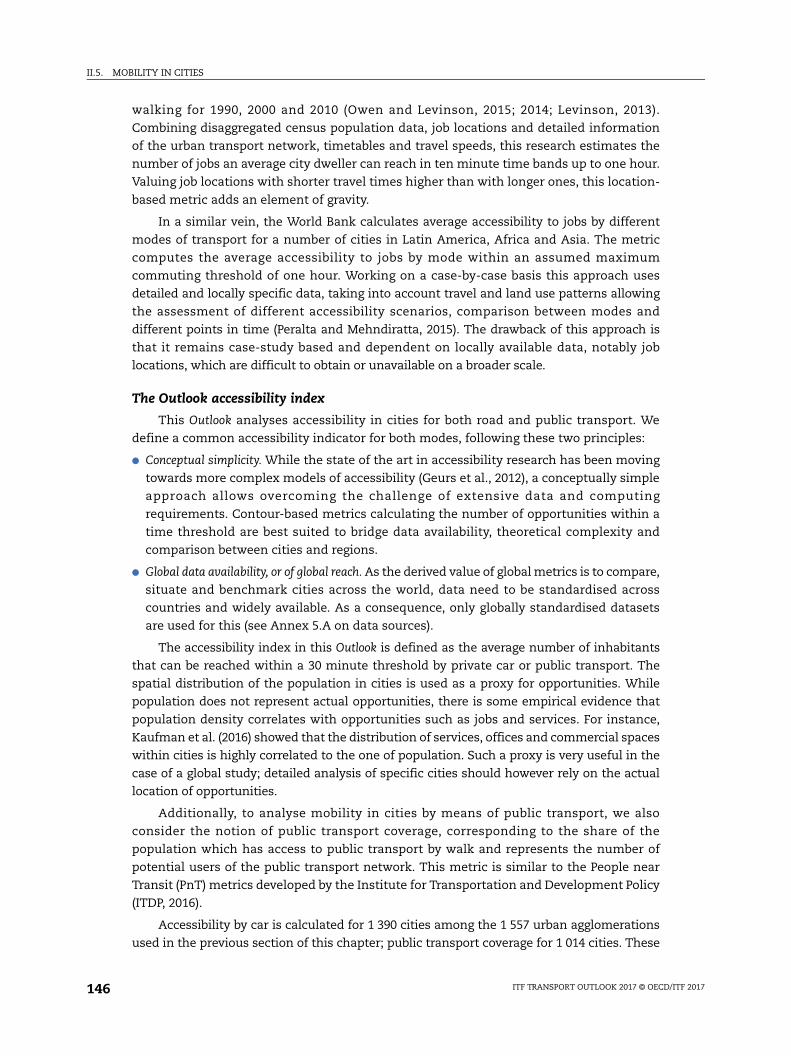
II.5. MOBILITY IN CITIES
walking for 1990, 2000 and 2010 (Owen and Levinson, 2015; 2014; Levinson, 2013).
Combining disaggregated census population data, job locations and detailed information
of the urban transport network, timetables and travel speeds, this research estimates the
number of jobs an average city dweller can reach in ten minute time bands up to one hour.
Valuing job locations with shorter travel times higher than with longer ones, this location-
based metric adds an element of gravity.
In a similar vein, the World Bank calculates average accessibility to jobs by different
modes of transport for a number of cities in Latin America, Africa and Asia. The metric
computes the average accessibility to jobs by mode within an assumed maximum
commuting threshold of one hour. Working on a case-by-case basis this approach uses
detailed and locally specific data, taking into account travel and land use patterns allowing
the assessment of different accessibility scenarios, comparison between modes and
different points in time (Peralta and Mehndiratta, 2015). The drawback of this approach is
that it remains case-study based and dependent on locally available data, notably job
locations, which are difficult to obtain or unavailable on a broader scale.
The Outlook accessibility index
This Outlook analyses accessibility in cities for both road and public transport. We
define a common accessibility indicator for both modes, following these two principles:
● Conceptual simplicity. While the state of the art in accessibility research has been moving
towards more complex models of accessibility (Geurs et al., 2012), a conceptually simple
approach allows overcoming the challenge of extensive data and computing
requirements. Contour-based metrics calculating the number of opportunities within a
time threshold are best suited to bridge data availability, theoretical complexity and
comparison between cities and regions.
● Global data availability, or of global reach. As the derived value of global metrics is to compare,
situate and benchmark cities across the world, data need to be standardised across
countries and widely available. As a consequence, only globally standardised datasets
are used for this (see Annex 5.A on data sources).
The accessibility index in this Outlook is defined as the average number of inhabitants
that can be reached within a 30 minute threshold by private car or public transport. The
spatial distribution of the population in cities is used as a proxy for opportunities. While
population does not represent actual opportunities, there is some empirical evidence that
population density correlates with opportunities such as jobs and services. For instance,
Kaufman et al. (2016) showed that the distribution of services, offices and commercial spaces
within cities is highly correlated to the one of population. Such a proxy is very useful in the
case of a global study; detailed analysis of specific cities should however rely on the actual
location of opportunities.
Additionally, to analyse mobility in cities by means of public transport, we also
consider the notion of public transport coverage, corresponding to the share of the
population which has access to public transport by walk and represents the number of
potential users of the public transport network. This metric is similar to the People near
Transit (PnT) metrics developed by the Institute for Transportation and Development Policy
(ITDP, 2016).
Accessibility by car is calculated for 1 390 cities among the 1 557 urban agglomerations
used in the previous section of this chapter; public transport coverage for 1 014 cities. These
ITF TRANSPORT OUTLOOK 2017 © OECD/ITF 2017146
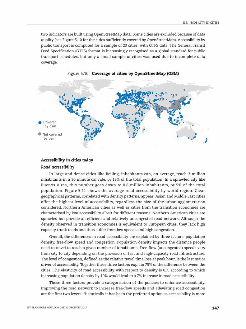
II.5. MOBILITY IN CITIES
two indicators are built using OpenStreetMap data. Some cities are excluded because of data
quality (see Figure 5.10 for the cities sufficiently covered by OpenStreetMap). Accessibility by
public transport is computed for a sample of 23 cities, with GTFS data. The General Transit
Feed Specification (GTFS) format is increasingly recognised as a global standard for public
transport schedules, but only a small sample of cities was used due to incomplete data
coverage.
Accessibility in cities today
Road accessibility
In large and dense cities like Beijing, inhabitants can, on average, reach 3 million
inhabitants in a 30 minute car ride, or 13% of the total population. In a sprawled city like
Buenos Aires, this number goes down to 0.8 million inhabitants, or 5% of the total
population. Figure 5.11 shows the average road accessibility by world region. Clear
geographical patterns, correlated with density patterns, appear: Asian and Middle East cities
offer the highest level of accessibility, regardless the size of the urban agglomeration
considered. Northern American cities as well as cities from the transition economies are
characterised by low accessibility albeit for different reasons. Northern American cities are
sprawled but provide an efficient and relatively uncongested road network. Although the
density observed in transition economies is equivalent to European cities, they lack high
capacity trunk roads and thus suffer from low speeds and high congestion.
Overall, the differences in road accessibility are explained by three factors: population
density, free-flow speed and congestion. Population density impacts the distance people
need to travel to reach a given number of inhabitants. Free-flow (uncongested) speeds vary
from city to city depending on the provision of fast and high-capacity road infrastructure.
The level of congestion, defined as the relative travel time loss at peak hour, is the last major
driver of accessibility. Together these three factors explain 75% of the difference between the
cities. The elasticity of road accessibility with respect to density is 0.7, according to which
increasing population density by 10% would lead to a 7% increase in road accessibility.
These three factors provide a categorisation of the policies to enhance accessibility.
Improving the road network to increase free-flow speeds and alleviating road congestion
are the first two levers. Historically it has been the preferred option as accessibility is more
Figure 5.10. Coverage of cities by OpenStreetMap (OSM)
Covered by osm
Not covered by osm
ITF TRANSPORT OUTLOOK 2017 © OECD/ITF 2017 147
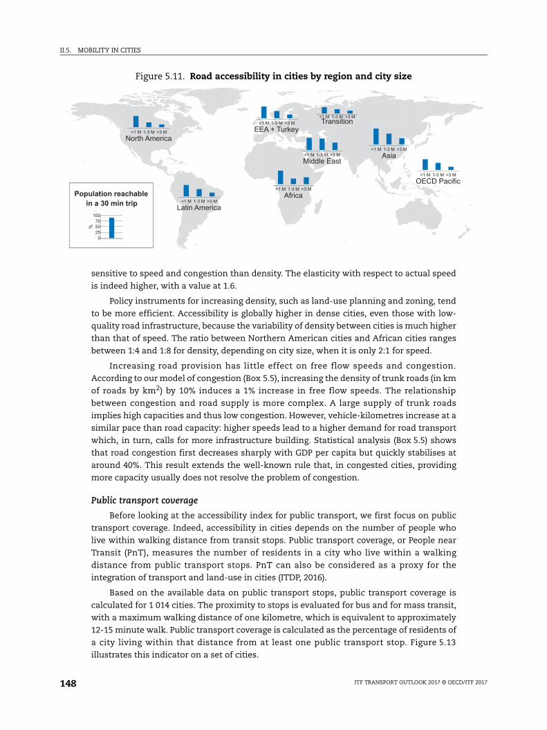
II.5. MOBILITY IN CITIES
sensitive to speed and congestion than density. The elasticity with respect to actual speed
is indeed higher, with a value at 1.6.
Policy instruments for increasing density, such as land-use planning and zoning, tend
to be more efficient. Accessibility is globally higher in dense cities, even those with low-
quality road infrastructure, because the variability of density between cities is much higher
than that of speed. The ratio between Northern American cities and African cities ranges
between 1:4 and 1:8 for density, depending on city size, when it is only 2:1 for speed.
Increasing road provision has little effect on free flow speeds and congestion.
According to our model of congestion (Box 5.5), increasing the density of trunk roads (in km
of roads by km2) by 10% induces a 1% increase in free flow speeds. The relationship
between congestion and road supply is more complex. A large supply of trunk roads
implies high capacities and thus low congestion. However, vehicle-kilometres increase at a
similar pace than road capacity: higher speeds lead to a higher demand for road transport
which, in turn, calls for more infrastructure building. Statistical analysis (Box 5.5) shows
that road congestion first decreases sharply with GDP per capita but quickly stabilises at
around 40%. This result extends the well-known rule that, in congested cities, providing
more capacity usually does not resolve the problem of congestion.
Public transport coverage
Before looking at the accessibility index for public transport, we first focus on public
transport coverage. Indeed, accessibility in cities depends on the number of people who
live within walking distance from transit stops. Public transport coverage, or People near
Transit (PnT), measures the number of residents in a city who live within a walking
distance from public transport stops. PnT can also be considered as a proxy for the
integration of transport and land-use in cities (ITDP, 2016).
Based on the available data on public transport stops, public transport coverage is
calculated for 1 014 cities. The proximity to stops is evaluated for bus and for mass transit,
with a maximum walking distance of one kilometre, which is equivalent to approximately
12-15 minute walk. Public transport coverage is calculated as the percentage of residents of
a city living within that distance from at least one public transport stop. Figure 5.13
illustrates this indicator on a set of cities.
Figure 5.11. Road accessibility in cities by region and city size
<1 M 1-3 M >3 MEEA + Turkey
<1 M 1-3 M >3 MAsia
<1 M 1-3 M >3 MAfrica
<1 M 1-3 M >3 MLatin America
<1 M 1-3 M >3 MMiddle East
<1 M 1-3 M >3 MNorth America
<1 M 1-3 M >3 MOECD Pacific
0255075
100
Population reachablein a 30 min trip
%
<1 M 1-3 M >3 MTransition
ITF TRANSPORT OUTLOOK 2017 © OECD/ITF 2017148
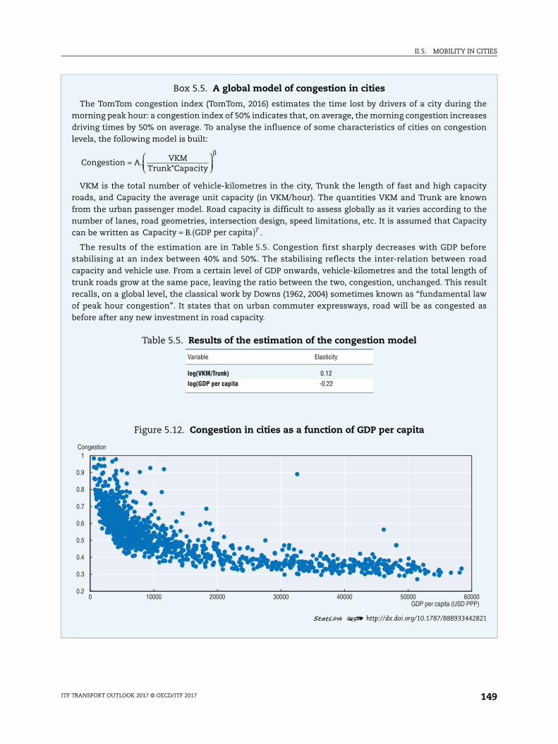
II.5. MOBILITY IN CITIES
he ses ion
ity wn the ity
re ad of ult aw as
821
0)
Box 5.5. A global model of congestion in cities
The TomTom congestion index (TomTom, 2016) estimates the time lost by drivers of a city during tmorning peak hour: a congestion index of 50% indicates that, on average, the morning congestion increadriving times by 50% on average. To analyse the influence of some characteristics of cities on congestlevels, the following model is built:
VKM is the total number of vehicle-kilometres in the city, Trunk the length of fast and high capacroads, and Capacity the average unit capacity (in VKM/hour). The quantities VKM and Trunk are knofrom the urban passenger model. Road capacity is difficult to assess globally as it varies according to number of lanes, road geometries, intersection design, speed limitations, etc. It is assumed that Capaccan be written as .
The results of the estimation are in Table 5.5. Congestion first sharply decreases with GDP befostabilising at an index between 40% and 50%. The stabilising reflects the inter-relation between rocapacity and vehicle use. From a certain level of GDP onwards, vehicle-kilometres and the total lengthtrunk roads grow at the same pace, leaving the ratio between the two, congestion, unchanged. This resrecalls, on a global level, the classical work by Downs (1962, 2004) sometimes known as “fundamental lof peak hour congestion”. It states that on urban commuter expressways, road will be as congestedbefore after any new investment in road capacity.
Congestion A VKMTrunk*Capacity
=⎛⎝⎜
⎞⎠⎟
.β
Capacity B GDP per capita= ( ). g
Table 5.5. Results of the estimation of the congestion model
Variable Elasticity
log(VKM/Trunk) 0.12
log(GDP per capita -0.22
Figure 5.12. Congestion in cities as a function of GDP per capita
1 2 http://dx.doi.org/10.1787/888933442
0.2
0.3
0.4
0.5
0.6
0.7
0.8
0.9
1
0 10000 20000 30000 40000 50000 6000
Congestion
GDP per capita (USD PPP
ITF TRANSPORT OUTLOOK 2017 © OECD/ITF 2017 149
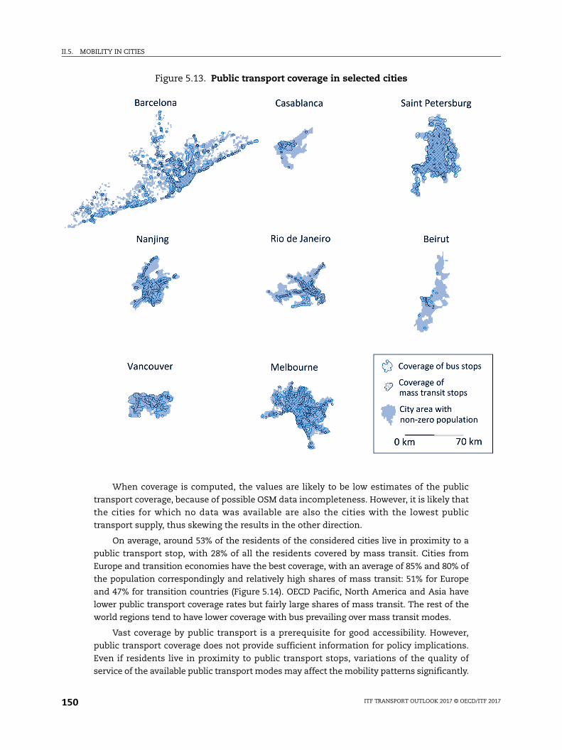
II.5. MOBILITY IN CITIES
When coverage is computed, the values are likely to be low estimates of the public
transport coverage, because of possible OSM data incompleteness. However, it is likely that
the cities for which no data was available are also the cities with the lowest public
transport supply, thus skewing the results in the other direction.
On average, around 53% of the residents of the considered cities live in proximity to a
public transport stop, with 28% of all the residents covered by mass transit. Cities from
Europe and transition economies have the best coverage, with an average of 85% and 80% of
the population correspondingly and relatively high shares of mass transit: 51% for Europe
and 47% for transition countries (Figure 5.14). OECD Pacific, North America and Asia have
lower public transport coverage rates but fairly large shares of mass transit. The rest of the
world regions tend to have lower coverage with bus prevailing over mass transit modes.
Vast coverage by public transport is a prerequisite for good accessibility. However,
public transport coverage does not provide sufficient information for policy implications.
Even if residents live in proximity to public transport stops, variations of the quality of
service of the available public transport modes may affect the mobility patterns significantly.
Figure 5.13. Public transport coverage in selected cities
ITF TRANSPORT OUTLOOK 2017 © OECD/ITF 2017150
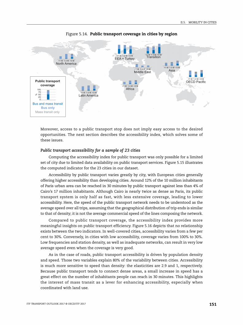
II.5. MOBILITY IN CITIES
Moreover, access to a public transport stop does not imply easy access to the desired
opportunities. The next section describes the accessibility index, which solves some of
these issues.
Public transport accessibility for a sample of 23 cities
Computing the accessibility index for public transport was only possible for a limited
set of city due to limited data availability on public transport services. Figure 5.15 illustrates
the computed indicator for the 23 cities in our dataset.
Accessibility by public transport varies greatly by city, with European cities generally
offering higher accessibility than developing cities. Around 12% of the 10 million inhabitants
of Paris urban area can be reached in 30 minutes by public transport against less than 4% of
Cairo’s 17 million inhabitants. Although Cairo is nearly twice as dense as Paris, its public
transport system is only half as fast, with less extensive coverage, leading to lower
accessibility. Here, the speed of the public transport network needs to be understood as the
average speed over all trips, assuming that the geographical distribution of trip ends is similar
to that of density; it is not the average commercial speed of the lines composing the network.
Compared to public transport coverage, the accessibility index provides more
meaningful insights on public transport efficiency. Figure 5.16 depicts that no relationship
exists between the two indicators. In well-covered cities, accessibility varies from a few per
cent to 30%. Conversely, in cities with low accessibility, coverage varies from 100% to 30%.
Low frequencies and station density, as well as inadequate networks, can result in very low
average speed even when the coverage is very good.
As in the case of roads, public transport accessibility is driven by population density
and speed. Those two variables explain 80% of the variability between cities. Accessibility
is much more sensitive to speed than density: the elasticities are 2.9 and 1, respectively.
Because public transport tends to connect dense areas, a small increase in speed has a
great effect on the number of inhabitants people can reach in 30 minutes. This highlights
the interest of mass transit as a lever for enhancing accessibility, especially when
coordinated with land use.
Figure 5.14. Public transport coverage in cities by region
<1 M 1-3 M >3 MEEA + Turkey
<1 M 1-3 M >3 MAsia
<1 M 1-3 M >3 MLatin America
<1 M 1-3 M >3 MMiddle East
<1 M 1-3 M >3 MNorth America
<1 M 1-3 M >3 MOECD Pacific
<1 M 1-3 M >3 MAfrica
0255075
100
Public transportcoverage
%
Bus and mass transit
Mass transit onlyBus only
<1 M 1-3 M >3 MTransition
ITF TRANSPORT OUTLOOK 2017 © OECD/ITF 2017 151
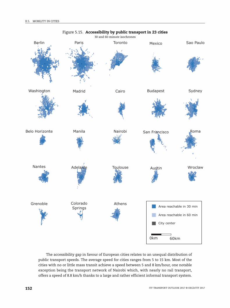
II.5. MOBILITY IN CITIES
The accessibility gap in favour of European cities relates to an unequal distribution of
public transport speeds. The average speed for cities ranges from 5 to 15 km. Most of the
cities with no or little mass transit achieve a speed between 5 and 8 km/hour, one notable
exception being the transport network of Nairobi which, with nearly no rail transport,
offers a speed of 8.8 km/h thanks to a large and rather efficient informal transport system.
Figure 5.15. Accessibility by public transport in 23 cities30 and 60-minute isochrones
ITF TRANSPORT OUTLOOK 2017 © OECD/ITF 2017152
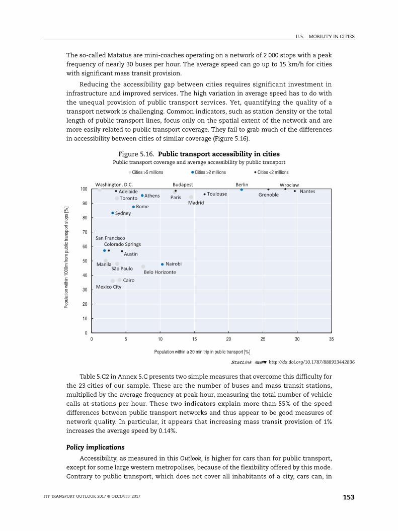
II.5. MOBILITY IN CITIES
442836
The so-called Matatus are mini-coaches operating on a network of 2 000 stops with a peak
frequency of nearly 30 buses per hour. The average speed can go up to 15 km/h for cities
with significant mass transit provision.
Reducing the accessibility gap between cities requires significant investment in
infrastructure and improved services. The high variation in average speed has to do with
the unequal provision of public transport services. Yet, quantifying the quality of a
transport network is challenging. Common indicators, such as station density or the total
length of public transport lines, focus only on the spatial extent of the network and are
more easily related to public transport coverage. They fail to grab much of the differences
in accessibility between cities of similar coverage (Figure 5.16).
Table 5.C2 in Annex 5.C presents two simple measures that overcome this difficulty for
the 23 cities of our sample. These are the number of buses and mass transit stations,
multiplied by the average frequency at peak hour, measuring the total number of vehicle
calls at stations per hour. These two indicators explain more than 55% of the speed
differences between public transport networks and thus appear to be good measures of
network quality. In particular, it appears that increasing mass transit provision of 1%
increases the average speed by 0.14%.
Policy implications
Accessibility, as measured in this Outlook, is higher for cars than for public transport,
except for some large western metropolises, because of the flexibility offered by this mode.
Contrary to public transport, which does not cover all inhabitants of a city, cars can, in
Figure 5.16. Public transport accessibility in citiesPublic transport coverage and average accessibility by public transport
1 2 http://dx.doi.org/10.1787/888933
Washington, D.C.
São Paulo
Mexico City
Toronto
Manila
CairoBelo Horizonte
ParisMadrid
San Francisco
SydneyRome
Athens
Nairobi
Berlin
Colorado Springs
Adelaide
Austin
Budapest
Toulouse Grenoble
WroclawNantes
0
10
20
30
40
50
60
70
80
90
100
0 5 10 15 20 25 30 35
Popu
latio
n w
ithin
100
0m fr
om p
ublic
tran
spor
t sto
ps [%
]
Population within a 30 min trip in public transport [%]
Cities >5 millions Cities >2 millions Cities <2 millions
ITF TRANSPORT OUTLOOK 2017 © OECD/ITF 2017 153
II.5. MOBILITY IN CITIES
ve on, all
ge-ile vel nd to es,
on, res es al,
uel ity. the ity,
nal ual are ust for
theory go between any two places. However, promoting accessibility by car raises many
issues, not least because of congestion (see also the Outlook section below). The road
infrastructure required to accommodate a car-oriented accessibility can be very difficult to
build and maintain, especially in dense cities.
Public transport, on the other hand, can deliver accessibility to the greatest number.
Investment in transport infrastructure needs to be coupled with wider policy packages,
including travel demand management, land-use planning and promotion of active modes.
Innovative mobility solutions, such as car-sharing or demand-responsive buses, can also be
promoted to form part of the transport options for travellers. Indeed, a recent study by ITF
(2016) shows that these two mobility options, if implemented together with adequate mass
transit, can provide high levels of accessibility at a reasonable cost and bring additional
benefits, such as reduced public parking space and emission reductions (Box 5.6).
Currently, accessibility by public transport is especially low in developing cities, where
the motorisation rate is also the lowest. Many inhabitants are thus excluded from fast access
to opportunities in these cities. This raises a major equity issue that also applies, to a lesser
extent, to North American cities. As investing in public transport infrastructure is costly,
there is also a significant policy challenge here: how to develop a mass transit network while
Box 5.6. The ITF Shared Mobility Model
The advent of shared mobility on a large scale could change travel patterns in cities and improaccessibility significantly. The ITF Shared Mobility simulation model (ITF 2016), developed for LisbPortugal, shows that the car fleet needed for daily commuting can be reduced to 3% of today’s fleet iftrips are made using a comprehensive shared mobility platform.
The Shared Mobility model simulates the current situation as a baseline and assesses the possible larscale deployment of a shared vehicle fleet that provides on-demand transport in different scenarios, whkeeping the same level of mobility. The shared alternatives in the model are designed to provide high leof acceptance by current car drivers and include on-demand door-to-door rides by “Shared Taxis” apre-booked transfer-free rides at pop-up stops by “Taxi-Buses”. While rail and subway services continueoperate as today in the shared-mobility scenarios, all other motorised modes, including taxis and busare replaced with shared alternatives.
The main findings of the study, besides the drastic car fleet reduction, include a decrease in congestiemissions reduced by one-third, and 95% less space needed for public parking. The total vehicle-kilomettravelled is 37% less during the peak hours compared to today, while each car is running almost ten timmore kilometres than currently. The induced shorter vehicle lifetimes lead to more frequent fleet renewwhich enables a quicker fleet turnover and a faster penetration of fuel-efficient or alternative ftechnologies. The shared mobility scenarios also result in cheaper trips due to more efficient use of capacOther benefits include the decrease in the number of transfers and better accessibility. Figure 5.16 shows comparison of accessibility to jobs in the baseline and the shared mobility scenarios. With shared mobilthe majority of grid cells have at least 75% of the jobs in the city reachable within 30 minutes.
The challenges for policy makers lie in the creation of the right market conditions and operatioframeworks. While a sudden change to a complete shared mobility system is not conceivable, a gradinstallation is plausible and may already yield large benefits. In one of the scenarios, individual cars allowed to drive in the city two working days per week, while other days the shared mobility system mbe used. This results in significant reductions of congestion and emissions, and could be an opportunity car owners to shift to the shared mobility service gradually.
ITF TRANSPORT OUTLOOK 2017 © OECD/ITF 2017154
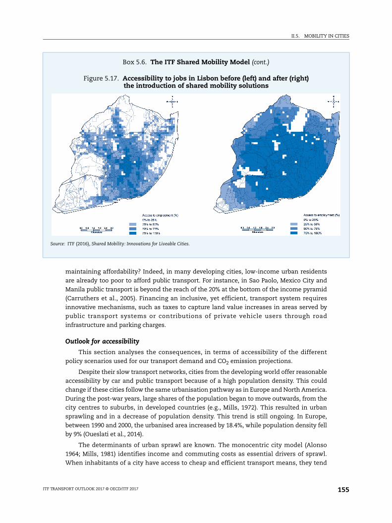
II.5. MOBILITY IN CITIES
maintaining affordability? Indeed, in many developing cities, low-income urban residents
are already too poor to afford public transport. For instance, in Sao Paolo, Mexico City and
Manila public transport is beyond the reach of the 20% at the bottom of the income pyramid
(Carruthers et al., 2005). Financing an inclusive, yet efficient, transport system requires
innovative mechanisms, such as taxes to capture land value increases in areas served by
public transport systems or contributions of private vehicle users through road
infrastructure and parking charges.
Outlook for accessibility
This section analyses the consequences, in terms of accessibility of the different
policy scenarios used for our transport demand and CO2 emission projections.
Despite their slow transport networks, cities from the developing world offer reasonable
accessibility by car and public transport because of a high population density. This could
change if these cities follow the same urbanisation pathway as in Europe and North America.
During the post-war years, large shares of the population began to move outwards, from the
city centres to suburbs, in developed countries (e.g., Mills, 1972). This resulted in urban
sprawling and in a decrease of population density. This trend is still ongoing. In Europe,
between 1990 and 2000, the urbanised area increased by 18.4%, while population density fell
by 9% (Oueslati et al., 2014).
The determinants of urban sprawl are known. The monocentric city model (Alonso
1964; Mills, 1981) identifies income and commuting costs as essential drivers of sprawl.
When inhabitants of a city have access to cheap and efficient transport means, they tend
Box 5.6. The ITF Shared Mobility Model (cont.)
Figure 5.17. Accessibility to jobs in Lisbon before (left) and after (right) the introduction of shared mobility solutions
Source: ITF (2016), Shared Mobility: Innovations for Liveable Cities.
ITF TRANSPORT OUTLOOK 2017 © OECD/ITF 2017 155
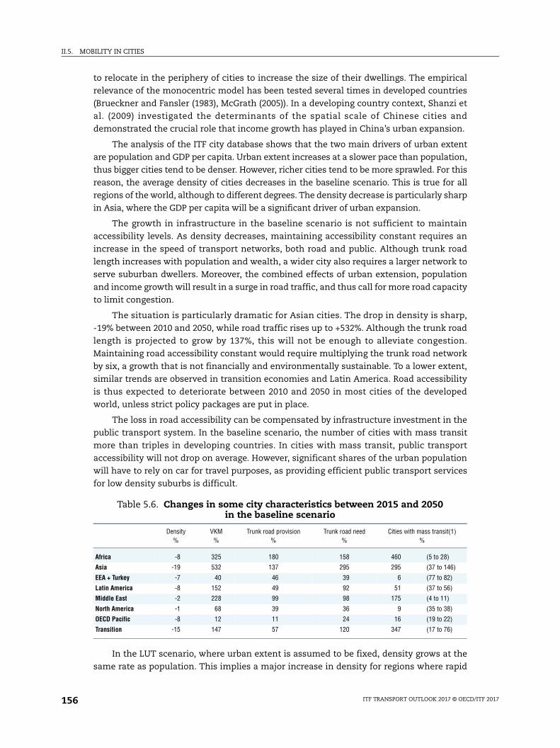
II.5. MOBILITY IN CITIES
to relocate in the periphery of cities to increase the size of their dwellings. The empirical
relevance of the monocentric model has been tested several times in developed countries
(Brueckner and Fansler (1983), McGrath (2005)). In a developing country context, Shanzi et
al. (2009) investigated the determinants of the spatial scale of Chinese cities and
demonstrated the crucial role that income growth has played in China’s urban expansion.
The analysis of the ITF city database shows that the two main drivers of urban extent
are population and GDP per capita. Urban extent increases at a slower pace than population,
thus bigger cities tend to be denser. However, richer cities tend to be more sprawled. For this
reason, the average density of cities decreases in the baseline scenario. This is true for all
regions of the world, although to different degrees. The density decrease is particularly sharp
in Asia, where the GDP per capita will be a significant driver of urban expansion.
The growth in infrastructure in the baseline scenario is not sufficient to maintain
accessibility levels. As density decreases, maintaining accessibility constant requires an
increase in the speed of transport networks, both road and public. Although trunk road
length increases with population and wealth, a wider city also requires a larger network to
serve suburban dwellers. Moreover, the combined effects of urban extension, population
and income growth will result in a surge in road traffic, and thus call for more road capacity
to limit congestion.
The situation is particularly dramatic for Asian cities. The drop in density is sharp,
-19% between 2010 and 2050, while road traffic rises up to +532%. Although the trunk road
length is projected to grow by 137%, this will not be enough to alleviate congestion.
Maintaining road accessibility constant would require multiplying the trunk road network
by six, a growth that is not financially and environmentally sustainable. To a lower extent,
similar trends are observed in transition economies and Latin America. Road accessibility
is thus expected to deteriorate between 2010 and 2050 in most cities of the developed
world, unless strict policy packages are put in place.
The loss in road accessibility can be compensated by infrastructure investment in the
public transport system. In the baseline scenario, the number of cities with mass transit
more than triples in developing countries. In cities with mass transit, public transport
accessibility will not drop on average. However, significant shares of the urban population
will have to rely on car for travel purposes, as providing efficient public transport services
for low density suburbs is difficult.
In the LUT scenario, where urban extent is assumed to be fixed, density grows at the
same rate as population. This implies a major increase in density for regions where rapid
Table 5.6. Changes in some city characteristics between 2015 and 2050 in the baseline scenario
Density %
VKM %
Trunk road provision %
Trunk road need %
Cities with mass transit(1) %
Africa -8 325 180 158 460 (5 to 28)
Asia -19 532 137 295 295 (37 to 146)
EEA + Turkey -7 40 46 39 6 (77 to 82)
Latin America -8 152 49 92 51 (37 to 56)
Middle East -2 228 99 98 175 (4 to 11)
North America -1 68 39 36 9 (35 to 38)
OECD Pacific -8 12 11 24 16 (19 to 22)
Transition -15 147 57 120 347 (17 to 76)
ITF TRANSPORT OUTLOOK 2017 © OECD/ITF 2017156
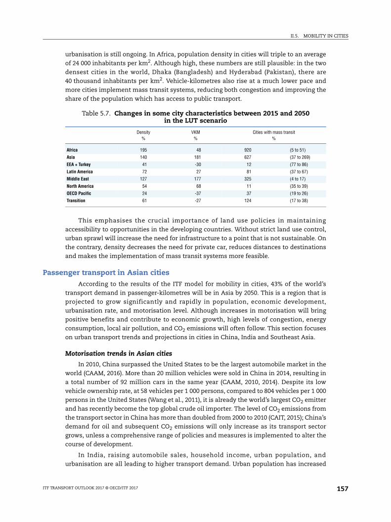
II.5. MOBILITY IN CITIES
urbanisation is still ongoing. In Africa, population density in cities will triple to an average
of 24 000 inhabitants per km2. Although high, these numbers are still plausible: in the two
densest cities in the world, Dhaka (Bangladesh) and Hyderabad (Pakistan), there are
40 thousand inhabitants per km2. Vehicle-kilometres also rise at a much lower pace and
more cities implement mass transit systems, reducing both congestion and improving the
share of the population which has access to public transport.
This emphasises the crucial importance of land use policies in maintaining
accessibility to opportunities in the developing countries. Without strict land use control,
urban sprawl will increase the need for infrastructure to a point that is not sustainable. On
the contrary, density decreases the need for private car, reduces distances to destinations
and makes the implementation of mass transit systems more feasible.
Passenger transport in Asian citiesAccording to the results of the ITF model for mobility in cities, 43% of the world’s
transport demand in passenger-kilometres will be in Asia by 2050. This is a region that is
projected to grow significantly and rapidly in population, economic development,
urbanisation rate, and motorisation level. Although increases in motorisation will bring
positive benefits and contribute to economic growth, high levels of congestion, energy
consumption, local air pollution, and CO2 emissions will often follow. This section focuses
on urban transport trends and projections in cities in China, India and Southeast Asia.
Motorisation trends in Asian cities
In 2010, China surpassed the United States to be the largest automobile market in the
world (CAAM, 2016). More than 20 million vehicles were sold in China in 2014, resulting in
a total number of 92 million cars in the same year (CAAM, 2010, 2014). Despite its low
vehicle ownership rate, at 58 vehicles per 1 000 persons, compared to 804 vehicles per 1 000
persons in the United States (Wang et al., 2011), it is already the world’s largest CO2 emitter
and has recently become the top global crude oil importer. The level of CO2 emissions from
the transport sector in China has more than doubled from 2000 to 2010 (CAIT, 2015); China’s
demand for oil and subsequent CO2 emissions will only increase as its transport sector
grows, unless a comprehensive range of policies and measures is implemented to alter the
course of development.
In India, raising automobile sales, household income, urban population, and
urbanisation are all leading to higher transport demand. Urban population has increased
Table 5.7. Changes in some city characteristics between 2015 and 2050 in the LUT scenario
Density %
VKM %
Cities with mass transit %
Africa 195 48 920 (5 to 51)
Asia 140 181 627 (37 to 269)
EEA + Turkey 41 -30 12 (77 to 86)
Latin America 72 27 81 (37 to 67)
Middle East 127 177 325 (4 to 17)
North America 54 68 11 (35 to 39)
OECD Pacific 24 -37 37 (19 to 26)
Transition 61 -27 124 (17 to 38)
ITF TRANSPORT OUTLOOK 2017 © OECD/ITF 2017 157
II.5. MOBILITY IN CITIES
from 60 million in 1951 to 410 million in 2015 (United Nations, 2014). The number and size
of cities have also increased, which will ultimately increase travel demand and total
distance travelled. The number of cars has grown from 16 million in 1990 to almost
40 million in 2000, reaching a total number of 131 million in 2014 (IEA, 2015). Most of these
vehicles are motorcycles and only 21 million of them are passenger cars. Compared to
China, India has a much smaller car market but the transport sector is still a leading
contributor to Indian cities’ CO2 emissions mainly because of motorcycles. India’s
passenger vehicle market is heavily dominated by motorcycles, which are the fastest
growing type of vehicle in India, with an average annual growth rate that is higher than all
other types of motor vehicles. Hence, in addition to CO2 emissions, local air pollution is a
major problem in Indian cities.
Local air pollution from transport activities, along with traffic congestion, are pressing
challenges in many Southeast Asian countries. Transport demand in Southeast Asia has
been steadily increasing over the past three decades and has not shown any signs of
slowing down. Recent statistics from the IEA (2015) show that the number of motorcycles
has grown by 177% in Vietnam between 2000 and 2013. The increase in cars was 600% in
the same period. In Malaysia, the growth in cars is 148%, while the Philippines saw a
relatively lower percentage at 44% over the same period of time. Indonesia has also
experienced high vehicle growth rates for both motorcycles and cars, with an over 600%
and 280% increase respectively. Most cars have also become single occupancy vehicles
most of the time, leading to greater time delays in urban cities. It is not surprising that due
to its affordability and practicality, motorcycles are the leading transport mode choice in
many Southeast Asian cities. In Vietnam, 95% of all vehicles are motorcycles. These
increases in motorcycles could be a reflection of the lack of an adequate public transport
system and the general appeal of personal mobility over public transport. Transport
challenges exist in smaller Southeast Asian countries too. Traffic congestion costs
Cambodia around USD 6 million per month as a result of lower economic efficiency and the
loss of working time and fuel (Sotheary and Kunthear, 2015). In Kuala Lumpur, the World
Bank estimated the costs of traffic congestion to be 1.1% to 1.2% of the national GDP in 2014
(Sander et al., 2015).
Although the transport priorities in most Asian cities are traffic congestion and local
air pollution, their transport sectors have increasingly become a bigger contributor of CO2
emissions. The high motorisation rate in Vietnam led to a 190% increase in its CO2
emissions from the transport sector between 2000 and 2010, which is higher than China
(160%) and India (100%) over the same period (CAIT, 2015). Indonesia, Cambodia and
Malaysia also recorded significant increases of transport-induced emissions. The
Philippines was the only country selected in this study not to witness a growth in its
transport emissions. As carbon emissions become a pressing concern in the region, there
is now a greater sense of urgency for Asian cities to adopt more sustainable transport
development policies and measures.
In order to successfully reduce carbon emissions, it is important to first identify
measures that will also provide climate co-benefits through the development of energy
efficient and low carbon transport systems in Asia. Policies and measures that support the
adoption of advanced vehicle technology and alternative fuel will reduce CO2 emission by
improving energy intensity. However, as a result of the increasing number of vehicles in
Asia, advancing vehicle and fuel technology will not be enough to reduce CO2 emissions, as
the growth of vehicle ownership and use surpass technological improvements. A range of
ITF TRANSPORT OUTLOOK 2017 © OECD/ITF 2017158
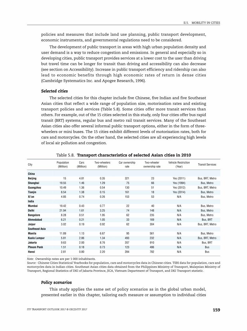
II.5. MOBILITY IN CITIES
vices
etro
tro
etro
tro
tro
tro
tro
tro
T
etro
tro
etro
T
ars and istry of
policies and measures that include land use planning, public transport development,
economic instruments, and governmental regulations need to be considered.
The development of public transport in areas with high urban population density and
user demand is a way to reduce congestion and emissions. In general and especially so in
developing cities, public transport provides services at a lower cost to the user than driving
but travel time can be longer for transit than driving and accessibility can also decrease
(see section on Accessibility). Increase in public transport efficiency and ridership can also
lead to economic benefits through high economic rates of return in dense cities
(Cambridge Systematics Inc. and Apogee Research, 1996).
Selected cities
The selected cities for this chapter include five Chinese, five Indian and five Southeast
Asian cities that reflect a wide range of population size, motorisation rates and existing
transport policies and services (Table 5.8). Some cities offer more transit services than
others. For example, out of the 15 cities selected in this study, only four cities offer bus rapid
transit (BRT) systems, regular bus and metro rail transit services. Many of the Southeast
Asian cities also offer several informal public transport options, either in the form of three-
wheelers or mini buses. The 15 cities exhibit different levels of motorisation rates, both for
cars and motorcycles. On the other hand, the selected cities are all experiencing high levels
of local air pollution and congestion.
Policy scenarios
This study applies the same set of policy scenarios as in the global urban model,
presented earlier in this chapter, tailoring each measure or assumption to individual cities
Table 5.8. Transport characteristics of selected Asian cities in 2010
CityPopulation (Million)
Cars (Million)
Two-wheelers (Million)
Car ownership rate
Two-wheeler ownership rate
Vehicle Restriction (Year)
Transit Ser
China
Beijing 15 4.81 0.35 321 23 Yes (2011) Bus, BRT, M
Shanghai 19.55 1.46 1.29 75 66 Yes (1994) Bus, Me
Guangzhou 10.49 1.36 0.54 130 51 Yes (2012) Bus, BRT, M
Tianjin 8.54 1.38 0.15 161 18 Yes (2014) Bus, Me
Xi’an 4.85 0.74 0.26 153 53 N/A Bus, Me
India
Mumbai 19.42 0.43 0.77 22 40 N/A Bus, Me
Delhi 21.94 1.61 3.25 74 148 N/A Bus, Me
Bangalore 8.28 0.51 1.95 62 235 N/A Bus, Me
Ahmedabad 6.21 0.21 1.05 33 169 N/A Bus, BR
Jaipur 3.02 0.19 0.92 62 304 N/A Bus, BRT, M
Southeast Asia
Manila 11.89 1.13 6.67 95 561 N/A Bus, Me
Kuala Lumpur 5.81 2.86 1.34 493 232 N/A Bus, BRT, M
Jakarta 9.63 2.00 8.76 207 910 N/A Bus, BR
Phnom Penh 1.51 0.18 0.73 123 486 N/A Bus
Hanoi 2.81 0.80 2.20 284 782 N/A Bus
Note: Ownership rates are per 1 000 inhabitants. Source: Chinese Cities Statistical Yearbooks for population, cars and motorcycles data in Chinese cities. TERI data for population, cmotorcycles data in Indian cities. Southeast Asian cities data obtained from the Philippines Ministry of Transport, Malaysian MinTransport, Regional Statistics of DKI of Jakarta Province, JICA, Vietnam Department of Transport, and DKI Transport statistic.
ITF TRANSPORT OUTLOOK 2017 © OECD/ITF 2017 159
II.5. MOBILITY IN CITIES
(see Tables in Annex 5.D). Although each scenario contains a different set of policy
assumptions, the framework for estimating transport demand and CO2 emissions is similar
across all scenarios. The scenario outcomes are not predictions, but different possible
futures based on the assumptions applied in each scenario.
The projection of transport demand in Chinese and Indian cities were estimated
differently from the Southeast Asian cities due to data availability, which is a wider
challenge in the region (Box 5.7).
Box 5.7. Transport data in Asia and the Pacific: Challenges and opportunities
“If you cannot measure it, you cannot improve it”, goes the quote popularly attributed to Lord Kelvin (William Thomson). The need for reliable, robust data sets is felt particularly by those working towards sustainable transport in the developing world. Better data provides direction for informed action: for example, the Cities Air, Climate, Transport database (www.citiesact.org) covering nearly 500 cities across Asia shows that 97% of these cities are not meeting air pollution targets. Identifying what modes of transport generate the air pollution would be a critical point of action.
The Asian Development Bank, together with its partners, is currently undertaking a regional project to improve the quality of transportation data in Asia and the Pacific, and widen the access to this data. The project – “Better Transport Data for Sustainable Transport Policies and Investment Planning” – intends to collect, collate and generate insights from currently available transport data in forty (40) of ADB’s developing member countries (DMCs). The data will be shared through a publicly accessible portal, and used as inputs to a transportation model to assess the potential impacts of future transport scenarios in these countries.
A key challenge towards benchmarking across countries in Asia is the non-availability of standardized definitions. A notable example relates to road vehicles. Each country is using its own set of vehicle categories, most often derived from the usage of the vehicles, which does not follow internationally-recognized classifications. Simple steps can be taken to harmonise, such as using publications like the “Illustrated Glossary for Transport Statistics” (ITF et al., 2009); these guidelines could be further enriched by feedback from users in Asia and the Pacific.
The non-collection of key transport data is also a challenge in the region. Average vehicle-kilometres driven by different vehicle sub-segments, for example, are not commonly collected by developing and middle-income countries. The non-availability of such information prevents generation of other important indicators for transport. Moreover, access to readily-available disaggregated data is often limited. Solutions need not be complicated: collection of data for additional indicators, such as vehicle-kilometres driven, can easily be incorporated into the vehicle registration and renewal processes.
City-level transport data in the region most often comes from ad hoc initiatives, supported by external parties, and is limited to the main cities in developing and middle-income countries. Inconsistencies can sometimes be found between datasets for the same parameter generated by different government agencies from the same country. Increasing the vertical integration between relevant stakeholders through discussions and workshops on transport data collection can accelerate the generation of quality data in the region. Local governments can be better capacitated in transport data collection and tapped to contribute to an integrated database.
ITF TRANSPORT OUTLOOK 2017 © OECD/ITF 2017160
II.5. MOBILITY IN CITIES
Travel demand projections for the Chinese and Indian cities were developed using the
ASIF (Activity, Structure, Intensity, Fuel type) approach (Schipper et al., 2000), where their
motorisation rates were modelled based on South Korea and Japan’s historical motorisation
rates for cars and motorcycles, while projections for bus and passenger rail transportation
demand follow population density growth (ITF, 2015). For the five Southeast Asian cities,
household travel survey data that included individual trip data such as mode choice, travel
distance, travel time, and socioeconomic variables were obtained from the Japan
International Cooperation Agency (JICA). These data supported the construction of five mode
choice models (multinomial logit), which enabled the projections of 2050 travel demand and
CO2 emissions using parameters derived from the choice models.
Baseline
In the baseline scenario, no major new public transport development, economic
instruments, or governmental regulations will be implemented in the selected cities, apart
from those that have already been introduced. For example, existing restrictions on vehicle
registration in Chinese cities will continue but not spread to other cities that currently do not
have such regulations. Motor vehicle ownership and use will continue to increase for cities
without any restrictions on vehicle growth. These cities include all five Indian cities and one
Chinese city, i.e. Xi’an. There is no substantial effort to improve public transport services, in
terms of reducing bus and rail travel time or developing BRT systems in cities where such
systems are currently unavailable. Similar assumptions were made for Southeast Asian cities.
Advanced vehicle technology and alternative vehicle fuel use will continue to penetrate the
market but at a relatively low rate, especially for Indian cities. There will also be no significant
improvement in fuel efficiency standards, which coincides with the IEA 4DS (IEA, 2015).
ROG Scenario
In the ROG scenario, city governments play a larger role in regulating vehicle use and
ownership. Governmental regulations and standards refer to non-market based policies,
such as restrictions on annual vehicle ownership growth and fuel economy standards. A
cap on vehicle growth rate through tight vehicle quota control regulations will ensure
reductions in congestion, local air pollution and global carbon emissions. Auctions or
lottery schemes that distribute the limited number of license plates available will
accompany such regulations, as currently implemented in cities such as Singapore,
Shanghai and Beijing. In this scenario, restrictions on vehicle registration will exist in all
Chinese cities and their quotas will gradually decrease between 2030 and 2050. Fuel
efficiency standards in this scenario follow the assumptions made in the IEA 2DS (IEA,
Box 5.7. Transport data in Asia and the Pacific: Challenges and opportunities (cont.)
The “Better Transport Data” initiative underlines the importance of accounting for local contexts, priorities, resources, and capacities when looking into transport data. At the same time, countries in the region can benefit from mutual sharing of experiences and methods, as well as in having standard guidelines for defining, and collecting transport data. The availability of openly accessible and curated data – through a web portal and possible crowd-sourcing tools – is also envisioned to generate interest, both from state and non-state actors, in improving transport data and research in the region.
ITF TRANSPORT OUTLOOK 2017 © OECD/ITF 2017 161
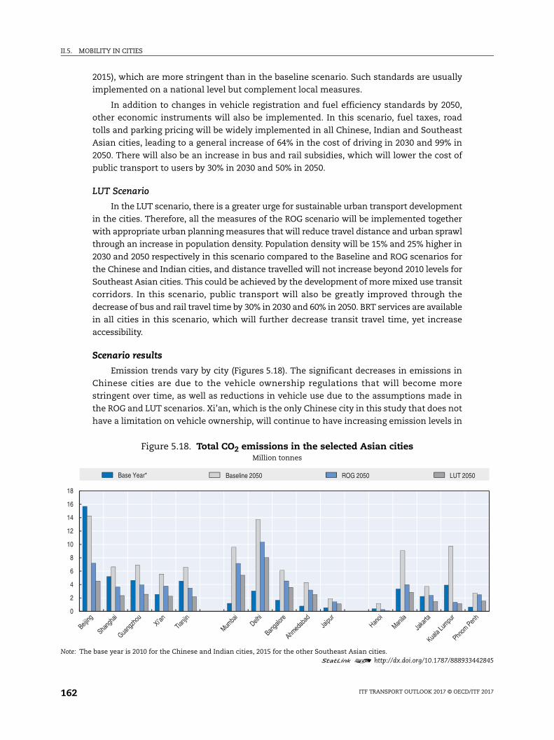
II.5. MOBILITY IN CITIES
442845
0
2015), which are more stringent than in the baseline scenario. Such standards are usually
implemented on a national level but complement local measures.
In addition to changes in vehicle registration and fuel efficiency standards by 2050,
other economic instruments will also be implemented. In this scenario, fuel taxes, road
tolls and parking pricing will be widely implemented in all Chinese, Indian and Southeast
Asian cities, leading to a general increase of 64% in the cost of driving in 2030 and 99% in
2050. There will also be an increase in bus and rail subsidies, which will lower the cost of
public transport to users by 30% in 2030 and 50% in 2050.
LUT Scenario
In the LUT scenario, there is a greater urge for sustainable urban transport development
in the cities. Therefore, all the measures of the ROG scenario will be implemented together
with appropriate urban planning measures that will reduce travel distance and urban sprawl
through an increase in population density. Population density will be 15% and 25% higher in
2030 and 2050 respectively in this scenario compared to the Baseline and ROG scenarios for
the Chinese and Indian cities, and distance travelled will not increase beyond 2010 levels for
Southeast Asian cities. This could be achieved by the development of more mixed use transit
corridors. In this scenario, public transport will also be greatly improved through the
decrease of bus and rail travel time by 30% in 2030 and 60% in 2050. BRT services are available
in all cities in this scenario, which will further decrease transit travel time, yet increase
accessibility.
Scenario results
Emission trends vary by city (Figures 5.18). The significant decreases in emissions in
Chinese cities are due to the vehicle ownership regulations that will become more
stringent over time, as well as reductions in vehicle use due to the assumptions made in
the ROG and LUT scenarios. Xi’an, which is the only Chinese city in this study that does not
have a limitation on vehicle ownership, will continue to have increasing emission levels in
Figure 5.18. Total CO2 emissions in the selected Asian citiesMillion tonnes
Note: The base year is 2010 for the Chinese and Indian cities, 2015 for the other Southeast Asian cities.1 2 http://dx.doi.org/10.1787/888933
0
2
4
6
8
10
12
14
16
18
Base Year* Baseline 2050 ROG 2050 LUT 205
ITF TRANSPORT OUTLOOK 2017 © OECD/ITF 2017162
II.5. MOBILITY IN CITIES
the Baseline and ROG scenarios. CO2 emissions will only decrease in Xi’an when a wider
range of policies and measures are implemented as assumed in the LUT scenario.
Emission projections in Indian cities differ from those in the five selected Chinese
cities and will follow a much more linear trend over the next few decades. Nevertheless,
the rate of growth could decrease, as shown in the ROG and LUT scenarios, if cities
implement appropriate transport policies to change travel demand and behaviour, and if
the pace of technological progress is quicker.
As for the Southeast Asian cities, the policy scenarios trigger the largest decrease in
CO2 emissions from the baseline to the LUT scenario in 2050 for Hanoi (90%) and Kuala
Lumpur (88%). These decreases largely result from the shift from cars to public transport
options. The difference in CO2 emission reduction between the LUT and ROG scenarios is
the smallest for Kuala Lumpur (18%) and largest for Hanoi (124%), which shows that the
impact of the same combination of policy measures will vary depending on a city’s existing
transport mode choice, preferences, alternatives, and policies.
Policy options for sustainable transport in Asian cities
Achieving low-carbon mobility in Asian cities requires targeted policies, which differ
according to the varying transport preferences, constraints and needs found in different
cities. The same set of policies and measures can trigger different outcomes. Cities are
diverse in terms of the modes available and existing transport services, which leads to
different policy impacts, even within the same country or region. This calls for special
attention to be paid to the local context when examining the policy options of a city. The
following paragraphs conclude by bringing forward some common elements for sustainable
transport in Asia cities.
Government regulations are complementary to economic instruments in reducing car
use and CO2 emissions. Xi’an, the only Chinese city selected in this study without an
existing regulation on vehicle registration restriction, had the lowest number of cars in
2010 in China. However, without governmental regulation, its total number of vehicles
increases by 82% in 2050 (baseline scenario). In the five Indian cities selected for this study,
the increase in cars can be as high as 96% for the same time horizon, as is the case in
Mumbai. These outcomes can be avoided by a mix of government regulation and economic
instruments, in the form of fuel taxes, road pricing, parking fee, or transit subsidies, which
provide incentives to drive less and use public transport more.
To be fully efficient, economic instruments need be coupled with integrated land-use
and transport planning. Land-use and transport planning strategies can change the density
of urban cities and diversity of activities in neighbourhoods. It reduces the average distance
travelled, transport demand and CO2 emissions subsequently. Given their high population
density, Chinese and Indian cities are well suited for the development of efficient public
transport systems. The effect of the policies in the LUT scenario is particularly high in
reducing CO2. Emphasising public transport services using high capacity vehicles also
reduces congestion and emissions.
Since the share of motorised two-wheelers is high in most developing Asian cities,
especially in Southeast Asia, economic instruments need also apply to them. These
include road tolls and parking policies that will serve as transport demand management
tools for both types of vehicle. In addition, the high shares of motorcycles often hide an
issue with public transport provision. The regulation of motorcycles can only go hand in
ITF TRANSPORT OUTLOOK 2017 © OECD/ITF 2017 163
II.5. MOBILITY IN CITIES
hand with an improvement of public transport, or cities face the risk of significant loss of
accessibility.
The low modal shares for public transport in some Southeast Asian cities can also be
explained by the existence of informal public transport services. Such services provide
more flexible route and often at a lower cost than structured public transport. Since the
cost of public transport is relatively low in Chinese, Indian and Southeast Asian cities, the
provision of further transit subsidies may not be effective in encouraging greater public
transport use. Another way to increase its appeal is to improve the quality of the services,
for example, by decreasing travel time. This implies the development of faster travel
modes. Speed can be further enhanced by using dedicated roadways or introducing BRT
systems, and enabling smoother transfers between vehicles and other transport modes.
The LUT scenario reflects the improvement of bus and passenger rail travel time and
the availability of BRT systems in all 15 cities. Compared to the baseline scenario, bus
ridership will increase by 28 to 117% in Chinese cities and by 36 to 138% in Indian cities in
2030. Bus ridership in the ROG scenario, which only includes transit subsidies as a policy to
increase ridership, increases on a much smaller scale. A similar trend is observed for
passenger rail ridership. The improvement of the quality of the public transport network
appears much more efficient in encouraging mode shift than pure economic instruments.
Finally, the results highlight the importance of timing in policy implementation. Cities
should act now to reduce transport CO2 emissions. In 2010, Beijing had the highest
passenger light duty vehicle demand in China, most certainly because it only started
regulating the growth in private cars in 2011, whereas Shanghai proposed its vehicle
ownership policy 25 years earlier in 1986 and implemented it in 1994. Despite having a
larger population and higher GDP level, Shanghai has managed to keep its vehicle
ownership rate low, not just because it implemented a vehicle restriction policy, but also
because it started early while its vehicle ownership rate was still relatively low.
Since most of the rapidly growing cities are still at the beginning of their motorisation
growth projections, cities have to act now to avoid greater levels of traffic congestion, local
air pollution and CO2 emissions. The rate of vehicle ownership need not follow population
and GDP increases as proven by cities such as Shanghai, Hong Kong and Singapore. At the
same time, higher travel demand, measured in passenger kilometre, need not imply higher
emission levels, as more energy efficient transport modes could be chosen for the same
distance travelled. The integration of land-use and transport planning policies will
continue to maintain a desirable level of accessibility and prevent significant urban sprawl,
which will then reduce total distance travelled over time. Together with adequate
infrastructure investment, robust pricing policies, improved transport services, and higher
market penetration rates of energy efficient vehicles and fuel, cities will be able to achieve
sustainable transport.
References
Alonso, W. (1964), Location and Land Use. Towards a Theory of Land Rent, Harvard University Press, Cambridge (Massachusetts).
Banister, D. (2008), “The sustainable mobility paradigm”, Transport Policy, New Developments in Urban Transportation Planning 15, 73-80, http://dx.doi.org/10.1016/j.tranpol.2007.10.005.
Beijing Environmental Protection Bureau (2014), The sources of local pollution in Beijing.
ITF TRANSPORT OUTLOOK 2017 © OECD/ITF 2017164
II.5. MOBILITY IN CITIES
Bhat, C.R. et al. (2005), Measuring Access to Public Transportation Services: Review of Customer Oriented Transit Performance Measures and Methods of Transit Submarket Identification, Centre for Transportation Research University of Texas, www.utexas.edu/research/ctr/pdf_reports/0_5178_1.pdf.
BMCC and BTRC (2004), The Outline of Beijing Transport Development, Beijing Municipal Committee of Communication and Beijing Transport Research Center, Beijing.
Bowman, J.L., Ben-Akiva and M.E. (2001), Activity-based disaggregate travel demand model system with activity schedules. Transportation Research Part A: Policy and Practice 35, 1-28, http://dx.doi.org/10.1016/S0965-8564(99)00043-9.
Brueckner and Fansler (1983), “The economics of urban sprawl: Theory and evidence on the spatial sizes of cities”, Review of Economics and Statistics, Vol. 65, No. 3, pp. 479-482.
CAAM (2010), “Automotives Statistics”, 2010 China Vehicle Sales, China Association of Automobile Manufacturers, Beijing, www.caam.org.cn, assessed March 12, 2016.
CAAM (2014), “Automotives Statistics”, 2014 China Vehicle Sales, China Association of Automobile Manufacturers, Beijing, www.caam.org.cn, assessed March 12, 2016.
Cai, H. and S. Xie (2007), “Estimation of vehicular emission inventories in China from 1980 to 2005”, Atmospheric Environment, Vol. 41, pp. 8963-8979.
CAIT (2015), CAIT Climate Data Explorer, World Resources Institute, Washington, DC, www.cait.wri.org, assessed July 3, 2016.
Cambridge Systematics Inc. and Apogee Research (1996), “Measuring and Valuing Transit Benefits and Disbenefits: Summary,” Transit Cooperative Research Program Report 20, Transport Research Board, National Academy Press.
Carruthers, R. et al. (2005), “Affordability of Public Transport in Developing Countries”, Transport Papers, TP-3, January 2005, The World Bank Group, Washington, DC.
Cervero, R. and G. Arrington (2008), “Vehicle Trip Reduction Impacts of Transit-Oriented Housing”, Journal of Public Transportation, Vol. 11.
Chambliss, S. et al. (2013), The Impact of Stringent Fuel and Vehicle Standards on Premature Mortality and Emissions, The International Council on Clean Transportation. www.theicct.org/global-health-roadmap.
Chattopadhyay, S. and E. Taylor (2012), “Do Smart Growth Strategies Have a Role in Curbing Vehicle Miles Traveled? A Further Assessment Using Household Level Survey Data”, The B.E. Journal of Economic Analysis and Policy, Vol. 12.
Chen, G. and J. Kauppila (2017), “Global Urban Passenger Travel Demand and CO2 Emissions to 2050: A New Model”, presented at the 96th TRB Annual Meeting.
Daly, H. and B.P. Ó Gallachóir (2011), “Modelling private car energy demand using a technological car stock model”, Transportation Research Part D: Transport and Environment, Vol. 16, pp. 93-101.
Downs, A. (2004), Stuck in Traffic. Coping with Peak-Hour Traffic Congestion, Brookings Institution Press, Washington, DC.
Downs, A. (1962), “The Law of Peak-Hour Expressway Congestion”, Traffic Quarterly, Vol. 16/3, pp. 393-409.
Ewing, R. and R. Cervero (2010), “Travel and the built environment: a meta-analysis”, Journal of American Planning, Vol. 76/3, pp. 265-294.
Franco et al. (2014), “Real-world exhaust emissions from modern diesel cars, a meta-analysis of PEMs emissions data from EU (EURO 6) and US (TIER 2 BIN 5/ULEV II) diesel passenger cars”, ICCT White Paper.
Geerlings, H. and D. Stead (2003), “The integration of land use planning, transport and environment in European policy and research”, Transport Policy, Urban Transport Policy Instruments, Vol. 10, pp. 187-196.
Geurs, K.T. et al. (2012), Accessibility Analysis and Transport Planning. Challenges for Europe and North America, Edward Elgar, Cheltenham, www.elgaronline.com/view/9781781000106.xml.
Geurs, K.T and B. van Wee (2004), “Accessibility evaluation of land-use and transport strategies: Review and research directions”, Journal of Transport Geography, Vol. 12, 2004, pp. 127-140.
Greening, L.A. (2004), “Effects of human behavior on aggregate carbon intensity of personal transportation: comparison of 10 OECD countries for the period 1970-1993”, Energy Economics, Vol. 26, pp. 1-30.
Handy, S.L. and D.A. Niemeier (1997), “Measuring Accessibility: An Exploration into Issues and Alternatives Environment and Planning, Vol. 29/7, pp. 1175-1194.
ITF TRANSPORT OUTLOOK 2017 © OECD/ITF 2017 165
II.5. MOBILITY IN CITIES
Hansen, W.G. (1959), “How accessibility shapes land use”, Journal of the American Institute of Planners, Vol. 25, pp. 73-76.
He, D., H. Liu, K. He, F. Meng, Y. Jiang, M. Wang, J. Zhou, P. Calthorpe, J. Guo, Z. Yao, and Q. Wang (2013), “Energy Use of, and CO2 Emissions from China’s Urban Passenger Transport Sector – Carbon Mitigation Scenarios Upon the Transport Mode Choices”, Transport Research Part A, Vol. 53, pp. 53-67.
Holz-Rau, C., J. Scheiner and K. Sicks (2014), “Travel Distances in Daily Travel and Long-Distance Travel: What Role is Played by Urban Form?” Environment and Planning A, Vol. 46, pp. 488-507.
IEA (2015), Energy Technology Perspectives 2015. OECD Publishing, Paris, http://dx.doi.org/10.1787/energy_ tech-2015-en.
IEA (2016), World Energy Outlook 2016. IEA, Paris, http://dx.doi.org/10.1787/weo-2016-en.
ICCT (2014), Global Transportation Roadmap Model, www.theicct.org/global-transportation-roadmap-model.
ITDP (2016), People Near Transit: Improving Accessibility and Rapid Transit Coverage in Large Cities, New York.
ITF (2016), “Shared Mobility: Innovation for Liveable Cities”, International Transport Forum Policy Papers, No. 21, OECD Publishing, Paris, http://dx.doi.org/10.1787/5jlwvz8bd4mx-en.
ITF (2015), Low-Carbon Mobility for Mega Cities: What Different Policies Mean for Urban Transport Emissions in China and India. OECD, International Transport Forum, www.itf-oecd.org/sites/default/files/docs/2016-01-19_report_china_india_bd.pdf.
ITF, Eurostat and UNECE (2009), Illustrated Glossary for Transport Statistics.
Jovicic, G. and C.O. Hansen (2003), “A passenger travel demand model for Copenhagen”, Transportation Research Part A: Policy and Practice, Vol. 37, pp. 333-349.
Kaufmann, T., L. Radaelli and E. Shmueli (2016), “Quantitative Land Use Planning: Deploying Data-Driven Methods in The Practice of City Planning”, submitted for publication to the Proceedings of the National Academy of Sciences of the United States of America.
Kitamura, R., C. Chen, R.M. Pendyala and R. Narayanan (2000), “Micro-simulation of daily activity-travel patterns for travel demand forecasting”, Transportation, Vol. 27, pp. 25-51.
Koppelman, F.S. and C. Bhat (2006), A Self Instructing Course in Mode Choice Modeling: Multinomial and Nested Logit Models, US Department of Transportation, Federal Transit Administration 31.
Levinson, D. (2013), “Access Across America”, Center for Transportation Studies, University of Minnesota, http://access.umn.edu/research/america/auto/2013/.
Litman, T. (2016), Land-Use Impacts on Transport How Land Use Factors Affect Travel Behavior, Victoria Transport Policy Institute, Canada.
Litman, T. (2004), “Transit price elasticities and cross-elasticities”, Journal of Public Transportation, Vol. 7/3.
Litman, T. and D. Burwell (2006), “Issues in sustainable transportation”, International Journal of Global Environmental Issues, Vol. 6, pp. 331-347.
Mandel, B., M. Gaudry and W. Rothengatter (1997), “A disaggregate Box-Cox Logit mode choice model of intercity passenger travel in Germany and its implications for high-speed rail demand forecasts”, Ann Reg Sci, Vol. 31, pp. 99-120.
McGrath, D.T. (2005), “More evidence on the spatial scale of cities”, Journal of Urban Economics, Vol. 58/1, pp. 1-10.
Metz, D. (2012), “Demographic determinants of daily travel demand”, Transport Policy, Vol. 21, pp. 20-25.
Metz, D. (2010), “Saturation of Demand for Daily Travel”, Transport Reviews, Vol. 30, pp. 659-674.
Meyer, I., S. Kaniovski and J. Scheffran (2012), “Scenarios for regional passenger car fleets and their CO2emissions”, Energy Policy, Modeling Transport (Energy) Demand and Policies, Vol. 41, pp. 66-74.
Meyer, I., M. Leimbach and C.C. Jaeger (2007), “International passenger transport and climate change: A sector analysis in car demand and associated emissions from 2000 to 2050”, Energy Policy, Vol. 35, pp. 6332-6345.
Meyer, M.D. (1999), “Demand management as an element of transportation policy: using carrots and sticks to influence travel behavior”, Transportation Research Part A: Policy and Practice, Vol. 33, pp. 575-599.
Mills, D.E. (1981), “Growth, speculation and sprawl in a monocentric city”, Journal of Urban Economics, Vol. 10/2, pp. 201-226.
ITF TRANSPORT OUTLOOK 2017 © OECD/ITF 2017166
II.5. MOBILITY IN CITIES
Mokhtarian, P.L. and C. Chen (2004), “TTB or not TTB, that is the question: a review and analysis of the empirical literature on travel time (and money) budgets”, Transportation Research Part A: Policy and Practice, Vol. 38, pp. 643-675.
Murray, A.T. et al. (1998), “Public Transportation Access”, Transport Research Part D: Transport and Environment, Vol. 3/5, pp. 319-328.
Newman, P. and J. Kenworthy (2011), “Peak Car Use: Understanding the Demise of Automobile Dependence”, Journal of World Transport Policy and Practice, Vol. 127, pp. 31-42.
OMNIL (2012), Enquête Globale Transport, La mobilité en Ile-de-France, Cahier Numéro 1.
Oueslati, W. et al. (2014), “Determinants of urban sprawl in European cities”, Urban Studies, Vol. 52/9, pp. 1594-1614.
Owen, A. and D. Levinson (2015), “Access Across America: Walking 2014”, Center for Transportation Studies, University of Minnesota, http://access.umn.edu/research/america/walking/2014/documents/CTS15-03.pdf.
Owen, A. and D. Levinson (2014), “Access Across America: Transit 2014”, Center for Transportation Studies, University of Minnesota, http://access.umn.edu/research/america/transit/2014/.
Paez, A. (2016), “Access and social complexity: identifying and managing access requirements across social groups and across the world”, in Sclar, C. et al., Improving urban access. New approaches to funding transport investment, Earthscan, London and New York, pp. 190-217.
Paulley, N., R. Balcombe, R. Mackett, H. Titheridge, J. Preston, M. Wardman, J. Shires and P. White (2006), “The demand for public transport: The effects of fares, quality of service, income and car ownership”, Transport Policy, Innovation and Integration in Urban Transport Policy, Vol. 13, pp. 295-306.
Peralta, T. (2015), “Mobility for all: Getting the right urban indicator. Shifting from the proximity of transport to the accessibility of opportunities”, Connections, Note 25, November 2015, The World Bank, www.worldbank.org/en/topic/transport/brief/connections-note-25.
Peralta, T. and S.R. Mehndiratta (2015), “Accessibility analysis of growth patterns in Buenos Aires. Density, employment and spatial form”, Transportation Research Record: Journal of the Transportation Research Board, Vol. 2512.
Pesaresi, M. and M. Carneiro Freire Sergio (2014), Buref – producing a global reference layer of built-up by integrating population and remote sensing data.
Poelman, H. and L. Dijkstra (2015), “Measuring access to public transport in European cities”, Regional Working Paper, 01/2015, European Commission, http://ec.europa.eu/regional_policy/sources/docgener/work/2015_01_publ_transp.pdf.
Sander, G. et al. (2015), Malaysia economic monitor: transforming urban transport, Washington, DC, World Bank Group.
Shanzi, K. et al. (2009), “Determinants of urban spatial scale: Chinese cities in transition”, Urban Studies, Vol. 46/13, pp. 1-19.
Schafer, A. (2012), “Introducing behavioral change in transportation into energy/economy/environment models”, Policy Research Working Paper Series, No. 6234, The World Bank.
Schafer, A. (1998) “The global demand for motorized mobility”, Transportation Research Part A: Policy and Practice, Vol. 32, pp. 455-477.
Schafer, A. and D.G. Victor (2000), “The future mobility of the world population”, Transportation Research Part A: Policy and Practice, Vol. 34, pp. 171-205.
Schafer, A. and D.G. Victor (1999), “Global passenger travel: implications for carbon dioxide emissions”, Energy, Vol. 24, pp. 657-679.
Schipper, L, C. Marie-Lilliu and R. Gorham, (2000), Flexing the Link between Transport and Greenhouse Gas Emissions: A Path for the World Bank, Washington, DC, World Bank.
Singh, S.K. (2006), “Future mobility in India: Implications for energy demand and CO2 emission”, Transport Policy, Vol. 13, pp. 398-412.
Sotheary, P. and M. Kunthear (2015), “Congestion costing $6 million a month”, The Phnom Penh Post, www.phnompenhpost.com/national/congestion-costing-6-million-month, accessed 19 October 2016.
TERI (2015), Unpublished Transport Data for Indian Cities, The Energy and Resources Institute, New Delhi.
TfL (2010), Travel in London Report 2, Transport for London.
ITF TRANSPORT OUTLOOK 2017 © OECD/ITF 2017 167
II.5. MOBILITY IN CITIES
TomTom (2016), TomTom Traffic Index. Measuring congestion worldwide, www.tomtom.com/fr_fr/trafficindex/.
United Nations (2014), “World urbanization prospects: The 2014 Revision”, United Nations Publications, New York.
Viegas, J. and L. Martinez (2016), “Practical approaches to measuring access and social inclusion. Lessons from Lisbon”, in Sclar, C. et al., Improving urban access. New approaches to funding transport investment, Earthscan, London and New York, pp. 170-189.
Vovsha, P., E. Petersen and R. Donnelly (2002), “Microsimulation in Travel Demand Modeling: Lessons Learned from the New York Best Practice Model”, Transportation Research Record: Journal of the Transportation Research Board, Vol. 1805, pp. 68-77.
Wang, Y., T.F. Welch, B. Wu, X. Ye and F.W. Ducca (2016), “Impact of transit-oriented development policy scenarios on travel demand measures of mode share, trip distance and highway usage in Maryland”, KSCE J Civ Eng, Vol. 20, pp. 1006-1016.
Wang, Y., J. Teter, and D. Sperling (2011), “China’s Soaring Vehicle Population: Even Greater Than Forecasted?” Energy Policy, Vol. 39, No. 6, pp. 3296-3306.
Wen, C.-H., Y.-C. Chiou and W.-L. Huang (2012), “A dynamic analysis of motorcycle ownership and usage: A panel data modeling approach”, Accident Analysis & Prevention, PTW + Cognitive impairment and Driving Safety, Vol. 49, pp. 193-202.
WHO (2016), Ambient air pollution: A global assessment of exposure and burden of disease, World Health Organisation, Geneva.
Yan, X. and R.J. Crookes (2010), “Energy demand and emissions from road transportation vehicles in China”, Progress in Energy and Combustion Science, Vol. 36, pp. 651-676.
Zahavi, Y. and A. Talvitie (1980), “Regularities in Travel Time and Money Expenditures”, Transportation Research Record: Journal of the Transportation Research Board, pp.13-19.
ITF TRANSPORT OUTLOOK 2017 © OECD/ITF 2017168
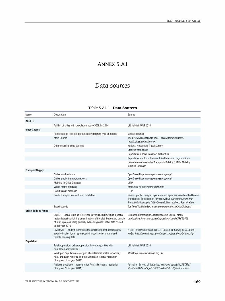
II.5. MOBILITY IN CITIES
General /
on
nd p
ANNEX 5.A1
Data sources
Table 5.A1.1. Data Sources
Name Description Source
City List
Full list of cities with population above 300k by 2014 UN Habitat, WUP2014
Mode Shares
Percentage of trips (all purposes) by different type of modes Various sources
Main Source The EPOMM Modal Split Tool - www.epomm.eu/tems/result_cities.phtml?more=1
Other miscellaneous sources National Household Travel Survey
Statistic year books
Reports from local transport authorities
Reports from different research institutes and organizations
Union Internationale des Transports Publics (UITP), Mobility in Cities Database
Transport Supply
Global road network OpenStreetMap, www.openstreetmap.org/
Global public transport network OpenStreetMap, www.openstreetmap.org/
Mobility in Cities Database UITP
World metro database http://mic-ro.com/metro/table.html
Rapid transit database ITDP
Public transport network and timetables Various public transport operators and agencies based on the Transit Feed Specification format (GTFS), www.transitwiki.orgTransitWiki/index.php?title=General_Transit_Feed_Specificati
Travel speeds TomTom Traffic Index, www.tomtom.com/en_gb/trafficindex/
Urban Built-up Areas
BUREF – Global Built-up Reference Layer (BUREF2010) is a spatial raster dataset containing an estimation of the distribution and density of built-up areas using publicly available global spatial data related to the year 2010
European Commission, Joint Research Centre, http://publications.jrc.ec.europa.eu/repository/handle/JRC90459
LANDSAT – Landsat represents the world’s longest continuously acquired collection of space-based moderate-resolution land remote sensing data.
A joint initiative between the U.S. Geological Survey (USGS) aNASA, http://landsat.usgs.gov//about_project_descriptions.ph
Population
Total population, urban population by country, cities with population above 300K
UN Habitat, WUP2014
Worldpop population raster grid at continental scales for Africa, Asia, and Latin America and the Caribbean (spatial resolution of approx. 1km; year 2010).
Worldpop, www.worldpop.org.uk/
National population raster grid for Australia (spatial resolution of approx. 1km; year 2011)
Australian Bureau of Statistics, www.abs.gov.au/AUSSTATS/[email protected]/DetailsPage/1270.0.55.0072011?OpenDocument
ITF TRANSPORT OUTLOOK 2017 © OECD/ITF 2017 169
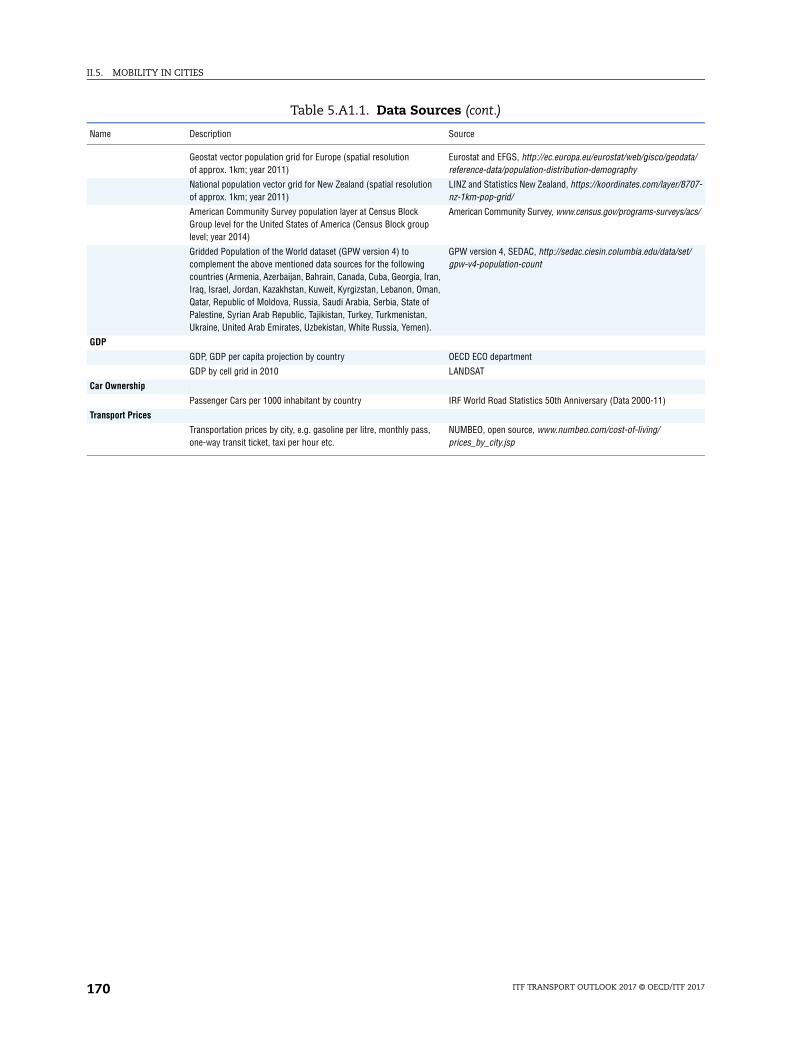
II.5. MOBILITY IN CITIES
odata/
r/8707-
ys/acs/
/set/
Table 5.A1.1. Data Sources (cont.)
Name Description Source
Geostat vector population grid for Europe (spatial resolution of approx. 1km; year 2011)
Eurostat and EFGS, http://ec.europa.eu/eurostat/web/gisco/gereference-data/population-distribution-demography
National population vector grid for New Zealand (spatial resolution of approx. 1km; year 2011)
LINZ and Statistics New Zealand, https://koordinates.com/layenz-1km-pop-grid/
American Community Survey population layer at Census Block Group level for the United States of America (Census Block group level; year 2014)
American Community Survey, www.census.gov/programs-surve
Gridded Population of the World dataset (GPW version 4) to complement the above mentioned data sources for the following countries (Armenia, Azerbaijan, Bahrain, Canada, Cuba, Georgia, Iran, Iraq, Israel, Jordan, Kazakhstan, Kuweit, Kyrgizstan, Lebanon, Oman, Qatar, Republic of Moldova, Russia, Saudi Arabia, Serbia, State of Palestine, Syrian Arab Republic, Tajikistan, Turkey, Turkmenistan, Ukraine, United Arab Emirates, Uzbekistan, White Russia, Yemen).
GPW version 4, SEDAC, http://sedac.ciesin.columbia.edu/datagpw-v4-population-count
GDP
GDP, GDP per capita projection by country OECD ECO department
GDP by cell grid in 2010 LANDSAT
Car Ownership
Passenger Cars per 1000 inhabitant by country IRF World Road Statistics 50th Anniversary (Data 2000-11)
Transport Prices
Transportation prices by city, e.g. gasoline per litre, monthly pass, one-way transit ticket, taxi per hour etc.
NUMBEO, open source, www.numbeo.com/cost-of-living/prices_by_city.jsp
ITF TRANSPORT OUTLOOK 2017 © OECD/ITF 2017170
II.5. MOBILITY IN CITIES
ANNEX 5.A2
Methodology for the global urban passenger model
The scope of this study is all the urban agglomerations with population above
300 thousand, following the definition of UN World Population Prospects (2014 Revision).
The full city list contains 1692 cities. The general model structure comprises six sub-models.
The transport system is composed by three highly interrelated sub-models: Travel
Demand, Transport Supply and Vehicle Fleet. The dynamics among the sub-models play a
fundamental role in the quantitative analysis. The interaction between land-use and
transport system is represented as Land-use sub-model influencing the mode choice and
vehicle ownership and in turn being affected by the transport supply level. The Exogenous
Sub-model contains the inputs of population, economy and vehicle technology providing
exogenous drivers to the transport system. The outcomes of Vehicle Fleet sub-model feed
into the Environment sub-model to compute the CO2 emissions. The sub-models are
structured as the following:
● Replicating the UN Habitat approach to project the urban population from 2030 to 2050;
● A sigmoid curve to forecast the GDP growth rates for the cities. The relationship between
the national share of urban population concentration and the national share of urban
GDP concentration follows an S-shaped curve;
● Regression models for urban transport supply, including road provision and public transport
supply;
● Discrete choice model to estimate the modal split of each city;
● A sigmoid curve to forecast the passenger car ownership and assumptions to infer the
share of other type of vehicles;
● CO2 intensities and technological pathways by mode for converting vehicle activities
into CO2 emission (IEA, Mobility Model).
The urban boundary for each selected city is provided by the Global Built-up Reference
Layer (BUREF2010) (Pesaresi and Carneiro Freire Sergio, 2014) and complimented by the
space-based land remote sensing data LANDSAT of year 2010. This global urban boundary
layer is used to intersect other GIS-based transport data layers to get the transport supply
indicators for each urban area, such as the road and public transport supply within each
urban boundary. The GDP at city level in the base year is estimated by redistributing the
national GDP volume from the OECD Environment Directorate into the urban areas according
to the GDP distribution map obtained from LANDSAT 2010, which provides GDP raster that
measures the GDP density for each cell grid (1 square km resolution).
ITF TRANSPORT OUTLOOK 2017 © OECD/ITF 2017 171
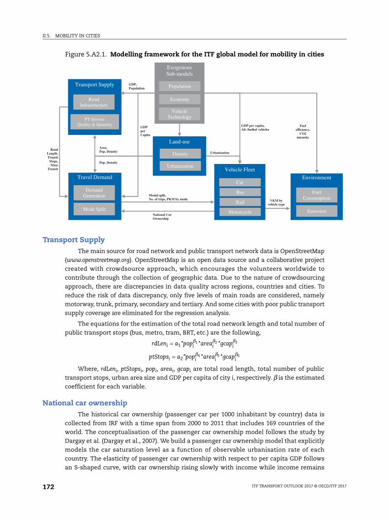
II.5. MOBILITY IN CITIES
Transport SupplyThe main source for road network and public transport network data is OpenStreetMap
(www.openstreetmap.org). OpenStreetMap is an open data source and a collaborative project
created with crowdsource approach, which encourages the volunteers worldwide to
contribute through the collection of geographic data. Due to the nature of crowdsourcing
approach, there are discrepancies in data quality across regions, countries and cities. To
reduce the risk of data discrepancy, only five levels of main roads are considered, namely
motorway, trunk, primary, secondary and tertiary. And some cities with poor public transport
supply coverage are eliminated for the regression analysis.
The equations for the estimation of the total road network length and total number of
public transport stops (bus, metro, tram, BRT, etc.) are the following,
Where, rdLeni, ptStopsi, popi, areai, gcapi are total road length, total number of public
transport stops, urban area size and GDP per capita of city i, respectively. b is the estimated
coefficient for each variable.
National car ownershipThe historical car ownership (passenger car per 1000 inhabitant by country) data is
collected from IRF with a time span from 2000 to 2011 that includes 169 countries of the
world. The conceptualisation of the passenger car ownership model follows the study by
Dargay et al. (Dargay et al., 2007). We build a passenger car ownership model that explicitly
models the car saturation level as a function of observable urbanisation rate of each
country. The elasticity of passenger car ownership with respect to per capita GDP follows
an S-shaped curve, with car ownership rising slowly with income while income remains
Figure 5.A2.1. Modelling framework for the ITF global model for mobility in cities
Road Length,Transit
Stops,Mass
Transit
Modal split,No. of trips, PKM by mode
Travel Demand
Demand Generation
Mode Split
Transport Supply
Road Infrastructure
PT Service Quality & Quantity
Environment
Fuel Consumption
Emission
VKM by vehicle type
Fuel efficiency,
CO2 intensity
Land-use
Density
Urbanization
Exogenous Sub-models
Population
Economy
Vehicle Technology
GDP per capita,Alt. fuelled vehicles
National Car Ownership
Urbanization
Area,Pop. Density
GDP, Population
Pop. Density
GDP per Capita
Vehicle Fleet
Car
Bus
Rail
Motorcycle
rdLen a pop area gcapi i i i= 11 2 3* * *b b b
ptStops a pop area gcapi i i i= 24 5 6* * *b b b
ITF TRANSPORT OUTLOOK 2017 © OECD/ITF 2017172
II.5. MOBILITY IN CITIES
low, accelerating while income goes through medium levels, and slowing down again as
incomes reach high levels.
Where, i is the country, n is the continent, j is the income group, uRate is the urbanisation
rate, gcap is the GDP per capita, bn denotes the constant term of the saturation level, u is the
coefficient for urbanisation rate, gr is the growth rate, and m is the midpoint of the curve.
Car ownership is modelled as the dependent variable in the first instance, based on
urbanisation rate and per capita income. The predicted car ownership is then treated as an
independent variable in the development of mode share models.
Transport costsFuel price (gasoline price per litre) at city level is mainly from an open source database
Numbeo (www.numbeo.com/), and complemented by the national level data (pump prices of
the most widely sold grade of gasoline) collected from World Bank. A city without fuel price
data collected is assumed to have the same price as its closest city in the same country
which has fuel price observed. If no such city was found, the fuel price level is assumed to
be equal to the national average price collected from the World Bank. The fuel price growth
rates by different country groups are taken from IEA’s MoMo model to forecast the future
fuel prices from 2010 to 2050.
Transit ticket price per trip is also collected from the same data source. A regression
model is estimated to predict the transit ticket price in the future. The formulation is,
Where, cj is the constant term of country group j, b7 is the estimated coefficient of GDP
per capita.
Parking price is collected from the a parking rate survey carried out by Colliers
International in 2011 (Moore, 2011). Daily parking cost parkingi is a function of car density
(cars per square kilometre) carDensi and public transport stop density (number of public
transport stops per square kilometre) ptDensi.
Mode choiceExisting studies show that the aggregated mode share for each city is a function of urban
development status, including urban scale, geography, economy, land use, personal
behaviour and public policy (He et al., 2013, 2011; Norley, 2015). It aims to answer the
questions on what are the impacts of urban development policies related to socio-economic
development, car ownership, urban structure, road supply, public transport provision and
pricing indicators on the aggregated modal split of a city. Mode shares are the parameters
which are sensitive to the urban development policies. It is an alternative to the usual
individual-based or trip-based behavioural logit models used in travel demand modelling. A
standard multinomial logit model is applied.
carOwnb exp u uRateexp gr gcap mi
n i
j i j=
++ − −
( )( ( ))
**1
ptFare c gcapi j i= * b7
parking d carDens ptDensi i i= * *b b8 9
P e
eni
U
jUnj
ni=
∑U ASC carOwn fPrice pPark rDensC C cown i fpx i pk i rds ii
= + + + +b b b b* * * *
ITF TRANSPORT OUTLOOK 2017 © OECD/ITF 2017 173
II.5. MOBILITY IN CITIES
Where, ASC is alternative specific constant, β is estimated coefficients, fPrice is fuel
price, pPark is parking cost, ptFare is transit ticket price (single trip), rDens is road density,
ptDens is density of public transport stops, mass is the availability of mass transit mode,
gcap is GDP per capita, and C, PT, W, B, M are car, public transport, walk, bicycle, motorcycle,
respectively.
The data set contained 247 observations, with an average weighted mode share in
value of 42% for car, 30% for public transport, 18% for walk, 6% for bike and 3% for
motorcycle. The calibrated model has ρ2 = 0.279, showing a satisfactory explanatory power
of the mode choice, and all the variables are statistically significant.
The values for the calibrated parameters, such as the preference factors, are plausible
and in line with other studies that suggest higher preference for personal car as compared
to public transport and bicycle to be the least preferred mode. All the coefficients are
statistically significant. The calibrated coefficients indicate that car ownership and road
density have positive impacts on the car use. Positive impacts of transit stop density and
the availability of mass transit are found on the use of public transport. The pricing
variables, namely, fuel price, parking cost and transit fare are found to have negative
impacts on the use of corresponding mode. We find urban density to contribute positively
to the ridership of public transport and the use of non-motorised modes and the values of
the coefficients are higher in for the public transport, followd by walking and cycling. GDP
per capita uses as proxy for income level is found to have negative impacts on the use of
motorcycle and non-motorised modes. This finding is in line with the existing studies that
the increasing income leads to the growing demand for faster and more convenient
transport modes.
Trip rates and distancesAverage trip rate in this study means number of trips per day per person considering
all trip purposes. In trip generation analysis, the approach involves setting up model to
represent the relationship between trip rates and the socio-economic characteristics. In
this study, we used a simple regression analysis to find the relationship between the
observed average trip rates from the household travel surveys and the GDP per capita.
Average travel distance is defined as the single trip distance regardless of trip purpose.
We used the observed sample trip distances to establish a relationship between average
distance by private vehicle and the urban area size. We also obtained average differences
in travel distance between different modes, such as average travel distances by public
transport is 45% longer than car, distance of a bike trip is usually around 32% of a car trip
distance. Based on available data, we made such a simplified average value for all cities
over our study time period. If more and better data are collected in the future, the trip rates
and trip distance estimations will be enhanced. The methodology will be further improved
by including more explanatory variables on travel distances by mode, such as land-use
mix, population density, and possibility evolve over time as well.
U ASC ptDens massPT PT ptds i mast i tpxi= + + + +b b b b* * *ptFare *pi pdsPT
oopDensi
U ASC *popDens *gcapW W pds i gcap ii W W= + +β β
U ASC *popDens *gcapB B pds i gcap ii B B= + +β β
U ASC *popDens *gcapM M pds i gcap ii M M= + +β β
ITF TRANSPORT OUTLOOK 2017 © OECD/ITF 2017174
II.5. MOBILITY IN CITIES
Vehicle technology and CO2 emissionThe transport scenarios are translated into CO2 emission scenarios by applying
transport technology paths. The technology assumptions and emission calculations are
taken from the IEA’s MoMo model and the Energy Technologies Perspectives. The scenario
used for the baseline is the four degree scenario (4DS) in the World Energy Outlook, which
corresponds to a context in which broad policy commitments and plans that have been
announced by countries are implemented. Under this scenario fuel economy standards are
tightened and there is progressive, moderate uptake of advanced vehicle technologies (IEA,
2013 and Dulac, 2013). The result is a slow but sustained decrease in fuel intensity of travel
and carbon intensity of fuel for all vehicles. Such a decrease is in general higher within the
OECD region.
ITF TRANSPORT OUTLOOK 2017 © OECD/ITF 2017 175
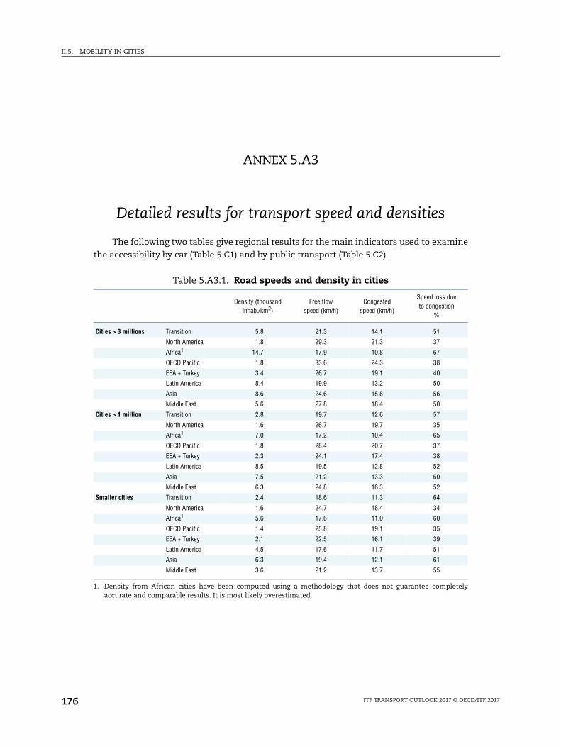
II.5. MOBILITY IN CITIES
ANNEX 5.A3
Detailed results for transport speed and densities
The following two tables give regional results for the main indicators used to examine
the accessibility by car (Table 5.C1) and by public transport (Table 5.C2).
Table 5.A3.1. Road speeds and density in cities
Density (thousand inhab./km2)
Free flow speed (km/h)
Congested speed (km/h)
Speed loss due to congestion
%
Cities > 3 millions Transition 5.8 21.3 14.1 51
North America 1.8 29.3 21.3 37
Africa1 14.7 17.9 10.8 67
OECD Pacific 1.8 33.6 24.3 38
EEA + Turkey 3.4 26.7 19.1 40
Latin America 8.4 19.9 13.2 50
Asia 8.6 24.6 15.8 56
Middle East 5.6 27.8 18.4 50
Cities > 1 million Transition 2.8 19.7 12.6 57
North America 1.6 26.7 19.7 35
Africa1 7.0 17.2 10.4 65
OECD Pacific 1.8 28.4 20.7 37
EEA + Turkey 2.3 24.1 17.4 38
Latin America 8.5 19.5 12.8 52
Asia 7.5 21.2 13.3 60
Middle East 6.3 24.8 16.3 52
Smaller cities Transition 2.4 18.6 11.3 64
North America 1.6 24.7 18.4 34
Africa1 5.6 17.6 11.0 60
OECD Pacific 1.4 25.8 19.1 35
EEA + Turkey 2.1 22.5 16.1 39
Latin America 4.5 17.6 11.7 51
Asia 6.3 19.4 12.1 61
Middle East 3.6 21.2 13.7 55
1. Density from African cities have been computed using a methodology that does not guarantee completely accurate and comparable results. It is most likely overestimated.
ITF TRANSPORT OUTLOOK 2017 © OECD/ITF 2017176
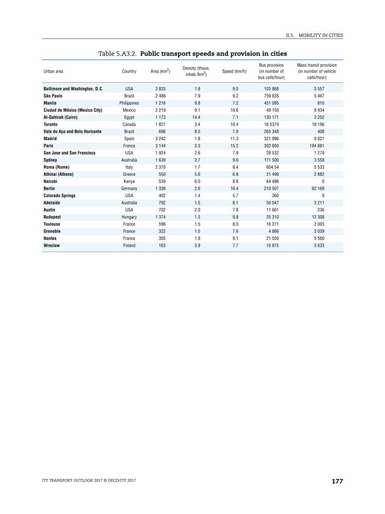
II.5. MOBILITY IN CITIES
ision hicle
Table 5.A3.2. Public transport speeds and provision in cities
Urban area Country Area (km2)Density (thous.
inhab./km2)Speed (km/h)
Bus provision (in number of
bus calls/hour)
Mass transit prov(in number of ve
calls/hour)
Baltimore and Washington, D.C. USA 3 833 1.8 9.0 103 868 3 557
São Paulo Brazil 2 488 7.9 9.2 759 835 5 467
Manila Philippines 1 216 9.8 7.2 451 095 810
Ciudad de México (Mexico City) Mexico 2 219 9.1 10.6 49 150 8 934
Al-Qahirah (Cairo) Egypt 1 173 14.4 7.1 130 171 3 252
Toronto Canada 1 827 3.4 10.4 16 5374 18 196
Vale do Aço and Belo Horizonte Brazil 696 8.5 7.8 265 348 408
Madrid Spain 3 242 1.8 11.3 321 996 9 021
Paris France 3 144 3.3 15.2 302 693 184 881
San Jose and San Francisco USA 1 924 2.6 7.9 28 532 1 279
Sydney Australia 1 639 2.7 9.6 171 500 3 558
Roma (Rome) Italy 2 370 1.7 8.4 604 54 5 533
Athínai (Athens) Greece 550 5.6 6.8 21 499 2 882
Nairobi Kenya 539 6.0 8.8 64 496 0
Berlin Germany 1 336 2.6 16.4 210 507 62 169
Colorado Springs USA 402 1.4 5.7 360 0
Adelaide Australia 792 1.5 8.1 50 047 3 211
Austin USA 702 2.0 7.8 11 661 236
Budapest Hungary 1 374 1.3 9.8 25 310 12 308
Toulouse France 596 1.5 8.0 16 271 2 003
Grenoble France 322 1.5 7.6 4 866 3 039
Nantes France 305 1.9 9.1 21 550 5 560
Wroclaw Poland 163 3.9 7.7 10 875 3 633
ITF TRANSPORT OUTLOOK 2017 © OECD/ITF 2017 177
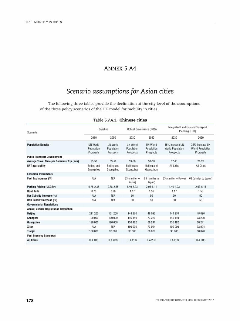
II.5. MOBILITY IN CITIES
rt
e UN lation ts
s
Japan)
1
S
ANNEX 5.A4
Scenario assumptions for Asian cities
The following three tables provide the declination at the city level of the assumptions
of the three policy scenarios of the ITF model for mobility in cities.
Table 5.A4.1. Chinese cities
ScenarioBaseline Robust Governance (ROG)
Integrated Land Use and TranspoPlanning (LUT)
2030 2050 2030 2050 2030 2050
Population Density UN World Population Prospects
UN World Population Prospects
UN World Population Prospects
UN World Population Prospects
15% increase UN World Population
Prospects
25% increasWorld Popu
Prospec
Public Transport Development
Average Travel Time per Commute Trip (min) 53-58 53-58 53-58 53-58 37-41 21-23
BRT availability Beijing and Guangzhou
Beijing and Guangzhou
Beijing and Guangzhou
Beijing and Guangzhou
All Cities All Citie
Economic Instruments
Fuel Tax Increase (%) N/A N/A 33 (similar to Korea)
63 (similar to Japan)
33 (similar to Korea) 63 (similar to
Parking Pricing (USD/hr) 0.78-2.35 0.78-2.35 1.40-4.23 2.03-6.11 1.40-4.23 2.03-6.1
Road Tolls 0.78 0.78 1.17 1.56 1.17 1.56
Bus Subsidy Increase (%) N/A N/A 30 50 30 50
Rail Subsidy Increase (%) N/A N/A 30 50 30 50
Governmental Regulations
Annual Vehicle Registration Restriction
Beijing 211 200 151 200 144 270 48 090 144 270 48 090
Shanghai 100 000 100 000 146 440 73 220 146 440 73 220
Guangzhou 120 000 120 000 136 482 68 241 136 482 68 241
Xi’an N/A N/A 100 000 73 904 100 000 73 904
Tianjin 100 000 90 000 90 000 68 820 90 000 68 820
Fuel Economy Standards
All Cities IEA 4DS IEA 4DS IEA 2DS IEA 2DS IEA 2DS IEA 2D
ITF TRANSPORT OUTLOOK 2017 © OECD/ITF 2017178
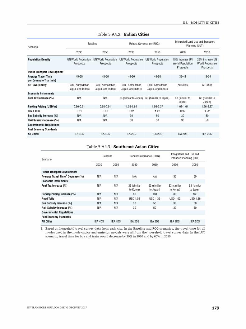
II.5. MOBILITY IN CITIES
port
se UN ulation cts
4
es
lar to )
.37
S
Table 5.A4.2. Indian Cities
ScenarioBaseline Robust Governance (ROG)
Integrated Land Use and TransPlanning (LUT)
2030 2050 2030 2050 2030 2050
Population Density UN World Population Prospects
UN World Population Prospects
UN World Population Prospects
UN World Population Prospects
15% increase UN World Population
Prospects
25% increaWorld Pop
Prospe
Public Transport Development
Average Travel Time per Commute Trip (min)
45-60 45-60 45-60 45-60 32-42 18-2
BRT availability Delhi, Ahmedabad, Jaipur, and Indore
Delhi, Ahmedabad, Jaipur, and Indore
Delhi, Ahmedabad, Jaipur, and Indore
Delhi, Ahmedabad, Jaipur, and Indore
All Cities All Citi
Economic Instruments
Fuel Tax Increase (%) N/A N/A 63 (similar to Japan) 63 (Similar to Japan) 63 (similar to Japan)
63 (SimiJapan
Parking Pricing (USD/hr) 0.60-0.91 0.60-0.91 1.08-1.64 1.56-2.37 1.08-1.64 1.56-2
Road Tolls 0.61 0.61 0.92 1.22 0.92 1.22
Bus Subsidy Increase (%) N/A N/A 30 50 30 50
Rail Subsidy Increase (%) N/A N/A 30 50 30 50
Governmental Regulations
Fuel Economy Standards
All Cities IEA 4DS IEA 4DS IEA 2DS IEA 2DS IEA 2DS IEA 2D
Table 5.A4.3. Southeast Asian Cities
ScenarioBaseline Robust Governance (ROG)
Integrated Land Use and Transport Planning (LUT)
2030 2050 2030 2050 2030 2050
Public Transport Development
Average Travel Time1 Decrease (%) N/A N/A N/A N/A 30 60
Economic Instruments
Fuel Tax Increase (%) N/A N/A 33 (similar to Korea)
63 (similar to Japan)
33 (similar to Korea)
63 (similar to Japan)
Parking Pricing Increase (%) N/A N/A 80 160 80 160
Road Tolls N/A N/A USD 1.02 USD 1.36 USD 1.02 USD 1.36
Bus Subsidy Increase (%) N/A N/A 30 50 30 50
Rail Subsidy Increase (%) N/A N/A 30 50 30 50
Governmental Regulations
Fuel Economy Standards
All Cities IEA 4DS IEA 4DS IEA 2DS IEA 2DS IEA 2DS IEA 2DS
1. Based on household travel survey data from each city. In the Baseline and ROG scenarios, the travel time for all modes used in the mode choice and emission models were all from the household travel survey data. In the LUT scenario, travel time for bus and train would decrease by 30% in 2030 and by 60% in 2050.
ITF TRANSPORT OUTLOOK 2017 © OECD/ITF 2017 179

ITF Transport Outlook 2017 © OECD/ITF 2017
Statistical annex
Rail freight transport . . . . . . . . . . . . . . . . . . . . . . . . . . . . . . . . . . . . . . . . . . . . . . . . . . . . 182
Road freight transport . . . . . . . . . . . . . . . . . . . . . . . . . . . . . . . . . . . . . . . . . . . . . . . . . . . 183
Inland waterway freight transport . . . . . . . . . . . . . . . . . . . . . . . . . . . . . . . . . . . . . . . . . 184
Oil pipeline transport . . . . . . . . . . . . . . . . . . . . . . . . . . . . . . . . . . . . . . . . . . . . . . . . . . . . 185
Total inland freight transport . . . . . . . . . . . . . . . . . . . . . . . . . . . . . . . . . . . . . . . . . . . . . 186
Coastal shipping . . . . . . . . . . . . . . . . . . . . . . . . . . . . . . . . . . . . . . . . . . . . . . . . . . . . . . . . 187
Rail container transport. . . . . . . . . . . . . . . . . . . . . . . . . . . . . . . . . . . . . . . . . . . . . . . . . . 188
Maritime container transport . . . . . . . . . . . . . . . . . . . . . . . . . . . . . . . . . . . . . . . . . . . . . 189
Passenger transport by rail . . . . . . . . . . . . . . . . . . . . . . . . . . . . . . . . . . . . . . . . . . . . . . . 190
Passenger transport by private car. . . . . . . . . . . . . . . . . . . . . . . . . . . . . . . . . . . . . . . . . 191
Passenger transport by bus and coach . . . . . . . . . . . . . . . . . . . . . . . . . . . . . . . . . . . . . 192
Total passenger transport by road . . . . . . . . . . . . . . . . . . . . . . . . . . . . . . . . . . . . . . . . . 193
Total inland passenger transport . . . . . . . . . . . . . . . . . . . . . . . . . . . . . . . . . . . . . . . . . . 194
Road traffic injury accidents . . . . . . . . . . . . . . . . . . . . . . . . . . . . . . . . . . . . . . . . . . . . . . 195
Road traffic casualties (injuries plus fatalities) . . . . . . . . . . . . . . . . . . . . . . . . . . . . . . 196
Road traffic injuries . . . . . . . . . . . . . . . . . . . . . . . . . . . . . . . . . . . . . . . . . . . . . . . . . . . . . 197
Road traffic fatalities . . . . . . . . . . . . . . . . . . . . . . . . . . . . . . . . . . . . . . . . . . . . . . . . . . . . 198
Road traffic fatalities, per million inhabitants . . . . . . . . . . . . . . . . . . . . . . . . . . . . . . . 199
Road traffic fatalities, per million motor vehicles . . . . . . . . . . . . . . . . . . . . . . . . . . . . 200
Investment in rail transport infrastructure . . . . . . . . . . . . . . . . . . . . . . . . . . . . . . . . . 201
Investment in road transport infrastructure . . . . . . . . . . . . . . . . . . . . . . . . . . . . . . . . 202
Investment in inland waterway transport infrastructure. . . . . . . . . . . . . . . . . . . . . . 203
Total investment in inland transport infrastructure . . . . . . . . . . . . . . . . . . . . . . . . . . 204
Investment in sea port infrastructure . . . . . . . . . . . . . . . . . . . . . . . . . . . . . . . . . . . . . . 205
Investment in airport infrastructure . . . . . . . . . . . . . . . . . . . . . . . . . . . . . . . . . . . . . . . 206
Rail infrastructure maintenance expenditure . . . . . . . . . . . . . . . . . . . . . . . . . . . . . . . 207
Road infrastructure maintenance expenditure . . . . . . . . . . . . . . . . . . . . . . . . . . . . . . 208
Inland waterway infrastructure maintenance expenditure . . . . . . . . . . . . . . . . . . . . 209
Sea port infrastructure maintenance expenditure . . . . . . . . . . . . . . . . . . . . . . . . . . . 210
Airport infrastructure maintenance expenditure . . . . . . . . . . . . . . . . . . . . . . . . . . . . 211
Total spending on road infrastructure investment and maintenance . . . . . . . . . . . 212
Total inland transport infrastructure investment as a percentage of GDP . . . . . . . 213
181
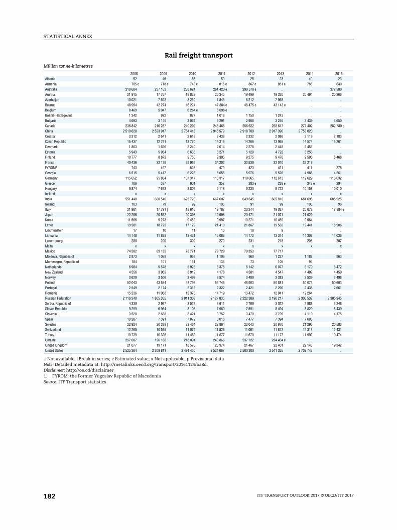
STATISTICAL ANNEX
01523408066
..
..
..
..5080 p..
8361....
68..
7861329410
x259684 e....
06..
3607
x..
63..
7250980361
..45483975..
833174..
42..
Rail freight transport
.. Not available; | Break in series; e Estimated value; x Not applicable; p Provisional dataNote: Detailed metadata at: http://metalinks.oecd.org/transport/20161124/ba8d.Disclaimer: http://oe.cd/disclaimer1. FYROM: the Former Yugoslav Republic of MacedoniaSource: ITF Transport statistics
Million tonne-kilometres
2008 2009 2010 2011 2012 2013 2014 2Albania 52 46 66 50 25 23 40Armenia 705 e 718 e 743 e 816 e 867 e 851 e 786 6Australia 218 684 237 163 258 624 261 420 e 290 570 e .. .. 372 5Austria 21 915 17 767 19 833 20 345 19 499 19 320 20 494 20 2Azerbaijan 10 021 7 592 8 250 7 845 8 212 7 958 ..Belarus 48 994 42 274 46 224 47 384 e 48 475 e 43 143 e ..Belgium 8 469 5 947 6 264 e 6 698 e .. .. ..Bosnia-Herzegovina 1 242 992 877 1 018 1 150 1 243 ..Bulgaria 4 693 3 145 3 064 3 291 2 908 3 246 3 439 3 6Canada 236 842 216 287 240 292 248 468 256 622 258 617 277 402 282 7China 2 510 628 2 523 917 2 764 413 2 946 579 2 918 709 2 917 390 2 753 020Croatia 3 312 2 641 2 618 2 438 2 332 2 086 2 119 2 1Czech Republic 15 437 12 791 13 770 14 316 14 266 13 965 14 574 15 2Denmark 1 863 1 696 2 240 2 614 2 278 2 448 2 453Estonia 5 943 5 934 6 638 6 271 5 129 4 722 3 256Finland 10 777 8 872 9 750 9 395 9 275 9 470 9 596 8 4France 40 436 32 129 29 965 34 202 32 539 32 010 32 217FYROM1 743 497 525 479 423 421 411 2Georgia 6 515 5 417 6 228 6 055 5 976 5 526 4 988 4 2Germany 115 652 95 834 107 317 113 317 110 065 112 613 112 629 116 6Greece 786 537 601 352 283 e 238 e 343 e 2Hungary 9 874 7 673 8 809 9 118 9 230 9 722 10 158 10 0Iceland x x x x x x xIndia 551 448 600 546 625 723 667 607 649 645 665 810 681 698 685 9Ireland 103 79 92 105 91 99 100Italy 21 981 17 791 | 18 616 19 787 20 244 19 037 20 072 17 9Japan 22 256 20 562 20 398 19 998 20 471 21 071 21 029Korea 11 566 9 273 9 452 9 997 10 271 10 459 9 564Latvia 19 581 18 725 17 179 21 410 21 867 19 532 19 441 18 9Liechtenstein 17 10 11 10 10 9 ..Lithuania 14 748 11 888 13 431 15 088 14 172 13 344 14 307 14 0Luxembourg 280 200 309 270 231 218 208 2Malta x x x x x x xMexico 74 582 69 185 78 771 79 729 79 353 77 717 ..Moldova, Republic of 2 873 1 058 959 1 196 960 1 227 1 182 9Montenegro, Republic of 184 101 151 136 73 105 94Netherlands 6 984 5 578 5 925 6 378 6 142 6 077 6 170 6 4New Zealand 4 556 3 962 3 919 4 178 4 581 4 547 4 492 4 4Norway 3 629 3 506 3 498 3 574 3 489 3 383 3 539 3 4Poland 52 043 43 554 48 795 53 746 48 903 50 881 50 073 50 6Portugal 2 549 2 174 2 313 2 322 2 421 2 290 2 438 2 6Romania 15 236 11 088 12 375 14 719 13 472 12 941 12 264Russian Federation 2 116 240 1 865 305 2 011 308 2 127 835 2 222 389 2 196 217 2 300 532 2 305 9Serbia, Republic of 4 339 2 967 3 522 3 611 2 769 3 022 2 988 3 2Slovak Republic 9 299 6 964 8 105 7 960 7 591 8 494 8 829 8 4Slovenia 3 520 2 668 3 421 3 752 3 470 3 799 4 110 4 1Spain 10 287 7 391 7 872 8 018 7 477 7 394 7 603Sweden 22 924 20 389 | 23 464 22 864 22 043 20 970 21 296 20 5Switzerland 12 265 10 565 11 074 11 526 11 061 11 812 12 313 12 4Turkey 10 739 10 326 11 462 11 677 11 670 11 177 11 992 10 4Ukraine 257 007 196 188 218 091 243 866 237 722 224 434 e ..United Kingdom 21 077 19 171 18 576 20 974 21 467 22 401 22 143 19 3United States 2 525 364 2 309 811 2 491 450 2 524 667 2 500 300 2 541 355 2 702 743
ITF TRANSPORT OUTLOOK 2017 © OECD/ITF 2017182
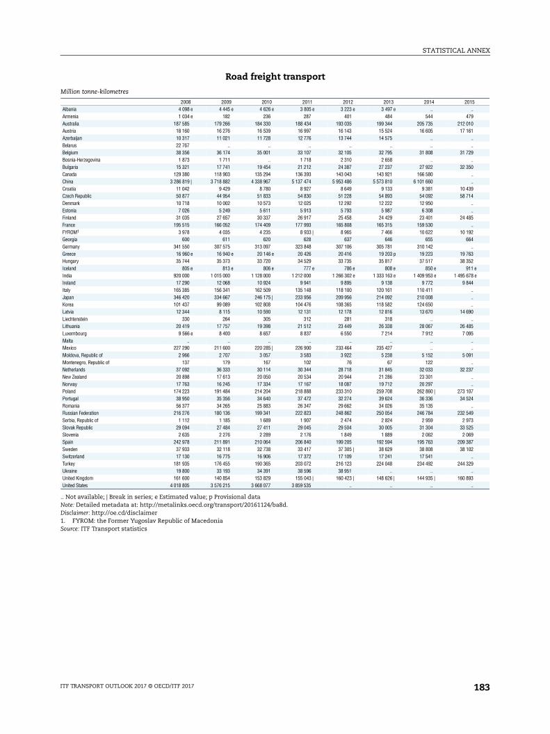
STATISTICAL ANNEX
015..
791061
..
..29
..50
..
..3914
..
..85..
9264
..635211 e78 e44
..
..
..90
..8595....
91..
37....
0724
..497325698702..
29..
93..
Road freight transport
.. Not available; | Break in series; e Estimated value; p Provisional dataNote: Detailed metadata at: http://metalinks.oecd.org/transport/20161124/ba8d.Disclaimer: http://oe.cd/disclaimer1. FYROM: the Former Yugoslav Republic of MacedoniaSource: ITF Transport statistics
Million tonne-kilometres
2008 2009 2010 2011 2012 2013 2014 2Albania 4 098 e 4 445 e 4 626 e 3 805 e 3 223 e 3 497 e ..Armenia 1 034 e 182 236 287 401 484 544 4Australia 187 585 179 266 184 330 188 434 193 035 199 344 205 735 212 0Austria 18 160 16 276 16 539 16 997 16 143 15 524 16 605 17 1Azerbaijan 10 317 11 021 11 728 12 776 13 744 14 575 ..Belarus 22 767 .. .. .. .. .. ..Belgium 38 356 36 174 35 001 33 107 32 105 32 795 31 808 31 7Bosnia-Herzegovina 1 873 1 711 .. 1 718 2 310 2 658 ..Bulgaria 15 321 17 741 19 454 21 212 24 387 27 237 27 922 32 3Canada 129 380 118 903 135 294 136 393 143 043 143 921 166 580China 3 286 819 | 3 718 882 4 338 967 5 137 474 5 953 486 5 573 810 6 101 660Croatia 11 042 9 429 8 780 8 927 8 649 9 133 9 381 10 4Czech Republic 50 877 44 954 51 833 54 830 51 228 54 893 54 092 58 7Denmark 10 718 10 002 10 573 12 025 12 292 12 222 12 950Estonia 7 026 5 249 5 611 5 913 5 793 5 987 6 308Finland 31 035 27 657 30 337 26 917 25 458 24 429 23 401 24 4France 195 515 166 052 174 409 177 993 165 808 165 315 159 530FYROM1 3 978 4 035 4 235 8 933 | 8 965 7 466 10 622 10 1Georgia 600 611 620 628 637 646 655 6Germany 341 550 307 575 313 097 323 848 307 106 305 781 310 142Greece 16 960 e 16 940 e 20 146 e 20 426 20 416 19 203 p 19 223 19 7Hungary 35 744 35 373 33 720 34 529 33 735 35 817 37 517 38 3Iceland 805 e 813 e 806 e 777 e 786 e 808 e 850 e 9India 920 000 1 015 000 1 128 000 1 212 000 1 266 302 e 1 333 163 e 1 409 953 e 1 495 6Ireland 17 290 12 068 10 924 9 941 9 895 9 138 9 772 9 8Italy 165 385 156 341 162 509 135 148 118 100 120 161 110 411Japan 346 420 334 667 246 175 | 233 956 209 956 214 092 210 008Korea 101 437 99 089 102 808 104 476 108 365 118 582 124 650Latvia 12 344 8 115 10 590 12 131 12 178 12 816 13 670 14 6Liechtenstein 330 264 305 312 281 318 ..Lithuania 20 419 17 757 19 398 21 512 23 449 26 338 28 067 26 4Luxembourg 9 566 e 8 400 8 657 8 837 6 550 7 214 7 912 7 0Malta .. .. .. .. .. .. ..Mexico 227 290 211 600 220 285 | 226 900 233 464 235 427 ..Moldova, Republic of 2 966 2 707 3 057 3 583 3 922 5 238 5 152 5 0Montenegro, Republic of 137 179 167 102 76 67 122Netherlands 37 092 36 333 30 114 30 344 28 718 31 845 32 033 32 2New Zealand 20 898 17 613 20 050 20 534 20 944 21 286 23 301Norway 17 763 16 245 17 334 17 167 18 087 19 712 20 297Poland 174 223 191 484 214 204 218 888 233 310 259 708 262 860 | 273 1Portugal 38 950 35 356 34 640 37 472 32 274 39 624 36 336 34 5Romania 56 377 34 265 25 883 26 347 29 662 34 026 35 135Russian Federation 216 276 180 136 199 341 222 823 248 862 250 054 246 784 232 5Serbia, Republic of 1 112 1 185 1 689 1 907 2 474 2 824 2 959 2 9Slovak Republic 29 094 27 484 27 411 29 045 29 504 30 005 31 304 33 5Slovenia 2 635 2 276 2 289 2 176 1 849 1 889 2 062 2 0Spain 242 978 211 891 210 064 206 840 199 205 192 594 195 763 209 3Sweden 37 933 32 118 32 738 33 417 37 305 | 38 629 38 808 38 1Switzerland 17 130 16 775 16 906 17 372 17 109 17 241 17 541Turkey 181 935 176 455 190 365 203 072 216 123 224 048 234 492 244 3Ukraine 19 800 33 193 34 391 38 596 38 951 .. ..United Kingdom 161 600 140 854 153 829 155 043 | 160 423 | 148 626 | 144 935 | 160 8United States 4 018 805 3 576 215 3 668 077 3 859 535 .. .. ..
ITF TRANSPORT OUTLOOK 2017 © OECD/ITF 2017 183
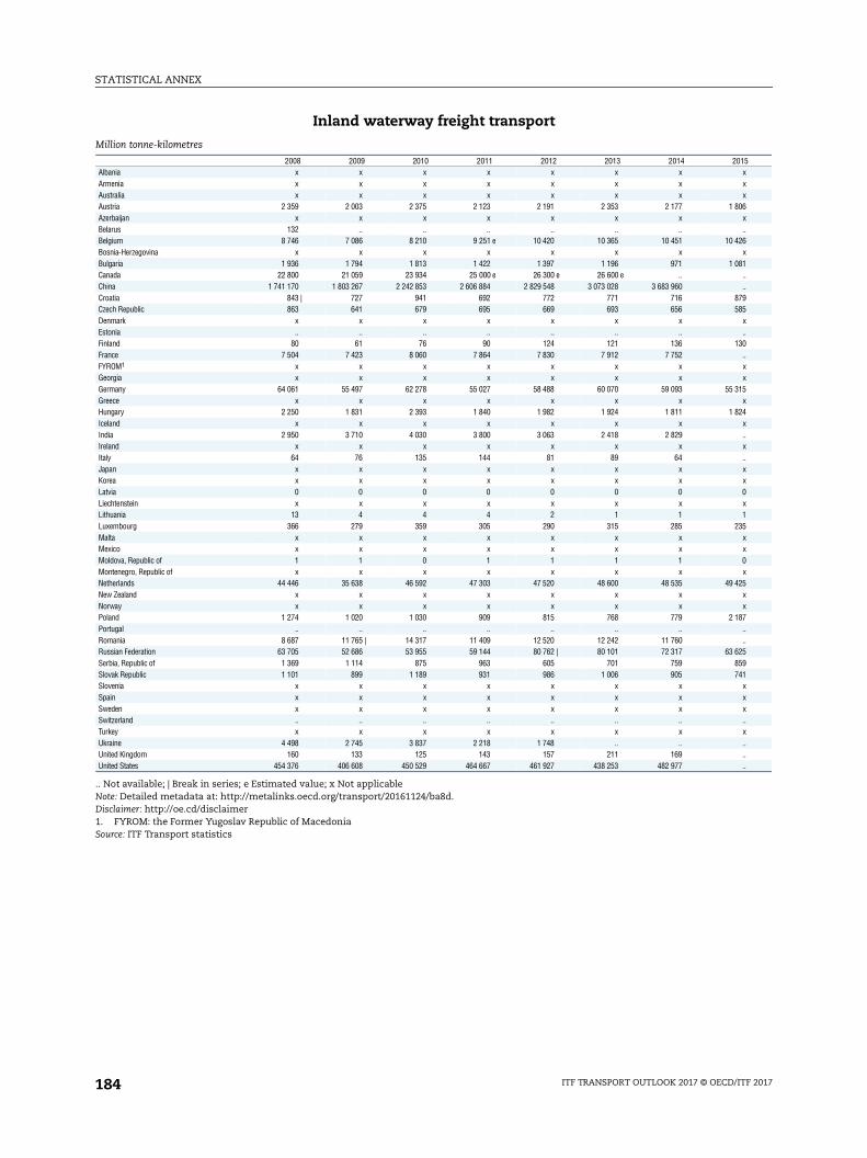
STATISTICAL ANNEX
015xxx
06x..
26x
81....
7985
x..
30..xx
15x
24x..x..xx0x1
35xx0x
25xx
87....
255941
xxx..x......
Inland waterway freight transport
.. Not available; | Break in series; e Estimated value; x Not applicableNote: Detailed metadata at: http://metalinks.oecd.org/transport/20161124/ba8d.Disclaimer: http://oe.cd/disclaimer1. FYROM: the Former Yugoslav Republic of MacedoniaSource: ITF Transport statistics
Million tonne-kilometres
2008 2009 2010 2011 2012 2013 2014 2Albania x x x x x x xArmenia x x x x x x xAustralia x x x x x x xAustria 2 359 2 003 2 375 2 123 2 191 2 353 2 177 1 8Azerbaijan x x x x x x xBelarus 132 .. .. .. .. .. ..Belgium 8 746 7 086 8 210 9 251 e 10 420 10 365 10 451 10 4Bosnia-Herzegovina x x x x x x xBulgaria 1 936 1 794 1 813 1 422 1 397 1 196 971 1 0Canada 22 800 21 059 23 934 25 000 e 26 300 e 26 600 e ..China 1 741 170 1 803 267 2 242 853 2 606 884 2 829 548 3 073 028 3 683 960Croatia 843 | 727 941 692 772 771 716 8Czech Republic 863 641 679 695 669 693 656 5Denmark x x x x x x xEstonia .. .. .. .. .. .. ..Finland 80 61 76 90 124 121 136 1France 7 504 7 423 8 060 7 864 7 830 7 912 7 752FYROM1 x x x x x x xGeorgia x x x x x x xGermany 64 061 55 497 62 278 55 027 58 488 60 070 59 093 55 3Greece x x x x x x xHungary 2 250 1 831 2 393 1 840 1 982 1 924 1 811 1 8Iceland x x x x x x xIndia 2 950 3 710 4 030 3 800 3 063 2 418 2 829Ireland x x x x x x xItaly 64 76 135 144 81 89 64Japan x x x x x x xKorea x x x x x x xLatvia 0 0 0 0 0 0 0Liechtenstein x x x x x x xLithuania 13 4 4 4 2 1 1Luxembourg 366 279 359 305 290 315 285 2Malta x x x x x x xMexico x x x x x x xMoldova, Republic of 1 1 0 1 1 1 1Montenegro, Republic of x x x x x x xNetherlands 44 446 35 638 46 592 47 303 47 520 48 600 48 535 49 4New Zealand x x x x x x xNorway x x x x x x xPoland 1 274 1 020 1 030 909 815 768 779 2 1Portugal .. .. .. .. .. .. ..Romania 8 687 11 765 | 14 317 11 409 12 520 12 242 11 760Russian Federation 63 705 52 686 53 955 59 144 80 762 | 80 101 72 317 63 6Serbia, Republic of 1 369 1 114 875 963 605 701 759 8Slovak Republic 1 101 899 1 189 931 986 1 006 905 7Slovenia x x x x x x xSpain x x x x x x xSweden x x x x x x xSwitzerland .. .. .. .. .. .. ..Turkey x x x x x x xUkraine 4 498 2 745 3 837 2 218 1 748 .. ..United Kingdom 160 133 125 143 157 211 169United States 454 376 406 608 450 529 464 667 461 927 438 253 482 977
ITF TRANSPORT OUTLOOK 2017 © OECD/ITF 2017184
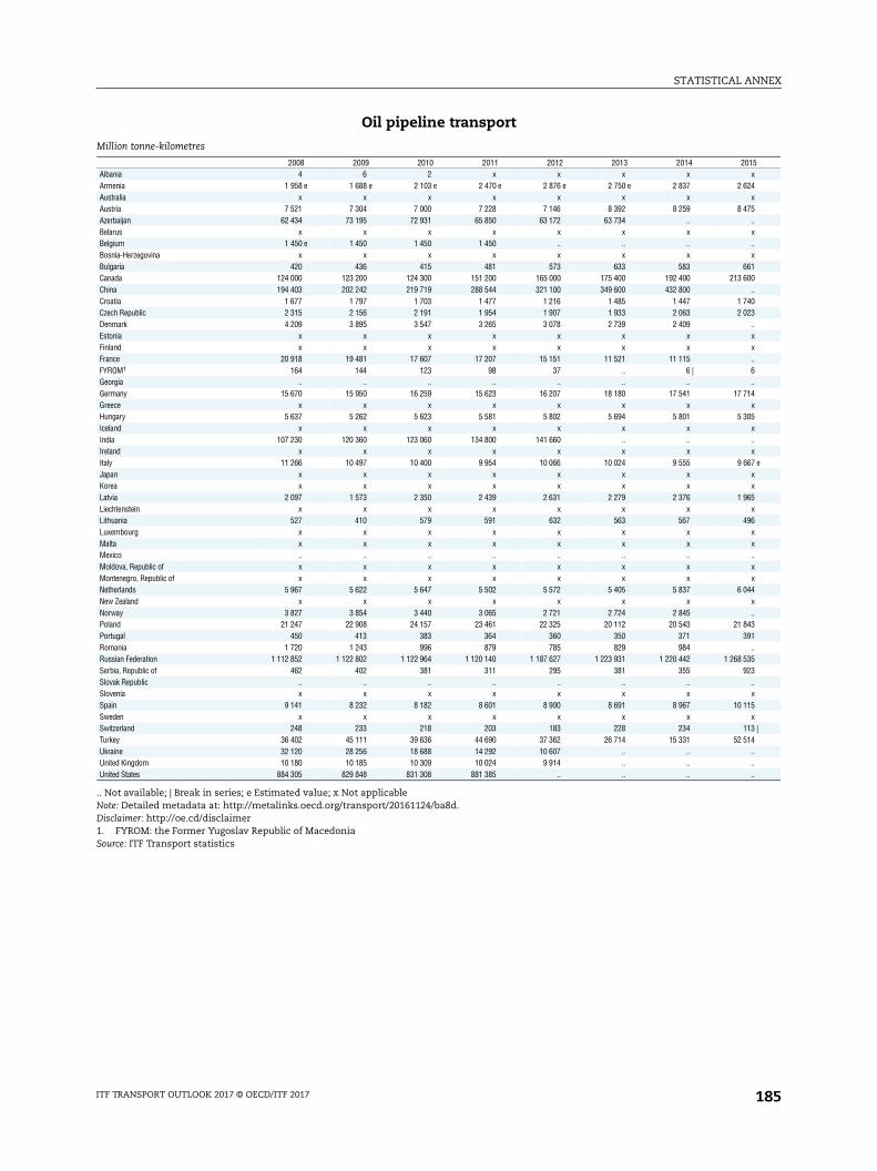
STATISTICAL ANNEX
015x
24x
75..x..x
6100..
4023..xx..6..
14x
05x..x
67 exx
65x
96xx..xx
44x..
4391
..3523..x
15x
13 |14......
Oil pipeline transport
.. Not available; | Break in series; e Estimated value; x Not applicableNote: Detailed metadata at: http://metalinks.oecd.org/transport/20161124/ba8d.Disclaimer: http://oe.cd/disclaimer1. FYROM: the Former Yugoslav Republic of MacedoniaSource: ITF Transport statistics
Million tonne-kilometres
2008 2009 2010 2011 2012 2013 2014 2Albania 4 6 2 x x x xArmenia 1 958 e 1 688 e 2 103 e 2 470 e 2 876 e 2 750 e 2 837 2 6Australia x x x x x x xAustria 7 521 7 304 7 000 7 228 7 146 8 392 8 259 8 4Azerbaijan 62 434 73 195 72 931 65 850 63 172 63 734 ..Belarus x x x x x x xBelgium 1 450 e 1 450 1 450 1 450 .. .. ..Bosnia-Herzegovina x x x x x x xBulgaria 420 436 415 481 573 633 583 6Canada 124 000 123 200 124 300 151 200 165 000 175 400 192 400 213 6China 194 403 202 242 219 719 288 544 321 100 349 600 432 800Croatia 1 677 1 797 1 703 1 477 1 216 1 485 1 447 1 7Czech Republic 2 315 2 156 2 191 1 954 1 907 1 933 2 063 2 0Denmark 4 209 3 895 3 547 3 265 3 078 2 739 2 409Estonia x x x x x x xFinland x x x x x x xFrance 20 918 19 481 17 607 17 207 15 151 11 521 11 115FYROM1 164 144 123 98 37 .. 6 |Georgia .. .. .. .. .. .. ..Germany 15 670 15 950 16 259 15 623 16 207 18 180 17 541 17 7Greece x x x x x x xHungary 5 637 5 262 5 623 5 581 5 802 5 694 5 801 5 3Iceland x x x x x x xIndia 107 230 120 360 123 060 134 800 141 660 .. ..Ireland x x x x x x xItaly 11 266 10 497 10 400 9 954 10 066 10 024 9 555 9 6Japan x x x x x x xKorea x x x x x x xLatvia 2 097 1 573 2 350 2 439 2 631 2 279 2 376 1 9Liechtenstein x x x x x x xLithuania 527 410 579 591 632 563 567 4Luxembourg x x x x x x xMalta x x x x x x xMexico .. .. .. .. .. .. ..Moldova, Republic of x x x x x x xMontenegro, Republic of x x x x x x xNetherlands 5 967 5 622 5 647 5 502 5 572 5 405 5 837 6 0New Zealand x x x x x x xNorway 3 827 3 854 3 440 3 065 2 721 2 724 2 845Poland 21 247 22 908 24 157 23 461 22 325 20 112 20 543 21 8Portugal 450 413 383 364 360 350 371 3Romania 1 720 1 243 996 879 785 829 984Russian Federation 1 112 852 1 122 802 1 122 964 1 120 140 1 187 627 1 223 931 1 220 442 1 268 5Serbia, Republic of 462 402 381 311 295 381 355 9Slovak Republic .. .. .. .. .. .. ..Slovenia x x x x x x xSpain 9 141 8 232 8 182 8 601 8 900 8 691 8 967 10 1Sweden x x x x x x xSwitzerland 248 233 218 203 183 228 234 1Turkey 36 402 45 111 39 636 44 690 37 362 26 714 15 331 52 5Ukraine 32 120 28 256 18 688 14 292 10 607 .. ..United Kingdom 10 180 10 185 10 309 10 024 9 914 .. ..United States 884 305 829 848 831 308 881 385 .. .. ..
ITF TRANSPORT OUTLOOK 2017 © OECD/ITF 2017 185
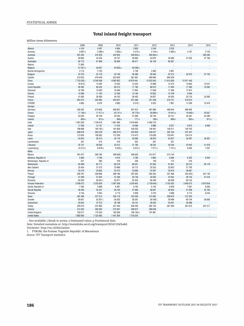
STATISTICAL ANNEX
015..
439008
..
..
..
..42
..
..4182
..
..83..
76....
579011 e
..40
..
..
..61
..1837....
54..
78....
4076
..54030544..
85..
17......
Total inland freight transport
.. Not available; | Break in series; e Estimated value; p Provisional dataNote: Detailed metadata at: http://metalinks.oecd.org/transport/20161124/ba8d.Disclaimer: http://oe.cd/disclaimer1. FYROM: the Former Yugoslav Republic of MacedoniaSource: ITF Transport statistics
Million tonne-kilometres
2008 2009 2010 2011 2012 2013 2014 2Albania 4 154 4 497 4 694 3 855 3 248 3 520 ..Armenia 3 697 e 2 588 e 3 082 e 3 573 e 4 144 e 4 085 e 4 167 3 7Australia 391 045 416 429 442 954 449 854 e 483 605 e .. .. 584 5Austria 49 955 43 350 45 747 46 693 44 979 45 589 47 535 47 7Azerbaijan 82 772 91 808 92 909 86 471 85 128 86 267 ..Belarus 71 893 .. .. .. .. .. ..Belgium 57 021 e 50 657 50 925 e 50 506 e .. .. ..Bosnia-Herzegovina 3 115 2 703 .. 2 736 3 460 3 901 ..Bulgaria 22 370 23 116 24 746 26 406 29 265 32 312 32 915 37 7Canada 513 022 479 449 523 820 561 061 590 965 604 538 ..China 7 733 020 | 8 248 308 9 565 952 10 979 481 12 022 843 11 913 828 12 971 440Croatia 16 874 | 14 594 14 042 13 534 12 969 13 475 13 663 15 2Czech Republic 69 492 60 542 68 473 71 795 68 070 71 484 71 385 76 5Denmark 16 790 15 593 16 360 17 904 17 648 17 409 17 812Estonia 12 969 11 183 12 249 12 184 10 922 10 709 9 564Finland 41 892 36 590 40 163 36 402 34 857 34 020 33 133 33 0France 264 373 225 085 230 041 237 266 221 328 216 757 210 613FYROM1 4 885 4 676 4 883 9 510 | 9 425 7 887 11 039 10 4Georgia .. .. .. .. .. .. ..Germany 536 933 474 856 498 951 507 815 491 866 496 644 499 405Greece 17 746 e 17 477 e 20 747 e 20 778 e 20 699 e 19 441 p 19 566 e 20 0Hungary 53 505 50 139 50 545 51 068 50 749 53 157 55 287 55 4Iceland 805 e 813 e 806 e 777 e 786 e 808 e 850 e 9India 1 581 630 1 739 618 1 881 090 2 018 600 2 056 723 .. ..Ireland 17 393 12 147 11 016 10 046 9 986 9 237 9 872 9 9Italy 198 696 184 705 | 191 660 165 033 148 491 149 311 140 102Japan 368 676 355 229 266 573 | 253 954 230 427 235 163 231 037Korea 113 003 108 362 112 260 114 473 118 636 129 041 134 214Latvia 34 022 28 413 30 119 35 980 36 676 34 627 35 487 35 5Liechtenstein 347 274 316 322 291 327 ..Lithuania 35 707 30 059 33 412 37 195 38 255 40 246 42 942 41 0Luxembourg 10 212 e 8 879 e 9 325 e 9 412 e 7 071 e 7 747 e 8 405 7 5Malta .. .. .. .. .. .. ..Mexico 301 872 280 785 299 056 | 306 629 312 817 313 144 ..Moldova, Republic of 5 840 3 766 4 016 4 780 4 883 6 466 6 335 6 0Montenegro, Republic of 321 280 318 238 149 172 216Netherlands 94 489 83 171 88 278 89 527 87 952 91 927 92 575 94 1New Zealand 25 454 21 575 23 969 24 712 25 525 25 833 27 793Norway 25 219 23 605 24 272 23 806 24 297 25 819 26 681Poland 248 787 258 966 288 186 297 004 305 353 331 469 334 255 | 347 7Portugal 41 949 37 943 37 336 40 158 35 055 42 264 39 145 37 5Romania 82 020 58 361 | 53 571 53 354 56 439 60 038 60 143Russian Federation 3 509 073 3 220 929 3 387 568 3 529 942 3 739 640 | 3 750 303 3 840 075 3 870 6Serbia, Republic of 7 282 5 668 6 467 6 792 6 143 6 928 7 061 8 0Slovak Republic 39 494 35 347 36 705 37 936 38 081 39 505 41 038 42 7Slovenia 6 155 4 944 5 710 5 928 5 319 5 688 6 172 6 2Spain 262 406 227 514 226 118 223 459 215 582 208 679 212 333Sweden 60 857 52 507 | 56 202 56 281 59 348 | 59 599 60 104 58 6Switzerland 29 643 27 573 28 198 29 101 28 353 29 281 30 088Turkey 229 076 231 892 241 463 259 439 265 155 261 939 261 815 307 3Ukraine 313 425 260 382 275 007 298 972 289 028 .. ..United Kingdom 193 017 170 343 182 839 186 183 e 191 961 .. ..United States 7 882 850 7 122 482 7 441 364 7 730 254 .. .. ..
ITF TRANSPORT OUTLOOK 2017 © OECD/ITF 2017186
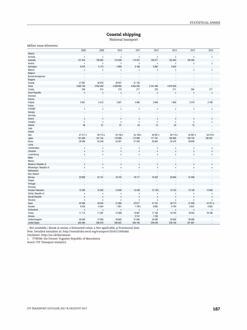
STATISTICAL ANNEX
015..x..x..x..........
17x....
80..x....xx......
19 e81....xxx....xx............
56xxx
77 p23
x89......
Coastal shippingNational transport
.. Not available; | Break in series; e Estimated value; x Not applicable; p Provisional dataNote: Detailed metadata at: http://metalinks.oecd.org/transport/20161124/ba8d.Disclaimer: http://oe.cd/disclaimer1. FYROM: the Former Yugoslav Republic of MacedoniaSource: ITF Transport statistics
Million tonne-kilometres
2008 2009 2010 2011 2012 2013 2014 2Albania .. .. .. .. .. .. ..Armenia x x x x x x xAustralia 121 916 109 622 116 208 113 357 102 577 104 462 105 404Austria x x x x x x xAzerbaijan 6 076 6 173 4 859 5 186 5 062 4 632 ..Belarus x x x x x x xBelgium .. .. .. .. .. .. ..Bosnia-Herzegovina .. .. .. .. .. .. ..Bulgaria .. .. .. .. .. .. ..Canada 27 852 26 678 29 547 31 735 .. .. ..China 3 285 100 3 952 400 4 599 900 4 935 500 5 341 200 4 870 500 ..Croatia 248 214 210 217 222 211 205 2Czech Republic x x x x x x xDenmark .. .. .. .. .. .. ..Estonia .. .. .. .. .. .. ..Finland 2 937 2 513 3 621 3 966 2 840 1 900 2 010 2 1France .. .. .. .. .. .. ..FYROM1 x x x x x x xGeorgia .. .. .. .. .. .. ..Germany .. .. .. .. .. .. ..Greece x x x x x x xHungary x x x x x x xIceland 48 57 47 43 12 32 13India .. .. .. .. .. .. ..Ireland .. .. .. .. .. .. ..Italy 47 017 e 49 173 e 53 156 e 53 708 e 50 287 e 49 112 e 52 961 e 54 5Japan 187 859 167 135 179 898 174 900 177 791 184 860 183 120 180 3Korea 29 590 25 249 23 281 27 220 25 804 30 476 29 848Latvia .. .. .. .. .. .. ..Liechtenstein x x x x x x xLithuania x x x x x x xLuxembourg x x x x x x xMalta .. .. .. .. .. .. ..Mexico .. .. .. .. .. .. ..Moldova, Republic of x x x x x x xMontenegro, Republic of x x x x x x xNetherlands .. .. .. .. .. .. ..New Zealand .. .. .. .. .. .. ..Norway 22 860 22 141 18 703 19 717 18 432 20 663 21 058Poland .. .. .. .. .. .. ..Portugal .. .. .. .. .. .. ..Romania .. .. .. .. .. .. ..Russian Federation 12 450 12 042 12 640 13 239 12 138 | 12 133 13 126 14 9Serbia, Republic of x x x x x x xSlovak Republic x x x x x x xSlovenia x x x x x x xSpain 45 396 40 040 41 666 42 811 41 761 40 773 41 848 44 9Sweden 8 255 6 504 7 851 7 794 | 6 892 6 764 6 637 6 9Switzerland x x x x x x xTurkey 11 114 11 397 12 569 15 961 17 158 19 725 18 553 19 1Ukraine .. .. .. 2 747 1 702 .. ..United Kingdom 48 400 47 600 40 800 41 600 34 000 28 000 26 000United States 303 495 286 578 280 822 263 105 229 349 239 158 251 801
ITF TRANSPORT OUTLOOK 2017 © OECD/ITF 2017 187
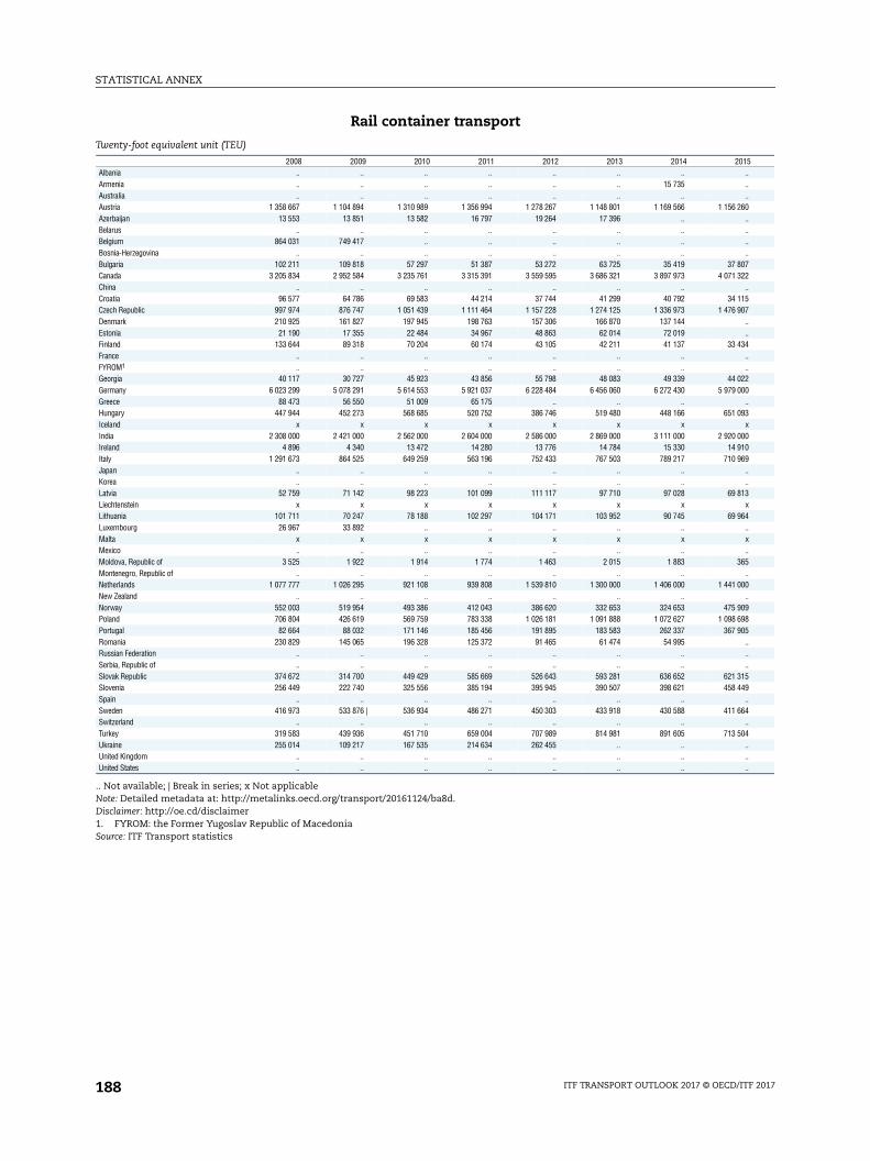
STATISTICAL ANNEX
015......
60........
0722..
1507
..
..34....
2200..
93x
001069....
13x
64..x..
65..
00..
099805
..
..
..1549
..64
..04
..
..
..
Rail container transport
.. Not available; | Break in series; x Not applicableNote: Detailed metadata at: http://metalinks.oecd.org/transport/20161124/ba8d.Disclaimer: http://oe.cd/disclaimer1. FYROM: the Former Yugoslav Republic of MacedoniaSource: ITF Transport statistics
Twenty-foot equivalent unit (TEU)
2008 2009 2010 2011 2012 2013 2014 2Albania .. .. .. .. .. .. ..Armenia .. .. .. .. .. .. 15 735Australia .. .. .. .. .. .. ..Austria 1 358 667 1 104 894 1 310 989 1 356 994 1 278 267 1 148 801 1 169 566 1 156 2Azerbaijan 13 553 13 851 13 582 16 797 19 264 17 396 ..Belarus .. .. .. .. .. .. ..Belgium 864 031 749 417 .. .. .. .. ..Bosnia-Herzegovina .. .. .. .. .. .. ..Bulgaria 102 211 109 818 57 297 51 387 53 272 63 725 35 419 37 8Canada 3 205 834 2 952 584 3 235 761 3 315 391 3 559 595 3 686 321 3 897 973 4 071 3China .. .. .. .. .. .. ..Croatia 96 577 64 786 69 583 44 214 37 744 41 299 40 792 34 1Czech Republic 997 974 876 747 1 051 439 1 111 464 1 157 228 1 274 125 1 336 973 1 476 9Denmark 210 925 161 827 197 945 198 763 157 306 166 870 137 144Estonia 21 190 17 355 22 484 34 967 48 863 62 014 72 019Finland 133 644 89 318 70 204 60 174 43 105 42 211 41 137 33 4France .. .. .. .. .. .. ..FYROM1 .. .. .. .. .. .. ..Georgia 40 117 30 727 45 923 43 856 55 798 48 083 49 339 44 0Germany 6 023 299 5 078 291 5 614 553 5 921 037 6 228 484 6 456 060 6 272 430 5 979 0Greece 88 473 56 550 51 009 65 175 .. .. ..Hungary 447 944 452 273 568 685 520 752 386 746 519 480 448 166 651 0Iceland x x x x x x xIndia 2 308 000 2 421 000 2 562 000 2 604 000 2 586 000 2 869 000 3 111 000 2 920 0Ireland 4 896 4 340 13 472 14 280 13 776 14 784 15 330 14 9Italy 1 291 673 864 525 649 259 563 196 752 433 767 503 789 217 710 9Japan .. .. .. .. .. .. ..Korea .. .. .. .. .. .. ..Latvia 52 759 71 142 98 223 101 099 111 117 97 710 97 028 69 8Liechtenstein x x x x x x xLithuania 101 711 70 247 78 188 102 297 104 171 103 952 90 745 69 9Luxembourg 26 967 33 892 .. .. .. .. ..Malta x x x x x x xMexico .. .. .. .. .. .. ..Moldova, Republic of 3 525 1 922 1 914 1 774 1 463 2 015 1 883 3Montenegro, Republic of .. .. .. .. .. .. ..Netherlands 1 077 777 1 026 295 921 108 939 808 1 539 810 1 300 000 1 406 000 1 441 0New Zealand .. .. .. .. .. .. ..Norway 552 003 519 954 493 386 412 043 386 620 332 653 324 653 475 9Poland 706 804 426 619 569 759 783 338 1 026 181 1 091 888 1 072 627 1 098 6Portugal 82 664 88 032 171 146 185 456 191 895 183 583 262 337 367 9Romania 230 829 145 065 196 328 125 372 91 465 61 474 54 995Russian Federation .. .. .. .. .. .. ..Serbia, Republic of .. .. .. .. .. .. ..Slovak Republic 374 672 314 700 449 429 585 669 526 643 593 281 636 652 621 3Slovenia 256 449 222 740 325 556 385 194 395 945 390 507 398 621 458 4Spain .. .. .. .. .. .. ..Sweden 416 973 533 876 | 536 934 486 271 450 303 433 918 430 588 411 6Switzerland .. .. .. .. .. .. ..Turkey 319 583 439 936 451 710 659 004 707 989 814 981 891 605 713 5Ukraine 255 014 109 217 167 535 214 634 262 455 .. ..United Kingdom .. .. .. .. .. .. ..United States .. .. .. .. .. .. ..
ITF TRANSPORT OUTLOOK 2017 © OECD/ITF 2017188
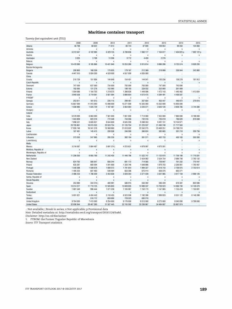
STATISTICAL ANNEX
01560
x22 p
x..x
93..
65....
12x....
54..x
16..
80x..
0048
..
..
..56
x93
x....xx
8132470714
..26
xx
967091
x98
..00
..
Maritime container transport
.. Not available; | Break in series; x Not applicable; p Provisional dataNote: Detailed metadata at: http://metalinks.oecd.org/transport/20161124/ba8d.Disclaimer: http://oe.cd/disclaimer1. FYROM: the Former Yugoslav Republic of MacedoniaSource: ITF Transport statistics
Twenty-foot equivalent unit (TEU)
2008 2009 2010 2011 2012 2013 2014 2Albania 46 798 68 622 71 614 80 744 87 909 109 054 99 350 104 0Armenia x x x x x x xAustralia 6 312 647 6 102 990 6 329 135 6 788 836 7 060 177 7 164 877 7 404 823 p 7 902 1Austria x x x x x x xAzerbaijan 3 025 3 768 13 306 9 712 4 459 2 276 ..Belarus x x x x x x xBelgium 10 478 990 9 185 866 10 431 840 10 253 280 9 915 814 9 886 286 9 725 574 9 928 2Bosnia-Herzegovina .. .. .. .. .. .. ..Bulgaria 200 863 168 339 170 835 179 167 212 369 218 999 236 944 242 8Canada 4 447 910 3 924 200 4 520 000 4 557 000 4 935 000 .. ..China .. .. .. .. .. .. ..Croatia 210 729 151 926 144 649 154 451 144 041 130 236 138 278 181 9Czech Republic x x x x x x xDenmark 747 000 637 000 734 000 782 000 763 000 747 000 743 000Estonia 182 065 131 278 152 060 198 193 228 032 253 900 261 069Finland 1 594 686 1 104 755 1 219 575 1 398 630 1 449 596 1 472 143 1 440 462 1 413 6France 3 940 558 3 719 061 3 921 094 3 890 854 4 073 475 4 284 491 4 436 507FYROM1 x x x x x x xGeorgia 253 811 181 613 226 115 299 461 357 654 403 447 446 972 379 8Germany 15 667 000 11 915 000 13 096 000 15 271 000 15 325 000 15 552 000 15 905 000Greece 1 036 980 1 025 729 1 187 487 2 054 064 3 220 371 3 620 126 3 928 785 3 744 3Hungary x x x x x x xIceland .. .. .. .. .. .. ..India 6 578 000 6 863 000 7 561 000 7 651 000 7 714 000 7 453 000 7 960 000 8 198 0Ireland 1 043 809 823 218 772 548 744 056 732 316 726 019 796 620 876 8Italy 7 896 531 6 605 651 8 644 600 8 645 200 9 398 353 9 491 151 10 104 971Japan 20 705 861 18 015 533 20 533 734 21 135 704 21 225 537 21 490 748 21 717 563Korea 17 926 748 16 341 378 19 368 960 21 610 502 22 550 275 23 469 251 24 798 210Latvia 167 491 145 415 208 508 246 590 366 824 385 665 391 218 359 7Liechtenstein x x x x x x xLithuania 373 263 247 995 295 226 382 194 381 371 402 733 450 183 350 3Luxembourg x x x x x x xMalta .. .. .. .. .. .. ..Mexico 3 316 087 2 884 487 3 691 374 | 4 223 631 4 878 097 4 875 281 ..Moldova, Republic of x x x x x x xMontenegro, Republic of x x x x x x xNetherlands 11 206 050 9 955 769 11 242 400 11 446 796 11 522 747 11 133 970 11 756 188 11 719 2New Zealand .. .. .. .. 2 424 902 2 524 754 2 686 756 2 792 1Norway 624 762 585 647 656 244 691 172 714 565 729 947 761 332 770 4Poland 635 387 660 594 1 041 690 1 330 746 1 648 886 1 979 703 2 256 061 1 793 4Portugal 1 548 388 1 508 678 1 690 073 1 791 644 1 994 327 2 418 743 2 706 975 2 752 6Romania 1 405 333 607 483 548 094 653 306 675 414 659 375 663 271Russian Federation 2 486 233 1 786 509 2 454 838 3 028 264 3 371 039 3 501 985 3 617 159 2 906 1Serbia, Republic of x x x x x x xSlovak Republic x x x x x x xSlovenia 353 880 334 316 | 480 981 586 915 556 392 596 429 676 381 802 6Spain 13 314 317 11 719 125 12 505 803 13 849 935 13 999 337 13 709 523 14 066 730 14 149 4Sweden 1 081 549 996 444 1 071 238 1 165 087 1 150 775 1 147 065 1 155 418 1 150 6Switzerland x x x x x x xTurkey 5 091 621 4 404 442 5 743 455 6 523 506 7 192 396 7 899 933 8 351 122 8 146 3Ukraine .. 516 712 659 690 729 523 693 210 .. ..United Kingdom 8 764 000 7 415 000 8 254 000 8 176 000 8 013 000 8 273 000 9 540 000 9 799 0United States 32 006 944 28 467 280 31 507 445 32 745 592 33 236 967 34 484 687 35 867 974
ITF TRANSPORT OUTLOOK 2017 © OECD/ITF 2017 189
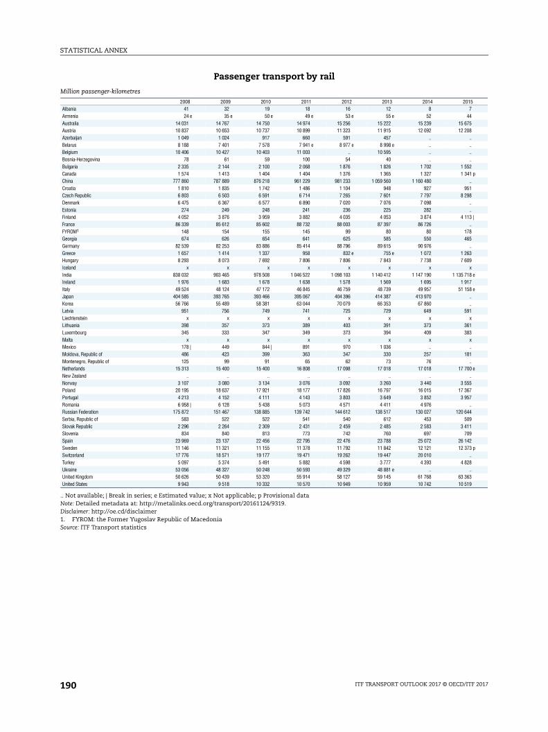
STATISTICAL ANNEX
0157
447508
..
..
..
..5241 p..
5198....
13 |..
7865
..6309
x18 e1758 e....
91x
6183
x..
81..
00 e..
556757
..440911094273 p..
28..
6319
Passenger transport by rail
.. Not available; | Break in series; e Estimated value; x Not applicable; p Provisional dataNote: Detailed metadata at: http://metalinks.oecd.org/transport/20161124/9319.Disclaimer: http://oe.cd/disclaimer1. FYROM: the Former Yugoslav Republic of MacedoniaSource: ITF Transport statistics
Million passenger-kilometres
2008 2009 2010 2011 2012 2013 2014 2Albania 41 32 19 18 16 12 8Armenia 24 e 35 e 50 e 49 e 53 e 55 e 52Australia 14 031 14 767 14 750 14 974 15 256 15 222 15 239 15 6Austria 10 837 10 653 10 737 10 899 11 323 11 915 12 092 12 2Azerbaijan 1 049 1 024 917 660 591 457 ..Belarus 8 188 7 401 7 578 7 941 e 8 977 e 8 998 e ..Belgium 10 406 10 427 10 403 11 003 .. 10 595 ..Bosnia-Herzegovina 78 61 59 100 54 40 ..Bulgaria 2 335 2 144 2 100 2 068 1 876 1 826 1 702 1 5Canada 1 574 1 413 1 404 1 404 1 376 1 365 1 327 1 3China 777 860 787 889 876 218 961 229 981 233 1 059 560 1 160 480Croatia 1 810 1 835 1 742 1 486 1 104 948 927 9Czech Republic 6 803 6 503 6 591 6 714 7 265 7 601 7 797 8 2Denmark 6 475 6 367 6 577 6 890 7 020 7 076 7 098Estonia 274 249 248 241 236 225 282Finland 4 052 3 876 3 959 3 882 4 035 4 053 3 874 4 1France 86 339 85 612 85 602 88 732 88 003 87 397 86 726FYROM1 148 154 155 145 99 80 80 1Georgia 674 626 654 641 625 585 550 4Germany 82 539 82 253 83 886 85 414 88 796 89 615 90 976Greece 1 657 1 414 1 337 958 832 e 755 e 1 072 1 2Hungary 8 293 8 073 7 692 7 806 7 806 7 843 7 738 7 6Iceland x x x x x x xIndia 838 032 903 465 978 508 1 046 522 1 098 103 1 140 412 1 147 190 1 135 7Ireland 1 976 1 683 1 678 1 638 1 578 1 569 1 695 1 9Italy 49 524 48 124 47 172 46 845 46 759 48 739 49 957 51 1Japan 404 585 393 765 393 466 395 067 404 396 414 387 413 970Korea 56 766 55 489 58 381 63 044 70 079 66 353 67 860Latvia 951 756 749 741 725 729 649 5Liechtenstein x x x x x x xLithuania 398 357 373 389 403 391 373 3Luxembourg 345 333 347 349 373 394 409 3Malta x x x x x x xMexico 178 | 449 844 | 891 970 1 036 ..Moldova, Republic of 486 423 399 363 347 330 257 1Montenegro, Republic of 125 99 91 65 62 73 76Netherlands 15 313 15 400 15 400 16 808 17 098 17 018 17 018 17 7New Zealand .. .. .. .. .. .. ..Norway 3 107 3 080 3 134 3 076 3 092 3 260 3 440 3 5Poland 20 195 18 637 17 921 18 177 17 826 16 797 16 015 17 3Portugal 4 213 4 152 4 111 4 143 3 803 3 649 3 852 3 9Romania 6 958 | 6 128 5 438 5 073 4 571 4 411 4 976Russian Federation 175 872 151 467 138 885 139 742 144 612 138 517 130 027 120 6Serbia, Republic of 583 522 522 541 540 612 453 5Slovak Republic 2 296 2 264 2 309 2 431 2 459 2 485 2 583 3 4Slovenia 834 840 813 773 742 760 697 7Spain 23 969 23 137 22 456 22 795 22 476 23 788 25 072 26 1Sweden 11 146 11 321 11 155 11 378 11 792 11 842 12 121 12 3Switzerland 17 776 18 571 19 177 19 471 19 262 19 447 20 010Turkey 5 097 5 374 5 491 5 882 4 598 3 777 4 393 4 8Ukraine 53 056 48 327 50 248 50 593 49 329 48 881 e ..United Kingdom 50 626 50 439 53 320 55 914 58 127 59 145 61 768 63 3United States 9 943 9 518 10 332 10 570 10 949 10 959 10 742 10 5
ITF TRANSPORT OUTLOOK 2017 © OECD/ITF 2017190
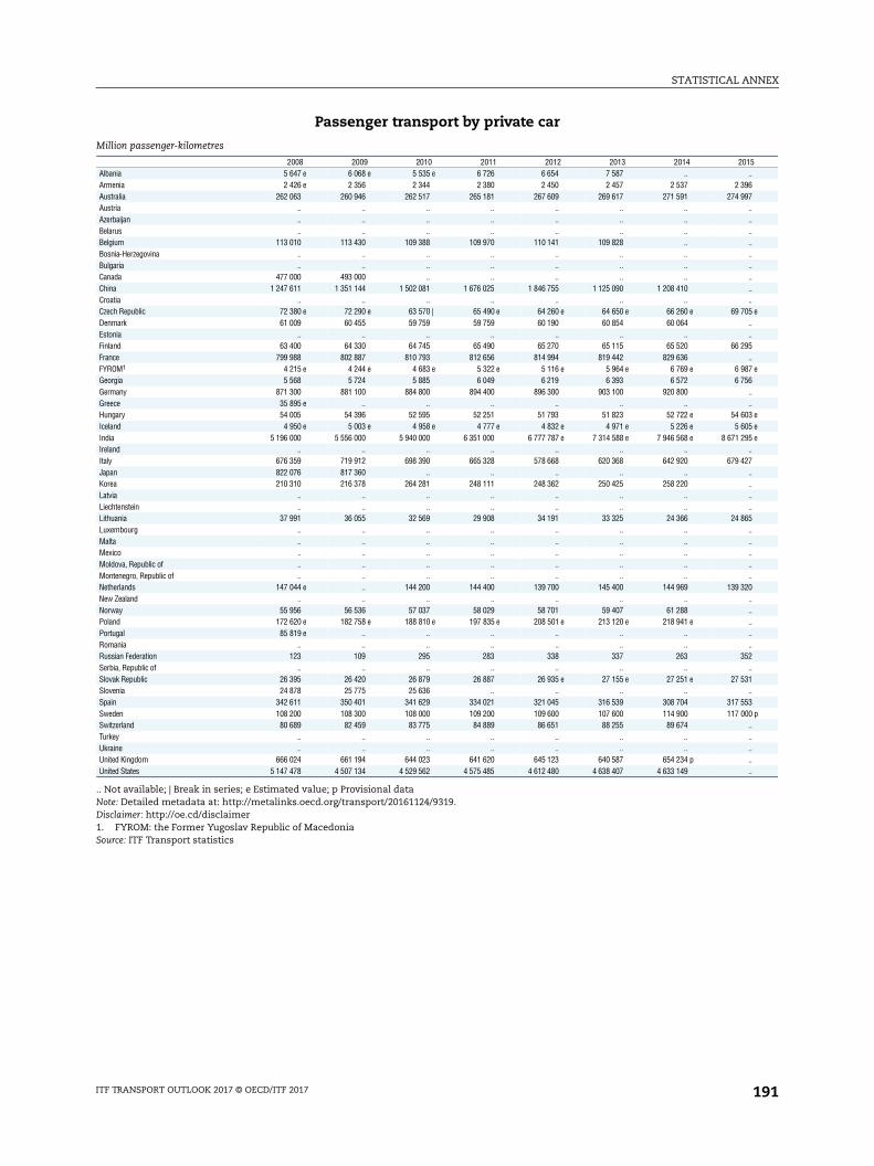
STATISTICAL ANNEX
015..
9697
..
..
..
..
..
..
..
..
..05 e....
95..
87 e56
..
..03 e05 e95 e..
27........
65..........
20..........
52..
31..
5300 p..........
Passenger transport by private car
.. Not available; | Break in series; e Estimated value; p Provisional dataNote: Detailed metadata at: http://metalinks.oecd.org/transport/20161124/9319.Disclaimer: http://oe.cd/disclaimer1. FYROM: the Former Yugoslav Republic of MacedoniaSource: ITF Transport statistics
Million passenger-kilometres
2008 2009 2010 2011 2012 2013 2014 2Albania 5 647 e 6 068 e 5 535 e 6 726 6 654 7 587 ..Armenia 2 426 e 2 356 2 344 2 380 2 450 2 457 2 537 2 3Australia 262 063 260 946 262 517 265 181 267 609 269 617 271 591 274 9Austria .. .. .. .. .. .. ..Azerbaijan .. .. .. .. .. .. ..Belarus .. .. .. .. .. .. ..Belgium 113 010 113 430 109 388 109 970 110 141 109 828 ..Bosnia-Herzegovina .. .. .. .. .. .. ..Bulgaria .. .. .. .. .. .. ..Canada 477 000 493 000 .. .. .. .. ..China 1 247 611 1 351 144 1 502 081 1 676 025 1 846 755 1 125 090 1 208 410Croatia .. .. .. .. .. .. ..Czech Republic 72 380 e 72 290 e 63 570 | 65 490 e 64 260 e 64 650 e 66 260 e 69 7Denmark 61 009 60 455 59 759 59 759 60 190 60 854 60 064Estonia .. .. .. .. .. .. ..Finland 63 400 64 330 64 745 65 490 65 270 65 115 65 520 66 2France 799 988 802 887 810 793 812 656 814 994 819 442 829 636FYROM1 4 215 e 4 244 e 4 683 e 5 322 e 5 116 e 5 964 e 6 769 e 6 9Georgia 5 568 5 724 5 885 6 049 6 219 6 393 6 572 6 7Germany 871 300 881 100 884 800 894 400 896 300 903 100 920 800Greece 35 895 e .. .. .. .. .. ..Hungary 54 005 54 396 52 595 52 251 51 793 51 823 52 722 e 54 6Iceland 4 950 e 5 003 e 4 958 e 4 777 e 4 832 e 4 971 e 5 226 e 5 6India 5 196 000 5 556 000 5 940 000 6 351 000 6 777 787 e 7 314 588 e 7 946 568 e 8 671 2Ireland .. .. .. .. .. .. ..Italy 676 359 719 912 698 390 665 328 578 668 620 368 642 920 679 4Japan 822 076 817 360 .. .. .. .. ..Korea 210 310 216 378 264 281 248 111 248 362 250 425 258 220Latvia .. .. .. .. .. .. ..Liechtenstein .. .. .. .. .. .. ..Lithuania 37 991 36 055 32 569 29 908 34 191 33 325 24 366 24 8Luxembourg .. .. .. .. .. .. ..Malta .. .. .. .. .. .. ..Mexico .. .. .. .. .. .. ..Moldova, Republic of .. .. .. .. .. .. ..Montenegro, Republic of .. .. .. .. .. .. ..Netherlands 147 044 e .. 144 200 144 400 139 700 145 400 144 969 139 3New Zealand .. .. .. .. .. .. ..Norway 55 956 56 536 57 037 58 029 58 701 59 407 61 288Poland 172 620 e 182 758 e 188 810 e 197 835 e 208 501 e 213 120 e 218 941 ePortugal 85 819 e .. .. .. .. .. ..Romania .. .. .. .. .. .. ..Russian Federation 123 109 295 283 338 337 263 3Serbia, Republic of .. .. .. .. .. .. ..Slovak Republic 26 395 26 420 26 879 26 887 26 935 e 27 155 e 27 251 e 27 5Slovenia 24 878 25 775 25 636 .. .. .. ..Spain 342 611 350 401 341 629 334 021 321 045 316 539 308 704 317 5Sweden 108 200 108 300 108 000 109 200 109 600 107 600 114 900 117 0Switzerland 80 689 82 459 83 775 84 889 86 651 88 255 89 674Turkey .. .. .. .. .. .. ..Ukraine .. .. .. .. .. .. ..United Kingdom 666 024 661 194 644 023 641 620 645 123 640 587 654 234 pUnited States 5 147 478 4 507 134 4 529 562 4 575 485 4 612 480 4 638 407 4 633 149
ITF TRANSPORT OUTLOOK 2017 © OECD/ITF 2017 191
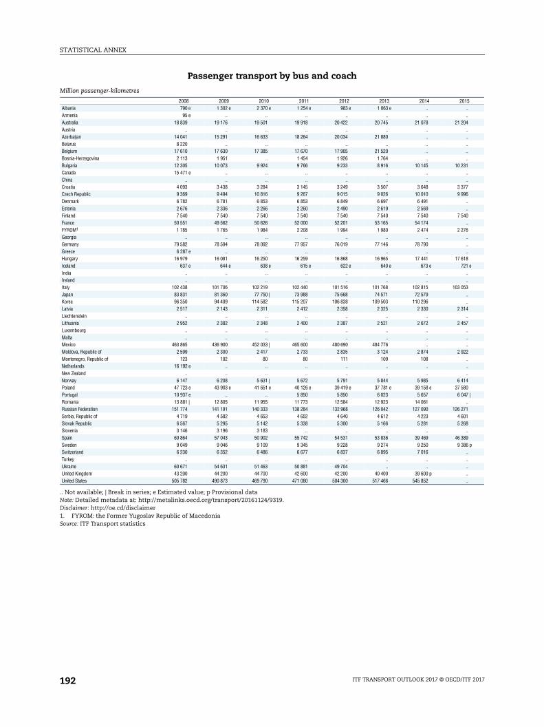
STATISTICAL ANNEX
015....
04..........
31....
7796....
40..
76......
1821 e
..
..53
..
..14..
57......
22......
148047 |..
710168
..8986 p..........
Passenger transport by bus and coach
.. Not available; | Break in series; e Estimated value; p Provisional dataNote: Detailed metadata at: http://metalinks.oecd.org/transport/20161124/9319.Disclaimer: http://oe.cd/disclaimer1. FYROM: the Former Yugoslav Republic of MacedoniaSource: ITF Transport statistics
Million passenger-kilometres
2008 2009 2010 2011 2012 2013 2014 2Albania 790 e 1 302 e 2 370 e 1 254 e 983 e 1 063 e ..Armenia 95 e .. .. .. .. .. ..Australia 18 839 19 176 19 501 19 918 20 422 20 745 21 078 21 2Austria .. .. .. .. .. .. ..Azerbaijan 14 041 15 291 16 633 18 264 20 034 21 880 ..Belarus 8 220 .. .. .. .. .. ..Belgium 17 610 17 630 17 385 17 670 17 905 21 520 ..Bosnia-Herzegovina 2 113 1 951 .. 1 454 1 926 1 764 ..Bulgaria 12 305 10 073 9 924 9 766 9 233 8 916 10 145 10 2Canada 15 471 e .. .. .. .. .. ..China .. .. .. .. .. .. ..Croatia 4 093 3 438 3 284 3 145 3 249 3 507 3 648 3 3Czech Republic 9 369 9 494 10 816 9 267 9 015 9 026 10 010 9 9Denmark 6 782 6 781 6 853 6 853 6 849 6 697 6 491Estonia 2 676 2 336 2 266 2 260 2 490 2 619 2 569Finland 7 540 7 540 7 540 7 540 7 540 7 540 7 540 7 5France 50 551 49 562 50 626 52 000 52 201 53 165 54 174FYROM1 1 785 1 765 1 984 2 208 1 994 1 980 2 474 2 2Georgia .. .. .. .. .. .. ..Germany 79 582 78 594 78 092 77 957 76 019 77 146 78 790Greece 6 287 e .. .. .. .. .. ..Hungary 16 979 16 081 16 250 16 259 16 868 16 965 17 441 17 6Iceland 637 e 644 e 638 e 615 e 622 e 640 e 673 e 7India .. .. .. .. .. .. ..Ireland .. .. .. .. .. .. ..Italy 102 438 101 706 102 219 102 440 101 516 101 768 102 815 103 0Japan 83 831 81 360 77 750 | 73 988 75 668 74 571 72 579Korea 96 350 94 409 114 582 115 207 106 838 109 503 110 296Latvia 2 517 2 143 2 311 2 412 2 358 2 325 2 330 2 3Liechtenstein .. .. .. .. .. .. ..Lithuania 2 952 2 382 2 348 2 400 2 387 2 521 2 672 2 4Luxembourg .. .. .. .. .. .. ..Malta .. .. .. .. .. .. ..Mexico 463 865 436 900 452 033 | 465 600 480 690 484 776 ..Moldova, Republic of 2 599 2 300 2 417 2 733 2 835 3 124 2 874 2 9Montenegro, Republic of 123 102 80 80 111 109 108Netherlands 16 192 e .. .. .. .. .. ..New Zealand .. .. .. .. .. .. ..Norway 6 147 6 208 5 631 | 5 672 5 791 5 844 5 985 6 4Poland 47 723 e 43 903 e 41 651 e 40 126 e 39 419 e 37 781 e 39 158 e 37 5Portugal 10 937 e .. .. 5 850 5 850 6 023 5 657 6 0Romania 13 881 | 12 805 11 955 11 773 12 584 12 923 14 061Russian Federation 151 774 141 191 140 333 138 284 132 968 126 042 127 090 126 2Serbia, Republic of 4 719 4 582 4 653 4 652 4 640 4 612 4 223 4 6Slovak Republic 6 567 5 295 5 142 5 338 5 300 5 166 5 281 5 2Slovenia 3 146 3 196 3 183 .. .. .. ..Spain 60 864 57 043 50 902 55 742 54 531 53 836 39 469 46 3Sweden 9 049 9 046 9 109 9 345 9 228 9 274 9 250 9 3Switzerland 6 230 6 352 6 486 6 677 6 837 6 895 7 016Turkey .. .. .. .. .. .. ..Ukraine 60 671 54 631 51 463 50 881 49 704 .. ..United Kingdom 43 200 44 200 44 700 42 600 42 200 40 400 39 600 pUnited States 505 782 490 873 469 790 471 080 504 300 517 466 545 852
ITF TRANSPORT OUTLOOK 2017 © OECD/ITF 2017192
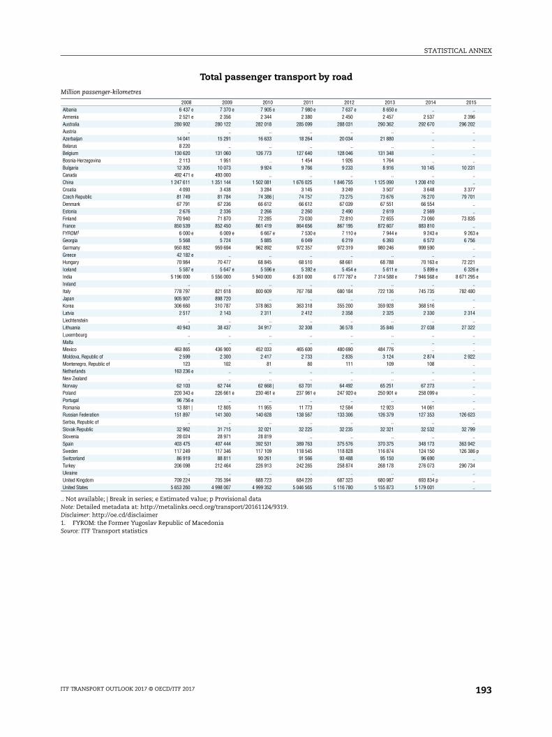
STATISTICAL ANNEX
015..
9602
..
..
..
..
..31
..
..7701
..
..35..
63 e56
..
..2126 e95 e..
80....
14..
22......
22..............
23..
99..
4286 p..
34......
Total passenger transport by road
.. Not available; | Break in series; e Estimated value; p Provisional dataNote: Detailed metadata at: http://metalinks.oecd.org/transport/20161124/9319.Disclaimer: http://oe.cd/disclaimer1. FYROM: the Former Yugoslav Republic of MacedoniaSource: ITF Transport statistics
Million passenger-kilometres
2008 2009 2010 2011 2012 2013 2014 2Albania 6 437 e 7 370 e 7 905 e 7 980 e 7 637 e 8 650 e ..Armenia 2 521 e 2 356 2 344 2 380 2 450 2 457 2 537 2 3Australia 280 902 280 122 282 018 285 099 288 031 290 362 292 670 296 2Austria .. .. .. .. .. .. ..Azerbaijan 14 041 15 291 16 633 18 264 20 034 21 880 ..Belarus 8 220 .. .. .. .. .. ..Belgium 130 620 131 060 126 773 127 640 128 046 131 348 ..Bosnia-Herzegovina 2 113 1 951 .. 1 454 1 926 1 764 ..Bulgaria 12 305 10 073 9 924 9 766 9 233 8 916 10 145 10 2Canada 492 471 e 493 000 .. .. .. .. ..China 1 247 611 1 351 144 1 502 081 1 676 025 1 846 755 1 125 090 1 208 410Croatia 4 093 3 438 3 284 3 145 3 249 3 507 3 648 3 3Czech Republic 81 749 81 784 74 386 | 74 757 73 275 73 676 76 270 79 7Denmark 67 791 67 236 66 612 66 612 67 039 67 551 66 554Estonia 2 676 2 336 2 266 2 260 2 490 2 619 2 569Finland 70 940 71 870 72 285 73 030 72 810 72 655 73 060 73 8France 850 539 852 450 861 419 864 656 867 195 872 607 883 810FYROM1 6 000 e 6 009 e 6 667 e 7 530 e 7 110 e 7 944 e 9 243 e 9 2Georgia 5 568 5 724 5 885 6 049 6 219 6 393 6 572 6 7Germany 950 882 959 694 962 892 972 357 972 319 980 246 999 590Greece 42 182 e .. .. .. .. .. ..Hungary 70 984 70 477 68 845 68 510 68 661 68 788 70 163 e 72 2Iceland 5 587 e 5 647 e 5 596 e 5 392 e 5 454 e 5 611 e 5 899 e 6 3India 5 196 000 5 556 000 5 940 000 6 351 000 6 777 787 e 7 314 588 e 7 946 568 e 8 671 2Ireland .. .. .. .. .. .. ..Italy 778 797 821 618 800 609 767 768 680 184 722 136 745 735 782 4Japan 905 907 898 720 .. .. .. .. ..Korea 306 660 310 787 378 863 363 318 355 200 359 928 368 516Latvia 2 517 2 143 2 311 2 412 2 358 2 325 2 330 2 3Liechtenstein .. .. .. .. .. .. ..Lithuania 40 943 38 437 34 917 32 308 36 578 35 846 27 038 27 3Luxembourg .. .. .. .. .. .. ..Malta .. .. .. .. .. .. ..Mexico 463 865 436 900 452 033 465 600 480 690 484 776 ..Moldova, Republic of 2 599 2 300 2 417 2 733 2 835 3 124 2 874 2 9Montenegro, Republic of 123 102 81 80 111 109 108Netherlands 163 236 e .. .. .. .. .. ..New Zealand .. .. .. .. .. .. ..Norway 62 103 62 744 62 668 | 63 701 64 492 65 251 67 273Poland 220 343 e 226 661 e 230 461 e 237 961 e 247 920 e 250 901 e 258 099 ePortugal 96 756 e .. .. .. .. .. ..Romania 13 881 | 12 805 11 955 11 773 12 584 12 923 14 061Russian Federation 151 897 141 300 140 628 138 567 133 306 126 379 127 353 126 6Serbia, Republic of .. .. .. .. .. .. ..Slovak Republic 32 962 31 715 32 021 32 225 32 235 32 321 32 532 32 7Slovenia 28 024 28 971 28 819 .. .. .. ..Spain 403 475 407 444 392 531 389 763 375 576 370 375 348 173 363 9Sweden 117 249 117 346 117 109 118 545 118 828 116 874 124 150 126 3Switzerland 86 919 88 811 90 261 91 566 93 488 95 150 96 690Turkey 206 098 212 464 226 913 242 265 258 874 268 178 276 073 290 7Ukraine .. .. .. .. .. .. ..United Kingdom 709 224 705 394 688 723 684 220 687 323 680 987 693 834 pUnited States 5 653 260 4 998 007 4 999 352 5 046 565 5 116 780 5 155 873 5 179 001
ITF TRANSPORT OUTLOOK 2017 © OECD/ITF 2017 193
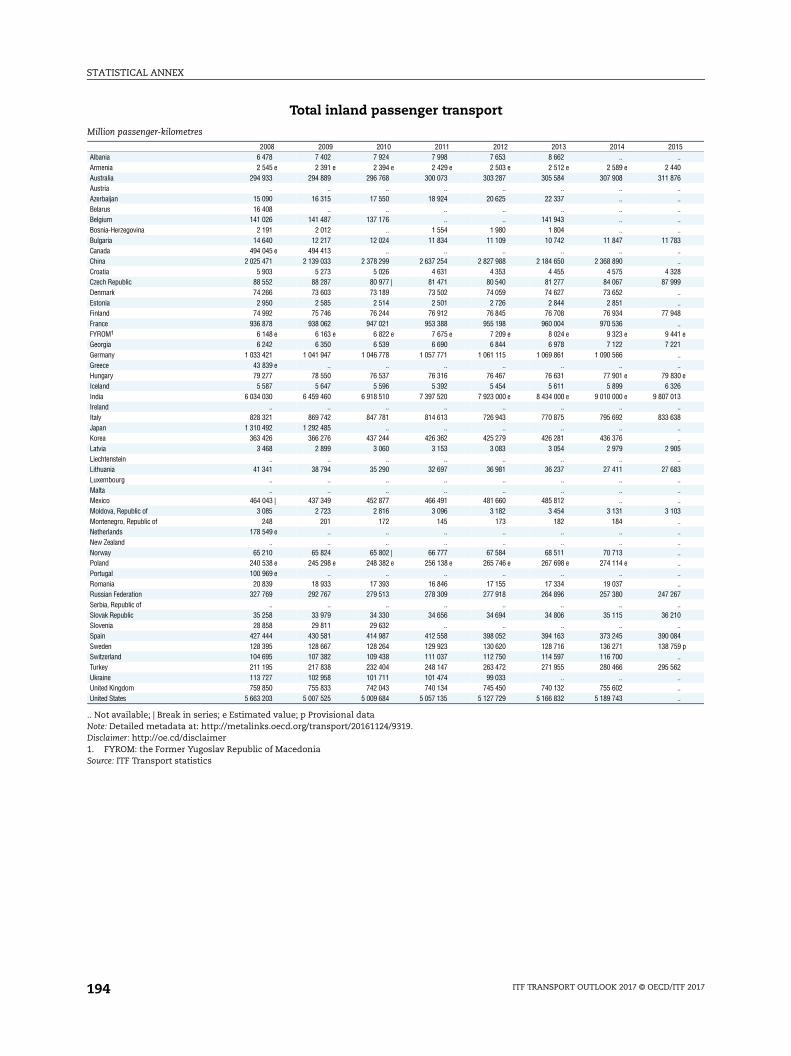
STATISTICAL ANNEX
015..
4076
..
..
..
..
..83
..
..2899
..
..48..
41 e21
..
..30 e2613..
38....
05..
83......
03..............
67..
10..
8459 p..
62......
Total inland passenger transport
.. Not available; | Break in series; e Estimated value; p Provisional dataNote: Detailed metadata at: http://metalinks.oecd.org/transport/20161124/9319.Disclaimer: http://oe.cd/disclaimer1. FYROM: the Former Yugoslav Republic of MacedoniaSource: ITF Transport statistics
Million passenger-kilometres
2008 2009 2010 2011 2012 2013 2014 2Albania 6 478 7 402 7 924 7 998 7 653 8 662 ..Armenia 2 545 e 2 391 e 2 394 e 2 429 e 2 503 e 2 512 e 2 589 e 2 4Australia 294 933 294 889 296 768 300 073 303 287 305 584 307 908 311 8Austria .. .. .. .. .. .. ..Azerbaijan 15 090 16 315 17 550 18 924 20 625 22 337 ..Belarus 16 408 .. .. .. .. .. ..Belgium 141 026 141 487 137 176 .. .. 141 943 ..Bosnia-Herzegovina 2 191 2 012 .. 1 554 1 980 1 804 ..Bulgaria 14 640 12 217 12 024 11 834 11 109 10 742 11 847 11 7Canada 494 045 e 494 413 .. .. .. .. ..China 2 025 471 2 139 033 2 378 299 2 637 254 2 827 988 2 184 650 2 368 890Croatia 5 903 5 273 5 026 4 631 4 353 4 455 4 575 4 3Czech Republic 88 552 88 287 80 977 | 81 471 80 540 81 277 84 067 87 9Denmark 74 266 73 603 73 189 73 502 74 059 74 627 73 652Estonia 2 950 2 585 2 514 2 501 2 726 2 844 2 851Finland 74 992 75 746 76 244 76 912 76 845 76 708 76 934 77 9France 936 878 938 062 947 021 953 388 955 198 960 004 970 536FYROM1 6 148 e 6 163 e 6 822 e 7 675 e 7 209 e 8 024 e 9 323 e 9 4Georgia 6 242 6 350 6 539 6 690 6 844 6 978 7 122 7 2Germany 1 033 421 1 041 947 1 046 778 1 057 771 1 061 115 1 069 861 1 090 566Greece 43 839 e .. .. .. .. .. ..Hungary 79 277 78 550 76 537 76 316 76 467 76 631 77 901 e 79 8Iceland 5 587 5 647 5 596 5 392 5 454 5 611 5 899 6 3India 6 034 030 6 459 460 6 918 510 7 397 520 7 923 000 e 8 434 000 e 9 010 000 e 9 807 0Ireland .. .. .. .. .. .. ..Italy 828 321 869 742 847 781 814 613 726 943 770 875 795 692 833 6Japan 1 310 492 1 292 485 .. .. .. .. ..Korea 363 426 366 276 437 244 426 362 425 279 426 281 436 376Latvia 3 468 2 899 3 060 3 153 3 083 3 054 2 979 2 9Liechtenstein .. .. .. .. .. .. ..Lithuania 41 341 38 794 35 290 32 697 36 981 36 237 27 411 27 6Luxembourg .. .. .. .. .. .. ..Malta .. .. .. .. .. .. ..Mexico 464 043 | 437 349 452 877 466 491 481 660 485 812 ..Moldova, Republic of 3 085 2 723 2 816 3 096 3 182 3 454 3 131 3 1Montenegro, Republic of 248 201 172 145 173 182 184Netherlands 178 549 e .. .. .. .. .. ..New Zealand .. .. .. .. .. .. ..Norway 65 210 65 824 65 802 | 66 777 67 584 68 511 70 713Poland 240 538 e 245 298 e 248 382 e 256 138 e 265 746 e 267 698 e 274 114 ePortugal 100 969 e .. .. .. .. .. ..Romania 20 839 18 933 17 393 16 846 17 155 17 334 19 037Russian Federation 327 769 292 767 279 513 278 309 277 918 264 896 257 380 247 2Serbia, Republic of .. .. .. .. .. .. ..Slovak Republic 35 258 33 979 34 330 34 656 34 694 34 806 35 115 36 2Slovenia 28 858 29 811 29 632 .. .. .. ..Spain 427 444 430 581 414 987 412 558 398 052 394 163 373 245 390 0Sweden 128 395 128 667 128 264 129 923 130 620 128 716 136 271 138 7Switzerland 104 695 107 382 109 438 111 037 112 750 114 597 116 700Turkey 211 195 217 838 232 404 248 147 263 472 271 955 280 466 295 5Ukraine 113 727 102 958 101 711 101 474 99 033 .. ..United Kingdom 759 850 755 833 742 043 740 134 745 450 740 132 755 602United States 5 663 203 5 007 525 5 009 684 5 057 135 5 127 729 5 166 832 5 189 743
ITF TRANSPORT OUTLOOK 2017 © OECD/ITF 2017194
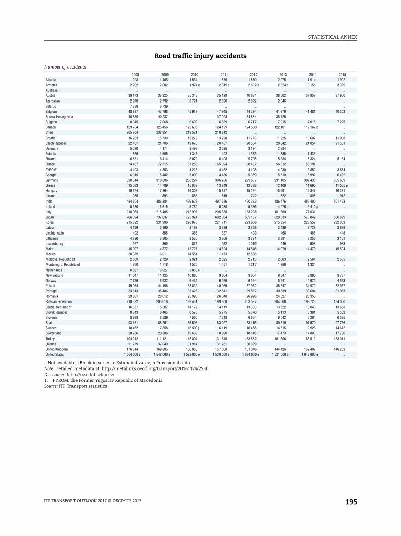
STATISTICAL ANNEX
0159299..
60....
03..
25....
3861....
64..
54325965 p311223....
99538945618304
..35
..
..37636753
..0038028556723611
..03
..
Road traffic injury accidents
.. Not available; | Break in series; e Estimated value; p Provisional dataNote: Detailed metadata at: http://metalinks.oecd.org/transport/20161124/225f.Disclaimer: http://oe.cd/disclaimer1. FYROM: the Former Yugoslav Republic of MacedoniaSource: ITF Transport statistics
Number of accidents
2008 2009 2010 2011 2012 2013 2014 2Albania 1 208 1 465 1 564 1 876 1 870 2 075 1 914 1 9Armenia 2 202 2 002 1 974 e 2 319 e 2 602 e 2 824 e 3 156 3 3Australia .. .. .. .. .. .. ..Austria 39 173 37 925 35 348 35 129 40 831 | 38 502 37 957 37 9Azerbaijan 2 970 2 792 2 721 2 890 2 892 2 846 ..Belarus 7 238 6 739 .. .. .. .. ..Belgium 48 827 47 798 45 918 47 945 44 234 41 279 41 481 40 3Bosnia-Herzegovina 40 859 40 237 .. 37 928 34 884 35 725 ..Bulgaria 8 045 7 068 6 609 6 639 6 717 7 015 7 018 7 2Canada 129 764 125 456 125 636 124 199 124 500 122 101 112 167 pChina 265 204 238 351 219 521 210 812 .. .. ..Croatia 16 283 15 730 13 272 13 228 11 773 11 225 10 607 11 0Czech Republic 22 481 21 706 19 676 20 487 20 504 20 342 21 054 21 5Denmark 5 020 4 174 3 498 3 525 3 124 2 984 ..Estonia 1 869 1 505 1 347 1 492 1 383 1 385 1 435Finland 6 881 6 414 6 072 6 408 5 725 5 334 5 324 5 1France 74 487 72 315 67 288 65 024 60 437 56 812 58 191FYROM1 4 403 4 353 4 223 4 462 4 108 4 230 3 852 3 8Georgia 6 015 5 482 5 099 4 486 5 359 5 510 5 992 6 4Germany 320 614 310 806 288 297 306 266 299 637 291 105 302 435 305 6Greece 15 083 14 789 15 032 13 849 12 398 12 109 11 690 11 5Hungary 19 174 17 864 16 308 15 827 15 174 15 691 15 847 16 3Iceland 1 085 893 883 849 742 822 808 9India 484 704 486 384 499 628 497 686 490 383 486 476 489 400 501 4Ireland 5 580 6 615 5 780 5 230 5 376 4 976 p 5 412 pItaly 218 963 215 405 212 997 205 638 188 228 181 660 177 031Japan 766 394 737 637 725 924 692 084 665 157 629 033 573 842 536 8Korea 215 822 231 990 226 878 221 711 223 656 215 354 223 552 232 0Latvia 4 196 3 160 3 193 3 386 3 358 3 489 3 728 3 6Liechtenstein 402 358 366 327 403 468 465 4Lithuania 4 796 3 805 3 530 3 266 3 391 3 391 3 256 3 1Luxembourg 927 869 876 962 1 019 949 908 9Malta 15 007 14 877 13 727 14 624 14 546 14 070 14 473 15 5Mexico 30 379 16 011 | 14 581 11 473 12 888 .. ..Moldova, Republic of 2 869 2 729 2 921 2 825 2 713 2 603 2 564 2 5Montenegro, Republic of 1 760 1 718 1 520 1 451 1 217 | 1 266 1 334Netherlands 8 897 6 927 3 853 e .. .. .. ..New Zealand 11 647 11 125 10 886 9 804 9 604 9 347 8 880 9 7Norway 7 726 6 922 6 434 6 079 6 154 5 241 4 972 4 5Poland 49 054 44 196 38 832 40 065 37 062 35 847 34 970 32 9Portugal 33 613 35 484 35 426 32 541 29 867 30 339 30 604 31 9Romania 29 861 28 612 25 996 26 648 26 928 24 827 25 355Russian Federation 218 322 203 618 | 199 431 199 868 203 597 204 068 199 723 184 0Serbia, Republic of 16 651 15 807 14 179 14 119 13 333 13 522 13 043 13 6Slovak Republic 8 343 6 465 6 570 5 775 5 370 5 113 5 391 5 5Slovenia 8 938 8 589 7 560 7 218 6 864 6 542 6 264 6 5Spain 93 161 88 251 85 503 83 027 83 115 89 519 91 570 97 7Sweden 18 462 17 858 16 500 | 16 119 16 458 14 815 12 926 14 6Switzerland 20 736 20 506 19 609 18 990 18 148 17 473 17 803 17 7Turkey 104 212 111 121 116 804 131 845 153 552 161 306 168 512 183 0Ukraine 51 279 37 049 31 914 31 281 30 699 .. ..United Kingdom 176 814 169 805 160 080 157 068 151 346 144 426 152 407 146 2United States 1 664 000 e 1 548 000 e 1 572 000 e 1 530 000 e 1 634 000 e 1 621 000 e 1 648 000 e
ITF TRANSPORT OUTLOOK 2017 © OECD/ITF 2017 195
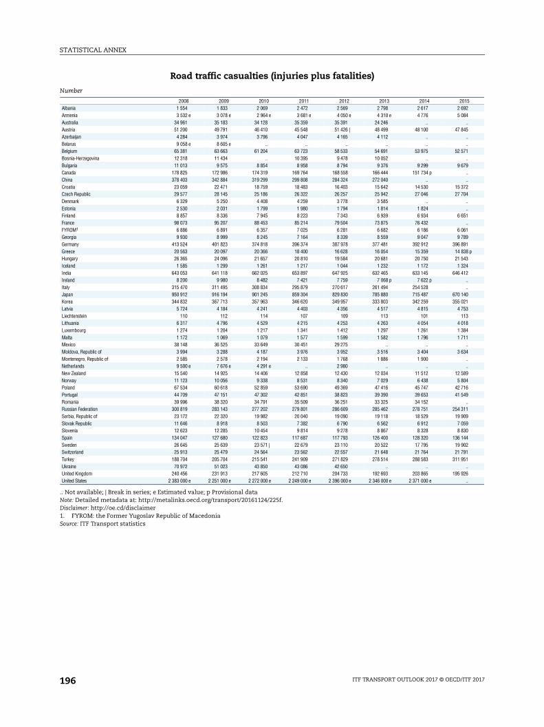
STATISTICAL ANNEX
0159284..
45....
71..
79....
7204....
51..
61899138 p432412....
40215313188411
..34
..
..89041649
..1109593044029151
..26
..
Road traffic casualties (injuries plus fatalities)
.. Not available; | Break in series; e Estimated value; p Provisional dataNote: Detailed metadata at: http://metalinks.oecd.org/transport/20161124/225f.Disclaimer: http://oe.cd/disclaimer1. FYROM: the Former Yugoslav Republic of MacedoniaSource: ITF Transport statistics
Number
2008 2009 2010 2011 2012 2013 2014 2Albania 1 554 1 833 2 069 2 472 2 569 2 798 2 617 2 6Armenia 3 532 e 3 078 e 2 964 e 3 681 e 4 050 e 4 310 e 4 776 5 0Australia 34 961 35 183 34 128 35 359 35 391 24 246 ..Austria 51 200 49 791 46 410 45 548 51 426 | 48 499 48 100 47 8Azerbaijan 4 284 3 974 3 796 4 047 4 165 4 112 ..Belarus 9 058 e 8 605 e .. .. .. .. ..Belgium 65 381 63 663 61 204 63 723 58 533 54 691 53 975 52 5Bosnia-Herzegovina 12 318 11 434 .. 10 395 9 478 10 052 ..Bulgaria 11 013 9 575 8 854 8 958 8 794 9 376 9 299 9 6Canada 178 825 172 986 174 319 169 764 168 558 166 444 151 734 pChina 378 403 342 884 319 299 299 808 284 324 272 040 ..Croatia 23 059 22 471 18 759 18 483 16 403 15 642 14 530 15 3Czech Republic 29 577 28 145 25 186 26 322 26 257 25 942 27 046 27 7Denmark 6 329 5 250 4 408 4 259 3 778 3 585 ..Estonia 2 530 2 031 1 799 1 980 1 794 1 814 1 824Finland 8 857 8 336 7 945 8 223 7 343 6 939 6 934 6 6France 98 073 95 207 88 453 85 214 79 504 73 875 76 432FYROM1 6 886 6 891 6 357 7 025 6 281 6 682 6 186 6 0Georgia 9 930 8 999 8 245 7 164 8 339 8 559 9 047 9 7Germany 413 524 401 823 374 818 396 374 387 978 377 481 392 912 396 8Greece 20 563 20 097 20 366 18 400 16 628 16 054 15 359 14 8Hungary 26 365 24 096 21 657 20 810 19 584 20 681 20 750 21 5Iceland 1 585 1 299 1 261 1 217 1 044 1 232 1 172 1 3India 643 053 641 118 662 025 653 897 647 925 632 465 633 145 646 4Ireland 8 200 9 980 8 482 7 421 7 759 7 068 p 7 622 pItaly 315 470 311 495 308 834 295 879 270 617 261 494 254 528Japan 950 912 916 194 901 245 859 304 829 830 785 880 715 487 670 1Korea 344 832 367 713 357 963 346 620 349 957 333 803 342 259 355 0Latvia 5 724 4 184 4 241 4 403 4 356 4 517 4 815 4 7Liechtenstein 110 112 114 107 109 113 101 1Lithuania 6 317 4 796 4 529 4 215 4 253 4 263 4 054 4 0Luxembourg 1 274 1 204 1 217 1 341 1 412 1 297 1 261 1 3Malta 1 172 1 069 1 079 1 577 1 599 1 582 1 796 1 7Mexico 38 148 36 525 33 649 30 451 29 275 .. ..Moldova, Republic of 3 994 3 288 4 187 3 976 3 952 3 516 3 404 3 6Montenegro, Republic of 2 585 2 578 2 194 2 133 1 768 1 886 1 900Netherlands 9 500 e 7 676 e 4 291 e .. 2 980 .. ..New Zealand 15 540 14 925 14 406 12 858 12 430 12 034 11 512 12 5Norway 11 123 10 056 9 338 8 531 8 340 7 029 6 438 5 8Poland 67 534 60 618 52 859 53 690 49 369 47 416 45 747 42 7Portugal 44 709 47 151 47 302 42 851 38 823 39 390 39 653 41 5Romania 39 996 38 320 34 791 35 509 36 251 33 325 34 152Russian Federation 300 819 283 143 277 202 279 801 286 609 285 462 278 751 254 3Serbia, Republic of 23 172 22 320 19 982 20 040 19 090 19 118 18 529 19 9Slovak Republic 11 646 8 918 8 503 7 382 6 790 6 562 6 912 7 0Slovenia 12 623 12 285 10 454 9 814 9 278 8 867 8 328 8 8Spain 134 047 127 680 122 823 117 687 117 793 126 400 128 320 136 1Sweden 26 645 25 639 23 571 | 22 679 23 110 20 522 17 795 19 9Switzerland 25 913 25 479 24 564 23 562 22 557 21 648 21 764 21 7Turkey 188 704 205 704 215 541 241 909 271 829 278 514 288 583 311 9Ukraine 70 972 51 023 43 850 43 086 42 650 .. ..United Kingdom 240 456 231 913 217 605 212 710 204 733 192 693 203 865 195 9United States 2 383 000 e 2 251 000 e 2 272 000 e 2 249 000 e 2 396 000 e 2 346 000 e 2 371 000 e
ITF TRANSPORT OUTLOOK 2017 © OECD/ITF 2017196
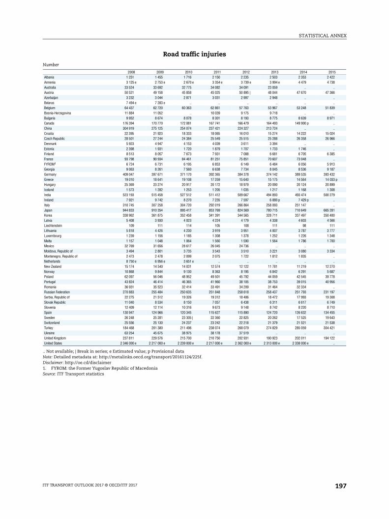
STATISTICAL ANNEX
0152238..
66....
39..
71....
2466....
85..
13873233 p990879....
81006611774800
..34
..
..70877856
..9708491055433821
..22
..
Road traffic injuries
.. Not available; | Break in series; e Estimated value; p Provisional dataNote: Detailed metadata at: http://metalinks.oecd.org/transport/20161124/225f.Disclaimer: http://oe.cd/disclaimer1. FYROM: the Former Yugoslav Republic of MacedoniaSource: ITF Transport statistics
Number
2008 2009 2010 2011 2012 2013 2014 2Albania 1 251 1 455 1 716 2 150 2 235 2 503 2 353 2 4Armenia 3 125 e 2 753 e 2 670 e 3 354 e 3 739 e 3 994 e 4 479 4 7Australia 33 524 33 692 32 775 34 082 34 091 23 059 ..Austria 50 521 49 158 45 858 45 025 50 895 | 48 044 47 670 47 3Azerbaijan 3 232 3 044 2 871 3 031 2 997 2 948 ..Belarus 7 494 e 7 283 e .. .. .. .. ..Belgium 64 437 62 720 60 363 62 861 57 763 53 967 53 248 51 8Bosnia-Herzegovina 11 884 11 052 .. 10 039 9 175 9 718 ..Bulgaria 9 952 8 674 8 078 8 301 8 193 8 775 8 639 8 9Canada 176 394 170 770 172 081 167 741 166 479 164 493 149 900 pChina 304 919 275 125 254 074 237 421 224 327 213 724 ..Croatia 22 395 21 923 18 333 18 065 16 010 15 274 14 222 15 0Czech Republic 28 501 27 244 24 384 25 549 25 515 25 288 26 358 26 9Denmark 5 923 4 947 4 153 4 039 3 611 3 394 ..Estonia 2 398 1 931 1 720 1 879 1 707 1 733 1 746Finland 8 513 8 057 7 673 7 931 7 088 6 681 6 705 6 3France 93 798 90 934 84 461 81 251 75 851 70 607 73 048FYROM1 6 724 6 731 6 195 6 853 6 149 6 484 6 056 5 9Georgia 9 063 8 261 7 560 6 638 7 734 8 045 8 536 9 1Germany 409 047 397 671 371 170 392 365 384 378 374 142 389 535 393 4Greece 19 010 18 641 19 108 17 259 15 640 15 175 14 564 14 0Hungary 25 369 23 274 20 917 20 172 18 979 20 090 20 124 20 8Iceland 1 573 1 282 1 253 1 205 1 035 1 217 1 168 1 3India 523 193 515 458 527 512 511 412 509 667 494 893 493 474 500 2Ireland 7 921 9 742 8 270 7 235 7 597 6 880 p 7 429 pItaly 310 745 307 258 304 720 292 019 266 864 258 093 251 147Japan 944 833 910 354 895 417 853 769 824 569 780 715 710 649 665 2Korea 338 962 361 875 352 458 341 391 344 565 328 711 337 497 350 4Latvia 5 408 3 930 4 023 4 224 4 179 4 338 4 603 4 5Liechtenstein 109 111 114 105 108 111 98 1Lithuania 5 818 4 426 4 230 3 919 3 951 4 007 3 787 3 7Luxembourg 1 239 1 156 1 185 1 308 1 378 1 252 1 226 1 3Malta 1 157 1 048 1 064 1 560 1 590 1 564 1 786 1 7Mexico 32 769 31 656 28 617 26 045 24 736 .. ..Moldova, Republic of 3 494 2 801 3 735 3 543 3 510 3 221 3 080 3 3Montenegro, Republic of 2 473 2 478 2 099 2 075 1 722 1 812 1 835Netherlands 8 750 e 6 956 e 3 651 e .. .. .. ..New Zealand 15 174 14 540 14 031 12 574 12 122 11 781 11 219 12 2Norway 10 868 9 844 9 130 8 363 8 195 6 842 6 291 5 6Poland 62 097 56 046 48 952 49 501 45 792 44 059 42 545 39 7Portugal 43 824 46 414 46 365 41 960 38 105 38 753 39 015 40 9Romania 36 931 35 523 32 414 33 491 34 209 31 464 32 334Russian Federation 270 883 255 484 250 635 251 848 258 618 258 437 251 793 231 1Serbia, Republic of 22 275 21 512 19 326 19 312 18 406 18 472 17 993 19 3Slovak Republic 11 040 8 534 8 150 7 057 6 438 6 311 6 617 6 7Slovenia 12 409 12 114 10 316 9 673 9 148 8 742 8 220 8 7Spain 130 947 124 966 120 345 115 627 115 890 124 720 126 632 134 4Sweden 26 248 25 281 23 305 | 22 360 22 825 20 262 17 525 19 6Switzerland 25 556 25 130 24 237 23 242 22 218 21 379 21 521 21 5Turkey 184 468 201 380 211 496 238 074 268 079 274 829 285 059 304 4Ukraine 63 254 45 675 38 975 38 178 37 519 .. ..United Kingdom 237 811 229 576 215 700 210 750 202 931 190 923 202 011 194 1United States 2 346 000 e 2 217 000 e 2 239 000 e 2 217 000 e 2 362 000 e 2 313 000 e 2 338 000 e
ITF TRANSPORT OUTLOOK 2017 © OECD/ITF 2017 197

STATISTICAL ANNEX
01570460579
..
..32
..08
..
..4838....
66..
48025905 p44163366
..5921872
413611
..00
..2119173893
..1401102089595330 |..
0400 e
Road traffic fatalities
.. Not available; | Break in series; e Estimated value; p Provisional dataNote: Detailed metadata at: http://metalinks.oecd.org/transport/20161124/225f.Disclaimer: http://oe.cd/disclaimer1. FYROM: the Former Yugoslav Republic of MacedoniaSource: ITF Transport statistics
Number
2008 2009 2010 2011 2012 2013 2014 2Albania 303 378 353 322 334 295 264 2Armenia 407 325 294 e 327 e 311 e 316 e 297 3Australia 1 437 1 491 1 353 1 277 1 300 1 187 1 150 1 2Austria 679 633 552 523 531 | 455 430 4Azerbaijan 1 052 930 925 1 016 1 168 1 164 ..Belarus 1 564 1 322 .. .. .. .. ..Belgium 944 943 841 862 770 724 727 7Bosnia-Herzegovina 434 382 .. 356 303 334 ..Bulgaria 1 061 901 776 657 601 601 660 7Canada 2 431 2 216 2 238 2 023 2 079 1 951 1 834 pChina 73 484 67 759 65 225 62 387 59 997 58 316 ..Croatia 664 548 426 418 393 368 308 3Czech Republic 1 076 901 802 773 742 654 688 7Denmark 406 303 255 220 167 191 ..Estonia 132 100 79 101 87 81 78Finland 344 279 272 292 255 258 229 2France 4 275 4 273 3 992 3 963 3 653 3 268 3 384FYROM1 162 160 162 172 132 198 130 1Georgia 867 738 685 526 605 514 511 6Germany 4 477 4 152 3 648 4 009 3 600 3 339 3 377 3 4Greece 1 553 1 456 1 258 1 141 988 879 795 8Hungary 996 822 740 638 605 591 626 6Iceland 12 17 8 12 9 15 4India 119 860 125 660 134 513 142 485 138 258 137 572 139 671 146 1Ireland 279 238 212 186 162 188 p 193 p 1Italy 4 725 4 237 4 114 3 860 3 753 3 401 3 381Japan 6 079 5 840 5 828 5 535 5 261 5 165 4 838 4 8Korea 5 870 5 838 5 505 5 229 5 392 5 092 4 762 4 6Latvia 316 254 218 179 177 179 212 1Liechtenstein 1 1 0 2 1 2 3Lithuania 499 370 299 296 302 256 267 2Luxembourg 35 48 32 33 34 45 35Malta 15 21 15 17 9 18 10Mexico 5 379 4 869 5 032 4 406 4 539 .. ..Moldova, Republic of 500 487 452 433 442 295 324 3Montenegro, Republic of 112 100 95 58 46 74 65Netherlands 750 720 640 661 650 570 570 6New Zealand 366 385 375 284 308 253 293 3Norway 255 212 208 168 145 187 147 1Poland 5 437 4 572 3 907 4 189 3 577 3 357 3 202 2 9Portugal 885 737 937 891 718 637 638 5Romania 3 065 2 797 2 377 2 018 2 042 1 861 1 818Russian Federation 29 936 27 659 | 26 567 27 953 27 991 27 025 26 958 23 1Serbia, Republic of 897 808 656 728 684 646 536 6Slovak Republic 606 384 353 325 352 251 295 3Slovenia 214 171 138 141 130 125 108 1Spain 3 100 2 714 2 478 2 060 1 903 1 680 1 688 1 6Sweden 397 358 266 | 319 285 260 270 2Switzerland 357 349 327 320 339 269 243 2Turkey 4 236 4 324 4 045 3 835 3 750 3 685 3 524 7 5Ukraine 7 718 5 348 4 875 4 908 5 131 4 824 p ..United Kingdom 2 645 2 337 1 905 1 960 1 802 1 770 1 854 1 8United States 37 423 33 883 32 999 32 479 33 561 32 719 32 675 35 2
ITF TRANSPORT OUTLOOK 2017 © OECD/ITF 2017198
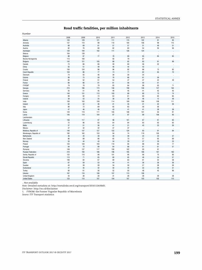
STATISTICAL ANNEX
01593155156
..
..65
..99
..
..8270
..
..49
..7164427465481136..
389195..
836326
..84
..3769237757
..6085575836263196..
2810
Road traffic fatalities, per million inhabitants
.. Not availableNote: Detailed metadata at: http://metalinks.oecd.org/transport/20161124/68d5.Disclaimer: http://oe.cd/disclaimer1. FYROM: the Former Yugoslav Republic of MacedoniaSource: ITF Transport statistics
Number
2008 2009 2010 2011 2012 2013 2014 2Albania 103 129 121 111 115 102 91Armenia 137 110 99 110 104 106 99 1Australia 68 69 61 57 57 51 49Austria 82 76 66 62 63 54 50Azerbaijan 120 104 102 111 126 124 ..Belarus 164 139 .. .. .. .. ..Belgium 88 87 77 78 69 65 65Bosnia-Herzegovina 113 100 .. 93 79 87 ..Bulgaria 142 121 105 89 82 83 91Canada 73 66 66 59 60 56 52China 55 51 49 46 44 43 ..Croatia 150 124 96 98 92 86 73Czech Republic 104 86 77 74 71 62 65Denmark 74 55 46 39 30 34 ..Estonia 99 75 59 76 66 61 59Finland 65 52 51 54 47 47 42France 66 66 61 61 56 50 51FYROM1 79 78 79 83 64 96 63Georgia 215 186 174 136 158 136 137 1Germany 55 51 45 49 45 41 42Greece 140 131 113 103 89 80 73Hungary 99 82 74 64 61 60 63Iceland 38 53 25 38 28 46 12India 100 103 109 114 109 108 108 1Ireland 62 52 46 41 35 41 42Italy 80 72 69 65 63 56 56Japan 47 46 46 43 41 41 38Korea 120 119 111 105 108 101 94Latvia 145 119 104 87 87 89 106Liechtenstein .. .. .. .. .. .. ..Lithuania 156 117 97 98 101 87 91Luxembourg 72 96 63 64 64 83 63Malta 37 51 36 41 21 43 23Mexico 47 42 42 37 37 .. ..Moldova, Republic of 140 137 127 122 124 83 91Montenegro, Republic of 182 162 153 94 74 119 105Netherlands 46 44 39 40 39 34 34New Zealand 86 89 86 65 70 57 65Norway 53 44 43 34 29 37 29Poland 143 120 103 110 94 88 84Portugal 84 70 89 84 68 61 61Romania 149 137 117 100 102 93 91Russian Federation 210 194 186 196 195 188 187 1Serbia, Republic of 122 110 90 101 95 90 75Slovak Republic 113 71 65 60 65 46 54Slovenia 106 84 67 69 63 61 52Spain 67 59 53 44 41 36 36Sweden 43 39 28 34 30 27 28Switzerland 47 45 42 40 42 33 30Turkey 60 61 56 52 50 48 45Ukraine 167 116 106 107 113 106 ..United Kingdom 43 38 30 31 28 28 29United States 123 110 107 104 107 103 102 1
ITF TRANSPORT OUTLOOK 2017 © OECD/ITF 2017 199
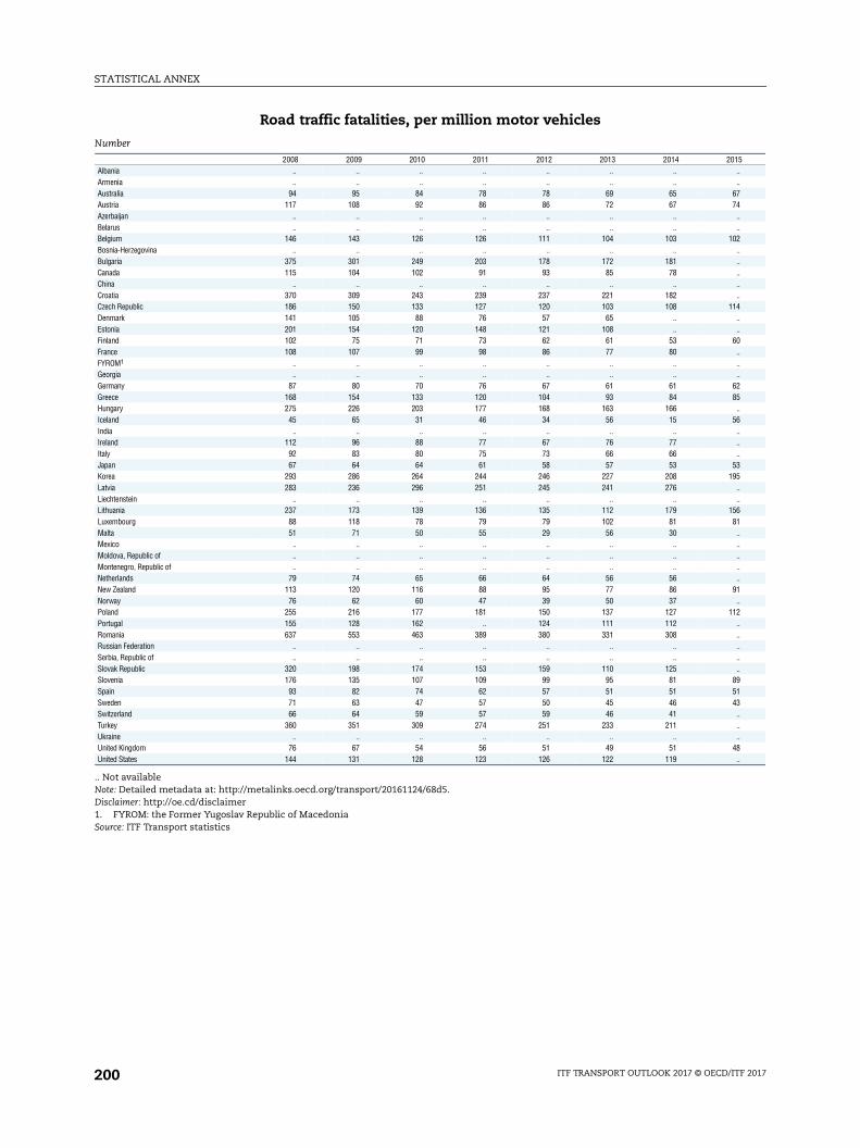
STATISTICAL ANNEX
015....
6774
..
..02
..
..
..
..
..14....
60......
6285
..56
..
..
..5395
..
..5681..........
91..
12..........
895143......
48..
Road traffic fatalities, per million motor vehicles
.. Not availableNote: Detailed metadata at: http://metalinks.oecd.org/transport/20161124/68d5.Disclaimer: http://oe.cd/disclaimer1. FYROM: the Former Yugoslav Republic of MacedoniaSource: ITF Transport statistics
Number
2008 2009 2010 2011 2012 2013 2014 2Albania .. .. .. .. .. .. ..Armenia .. .. .. .. .. .. ..Australia 94 95 84 78 78 69 65Austria 117 108 92 86 86 72 67Azerbaijan .. .. .. .. .. .. ..Belarus .. .. .. .. .. .. ..Belgium 146 143 126 126 111 104 103 1Bosnia-Herzegovina .. .. .. .. .. .. ..Bulgaria 375 301 249 203 178 172 181Canada 115 104 102 91 93 85 78China .. .. .. .. .. .. ..Croatia 370 309 243 239 237 221 182Czech Republic 186 150 133 127 120 103 108 1Denmark 141 105 88 76 57 65 ..Estonia 201 154 120 148 121 108 ..Finland 102 75 71 73 62 61 53France 108 107 99 98 86 77 80FYROM1 .. .. .. .. .. .. ..Georgia .. .. .. .. .. .. ..Germany 87 80 70 76 67 61 61Greece 168 154 133 120 104 93 84Hungary 275 226 203 177 168 163 166Iceland 45 65 31 46 34 56 15India .. .. .. .. .. .. ..Ireland 112 96 88 77 67 76 77Italy 92 83 80 75 73 66 66Japan 67 64 64 61 58 57 53Korea 293 286 264 244 246 227 208 1Latvia 283 236 296 251 245 241 276Liechtenstein .. .. .. .. .. .. ..Lithuania 237 173 139 136 135 112 179 1Luxembourg 88 118 78 79 79 102 81Malta 51 71 50 55 29 56 30Mexico .. .. .. .. .. .. ..Moldova, Republic of .. .. .. .. .. .. ..Montenegro, Republic of .. .. .. .. .. .. ..Netherlands 79 74 65 66 64 56 56New Zealand 113 120 116 88 95 77 86Norway 76 62 60 47 39 50 37Poland 255 216 177 181 150 137 127 1Portugal 155 128 162 .. 124 111 112Romania 637 553 463 389 380 331 308Russian Federation .. .. .. .. .. .. ..Serbia, Republic of .. .. .. .. .. .. ..Slovak Republic 320 198 174 153 159 110 125Slovenia 176 135 107 109 99 95 81Spain 93 82 74 62 57 51 51Sweden 71 63 47 57 50 45 46Switzerland 66 64 59 57 59 46 41Turkey 360 351 309 274 251 233 211Ukraine .. .. .. .. .. .. ..United Kingdom 76 67 54 56 51 49 51United States 144 131 128 123 126 122 119
ITF TRANSPORT OUTLOOK 2017 © OECD/ITF 2017200
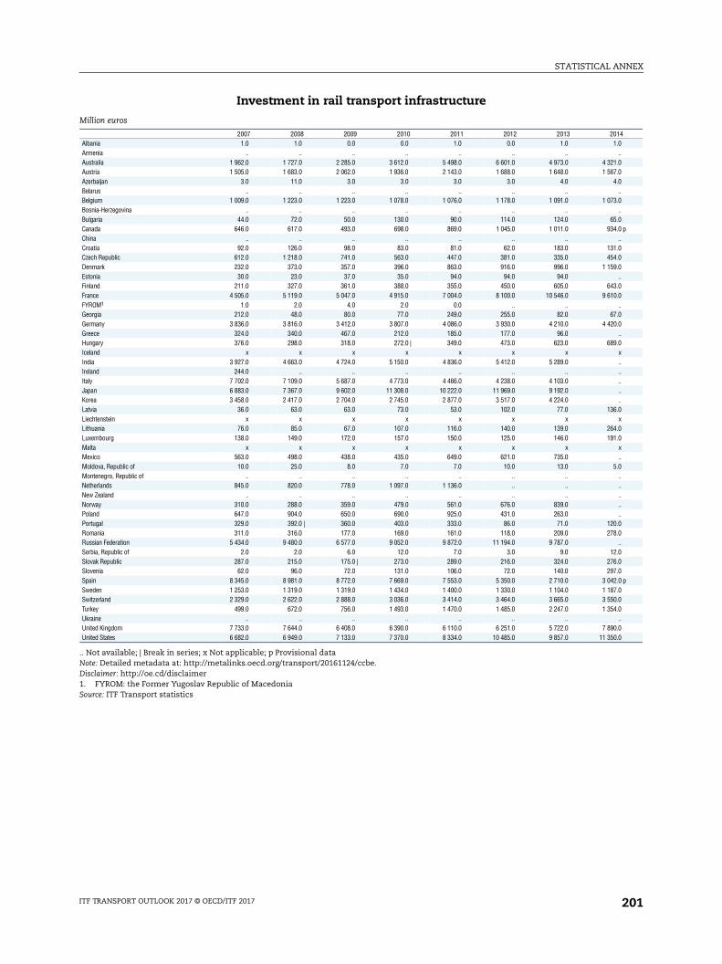
STATISTICAL ANNEX
0141.0
..1.07.04.0
..3.0
..5.04.0 p
..1.04.09.0
..3.00.0
..7.00.0
..9.0
x..........
6.0x
4.01.0
x..
5.0..........
0.08.0
..2.06.07.02.0 p7.00.04.0
..0.00.0
Investment in rail transport infrastructure
.. Not available; | Break in series; x Not applicable; p Provisional dataNote: Detailed metadata at: http://metalinks.oecd.org/transport/20161124/ccbe.Disclaimer: http://oe.cd/disclaimer1. FYROM: the Former Yugoslav Republic of MacedoniaSource: ITF Transport statistics
Million euros
2007 2008 2009 2010 2011 2012 2013 2Albania 1.0 1.0 0.0 0.0 1.0 0.0 1.0Armenia .. .. .. .. .. .. ..Australia 1 962.0 1 727.0 2 285.0 3 612.0 5 498.0 6 601.0 4 973.0 4 32Austria 1 505.0 1 683.0 2 062.0 1 936.0 2 143.0 1 688.0 1 648.0 1 56Azerbaijan 3.0 11.0 3.0 3.0 3.0 3.0 4.0Belarus .. .. .. .. .. .. ..Belgium 1 009.0 1 223.0 1 223.0 1 078.0 1 076.0 1 178.0 1 091.0 1 07Bosnia-Herzegovina .. .. .. .. .. .. ..Bulgaria 44.0 72.0 50.0 130.0 90.0 114.0 124.0 6Canada 646.0 617.0 493.0 698.0 869.0 1 045.0 1 011.0 93China .. .. .. .. .. .. ..Croatia 92.0 126.0 98.0 83.0 81.0 62.0 183.0 13Czech Republic 612.0 1 218.0 741.0 563.0 447.0 381.0 335.0 45Denmark 232.0 373.0 357.0 396.0 863.0 916.0 996.0 1 15Estonia 30.0 23.0 37.0 35.0 94.0 94.0 94.0Finland 211.0 327.0 361.0 388.0 355.0 450.0 605.0 64France 4 505.0 5 119.0 5 047.0 4 915.0 7 004.0 8 100.0 10 546.0 9 61FYROM1 1.0 2.0 4.0 2.0 0.0 .. ..Georgia 212.0 48.0 80.0 77.0 249.0 255.0 82.0 6Germany 3 836.0 3 816.0 3 412.0 3 807.0 4 086.0 3 930.0 4 210.0 4 42Greece 324.0 340.0 467.0 212.0 185.0 177.0 96.0Hungary 376.0 298.0 318.0 272.0 | 349.0 473.0 623.0 68Iceland x x x x x x xIndia 3 927.0 4 663.0 4 724.0 5 150.0 4 836.0 5 412.0 5 289.0Ireland 244.0 .. .. .. .. .. ..Italy 7 702.0 7 109.0 5 687.0 4 773.0 4 466.0 4 238.0 4 103.0Japan 6 883.0 7 367.0 9 602.0 11 308.0 10 222.0 11 969.0 9 192.0Korea 3 458.0 2 417.0 2 704.0 2 745.0 2 877.0 3 517.0 4 224.0Latvia 36.0 63.0 63.0 73.0 53.0 102.0 77.0 13Liechtenstein x x x x x x xLithuania 76.0 85.0 67.0 107.0 116.0 140.0 139.0 26Luxembourg 138.0 149.0 172.0 157.0 150.0 125.0 146.0 19Malta x x x x x x xMexico 563.0 498.0 438.0 435.0 649.0 621.0 735.0Moldova, Republic of 10.0 25.0 8.0 7.0 7.0 10.0 13.0Montenegro, Republic of .. .. .. .. .. .. ..Netherlands 845.0 820.0 778.0 1 097.0 1 136.0 .. ..New Zealand .. .. .. .. .. .. ..Norway 310.0 288.0 359.0 479.0 561.0 676.0 839.0Poland 647.0 904.0 650.0 690.0 925.0 431.0 263.0Portugal 329.0 392.0 | 360.0 403.0 333.0 86.0 71.0 12Romania 311.0 316.0 177.0 169.0 161.0 118.0 209.0 27Russian Federation 5 434.0 9 480.0 6 577.0 9 052.0 9 872.0 11 194.0 9 787.0Serbia, Republic of 2.0 2.0 6.0 12.0 7.0 3.0 9.0 1Slovak Republic 287.0 215.0 175.0 | 273.0 289.0 216.0 324.0 27Slovenia 62.0 96.0 72.0 131.0 106.0 72.0 140.0 29Spain 8 345.0 8 981.0 8 772.0 7 669.0 7 553.0 5 350.0 2 710.0 3 04Sweden 1 253.0 1 319.0 1 319.0 1 434.0 1 400.0 1 330.0 1 104.0 1 18Switzerland 2 329.0 2 622.0 2 888.0 3 036.0 3 414.0 3 464.0 3 665.0 3 55Turkey 499.0 672.0 756.0 1 493.0 1 470.0 1 485.0 2 247.0 1 35Ukraine .. .. .. .. .. .. ..United Kingdom 7 733.0 7 644.0 6 408.0 6 390.0 6 110.0 6 251.0 5 722.0 7 89United States 6 682.0 6 949.0 7 133.0 7 370.0 8 334.0 10 485.0 9 857.0 11 35
ITF TRANSPORT OUTLOOK 2017 © OECD/ITF 2017 201
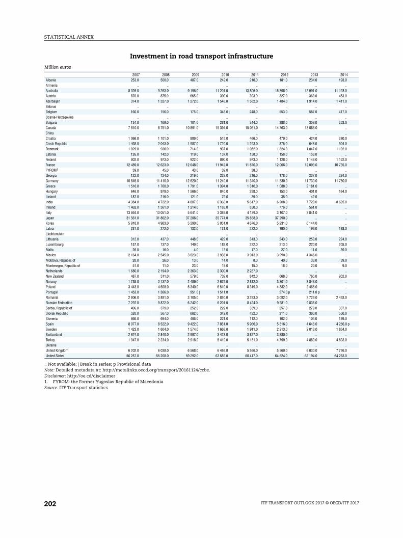
STATISTICAL ANNEX
0143.0
..8.03.01.0
..7.0
..3.0
..
..0.04.02.0
..2.05.0
..4.00.0
..4.0
..5.0
..
..
..
..8.0
..4.05.09.0
..9.09.0
..2.0
..
..
..3.0
..7.00.09.06.0 p4.0
..3.0
..6.03.0
Investment in road transport infrastructure
.. Not available; | Break in series; p Provisional dataNote: Detailed metadata at: http://metalinks.oecd.org/transport/20161124/ccbe.Disclaimer: http://oe.cd/disclaimer1. FYROM: the Former Yugoslav Republic of MacedoniaSource: ITF Transport statistics
Million euros
2007 2008 2009 2010 2011 2012 2013 2Albania 253.0 500.0 487.0 242.0 210.0 181.0 234.0 19Armenia .. .. .. .. .. .. ..Australia 8 026.0 9 263.0 9 196.0 11 201.0 13 806.0 15 898.0 12 991.0 11 12Austria 870.0 875.0 665.0 390.0 303.0 327.0 363.0 45Azerbaijan 374.0 1 327.0 1 272.0 1 546.0 1 562.0 1 484.0 1 914.0 1 41Belarus .. .. .. .. .. .. ..Belgium 166.0 156.0 175.0 348.0 | 248.0 553.0 587.0 41Bosnia-Herzegovina .. .. .. .. .. .. ..Bulgaria 134.0 169.0 101.0 281.0 344.0 388.0 359.0 25Canada 7 810.0 8 751.0 10 891.0 15 394.0 15 061.0 14 763.0 13 086.0China .. .. .. .. .. .. ..Croatia 1 066.0 1 101.0 909.0 515.0 466.0 479.0 424.0 28Czech Republic 1 493.0 2 043.0 1 987.0 1 720.0 1 293.0 876.0 648.0 60Denmark 1 029.0 936.0 714.0 937.0 1 052.0 1 324.0 1 047.0 1 10Estonia 126.0 142.0 119.0 137.0 158.0 158.0 158.0Finland 802.0 973.0 922.0 890.0 973.0 1 128.0 1 148.0 1 13France 12 489.0 12 623.0 12 648.0 11 942.0 11 876.0 12 006.0 12 093.0 10 73FYROM1 39.0 45.0 43.0 32.0 38.0 .. ..Georgia 122.0 124.0 219.0 232.0 216.0 178.0 237.0 22Germany 10 845.0 11 410.0 12 620.0 11 240.0 11 340.0 11 530.0 11 730.0 11 78Greece 1 516.0 1 760.0 1 791.0 1 394.0 1 310.0 1 088.0 2 181.0Hungary 646.0 979.0 1 566.0 840.0 298.0 153.0 401.0 16Iceland 187.0 216.0 121.0 79.0 39.0 38.0 42.0India 4 384.0 4 722.0 4 807.0 6 360.0 5 617.0 6 208.0 7 729.0 8 60Ireland 1 462.0 1 361.0 1 214.0 1 188.0 850.0 776.0 561.0Italy 13 664.0 13 051.0 5 641.0 3 389.0 4 129.0 3 107.0 2 841.0Japan 31 561.0 31 862.0 37 206.0 35 774.0 35 858.0 37 290.0 ..Korea 5 918.0 4 983.0 5 290.0 5 051.0 4 676.0 5 231.0 6 144.0Latvia 231.0 272.0 132.0 131.0 222.0 190.0 199.0 18Liechtenstein .. .. .. .. .. .. ..Lithuania 312.0 437.0 448.0 422.0 343.0 243.0 253.0 22Luxembourg 157.0 137.0 149.0 183.0 222.0 213.0 220.0 20Malta 26.0 16.0 4.0 13.0 17.0 27.0 11.0 3Mexico 2 164.0 2 545.0 3 023.0 3 938.0 3 913.0 3 990.0 4 346.0Moldova, Republic of 28.0 26.0 13.0 14.0 8.0 40.0 36.0 3Montenegro, Republic of 51.0 11.0 23.0 18.0 15.0 18.0 20.0Netherlands 1 680.0 2 194.0 2 363.0 2 300.0 2 287.0 .. ..New Zealand 487.0 511.0 | 579.0 732.0 842.0 668.0 765.0 95Norway 1 735.0 2 137.0 2 489.0 2 675.0 2 812.0 3 301.0 3 843.0Poland 3 443.0 4 508.0 5 340.0 6 510.0 8 319.0 4 382.0 2 465.0Portugal 1 453.0 1 366.0 951.0 | 1 511.0 .. 274.0 p 211.0 pRomania 2 806.0 3 891.0 3 105.0 2 850.0 3 283.0 3 092.0 2 729.0 2 49Russian Federation 7 297.0 9 872.0 6 242.0 6 201.0 8 424.0 9 281.0 9 836.0Serbia, Republic of 406.0 379.0 252.0 229.0 339.0 257.0 279.0 33Slovak Republic 520.0 567.0 662.0 342.0 432.0 311.0 360.0 55Slovenia 666.0 694.0 406.0 221.0 112.0 102.0 104.0 13Spain 8 077.0 8 522.0 9 422.0 7 851.0 5 966.0 5 316.0 4 646.0 4 26Sweden 1 423.0 1 604.0 1 574.0 1 668.0 1 911.0 2 213.0 2 013.0 1 86Switzerland 2 674.0 2 840.0 2 997.0 3 423.0 3 827.0 3 880.0 ..Turkey 1 947.0 2 234.0 2 918.0 5 419.0 5 181.0 4 799.0 4 880.0 4 80Ukraine .. .. .. .. .. .. ..United Kingdom 6 202.0 6 038.0 6 568.0 6 486.0 5 566.0 5 560.0 6 030.0 7 72United States 56 257.0 55 208.0 59 292.0 63 589.0 60 417.0 64 524.0 62 194.0 64 28
ITF TRANSPORT OUTLOOK 2017 © OECD/ITF 2017202

STATISTICAL ANNEX
0140.0
xx
0.00.0
..3.0
..1.0
..
..
..0.0
xx
2.00.0
xx
5.0x..x..x..xxxx
3.00.0
xx..x..xx....
4.0..
8.00.0
xxx
0.0x......
Investment in inland waterway transport infrastructure
.. Not available; | Break in series; x Not applicableNote: Detailed metadata at: http://metalinks.oecd.org/transport/20161124/ccbe.Disclaimer: http://oe.cd/disclaimer1. FYROM: the Former Yugoslav Republic of MacedoniaSource: ITF Transport statistics
Million euros
2007 2008 2009 2010 2011 2012 2013 2Albania 0.0 0.0 0.0 0.0 0.0 0.0 0.0Armenia x x x x x x xAustralia x x x x x x xAustria 4.0 3.0 5.0 11.0 2.0 3.0 11.0 1Azerbaijan .. .. .. .. .. 119.0 424.0 26Belarus .. .. .. .. .. .. ..Belgium 178.0 188.0 188.0 154.0 | 152.0 152.0 167.0 10Bosnia-Herzegovina .. .. .. .. .. .. ..Bulgaria 405.0 0.0 0.0 0.0 0.0 0.0 0.0Canada .. .. .. .. .. .. ..China .. .. .. .. .. .. ..Croatia 2.0 2.0 4.0 3.0 3.0 3.0 2.0Czech Republic 14.0 22.0 59.0 58.0 22.0 17.0 7.0 1Denmark x x x x x x xEstonia x x x x x x xFinland 5.0 2.0 2.0 2.0 1.0 2.0 3.0France 226.0 189.0 245.0 253.0 264.0 236.0 224.0 18FYROM1 x x x x x x xGeorgia x x x x x x xGermany 820.0 905.0 1 170.0 1 100.0 1 040.0 870.0 840.0 90Greece x x x x x x xHungary 4.0 0.0 3.0 1.0 0.0 0.0 0.0Iceland x x x x x x xIndia .. .. .. .. .. .. ..Ireland x x x x x x xItaly 29.0 34.0 27.0 42.0 36.0 52.0 136.0Japan x x x x x x xKorea x x x x x x xLatvia x x x x x x xLiechtenstein x x x x x x xLithuania 3.0 4.0 1.0 1.0 2.0 0.0 1.0Luxembourg 0.0 0.0 0.0 1.0 1.0 1.0 0.0Malta x x x x x x xMexico x x x x x x xMoldova, Republic of 0.0 0.0 0.0 0.0 1.0 0.0 0.0Montenegro, Republic of x x x x x x xNetherlands 263.0 270.0 361.0 252.0 263.0 .. ..New Zealand x x x x x x xNorway x x x x x x xPoland 13.0 21.0 25.0 25.0 29.0 0.0 0.0Portugal 10.0 7.0 5.0 1.0 1.0 3.0 0.0Romania 359.0 490.0 536.0 423.0 519.0 279.0 268.0 31Russian Federation 58.0 102.0 59.0 68.0 302.0 230.0 107.0Serbia, Republic of 24.0 36.0 19.0 21.0 26.0 25.0 15.0 1Slovak Republic 0.0 1.0 2.0 3.0 1.0 1.0 1.0Slovenia x x x x x x xSpain x x x x x x xSweden x x x x x x xSwitzerland 0.0 0.0 0.0 0.0 0.0 0.0 0.0Turkey x x x x x x xUkraine .. .. .. .. .. .. ..United Kingdom .. .. .. .. .. .. ..United States .. .. .. .. .. .. ..
ITF TRANSPORT OUTLOOK 2017 © OECD/ITF 2017 203
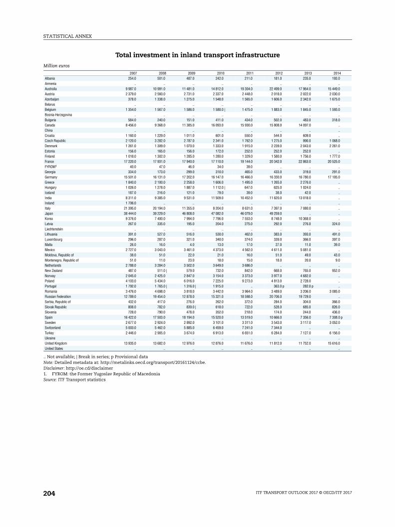
STATISTICAL ANNEX
0143.0
..9.00.05.0
..3.0
..8.0
..
..
..8.01.0
..7.05.0
..1.05.0
..
..
..
..
..
..
..
..4.0
..1.07.09.0
..3.09.0
..2.0
..
..
..5.0
..6.06.06.08.0 p2.0
..6.0
..6.0
..
Total investment in inland transport infrastructure
.. Not available; | Break in series; p Provisional dataNote: Detailed metadata at: http://metalinks.oecd.org/transport/20161124/ccbe.Disclaimer: http://oe.cd/disclaimer1. FYROM: the Former Yugoslav Republic of MacedoniaSource: ITF Transport statistics
Million euros
2007 2008 2009 2010 2011 2012 2013 2Albania 254.0 501.0 487.0 242.0 211.0 181.0 235.0 19Armenia .. .. .. .. .. .. ..Australia 9 987.0 10 991.0 11 481.0 14 812.0 19 304.0 22 499.0 17 964.0 15 44Austria 2 379.0 2 560.0 2 731.0 2 337.0 2 448.0 2 018.0 2 022.0 2 03Azerbaijan 378.0 1 338.0 1 275.0 1 548.0 1 565.0 1 606.0 2 342.0 1 67Belarus .. .. .. .. .. .. ..Belgium 1 354.0 1 567.0 1 586.0 1 580.0 | 1 475.0 1 883.0 1 845.0 1 59Bosnia-Herzegovina .. .. .. .. .. .. ..Bulgaria 584.0 240.0 151.0 411.0 434.0 502.0 483.0 31Canada 8 456.0 9 368.0 11 385.0 16 093.0 15 930.0 15 808.0 14 097.0China .. .. .. .. .. .. ..Croatia 1 160.0 1 229.0 1 011.0 601.0 550.0 544.0 609.0Czech Republic 2 120.0 3 282.0 2 787.0 2 341.0 1 762.0 1 275.0 990.0 1 06Denmark 1 261.0 1 309.0 1 070.0 1 333.0 1 915.0 2 239.0 2 043.0 2 26Estonia 156.0 165.0 156.0 172.0 252.0 252.0 252.0Finland 1 018.0 1 302.0 1 285.0 1 280.0 1 329.0 1 580.0 1 756.0 1 77France 17 220.0 17 931.0 17 940.0 17 110.0 19 144.0 20 342.0 22 863.0 20 52FYROM1 40.0 47.0 46.0 34.0 39.0 .. ..Georgia 334.0 173.0 299.0 310.0 465.0 433.0 319.0 29Germany 15 501.0 16 131.0 17 202.0 16 147.0 16 466.0 16 330.0 16 780.0 17 10Greece 1 840.0 2 100.0 2 258.0 1 606.0 1 495.0 1 265.0 2 276.0Hungary 1 026.0 1 278.0 1 887.0 1 112.0 | 647.0 625.0 1 024.0Iceland 187.0 216.0 121.0 79.0 39.0 38.0 42.0India 8 311.0 9 385.0 9 531.0 11 509.0 10 452.0 11 620.0 13 018.0Ireland 1 706.0 .. .. .. .. .. ..Italy 21 395.0 20 194.0 11 355.0 8 204.0 8 631.0 7 397.0 7 080.0Japan 38 444.0 39 229.0 46 808.0 47 082.0 46 079.0 49 259.0 ..Korea 9 376.0 7 400.0 7 994.0 7 796.0 7 553.0 8 748.0 10 368.0Latvia 267.0 335.0 195.0 204.0 275.0 292.0 276.0 32Liechtenstein .. .. .. .. .. .. ..Lithuania 391.0 527.0 516.0 530.0 462.0 383.0 393.0 49Luxembourg 296.0 287.0 321.0 340.0 374.0 339.0 366.0 39Malta 26.0 16.0 4.0 13.0 17.0 27.0 11.0 3Mexico 2 727.0 3 043.0 3 461.0 4 373.0 4 562.0 4 611.0 5 081.0Moldova, Republic of 38.0 51.0 22.0 21.0 16.0 51.0 49.0 4Montenegro, Republic of 51.0 11.0 23.0 18.0 15.0 18.0 20.0Netherlands 2 788.0 3 284.0 3 502.0 3 649.0 3 686.0 .. ..New Zealand 487.0 511.0 | 579.0 732.0 842.0 668.0 765.0 95Norway 2 045.0 2 425.0 2 847.0 3 154.0 3 373.0 3 977.0 4 682.0Poland 4 103.0 5 434.0 6 016.0 7 225.0 9 273.0 4 813.0 2 728.0Portugal 1 792.0 1 765.0 | 1 316.0 | 1 915.0 .. 363.0 p 282.0 pRomania 3 476.0 4 698.0 3 818.0 3 442.0 3 964.0 3 489.0 3 206.0 3 08Russian Federation 12 789.0 19 454.0 12 878.0 15 321.0 18 598.0 20 706.0 19 729.0Serbia, Republic of 432.0 417.0 276.0 262.0 372.0 284.0 304.0 36Slovak Republic 808.0 782.0 839.0 | 618.0 722.0 528.0 685.0 82Slovenia 728.0 790.0 478.0 352.0 218.0 174.0 244.0 43Spain 16 422.0 17 503.0 18 194.0 15 520.0 13 519.0 10 666.0 7 356.0 7 30Sweden 2 677.0 2 924.0 2 892.0 3 101.0 3 311.0 3 543.0 3 117.0 3 05Switzerland 5 003.0 5 462.0 5 885.0 6 459.0 7 241.0 7 344.0 ..Turkey 2 446.0 2 905.0 3 674.0 6 913.0 6 651.0 6 284.0 7 127.0 6 15Ukraine .. .. .. .. .. .. ..United Kingdom 13 935.0 13 682.0 12 976.0 12 876.0 11 676.0 11 812.0 11 752.0 15 61United States .. .. .. .. .. .. ..
ITF TRANSPORT OUTLOOK 2017 © OECD/ITF 2017204
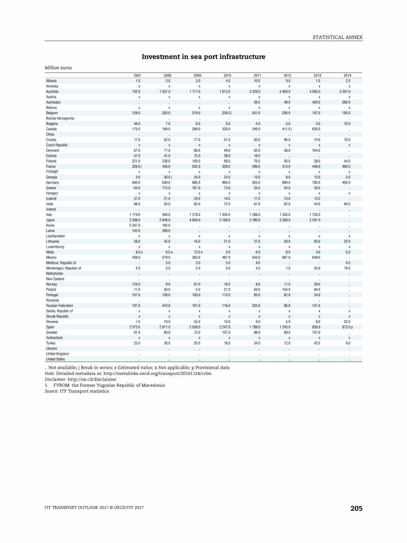
STATISTICAL ANNEX
0142.0
x1.0
x0.0
x0.0
..5.0
..
..0.0
x....
4.00.0
x3.00.0
..x..
4.0..........x
2.0x
5.0..
4.09.0
..
..
..
..
..
..
..xx
3.03.0 p
..x
9.0......
Investment in sea port infrastructure
.. Not available; | Break in series; e Estimated value; x Not applicable; p Provisional dataNote: Detailed metadata at: http://metalinks.oecd.org/transport/20161124/ccbe.Disclaimer: http://oe.cd/disclaimer1. FYROM: the Former Yugoslav Republic of MacedoniaSource: ITF Transport statistics
Million euros
2007 2008 2009 2010 2011 2012 2013 2Albania 1.0 3.0 3.0 4.0 10.0 9.0 1.0Armenia x x x x x x xAustralia 702.0 1 057.0 1 171.0 1 813.0 3 329.0 5 400.0 4 595.0 3 20Austria x x x x x x xAzerbaijan .. .. .. .. 59.0 49.0 420.0 26Belarus x x x x x x xBelgium 159.0 203.0 219.0 230.0 | 241.0 236.0 197.0 15Bosnia-Herzegovina .. .. .. .. .. .. ..Bulgaria 46.0 7.0 8.0 5.0 5.0 3.0 3.0 1Canada 175.0 184.0 299.0 320.0 249.0 411.0 | 630.0China .. .. .. .. .. .. ..Croatia 17.0 52.0 77.0 51.0 63.0 96.0 74.0 7Czech Republic x x x x x x xDenmark 67.0 71.0 66.0 49.0 62.0 58.0 164.0Estonia 57.0 41.0 75.0 39.0 18.0 .. ..Finland 221.0 238.0 100.0 69.0 76.0 56.0 39.0 4France 226.0 | 436.0 532.0 328.0 299.0 313.0 446.0 46FYROM1 x x x x x x xGeorgia 4.0 30.0 | 24.0 24.0 13.0 8.0 12.0Germany 640.0 630.0 685.0 965.0 925.0 890.0 780.0 45Greece 64.0 112.0 107.0 73.0 25.0 24.0 33.0Hungary x x x x x x xIceland 37.0 21.0 20.0 14.0 17.0 15.0 13.0India 66.0 55.0 65.0 72.0 61.0 62.0 44.0 6Ireland .. .. .. .. .. .. ..Italy 1 179.0 940.0 1 278.0 1 345.0 1 268.0 1 343.0 1 126.0Japan 2 506.0 2 849.0 4 656.0 2 169.0 2 290.0 3 280.0 2 291.0Korea 2 347.0 185.0 .. .. .. .. ..Latvia 142.0 269.0 .. .. .. .. ..Liechtenstein x x x x x x xLithuania 26.0 42.0 16.0 21.0 27.0 28.0 83.0 2Luxembourg x x x x x x xMalta 8.0 e 6.0 e 13.0 e 3.0 6.0 8.0 4.0Mexico 438.0 579.0 383.0 487.0 543.0 667.0 649.0Moldova, Republic of .. 5.0 3.0 5.0 4.0 .. ..Montenegro, Republic of 2.0 3.0 2.0 3.0 3.0 1.0 25.0 1Netherlands .. .. .. .. .. .. ..New Zealand .. .. .. .. .. .. ..Norway 123.0 9.0 81.0 19.0 8.0 11.0 29.0Poland 17.0 30.0 4.0 27.0 64.0 154.0 94.0Portugal 157.0 128.0 100.0 112.0 83.0 62.0 34.0Romania .. .. .. .. .. .. ..Russian Federation 197.0 410.0 181.0 116.0 325.0 86.0 147.0Serbia, Republic of x x x x x x xSlovak Republic x x x x x x xSlovenia 7.0 10.0 54.0 13.0 6.0 5.0 8.0 2Spain 2 573.0 2 871.0 2 508.0 2 247.0 1 789.0 1 245.0 830.0 87Sweden 81.0 60.0 72.0 107.0 88.0 69.0 101.0Switzerland x x x x x x xTurkey 23.0 30.0 20.0 16.0 34.0 72.0 43.0Ukraine .. .. .. .. .. .. ..United Kingdom .. .. .. .. .. .. ..United States .. .. .. .. .. .. ..
ITF TRANSPORT OUTLOOK 2017 © OECD/ITF 2017 205
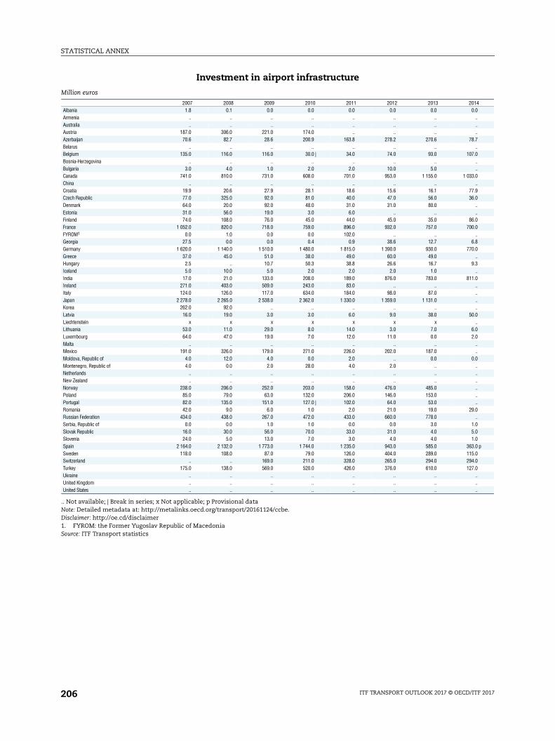
STATISTICAL ANNEX
0140.0
..
..
..8.7
..7.0
..
..3.0
..7.96.0
..
..6.00.0
..6.80.0
..9.3
..1.0
..
..
..
..0.0
..6.02.0
..
..0.0
..
..
..
..
..
..9.0
..1.05.01.03.0 p5.04.07.0
..
..
..
Investment in airport infrastructure
.. Not available; | Break in series; x Not applicable; p Provisional dataNote: Detailed metadata at: http://metalinks.oecd.org/transport/20161124/ccbe.Disclaimer: http://oe.cd/disclaimer1. FYROM: the Former Yugoslav Republic of MacedoniaSource: ITF Transport statistics
Million euros
2007 2008 2009 2010 2011 2012 2013 2Albania 1.8 0.1 0.0 0.0 0.0 0.0 0.0Armenia .. .. .. .. .. .. ..Australia .. .. .. .. .. .. ..Austria 187.0 306.0 221.0 174.0 .. .. ..Azerbaijan 70.6 82.7 28.6 200.9 163.8 278.2 270.6 7Belarus .. .. .. .. .. .. ..Belgium 135.0 116.0 116.0 30.0 | 34.0 74.0 93.0 10Bosnia-Herzegovina .. .. .. .. .. .. ..Bulgaria 3.0 4.0 1.0 2.0 2.0 10.0 5.0Canada 741.0 810.0 731.0 608.0 701.0 953.0 1 155.0 1 03China .. .. .. .. .. .. ..Croatia 19.9 20.6 27.9 28.1 18.6 15.6 16.1 7Czech Republic 77.0 325.0 92.0 81.0 40.0 47.0 56.0 3Denmark 64.0 20.0 92.0 48.0 31.0 31.0 80.0Estonia 31.0 56.0 19.0 3.0 6.0 .. ..Finland 74.0 108.0 76.0 45.0 44.0 45.0 35.0 8France 1 052.0 820.0 718.0 759.0 896.0 932.0 757.0 70FYROM1 0.0 1.0 0.0 0.0 102.0 .. ..Georgia 27.5 0.0 0.0 0.4 0.9 38.6 12.7Germany 1 620.0 1 140.0 1 510.0 1 480.0 1 815.0 1 390.0 930.0 77Greece 37.0 45.0 51.0 38.0 49.0 60.0 49.0Hungary 2.5 .. 10.7 50.3 38.8 26.6 16.7Iceland 5.0 10.0 5.0 2.0 2.0 2.0 1.0India 17.0 21.0 133.0 208.0 189.0 876.0 783.0 81Ireland 271.0 403.0 509.0 243.0 83.0 .. ..Italy 124.0 126.0 117.0 634.0 184.0 98.0 87.0Japan 2 278.0 2 265.0 2 538.0 2 362.0 1 330.0 1 359.0 1 131.0Korea 262.0 92.0 .. .. .. .. ..Latvia 16.0 19.0 3.0 3.0 6.0 9.0 38.0 5Liechtenstein x x x x x x xLithuania 53.0 11.0 29.0 8.0 14.0 3.0 7.0Luxembourg 64.0 47.0 19.0 7.0 12.0 11.0 0.0Malta .. .. .. .. .. .. ..Mexico 191.0 326.0 179.0 271.0 226.0 202.0 187.0Moldova, Republic of 4.0 12.0 4.0 0.0 2.0 .. 0.0Montenegro, Republic of 4.0 0.0 2.0 28.0 4.0 2.0 ..Netherlands .. .. .. .. .. .. ..New Zealand .. .. .. .. .. .. ..Norway 238.0 206.0 252.0 203.0 158.0 476.0 485.0Poland 85.0 79.0 63.0 132.0 206.0 146.0 153.0Portugal 82.0 135.0 151.0 127.0 | 102.0 64.0 53.0Romania 42.0 9.0 6.0 1.0 2.0 21.0 19.0 2Russian Federation 434.0 438.0 267.0 472.0 433.0 660.0 778.0Serbia, Republic of 0.0 0.0 1.0 1.0 0.0 0.0 3.0Slovak Republic 16.0 30.0 56.0 70.0 33.0 31.0 4.0Slovenia 24.0 5.0 13.0 7.0 3.0 4.0 4.0Spain 2 164.0 2 132.0 1 773.0 1 744.0 1 235.0 943.0 585.0 36Sweden 118.0 108.0 87.0 79.0 126.0 404.0 289.0 11Switzerland .. .. 169.0 211.0 328.0 265.0 294.0 29Turkey 175.0 138.0 569.0 520.0 426.0 376.0 610.0 12Ukraine .. .. .. .. .. .. ..United Kingdom .. .. .. .. .. .. ..United States .. .. .. .. .. .. ..
ITF TRANSPORT OUTLOOK 2017 © OECD/ITF 2017206
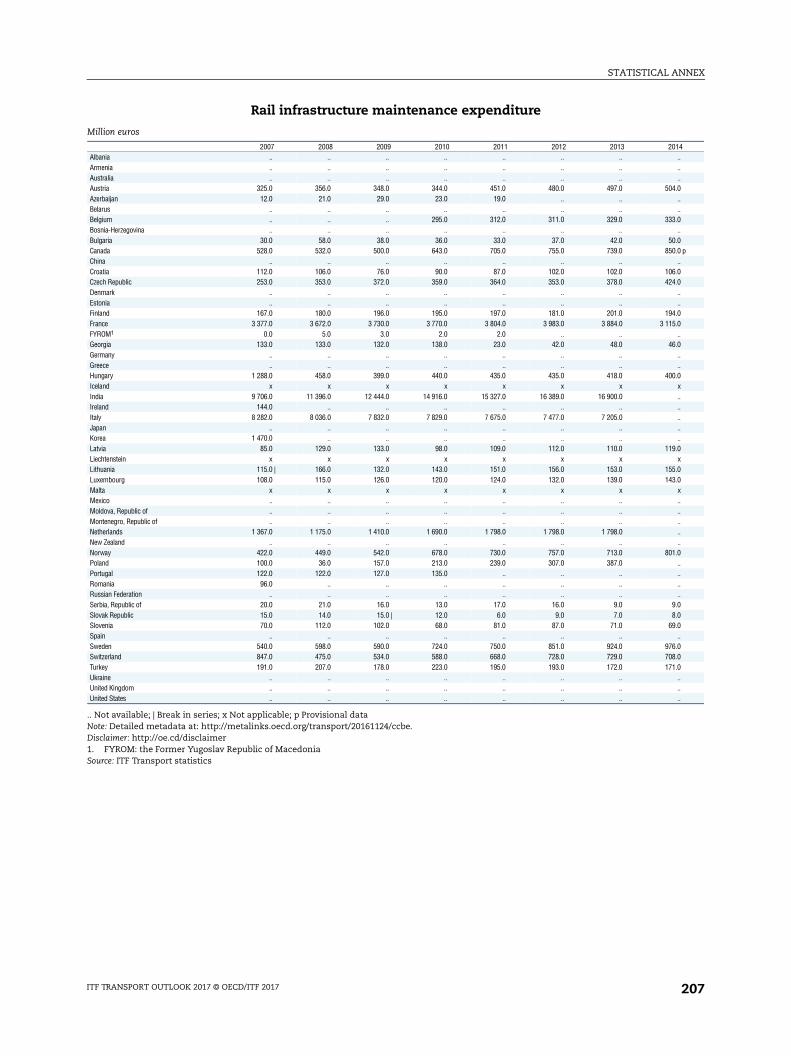
STATISTICAL ANNEX
014......
4.0....
3.0..
0.00.0 p
..6.04.0
..
..4.05.0
..6.0
..
..0.0
x..........
9.0x
5.03.0
x..........
1.0........
9.08.09.0
..6.08.01.0
..
..
..
Rail infrastructure maintenance expenditure
.. Not available; | Break in series; x Not applicable; p Provisional dataNote: Detailed metadata at: http://metalinks.oecd.org/transport/20161124/ccbe.Disclaimer: http://oe.cd/disclaimer1. FYROM: the Former Yugoslav Republic of MacedoniaSource: ITF Transport statistics
Million euros
2007 2008 2009 2010 2011 2012 2013 2Albania .. .. .. .. .. .. ..Armenia .. .. .. .. .. .. ..Australia .. .. .. .. .. .. ..Austria 325.0 356.0 348.0 344.0 451.0 480.0 497.0 50Azerbaijan 12.0 21.0 29.0 23.0 19.0 .. ..Belarus .. .. .. .. .. .. ..Belgium .. .. .. 295.0 312.0 311.0 329.0 33Bosnia-Herzegovina .. .. .. .. .. .. ..Bulgaria 30.0 58.0 38.0 36.0 33.0 37.0 42.0 5Canada 528.0 532.0 500.0 643.0 705.0 755.0 739.0 85China .. .. .. .. .. .. ..Croatia 112.0 106.0 76.0 90.0 87.0 102.0 102.0 10Czech Republic 253.0 353.0 372.0 359.0 364.0 353.0 378.0 42Denmark .. .. .. .. .. .. ..Estonia .. .. .. .. .. .. ..Finland 167.0 180.0 196.0 195.0 197.0 181.0 201.0 19France 3 377.0 3 672.0 3 730.0 3 770.0 3 804.0 3 983.0 3 884.0 3 11FYROM1 0.0 5.0 3.0 2.0 2.0 .. ..Georgia 133.0 133.0 132.0 138.0 23.0 42.0 48.0 4Germany .. .. .. .. .. .. ..Greece .. .. .. .. .. .. ..Hungary 1 288.0 458.0 399.0 440.0 435.0 435.0 418.0 40Iceland x x x x x x xIndia 9 706.0 11 396.0 12 444.0 14 916.0 15 327.0 16 389.0 16 900.0Ireland 144.0 .. .. .. .. .. ..Italy 8 282.0 8 036.0 7 832.0 7 829.0 7 675.0 7 477.0 7 205.0Japan .. .. .. .. .. .. ..Korea 1 470.0 .. .. .. .. .. ..Latvia 85.0 129.0 133.0 98.0 109.0 112.0 110.0 11Liechtenstein x x x x x x xLithuania 115.0 | 166.0 132.0 143.0 151.0 156.0 153.0 15Luxembourg 108.0 115.0 126.0 120.0 124.0 132.0 139.0 14Malta x x x x x x xMexico .. .. .. .. .. .. ..Moldova, Republic of .. .. .. .. .. .. ..Montenegro, Republic of .. .. .. .. .. .. ..Netherlands 1 367.0 1 175.0 1 410.0 1 690.0 1 798.0 1 798.0 1 798.0New Zealand .. .. .. .. .. .. ..Norway 422.0 449.0 542.0 678.0 730.0 757.0 713.0 80Poland 100.0 36.0 157.0 213.0 239.0 307.0 387.0Portugal 122.0 122.0 127.0 135.0 .. .. ..Romania 96.0 .. .. .. .. .. ..Russian Federation .. .. .. .. .. .. ..Serbia, Republic of 20.0 21.0 16.0 13.0 17.0 16.0 9.0Slovak Republic 15.0 14.0 15.0 | 12.0 6.0 9.0 7.0Slovenia 70.0 112.0 102.0 68.0 81.0 87.0 71.0 6Spain .. .. .. .. .. .. ..Sweden 540.0 598.0 590.0 724.0 750.0 851.0 924.0 97Switzerland 847.0 475.0 534.0 588.0 668.0 728.0 729.0 70Turkey 191.0 207.0 178.0 223.0 195.0 193.0 172.0 17Ukraine .. .. .. .. .. .. ..United Kingdom .. .. .. .. .. .. ..United States .. .. .. .. .. .. ..
ITF TRANSPORT OUTLOOK 2017 © OECD/ITF 2017 207
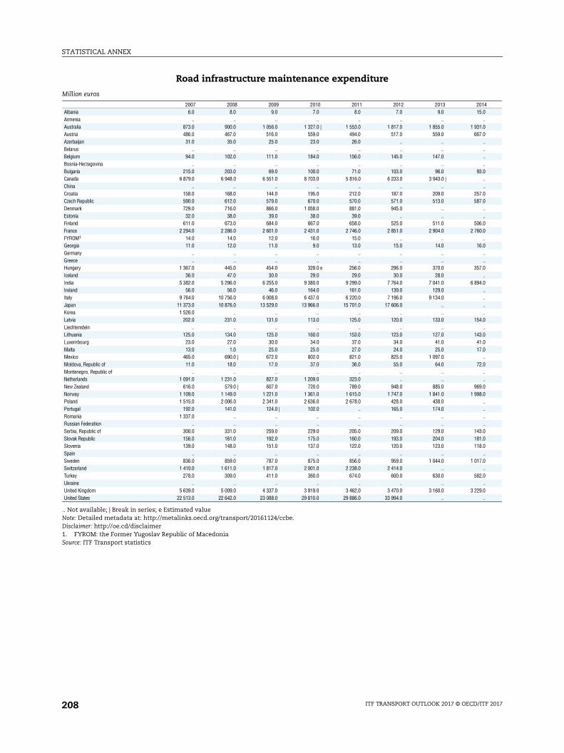
STATISTICAL ANNEX
0145.0
..1.07.0
..
..
..
..3.0
..
..7.07.0
..
..6.00.0
..6.0
..
..7.0
..4.0
..
..
..
..4.0
..3.01.07.0
..2.0
..
..9.08.0
..
..
..
..3.01.08.0
..7.0
..2.0
..9.0
..
Road infrastructure maintenance expenditure
.. Not available; | Break in series; e Estimated valueNote: Detailed metadata at: http://metalinks.oecd.org/transport/20161124/ccbe.Disclaimer: http://oe.cd/disclaimer1. FYROM: the Former Yugoslav Republic of MacedoniaSource: ITF Transport statistics
Million euros
2007 2008 2009 2010 2011 2012 2013 2Albania 6.0 8.0 9.0 7.0 8.0 7.0 9.0 1Armenia .. .. .. .. .. .. ..Australia 873.0 900.0 1 056.0 1 327.0 | 1 553.0 1 817.0 1 855.0 1 93Austria 486.0 467.0 516.0 559.0 494.0 517.0 559.0 66Azerbaijan 31.0 35.0 25.0 23.0 26.0 .. ..Belarus .. .. .. .. .. .. ..Belgium 94.0 102.0 111.0 184.0 156.0 145.0 147.0Bosnia-Herzegovina .. .. .. .. .. .. ..Bulgaria 215.0 203.0 69.0 100.0 71.0 103.0 96.0 9Canada 6 879.0 6 948.0 6 551.0 8 703.0 5 816.0 6 233.0 3 943.0 |China .. .. .. .. .. .. ..Croatia 158.0 168.0 144.0 195.0 212.0 187.0 209.0 25Czech Republic 590.0 612.0 579.0 670.0 570.0 571.0 513.0 58Denmark 729.0 716.0 866.0 1 058.0 881.0 945.0 ..Estonia 32.0 38.0 39.0 38.0 39.0 .. ..Finland 611.0 673.0 684.0 667.0 658.0 525.0 511.0 50France 2 294.0 2 286.0 2 601.0 2 431.0 2 746.0 2 851.0 2 904.0 2 76FYROM1 14.0 14.0 12.0 16.0 15.0 .. ..Georgia 11.0 12.0 11.0 9.0 13.0 15.0 14.0 1Germany .. .. .. .. .. .. ..Greece .. .. .. .. .. .. ..Hungary 1 367.0 445.0 454.0 328.0 e 256.0 296.0 370.0 35Iceland 36.0 47.0 30.0 29.0 29.0 30.0 28.0India 5 382.0 5 296.0 6 255.0 9 380.0 9 299.0 7 764.0 7 041.0 6 89Ireland 56.0 56.0 46.0 164.0 161.0 139.0 129.0Italy 9 764.0 10 756.0 6 008.0 6 437.0 6 220.0 7 196.0 9 134.0Japan 11 373.0 10 876.0 13 529.0 13 966.0 15 701.0 17 606.0 ..Korea 1 526.0 .. .. .. .. .. ..Latvia 202.0 231.0 131.0 113.0 125.0 120.0 133.0 15Liechtenstein .. .. .. .. .. .. ..Lithuania 125.0 134.0 125.0 160.0 153.0 123.0 127.0 14Luxembourg 23.0 27.0 30.0 34.0 37.0 34.0 41.0 4Malta 13.0 1.0 25.0 25.0 27.0 24.0 25.0 1Mexico 465.0 690.0 | 672.0 802.0 821.0 825.0 1 097.0Moldova, Republic of 11.0 18.0 17.0 37.0 36.0 55.0 64.0 7Montenegro, Republic of .. .. .. .. .. .. ..Netherlands 1 091.0 1 231.0 827.0 1 209.0 323.0 .. ..New Zealand 616.0 579.0 | 607.0 720.0 789.0 948.0 885.0 96Norway 1 109.0 1 149.0 1 221.0 1 361.0 1 615.0 1 747.0 1 841.0 1 99Poland 1 515.0 2 006.0 2 341.0 2 636.0 2 678.0 428.0 438.0Portugal 192.0 141.0 124.0 | 102.0 .. 165.0 174.0Romania 1 337.0 .. .. .. .. .. ..Russian Federation .. .. .. .. .. .. ..Serbia, Republic of 300.0 331.0 259.0 229.0 205.0 209.0 129.0 14Slovak Republic 156.0 161.0 192.0 175.0 160.0 193.0 204.0 18Slovenia 139.0 148.0 151.0 137.0 122.0 120.0 123.0 11Spain .. .. .. .. .. .. ..Sweden 836.0 859.0 787.0 875.0 856.0 959.0 1 044.0 1 01Switzerland 1 410.0 1 611.0 1 817.0 2 001.0 2 238.0 2 414.0 ..Turkey 278.0 309.0 411.0 360.0 674.0 600.0 630.0 58Ukraine .. .. .. .. .. .. ..United Kingdom 5 639.0 5 009.0 4 337.0 3 919.0 3 462.0 3 470.0 3 160.0 3 22United States 22 513.0 22 642.0 23 088.0 29 810.0 29 886.0 33 994.0 ..
ITF TRANSPORT OUTLOOK 2017 © OECD/ITF 2017208

STATISTICAL ANNEX
014..xx
9.0....
7.0..
1.0......
5.0xx
7.00.0 e
xx..x
1.0x..x..xxxx
2.00.0
xx..x..xx........
7.09.0
xxx..x......
Inland waterway infrastructure maintenance expenditure
.. Not available; e Estimated value; x Not applicableNote: Detailed metadata at: http://metalinks.oecd.org/transport/20161124/ccbe.Disclaimer: http://oe.cd/disclaimer1. FYROM: the Former Yugoslav Republic of MacedoniaSource: ITF Transport statistics
Million euros
2007 2008 2009 2010 2011 2012 2013 2Albania .. .. .. .. .. .. ..Armenia x x x x x x xAustralia x x x x x x xAustria .. .. .. .. 11.0 12.0 17.0 1Azerbaijan .. .. .. .. .. .. ..Belarus .. .. .. .. .. .. ..Belgium 76.0 87.0 131.0 65.0 58.0 71.0 66.0 2Bosnia-Herzegovina .. .. .. .. .. .. ..Bulgaria 788.0 2.0 1.0 1.0 2.0 1.0 1.0Canada .. .. .. .. .. .. ..China .. .. .. .. .. .. ..Croatia 2.0 3.0 1.0 1.0 1.0 1.0 1.0Czech Republic 3.0 2.0 2.0 2.0 2.0 3.0 5.0Denmark x x x x x x xEstonia x x x x x x xFinland 16.0 17.0 26.0 17.0 20.0 15.0 15.0 1France 58.0 60.0 61.0 60.0 61.0 61.0 e 61.0 e 6FYROM1 x x x x x x xGeorgia x x x x x x xGermany .. .. .. .. .. .. ..Greece x x x x x x xHungary 33.0 2.0 1.0 3.0 e 2.0 1.0 1.0Iceland x x x x x x xIndia .. .. .. .. .. .. ..Ireland x x x x x x xItaly 98.0 83.0 82.0 81.0 78.0 77.0 113.0Japan x x x x x x xKorea x x x x x x xLatvia x x x x x x xLiechtenstein x x x x x x xLithuania 2.0 3.0 1.0 1.0 1.0 2.0 2.0Luxembourg 0.0 0.0 0.0 0.0 0.0 0.0 0.0Malta x x x x x x xMexico x x x x x x xMoldova, Republic of 0.0 4.0 1.0 0.0 .. .. ..Montenegro, Republic of x x x x x x xNetherlands 492.0 583.0 693.0 544.0 343.0 .. ..New Zealand x x x x x x xNorway x x x x x x xPoland 2.0 2.0 3.0 8.0 17.0 8.0 21.0Portugal .. .. .. .. 0.0 1.0 1.0Romania 28.0 .. .. .. .. .. ..Russian Federation .. .. .. .. .. .. ..Serbia, Republic of 11.0 13.0 11.0 13.0 23.0 18.0 17.0 1Slovak Republic 1.0 4.0 2.0 2.0 2.0 3.0 4.0Slovenia x x x x x x xSpain x x x x x x xSweden x x x x x x xSwitzerland .. .. .. .. .. .. ..Turkey x x x x x x xUkraine .. .. .. .. .. .. ..United Kingdom .. .. .. .. .. .. ..United States .. .. .. .. .. .. ..
ITF TRANSPORT OUTLOOK 2017 © OECD/ITF 2017 209
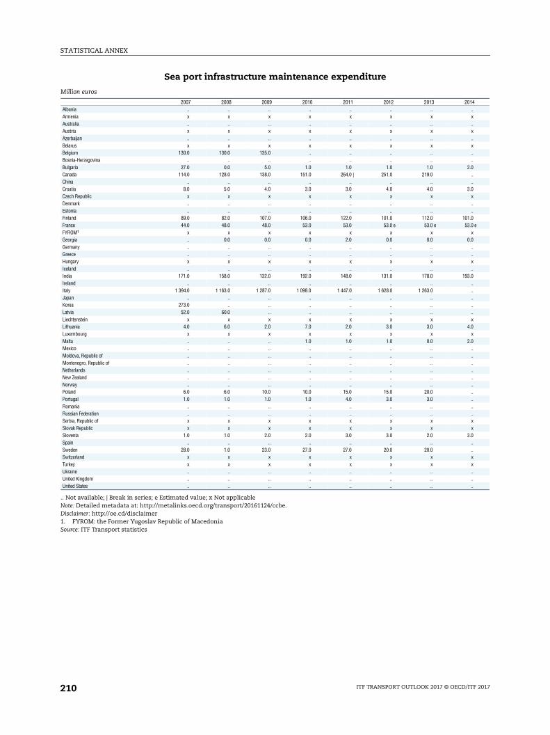
STATISTICAL ANNEX
014..x..x..x....
2.0....
3.0x....
1.03.0 e
x0.0
..
..x..
3.0..........x
4.0x
2.0....................xx
3.0....xx......
Sea port infrastructure maintenance expenditure
.. Not available; | Break in series; e Estimated value; x Not applicableNote: Detailed metadata at: http://metalinks.oecd.org/transport/20161124/ccbe.Disclaimer: http://oe.cd/disclaimer1. FYROM: the Former Yugoslav Republic of MacedoniaSource: ITF Transport statistics
Million euros
2007 2008 2009 2010 2011 2012 2013 2Albania .. .. .. .. .. .. ..Armenia x x x x x x xAustralia .. .. .. .. .. .. ..Austria x x x x x x xAzerbaijan .. .. .. .. .. .. ..Belarus x x x x x x xBelgium 130.0 130.0 135.0 .. .. .. ..Bosnia-Herzegovina .. .. .. .. .. .. ..Bulgaria 27.0 0.0 5.0 1.0 1.0 1.0 1.0Canada 114.0 128.0 138.0 151.0 264.0 | 251.0 219.0China .. .. .. .. .. .. ..Croatia 8.0 5.0 4.0 3.0 3.0 4.0 4.0Czech Republic x x x x x x xDenmark .. .. .. .. .. .. ..Estonia .. .. .. .. .. .. ..Finland 89.0 82.0 107.0 106.0 122.0 101.0 112.0 10France 44.0 48.0 48.0 53.0 53.0 53.0 e 53.0 e 5FYROM1 x x x x x x xGeorgia .. 0.0 0.0 0.0 2.0 0.0 0.0Germany .. .. .. .. .. .. ..Greece .. .. .. .. .. .. ..Hungary x x x x x x xIceland .. .. .. .. .. .. ..India 171.0 158.0 132.0 192.0 148.0 131.0 178.0 19Ireland .. .. .. .. .. .. ..Italy 1 394.0 1 163.0 1 287.0 1 098.0 1 447.0 1 628.0 1 263.0Japan .. .. .. .. .. .. ..Korea 273.0 .. .. .. .. .. ..Latvia 52.0 60.0 .. .. .. .. ..Liechtenstein x x x x x x xLithuania 4.0 6.0 2.0 7.0 2.0 3.0 3.0Luxembourg x x x x x x xMalta .. .. .. 1.0 1.0 1.0 0.0Mexico .. .. .. .. .. .. ..Moldova, Republic of .. .. .. .. .. .. ..Montenegro, Republic of .. .. .. .. .. .. ..Netherlands .. .. .. .. .. .. ..New Zealand .. .. .. .. .. .. ..Norway .. .. .. .. .. .. ..Poland 6.0 6.0 10.0 10.0 15.0 15.0 20.0Portugal 1.0 1.0 1.0 1.0 4.0 3.0 3.0Romania .. .. .. .. .. .. ..Russian Federation .. .. .. .. .. .. ..Serbia, Republic of x x x x x x xSlovak Republic x x x x x x xSlovenia 1.0 1.0 2.0 2.0 3.0 3.0 2.0Spain .. .. .. .. .. .. ..Sweden 28.0 1.0 23.0 27.0 27.0 20.0 20.0Switzerland x x x x x x xTurkey x x x x x x xUkraine .. .. .. .. .. .. ..United Kingdom .. .. .. .. .. .. ..United States .. .. .. .. .. .. ..
ITF TRANSPORT OUTLOOK 2017 © OECD/ITF 2017210
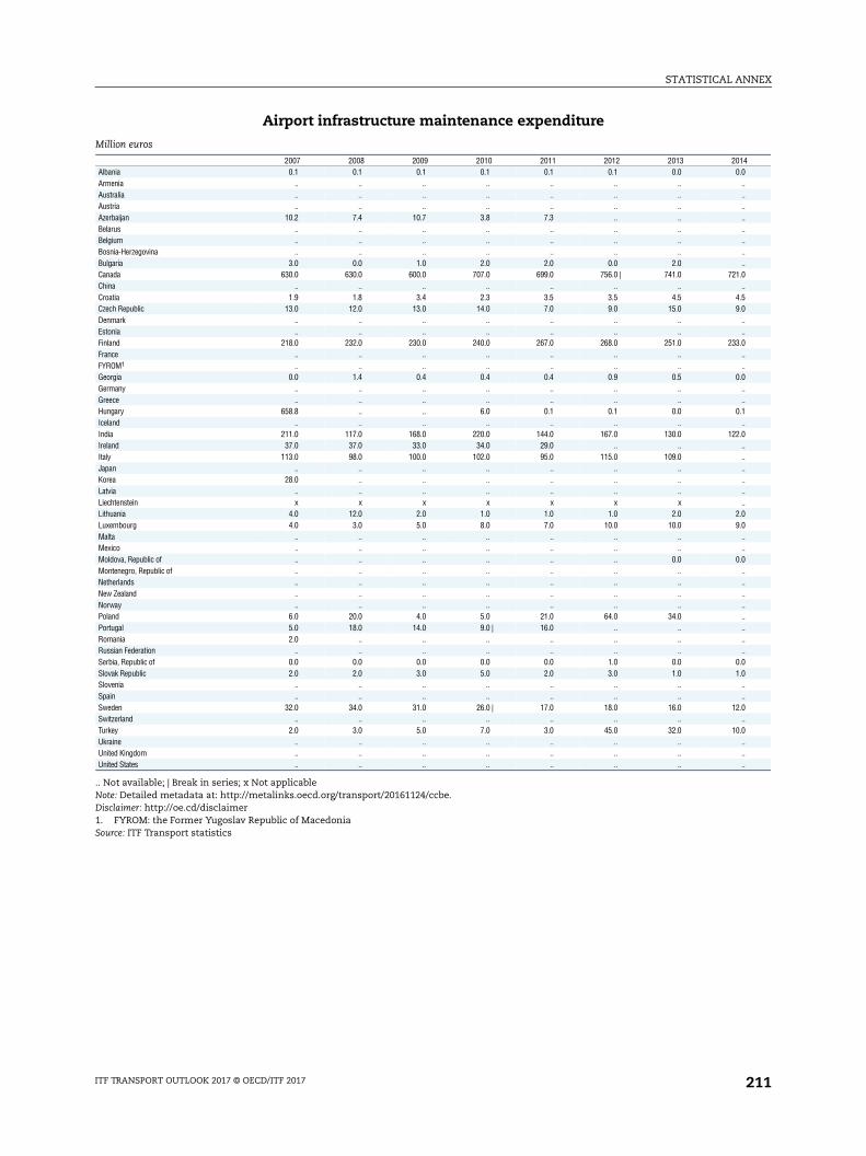
STATISTICAL ANNEX
0140.0
..
..
..
..
..
..
..
..1.0
..4.59.0
..
..3.0
..
..0.0
..
..0.1
..2.0
..
..
..
..
..
..2.09.0
..
..0.0
..
..
..
..
..
..
..
..0.01.0
..
..2.0
..0.0
..
..
..
Airport infrastructure maintenance expenditure
.. Not available; | Break in series; x Not applicableNote: Detailed metadata at: http://metalinks.oecd.org/transport/20161124/ccbe.Disclaimer: http://oe.cd/disclaimer1. FYROM: the Former Yugoslav Republic of MacedoniaSource: ITF Transport statistics
Million euros
2007 2008 2009 2010 2011 2012 2013 2Albania 0.1 0.1 0.1 0.1 0.1 0.1 0.0Armenia .. .. .. .. .. .. ..Australia .. .. .. .. .. .. ..Austria .. .. .. .. .. .. ..Azerbaijan 10.2 7.4 10.7 3.8 7.3 .. ..Belarus .. .. .. .. .. .. ..Belgium .. .. .. .. .. .. ..Bosnia-Herzegovina .. .. .. .. .. .. ..Bulgaria 3.0 0.0 1.0 2.0 2.0 0.0 2.0Canada 630.0 630.0 600.0 707.0 699.0 756.0 | 741.0 72China .. .. .. .. .. .. ..Croatia 1.9 1.8 3.4 2.3 3.5 3.5 4.5Czech Republic 13.0 12.0 13.0 14.0 7.0 9.0 15.0Denmark .. .. .. .. .. .. ..Estonia .. .. .. .. .. .. ..Finland 218.0 232.0 230.0 240.0 267.0 268.0 251.0 23France .. .. .. .. .. .. ..FYROM1 .. .. .. .. .. .. ..Georgia 0.0 1.4 0.4 0.4 0.4 0.9 0.5Germany .. .. .. .. .. .. ..Greece .. .. .. .. .. .. ..Hungary 658.8 .. .. 6.0 0.1 0.1 0.0Iceland .. .. .. .. .. .. ..India 211.0 117.0 168.0 220.0 144.0 167.0 130.0 12Ireland 37.0 37.0 33.0 34.0 29.0 .. ..Italy 113.0 98.0 100.0 102.0 95.0 115.0 109.0Japan .. .. .. .. .. .. ..Korea 28.0 .. .. .. .. .. ..Latvia .. .. .. .. .. .. ..Liechtenstein x x x x x x xLithuania 4.0 12.0 2.0 1.0 1.0 1.0 2.0Luxembourg 4.0 3.0 5.0 8.0 7.0 10.0 10.0Malta .. .. .. .. .. .. ..Mexico .. .. .. .. .. .. ..Moldova, Republic of .. .. .. .. .. .. 0.0Montenegro, Republic of .. .. .. .. .. .. ..Netherlands .. .. .. .. .. .. ..New Zealand .. .. .. .. .. .. ..Norway .. .. .. .. .. .. ..Poland 6.0 20.0 4.0 5.0 21.0 64.0 34.0Portugal 5.0 18.0 14.0 9.0 | 16.0 .. ..Romania 2.0 .. .. .. .. .. ..Russian Federation .. .. .. .. .. .. ..Serbia, Republic of 0.0 0.0 0.0 0.0 0.0 1.0 0.0Slovak Republic 2.0 2.0 3.0 5.0 2.0 3.0 1.0Slovenia .. .. .. .. .. .. ..Spain .. .. .. .. .. .. ..Sweden 32.0 34.0 31.0 26.0 | 17.0 18.0 16.0 1Switzerland .. .. .. .. .. .. ..Turkey 2.0 3.0 5.0 7.0 3.0 45.0 32.0 1Ukraine .. .. .. .. .. .. ..United Kingdom .. .. .. .. .. .. ..United States .. .. .. .. .. .. ..
ITF TRANSPORT OUTLOOK 2017 © OECD/ITF 2017 211
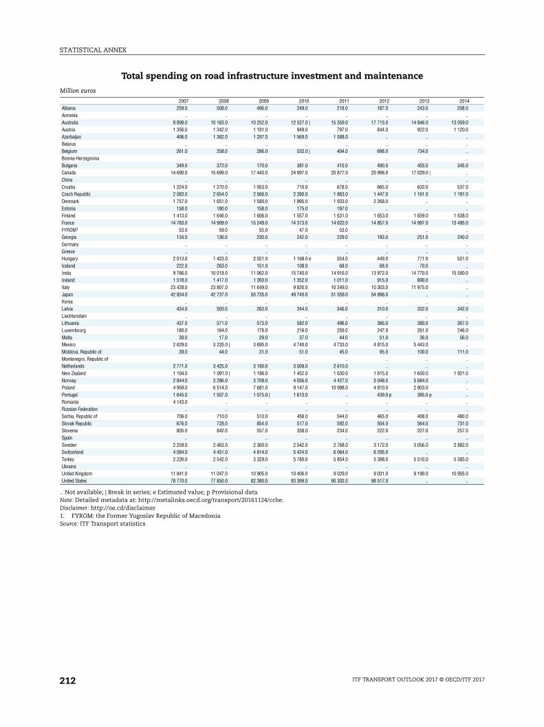
STATISTICAL ANNEX
0148.0
..9.00.0
..
..
..
..5.0
..
..7.01.0
..
..8.05.0
..0.0
..
..1.0
..0.0
..
..
..
..2.0
..7.06.06.0
..1.0
..
..1.0
..
..
..
..
..0.01.07.0
..2.0
..5.0
..5.0
..
Total spending on road infrastructure investment and maintenance
.. Not available; | Break in series; e Estimated value; p Provisional dataNote: Detailed metadata at: http://metalinks.oecd.org/transport/20161124/ccbe.Disclaimer: http://oe.cd/disclaimer1. FYROM: the Former Yugoslav Republic of MacedoniaSource: ITF Transport statistics
Million euros
2007 2008 2009 2010 2011 2012 2013 2Albania 259.0 508.0 496.0 249.0 218.0 187.0 243.0 20Armenia .. .. .. .. .. .. ..Australia 8 899.0 10 163.0 10 252.0 12 527.0 | 15 359.0 17 715.0 14 846.0 13 05Austria 1 356.0 1 342.0 1 181.0 949.0 797.0 844.0 922.0 1 12Azerbaijan 406.0 1 362.0 1 297.0 1 569.0 1 588.0 .. ..Belarus .. .. .. .. .. .. ..Belgium 261.0 258.0 286.0 532.0 | 404.0 698.0 734.0Bosnia-Herzegovina .. .. .. .. .. .. ..Bulgaria 349.0 372.0 170.0 381.0 415.0 490.0 455.0 34Canada 14 690.0 15 699.0 17 443.0 24 097.0 20 877.0 20 996.0 17 029.0 |China .. .. .. .. .. .. ..Croatia 1 224.0 1 270.0 1 053.0 710.0 678.0 665.0 633.0 53Czech Republic 2 083.0 2 654.0 2 566.0 2 390.0 1 863.0 1 447.0 1 161.0 1 19Denmark 1 757.0 1 651.0 1 580.0 1 995.0 1 933.0 2 268.0 ..Estonia 158.0 180.0 158.0 175.0 197.0 .. ..Finland 1 413.0 1 646.0 1 606.0 1 557.0 1 631.0 1 653.0 1 659.0 1 63France 14 783.0 14 909.0 15 249.0 14 373.0 14 622.0 14 857.0 14 997.0 13 49FYROM1 53.0 59.0 55.0 47.0 53.0 .. ..Georgia 134.0 136.0 230.0 242.0 229.0 193.0 251.0 24Germany .. .. .. .. .. .. ..Greece .. .. .. .. .. .. ..Hungary 2 013.0 1 423.0 2 021.0 1 168.0 e 554.0 449.0 771.0 52Iceland 222.0 263.0 151.0 108.0 68.0 68.0 70.0India 9 766.0 10 018.0 11 062.0 15 740.0 14 916.0 13 972.0 14 770.0 15 50Ireland 1 518.0 1 417.0 1 260.0 1 352.0 1 011.0 915.0 690.0Italy 23 428.0 23 807.0 11 649.0 9 826.0 10 349.0 10 303.0 11 975.0Japan 42 934.0 42 737.0 50 735.0 49 740.0 51 559.0 54 896.0 ..Korea .. .. .. .. .. .. ..Latvia 434.0 503.0 263.0 244.0 346.0 310.0 332.0 34Liechtenstein .. .. .. .. .. .. ..Lithuania 437.0 571.0 573.0 582.0 496.0 366.0 380.0 36Luxembourg 180.0 164.0 178.0 216.0 259.0 247.0 261.0 24Malta 38.0 17.0 29.0 37.0 44.0 51.0 36.0 5Mexico 2 629.0 3 235.0 | 3 695.0 4 740.0 4 733.0 4 815.0 5 443.0Moldova, Republic of 39.0 44.0 31.0 51.0 45.0 95.0 100.0 11Montenegro, Republic of .. .. .. .. .. .. ..Netherlands 2 771.0 3 425.0 3 190.0 3 509.0 2 610.0 .. ..New Zealand 1 104.0 1 091.0 | 1 186.0 1 452.0 1 630.0 1 615.0 1 650.0 1 92Norway 2 844.0 3 286.0 3 709.0 4 036.0 4 427.0 5 048.0 5 684.0Poland 4 959.0 6 514.0 7 681.0 9 147.0 10 998.0 4 810.0 2 903.0Portugal 1 645.0 1 507.0 1 075.0 | 1 613.0 .. 439.0 p 385.0 pRomania 4 143.0 .. .. .. .. .. ..Russian Federation .. .. .. .. .. .. ..Serbia, Republic of 706.0 710.0 510.0 458.0 544.0 465.0 408.0 48Slovak Republic 676.0 728.0 854.0 517.0 592.0 504.0 564.0 73Slovenia 805.0 842.0 557.0 358.0 234.0 222.0 227.0 25Spain .. .. .. .. .. .. ..Sweden 2 259.0 2 463.0 2 360.0 2 542.0 2 768.0 3 172.0 3 056.0 2 88Switzerland 4 084.0 4 451.0 4 814.0 5 424.0 6 064.0 6 295.0 ..Turkey 2 226.0 2 542.0 3 329.0 5 780.0 5 854.0 5 398.0 5 510.0 5 38Ukraine .. .. .. .. .. .. ..United Kingdom 11 841.0 11 047.0 10 905.0 10 406.0 9 029.0 9 031.0 9 190.0 10 95United States 78 770.0 77 850.0 82 380.0 93 399.0 90 302.0 98 517.0 ..
ITF TRANSPORT OUTLOOK 2017 © OECD/ITF 2017212
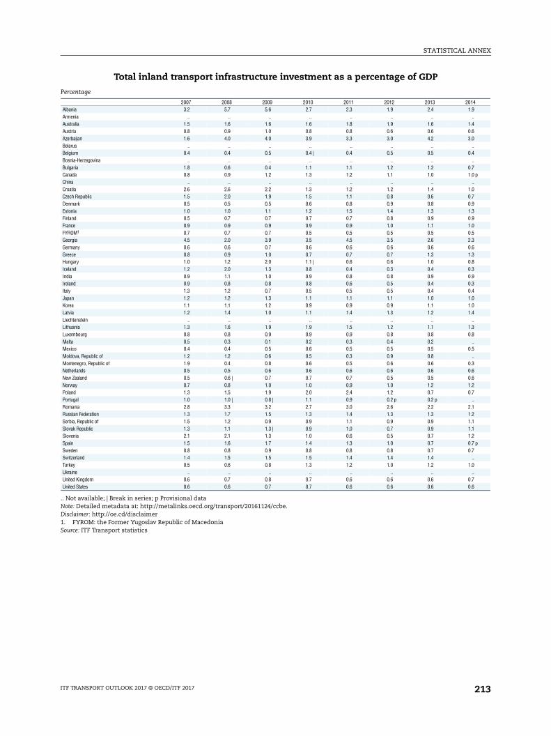
STATISTICAL ANNEX
0141.9
..1.40.63.0
..0.4
..0.71.0 p
..1.00.70.91.30.91.00.52.30.61.30.80.30.90.30.41.01.01.4
..1.30.8
..0.5
..0.30.60.61.20.7
..2.11.21.11.11.20.7 p0.7
..1.0
..0.70.6
Total inland transport infrastructure investment as a percentage of GDP
.. Not available; | Break in series; p Provisional dataNote: Detailed metadata at: http://metalinks.oecd.org/transport/20161124/ccbe.Disclaimer: http://oe.cd/disclaimer1. FYROM: the Former Yugoslav Republic of MacedoniaSource: ITF Transport statistics
Percentage
2007 2008 2009 2010 2011 2012 2013 2Albania 3.2 5.7 5.6 2.7 2.3 1.9 2.4Armenia .. .. .. .. .. .. ..Australia 1.5 1.6 1.6 1.6 1.8 1.9 1.6Austria 0.8 0.9 1.0 0.8 0.8 0.6 0.6Azerbaijan 1.6 4.0 4.0 3.9 3.3 3.0 4.2Belarus .. .. .. .. .. .. ..Belgium 0.4 0.4 0.5 0.4 | 0.4 0.5 0.5Bosnia-Herzegovina .. .. .. .. .. .. ..Bulgaria 1.8 0.6 0.4 1.1 1.1 1.2 1.2Canada 0.8 0.9 1.2 1.3 1.2 1.1 1.0China .. .. .. .. .. .. ..Croatia 2.6 2.6 2.2 1.3 1.2 1.2 1.4Czech Republic 1.5 2.0 1.9 1.5 1.1 0.8 0.6Denmark 0.5 0.5 0.5 0.6 0.8 0.9 0.8Estonia 1.0 1.0 1.1 1.2 1.5 1.4 1.3Finland 0.5 0.7 0.7 0.7 0.7 0.8 0.9France 0.9 0.9 0.9 0.9 0.9 1.0 1.1FYROM1 0.7 0.7 0.7 0.5 0.5 0.5 0.5Georgia 4.5 2.0 3.9 3.5 4.5 3.5 2.6Germany 0.6 0.6 0.7 0.6 0.6 0.6 0.6Greece 0.8 0.9 1.0 0.7 0.7 0.7 1.3Hungary 1.0 1.2 2.0 1.1 | 0.6 0.6 1.0Iceland 1.2 2.0 1.3 0.8 0.4 0.3 0.4India 0.9 1.1 1.0 0.9 0.8 0.8 0.9Ireland 0.9 0.8 0.8 0.8 0.6 0.5 0.4Italy 1.3 1.2 0.7 0.5 0.5 0.5 0.4Japan 1.2 1.2 1.3 1.1 1.1 1.1 1.0Korea 1.1 1.1 1.2 0.9 0.9 0.9 1.1Latvia 1.2 1.4 1.0 1.1 1.4 1.3 1.2Liechtenstein .. .. .. .. .. .. ..Lithuania 1.3 1.6 1.9 1.9 1.5 1.2 1.1Luxembourg 0.8 0.8 0.9 0.9 0.9 0.8 0.8Malta 0.5 0.3 0.1 0.2 0.3 0.4 0.2Mexico 0.4 0.4 0.5 0.6 0.5 0.5 0.5Moldova, Republic of 1.2 1.2 0.6 0.5 0.3 0.9 0.8Montenegro, Republic of 1.9 0.4 0.8 0.6 0.5 0.6 0.6Netherlands 0.5 0.5 0.6 0.6 0.6 0.6 0.6New Zealand 0.5 0.6 | 0.7 0.7 0.7 0.5 0.5Norway 0.7 0.8 1.0 1.0 0.9 1.0 1.2Poland 1.3 1.5 1.9 2.0 2.4 1.2 0.7Portugal 1.0 1.0 | 0.8 | 1.1 0.9 0.2 p 0.2 pRomania 2.8 3.3 3.2 2.7 3.0 2.6 2.2Russian Federation 1.3 1.7 1.5 1.3 1.4 1.3 1.3Serbia, Republic of 1.5 1.2 0.9 0.9 1.1 0.9 0.9Slovak Republic 1.3 1.1 1.3 | 0.9 1.0 0.7 0.9Slovenia 2.1 2.1 1.3 1.0 0.6 0.5 0.7Spain 1.5 1.6 1.7 1.4 1.3 1.0 0.7Sweden 0.8 0.8 0.9 0.8 0.8 0.8 0.7Switzerland 1.4 1.5 1.5 1.5 1.4 1.4 1.4Turkey 0.5 0.6 0.8 1.3 1.2 1.0 1.2Ukraine .. .. .. .. .. .. ..United Kingdom 0.6 0.7 0.8 0.7 0.6 0.6 0.6United States 0.6 0.6 0.7 0.7 0.6 0.6 0.6
ITF TRANSPORT OUTLOOK 2017 © OECD/ITF 2017 213

ITF Transport Outlook 2017 © OECD/ITF 2017
Glossary
2DS scenario: The 2DS scenario of the International Energy Agency (IEA) lays out an
energy system deployment pathway and an emissions trajectory consistent with at least a
50% chance of limiting the average global temperature increase to 2°C. For instance, the
world average on-road fuel efficiency of passenger cars is 4.4 litres gasoline equivalent per
100 kilometres in 2050, down from 6.4 litres in the baseline.
4DS scenario: The 4°C Scenario (4DS) of the International Energy Agency (IEA) takes
into account recent pledges by countries to limit emissions and improve energy efficiency,
which help limit the long-term temperature increase to 4°C. In many respects the 4DS is
already an ambitious scenario, requiring significant changes in policy and technologies.
For example, this corresponds to a global average for on-road fuel efficiency of passenger
cars of 6.4 litres gasoline equivalent per 100 kilometres in 2050 compared to 10.3 litres
gasoline equivalent per 100 kilometres in 2015.
Accessibility: Accessibility is defined as the ease of reaching valued destinations or
opportunities, such as people, jobs, markets, and other services. Accessibility by air
measures the travel time from any city of at least 300,000 inhabitants to an alpha-city,
representing a global centre of economic activity. Accessibility in cities computes the share of
the population that can be reached within 30min by car and public transport respectively
in a given city.
Air service agreement: Agreement between two parties, usually countries, with
respect to the furniture of air services. Such agreements can have provisions on the
maximum allowed frequency, seat capacity, on the airports of operations, on fares or on
the nationality of carriers operating between the two countries.
Asia: All Asian countries excluding Japan and South-Korea, which are part of OECD-
Pacific.
Biofuel: Fuels that are directly or indirectly produced from organic material, i.e.
biomass, such as plant materials or animal waste. Biofuel in this publication here refers to
liquid biofuels, such as ethanol or biodiesel.
Bus Rapid Transit (BRT): Buses running in lanes separated from the general traffic,
with high standards of quality of service, in particular regarding frequency and reliability.
Bulk ship (bulkers): Ships transporting goods in unpackaged bulk, such as grains, coal,
ore or cement.
Car: A road motor vehicle, other than a moped or a motorcycle, primarily designed to
carry one or more persons. This includes SUVs and is equivalent in the text to Passenger
Light Duty Vehicle (PLDV).
City: Used as a generic term to designate all urban agglomerations having more than
300 000 inhabitants. The boundaries of the city in the Outlook tend to go beyond
administrative boundaries (see Urban agglomeration).
215
GLOSSARY
Congestion: The relative travel time loss at peak hour on the road network, due slower
travel speeds as a consequence of high travel demand.
Container ship: A ship fitted throughout with fixed or portable cell guides for the
exclusive carriage of containers.
Domestic non-urban transport: All transport activity within a country, passenger and
freight, excluding transport in cities.
EEA + Turkey: The twenty-eight members of the EU plus Switzerland, Norway, Iceland
and Turkey.
Free-flow speed: Average speed a vehicle can travel according to the road type,
excluding congestion or other constraints (traffic lights, weather conditions etc.).
Herfindahl–Hirschman Index (h-index): Index measuring competition (in this
Outlook, for the aviation market), defined as the sum of the squared market-shares of each
individual firm (in our case, airlines). The h-index varies between 0 and 1, with 0
corresponding to atomistic competition and 1 to a monopolistic situation.
Liquefied natural gas (LNG): Natural gas consists mainly of methane occurring
naturally in underground deposits, associated with crude oil or gas recovered from coal
mines (colliery gas). To facilitate its transportation, natural gas may be converted to liquid
form by reducing its temperature to160°C under atmospheric pressure. It then becomes
liquefied natural gas (LNG).
Local pollutants: Elements of ambient air pollution, including emissions of mono-
nitrogen oxides (NOx), sulphate (SO4) and fine particulate matter (PM2.5).
Low-cost carrier (LCC): Air carrier which offers lower fares in exchange for lower
comfort. Extras, such as food on board, checked-in luggage or seat placement usually
generate additional fees. Low-cost carriers share some cost-cutting practices, such as
having a single type of aircraft or maximising aircraft usage by flying only short distances.
Mass transit: Bus Rapid Transit (BRT) or urban rail (metro included).
Mega-ship: Very large container ship with a capacity larger than 13 000 TEU.
Middle East: Middle East including Israel.
Mode: Contrasting types of transport service relevant to the comparison being made:
e.g. road, rail, waterway, air or private car, powered two-wheelers, bus, metro, urban rail.
Mode split/mode share: Percentage of total passenger-kilometres accounted for by a
single mode of transport; percentage of total freight tonne-kilometres or tonnes lifted
accounted for by a single mode.
MoMo model: The IEA Mobility Model is global transport spreadsheet model
containing detailed by-mode, by-fuel and by-region historical data and projections to 2050
for the transport sector, related energy use and greenhouse gas emissions.
Motorcycle: Powered two-wheeled vehicles, motorcycles and scooters, equivalent in
this text to two-wheelers.
New Policy Scenario: The New Policies Scenario serves as the IEA baseline scenario. It
takes account of broad policy commitments and plans that have been announced by
countries, including national pledges to reduce greenhouse-gas emissions and plans to
phase out fossil-energy subsidies, even if the measures to implement these commitments
have yet to be identified or announced.
Non-motorised modes: Walking and biking.
ITF TRANSPORT OUTLOOK 2017 © OECD/ITF 2017216
GLOSSARY
North America: United States and Canada. Mexico is part of Latin-America in this
report.
OECD Pacific: Australia, Japan, New Zealand and South Korea.
Passenger-kilometre (pkm): Unit of measurement for passenger transport activity
representing the transport of one passenger over a distance of one kilometre.
Revenue Passenger Kilometre: Measure of passenger traffic: number of paying
passengers multiplied by the kilometres flown
Shared mobility: Large-scale deployment of shared vehicle fleets providing on-
demand transport.
Urban agglomeration: The city and its surrounding areas based on contiguous built-
up land.
Tankers: Ships transporting liquid cargo, especially oil and oil products.
TEU (Twenty-foot Equivalent Unit): A statistical unit based on an ISO container of
20 foot length (6.10 m) to provide a standardised measure of containers of various capacities
and for describing the capacity of container ships or terminals. One 20 Foot ISO container
equals 1 TEU.
Three-wheeler: Powered three-wheeled vehicles, such as auto-rickshaws in India.
Tonne-kilometre (tkm): Unit of measurement of goods transport which represents the
transport of one tonne of goods over a distance of one kilometre.
Transition economies: Former Soviet Union countries and Non-EU South-Eastern
Europe.
Transit-oriented development: A dense development with access to public transport
in walking distance and characterised by a mix of residential, employment, commercial
and other uses.
Two-wheelers: Powered two-wheeled vehicles, motorcycles and scooters. Equivalent
in this text to motorcycles.
Vehicle-kilometre: A unit of measurement for transport demand, freight and
passenger, representing any movement of a vehicle over a distance of one kilometre.
ITF TRANSPORT OUTLOOK 2017 © OECD/ITF 2017 217


ITF Transport Outlook 2017 © OECD/ITF 2017
List of acronyms
ACI Airport Council International
ADB Asian Development Bank
BAU Business as usual
BRT Bus Rapid Transit
CORSIA Carbon Offsetting and Reduction Scheme for International Aviation
ECLAC Economic Commission for Latin America
EEA European Economic Area
EFTA European Free Trade Area
FIA Fédération International de l’Automobile (International Automobile Federation)
GDP Gross Domestic Product
GIS Geographical Information Systems
GTFS General Transit Feed Specification
HSR High-speed rail
IATA International Air Transport Association
ICAO International Civil Aviation Organisation
ICCT International Council for Clean Transportation
IEA International Energy Agency
IMF International Monetary Fund
IMO International Maritime Organisation
IRF International Road Federation
IRTAD International Traffic Safety Data and Analysis Group
ITDP Institute for Transportation and Development Policy
ITF International Transport Forum
JICA Japan International Cooperation Agency
LCC Low-cost carrier
LNG Liquefied natural gas
LUT Integrated Land Use and Transport Planning (scenario for Chapter 5)
MBM Market-based measure
MTEU Million Twenty Foot Equivalent Unit
OSM OpenStreetMap
PLDV Passenger Light Duty Vehicle
PnT People near Transit
PPP Purchasing power parity
ROG Robust Governance (scenario for Chapter 5)
SDG Sustainable Development Goals
TEU Twenty Foot Equivalent Unit
TOD Transit-Oriented Development
UITP International Association of Public Transport
219

LIST OF ACRONYMS
UNCTAD United Nations Committee for Trade and Development
UNFCCC United Nations Framework Convention on Climate Change
USA United States of America
VKM Vehicle-kilometre
WBCSD World Business Council on Sustainable Development
WTO World Trade Organisation
ITF TRANSPORT OUTLOOK 2017 © OECD/ITF 2017220
ORGANISATION FOR ECONOMIC CO-OPERATION AND DEVELOPMENT
The OECD is a unique forum where governments work together to address the economic, social and
environmental challenges of globalisation. The OECD is also at the forefront of efforts to understand and
to help governments respond to new developments and concerns, such as corporate governance, the
information economy and the challenges of an ageing population. The Organisation provides a setting
where governments can compare policy experiences, seek answers to common problems, identify good
practice and work to co-ordinate domestic and international policies.
The OECD member countries are: Australia, Austria, Belgium, Canada, Chile, the Czech Republic,
Denmark, Estonia, Finland, France, Germany, Greece, Hungary, Iceland, Ireland, Israel, Italy, Japan, Korea,
Latvia, Luxembourg, Mexico, the Netherlands, New Zealand, Norway, Poland, Portugal, the Slovak Republic,
Slovenia, Spain, Sweden, Switzerland, Turkey, the United Kingdom and the United States. The European Union
takes part in the work of the OECD.
OECD Publishing disseminates widely the results of the Organisation’s statistics gathering and
research on economic, social and environmental issues, as well as the conventions, guidelines and
standards agreed by its members.
THE INTERNATIONAL TRANSPORT FORUM
The International Transport Forum is an intergovernmental organisation with 57 member countries.
It acts as a think tank for transport policy and organises the Annual Summit of transport ministers. ITF is
the only global body that covers all transport modes. The ITF is politically autonomous and administratively
integrated with the OECD.
The ITF works for transport policies that improve peoples’ lives. Our mission is to foster a deeper
understanding of the role of transport in economic growth, environmental sustainability and social inclusion
and to raise the public profile of transport policy.
The ITF organises global dialogue for better transport. We act as a platform for discussion and pre-
negotiation of policy issues across all transport modes. We analyse trends, share knowledge and promote
exchange among transport decision-makers and civil society. The ITF’s Annual Summit is the world’s
largest gathering of transport ministers and the leading global platform for dialogue on transport policy.
The Members of the Forum are: Albania, Armenia, Argentina, Australia, Austria, Azerbaijan, Belarus,
Belgium, Bosnia and Herzegovina, Bulgaria, Canada, Chile, China (People’s Republic of), Croatia, Czech
Republic, Denmark, Estonia, Finland, France, Former Yugoslav Republic of Macedonia, Georgia, Germany,
Greece, Hungary, Iceland, India, Ireland, Israel, Italy, Japan, Korea, Latvia, Liechtenstein, Lithuania,
Luxembourg, Malta, Mexico, Republic of Moldova, Montenegro, Morocco, the Netherlands, New Zealand,
Norway, Poland, Portugal, Romania, Russian Federation, Serbia, Slovak Republic, Slovenia, Spain, Sweden,
Switzerland, Turkey, Ukraine, the United Kingdom and the United States.
OECD PUBLISHING, 2, rue André-Pascal, 75775 PARIS CEDEX 16
(74 2017 01 1 P) ISBN 978-92-82-10799-7 – 2017
ITF Transport Outlook 2017
ITF Transport Outlook 2017The ITF Transport Outlook provides an overview of recent trends and near-term prospects for the transport sector at a global level. It also presents long-term projections for transport demand to 2050 for freight (maritime, air and surface) and passenger transport (car, rail and air) as well as related CO2 emissions, under different policy scenarios.
This edition specifically looks at how the main policy, economic and technological changes since 2015, along with other international developments such as the UN Sustainable Development Goals, are shaping the future of mobility. A special focus on accessibility in cities highlights the role of policies in shaping sustainable transport systems which provide equal access to all.
Contents
Part I. Global Outlook for transport
Chapter 1. The transport sector today
Chapter 2. Transport demand and CO2 emissions to 2050
Part II. Sectorial Outlook
Chapter 3. International freight
Chapter 4. International passenger aviation
Chapter 5. Mobility in cities
ISbn 978-92-82-10799-774 2017 01 1 P
Consult this publication on line at http://dx.doi.org/10.1787/9789282108000-en.
This work is published on the OECD iLibrary, which gathers all OECD books, periodicals and statistical databases. Visit www.oecd-ilibrary.org for more information.
9HSTCSC*bahjjh+
ITF Tran
spo
rt Ou
tloo
k 2017