its-related transport concepts and organisations ... · ejtir 18(1), 2018, pp.91-111 92 ma and...

EJTIR Issue 18(1), 2018

pp. 91-111

ISSN: 1567-7141 http://tlo.tbm.tudelft.nl/ejtir

Bayesian networks for constrained location choice modeling using structural restrictions and model averaging

Tai-Yu Ma1 Luxembourg Institute of Socio-Economic Research, Luxembourg

Sylvain Klein 2 Luxembourg Institute of Socio-Economic Research, Luxembourg

In this work, we propose a Bayesian network approach by using structural restrictions and a

model averaging algorithm for modeling the location choice of discretionary activities. In a first stage, we delimit individuals’ location choice which is set by generating an ellipse that uses empirical detour factors and a home-work axis. The choice set is further refined by an individual’s space-time constraints in order to identify the constrained destination choice set. We use structural restrictions and a model averaging method to learn the network structure of the Bayesian network in order to predict the heuristics of individuals’ location selection. The empirical study shows the proposed method can effectively obtain Bayesian networks with a consistent dependency structure. The empirical study suggests activity schedule factors significantly influence location choice decisions. Keywords: Location choice, Choice set generation, Bayesian networks, Structure learning, Space-time behaviour

1. Introduction

A Bayesian network (BN) is a graphic probabilistic model for representing conditional dependency between a set of random variables. It has been widely applied in bioinformatics, engineering, data mining, etc., for diagnosis, inference and prediction under uncertainty (Friedman et al. 2000, Margaritis 2003, Sachs et al., 2005). A BN is a direct acyclic graph characterized by its topological structure and probability distributions associated with the nodes. The theoretical development of BNs is due to the significant contributions of Pearl (1988, 2009). As a statistical model, BNs involve two learning tasks: structure learning and parameter learning. The first task concerns identifying the typology (dependency structure) of BNs with the presence or absence of arcs, and the second concerns estimating the parameters (marginal /conditional probability distributions) in the graph.

It has been proven that finding exact dependency structures for BNs is an NP hard problem (Cooper, 1990; Dagum and Luby, 1993). As a result, different structure learning heuristics have been proposed (Koller and Friedman, 2013). These methods can be classified into three categories: 1) score-based approach, 2) constraint-based approach, and 3) hybrid approach. The score-based approach consists of finding a BN with the highest fitness scores. Methods proposed in this

1 A: LISER, 11 Porte des Sciences, 4366 Esch-sur-Alzette, Luxembourg T: +352 585 855 308 F: +352 585 855 700 E: [email protected] 2 A: LISER , 11 Porte des Sciences, 4366 Esch-sur-Alzette, Luxembourg T: +352 585 855 310 F: +352 585 855 700 E: [email protected]

https://www.tudelft.nl/en/tpm/about-the-faculty/departments/engineering-systems-and-services/research/ejtir/

mailto:tai-yu.ma@

EJTIR 18(1), 2018, pp.91-111 92

Ma and Klein Bayesian networks for constrained location choice modeling using structural restrictions and model averaging

category include the Hill-Climbing algorithm and the Tabu search algorithm (Bouckaert, 1995). These methods use some score functions to measure the fitness between data and the model. A greedy search strategy is generally used to find a BN with the highest fitness score in the search space. In opposition to the score-based approach, the constraint-based approach applies a sequence of conditional independence tests to evaluate independence relationships between variables and then to build a BN accordingly. Methods in this category include the inductive causation algorithm (Verma and Pearl 1990, 1992), GS algorithm (Margaritis, 2003), IAMB algorithm (Tsamardinos et al., 2003a), Inter-IAMB algorithm (Yaramakala and Margaritis, 2005), and MMPC algorithm (Tsamardinos et al., 2003b). In these methods, the Markov blanket detection algorithms and stepwise forward selection scheme are used to reduce the number of conditional independence tests in the graph. As regards the hybrid approach, it uses constraints to reduce the search space at a first stage and then the score-based approaches can be used to find an optimal BN structure in the pruned space. The MMHC and RSMAX2 are two representative algorithms in this category (Tsamardinos et al. 2006).

Despite the computational complexity of these algorithms in finding a dependency structure from data, the robustness of the obtained BN might be considered a drawback. For this issue, certain techniques based on bootstrap resampling and the model averaging approach have been proposed in order to identify a statistically-sound BN structure from the data (Claeskens and Hjort 2008; Efron and Tibshirani, 1993; Scutari and Nagarajan, 2013). Moreover, past studies have shown that using structural restrictions based on expert prior knowledge for the learning of BN structures from data can effectively improve the obtained network structures (de Campos and Castellano, 2007; Ma et al., 2016). Hence, we propose a hybrid structure learning approach by combining the aforementioned techniques in learning BN structures and applying them to the location choice modeling of the discretionary activity of commuters. Note that in transportation research, BNs have been applied for travel-activity pattern generation (Janssens et al. 2004, 2006), travel mode choice modeling (Xie and Waller, 2010; Ma 2015; Ma et al. 2016), synthetic population generation (Sun and Erath, 2015) and automatic transport mode detection from GPS-data (Xiao et al., 2015). However, identifying the network structure of Bayesian networks from data is still an active research area in machine learning and artificial intelligence research areas.

Two contributions are made in this paper. Firstly, we propose a location choice set generation method using empirical detour factors of individuals’ home-work axis and space-time constraints to delimit possible choice alternatives. The empirical study shows the proposed method can effectively generate choice alternatives containing observed ones with a high matching rate and at the same time keeping the choice set size reasonable. Secondly, we propose a hybrid learning algorithm of the BN structure for predicting individuals’ heuristic rules of selecting discretionary activity location by using structural restrictions from prior knowledge and a model averaging approach. Several experiments are designed to test the influence of model parameters in the obtained network structures.

The remainder of the paper is organized as follows. Section 2 presents the literature review in location choice modeling of discretionary activities. Section 3 proposes a hybrid structure learning method of Bayesian networks based on structural restrictions and the model averaging approach. In Section 4, we present the empirical data used in this study. The list of determinants for location choice modeling is discussed. We propose a location choice set generation method based on the empirical detour factor and space-time constraints of individuals. For location choice modeling, we test the proposed structure learning algorithms on the obtained results and compare its performance with other classification methods. Three experiments and a sensitivity analysis are conducted to test the influence of model parameters on the obtained network structure. Finally, conclusions are drawn and future extensions are discussed.

EJTIR 18(1), 2018, pp.91-111 93


2. Literature on location choice modeling

Location choice modeling of activities has received increasing interest within the transportation research community (Kitamura, 1984; Arentze and Timmermans, 2007; Scott and He, 2012). Unlike mode choice decision making, location choice is more complicated due to the issue of how to generate choice alternatives in the individual’s choice set. The researcher usually uses a two-step procedure by first generating a constrained location choice set and then applying discrete choice models such as the multinomial logit models to predict individuals’ location choices (Arentze and Timmermans 2005; Scott and He, 2012). For the activity location choice set, it is assumed spatial choice behavior is generally guided by a person’s space-time constraints (available travel time budget, opening hours of stores, etc.), activity scheduling, mode of transport and socio-demographic attributes (Thill, 1992; Scott and He, 2012; Arentze et al., 2013). Disregard of this stage would produce a biased estimation due to non-negative probabilities assigned to unrealistic choice alternatives.

For this purpose, the potential path area method (Miller, 1991; Kwan and Hong 1998; Yoon et al. 2012; Scott and He 2012) computes ‘reachable’ zones (areas) from an origin under available travel time budget for that trip. A location choice set is delimited by selecting reachable zones with non-zero opportunities of activity. The implementation of the potential path area method requires additional data in terms of the spatial distribution of activity opportunities and the transportation network. Another important aspect in the location choice set generation of individuals is considering sequential activity locations in a trip chaining context. The detour time from/to locations of fixed activities influence individuals’ discretionary activity location choice (Kitamura, 1984). Kitamura et al. (1998) found that time of day and duration of stay at activity location influences location choice. Generating activity location chose set needs to incorporate both space-time constraints and the sequence of activity locations.

As regards the discrete choice modeling of activity location, most studies applied the multinomial logit model or constrained logit models (Martínez et al. 2009; Scott and He, 2012). The determinants are related to attractiveness of activity location, travel time to destination, available time for activity and person/household situations (Ettema and Timmermans, 2007; Bernardin et al. 2009; Scott and He, 2012). In contrast to the discrete choice modeling framework based on random utility theory, some heuristic rule-based approaches have been proposed. For example, Arentze and Timmermans (2005, 2007) applied a classification and regression tree (CART) for shopping location choice modeling. The authors found individuals’ activity schedule limits feasible time-windows for location choice. Moreover, they used space-time constraints revealed in travel diary data for constrained location choice set generation and then applied the CART method for estimating the decision tree which best describes the observation. The reader is referred to some recent studies in activity location choice modeling (Scott and He, 2012; Huang and Levinson, 2015; Arentze et al. 2013).

3. Proposed Bayesian networks approach based on structural restrictions and model averaging approach

In this section, we firstly present the hybrid structure learning algorithm of Bayesian networks for identifying heuristic rules used for individuals’ location choice decisions. The choice set generation method and its empirical study will be presented in Section 4.2.

The proposed structure learning algorithm comprises two steps. In the first step, we obtain absence/existence relationships between some explanatory variables based on our prior knowledge and then use them as structure restrictions in the network structure learning. By doing so, the obtained BNs would be more consistent with known dependency relationships of

EJTIR 18(1), 2018, pp.91-111 94


variables and reduce the size of search space. The second step consists of applying a model averaging approach to obtain a robust BN. The proposed method is described as follows.

Proposed algorithm

1. Input an empirical data D and a set of variables V. Set up restriction relationships (existence or absence of dependent/causal relationships between pairs of variables and ordering relationships of a set of variables) based on expert knowledge and prior knowledge.

2. Generate randomly n datasets from D by bootstrap methods (Efron and Tibshirani, 1993). Set unknown true BNs be empty, i.e. 𝑆∗(𝑿∗, 𝑨∗) = ∅, where 𝑿∗ is a set of nodes and 𝑨∗ a set of directed arcs.

3. For each data set 𝐷𝑖 , 𝑖 = 1, … , 𝑛, learn a best-fit BN by using the score-based, constraint-based or hybrid learning algorithms (Koller and Friedman, 2013). Note that the presence of arcs and the direction of arcs are determined by some fitness scores (e.g. BIC score) according to implied learning algorithms. Let 𝑆𝑖(𝑿𝑖, 𝑨𝒊), 𝑖 = 1, … , 𝑛 denote the learned BNs where 𝑿𝑖 is the set of nodes and 𝑨𝒊 is the set of arcs in the graph.

4. Evaluate the empirical probability that each arc belongs to the unknown true BN as

�̂�(𝑎) =1

𝑛∑ 𝛿{𝑎∈𝑨𝒊}

𝑛𝑖=1 (1)

where 𝛿{𝑎∈𝑨𝒊} is an indicator function if an arc a belong to the learned BN 𝑨𝒊 , and 0

otherwise. The empirical probability represents the degree of belief �̂�(𝑎) that an arc belong to the true BN. If the degree of belief of an arc a, �̂�(𝑎), is greater than a significance threshold 𝛽, then a is retained in the true structure.

5. As the true BN is unknown, we need a statistical method to determine 𝛽. For this

purpose, we order the beliefs of arcs by ascending order as 𝐩 = {0 ≤ �̂�(𝑎1) ≤ �̂�(𝑎2) ≤

… ≤ �̂�(𝑎𝑘) ≤ ⋯ ≤ �̂�(𝑎𝑛𝑘) ≤ 1}. Let �̃� = {0,0, … ,0,1,1,… ,1} be the set of indicators

characterizing whether an arc in 𝐩 is significant (1) or non-significant (0). The proportion of 1s is determined by a parameter t, which is based on the solution of minimization of the 𝐿1-norm distance between the cumulative distribution functions of �̂� and �̃� (Scutari and Nagarajan, 2013). The 𝐿1-norm distance is defined as

𝐿1(𝑡; �̂�) = ∫|𝐹𝒑(𝒙) − 𝐹𝒑(𝒙; 𝑡)|𝑑𝑥 (2)

where 𝐹𝒑(𝒙) and 𝐹𝒑(𝒙; 𝑡) are the empirical cumulative distribution functions of �̂� and �̃�,

respectively, defined as

𝐹𝒑(𝑥) =1

𝑛𝑘

∑ 1{𝑝(𝑎𝑖 )<𝑥}𝑛𝑘

𝑖=1 (3)

𝐹𝒑(𝒙) = {0𝑡1

ififif

𝑥 ∈ (−∞, 0)𝑥 ∈ [0,1)

𝑥 ∈ [1, +∞) (4)

where 𝑛𝑘 of (3) is the number of elements in �̂�.

The optimal 𝑡, �̂�, which minimizes the 𝐿1-norm distance is defined as

�̂� = argmin𝑡 𝐿1(𝑡; �̂�) (5)

EJTIR 18(1), 2018, pp.91-111 95


The significance threshold 𝛽 is the inverse function of �̂� , i.e. 𝛽 = 𝐹𝒑−1(�̂�). Based on the

significance threshold 𝛽, an arc 𝑎𝑖 is retained in the true structure if its belief of arcs �̂�𝑎𝑖 is

greater than 𝛽 (see Figure 1), i.e.

𝑎𝑖 ∈ 𝐴∗ if �̂�𝑎𝑖> β (6)

As regards the fitness score, the BDeu score (Heckerman et al., 1995) and BIC score (Schwarz

1978) are two widely-used fitness scores for the structure learning of BNs. The higher the fitness

score is, better the model fits the data. The reader is referred to Koller and Friedman. (2013) for a

more detailed description.

Figure 1. Empirical cumulative distribution functions 𝐹𝒑(𝑥) (points) and 𝐹𝒑(𝒙) (dashed line).

4. Experiment

In this section, we apply the proposed learning algorithm to predict heuristic rules of selecting the locations of daily discretionary activities of individuals. We assume individuals use some simple heuristics to select their discretionary activity location. These heuristics represent the trade-off between travel time and the attractiveness of locations (Arentze and Timmermans 2005, 2007). Firstly, we present the empirical data and the proposed detour-factor based space-time constrained method for activity location choice set generation. Then we apply the proposed algorithm to learn a statistically-sound BN for predicting the heuristic rules. Three experiments are conducted with respect to the effects of structural restrictions, resampling size and embedded learning algorithms on the performance of the obtained BNs. The validation of the proposed method is based on a 5-fold cross validation method.

4.1 Data and preliminary analysis The empirical data used is a one-day travel diary data for the cross-border workers of Luxembourg in 2011-2012 (Enaux and Gerber, 2014; Ma et al. 2016). The survey area contains three cross-border areas of Luxembourg in Germany, France and Belgium. A total of 7235 respondents’ daily mobility data was collected, representing a response rate of 18%. We limit ourselves by using the sample drawn from the France-Luxembourg cross border area only (955 individuals). The empirical survey data contains individuals’ socio-demographic characteristics, trip purpose, destination at the level of municipality (also called zone interchangeably), travel time, transport mode, departure time, etc.

EJTIR 18(1), 2018, pp.91-111 96


Initial trip purposes in the survey can be distinguished as location-fixed activities, including 1) home, and 2) work, and location-flexible activities (or discretionary activities), including 3) Pick-up/drop-off, 4) Going out for food, 5) Shopping 6) Personal business (visit to doctor, bank, training, etc.), 7) Social activity (visiting family / friends) and 8) Walking or taking a ride, 9) Leisure, sport or culture, 10) Others. We focus on discretionary activity location choice modeling at the level of the municipality as it is the level of detail in the survey. After the data clearing process, there remained a total of 1553 trips involving discretionary activities (955 cross-border workers) used for this study. The descriptive statistics of the sample is shown in Table 1. Males represent 51% of the sample. The average age is around 39 years old. Approximately 77% of individuals live as a couple. The average household income is within 3000-6000 euros. The average number of children in the household is 0.9. 82% of the respondents have a full-time job. As regards mobility, the average number of cars in the household is 1.9 and average number of trips is 4.4 trips/day. The average daily total travel time is around 140 minutes due to high car usage (78%) and also due to frequent traffic congestion in Luxembourg and its cross-border area. As regards the purpose of discretionary activities, pick up/drop offs are the main purpose (48.1%), going out for food (19.7%) and shopping (14.3) are the second most frequent purposes. Personal business (visit to doctor, bank, training, etc.) accounts for about 5.7% and the other purposes are less than 5%. The spatial distribution of the sample in the studied area is shown in Figure 2. It includes Luxembourg and the cross-border area on the French side. As shown in Figure 2 (left), workplace of the sample is mainly located in Luxembourg City. The location of discretionary activities of the sample is in line with their home location or workplace.

Figure 2. Spatial distribution of the locations of residence, workplaces and discretionary activities in the Luxembourg case study area. Left: locations of home and workplace; Right: locations of discretionary activities.

EJTIR 18(1), 2018, pp.91-111 97


Table 1. Descriptive statistics of the sample

Variable Mean Std. Dev.

Gender 0.51 0.50

Age 38.73 7.98

Couple 0.77 0.42

Number of persons in the household 3.09 1.19

Number of children in the household 0.91 0.94

Fulltime job 0.82 0.39

Number of cars in the household 1.94 0.74

Number of trips per day 4.38 1.39

Daily total travel time (minute) 139.36 48.59

Transport mode of trip

Foot Motorbike/bicycle

Car PT

17.7% 0.3%

77.9% 4.1%

Trip purpose of discretionary activity

1 Pick-up/drop-off

3 Going out for food 4 Shopping

5 Personal business (visit to doctor, bank, training etc.) 6 Social activity (visiting family / friends)

7 Walking or taking a ride

8 Leisure, sport or culture 10 Others

48.10%

19.70% 14.29%

5.67% 3.28%

1.93%

4.06% 2.96%

The conceptual framework of location choice determinants is shown in Figure 3. The location

choice set is determined by the spatial setting (activity locations, attractiveness and accessibility

of zones, etc.) and temporal constraints (opening hours of stores, individuals’ activity schedule

and available travel time to reach that location). Location choice set of individuals is determined

by their potential reachable area under individuals’ space-time constraints and their transport

mode availability (described later). As empirical location choice set is generally unavailable, the

researcher may apply the space-time constraint methods to generate the location choice set with a

large number of alternatives (Miller, 1991; Kwan and Hong, 1998). This may raise theoretical and

computational concerns by applying the random utility theory for location choice modeling

(Guevara and Ben-Akiva, 2013). Instead, we adopt an alternative approach that predicts the

heuristic rules used by individuals to select their location (Arentze and Timmermans 2005, 2007).

We define 6 heuristic rules, from the simplest to the more complicated, for selecting discretionary

activity locations as: 1) to minimize travel time from current location, 2) maximizing

attractiveness, 3) minimizing travel time to the work place, 4) minimizing travel time to home

location, 5) random non-dominated choice based on the two criteria (time and attractiveness) and

6) others. The first rule assumes individuals tend to select a nearby location to reduce undesired

travel time. The second rule assumes the attractiveness of location, measured by number of

activity-type-specific opportunities (registered shops etc.) in a zone, plays the most important

role in their decision. The third and fourth rules consider trip chaining behavior (home-based

tour / workplace based tour) by assuming a minimum travel time rule of selecting locations.

Rule 5 assumes a second-best choice behavior based on the criteria of travel time and

attractiveness of location. Rule 6 summarizes all other reasons. Note that an observed location

choice may satisfy several heuristics. In that case, we assign only one rule by assuming simpler

rules are preferred.

EJTIR 18(1), 2018, pp.91-111 98


Figure 3. Conceptual framework of location choice determinants (Arentze and Timmermans, 2005)

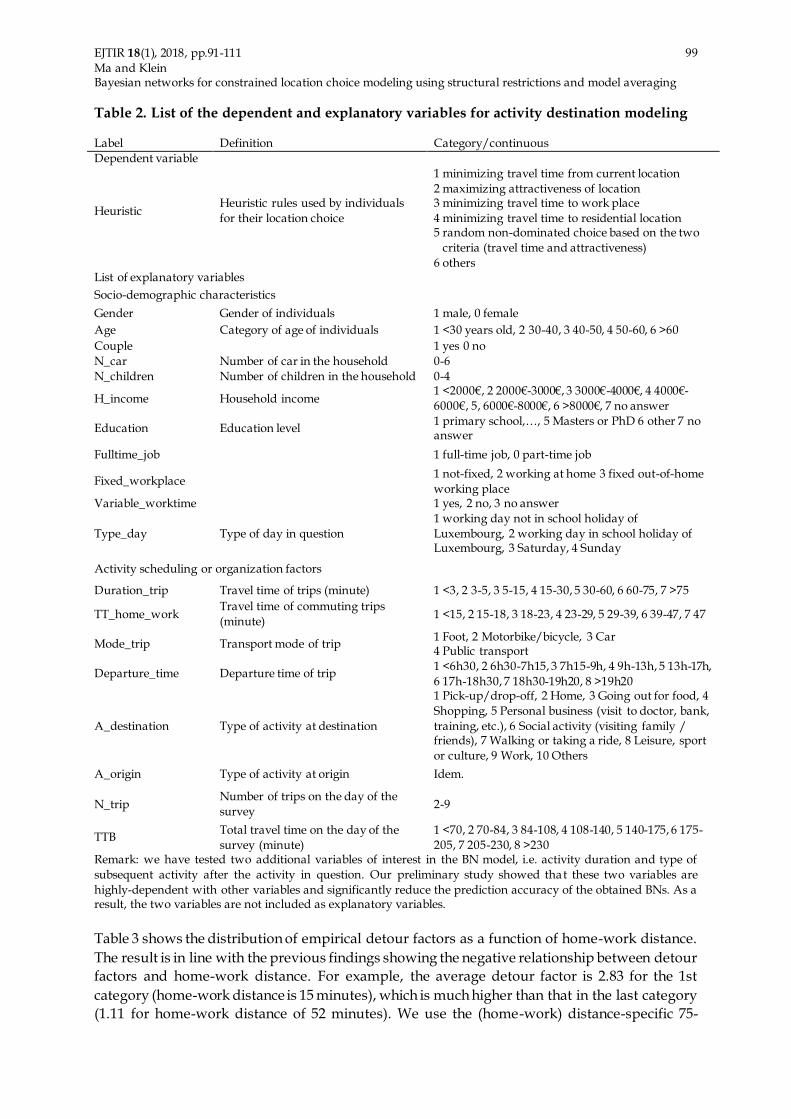
As regards the determinants of location choice of discretionary activities, they are selected by

individual and household situations, schedule context and spatial-temporal constraints of

individuals. The final retained 19 explanatory variables for the BNs is listed in Table 2. The

dependent variable is the heuristic rule of selecting locations. We collected spatial attractiveness

data in terms of number of opportunities (stores) in each municipality of the studied area,

including shopping (supermarkets, shopping malls, etc.), leisure activity, restaurants, personal

business (bank, pharmacy, post-office, etc.). Moreover, transportation network data is used for

computing mode-specific travel time matrices between origins and destinations in the studied

area. Note that the continuous variables are discretized to learn the discrete BNs by the quantile-

based discretization methods (Scutari and Denis 2014).

4.2 Location choice set generation We generate each individual’s location choice set based on the assumption that discretionary

activity locations are generally situated around the axis of home and work locations and within

available travel time constraints for reaching the destination (Kwan and Hong, 1998). The

proposed method is a two-step procedure: in the first step, we delimit a larger potential location

choice set, also called potential path area, around the home-work axis based on an empirical

detour factor; in the second step, selecting feasible location alternatives within the potential path

area based on observed travel time of trips and used mode of transport of trips.

In the literature, the detour factor is defined as “the spatial deviation an individual makes to

conduct a discretionary activity” (Justen et al, 2013). Instead of using the straight-line distance as

measurement, we use shortest path travel time during off-peak hours to reflect better the

“distance” in terms of travel time taken to conduct a discretionary activity. Unless otherwise

stated, the ‘distance’ is related to this measurement. We calculate the detour factor as the ratio of

home-work location distance and distance summation of observed activity location to home and

work locations. The empirical study (Justen et al. 2013) showed that the higher home-work

distance is, the lower the detour factors an individual is willing to travel to participate in an

activity. Moreover, the authors showed the empirical detour factors can be used to compute a

home-work centered ellipse to delimit the choice set of discretionary activities. This method has

been shown to be able to generate a choice set covering observed location choices and

considerably reducing choice set size.

EJTIR 18(1), 2018, pp.91-111 99


Table 2. List of the dependent and explanatory variables for activity destination modeling

Label Definition Category/continuous

Dependent variable

Heuristic

Heuristic rules used by individuals

for their location choice

1 minimizing travel time from current location

2 maximizing attractiveness of location 3 minimizing travel time to work place

4 minimizing travel time to residential location 5 random non-dominated choice based on the two

criteria (travel time and attractiveness)

6 others List of explanatory variables

Socio-demographic characteristics

Gender Gender of individuals 1 male, 0 female

Age Category of age of individuals 1 <30 years old, 2 30-40, 3 40-50, 4 50-60, 6 >60

Couple 1 yes 0 no

N_car Number of car in the household 0-6

N_children Number of children in the household 0-4

H_income Household income 1 <2000€, 2 2000€-3000€, 3 3000€-4000€, 4 4000€-

6000€, 5, 6000€-8000€, 6 >8000€, 7 no answer

Education Education level 1 primary school,…, 5 Masters or PhD 6 other 7 no answer

Fulltime_job 1 full-time job, 0 part-time job

Fixed_workplace 1 not-fixed, 2 working at home 3 fixed out-of-home

working place Variable_worktime 1 yes, 2 no, 3 no answer

Type_day Type of day in question

1 working day not in school holiday of

Luxembourg, 2 working day in school holiday of Luxembourg, 3 Saturday, 4 Sunday

Activity scheduling or organization factors

Duration_trip Travel time of trips (minute) 1 <3, 2 3-5, 3 5-15, 4 15-30, 5 30-60, 6 60-75, 7 >75

TT_home_work Travel time of commuting trips

(minute) 1 <15, 2 15-18, 3 18-23, 4 23-29, 5 29-39, 6 39-47, 7 47

Mode_trip Transport mode of trip 1 Foot, 2 Motorbike/bicycle, 3 Car 4 Public transport

Departure_time Departure time of trip 1 <6h30, 2 6h30-7h15, 3 7h15-9h, 4 9h-13h, 5 13h-17h,

6 17h-18h30, 7 18h30-19h20, 8 >19h20

A_destination Type of activity at destination

1 Pick-up/drop-off, 2 Home, 3 Going out for food, 4

Shopping, 5 Personal business (visit to doctor, bank,

training, etc.), 6 Social activity (visiting family / friends), 7 Walking or taking a ride, 8 Leisure, sport

or culture, 9 Work, 10 Others

A_origin Type of activity at origin Idem.

N_trip Number of trips on the day of the

survey 2-9

TTB Total travel time on the day of the

survey (minute)

1 <70, 2 70-84, 3 84-108, 4 108-140, 5 140-175, 6 175-

205, 7 205-230, 8 >230 Remark: we have tested two additional variables of interest in the BN model, i.e. activity duration and type of

subsequent activity after the activity in question. Our preliminary study showed that these two variables are

highly-dependent with other variables and significantly reduce the prediction accuracy of the obtained BNs. As a result, the two variables are not included as explanatory variables.

Table 3 shows the distribution of empirical detour factors as a function of home-work distance.

The result is in line with the previous findings showing the negative relationship between detour

factors and home-work distance. For example, the average detour factor is 2.83 for the 1st

category (home-work distance is 15 minutes), which is much higher than that in the last category

(1.11 for home-work distance of 52 minutes). We use the (home-work) distance-specific 75-

EJTIR 18(1), 2018, pp.91-111 100


percentile detour factor to compute the ellipse of the choice set and verify whether the observed

location choice zone falls inside the generated choice set. The result is shown in Table 4. The

average size (i.e. number of zones) of choice set is around 213 with a standard deviation of 166.

The matching rate is around 94.5%, showing the choice set generated by the detour factor based

ellipse can effectively cover reported observations. However, the choice set size is still very high

compared to realistic situations for activity location choices. To address this issue, the second step

computes reachable zones from an individual’s current activity location given an available travel

time budget to their next activity. The trip travel time and used transport mode can be extracted

from the empirical mobility survey data providing travel time constraints to delimit plausible

activity locations within the potential path area. This second step can significantly reduce the size

of the generated choice set. An example is shown in Figure 4. Note that the proposed two-step

method is different from the method of Justen et al (2013) in terms of distance measure and

mode-specific trip travel time for computing reachable zones.

Table 4 shows that when applying observed trip travel time constraints to delimit the reachable

area in the ellipse, the size of the choice set becomes much smaller, with an average of 10.4

alternatives. The choice set size reduction from the ellipse is around 95%. The matching rate is

around 72%, showing a high level of reproduction of observed location choices. By extending the

travel time budget by 10 minutes, we found the matching rate increases to a level of 76% with the

average choice set size of 14.6. When further extending trip travel time by 20 and 30 minutes, we

found only marginal increases in the matching rates for the generated choice set. The result

suggests travelers may choose locations far from current activity locations to support their trip

chaining organization of planned activities. Table 5 reports the distribution of choice set sizes

with respect to different methods for choice set generation.

Figure 4. Example of potential area of discretionary activity locations delimited by the ellipse identified by home-work axis and the detour factors in the study.

EJTIR 18(1), 2018, pp.91-111 101


Table 3. Empirical results of detour factor

Home-work

theoretical travel

time by car (minute)

Percentile

Detour factor

Obs. 5% 10% 25% 50% 75% 90% 95% Mean Std. Dev.

15 5% 94 1.13 1.14 1.23 1.42 2.11 5.90 9.00 2.83 5.54

18 10% 78 1.11 1.11 1.15 1.17 1.34 1.89 2.17 1.36 0.40

23 25% 288 1.06 1.08 1.09 1.18 1.27 1.61 1.82 1.29 0.48

29 50% 326 1.05 1.07 1.10 1.19 1.31 1.50 1.71 1.25 0.30

39 75% 388 1.03 1.04 1.06 1.13 1.18 1.36 1.47 1.19 0.33

47 90% 192 1.04 1.05 1.09 1.12 1.15 1.28 1.44 1.15 0.13

52 95% 160 1.02 1.03 1.05 1.09 1.15 1.22 1.28 1.11 0.10

Table 4. Location choice set size and its matching with the observation under different location choice set generation methods

Label Method Mean Std. Err. Matching (%)

Reduction of choice set size in %

Method 1 Detour factor based

(75-percentile) ellipse 212.6 166.0 94.46 -

Method 2 M1+Space-time constraint 10.4 12.7 71.86 95.1%

Method 3 M2 + 10min 14.6 13.3 75.85 93.1%

Method 4 M2 + 20min 17.8 14.8 76.18 91.6%

Method 5 M2 + 30min 19.4 16.4 76.24 90.9%

Table 5. Location choice size distribution under different location choice set generation methods

Size of choice

set

Method 2

Method 3

Method 4

Method 5

% Matching (%) % Matching (%) % Matching (%) % Matching (%)

1 location 27.8 84.3 18.2 90.1 17.7 90.2 17.1 90.6

2-4 locations 16.7 78.8 4.1 82.8 2.2 88.2 2.5 89.7

5-8 locations 13.8 60.9 13.6 75.4 6.8 66.0 6.5 66.3

9-12 locations 12.6 61.0 16.7 73.5 14.7 70.6 13.1 68.5

12-20 locations 13.1 65.0 23.1 70.8 22.8 73.7 20.5 73.3

>20 locations 16.0 66.7 24.3 70.8 35.8 74.3 40.3 74.9

Total

71.86

75.85

76.18

76.24

4.3 Bayesian network for modeling location choice heuristics In this section, we apply the proposed structure learning algorithm to forecast heuristic rules for

location choice of discretionary activities. Three experiments are designed to test the influence of

structural restriction, resampling size and embedded learning algorithm on the obtained network

structure. The implementation is based on the bnlean package (Scutari, 2010) of R statistical

computing software (R Development Core Team, 2015). We use Matlab software to identify

location choice heuristic rules of reported location choices in the data. The individuals’

EJTIR 18(1), 2018, pp.91-111 102


constrained choice sets are generated by the detour factor based (75-percentile) ellipse (method 1

in Table 4) method which covers 94.46% observed activity location choice.

4.3.1 Experiment 1: the effect of structural restrictions In this section, we first test the effect of structural restrictions on the obtained BNs. Three scenarios are designed in order of increasing restriction for the experiments. (1) no restriction; (2) restriction set 1: arcs from outcome variable (heuristics) to the explanatory variables are prohibited; (3) restriction set 2: restriction set 1 plus the restrictions that arc from activity scheduling or organization factors to socio-demographic characteristics (see Table 2) are prohibited. The embedded structure learning algorithm in the model averaging is a hill climbing (HC) algorithm (Bouckaert, 1995).

The result shows that using structural restrictions can effectively improve the obtained network structure (Table 6). We found the 5-fold cross validation error for the BN learned under Set 2 restrictions is smallest (0.3446) compared to that of no restriction (0.4168) and of Set 1 restrictions (0.3613). Figure 5 shows the obtained network structures. In Figure 5(a), there is an inverse cause-effect from heuristic to trip duration. In Figure 5(b), we found an inverse cause-effect arc from activity at destination to number of children. The other arcs are quite stable compared to the other cases. Finally, in Figure 5(c), we found the obtained network structure is more consistent with our prior knowledge. We summarize the insights of the final retained BN as follows.

Location choice heuristics are directly influenced by available trip travel time and mode of transport.

Mode choice is influenced by daily total travel time budget, which is further determined by home-work commuting travel time.

Mode choice affects activity type choice at destination and indirectly impacts departure time choice and travel time of trip.

Number of total daily trips and type of day in question (working day or holiday, etc.) have no significant effect.

For socio-demographic characteristics, gender (male/female) determines relationship status (couple/single), number of children, full-time/part-time job, home-work commuting travel time. Number of cars in the household is influenced by relationship status and full-time / part-time job status. Note that some conditional relationships between socio-demographic variables (e.g. ‘gender’ and ‘number of children’ in Figure 5(c)) cannot be interpreted as causal relationship in explaining individuals’ choice behavior. This is because the proposed BN approach is a data-driven approach which may learn BNs containing some undesired links. Consequently, one needs to use prior knowledge to define relevant structural restrictions to improve the obtained BN structures.

Household income is influenced by education level, relationship status and number of cars in the household.

The result is consistent with our previous work in mode choice modeling (Ma et al., 2016), showing that structural restrictions based on prior knowledge of the structure learning of BNs can effectively improve the quality of the obtained network structure.

EJTIR 18(1), 2018, pp.91-111 103


Table 6. Influence of the structural restrictions on the obtained results

No restriction Restriction set 1 Restriction set 2

N of nodes 20 20 20

Number of arcs 25 26 26

Log-Likelihood -23621 -23589 -23632

BIC -28093 -26772 -27932

BDeu -25220 -25102 -25207

Threshold of significant edges 0.52 0.49 0.50

5-fold cross validation error 0.4168 0.3613 0. 3446

(a)

(b)

(c)

Figure 5. (a)Structure learning result without structural restrictions; (b) with Set 1 structural restrictions; (c) with Set 2 structural restrictions

4.3.2 Experiment 2: the effect of resampling size The second experiment tests the influence of resampling size on the obtained network structure. We use the set 2 restrictions to learn the network structure. Table 7 shows there is no significant effect when comparing the 5-fold cross validation error and the BIC and BDeu scores over different resampling size. We found the embedded hill-climbing algorithm performs best comparted to the constraint-based algorithm (IAMB) and the hybrid algorithm (MMHC).

EJTIR 18(1), 2018, pp.91-111 104


Table 7. Influence of the number of bootstrap resampling on the obtained results

N=100 N=500 N=1000

HC IAMB MMHC HC IAMB MMHC HC IAMB MMHC

N of nodes 20 20 20 20 20 20 20 20 20

N of links 26 12 7 25 12 7 25 12 7

Likelihood -23632 -24554 -25803 -23774 -24448 -25803 -23647 -24443 -25803

BIC -27932 -27694 -26807 -27875 -27676 -26807 -27862 -27558 -26807

BDeu score -25207 -25789 -26502 -25287 -25700 -26502 -25203 -25664 -26502

threshold 0.50 0.52 0.43 0.43 0.49 0.47 0.46 0.48 0.46

5-fold cross validation error 0.3446 0.3574 0.4618 0.3447 0.3540 0.4635 0.3540 0.3574 0.4457

Comp. time (second) 0 5 6 42 31 28 87 66 56

4.3.3 Experiment 3: the effect of embedded structure learning algorithms We further test the influence of the embedded structure learning algorithms on the obtained network structure. Again, the set restrictions are used for learning the network structures. The result in Table 8 shows the score-based learning algorithm performs best compared to the constraint-based and the hybrid algorithms. The 5-fold cross validation error for the HC learning algorithm is 0.3446. The number of arcs in the obtained networks for the score-based algorithms is much higher (26) than that of constraint-based learning algorithms (ranging from 4 to 14) and of the hybrid learning algorithms (ranging from 2 to 7). The result is consistent with our previous study (Ma et al. 2016). Related studies in comparing the performance of structure learning algorithms can be found in Acid et al. (2004).

Table 8. Comparison of embedded structure learning algorithms on the obtained results

Score-based Constraint-based Hybrid

HC TABU GS IAMB Inter-IAMB MMPC MMHC RSMAX2

N of nodes 20 20 20 20 20 20 20 20

N of links 26 26 4 12 14 8 7 2

Likelihood -23632 -23625 -26579 -24554 -24118 -25844 -25803 -26600

BIC -27932 -28038 -26975 -27694 -28513 -27113 -26807 -26950

BDE -25207 -25238 -26960 -25789 -25923 -26640 -26502 -26952

5-fold cross

validation error 0. 3446 0.3579 0.4465 0.3574 0.3601 0.4525 0.4618 0.4465

Table 9 shows the confusion matrix of the predictions based on the BN with Set 2 restrictions and the hill climbing algorithm. We found that minimizing travel time from current location (heuristic 1) is the most used location choice heuristic (55.3% of total observations). Minimizing travel time to residential location (heuristic 4) accounts for 9.0% and maximizing attractiveness of location scores 8.2% (heuristic 2). Minimizing travel time to work place (heuristic 3) and random non-dominated choice based on the two criteria (heuristic 5) have been less used. The other rule accounts for 25.8%. As shown in Table 9, heuristic 1 and heuristic 6 are well predicted with 84.7% and 63.2% correct predictions, respectively. The other heuristics show lower prediction accuracy. Note that identified decision rules (heuristics) may depend on choice set generation. The prediction accuracy with respect to each heuristic rule might be read with caution. Moreover, prediction accuracy might be improved by incorporating some relevant variables such as an indicator of whether the next activity is home or work.

EJTIR 18(1), 2018, pp.91-111 105


Table 9. Confusion Matrix of Bayesian networks based on a 5-fold cross validation method

PRED.

OBS. Heuristic 1 Heuristic 2 Heuristic 3 Heuristic 4 Heuristic 5 Heuristic 6 Total

Heuristic 1 552(84.7%) 2(0.3%) 2(0.3%) 3(0.5%) 0(0.0%) 93(14.3%) 652(55.3%)

Heuristic 2 25(25.8%) 2(2.1%) 0(0.0%) 6(6.2%) 0(0.0%) 64(66.0%) 97(8.2%)

Heuristic 3 2(28.6%) 0(0.0%) 0(0.0%) 2(28.6%) 0(0.0%) 3(42.9%) 7(0.6%)

Heuristic 4 12(11.3%) 5(4.7%) 0(0.0%) 12(11.3%) 0(0.0%) 77(72.6%) 106(9.0%)

Heuristic 5 4(33.3%) 0(0.0%) 0(0.0%) 1(8.3%) 0(0.0%) 7(58.3%) 12(1.0%)

Heuristic 6 98(32.2%) 3(1.0%) 0(0.0%) 11(3.6%) 0(0.0%) 192(63.2%) 304(25.8%)

The detailed marginal and conditional probability tables of the final retained BN is shown in Figure 6. We can obtain new insights from the probability distributions of the learned BNs and use them to infer probability changes by introducing new pieces of evidence from other nodes.

Figure 6. Marginal probability tables of the Bayesian network based on the Hill-Climbing algorithm with Set 2 structural restrictions

4.4 Sensitivity analysis and comparison with other classification methods We further investigate the influence of the explanatory variables on the location choice heuristics. For this purpose, two metrics are used: entropy reduction (mutual information, MI) and variance of node belief (Peal 1998). The entropy reduction computes the entropy reduction due to introducing new evidence for one variable in the network. The variance of node belief computes the square of expected change of the beliefs (probabilities) on the target node due to new findings from one variable. The sensitivity analysis is shown in Table 10. We found, as expected, trip travel time and mode of transport are the two most influential variables for the location choice heuristic choice, with the highest MIs of 0.27014 and 0.22476, respectively. Departure time (MI=0.07217) and activity type at destination (MI=0.07067) also have influence on the choice of heuristic rules. The other variables have less significant effect on the choice of heuristics. The result is in line with a previous study (Arentze and Timmermans, 2005) which shows that activity schedule factors, which impose travel time constraints, significantly influence location choice decisions.

EJTIR 18(1), 2018, pp.91-111 106


Table 10. Sensitivity of mode choice to a finding at another node

Node Mutual

information Percent Variance of beliefs

Duration_trip 0.27014 16.200 0.03989

Mode_trip 0.22476 13.500 0.04821

Departure_time 0.07217 4.340 0.01334

A_destination 0.07067 4.250 0.01641

TTB 0.00871 0.524 0.00189

A_origin 0.00370 0.223 0.00062

TT_home_work 0.00192 0.115 0.00042

Gender 0.00008 0.005 1.83E-05

N_children 0 9.81E-05 4E-07

Fixed_workplace 0 5.45E-05 2E-07

Couple 0 3.25E-05 1E-07

Age 0 1.13E-05 0

N_car 0 1.12E-05 0

N_trip 0 0 0

H_income 0 0 0

Type_day 0 0 0

Fulltime_job 0 0 0

Variable_worktime 0 0 0

Education 0 0 0

We compare the performance of BNs with four widely-used classification methods, namely the decision tree (Breiman et al. 1984), support vector machine (SVM) (Vapnik, 1995), k-nearest neighbor (KNN) methods (Shakhnarovish et al. 2005), and random forest method (Brieman 2001). We use a Gaussian kernel for the SVM method. Note that ransom forests method is an ensemble leaning method which consists of using bootstrap techniques to learn a set of decision trees from samples and then predicting classification outcomes based on the average performance of trees. Moreover, it can compute variable importance measures based on a predictive error measure for feature selection (Svetnik et al. 2004). The result reported here is the average of 5 independent runs for each method based on the 5-fold cross validation method. Table 11 shows Random forest method performs best compared to the other three methods with an average 67.15% corrected prediction rate for 20% test datasets. BNs and the decision tree method perform similar (64.67% and 64.48% correct predictions, respectively) but better than that obtained by the SVM and KNN methods (62.71% and 61.34% correct predictions, respectively). The result is in line with the empirical study showing random forest methods perform as good as or better than decision tree methods and SVM methods. When comparing the performance of BNs and the decision tree method, our result is in line with the empirical study of Heckerman (2008). However, some empirical studies showed BNs outperformed the decision tree method (Janssens et al. 2004). The advantage of BNs compared to the decision tree method resides in its natural representation of dependency structures for easier understanding and interpretation. Janssens et al. (2006) showed integrated a learned structure of BNs into node selection of decision tree methods can effectively improve the prediction accuracy and its interpretation compared to classical decision three method. Moreover, the BN presents advantages in small sample size situations for reasoning under uncertainty.

We further examine the results obtained by BNs and the random forest method. Table 12 reports the average confusion matrix on 20% test datasets obtained by the random forest method. The

EJTIR 18(1), 2018, pp.91-111 107


result shows that the random forest method improves significantly the prediction accuracy for individuals using Heuristic rule 4 (45.3% accuracy compared to 11.3% for BNs) and Heuristic rule 1 (89% accuracy v.s. 84.7% for BNs), but it performs worse for Heuristic 6 (51.6% accuracy v.s. 63.2% for BNs). Table 13 shows the variable importance measures obtained by the random forest methods. The result shows duration of trips and mode of trips are the two most important determinants. Moreover the important determinants obtained by the two methods are present small difference.

Table 11. Comparison of corrected prediction rates of BNs and the other four classification methods using a 5-fold cross validation method

BN Decision tree SVM KNN Random forest

64.67% 64.48% 62.71% 61.34% 67.15%

Table 12. Average confusion Matrix obtained by the random forest method using a 5-fold cross validation method

PRED. OBS.

Heuristic 1 Heuristic 2 Heuristic 3 Heuristic 4 Heuristic 5 Heuristic 6 Total

Heuristic 1 580(89.0%) 7(1.1%) 0(0.0%) 2(0.3%) 0(0.0%) 63(9.7%) 652(55.3%)

Heuristic 2 32(33.0%) 6(6.2%) 0(0.0%) 9(9.3%) 0(0.0%) 50(51.5%) 97(8.2%)

Heuristic 3 3(42.9%) 2(28.6%) 0(0.0%) 0(0.0%) 0(0.0%) 2(28.6%) 7(0.6%)

Heuristic 4 7(6.6%) 2(1.9%) 0(0.0%) 48(45.3%) 00.0%) 49(46.2%) 106(9.0%)

Heuristic 5 4(33.3%) 0(0.0%) 0(0.0%) 2(16.7%) 00.0%) 6(50.0%) 12(1.0%)

Heuristic 6 115(37.8%) 8(2.6%) 0(0.0%) 24(7.9%) 00.0%) 157(51.6%) 304(25.8%)

Table 13. Variable importance measures obtained by the random forest method

Mean decrease accuracy Mean decrease Gini

Duration_trip 76.09 123.30

Mode_trip 62.86 72.03

A_origin 26.53 38.29

A_destination 18.61 37.99

Departure_time 16.94 54.62

TT_home_work 15.11 49.86

Fulltime_job 10.38 14.35

N_car 9.35 25.54

Education 8.83 34.06

TTB 7.59 43.67

Gender 6.35 16.46

Couple 5.69 12.14

N_children 4.93 31.19

N_trip 4.09 42.02

Age 2.75 29.57

H_income 1.24 39.22

Variable_worktime 0.98 16.93

Fixed_workplace -3.04 5.46

Type_day -4.11 9.63

Remark: in grey: 8 most influential variables obtained by BNs in Table 10

EJTIR 18(1), 2018, pp.91-111 108


5. Conclusion

This study proposed a new methodology by using Bayesian networks as a rule-based model for

predicting location choice heuristics of discretionary activities. In contrast to existing studies, the

proposed approach allows for the learning of a Bayesian network structure with more consistent

relationships between variables and higher correct predictions by using a model averaging

method and structural restrictions based on prior knowledge. We tested the influence of

structural restrictions, resampling size and embedded learning algorithms on the obtained

network structures. The findings show that using structural restrictions in the structure learning

of Bayesian networks can improve the obtained networks. Moreover, we found the score-based

learning algorithm embedded in the model averaging method provides consistent network

structures. Our sensitivity analysis shows that trip duration and mode of transport most

influence the heuristic rules involved in location selection of discretionary activity.

In terms of location choice set generation, we proposed a new approach by using empirical

detour factors and home-workplace axis to generate a larger choice set, which is later refined by

transport mode and travel time constraint to delimit a reasonable location choice set. Our finding

shows that the proposed choice set generation method can significantly reduce the size of the

generated choice set while still keeping a high cover rate of the reported location choice in the

generated choice set. Further research is necessary to improve the predictive accuracy of the

model by introduci`ng relevant variables related to trip chaining behavior. Moreover, identifying

relevant features by applying feature selection techniques based on random forest methods could

provide improved network structures to get higher predictive accuracy.

Acknowledgement

This work is supported by the Luxembourg National Research Fund (C14/SR/8330766) under the CONNECTING project (Consequential Life Cycle Assessment of multi-modal mobility policies - the case of Luxembourg). The used database relies on the work of the CABaC 2010–2013 research project (Construction and Analysis of a Knowledge Base on mobility habits and attitudes towards energy of cross-border workers in Luxembourg, FNR INTER/CNRS/09/01). The Survey was funded by the Ministry of Higher Education of Luxembourg.

References

Acid, S., de Campos, L.M., Fernandez-Luna, J., Rodriguez, S., Rodriguez, J. and Salcedo, J. (2004). A comparison of learning algorithms for Bayesian networks: a case study based on data from an emergency medical service. Artificial Intelligence in Medicine, 30, 215–232.

Arentze, T.A. and Timmermans, H.J.P. (2005). An analysis of context and constraints dependent shopping behaviour using qualitative decision principles. Urban Studies, 42, 435–448.

Arentze, T. and Timmermans, H.J.P. (2007). Robust approach to modeling choice of locations in daily activity sequences. Transportation Research Record, 2003, 59-63.

Arentze, T.A. and Timmermans, H.J.P. (2009). A need-based model of multi-day, multi-person activity generation. Transportation Research Part B, 43, 251–265.

Arentze, T.A., Ettema, D. and Timmermans, H.J.P. (2013). Location choice in the context of multiday activity-travel patterns: model development and empirical results. Transportmetrica A, 9(2), 107-123.

EJTIR 18(1), 2018, pp.91-111 109


Bernardin, V., Koppelman, F. and Boyce, D. (2009). Enhanced destination choice models incorporating agglomeration related to trip chaining while controlling for spatial competition. Transportation Research Record, 2132, 143–151.

Bouckaert, R. R. (1995). Bayesian belief networks: from construction to inference . Ph.D. Thesis. University of Utrecht.

Breiman, L., Friedman, J. H., Olshen, R. A. and Stone, C. J. (1984). Classification and Regression Trees. Belmont, CA: Wadsworth.

Brieman, L. (2001). Random forests. Machine Learning, 45, 5–32.

Claeskens, G. and Hjort, N.L. (2008). Model selection and model averaging. Cambridge, UK: Cambridge University Press.

Cooper, G. (1990). The Computational Complexity of Probabilistic Inference Using Bayesian Belief Networks. Artificial Intelligence, 42, 393-405.

Dagum, P. and Luby, M. (1993). Approximating probabilistic inference in Bayesian belief networks is NP-hard. Artificial Intelligence, 60(1), 141-153.

de Campos, L.M. and Castellano, J.G. (2007). Bayesian network learning algorithms using structural restrictions. International Journal of Approximate Reasoning, 45(2), 233–254.

Efron, B. and Tibshirani, R.J. (1993). An introduction to the bootstrap. London, UK: Chapman & Hall.

Enaux, C., Gerber, P., 2014. Beliefs about energy, a factor in daily ecological mobility? Journal of Transport Geography, 41, 154-162.

Ettema, D. and Timmermans, H., 2007. Space–time accessibility under conditions of uncertain travel times: theory and numerical simulations. Geographical Analysis, 39, 217–240.

Friedman, N., Linial, M. and Nachman, I. (2000). Using Bayesian Networks to Analyze Expression Data. Journal of Computational Biology, 7, 601-620.

Guevara C.A. and Ben-Akiva, M.E. (2013). Sampling of alternatives in Logit Mixture models. Transportation Research Part B, 58, 185–198.

Heckerman, D., Geiger, D. and Chickering, D.M. (1995) Learning Bayesian networks: the

combination of knowledge and statistical data. Machine Learning, 20, 197–243.

Heckerman, D. (2008). A Tutorial on Learning with Bayesian Networks. In Holmes, D.E., and Jain L.C. (eds.). Innovations in Bayesian Networks: Theory and Applications, pp 33-82.

Huang, A. and Levinson, D. (2015) Axis of travel: Modeling non-work destination choice with GPS data. Transportation Research Part C, 58, 208-223.

Janssens, D., Wets, G., Brijs, T., Vanhoof, K., Arentze, T.A. and Timmermans, H.J.P. (2004). Improving performance of multiagent rule-based model for activity pattern decisions with Bayesian networks. Transportation Research Record, 1894, 75-83.

Janssens, D., Wets, G., Brijs, T., Vanhoof, K., Arentze, T.A. and Timmermans, H.J.P. (2006). Integrating Bayesian networks and decision trees in a sequential rule-based transportation model. European Journal of operational research, 175, 16-34.

Justen, A., Martínez, F.J. and Cortés, C.E. (2013) The use of space-time constraints for the selection of discretionary activity locations. Journal of Transport Geography, 33, 146-152.

Kitamura, R. (1984) Incorporating trip chaining into analysis of destination choice, Transportation Research Part B, 18 (1) 67–81.

Kitamura R, Chen C. and Narayanan, R. (1998). The effects of time of day, activity duration and home location on travelers' destination choice behavior. Transportation Research Record, 1645, 76-81.

EJTIR 18(1), 2018, pp.91-111 110


Koller D. and N. Friedman. (2013). Probabilistic graphical models principles and techniques. MIT press. Cambridge, Massachusetts. London, England.

Kwan, M.-P. and Hong, X.-D. (1998). Network-based constraints-oriented choice set formation using GIS. Geographical Systems, 5, 139–162.

Ma, T-Y (2015) Bayesian networks for multimodal mode choice behavior modelling: a case study for the cross border workers of Luxembourg. Transportation research procedia, 10, 870-880.

Ma, T.-Y., Chow, J.Y.J. and Xu, J. (2017). Causal structure learning for travel mode choice using structural restrictions and model averaging algorithm. Transportmetrica A, 13(4), 299-325.

Margaritis, D. (2003). Learning Bayesian Network Model Structure from Data . Ph.D. thesis, School of Computer Science, Carnegie-Mellon University, Pittsburgh.

Martínez, F, Aguila, F. and Hurtubia, R. (2009). The constrained multinomial logit: A semi-compensatory choice model. Transportation Research Part B, 43, 365–377.

Miller, H.J. (1991). Modeling accessibility using space–time prism concepts within geographical information systems. International Journal of Geographical Information Systems , 5, 287–301.

Pearl J. (1988). Probabilistic Reasoning in Intelligent Systems: Networks of Plausible Inference . Morgan Kaufmann.

Pearl, J. (2009). Causality: Models, Reasoning, and Inference. 2nd edition, Cambridge University Press, Cambridge, UK.

R Development Core Team. 2015. R: a language and environment for statistical computing. Vienna, Austria: R Foundation for Statistical Computing. Available on http://www.R-project.org

Sachs, K., Perez, O., Pe'er, D., Lauffenburger, D.A. and Nolan, G.P. (2005). Causal Protein-Signaling Networks Derived from Multiparameter Single-Cell Data. Science, 308 (5721), 523-529.

Scott, D.M. and He, S.Y. (2012) Modeling constrained destination choice for shopping: A GIS-based, time-geographic approach. Journal of Transport Geography, 23, 60-71.

Scutari, M. 2010. Learning Bayesian Networks with the bnlearn R Package. Journal of Statistical Software, 35 (3), 1–22.

Scutari, M. and Nagarajan, R. (2013). Identifying significant edges in graphical models of molecular networks. Artificial Intelligence in Medicine, 57, 207– 217.

Scutari, M. and Denis, J.-B. (2014). Bayesian Networks: With Examples in R. CRC press

Shakhnarovish, G., Darrell, T. and Indyk, P (eds.) (2005). Nearest-Neighbor Methods in Learning and Vision. MIT Press

Sun, L. and Erath, A. 2015. A Bayesian Network Approach for Population Synthesis. Transportation Research Part C, 61, 49–62.

Svetnik V, Liaw, A, Tong, C, Wang, T (2004) Application of Breiman’s random forest to modeling structure-activity relationships of pharmaceutical molecules. In: F. Roli, J. Kittler, and T. Windeatt (Eds.): MCS 2004, LNCS 3077, 334–343, Springer-Verlag Berlin Heidelberg.

Schwarz, G. E. (1978). Estimating the Dimension of a Model. The Annals of Statistics, 6 (2), 461–464.

Thill, J.C. (1992). Choice set formation for destination choice modeling. Progress in Human Geography, 16, 361–382.

Tsamardinos, I., Aliferis, C.F. and Statnikov, A. (2003a). Algorithms for Large Scale Markov Blanket Discovery. Proceedings of the Sixteenth International Florida Artificial Intelligence Research Society Conference, pp. 376-381. AAAI Press.

Tsamardinos, I., Aliferis, C.F. and Statnikov, A. (2003b). Time and Sample Efficient Discovery of Markov Blankets and Direct Causal Relations. In: Proceedings of the Ninth ACM SIGKDD International Conference on Knowledge Discovery and Data Mining , pp. 673-678.

EJTIR 18(1), 2018, pp.91-111 111


Tsamardinos, I., Brown, L.E. and Aliferis, C.F. (2006). The max-min hill-climbing Bayesian network structure learning algorithm. Machine Learning, 65, 31–78.

Vapnik, V. N. (1995). The Nature of Statistical Learning Theory. Springer-Verlag.

Verma, T. and Pearl, J. (1990). Equivalence and synthesis of causal models. Proceedings of 6th Annual Conference on Uncertainty in Artificial Intelligence , pp. 255–268, Elsevier Science.

Verma, T. and Pearl, J. (1992). An algorithm for deciding if a set of observed independencies has a causal explanation. Proceedings of the Eighth Conference on Uncertainty in Artificial Intelligence , pp. 323–330.

Xiao, G., Juan, Z and Zhang, C. (2015). Travel Mode Detection based on GPS Track Data and Bayesian Networks. Computers. Environment and Urban Systems, 54, 14–22.

Xie, C. and Waller, S.T. (2010). Estimation and application of a Bayesian network model for discrete travel choice analysis. Transportation Letters: The International Journal of Transportation Research , 2, 125-144

Yaramakala, S. and Margaritis, D. (2005). Speculative Markov Blanket Discovery for Optimal Feature Selection. Proceedings of the Fifth IEEE International Conference on Data Mining . pp. 809-812. IEEE Computer Society.

Yoon, S.Y., Deutsch, K., Chen, Y. and Goulias, K.G. (2012) Feasibility of using time–space prism to represent available opportunities and choice sets for destination choice models in the context of dynamic urban environments. Transportation, 39(4), 807-823.

its-related transport concepts and organisations ... · ejtir 18(1), 2018, pp.91-111 92 ma and...

Documents