iv.4 eop section of the central bureau
TRANSCRIPT

IERS Annual Report 2000 55
IV.4 EOP Section of the Central Bureau
This section presents the activities and results concerning the formerEOP Section of the Central Bureau of the IERS in Paris. Startingfrom 1 January 2001, the Earth Orientation Parameters ProductCenter (EOP-PC) is replacing this section. The text was writtenunder the responsibility of Daniel Gambis (Observatoire de Paris).Figures and Tables are available at the web site: <http://hpiers.obspm.fr/eop-pc>.
The International Celestial and Terrestrial Reference Systems (resp.ICRS, ITRS) are defined by their origins, directions of axes and, inthe case of the ITRS, length unit.
ICRS: The ICRS is described by Arias et al. (1995). Its origin is atthe barycenter of the solar system. The directions of its axes arefixed with respect to the quasars to better than ± 20 microarcseconds;they are aligned with those of the FK5 within the uncertainty of thelatter (± 80 milliarcseconds). The ICRS is realized by estimates ofthe coordinates of a set of quasars, the International Celestial Ref-erence Frame, ICRF (Ma and Feissel, 1997). The maintenance ofthe ICRS/ICRF is under the responsibility of ICRS Product Center(<http://hpiers.obspm.fr/icrs-pc>).
ITRF: The ITRS origin is at the center of mass of the whole Earth,including the oceans and the atmosphere. Its length unit is themeter (SI), defined in a local Earth frame according to the relativis-tic theory of gravitation. The orientation of its axes is consistentwith that of the BIH System at 1984.0 within ± 3 milliarcseconds.Its time evolution in orientation is such that it has no residual rota-tion relative to the Earth’s crust. The ITRS is realized by estimatesof the coordinates and velocities of a set of observing stations, theInternational Terrestrial Reference Frame, ITRF. A new ITRF realiza-tion (ITRF2000) is now available at the web site: <http://lareg.ensg.ign.fr/ITRF/>.
The values of the constants are adopted from recent analyses; insome cases they differ from the current IAU and IAG conventionalones. The models represent, in general, the state of the art in thefield concerned. The IERS conventions used in this report are theIERS Conventions (1996), published as IERS Technical Note 21.New IERS Conventions 2000 will be published in the course of 2001.Two key aspects concern a new nutation model which will be adoptedas of 1 January 2003 and the definition of Celestial IntermediatePole (IAU Commission 19 web site: <http://danof.obspm.fr/iaucom19/>).
IV.4 EOP Section of the Central Bureau
4.1 General Description
The IERS Conventions
Reference systems
IERS constants and models

IERS Annual Report 200056
IV. Reports of Bureaus, Centres and Representatives
The IERS Earth Orientation Parameters (EOP) describe the trans-formation between both the ITRS and the ICRS, including the con-ventional Precession-Nutation model.
The parameters x and y are the coordinates of the CelestialEphemeris Pole (CEP) relative to the IERS Reference Pole (IRP).The CEP differs from the instantaneous rotation axis by quasi-diur-nal terms with amplitudes under 0.01" (Seidelmann, 1982). The x-axis is in the direction of the IERS Reference Meridian (IRM); the y-axis is in the direction 90 degrees West longitude. The need foraccurate definition of reference systems brought about by unprec-edented observational precision requires the adoption of a new ref-erence: the Celestial Intermediate Pole (CIP); see definition in IAUResolution B1.7 at the web site: <http://danof.obspm.fr/iaucom19>.The implementation of the CIP will be on 1 January 2003.
VLBI and LLR observations have shown the existence of deficien-cies in the IAU 1976 Precession and in the IAU 1980 Theory ofNutation; however, these models are kept as a part of the IERSstandards, and the observed differences with respect to the con-ventional celestial pole position defined by the models are moni-tored and reported by the IERS. The celestial pole offsets, dψ, dε,are the offsets in longitude and in obliquity of the celestial pole withrespect to its position defined by the conventional IAU precession/nutation models. A conventional correction model is available in theIERS Conventions (1996). It matches the observations within ±0.001". The implementation of the new nutation model in January2003 is assumed to lead to an agreement of 0.2 milliarcsecond(mas) with the VLBI observations.
UT1 is related to the Greenwich mean sidereal time (GMST) by aconventional relationship (Aoki et al., 1982); it gives access to thedirection of the IRM in the ICRS, reckoned around the CEP axis. Itis expressed as the difference UT1–TAI or UT1–UTC.
TAI is the atomic time scale derived by the BIPM; its unit intervalis exactly one SI second at sea level. The origin of TAI is such thatUT1–TAI ≈ 0 on 1958 January 1. The instability of TAI is about 6orders of magnitude smaller than that of UT1. The Terrestrial TimeTT is realized in practice as TAI + 32.184s (McCarthy, 1996, chap-ter 11, p. 83). Observed values of UT1–TAI over 1962–2001 are givenin Table 1.
UTC is defined by the CCIR (International Radio ConsultativeCommittee) Recommendation 460-4 (1986), it differs from TAI byan integer number of seconds, in such a way that UT1–UTC re-mains smaller than 0.9 s in absolute value. The decision to intro-duce a leap second in UTC to meet this condition is the responsi-bility of IERS. According to the CCIR Recommendation, first prefer-ence is given to the opportunities at the end of December and June,and second preference to those at the end of March and Septem-
The Earth Orientation Parameters
Coordinates of the pole
Celestial pole offsets
Universal time andduration of the day

IERS Annual Report 2000 57
IV.4 EOP Section of the Central Bureau
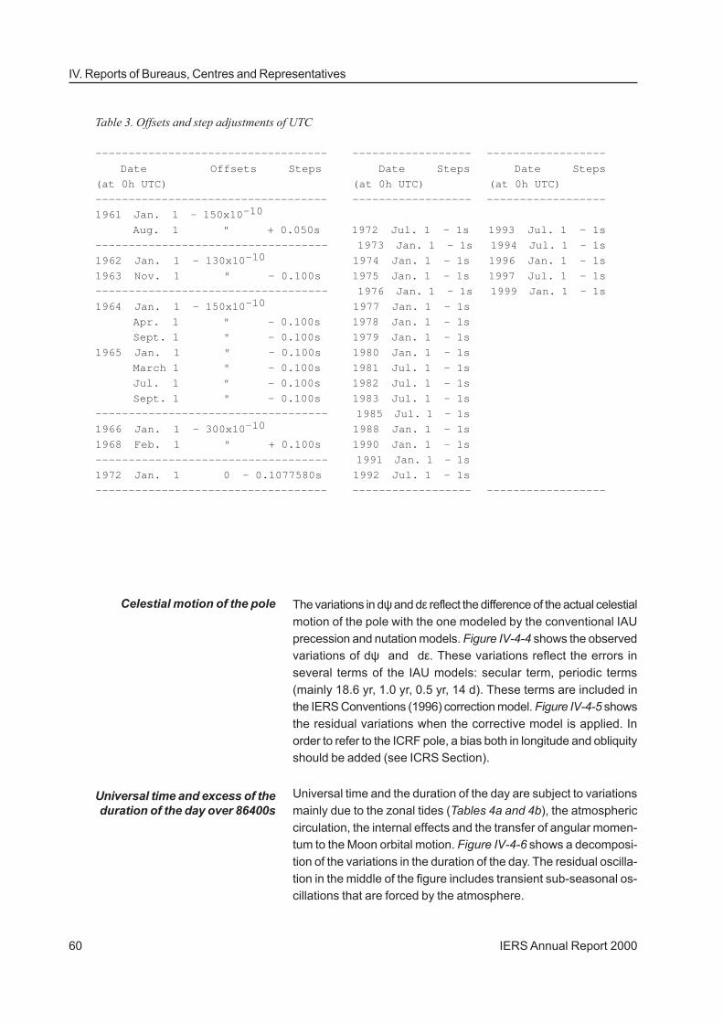
ber. Since the system was introduced in 1972 only dates in Juneand December have been used. The relationship of UTC with TAI isgiven in Table 2; the corresponding offsets and step adjustments ofUTC are given in Table 3.
The “leap second” procedure is affecting the activities of moderncommunication and navigation systems. In order to envisage thepossibility to redefine the Coordinated Universal Time (UTC), vari-ous working groups were created within the IAU and the ITU (Inter-national Telecommunication Union). During the ITU meetings dis-cussions developed on the implication of changes on scientific,governmental, commercial and regulatory interests. Resolutions willbe proposed at the CCTF (Comité Consultatif des Temps etFréquences) in the course of 2003.
DUT1 is the difference UT1–UTC, expressed with a precision of0.1 s, which is broadcasted with the time signals. The changes inDUT1 are decided by the EOP Product Center of the IERS. In thepast, UT2 was used; it was derived from UT1 by adding the follow-ing conventional annual and semi annual terms:
UT2–UT1 = 0.0220 sin2πt – 0.0120 cos2πt– 0.0060 sin4πt + 0.0070 cos4πt
the unit being the second and t being the date in Besselian years:
t = 2000.000 + (MJD – 51544.03) / 365.2422.The difference between the astronomically determined duration ofthe day and 86400s of TAI, is also called excess on the length ofday and designed by D or LOD. Its relationship with the angularvelocity of the Earth ω is:
ω = Ω (1 − D/T),
with T = 86 400 s and Ω the mean pole rate.
ω = 72 921 151.467 064 – 0.843 994 803 D,
where ω is in picoradians/s and D in milliseconds.It is useful to differentiate in some details the various forms of
universal time series that can be derived from different observingsystems. UT1 can be obtained only from inertial technique likeVLBI. Other techniques (e.g. LLR) may estimate the Earth’s orien-tation relatively to a dynamical frame which is different of ICRS.
UT1, hence D and ω, are subject to variations under the effect ofzonal tides. The model which is a part of IERS Conventions (1996)includes 62 periodic components, with periods ranging from 5.6days to 18.6 years. UT1R, DR, and ωR are the values of UT1, D,and ω corrected for the short-term part of the model, i.e., the 41components with periods under 35 days. The model is listed inTable 4a and Table 4b. A new model taking into account oceaniceffects and recommended to users will be published in the IERSConventions 2000.

IERS Annual Report 200058
IV. Reports of Bureaus, Centres and Representatives
Table 1. Observed values of UT1–TAI, 1962–2001
The uncertainty of UT1–TAI is smaller than 2 units of the last digit listed.TT–UT1 can be obtained from this table using the expression: TT–UT1 = 32.184s – (UT1–TAI).————————————————————————————————————————————————————————————————————————————————
Date UT1-TAI Date UT1-TAI Date UT1-TAI Date UT1-TAI
(s) (s) (s) (s)
————————————————————————————————————————————————————————————————————————————————
1962 JAN 1 -1.813 1972 JAN 1 -10.045 1982 JAN 1 -19.983 1992 JAN 1 -26.1252 APR 1 -1.936 APR 1 -10.347 APR 1 -20.184 APR 1 -26.3562 JUL 1 -2.058 JUL 1 -10.638 JUL 1 -20.391 JUL 1 -26.5569 OCT 1 -2.142 OCT 1 -10.888 OCT 1 -20.550 OCT 1 -26.7146
1963 JAN 1 -2.289 1973 JAN 1 -11.189 1983 JAN 1 -20.773 1993 JAN 1 -26.9378 APR 1 -2.407 APR 1 -11.489 APR 1 -21.036 APR 1 -27.1734 JUL 1 -2.551 JUL 1 -11.771 JUL 1 -21.250 JUL 1 -27.4010 OCT 1 -2.659 OCT 1 -12.016 OCT 1 -21.400 OCT 1 -27.5748
1964 JAN 1 -2.847 1974 JAN 1 -12.301 1984 JAN 1 -21.6042 1994 JAN 1 -27.8004 APR 1 -3.043 APR 1 -12.553 APR 1 -21.7603 APR 1 -28.0202 JUL 1 -3.217 JUL 1 -12.814 JUL 1 -21.9018 JUL 1 -28.2171 OCT 1 -3.350 OCT 1 -13.023 OCT 1 -22.0074 OCT 1 -28.3738
1965 JAN 1 -3.558 1975 JAN 1 -13.292 1985 JAN 1 -22.1587 1995 JAN 1 -28.6014 APR 1 -3.761 APR 1 -13.554 APR 1 -22.3058 APR 1 -28.8437 JUL 1 -3.964 JUL 1 -13.799 JUL 1 -22.4516 JUL 1 -29.0614 OCT 1 -4.139 OCT 1 -13.999 OCT 1 -22.5333 OCT 1 -29.2196
1966 JAN 1 -4.360 1976 JAN 1 -14.274 1986 JAN 1 -22.6872 1996 JAN 1 -29.4447 APR 1 -4.586 APR 1 -14.545 APR 1 -22.8157 APR 1 -29.6292 JUL 1 -4.817 JUL 1 -14.812 JUL 1 -22.9292 JUL 1 -29.8129 OCT 1 -5.006 OCT 1 -15.054 OCT 1 -23.0058 OCT 1 -29.9362
1967 JAN 1 -5.248 1977 JAN 1 -15.336 1987 JAN 1 -23.1382 1997 JAN 1 -30.1110 APR 1 -5.476 APR 1 -15.595 APR 1 -23.2788 APR 1 -30.2914 JUL 1 -5.700 JUL 1 -15.850 JUL 1 -23.3972 JUL 1 -30.4731 OCT 1 -5.871 OCT 1 -16.062 OCT 1 -23.4816 OCT 1 -30.6087
1968 JAN 1 -6.111 1978 JAN 1 -16.351 1988 JAN 1 -23.6356 1998 JAN 1 -30.7818 APR 1 -6.344 APR 1 -16.651 APR 1 -23.7823 APR 1 -30.9622 JUL 1 -6.573 JUL 1 -16.917 JUL 1 -23.9100 JUL 1 -31.1004 OCT 1 -6.775 OCT 1 -17.123 OCT 1 -23.9771 OCT 1 -31.1582
1969 JAN 1 -7.021 1979 JAN 1 -17.402 1989 JAN 1 -24.1159 1999 JAN 1 -31.2833 APR 1 -7.274 APR 1 -17.670 APR 1 -24.2443 APR 1 -31.3840 JUL 1 -7.521 JUL 1 -17.918 JUL 1 -24.3857 JUL 1 -31.4801 OCT 1 -7.734 OCT 1 -18.112 OCT 1 -24.4899 OCT 1 -31.5307
1970 JAN 1 -7.997 1980 JAN 1 -18.355 1990 JAN 1 -24.6713 2000 JAN 1 -31.6445 APR 1 -8.271 APR 1 -18.582 APR 1 -24.8631 APR 1 -31.7235 JUL 1 -8.526 JUL 1 -18.792 JUL 1 -25.0386 JUL 1 -31.7959 OCT 1 -8.722 OCT 1 -18.970 OCT 1 -25.1803 OCT 1 -31.8253
1971 JAN 1 -8.985 1981 JAN 1 -19.196 1991 JAN 1 -25.3813 2001 JAN 1 -31.9068 APR 1 -9.237 APR 1 -19.414 APR 1 -25.5871 APR 1 -31.9744 JUL 1 -9.503 JUL 1 -19.629 JUL 1 -25.7735 OCT 1 -9.741 OCT 1 -19.777 OCT 1 -25.9204
————————————————————————————————————————————————————————————————————————————————

IERS Annual Report 2000 59
IV.4 EOP Section of the Central Bureau
The main components of polar motion are a free oscillation (Chand-ler wobble) with a period of 1.2 year and an oscillation which isforced by the seasonal mass redistribution in the atmosphere andoceans. The beating period of the two terms is approximately 6years. A slow, irregular drift towards the west is superimposed tothe cyclic variation.
Figures IV-4-1 and IV-4-2 show a filtering of x and y coordinatesof the pole since 1890 obtained by CENSUS X-11 (Shiskin et al.,1965) modified to take into account two main periodic components.The series shown is EOP(IERS) C 01. The residual motion in thelower part of the figures includes irregularities with recurrence timesranging from days to years that are forced by the atmosphere, asshown on Figure IV-4-3 for EOP(IERS) C 04.
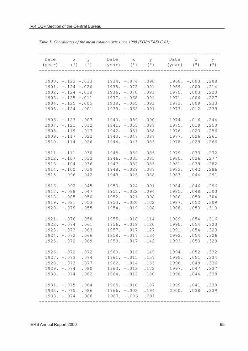
Table 5 gives yearly coordinates of the mean rotation axis in theIERS Terrestrial Reference Frame, obtained by filtering the Chan-dler and seasonal terms. Their uncertainty is about 0.010".
Table 2. Relationship between TAI and UTC———————————————————————————————————————————————————————————————————————————————
Limits of validity (at 0h UTC) TAI – UTC
———————————————————————————————————————————————————————————————————————————————
1961 Jan. 1 - 1961 Aug. 1 1.422 818 0s + (MJD - 37 300) x 0.001 296s
Aug. 1 - 1962 Jan. 1 1.372 818 0s + ""
1962 Jan. 1 - 1963 Nov. 1 1.845 858 0s + (MJD - 37 665) x 0.001 123 2s
1963 Nov. 1 - 1964 Jan. 1 1.945 858 0s + ""
1964 Jan. 1 - April 1 3.240 130 0s + (MJD - 38 761) x 0.001 296s
April 1 - Sept. 1 3.340 130 0s + ""
Sept. 1 - 1965 Jan. 1 3.440 130 0s + ""
1965 Jan. 1 - March 1 3.540 130 0s + ""
March 1 - Jul. 1 3.640 130 0s + ""
Jul. 1 - Sept. 1 3.740 130 0s + ""
Sept. 1 - 1966 Jan. 1 3.840 130 0s + ""
1966 Jan. 1 - 1968 Feb. 1 4.313 170 0s + (MJD - 39 126) x 0.002 592s
1968 Feb. 1 - 1972 Jan. 1 4.213 170 0s + ""
1972 Jan. 1 - Jul. 1 10s
Jul. 1 - 1973 Jan. 1 11s ————————————————————————————————————
1973 Jan. 1 - 1974 Jan. 1 12s Limits of validity (at 0h UTC)
1974 Jan. 1 - 1975 Jan. 1 13s ————————————————————————————————————
1975 Jan. 1 - 1976 Jan. 1 14s 1988 Jan. 1 - 1990 Jan. 1 24s
1976 Jan. 1 - 1977 Jan. 1 15s 1990 Jan. 1 - 1991 Jan. 1 25s
1977 Jan. 1 - 1978 Jan. 1 16s 1991 Jan. 1 - 1992 Jul. 1 26s
1978 Jan. 1 - 1979 Jan. 1 17s 1992 Jul. 1 - 1993 Jul 1 27s
1979 Jan. 1 - 1980 Jan. 1 18s 1993 Jul. 1 - 1994 Jul. 1 28s
1980 Jan. 1 - 1981 Jul. 1 19s 1994 Jul. 1 - 1996 Jan. 1 29s
1981 Jul. 1 - 1982 Jul. 1 20s 1996 Jan. 1 - 1997 Jul. 1 30s
1982 Jul. 1 - 1983 Jul. 1 21s 1997 Jul. 1 - 1999 Jan 1 31s
1983 Jul. 1 - 1985 Jul. 1 22s 1999 Jan. 1 - 32s
1985 Jul. 1 - 1988 Jan. 1 23s
———————————————————————————————————————————————————————————————————————————————
Irregularities of the Earth’s Rotation
Polar motion
IERS Annual Report 200060
IV. Reports of Bureaus, Centres and Representatives
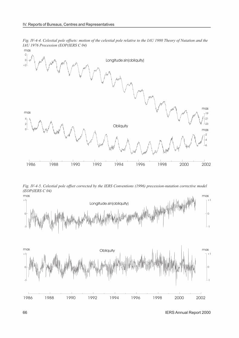
The variations in dψ and dε reflect the difference of the actual celestialmotion of the pole with the one modeled by the conventional IAUprecession and nutation models. Figure IV-4-4 shows the observedvariations of dψ and dε. These variations reflect the errors inseveral terms of the IAU models: secular term, periodic terms(mainly 18.6 yr, 1.0 yr, 0.5 yr, 14 d). These terms are included inthe IERS Conventions (1996) correction model. Figure IV-4-5 showsthe residual variations when the corrective model is applied. Inorder to refer to the ICRF pole, a bias both in longitude and obliquityshould be added (see ICRS Section).
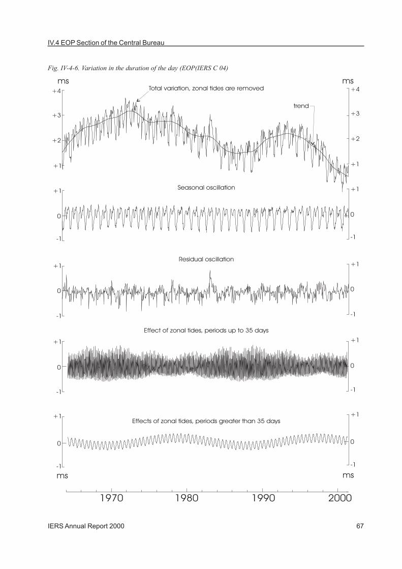
Universal time and the duration of the day are subject to variationsmainly due to the zonal tides (Tables 4a and 4b), the atmosphericcirculation, the internal effects and the transfer of angular momen-tum to the Moon orbital motion. Figure IV-4-6 shows a decomposi-tion of the variations in the duration of the day. The residual oscilla-tion in the middle of the figure includes transient sub-seasonal os-cillations that are forced by the atmosphere.
Table 3. Offsets and step adjustments of UTC
——————————————————————————————————— —————————————————— ——————————————————
Date Offsets Steps Date Steps Date Steps
(at 0h UTC) (at 0h UTC) (at 0h UTC)
——————————————————————————————————— —————————————————— ——————————————————
1961 Jan. 1 - 150x10-10
Aug. 1 " + 0.050s 1972 Jul. 1 - 1s 1993 Jul. 1 - 1s
——————————————————————————————————— 1973 Jan. 1 - 1s 1994 Jul. 1 - 1s
1962 Jan. 1 - 130x10-10 1974 Jan. 1 - 1s 1996 Jan. 1 - 1s
1963 Nov. 1 " - 0.100s 1975 Jan. 1 - 1s 1997 Jul. 1 - 1s
——————————————————————————————————— 1976 Jan. 1 - 1s 1999 Jan. 1 - 1s
1964 Jan. 1 - 150x10-10 1977 Jan. 1 - 1s
Apr. 1 " - 0.100s 1978 Jan. 1 - 1s
Sept. 1 " - 0.100s 1979 Jan. 1 - 1s
1965 Jan. 1 " - 0.100s 1980 Jan. 1 - 1s
March 1 " - 0.100s 1981 Jul. 1 - 1s
Jul. 1 " - 0.100s 1982 Jul. 1 - 1s
Sept. 1 " - 0.100s 1983 Jul. 1 - 1s
——————————————————————————————————— 1985 Jul. 1 - 1s
1966 Jan. 1 - 300x10-10 1988 Jan. 1 - 1s
1968 Feb. 1 " + 0.100s 1990 Jan. 1 - 1s
——————————————————————————————————— 1991 Jan. 1 - 1s
1972 Jan. 1 0 - 0.1077580s 1992 Jul. 1 - 1s
——————————————————————————————————— —————————————————— ——————————————————
Celestial motion of the pole
Universal time and excess of theduration of the day over 86400s

IERS Annual Report 2000 61
IV.4 EOP Section of the Central Bureau
Table 4a. Earth rotation variations due to zonal tides with periods up to 35 days
UT1R, DR, ωR represent the corrected values of UT1, of the duration of the day D and of theangular velocity of the Earth ω, according to IERS Conventions (1996).The units are 10-4 s for UT, 10-5 s for D, and 10-14 rad/s for ω.————————————————-———————————————————————————————————-—————————————————
ARGUMENTS PERIODS COEFFICIENTS
N ——————————————————— —————————— —————————————————————————————
l l’ F D Ω DAYS UT1-UT1R D-DR ω-ωR—————— ——————————————————— —————————— —————————————————————————————
sin cos cos
1 1 0 2 2 2 5.64 -0.024 0.26 -0.22
2 2 0 2 0 1 6.85 -0.040 0.37 -0.31
3 2 0 2 0 2 6.86 -0.099 0.90 -0.76
4 0 0 2 2 1 7.09 -0.051 0.45 -0.38
5 0 0 2 2 2 7.10 -0.123 1.09 -0.92
6 1 0 2 0 0 9.11 -0.039 0.27 -0.22
7 1 0 2 0 1 9.12 -0.411 2.83 -2.39
8 1 0 2 0 2 9.13 -0.993 6.83 -5.76
9 3 0 0 0 0 9.18 -0.018 0.12 -0.10
10 -1 0 2 2 1 9.54 -0.082 0.54 -0.45
11 -1 0 2 2 2 9.56 -0.197 1.30 -1.10
12 1 0 0 2 0 9.61 -0.076 0.50 -0.42
13 2 0 2 -2 2 12.81 0.022 -0.11 0.09
14 0 1 2 0 2 13.17 0.025 -0.12 0.10
15 0 0 2 0 0 13.61 -0.299 1.38 -1.17
16 0 0 2 0 1 13.63 -3.208 14.79 -12.48
17 0 0 2 0 2 13.66 -7.757 35.68 -30.11
18 2 0 0 0 -1 13.75 0.022 -0.10 0.08
19 2 0 0 0 0 13.78 -0.338 1.54 -1.30
20 2 0 0 0 1 13.81 0.018 -0.08 0.07
21 0 -1 2 0 2 14.19 -0.024 0.11 -0.09
22 0 0 0 2 -1 14.73 0.047 -0.20 0.17
23 0 0 0 2 0 14.77 -0.734 3.12 -2.64
24 0 0 0 2 1 14.80 -0.053 0.22 -0.19
25 0 -1 0 2 0 15.39 -0.051 0.21 -0.17
26 1 0 2 -2 1 23.86 0.050 -0.13 0.11
27 1 0 2 -2 2 23.94 0.101 -0.26 0.22
28 1 1 0 0 0 25.62 0.039 -0.10 0.08
29 -1 0 2 0 0 26.88 0.047 -0.11 0.09
30 -1 0 2 0 1 26.98 0.177 -0.41 0.35
31 -1 0 2 0 2 27.09 0.435 -1.01 0.85
32 1 0 0 0 -1 27.44 0.534 -1.22 1.03
33 1 0 0 0 0 27.56 -8.261 18.84 -15.90
34 1 0 0 0 1 27.67 0.544 -1.24 1.04
35 0 0 0 1 0 29.53 0.047 -0.10 0.08
36 1 -1 0 0 0 29.80 -0.055 0.12 -0.10
37 -1 0 0 2 -1 31.66 0.118 -0.23 0.20
38 -1 0 0 2 0 31.81 -1.824 3.60 -3.04
39 -1 0 0 2 1 31.96 0.132 -0.26 0.22
40 1 0 -2 2 -1 32.61 0.018 -0.03 0.03
41 -1 -1 0 2 0 34.85 -0.086 0.15 -0.13
——————————————————————————————————————————————————————————————————————

IERS Annual Report 200062
IV. Reports of Bureaus, Centres and Representatives
Table 4b. Earth rotation variations due to zonal tides with periods longer than 35 days
UT1R’, DR’, ωR’ represent the corrected values of UT1, of the duration of the day D and of theangular velocity of the Earth ω, based on Yoder et al. (1981), with K/C = 0.94.The units are 10-4 s for UT, 10-5 s for D, and 10-14 rad/s for ω.
——————————————————————————————————————————————————————————————————————
ARGUMENTS PERIODS COEFFICIENTS
N ——————————————————— —————————— —————————————————————————————
l l’ F D Ω DAYS UT1-UT1R’ D-DR’ ω-ωR’—————— ——————————————————— —————————— —————————————————————————————
sin cos cos
42 0 2 2 -2 2 91.31 -0.057 0.04 -0.03
43 0 1 2 -2 1 119.61 0.033 -0.02 0.01
44 0 1 2 -2 2 121.75 -1.885 0.97 -0.82
45 0 0 2 -2 0 173.31 0.251 -0.09 0.08
46 0 0 2 -2 1 177.84 1.170 -0.41 0.35
47 0 0 2 -2 2 182.62 -48.247 16.60 -14.01
48 0 2 0 0 0 182.63 -0.194 0.07 -0.06
49 2 0 0 -2 -1 199.84 0.049 -0.02 0.01
50 2 0 0 -2 0 205.89 -0.547 0.17 -0.14
51 2 0 0 -2 1 212.32 0.037 -0.01 0.01
52 0 -1 2 -2 1 346.60 -0.045 0.01 -0.01
53 0 1 0 0 -1 346.64 0.092 -0.02 0.01
54 0 -1 2 -2 2 365.22 0.828 -0.14 0.12
55 0 1 0 0 0 365.26 -15.359 2.64 -2.23
56 0 1 0 0 1 386.00 -0.138 0.02 -0.02
57 1 0 0 -1 0 411.78 0.035 -0.01 0.00
58 2 0 -2 0 0 1095.17 -0.137 -0.01 0.01
59 -2 0 2 0 1 1305.47 0.422 -0.02 0.02
60 -1 1 0 1 0 3232.85 0.040 0.00 0.00
61 0 0 0 0 2 3399.18 7.900 0.15 -0.12
62 0 0 0 0 1 6790.36 -1617.268 -14.95 12.62
——————————————————————————————————————————————————————————————————————
Mean anomaly of the Moon l = 134°.96 + 13°.064993(MJD–51544.5)
Mean anomaly of the Sun l’ = 357°.53 + 0°.985600(MJD–51544.5)
Mean longitude of the Moon F = 93°.27 + 13°.229350(MJD–51544.5)
from the node of the Moon F = L - ΩL : Mean longitude of the Moon
Mean elongation of the Moon D = 297°.85 + 12°.190749(MJD–51544.5)
from the Sun
Mean longitude of the ascending Ω = 125°.04 – 0°.052954(MJD–51544.5)node of the Moon

IERS Annual Report 2000 63
IV.4 EOP Section of the Central Bureau
Fig. IV-4-1. X-coordinate of the pole (EOP(IERS) C 04)
Fig. IV-4-2. Y-coordinate of the pole (EOP(IERS) C 04)

IERS Annual Report 200064
IV. Reports of Bureaus, Centres and Representatives
Table 6 gives mean annual values of the excess of the duration ofthe day D, which are available for the last four centuries. For theinterval 1623–1955, the data are those provided by L.V. Morrison,Royal Greenwich Observatory, interpolated for the middle of theyear. The mean solar time has been referred to the dynamical timescale derived from the time argument of the lunar ephemeris. Theduration of the day has been obtained:
– from 1623 to 1860, by derivative of cubic splines fitted on indi-vidual values of the difference between mean solar time and dy-namical time,– from 1861 to 1955, by a 5-point quadratic convolute.
More information on the computation of the duration of the day isavailable in Stephenson and Morrison (1984), with an estimation ofthe accuracy of these evaluations. From 1956 up to present, theduration of the day has been obtained from the BIH/IERS values ofUT1–TAI; the table gives annual averages. At the level of precisionof these values of the duration of the day, the unit of the dynamicaltime and the unit of TAI can be considered as having the sameduration. Thus D is expressed in present SI units. The table givesalso the values of the angular velocity of the Earth’s rotation ωderived from the listed values of D.
Fig. IV-4-3. Irregular variations in polar motion (EOP(IERS) C 04 filtered by CENSUS X-11)
IERS Annual Report 2000 65
IV.4 EOP Section of the Central Bureau
Table 5. Coordinates of the mean rotation axis since 1900 (EOP(IERS) C 01)
———————————————————————————————————————————————————————————————— Date x y Date x y Date x y (year) (") (") (year) (") (") (year) (") (")————————————————————————————————————————————————————————————————
1900. -.122 -.033 1934. -.074 .090 1968. -.003 .208 1901. -.124 -.026 1935. -.072 .091 1969. .000 .214 1902. -.124 -.018 1936. -.070 .091 1970. .003 .220 1903. -.125 -.011 1937. -.068 .091 1971. .006 .227 1904. -.125 -.005 1938. -.065 .091 1972. .009 .233 1905. -.124 .001 1939. -.062 .091 1973. .012 .239
1906. -.123 .007 1940. -.059 .090 1974. .016 .244 1907. -.121 .012 1941. -.055 .089 1975. .019 .250 1908. -.119 .017 1942. -.051 .088 1976. .023 .256 1909. -.117 .022 1943. -.047 .087 1977. .026 .261 1910. -.114 .026 1944. -.043 .086 1978. .029 .266
1911. -.111 .030 1945. -.039 .086 1979. .033 .272 1912. -.107 .033 1946. -.035 .085 1980. .036 .277 1913. -.104 .036 1947. -.032 .086 1981. .039 .282 1914. -.100 .039 1948. -.029 .087 1982. .042 .286 1915. -.096 .042 1949. -.026 .088 1983. .044 .291
1916. -.092 .045 1950. -.024 .091 1984. .046 .296 1917. -.088 .047 1951. -.022 .094 1985. .048 .300 1918. -.085 .050 1952. -.021 .098 1986. .050 .304 1919. -.081 .053 1953. -.020 .102 1987. .052 .309 1920. -.079 .055 1954. -.019 .108 1988. .053 .313
1921. -.076 .058 1955. -.018 .114 1989. .054 .316 1922. -.074 .061 1956. -.018 .120 1990. .054 .320 1923. -.073 .063 1957. -.017 .127 1991. .054 .323 1924. -.072 .066 1958. -.017 .134 1992. .054 .326 1925. -.072 .069 1959. -.017 .142 1993. .053 .329
1926. -.072 .072 1960. -.016 .149 1994. .052 .332 1927. -.073 .074 1961. -.015 .157 1995. .051 .334 1928. -.073 .077 1962. -.014 .165 1996. .049 .336 1929. -.074 .080 1963. -.013 .172 1997. .047 .337 1930. -.074 .082 1964. -.012 .180 1998. .044 .338
1931. -.075 .084 1965. -.010 .187 1999. .041 .339 1932. -.075 .086 1966. -.008 .194 2000. .038 .339 1933. -.074 .088 1967. -.006 .201————————————————————————————————————————————————————————————————
IERS Annual Report 200066
IV. Reports of Bureaus, Centres and Representatives
Fig. IV-4-4. Celestial pole offsets: motion of the celestial pole relative to the IAU 1980 Theory of Nutation and theIAU 1976 Precession (EOP(IERS C 04)
Fig. IV-4-5. Celestial pole offset corrected by the IERS Conventions (1996) precession-nutation corrective model(EOP(IERS C 04)
IERS Annual Report 2000 67
IV.4 EOP Section of the Central Bureau
Fig. IV-4-6. Variation in the duration of the day (EOP(IERS C 04)

IERS Annual Report 200068
IV. Reports of Bureaus, Centres and Representatives
Table 6. Excess of the duration of the day to 86400s and Angular velocity of the Earth’s rotation, since 1623———————————————————————— ———————————————————————— ————————————————————————
DATE D ω DATE D ω DATE D ω (years) (ms) (prad/s) (years) (ms) (prad/s) (years) (ms) (prad/s)
———————————————————————— ———————————————————————— ———————————————————————— 72 921.. 72 921.. 72 921.. 1671.5 -3. 154. 1721.5 0.2 151.3 1672.5 -3. 154. 1722.5 0.2 151.3 1623.5 -11. 161. 1673.5 -3. 154. 1723.5 0.1 151.4 1624.5 -11. 161. 1674.5 -3. 154. 1724.5 0.1 151.4 1625.5 -10. 160. 1675.5 -3. 154. 1725.5 0.1 151.4 1626.5 -10. 160. 1676.5 -3. 154. 1726.5 0.1 151.4 1627.5 -9. 159. 1677.5 -3. 154. 1727.5 0.1 151.4 1628.5 -9. 159. 1678.5 -3. 154. 1728.5 0.2 151.3 1629.5 -8. 158. 1679.5 -2. 153. 1729.5 0.2 151.3 1630.5 -8. 158. 1680.5 -2. 153. 1730.5 0.2 151.3
1631.5 -8. 158. 1681.5 -2. 153. 1731.5 0.2 151.3 1632.5 -7. 157. 1682.5 -2. 153. 1732.5 0.2 151.3 1633.5 -7. 157. 1683.5 -2. 153. 1733.5 0.2 151.3 1634.5 -7. 157. 1684.5 -2. 153. 1734.5 0.2 151.3 1635.5 -6. 157. 1685.5 -2. 153. 1735.5 0.2 151.3 1636.5 -6. 157. 1686.5 -1. 152. 1736.5 0.3 151.2 1637.5 -6. 157. 1687.5 -1. 152. 1737.5 0.3 151.2 1638.5 -5. 156. 1688.5 -1. 152. 1738.5 0.3 151.2 1639.5 -5. 156. 1689.5 -1. 152. 1739.5 0.3 151.2 1640.5 -5. 156. 1690.5 -1. 152. 1740.5 0.3 151.2
1641.5 -4. 155. 1691.5 -1. 152. 1741.5 0.3 151.2 1642.5 -4. 155. 1692.5 -1. 152. 1742.5 0.3 151.2 1643.5 -4. 155. 1693.5 0. 151. 1743.5 0.4 151.1 1644.5 -4. 155. 1694.5 0. 151. 1744.5 0.4 151.1 1645.5 -4. 155. 1695.5 0. 151. 1745.5 0.4 151.1 1646.5 -3. 154. 1696.5 0. 151. 1746.5 0.4 151.1 1647.5 -3. 154. 1697.5 0. 151. 1747.5 0.4 151.1 1648.5 -3. 154. 1698.5 0. 151. 1748.5 0.4 151.1 1649.5 -3. 154. 1699.5 0. 151. 1749.5 0.4 151.1 1650.5 -3. 154. 1700.5 0.1 151.4 1750.5 0.4 151.1
1651.5 -3. 154. 1701.5 0.2 151.3 1751.5 0.4 151.1 1652.5 -3. 154. 1702.5 0.2 151.3 1752.5 0.4 151.1 1653.5 -3. 154. 1703.5 0.3 151.2 1753.5 0.4 151.1 1654.5 -3. 154. 1704.5 0.3 151.2 1754.5 0.4 151.1 1655.5 -3. 154. 1705.5 0.3 151.2 1755.5 0.4 151.1 1656.5 -3. 154. 1706.5 0.3 151.2 1756.5 0.4 151.1 1657.5 -3. 154. 1707.5 0.3 151.2 1757.5 0.4 151.1 1658.5 -3. 154. 1708.5 0.4 151.1 1758.5 0.4 151.1 1659.5 -3. 154. 1709.5 0.3 151.2 1759.5 0.4 151.1 1660.5 -3. 154. 1710.5 0.3 151.2 1760.5 0.4 151.1
1661.5 -3. 154. 1711.5 0.3 151.2 1761.5 0.4 151.1 1662.5 -3. 154. 1712.5 0.3 151.2 1762.5 0.3 151.2 1663.5 -3. 154. 1713.5 0.3 151.2 1763.5 0.3 151.2 1664.5 -3. 154. 1714.5 0.3 151.2 1764.5 0.3 151.2 1665.5 -3. 154. 1715.5 0.2 151.3 1765.5 0.3 151.2 1666.5 -3. 154. 1716.5 0.2 151.3 1766.5 0.3 151.2 1667.5 -3. 154. 1717.5 0.2 151.3 1767.5 0.3 151.2 1668.5 -3. 154. 1718.5 0.2 151.3 1768.5 0.3 151.2 1669.5 -3. 154. 1719.5 0.2 151.3 1769.5 0.3 151.2 1670.5 -3. 154. 1720.5 0.2 151.3 1770.5 0.3 151.2
———————————————————————— ———————————————————————— ————————————————————————

IERS Annual Report 2000 69
IV.4 EOP Section of the Central Bureau
Table 6 (cont.).———————————————————————— ———————————————————————— ————————————————————————
DATE D ω DATE D ω DATE D ω (years) (ms) (prad/s) (years) (ms) (prad/s) (years) (ms) (prad/s)
———————————————————————— ———————————————————————— ———————————————————————— 72 921.. 72 921.. 72 921.. 1771.5 0.3 151.2 1821.5 -0.81 152.15 1871.5 -2.59 153.65 1772.5 0.2 151.3 1822.5 -0.99 152.30 1872.5 -2.55 153.62 1773.5 0.2 151.3 1823.5 -1.16 152.45 1873.5 -2.10 153.24 1774.5 0.2 151.3 1824.5 -1.32 152.58 1874.5 -2.03 153.18 1775.5 0.2 151.3 1825.5 -1.42 152.67 1875.5 -1.77 152.96 1776.5 0.2 151.3 1826.5 -1.49 152.72 1876.5 -1.37 152.62 1777.5 0.2 151.3 1827.5 -1.50 152.73 1877.5 -1.24 152.51 1778.5 0.2 151.3 1828.5 -1.48 152.72 1878.5 -0.90 152.23 1779.5 0.2 151.3 1829.5 -1.41 152.66 1879.5 -0.49 151.88 1780.5 0.2 151.3 1830.5 -1.30 152.56 1880.5 -0.23 151.66
1781.5 0.2 151.3 1831.5 -1.14 152.43 1881.5 -0.06 151.52 1782.5 0.1 151.4 1832.5 -0.94 152.26 1882.5 -0.15 151.59 1783.5 0.1 151.4 1833.5 -0.73 152.08 1883.5 -0.33 151.75 1784.5 0.1 151.4 1834.5 -0.52 151.91 1884.5 -0.24 151.67 1785.5 0.0 151.5 1835.5 -0.34 151.75 1885.5 -0.15 151.59 1786.5 0.0 151.5 1836.5 -0.18 151.62 1886.5 -0.05 151.51 1787.5 -0.1 151.6 1837.5 -0.04 151.50 1887.5 -0.04 151.50 1788.5 -0.2 151.6 1838.5 0.09 151.39 1888.5 -0.18 151.62 1789.5 -0.3 151.7 1839.5 0.19 151.31 1889.5 -0.25 151.68 1790.5 -0.5 151.9 1840.5 0.27 151.24 1890.5 -0.48 151.87
1791.5 -0.6 152.0 1841.5 0.33 151.19 1891.5 -0.58 151.96 1792.5 -0.7 152.1 1842.5 0.37 151.15 1892.5 -0.42 151.82 1793.5 -0.9 152.2 1843.5 0.39 151.14 1893.5 -0.13 151.58 1794.5 -0.9 152.2 1844.5 0.40 151.13 1894.5 0.33 151.19 1795.5 -1.0 152.3 1845.5 0.41 151.12 1895.5 0.86 150.74 1796.5 -1.0 152.3 1846.5 0.41 151.12 1896.5 1.53 150.18 1797.5 -1.0 152.3 1847.5 0.40 151.13 1897.5 2.16 149.64 1798.5 -1.0 152.3 1848.5 0.39 151.14 1898.5 2.64 149.24 1799.5 -1.0 152.3 1849.5 0.38 151.15 1899.5 3.00 148.94 1800.5 -0.87 152.20 1850.5 0.36 151.16 1900.5 3.31 148.67
1801.5 -0.75 152.10 1851.5 0.33 151.19 1901.5 3.60 148.43 1802.5 -0.61 151.98 1852.5 0.30 151.21 1902.5 3.70 148.34 1803.5 -0.46 151.86 1853.5 0.26 151.25 1903.5 3.69 148.35 1804.5 -0.34 151.75 1854.5 0.23 151.27 1904.5 3.55 148.47 1805.5 -0.23 151.66 1855.5 0.20 151.30 1905.5 3.40 148.60 1806.5 -0.14 151.59 1856.5 0.17 151.32 1906.5 3.48 148.53 1807.5 -0.06 151.52 1857.5 0.15 151.34 1907.5 3.57 148.45 1808.5 -0.01 151.48 1858.5 0.11 151.37 1908.5 3.65 148.39 1809.5 0.03 151.44 1859.5 -0.02 151.48 1909.5 3.71 148.34 1810.5 0.05 151.42 1860.5 -0.34 151.75 1910.5 3.77 148.29
1811.5 0.05 151.42 1861.5 -0.81 152.15 1911.5 3.86 148.21 1812.5 0.04 151.43 1862.5 -1.19 152.47 1912.5 3.89 148.18 1813.5 0.01 151.46 1863.5 -1.35 152.61 1913.5 3.62 148.41 1814.5 -0.04 151.50 1864.5 -1.61 152.83 1914.5 3.18 148.78 1815.5 -0.11 151.56 1865.5 -2.13 153.26 1915.5 2.92 149.00 1816.5 -0.18 151.62 1866.5 -2.76 153.80 1916.5 2.74 149.15 1817.5 -0.28 151.70 1867.5 -2.89 153.91 1917.5 2.35 149.48 1818.5 -0.39 151.80 1868.5 -2.60 153.66 1918.5 2.05 149.74 1819.5 -0.51 151.90 1869.5 -2.59 153.65 1919.5 1.76 149.98 1820.5 -0.65 152.02 1870.5 -2.51 153.59 1920.5 1.48 150.22
———————————————————————— ———————————————————————— ————————————————————————

IERS Annual Report 200070
IV. Reports of Bureaus, Centres and Representatives
Table 6 (cont.).———————————————————————— ————————————————————————
DATE D ω DATE D ω (years) (ms) (prad/s) (years) (ms) (prad/s)
———————————————————————— ———————————————————————— 72 921.. 72 921.. 1921.5 1.51 150.19 1971.5 2.90 149.02 1922.5 1.28 150.39 1972.5 3.13 148.83 1923.5 0.98 150.64 1973.5 3.05 148.89 1924.5 0.93 150.68 1974.5 2.72 149.17 1925.5 0.81 150.78 1975.5 2.69 149.20 1926.5 0.56 150.99 1976.5 2.91 149.01 1927.5 0.18 151.32 1977.5 2.77 149.13 1928.5 -0.22 151.65 1978.5 2.88 149.04 1929.5 -0.35 151.76 1979.5 2.61 149.26 1930.5 -0.19 151.63 1980.5 2.30 149.53
1931.5 -0.10 151.55 1981.5 2.16 149.64 1932.5 -0.07 151.53 1982.5 2.16 149.64 1933.5 -0.06 151.52 1983.5 2.28 149.54 1934.5 -0.08 151.53 1984.5 1.52 150.18 1935.5 0.00 151.47 1985.5 1.45 150.24 1936.5 0.08 151.40 1986.5 1.23 150.43 1937.5 0.22 151.28 1987.5 1.36 150.32 1938.5 0.47 151.07 1988.5 1.32 150.35 1939.5 0.78 150.81 1989.5 1.53 150.18 1940.5 1.09 150.55 1990.5 1.94 149.83
1941.5 1.25 150.41 1991.5 2.04 149.75 1942.5 1.31 150.36 1992.5 2.22 149.59 1943.5 1.35 150.33 1993.5 2.37 149.47 1944.5 1.41 150.28 1994.5 2.17 149.64 1945.5 1.41 150.28 1995.5 2.31 149.52 1946.5 1.35 150.33 1996.5 1.83 149.92 1947.5 1.30 150.37 1997.5 1.84 149.91 1948.5 1.25 150.41 1998.5 1.37 150.31 1949.5 1.20 150.45 1999.5 0.99 150.63 1950.5 1.15 150.50 2000.5 0.72 150.86 ———————————————————————— 1951.5 1.10 150.54 1952.5 1.05 150.58 1953.5 0.99 150.63 1954.5 0.92 150.69 1955.5 0.86 150.74 1956.5 0.89 150.72 1957.5 1.34 150.34 1958.5 1.37 150.31 1959.5 1.31 150.36 1960.5 1.19 150.46
1961.5 1.09 150.55 1962.5 1.30 150.37 1963.5 1.54 150.17 1964.5 1.92 149.85 1965.5 2.21 149.60 1966.5 2.41 149.43 1967.5 2.37 149.47 1968.5 2.48 149.37 1969.5 2.67 149.21 1970.5 2.71 149.18————————————————————————

IERS Annual Report 2000 71
IV.4 EOP Section of the Central Bureau
One of the tasks of the Earth Orientation Parameters Product Center(EOP-PC) is to perform combined EOP series from the individualtechniques, VLBI, SLR, GPS, LLR and DORIS. Various solutions,namely Bulletin B, EOP(IERS) C 01, C 02, C 03 and C 04 are thuspublished to fulfill the requirements of users, operational and scien-tific. They are available at the ftp/web site: hpiers.obspm.fr/eop-pc.The continuous improvement of the results derived from these geo-detic techniques and the development of new methods of combina-tion made possible the improvement of combined solutions;precisions of about 0.15 mas in polar motion and 15 microsecondsfor UT1 are currently obtained.
The maintenance of the reference systems consistency and itslong-term stability require long and homogeneous EOP series. Therealization of combined solutions must take advantage of the avail-ability and the qualities of the independent series at the varioustime scales. They are assumed to contain no jump and negligiblesystematic errors.
The first step in the general procedure for deriving the multi-tech-nique combined solutions is the evaluation for each series of thesystematic errors corrections, bias and drift, in order to translate itto the IERS system. A known source of relative drifts in x, y andUT1–UTC is the variety of processes chosen by the analysis centersto control the time evolution of the adjusted terrestrial referenceframes, complicated by the sampling of the tectonic plates andplate margins. The formal uncertainties given by the analysis centersbeing an internal consistency estimate, usually an external calibra-tion has to be made in order to reflect the real external uncertainty.This is done using the Allan variance analysis (Gray and Allan,1974; Gambis, 2001) of the differences between series without anyreference to a combined series. When three or more series of simi-lar quality and time resolution can be differenced, the pair varianceof the noise of each series can be evaluated, provided that theirerrors are considered statistically independent. The pair variancethus obtained is used as an estimate of the uncertainty of a singledetermination in a given series; its ratio with the rms formal uncer-tainty over the same period provides a scaling factor, from whichthe weighting of the combined individual results is based. Weight-ing of the series entering into the combined solution are thus esti-mated. The combined C 04 is now permanently updated on a nearreal-time basis.
EOP(IERS) C 01 is a series of the Earth Orientation Parametersgiven at 0.1 year interval from 1846 to 1889 and 0.05 year intervalfrom1890 until now. For many decades, the observations were made
4.2 Operational Activity
Overview
Combination of EOP Series
General Combination Procedure
Long-term Solution: C 01(1846–2001)

IERS Annual Report 200072
IV. Reports of Bureaus, Centres and Representatives
using mostly visual and photographic zenith telescopes. Since theadvent of the space era in the 1960s, new geodetic techniqueswere applied for geodynamics. Now, the global observing activityinvolves Very Long Baseline Radio Interferometry (VLBI), Lunar andSatellite Laser Ranging (LLR, SLR), Global Positioning System(GPS) and more recently DORIS.
The C 01 series is based on the following solutions:– 1846–1899: Fedorov et al. (1972) polar motion solution derivedfrom three series of absolute declination programs (Pulkovo, Green-wich, Washington).– 1900–1961: Vondrak et al. (1995) solution derived from opticalastrometry analyses based on the Hipparcos reference frame. Theseries gives polar motion, celestial pole offsets and Universal Time(since 1956).– 1962–now: BIH and IERS solutions (BIH and IERS annual reports).
Other series, based on normal points solutions given at varioustime intervals, are also proposed to users, i.e. C 02 (5-day inter-vals), C 03 (one-day intervals) (Gambis, 1996a and 1996b; Eisopand Gambis, 1997). These series are respectively consistent oneto another. They use the full correlation matrix when available. Re-cently there were new developments in the normal point series C 02and C 03 in which the estimation of the solution given at the centraldates of the n-day interval is made using a least-square fit for allEOP components. Although the L2 estimation has been exten-sively used for data analysis, it has some drawbacks linked toproblems of ill-conditioning and in the non-detection of outliers. Al-ternative methods based on robust estimators like M-Huber can beused. These estimators are a generalization of both the L1 and L2class. They have been implemented in our analyses and are nowcurrently used (Bougeard M.L., Gambis D. and R. Ray, 1999;Gambis et al., 2000).
Taking advantage of the recomputations of various individual series,EOP(IERS) C 04 is currently recomputed. In the course of the analy-ses the determination of the systematic corrections of individualseries entering into the combination and the weighting procedureare re-examined. Table 7 and Table 8 give the characteristics of thesmoothing adopted for each time interval. The variations with peri-ods shorter than the value in the table are smoothed out, exceptthe short term variations in UT1 due to zonal tides and the 14 dterms in celestial pole offsets which are first removed using a modelthen added back at the end of the series combination process.Table 9 shows the uncertainty of one daily value of EOP for eachperiod. Table 10 shows the agreement and consistencies of thecurrent solutions. The Bulletin B is issued on a monthly basis and
Middle-term Solution: C 02(1962–2001), C 03 (1993–2001)
Operational Solution:EOP(IERS) C 04

IERS Annual Report 2000 73
IV.4 EOP Section of the Central Bureau
is “frozen”, contrarily to NEOS Bulletin A and IERS C 04 which arepermanently updated.
Different approaches are used for prediction of the Earth rotationparameters.
• Polar Motion: The formalism uses at first a floating period fitfor both the Chandler and annual components estimation overa past time interval of several years. An autoregressive filter isthen applied on the short-term residuals series and used forthe prediction. The predictions of the nutation offsets dψ anddε are based on an empirical model (McCarthy, 1996).
• Universal Time: The present formalism used is based on theassumption that the long-term fluctuations (annual and semi-annual) of the preceding year are valid over the next few months.For short-term variations prediction, an autoregressive processis used. The following Table 11 shows the current accuracy ofthe EOP solutions and also the skills of the predictions.
Predictions
Table 7. Frequency filtering characteristic of smoothing for polar motion and celestial poleoffsets, [EOP(IERS) C 04]———————————————————————————————————————————————————————————————
Epsilon PERIOD FOR REMAINING AMPLITUDE Years
5% 50% 95%
—————————— —————————— ——————————— —————————— ———————————
10-0.6 3.2d 10.0d 17.0d 1983-1985
10+0.6 2.0d 6.3d 10.7d 1986-1989
10+1.0 1.7d 5.4d 9.2d 1990-1991
10+1.4 1.5d 4.5d 7.9d 1992
10+1.6 1.4d 4.2d 7.3d 1993
10+2.0 1.2d 3.7d 6.3d 1994-2000
———————————————————————————————————————————————————————————————
Table 8. Frequency filtering characteristic of smoothing for Universal Time, [EOP(IERS) C 04]———————————————————————————————————————————————————————————————
Epsilon PERIOD FOR REMAINING AMPLITUDE Years
5% 50% 95%
—————————— —————————— ——————————— —————————— ———————————
10-0.5 3.0d 9.6d 16.3d 1983-1987
10+0.2 2.3d 7.4d 12.5d 1988-1989
10+1.0 1.7d 5.4d 9.2d 1990-1991
10+1.5 1.5d 4.5d 7.6d 1992-1993
10+2.0 1.2d 3.7d 6.3d 1994-2000
———————————————————————————————————————————————————————————————

IERS Annual Report 200074
IV. Reports of Bureaus, Centres and Representatives
The data analyzed in the present Annual Report were provided bythe various analysis centers together with their solutions. Table 12gives the earth orientation and reference frames results submittedin 2001.
This is an updated version of our previous solution of 1997, withslightly more observed data used and a different approach to ob-servatories where more instruments were active. The observationsof latitude and universal time variations made at 33 observatories allover the world with 47 instruments of different types are used toderive Earth Orientation Parameters (EOP) in the interval 1899.7–1992.0. To this end, all available results (latitude, universal time,star altitude) based on individual star or star pair observations (thatwere originally referred to local star catalogs) are re-reduced to theHIPPARCOS Catalogue and the present IAU standards. In cases
Table 9. Uncertainty of one daily value, [EOP(IERS) C 04]————————————————————————————————————————————————————————————————————————
EOP Unit 1962-67 1968-71 1972-79 1980-83 1984-95 1996-2000
————————————————————————————————————————————————————————————————————————
X mas 30 20 15 2 0.5 0.2
Y mas 30 20 15 2 0.5 0.2
UT1-UTC 0.1ms 20 15 10 4 0.4 0.2
LOD 0.1ms 14 10 7 2 0.3 0.2
dPsi.sin(Eps) mas - - - 3 0.6 0.3
dEps mas - - - 2 0.6 0.3
————————————————————————————————————————————————————————————————————————
Table 10. Mean and standard deviation of the differences between different solutions over 2000—————————————————————————————————————————————————————————————————————
EOP Unit SPACE 2000 - IERS C04 NEOS final - IERS C04
mean std deviation mean std deviation
—————————————— —————— ————————————————————— ——————————————————————
X mas -0.03 0.09 0.02 0.05
Y mas 0.01 0.07 0.01 0.05
UT1-UTC 0.1ms 0.00 0.11 0.04 0.22
dPsi.sin(Eps) mas - - -0.15 0.48
dEps mas - - -0.04 0.31
—————————————————————————————————————————————————————————————————————
Table 11. Assessment of the predictions precision over 2000——————————————————————————————————————————————————————————————
Solutions Sample Terrest. Pole UT Celest. Pole
Time 0.001" 0.0001s 0.001"
——————————————————————————————————————————————————————————————
Smoothed 1-d, 5-d 0.2 0.2 0.3
Raw 5-d 0.2 0.2 0.3
Prediction 10d 5.0 20.0 0.3
30d 11.0 77.0 0.3
——————————————————————————————————————————————————————————————
4.3 Analysis Centers GlobalSolutions
Astrometry
AICAS

IERS Annual Report 2000 75
IV.4 EOP Section of the Central Bureau
when two or more instruments of the same type were active at anobservatory (Mizusawa, Poltava, Pulkovo, Richmond, Shanghai andWashington), the observations were merged into a single serieswith the estimated steps removed.
The apparent places of the observed stars are calculated usingrelevant parts of the IERS Conventions (1996). About four thousanddifferent Hipparcos stars were observed throughout the interval inquestion. Special care is devoted to double and/or multiple starswhose proper motions (and sometimes also positions) are correctedin order to be consistent with the other observations. These correc-tions are derived from the trends in the residuals of the respectivestar observations. They are applied only when sufficiently long se-ries of ground-based observations are available and the correctionsthemselves are statistically significant; about twenty per cent ofthe observed Hipparcos stars are corrected. Additional correctionsare also applied before the solution is made, such as the secularmotions of the instruments (due to plate tectonics, using the geo-physical model NNR NUVEL1), certain instrumental constants (platescale, micrometer value), deformations of the apparent almucantar(due to anomalous refraction), oceanic tide-loading effects in thedirection of the local verticals of the observatories. Short-periodiczonal tide variations in the speed of rotation of the Earth (due todeformations of the solid Earth) are removed from the observedvalues of universal time but they are added back to the values ofUT1–TAI estimated from the solution.
From more than four million observations, almost thirty thou-sand unknown parameters are estimated in a single least-squaressolution with constraints. Such a large system of linear equationsis solved using a modified Cholesky decomposition of the sparsematrix of normal equations, taking into account their specific form.The estimated parameters comprise polar motion (i.e. motion ofthe spin axis in terrestrial reference frame) and celestial pole off-sets (motion of the same axis in celestial reference frame), at five-day intervals in the whole time span. After 1956, when the Interna-tional Atomic Time scale (TAI) became available, the differencesbetween universal time UT1 and TAI are also determined, again atfive-day intervals. In addition to these, combinations of Love num-bers Lambda = 1 + k – l (governing the solid Earth tidal variationsof the local verticals) are estimated, together with the small correc-tions of station coordinates and the seasonal effects in latitude/longitude (i.e. a constant, secular trend, semi-annual and annualterms) at each observatory. The latter are mutually tied by 18 con-straints (these are meant to fix the terrestrial reference frame tothe one defined by initially chosen station coordinates and to re-duce the systematic deviations of individual instruments due toseasonal effects of refraction).

IERS Annual Report 200076
IV. Reports of Bureaus, Centres and Representatives
Observing technique: VLBI, group delay observables. Data span:January 1984 – December 2000 (2376 sessions), worldwide set ofVLBI observations, 24 hours sessions. Number of sites: 71. Numberof radio sources: 730
Type of results: EOP, RSC, SSC/SSV; – Station coordinates andvelocities; – Right ascension and declination of radio sources; –Earth orientation parameters (x,y,UT1–UTC,dpsi,deps) correctedfor short periodic variations according to Gipson (1996); – Refer-ence epochs for UT1–UTC and polar motion: midnight epochs; –Reference epochs for nutation offsets: beginning of each session.
Connection between systems: – The orientation of CRF is de-fined by no-net-rotation constraints for 209 ICRF defining sources;– Definition of initial translation and rotation of the TRF: conditionthat the sum of adjustments of 12 sites with respect to ITRF97 iszero; – The evolution of the TRF velocity field is defined by introduc-ing the condition that the sum of adjustments of the velocities of fivesites with respect to ITRF97 is zero.
Solution gsf2001b estimates station position and velocity param-eters to define TRF/CRF for computing EOP time series. Sourcepositions are also estimated. The TRF is attached to ITRF2000 byimposing no-net-rotation and no-net translation conditions for thepositions of a subset of stations and to NUVEL1-A NNR by similarconditions from velocities of a subset of stations. The CRF is at-tached to the ICRF by a no-net-rotation condition using the 212ICRF defining sources. All available dual-band Mark-3/Mark-4 VLBIobservations from 03-AUG-1979 through 03-APR-2001, 3051999measurements of group delays were used in a combined solution.
Parameters are split onto three groups: 1) global parameters es-timated over all sessions; 2) local parameters estimated for each24-hour session individually; 3) segmented parameters estimatedover 20–60 minutes time span.
Positions and velocities of all stations were estimated as globalparameters. Positions of 552 sources were estimated as globalparameters. Criteria for generating the list of these 552 sources:either 1) the source was observed during 2 or more sessions, inwhich it had 2 or more good observations, and the source had 40 ormore good observations; or 2) the source was observed only duringone session and had 25 or more good observations. Sources whichwere observed less than 2 times in any session were excluded.Positions of the other 138 sources were estimated for each ses-sion individually.
Two source catalogues are provided, gsf2001b.crfg – catalogueof 552 sources estimated as global parameters; gsf2001b.crfl –catalogue of 138 sources estimated as local parameters. Meansite gradients were computed from GSFC Data Assimilation Office
Very Long Baseline RadioInterferometry
BKG
GSFC
IERS Annual Report 2000 77
IV.4 EOP Section of the Central Bureau
(DAO) model for met data from 1990–95. Atmospheric gradient de-lay is modeled as:
tau = m_grad(el,az) * [GN*cos(az)+GE*sin(az)],where el and az are the elevation and azimuth of the observation
and the gradient mapping function is m_grad. The gradient vectorhas east and north components GE and GN.
The solution was obtained from analysis of 2155 VLBI observationsessions since Sep-1980 till 13-Mar-2001 (among them 410 – NEOS-A, 589 – IRIS-A, 72 – IRIS-P, 142 – IRIS-S, 76 – CORE-A, 52 –CORE-B and the others). Model of reduction follows IERS Conven-tions (1996) except relativistic correction which was computed ac-cording to IERS Standards (1992). Celestial reference frame wasfixed to ICRF-Ext.1. The solutions were obtained by using OCCAMsoftware version 3.6. Wet tropospheric delays and clock offsetswere modeled as random walk stochastic process and estimatedusing Kalman filter technique. Pole coordinates, UT1–UTC and nu-tation angles have been estimated. Terrestrial reference frame ITRF97with the associated velocity field was used for station coordinates.
The solution EOP(OPA) 01 R 02 consists in a series of estimatedEOP (x, y, UT1–UTC, dPsi, dEpsilon) based on 24-hour observingsessions available in the IVS Data Centers for 1999 and 2000. Thedata analysis uses as adopted references the ITRF97 and its veloc-ity field for the terrestrial frame and ICRF-Ext.1 for the celestialframe. The x, y, and UT1 results have no diurnal/semi diurnal varia-tions (taken off by using the Ray 1995 model).
The VLBI analysis center at the Shanghai Observatory of ChineseAcademy of Sciences analyze in this year the MKIII VLBI groupdelay observations between Aug 1979 and Feb 2001. The solutionsproduce the full set of RSC, SSC, SSV and EOP. Using almost allgeodetic and astrometric experiments from the NASA Crustal Dy-namics Project, POLARIS/IRIS organized by NOAA, the Commu-nications Research Laboratory (Japan), the Geographical SurveyInstitute (Japan), the University of Bonn Geodetic Institute, the Na-tional Astronomical Observatory (Japan), the Naval Research Labo-ratory Reference Frame Program, the USNO NAVNET/NAVEX, theNASA Space Geodesy Program-GSFC, the National Earth Orien-tation Service (USA), CORE project, and APSG VLBI observations,the data include 2928 sessions and 2,534,349 group delay obser-vations. There are 113 sites and 675 sources in the analysis. Theorigin and orientation of the TRF are connected to ITRF97 at 1997.0by applying no-net-horizontal-translation and no-net-rotation con-straints to the position adjustments of 12 stations with uniform sta-tion weighting for both constraints. The evolution of the TRF is con-
IAA
OPA
SHA

IERS Annual Report 200078
IV. Reports of Bureaus, Centres and Representatives
nected to NNR-NUVEL1A by applying no-net-horizontal-translationand no-net-rotation constraints to the velocity adjustments of fivestations with uniform station weighting for both constraints. Theright ascension origin and orientation of the CRF are connected toICRF-Ext.1 by applying a no-net-rotation constraint to the positionadjustments of the 212 ICRF95 defining sources with weightingproportional to the precision of the source positions. Three-dimen-sional velocities are adjusted for all sites with constraints for thosesites with insufficient data. EOP values from 24-hr sessions areavailable at minimum weekly, and there are continuous periods upto two-weeks duration.
The solution is based on the LLR data acquired since the beginningof the observations (1970) until December 2000. The cartesian sta-tion coordinates of five sites and their velocities using weak con-straints, are estimated. Differences between the three McDonaldsites are constrained to local surveys. The model for calculatingthe station coordinates comprises of tidal displacements due tosolid earth and polar tides, ocean loading, variations of latitude inagreement with IERS Conventions (1996). Diurnal and semidiurnaltidal variations in UT1 and relativistic contraction in the geocentricframe have been regarded as well. Corrections to precession andsome nutation terms are applied or estimated. Input Earth rotationvalues are taken from a solution of R. Gross (JPL). This solution iscalled COMB2000 and is aligned with the IERS system. Daily cor-rections for UT0 and VOL are determined after the global fit. A totalnumber of 1566 values have been computed. The ephemeris of themajor solar system bodies are computed with the FSG ephemerisprogram, the lunar librations were integrated simultaneously. Theinitial values for the integration are essentially taken from theephemeris DE200.
Paris Observatory Lunar Analysis Center presents two solutions forthe orientation of the celestial dynamical ecliptic reference frame(OPA 01) M 01 & M 02 and two series for UT0–UTC and variation oflatitude VOL (OPA 01) M 03 & M 04.
Solution OPA 01 M01 gives the position of inertial mean eclipticof J2000.0 with respect to a celestial coordinate system tied to themean CEP of J2000.0, and solution OPA 01 M02 gives it with re-spect to the IERS celestial reference system (ICRF). These solu-tions result from weighted fits of the Moon orbital motion theoryELP2000-96 and the improved Moons’ theory of libration to 14754LLR normal points provided by McDonald, Haleakala and Grasseobservatories between January 1972 and March 2001. The fits usedthe values of parameters x, y, and UT1–UTC provided by the seriesEOP(IERS) C 04 and the LLR stations coordinates from ITRF94.
Lunar Laser Ranging
FSG
OPA
IERS Annual Report 2000 79
IV.4 EOP Section of the Central Bureau
For OPA 01 M01 the fit involves an analytical representation of pre-cession-nutation. For OPA 01 M 02 we used the IERS numericalcorrections dPsi and dEpsilon.
Values of UT0–UTC and variation of latitude VOL have been de-termined by analyzing LLR observations from 1995 till 2000 for nightswith four normal points at least. We used the results of the previousfit given by the solution OPA 01 M 01. Series OPA 01 M 03 con-tains 282 values of UT0–UTC and VOL from the observations pro-vided by Grasse and series OPA 01 M 04 contains 178 values fromMcDonald.
The University of Texas McDonald Observatory (UTXMO) has sub-mitted SSC and EOP results for the 2000 IERS Annual report. Theanalysis used the total set of lunar laser ranging data available. Atotal of 14803 normal points were acquired between September,1969 and December, 2000 from the following stations: McDonaldObservatory 2.7m telescope (which ceased operation in 1985), theMcDonald Laser Ranging Station (saddle site and Mt. Fowlkes site)near Fort Davis, Texas, the Haleakala Observatory on Maui, Hawaii(which ceased operation in 1990), the Observatoire de Côte d’Azurstation in Grasse, France were used in this solution. The node ofthe EMbary orbit was fixed to the MIT ITR-78 ephemeris to tie thelongitude of the celestial reference frame. The orientation of theterrestrial reference frame was fixed to the EOP(CSR) 95 L 01 EOPseries at 11 Jan 1985. There were sufficient data for 1514 station/reflector pair estimates of UT0–UTC including 99 UT0 estimates on69 nights in 2000. The time interval between EOP values varied dueto the phase of the Moon and to weather but the average intervalwas about 4 days.
The solution made available to the IERS by the CODE AnalysisCenter of the IGS for the 2000 submission was produced using asobservations 7.5 years of GPS data of the global IGS network andfixing 50 stations to the corresponding ITRF2000 site coordinatesand velocities. The UT1–UTC series was obtained by integration ofthe estimated LOD values (the first UT1–UTC value fixed to thecorresponding C04 value). The time interval covered by the solutionstarts on day 200 of the year 1993 (July 19, 1993) and ends on day135, 2001 (May 15, 2001). The spacing between subsequent EOPvalues is one day. The number of daily global IGS stations proc-essed at CODE grew from about 35 (in 1993) to about 140 (in 2001).Regarding the satellite orbits the series is not homogeneous be-cause the satellite orbit modeling was changed (improved) a fewtimes. Concerning the EOP series we have to mention that sub-daily EOP variations were modeled (Ray model) starting with Janu-ary 1, 1995.
UTXMO
Global Positioning System
CODE

IERS Annual Report 200080
IV. Reports of Bureaus, Centres and Representatives
Earth Orientation Parameters (EOP(GFZ)01P01) have been esti-mated from the analysis of the global GPS data spanning 8 yearsfrom January 1993 to March 2001 using the GFZ analysis softwarepackage EPOS.P.V2. The daily EOP results (EOP(GFZ)01P01 withx, y, LODR, UT1R–TAI) are consistent with the global Set of StationCoordinates (SSC(GFZ) 00 P 01) computed for the year 2000 ITRFsubmission. The orientation of the system was defined by applyingno-net-rotation constraints both for the site coordinates and thesite velocities, as a reference the ITRF97_IGS_RS51.SNX refer-ence frame including velocities was used.
Data: The initial data acquired at the GFZ IGS Analysis Centerare the 30 sec RINEX data from the IGS Core stations collected atthe global IGS data centers. For the analysis itself undifferencedionospheric free phases were used. Starting with February 8, 1998(GPS week 944) the elevation cut-off was changed from 20 to 15degrees and the sample rate was changed from 6 minutes to 5minutes. P-code data entered into the analysis to preset the ambi-guities. The identified ambiguities were constrained to the expectedP-code accuracy. We use 24 hour data segments in the analysis.Starting from the GPS week 971 (16 August 1998) we have intro-duced the so-called ambiguity fixing in our analysis.
Analysis: The solutions were obtained by using GFZ EPOS.P.V2Software package, which is adapted to the IERS Standards. Theadjusted parameter set results from a HELMERT blocking. For eachparameter the time resolution can be chosen freely. The orbitalelements are adjusted independently from day to day.
The Earth Rotation Parameters (pole coordinates and length ofday) were adjusted as daily values independent from day to day.Since June 30, 1996 the daily and sub-daily polar motion and UT1are modeled according to the IERS 1996 Standards. To get a stablereference for the pole parameter determination a set of core sta-tions was fixed. Their number and nominal values vary from year toyear. The whole series is homogenized to compensate for jumpsoriginating from the changes in the reference frame and is alignedto our coordinate solution SSC(GFZ) 00 P 01. The orientation ofthe system was defined by applying loose no-net-rotation constraintsboth for the site coordinates and the site velocities, as a referencethe ITRF97 (ITRF97_IGS_RS51.SNX) reference frame including ve-locities was used (the alignment is of the order of (0.2 mas).
The most recent velocity and position solution from JPL is basedon nearly ten years of data from 91jan22 through 00oct28. Positionand velocity estimates were included for 168 sites with two or moreyears of data and official site log information. Sixty extra sites whichlacked sufficient site log data were included in the stacov file butnot in the sinex file. Daily estimation was carried out with JPL’s
GFZ
JPL

IERS Annual Report 2000 81
IV.4 EOP Section of the Central Bureau
GIPSY software using strategies which generally adhered to IERS/IGS standards. Antenna height corrections were applied directlywhile uncalibrated offsets due to equipment changes or co-seismicmotion were estimated as necessary. Each daily coordinate andEOP was aligned with ITRF97 by estimation and application of threerotations, three translations, and one scale. The translation andscale time series represent the daily offsets between the GPS im-plied origin and scale and those of ITRF97. Positions, velocities,and time series of latitude, longitude, height, polar motion, length ofday, geocenter, and scale estimates are also available via the internetat <http://sideshow.jpl.nasa.gov /mbh/series.html>.
By about 17h each UTC day, the U.S. Naval Observatory (USNO)determines the UT1-like quantity UTGPS for UTC noon the previousday. This quantity is determined from the combined Rapid GPSsatellite orbits produced by the International GPS Service (IGS).The IGS combined Rapid orbits for 12 to 16 GPS satellites areconsidered in producing each day’s UTGPS. These combined Rapidorbits are, in turn, produced from the Rapid orbits submitted to theIGS by the Analysis Centers of the IGS, including USNO.
The software which determines UTGPS finds, for each satellite itconsiders, the relation between the satellite’s Earth-referenced IGSorbit and a model of this satellite’s orbit plane in inertial space. Thesoftware propagates each orbit-plane model using standard mod-els of gravitational accelerations and an empirical model represent-ing the radiation-pressure acceleration observed during several pastyears of in-flight experience. From the relation between the IGSand modeled orbits, the software finds a single-satellite estimate ofUniversal Time. Taking the median of these estimates gives UTGPS.
This submission is derived from solution EOP(USNO) 01 P 02.However the long-term variations which are not related to UT1 (dueto orbit modeling errors and to nodal excitations induced by geo-physical fluid motions) have been removed by applying a high-passfilter based on a comparison to less frequent VLBI determinations.The calibration process interpolates the GPS-based UT series tothe epochs of all available VLBI determinations of UT1 (24-hour andIntensive sessions) using a cubic spline. These splined residualsare then high-passed smoothed using a Gaussian filter, fully trans-mitting variations with periods less than 10 days and attenuating by50% those at about 26 days. The resulting low-pass curve is treatedas a calibration trend and subtracted from the GPS UT. This cre-ates a high-passed GPS UT1-like series that should not suffer fromthe long-term systematic effects seen in most GPS series basedon integrated LOD. In this way, this submission is intended to pro-vide quasi-independent estimates of high-frequency UT1 variations.
USNO 01
USNO 02

IERS Annual Report 200082
IV. Reports of Bureaus, Centres and Representatives
The SLR solution CGS 01 L 01 provides SSC/SSV at the referenceepoch 970101 and 3-day EOP derived from Lageos I (Jan 1984 –Dec 2000) and Lageos II (Nov 1992 – Dec 2000) data.
The solution is obtained using the NASA/GSFC GeodynII/Solvesoftware for the analysis of 30-day arcs and their combination toderive estimates of three dimensional site coordinates and 3-D ve-locities, 30-day C20 zonal coefficients and 3-day EOP (x,y,UT1–UTC) and with loose constraints on SSC/SSV.
The normal points collected from the worldwide network areanalyzed using ITRF97 as a priori site coordinates and velocities,IERS Bulletin B for a priori EOP values, EGM96 geopotential (up todegree 70) and its own tides model. The secular drift and the influ-ence of the dynamical pole on C21 and S21 coefficients, all themajor planets perturbations as well as the relativistic effects havebeen applied. Residual unmodeled effects on the satellite orbit inthe along-track direction are minimized by the estimation of fort-nightly empirical accelerations.
The solution provided by the Central Laboratory for Geodesy SC/SSV/EOP 01 L 01 is based on the analysis of 1 389 906 Lageos-1and Lageos-2 normal points covered the time span April 1984 –December 2000 and January 1993 – December 2000 respectively.
The analyses are made using the revised version 4.0 of the Satel-lite Laser Ranging Processor (SLRP) software developed at theCLG. Monthly arcs for the period are first analyzed and then com-bined to obtain the global solution. The gravity field model used isJGM3. The orientation of the terrestrial frame is defined by con-straining three latitudes – Haleakala (7210), Greenbelt (7105) andMatera (7939) and two longitudes – Greenbelt and Matera to theirITRF97 values. The time evolution is constrained by adopting the 3-D ITRF97 velocities of Haleakala and Greenbelt. Estimates of 3-Dsite coordinates of 94 sites and 3-D velocities of 63 sites with goodtracking history were derived using ITRF97 as a priori values. Earthorientation parameters (x, y, UT1) were estimated at 1 day intervalkeeping UT1R–UTC fixed at the IERS values at the end of eachmonthly arc and using IERS Bulletin B as a priori values. Length ofthe day (LOD) series were calculated by differencing the estimatedUT1 series. A few more parameters were obtained in the globalsolution like geogravitational constant, selected sets of geopotentialcoefficients and ocean loading parameters, dynamic orbital param-eters.
The GAOUA 01 L 01 solution is obtained by processing the SLRglobal network data of Lageos-1 acquired since September 1, 1983through January 23, 2001 and Lageos-2 since October 24, 1992through January 23, 2001. The data consists of 1.090.776 normal
Satellite Laser Ranging
CGS
CLG
GAOUA

IERS Annual Report 2000 83
IV.4 EOP Section of the Central Bureau
points for Lageos-1 and 515.485 normal points for Lageos-2 thathave been processed using Kiev-Geodynamics-5.2 software. Thesolution include the ERP (x, y, UT–UTC) sets at three-day intervalssince MJD 45583 till MJD 51952, coordinates of 100 stations atepoch January 1, 1997 (MJD 50449) and velocities of 70 stationslocated at 49 sites with good observing histories. The terrestrialreference frame is attached to ITRF96 by fixing the latitude of sta-tions 7105 (Washington) and 7210 (Maui) and longitude of station7105. The station velocities are linked to NNR-NUVEL1A by fixingthe rates of these parameters to the values given by the NNR-NUVEL1A model. The velocities of 30 stations which velocities werenot estimated were modeled using the NNR-NUVEL1A model. Trans-formation between the Celestial and Terrestrial Reference Framesis modeled using IAU (1976) precession model, IAU (1980) nuta-tion model and a priori values of celestial pole offsets and ERPtaken from the EOP(IERS) C 04 series.
The solution EOP(IAA) 01 L 01 is based on the SLR observationsof Lageos since Jan 1983 till Feb 2001, the solution EOP(IAA)01 L 02 is based on the SLR observations of Lageos and Lageos2since Oct 1992 till Feb 2001. The model IERS Conventions 1996with small exceptions was used for the reduction of observations.The length of arc was equal to five days (increasing of arc wasapplied when necessary). UT–UTC was estimated from free-run-ning UT series computed summarizing of LOD and corrected forhigh-frequency variations obtained from comparison withEOP(IERS) C 04. To densify series overlapping arcs with one dayshift was used. Station coordinates and velocities was not adjustedand was adopted from ITRF97. The analysis was done using theGROSS program package.
A Kalman filter has been used to combine independent measure-ments of the Earth’s orientation taken by the space-geodetic tech-niques of LLR, SLR, VLBI, and GPS. Prior to their combination,each series was adjusted to have the same bias and rate, the stateduncertainties of the measurements were adjusted, and data pointsconsidered to be outliers were deleted. The resulting combination,EOP(JPL) 01 C 01, also known as SPACE2000, spans September28, 1976 to January 6, 2001 at 1-day intervals and has been alignedwith the IERS combination EOP(IERS) C 04 during 1987–2000.Diurnal and semidiurnal tidal variations are not included in the re-ported polar motion (PMX, PMY) and UT1–UTC values since theyhave not been added back after having been removed (when neces-sary) from the measurements prior to their combination.
IAA
Combination
JPL01

IERS Annual Report 200084
IV. Reports of Bureaus, Centres and Representatives
A Kalman filter has been used to combine the space-geodetic Earthorientation series comprising SPACE2000 (EOP(JPL) 01 C 01; seedescription) with the BIH (Li, BIH Annual Report for 1984, pp. D31-D63) and ILS optical astrometric series. Prior to their combinationwith SPACE2000, the optical astrometric series were corrected tohave the same bias, rate, and annual term as SPACE2000, thestated uncertainties of the optical astrometric series were adjustedto be consistent with the scatter of their residuals, and outlyingdata points were deleted. The adjusted optical astrometric serieswere then combined with SPACE2000 in two steps: (1) the BIHseries was combined with SPACE2000 to form COMB2000(EOP(JPL) 01 C 02), a combined series of smoothed, interpolatedpolar motion and UT1–UTC values spanning January 20, 1962 toJanuary 5, 2001 at 5-day intervals, and (2) the ILS series was com-bined with COMB2000 to form POLE2000 (EOP(JPL) 01 C 03), acombined series of smoothed, interpolated polar motion values span-ning January 20, 1900 to December 21, 2000 at 30.4375-day inter-vals. As with SPACE2000, both COMB2000 and POLE2000 havebeen aligned with the IERS combined EOP series EOP(IERS) C 04during 1987–2000, and diurnal and semidiurnal tidal variations arenot included in either the COMB2000 or POLE2000 reported polarmotion (PMX, PMY) or UT1–UTC values.
The description of the EOP (NEOS) 1 C01 is available in the Ex-planatory Supplement for Bulletins A and B or in the Sub-bureaureport in the present Annual Report volume, section IV.5.
Note (1): EOP headings.Tp: coordinates of the pole,T : universal time,Cp: celestial pole offsets.
Note (2): Station velocities.Es: estimated together with the SSC,A : adopted from the same SSC,I6: adopted from the ITRF96 velocity field,I7: adopted from the ITRF97 velocity field,N1: adopted from the Nuvel NNR-1 model,NA: adopted from the Nuvel NNR-1A model,A2: adopted from the AM0-2 model,No: not considered.
JPL02 & JPL03
USNO
Notes to Table 12

IERS Annual Report 2000 85
IV.4 EOP Section of the Central Bureau
Table 12. Earth orientation and reference frames results submitted in 2001
——————————————————————————————————————————————————————————————————————————————Centers & Earth orientation Celestial frames Terrestrial framesData span Nb of date (1) Nb of sources Nb of sites Vel.(2)
VLBI————— —————————————————— ————————————————— —————————————————— ———————BKG EOP(BKG) 01 R 01 RSC(BKG) 01 R 01 SSC(BKG) 01 R 011984-2000 2280 Tp T Cp 667 EsGSFC EOP(GSFC) 01 R 01 RSC(GSFC) 01 R 01 SSC(GSFC) 01 R 011979-2000 2744 Tp T Cp 552 EsGSFC EOP(GSFC) 01 R 02 RSC(GSFC) 01 R 02 SSC(GSFC) 01 R 021980-2000 367 Tp T 137 EsIAA EOP(IAA) 01 R 01 RSC(WGRF) 99 R 01 SSC(IERS) 97 C 011980-2000 2155 Tp T Cp 667 I7OPA EOP(OPA) 01 R 02 RSC(WGRF) 99 R 01 SSC(IERS) 97 C 011999-2000 106 Tp T Cp 667 I7SHA EOP(SHA) 01 R 01 RSC(SHA) 01 R 01 SSC(SHA) 01 R 011979-2000 2928 Tp T Cp 467 Es
LLR—————— —————————————————— ————————————————— —————————————————— ———————FSG EOP(FSG) 01 M 01 - SSC(FSG) 01 M 011970-2000 1566 .. T .. - EsUTXMO EOP(UTXMO)01 M 01 - SSC(UTXMO)01 M 011970-2000 1514 .. T .. - EsOPA EOP(OPA) 01 M 03 - EPH(OPA) 01 M 011995-2000 282 .. T .. - I6OPA EOP(OPA) 01 M 04 - EPH(OPA) 01 M 011995-2000 178 .. T .. - I6
GPS—————— —————————————————— ————————————————— —————————————————— ———————CODE EOP(CODE) 01 P 01 - SSC(CODE) 01 P 011993-2000 2858 Tp . .. - EsGFZ EOP(GFZ) 00 P 01 - SSC(GFZ) 00 P 011993-2000 2986 Tp . .. - EsJPL EOP(JPL) 01 P 01 - SSC(JPL) 01 P 011992-2000 2854 Tp . .. - Es
SLR—————— —————————————————— ————————————————— —————————————————— ———————CGS EOP(CGS) 01 L 01 - SSC(CGS) 01 L 011984-2000 2060 Tp . .. - I7CLG EOP(CLG) 01 L 01 - SSC(CLG) 01 L 011984-2000 6119 Tp . .. - EsGAOUA EOP(GAOUA)01 L 01 - SSC(GAOUA)01 L 011983-2000 2115 Tp . .. - EsIAA EOP(IAA) 01 L 01 - SSC(IERS) 97 C 011983-2000 6151 Tp . .. - I7IAA EOP(IAA) 01 L 02 - SSC(IERS) 97 C 011992-2000 3030 Tp . .. - I7
COMBINED- —————————————————— ————————————————— —————————————————— ———————JPL EOP(JPL) 01 C 01 - - -1976-2000 8867 Tp T .. - - -JPL EOP(JPL) 01 C 02 - - -1962-2000 2847 Tp . .. - - -JPL EOP(JPL) 01 C 03 - - -1900-2000 1212 Tp . .. - - -USNO EOP(USNO) 01 C 01 - - -1973-2000 10226 Tp T Cp - - -——————————————————————————————————————————————————————————————————————————————
IERS Annual Report 200086
IV. Reports of Bureaus, Centres and Representatives
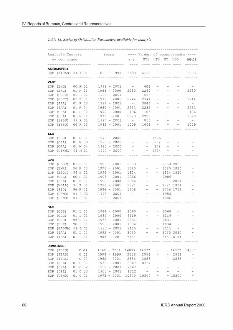
Table 13. Series of Orientation Parameters available for analysis
————————————————————————————————————————————————————————————————————————
Analysis Centers Years ———— Number of measurements ————
by technique x,y UT1 UT0 UT LOD ∆ψ ∆ε———————————————————— ———————————— ———— ———— ———— ———— ———— ——————ASTROMETRYEOP (AICAS) 01 A 01 1899 - 1991 6693 6693 - - - 6693
———————————————————— ———————————— ———— ———— ———— ———— ———— ——————VLBIEOP (BKG) 00 R 01 1999 - 2001 - 602 - - - -EOP (BKG) 01 R 01 1984 - 2000 2280 2280 - - - 2280EOP (GSFC) 00 R 01 1999 - 2001 - 596 - - - -EOP (GSFC) 01 R 01 1979 - 2001 2744 2744 - - - 2744EOP (IAA) 01 R 03 1984 - 2001 - 3846 - - - -EOP (IAA) 01 R 04 1980 - 2001 2232 2232 - - - 2232EOP (OPA) 01 R 02 1999 - 2000 106 106 - - - 106EOP (SHA) 01 R 01 1979 - 2001 2928 2928 - - - 2928EOP (SPBU) 99 R 01 1997 - 2001 - 866 - - - -EOP (SPBU) 00 R 03 1983 - 2001 1009 1009 - - - 1009
———————————————————— ———————————— ———— ———— ———— ———— ———— ——————LLREOP (FSG) 01 M 01 1970 - 2000 - - 1566 - - -EOP (OPA) 01 M 03 1995 - 2000 - - 282 - - -EOP (OPA) 01 M 04 1995 - 2000 - - 178 - - -EOP (UTXMO) 01 M 01 1970 - 2000 - - 1514 - - -
———————————————————— ———————————— ———— ———— ———— ———— ———— ——————GPSEOP (CODE) 01 P 01 1993 - 2001 2858 - - 2858 2858 -EOP (EMR) 96 P 03 1996 - 2001 1820 - - 1820 1820 -EOP (ESOC) 96 P 01 1996 - 2001 1824 - - 1824 1824 -EOP (GFZ) 00 P 01 1993 - 2001 2986 - - 2986 - -EOP (JPL) 01 P 01 1992 - 2000 2854 - - - 2854 -EOP (NOAA) 96 P 01 1996 - 2001 1821 - - 1821 1821 -EOP (SIO) 96 P 01 1996 - 2001 1756 - - 1756 1756 -EOP (USNO) 01 P 02 1995 - 2001 - - - 1953 - -EOP (USNO) 01 P 01 1995 - 2001 - - - 1946 - -
———————————————————— ———————————— ———— ———— ———— ———— ———— ——————SLREOP (CGS) 01 L 01 1984 - 2000 2060 - - 2060 - -EOP (CLG) 01 L 01 1984 - 2000 6119 - - 6119 - -EOP (CSR) 95 L 01 1976 - 2001 2831 - - 2831 - -EOP (DUT) 98 L 01 1993 - 2001 1034 - - 1034 - -EOP (GAOUA) 01 L 01 1983 - 2001 2115 - - 2115 - -EOP (IAA) 01 L 02 1992 - 2001 3030 - - 3030 3030 -EOP (IAA) 01 L 01 1983 - 2001 6151 - - 6151 6151 -
———————————————————— ———————————— ———— ———— ———— ———— ———— ——————COMBINEDEOP (IERS) C 04 1962 - 2001 14877 14877 - - 14877 14877EOP (IERS) C 03 1998 - 1999 2556 2556 - - 2556 -EOP (IERS) C 02 1962 - 2001 2886 2886 - - 2886 -EOP (JPL) 01 C 01 1976 - 2001 8867 8867 - - - -EOP (JPL) 01 C 02 1962 - 2001 2847 - - - - -EOP (JPL) 01 C 03 1900 - 2001 1212 - - - - -EOP (USNO) 01 C 01 1973 - 2001 10300 10300 - - 10300 -
————————————————————————————————————————————————————————————————————————

IERS Annual Report 2000 87
IV.4 EOP Section of the Central Bureau
The Earth orientation series available for analysis are described inTable 13. They include the 38 series received from 27 AnalysisCenters.
A known source of relative drifts in x, y and UT1–UTC is the varietyof processes chosen by the analysis centers to control the timeevolution of the adjusted terrestrial reference frames, complicatedby the sampling of the tectonic plates and plate margins in theactual observing networks. The NNR-NUVEL1A model (DeMets etal., 1990; DeMets et al., 1994) is recommended in the IERS Con-ventions (1996). The various ways in which the time evolution isglobally constrained to follow a reference model reflect themselvesin the EOP time series.
The calibration of the formal uncertainties associated with theEOP determinations which are combined is derived from the pairvariance analysis of the differences between series, without con-sidering any combined series in the process. The analysis followsthe method of Gray and Allan (1974) extended to the case of corre-lated errors. When three or more series of similar quality and timeresolution can be differenced, the pair variance of the noise of eachseries can be evaluated. In the case of series based on the samedata set, the estimation model includes consideration of their pos-sible correlation whenever permitted by the information available.The pair variance thus obtained is referred to as the estimated un-certainty of a single determination in a given series; its ratio withthe rms formal uncertainty over the same period provides a scalingfactor.
The weighting of the combined individual results is based on thequadratic sum of estimated uncertainties, obtained by multiplyingthe formal uncertainty of the original determination by the previ-ously described scale factors of the series to which they belong,and of a term which reflects the uncertainty of the systematic cor-rection applied. The effective weighting of the individual series ob-tained from the same data set (VLBI, GPS, SLR) is appropriatelymodified to take into account the resulting redundancy.
In the case of satellite techniques (SLR, GPS), the numbers inthe columns labeled “UT-UTC” refer to the high frequency content ofthe results, i.e. for periods shorter than about 60 days.
EOP(IERS) C 01 is under the form of normal values at 0.05 yearintervals since 1846 with associated formal uncertainties. It servesas a reference for the evaluation of systematic differences of thecompared series. This solution is intended for long term studies.Figure IV-4-7 represents the pole path over 1996 until 2001. Themean pole path since 1900 is represented in solid line. EOP(IERS) C 01 is based on the following data.
4.4 Yearly Analyses
General Combination of Series
Presentation of the CombinedSolutions
Reference series of EOP at 0.05 yearinterval, EOP(IERS) C 01:
Tables 14, 15, 16
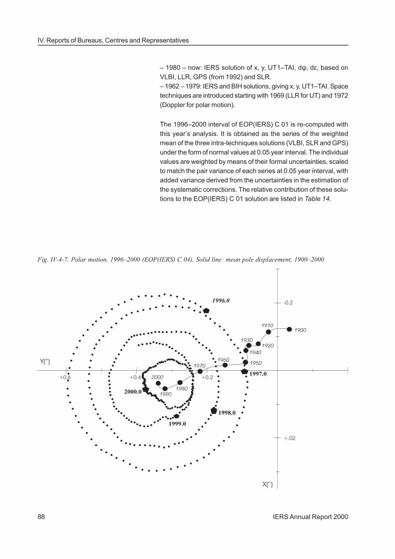
IERS Annual Report 200088
IV. Reports of Bureaus, Centres and Representatives
– 1980 – now: IERS solution of x, y, UT1–TAI, dψ, dε, based onVLBI, LLR, GPS (from 1992) and SLR.– 1962 – 1979: IERS and BIH solutions, giving x, y, UT1–TAI. Spacetechniques are introduced starting with 1969 (LLR for UT) and 1972(Doppler for polar motion).
The 1996–2000 interval of EOP(IERS) C 01 is re-computed withthis year’s analysis. It is obtained as the series of the weightedmean of the three intra-techniques solutions (VLBI, SLR and GPS)under the form of normal values at 0.05 year interval. The individualvalues are weighted by means of their formal uncertainties, scaledto match the pair variance of each series at 0.05 year interval, withadded variance derived from the uncertainties in the estimation ofthe systematic corrections. The relative contribution of these solu-tions to the EOP(IERS) C 01 solution are listed in Table 14.
Fig. IV-4-7. Polar motion, 1996–2000 (EOP(IERS) C 04). Solid line: mean pole displacement, 1900–2000

IERS Annual Report 2000 89
IV.4 EOP Section of the Central Bureau
Table 14. EOP(IERS) C 01: Percentage of the contribution of various techniques in the final solution—————————————————————————————————————————————————————————————————————
TECHNIQUE POLAR MOTION UT1-UTC LOD NUTATION OFFSET
—————————————————————————————————————————————————————————————————————
IERS VLBI 20 100 10 100
IERS SLR 10 - - -
IERS GPS 70 - 90 -
—————————————————————————————————————————————————————————————————————
Table 15. EOP(IERS) C 01: Evolution of the mean uncertainties———————————————————————-———————————————————————————————————————-————————————————
X Y UT1-UTC dψ dε YEARS ——————————— ——————————— ————————————— ——————————— ————————————
Nb σ Nb σ Nb σ Nb σ Nb σ /year (mas) /year (mas) /year (0.1ms) /year (mas) /year (mas)
—————————— ——————————— ——————————— ————————————— ——————————— ————————————
1846-1889 10 80. 10 90. - - - - - -
1890-1900 20 50. 20 70. - - - - - -
1900-1961 20 30. 20 40. - - - - - -
1962-1972 20 15. 20 15. 20 15. - - - -
1973-1979 20 10. 20 10. 20 5. - - - -
1980-1983 20 1.2 20 1.1 20 1.2 20 2.0 20 0.5
1984-1987 20 0.16 20 0.15 20 0.11 20 0.20 20 0.10
1988-1995 20 0.11 20 0.11 20 0.08 20 0.16 20 0.08
1995-2000 20 0.08 20 0.08 20 0.04 20 0.06 20 0.04
———————————————————————-———————————————————————————————————————-————————————————
Table 16. EOP(IERS) C 01: Earth orientation parameters at 0.05 yr interval
—————————————————————————————————————————————————————————————————————————————————————
Date Normal values Uncertainties
———————— ———————————————————————————————————————————————— ——————————————————————————
Bessel. x y UT1-UTC LOD dψ dε x y UT1 LOD dψ dε year " " s s 0.001" 0.001" 0.0001s 0.001"
———————— ——————— ——————— ———————— ———————— —————— ————— ———————— ———————— ——————
2000.00 .043240 .377693 .3554825 .0009023 -50.46 -2.44 .009.012 .016.002 .05.022000.05 .052402 .375673 .3413541 .0008776 -51.51 -2.92 .008.010 .011.002 .04.022000.10 .060578 .372437 .3250566 .0008094 -50.23 -3.48 .008.010 .012.002 .04.022000.15 .068039 .365452 .3071142 .0009868 -49.81 -4.66 .010.010 .016.005 .06.022000.20 .074497 .357951 .2899853 .0008020 -49.55 -5.15 .010.011 .010.003 .03.012000.25 .075411 .345975 .2762529 .0008396 -47.65 -5.71 .010.012 .020.003 .06.022000.30 .082297 .343177 .2552617 .0012363 -47.61 -6.21 .007.010 .014.005 .04.022000.35 .088037 .331942 .2358645 .0008132 -47.54 -6.58 .008.010 .018.002 .05.032000.40 .096328 .321422 .2198827 .0006230 -48.98 -7.18 .006.008 .014.002 .04.022000.45 .113551 .304341 .2064849 .0004528 -51.74 -6.51 .009.008 .020.002 .06.022000.50 .110095 .279075 .2040671 .0000078 -54.23 -6.58 .010.007 .024.002 .09.032000.55 .096143 .261651 .2004162-.0001027 -56.25 -6.15 .007.008 .011.002 .04.022000.60 .083051 .248520 .1987965 .0000841 -58.40 -6.31 .011.012 .017.005 .08.032000.65 .058367 .242754 .1949480 .0004127 -60.77 -6.56 .008.011 .015.004 .06.022000.70 .025943 .239566 .1871300 .0002841 -59.88 -5.77 .007.008 .012.002 .06.022000.75 -.005736 .246950 .1747323 .0008476 -60.10 -5.05 .007.007 .020.004 .08.022000.80 -.035990 .262843 .1599588 .0008995 -57.11 -3.77 .007.009 .014.002 .04.022000.85 -.059984 .292223 .1391539 .0010610 -54.98 -3.79 .007.008 .012.002 .06.022000.90 -.076903 .325406 .1205417 .0009176 -55.13 -2.77 .009.009 .019.002 .09.032000.95 -.082693 .357049 .1045876 .0006411 -53.18 -1.91 .010.010 .017.002 .06.03
—————————————————————————————————————————————————————————————————————————————————————
IERS Annual Report 200090
IV. Reports of Bureaus, Centres and Representatives
This series is available from 1962. For each date at 5-day intervals,individual determinations available within ±2.5 days are brought tothe central date by a modeled time variation of each of the EOP.The combined normal values are obtained by a weighted least squareadjustment taking into account the covariance matrices of the indi-vidual determinations. The a priori standard deviations are based onthe formal uncertainties associated with the individual values of theEOP, scaled to match the pair variance of the series, with addedvariances. The GPS series were first combined prior to the compi-lation of EOP(IERS). The uncertainties given in Table 17 representthe short-term instability of the normal values.
This series is available from 1993. It is only continuous for polarmotion. For each date at one-day interval, all individual determina-tions of universal time available within ± 0.5 days are brought to thecentral date by a modeled time variation of UT and corrected fortheir difference with the IERS System. A weighted mean is thenperformed; the a priori standard deviations of the individual valuesare based on the formal uncertainties, scaled to match the pairvariance of the series, with added variances.
This series continues the one available since 1962. After being ho-mogenized and merged, the contributing series of each of the EOPare slightly smoothed by the Vondrak algorithm. The filter charac-teristics, given in Table 23, are selected so that the weighted rmsresiduals of the original EOP series in a given time interval matchtheir estimated precision. The series are given at one-day intervalsand can be interpolated linearly; the oscillations in UT and in dura-tion of the days due to zonal tides for periods under 35 days, aswell as the 14d terms in dψ and dε are present in the series.
EOP(IERS) C 04 series and its continuation until the current dateis available at the web site: <http://hpiers.obspm.fr/eop-pc>.
Combined series at 5-day intervals,EOP(IERS) C 02: Table 17
Combined series of EOP (normalpoints) at 1-day interval,
EOP(IERS) C 03: Table 18
Combined daily series,EOP(IERS) C 04: Table 19

IERS Annual Report 2000 91
IV.4 EOP Section of the Central Bureau
Table 17. EOP(IERS) C 02: Average uncertainty of the normal point solution given at five-day intervals
————————————————————————————————————————————————————
YEARS σ(X) σ(Y) σ(UT1) σ(dψ) σ(dε) 0.001" 0.0001s 0.001"
————————————————————————————————————————————————————
1962-1967 30 30 20 - -
1968-1971 25 25 17 - -
1972-1979 11 11 10 - -
1980-1983 2 2 3 2 1
1984-1989 0.4 0.4 0.2 0.5 0.3
1990-2000 0.2 0.2 0.1 0.3 0.2
————————————————————————————————————————————————————
Table 18. EOP(IERS) C 03: Number of values and average uncertainty
———————-——————————————————————————————————————-———————————————————————————————
X Y UT1-UTC dψ dε (mas) (mas) (0.1ms) (mas) (mas)
YEAR —————————— —————————— —————————— —————————— ——————————
Nb σ Nb σ Nb σ Nb σ Nb σ———————— ———— ———— ———— ———— ———— ———— ———— ———— ———— ————
1993 365 0.41 365 0.38 236 0.26 70 0.23 70 0.11
1994 365 0.32 365 0.32 194 0.17 52 0.17 52 0.08
1995 365 0.28 365 0.26 216 0.14 52 0.17 52 0.08
1996 366 0.28 366 0.27 215 0.15 53 0.17 53 0.08
1997 365 0.28 365 0.27 257 0.15 53 0.17 53 0.08
1998 365 0.25 365 0.12 257 0.15 53 0.17 53 0.08
1999 365 0.10 365 0.10 259 0.08 88 0.17 88 0.08
2000 366 0.10 365 0.10 259 0.08 88 0.17 88 0.08
——————————————————————————————————————————————-———————————————————————————————
Table 19. EOP(IERS) C 04: Uncertainty of a daily value
————————————————————————————————————————————————————————————————————————————
EOP Unit 1962-67 1968-71 1972-79 1980-83 1984-95 1996-2000
————————————————————————————————————————————————————————————————————————————
X mas 30 20 15 2 0.7 0.2
Y mas 30 20 15 2 0.7 0.2
UT1-UTC 0.1ms 20 15 10 4 0.4 0.2
LOD 0.1ms 14 10 7 1.5 0.3 0.2
dPsi.sin(Eps) mas(1) 12 9 5 3 0.6 0.3
dEps mas(1) 2 2 2 2 0.6 0.3
————————————————————————————————————————————————————————————————————————————
Note (1): Prior to 1984, dψ, dε are evaluated by an empirical model.

IERS Annual Report 200092
IV. Reports of Bureaus, Centres and Representatives
The combination of series of EOP which is described in the abovesections is based on two major hypotheses:
• the high frequency behaviors of the series combined arestatistically independent,
• the applied corrections (bias and drift) appropriately model theirsystematic differences.
The high frequency correlation of the individual series has beeninvestigated. Each series is first corrected for known effects (ef-fects of zonal tides in UT, 14d term in dψ and dε), and high passfiltered by a Vondrak smoothing (Bulletin B degree of smoothing,Table 23). The series of residuals are then correlated two by two,considering only dates less than 0.25 day apart. The correlationsare lower than +0.3 across techniques and lower than +0.5 withinthe same technique.
Systematic differences: when estimating by weighted leastsquares the systematic differences between pairs of series underthe form of a bias and a linear drift over common time intervals, theweighted rms postfit residuals found are consistent with the a prioriuncertainties used in the computation of EOP(IERS) C 01.
The individual series used in the computation of EOP(IERS) C 01,C 02, C 03, C 04 are compared with EOP(IERS) C 04 over 1999–2000 in Table 20.
The formal uncertainties are the averages of those given by theanalysis centers after removing the spurious values (values > 3sigma). The rms is the root mean square residual obtained from thecomparison to EOP(IERS) C 04.
Two daily combined EOP series obtained by JPL and NEOS arecompared with EOP(IERS) C 04 and between themselves. The mainfeatures of the implementation of the three series are quite similar.They are based on a limited number of VLBI and SLR series, GPSbeing introduced mid-1992. The unification of the systems is ob-tained by correcting the individual series for a bias and a linear drift.The weighting of individual values is based on their original standarderror, multiplied by a scaling factor specific to each series. Theyare low-pass filtered, with a frequency cutoff corresponding to a fewdays.
Table 21 gives the systematic long term differences between thethree series. The standard deviations are consistent with the esti-mated quality of EOP(IERS) C 04.
Table 22 gives an estimation of the stability of the IERS, JPL andNEOS series, based on their intercomparison, for sampling timesof 1 through 64 days. The three series have similar characteristics.
Comparison of Series with theEOP(IERS) C 04
Series used in the computation ofEOP(IERS) solutions
Consistency of daily combinedEOP series

IERS Annual Report 2000 93
IV.4 EOP Section of the Central Bureau
Table 20. Formal uncertainties and rms residuals of individual determinations of the EOP, 1999–2000
———————————————————————————————————————————————————————————————————————————Individual Errors X Y UT1-UTC dPsi dEps D sample Series 0.001" 0.001" 0.0001s 0.001" 0.001" 0.0001s timeVLBI ————— ——————— —————— —————— ——————— —————— —————— ——————— ——————EOP (BKG) formal: 0.17 0.13 0.09 0.25 0.10 - 1d00 R 02 rms: 0.17 0.13 0.15 0.28 0.12 -EOP (BKG) formal: - - 0.18 - - - 0.05d00 R 01 rms: - - 0.19 - - -EOP (GSFC) formal: 0.14 0.12 0.07 0.24 0.09 - 1d00 R 01 rms: 0.14 0.10 0.14 0.40 0.15 -EOP (GSFC) formal: - - 0.17 - - - 0.05d01 R 01 rms: - - 0.15 - - -EOP (IAA) formal: 0.12 0.10 0.06 0.21 0.08 - 1d01 R 03 rms: 0.17 0.16 0.12 0.37 0.16 -EOP (IAA) formal: - - 0.15 - - - 0.05d01 R 04 rms: - - 0.15 - - -EOP (OPA) formal: 0.09 0.07 0.04 0.06 0.06 - 1d01 R 02 rms: 0.22 0.32 0.12 0.29 0.15 -EOP (SHA) formal: 0.14 0.12 0.07 0.20 0.08 - 1d01 R 01 rms: 0.16 0.11 0.14 0.29 0.13 -EOP (SPBU) formal: 0.09 0.08 0.04 0.20 0.08 - 1d00 R 03 rms: 0.14 0.13 0.09 0.30 0.14 -EOP (SPBU) formal: - - 0.19 - - - 0.5d99 R 01 rms: - - 0.16 - - -GPS —————— ——————— —————— —————— ——————— —————— —————— ——————— ——————EOP (CODE) formal: 0.01 0.02 - - - 0.01 1d01 P 01 rms: 0.09 0.08 - - - 0.24EOP (EMR) formal: 0.06 0.06 - - - 0.10 1d96 P 03 rms: 0.21 0.27 - - - 0.92EOP (ESOC) formal: 0.03 0.03 0.04 - - 0.03 1d96 P 01 rms: 0.16 0.15 0.52 - - 0.32EOP (GFZ) formal: 0.01 0.01 - - - 0.01 1d01 P 01 rms: 0.07 0.08 - - - 0.32EOP (JPL) formal: 0.06 0.06 - - - 0.16 1d01 P 01 rms: 0.11 0.11 - - - 0.32EOP (NOAA) formal: 0.03 0.03 - - - 0.19 1d96 P 01 rms: 0.27 0.27 - - - 0.80EOP (SIO) formal: 0.06 0.07 - - - 0.16 1d96 P 01 rms: 0.16 0.10 - - - 0.36EOP (USNO) formal: - - - - - - 1d01 P 01 rms: - - 0.30 - - -SLR —————— ——————— —————— —————— ——————— —————— —————— ——————— ——————EOP (CGS) formal: 0.12 0.12 - - - - 3d00 L 01 rms: 0.58 0.55 - - - -EOP (CSR) formal: 0.35 0.35 0.29 - - - 3d95 L 01 rms: 0.44 0.30 1.13 - - -EOP (CLG) formal: 0.29 0.28 - - - - 3d01 L 01 rms: 1.51 1.45 - - - -EOP (DUT) formal: 0.11 0.11 - - - - 3d98 L 01 rms: 0.35 0.37 - - - -EOP (GAOUA) formal: 0.18 0.16 - - - - 3d01 L 01 rms: 0.30 0.28 - - - -EOP (IAA) formal: 0.07 0.07 0.04 - - 0.04 5d00 L 01 rms: 0.22 0.19 0.37 - - 0.22EOP (IAA) formal: 0.05 0.05 0.03 - - 0.03 5d00 L rms: 0.19 0.16 0.29 - - 0.18LLR —————— ——————— —————— —————— ——————— —————— —————— ——————— ——————EOP (FSG) formal: - - 0.62 - - - 0.05d01 M 01 rms: - - 1.46 - - -EOP (UTXMO) formal: - - 3.32 - - - 0.05d01 M 01 rms: - - 1.21 - - -EOP (OPA) formal: - - 0.27 - - - 0.05d01 M 03 rms: - - 0.56 - - -EOP (OPA) formal: - - 0.44 - - - 0.05d01 M 04 rms: - - 0.41 - - -———————————————————————————————————————————————————————————————————————————

IERS Annual Report 200094
IV. Reports of Bureaus, Centres and Representatives
Table 21. Differences between combined daily series of EOP over 1996–2000
The differences are expressed under the form: A + A’(t–1997.0), where t is the datein Besselian years. R is the rms residual after the adjustment of A and A’.Units: x, y, dψ, dε: A and R in 0.001", A’ in 0.001"/yr
UT1–UTC: A and R in 0.0001s, A’ in 0.0001s/yr——————————————————————————————————————————————————————————————————
SOLUTIONS JPL – IERS NEOS – IERS NEOS – JPL
——————————————————————————————————————————————————————————————————
X A 0.052 ± 0.004 -0.021 ± 0.004 -0.073 ± 0.002
A’ -0.033 ± 0.002 -0.080 ± 0.002 0.028 ± 0.001
R 0.109 0.091 0.063
——————————————————————————————————————————————————————————————————
Y A -0.033 ± 0.004 -0.037 ± 0.004 -0.016 ± 0.003
A’ 0.020 ± 0.002 0.004 ± 0.002 -0.010 ± 0.001
R 0.102 0.091 0.060
——————————————————————————————————————————————————————————————————
UT1-UTC A 0.019 ± 0.006 0.013 ± 0.008 0.002 ± 0.003
A’ -0.012 ± 0.003 0.007 ± 0.004 0.010 ± 0.002
R 0.191 0.240 0.093
——————————————————————————————————————————————————————————————————
dPsi A - - -0.206 ± 0.019 - -
R - - 0.557 - -
——————————————————————————————————————————————————————————————————
dEps A - - -0.011 ± 0.012 - -
R - - 0.339 - -
——————————————————————————————————————————————————————————————————
JPL: series 01 C 01NEOS:series 01 C 01IERS: series C 04
Table 22. Allan variance analysis of the combined series of EOP for sampling timesof 1 through 64 days based on the 1996–2000 data———————————————————————————————————————————————————————————
Combined Sampling X Y UT1-UTC
EOP Series time (0.001") (0.001") (0.0001s)
———————————————————————————————————————————————————————————
IERS C 04 1 d 0.10 0.18 0.04
8 d 0.03 0.07 0.07
32 d 0.02 0.04 0.04
64 d 0.01 0.03 0.03
JPL 01 C 01 1 d 0.09 0.18 0.03
8 d 0.04 0.07 0.01
32 d 0.02 0.04 0.01
64 d 0.02 0.03 0.01
NEOS 01 C 01 1 d 0.09 0.18 0.09
8 d 0.03 0.06 0.06
32 d 0.02 0.03 0.02
64 d 0.02 0.02 0.01
———————————————————————————————————————————————————————————

IERS Annual Report 2000 95
IV.4 EOP Section of the Central Bureau
An advanced version of EOP(IERS) C 04 is distributed monthly inIERS Bulletin B. The time series of EOP issued in Bulletin B arebased on the annual analysis described in the above sections,applied to the series provided weekly or monthly by the operationalanalysis centers. Each of the series available is referred to theIERS System considering a bias and a linear drift derived fromprevious analyses. The formal uncertainties are scaled to reflectthe real uncertainty of the data. All series of determinations of thesame parameters are then merged, and the five resulting series (x,y, UT1, dψ, dε) are smoothed with the adopted degree of smoothing.UT1 is treated under the form of UT1R (effect of zonal tides withperiods under 35 d removed), and dψ, dε are treated under the formof residuals to a modeled correction; these modeled correctionsare added back at the end of the processing. The degrees ofsmoothing used in 2000 are given in Table 23. They are chosen asallowed by the precision of the input series. The rms differencesbetween the Bulletin B series and EOP(IERS) C 04 in 2000 are0.2 mas on x, y, 0.02 ms on UT1, and 0.0003" on dψ sinε and dε.
Two different approaches are used for prediction of the Earth rota-tion parameters.
• Universal Time: The formalism used is based on the assumptionthat the long-term fluctuations (annual and semi-annual) of thepreceding year are valid over the next few months. For short-term variations prediction, an autoregressive process is used.
• Polar Motion: The formalism uses at first a floating period fitfor both Chandler and annual components estimation. Anautoregressive filter is then applied on the short-term variations.
IERS Bulletin B
Table 23. Bulletin B: Transfer functions of smoothings by Vondrak algorithm—————————————————————————————————————————————————————————————————————————————
Period for
Epsilon Remaining amplitude Parameters involved
5% 50% 95%
—————————————————————————————————————————————————————————————————————————————
10-2 6d 15d 25d dψ, dε through B96 (Dec 1995)—————————————————————————————————————————————————————————————————————————————
10-0.5 6d 8d 12d x, y, UT1, LOD through B96 (Dec 1995)
—————————————————————————————————————————————————————————————————————————————
10+2 2d 3d 5d all parameters starting with B97 (Jan 1996)
—————————————————————————————————————————————————————————————————————————————

IERS Annual Report 200096
IV. Reports of Bureaus, Centres and Representatives
The content of Bulletin B is as follows (7 sections):
1. Smoothed values of x, y, UT1R–UTC, UT1R–TAI, dψ, dε, sampledat five-day interval. Final Bulletin B values over one month andprovisional extension over the next four months. The smoothingsare based on the Vondrak (1977) algorithm, with degrees ofsmoothing indicated in the legend (see also Feissel andLewandowski, 1984). However, the oscillations in UT and induration of the day due to zonal tides with periods under 35
Table 24. Bulletins A and B: Individual series contributing to IERS, January 2000
The formal uncertainties are those which are reported by the contributors. They are used in thecombinations for Bulletins A and B after being calibrated by statistical assessment.
——————————————————————————————————————————————————————————————————————————
INDIVIDUAL SERIES FORMAL UNCERTAINTIES
CONTRIBUTING TO SAMPLING BASED ON 1999-2000 DATA
TIME ———————————— —————————————— ———————————
IERS BULLETINS Terrest.Pole UT LOD Celest.Pole
A AND B 0.001" 0.0001s 0.001"
———————————————————— ———————— ———————————— —————————————— ———————————VLBIEOP(GSFC) 00 R 01 7d -- 0.21 -- --EOP(GSFC) 00 R 02 7d 0.64 0.29 -- 0.15EOP(BKG) 00 R 01 7d -- 0.22 -- --EOP(BKG) 00 R 02 7d 0.16 0.09 -- 0.08EOP(IAA) 98 R 01 7d 0.10 0.04 -- 0.10EOP(IAA) 00 R 04 7d -- 0.18 -- --EOP(USNO)+ 99 R 01 7d 0.14 0.06 0.20 0.13EOP(USNO)+ 99 R 02 1-3 d -- 0.23 -- --EOP(SPBU) 99 R 01 1-3 d -- 0.22 -- --
———————————————————— ———————— ———————————— —————————————— ———————————SLREOP(CGS) 97 L 02 3d 0.28 0.25 * -- --EOP(CSR) 95 L 01 3d 0.39 0.31 * -- --EOP(DUT) 98 L 01 3d 0.11 0.10 * -- --EOP(IAA) 98 L 02 1d 0.05 0.04 * 0.04 --EOP(MCC) 97 L 01 3d 0.05 -- 0.10 --
———————————————————— ———————— ———————————— —————————————— ———————————GPSEOP(CODE) 98 P 01 1d 0.05 -- 0.10 --EOP(EMR) 96 P 03 1d 0.07 1.05 * 0.13 --EOP(ESOC) 96 P 01 1d 0.02 0.03 * 0.03 --EOP(GFZ) 96 P 02 1d 0.01 0.01 * 0.01 --EOP(JPL) 96 P 03 1d 0.04 0.14 * 0.14 --EOP(NOAA) 96 P 01 1d 0.03 0.10 * 0.19 --EOP(SIO) 96 P 01 1d 0.07 0.45 * 0.16 --EOP(IGS) 95 P 02 1d 0.05 0.17 * 0.08 --EOP(IGS) 96 P 02 1d 0.08 0.29 * 0.14 --——————————————————————————————————————————————————————————————————————————
* The satellite techniques provide information on the rate of change of Universal Time contaminated byeffects due to non modeled orbit node motion. VLBI-based results have been used to minimize drifts

IERS Annual Report 2000 97
IV.4 EOP Section of the Central Bureau
days, as well as the 14 days term in dψ, dε, are present in fullsize in the series.
2. Daily values of x, y, UT1–UTC, UT1–UT1R, D, dψ, dε, sameseries as in section 1.
3. Five-day normal values of x, y, UT1–UTC, dψ, dε, and their un-certainties based on a combination of the series of section 6.
4. Smoothed values of DR and ωR, with the same degree ofsmoothing than for UT1R–UTC.
5. Current values of UTC–TAI and DUT1, reproducing IERS BulletinsC and D.
6. Statistics on the data used.7. Data of IERS analysis centers (available only in electronic distri-
bution). In this section, the original results received from the IERSanalysis centers and used for the solution listed in sections 1 to3 are reproduced. These results are those which are availableone to five weeks after the observation dates. Updated resultsreceived later are stored, but as a general rule, they are notprinted in Bulletin B. The series used in January 2000 are listedin Table 24.
Let us consider two series of EOP (x, y, UT1, dψ, dε) and (x', y',UT1', dψ', dε') respectively. Each of them is referred to a celestialframe defined by the adopted Radio Source Coordinates (RSC) andto a terrestrial frame defined by the adopted Set of Station Coordi-nates (SSC). The celestial reference frames, respectively denotedCRF and CRF' present systematic differences, which can be de-scribed by an elementary rotation matrix A. The coordinates in bothsystem, [CRF] and [CRF'] respectively, are linked by the relation:
[CRF] = A [CRF']
In the same way the terrestrial reference frames, TRF and TRF'respectively, are linked through an elementary rotation:
[TRF] = R [TRF']
If the EOP series were consistent, then the systematic differencesin the pole coordinates, ∆x and ∆y, in the universal time, ∆UT1,and in the celestial pole offsets, ∆dψ and ∆dε would be only due tothe rotation angles (A1, A2, A3) between the two celestial framesand the rotation angles (R1, R2, R3) between the two terrestrialframes, with:
∆x = x' – x∆y = y' – y∆UT1 = UT1' – UT1∆dψ = dψ' − dψ∆dε = dε' − dε
4.5 Consistency of IERSResults
Consistency of IERS EOP Serieswith ITRS and ICRS at a
Reference Epoch

IERS Annual Report 200098
IV. Reports of Bureaus, Centres and Representatives
It can be shown that these systematic differences would satisfy thefollowing relationships with an accuracy of a few microarcseconds:
∆x = R2∆y = R1∆UT1 = (–R3 + A3)/ f (1)∆dψ = A2/sinε∆dε = –A1
where f is the conversion factor from Universal Time to siderealtime, and ε is the obliquity of the ecliptic.
It is worthwhile to know to which extent the relationships (1) aresatisfied. Each comparison will be made naturally with respect tothe same data set (CRF, TRF, EOP), that is the ICRF, the ITRF andthe corresponding EOP series of the IERS.
The closure of relationships (1) characterizes the internal con-sistency of the set of IERS results, time series and reference frames.In this objective the quantities:
C(x) = ∆x – R2C(y) = ∆y – R1C(UT1) = f. UT1 – (–R3 + A3)C(dψ) = ∆ dψ –A2/sinεC(dε) = ∆ dε –(–A1)
are computed.
We consider two terrestrial frames, each one having its own veloc-ity field. The corresponding series of EOP, the relative drifts
1,, TUyx ∆∆∆ between the series of EOP can be predicted byrelationships (2), obtained as the time derivatives of the first threerelationships (1):
2Rx =∆ ; 1Ry =∆ ; 31 RTU −=∆ (2)
where .1R ,
.2R ,
.
3R are the rates of change of the rotation angles
between the two terrestrial reference frames. These relationshipsare used to compare the drifts of the EOP series relative toEOP(IERS) C 01 with their predicted values based on the definitionof the corresponding terrestrial velocity field.
The present consistency analysis consists in two steps. The firststep is the computation of the biases and slopes of the individualEOP parameters (nutation in longitude, nutation in obliquity) withrespect to the combined parameters of the series EOP(IERS) C 01.The second step is the comparison, given hereafter, between thesebiases and slopes, and those theoretically produced by the rota-tions between the reference frames, as already explained.
Results for the EOP Series (2000)
Time evolution of the IERS EOPseries relative to ITRF

IERS Annual Report 2000 99
IV.4 EOP Section of the Central Bureau
Consistency analysis extends over the period 1988–2001, ex-cept for the recent VLBI series produced by the Paris Observatorysince 1999 (OPA). The data before 1988 were not involved, be-cause they are considered to be of less quality. Bias and trendhave been computed with respect to the epoch 1997.0 expressedin Julian year.
Actually since the year 1998, the angles between the individualTRF and the ITRF have not been computed by the ITRF ProductCenter of the IERS (located at the Institut Géographique National,France, formerly known as the ITRF Section of the Central Bureau)for some technical reason. In turn consistency analyses of the lastlong term series up to 2001.0, collected by the IERS EOP ProductCenter in the framework of the Annual Report 2000, cannot be madesystematically for polar motion and UT1, because the angles R1,R2, R3 are not available for computing the corresponding closurerelations.
For this reason the analysis has been restricted to 7 series, 5 ofthem derived from VLBI processing, and 2 from SLR processing.Table 25 gives the evaluations of the internal consistency for EOPseries, involving SSC or RSC, of which the orientation is known.The celestial frames angles can be found in Celestial System Sec-tion.
For VLBI series, the associated radio-source catalogue eithercorresponds to the ICRF (zero angles, case of IAA, OPA and SHAseries) or to celestial frame departing from the ICRF at the level of50 microarcseconds (case of BKG and GSFC series). In turnconsistency of nutation offsets of these series can be fullyinvestigated. Acceptable consistency, less than 100 microarc-seconds, is obtained for celestial pole offset (dψsinε, dε) of theBKG, GSFC, IAA and SHA series. Celestial pole offsets of OPAseries present inconsistencies, which may be caused by theshortness of the time span (two years).
Polar motion and UT1 consistencies have been investigated in thecase of two VLBI series (IAA, OPA), and two SLR series fromLAGEOS observations (IAA L 01, IAA L 02). These 4 series arereferred either to ITRF 2000 or to terrestrial frames, which do notpresent any net rotation with respect to ITRF 2000. Let us noticethat for other VLBI series the rotation matrix with respect to ITRF2000 remains unknown. Polar motion consistency smaller than 100microarcseconds is reached only for SLR series IAA L 01. UT1consistency is under this threshold for (IAA) VLBI series and the 2(IAA) SLR series.
Nutation offsets consistency
Polar motion and UT1 consistency
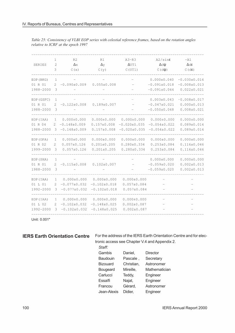
IERS Annual Report 2000100
IV. Reports of Bureaus, Centres and Representatives
Table 25: Consistency of VLBI EOP series with celestial reference frames, based on the rotation anglesrelative to ICRF at the epoch 1997
——————————————————————————————————————————————————————————————————————————————————
1 R2 R1 A3-R3 A2/sinε -A1
SERIES 2 ∆x ∆y ∆UT1 ∆dψ ∆dε 3 C(x) C(y) C(UT1) C(dψ) C(dε)——————————————————————————————————————————————————————————————————————————————————
EOP(BKG) 1 - - - 0.000±0.040 -0.030±0.016
01 R 01 2 -0.090±0.009 0.055±0.008 - -0.091±0.018 -0.008±0.013
1988-2000 3 - - - -0.091±0.044 0.022±0.021
——————————————————————————————————————————————————————————————————————————————————
EOP(GSFC) 1 - - - 0.003±0.043 -0.008±0.017
01 R 01 2 -0.122±0.008 0.189±0.007 - -0.047±0.021 0.000±0.013
1988-2000 3 - - - -0.050±0.048 0.008±0.021
——————————————————————————————————————————————————————————————————————————————————
EOP(IAA) 1 0.000±0.000 0.000±0.000 0.000±0.000 0.000±0.000 0.000±0.000
01 R 04 2 -0.148±0.009 0.157±0.008 -0.020±0.035 -0.054±0.022 0.089±0.014
1988-2000 3 -0.148±0.009 0.157±0.008 -0.020±0.035 -0.054±0.022 0.089±0.014
——————————————————————————————————————————————————————————————————————————————————
EOP(OPA) 1 0.000±0.000 0.000±0.000 0.000±0.000 0.000±0.000 0.000±0.000
01 R 02 2 0.057±0.126 0.201±0.205 0.280±0.334 0.253±0.084 0.116±0.046
1999-2000 3 0.057±0.126 0.201±0.205 0.280±0.334 0.253±0.084 0.116±0.046
——————————————————————————————————————————————————————————————————————————————————
EOP(SHA) 1 - - - 0.000±0.000 0.000±0.000
01 R 01 2 -0.115±0.008 0.102±0.007 - -0.059±0.020 0.002±0.013
1988-2000 3 - - - -0.059±0.020 0.002±0.013
——————————————————————————————————————————————————————————————————————————————————
EOP(IAA) 1 0.000±0.000 0.000±0.000 0.000±0.000 - -
01 L 01 2 -0.077±0.032 -0.102±0.018 0.057±0.084 - -
1992-2000 3 -0.077±0.032 -0.102±0.018 0.057±0.084 - -
——————————————————————————————————————————————————————————————————————————————————
EOP(IAA) 1 0.000±0.000 0.000±0.000 0.000±0.000 - -
01 L 02 2 -0.102±0.032 -0.148±0.025 0.002±0.087 - -
1992-2000 3 -0.102±0.032 -0.148±0.025 0.002±0.087 - -
——————————————————————————————————————————————————————————————————————————————————
Unit: 0.001"
For the address of the IERS Earth Orientation Centre and for elec-tronic access see Chapter V.4 and Appendix 2.
Staff:Gambis Daniel, DirectorBaudouin Pascale , SecretaryBizouard Christian, AstronomerBougeard Mireille, MathematicianCarlucci Teddy, EngineerEssaïfi Najat, EngineerFrancou Gérard, AstronomerJean-Alexis Didier, Engineer
IERS Earth Orientation Centre
IERS Annual Report 2000 101
IV.4 EOP Section of the Central Bureau
Arias E.F., Charlot P., Feissel M., Lestrade J.-F., 1995: Theextragalactic reference system of the International Earth RotationService, ICRS, Astron. Astrophys. 303, 604–608.
Aoki S., Guinot B., Kaplan G.H., Kinoshita H., McCarthy D.D.,Seidelmann P.K., 1982: Astron. Astrophys. 105, 1.
Boucher C. and Altamimi Z., 1989: The initial IERS TerrestrialReference Frame, IERS Technical Note No1, Observatoire deParis.
Boucher C., Altamimi Z., Sillard P., 1999: The 1997 InternationalTerrestrial Reference Frame ITRF97, IERS Technical Note No27, Observatoire de Paris.
Bougeard M., Gambis D., Ray R., 2000: Algorithms for boxconstrained M-estimation: fitting large data sets with applicationsto Earth Orientation Parameters series, Physics and Chemistryof the Earth 25, 9–11, pp. 679–685.
DeMets C., Gordon R.G., Argus D.F., Stein S., 1990: Current platemotions, Geophys. J. Int. 101, 425.
DeMets, C., Gordon R.G., Argus D.F., Stein S., 1994: Effect ofRecent Revisions to the Geomagnetic Reversal Time Scale onEstimates of Current Plate Motions, Geophys. Res. Lett. 21, 2191–2194.
Eisop E. and Gambis D., 1997: The combined solutions of theIERS Central Bureau, Proc. Journées Systèmes de référence,Praha, p. 104.
Fedorov E.P., Korsun A.A., Mayor S.P., Pantscheenko N.I., TaradyV.K., Yatskiv, YA. S., 1972: Dvizhenie polyusa Zemli s 1890.0 po1969.0. Naukova dumka, Kiev.
Feissel M. and Lewandowski W., 1984: Bull. Géod. 58, 464.Frede V., 1999: PhD thesis, Paris Observatory.Gambis D., 1996a: Multi-technique EOP combinations, Proceedings
of the 1996 IGS Analysis Center Workshop, Silver Spring. MD,edited by P. Van Scoy and R.E. Neilan, Pasadena, CA, JPL, JPLPublication 96–23.
Gambis D., 1996b: Monitoring Earth Rotation using varioustechniques, current results and future prospects, Proc. coll. IAU165, Dynamics and astrometry of natural and artificial celestialbodies
Gambis D. (ed.), IERS Annual Reports for 1998 and 1999,Observatoire de Paris, Paris, France.
Gambis D., Bougeard M., Jean-Alexis D., 2000: New methodologyfor Earth Orientation Time Series Combination, J. of Geodesy(submitted).
Gambis D., 2001: Allan Variance analysis applied to Earth orientationAnalysis, Adv. Space Research, (in press).
Gray J.E. and Allan D.W., 1974: Proc. 28th Ann. Symp. on FrequencyControl, 243.
References

IERS Annual Report 2000102
IV. Reports of Bureaus, Centres and Representatives
Gross R.S., 1990: The secular drift of the rotation pole, EarthRotation and Coordinate Reference Frames, IAG Symposium 105,C. Boucher and G. A. Wilkins (eds.), pp. 146–153, Springer-Verlag,New York.
Ma C. and Feissel M. (eds.), 1997: Definition and Realization of theInternational Celestial Reference System by VLBI Astrometry ofExtragalactic Objects, IERS Technical Note No 23, Observatoirede Paris.
McCarthy D.D. (ed.), 1996: IERS Conventions (1996), IERS TechnicalNote No 21, Observatoire de Paris.
Minster J.B. and Jordan T.H., 1978: J. Geophys. Res. 83, 5331.Seidelmann P.K., 1982: Celest. Mech. 27, 79.Shiskin J., Young A.H., Musgrave J.C., 1965: The X-11 variant of
the Census Method II seasonal adjustment program, U.S. Dept.of Commerce, Bureau of the Census, Technical Paper No 15.
Stephenson F.R. and Morrison L.V., 1984: Long term changes inthe rotation of the Earth: 700 B.C. to A.D. 1980, Phil. Trans. Roy.Soc. London A313, p. 47.
Vondrak J., 1977: Bull. Astron. Czechoslovaquia 28, 84.Vondrak J., Ron C., Pesek I., Cepek A., 1995: Astron. Astrophys.
297, 899–906.Yoder C.F., Williams J.G., Parke M.E., 1981: J. Geophys. Res. 86,
881.Yumi S. and Yokoyama K., 1980: Results of the International Latitude
Service in a homogeneous system 1899.9–1979.0, Publ. of theCentral Bureau of the International Polar Motion Service,Mizusawa.
Zhu S.Y. and Mueller I.I., 1983: Effects of adopting new precession,nutation and equinox corrections on the terrestrial referenceframes, Bull. Géod. 54, 29.
Daniel Gambis, Pascale Baudouin, Christian Bizouard,Mireille Bougeard, Teddy Carlucci, Najat Essaifi,
Gérard Francou, Didier Jean-Alexis