ivf a - nasa · interacting vortex geometry modifications ... interacting vortices and the shed...
TRANSCRIPT
NASA Contractor Report 165893
r
A Doublet Lattice Method for theDetermination of Rotor Induced
Empennage Vibration Airloads --Analysis Description andProgram Documentation
Santu. T. Gangwani
UNITED TECHNOLOGIES RESEARCH CENTER
East Hartford, CT 06108
Contract NASl-16058
June 1982
IVf ANational Aeronautics andSpace Administration
Langley Research CenterHampton, Virginia 23665AC 804 827-3966
https://ntrs.nasa.gov/search.jsp?R=19820023419 2018-06-12T12:53:41+00:00Z

A DOUBLET LATTICE METHOD FOR THE DETERMINATION
OF ROTOR INDUCED EMPENNAGE VIBRATION AIRLOADS -
ANALYSIS DESCRIPTION AND PROGRAM DOCUMENTATION
TABLE OF CONTENTS
LIST OF FIGURES ...........................
LIST OF TABLES .........................
SUMMARY • • • • • • • • • • • • • • • • " • " " • • " " " " " • " • "
I. INTRODUCTION ..........................
LIST OF SYMBOLS ...........................
II. GENERAL FORMULATION ......................
Statement of the Problem ....................
Basic Equations ......................
Solution of the Laplace Equation ................
The Boundary and the Trailing Edge Conditions .........
Discussion of Numerical Method .................
Determination of Pressure Distributions ..........
Modeling of Nonlinear Suction Loads ..............
III. DESCRIPTION OF COMPUTER PROGRAM ................
Numerical Method of Solution ..................
Discussion of Options .....................
Coupling with Program F389 ...................
Interacting Vortex Geometry Modifications ..........
Future Capabilities ........................
IV. PROGRAM RIEVA DOCUMENTATION .................
Subroutine Descriptions ....................
Input Description ........................
Output Description .......................
iv
vi
2
6
6
7
8
8
9
i0
ii
15
15
16
17
18
18
20
20
22
3O
•iI

TABLEOFCONTENTS(Cont'd)
Page
V. RESULTS AND DISCUSSION ...................... 34
Vl. CONCLUSIONS AND RECOMMENDATIONS ................. 37
VII. REFERENCES ........................... 38
TABLE ............................... 39
APPENDIX A .............................. 40
APPENDIX B .............................. 41
FIGURES .............................. 42
iii

LIST OFFIGURES
Figures
i
2
3
4
5
6
7
8
9
i0
ii
12
13
14
15
16
17
18
Wing/Vortex Geometry and Comparison of Measured and
Predicted Chordwise Distribution from Reference 3 .....
Schematic of Main Rotor Tip Vortex/Empennage Interaction. •
Wing Coordinate System ..................
Modeling of Wing and Its Wake ..............
Simplified Model Showing Interaction Effects .......
Modeling of Suction Effects ................
Flow Chart for Rotor/Tail Vibratory Excitation .......
Vortex Geometry Modification ...............
Maximum Fb Variation around Azimuth ............
An Example of Splitting of Rotor Wake into Two Parts . . .
Variation of Induced Velocity at Stabilizer ........
Vortex Geometry at Step No. i ...............
Vortex Geometry at Step No. 7 ...............
Vortex Geometry at Step No. 12 ..............
Stabilizer Airloads Time History .............
Chordwise Airload Variation at Step No. i .........
Chordwise Airload Variation at Step No. 7 .........
Vortex Geometry at Step No. 7 ...............
42
42
43
44
45
46
47
48
49
50
51
52
53
54
55
56
57
58
iv

LIST OF FIGURES (Cont'd)
Figures
19
20
21
Nonlinear Suction Airloads ................
Stabilizer Airloads Time History .............
Variation of Total Loads Over One Blade Passags
eTPP = -14.42 deg .....................
Page
59
60
61
v

LIST OF TABLES
Table
i
Page
Black Hawk Check Case Parameters .............. 39
•vl

A DOUBLETLATTICEMETHODFORTHEDETERMINATIONOFROTORINDUCEDEMPENNAGEVIBRATIONAIRLOADS-ANALYSISDESCRIPTIONANDPROGRAMDOCUMENTATION*
SUMMARY
An efficient state-of-the-art method has been developed to determinethe unsteady vibratory airloads produced by the interaction of the mainrotor wake with a helicopter empennage. This method has been incorporatedinto a computer program, Rotor Induced EmpennageVibration Analysis (RIEVA).The program requires the main rotor wake position and the strength of thevortices located near the empennagesurfaces. A nonlinear lifting surfaceanalysis is utilized to predict the aerodynamic loads on the empennagesurfaces in the presence of these concentrated vortices. The analysishas been formulated to include all pertinent effects such as suction of theinteracting vortices and the shed vorticity behind the empennagesurfaces.The analysis employs a stepwise solution (time domain); that is, a periodcorresponding to one blade passage is divided into a large numberof timeintervals and unsteady airloads are computedat each step. The output ofthe program consists of chordwise and spanwise airload distributions onthe empennagesurfaces. The airload distributions are harmonically analyzedand formulated for input into the Coupled Rotor/Airframe Vibration Analysis(Ref. 6). This report describes the theoretical development for the analysis,the RIEVAprogram documentation and output of a sample case of the program.
*The research effort which led to the results in this report was financiallysupported by the Structures Laboratory, USARTL,(AVRADCOM).

I. INTRODUCTION
The unsteady airloads produced by the interaction of the main rotor wakewith the helicopter empennage(horizontal stabilizer/vertical fin) can be amajor source of vibratory loads on a helicopter (Ref. i). An efficient state-of-the-art method has been developed to determine these unsteady airloads dueto the passage of concentrated main rotor wake vortices in the vicinity ofthe empennage. Since future helicopters are expected to be operating withhigh disk loading resulting in strong blade tip vortices in the rotor wake,the order of magnitude of these unsteady airloads will be significantlyhigher. As a consequence, these airloads will have to be determined in theearly design and development stage to insure an efficient design. Therefore,the main purpose behind the development of this analysis is to establish aneffective reliable methodology which can be utilized to analytically predictthese rotor wake induced empennageairloads.
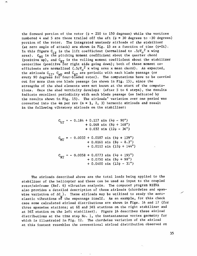
The prediction of these aerodynamic forces requires suitable analysistechniques for the description of the nonuniform flow environment in whichthe empennageoperates. The technique used herein involves the utilizationof two basic programs to study these main rotor wake/empennageinteractionphenomena. A wake analysis (Ref. 7) is used to determine the main rotorwake position and the strength of the vortices that are located near theempennagesurfaces, and a nonlinear lifting surface analysis is utilized topredict the aerodynamic loads on empennagesurfaces in the presence of theseconcentrated vortices. This nonlinear analysis, called RIEVA (Rotor InducedEmpennageVibration Airloads), has been formulated to include all pertinentflow phenomenasuch as the suction effects of the interacting vortices, span-wise induced effects, etc. For the steady-state flow case, the basic methodused has predicted accurately the pressures on a swept wing in the presenceof prescribed vortices as indicated by the results shownin Fig. 1 (Ref. 2and 3). The present effort involves the extension of this analysis to accountfor the unsteady main rotor wake induced effects and also the effect of shedvorticity behind the empennagesurfaces. The present method is an improve-ment over recently developed methods (e.g., Refs. 4 and 5) for the predictionof airloads because it includes nonlinear effects due to the interacting mainrotor tip vortices.

LIST OFSYMBOLS
A
Amnijw
0
CL, CM, CR
CLT, CMT' CRT
CP
CT
D
N
n
po
Pu
pA
R
r
r c
S
U,V,W
V o
a constant, 112_2."
N'
an element of the influence matrix.
mean chord length of lifting surface, feet.
lift, pitching moment (about quarter-chord) and rolling
moment coefficients, respectively, of the lifting surface;
nondimensionalized to (q * Area), (q * Area * _) and
(q * Area * _) respectively, where q = i/2pVo2.
lift, pitching moment and rolling moment coefficients,
respectively, corresponding to total loads (potential
plus suction airloads).
2pressure coefficient_2(po - p)/pV ° .
rotor thrust coefficient.
doublet strength, ft2/sec.
number of the collocation points.
subscript indicating surface normal direction.
free stream pressure, lb/ft 2.
static pressure at a point on upper surface, lb/ft 2.
static pressure at a point at lower surface, lb/ft 2.
rotor radius, feet.
radial distance from a vortex center.
viscous core radius of a vortical element.
lifting surface area.
the axial, radial and the swirl velocity components of a
vortex point.
free stream velocity, ft/sec.
i"
v
LIST OF SYMBOLS (Cont'd)
vn
Vimom
wmn
o
_TPP
Bo
Yt
r
rb
AD
A£
AV
At
ACP
rlo
P
iJ
4
.J,
normal component of the velocity.
uniform induced velocity of rotor (momentum)_ ft/sec.
normal velocity component at a collocation point due
to all known effects_ft/sec.
components of the lifting surface coordinate system.
the vertical distances of the two ends (A and B) of a
vortex element from the surface, respectively, feet.
the angle-of-attack of lifting surface with respect
to free stream.
i
rotor tip path plane angle-of-attack, positive aft,
blade coning angle.
turbulent kinematic viscosity of the vortex core.
circulation_ft2/sec.
rotor blade bound circulation_ft2/sec.
incremental doublet strength, ft2/sec.
incremental lift airload, lb/ft
tangential velocity increment due to singularity.
time increment for one computational step.
equals 2(p£- pu)/PVo 2.
advance ratio, Vo/_R.
distance along the direction perpendicular to the vortex -
axis direction.
free stream densityjlb-sec2/ft 4.
rotor solidity.

LIST OFSYMBOLS(Cont'd)
+u
disturbance potential distribution.
potential at a point on the lower surface.
potential at a point at the upper surface.
blade azimuthal angle.
rotor rotational speed,radians/sec.

II. GENERALFORMULATION
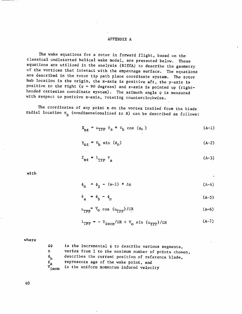
The basic tools utilized to determine the influence of rotor airflowon empennageexcitations are the UTRCRotorcraft WakeAnalysis (Ref. 7)and a nonlinear lifting surface analysis for unsteady three-dimensionalflow. The wake analysis is used to determine the main rotor wake inducedeffects near the empennagesurfaces and to provide the positions andstrengths of the vortices located near the empennagesurface. The detaileddescription of the technical approach, applications, and correlation re-suits for the Rotorcraft WakeAnlaysis are presented in Ref. 7. The pathsand spacings of the vortices which would interact with the empennagesur-faces, that is, those trailed off near the aft (4 = 0°) portion of therotor and near the forward (4 = 180°) portion of the rotor are shown sche-
matically in Fig. 2. Once the position of the interacting wake is defined,
the problem is reduced to the prediction of aerodynamic loads on lifting
surfaces in the presence of concentrated vortices. The analytical formula-
tion of this problem is described below.
Statement of the Problem
The objective of the analysis is the prediction of the unsteady airloads
on low to moderate aspect ratio lifting surface generated by the close passage
of the concentrated rotor vortices moving with the free stream. The lifting
surface is assumed to be operating at low angles of attack, with no flow
separation and the position and the strengths of the interacting vortices
are known at all instants of time. The analysis considers the unsteady incom-
pressible flow over a swept, three-dimensional wing surface of arbitrary shape
at a given angle of attack. Lifting surface theory is used to predict, in
time domain, the wing loading distributions due to the movement of the inter-
acting vortices near the surface. The analysis includes the unsteady and
suction effects of the interacting vortices, the unsteady effects of far main
wake, and the unsteady effects of the shed vorticity behind the lifting sur-
face. The interacting (viscous line) vortices are represented by finite
segments of vortical elements during their interaction with the lifting sur-
faces.
Basic Equations
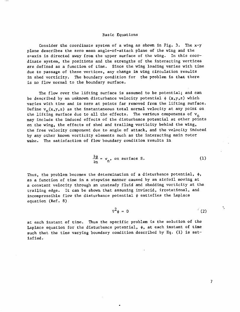
Consider the coordinate system of a wing as shownin Fig. 3. The x-yplane describes the zero meanangle-of-attack plane of the wing and thez-axis is directed away from the upper surface of the wing. In this coor-dinate system, the positions and the strengths of the interacting vorticesare defined as a function of time. Since the wing loading varies with timedue to passage of these vortices, any change in wing circulation resultsin shed vorticity. The boundary condition for the problem is that thereis no flow normal to the boundary surface.
The flow over the lifting surface is assumedto be potential; and canbe described by an unknowndisturbance velocity potential 4 (x,y,z) whichvaries with time and is zero at points far removedfrom the lifting surface.Define Vn(X,y,z ) as the instantaneous total normal velocity at any point onthe lifting surface due to all the effects. The various componentsof vnmay include the induced effects of the disturbance potential at other pointson the wing, the effects of shed and trailing vorticity behind the wing,the free velocity componentdue to angle of attack, and the velocity inducedby any other knownvorticity elements such as the interacting main rotorwake. The satisfaction of flow boundary condition results in
_-_= v , on surface S._n n
(i)
Thus, the problem becomesthe determination of a disturbance potential, 4,as a function of time in a stepwise manner caused by an airfoil moving ata constant velocity through an unsteady fluid and shedding vorticity at thetrailing edge. It can be shownthat assuming inviscid, irrotational, andincompressible flow the disturbance potential 4 satisfies the Laplaceequation (Ref. 8)
V24 = 0 s(2)
at each instant of time. Thus the specific problem is the solution of theLaplace equation for the disturbance potential, 4, at each instant of timesuch that the time varying boundary condition described by Eq. (i) is sat-isfied.

Solution of the Laplace Equation
It can be shownthat the potential function induced by singularitiessuch as a source, or doublet, will identically satisfy the Laplace equa-tion and will vanish at infinity. Therefore, the solution of the Laplaceequation is one of finding a singularity distribution on the surface Sthat satisfies the normal boundary conditions in Eq. (i). Since a sourcedistribution alone does not produce any resultant lift, a doublet distribu-tion is required.
If D denotes a surface doublet distribution whose axis is everywherealong the outward normal to the local surface S, the potential induced atany point P is given by
__ ^ _+
D n.r
_p = 47 r3S
ds (3)
where r is the distance vector from doublet origin on S to point P, and n
is the unit vector outward normal on the elemental local surface ds, and
S is the total surface on which doublets are distributed. In general, the
surface S consists of the upper and lower surfaces of the lifting surface
and the wake surfaces.
Substitution of Eq. (3) into Eq. (i) results in the following integral
equation
]i _ n.r ds = v (4)
47 _n 3 nr
The integration of the above equation determines the required doublet
distribution D. This is carried out numerically in the analysis.
The Boundary and the Trailing Edge Conditions
The flow tangency boundary conditions (Eq. (i)) should be satisfied on
the true wetted surface of the lifting surface as has been done in Ref. 3.
This results in computations of the surface pressures on the upper and lower
surfaces of the airfoil separately. But for this analysis, it is adequate
to compute only the pressure differences between the upper and the lower sur-
faces. This is sufficient since no flow-separation is expected and thickness
8

effects are expected to be small. As a result, the no-flow boundary conditionsare satisfied only along the meanline of the airfoil, thus the thickness andthe curvature effects for the computations of the airloads have been ignored.This reduces computational time required and thus makes the analysis moreefficient. Therefore, in this analysis the doublet distribution on the wingrepresents the distribution of the potential difference between the upperand lower surfaces, or
D(x,y,z) = _u(X,y,z) - _£(x,y,z) (5)
So far, in the development of the equations, wake trailing behind the
wing has not been considered. It can be shown, by using the Helmholtz vor-
ticity theorem along the trailing edge of the wing, that the doublet
strengths of the wake trailing and shed elements can be expressed in terms
of the doublet strengths imparted to those elements as they leave the wing.
Thus, the elements on the wake do not introduce any new unknowns. In this
analysis the wing wake geometry is assumed to be planar and consisting of
the trailing elements extending to infinity and a finite number of shed
elements, as shown in Fig. 4.
Discussion of Numerical Method
In order to integrate Eq. (4), the surface of a wing is assumed to be
divided into a finite number of quadrilateral elements, as shown in Fig. 4.
The value of the doublet strength D is assumed to be constant over each
surface element and that the axis of the doublet is directed along the
local surface normal at each control point which is at the centroid of
each element. A numerical procedure is then utilized such that Eq. (4)
is satisfied at a finite number of points corresponding to the centroids
of the various elements representing the wing surface.
It can be shown, by analogy with electromagnetic theory, that the flow
induced by a doublet distribution of density D over a given area is the
same as that due to a vortex of strength D around its boundary. Therefore,
numerically the doublet distribution on the surface of the wing corresponds
to a network of vortex elements as indicated in Fig. 4. The Biot-Savart
law is utilized to obtain the velocity field induced by the network of vortex
elements. Further discussion of this approach and specifically the discus-
sion of the computer procedure by which this is accomplished is provided in
a later section (see Section III).

Determination of Pressure Distributions
Once the doublet distribution has been obtained, Bernoulli's equationis utilized for the determination of wing pressure loading under the assump-tion of potential flow. The loading may be described by a pressure coefficientdefined as follows
=gCp (p£ - pu)/ _ PVo2 (6)
Considering a differential element of doublet, AD, which represents the
elemental circulation, and the velocity, AV, Just above and below the thin
elemental sheet at the mean line (average velocity V) of length, dx, the
circulation is
DD (7)AD = 2 AV dx, or 2AV - _x
If pressure at a distance far from the airfoil is Po' Bernoulli's equation
between the upper and lower surfaces (Ref. 8) becomes
1 V° 2 iP + Po = p _u + (V + AV) 2 + pu3t 2 p(8)
and
2 _¢_ 1 AV)2i V t p _ p -- + (V - + p£ (9)
Combining Eqs. (5), (6), (7), (8), and (9) results in
AC - 2 (V $I) _D )p Vo2 _x + -_t
(io)
i0

Modeling of Nonlinear Suction Loads
Suction lift is the componentof lift which results from the lowpressure region within the vortices when they are in the close proximityto a lifting surface. The close interaction of a concentrated free vortexwith a lifting surface can be separated into two mechanisms;one, theinfluence of the vortex induced velocity field, and second, the effect ofthe viscous core on the near field pressure distribution of the liftingsurface. The first effect can be easily accounted for by including itduring the determination of the potential flow field. For example, thedoublet lattice method discussed in the earlier sections adequately in-eludes the influence of the vortex induced velocity field. The modelingof the second mechanism, the nonlinear suction lift, is of significancebecause available experimental measurementsclearly indicate that large in-cremental suction peaks are generated during the close wing vortex inter-action and these suction peaks cannot be adequately handled by the conven-tional wing theories. The following section describes the analytical formu-lation of the suction load model incorporated in this analysis.
In general, the relative velocity at any point on a real (viscous)vortex element moving with the free stream can be described by three com-ponents, these being the swirl componentw, the radial componentv, and theaxial componentu. For example, all three of these componentsexist in thecore of a vortex during its formation near a blade tip (or near a leadingedge of a highly swept wing). During its travel from the blade tip toempennagesurface, the vortex element goes through a roll up process where-by the radial and axial componentsof velocity becomenegligible and thevortex segmentcan then be represented by an element of a Rankine type vortex.For a Rankine type of vortex (with circulation P) the tangential velocitycomponent is that of a potential line vortex outside of the viscous coreregion,
w = P/2_r, for r > r , (ii)- c
and the velocity componentis that of a rotating rigid body inside theviscous core region
w = Pr/2_r 2 for r _ (12)c ' re'
so that all of the vorticity is confined to the viscous core. If we consider
a Ranklne vortex moving with a velocity, Vo, in the vortex outer region,
the radial pressure gradient of the vortex is solely balanced by the cen-
trifugal force term,
ii

0w2/r = dp/dr (13)
neg±ec_ea"- " for r > r .c
The above equation is obtained from the Navler-Stokes equations described
in cylindrical coordinates where the viscous and convective terms are
The integration of the above equation gives
p = p_ -/pF2/4_2r 3 dr
r
(14)
or
p -,p _-pF2/8_2r 2 (14)
Defining the static pressure coefficient C asP
2
C = 2(p_ - p)/0Vp o
(15)
then for a vortex in a free stream
C = (F/2_rV)2 (16)p o
The centerline of the vortex is assumed to be a streamline. Utilizing the
method of images to satisfy the condition of no flow on the flat surface,
the incremental ACp at any point (r) on the surface is given by
or
where
AC = 2CP P
AC - A(F/V )2/r2p o
A = i/2_ 2
(17)
(18)
12
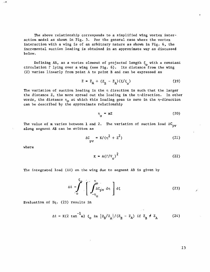
The above relationship corresponds to a simplified wing vortex inter-action model as shownin Fig. 5. For the general case where the vortexinteraction with a wing is of an arbitrary nature as shown in Fig. 6, theincremental suction leading is obtained in an approximate way as discussedbelow.
Defining AB, as a vortex element of projected length go with a constantcirculation r lying over a wing (see Fig. 6). Its distance from the wing(Z) varies linearly from point A to point B and can be expressed as
Z = ZA + (ZB - ZA)(_/_o) (19)
The variation of suction loading in the q direction is such that the larger
the distance Z, the more spread out the loading in the _-direction. In other
words, the distance no at which this loading goes to zero in the n-direction
can be described by the approximate relationship
q -- mZ (20)O
The value of m varies between i and 2.
along segment AB can be written as
where
&C
pv
The variation of suction load ACpv
= K/(22 + Z2) (21)
K = A(r/v )2 (22)o
The integrated load (_) on the wing due to segment AB is given by
Ag = .,[ _Cpv dq d _O
Evaluation of Eq. (23) results in
(23)/
-iA% = K(2 tan m) go _n [ZB/ZA[/(Z B - ZA) if ZB # ZA (24)
13

and
A_ = K(2 tan-lm)_o/Z A if ZB _ ZA
1Similarly, the evaluation of the center of pressure of this load A£
(denoted by point P in Fig. 6) is given by
(25)
where
8 = _o [I/(%nIZB/ZAI)- ZA/(ZB- ZA)if ZB # ZAI ,
(26)
8 = _o12 if ZB = ZA (27)
Equations (24) through (27) are used in this analysis to compute the suction
loads. The value of constants A (Eq. (17)) and m (Eq. (20)) can be varied
through input. Also, the values of ZA or Z are always assumed to be greaterthan the viscous core radius of the vortex _lement AB.
14

III. DESCRIPTIONOF COMPUTERPROGRAM
The analysis described in Section II has been incorporated into the computerprogram RIEVA (Rotor Induced EmpennageVibration Airloads). The flow chart ofthe key computational steps is shownin Fig. 7. The basic assumptions of thenonlinear lifting surface theory previously described are inherent in theprogram.
(a) It is assu_ed that the strength and position of the interactingvortex elements are knownat all instants. In general, the circulation andthe coordinates of the interacting vortical elements are input to the program.The program does have a capability, however, to compute internally thecoordinates of interacting wake elements corresponding to a classical undis-torted rotor wake. The equations for the description of a classical wakeare given in APPENDIXA.
(b) The distortions of the interacting vortex elements due to loadingon empennagesurfaces are not included.
(c) The wake behind the stabilizer/fin trailing edges is assumedtoconsist of semi-infinite trailing elements and finite shed elements, alllying in the plane of the corresponding lifting surface (see Fig. 4). Noroll up effects or distortions of this wake are included.
Numerical Method of Solution
The numerical procedure involved in applying the lifting surface methodconsists of dividing the surface into a numberof appropriately shaped boxes.The numberof these boxes is arbitrary and it is controlled through input.The magnitude of the doublet strength D over each box is assumedto be unl-form. The total velocity induced perpendicular to the surface at a colloca-tion point (centroid of the box) consists of that due to the vorticity ofall other boxes on the surface, the effects of the concentrated interactingvortices, the velocity induced by the far rotor wake and that due to all thetrailing and shed vortlcity elements starting at the trailing edge of thelifting surface. Whenthe flow tangency requirements on the surface aresatisfied at each time step, the problem of calculating the doublet strengthsis reduced to one of solving N linear algebraic equations, where N is thenumber of boxes on the lifting surface. Specifically, if Amni_ is the aero-dynamic influence coefficient at the centroid of the box mn du_ to the effectof box iJ and w is the normal componentof the velocity at collocationmn
15

point mn due to all knownvorticity elements and due to angle of attack, thesatisfaction of the boundary conditions results in the following relationship
7 Z
i j Am ijDij-w mn(28)
Since the coordinate system chosen in this analysis is fixed to the wing
at all times, the influence coefficients matrix Amnij is computed onlY onceand stored for use at subsequent steps.
Discussion of Options
One of the essential features of the RIEVA analysis is that the total
main rotor wake has been split into two parts for the computations of in-
duced velocities at the collocation points. One is the interacting elements
represented by a small number of concentrated vortices which come very close
to empennage surfaces causing high harmonic induced effects. The other is
the induced velocities due to the rest of the wake (far wake) varying at a
relatively low magnitude. As a result, far wake induced velocities are com-
puted at relatively large intervals of time and their magnitude at intermediate
intervals is calculated by interpolation. As mentioned earlier, this pro-
cedure results in savings of computational time without the elimination of
high frequency effects. Some additional advantages are discussed below.
As indicated by the Biot-Savart law, the magnitudes of the high frequency
airloads induced on the empennage surface depend upon the relative distance
between the surface and the interacting vortex elements (besides the circula-
tions of the vortex elements). For a helicopter rotor in forward flight,
only the undistorted wake can be described by analytical means. It is very
difficult to compute accurately the distortions of the wake elements while
they move from rotor blade to the empennage surface. In fact, some of these
interacting elements go through distortions of very large magnitude due to
encounters with rotor hub, fuselage, etc. Therefore, the positions of the
interacting vortices with respect to the empennage surfaces can only be
approximated. In the RIEVA analysis, since the interacting rotor wake is
represented by a limited number of vortices (normally blade tip vortices),
it becomes relatively easy to modify their geometry and thus compute the air-
loads corresponding to the modified wake geometry. As a result, once the
approximate position of the wake is defined, the interactions could be real-
istically assumed to occur anywhere within the envelope described by varying
the distance between the empennage surfaces and the vortices. The analysis
16

is flexible enough to consider many types of interactions. Specifically, the
interacting vortices can be arbitrarily moved closer to the empennage surface
to determine the magnitude of the critical airloads corresponding to the
extreme cases of wake distortions. Thus, wake distortion effects can be
accounted for indirectly and thereby the analytical computations of the
distorted rotor wake geometry are avoided.
The various options available in the RIEVA analysis for describing the
interacting wake coordinates and the rotor induced velocities are described
below.
For interacting wake geometry description, the user has the option to
input the coordinates of interacting wake elements at each instant of time.
This is particularly useful for those cases where the distorted wake geo-
metry is known. Alternately, the user can utilize the wake coordinates
computed internally by the RIEVA analysis. For a given flight condition
and rotor parameters, the program computes the wake coordinates corresponding
to the classical undistorted skewed helical wake.
Also, for the inclusion of far wake effects, there are two options
available. For one option the user can compute the induced velocities at
empennage points due to all or part of the rotor wake by utilizing a
Rotorcraft Wake Analysis (Ref. 7) and input these velocities to the RIEVA
analysis. Alternatively it may be assumed that the far wake induces a
uniform velocity at the empennage points and its magnitude is described
through input. This approximation may be valid for some high speed flight
conditions. The coupling of program RIEVA with the Rotorcraft Wake Analysis
is further discussed in the following section.
Coupling With Program F389
As indicated in the flow chart (Fig. 7), the Rotorcraft Wake Analysis
(Program F389, Ref. 7) may be utilized to obtain some of the inputs required
for the execution of program RIEVA. These inputs may be divided into three
convenient groups as described below.
i. The circulations of the interacting vortex elements can be deter-
mined by utilizing the Program F389. For a given rotor configuration, with
known control inputs, Program F389 computes the radial and azimuthal distribu-
tion of the blade circulation, rb(r,_). Once the distribution, Fb(r,_), is
prescribed, the circulations of the interacting vortices can be very easily
estimated by using a simple roll up theory. Normally these interacting vor-
tices will consist of only the blade tip vortices that are trailed off the
fore and the aft portions of the rotor disk.
17
2. The induced velocities at the empennagecollocation points due tomain rotor wake maybe computedby utilizing the Program F389. Normally,these induced velocities are computedat coarse intervals of time and theeffects of the interacting elements (elements in group i. above) are ex-cluded from these computations (this is done to avoid redundancy).
3. If desired, the coordinates of the interacting elements can alsobe obtained from the output of the computer program F389.
Interacting Vortex GeometryModifications
This section describes the procedures utilized by the RIEVAprogram toautomatically modify the geometry of the interacting wake elements in casethese elements intersect the empennagesurfaces. This is carried out in avery approximate manner. The use of this procedure is optional and it isspecified through input to the program.
Figure 8 illustrates the modifications involved. The modifications areconfined to junction points (where the various elements of vortex meet). Thejunction point nearest to the wing surface (only if the vortex element is cut)is modified, as shownin Fig. 8. The junction point is always kept at leastone core radius (viscous core radius rc) away from the surface. Also themodified junction points at locations above the wing are not allowed topenetrate the surface at subsequent time steps, but instead they are allowedto slide over the wing surface (or even somedistance beyond the trailingedge, this distance being specified through input).
The modifications described above involve the changing of only theZ-coordinate of the affected vortex elements. No attempt is madeto deter-mine the vortex displacements from their original position due to the wingvorticity field.
Future Capabilities
Someof the improvements that maybe carried out in the future to enhancethe capabilities of the RIEVAprogram are discussed in the following section.
1. At present a considerable amount of user judgement is required todivide the main rotor wake into two parts; one, the interacting elements andtwo, the far wake elements. A procedure should be developed and then in-corporated in the RIEVAanalysis wherebythis splitting of wake is carriedout automatically within the program.
18

2. The nature of the interaction between the main rotor vortices andthe vertical tail is such that significantly large streamline velocitiesmay be induced on the tail surface by these interacting vortices. This span-wise variation of the streamwise velocity results in a significant amountof vibratory airloads being generated by the vertical tail. At present,RIEVAanalysis does not account for these effects.
3. The coding and the dimensions of the RIEVAprogram should be modifiedso that the airloads acting on the vertical fin and the horizontal stabilizercan be computedsimultaneously.
4. Flow separation effects should be included in the RIEVAanalysis.Normally, when a vortex is close to the surface, flow separation occurs onthe upwashside of the vortex.
19

IV. PROGRAMRIEVADOCUMENTATION
The computer program for the determination of rotor induced empennagevibration airloads (RIEVA) incorporates a numberof key options. Theinclusion of these options results in computer efficiency and providesflexibility on the type and source of the interacting wake elements.
The program documentation includes
(i)(ii)
(lii)
a brief description of program subroutines,
a detailed description of input data 9
a brief description of program output.
Subroutine Descriptions
A brief description of each of the subroutines is given below in
alphabetical order.
Subroutine COLLOC
This subroutine computes the aerodynamic influence coefficient matrix
_mnij at the first time step and stores it on unit i0 for use at subsequente steps. It also computes the coordinates of the collocation points and
prints out the coordinates, if requested.
Subroutine DMAT
This subroutine computes the solution of a set of simultaneous algebraic
equations of order N.
Subroutine GETVlS
This subroutine interpolates input induced velocity components corre-
sponding to the far rotor wake at the intermediate time steps.
Subroutine HARMPM
This subroutine computes the harmonic coefficients of the wing
aerodynamics loads.
20

Subroutine LOADER
This subroutine reads in the loader input data.
Subroutine LOADS
This subroutine computes and then prints out the wing aerodynamic loading
distribution AC at each time step. Also, the total wing aerodynamic loads
are computed an_ printed out.
Subroutine MAIN
This is the main routine. It calls subroutines LOADER, PRNT, WLINPT,
COLLOC, VRTXG, SLOAD, GETVIS, VELKNW, SOLVEG, LOADS and HARMPM and prints
out the harmonics of the wing alrloads. It also prints out the instantaneous
geometry of the interacting vortices.
Subroutine OUTPUT
This is a general subroutine which prints out the chordwise and spanwise
distribution of the various quantities (e.g., doublet distribution D, pressure
distribution Ac' , etc.)P
Subroutine PRNT
This subroutine prints out all the input loader data.
Subroutine SLOAD
This subroutine computes the nonlinear suction airloads, when requested.
Subroutine SOLVEG
This subroutine sets up the simultaneous set of algebraic equations to
be solved at each time step, and also, outputs the computed doublet distribu-
tion.
Subroutine UVW
This subroutine computes the induced velocities due to a vortical element.
Subroutine VELKNW
This subroutine computes the induced velocities at the collocation points
due to the interacting vortices and also due to the wing wake trailing and
shed elements.
21

Subroutine VRTXG
This subroutine computes the coordinates of the interacting main rotor
vortices corresponding to a classical undistorted wake model.
Subroutine WLINPT
This subroutine reads in the main rotor far wake induced velocities and
converts them to the wing coordinate system. It also prints out the
distribution of the normal component of these far wake induced velocities
corresponding to each time step.
Input Description
The required input to the program consists of the following major punched
card data blocks, in order of loading:
Ii Wing (Empennage), Vortex Geometry and other Solution Control
Data (in Loader Format)
II. Induced Velocity Data due to Far Main Rotor Wake (Optional)
III. Interacting Vortex Geometry Data (Optional)
Details for preparing these blocks of data are given in the following
sections.
I. Empennage, Vortex Geometry and Other Solution Control Data
This block of data is split into the following three groups.
(a) Solution Control Parameters
(b) Empennage
(c) Vortex Geometry Parameters (Optional)
The group (a) contains the data that determines which of the various
options are to be exercised. The data in this group are loaded in an
array (SCP). The group (b) contains data that describes the empennage sur-
face geometry and the free stream parameters. This group of data is
stored in WCP array. The group (c) contains the rotor data needed to des-
cribe the interacting main rotor wake geometry based on a classical undistorted
model of the rotor wake. This group of data is stored in array VCP. If
internal computation of the interacting wake geometry is not required, this
group of data may be omitted.
22

The order in which the groups of data are loaded is arbitrary. Theformat for these data is as_llows:
A N L DATA(L)DATA(L+l) .... DATA(L+4) (AI, 11, 14, 5F12.0)
where A, in Columni, represents the letter S, W or V corresponding to arraysSCP,WCPor VCP. N is the numberof data items to be input on the cardColumn2; N must not exceed 5. L is the location or identifying number ofthe first data item on the card Columns3-6, right adjusted. DATA(L+j)represents the various data items on the card, Columns7-18, 19-30, 31-42,43-54, and 55-66, in floating point format. The locations for the variousdata are listed below along with definitions and other pertinent comments.Note that somelocations are intentionally left blank.
(a) SCPArra_Data
Location Item Description
1 Nw The number of lifting surfaces. For
horizontal stabilizer NW=2. , one for
each semi-span. For vertical tail,
NW=I. At present both stabilizer andfin cannot be modeled simultaneously.
2 MYES MYES-1., doublet lattice method is
applied. MYES=0., no doublet solution
required; this option is used if only
nonlinear suction loads are desired.
3 NSHED Specifies the number of shed elements
to be included in the wing wake.
Range is 0. to 5. (see Fig. 4).
4 MSYM Normally MSYM=0. When MSYM=I., the pro-
gram assumes symmetrical loading on both
the right and left hand sides of the
stabilizer.
5 NVORT Specifies the number of interacting
vortices. Range is 0. to 8.
6 IVGEOM Option for the description of the inter-
acting wake elements. IVGEOM=0, rotor
wake data specified via loader inputs
in VCP array (group c). IVEGOM=I,
interacting wake data input at each time
step. This is described separately (data
block II, Page 29). 23

24
Location
7
9
i0
ii
12
13
Item
NFARF
MODVG
EXT
INSUC
NT
AT 2
MHDO
Description
Option for including the far wake
induced velocity effects. If NFARF=l,
this component of the induced velocities
is to be input as described separately
(data block II). If NFARF=0, no data
are read in. If desired, under this
option (NRARF=0), these effects may
be accounted via input in location 19
of SCP array.
Option to modify the interacting vortex
geometry if the vortex gets cut by the
empennage surface (see Section II,
Page 13). For MODVG=0, no modifications
are carried out.
If MODVG=I (previous location), the
area of the wing surface over which the
modifications are to be carried out is
extended via input in this location, i.e.,
the modifications of the vortex are carried
out even beyond the wing surface. EXT
is nondimensionalized with respect to the
mean chord length of the wing.
Option to include the computations of
nonlinear suction loads. INSUC=I, loads
are computed. INSUC=0, no loads are
computed.
Specifies the total number of time steps
for which computations are to be carried
out.
Specifies time increment per step, secs.
Option to perform an harmonic analysis
of the computed air loads over one period.
For MHDO=I, Yes and for MHDO=0, No. The
number of points per period is specified
in location 15.
Location
14
15
16
17
18
19
20
21
22
23
Item
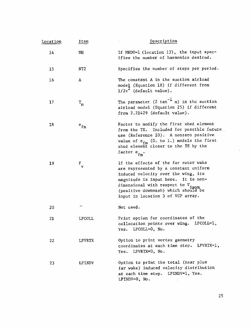
NH
NT2
A
Tn
efm
FV
LPCOLL
LPVRTX
LPINDV
Description
If MHDO=I (location 13), the input spec-
ifies the number of harmonics desired.
Specifies the number of steps per period.
The constant A in the suction airload
model (Equation 18) if different from
i/2_ 2 (default value).
The parameter (2 tan -I m) in the suction
airload model (Equation 25) if different
from 2.21429 (default value).
Factor to modify the first shed element
from the TE. Included for possible future
use (Reference i0). A nonzero positive
value of efm (0. to i.) models the firstshed element closer to the TE by the
factor efm.
If the effects of the far rotor wake
are represented by a constant uniform
induced velocity over the wing, its
magnitude is input here. It is non-
dimensional with respect to Vimom
(positive downwash) which should be
input in location 3 of VCP array.
Not used.
Print option for coordinates of the
collocation points over wing. LPCOLL=I,
Yes. LPCOLL=0, No.
Option to print vortex geometry
coordinates at each time step.
Yes. LPVRTX=0, No.
LPVRTX=I,
Option to print the total (near plus
far wake) induced velocity distribution
at each time step. LPINDV=I, Yes.
LPINDV=O, No.
25

26
Location Item
24 LPDBLT
25 LPPRCP
26 LPFARW
27 LPSUCD
28 IDEBUG
(b) WCP Arrax Data
1-2 XI,Y 1
3-4 X2,Y 2
5-6 X3,Y 3
7-8 X4,Y 4
9 Nc
i0 Ns
11-20 (")
Description
Option to print the doublet distribution
at each time step. LPDBLT=I, Yes.
LPDBLT=0, No.
Option to print the airload distribution
AC at each time step. LPPRCP=I, Yes.
LP_RCP=0, No.
Option to print the inputted (data block
II) far-wake V i distribution. LPFARW=I,
Yes. LPFARW=0, No.
Option to print the computed nonlinear
suction airloads. LPSUCD=I, Yes.
LPSUCD=O, No.
Option to print debug parameters.
Always input IDEBUG=0.
X and Y coordinates of corner i of the
first surface in the wing coordinate
system illustrated by Figure 4 (feet).
X and Y coordinates of corner 2 (feet).
X and Y coordinates of corner 3 (feet).
X and Y coordinates of corner 4 (feet).
Number of chordwise stations for the
lattice of the first wing.
Number of spanwise stations for the
lattice of the first wing.
Specifies the parameters for the
second wing in the same order as for
the first wing (in locations i through
10).
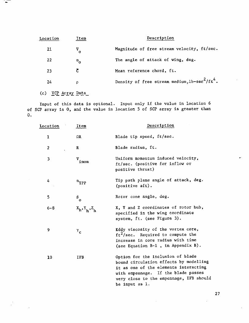
Location Item Description
21 Vo
Magnitude of free stream velocity, ft/sec.
22 o_o
The angle of attack of wing, deg.
23 Mean reference chord, ft.
24 p Density of free stream medium31b-see2/ft 4.
(c) VCP Array Data
Input of this data is optional. Input only if the value in location 6
of SCP array is 0, and the value in location 5 of SCP array is greater than
0.
Location Item Description
l _R Blade tip speed, ft/sec.
2 R Blade radius, ft.
Vimom
Uniform momentum induced velocity,
ft/sec. (positive for inflow or
positive thrust)
_TPP Tip path plane angle of attack, deg.
(positive aft).
5
6-8
6o
Xh,Yh,Z h
Rotor cone angle, deg.
X, Y and Z coordinates of rotor hub,
specified in the wing coordinate
system, ft. (see Figure 3).
YcEddy viscosity of the vortex core,
ft2/sec. Required to compute the
increase in core radius with time
(see Equation B-I , in Appendix B).
i0 IFB Option for the inclusion of blade
bound circulation effects by modelling
it as one of the elements interacting
with empennage. If the blade passes
very close to the empennage, IFB should
be input as i.
_T
27

28
Location
ii
12
13
14-20
21
22
23
24
25
26
27
28-29
Item
fb
Nb
LR
a
A_
A_ru
r
co
rb
A_ 2
Description
Nondimensional factor (between 0. to
i.) to multiply the maximum blade cir-
culation in order to get effective circula-
tion.
Number of rotor blades.
This is the input required to make the
time reference of data block II compatible
with the time reference of the interacting
wake geometry. LR is the reference stepnumber in data block II that corresponds
to starting time (t=0) of wake geometry
computations.
Not used.
Azimuthal location at which the first
point of the vortex is trailed, deg.
(see Equation A-4).
Age of the first point of the vortex, deg.
(see Equation A-5).
Azimuthal increment, deg.
A-4).
(see Equation
Time for the vortex to rollup to the
initial core radius rco specified in
location 25, deg.
Initial core radius of the vortex, ft.
Radial location on blade from which
the vortex is trailed (nondimensional).
rb=l corresponds to tip vortex (see
Equations A-l, A-2).
Azimuthal increment used in the compu-
tation of the far wake effects, deg.
Required for the aft forming vortex only.
Not used.

Location Item Description
30 Nv
Number of segments representing the
vortex. Maximum of 9.
31-39 Fv
Circulations of segments, ft2/sec.
40 Not used.
41-59 (") Corresponding data for the second
vortex similar to those for the
first vortex in locations 21-39.
._ 60-179 (") Similar data for the remaining six
vortices.
II. Induced Velocity Data.(Optional)
This block of data is required only if the value of location 7 of the
SCP array (see data group a) is 1.0. F389 (Ref. 7) (see Section III, Page
17) generates this data in a format which is compatible with the input
requirements of RIEVA program. This block of data consists of three com-
ponents of the instantaneous induced velocity at each of the collocation
points. These induced velocities are described in the rotor tip path plane
coordinate system (see Appendix A). Also, these induced velocities are
described for various time steps; the total time covered being exactly
the time for one blade passage. The first card of this data block contains
three quantities; LS, AT, and NTOT is the format (12, F20.0, 15). LS is
the total number of time steps, AT, is the tlme in seconds corresponding
to each step and NTOT is the total number of collocation points. The
total number of quantities (Nd) contained in the data (following the firstcard) is
Nd = 3 x LS x NTOT
where 3 represents the three components of induced velocity.
These Nd numbers are input in order with six quantities per data card,
in the format (6F12.0).
III. Interacting Vortex Geometry Data (Optional)
This block of data is required only if the value of location 6 of
SCP array (see data group a) is 1.0. This input data block describes
the instantaneous locations and strengths of all the inter@cting vortex
elements. This option may be utilized if the interaction between the
empennage and the vortices is of non-perlodic (transient) nature. Also,
if the main rotor wake distortions are known, the wake data for these
distorted elements may be input via this block.
For each of the vortices, the following quantities are input. 29

Card # Quantity or 0uantities Format
1 N (Number of vortex points) (I5)v
2 x,y,z,R,Gv (for first point) (5FI0.6)
where: x,y,z are the coordinates
in the wing coordinate system,
R,Gv are the viscous core radius
and the circulation respectively.
3 x,y,z,R,Gv (for second point) (5FI0.6)
Nv+l x,y,z,R,Gv (for Nvth point) (5FI0.6)
The above information is input for all the NVORT (see location 5
of SCP array) vortices.
The above'information is repeated for each time step until data for
all time steps has been input.
Output Description
A brief description of the printed output generated by the RIEVA
program is given here. The amount and the nature of the output for a
particular run is controlled through the exercise of various print
options specified via input in locations 21-27 of the SCP array (see
Section IV, Page 25).
The RIEVA program output can be classified into the following ten
major categories (in order of output).
i. Listing of Input Loader Data
2. Listing of Input Far-Wake Induced Velocities
3. Coordinates of Collocation Points
4. Instantaneous Description of Interacting Vortices
5. Instantaneous Induced Velocity Distribution
6. Instantaneous Doublet Distribution
7. Instantaneous Airload Distribution
8. Instantaneous Integrated Airloads
9. Nonlinear Suction Loads (if present)
i0. Harmonics of Airloads
3O

The categories 2., 3., 5., 6., and 7. listed above involve thechordwise and spanwise variation of the various quantities and areprinted out in a similar format by the subroutine OUTPUT.Category 3.provides the coordinates of the various collocation points over allthe surfaces, and the numbers in the output categories 2., 5., 6.,and 7. represent the values of the various quantities at the corres-ponding points (listed in category 3.).
Most of the output of RIEVAanalysis is self-explanatory; only abrief description of each category is provided. No samples of theoutput are included here. Also it should be noted that categories 4.through 8. are output at each time step.
i. Listing of Input Loader Data
This is output by Subroutine PRNT, which lists the values of all
the input loader data (discussed in Section IV. under Input Descrip-
tion: Data Block I.).
2. Listing of Input Far-Wake Induced Velocities
This is output by Subroutine WLINPT, which lists the input induced
velocities at the empennage points. First the total number of time
intervals and the time (in seconds) corresponding to each interval are
printed out.
3. Coordinates of Collocation Points
This output by Subroutine COLLOC, which lists first the x-coordinate
of the control points and then the y-coordinate of the control points in
the wing coordinate system. Before these collocation points are listed,
the coordinates of the corners of the various control surfaces modeled
(along with some flight parameters) are given first.
4. Instantaneous Vortex Geometry
This is output from program MAIN and consists of the description of
position and strength of the various elements of the interacting vortices.
First the step number and the time (in seconds) corresponding to that
step are printed out. Next, for each junction point of the interacting
vortices, x, y and z coordinates (in wing coordinate system) are listed.
Also the circulation (ft**2/sec.) and the viscous core radius (feet) of
each of the elements are listed. Finally a quantity ZMOD is listed. If J
31

the value of ZMODis 1.0, it indicates that the z-coordinate of the junctioncorresponding to that point has been altered according to the proceduregiven in Section III, Page 18).
5. Induced Velocity Distribution
This is output by Subroutine SOLVEG, which describes the instantaneous
total induced velocity (due to far wake plus interacting wake) distribution
(positive downwash).
6. Doublet Distribution (listed as 'SOLUTION GAMMAS')
This is output by Subroutine SOLVEG, which lists the computed doublet
distribution over the control surfaces. A positive value corresponds to
a clockwise direction of the vortical elements around the box (see Fig. 4.).
7. Attached Flow Airload Distribution
This is output by Subroutine LOADS, which describes the unsteady AC P
(ACp=Cp - Cpu_,_ or airload distribution over the surface.
8. Integrated Airloads
This is output by Subroutine LOADS. At the end of the output of each
step, the integrated loads for the total surface are listed. Both the
nondimensional coefficients CL, C., and C , and the dimensional loads Lm R(ibs), PM (lb.-ft.) and RM (lb.-ft.) are printed out.
9. Nonlinear Suction Loads (if present)
This is output from program MAIN and consists of the integrated
suction loads (ACLv, ACLM and ACRM) for all the time steps over oneblade passage. These are listed under the heading "Suction Loads
Variation".
i0. Harmonics of Airloads
This is printed out from program MAIN. The airload (CL, _ or CR)
variation over one blade passage is converted into mN b per rev(N b =
number of blades, m=l,2,3,etc) harmonic airloads. For example total CL
is expressed as
32
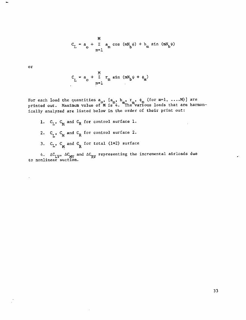
M
CL = a + E a cos __(mNb¢) + bo m mrn=l
sin (mNb )
or
M
CL ao + l rm sin (mNb_ + Cm)m=l
[a , b , r , _ (for m=l, .... M)] areFor each load the quantities ao, m m mprinted out. Maximum value of M is 4. mThe various loads that are harmon-
ically analyzed are listed below in the order of their print out:
i. CL, CM and CR for control surface I.
2. CL, CM and CR for control surface 2.
3. CL, CM and CR for total (i+2) surface
4. ACLv, ACMv and ACRv representing the incremental airloads dueto nonlinear suction.
33

V. RESULTSANDDISCUSSION
This section presents and analyzes the results obtained from theRIEVA (Rotor Induced EmpennageVibration Airloads) program for somerealistic check cases.
The basic check case chosen involved the computation of the unsteadyairloads acting on the Black Hawkhorizontal stabilizer surface for a highspeed forward flight condition of 172 knots. Calculation of the strengthof the interacting vortex elements and the induced velocities at thestabilizer points due to the rotor far wake were necessary before RIEVAcould be executed. An undistorted classical wake model and trimmed for-ward flightwere assumedfor the calculations. The various flight andcontrol parameters for this case are listed in Table I. The variationof the maximumblade circulation (Fbm) with blade azimuth position (4)is shownin Fig. 9. The total rotor wake has been split into two parts,one, the interacting wake elements and two, the far wake as showninFig. i0. The interacting wake elements comprised the segments of the bladetip vortices trailed off the forward and aft portions of the rotor (30 deg.on each side of the centerline or the x-axis). The circulations of thesetip vortex elements were the values of Fbmin Fig. 9.
The far wake induced velocities at the stabilizer points were computed(using Rotorcraft WakeAnalysis F389) at time intervals corresponding to A_(_ * At) of 15 degrees. For one representative point on the stabilizersurface (at quarter chord point on the centerline), the variation of thefar wake induced velocity with time is shownin Fig. ii. Also showninFig. Ii is the variation of the total induced velocity (due to interactingwake plus far wake) with time. Examination of Fig. ii reveals that mostof the high frequency variation of the total induced velocity is caused bythe interacting wake elements. This result substantiates the assumptionthat the computations of the far-wake induced velocities are only necessaryat coarse intervals of time.
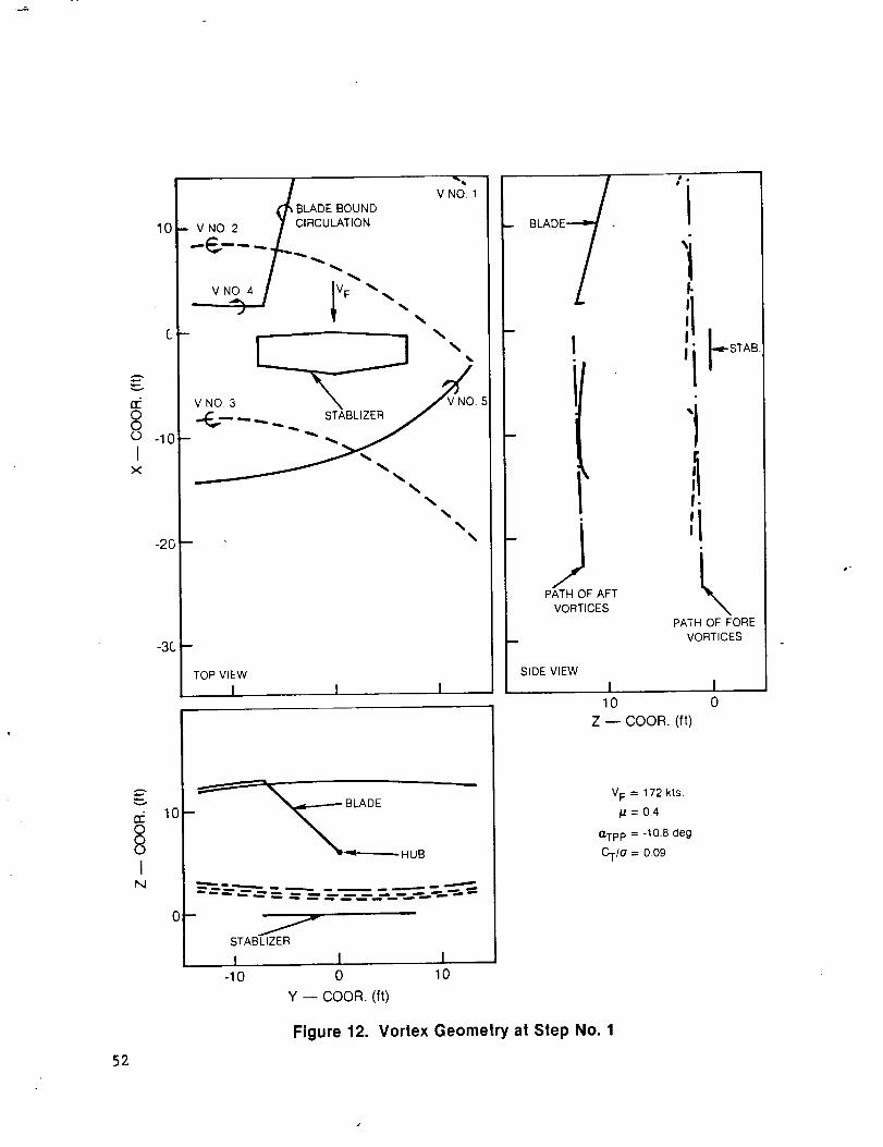
RIEVAwas used to calculate the instantaneous positions of the inter-acting vortex elements at fine intervals of time. For the basic case thetotal time corresponding to one blade passage (T = 0.05814 seconds) wasdivided into 12 equal steps and the computations were carried out every.004845 seconds. At three such instants (steps i, 7, and 12) the pathsand spacings of the interacting rotor blade tip vortices with respect to thehorizontal stabilizer are described in Figs. 12, 13, and 14, respectively.In these figures, the vortices numberedi, 2, and 3 are those trailed off
34
the forward portion of the rotor (4 " 210 to 150 degrees) while the vorticesnumbered4 and 5 are those trailed off the aft (4 = 30 degrees to -30 degrees)portion of the rotor. The integrated unsteady airloads of the stabilizer(at zero angle of attack) are shownin Fig. 15 as a function of time (4=_t).In this figure C T is the lift coefficient (normalized to .5pVo2 x wingarea). CMTis t_e pitching momentcoefficient about the quarter chord(positive up), and CRTis the rolling momentcoefficient about the stabilizercenterline (positive for right side going down); both of these momentco-efficients are normalized (.SpVo2 x wing area x meanchord). As expected,the airloads CLT, CMTand CRTare periodic with each blade passage (orevery 90 degrees for four-bladed rotor). The computations have to be carriedout for more than one blade passage (as shownin Fig. 15), since thestrengths of the shed elements were not known at the start of the computa-tions. Once the shed vorticity develop_ (after 5 to 6 steps), the resultsindicate excellent periodicity with each blade passage (as indicated bythe results shownin Fig. 15). The airloads' variation over one period wasconverted into the 4mper rev (m = i, 2, 3) harmonic airloads and resultin the following vibratory airloads on the stabilizer:
CLT= - 0.184 + 0.127 sin (44 - 90°)+ 0.068 sin (84 + 168 °)
+ 0.032 sin (124 - 36 °)
CMT = - 0.0032 + 0.0187 sin (44 + 129 °)+ 0.0161 sin (84 - 8.3 °)
+ 0.0112 sin (124 + 144 °)
CRT = - 0.0058 + 0.0773 sin (44 + 195 °)+ 0.0750 sin (84 + 98 °)
+ 0.0400 sin (124 - 31 °)
The airloads described above are the total loads being applied to the
stabilizer of the helicopter and these can be used as input to the coupled
rotor/airframe (Ref. 6) vibration analysis. The computer program RIEVA
also provides a detailed description of these airloads (chordwise and span-
wise variation of AC ). These airloads may be utilized to study the aero-
elastic vibrations o_ the empennage itself. As an example, for this check
case some calculated airload distributions are shown in Figs. 16 and 17 (for
three spanwlse stations; at 6% and 56% stations on the right stabilizer and
at 56% station on the left stabilizer). Figure 16 describes these airload
distributions at the time step No. i, the instantaneous vortex geometry for
which is illustrated in Fig. 12. The chordwise variation of the alrload
at this instant resembles the conventional airload distribution observed on
J
35

an airfoil at a negative angle of attack. But when a concentrated vortexis directly above the stabilizer (such as vortex number 2 in Fig. 13),these chordwise airload distributions look totally different. This isclearly indicated by the distribution of the airloads described in Fig. 17,which correspond to the time for which the instantaneous vortex geometry isdescribed in Fig. 13. These deviations are obviously due to the unsteadyeffects caused by the presence of the moving vortex.
As indicated by Figs. 12, 13 and 14, the closest distance betweenthe stabilizer surface and the interacting vortices is approximately 1.5feet. If this distance were smaller (say less than three times theviscous core radius of the vortex), either due to wake distortion or dueto change in tip path plane angle of attack, an additional componentofthe airloads results. As discussed before, this componentof the air-loads is due to the nonlinear suction effects that occur when the vortexpasses very close to a surface.
An additional check case was run to verify the modeling of the non-linear suction airloads in the RIEVAanalysis. This case corresponds tothe same flight conditions as described earlier (see Table I) except thatthe tip path plane angle was arbitrarily increased to -14.42 degrees.This was done to let the vortices off the front portion of the rotor passvery close (within 2 inches) to the horizontal stabilizer surface (seevortex #2 in Fig. 18). As a result of close stabilizer-vortex interaction,significant nonlinear suction airloads result and as shownin Fig. 19 forone blade passage. These incremental suction airloads (ACLv, ACMv, ACRv)have to be added appropriately to the potential flow loads (CL, CM, and CRshownin Fig. 20) in order to determine the total loads CLT, CMTand C_T.These total loads are shownin Fig. 21 for one blade passage. It shouldbe rememberedthat the loads described in Fig. 21 have been computedunderthe assumption that no flow separation of any kincl occurs. Normally flowseparation occurs on the upwashside of the vortex during the close airfoil-vortex interaction. At present the RIEVAanalysis does not account forthese flow separation effects.
36

Vl. CONCLUSIONSANDRECOMMENDATIONS
A computer program (RIEVA) has been developed that predicts theunsteady aerodynamic forces that are imposed on the empennagesurfacedue to its interactions with the main rotor wake. The program wasexercised to determine the vibration airloads acting on the BlackHawkhorizontal stabilizer for a high speed (_ = 0.4) forward flightcondition. The following are specific conclusions obtained fromanalysis of the Black Hawksimulation.
i. The results demonstrate that it is possible to compute the
high frequency empennage vibration airloads (up to 16 revolu-
tion) efficiently (reasonable amount of computer time) by
utilizing this analysis. This check case required only 4 to
5 minutes computer time on an IBM 370 system.
2. No numerical problems were encountered, and the airload
harmonics converged quickly.
The following future activities are recommended:
,
i. A correlation study should be carried out to compare the RIEVA
predicted empennage airloads with test data.
, The RIEVA analysis should be extended to account for the span-
wise variation in streamwise velocity (nonuniform free stream
velocity). The inclusion of this feature will result in the
analytically correct computation of the vertical tail airloads
and provide the capability of studying the blade finite tip-
vortex interaction problem.
The draft copy of the present report was prepared in 1981. Since then alimited correlation study has been carried out wherein the RIEVA predicted
stabilizer airloads have been compared with the CH-53A flight test data.
The results indicate a reasonably good correlation between analytical
predictions and the flight test data. These results are presented in the
following Reference:
Gangwani S. T.: Determination of Rotor Wake Induced Empennage Airloads.
Presented at the American Helicopter Society National Specialists' Meeting
on Helicopter Vibration, Hartford, CT., November 2-4, 1981.
37

Vll. REFERENCES
le
.
e
.
1
.
.
.
.
Sheriden P. F. and R. P. Smith: Interactional Aerodynamics - A New
Challenge to Helicopter Technology. Presented at the 35th Annual
National Forum of the American Helicopter Society, Washington, D. C.,
May 1979, Preprint No. 79-59.
White, R. P., Jr., S. T. Gangwani and J. C. Balcerak: A Theoretical
and Experimental Investigation of Vortex Flow Control for High Lift
Generation. Report ONR-CR212-223-3, prepared by RASA, a Division
of Systems Research Laboratories, Inc., Newport News, Virginia,
December 1976.
White R. P., Jr., S. T. Gangwani and D. S. Janakiram: A Theoretical
and Experimental Investigation of Vortex Flow Control for High Lift
Generation. Report ONR-CR212-223-4, prepared by RASA, a Division
of Systems Research Laboratories, Inc., Newport News, Virginia,
December 1977.
Jordan, P. F. : Reliable Lifting Surface Solutions for Unsteady
Flow. AIAA 16th Aerospace Sciences Meeting, Huntsville, Alabama,
January 1978.
Geissler, W.: Nonlinear Unsteady Potential Flow Calculations for
Three-Dimensional Oscillating Wings. AIAA Journal, Vol. 16, No. ii,
pp. 168-174, September 1978.
Sopher R., R. E. Studwell, S. Cassarino and S. B. R. Kottapalli:
Coupled Rotor/Airframe Vibration Analysis, NASA CR-3582
Contract NASI-16058, June 1982.
Landgrebe, A. J. and T. A. Egolf: Rotorcraft Wake Analysis for the
Prediction of Induced Velocities. USAAMRDL Tech. Report 75-45,
Eustis Directorate, USAAMRDL, Fort Eustis, Virginia, January 1976.
Karamacheti, K.: Principles of Ideal-Fluid Aerodynamics. John Wiley
and Sons, Inc., 1966.
Piaziali, R. A.: Method for the Solution of the Aeroelastic Response
Problems for Rotating Wings. Journal of Sound and Vibration, Vol. 4,
No. 3, pp. 445-486, November 1966.
38

Table I
BLACKHAWKCHECKCASEPARAMETERS
Free Stream Velocity, Knots
AdvanceRatio,
Blade Radius, Feet
Thrust, Pounds
CTIO
Tip Path Plane Angle, Degree
ConeAngle, Degree
Uniform MomentumInduced Velocity, FPS
Rotor Solidity, o
Numberof Blades
Hub X-coordinate, Feet
Hub Y-coordinate, Feet
Hub Z-coordinate, Feet
Area of Stabilizer, Square Feet
MeanChord of Stabilizer, Feet
Stabilizer Angle of Attack, Degree
172.0
0.39
26.83
17,203
.0902
-10.8
3.66
6.67
0.0821
4.0
28.25
0.0
6.25
44.45
3.083
0.000
39
APPENDIXA
The wake equations for a rotor in forward flight, based on theclassical undistorted helical wake model, are presented below. Theseequations are utilized in the analysis (RIEVA) to describe the geometryof the vortices that interact with the empennagesurface. The equationsare described in the rotor tip path plane coordinate system. The rotorhub location is the origin, the x-axls is positive aft, the y-axis ispositive to the right (_ = 90 degrees) and z-axls is pointed up (right-handed cartesian coordinate system). The azimuth angle _ is measuredwith respect to positive x-axis, rotating counterclockwise.
The coordinates of any point n on the vortex trailed from the bladeradial location r b (nondimensionalized to R) can be described as follows:
Xnt = _TPPOa+ rb cos (On)
Ynt = rb sin (¢n)
Znt = ITPP _a
(A-I)
(A-2)
(A-3)
with
cn = ¢i - (n-l) * A_
Sa = Sb - _n
_rpp = Vo cos (_reP)/SR
ITp P _ - Vimom/_R + Vo sin (aTpp)/_R
(A-4)
(A-5)
(A-6)
(A-7)
where
_ is the incremental _ to describe various segments,
n varies from i to the maximum number of points chosen,
#b describes the current position of reference blade,
_a represents age of the wake point, and
Vimom is the uniform momentum induced velocity
40

APPENDIXB
The mathematical model for the determination of the viscous core radiusof the blade tip vortices is described in this appendix. In the RIEVAanalysisthe computation of the core radii is required only whenthe interacting vorticescomevery close to the empennagesurface. It is assumedthat after roll up,the viscous cores can be represented by a constant turbulent eddy viscositymodel. Under this assumption the core radius r c, increases with time as givenby the following relationship:
r 2 = r2 + B2_t (_a__ru)/_ (B-l)e co
where
rco - core radius at time of roll up, _ru'
Yt = turbulent eddy viscosity of core.
B2 = a constant, (0.716) 2•
_a = age of the vortex element,
= rotational speed
The magnitudes of rco, _ru and ?t have to be obtained empirically and inputto the RIEVAprogram.
41
15% CHORD
- _ -- THEORY
1 i i I I I J I I I0 20 40 60 8O 100
% SPAN
tIt
STRAKEVORTEX _" I
t VORTEXt
LEADING
EDGE
VORTEX
Figure 1. Wing/Vortex Geometry and Comparison of Measured and PredictedChordwise Pressure Distribution from Reference 3
rPATH OF AFT MAIN
PATH OF FORE MAIN
ROTOR TIP VORTEX
Figure 2. Schematic of Main Rofor Tip Vortex/Empennage Inferaction
42

N
o
_ ×
Z w
_oEw LI3
F'_LL
X
W
_Z
.J _J'J Z
E
G_1trimC_C
wE
ooC_o_r-
in
c_a_Im
LL
43

o
I
m
c
Cim
o
cimm
"oo
L_
.__
44

y..-,.-,,,======,___
INTERACTINGVORTEX
__K'_ LIFTING
SURFACE
vo_xo /_ VOc_E&
LOADS ,' I _ "Cpv_ .,," _ VISCOUS
-_ ..""" A "_ _ / VORTEX
I
_ r
SUCTION INFLUENCE
DISTANCE 2_o
Y
BACK VIEW
Figure 5. Simplified Model Showing Interaction Effects
45

II/
/
I
II
I
I
\\\\
IIII
n_ -.-.-._ D .N
n'1
_r/,
N
//
/
, // _
g/
Z
uo
I,LI
C0
wm
ffl
0
e-.im
.B
46

INPUT
TAIL SURFACE GEOMETRY
ANGLE OF ATTACK, a
FREE STREAM VELOCITY, v o
FROM ROTORCRAFT WAKE
ANALYSIS FOR EACH A t
w 1 INTERACTING WAKE COORDS
FWl CIRCULATIONS
VT 1/w 2, VT1 /I 2
(SECONDARY INDUCED EFFECTS)
ROTOR/TAIL SURFACE AERO INTERACTION MODULE
DESCRIBE TAIL SURFACE
COLLOCATION POINTS
COMPUTE GEOMETRIC
INFLUENCE COEFFS, (Aij) FORDOUBLET STRENGTHS
I DESCRIBE PRIMARY ROTOR I
WAKE ELEMENTS AT
SUBINTERVALS (A12)
1I COMPUTE VT1/W 1 AT 1EACH At2 USING rWl
COMPUTE VT1/w 2 & VT1/i 2
AT EACH At 2 BY INTERPOLATION
COMPUTE INFLUENCE OF TAIL
SHED AND TRAILING WAKE
ELEMENTS VT2/W T
CALCULATE FOR EACH ,4.t2.
V T = VT1/w 1 + VT1/w 2 + VT1/I 2 +
VT1/W T + V O SIN a
CALCULATE PANEL DOUBLET
STRENGTHS (Odj) BY USING NOFLOW BOUNDARY CONDITIONS
COMPUTE LOADING AND
TRANSFER TAIL EXCITATIONS
TO VIBRATIONS PROGRAM
VIBRATORY
TAI L
EXCITATION
tTO COUPLED
ROTOR/AIRFRAME
VIBRATION
ANALYSIS
ADDITIONAL NOTATION
T TAIL
I OTHER INTERFERENCE COMPONENTS
Figure 7. Flow Chart for Rotor/Tail Vibratory Excitation
47

48
I
/
//
'9L"
E0
t_X
0
imI.L

6O0
, ,oo_ 4O0
200 -
_oot0 L I I 1 I 1
0 60 120 180 240 300 360
BLADE AZIMUTH _ (deg)
Figure 9. Maximum Fb Variation Around Azimuth
(feet squarelsec)
49

l.I.I
n"
i.i_I.L0
I---rr
COI-'-rr
0
I--LI.I
CO -rI'-- I--Z
I.IJ
rn_z >_
I I:i
%\
\
/
\
\\
\\
\
50

40
0313..LLv 30
,,-fi,
20
o
_0SI--
- _TOTAL V i
,I I I I l0 15 30 45 60 75 90
TIME (_t) IN deg
Figure 11. Variation of Induced Velocity at Stablizier
(At Quarter Chord Point on Wing Centerline)
51
10
C
i -10
-2O
-3(.
oI
N
0
52
.h/ v_BLADE BOUND
- V NO. 2 CIRCULATION
VNO. 4 / IVF "_"
VNO. 3 .5
STABLIZER
-- %
B
TOP VIEW
I I I
STABLIZER
I I I-10 0 10
Y -- COOR. (ft)
BLADE_.
# •
IiI.
'I
PATH OF AFT
VORTICES
I
PATH OF FORE
VORTICES
SIDE VIEW
! I10 0
Z -- COOR. (ft)
V F 172 kts.
/3=0.4
aTp P = -10.8 deg
CTIO = 0.09
Figure 12. Vortex Geometry at Step No. 1

8(,3
IN
v
8O
I
TOP VIEWSIDE VIEW
10
BACK VIEW
HUB_
_mD
m
STABILIZER
I I I._-10 0 10
Y -- COOR. (ft)
iiPATH OF
FOREVORTICES
ilI,
I,j
' IiI.
'_""PATH OF AFT | ]
VORTICES
I I10 0
Z -- COOR. (ft)
k/F = 172kts,
/J = 0.4
O-TpP = -10.8 deg
CT/O = 0.09
Figure 13. Vortex Geometry at Step No. 7
53

v
r_OO(.3
IN
10
0
0 -10
-20
-3O
10
(2
VNO 1
/vF ,,
VNO2 _ Z
-- _ ,....... STABLIZER / V NO..4
- V NO V NO, 5y
m
%
TOP VIEW
i I
BACK VIEW
v
v
HUB ------.-jD_
" E"=-='--=m
STABLIZER
I I I-10 0 10
Y -- COOR (ft)
kPATH OF AFT
VORTICES
I
PATH OF FORE .._
VORTICES J
SIDE VIEW f
I iiI
I.
'1
t
ii,10 0
Z -- COOR, (ft)
V F = 172 kts.
#=0.4
o.TpP = -10.8 deg
CTIG = 0.09
Figure 14. Vortex Geometry at Step No. 1254

o
0.1nTpp= - 10.8 deg
0
-0.1 -
-0.2
-0.3
-0.4
0.02
0.01
0
E; -0.01o
-0.02
-0.03
-0.O4
-0.0. _ I J I n I nI I I
rr¢..)
0.15
0.10
0.05
0
-0.05
-0.10
-0.15
-0.20 I i !0 30
u I I I J I I I I60 90 120 150
TIME ( _= .Qt) deg
Figure 15. Stabilizer Airloads Time History55

0.4
_L(._<3
|
0.3
0.2
0.1
0.4
0.3 -- _b 56% SPAN
-kO.
o:i.0.2--
<3
O.
<1i
0.3
0.2
0.1
00
_ I I i I v
20 40 60 8O 100
PERCENT CHORD
Figure 16. Chordwise Airload Variation at Step No. "1
56

Q.O
!
6% SPAN
0.1
-0.1
-0.2 I I I I
0.2
0.1
a oo
I
-0.1
-0.2
-0.3
m
I I I I
CD.0
l
0.4
0.3
0.2
0.1
00
" -56% SPAN
20 4O 60 80 100
PERCENT CHORD
Figure 17. Chordwise Airload Variation at Step No. 7
57

O
O -10
-20
i 10
IN
VNO, 1 '_ _BOL
10 - _ \cIF
-.._Iv_
oSTABLIZER %
%" %
V NO, 3 V NO. 5
%%
%%
.30 i "*'
TOP VIEW
- I l I
BACK VIEW
STABLIZER
I 1 I-10 0 10
Y -- COOR. (ft)
jPATH OF
FORE
VORTICES
JJiiI.
PATH OF | IAFT
VORTICES
SIDE VIEW
IlO o
Z -- COOR. (ft)
V F = 172 kts.
/.Z = 0,4
O.Tp P = -14.42 deg
CT/O' = 0.09
Figure 18. Vortex Geometry at Step No. 758

0.4
>,
<_ 0.2
0
I I I I I
>
o.,,,j
I--ZLLI
0
-ro
n
O_
-0.2
-0.4
-0.6 I I I 1 I
>rr
o
t--ZLLI
0
_.1_.10rr
t.0
0.5
0
-0.5
-1.00 60 75 9015 30 45
TIME (E),,t)IN deg
Figure 19. Nonlinear Suction Airloads
59

J(.b
0.4OZTp P = - 14.42 deg
-0.2
0,10
0.05
0
-0.05
-0.10
-0.15 I J I , I i I i I i I i
rro
0.4
0.2
0--
-0.2 --
-0.4 --
-O.E
0 30 60 90 120 150
TIME ( _ = ,O,t) deg
Figure 20. Stabilizer Airloads Time History
6O

0p-LL
0.6'
0.4
0.2
0
-0.2
-04
-0.6 I I I
I--,3;0I.--ZLLI
0
"1-oI--
Q_
0.5
m
-0.5 -
-I .0 I I I
2.0
l--
n- 1.00I--ZLU
00
.,_1,.,_10 -1.0rr"
-2.0 I I I0 30 60
TIME (_t) deg
90
Figure 21. V_riation of Total Loads Over One Blade Passage otTp P = - 14.42 deg
61

I. Report No. 2. GovernmentAccessionNo. 3.NASA CR-165893
4. Title and Subtitle 5,
A DOUBLET LATTICE METHOD FOR THE DETERMINATION OF ROTOR
INDUCED EMPENNAGE VIBRATION AIRLOADS - ANALYSIS 6,
DESCRIPTION AND PROGRAM DOCUMENTATION
7. Author(s) 8.
Santu T. Gangwani
g. PerformingOrganization Nameand Address
United Technologies Research Center
Silver Lane
East Hartford, CT 06108
12. SponsoringAgencyName and Address
NASA Langley Research Center
Hampton, VA 23665
Recipient'sCatalogNo.
Report Date
June 1982
PerformingOrganizationCode
PerformingOrganization Rel:>ortNo.
UTRC81- 7
10. Work Unit No,
"11.Contractor Grant No.
NASI-16058
13. Type of Report and PeriodCovered
Contractor Report
14. SponsoringAgencyCode
15. SupplementaryNotes
16. Abstract
An efficient state-of-the-art method has been developed to determine the
unsteady vibratory airloads produced by the interaction of the main rotor
wake with a helicopter empennage. This method has been incorporated into
a computer program, Rotor Induced Empennage Vibration Analysis (RIEVA).
The program requires the main rotor wake position and the strength of the
vortices locates near the empennage surfaces. A nonlinear lifting surface
analysis is utilized to predict the aerodynamic loads on the empennage
surfaces in the presence of these concentrated vortices. The analysis
has been formulated to include all pertinent effects such as suction of the
interacting vortices and the shed vorticity behind the empennage surfaces.
The analysis employs a time domain solution. The output of the program
consists of chordwise and spanwise airload distributions on the empennage
surfaces. The airload distributions are harmonically analyzed and
formulated for input into the Coupled Rotor/Airframe Vibration Analysis.
17. Key Words (Suggestedby Auihoris))
Empennage
Rotor wake
Vibratory Unsteady Airloads
m
19. Security Oauif. (of thisreport)
Unclassified
20. SecuritvClauif.(ofthis _ge)
Unclassified
18. DistributionStatement'"
Unlimited - Unclassified
21. No. of Pages61
22. Price
,-30s For sale by the National Technical InformationService, Springfield, Virginia 22161