j anim sci 2012 johnson 4741 51

8/11/2019 j Anim Sci 2012 Johnson 4741 51

http://slidepdf.com/reader/full/j-anim-sci-2012-johnson-4741-51 1/13

I. R. Johnson, J. France, J. H. M. Thornley, M. J. Bell and R. J. Eckardsheep

A generic model of growth, energy metabolism, and body composition for cattle and

doi: 10.2527/jas.2011-5053 originally published online August 7, 20122012, 90:4741-4751. J ANIM SCI

http://www.journalofanimalscience.org/content/90/13/4741the World Wide Web at:

The online version of this article, along with updated information and services, is located on

www.asas.org

at Fac De Estud Dup Cuautitlan on July 14, 2014www.journalofanimalscience.orgDownloaded from at Fac De Estud Dup Cuautitlan on July 14, 2014www.journalofanimalscience.orgDownloaded from

http://http//www.journalofanimalscience.org/content/90/13/4741


http://www.asas.org/

http://www.journalofanimalscience.org/







http://www.asas.org/




4741

© 2012 American Society of Animal Science. All rights reserved . J. Anim. Sci. 2012.90:4741–4751

doi:10.2527/jas2011-5053

Key words: animal growth model, body composition, cattle, Gompertz equation, metabolizable energy, sheep

ABSTRACT: A generic daily time-step model of

animal growth and metabolism for cattle and sheep

is described. It includes total BW as well as protein,

water, and fat components, and also energy components

associated with the growth of protein and fat, and

activity costs. Protein decay is also incorporated,

along with the energy costs of resynthesising degraded

protein. Protein weight is taken to be the primary

indicator of metabolic state, and fat is regarded as a

potential source of metabolic energy for physiological

processes such as the resynthesis of degraded protein.

Normal weight is defined as maximum protein and

the associated fat component so that if the BW of the

animal exceeds the normal value, all excess weight

is in the form of fat. It is assumed that the normal

fat fraction increases from birth to maturity. There

are relatively few parameters, all of which have a

reasonable physiological interpretation, which helps

simplify choosing parameters for different animal

types and breeds. Simulations for growing and mature

cattle and sheep in response to varying available ME

are presented and comparisons with empirical curves

reported in the literature for body composition are in

excellent agreement.

A generic model of growth, energy metabolism, and body composition for

cattle and sheep1

I. R. Johnson,*2 J. France,† J. H. M. Thornley,† M. J. Bell,* and R. J. Eckard*

*Melbourne School of Land and Environment, University of Melbourne, VIC 3010, Australia; and †Centre for Nutrition

Modelling, Department of Animal & Poultry Science, University of Guelph, Guelph, Ontario N1G 2W1, Canada

INTRODUCTION

Animal processes are modeled at different levels

of complexity, ranging from detailed ruminant nutri-

tion models to simple growth curve response (for a

discussion, see Thornley and France, 2007). Detailed

models of rumen metabolism, although offering under-

standing of processes such as animal response to feed

composition (e.g., Baldwin et al., 1987; Dijkstra et al.,

1992; Dijkstra, 1994; Baldwin, 1995; Gerrits et al.,

1997; Thornley and France, 2007), may be too com-

plex to be readily parameterized for different animal

types and breeds, or to apply routinely in biophysical

pasture simulation models. Similarly, describing ani-

mal growth directly with growth functions, such as the

Gompertz equation, may give reliable description of

experimental data, but this approach alone cannot be

applied directly to conditions of variable available pas-

ture. For a whole-system biophysical model, striking

a balance among complexity, realism, and versatility

allows the model to be applied quite readily to differ-

ent animal breeds and respond dynamically to pasture

availability and quality.

We describe an energy-driven model of animal

growth and metabolism that was developed primar-

ily for integration into biophysical pasture simulation

models, such as the Hurley Pasture Model (Thornley,1998), the SGS Pasture Model (Johnson et al., 2003),

and DairyMod (Johnson et al., 2008), although its

use is not restricted to being applied in this way. The

models have been applied extensively in Australia,

New Zealand, the UK, and other locations to address

questions such as the impacts of climate variability,

drought, business risk, and climate change on pasture

productivity.

1We thank Brad Walmsley for helpful discussions. We are gratefulfor funding from Dairy Australia, Melbourne; Meat and Livestock

Australia, Sydney; the University of Melbourne; and the Australian

Government Department of Agriculture, Fisheries and Forestry,

Canberra, under its Australia’s Farming Future Climate Change

Research Program, through the Southern Livestock Adaptation

Research Program. We also thank the Canada Research Chairs Program,

National Science and Engineering Reserch Council, Ottawa. Finally,

we thank 2 anonymous referees for helpful comments.2Corresponding author: [email protected]

Received December 21, 2011.

Accepted July 24, 2012.

at Fac De Estud Dup Cuautitlan on July 14, 2014www.journalofanimalscience.orgDownloaded from







Johnson et al.4742

METHODS

Animal Care and Use Committee approval was not

obtained for this study because no animals were used.

Model Overview

The model describes animal growth and energy dy-

namics for cattle and sheep in response to available en-ergy, and includes body protein, water, and fat. Model pa-

rameters have direct physiological interpretation, which

facilitates prescribing parameter values to represent dif-

ferent animal species and breeds. Animal protein weight

is taken to be the primary indicator of metabolic state,

whereas fat is regarded as a potential source of metabolic

energy for physiological processes, such as the resynthesis

of degraded protein. The growth of protein is defined us-

ing a Gompertz equation, which is widely used in animal

modelling for sigmoidal growth responses. This equation

is described below. For more detail, see Thornley and

France (2007). Fat growth is secondary and depends oncurrent protein weight, as well as maximum potential fat

fraction of BW, which varies throughout the growth of

the animal as defined by total BW. Protein is subject to

turnover. Therefore, maintaining current protein reserves

requires the resynthesis of degraded proteins. This main-

tenance, along with the energy required for activity, takes

precedence over growth of new tissue. New growth of fat

depends on current protein weight, as well as the maxi-

mum potential fat fraction of BW, with this maximum

varying throughout the growth of the animal. Although

the Gompertz equation could also be used to describe fat

growth as done by Emmans (1997), our approach allows

the model to be adapted to respond to restricted energy

intake by viewing fat as a stored source of energy. There-

fore, body composition during growth and at maturity

is determined by available energy with (as will be seen)

reduced fat fraction generally occurring when energy is

restricted. We have not incorporated the effect of diet pro-

tein composition or quality on body composition. Thus,growth and variation in body composition are determined

by available energy. All model variables with units are

listed in Table 1, and model parameters with suggested

default values are provided in Table 2.

In the analysis below, energy costs associated with

growth are calculated according to the standard ap-

proach, whereby if the energy content of body tissue is

ε MJ kg –1 and the ef ficiency of growth is Y , then the

energy required per unit growth, E MJ kg –1, is

E = ε/Y. [1]

The corresponding energy lost as heat during the synthe-

sis of 1 kg due to respiration, R MJ kg –1, is

R = ε[(1 – Y )/Y ] [2]

where heat loss is accompanied by respiration of CO2.

Energy contents and ef ficiencies for protein and fat syn-

thesis differ, with the same values used for cattle and

sheep (Table 2): their derivation is discussed later. With

these values, it can be seen that the energy costs of syn-

Table 1. Model variables to describe animal growth and body composition from birth to maturity, in relation to

available energy1

Variable Definition Units

t time d

W empty BW (EBW) kg

W P , W H , W F protein, water, fat components of W kg

W F,norm , W F,min , W F,max normal, minimum, and maximum body fat weight kg

f F body fat fraction kg fat (kg EBW) –1

f F,norm normal body fat fraction kg fat (kg EBW) –1

E P,g , E P,g,req actual and required energy for protein growth MJ d –1

E P,maint , E P,maint,req actual and required energy for resynthesis of degraded protein MJ d –1

E P,maint,net , E P,maint,net,req actual and required net energy for protein maintenance MJ d –1

E P,d energy returned through protein degradation MJ d –1

E F,g , E F,g,req actual and required energy for fat growth MJ d –1

E act activity energy MJ d –1

E maint , E maint,req actual and required maintenance energy which is the sum of protein maintenance

and activity energy requirements

MJ d –1

E req,norm , E req,max actual and required energy for normal and maximum growth, including maintenance MJ d –1

Δ F d , Δ F d,max actual and maximum rate of fat catabolism kg fat d –1

E F,d , E F,d,max actual and maximum energy released through rate of fat catabolism MJ d –1

E P,g,avail , E F,g,avail energy available for protein and fat growth MJ d –1

E in energy available from intake MJ d –1

1Body composition components are protein, water and fat. Energy dynamics include requirements for protein and fat growth, resynthesis of degraded protein,

and animal activity.








Growth model for cattle and sheep 4743

thesising 1 kg of protein excluding the costs of resyn-

thesis of degraded protein and fat are 49.2 and 55.4 MJ

kg –1, respectively. However, because protein growth

also is associated with accumulation of body water (as

discussed later), increasing total BW by 1 kg with no ac-tual fat growth requires substantially less energy. There-

fore, it is important when discussing the energy cost of

growth to be clear as to the composition of the growth.

As the animal grows from birth to maturity, the fat com-

position generally increases and so the overall energy

required per unit of total BW gain will increase, as found

by Wright and Russell (1984).

Once potential protein and fat growth are known, as

well as energy costs for the resynthesis of degraded protein

and activity costs, the actual growth is calculated in rela-

tion to available energy intake. Under restricted intake, fat

catabolism may occur to supply energy for other processes.

Body Composition During Growth

Denoting empty BW by W kg, and protein, water,

and fat components by W P ,, W H and W F kg respectively,

these are related by

W = W P + W H + W F . [3]

The ash component of BW is not specifically included as

it is generally a small proportion of the total and is propor-

tional to protein (Williams, 2005). It is assumed that water

and protein weights are in direct proportion, so that

Table 2. Model parameters and default values1,2

Parameter Definition Units

Body composition

λ ratio of BW water to protein Cattle: 3 (kg water) (kg protein) –1

Sheep: 3.5 (kg water) (kg protein) –1

W b birth weight Cattle: 50 kg

Sheep: 6 kg

W mat,norm normal mature BW Cattle: 600 kg

Sheep: 60 kg f F,b birth body fat fraction (also the minimum) Cattle: 0.06

Sheep: 0.1

f F,mat,norm normal mature body fat fraction Cattle: 0.30 kg fat (kg EBW) –1

Sheep: 0.25 kg fat (kg EBW) –1

f F,mat,max maximum mature body fat fraction Cattle: 0.45 kg fat (kg EBW) –1

Sheep: 0.33 kg fat (kg EBW) –1

Growth coef ficients

μ Gompertz coef ficient: initial proteinspecific growth rate during growth Cattle: 0.012 d –1

Sheep: 0.04 d –1

k P Protein degradation coef ficient Cattle: 2.3 d –1

Sheep: 3.0 d –1

k F,g fat growth coef ficient: maximum daily fat deposition as a fraction of WP Cattle: 0.03 kg fat (kg protein) –1 d –1

Sheep: 0.2 kg fat (kg protein) –1 d –1

k F,d fat catabolism coef ficient 0.005 kg fat (kg protein) –1 d –1

αact activity energy coef ficient 0.025 MJ kg –1 d –1

Energy parameters

e P protein energy content 23.6 MJ kg –1

e F fat energy content 39.3 MJ kg –1

Y P ef ficiency of protein synthesis 0.48

Y F ef ficiency of fat synthesis 0.71

Y P,d ef ficiency of protein degradation 0.9

Y F,d ef ficiency of fat catabolism 0.95

Derived parameters

D Gompertz parameter d –1

W P,mat

mature maximum protein weight kg

W mat,max maximum mature weight kg

1The values for parameters λ, μ, W b, W mat,max, f F,b, f F,mat,norm, f F,mat,max, and k F,g have been selected to give similar model behavior to the data summarized

in Fox and Black (1984) for cattle and Lewis and Emmans (2007) for sheep. All other parameters have been selected to give general expected behavior of the

model, as discussed in the text.2Body composition parameters define body composition components of protein, water, and fat at birth and normal mature BW. Body composition parameters

will vary among different animal types and breeds. Growth coef ficients define growth characteristics of protein and fat, degradation of protein, fat catabolism,

and activity costs. Energy parameters are defined for the energy densities and ef ficiencies of synthesis for protein and fat, and ef ficiencies of protein degradation

and fat catabolism. EBW refers to empty BW.








Johnson et al.4744 Johnson et al.4744

W H = P [4]

where is a dimensionless constant. Thus, Eq. [3]

becomes

W = (1 + )W P + W F . [5]

Protein is the primary component of growth with fat

f F = W F /W [6]

kg fat (kg empty BW) –1, Eq. [5] and [6] can be combined

to give the individual protein, water, and fat components

as

W P = [(1 – f F )/(1 + )]W ,

W H = [(1 – f F )/(1 + )]W ,

W F = f F W . [7]

Body fat fraction is generally seen to increase with BW

associated fat growth, with the corresponding fat fraction

at maturity denoted by f F,mat, norm. It is assumed that during

growth, the normal fat fraction increases linearly so that

f W

W

f f f W W

W

F normF norm

F b F mat norm F bnorm b

mat norm

,

,

, , , ,

,

=

= + −( ) −

−W W b

[8]

where f F,b is the fat fraction at birth, and subscripts mat and norm refer to mature and normal. Combining Eq. [5]

and [8] gives a quadratic equation for W F,norm as a func-

tion of W P , which is

aW F,norm2 + bW F,norm + c = 0 [9]

a = ( f F,mat,norm – f F,b)/(W mat,norm – W b)

b = ( f F,b – 1) + a[2W P (1 + ) – Wb]

c = f F,bW P (1 + )

+ aW P (1 + )[W P (1 + ) – W b] [10]

which is solved in the standard way, with the physiologi-

cally valid solution being

( )214

2 F,norm

W b b aca

= − − − [11]

to give the normal fat weight, W F,norm, as a function of

current protein weight, W P , the birth fat fraction, f F,b,

and the normal mature fat fraction, f F,mat, norm.

For growth above normal, BW increases are entire-

W mat,max, the protein weight is the same as that at nor-

mal mature BW, and hence

(1 – f F,mat,norm)W mat,norm

= (1 – f F,mat,max)W mat,max [12]

where f F,mat,norm -

mum mature empty BW, W mat,max, which gives

1 =

1

F,mat,norm

mat,max mat,norm

F,mat,max

f W W

f

− − [13]

for W mat,max in terms of the normal mature BW and cor-

responding prescribed fat fractions. (This means that

W mat,max is a derived quantity and not a prescribed pa-

rameter.) With the default values for cattle and sheep

12% greater than the normal for cattle and sheep, re-

-

mum fat component of empty BW to that during normal

growth is taken to be constant, so that

, , , ,

, ,

, , , ,

1

1

F mat max F mat norm

F max F norm

F mat norm F mat max

f f W W

f f

−=

− . [14]

water and fat components, in terms of the fat fractions

weight ( f F,b, f F,mat,norm, f F,mat,max, respectively) in terms

of the current protein weight (W P ) and normal mature

weight (W mat,norm).

Growth and Energy Dynamics

For potential protein growth, the net accumulation of

protein, which includes protein synthesis and degradation, is

dW

dt W e P

P

Dt = −µ

[15]

where t (d) is time, μ (d –1







Growth model for cattle and sheep 4745Growth model for cattle and sheep 4745

rate for W P , and D (d –1 -

has solution

(1 e )= exp

Dt

P P,bW W

D

− −

[16]

where W P,b is the initial, or birth, protein mass. The ma-

ture, or asymptotic, protein weight is

W P,mat = W P,be μ /D [17]

so that

D = μln(W P,mat /W P,b). [18]

Although Eq. [16] is an analytical solution for W P

through time for potential growth, we shall consider

convenient to write Eq. [15] for the protein growth rate

as a rate-state equation so that it is independent of time.

This is readily derived by eliminating the term e – Dt by

using Eq. [16] giving

d

d

W

t DW

W

W

P P mat

P

=

ln

,

. [19]

According to this formulation, the Gompertz

equation for W P

W P,mat , and parameter D, Eq. [18], which depends

on the initial value W P,b μ.For more discussion of the Gompertz equation, see

Thornley and France (2007).

Using Eq. [1], the daily energy cost (MJ d –1) associ-

ated with protein growth as given by Eq. [19] is

d=

d P P

P,g,req

P

W E

Y t

. [20]

It is assumed that protein is subject to continual break-

down, with linear decay rate k P d –1, so that the protein

decay rate is

k P W P [21]

and the energy required to resynthesis this protein (MJ

d –1) is

E P,maint,req = (1/Y P ) P k P W P . [22]

Also, it is assumed that not all energy is released to

the animal metabolic energy pool during protein de-

cay, but that some is lost as heat. Denoting this by

Y P,d , during protein decay the energy returned to the

energy pool is

E P ,d = Y P,d P k P W P [23]

and the remainder of the energy is lost as heat. Combin-

ing Eq. [22] and [23], the net energy required for protein

resynthesis (MJ d –1) is

E E E

Y Y k W

P maint net req P maint req P d

P

P d P P P

, , , , , ,

,

= −

= −

1ε

[24]

which is referred to as the protein maintenance energy

requirement.

Now consider the growth of the fat component

where it is assumed that

d

d

W

t W

W

W F

F,g P F

F,max

= −

k 1

, [25]

where k F,g , d –1, is a fat growth parameter. According to

this equation, fat growth approaches the current poten-

W F,max) asymptotically, with fat growth

potential being directly related to current protein weight,

W P , so that absolute potential fat growth increases as

protein weight increases. We relate fat growth potential

to protein weight because of the assumption that meta-

The energy required for fat growth, E F,g,req (MJ

d –1), using Eq. [1], is

d =

d

F F F,g,req

F

W E

Y t

. [26]

associated with animal physical activity, which is as-

sumed to be given by

E act = act W [27]

(MJ d –1) where parameter act MJ kg –1 d –1 is the energy

requirement for animal activity per unit of BW. Increas-

animals on hilly terrain. The default value for both sheep

and cattle (Table 2) is 0.025 MJ kg –1 d –1 so that, for

E act = 15 MJ d –1, whereas

for a 60 kg sheep, it is 1.5 MJ d –1. Although we have not

maintaining body temperature, these could be included

in this term if necessary.








Johnson et al.4746 Johnson et al.4746

Combining protein maintenance costs, Eq. [24], with

activity costs, Eq. [27], gives the total maintenance energy

requirement as

E maint,req = E P,maint,net,req + E act . [28]

Eq. [25] for the potential fat growth rate allows body fat

t (d) is simply

F,norm F F F,g,norm,req

F

W W E

Y t

− =

[29]

t =1 d. Of course, this

E F,g,norm,req E F,g,req . [30]

-

quired is

F,max F F F,g,max,req

F

W W E

Y t

− =

[31]

with

E F,g,max,req E F,g,req . [32]

Finally, the energy required for normal growth is

E req,norm

= E P,g,req

+ E maint,req

+ E F,g,norm,req

[33]

E req,max = E P,g,req + E maint,req + E F,g,max,req . [34]

Model Solution in Relation to Available Energy

protein, the associated water and fat, and the correspond-

ing energy costs. In practice, growth is dictated by available

energy, and the present theory is now applied to this more

required for prescribed protein and fat growth rates, but they

energy, that is,

d;

d P P

P,g,avail

P

W Y E

t =

P,g,avail P,g,req E E ≤

[35]

and

d;

d F F

F,g,avail

F

W Y E

t =

F,g,avail F,g,req E E ≤

. [36]

Forward differences with a daily time-step are used to

calculate protein and fat components on day t (d) to their

values and growth rates on day t -1 according to

W W t W

t W W t

W

t

P t P t

P t

F t F t

F t

, ,

,

, ,

,

= +

= +

−−

−−

1

1

1

1

d

dd

d [37]

wheret is the time-step with

t = 1 d. [38]

We now address 3 sets of circumstances where the

available intake energy, E in (MJ d –1

for normal growth, is less than or equal to that for normal

than maintenance requirements.

E in Exceeds Requirements for Normal Growth. If the

available energy from intake, E in

normal growth, then

E req,norm < E in E req,max . [39]

Protein growth and all maintenance costs are met, with any

remaining energy being used for fat growth, so that

E maint = E maint,req

E P,g = E P,g,req

E F,g = E in – ( E P,g + E maint ) [40]

with E P,g and E F,g being used in Eq. [35] to [38] to calculate

W P,t and W F,t .

E in Exceeds Maintenance Requirement But Is Less

Than Normal Growth Requirement. Under these circum-

stances,

E maint E in < E req,norm [41]

and it is assumed that maintenance costs are met with the

remainder of the available energy being fat and protein

growth, so that growth is reduced. The energy available for

growth is partitioned between protein and fat on a pro rata

basis according to requirement, so that








Growth model for cattle and sheep 4747Growth model for cattle and sheep 4747

( )

( )

m ai nt m ai nt ,r eq

P,g,req

P,g in maint,req

P,g,req F,g,norm,req

F,g,norm,req

F,g in maint,req

P,g,req F,g,norm,req

E E

E E E E

E E

E E E E

E E

=

= − +

= − + [42]

and, again, E P,g and E F,g are used in Eq. [35] to [38] tocalculate W P,t and W F,t .

E in is Less than Maintenance Requirement . These

available energy being used for activity and mainte-

nance. For this scenario, ME intake is constrained by

E in < E maint,req [43]

and fat catabolism can occur.

As for fat growth, fat catabolism is assumed to be

related to animal protein weight, which is an indication

of its metabolic state, and also related to available body

catabolism is given by

, ,= F F,min

d max F d P

F,max F,min

W W F k W

W W

− − [44]

(kg fat d –1), where k F ,d [kg fat (kg protein) –1 d –1]is a

fat decay parameter. W F,max

given by Eq. [14], and W F,min is the minimum fat weight

where the minimum fat fraction is assumed to be equiva-

rate of fat catabolism is equivalent to the fraction k F ,d of

-

ing breakdown, there will be some energy lost as heat,

Y F ,d , the

ME available from fat catabolism is

E F,d,mx = Y F,d F F d,mx . [45]

The actual daily fat catabolism is now

E F,d = min( E F,d,mx, E m,req – E in) [46]

-

-

tial satisfaction of maintenance requirements.

According to this approach, if available energy from

intake and fat catabolism does not meet maintenance re-

quirements there will be a reduction in protein weight

and less activity. The reduction in activity is consistent

with reduced grazing. Note that fat catabolism does not

occur to support new protein growth, only the mainte-

Parameter Values

The model requires 3 broad categories of parameter

-

gy parameters. These characterizations are used in Table

2. Body composition (such as normal mature BW and fat

sheep) and breeds and we have chosen typical values. We

now discuss the basis for the choice of parameter values

in the simulations that follow, although these may differ

between animal types and breeds. All parameters have a

direct physiological interpretation which allows them to be

derived from basic information relating to animal growth

and metabolism.

The energy density values are taken directly from Em-

mans (1997), and are 23.6 and 39.3 MJ kg for protein

parameter values given in that paper. For protein, these

are the energy for catabolism, 5.63 MJ (kg protein) –1, heat

loss associated with protein synthesis and urine production,

35.5 MJ (kg protein) –1 and 4.67 MJ (kg N) –1, respectively,

which give the energy for protein retention as 48.8 MJ (kg

protein) –1

the heat loss associated with fat production is 39.3 MJ (kg

fat) –1 so that the energy for fat retention is 55.7 MJ (kg

fat) –1

parameters (Table 2) are assumed to be constant for animal

types and breeds.

namely, μ, k F,d , k P

of these parameters directly affect the rate of BW gain and

-

rameter values used here, along with the birth and mature

body composition parameters, were selected to give similar

body composition during growth as the data summarized

protein synthesis to protein accretion is greater in cattle

than sheep (Bergen, 2008), which implies that the protein

degradation rate, k P , is greater in sheep than in cattle. Sug-gested values are 2.3% d –1 and 3% d –1 for cattle and sheep

respectively, which give protein maintenance costs in ma-

ture animals of 67 and 8.4 MJ d –1 for cattle and sheep at

600 kg and 60 kg empty BW (EBW), respectively. These

values are in broad agreement with estimated costs from

feeding standards calculations (e.g., SCA, 1990), although

it should be noted that our estimates are based on protein

mass, and so depend on both body mass and protein frac-

tion.







Johnson et al.4748

and the value 0.025 MJ kg –1 d –1 is used here for both cattle

and sheep, so that activity costs of mature animals are ap-

proximately 75% of total energy requirements. These val-

ues are in broad agreement with the empirical response

curves in the Australian Feeding Standards (SCA, 1990).

RESULTS

The first set of illustrations consider growth and bodycomposition for cattle and sheep under maximum growth

conditions, which allows us to compare the model results

with observations summarised by Fox and Black (1984) for

cattle and Lewis and Emmans (2007) for sheep. In these

papers, the authors collated experimental data and summa-

rized relationships between body components with fitted

empirical curves. Summarizing large amounts of experi-

mental data in this way is one of the primary applications

of empirical models, as discussed by Thornley and France

(2007). As mentioned in the previous section, we have se-

lected the body composition and growth parameters based

on these empirical responses, although we have not used the

specific mathematical formulation of those responses in the

present model structure.

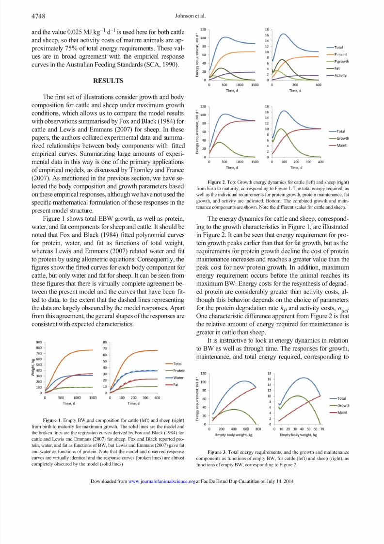
Figure 1 shows total EBW growth, as well as protein,

water, and fat components for sheep and cattle. It should be

noted that Fox and Black (1984) fitted polynomial curves

for protein, water, and fat as functions of total weight,

whereas Lewis and Emmans (2007) related water and fat

to protein by using allometric equations. Consequently, the

figures show the fitted curves for each body component for

cattle, but only water and fat for sheep. It can be seen from

thesefi

gures that there is virtually complete agreement be-tween the present model and the curves that have been fit-

ted to data, to the extent that the dashed lines representing

the data are largely obscured by the model responses. Apart

from this agreement, the general shapes of the responses are

consistent with expected characteristics.

The energy dynamics for cattle and sheep, correspond-

ing to the growth characteristics in Figure 1, are illustrated

in Figure 2. It can be seen that energy requirement for pro-

tein growth peaks earlier than that for fat growth, but as the

requirements for protein growth decline the cost of protein

maintenance increases and reaches a greater value than the

peak cost for new protein growth. In addition, maximum

energy requirement occurs before the animal reaches its

maximum BW. Energy costs for the resynthesis of degrad-ed protein are considerably greater than activity costs, al-

though this behavior depends on the choice of parameters

for the protein degradation rate k P and activity costs, αact .

One characteristic difference apparent from Figure 2 is that

the relative amount of energy required for maintenance is

greater in cattle than sheep.

It is instructive to look at energy dynamics in relation

to BW as well as through time. The responses for growth,

maintenance, and total energy required, corresponding to

Figure 1. Empty BW and composition for cattle (left) and sheep (right)

from birth to maturity for maximum growth. The solid lines are the model and

the broken lines are the regression curves derived by Fox and Black (1984) for

cattle and Lewis and Emmans (2007) for sheep. Fox and Black reported pro-

tein, water, and fat as functions of BW, but Lewis and Emmans (2007) gave fat

and water as functions of protein. Note that the model and observed response

curves are virtually identical and the response curves (broken lines) are almost

completely obscured by the model (solid lines)

Figure 2. Top: Growth energy dynamics for cattle (left) and sheep (right)

from birth to maturity, corresponding to Figure 1. The total energy required, aswell as the individual requirements for protein growth, protein maintenance, fat

growth, and activity are indicated. Bottom: The combined growth and main-

tenance components are shown. Note the different scales for cattle and sheep.

Figure 3. Total energy requirements, and the growth and maintenance

components as functions of empty BW, for cattle (left) and sheep (right), as

functions of empty BW, corresponding to Figure 2.









Figure 2, are shown in Figure 3. There is a nonlinear re-

lationship between the energy required for maintenance

and total empty BW, which is often characterized by an

empirical allometric response. Although not shown here,

this response is very similar to the BW raised to the power

between 0.73 and 0.75, which is widely used in feed evalua-

tion systems and simulation models (ARC, 1981; Finlayson

et al., 1995; National Research Council, 2001).

The analysis so far has considered growth under opti-

mal conditions of nonlimiting intake as defined by E req, Eq.

[34], and we now consider the situation where intake does

not satisfy maximum demand. It may be neither desirable

nor practical for animals to grow to their absolute maxi-

mum, due to restricted feed or the fact that maximum body

fat may only be achieved through supplementary feeding.

The illustrations in Figure 4 show animal growth with en-

ergy intake at maintenance plus 100, 90, 80, and 70% of po-

tential growth (protein and fat) energy requirement during

animal growth, as given by Eq. [33]. The results are as ex-

pected, with growth being reduced under restricted intake.For example, the time to reach half mature BW at full intake

is 270 d for cattle and 70 d for sheep, whereas with 70%

intake requirement it is 342 and 99 d, which correspond to

increases of 27 and 41%, respectively.

Animal growth rate and that of individual components

vary through time and also in response to relative intake.

This is illustrated in Figure 5 for both cattle and sheep, cor-

responding to the growth dynamics in Figure 4, where the

general pattern of the growth rate is consistent with sigmoi-

dal growth. It can be seen that growth rates of all compo-

nents are reduced as intake declines, and that the time for

peak growth rate is delayed, most noticeably for the fat

component.

The simulations in Figures 4 and 5 are for animals un-

der feeding regimes that provide full maintenance plus a

fixed proportion of growth requirements. These illustrationsare important as a means of examining the performance of

the model but, in practice, the intake is likely to vary in re-

sponse to both pasture quality and availability, as well as

management. The model can be applied directly to any feed-

ing regime and can respond to varying pasture availability.

As a simple example, the above simulations are repeated

but with intake taken to be full maintenance plus a propor-

tion of growth requirement that varies randomly between

Figure 4. Growth dynamics for growing cattle (left) and sheep (right)

for intake either at full requirement (100%) or maintenance plus 90, 80, and

70% growth requirement as indicated. Note the different scales.

Figure 5. Total animal growth rate and that of the protein, water, and fat

components of BW, as indicated, during growth for cattle (left) and sheep (right),

corresponding to Figure 4. The solid lines are maintenance plus 100% growth

requirement, large dashes 90%, small dashes 80%, and dots 70%. Note the dif-

ferent scales.

Figure 6. Top: Growth dynamics for growing cattle (left) and sheep

(right), for intake either at full requirement (100%) or maintenance requirement

plus 70% growth requirement, as well as switching randomly between these 2

regimens (R). Bottom: The corresponding total, growth, and maintenance en-

ergy requirements, as indicated for the R simulations. Note the different scales.

Figure 7. Growth dynamics for mature cattle (left) and sheep (right)

under a range of feed intakes. Left: Empty BW and components as indicated,

with intake either at 90% (large dashes), 80% (small dashes), or 70% (dots)

of mature maintenance requirement as indicated. (The colors and line styles

are consistent with Figure 5.).








Johnson et al.4750

70% and 100% of normal growth requirement, so that it

fits somewhere between the illustrations shown in Figures

4 and 5. This could apply, for example, to situations where

supplementary feeding is provided to ensure intake meets

a required minimum. The results for EBW, W , and energy

requirements are shown in Figure 6 where it can be seen

that, as expected, W lies between the 2 fixed regimens. Also,

although there are fluctuations in energy supply, the actual

growth curves for W are quite smooth, demonstrating thatBW growth is buffered in relation to moderate fluctuations

in intake.

One characteristic of the simulations illustrated in Fig-

ures 4, 5, and 6 for growing animals is that there was no fat

catabolism because, according to these feeding strategies,

maintenance costs are always met. In practice, intake will

vary and, particularly when animals are close to maturity,

there may be some fat loss to satisfy energy requirements.

To explore this, the final set of illustrations considers mature

animals with intake reduced from mature maintenance re-

quirement. The above analysis applies without modification,

although for animals at their mature optimum BW, there

will be no energy requirements for growth. Consequently,

for a mature animal that has less than its optimum protein

or fat composition, intake requirement may be greater than

for the equivalent animal at optimum BW because there is

a growth energy requirement, notwithstanding the fact that

activity costs will fall slightly as an animal loses BW. In

these next illustrations, that consider the effect of restricted

intake on mature animals, intake is prescribed as fractions of

the mature maintenance requirement at optimum fat com-

position.

The total EBW, as well as the protein, water, and fatcomponents, are shown in Figure 7 for animals receiving

90, 80, and 70% of mature maintenance requirement. It can

be seen that in all cases the weight components fall as ex-

pected. However, note that fat decline is virtually identical

for the 80 and 70% regimens, which is due to fat catabolism

occurring at the maximum rate (Eq. [45]). Consequently, the

protein weight decline is more rapid for the 70% regimen.

(The changes in protein weight may be dif ficult to detect

in this figure due to the relative size of this pool, although

it should be noted that the fractional decline in protein is

identical to that for water because these components are in

direct proportion, Eq. [4]).

DISCUSSION

We have described a daily time-step model of animal

growth and metabolism. The model is generic and has been

applied to sheep and cattle, although it can be used for

other animal types by changing the basic parameters. The

model describes body composition in terms of protein, fat,

and water. Protein growth is seen as the primary indicator

of metabolic status, with the role of fat being as a store of

energy reserves. The parameters to be prescribed fall into 3

categories. Animal BW characteristics are defined in terms

of birth and normal mature weights (W b and W max,norm,

respectively), fat fractions at birth, normal mature weight,

and maximum mature weight ( f F,b, f F,mat,norm, f F,mat,max),

and the water to protein ratio ( λ). Growth dynamics are de-

fined through the Gompertz growth coef ficient ( μ), protein

degradation coef ficient (k P ), fat growth and degradation co-

ef ficients (k F,g , k F,d ) and activity energy coef ficient (αact ).Finally, energy dynamics include energy densities for pro-

tein and fat (ε P , ε F ), their ef ficiencies of synthesis (Y P , Y F ),

and their ef ficiencies of degradation (Y P,d , Y F ,d ). The first

group of parameters defines the general BW characteristics

of the animal, the second its growth characteristics and the

energy parameters are the third group which are assumed to

be constants that apply to all animal types. All model vari-

ables and parameters are listed in the tables with suggested

default parameter values. An important feature of the model

is that each parameter has a direct physiological interpreta-

tion which facilitates adapting the model to different animal

types and breeds. We have derived suggested parameter

values from a range of sources rather than attempting to fit

the model to a specific data set, which is consistent with the

approach discussed by Hopkins and Leipold (1996). Part of

our aim has been to design the model for use in biophysi-

cal pasture simulation models that integrate the interactions

between the animal, pasture, soil water and nutrients, such

as DairyMod (Johnson et al., 2008) and the SGS Pasture

Model (Johnson et al., 2003). The structure of these mod-

els provides users with an interface that gives them direct

access to meaningful parameters which can be prescribed

to represent different animal species and breeds. Althoughour treatment of animal growth and metabolism is relatively

simple, we have focused on the key underlying processes of

protein and fat growth, along with maintenance of protein

in relation to resynthesis of degraded protein, and costs of

animal activity. The model does not include effects of diet

quality, and so it is assumed that once protein growth has

been determined in relation to available energy, that growth

is not restricted by the protein concentration in the diet. This

will be applicable in many situations, such as sheep or cattle

grazing fertilized perennial ryegrass swards or swards with

a legume present. We have presented simulations for grow-

ing and mature animals under a range of feeding levels andthe model behavior is physiologically realistic. For exam-

ple, for growing animals under limited intake, growth slows

and fat fraction of BW falls; whereas for mature animals, fat

catabolism occurs to support protein maintenance.

Other models at various levels of complexity have been

described in the literature ranging from a detailed treatment

of physiology, such as Baldwin et al. (1987), Dijkstra et

al. (1992), Dijkstra (1994), Baldwin (1995), Gerrits et al.

(1997), and Thornley and France (2007), to simpler whole

animal approaches such as Oltjen et al. (1986), Finlayson et








al. (1995), Emmans (1997), Freer et al. (1997), and Graux et

al. (2011). The present model differs from these in its rela-

tively simple structure and ease of parameterization, its flex-

ible treatment of variation in animal body composition, and

the avoidance of the use of empirical response functions for

individual metabolic processes.

A central feature of the model is that protein growth is

defined using a Gompertz equation, which is written as a

rate-state equation so that protein growth rate is a functionof protein weight rather than time. This is then inverted to

calculate the actual protein growth in relation to available

energy, which allows the model to respond dynamically

to available energy intake. Fat growth is related to protein,

reflecting the fact that protein is the primary indicator of

metabolic state. Protein is subject to continual decay and

the resynthesis of degraded protein is termed protein main-

tenance. Thus, for growing animals, energy is required for

protein maintenance and growth, fat growth, and activity

energy. If there is insuf ficient energy to meet the metabolic

demands of the protein maintenance and activity, then fat

can be catabolized as an additional source of energy.

Empirical curves describing body composition are of-

ten used to summarize the data, and we have used curves

given by Fox and Black (1984) for cattle and Lewis and

Emmans (2007) for sheep to compare model behavior with

experimental observations. (It should be emphasized that

the mathematical curves are used as summaries of experi-

mental data and are not part of the present model formu-

lation.) By defining appropriate birth and mature BW and

compositions, as well as growth parameters, the model

gives almost complete agreement with the observations

and displays generally expected characteristics of animalgrowth and metabolism.

Apart from BW and composition parameters, only

3 growth parameters are changed for the cattle and sheep

simulations, which are the Gompertz coef ficient and a

single coef ficient for each of protein and fat growth. These

are μ, k F,g , and k P , in Eq. [15], [25], and [21]. With a ba-

sic knowledge of animal body composition under normal

growth conditions, such as normal mature BW and fat frac-

tion, and growth characteristics, it is quite straightforward

to apply the model to different breeds of cattle or sheep. In

the illustrations we have presented here, ef ficiencies for the

synthesis of fat and protein and their energy densities have been taken to be constant for sheep and cattle. Although this

can be expected to be true for the densities, it is possible that

ef ficiencies differ slightly among animal types and breeds.

The model is versatile and robust, and directly appli-

cable to variable energy supply. It has the potential to be in-

tegrated into biophysical pasture simulation models that re-

quire a mechanistic treatment of the interactions among the

grazing animal, pasture, and soil nutrients, and for detailed

analysis of the growth and energy dynamics of animals dur-

ing growth or at maturity in response to available energy.

LITERATURE CITED

ARC. 1981. The nutrient requirements of farm livestock. No. 2: Ruminants.

2nd ed. Agricultural Research Council, London.

Baldwin, R. L. 1995. Modeling Ruminant Digestion and Metabolism. Chap-

man & Hall, London.

Baldwin, R. L., J. France, D. E. Beever, M. Gill, J. H. M. Thornley. 1987.

Metabolism of the lactating dairy cow. III. Properties of mechanistic

models suitable for evaluation of energetic relationships and factors in-

volved in the partition of nutrients. J. Dairy Res. 54:133–145.

Bergen, W. G. 2008. Measuring in vivo intracellular protein degradation ratesin animal systems. J. Anim. Sci. 86:E3–E12.

Dijkstra, J. 1994. Simulation of the dynamics of protozoa in the rumen. Br. J.

Nutr. 72:679–699.

Dijkstra, J., H. D. St. C. Neal, D. E. Beever, and J. France. 1992. Simulation of

nutrient digestion, absorption and outflow in the rumen: Model descrip-

tion. J. Nutr. 122:2239–2256.

Emmans, G. C. 1997. A method to predict the food intake of domestic animals

from birth to maturity as a function of time. J. Theor. Biol. 186:189–199.

Finlayson, J. D., O. J. Cacho, and A. C. Bywater. 1995. A simulation model

of grazing sheep: I. Animal growth and intake. Agric. Syst. 48:1–25.

Fox, D. G. and J. R. Black. 1984. A system for predicting body composition

and performance of growing cattle. J. Anim. Sci. 58:725–739.

France, J., M. Gill, J. H. M. Thornley, and P. England. 1987. A model of

nutrient utilization and body composition in beef cattle. Anim. Prod.

44:371–385.Freer, M., A. D. Moore, and J. R. Donnelly. 1997. GRAZPLAN: Decision

support systems for Australian grazing enterprises—II. The animal

biology model for feed intake, production and reproduction and the

GrazFeed DSS. Agric. Syst. 54:77–126.

Gerrits, W. J. J, J. Dijkstra, and J. France. 1997. Description of a model inte-

grating protein and energy metabolism in pre-ruminant calves. J. Nutr.

127:1229–1242.

Graux, A.-I, M. Gaurut, J. Agabriel, R. Baumont, R. Delagarde, L. Delaby,

and J.-F. Soussana. 2011. Development of the pasture simulation model

for assessing livestock production under climate change. Agric. Eco-

syst. Environ. 144:69–91.

Hopkins, J. C., and R. J. Leipold. 1996. On the dangers of adjusting the pa-

rameter values of mechanism-based mathematical models. J. Theor.

Biol. 183:417–427.

Johnson, I. R., D. F. Chapman, V. O. Snow, R. J. Eckard, A. J. Parsons, M. G.Lambert, and B. R. Cullen. 2008. DairyMod and EcoMod: Biophysical

pastoral simulation models for Australia and New Zealand. Aust. J. Exp.

Agric. 48:621–631.

Johnson, I. R, G. M. Lodge, and R. E. White. 2003. The Sustainable Grazing

Systems Pasture Model: Description, philosophy and application to the

SGS National Experiment. Aust. J. Exp. Agric.43:711–728.

Lewis, R. M., and G. C. Emmans. 2007. Genetic selection, sex and feeding

treatment affect the whole-body chemical composition of sheep. Ani-

mal 1(10):1427–1434.

Ministry of Agriculture, Fisheries and Food. 1975. Tech. Bull. 33. Energy al-

lowances and feeding systems for ruminants. Her Majesty’s Stationery

Of fice, London.

National Research Council. 2001. Nutrient requirements of dairy cattle. 7th

rev. ed. National Academies Press, Washington.

Oltjen, J. W., A. C. Bywater, R. L. Baldwin, and W. N. Garrett. 1986. Devel-opment of a dynamic model of beef cattle growth and composition. J.

Anim. Sci. 62:86–97.

SCA. 1990. Feeding Standards for Australian Livestock—Ruminants. 1990.

Standing Committee on Agriculture and Resource Management, Rumi-

nants Subcommittee. CSIRO Publ., Melbourne, VIC, Australia.

Thornley, J. H. M. 1998. Grassland Dynamics: An Ecosystem Simulation

Model. CAB Int., Wallingford, UK.

Thornley, J. H. M., and J. France. 2007. Mathematical Models in Agriculture.

CAB International. Wallingford, UK.

Williams, C. B. 2005. Technical Note: A dynamic model to predict the com-

position of fat-free matter gains in cattle. J. Anim. Sci. 83:1262–1266.

Wright, I. A., and A. J. F. Russell. 1984. Partition of fat, body composition and

body condition score in mature cows. Anim. Prod. 38:23–32.








Referenceshttp://www.journalofanimalscience.org/content/90/13/4741#BIBLThis article cites 18 articles, 6 of which you can access for free at:

Citationshttp://www.journalofanimalscience.org/content/90/13/4741#otherarticlesThis article has been cited by 1 HighWire-hosted articles:

http://www.journalofanimalscience.org/content/90/13/4741#BIBL


http://www.journalofanimalscience.org/content/90/13/4741#otherarticles




j anim sci 2012 johnson 4741 51

Documents