ESD-TR-69-193

J ESD RECORD COPY RETURN TO

SCIENTIFIC & TECHNICAL INFORMATION DIVISION {ESTI), BUILDING 1211

ESD ACCESSION LIST ESTI Call Nr 66967

-/—« cys.

INCREMENTAL METHODS FOR COMPUTER GRAPHICS

D. Cohen

April 1969

DIRECTORATE OF PLANNING AND TECHNOLOGY ELECTRONIC SYSTEMS DIVISION AIR FORCE SYSTEMS COMMAND UNITED STATES AIR FORCE L. G. Hanscom Field, Bedford, Massachusetts

Sponsored by: Advanced Research Projects Agency Washington, D. C.

ARPA Order No. 952

This document has been approved for public release and sale; its distribution is unlimited.

(Prepared under Contract No. FI9628-68-C-0379 by Harvard University, Cambridge, Massachusetts.)

ADOM^

LEGAL NOTICE

When U. S. Government drawings, specifications or other data are used for any purpose other than a definitely related government procurement operation, the government thereby incurs no responsibility nor any obligation whatsoever; and the fact that the government may have formulated, furnished, or in any way sup- plied the said drawings, specifications, or other data is not to be regarded by implication or otherwise as in any manner licensing the holder or any other person or conveying any rights or permission to manufacture, use, or sell any patented invention that may in any way be related thereto.

OTHER NOTICES

Do not return this copy. Retain or destroy.

ESD-TR-69-I93

INCREMENTAL METHODS FOR COMPUTER GRAPHICS

D. Cohen

April 1969

DIRECTORATE OF PLANNING AND TECHNOLOGY ELECTRONIC SYSTEMS DIVISION AIR FORCE SYSTEMS COMMAND UNITED STATES AIR FORCE L. G. Hanscom Field, Bedford, Massachusetts

Sponsored by: Advanced Research Projects Agency Washington, D. C.

ARPA Order No. 952

This document has been approved for public release and sale; its distribution is unlimited.

(Prepared under Contract No. FI9628-68-C-0379 by Harvard University, Cambridge, Massachusetts.)

FOREWORD

This report describes work accomplished under Contract F-19628- 68-C-0379 from June 1968 through April 1969. This contract is concerned with research on computer graphics and computer networking. In particular it is directed to the development of new insights into the creation, analysis and presentation of information. This report is concerned with incremental methods for computer graphics.

The report is based on a thesis submitted April 30, 1969 by Mr. Dan Cohen to Harvard University, Division of Engineering and Applied Physics in partial fulfillment of the requirements for the degree of Doctor of Philosophy.

Professor Anthony G. Oettinger was the principal investigator for the contract. Dr. Lawrence G. Roberts was the ARPA director. Dr. Sylvia R. Mayer was the ARPA agent at Electronic Systems Division. Lt John McLean of Electronic Systems Division provided technical guidance.

This technical report has been reviewed and is approved.

,.x< < C i ' P

SYLVIA R. MAYER WILLIAM F. HEISLER, Colonel, USAF Research Psychologist Chief, Command Systems Division Command Systems Division Directorate of Planning & Technology Directorate of Planning & Technology

Lawrence G. Roberts Special Assistant for Information Sciences, ARPA

li

ABSTRACT

This report is concerned with incremental methods for computer graphics. The application of the incremental approach to some advanced problems in computer graphics is discussed and demonstrated. In Section II, the problem of fast curve generation and display is discussed. This section uses the mathematical approach to curves as a perspective projection of polynomial-curves in higher-dimensional spaces. Section III, also discusses a fast generation of curves, but using another mathe- matical approach, the linear-differences method, only two-dimensional curves are discussed. Section IV, shows how to make the Warnock algorithm, for hidden lines elimination, incremental. Section V, dis- cusses the generation of half-tone images, in real-time. The technique suggested there requires a special-purpose hardware to be built. Section VI, discusses an incremental method for finding the intersection of given line-segments. The technique suggested there also requires a special hardware for implementation.

in

SECTION I

SECTION II

TABLE OF CONTENTS

INTRODUCTION

DISPLAY OF CURVES

II. 1 Introduction

II. 2 On 2D Curves (Perspective Approach)

II. 3 On 3D Curves (Perspective Approach)

II. 4 The Incremental Method for Fast Generation of Polynomials

II. 5 The Errors in the Incremental Computation of Polynomials

II. 6 Comparison of the Perspective and the Linear Differences Methods for Curve Generation

II. 7 Mathematical Justifications

SECTION IE : LINEAR DIFFERENCES CURVES

III. 1 Summary

III. 2 The Equivalence of the Various Definitions

III. 3 Obtaining the Generating Matrix for a Conic (Implicit Form)

III. 4 Obtaining the Generating Matrix for a Conic (Geometric Approach)

Page

1

2

I

3

5

5

12

15

18

25

Z5

27

29

31

III. 5 Characterization of Conies by the Generating Matrices 33

III. 6 On the Spacing Between Successive Points 36

III. 7 Straight Lines as Degenerate Conies 38

III. 8 On Curves Created by Matrices with a Non-unit Determinant 39

III. 9 Programming Aspects of Coding the Linear Difference Scheme 41

III. 10 Examples 42

SECTION IV : INCREMENTAL METHODS FOR HIDDEN-LINE ELIMINATION 56

IV. 1 Introduction 56

IV. 2 A Brief Discussion of the Warnock Algorithm 57

IV. 3 The Incremental Approach to the Warnock Algorithm 58

IV. 4 The Incremental Solution for the In/Out Problem for Polygons 63

Page

SECTION V : PRODUCTION OF HALF-TONE IMAGES IN REAL TIME 70

V. 1 Introduction 70

V. 2 Line Controller for Generalized Coordinates 71

V. 3 Production of TV-scan Images 73

V. 4 Production of Radar Scan Images 78

SECTION VI : FAST INTERSECTING OF LINES 83

VI. 1 Introduction 83

VI. 2 The Sutherland Interpolator 83

VI. 3 Lines Intersector 90

VI. 4 On String-Line Intersecting 97

REFERENCES 103

VI

LIST OF FIGURES

Fi Ku re No.

II. 4. 1

II. 4. 2

II. 4. 3

Page

Schematic drawing of the hardware for the forward differences technique 9

The behavior graph of the system in Fig. II. 4. 1 10

The hardware for the backward differences technique 11

II. 4. 4 The behavior graph of the system in Fig. II. 4. 3 11

2 2 III. 4. 1 The ellipse %K + ^ = 1 32

X* /

III. 4. 2 A tilted hyperbola 33

III. 10. 1 A circle (generated by the LDM) 44

III. 10. 2 A circle (generated by the PM) 45

III. 10.3 Two ellipses 46

III. 10.4 A family of hyperbolas 47

III. 10. 5 A circular spiral 48

III. 10.6 An elliptic spiral 49

III. 10. 7 A star 50

III. 10.8 A star spiral 51

III. 10. 9 A quadratic parabola 52

III. 10. 10 A cubic 53

III. 10. 11 An oscillated hyperbola 54

III. 10. 12 A family of curves 55

IV. 3. 1 A window subdivided into 4 subwindows 58

IV. 3. 2 Subwindows divided into subwindows 59

IV. 3.3 A tree representation of Figure IV. 3. 2 60

IV. 3.4 The relations between the polygon/window relations 62

VII

Figure No. Page

IV. 3. 5 The simplest Warnock algorithm for line drawing 64

IV. 4. 1 A polygon describing the digit "4" 66

IV. 4. 2 A Karnaugh map for the signs conditions 67

IV. 4. 3 Examples for window/line relations 69

V. 2. 1 Intensity profile 72

V. 2. 2 A shader for constants intensities 74

V. 2. 3 A shader for linear intensities 75

V. 4. 1 A scheme for generating X and Y 79

V. 4. 2 A multiplication free scheme for computing X and Y 80

V.4.3 An {r , <f>) shading system 82

VI. 2.1 A line intersecting the y-axis 84

VI. 2.2 X scaling does not change the intersection 86

VI. 2. 3 Using the Sutherland interpolator as a divider 87

VI. 2.4 A schematic drawing of the Sutherland interpolator 88

VI. 2. 5 The states of the Sutherland interpolator 90

VI. 2. 6 The control logic for the Sutherland interpolator 91

VI. 3. 1 Intersection of segments, which are not parallel to the axes 93

VI. 3. 2 Figure VI. 3. 1 after the rotation 93

VI. 3. 3 The segments {P.,P_} are trivially rejected 96

VI. 4. 1 A line and a string 98

VI. 4. 2 The line/segments intersector 100

VI. 4. 3 The operation of the line/segments intersector 101

Vlll

SECTION I

INTRODUCTION

The spirit of the incremental methods is to organize the steps

of a computation so that each step can use information prepared by-

earlier steps. Such procedures eliminate redundant repetitive

computation, and simplify each computation step.

In this thesis I will exhibit five examples of incremental methods.

The examples shown here all apply to computer graphics. Computer

graphics is particularly responsive to the application of incremental

methods because a large amount of information must be processed

quickly to produce a picture, while the basic operations to be per-

formed on the data are relatively simple. Computer graphics is

also particularly receptive to incremental techniques because con-

ventional general-purpose computers do not do this job nearly as

well as it can be done by incremental techniques. Moreover, the

incremental approach is applicable to a wide variety of computing

problems, and not to computer graphics only.

The five examples exhibited here are: linear-difference scheme

for curve generation, perspective scheme for curve generation, the

Warnock algorithm for hidden-line elimination, half-tone image pro-

duction and a fast lines-intersecting technique.

The incremental method for perspective curves, which is described

in Section II, was implemented in the three-dimensional-graphic-

hardware project at Harvard, and was simulated on the PDP-1 computer.

The incremental method for generating curves, which is described in

Section III, is used by a PDP-1 system for drawing curves on a CRT,

from which the pictures appended.to that section were taken. The

search-ordering strategy which makes the University of Utah hidden-

line elimination algorithm incremental was incorporated into their

hidden-line elimination system by its author, John Warnock. This

approach is described in Section IV. A variation of the incremental

method for half-tone image production, which is described in Section V,

was implemented in hardware by the General Electric Company.

1

SECTION II

DISPLAY OF CURVES

(II. 1) Introduction

The ability to display straight lines on a CRT is a standard

feature of these devices. However, many applications require

curvilinear display. Typical schematic drawings like block-diagrams

and logic-designs can be drawn with straight lines only, but attempts

to display real world objects like machined components require curve

display since the world is not rectilinear.

Any curved segment can be displayed accurately up to the scope

resolution by displaying a set of points close enough together on the

curve. Curve display by separate calculation and separate storage

of each point is not feasible for many applications which are restricted

by real time requirements or by storage limitation. A similar diffi-

culty, existing in the past for straight lines, has been resolved by the

introduction of line-generators which generate all the points of a line

segment given its end points. Carrying this approach forward to

curves leads to a "curve-generator", based upon a small number of

parameters, which can generate a curve segment in real time.

Two incremental curve generators are suggested in this work.

One is based on a three-dimensional perspective approach (Section II)

and the other on a two-dimensional approach (Section III). Both

generate points on the curve so that these points may then be connected

by a line generator.

Each of these curve generators can generate a family of curves.

The two families are not the same, but both include all the conies. A

comparison of these generators is made in (II. 6). The mathematical

justification of our methods, and of the assumptions used in this section

can be found in (II. 7).

up to the scope resolution

(II. 2) On 2D Curves (Perspective Approach)

As the displaying screen is a 2D surface, 2D curves are the core

of any curve representation. The ability to specify and display curves

in 2D is the key to representing curves in any space. In (II. 7. 1), we

prove that any conic segment in 2D is a perspective image of the

canonic-parabola in 3D , or of its images under linear transforma-

tions. Therefore the problem of specifying a conic segment in 2D

is equivalent to the problem of finding the linear transformation of

the canonic-parabola which transforms it into a 3D curve whose 3D

perspective projection is the desired conic. As any linear trans-

formation can be realized by a matrix multiplication, the problem of

specifying a conic segment is replaced by the problem of finding the

matrix of the linear transformation. This concept of perspective

images was already discussed in the late 19th century*- *» *• K

The family of conies includes ellipses and circles, hyperbolas,

parabolas and straight lines as a degenerate case. Conies never

intersect themselves and never have an inflection point, as shown in

(II. 7. 1). If more general curves are required, one can use an

"mth-degree-conic" which is defined to be the perspective projection

of a 3D curve whose components are polynomials of degree m in some

parameter t. "Conies" usually mean "2nd-degree-conies " but I will

not distinguish them from the general case, in spite of the importance

of second degree conies for many applications. Properties of the

mth-degree-conics can be found in an unpublished memorandum by

Professor S. A. Coons and in [4]. In general, the higher m is, the

more general is the mth-degree-conic, but of course, more conditions

are required to specify it uniquely. In order to simplify the notation

hereafter, we will use m = 3. The changes required for other values

of m are self-evident.

The canonic parabola in 3D is the curve given by (x, y, z) = (t ,t, 1).

The explicit form of the mth-degree-conic (for m = 3) is:

3 2 x = x(t) = x^t + x?t + x,t + xfl

y = y(t) = y3t3 + y2t2 + Ylt + yQ

3 2 z = z(t) = z t + z?t + z,t + zfi

which can also be written as:

(x,y,z) = (t3,t2,t, 1)

X3 ^3 Z3

x2 vz z2

xl *i zl

xo ^0 2o

A computational implementation of this representation, for generating 3 2 a sequence of points on the curve may consist of storing {t ,t , t, 1}

and using a matrix multiplier for getting the (x,y, z) values. This is

very useful for devices which happen to have a matrix multiplier

capable of performing the multiplication of a [lx(m+l)] vector by a

[(m+l)x3] matrix. The scheme can be improved by generating the

sequence {t ,t , t, 1} instead of storing it. This sequence can be

generated very fast incrementally. However generating the polyno- r 3 2 i

mials x(t), y(t) and z(t) can be done as fast as generating the |t ,t , t, 1/

sequence. The curve generator should therefore generate successive

values of x(t), y(t), z(t) and project these points on the scope plane by 2

dividing x(t) and y(t) by z(t) to get the scope coordinates of the points .

An M matrix multiplier is a device which can store an £xk matrix A and multiply it by any given 1 xf vector V, to find the lxk vector VA. This operation requires ixk multiplications and (£-l)xk additions. By using parallel processing, a matrix multiplier can execute the multi- plication in i. multiply-times only. Such a 4x4 matrix multiplier is de- scribed in the final report of Harvard contract XG-2972. 2 It is easy to see that if the viewing plane is z=l, and the projection

center is the origin, then the point (x, y, z) is projected on the point

( —, •*•, 1) on the viewing plane. Zi Zj

The scope coordinates are given to a line generator which generates

line segments between the curve points while the new points are

generated. The incremental method for generating successive values

of (x(t), y(t), z(t)} is described in (II. 4) below.

(II. 3) On 3D Curves (Perspective Approach)

For many applications it is very important to specify curves

which satisfy conditions in the 3D space. After meeting these condi-

tions, the curves are projected into the 2D space for display. One

can easily generalize the 2D methods to 3D by introducing one more

component and treating a 3D curve as a perspective projection of some

4D curve into 3D space. As in the 2D case, specifying a curve is

equivalent to finding some matrix. Because of the additional compo-

nent, there are more unknowns than in 2D in the equations defining

the matrix and more conditions are required to specify curves uniquely.

The perspective transformation from the 4D space to the 3D space (for

curve definition) and the transformation from the 3D space to the 2D

space (for display) can be combined in one perspective transformation,

in order to simplify the displaying process.

Consider the following example: let {x(t), y(t), z(t), w(t)} be a

curve in the 4D space. Its perspective projection into the 3D space is

the following curve: [—TTT, ,77, —\rr) whose 2D perspective projection 6 \w(t) ' w(t) ' w(t) J r r f J

is the following curve:

( x(t) . %s& jdii . -£i£l\ /*iil yit) ^w(t) • w(t)' w(t) • w(t)J ^z(t)' z(t)

Note that there is no need to evaluate w(t) at all. There is only need

to evaluate (x(t), y(t), z(t)} and to display {x(t)/z(t), y(t)/z(t)}, exactly

as in the 2D case, since the 3D curve is displayed in 2D regardless of

the dimension of the space in which it is defined.

(II. 4) The Incremental Method for Fast Generation of Polynomials

For each of the 3 components {x(t), y(t), z(t)} we have to evaluate

a polynomial of degree m, at some set of values of the parameter

{tp., t, , t?. . . t-J . For simplicity we choose the range of t to be [0, 1]

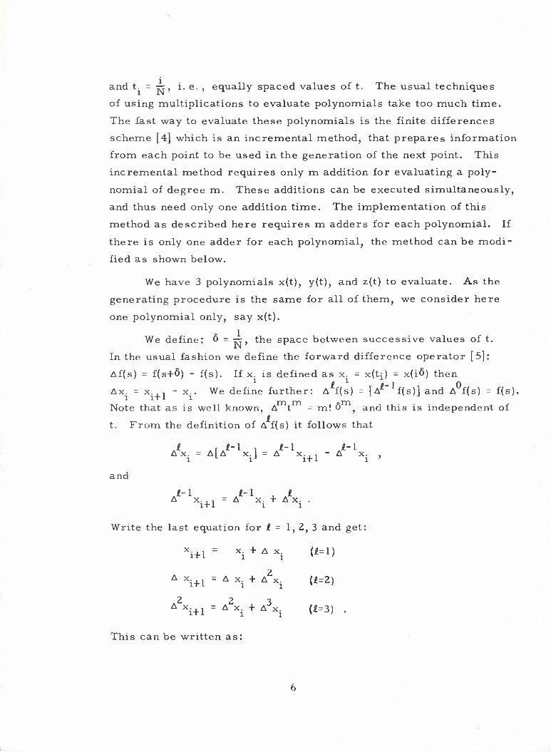
and t. = -sr, i.e., equally spaced values of t. The usual techniques

of using multiplications to evaluate polynomials take too much time.

The fast way to evaluate these polynomials is the finite differences

scheme [4] which is an incremental method, that prepares information

from each point to be used in the generation of the next point. This

incremental method requires only m addition for evaluating a poly-

nomial of degree m. These additions can be executed simultaneously,

and thus need only one addition time. The implementation of this

method as described here requires m adders for each polynomial. If

there is only one adder for each polynomial, the method can be modi-

fied as shown below.

We have 3 polynomials x(t), y(t), and z(t) to evaluate. As the

generating procedure is the same for all of them, we consider here

one polynomial only, say x(t).

We define: 6 = -rj, the space between successive values of t.

In the usual fashion we define the forward difference operator [5]:

Af(s) = f(s+6) - f(s). If x. is defined as x. = x^) = x(i6) then

Ax. = x.,, - x.. We define further: A f(s) = [ A1"1 f(s)] and A°f(s) = f(s).

Note that as is well known, At = m! 6 f and this is independent of

t. From the definition of A f(s) it follows that

J .rJ-1 i J-l J-l

and

Ax. = A[A x.l = A x. , , - A l L iJ l+l l

£-1 £-1 £ A x. , , = A x. + A x. . l + l l l

Write the last equation for £ = 1, 2, 3 and get:

x. + 1 = x.+Ax. (£=1)

A x.+1 = A x. + A2x. (£=2)

A x. + 1 = A2x. + A3x. (£=3) .

This can be written as:

r\ r' ° °\/ x\ A x

A.

1 1 0 0

0 110

0 0 11

kO 0

A x

A x I U U I 1 ) I A x

\A3x/i+1 \0 0 0 1/ \A3xA

or F.,, = SF. l+l l

where F. is the Forward differences vector at x = x., and S is the

above matrix.

We define the backward difference operator by Vf(s) = f(s) - f(s-6).

V and V are defined similarly to A and A . In general V f(s) = A f(s-jPS).

It is easy to see that V x. , , = V x. + V x. . , . ' l+l I l+l

Substituting i. = 1, 2, 3 gives:

x. i+1

x. + V x l l+l

V x.+1 = V x. t 7'xl+I

V2x+1 . V\ • v3Xi+1

which implies:

^2x. . , = V2X. + V3

X.X1 = V2X. + V3

X. l+l I l+l l l

V x. . = V x. + V2X. = V x. + V2

X. + V3X.

l+l l l+l ill

L+l x. + V x

I l+l x. + V x. + V2X. + V3

X l l l i

This can be written as:

' x

V2x

>V3x

1111

0 111

0 0 11

\/-" x

V2x

i+1 \0 0 0 1/ W3

or B.,, = TB. l+l l

where B. is the Backward differences vector at x = x. and T is the I — i

above matrix. We have in mind placing the current values of x., m S. Vx.... V x. (or the V x.) in a set of fast registers. The successive

I I l

values in the x. register are used for the display and the other regis-

ters are used for conveying information from each point to its

descendants. The A x register does not have to be modified as t

changes over its range, because At = V t = m'.o . Let us

factorize S and T to indicate the computational procedure:

'l 1 0 0

0 110

0 0 1

0 0 0

S =

T =

1 1 1

0 1 1

0 0 1

0 0 0

1 0 0 0

0 1 0 0

0 0 1 1

0 0 0 1

1 0 0 0

0 1 1 0

0 0 1 0

0 0 0 1 J >

1 1 0 0

0 1 0 0

0 0 1 0

0 Mi

0 0 1

A3A2A1

110 0

0 10 0

0 0 10

0 0 0 1

1 0 0 0

0 1 1 0

0 0 1 0

0 0 0 1

1 o o oN

0 10 0

0 0 11

0 0 0 1 J

- A1A2A3

,£-1 A. is the operation of adding the V x (or the A x) register to the V x £-1

(or the A x) register. S is equivalent to executing A. , then A_,

then A_. T is equivalent to the execution of the same operations, in

reverse order. There are only three additions involved in either of

these methods. However, there is a basic difference between them.

In the forward difference scheme, each "new" value A x. . , depends k i+l r

only on "old" values A x., but in the backward difference scheme, each

"new" value V x. , , depends on the current values of the registers, I JH-1 "old" V x. and "new" V x. , , . It is therefore possible to execute all

I l+l the additions for the forward difference method scheme in parallel,

consuming only one addition time for evaluation successive values of

the polynomials. This however requires a great deal of hardware.

The backward difference scheme is more economical for sequential

computation, but consumes m addition-times. Schematic drawings

for the two methods are shown in Figures II. 4. 1 and II. 4. 3.

The behavior graphs of these systems are shown in Figures

II. 4. 2 and II. 4. 4. The behavior graph of the forward difference scheme

Behavior graphs are sort of "occurrence-graph" [18].

(i) INITIAL LOADING (f) LOADING (a) ADDITION

(d) DISPLAY

ft

R1

+ )°\

AX

l

R2

+ )a

A2X

R3

+ ) a

A3X

»3

Figure 11.4.1 : Schematic drawing of the hardware for the forward differences

technique.

9 '•-,'• .

I } CM I o

rol o

k K * N I

0

i CM

CO o

to

ro o

k * ~*

•o

CM

CO O

i i

> i

ro

ro O

K K r-. > i

•i CM

I

ro

w| ]p\ _S\

i;;ure 11.4.2 ; The behavior graph of the system in figure [1.4,

1 0

12

"3

Q|

a

a-

Figure II.4.3 : The hardware for the backward differences technique.

i4 f4 a3 f3 a 2 f2 ai t\ U a3 h a2 h a, l\ U X? >0 X5 »p >Q if) >0 —X5 >0 X) »0 X) X> X) X>0-

V

Figure II.4.A : The behavior graph of the system in figure 11.4.3

1 1

has 3 parallel paths which indicate the parallel processing. It is

possible to introduce some parallelism in the backward difference

scheme, but this requires more hardware than is needed for the

forward difference scheme. However the critical operation is the

division. If the division is slower than 3 additions (as it always is

in digital systems) there is no sense in providing the extra hardware

which is required by the forward difference method. In this case,

both the forward and the backward difference method require on

divide-time. £

The forward difference scheme is initialized by loading Ax.(O)

into the registers, and the backward difference scheme is initialized I

by loading V x.(0).

In (II. 7. 2) we show how the initial differences {V x.(0)} and

{AX.(O)} can be found. I

(II. 5) The Errors in the Incremental Computation of Polynomials

The iteration process which is described in the preceding

subsection may introduce some errors due to the finite precision of

the machine. We cannot, in general, better the precision, but we

can modify the iterations to minimize the errors where they are most

important, at the end-points (e. g. , for curve closure).

The source of the errors is not the iteration process itself

(which is multiplication free) but the propagation of the errors in the

initial values of the differences.

We can change the initial values of the differences in order to

make the iterations end as close as possible to the prespecified end-

point. We show now a method which converges to an end-point which N is within y machine resolution points from the given end-point, where

N is the number of iterations.

Consider first the forward differences scheme. Define:

e = [1, 0,0, 0].and S = I + H,

12

/O 1 0 0 \

H

0 0

1 0

1 and F(n) =

\0 0 0 0/

/ x(n6) \

A x(n6)

A2x(n6)

\ A3x(n6) /

We showed that F(n) = SnF(0) and x(n6) = eF(n). The computed end-

point is x(N6) = eS F(0). Let x be the given end-point. Hence, the

error introduced by the iterations is:

E = xe - x(N) = x - [x(0) + NAx(O) + f^J A2x(0) + (3)

A3x(0)].

N\ 3 Dividing the error by [ a ] is a correction for A x(0). The remainder

of this division divided by I , I is a correction for A x(0), and the

remainder of the second division divided by N is a correction for Ax(0).

These 3 corrections reduce the magnitude of the error to be less than

N. By changing Ax(0) by one resolution unit, the magnitude of the error N can be reduced not to exceed rr.

This correction process can be programmed as follows:

(1) xe - [x(0) + NAx(O) + W A2x(0) + fa)

"A- A3x(0)]

(3) A°x(0) + e. A3x(0)

(4) fl

(!)

(5) A2x(0) + e2 »A2x(0)

(6) »-(?)'3-(?) N -> e.

13

(7) Ax(0) + eY » Ax(0)

(8) if [E - f^)e3 - f^J e2 - Ne^ >j then Ax(0) + 1 »Ax(0)

(9) if [E - me3 - (2) e2 " Ne^ < -j then Ax(0) - 1 )Ax(0)

For the backward difference scheme a similar correcting method

works by using:

x(n6) = eTnB(0) where T = I + H + H2 + H3

and

Tn = I + nH + [n + ff\ ]H2 t [n + 2 M + M ]H3 .

If we do not want to change Ax(0), and we wish also to get the

right value for Ax(N) then another correcting scheme can be applied.

Expand F(N) = SNF(0) and get:

x(N) = x(0) + NAx(O) + f ^ ) A2x(0) + f jj A3x(0)

Ax(N) = Ax(0) + N A2x(0) + f Jj A3X(0)

A2x(N) = A2x(0) + N A3x(0)

A3x(N) = A3x(0)

x(0) and x(N) are given by:

x(0) - d x

x(N) =a+b+c+d X X X X

Ax(0) and Ax(N) can be found directly by:

Ax(0) = a 63 + b 62 + c 6 X X X

Ax(N) = a (63 + 362 + 36) + b (S2 + 26) + c 6 X X X

14

2 3 Using these values, A x(0) and A x(0) are found from the following

equations:

AVT\ ? /TVM i c(0) = x(N) - x(0) - NAx(O) (N) ^(0, • (?) A,

N A2x(0) + ( ^ I A"x(0)

2 3 Using the values of A x(0) and A x(0) which satisfy (as close as possible)

these equations reduce the errors in x(N) and Ax(N). For backward

differences a similar method exists.

(II. 6) Comparison of the Perspective and the Linear Differences Methods for Curve Generation

The LDM (Linear Difference Method) is described in Section III.

In this section I have described the PM (Perspective Method) for curve

generation.

I compare the two methods, the LDM and the PM (for m=2) accord-

ing to:

- complexity of points generation,

- variety of curves and speed of generation,

- complexity of the mathematics involved,

- sensitivity to errors.

The complexity of points generation

The PM requires 6 additions and 2 divisions per point. If enough

hardware is available then all the additions can be carried out in parallel,

and so can the divisions. Hence the time which is consumed by each

point is between 1-add-time plus 1-divide-time and 6-add-times plus

2-divide-times.

The LDM requires 4 multiplications and 2 additions. If the hard-

ware is available then the multiplications can be performed in parallel,

and so can the additions. Hence the time which is consumed per point

is between 1-add-time plus 1-multiply-time and 2-add-times plus

4-multiply-time s.

15

If the curves are generated by software it is preferred to use

the LDM. If hardware is used then the comparison depends on the

speed and the cost of the components involved.

Variety of curves and speed of generation

The PM can generate only conic segments; ellipses, parabolas,

hyperbolas and straight lines. It cannot generate complete ellipses

and circles. The LDM can generate complete ellipses and arcs of

hyperbolas and generalized parabolas (y = x ) which do not pass through

the origin or through infinity. In addition the LDM can also generate

straight lines, elliptic spirals, stars and various other shapes as

described and illustrated in Section III.

The LDM generates the conies always at a "good-speed" . The

PM is not always able to generate a conic section at a "good-speed".

For example, it is impossible for the PM to generate a circular arc

at a uniform speed. Because of its good-speed-property the LDM

needs fewer iterations to display a curve than the PM. (See the figures

in in. 10).

Complexity of the mathematics involved

There is a simple method for finding the parametric matrix for

any conic segment given by its end-points (see II. 7 and [6]). This

method can be used for finding the matrices which together represent

a complete ellipse. However, although it is relatively simple to find

the parametric matrix, as required by the PM, it is not always easy

to perform the shape invariant transformations [4] which are required

to improve the generation speed.

There is no simple way to find the generating matrix for a given

conic segment, as required by the LDM, because finding the matrix is

equivalent to finding sines and cosines. However it is relatively very

easy to find the generating matrix for a conic (not only a segment) from

its implicit form or from its geometrical properties.

A curve is said to be generated at a "good-speed" if the distance between successive points decreases when the radius of curvature decreases.

16

The simple manipulation of curves, such as rotation, translation,

stretching and scaling do not have to be performed on each data point.

In the PM all these operations can be performed on the parametric

matrix. In the LDM only the stretching and rotation (in some cases)

have to be performed on the matrix. The other operations do not

need any operation on the matrix, and are carried out by the specifi-

cation of the initial point (and initial difference), because the same

generating matrix generates a whole family of curves.

Sensitivity to errors

Both, the PM and LDM may introduce roundoff errors. These

roundoffs propagate during the iterations, and might result in a large

error after N iterations. We show in this section that the error in

evaluation each polynomial for the PM can be reduced to be less than N y in magnitude at the end points. We can do that because the iteration

involve only additions which do not introduce new roundoff errors. The

LDM uses multiplications which are rounded off, introducing possibly

new truncation errors, of one machine-re solution unit, at each step.

These roundoff errors are accumulated and multiplied by T . Hence

the LDM is more sensitive to errors, then the PM. In some cases the

LDM becomes so sensitive that it cannot be used. For example: A

definition of a hyperbola by its implicit form and a point which is very

close to an asymptote. The reason for this kind of sensitivity is that

the same generating matrix generates a family of hyperbolas which all

converge to the same asymptotes.

The PM does not have a 1-1 correspondence between curves and

matrices, unlike the LDM. It is possible to change the representing

matrix of a curve (even by splitting the curve into some sections) in

order to make the iteration less sensitive. By this operation the sensi-

tivities due to a small denominator, or to small numerators may be

improved.

Unfortunately the generating matrices for the LDM are unique

(up to the generation speed) and do not have any freedom which can be

used for improving the sensitivity to errors.

17

(II. 7) Mathematical Justifications

The purpose of this subsection is to justify mathematically some

results which are used in the section without proof.

(II. 7. 1) We will define a family of curves, <r , which con- ' m,n' n

sists of curves in R , whose components are polynomials of degree

m in some parameter t. The perspective projection of cr , into n ~ 1 '

R is called here n . We will prove the following results: m, n °

(a) If S e 7T2 -i tnen S is a conic segment;

(b) If S is a conic segment then S eL -i>

(c) There exists S e cr~ such that for any P e IT, , there

exists a linear transformation T, such that P is the

perspective projection of TS;

(d) Conies do not intersect themselves.

Let cr be the family of curve segments in R , with each component

being a polynomial in t, with degree not exceeding m. S e cr implies m '

S = (s(t)} = {x,(t),x-,(t). .. x (t)} where x.(t) = 2 a..tJ. Let n be 1 ' 2V nx ' ix ' j = o ij m, n

the perspective projection of cr in P , the perspective space obtained n ' n from R by dividing each component x. by x . Note that P is isomor-

phic to the closed R

If S = { s(t)} = {x, (t), x?(t). . . x(t)} e cr , then its projection in Dn . P is:

JXl(t) x2(t) ^-i^)] p = {p(t)}Mx^'x^)----iT(rrj eVn •

(a) We want to show that if S e 7T-, _ then S is a conic segment.

Proof (following L. G. Roberts [6]): Consider Tl2 _, with the

following notation: x = x,, y = x2 and w = x_. Let

2 x = x(t) = Xpt + x,t + X-

2 y = y(t) = y2t + yxt + yQ

2 w =w(t) = w?t +w.t + w_

18

In short, this can be written as:

x 2 ^2

p = p(t) = (x,y,w) = (t ,t, 1) x,

w2\

w. TA,

x, ^o y0

2 where T = (t , t, 1) and A is the above matrix.

If A is a nonsingular matrix, define:

0 0 l\

w.

0

1

2 0

0 0/

*-l -1 A = A MA * -

then:

-1. -1, # * pCp = (TA)C(TA) = (TA)(A MA )(A T ) = T

for all t. This proves that the arc TA is a conic segment. If A is

singular, then there exists a non-zero vector V such that AV = 0, and /a\

TAV = pV = (x, y, w) ax + by + cw = 0. Hence TA is a straight

line, which is a degenerate conic.

(b) We proved above that if P e 7T-, , then Pisa conic segment (or a line

segment, which is a degenerate case of a conic). The converse is more

important: any conic segment belongs to fl~ . We prove this as follows: *

Proof: Let vCv = 0 be the implicit equation of the conic, and let vQ and

v, be the start and end points of the segment. Let v_ be the intersection

of the two tangents to the conic through vn and v, . Note that the tangents 2 3 do not necessarily intersect in R , but they must intersect in P .

Consider the matrix

/ l ' -2 1 \ /'i

A = JV = 0 2 -2 fv

\ o 0 1 / 1 v„

19

where f is a scalar. It satisfies the following conditions:

(i) for t = 1, TA = Vj : (1,1,1) A = (1,1,1) JV = (1,0, 0) V = vj

(ii) for t = 0, TA = VQ : (0, 0, 1) A = (0, 0, 1) J V = (0, 0, 1) V = vQ

* (iii) TA is a conic arc because (TA) C (TA) = 0 for all t.

This is proved by:

V C V M hY fvr C fvr

vlCvl* fVjCvT* VJCVQ* \

fvTCVl* fvTCvT* fvTCvQ*

vo/ \vo/ \v0Cvl* fvoCvT* V0CV/

0 0 a\

0 b 0

0 0 /

where a = v,Cv * and b = f v„Cv *

viCvi* = voCvo>; 0 because v, and v„ are on the conic.

vTCv * = v.Cv * = 0 because v„ is on the tangent to the conic

through v, .

vTCv * = vfiCv_* = 0 because of a similar reason.

With no loss of generality we can assume that C is a positive definite 2 form. In this case, a = v,Cv * = vXv.* < 0 and b = f v„Cv * > 0.

Next we consider the product ACA* = JVC V* J* :

1 l\ / 0 0 a\

J(V C V*)J* = 0 2-2

0 0 I / \ a 0 0 / \ 1

where c = 2a + 4b. Hence

0 0 \

2 0

•2 1

•c

a

4b 0

0 0

(TA) C (TA)* =T(J V C V* J*)T* = ct4 - 2ct3 + ct2 = ct2(l-t)2 .

20

This expression vanishes for all values of t if c = 0. This con-

dition can be satisfied by the proper choice of f, namely

f2= "vicV 2vTCvT*

We showed in (iii) that TA is a part of the conic VCV* = 0, and

we showed in (i) and (ii) that the end points of TA are v» and v, .

This completes the proof of the converse claim.

(c) Corollary: Any conic segment can be obtained from any non-

degenerate conic segment by a linear transformation.

Proof: Let v, = TA. be a non-degenerate conic segment. Let

v-p = TA? be another segment. v? is obtained from v, by the linear

transformation T = A. A2, as v,T = TA.(AJ A_) = TA_ = v.,. Note

that if v, is the "canonical-parabola" v = (t , t, 1) then A, = I, the

unit matrix, and T = A?) which means that v2 is obtained from the

canonic-parabola by using the representation matrix of v? as the

transformation.

(II. 7. 2) The forward and the backward difference schemes need

initialization by loading the values of Ax.(0) or V x.(0) to the appro-

priate registers. We will find first A x^(t) then we will find Ax.(0) by

substituting t = 0. Later we will find V*x.(t) and substitute t = 0 to

get the V£x.(0).

We use the fact that the V and the A are linear operators in the

evaluation of the differences of the polynomial x(t):

A t3 = 3t26 + 3t62 + 63

A t2 = 2t6 + 62

At =6

A2t3 = 6t62 + 663

A2t2 = 262

A3t3 = 663 .

21

3 2 Let x(t) = a_t + a2t + a,t + a_. Then:

A x(t) = (a^ + a262 + a363) + t(2a26 + 3a362) + 3a 6t2

A2x(t) = (2a262 + 6a363) + 6a362t

A3x(t) = 6a363 .

Substitute t = 0 and get:

x(0) = aQ

A x(0) = aL6 + a262 + a 63

A2x(0) = 2a262 + 6a363

A3x(0) = 6a363 .

Find the backward differences by:

V t3 = 3t26-3t62 + 63

V t2 = 2t6 - 62

V t = 6

V2t3 = 6tS2 - 663

V2t2 = 262

V3t3 = 6t3 .

3 2 Again let x(t) = a_t + a2t + a,t + a_. Then:

V x(t) = (ai6-a262 + a363) + (2a26-3a362) + 3a36t'

V2x(t) = (2a262 - 6a363) + 6a362

t

V3x(t) = 6a363 .

Substitute t = 0 and get:

22

x(0) = a 0

V x(0) = a16-a26'i + a3

V2X(0) 8 2a262 - 6a363

V3X(0) = 6a363 .

To summarize: Let the curve be given by

w \

[x(t),y(t),w(t)] = [t3,t2,t, 1]

The Forward Differences Scheme:

We showed in (II. 4) that:

x

x

x

w

"w

1 / w

= TA

F(n)

/ Xn\ rl ° °\7 x(o)\ A x \ 0 1 1 0 \[ A x(0)

n

Jx A x(0)

n l " " " / 1 A2X(0) /

\A3x / \0 0 0 1/ \A3x(0)/

,n S F(0)

where x = x(n6). Then we showed that: n

x

F(0) = a 63 + b 62 + c

K. X

6a 53 + 2b 62

X X

6a 63

x

\ /0 0 0 1

5\ [1110

6 2 0 0

/ \6 0 0 0/ \

= QDA

1'

\0I

Combine together and get:

[x(n6),y(n6),w(n6)] = [1, 0, 0, 0]SnF(0) = [1, 0, 0, 0]SnQDA

which may be verified by checking that:

[1,0, 0,0]SnQD = [(n6)3(n6)2n6 1] .

23

The Backward Differences Scheme:

We showed that:

B(n) =

where x = x(n6). Then we showed that n

B(0) =

r 0 0 1

i -1 1 0

-6 2 0 0

\6 0 0 0

Combine together and get:

[x(n6) y(n6) w(n6)] = [100 0]TnQDA

which may be verified by checking that:

[10 0 0]TnQD = [(nS)3 (n6)2 (n6) 1] .

TnB(0)

QDA |

24

SECTION in

LINEAR DIFFERENCES CURVES

III. 1 Summary

We are interested in the family of curves of the form:

n = {P(s)|P(s) = TsP(0) • 0<s<co}

where T is a 2x2 real matrix, P(0) is the initial point in 2D space,

and s is a continuous variable.

These curves can be displayed by generating the sequence of

points (P(n)} where n is an integer, and connecting successive points

by straight lines. The sequence {P(n)} can be generated incrementally

by using:

P(n+1) - TP(n) .

The simplicity of this iteration makes it very attractive for digital

systems involving either a special hardware or conventional program-

ming.

There are several different definitions for these linear-differences-

curves. The main ones are:

(a) P(n+1) = TP(n) or P(n) = TnP(0) .

(b) AP(n+l) = T^Pfn) where AP(n) = P(n+1) - P(n) .

(c) AP(n) = T2P(n) .

(d) dPtni __ T3p(n)

All these definitions are equivalent. In (III. 2) below we prove this,

and show the connection between T, , T^, T_ and T. Although we use

only the first of these definitions we want to point out that, for some

applications, the other definitions might be more appropriate, (or

even still other definitions).

In (III. 3) below we prove that any origin-centered-conic may be

generated by the above process. The proof is constructive and gives a

1 2*2 An origin-centered-conic is defined by ax + 2bxy + cy = d.

25

"recipe" for getting the generating matrix T, for any conic specified

by its implicit form. As corollaries from this theorem we get the

generating matrices for circles and hyperbolas. Each of the generating

matrices obtained by this method belongs to a one-parameter family

of matrices, all of which generate the same curves but at different

speeds. The free parameter can be used to control the generating

speed, for example, by specifying P(l) on the curve; (with P(0) already

specified).

In (III. 4) we show that if two curves are obtained from each

other by a linear transformation, then their generating matrices are

similar (in the usual mathematical sense). As a result we have a

method for constructing the generating matrices for ellipses and

hyperbolas according to their geometrical properties.

In (III. 5) we show that the condition det(T) = 1 implies that T

generates:

(a) an ellipse if |trace(T)| <2

(b) a straight line if |trace(T)| = 2

(c) an hyperbola if |trace(T)| >2 .

Next we are concerned with the "speed" of the conic generation, where

the "speed" is defined as the distance between successive computer-

generated points. In (III. 6) we show that unlike the perspective method,

the LDM makes it possible to generate a circle with a uniform speed

(i. e. , equally spaced points) and hyperbolas with the right kind of

speed (i. e. , the speed decreases down as the radius of curvature de-

creases). As a corollary from the equally spaced circle generation

it follows that it is possible to generate ellipses with the right kind of

speed. Next we show the connection between the area of successive

triangles A and det(T). In particular we show that the areas of all

the triangles of a conic are constant. This implies that the spacing

on a conic is necessarily good.

A is the triangle whose vertices are P(n), P(n+1) and the origin.

26

It is important to mention that the family of conies includes

two kinds of straight lines, the ones which pass through the origin,

and the ones which do not. In (III. 7) we discuss these lines.

In (III. 8) we discuss the curves which are generated by matrices

with a non-unit determinant. We show that for any a, the curve

y = kx can be generated by the iteration, as well as elliptic spirals.

Finally, in (III. 9) we discuss some programming aspects of

coding the iteration.

(III. 2) The Equivalence of the Various Definitions

We will show that the 4 following definitions of linear-differences

curves, are essentially equivalent, in the sense that they define the

same family of curves.

(a) P = TP . n n-1

(b) AP = T.AP , x n 1 n-1

(c) APn = T P n en

dP (d) -r-S = T-P dn 3 n

We will show the equivalence of each definition to (a).

(III. 2. a) (a) implies (b), i. e. , if a curve belongs to the family

which is defined by (a), then it also belongs to the family of curves

which is defined by (b).

P . . = TP : P = TP . n+1 n ' n n-1

AP = P . . - P - TP - TP . = T(P - P ,) = TAP . (QED) n n+1 n n n-1 v n n-1 n-1

(b) does not imply (a), but:

P , . = AP + P = AP + AP , + P ,=...= AP + . . . + AP, n+1 nnnn-ln-1 n 1

+ APQ + pQ = TnApo + Tn-1AP0+...+ APQ + PQ

= (Tn+ Tn_1 + ...I)AP0 + P0 .

27

Assume that 1 is not an eigenvalue of T, then we can write:

then

APQ = (T - I)P0 ,

Pn+1 = (Tn + Tn_1 + • • • + «(T " U^o + P0

= Tn+1P0 + (P0 " ^0}

which shows that (b) defines the same curves as (a) but they might be

off-centered by E = P~ - P„. The reason for this possible displacement

is that (a) requires only an initial P., but (b) requires initial Pn and

APQ. If APQ = TPQ - P = (T - I)P„ then E = 0, and there is no center

displacement.

If 1 is an eigenvalue of T, then T generates a straight line,

which obviously can be generated by (a).

(III. 2.b) (a) implies (c):

AP = P .. - P = (T - I)P = T,P . n n+1 n n en

(c) implies (a):

P .. = P + AP =P +T_P =(T-+I)P . n+ln nn2n c n

(III. 2.c) (a) implies (d):

P(n) = TnP(0)

^^ = (£gT)TnP(0) = (jegT)P(n) = T3P(n) .

(d) implies (a):

dgtel . T3P(n)

P(n) = enT3A ;

substitute n = 0 and get A = P(0),

P(n) = (eT3)nP(0) = TnP(0) .

Note that if T has non-positive eigenvalues then there does not exist a

real matrix T, = £gT, and (a) does not imply (d).

28

For displaying an off-centered curve, one can generate the

(P(n)} using (a), and add some displacement to each point, or posi-

tion the initial point P(0), and generate the (AP(n)} using (b). The

latter scheme saves the addition of the displacement to each point,

and is, therefore, preferred if a special-purpose hardware is not

available.

(III. 3) Obtaining the Generating Matrix for a Conic (Implicit Form)

Theorem: For any given origin-centered non-degenerate conic, there

exists a one parameter family of matrices {T(k)} which

generate the conic, and det[T(k)] = 1 for all k.

Proof:

P*CP = P* P = d

We construct a matrix T, such that if P. is on the conic, then so is ' 1 '

P. . , = T P.. Consider P. , . = P. + AP.. Define : I+I I I+I I I

E = (P. + AP.)* C (P. + AP.) - P* C P. . I i' . I l l I

Expand it:

E = 2ax(Ax) + a(Ax)2 + 2by(Ax) + b(Ay)(Ax)

2 + 2bx(Ay) + b(Ax)(Ay) + 2cy(Ay) + c(Ay)

= (Ax)- [2ax + 2by + a(Ax) + b(Ay)] + (Ay). [2bx + 2cy + b(Ax) + c(Ay)].

For Ax, Ay and any k which satisfy the following:

Ax = k[2bx + 2cy + b(Ax) + c(Ay)]

Ay = -k[2ax + 2bx + a(Ax) + b(Ay)]

E vanishes, which means that P. , , is on the conic. Separate Ax and Ay: ' i+I

(1 - kb)Ax -kc Ay = 2k[bx + cy]

ka Ax + (1 + kb)Ay = -2k[ax + by]

which is in matrix form:

29

I - k •a -b

Ax' 2k

[b ra -bj

/x\

y/

Introduce:

then.

0 la b1

-1 0/ \b cj

(I - kG)AP = 2kGP .

b c

-a -b,

The matrix (I - kG) is invertible for all (except two, at most) values

of k:

1. AP = 2k(I - kG) GP

-1 P.j., = P. + AP. = [I + 2k(I - kG) G]P. .

I+I I I L J l

-1 2 Hence T(k) = I + 2k(I - kG) G. Substitute a, b, c and define e = b - ac.

Then for k / e :

T(k) = 1

l-k2e

l+2kb+k e

l-k2e

2kc

l-2kb+k e

It is easy to verify that det(T) = 1, for all k.

Consider the trace of T(k):

trace(T) ~ 2 x— j 1-k e

/ N < 2 if e < 0

trace(T) = < = 2 if e = 0

> 2 if e > 0

for all k

It is well-known that e < 0 implies an ellipse, e > 0 implies an hyperbola,

and e = 0 implies straight lines.

30

2 £ Corollary: The generating matrix for the circle x + y = a is obtained

by substituting a = c = 1 and b = 0 (e = -1):

2 K 2k \ / cos 8 -sin 9

T C 1-t-k2 \ -2!

2 2 For the hyperbola x - y = (3, substitute a = -c = 1 and b = 0 (e = +1):

T H" l-kZ

l+k2

\ •2k l+k

-2k -2k where 9 = arctg j and 9 = argth x . l+k* 1-k*

(III. 4) Obtaining the Generating Matrix for a Conic (Geometric Approach)

Theorem: If T generates the curveII , and the linear transformation H,

maps II into the curve 2, such that S = HTI then the generating

matrix of S is S = HTH

Proof: Let II = (P(n)} and 2 = {S(n)> such that S(n) = HP(n) for all n,

then:

S(n+1) = H P(n+1) = H T P(n) -HTH'1 S(n) . QED

Namely, S and T are "similar matrices", and have the same eigenvalues

(and therefore the same determinant and trace).

This theorem suggests another method for finding the generating

matrices for ellipses and hyperbola. Consider the ellipse, whose axes

are parallel to the X-Y axes, the length of the horizontal axis is 2\,

and the length of the vertical axis is 2^., as shown in Figure III. 4. 1.

This ellipse is obtained from the unit circle by the transformation:

If this ellipse was tilted by the angle a then it could be obtained from

the unit circle by the transformation R(a)D, where

31

•X

2 2 Figure III. 4. 1: The ellipse ^2 + ^ = *

cosa -sma R(a) =

sin a cos a

-1,

2 2 The generating matrix of x - y = 1 is

Hence the generating matrix of the ellipse is E = R(a)DR(6)D R(-a).

:g matrix of

Ich^ sh^

sh^ chjzf

Consider the hyperbola in Figure III. 4. 2, which is obtained from 2 2 x - y =1 by the transformation

cosa -sma H = R(a)D =

sin a cosaj 0

Hence its generating matrix is:

T = RfaJDTj^D"1 R(-a)

32

Figure III. 4. 2; A tilted hyperbola

(III. 5) Characterization of Conies by the Generating Matrices

Theorem: If n = (P(s) |P(s) = TSPQ} and det(T) = 1, then n is a

conic, whose type depends on trace(T). i

Proof: Assume that T / tl as these cases generate either P re'

peatedly or P and -P_ alternately. Let

'a b^

c dj

Consider the following cases:

(a) |a+d|>2 (b) |a+d|=2 (c) |a+d|<2 .

Case (a): If |a+d| > 2. Consider X, an eigenvalue of T,

a+d ^ (a+d) - 1 .

T can be written as:

T = QDQ"1 where Q b ^-d

X-a c and D

0 X

33

D can be written as

D = STHS where S = /chj2( shjaf

and T„ = 1 -1 / \ sh <f> chp

where ch/ = --(X. + — ) and shj(((X. - r-)« Hence,

T = QDQ"1 = (QS)TH(QS)_1 .

T„ generates the hyperbola H, and T generates the hyperbola (QS)H.

Case (b): If a+d = 2 and c / 0 then:

/a-1 l\/l l\/a-l 1V_1

c 0/ 0 1/ 1 c 0, QLQ

-I

\

The matrix L

rl 1

lO 1, generates lines since

P* = L po = \

1 I P = P + I • 0 0 . 0 1/ u u 10

0'

Because L. generates a line so does T. If a+d = -2 and c / 0 then

1 'a+1 -1\ I-I 1\ /a+1 -1

T = 0 -1 0,

•1 1 The matrix | generates a line, or two lines, and so does T.

0 -1

If c = 0 then:

-1 b' T =

0 -\t

which generates one or two lines.

Case (c): If |a+d| > 2, consider X., an eigenvalue of T,

a+d •'"\M (a+d) = e

34

where cos 9 = -^(a+d) and

sin 6 VT1 (a+d)'

The sign of sin 6 is chosen to be like the sign of b, because of a

reason that becomes clear later. Note that b / 0 because b = 0 implies

ad = 1, which implies |a+d| > 2. We will show later the existence of

a real matrix Q such that

T = QTCQ_1 = Q cos 0 sin 9

i-sin 6 cos 9 Q

-1

As T generates the circle C, T generates a linear transformation of

it, which is the ellipse QC. We will construct the matrix Q. As T

and T do not determine Q uniquely, we can expect some freedom in

the solution for Q.

QT Q c 1

V w

cos 9 sin 9

i-sin 9 cos 9

w

\" XI

/:

\C

= T

Equate components:

(E, ): a = (xw - yz)cos 9 - (xz + yw)sin 9

(E2): b = (x + y)sin9

(E_): c = -(z + w)sin9

(E.): d = (xw - yz)cos 9 + (xz + yw)sin 9

(E5): 1 = xw - yz .

2 2 2 2 2 2 The identity (xw - yz) + (xz + yw) = (x + y )(z + w ) shows that

one of the equations E, through E, can be discarded, and we can im-

pose another external condition on the system. We choose y = 0, then

x

•yf. sin 9 Vb sin 9

sin 9 w =

X Vb sin 9

35

d-a d-a

2x sin9 Z~yjb sin 9

Note that b sin 6 > 0. We get:

o- l

2Vb sin9 \ d-a 2 sine /

This is the real matrix Q such that T = QT Q , hence c

2b 0 W cos6 sine \ / 2b 0

(d-a 2 sin6/ \-sin6 cos 6/ \d-a 2 sin6J

This completes the proof of the theorem.

(III. 6) On the Spacing Between Successive Points

2 2 Theorem: Let us consider the circle x + y = 1, and the hyperbola

2 2 /1\ x - y = 1, both passing through the point P. = (_) . The

circle is generated by the matrix T_, and the hyperbola by

T-. where

cos 6 -sin6\ [ch^ sh^ , and TH

cos 6 / \sh p chp

The point P on the circle is

/cos(n6)

I sm(n6)

and the point P on the hyperbola is

JchW)' P = T„ P„ = n H 0

i s iW),

Let d be the distance between P and P , , . We want to n n n+1 show that d is constant for the circle, but is an increasing

function of |n| for the hyperbola.

36

Proof: For the circle:

'cos(n8)l P =

jSin (n6)J

2 2 d = (x , , - x ) + (y - y ) n n+1 n 7n+l 7n

2 2 = [cos(n+l)6 - cosnB] + [sin(n+l)6 - sinn9]

r -, . 2n+l Q . 9-, , r, 2n+l n . 9,2 = {- c. sin—5— Qsm-pJ + [Z cos —p— 9 sin •=• \

. . 2 9r 2 2n+l _ . 2 2n+l o1 . 2 9 = 4 sin y[sm —^— 9 + cos —^— 9J = 4 sin y

which is independent of n. QED

For the hyperbola P = n

d = (x , - x ) + (y . i - y ) n n+1 n ' n+i n

2 2 = [ch(n+l)jzf - chnj^] + [sh(n+l)j*< - shn/]

= [2 sh ^4 sh |]2 + [2 ch ^S±I/ sh {f

A , 2 ^r ,2 2n+l j . . 2 2n+l y-, = 4 sh -X-Lsh —^— p + ch —p—j6j

- 4 sh2 f ch(2n+l)*f

which is an increasing function of |n| . QED

This theorem is illustrated in Figures III. 10. 1 through III. 10.4.

Theorem: The Areas Law: Let P = TnP. and let T = det(T). Let S. n 0 l be the triangle whose vertices are the origin and the points

P and P ... Let A be the area of S . Then, A = T A„. n n+l n n ' n U

Proof:

/

Ao= 2(xoyi" ^V = i(xoyo)

37

Substitute Pj = TPQ and get A = -^PQGTPQ. Similarly

Consider

An = -|p*(TnMGT)TnP0

T GT -c

•d b

•ac + ac -be + ad

•ad + be -bd + bd

and (T ) GT = T G. Substitute above and get

TG

1 n* An " 2P'0[<Tn> GTn]TPQ = iTnP0GTP0 = rnA0 . QED

The reader should notice that although there is a similarity this

is not the Kepler area law.

Corollary: On a conic all the areas {A } are equal.

Corollary: The distance between successive points on ellipses gets

smaller -when the distance of the points from the origin gets longer.

It is clear that by stretching a uniformly spaced circle into an

ellipse the uniform spacing is changing into a good spacing.

The first theorem shows that it is possible to generate conies in

good spacing, but because of the second theorem any matrix which

generates a conic, must generate it in good spacing.

(III. 7) Straight Lines as Degenerate Conies

There are two kinds of straight lines which are degenerate conies,

The ones which pass through the origin, and the ones which do not.

The lines which pass through the origin are asymptotes to hyper-

bolas, and are generated by the same matrices which generate the

hyperbolas when the initial points are eigenvectors of the matrices.

38

The matrices T, which generate hyperbolas satisfy det(T) = 1

and trace(T) > 2. These conditions guarantee the existance of two

distinct eigenvectors, which introduce the two asymptotes.

The lines which do not pass through the origin, are arcs of an

ellipse whose major axis is infinite. For example, the ellipse whose

axes are of length infinity and of length u, is the two parallel lines

y = tu. The implicit form of the ellipse is y = \i. . Using the method

of (III. 3), and substituting a = b = Oj c = 1 (e = -1) we get:

/ 2 'H4c 2k

T(k) = 5 1+k^ 0 1+k2

As expected, trace[T(k)] = 2.

This matrix, with the initial point P„ = (x„, y„) generates the

line y = y», in the positive direction along the ellipse, which is to

the right for y_ > 0 and to the left for y_< 0. All the points of the

form P, = (x„, 0) are eigenvectors of T, corresponding to the eigen-

value 1, and therefore are not changed by the iteration. It is easy to

show that T does not have any other eigenvectors.

The generating matrices of proper ellipses [det(T) = 1, |trace(T)| < 2]

do not have any real eigenvectors, and cannot generate any lines.

(III. 8) On Curves Created by Matrices with a Non-unit Determinant

This section suggests, implicitly, building special hardware for

the iteration P(n+1) = T P(n) or AP(n+l) = T AP(n). This hardware can,

as shown before, generate conies. However it is interesting to know

what happens if one iterates with a matrix with non-unit determinant

(which is a necessary condition for conies). In this subsection we

answer this question.

It should be noted that if T has negative eigenvalues then the

function T is not well defined and required an extra care for getting

continuity. However by observing only integer powers of T, most of

this danger is bypassed.

39

-1/2 (III. 8.1) Consider the cases T = det(T) > 0. The matrix S = T ' T

satisfies det(S) = 1, and S generates some conic. If S generates an

ellipse then T generates an elliptic spiral which winds outward to

infinity if T > 1, or winds inward to zero if T < 1. See Figures III. 10. 5

through III. 10.8.

If S generates an hyperbola, then T has two distinct eigenvalues,

X and u. If both are positive then we can define a by X = u. Then

which shows that T generates a linear transformation of y = kx . If

both are negative then -T has two positive eigenvalues. T generates

points which alternate between the curve which is generated by -T

from P„, and the curve which is generated by -T from -P.. Note that

a = -1 implies an hyperbola, and a = 0 (i. e. , 1 is an eigenvalue of T)

implies a straight line. See Figures III. 10. 9 through III. 10. 11.

If S generates a straight line then if T f 1, T generates lines

which belong to a family of curves, all of which pass through the ori-

gin, and go to infinity. The shape of these curves is illustrated in

Figure III. 10. 12. T generates these curves (or a linear transformation

of them). Note that one straight line belongs to this family.

(III. 8. 2) Consider r = det(T) = 0. If T is a non-zero matrix

then dim[Range(T)] = 1, which means that all {P(s)} belongs to a

1-dimensional space. Hence T generates a straight line through the

origin.

(III. 8. 3) Consider T = det(T) < 0. If det(T) < 0 then det(T2) > 0. 2

Hence T generates one of the curves discussed before. Every second

point {P(2n)} which is generated by T is on the curve which is generated 2 , i

by T . The other points iP(2n+l)} are on the curve which is generated 2

by T through P(l). Hence T generates a sequence of points which

oscillate between two curves of the same type.

40

(III. 9) Programming Aspects of Coding the Linear Difference Scheme

This section suggests an incremental method for generating curves.

We pointed out in (III. 2) that the scheme which is used for generating

the (P(n)} can be used for generating the (iP(n)}.

This iteration can be implemented either by conventional pro-

gramming or by hardware. We give in this subsection some "coding-

tips" for programming the linear differences scheme.

(III. 9. 1) When P(n+1) - T P(n) is coded there is no need to store

the array of {P(n)}, as one can do only with the current value of P,

i.e. , the values of x and y. The straightforward coding of the iteration

is:

ax + by

ex + dy

temp

temp

y

X

The need for the temporary storage "temp" rises because x cannot be

changed before it is used for the y calculation. However, the iteration

can be defined such that x(n+l) is expressed by means of x(n) and y(n),

but y(n+l) is expressed by x(n+l) and y(n).

Consider the following identity:

1 0

c/a (ad-bc)/a

An+1

(ad-bc)/a / \0

/*

Un

This may be coded as:

ax + by > x

ax + py »y (

41

where a = — and (3 = . If a = 0 but d / 0, a similar scheme works. a a This eliminates the need for the temporary storing.

(III. 9. 2) The well-known iteration:

x - 6. y >x

y + 6- x > y

generates an ellipse, because y uses the "new" x as set by the first

statement. This iteration can be formulated as:

x , = x - 6- y n+1 n n

y ., = y + 6-x . i = (1 - 6 )y + 6X ' n+1 }n n+1 v "n n

or

IA (l -MM EP(n)

2 det(E) = 1, trace(E) = 2-6 < 2, hence E generates an ellipse.

(III. 9. 3) The iteration:

X + 0- y > x

y + 0- x >y

generates a hyperbola, because it is equivalent to:

1 6

2I

and det(H) = 1, trace(H) = 2 + 62 > 2.

(III. 10) Examples

All the pictures (except III. 10. 2) which are appended to this sub-

section were taken from a PDP-1 program which generates curves

using the method which is discussed in this section.

Figure III. 10. 1: A circle generated by 16 segments. Note the uniform

spacing.

42

Figure III. 10. 2: A circle which was generated according to the method

which is discussed in Section II. Note the non-uniform

spacing.

Figure III. 10. 3: 2 ellipses. The generated points are marked by-

asterisks. Note the "good" spacing, regardless of

the starting point.

Figure III. 10. 4: A family of hyperbolas, all of which were generated

by the same matrix. Note the good spacing.

Figure III. 10. 5: A circular spiral which is generated by a circle-

generating matrix, multiplied by a scalar, which

has a magnitude less than 1.

Figure III. 10. 6: An elliptic spiral which is generated by an ellipse-

generating matrix, multiplied by a scalar whose

magnitude is less than 1.

Figure III. 10. 7: A star is generated by a rotation matrix, with 9 = 27T/5.

Figure III. 10. 8: A star spiral is generated by the matrix of picture 7,

multiplied by a scalar whose magnitude is less than 1. 2

Figure III. 10. 9: The parabola y = x is generated by the matrix

T = diag{a,a }. Each part of the parabola has to

be generated separately. 3

Figure III. 10. 10: The cubic y = x is generated by the matrix

T = diag{a,a }. Each part of the cubic has to be

generated separately.

FigureIII.10.11: The sequence of points 1-2-3-4-5-6-7-8-9-1 0 was

generated by the matrix -H, where H is the generating

matrix of the hyperbolas 1-3-5-7-9 and 2-4-6-8-10.

Figure III. 10. 12: A family of curves which is generated by a matrix

which has two equal eigenvalues, but only one inde-

pendent eigenvector. As discussed before, this

family contains one straight line, which is in this

example the X-axis.

43

Figure III.10.

Figure III.10.2

figure III.10

Figure III.10.4

Figure III.10.5

Figure III.10.6

rifcure ill.10.7

Figure III.10.8

Figure III.10.9

Figure III.10.10

Figure III.10.ll

Figure III.10.12

SECTION IV

INCREMENTAL METHODS FOR HIDDEN-LINE ELIMINATION

(IV. 1) Introduction

Producing pictures with hidden lines elimination (HLE) in real

time is one of the biggest challenges in computer graphics. For some

years there have existed some programs for generating pictures with

HLE, like [7], [8], [9], [10], [11], [12], [13], and [14]. All of them

are many orders of magnitude away from real time computation.

There exists only one system which produces images, with HLE in

real time. This is a special-purpose system which was designed and

built by GE for NASA, [15], at a cost of about $3, 000, 000.

Recently, John Warnock of the University of Utah devised an

algorithm [16], which for the first time brings some hope for econo-

mical real time HLE. The programs mentioned before use a

straightforward brute force algorithm which checks each possibly-seen

entity against each possibly-hiding entity. This checking of "all

against all" makes the required amount of computation to be propor-

tional to the square of the number of defined objects. The Warnock

algorithm (WA) deals with the objects according to the order in which

they are located in the picture, not according to their arbitrary order

in the data structure. The amount of computation required by the WA

grows at a rate less then the square of the complexity. In (IV. 2) we

describe briefly the WA. In (IV. 3) we show an incremental approach

to the WA which eliminates redundant computation by organizing the

computation in such a way which saves at any step the information

which can be used in later steps. It is estimated that this approach

can cut the required amount of computation for a typical simple figure

(like the picture of a house), by an order of magnitude. A most time-

consuming problem, which is at the core of most HLE programs, is

finding whether a given point is inside of a given polygon. In (IV. 4)

we show an incremental method for solving this problem.

By Mr. Warnock and others.

56

(IV. 2) A Brief Discussion of the Warnock Algorithm

The WA has two basic logical units, a "control-unit" and a

"looking-unit". The control unit chooses a portion of the picture,

which I call a window, and tells the looking-unit to work on it.

The looking unit considers this specified subpicture (the "window")

and finds what is seen in this window, or announces a failure to find

it, due to a too complex situation. In case of success, the control

unit outputs the results to some display system. In case of failure,

the window is put on a list of "unsolved-windows ". Later each un-

solved window is subdivided into some smaller windows, each of

which is given to the looking-unit for consideration. The looking-unit

never announces failure when the size of the window has been reduced

to a single resolution unit of the display. This guarantees that the

algorithm is always completed in a finite number of steps. The pro-

cess continues until all the portions of the picture are solved.

There are many possible versions of the algorithm, depending

on the complexity of the looking-unit and the control-unit. The simplest

looking-unit is one which announces failure if any vertex (point) or

edge (line) is seen in the window, i. e. , if its projection lies inside

the window, and no opaque surface is between it and the observation

point. If there is some surface which hides everything else in the

given window, then the looking-unit tells the display system that the

"color" of the window is the "color" of this polygon. If nothing is seen

in the window, then the looking-unit announces the window to have the

"color" of the background (mostly black). The simplest control-unit

is the one which always divides windows into four identical quarters.

A more sophisticated looking-unit can handle more complex

situations, like a window with a single line in it. Handling these win-

dows, without announcing failure saves a considerable amount of com-

putation; the more sophisticated the looking-unit is, i.e., the more

complex situations can be handled without announcing failure, the less

subdivision is required.

The simplest control-unit always subdivides windows in the middle;

however, it is advantageous to subdivide windows, at some complex

57

point, like a vertex. By subdivision at a complex point, the com-

plexity is most often reduced to a simpler case.

There is a wide range of looking-units and control-units which

can be used with the algorithm. A beautiful property of the algorithm

is the independence of the structure of the control-unit and the looking-

unit.

(IV. 3) The Incremental Approach to the Warnock Algorithm

The basic idea of the incremental approach is reordering the

computational procedure in such a way that essential information can

be saved, and used in later steps. Storing this information eliminates

the need to ask the most time-consuming questions more than once.

Let W = {W,, W2, W_, W4) be a window which is divided into

the 4 windows: W,, W2, W_, W, as shown below:

wl w2

W3 W4

Figure IV. 3. 1: A window subdivided into 4 subwindows

Let the index 1 always denote the upper left corner, 2 for the upper

right corner, 3 for the lower left and 4 for the lower right one. If

{W.,, W.,, W.,, W. .}. If W.. is I il' i2' i3' i4 IJ

subdivided we have W.

W. is subdivided we have W. - {W.,, W.7, W.,, W.J. l il' i<i' i3' i4 {W. ., Ik = 1,2, 3, 4} and so on

58

Let us consider the following window, W:

W21

wl

W23 W24

W31 W32

w„

W33 W34

Figure IV. 3. 2; Subwindows divided into subwindows

The window W, with its subdivisions, as shown in the above figure,

can be represented by:

w = {wv w2, w3, w4}

w2 ={w21, w22, w23, w24}

w3 = {w31, w32, w33, w34}

W22 = {W22P W222' W223' W224} •

By substitution we get the following representation:

w = {wp {w21, {w221, w222, w223, w224}, w23, w24},

{w31,w32,w33,w34},w4} .

The graphical representation of the above is as follows:

59

W21/^2 W23 W24 W31 W32 W33 W34

W221 W222 W223 W224

Figure IV. 3. 3: A tree representation of Figure IV. 3. 2

Each node {W.. } corresponds to a window. A window which is ij. . .

declared to be too complicated is represented by a node with 4 sons,

a solved window is represented by a terminal node. The task of

the control-unit is to decide which node should be considered next.

Tree scanning can be done in many ways. One of these is the

"constant-depth walk" . In this example, a constant-depth-walk

visits the nodes in the following order:

{w, wlf w2, w3, w4, w21, w22, w23, w24, w31, w32, w33,

W34'W221'W222'W223'W224^ "

This order is achieved by starting with W, and keeping a FIFO (First

In, First Out) stack for the unsolved windows. This ordering implies

that windows are processed in the order of their sizes.

The incremental approach is to scan the problems-tree by a 2

prefix-walk , which is achieved by keeping the unsolved problems in

1 See [17].

'See [17].

60

a LIFO (Last In, First Out) stack, instead of a FIFO stack. In our

example, the prefix walk is:

(w, Wj, w2, w21, w22, w221, w222, w223, w224, w23, w24,

w3,w31,w32,w33,w34,w4} .

The length of this LIFO stack cannot exceed N, the maximal number

of subdivisions which is the base-2 logarithm of the scope size (e. g. ,

N = 10 for a 1024x1024 scope). There are never more than N open,

unsolved problems, which reduces the amount of storage required.

The most time-consuming problem is finding the relation

between a given polygon and a window. This relation is one of the

following:

(a) the polygon is outside the window,

(b) the polygon surrounds the window,

(c) some edges of the polygon intersect the window, but no

vertex is inside the window,

(d) some vertices of the polygon are inside the window.

If the polygon P is outside the window W (property (a)) then P is out-

side any subwindow of W.

If P surrounds W, it also surrounds any subwindow of W.

If P has no vertex inside W, it has no vertex in any W., but P may

be outside some W., or surrounds some W.. i' J

If P has any vertex inside W, then all the above relations can hold

between P and W.. 1

This can be represented in the following diagram:

61

Figure IV. 3. 4: The relations between the polygon/window relations

Outsideness and surroundedness are terminal because they do not

change for descendants. When any terminal-relation exists between

a window W and a polygon P, this relation is known to hold between

P and any subwindow of W. The classification of the relations into

terminal and non-terminal is the key to the incremental approach,

and to the prefix-walk. When a relation is found between a window

W and a polygon P, the relation is stored. If this is a terminal rela-

tion, then it is known to hold between P and any descendant of W (i. e. ,

subwindow). This saves the repeated checking for the relation be-

tween polygons and windows. If, when a polygon is considered, there

is no terminal relation between it and any ancestor of the window,

then the program should look for it. The relation between windows and

polygons are stored in a stack which is associated with the polygons.

The length of the stack is N (as defined before) and each entry can be

expressed by 2 bits. Hence, by associating a stack of size 2N bits

with each polygon we can convey its relation with any window, to all

of its descendants. This works only for prefix walk, and not for

62

constant-depth walk, because the number of open-problems on constant-

depth walk can be as high as 4 , and associating 2- 4 bits to each

polygon is very likely to be infeasible. The prefix walk contains never

more than N open-windows. A flow chart of the algorithm, using the

simplest looking-unit and the simplest control-unit is shown in

Figure IV.3.5.

(IV. 4) The Incremental Solution for the In/Out Problem for Polygons

In the core of all HLE programs there is a solution for the in/out

problem. The computation required for solving this problem is a great

portion of the total computation required for HLE. It is very important,

therefore, to improve the technique for solving this problem. We will

show an incremental solution for this problem, and outline the hard-

ware implementation of this technique.

The In/Out problem for polygons can be stated by:

(Ql): "Is the point P-, inside the polygon P?"

Another form of this problem is:

(Q2): "Does the polygon P surround the point P0?"

A generalization of (Q2) is the following:

(Q3): "How many times does the polygon P surround the point Pn?"

If the edges of the polygon P do not intersect themselves, then

(Q2) and (Q3) are equivalent. But this is not necessarily the case.

There are two techniques for solving this problem. One is based

on angles summation and the other on intersections of the polygon and

a line from the point P_ to infinity. The angle summation technique

works as follows. Define: 6. = K P.P.P. , , where -7T < 6. 77 . Compute l I 0 l+l l

An N-vertices polygon is given by the ordered set of its vertices {P. |i = 1,2. . .N). We define PL = P1? such that the edges are

E. = P~P., , for i = 1,2. . .N. l li+l '

63

START

I PUSH THE WHOLE WINDOW TO STACK

YES

DONE

IS STACK EMPTY ?

NO

GET A WINDOW

FROM THE STACK

IS ANYTHING SEEN IN THIS WINDOW ?

NO

SUBDIVIDE THE WINDOW', AND PUSH TO THE STACK ALL THE

NEW SUBWINDOWS

I Figure IV.J.5 : The simplest Warnock algorithm for line drawing"

N or = 2 9. .

i=l i

Here cr is the total angular change of the polygon P around the point P_.

If P surrounds the point n times then o" = 277n. Note that n and cr may

be positive or negative, depending on the sense of the polygon. Note

that according to Euler's theorem

n = — - — C — 277 277i J z

P„ is outside P if n = 0, and inside otherwise. Hence <r = 0 if P„ is

inside, and |cr] > 2TT if P„ is outside.

In implementing this technique one computes

N o- = s e. ,

i=i 1

and announces insideness if |cr| ^ 77^ ancj outsideness otherwise. The

computation of the angles {9.}, is very expensive timewise although 1 77

each 9. has to be computed only with accuracy of e = - .

The other technique, the ray-method works as follows: we define

a ray from P~ to infinity. For simplicity in this discussion we assume

that P = (0, 0). Let the ray be R = {0 < x < co, y = 0} . We check all

the edges of P to find if they intersect R. Let n be the count of inter-

sections. P„ is announced to be outside, if n is even, and inside

otherwise.

The angles-summation method can answer the problem (Q3). The

ray method can answer only (Q2) for certain cases, but is much faster

since intersecting the {E.} with R is simpler than finding the {9.}.

Consider, for example, a polygon which describes the digit "4",

as illustrated in Figure IV. 4. 1. Consider the points A, B, C and D.

Applying both methods to these points shows that A is inside but B and

D are outside. However the two methods do not agree about the point

C. According to the angle-summation method C is inside (twice) but it

65

/ /

• A

•C

•D

Figure IV. 4. 1: A polygon describing the digit "4"

is outside according to the ray method. The technique described below

is as powerful as the angle-summation method, and is at least as fast

as the ray method.

The order of the vertices in the definition of P implies a direc-

tion (clockwise or counterclockwise) for the polygon. This direction

is used to associate a value (plus or minus one) to each intersection

of edges and the ray R. The algebraic sum of the values of the inter-

sections is the number of times in which P surrounds the point Pn.

For simplicity again let P = (0, 0). We choose the ray to be

R = {0 < x < co, y = 0} . The edge E. intersects R only if y. and y ,

have different signs . The value of the intersection is defined to be

+ 1 if y. ^ 0, and -1 if v. < 0. If E. does not intersect R the value of ' I ' 'l I

their intersection is defined to be zero.

By considering only the signs of (x., y.) and (x. ., y. , , ) we can

obtain the value of the intersections for the following cases:

1 Note that zero is always considered as a positive number.

66

Uase X. 1 ^i_ 1+1 yi+l V(V = value)

(a) - 1

- $ 0

(b) $ + * + 0

(c) $ - $ - 0

(d) + + + - +1

(e) + + + - -1

(f) + - - - + 1 or 0

(g) - + + - + 1 or 0

(h) - + + + -1 or 0

(i) + - - + -1 or 0

Cases (a)-(e) cover 12 out of the 16 possible sign combinations. The

other 4 combinations are (f)-(i). The intersection values in these cases

have to be found by using arithmetic operation. A possible set of rules

which resolves these cases is the following.

Cases (f) and (g): if x,y2 < XoYi then V = +1, otherwise V = 0.

Cases (h) and (i): if x.y, > x^y^ then V = -1, otherwise V = 0.

For the general case, where Pn is not the origin, these cases are

described by the following Karnaugh map:

VA='

0 0 ? +1

0 0 0 ?

? 0 0 0

-1 ? 0 0

xA = 1 if X < XQ

>xA=l yA = i if y4 y,

'B

1 if x , < xn l+l 0

= 1 if yi+i <y0

Figure IV. 4. Z: A Karnaugh map for the signs conditions

1 "$" for don't care.

67

The (?) indicate the cases in which more computation is required for

finding V.

The In/Out problem as described before deals with the relations

between a polygon and a point. The WA deals with relations between

polygons and windows. Since a point may be considered as a degenerate

window, solving the relations between windows and polygons is a more

general problem then solving the relations between polygons and points,

as described before. The technique in this case is to check all the

polygon vertices {P.} for intersections of the edges {E.} and the window

sides, and for being inside the window, W. If some vertices are inside

W then this is a case of complexity (d) as defined in II. 3. If no ver-

tices are inside W, but some edges intersect W then this is a case of

complexity (c). If no vertex is inside W, and no edge intersects W then

this is either case (a) of the window being outside the polygon, or case

(b) of the polygon surrounding the window W. It is still to be resolved

whether this is case (a) or (b).

The same relation (outsideness or surroundedness) which holds

between the polygon and the window W holds also between the polygon

and each of the window corners. Hence, it can be found for W by

finding it for any one corner using the method described earlier. How-

ever, this computation which scans all the {E.} can be combined with

checking the {E.} for intersecting the window sides, as both computations

require common calculations and comparisons.

It is feasible to build a special-purpose hardware, using this

technique, which scans once all the {p.} and announces which portions

of the \E.} are inside the window W, if any. If none, it announces an

outsideness or surroundedness relation. This "box" can get the re-

quired information {P.} by using a direct channel to some memory

and work in parallel and independent of the host computer.

This hardware is primarily a clipping-divider [19] which clears

some n-register when it starts working on a new polygon, and updates

it when working on the polygon edges. After the last edge has been pro-

cessed, the n-register contains the number of times in which the polygon

68

surrounds some window corner. If there are no intersections then

the n-register shows how many times P surrounds W. For each edge,

E., the clipping divider compares the coordinates of P. and P. , with

the window coordinates. These comparisons are the inputs needed

for updating the n-register according to the table of Figure IV. 4. 2.

In the 4 complicated cases (which are indicated by - ?- in the table)

the clipping-divider cannot make a trivial decision either and finds a

point P , on the edge E., which together with each vertex is used for

two simple decisions. This point P , enables the In/Out logic to make

two decisions according to the table. This may be illustrated by the

example in Figure IV. 4. 3.

V = 0

V = +l

Figure IV. 4. 3: Examples for window/line relations

69

SECTION V

PRODUCTION OF HALF-TONE IMAGES IN REAL TIME

(V. 1) Introduction

Most computer display systems use calligraphic (line drawing)

scopes. Real world pictures (like the ones produced by cameras and

TV) are half-tone images. Production of real time half-tone images,

at a feasible cost has been for a long time, a challenge for computer

graphics.

The reason why this challenge was not met for a long time, is 2

the huge number of points which have to be intensified for displaying

a half-tone image. The bigger this number is, the less time is available

per point. The short time which is available per point, might be enough

for intensity calculation, but not for random beam positioning. For this

reason, any half-tone image production must be based on some standard

scanning pattern with the beam intensity-modulated according to the

image to be displayed.

Using a scan technique for displaying introduces a sorting problem.

The scanning requires a certain order in which the data must be arranged,

while the data is generated by the computer according to some order

which does not necessarily agree with the scan order. This need for

sorting creates what is known as the "scan-conversion" problem. In

this section we describe two methods for producing a half-tone image.

One, which is based on a TV scan by using Cartesian coordinates, is

described in (V. 3). The other method, which is based on a radar scan

using polar coordinates, is described in (V. 4).

There exists a system in the MSC (NASA) in Houston, Texas, which was built by GE for about $3, 000, 000. [15].

2 For a 512x512 raster scope, with refreshing rate of 30 times per second,

about 7. 5- 10" points have to be intensified per second, which is about 133 vsec per point.

70

Both techniques use the same two functional units, a line-controller

(LC) and a line-controller-interface (LCI). The LC generates the

scanning and modulates the beam intensity according to its position.

The LCI prepares information for the LC. There is a trade-off between

the complexity of the LCI and program which feeds it. The simpler the

LCI is, the more has to be computed by the program, and vice versa.

The main feature which makes these techniques feasible is supplying

information only about the points in which the intensity rule changes

along scan lines, instead of supplying information about each point.

In (V. 2) below we describe the general LC, which might work for

any 2D-coordinates system.

(V. 2) Line Controller for Generalized Coordinates

As the scope face is a 2D surface, there are many ways to map

it by using some 2D-coordinate system, which is not necessarily car-

tesian.

Let (u, v) be the coordinate system which is used to cover the

scope face. Without loss of generality we can assume that the displayed

area is:

{(u, v), 0*u*l, 0*v*l} .

This coordinate system is useful only if there exists a fast technique

for generating the scan lines: {(u, v.), 0 * u * 1} for all values of v..

Let us assume that this is the case.

A (u, v)-scan image is the following sequence of intensities:

{{i(u,v) | 0 < u< 1} , 0<v<l}2

The image is generated by generating the sequence

{vQ = 0, vp v2 ..., vN= 1}

synchronized with displaying a frame, and supplying the scan lines:

If the scanning is generated in an analog technique, the LC is syn- chronized with the scanning.

i hereafter is for 'intensity1.

71

(i(u,vn), 0 <u < 1}

for each v . n

The LCI prepares a list of positions at which the intensity rules

change along the scan line v = v . For simplicity we assume that all

intensity rules are just constant intensity in some area. We will des-

cribe other intensity rules below. An intensity profile like the following: >

I

1Di

lCj

XA-L

P-U

Hi u. u. u u=l

Figure V. 2. 1; Intensity profile

is described by the following list:

(0, lB)(ull ic)(u2, iA)(^3, iD)(u4, iA) •

The intensity which is associated with each u. is displayed between

u = u. and u = u., , (if there is no u., , , then u. , , = 1). , J J+1 J+1 J+1

When the LC starts displaying a frame it clears its v-register (VR)

its u-register (UR) and loads its intensity register (IR) from the first

piece of data. The UR and the VR are used for controlling the beam

position and generating the scan, the IR modulates the displayed intensity.

72

The next data (u.,i.) is loaded into the next-u-register (NUR) and into

the next-intensity-register (NIR). For displaying each point, the UR

is incremented by some $U, and the IR sent to the scope. If the in-

cremented UR is equal to the content of the NUR, then the NIR is

jammed into the IR for the next point, and new data is entered into

the NUR, and the NIR. When the UR reaches the value u = 1, the

VR is incremented by 6"V, and the UR and the IR are loaded from the

NUR (which contains u = 0) and the NIR, while new data is placed in

them. When the VR reaches V = 1 it is the end of the frame. Note

that the magnitude of 6u determines the resolution along scan lines,

as well as the scan velocity, and the magnitude of 6v determines the

number of lines per frame.

The organization of this LC is illustrated in Figure V. 2. 2. If

the shade between successive data points {u.} is not constant, but

changes linearly with u, (i. e. , — is constant) then 2 more registers

are needed, the -r— - register (IUR) and the next - — - register (NIUR).

The organization of this LC is illustrated in Figure V. 2. 3.

The generalization for higher degrees of shading rules is obvious,

and would follow the polynomial generation scheme described in (II. 4).

Note that if Su is of the form 2 , then adding 6u is only a

counting operation, and the U = 1 condition is recognized by a carry

from the most significant bit, or by the change of the UR to zero.

When this condition is detected, there is no need to clear the UR by

loading the NUR to it, as the binary representation of u = 1 can be

u = 0. The above remarks hold also for SV.

Note also that the process of scanning which involves repetitive

addition of the Su to the UR, and of the 6V to the VR is a simple inte-

gration process which can be carried out by analog means.

(V. 3) Production of TV-scan Images

The technique described below was first suggested by Professor

D. Evans of the University of Utah. The version which is described

below, and which was simulated on a PDP-1 computer is a result of

many discussions with Professor I. Sutherland.

73

Kiyure V.2.2 : A shader tor constants intensities

71

cr

3> or

i>*<ti

igurc V. .'. ! : A SIK-UUT 1 >»r

1 inoar i ntrnsi t ics .

7S

The TV-scan is based on cartesian coordinates where the (u, v)

of (IV. 2) are replaced by (x, y). The LC is exactly as described

there, however, the LCI can take advantage of the properties of

cartesian coordinates, and perform some operations which otherwise

have to be done by the program.

The LCI is able to accept a description of a linear shading rule

line, and produce by itself the data about all the intersections of this

line with scan lines. This is done by the following scheme; consider

the line P,P? which initiates the following linear shading rule:

9i 9i i(x,y) = i(xpy1) + (x - x^-^ f (y - y^-g^

For the scan line y = y where y, "* y ^ y~ the LC needs the following

information:

/ . 9i , n' n' 9x

x2'xl where x = x, + (v - y,) which is the x coordinate of the inter-

n 1 wn ] 1 y_ - y.

section of P,P, with the scan line y - y , and i is: 12 ' 7n' n

ln = i(Vyn' = i(xl'yl> + (xn " Xl)fe + (yn " ^1>^

which is the intensity at (x ,y ), the intersection point.

For the next scan line y = y , , = y + 6y the LC needs the following

information:

(xn+l' 9i >

n+1' 8x'

where

Xn+1 = xi+ (yn-j y i) = x + °y • ~r~ > '! y,-yi n dy

and

i. e. , this shading rule applies on the right of this line, while the scanning goes left to right.

76

Vl = i(xl'yl) + (xn+l -^h +(yn+l -yl)8 9y

, 3i dx . 3i xc . di t n 3x dy 8y ' n dy 7

Hence, the LCI can generate the {x } and the {i } for successive scan j n. n

lines if it is given 6y • -s— and 6y • Q-, in addition to the data about P, ,

the first intersection with the scan lines. It needs also some infor-

mation which indicates where P? is, to terminate this shading rule.

To summarize: The LCI can feed the LC with all the needed

data for a shading rule boundary if it has the following information for

each shading rule boundary:

, dx R dl c .. . 31 > (xl'Vl' dy y'dy ^^l'^' 9x"'n)

where (x,,y,) is the first intersection of the shading boundary with the

scan lines.

dx dy

indicates the slope of the boundary

- dl Oy-— the intensity change along the boundary, as a result

of changing y

I(x.,y.) the intensity at (x.,y.)

3I_ 3x

the intensity change along the scan line, as a result

of changing x

y2 "yl 57 N = r the number of scan lines which intersect this boundary. Ov

From this information it can generate for each scanning line the

(x , i , -r—) which are needed by the LC. n' n 3x

The usefulness of this LCI depends on the nature of the picture.

If it has many long lines which are intensity rule boundaries it pays

off to build such an LCI, otherwise a simple output channel from the

computer storage can serve as a LCI.

77

(V. 4) Production of Radar Scan Images

The radar scan is generated by using the polar coordinates (r, <f>)

over the domain 0 < r < \^ o < ^ < 277. The scan lines are the radii

{(rj), 0 < r < 1}, for all J.

We will describe below a LC which uses the (r ,/) coordinates,

but generates the (x, y) coordinates for the scan, as required by the 2

orthogonal deflection mechanism of the CRT's. It uses r rather than

r, because mathematically it is easier to find the square of a distance

between two given points rather than finding the distance itself.

The operation of this LC is along the lines described in (V. 2) 2

before, where u is replaced by r , and V by j^/277.

The (x, y) coordinates for (r, p1) are:

x = r cos p1

y = r sin/ .

The cos p1 and sin/ define the direction of the scan line, and are

supplied by the LCI for each scan line. The 2 multiplications which

are needed for the x and y calculation can be replaced by two additions

because r is incremented linearly. The (x, y) generation can be gen-

erated by a scheme such as the one shown in Figure V. 4. 1. Another

possible implementation is shown in Figure V. 4. 2.

Note that the r-register has no function in this implementation.

Note also that if the r-register has m bits, and the cos p and sinp

have n bits then the x and y registers need m + n bits.

2 Next we have to generate r for the comparison of the u-register

2 with the next-u-register (see V. 2). The {r } can be generated, of

course, by a multiplication. But this multiplication can be replaced

by an addition, by using:

r-1 r = 2 (2n + 1) .

n=0

78

NEW POINT.

COS (f>

1 nc\ . X y^^

TY\ Y w— t

sin cf>

Figure V.A.I : A scheme for generating X and Y.

79

COS <fi

I igure V.4.2 : A multiplication 1 ret1 scheme tor computing .< and Y

80

Note that adding 2n + 1 is implemented by adding n, shifted left one bit,

and adding 1 to the least-significant bit.

Incorporating all the above to one system suggests the implemen-

tation shown in Figure V. 4. 3.

81

KLgurc V.4.3 : An ir:',:f shading system.

82

SECTION VI

FAST INTERSECTING OF LINES

(VI. 1) Introduction

Another problem in computer graphics is the line intersecting

problem, i.e., finding if two given line segments intersect, and if

so, where.

The mathematics required for solving this problem directly and

classically is simple, in principle, and requires only some additions,

multiplications and a division. However for some applications, the

time required to do these operations precludes solving this problem

in real time.

Our goal is to achieve a method for solving this problem very

quickly which can be implemented by special-purpose hardware. It

is impossible to separate the method from its hardware implementation.

In (VI. 2) below we show and describe the operation of the

"Sutherland interpolator" which is the core of the line intersecting.

A description of the Sutherland interpolator can be found in [19].

In (VI. 3) we show how the Sutherland interpolators are used for

intersecting line segments.

In (VI. 4) we describe a device which can get (from some memory,

via a channel) a string of contiguous line segments, and finds the inter-

sections of these segments with a given segment.

(VI. 2) The Sutherland Interpolator

The basic function of the Sutherland Interpolator (SI) is finding

the intersection of a given segment with one of the coordinates axes.

Let the segment be PAP

B, where PA = (XA> YA) and PB = (XB>YB)'

Finding the intersection of this segment with the y-axis is finding the

value y„, such that the point P„ = (0,yn) is on the segment PA

PTD,

as

shown in Figure VI. 2. 1:

83

• X

Figure VI. 2. 1; A line intersecting the y-axis

The solution P satisfies:

'B Yi

*A " y0 XA

It is self-evident that P is between P and P or P e (P., P ) if

and only if x. and xR have different signs, or x.xR < 0.

Eliminating y_ from the above condition yields:

0

XByA " xAyB xT VB ~A

Note that x»xR < 0 implies that xR - x. / 0.

The basic operation of the SI is finding P , the midpoint, of

the given segment:

P = (x , y ) where x m' Jm m 2(xA + xB) and ym - 2 VyA • fi 2<VA + yR) •

If x =0 then y_ = y and the problem is solved. Otherwise: if x m 0 m m

has the same sign as x. then the solution, P_, is between P and A '0' m Pr, :P„ f (P , Pxj). If x has the same sign as x„ then PA e (P , P . ). B 0 m' B rn fe B 0 m' A

84

Note that xAx_ < 0 implies that either x xA < 0 or x x„ < 0, but A B r m A m B not both.

To summarize: after one iteration of finding midpoint we either

solve the problem (if x = 0) or reduce the problem to a similar one r m with the segment (P ,P.)or(P , P„) instead of (P ., P„). Note that 6 x m' A' v m' B v A' B the width of the new segment is half of the width of the original segment.

By iterating this operation M times, replacing at each step one

of the end-points by the midpoint, the width of the segment is reduced

by the factor 2 . For N-bit numbers this process cannot last more

than N steps until the problem is solved, either by hitting P~ or by

default when the width of the segment which contains P. is reduced to

one unit.

Each step consumes one add-time. No time is required for the

division by 2, which is achieved by the way the registers are connected,

ignoring the least significant bit of the adder, and reproducing its most

significant bit (the sign bit).

The total duration of this process for N-bits number is bounded

by N-add-times (plus a little overhead) which is equivalent to one-divide-

time.

Before describing the logic and the control of the hardware imple-

mentation of the SI, we make some remarks:

if x,x? > 0: undefined

Define S{x, , y, , x-,, y-,} = < if x, = x2 = 0: undefined

x2yl " xly2 otherwise:

From the definition it follows that the solution of

and y ( (y,,y7)

x2 " xl

xl

is

V2 " V x2

85

It is easy to verify that for any a / 0:

As illustrated in Figure VI. 2. 2.

Y

ax +> X

Figure VI. 2. 2; X scaling does not change the intersection

The accuracy of the solution depends on the slope of the segment. The

flatter the segment is, the less sensitive the solution is. Therefore

it is advised to normalize the x's, by scaling them up, before loading

the X-registers.

It is also easy to verify that:

S{-1, 0,b-l,a} = | (for b > 1)

which suggests a way of using the SI for division. This identity can

be illustrated by the following figure:

86

*x

Figure VI. 2. 3: Using the Sutherland interpolator as a divider

If b < 1 but 2*b > 1, then:

S{-1, 0,2^-1, a} = a 7-l a " C b 2*b

and

2£S{-1, O.EVl.a} = 2*S{-2"£, 0,b-2~£,a} =| .

The Operation of the Hardware Implementation

After loading the x,,y,,x-,,y2 registers, and verifying that

x.x, < 0, the iterations can start.

Step (a): x1 + x2 —» S x, and y1 + y2 —>Sy. Then continue

with steps (b), (c), and (d) simultaneously.

Step (b): If Ex = 0 then yQ = 22y, stoP tne iterations.

Step (c): If sign (2x) = sign(Xl) then: -|sx —*x1;^2y >Yl

Then go to step (a).

Step (d): If sign(Sx) = sign(x2) then: 22x >x2; ^y—>YZ-

The organization of this logic is illustrated in Figure VI. 2. 4.

87

•©*

>- K]

X Kk •©*

c

J> >- OJ

l> X

.? '</>

<^>—^—K^>

LU

eT

*->-°

Z O

o f— IT o LU LU N f-

LU O

LU Q:

"3 t =3 LU

ij;urt' VT.2.A : A schematic

drawing of the Sutherland

Interpolator.

88

Remarks

(a) The division by 2 is achieved by ignoring the LSB (least

significant bit) of the sums, and reproducing the sign

bits. In 2's complement arithmetic negative numbers do

not converge to zero, by repeated arithmetic right shift,

but to -1. Hence in step (b) it is important to check also

for 2x = -1.

(b) If N-bits adders are used for N-bits numbers it is necessary

to add the logic for detecting overflow. However, as the

least significant sum bit is ignored, and only the least signi-

ficant carry-bit is used, the last adder stage can be replaced

by an "AND" gate, freeing one adder stage for taking care of

the overflow which can be done by treating the numbers as

(N+l)-bits numbers, with the sign bit reproduced, which do

not overflow.

(c) Checking for signs equality between x, and x^ can be done

during the iterations, instead of before them. If sign(x,) = sign(xp)

then

[sign(Sx) - signfx^]- AND- [sign(Ex) = sign(x2)] ,

which is an easily detected condition.

The Control of the SI

The SI can be in one of the following states:

(A) waiting for input in the registers;

(B) iterating;

(C) waiting for output from the y-adder, to be recorded.

State (A) is always followed by state (B).

State (B) is followed by state (C) only in case of success (intersection)

or by state (A) in case of failure (no intersection).

State (C) is always followed by state (A).

This can be represented by the graph shown in Figure VI. 2. 5.

89

Figure VI. 2. 5: The states of the Sutherland interpolator

Let us assign 2-bits codes to the states:

(0, 0) - State (A)

(0, 1) - State (B)

(1,1) - State (C) .

The remaining code (1, 0) will be used as a transit state between (C)

and (A) to insure that (B) does not occur accidentally. The control

logic can be implemented as shown in Figure VI. 2. 6.

(VI. 3) Lines Intersector

The SI as described in (VI. 2) is capable of intersecting segments

with the Y-axis. In this section we will describe how to intersect any

two segments, given by their end-points.

For intersecting P.P-, with a line which is parallel to the Y-axis:

x = xn, a simple coordinates translation is required. It is easy to

verify that if P_ = (x„, y„) is the intersection of P.P_ and x = x~ then:

x0 = S^XA " x0'yA'XB " x0'yB* '

Intersections of segments with the X-axis or with lines parallel

to it can be found by changing the roles of x and y in the SI. Example:

the intersection of P.P_ with y = y„ is P„ = (x„, y~) where:

y0 = S{yA " y0'xA'yB " y0>yB} *

90

Figure VI.2.6 : The control logic for the Sutherland Interpolator.

91

Next we consider the problem of intersecting P.P and P.P.,

where neither segment is parallel to the coordinate axes. The

solution P„ = (xn, yn) satisfies:

XA ' "xo XR "xn xl "xn x2 " x0 and

^A' '*o yB "^0 y\ "yo y2 ~?0

Eliminating x„ and y •

- UAyB " xByA)(x2 ' xl> " ^2 " x2yi)(xB " XA}

X° {yB " yA)(x2 " xl> " ^2 " yl)(xB " XA}

- (xAyB " xByA)(y2 ~ yi>" (xiy2 - x2yi)(yB ; yA}

Y° " {yB " yA)(x2 " xl> " (y2 " yl)(xB " XA>

Needless to say, these equations are not the basis of our technique.

A possible solution, is reducing the problem into a solved one,

by rotating the plane until the line P, P2 is parallel to the Y-axis,

then using the SI to find the intersection in the rotated plane, and

rotating back to get the true intersection point.

The disadvantage of this technique is twofold. First it requires

rotation of the 4 given points plus the solution point. Rotating each

point requires 4 multiplications. Hence, all together 20 multiplica-

tions are needed. However, all the multiplication required for rotating

the 4 given points can be done in parallel consuming only one multiply-

time (but 16 different hardware multipliers). Second, for rotating

points, we need the sine and the cosine of the angle between the line

P,P? and the coordinate axes.

We shall show how to avoid these difficulties by using only 4 to

6 multiplications, avoiding the back-rotation and avoiding the need for

sines and cosines. We will do it by the following scheme:

92

Consider the example in Figure VI. 3. 1:

Figure VI. 3.1: Intersection of segments, which are not parallel to the axes

where 0 is the angle between the X-axis and the normal to P.P- from

the origin. Rotate the plane by -0, and denote the new quantities by

primes, as shown in Figure VI. 3. 2.

Y1

X1

Figure VI. 3. 2: Figure VI. 3. 1 after the rotation

93

The relation between P1 and P is:

cos 0 -sin 0 (x',y') = (x,y)

sin 9 cos 9;

P' is found easily as PJ P' is parallel to the Y-axis:

P0 = (x0'y0) Where X0 = X1 and y0 = S{xA~X0'yA'XB~X0'yB}

Note that 6 multiplications are saved, (out of the 20) as yj , xi>, yi

are not needed.

From triangle similarity we get:

x' • XA V1

- X1 xo - X1 xo

yA

~yB

"y0

"y0 "

lpopAl

XB lpopBl

and

XA~ x0 XB " x0

YA " Y(

B yt

iP0PA

I^B"

'here |P.P.| denotes the length of the segment P.P.. As J J

and POP

AI = lpopAl P'P' \ - p P

OB1 ' OB

we get:

XA " x0 XB " x0

yA~y( yB "y(

x' - x1 xA 0 x' - x' XB 0

By using only 6 multiplications we can get xj. , x' , x' and then finding

P0by:

x0 = S'XA " x0' XA' XB " x0' XB'

and

y0 = S<XA xn> ^A' XR xn> Vi '0' B '0» >B )

This eliminates the need for back-rotation. Note that both Si's above

have the same values in their X-registers, and can be combined to one

unit, having 6 registers, and 3 adders.

94

Next, we want to show how we can do without sin0 and cos 9.

Consider P.P~:

Ax = x2 - x, = -X sin 9

where X = +|P P2

Ay = Yo " Y\ ~ ^ cos ®

From x" = x cos 9 + y sin 9, one gets:

Xx1 = x- Ay - y- Ax .

The SI is homogeneous in the x coordinates, so we have;

xQ = S{XxJ^ - Xx^, xA, Xx£ - Xx', xB}

y0 = S{Xx^ - Xx^, yA, Xx^ - Xx^, yB)

where:

XxA = XA' Ay " yA' Ax

XxB =xB-Ay-yB-Ax

Xxo = xr Ay " yr Ax • The SI rejects the case in which the intersection is outside P A P„, A a but does not reject if the intersection is outside P^P-,. If one

cares for this condition as well, he should check for it when the re-

sult is announced.

If many segments have to be intersected with P.P2, the problem

is solved using only 4 parallel multiplications per segment, as

Xx0 = XlAy " yiAx

depends only on P, and P^.

Note that the above technique does not treat P.PR and P.P,

symmetrically, and is oriented to consider P.PR as a segment but

P,P_ as a line which causes the need for the extra checking for

P_ e (P, , P2). If time is critical, and if we wish to consider both

P.PR and P.P, as segments, then we use 2 similar units which compute

95

in parallel both (xA - x^j, x^ - x^j) and (xj - x^, x£ - x^) . The trivial

rejection can be done simultaneously for both cases.

Another trivial rejection can be used by checking, prior (or in

parallel) to any other computation the condition:

(xA > XjJ.AND. (xB > Xj). AND. (xA > x2). AND. (xB > x2)

.OR. (xA < x1).AND. (xB < Xj).AND.(xA < x2).AND.(xB < x2)

.OR. (yA>Yl).AND.(yB > y}). AND. (yA > y2). AND. (yfi > y2)

.OR. (yA<Yl).AND.(yB <Yl).AND.(yA <y2).AND.(yB <y2) .

If this condition holds, then obviously there is no intersection. In the

example of Figure VI. 3. 3 we illustrate all the trivial rejections.

P

Figure VI. 3. 3: The segments {P P } are trivially rejected A' rv

The double prime quantities are in a system which was rotated such that P]'P2 is parallel to the Y-axis.

96

(VI. 4) On String-Line Intersecting

In many real time applications it is essential to find in a very-

short time, all of the intersections of a given line with some sets of

contiguous segments. We call such contiguous segments set "strings'*.

We describe below a device which can perform this task. This

device is initialized by loading information about the line, then it is

given the data about the end-points of the segments, and it finds all

the intersections of these segments with the line specified earlier.

The time consumed by each point is between one multiplication-time

plus two addition times to one divide-time. With today's technology

one divide time is about the time required for fetching information from

memory.

The operation of this device is based on the method described in

(VI. 3). The device described here is able to handle some operations

in parallel. All the time-consuming operations, (namely fetching the

data, multiplication and interpolation) are organized such that each

of them starts as soon as possible, taking advantage of cases in which

the other operations are fast. Because these operations can work com-

pletely in parallel the time required per point is the duration of the

longest operations.

Let the strings be represented in memory by a sequence of triples

{b., x.,y.} where (x.,y.) are the coordinates of P., the i-th point, and

b. is a bit which is set to 'one' if there is a segment between P. i and

P., and it is 'zero' otherwise. Consider the example in Figure VI. 4. 1;

9 7

Figure VI. 4. 1: A line and a string

These segments are stored as:

(°, xi> y1)(1,x2, y2)(l,x3, y3)(l, x4,y4)(0, x5, y5)(l,x6,y6)(l,x7,y7)

The line P,P? to be intersected is defined by

C = My2 - yj)

5 = \{x.^ - x2)

6 = -(Cxj + Syj)

where X is a normalization factor. These quantities are calculated,

once per line, and loaded to the C, S and 6 registers.

After the initialization of the device the first triple is given to

it, which starts to process the data. When it is ready to accept the

next triple it calls its input channel. When an intersection is found

it calls the output channel to record the intersection point. The or-

ganization of the hardware is oriented toward a high degree of parallel

98

processing. The data about each point has to pass 2 multiplications

in parallel and 2 additions in sequence, before it is given to the SI,

together with the information about the previous point. If the b-bit

is found to be 'zero', the SI rejects the segment, otherwise it starts

its operation which might reject the segment if there is no inter-

section, or find the intersection point. In this case, the SI announces

success and calls the output channel to record the intersection.

The hardware organization is shown in Figure VI. 4. 2 and its

operation is described by the graph in Figure VI. 4. 3.

99

Y2 h-1

Figure VI.A.2 : The Iino/segments intersoctor.

c o

'l c o o CD

'_,_ to o k. CD CD C/) c CD

CT o c

Ill III CO L_

o c CD

CD

O

to

o

D i

O O -Q

CD

Figure VI. A. .'J : The operatio

oi the 1ine/.segments

intcrscctor.

REFERENCES

[1] Sutherland, Ivan E. , "A Head-Mounted Three -Dimensional Display, " Proceedings of the Fall Joint Computer Conference, 1968, p. 764.

[2] Baker, H. F. , Principles of Geometry, 6 vol. , Cambridge University Press, Cambridge, 1922.

[3] Winger, R. M. , An Introduction to Projective Geometry. Heath and Co. , Boston, 1923.

[4] Cohen, D. and Lee, T. M. P. , "Fast Drawing of Curves for Computer Display, " Proceedings of the SJCC, 1969.

[5] Hildebrand, F. B., "Introduction to Numerical Analysis, " McGraw- Hill, 1956, chapter 4.

[6] Roberts, L. G. , "Homogeneous Matrix Representation and Manipulation of n-Dimensional Constructs, " The Computer Display Review, Adams Associates, 1965.

[7] Roberts, L. G. , "Machine Perception of Three-Dimensional Bodies, " MIT Lincoln Laboratory TR-315, May 1963.

[8] Cohen, D. , "A Program for Drawing Bodies with the Hidden Lines Removed, " a term-project for course 6. 539 MIT, Fall 1965.

[9] Haynes, H. T. , "A Computer Method for Perspective Drawing," Master's Thesis, Texas A and M University, August 1965.

[10] Loutrel, P., "A Solution to the Hidden-Line Problem for Computer- Drawn Polyhedra, " Ph. D. Thesis, NYU, September 1967.

[11] Appel, A. , "The Notion of Quantitative Invisibility and the Machine Rendering of Solids, " Proceedings of the 22nd National Conference ACM.

[12] Wylie, Romney, Evans and Erdahl, "Half-Tone Perspective Drawing by Computer, " Technical Report 4-2, Computer Science, University of Utah, February 1968.

[13] Mathematical Application Group, Inc. (MAGI), "3-D Simulated Graphics, " Datamation, February 1968.

[14] Galimberti, R. and Montanari, U. , "An Algorithm for Hidden-Line Elimination, " Communication of the ACM, April 1969.

[15] NASA Contract NAS9-3916 with the General Electric Company Electronic Laboratory.

103

[16] Warnock, J., "A Hidden-Line Algorithm for Halftone Picture Representation, " University of Utah Technical Report 4-5, May 1968.

[17] Cheatham, T. C. , "The Theory and Construction of Compilers, " Computer Associates, 1967.

[18] Holt, A. and Shapiro, R., "Final Report for the Information System Theory Project, " Contract AF30(602)-4211, Applied Data Research, February 1968.

[19] Sproull, R. and Sutherland, I., "A Clipping Divider, " Proceedings of the Fall Joint Computer Conference, 1968.

104

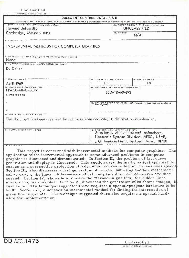
Unclassified Security Classification

DOCUMENT CONTROL DATA -R&D 'Security classification ol title, body of abstract and indexing annotation must be entered when the overall report is classified)

ORIGINA TING ACTIVITY (Corporate author)

Harvard University Cambridge, Massachusetts

2a. REPORT SECURITY CLASSIFICATION

UNCLASSIFIED 2b. GROUP

N/A 3 REPORT TITLE

INCREMENTAL METHODS FOR COMPUTER GRAPHICS

4 DESCRIPTIVE NOTES (Type ot report and inclusive dates)

None 5 AUTHORI5) fFirsf name, middle initial, last name)

D. Cohen

6 REPOR T DATE

April 1969 7a. TOTAL NO. OP PAGES

115 7b. NO. OF REFS

19 Ba. CONTRACT OR GRANT NO.

FI9628-68-C-0379 b. PROJEC T NO.

9a. ORIGINATOR'S REPORT NUMBER(S)

ESD-TR-69-193

9b. OTHER REPORT NO(S) (Any other numbers that may be assigned this report)

10. DISTRIBUTION STATEMENT

This document has been approved for public release and sale; its distribution is unlimited.

II. SUPPLEMENTARY NOTES 12. SPONSORING MILITARY ACTIVITY

Directorate of Planning and Technology, Electronic Systems Division, AFSC, USAF, L G Hanscom Field, Bedford, Mass. 01730

I 3. ABST R AC T

The This report is concerned with incremental methods for computer graphics application of the incremental approach to some advanced problems in computer graphics is discussed and demonstrated. In Section II, the problem of fast curve generation and display is discussed. This section uses the mathematical approach to curves as a perspective projection of polynomial-curves in higher-dimensional spaces Section III, also discusses a fast generation of curves, but using another mathemati cal approach, the linear-differences method, only two-dimensional curves are dis- cussed. Section IV, shows how to make the Warnock algorithm, for hidden lines elimination, incremental. Section V, discusses the generation of half-tone images, ii real-time. The technique suggested there requires a special-purpose hardware to be built. Section VI, discusses an incremental method for finding the intersection of given line-segments. The technique suggested there also requires a special hard- ware for implementation.

DD FORM I NOV S5 1473 Unclassified

Security Classification

uuciassuieg Security Classification

KEY WO RDS LINK A

Computer Graphics Curves Linear-Differences-Curves Half-Tone Images Hidden Lines Elimination Lines Intersecting Conies Shading

Unclassified Security Classification