j. fluid mech. (2016), . 792, pp. doi:10.1017/jfm.2016.110 ... · wake and wave resistance on...

J. Fluid Mech. (2016), vol. 792, pp. 829–849. c© Cambridge University Press 2016doi:10.1017/jfm.2016.110

829

Wake and wave resistance on viscous thin films

René Ledesma-Alonso1,†, Michael Benzaquen1,2, Thomas Salez1

and Elie Raphaël1

1Laboratoire de Physico-Chimie Théorique, UMR CNRS 7083 Gulliver, ESPCI ParisTech,PSL Research University, 10 Rue Vauquelin, 75005 Paris, France

2Capital Fund Management, 23 Rue de l’Université, 75007 Paris, France

(Received 25 July 2015; revised 21 January 2016; accepted 8 February 2016)

The effect of an external pressure disturbance, being displaced with a constant speedalong the free surface of a viscous thin film, is studied theoretically in the lubricationapproximation in one- and two-dimensional geometries. In the comoving frame, theimposed pressure field creates a stationary deformation of the interface – a wake – thatspatially vanishes in the far region. The shape of the wake and the way it vanishesdepend on both the speed and size of the external source and the properties of the film.The wave resistance, namely the force that has to be externally furnished in orderto maintain the wake, is analysed in detail. For finite-size pressure disturbances, itincreases with the speed, up to a certain transition value, above which a monotonicdecrease occurs. The role of the horizontal extent of the pressure field is studied aswell, revealing that for a smaller disturbance the latter transition occurs at a higherspeed. Eventually, for a Dirac pressure source, the wave resistance either saturates fora one-dimensional geometry, or diverges for a two-dimensional geometry.

Key words: lubrication theory, thin films, wakes

1. Introduction

A disturbance moving atop a fluid or a soft medium deforms the interface shapeof the latter, thereby producing a wake. This is a common phenomenon, which takesplace in various natural, scientific and industrial settings (Carusotto & Rousseaux2013) across several orders of magnitude, ranging from waves generated at thesurface of water by animals and watercraft (Kelvin 1887), to patterns observed duringthe deposition of thin polymer coatings (Kistler & Schweizer 1997). For instance, atthe geophysical scale, the study of gravity-driven flows around human-made obstaclesand landscape singularities is essential to understand and minimize the damage causedby natural disasters, such as snow avalanches (Glenne 1987), landslides (Campbell1989) and lava or mud flows (Huppert & Simpson 1980; Huppert 1982; Kondic 2003).In nanophysics, gaining insight into the intrusive effect of local probes, such as atomicforce microscopy (Ledesma-Alonso, Legendre & Tordjeman 2013; Ledesma-Alonso,Tordjeman & Legendre 2014; Wedolowski & Napiorkowskia 2015), is crucial in orderto improve further the measurement accuracy.

† Email address for correspondence: [email protected]

mailto:[email protected]

http://crossmark.crossref.org/dialog/?doi=10.1017/jfm.2016.110&domain=pdf

830 R. Ledesma-Alonso, M. Benzaquen, T. Salez and E. Raphaël

Similarly, the wake angle and the wave pattern generated behind a disturbancesailing at the surface of an inviscid liquid remain current topics of interest (Rabaud &Moisy 2013; Benzaquen, Darmon & Raphael 2014a; Darmon, Benzaquen & Raphael2014), because they are crucial for the naval industry. In fact, to be maintained,the wake continually consumes energy, the latter being radiated away from thedisturbance. This loss can be formulated into a force, called the wave resistance(Havelock 1918), which needs to be furnished by the controller in order to ensureconstant speed. The wave resistance associated with capillary–gravity wakes has thusbeen fully characterized for an incompressible inviscid flow (Raphael & de Gennes1996; Burghelea & Steinberg 2002; Benzaquen, Chevy & Raphael 2011), includingthe cases of Dirac and finite-size pressure distributions. The perturbative role ofviscosity on the inertial wave resistance (Richard & Raphael 1999) has also beenconsidered, as well as the effect of thickness for a viscous liquid film (Wedolowski& Napiorkowskia 2013).

In the context of viscous thin films (Oron, Davis & Bankoff 1997; Craster & Matar2009; Blossey 2012), a moving external disturbance and the associated wake at thefree surface may be used directly as a new kind of fine rheological probe (Decre &Baret 2003; Alleborn & Raszillier 2004). This idea was also proposed as a possiblemethod to measure slip at a solid–liquid boundary (Alleborn, Sharma & Delgado2007). Interestingly, despite the broad applicability of the lubrication theory and itsimportance for industrial processes, the study of the wake and the wave resistance insuch a context is a topic that has been little explored and remains an open question.For instance, the competition between visco-capillary relaxation and perturbationspeed, which might control the extent and lifespan of the wake generated by themoving perturbation, has not been studied. Imagine that the footprint left behindby the moving perturbation is arrested by performing a local quenching, before therelaxation of the thin film occurs (Orchard 1961; McGraw et al. 2012): this mayallow a narrow channel to be imprinted in the film, thus revealing the foundations ofa new nano-patterning technique. Additionally, one may be interested in estimatingand controlling the amount of energy that this technique requires, for which the waveresistance of a moving disturbance atop a viscous thin film must be well characterizedin detail.

In the present study, the surface pattern generated by a moving external pressuredisturbance along a viscous thin film is described theoretically, within the lubricationapproximation, for one-dimensional (1D) and two-dimensional (2D) systems. Thewave resistance is analysed in both cases, leading to analytical expressions of thisforce in terms of the disturbance speed and size, and the physical properties ofthe liquid film. Low- and high-speed regimes are described through asymptoticexpressions, which unveil the nature of the wave resistance in the lubrication context.

2. General case2.1. Thin-film equation for a moving pressure disturbance

We consider a viscous liquid film of thickness h0 deposited over a flat horizontalsubstrate. The equilibrium free surface of the film is flat as well, and perpendicularto the vertical direction z. An external pressure field ψ , moving along the horizontaldirection x with constant speed v> 0, is applied over the liquid film. As a result, theincompressible Newtonian fluid flow yields a stationary surface pattern h (see figure 1)in the frame of reference of the moving disturbance.

In the lubrication approximation, neglecting shear stress at the liquid–gas interfaceand assuming no slip at the substrate, the incompressible Stokes equation and

Wake and wave resistance on viscous thin films 831

x

y

z

(a) (b)

FIGURE 1. (Colour online) Schematic diagram of the surface profile h of a viscousthin film reacting to an external pressure disturbance ψ moving along time t at constantspeed v: (a) 1D and (b) 2D geometries.

conservation of volume lead to the following Reynolds equation (Oron et al. 1997):

∂h∂t=∇ ·

[(h0 + h)3

3µ∇plg

], (2.1)

where µ is the dynamic viscosity of the liquid and plg is the pressure jump at theliquid–gas interface. Under the lubrication hypothesis for the no-slip case, one can alsoneglect the normal viscous stress at the liquid–gas interface, and the pressure jump isthus given by the Young–Laplace equation. For small slopes, the latter reads:

plg =−γ1h+ ρgh+ψ, (2.2)

where 1 denotes the Laplacian operator in Cartesian coordinates, g is the accelerationof gravity, and γ and ρ are the liquid–gas surface tension and density difference,respectively. Equations (2.1) and (2.2) are coupled, and should be solved togetherin order to describe the dynamic response of the viscous thin film due to thedisplacement of the external pressure field.

We introduce the dimensionless variables:

X = κx, Y = y`, H = h

h0,

T = tτ, Ψ = ψ`

sextκ, Sext = sextκ

ρgh0`,

(2.3)

where the capillary length κ−1=√γ /(ρg) has been chosen as the characteristic lengthscale in the x direction, and ` is a reference length scale in the y direction, whichdepends on the dimension of the system: in 1D, one sets `= Ly, a unit length, and in2D, one sets `= κ−1. In turn, τ = 3µγ /[(ρg)2h3

0] is the visco-capillary time scale, andsext =

∫∫dx dyψ is the imposed load, where in 1D the integral over y is restricted to

the horizontal extent Ly. In the limit of small surface deformations H1, the thin-filmequation (TFE), obtained from the combination of (2.1) and (2.2), is given by

∂H∂T=−∇ · [∇(1H)−∇H − Sext∇Ψ ]. (2.4)


Let us introduce the capillary number Ca = µv/γ and the Bond numberBo = ρga2/γ , where a denotes the characteristic horizontal size of the externalpressure field. We now place ourselves in the frame of reference of the movingdisturbance, through the new variable U= X− VT , where the reduced speed V reads:

V = vτκ. (2.5)By assuming stationarity of the surface profile in this comoving frame, one hasH(X, Y, T)= ζ (U, Y) and thus (2.4) reduces to the partial differential equation:[

∂2

∂U2+ ∂2

∂Y2

]2

ζ −[∂2

∂U2+ ∂2

∂Y2

]ζ − V

∂ζ

∂U= Sext

[∂2

∂U2+ ∂2

∂Y2

]Ψ. (2.6)

In the following, we refer to (2.6) as the 2D TFE.Similarly, for a 1D geometry, in which the system is invariant with respect to the

Y direction, (2.4) is reduced to the ordinary differential equation:

ddU

[d3ζ

dU3− dζ

dU− Vζ

]= Sext

d2Ψ

dU2. (2.7)

After integrating once with respect to U, and considering the boundary conditionsζ = 0, dζ/dU = 0, d3ζ/dU3 = 0 and dΨ/dU = 0 at |U| → ∞ (since the liquid–gasinterface should be undisturbed far from the moving disturbance, and since the flowand pressure gradients vanish in the far field), one gets

d3ζ

dU3− dζ

dU− Vζ = Sext

dΨdU

. (2.8)

In the following, we refer to (2.8) as the 1D TFE.

2.2. Wave resistanceThe wave resistance r is the force that has to be externally furnished by the operator– i.e. the pressure field – in order to maintain the wake. According to Havelock’sformula (Havelock 1918), it reads:

r=∫∫

ψ(x, y)∂h∂x

dx dy, (2.9)

where in the 1D case the integral over y is restricted to the chosen horizontal extentLy. Defining the dimensionless wave resistance R through

R= rρgh2

0`, (2.10)

and recalling (2.3), one gets in the comoving frame:

R= Sext

κ`

∫∫Ψ (U, Y)

∂ζ

∂UdU dY. (2.11)

In the next two sections, we solve the 1D TFE and 2D TFE using Fourier analysis,and study the shape of their solutions and the wave resistance for different values ofthe two relevant dimensionless parameters: the reduced speed V and the Bond numberBo. One should keep in mind that

√Bo = aκ is the rescaled lateral extent of the

external pressure field. Also, note that, by linearity of the response, all the resultscorrespond to an arbitrary third dimensionless number Sext, the dimensionless load, asit can be absorbed in ζ . In the following, Sext is chosen to be positive, although thephysical foundations and the wave resistance are valid for any sign of Sext.


3. One-dimensional case3.1. Surface profile

Considering the 1D Fourier transforms ζ (Q) and Ψ (Q) (see § A.1) of the surfaceprofile and the pressure field, the 1D TFE given in (2.8) becomes

−(iQ3 + iQ+ V)ζ = iQSextΨ , (3.1)

where i = √−1 is the imaginary unit, and Q is the angular wavenumber in the Udirection. As a consequence, the profile ζ is described by

ζ (U)= Sext

2π

∫QΨ (Q) exp(iUQ)iV −Q(Q2 + 1)

dQ, (3.2)

where we recover the statement above that the dimensionless load Sext gives only aconstant prefactor in the linear response.

In order to account for the finite-size effects, we introduce a Lorentzian pressuredistribution:

Ψ (U)=√

Boπ(U2 + Bo)

,

Ψ (Q)= exp(−√Bo|Q|).

(3.3)

Note that∫

dUψ = 1, by construction, and that in the limit Bo→ 0 this pressuredistribution becomes Ψ (U) = δ(U), or Ψ (Q) = 1, where δ denotes the Diracdistribution.

The associated normalized surface profile is shown in figure 2, for different valuesof the reduced speed V and the Bond number Bo. At low speed, the deformationprofile is found to be nearly symmetric. In that case, the depression is centred at themaximum of the pressure field and it exponentially relaxes towards a flat horizontalsurface, far away from the perturbation. As we increase the speed V , the symmetry ofthe surface shape breaks and the depression is shifted towards the rear (left-hand sideof figure 2) of the driving pressure field, while a bump at the front (right-hand side offigure 2) grows with the disturbance speed. An exponential relaxation is still observedin the rear, with a shorter characteristic length scale as the speed increases, whilsteither a similar relaxation (for intermediate speeds) or an exponentially decayingoscillation (for high speeds) is discerned at the front.

These features can be understood by looking at the asymptotic solution of the 1DTFE. At a sufficiently distant position (|U|√Bo) from the pressure field, its overalleffect can thus be taken as an interior boundary condition in order to analyse thespatial spectrum of the solution in the far field. In that approximation, (2.8) has thethree asymptotic basis solutions

ζj ∼ exp(

Uλj

), (3.4)

for j= 1, 2, 3, where the wavelengths λj are given by the characteristic equation

λ3j +

1V(λ2

j − 1)= 0, (3.5)


0–10–15–20 –5 5 10 15 20

0.5

0

–0.5

–1.0

1.0

1.5

0.5

0

–0.5

–1.0

1.0

1.5

0.5

0

–0.5

–1.0

1.0

1.5

0.5

0

–0.5

–1.0

1.0

1.5

–1

0

1

2

3

0

–3

U

(a)

(b)

(c)

(d)

FIGURE 2. (Colour online) Normalized surface profile ζ (U), solution of (2.8) as givenby (3.2), using Lorentzian (see (3.3)) and Dirac (Bo→ 0) 1D pressure distributions, withdimensionless load Sext > 0, for different values of the reduced speed V and the Bondnumber Bo, as indicated.

and thus

λj =√

3(Ω

σj+ σj

Ω

)−1

,

σj = exp[

i2π

3( j− 1)

],

Ω = 3√

V +√

V 2 − 1.

(3.6)


–1

0

1

–210010–110–2 103102101

FIGURE 3. (Colour online) Real (solid) and imaginary (dashed) parts of the threedimensionless wavelengths λj of the asymptotic solution, as given by (3.6) for the 1Dcase, as a function of the speed ratio V =V/Vc= 3

√3 V/2, where V is the reduced speed.

Note that for V 6 1, Im(λj)= 0 for all the values of j; whereas for V > 1, Re(λ2) andRe(λ3) overlap.

Here, V is the speed ratio, V = V/Vc, defined from the critical speed Vc = 2/(3√

3).The dependence of λj on V is depicted in figure 3. Since Ω comes from an expressionthat may have different values (the roots of Ω6− 2V Ω3+ 1), we note that the correctvalue to be employed in (3.6) satisfies the relation [Re(Ω)]2= 1−[Im(Ω)]2 for V 6 1,and Im(Ω)= 0 for V > 1.

According to the signs of λj in figure 3, and in order to avoid any divergence ofthe profile at U = −∞, it follows that for U < 0 and |U| √Bo the shape of thesurface is necessarily given by

ζ =N1 exp(

Uλ1

), (3.7)

where N1 is a real constant and λ1 takes a real value Re(λ1) > 0. This indicates thatthe surface always presents a pure exponential relaxation towards a flat horizontalprofile at the rear of the perturbation, in the far field, no matter the speed. The typicaldistance λ1 over which this relaxation occurs becomes shorter as V increases, asobserved in figure 2.

On the other hand, for U > 0 and |U| √Bo, the behaviour of the asymptoticsolution depends strongly on V . When V < 1, according to the signs of λj in figure 3,and in order to avoid any divergence of the profile at U=+∞, the surface profile isdescribed in the far field by the superposition

ζ =N2 exp(

Uλ2

)+N3 exp

(Uλ3

), (3.8)

where N2 and N3 are real constants, and λ2 and λ3 are both real and negative with|λ2|< |λ3|. As a consequence, an overdamping of the surface perturbation is observedin the far field. The V =1 case corresponds to the critical damping situation for which


λ2 = λ3 =−1. Finally, for V > 1, λ2 and λ3 are complex conjugates, and so are thecorresponding amplitudes N2 and N3. Thus, one can write

ζ =N exp[

Re(λ2)URe(λ2)2 + Im(λ2)2

]cos[

Im(λ2)URe(λ2)2 + Im(λ2)2

+ φ], (3.9)

where N and φ are real constants. This indicates the presence of spatial oscillations atthe front of the perturbation in the far field, before the film surface attains its completerelaxation. In brief, the critical speed Vc denotes the reduced speed V at which atransition is observed from overdamped relaxation to damped oscillations, at the frontof the perturbation.

In addition to the far-field trends described above, which depend solely on thereduced speed V and the associated dimensionless characteristic lengths λj, one candiscern in figure 2 different near-field behaviours of the surface profiles that involve asecond dimensionless length

√Bo associated with the horizontal extent of the pressure

field. As already explained above, for a pressure distribution with sufficiently smallsize (

√Bo 1), the healing length of the profile is almost independent of Bo, and

approximately given by λj, which decreases as V increases. In contrast, for a largesize (

√Bo 1), the lateral extent of the profile is comparable with the typical size√

Bo of the pressure disturbance, as can be observed at low speed V in figure 2. Inthis√

Bo 1 case, the healing length decreases with increasing speed only for lowvelocities. Above the critical speed Vc typically, the healing length saturates, leadingto surface profiles that nearly follow the same trend, independently of V .

3.2. Wave resistanceInvoking (2.11) and the fact that in 1D one has ` = Ly, one gets the following 1Dexpression of the dimensionless wave resistance:

R= Sext

∫Ψ (U)

dζdU

dU. (3.10)

For a viscous thin film, it can be shown that the power exerted by the wave resistanceequals the viscous dissipated power in the bulk (see § A.3, (A 16)). This power balancehighlights the fact that the wave resistance is the force externally furnished by theoperator in order to maintain the stationary wake. Remarkably, owing to the nature ofthe TFE, the wave resistance is also related to the spatial energy spectral density (see§ A.2, (A 4)).

Combining (3.2) and (3.10) leads to

R= S2extV2π

∫Q2Ψ (Q)Ψ (−Q)

V2 +Q2(Q2 + 1)2dQ. (3.11)

Figure 4 displays the normalized wave resistance for a Lorentzian pressure distribution,as given by (3.3) and (3.11), as a function of the reduced speed V , and for differentvalues of the Bond number Bo. The wave resistance for a Dirac pressure distributionis also shown.

For the asymptotic case where V→ 0, a series expansion of the integrand in (3.11)leads to

R= S2extVπ[ f (Bo)+O(V2)], (3.12)


–6

–3

0

–9

–120 3 6–3–6

1

1 11

Dirac

2

4

0

–2

–4

FIGURE 4. (Colour online) Dimensionless wave resistance R (see (3.11)) normalized bythe square of the dimensionless load Sext, as a function of the reduced speed V , for a 1DDirac pressure distribution, and for a 1D Lorentzian pressure distribution (see (3.3)) withdifferent values of the Bond number Bo as indicated. The vertical dashed lines indicatethe crossover speeds Vs, estimated from (3.19) for different Bo. The horizontal dotted linecorresponds to the plateau value of 1/6 in the 1D Dirac case.

where f (Bo) is a function that depends only on the shape of the pressure field. Thispoints out the linear dependence of the wave resistance on V , in the low-speed regime,as observed in figure 4. For a Dirac pressure distribution one gets fδ(Bo) = π/4,whereas for a Lorentzian (see (3.3)), one has

fL(Bo)= 8Bo3/2∫ ∞

0

exp(−w)(w2 + 4Bo)2

dw. (3.13)

Both behaviours are depicted in figure 5. In addition, fL→π/4 when Bo→ 0, as forthe Dirac pressure distribution, whilst a series expansion at Bo→∞ yields

fL(Bo)= 12√

Bo[1+O(Bo−1)], (3.14)

as observed in figure 5.Considering the Dirac delta distribution, for any V , one finds (see § A.2 for details)

Rδ = −i√

3θ 3/2S2extV

2(θ 3 − 2θ 2 + 2θ − 1), (3.15)

with

θ = 3√

1− 2V 2 + 2V√

V 2 − 1, (3.16)

where V was defined after (3.6). For the asymptotic case where V →∞, a seriesexpansion leads to

Rδ = S2ext

6[1+O(V−2/3)]. (3.17)


–2

–1

0

0 3 6–3–6

1

2

DiracLorentz

FIGURE 5. (Colour online) Shape function f (see (3.12)) of the 1D pressure field inthe low-speed regime, as a function of the Bond number Bo. Both the Lorentzian (solid,see (3.13)) and the Dirac (dashed, see text) cases are represented.

This result indicates the singular feature that for a 1D Dirac pressure distribution thewave resistance saturates to a constant value at high speed, as observed in figure 4.

For a finite-size Lorentzian pressure distribution, we combine (3.3) and (3.11)(see § A.2 for details on the overall expression) and obtain, in the high-speed regimeV→∞,

RL = S2ext

4πVBo3/2[1+O(V−2)]. (3.18)

Therefore, a 1/V dependence of the wave resistance is asymptotically expected forfinite-size pressure fields at large speed, as indeed observed in figure 4.

For a Dirac pressure distribution, the reduced speed Vs at which the wave resistancesaturates can be defined by equating the low- and high-speed asymptotic expressionsof Rδ. This provides Vs = 2/3, consistent with the observation of figure 4. Similarly,for a finite-size Lorentzian pressure distribution, the reduced speed Vs at which thecrossover between the low- and high-speed regimes of RL occurs is defined by

Vs ∼ 12Bo3/4

√f (Bo)

, (3.19)

as observed in figure 4. In the case of small Bond number Bo, Vs scales as Bo−3/4;whereas for large values of Bo, Vs scales as Bo−1/2.

4. Two-dimensional case4.1. Surface profile

Considering the 2D Fourier transforms ζ (Q,K) and Ψ (Q,K) of the surface profile andthe pressure field, with the definitions given in § B.1, the 2D TFE of (2.6) becomes

[iQV − (Q2 +K2)2 − (Q2 +K2)]ζ = Sext(Q2 +K2)Ψ , (4.1)


(a)

(b)

FIGURE 6. (Colour online) Normalized thin-film surface profile in the presence of amoving Lorentzian pressure disturbance, with dimensionless load Sext > 0, Bond numberBo= 102, and reduced speed V = 10, computed from (4.2) and (4.3). Perspective views ofthe front (a) and the back (b), in arbitrary units and colour code.

where Q and K are the spatial angular frequencies in the U and Y directions,respectively. Consequently, the surface ζ (U, Y) of the thin film reads

ζ (U, Y)= Sext

4π2

∫∫(Q2 +K2) exp[i(QU +KY)]Ψ (Q,K)

iQV − (Q2 +K2)(1+Q2 +K2)dK dQ. (4.2)

In analogy with the previous 1D case, we introduce the following 2D axisymmetricfinite-size Lorentzian pressure distribution:

Ψ (U, Y)=√

Bo2π(U2 + Y2 + Bo)3/2

,

Ψ (Q,K)= exp[−√

Bo(Q2 +K2)].

(4.3)

We recall that, since a is the characteristic horizontal size of the pressure field,√Bo = aκ is the dimensionless size. When, Bo→ 0, the Dirac pressure distribution

Ψ (U, Y) = δ(U)δ(Y), or its equivalent Ψ (Q, K) = 1 in the frequency domain, isrecovered.

Surface patterns generated by a Lorentzian pressure disturbance, for severalcombinations of the parameters Bo and V , are illustrated in figures 6 and 7. Acommon feature of these profiles is the depression observed. In figure 6, owing tothe particular parameters employed (see caption) to generate the surface profile, a


–10–20 0 –10–20 0 –10–20 0

0

10

–10

0

10

–10

0

10

–10

0

10

–10

0

10

–10

–1

0

1

2

–2

1–1 0

0

–0.2

–0.4

0.2

–0.6

–0.8

–1.0

Y

Y

Y

Y

Y

U UU

FIGURE 7. (Colour online) Normalized thin-film surface profile (top view) computed from(4.2) and (4.3), for a dimensionless load Sext > 0, and different values of the Bond numberBo and the reduced speed V . In each panel, the pressure field travels from left to right,along the longitudinal coordinate U.

non-symmetric shape is shown. A rim surrounds the front of the depression andbecomes a wake, behind, that follows the straight translation path of the pressuredistribution along U.

In figure 7, for low speeds (V < 1), we find deformation profiles that are mostlysymmetric, with a main depression aligned with the maximum of the pressure fieldand followed by a monotonic relaxation towards a flat horizontal surface. In this


situation, the liquid-film surface relaxation occurs faster than the displacement of thepressure field: in real units, the displacement speed v is smaller than the characteristicspeed ρgh3

0κ/3µ at which the film relaxes and thus propagates information at itssurface. As the pressure acts on the surface by creating a moving depression, thefilm has enough time to move the dislodged liquid volume isotropically.

Like for the 1D case, an increase of the speed V induces a symmetry-breakingphenomenon, which above V' 1 consists of a level rising at the front (right-hand sideof the corresponding panels of figure 7) and a wake at the rear (left-hand side). In realunits, the relaxation of the liquid film now occurs with a speed ρgh3

0κ/3µ, which issmaller than the displacement speed v of the pressure field. In other words, the liquidvolume that is ejected by the applied pressure is not distributed isotropically becausethe information at the film surface does not propagate fast enough. This retardationeffect is similar to the Mach and Cerenkov physics (Carusotto & Rousseaux 2013),where the speed of the object becomes larger than the wave propagation speed in theconsidered medium.

For relatively moderate speeds, V ' 1, the protuberance at the front covers acrescent-shaped region that grows with the size of the pressure field

√Bo. The

maximum surface level at the front of the pressure field is located at Y = 0, whereasthe maximum of the wake, at each position U < 0, is located at Y ∼ |U|1/2. Incontrast, the local minimum of the wake is always placed at Y = 0. In addition, boththe local maximum and minimum of the wake present a rapid spatial exponentialrelaxation. As the speed grows in the range V ∈ [1, 102], the height of the frontal rimreduces, while the extent of the wake in the rear reaches a larger distance. The localmaximum at the front is still located at Y = 0, while the maximum height of thewake is now placed at Y ∼ |U|α, where the exponent α evolves from 1/2 at V ∼ 1 to1/4 at V ∼ 102. In fact, the 1/4 exponent in the high-speed regime indicates the samedynamics as the capillary levelling of a trench in a viscous thin film with no slipat the substrate (Baumchen et al. 2013; Benzaquen et al. 2014b). In this regime, thefilm seems to overlook the presence of the fast disturbance, perceiving the footprintleft by the latter as a 1D trench which the film tends to refill by capillary levelling.Therefore, when we compare the transverse profiles at different positions U < 0, wein fact discern different stages of the 1D levelling of a viscous film.

4.2. Wave resistance

Invoking (2.11) and the fact that in 2D one has `= κ−1, one gets the following 2Dexpression of the dimensionless wave resistance:

R= Sext

∫∫Ψ (U, Y)

∂ζ

∂UdU dY. (4.4)

Therefore, in combination with (4.2), one obtains

R= S2extV

4π2

∫∫Q2(Q2 +K2)Ψ (Q,K)Ψ (−Q,−K)Q2V2 + (Q2 +K2)2(1+Q2 +K2)2

dK dQ. (4.5)

Considering the polar coordinates (%, ϕ), an axisymmetric pressure field Ψ (%), asis the case for the Dirac and Lorentzian distributions presented in this study, andperforming an integration over ϕ (see § B.2) yields

R= S2ext

2πV

∫ ∞0

[1− %(%2 + 1)√

V2 + %2(%2 + 1)2

][Ψ (%)]2%3 d%. (4.6)


–6

–3

0

–9

–120 3 6–3–6

Dirac

2

4

0

–2

–4

1

1 11

1

3

FIGURE 8. (Colour online) Dimensionless wave resistance R normalized by the square ofthe dimensionless load Sext, as a function of reduced speed V , for a 2D Dirac pressuredistribution (see (B 7)), and for a 2D Lorentzian pressure distribution (see (4.3) and (4.6))with different values of the Bond number Bo as indicated. The vertical dashed linesindicate the crossover speeds Vs, estimated from (4.12) for different Bo.

For a Lorentzian distribution, a combination of (4.3) and (4.6) leads to thecorresponding wave resistance, the behaviour of which in terms of the reducedspeed V is shown in figure 8, for different values of Bo. The wave resistance for aDirac distribution is also represented.

In the asymptotic case where V→ 0, a series expansion of the integrand in (4.6)(see § B.2 for details) leads to

R= S2extV8π[F(Bo)+O(V2)], (4.7)

where F(Bo) is a function that depends only on the shape of the pressure field,pointing out the linear dependence of the wave resistance on V , in the lowreduced-speed regime. For a Dirac pressure field Fδ(Bo)= 1, whereas for a Lorentzianit is described by

FL(Bo)= 8Bo∫ ∞

0

exp(−w)w(w2 + 4Bo)2

dw. (4.8)

Both trends are illustrated in figure 9. For the Lorentzian FL(Bo) = 1 at Bo 1,the same behavior as for the Dirac pressure distribution, while a series expansion atBo→∞ gives

FL(Bo)= 12Bo[1+O(Bo−1)]. (4.9)

Coming back to the Dirac pressure distribution, a series expansion of (4.6) atV→∞ yields

Rδ =Γ ( 1

3)Γ (76)

8π3/2S2

extV1/3[1+O(V−1)], (4.10)

which indicates that the wave resistance of a 2D Dirac pressure diverges slowly withincreasing V .


LorentzDirac

0 3 6–3–6

–5

–4

–3

–2

–1

0

1

1

FIGURE 9. (Colour online) Shape function F (see (4.7)) of the 2D pressure field in thelow-speed regime, as a function of the Bond number Bo. Both the Lorentzian (solid,see (4.8)) and the Dirac (dashed, see text) cases are represented.

For a Lorentzian pressure distribution, a series expansion in the high-speed regimewhere V→∞ allows us to reduce the combination of (4.3) and (4.6) to

RL = 3S2ext

16πVBo2[1+O(V−2)]. (4.11)

This demonstrates that, for finite-size pressure fields in the high-speed regime whereV → ∞, the wave resistance behaves in the same way as in the 1D case, i.e.decreasing as 1/V .

For a Dirac distribution, the speed dependence of the wave resistance changes fromR∼ V to R∼ V1/3 at the reduced speed Vs = 5/3, which is obtained by equating thelow- and high-speed asymptotic expressions of Rδ. Similarly, for a finite-size pressuredistribution, the reduced speed Vs, at which the crossover between the two asymptoticregimes takes place, reads

Vs ∼√

32Bo2F(Bo)

, (4.12)

emerging when we match the low- and high-speed regimes of RL. At small Bondnumber Bo, the crossover speed is approximately given by Vs ∼ (Bo

√2/3)−1, whilst

for large values of Bo, it happens around Vs ∼ (Bo/3)−1/2.

5. ConclusionIn the present work, the effects of a pressure disturbance moving near the free

surface of a viscous thin film have been studied in detail. Depending on thedisturbance–speed regime, the existence of nearly symmetric and non-symmetricprofile shapes has been revealed by means of numerical methods. The nature of thewakes and bumps observed at the surface, as well as the lifespan of the trail andits relaxation towards a flat surface in the far field, have been explained throughasymptotic solutions, unveiling their reliance on several dimensionless parameters,namely the Bond number Bo, the dimensionless load Sext and the dimensionless


speed of the disturbance V , all of which are related to the geometrical and physicalproperties of the liquid film, and the density ρ, the air–liquid surface tension γ , thedynamic viscosity µ, the film thickness h0 and the pressure distribution through itstotal load sext and width a.

In addition, the wave resistance, which one must overcome in order to displacethe disturbance at constant speed, has been analysed. Even though the shape ofthe free surface is calculated numerically, the wave resistance can be derived indifferent asymptotic speed regimes, by means of analytical expressions for Diracdelta and Lorentzian pressure distributions. Moreover, a general expression of thewave resistance for a Dirac delta distribution in the 1D case has been presented.

We believe that the measurement of the wave resistance can be employed to deduceone of the physical properties of a viscous thin film, such as the above ρ, γ , µ orh0, when the remaining parameters are known. The working principle of a new finerheological probe may be based on this acquired insight. Additionally, in combinationwith local quenching, controlling the lifespan of the footprint generated by the movingperturbation might serve as the technological foundation of a new nano-patterningtechnique, which may allow for imprinting nano-channels over polymeric materials.This idea may provide an alternative to the current nano-lithography techniquesemployed to fabricate nano-devices and templates for electronics.

AcknowledgementsWe wish to thank D. Legendre, P. Tordjeman and A. Darmon for fruitful and very

interesting discussions.

Appendix A. Details of the one-dimensional caseA.1. Fourier transform

The Fourier transform in the 1D case is given by

f (Q)=∫ ∞−∞

f (U) exp(−iUQ) dU,

f (U)= 12π

∫ ∞−∞

f (Q) exp(iUQ) dQ.

(A 1)

A.2. Wave resistanceMultiplying (2.8) by the surface displacement, and integrating over the whole Udomain gives ∫ (

d3ζ

dU3− dζ

dU− Vζ

)ζ dU = Sext

∫ (dΨdU

)ζ dU. (A 2)

Some of the terms (the first two on the left-hand side and the one on the right-handside) of this equation can be simplified to∫

ζd3ζ

dU3dU =

[ζ

d2ζ

dU2− 1

2

(dζdU

)2]∞−∞= 0,∫

ζdζdU

dU =[

12(ζ )2

]∞−∞= 0,∫

ζdΨdU

dU = [ζΨ ]∞−∞ −∫Ψ

dζdU

dU =−∫Ψ

dζdU

dU,

(A 3)


0

2

4

–4

–2

10010–110–2 103102101

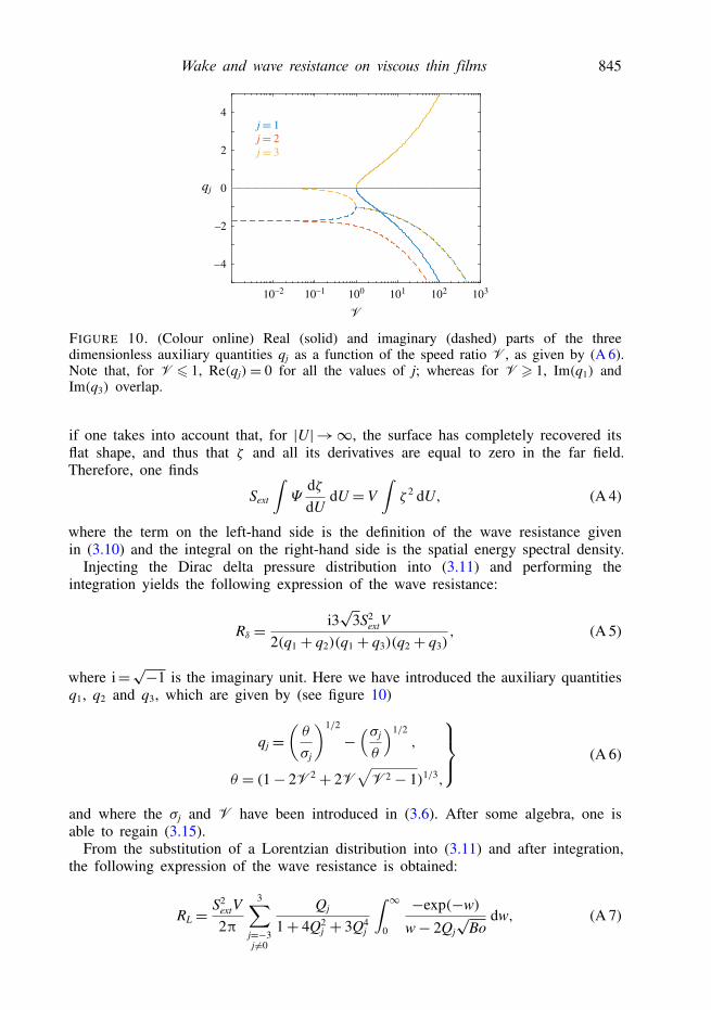
FIGURE 10. (Colour online) Real (solid) and imaginary (dashed) parts of the threedimensionless auxiliary quantities qj as a function of the speed ratio V , as given by (A 6).Note that, for V 6 1, Re(qj)= 0 for all the values of j; whereas for V > 1, Im(q1) andIm(q3) overlap.

if one takes into account that, for |U|→∞, the surface has completely recovered itsflat shape, and thus that ζ and all its derivatives are equal to zero in the far field.Therefore, one finds

Sext

∫Ψ

dζdU

dU = V∫ζ 2 dU, (A 4)

where the term on the left-hand side is the definition of the wave resistance givenin (3.10) and the integral on the right-hand side is the spatial energy spectral density.

Injecting the Dirac delta pressure distribution into (3.11) and performing theintegration yields the following expression of the wave resistance:

Rδ = i3√

3S2extV

2(q1 + q2)(q1 + q3)(q2 + q3), (A 5)

where i=√−1 is the imaginary unit. Here we have introduced the auxiliary quantitiesq1, q2 and q3, which are given by (see figure 10)

qj =(θ

σj

)1/2

−(σj

θ

)1/2,

θ = (1− 2V 2 + 2V√

V 2 − 1)1/3,

(A 6)

and where the σj and V have been introduced in (3.6). After some algebra, one isable to regain (3.15).

From the substitution of a Lorentzian distribution into (3.11) and after integration,the following expression of the wave resistance is obtained:

RL = S2extV2π

3∑j=−3j6=0

Qj

1+ 4Q2j + 3Q4

j

∫ ∞0

−exp(−w)

w− 2Qj√

Bodw, (A 7)


where Qj is the jth root of V2 +Q2(Q2 + 1)2, given by

Qj = 1√3

(θ

σj+ σj

θ− 2)1/2

, (A 8)

for j= 1, 2, 3, whereas for j= 4, 5, 6 we have Qj =−Qj−3. The σj and θ have beenintroduced in (3.6) and (A 6), respectively. The asymptotic behaviours for V→∞ canalso be obtained from (A 7), after making θ→ 1 and some algebra.

A.3. Viscous dissipationThe viscously dissipated power indicates the rate at which the external work isirreversibly converted into internal energy by viscous forces. For a thin film, theviscously dissipated power per unit length is expressed as

Φµ =µ∫ [∫ h

−h0

(∂υx

∂z

)2

dz

]dx, (A 9)

where υx is the horizontal component of the velocity within the film. Under theassumptions of the lubrication theory, the previous expression can be rewritten as

Φµ = 1µ

∫ ∫ h

−h0

[(z− h)

∂1p∂x

]2

dz

dx. (A 10)

Integration over the local film thickness and, afterwards, integration by parts yields

Φµ = 13µ

∫(h0 + h)3

(∂1p∂x

)2

dx

=∫1p

∂

∂x

[(h0 + h)3

3µ

(∂1p∂x

)]dx, (A 11)

since h and 1p and their derivatives with respect to x are equal to zero at |x|→∞.Making use of the 2D analogue of (2.1), allows us to find

Φµ =∫1p(∂h∂t

)dx. (A 12)

Now, invoking the dimensionless variables and placing ourselves in the movingreference frame, one has

Φµ =−vρgh20

∫1P

(∂ζ

∂U

)dU. (A 13)

Then, using the dimensionless equivalent of (2.2), one finds

Φµ =−vρgh20

∫ (− ∂

2ζ

∂U2+ ζ − SextΨ

)∂ζ

∂UdU. (A 14)


Once more, considering that ζ and its first derivative with respect to U are equalto zero at |U| →∞, the first two terms on the right-hand side of this equation arereduced to ∫

dζdU

d2ζ

dU2dU =

[12

(dζdU

)2]∞−∞= 0,∫

ζdζdU

dU =[

12(ζ )2

]∞−∞= 0.

(A 15)

Finally, using the definition given in (3.10), the viscously dissipated power can bewritten in terms of the wave resistance:

Φµ = ρgh20

τκVR= vr. (A 16)

As already mentioned, the product vr is the power required to displace the surfaceprofile at constant speed, and it also corresponds to the power dissipated within theviscous thin film during such a task.

Appendix B. Details of the two-dimensional caseB.1. Fourier transform

The Fourier transform in the 2D case is given by

f (Q,K)=∫ ∞−∞

∫ ∞−∞

f (U, Y) exp(−i[QU +KY]) dY dU,

f (U, Y)= 14π2

∫ ∞−∞

∫ ∞−∞

f (Q,K) exp(i[QU +KY]) dK dQ.

(B 1)

B.2. Wave resistanceStarting from (4.5), one considers the polar coordinates (%, ϕ), given by the relationsQ= % cos(ϕ) and K= % sin(ϕ), and multiplies both the numerator and denominator byi/V , in order to retrieve the following expression:

R= S2ext

4π2V

∫ ∞0

∫ 2π

0

%3 cos(ϕ)Ψ (%, ϕ)Ψ (%, ϕ +π)

cos(ϕ)+ i%

V(%2 + 1)

dϕ d%. (B 2)

Additionally, if the Fourier transform of the pressure field Ψ under consideration isaxisymmetric, a first integration of the previous equation over ϕ leads directly to (4.6).In brief, for an axisymmetric pressure field, one should use the following formula:∫ 2π

0

cos(ϕ) dϕcos(ϕ)+D

= 2∫ π

0


= 2

2D√1−D2

tanh−1

(D− 1) tan(ϕ

2

)√

1−D2

+ ϕ∣∣∣∣∣∣∣π

0

, (B 3)


which, considering that

limx→∞[tanh−1(x)] = iπ

2, (B 4)

can be rewritten as ∫ 2π

0


= 2π

(1+ iD√

1−D2

), (B 5)

in order to perform the aforementioned integration step. Moreover, a series expansionof the integrand in (4.6) near V = 0 leads to

R0 = S2extV2π

∫ ∞0[Ψ (%)]2 % d%

2(%2 + 1)2+O(V2)

, (B 6)

which can be rewritten in the form of (4.7).For a Dirac pressure distribution, (4.6) becomes

Rδ = S2ext

2πV

∫ ∞0

[1− %(%2 + 1)√

V2 + %2(%2 + 1)2

]%3 d%. (B 7)

A series expansion near V = 0 of the integrand yields

Rδ = S2extV2π

[∫ ∞0

% d%2(%2 + 1)2

+O(V2)

], (B 8)

which after integration is equal to

Rδ = S2extV8π[1+O(V2)]. (B 9)

Now, using the change of variables w= %(%2+ 1)/V , and a series expansion of theintegrand at V→∞, the integral in (B 7) can be approximated by∫ ∞

0

[1− %(%2 + 1)√

V2 + %2(%2 + 1)2

]%3 = V4/3

3

∫ ∞0

w1/3

(1− w√

1+w2

)+O(V1/3)

= Γ(

13

)Γ(

76

)4√

πV4/3 +O(V1/3), (B 10)

which allows us to obtain (4.10).

REFERENCES

ALLEBORN, N. & RASZILLIER, H. 2004 Local perturbation of thin film flow. Arch. Appl. Mech. 73,734–751.

ALLEBORN, N., SHARMA, A. & DELGADO, A. 2007 Probing of thin slipping films by persistentexternal disturbances. Can. J. Chem. Engng 85, 586–597.


BAUMCHEN, O., BENZAQUEN, M., SALEZ, T., MCGRAW, J. D., BACKHOLM, M., FOWLER, P.,RAPHAEL, E. & DALNOKI-VERESS, K. 2013 Relaxation and intermediate asymptotics of arectangular trench in a viscous film. Phys. Rev. E 88, 035001, 1–5.

BENZAQUEN, M., CHEVY, F. & RAPHAEL, E. 2011 Wave resistance for capillary gravity waves:finite-size effects. Europhys. Lett. 96, 34003, 1–5.

BENZAQUEN, M., DARMON, A. & RAPHAEL, E. 2014a Wake pattern and wave resistance foranisotropic moving disturbances. Phys. Fluids. 26, 092106, 1–7.

BENZAQUEN, M., FOWLER, P., JUBIN, L., SALEZ, T., DALNOKI-VERESS, K. & RAPHAEL, E. 2014bApproach to universal self-similar attractor for the leveling of thin liquid films. Soft Matt. 10,8608–8614.

BLOSSEY, R. 2012 Thin Liquid Films. Springer.BURGHELEA, T. & STEINBERG, V. 2002 Wave drag due to generation of capillary-gravity surface

waves. Phys. Rev. E 66, 051204, 1–13.CAMPBELL, C. S. 1989 Self-lubrication for long runout landslides. J. Geol. 97 (6), 653–665.CARUSOTTO, I. & ROUSSEAUX, G. 2013 The Cerenkov effect revisited: from swimming ducks to

zero modes in gravitational analogues. In Analogue Gravity Phenomenology, Lecture Notes inPhysics, vol. 870, pp. 109–144. Springer.

CRASTER, R. V. & MATAR, O. K. 2009 Dynamics and stability of thin liquid films. Rev. Mod.Phys. 81, 1131–1198.

DARMON, A., BENZAQUEN, M. & RAPHAEL, E. 2014 Kelvin wake pattern at large Froude numbers.J. Fluid Mech. 738 (R3), 1–8.

DECRE, M. M. J. & BARET, J.-C. 2003 Gravity-driven flows of viscous liquids over two-dimensionaltopographies. J. Fluid Mech. 487, 147–166.

GLENNE, B. 1987 Sliding friction and boundary lubrication of snow. J. Tribol. 109 (4), 614–617.HAVELOCK, T. H. 1918 Wave resistance: some cases of three-dimensional fluid motion. Proc. R.

Soc. Lond. A 95, 354–365.HUPPERT, H. E. 1982 The propagation of two-dimensional and axisymmetric viscous gravity currents

over a rigid horizontal surface. J. Fluid Mech. 121, 43–58.HUPPERT, H. E. & SIMPSON, J. E. 1980 The slumping of gravity currents. J. Fluid Mech. 99 (4),

785–799.KELVIN, LORD 1887 On ship waves. Proc. Inst. Mech. Engrs 38, 409–434.KISTLER, S. F. & SCHWEIZER, P. M. 1997 Liquid Film Coating. Scientific Principles and Their

Technological Implications. Chapman & Hall.KONDIC, L. 2003 Instabilities in gravity driven flow of thin fluid films. SIAM Rev. 45 (1), 95–115.LEDESMA-ALONSO, R., LEGENDRE, D. & TORDJEMAN, P. 2013 AFM tip effect on a thin liquid

film. Langmuir 29, 7749–7757.LEDESMA-ALONSO, R., TORDJEMAN, PH. & LEGENDRE, D. 2014 Dynamics of a thin liquid film

interacting with an oscillating nano-probe. Soft Matt. 10 (39), 7736–7752.MCGRAW, J. D., SALEZ, T., BAUMCHEN, O., RAPHAEL, E. & DALNOKI-VERESS, K. 2012 Self-

similarity and energy dissipation in stepped polymer films. Phys. Rev. Lett. 109, 128303,1–5.

ORCHARD, S. E. 1961 On surface leveling in viscous liquids and gels. Appl. Sci. Res. 11 (4),451–464.

ORON, A., DAVIS, S. H. & BANKOFF, S. G. 1997 Long-scale evolution of thin films. Rev. Mod.Phys. 69 (3), 931–980.

RABAUD, M. & MOISY, F. 2013 Ship wakes: Kelvin or Mach angle? Phys. Rev. Lett. 110, 214503,1–5.

RAPHAEL, E. & DE GENNES, P.-G. 1996 Capillary gravity waves caused by a moving disturbance:wave resistance. Phys. Rev. E 53, 3448–3455.

RICHARD, D. & RAPHAEL, E. 1999 Capillary-gravity waves: the effect of viscosity on the waveresistance. Europhys. Lett. 48 (1), 49–52.

WEDOLOWSKI, K. & NAPIORKOWSKIA, M. 2013 Capillary-gravity waves on a liquid film of arbitrarydepth: analysis of the wave resistance. Phys. Rev. E 88, 043014, 1–13.

WEDOLOWSKI, K. & NAPIORKOWSKIA, M. 2015 Dynamics of a liquid film of arbitrary thicknessperturbed by a nano-object. Soft Matt. 11, 2639–2654.

j. fluid mech. (2016), . 792, pp. doi:10.1017/jfm.2016.110 ... · wake and wave resistance on...

Documents