J. Fluid Mech. (2018), vol. 847, pp. 161–185. c© Cambridge University Press 2018doi:10.1017/jfm.2018.320

161

Large coherence of spanwise velocity inturbulent boundary layers

Charitha M. de Silva1,†, Kevin1, Rio Baidya1, Nicholas Hutchins1

and Ivan Marusic1

1Department of Mechanical Engineering, The University of Melbourne, Victoria 3010, Australia

(Received 13 September 2017; revised 26 February 2018; accepted 10 April 2018)

The spatial signature of spanwise velocity coherence in turbulent boundary layers hasbeen studied using a series of unique large-field-of-view multicamera particle imagevelocimetry experiments, which were configured to capture streamwise/spanwise slicesof the boundary layer in both the logarithmic and the wake regions. The frictionReynolds number of Reτ ≈ 2600 was chosen to nominally match the simulation ofSillero et al. (Phys. Fluids, vol. 26 (10), 2014, 105109), who had previously reportedoblique features of the spanwise coherence at the top edge of the boundary layerbased on the sign of the spanwise velocity, and here we find consistent observationsfrom experiments. In this work, we show that these oblique features in the spanwisecoherence relate to the intermittent turbulent bulges at the edge of the layer, and thusthe geometry of the turbulent/non-turbulent interface, with the clear appearance oftwo counter-oriented oblique features. Further, these features are shown to be alsopresent in the logarithmic region once the velocity fields are deconstructed basedon the sign of both the spanwise and the streamwise velocity, suggesting that theoften-reported meandering of the streamwise-velocity coherence in the logarithmicregion is associated with a more obvious diagonal pattern in the spanwise velocitycoherence. Moreover, even though a purely visual inspection of the obliqueness inthe spanwise coherence may suggest that it extends over a very large spatial extent(beyond many boundary layer thicknesses), through a conditional analysis, we showthat this coherence is limited to distances nominally less than two boundary layerthicknesses. Interpretation of these findings is aided by employing synthetic velocityfields of a boundary layer constructed using the attached eddy model, where the rangeof eddy sizes can be prescribed. Comparisons between the model, which employs anarray of self-similar packet-like eddies that are randomly distributed over the plane ofthe wall, and the experimental velocity fields reveal a good degree of agreement, withboth exhibiting oblique features in the spanwise coherence over comparable spatialextents. These findings suggest that the oblique features in the spanwise coherence arelikely to be associated with similar structures to those used in the model, providingone possible underpinning structural composition that leads to this behaviour. Further,these features appear to be limited in spatial extent to only the order of the large-scalemotions in the flow.

Key words: boundary layer structure, turbulent boundary layers, turbulent flows

† Email address for correspondence: desilvac@unimelb.edu.au

Dow

nloa

ded

from

htt

ps://

ww

w.c

ambr

idge

.org

/cor

e. IP

add

ress

: 128

.250

.0.9

9, o

n 28

May

201

8 at

03:

13:4

7, s

ubje

ct to

the

Cam

brid

ge C

ore

term

s of

use

, ava

ilabl

e at

htt

ps://

ww

w.c

ambr

idge

.org

/cor

e/te

rms.

htt

ps://

doi.o

rg/1

0.10

17/jf

m.2

018.

320

162 C. M. de Silva, Kevin, R. Baidya, N. Hutchins and I. Marusic

1. IntroductionIt is established that wall turbulence contains a significant element of coherence.

This structural nature of turbulent boundary layers has been the subject of manyinvestigations, and a great deal of effort and progress has been made in understandingthe processes that are responsible for the ordered turbulent fluctuations observed inwall-bounded turbulence. Robinson (1991) provides a comprehensive review ofearly findings focusing on the coherence in the near-wall and buffer region of theflow, while more recent findings are discussed in Marusic & Adrian (2012) andHerpin et al. (2013). Considerable effort has also been devoted to understanding theirself-sustaining mechanisms, with different viewpoints thoroughly discussed by Panton(2001).

Over the last decade, the presence of large-scale motions of the order of theboundary layer thickness has received considerable interest. These motions havebeen shown to be increasingly energetic at higher Reynolds numbers (Hutchins &Marusic 2007), to exist in both internal and external wall-bounded flows (Montyet al. 2009), to influence interfacial bulging (Falco 1977; Adrian, Meinhart &Tomkins 2000) and to carry substantial proportions of Reynolds shear stress andturbulence production (Ganapathisubramani, Longmire & Marusic 2003; Balakumar& Adrian 2007). Further, their effect on the smaller-scale fluctuations in the near-wallregion has recently been documented (see, for example, Mathis, Hutchins & Marusic(2009)). Longitudinally, these large-scale structures are known to incline forward at acharacteristic angle (Adrian et al. 2000; Marusic & Heuer 2007), while laterally theirwidth appears to increase with wall distance (Tomkins & Adrian 2003; Hutchins,Hambleton & Marusic 2005; Lee & Sung 2011), and they appear to exhibit somedegree of streamwise–spanwise organisation (Elsinga et al. 2010). More recently,the dynamics of these large-scale motions has also been examined through directnumerical simulations, which have access to increasingly higher Reynolds numbers(Flores & Jiménez 2010; Hwang & Cossu 2010; Lee et al. 2014; Lozano-Durán &Jiménez 2014).

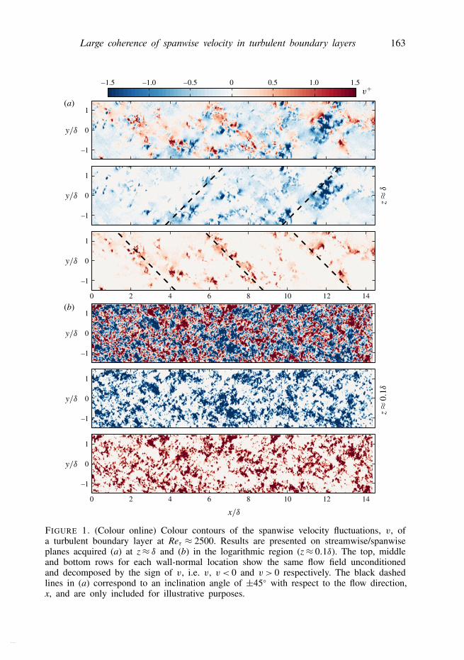
In this study, we focus on the large-scale spatial coherence of the spanwise velocity,which to date is largely unexplored. One distinct feature reported for this velocitycomponent is the large diagonal pattern observed on a plane parallel to the wall atthe edge of the boundary layer (Sillero, Jiménez & Moser 2014). This feature is bestdescribed with reference to figure 1(a), which shows a representative snapshot of thespanwise velocity fluctuations, v, from the present particle image velocimetry (PIV)experiment at a wall-normal height of z ≈ δ. Here, the boundary layer thickness,δ, corresponds to the wall distance where the mean streamwise velocity is 99 % ofthe free-stream velocity. From this velocity field, it is clear that coherent regions ofpositive and negative v appear to be counter-oriented at oblique angles and seemto have spatial extents in excess of δ. To date, most experimental datasets withdirect spatial information have had insufficient spatial domains to clearly visualisethis large-scale coherence. Moreover, experiments with large streamwise/spanwisedomains generally focus on the logarithmic region of boundary layers (Tomkins &Adrian 2003, and others), where the longest coherent regions of streamwise velocityappear to reside (Hutchins & Marusic 2007). The PIV experiments with very largespatial extents targeted at the logarithmic and wake regions of a boundary layerpresented herein offer a promising approach to carefully examine these large-scalemotions. It is worth noting that the persistent patterns observed in the v coherence atthe edge of the boundary layer are largely unaffected by the reference velocity (herebased on a Reynolds decomposition (Reynolds 1894)) as the mean spanwise velocity

Dow

nloa

ded

from

htt

ps://

ww

w.c

ambr

idge

.org

/cor

e. IP

add

ress

: 128

.250

.0.9

9, o

n 28

May

201

8 at

03:

13:4

7, s

ubje

ct to

the

Cam

brid

ge C

ore

term

s of

use

, ava

ilabl

e at

htt

ps://

ww

w.c

ambr

idge

.org

/cor

e/te

rms.

htt

ps://

doi.o

rg/1

0.10

17/jf

m.2

018.

320

Large coherence of spanwise velocity in turbulent boundary layers 163

–1

0

1

–1

0

1

0 2 4 6 8 10 12 14

–1

0

1

–1

0

1

–1

0

1

0 2 4 6 8 10 12 14

(b)

0 0.5–1.5 –1.0 –0.5 1.0 1.5

–1

0

1(a)

FIGURE 1. (Colour online) Colour contours of the spanwise velocity fluctuations, v, ofa turbulent boundary layer at Reτ ≈ 2500. Results are presented on streamwise/spanwiseplanes acquired (a) at z≈ δ and (b) in the logarithmic region (z≈ 0.1δ). The top, middleand bottom rows for each wall-normal location show the same flow field unconditionedand decomposed by the sign of v, i.e. v, v < 0 and v > 0 respectively. The black dashedlines in (a) correspond to an inclination angle of ±45◦ with respect to the flow direction,x, and are only included for illustrative purposes.

Dow

nloa

ded

from

htt

ps://

ww

w.c

ambr

idge

.org

/cor

e. IP

add

ress

: 128

.250

.0.9

9, o

n 28

May

201

8 at

03:

13:4

7, s

ubje

ct to

the

Cam

brid

ge C

ore

term

s of

use

, ava

ilabl

e at

htt

ps://

ww

w.c

ambr

idge

.org

/cor

e/te

rms.

htt

ps://

doi.o

rg/1

0.10

17/jf

m.2

018.

320

164 C. M. de Silva, Kevin, R. Baidya, N. Hutchins and I. Marusic

is nominally zero in a canonical turbulent boundary layer. However, prior works havereported differences in the u coherence based on the reference velocity at the edgeof the layer (see Kwon, Hutchins & Monty 2016). Figure 1(b) reproduces the samevelocity field in the logarithmic region, where the diagonal pattern for the spanwisecoherence is no longer obvious based on the sign of v (see also Sillero et al. 2014).In the present study, we attempt to address whether similar oblique features are stillpresent closer to the wall and how they can be extracted.

Over the last few decades, attempts to model the large-scale structural features inwall turbulence have received considerable attention, with models based on hairpinor packet-like structures being the most studied (summarised recently by Marusic &Adrian (2012)). For example, the models described by Perry and coworkers (see Perry& Chong 1982; Marusic & Perry 1995 and Perry & Marusic 1995) based on theattached eddy hypothesis (Townsend 1976) have been shown to reproduce the generalbehaviour of flow statistics in wall-bounded turbulence. Recent works have also shownthat this model can be used as a tool to aid understanding of structural observationsfrom numerical and experimental work (de Silva, Hutchins & Marusic 2016a), as theeddies used in the model can be prescribed.

Accordingly, encouraged by recent numerical observations by Sillero et al. (2014),this study aims to examine the large-scale oblique features of the spanwise coherencein turbulent boundary layers. We begin with a description of the experimentaldatabases in § 2. Section 3 presents conditional correlation analysis of the large-scalespanwise coherence in the wake region and § 4 presents evidence of similar obliquefeatures closer to the wall in the logarithmic region. Thereafter, § 5 describes howthese observations relate to the intermittent turbulent bulges at the edge of theboundary layer. Finally, in § 6, we test whether synthetic velocity fields constructedbased on the attached eddy model reproduce a similar behaviour in the spanwisecoherence to that observed experimentally. We also discuss whether this behaviour isassociated with the signature of a collection of self-similar eddies or perhaps due todifferent possible scenarios.

Throughout this work, the coordinate system x, y and z refers to the streamwise,spanwise and wall-normal directions respectively. Corresponding instantaneousstreamwise, spanwise and wall-normal velocities are represented by U, V and Wrespectively. Lower case letters u, v and w correspond to the fluctuating velocitycomponents. Overbars and 〈〉 denote average quantities and the superscript + refersto normalisation by viscous variables. For example, we use U+ = U/Uτ for velocity,where Uτ is the friction velocity.

2. Description of the experimentsThe experiments were performed in the High Reynolds Number Boundary Layer

Wind Tunnel (HRNBLWT) at the University of Melbourne. The working section ofthis facility has a large development length of approximately 27 m, permitting highReynolds numbers to be achieved at relatively low free-stream velocities (Nickelset al. 2005). This provides a uniquely thick boundary layer, resulting in a largermeasurable viscous length scale (and hence less acute spatial resolution issues).Unlike prior PIV campaigns in the HRNBLWT (de Silva et al. 2014; Squire et al.2016), which were tailored to achieve the highest Re possible from the facility, thepresent experiments were configured to obtain snapshots of very-large-scale structuresof O(10δ) with sufficient fidelity. Accordingly, the experiments were conducted at theupstream end of the test section (x≈ 5 m), where the boundary layer is thinner (with

Dow

nloa

ded

from

htt

ps://

ww

w.c

ambr

idge

.org

/cor

e. IP

add

ress

: 128

.250

.0.9

9, o

n 28

May

201

8 at

03:

13:4

7, s

ubje

ct to

the

Cam

brid

ge C

ore

term

s of

use

, ava

ilabl

e at

htt

ps://

ww

w.c

ambr

idge

.org

/cor

e/te

rms.

htt

ps://

doi.o

rg/1

0.10

17/jf

m.2

018.

320

Large coherence of spanwise velocity in turbulent boundary layers 165

Flow

Camera

Laser sheet

xy

z

FIGURE 2. (Colour online) The experimental set-up used to conduct large-field-of-viewplanar PIV experiments in the HRNBLWT to a capture a streamwise/spanwise (xy)plane. The red solid line corresponds to the combined field of view captured fromthe multicamera imaging system. For the present work, streamwise/spanwise planes arecaptured in the logarithmic region (z/δ ≈ 0.1) and at z/δ ≈ 0.4, 0.8 and 1.

Plane Wall-normal U∞ Reτ ν/Uτ Window size PIV frameslocation (m s−1) (µm) ≈l+ pixels

xy

z≈ 0.1δ

10 2400–2800 42 50 32× 32

3000z≈ 0.4δ 1000z≈ 0.8δ 3000

z≈ δ 1000

TABLE 1. Experimental parameters for the four PIV databases.

a thickness of δ ≈ 90 mm). We note that δ is still large relative to many boundarylayer facilities, but small compared with that achievable further downstream in theHRNBLWT.

In order to capture relatively well-resolved velocity fields with a streamwise extentof O(10δ), the field of view (FOV) was constructed by stitching eight high-resolution14 bit PCO 4000 PIV cameras, as shown in figure 2. The cameras were arrangedto quantify velocity fields on a streamwise/spanwise plane, hereafter referred to asan xy plane. The red solid line shows the combined FOV at different wall-normallocations from the eight cameras, which spans approximately 13δ or 1.3 m in thestreamwise direction and 3δ in the spanwise direction. Each camera had a sensor with4008 × 2672 pixels, yielding a spatial resolution of ∼65 µm pixel−1. Measurementswere acquired at 10 m s−1 and the xy planes were captured at four differentwall-normal locations spanning the logarithmic and wake regions of the flow. Wenote that the wall-normal location z≈ 0.1δ in the present database corresponds to thegeometric midpoint of the logarithmic region following the limits of the logarithmicregion proposed by Marusic et al. (2013). Key parameters of the experiments aresummarised in table 1. The friction velocity (Uτ ) and friction Reynolds number(Reτ ) are estimated by fitting the composite velocity profile of Chauhan, Monkewitz& Nagib (2009) to a streamwise-wall-normal PIV measurement at matched flowconditions in the same facility (see de Silva et al. (2015) for further details).

To maintain a constant z/δ across the long streamwise domain of the field of view,the laser sheet was tilted at a very shallow angle to accommodate the growth rate of

Dow

nloa

ded

from

htt

ps://

ww

w.c

ambr

idge

.org

/cor

e. IP

add

ress

: 128

.250

.0.9

9, o

n 28

May

201

8 at

03:

13:4

7, s

ubje

ct to

the

Cam

brid

ge C

ore

term

s of

use

, ava

ilabl

e at

htt

ps://

ww

w.c

ambr

idge

.org

/cor

e/te

rms.

htt

ps://

doi.o

rg/1

0.10

17/jf

m.2

018.

320

166 C. M. de Silva, Kevin, R. Baidya, N. Hutchins and I. Marusic

–1

0

1

–1

0

1

–1

0

1

–2 0 2 –2 0 2 –2 0 2

(a)

(b)

(c)

(d)

(e)

( f )

(g)

(h)

( i)

FIGURE 3. Wall-parallel slices of the correlation function of the spanwise velocityfluctuations, Rvv , at different wall-normal locations: (a,d,g) z≈ δ, (b,e,h) z≈0.4δ and (c, f,i)z≈ 0.1δ (logarithmic region). The positive contours (solid lines) are 0.05, 0.1, 0.2 and 0.4and the negative contours (dashed lines) are −0.02. Panels (a–c) present the unconditionalRvv , and panels (d–f ) and (g–i) present Rvv when v < 0 and v > 0 respectively.

the boundary layer. This growth rate in the present experiments closely approximatesto a linear growth over this streamwise extent with an error of <1 %. Further, for thepresent experiments, Uτ varied by less than <2 % across the streamwise extent ofthe FOV. Therefore, for simplicity, Uτ computed at the centre of the FOV was usedto normalise the entire streamwise extent of the FOV. Seeding for each experimentwas injected into the wind tunnel in between the blower fan and the facility’s flowconditioning section, to ensure that the flow entering the working section of thewind tunnel was not impacted by seeding hardware. The seeding was then circulatedthroughout the whole laboratory to obtain a homogeneous seeding density across thetest section. Particle illumination was provided by a Spectra Physics PIV400 Nd–YAGdouble pulse laser using a typical PIV optical configuration. However, to ensureadequate illumination levels across the large spatial extent of O(m), the laser sheetwas projected upstream through the working section. The image pairs were processedusing an in-house PIV package developed at the University of Melbourne (de Silvaet al. 2014). The final interrogation window size for each dataset is summarised intable 1. Further details on the experiments and the validation of the databases can befound in de Silva et al. (2015).

3. Oblique behaviour in spanwise velocity coherence3.1. Statistical coherence

As shown in figure 1, the spanwise velocity in a turbulent boundary layer appears toexhibit a spatial coherence, with features that are obliquely oriented to the directionof the flow towards the top edge of the layer. To quantify these strong persistentfeatures in the spanwise velocity coherence, figure 3 presents the two-point correlationfunction of the spanwise velocity, Rvv, at three wall-normal locations. Figure 3(a–c)

Dow

nloa

ded

from

htt

ps://

ww

w.c

ambr

idge

.org

/cor

e. IP

add

ress

: 128

.250

.0.9

9, o

n 28

May

201

8 at

03:

13:4

7, s

ubje

ct to

the

Cam

brid

ge C

ore

term

s of

use

, ava

ilabl

e at

htt

ps://

ww

w.c

ambr

idge

.org

/cor

e/te

rms.

htt

ps://

doi.o

rg/1

0.10

17/jf

m.2

018.

320

Large coherence of spanwise velocity in turbulent boundary layers 167

–1

0

1

–1

0

1

–2 0 2 –2 0 2 –2 0 2

(a)

(b)

FIGURE 4. Wall-parallel slices of the correlation function of the streamwise-velocityfluctuations, Ruu, at different wall-normal locations: (a) z≈ δ and (b) z≈ 0.1δ. The positivecontours (solid lines) are 0.05, 0.1, 0.2 and 0.4 and the negative contours (dashed lines)are −0.02.

corresponds to the unconditional normalised autocorrelation, Rvv(r, r ′)=v(r) · v(r ′)/σ 2v ,

where r ′ is the reference point and r is the moving point. Normalisation here is bythe corresponding standard deviation σv. In similar fashion, figures 3(d–f ) and 3(g–i)present the autocorrelation, Rvv, conditioned on the sign of the spanwise velocityfluctuations following

Rvv(r, r ′)|v(r′)<0 =v(r) · v(r ′)|v(r′)<0

σ 2v |v(r′)<0

and Rvv(r, r ′)|v(r′)>0 =v(r) · v(r ′)|v(r′)>0

σ 2v |v(r′)>0

.

(3.1a,b)

The results computed at the edge of the boundary layer (figure 3a,d,g) clearly showthat regions of positive and negative v appear to be statistically counter-oriented atoblique angles, in agreement with observations from instantaneous velocity fieldsshown previously in figure 1(a) (see also Sillero et al. 2014). Very similar correlationmaps to those produced at z ≈ δ are also exhibited at z ≈ 0.8δ (not shown here).Meanwhile, closer to the wall, Rvv appears to not exhibit such a tendency, whichalso concurs with observations from instantaneous snapshots (see figure 1b). However,the remaining characteristically squarish shape of Rvv closer to the wall (particularlyevident at z≈ 0.4δ) suggests that a superposition between two diagonals may still bepresent. In any case, it is evident that the oblique features of the spanwise coherenceappear clearest at the edge of the layer. Further, if one only includes the strongest vfluctuations, the diagonal pattern has an increasingly stronger signature (see figure 5and Sillero et al. 2014).

Encouraged by these results, figure 4 reproduces the equivalent two-point correlationfunction for the streamwise-velocity fluctuations, Ruu, again also conditioned basedon the sign of v. The results show a subtle degree of preferential orientation basedon the sign of v, at least at z ≈ δ, which is in agreement with prior observationsby Sillero et al. (2014). Other studies (e.g. Hutchins & Marusic 2007) have reportedinstantaneous large-scale u structures that appear to strongly meander on the xy planein the logarithmic region; therefore, some degree of preferential orientation might stillbe present at this wall height even though it is not clearly evident in Ruu conditioned

Dow

nloa

ded

from

htt

ps://

ww

w.c

ambr

idge

.org

/cor

e. IP

add

ress

: 128

.250

.0.9

9, o

n 28

May

201

8 at

03:

13:4

7, s

ubje

ct to

the

Cam

brid

ge C

ore

term

s of

use

, ava

ilabl

e at

htt

ps://

ww

w.c

ambr

idge

.org

/cor

e/te

rms.

htt

ps://

doi.o

rg/1

0.10

17/jf

m.2

018.

320

168 C. M. de Silva, Kevin, R. Baidya, N. Hutchins and I. Marusic

0.5

0

–0.5

–1.0

1.0

0.5

0

–0.5

–1.0

1.0

0.5

0

–0.5

–1.0

1.0

1–1–2 0 2 1–1–2 0 2

0–0.2–0.4 0–0.2 0.2(a)

(b)

(c)

FIGURE 5. (Colour online) Colour contours of streamwise (u) and spanwise (v) velocityfluctuations conditioned for (a) only when v <−σv , (b) only when v > σv and (c) v > σvor v <−σv . Results are presented at z≈ δ and the arrows in (c) show the correspondingconditionally averaged two-component velocity field. The + symbols correspond to thecentroid of each detected region.

on the sign of v. In § 4, we revisit these correlation functions in order to furtherexamine these features in the logarithmic region.

So far, we have examined the general nature of the two-point correlation functionsbased on the sign of v, revealing a degree of preferential orientation which appearsto have spatial extent of the order of the boundary layer thickness. Next, we examineconditionally averaged statistical properties in the near vicinity of these instantaneousfeatures. To perform this, a frame of reference attached to the centroid of regionsof strong u or v fluctuations is employed as the conditioning point (i.e. the locationat which 1x, 1y = 0). Specifically, for a fixed wall-normal location, conditionallyaveraged flow fields are computed for coherent regions of v in excess of one standarddeviation of the spanwise turbulence intensity (σv). We note in the present work thatas the databases are captured on wall-parallel planes of constant z/δ, a single thresholdcan be applied across the entire spatial extent. Further, to omit small islands of low-and high-velocity fluctuations that might be associated with noise in the measured

Dow

nloa

ded

from

htt

ps://

ww

w.c

ambr

idge

.org

/cor

e. IP

add

ress

: 128

.250

.0.9

9, o

n 28

May

201

8 at

03:

13:4

7, s

ubje

ct to

the

Cam

brid

ge C

ore

term

s of

use

, ava

ilabl

e at

htt

ps://

ww

w.c

ambr

idge

.org

/cor

e/te

rms.

htt

ps://

doi.o

rg/1

0.10

17/jf

m.2

018.

320

Large coherence of spanwise velocity in turbulent boundary layers 169

velocity fields, an area threshold equivalent to the Taylor microscale squared (λ2T) is

employed.Figure 5(a,b) presents the velocity fluctuation signature conditioned for strong

negatively and positively signed v (in excess of ±σv) respectively at z≈ δ. From theresults, it is immediately evident that 〈v〉 is counter-oriented dependent on its sign,and appears to have a spatial extent of 1–2δ along its principal axis at least at theedge of the layer. The results also show that 〈u〉 appears to exhibit a comparabledegree of preferential orientation based on the sign of v. We note that the degreeof preferential orientation in u from the computed conditional statistics is morepronounced than is evident from the two-point correlation, Ruu, conditioned on thesign of v (see figure 4), which is caused by conditioning on only the strongest vregions in figure 5. Finally, figure 5(c) presents 〈u〉 and 〈v〉 if one was to includeboth strong positive and negative signed v regions. Since conditioning on strongvelocity fluctuations near the edge of the boundary layer (z ≈ δ) is analogous toconditioning on low-speed regions of u, we observe qualitatively comparable results.More specifically, 〈u〉 exhibits a low-speed region flanked by high-speed regions,and 〈v〉 exhibits the signature of a counter-rotating vortex pair on an xy plane(vectors are plotted on figure 5(c) to demonstrate this arrangement). These signaturesare characteristic of an inclined hairpin-like structure/eddy (see Tomkins & Adrian2003; Adrian 2007; Elsinga et al. 2010, and others), which has been reported to bepresent instantaneously in turbulent boundary layers. In § 6, we test whether such aprescribed set of eddies can reproduce the behaviour in the v coherence observed inthe experiments.

3.2. Distribution of orientationTo reaffirm and characterise these oblique features instantaneously, we quantify thedistribution of their orientation. To perform this, the spanwise velocity fluctuations,v, are first deconstructed into regions that are higher and lower than one standarddeviation, σv. Binary representations are then computed for strong positive andnegative v following

positive binary image=

{1, if v > σv,0, otherwise

(3.2)

and

negative binary image=

{1, if v <−σv,0, otherwise

(3.3)

respectively. A representative example of a binary image computed for strong negativev regions (3.2) is shown in figure 6. To extract the orientation of the detected features(black regions), we follow a principal component analysis, where a set of orthonormalvectors are computed that have the maximum variance along each direction under theconstraint that the vectors are orthogonal to each other (a complete discussion can befound in Jolliffe (1986)). This process is analogous to fitting an ellipse to each feature(solid red lines in figure 6), where the major and minor axes of each ellipse representthe principal components. Next, the angle between the major axis (red dashed line)and the flow direction, θ , quantifies its orientation, as illustrated in figure 6(b).

Dow

nloa

ded

from

htt

ps://

ww

w.c

ambr

idge

.org

/cor

e. IP

add

ress

: 128

.250

.0.9

9, o

n 28

May

201

8 at

03:

13:4

7, s

ubje

ct to

the

Cam

brid

ge C

ore

term

s of

use

, ava

ilabl

e at

htt

ps://

ww

w.c

ambr

idge

.org

/cor

e/te

rms.

htt

ps://

doi.o

rg/1

0.10

17/jf

m.2

018.

320

170 C. M. de Silva, Kevin, R. Baidya, N. Hutchins and I. Marusic

–1

0

1

10 2 3 4 5 6

(a) (b)

FIGURE 6. (Colour online) (a) Binary representation of coherent regions of v satisfyingv < −σv at z ≈ δ. The red solid lines correspond to fitted ellipses in each region. (b)Schematic illustrating how the principal component analysis is employed to compute theorientation, θ , of one region in (a). Here, lx and ly correspond to the streamwise andspanwise extent of each region respectively.

25–25–50–75 0 50 75 25–25–50–75 0 50 75

0.010

0.005

0

0.015

0.010

0.005

0

0.015

p.d.

f.p.

d.f.

(a)

(b)

(c)

(d )

FIGURE 7. The p.d.f.s of the orientation, θ , of coherent regions of v conditioned for v <−σv (a,b) and v >σv (c,d) at different wall-normal locations: (a,c) z≈ δ and (b,d) z≈ 0.4δ.The shaded regions in (a,c) show the sensitivity to doubling or halving the threshold forv.

Figure 7 presents the probability density functions (p.d.f.s) of the orientation, θ , ofall detected coherent regions of v at the edge of the boundary layer (z≈ δ). It shouldbe noted that coherent regions that cross the edge of the FOV are excluded from thep.d.f. as their true spatial extent is not captured. Further, each p.d.f. is constructedwith approximately 104 detected ensembles; consequently, only a negligible differenceis observed by halving the number of ensembles. Figures 7(a,b) and 7(c,d) correspondto strong negative (v < −σv) and positive (v > σv) regions respectively. The resultsshow a strong likelihood at θ ≈±45◦, depending on the sign of v. These observationssuggest that the v coherence at the edge of the boundary layer throughout its existenceis seemingly preferentially angled at ±45◦ to the direction of the flow, rather thanvarying over a wide range of θ . The robustness of this behaviour to the chosenthreshold is quantified by the shaded regions in figure 7(a,c), which correspond to

Dow

nloa

ded

from

htt

ps://

ww

w.c

ambr

idge

.org

/cor

e. IP

add

ress

: 128

.250

.0.9

9, o

n 28

May

201

8 at

03:

13:4

7, s

ubje

ct to

the

Cam

brid

ge C

ore

term

s of

use

, ava

ilabl

e at

htt

ps://

ww

w.c

ambr

idge

.org

/cor

e/te

rms.

htt

ps://

doi.o

rg/1

0.10

17/jf

m.2

018.

320

Large coherence of spanwise velocity in turbulent boundary layers 171

results computed by either halving or doubling the threshold used (i.e. ±0.5σv and±2σv). We note that a subtle asymmetry for θ is present between v < −σv andpositive v > σv regions (see figure 7), which might be associated with the criteria tocompute θ and other experimental uncertainties (alignment of laser sheet/calibration).In any case, a strong preferential orientation at ≈±45◦ to the direction of the flow isclearly present based on the sign of v. Further, our results also show that the obliqueorientation is more pronounced if one only includes regions that have lengths of O(δ)(not reproduced here). This highlights the fact that the underpinning structures of thisbehaviour are likely to be associated with the large-scale motions prevalent in theboundary layer (Hutchins & Marusic 2007).

Figure 7(b,d) reproduces the p.d.f. of θ closer to the wall at z ≈ 0.4δ, where nostrong preferential orientation is observed instantaneously based only on the sign ofv when compared with the edge of the boundary layer. The results exhibit a subtlepreference in alignment at |θ | > ±50◦ at z ≈ 0.4δ. This observation is probably aconsequence of the v coherence on average exhibiting a slightly longer spanwise(y) extent than the streamwise direction on a xy plane (see the contours of Rvv at0.2 and 0.4 presented in figure 3b–i); consequently, there is an increased likelihoodthat the major axis of the fitted ellipses used to compute θ exceeds ±45◦ to thedirection of the flow. Furthermore, the boundary layer is composed of both small andlarge scales closer to the wall, unlike at z≈ δ, where δ-scaled features dominate (seefigure 1b). Therefore, to ensure that the behaviour reported for θ is associated withthe large-scale spanwise coherence, a p.d.f. of θ is recomputed from velocity fieldsthat are filtered to only include scales larger than δ. The results (not reproduced here)show negligible difference from those presented in figure 7(b,d). In § 4, we revisitthe statistical properties of the v coherence in order to further examine these featuresin the logarithmic region.

3.3. The spatial extent of the oblique featuresQualitatively, through visual inspections of the xy velocity fields, the diagonal-likepattern appears to extend throughout the full spatial domain (see figure 1), althoughon average it appears to be uncorrelated beyond 1–2δ (see figure 3). In fact,through visual inspections in numerical simulations, Sillero et al. (2014) observed theobliqueness in v coherence to be visible across a spanwise domain of (∼10δ), albeitqualitatively. Similar patterns have also been reported over large spatial extents insupersonic flow (Elsinga et al. 2010), where the signature of large-scale hairpin-likestructures is observed in the autocorrelation of the wall-normal swirl. Works inother wall-bounded flows, albeit in low Re/transitionally turbulent flows (planeCouette/Poiseuille flow Duguet & Schlatter 2013 and spiral turbulence/Taylor–Couetteflow Coles 1965; Van Atta 1966), have also observed similar oblique patterns inturbulent patches. These works reported that the large-scale flow distorts the shapeof turbulent patches and is responsible for their oblique growth (leading to obliqueturbulent stripes). We note that an examination of the growth of these oblique featureswould necessitate temporally resolved databases, which are unavailable in the presentwork. Instead, in the subsequent discussion, using the large instantaneous snapshots,we aim to quantify the spatial extent and any alignment between multiple obliquefeatures in the v coherence. Further, in § 6, we examine whether a collection oflarge-scale self-similar hairpin-like structures (following the attached eddy model) isable to reproduce the obliqueness in the v coherence.

To this end, the streamwise (lx) and spanwise (ly) lengths (illustrated in figure 6b)of coherent regions of v are extracted from a binary representation above a certain

Dow

nloa

ded

from

htt

ps://

ww

w.c

ambr

idge

.org

/cor

e. IP

add

ress

: 128

.250

.0.9

9, o

n 28

May

201

8 at

03:

13:4

7, s

ubje

ct to

the

Cam

brid

ge C

ore

term

s of

use

, ava

ilabl

e at

htt

ps://

ww

w.c

ambr

idge

.org

/cor

e/te

rms.

htt

ps://

doi.o

rg/1

0.10

17/jf

m.2

018.

320

172 C. M. de Silva, Kevin, R. Baidya, N. Hutchins and I. Marusic

0 0.5 1.0 0 0.5 1.0 1.5 2.0 2.5

1

2

3

4

0.5

1.0

1.5

p.d.

f.

(a) (b)

FIGURE 8. (a) The p.d.f.s of the streamwise (lx) and spanwise (ly) extents for coherentregions of v satisfying v <−σv at z≈ δ. Theu andp symbols in (a) correspond to lxand ly respectively. (b) The ratio ly/lx.

0 1.5–1.5 0 1.5–1.5

–1

0

1

0.04 0.06 0.08 0.10 0.04 0.06 0.08 0.10

p.d.f. p.d.f.(a) (b)

FIGURE 9. (Colour online) The p.d.f.s of centroid locations for coherent regions of vsatisfying v <−σv: (a) z≈ 0.4δ and (b) z≈ δ.

threshold, here chosen to be ±σv following the preceding discussion. The p.d.f.sof lx and ly are plotted in figure 8(a), showing good agreement between the twodistributions, hinting that the structures appear to mostly have a ratio of one betweentheir streamwise and spanwise lengths. To verify this observation, figure 8(b) presentsthe ratio ly/lx, which shows the expected peak at one. Further, these results alsoconcur with our previous findings that coherent regions of spanwise velocity areoriented at ±45◦ (i.e lx u ly) to the direction of the flow at the edge of the boundarylayer. The p.d.f.s of lx and ly in figure 8(a) also show that the spatial extent of eachbinary region extends up to ∼δ. However, this quantitative measure is dependenton the chosen threshold, and therefore should be taken with caution. Additionally,since these features appear to visually span much longer lengths (see figure 1), inthe subsequent discussion, we inspect any preferential alignment between multipleoblique features along counter-oriented diagonals.

Accordingly, instead of conditioning the velocity signal, we examine the centroidlocations of neighbouring coherent regions of v and construct a p.d.f. of theirlocations. Such a diagnostic is also less susceptible to any change in threshold,as a higher (or lower) threshold would simply lead to more (or less) centroidsbeing found still located in the near vicinity of the original centroid locations. Theresults are presented in figure 9, which shows colour contours corresponding to the

Dow

nloa

ded

from

htt

ps://

ww

w.c

ambr

idge

.org

/cor

e. IP

add

ress

: 128

.250

.0.9

9, o

n 28

May

201

8 at

03:

13:4

7, s

ubje

ct to

the

Cam

brid

ge C

ore

term

s of

use

, ava

ilabl

e at

htt

ps://

ww

w.c

ambr

idge

.org

/cor

e/te

rms.

htt

ps://

doi.o

rg/1

0.10

17/jf

m.2

018.

320

Large coherence of spanwise velocity in turbulent boundary layers 173

p.d.f.s of the aforementioned neighbouring centroid locations. Here, any preferentialarrangement of these centroids (coherent regions) will be reflected by a non-uniformdistribution. The p.d.f. for z ≈ 0.4δ shows no significant preferential organisationof strong negative v regions, while in the far wake (z ≈ δ), they appear to residepreferentially aligned at +45◦ (darker shaded regions) with an extent of 1–2δ aboutthe conditioning point. This quantitative estimate provides us with a measure of thesize of the underlying structures that lead to the preferentially aligned v structures. Itshould be noted that in the near vicinity of ∆x, ∆y= 0, due to the spatial extent ofthe region being conditioned, other centroids are not detected (which is manifested asa lower magnitude on the p.d.f.). Nevertheless, our results confirm that although thesefeatures appear to visually span much longer lengths (see figure 1), their placementis uncorrelated beyond 1–2δ and is limited in spatial extent to only the order ofthe large-scale motions (LSMs) in the flow. These findings are also supported bythe correlation results presented in § 3.1, where Rvv conditioned on v < 0 and v > 0is near zero beyond 2δ. Elsinga et al. (2010) also reported a streamwise–spanwisealignment of hairpin-like structures over comparable spatial extents, albeit using theswirling strength as a diagnostic and in a compressible turbulent boundary layer.We note, based on our observations, that the obliqueness in the v coherence is ofthe order of the LSMs in the flow; therefore, we expect these features to persist ina similar form at higher Re (where the LSMs show very little Re dependence forz/δ > 0.5). However, high-Re databases with comparable spatial extents would benecessary to confirm the presence of these features, which are unavailable in thepresent work.

4. Spanwise coherence in the logarithmic regionSo far, we have evidenced oblique features in the spanwise coherence at the top

edge of a turbulent boundary layer based on the sign of v (see figures 3 and 7).However, closer to the wall, simply considering only the sign of v showed no clearevidence, despite the characteristically squarish shape of the two-point correlationfunction, Rvv (see figure 3c, f,i). To examine this further, figure 10 presents Ruu andRvv decomposed by the signs of both u and v in the logarithmic region (z ≈ 0.1δ).We note that such a decomposition is analogous to the classical quadrant analysisusually reported between the streamwise and wall-normal velocity fluctuations, u andw (Wallace, Eckelmann & Brodkey 1972). Interestingly, when considering only onesign of u (i.e. either low- or high-speed region), an oblique signature in Rvv is present,albeit at a shallower angle than at the edge of the boundary layer (see figure 10).It can also be noted that the v coherence is counter-oriented between positive andnegative u (compare ‘quadrants’ 1 and 2 for example); therefore, the low and highstreamwise momentum is accompanied by counter-oriented positive (or negative) vregions. Moreover, the meandering behaviour of u also appears statistically in Ruu,following this quadrant conditioning. This observation suggests that the meanderingof the u coherence reported previously (see Hutchins & Marusic 2007) is likely to berelated to a more pronounced obliqueness of the spanwise coherence. We note thatthe lack of an oblique signature in the correlation functions based only on the signof v in the logarithmic region (see figure 3 and also Sillero et al. 2014) is due to thecounter-oriented arrangement based on the sign of u, combined with each quadrant(u> 0 and u< 0) contributing equally to the turbulence intensity (see the percentagecontributions in figure 10 in red font).

Figure 11 reproduces the same quadrant deconstruction based on the signs of u andv in the far-wake region at z≈ δ. It should be noted that, at the edge of the boundary

Dow

nloa

ded

from

htt

ps://

ww

w.c

ambr

idge

.org

/cor

e. IP

add

ress

: 128

.250

.0.9

9, o

n 28

May

201

8 at

03:

13:4

7, s

ubje

ct to

the

Cam

brid

ge C

ore

term

s of

use

, ava

ilabl

e at

htt

ps://

ww

w.c

ambr

idge

.org

/cor

e/te

rms.

htt

ps://

doi.o

rg/1

0.10

17/jf

m.2

018.

320

174 C. M. de Silva, Kevin, R. Baidya, N. Hutchins and I. Marusic

1–1 0 1–1 0

1–1 0 1–1 0

0.5

0

–0.5

0.5

0

–0.5

0.5

0

–0.5

0.5

0

–0.5

0.5

0

–0.5

0.5

0

–0.5

0.5

0

–0.5

0.5

0

–0.5

FIGURE 10. (Colour online) Wall-parallel slices of the correlation functions Rvv and Ruudeconstructed into quadrants based on the signs of u and v. Results are presented in thelogarithmic region (z≈ 0.1δ). The positive contours (solid lines) are 0.05, 0.1, 0.2 and 0.4and the negative contours (dashed lines) are −0.02. The percentage contributions of eachquadrant to the total turbulence intensity for u and v are shown in red font.

layer, only the negative u regions will tend to be in turbulent regions, while positiveu regions are likely to be potential flow. This is reflected by the higher contributionsto the turbulence intensity from quadrants 2 and 3 (where u < 0) to the turbulenceintensity. As a consequence, at the edge of the boundary layer, the pronouncedpreferential orientation exhibited by low-streamwise-momentum events (u< 0) on Rvvis still evident when only conditioned on the sign of v (see § 3.1). The Ruu plotsappear to show strong opposing preferential orientation based on the signs of both uand v, albeit with a shorter streamwise extent compared with the logarithmic region(see figure 10). This observation is in agreement with the turbulent bulges of u thatare observed in the wake region of a boundary layer, which have shorter streamwiseextents than the streamwise elongated streaky patterns of u coherence reported in thelogarithmic region (Hutchins & Marusic 2007). In short, our results support the factthat the clear obliqueness in the v coherence we observe at the edge of the boundarylayer appears to be related to low-streamwise-momentum events, and their orientationis shown here to be consistent throughout the boundary layer even closer to the wall(logarithmic region).

Dow

nloa

ded

from

htt

ps://

ww

w.c

ambr

idge

.org

/cor

e. IP

add

ress

: 128

.250

.0.9

9, o

n 28

May

201

8 at

03:

13:4

7, s

ubje

ct to

the

Cam

brid

ge C

ore

term

s of

use

, ava

ilabl

e at

htt

ps://

ww

w.c

ambr

idge

.org

/cor

e/te

rms.

htt

ps://

doi.o

rg/1

0.10

17/jf

m.2

018.

320

Large coherence of spanwise velocity in turbulent boundary layers 175

1–1 0 1–1 0

1–1 0 1–1 0

0.5

0

–0.5

0.5

0

–0.5

0.5

0

–0.5

0.5

0

–0.5

0.5

0

–0.5

0.5

0

–0.5

0.5

0

–0.5

0.5

0

–0.5

FIGURE 11. (Colour online) The autocorrelation functions presented in figure 10reproduced at the edge of the boundary layer (z≈ δ).

5. Impact on the turbulent bulges and their interfacesEncouraged by the fact that the v coherence exhibits strong oblique behaviour,

we suspect that the turbulent bulges (Robinson 1991) and the turbulent/non-turbulentinterface (hereafter referred to as the TNTI) may also display a tendency to beimpacted by this behaviour. In order to examine this further, we begin with a briefdiscussion on the detection of the TNTI, which has been spatially located using anumber of techniques in the past. These include methods based on thresholds ofvorticity (Bisset, Hunt & Rogers 2002; Mathew & Basu 2002; Jiménez et al. 2010),kinetic energy (de Silva et al. 2013; Chauhan, Philip & Marusic 2014), mean velocity(Anand, Boersma & Agrawal 2009) and velocity fluctuations (Heskestad 1965). In thepresent study, the velocity fields are obtained from PIV experiments; therefore, weemploy a kinetic energy threshold, which has been shown previously to be well-suitedto locating the TNTI from PIV databases (see de Silva et al. 2013 and Chauhan et al.2014). In order to associate the non-turbulent outer region with zero kinetic energy,we compute the kinetic energy in a frame moving with the free stream, i.e. the defectkinetic energy, which is defined according to

K = 12 [(U −U∞)2 + V2

]. (5.1)

Figure 12 shows a sample PIV image and the interface determined based onthe local defect kinetic energy K, using a threshold of K0 = 10−3((1/2)U2

∞).

Dow

nloa

ded

from

htt

ps://

ww

w.c

ambr

idge

.org

/cor

e. IP

add

ress

: 128

.250

.0.9

9, o

n 28

May

201

8 at

03:

13:4

7, s

ubje

ct to

the

Cam

brid

ge C

ore

term

s of

use

, ava

ilabl

e at

htt

ps://

ww

w.c

ambr

idge

.org

/cor

e/te

rms.

htt

ps://

doi.o

rg/1

0.10

17/jf

m.2

018.

320

176 C. M. de Silva, Kevin, R. Baidya, N. Hutchins and I. Marusic

0 2 4 6 8 10 12 14

–1

0

1

–3.2 –3.0 –2.8 –2.6 –2.4 –2.2 –2.0 –1.8 –1.6

FIGURE 12. (Colour online) Instantaneous colour contours of the kinetic energy deficit,K, for the same velocity field as shown in figure 1(a). Results are presented on an xyplane at z ≈ δ and colour levels are presented on a logarithmic scale. The solid blackline indicates the location of the TNTI computed as an iso-kinetic energy surface using athreshold of K0 = 10−3((1/2)U2

∞) and the + symbols correspond to the centroid of each

detected region.

0.5

0

–0.5

(a) (b) (c)

1–1 0 1–1 0 1–1 0

FIGURE 13. (Colour online) Conditionally averaged maps of the kinetic energy deficit,〈K〉, in the near vicinity of turbulent bulges on an xy plane at z ≈ δ. In (a), allturbulent bulges are included, while in (b,c), only bulges that yield negative or positive vrespectively when averaged across the spatial extent are shown. Colour levels are presentedon a logarithmic scale and are the same as in figure 12.

The appropriate threshold to be used depends on the flow, as well as on the levelof free-stream (background) turbulence and measurement noise. Here, it is chosensuch that the detected TNTI matches the appropriate intermittency between turbulentand non-turbulent regions for a given wall-normal location. We note that similarthresholds have also been employed by de Silva et al. (2013), Chauhan et al. (2014)and Philip et al. (2014) to characterise various interface properties such as the fractaldimension, intermittency and conditional averages. We also note that the chosenthreshold yields an interface that agrees well with the location that visually can beobserved to separate the turbulent flow (the shaded region) from the non-turbulentflow (the unshaded region where K ≈ 0) in figure 12.

To examine the detected turbulent bulges, statistical properties are built in the nearvicinity of these features with a frame of reference attached to their centroids (seefigure 12). Figure 13(a) represents the conditionally averaged kinetic energy deficitin the near vicinity of the detected turbulent bulges at z≈ δ, where, as expected, wesee that these turbulent bulges span approximately 1–2δ on average and appear tobe aligned to the mean flow direction. In figure 13(b,c), however, we include onlyregions where the average spanwise velocity fluctuation, v, within each turbulent

Dow

nloa

ded

from

htt

ps://

ww

w.c

ambr

idge

.org

/cor

e. IP

add

ress

: 128

.250

.0.9

9, o

n 28

May

201

8 at

03:

13:4

7, s

ubje

ct to

the

Cam

brid

ge C

ore

term

s of

use

, ava

ilabl

e at

htt

ps://

ww

w.c

ambr

idge

.org

/cor

e/te

rms.

htt

ps://

doi.o

rg/1

0.10

17/jf

m.2

018.

320

Large coherence of spanwise velocity in turbulent boundary layers 177

–3

–2

–1

0

1

2

3

–3

–2

–1

0

1

2

3(a) (b)

–2 0 2 –2 0 2

0.5 0.6 0.7 0.8 0.9 1.0 1.1

FIGURE 14. (Colour online) (a) The three-dimensional isosurface of strong positive vregions (v > σv), which exhibits clear preferential orientation of the v coherence acrossthe entire intermittent region. Results are presented from a direct numerical simulationdatabase of Sillero et al. (2013) at Reτ ≈ 2000 above z > 0.6δ, and the colour shadingcorresponds to the wall-normal height. (b) The corresponding three-dimensional TNTI. Thered ellipses highlight the signature of the oblique features in the v coherence in (a) whichare clearly visible in the geometry of the TNTI in (b).

bulge is either negative or positive. These results indicate that the orientation of theturbulent bulges is indeed affected by the obliqueness of the v coherence, and thestreamwise-aligned representation shown in figure 13(a) is a superposition betweenequally frequent yawed turbulent bulges. These results also concur with correlationfunctions presented in figure 11 for the low-streamwise-momentum events (u < 0),which are within the turbulent bulges.

To give a complete three-dimensional picture of how the v coherence impacts theturbulent bulges in the intermittent region in figure 14, we plot a three-dimensionalisosurface of strong positive v regions. Results are presented beyond z> 0.6δ and theisosurface is extracted from a volumetric numerical database of Sillero, Jiménez &Moser (2013) at Reτ ≈2000. The colour shading represents the wall-normal height andconfirms that the obliqueness in the v coherence extends throughout the intermittentregion of the flow and influences the orientation of the turbulent bulges at the edge ofthe layer (darker shaded regions). This, in turn, produces a signature of these obliquefeatures on the three-dimensional geometry of the TNTI (red ellipses in figure 14).

6. Observations from the attached eddy model

In § 3.1, we showed that the conditional velocity vector fields based on strong v

events in the wake region resemble a pair of inclined symmetrical vortices, at leastin an average sense when both the strong positive and negative v contributions areconsidered. Based on these observations and inspired by the attached eddy hypothesis(Townsend 1976) and attached eddy model (Marusic & Perry 1995; Perry & Marusic1995), here we test whether Λ-shaped eddies, which essentially are pairs of inclined

Dow

nloa

ded

from

htt

ps://

ww

w.c

ambr

idge

.org

/cor

e. IP

add

ress

: 128

.250

.0.9

9, o

n 28

May

201

8 at

03:

13:4

7, s

ubje

ct to

the

Cam

brid

ge C

ore

term

s of

use

, ava

ilabl

e at

htt

ps://

ww

w.c

ambr

idge

.org

/cor

e/te

rms.

htt

ps://

doi.o

rg/1

0.10

17/jf

m.2

018.

320

178 C. M. de Silva, Kevin, R. Baidya, N. Hutchins and I. Marusic

vortices, distributed randomly in the plane of the wall can produce similar behaviourfor the coherence of v to that observed in § 3.

To construct the synthetic velocity fields from the attached eddy model (hereafterreferred to as the AEM velocity fields), a packet of Λ-shaped eddies is used as arepresentative eddy. It must be stressed that the shape of the representative eddy hasnot been chosen in order to produce a particular statistical behaviour or to satisfy aparticular outcome. Instead, the representative eddy shapes and sizes prescribed inthis study follow prior works using the model (see Marusic 2001; Baidya et al. 2014;Woodcock & Marusic 2015 and de Silva et al. 2016a). The vortex rods that constituteeach Λ-shaped eddy are assumed to contain Gaussian distributed vorticities abouttheir cores (Perry & Marusic 1995), and to obtain the velocity field, Biot–Savartcalculations are performed over all vortex rods present in a single representative eddy.Thereafter, to include a hierarchical length-scale distribution of eddies, the resultantvelocity field from one representative eddy is scaled physically with the wall as theorigin and then randomly distributed in the plane of the wall. This process is thenrepeated for each hierarchical length scale.

The placement of each packet eddy in the plane of the wall is random, with amandated minimum distance between any two eddies (see de Silva et al. 2016b),whereas the height of each packet eddy follows a p.d.f. that adheres to the geometricprogression stated in Perry, Henbest & Chong (1986). These distributions ensure that alog law is returned for the mean flow and u2 statistics. Further, the spatial populationdensity of eddies is chosen such that we obtain the log-law constants to match theexperimental results (with κ ≈ 0.39 and A ≈ 4.3), and the velocity fluctuations arescaled such that the peak in the viscous scaled Reynolds shear stress is unity in thelogarithmic region, which has been empirically observed at sufficiently high Reynoldsnumbers (Buschmann, Indinger & Gad-el-Hak 2009). It is worth highlighting thatwe have not attempted to match all of the mean flow and Reynolds stresses fromthe synthetic datasets (see Marusic & Perry 1995 and Perry & Marusic 1995) tothe experiments. Instead, our focus here is on examining the v coherence from themodel, where the range of eddy sizes can be prescribed, and how it compares withour experimental findings. More extensive details on the computational process togenerate the synthetic databases and scaling of the velocity fields can be found in deSilva et al. (2016a).

For the present study, the AEM velocity fields are generated at a fixed Reynoldsnumber of Reτ = 3200, which is comparable to that analysed experimentally. Further,the spatial resolution (or grid spacing) and spatial domain size of the velocity fieldsare matched to the experimental databases. An in-depth analysis of these parameterscan be found in de Silva et al. (2016a). To ensure a sufficient degree of convergence,each dataset consists of 500 independent volumes from which wall-parallel slices areextracted at the same wall-normal locations as available from the experiments.

6.1. Spanwise velocity structures in the AEMA wall-parallel slice of an AEM velocity field is shown in figure 15. The colourcontours correspond to spanwise velocity fluctuations, v, and the Reynolds numberand wall height are chosen to match the experimental velocity field shown previouslyin figure 1. Qualitatively, the AEM and experimental velocity fields appear to becomparable; however, one notable difference is the lack of small-scale activity in themodel, as only the largest δ-scaled eddies are visible at the top edge of the layer infigure 15(a). However, despite these differences, the AEM velocity fields appear to

Dow

nloa

ded

from

htt

ps://

ww

w.c

ambr

idge

.org

/cor

e. IP

add

ress

: 128

.250

.0.9

9, o

n 28

May

201

8 at

03:

13:4

7, s

ubje

ct to

the

Cam

brid

ge C

ore

term

s of

use

, ava

ilabl

e at

htt

ps://

ww

w.c

ambr

idge

.org

/cor

e/te

rms.

htt

ps://

doi.o

rg/1

0.10

17/jf

m.2

018.

320

Large coherence of spanwise velocity in turbulent boundary layers 179

–1

0

1(a)

–1

0

1

–1

0

1

–1

0

1(b)

–1

0

1

–1

0

1

0 2 4 6 8 10 12 14

0 2 4 6 8 10 12 14

0 0.5 1.0 1.5–1.5 –1.0 –0.5

FIGURE 15. (Colour online) Colour contours of spanwise velocity fluctuations, v, from anAEM synthetic velocity field at Reτ ≈ 3200. Results are presented on streamwise/spanwiseplanes acquired (a) at z≈ δ and (b) in the logarithmic region (z≈ 0.1δ). The top, middleand bottom rows for each wall-normal location show the same flow field unconditionedand decomposed by the sign of v, i.e. top v, middle v < 0 and bottom v > 0. The blackdashed lines in (a) correspond to an inclination angle of ±45◦ with respect to the flowdirection, x, and are only included for illustrative purposes.

reproduce the δ-scaled oblique features in the spanwise coherence similarly to ourexperimental findings. This behaviour is likely to be associated with the v signatureat the top edge of a slanted Λ-shaped eddy, which we employ as our representative

Dow

nloa

ded

from

htt

ps://

ww

w.c

ambr

idge

.org

/cor

e. IP

add

ress

: 128

.250

.0.9

9, o

n 28

May

201

8 at

03:

13:4

7, s

ubje

ct to

the

Cam

brid

ge C

ore

term

s of

use

, ava

ilabl

e at

htt

ps://

ww

w.c

ambr

idge

.org

/cor

e/te

rms.

htt

ps://

doi.o

rg/1

0.10

17/jf

m.2

018.

320

180 C. M. de Silva, Kevin, R. Baidya, N. Hutchins and I. Marusic

Streamwise velocity

x

y

Spanwise velocity

Posi

tive

Neg

ativ

eZ

ero

(a)

(b)

(c)

(d)

x

y

FIGURE 16. (Colour online) (a) Schematic of a typical representative Λ eddy, wherethe blue region isolates the low-streamwise-momentum region that forms beneath the Λeddy and the red region corresponds to a higher-streamwise-momentum region. (b) Thecorresponding spanwise velocity, where the blue and red regions correspond to strongpositive and negative spanwise velocity fluctuations respectively. (c,d) Colour contours ofthe streamwise and spanwise velocity contributions respectively, from the Λ eddies shownin (a,b). The contour levels are equal for both velocity components and are computed onthe wall-parallel plane highlighted in grey in (a,b) at z≈ 0.9δ.

eddy shape (see figure 16b,d). Moreover, although the δ-scaled eddies in the AEMvelocity fields are randomly located relative to one another, visually they appear toform clusters aligned at ±45◦ (denoted by black dashed lines in figure 15) for muchlonger extents. These observations provide further support to our findings in § 3.3,where beyond ∼1–2δ the oblique patterns of the v coherence are not statisticallycorrelated with one another, even though they might appear to be when visuallyinspecting velocity fields.

In order to quantify these observations, in a similar manner to § 3.1, normalisedtwo-point correlation functions computed from the AEM velocity fields are presentedin figure 17. The contours represent Ruu and Rvv computed at the edge of the boundarylayer (z ≈ δ) and in the logarithmic region (z ≈ 0.1δ), conditioned on the sign of v.Interestingly, even though we are using an average representative structure to visualiseinstantaneous features, the correlation functions show strong similarity to those foundfrom the experimental databases (see figures 3 and 4) for both velocity components.More specifically, at the edge of the boundary layer (z≈ δ), the v coherence appears tobe preferentially aligned at ±45◦ depending on the sign of v, while closer to the wall,this behaviour is less pronounced. Similarly, for Ruu, in addition to the streamwiseelongated coherence associated with a packet-like structure (Marusic 2001) in thelogarithmic region, we observe a slight degree of preferential orientation based on thesign of v at the edge of the boundary layer. This behaviour is associated with the usignature at the top edge of a single Λ-shaped eddy (see figure 16c) once conditionedon the sign of v. Moreover, a deconstruction of Ruu and Rvv based on the signs ofu and v in a similar manner to § 4 (not reproduced here) also shows comparableresults to those obtained from the experiments. Collectively, from these observations,

Dow

nloa

ded

from

htt

ps://

ww

w.c

ambr

idge

.org

/cor

e. IP

add

ress

: 128

.250

.0.9

9, o

n 28

May

201

8 at

03:

13:4

7, s

ubje

ct to

the

Cam

brid

ge C

ore

term

s of

use

, ava

ilabl

e at

htt

ps://

ww

w.c

ambr

idge

.org

/cor

e/te

rms.

htt

ps://

doi.o

rg/1

0.10

17/jf

m.2

018.

320

Large coherence of spanwise velocity in turbulent boundary layers 181

1

0

–1

(a)

2–2 0

1

0

–1

1

0

–1

(b)1

0

–1

2–2 0 2–2 0

2–2 0 2–2 0 2–2 0

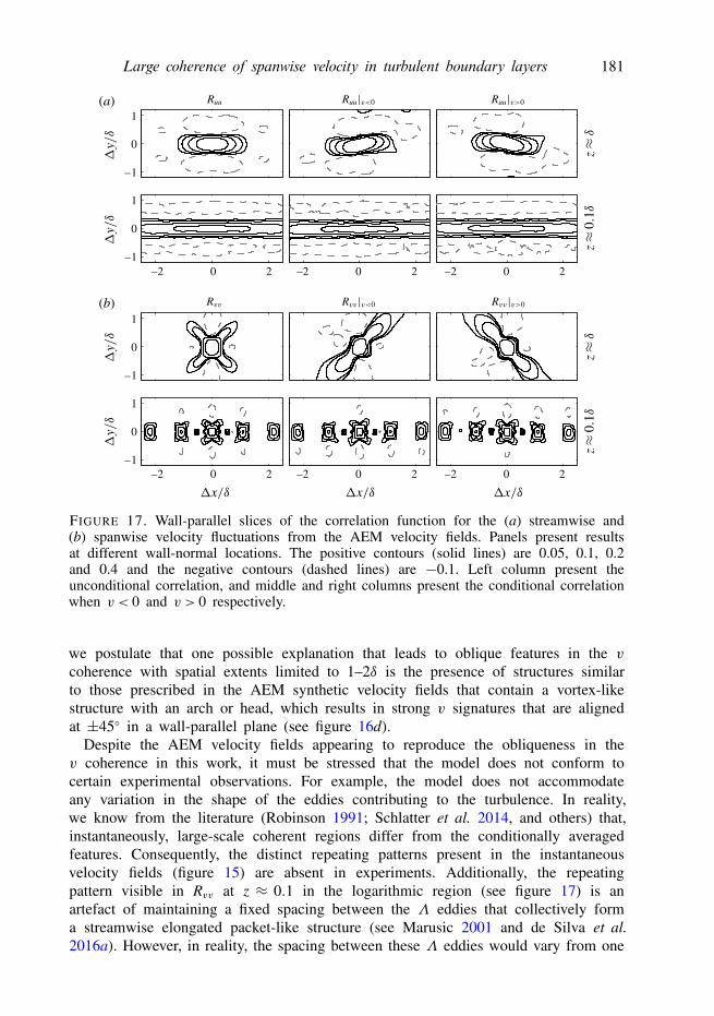
FIGURE 17. Wall-parallel slices of the correlation function for the (a) streamwise and(b) spanwise velocity fluctuations from the AEM velocity fields. Panels present resultsat different wall-normal locations. The positive contours (solid lines) are 0.05, 0.1, 0.2and 0.4 and the negative contours (dashed lines) are −0.1. Left column present theunconditional correlation, and middle and right columns present the conditional correlationwhen v < 0 and v > 0 respectively.

we postulate that one possible explanation that leads to oblique features in the v

coherence with spatial extents limited to 1–2δ is the presence of structures similarto those prescribed in the AEM synthetic velocity fields that contain a vortex-likestructure with an arch or head, which results in strong v signatures that are alignedat ±45◦ in a wall-parallel plane (see figure 16d).

Despite the AEM velocity fields appearing to reproduce the obliqueness in thev coherence in this work, it must be stressed that the model does not conform tocertain experimental observations. For example, the model does not accommodateany variation in the shape of the eddies contributing to the turbulence. In reality,we know from the literature (Robinson 1991; Schlatter et al. 2014, and others) that,instantaneously, large-scale coherent regions differ from the conditionally averagedfeatures. Consequently, the distinct repeating patterns present in the instantaneousvelocity fields (figure 15) are absent in experiments. Additionally, the repeatingpattern visible in Rvv at z ≈ 0.1 in the logarithmic region (see figure 17) is anartefact of maintaining a fixed spacing between the Λ eddies that collectively forma streamwise elongated packet-like structure (see Marusic 2001 and de Silva et al.2016a). However, in reality, the spacing between these Λ eddies would vary from one

Dow

nloa

ded

from

htt

ps://

ww

w.c

ambr

idge

.org

/cor

e. IP

add

ress

: 128

.250

.0.9

9, o

n 28

May

201

8 at

03:

13:4

7, s

ubje

ct to

the

Cam

brid

ge C

ore

term

s of

use

, ava

ilabl

e at

htt

ps://

ww

w.c

ambr

idge

.org

/cor

e/te

rms.

htt

ps://

doi.o

rg/1

0.10

17/jf

m.2

018.

320

182 C. M. de Silva, Kevin, R. Baidya, N. Hutchins and I. Marusic

(a) (b)1

0

–1

0 2 4 6 8 10 0 2 4 6 8 10

–2.2–2.4–2.6–2.8–3.0 –1.6–1.8–2.0–3.2

FIGURE 18. (Colour online) A comparison of instantaneous colour contours of kineticenergy, K, between (a) an experimental and (b) an AEM velocity field on an xy plane atz≈ δ. The solid black line indicates the location of the TNTI. The solid red lines indicatethe principal axis of each turbulent patch detected.

packet-like structure to another, which would suppress the periodic pattern observedin Rvv.

To further illustrate how the instantaneous coherent regions differ from bulk featuresin boundary layers, figure 18 shows colour contours of kinetic turbulent energy atz ≈ δ. The results highlight that the turbulent patches from the experiments arealigned over a wide range of angles to the flow direction (red solid lines), unlikethe model where θ ≈ 0◦ for most turbulent patches (unless they happen to overlap)due to the nature of their placement. Similar evidence for instantaneous structuresbeing misaligned from the main flow direction is also a common observation foru coherence. For example, at low Re, it is illustrated in the models of Jeong et al.(1997) and the instability mechanism of Schoppa & Hussain (2002). Furthermore,scalar visualisation by Delo, Kelso & Smits (2004) also suggests that individualturbulence bulges appear to tilt sideways. Therefore, although the obliqueness inthe v coherence is captured by the AEM velocity fields, further refinement ofthe representative structures in the model would be necessary in order to bettercapture the instantaneous flow features. These modifications are likely to involve theinclusion of a range of representative eddies that are not necessarily forced to bestreamwise-aligned or symmetric.

7. Summary and conclusionsThis paper examines the large-scale oblique pattern in the spanwise velocity

component in turbulent boundary layers using a set of unique large-field-of-view PIVmeasurements. The experiments are configured to capture a sufficiently large spatialdomain of the order of several boundary layer thicknesses in both the streamwiseand spanwise directions. Consistent with Sillero et al. (2014), analysis of two-pointcorrelation functions reveals pronounced oblique features of the spanwise coherenceat the edge of the boundary layer, which are counter-oriented based on the sign ofv. These observations are shown to relate to the intermittent turbulent bulges at theedge of the layer, with the clear presence of two counter-oriented oblique features.Moreover, we find that these oblique features also extend closer to the wall and arepresent in the logarithmic region once the velocity fields are deconstructed basedon the signs of both u and v. Through this analysis, we show that the obliquenessis also present in the streamwise coherence, albeit more subtly. Consequently, theoften-reported meandering of the u coherence (Hutchins & Marusic 2007) appears tobe associated with more obvious diagonal features of the spanwise coherence.

Dow

nloa

ded

from

htt

ps://

ww

w.c

ambr

idge

.org

/cor

e. IP

add

ress

: 128

.250

.0.9

9, o

n 28

May

201

8 at

03:

13:4

7, s

ubje

ct to

the

Cam

brid

ge C

ore

term

s of

use

, ava

ilabl

e at

htt

ps://

ww

w.c

ambr

idge

.org

/cor

e/te

rms.

htt

ps://

doi.o

rg/1

0.10

17/jf

m.2

018.

320

Large coherence of spanwise velocity in turbulent boundary layers 183

Through a conditional correlation analysis, we also show that the obliqueness inthe v coherence is limited to within two boundary layer thicknesses, even thougha purely visual inspection of velocity fields suggests that they appear to extend forvery long extents. These quantitative estimates are in line with the size of the large-scale motions thought to exist in the wake region of a boundary layer (Adrian et al.2000; Tomkins & Adrian 2003). Further, the conditional analysis also shows that theu coherence of these features is comparable in size to the large regions of uniformstreamwise momentum reported in boundary layers (Meinhart & Adrian 1995; de Silvaet al. 2016a).

To complement and aid the interpretation of our findings from the experiments,synthetic velocity fields are generated by following the attached eddy model, wherethe boundary layer is conceived as a collection of randomly located self-similareddies that have prescribed sizes. These synthetic datasets are shown to produceoblique features in the spanwise coherence with spatial extents similar to thoseobserved from the experiments. More specifically, analysis of the synthetic databasesreveals correlation functions and conditional statistics that resemble those from theexperiments. Hence, these findings suggest that the oblique features in the spanwisecoherence might result from similar structures to those used in the model, withpopulation and length-scale distributions similar to those prescribed in the model.

Acknowledgement

The authors gratefully acknowledge the financial support of the Australian ResearchCouncil.

REFERENCES

ADRIAN, R. J. 2007 Hairpin vortex organization in wall turbulence. Phys. Fluids 19 (4), 041301.ADRIAN, R. J., MEINHART, C. D. & TOMKINS, C. D. 2000 Vortex organization in the outer region

of the turbulent boundary layer. J. Fluid Mech. 422, 1–54.ANAND, R. K., BOERSMA, B. J. & AGRAWAL, A. 2009 Detection of turbulent/non-turbulent interface

for an axisymmetric turbulent jet: evaluation of known criteria and proposal of a new criterion.Exp. Fluids 47 (6), 995–1007.

BAIDYA, R., PHILIP, J., MONTY, J. P., HUTCHINS, N. & MARUSIC, I. 2014 Comparisons ofturbulence stresses from experiments against the attached eddy hypothesis in boundary layers.In Proc. 19th Aust. Fluid Mech. Conf, Australian Fluid Mechanics Society.

BALAKUMAR, B. J. & ADRIAN, R. J. 2007 Large- and very-large-scale motions in channel andboundary-layer flows. Phil. Trans. R. Soc. Lond. A 365 (1852), 665–681.

BISSET, D. K., HUNT, J. C. R. & ROGERS, M. M. 2002 The turbulent/non-turbulent interfacebounding a far wake. J. Fluid Mech. 451, 383–410.

BUSCHMANN, M. H., INDINGER, T. & GAD-EL-HAK, M. 2009 Near-wall behavior of turbulentwall-bounded flows. Intl J. Heat Fluid Flow 30 (5), 993–1006.

CHAUHAN, K., PHILIP, J. & MARUSIC, I. 2014 Scaling of the turbulent/non-turbulent interface inboundary layers. J. Fluid Mech. 751, 298–328.

CHAUHAN, K. A., MONKEWITZ, P. A. & NAGIB, H. M. 2009 Criteria for assessing experiments inzero pressure gradient boundary layers. Fluid Dyn. Res. 41 (2), 021404.

COLES, D. 1965 Transition in circular Couette flow. J. Fluid Mech. 21 (3), 385–425.DELO, C. J., KELSO, R. M. & SMITS, A. J. 2004 Three-dimensional structure of a low-Reynolds-

number turbulent boundary layer. J. Fluid Mech. 512, 47–83.DUGUET, Y. & SCHLATTER, P. 2013 Oblique laminar–turbulent interfaces in plane shear flows. Phys.

Rev. Lett. 110 (3), 034502.

Dow

nloa

ded

from

htt

ps://

ww

w.c

ambr

idge

.org

/cor

e. IP

add

ress

: 128

.250

.0.9

9, o

n 28

May

201

8 at

03:

13:4

7, s

ubje

ct to

the

Cam

brid

ge C

ore

term

s of

use

, ava

ilabl

e at

htt

ps://

ww

w.c

ambr

idge

.org

/cor

e/te

rms.

htt

ps://

doi.o

rg/1

0.10

17/jf

m.2

018.

320

184 C. M. de Silva, Kevin, R. Baidya, N. Hutchins and I. Marusic

ELSINGA, G. E., ADRIAN, R. J., VAN OUDHEUSDEN, B. W. & SCARANO, F. 2010Three-dimensional vortex organization in a high-Reynolds-number supersonic turbulent boundarylayer. J. Fluid Mech. 644, 35–60.

FALCO, R. E. 1977 Coherent motions in the outer region of turbulent boundary layers. Phys. Fluids20, S124–S132.

FLORES, O. & JIMÉNEZ, J. 2010 Hierarchy of minimal flow units in the logarithmic layer. Phys.Fluids 22 (7), 071704.

GANAPATHISUBRAMANI, B., LONGMIRE, E. K. & MARUSIC, I. 2003 Characteristics of vortexpackets in turbulent boundary layers. J. Fluid Mech. 478, 35–46.

HERPIN, S., STANISLAS, M., FOUCAUT, J. M. & COUDERT, S. 2013 Influence of the Reynoldsnumber on the vortical structures in the logarithmic region of turbulent boundary layers.J. Fluid Mech. 716, 5–50.

HESKESTAD, G. 1965 Hot-wire measurements in a plane turbulent jet. Trans. ASME J. Appl. Mech.32 (4), 721–734.

HUTCHINS, N., HAMBLETON, W. T. & MARUSIC, I. 2005 Inclined cross-stream stereo particle imagevelocimetry measurements in turbulent boundary layers. J. Fluid Mech. 541, 21–54.

HUTCHINS, N. & MARUSIC, I. 2007 Evidence of very long meandering features in the logarithmicregion of turbulent boundary layers. J. Fluid Mech. 579, 1–28.

HWANG, Y. & COSSU, C. 2010 Self-sustained process at large scales in turbulent channel flow. Phys.Rev. Lett. 105 (4), 044505.

JEONG, J., HUSSAIN, F., SCHOPPA, W. & KIM, J. 1997 Coherent structures near the wall in aturbulent channel flow. J. Fluid Mech. 332, 185–214.

JIMÉNEZ, J., HOYAS, S., SIMENS, M. P. & MIZUNO, Y. 2010 Turbulent boundary layers and channelsat moderate Reynolds numbers. J. Fluid Mech. 657, 335–360.

JOLLIFFE, I. T. 1986 Principal component analysis and factor analysis. In Principal ComponentAnalysis, pp. 115–128. Springer.

KWON, Y. S., HUTCHINS, N. & MONTY, J. P. 2016 On the use of the Reynolds decomposition inthe intermittent region of turbulent boundary layers. J. Fluid Mech. 794, 5–16.

LEE, J., LEE, J. H., CHOI, J. I. & SUNG, H. J. 2014 Spatial organization of large- and very-large-scale motions in a turbulent channel flow. J. Fluid Mech. 749, 818–840.

LEE, J. H. & SUNG, H. J. 2011 Very-large-scale motions in a turbulent boundary layer. J. FluidMech. 673, 80–120.

LOZANO-DURÁN, A. & JIMÉNEZ, J. 2014 Time-resolved evolution of coherent structures in turbulentchannels: characterization of eddies and cascades. J. Fluid Mech. 759, 432–471.

MARUSIC, I. 2001 On the role of large-scale structures in wall turbulence. Phys. Fluids 13, 735–743.MARUSIC, I. & ADRIAN, R. J. 2012 The eddies and scales of wall turbulence. In Ten Chapters in

Turbulence (ed. P. A. Davidson, K. Yukio & K. R. Sreenivasan). Cambridge University Press.MARUSIC, I. & HEUER, W. D. 2007 Reynolds number invariance of the structure inclination angle

in wall turbulence. Phys. Rev. Lett. 99 (11), 114504.MARUSIC, I., MONTY, J. P., HULTMARK, M. & SMITS, A. J. 2013 On the logarithmic region in

wall turbulence. J. Fluid Mech. 716, R3.MARUSIC, I. & PERRY, A. E. 1995 A wall-wake model for the turbulence structure of boundary

layers. Part 2. Further experimental support. J. Fluid Mech. 298, 389–407.MATHEW, J. & BASU, A. J. 2002 Some characteristics of entrainment at a cylindrical turbulence

boundary. Phys. Fluids 14 (7), 2065–2072.MATHIS, R., HUTCHINS, N. & MARUSIC, I. 2009 Large-scale amplitude modulation of the small-scale

structures in turbulent boundary layers. J. Fluid Mech. 628, 311–337.MEINHART, C. D. & ADRIAN, R. J. 1995 On the existence of uniform momentum zones in a

turbulent boundary layer. Phys. Fluids 7, 694.MONTY, J. P., HUTCHINS, N., NG, H. C. H., MARUSIC, I. & CHONG, M. S. 2009 A comparison

of turbulent pipe, channel and boundary layer flows. J. Fluid Mech. 632, 431–442.NICKELS, T. B., MARUSIC, I., HAFEZ, S. & CHONG, M. S. 2005 Evidence of the k−1 law in a

high-Reynolds-number turbulent boundary layer. Phy. Rev. Lett. 95 (7), 074501.

Dow

nloa

ded

from

htt

ps://

ww

w.c

ambr

idge

.org

/cor

e. IP

add

ress

: 128

.250

.0.9

9, o

n 28

May

201

8 at

03:

13:4

7, s

ubje

ct to

the

Cam

brid

ge C

ore

term

s of

use

, ava

ilabl

e at

htt

ps://

ww

w.c

ambr

idge

.org

/cor

e/te

rms.

htt

ps://

doi.o

rg/1

0.10

17/jf

m.2

018.

320

Large coherence of spanwise velocity in turbulent boundary layers 185

PANTON, R. L. 2001 Overview of the self-sustaining mechanisms of wall turbulence. Prog. Aerosp.Sci. 37 (4), 341–383.

PERRY, A. E. & CHONG, M. S. 1982 On the mechanism of wall turbulence. J. Fluid Mech. 119,106–121.

PERRY, A. E., HENBEST, S. M. & CHONG, M. 1986 A theoretical and experimental study of wallturbulence. J. Fluid Mech. 165, 163–199.

PERRY, A. E. & MARUSIC, I. 1995 A wall-wake model for the turbulence structure of boundarylayers. Part 1. Extension of the attached eddy hypothesis. J. Fluid Mech. 298, 361–388.

PHILIP, J., MENEVEAU, C., DE SILVA, C. M. & MARUSIC, I. 2014 Multiscale analysis of fluxes atthe turbulent/non-turbulent interface in high Reynolds number boundary layers. Phys. Fluids26 (1), 015105.

REYNOLDS, O. 1894 On the dynamical theory of incompressible viscous fluids and the determinationof the criterion. Proc. R. Soc. Lond. A 56 (336–339), 40–45.

ROBINSON, S. K. 1991 Coherent motions in the turbulent boundary layer. Annu. Rev. Fluid Mech.23 (1), 601–639.

SCHLATTER, P., LI, Q., ÖRLÜ, R., HUSSAIN, F. & HENNINGSON, D. S. 2014 On the near-wallvortical structures at moderate Reynolds numbers. Eur. J. Mech. (B/Fluids) 48, 75–93.

SCHOPPA, W. & HUSSAIN, F. 2002 Coherent structure generation in near-wall turbulence. J. FluidMech. 453, 57–108.

SILLERO, J. A., JIMÉNEZ, J. & MOSER, R. D. 2013 One-point statistics for turbulent wall-boundedflows at Reynolds numbers up to δ+ = 2000. Phys. Fluids 25 (10), 105102.

SILLERO, J. A., JIMÉNEZ, J. & MOSER, R. D. 2014 Two-point statistics for turbulent boundarylayers and channels at Reynolds numbers up to δ+ = 2000. Phys. Fluids 26 (10), 105109.

DE SILVA, C. M., GNANAMANICKAM, E. P., ATKINSON, C., BUCHMANN, N. A., HUTCHINS, N.,SORIA, J. & MARUSIC, I. 2014 High spatial range velocity measurements in a high Reynoldsnumber turbulent boundary layer. Phys. Fluids 26 (2), 025117.

DE SILVA, C. M., HUTCHINS, N. & MARUSIC, I. 2016a Uniform momentum zones in turbulentboundary layers. J. Fluid Mech. 786, 309–331.

DE SILVA, C. M., PHILIP, J., CHAUHAN, K., MENEVEAU, C. & MARUSIC, I. 2013 Multiscalegeometry and scaling of the turbulent–nonturbulent interface in high Reynolds number boundarylayers. Phys. Rev. Lett. 111, 044501.

DE SILVA, C. M., SQUIRE, D. T., HUTCHINS, N. & MARUSIC, I. 2015 Towards capturing largescale coherent structures in boundary layers using particle image velocimetry. In Proc. 6thAust. Conf. Laser Diag. Fluid Mech. Comb., pp. 1–4. University of Melbourne.

DE SILVA, C. M., WOODCOCK, J. D., HUTCHINS, N. & MARUSIC, I. 2016b Influence of spatialexclusion on the statistical behavior of attached eddies. Phys. Rev. Fluids 1, 022401.

SQUIRE, D. T., MORRILL-WINTER, C., HUTCHINS, N., MARUSIC, I., SCHULTZ, M. P. & KLEWICKI,J. C. 2016 Smooth- and rough-wall boundary layer structure from high spatial range particleimage velocimetry. Phys. Rev. Fluids 1 (6), 064402.

TOWNSEND, A. A. 1976 The Structure of Turbulent Shear Flow, 2nd edn. Cambridge UniversityPress.

TOMKINS, C. D. & ADRIAN, R. J. 2003 Spanwise structure and scale growth in turbulent boundarylayers. J. Fluid Mech. 490, 37–74.

VAN ATTA, C. 1966 Exploratory measurements in spiral turbulence. J. Fluid Mech. 25 (03), 495–512.WALLACE, J. M., ECKELMANN, H. & BRODKEY, R. S. 1972 The wall region in turbulent shear

flow. J. Fluid Mech. 54 (1), 39–48.WOODCOCK, J. D. & MARUSIC, I. 2015 The statistical behaviour of attached eddies. Phys. Fluids

27 (1), 015104.

Dow

nloa

ded

from

htt

ps://

ww

w.c

ambr

idge

.org

/cor

e. IP

add

ress

: 128

.250

.0.9

9, o

n 28

May

201

8 at

03:

13:4

7, s

ubje

ct to

the

Cam

brid

ge C

ore

term

s of

use

, ava

ilabl

e at

htt

ps://

ww

w.c

ambr

idge

.org

/cor

e/te

rms.

htt

ps://

doi.o

rg/1

0.10

17/jf

m.2

018.

320