j. ksiam vol.20, no.3, 175 202, 2016 s industrial
TRANSCRIPT

J. KSIAM Vol.20, No.3, 175–202, 2016 http://dx.doi.org/10.12941/jksiam.2016.20.175
[SPECIAL SECTION : Mathematics in Industry ]
INDUSTRIAL MATHEMATICS IN ULTRASOUND IMAGING
JAESEONG JANG1 AND CHI YOUNG AHN2,†
1DEPARTMENT OFCOMPUTATIONAL SCIENCE AND ENGINEERING, YONSEI UNIVERSITY, SEOUL, KOREA
E-mail address: [email protected]
2DIVISION OF INTEGRATEDMATHEMATICS, NATIONAL INSTITUTE FORMATHEMATICAL SCIENCES,DAEJEON, KOREA
E-mail address: [email protected]
ABSTRACT. Ultrasound imaging is a widely used tool for visualizing human body’s inter-nal organs and quantifying clinical parameters. Due to its advantages such as safety, non-invasiveness, portability, low cost and real-time 2D/3D imaging, diagnostic ultrasound industryhas steadily grown. Since the technology advancements suchas digital beam-forming, Dopplerultrasound, real-time 3D imaging and automated diagnosis techniques, there are still a lot of de-mands for image quality improvement, faster and accurate imaging, 3D color Doppler imagingand advanced functional imaging modes. In order to satisfy those demands, mathematics shouldbe used properly and effectively in ultrasound imaging. Mathematics has been used commonlyas mathematical modelling, numerical solutions and visualization, combined with science andengineering. In this article, we describe a brief history ofultrasound imaging, its basic prin-ciple, its applications in obstetrics/gynecology, cardiology and radiology, domestic-industrialproducts, contributions of mathematics and challenging issues in ultrasound imaging.
1. INTRODUCTION
Ultrasound imaging system visualizes organs inside human body using sound waves withthe frequency range of1∼15 MHz higher than human audible frequency. Due to the variousadvantages of non-invasiveness, safety, portability(seeFig. 1), relatively low cost and real-time imaging over other imaging modalities such as CT and MRI, it is widely used in variousdiagnostic fields of obstetrics and gynecology, cardiology, radiology, and so on.
Recently, it was reported that ultrasound market size was growing and the ultrasound mar-ket including diagnostic ultrasound would be worth about6.23 billion USD in 2020 [1, 2]. In
Received by the editors August 17 2016; Revised August 28 2016; Accepted in revised form August 29 2016;Published online September 5 2016.
2000Mathematics Subject Classification.68U10, 92C50.Key words and phrases.Industrial Mathematics, Ultrasound Imaging, Ultrasound Examinations, Image Pro-
cessing, Technology Advances, Mathematical Modelling.† Corresponding author.
175

176 J. JANG AND C. Y. AHN
FIGURE 1. Ultrasound imaging systems of major companies: GE, Philips,Siemens, Samsung Medison and Alpinion (from their homepages). The threecompanies of (a)-(c) have over half of global ultrasound market share [3]. Thetwo companies of (d) and (e) are leading domestic companies.
order to have bigger market share, each global company triesto develop competitive imag-ing technologies and to expand ultrasound use in other applications. For example, one of themost promising technologies affected by increased computational power is real-time 3D ultra-sound imaging. It is capable of providing good 3D visualization of organs at the faster rateof about30 volumes per seconds compared to volumetric imaging modalities such as CT andMRI. However, its resolution is not good enough so that it often fails to discriminate featuressmaller than a few millimeters. Because of this resolution limitation, real-time 3D ultrasoundimaging is not frequently adopted for clinical examinations in radiology. Whereas, it is mean-ingfully used for observing cardiac wall motion in cardiology or for distinguishing betweentissues and surrounding fluids in obstetrics and gynecology. In order to circumvent the reso-lution problem, each company concentrates on fusion imaging technique that incorporates twoimages acquired from two different imaging modalities: real-time ultrasound images and CTor MRI images acquired earlier. It is able to provide more anatomical information indistin-guishable with the resolution of real-time 3D ultrasound imaging and expand ultrasound usein radiology. As other examples of the promising technologies, we can consider image qualityenhancement, faster imaging, 3D color Doppler imaging, computer-aided detection (CADe),computer-aided diagnosis (CADx) and advanced functional imaging modes such as elasticityimaging and vortex flow imaging. They are also very interesting and challenging issues to beimproved in ultrasound imaging.
Then how can we advance and innovate ultrasound imaging technologies? Like in otherindustries,Mathematicshas played an important role in ultrasound imaging and medical diag-nosis already. For acquiring gray-level echo images and color Doppler images,Mathematicsis used in various parts of time-delay computation for beam-forming, Fourier tranform of ul-trasound signal for signal processing or filter design, auto-correlation computation for meanfrequency estimation, linear interpolation for scan conversion, and so on [4, 5].Mathematics

INDUSTRIAL MATHEMATICS IN ULTRASOUND IMAGING 177
is also used to extract functional information from ultrasound images. In order to avoid labor-intensive and time-consuming manual measurements on gray-scale echo images, automatedsegmentation and motion tracking algorithms are demanded.The automated measurementmethods are based on partial differential equation, numerical analysis, statistics as well as theinterpretation of acoustic fields and speckles as inherent appearance in ultrasound imaging.Therefore, we can see that various levels of mathematical modelling and methods are appliedto acquire ultrasound images and to generate functional information for clinical evaluations.
Moreover,Mathematicsis essential in cases of elasticity imaging and vortex flow imagingmentioned above. Elasticity imaging is an imaging mode to map the stiffness of soft tissuessuch as liver or breast, and it can be implemented by reconstructing elastic modulus frommeasured displacements governed by the elastic equation:
∇ · (µ(∇u+∇ut)) +∇(λ∇ · u) = ρ
∂2
∂t2u, (1.1)
whereu denotes the displacement vector,∇ut the transpose of the matrix∇u, ρ the density
of the soft tissue as elastic material,µ the shear modulus withµ = E2(1+ν) andλ the Lamé
coefficient withλ = νE(1+ν)(1−2ν) . Here,E andν are Young’s modulus and Poisson’s modulus,
respectively.Vortex flow imaging is an imaging mode to quantify the vorticity of intra-ventricular blood
flows and to offer possible clinical indices. Since the vorticity fields are obtained by taking thecurl operator to velocity fields of flows, the velocity fields should be exactly computed. Thevelocity fields can be computed by solving the Navier-Stokesequation:
ρ
(
∂v
∂t+ v · ∇v
)
= −∇p+ µ∇2v in Ωt,
∇ · v = 0 in Ωt,
(1.2)
whereΩt denotes the intra-ventricular domain varying within the heartbeat cycleT , v thevelocity fields,ρ the blood density andµ the blood viscosity.
The displacements of soft tissues and the motion of blood flows are understood throughphysics-based mathematical modelling using elastic and fluid equations. Under those math-ematical models, we deal with measurements obtained through ultrasound imaging systems,construct the overall phenomenon from the partially measured data and quantify clinicallymeaningful information. The point is that ultrasound imaging technologies will be advancedand innovated throughMathematics.
The aim of this paper is to describe the importance and value of Mathematicsin ultrasoundimaging and to share them with other scientists and engineers. In this paper, we describe a briefhistory of ultrasound imaging, basic imaging principle, its applications in major diagnosticfields, domestic-industrial products and contributions ofmathematics, especially for beginnersto understand ultrasound imaging and pay much attention to it. Furthermore, we introduce hottopics and challenging issues related to ultrasound imaging. They have to be resolved for theadvancements of ultrasound imaging technology. We hope many mathematicians recognizehow mathematics is used and contributes much to ultrasound technology innovation.

178 J. JANG AND C. Y. AHN
2. THE HISTORY OFDIAGNOSTIC ULTRASOUND IMAGING
The history of ultrasound imaging starts with the history ofsonar, the abbreviation of SOundNavigation And Ranging, measuring the depth of water using sound wave. In the late 1800s,the theoretic and practical foundation for sonar and ultrasound imaging was established by amathematical equation describing sound wave and the discovery of piezo-electricity, electricityresulting from pressure. L. Rayleigh described sound wave as a mathematical equation in hispaper “the Theory of Sound” published in 1877 and P. Curie andhis brother J. Curie discoveredthe piezo-electric effect in certain crystals in 1880 [6–8].
Since the sinking of the Titanic in 1912 and World War I, echo-ranging systems were de-manded to detect icebergs or submarines. In 1917, P. Langevin, one of the Curie brothers’first students developed practical underwater echo-ranging systems using the piezo-electricityfor transducer, a device converting a voltage difference toa mechanical stress and reverselyconverting a mechanical pressure to an electric potential.During World War II, echo-rangingtechnique was applied to electromagnetic waves and became radar, the abbreviation of RAdioDetection And Ranging.
Echo-ranging system as a diagnostic device to probe the human body was not developeduntil the 1940’s. K. Dussik used ultrasound to diagnose brain tumor by transmitting an ultra-sound beam through the human skull in 1942 [6, 7, 9]. He is regarded as the first-time userof ultrasound for medical diagnosis. In 1948, G. Ludwig usedA-mode ultrasound system todetect gallstones [7, 10]. The A-mode shows a signal profile representing the instantaneousecho signal amplitude over time after transmission of the acoustic pulse.
FIGURE 2. Illustration of the A-mode and B-mode displays. A 2D B-modeimage consists of multiple and sequential B-mode lines.
After that time, innovative advances of ultrasound imagingtechnologies have followed. Inthe 1950s, 2D B-mode ultrasound imaging system was developed and applied to detect breasttumors and to diagnose in the obstetrics and gynecology fields [6,11]. The B-mode representsthe brightness converted from the amplitude of the echo signals. Fig. 2 illustrates the A-modeand B-mode displays.

INDUSTRIAL MATHEMATICS IN ULTRASOUND IMAGING 179
Since the first implementation of ultrasonic Doppler techniques in Japan in 1955 [12], var-ious Doppler techniques including the continuous wave Doppler, spectral wave Doppler, andcolor Doppler ultrasound were developed through the 1960s and the 1970s [7, 13–17]. Theemergency of 3D ultrasound technology in the 1980s was capable of capturing 3D images of afetus [18,19]. Thanks to the continuous improvements of image quality and 3D imaging capa-bilities, ultrasound technology became more sophisticated and capable of real-time 3D imagingin the 1990s [20].
From the 2000s to present, 2D arrays of transducers were usedfor real-time 3D imaging,ultrasound imaging system became miniaturized gradually and ultrasound imaging technologyis developing steadily for improving image quality, reducing costs, reducing exam times andbeing applied to wider diagnostic areas. Recently, hand-carried systems became available. Itis becoming common with significant growth and can be used forclinical assessments even indeveloping countries [21, 22] due to the portability and lowcost in addition to higher imagequality obtained by using special ultrasound probes for transesophageal echocardiography andtransverginal echo [23,24].
More detailed information about the history of ultrasound imaging can be found at the ref-erences [4,6].
3. BASIC PRINCIPLE OFULTRASOUND IMAGING
Probe(Transducers )
Beam-formingTime gain
compensation
Quadrature
demodulation
Log-
compression
Scan
conversion
Display
Envelope
detection
Logarithmic curve
amplitude of signals
gra
y-s
ca
le
bri
gh
tnes
s
(in frequency domain )
(I^2+Q^2)^0.5
I
Q
gain (dB) =
20 log10 (Aout/Ain)
scanlines
data s
ample
s
FIGURE 3. Block diagram of ultrasound B-mode imaging.
In this section, we describe the basic principle of ultrasound imaging, especially focusing ongray-scale echo images, called the B-mode images. Fig. 3 shows intuitively that mathematics,combined with science and engineering, is used in the process of ultrasound B-mode imaging.Furthermore, we deal with the mathematical models on acoustic fields, fundamental in ultra-sound imaging, and describe their applications. We can see that mathematics is applied usuallyas mathematical modelling, numerical solutions and visualization.

180 J. JANG AND C. Y. AHN
3.1. Ultrasound B-mode imaging. An ultrasound image consists of several sequential scan-lines (around128 ∼ 512 scanlines), each of which is usually acquired through transmissionand reception beam-forming using transducer arrays. The transmission beam-forming is tocontrol electronically time delays for ultrasound beam emitted from the transducer arrays tobe focused at a point on each scanline. The reception beam-forming is to control electron-ically time delays to accumulate back-scattered echo signals from a specific position, calledthe received focal point, on scanlines. We note that the received focal point can be changeddynamically on each scanline.
As sound travels through a material, the amplitude or intensity is decreased due to threefactors: absorption, scattering and beam divergence. We start describing mathematically theultrasound imaging principle, together with beam-forming, considering the time gain compen-sation of the received and beam-formed echo signals [25,26].
3.1.1. Beam-forming and gain compensation.LetN be the number of transducers,rj the po-sition of thej-th transducer andpj the received signal atrj for j = 1, · · · , N . We assume thattransducers are very small, sample positions on each scanline are far away from the transducersand the impulse response is given in the form of Dirac delta function. Then, for sample positionr = (x, y, z) on a given scanline, the amplitude of the received signal at time t is expressed as
p(t) =
N∑
j=1
pj(t− τj) = K
N∑
j=1
δ
(
t−|rj − r|
c
)
, (3.1)
whereτj is the delayed time andK a constant depending on depth.
3.1.2. Quadrature demodulation and envelope detection.Let f0 be the center frequency oftransmission signals. Then the amplitude (3.2) of the beam-formed signal along the givenscanline can be expressed as
p(t) = a(t) cos(2πf0t+ φ(t))
=a(t)
2
(
ei(2πf0t+φ(t)) + e−i(2πf0t+φ(t)))
,(3.2)
wherea(t) andφ(t) are the amplitude and the phase of the received signal, respectively. Inorder to remove signals with high-frequency and obtain meaningful signal with low-frequency,we perform the quadrature demodulation. By settingp(t) = p(t)e−2πf0t and applying a low-pass filter top(t), we can obtain a base-band complex signala(t)
2 eiφ(t). Its real and imaginaryparts are called In-phase and Quadrature signals, denoted by I(t) andQ(t), respectively.
I(t) = Re
(
a(t)
2eiφ(t)
)
,
Q(t) = Im
(
a(t)
2eiφ(t)
)
.
(3.3)
After the envelope detection by taking√
I(t)2 +Q(t)2 from the quadrature demodulated sig-nalsI(t) andQ(t), logarithmic compression follows.

INDUSTRIAL MATHEMATICS IN ULTRASOUND IMAGING 181
3.1.3. Logarithmic compression.Most of clinically meaningful signals are appeared with thesmall value in the wide range of amplitude. The logarithmic compression is required to displaythese meaningful signals in the 256 gray-scale values. The image intensityI(t) is expressed as
I(t) =Imax − Imin
lnAmax − lnAminln
(
A(t)
Amin
)
+ Imin, (3.4)
whereImax andImin are the maximum and minimum intensity values, to be displayed finallyin the gray-scale, respectively, andAmax andAmin the maximum and minimum amplitudevalues with the range of interest, respectively.
3.1.4. Digital scan conversion and display.These intensity values at the sample positionsalong each scanline are displayed on a video screen through scan conversion process for thespatially arrangement. Scan conversion is performed by using bi-linear interpolation.
In order to improve the B-mode image, some signal/image processing methods may be usedadditionally.
3.2. Acoustic fields. Jensen [27] derived an inhomogeneous wave equation describing thepropagation and scattering of ultrasound in an inhomogeneous medium, derived a mathemat-ical model for the received pulse-echo pressure fields by considering the surface shape of asingle transducer element used in diagnostic ultrasound and showed simulated pressure fieldcompared to a measured field. In this subsection, we describethe mathematical models andtheir applications.
3.2.1. Mathematical modelling.Let p(r, t) be the pressure variation caused by ultrasoundpropagation at the positionr and timet, c(r) the propagation speed andρ(r) the materialdensity. Then the inhomogeneous wave equation is derived as
∇2p−1
c02∂2p
∂t2= −
2(δc)
c03∂2p
∂t2+
1
ρ0∇(δρ) · ∇p, (3.5)
wherec0 is the mean propagation speed,ρ0 the mean density,δc the speed variation fromc0andδρ the density variation fromρ0.
Let pr(t) the received signal at the transducer surface andEm(t) at timet. Thenpr(t) iswritten as
pr(t) =ρ0
2c02Em(t) ∗
t
∂3v(t)
∂t3∗t
[(
δρ(r)
ρ0−
2(δc(r))
c0
)
∗r
H(r, t)
]
, (3.6)
where∗t
and ∗r
mean the time convolution and spatial convolution, respectively. Note that
ρ02c02
Em(t) ∗t
∂3v(t)∂t3
is the pulse-echo including the transducer excitation and the electrome-
chanical impulse response during the emission/reception of the pulse,δρ(r)ρ0− 2(δc(r))
c0is the
inhomogeneities in tissue andH(r, t) is the pulse echo spatial impulse response given byH(r, t) = h(r, t) ∗
th(r, t) with h(r, t) =
∫
Sδ(t−|r−r0|/c0)
2π|r−r0|dr0 for the transducer surfaceS.
For validating the derived mathematical model (3.6), a simulation was performed under thesetup that a plane reflector was placed at focal point. According to an excited Dirac impulse,

182 J. JANG AND C. Y. AHN
impulse responses were computed at the distances of three different positions from transducersurface and compared to measured responses.
3.2.2. Field II simulation program.Afterward Jensen [28, 29] improved the mathematicalmodel (3.6) for the propagation and scattering of acoustic fields by considering acoustic fieldsfrom arbitrarily shaped, apodized and excited transducersand dealing with the imaging prin-ciple, and developed a simulation program based on the derived mathematical model and run-ning under MATLAB software. It is called Field II. Using Field II simulation program, wecan simulate ultrasound transducer fields and generate somegray-level echo and color Dopplerimages similar to real ultrasound images acquired in ultrasound imaging system as depictedin Fig. 4. Field II is widely used in several companies, universities and departments because
FIGURE 4. Examples of ultrasound synthetic images generated by using Field II.
it is very helpful for scientists and engineers to understand ultrasound imaging and study im-age processing methods such as speckle reduction on the synthetic images. It is available at:http://field-ii.dk/.
4. APPLICATIONS OFDIAGNOSTIC ULTRASOUND IMAGING
Thanks to the advanced imaging technologies such as image quality enhancement, real-time 3D imaging and the miniaturization of equipment, ultrasound is widely applied to variousdiagnostic fields of obstetrics and gynecology(OB/GYN), cardiology, radiology, urology, andso on. We note that applications in OB/GYN, cardiology and radiology account for about70% of the entire ultrasound examinations. In this section,we provide brief explanations ofultrasound imaging applications in major three diagnosticareas.

INDUSTRIAL MATHEMATICS IN ULTRASOUND IMAGING 183
4.1. OB/GYN ultrasound. Since the 1950’s, ultrasound has been used for the diagnosisofgestation and women’s health. The ultrasound market for OB/GYN examinations has contin-ued to increase. The main issues of ultrasound imaging in OB/GYN is to improve the imagequality for detecting endometriosis and gynecological cancer, diagnosing early miscarriageand ectopic pregnancy, and evaluating fetal growth. Especially the performance enhancementof static and real-time 3D imaging is still a hot issue for easier detection of fetal abnormalitiesin obstetrics.
4.1.1. Ultrasound examinations.Fetal ultrasound examinations are classified into four parts:first-trimester examination, standard second- or third-trimester examination, limited examina-tion and specialized examinations [30]. Most of the examinations performed by observing ormeasuring target objects: the presence, size, location andnumber of gestational sac(s), fetalpresentation, amniotic fluid volume, cardiac activity, placental position, fetal biometry, fetalheart activity, and so on.
On the other hand, gynecological examinations such as the detection of endometriosis andgynecological cancer are performed commonly by transvaginal scans, with the probe designedto be placed in the vagina of patient. Since the scanhead of the probe is closely adjacentto uterus, the transvaginal scans provide better image qualities and are useful for the earlydiagnosis of miscarriage and ectopic pregnancies.
Recent advances of static and real-time 3D ultrasound imaging through various image pro-cessing and volume rendering techniques have enabled performing more accurate diagnosis forectopic pregnancy [31] and providing more accurate diagnostic information: abnormalities andanomalies by visualizing fetal face, brain, spine, and skeleton [32], fetal weight obtained bymeasuring abdominal, thigh, arm volumes and head circumference [33–35], and the volumesof lung and heart [36, 37]. High quality images and accurate boundary extraction are requiredfor fetal examinations.
In addition, Doppler ultrasound is indispensable for detecting fetal heartbeat as well as bloodflow characteristics in the various fetal blood vessels: umbilical artery, aorta, middle cerebralarteries, uterine arcuate arteries and inferior vena cava.Power or color Doppler images areused for examinations of fetal middle cerebral artery and cerebral venous [38,39]. Blood flowto fetus through umbilical cord is also observed by color Doppler images [40, 41]. Note thatcolor Doppler images reflect one-directional velocity components of blood flow along scanlinesand power Doppler shows the volume of blood, rather than its velocity.
4.1.2. Innovative technologies for OB/GYN.Samsung Medison, a leading domestic company,has released recently a premium ultrasound system ‘WS80A with Elite’ with superior ultra-sound imaging techniques for OB/GYN examinations:S-Harmonic, ClearVision
TM, Realistic
VueTM
, Crystal Vue, etc. Among them, we pay attention toCrystal Vuean advanced renderingtechnique to enhance the image contrast of 3D volume data. Itis capable of imaging the in-terface of bone and soft tissue with high accuracy and providing intuitive information on thecontour of fetal skeleton, face and brain. Lately,Crystal Vuehas been featured on the frontcover of Ultrasound in Obstetrics & Gynecology (UOG), a renowned journal in the women’s

184 J. JANG AND C. Y. AHN
healthcare industry [42]. The images of fetal spine and ribsobtained byCrystal Vuewereselected as the Picture of the Month by UOG. They provide remarkably clear and realisticinformation of fetal spine and ribs.
Together with the advanced rendering technique, ElastoScanTM
for gynecology is also beingpromoted. It is used to diagnose benign gynecological disorders and to differentiate uterinefibroids and adenomyosis. We can appreciate the remarkable images acquired by SamsungMedison’s innovative imaging technologies at: http://www.samsungmedison.com/ultrasound/ob-gyn/ws80a-with-elite/.
4.2. Cardiological ultrasound. Due to the high temporal resolution of ultrasound imaging,cardiac ultrasound (echocardiography) has been very successful in providing a quick assess-ment of the overall health of heart, a very fast moving complex organ positioned deep withinthe body. Ultrasound examinations of heart functions related to cardiac wall motion, valve mo-tion and blood flow are performed by various ultrasound imaging modes: gray-scale imaging,tissue Doppler imaging, color Doppler imaging and real-time 3D imaging. Note that tissueDoppler images represent the velocity of cardiac wall motion.
4.2.1. Ultrasound examinations.Echocardiographic examinations include numerous diagnos-ing items: valvular heart disease, hypertensive heart disease, ischemic heart disease, cardiactumors, evaluation of the left and right atrium, evaluationof left ventricle(LV) systolic/diastolicfunction, congenital heart disease, diseases of the aorta,and so on. For more detailed descrip-tion on echocardiographic examinations, we refer to the literature ‘The Echocardiographer’sPocket Reference’ by T. Reynolds(2013) [43].
Among echocardiographic examinations, we consider only evaluation of LV function in-cluding dimensions, volumes, wall thickness, LV mass, LV mass index, longitudinal motion,radial motion, circumferential, segmental wall motion, wall motion score index, etc. For itsquantitative assessment, wall motion tracking and LV volume quantification at each time isneeded. To avoid labor-intensive and time-consuming manual LV tracing process, demand forautomated LV tracking and analysis methods has been rapidlygrowing and there have beenplenty of studies on LV tracking methods. In Section 6, we represent a problem on LV motiontracking and solutions by mathematical modelling.
4.2.2. A software for quantifying cardiac function.Automated LV tracking methods can be ap-plied to analyze and quantify LV function. TomTec is a leading company in medical imagingsoftware solutions and offers industry partners or clinicians various solutions for quantifyingcardiac function based on 2D and 3D echocardiography. As an example of software solutions,TomTec developed AutoStrainc© by applying automated LV tracking method to visualize LVfunction quantitatively. AutoStrainc© provides automated LV function analysis based on car-diac apical long axis views. It visualizes longitudinal strain results, obtained by 2D speckletracking, to be color-coded in the individual clips and combined in a Bull’s-eye plot.
4.2.3. A software for visualizing and quantifying blood flows.On the other hand, anotherimaging software company AMID has recently developed ‘hi-def flow tracking’ a software

INDUSTRIAL MATHEMATICS IN ULTRASOUND IMAGING 185
for visualizing and quantifying the motion of blood flow (http://www.amid.net). It is alsocalled Omega Flow (Siemens, Mountain View, CA). It is not based on color Doppler images,but echo-PIV technique applied to contrast-enhanced echocardiographic images. Along withstudies on its clinical possibility and feasibility, this software continues to develop to be usedto evaluate cardiac function clinically.
4.3. Radiological ultrasound. Ultrasound examinations in radiology consist of abdominal,vascular, musculoskeletal, breast, thyroid ultrasonographies, and so on. Most of ultrasound ex-aminations are performed by observing main features or measuring the shape and size of targetobjects using gray-scale B-mode images. Doppler ultrasound is used typically for evaluatingblood flow through blood vessels.
4.3.1. Ultrasound examinations.Abdominal ultrasonography is used for diagnosing the dis-eases of liver, gallbladder, spleen, pancreas, kidneys andbladder. As an example, liver isscanned to examine focal liver disease, diffuse liver disease and hepatic vasculature.
Vascular ultrasound is adopted typically for observing common/internal carotid artery anddiagnosing carotid stenosis and chronic mesenteric ischaemia. According to carotid arterystenosis, gray-scale B-mode images is used for characterizing plaques into four types andDoppler ultrasound is used for evaluating both the macroscopic appearance of plaques andflow characteristics [44].
Musculoskeletal ultrasound is a fast and dynamic way to examine shoulder impingement,shoulder instability and rotator cuff disorders. It also allows evaluation of the joint, tendons andligaments by imaging elbow anatomy and wrist anatomy. Moreover, it is used for diagnosinghand, hip, knee, ankle/foot, etc.
Breast ultrasound enables evaluating a symptomatic young or pregnant patient, to evaluatea palpable lump with negative or equivocal mammographic findings, and to distinguish be-tween benign and malignant characteristics. Benign characteristics of breast lesions includewell-circumscribed and hyperechoic tissue, wider than deep and gently curving smooth lobu-lation. Meanwhile, malignant characteristics contain sonographic spiculation, deeper (taller)than wide, micro-lobulation, thick hyperechoic halo, angular margins and markedly hypoe-choic nodule [45].
Ultrasonography of thyroid is used to diagnose multi-nodular goitre, colloid cyst and thy-roglossal duct cyst. Especially for diagnosing intra-nodular vascularity, Doppler ultrasoundis required. Large cystic component, comet tail artifact and halo are regarded as benign sono-graphic features of multi-nodular goitre, while intra-nodular blood flow, large size and presenceof micro-calcification are classified as malignant features.
In addition, ultrasound elastography is used for evaluating liver disease or detecting tumorsof breast and thyroid by providing additional stiffness information of tissues [46, 47]. Differ-ent from the conventional ultrasound imaging modes, it is a relatively new imaging mode forvisualizing qualitatively or quantitatively the stiffness information of tissues.
4.3.2. High technologies for radiology ultrasound.For radiology examinations, Samsung Medi-son has released a premium ultrasound system ‘RS80A with Prestige’ with high technologies:

186 J. JANG AND C. Y. AHN
S-Harmonic, HQ Vision, NeedleMateTM
, CEUS+, S-Fusion, S-Tracking, S-DetectTM
for Breast,S-Detect
TMfor Thyroid, S-Shearwave, ElastoScan
TM, etc. We can see the Samsung Medison’s
high technologies at: http://www.samsungmedison.com/ultrasound/general-imaging/rs80a/.
5. DOMESTIC-INDUSTRIAL PRODUCTS AND IMAGING TECHNOLOGIES
Samsung Medison and Alpinion are leading companies in domestic ultrasound imaging in-dustry. They have released many ultrasound imaging systemsfor OB/GYN, cardiology andradiology examinations. In this section, we deal with majorimaging features contained in theultrasound systems of Samsung Medison and Alpinion, and seehow mathematics is related tothe imaging features.
Based on the product information provided through the website or brochure, we comparethe imaging technologies of WS80A with Elite and E-CUBE 15EX(Women’s Health), whichare high-performance imaging systems for OB/GYN application, of Samsung Medison andAlpinion, respectively. Table 1 shows most of imaging technologies are implemented by beam-forming methods, signal processing, image processing methods such as speckle reduction, edgeenhancement, contrast enhancement, edge detection and image segmentation, digital scan con-version and elasticity imaging methods. 3D volume rendering and visualization techniques areused very much, especially for OB/GYN applications. As we know already, these ultrasoundimaging technologies are basically based on mathematical modelling, numerical solution andvisualization.
TABLE 1. Comparison of imaging technologies of two domestic companies:Samsung Medison and Alpinion for OB/GYN ultrasound.(SCI: spatial com-pound imaging, FCI: frequency compound imaging, DSC: digital scan conversion)
Samsung Medison (WS80A with Elite) Alpinion (E-CUBE 15EX)Features Technologies
S-Harmonic Harmonic Imaging signal processing (filter design)ClearVision
TMOptimal Imaging Suite
TMspeckle reduction, edge enhancement,
contrast enhancement, SCI, FCI5D Heart Color (Fetal heart examination) - 3D volume rendering, visualization
5D Limb Vol. - edge detection, automated measurement5D CNS+ (Fetal brain measurement) - visualization, segmentation
5D NT (Nuchal translucency measurement) Auto NT (Nuchal Translucency) 3D volume rendering, segmentation5D Follicle (Follicle measurement) - 3D visualization, segmentation
Realistic VueTM
Volume MasterTM
, Live HQTM
3D volume rendering, 3D DSCCrystal Vue - 3D volume rendering, 3D DSC
ElastoScanTM
Elastography elasticity imagingE-Breast
TM(ElastoScan
TMfor Breast)
E-ThyroidTM
(ElastoScanTM
for Thyroid)S-Detect - segmentation, edge detection
S-Vue Transducer Crystal SignatureTM
transducer manufactureWide angle endocavity transducer Extreme High Density Endovaginal transducer beam-forming, DSC
(E3-12A, Max210o) (EV3-10X / EC3-10X, Max230o)- Flow State mathematical modelling, optimization- Auto Trace PW, CW edge detection- Xpeed
TMmathematical modelling, optimization

INDUSTRIAL MATHEMATICS IN ULTRASOUND IMAGING 187
On the other hand, we compare the imaging features of two systems HS70A and E-CUBE15EX(Cardiology) for cardiology application. Like in OB/GYN ultrasound, most of the imag-ing technologies shown in Table 2 are implemented by beam-forming methods, signal process-ing, image processing methods including cardiac wall motion tracking, digital scan conversionand elasticity imaging methods. Compared to OB/GYN ultrasound, two systems do not equip3D volume rendering methods, but wall motion tracking methods. In order to develop accu-rate wall motion tracking methods, understanding and mathematical modelling of cardiac wallmotion are indispensable for the technology advancements of cardiology ultrasound.
We note that Samsung Medison and Alpinion lack real-time 3D echocardiography in theirreleased cardiac ultrasound imaging systems, as shown in Table 2. Real-time 3D echocardiog-raphy is related to beam-forming algorithms for 2D arrays, 3D rendering and visualization, 3Dwall motion tracking methods, spatial/temporal resolution enhancement, and so on.
TABLE 2. Comparison of imaging technologies of two domestic companies:Samsung Medison and Alpinion for cardiology ultrasound.
Samsung Medison (HS70A) Alpinion (E-CUBE 15EX)Features Technologies
S-Harmonic Advanced Harmonic Imaging signal processing (filter design)- Anatomical M-mode edge detection- Auto IMT edge detection
Arterial Analysis - edge detection, strain analysis(detection of functional changes of vessels)
Strain+ CUBE StrainTM
wall motion analysis, motion trackingStress Echo Stress Echo wall motion analysis, motion tracking
- Echo MasterTM
measurement- Auto Trace PW, CW edge detection
S-DetectTM
- segmentation, edge detectionE-Breast
TM- elasticity imaging
E-ThyroidTM
- elasticity imagingS-Vue Transducer high density single crystal phased array transducer transducer manufacture
Advanced QuickScanTM
XpeedTM
mathematical modelling, optimization
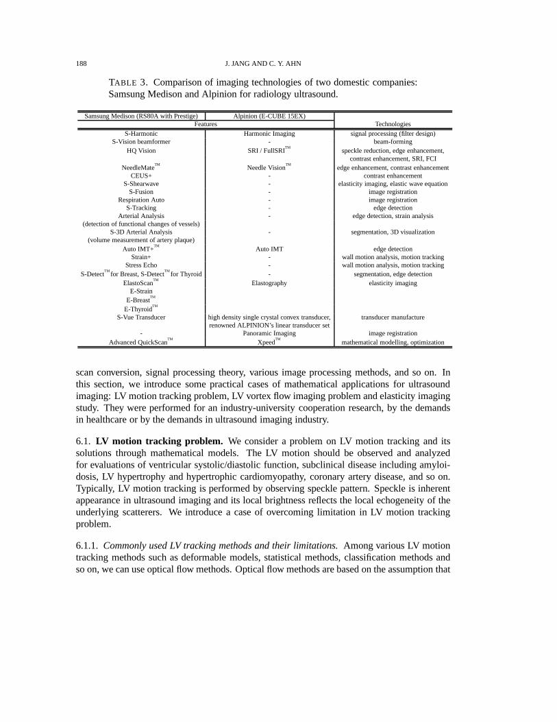
According to radiology applications, the imaging featuresof RS80A with Prestige and E-CUBE 15EX are listed in Table 3. Among the imaging features, S-Shearwave, S-Fusion andRespiration Auto are added imaging features for radiology ultrasound imaging. S-Shearwavecomputes the propagate velocity of the shearwave through the targeted lesion using elastic waveequation, while S-Fusion and Respiration Auto are based on image registration methods. S-Fusion enables simultaneous localization of a lesion with areal-time ultrasound in conjunctionwith other 3D volumetric imaging modalities. Unlike the conventional image fusion technol-ogy, Samsung offers a quicker and more precise registrationprocess. Respiration Auto featureminimizes registration differences between the inhaled CTand exhaled ultrasound scan imagesby generating compensated exhaled CT image.
6. APPLICATION CASES OFMATHEMATICS
As shown in the previous sections, mathematics is widely used in ultrasound imaging. Fromthe understanding of wave propagation and its scattering, beam-forming algorithms, digital
188 J. JANG AND C. Y. AHN
TABLE 3. Comparison of imaging technologies of two domestic companies:Samsung Medison and Alpinion for radiology ultrasound.
Samsung Medison (RS80A with Prestige) Alpinion (E-CUBE 15EX)Features Technologies
S-Harmonic Harmonic Imaging signal processing (filter design)S-Vision beamformer - beam-forming
HQ Vision SRI / FullSRITM
speckle reduction, edge enhancement,contrast enhancement, SRI, FCI
NeedleMateTM
Needle VisionTM
edge enhancement, contrast enhancementCEUS+ - contrast enhancement
S-Shearwave - elasticity imaging, elastic wave equationS-Fusion - image registration
Respiration Auto - image registrationS-Tracking - edge detection
Arterial Analysis - edge detection, strain analysis(detection of functional changes of vessels)
S-3D Arterial Analysis - segmentation, 3D visualization(volume measurement of artery plaque)
Auto IMT+TM
Auto IMT edge detectionStrain+ - wall motion analysis, motion tracking
Stress Echo - wall motion analysis, motion trackingS-Detect
TMfor Breast, S-Detect
TMfor Thyroid - segmentation, edge detection
ElastoScanTM
Elastography elasticity imagingE-Strain
E-BreastTM
E-ThyroidTM
S-Vue Transducer high density single crystal convex transducer, transducer manufacturerenowned ALPINION’s linear transducer set
- Panoramic Imaging image registrationAdvanced QuickScan
TMXpeed
TMmathematical modelling, optimization
scan conversion, signal processing theory, various image processing methods, and so on. Inthis section, we introduce some practical cases of mathematical applications for ultrasoundimaging: LV motion tracking problem, LV vortex flow imaging problem and elasticity imagingstudy. They were performed for an industry-university cooperation research, by the demandsin healthcare or by the demands in ultrasound imaging industry.
6.1. LV motion tracking problem. We consider a problem on LV motion tracking and itssolutions through mathematical models. The LV motion should be observed and analyzedfor evaluations of ventricular systolic/diastolic function, subclinical disease including amyloi-dosis, LV hypertrophy and hypertrophic cardiomyopathy, coronary artery disease, and so on.Typically, LV motion tracking is performed by observing speckle pattern. Speckle is inherentappearance in ultrasound imaging and its local brightness reflects the local echogeneity of theunderlying scatterers. We introduce a case of overcoming limitation in LV motion trackingproblem.
6.1.1. Commonly used LV tracking methods and their limitations.Among various LV motiontracking methods such as deformable models, statistical methods, classification methods andso on, we can use optical flow methods. Optical flow methods arebased on the assumption that

INDUSTRIAL MATHEMATICS IN ULTRASOUND IMAGING 189
that the intensity of a moving object is constant over time. Let I(r, t) represent the intensityof echocardiography at the locationr = (x, y) and the timet. Then the noisy time-varyingimagesI(r, t) approximately satisfy
u(r, t) · ∇I(r, t) +∂
∂tI(r, t) ≈ 0, (6.1)
whereu(r, t) is the velocity or displacement vector to be estimated. Especially, Lucas andKanade [48] used the locally constant motion to compute the velocity u(r0, t) at a targetlocation r0 = (x0, y0) and timet by forcing constant velocity in a local neighborhood ofr0 = (x0, y0) denoted byN (r0). Following them, Barronet al. [49] proposed an improvedmodel to estimate the velocityu(r0, t) by minimizing the weighted least square criterion in theneighborhoodN (r0):
u(r0, t) := argminu
∫
N (r0)
[
w(r− r0)
(
u(r, t) · ∇I(r, t) +∂
∂tI(r, t)
)2]
dr, (6.2)
wherew is a weight function.On the other hand, region-based method (also known as the block matching or pattern match-
ing method) can be also used as the LV motion tracking. Duanet al. [50] used the region-basedmethod with cross-correlation coefficient as similarity measure as follows. For given two con-secutive imagesI(·, t) andI(·, t +∆t), the displacementu(r, t) at each positionr and timetis estimated by maximizing the cross-correlation coefficient:
u(r0, t) := argmaxu
∫
N (r0)[I(r, t)I(r + u, t+∆t)]dr
√
∫
N (r0)[I(r, t)]2dr
√
∫
N (r0)[I(r+ u, t+∆t)]2dr
. (6.3)
However, there often exist some incorrectly tracked pointsin practical environment due to ul-trasound artifacts, dropouts, or shadowing phenomena of cardiac wall [51]. It is problematicto track the LV border in ultrasound images with unclear speckle pattern or weak signals. Inorder to overcome this problems, Ahn [52] proposed a mathematical model for robust myocar-dial border tracking by considering an affine transformation to describe a global motion that issynthesized by integrating local deformations.
6.1.2. A mathematical modelling for robust LV tracking.We denote the LV border traced atinitially selected frame by a parametric contourC∗ = r∗(s) = (x∗(s), y∗(s)) | 0 ≤ s ≤ 1that can be identified as itsn tracking pointsr∗1 = r
∗(s1), · · · , r∗n = r
∗(sn). Here,0 =s1 < s2 < · · · < sn = 1. Let C(t) = r(s, t) = (x(s, t), y(s, t)) | 0 ≤ s ≤ 1 bethe contour deformed fromC(0) = C∗ at time t. The motion of the contourC(t) will bedetermined by an appropriately chosen velocityU(t) indicating a time change of trackingpoints(r1(t), · · · , rn(t)):
U(t) :=
1(t)...
n(t)
=
d
dt
r1(t)...
rn(t)
with
r1(0)...
rn(0)
=
r∗1...r∗n

190 J. JANG AND C. Y. AHN
Here, we identify the contourC(t) with tracking points(r1(t), · · · , rn(t)). We computeU(t)for each timet by minimizing the following energy functional reflecting local-to-global defor-mation:
Et(U) :=1
2
n∑
i=1
∫
N (ri(t))w(r′ − ri(t))
ui · ∇I(r′, t) + ∂∂tI(r
′, t)2
dr′
+λ
∣
∣
∣
∣
ri(t) + ui −
[
a1(U) a2(U)a3(U) a4(U)
]
r∗i −
[
a5(U)a6(U)
]∣
∣
∣
∣
2
(6.4)
whereλ is a nonnegative parameter and the affine coefficientsa1(U), · · · , a6(U) at timet aregiven by
a1(U) a3(U)a2(U) a4(U)a5(U) a6(U)
=(
Φ(C∗)TΦ(C∗))−1
Φ(C∗)T
(r1(t) + u1)T
...(rn(t) + un)
T
, Φ(C∗) :=
r∗1T 1...
...r∗nT 1
.
This study has been performed as an industry-university cooperation research. Based on theproposed model, LV tracking methods of improved performance are being developed.
6.2. A new imaging mode: vortex flow imaging. Vortex flow imaging has recently attractedmuch attention as a new application for evaluating blood flow[53–55], because it visualizesand quantifies time-varying blood flow inside LV using available ultrasound data. It has shownthe potential possibility and availability for evaluatingblood flow. In order to compute thevelocity fields of blood flow, it is required to model blood flowbased on fluid equation.
6.2.1. A reconstruction problem of blood flow.With echo-PIV(particle image velocimetry)[56, 57] being representative, there are several methods tocompute and visualize the velocityfields of blood flow inside LV. Echo-PIV is based on optical flowmethods tracking the specklepatterns of blood flow to estimate blood motion. However, Echo-PIV is not completely nonin-vasive because it requires the intravenous injection of a contrast agent to obtain images suitablefor the speckle tracking algorithm. To develop less invasive techniques, methods to reconstructblood flows from color Doppler images have been proposed [58–63]. We represent mathe-matical models to reconstruct the velocity of blood flow, especially using color Doppler datareflecting one-directional velocity components of blood flow along scanlines.
6.2.2. A mathematical modelling of 3D blood flow.Let D be a 3D imaging domain,Ω(t) atime-varying LV region satisfyingΩ(t) ⊆ D ⊆ R
3, andT a beat cycle. For the beat cycleT ,we consider a spatial-temporal domainΩT defined byΩT :=
⋃
0<t<T
Ω(t)× t ⊆ D × (0, T ).
Let v(r, t) be a velocity field of the blood flow inΩt ∈ ΩT at timet. Then the fluid equationsgoverning the blood flowv is given by the 3D incompressible Navier-Stokes equations:
ρ
(
∂v
∂t+ v · ∇v
)
= −∇p+ µ∇2v in Ωt,
∇ · v = 0 in Ωt.
(6.5)

INDUSTRIAL MATHEMATICS IN ULTRASOUND IMAGING 191
In order to solve (6.5), we need proper boundary conditions or some conditions based onultrasound measurement data as follows:
Let a(r) be scanline directional unit vector at the positionr ∈ D andD(r, t) color Dopplerimage inΩt. GivenD(r, t), we then consider an inverse problem to find a 3D vector fieldv = (u, v, w) satisfying the following condition:
a(r) · v(r, t) = D(r, t). (6.6)
However, in clinical practice, it is currently very difficult to acquire 3D color Doppler imagesgiven by (6.6). A mathematical model appropriate to the measurements on 2D ultrasoundimaging should be considered.
6.2.3. A reconstruction model with mass-source term.Janget al. [64] suggested a 2D re-construction model using incompressible Navier-Stokes equations with mass-source terms toreflect 3D motion of blood flow as the following: LetD be a 2D imaging domain andΩ(t)the cross-section of the LV region in the A3CH view so that they satisfyΩ(t) ⊆ D ⊆ R
2 andv(x, t) = (u(x, t), v(x, t)) the velocity fields of flow at the positionx ∈ D and timet. Thenthe fluid equations governing the blood flow on the imaging planeD are modeled as
∂u
∂t+ u
∂u
∂x+ v
∂u
∂y= −
1
ρ
∂p
∂x+
µ
ρ∇2u+
µ
3ρ2∂s
∂x,
∂v
∂t+ u
∂v
∂x+ v
∂v
∂y= −
1
ρ
∂p
∂y+
µ
ρ∇2v +
µ
3ρ2∂s
∂y,
∂u
∂x+
∂v
∂y=
s
ρ,
(6.7)
We note that this model (6.7) is equivalent to a 2D incompressible flow having a source-sinkdistributions(x, t) [65]. In order to solve (6.7), we consider color Doppler images measuredpractically in the imaging planeD. We set the 3D coordinate system for thexy-plane to containΩ(t) and thez-axis to be normal to this plane. LetD(x, t) be the measured color Doppler data,expressed as the inner product of the scanline vector and thevelocity vector
D(x, t) = (a1(x), a2(x)) · (u(x, t), v(x, t)). (6.8)
Therefore, we obtain a mathematical problem to findv satisfying (6.7) and (6.8) simultane-ously. Some numerical simulations are performed for solving the given problem and validatingthe proposed mathematical model.
6.3. Acoustic radiation force-based elastography.Acoustic radiation force(ARF) is causedby absorbed ultrasound wave energy while ultrasound wave propagates through soft tissues.The absorbed energy accumulates in tissue and it generates volume force in the propagationdirection of ultrasound beam. This ARF technique enables inducing stress at desired positionand measuring response to the stress with a single ultrasound system, whereas other elastogra-phy techniques require manual push or additional devices toinduce stress or shear waves [66].We consider ARF-based shear wave elasticity imaging (SWEI)that maps tissue elasticity by

192 J. JANG AND C. Y. AHN
measuring the propagation speed of shear waves generated byARF. The propagation speedcis expressed as
c =
√
µ
ρ,
whereµ andρ are the shear modulus and density of tissue, respectively. We note that tissueelasticity can be quantified by estimatingc.
FIGURE 5. A description of elasticity imaging using shear wave. Thepropa-gation of shear wave is observed through ultrasound images,acquired from aresearch ultrasound system E-CUBE 12R (Alpinion, Korea).
6.3.1. Mathematical model.An inverse problem for ARF-based ultrasound elastography is toreconstruct the shear modulusµ from the measured axial movementw which satisfies
ρ∂2w
∂t2= µ∇2w + fz in R
3 × (0, T ), (6.9)
wherefz is induced ARF in the axial direction, that is, the vertical direction in imaging planesshown in Fig. 5. Note that the excitationfz and the induced displacementw are not time-harmonic. Let supp(fz) be the support offz in the spatio-temporal domain. Then, we assumethat supp(fz) is given because it is possible to change a focal point for inducing ARF. More-over, we assume thatfz = 0 out of supp(fz) to avoid the difficulty in quantifyingfz dueto the uncertainty of medium [67]. Then, the inverse problemis formulated as a problem toreconstruct the shear modulusµ from the measured axial movementw satisfying
ρ∂2w
∂t2= µ∇2w in (R3 × (0, T )) \ supp(fz). (6.10)

INDUSTRIAL MATHEMATICS IN ULTRASOUND IMAGING 193
Nightingaleet al. [68] suggested the algebraic inversion of the equation in (6.10) to estimateµρ :
µ
ρ=
∂2w∂t2
∇2w(6.11)
However, it could be unstable since numerical approximation of second-order derivatives in(6.10) are sensitive to noise. In many approaches, wave propagation speed is estimated bycomputingµ
ρ instead of the direct inversion [46,47,69].
t
w(r, t)
r
A
B
C
Tx
Tz
c =cxcz
√
c2x + c2zcx =
|rA − rB|
Txcz =
|rA − rC |
Tz
Wavefronts
A B
C
c
cx
cz
FIGURE 6. Illustration of time delaysTx and Tz for estimating the lateralspeedcx and axial speedcz of shear wave propagation.
We consider time delay to estimate the shear wave propagation speed. As shown in Fig. 6,let Tx be the time delay, that is, the difference between arrival times of the displacement signalby shear wave propagation at two positionsA andB placed on a lateral line. Then the shearwave propagation speedcx in the lateral direction is given by
cx =|rA − rB |
Tx, (6.12)
whererA andrB are the coordinates ofA andB, respectively. Therefore,Tx is computed by
Tx = arg maxτ∈(0,T )
∫ T
0w(x1, t)w(x2, t− τ)dt. (6.13)
Since the wave propagation direction may not be parallel to the lateral direction (Fig. 6) inmany cases of ARF-based excitation, we deal with the shear wave propagation speedcz in theaxial direction. Likewise, letTz be the time delay, that is, the difference between arrival times

194 J. JANG AND C. Y. AHN
of the displacement signal by shear wave propagation at two positionsA andC placed on aaxial line. Thencz is expressed as
cz =|rA − rC |
Tz, (6.14)
whererC is the coordinate ofC. From cx and cz, we can compute the propagation speedvelocity c [70]:
c =cxcy
√
c2x + c2z. (6.15)
t
w(r, t)
r
Soft
Hard
Softt = T (r)
Wav
epr
opag
ation
r
FIGURE 7. A simple description of TOF approach. The disturbance of bluecurve corresponds to the displacement at offset from the source. Arrival timeof the wave-front is tracked by the red line.
6.3.2. Eikonal equation-based approaches.As illustrated in Fig. 7, wave propagation speedcan be estimated from the slope between offset position and arrival time of wave-front. Thepropagation speedc can be estimated by the gradient of arrival timeT using the Eikonal equa-tion [71]:
|∇T | =1
c, (6.16)
whereT (r) is defined by
T (r) = inft > 0 : |w(r, t)| > 0. (6.17)
In a realistic case,T (r) is estimated by using a fixed thresholdδ above a noise level of theestimatedw(r, t) [72]:
T (r) ≈ inft > 0 : |w(r, t)| > δ. (6.18)
As an alternative way, the biased cross-correlationC is suggested by McLaughlinet al. [73]
T (r) ≈ arg maxτ∈(0,T )
1
T
∫ T
0w(rref, t)w(r, t− τ)dt for rref a reference point, (6.19)

INDUSTRIAL MATHEMATICS IN ULTRASOUND IMAGING 195
where
w(r, t) =
w(r, t) if 0 ≤ t ≤ T,
w(r, t − T ) if t ≥ T,
w(r, t + T ) if t ≤ 0.
(6.20)
7. CURRENT HOT TOPICS ANDCHALLENGING ISSUES
In this section, we introduce current hot topics in ultrasound imaging, especially in thedomestic ultrasound industry. Samsung Medison, a global medical equipment company and aleading domestic company, has recently published some white papers [74–80] on: S-Detect
TM,
5D CNS, E-ThyroidTM
, E-BreastTM
(breast ElastoScanTM
), S-Shearwave, Aterial Analysis, andso on. The white papers report the advantages and shortcomings of each technology.
7.1. Hot topics in ultrasound imaging.
• S-DetectTM
is a software analyzing the features of lesions and assessing the possibilityof malignancy. It uses a machine learning-based algorithm [81]. By showing excellentagreement of91.2% with the assessment of breast dedicated radiologist in interpretingthe breast mass, it is suggested as a good decision-making support for the beginnersor non-breast radiologists. However, with the sensitivityof 84.6% at the same time, itmissed two breast cancers of relatively circumscribed isoechoic and hypoechoic masseswith suspicious clinical findings. Therefore, it is reported that circumscribed malignantmasses may be remained as the limitation of S-Detect
TMand S-Detect
TMis not available
to find subtle suspicious features [74].• A semi-automatic method is proposed for biometric measurements of fetal central ner-
vous system(CNS) from 3D ultrasound volume data of brain. Itreduce the number ofoperations and examination time. Its high success rate>90% is reported under clinicalevaluation [75].
• E-ThyroidTM
uses carotid artery pulsation, not external compression byfree hands, as acompression source. While E-Thyroid
TMeffectively differentiates malignant from be-
nign in most thyroid nodules including calcified nodule, theextreme location of a nod-ule in the tyroid can affect the results [76].
• E-BreastTM
is helpful for characterizing different regions as a complementary diagnosticimaging technology, based on strain imaging technique. However, it would be impor-tant not to evaluate a lesion from an isolated manner with strain ratio generated fromE-Breast
TM[77].
• S-Shearwave is a technology enabling quantitative analysis of tissue stiffness for as-sessing liver fibrosis. Unlike the color map used in the conventional elasticity imaging,S-Shearwave displays the stiffness value and Reliable Measurement Index(RMI) forthe region of interest [78].
Among them, S-DetectTM
, 5D CNS and Aterial Analysis are CADe/CADx softwares. Thereare numerous demands of CADe and CADx for many medical imaging methodologies [82–85]as well as ultrasound [86–88]. According to the applications, CADe is implemented by various

196 J. JANG AND C. Y. AHN
image processing methods: histogram-based thresholding and active contours for segmentinganomaly [83], neural network-based approaches for robust segmentation [89–91]. In the lit-eratures [86, 87], it is reported that neural network and support vector machine techniques areused for CADx.
On the other hand, currently commercialized elasticity imaging modes:E-ThyroidTM
, E-Breast
TM, S-Shearwave [76–78] are commonly used as a complementary diagnostic tool. It
is required to quantify more accurately the stiffness of tissues.Fusion imaging techniques have been used for volume navigation of 2D ultrasound images
within other 3D CT or MR images. In order to register different images acquired from med-ical imaging modalities, the fusion imaging techniques have been developed with the help oflandmarks, position sensors, or electromagnetic needle tracking [92–94]. As real-time 3D ul-trasound imaging becomes feasible, fusion imaging technique for 3D volume data is consideredas a promising tool for computer-aided surgery [94–96]. In 3D fusion imaging, external devicessuch as landmarks, position sensors or electromagnetic needle tracking can be removed [97,98].Samsung Medison developed the fusion imaging techniques called S-Fusion.
Additionally, we introduce some issues in ultrasound imaging, related to mathematical mod-elling, numerical solutions, image processing and visualization.
7.2. Issues on LV tracking methods.
• Real-time 3D ultrasound imaging is capable of providing good 3D visualization of or-gans. However, its resolution is not good enough to discriminate features smaller thana few millimeters and LV tracking methods based on speckles are not appropriate tobe applied to 3D ultrasound images. We can consider 3D LV tracking by constructingthe motion of 3D LV shape from 2D LV borders, which are extracted by applying LVtracking methods to multiple 2D echocardiography data. Howcan we model the rela-tionship between the change of LV borders observed on 2D echocardiography and the3D LV shape?
• LV motion tracking methods include inevitable limitation on 2D echocardiographybecause of the helical structure of cardiac ventricular anatomy. For a heartbeat cycle,it is difficult to track a portion of LV border designated at the initial stage on a 2Dultrasound image. In fact, it gets out of the imaging plane. How can we model therelationship between the change of LV borders observed on 2Dechocardiography andthe 3D helical behavior of cardiac motion?
7.3. Issues on vortex flow imging.
• Vortex flow imaging consists of defining LV geometry from echocardiographic imagesand reconstructing the velocity field of blood flow in the moving LV region. Let usassume that the acquisition of 3D color Doppler imaging at high frame rate is available.Can we model an inverse problem for reconstructing the 3D velocity field of blood flowfrom the partial velocity information obtained through the3D color Doppler images?[99].

INDUSTRIAL MATHEMATICS IN ULTRASOUND IMAGING 197
7.4. Issues on elasticity imaging.
• Inherent low SNR of the estimatedw makes the direct inversion (6.11) difficult so thatmany models reconstructingc are based on the time-of-flight(TOF)-based approaches.However, they do not fully guarantee stability in practicalsituations since the inverseof time-delay or|∇T | are still necessary for the speed estimation. In order to overcomethe problem, Wanget al. suggest a fitting model for the estimatedT (r) [100]
T (r) = β · r+ t0, (7.1)
wheret0 is a fitting parameter andβ a fitting parameter vector satisfying
|β| = c. (7.2)
However, in inhomogeneous medium, the fitting model (7.1) could not describeT (r)properly because refraction on the boundary between different tissues makes non-lineardistortion of arrival-time. We need a modified fitting model for T (r) which assumesthe presence of anomaly.
8. CONCLUSION
Ultrasound imaging industry is very promising in terms of technology advancements as wellas the market size and growth. Like in other industries, the ultrasound imaging technologieshave been advanced and innovated throughMathematics. In this article, we described the his-tory of ultrasound imaging, its basic principle, its diagnostic applications, domestic-industrialproducts, practical use of mathematics, hot topics and challenging issues related to ultrasoundimaging. Through them, we confirmed thatMathematicshas been used commonly as mathe-matical modelling, numerical solutions and visualization, combined with science, engineeringand medicine in ultrasound imaging.
The practical use ofMathematicsin ultrasound imaging requires the understanding of humanbody and imaging system overall. Based on that understanding, we should perform physics-based mathematical modelling, deal with the measurement data acquired through ultrasoundimaging systems and solve various problems and challengingissues in ultrasound imaging.
Currently, there are still numerous demands of technology advancements in healthcare andultrasound imaging industry, especially in domestic ultrasound industry. As we have seen be-fore, Mathematicscan contribute to the advances and innovation of ultrasoundimaging tech-nology. We hope many mathematicians contribute much to ultrasound technology innovation.
ACKNOWLEDGEMENTS
This work was supported by the National Institute for Mathematical Sciences(NIMS) andthe National Research Foundation of Korea (NRF) grants funded by the Korea government(No.NRF-20151009350). We would like to thank reviewers for their detailed comments and sug-gestions to improve the paper. Also, we thank Haeeun Han for her help with rendering theTOC art.

198 J. JANG AND C. Y. AHN
REFERENCES
[1] Medical Equipment Market Size & Growth - Diagnostic Imaging[Ultrasound Systems] Market,Global 2006-2013, USD Constant Millions, Global Data, https://medical.globaldata.com.
[2] Medical Equipment Market Size & Growth - Diagnostic Imaging[Ultrasound Systems] Market,Global 2013-2020, USD Constant Millions, Global Data, https://medical.globaldata.com.
[3] Medical Equipment Market Size & Growth - Diagnostic Imaging[Ultrasound Systems] Company Shaare ByPercentage,Global 2012, USD Constant Millions, Global Data, https://medical.globaldata.com.
[4] T. Szabo,Diagnostic Ultrasound Imaging: Inside Out, Academic Press, Boston University, 2004.[5] D. H. Evans and W. N. McDicken,Doppler Ultrasound - Physics, Instrumentation and Signal Processing,
2nd ed., John Wiley and Sons, New York, 2000.[6] J. Woo, A short history of the developments of ultrasound in obstetrics and gynecology.http://www.ob-
ultrasound.net/hydrophone.html, 1999.[7] A.M. King, Development, advances and applications of diagnostic ultrasound in animals, The Veterinary
Journal,1713 (2006), 408–420.[8] J. Curie and P. Curie,Development par pression de l’ectricite polaire dans les cristaux hemidres a faces
inclinees, Compte Rendue de l’ Acadamie Scientifique,91 (1880), 294–295.[9] K. T. Dussik,Über die Möglichkeit, hochfrequente mechanische Schwingungen als diagnostisches Hilfsmittel
zu verwerten, Zeitschrift für die gesamte Neurologie und Psychiatrie,174(1) (1942), 153–168.[10] G. D. Ludwig and F. W. Struthers,Considerations underlying the use of ultrasound to detect gall stones and
foreign bodies in the tissues, United States Navy Medical Research Institute Report,4 (1949), 1–27.[11] I. Donald, J. Macvicar and T. G. Brown,Investigation of abdominal masses by pulsed ultrasound, Lancet,1
(1958), 1189–1195.[12] Y. Nimura, History of pulse and echo Doppler ultrasound in Japan, Cardiac Doppler Diagnosis, Martimus
Nijoff Publishers, Boston, 1983.[13] R. W. J. Felix, B. Sigel, R. J. Gibson, J. Williams and G. L. Popky,Pulsed Doppler ultrasound detection of
flow disturbances in arteriosclerosis, J. Clin. Ultrasound,4(4) (1976), 275–282.[14] D. S. Evans and F. B. Cockett,Diagnosis of deep-vein thrombosis with an ultrasonic Doppler technique, Br.
Med. J.,2 (1969), 802–804.[15] P. N. T. Wells,A range-gated ultrasonic Doppler system, Medical and Biological Engineering,7(6) (1969),
641–652.[16] G. R. Curry and D. N. White,Color coded ultrasonic differential velocity arterial scanner (Echoflow), Ultra-
sound Med. Biol.,4 (1978), 27–35.[17] B. Sigel,A brief history of Doppler ultrasound in the diagnosis of peripheral vascular disease, Ultrasound
Med. Biol.,24(2) (1998), 169–176.[18] J. F. Brinkley, S. K. Muramatsu, W. D. McCallum and R. L. Popp,In vitro evaluation of an ultrasonic three-
dimensional imaging and volume system, Ultrasonic Imaging,4(2) (1982), 126–139.[19] K. Baba, K. Satoh, S. Sakamoto, T. Okai and S. Ishii,Development of an ultrasonic system for three-
dimensional reconstruction of the fetus, Journal of Perinatal Medicine-Official Journal of the WAPM, 17(1)(1989), 19–24.
[20] J. Deng, J. E. Gardener, C. H. Rodeck and W. R. Lees,Fetal echocardiography in three and four dimensions,Ultrasound Med. Biol.,22(8) (1996), 979–986.
[21] S. L. Kobal, S. S. Lee, R. Willner, F. E. A. Vargas, H. Luo,C. Watanabe, Y. Neuman, T. Miyamoto andR. J. Siegel,Hand-carried cardiac ultrasound enhances healthcare delivery in developing countries, Am. J.Cardiol.,94(4) (2004), 539-541.
[22] H. Shmueli, Y. Burstein, I. Sagy, Z. H. Perry, R. Ilia, Y.Henkin, T. Shafat, N. Liel-Cohen and S. L.Kobal, Briefly Trained Medical Students Can Effectively Identify Rheumatic Mitral Valve Injury Using aHand?Carried Ultrasound, Echocardiography,30(6) (2013), 621–626.
INDUSTRIAL MATHEMATICS IN ULTRASOUND IMAGING 199
[23] J. S. Shanewise, A. T. Cheung, S. Aronson, W. J. Stewart,R. L. Weiss, J. B. Mark, R. M. Savage, P. Sears-Rogan, J. P. Mathew, M. A. Quiñones, M. K. Cahalan MK and J. S. Savino, ASE/SCA guidelines for per-forming a comprehensive intraoperative multiplane transesophageal echocardiography examination: recom-mendations of the American Society of Echocardiography Council for Intraoperative Echocardiography andthe Society of Cardiovascular Anesthesiologists Task Force for Certification in Perioperative TransesophagealEchocardiography, Anesth. Analg.,89(4) (1999), 870–884.
[24] H. F. Andersen,Transvaginal and transabdominal ultrasonography of the uterine cervix during pregnancy,Journal of Clinical Ultrasound,19(2) (1991), 77–83.
[25] J. A. Jensen, D. Gandhi and W. D. O’Brien,Ultrasound fields in an attenuating medium, Proceedings of theIEEE 1993 Ultrasonics Symposium, 1993.
[26] A. Macovski,Ultrasonic imaging using arrays, Proceedings of the IEEE, 1979.[27] J. A. Jensen,A Model for the Propagation and Scattering of Ultrasound in Tissue, J. Acoust. Soc. Am.,89
(1991), 182–191.[28] J. A. Jensen and N. B. Svendsen,Calculation of pressure fields from arbitrarily shaped, apodized, and excited
ultrasound transducers, IEEE Trans. Ultrason., Ferroelec., Freq. Contr.,39 (1992), 262–267.[29] J. A. Jensen,Field: A Program for Simulating Ultrasound Systems, the 10th Nordic-Baltic Conference on
Biomedical Imaging Published in Medical & Biological Engineering & Computing,34 (1996), 351–353.[30] AIUM, AIUM Practice Parameter for the Performance of Obstetric Ultrasound Examinations,
http://www.aium.org/resources/guidelines/obstetric.pdf, 2013.[31] R. Rastogi, G. L. Meena, N. Rastogi and V. Rastogi,Interstitial ectopic pregnancy: A rare and difficult
clinicosonographic diagnosis, J. Hum. Reprod. Sci.,1(2) (2008), 81–82.[32] L. F. Gonçalves, W. Lee, J. Espinoza and R. Romero,Three-and 4-Dimensional Ultrasound in Obstetric Prac-
tice Does It Help?, J. Ultrasound Med.,24(12) (2005), 1599–1624.[33] N. J. Dudley,A systematic review of the ultrasound estimation of fetal weight, Ultrasound Obstet. Gynecol.,
25(1) (2005), 80–89.[34] S. Feng, K. S. Zhou and W. Lee,Automatic fetal weight estimation using 3D ultrasonography, Proceedings of
Medical Imaging 2012: Computer-Aided Diagnosis, California, USA 2012.[35] I.-W. Lee, C.-H. Chang, Y.-C. Cheng, H.-C. Ko and F.-M. Chang,A review of three-dimensional ultrasound
applications in fetal growth restriction, Journal of Medical Ultrasound,20(3) (2012), 142–149.[36] S. Yagel, S. M. Cohen, I. Shapiro and D. V. Valsky,3D and 4D ultrasound in fetal cardiac scanning: a new
look at the fetal heart, Ultrasound Obstet. Gynecol.,29(1) (2007), 81–95.[37] B. Messing, S. M. Cohen, D. V. Valsky, D. Rosenak, D. Hochner-Celnikier, S. Savchev and S. Yagel,Fetal
cardiac ventricle volumetry in the second half of gestationassessed by 4D ultrasound using STIC combinedwith inversion mode, Ultrasound Obstet. Gynecol.,30(2) (2007), 142–151.
[38] H. Laurichesse–Delmas, O. Grimaud, G. Moscoso and Y. Ville, Color Doppler study of the venous circula-tion in the fetal brain and hemodynamic study of the cerebraltransverse sinus, Ultrasound in Obstetrics andGynecology,13(1) (1999), 34–42.
[39] R. K. Pooh and K. Pooh, K,.Transvaginal 3D and Doppler ultrasonography of the fetal brain, Seminars inperinatology 2001,25(1) (2001), 38–43.
[40] W. Sepulveda, I. Rojas, J. A. Robert, C. Schnapp and J. L.Alcalde,Prenatal detection of velamentous insertionof the umbilical cord: a prospective color Doppler ultrasound study, Ultrasound in obstetrics & gynecology,21(6) (2003), 564–569.
[41] D. E. Fitzgerald and J. E. Drumm,Non-invasive measurement of human fetal circulation usingultrasound: anew method, Br. Med. J.,2(6100) (1977), 1450–1451.
[42] A. Dall’Asta, G. Paramasivam, C. C. Lees,Crystal Vue technique for imaging fetal spine and ribs, Ultrasoundin Obstetrics & Gynecology ,47(3) (2016), 383–384.
[43] T. Reynolds,The Echocardiographer’s Pocket Reference, 4th Edition, Arizona Heart Institute, Phoenix, Ari-zona, USA, 2013.

200 J. JANG AND C. Y. AHN
[44] E. G. Grant, C. B. Benson, G. L. Moneta, A. V. Alexandrovet al., Carotid artery stenosis: gray-scaleand Doppler US diagnosis–Society of Radiologists in Ultrasound Consensus Conference, Radiology,229(2)(2003), 340–346.
[45] A. T. Stavros, D. Thickman, C. L. Rapp, M. A. Dennis, S. H.Parker and G. A. Sisney,Solid breast nodules:use of sonography to distinguish between benign and malignant lesions, Radiology,196(1) (1995), 123–134.
[46] M. L. Palmeri, M. H. Wang, J. J. Dahl, K. D. Frinkley and K.R. Nightingale,Quantifying hepatic shearmodulus in vivo using acoustic radiation force, Ultrasound in Medicine & Biology,34(4) (2008), 546–558.
[47] M. Tanter, J. Bercoff, A. Athanasiou, T. Deffieux, J.-L.Gennisson, G. Montaldo, M. Muller, A. Tardivonand M. Fink,Quantitative assessment of breast lesion viscoelasticity: initial clinical results using supersonicshear imaging, Ultrasound in Medicine & Biology,34(9) (2008), 1373–1386.
[48] B. Lucas, T. Kanade,An iterative image restoration technique with an application to stereo vision, Proceedingsof DARPA IU Workshop, (1981), 121–130.
[49] J. L. Barron, D. J. Fleet, S. S. Beauchemin,Performance of optical flow techniques, Int. J. Comput. Vision,12(1) (1994), 43–77.
[50] Q. Duan, E. D. Angelini, S. L. Herz, C. M. Ingrassia, K. D.Costa, J. W. Holmes, S. Homma and A. F. Laine,Region-Based Endocardium Tracking on Real-Time Three-Dimensional Ultrasound, Ultrasound Med. Biol.,35(2) (2009), 256–265.
[51] K. Y. E. Leung, M. G. Danilouchkine, M. van Stralen, N. deJong, A. F. van der Steen and J. G. Bosch,Left ventricular border tracking using cardiac motion models and optical flow, Ultrasound Med. Biol.,37(4)(2011), 605–616.
[52] C. Y. Ahn, Robust Myocardial Motion Tracking for Echocardiography: Variational Framework IntegratingLocal-to-Global Deformation, Computational and Mathematical Methods in Medicine,2013(2013), 974027.
[53] G.-R. Hong, G. Pedrizzetti, G. Tonti, P. Li, Z. Wei, J. K.Kim, A. Baweja, S. Liu, N. Chung, H. Houle, J.Narula, and M. A. Vannan,Characterization and Quantification of Vortex Flow in the Human Left Ventricleby Contrast Echocardiography Using Vector Particle Image Velocimetry, JACC: Cardiovascular Imaging,1(6)(2008), 705-717.
[54] P. P. Sengupta, G. Pedrizzetti, P. J. Kilner, A. Kheradvar, T. Ebbers, G. Tonti, A. G. Fraser and J. Narula,Emerging Trends in CV Flow Visualization, JACC: Cardiovascular Imaging,5(3) (2012), 305-316.
[55] D. R. Muñoz, M. Markl, J. L. Moya Mur, A. Barker, C. Fernández-Golfin, P. Lancellotti and J. L. Z. Gómez,Intracardiac flow visualization: current status and futuredirections, European Heart Journal- CardiovascularImaging,14 (2013), 1029-1038.
[56] H. Gao, P. Claus, M.-S. Amzulescu, I. Stankovic, J. D’Hooge and J.-U. Voigt,How to optimize intracardiacblood flow tracking by echocardiographic particle image velocimetry? Exploring the influence of data ac-quisition using computer-generated data sets, European Heart Journal Cardiovascular Imaging,13(6) (2012),490-499.
[57] H. Gao, B. Heyde and J. D’Hooge,3D Intra-cardiac flow estimation using speckle tracking: a feasibility studyin synthetic ultrasound data, Proceedings of the IEEE International Ultrasonics Symposium (IUS’13), Prague,Czech Republic, July 2013.
[58] D. Garcia, J. C. Del Álamo, D. Tanné, R. Yotti, C. Cortina, É. Bertrand, J. C. Antoranz, E. Pérez-David, R.Rieu, F. Fernández-Avilés and others,Two-dimensional intraventricular flow mapping by digital processingconventional color-doppler echocardiography images,IEEE Transactions on Medical Imaging,29(10) (2010),1701–1713.
[59] S. Ohtsuki and M. Tanaka,The flow velocity distribution from the Doppler informationon a plane in three-Dimensional flow,Journal of Visualization,9(1) (2006), 69–82.
[60] M. Arigovindan, M. Suhling, C. Jansen, P. Hunziker and M. Unser,Full motion and flow field recovery fromecho Doppler data,IEEE Transactions on Medical Imaging,26(1) (2007), 31–45.
[61] A. Gomez, K. Pushparajah, J. M. Simpson, D. Giese, T. Schaeffter and G. Penney,A sensitivity analysis on 3Dvelocity reconstruction from multiple registered echo Doppler views,Medical Image Analysis,17(6) (2013),616–631.

INDUSTRIAL MATHEMATICS IN ULTRASOUND IMAGING 201
[62] A. Gomez, A. de Vecchi, M. Jantsch, W. Shi, K. Pushparajah, J. M. Simpson, N. P. Smith, D. Rueckert, T.Schaeffter and G. P. Penney,4D blood flow reconstruction over the entire ventricle from wall motion andblood velocity derived from ultrasound data,IEEE Trans. on Medical Imaging,34(11) (2015), 2298–2308.
[63] F. Mehregan, F. Tournoux, S. Muth, Pibarot, Philippe and R. Rieu, G. Cloutier and D. Garcia,Doppler vor-tography: a color doppler approach to quantification of intraventricular blood flow vortices,Ultrasound inMedicine and Biology,40(1) (2014), 210–221.
[64] J. Jang, C. Y. Ahn, K. Jeon, J. Heo, D. Lee, C. Joo, J.-i. Choi and J. K. Seo,A reconstruction method ofblood flow velocity in left ventricle using color flow ultrasound, Computational and Mathematical Methods inMedicine,2015(2015), 108274.
[65] G. K. BatchelorAn Introduction to Fluid Dynamics, Cambridge Mathematical Library, Cambridge UniversityPress, Cambridge, UK, 2000.
[66] A. Sarvazyan, T. J. Hall, M. W. Urban, M. Fatemi, S. R. Aglyamov and B. S. Garra,An overview of elastog-raphy - an emrging branch of medical imaging, Current Medical Imaging Reviews,7 (2011), 255–282.
[67] J. Bercoff, M. Tanter and M. Fink,Supersonic shear imaging: a new technique for soft tissue elasticity map-ping, IEEE Transactions on Ultrasonics, Ferroelectrics, and Frequency Control,51 (2004), 396–409.
[68] K. Nightingale, S. McAleavey and G. Trahey,Shear-wave generation using acoustic radiation force: in vivoand ex vivo results, Ultrasound in Medicine & Biology,29(12) (2003), 1715–1723.
[69] N. C. Rouze, M. H. Wang, M. L. Palmeri and K. R. Nightingale,Robust estimation of time-of-flight shear wavespeed using a radon sum transformation, IEEE Transactions on Ultrasonics, Ferroelectrics, and FrequencyControl,57(12) (2010), 2662–2670.
[70] P. Song, A. Manduca, H. Zhao, M. W. Urban, J. F. Greenleafand S. Chen,Fast shear compounding usingrobust 2-d shear wave speed calculation and multi-directional filtering, Ultrasound in Medicine & Biology,40(6) (2014), 1343–1355.
[71] L. Ji, J. R. McLaughlin, D. Renzi and J.-R. Yoon,Interior elastodynamics inverse problems: shear wave speedreconstruction in transient elastography, Inverse Problems,19(6) (2003), S1.
[72] J. McLaughlin and D. Renzi,Using level set based inversion of arrival times to recover shear wave speed intransient elastography and supersonic imaging, Inverse Problems,22(2) (2006), 707.
[73] J. McLaughlin and D. Renzi,Shear wave speed recovery in transient elastography and supersonic imagingusing propagating fronts, Inverse Problems,22(2) (2006), 681.
[74] E. Y. Ko, S-DetectTM
in Breast Ultrasound : Initial Experience, White Paper, WP201411-SMC-SDetect, Sam-sung Medison, 2014.
[75] K. Lee, J. Yoo and S. Kim,A novel semi-automatic method for biometric measurements of the fetal brain,White Paper, WP201412-5D-CNS, Samsung Medison, 2014.
[76] V. F. Duda and C. Köhler,An improved quantification tool for breast ElastoScanTM
: E-BreastTM
, White Paper,WP201503-E-Breast
TM, Samsung Medison, 2015.
[77] D. J. Lim and M. H. Kim,Experiences of Intrinsic Compression Ultrasound Elastography (E-ThyroidTM
)
in Differentiating Benign From Malignant Thyroid Nodule, White Paper, WP201504-E-ThyroidTM
, SamsungMedison, 2015.
[78] W. K. Jeong,Liver stiffness measurement using S-Shearwave : initial experience, White Paper, CS201505-S-Shearwave, Samsung Medison, 2015.
[79] J. H. Yoon, H. J. Chang, J. W. Kim and N. ChungThe value of multi-directional movement of carotid artery asa novel surrogate marker for acute ischemic stroke assessedby Arterial Analysis, White Paper, WP201506-ArterialAnalysis, Samsung Medison, 2015.
[80] A. Martegani and L. Aiani,Technological advancements improve the sensitivity of CEUS diagnostics, WhitePaper, WP201507-CEUS, Samsung Medison, 2015.
[81] Samsung Applies Deep Learning Technology to Diagnostic Ultrasound Imaging,Samsung Newsroom,https://news.samsung.com.
[82] R. A. Castellino,Computer aided detection (CAD): an overview, Cancer Imaging,5(1) (2005), 17–19.

202 J. JANG AND C. Y. AHN
[83] A. Jalalian, S. B. Mashohor, H. R. Mahmud, M. I. B. Saripan, A. R. B. Ramli and B. Karasfi,Computer-aideddetection/diagnosis of breast cancer in mammography and ultrasound: a review, Clin. Imaging,37(3) (2013),420–426.
[84] K. Doi, Computer-aided diagnosis in medical imaging: historical review, current status and future potential,Comput. Med. Imaging Graph.,31(4) (2007), 198–211.
[85] B. van Ginneken, C. M. Schaefer-Prokop and M. Prokop,Computer-aided diagnosis: how to move from thelaboratory to the clinic, Radiology,261(3) (2011), 719–732.
[86] B. Lei, E. L. Tan, S. Chen, L. Zhuo, S. Li, D. Ni and T. Wang,Automatic recognition of fetal facial standardplane in ultrasound image via fisher vector, PloS one,10(5) (2015), e0121838.
[87] S. Joo, Y. S. Yang, W. K. Moon and H. C. Kim,Computer-aided diagnosis of solid breast nodules: use of anartificial neural network based on multiple sonographic features, IEEE Trans. Med. Imaging,23(10) (2004),1292–1300.
[88] S. H. Kim, J. M. Lee, K. G. Kim, J. H. Kim, J. Y. Lee, J. K. Hanand B. I. Choi,Computer-aided image analysisof focal hepatic lesions in ultrasonography: preliminary results, Abdom. Imaging,34(2) (2009), 183–191.
[89] R. Llobet, J. C. Pérez-Cortés, A. H. Toselli and A. Juan,Computer-aided detection of prostate cancerInter-national Journal of Medical Informatics,76(7) (2007), 547–556.
[90] D. R. Chen, R. F. Chang, W. J. Kuo, M. C. Chen and Y. L. Huang, Diagnosis of breast tumors with sonographictexture analysis using wavelet transform and neural networks, Ultrasound Med. Biol.,28(10) (2002), 1301–1310.
[91] Y. L. Huang and D. R. Chen,Watershed segmentation for breast tumor in 2-D sonography, Ultrasound Med.Biol., 30(5) (2004), 625–632.
[92] D. L. Sandulescu, D. Dumitrescu, I. Rogoveanu and A. Saftoiu,Hybrid ultrasound imaging techniques (fusionimaging), World J. Gastroenterol.,17(1) (2011), 49–52.
[93] W. Wein, S. Brunke, A. Khamene, M. R. Callstrom and N. Navab,Automatic CT-ultrasound registration fordiagnostic imaging and image-guided intervention, Med. Image Anal.,12(5) (2008), 577–585.
[94] T. Lange, N. Papenberg, S. Heldmann, J. Modersitzki, B.Fischer, H. Lamecker and P. M. Schlag,3Dultrasound-CT registration of the liver using combined landmark-intensity information, Int. J. Comput. Assist.Radiol. Surg.,4(1) (2009), 79–88.
[95] M. W. Lee, Fusion imaging of real-time ultrasonography with CT or MRI for hepatic intervention, Ultra-sonography,33(4) (2014), 227–239.
[96] C. Ewertsen, A. Saftoiu, L. G. Gruionu, S. Karstrup and M. B. Nielsen,Real-time image fusion involvingdiagnostic ultrasound, Am. J. Roentgenol.,200(3) (2013), W249–W255.
[97] B. C. Porter, D. J. Rubens, J. G. Strang, J. Smith, S. Totterman and K. J. Parker,Three-dimensional registrationand fusion of ultrasound and MRI using major vessels as fiducial markers, IEEE Trans. Med. Imaging,20(4)(2001) 354–359.
[98] A. Roche, S. Pennec, G. Malandain and N. Ayache,Rigid registration of 3-D ultrasound with MR images:a new approach combining intensity and gradient information, IEEE Trans. Med. Imaging,20(10) (2001),1038–1049.
[99] J. Jang, C. Y. Ahn, J.-I. Choi and J. K. Seo,Inverse Problem for Color Doppler Ultrasound-Assisted Intracar-diac Blood Flow Imaging, Computational and Mathematical Methods in Medicine,2016(2016), 6371078.
[100] M. H. Wang, M. L. Palmeri, V. M. Rotemberg, N. C. Rouze and K. R. Nightingale,Improving the robust-ness of time-of-flight based shear wave speed reconstruction methods using ransac in human liver in vivo,Ultrasound in Medicine & Biology,36(5) (2010), 802–813.

J. KSIAM Vol.20, No.3, 203–224, 2016 http://dx.doi.org/10.12941/jksiam.2016.20.203
SORET, HALL CURRENT, ROTATION, CHEMICAL REACTION AND THERM ALRADIATION EFFECTS ON UNSTEADY MHD HEAT AND MASS TRANSFER
NATURAL CONVECTION FLOW PAST AN ACCELERATED VERTICAL PLATE
M. VENKATESWARLU1,†, D. VENKATA LAKSHMI 2, AND K. NAGA MALLESWARA RAO 3
1DEPARTMENT OFMATHEMATICS, V. R. SIDDHARTHA ENGINEERINGCOLLEGE, KANUR, KRISHNA (DIST),ANDHRA PRADESH, INDIA -520007
E-mail address: [email protected], [email protected]
2DEPARTMENT OF MATHEMATICS, BAPATLA WOMEN’S ENGINEERING COLLEGE, BAPATLA , GUNTUR
(DIST), ANDHRA PRADESH, INDIA -522102
3DEPARTMENT OF MECHANICAL ENGINEERING, V. R. SIDDHARTHA ENGINEERING COLLEGE, KANUR,KRISHNA (DIST), ANDHRA PRADESH, INDIA -520007
ABSTRACT. The heat and mass transfer characteristics of the unsteadyhydromagnetic naturalconvection flow with Hall current and Soret effect of an incompressible, viscous, electricallyconducting, heat absorbing and optically thin radiating fluid flow past a suddenly started ver-tical infinite plate through fluid saturated porous medium ina rotating environment are takeninto account in this paper. Derivations of exact analyticalsolutions are aimed under differentphysical properties. The velocity, concentration and temperature profiles, Sherwood numberand Nusselt number are easily examined and discussed via theclosed forms obtained. Soreteffect and permeability parameter tends to accelerate primary and secondary fluid velocitieswhereas hall current, radiation and heat absorption have reverse effect on it. Radiation and heatabsorption have tendency to enhance rate of heat transfer atthe plate. The results obtained heremay be further used to verify the validity of obtained numerical solutions for more complicatedtransient free convection fluid flow problems.
NOMENCLATURE
u∗ fluid velocity inx∗ direction DT thermal diffusivity t∗ timew∗ fluid velocity inz∗ direction q∗r radiating flux vector T ∗ fluid temperatureg acceleration due to gravity m hall current parameter
Received by the editors March 21 2016; Revised June 23 2016; Accepted in revised form July 8 2016; Publishedonline September 8 2016.
2000Mathematics Subject Classification.76R10, 76W05, 80A20, 80A32.Key words and phrases.MHD, Hall current, soret effect, Thermal radiation and chemical reaction.† Corresponding author.
203

204 M. VENKATESWARLU, D. VENKATA LAKSHMI, AND K. NAGA MALLES WARA RAO
K∗
1 permeability of porous medium kT thermal conductivity of the fluidB0 uniform magnetic field C∗ species concentrationcp specific heat at constant pressure Q0 heat absorption coefficientK∗
r chemical reaction parameter T ∗
w temperature of the wallC∗
w concentration of the wall T ∗
∞fluid temperature in the free stream
C∗
∞species concentration in the free streamU(t∗) time dependent velocity
a∗ mean absorption coefficient Gr thermal Grashof numberGm Solutal Grashof number Pr Prandtl numberR1 non dimensional constant Kr Chemical reaction numberR Radiation parameter K2 Rotation parameterM Magnetic parameter DM chemical molecular diffusiveSc Schmidt number K1 Permeability parameterS0 Soret number t0 characteristic timeU0 characteristic velocity
GREEK SYMBOLSρ fluid density βT coefficient of thermal expansionβC coefficient expansion for species concentrationΩ uniform angular velocityσ electrical conductivity ν kinematic coefficient of viscosityωe cyclotron frequency τe electron collision timeσ∗ Stefan–Boltzmann constant φ Heat absorption parameter
1. INTRODUCTION
In recent years, the problems of hydromagnetic free convective and heat transfer flow in aporous medium plays an important role in several scientific and industrial processes such asproblems of boundary layer flow control, plasma studies, thermo nuclear fusion, furnace de-sign, geothermal energy extraction, metallurgy, chemical, mineral and petroleum engineering,solar power technology etc. and on the performance of so manyengineering devices usingelectrically conducting fluids, namely, MHD accelerators,MHD generators, nuclear reactors,MHD pumps, MHD flow-meters, plasma jet engines, etc. Raptis and Kafousias [1] investi-gated Magnetohydrodynamic free convection flow and mass transfer through porous mediumbounded by an infinite vertical porous plate with constant heat flux. Raptis [2] discussed freeconvection and mass transfer effects on the oscillatory flowpast an infinite moving verticalisothermal plate with constant suction and heat sources. Unsteady hydromagnetic free convec-tion flow with Hall current mass transfer and variable suction through a porous medium near aninfinite vertical porous plate with constant heat flux was studied by Sattar [3]. Lai and Kulacki[4] analyzed Non-Darcy mixed convection along a vertical wall in a saturated porous medium.Comprehensive reviews of natural convection boundary layer flow over various geometricalbodies with heat and mass transfer in porous and non-porous media are well documented by

205
Eckert and Drake [5], Gebhartet al. [6], Nield and Bejan [7], Pop and Ingham [8] and In-croperaet al. [9]. Sethet al. [10] investigated on effects of hall current on hydromaggneticfree convection flow with heat and mass transfer of a heat absorbing fluid past an impulsivelymoving vertical plate with ramped temperature.
Moreover, the chemical reaction, heat and mass transfer on MHD flow over a vertical stretch-ing surface with heat source and thermal stratification havebeen presented by Kandasamyetal. [11]. Dursunkaya and Worek [12] analyzed diffusion-thermo and thermal diffusion effectsin transient and steady natural convection from vertical surface. Postelnicu [13] studied theinfluence of a magnetic field on heat and mass transfer by natural convection from vertical sur-faces in porous media considering soret and dufour effects.Alam and Rahman [14] considereddufour and soret effects on MHD free convective heat and masstransfer flow past a vertical flatplate embedded in a porous medium.
It is observed that when the density of an electrically conducting fluid is low and/or appliedmagnetic field is strong, Hall current is produced in the flow-field which plays an important rolein determining flow features of the problems because it induces secondary flow in the flow-field.Keeping in view this fact, significant investigations on hydromagnetic free convection flowpast a flat plate with Hall effects under different thermal conditions are carried out by severalresearchers in the past. Mention may be made of the research studies of Pop and Watanabe[15], Abo-Eldahab and Elbarbary [16], Takharet al. [17] and Sahaet al. [18]. It is worthy tonote that Hall current induces secondary flow in the flow-fieldwhich is also the characteristicsof Coriolis force. Therefore, it becomes very important to compare and contrast the effectsof these two agencies and also to study their combined effects on such fluid flow problems.Satya Narayanaet al. [19] studied the effects of Hall current and radiation–absorption onMHD natural convection heat and mass transfer flow of a micropolar fluid in a rotating frameof reference. Sethet al. [20] investigated effects of Hall current and rotation on unsteadyhydromagnetic natural convection flow of a viscous, incompressible, electrically conductingand heat absorbing fluid past an impulsively moving verticalplate with ramped temperature ina porous medium taking into account the effects of thermal diffusion.
Al-Odat and Al-Azab [21] studied the influence of magnetic field on unsteady free convec-tive heat and mass transfer flow along an impulsively startedsemi-infinite vertical plate takinginto account a homogeneous chemical reaction of first order.The effect of radiation on the heatand fluid flow over an unsteady stretching surface has been analyzed by El-Aziz [22]. Singhet al. [23] studied the heat transfer over stretching surface in porous media with transversemagnetic field. Singhet al. [24] and [25] also investigated MHD oblique stagnation-point flowtowards a stretching sheet with heat transfer for steady andunsteady cases. Elbashbeshyetal. [26] investigated the effects of thermal radiation and magnetic field on unsteady bound-ary layer mixed convection flow and heat transfer problem from a vertical porous stretchingsurface. The opposing buoyancy effects on simultaneous heat and mass transfer by naturalconvection in a fluid saturated porous medium investigated by Angirasaet al. [27]. Ahmed[28] investigates the effects of unsteady free convective MHD flow through a porous mediumbounded by an infinite vertical porous plate. Ahmed Sahin [29] studied the Magneto hydrody-namic and chemical reaction effects on unsteady flow, heat and mass transfer characteristics in

206 M. VENKATESWARLU, D. VENKATA LAKSHMI, AND K. NAGA MALLES WARA RAO
a viscous, incompressible and electrically conduction fluid over a semi-infinite vertical porousplate in a slip-flow regime. Recently, Venkateswarluet al. [30-35] investigated heat and masstransfer effects on convective MHD flows through porous medium in presence of thermal radi-ation and chemical reaction.
The objective of the present investigation is to study an unsteady natural convection flow of aviscous, incompressible and electrically conducting fluidwith radiative heat and mass transferpast an impulsively moving vertical plate embedded in a fluidsaturated porous medium takinginto account the effects of the thermal diffusion, hall current, rotation, chemical reaction andthermal radiation.
The rest of the present paper is arranged in the following fashion. The problem is formulatedin section 2. Analysis of the existence of unique exponential type solutions are given in section3. Results and discussions in section 4 are followed by the concluding remarks in section 5.
2. FORMATION OF THE PROBLEM
FIGURE 1. Physical model and coordinate system

207
We consider unsteady MHD natural convection flow of an incompressible, viscous, electri-cally conducting and temperature dependent heat absorbingand optically thin radiating fluidpast a moving infinite vertical plate embedded in a porous medium taking Soret and Hall effectsinto account. Select the coordinate system in such way thatx∗-axis is along the length of theplate in the upward direction andy∗-axis normal to the plane of the plate in the fluid. A uniformtransverse magnetic fieldB0 is applied parallel toy∗-axis. Both the fluid and plate are in rigidbody rotation with uniform angular velocityΩ abouty∗-axis. Initially i.e. at timet∗ ≤ 0, boththe fluid and plate are at rest and at uniform temperatureT ∗
∞. Also species concentration within
the fluid is maintained at uniform concentrationC∗
∞. At time, t∗ > 0 plate starts moving with
time dependent velocityU(t∗) in x∗ direction and temperature of the plate is raised or loweredto T ∗
∞+(T ∗w−T ∗
∞)t∗
t0whent∗ ≤ t0, and thereafter, i.e. att∗ > t0 plate is maintained at uniform
temperatureT ∗
w. Also, at timet∗ > 0 species concentration at the surface of the plate is raisedto uniform species concentrationC∗ = C∗
w and is maintained thereafter. Geometry of the flowproblem is presented in Fig. 1. Since plate is of infinite extent alongx∗ andz∗ directions and iselectrically non-conducting, all physical quantities depend ony∗ andt∗ only. It is assumed thatthe induced magnetic field produced by fluid motion is negligible in comparison to the appliedone. This assumption is valid because magnetic Reynolds number is very small for metallicliquids and partially ionized fluids [36]. Also no external electric field is applied so the effectof polarization of fluid is negligible.
Keeping in view of the above assumptions, the governing equations for unsteady MHDnatural convection flow of a viscous, incompressible, electrically conducting and temperaturedependent heat absorbing and optically thin heat radiatingfluid in a uniform porous mediumtaking Hall current, Soret, Rotation and Chemical reactioneffects into account are given by
Continuity equation:∂v∗
∂y∗= 0 (2.1)
Momentum conservation equations:
∂u∗
∂t∗+ 2Ωw∗ = ν
∂2u∗
∂y∗2−
σB20
ρ
[
u∗ +mw∗
1 +m2
]
+ gβT (T ∗− T ∗
∞)
+ gβC (C∗− C∗
∞)− ν
u∗
K∗
1
(2.2)
∂w∗
∂t∗− 2Ωu∗ = ν
∂2w∗
∂y∗2+
σB20
ρ
[
mu∗ − w∗
1 +m2
]
− νw∗
K∗
1
(2.3)
Energy conservation equation:
∂T ∗
∂t∗=
kT
ρcp
∂2T ∗
∂y∗2−
Q0
ρcp(T ∗
− T ∗
∞)−
1
ρCp
∂q∗r∂y∗
(2.4)
Mass diffusion equation:
∂C∗
∂t∗= DM
∂2C∗
∂y∗2+DT
∂2T ∗
∂y∗2−K∗
r (C∗− C∗
∞) (2.5)

208 M. VENKATESWARLU, D. VENKATA LAKSHMI, AND K. NAGA MALLES WARA RAO
wherem = ωeτe is the Hall current parameter,u∗− fluid velocity inx∗− direction,w∗− fluidvelocity alongz∗ direction,g− acceleration due to gravity,ρ− fluid density,βT− coefficientof thermal expansion,βC− coefficient of concentration expansion,t∗− time,Ω− angular ve-locity, K∗
1− permeability of porous medium,B0− magnetic induction,T ∗− fluid temperature,kT− thermal conductivity,C∗− species concentration,σ− electrical conductivity,cp− specificheat at constant pressure,DM− chemical molecular diffusivity,DT− thermal diffusivity,q∗r−radiating flux vector,ν− kinematic coefficient of viscosity,Q0− heat absorption coefficient,K∗
r− chemical reaction parameter,ωe− cyclotron frequency andτe− electron collision timerespectively.
The initial and boundary conditions for the fluid flow problemare given below
u∗ = w∗ = 0, T ∗ = T ∗
∞, C∗ = C∗
∞at y∗ ≥ 0 and t∗ ≤ 0
u∗ = U(t∗), w∗ = 0, C∗ = C∗
w at y∗ = 0 and t∗ > 0
T ∗ = T ∗∞+(T ∗
w−T ∗∞)t∗
t0at y∗ = 0 and 0 < t∗ ≤ t0
T ∗ = T ∗
w at y∗ = 0 and t∗ > t0u∗ → 0, w∗ → 0, T ∗ → T ∗
∞, C∗ → C∗
∞as y∗ → ∞ and t∗ > 0
(2.6)
whereT ∗
w− temperature of the wall,C∗
w− concentration of the wall,T ∗
∞− fluid temperature
in the free stream,C∗
∞−species concentration in the free stream andU(t∗)− time dependent
velocity respectively.In the case of an optically thin gray fluid the local radiant [37] absorption is expressed as
∂q∗r∂y∗
= −4a∗σ∗(
T ∗4∞
− T ∗4)
(2.7)
wherea∗ is mean absorption coefficient andσ∗ is Stefan–Boltzmann constant.It is assumed that the temperature difference within the fluid flow is sufficiently small such
that the fluid temperatureT ∗4 may be expressed as a linear function of the temperature. Thisis accomplished by expandingT ∗4 in a Taylor’s series about free stream temperatureT ∗
∞. By
neglecting second and higher order terms,T ∗4 is expressed as,
T ∗4≈ 4T ∗3
∞T ∗
− 3T ∗4∞
(2.8)
Using the equations (2.7) and (2.8) in the last term of equation (2.4) we obtain
∂T ∗
∂t∗=
kT
ρcp
∂2T ∗
∂y∗2−
Q0
ρcp(T ∗
− T ∗
∞)−
16a∗σ∗T ∗3∞
ρCp
(T ∗− T ∗
∞) (2.9)
In order to write the governing equations and the boundary conditions in dimensional form,the following non-dimensional quantities are introduced.
y =y∗
U0t0, u =
u∗
U0, w =
w∗
U0, t =
t∗
t0, T =
T ∗ − T ∗
∞
T ∗
w − T ∗
∞
, C =C∗ − C∗
∞
C∗
w − C∗
∞
(2.10)
Equations (2.2), (2.3), (2.5), and (2.9) reduce to the following dimensional form.
∂u
∂t+ 2K2w =
∂2u
∂y2−
M(u+mw)
1 +m2+GrT +GmC −
u
K1(2.11)
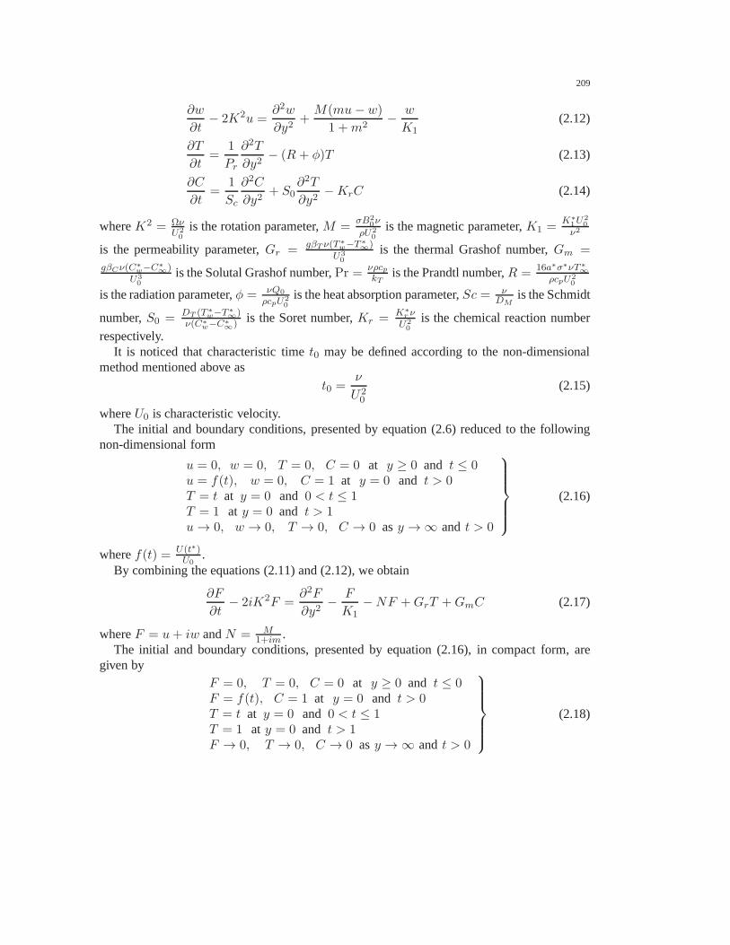
209
∂w
∂t− 2K2u =
∂2w
∂y2+
M(mu− w)
1 +m2−
w
K1(2.12)
∂T
∂t=
1
Pr
∂2T
∂y2− (R + φ)T (2.13)
∂C
∂t=
1
Sc
∂2C
∂y2+ S0
∂2T
∂y2−KrC (2.14)
whereK2 = ΩνU2
0
is the rotation parameter,M =σB2
0ν
ρU2
0
is the magnetic parameter,K1 =K∗
1U2
0
ν2
is the permeability parameter,Gr = gβT ν(T ∗w−T ∗
∞)U3
0
is the thermal Grashof number,Gm =
gβCν(C∗w−C∗
∞)U3
0
is the Solutal Grashof number,Pr = νρcpkT
is the Prandtl number,R = 16a∗σ∗νT ∗∞
ρcpU2
0
is the radiation parameter,φ = νQ0
ρcpU2
0
is the heat absorption parameter,Sc = νDM
is the Schmidt
number,S0 = DT (T ∗w−T ∗
∞)ν(C∗
w−C∗∞) is the Soret number,Kr = K∗
r ν
U2
0
is the chemical reaction number
respectively.It is noticed that characteristic timet0 may be defined according to the non-dimensional
method mentioned above as
t0 =ν
U20
(2.15)
whereU0 is characteristic velocity.The initial and boundary conditions, presented by equation(2.6) reduced to the following
non-dimensional form
u = 0, w = 0, T = 0, C = 0 at y ≥ 0 and t ≤ 0u = f(t), w = 0, C = 1 at y = 0 and t > 0T = t at y = 0 and 0 < t ≤ 1T = 1 at y = 0 and t > 1u → 0, w → 0, T → 0, C → 0 asy → ∞ and t > 0
(2.16)
wheref(t) = U(t∗)U0
.By combining the equations (2.11) and (2.12), we obtain
∂F
∂t− 2iK2F =
∂2F
∂y2−
F
K1−NF +GrT +GmC (2.17)
whereF = u+ iw andN = M1+im
.The initial and boundary conditions, presented by equation(2.16), in compact form, are
given byF = 0, T = 0, C = 0 at y ≥ 0 and t ≤ 0F = f(t), C = 1 at y = 0 and t > 0T = t at y = 0 and 0 < t ≤ 1T = 1 at y = 0 and t > 1F → 0, T → 0, C → 0 asy → ∞ and t > 0
(2.18)

210 M. VENKATESWARLU, D. VENKATA LAKSHMI, AND K. NAGA MALLES WARA RAO
In order to investigate the flow features of the fluid generated due to uniformly acceleratedmovement of the plate, we considerf(t) = R1t, whereR1-a non-dimensional constant.
It is now important to calculate physical quantities of primary interest, which are the localwall shear stress or skin friction coefficient, the local surface heat flux and the local surfacemass flux. Given the velocity, temperature and concentration fields in the boundary layer, theshear stressτw, the heat fluxqwand mass fluxjw are obtained by
τw = µ
[
∂F
∂y
]
y=0
(2.19)
qw = −α
[
∂T
∂y
]
y=0
(2.20)
jw = −Dm
[
∂C
∂y
]
y=0
(2.21)
In non-dimensional form the skin-friction coefficientCf , heat transfer coefficientNu and masstransfer coefficientSh are defined as
Cf =τw
ρν2(2.22)
Nu =ν
Uo
qw
kT (T ∗
w − T ∗
∞)
(2.23)
Sh =ν
Uo
jw
Dm (C∗
w − C∗
∞)
(2.24)
Using non-dimensional variables in equation (2.10) and equations (2.19) to (2.21) into equa-tions (2.22) to (2.24), we obtain the physical parameters
Cf =
[
∂F
∂y
]
y=0
(2.25)
Nu = −
[
∂T
∂y
]
y=0
(2.26)
Sh = −
[
∂C
∂y
]
y=0
(2.27)
3. SOLUTION OF THE PROBLEM
Equations (2.13), (2.14) and (2.17) are coupled, nonlinearpartial differential equations andthese cannot be solved in closed form. So, we reduced these nonlinear partial differentialequations into a set of ordinary differential equations, which can be solved analytically. Thiscan be done by assuming the trial solutions for the velocity,temperature and concentration ofthe fluid as
F (y, t) = F0(y) + ε exp (iωt)F1(y) + o(
ε2)
+ ............ (3.1)
T (y, t) = T0(y) + ε exp (iωt)T1(y) + o(
ε2)
+ ............ (3.2)

211
C(y, t) = C0(y) + ε exp (iωt)C1(y) + o(
ε2)
+ ............ (3.3)
whereω is frequency of oscillation andε << 1.Substituting (3.1), (3.2), and (3.3) in equations (2.13), (2.14), and (2.17), then equating the
harmonic and non-harmonic terms and neglecting the higher order terms ofo(
ε2)
, we obtain
F ′′
0 −
[
N +1
K1− 2iK2
]
F0 = −(GrT0 +GmC0) (3.4)
F ′′
1 −
[
N +1
K1− 2iK2 + iω
]
F1 = −(GrT1 +GmC1) (3.5)
T ′′
0 − Pr(R+ φ)T0 = 0 (3.6)
T ′′
1 − Pr(R+ φ+ iω)T1 = 0 (3.7)
C ′′
0 − ScKrC0 = −ScS0T′′
0 (3.8)
C ′′
1 − Sc(Kr + iω)C1 = −ScS0T′′
1 (3.9)
where prime denotes the ordinary differentiation with respect toy.The corresponding boundary conditions can be written as
F0 = 0, F1 = 0 , T0 = 0, T1 = 0, C0 = 0 , C1 = 0 at y ≥ 0 and t ≤ 0F0 = f(t), F1 = 0 , C0 = 1 , C1 = 0 at y = 0 and t > 0T0 = t, T1 = 0 at y = 0 and 0 < t ≤ 1T0 = 1, T1 = 0 at y = 0 and t > 1F0 → 0, F1 → 0 , T0 → 0, T1 → 0, C0 → 0 , C1 → 0 asy → ∞ and t > 0
(3.10)
Solving equations (3.4)-(3.9) under the boundary condition (3.10) we obtain the velocity, tem-perature and concentration distribution in the boundary layer as
F (y, t) = A11 exp(−A3y) +A13 exp(−A1y) +A14 exp(−A9y) (3.11)
T (y, t) = t exp(−A1y) (3.12)
C (y, t) = A6 exp(−A1y) +A7 exp(−A3y) (3.13)
The Skin friction, Nusselt number and Sherwood number are important physical parametersfor this type of boundary layer flow.
Skin friction coefficient:Knowing the velocity field, the skin friction coefficient canbe obtained, which is in non-dimensional form is given by
Cf =
(
∂F
∂y
)
y=0
= − [A3A11 +A1A13 +A9A14] (3.14)

212 M. VENKATESWARLU, D. VENKATA LAKSHMI, AND K. NAGA MALLES WARA RAO
Nusselt number:Knowing the temperature field, the rate of heat transfer coefficient can be obtained, which is innon-dimensional form is given, in terms of the Nusselt number, is given by
Nu = −
(
∂T
∂y
)
y=0
= tA1 (3.15)
Sherwood number:Knowing the concentration field, the rate of mass transfer coefficient can be obtained, which isin non-dimensional form, in terms of the Sherwood number, isgiven by
Sh = −
(
∂C
∂y
)
y=0
= A1A6 +A3A7 (3.16)
Here the constants are not given due shake of brevity.
4. RESULTS AND DISCUSSIONS
In order to investigate the influence of various physical parameters such as hall current pa-rameterm, Soret effectS0, rotation parameterK2, magnetic parameterM , radiation parameterR, permeability parameterK1, heat absorption parameterφ, Prandtl numberPr, thermal buoy-ancy forceGr, solutal buoyancy forceGm, chemical reaction parameterKr, mass diffusionparameterSc and timet on the flow-field, primary velocityu, secondary velocityw, tem-peratureT and concentrationC have been studied analytically and computed results of theanalytical solutions, presented by equations (3.11)-(3.13) are displayed graphically from Figs.2 to 22. In the present study following default parameter values are adopted for computations:Gr = 4, Gm = 3, Pr = 0.71, Kr = 0.5, R = 2.0, m = 0.5, K2 = 2.0, ω = 0.5, M =1.0, Sc = 0.6, R1 = 0.5, t = 0.5, K1 = 0.5, φ = 3.0 andS0 = 0.5. It is observed fromFigures. 2 to 14 fluid primary velocityu and fluid secondary velocityw attain a distinctivemaximum value near the surface of the plate and then decreaseproperly on increasing bound-ary layer coordinatey to approach free stream value. Fig. 2 depicts the influence ofhall currentparameterm on the primary velocityu and secondary velocityw.
It is evident from Fig. 2,u increases on increasingm in a region near to the plate and itdecreases on increasingm in the region away from the plate whereasw increases on increasingm throughout the boundary layer region. This implies that, hall current tends to acceleratesecondary fluid velocity throughout the boundary layer region which is consistent with the factthat hall current induces secondary flow in the flow field. Hallcurrent tends to accelerate pri-mary fluid velocity in a region close to the plate whereas it has a reverse effect on fluid primaryvelocity in the region away from the plate. It is perceived from Fig. 3 that, primary velocityu decreases on increasing rotation parameterK2 whereas secondary velocityw increases onincreasingK2 in the region near to the plate and it decreases on increasingK2 in the regionaway from the plate. This implies that, rotation tends to retard primary fluid velocity through-out the boundary layer region. Although rotation is known toinduce secondary fluid velocity

213
FIGURE 2. Influence ofm onvelocity profiles.
FIGURE 3. Influence ofK2
on velocity profiles.
in the flow-field by suppressing the primary fluid velocity, its accelerating effect is prevalentonly in the region near to the plate whereas it has a reverse effect on secondary fluid velocityin the region away from the plate. This is due to the reason that Coriolis force is dominant inthe region near to the axis of rotation. Fig. 4 depicts the effect of radiation parameterR on theprimary velocityu and secondary velocityw of the flow field.
FIGURE 4. Influence ofR on velocity profiles.
The radiation parameterR is found to decelerate both the primary velocityu and secondaryvelocityw of the flow field at all points. This is because radiation parameter have tendency toreduce fluid temperature which is clearly evident from Fig. 16. Higher the radiation parameter,the more sharper is the reduction in velocity.

214 M. VENKATESWARLU, D. VENKATA LAKSHMI, AND K. NAGA MALLES WARA RAO
It is observed that from Fig. 5 bothu andw decreases on increasing heat absorption pa-rameterφ. This implies that heat absorption tend to retard the primary and secondary fluidvelocities.
FIGURE 5. Influence ofφ on velocity profiles.
This is because heat absorption have tendency to reduce fluidtemperature which is clearlyevident from Fig. 15. The effect of Grashof numbers for heat transferGr and mass transferGm on the primary velocityu and secondary velocityw of the flow field are presented in Figs.6 and 7.
FIGURE 6. Influence ofGr
on velocity profiles.FIGURE 7. Influence ofGm
on velocity profiles.
A study of the curves shows that the Grashof numbers for heat transferGr and mass transferGm accelerate the primary velocityu and secondary velocityw of the flow field at all points.Comparing the curves of Figs. 6 and 7, it is further observed that the increase in velocity of the

215
flow fields more significant in presence of mass transfer. Thus, mass transfer has a dominanteffect on the flow field.
The nature of primary velocityu and secondary velocityw in presence of foreign speciessuch as Hydrogen(Sc = 0.20), Helium (Sc = 0.30), Water vapour(Sc = 0.60), Ammonia(Sc = 0.78) is shown in Fig. 8. The flow field surffers a decrease in primaryvelocity u andsecondary velocityw at all points in presence of heavier diffusing species. It isobserved fromFig. 9 primary velocityu and secondary velocityw increase on increasing timet. This impliesthat primary and secondary fluid velocities are getting accelerated with the progress of time.
FIGURE 8. Influence ofSc
on velocity profiles.FIGURE 9. Influence oft onvelocity profiles.
Fig. 10 displays the effect of the chemical reaction parameter Kr on primary velocityuand secondary velocityw of the flow field at all points. It is seen, that primary velocity u andsecondary velocityw decreases with increasing the chemical reaction parameterKr. Fig. 11
FIGURE 10. Influence ofKr
on velocity profiles.FIGURE 11. Influence ofS0
on velocity profiles.

216 M. VENKATESWARLU, D. VENKATA LAKSHMI, AND K. NAGA MALLES WARA RAO
displays the effect of the Soret numberS0 on primary velocityu and secondary velocityw ofthe flow field at all points. It is seen, that primary velocityu and secondary velocityw increaseswith increasing the Soret numberS0.
Fig. 12 depicts the effect of Magnetic parameterM on primary velocityu and secondaryvelocity w of the flow field. The Magnetic parameterM is found to decrease the primaryvelocityu and secondary velocityw of the flow field at all points. Fig. 13 depicts the influenceof porosity parameterK1 on primary velocityu and secondary velocityw of the flow field. It isevident from Fig. 13,u increases on increasingK1 in a region near to the plate and it decreaseson increasingK1 in the region away from the plate whereasw increases on increasingK1
throughout the boundary layer region.
FIGURE 12. Influence ofMon velocity profiles.
FIGURE 13. Influence ofK1
on velocity profiles.
Fig. 14 shows the plot of primary velocityu and secondary velocityw of the flow fieldagainst different values of prandtl numberPr taking other parameters are constant. The values
FIGURE 14. Influence ofPr on velocity profiles.

217
of the prandtl number are chosen for air(Pr = 0.71), electrolytic solution(Pr = 1.00), water(Pr = 7.00) and water at40C (Pr = 11.40). It is observed that the primary velocityu andsecondary velocityw of the flow field decreases in magnitude as prandtl numberPr increases.Thus higher prandtl number leads to faster cooling of the plate.
Figs. 15 and 16 depict the effect of heat absorption parameter φ and radiation parameterR on the temperatureT of the flow field. It is observed that heat absorption parameter φ andradiation parameterR are found to decelerate the temperatureT of the flow field at all point.
FIGURE 15. Influence ofφon temperature profiles.
FIGURE 16. Influence ofRon temperature profiles.
Figs. 17 and 18 depict the effect of timet and prandtl numberPr on the temperatureTof the flow field. The prandtl number defines the ratio of momentum diffusivity to thermaldiffusivity. The values of the prandtl number are chosen forair (Pr = 0.71), electrolytic
FIGURE 17. Influence oft ontemperature profiles.
FIGURE 18. Influence ofPr
on temperature profiles.

218 M. VENKATESWARLU, D. VENKATA LAKSHMI, AND K. NAGA MALLES WARA RAO
solution(Pr = 1.00), water(Pr = 7.00) and water at40C (Pr = 11.40). It is noticed that thefluid temperatureT increases in magnitude on increasing timet and it decreases on increasingthe prandtl numberPr at all points of the flow field.
It is observed from Figs. 19 and 20 that species concentration C decreases on increasingSchmidt numberSc whereas it increases on increasing timet. This implies that there is anenhancement in species concentration with the progress of time throughout the boundary layerregion.
FIGURE 19. Influence ofSc
on concentration profiles.FIGURE 20. Influence oft onconcentration profiles.
Figs. 21 and 22 depict effect of Soret numberSo and chemical reaction parameterKr onconcentration distribution of the flow field. The species concentrationC is found to increases
FIGURE 21. Influence ofS0
on concentration profiles.FIGURE 22. Influence ofKr
on concentration profiles.
on increasing Soret numberSo whereas it is decreases on increasing the chemical reaction

219
parameterKr. Table 1. Represents the numerical values of heat transfer coefficientNu fordifferent values of radiation parameterR, Prandtl numberPr and heat absorption parameterφ.Nusselt numberNu increases on increasingR, Pr, andφ. Also the value ofNu is least forMercury and highest for Water at40C.
TABLE 1. Nusselt numberNu whent = 0.5.
R Pr φ Nu R Pr φ Nu
2.0 0.71 3.0 0.9421 2.0 7.00 3.0 2.95804.0 0.71 3.0 1.1147 2.0 11.40 3.0 3.77496.0 0.71 3.0 1.2639 2.0 0.71 1.0 0.72978.0 0.71 3.0 1.3973 2.0 0.71 3.0 0.94212.0 0.71 3.0 0.9421 2.0 0.71 5.0 1.11472.0 1.00 3.0 1.1180 2.0 0.71 7.0 1.2639
Table 2. Represents the numerical values of skin friction coefficientCf for different valuesof Hall current parameterm, rotation parameterK2, radiation parameterR and heat absorptionparameterφ. Skin friction coefficientCf increases on increasingm whereasCf decreaseson increasingR andφ for both primary and secondary velocities. It is observed that skin
TABLE 2. Skin friction coefficient whenKr = 0.5, So = 0.5,M = 1,K1 =0.5, Gr = 4, Gm = 3, R1 = 0.5, ω = 0.5, Sc = 0.6, t = 0.5, Pr = 0.71.
m K2 R φSkin friction coefficientCf
Primary Secondary0.5 2.0 2.0 3.0 1.0138 0.87421.0 2.0 2.0 3.0 1.0232 0.92501.5 2.0 2.0 3.0 1.0429 0.95092.0 2.0 2.0 3.0 1.0600 0.96320.5 2.0 2.0 3.0 1.0138 0.87420.5 4.0 2.0 3.0 0.5745 1.07190.5 6.0 2.0 3.0 0.2914 1.16600.5 8.0 2.0 3.0 0.0857 1.23310.5 2.0 2.0 3.0 1.0138 0.87420.5 2.0 4.0 3.0 0.9870 0.85820.5 2.0 6.0 3.0 0.9665 0.84700.5 2.0 8.0 3.0 0.9501 0.83870.5 2.0 2.0 1.0 1.0525 0.90010.5 2.0 2.0 3.0 1.0138 0.87420.5 2.0 2.0 5.0 0.9870 0.85820.5 2.0 2.0 7.0 0.9665 0.8470
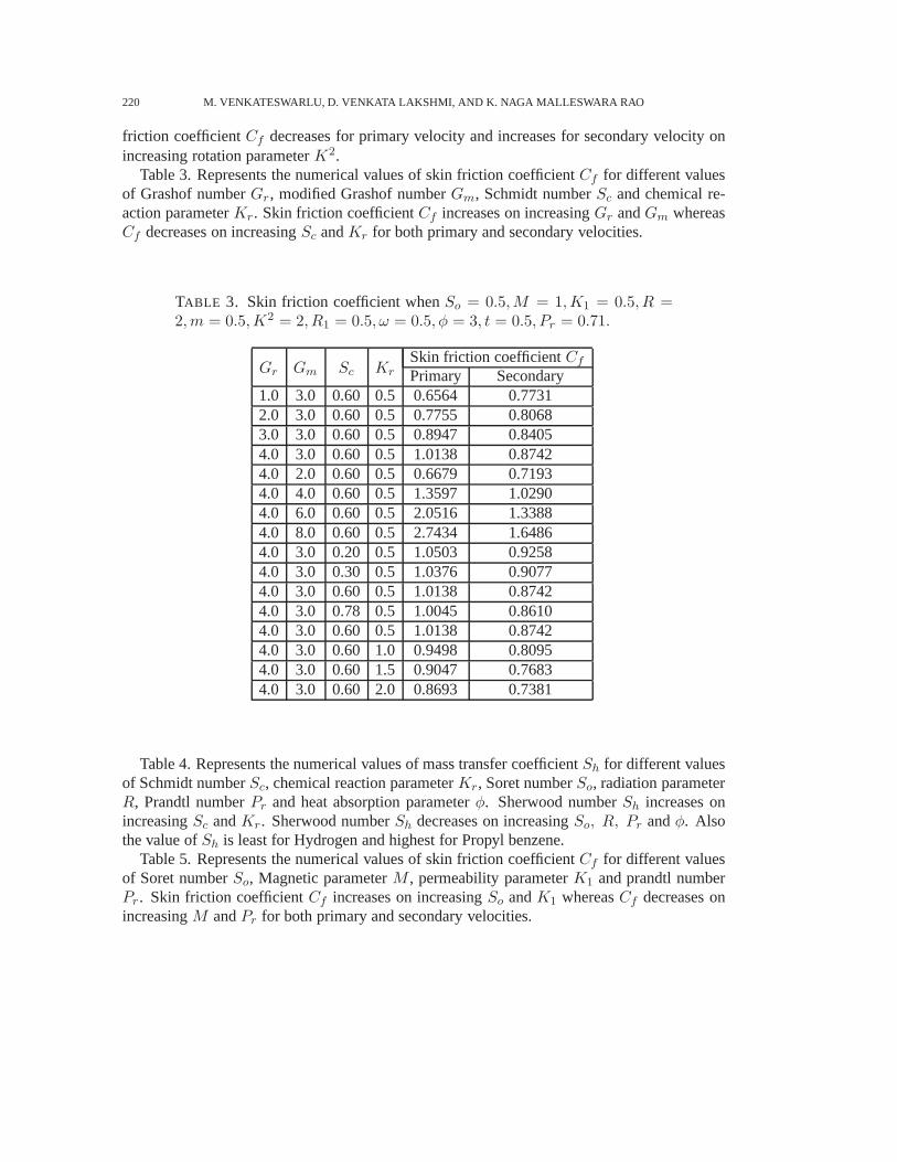
220 M. VENKATESWARLU, D. VENKATA LAKSHMI, AND K. NAGA MALLES WARA RAO
friction coefficientCf decreases for primary velocity and increases for secondaryvelocity onincreasing rotation parameterK2.
Table 3. Represents the numerical values of skin friction coefficientCf for different valuesof Grashof numberGr, modified Grashof numberGm, Schmidt numberSc and chemical re-action parameterKr. Skin friction coefficientCf increases on increasingGr andGm whereasCf decreases on increasingSc andKr for both primary and secondary velocities.
TABLE 3. Skin friction coefficient whenSo = 0.5,M = 1,K1 = 0.5, R =2,m = 0.5,K2 = 2, R1 = 0.5, ω = 0.5, φ = 3, t = 0.5, Pr = 0.71.
Gr Gm Sc KrSkin friction coefficientCf
Primary Secondary1.0 3.0 0.60 0.5 0.6564 0.77312.0 3.0 0.60 0.5 0.7755 0.80683.0 3.0 0.60 0.5 0.8947 0.84054.0 3.0 0.60 0.5 1.0138 0.87424.0 2.0 0.60 0.5 0.6679 0.71934.0 4.0 0.60 0.5 1.3597 1.02904.0 6.0 0.60 0.5 2.0516 1.33884.0 8.0 0.60 0.5 2.7434 1.64864.0 3.0 0.20 0.5 1.0503 0.92584.0 3.0 0.30 0.5 1.0376 0.90774.0 3.0 0.60 0.5 1.0138 0.87424.0 3.0 0.78 0.5 1.0045 0.86104.0 3.0 0.60 0.5 1.0138 0.87424.0 3.0 0.60 1.0 0.9498 0.80954.0 3.0 0.60 1.5 0.9047 0.76834.0 3.0 0.60 2.0 0.8693 0.7381
Table 4. Represents the numerical values of mass transfer coefficientSh for different valuesof Schmidt numberSc, chemical reaction parameterKr, Soret numberSo, radiation parameterR, Prandtl numberPr and heat absorption parameterφ. Sherwood numberSh increases onincreasingSc andKr. Sherwood numberSh decreases on increasingSo, R, Pr andφ. Alsothe value ofSh is least for Hydrogen and highest for Propyl benzene.
Table 5. Represents the numerical values of skin friction coefficientCf for different valuesof Soret numberSo, Magnetic parameterM , permeability parameterK1 and prandtl numberPr. Skin friction coefficientCf increases on increasingSo andK1 whereasCf decreases onincreasingM andPr for both primary and secondary velocities.

221
TABLE 4. Sherwood numberSh whent = 0.5.
Sc Kr S0 R Pr φ Sh Sc Kr S0 R Pr φ Sh
0.20 0.5 0.5 2.0 0.71 3.0 0.0611 0.60 0.5 0.5 2.0 0.71 3.0 0.32880.30 0.5 0.5 2.0 0.71 3.0 0.0846 0.60 0.5 0.5 4.0 0.71 3.0 0.27930.60 0.5 0.5 2.0 0.71 3.0 0.1479 0.60 0.5 0.5 6.0 0.71 3.0 0.23610.78 0.5 0.5 2.0 0.71 3.0 0.1826 0.60 0.5 0.5 8.0 0.71 3.0 0.19720.60 0.5 0.5 2.0 0.71 3.0 0.1479 0.60 0.5 0.5 2.0 0.71 3.0 0.32880.60 1.0 0.5 2.0 0.71 3.0 0.4089 0.60 0.5 0.5 2.0 1.00 3.0 0.27830.60 1.5 0.5 2.0 0.71 3.0 0.6055 0.60 0.5 0.5 2.0 7.00 3.0 -0.26450.60 2.0 0.5 2.0 0.71 3.0 0.7692 0.60 0.5 0.5 2.0 11.40 3.0 -0.50820.60 0.5 0.2 2.0 0.71 3.0 0.4601 0.60 0.5 0.5 2.0 0.71 1.0 0.38850.60 0.5 0.4 2.0 0.71 3.0 0.3725 0.60 0.5 0.5 2.0 0.71 3.0 0.32880.60 0.5 0.6 2.0 0.71 3.0 0.2850 0.60 0.5 0.5 2.0 0.71 5.0 0.27930.60 0.5 0.8 2.0 0.71 3.0 0.1974 0.60 0.5 0.5 2.0 0.71 7.0 0.2361
TABLE 5. Skin friction coefficient whenGr = 4, Gm = 3,Kr = 0.5, φ =3, R = 2,m = 0.5,K2 = 2, ω = 0.5, R1 = 0.5, Sc = 0.6, t = 0.5.
So M K1 PrSkin friction coefficientCf
Primary Secondary0.2 1.0 0.5 0.71 0.9865 0.85200.4 1.0 0.5 0.71 1.0047 0.86680.6 1.0 0.5 0.71 1.0229 0.88150.8 1.0 0.5 0.71 1.0411 0.89630.5 1.0 0.5 0.71 1.0138 0.87420.5 2.0 0.5 0.71 0.8966 0.80630.5 3.0 0.5 0.71 0.7895 0.75550.5 4.0 0.5 0.71 0.6918 0.71660.5 1.0 0.1 0.71 0.3167 0.34630.5 1.0 0.2 0.71 0.7323 0.56780.5 1.0 0.3 0.71 0.8926 0.71200.5 1.0 0.4 0.71 0.9705 0.80770.5 1.0 0.5 0.71 1.0138 0.87420.5 1.0 0.5 1.00 0.9865 0.85790.5 1.0 0.5 7.00 0.8335 0.79370.5 1.0 0.5 11.40 0.8013 0.7853

222 M. VENKATESWARLU, D. VENKATA LAKSHMI, AND K. NAGA MALLES WARA RAO
5. CONCLUSION
An investigation of the effects of hall current, Soret number, chemical reaction parmeterand rotation parameter on unsteady hydromagnetic natural convection flow with heat and masstransfer of a viscous, incompressible, electrically conducting and optically thick radiating fluidpast an impulsively moving vertical plate embedded in a fluidsaturated porous medium iscarried out. Important findings are as follows:
• Hall current tends to accelerate secondary fluid velocity throughout the boundary layerregion. Hall current tends to accelerate primary fluid velocity in a region close to theplate whereas it has a reverse effect on the primary fluid velocity in the region awayfrom the plate.
• Rotation tends to retard primary fluid velocity throughout the boundary layer regionand accelerate secondary fluid velocity only in the region near to the plate whereas ithas a reverse effect on secondary fluid velocity in the regionaway from the plate.
• Thermal and concentration buoyancy forces tend to accelerate both the primary andsecondary fluid velocities throughout the boundary layer region.
• Primary and secondary fluid velocities are getting accelerated with the progress of timethroughout the boundary layer region.
• Heat absorption parameter, thermal radiation and Prandtl number tend to retard fluidtemperature and there is an enhancement in fluid temperaturewith the progress of timethroughout the boundary layer region.
• Mass diffusion and chemical reaction parameter tends to retard species concentrationand there is an enhancement in species concentration with the progress of time andSoret number throughout the boundary layer region.
• Radiation parameter, heat absorption parameter, Schmidt number, chemical reactionparameter, magnetic parameter and Prandtl number tends to retard skin friction coeffi-cient and there is an enhancement in skin friction coefficient on increasing Hall currentparameter, Grashof number, modified Grashof number, Soret number and permeabilityparameter for both primary and secondary velocities. But skin friction coefficient de-creases on increasing rotation parameter for primary velocity whereas it has a reverseeffect for secondary velocity.
• Radiation parameter, Prandtl number and heat absorption parameter have tendency toincrease the heat transfer coefficient.
• Schmidt number and chemical reaction parameter have tendency to accelerate the masstransfer coefficient. Soret number, radiation parameter, Prandtl number and heat ab-sorption parameter retard the fluid concentration.
ACKNOWLEDGEMENTS
The first author is thankful to V. R. Siddhartha Engineering College, Kanuru, Vijayawada,Andhra Prades, India for providing necessary research facilities to publish this paper. Theauthors are thankful for the suggestions and comments of thereferees, which have led to im-provement of the paper.
223
REFERENCES
[1] A. Raptis and N. Kafoussias:Magnetohydrodynamic free convection flow and mass transferthrough porousmedium bounded by an infinite vertical porous plate with constant heat flux, Can. J. Phys,60(1982), 1725–1729.
[2] A. Raptis: Free convection and mass transfer effects on the oscillatory flow past an infinite moving verticalisothermal plate with constant suction and heat sources. Astrophy Space Sci,86(1982), 43–53.
[3] M. A. Sattar: Unsteady hydromagnetic free convection flow with Hall current mass transfer and variablesuction through a porous medium near an infinite vertical porous plate with constant heat flux,Int. J. EnergyResearch,17(1993), 1–5.
[4] F.C. Lai and F. A. Kulacki:Non-Darcy mixed convection along a vertical wall in a saturated porous medium.J. Heat Transfer.113(1991), 252–255.
[5] E. R. Eckert and R. M. Drake:Analysis of heat and mass transfer. NY: Mc-Graw Hill, 1972.[6] B. Gebhart , Y. Jaluria , R. L. Mahajan and B. Sammakia:Buoyancy induced flow and transport, New York
Hemisphere, 1998.[7] D. A. Nield and A. Bejan:Convection in porous media, 3rd ed. NY: Springer, 2006.[8] I. Pop and D. B. Ingham:Convective heat transfer: mathematical and computationalmodelling of viscous
fluids and porous media, Oxford: Pergamon, 2001.[9] F. P. Incropera, T. L. Bergman, A. S. Lavine and D. P. Dewitt: Fundamentals of heat and mass transfer, NY:
John Wiley & Sons, 2011.[10] G. S. Seth, S. Sarkar and G. K. Mahato:Effects of hall current on hydromaggnetic free convection flow
with heat and mass transfer of a heat absorbing fluid past an impulsively moving vertical plate with rampedtemperature, Int. J. Heat & Tech,31 (2013), 85-96.
[11] R. Kandasamy, K. Periasamy and K. K. Sivagnana Prabhu:Chemical reaction, heat and mass transfer onMHD flow over a vertical stretching surface with heat source and thermal stratification effects, Int. J. Heatand Mass Transfer,48 (2005), 4557-4561.
[12] Z. Dursunkaya and W.M. Worek:Diffusion-thermo and thermal-diffusion effects in transient and steady nat-ural convection from vertical surface, Int. J. Heat and Mass Transfer,35(1992), 2060–2065.
[13] A. Postelnicu:Influence of a magnetic field on heat and mass transfer by natural convection from verticalsurfaces in porous media considering Soret and Dufour effects, Int. J. Heat and Mass Transfer,47(2004),1467–1472.
[14] M.S. Alam, M.M. Rahman:Dufour and Soret effects on MHD free convective heat and masstransfer flow pasta vertical flat plate embedded in a porous medium, J. Naval Architecture and Marine Engg,2(2005), 55–65.
[15] I Pop and T. Watanabe:Hall effect on magnetohydrodynamic free convection about asemi-infinite vertical flatplate, Int. J. Eng Sci,32(1994), 1903–1911.
[16] Abo-Eldahab and E. M. E Elbarbary:Hall current effect on magnetohydrodynamic free-convection flow pasta semi infinite vertical plate with mass transfer, Int. J. Eng Sci, 39(2001), 1641–1652.
[17] H. S. Takhar, S. Roy and G. Nath:Unsteady free convection flow over an infinite vertical porous plate due tothe combined effects of thermal and mass diffusion, magnetic field and Hall currents. Int. J. Heat and MassTransfer,39 (2003), 825–834.
[18] L. K. Saha, S. Siddiqa and M. A. Hossain:Effect of Hall current on MHD natural convection flow fromvertical permeable flat plate with uniform surface heat flux, Appl. Math Mech Engg Ed,32(2011), 127–146.
[19] P. V. Satya Narayana, B. Venkateswarlu and S. Venkataramana:Effects of Hall current and radiation absorp-tion on MHD micropolar fluid in a rotating system, Ain Shams Eng J,4(2013), 843–854.
[20] G. S. Seth, G. K. Mahato and S. Sarkar:Effects of Hall current and rotation on MHD natural convection flowpast an impulsively moving vertical plate with ramped temperature in the presence of thermal diffusion withheat absorption, Int. J. Energy Tech,5(2013), 1–12.
[21] M. Q. Al-Odat and Al-Azab:Influence of chemical reaction on transient MHD free convection over a movingvertical plate, Emirates J. Engg. Res,12 (2007), 15-21.

224 M. VENKATESWARLU, D. VENKATA LAKSHMI, AND K. NAGA MALLES WARA RAO
[22] M.A. El-Aziz: Radiation effect on the flow and heat transfer over an unsteady stretching sheet, InternationalCommunications in Heat and Mass Transfer,36(2009), 521-524.
[23] P. Singh, N.S. Tomer and D. Sinha:Numerical study of heat transfer over stretching surface inporous me-dia with transverse magnetic field, Proceeding of International Conference on Challenges andapplication ofMathematics in Sciences and Technology, ISBN 023- 032-875-X, 2010, 422-430.
[24] P. Singh, N. S. Tomer, S. Kumar and D. Sinha:MHD oblique stagnation-point flow towards a stretching sheetwith heat transfer, International Journal of Applied Mathematics and Mechanics,6(2010), 94-111.
[25] P. Singh, A. Jangid, N. S. Tomer, S. Kumar and D. Sinha:Effects of thermal radiation and magnetic field onunsteady stretching permeable sheet in presence of free stream velocity, International Journal of Informationand Mathematical Sciences,6 (2010), 63-69.
[26] E. M. E. Elbashbeshy, D. M. Yassmin and A. A. Dalia:Heat transfer over an unsteady porous stretchingsurface embedded in a porous medium with variable heat flux inthe presence of heat source or sink, AfricanJournal of Mathematics and Computer Science Research,39(2010), 68-73.
[27] D. Angirasa, G. P. Peterson, and I. Pop:Combined heat and mass transfer by natural convection with opposingbuoyancy effects in a fluid saturated porous medium, Int. J. Heat and Mass Transfer,40(1997), 2755-2773.
[28] S. Ahmed:Effects of unsteady free convective MHD flow through a porousmedium bounded by an infinitevertical porous plate, Bull. Cal. Math. Soc.,99 (2007), 511-522.
[29] Ahmed Sahin:Influence of chemical reaction on transient MHD free Convective flow over a vertical plate inslip-flow Regime, Emirates Journal for Engineering Research,15 (2010), 25-34.
[30] Venkateswarlu Malapati and Padma Polarapu:Unsteady MHD free convective heat and mass transfer in aboundary layer flow past a vertical permeable plate with thermal radiation and chemical reaction, ProcediaEngineering, 127(2015), 791-799.
[31] Manjula Jonnadula, Padma Polarapu, Gnaneswara Reddy Mand Venakateswarlu M: Influence of thermalradiation and chemical reaction on MHD flow, heat and mass transfer over a stretching surface, ProcediaEngineering, 127(2015), 1315-1322.
[32] M. Venkateswarlu, G. V. Ramana Reddy and D. V. Lakshmi:Radiation effects on MHD boundary layer flowof liquid metal over a porous stretching surface in porous medium with heat generation, Journal of the KoreanSociety for Industrial and Applied Mathematics,19 (2015), 83-102.
[33] M. Venkateswarlu, G. V. Ramana Reddy and D. V. Lakshmi: Thermal diffusion and radiation effects on un-steady MHD free convection heat and mass transfer flow past a linearly accelerated vertical porous platewith variable temperature and mass diffusion, Journal of the Korean Society for Industrial and AppliedMathematics,18 (2014), 257-268.
[34] M. Venkateswarlu, G. V. Ramana Reddy and D. V. Lakshmi:Diffusion-thermo effects on MHD flow past aninfinite vertical porous plate in the presence of radiation and chemical reaction, International Journal ofMathematical Archive, 4 (2013), 39-51.
[35] M. Venkateswarlu, G. V. Ramana Reddy and D. V. Lakshmi:Effects of chemical reaction and heat gen-eration on MHD boundary layer flow of a moving vertical plate with suction and dissipation,EngineeringInternational,1 (2013), 27-38.
[36] K. R. Cramer and S. I. Pai:Magnetofluid dynamics for Engineers and Applied physicists, McGraw Hill BookCompany, NY,1973.
[37] A. Raptis:Free convective oscillatory flow and mass transfer past a porous plate in the presence of radiationfor an optically thin fluid, Thermal Sci,15(2011), 849-857.

J. KSIAM Vol.20, No.3, 225–242, 2016 http://dx.doi.org/10.12941/jksiam.2016.20.225
AN OPTIMIZATION APPROACH FOR COMPUTING A SPARSE MONO-CYCLI CPOSITIVE REPRESENTATION
KYUNGSUP KIM
DEPARTMENT OFCOMPUTER ENGINEERING, CHUNGNAM NATIONAL UNIVERSITY, DAEJEON, 305-764,KOREA
E-mail address: [email protected]
ABSTRACT. The phase-type representation is strongly connected withthe positive realizationin positive system. We attempt to transform phase-type representation into sparse mono-cyclicpositive representation with as low order as possible. Because equivalent positive representa-tions of a given phase-type distribution are non-unique, itis important to find a simple sparsepositive representation with lower order that leads to moreeffective use in applications. AHypo-Feedback-Coxian Block (HFCB) representation is a good candidate for a simple sparserepresentation. Our objective is to find an HFCB representation with possibly lower order,including all the eigenvalues of the original generator. Weintroduce an efficient nonlinearoptimization method for computing an HFCB representation from a given phase-type represen-tation. We discuss numerical problems encountered when finding efficiently a stable solution ofthe nonlinear constrained optimization problem. Numerical simulations are performed to showthe effectiveness of the proposed algorithm.
1. INTRODUCTION
The positive realization problem has been independently studied in the system theory andprobability theory communities [1, 2, 3, 4]. The phase-typerepresentation (so called, posi-tive representation) is strongly connected with the positive realization in system theory [5].The relation between the Laplace-Stieltjes transform (LST) of a probability distribution anda corresponding phase-type representation is similar to that between a transfer function and acorresponding state space realization.
Because equivalent positive representations of a given phase-type(PH) distribution are non-unique [6], finding smaller and simpler matrix representations for PH-distributions has becomean important theoretical and practical issue. In modeling and simulation applications, the im-portance of simple sparse representations comes from the fact that the computational complex-ity of PH-distributed random-variate generation depends on the representation [7, 8]. Finding
Received by the editors August 3 2016; Revised September 9 2016; Accepted in revised form September 9 2016;Published online September 13 2016.
2000Mathematics Subject Classification.60J27, 93B15.Key words and phrases.Phase-type representation, Hypo-feedback-Coxian block,Constrained nonlinear opti-
mization, Positive realization, Positive system.
225

226 K. KIM
smaller, simpler and structured representations with lower order can lead to more effective useof PH-distribution random number generators in stochasticmodeling and simulation.
There are some important approaches for minimal and specially structured positive realiza-tion such as the triangular, bi-diagonal, mono-cyclic, anduni-cyclic representations [5, 9].Every phase-type distribution has a mono-cyclic representation with larger order [9]. Themono-cyclic representation is a natural extension of a generator with a bi-diagonal matrix. Themono-cyclic representations are referred to as feed-back Erlang representations (or feed-backCoxian representations) due to their structures [9]. We introduce a Hypo-Feedback-CoxianBlock (HFCB) representation covering Erlang, Coxian, Feedback Erlang (FE) and FeedbackCoxian (FC) representations. These approach can be appliedto the sparse positive realizationof positive system since it has the same structure [3, 5]. Similar constructive methods of simplecompact positive realizations for general transfer functions have been extensively discussed inthe positive system [2, 4, 10, 11]. The main objective of thispaper is to compute an HFCBpositive representation with a lower order using nonlinearoptimization method.
Finding the roots of polynomials is an important task for finding a proper HFCB representa-tion. A coefficient relation function between the roots and coefficients of a polynomial can beused to find all of the roots of a given polynomial simultaneously and in parallel, instead of us-ing a deflation method finding the roots one by one such as Laguerre’s and Newton-Raphson’s[12]. A constrained nonlinear optimization problem computing a sparse mono-cyclic represen-tation is formulated by using coefficient relation function. We discuss the numerical method tofind a optimal solution of the constrained nonlinear optimization problem depending on howto choose an initial value.
The rest of this paper is organized as follows. Section 2 provides some relevant backgroundmaterial, including definitions and preliminary results. In Section 3, various structured phase-type representations classified into acyclic and cyclic forms and their properties are considered.Numerical optimization methods for finding a sparse mono-cyclic representation with possiblysmall order are discussed in Section 4. The numerical experiments are presented in Section 5.Finally, Section 6 concludes the paper.
2. PHASE-TYPE DISTRIBUTIONS
Before proceeding, we introduce some basic notations. Ann × n non-negative matrixAis denoted byA ≥ 0 if its entries are non-negative and at least one entry is positive. A strictpositive matrixA = [aij ] is denotedA > 0 if all entriesaij > 0. We discuss the phase-type distribution for a non-negative random variableX in terms of a continuous-time Markovprocess. A continuous-time Markov process is defined on ann+ 1 finite state space. The rowvectorα gives the initial probability vector. A phase-type (PH) distribution is defined as thedistribution of the time needed for absorption in a Continuous-Time Markov Chain (CTMC)with one absorbing state. If then+1 state is an absorbing state and all other states are transient,the infinitesimal generator matrix of the Markov chain in theform of the augmented matrix

AN OPTIMIZATION APPROACH FOR COMPUTING A SPARSE MONO-CYCLIC POSITIVE REPRESENTATION227
tuple(T , b, α), called the augmented phase-type representation, can be defined by
T =
[
T −T10 0
]
, b = en+1,
α =[
α αn+1
]
,
(2.1)
where0 refers to the column vector, row vector or matrix with all entries equal to zero inthe case without ambiguity,ek is ak-th standard basis vector with zeros, except thek-th one,which is 1, and1 is the column vector with all entries being one. We can see that αn+1 = 0if α1 = 1, andαn+1 = 1 − α1 otherwise. PH distributions are commonly represented bya vector-matrix tuple(α, T ) that describes the transient part of the CTMC. The vector-matrixtuple (α, T ) denotes a phase-type representation (or a phase-type generator) of a phase-typedistribution ifα andT have following properties:Tii < 0, Tij ≥ 0 for i 6= j, α1 ≤ 1, α ≥ 0,andT1 ≤ 0. Equivalently, a phase-type representation is regarded asthe positive realization(representation) of positive system [5].
The probability density function (PDF), cumulative distribution function (CDF), and Laplace-Stieltjes Transform (LST) of the PDF, respectively, are defined by
f(x) = α exp(Tx)(−T1)F (x) = 1− α exp(Tx)1F ∗(s) = E(exp(sX)) = α(sI − T )−1(−T1)
whereE(X) means an expectation of a random variableX.The particular structured representation problem has beenstudied as an important work in
the theory of phase-type representations [5]. Depending ontheir structures, we can typicallydivide a phase-type representation into two classes: an acyclic subclass and a cyclic subclass.In the concept of graph theory, the acyclic class consists ofa vector-matrix pair(α, T ), whichthe generatorT represents an acyclic transition graph andα is a positive vector.
The concepts of PH-simplicity and PH-majorization are useful tools in the study of PH-distributions [6, 13]. For a givenT , PH(T ) denotes the set of all distributions with a phase-type representation(α, T ). For two generatorsT andS,S is said to PH-majorizeT if PH(T ) ⊂PH(S). T is called by PH-simple if for any differentα andβ, (α, T ) and(β, T ) representdifferent distributions.S PH-majorizesT if and only if there exists a non-negative matrixPsuch that
TP = PS, P1 = 1. (2.2)
This means that(α, T ) and(αP, S) represent the same phase-type distribution. We note that anon-negative condition ofP is not necessary for the existence of a new phase-type representa-tion (αP, S). The non-negative condition ofP is replaced byαP ≥ 0.
A multiset is defined by a collection of elements in which certain elements may occur morethan once. Let|A| be the cardinality ofA. A multisetA⊎B denotes an additive union (countingmultiplicities) in multiset such that|A ⊎B| = |A|+ |B|.
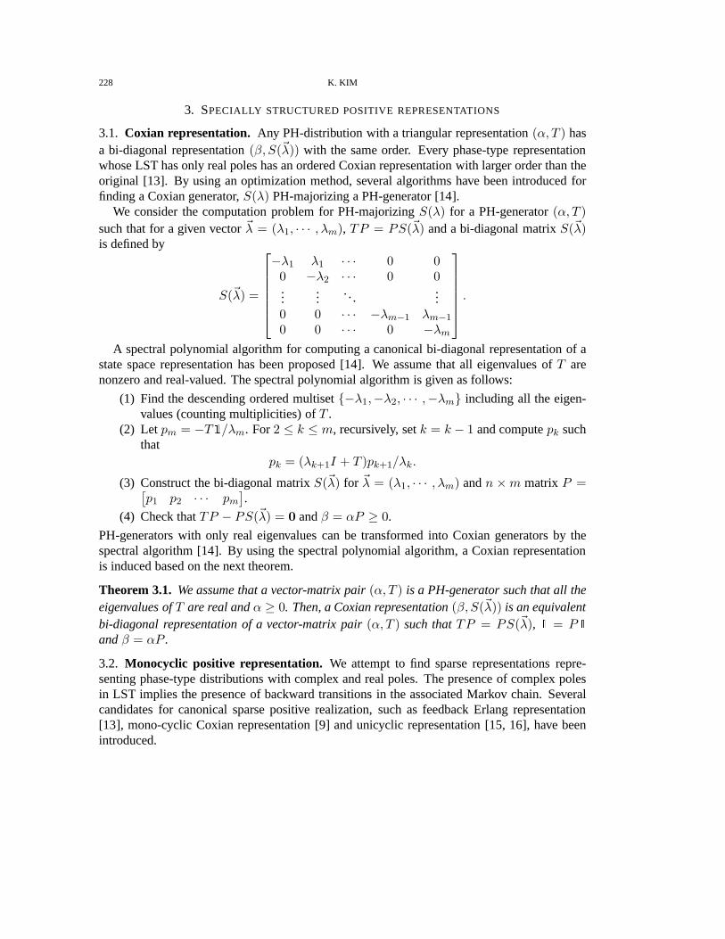
228 K. KIM
3. SPECIALLY STRUCTURED POSITIVE REPRESENTATIONS
3.1. Coxian representation. Any PH-distribution with a triangular representation(α, T ) hasa bi-diagonal representation(β, S(~λ)) with the same order. Every phase-type representationwhose LST has only real poles has an ordered Coxian representation with larger order than theoriginal [13]. By using an optimization method, several algorithms have been introduced forfinding a Coxian generator,S(λ) PH-majorizing a PH-generator [14].
We consider the computation problem for PH-majorizingS(λ) for a PH-generator(α, T )such that for a given vector~λ = (λ1, · · · , λm), TP = PS(~λ) and a bi-diagonal matrixS(~λ)is defined by
S(~λ) =
−λ1 λ1 · · · 0 00 −λ2 · · · 0 0...
.... ..
...0 0 · · · −λm−1 λm−1
0 0 · · · 0 −λm
.
A spectral polynomial algorithm for computing a canonical bi-diagonal representation of astate space representation has been proposed [14]. We assume that all eigenvalues ofT arenonzero and real-valued. The spectral polynomial algorithm is given as follows:
(1) Find the descending ordered multiset−λ1,−λ2, · · · ,−λm including all the eigen-values (counting multiplicities) ofT .
(2) Letpm = −T1/λm. For2 ≤ k ≤ m, recursively, setk = k − 1 and computepk suchthat
pk = (λk+1I + T )pk+1/λk.
(3) Construct the bi-diagonal matrixS(~λ) for ~λ = (λ1, · · · , λm) andn ×m matrixP =[
p1 p2 · · · pm]
.
(4) Check thatTP − PS(~λ) = 0 andβ = αP ≥ 0.
PH-generators with only real eigenvalues can be transformed into Coxian generators by thespectral algorithm [14]. By using the spectral polynomial algorithm, a Coxian representationis induced based on the next theorem.
Theorem 3.1. We assume that a vector-matrix pair(α, T ) is a PH-generator such that all theeigenvalues ofT are real andα ≥ 0. Then, a Coxian representation(β, S(~λ)) is an equivalentbi-diagonal representation of a vector-matrix pair(α, T ) such thatTP = PS(~λ), 1 = P1andβ = αP .
3.2. Monocyclic positive representation. We attempt to find sparse representations repre-senting phase-type distributions with complex and real poles. The presence of complex polesin LST implies the presence of backward transitions in the associated Markov chain. Severalcandidates for canonical sparse positive realization, such as feedback Erlang representation[13], mono-cyclic Coxian representation [9] and unicyclicrepresentation [15, 16], have beenintroduced.

AN OPTIMIZATION APPROACH FOR COMPUTING A SPARSE MONO-CYCLIC POSITIVE REPRESENTATION229
An n × n matrix A is said to be reducible if there exists a permutation matrixP such
that P tAP =
[
B C0 D
]
whereB andD are square matrices andP t is the transpose ofP .
Otherwise,A is said to be irreducible . DefineEij be then × n matrix that has only a one inthe position(i, j) and zeros otherwise. IfA is irreducible and for anyaij 6= 0, A − aijEij isreducible, then A is said to be nearly reducible. Suppose A isann×n nearly reducible matrix[17]. Then, there exist permutation matricesP andQ and an integers > 1 such that
PAQ =
A1 B1 · · · 0 0
0 A2 · · · 0 0
.. .0 0 · · · As−1 Bs−1
Bs 0 · · · 0 As
(3.1)
where eachBi has exactly one entry equal to one and eachAi is nearly reducible. When allBi’s are1× 1, this is a simplified form for nearly reducible matrices. We note that this form isa good candidate as a simple sparse representation of a phase-type distribution with complexpoles.
The simplest cyclic representations are obtained by addinga feedback on an Erlang repre-sentation, which is called a Feedback Erlang (FE) representation or mono-cyclic representation[16, 9]. A new type of representation can be obtained by adding a feedback to the Coxian rep-resentation. It is specially denoted as a Feedback Coxian (FC) representation if the transitionmatrix of a vector matrix pair can be obtained by adding feedback to the Coxian representation.Thus, for a given vector~λ = (λ1, · · · , λm) and0 ≤ z < 1, an FC representation(α,M(~λ, z))is defined by
M(~λ, z) =
−λ1 λ1 · · · 0 00 −λ2 · · · 0 0...
.... . .
......
0 0 · · · −λm−1 λm−1
zλm 0 · · · 0 −λm
(3.2)
We can see that the matrixM(~λ, z) is a simple nearly reducible matrix.
Lemma 3.2. Let P be a permutation matrix and~λ′ = ~λP . Then an FC representation(α,M(~λ′, z)) has the same eigenvalue multiset.
Proof. The characteristic polynomialp(s) = det(sI − M(~λ, z)) is given byp(s) = (s +λ1)(s + λ2) · · · (s + λm)− θ whereθ = zλ1λ2 · · ·λm. Since the characteristic polynomial isindependent of the order of the entries of~λ, the FC representation(α,M(~λ′, z)) has the sameeigenvalue multiset.

230 K. KIM
We can resort~λ in ascending order representing the given characteristic polynomial. FC rep-resentations have more free parameters than FE representations. We define a Hypo-Feedback-Coxian Block (HFCB) representation as a generalized form, covering Erlang, Coxian, FE andFC block representation.
Definition 3.1. A Hypo-Feedback-Coxian Block (HFCB) representation is defined as a tran-sient generator having the following structure
M =
M1 M∗
1 · · · 0 0
0 M2 · · · 0 0
......
. . ....
...0 0 · · · MJ−1 M∗
J−10 0 · · · 0 MJ
(3.3)
whereMi is a feedback CoxianM(~λ, z) or CoxianS(λ) for eachi and M∗
j is defined byM∗
j = (−Mj)1e1, wheree1 is the first standard basis vector.
In the above definition, if cyclicMi is an FE, it is denoted by a Hypo-Feedback-Erlang Block(HFEB) as a special case of HFCB [8]. It has been proven that every phase-type representationcan be transformed into a mixture of HFEB representations [5, 9].
Algorithm 1 A cyclic spectral polynomial algorithmInput: (α, T )
Output: P andβ = αP
(1) Choose an appropriate HFCB generatorM such that the eigenvalue multiset ofM
includes all eigenvalues ofT counting multiplicities.(2) Give an initial column vectorpm = −T1.(3) ζk is defined by the number of nonzero elements of thek-th column ofM andcj,k is
the(j, k)-th element ofM. For a givenpk and1 < k ≤ m, recursively, setk = k − 1and computepk as follows(a) if ζk = 2,
pk = (λk+1I + T )pk+1/λk (3.4)(b) if ζk = 3 andck+n′,k 6= 0,
pk = ((λk+1I + T )pk+1 − ck+n′,k+1pk+n′)/ck,k+1 (3.5)
(4) ConstructP =[
p1 p2 · · · pm]
(5) Finally, check thatTP = PM andαP ≥ 0, and returnβ = αP andP .
We propose a cyclic spectral polynomial algorithm to compute a transform matrixP gener-atingM from a representation(α, T ) in Algorithm 1. Finally, check two facts:TP = PM
andαP ≥ 0. In the next section, we will discuss how to find an appropriate HFCB generatorM with lower order in the first step in Algorithm 1.

AN OPTIMIZATION APPROACH FOR COMPUTING A SPARSE MONO-CYCLIC POSITIVE REPRESENTATION231
Theorem 3.3. We assume that a vector-matrix pair(α, T ) is a PH-generator such that allthe eigenvalues ofT are real and complex numbers andα ≥ 0. Then the matrixP satisfiesthat TP = PM and the eigenvalue multiset (counting multiplicities) ofT is included alleigenvalues of the HFCB matrixM in Eq. (3.3) .
Proof. First, we assume that an eigenvalue multiset (counting multiplicities) of T is includedin the multiset of eigenvalues of the HFCB matrixM. However, it is postponed how tofind M satisfying the assumption to the next section. A matrixP is computed by Algo-rithm 1. We will show that we can obtainP such thatTP = PM. We haveTP =[
Tp1 Tp2 · · · Tpm−1 Tpm]
and setpm = −T1. The last column ofM has only twononzero values. From Algorithm 1, we obtainTpm = λm−1pm−1 − λmpm. For1 < k < m,sincek-th column ofM has two or three nonzero elements, we have two casesTpk+1 =ck,k+1pk − λk+1pk+1 + ck+n′,k+1pk+n′ or Tpk+1 = λkpk − λk+1pk+1 in each step. Forthe first column ofM, we have two casesTp1 = −λ1p1 + c1+n′,1p1+n′ or Tp1 = −λ1p1.Therefore, we can see thatTP = PM.
4. OPTIMIZATION METHOD FOR FINDING A SPARSEHFCB REPRESENTATION
We consider the properties of FE blocks and FC blocks. For a given FE blockM(~λ, z) withλi = λ > 0 and a constantλ, the eigenvalue multiset ofM(~λ, z) can be computed explicitlyin a closed form [9].
Lemma 4.1. [9] Assume that we have a real rootµ0 = −λ + λz1/m and a complex rootµ1 = a + ib. Then eachn-th root µk of its characteristic polynomial equation of an FErepresentationM(~λ, z) is simply obtained by
µk = −λ(1− z1
m cos2kπ
m) + iz
1
mλ sin2kπ
m(4.1)
for 0 ≤ k < m, where~λ = (λ, · · · , λ), and the parameters of the representation can uniquelybe determined by
λ =1
2
(
2a− b tanπ
m+ b cot
π
m
)
(4.2)
z =b(tan π
m + cot πm)
2λ(4.3)
for a givenµ1 and an integerm > 2.
For a complex rootµ1 = a + ib, we can obtain an FE blockM(~λ, z) such that~λ =(λ, · · · , λ) and z are defined by Eqs (4.2) and (4.3). We consider a lower bound problemof the order of a phase-type generatorT including a given complex eigenvalue. It is relatedto the continuous version of famous Kolmogorov’s remark: “for a fixed integerm, what is themultiset of all complex numbers that are eigenvalues of an order-n stochastic matrix?” [13].

232 K. KIM
Lemma 4.2. [13] Let (α, T ) be a generator of phase-type distribution with a maximal realeigenvalueµ0 and with any complex eigenvalueµ1 = −a+ bi (a > 0). Then the orderm of Tsatisfies
|b|
a− |µ0|≤ cot
π
m(4.4)
It has been shown that a wedge as in (4.4) contains all eigenvalues ofT using an invariantpolytope argument [13]. By using the result of Lemma 4.2, we can determine the lower boundof the order of an FC block includingµ1 because an FC block is regarded as a special caseof a phase-type representation. Since the eigenvalue multiset of FE block computed by usingLemma 4.1 covers at most two or three eigenvalues of the original matrixT , the total order ofM gets larger. On other hand, because FC blocks have more free parameters, we can find anFC block including more common eigenvalues ofT than that of FE block. So we can reducethe total order ofM.
The relationship of the roots of a polynomial equation and its coefficients has been studied inthe complex analysis field [18]. It is closely related to a typical theorem of [18], which showsa connection between the roots of the polynomial and the generator (~λ, z) of an FC matrixM(~λ, z).
Lemma 4.3. Assume that a diagonal vector~λ = (λ1, λ2, · · · , λm) of the mono-cyclic matrixM(~λ, z) in (3.2) lies in a circular region whose center isλ and a given radiusr > 0.
(1) Then, all of the rootsµ1, · · · , µm of the polynomial equationp(s) = (s + λ1)(s +λ2) · · · (s+ λm)− θ = 0 lie on or within one of then circles, which have the commonradius r and whose centers,µk’s, are given byµk = −λ + exp(2ikπm )|θ|1/m, whereθ = zλ1λ2 · · ·λm.
(2) If thesem circles are mutually external, each circle contains precisely one of the rootsµ1, · · · , µm of the polynomial equationp(s).
(3) If λ = E(λk), then we have|θ|1/m ≤ |λ|z1
n , and equality holds if and only ifλk = λfor all k.
Proof. Proofs for the first and the second can be shown by using the results of [18]. Thearithmetic mean is larger than or equal to the geometric meanand the equality only holds ifλk = λ for all k. The third is trivial.
Lemma 4.3 shows the connection betweenλk in M(~λ, z) and the root multisetµkof p(s). With the help of a numerical procedure, we can depict the feasible regions of theeigenvalues ofM(~λ, z) for a givenr.
Example 4.1. By using a random number generator, for given0 ≤ z < 1 and r > 0, wegenerate a random number vector~λ such thatλ−r ≤ λk ≤ λ+r andλ = E(λk). We computeall the rootsµk of the characteristic polynomialp(s) depending on a random number vector~λ with respect toz = 0.5 and λ = 2. Figure 1 shows a relationship between the eigenvaluesµk of an FC blockM(~λ, z) and a random number vector~λ for n = 5 or n = 6. In Fig. 1,
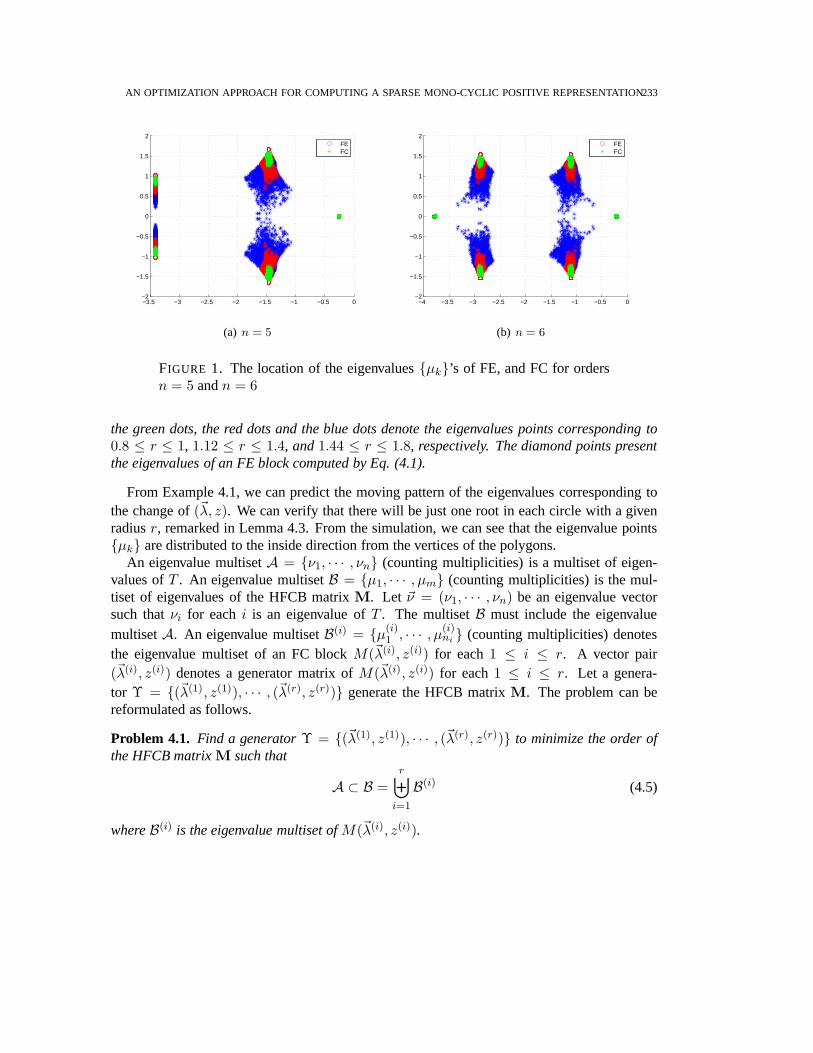
AN OPTIMIZATION APPROACH FOR COMPUTING A SPARSE MONO-CYCLIC POSITIVE REPRESENTATION233
−3.5 −3 −2.5 −2 −1.5 −1 −0.5 0−2
−1.5
−1
−0.5
0
0.5
1
1.5
2
FEFC
(a) n = 5
−4 −3.5 −3 −2.5 −2 −1.5 −1 −0.5 0−2
−1.5
−1
−0.5
0
0.5
1
1.5
2
FEFC
(b) n = 6
FIGURE 1. The location of the eigenvaluesµk’s of FE, and FC for ordersn = 5 andn = 6
the green dots, the red dots and the blue dots denote the eigenvalues points corresponding to0.8 ≤ r ≤ 1, 1.12 ≤ r ≤ 1.4, and1.44 ≤ r ≤ 1.8, respectively. The diamond points presentthe eigenvalues of an FE block computed by Eq. (4.1).
From Example 4.1, we can predict the moving pattern of the eigenvalues corresponding tothe change of(~λ, z). We can verify that there will be just one root in each circle with a givenradiusr, remarked in Lemma 4.3. From the simulation, we can see that the eigenvalue pointsµk are distributed to the inside direction from the vertices ofthe polygons.
An eigenvalue multisetA = ν1, · · · , νn (counting multiplicities) is a multiset of eigen-values ofT . An eigenvalue multisetB = µ1, · · · , µm (counting multiplicities) is the mul-tiset of eigenvalues of the HFCB matrixM. Let ~ν = (ν1, · · · , νn) be an eigenvalue vectorsuch thatνi for eachi is an eigenvalue ofT . The multisetB must include the eigenvaluemultisetA. An eigenvalue multisetB(i) = µ
(i)1 , · · · , µ
(i)ni (counting multiplicities) denotes
the eigenvalue multiset of an FC blockM(~λ(i), z(i)) for each1 ≤ i ≤ r. A vector pair(~λ(i), z(i)) denotes a generator matrix ofM(~λ(i), z(i)) for each1 ≤ i ≤ r. Let a genera-tor Υ = (~λ(1), z(1)), · · · , (~λ(r), z(r)) generate the HFCB matrixM. The problem can bereformulated as follows.
Problem 4.1. Find a generatorΥ = (~λ(1), z(1)), · · · , (~λ(r), z(r)) to minimize the order ofthe HFCB matrixM such that
A ⊂ B =r⊎
i=1
B(i) (4.5)
whereB(i) is the eigenvalue multiset ofM(~λ(i), z(i)).

234 K. KIM
We note that the problem is closely related to the simultaneous root finding problem of apolynomial [12]. Finding the roots of polynomials is an important task for various areas ofsignal processing, such as filter and wavelet design, spectral estimation, phase unwrapping,and communication. The constrained relation between the roots and coefficients of a polyno-mial can be used to find all of the roots of a given polynomial simultaneously, instead of usingsequential methods, such as Laguerre’s and Newton-Raphson’s [12]. Sincepi(s) the charac-teristic is polynomial of each FC block matrixM(~λ(i), z(i)), the characteristic functionp(s) ofthe HFCB matrixM is p(s) = p1(s)p2(s) · · · pr(s).
Lemma 4.4. For any generator(~λ(i), z(i)) ∈ Υ, assume thatB(i) denotes the eigenvaluemultiset (counting multiplicities) of the sub-blockM(~λ(i), z(i)) of the HFCB matrixM. Thenit satisfies the coefficient relation equations such that each φk is defined by
φ1 ,
mi∑
k=1
λ(i)k −
mi∑
k=1
(−µ(i)k ) = 0
φ2 ,
mi∑
k<j
λ(i)k λ
(i)j −
mi∑
i<j
(−1)2µ(i)k µ
(i)j = 0
...
φmi, (1− z(i))λ
(i)1 · · ·λ(i)
mi− (−1)miµ
(i)1 · · ·µ(i)
mi= 0
(4.6)
for eachµ(i)k ∈ B(i).
Proof. We will show that for given generatorΥ andB(i), the coefficient relation equationsbetween roots and coefficients of a polynomial as (4.6) can bedefined. The characteristicpolynomialpi(s) = det(sI −M(~λ(i), z(i)))) for eachi is given by
pi(s) = (s+ λ(i)1 )(s + λ
(i)2 ) · · · (s+ λ(i)
mi)− θ (4.7)
whereθ = z(i)λ(i)1 λ
(i)2 · · · λ
(i)mi andmi is an order ofM(~λ(i), z(i)). The eigenvalue multiset of
M(~λ(i), z(i)) is equal to the root multiset of the polynomialpi(s). The polynomialpi(s) canbe rewritten in the form
pi(s) =
mi∏
k=1
(s− µ(i)k ). (4.8)
All coefficient relation functionsφi’s can be defined by comparing with coefficients of (4.7)and (4.8) with respect to(~λ(i), z(i)) , (λ
(i)1 , · · · , λ
(i)mi , z
(i)) and~µ(i) , (µ(i)1 , µ
(i)2 · · · , µ
(i)mi), re-
spectively. Therefore we can obtain the relation equations, φk ’s, between roots and coefficientsof a polynomial, comparing the coefficients induced from theeigenvalue multisetB(i) with thecoefficients of the characteristic polynomialpi(s) of each FC block matrixM(~λ(i), z(i)).
B(i) is partitioned into a fixed multisetF (i) and a flexible multisetU (i) = B(i) − F (i). Letus set~s = (~λ(i), z(i)). For eachU (i), we define a vector~u by ~u = (u1, · · · , ud) for uk ∈ U (i)

AN OPTIMIZATION APPROACH FOR COMPUTING A SPARSE MONO-CYCLIC POSITIVE REPRESENTATION235
andd = |U (i)| where|A| is defined by the cardinality ofA. A free parameter vector~x isdefined by~x = (Re(~u), Im(~u)). We define a fixed vector~xc = (Re(~v), Im(~v)), where~v = (v1, · · · , vd′) for eachvk ∈ F (i).
For all integers with1 ≤ k ≤ mi, the coefficient relation functionsφk can be defined in theform, φk(~x, ~xc,~s). Set~φ = (φ1, · · · , φmi
) as in (4.6). The coefficient relation vector function~φ : Rn → Rmi represents smooth nonlinear functions defined by Eq. (4.6),wheren is thedimension of the vector(~x, ~xc,~s). We formulate a constrained nonlinear optimization problemto compute an FC blockM(~λ(i), z(i)) whose eigenvalue multiset includesF (i).
Problem 4.2. For each multisetF (i), find a solution(~x,~s) of a nonlinear objective functionf(~x,~s) subject to equation or inequality constraints such that
min~x,~s
f(~x,~s)
s.t. bl ≤ ~x ≤ bu
0 <~s ≤ cu
~φ(~x, ~xc,~s) = 0.
(4.9)
for a fixed parameter~xc wherebl is a lower bound vector,bu is an upper bound vector, and theobjective functionf(~x,~s) in (4.9) is given by
f(~x,~s) = −mi∑
k=1
lnλk. (4.10)
Now we consider what reasonable constraints are given in theconstrained optimization prob-lem in (4.9). BecauseM(~λ(i), z(i)) andT are phase-type, all the real values of eigenvalues are
negative, i.e.,Re(µ(i)k ) < 0 for anyµ(i)
k ∈ B(i). We can set the upper bounds zerobu = 0 for
the real numbers, becauseRe(µ(i)k ) < 0. The other bounds,bl andbu, are given in a proper
bound from initial values for the algorithm to be convergence. We can see that the entries~λ(i)
are positive and0 ≤ z(i) < 1. The upper boundcu for ~λ(i) are given in an appropriate boundfrom initial values.
Remark 4.5. • We can assume that first and second derivatives of the objective functionsand constraints are available because~φ consists of polynomials.
• We note that roots of the polynomial in (4.8) depend continuously on its coefficients.That is well-known as the use of Rouche’s Theorem[19]. A small change in the coeffi-cients ofp(s) causes only a small change in the roots of the polynomial.
• Using the result of Lemma 4.4, Problem 4.1 can be reformulated in the form of aconstrained nonlinear optimization problem for the coefficient relation functions withrespect to(~x,~s) in Problem 4.2. By solving a constrained nonlinear optimization inProblem 4.2, we find a generator(~λ(i), z(i)) andU (i) for a fixedF (i).
Our objective is to find a HFCB representation with possible lower order, whose eigenvaluemultiset includes all eigenvalues ofT . We will discuss numerical problems for finding a HFCB

236 K. KIM
representation with lower order by using a nonlinear optimization method. Our strategy isto obtain the optimal solutions by extending some partiallyknown solutions recursively asfollows:
(1) Initially, compute an FE blockM(~λ(i), z(i)) such thatF (i) = A⋂
B(i) is nonempty,using Lemma 4.1.
(2) We choose a target multisetT such thatA ⊃ T ⊃ F (i). SetFk = F (i)
(3) We choose a new multisetFk(⊂ T ) corresponding to~xc after~xc moves a little andsolve Problem 4.2 for a new multisetFk, recursively. If Problem 4.2 is solved finally,then we can obtain a generator(~λ(i), z(i)) such thatF (i) = T = A
⋂
B(i).(4) If there is more additional target multisetT , then go to Step 2. Otherwise, go to the
next step.(5) Finally, we obtain aM(~λ(i), z(i)) whose eigenvalue multiset includesF (i) = A
⋂
B(i)
We need to discuss the efficient numerical algorithm at the third step in the above method.While a nonlinear optimization method is a powerful tool to find an optimal solution, there areseveral potential difficulties to solve some problems such as divergence and instability. Mostof the numerical methods for solving the nonlinearly constrained optimization problems meeta danger converging to a local minimal point or diverging, depending on initial values.
We propose alinear search algorithm in Algorithm 2. We can generate a sequence ofiterates that converges to an optimal solution provided that the initial value is sufficiently closeto that optimal solution. A basic idea is to make shift by following a straight line to a finalpoint from an initial point knowing a solution, and find a solution of the next stage using theprevious value as an initial value.
We choose a target multisetT ⊂ A, to which the multisetFk expands in each iteration.Initially, assume that an optimal solution~xc,0 of Problem 4.2 is already computed and can beused as an initial vector, because theµk’s in (4.8) are explicitly computed by using Lemma 4.1.nd denotes the number of segments. It is related with the lengthof change. If the procedurefails, then in order to avoid diverging we can try to execute the algorithm again after increasingnd recursively until some threshold. For0 ≤ k ≤ nd − 1, compute~xc,k+1 such that
~xc,k+1 = ~xc,k + ~d (4.11)
where~d =~xc−~xc,0
nd. LetFk correspond to~xc,k. We find(~x,~s) corresponding toFk by solving
Problem 4.2 recursively, until arriving at the final destination. If the multisetFk arrives at thefinal destination multisetT successfully, then the adaptive process succeeds. We can obtaina vector(~x,~s) for a target multisetT . Additionally, if the procedure fails, then, in order toavoid diverging, we can try to execute the algorithm again after increasingnd recursively untila given threshold.
Finally, we implement a complete algorithm transforming from a given phase-type repre-sentation to an HFCB representation(β,M), which has as minimal order as possible in Algo-rithm 3. First, we compute an eigenvalue multisetA of T . Recursively, we find an FC blockM(~λ(i), z(i)) including a chosen eigenvalueµ ∈ A. We typically have two cases: an FC blockfor a complex eigenvalue and a Coxian block for a real eigenvalue. For a complex eigenvalue

AN OPTIMIZATION APPROACH FOR COMPUTING A SPARSE MONO-CYCLIC POSITIVE REPRESENTATION237
Algorithm 2 LineSearch(B, F , T ,~s)
Input: B, F , T ,~sOutput: ~s, Flag, B
1: Compute a vector~x with respect toU = B − F2: Compute an initial vector~xc,0 with respect toF3: Compute~xc with respect to a target multisetT4: Set a segment numbernd
5: ~d =~xc−~xc,0
nd
6: for 0 ≤ k < nd do7: Set~xc,k+1 = ~xc,k + ~d8: Compute a new solution(~x,~s) of Problem 4.2 for an old value(~x,~s) and~xc,k+1
9: ComputeF corresponding to~xc,k+1
10: if No solutionthen11: return Flag = False12: else13: Flag = True14: end if15: Resort~λ(i) in ascending order16: update~s using~λ(i)
17: end for18: B is updated by using(~x, ~xc)19: return ~s, Flag, B
µ, an FC induced fromµ possibly includes other elements ofA. Choose a subset collectionP = S1, · · · ,SN such thatSk ⊂ Ω, Sk ∩F = ∅, and|Sk| ≤ |Sj | for k > j. If w ∈ Sk, thenw ∈ Sk. UsingP, we can choose a new target multisetT (⊃ F) as large as possible. Compute(~λ(i), z(i)) corresponding toT by applying the linear search algorithm. We can reduce the totalorder of the HFCB matrixM depending on how to choose a target multisetT . The processcontinues until all complex numbers fromΩ are removed. Next, for a selected real eigenvalueµ ∈ Ω, we compute~λ(i) = µ, mi = 1 andz = 0, which generate the Coxian block. We thenresort a generatorΥ in the ascending order of the minimal number of~λ(i). Finally, we computean HFCB representationM andP using a generatorΥ such thatTP = PM. We can obtain atransformation matrixP andM satisfyingTP = PM.
Finally, we note the initial vectorβ corresponding to the obtained mono-cyclic representa-tion can be negative. Even thoughT has a Coxian generatorS(~λ) as Theorem 3.1, the positivityof β is not guaranteed. The order of the resulting Coxian generator can be larger than that of theoriginal one. The process for finding suchP andS is called the Coxianization of PH-generatorT . The Coxianization of a PH-generator with only real eigenvalues has been proven to be fea-sible; three numerical methods for Coxianization have beenintroduced and their performanceswere compared [14].

238 K. KIM
Algorithm 3 Compute an HFCB representation.
Input: (α, T )Output: (β,M)
1: Compute the eigenvalue multisetA of T2: IndexA in descending order of their real values3: Ω = A, i = 04: while Ω is nonemptydo5: i = i+ 16: if Ω has any complex numberthen7: Select a complex numberµ ∈ Ω with a maximal real value8: Choose a proper numbermi satisfying the inequality in (4.4)9: Compute (~λ(i), z(i)) and an eigenvalue multisetB = µ0, · · · , µmi−1 of
M(~λ(i), z(i)) by using Lemma 4.1.10: F = µ, µ11: Choose a subset collectionP = S1, · · · ,SN such thatSk ⊂ Ω, Sk ∩ F = ∅,
|Sk| ≤ |Sj | for k > j, and ifw ∈ Sk, thenw ∈ Sk.12: for t = 1 : N do13: T = F ∪ St
14: [ ~s, Flag, B]= LineSearch(B, F , T ,~s)15: if Flag == True then16: Compute(~λ(i), z(i)) using~s, and insert it intoΥ.17: Break18: end if19: end for20: else21: Select a maximal real valueµ ∈ Ω with22: B = µ
23: ~λ(i) = µ, mi = 1 andzi = 0.24: end if25: Ω = Ω− B ∩ A26: end while27: Resort a generatorΥ in the ascending order of the minimal number of~λ(i)
28: By using Algorithm 1, compute a HFCB representationM andP using a generatorΥ suchthatTP = MP
29: Computeβ = αP30: return (β,M)
To make the initial vector non-negative, additional stateshave to be added to the distributionsimilarly. If β contains at least one negative element then a further transformation is requiredto obtain a PH representation. We can extend the PH generatorby adding an Erlang tail as
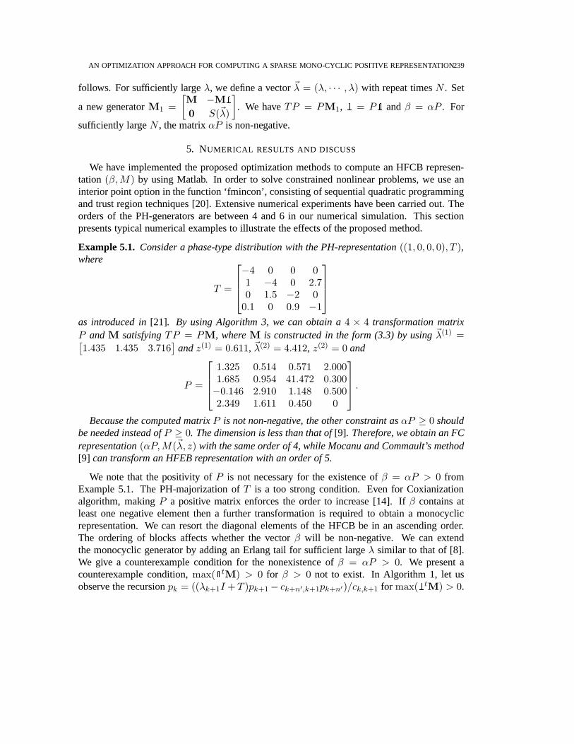
AN OPTIMIZATION APPROACH FOR COMPUTING A SPARSE MONO-CYCLIC POSITIVE REPRESENTATION239
follows. For sufficiently largeλ, we define a vector~λ = (λ, · · · , λ) with repeat timesN . Set
a new generatorM1 =
[
M −M10 S(~λ)
]
. We haveTP = PM1, 1 = P1 andβ = αP . For
sufficiently largeN , the matrixαP is non-negative.
5. NUMERICAL RESULTS AND DISCUSS
We have implemented the proposed optimization methods to compute an HFCB represen-tation (β,M) by using Matlab. In order to solve constrained nonlinear problems, we use aninterior point option in the function ‘fmincon’, consisting of sequential quadratic programmingand trust region techniques [20]. Extensive numerical experiments have been carried out. Theorders of the PH-generators are between 4 and 6 in our numerical simulation. This sectionpresents typical numerical examples to illustrate the effects of the proposed method.
Example 5.1. Consider a phase-type distribution with the PH-representation ((1, 0, 0, 0), T ),where
T =
−4 0 0 01 −4 0 2.70 1.5 −2 00.1 0 0.9 −1
as introduced in[21]. By using Algorithm 3, we can obtain a4 × 4 transformation matrixP andM satisfyingTP = PM, whereM is constructed in the form (3.3) by using~λ(1) =[
1.435 1.435 3.716]
andz(1) = 0.611, ~λ(2) = 4.412, z(2) = 0 and
P =
1.325 0.514 0.571 2.0001.685 0.954 41.472 0.300−0.146 2.910 1.148 0.5002.349 1.611 0.450 0
.
Because the computed matrixP is not non-negative, the other constraint asαP ≥ 0 shouldbe needed instead ofP ≥ 0. The dimension is less than that of[9]. Therefore, we obtain an FCrepresentation(αP,M(~λ, z) with the same order of 4, while Mocanu and Commault’s method[9] can transform an HFEB representation with an order of 5.
We note that the positivity ofP is not necessary for the existence ofβ = αP > 0 fromExample 5.1. The PH-majorization ofT is a too strong condition. Even for Coxianizationalgorithm, makingP a positive matrix enforces the order to increase [14]. Ifβ contains atleast one negative element then a further transformation isrequired to obtain a monocyclicrepresentation. We can resort the diagonal elements of the HFCB be in an ascending order.The ordering of blocks affects whether the vectorβ will be non-negative. We can extendthe monocyclic generator by adding an Erlang tail for sufficient largeλ similar to that of [8].We give a counterexample condition for the nonexistence ofβ = αP > 0. We present acounterexample condition,max(1tM) > 0 for β > 0 not to exist. In Algorithm 1, let usobserve the recursionpk = ((λk+1I + T )pk+1− ck+n′,k+1pk+n′)/ck,k+1 for max(1tM) > 0.

240 K. KIM
When pk+1 and pk+n′ are positive, andck+n′,k > λk ( or 1tM > 0), negative entries inpk−1 can appear. Therefore, we cannot obtainαP ≥ 0 for anyα ≥ 0. In the next example,we can verify different properties of two cases,1tM ≤ 0 and1tM > 0 by using numericalsimulations.
Example 5.2. Consider a phase-type distribution with the PH-representation (α, T ) such that
T =
−6.0 0.6 0.6 0.6 32 −4.5 0 0 0.10 2 −3.5 0 00 0 2 −3 00 0 0 2 −2
While Mocanu and Commault’s method[9] can transformT into an HFEB representation withorder of 8, we can obtain a5 × 6 matrixP and an HFCB generatorM with an order of 6 byusing Algorithm 3. We can see that the matrixP is not non-negative. The proposed method canderive multiple solutions depending on an given initial value. Formax(1tM) ≤ 0, we couldobtainα ≥ 0 such thatαP ≥ 0 after attempting several times. For example, there are twotypical cases after applying the proposed algorithm.
(1) The first case has~λ(1) = 1.120, z(1) = 0, ~λ(2) = (2.673, 2.678, 3.116, 4.49201, 6.366)
andz(2) = 0.0591. For max(1tM) ≤ 0, we obtainedα ≥ 0 such thatαP ≥ 0 afterseveral trials.
(2) In the second case, we have~λ(1) = 1.12084, z(1) = 0, ~λ(2) = (1.517, 3.660, 3.660,
3.660, 6.420) andz(2) = 0.096. For max(1tM) > 0, we computeP for several times.Typically, we can obtainP such as
P =
−0.202 2.084 0.920 0.858 0.940 1.2−0.127 1.043 0.481 0.090 1.914 2.4−0.107 0.644 0.099 1.156 2.507 1.5−0.113 0.539 0.936 1.686 1.753 1.0−0.259 2.840 1.468 1.206 0.5463 0
.
Because all entries of the first column are negative, we can see thatmin(αP ) < 0 foranyα ≥ 0.
In order to show that the proposed method has good performance, a large set of random PHgenerators samples were generated in the next example. The random matricesT are dense, butthe canonical representations obtained by the proposed method are sparse.
Example 5.3. A 31 samples ofT with order 5 and 4 complex eigenvalues are generated ran-domly. Then for each sample, the proposed method and Mocanu and Commault’s method[9]are applied to obtainHFCB andHFEB, respectively. For each algorithm, we determineM
andβ = αP and check non-negativity ofβ. We compared the orders of the HFCB generatorsand HFEB generators. LetdFC anddFE be the order ofHFCB andHFEB, respectively.

AN OPTIMIZATION APPROACH FOR COMPUTING A SPARSE MONO-CYCLIC POSITIVE REPRESENTATION241
1 2 30
2
4
6
8
10
12
14
16
18
dFE
−dFC
Num
ber
FIGURE 2. Histogram of the orderdFE minus the orderdFC
In Fig. 2, we plotdFE − dFC . We could see that the order of the solution obtained by us-ing the proposed method is smaller than that of the solution obtained by using Mocanu andCommault’s method[9].
We note that there are several similar approaches to find compact PH representations with aunicyclic structure [15, 21]. A unicyclic block has more flexibility than FE block or FC block,since the representation has more free parameter and is denser. Since a unicyclic block has toomany free parameters (2m− 1) comparing to the number of equations (m), it is impossible toobtain a stable optimal solution using numerical method. Soa modified unicyclic block wasintroduced [15]. A modified unicyclic block approach reduces the free parameter number tom.Thus, the values ofm free parameters can be obtained by solvingm equations. When the giveneigenvalue set frequently has no feasible solution, it cannot be applied. On the other hand, forthe case, the proposed method can obtain a feasible solutionby solving Problem 4.2.
Furthermore, the importance of simple sparse representations comes from the fact that thecomputational complexity of PH-distributed random-variate generation depends on the repre-sentation in simulation applications [8]. The FC block approach can lead to more effectiverandom number generation of PH-distributions in stochastic modeling and analysis becausethe number of its feedback loop can be reduced.
6. CONCLUSION
We tried to transform a phase-type representation into a sparse HFCB representation withan order as low as possible. We introduced a numerical methodfor computing an HFCB repre-sentation by solving a nonlinear optimization problem. To find a sparse HFCB representationwith lower order, including the multiset of eigenvalues of the original generator, we developeda numerical algorithm solving a constrained nonlinear optimization program. We discussedsome numerical issues in efficiently finding a stable solution of the nonlinear constrained op-timization problem. The proposed method can be applied to the sparse positive realization ofpositive system.

242 K. KIM
ACKNOWLEDGEMENTS
The author thanks the editor and the referees for their careful reading of the manuscript.This work was supported by research fund of Chungnam National University.
REFERENCES
[1] C. Altafini. Minimal eventually positive realizations of externally positive systems.Automatica, 68 (2016),140–147.
[2] L. Benvenuti, L. Farina, and B. D. O. Anderson. Filteringthrough combination of positive filters.Circuits andSystems I: Fundamental Theory and Applications, IEEE Transactions on, 46(12) (1999), 1431–1440.
[3] L. Farina and S. Rinaldi.Positive Linear Systems: Theory and Applications. Wiley Interscience, 2000.[4] B. Nagy, M. Matolcsi, and M. Szilvasi. Order Bound for theRealization of a Combination of Positive Filters.
IEEE Transactions on Automatic Control, 52(4) (2007), 724–729.[5] C. Commault and S. Mocanu. Phase-type distributions andrepresentations: Some results and open problems
for system theory.International Journal of Control, 76(6) (2003), 566–580.[6] C. A. O’Cinneide. On non-uniqueness of representationsof phase-type distributions.Communications in Sta-
tistics. Stochastic Models, 5(2) (1989), 247–259.[7] G. Horvath, P. Reinecke, M. Telek, and K. Wolter. Efficient Generation of PH-distributed Random.Lecture
Notes in Computer Science, 7314(2012), 271–285.[8] G. Horvath, P. Reinecke, M. Telek, and K. Wolter. Heuristic representation optimization for efficient genera-
tion of PH-distributed random variates.Annals of Operations Research, (2014), 1–23.[9] S. Mocanu and C. Commault. Sparse representations of phase-type distributions.Communications in Statis-
tics. Stochastic Models, 15(4) (1999), 759–778.[10] K. Kim. A construction method for positive realizations with an order bound.Systems & Control Letters, 61(7)
(2012), 759–765.[11] K. Kim. A constructive positive realization with sparse matrices for a continuous-time positive linear system.
Mathematical Problems in Engineering, 2013(2013), 1–9.[12] D. S. Huang. A constructive approach for finding arbitrary roots of polynomials by neural networks.IEEE
Transactions on Neural Networks, 15(2) (2004), 477–491.[13] C. A. O’Cinneide. Phase-Type Distributions and Invariant Polytopes.Advances in Applied Probability, 23(3)
(1991), 515–535.[14] Q.-M. He, H. Zhang, and J. Xue. Algorithms for Coxianization of Phase-Type Generators.INFORMS J. on
Computing, 23(1) (2011), 153–164.[15] I. Horvath and M. Telek. A heuristic procedure for compact Markov representation of PH distributions. In
ValueTools, 2014.[16] C. A. O’Cinneide. Phase-type distributions: open problems and a few properties.Stochastic Models, 15(4)
(1999), 731–757.[17] D. J. Hartfiel. A simplified form for nearly reducible andnearly decomposable matrices, 1970.[18] J. L. Walsh. On the location of the roots of certain typesof polynomials.Transactions of American Mathematic
Society, 24 (1922), 163–180.[19] J. M. Ortega.Numerical Analysis: A Second Course. Classics in Applied Mathematics. Society for Industrial
and Applied Mathematics, 1990.[20] R. a. Waltz, J. L. Morales, J. Nocedal, and D. Orban. An interior algorithm for nonlinear optimization that
combines line search and trust region steps.Mathematical Programming, 107(3) (2006), 391–408.[21] Q.-M. He and H. Zhang. A Note on Unicyclic Representations of Phase Type Distributions.Stochastic Models,
21(2-3) (2005), 465–483.

J. KSIAM Vol.20, No.3, 243–259, 2016 http://dx.doi.org/10.12941/jksiam.2016.20.243
A MASS LUMPING AND DISTRIBUTING FINITE ELEMENT ALGORITHM FORMODELING FLOW IN VARIABLY SATURATED POROUS MEDIA
M. S. ISLAM
DEPARTMENT OFMATHEMATICS, SHAHJALAL UNIVERSITY OF SCIENCE& T ECHNOLOGY, SYLHET-3114,BANGLADESH
E-mail address: sislam [email protected]
ABSTRACT. The Richards equation for water movement in unsaturated soil is highly nonlinearpartial differential equations which are not solvable analytically unless unrealistic and oversim-plifying assumptions are made regarding the attributes, dynamics, and properties of the physi-cal systems. Therefore, conventionally, numerical solutions are the only feasible procedures tomodel flow in partially saturated porous media. The standardFinite element numerical tech-nique is usually coupled with an Euler time discretizationsscheme. Except for the fully explicitforward method, any other Euler time-marching algorithm generates nonlinear algebraic equa-tions which should be solved using iterative procedures such as Newton and Picard iterations.In this study, lumped mass and distributed mass in the frame of Picard and Newton iterativetechniques were evaluated to determine the most efficient method to solve the Richards equa-tion with finite element model. The accuracy and computational efficiency of the scheme and ofthe Picard and Newton models are assessed for three test problems simulating one-dimensionalflow processes in unsaturated porous media. Results demonstrated that, the conventional massdistributed finite element method suffers from numerical oscillations at the wetting front, espe-cially for very dry initial conditions. Even though small mesh sizes are applied for all the testproblems, it is shown that the traditional mass-distributed scheme can still generate an incorrectresponse due to the highly nonlinear properties of water flowin unsaturated soil and cause nu-merical oscillation. On the other hand, non oscillatory solutions are obtained and non-physicssolutions for these problems are evaded by using the mass-lumped finite element method.
1. INTRODUCTION
The Richards equation is the governing equation for movement of water flow in partiallysaturated porous media, contains nonlinearities arising from pressure head dependencies insoil moisture and hydraulic conductivity. It is practically impossible to solve the equationanalytically in unsaturated soil profiles with complex initial boundary conditions due to itshighly nonlinear nature. Therefore numerical approximations are typically used to solve theunsaturated flow equations. The standard approximations that are applied to the spatial domain
Received by the editors May 31 2016; Revised September 9 2016; Accepted in revised form September 9 2016;Published online September 16 2016.
2000Mathematics Subject Classification.65M60,76S05.Key words and phrases.Richards equation, Mass lumping, Mass distributing, Numerical solution, Variably
saturated flow.
243

244 M. S. ISLAM
are the finite difference and finite element methods are two popular schemes [1, 2]. Variationsof the standard finite difference and finite element methods,such as the sub domain finiteelement method have also been successfully used to solve these problems [3]. The choice ofusing either finite difference or finite element method for the solution of variably saturatedflow problems is largely personal and promoters of a particular method can easily support thestrengths of their preferred solution approach. This can cause problems when a choice has tobe made between these approaches, as it is difficult to independently evaluate the methods in asubstantial technique.
Several studies have explored the finite element solution [3, 4, 5, 6, 7]. Discussion aboutefficiency of mass types, element orders, and matrix solution methods, as well as influence ofmethods of numerical integration for the Richards equationare found few of these studies. Themain reason of this is the consistent (distributed) mass scheme with high order elements hasbeen typically accepted to be superior for solving complex nonlinear physical problems. Pre-vious studies established that the numerical solution withconsistent mass formulation showsoscillation [3, 5, 4, 6] but they are not explained about the reason of oscillations and methodshow to avoid the oscillations. Numerical oscillations is a significant factor to diverge the so-lution of Richards equation when simulate a sharp wetting front entering a dry soil profile. Toovercome this difficulty, it is necessary to reduce the size of the element and time step size.But the reduction in element size could drastically increase the simulation time, as a result thenumerical method becomes less attractive.
Numerical solution using pressure based formulation coupled with backward Euler timediscretization is shown to produce unacceptably large massbalance errors for many examplecalculations. It is true for both finite difference and finiteelement approximation in space,although finite elements are generally inferior to finite differences. Because use of pressurehead formulation with a simple time-stepping method is common, these findings appear tohave significant practical implications. Almost, all unsaturated flow simulations use either thehead-based or the moisture content-based formulation of Richards equation. A variety of finitedifference and finite element solution techniques have beenused with each of these equationforms [3, 8, 9, 10, 11]. Numerical algorithm based on mixed form of Richards equation havebeen proposed and mass balance errors occur in standard head-based numerical solution [12].
Fully implicit backward Euler time approximation applied to the mixed form of Richardsequation is mass conserving solution procedure for the unsaturated flow equation. Proper ex-pansion of the time derivative produces a simple computational algorithm that is perfectly massconservative for numerical approximation that preserves spatial symmetry. Thus the finite dif-ference and finite element approximations using this mixed formulation are perfectly massconservative. This approach is show to be superior to the standard head-based approximationswhile requiring no more computational effort. However conservation of mass is shown to beinadequate to guarantee good numerical solutions. For infiltration into dry soils, finite elementapproximations produce oscillatory solutions even while conserving mass. It is shown that di-agonalization of the time matrix, which occurs naturally infinite difference approximations,is necessary and sufficient to guarantee oscillations free solutions. Mass conserving solutionprocedure is presented by the use of modified definition of capacity term to force global mass

MASS LUMPING AND DISTRIBUTING FINITE ELEMENT ALGORITHM 245
balance and illustrated the importance of mass lumping in finite element solutions to unsatu-rated flow problems [5]. The significance of mass lumping is also shown and report good finiteelement solutions without mass lumping [3, 4, 10, 11]. Most of the studies are used a one-stepEuler time-marching algorithm with the head-based versionof Richards equation.
For stability reasons an implicit time discretization requiring evaluation of the nonlinear co-efficients at the current time level, is generally used to solve the equation numerically. Newtonand Picard iterative schemes are commonly used to linearizethe resulting discrete system ofequations, with the Picard scheme being the more popular of the two [3, 11, 13, 14, 15]. Picardmethod is the most intuitive linearization of Richards equation, computationally inexpensiveon a per-iteration basis, and preserves symmetry of the discrete system of equations. However,some studies shown experimentally, the method may diverge under certain conditions [7, 10]and verified theoretically [16].
On the other hand, the Newton scheme, which is quadraticallyconvergent [7, 17, 18] yieldscomplex non symmetric system matrices and expensive than Picard linearization, and can bemore robust than Picard for certain flow problems. The drawback of Newton’s method is that itis only locally convergent and involves the computation of derivatives. Although the use of thesolution of the last time step to start the Newton iterationsimproves considerably the robustnessof Newton’ method, in the degenerate case (saturated/unsaturated flow) the convergence isensured only when a regularization step is applied and underadditional constraints on thediscretization parameters. While the Newton and the Picardschemes are generally robust,these iterative methods entail computational costs associated with having to evaluate and solvethe system of equations repeatedly for each time step.
The objective of this study is to investigate the numerical behavior of finite element solutionof Richards equation including the suitability of lumped mass and distributed mass. The workis also focused on determining the method which would offer astable solution without requir-ing the resizing of the finite element mesh structure. Realistic initial and Dirichlet boundaryconditions are imposed in the numerical simulator to the head-based form of Richards equation.To reduce the CPU time and maintain small truncation error, an adaptive time-stepping strat-egy is implemented. The nonlinear matrix equations are solved using the Picard and Newtoniteration schemes. The performance of the algorithm is shown to be superior to the conven-tional pressure head-based form and can be easily used in layered porous media without anyextraordinary treatment.
2. GOVERNING EQUATION AND DISCRETIZATION
The partial differential equation describing fluid flow in partially saturated porous media,Richards equation, is obtained by combining Darcy’s law with the continuity equation. Forone-dimensional vertical flow in unsaturated soils, pressure head-based Richards equation iswritten as
C(ψ)∂ψ
∂t=
∂
∂z
(
K(ψ)
(
∂ψ
∂z+ 1
))
(2.1)

246 M. S. ISLAM
where,ψ is the pressure head [L], t is time [T ], z denotes the vertical distance from the soilsurface assumed positive downward [L], K(ψ) is the hydraulic conductivity [LT−1], C(ψ) =dθdψ
is the specific fluid capacity [L−1], θ is the volumetric water content.The pressure head-based form can be successfully used in both saturated and unsaturated
zones as well as in layered and composite porous materials. However, several studies haveshown that it suffers from convergence difficulties and poormass balance in modeling infiltra-tion into very dry media unless very fine discretizations areused [5, 7, 14, 19, 20, 21, 22, 23]which, in turn, makes the computation very expensive. The time steps required for convergenceare several orders of magnitude smaller than is required forreasonable temporal discretization[19]. The reason for these problems is highly nonlinear nature of the saturation-pressure func-tion under dry initial conditions, causing very high fluid pressure gradient near the wettingfront and huge computational cost.
Solution of Richards equation requires knowledge of hydraulic conductivity and fluid con-tent versus fluid pressure head. These relationships are known as the hydraulic properties ofthe porous media. In this study, the most commonly used relationships are the van Genuchten[24] model. This model illustrated in detail as follows
θ (ψ) = θr +θs − θr
[1 + |αψ|n]mif ψ ≤ 0 (2.2)
θ (ψ) = θs if ψ > 0 (2.3)
K (ψ) = Ks
[
θ − θrθs − θr
] 1
2
1−
[
1−
(
θ − θrθs − θr
) 1
m
]m2
if ψ ≤ 0 (2.4)
K (ψ) = Ks if ψ > 0 (2.5)
c (ψ) = αmnθs − θr
[1 + |αψ|n]m+1|αψ|n−1 if ψ ≤ 0 (2.6)
c (ψ) = 0 if ψ > 0 (2.7)
Due to the nonlinear nature of the Richards equation (2.1), it should be solve numerically,finite element Galarkin discretization in space and a finite difference discretization of the timederivative term are used. To develop the finite element approximation of the pressure head-based Richards equation, the weak formulation of the dependent variable and the constitutiverelations were approximated using interpolating polynomials [6, 25]. It was assumed that thehydraulic conductivity as well as capacitance varies linearly within each element [26]:
ψ (z, t) ≈ ψ (z, t) =M∑
j=1
ψj(t)Nj (z) (2.8)
K ≈ K =
M∑
j=1
KjNj (z) (2.9)

MASS LUMPING AND DISTRIBUTING FINITE ELEMENT ALGORITHM 247
C ≈ C =
M∑
j=1
CjNj (z) (2.10)
whereM is the number of elements,Nj (z) is the selected basis function, andψj(t) is theassociated and time-dependent unknown coefficients representing the solution of flow equationat nodes within the domain. The goal of the finite element approximation is to minimize theerror and this can be accomplished by introducing the weightfunction, Nj (z), and settingoperatorL(ψ) to be orthogonal toNj (z):
∫
Ω
L(
ψ)
Nj (z) dΩΩ =
∆z∫
0
(
C (ψ)∂ψ (z, t)
∂z−
∂
∂z
[
K (ψ)∂ψ (z, t)
∂z
]
+∂K(ψ)
∂z
)
Nj (z) dz
= 0 (2.11)
Performing integration by parts to reduce the second derivative and using fully implicit back-ward Euler time-marching algorithm with the solution is assumed to be known at time levelnand unknown at time leveln+ 1, one can discretize the time derivative in (2.11) to yield [27]:
[A] ψn+1
j + [F ]
ψn+1j − ψnj
∆t
= B (2.12)
where:
[A] =
∫ ∆z
0
K∂Ni(z)
∂z
∂Nj(z)
∂zdz (2.13)
[F ] =
∫ ∆z
0
CNi(z)Nj(z)dz (2.14)
B = −
∫ ∆z
0
∂K
∂zNj(z)dz (2.15)
One can found the detail evaluations of the above integrals and assembly of the global matricesin the literature [28]. The final results are highlighted herein, first for the stiffness mass matrix[F ]:
[F ] =∆z
12
3C1+ C
2C
1+ C
20 · · · 0
C1+ C
2C
1+ 6C
2+ C
3C
2+ C
3· · · 0
......
. . .. . .
......
... CN−2
+ CN−1
CN−2
+ 6CN−1
+ CN
CN−1
+ CN
0 0 · · · CN−1
+ CN
CN−1
+ 3CN

248 M. S. ISLAM
Similarly matrix [A] is assemble to form:
[A] =1
2∆z
K1+K
2−K
1−K
20 · · · 0
−K1−K
2K
1+ 2K
2+K
3−K
2−K
3· · · 0
......
. . .. . .
......
... −KN−2
−KN−1
KN−2
+ 2KN−1
+KN
−KN−1
−KN
0 0 · · · −KN−1
−KN
KN−1
+KN
Finally the driving force vector[B] can be assembled to produce:
[B] =1
2
K1+K
2
K3−K
1
...K
i+1−K
i−1
...K
N−K
N−1
+
q0(t)0...0...
−qL(t)
whereq0(t) is the net flux at the upper end andq
L(t) is the imposed flux at the lower end of
the spatial domain.Upon substituting these matrices in (2.12) and rearrangingthe finite element approximation
of the pressure head-based form Richards equation can be written in matrix form as [28]:[
(
Cn+1i−1 + Cn+1
i
) ∆z
12∆t+
(
Kn+1i−1 +Kn+1
i
)
2∆z
]
ψn+1i−1
+
[
(
Cn+1i−1 + 6Cn+1
i + Cn+1i+1
) ∆z
12∆t+
(
Kn+1i−1 + 2Kn+1
i +Kn+1i+1
)
2∆z
]
ψn+1i
+
[
(
Cn+1i + Cn+1
i+1
) ∆z
12∆t+
(
Kn+1i +Kn−1
i+1
)
2∆z
]
ψn+1i+1
=
[
(
Cn+1i−1 + 6Cn+1
i + Cn+1i+1
) ∆z
12∆t
]
ψni −Kn+1i+1 −Kn+1
i−1
2(2.16)
This formulation is called the finite element approximationof the pressure head-based formRichards equation with distributed mass matrix.
The finite element formulation of flow equation with lumped mass matrix is as follows [27]:[
Kn+1i−1 +Kn+1
i
2∆z
]
ψn+1i−1 +
[
∆z
∆tCn+1i +
(
Kn+1i−1 + 2Kn+1
i +Kn+1i+1
)
2∆z
]
ψn+1i
+
[
Kn+1i +Kn+1
i+1
2∆z
]
ψn+1i+1 =
∆z
∆tCn+1i ψni −
Kn+1i+1 −Kn+1
i−1
2(2.17)

MASS LUMPING AND DISTRIBUTING FINITE ELEMENT ALGORITHM 249
3. ITERATIVE METHODS
The Richards equation (2.12) can be written in the followingvector form
A(
Ψn+1)
Ψn+1 + F(
Ψn+1) Ψn+1 −Ψn
∆t= q
(
tn+1)
− b(Ψn+1) (3.1)
3.1. Newton scheme. Let us consider
f(
Ψn+1)
= A(
Ψn+1)
Ψn+1 + F(
Ψn+1) Ψn+1 −Ψn
∆t−q(
tn+1)
− b(
Ψn+1)
= 0 (3.2)
Herem stands for iteration index, so the Newton scheme [28] is
f′ (
Ψn+1, m)
h = −f(
Ψn+1, m)
(3.3)
whereh = Ψn+1,m+1 −Ψn+1,m (3.4)
and
f′
ij = λAij +1
∆tn+1Fij +
∑
s
∂Ais
∂ψn+1j
ψn+1s
+1
∆tn+1
∑
s
∂Fis
∂ψn+1j
(
ψn+1s − ψns
)
+∂bi
∂ψn+1j
(3.5)
is theij th component of the Jacobian matrixf′(
Ψn+1)
.
3.2. Picard Scheme. The simple formulation of Picard scheme [28] can be obtaineddirectlyfrom (2.12) by iterating with all linear occurrences ofΨn+1 taken at the current iteration levelm+ 1 and all nonlinear occurrences at the previous levelm. We get,
[
A(
λΨn+1,m)
+1
∆tF(
Ψn+1,m)
]
h = −f(
Ψn+1,m)
. (3.6)
4. NUMERICAL SIMULATIONS
All numerical simulations are done by CATHY (CATchment HYdrology) model that fea-tures elements of the sequential iterative coupling schemes. CATHY is a physically-based hy-drological model where the surface module resolves the one-dimensional (1D) diffusion waveequation and the subsurface module solves the three-dimensional (3D) Richards equation. Cou-pling between these two equations is based on an extension ofthe boundary condition switchingprocedure used in some subsurface models for the handling ofatmospheric inputs on the landsurface boundary of the catchment. The main objective of this work is to assess, via sensitiv-ity analysis, the accuracy, computational effort and mass balance limitations for the CATHYmodel over the frame of lumped mass and distributed mass along with the three tests of soilhydraulic parameters which make soil retention functions are highly nonlinear. For the case ofconvergence criterion, dynamic time stepping control is used to adjust step size of time duringsimulation according to the convergence behavior of the nonlinear iteration scheme. Nonlin-ear tolerance (tol = 10−3) is specified for each time step, along with a maximum number of

250 M. S. ISLAM
iterations,maxit(= 10) . The simulation begins with a time step size of∆t0 and proceedsuntil time Tmax. The current time step size is increased by a factor of∆tmag (= 1.20) to amaximum size of∆tmax if convergence is achieved in fewer thanmaxit1 (= 5) iterations, it isremain unchanged if convergence required betweenmaxit1 andmaxit2 (= 8) iterations, andit is decreased by a factor of∆tred(= 0.5) to a minimum of∆tmin if convergence requiredmore thanmaxit2 iterations. If convergence is not achieved withinmaxit, the solution at thecurrent time level is recomputed using a reduced time step size to the minimum time step size∆tmin. For the first time step of simulation, the initial conditions are used as the first solutionestimate for the iterative procedure. For subsequent time steps of simulation the pressure headsolution from the previous step is used as the first estimate.Thus time step size has a directeffect on convergence behavior, via its influence on the quality of the initial solution estimate.Back-stepping is also triggered if linear solver failed or if the convergence or residual errorsbecome larger than maximum allowable convergence or residual error in the nonlinear solution.In the nonlinear iterative methods, the infinity norm (l∞) of the convergence error is used as thetermination criterion; that is, when
∥
∥Ψn+1,m+1 −Ψn+1,m∥
∥ ≤ tol is satisfied, convergence isachieved [29]. The residual error (
∥
∥f(
Ψn+1,m)∥
∥) is computed usingl∞ andl2 norms.One measure of a numerical simulator is its ability to conserve global mass over the domain
of interest. Satisfying the mass balance is necessary but not completely adequate prerequisitefor a correct solution [7]. To measure the ability of the simulator to conserve mass, one of themost widely used criteria for evaluating the accuracy of a numerical scheme [7] is the massbalance error given by
Mass Balance Error=
∣
∣
∣
∣
1−Total additional mass in the domain
Total net flux into the domain
∣
∣
∣
∣
where the additional mass in the domain is the difference between the mass measured at anyinstant t and the initial mass in the domain, and the total netflux into the domain is the fluxbalance integrated in time up tot. For the finite element approximation, this is calculated bythe following formula [7]:
MB(t) =
E−1∑
i=1
(
θn+1i − θ0i
)
(∆z) +(
θn+10 − θ00
) (
∆z2
)
+(
θn+1E − θ0E
) (
∆z2
)
n+1∑
j=1
(
qjo − qjN
)
(∆t)
(4.1)
withN = E+1 nodesz0, z1, z2, . . . . . . , zE, and constant nodal spacing∆z is consideredandq0 andqN being boundary fluxes calculated from the finite element equations associatedwith the boundary modesz0 andzN .
5. RESULTS AND DISCUSSIONS
To assure the purposes of this work, sum up three one-dimensional test problems on whichthese investigations were based, examine methods for quantifying the efficiency, accuracy andapplicability of the resultant solutions, and draw methodsto evaluate the computational work

MASS LUMPING AND DISTRIBUTING FINITE ELEMENT ALGORITHM 251
required to achieve the results. A set of numerical experiments along with lumped and con-sistent mass was performed, to assess the robustness of the approach, to investigate methodsfor improving the efficiency of solutions to Richards equation and to evaluate the advantage ofusing the technique.
5.1. Test Problem 1. It is a benchmark test problem that has been previously examined [22,23, 31, 32, 33]. The domain of this test problem is short and saturated conditions are notdeveloped. To run CATHY model, two sets of nodal spacing are used (that is, 126 and 251nodes are used). To assess the oscillation of the solution profile between mass lumping anddistributed mass, very small time step(∆tmin = 10−8 s) is used. In this test case, constantpressure head boundary conditions are imposed, at the bottom and top of the soil column are−10m and−0.75m respectively. The initial pressure head is−10m. Since the initial andboundary conditions are not consistent, so a steep gradientin the pressure head is setup. A0.3m column of soil with van Genuchten parametersθs = 0.368, θr = 0.102, α = 3.35/m,n = 2.0 andKs = 7.970m/day.
The pressure head profiles of the finite element results for lumped and distributed massmatrix for 126 and 251 nodes are shown in the FIGURE 1 and FIGURE 2 respectively. Notethat Pic=Picard & New=Newton in FIGURES. The agreement is quite perfect if using thelumped mass for both the Picard and Newton iteration. Few numerical oscillations are producesat the bottom of the soil column based on the consistent mass scheme and it does not improveeven with larger grid spacing. This dissimilarity occurs only for the handling of time (mass)matrices in the two solution procedures.
FIGURE 1. Pressure headprofiles at 21600s for thePicard and Newton iterativeschemes for the lumped anddistributed mass of 125 lay-ers.
FIGURE 2. Pressure headprofiles at 21600s for thePicard and Newton iterativeschemes for the lumped anddistributed mass of 250 lay-ers.

252 M. S. ISLAM
Satisfactory cumulative mass balance errors and nonlineariterations per time step for thePicard scheme are shown in FIGURE 3 and FIGURE 4 respectively. Similar behaviors are
FIGURE 3. Mass balance re-sult for the Picard iterativescheme for the lumped anddistributed mass of 250 lay-ers.
FIGURE 4. Convergence re-sult for the Picard iterativescheme for the lumped anddistributed mass of 250 lay-ers.
observed for the Newton iteration technique. The evaluatedmethods clearly outperform thepredictable algorithm and these methods seem to handle thistest case without any significantproblems. It is also noted that the performance of the schemes in all cases is very similar tothat of the published reports [23, 31, 32, 33]. The computational statistics of the methods underthese conditions is shown in TABLE 1.
TABLE 1. Computational statistics of the Test Problem 1.Note: Dist=Distributed,ite=iteration,CMBE=Cumulativemass balance error.
No. of layers Technique Mass No. of time steps NL ite/ Time step CMBE
125Picard
Lump 2622 5.02 1.2954e-4Dist 3783 5.02 5.9864e-5
NewtonLump 6130 5.02 1.2940e-4Dist 9620 5.01 5.9181e-5
250Picard
Lump 1372 5.02 1.1228e-4Dist 1360 5.02 3.7021e-5
NewtonLump 3008 5.14 1.1114e-4Dist 4281 5.01 3.3256e-5

MASS LUMPING AND DISTRIBUTING FINITE ELEMENT ALGORITHM 253
Graphical results and statistics of the simulation clearlyindicate that the mass lumping tech-nique is robust than the mass distributing technique for thenumerical solution of Richardsequation.
5.2. Test Problem 2. It is a very difficult vertical infiltration one-dimensionalproblem of10m high soil column for the van Genuchten model with the soil parametersθs = 0.301,θr = 0.093, α = 5.47/m, n = 4.264 andKs = 5.040m/days. In order to evaluate theinfluence of the algorithm, two sets of grid spacing, one of them is very dense (e.g.,∆z =0.05m and0.025m) and very small time step size (i.e., for∆z = 0.05m, ∆tmin = 10−5s andfor ∆z = 0.025m, ∆tmin = 10−15 s) are considered and has been already analyzed in details[23, 30, 33]. It has constant head boundary conditions at both top (ψ (10, t) = 0.1) and bottom(ψ (0, t) = 0.0) boundaries and a hydrostatic equilibrium initial condition (ψ (z, 0) = −z).The set of conditions investigated represents range of medium and auxiliary conditions thatare representative of a difficult class of infiltration problem frequently solved using Richardsequation.
The pressure head profile from the solution for Test Problem 2of 200 layers is shown inFIGURE 5. It is shown that mass distributed finite element method suffers from numerical
FIGURE 5. Pressure head profiles at17280s for the Picard and Newton itera-tive schemes for the lumped and distributed mass of 200 layers.
oscillations at the wetting front but the lumped mass schemeoffered oscillations free stablesolution for dry initial conditions. The results hold for the iterative solution to the discretizedversion of the pressure head Richards equation including Picard and Newton techniques. Toavoid the divergence, mesh and step size are reduced and FIGURE 6 represents pressure headsolution of 400 layers with very small time step size∆tmin = 10−15 s for mass lumped anddistributed mass. Still, the consistent mass scheme of Picard and Newton methods exhibits

254 M. S. ISLAM
FIGURE 6. Pressure head profiles at17280s for the Picard and Newton itera-tive schemes for the lumped and distributed mass of 400 layers.
significant numerical errors ahead of the infiltration frontbut such oscillations are not presentin the mass lumping formulation. Because the only difference between two solution proce-dures is the treatment of the time derivative term, these results imply that diagonalized time(mass) matrices are to be preferred. The cumulative mass balance errors plots are shown in
FIGURE 7. Mass balance re-sult for the Picard iterativescheme for the lumped anddistributed mass of 400 lay-ers.
FIGURE 8. Convergence re-sult for the Picard iterativescheme for the lumped anddistributed mass of 400 lay-ers.
FIGURE 7 for lumped and distributed mass of Picard scheme of 400 layers case. It is evident

MASS LUMPING AND DISTRIBUTING FINITE ELEMENT ALGORITHM 255
that excellent mass balance errors are shown for mass lumping case and this implies the nu-merical results are strictly maintained accuracy. Same error profile is obtained by the Newtonmethod. FIGURE 8 is the graphical representation of the convergence behavior of the lumpedand distributed mass of Picard scheme in terms of the number of nonlinear iterations requiredat each time step. It is found most striking here the very different behavior between the lumpedand distributed schemes during the simulation period. Where the consistent mass scheme isforced to take very small step sizes from the beginning to theend of the simulation, that is,constants convergence oscillations are shown in the simulation of distributed mass procedure.A comparison of computational statistics, such as the cumulative mass balance errors, the totalnumber of time steps, and the nonlinear iterations per time steps for the various runs for thetwo time matrices approaches, are tabulated in TABLE 2.
TABLE 2. Computational statistics of the Test Problem 2.Note: Dist=Distributed, ite=iteration, CMBE=Cumulativemass balance error.
No. of layers Technique Mass No. of time steps NL ite/ Time step CMBE
200Picard
Lump 2109 5.49 5.3998e-2Dist 4679 5.06 6.0757e-2
NewtonLump 1137 5.73 5.4068e-2Dist 764 5.49 6.1042e-2
400Picard
Lump 4028 5.60 5.0243e-2Dist 9760 5.20 5.9236e-2
NewtonLump 2539 5.56 5.0267e-2Dist 2072 5.42 5.9502e-2
From these statistics in TABLE 2 it can be concluded that all runs have adequate and com-parable accuracy for the case of mass lumping. Thus the flow equation is one that benefits frommass lumping in finite element approximation.
5.3. Test Problem 3. This test study consists of vertical infiltration with redistribution [30,35]. Current problem considers a one-dimensional soil column of5m deep discretized for twosets of vertical resolution∆z = 0.0250m and0.0125m. Constant head boundary conditionψ (0, t) = 0.0 at the bottom of the domain and a time dependent boundary condition ψ (10, t) =−10(1.0 − 1.01e−t) at the top of the domain with hydrostatic equilibrium initial conditionsψ (z, 0) = −z are applied. The time varying boundary condition yields a difficult two-frontproblem. This soil column is parameterized using the van Genuchten relationships withθs =0.301, θr = 0.093, α = 5.47/m, n = 4.264.0 andKs = 5.040m/days.
FIGURE 9 and FIGURE 10 show the comparison of pressure head solution profiles forthe cases of lumped and consistent mass of 200 and 400 layers respectively and the solutionobtained with lumped mass is very similar to the previous studies [30, 36]. Picard and Newtoniterative techniques with lumped and distributed mass schemes are achieved convergence withthe minimum time step size∆tmin = 10−18days. Run of Newton iteration of distributed
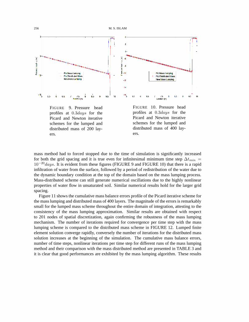
256 M. S. ISLAM
FIGURE 9. Pressure headprofiles at 0.3days for thePicard and Newton iterativeschemes for the lumped anddistributed mass of 200 lay-ers.
FIGURE 10. Pressure headprofiles at 0.3days for thePicard and Newton iterativeschemes for the lumped anddistributed mass of 400 lay-ers.
mass method had to forced stopped due to the time of simulation is significantly increasedfor both the grid spacing and it is true even for infinitesimalminimum time step∆tmin =10−20days. It is evident from these figures (FIGURE 9 and FIGURE 10) thatthere is a rapidinfiltration of water from the surface, followed by a period of redistribution of the water due tothe dynamic boundary condition at the top of the domain basedon the mass lumping process.Mass-distributed scheme can still generate numerical oscillations due to the highly nonlinearproperties of water flow in unsaturated soil. Similar numerical results hold for the larger gridspacing.
Figure 11 shows the cumulative mass balance errors profile ofthe Picard iterative scheme forthe mass lumping and distributed mass of 400 layers. The magnitude of the errors is remarkablysmall for the lumped mass scheme throughout the entire domain of integration, attesting to theconsistency of the mass lumping approximation. Similar results are obtained with respectto 201 nodes of spatial discretization, again confirming therobustness of the mass lumpingmechanism. The number of iterations required for convergence per time step with the masslumping scheme is compared to the distributed mass scheme inFIGURE 12. Lumped finiteelement solution converge rapidly, conversely the number of iterations for the distributed masssolution increases at the beginning of the simulation. The cumulative mass balance errors,number of time steps, nonlinear iterations per time step fordifferent runs of the mass lumpingmethod and their comparison with the mass distributed method are presented in TABLE 3 andit is clear that good performances are exhibited by the mass lumping algorithm. These results

MASS LUMPING AND DISTRIBUTING FINITE ELEMENT ALGORITHM 257
FIGURE 11. Mass balanceresult for the Picard iterativescheme for the lumped anddistributed mass of 400 lay-ers.
FIGURE 12. Convergenceresult for the Picard iterativescheme for the lumped anddistributed mass of 400 layers
are illustrative of numerical comparisons and indicate clearly that diagonal time matrices aresuperior to the distributed matrices.
TABLE 3. Computational statistics of the Test Problem 3.Note: Dist=Distributed, ite=iteration, CMBE=Cumulativemass balance error,NF=Simulation not finished.
No. of layers Technique Mass No. of time steps NL ite/ Time step CMBE
200Picard
Lump 2010 3.77 1.3358e-2Dist 3402 3.44 1.5059e-2
NewtonLump 1736 3.61 1.3354e-2Dist NF NF NF
400Picard
Lump 3579 4.37 1.3419e-2Dist 6896 3.49 1.5226e-2
NewtonLump 2865 4.13 1.3416e-2Dist NF NF NF
6. CONCLUSION
A simple one-dimensional finite element model for flow equation into homogeneous soilswas presented and the algorithm was implemented by applyingthe traditional iterative formu-lations, Picard and Newton based on lumped and distributed mass. Lumping scheme ensures
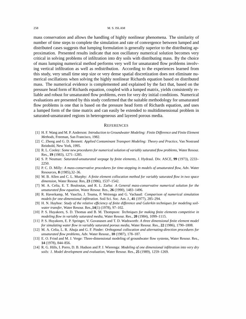
258 M. S. ISLAM
mass conservation and allows the handling of highly nonlinear phenomena. The similarity ofnumber of time steps to complete the simulation and rate of convergence between lumped anddistributed cases suggests that lumping formulation is generally superior to the distributing ap-proximation. Presented results indicate that non oscillatory numerical solution becomes verycritical in solving problems of infiltration into dry soils with distributing mass. By the choiceof mass lumping numerical method performs very well for unsaturated flow problems involv-ing vertical infiltration as well as redistribution. According to the experiences learned fromthis study, very small time step size or very dense spatial discretization does not eliminate nu-merical oscillations when solving the highly nonlinear Richards equation based on distributedmass. The numerical evidence is complemented and explainedby the fact that, based on thepressure head form of Richards equation, coupled with a lumped matrix, yields consistently re-liable and robust for unsaturated flow problems, even for very dry initial conditions. Numericalevaluations are presented by this study confirmed that the suitable methodology for unsaturatedflow problems is one that is based on the pressure head form of Richards equation, and usesa lumped form of the time matrix and can easily be extended to multidimensional problem insaturated-unsaturated regions in heterogeneous and layered porous media.
REFERENCES
[1] H. F. Wang and M. P. Anderson:Introduction to Groundwater Modeling: Finite Difference and Finite ElementMethods, Freeman, San Francisco, 1982.
[2] C. Zheng and G. D. Bennett:Applied Contaminant Transport Modeling: Theory and Practice,Van NostrandReinhold, New York, 1995.
[3] R. L. Cooley:Some new procedures for numerical solution of variably saturated flow problems,Water Resour.Res.,19 (1983), 1271–1285.
[4] S. P. Neuman:Saturated-unsaturated seepage by finite elements,J. Hydraul. Div. ASCE,99 (1973), 2233–2250.
[5] P. C. D. Milly: A mass-conservative procedures for time-stepping in models of unsaturated flow,Adv. WaterResources,8 (1985),32–36.
[6] M. B. Allen and C. L. Murphy:A finite element collocation method for variably saturated flow in two spacedimension, Water Resour. Res,23 (1986), 1537–1542.
[7] M. A. Celia, E. T. Bouloutas, and R. L. Zarba:A General mass-conservative numerical solution for theunsaturated flow equation, Water Resour. Res.,26 (1990), 1483–1496.
[8] R. Haverkamp, M. Vauclin, J. Touma, P. Weirenga and G. Vachaud: Comparison of numerical simulationmodels for one-dimensional infiltration. Soil Sci. Soc. Am. J.,41 (1977), 285–294.
[9] H. N. Hayhoe:Study of the relative efficiency of finite difference and Galerkin techniques for modeling soil-water transfer, Water Resour. Res.,14(1) (1978), 97–102.
[10] P. S. Huyakorn, S. D. Thomas and B. M. Thompson:Techniques for making finite elements competitive inmodeling flow in variably saturated media,Water Resour. Res.,20 (1984), 1099–1115.
[11] P. S. Huyakorn, E. P. Springer, V. Guvanasen and T. D. Wadsworth:A three dimensional finite element modelfor simulating water flow in variably saturated porous media, Water Resour. Res.,22 (1986), 1790–1808.
[12] M. A. Celia, L. R. Ahuja and G. F. Pinder:Orthogonal collocation and alternating-direction procedures forunsaturated flow problems, Adv. Water Resour.,10 (1987), 178–187.
[13] E. O. Frind and M. J. Verge: Three-dimensional modelingof groundwater flow systems, Water Resour. Res.,14 (1978), 844–856.
[14] R. G. Hills, I. Porro, D. B. Hudson and P. J. Wierenga:Modeling of one dimensional infiltration into very drysoils: 1. Model development and evaluation,Water Resour. Res.,25 (1989), 1259–1269.

MASS LUMPING AND DISTRIBUTING FINITE ELEMENT ALGORITHM 259
[15] P. Ross:Efficient numerical methods for infiltration using Richards’ equation,Water Resour. Res.,26 (1990),279–290.
[16] A. A. Aldama and C. Paniconi:An analysis of the convergence of Picard iterations for implicit approximationsof Richards’ equation,in Proceedings of the IX International Conference on Computational Methods in WaterResources, edited by T. F. Russell, R. E. Ewing, C. A. Brebbia, W. G. Gray, and G. F. Pinder, 521–528,Computational Mechanics Publications, Billerica, Mass, 1992.
[17] L. Bergamaschi and M. Putti:Mixed finite elements and Newton-type linearizations for the solution for theunsaturated flow equation,Int. J. Numer. Meth. Eng.,45 (1999), 1025–1046.
[18] F. Lehmann and P. H. Ackerer:Comparison of iterative methods for improved solutions of the fluid flowequation in partially saturated porous media,Transport in Porous Media,31 (1998), 275–292.
[19] P. A. Forsyth, Y. S. Wu, and K. Pruess:Robust numerical methods for saturated-unsaturated flow with dryinitial conditions in heterogeneous media,Adv. Water Resour.,18 (1995), 25–38.
[20] M.R. Kirkland, R.G. Hills, P.J. Wierenga: Algorithms for solving Richards equation for variably saturatedsoils, Water Resour. Res.,28 (1992) 2049–2058.
[21] C.W. Li: A simplified Newton method with linear finite elements for transient unsaturated flow, Water Resour.Res.,29 (1993) 965–971.
[22] K. Rathfelder and L. M. Abriola:Mass conservative numerical solutions of the head-based Richards equation,Water Resour. Res.,30 (1994), 2579–2586.
[23] M. D. Tocci, C. T. Kelley, and C. T. Miller:Accurate and economical solution of the pressure-head formofRichards’ equation by the method of lines, Adv. Water Resour.,20(1) (1997), 1–14.
[24] M. T. van Genuchten:A Closed-form Equation for Predicting the Hydraulic Conductivity of UnsaturatedSoils,Soil Sci. Soc. Am. J.,44 (1980), 892–898.
[25] K. S. Zadeh, S.B. Shah:Mathematical modeling and parameter estimation of axonal cargo transport, J.Comput. Neurosci.,28 (2010), 495–507.
[26] K. S. Zadeh:Parameter estimation in flow through partially saturated porous materials,J. Comput. Phys.,227(24) (2008), 10243–10262.
[27] K. S. Zadeh:A mass-conservative switching algorithm for modeling flow in variably saturated porous media,J. Comput. Phys.,230 (2011), 664–679.
[28] C. Paniconi, A. A. Aldama and E. F. Wood:Numerical evaluation of iterative and noniterative methods forthe solution of the nonlinear Richards equation,Water Resour. Res.,27 (1991), 1147–1163.
[29] H. Matthies and G. Strang:The solution of nonlinear finite element equations, Int. J. Numer. Methods Eng.,14 (1979), 1613–1626.
[30] C. T. Miller, C. Abhishek and M. Farthing:A spatially and temporally adaptive solution of Richards’ equation,Adv. Water Resources.,29 (2006), 525–545.
[31] M. S. Islam and M. K. Hasan:Accurate and economical solution of Richards’ equation by the method of linesand comparison of the computational performance of ODE solvers,International Journal of Mathematics andComputer Research,2 (2013), 328–346.
[32] M. S. Islam: Selection of internodal conductivity averaging scheme forunsaturated flow in homogeneousmedia,International J. of Engineering,28 (2015), 490–498.
[33] M. S. Islam:Consequence of Backward Euler and Crank-Nicolson techniques in the finite element model forthe numerical solution of variably saturated flow problems,J. KSIAM 19(2) (2015), 197–215.
[34] C. T. Miller, G. A. Williams, C. T. Kelley, and M. D. Tocci: Robust solution of Richards’ equation for nonuniform porous media,Water Resour. Res.,34 (1998), 2599–2610.
[35] C. E. Kees and C. T. Miller:Higher order time integration methods for two-phase flow,Adv. Water Resources,25(2) (2002), 159–177.
[36] M. S. Islam and M. K. Hasan:An investigation of temporal adaptive solution of Richards’ equation for sharpfront problems, IOSR Journal of Mathematics,10(2) (2014), 106–117.

J. KSIAM Vol.20, No.3, 261–275, 2016 http://dx.doi.org/10.12941/jksiam.2016.20.261
NUMERICAL SOLUTION OF AN INTEGRO-DIFFERENTIAL EQUATIONARISING IN OSCILLATING MAGNETIC FIELDS
KOUROSH PARAND1,2,† AND MEHDI DELKHOSH1
1 DEPARTMENT OFCOMPUTERSCIENCES, SHAHID BEHESHTIUNIVERSITY, TEHRAN, IRAN.E-mail address: k [email protected] address: [email protected]
2 DEPARTMENT OFCOGNITIVE MODELLING, INSTITUTE FORCOGNITIVE AND BRAIN SCIENCES, SHAHID
BEHESHTI UNIVERSITY, TEHRAN, IRAN.
ABSTRACT. In this paper, an integro-differential equation which arises in oscillating magneticfields is studied. The generalized fractional order Chebyshev orthogonal functions (GFCF)collocation method used for solving this integral equation. The GFCF collocation method canbe used in applied physics, applied mathematics, and engineering applications. The results ofapplying this procedure to the integro-differential equation with time-periodic coefficients showthe high accuracy, simplicity, and efficiency of this method. The present method is convergingand the error decreases with increasing collocation points.
1. INTRODUCTION
In this section, Spectral methods and some basic definitionsand theorems which are usefulfor our method have been introduced.
1.1. Spectral methods.Spectral methods have been developed rapidly in the past twodecades.They have been successfully applied to numerical simulations in many fields, such as heat con-duction, fluid dynamics, quantum mechanics, etc. These methods are powerful tools to solvedifferential equations. The key components of their formulation are the trial functions and thetest functions. The trial functions, which are the linear combinations of suitable trial basisfunctions, are used to provide an approximate representation of the solution. The test functionsare used to ensure that the differential equation and perhaps some boundary conditions are sat-isfied as closely as possible by the truncated series expansion. This is achieved by minimizingthe residual function that is produced by using the truncated expansion instead of the exactsolution with respect to a suitable norm [1, 2, 3, 4, 5, 6, 7, 8,9, 10].
Received by the editors April 26 2016; Revised September 12 2016; Accepted in revised form September 122016; Published online September 20 2016.
2000Mathematics Subject Classification.34B05, 34K28, 78A35, 47G20.Key words and phrases.Fractional order of the Chebyshev functions, Integro-differential equations, Oscillating
magnetic fields, Collocation method, Integral equations.† Corresponding author.
261

262 K. PARAND AND M. DELKHOSH
1.2. Basical definitions. In this section, some basic definitions and theorems which are usefulfor our method have been introduced [11].Definition 1. For any real functionf(t), t > 0, if there exists a real numberp > µ, such thatf(t) = tpf1(t), wheref1(t) ∈ C(0,∞), is said to be in spaceCµ, µ ∈ ℜ, and it is in the spaceCnµ if and only if fn ∈ Cµ, n ∈ N .
Definition 2. The fractional derivative off(t) in the Caputo sense by the Riemann-Liouvillefractional integral operator of orderα > 0 is defined as [12, 13]:
Dαf(t) =1
Γ(m− α)
∫ t
0(t− s)m−α−1Dmf(s) ds, α > 0,
for m− 1 < α ≤ m, m ∈ N, t > 0, m is the smallest integer greater thanα, andf ∈ Cm−1.
Some properties of the operatorDα are as follows. Forf ∈ Cµ, µ ≥ −1, α, β ≥ 0, γ ≥ −1,N0 = 0, 1, 2, · · · and constantC:
(i) DαC = 0,
(ii) DαDβf(t) = Dα+βf(t), (1.1)
(iii) Dαtγ =
0, γ ∈ N0 andγ < ⌈α⌉,
Γ(γ+1)Γ(γ−α+1) t
γ−α, γ ∈ N0 andγ ≥ ⌈α⌉ or γ /∈ N andγ > ⌊α⌋,(1.2)
(iv) Dα(
n∑
i=1
cifi(t)) =
n∑
i=1
ciDαfi(t), where ci ∈ R. (1.3)
Definition 3. Suppose thatf(t), g(t) ∈ C[0, η] andw(t) is a weight function, then
‖ f(t) ‖2w =
∫ η
0f2(t)w(t)dt,
〈f(t), g(t)〉w =
∫ η
0f(t)g(t)w(t)dt.
Theorem 1. (Generalized Taylor’s formula) Suppose thatf(t) ∈ C[0, η] andDkαf(t) ∈C[0, η], wherek = 0, 1, ...,m, 0 < α ≤ 1 andη > 0. Then we have
f(t) =
m−1∑
i=0
tiα
Γ(iα + 1)Diαf(0+) +
tmα
Γ(mα+ 1)Dmαf(ξ), (1.4)
with 0 < ξ ≤ t, ∀t ∈ [0, η]. And thus
|f(t)−m−1∑
i=0
tiα
Γ(iα+ 1)Diαf(0+)| ≤ Mα
tmα
Γ(mα+ 1), (1.5)
whereMα ≥ |Dmαf(ξ)|.Proof: See Ref. [14].
The organization of the paper is expressed as follows: in section 2, the mathematical prelim-inaries to the problem is expressed. In section 3, the GFCFs and their properties are obtained.

SOLVING THE INTEGRO-DIFFERENTIAL EQUATIONS 263
In section 4, the work method is explained. Applications of the proposed method are shown insection 5. Finally, a brief conclusion is given in the last section.
2. MATHEMATICAL PRELIMINARIES
The integro-differential equation [15, 16]
d2y
dt2= g(t) − a(t)y(t) + b(t)
∫ t
0cos(wps)y(s)ds (2.1)
wherea(t), b(t) and g(t) are given periodic functions of time may be easily found in thecharged particle dynamics for some field configurations. Taking for instance the three mutu-ally orthogonal magnetic field componentsBx = B1 sin(wpt), By = 0, Bz = B0, the nonrel-ativistic equations of motion for a particle of massm and chargeq in this field configurationare
md2x
dt2= q
(B0
dy
dt
), (2.2)
md2y
dt2= q
(B1 sin(wpt)
dz
dt−B0
dx
dt
), (2.3)
md2z
dt2= q
(−B1 sin(wpt)
dy
dt
). (2.4)
By integration of (2.2) and (2.4) and replacement of the timefirst derivatives ofz andx in (2.3)one has (2.1) with
a(t) = w2c + w2
f sin2(wpt), b(t) = w2
fwp sin(wpt), (2.5)
g(t) = wf sin(wpt)z′(0) + w2
cy(0) +wcx′(0), (2.6)
wherewc = qB0/m andwf = qB1/m. Making the additional simplification thatx′(0) = 0andy(0) = 0, equation (2.1) is finally written as [16]
d2y
dt2= wf sin(wpt)z
′(0) −(w2c + w2
f sin2(wpt)
)y(t)
+(w2fwp sin(wpt)
) ∫ t
0cos(wps)y(s)ds (2.7)
In this study, we consider the equation (2.1) with the following initial conditions
y(0) = β0, y′(0) = β1 (2.8)
There are methods to solve this equation, such as, He’s Homotopy perturbation method [16],Chebyshev wavelet [17], Legendre multi-wavelets [18], Local polynomial regression [19],Shannon wavelets [20], Variational iteration method [21] and Homotopy analysis method [22].
In this paper, we attempt to introduce a new method based on the generalized fractionalorder Chebyshev orthogonal functions (GFCFs) of the first kind for solving the equation (2.1)with the initial conditions (2.8).

264 K. PARAND AND M. DELKHOSH
3. THE GENERALIZED FRACTIONAL ORDER CHEBYSHEV FUNCTIONS
In this section, first, the generalized fractional order of the Chebyshev functions (GFCF)have been defined, and then some properties and convergence of them for our method havebeen introduced.
3.1. The Chebyshev functions.The Chebyshev polynomials have been used in numericalanalysis, frequently, including polynomial approximation, Gauss-quadrature integration, inte-gral and differential equations and spectral methods. Chebyshev polynomials have many prop-erties, for example orthogonal, recursive, simple real roots, complete in the space of polyno-mials. For these reasons, many researchers have employed these polynomials in their research[23, 24, 25, 26, 27, 28].
Using some transformations, the number of researchers extended Chebyshev polynomials tosemi-infinite or infinite domains, for example by usingx = t−L
t+L, L > 0 the rational functions
introduced [29, 30, 31, 32, 33, 34].In the proposed work, by transformationz = 1−2( t
η)α, α > 0 on the Chebyshev polynomi-
als of the first kind, the fractional order of the Chebyshev orthogonal functions in the interval[0, η] have been introduced, that they can use to solve these integro-differential equations.
3.2. The GFCFs definition. The efficient methods have been used by many researchers tosolve the differential equations (DE) is based on the seriesexpansion of the form
∑ni=0 cit
i,such as Adomian decomposition method [35] and Homotopy perturbation method [36]. Butthe exact solution of many DEs can’t be estimated by polynomial basis. Therefore, we havedefined a new basis for Spectral methods to solve them as follows:
Φn(t) =n∑
i=0
citiα.
Now by transformationz = 1−2( tη)α,α, η > 0 on classical Chebyshev polynomials of the first
kind, we defined the GFCFs in the interval[0, η], that be denoted byηFTαn (t) = Tn(1−2( t
η)α).
By this definition, the singular Sturm-Liouville differential equation of classical Chebyshevpolynomials become:
√ηα − tα
tα2−1
d
dt
[√ηα − tα
tα2−1
d
dtηFTα
n (t)
]+ n2α2
ηFTαn (t) = 0, t ∈ [0, η]. (3.1)
TheηFTαn (t) can be obtained using the recursive relation as follows (n = 1, 2, · · · ):
ηFTα0 (t) = 1 , ηFTα
1 (t) = 1− 2( tη)α,
ηFTαn+1(t) = (2− 4( t
η)α) ηFTα
n (t)− ηFTαn−1(t).
The analytical form ofηFTαn (t) of degreenα is given by
ηFTαn (t) =
n∑
k=0
(−1)kn22k(n+ k − 1)!
(n− k)!(2k)!(t
η)αk

SOLVING THE INTEGRO-DIFFERENTIAL EQUATIONS 265
=n∑
k=0
βn,k,η,α.tαk, t ∈ [0, η], (3.2)
where
βn,k,η,α = (−1)kn22k(n+ k − 1)!
(n − k)!(2k)!ηαkand β0,k,η,α = 1.
Note thatηFTαn (0) = 1 andηFTα
n (η) = (−1)n.
The GFCFs are orthogonal with respect to the weight functionw(t) = tα2−1
√ηα−tα
in the interval
[0, η]: ∫ η
0ηFTα
n (t) ηFTαm(t)w(t)dt =
π
2αcnδmn. (3.3)
whereδmn is Kronecker delta,c0 = 2, andcn = 1 for n ≥ 1. Eq. (3.3) is provable usingproperties of orthogonality in the Chebyshev polynomials.Figs. 1 shown graphs of GFCFs for various values ofn andα andη = 5.
(a) (b)
FIGURE 1. (a) Graph of the GFCFs withα = 0.25 and various values ofn.(b) Graph of the GFCFs withn = 5 and various values ofα.
3.3. Approximation of functions. Any functiony(t) ∈ C[0, η] can be expanded as follows:
y(t) =∞∑
n=0
an ηFTαn (t),
where the coefficientsan obtain by inner product:
〈y(t), ηFTαn (t)〉w = 〈
∞∑
n=0
an ηFTαn (t), ηFTα
n (t)〉w
and using the property of orthogonality in the GFCFs:
an =2α
πcn
∫ η
0ηFTα
n (t)y(t)w(t)dt, n = 0, 1, 2, · · · .

266 K. PARAND AND M. DELKHOSH
In practice, we have to use firstm-terms GFCFs and approximatey(t):
y(t) ≈ ym(t) =
m−1∑
n=0
an ηFTαn (t) = ATΦ(t), (3.4)
with
A = [a0, a1, · · · , am−1]T , (3.5)
Φ(t) = [ηFTα0 (t), ηFTα
1 (t), · · · , ηFTαm−1(t)]
T . (3.6)
3.4. Convergence of the method.The following theorem shows that by increasingm, theapproximation solutionfm(t) is convergent tof(t) exponentially.Theorem 2. Suppose thatDkαf(t) ∈ C[0, η] for k = 0, 1, ...,m, andηF
αm is the subspace
generated byηFTα0 (t),η FTα
1 (t), · · · ,η FTαm−1(t). If fm = ATΦ (in Eq. (3.4)) is the best
approximation tof(t) from ηFαm, then the error bound is presented as follows
‖ f(t)− fm(t) ‖w≤ηmαMα
2mΓ(mα+ 1)
√π
α.m!,
whereMα ≥ |Dmαf(t)|, t ∈ [0, η].
Proof. By theorem 1,y =∑m−1
i=0tiα
Γ(iα+1)Diαf(0+) and
|f(t)− y(t)| ≤ Mαtmα
Γ(mα+ 1),
sinceATΦ(t) is the best approximation tof(t) in ηFαm andy ∈ ηF
αm, one has
‖ f(t)− fm(t) ‖2w ≤ ‖ f(t)− y(t) ‖2w
≤ M2α
Γ(mα+ 1)2
∫ η
0
tα2+2mα−1
√ηα − tα
dt
=M2
α
Γ(mα+ 1)2η2mαπ
α22mm!.
Now by taking the square roots, the theorem can be proved.
Theorem 3. The generalized fractional order of the Chebyshev functionηFTαn (t), has pre-
ciselyn real zeros on interval(0, η) in the form
tk = η
(1− cos( (2k−1)π
2n )
2
) 1
α
, k = 1, 2, · · · , n.
Moreover, ddt η
FTαn (t) has preciselyn− 1 real zeros on interval(0, η) in the following points:
t′k = η
(1− cos(kπ
n)
2
) 1
α
, k = 1, 2, · · · , n− 1.
SOLVING THE INTEGRO-DIFFERENTIAL EQUATIONS 267
Proof. The Chebyshev polynomialTn(x) hasn real zeros [37, 38]:
xk = cos
((2k − 1)π
2n
), k = 1, 2, · · · , n,
thereforeTn(x) can be written as
Tn(x) = (x− x1)(x− x2) · · · (x− xn).
Using transformationx = 1− 2( tη)α yields to
FTαn (t) = ((1 − 2(
t
η)α)− x1)((1 − 2(
t
η)α)− x2) · · · ((1− 2(
t
η)α)− xn),
so, the real zeros ofηFTαn (t) aretk = η(1−xk
2 )1
α .Also, the real zeros ofd
dtTn(t) occurs in the following points [37]:
x′k = cos(kπ
n), k = 1, 2, · · · , n− 1.
Same as in previous, the absolute extremes ofηFTαn (t) aret′k = η(
1−x′k
2 )1
α .
4. APPLICATION OF THEGFCFCOLLOCATION METHOD
In this section, the GFCFs collocation method is applied to solve the integro-differentialequation in the Eq. (2.1).For satisfying the boundary conditions, the conditions in the Eq. (2.8) are satisfied as follows:
ym(t) = β0 + β1 t+ t2 ym(t), (4.1)
whereym(t) is defined in the Eq. (3.4). Now,ym(t) = β0 and ym′(t) = β1 whent tends to
zero, so the conditions in the Eq. (2.8) are satisfied.To apply the collocation method, the residual function is constructed by substitutingym(t)
in the Eq. (4.1) fory(t) in the integro-differential equation (2.1):
Res(t) =d2y
dt2− g(t) + a(t)y(t) − b(t)
∫ t
0cos(wps)y(s)ds. (4.2)
The equations for obtaining the coefficientaim−1i=0 arise from equalizingRes(t) to zero on
m collocation points:
Res(ti) = 0, i = 0, 1, ...,m − 1. (4.3)
In this study, the roots of the GFCFs in the interval[0, η] (Theorem 3) are used as collocationpoints. By solving the obtained set of equations, we have theapproximating functionym(t).And also consider that all of the computations have been doneby Maple 18 on a laptop withCPU Core i7, Windows 8.1 64bit, and 8GB of RAM.

268 K. PARAND AND M. DELKHOSH
5. ILLUSTRATIVE EXAMPLES
In this section, by using the present method, some well-known examples are solved to showefficiently and applicability GFCFs method based on Spectral method. The present method isapplied to solve the integro-differential equation (2.1) and their outputs are compared with thecorresponding analytical solution. These examples studied also by Dehghan [16], Khan [18]and Pathak [21], we will compare our results with their results to show the effectiveness of thepresent method.
Example 1. Consider the equation (2.1) with [16, 18, 21]
wp = 2, a(t) = cos(t), b(t) = sin(t/2), β0 = 1, β1 = 0
g(t) = cos(t)− t sin(t) + cos(t) (t sin(t) + cos(t))
− sin(t/2)
(2
9sin(3t)− t
6cos(3t) +
t
2cos(t)
).
The exact solution of this equation isy(t) = t sin(t) + cos(t). By applying the techniquedescribed in the last section, for satisfying the boundary conditions, the conditions are satisfiedasym(t) = 1 + t2 ym(t). The residual function is constructed as follows:
Res(t) =d2y
dt2− g(t) + a(t)y(t) − b(t)
∫ t
0cos(wps)y(s)ds.
Therefore, to obtain the coefficientaim−1i=0 ; Res(t) is equalized to zero atm collocation point.
By solving this set of nonlinear algebraic equations, we canfind the approximating functionym(t). Figure 2 shows the logarithmic graph of the absolute error and the residual error of theapproximate solution and the analytic solution form = 20 andα = 0.50.
(a) (b)
FIGURE 2. The logarithmic graphs of the absolute error and the residual errorfor example 1 withm = 20 andα = 0.50. Graph of the (a) absolute, (b)residual error.

SOLVING THE INTEGRO-DIFFERENTIAL EQUATIONS 269
The resulting graph in comparison to the presented method and the exact solution is shownin Figure 3(a). In Figure 3(b) to show the convergence of the present method, we showed thatby increasing them the residual function decreases, whereα = 0.50.
(a) (b)
FIGURE 3. (a) Obtained graph in comparison to the exact solution with m =20 andα = 0.50. (b) Residual functions form = 10, 15, 20 andα = 0.50,to show the convergence rate of the GFCF method for example 1.
Table 1 compares the error norm‖y − ym‖2 by the present method and Dehghan [16] forexamples 1-3.
TABLE 1. Comparison of error norm‖y − ym‖2 by Dehghan [16] and thepresent method for examples 1-3
Example Dehghan [16] Present method
Example 1 6.826965141905116e-13 1.4691408679507079e-20Example 2 2.440936203513114e-13 8.8876680000000000e-39Example 3 3.279510650660257e-12 2.6061709227703975e-95
Table 2 compares the obtained values ofy(t) by the present method and the values given byKhan [18] (Legendre multi-wavelets) and Pathak [21] (Variational iteration method), it showsthat the results obtained in the present method are more accurate.

270 K. PARAND AND M. DELKHOSH
TABLE 2. Obtained values ofy(t) for example 1 by Khan, Pathak, and thepresent method withm = 20.
t Khan [18] Pathak [21] Present method Exact Solution Abs. Err. Res. Err.
0.1 1.006711649 1.004987505 1.004987506944 1.004987506942 1.997e-12 3.329e-90.2 1.019729643 1.019800356 1.019800443994 1.019800444000 5.546e-12 3.391e-90.3 1.043967189 1.043991584 1.043992551130 1.043992551124 6.216e-12 1.032e-90.4 1.078484444 1.076823090 1.076828330937 1.076828330926 1.072e-11 3.318e-90.5 1.116769872 1.117276231 1.117295331180 1.117295331192 1.182e-11 1.190e-90.6 1.164117090 1.164067124 1.164121098922 1.164121098946 2.436e-11 3.746e-90.7 1.216007719 1.215666930 1.215794568347 1.215794568350 3.654e-12 1.388e-90.8 1.270604841 1.270327190 1.270591582096 1.270591582066 2.975e-11 2.415e-90.9 1.326616801 1.326109990 1.326604186976 1.326604186935 4.096e-11 3.827e-9
Example 2. Consider the equation (2.1) with [16, 18, 21]
wp = 1, a(t) = − sin(t), b(t) = sin(t), β0 = 1, β1 = 2/3
g(t) =1
9e−
t3 − sin(t)
(e−
t3 + t
)
− sin(t)
(− 3
10cos(t)e−
t3 +
9
10sin(t)e−
t3 + cos(t) + t sin(t)− 7
10
).
The exact solution of this equation isy(t) = e−t3 + t. By applying the technique described in
the last section, the conditions are satisfied as :ym(t) = 1 + 23t+ t2 ym(t), and construct the
residual functions as follows:
Res(t) =d2y
dt2− g(t) + a(t)y(t) − b(t)
∫ t
0cos(wps)y(s)ds.
Figure 4 shows the logarithmic graph of the absolute error and the residual error of the approx-imate solution and the exact solution form = 20 andα = 0.50.
(a) (b)
FIGURE 4. The logarithmic graphs of the (a) absolute error and the (b) resid-ual error for example 2 withm = 20 andα = 0.50.

SOLVING THE INTEGRO-DIFFERENTIAL EQUATIONS 271
The resulting graph in comparison to the present method and the exact solution is shownin Figure 5 (a). To show the convergence of the present methodto solve this example withα = 0.50 in Figure 5 (b), we showed that by increasing them the residual function decreases.
(a) (b)
FIGURE 5. (a) Obtained graph in comparison with the exact solution withm = 20 andα = 0.50. (b) Residual functions form = 10, 15, 20 andα =0.50, to show the convergence rate of GFCF method for example 2.
Table 1 compares the error norm‖y − ym‖2 by the present method and Dehghan [16] forexamples 1-3. Table 3 compares the obtained values ofy(t) by the present method and thevalues given by Khan [18] (Legendre multi-wavelets) and Pathak [21] (Variational iterationmethod), it shows that the results obtained in the present method are more accurate.
TABLE 3. Obtained values ofy(t) for example 2 by Khan (Legendre multi-wavelets), Pathak (Variational iteration method), and thepresent method withm = 20
t Khan [18] Abs. Err. Present method Exact Solution Abs. Res.Pathak [21] Err. Err.
0.1 1.067409867 5.0900e-13 1.06721610048200590204 1.06721610048200590204 2.5e-21 4.1e-180.2 1.135498873 1.3237e-10 1.13550698503161773772 1.13550698503161773773 6.6e-21 4.0e-180.3 1.204831254 3.4433e-09 1.20483741803595957317 1.20483741803595957316 6.8e-21 1.1e-180.4 1.275363888 3.4759e-08 1.27517331904294745400 1.27517331904294745399 1.2e-20 3.7e-180.5 1.346379637 2.0843e-07 1.34648172489061407403 1.34648172489061407404 1.2e-20 1.2e-180.6 1.418729558 ———— 1.41873075307798185864 1.41873075307798185866 2.6e-20 3.9e-180.7 1.491932333 ———— 1.49188956633678166437 1.49188956633678166437 5.1e-21 1.4e-180.8 1.565927886 ———— 1.56592833836464869274 1.56592833836464869271 2.8e-20 2.4e-180.9 1.640830867 ———— 1.64081822068171786610 1.64081822068171786606 4.1e-20 3.8e-18

272 K. PARAND AND M. DELKHOSH
Example 3. Consider equation (2.1) with [16, 18, 21]
wp = 3, a(t) = 1, b(t) = sin(t) + cos(t), β0 = 2, β1 = −5,
g(t) = −t3 + t2 − 11t+ 4− (sin(t) + cos(t))
(− t3
3sin(3t)− t2
3cos(3t)− 13
27cos(3t)− 13
9t sin(3t)
+t2
3sin(3t) +
16
27sin(3t) +
2t
9cos(3t) +
13
27),
The exact solution of this equation isy(t) = −t3 + t2 − 5t + 2. By applying the techniquedescribed in the last section, the conditions are satisfied as : ym(t) = 2 − 5t + t2 ym(t). Theresidual function is constructed as follows :
Res(t) =d2y
dt2− g(t) + a(t)y(t) − b(t)
∫ t
0cos(wps)y(s)ds.
Figure 6 shows the logarithmic graph of the absolute error and the residual error of theapproximate solution and the exact solution form = 5 andα = 0.50.
(a) (b)
FIGURE 6. The logarithmic graphs of the (a) absolute error and the (b) resid-ual error for example 2 withm = 5 andα = 0.50.

SOLVING THE INTEGRO-DIFFERENTIAL EQUATIONS 273
The resulting graph in comparison to the present method and the exact solutions is shown inFigure 7.
FIGURE 7. Obtained graph in comparison to the exact solution for example 3with m = 5 andα = 0.50.
Table 1 compares the error norm‖y − ym‖2 by the present method and Dehghan [16] forexamples 1-3. Table 4 compares the obtained values ofy(t) by the present method and thevalues given by Khan [18] (Legendre multi-wavelets) and Pathak [21] (Variational iterationmethod), it shows that the results obtained in the present method are more accurate.
TABLE 4. Obtained values ofy(t) for example 3 by Khan, Pathak, and thepresent method withm = 5.
t Khan [18] Abs. Err. Present Exact Abs. Res.Pathak [21] method Solution Err. Err.
0.1 1.510232801 ———— 1.50900000 1.509 0 4.331e-490.2 1.031768407 0.0000e-00 1.03200000 1.032 0 3.845e-500.3 0.563149603 ———— 0.56300000 0.563 0 2.869e-490.4 0.096626905 1.5399e-12 0.09600000 0.096 0 5.244e-490.5 -0.373166748 ———— -0.37500000 -0.375 0 6.837e-490.6 -0.856012437 4.1554e-11 -0.85600000 -0.856 0 7.799e-490.7 -1.353869376 ———— -1.35300000 -1.353 0 8.296e-490.8 -1.871984718 2.1376e-10 -1.87200000 -1.872 0 8.489e-490.9 -2.419488059 ———— -2.41900000 -2.419 0 8.517e-49

274 K. PARAND AND M. DELKHOSH
6. CONCLUSION
The main goal of this paper was to introduce a new orthogonal basis, namely the generalizedfractional order of the Chebyshev orthogonal functions (GFCF) to construct an approximationto the solution of the integro-differential equation arising in oscillating magnetic fields. Thepresented results show that the introduced basis for the collocation spectral method is efficientand applicable. Our results have better accuracy with lesser m, and the absolute error as com-pared to the exact solution. A comparison was made of the exact solution and the presentmethod. As shown, the method is converging and has an approximate accuracy and stability,and the error decreases with increasingm.
ACKNOWLEDGEMENTS
The authors are very grateful to reviewers and editor for carefully reading the paper and fortheir comments and suggestions which have improved the paper.
REFERENCES
[1] J.P. Boyd,Chebyshev spectral methods and the Lane-Emden problem, Numer. Math. Theor. Meth. Appl.,4(2)(2011) 142–157.
[2] K. Parand, M. Nikarya, J.A. Rad,Solving non-linear Lane-Emden type equations using Besselorthogonalfunctions collocation method, Celest. Mech. Dyn. Astr.,16(21) (2013) 97–107.
[3] J. Shen, T. Tang, L.L. Wang,Spectral Methods Algorithms, Analysis and Applications, 1st edition, Springer,New York (2001).
[4] J.A. Rad, K. Parand, L.V. Ballestra,Pricing European and American options by radial basis pointinterpola-tion, Appl. Math. Comput.,251(2015) 363–377.
[5] L. D’Amore, Remarks on numerical algorithms for computing the inverse Laplace transform, Ricerche mat.,63(2) (2014) 239–252.
[6] K. Parand, M. Dehghan, A. Pirkhedri,The Sinc-collocation method for solving the Thomas-Fermi equation,J. Comput. Appl. Math.,237(1) (2013) 244–252.
[7] J. Shen, T. Tang,High Order Numerical Methods and Algorithms. Chinese Science Press, Chinese (2005).[8] J.A. Rad, K. Parand, S. Kazem,A Numerical Investigation to Viscous Flow Over NonlinearlyStretching Sheet
with Chemical Reaction, Heat Transfer and Magnetic Field, Int. J. Appl. Comput. Math., doi:10.1007/s40819-016-0143-1, (2016) 1–17.
[9] J.A. Rad, K. Parand, S. Abbasbandy,Local weak form meshless techniques based on the radial point interpo-lation (RPI) method and local boundary integral equation (LBIE) method to evaluate European and Americanoptions, Commun. Nonlinear Sci. Num. Simul.,22(1) (2015) 1178–1200.
[10] K. Parand, M. Dehghan, A. Taghavi,Modified generalized Laguerre function Tau method for solving laminarviscous flow: The Blasius equation, Int. J. Numer. Method. H.,20(7) (2010) 728–743.
[11] S. Kazem, S. Abbasbandy, S. Kumar,Fractional-order Legendre functions for solving fractional-order differ-ential equations, Appl. Math. Modell.,37(2013) 5498–5510
[12] A.A. Kilbas, H.M. Srivastava, J.J. Trujillo,Theory and Applications of Fractional Differential Equations,Elsevier, San Diego, 2006.
[13] M. Delkhosh,Introduction of Derivatives and Integrals of Fractional order and Its Applications, Appl. Math.Phys.,1(4) (2013) 103–119.
[14] Z. Odibat, S. Momani,An algorithm for the numerical solution of differential equations of fractional order, J.Appl. Math. Inform.26 (2008) 15–27.

SOLVING THE INTEGRO-DIFFERENTIAL EQUATIONS 275
[15] J.M. Machado, M.Tsuchida,Solutions for a class of integro-differential equations with time periodic coeffi-cients, Appl. Math. E-Notes,2 (2002) 66–71.
[16] M. Dehghan, F. Shakeri,Solution of an Integro-Differential Equation Arising in Oscillating Magnetic FieldsUsing He’s Homotopy Perturbation Method, Prog. Electromag. Res.,78 (2008) 361–376.
[17] M. Ghasemi,Numerical technique for integro-differential equations arising in oscillating magnetic fields,Iranian J. Sci. Tech.,38A4 (2014) 473–479.
[18] Y. Khan, M. Ghasemi, S. Vahdati, M. Fardi,Legendre Multi-Wavelets to Solve oscillating magnetic fieldsintegro-differential equations, U.P.B. Sci. Bull. Ser. A,76(1) (2014) 51–58.
[19] F. Li, T. Yan, L. Su,Solution of an Integral-Differential Equation Arising in Oscillating Magnetic Fields UsingLocal Polynomial Regression, Adv. Mech. Eng., (2014) 9 pages.
[20] K. Maleknejad, M. Hadizadeh, M. Attary,On The Approximate Solution of Integro-Differential EquationArising in Oscillating Magnetic Fields, App. Math.,58(5) (2013) 595–607.
[21] M.R Pathak, P. Joshi,High Order Numerical Solutionof a Volterra Integro-Differential Equation Arising inOscillating Magnetic Fields using Variational Iteration Method, Int. J. Adv. Sci. Tech.,69 (2014) 47–56.
[22] H. Saberi-Nik, S. Effati, R. Buzhabadi,Analytic approximate solution for an integro-differential equationarising in oscillating magnetic fields using homotopy analysis method, Iranian J. Optim.,3 (2010) 518–535.
[23] M.R. Eslahchi, M. Dehghan, S. Amani,Chebyshev polynomials and best approximation of some classes offunctions, J. Numerical Math.,23 (1) (2015) 41–50.
[24] K. Parand, M. Delkhosh,Solving Volterra’s population growth model of arbitrary order using the generalizedfractional order of the Chebyshev functions, Ricerche Mat.,65 (2016) 307–328.
[25] E. H. Doha, A.H. Bhrawy, S. S. Ezz-Eldien ,A Chebyshev spectral method based on operational matrix forinitial and boundary value problems of fractional order, Comput. Math. Appl.,62 (2011) 2364–2373.
[26] A. Nkwanta and E.R. Barnes,Two Catalan-type Riordan arrays and their connections to the Chebyshev poly-nomials of the first kind, J. Integer Seq.,15 (2012) 1–19.
[27] A.H. Bhrawy, A.S. Alofi,The operational matrix of fractional integration for shifted Chebyshev polynomials,Appl. Math. Lett.,26 (2013) 25–31.
[28] A. Saadatmandi, M. Dehghan,Numerical solution of hyperbolic telegraph equation usingthe Chebyshev taumethod, Numer. Meth. Part. D. E.,26 (1) (2010) 239–252.
[29] K. Parand, A. Taghavi, M. Shahini,Comparison between rational Chebyshev and modified generalized La-guerre functions pseudospectral methods for solving Lane-Emden and unsteady gas equations, Acta Phys.Pol. B,40(12) (2009) 1749–1763.
[30] K. Parand, M. Shahini, A. Taghavi,Generalized Laguerre polynomials and rational Chebyshev collocationmethod for solving unsteady gas equation, Int. J. Contemp. Math. Sci.,4(21) (2009) 1005–1011.
[31] K. Parand, S. Abbasbandy, S. Kazem, A.R. Rezaei,An improved numerical method for a class of astrophysicsproblems based on radial basis functions, Phy. Scripta,83 (2011) 015011, 11 pages.
[32] K. Parand, M. Shahini,Rational Chebyshev pseudospectral approach for solving Thomas-Fermi equation,Phys. Lett. A,373(2009) 210–213.
[33] K. Parand, S. Khaleqi,The Rational Chebyshev of Second Kind Collocation Method for Solving a Class ofAstrophysics Problems, Euro. Phys. J. Plus,131(2016) 1–24.
[34] K. Parand, M. Shahini, M. Dehghan,Solution of a laminar boundary layer flow via a numerical method,Commun. Nonlinear Sci. Num. Simul.,15(2) (2010) 360–367.
[35] G. Adomian,Solving Frontier problems of Physics: The decomposition method, Kluwer Academic Publishers,1994.
[36] S.J. Liao,The proposed homotopy analysis technique for the solution of nonlinear problems, PhD thesis,Shanghai Jiao Tong University, 1992.
[37] M.S.H. Chowdhury, I. Hashim,Solution of a class of singular second-order IVPs by Homotopy-Perturbationmethod, Phys. Lett. A,365(2007) 439–447.
[38] M.A. Darani, M. Nasiri,A fractional type of the Chebyshev polynomials for approximation of solution oflinear fractional differential equations, Comp. Meth. Diff. Equ.,1 (2013) 96–107.