j.-p petit, g d’agostini, n debergh to cite this version
TRANSCRIPT

HAL Id: hal-03285671https://hal.archives-ouvertes.fr/hal-03285671
Preprint submitted on 12 Aug 2021
HAL is a multi-disciplinary open accessarchive for the deposit and dissemination of sci-entific research documents, whether they are pub-lished or not. The documents may come fromteaching and research institutions in France orabroad, or from public or private research centers.
L’archive ouverte pluridisciplinaire HAL, estdestinée au dépôt et à la diffusion de documentsscientifiques de niveau recherche, publiés ou non,émanant des établissements d’enseignement et derecherche français ou étrangers, des laboratoirespublics ou privés.
Janus cosmological modelJ.-P Petit, G d’Agostini, N Debergh
To cite this version:
J.-P Petit, G d’Agostini, N Debergh. Janus cosmological model. 2021. hal-03285671

Janus Cosmological Model
J.-P. Petit ,∗ G. d’Agostini ,† and N. Debergh ‡
Manaty Research Group(Dated: August 16, 2021)
The attempt to build a bimetric universe model made by S. Hossenfelder in 2008 could not produceany confrontations with the observation because of the violation of the equivalence principle. Byusing this technique again, with a subsequent modification of the signs of the terms the principlesof equivalence and action-reaction are both satisfied in the model. Masses of the same sign attracteach other according to Newton’s law, while masses of opposite signs repels each other according toanti-Newton’s law. The evolution equations are established on the basis of a generalized principleof conservation of the global energy. The observational data of the acceleration of the expansionof the sector of the positive masses leads to the conclusion that the global energy of the systemis negative, dominated by the energy of the negative masses, which replace both the dark matterand the dark energy. The calculation gives then an excellent agreement with the data of 700 typeIa supernovae. Numerical simulations, integrating this dominance of negative masses, give a newscheme of large scale structure formation. The negative masses, associated with a shorter Jeanstime, form first a regular network of spheroidal conglomerates. Confined in the interstitial spacethe positive mass acquires a structure comparable to joined soap bubbles. The compression of thepositive mass according to flat plates leads to a rapid rise in temperature, followed by an equallyrapid radiative cooling, which is favorable to the constitution of galaxies. On the other hand, theconglomerates of negative mass behave like immense protostars with a cooling time exceeding theage of the universe and lost in this form, giving birth neither to stars and galaxies, nor to heavyatoms, for lack of fusion reactions. Life is therefore absent in this negative sector. The phenomenonof the Great Repeller is interpreted by the presence of one of these conglomerates of negative mass,geometrically invisible, which occupy the center of the great voids of the Very Large-scale Structure(VLS). The negative mass invades the space between the galaxies and exerts on them a counterpressure that confines them, while giving their rotational curves a flat firmness at the periphery.Two-dimensional (2D) numerical simulations of a galaxy confined by its negative mass environmentgive rise to a barred spiral lasting for thirty years and thus shed light on the nature of an essentiallydissipative phenomenon, reflecting the braking of the galaxy’s rotation.
We construct the group associated with this new geometry, including a matter-antimatter symme-try. The existence of negative masses and energies imposes the use of an extension of the completePoincaré group through a global charge, parity, and time reversal (CPT) symmetry. The matter-antimatter symmetry is thus also present in the negative sector, which makes it possible to takeadvantage of Andrei Sakharov’s idea and to conclude that the invisible components of the universeare constituted by the copy of our own antimatter, endowed with a negative mass. It is predictedthat laboratory antimatter with negative mass will behave like ordinary matter. The theme ofthis T-symmetry is then projected into the quantum domain where, classically, the negative en-ergy states, considered as non-physical, are banished and choosing an anti-linear and anti-unitarytime reversal operator. We show that by choosing a linear and unitary operator the existence ofnegative energy states is imposed. We conjecture that this extension of quantum mechanics couldallow to quantify gravitation. The model is extended in the past by developing an alternative tothe inflation model, with two sets of constants and scale factors of space and time varying jointly,in such a way that the equations of physics, in both sectors, are conserved. Lorentz invariance isthus preserved and incompatibilities with observations disappear. Cosmic homogeneities in bothsectors are ensured thanks to a variable speed of light regime. In such a context, if the density inthe negative sector is higher, its space scale factor is smaller while the speed of light is higher. Wethen consider the development of gravitational instability in the two photon gases. This one is notobservable inside the same sector because its length of Jeans is then identified with the horizon. Onthe other hand this instability, developing in the negative sector, with a weaker Jeans length, leavesa weak imprint in the positive world, which constitutes an alternative interpretation of the cosmicmicrowave background (CMB) fluctuations. Its analysis in this new context allows to have accessto the scale factor of the negative sector and to the value of the speed of light which correspondsto it. We conclude that the distances, measured in the negative sector, are one hundred timesshorter, while the speed of light is ten times higher. This reduces the duration of interstellar travels,carried out according to the geodesics of the negative sector, which would become from then on notimpossible.
PACS numbers: 04.50.-h, 95.35.+d, 95.30.Sf, 11.10.EfKeywords: bigravity; bimetric; antigravity; coupled field equations; bimetric universes; runaway effet; nega-tive mass; negative energy; negative lensing; dark matter; dark energy; cosmological constant; action-reactionprinciple; equivalence principle; generalized energy conservation; T operator; primeval antimatter

2
I. INTRODUCTION
Cosmology and theoretical physics have been undergoing for decades a profound, unprecedented crisis. Years goby and all attempts to show the dark matter in tunnels, mines, or in space, have been failures. We have no modelthat makes physical sense of the phenomenon of accelerating expansion, that is to say, what the negative pressureassociated with dark energy means. However, the cosmological model currently considered as standard is essentiallybased on the existence of a cold dark matter whose existence has not been demonstrated. Let’s add that articles arepublished daily evoking quantum aspects related to gravitation, describing phenomena that are not observed, whileno one has succeeded to date in quantifying gravitation. Finally, to complete the picture, there is no explanation forthe lack of observation of primordial antimatter, which represents nothing more than half of the cosmic content, loston the way.
It is said that in order to validate an extraordinary model one needs extraordinary evidence. Let’s turn this sentencearound and say that in the face of an extraordinary crisis, which has been going on for more than half a century, weneed to consider extraordinary ideas.
This has given rise to everything that has been published about string theory for decades. But, as pointed out in2006 by Lee Smolin, through his book “The trouble with physics” [1] and by Peter Woit in another book, publishedthe same year, “Not Even Wrong” [2], we can now consider this attempt at a paradigm shift as a failure.
II. NEGATIVES MASSES
Among the innovations envisaged is the introduction of negative masses in the cosmological model.
II.1. Failure of the introduction of negative masses in General Relativity (GR)
In 1957 H. Bondi [3] examines its implications by considering the introduction of these masses in the model ofgeneral relativity, based on the field equation introduced in 1917 by A. Einstein:
Rµν − 12Rgµν + Λgµν = χTµν . (1)
Whatever the nature of the source of the field, represented on the right hand side of the equation, its solution is asingle metric from which we calculate the geodesic trajectories that test-particles will follow in different ways whateverthe sign of their mass. This conclusion is formulated in the following way:
• Positive masses attract both positive and negative masses, and
• Negative masses repel both positive and negative masses.
This leads to a phenomenon which has been called runaway. Let’s consider for example a pair of masses of thesame absolute value but of opposite signs. The positive mass runs away, pursued by the negative mass. Both thenundergo a uniform acceleration motion but the overall kinetic energy of the couple remains constant because that ofthe negative mass is negative.
In 2017 J. Farnes [4] proposed a model, which he qualifies as a toy model, where he tries, with an introduction ofnegative mass, to account for both the effects attributed to the dark matter and those of the dark energy, representedby the presence of the cosmological constant in the Field equation. However, this constant is equivalent to a constantnegative density. The author then invokes a phenomenon of continuous creation of negative mass, not described.Thus he only complicates the problem a little more. As for the runaway phenomenon, which is always present, hemakes the hypothesis that it would be at the origin of the cosmic rays.

3
II.2. Massive bigravity
If we want to be rid of the runaway phenomenon, the positive and negative test-particles must follow differentgeodesic paths, coming from two different metrics g(+)
µν and g(−)µν , themselves generating two different Ricci tensors
R(+)µν and R
(−)µν . Such models can then be called bimetric. The first attempt, in 2002, is that of T. Damour and I.
Kogan ([5, 6]) to which they give the name of bigravity. Bigravity because there are two sources of the gravitationalfield and massive because the authors consider that the interactions are played through gravitons supposedly endowedwith a mass spectrum. They consider “two branes floating in a higher dimensional space” with a coupling betweentheir respective points. They then show that the model must consist of two coupled field equations where the firstmembers are analogous to the Einstein equation, the second members comprising two source terms, the second tLµν
and tRµν corresponding to the coupling between the two entities. The two sets of masses are described as “Right” and“Left”:
2M2L
(Rµν
(gL
))− 1
2gLµνR
(gL
)+ ΛLg
Lµν = tLµν + TL
µν ,
2M2R
(Rµν
(gR
))− 1
2gRµνR
(gR
)+ ΛRg
Rµν = tRµν + TR
µν .
(2)
This system of equations follows from the Lagrangian:
S =∫
d4x√
−gR
(M2
RR (gR) − ΛR
)+
∫d4x
√−gL
(M2
LR (gL) − ΛL
)+
∫d4x
√−gRL (ΦR, gR) +
∫d4x
√−gLL (ΦL, gL) − µ4
∫d4x (gRgR)
1/4V (gL, gR) . (3)
They introduce Lagrangian densities in the action: the Ricci terms RRLR√
−gR, RL√
−gL, the terms cor-responding to positive matter LR
√−gR and negative matter LL
√−gL, are based on the corresponding four-
dimensional hypervolumes√
−gR dx0 dx1 dx2 dx3 and√
−gL dx0 dx1 dx2 dx3. They introduce an interaction term:µ
(gRgL
)1/4 √−gL dx0 dx1 dx2 dx3 based on an “average volume factor”
(gRgL
)1/4.They specify that their system of equations must satisfy the Bianchi identities. But their test does not lead to any
model, because they cannot specify the nature of the interaction terms.
II.3. Bimetric theory with exchange symmetry
After a first draft published in 2006 [7], S. Hossenfelder published in 2008 in the journal PRD a theoretical essayentitled “Bimetric theory with exchange symmetry” [8]. As she says in her section I of [8], we quote:
We consider a bi-metric theory with metrics g and h of Lorentzian signature that define two different waysof measuring angles, distances and volumes on a manifold M .
Still in this section I, she writes:
We will further introduce two sorts of matter on M : one that moves according to the usual metric g andthe measures it implies, the other that moves according to the other metric h. We will refer to these fieldsas g-fields and h-fields, respectively.
Using her “pull over” technique, she defines an action that corresponds to her equation (32) in her section IV:
S =∫
d4x√
−g(
(g)R/8πG+ L (ψ))
+√
−hPh
(L
(ϕ
))+
∫d4x
√−h
((h)R/8πG+ L
(ϕ
))+
√−gPg (L (ψ)) , (4)
where:
• (g)R and (h)R are Ricci’s scalars associated with its metrics g and h,
• g and h being the determinants of both metrics, d4x√
−g and d4x√
−h are the corresponding 4-volumes, and

4
• ψ is the g-field and ϕ the h-fields.
She then performs a “bi-variation”. It is then necessary to introduce a coupling relation, which she does with herequation (27) in her section III:
δhκλ = −[a−1]µ
κ
[a−1]ν
λδgµν . (5)
This is the covariant version of the coupling relationship that we used in our article [9], in a work subsequent to hers.Hence the obvious kinship between the two systems of coupled field equations. Hers corresponds to her equations(34) and (35) in section IV of her article, and is written as follows:
(g)Rκν − 12gκν
(g)R = Tκν − V
√h
ga
ννa
κκT νκ,
(h)Rνκ − 12hνκ
(h)R = T νκ −W
√g
haκ
κaννTκν .
(6)
She specifies, like Damour, that the equations satisfy the Bianchi identities.It is important, in order to understand her article, to identify the proposed goals. We will quote her sentences.In her section VII she writes:
The model we laid is purely classical. We will assume that the field content for both, the g-field and theh-field, is identical, such as we have two copies of the Standard Model.
His test therefore represents a variation of the standard model, introducing two materials with a coupling betweenthem. If we removed the interaction terms the system would become:
(g)Rκν − 12gκν
(g)R = Tκν ,
(h)Rνκ − 12hνκ
(h)R = T νκ.
(7)
The nature of the source tensors is defined in its section VI:T 0
0 = ρ, T ii = p,
T 00 = ρ, T i
i = p,(8)
where ρ is the density of the second species and p its pressure. In section VIII another precision is brought, wequote:
The kinetic energies are still strictly positive and conserved.
As the kinetic energy of the second species is 12ρν
2 (it makes the hypothesis that the limiting velocities in the twopopulations on the same: c = c = 1) this results in ρ > 0.
When she introduces her coupling terms, both of these include scalars that are determinants of what she callspullovers: [Pg]εε and
[Ph
]ν
ν. In section VI, when she examines the impact of the introduction of these coupling terms
on the dynamics of the system, she constructs from two Friedmann–Lemaître–Robertson–Walker (FLRW) metrics.In her paper these are her equations (38) and (39):
ds2 = − dt2 + a2
1 − kr
(dr2 + dΩ2)
,
ds2 = − dt2 + b2
1 − kr
(dr2 + dΩ2)
,
(9)
where a and b are scale factors. She considers different combinations with positive values of the scalars V and W .Thus his system of equations (6) reveals an “antigravitation”, that is to say the fact that the particles of the twospecies repel each other. Indeed, let us consider a region of space where the masses of the first species are dominant.The system becomes:
(g)Rκν − 12gκν
(g)R = Tκν ,
(h)Rνκ − 12hνκ
(h)R = −W√g
haκ
κaννTνκ.
(10)

5
The antigravity effect is produced by introducing, in an ad hoc manner, the minus signs preceding the quantitiesV and W in the system of coupled field equations.
Conclusion: the particles of the first kind, creators of the source of the field Tκν , attract each other while they repelthose of the second kind.
Reverse situation: in a region of space where it is the second species that dominates the system becomes:
(g)Rκν − 12gκν
(g)R = −V
√h
ga
ννa
κκT νκ,
(h)Rνκ − 12hνκ
(h)R = T νκ.
(11)
If the particles of the second kind, responsible for the source term, attract each other, they repel the particles ofthe first kind.
The action-reaction principle is thus satisfied, which makes the runaway effect disappear [3]. If we consider thatthe inertial mass of a particle represents the way it reacts, if it is placed in a given gravitational field, then the inertialmass of the particles of the second species is negative. On the other hand, as ρ > 0, their gravitational mass ispositive. The model of S. Hossenfelder therefore does not satisfy the equivalence principle. In a later article [10] shewrites, we quote:
Bimetric theories generically violate the equivalence principle because now have two different ways ofcoupling to gravity.
We will see later that this is not a general property of bimetric systems, but that it follows from the particularchoice made by S. Hossenfelder. Concerning the global dynamics of the system, as she wishes to remain within theframework of a classical model (see her sentences in section VII: “The model we lay out is purely classical” and “bothdensities are of the same order of magnitude”), she is obliged to consider that this coupling phenomenon between thetwo species remains weak. At the end of section V she writes, we quote:
Both types of fields only interact gravitationally, so the h-fields constitute a kind of very weakly interactingdark matter.
However, it is not because the two types of matter interact by the force of gravity that one can conclude thatthe coupling effect is weak, since masses of the same species also interact by the force of gravity. This representsan additional implicit assumption of the author, which translates into the necessity to opt for low values of couplingconstants cV and cW , in order to stick as closely as possible to the standard model
After having cleared all these clarifications and going towards the conclusions the author writes, we quote:
If there was a localized source of negative energy, it would act as gravitational lens – but unlike usual matterthis would be a diverging lens since it would repel (usual) photons. Such lensing event would typically lowerthe luminosity of the source, an effect that could potentially add up over distance if the distribution of suchsources is substantial. The detection of a diffractive lensing event could serve as the smoking gun signalfor the here proposed scenario.
This effect of negative gravitational lensing, an effect created by a negative energy source, which results in it fromthe signs less introduced in the equations, has been previously described in [11].
In 2018 S. Hossenfelder published a book entitled “Lost in maths” and she concludes:
To escape, physicists must rethink their methods. Only by embracing reality as it is can science discoverthe truth.
In the present situation the search for a favorable outcome must result from a harmonious collaboration betweenthe geometrical imagination of the mathematician and the intuition of the physicist, with the aim of accounting forthe observational data. Sabine Hossenfelder contributed in the first part of the process by providing a sophisticatedand precise mathematical framework. There was progress with respect to the GR model where the introduction ofnegative mass resulted in a violation of the action-reaction principle and in an uncontrollable acceleration of couplesof opposite masses in energy variation. But in reading his article the physicist will suggest, intuitively, that if wecould turn to a model that satisfies both:
• The principle of action-reaction, and
• The principle of equivalence.It would be even better.

6
II.4. Bimetric model satisfying the principles of equivalence and action-reaction
Can S. Hossenfelder’s approach be modified in such a way that these two principles are satisfied this time? Theanswer is positive.
Indeed, the theorist is free to choose the signs of the terms, in the Lagrangian, which will be reflected in the sourceterms of the field equations. Thus, by taking exactly the same approach, but with different choices of signs, we modifythe system of two coupled field equations. Moreover we introduce different Einstein constants χ and χ, different apriori scaling factors, as well as different a priori light speeds c and c.
This corresponds to the Janus Cosmological Model (JCM):
(g)Rκν − 12gκν
(g)R = χ
[Tκν + V
√h
ga
ννa
κκTκν
], (12a)
(h)Rνκ − 12hνκ = −χ
[T νκ +W
√g
ha
κκa
ννTνκ
]. (12b)
We find the same laws of interaction:
• Masses of the same sign attract each other according to Newton, and
• Masses of opposite signs repel each other according to the “anti-Newton”.
The action-reaction principle is satisfied. But this time, in the source tensors of the field, the equivalence principle isalso satisfied:
m < 0, p < 0, ρ < 0. (13)
As far as Schwarzschild’s external solutions are concerned, nothing has changed. To consider the evolution of thissystem of two interacting materials, we will write the FLRW metrics, allowing the system to have two speeds oflight. One speed c for (ordinary photons) of positive energy and one speed c for photons of negative energy, travellingaccording to the null geodesic of the metric h. We introduce a common chronological marker x0:
ds2 = −dx02 + a2[
dr2
1 − kr2 + dθ2 + sin2 θ dφ2], (14a)
ds2 = −dx02 + b2[
dr2
1 − kr2 + dθ2 + sin2 θ dφ2]. (14b)
So we have a single manifold M equipped with two metrics g and h. The cosmic history resulting from theintroduction of these metrics in the field equations will be translated by the functions giving the evolution of the scalefactors a (t) and b (t). We write the system of field equations in mixed form:
(g)Rνκ − 1
2δνκ
(g)R = χ
[T ν
κ + V
√h
gaν
νaκκT
νκ
], (15a)
(h)Rκν − 1
2δκν
(h)R = −χ[T
κν +W
√g
ha
κκa
ννT
κν
]. (15b)
The source tensors of the field are given the form:
T νµ =
ρc2 0 0 0
0 −p 0 00 0 −p 00 0 0 −p
and T νµ =
ρc2 0 0 00 −p 0 00 0 −p 00 0 0 −p
. (16)

7
By introducing these metrics into the equations we obtain two pairs of differential equations, the first pair containingthe first and second derivatives of the corresponding scale factor a and the second pair containing the first and secondderivatives of the second scale factor b:
a = dadx0 , a = d2a
dx02 , b = dbdx0 , and b = d2a
dx02 . (17)
We get the equations:
− χ
[ρc2 + V
b3
a3 ρc2]
= 3ka2 + 3a2
a2 , (18)
− χ
[ρc2 + V
b3
a3 ρc2 + p+ V
b3
a3 p
]= − k
a2 − a2
a2 − 2aa, (19)
χ
[ρc2 +W
a3
b3 ρc2]
= 3kb2 + 3b2
b2 , (20)
χ
[ρc2 +W
a3
b3 ρc2 + p+W
a3
b3 p
]= − k
b2 − b2
b2 − 2bb. (21)
We will not, as Hossenfelder does, consider the parameters V and W as independent quantities. Their values aredetermined from the system of equations (18), (19), (20), and (21) to which we add the hypothesis of a generalizedconservation of energy. The detailed calculation is given in Appendix A. It is modelled on the classical calculation ofthe FLRW solution of Einstein’s equation, which results in an energy conservation relationship of:
ρc2a3 = const. (dust universe),ρc2a4 = const. (radiation dominated universe).
(22)
Here we get something similar (the detail of the calculation is given in Appendix A).Equations (20) and (21) then give:
ddt
[ρc2 + V
b3
a3 ρc2]
[ρc2 + V
b3
a3 ρc2 + p+ V
b3
a3 p
] + 3a
dadt = 0. (23)
And equations (20) and (21) give:
ddt
[ρc2 +W
a3
b3 ρc2]
[ρc2 +W
a3
b3 ρc2 + p+W
a3
b3 p
] + 3b
dbdt = 0. (24)
II.5. Both sectors correspond to dust universes
ddt
[ρc2a3 + V ρc2b3]
= ddt
[Wρc2a3 + ρc2b3]
= 0. (25)
Introducing the hypothesis of a generalized conservation of the energy, it gives:
V = W = 1, (26)
ρc2a3 + ρc2b3 = E = const. (27)

8
We can show, just as we have that:
χ = −8πGc4 , (28)
that we get:
χ = −8πGc4 , (29)
a = c
√−k − 8πG
3c4E
a, (30)
b = c
√−k + 8πG
3c4E
b, (31)
a
a= −8πG
3c2 E, (32)
b
b= 8πG
3c2 E. (33)
As the measurements referring to our sector show an acceleration ([12–14]) we deduce that the global energy E isnegative. Negative mass dominates. This confirms the hypothesis that had prevailed to lead to interesting numericalsimulations [11]. Equation (30) and (31) impose that k = k = 1. These equations are therefore written:
1a
d2a
dx02 = −8πG3c2 E, (34)
1b
d2b
dx02 = 8πG3c2 E. (35)
With x0 = ct, we can then write equation (33) according as:
a2 d2a
dt2 = 8πG |E0| a30. (36)
The phenomenon of acceleration of the expansion, observed in the sector of the positive masses is thus due to thepredominance of the negative mass. The exact solution of such an equation has been given by William Bonnor [15].This type of solution was previously described in [16]. Only the part of the solution corresponding to the matterdominated era can be considered. By pushing this solution to the origin of time, the zero value of the chronologicalvariable, the mathematical solution gives a non-zero scale factor a value. The model accounts for the accelerationof the expansion ([12–14]). The mainstream Lambda cold dark matter (ΛCDM) model predicts an exponentialexpansion related to the fact that the energy-matter equivalent of the cosmological constant remains unchanged whenthe universe expands. Conversely, the density of negative mass decreases and equation (36) assigns an asymptote tothis expansion.
II.6. Fit to local relativistic observational data
The agreement is immediate. As noted by S. Hossenfelder in section IV of his article:Since both kinds of matter repel, one would expect the amount of h-matter in our vicinity to presently bevery small.
So the system becomes:(g)Rκν − 1
2gκν(g)R+ Λgκν = χTκν , (37)
(h)Rνκ − 12hνκ
(h)R+ Λhνκ = −χ√g
ha
κκa
ννTνκ. (38)
The first equation is simply that of the classical GR. So all local verifications like the explanation of the advanceof Mercury’s perihelion and the deviation of light rays by the Sun also derive from the model.

9
III. SOLUTIONS
III.1. Homogeneous solution
III.1.a. Fit the observational data from 700 type Ia supernovae
The comparison of the predictions of this model with the data of 700 type Ia supernovae proved to be excellent.See Fig. 1 extracted from [17].
32
34
36
38
40
42
44
46
0 0.2 0.4 0.6 0.8 1 1.2 1.4z
ΛCDM with (ΩM , ΩΛ) = (0.295, 0.705)
Bimetric with q0 = −0.087
µ=
m∗ B−
M(G
)+α
X−β
C
FIG. 1. Hubble diagram compared with two models (linear redshift z scale) [17].
III.1.b. Radiation dominated era
The system of equations (18), (19), (20), and (21) coupled with the generalized conservation hypothesis of radiativeenergy:
ρrc2a4 + ρ
rc2b4 = E, (39)
gives:
V = b
a, and, W = a
b, (40)
− χE
a4 = 3ka2 + 3a2
a2 , (41)
− χE
3a4 = − k
a2 − a2
a2 − 2aa, (42)
χE
b4 = 3kb2 + 3b2
b2 , (43)
10
χE
3b4 = − k
b2 − b2
b2 − 2bb. (44)
In equation (41) the continuity of the energy content imposes k = −1. It comes:
a =√
1 − |χE|3a2 , (45)
a = 8πG |E|3a3 > 0. (46)
The phenomenon of the acceleration of the expansion is also present in the positive sector during the radiationdominated era. The opposite phenomenon in the negative sector:
b = −8πG |E|3b3 < 0. (47)
III.2. Non homogeneous steady state solution
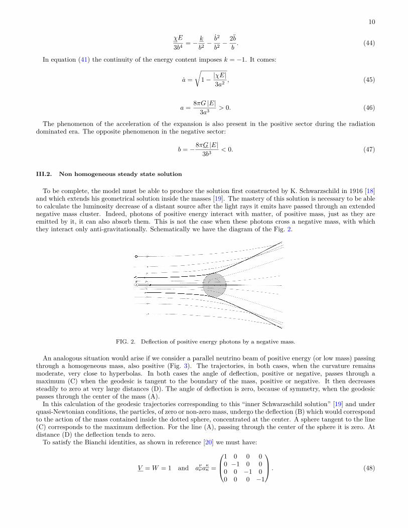
To be complete, the model must be able to produce the solution first constructed by K. Schwarzschild in 1916 [18]and which extends his geometrical solution inside the masses [19]. The mastery of this solution is necessary to be ableto calculate the luminosity decrease of a distant source after the light rays it emits have passed through an extendednegative mass cluster. Indeed, photons of positive energy interact with matter, of positive mass, just as they areemitted by it, it can also absorb them. This is not the case when these photons cross a negative mass, with whichthey interact only anti-gravitationally. Schematically we have the diagram of the Fig. 2.
FIG. 2. Deflection of positive energy photons by a negative mass.
An analogous situation would arise if we consider a parallel neutrino beam of positive energy (or low mass) passingthrough a homogeneous mass, also positive (Fig. 3). The trajectories, in both cases, when the curvature remainsmoderate, very close to hyperbolas. In both cases the angle of deflection, positive or negative, passes through amaximum (C) when the geodesic is tangent to the boundary of the mass, positive or negative. It then decreasessteadily to zero at very large distances (D). The angle of deflection is zero, because of symmetry, when the geodesicpasses through the center of the mass (A).
In this calculation of the geodesic trajectories corresponding to this “inner Schwarzschild solution” [19] and underquasi-Newtonian conditions, the particles, of zero or non-zero mass, undergo the deflection (B) which would correspondto the action of the mass contained inside the dotted sphere, concentrated at the center. A sphere tangent to the line(C) corresponds to the maximum deflection. For the line (A), passing through the center of the sphere it is zero. Atdistance (D) the deflection tends to zero.
To satisfy the Bianchi identities, as shown in reference [20] we must have:
V = W = 1 and aννa
κκ =
1 0 0 00 −1 0 00 0 −1 00 0 0 −1
. (48)

11
FIG. 3. Deflection of positive energy neutrinoss by a positive mass.
By developing a calculation similar to the construction of the interior metric given in [21] we write:
ds(+)2 = −eν(+)dx02 + eλ(+)
dr2 + r2 dφ2 + r2 sin2 θ dφ2,
ds(−)2 = −eν(−)dx02 + eλ(−)
dr2 + r2 dφ2 + r2 sin2 θ dφ2.(49)
The rest of the calculation depends on the mass considered, assumed to be of constant density, positive or negative,contained inside a sphere of radius rS. Let us start by considering the case of a positive mass. Similarly to equation(14.15) of reference [21] we pose:
eλ(+)= 1 − 2m(+)
r, (50)
and, similarly to equation (14.18) of reference [21] we pose:
m(+) (r) = G(+)
c(+)2
∫ r
04πr2ρ(+) dr. (51)
The calculation leads to the classical Tolman–Oppenheimer–Volkoff (TOV) equation [22]:
p(+)′
c(+)2 = −m(+) + 4πGp(+)r3/c(+)4
r(r − 2m(+)
) (ρ(+) + p(+)
c(+)2
). (52)
But we have:
m(+) (r) = G
c(+)24πr3ρ(+)
3 , (53)
which gives:
p(+)′
c(+)2 = −4πGr3
(ρ(+)c(+)2
/3 + p(+))
c(+)4r2
(1 − 8πGρ
3c(+)2 r2) (
ρ(+) + p(+)
c(+)2
). (54)
By posing, classically ([21], eq. 14.28):
R(+)2 = 3c(+)2
8πGρ(+) , (55)
we know that in the Newtonian approximation we find the Euler equation:
dp(+)
dr = −GM (+) (r) ρ(+)
r2 . (56)
When we conduct a similar calculation for the second species we obtain:
p(+)′
c(+)2 = −m(+) − 4πGp(+)r3/c(+)4
r(r + 2m(+)
) (ρ(+) − p(+)
c(+)2
), (57)

12
which also tends to the Euler equation in the Newtonian approximation. Compatibility is ensured asymptotically.This also corresponds to the asymptotic satisfaction of the Euler identities in the Newtonian approximation. If werepeat this calculation assuming that the field is this time created by a negative mass we will have the same resultconcerning the compatibility, still in this Newtonian approximation. We can finish this calculation by obtaining theexplicit forms of the two metrics, always in a quasi-Newtonian perspective, with ε = 1 if the mass creating the fieldis positive and ε = −1 if it is negative:
ds(+)2 =[
32
(1 − ε
r2S
R2
)1/2
− 12
(1 − ε
r2
R2
)1/2]2
dx02 − dr2
1 − ε r2
R2
− r2 (dθ2 + sin2 θ dφ2)
, (58)
ds(−)2 =[
32
(1 + ε
r2S
R2
)1/2
− 12
(1 + ε
r2
R2
)1/2]2
dx02 − dr2
1 + ε r2
R2
− r2 (dθ2 + sin2 θ dφ2)
. (59)
These two metrics are connected to the two classical outer Schwarzschild metrics.The GR paradigm can be summarized in the phrase:
The universe is an M4 manifold, equipped with a metric, solution of equation (1).
The present model is an extension of GR:
The universe is an M4 manifold, equipped with two metrics, solutions of the system of coupled field equa-tions (12a) and (12b).
In these conditions the GR represents only the approximation of this model, in the regions where the negative masscan be neglected, i.e. in the neighborhood of the Sun.
This is obviously an extremely ambitious proposal, which requires, to be credible, the maximum of observationalconfirmations. This is what we will try to build in the following sections.
IV. AT GALAXY SCALE
IV.1. A new scenario for the construction of the very large structure
If we apply to the system of equations (12a) and (12b) a double Newtonian approximation, the interaction laws arespecified and are Newtonian and anti-Newtonian. Starting from such an interaction scheme, numerical simulationshave been performed. Starting from a totally symmetrical configuration, we observe a percolation of the two species[23] (see Fig. 4).
(a) (b)
FIG. 4. Result of a simulation with ρ+ = |ρ−|. (a) Spatial distribution of the two populations. (b) White: population 1; grey:population 2.
But this does not fit with the observational data, where the positive mass presents a lacunar structure with largevoids. By introducing then this dissymmetry the new species, endowed with a shorter Jeans time, is the first, due toits shorter Jeans’s time, to give birth, by gravitational instability, to a regular distribution of spheroidal clusters (seeFig. 5).
The positive mass then adopts a lacunar structure by occupying the remaining space. We note in passing thatthis formation scheme of the VLS implies, at the time of its constitution, a strong compression of the positive mass,
13
(a) (b) (c)
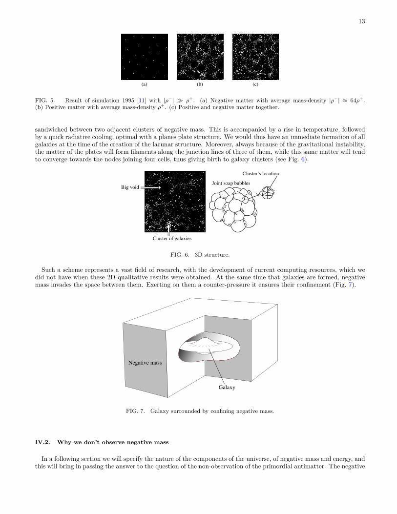
FIG. 5. Result of simulation 1995 [11] with |ρ−| ≫ ρ+. (a) Negative matter with average mass-density |ρ−| ≈ 64ρ+.(b) Positive matter with average mass-density ρ+. (c) Positive and negative matter together.
sandwiched between two adjacent clusters of negative mass. This is accompanied by a rise in temperature, followedby a quick radiative cooling, optimal with a planes plate structure. We would thus have an immediate formation of allgalaxies at the time of the creation of the lacunar structure. Moreover, always because of the gravitational instability,the matter of the plates will form filaments along the junction lines of three of them, while this same matter will tendto converge towards the nodes joining four cells, thus giving birth to galaxy clusters (see Fig. 6).
Cluster of galaxies
Joint soap bubblesBig void
Cluster’s location
FIG. 6. 3D structure.
Such a scheme represents a vast field of research, with the development of current computing resources, which wedid not have when these 2D qualitative results were obtained. At the same time that galaxies are formed, negativemass invades the space between them. Exerting on them a counter-pressure it ensures their confinement (Fig. 7).
Negative mass
Galaxy
FIG. 7. Galaxy surrounded by confining negative mass.
IV.2. Why we don’t observe negative mass
In a following section we will specify the nature of the components of the universe, of negative mass and energy, andthis will bring in passing the answer to the question of the non-observation of the primordial antimatter. The negative
14
mass components emit photons of negative energy, which follow the null geodesics constructed from the second metric.For an observer made of positive mass to observe structures made of negative mass it would be necessary that thenegative energy photons follow a geodesic path belonging to the set derived from the metric describing the behaviourof particles of positive mass and energy. But these two sets are disjoints. So the absence of observation of thesenegative mass elements is based on purely geometrical grounds.
IV.3. The Great Repeller phenomenon
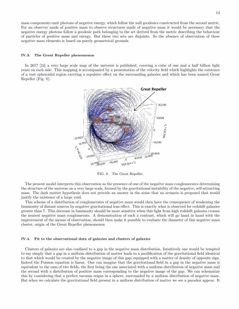
In 2017 [24] a very large scale map of the universe is published, covering a cube of one and a half billion lightyears on each side. This mapping is accompanied by a presentation of the velocity field which highlights the existenceof a vast spheroidal region exerting a repulsive effect on the surrounding galaxies and which has been named GreatRepeller (Fig. 8).
Hercules
ShapleyArch
Great attractorPerseus-Pisces
Lepus
Great Repeller
FIG. 8. The Great Repeller.
The present model interprets this observation as the presence of one of the negative mass conglomerates determiningthe structure of the universe on a very large scale, formed by the gravitational instability of the negative, self-attractingmass. The dark matter hypothesis does not provide an answer in the sense that no scenario is proposed that wouldjustify the existence of a large void.
This scheme of a distribution of conglomerates of negative mass would then have the consequence of weakening theluminosity of distant sources by negative gravitational lens effect. This is exactly what is observed for redshift galaxiesgreater than 7. This decrease in luminosity should be more sensitive when this light from high redshift galaxies crossesthe nearest negative mass conglomerate. A demonstration of such a contrast, which will go hand in hand with theimprovement of the means of observation, should then make it possible to evaluate the diameter of this negative masscluster, origin of the Great Repeller phenomenon
IV.4. Fit to the observational data of galaxies and clusters of galaxies
Clusters of galaxies are also confined to a gap in the negative mass distribution. Intuitively one would be temptedto say simply that a gap in a uniform distribution of matter leads to a modification of the gravitational field identicalto that which would be created by the negative image of this gap, equipped with a matter of density of opposite sign.Indeed the Poisson equation is linear. One can imagine that the gravitational field in a gap in the negative mass isequivalent to the sum of two fields, the first being the one associated with a uniform distribution of negative mass andthe second with a distribution of positive mass corresponding to the negative image of the gap. We can schematizethis by considering that a perfect vacuum reigns in a sphere, surrounded by a uniform distribution of negative mass.But when we calculate the gravitational field present in a uniform distribution of matter we see a paradox appear. It

15
is non-zero and its intensity increases proportionally to the distance to a point arbitrarily chosen as the origin of theradial coordinate r:
d2Ψdr2 + 2
r
dΨdr = 4πGρ. (60)
Solution:
Ψ = 4πGρ3 r2, then #—g = −8πGρ
3#—r . (61)
The field in the density sphere is inverted. So the sum of the two gives zero. We conclude that if we base ourselveson the Poisson equation, the field inside a gap is zero.
We must consider the origin of the Poisson equation. For a finite distribution of matter, in space, we can useGreen’s theorem to calculate the flow through a closed surface of a force derived from a Newtonian force. The Poissonequation of the gravitational potential Ψ is then similar to that referring to the electric potential. There is a changeof sign related to the fact that a positive electric charge creates a field which repels a test particle of electric charge+1 while a positive mass attracts a test mass of mass +1.
But we can no longer extend this mode of construction for an infinite mass distribution.We must then start from the Poisson equation as a linearized form of the field equation. Let’s see how the calculation
is conducted [25].By neglecting the speed before c the matter energy tensor is written:
Tµν =
ρ0 0 0 00 0 0 00 0 0 00 0 0 0
. (62)
Classically one assumes the flow to be stationnary and therefore the metric to be time-independant. Using thecoordinates of special relativity ct, x, y, and z, one considers a time-independent metric which is the sum of theLorentz metric and a small time-independant perturbation εγµν :
gµν = ηµν + εγµν . (63)
If we neglect the term of the order of ερ0, the Laue scalar Tµµ is:
Tµµ = Tr
ρ0 0 0 00 0 0 00 0 0 00 0 0 0
= ρ0, (64)
and the right side of the field equation is to the first order in small quantities ρ0, v/c, and εγµν :
χ
(Tµν − 1
2gµνT
)= χ
ρ0 0 0 0
0 0 0 00 0 0 00 0 0 0
− 12
ρ0 0 0 00 −ρ0 0 00 0 −ρ0 00 0 0 −ρ0
= −χρ0
2 δµν . (65)
Neglecting the second-order terms in εγµν gives the following approximate form for the contracted Riemann tensor:
Rµν ≈ 12 [ln (−g)]|µ|ν −
βµ ν
|β. (66)
Consider first the case µ = ν = 0. Since we are considering a time-independent metric, we are left with the equation:βµ ν
|β
=(gαβ [00, α]
)|β = −χρ0
2 . (67)
The Christoffel symbol of the first kind is defined by:
[00, α] = 12
(g0α|0 + gα0|0 − g00|α
). (68)

16
Since the Lorentz metric is constant in space and time, this simplifies to:
[00, α] = −ε
2γ00|α. (69)
Furthermore γ00 is time-independent, so [00, 0] is zero. Neglecting the second-order terms in εγµν , we then have:
gβα [00, α] = ε
2γ00|β , (70)
which is zero for β = 0.Substituting in (66), we obtain an approximate field equation for γ00:
ε
3∑β=0
γ00|β|β = −χρ0, (71)
or, by virtue of time independence,
ε
3∑i=0
γ00|i|i = −χρ0. (72)
This makes it possible to show a gravitational potential according to:
Ψ = c2
2 εγ00. (73)
By opting for the definition of the Einstein constant according to:
χ = −8πGc2 . (74)
We obtain the Poisson equation:
∆Ψ = 4πGρ. (75)
But, in this approach, it should be noted that everything is based on the fact that we can consider a stationarymetric solution, in the zero order, expressed in the form of a Lorentz metric ηµν , immediately associated to a portionof empty space. In the above, the perturbation of the metric εγµν is due to a density of finite extension. It is notpossible to reconcile this approach on the basis of a non-empty, uniform and infinite density of order zero.
The conclusion is that it is simply impossible to definea gravitational potential in a uniform matter distribution.
The Poisson equation cannot be used. In such a medium the mass points are attracted in the same way in alldirections and the resultant of this force is zero. The solution (61) is therefore not physical.
Conclusion: a gap in a negative mass distribution:
• Allows to confine the galaxy lodged in this lacuna, and
• Produces a positive gravitational lensing effect, which then gives the impression that it is due to a dark matterof positive mass.
IV.5. The model accounts for the flatness of the rotation curves of galaxies
This is a result that should be credited to Jamie Farnes [4]. In 2018 he implemented a simulation where a Hernquistgalaxy, composed of 5,000 positive mass points, is surrounded by 45,000 negative masses. As a result these negativemasses, exerting their repulsive action on the components of this galaxy, makes possible high rotational speeds at theperiphery (see Fig. 9).

17
FIG. 9. Rotation curve from [4]. The light grey curve gives the profile of the rotation curve (mean circular velocity) for thisgalaxy, whereas the black curve represents this profile in the absence of the negative mass environment. Shaded areas indicatestandard errors.
IV.6. Galaxy modeling
It has been possible to build a model of a galaxy with spherical symmetry surrounded by negative mass, the latterhaving a confining effect on it. Self-gravitating stellar systems had already been modeled in 1942 by S. Chandrasekhar[26] using a solution of the Maxwell-Boltzmann type of the Vlasov equation, coupled with the Poisson equation. Thestars in galaxies form non-collision sets. The Boltzmann equation is written as follows:
∂f
∂t+ #—v · #—∇rf − #—∇rΨ · #—∇vf = 0. (76)
Ψ being the gravitational potential and ρ the mass density, Poisson’s equation is
∆Ψ = 4πGρ. (77)
#—v0 = ⟨ #—v ⟩ being the mean velocity, residual velocity (term used by astrophysicists, while fluid mechanics will speakof thermal agitation velocity) is #—
V = #—v − #—v0, we define an operator:
D ≡ ∂
∂t+ #—v0 · #—∇r. (78)
We can then consider two Vlasov equations, written in terms of residual velocities, coupled by the Poisson equation.These equations are written:
Df + #—
V · #—∇rf − #—∇vf ·(
#—∇rΨ + D #—v0
)− #—∇v
#—
V : #—∇ #—v0 = 0, (79)
Df + #—
V · #—∇rf − #—∇vf ·(
#—∇rΨ + D #—v0
)− #—∇v
#—
V : #—∇ #—v0 = 0. (80)
The terms #—∇v#—
V and #—∇ #—v0 are the dyadic matrices [25] formed from the different vectors and gradients. The term#—∇v
#—
V : #—∇ #—v0 represents the scalar product of two dyads defined ([25] page 16 eq. 1.31.4) by A : B = AjiB
ji . The
logarithm of Maxwell Boltzmann’s distribution function f is a spherical polynomial as a function of the components(U, V,W ) of the residual velocity. Elliptic solutions have been developed, where the Maxwell Boltzmann functionis only a special case, where ln f is then a polynomial of degree 2 as a function of these components. We knowthat the distribution of stellar residual velocities around the sun is not isotropic but corresponds to an ellipsoid ofvelocities where one of the axes is roughly double the other two. A model of a spheroidal galaxy (or globular cluster)corresponding to Fig. 10 has been constructed.
In spherical symmetry the two transverse axes of the ellipsoid of the velocities, which are equal, differ from the axispointing towards the center of the galaxy. For an axisymmetric system the two transverse axes differ, which has been

18
O
x
z
R
FIG. 10. Ellipsoid of velocities in spherical symmetry.
developed in reference [27]. In the configuration of figure 7 the shape of the velocity distribution function correspondsto a peculiar spherically symmetric configuration:
ln f = lnA (r) − V 2
⟨v2⟩+ a (r)
(#—
V · #—r)2. (81)
For the negative mass environment a Maxwellian velocity distribution is used:
ln f = lnA (r) − V 2
⟨v2⟩. (82)
By introducing these functions into the two Vlasov equations (79) and (80), in stationary regime, and coupling withthe Poisson equation. The calculation is facilitated by the use of dyadic algebra [25]. We obtain exact solutions thatmodel the confinement of this spheroidal galaxy corresponding to Fig 11.
FIG. 11. Spheroidal galaxy, or globular cluster, or cluster of galaxies.
This model highlights the role of the negative mass environment that confines both spheroidal galaxies, clustersof galaxies and, in the case of galaxies, allows to reconstruct the flatness of their rotation curves. These objects of
19
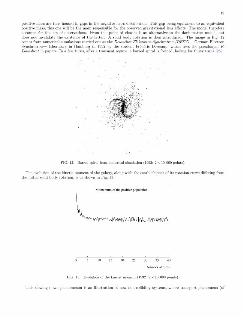
positive mass are thus housed in gaps in the negative mass distribution. This gap being equivalent to an equivalentpositive mass, this one will be the main responsible for the observed gravitational lens effects. The model thereforeaccounts for this set of observations. From this point of view it is an alternative to the dark matter model, butdoes not invalidate the existence of the latter. A solid body rotation is then introduced. The image in Fig. 12comes from numerical simulations carried out at the Deutsches Elektronen-Synchrotron (DESY) —German ElectronSynchrotron— laboratory in Hamburg in 1992 by the student Frédéric Descamp, which uses the pseudonym F.Landsheat in papers. In a few turns, after a transient regime, a barred spiral is formed, lasting for thirty turns [28].
FIG. 12. Barred spiral from numerical simulation (1992: 2 × 10, 000 points).
The evolution of the kinetic moment of the galaxy, along with the establishment of its rotation curve differing fromthe initial solid body rotation, is as shown in Fig. 13.
Momentum of the positive population
Number of turns
0 5 10 15 20 25 30 35 40
FIG. 13. Evolution of the kinetic moment (1992: 2 × 10, 000 points).
This slowing down phenomenon is an illustration of how non-colliding systems, where transport phenomena (of

20
heat and angular momentum) are absent, occur. In the case of spiral galaxies these exchanges are played out bymeans of density waves, which appear in the distribution of positive masses with their counterpart in the world ofnegative masses, as numerical simulations have shown. For thirty years astrophysicists have thought that the spiralstructures of galaxies were the sign of a braking phenomenon. A recent paper [29] presents observational evidenceof this dynamical friction phenomenon. The authors conclude that this supports the hypothesis of the existence of adark matter halo, according to them, responsible for such braking. But we can also consider this study as bringing anargument in favor of a braking resulting from the interaction between the mass of the galaxy and its negative massenvironment.
V. TIME AND T-SYMETRY
V.1. Primordial antimatter, nature of the negative mass
In the accepted scientific scheme, matter and antimatter are formed from primitive radiation, as long as the energy ofphotons exceeds the energy equivalent of these matter-antimatter pairs. When the expansion lowers this temperaturethese syntheses cease and these elements disappear by annihilation. Fossil radiation is considered as the remnantof these annihilations. There is currently no theoretical model that explains why one particle of matter in a billionremained, nor why we have never had to highlight its counterpart in the form of primordial antimatter.
The Russian Andrei Sakharov ([30–32]) started from a synthesis image of baryons from quarks and antiquarks fromanti-baryons. According to him the rate of synthesis of baryons would have been faster than that of anti-baryons.The expansion would have frozen this situation and there would exist in our universe a remnant of free antiquarks, inthe ratio three to one. He further suggested that a twin universe would coexist with our universe, which would haveknown an opposite situation and where anti-baryons and quarks would subsist in the free state. He also suggestedthat the time arrow of this other universe would be opposite to ours and that it would be enantiomorphic. But hehad not envisaged the involvement of these two regions. Figure 14 is a didactic image illustrating Sakharov’s model.
MM′
Space (reduced to one dimension)
Singularity
Φ
Arrows of time
FIG. 14. Didactic image of Andrei Sakharov model.
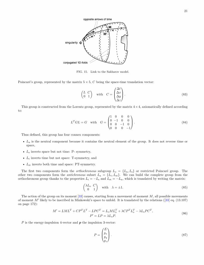
We can consider the cosmological model with negative masses as suggesting the following scheme in Fig. 15.One can imagine a reversal of time at the time of the Big Bang, a situation that brings a form of answer to the
question “what was there before the Big Bang?”It so happens that in 1970 the French mathematician J.-M. Souriau brought an original answer to T-symmetry. His
approach is the following. Starting from Minkowski’s isometry group, the complete Poincaré group, he determines,by the technique of the group’s coadjoint action on the dual of his Lie algebra [33], the characteristics of the motionsof the different particles that inscribe their motions in it. These objects are of two kinds:
• Photons, characterized by their E energy and spin s, and
• Particles with an energy E (with a rest mass m, according to E = mc2) and an impulse p.
21
FIG. 15. Link to the Sakharov model.
Poincaré’s group, represented by the matrix 5 × 5, C being the space-time translation vector:
(L C0 1
)with C =
∆t∆x∆y∆z
. (83)
This group is constructed from the Lorentz group, represented by the matrix 4 × 4, axiomatically defined accordingto:
LTGL = G with G =
1 0 0 00 −1 0 00 0 −1 00 0 0 −1
. (84)
Thus defined, this group has four connex components:
• Ln is the neutral component because it contains the neutral element of the group. It does not reverse time orspace,
• Ls inverts space but not time: P- symmetry,
• Lt inverts time but not space: T-symmetry, and
• Lst inverts both time and space: PT-symmetry.
The first two components form the orthochronous subgroup Lo = Ln, Ls or restricted Poincaré group. Theother two components form the antichronous subset La = Lt, Lst. We can build the complete group from theorthochronous group thanks to the properties Lt = −Ls and Lst = −Ln, which is translated by writing the matrix:(
λLo C0 1
)with λ = ±1. (85)
The action of the group on its moment [33] causes, starting from a movement of moment M , all possible movementsof moment M ′ likely to be inscribed in Minkowski’s space to unfold. It is translated by the relations ([33] eq. (13.107)on page 172):
M ′ = LMLT + CPTLT − LPCT = LoMLTo + λCPTLT
o − λLoPCT ,
P ′ = LP = λLoP.(86)
P is the energy-impulsion 4-vector and p the impulsion 3-vector:
P =
Epx
py
pz
. (87)

22
From the examination of these relations (86) and (87) we find the result of Souriau ([33] page 190, equation (14.67)):T-symmetry reverses the energy and pulse, but not the spin.So that the analysis of the properties of space-time shows that T-symmetric motions should be included, that would
simply be those of particles of opposite energy, for photons, and of negative mass for matter. Until 2011 nothingemerged from our physics that could give credit to this idea. But the discovery of the acceleration of expansion,attributed to the action of negative energy, gave credence to the idea that there could exist particles with negativeenergy, which could be particles with negative mass and photons with negative energy. This possibility of inversionof the time coordinate can be read in any case in the expression of the metric, invariant by T-symmetry, P-symmetryand PT-symmetry:
ds2 = c2 dt2 − dx2 − dy2 − dz2. (88)
But this inversion of the time coordinate t does not automatically mean the inversion of the proper time s!The cosmological model hosts negative masses and negative energy photons that and our instruments cannot
capture. It is a simple extension of Minkowski’s geometry. As this inversion goes hand in hand with the inversion oftime we call it:
Janus Model.
The two folds are linked by a PT-symmetry relationship, like Sakharov’s twin universes.The matter-antimatter duality finds its geometrical translation by inscribing the movements in a Kaluza 5D space.
The corresponding group is then translated by the matrices 5 × 5:µ 0 ϕ0 λLo C0 0 1
with λ = ±1µ = ±1 . (89)
The value µ = −1 represents a C-symmetry. This doubles the number of related components in the group. Thegroup acts on the five-dimensional Kaluza space-time:
ζ, t, x, y, z .
The translation subgroup is introduced along this fifth dimension. According to Noether’s theorem this is translatedby the constant of a scalar q, which is then the electric charge.
Matter/antimatter symmetry is geometrically translated by the inversion of the fifth dimension ζ. Let us start fromFeynmann’s idea according to which by applying to a particle a double inversion of space and time, it behaves like anantimatter particle. This is concretized by passing to the Janus group:λµ 0 ϕ
0 λLo C0 0 1
with λ = ±1µ = ±1 . (90)
Through the matrix the value λ = −1 operates an inversion of space and time, at the same time as an inversion ofthe electrical charge. In passing, the inversion of time leads to the inversion of energy and mass. This Λ-symmetryis that which corresponds to the Janus cosmological model. By adding the value µ = −1 we install the duality ofantimatter in the world of negative masses.
Let us note in passing that one can add as many additional dimensions to Minkowski’s space as quantum chargesqi:
λµ 0 . . . 0 0 ϕ10 λµ . . . 0 0 ϕ2. . . . . . . . . . . . . . . . . .0 0 . . . λµ 0 ϕp
0 0 . . . 0 λLo C0 0 . . . 0 0 1
×
ζ1ζ2. . .ζp
ξ1
. (91)
The complete calculation of the action of this group on its momentum is given in Appendix B and leads to:
q′i = λµqi,
M ′ = LMLT + CPTLT − LPCT = LoMLTo + λCPTLT
o − λLoPCT ,
P ′ = LP = λLoP.
(92)
So there are two antimatters:

23
• The C-symmetric of ordinary antimatter, with positive mass and positive energy. Let us call it “antimatter inthe sense of Dirac”, and
• The PT-antimatter, PT-symmetric of our own matter, with negative mass and negative energy, which we willcall “antimatter in the sense of Feynmann”.
If Sakharov’s idea is then implemented, the world of negative masses would be populated with antimatter of negativemass and energy. Essentially:
• Negative mass antiprotons,
• Negative mass anti-neutrons,
• Negative mass anti-electrons,
• Photons of negative energy, and
• A residue of negative energy quarks.
It is of course impossible to highlight these components individually, especially since this negative mass is almostabsent in the solar system.
The model is falsifiable on many levels. With the foreseeable progress of observation techniques, it will be possibleto try to detect at the center of the Great Repeller formation the presence of a conglomerate of negative mass, whichwould then reveal its presence by a significant attenuation of the magnitude of the distant sources. If this attenuationreveals the presence of an object of limited size, it will invalidate any interpretation in terms of a gap in the darkmatter.
The cooling time of a protostar increases with its mass. These conglomerates, which form rapidly after decoupling,can be compared to protostars of gigantic mass whose cooling time exceeds the age of the universe. They are thusspheroidal sets made up of anti-hydrogen and anti-helium emitting negative energy photons, which our instrumentscannot capture, in the red and infrared range. In this world of negative masses, there is no atom heavier than these.There are no stars, no galaxies, no planets.
Life is absent from it.
• The Janus Model provides an answer to the question of the lack of observation of primordial antimatter.
• It predicts in passing that antimatter created in the laboratory, with a positive mass, will behave like ordi-nary matter in experiments to demonstrate its behavior in the Earth’s gravitational field (Gbar and Alphaexperiments).
• It is the only one to attribute a precise identity to the invisible components of the universe and to specify thenature of the objects which do not constitute it.
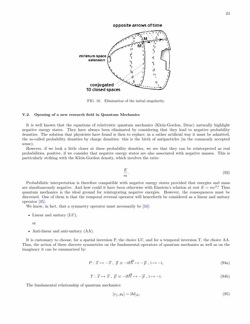
• If one replaces the singularity Big Bang by a bridge connecting the two folds of universe in interaction, which arein a way the Right side and the upside down side of the hypersurface space-time, the model brings an originalanswer to the question “what was there before the Big Bang?” (see Fig. 16).
The inversion of the time coordinate is not a problem in this extension of general relativity since metrics, fieldequations, for all equations of physics are time-reversible. What does Quantum Mechanics have to say about this?If we refer to a reference work, that of S. Weinberg [34] in section 2.6 (pages 74 to 76). We will find two arbitrarychoices concerning the operators P and T for the inversion of space and time. In order to avoid the emergence ofnegative energy states, which are considered a priori impossible, the following two arbitrary choices can be made,
• P linear and and unitary (LU),
or
• T antilinear and anti-unitary (AA).
24
FIG. 16. Elimination of the initial singularity.
V.2. Opening of a new research field in Quantum Mechanics
It is well known that the equations of relativistic quantum mechanics (Klein-Gordon, Dirac) naturally highlightnegative energy states. They have always been eliminated by considering that they lead to negative probabilitydensities. The solution that physicists have found is then to replace, in a rather artificial way it must be admitted,the so-called probability densities by charge densities: this is the birth of antiparticles (in the commonly acceptedsense).
However, if we look a little closer at these probability densities, we see that they can be reinterpreted as realprobabilities, positive, if we consider that negative energy states are also associated with negative masses. This isparticularly striking with the Klein-Gordon density, which involves the ratio:
E
m. (93)
Probabilistic interpretation is therefore compatible with negative energy states provided that energies and massare simultaneously negative. And how could it have been otherwise with Einstein’s relation at rest E = mc2? Thusquantum mechanics is the ideal ground for reintegrating negative energies. However, the consequences must bediscerned. One of them is that the temporal reversal operator will henceforth be considered as a linear and unitaryoperator [35].
We know, in fact, that a symmetry operator must necessarily be [34]:
• Linear and unitary (LU),
or
• Anti-linear and anti-unitary (AA).
It is customary to choose, for a spatial inversion P, the choice LU, and for a temporal inversion T, the choice AA.Thus, the action of these discrete symmetries on the fundamental operators of quantum mechanics as well as on theimaginary it can be summarized by:
P : #—x 7→ − #—x , #—p ≡ −iℏ #—∇ 7→ − #—p , i 7→ −i, (94a)
T : #—x 7→ #—x , #—p ≡ −iℏ #—∇ 7→ − #—p , i 7→ −i. (94b)
The fundamental relationship of quantum mechanics:
[xj , pk] = iℏδjk, (95)
25
is then invariant under (94a) as well as under (94b).Moreover, the symmetry PT (t 7→ −t, i 7→ −i) thus chosen ensures the invariance of the energies:
E 7→ H ≡ iℏ ∂∂t. (96)
Positive energies, if we limit ourselves to them, therefore remain exclusively positive. On the contrary, in [35] wehave opted for the choice LU, for the two inversions, which leads to the following result:
P : #—x 7→ − #—x , #—p ≡ −iℏ #—∇ 7→ − #—p , i 7→ i, (97a)
T : #—x 7→ #—x , #—p ≡ −iℏ #—∇ 7→ #—p , i 7→ i, (97b)
both ensuring the invariance of (94). The major difference is that the symmetry PT leads this time to a change ofsign at the level of the energies:
H ≡ iℏ ∂∂t
7→ −H. (98)
There is nothing to prevent, physically, mathematically and from a probabilistic point of view, to consider thesenegative energy states as long as they are assigned a negative mass. Moreover, it even seems that this additionalpossibility is more rigorous if we stick to mathematics, since implying that T is linear, it is in agreement with its usualrealization (cf. [34] Eq. (2.3.16), p. 58, for example):
T = diag (−1, 1, 1, 1) . (99)
V.3. Challenging the inflation model
If we want to arrive at a coherent cosmological model, we have to negotiate all the elements coming from theobservations. One of them is the extreme homogeneity of the CMB, image of the early universe. The only explanationput forward so far is the hypothesis of a considerable inflation, attributed to a field of inflatons. As no alternativetheory was presented, this model ended up being considered as part of a “standard model”, whereas no credible modelof inflaton was born.
Various attempts have been made [36] using a variable speed of light. But these attempts have been hampered bythe loss of Lorentz invariance. Moreover, the observational data were opposed to the variation of c, if only throughits influence on the fine structure constant.
Although the scientific community did not pay attention to this model, as early as 1988, that is to say 33 yearsago, we published an article [37] where we introduced the idea of joint variation of all the constants of physics, inagreement with the correlative variation of space and time gauges.
In a second paper [38] an attempt was made to deal with the redshift phenomenon by trying to introduce a differentvariation of the electromagnetic parameters. But later, years later, in [11] we abandoned this idea and preferred tosituate this phase “with variable constants”, as part of the radiative era.
These constants, as well as these two gauges, are present in the equations of physics, remembering:
• The field equation,
• Maxwell’s equations, and
• Quantum mechanic’s equations.
The quantities to consider are:
• The six constants of physics:
– G: constant of gravitation,– c: speed of light,– h: Planck constant,– e: elementary electric charge,
26
– µ0: magnetic permeability of vacuum, and– m: all kinds of masses. We suppose all masses experience the same gauge variation.
• To this must be added:
– a: space scale factor, and– t: time scale factor.
We must therefore consider varying these eight quantities together:
G, c, h, e, µ0,m, a, t . (100)
We then show [11] that there is only one generalized gauge relation, involving these eight quantities, leaving all thephysics equations invariant. The details of the establishment of these different relations can be found in Appendix C.
In these conditions, if we choose one of these quantities as a variable, the other seven are deduced. As the equationsof physics remain invariant, the same is true for the fine structure constant. Lorentz invariance is also assured. It isconvenient to take the scale factor a, related to the expansion process, as a guiding variable. The variations are then:
G ∝ 1a
; c ∝ 1√a
; h ∝ a3/2 ; e ∝√a ; µ0 ∝ a ; m ∝ a ; t ∝ a3/2. (101)
Considering the variables ε0, dielectric constant of vacuum, and µ0 are linked, it comes that ε0 is absolute constant.We verify the invariance of the Lorentz metric:
ds2 = c2 dt2 − dx2 − dy2 − dz2, (102)
according to the above relationships.As recalled in appendix C, these gauge relations imply that:
• All characteristic lengths vary as a,
• All characteristic times vary as t, and
• All energies are conserved.
The third property is then in contradiction with redshift measurements, which boil down to evaluate the energy lossof photons, due to the expansion. Thus this form of “gauge” evolution can only be located during the radiative era.
What is the observable, related to this mode of evolution (of gauge), if there is no redshift? Answer: it is theevolution of the cosmological horizon:
Hcosmo =∫cdt ∝
∫ 1√a
d(a3/2
)∝ a. (103)
There is therefore no longer any need for inflation.The question remains: when does this mechanism arise?The “direct” observational data are those of the redshift. Beyond that, we reconstruct the situation of the cosmos
through a model. If we limit the redshift to the first hundredth of a second, as S. Weinberg did in his book “The FirstThree Minutes”, this physics seems to be known in a satisfactory way. The first confirmation was the discovery of theprimitive radiation background, interpreted as resulting from an annihilation between pairs of particles of matter andantimatter. Recalling that until now, the absence of observation of primordial antimatter could not be explained.
The fact that “all energies are conserved in the phase with variable constants” would oppose a number of phenomena,such as deionization or others. We can deduce that if this mechanism of drift of constants intervenes it could be beforethis first hundredth of a second.
It remains quite problematic to try to give a description of the universe by going further back in time. We only knowthat the density took extremely high values. When the temperature exceeds 1012 K, we consider that the universewould be a mixture of quarks in free state and gluons. A situation that we try to reconstitute in colliders using heavyions, such as gold or lead. If the theory of considering baryons and mesons as assemblies of quarks has proved to befruitful, giving rise to the standard model, it remains a model, insofar as it has not been possible to make observationsof quarks in the free state. On the other hand, attempts to describe the physical content of higher energies, throughthe theory of supersymmetry, have not held their promises experimentally. It is perhaps more realistic to admitmodestly that we do not really know what happens when we try to go further back in time.

27
When we try to create a model of a neutron star we come across problems of a similar nature. When we try todescribe the contents of the star, as we go deeper into its entrails, we are led to consider a progressive decompositionof the matter into more and more fundamental components. At the surface of the star: iron plasma, totally ionized.Then, when we go down, the nuclei break up and it is a mixture of electrons and nucleons in the free state. Deeperstill, it is the electrons that combine with protons to give neutrons. Electrons that cease to “exist”, for lack of space,remembering that their wave function has a spatial extension 1850 times greater than that of neutrons and protons.But the medium still keeps its plasma status, as long as the electric charges of the protons can be neutralized bymesons, whose size is 207 times shorter that the one of electrons. Finally, when it is the mesons’s turn to run outof space, the content is described as only formed by neutrons. Finally, when the density increases again, theoristspropose a star core constituted by a plasma of quarks and gluons. And in fact this descent to the heart of neutronstars is a way to go back in the past of the universe.
When the mass of the neutron star increases again, the model proposed by the theorist is the black hole, built froma solution of the field equation referring to a portion of space free of any content.
V.4. The question of time
In classical chronology, the history of the universe is attached to a time variable t. But what is its physicalmeaning? How to conceive a clock, on a simple conceptual level, when the different components are animated bythermal agitation speeds that are significantly close to the speed of light.
One can envisage a kind of conceptual clock constituted by two masses orbiting around a common center of gravity(Fig. 17). The most significant way to talk about a time is to link this measurement to an angle. It is the rotationof the second hand on the watch, the period of rotation of the Earth around the Sun, or the rotation of the MilkyWay on itself. The measure of time will thus be the measure of a number of revolutions of our elementary clock, bysupposing that this one manages to avoid any collision with its surrounding medium, made up of increasingly fastparticles.
CG
m
m
r
FIG. 17. Elementary clock (CG is the center of gravity).
In a system where the constants do not vary, this is the case for the masses and the constant G of gravitation.The radius of gyration of the system and the period of rotation are also invariant. In these conditions our elementaryclock will count a finite number of revolutions if we go back to a situation where the universe is assimilable to a point.This number of revolutions is then identified with the chosen variable t, which would constitute a good chronologicalindicator.
It is completely different if we place ourselves in a gauge context, with variable constants. The radius of gyrationvaries like the space gauge a. The gravitational constant varies as the inverse of a while the masses vary as a. Thecalculation of the period of the system shows that it varies like the time gauge t, i.e. it is shorter and shorter as wego back in time. The number of revolutions made by our clock is:
N =∫ dt
t= ln t =
∫a1/2 daa3/2 = ln a. (104)
Thus, from the state, the moment when the spatial extension of the universe will be null until today our clockwould total an infinite number of turns. Conversely, to go back to a hypothetical instant zero, in this mode of cosmicevolution, evokes the aphorism of Zeno according to which Achilles, pursuing a tortoise, never manages to catch upwith it.

28
V.5. Time or entropy?
The relativistic formulation of the velocity distribution function is:
f = n( m
2πkT
)3/2 1cK2
(mc2
kT
)√2kTm
exp
−mc2√1 − v2
c2
, (105)
where m is the rest mass, T the temperature, n the number of density and K2 a Bessel function. If β =(
⟨v2⟩c2
)1/2≪ 1
then we get the classical Maxwell-Boltzmann velocity distribution function:
f = n( m
2πkT
)3/2e−mv2/2kT . (106)
Let us compute the entropy per baryon, as defined by:
s = −k
n
∫∫∫f ln f dudv dw = −k⟨ln f⟩, (107)
where k is the Boltzmann’s constant. We have n ∝ a−3, v2 ∝ c2 ∝ a−1, and m ∝ a, so that:
s ∝ ln a ∝ ln t. (108)
The entropy per baryon identifies to the so-called “conformal time”.
VI. OPEN QUESTIONS
VI.1. Something still missing
The extreme homogeneity of the CMB has led to the proposal of the existence of a fantastic inflation, without anyother justification than this single observational data. The model including a “variable constant” step, described bya gauge process, leads to a variable c evolution where the cosmological horizon follows the variation of the space scalefactor, which is another way to justify this great homogeneity. But the question to be answered is:
What causes this regime change?
In classical cosmology, and in the phase of the Janus model that follows the decoupling, the masses in the universedo not expand. It is the photons that expand and their wavelength then follows the growth of the space scale factora.
We have seen, when we went inside a neutron star, how its content tended to simplify. At the center of the star:neutrons. In order for them to exist, they must be able to install their wave function in the disposable space. Theorder of magnitude of the minimal space required can be the Compton length of neutrons which is of the order of10−15 meters. What happens when the density of the medium is such that the average distance between neutronsbecomes smaller than this length? There is no clear answer to this question.
The same question can be asked when we try to retrace the course of events in the universe. If we draw a parallelwith the neutron star model, we would be led to consider a medium made up of neutrons and antineutrons, which aremore and more closely packed together. A critical moment would then occur, resulting in the transition to a regimeof variable constants, where the Compton length of the neutrons ceases to be constant and varies as the space scalefactor a. But this is only a conjecture. However, it is not more problematic than the scheme proposed by the inflationtheory. We can represent on Fig. 18 the way in which the different constants evolve. On the x-axis, in logarithmiccoordinates, a parameter of evolution such as time, the unit value corresponds to the transition between the tworegimes. After this time, the constants adopt the values that we know today. If we calculate the Planck length, wenotice that it also follows the evolution of the space scale factor, while the Planck time follows that of the time scalefactor.

29
10−2 10−1 100 10110−3
10−2
10−1
100
101
102
G
c
e
m, µ0
h
1
discoupling
FIG. 18. Schematic evolution of constants in log-log coordinate.
VI.2. An alternative interpretation of CMB fluctuations
In the field equations, the energy-matter content in the form of radiation contributes to the field, as does matter.In radiative eras these contents are in the majority.
It is quite legitimate to ask whether a form of gravitational instability could occur in this radiation-dominatedmedium, in a gas of photons. Let us suppose that somewhere in the universe there is a region of characteristicdimension L where the content is greater than what is around it. If nothing happens, we can consider that thisoverdensity of radiation will dissipate in a time L/c.
If we abandon a lump of material of diameter L to the only forces of gravity it will implode according to a lawL ∝ t3/2 or, put differently, this will occur with a characteristic accretion time tJ ∝ L2/3. By introducing theconservation of mass ρm ∝ L−3 we obtain an implosion time (or Jeans time) tJ ∝ ρ
−1/2m .
If now it is a question of an overdensity of radiation this one will create a gravitational field. The evolution of sucha cluster will be according to L ∝ t1/2. But as we have then ρr ∝ L−4, we will have an implosion time tJ ∝ ρ
−1/2r .
This overdensity will increase if the dispersion time is greater than the accretion time, i.e. if Lc > tJ; in other words,
the gravitational instability will occur on distance scales greater than:
LJ = ctJ. (109)
We find then, in this mechanism of a gravitational instability of the photon gas, the equivalent of the Jeans lengthof the matter. But this one is then of the order of the cosmological horizon. This is the reason why we have neverbeen concerned with a phenomenon which would then be fundamentally unobservable, although it creates fluctuationswhose order of magnitude of the wavelength is the Jeans length in the radiative medium.
These fluctuations being able to occur during the phases of evolution with variable constants, in the two populations,of positive or negative energy, they are not only translated by a fluctuation of but would also affect the values of theconstants, with two fields translating variations of the sets:
G(+), c(+), h(+), e(+), µ(+)0 ,m(+), a(+), t(+)
, (110)
linked by:
G(+) ∝ 1a(+) ; c(+) ∝ 1√
a(+); h(+) ∝ a(+)3/2 ; e(+) ∝
√a(+) ; µ(+)
0 ∝ a(+) ; m(+) ∝ a(+) ; t(+) ∝ a(+)3/2, (111)
and: G(−), c(−), h(−), e(−), µ
(−)0 ,m(−), a(−), t(−)
, (112)
linked by:
G(−) ∝ 1a(−) ; c(−) ∝ 1√
a(−); h(−) ∝ a(−)3/2 ; e(−) ∝
√a(−) ; µ(−)
0 ∝ a(−) ; m(−) ∝ a(−) ; t(−) ∝ a(−)3/2. (113)
30
We thus see the idea of a multiverse, made up of “universe bubbles” forming a pavement, endowed with their ownset of constants, with the corresponding values of the scaling factors. But, unlike what others envisage, the equationswould remain the same from one cell to another and, in fact, their histories would not be fundamentally different. Allcells of negative energy would give rise, in their dominated matter era, to a regular distribution of spheroidal clusters.In the positive energy cells we would find lacunar structures, giving birth to galaxies and stars.
But in these sets a difference of their: a(+) ≫ a(−). As the Jeans lengths are such that L(+)J ∝ a(+) and L(−)
J ∝ a(−),the spatial distributions of the fluctuations are very different in the two populations. If the negative medium keeps atotal homogeneity during its radiative phase, the fluctuations of density of its radiation cause a weak response in thepositive world.
And therein lies, in our opinion, the origin of the fluctuations of the CMB. Their analysis, by identifying thefundamental fluctuation, which is of the order of one degree, gives us access to the relationship:
L(−)J
L(+)J
= a(−)
a(+) ≈ 10−2. (114)
Since these fluctuations occur as part of the gauge phenomenon, they also affect the values of the physics constantsand:
c(−)
c(+) =√a(+)
a(−) ≈ 10 ; G(−)
G(+) = a(+)
a(−) ≈ 100 ; h(−)
h(+) =(a(−)
a(+)
)3/2
≈ 10−3 ; m(−)
m(+) = a(−)
a(+) ≈ 10−2. (115)
We also have:
t(−)
t(+) = t(−)J
t(+)J
=(a(−)
a(+)
)3/2
≈ 10−3. (116)
The time of Jeans, in negative masses, is then thousand times shorter than that of positive species. This justifies thescheme of formation of the very large scale structure of the universe, according to which it is the spheroidal clustersof negative mass which are formed first.
As the thermal agitation velocity follow the gauge process, for numerical simulations of the formation of this verylarge scale structure we have the data:
⟨v(−)⟩⟨v(+)⟩
=√a(+)
a(−) ≈ 10. (117)
VI.3. The problem of interstellar travel
The nearest planetary system, linked to the nearest stars, is four light years away. This fact made that until now itwas considered that the idea of being able one day to realize trips towards these close systems would be unthinkableat the scale of a human vacuum. But the new geometric context changes things. The universe is a variety equippedwith two different metrics. All the points of the variety are located with the help of dimensionless coordinates:
ξ0, ξ1, ξ2, ξ3. (118)
Let two points A and B be distant, with coordinates:ξ0, ξ1
A, 0, 0
andξ0, ξ1
B , 0, 0. (119)
The distance between these two points will be different depending on whether it is covered in the positive or negativemass sector:
L(+) = a(+) (ξ1
B − ξ1A
)≈ 100L(−) = 100a(−) (
ξ1B − ξ1
A
). (120)
If a vehicle had a technology allowing it to reverse its mass (and that of its passengers) the distance it would haveto cover would be a hundred times shorter. Moreover the speed limit, at that of the light in the negative sector, wouldbe raised of a factor ten. From where a priori a weaker travel time of three orders of magnitude.
Thus interstellar travel becomes non-impossible.

31
Once arrived at its destination, the vehicle would only have to operate a new mass inversion to find itself in thepositive sector. During its journey, the passengers of this vehicle would lose all possibility of having observations ofthe positive mass environment, always present but now invisible to it. Inversely, they would be the spectators of thenegative world scenery, that is to say, they would be able to see the spheroidal clusters of negative mass, emitting inthe red and the infrared. At the moment of the mass inversion two equivalent volumes, positive and negative sectorswould be exchanged. If the vehicle performs its mass inversion when it is in the atmosphere, it will no longer bevisible to observers made up of positive mass and will seem to dematerialize in their eyes.
As the negative sector, in the solar system, is ultra rarefied, the content of the equivalent volume which will takethe place of the one occupied by the vehicle will be filled with photons and very rare atoms of anti-hydrogen andanti-helium whose masses, having also undergone an inversion, became positive and will annihilate in contact withthe atoms and molecules of the atmosphere, by producing gamma rays. The irruption of the air molecules in a spaceperceived as quasi empty will produce a disturbance of aerodynamic nature.
This process of mass inversion is equivalent to swapping adjacent contents located on the front and back of thehypersurface. It is thus a problem of topology. For there to be historical continuity it is necessary that the vehicleand its passengers follow a continuous line of universe, continuing their progression towards the future. The fact ofmomentarily moving in the negative sector does not mean that the passengers would see their own time reversed,that is to say that they would not reappear in their own past. This path would make them cross on their way thesmall quantity of antimatter present in the negative sector, endowed then with the same sign of the mass. Of whichthe vehicle and this antimatter could interact. But the vehicle could then protect itself from this flow of antimatter,comparable to the solare wind emitted by the sun, from which the Earth protects itself with the shield constitutedby its magnetic field.
VI.4. The problem of swapping volumes between adjacent sectors
A first scheme of mass inversion has been evoked in [39], through a reinterpretation of the Schwarzschild solutionof the Einstein equation.
According to the scheme of special relativity the energy equivalent to a mass M is Mc2. If the amount of energyneeded to invert this mass was of this order, this technology would be problematic. We are faced with the problemof swapping two adjacent volumes of 4D hypersurfaces. It is convenient to consider the positive and negative sectorsas a kind of “parallel universe”. But the picture is immediately misleading because one can hardly take into accountthe considerable difference between scale factors a(+) and a(−). If we disregard this, we can give a 2D image of thesetwo folds by simply representing them by two parallel planes (Fig. 19).
FIG. 19. Before surgery.
The alteration that we consider to give to these two folds is a local variation of the curvature, equivalent to alocal concentration of energy. We will present a solution referring to a 2D toy model, where the permutation of twoadjacent domains, whose borders are cerce, is operated by an operation described in topology by the word surgery.
A technological device causes a concentration of positive energy, in the positive sector, in the external vicinity ofthe wall. This is shown in this sequence of didactic images, by a kind of groove (Fig. 20).
We then split the object by presenting only half of it in order to perceive the curvature given to the surfaces(Fig. 21). We suppose that the alteration of the curvature, in the upper fold, supposed to translate a concentrationof energy, would cause a “curvature induced” in the adjacent fold.
The geometrical operation of surgery involves the creation of an infinite curvature along a circle. In the field ofphysics this could be a very pronounced curvature, associated with a very high local density of energy. It is necessaryto understand that when this one is operated the adjacent parts of folds 1 and 2 have been exchanged (Fig. 22).

32
FIG. 20. Preparation of the surgery.
FIG. 21. The surgery occurs along a circle.
FIG. 22. The exchanged portions.
This is equivalent to Fig. 23.
FIG. 23. After surgery.
To illustrate the suggested scheme we represent the reduction of the grey portion in Fig 24.This is only a toy model. This said, techniques to concentrate energy in a region of space forming a thin layer can
be envisaged, for example by imparting energy to nuclei possessing a long-lived metastable excitation level, as weknow they exist.

33
FIG. 24. Disappearance of the portion from fold 2.
VII. CONCLUSION
Cosmology and theoretical physics have been in crisis for more than half a century. There is still no theory toexplain the non-observation of primordial antimatter. Attempts have been made to reconstruct a standard model byinvoking the existence of a hypothetical dark matter and by attributing the cosmic acceleration to a negative darkenergy of unspecified nature. All the experiments in which one has tried to give an identity to the dark matter havebeen failures, whether in mines, tunnels or in space, on board the International Space Station (ISS).
It is therefore quite legitimate to consider a profound change of paradigm to try to get out of this impasse, providedthat a maximum of support based on the confirmation of observational data is ensured. The model involves theintegration of GR in an extended geometric context, where the universe is considered as an M4 manifold equippedwith two metrics, the first corresponding to ordinary matter and the second to species of mass and negative energy.Such a system must then refer to a system of two coupled field equations, the first one identifying with the Einsteinequation in regions where negative mass is absent
A first attempt at a bimetric description was made in 2002 by T. Damour and I. Kogan, which was unsuccessful,as they were unable to define the interaction between the two species. In 2008 S. Hossenfelder proposes a geometricalcontext derived from a Lagrangian. As at the time the acceleration of the expansion is not yet validated, she tries tofit with the standard scheme. Although it satisfies the principle of action-reaction, which represents an improvementwith respect to the introduction of negative masses in GR which makes the unmanageable runaway phenomenonappear, her choices of signs made lead to a violation of the principle of equivalence and to the impossibility of makingpredictions that can be confronted with observations.
We then take up this approach with a good choice of signs, which allows to satisfy both the action-reaction principleand the equivalence principle with the interaction law:
• Masses of the same sign attract each other according to Newton’s law, and
• Masses of opposite signs repels each other according to “anti-Newton”.
The model includes a generalized principle of conservation of energy. The joint gravitational instabilities lead toa separation of the two species. The negative mass density being then negligible in the solar system, this allowsthe model to agree with the local relativistic data. The exact joint solutions are constructed. The fact that theexpansion accelerates shows that the negative energy content is dominant, and drives the dynamics of the systemwith an excellent agreement with observational data from 700 type Ia supernovae.
Using numerical simulations performed in the nineties, based on the same interaction laws, but considered at thetime as a simple empirical hypothesis, we show that a deeply dissymmetric situation leads to a large-scale structurewhere the negative masses, endowed with a shorter Jeans time, are the first to give birth to a regular arrangement ofspheroidal clusters, pushing the positive mass into the remaining space, and thus conferring on it a lacunar structure,comparable to joined soap bubbles. This new description of the creation of the very large structure goes through acompression of the positive mass, according to flat plates, giving a fast and optimal radiative cooling, and suggests acomplete resumption of the pattern of galaxy formation. The continuation of the gravitational instability leads to anaccumulation of the mass along the junction lines of three empty cells, in the center of which are lodged spheroidalclusters of negative mass. This mass also forms clusters of galaxies at the junction points of four of these cells.
The accretion phenomenon also leads to a heating of the negative mass clusters, which then behave as a kind ofprotostars, with a cooling time higher than the age of the universe. Neither galaxies nor stars are formed there. Asfusion reactions cannot take place there, this negative world contains neither heavy atoms nor planets, and life isabsent. The negative mass clusters only radiate, emitting photons of negative energy, in the red and infrared ranges.
The phenomenon of the Great Repeller, discovered in 2017, reflects the presence of one of these negative massclusters. These are freely crossed by photons of positive energy emitted by the galaxies of the background. This
34
interaction leads to a reduction of the luminosity of the distant sources (z > 7) which is consistent with the obser-vations. It is suggested that the luminosity contrast of the background galaxies should reveal the diameter of such aconglomerates.
When galaxies form, negative mass invades the space between them and exerts on them a counter pressure, whichconfines them. This situation confers to their rotation curves a flat shape at the periphery. This phenomenon ofconfinement also plays at the scale of clusters of galaxies. It is shown that this configuration is accompanied bygravitational lensing effects, which have been considered until now as the irrefutable proof of the presence of a largehalo of positive mass dark matter.
In the nineties, 2D numerical simulations where we studied the behavior of a rotating galaxy, interacting with anenvironment of negative mass have allowed to show a barred spiral persisting for thirty turns. This persistence resultsfrom the dissipative nature of the phenomenon. The appearance of density waves, which have their counterpart in thesurrounding negative mass distribution, represents the way in which non-colliding systems can exchange energy. Thesimulations highlight the slowing down of the rotation, which has just been recently highlighted through observations,but where the authors impute this phenomenon to an interaction with a dark Matter halo of positive mass, while weattribute them to a dynamic friction on the negative mass environment.
This new geometrical context is linked to an extension of the associated group, which is no longer the restrictedPoincaré group, but the extended Poincaré group, including the elements of the group reversing the time, thusreversing the energy and the mass. By adding a fifth dimension we refind the theme of a matter-antimatter symmetrycorresponding to the inversion of this dimension. The universe of negative masses then corresponds to a CPT-symmetry. The matter-antimatter symmetry is also present in the world of negative species. This allows us to takeup the hypothesis proposed in 1967 by Andrei Sakharov according to which the synthesis of baryons from quarks ofpositive energy would have been, in our positive sector, faster than that of antibaryons, from antiquarks of positiveenergy. The opposite situation in the world of negative energies. This solves the paradox of the non observation ofprimordial antimatter. It is not, as A. Sakharov suggested, in a twin universe. It constitutes that part of the universe,which dominates all its dynamics, but escapes the observations, on the basis of purely geometrical considerations: Thegeodesic nulls of the two species form disjoint sets. This implies that two types of antimatter exist in the universe, ofopposite masses. Only the first can be created in the laboratory. In the earth’s gravitational field it will behave likeordinary matter and “will not fall upwards”.
This theme of a T-symmetry is examined in a quantum mechanical context. It is known that negative energy statesare banned from the outset in quantum field theory, simply by assuming that they are physically impossible. Thisleads to the ad hoc hypothesis of opting for an anti-unitary and anti-linear time reversal operator. It is shown that byopting for a linear and unitary operator the existence of negative energy states is imposed. Such a situation requiresa systematic extension of quantum theory, if only to justify the negative energy states constituting the dark energy.We conjecture that this approach could be the key to the quantization of gravitation.
Building on previous work, we extend the model into the past by switching to two regimes of variable constantswhere in each species all the constants of physics vary jointly with space and time scale factors, in such a way thatthe equations of physics, in both drives, remain invariant. The Lorentz invariance is then preserved and the modelbecomes fully compatible with the observations. For example the fine structure constant becomes invariant. Thismodel with variable light velocities is an alternative to the model based on the existence of an inflaton field, for whichno credible model is available. This context implies a redefinition of cosmic time evoking Zeno’s paradox.
We deduce from this approach a link between the scale factors and the speed of light in the two sectors. If thedensity in the negative sector is higher, then the scale factor is shorter and the speed of light higher. We then considerthe impact of a gravitational instability taking place in the gas of photons, in both sectors. The phenomenon is notobservable within the same sector since the corresponding Jeans length is identified with the cosmological horizon.But the fluctuations that appear in the negative sector, whose wavelength also corresponds to the cosmological horizonof the negative species, leave their imprint, weak, in the positive world and this leads to an alternative interpretationof the CMB fluctuations. Based on the value of the characteristic wavelength of these fluctuations, we deduce anevaluation of the scale factor of the negative sector, which is one hundred times smaller than that of our positiveworld, while the speed of light is then ten times higher. This has the effect of reducing by three orders of magnitudethe durations of possible intersideral journeys which thus become non-impossible.

35
Appendix A: Compatibility conditions
The equations are:
− χ
[ρc2 + V
b3
a3 ρc2]
= 3ka2 + 3a2
a2 , (A1)
− χ
[p+ V
b3
a3 p
]= − k
a2 − a2
a2 − 2aa, (A2)
− χ
[ρc2 +W
a3
b3 ρc2]
= 3kb2 + 3b2
b2 , (A3)
− χ
[p+W
a3
b3 p
]= − k
b2 − b2
b2 − 2bb. (A4)
A linear combination of (A1) and (A2) gives:
− χ
2
[ρc2 + V
b3
a3 ρc2 + p+ V
b3
a3 p
]= −3a
a. (A5)
Another one:
− χ
2
[ρc2 + V
b3
a3 ρc2 + p+ V
b3
a3 p
]= k
a2 + a2
a2 − 2aa
= k
a2 − ddx0
(a
a
). (A6)
We differentiate (A1) with respect to t:
− χddζ
[ρc2 + V
b3
a3 ρc2]
= −6ka3 a+ 3 d
dx0
(a2
a2
)= −6k
a3 a+ 6 aa
ddx0
(a
a
), (A7)
combining to (A6):
d
dζ
[ρc2 + V
b3
a3 ρc2]
+ 3 aa
[ρc2 + V
b3
a3 ρc2 + p+ V
b3
a3 p
]= 0, (A8)
or
d[ρc2 + V
b3
a3 ρc2]
[ρc2 + V
b3
a3 ρc2 + p+ V
b3
a3 p
] + 3daa
= 0. (A9)
Treating equations (28) and (29) in the same way we obtain:
d[ρc2 +W
a3
b3 ρc2]
[ρc2 +W
a3
b3 ρc2 + p+W
a3
b3 p
] + 3dbb
= 0. (A10)
First case: the two universes are dust universes:
d[ρc2 +W
a3
b3 ρc2]
[ρc2 +W
a3
b3 ρc2] + 3db
b= 0. (A11)

36
The hypothesis of a generalized conservation of energy:
ρmc2a3 + ρ
mc2b3 = E, (A12)
leads to:
V = W = 1. (A13)
Second case: both sectors are dominated by radiation:
p = ρc2
3 and p =ρc2
3 . (A14)
The hypothesis of a generalized conservation of energy in the form of radiation:
prc2a4 + ρ
rc2b4 = E, (A15)
leads to:
V = a
band W = b
a. (A16)
Appendix B: Calculation of the group’s action on its space of moments
The group is represented by the matrices:
a =
λµ 0 ϕ0 λLo C0 0 1
with λ = ±1µ = ±1 . (B1)
For convenience of calculation we will carry out this one with:λµ 0 ϕ0 L C0 0 1
with λ = ±1µ = ±1 . (B2)
The element of its Lie algebra is then:
Z ≡
0 0 ε0 δL γ0 0 0
. (B3)
The group is differentiated in the vicinity of its neutral element. Under these conditions δL can be put in the formGω where G is the Gramm matrix and ω an antisymmetric matrix:
Z =
0 0 ε0 Gω γ0 0 0
. (B4)
For computational convenience, we write the action of the group on its Lie algebra Z ′ = a−1Za instead of Z ′ =aZa−1, which is equivalent to computing the action of the inverse of the element of the group on the element of itsLie algebra, but the result will be equivalent since the set of inverses also represents the group. It comes:0 0 ε′
0 Gω′ γ′
0 0 0
=
0 0 λµε0 GLTωL γGLTG+GLTωC0 0 0
, (B5)
which gives:
ε′ = λµε,
ω′ = LTωL,
γ′ = GLTGγ +GLTωC.
(B6)

37
We are looking for the dual of the group’s action on its Lie algebra. The element of this Lie algebra depends on 11parameters:
Z = Z (ωsx, ωsy, ωsz, ωfx, ωfy, ωfz, γt, γx, γy, γz, ε) . (B7)
The moment space of the group will thus be a vector space of dimension 11. It can be put in the form of anantisymmetric matrix M of format 4 × 4, depending on six parameters, a quadrivector P and a scalar q. The dualitycan thus be ensured by the constancy of the scalar:
12 Tr (Mω) + PTGγ + qε, (B8)
which gives:
12 Tr (Mω) + PTGγ + qε = 1
2 Tr(M ′LTωL
)+ P ′TG
(GLTωC +GLTGγ
)+ q′λµε. (B9)
It comes immediately:
q = λµq′, (B10)
PT = P ′TLT =⇒ P = LP ′. (B11)
We know that we can perform a circular permutation in the trace:
Tr(M ′LTωL
)= Tr
(LM ′LTω
). (B12)
The identification on the ω terms gives:
12 Tr (Mω) = 1
2 Tr(LM ′LTω
)+ PTLTωC. (B13)
The term PTLTωC is the scalar product of the row vector PT by the column vector LTωC. We can thereforewrite, after having performed a circular permutation in the trace:
PTLTωC = Tr(LTωCPT
)= Tr
(CPTLTω
). (B14)
Thus the equation (B13) provides:
M = LM ′LT + 2CP ′TLT . (B15)
But:
CPTLT = 12
[sym
(CPTLT
)+ antisym
(CPTLT
)]. (B16)
Knowing that the trace of the product of a symmetrical matrix by an antisymmetrical matrix is equal to zero:
Tr[(CPTLT + LPCT
)× ω
]= 0, (B17)
it remains:12 Tr (Mω) = 1
2 Tr(LM ′LTω
)+ 1
2 Tr[(CPTLT − LPCT
)× ω
]. (B18)
Which provides the last equation of the group’s action on its moment:
M = LM ′LT + CP ′LT − LP ′CT . (B19)
We make the inversion parameter reappear by L = λLo and group the results together:
q = λµq′, (B20)
M = LoM′LT
o + λCP ′LTo − λLoP
′CT , (B21)

38
P ′ = λLoP. (B22)
P is the energy-impulsions 4-vector:
P =
Epx
py
pz
. (B23)
Equations (B20), (B21), and (B22) represent an extension of equations 13.107 of reference [33]. The relation (B22)makes it possible to find Souriau’s relation ([27] page 190, equations 14.67). The inversion of time (λ = −1) leads tothe inversion of energy and of the impulse vector #—p . The matrix M depending on six parameters can be decomposedinto two vectors. The vector f is what Souriau calls the passage and s is the spin:
M =
0 −sz sy fx
sz 0 −sx fy
−sy sx 0 fz
−fx −fy −fz 0
. (B24)
The passage f is not an intrinsic attribute of the motion because it can be cancelled by a change of variableaccompanying the particle. Only the spin remains, of which Souriau demonstrated in 1970 its geometrical nature. Bycancelling the spatio-temporal translation C the relation (B21), where λ does not appear, shows that the inversionof time does not modify the spin vector. With this way of carrying out the calculation one obtains the result of theaction of the group on a movement, characterized by the quantities E′, #—p ′, #—s ′ gives another movement E, #—p , #—s .It is the relation (B20) which informs on the fact that starting from a motion representing that of a particle of matter:
• (λ = −1;µ = 1) results in a PT-symmetry plus a C-symmetry. One thus obtains the movement of a particle ofnegative mass.
• (λ = 1;µ = −1) operates a C-symmetry. The movement obtained is that of an antiparticle in the sense of Dirac,of positive mass.
• (λ = −1;µ = −1) represents a PT-symmetry. The motion is that of an antiparticle of negative mass (antiparticlein the sense of Feynmann).
Appendix C: Construction of generalized gauge relations
We will assume that during the radiation dominated era all forms of energy are conserved, including the energy ofthe photons. Let a be the space scale factor. This hypothesis will give a single universal gauge relationship:
Eφ = hc
λφ= const. =⇒ hc ∝ a. (C1)
Let’s write the metric:
gµν = aηµν , (C2)
where
ηµν =
1 0 0 00 −1 0 00 0 −1 00 0 0 −1
(C3)
is the Lorentzian metric.a is a scale factor. gµν is a conformal metric:
ds2 = a2[(
dξ0)2 −(dξ1)2 −
(dξ2)2 −
(dξ3)2
]. (C4)
We shall assume that the scale factor a will rule all the evolution process in radiation dominated era. Angles areconserved. Lengths vary like a. Energies are conserved.

39
s is a length. We may introduce some cosmic time and speed of light, writing the metric:
ds2 = c2 dt2 − a2[(
dξ1)2 +(dξ2)2 +
(dξ3)2
]. (C5)
Let’s introduce variable speed of light:
c = c⋆ (a) . (C6)
Introduce a time scale, through:
dt = t⋆ (a) dξ0. (C7)
Then:
ds2 =[c⋆2 (a) t⋆2 (a)
] (dξ0)2 − a2
[(dξ1)2 +
(dξ2)2 +
(dξ3)2
](C8)
ξ0, ξ1, ξ2, ξ3are adimensional quantities, which are not involved in the gauge process. Lorentz invariance is
ensured if:
c⋆t⋆ = a. (C9)
The constants of physics are:
G,m, c, h, e, µ0 . (C10)
Let’s express all those “constants” of physics, introducing the following adimensional forms:
G = G⋆Γ, (C11)
m = m⋆ϑ, (C12)
c = c⋆γ, (C13)
h = h⋆θ, (C14)
e = e⋆ε, (C15)
µ0 = µ⋆0σ. (C16)
Write the conservation of energies:
mc2 = const. =⇒ m⋆c⋆2 = const., (C17)
hν = const. =⇒ h⋆
t⋆= const. (C18)
The conservation of the gravitational energy gives:
Gm2
r= const. =⇒ G⋆m⋆2
a= const. (C19)
From (C1):
h⋆c⋆ ∝ a. (C20)
Express gauge invariance of the Schwarzschild’s length:
Rs = 2Gmc2 ∝ a =⇒ G⋆m⋆
c⋆2 ∝ a. (C21)

40
Introduce gauge invariance of Kepler’s law:
(orbit period)2 ∝ (orbit radius)3 =⇒ t⋆2 ∝ a3 or a ∝ t⋆2/3. (C22)
We get:
a = c⋆t⋆ =⇒ c ∝ t−13 ∝ 1√
a, (C23)
and:
m⋆ ∝ a, (C24)
G⋆ ∝ 1a. (C25)
Assume that the number of species is conserved:
n ∝ 1a3 and ρ = nm =⇒ ρ⋆ ∝ 1
a2 . (C26)
By the way the Planck’s length RP is also gauge invariant:
RP =√hG
c3 ∝√h⋆G⋆
c⋆3 ∝ a, (C27)
whence the Planck’s time tP :
tP =√hG
c5 ∝√h⋆G⋆
c⋆5 ∝ t⋆. (C28)
Express the gauge invariance of Bohr’s radius:
RBohr = h2
mee2 ∝ a =⇒ h⋆2
m⋆e⋆2 ∝ a =⇒ e⋆ ∝√a. (C29)
Express the gauge invariance of any atomic structure. The fine-structure constant α must be an absolute constant,and:
α = e2
ε0hc∝ const. =⇒ e⋆2
ε⋆0h
⋆c⋆∝ const. =⇒ ε⋆
0 = const. (C30)
As:
c = 1√µ0ε0
=⇒ µ⋆0 = c⋆2 ∝ a. (C31)
Assuming conservation of charged species:
ne ∝ 1a3 and ρe = ne =⇒ ρ⋆
e ∝ a−5/2. (C32)
Express that the electromagnetic energy is constant, gauge invariant:
Eelectr = a3ε0E2 =⇒ E⋆ ∝ a−3/2, (C33)
Emagnet = a3 B2
2µ0=⇒ B⋆ ∝ 1
a. (C34)
The gauge invariance of kinetic energy (and relativistic energy) gives:
v⋆ ∝ c⋆ ∝ 1√a. (C35)
In this gauge process the so called constants of physics are no longer absolutely constant. The following quantitiesare involved in an universal generalized gauge process:
G,m, c, h, e, µ0, a, t⋆ . (C36)
We can express any set of seven of those quantities and express their variation with respect to the eighth.

41
Generalized gauge invariance of the equations of physics
We can now show that all equations of physics are gauge-invariant with respect to this generalized gauge variationlaw.
Consider Maxwell equations:
∇ × E = −∂B
∂t(C37)
is gauge-invariant because:
E⋆
a∝ B⋆
t⋆. (C38)
Obviously ∇ ·B = 0 is gauge-invariant.Electron-electron collision cross section is:
Q = 4πe4ε20
m2e⟨Ve⟩2 ∝ e⋆4
m⋆2c⋆2 ∝ a2 (C39)
(we can check that the Debye’s length ∝ a. In general, all physical lengths of physics, like Jeans’s length, vary like a,while all characteristic times, like Jeans’s time or Planck’s time, vary like t⋆).
Current density is (Ohm’s law):
J = e2E
meQ⟨Ve⟩∝ e⋆2E⋆
m⋆a2a−1/2 ∝ 1a3 . (C40)
The invariance of:
∇ ×B = µ0J + 1c2∂E
∂t(C41)
is ensured. Same thing for Poisson equation:
∆V + ρe
4πε0= 0 with V ∝ 1√
a. (C42)
Shifting to General relativity formalism we can check that the field equation is also gauge-invariant.
Rµν − 1
2Rgµν = χTµ
ν (C43)
It depends how we define the Einstein’s constant. In old book where we write:
Tµν =
ρ 0 0 00 − p
c2 0 00 0 − p
c2 00 0 0 − p
c2
=⇒ χ = −8πGc2 , (C44)
today, we find in literature:
Tµν =
ρc2 0 0 0
0 −p 0 00 0 −p 00 0 0 −p
=⇒ χ = −8πGc4 . (C45)
Anyway:
χTµν ∝ 1
a2 Rµν ∝ 1
a. (C46)
Of course the Poisson equation invariance is obviously ensured, for it is nothing but the Newtonian approximationof the above field equation.

42
The gauge invariance of Schrödinger equation is ensured too:
− ℏ2
2m∇2Ψ + UΨ = iℏ∂Ψ∂t
(C47)
goes with:
h⋆
m⋆a∝ 1t⋆
=⇒ t⋆2 ∝ a3. (C48)
Let us check Boltzmann equation:
∂f
∂t+ vi ∂f
∂ri− ∂ϕ
∂ri
∂f
∂ri=
∫∫(f ′f ′
1 − ff1) gbdbdε. (C49)
From Boltzmann equation we can derive Navier-Stockes’s equations, applying to all kinds of fluids, includingplasmas. With a zero second membre it becomes Vlasov equation. Coupled to Poisson and applying to self-gravitatingsets of mass points it is the key for understanding galactic dynamics.
Introducing adimensional form η for the distribution of velocities:
f = n
⟨V ⟩3 exp(
− V 2
⟨V ⟩2
)∝ 1a3c⋆3 η, (C50)
n ∝ 1a3 ϕ ∝ G⋆m⋆
a⋆φ. (C51)
The equation, written into adimensional form, becomes:
1t⋆∂η
∂ξ0 + c⋆
aβi ∂η
∂ξi− G⋆m⋆
a2c⋆
∂φ
∂ξi
∂η
∂βi= c⋆
a
∫∫(η′η′
1 − ηη1) γα dα dω d3β, (C52)
whence:1t⋆
∝ c⋆
a∝ G⋆m⋆
a2c⋆. (C53)
By the way, all pressures are energy densities. As energy is conserved in our model we have:
pra3 = const. =⇒ a ∝ 1
3√pr. (C54)
We have shown that all equations of physics fit our generalized gauge relationship system. Conversely, we couldbuild it, searching invariance properties of this set of equations.
This gauge process cannot fits matter dominated era. In effect, if photon’s energy is conserved no redshift would beobserved, so that we suggest that such generalized gauge process would only refer to radiation dominated era. Sometransition would occur. Then in this new regime G,m, c, h, e, µ0 behave like absolute constants.
During the “variable constants” era the definition of the cosmic time is somewhat delicate. Right now, as aconvenient time-marker let’s take τ = t⋆
tcr, where tcr is a critical time, so that we have:
a ∝ τ2/3 G ∝ τ−2/3 m ∝ τ2/3 h ∝ τ c ∝ τ−1/3 e ∝ τ1/3. (C55)
In addition:
pr ∝ τ−2 ρr ∝ τ−4/3. (C56)
[1] L. Smolin, The Trouble with Physics: The Rise of String Theory, the Fall of a Science, and what Comes Next, A MarinerBook (Houghton Mifflin, 2006).
[2] P. Woit, Not Even Wrong: The Failure of String Theory and the Continuing Challenge to Unify the Laws of Physics(Jonathan Cape, 2006).

43
[3] H. Bondi, Negative Mass in General Relativity, Rev. Mod. Phys. 29, 423 (1957).[4] J. S. Farnes, A unifying theory of dark energy and dark matter: Negative masses and matter creation within a modified
ΛCDM framework, Astron. Astrophys. 620, A92 (2018), arXiv:1712.07962 [physics.gen-ph].[5] T. Damour and I. I. Kogan, Effective Lagrangians and universality classes of nonlinear bigravity, Phys. Rev. D 66, 104024
(2002).[6] T. Damour, I. I. Kogan, and A. Papazoglou, Nonlinear bigravity and cosmic acceleration, Phys. Rev. D 66, 104025 (2002).[7] S. Hossenfelder, Anti-gravitation, Phys. Lett. B 636, 119 (2006).[8] S. Hossenfelder, Bimetric theory with exchange symmetry, Phys. Rev. D 78, 044015 (2008).[9] J.-P. Petit and G. d’Agostini, Lagrangian derivation of the two coupled field equations in the Janus cosmological model,
Astrophys. Space Sci. 357, 67 (2015).[10] S. Hossenfelder, Static scalar field solutions in symmetric gravity, Class. Quantum Gravity 33, 185008 (2016).[11] J.-P. Petit, Twin universes cosmology, Astrophys. Space Sci. 226, 273 (1995).[12] S. Perlmutter et al. (The Supernova Cosmology Project), Measurements of Ω and Λ from 42 High-Redshift Supernovae,
Astrophys. J. 517, 565 (1999), arXiv:astro-ph/9812133 [astro-ph].[13] A. G. Riess et al., Type Ia Supernova Discoveries at z > 1 from the Hubble Space Telescope: Evidence for Past Deceleration
and Constraints on Dark Energy Evolution, Astrophys. J. 607, 665 (2004).[14] B. P. Schmidt et al., The High-Z Supernova Search: Measuring Cosmic Deceleration and Global Curvature of the Universe
Using Type Ia Supernovae, Astrophys. J. 507, 46 (1998).[15] W. B. Bonnor, Negative mass in general relativity, Gen. Relativ. Gravit. 21, 1143 (1989).[16] J.-P. Petit and G. d’Agostini, Negative mass hypothesis in cosmology and the nature of dark energy, Astrophys. Space Sci.
354, 611 (2014).[17] G. d’Agostini and J.-P. Petit, Correction to: Constraints on Janus Cosmological model from recent observations of super-
novae type Ia, Astrophys. Space Sci. 363, 154 (2018).[18] K. Schwarzschild, Über das Gravitationsfeld einer Kugel aus inkompressibler Flüssigkeit nach der Einsteinschen Theorie,
Sitzungsber. Preuss. Akad. Wiss. Berlin Jan–Jun 1916, 424 (1916), [On the gravitational field of a sphere of incompressiblefluid according to Einstein’s theory, arXiv:physics/9912033 [physics.hist-ph]].
[19] K. Schwarzschild, Über das Gravitationsfeld eines Massenpunktes nach der Einsteinschen Theorie, Sitzungsber. Preuss.Akad. Wiss. Berlin Jan–Jun 1916, 189 (1916), [On the gravitational field of a mass point according to Einstein’s theory,arXiv:physics/9905030 [physics.hist-ph]].
[20] J.-P. Petit, G. d’Agostini, and N. Debergh, Physical and mathematical consistency of the Janus Cosmological Model(JCM), Prog. Phys. 15, 38 (2019).
[21] R. Adler, M. Bazin, and M. Schiffer, Introduction to general relativity (McGraw-Hill, Inc., 1975).[22] J. R. Oppenheimer and H. Snyder, On continued gravitational contraction, Phys. Rev. 56, 455 (1939).[23] J.-P. Petit, The missing-mass problem, Nuovo Cimento B Serie 109, 697 (1994).[24] Y. Hoffman, D. Pomarède, R. B. Tully, and H. M. Courtois, The dipole repeller, Nat. Astron. 1, 0036 (2017).[25] S. Chapman and T. G. Cowling, The Mathematical Theory of Non-uniform Gases (Cambridge University Press, 1970).[26] S. Chandrasekhar, Principles of Stellar Dynamics (Dover, 1942).[27] J.-P. Petit and G. Monnet, Axisymmetrical elliptical exact solution of the couple Vlasov plus Poisson, in La dynamique
des galaxies spirales, 241, edited by Weliachew, L. (Centre National de la Recherche Scientifique, 1974) p. 391.[28] J.-P. Petit, P. Midy, and F. Landsheat, Twin matter against dark matter, in Where is the matter? (International Conference
on Astrophysics and Cosmology, 2001).[29] R. Chiba and R. Schönrich, Tree-ring structure of Galactic bar resonance, Mon. Not. R. Astron. Soc. 505, 2412 (2021),
arXiv:2102.08388 [astro-ph.GA].[30] A. D. Sakharov, Violation of CP Invariance, C Asymmetry, and Baryon Asymmetry of the Universe, Zh. Eksp. Teor. Fiz.
5, 32 (1967), [Sov. Phys. JETP 5, 24 (1967)].[31] A. D. Sakharov, Baryon asymmetry of the universe, Zh. Eksp. Teor. Fiz. 76, 1172 (1979), [Sov. Phys. JETP 49, 594
(1979)].[32] A. D. Sakharov, Cosmological models of the universe with reversal of time arrow, Zh. Eksp. Teor. Fiz. 79, 689 (1980),
[Sov. Phys. JETP 52, 349 (1980)].[33] J.-M. Souriau, Structure of Dynamical Systems (Structure Des Systèmes Dynamiques): A Symplectic View of Physics,
Progress in mathematics (Birkhäuser, 1997).[34] S. Weinberg, The Quantum Theory of Fields: Volume 1, Foundations (Cambridge University Press, 2005).[35] N. Debergh, J.-P. Petit, and G. d’Agostini, On evidence for negative energies and masses in the dirac equation through a
unitary time-reversal operator, J. Phys. Commun. 2, 115012 (2018).[36] J. Magueijo, New varying speed of light theories, Rep. Prog. Phys. 66, 2025 (2003).[37] J.-P. Petit, An Interpretation of Cosmological Model with Variable Light Velocity, Mod. Phys. Lett. A 3, 1527 (1988).[38] J.-P. Petit, Cosmological Model with Variable Light Velocity: the Interpretation of Red Shifts, Mod. Phys. Lett. A 3, 1733
(1988).[39] J.-P. Petit and G. d’Agostini, Cancellation of the central singularity of the schwarzschild solution with natural mass
inversion process, Modern Physics Letters A 30, 1550051 (2015).