Developing spectral processingapplications

Victor Lazzarini,MTL, NUI Maynooth, Ireland

1. May 2004

Abstract

Spectral processing techniques deal withfrequency-domain representations of signals. Thistext will explore different methods and approachesof frequency-domain processing from basicprinciples. The discussion will be mostly non-mathematical, focusing on the practical aspects ofeach technique. However, wherever necessary, wewill demonstrate the mathematical concepts andformulations that underline the process. Thisarticle is completed with an overview of thespectral processing classes in the Sound ObjectLibrary. Finally, A simple example is given toprovide some insight into programming using thelibrary.

1. The Discrete Fourier Transform

The Discrete Fourier Transform (DFT) is ananalysis tool that is used to convert a time-domaindigital signal into its frequency-domainrepresentation. A complementary tool, the IDFT,does the inverse operation. In the process oftransforming the spectrum, we start with a real-valued signal, composed of the waveform samplesand we obtain a complex-valued signal, composedof the spectrum samples. Each pair of values (thatmake up a complex number) generated by thetransform is representing a particular frequencypoint in the spectrum. Similarly, each single (real)number that composes the input signal representsa particular time point. The DFT is said torepresent a signal at a particular time, as if it was a‘snapshot’ of its frequency components.

One way of understanding how the DFT works itsmagic is by looking at its formula and trying towork out what it does:

∑−

=

− −=×=1

0

/2 1,...,2,1,0 )(1)),((n

n

Nknj NkenxN

knxDFT π

(1)

The whole process is one of multiplying an inputsignal by complex exponentials and adding up theresults to obtain a series of complex numbers thatmake up the spectral signal. The complexexponentials are nothing more than a series of

complex sinusoids, made up of cosine and sineparts:

)/2sin()/2cos(/2 NknjNkne Nknj πππ −=−

(2)

The exponent j2πkn/N determines the phase angleof the sinusoids, which in turn is related to itsfrequency. When k=1, we have a sinusoid with itsphase angle varying as 2πn/N. This will of coursecomplete a whole cycle in N samples, so we cansay its frequency is 1/N (to obtain a value in Hz,we just have to multiply it by the sampling rate).All other sinusoids are going to be whole-numbermultiples of that frequency, for 1 < k < N-1. Thenumber N is the number of points in the analysis,or the number of spectral samples (each one acomplex number), also known as the transformsize. Now we can see what is happening: for eachparticular frequency point k, we multiply the inputsignal by a sinusoid and then we sum all thevalues obtained (and scale the result by 1/N).

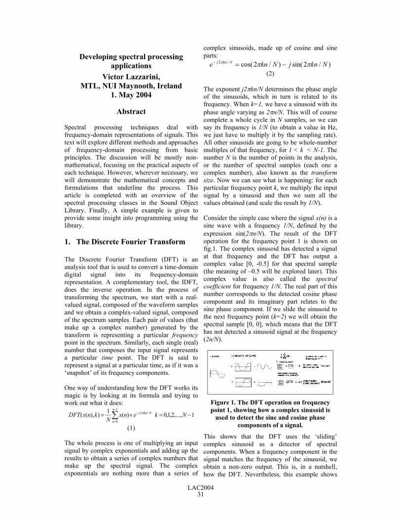
Consider the simple case where the signal x(n) is asine wave with a frequency 1/N, defined by theexpression sin(2πn/N). The result of the DFToperation for the frequency point 1 is shown onfig.1. The complex sinusoid has detected a signalat that frequency and the DFT has output acomplex value [0, -0.5] for that spectral sample(the meaning of –0.5 will be explored later). Thiscomplex value is also called the spectralcoefficient for frequency 1/N. The real part of thisnumber corresponds to the detected cosine phasecomponent and its imaginary part relates to thesine phase component. If we slide the sinusoid tothe next frequency point (k=2) we will obtain thespectral sample [0, 0], which means that the DFThas not detected a sinusoid signal at the frequency(2n/N).

Figure 1. The DFT operation on frequencypoint 1, showing how a complex sinusoid is

used to detect the sine and cosine phasecomponents of a signal.

This shows that the DFT uses the ‘sliding’complex sinusoid as a detector of spectralcomponents. When a frequency component in thesignal matches the frequency of the sinusoid, weobtain a non-zero output. This is, in a nutshell,how the DFT. Nevertheless, this example shows

LAC200431

only the simplest analysis case. In any case, thefrequency 1/N is a special one, known as thefundamental frequency of analysis. As mentionedabove, the DFT will analyse a signal as composedof sinusoids at multiples of this frequency.

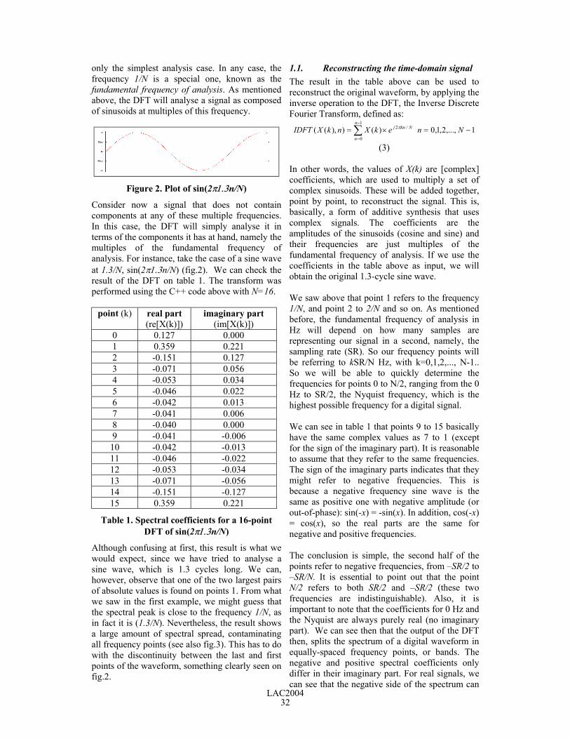
Figure 2. Plot of sin(2π1.3n/N)

Consider now a signal that does not containcomponents at any of these multiple frequencies.In this case, the DFT will simply analyse it interms of the components it has at hand, namely themultiples of the fundamental frequency ofanalysis. For instance, take the case of a sine waveat 1.3/N, sin(2π1.3n/N) (fig.2). We can check theresult of the DFT on table 1. The transform wasperformed using the C++ code above with N=16.

point (k) real part(re[X(k)])

imaginary part(im[X(k)])

0 0.127 0.0001 0.359 0.2212 -0.151 0.1273 -0.071 0.0564 -0.053 0.0345 -0.046 0.0226 -0.042 0.0137 -0.041 0.0068 -0.040 0.0009 -0.041 -0.006

10 -0.042 -0.01311 -0.046 -0.02212 -0.053 -0.03413 -0.071 -0.05614 -0.151 -0.12715 0.359 0.221

Table 1. Spectral coefficients for a 16-pointDFT of sin(2π1.3n/N)

Although confusing at first, this result is what wewould expect, since we have tried to analyse asine wave, which is 1.3 cycles long. We can,however, observe that one of the two largest pairsof absolute values is found on points 1. From whatwe saw in the first example, we might guess thatthe spectral peak is close to the frequency 1/N, asin fact it is (1.3/N). Nevertheless, the result showsa large amount of spectral spread, contaminatingall frequency points (see also fig.3). This has to dowith the discontinuity between the last and firstpoints of the waveform, something clearly seen onfig.2.

1.1. Reconstructing the time-domain signalThe result in the table above can be used toreconstruct the original waveform, by applying theinverse operation to the DFT, the Inverse DiscreteFourier Transform, defined as:

∑−

=

−=×=1

0

/2 1,...,2,1,0 )()),((n

n

Nknj NnekXnkXIDFT π

(3)

In other words, the values of X(k) are [complex]coefficients, which are used to multiply a set ofcomplex sinusoids. These will be added together,point by point, to reconstruct the signal. This is,basically, a form of additive synthesis that usescomplex signals. The coefficients are theamplitudes of the sinusoids (cosine and sine) andtheir frequencies are just multiples of thefundamental frequency of analysis. If we use thecoefficients in the table above as input, we willobtain the original 1.3-cycle sine wave.

We saw above that point 1 refers to the frequency1/N, and point 2 to 2/N and so on. As mentionedbefore, the fundamental frequency of analysis inHz will depend on how many samples arerepresenting our signal in a second, namely, thesampling rate (SR). So our frequency points willbe referring to kSR/N Hz, with k=0,1,2,..., N-1..So we will be able to quickly determine thefrequencies for points 0 to N/2, ranging from the 0Hz to SR/2, the Nyquist frequency, which is thehighest possible frequency for a digital signal.

We can see in table 1 that points 9 to 15 basicallyhave the same complex values as 7 to 1 (exceptfor the sign of the imaginary part). It is reasonableto assume that they refer to the same frequencies.The sign of the imaginary parts indicates that theymight refer to negative frequencies. This isbecause a negative frequency sine wave is thesame as positive one with negative amplitude (orout-of-phase): sin(-x) = -sin(x). In addition, cos(-x)= cos(x), so the real parts are the same fornegative and positive frequencies.

The conclusion is simple, the second half of thepoints refer to negative frequencies, from –SR/2 to–SR/N. It is essential to point out that the pointN/2 refers to both SR/2 and –SR/2 (these twofrequencies are indistinguishable). Also, it isimportant to note that the coefficients for 0 Hz andthe Nyquist are always purely real (no imaginarypart). We can see then that the output of the DFTthen, splits the spectrum of a digital waveform inequally-spaced frequency points, or bands. Thenegative and positive spectral coefficients onlydiffer in their imaginary part. For real signals, wecan see that the negative side of the spectrum can

LAC200432

always be inferred from the positive side, so it is,in a way, redundant.

1.2. Rectangular and polar formatsIn order to understand further the informationprovided by the DFT, we can convert therepresentation of the complex coefficients, fromreal/imaginary pairs to one that is more useful tous. The amplitude of a component is given by themagnitude of each complex spectral coefficient.The magnitude (or modulus) of a complex numberz is:

22 ][][ zimzrez += (4)

As a real signal is always split into positive andnegative frequencies, the amplitude of a point willbe ½ the ‘true’ value. The values obtained by themagnitude conversion are know as the amplitudespectrum of a signal. The amplitude spectrum of areal signal is always mirrored at 0 Hz.

The other conversion that complements themagnitude provides the phase angle (or offset) ofthe coefficient, in relation to a cosine wave. Thisyields the phase offset of a particular component,and it is obtained by the following relationship:

][][arctan)(

zrezimz =θ (5)

The result of converting the DFT result in thisway is called the phase spectrum. For real signals,it is always anti-symmetrical around 0 Hz. Theprocess of obtaining the magnitude and phasespectrum of the DFT is called cartesian-to-polarconversion.

Figure 3. Magnitude spectrum from a 16-pointDFT of sin(2π1.3n/N).

We can see from fig.3 that the DFT results are notalways clear. In fact unless the signal has all itscomponents at multiples of the fundamentalfrequency of analysis, there will be a spectral

spread over all frequency points. In addition tothese problems, the DFT in the present form, as aone-shot, single-frame transform, will not be ableto track spectral changes. This is because it takes asingle ‘picture’ of the spectrum of a waveform at acertain time. For a more thorough view of theDFT theory, please refer to (Jaffe, 1987a) and(Oppenheimer and Schafer, 1975).

2. Applications of the DFT:Convolution

The single-frame DFT analysis as explored abovehas one important application, the convolution oftime-domain signals through spectralmultiplication. Before we proceed to explore thistechnique, it is important to note that the DFT isvery seldom implemented in the direct formshown above. More usually, we will findoptimised algorithms that will calculate the DFTmuch more efficiently. These are called the FastFourier Transform (FFT). Their result is in allaspects, equivalent to the DFT as described above.The only difference is in the way the calculation isperformed. Also, because the FFT is based onspecialised algorithms, they will only work with acertain number of points (N, the transform size).For instance, the standard FFT algorithm usesonly power-of-two (2,4,..., 512, 1024...) sizes.From now on, when we refer to the DFT, we willimply the use of a fast algorithm for itscomputation.

Convolution is an operation with signals, just likemultiplication or addition, defined as:

∑=

−=∗=n

mmnxmynxnynw

0)()()()()(

(6)

One important aspect of time-domain convolutionis that it is equivalent to the multiplication ofspectra (and vice-versa). In other words, if y(n)and h(n) are two waveforms whose fouriertransforms are Y(k) and H(k), then:

)()()]()([ )()()]()([

kHkYnhnyDFTkHkYnhnyDFT

∗==∗

(7)

This means that if the DFT is used to transformtwo signals into their spectral domain and the twospectra can be multiplied together, the result canbe transformed back to the time-domain as theconvolution of the two inputs. In this type ofoperation, we generally have an arbitrary soundthat is convoluted with a shorter signal, called the

LAC200433

impulse response. The latter can be thought of as amix of scaled and delayed unit sample functionsand also as the list of the gain values in a tappeddelay-line. The convolution operation will imposethe spectral characteristics of this impulse signalinto the other input signal. There are three basicapplications for this technique:

(1) Early reverberation: the impulse response is atrain of pulses, which can be obtained byrecording room reflections in reaction to ashort sound.

(2) Filtering: the impulse response is a series ofFIR filter coefficients. Its amplitude spectrumdetermines the shape of the filter.

(3) Cross-synthesis: the impulse response is anarbitrary sound, whose spectrum will bemultiplied with the other sound. Theircommon features will be emphasized and theoverall effect will be one of cross-synthesis.

Depending on the application, we might use atime-domain impulse response, whose transformis then used in the process. On other situations, wemight start with a particular spectrum, which isdirectly used in the process. The advantage of thisis that we can define the frequency-domaincharacteristics that we want to impose on the othersound.

2.1. A DFT-based convolution applicationWe can now look at the nuts and bolts of theapplication of the DFT in convolution. The firstthing to consider is that, since we are using realsignals, there is no reason to use a DFT thatoutputs both the positive and negative sides of thespectrum. We know that the negative side can beextracted from the positive, so we can use FFTalgorithms that are optimised for the real signals.The discussion of specific aspects of thesealgorithms is beyond the scope of this text, butwhenever we refer to the DFT, we will imply theuse of a real input transform.

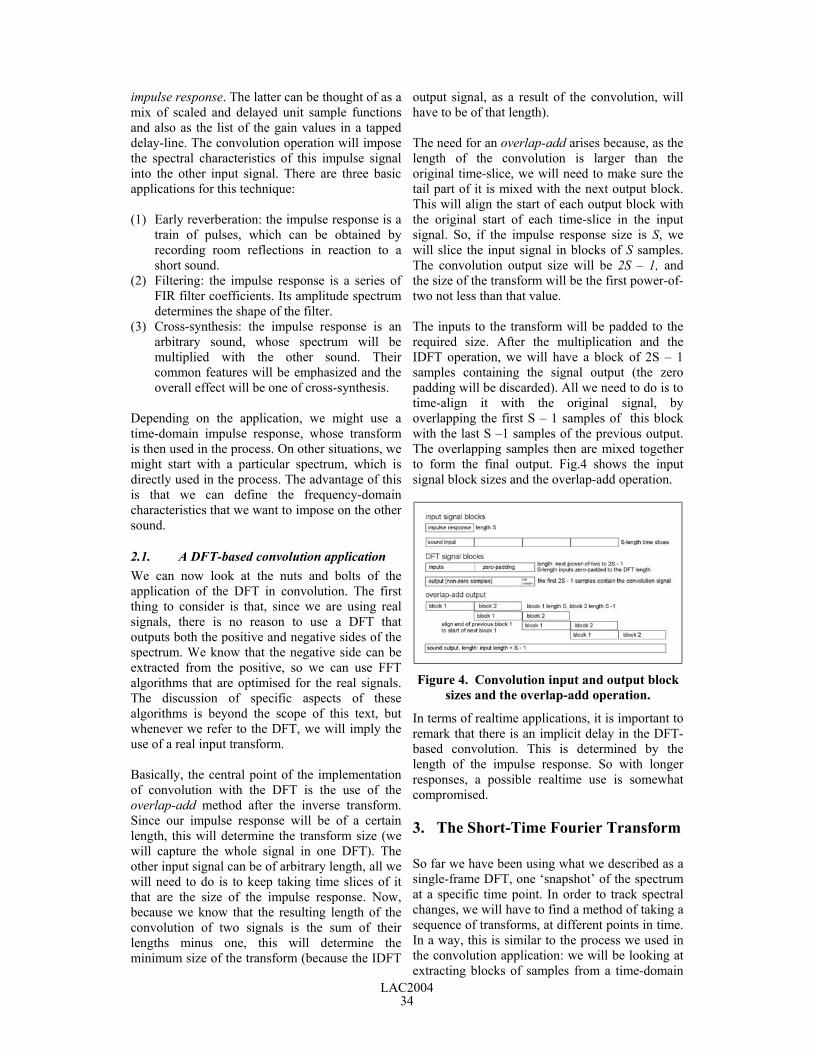
Basically, the central point of the implementationof convolution with the DFT is the use of theoverlap-add method after the inverse transform.Since our impulse response will be of a certainlength, this will determine the transform size (wewill capture the whole signal in one DFT). Theother input signal can be of arbitrary length, all wewill need to do is to keep taking time slices of itthat are the size of the impulse response. Now,because we know that the resulting length of theconvolution of two signals is the sum of theirlengths minus one, this will determine theminimum size of the transform (because the IDFT

output signal, as a result of the convolution, willhave to be of that length).

The need for an overlap-add arises because, as thelength of the convolution is larger than theoriginal time-slice, we will need to make sure thetail part of it is mixed with the next output block.This will align the start of each output block withthe original start of each time-slice in the inputsignal. So, if the impulse response size is S, wewill slice the input signal in blocks of S samples.The convolution output size will be 2S – 1, andthe size of the transform will be the first power-of-two not less than that value.

The inputs to the transform will be padded to therequired size. After the multiplication and theIDFT operation, we will have a block of 2S – 1samples containing the signal output (the zeropadding will be discarded). All we need to do is totime-align it with the original signal, byoverlapping the first S – 1 samples of this blockwith the last S –1 samples of the previous output.The overlapping samples then are mixed togetherto form the final output. Fig.4 shows the inputsignal block sizes and the overlap-add operation.

Figure 4. Convolution input and output blocksizes and the overlap-add operation.

In terms of realtime applications, it is important toremark that there is an implicit delay in the DFT-based convolution. This is determined by thelength of the impulse response. So with longerresponses, a possible realtime use is somewhatcompromised.

3. The Short-Time Fourier Transform

So far we have been using what we described as asingle-frame DFT, one ‘snapshot’ of the spectrumat a specific time point. In order to track spectralchanges, we will have to find a method of taking asequence of transforms, at different points in time.In a way, this is similar to the process we used inthe convolution application: we will be looking atextracting blocks of samples from a time-domain

LAC200434

signal and transform them with the DFT. This isknown as the Short-Time Fourier Transform. Theprocess of extracting the samples from a portionof the waveform is called windowing. In otherwords, we are applying a time window to thesignal, outside which all samples are ignored.

Figure 5. Rectangular window anddiscontinuities in the signal.

Time windows can have all sorts of shapes. Theone we used in the convolution example isequivalent to a rectangular window, where allwindow contents are multiplied by one. Thisshape is not very useful in STFT analysis, becauseit can create discontinuities at the edges of thewindow (fig.5). This is the case when the analysedsignal contains components that are not integermultiples of the fundamental frequency ofanalysis. These discontinuities are responsible foranalysis artifacts, such as the ones observed in theabove discussion of the DFT, which limit the itsusefulness.

Figure 6. Windowed signal, where the endstend towards 0.

Other shapes that tend towards 0 at the edges willbe preferred. As the ends of the analysed segmentmeet, they eliminate any discontinuity (fig.6).

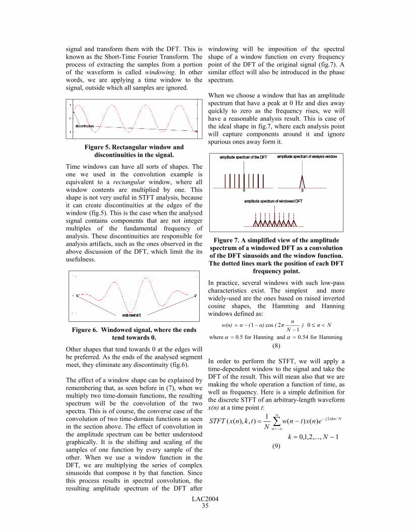
The effect of a window shape can be explained byremembering that, as seen before in (7), when wemultiply two time-domain functions, the resultingspectrum will be the convolution of the twospectra. This is of course, the converse case of theconvolution of two time-domain functions as seenin the section above. The effect of convolution inthe amplitude spectrum can be better understoodgraphically. It is the shifting and scaling of thesamples of one function by every sample of theother. When we use a window function in theDFT, we are multiplying the series of complexsinusoids that compose it by that function. Sincethis process results in spectral convolution, theresulting amplitude spectrum of the DFT after

windowing will be imposition of the spectralshape of a window function on every frequencypoint of the DFT of the original signal (fig.7). Asimilar effect will also be introduced in the phasespectrum.

When we choose a window that has an amplitudespectrum that have a peak at 0 Hz and dies awayquickly to zero as the frequency rises, we willhave a reasonable analysis result. This is case ofthe ideal shape in fig.7, where each analysis pointwill capture components around it and ignorespurious ones away form it.

Figure 7. A simplified view of the amplitudespectrum of a windowed DFT as a convolutionof the DFT sinusoids and the window function.The dotted lines mark the position of each DFT

frequency point.

In practice, several windows with such low-passcharacteristics exist. The simplest and morewidely-used are the ones based on raised invertedcosine shapes, the Hamming and Hanningwindows defined as:

Hammingfor .540 and Hanningfor 0.5 where

01

2cos1

==

<≤−

−−=

αα

Nn) N

nπ(α)(αw(n)

(8)

In order to perform the STFT, we will apply atime-dependent window to the signal and take theDFT of the result. This will mean also that we aremaking the whole operation a function of time, aswell as frequency. Here is a simple definition forthe discrete STFT of an arbitrary-length waveformx(n) at a time point t:

1,...,2,1,0

)()(1),),(( /2

−=

−= ∑∞

−∞=

−

Nk

enxtnwN

tknxSTFTn

Nknj π

(9)

LAC200435

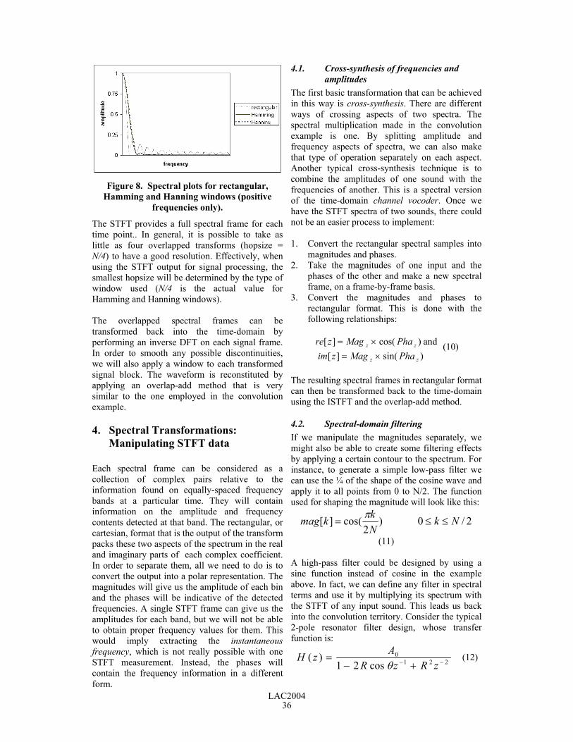
Figure 8. Spectral plots for rectangular,Hamming and Hanning windows (positive

frequencies only).

The STFT provides a full spectral frame for eachtime point.. In general, it is possible to take aslittle as four overlapped transforms (hopsize =N/4) to have a good resolution. Effectively, whenusing the STFT output for signal processing, thesmallest hopsize will be determined by the type ofwindow used (N/4 is the actual value forHamming and Hanning windows).

The overlapped spectral frames can betransformed back into the time-domain byperforming an inverse DFT on each signal frame.In order to smooth any possible discontinuities,we will also apply a window to each transformedsignal block. The waveform is reconstituted byapplying an overlap-add method that is verysimilar to the one employed in the convolutionexample.

4. Spectral Transformations:Manipulating STFT data

Each spectral frame can be considered as acollection of complex pairs relative to theinformation found on equally-spaced frequencybands at a particular time. They will containinformation on the amplitude and frequencycontents detected at that band. The rectangular, orcartesian, format that is the output of the transformpacks these two aspects of the spectrum in the realand imaginary parts of each complex coefficient.In order to separate them, all we need to do is toconvert the output into a polar representation. Themagnitudes will give us the amplitude of each binand the phases will be indicative of the detectedfrequencies. A single STFT frame can give us theamplitudes for each band, but we will not be ableto obtain proper frequency values for them. Thiswould imply extracting the instantaneousfrequency, which is not really possible with oneSTFT measurement. Instead, the phases willcontain the frequency information in a differentform.

4.1. Cross-synthesis of frequencies andamplitudes

The first basic transformation that can be achievedin this way is cross-synthesis. There are differentways of crossing aspects of two spectra. Thespectral multiplication made in the convolutionexample is one. By splitting amplitude andfrequency aspects of spectra, we can also makethat type of operation separately on each aspect.Another typical cross-synthesis technique is tocombine the amplitudes of one sound with thefrequencies of another. This is a spectral versionof the time-domain channel vocoder. Once wehave the STFT spectra of two sounds, there couldnot be an easier process to implement:

1. Convert the rectangular spectral samples intomagnitudes and phases.

2. Take the magnitudes of one input and thephases of the other and make a new spectralframe, on a frame-by-frame basis.

3. Convert the magnitudes and phases torectangular format. This is done with thefollowing relationships:

)sin(][ and )cos(][

zz

zz

PhaMagzimPhaMagzre

×=×= (10)

The resulting spectral frames in rectangular formatcan then be transformed back to the time-domainusing the ISTFT and the overlap-add method.

4.2. Spectral-domain filteringIf we manipulate the magnitudes separately, wemight also be able to create some filtering effectsby applying a certain contour to the spectrum. Forinstance, to generate a simple low-pass filter wecan use the ¼ of the shape of the cosine wave andapply it to all points from 0 to N/2. The functionused for shaping the magnitude will look like this:

2/0 )2

cos(][ NkNkkmag ≤≤=

π

(11)

A high-pass filter could be designed by using asine function instead of cosine in the exampleabove. In fact, we can define any filter in spectralterms and use it by multiplying its spectrum withthe STFT of any input sound. This leads us backinto the convolution territory. Consider the typical2-pole resonator filter design, whose transferfunction is:

2210

cos21)( −− +−

=zRzR

AzHθ

(12)

LAC200436

Here, θ is the pole angle and R its radius (ormagnitude), parameters that are related to the filtercentre frequency and bandwidth, respectively. Thescaling constant A0 is used to scale the filteroutput so that it does not run wildly out-of-range.Now if we evaluate this function for evenly-spaced frequency points z = e j2πk/N, we will revealthe discrete spectrum of that filter. All we need todo is to do a complex multiplication of the resultwith the STFT of an input sound.

The mathematical steps used to obtain thespectrum of the filter are based on Euler’srelationship, which splits the complex sinusoidal ejω into its real and imaginary parts, cos(ω) andjsin(ω). Once we obtained the spectral points inthe rectangular form A0(a + ib)-1, all we need is tomultiply them with the STFT points of the originalsignal. This will in reality turn out to be a complexdivision:

lyrespective output, andfilter signal,input theof spectra theare and , where

]][[]][[]][[]][[

]])[[]][[(]])[[]][[(][

10

0

10

Y[k]F[k]AX[k]

kFimkFrekXimkXreA

kFimkFreAkXimkXrekY

-

++

=

=+×+=

=−

(13)

There are many more processes that can bedevised for transforming the output of the STFT.The examples given here are only the start. Theyrepresent some classic approaches, but severalother, more radical techniques can be explored.

5. Tracking the Frequency: the PhaseVocoder.

As we observed, although we can manipulate thefrequency content of spectra, through their phases,the STFT does not have enough resolution to tellus what frequencies are present in a sound. Wewill have to find a way of tracking theinstantaneous frequencies in each spectral band. Awell-known technique known as the PhaseVocoder (PV) (Flanagan and Golden, 1966) canbe employed to do just that.

The STFT followed by a polar conversion can alsobe seen as a bank of parallel filters. Its output iscomposed of the values for the magnitudes andphases at every time-point or hop period for eachbin. The first step in transforming the STFT into aPhase Vocoder is to generate values that areproportional to the frequencies present in a sound.This is done ideally by the taking the timederivative of the phase, but we can approximate itby computing the difference between the phase

value of consecutive frames, for each spectralband. This simple operation, although not yieldingthe right value for the frequency at a spectralband, will output one that is proportional to it.

By keeping track of the phase differences, we cantime-stretch or compress a sound, without alteringits frequency content (in other words, its pitch).We can perform this by repeating or skippingspectral blocks, to stretch or compress the data.Because we are keeping the phase differencesbetween the frames, when we accumulate thembefore resynthesis, we will reconstruct the signalback with the correct original phase values. Weare keeping the same hop period between frames,but because we use the phase difference tocalculate the next phase value, the phases will bekept intact, regardless of the frame readout speed.

One small programming point needs to be made inrelation to the phase calculation. The inversetangent function outputs the phase in the range of–π to π. When the phase differences arecalculated, they might exceed this range. In thiscase, we have to bring them down to the expectedinterval (known as principal values). This processis sometimes called phase unwrapping.

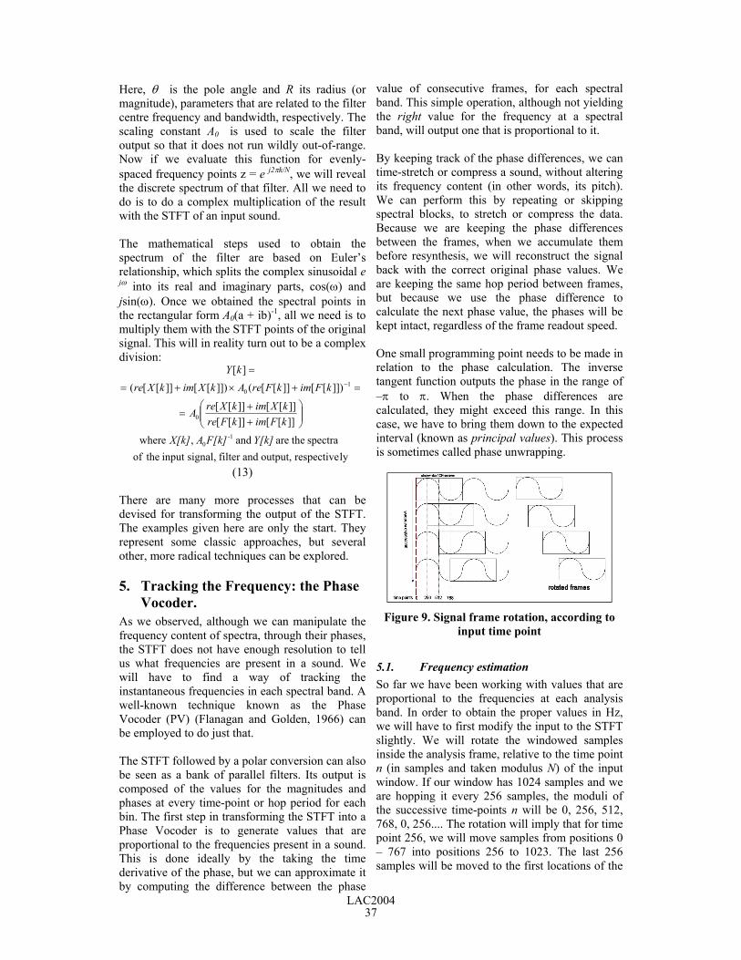
Figure 9. Signal frame rotation, according toinput time point

5.1. Frequency estimationSo far we have been working with values that areproportional to the frequencies at each analysisband. In order to obtain the proper values in Hz,we will have to first modify the input to the STFTslightly. We will rotate the windowed samplesinside the analysis frame, relative to the time pointn (in samples and taken modulus N) of the inputwindow. If our window has 1024 samples and weare hopping it every 256 samples, the moduli ofthe successive time-points n will be 0, 256, 512,768, 0, 256.... The rotation will imply that for timepoint 256, we will move samples from positions 0– 767 into positions 256 to 1023. The last 256samples will be moved to the first locations of the

LAC200437

block. A similar process is applied to the othertime points (fig. 9).

The mathematical reasons for this input rotationare somewhat complex, but the graphicrepresentation shown on fig. 9 goes some way onhelping us understand the process intuitively. Aswe can see the rotation process has the effect ofaligning the phase of the signal in successiveframes. This will help us obtain the rightfrequency values, but we will better understand itafter seeing the rest of the process. In fact, theinput rotation renders the STFT formulationmathematically correct, as we have been using anon-rigorous and simpler approach (which so farhas worked for us).

After the rotation, we can take the DFT of theframe as usual and convert the result into polarform. The phase differences for each band are thencalculated. This now tells us how much eachdetected frequency deviates from the centrefrequency of its analysis band. The centrefrequencies are basically the DFT analysisfrequencies 2πk/N, in radians. So, to obtain theproper detected frequency value, we only needadd the phase differences to the centre frequencyfor each analysis band, scaled by the hopsize. Thevalues in Hz can be obtained by multiplying theresult, which is given in radians per hopsizesamples, by SR/[2π x hopsize] (SR is, of course,the sampling rate in samples/sec).

Here is a summary of the steps involved in phasevocoder analysis:1. Extract N samples from a signal and apply an

analysis window. Rotate the samples in thesignal frame according to input time n mod N.

2. Take the DFT of the signal.3. Convert rectangular coefficients to polar

format.4. Compute the phase difference and bring the

value to the -π to +π range.5. Add the difference values to 2πkD/N, and

multiply the result by SR/2πD, where D is thehopsize in samples. For each spectral band,this result yields its frequency in Hz, and themagnitude value, its peak amplitude.

5.2. Phase vocoder resynthesisPhase Vocoder data can be resynthesised using avariety of methods. Since we have blocks ofamplitude and frequency data, we can use somesort of additive synthesis to playback the spectralframes. However, a more efficient way ofconverting to time-domain data for arbitrarysounds with many components is to use an

overlap-add method similar to the one in theISTFT. All we need to do is retrace the steps takenin the forward transformation:

1. Convert the frequencies back to phasedifferences in radians per I samples bysubtracting them from the centre frequenciesof each channel, in Hz, kSR/N, andmultiplying the result by 2πI/SR, where I isthe synthesis hopsize.

2. Accumulate them to compute the currentphase values.

3. Perform a polar to rectangular conversion.4. Take the IDFT of the signal frame.5. Unrotate the samples and apply a window to

the resulting sample block.6. Overlap-add consecutive frames.

As a word of caution, it is important to point outthat all DFT-based algorithms will have somelimits in terms of partial tracking. The analysiswill be able to resolve a maximum of onesinusoidal component per frequency band. If twoor more partials fall within one band, the phasevocoder will fail to output the right values for theamplitudes and frequencies of each of them.Instead, we will have an amplitude-modulatedcomposite output, in many ways similar to beatfrequencies. In addition, because the DFT splitsthe spectrum in equal-sized bands, this problemwill mostly affect lower frequencies, where bandsare perceptually larger. However, we can say thatin general, the phase vocoder is a powerful toolfor transformation of arbitrary signals.

5.3. Spectral morphingA typical transformation of PV data is spectralinterpolation, or morphing. It is a more generalversion of the spectral cross-synthesis examplediscussed before. Here, we interpolate between thefrequencies and amplitudes of two spectra, on aframe-by-frame basis.

Spectral morphing can produce very interestingresults. However, its effectiveness depends verymuch on the spectral qualities of the two inputsounds. When the spectral data does not overlapmuch, interpolating will sound more or less likecross-fading, which can be achieved in the time-domain for much less trouble. There are manymore transformations that can be devised formodifying PV data. In fact, any numbermanipulation procedure that generates a spectralframe in the right format can be seen as a validspectral process. Whether it will produce amusically useful output is another question.Understanding how the spectral data is generated

LAC200438

in analysis is the first step in designingtransformations that work.

For a more detailed look into the theory of thePhase Vocoder, please refer to the JamesFlanagan’s original article on the technique. Otherdescriptions of the technique are also found in(Dolson, 1986) and (Moore, 1990).

6. The Instantaneous FrequencyDistribution

An alternative method of frequency estimation isgiven by the instantaneous frequency distribution(IFD) algorithm proposed by Toshihiko Abe (Abeet al, 1997). It uses some of the principles alreadyseen in the phase vocoder, but its mathematicalformulation is more complex. The basic idea,which is also present in the PV algorithm, is thatthe frequency, or more precisely, theinstantaneous frequency detected at a certain bandis the time derivative of the phase. Using Euler’srelationship, we can define the output of the STFTin polar form. This is shown below, using ω =2πk/N:

),(),(),),(( tjetRtknxSTFT ωθω ×= (14)

The phase detected by band k at time-point t isθ(2πkn/N, t) and the magnitude is R(2πkn/N, t).The Instantaneous Frequency Distribution of x(n)at time t is then the time derivative of the STFTphase output:

),(),),(( tt

tknxIFD ωθ∂∂

= (15)

This can be intuitively understood as themeasurement of the rate of rotation of the phaseof a sinusoidal signal. In the phase vocoder, weestimated it by crudely taking the differencebetween phase values in successive frames. TheIFD actually calculates the time derivative of thephase directly, from data corresponding to a singletime-point:

+=)),(()),('(

),),((kmxDFTkmxDFT

imagtknxIFDt

tω

(16)

The mathematical steps involved in the derivationof the IFD are quite involved. However, if wewant to implement the IFD, all we need is toemploy its definition in terms of DFTs, as given

above. We can use the straight DFT of awindowed frame to obtain the amplitudes and usethe IFD to estimate the frequencies. Also, becausewe are using the straight transform of a windowedsignal, there is no need to rotate the input, as inthe phase vocoder. If we look back at the DFT asdefined in (19), we see that it, in fact, does notinclude the multiplication by a complexexponential (as does the STFT). Finally, thederivative of the analysis window is generated bycomputing the differences between its consecutivesamples..

7. Tracking spectral components:Sinusoidal Modelling

Sinusoidal modelling techniques are based on theprinciples that we have held all along as thebackground to what we have done so far: thattime-domain signals are composed of the sum ofsinusoidal waves of different amplitudes,frequencies and phases. The number of sinusoidalcomponents present in the spectrum will varyfrom sound to sound, and also can varydynamically during the evolution of a singlesound. As we have pointed out before, since weare still using STFT-based spectral analysis, at anypoint in time, the maximum resolution ofcomponents will depend on the size of eachanalysis band. Partial tracking will, therefore, notbe suitable for spectrally dense sounds. However,there will be many musical signals that can bemanipulated through this method.

7.1. Sinusoidal AnalysisThe principle behind sinusoidal analysis is verysimple, although its implementation is somewhatinvolved. Using the magnitudes from STFTanalysis, we will identify the spectral peaks at theintegral frequency points (STFT bins or bands).The identified peaks will have to be above acertain threshold, which will help separate thedetected sinusoid components from transientspectral features. The exact peak position andamplitude can be estimated by using aninterpolation procedure based on the magnitudesof the bins around the peaks. With the interpolatedbin positions we can then find the exact values forthe frequencies and phases obtained originallyfrom the IFD/STFT input, again throughinterpolation. These will then, together with theamplitude, form a ‘track', linked to each detectedpeak (fig. 11). However the track will only exist assuch if there is some consistency in consecutiveframes, ie. if there is some matching betweenpeaks found at each time-point. When peaks areshort-lived, they will not make a track.

LAC200439

Conversely, when a peak disappears, we will haveto wait a few frames to declare the track asfinished. So most of the process becomes one oftrack management, which accounts for the moreinvolved aspects of the algorithm.

As seen in fig.10, the sinusoidal analysis willoutput tracks made up of frequencies, amplitudesand phases. This in turn can be used for additivere-synthesis of the signal or of portions of itsspectrum. One typical method involves the use ofthe phase and frequency parameters to calculatethe varying phase used to drive an oscillator. Thisuses the two parameters in a cubic interpolation,which is not only mathematically involved, butalso computationally intensive. A simpler versioncan be formulated that would employ only thefrequency and amplitudes interpolated linearly.This is simpler, more efficient and for manyapplications sufficiently precise. Also, since we donot require the phase parameter, we can simplifythe analysis algorithm to calculate onlyfrequencies and amplitudes for each track. Thisversion could employ either the IFD (as shown infig.12) or the Phase Vocoder, as discussed in theprevious sections, to provide the magnitude andfrequency inputs.

Figure 10. Sinusoidal analysis and trackgeneration from a time-domain signal x(n).

7.2. Additive resynthesisThe additive resynthesis procedure will take thetrack frames and use a frame-by-frameinterpolation of the amplitudes and frequencies ofeach track to drive a bank of sinewave oscillators(fig.12). We will only need to be careful aboutusing the track IDs to perform the interpolationbetween the frames. Also, when a track iscreated/destroyed, we will create an amplitudeonset/decay so that we do not have discontinuitiesin the output signal. We will be usinginterpolating lookup oscillators, with a table sizeof 1024 points to generate the signal for eachtrack. Each sine wave component will be thenmixed into the output.

Figure 11. The additive synthesis process.

The main point about this type of analysis is that itis designed to track the sinusoidal components ofa signal. Some sounds will be more suitable forthis analysis than others. Distributed spectra willnot be tracked very effectively, since itscomplexity will not suit the process. However, forcertain sounds with both sinusoidal content andsome more noise-like/transient elements, we couldin theory obtain these ‘residual’ aspects of thesound by subtracting the resynthesised sound fromthe original. That way, we would be able toseparate these two elements and perhaps processthem individually. A more precise method ofresynthesis, using the original phases is requiredfor the residual extraction to work. This idea isdeveloped in the Spectral Modelling Synthesis(SMS) technique (Serra, 1997).

8. Spectral processing with the SoundObject Library

The Sound Object (SndObj) library (Lazzarini,2000) is a multi-platform music and audioprocessing C++ class library. Its 100-plus classesfeature support for the most important time andfrequency-domain processing algorithms, as wellas basic soundfile, audio and MIDI IO services.The library is available for Linux, Irix, OS X andWindows; its core classes are fully portable to anysystem with ANSI C/C++ compilers.

The spectral processing suite of classes of theSndObj version 2.5.1 include the following:

(a) Analysis/Resynthesis:FFT STFT analysisIFFT ISTFT resynthesisPVA Phase Vocoder AnalysisPVS Phase Vocoder SynthesisIFGram IFD + Amps (and phases) analysis

LAC200440

SinAnal Sinusoidal track analysisSinSyn Sinusoidal synthesis (cubic interpolation)AdSyn Sinusoidal synthesis (linear interpolation)Convol FFT-based convolution

(b) Spectral ModificationsPVMorph PV data interpolationSpecMult spectral productSpecCart polar-rectangular conversionSpecSplit/SpecCombine split/combine amps & phasesSpecInterp spectral interpolationSpecPolar rectangular-polar conversionSpecThresh thresholdingSpecVoc cross-synthesis

(c) Input/OutputPVRead variable-rate PVOCEX file readoutSpecIn spectral inputSndPVOCEX PVOCEX file IOSndSinI0 sinusoidal analysis file IO

In addition, the library provides a developmentframework for the addition of further processes.The processing capabilities can be fully extendedby user-defined classes.

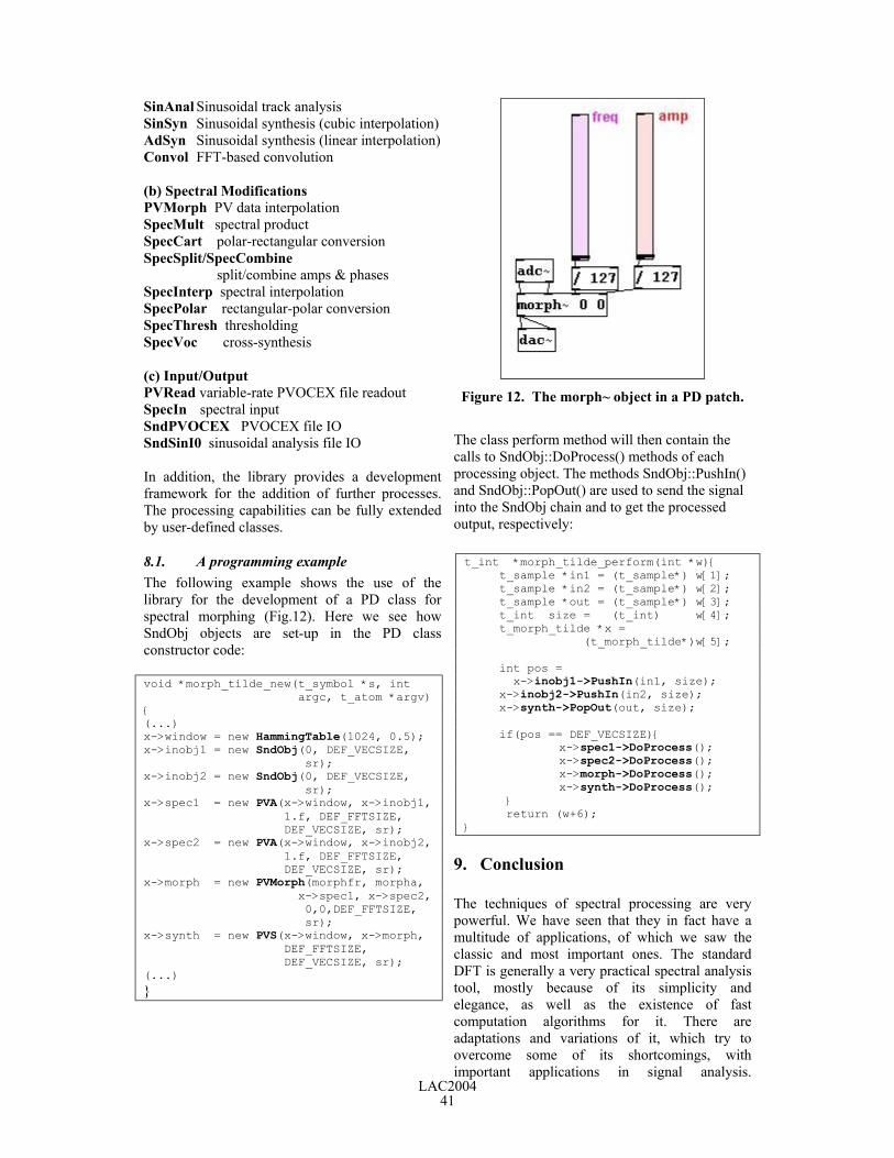
8.1. A programming exampleThe following example shows the use of thelibrary for the development of a PD class forspectral morphing (Fig.12). Here we see howSndObj objects are set-up in the PD classconstructor code:

void *morph_tilde_new(t_symbol *s, int argc, t_atom *argv){(...)x->window = new HammingTable(1024, 0.5);x->inobj1 = new SndObj(0, DEF_VECSIZE, sr);x->inobj2 = new SndObj(0, DEF_VECSIZE, sr);x->spec1 = new PVA(x->window, x->inobj1, 1.f, DEF_FFTSIZE, DEF_VECSIZE, sr);x->spec2 = new PVA(x->window, x->inobj2, 1.f, DEF_FFTSIZE, DEF_VECSIZE, sr);x->morph = new PVMorph(morphfr, morpha, x->spec1, x->spec2, 0,0,DEF_FFTSIZE, sr);x->synth = new PVS(x->window, x->morph, DEF_FFTSIZE, DEF_VECSIZE, sr);(...)}

Figure 12. The morph~ object in a PD patch.

The class perform method will then contain thecalls to SndObj::DoProcess() methods of eachprocessing object. The methods SndObj::PushIn()and SndObj::PopOut() are used to send the signalinto the SndObj chain and to get the processedoutput, respectively:

t_int *morph_tilde_perform(int *w){ t_sample *in1 = (t_sample*) w[1]; t_sample *in2 = (t_sample*) w[2]; t_sample *out = (t_sample*) w[3]; t_int size = (t_int) w[4]; t_morph_tilde *x = (t_morph_tilde*)w[5];

int pos = x->inobj1->PushIn(in1, size); x->inobj2->PushIn(in2, size); x->synth->PopOut(out, size);

if(pos == DEF_VECSIZE){x->spec1->DoProcess();x->spec2->DoProcess();

x->morph->DoProcess();x->synth->DoProcess();

} return (w+6);}

9. Conclusion

The techniques of spectral processing are verypowerful. We have seen that they in fact have amultitude of applications, of which we saw theclassic and most important ones. The standardDFT is generally a very practical spectral analysistool, mostly because of its simplicity andelegance, as well as the existence of fastcomputation algorithms for it. There areadaptations and variations of it, which try toovercome some of its shortcomings, withimportant applications in signal analysis.

LAC200441

Nevertheless their use in sound processing andtransformation is still somewhat limited. Inaddition to Fourier-based processes, which haveso far been the most practical and useful ones toimplement, there are other methods of spectralanalysis. The most important of these is theWavelet Transform (Meyer, 1991), which so farhas had limited use in audio signal processing.

10. Bibliography

Abe T, et al (1997). “The IF spectrogram: a newspectral representation,” Proc. ASVA 97: 423-430.Dolson, M (1986). “The Phase Vocoder Tutorial”.Computer Music Journal, 10(4): 14-27. MITPress, Cambridge, Mass.Flanagan, JL, Golden RM (1966). “PhaseVocoder”. Bell System Technical Journal 45:1493-1509.Jaffe, D (1987a). “Spectrum Analysis Tutorial,Part 1: The Discrete Fourier Transform”.Computer Music Journal, 11(2): 9-24. MIT Press,Cambridge, Mass.Jaffe, D (1987b). “Spectrum Analysis Tutorial,Part 2: Properties and Applications of the DiscreteFourier Transform”. Computer Music Journal,11(2): 17-35. MIT Press, Cambridge, Mass.Lazzarini, V (2000). “The Sound Object Library”.Organised Sound 5 (1). Cambridge UniversityPress, Cambridge.McCaulay, RJ, Quatieri, TF (1986). “SpeechAnalysis/Synthesis Based on a SinusoidalRepresentation”. IEEE Trans. On Acoustics,Speech, and Signal Processing, ASSP-34 (4).Meyer, Y (ed.)(1991). Wavelets and applications.Springer-Verlag, Berlin,1991Moore, FR (1990). Elements of Computer Music.Prentice-Hall, Englewood Cliffs, N.J.Openheim, AV, Schafer, RW (1975). DigitalSignal Processing. Prentice Hall, EnglewoodCliffs, N.J.Serra, X. (1997). “Musical Sound Modelling withSinusoids plus Noise”. in: G.D. Poli et al (eds.),Musical Signal Processing, Swets & ZeitlingerPublishers, AmsterdamSteiglitz, K (1995). A Signal Processing Primer.Addison-Wesley Publ., Menlo Park, Ca.

LAC200442