jabuti – java bytecode understanding and testing
TRANSCRIPT
UNIVERSIDADE DE SAO PAULOINSTITUTO DE CIENCIAS MATEMATICAS E DE COMPUTACAO
DEPARTAMENTO DE CIENCIAS DE COMPUTACAO E ESTATISTICA
Caixa Postal 668 – CEP 13560-970 – Sao Carlos, SP – Fone (16) 273-9655 – Fax (16) 273-9751
http://www.icmc.usp.br
JaBUTi – Java BytecodeUnderstanding and Testing
User’s Guide
Version 1.0 – Java
A. M. R. Vincenzi†, W. E. Wong§, M. E. Delamaro‡ and J. C. Maldonado†
†Instituto de Ciencias Matematicas e de ComputacaoUniversidade de Sao Paulo
Sao Carlos, Sao Paulo, Brazil{auri, adenilso, jcmaldon}@icmc.usp.br
§Department of Computer ScienceUniversity of Texas at Dallas
Richardson, Texas, [email protected]
‡Faculdade de InformaticaCentro Universitario Eurıpides de Marılia
Marılia, Sao Paulo, [email protected]
Sao Carlos, SP, BrazilMarch, 2003

Contents
Abstract ii
1 Introduction 1
2 Background 12.1 Java Bytecode . . . . . . . . . . . . . . . . . . . . . . . . . . . . . . . . . . . . . . . . 12.2 Dependence Analysis for Java Bytecode . . . . . . . . . . . . . . . . . . . . . . . . . . 2
2.2.1 Constructing the Instruction Graph . . . . . . . . . . . . . . . . . . . . . . . . 32.2.2 Augmenting the IG: Data-Flow IG . . . . . . . . . . . . . . . . . . . . . . . . 62.2.3 Constructing Data-Flow Block Graph (BG) . . . . . . . . . . . . . . . . . . . . 10
2.3 Intra-method Structural Testing Requirements . . . . . . . . . . . . . . . . . . . . . . 132.3.1 Control-Flow Testing Requirements . . . . . . . . . . . . . . . . . . . . . . . . 132.3.2 Complexity Analysis of Control-Flow Testing Criteria . . . . . . . . . . . . . . 142.3.3 Data-Flow Testing Requirements . . . . . . . . . . . . . . . . . . . . . . . . . . 142.3.4 Complexity Analysis of Data-Flow Testing Criteria . . . . . . . . . . . . . . . . 15
2.4 Dominators and Super-Block Analysis . . . . . . . . . . . . . . . . . . . . . . . . . . . 152.5 Program Slicing . . . . . . . . . . . . . . . . . . . . . . . . . . . . . . . . . . . . . . . . 182.6 Complexity Metrics . . . . . . . . . . . . . . . . . . . . . . . . . . . . . . . . . . . . . . 19
3 The Vending Machine Example 19
4 JaBUTi Functionality and Graphical Interface 22
5 How to Create a Testing Project 24
6 How to use JaBUTi as a Coverage Analysis Tool 276.1 How the testing requirements are highlighted . . . . . . . . . . . . . . . . . . . . . . . 296.2 How to generate testing reports . . . . . . . . . . . . . . . . . . . . . . . . . . . . . . . 336.3 How to generate an HTML version of a JaBUTi report . . . . . . . . . . . . . . . . . . 376.4 How to include a test case . . . . . . . . . . . . . . . . . . . . . . . . . . . . . . . . . . 396.5 How to import test cases from JUnit framework . . . . . . . . . . . . . . . . . . . . . . 436.6 How to mark a testing requirement as infeasible . . . . . . . . . . . . . . . . . . . . . . 47
7 How to use JaBUTi as a Slicing Tool 49
8 How to use the JaBUTi’s Static Metrics Tool 518.1 LK’s Metrics Applied to Classes . . . . . . . . . . . . . . . . . . . . . . . . . . . . . . 51
8.1.1 NPIM – Number of public instance methods in a class . . . . . . . . . . . . . . 518.1.2 NIV – Number of instance variables in a class . . . . . . . . . . . . . . . . . . . 518.1.3 NCM – Number of class methods in a class . . . . . . . . . . . . . . . . . . . . 518.1.4 NCV – Number of class variables in a class . . . . . . . . . . . . . . . . . . . . 518.1.5 ANPM – Average number of parameters per method . . . . . . . . . . . . . . . 518.1.6 AMZ – Average method size . . . . . . . . . . . . . . . . . . . . . . . . . . . . 518.1.7 UMI – Use of multiple inheritance . . . . . . . . . . . . . . . . . . . . . . . . . 518.1.8 NMOS – Number of methods overridden by a subclass . . . . . . . . . . . . . . 518.1.9 NMIS – Number of methods inherited by a subclass . . . . . . . . . . . . . . . 528.1.10 NMAS – Number of methods added by a subclass . . . . . . . . . . . . . . . . 528.1.11 SI – Specialization index . . . . . . . . . . . . . . . . . . . . . . . . . . . . . . . 52
8.2 CK’s Metrics Applied to Classes . . . . . . . . . . . . . . . . . . . . . . . . . . . . . . 528.2.1 NOC – Number of Children . . . . . . . . . . . . . . . . . . . . . . . . . . . . . 528.2.2 DIT – Depth of Inheritance Tree . . . . . . . . . . . . . . . . . . . . . . . . . . 528.2.3 WMC – Weighted Methods per Class . . . . . . . . . . . . . . . . . . . . . . . 52
i

8.2.4 LCOM – Lack of Cohesion in Methods . . . . . . . . . . . . . . . . . . . . . . . 538.2.5 RFC – Response for a Class . . . . . . . . . . . . . . . . . . . . . . . . . . . . . 538.2.6 CBO – Coupling Between Object . . . . . . . . . . . . . . . . . . . . . . . . . . 53
8.3 Another Metrics Applied to Methods . . . . . . . . . . . . . . . . . . . . . . . . . . . . 538.3.1 CC – Cyclomatic Complexity Metric . . . . . . . . . . . . . . . . . . . . . . . . 53
8.4 The Static Metrics GUI . . . . . . . . . . . . . . . . . . . . . . . . . . . . . . . . . . . 54
9 JaBUTi em dispositivos moveis 56
10 JaBUTi Evolution 60
References 62
ii

Abstract
This report describes the main functionalities of JaBUTi (Java Bytecode Understandingand Testing) toolsuite. JaBUTi is designed to work with Java bytecode such that no sourcecode is required to perform its activities. It is composed by a coverage analysis tool, by aslicing tool, and by a complexity metric’s measure tool. The coverage tool can be used toassess the quality of a given test set or to generate test set based on different control-flowand data-flow testing criteria. The slicing tool can be used to identify fault-prone regions inthe code, being useful for debugging and also for program understanding. The complexitymetric’s measure tool can be used to identify the complexity and the size of each classunder testing, based on static information. A simple example that simulates the behaviorof a vending machine is used to illustrate such tools.
iii
1 Introduction
JaBUTi is a set of tools designed for understanding and testing of Java programs. The main advantage
of JaBUTi is that it does not require the Java source code to perform its activities. Such a characteristic
allows, for instance, to use the tool for testing Java-based components.
This report describes the functionalities of JaBUTi – Version 1.0 and how the tester can use it to
create testing projects through its graphical interface. Although JaBUTi can be run using scripts, in
this report this aspect is not addressed. To illustrate the operational aspects of JaBUTi, through its
graphical interface, we are using a simple example, adapted from Orso et al. [15], that simulates the
behavior of a vending machine.
The rest of this report is organized as follows. Section 2 presents some background information
about Java bytecode and a detailed description about the underlying models used by JaBUTi to derive
intra-method testing requirements. A brief description of program slicing and complexity metrics
are also presented in Section 2. Section 3 describes the example that we will use to illustrate the
functionalities of JaBUTi. Section 5 describes how to create a testing project. Section 6 illustrates
how to use JaBUTi as a coverage analysis testing tool for Java programs/components. Section 7 shows
how to use JaBUTi functionalities to localize faults. In Section 8 describes the set of static metrics
implemented in JaBUTi. Finally, in Section 10, we present the perspectives for JaBUTi evolution.
2 Background
In this section we give an overview on Java bytecode, a brief overview on dependence analysis, including
control-flow and data-flow testing criteria, and also a brief overview on program slicing and on static
metrics. In case of Java bytecode, the interested reader can consult [11] for a complete reference about
the JVM specification, as well as, the bytecode instruction set. Considering dependence analysis on
Java bytecode, the interested reader can refer to [34]. More details on control-flow and data-flow
testing criteria can be found in [19, 22]. A good survey on program slicing can be found in [23]. The
static metrics implemented in JaBUTi can be found elsewhere [12, 4].
2.1 Java Bytecode
One of the main reasons why Java has become so popular is the platform independence provided by
its runtime environment, the Java Virtual Machine (JVM). The so called class file is a portable binary
representation that contains class related data such as the class name, its superclass name, information
about the variables and constants and the bytecode instructions of each method.
Bytecode instructions can be seen as an assembly-like language that retains high-level information
about the program. A bytecode instruction is represented by a one-byte opcode followed by operand
values, if any. Each one-byte opcode has a mnemonic that is more meaningful than the opcode itself.
The instructions are typed and a letter preceding the mnemonic name represents the data type handled
by each instruction explicitly. The convention is to use the letter i for integer, l for long, s for short,
b for byte, c for char, f for float, d for double, and a for reference (objects and arrays). For example,
the instruction that pushes a one-byte integer value onto the top of the JVM operand stack has the
1

opcode 16, mnemonic bipush, and requires one operand (the one-byte integer value). The instruction
bipush 9 pushes the value 9 onto the top of the JVM operand stack.
The JVM has a stack frame on which a frame is inserted for every method invocation. Such a
frame is composed by a local variable vector, which contains all the local variables used in the current
method, and by an operand stack to perform the execution of the bytecode instructions. For instance,
considering the statement “a = b + c”, part of the local variable vector and part of the operand stack
required to execute such a statement are illustrated in Figure 1.
Slot Variable
· · · · · ·
2 a
3 b
4 c
· · · · · ·
(a) Local Variable Vector
Bytecode Instruction Operand Stack
12: iload 3 Value of b· · ·
13: iload 4 Value of cValue of b· · ·
14: iadd Value of b + c· · ·
15: istore 2 · · ·
(b) Operand Stack Simulation
Figure 1: Simple bytecode instruction execution.
Considering our example, variables a, b and c correspond to local variables 2, 3 and 4, respectively.
The bytecode instructions iload 3 and iload 4 load the value of b and c onto the top of the operand
stack. The instruction iadd pops two operands from the stack, executes the additions of such operands,
and pushes back the result onto the top of the stack. Finally, the instruction istore 2 pops the result
from the top of the stack, storing it into local variable 2 (variable a).
The complete set of bytecode instructions, illustrated in Table 1 is composed by 204 instruction.
From this set, there are 3 reserved instructions and 43 that may raise an exception (bytecode instruc-
tions highlighted in bold). Only athrow can throw an exception explicitly, all the others 42 instructions
may throw exceptions implicitly.
Although bytecode instructions resemble an assembly-like language, a class file retains very high-
level information about a program. The idea behind JaBUTi is to provide as much information as
possible, such that the user can have a better understanding of the program, even if the original
source code is not available. In the next section we explain how to collect control-flow and data-flow
information from the bytecode and how to use this information to provide intra-method coverage
criteria for Java programs at bytecode level.
2.2 Dependence Analysis for Java Bytecode
The section below was extracted from [27] and is replicated here with minor changes.
The most common underlying model to establish control-flow testing criteria [14, 20] is the control-
flow graph (CFG), from which the testing requirements are derived. Data-flow testing criteria [8, 19, 13]
use the Def-Use graph (DUG), which is an extension of the CFG with information about the set of
variables defined and used in each node and each edge of the CFG. In this report, the DUG for
Java bytecode is called data-flow block graph (BG). From the BG both control and data-flow testing
requirements can be derived.
Before constructing the BG for a method, we construct its data-flow instruction graph (IG). Infor-
mally, an IG is a graph where each node contains a single bytecode instruction and the edges connect
instructions that might be executed in sequence. IG also contains information about the kind of ac-
2

Table 1: Bytecode instruction setGroup Subgroup Instruction Set
Do nothing - nop
Load and Store Load a local variable onto the operandstack
aload, aload 〈n〉†, dload, dload 〈n〉, fload, fload 〈n〉,iload, iload 〈n〉, lload, lload 〈n〉
Store a value from the operand stackinto a local variable
astore, astore 〈n〉, dstore, dstore 〈n〉, fstore, fstore 〈n〉,istore, istore 〈n〉, lstore, lstore 〈n〉
Load a constant onto the operand stack bipush, sipush, ldc, ldc w, ldc2 w, aconst null,dconst 〈d〉, fconst 〈f〉, iconst m1, iconst 〈i〉, lconst 〈l〉
Giving access to more local variablesusing a wider index or to a larger im-mediate operand
wide
Arithmetic Add dadd, fadd, iadd, laddSubtract dsub, fsub, isub, lsubMultiply dmul, fmul, imul, lmulDivide ddiv, fdiv, idiv, ldiv
Remainder drem, frem, irem, lrem
Negate dneg, fneg, ineg, lnegShift ishl, ishr, iushr, lshl, lshr, lushrBitwise iand, ior, ixor, land, lor, lxorLocal Variable Increment iincComparison dcmpg, dcmpl, fcmpg, fcmpl, lcmp
Type Conversion - d2f, d2i, d2l, f2d, f2i, f2l, i2b, i2c, i2d, i2f, i2l, i2s, l2d,l2f, l2i
Object Creation Create Class Instance new
and Manipulation Create Array newarray, anewarray, multianewarray
Access Fields of Classes getfield, getstatic, putfield, putstatic
Load an array component onto theoperand stack
aaload, baload, caload, daload, faload, iaload, laload,saload
Store a value from the operand stack asan array component
aastore, bastore, castore, dastore, fastore, iastore,lastore, sastore
Get the array length arraylength
Check properties of class instances orarrays
checkcast, instanceof
Control Transfer Unconditional Branch goto, goto w, jsr, jsr w, ret, athrow
Conditional Branch if acmpeq, if acmpne, if icmpeq, if icmpge, if icmpgt,if icmple, if icmplt, if icmpne, ifeq, ifge, ifgt, ifle, iflt,ifne, ifnonnull, ifnull
Compound Conditional Branch lookupswitch, tableswitchMethod Access Invocation invokeinterface, invokespecial, invokestatic,
invokevirtual
Return areturn, dreturn, freturn, ireturn, lreturn, return
Stack Management - dup, dup x1, dup x2, dup2, dup2 x1, dup2 x2, pop,pop2, swap
Synchronization - monitorenter, monitorexit
Reserved - breakpoint, impdep1, impdep2†〈n〉 represents a valid index into the local variable array of the current frame [11].
cesses (definition or use) the bytecode instructions make. The BG is obtained by applying a reduction
algorithm to the IG. Such an algorithm combines several IG nodes in a single BG node by identifying
blocks of bytecode instructions that are always executed in sequence. The construction of IG and BG
requires static analysis of Java bytecode instructions. In Sections 2.2.1 and 2.2.2 we explain how to
construct the IG and how the data-flow information is collected, respectively. In Section 2.2.3 the
algorithm to generate the BG from the IG is described.
2.2.1 Constructing the Instruction Graph
Some features of Java bytecode should be carefully handled when performing control-flow analysis:
• The use of intra-method subroutine calls. The JVM has two instructions jsr and ret that allow
a piece of the method code to be “called” from several points in the same method. This is used
to implement the finally block of Java.
3
• Exception handlers. Each piece of code inserted in a catch block in a Java program is an exception
handler. The execution of such code is not done by ordinary control flow, but by the throwing
of an exception.
To deal with the exception-handling mechanism of Java two kinds of edges are used in the IG: pri-
mary edges representing the regular control-flow, i.e., when no exception is thrown; and secondary
edges representing the exception-handling control-flow.
Formally, an IG of a method m is defined as a directed graph IG(m) = (NI,EIp, EIs, si, T I)
where each node n ∈ NI contains a single instruction of m. EIp represents the set of primary edges
and EIs the set of secondary edges. If an instruction j, corresponding to the node nj ∈ NI, can
be executed after an instruction i, corresponding to the node ni ∈ NI, then a primary edge from ni
to nj exists, (ni, nj) ∈ EIp. If an instruction i, corresponding to the node ni ∈ NI, is in the scope
of an exception-handler that begins in an instruction j, corresponding to the node nj ∈ NI, then a
secondary edge exists from ni to nj, (ni, nj) ∈ EIs1. The start node si corresponds to the node that
contains the first instruction of m. Conversely, TI is the set of termination nodes, i.e., nodes that
contain an instruction that ends the method execution.
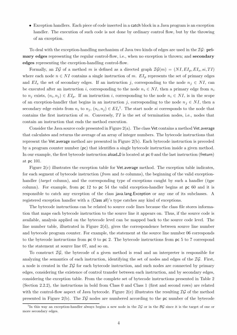
Consider the Java source code presented in Figure 2(a). The class Vet contains a method Vet.average
that calculates and returns the average of an array of integer numbers. The bytecode instructions that
represent the Vet.average method are presented in Figure 2(b). Each bytecode instruction is preceded
by a program counter number (pc) that identifies a single bytecode instruction inside a given method.
In our example, the first bytecode instruction aload 0 is located at pc 0 and the last instruction (freturn)
at pc 101.
Figure 2(c) illustrates the exception table for Vet.average method. The exception table indicates,
for each segment of bytecode instruction (from and to columns), the beginning of the valid exception-
handler (target column), and the corresponding type of exceptions caught by such a handler (type
column). For example, from pc 12 to pc 54 the valid exception-handler begins at pc 60 and it is
responsible to catch any exception of the class java.lang.Exception or any one of its subclasses. A
registered exception handler with a 〈Class all〉’s type catches any kind of exceptions.
The bytecode instructions can be related to source code lines because the class file stores informa-
tion that maps each bytecode instruction to the source line it appears on. Thus, if the source code is
available, analysis applied on the bytecode level can be mapped back to the source code level. The
line number table, illustrated in Figure 2(d), gives the correspondence between source line number
and bytecode program counter. For example, the statement at the source line number 06 corresponds
to the bytecode instructions from pc 0 to pc 2. The bytecode instructions from pc 5 to 7 correspond
to the statement at source line 07, and so on.
To construct IG, the bytecode of a given method is read and an interpreter is responsible for
analyzing the semantics of each instruction, identifying the set of nodes and edges of the IG. First,
a node is created in the IG for each bytecode instruction, and such nodes are connected by primary
edges, considering the existence of control transfer between each instruction, and by secondary edges,
considering the exception table. From the complete set of bytecode instructions presented in Table 2
(Section 2.2.2), the instructions in bold from Class 0 and Class 1 (first and second rows) are related
with the control-flow aspect of Java bytecode. Figure 2(e) illustrates the resulting IG of the method
presented in Figure 2(b). The IG nodes are numbered according to the pc number of the bytecode
1In this way an exception-handler always begins a new node in the IG or in the BG since it is the target of one ormore secondary edges.
4

(e) Vet.average data−flow Instruction Graph
27 fadd 28 putfield #3 <Field float out> 31 iinc 2 1 34 iload_2 35 aload_0 36 getfield #2 <Field int[] v> 39 arraylength 40 if_icmplt 15 43 aload_0 44 aload_0 45 getfield #3 <Field float out> 48 iload_2
49 i2f 50 fdiv 51 putfield #3 <Field float out> 54 jsr 82 57 goto 91 60 astore_3 61 aload_0 62 fconst_0 63 putfield #3 <Field float out> 66 iconst_0 67 istore_2 68 jsr 82 71 goto 91 74 astore 4 76 jsr 82 79 aload 4 81 athrow 82 astore 5 84 aload_0 85 aconst_null 86 putfield #2 <Field int[] v> 89 ret 5 91 aload_0 92 iload_2 93 i2f 94 invokevirtual #5 <Method void print(float)> 97 aload_0 98 getfield #3 <Field float out> 101 freturn
/*01*/public class Vet { /*02*/ int v[];/*03*/ float out;/*04*/ /*05*/ float average(int[] in) {/*06*/ v = in;/*07*/ out = 0.0f;/*08*/ int i = 0;/*09*//*10*/ try {/*11*/ while (i < v.length) {/*12*/ out += v[i];/*13*/ i++;/*14*/ }/*15*/ out = out / i;/*16*/ } catch (Exception e) {/*17*/ out = 0.0f;/*18*/ i = 0;/*19*/ } finally {/*20*/ v = null;/*21*/ }/*22*/ print((float) i);/*23*/ return out;/*24*/ }/*25*/
Line 18: pc = 66Line 19: pc = 68Line 20: pc = 74Line 22: pc = 91Line 23: pc = 97
(d) Line number table
1 aload_1 2 putfield #2 <Field int[] v> 5 aload_0 6 fconst_0 7 putfield #3 <Field float out> 10 iconst_0 11 istore_2 12 goto 34 15 aload_0 16 dup 17 getfield #3 <Field float out> 20 aload_0 21 getfield #2 <Field int[] v> 24 iload_2 25 iaload
(b) Vet.average bytecode instructions
(a) Vet.java source code
26 i2f
/*26*/ public void print(float n) {/*27*/ System.out.print(n + "\n");/*28*/ }/*29*/}
from to target type 12 54 60 <Class java.lang.Exception> 12 57 74 <Class all> 60 71 74 <Class all>
0 aload_0
74 79 74 <Class all>
(c) Exception table
Line 6: pc = 0Line 7: pc = 5Line 8: pc = 10Line 11: pc = 12Line 12: pc = 15Line 13: pc = 31Line 11: pc = 34Line 15: pc = 43Line 16: pc = 54Line 17: pc = 60
U = {L@2}
U = {[email protected]}
U = {L@0}
U = {[email protected]}
U = {[email protected][]}
D = {L@3}D = {L@5}
D = {L@5}
U = {L@0}
U = {[email protected]}
U = {L@0}
U = {L@4}
D = {L@5}
D = {L@4}
U = {L@0}
D = {L@0, L@1, [email protected], [email protected]}U = {L@0}
U = {L@1}
D = {[email protected]}
D = {[email protected]}
U = {L@0}
D = {L@2}U = {L@2}
U = {L@2}
0
1
2
7
...12
34
60
...40
43
15
...
76
44
45
...54
54.82
...21
24
25
31
...54.89
57
91
74.82
79
81
...97
98
101
68
68.82
71
...68.89
...74.89
...
74
Figure 2: Illustration of the data-flow IG.
instruction it represents. Section 2.2.2 describes how to identify the set Di of defined variables and the
set Ui of used variables associated to each node of IG. Observe that at bytecode level it is not possible
to distinguish between a p-use and a c-use. Later, in the computation of the data-flow criteria, nodes
with more than one outgoing edge will have the uses associated to such edges, as if they were p-uses.
Since in the IG each bytecode instruction corresponds to a node, the number of nodes and edges
can be very large, even for methods with a few lines of code. In case of the IG in Figure 2(e), some
5
nodes are omitted in order to reduce the size of the IG and to make it more readable. Ellipsis (“•••”)
are used to represent omitted nodes.
Primary edges are represented by continuous lines and secondary edges by dotted lines. Observe
that there are a large number of secondary edges connecting the nodes in the scope of a given exception-
handler to the first node of the handler. For example, according to the exception table of Figure 2(c)
the exception-handler located at pc 60 is responsible to catch all exceptions of java.lang.Exception class
raised from pc 12 to pc 54. So, there are secondary edges connecting all nodes in this range to node
60. The same applies to the other exception-handlers.
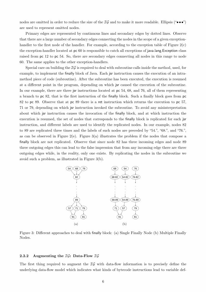
Special care on building the IG is required to deal with subroutine calls inside the method, used, for
example, to implement the finally block of Java. Each jsr instruction causes the execution of an intra-
method piece of code (subroutine). After the subroutine has been executed, the execution is resumed
at a different point in the program, depending on which jsr caused the execution of the subroutine.
In our example, there are three jsr instructions located at pc 54, 68, and 76, all of them representing
a branch to pc 82, that is the first instruction of the finally block. Such a finally block goes from pc
82 to pc 89. Observe that at pc 89 there is a ret instruction which returns the execution to pc 57,
71 or 79, depending on which jsr instruction invoked the subroutine. To avoid any misinterpretation
about which jsr instruction causes the invocation of the finally block, and at which instruction the
execution is resumed, the set of nodes that corresponds to the finally block is replicated for each jsr
instruction, and different labels are used to identify the replicated nodes. In our example, nodes 82
to 89 are replicated three times and the labels of such nodes are preceded by “54.”, “68.”, and “76.”,
as can be observed in Figure 2(e). Figure 3(a) illustrates the problem if the nodes that compose a
finally block are not replicated. Observe that since node 82 has three incoming edges and node 89
three outgoing edges this can lead to the false impression that from any incoming edge there are three
outgoing edges while, in the reality, only one exists. By replicating the nodes in the subroutine we
avoid such a problem, as illustrated in Figure 3(b).
.
.
.
89
54
82
68 76
57 71 79
91 81
(a)
.
.
.
54.89
.
.
.
68.89
.
.
.
76.89
54
54.82
57
91
68
68.82
71
76
76.82
79
81
(b)
Figure 3: Different approaches to deal with finally block: (a) Single Finally Node (b) Multiple FinallyNodes.
2.2.2 Augmenting the IG: Data-Flow IG
The first thing required to augment the IG with data-flow information is to precisely define the
underlying data-flow model which indicates what kinds of bytecode instructions lead to variable def-
6

inition/use and also how to consider reference and array variables. By analyzing the set of bytecode
instructions obtained from [11] we classify such instructions in eleven different classes, according to
their relation with the data-flow at bytecode level. Table 2 illustrates these classes of instructions.
Table 2: Different classes of bytecode instruction.
Class Bytecode Instructions Data-Flow Implication
0 athrow, goto, goto w, if acmpeq, if acmpne,if icmpeq, if icmpge, if icmpgt, if icmple, if icmplt,if icmpne, ifeq, ifge, ifgt, ifle, iflt, ifne, ifnonnull,ifnull, lookupswitch, tableswitch, areturn, dreturn,freturn, ireturn, lreturn, return, ret, monitorenter,monitorexit, pop, pop2, breakpoint, impdep1, impdep2,nop, checkcast, wide, swap
Instructions in this class have no implication forthe flow of data.
1 invokeinterface, invokespecial, invokestatic,invokevirtual, jsr, jsr w, dadd, ddiv, dmul, dneg,drem, dsub, fadd, fdiv, fmul, fneg, frem, fsub, iadd,iand, idiv, imul, ineg, ior, irem, ishl, ishr, isub, iushr,ixor, ladd, land, ldiv, lmul, lneg, lor, lrem, lshl, lshr,lsub, lushr, lxor, arraylength, instanceof, aconst null,bipush, dconst, fconst, iconst, lconst, sipush, ldc,ldc w, ldc2 w, d2f, d2i, d2l, f2d, f2i, f2l, i2b, i2c,i2d, i2f, i2l, i2s, l2d, l2f, l2i, new, multianewarray,anewarray, newarray, dcmpg, dcmpl, fcmpg, fcmpl,lcmp
Instructions in this class have no implication forthe flow of data. In addition, they leave an unknownelement at the top of the operand stack. Accesses tosuch element will not characterize any use or defini-tion. For example, instruction new pushes an objectreference onto the stack. Further use of such refer-ence as a field access is not regarded as a definitionor use.
2 aaload, baload, caload, daload, faload, iaload, laload,saload
Loads an array element to the top of the operandstacks and indicating the use of the array.
3 aastore, bastore, castore, dastore, fastore, iastore, las-tore, sastore
Stores the value on the top of the operand stack intoan array element, indicating the definition of thearray.
4 putfield Stores the value on the top of the operand stack intoan instance field, indicating the definition of suchan instance field.
5 putstatic Stores the value on the top of the operand stack intoa class field, indicating the definition of such a classfield.
6 dup, dup2, dup x1, dup x2, dup2 x1, dup2 x2 Duplicates the value onto the top of the operandstack and has no implication for the flow of data.
7 aload, dload, fload, iload, lload Loads the value of a given local variable onto the topof the operand stack, indicating a use of such a localvariable.
8 astore, dstore, fstore, istore, lstore Stores the value on the top of the operand stack intoa local variable, indicating a definition of such avariable.
9 getfield Loads an instance field onto the top of the operandstack, indicating a use of such an instance field.
10 getstatic Loads a class field onto the top of the operand stack,indicating a use of such a class field.
11 iinc Increments the value of a given local variable, indi-cating a use and a definition of such a local vari-able.
The division into such classes was based on the kind of definitions and uses that we would like to
identify. In Java and Java bytecode, the variables can be classified in two types: basic or reference
types. Fields of a class can be of basic or reference type and are classified as instance or class fields,
depending on whether they are unique to each object of the class or unique to the entire class (static
fields), respectively. Local variables declared inside a method can also be of basic or reference type.
An aggregated variable (array) is of reference type. To deal with aggregated variables we are following
the approach proposed by Horgan and London [9], which considers an aggregated variable as a unique
storage location such that when a definition (use) of any element of the aggregated variable occurs,
what is considered to be defined (used) is the aggregated variable and not a particular element.
Moreover, in their data-flow model, a definition of a given variable blocks previous definitions of the
7

same variable. So, in our data-flow model the following guidelines apply to identify definitions and
uses of variables:
1. Aggregated variables are considered as a unique storage location and the definition/use of any
element of the aggregated variable a[] is considered to be a definition/use of a[]. So, in the
statement “a[i] = a[j] + 1” there is a definition and a use of the aggregated variable a[].
2. If an aggregate variable a[][] is defined, an access to its elements is considered a definition or
use of a[][]. Then, in the statement “a[0][0] = 10” there exists a definition of a[][] and in the
statement “a[0] = new int[10]” there is a definition of a[].
3. Every time an instance field (or an array element) is used (defined) there is a use of the reference
variable used to access the field and a use (definition) of the field itself. Considering ref 1 and
ref 2 as reference variables of a class C which contains two instance fields x and y of type int, in
the statement “ref 1.x = ref 2.y” there are uses of the reference variables ref 1 and ref 2, a use
of the instance field ref 2.y, and a definition of the instance field ref 1.x. Since instance fields
are valid in the entire scope of a given class, each instance field used in the context of a given
method is considered to have a definition in the first node of the IG.
4. Class fields (static fields) can be considered as global variables and do not require a reference
variable to be accessed. Considering a class C with a static fields w and z, in the statement “C.z
= C.w + y” there are a use of C.w and a definition of C.z. Even if a static field is accessed using
a reference variable ref 1 of class C, such that “ref 1.w = 10”, at bytecode level, such a reference
is converted to the class name and there is no use of the reference variable in this statement.
Since static fields are in the entire scope of a given class, each static field used in the context of
a given method is considered to have a definition in the first node of the IG.
5. A method invocation such as ref 1.foo(e 1, e 2, . . ., e n) indicates a use of the reference variable,
ref 1. The rules for definition and use identification inside expressions e 1, e 2, . . ., e n are the
same as described on items 1 to 4.
6. For instance methods, a definition of this is assigned to the first node of the IG, and also the
definition of each local variable corresponding to the formal parameters of such a method, if any.
For class methods, only the local variables corresponding to the parameters are considered, no
instance is required to invoke such a method.
Based on these guidelines and on the different classes of bytecode instructions, the IG of a given
method is traversed and to each node of such a graph a set Di of defined variables, and a set Ui of used
variables are assigned. Before explaining how these two sets are created, it is important to know how
these different kinds of variables are treated at the bytecode level. Method parameters and variables
declared inside the method are treated as local variables and are bound to the JVM local variable
table as follows: if it is an instance method, local variable zero, referenced here as L@0, is bound to the
reference to the current object (this), i.e., the object that caused the method invocation. The formal
parameters, if any, are bound to the local variable one (L@1), two (L@2), and so on, depending on the
type and on the number of parameters. Finally, the variables declared inside the method are bound
to the remaining local variables, also depending on the type and the number of declared variables.
For example, considering the source code of the method Vet.average, it can be observed that it is an
8

instance method which accepts one parameter in and declares one local variable i. L@0 corresponds
to reference to the current object. The formal parameter in corresponds to L@1, and the variable
i corresponds to L@2. Three other local variables (L@3, L@4 and L@5) are used by the compiler to
implement the exception-handling mechanism. The method accesses two instance fields: v, and out.
Since they are instance fields, they require a reference to an object of class Vet to be accessed. When
no reference is used preceding a field, the reference to the current object is used. So, v and out are
referenced in the bytecode of our example as [email protected] and [email protected].
To analyze the IG we implemented a simulator that interprets bytecode instructions and identifies
the type and the source of data manipulated by each instruction. For example, suppose the current
instruction to be analyzed is iload 2. Such an instruction, when interpreted by the JVM, pushes onto
the top of the operand stack an integer value stored in L@2. Our simulator, instead of pushing an
actual value, pushes onto the top of the stack an indication in the form “<type> - <data source>” to
be used when interpreting the next bytecode instructions. <type> corresponds to the data type being
manipulated, and <data source> to the source of each data. In this example, instruction iload 2 pushes
an indication like “int - L@2”, since L@2 is a data source of an integer value. Moreover, the load instruc-
tion characterizes a use of L@2 so this variable is inserted in the set of used variables associated to the
current node of the IG graph. Different indications are used to represent the different types of storage
places, as described above. In Figure 4(a), second column, there are different kinds of indications placed
onto the top of the operand stack when the bytecode instructions in the first column are interpreted.
For a class field (static field) the indication is in the form “<type> - S@<class name>.<field name>”,
where <type> is the type of the static field, <class name> is the class name, and <field name> is the
name of the static field. A detailed description of the interpreter and all kinds of indications can be
found in [26].
Considering the IG presented in Figure 2(e), there are the definitions of L@0, L@1, [email protected], and
[email protected] associated with node 0. Moreover, node 0 also contains a bytecode instruction of Class 7
(aload 0), which indicates a use of the loaded local variable, L@0 in this case. Observe that the
bytecode instruction at pc 0 is one of the bytecode instructions that corresponds to the statement
“v = in” at source code line 6 of Figure 2(a). The use exists because before initializing such a field,
which is carried out when the instruction located at pc 2 is executed, the reference to the current
object (L@0) has to be loaded onto the top of the operand stack, characterizing the use of such a local
variable.
At node 2, the putfield instruction, which belongs to Class 4, indicates a definition of an instance
field, in our case the instance field v, referenced as [email protected]. So, the set of defined variables at node 2
contains the element [email protected]. Finally, the instruction at node 25, iaload, belongs to Class 2 and indicates
a use of an element of an array of integers, so the set of used variables at node 25 contains the element
One important point to be observed is that, when evaluating a given instruction, the current top
of the operand stacks can have more that one configuration, depending on the path used to reach the
instruction. Since it is possible to reach a given node through different instruction sequences, each
different possible stack configuration needs to be evaluated to find the complete set of defined/used
variables in a IG node. This is performed by traversing the IG as many times as necessary, until all
possible combinations have been evaluated, and the complete set of defined/used variables on each
node have been found.
9
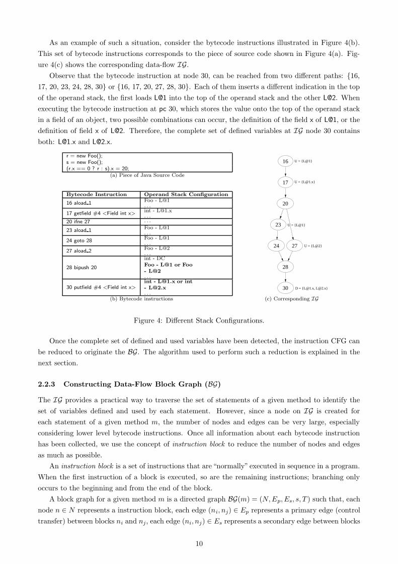
As an example of such a situation, consider the bytecode instructions illustrated in Figure 4(b).
This set of bytecode instructions corresponds to the piece of source code shown in Figure 4(a). Fig-
ure 4(c) shows the corresponding data-flow IG.
Observe that the bytecode instruction at node 30, can be reached from two different paths: {16,
17, 20, 23, 24, 28, 30} or {16, 17, 20, 27, 28, 30}. Each of them inserts a different indication in the top
of the operand stack, the first loads L@1 into the top of the operand stack and the other L@2. When
executing the bytecode instruction at pc 30, which stores the value onto the top of the operand stack
in a field of an object, two possible combinations can occur, the definition of the field x of L@1, or the
definition of field x of L@2. Therefore, the complete set of defined variables at IG node 30 contains
both: [email protected] and [email protected].
r = new Foo();s = new Foo();(r.x == 0 ? r : s).x = 20;
(a) Piece of Java Source Code
Bytecode Instruction Operand Stack Configuration
16 aload 1 Foo - L@1· · ·
17 getfield #4 <Field int x> int - [email protected]· · ·
20 ifne 27 · · ·
23 aload 1 Foo - L@1· · ·
24 goto 28 Foo - L@1· · ·
27 aload 2 Foo - L@2· · ·
28 bipush 20
int - DCFoo - L@1 or Foo
- L@2
· · ·
30 putfield #4 <Field int x>int - [email protected] or int
· · ·D = {[email protected], [email protected]}
U = {L@2}
U = {L@1}
U = {[email protected]}
U = {L@1}16
17
20
23
2724
28
30
(b) Bytecode instructions (c) Corresponding IG
Figure 4: Different Stack Configurations.
Once the complete set of defined and used variables have been detected, the instruction CFG can
be reduced to originate the BG. The algorithm used to perform such a reduction is explained in the
next section.
2.2.3 Constructing Data-Flow Block Graph (BG)
The IG provides a practical way to traverse the set of statements of a given method to identify the
set of variables defined and used by each statement. However, since a node on IG is created for
each statement of a given method m, the number of nodes and edges can be very large, especially
considering lower level bytecode instructions. Once all information about each bytecode instruction
has been collected, we use the concept of instruction block to reduce the number of nodes and edges
as much as possible.
An instruction block is a set of instructions that are “normally” executed in sequence in a program.
When the first instruction of a block is executed, so are the remaining instructions; branching only
occurs to the beginning and from the end of the block.
A block graph for a given method m is a directed graph BG(m) = (N,Ep, Es, s, T ) such that, each
node n ∈ N represents a instruction block, each edge (ni, nj) ∈ Ep represents a primary edge (control
transfer) between blocks ni and nj, each edge (ni, nj) ∈ Es represents a secondary edge between blocks
10

ni and nj, s corresponds to the start block, and T is the set of termination blocks. For each block
two sets Di and Ui are assigned. They contain the sets of defined and used variables in the block,
respectively.
The algorithm used to reduce a data-flow IG to a data-flow BG is presented in Figure 5. In line
14 of the algorithm, a decision is taken whether the current instruction x being analyzed is the last
one in the current block or not. It will be the last one if at least one of the following conditions holds:
• x is a jump, goto, ret or invoke instruction;
• x has more than one primary successor;
• the single primary successor of x has more than one (primary or secondary) predecessor;
• the single primary successor of x has not the same set of secondary successors of x.
# Input: iG, the instruction-CFG GI = 〈NI, EIp, EIs, si, T I〉 to be reduced;# Output: bG, the block CFG bG = 〈N, Ep, Es, s, T 〉
01 s := NewNodeTo(si)02 foreach x ∈ N
03 if x has no successor04 T := T ∪ {x}
# Auxiliary function: NewNodeTo# Input: A node y from iG
# Output: A node from bG where y has been inserted
05 ins := the instruction in y
06 if the node y has already been visited07 return the node w ∈ N that contains ins
08 CurrentNode := new block node09 N := N ∪ {CurrentNode}10 x := y
11 repeat12 Include x as part of CurrentNode
13 Mark x as visited14 if x should terminated the current block15 foreach v such that (x, v) ∈ EIp
16 Ep := Ep ∪ {(CurrentNode, NewNodeTo(v))}17 foreach v such that (x, v) ∈ EIs
18 Es := Es ∪ {(CurrentNode, NewNodeTo(v))}19 x := null
20 else21 if there exists a v such that (x, v) ∈ EIp
22 x := v
23 else24 x := null
25 while x 6= null
26 return CurrentNode
Figure 5: Algorithm to generate the CFG from bytecode.
Zhao [33] proposes a different approach to construct the CFG of a given method. According to
Zhao’s approach, if an exception-handler is present, a new node is also created for any instruction that
may throw an exception explicitly (instruction athrow) or implicitly (other 42 instructions), which can
increase significantly the number of nodes in the CFG. Moreover, to correctly implement the approach
11

to generate the CFG as proposed by Zhao [33] it is necessary to check the subclasses of each exception
that may be raised and to identify if there is any exception-handler that can catch this particular
exception. In our implementation we decide to use a more pragmatic approach to construct the BG,
expecting to obtain simpler and more readable graphs.
As mentioned earlier, two points that should be highlighted are: first, when we have subroutine
calls, the set of statement blocks representing the subroutine is expanded for every call, i.e., the
statements of a given subroutine may appear more than once in the BG within different nodes, once
for each subroutine call.
Second, observe that since the set of bytecode instructions on each statement block might not throw
all kind of handled exceptions, our BG may have “false” (or spurious) secondary edges. Moreover, the
execution of a given block can be interrupted in any place, when an exception is thrown, so in the
presence of exceptions the block may not have the “atomicity” characteristic mentioned above. On
the other hand, this approach simplifies both the construction of the BG and also its interpretation,
since the number of nodes is reduced. An alternative approach to construct a CFG to deal with
exception-handling constructions is described by Sinha and Harrold [21] such that no false edges are
generated. Although, the proposed technique considers only exceptions generated explicitly, i.e., the
ones originate by the throw statement [21].
D = {}
U = {L@0, L@2, [email protected][], [email protected]}D = {L@2, [email protected]}
U = {L@0}D = {L@2, L@3, [email protected]}
U = {}D = {L@4}
U = {}D = {L@5, [email protected]}
U = {L@4}D = {} D = {}
U = {L@0, [email protected]}
D = {L@0, L@1, L@2, [email protected], [email protected]}U = {L@0}
D = {}U = {L@0, L@2, [email protected]}
D = {[email protected]}U = {L@0, L@2, [email protected]}
D = {}U = {}
D = {L@5, [email protected]}U = {}
D = {L@5, [email protected]}U = {}
U = {L@0, L@2}
0
34
4315
60
74
54
60.82
74.82
54.82
91
9779
Figure 6: Vet.average’s BG.
After the BG has been constructed, a simple analysis is carried out to eliminate unnecessary nodes,
i.e., nodes that contain only a single goto instruction. They can be eliminated by directly connecting
its in-coming edges as the in-coming edges of its successor. Figure 6 illustrated the BG obtained by
applying the reduction algorithm to the IG of Figure 2(e). BG represents the underlying model used to
derive control-flow and data-flow testing requirements. The label of a given block in BG is the program
counter number of its first instruction. The labels of the replicated nodes, i.e., nodes corresponding to
a subroutine, are preceded by the label of the node that invoked the subroutine. Observe that since
instruction node 68 of IG now composes the block node 60 in BG, instructions nodes 68.82 of IG
12
correspond to block node 60.82 in BG. All the other replicated instruction nodes that correspond to
the finally block, i.e., instruction nodes 84, 85, 86 and 89 in IG, are part of the block nodes xx.82 in
BG.
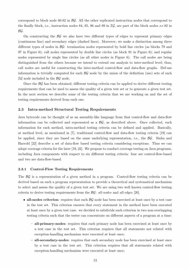
On constructing the BG we also have two different types of edges to represent primary edges
(continuous line) and secondary edges (dashed lines). Moreover, we make a distinction among three
different types of nodes in BG: termination nodes represented by bold line circles (as blocks 79 and
97 in Figure 6); call nodes represented by double line circles (as block 91 in Figure 6); and regular
nodes represented by single line circles (as all other nodes in Figure 6). The call nodes are being
distinguished from the others because we intend to extend our analysis to inter-method level; thus,
call nodes are useful for constructing the inter-method control-flow and data-flow graphs. Def-use
information is trivially computed for each BG node by the union of the definition (use) sets of each
IG node included in the BG node.
Once the BG has been obtained, different testing criteria can be applied to derive different testing
requirements that can be used to assess the quality of a given test set or to generate a given test set.
In the next section we describe some of the testing criteria that we are working on and the set of
testing requirements derived from each one.
2.3 Intra-method Structural Testing Requirements
Java bytecode can be thought of as an assembly-like language from that control-flow and data-flow
information can be collected and represented as a BG, as described above. Once collected, such
information for each method, intra-method testing criteria can be defined and applied. Basically,
at method level, as mentioned in [7], traditional control-flow and data-flow testing criteria [19] can
be applied, since they are based on the same underlying representation, i.e., the BG. Sinha and
Harrold [22] describe a set of data-flow based testing criteria considering exceptions. Thus we can
adopt coverage criteria for the later [19, 22]. We propose to conduct coverage testing on Java programs,
including Java components with respect to six different testing criteria: four are control-flow-based
and two are data-flow-based.
2.3.1 Control-Flow Testing Requirements
The BG is a representation of a given method in a program. Control-flow testing criteria can be
derived based on such a program representation to provide a theoretical and systematical mechanism
to select and assess the quality of a given test set. We are using two well known control-flow testing
criteria to derive testing requirements from the BG: all-nodes and all-edges [20].
• all-nodes criterion: requires that each BG node has been exercised at least once by a test case
in the test set. This criterion ensures that every statement in the method have been executed
at least once by a given test case. we decided to subdivide such criterion in two non-overlapping
testing criteria such that the tester can concentrate on different aspects of a program at a time:
– all-primary-nodes: requires that each primary node has been exercised at least once by
a test case in the test set. This criterion requires that all statements not related with
exception-handling mechanism were executed at least once;
– all-secondary-nodes: requires that each secondary node has been exercised at least once
by a test case in the test set. This criterion requires that all statements related with
exception-handling mechanism were executed at least once;
13

• all-edges criterion: requires that each BG edge has been exercised at least once by a test case
in the test set. This criterion ensures that every possible control transfer in the method has
been executed at least once by a given test case. Since in our BG there are two different types
of edges, we decided to subdivide such criterion in two non-overlapping testing criteria:
– all-primary-edges: requires that each primary edge has been exercised at least once by
a test case in the test set. This criterion requires that all conditional expressions were
evaluated as true and false at least once;
– all-secondary-edges: requires that each secondary edge has been exercised at least once
by a test case in the test set. This criterion requires that each exception-handler be executed
at least once from each node where an exception might be raised.
To illustrate how such criteria can be applied, Table 3 presents the set of testing requirements
required by each one of them, considering the BG of the method Vet.average (Figure 6).
Table 3: Set of control-flow testing requirements for Vet.average BG.Criterion Testing Requirements
all-nodesall-primary-nodes {0, 15, 34, 43, 54, 54.82, 91, 97}
all-secondary-nodes {60, 60.82, 74, 74.82, 79}
all-edgesall-primary-edges
{(0,34), (15,34), (34,15), (34,43), (43,54), (54,54.82), (54.82,91),(60,60.82), (60.82,91), (74,74.82), (74.82,79), (91,97) }
all-secondary-edges{(15,60), (15,74), (34,60), (34,74), (43,60), (43,74), (54,74), (60,74),(74,74)}
2.3.2 Complexity Analysis of Control-Flow Testing Criteria
TO BE DONE...
2.3.3 Data-Flow Testing Requirements
With respect to data-flow testing, we are using the well known all-uses criterion [19] that is composed
of the all-c-uses and all-p-uses criteria. A precise definition about these criteria can be found in [19].
A use represents the use of a variable in a statement. If the value of a variable is used for some
computation, it is a c-use (Computational Use), whereas if the value is used in a predicate that
determines which branch is to be executed, it is a p-use (Predicate Use). Let bi and bj to be two
points in the bytecode where a variable x is defined and used, respectively. This definition and this
use are referred to as di(x) and uj(x), respectively. The pair (di(x), uj(x)) is a def-use pair if there is
a definition clear path with respect to x from bi to bj , i.e., x is not defined at any point other than bi.
The pair is also said feasible if there exists a test case t such that the execution of the method on t
causes such definition clear path from bi to bj to be traversed.
For an example of a c-use, consider the DUG of Figure 6. At node 0, the variable definition set
contains the variable [email protected], which represents the instance variable v in the corresponding source code.
At node 15 there is a use of [email protected] to compute the sum of its elements, determining a c-use pair w.r.t.
[email protected] from node 0 to node 15 (c-use). On the other hand, at node 15, there is a definition of L@2
that represents the local variable i in the corresponding source code. Such a variable is used in the
predicate located at node 34 to evaluate if the end of v has been reached. Thus, there is a p-use
pair w.r.t. L@2 from node 15 to node 34. From the bytecode, it is not possible to distinguish p-uses
14

and c-uses. In our implementation of all-uses criterion we assume that a use in a node with more
than one out-going edge is a p-use and associate it with each of those edges. As with the all-edges
criterion, we divided the all-uses criterion such that two sets of non-overlapping testing requirements
are obtained, to consider the primary and secondary edges. We named such criteria all-primary-uses
and all-secondary-uses, respectively. The first takes all the def-use pairs for which there exists a path
of primary edges only. The other def-use pairs are required by the second.
To illustrate how such criteria can be applied, Table 4 presents the set of testing requirements
required by each one of than, considering the BG of the method Vet.average (Figure 6).
A test set T may be evaluated against the all-uses criterion (all-primary-uses/all-secondary-uses) by
computing the ratio of the number of def-use pairs covered to the total of all-uses (all-primary-uses/all-
secondary-uses) requirements. The same applies to all-nodes and all-edges (all-primary-edges/all-
secondary-edges) criteria. More details about the testing criteria definition can be found in [26].
Table 4: Set of data-flow testing requirements for Vet.average BG.Criterion Testing Requirements
all-uses
all-primary-uses
〈L@0, 0, (15, 34)〉 〈L@0, 0, (34, 15)〉 〈L@0, 0, (34, 43)〉〈L@0, 0, (43, 54)〉 〈L@0, 0, (60, 60.82)〉 〈L@0, 0, 54.82〉〈L@0, 0, 60.82〉 〈L@0, 0, 74.82〉 〈L@0, 0, 91〉〈L@0, 0, 97〉 〈[email protected], 0, (43, 54)〉 〈[email protected], 15, (43, 54)〉
〈[email protected], 43, 97〉 〈[email protected], 60, 97〉 〈[email protected], 0, (15, 34)〉〈[email protected], 0, (34, 15)〉 〈[email protected], 0, (34, 43)〉 〈[email protected][], 0, (15, 34)〉〈L@2, 0, (15, 34)〉 〈L@2, 0, (34, 15)〉 〈L@2, 0, (34, 43)〉〈L@2, 0, (43, 54)〉 〈L@2, 0, 91〉 〈L@2, 15, (15, 34)〉〈L@2, 15, (34, 15)〉 〈L@2, 15, (34, 43)〉 〈L@2, 15, (43, 54)〉
〈L@2, 15, 91〉 〈L@2, 60, 91〉 〈L@4, 74, 79〉
all-secondary-uses
〈L@0, 0, (15, 60)〉 〈L@0, 0, (15, 74)〉 〈L@0, 0, (34, 60)〉〈L@0, 0, (34, 74)〉 〈L@0, 0, (43, 60)〉 〈L@0, 0, (43, 74)〉〈L@0, 0, (60, 74)〉 〈[email protected], 0, (43, 60)〉 〈[email protected], 0, (43, 74)〉
〈[email protected], 15, (43, 60)〉 〈[email protected], 15, (43, 74)〉 〈[email protected], 43, (43, 60)〉〈[email protected], 43, (43, 74)〉 〈[email protected], 0, (15, 60)〉 〈[email protected], 0, (15, 74)〉〈[email protected], 0, (34, 60)〉 〈[email protected], 0, (34, 74)〉 〈[email protected][], 0, (15, 60)〉〈[email protected][], 0, (15, 74)〉 〈L@2, 0, (15, 60)〉 〈L@2, 0, (15, 74)〉〈L@2, 0, (34, 60)〉 〈L@2, 0, (34, 74)〉 〈L@2, 0, (43, 60)〉〈L@2, 0, (43, 74)〉 〈L@2, 15, (15, 60)〉 〈L@2, 15, (15, 74)〉〈L@2, 15, (34, 60)〉 〈L@2, 15, (34, 74)〉 〈L@2, 15, (43, 60)〉〈L@2, 15, (43, 74)〉
2.3.4 Complexity Analysis of Data-Flow Testing Criteria
TO BE DONE...
2.4 Dominators and Super-Block Analysis
Studies have shown that it is important to generate a test set with high coverage while testing C
programs so that more faults are likely to be detected[16, 31, 32]. The same applies to Java programs
without lost of generality. To explain our approach to increase the coverage as soon as possible w.r.t.
a given test criterion (all-blocks in our example), consider the BG presented in Figure 6. The main
idea is to assign different weights to each BG node based on dominator analysis and “super block” [1].
The objective is to generate a test to cover one of the areas with the highest weight, if possible, before
other areas with a lower weight are covered so that the maximum coverage can be added in each single
execution. In this way, we provide useful hints on how to generate efficient test cases to increase,
15

as much as possible with as few tests as possible, the control-flow (such as block and decision) and
data-flow coverage (such as all-uses) of the programs being tested.
Basically, a super-block is a subset of nodes with the property that if any node in a super block
is covered then all nodes in that super block are covered2. Pre- and post-dominator relationships
among nodes are used to identify the set of super blocks from a given BG. According to [1], a node u
pre-dominates a node v denoted as upre→ v, if every path from the entry node to v contains u. A node
w post-dominates a node v denoted as upost→ v, if every path from v to the exit node contains w. For
example, in Figure 6, nodes 0 and 34 pre-dominate node 74 and nodes 74.82 and 79 post-dominate
it. Pre- and post-dominator relationships can be expressed in the form of pre- and post dominator
trees, respectively. upre→ v iff there is a path from u to v in the predominator tree. Similarly, w
post→ v
iff there is a path from w to v in the post-dominator tree. Figures 7(a) and 7(b) show the pre- and
post-dominator trees of the BG in Figure 6.
The dominator relationship amongst BG’s nodes is represented by a “basic block dominator graph”
that corresponds to the union of the pre- and post-dominator trees. Figure 7(c) shows the basic block
dominator graph of the BG in Figure 6.
From the basic block dominator graph, strongly connected components (super blocks) are identified
and the corresponding super block dominator graph is obtained. A strongly connected component has
a property that every node in the component dominates all other nodes in that component. For
example, nodes {74, 74.82, 79} compose a strongly connected component.
Figure 7(d) represents the super block dominator tree of the BG in Figure 6. From this represen-
tation it is possible to calculate the weight of each BG node. Basically, the weight of a given node is
the number of nodes that have not been covered but will be if that block is covered. In Figure 8(a),
the initial weight of each super block is show on the bottom of each node.
For example, to arrive at node 54.82 in Figure 6 requires the execution also to go through nodes 0,
34, 43, and 54. After arriving in node 54.82, nodes 91 and 97 will also be executed. This implies node
54.82 is dominated by nodes 0, 34, 43, 54, 91 and 97. It also means nodes 0, 34, 43, 54, 91 and 97 will
be covered (if they haven’t been) by a test execution if that execution covers node 54.82. Assuming
none of the blocks is covered so far, we say that node 54.82 has a weight of at least 7 because covering
it will increase the coverage by at least seven nodes. Using the same approach, node 15 has a weight of
3 since its coverage only guarantees an increase of coverage by at least three nodes. A very important
note is that while assigning the weight to a given node, we use a conservative approach by counting
only the additional nodes that will definitely be covered because of the coverage of this given node.
This is why we use the phrase “at least” in the above statements. Of course, covering a node of a
weight 7 (like node 54.82 in our example) may end up covering more than seven blocks (por ex., the
execution can go through nodes 0, 34, 15, 34, 43, 54 before it reaches node 54.82 and continues though
nodes 91 and 97). Nevertheless, the additional nodes (node 15 in our example) are not guaranteed to
be covered.
Since node 54.82 has a higher weight than node 15, we say that node 54.82 has a higher priority
to be covered than node 15 (i.e., tests that cover node 54.82 have a higher priority to be executed
than tests that only cover node 15)3 so that the maximum node coverage can be added in each single
2Assuming that the underlying hardware does not fail and no exception is raised during the execution of a test3Observe that, we are using the term high priority only considering the coverage that will be obtained. The tester,
based on his experience may desire to cover first a node with a lower weight but that has a higher complexity in terms ofimplementation, i.e., depending on the criticality of a given part of the code, or based on another assumption, the testercan choose to cover a different node first and then, by recomputing the weight, to use the weight information to increasethe coverage faster.
16

0
34
15 43 60 74 91
54 60.82 74.82 97
54.82 79
(a) Pre-Dominator Tree
0
1534 43 54 60
74
79
74.82
54.82 60.82
91
97
(b) Post-dominator Tree
0
34
15 436074 91
5460.8274.82
54.82
97
79
(c) Basic Block Dominator Tree
0, 34
15 43 60 74, 74.82, 79 91, 97
54 60.82
54.82
(d) Super Block Dominator Tree
Figure 7: Control-Flow Dependence Analysis.
7
3 3 3 5 4
4 6
20, 34
15 43 60 74, 74.82, 79 91, 97
54 60.82
54.82
(a)
3 0
0 2
0
0
1 0 1
15 43 60 74, 74.82, 79 91, 97
54 60.82
54.82
0, 34
(b)
Figure 8: Super block dominator graph with weights: (a) before any test case execution, and (b) afterthe execution of one test case.
execution. In this way, the node coverage can be increased as much as possible with as few tests as
possible.
After executing certain tests the weights of nodes that are not covered by these tests may change.
For example, after the execution of a test (say t1) that covers node 54.82 (which also guarantees the
coverage of node 0, 34, 43, 54, 91 and 97), the execution of another test (say t2) to cover node 15 will
17
increase the coverage by only one node (namely, node 15 itself). This is because nodes 0 and 34 have
already been covered by test t1 and the execution of other tests (such as t2) will not change this fact.
Under this scenario, after t1 has been executed, node 15 will have weight one. This implies that after
a test (t1 in our case) is executed to cover node 54.82, the priority, in terms of increasing the coverage,
of executing another test (t2 in our case) to cover node 15 may be reduced.
This procedure is applied recursively after the execution of each test to recompute the weight of
each node that has not been covered by the current tests, as well as the priority of tests to be executed
for covering such nodes. The objective is to continue this recursive procedure until all the blocks, if
possible, are covered by at least one test (i.e., achieve 100% node coverage) or the execution will stop
after a predefined time-out been reached. In the latter case, although tests so executed might not
give 100% node coverage, they still provide as high a block coverage as possible. In the reality, as
mentioned in [1], the tester only needs to create test cases that covers one node of each leaf node in
the super block dominator graph to cover all the other nodes.
2.5 Program Slicing
Computer programmers break apart large programs into smaller coherent pieces. Each of these pieces:
functions, subroutines, modules, or abstract datatypes, is usually a contiguous piece of program text.
Programmers also routinely break programs into one kind of coherent piece which is not contiguous.
When debugging unfamiliar programs programmers use program pieces called slices which are sets
of statements related by their flow of control or data. The statements in a slice are not necessarily
textually contiguous, but may be scattered through a program [29]. A program slice consists of the
parts of a program that (potentially) affect the values computed at some point of interest. Such a
point of interest is referred to as a slicing criterion, and is typically specified by a location in the
program in combination with a subset of the program’s variables and/or statements. The task of
computing program slices is called program slicing. The original definition of program slicing was
proposed by Weiser in 1979 [28, 30]. Today, a lot of slightly different notions of program slices can be
found in the literature, as well as a number of criteria to compute them [23]. An important distinction
exists between a static and a dynamic slice. Static slices are computed without making assumptions
regarding a program’s input, whereas the computation of dynamic slices relies on a the execution trace
information of specific test case.
Program slicing is a broadly applicable program analysis technique that can be used to perform
different software engineering activities, such as: program understanding, debugging, testing, par-
allelization, re-engineering, maintenance, and others [6]. In the context of JaBUTi, the three most
important activities are program understanding, debugging and testing.
Program understanding uses program slicing to help engineers to understand code. For exam-
ple, a backward slice from a point in the program identifies all parts of the code that contribute to
that point. A forward slice identifies all parts of the code that can be affected by the modification to
the code at the slice point.
Testing and Regression Testing also uses slicing. For example, suppose a proposed program
modification only changes the value of variable v at program point p. If the forward slice with respect
to v and p is disjoint from the coverage of regression test t, then test t does not have to be rerun.
Suppose a coverage tool reveals that a use of variable v at program point p has not been tested. What
input data is required in order to cover p? The answer lies in the backward slice of v with respect to
p.
18

In Section 7 it is described the characteristics JaBUTi’s slicing tool and how to use it to smart
debugging and fault localization.
2.6 Complexity Metrics
Complexity metrics are very useful to several software engineering tasks. Their main objective is to
provide different kinds of measure of a project/program such that further projects can use the historical
database to better estimate time, cost and complexity of new projects. There are different kinds of
complexity metrics. For example, Lorenz e Kidd [12] defined a set of design metrics to evaluate static
characteristics of an OO software project. The proposed set of metrics is divided into three groups: 1)
Class Size Metrics to quantify individual classes; 2) Class Inheritance Metrics to evaluate the
quality of using inheritance; and 3) Class Internal Metrics to evaluate general characteristics of a
class.
Another well-known set of metrics, proposer by Chidamber and Kemerer [4], is composed by six
design metrics six design metrics developed to evaluate the complexity of a given class.
Utsonomia [24] have studied and adapted both sets of design metrics for Java bytecode. JaBUTi
implements such adapted metrics to allow a tester to collect static metrics information for the classes
under testing.
Another benefit of complexity metrics is that the collected information can be used to establish
incremental testing strategies by prioritizing the test of certain classes, reducing the cost and improving
the quality of the testing activity. For instance, JaBUTi prioritizes testing requirements based on
coverage information. By using complexity metrics, the class’s inheritance, size, and complexity can
be combined with coverage information, providing additional hints to reduce the cost of test case
generation.
In Section 8 it is described how to use JaBUTi to collect static information about the classes under
testing, considering the set of complexity metrics adapted from Lorenz e Kidd [12] and Chidamber
and Kemerer [4] works.
3 The Vending Machine Example
To illustrate the JaBUTi’s functionalities we will use a simple example, adapted from [15], consist-
ing of a component and an application that uses it. Figure 9 shows the Java source code of the
VendingMachine application and of the Dispenser component. Although JaBUTi does not require the
source code available to perform its operations, we show it here to ease the understanding of the
vending machine application.
This source code implements a typical vending machine that is able to dispense specific items
to a customer under certain conditions. The basic operations that a given customer may perform
are: (1) to insert a coin of 25 cents into the machine (VendingMachine.inservCoin()); (2) to ask the
machine to return the inserted and not consumed coins (VendingMachine.returnCoin()); and (3) to ask
the machine to vend a specific item (VendingMachine.vendItem()). The Dispenser component keeps
information about the price of each item and which items are valid and available. The basic steps
performed by the Dispenser component are:
1. Checks if at least one coin have been inserted;
2. Checks if a valid item have been selected;
19
3. Checks if the valid item selected is available;
4. Checks if the credit is enough to buy the valid available selected item.
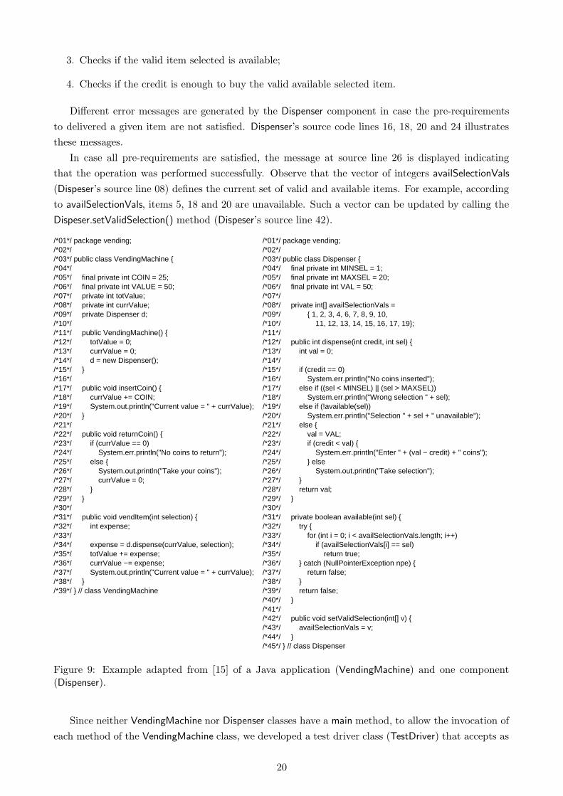
Different error messages are generated by the Dispenser component in case the pre-requirements
to delivered a given item are not satisfied. Dispenser’s source code lines 16, 18, 20 and 24 illustrates
these messages.
In case all pre-requirements are satisfied, the message at source line 26 is displayed indicating
that the operation was performed successfully. Observe that the vector of integers availSelectionVals
(Dispeser’s source line 08) defines the current set of valid and available items. For example, according
to availSelectionVals, items 5, 18 and 20 are unavailable. Such a vector can be updated by calling the
Dispeser.setValidSelection() method (Dispeser’s source line 42).
/*24*/ System.err.println("Enter " + (val − credit) + " coins");
/*02*//*03*/ public class VendingMachine {/*04*//*05*/ final private int COIN = 25;/*06*/ final private int VALUE = 50;/*07*/ private int totValue;/*08*/ private int currValue;/*09*/ private Dispenser d;/*10*//*11*/ public VendingMachine() {/*12*/ totValue = 0;/*13*/ currValue = 0;/*14*/ d = new Dispenser();/*15*/ }/*16*//*17*/ public void insertCoin() {/*18*/ currValue += COIN;/*19*/ System.out.println("Current value = " + currValue);/*20*/ }/*21*//*22*/ public void returnCoin() {/*23*/ if (currValue == 0)/*24*/ System.err.println("No coins to return");/*25*/ else {/*26*/ System.out.println("Take your coins");/*27*/ currValue = 0;/*28*/ }/*29*/ }/*30*//*31*/ public void vendItem(int selection) {/*32*/ int expense;/*33*//*34*/ expense = d.dispense(currValue, selection);/*35*/ totValue += expense;/*36*/ currValue −= expense;/*37*/ System.out.println("Current value = " + currValue);/*38*/ }/*39*/ } // class VendingMachine
/*01*/ package vending;/*02*//*03*/ public class Dispenser {/*04*/ final private int MINSEL = 1;/*05*/ final private int MAXSEL = 20;/*06*/ final private int VAL = 50;/*07*//*08*/ private int[] availSelectionVals =/*09*/ { 1, 2, 3, 4, 6, 7, 8, 9, 10,/*10*/ 11, 12, 13, 14, 15, 16, 17, 19};/*11*//*12*/ public int dispense(int credit, int sel) {/*13*/ int val = 0;/*14*//*15*/ if (credit == 0)/*16*/ System.err.println("No coins inserted");/*17*/ else if ((sel < MINSEL) || (sel > MAXSEL))/*18*/ System.err.println("Wrong selection " + sel);/*19*/ else if (!available(sel))
/*21*/ else {/*22*/ val = VAL;/*23*/ if (credit < val) {
/*25*/ } else/*26*/ System.out.println("Take selection");/*27*/ }/*28*/ return val;/*29*/ }/*30*//*31*/ private boolean available(int sel) {/*32*/ try {/*33*/ for (int i = 0; i < availSelectionVals.length; i++)/*34*/ if (availSelectionVals[i] == sel)/*35*/ return true;/*36*/ } catch (NullPointerException npe) {/*37*/ return false;/*38*/ }/*39*/ return false;/*40*/ }/*41*//*42*/ public void setValidSelection(int[] v) {/*43*/ availSelectionVals = v;/*44*/ }/*45*/ } // class Dispenser
/*20*/ System.err.println("Selection " + sel + " unavailable");
/*01*/ package vending;
Figure 9: Example adapted from [15] of a Java application (VendingMachine) and one component(Dispenser).
Since neither VendingMachine nor Dispenser classes have a main method, to allow the invocation of
each method of the VendingMachine class, we developed a test driver class (TestDriver) that accepts as
20
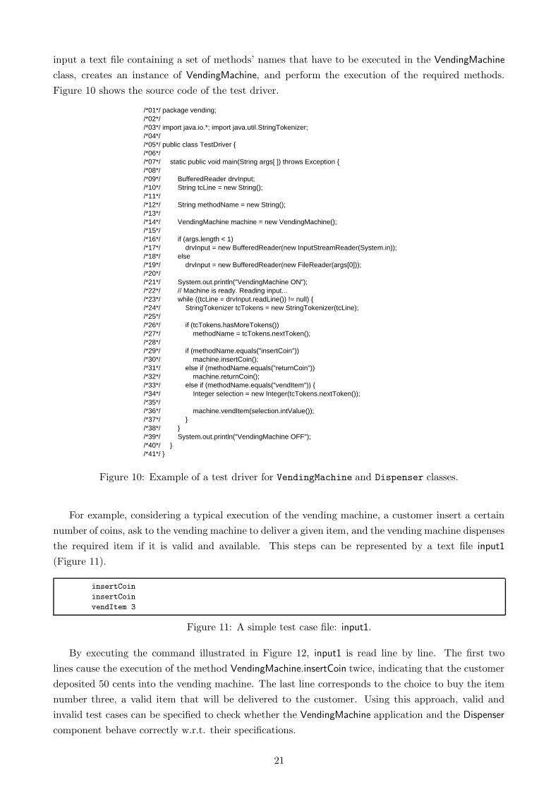
input a text file containing a set of methods’ names that have to be executed in the VendingMachine
class, creates an instance of VendingMachine, and perform the execution of the required methods.
Figure 10 shows the source code of the test driver.
/*41*/ }
/*02*//*03*/ import java.io.*; import java.util.StringTokenizer;/*04*//*05*/ public class TestDriver {/*06*//*07*/ static public void main(String args[ ]) throws Exception {/*08*//*09*/ BufferedReader drvInput;/*10*/ String tcLine = new String();/*11*//*12*/ String methodName = new String();/*13*//*14*/ VendingMachine machine = new VendingMachine();/*15*//*16*/ if (args.length < 1)/*17*/ drvInput = new BufferedReader(new InputStreamReader(System.in));/*18*/ else/*19*/ drvInput = new BufferedReader(new FileReader(args[0]));/*20*//*21*/ System.out.println("VendingMachine ON");/*22*/ // Machine is ready. Reading input.../*23*/ while ((tcLine = drvInput.readLine()) != null) {/*24*/ StringTokenizer tcTokens = new StringTokenizer(tcLine);/*25*//*26*/ if (tcTokens.hasMoreTokens())/*27*/ methodName = tcTokens.nextToken();/*28*//*29*/ if (methodName.equals("insertCoin"))/*30*/ machine.insertCoin();/*31*/ else if (methodName.equals("returnCoin"))/*32*/ machine.returnCoin();/*33*/ else if (methodName.equals("vendItem")) {/*34*/ Integer selection = new Integer(tcTokens.nextToken());/*35*//*36*/ machine.vendItem(selection.intValue());/*37*/ }/*38*/ }/*39*/ System.out.println("VendingMachine OFF");/*40*/ }
/*01*/ package vending;
Figure 10: Example of a test driver for VendingMachine and Dispenser classes.
For example, considering a typical execution of the vending machine, a customer insert a certain
number of coins, ask to the vending machine to deliver a given item, and the vending machine dispenses
the required item if it is valid and available. This steps can be represented by a text file input1
(Figure 11).
insertCoin
insertCoin
vendItem 3
Figure 11: A simple test case file: input1.
By executing the command illustrated in Figure 12, input1 is read line by line. The first two
lines cause the execution of the method VendingMachine.insertCoin twice, indicating that the customer
deposited 50 cents into the vending machine. The last line corresponds to the choice to buy the item
number three, a valid item that will be delivered to the customer. Using this approach, valid and
invalid test cases can be specified to check whether the VendingMachine application and the Dispenser
component behave correctly w.r.t. their specifications.
21
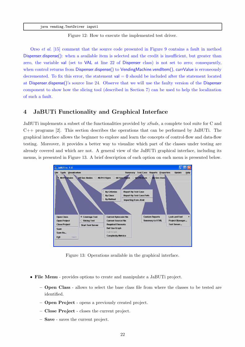
java vending.TestDriver input1
Figure 12: How to execute the implemented test driver.
Orso et al. [15] comment that the source code presented in Figure 9 contains a fault in method
Dispenser.dispense(): when a available item is selected and the credit is insufficient, but greater than
zero, the variable val (set to VAL at line 22 of Dispenser class) is not set to zero; consequently,
when control returns from Dispenser.dispense() to VendingMachine.vendItem(), currValue is erroneously
decremented. To fix this error, the statement val = 0 should be included after the statement located
at Dispenser.dispense()’s source line 24. Observe that we will use the faulty version of the Dispenser
component to show how the slicing tool (described in Section 7) can be used to help the localization
of such a fault.
4 JaBUTi Functionality and Graphical Interface
JaBUTi implements a subset of the functionalities provided by xSuds, a complete tool suite for C and
C++ programs [2]. This section describes the operations that can be performed by JaBUTi. The
graphical interface allows the beginner to explore and learn the concepts of control-flow and data-flow
testing. Moreover, it provides a better way to visualize which part of the classes under testing are
already covered and which are not. A general view of the JaBUTi graphical interface, including its
menus, is presented in Figure 13. A brief description of each option on each menu is presented below.
Figure 13: Operations available in the graphical interface.
• File Menu - provides options to create and manipulate a JaBUTi project.
– Open Class - allows to select the base class file from where the classes to be tested are
identified.
– Open Project - opens a previously created project.
– Close Project - closes the current project.
– Save - saves the current project.
22
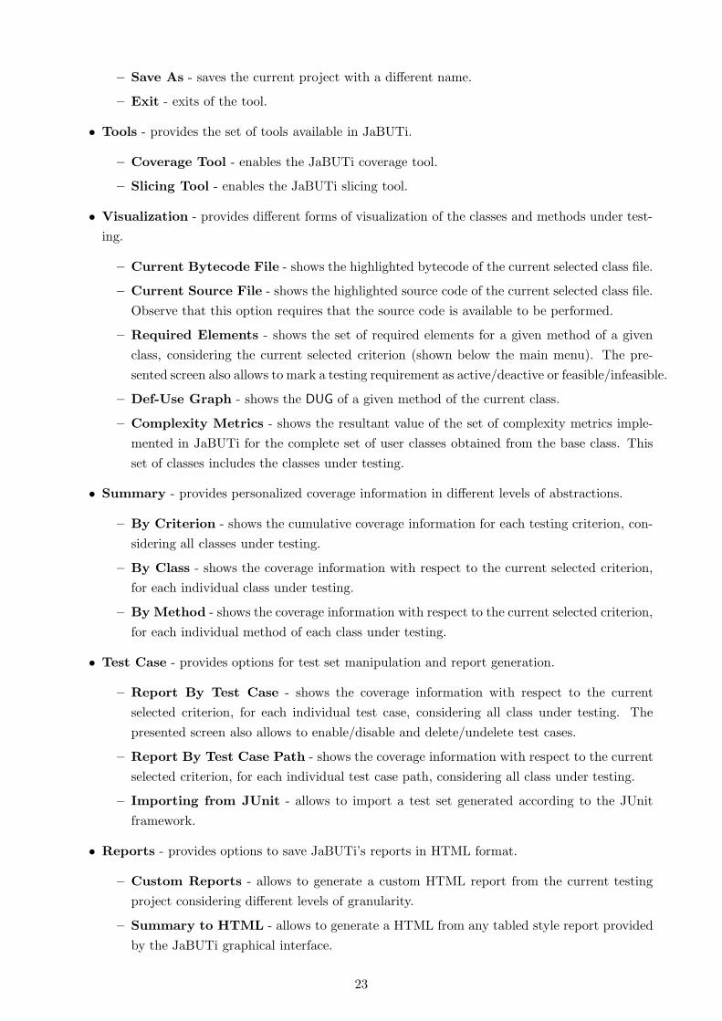
– Save As - saves the current project with a different name.
– Exit - exits of the tool.
• Tools - provides the set of tools available in JaBUTi.
– Coverage Tool - enables the JaBUTi coverage tool.
– Slicing Tool - enables the JaBUTi slicing tool.
• Visualization - provides different forms of visualization of the classes and methods under test-
ing.
– Current Bytecode File - shows the highlighted bytecode of the current selected class file.
– Current Source File - shows the highlighted source code of the current selected class file.
Observe that this option requires that the source code is available to be performed.
– Required Elements - shows the set of required elements for a given method of a given
class, considering the current selected criterion (shown below the main menu). The pre-
sented screen also allows to mark a testing requirement as active/deactive or feasible/infeasible.
– Def-Use Graph - shows the DUG of a given method of the current class.
– Complexity Metrics - shows the resultant value of the set of complexity metrics imple-
mented in JaBUTi for the complete set of user classes obtained from the base class. This
set of classes includes the classes under testing.
• Summary - provides personalized coverage information in different levels of abstractions.
– By Criterion - shows the cumulative coverage information for each testing criterion, con-
sidering all classes under testing.
– By Class - shows the coverage information with respect to the current selected criterion,
for each individual class under testing.
– By Method - shows the coverage information with respect to the current selected criterion,
for each individual method of each class under testing.
• Test Case - provides options for test set manipulation and report generation.
– Report By Test Case - shows the coverage information with respect to the current
selected criterion, for each individual test case, considering all class under testing. The
presented screen also allows to enable/disable and delete/undelete test cases.
– Report By Test Case Path - shows the coverage information with respect to the current
selected criterion, for each individual test case path, considering all class under testing.
– Importing from JUnit - allows to import a test set generated according to the JUnit
framework.
• Reports - provides options to save JaBUTi’s reports in HTML format.
– Custom Reports - allows to generate a custom HTML report from the current testing
project considering different levels of granularity.
– Summary to HTML - allows to generate a HTML from any tabled style report provided
by the JaBUTi graphical interface.
23

• Properties - provides general configuration options.
– Look and Feel - allows to change the look and feel style considering three different options:
Metal (default), Motif, and Windows.
– Project Manager... - allows to verify and change the current set of classes under testing
in the current project.
• Update - provides a visual information every time an event that affect the coverage occurs. For
example, such a button becomes red in case additional test cases are imported or appended in
the end of the trace file to indicate that a new event that affects the coverage information occurs.
As soon as it is clicked, its background color changes to grey.
• Help - provides only one option to show information about the authors/developers of JaBUTi.
JaBUTi requires the creation of a testing project, such that the tester can specify only once the
set of classes to be instrumented and tested. Section 5 describes how to create a JaBUTi’s testing
project. After having created the project, JaBUTi provides to the tester a coverage analysis tool, a
slicing tool and a static metric measure tool. The coverage analysis tool is described in Section 6.
Section 7 describes the slicing tool, and Section 8 describes the measure tool.
5 How to Create a Testing Project
In JaBUTi the testing activity requires the creation of a testing project. A testing project is charac-
terized by a file storing the necessary information about (i) the base class file, (ii) the complete set of
classes required by the base class, (iii) the set of classes to be instrumented (tested), and (iv) the set
of classes that are not under testing. Additional information, such as the CLASSPATH environment
variable necessary to run the base class is also stored in the project file, whose extension is .jbt. Dur-
ing the execution of any .class file that belongs to the set of classes under testing of a given project,
dynamic control-flow information (execution trace) is collected and saved in a separate file that has
the same name of the project file but with a different extension (.trc).
For example, considering the vending machine example, described in Section 3, the vending package
is composed by three .java files: VendingMachine.java, Dispenser.java and TestDriver.java. Suppose that
these files are saved in a directory named ~\example. The directory structure is like:
auri@AURIMRV ~
$ ls -l example/*
-rw-r--r-- 1 auri 1313 Aug 6 09:07 Dispenser.java
-rw-r--r-- 1 auri 1340 Aug 6 09:07 TestDriver.java
-rw-r--r-- 1 auri 923 Aug 6 09:07 VendingMachine.java
To compile such an application one of the following command can be used:
auri@AURIMRV ~
$ javac -d example example/*.java
or
24

auri@AURIMRV ~
$ javac -g -d example example/*.java
Observe that in the later command, the debug option is activated, thus, the generated .class files
contains more information, such as the real variable names. In this report we are using class files
compiled with the debug option.
After the Java source files have been compiled, the ~\example directory contains the following
structure:
auri@AURIMRV ~
$ ls -l example/*
-rw-r--r-- 1 auri 1313 Aug 6 09:07 Dispenser.java
-rw-r--r-- 1 auri 1340 Aug 6 09:07 TestDriver.java
-rw-r--r-- 1 auri 923 Aug 6 09:07 VendingMachine.java
example/vending:
vending:
total 6
-rw-r--r-- 1 auri 1478 Aug 6 09:49 Dispenser.class
-rw-r--r-- 1 auri 1340 Aug 6 09:49 TestDriver.class
-rw-r--r-- 1 auri 1253 Aug 6 09:49 VendingMachine.class
Now, from the generated .class files, the user can create a project using JaBUTi. To do this, the first
step is to invoke JaBUTi’s graphical interface. Supposing that JaBUTi is installed on ~\Tools\jabuti,
the command below causes the invocation of its graphical interface.
auri@AURIMRV ~/example
$ java -cp ".;..\Tools\jabuti;\
>..\Tools\jabuti\lib\BCEL.jar;\
>..\Tools\jabuti\lib\jviewsall.jar;\
>..\Tools\jabuti\lib\crimson.jar;\
>..\Tools\jabuti\lib\junit.jar" gui.JabutiGUI
Observe that the tool requires that some third-party libraries (BCEL [5] to manipulate the Java
bytecode files, ILOG JViews [10] to visualize the DUG, Crimson to manipulate XML files4, and JU-
nit [3] to import test sets.) to be included in the CLASSPATH to allow its execution. The current
directory, (“.” in our example), and the base directory of the tool (..\Tools\jabuti) are also in-
cluded to allow the correct execution of our example and the tool itself. If desired, the user can set the
CLASSPATH environment variable as a system variable that is initialized during the boot process. In
this case, to call JaBUTi’s GUI, the parameter -cp can be omitted. Figure 14 illustrates the JaBUTi’s
initial window.
To create a new project, the first step is to select a base .class file from File → Open Class menu.
A dialog window, as illustrated in Figure 15(a) appears. From this dialog window, the tester selects
the directory where the base class file is located and then select the base class file itself (Figure 15(b)).
Once the base class file is selected the tool automatically identifies the package that it belongs (if
any) and fills out the Package field with the package’s name. The Classpath should contains only the
path necessary to run the selected base class. In our example, since the tool is being called inside the
4Such a package is required when a java compiler under version 1.4.1 is used (considering the Sun compiler)).
25

Figure 14: JaBUTi main window.
~\example directory, to run vending.TestDriver it is necessary that the Classpath field contains only
the current directory, as shown in Figure 15(b).
(a) (b)
Figure 15: Open Class: (a) Selecting the directory and (b) Selecting the main class file.
By clicking the Open button (Figure 15(b)), the Project Manager window, as illustrated in Fig-
ure 16, will be displayed. From the selected base class file (TestDriver in our example) the tool identi-
fies the complete set of system and non-system class files necessary to execute TestDriver. Currently,
JaBUTi does not allows the instrumentation of system class files. Therefore, the complete set of non-
system class files (user’s classes) relate to TestDriver can be instrumented. From the Project Manager
window (left side) the user can select the class files that will be tested. At least one class file must
be selected. In our example, we select VendingMachine and Dispenser to be instrumented. TestDriver
was not selected since it is only the driver that allows the tester to observe whether the behavior of
VendingMachine and Dispenser are correct with respect to their specification.
Moreover, the tester must give a name to the project being created (vending.jbt in our example) by
clicking on the Select button. By clicking on the Ok button, JaBUTi creates a new project (vending.jbt
26

Figure 16: Selecting the class files to be tested.
in our example), constructs the DUG for each method of each class under testing, derives the complete
set of testing requirements for each criterion, calculates the weight of each testing requirement, and
presents the bytecode of a given class under testing. By creating a project, the tester does not need
to go through this entire process again if he/she intends to test the same set of class files. Next time,
he/she can just go to File → Open Project menu option and reload a previously saved project.
Once the project is created, the tester just need to open it and the tool automatically detects
the classes that compose it. JaBUTi can be used for analyzing the coverage of a given class file, for
debugging the class file using the slice tool and for collecting static metrics information. JaBUTi also
allows the visualization of the Def-Use Graph (DUG) of each method in a given class file as well as
the visualization of the source code, when available. Different kinds of testing reports can also be
generated considering different levels of abstraction. The following sections describe these features in
detail.
6 How to use JaBUTi as a Coverage Analysis Tool
By default, the tool displays the bytecode instead of the Java source code, since the source code may
not be available. The user can use the Visualization menu to change the display to show the bytecode
or source code, as well as the DUG of each method in the current class. As can be observed in
Figure 17, JaBUTi uses different colors to provide hints to the tester to ease the test generation. The
different colors represent requirements with different weights, and the weights are calculated based on
dominator and super-block analysis [1]. Informally, the weight of a testing requirement corresponds
to the number of testing requirements that will be covered if this particular requirement is covered.
Therefore, covering the requirement with the highest weight will increase the coverage faster5. The
weight schema is used in all views of a given class/method: bytecode, source code and DUG. Figure 17
shows part of the colored bytecode of the Dispenser.dispense() method before the execution of any
test case and Figure 18 part of the DUG of the same method. The different colors correspond to the
weight of each node, considering the All-Pri-Nodes criterion. Observe that the color bar (below the
main menu) goes from white (weight 0) to red (weight 13).
5Observe that the weight is calculated considering only the coverage information and should be seen as hints. It doesnot take into account, for instance, the complexity or the criticality of a given part of the program. The tester, basedon his/her experience may desire to cover first a requirement with a lower weight but that has a higher complexity orcriticality and then, after recomputing the weights, uses the hints provided by JaBUTi to increase the coverage faster.
27

In our example, observe that the node 105 in Figure 18, composed by bytecote instructions from
105 to 112 (Figure 17), is one of the highest weight. In this way, a test case that exercises node 105
increases the coverage in at least 13. A requirement with weight zero is a covered requirement and it
is painted in white.
Although the source code is not required by JaBUTi, when it is available, the corresponding source
code of the current class can also be displayed in colors, mapped back from the bytecode, facilitating
the identification of which part of the code should be covered first. For example, Figure 19 shows that
the statement on line 24 has the highest priority w.r.t. the All-Pri-Nodes criterion. By covering this
particular node, at least 13 other nodes will be covered.
Figure 17: Dispenser.dispenser method: bytecode prioritized w.r.t. All-Pri-Nodes criterion.
Considering the DUG presented in Figure 18, it can be observed that there are two different
types of nodes, represented by single and double line circles. As described in Section 2.2, double
circles represent call nodes, i.e., nodes where exists a method call to another method. This nodes
are identified since we intend to extend our tool to deal, not only with intra-method testing criteria,
but also with inter-method testing criteria that requires the identification of the relationship among
methods. Bold circles, not visible in Figure 18, represent exit nodes. Observe that methods in Java
can have more that one exit node due to the exception-handling mechanism. All the other nodes are
represented as single line circles. We also have two different types of edges to represent the “normal”
control-flow (continuous line – Primary Edges) and exception control-flow (dashed lines – Secondary
Edges). Figure 18 does not contain exception edges. Primary and secondary edges can be hidden by
deselecting the Show Primary and Show Secondary Edges check box, respectively. The node information
shown when the cursor is moved onto the node, as illustrated in Figure 18, can also be disabled by
deselecting the Show Node Info check box.
28

Figure 18: Dispenser.dispenser method: DUG prioritized w.r.t. All-Pri-Nodes criterion.
Figure 19: Dispenser.dispenser method: source code prioritized w.r.t. All-Pri-Nodes criterion.
6.1 How the testing requirements are highlighted
As can be observed above the main menu in Figure 17, JaBUTi supports the application of six
structural testing criteria, as described in Section 2.3: All-Pri-Nodes, All-Sec-Nodes, All-Pri-Edges,
All-Sec-Edges, All-Pri-Uses, and All-Sec-Uses. Depending on which criterion is active, the bytecode,
29
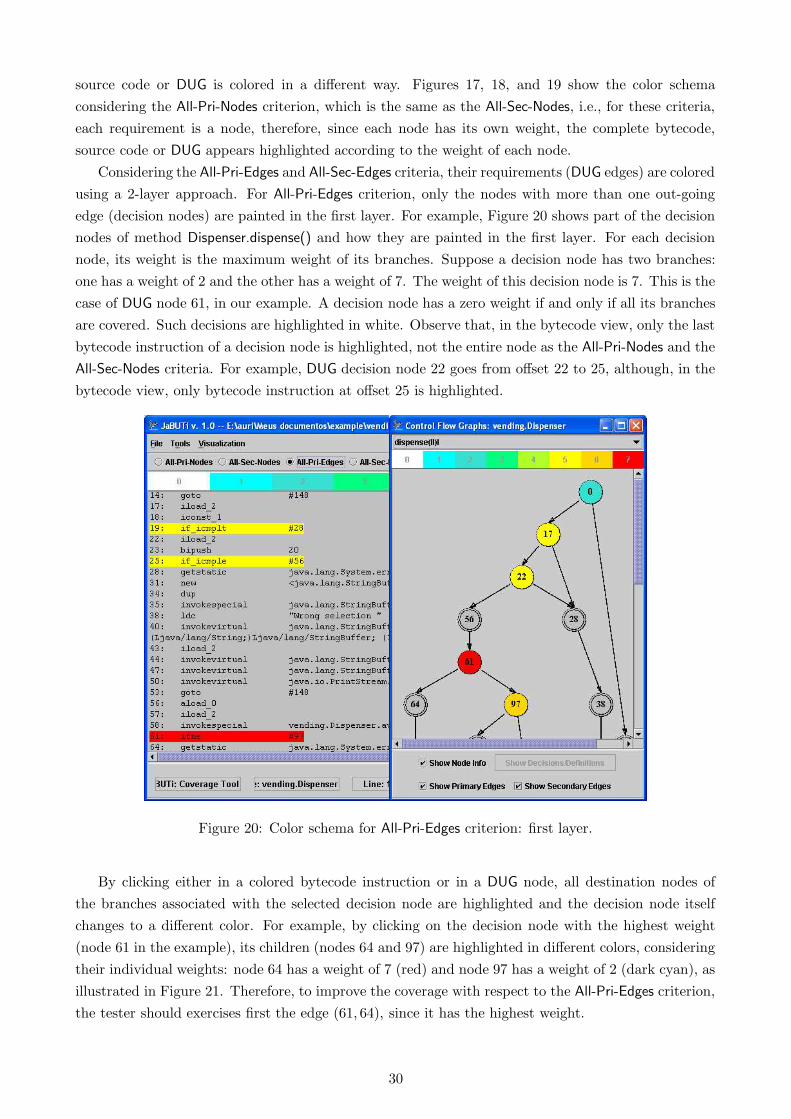
source code or DUG is colored in a different way. Figures 17, 18, and 19 show the color schema
considering the All-Pri-Nodes criterion, which is the same as the All-Sec-Nodes, i.e., for these criteria,
each requirement is a node, therefore, since each node has its own weight, the complete bytecode,
source code or DUG appears highlighted according to the weight of each node.
Considering the All-Pri-Edges and All-Sec-Edges criteria, their requirements (DUG edges) are colored
using a 2-layer approach. For All-Pri-Edges criterion, only the nodes with more than one out-going
edge (decision nodes) are painted in the first layer. For example, Figure 20 shows part of the decision
nodes of method Dispenser.dispense() and how they are painted in the first layer. For each decision
node, its weight is the maximum weight of its branches. Suppose a decision node has two branches:
one has a weight of 2 and the other has a weight of 7. The weight of this decision node is 7. This is the
case of DUG node 61, in our example. A decision node has a zero weight if and only if all its branches
are covered. Such decisions are highlighted in white. Observe that, in the bytecode view, only the last
bytecode instruction of a decision node is highlighted, not the entire node as the All-Pri-Nodes and the
All-Sec-Nodes criteria. For example, DUG decision node 22 goes from offset 22 to 25, although, in the
bytecode view, only bytecode instruction at offset 25 is highlighted.
Figure 20: Color schema for All-Pri-Edges criterion: first layer.
By clicking either in a colored bytecode instruction or in a DUG node, all destination nodes of
the branches associated with the selected decision node are highlighted and the decision node itself
changes to a different color. For example, by clicking on the decision node with the highest weight
(node 61 in the example), its children (nodes 64 and 97) are highlighted in different colors, considering
their individual weights: node 64 has a weight of 7 (red) and node 97 has a weight of 2 (dark cyan), as
illustrated in Figure 21. Therefore, to improve the coverage with respect to the All-Pri-Edges criterion,
the tester should exercises first the edge (61, 64), since it has the highest weight.
30
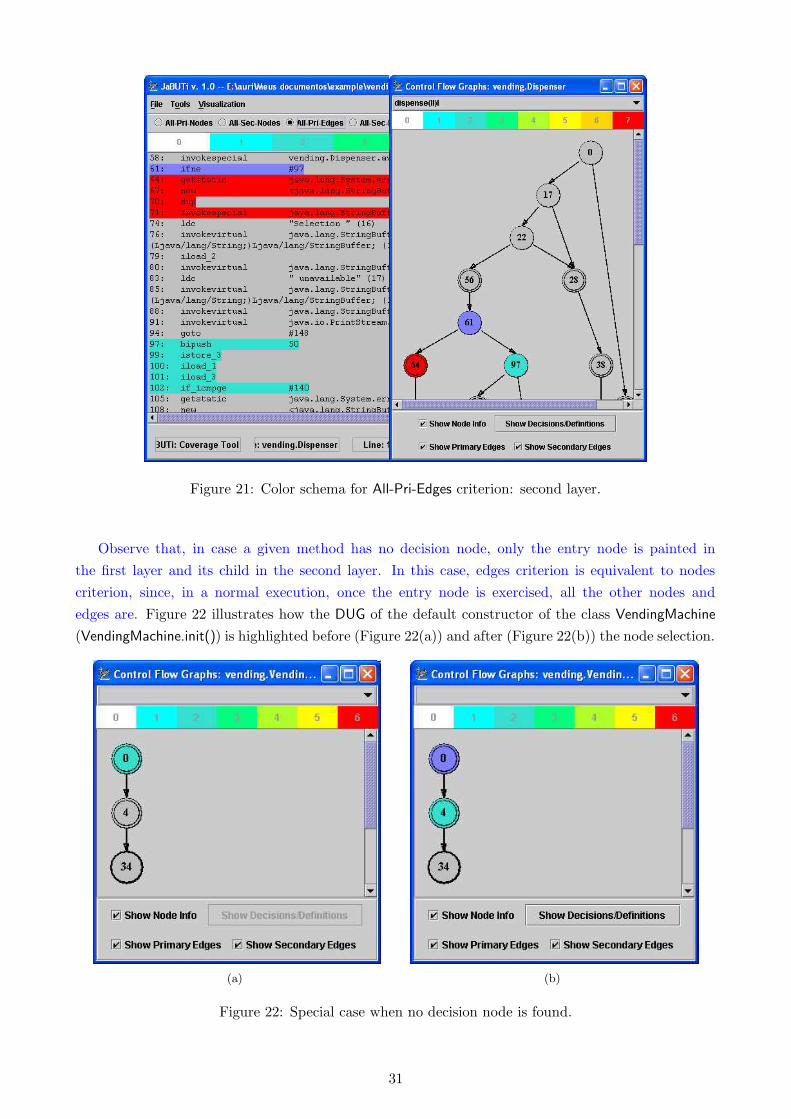
Figure 21: Color schema for All-Pri-Edges criterion: second layer.
Observe that, in case a given method has no decision node, only the entry node is painted in
the first layer and its child in the second layer. In this case, edges criterion is equivalent to nodes
criterion, since, in a normal execution, once the entry node is exercised, all the other nodes and
edges are. Figure 22 illustrates how the DUG of the default constructor of the class VendingMachine
(VendingMachine.init()) is highlighted before (Figure 22(a)) and after (Figure 22(b)) the node selection.
(a) (b)
Figure 22: Special case when no decision node is found.
31

For the All-Sec-Edges criterion, the same approach is used. In the first layer, all nodes with at
least one secondary out-going edge, instead of decision nodes, are highlighted. For each such a node,
its weight is the maximum weight of its branches and a node with more that one secondary out-going
edge is considered covered (zero weight) if and only if all exception-handler associated with such a
node is covered.
Figure 23 and 24 shows the first and the second layer of Dispenser.available() method, considering
the All-Sec-Edges criterion, respectively. In this example, in the first layer, all highlighted nodes has
the same weigh (one) since it has only one valid exception-handler for the entire method. In the
bytecode view, only the last bytecode instruction of each node is highlighted. For example, node 20
goes from offset 20 to 26, therefore, bytecode instruction at offset 26 is highlighted. By clicking on
such an instruction or on the DUG node 20, Figure 24 shows the resultant color schema of the second
layer.
Figure 23: Color schema for All-Sec-Edges criterion: first layer.
Similar to a decision and its branches are displayed, a 2-layer representation is also used to display
def-use associations for the All-Pri-Uses and All-Sec-Uses criteria. The first layer shows all the definitions
which have at least one c-use or p-use association. Clicking on a definition goes to the second layer
displaying all c-use and p-use associated with the selected definition. For each definition, its weight
is the maximum weight of its c-uses or p-uses. For example, suppose a definition has three def-use
associations, one c-use and two p-uses, and the weights of these associations are 5, 3 and 7, respectively.
The weight of this definition is 7. A definition has a zero weight if and only if all its c-uses and p-uses
are covered. Such definitions are displayed with a white background.
Since even in the bytecode, more than one variable may be defined in the same offset, if desired,
by clicking with the right mouse button over a definition point (bytecode offset, source code line or
DUG node), a pop-up menu is opened showing all the variables defined in that point such that it is
32
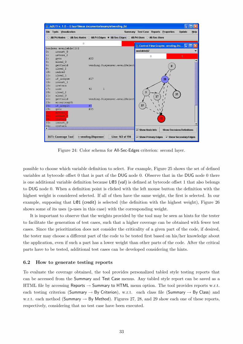
Figure 24: Color schema for All-Sec-Edges criterion: second layer.
possible to choose which variable definition to select. For example, Figure 25 shows the set of defined
variables at bytecode offset 0 that is part of the DUG node 0. Observe that in the DUG node 0 there
is one additional variable definition because L@3 (val) is defined at bytecode offset 1 that also belongs
to DUG node 0. When a definition point is clicked with the left mouse button the definition with the
highest weight is considered selected. If all of then have the same weight, the first is selected. In our
example, supposing that L@1 (credit) is selected (the definition with the highest weight), Figure 26
shows some of its uses (p-uses in this case) with the corresponding weight.
It is important to observe that the weights provided by the tool may be seen as hints for the tester
to facilitate the generation of test cases, such that a higher coverage can be obtained with fewer test
cases. Since the prioritization does not consider the criticality of a given part of the code, if desired,
the tester may choose a different part of the code to be tested first based on his/her knowledge about
the application, even if such a part has a lower weight than other parts of the code. After the critical
parts have to be tested, additional test cases can be developed considering the hints.
6.2 How to generate testing reports
To evaluate the coverage obtained, the tool provides personalized tabled style testing reports that
can be accessed from the Summary and Test Case menus. Any tabled style report can be saved as a
HTML file by accessing Reports → Summary to HTML menu option. The tool provides reports w.r.t.
each testing criterion (Summary → By Criterion), w.r.t. each class file (Summary → By Class) and
w.r.t. each method (Summary → By Method). Figures 27, 28, and 29 show each one of these reports,
respectively, considering that no test case have been executed.
33
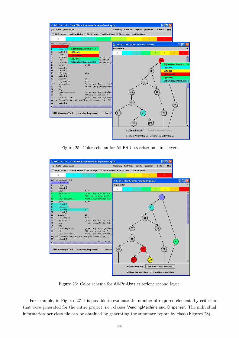
Figure 25: Color schema for All-Pri-Uses criterion: first layer.
Figure 26: Color schema for All-Pri-Uses criterion: second layer.
For example, in Figures 27 it is possible to evaluate the number of required elements by criterion
that were generated for the entire project, i.e., classes VendingMachine and Dispenser. The individual
information per class file can be obtained by generating the summary report by class (Figures 28).
34
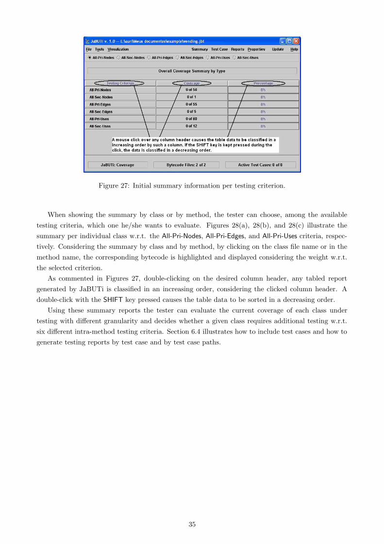
Figure 27: Initial summary information per testing criterion.
When showing the summary by class or by method, the tester can choose, among the available
testing criteria, which one he/she wants to evaluate. Figures 28(a), 28(b), and 28(c) illustrate the
summary per individual class w.r.t. the All-Pri-Nodes, All-Pri-Edges, and All-Pri-Uses criteria, respec-
tively. Considering the summary by class and by method, by clicking on the class file name or in the
method name, the corresponding bytecode is highlighted and displayed considering the weight w.r.t.
the selected criterion.
As commented in Figures 27, double-clicking on the desired column header, any tabled report
generated by JaBUTi is classified in an increasing order, considering the clicked column header. A
double-click with the SHIFT key pressed causes the table data to be sorted in a decreasing order.
Using these summary reports the tester can evaluate the current coverage of each class under
testing with different granularity and decides whether a given class requires additional testing w.r.t.
six different intra-method testing criteria. Section 6.4 illustrates how to include test cases and how to
generate testing reports by test case and by test case paths.
35
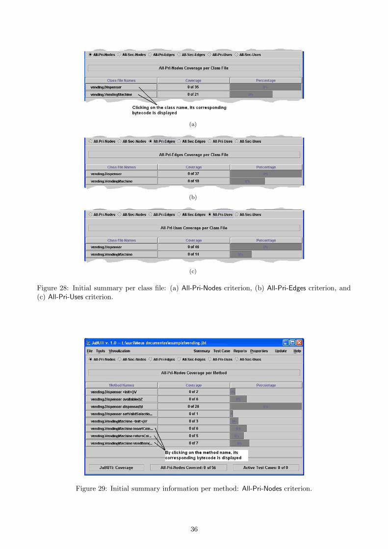
(a)
(b)
(c)
Figure 28: Initial summary per class file: (a) All-Pri-Nodes criterion, (b) All-Pri-Edges criterion, and(c) All-Pri-Uses criterion.
Figure 29: Initial summary information per method: All-Pri-Nodes criterion.
36

6.3 How to generate an HTML version of a JaBUTi report
As mentioned above, any kind of tabled report presented in JaBUTi’s graphical interface can be saved
as an HTML file through the Reports → Summary to HTML menu option. For example, Figure 30(a)
shows how to create a summary-by-criterion.html file, corresponding to the current JaBUTi screen.
Figure 30(b) illustrates the generated HTML file in a browser window. In this way the tester can
collect and save different testing report showing the evolution of the testing activity.
(a) (b)
Figure 30: Example of an HTML report generated by JaBUTi.
A different kind of report can be generated through the Reports → Custom Report menu option.
By selecting this option, a dialog windows, as illustrated in Figure 31(a), appears and the tester can
choose the level of information that will be saved in a HTML file. Observe that to save information
at method level it is also required to save information about the class and project level, since the
information is saved hierarchically. Part of a complete report for the entire project is presented in
Figure 31(b).
37

(a) (b)
Figure 31: Example of custom HTML report generated by JaBUTi for the entire project.
38

6.4 How to include a test case
JaBUTi is designed to support test case set adequacy evaluation and to provide guidance in test case
selection. If there is a previously developed test set, e.g. a functional test set, such a test set can be
evaluated against the structural testing criteria implemented by JaBUTi. This allows the tester to
check, for example, whether all instructions/statements are executed by a particular test set. If they
are not yet executed, additional test cases can be developed to improve the quality of the previous
test set.
On the other hand, if there is no previous test set available, the tester can use the hints provided by
the tool to create test cases aiming at to cover the different testing requirements generated by JaBUTi
based on its structural criteria. Once the test criteria can be applied incrementally, the tester can
start by developing an adequate test set w.r.t. the All-Pri-Nodes criterion, then, if necessary, to develop
additional test cases to evolve the All-Pri-Nodes-adequate test set to a All-Pri-Edges-adequate test set,
and later, if necessary, to develop additional test cases to evolve it to an All-Pri-Uses-adequate test
set. All these criteria, prefixed by All-Pri-, are related with the normal program execution. If desired,
the tester can check the coverage of the exception-handling mechanism, by using the All-Sec-Nodes,
All-Sec-Edges and All-Sec-Uses criteria. The idea is to use these criteria incrementally to reduce their
complexity and also to allow the tester to deal with the cost and time constraints.
JaBUTi allows to include test cases in two different ways: 1) using the JaBUTi’s class loader; or 2)
importing from a JUnit test set. The first is done by a command line application (probe.ProberLoader,
the JaBUTi’s class loader). This command line application extends the default Java class loader [11]
such that, from a given testing project, it identifies which classes should be instrumented before to
be loaded and executed. By detecting that a given class belongs to the set of classes under testing,
JaBUTi’s class loader inserts the probes to collect the execution trace and then loads the instrumented
class file to be executed. The trace information w.r.t. the current execution is appended in a trace
file with the same name of the testing project but with the extension .trc instead of .jbt.
For example, the test case file input1, presented in Figure 32, touches the testing requirement
(considering the All-Pri-Nodes criterion) with the highest weight illustrated in Figure 19 and also
reveals a fault contained in the Dispenser component. Such a test case will be used in the next section
to show how to use JaBUTi to ease the fault localization.
auri@AURIMRV ~/example
$ cat input1
insertCoin
vendItem 3
Figure 32: Example of test case file.
The command line in Figure 33(a) shows the output of the vending.TestDriver when executed by
the default class loader. Figure 33(b) shows the resultant output when vending.TestDriver is executed
using the JaBUTi’s class loader. The execution of the command as shown in Figure 33(b) causes the
vending.trc to be generated/updated with the execution path of test case file input1.
Considering Figure 33(b), observe that the CLASSPATH variable is set containing all the paths
necessary to run the JaBUTi’s class loader and also the vending machine example. The next pa-
rameter, probe.ProberLoader, is the name of the JaBUTi’s class loader. It demands two parameters
to execute: the name of the project (-P vending.jbt), and the name of the base class to be executed
(vending.TestDriver). In our example, since vending.TestDriver requires one parameter to be executed,
39

auri@AURIMRV ~/example
$ java -cp "." vending.TestDriver input1
VendingMachine ON
Current value = 25
Enter 25 coins
Current value = -25
VendingMachine OFF
auri@AURIMRV ~/example
$ java -cp ".;..\Tools\jabuti;\
>..\Tools\jabuti\lib\BCEL.jar;\
>..\Tools\jabuti\lib\crimson.jar;\
> probe.ProberLoader -P vending.jbt \
> vending.TestDriver input1
Project Name: vending.jbt
Trace File Name: vending.trc
Processing File vending.jbt
VendingMachine ON
Current value = 25
Enter 25 coins
Current value = -25
VendingMachine OFF
(a) (b)
Figure 33: vending.TestDriver output: (a) default class loader, and (b) JaBUTi class loader.
this parameter is also provided (input1). During the execution of vending.TestDriver, VendingMachine
and Dispenser classes are required to be loaded. From the project file (vending.jbt) the JaBUTi’s class
loader detects that these class files have to be instrumented before to be executed. The instrumentation
is performed on-the-fly every time the probe.ProberLoader is invoked.
The resultant execution trace information, corresponding to the execution of the test case input1,
is appended in the end of the trace file vending.trc . Every time the size of the trace file increase,
the Update button in the JaBUTi’s graphical interface becomes red, indicating that the coverage
information can be updated considering the new test case(s). Figure 34 illustrates this event.
Figure 34: Update button with a different background color: new test case(s) available.
By clicking on the Update button, JaBUTi imports the new test case(s), empties the trace file
vending.trc and updates the coverage information and the weights for each testing criterion. For
example, after the importation of test case input1, the weight of the Java source code w.r.t. the
All-Pri-Nodes criterion changed as illustrated in Figure 35.
Comparing the updated source of Figure 35 (front) with the one presented in Figure 35 (back) it can
be observed that the requirement with the highest changed from source line 24 (now covered – painted
in white) to source line 20. Considering the entire project, Figure 36(b) shows the updated coverage for
each method in the Dispenser and VendingMachine classes w.r.t. the All-Pri-Nodes criterion. Observe
that input1 covered 13 primary nodes (50%) of Dispenser.dispense method and 36 of 56 primary nodes
(64%) considering the entire project. By accessing the Test Case → Report by Test Case menu option,
the tester can visualize the coverage of the entire project by test case, as illustrated in Figure 36(a).
If desired, the tester can develop additional test cases to improve the coverage w.r.t. All-Pri-Nodes
criterion. For example, besides input1, Table 5 shows four additional test cases developed to improve
the coverage of such a criterion.
40

Figure 35: Dispenser.dispenser() method before and after the weight’s updating w.r.t. All-Pri-Nodescriterion.
(a) Report by test case (b) Summary by Method
Figure 36: Updated coverage after test case input1.
JaBUTi also allows to visualize the coverage of a given test case by each execution path
(Test Case → Report by Test Case Path), i.e., during the execution of a single test case, several meth-
ods can be executed, and each one can be executed several times. Each method execution is considered
as a different execution path. Therefore, a test case is composed by zero or more test paths, one for
each individual method execution. Figure 37 shows this kind of report. For instance, test case 0001
is composed by six paths numbered from 0001-0 to 0001-5. Besides the coverage by path, the report
also shows additional information about each path, collected during the execution.
41

Table 5: Adequate test set to the Dispenser component.
Name Content Correct output
input1 insertCoin novendItem 3
input2 insertCoin yesvendItem 18
input3 insertCoin yesinsertCoinvendItem 25
input4 vendItem 3 yes
input5 insertCoin yesinsertCoinvendItem 3
Figure 37: Testing report by execution path w.r.t. the All-Pri-Nodes criterion.
42
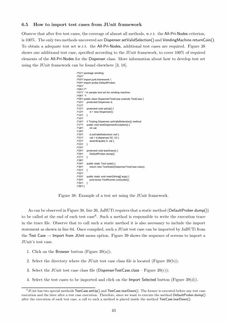
6.5 How to import test cases from JUnit framework
Observe that after five test cases, the coverage of almost all methods, w.r.t. the All-Pri-Nodes criterion,
is 100%. The only two methods uncovered are Dispenser.setValidSelection() and VendingMachine.returnCoin().
To obtain a adequate test set w.r.t. the All-Pri-Nodes, additional test cases are required. Figure 38
shows one additional test case, specified according to the JUnit framework, to cover 100% of required
elements of the All-Pri-Nodes for the Dispenser class. More information about how to develop test set
using the JUnit framework can be found elsewhere [3, 18].
/*36*/ }
/*02*//*03*/ import junit.framework.*;/*04*/ import probe.DefaultProber;/*05*//*06*/ /**/*07*/ * A sample test set for vending machine./*08*/ *//*09*/ public class DispenserTestCase extends TestCase {/*10*/ protected Dispenser d;/*11*//*12*/ protected void setUp() {/*13*/ d = new Dispenser();/*14*/ }/*15*//*16*/ // Testing Dispenser.setValidSelection() method/*17*/ public void testDispenserException() {/*18*/ int val;/*19*//*20*/ d.setValidSelection( null );/*21*/ val = d.dispense( 50, 10 );/*22*/ assertEquals( 0, val );/*23*/ }/*24*//*25*/ protected void tearDown() {/*26*/ DefaultProber.dump();/*27*/ }/*28*//*29*/ public static Test suite() {/*30*/ return new TestSuite(DispenserTestCase.class);/*31*/ }/*32*//*33*/ public static void main(String[] args) {/*34*/ junit.textui.TestRunner.run(suite());/*35*/ }
/*01*/ package vending;
Figure 38: Example of a test set using the JUnit framework.
As can be observed in Figure 38, line 26, JaBUTi requires that a static method (DefaultProber.dump())
to be called at the end of each test case6. Such a method is responsible to write the execution trace
in the trace file. Observe that to call such a static method it is also necessary to include the import
statement as shown in line 04. Once compiled, such a JUnit test case can be imported by JaBUTi from
the Test Case → Import from JUnit menu option. Figure 39 shows the sequence of screens to import a
JUnit’s test case.
1. Click on the Browser button (Figure 39(a));
2. Select the directory where the JUnit test case class file is located (Figure 39(b));
3. Select the JUnit test case class file (DispenserTestCase.class – Figure 39(c));
4. Select the test cases to be imported and click on the Import Selected button (Figure 39(d)).
6JUnit has two special methods TestCase.setUp() and TestCase.tearDown(). The former is executed before any test caseexecution and the later after a test case execution. Therefore, since we want to execute the method DefaultProber.dump()after the execution of each test case, a call to such a method is placed inside the method TestCase.tearDown().
43

(a) (b)
(c) (d)
Figure 39: Sequence of Steps to Import a JUnit Test Cases.
In our example (Figure 39(d)), there is only one test case to be imported. Observe that the name
of such a test case testDispenserException is highlighted in green. This is because JUnit framework
provides several assertions statements, like the one at line 22 of Figure 38, that allows to verify if the
test case’s output is according to its specification or not. We use a green background color to represent
test cases that behave accordantly to their specifications and a red background color to represent the
ones that do not.
As soon as JaBUTi detects a new test case execution trace is appended in the end of the trace
file, the Update button becomes red indicating that the coverage needs to be updated. Updated the
coverage information, Figure 40 shows the summary report by methods and the corresponding coverage
w.r.t. the All-Pri-Nodes criterion. The summary report by criterion can be seen in Figure 41
After the execution of these six test cases, all methods of the Dispenser component are 100%
covered w.r.t. the All-Pri-Nodes criterion, but this test set is adequate to the VendingMachine class.
More specifically, the VendingMachine.returnCoin method is not covered yet. So, after six test cases, the
coverage of the entire project w.r.t. All-Pri-Nodes and All-Sec-Nodes are 91% and 100%, respectively.
The coverage for the All-Pri-Edges and the All-Sec-Edges are 89% and 20%, respectively, and the
coverage for the All-Pri-Uses and All-Sec-Uses are 81% and 25%, respectively.
44

Figure 40: Updated coverage after six test cases w.r.t. the All-Pri-Nodes criterion.
Figure 41: Updated coverage after six test cases w.r.t. all criteria.
Independently of the number of test cases available, if desired, the tester can enable/disable any
combination of test cases by accessing the Test Case → Report By Test Case menu option and choosing
which test case should be enabled/disabled. Once a different subset of test cases are enabled/disabled
all the coverage information should be updated by clicking on the Update button. Figure 42(a) shows
the complete test set with all test cases enabled. Figure 42(b) shows the updated coverage considering
only the test cases number 2 and 5.
Using the resource of activate/deactivate test cases, the tester can evaluate how the coverage
changes, considering different combinations of test case. Moreover, besides activate/deactivate test
cases, the tester can also mark a test case to be deleted. Once a test case is marked to be deleted it
is only logically deleted. Such a test case is physically deleted when the project is saved and closed.
While the project is not closed, a test case marked as deleted can be undeleted.
45

(a) (b)
Figure 42: Summary by test case: (a) all enabled, and (b) 2 and 5 enabled.
46

6.6 How to mark a testing requirement as infeasible
When applying structural testing criteria, one problem is to identify infeasible testing requirements
since, in general, it is an undecidable problem. Vergilio [25] developed some heuristics to automatically
determine infeasible testing requirements but such heuristics are not yet implemented in JaBUTi.
Therefore, it is a responsibility of the tester to identify such infeasible testing requirements.
By accessing the Visualization → Required Elements menu option, JaBUTi allows the tester to visu-
alize and mark testing requirements as infeasible, as well as activate/deactivate testing requirements.
Once a testing requirement is marked as infeasible or deactivated, the Update button becomes red
indicating that the coverage information should be updated to reflect such a change. For example,
Figure 43 shows part of the testing requirements for the method Vending.returnCoin() method, consid-
ering the All-Pri-Nodes criterion.
Figure 43: Dispenser.dispense() required elements for the All-Pri-Nodes criterion.
Considering Figure 43, two uncovered requirements were marked as infeasible, primary nodes 7
and 26. Since the tester can mark erroneously a testing requirement as infeasible, in case such a testing
requirement is covered in the future by an additional test case, the tool indicates such a inconsistency,
highlighting the infeasible check box of a covered testing requirement in red, as illustrated in Figure 44.
In this case, primary node 26 is covered by the new test case added to exercise the Vending.returnCoin()
method, so node 26 is feasible.
During the importation of a given test case, the tester has to check whether the obtained output
is correct w.r.t. the specification. As can be observed in Table 5, only test case number 1 does not
behave according to the specification. Once any discrepancy is detected, the fault should be localized
and corrected. One alternative for fault localization is slicing. In the next section we describe how to
use the slicing tool implemented in JaBUTi to help the fault localization and smart debugging.
47

Figure 44: Dispenser.dispense() infeasible requirements erroneously identified.
48

7 How to use JaBUTi as a Slicing Tool
The JaBUTi slicing tool is available through the Tools → Slicing Tool menu option. The slicing tool
implements only a simple heuristic based on control-flow information. As a future work, additional
heuristics will be implemented considering not only control-flow but also data-flow information.
By changing to the slicing tool, the tester has to choose, among the test cases, the ones that cause
the fault and the ones that do not reveal the fault. Based on the execution path of the failed and
succeed test cases, the tool highlights the part of the code more probable to contain the fault.
JaBUTi uses a simple dynamic slice criterion, based on control-flow information, to identify a
subset of statements more probable to contain the fault. The idea is (1) to compute the failed set FS
of BG nodes (the execution path) of a failed test case, which includes all statements executed by the
failed test case, (2) to compute the succeed set SS of BG nodes considering succeed test case(es), and
(3) to calculate the difference and the intersection of these sets to prioritize the statements executed
by the failed test case.
Using such an approach, instead of the complete set of BG nodes N (which represents all statements
of a method), the tester has only to consider the subset of BG nodes present in FS , since the other
BG nodes contains the statements not executed by the failed test case and cannot contain the fault.
Moreover, considering the subset of nodes executed by the succeed test cases, the most probably
location of the fault is in the statements executed by the failed test case but not executed by the
succeed test cases, i.e., the subset FS \ SS . Thus, such a subset of statements has a highest priority
and should be analyzed first. If the fault is not located on this subset, due to data dependence that
can lead to a data-flow dependent fault, the tester has to analyze the other statements executed by
both the failed and by the succeed test cases, i.e., the subset FS ∩ SS. In this way, we can provide
an incremental search for the fault, trying to reduce the time and the cost to locate the fault in a
program.
For example, consider the BG presented in Figure 6. N is the complete set of BG nodes (N =
{0, 15, 34, 43, 54, 54.82, 60, 60.82, 74, 74.82, 79, 91, 97}). Suppose a failed test case that goes though BG
nodes FS = {0, 34, 15, 34, 43, 54, 54.82, 91, 97} and a successful test case that goes trough BG nodes
SS = {0, 34, 43, 60, 60.82, 91, 97}. The most probably locations for the fault are in the statements in
nodes 15, 54 or 54.82, since they are only executed by the failure test case (FS \ SS). If the fault is
not located on such statements, it will be found in the other statements that compose the BG nodes
0, 34, 43, 91 and 97 (FS ∩ SS). All the other BG nodes have not to be analyzed.
The approach described above is based only on control-flow information. The success of such an
approach depends on which test cases are selected as the successful test cases. It is important to select
successful test cases that execute the related functionalities of the program as the ones executed by
the failure test case. In this way, the difference between the two sets FS and SS will result in subset
with a few BG nodes, reducing the number of statements that have to be analyzed first.
In our Vending Machine example, test case 0001 reveals the fault and test case 0006 does not. The
tester can first select only the failed test case, as illustrated in Figure 45(a), and checks the execution
path of this test case as illustrated in Figure 46(a). The red lines indicate the statements that are
executed by the failed test case and the white lines indicates the statements not executed. Since there
is a fault, it must be located among these red statements.
After having observed the failed test case execution path, the tester can enable one or more
additional succeed test cases (Figure 45(b)), such that the tool can identify, among the statements
49

(a) (b)
Figure 45: Slicing tool test case selection: (a) only the failed test case, and (b) a failed and a succeedtest cases.
executed ny the failed test case, the dice more probable to contain the fault (statements only executed
by the failed test case) and the ones less probable (the ones executed for both the failed and the
succeed test cases.) Figure 46(b) shows in yellow (weight 1) the statements touched by test cases
number 0001 and 0006 and in red (weight 2) the statements only executed by test case number 0001.
The rationale of such an approach is that, in theory, the fault is more probable to be located at the
statements executed only by the failed test case. Although, it can happen that the fault is localized in
other than the red statements, but the red points can be used at least as a good starting point, trying
to reduce the search space for fault localization.
Once the fault is located and corrected, the testing activity is restarted by creating a new project
to revalidate the corrected program. In this case, previous test sets can be used to revalidate the
behavior of the new program and also to check if new faults were not introduced by the changes.
(a) (b)
Figure 46: Highlighted execution path: (a) fail test case execution path, and (b) fail test case executionpath intersected by the success test case execution path.
50

8 How to use the JaBUTi’s Static Metrics Tool
Adicionalmente, na Secao 8.3, a metrica que avalia a complexidade ciclomatica de McCabe [17] de
cada metodo tambem foi implementada para identificar os metodos de “maior” complexidade dentro
de uma dada classe.
8.1 LK’s Metrics Applied to Classes
8.1.1 NPIM – Number of public instance methods in a class
Metrica calculada atraves da contagem do numero de metodos de instancia publicas na classe.
8.1.2 NIV – Number of instance variables in a class
Metrica calculada atraves da contagem do numero de variaveis de instancia na classe, o que inclui as
variaveis public, private e protected disponıveis para as instancias.
8.1.3 NCM – Number of class methods in a class
Metrica calculada atraves da contagem do numero de metodos static na classe.
8.1.4 NCV – Number of class variables in a class
Metrica calculada atraves da contagem do numero de variaveis static na classe.
8.1.5 ANPM – Average number of parameters per method
Metrica calculada atraves da divisao entre o somatorio do numero de parametros de cada metodo da
classe pelo numero total de metodos da classe.
Variacao: numero maximo de parametros em um metodo da classe.
8.1.6 AMZ – Average method size
Metrica calculada atraves da divisao entre a soma do numero de linhas de codigo dos metodos da
classe pelo numero de metodos na classe (soma dos metodos instancia e classe).
Variacoes: media do numero de instrucoes do bytecode e tamanho do bytecode.
8.1.7 UMI – Use of multiple inheritance
Como a heranca multipla nao se aplica a linguagem JAVA sera definida uma variacao a esta metrica.
Variacao: numero de interfaces implementadas pela classe (Number of interfaces implemented -
NINI).
8.1.8 NMOS – Number of methods overridden by a subclass
Metrica calculada atraves da contagem do numero de metodos definidos na subclasse com o mesmo
nome de metodos de sua superclasse.
51

8.1.9 NMIS – Number of methods inherited by a subclass
Metrica calculada atraves da contagem do numero de metodos herdados pela subclasse de suas super-
classes.
8.1.10 NMAS – Number of methods added by a subclass
Metrica calculada atraves da contagem do numero de novos metodos adicionados pelas subclasses.
8.1.11 SI – Specialization index
Metrica calculada atraves da divisao entre o resultado da multiplicacao de NMOS e DIT (metrica de
CK) pelo numero total de metodos.
8.2 CK’s Metrics Applied to Classes
8.2.1 NOC – Number of Children
Metrica calculada atraves da contagem do numero de subclasses imediatas subordinadas a classe na
arvore de hierarquia.
8.2.2 DIT – Depth of Inheritance Tree
E o maior caminho da classe a raiz na arvore de hierarquia de heranca. Interfaces tambem sao
consideradas, ou seja, o caminho atraves de uma hierarquia de interfaces tambem pode ser o que da
a profundidade de uma classe.
Variacao: como a representacao de programa utilizada nao inclui todas as classes ate a raiz da
arvore de hierarquia, sera utilizado o caminho da classe ate a primeira classe que nao pertence a
estrutura do programa.
8.2.3 WMC – Weighted Methods per Class
Metrica calculada atraves da soma da complexidade de cada metodo. Nao se define qual tipo de
complexidade pode ser utilizada, assim serao aplicadas as seguintes variacoes:
• Utiliza-se o valor 1 como complexidade de cada metodo; assim WMC 1 e o numero de metodos
na classe;
• Utiliza-se a metrica CC para a complexidade de cada metodo; esta metrica sera chamada
WMC CC;
• Utiliza-se a metrica LOCM para a complexidade de cada metodo; esta metrica sera chamada
WMC LOCM;
• Utiliza-se o tamanho do metodo (numero de instrucoes) para a complexidade de cada metodo;
esta metrica sera chamada WMC SIZE;
52

8.2.4 LCOM – Lack of Cohesion in Methods
Metrica calculada atraves da contagem do numero de pares de metodos na classe que nao compar-
tilham variaveis de instancia menos o numero de pares de metodos que compartilham variaveis de
instancia. Quando o resultado e negativo, a metrica recebe o valor zero. Os metodos estaticos nao sao
considerados na contagem, uma vez que so as variaveis de instancia sao tomadas.
Variacoes:
• Considerar so a coesao entre metodos estaticos; esta metrica sera chamada LCOM 2;
• Considerar a coesao de metodos estaticos ou de instancia; esta metrica, chamada LCOM 3 pode
ser calculada como LCOM − LCOM 2;
8.2.5 RFC – Response for a Class
Metrica calculada atraves da soma do numero de metodos da classe mais os metodos que sao invocados
diretamente por eles. E o numero de metodos que podem ser potencialmente executados em resposta
a uma mensagem recebida por um objeto de uma classe ou por algum metodo da classe. Quando um
metodo polimorfico e chamado para diferentes classes, cada diferente chamada e contada uma vez.
8.2.6 CBO – Coupling Between Object
Ha acoplamento entre duas classes quando uma classe usa metodos e/ou variaveis de instancia de
outra classe. Metrica calculada atraves da contagem do numero de classes as quais uma classe esta
acoplada de alguma forma, o que exclui o acoplamento baseado em heranca. Assim, o valor CBO
de uma classe A e o numero de classes das quais a classe A utiliza algum metodo e/ou variavel de
instancia.
8.3 Another Metrics Applied to Methods
8.3.1 CC – Cyclomatic Complexity Metric
Metrica que calcula a complexidade do metodo, atraves dos grafos de fluxo de controle que descreve
a estrutura logica do metodo.
Os grafos de fluxo consistem de nos e ramos, onde os nos representam comandos ou expressoes e
os ramos representam a transferencia de controle entre estes nos.
A metrica pode ser calculada das seguintes formas:
• O numero de regioes do grafo de fluxo corresponde a Complexidade Ciclomatica;
• A Complexidade Ciclomatica, V(G), para o grafo de fluxo G e definida como:
V(G) = E - N + 2
onde, V(G) mede os caminhos linearmente independentes encontrados no grafo, E e o numero
de ramos do grafo de fluxo e N o numero de nos.
• A Complexidade Ciclomatica, V(G), para o grafo de fluxo G e definida como:
V(G) = P(G)+1
53
onde, P(G) e o numero de nos predicativos contidos no grafo de fluxo G. Os nos predicativos
sao comandos condicionais (if, while, ...) com um ou mais operadores booleanos (or, and, nand,
nor). Um no e criado para cada no ‘a’ ou ‘b’ de um comando IF a OR b.
Outras formas de se calcular a Complexidade Ciclomatica sao:
• V(G) = numero de regioes de G;
• V(G) = numero de ramos - numero de nos + 2;
• V(G) = numero de nos predicativos + 1.
Variacoes: a metrica e aplicada a metodos mas pode ser aplica a classe atraves da soma ( ver
WMC CC), da media (que sera chamada CC AVG) e do maximo (CC MAX) entre os metodos.
8.4 The Static Metrics GUI
The set of static metrics implemented in JaBUTi can be accessed by the Visualization → Complexity Metrics
menu option. Figure 47(a) illustrates the window that will be displayed, considering the vending.jbt
project file. Each line corresponds to a given user class and each column is the resultant value of
a given static metric applied to such a class. Observe that not only the classes under testing are
displayed but also the other user classes required by the base class. A user class not required to be
instrumented appears between braces. The idea is to allow the tester to visualize the metrics with
respect to all possible classes that can be instrumented such that he/she can decide later to select
such classes to be tested.
By moving the mouser cursor onto the head of a given column, it is displayed a tip, giving a brief
description of the corresponding metric of such a column. For example, Figure 47(b) shows the tip for
the CBO metrics, responsible to measure the coupling between objects.
54
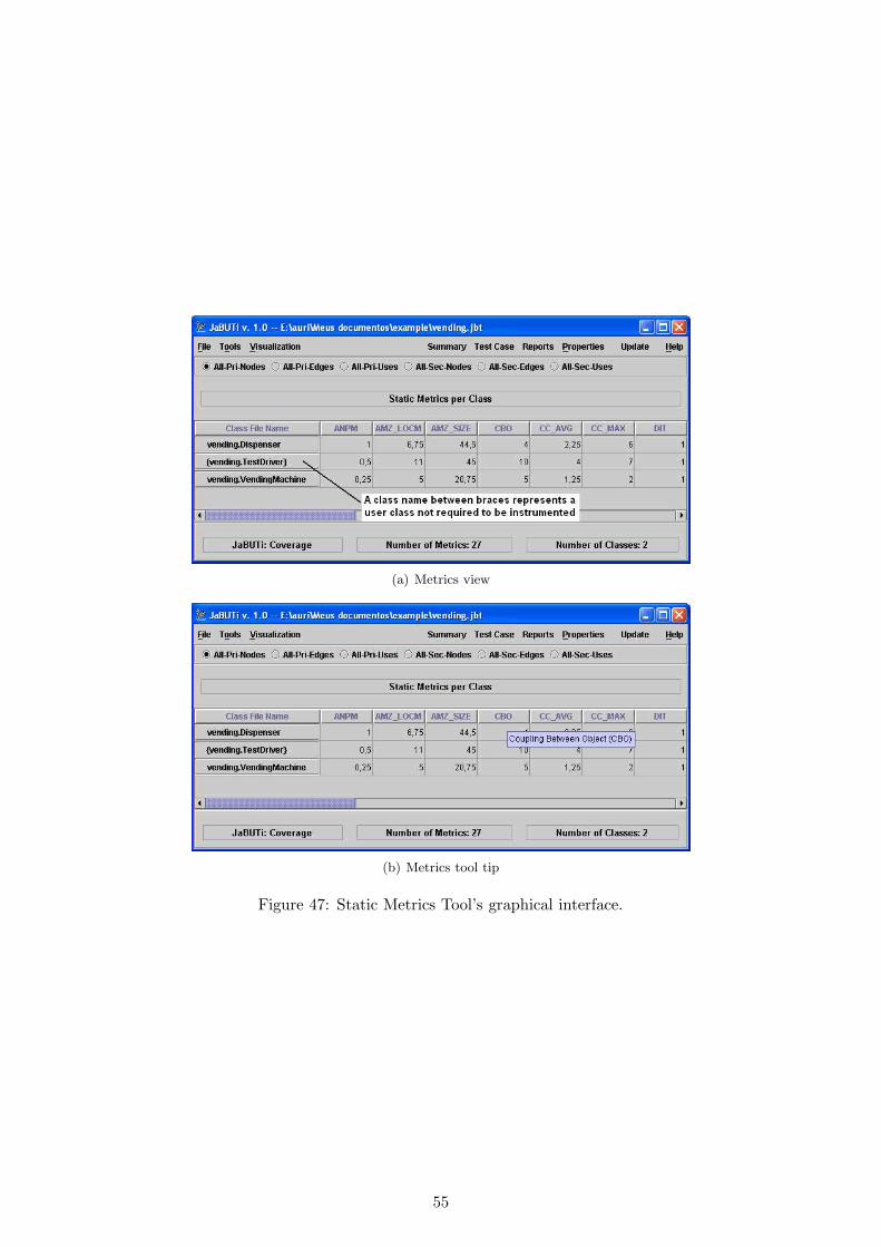
(a) Metrics view
(b) Metrics tool tip
Figure 47: Static Metrics Tool’s graphical interface.
55
9 JaBUTi em dispositivos moveis
A ferramenta JaBUTi foi adaptada para ser utilizada no teste de programas Java que rodam em
dispositivos moveis como PDAs ou telefones celulares. Mais precisamente, que estao de acordo com o
perfil MIDP (Mobile Information Device Profile).
Essa secao descreve as diferencas na utilizacao da ferramenta para o teste desse tipo de software.
As mudancas de procedimento dizem respeito, principalmente, a instrumentacao e execucao dos casos
de teste. Como os programas instrumentados devem executar em dispositivos moveis,7 o tipo de
instrumentacao deve ser adequada aquele ambiente. Alem disso, os dados de execucao (trace) devem
ser analisados pela JaBUTi, no desktop.
Assim, a primeira mudanca a ser feita e a instalacao de um servidor que vai ser responsavel pela
aquisicao dos dados de execucao dos programas e a geracao do arquivo de trace que e tratado pela
JaBUTi. O servidor pode ser instalado atraves de um programa chamado diretamente na linha de
comando ou de dentro da propria ferramenta.
Na chamada direta, o programa deve receber dois argumentos, como mostra a descricao abaixo:
> java -cp <classpath Jabuti> br.jabuti.device.ProberServer <port> <filename>
O primeiro argumento indica o numero da porta a qual o servidor vai se anexar. O segundo e o
nome de um arquivo de configuracao que descreve quais sao os programas que devem ser tratados pelo
servidor. Um servidor pode tratar de mais de um programa em execucao ao mesmo tempo. O formato
do arquivo de configuracao e bastante simples. Ele possui, para cada programa a ser tratado, duas
linhas, contendo a identificacao do programa e o nome do arquivo de trace onde os dados de execucao
devem ser gravados. Por exemplo:
PropExample
/home/user/Demos/PropExample.trc
Foo
/home/foo/foo.trc
No arquivo de configuracao acima, dois programas poderao ser tratados pelo servidor. Um bati-
zado de “‘PropExample” e outro batizado de “Foo”. Quando o servidor recebe dados de execucao do
primeiro, esses dados serao gravados no arquivo “/home/user/Demos/PropExample.trc” e do segundo,
no arquivo “/home/foo/foo.trc”. Note que o nome do programa nao esta relacionado com a sessao de
teste criada para o teste. Esse nome e atribuıdo pelo testador no momento da instrumentacao, como
sera descrito adiante.
Um exemplo de utilizacao do comando que instala o servidor seria:
java -cp Jabuti-bin.zip br.jabuti.device.ProberServer 1988 config.txt
A instalacao atraves da ferramenta JaBUTi e feita atraves da opcao “Properties/Test Server”. Com
essa operacao abre-se a janela mostrada na Figura 48. Nela o testador deve selecionar a porta em que
o servidor sera instalado e o arquivo de configuracao. Pode, tambem, editar esse arquivo e salva-lo, se
necessario. O testador deve, ainda, selecionar a opcao “Mobile device”, que indica o tipo de servidor
desejado.
7Quando nos referimos a dispositivos moveis incluımos os simuladores que, apesar de executarem no desktop, estaosujeitos aos mesmos tipos de limitacoes do perfil MIDP.
56

Figure 48: Instalacao do servidor para dispositivos moveis.
Outra diferenca na execucao da sessao de teste para dispositivos moveis esta na instrumentacao e
do programa em teste e na execucao dos casos de teste. O programa e instrumentado e gera-se um
arquivo .jar contendo todas as classes que compoem o programa, instrumentando-se aquelas que foram
escolhidas na criacao do projeto de teste. O comando que realiza a instrumentacao e o seguinte:
java -cp <classpath Jabuti> br.jabuti.device.ProberInstrum <opc~oes> <classe base>
A classe base refere-se ao nome da classe do MIDlet que se deseja testar. Deve-se notar que
num unico “pacote” e possıvel colocar-se diversos MIDlets distintos. Porem, somente um pode ser
instrumentado de cada vez. As opcoes de instrumentacao sao as seguintes:
<-d diretorio>: indica o diretorio no qual se encontra o arquivo de projeto. E opcional e, se nao
for fornecido, assume-se o diretorio corrente;
<-p projeto>: nome do arquivo de projeto, criado pela JaBUTi, que corresponde a sessao de teste.
Argumento obrigatorio;
<-o arquivo>: da o nome do arquivo .jar onde serao gravadas as classes instrumentadas do pro-
grama. Como as classes instrumentadas fazem chamadas a metodos localizados em classes da
JaBUTi, essas classes sao, tambem, adicionadas ao arquivo de saıda;
<-name midlet id>: e o nome que sera dado ao programa em teste. E esse nome que identifica o
MIDlet para o servidor de teste, como visto anteriormente;
<-h end. servidor>: esse parametro fornece o endereco onde o servidor de teste foi instalado, no
formato “128.123.82.71:1988” ou “myserver.com.br:1988”. E um parametro opcional. Caso nao
seja fornecido, os dados nao serao enviados a nenhum servidor. Nao utilizar essa opcao torna
57

a execucao do programa inutil em termos de teste, propriamente dito, mas pode ser util para
a depuracao da ferramenta. Os dados de teste podem ser exibidos na saıda padrao ou num
arquivo, como sera visto a seguir;
<-temp arquivo>: utiliza o arquivo especificado como deposito temporario dos dados de trace,
no dispositivo. Isso permite que, em dispositivos que possuem sistema de arquivos, os dados
fiquem armazenados ali, salvando espaco na memoria principal. O nome “ STDOUT ” indica
que os dados devem ser escritos na saıda padrao do didpositivo movel. Isso so faz sentido se a
execucao for feita num simulador no desktop, poi, em geral os dispositivos moveis nao apresentam
resultados na saıda padrao;
<-mem valor>: especifica um threshold de memoria disponıvel que deve ser respeitado para ar-
mazenamento dos dados de trace. Quando a quantidade de memoria cai abaixo desse valor os
dados sao enviados para o servidor de teste, ou armazenados no arquivo temporario. O valor
pode ser dado em bytes (por exemplo, 1024), em kbytes ou em mbytes (por exemplo, 128K ou
3M). E um parametro opcional e, se nao fornecido, assume o valor zero, indicando que nao existe
threshold e os dados sao sempre armazenados, ate que a execucao termine;
<-nokeepalive>: se utilizado, esse parametro indica que a conexao (TCP) entre o dispositivo e o
servidor de teste nao deve ser mantida durante toda a execucao do programa. Assim, cada vez
que dados devem ser transmitidos, uma nova conexao e criada. Isso pode representar economia
nos dispositivos em que a utilizacao de rede e cara e paga em funcao do tempo de utilizacao. A
utilizacao da opcao “<-temp arquivo>” ja determina que a conexao nao sera mantida viva pois
todos os dados de execucao sao gravados no arquivo temporario e somente no final da execucao
do MIDlet os dados sao enviados ao servidor.
Seguem-se alguns exemplos da utilizacao do instrumentador, com alguma combinacoes de paramet-
ros.
java -cp Jabuti-bin.zip br.jabuti.device.ProberInstrum -name PropExample
-p Propexample.jbt -o PropExample.jar -h 200.188.151.130:2000 example.PropExample
Nesse exemplo, o programa, cuja sessao de teste esta descrita no projeto chamado “PropExam-
ple”, recebeu o nome de “PropExample”, que tambem e o nome dado ao arquivo .jar de saıda. Os
dados de trace serao enviados ao endereco “200.188.151.130:2000” e a classe do MIDlet e “exam-
ple.PropExample”. Como nao foi estabelecido um threshold de memoria, todos os dados serao ar-
mazenados e somente enviados no final da execucao do programa. Mesmo assim, a conexao entre o
dispositivo e o servidor de teste e aberta no inıcio da execucao do MIDlet e permanece aberta ate o
final do envio dos dados.
java -cp Jabuti-bin.zip br.jabuti.device.ProberInstrum -name PropExample
-p Propexample.jbt -o PropExample.jar -h 200.188.151.130:2000 -nokeepalive
example.PropExample
O mesmo do exemplo anterior, porem a conexao nao permanece aberta o tempo todo. Ela so e
criada no inıcio da execucao, para que seja verificada se realmente pode ser criada e depois, no final,
quando os dados forem enviados.
58

java -cp Jabuti-bin.zip br.jabuti.device.ProberInstrum -name PropExample
-p Propexample.jbt -o PropExample.jar -h 200.188.151.130:2000 -nokeepalive
-mem 512M example.PropExample
Nesse caso, os dados sao enviados periodicamente, quando a quantidade de memoria disponıvel
estiver abaixo do valor estabelecido, ou seja 512 mega-bytes. Como e improvavel que algum dispositivo
tenha uma memoria livre desse tamanho, o que deve ocorrer e que a cada dado de trace coletado, este
seja imediatamente enviado para o servidor. Como a opcao “-nokeepalive” foi utilizada, isso significa
que a cada dado coletado, uma nova conexao e criada, o que pode interferir sobremaneira na execucao
do MIDlet.
java -cp Jabuti-bin.zip br.jabuti.device.ProberInstrum -name PropExample
-p Propexample.jbt -o PropExample.jar -h 200.188.151.130:2000 -nokeepalive
-temp /root1/temp.txt example.PropExample
Com a utilizacao do arquivo temporario, os dados de trace sao sempre enviados para esse arquivo
e somente no final enviados para o servidor. Assim nao sao criadas, constantemente, conexoes.
java -cp Jabuti-bin.zip br.jabuti.device.ProberInstrum -name PropExample
-p Propexample.jbt -o PropExample.jar -temp __STDOUT__ example.PropExample
Os dados de teste coletados sao apresentados na saıda padrao do dispositivo. Como nao foi
fornecido o threshold de memoria esse resultado so e apresentado no final da execucao.
Depois de instrumentadas as classes, e necessario ainda mais um passo para que o programa possa
ser executado. E a pre-verificacao do bytecode e o empacotamento num unico arquivo. Isso e feito
com o comando descrito a seguir:
> java -cp <classpath Jabuti> br.jabuti.device.Preverify <opc~oes>
Os argumentos fornecidos para a execucao sao os seguintes:
<-source arquivo>: esse argumento e obrigatorio e indica qual e o arquivo .jar onde estao as classes
originais do programa a ser carregado no dispositivo movel. Note-se que, como comentado
anteriormente, esse arquivo pode conter diversos MIDlets, alem daquele sendo testado;
<-instr arquivo”>: e o nome do arquivo .jar que foi criado no passo anterior, a instrumentacao. O
que o programa ira fazer e substituir no arquivo original, as classes que foram instrumentadas,
mantendo as demais como estao;
<-o arquivo>: indica o nome do arquivo .jar de saıda. E um argumento opcional e, caso nao
seja fornecido, assume-se o mesmo nome do arquivo original. Nesse caso, o arquivo original e
sobrescrito;
<-jad arquivo>: especifica o nome do arquivo .jad a ser gerado, com as informacoes sobre o“pacote”
gerado. E opcional e, se nao for fornecido, nada e gerado;
59

<-WTK diretorio>: a JaBUTi nao realiza a pre-verificacao por si so. Ela utiliza o toolkit de
desenvolvimeto wireless da SUN para efetuar tal tarefa. Por isso, o testador deve indicar qual e
o diretorio onde encontra-se o WTK.
Um exemplo de sua utilizacao seria:
java -cp Jabuti-bin.zip br.jabuti.device.Preverify -source Demos.jar
-instr PropExample.jar -o Demos.jar -jad Demos.jad -WTK /home/user/WTK22
Concluıdo esse passo, o programa esta pronto para ser executado num simulador ou dispositivo
movel. Os dados, dependendo do tipo de instrumentacao, pode ser enviado ao servidor selecionado
ou simplesmente escrito num arquivo temporario. Deve-se notar que na maioria dos dispositivos, o
usuario deve fornecer autorizacao para algumas operacoes privilegiadas como a criacao de uma conexao
de rede ou leitura/escrita de arquivos. Por isso, a instrumentacao pode alterar o comportamento do
MIDlet, fazendo com que o programa seja interrompido e tal autorizacao solicitada. Isso porem, nao
deve representar problema pois, apos a exibicao de uma janela de solicitacao de autorizacao, como a
da Figura 49, o programa segue normalmente.
Para se executar o programa utilizando o simulador do WTK pode-se utilizar o comando:
/home/user/WTK22/bin/emulator.exe -Xdescriptor:Demos.jad
Figure 49: Execucao no emulador: autorizacao para criar conexao.
10 JaBUTi Evolution
Currently, JaBUTi is composed by a coverage analysis testing tool, a slicing too, and a static metrics
tool for Java programs. The tool uses the Java bytecode (.class files) instead of the Java source code
60

to collect the information necessary to perform its activities. This characteristics allows the tool to
be used to test any kind of Java program, including Java components.
Since most part of the testing criteria currently developed for component based testing are func-
tional testing criteria, by implementing a set of structural testing criteria applied directly in the Java
bytecode, JaBUTi enables the structural testing of Java components and also the identification of
which part of such components needs more test or has not yet been covered.
Even when no source code is available, the tester can at least identify which part of the bytecode
requires more test, or, in case of a fault is identified, which part of the component is more probable to
contain that fault. This information can be given to the component provider such that the component
user can receive another corrected version of the component.
Improvements forth coming of JaBUTi are:
• Development of additional testing criteria to deal not only with intra-method testing but also
with inter-method and inter-class testing;
• Development of additional heuristic to improve the slicing tool, such that a smart debugging
and a ease fault localization to be possible. We intent to investigate different slicing criteria,
including the ones that consider also data-flow information, to implement on JaBUTi different
heuristics to help the tester on fault localization and smarting debug;
• Development of a set of complexity metrics to help the definition of a incremental testing strategy
considering the complete hierarchy of the classes under testing;
• Evaluation, development and implementation of heuristics to automatically identify part of the
infeasible testing requirements;
• Implementation of algorithms to optimize the number of testing requirements to be evaluated,
using the essential-branches’ concept;
• Improvement in the graphical interface to ease the testing activity as much as possible.
Moreover, to show the benefices of the tool, experiments will be carried out exploring the different
aspects of JaBUTi.
Acknowledgments
The authors would like to thank the Brazilian Funding Agencies – CNPq, FAPESP and CAPES –
and the Telcordia Technologies (USA) for their partial support to this research. The authors would
also like to thank the creators of the turtle image used as symbol of JaBUTi found at http://www.
indiancanyonvillage.org/.
61
References
[1] H. Agrawal. Dominators, super block, and program coverage. In SIGPLAN – SIGACT Symposiumon Principles of Programming Languages – POPL’94, pages 25–34, Portland, Oregon, January1994. ACM Press.
[2] H. Agrawal, J. Alberi, J. R. Horgan, J. Li, S. London, W. E. Wong, S. Ghosh, and N. Wilde.Mining system tests to aid software maintenance. IEEE Computer, 31(7):64–73, July 1998.
[3] K. Beck and E. Gamma. JUnit cookbook. web page, 2002. Available on-line: http://www.
junit.org/ [01-20-2003].
[4] S. R. Chidamber and C. F. Kemerer. A metric suite for object oriented design. IEEE Transactionson Software Engineering, 20(6):476–493, June 1994.
[5] M. Dahm. Byte code engineering with the BCEL API. Technical Report B-17-98, Freie UniversitatBerlin – Institut fur Informatik, Berlin – German, April 2001. Available on-line at: http:
//bcel.sourceforge.net/ [04-13-2002].
[6] Inc. GrammaTech. Dependence graphs and program slicing. White Paper, March 2000. Availableon-line: http://www.grammatech.com/research/.
[7] M. J. Harrold and G. Rothermel. Performing data flow testing on classes. In Second ACMSIGSOFT Symposium on Foundations of Software Engineering, pages 154–163, New York, NY,December 1994. ACM Press.
[8] P. M. Herman. A data flow analysis approach to program testing. Australian Computer Journal,8(3):92–96, November 1976.
[9] J. R. Horgan and S. A. London. Data flow coverage and the C language. In Symposium SoftwareTesting, Analysis, and Verification, pages 87–97, Victoria, British Columbia, Canada, October1991. ACM Press.
[10] ILOG, Inc. Ilog jviews component suite. web page, 2003. http://www.ilog.com/products/
jviews/.
[11] T. Lindholm and F. Yellin. The Java Virtual Machine Specification. Addison-Wesley, 2 edition,1999.
[12] M. Lorenz and J. Kidd. Object-Oriented Software Metrics: A Practical Guide. Prentice Hall,Englewood Cliffs, New Jersey, 1994. Object-Oriented Series.
[13] J. C. Maldonado. Potential-Uses Criteria: A Contribution to the Structural Testing of Software.Doctoral dissertation, DCA/FEE/UNICAMP, Campinas, SP, Brazil, July 1991. (in Portuguese).
[14] T. McCabe. A complexity measure. IEEE Transactions on Software Engineering, 2(4):308–320,December 1976.
[15] A. Orso, M. J. Harrold, D. Rosenblum, G. Rothermel, H. Do, and M. L. Soffa. Using componentmetacontent to support the regression testing of component-based software. In IEEE InternationalConference on Software Maintenance (ICSM’01), pages 716–725, Florence, Italy, November 2001.IEEE Computer Society Press.
[16] P. Piwowarski, M. Ohba, and J. Caruso. “Coverage measurement experience during functiontest”. In Proceedings of the 15th International Conference on Software Engineering, pages 287–301, Baltimore, MD, May 1993.
[17] R. S. Pressman. Software Engineering – A Practitioner’s Approach. McGraw-Hill, 5 edition,2000.
62
[18] J. B. Rainsberger. JUnit: A starter guide. Web Page, 2003. Available on-line: http://www.
diasparsoftware.com/articles/JUnit/jUnitStarterGuide.html.
[19] S. Rapps and E. J. Weyuker. Selecting software test data using data flow information. IEEETransactions on Software Engineering, 11(4):367–375, April 1985.
[20] M. Roper. Software Testing. McGrall Hill, 1994.
[21] S. Sinha and M. J. Harrold. Analysis of programs with exception-handling constructs. In ICSM’98– International Conference on Software Maintenance, pages 348–357, Bethesda, MD, November1998.
[22] S. Sinha and M. J. Harrold. Criteria for testing exception-handling constructs in Java programs.In International Conference on Software Maintenance, pages 265–274, Oxford, England, August1999. IEEE Computer Society Press.
[23] F. Tip. A survey of program slicing techniques. Journal of Programming Languages, 3:121–189,1995.
[24] C. T. Utsonomia. Estudo e aplicacao de metricas para sistemas orientados a objeto. Exame geralde qualificacao, Universidade Estadual do Parana, Departamento de Informatica, Curitiba, PR,August 2002.
[25] S. R. Vergilio. Criterios Restritos: Uma Contribuicao para Aprimorar a Eficacia da Atividade deTeste de Software. PhD thesis, DCA/FEEC/UNICAMP, Campinas, SP, July 1997.
[26] A. M. Vincenzi, W. E. Wong, M. E. Delamaro, A. S. Simao, and J. C. Maldonado. Structuraltesting of object-oriented programs. Technical report, ICMC/USP, 2003. (in preparation).
[27] A. M. R. Vincenzi, M. E. Delamaro, J. C. Maldonado, and W. E. Wong. Java bytecode staticanalysis: Deriving structural testing requirements. In 2nd UK Software Testing Workshop –UK-Softest’2003, pages –, Department of Computer Science, University of York, York, England,September 2003. University of York Press. (accepted for publication).
[28] M. Weiser. Program Slicing: Formal, Psychological and Practical Investigations of an AutomaticProgram Abstraction Method. Phd thesis, The University of Michigan, Ann Arbor , Michigan,1979.
[29] M. Weiser. Programmers use slices when debugging. Communications of the ACM, 25(7):446–452,1982.
[30] M. Weiser. Program slicing. IEEE Transactions on Software Engineering, 10(4):352–357, July1984.
[31] W. E. Wong, J. R. Horgan, S. London, and A. P. Mathur. Effect of test set size and block coverageon fault detection effectiveness. In Fifth IEEE International Symposium on Software ReliabilityEngineering, pages 230–238, Monterey, CA, November 1994.
[32] W. E. Wong, J. R. Horgan, S. London, and A. P. Mathur. “Effect of test set minimization onfault detection effectiveness”. Software-Practice and Experience, 28(4):347–369, April 1998.
[33] J. Zhao. Analyzing control flow in Java bytecode. In 16th Conference of Japan Society forSoftware Science and Technology, pages 313–316, September 1999.
[34] J. Zhao. Dependence analysis of Java bytecode. In 24th IEEE Annual International ComputerSoftware and Applications Conference (COMPSAC’2000), pages 486–491, Taipei, Taiwan, Octo-ber 2000. IEEE Computer Society Press.
63