Duality and Optimality of Auctions for Uniform Distributions∗

Yiannis Giannakopoulos† Elias Koutsoupias‡

January 15, 2018

Abstract

We develop a general duality-theory framework for revenue maximization in additiveBayesian auctions. The framework extends linear programming duality and complementarityto constraints with partial derivatives. The dual system reveals the geometric nature ofthe problem and highlights its connection with the theory of bipartite graph matchings.We demonstrate the power of the framework by applying it to a multiple-good monopolysetting where the buyer has uniformly distributed valuations for the items, the canonicallong-standing open problem in the area. We propose a deterministic selling mechanism calledStraight-Jacket Auction (SJA), which we prove to be exactly optimal for up to 6 items, andconjecture its optimality for any number of goods. The duality framework is used not onlyfor proving optimality, but perhaps more importantly for deriving the optimal mechanismitself; as a result, SJA is defined by natural geometric constraints.

1 Introduction

The problem of maximizing revenue in multidimensional Bayesian auctions is one of the mostprominent within the area of Mechanism Design. An auctioneer wants to sell a number of itemsto some potential buyers (bidders). Each bidder has a value for every item; this is the maximumprice that she is willing to pay to get the item and it is a private information. The value of aset of items is simply the sum of the values of the items in the set (additive valuations). Thebuyers submit their bids and the auctioneer must decide, perhaps with randomization, whatitems to allocate to each player and how much to charge each one of them for this transaction.The seller has some prior (incomplete) knowledge about how much each player values the items,captured by a (joint) probability distribution over the space of all possible valuations. However,assuming standard selfish game-theoretic behavior, the players would lie about their true valuesand submit false bids if this is to increase their personal gain. The goal is to design auctionprotocols that maximize the total expected revenue of the seller, by also ensuring the truthfulparticipation of the bidders.

For the single-dimensional case where only one item is to be auctioned among the players,the seminal work of Myerson [26] has completely settled the problem. His solution is simpleand elegant: the optimal auction is deterministic and easy to describe by a “virtual valuations”transformation and reduction to a social welfare maximization problem which can be solvedusing the well-studied VCG auction [27, 18].

Unfortunately, for the many-items setting these elegant properties and results do not holdin general. It is very likely that there is no simple closed-form description of optimal revenueauctions, especially in a unified way similar to Myerson’s solution. However, for the most∗The research leading to these results has received funding from the European Research Council under the

European Union’s Seventh Framework Programme (FP7/2007-2013) / ERC grant agreement 321171.A preliminary version of this paper appeared in [13].†Department of Computer Science, University of Oxford. Email: ygiannak@cs.ox.ac.uk‡Department of Computer Science, University of Oxford. Email: elias@cs.ox.ac.uk

1

arX

iv:1

404.

2329

v4 [

cs.G

T]

15

Jan

2018

commonly studied probability distributions, e.g., the uniform and normal, we would like to havesuch clear, closed-form descriptions of the optimal auctions, or at least algorithms—preferablysimple and intuitive—that compute optimal auctions (their allocation and payment functions).But we are far from such a goal. There exists no interesting continuous probability distributionfor which we know the optimal auction for more than three items. The difficulty of the problemis illustrated by the lack of general results for the canonical case of uniform i.i.d. valuationsin the unit interval [0, 1] even for a single bidder. In this work, we resolve this case for up to6 items. We give an exact, analytic and intuitive way of computing the optimal prices; thesolution is in closed-form, but involves roots of polynomials of degree equal to the number ofitems. We do that as a special application of a much more general construction: a duality-theoryframework for proving exact and approximate optimality of many-bidder multi-item auctionsfor arbitrary continuous distributions. We expect this framework to be essential for helpinggeneralizing Myerson’s solution to many-items settings, the holy grail of auction theory.

It is known that even in the simple case of one bidder, randomized auctions can performstrictly better than deterministic ones [17, 16, 23, 30, 9]. Manelli and Vincent [23] provide somesufficient conditions for deterministic auctions to be optimal, but these are quite involved, inthe form of functional inequalities that incorporate abstract partitions of the valuation space,and admittedly difficult to interpret. They were able to instantiate them though for the caseof two and three uniform i.i.d. distributions and completely determine an optimal deterministicauction. For more items, it is not known whether the optimal auction is a deterministic one.Our results here show that the optimal auction for up to 6 items is indeed deterministic. Weconjecture that this is true for any number of items; we also conjecture that for more than onebidder the optimal auction is not deterministic. Hart and Nisan [15] have provided a very simplesufficient condition in the case of two i.i.d. items for the deterministic full-bundle auction to beoptimal and deploy it to show that this is the case for the equal-revenue distribution. Finally,Daskalakis et al. [9] were also able to deal with the special case of two items and independent(not necessarily identical) exponential distributions and give an exact solution, which in thiscase is randomized. Essentially this is all that was known prior to our work regarding exactdescriptions of optimal auctions with continuous probability distributions,

Given the difficulty of designing optimal auctions, Hart and Nisan [15] study the performanceof the two most straightforward deterministic mechanisms for the single-buyer setting: the onethat sells all items in a full bundle and the one that sells each item independently. They provideelegant approximation ratio guarantees (logarithmic with respect to the number of items) thathold universally for all product (independent) distributions, without even assuming standardregularity conditions (as, e.g., in [6, 23, 26]). Li and Yao [20] further improved their results.The difficulty of providing exact optimal solutions for multi-item settings is further supportedby a recent computational hardness result by Daskalakis et al. [8], where it is shown that evenfor a single buyer and independent (but not identical) valuations with finite support of size 2,it is #P-hard to compute the allocation function of an optimal auction. However this does notexclude the possibility of efficiently computing approximate solutions. In fact, Cai and Huang[5] and Daskalakis and Weinberg [7] have presented PTAS (polynomial-time approximationschemes) for i.i.d. settings.

Daskalakis, Deckelbaum, and Tzamos [9] have also published a duality approach to theproblem, inspired by optimal transport theory. With its use, they gave optimal mechanismsfor two-item settings for exponential distributions. Their approach assumes independent itemdistributions that either have unbounded interval supports and decrease more steeply than1/x2 or bounded ones but they vanish to zero at the right bound of the interval. Thus theirmethod cannot be directly applied to uniform valuations. Our aim is to provide a duality theoryframework for multi-item optimal auctions, which is as general and clean as possible for manybidders and arbitrary joint distributions (not necessarily independent ones). For that reason, wedeploy a “proof-from-scratch” approach directly inspired by linear programming duality which is

2

easily comprehensible and applicable, and with which the reader will immediately feel familiar.At their core, the two duality frameworks are based on similar ideas; although we expect ourframework to have wider applicability, we also believe that there will be special cases in whichthe framework of [9] will be more suitable to apply.

Finally, we mention some very recent developments after the initial conference version [13] ofour paper: in a ground-breaking work Babaioff et al. [3] showed that a constant approximationof the optimal revenue can be achieved for the case of one bidder and independent items by verysimple deterministic mechanisms, using a core-tail decomposition technique inspired by [20], andYao [36] later generalized this idea to many-player settings.

1.1 Model and Notation

We denote the real unit interval by I = [0, 1], the nonnegative reals by R+ = [0,∞). Weconsider auctions of n bidders who are interested in buying any subset of m items. For anypositive integer m we use the notation [m] = {1, 2, . . . ,m}. The value of bidder i for itemj is in interval Di,j = [Li,j , Hi,j ] ⊆ R+; we denote by Di =

∏mj=1Di,j the hyperrectangle of

all possible values of bidder i, and by D =∏ni=1Di the space of all valuation inputs to the

mechanism. The seller knows some probability distribution over D with an almost everywhere1

(a.e.) differentiable density function f . Intervals Di,j need not be bounded; that is, we allowHi,j ∈ R ∪ {∞}.

Let 0m = (0, 0, . . . , 0) and 1m = (1, 1, . . . , 1) denote the m-dimensional zero and unit vec-tors, respectively. We will drop subscript m whenever this causes no confusion. For two m-dimensional vectors x = (x1, x2, . . . , xm) and y = (y1, y2, . . . , ym) we write x ≤ y as a shortcutfor xj ≤ yj for all j ∈ [m]. For any matrix x ∈ Rn×m, xi will denote its i-th (m-dimensional) rowvector. For a function f : Rn×m → R and i ∈ [n] we denote ∇if(x) ≡ (∂f(x)

∂xi,1, ∂f(x)∂xi,2

, . . . , ∂f(x)∂xi,m

);notice how only the derivatives with respect to the variables in row xi appear. Finally, weuse the standard game theoretic notation x−j = (x1, x2 . . . , xj−1, xj+1, . . . , xm) to denote theresulting vector if we remove x’s j-th coordinate. Then, x = (x−j , xj). Similarly, x−(i,j) willdenote all values of the n×m matrix x when we remove the (i, j)-th entry. For a large part ofthe paper we will restrict our attention to a single bidder. In this case, we drop the subscript icompletely; for example, we write Lj instead of L1,j .

1.1.1 Mechanisms and Truthfulness

In this paper we study auctions for selling m items to n bidders when bidder i ∈ [n] has anonnegative valuation xi,j ∈ Di,j for item j ∈ [m]. This is private information of the bidder,and intuitively represents the amount of money she is willing to pay to get this item. The sellerhas only some incomplete prior knowledge of the valuations x in the form of a joint probabilitydistribution F over D from which x is drawn.

A direct revelation mechanism (auction) M = (a,p) on this setting is a protocol which,after receiving a bid vector x′i from each bidder i as input (the bidder may lie about her truevaluations xi and misreport x′i 6= xi), offers item j to bidder i with probability ai,j(x′) ∈ [0, 1],and bidder i pays pi(x′) ∈ R. We assume that each item can only be sold to at most one bidder,or equivalently

∑i ai,j(x′) ≤ 1. The total revenue extracted from the auction is

∑i pi(x′). If we

want to restrict our attention only to deterministic auctions, we take ai,j(x′) ∈ {0, 1}. Noticealso that we do not demand nonnegative payments p ≥ 0, i.e., we don’t assume what is knownas the No Positive Transfers (NPT) condition, since that is not explicitly needed for our results.However, as argued, e.g., in [15, Sect. 2.1], assuming such a condition would be without loss ofgenerality for the revenue maximization problem.

1With respect to the standard Lebesgue measure µ in Rn×m.

3

More formally, a mechanism consists of an allocation function a : D −→ In×m, whichsatisfies

∑i ai,j(x) ≤ 1 for all x ∈ D and all items j ∈ [m], paired with payment functions

pi : D −→ R. We consider each bidder having additive valuations for the items, her “happiness”when she has (true) valuations xi and players report x′ = (x′−i,x′i) to the mechanism beingcaptured by her utility function

ui(x′|xi) ≡ ai(x′) · xi − pi(x′) =m∑j=1

ai,j(x′)xi,j − pi(x′), (1)

the expected sum of the valuations she receives from the items she manages to purchase minusthe payment she has to submit to the seller for this purchase. The player is completely rationaland selfish, wanting to maximize her utility, and that’s why she will not hesitate to misreportx′i instead of her private values xi if this is to give her a higher utility in (1). On the otherhand, the seller’s happiness is captured by the total revenue of the mechanism

n∑i=1

pi(x′) =n∑i=1

(ai(x′) · xi − ui(x′|xi)

), (2)

which is a simple rearrangement of (1).It is standard in Mechanism Design to ask for auctions to respect the following two proper-

ties, for any player i ∈ [n]:

• Individual Rationality (IR): ui(x|xi) ≥ 0 for all x ∈ D

• Incentive Compatibility (IC): ui(x|xi) ≥ ui((x−i,x′i)|xi) for all x ∈ D and x′i ∈ Di

The IR constraint corresponds to the notion of voluntary participation, that is, a bidder cannotharm herself by truthfully taking part in the auction, while IC captures the fundamental prop-erty that truthtelling is a dominant strategy2 for the bidder in the underlying game, i.e. shewill never receive a better utility by lying. Auctions that satisfy IC are also called truthful.From now on we will focus on truthful IR mechanisms, and so we will relax notation ui(x|xi)to just ui(x), considering bidder’s utility as a function ui : D −→ R+. The following is anelegant, extremely useful analytic characterization of truthful mechanisms due to Rochet [31].For proofs of this we recommend [15, 24].

Theorem 1. An auction M = (a,p) is truthful (IC) if and only if the utility functions ui thatinduces have the following properties with respect to the i-th row coordinates, for all bidders i:

1. ui(x−i, ·) is a convex function

2. ui(x−i, ·) is almost everywhere (a.e.) differentiable with

∂ui(x)∂xi,j

= ai,j(x) for all items j ∈ [m] and a.e. x ∈ D. (3)

The allocation function ai is a subgradient of ui.

Theorem 1 essentially establishes a kind of correspondence between truthful mechanismsand utility functions. Not only does every auction induce well-defined utility functions for thebidders, but also conversely, given nonnegative convex functions that satisfy the properties ofthe theorem, we can fully recover a corresponding mechanism from expressions (3) and (2).

2In this work, we consider Dominant Strategy Incentive Compatibility (DSIC), the strongest notion of incentivecompatibility in which the bidders know all values.

4

1.1.2 Optimal Auctions

In this paper we study the problem of maximizing the seller’s expected revenue based on hisprior knowledge of the joint distribution F , under the IR and IC constraints, thus (by Theorem 1and (2))

supu1,...,un

n∑i=1

∫D

(∇ui(x) · xi − ui(x)) dF (x) (4)

over the space of nonnegative convex functions ui on D having the propertiesn∑i=1

∂ui(x)∂xi,j

≤ 1 (zj(x))

∂ui(x)∂xi,j

≥ 0 (si,j(x))

for a.e. x ∈ D, all i ∈ [n] and j ∈ [m].

1.1.3 Deterministic Auctions

Given the characterization of Theorem 1, in case one wants to focus on deterministic auctionsthen it is enough to consider only utility functions that are the maximum of affine hyperplaneswith slopes either 0 or 1 with respect to any direction (see, e.g., [32]). So, for example, anysingle-bidder (n = 1) deterministic and symmetric3 auction corresponds to a utility function ofthe form

u(x) = maxJ⊆[m]

∑j∈J

xi − p|J |

,where pr is the price offered to the buyer for any bundle of r items, r ∈ [m].

2 Outline of Our Work

We give here an outline of our work which bypasses many technical issues but brings out afew central ideas. The reader may also find it helpful to revisit this outline during the moretechnical exposition later on.

2.1 Duality for a Single Bidder

We first develop a general duality framework that applies to almost all interesting continu-ous probability distributions (Section 3). We view the problem of maximizing revenue as anoptimization problem in which the unknowns are the utility functions ui(x) of the bidders (Pro-gram (4)). There are two main restrictions imposed to these functions by truthfulness (seeTheorem 1): the convexity restriction (the utility function ui(x) must be convex with respectto the private values xi of bidder i) and the gradient restriction (the derivatives of this functionmust be nonnegative and they have to be at most 1 for every item).

We simplify things by dropping the convexity constraint and keep only the gradient con-straints. Surprisingly, the convexity constraint can be recovered for free from the optimalsolution of the remaining constraints for a large class of distributions which includes the uni-form distribution. We view the resulting formulation as an infinite linear program with variablethe utility function of the bidder. Its essential constraints (labeled by (zj) in (4)) are that the

3This means that the auction does not discriminate between items, i.e., any permutation of the valuationsprofile x results to the same permutation of the output allocation vector a(x).

5

derivatives for each item must be at most 1 and its objective is to maximize the expected valueof∑i∇iui(x) · x− ui(x). We carefully rewrite the integral in (4) to bring it into a form which

does not include any derivatives. Remarkably, Myerson’s solution for the special case of oneitem is based on a different rewriting of the system in which the primal variables are the deriva-tives of the utility, instead of the utility itself. In fact, since the allocation constraints involveexactly the derivatives, this is the most natural choice of primal variables. Unfortunately suchan approach does not seem to work for the case of many items, since the partial derivativesare not independent functions and, if we treat them as such, we run the risk of violating thegradient constraints.

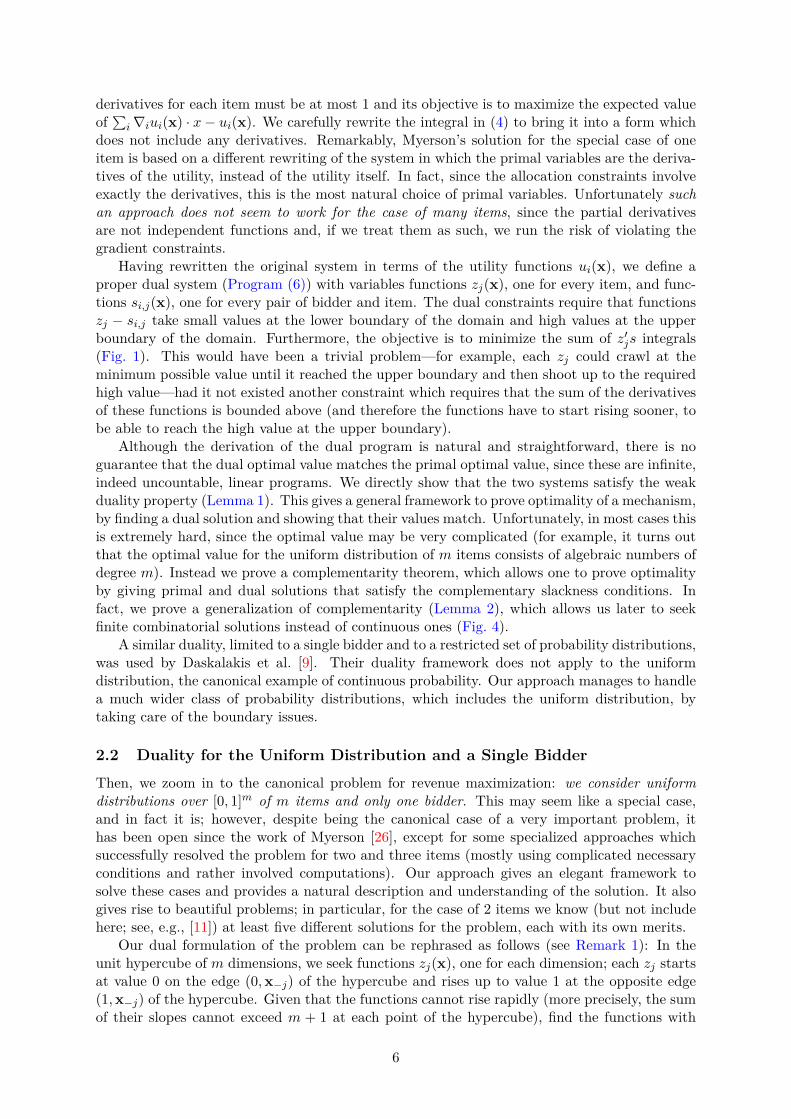
Having rewritten the original system in terms of the utility functions ui(x), we define aproper dual system (Program (6)) with variables functions zj(x), one for every item, and func-tions si,j(x), one for every pair of bidder and item. The dual constraints require that functionszj − si,j take small values at the lower boundary of the domain and high values at the upperboundary of the domain. Furthermore, the objective is to minimize the sum of z′js integrals(Fig. 1). This would have been a trivial problem—for example, each zj could crawl at theminimum possible value until it reached the upper boundary and then shoot up to the requiredhigh value—had it not existed another constraint which requires that the sum of the derivativesof these functions is bounded above (and therefore the functions have to start rising sooner, tobe able to reach the high value at the upper boundary).

Although the derivation of the dual program is natural and straightforward, there is noguarantee that the dual optimal value matches the primal optimal value, since these are infinite,indeed uncountable, linear programs. We directly show that the two systems satisfy the weakduality property (Lemma 1). This gives a general framework to prove optimality of a mechanism,by finding a dual solution and showing that their values match. Unfortunately, in most cases thisis extremely hard, since the optimal value may be very complicated (for example, it turns outthat the optimal value for the uniform distribution of m items consists of algebraic numbers ofdegree m). Instead we prove a complementarity theorem, which allows one to prove optimalityby giving primal and dual solutions that satisfy the complementary slackness conditions. Infact, we prove a generalization of complementarity (Lemma 2), which allows us later to seekfinite combinatorial solutions instead of continuous ones (Fig. 4).

A similar duality, limited to a single bidder and to a restricted set of probability distributions,was used by Daskalakis et al. [9]. Their duality framework does not apply to the uniformdistribution, the canonical example of continuous probability. Our approach manages to handlea much wider class of probability distributions, which includes the uniform distribution, bytaking care of the boundary issues.

2.2 Duality for the Uniform Distribution and a Single Bidder

Then, we zoom in to the canonical problem for revenue maximization: we consider uniformdistributions over [0, 1]m of m items and only one bidder. This may seem like a special case,and in fact it is; however, despite being the canonical case of a very important problem, ithas been open since the work of Myerson [26], except for some specialized approaches whichsuccessfully resolved the problem for two and three items (mostly using complicated necessaryconditions and rather involved computations). Our approach gives an elegant framework tosolve these cases and provides a natural description and understanding of the solution. It alsogives rise to beautiful problems; in particular, for the case of 2 items we know (but not includehere; see, e.g., [11]) at least five different solutions for the problem, each with its own merits.

Our dual formulation of the problem can be rephrased as follows (see Remark 1): In theunit hypercube of m dimensions, we seek functions zj(x), one for each dimension; each zj startsat value 0 on the edge (0,x−j) of the hypercube and rises up to value 1 at the opposite edge(1,x−j) of the hypercube. Given that the functions cannot rise rapidly (more precisely, the sumof their slopes cannot exceed m + 1 at each point of the hypercube), find the functions with

6

minimum sum of integrals. Alternatively, we can view it as a problem in the m+ 1 hypercube:each function zj defines a hypersurface which starts at the edge (0,x−j) of the hypercube, endsat the opposite edge (0,x−j), and they collectively cannot grow rapidly; we seek to minimizethe sum of volumes beneath these surfaces (Fig. 1a). The remaining dual constraints sj donot appear anywhere, since for this application to the case of uniform distribution, we makethe choice to relax even further the primal Program (4) by dropping the corresponding (si,j)constraints that require the derivatives to be nonnegative; as we’ll see, this is again without lossfor the revenue optimality.

2.3 The Straight-Jacket Auction (SJA)

This dual system suggests in a natural way a selling mechanism, the Straight-Jacket Auction(SJA). We explain the intuition behind the mechanism and give a formal definition in Section 4.SJA is defined so that for every bundle of items A with |A| = r, the price pr for A is determinedby the requirement that the volume of the r-dimensional body in which the mechanism sells anonempty subset of A is exactly equal to r/(m+ 1).

The aim of the remaining and more technical part of the paper is to develop the toolkit toprove that SJA is optimal for any number of items; however, we manage to prove optimalityonly for up to 6 items.

The straightforward way for proving the optimality of SJA would be to find a pair of primaland dual solutions that have the same value. Although we know such explicit solutions for thecase of two items, there does not seem to exist a natural solution of the dual program which canbe easily described for more that two items. How then can we show optimality in such cases?We do not give an explicit dual solution, but we only show that a proper solution exists and relyon complementarity to show optimality.

2.4 Proof of Optimality of SJA

A central notion in our development is the notion of deficiency: the k-deficiency of a body Sin m dimensions is |S| − k (

∑j |S[m]\{j}|), where S[m]\{j} denotes the projection of S on the

hyperplane xj = 0 (this is an (m−1)-dimensional body). In particular, we are interested in thedeficiency of the subsets of U∅, the valuation subspace in which the auction sells a nonemptybundle. The main tool for proving the optimality of SJA is the following: To show that theSJA is optimal it suffices to show that no set S of points inside U∅ has positive 1

m+1 -deficiency(Theorem 4).

The fact that this is sufficient is based mainly on the observation that finding a feasible dualsolution is, in disguise, a perfect matching problem between the hypercube and its boundaries(taken with appropriate multiplicities). If Hall’s condition for perfect matchings (see, e.g.,[22, Theorem 1.1.3]) could apply to infinite graphs, under some continuity assumptions thesufficiency of the above would be evident. However, Hall’s theorem does not hold for infinitegraphs in general [1] and, even worse, the continuity assumptions seem hard to establish. Webypass both problems by considering an interesting discretized version of the problem thattakes advantage of Hall’s theorem and the piecewise continuity; we then apply approximatecomplementarity to prove optimality.

The technical core in our proof for the optimality of SJA consists of establishing that nopositive deficiency subset of U∅ exists. Let us call such a set a counterexample. To provethat no counterexample exists, we first argue that such a counterexample would have certainproperties and then show that no counterexample with these properties exists. We first showthat we can restrict our attention to special types of counterexamples, those that are upwardsclosed and symmetric (Lemma 7). Ideally, we would like to restrict our attention even fur-ther to box-like counterexamples, those that are the intersection of an m-dimensional box andU∅. This would restrict significantly the search of counterexamples, and in fact a well-known

7

isoperimetric lemma by Loomis and Whitney [21] (see Lemma 9), and a generalization by Bol-lobas and Thomason [4] show that this is actually true when we remove the restriction that thecounterexample must lie inside some fixed body (in our case, inside U∅). Unfortunately, we canonly establish this claim for 2 items. Instead, we prove a weaker version of it: we show that if acounterexample exists, it must be closed under taking the convex hull of all symmetric imagesof a point (Lemma 12). Furthermore, the requirement on deficiency provides a lower bound onthe volume of the counterexample (Lemmas 10 and 11).

By exploiting these properties, we show that no counterexample exists for 6 or fewer items(Theorem 3). The case of 4 or fewer items is straightforward, but the case of 5 items isqualitatively more challenging. The main reason for this difficulty is that the optimal mechanismfor 5 items never sells a bundle of 4 items (equivalently, the price for 4 items is equal to theprice of 5 items). The case of 6 items is similar to the case of 5 items; the optimal mechanismdoes not sell any bundles of 5 items. However, all these cases are being treated in a unified wayin the proof of the theorem that avoids tiresome case analysis. We must point out here thatTheorem 3 is essentially the only ingredient of this paper whose proof does not work for morethan 6 items.

3 Duality

Motivated by traditional linear programming duality theory, we develop a duality theory frame-work that can be applied to the problem (4) of designing auctions with optimal expected revenue.By interpreting the derivatives as differences, we can view this as an (infinite) linear programand we can find its dual. The variables of the primal linear program are the values of the func-tions ui(x). The labels (zj(x)) and (si,j(x)) on the constraints of Program (4) are the analogof the dual variables of a linear program.

To find its dual program, we first rewrite the objective function in terms of the ui’s insteadof their derivatives. In particular, by integration by parts we have∫

D

∂ui(x)∂xi,j

xi,jf(x) dx =∫D−(i,j)

[ui(x)xi,jf(x)]xi,j=Hi,j

xi,j=Li,jdx−(i,j) −

∫Dui(x)∂(xi,jf(x))

∂xi,jdx

=∫D−(i,j)

[ui(x)xi,jf(x)]xi,j=Hi,j

xi,j=Li,jdx−(i,j) −

∫Dui(x)f(x) dx−

∫Dui(x)xi,j

∂f(x)∂xi,j

dx

to rewrite the objective of the primal program asn∑i=1

∫D

(∇ui(x) · xi − ui(x)) dF (x) =n∑i=1

m∑j=1

∫D−(i,j)

Hi,j ui(Hi,j ,x−(i,j)) f(Hi,j ,x−(i,j)) dx−(i,j)

(5)

−n∑i=1

m∑j=1

∫D−(i,j)

Li,j ui(Li,j ,x−(i,j)) f(Li,j ,x−(i,j)) dx−(i,j)

−n∑i=1

∫Dui(x) ((m+ 1)f(x) + xi · ∇if(x)) dx.

Notice that some of the above expressions make sense only for bounded domains (i.e., whenHi,j is not infinity), but it is possible to extend the duality framework to unbounded domains,by carefully replacing these expressions with their limits when they exist or by appropriatelytruncating the probability distributions. For the main results in this work we deal only withbounded domains, but for completeness and future reference we provide a treatment of thegeneral case in Appendix C.

We also relax the original problem by replacing the convexity constraint by the much milderconstraint of absolute continuity; absolute continuity allows us to express functions as integrals of

8

their derivatives. We can restate this as follows: truthfulness in general imposes two conditionson the solution of allocating the items to bidders (see Theorem 1): the first condition is thatthe utility is convex; the second one is that the allocations must be gradients of the utility.It seems that in most cases, including the important Myersonian case of one item and regulardistributions, when we optimize revenue the convexity constraint is redundant. Later on, whenwe will be applying the duality framework to the case of uniform distributions we will alsodrop the constraints of nonnegative allocation probabilities (i.e., the (sj(x)) constraints in (4)).In many cases, dropping these constraints might have no effect on the value of the program.However, there are cases in which these constraints are essential. In particular, they are neededeven for the case of one item when the probability distributions are not regular. We give anin-depth discussion of this topic in Appendix B.

To find the dual program, we have to take extra care on the boundaries of the domain,since the derivatives correspond to differences from which one term is missing (the one thatcorresponds to the variables outside the domain). This is a point where our approach differsfrom that of Daskalakis et al. [9], which applies only to special distributions and in particularit does not apply to the uniform distribution. Inside the domain, the dual constraint thatcorresponds to the primal variable ui(x) is

∑j∂zj(x)∂xi,j

≤ (m+ 1)f(x) + xi · ∇if(x).So, the dual program that we propose is

infz1,...,zm

∫ m∑j=1

zj(x) dx (6)

subject to

m∑j=1

(∂zj(x)∂xi,j

− ∂si,j(x)∂xi,j

)≤ (m+ 1)f(x) + xi · ∇if(x) (ui(x))

zj(Li,j ,x−(i,j))− si,j(Li,j ,x−(i,j)) ≤ Li,jf(Li,j ,x−(i,j)) (ui(Li,j ,x−(i,j)))zj(Hi,j ,x−(i,j))− si,j(Hi,j ,x−(i,j)) ≥ Hi,jf(Hi,j ,x−(i,j)) (ui(Hi,j ,x−(i,j)))

zj(x), si,j(x) ≥ 0

The above intuitive derivation of this dual is used only for illustration and for explaininghow we came up with it. None of the results rely on the actual way of coming up with the dualproblem. However, the derivation is useful for intuition and for suggesting traditional linearprogramming machinery for these infinite systems; for example, although we don’t directly useany results from the theory of linear programming duality, we are motivated by it to provesimilar connections between our primal and dual programs.

One can interpret this dual as follows: For the sake of clarity, assume a single bidder anddrop the si,j constraints; we seek m functions zj defined inside the hyperrectangle [L1, H1] ×· · · × [Lm, Hm] such that

• in the j-th direction, function zj starts at value (at most) Ljf(Lj ,x−j) and ends at value(at least) Hjf(Hj ,x−j); this must hold for all x−j .

• at every point of the domain, the sum of the derivatives of functions zj cannot exceed(m+ 1)f(x) + x · ∇f(x).

• the sum of the integrals of these functions is minimized.

For a significant portion of this paper, we materialize this duality framework by applying itto the case of i.i.d. uniform distributions over the unit interval Im. Therefore, let’s clearly stateour dual constrains for ease of reference:

9

(a) Feasible solutions z1, z2 to the two-items dual pro-gram. Each function zj has to start at 0 on the en-tire axis xj = 0 and rise to 1. At no point of the2-dimensional cube the sum of their slopes is allowedto exceed 3, and the objective is to keep them as low aspossible, i.e., minimize the volume under their curves.

feasible

optimal

z(x)

1

x10 1/2

slope=2

(b) For the special case of a single item, the dual feasi-ble function z has to start at 0 and rise to 1 or higherwhen x = 1, with a slope of at most 2. The optimalfunction minimizes the area below it. It is not difficultto see that the optimal solution is to remain at value0 until x = 1/2 and then increase steadily to 1; theoptimal dual objective is equal to the gray area. Thiscorresponds exactly to the well-known optimal solutionof Myerson with reserve price of 1/2.

Figure 1: Geometric interpretation of the dual Program (6) for the case of a single bidder and m = 1, 2 uniformi.i.d. items.

Remark 1 (Duality for Uniform Domains). The dual constraints (in Program (6)) for the single-bidder m-items uniform i.i.d. setting over Im become

m∑j=1

∂zj(x)∂xj

≤ m+ 1 (u(x))

zj(0,x−j) = 0 (u(0,x−j))zj(1,x−j) ≥ 1 (u(1,x−j))

zj(x) ≥ 0

A geometric interpretation of this dual for the case of one and two items, based on the previousdiscussion, can be found in Fig. 1.

Let us also mention parenthetically that one can derive Myerson’s results by selecting asvariables not the utilities ui(x), but their derivatives. In fact, since the allocation constraintsinvolve exactly the derivatives, this is the natural choice of primal variables. Unfortunately,such an approach does not seem to work for more than one item because the derivatives arenot independent functions. If we treat them as independent, we lose the power of the gradientsconstraint.

3.1 Duality and Complementarity

The way that we derived the dual system does not yet provide any rigorous connection withthe original primal system. We now prove that this is indeed a weak dual, in the sense that

10

the value of the dual minimization Program (6) cannot be less than the value of the primalprogram.

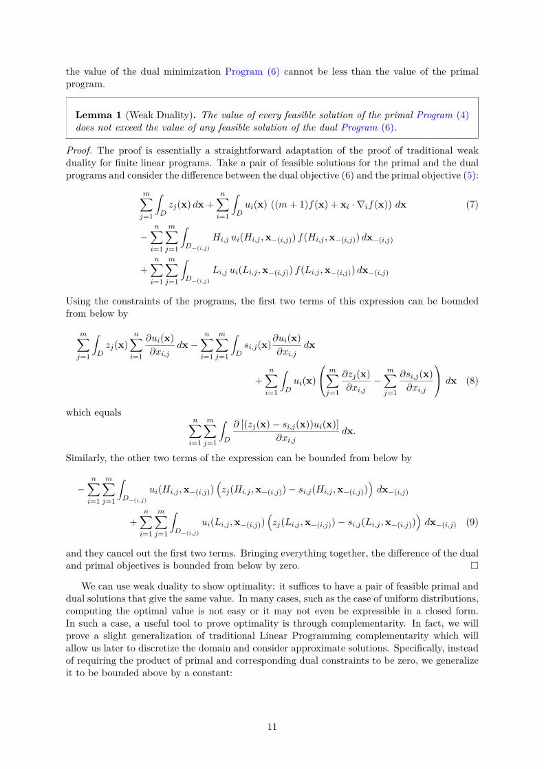
Lemma 1 (Weak Duality). The value of every feasible solution of the primal Program (4)does not exceed the value of any feasible solution of the dual Program (6).

Proof. The proof is essentially a straightforward adaptation of the proof of traditional weakduality for finite linear programs. Take a pair of feasible solutions for the primal and the dualprograms and consider the difference between the dual objective (6) and the primal objective (5):

m∑j=1

∫Dzj(x) dx +

n∑i=1

∫Dui(x) ((m+ 1)f(x) + xi · ∇if(x)) dx (7)

−n∑i=1

m∑j=1

∫D−(i,j)

Hi,j ui(Hi,j ,x−(i,j)) f(Hi,j ,x−(i,j)) dx−(i,j)

+n∑i=1

m∑j=1

∫D−(i,j)

Li,j ui(Li,j ,x−(i,j)) f(Li,j ,x−(i,j)) dx−(i,j)

Using the constraints of the programs, the first two terms of this expression can be boundedfrom below by

m∑j=1

∫Dzj(x)

n∑i=1

∂ui(x)∂xi,j

dx−n∑i=1

m∑j=1

∫Dsi,j(x)∂ui(x)

∂xi,jdx

+n∑i=1

∫Dui(x)

m∑j=1

∂zj(x)∂xi,j

−m∑j=1

∂si,j(x)∂xi,j

dx (8)

which equalsn∑i=1

m∑j=1

∫D

∂ [(zj(x)− si,j(x))ui(x)]∂xi,j

dx.

Similarly, the other two terms of the expression can be bounded from below by

−n∑i=1

m∑j=1

∫D−(i,j)

ui(Hi,j ,x−(i,j))(zj(Hi,j ,x−(i,j))− si,j(Hi,j ,x−(i,j))

)dx−(i,j)

+n∑i=1

m∑j=1

∫D−(i,j)

ui(Li,j ,x−(i,j))(zj(Li,j ,x−(i,j))− si,j(Li,j ,x−(i,j))

)dx−(i,j) (9)

and they cancel out the first two terms. Bringing everything together, the difference of the dualand primal objectives is bounded from below by zero.

We can use weak duality to show optimality: it suffices to have a pair of feasible primal anddual solutions that give the same value. In many cases, such as the case of uniform distributions,computing the optimal value is not easy or it may not even be expressible in a closed form.In such a case, a useful tool to prove optimality is through complementarity. In fact, we willprove a slight generalization of traditional Linear Programming complementarity which willallow us later to discretize the domain and consider approximate solutions. Specifically, insteadof requiring the product of primal and corresponding dual constraints to be zero, we generalizeit to be bounded above by a constant:

11

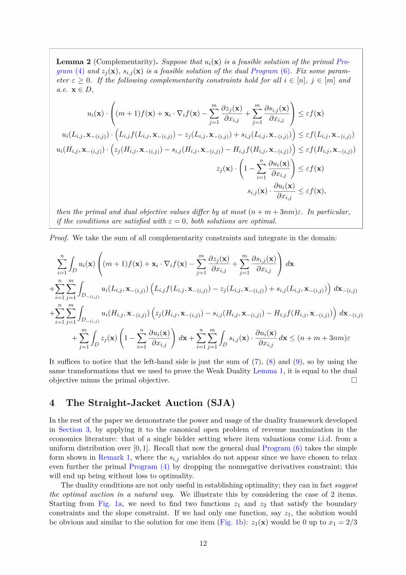
Lemma 2 (Complementarity). Suppose that ui(x) is a feasible solution of the primal Pro-gram (4) and zj(x), si,j(x) is a feasible solution of the dual Program (6). Fix some param-eter ε ≥ 0. If the following complementarity constraints hold for all i ∈ [n], j ∈ [m] anda.e. x ∈ D,

ui(x) ·

(m+ 1)f(x) + xi · ∇if(x)−m∑j=1

∂zj(x)∂xi,j

+m∑j=1

∂si,j(x)∂xi,j

≤ εf(x)

ui(Li,j ,x−(i,j)) ·(Li,jf(Li,j ,x−(i,j))− zj(Li,j ,x−(i,j)) + si,j(Li,j ,x−(i,j))

)≤ εf(Li,j ,x−(i,j))

ui(Hi,j ,x−(i,j)) ·(zj(Hi,j ,x−(i,j))− si,j(Hi,j ,x−(i,j))−Hi,jf(Hi,j ,x−(i,j))

)≤ εf(Hi,j ,x−(i,j))

zj(x) ·(

1−n∑i=1

∂ui(x)∂xi,j

)≤ εf(x)

si,j(x) · ∂ui(x)∂xi,j

≤ εf(x),

then the primal and dual objective values differ by at most (n+m+ 3nm)ε. In particular,if the conditions are satisfied with ε = 0, both solutions are optimal.

Proof. We take the sum of all complementarity constraints and integrate in the domain:

n∑i=1

∫Dui(x)

(m+ 1)f(x) + xi · ∇if(x)−m∑j=1

∂zj(x)∂xi,j

+m∑j=1

∂si,j(x)∂xi,j

dx

+n∑i=1

m∑j=1

∫D−(i,j)

ui(Li,j ,x−(i,j))(Li,jf(Li,j ,x−(i,j))− zj(Li,j ,x−(i,j)) + si,j(Li,j ,x−(i,j))

)dx−(i,j)

+n∑i=1

m∑j=1

∫D−(i,j)

ui(Hi,j ,x−(i,j))(zj(Hi,j ,x−(i,j))− si,j(Hi,j ,x−(i,j))−Hi,jf(Hi,j ,x−(i,j))

)dx−(i,j)

+m∑j=1

∫Dzj(x)

(1−

n∑i=1

∂ui(x)∂xi,j

)dx +

n∑i=1

m∑j=1

∫Dsi,j(x) · ∂ui(x)

∂xi,jdx ≤ (n+m+ 3nm)ε

It suffices to notice that the left-hand side is just the sum of (7), (8) and (9), so by using thesame transformations that we used to prove the Weak Duality Lemma 1, it is equal to the dualobjective minus the primal objective.

4 The Straight-Jacket Auction (SJA)

In the rest of the paper we demonstrate the power and usage of the duality framework developedin Section 3, by applying it to the canonical open problem of revenue maximization in theeconomics literature: that of a single bidder setting where item valuations come i.i.d. from auniform distribution over [0, 1]. Recall that now the general dual Program (6) takes the simpleform shown in Remark 1, where the si,j variables do not appear since we have chosen to relaxeven further the primal Program (4) by dropping the nonnegative derivatives constraint; thiswill end up being without loss to optimality.

The duality conditions are not only useful in establishing optimality; they can in fact suggestthe optimal auction in a natural way. We illustrate this by considering the case of 2 items.Starting from Fig. 1a, we need to find two functions z1 and z2 that satisfy the boundaryconstraints and the slope constraint. If we had only one function, say z1, the solution wouldbe obvious and similar to the solution for one item (Fig. 1b): z1(x) would be 0 up to x1 = 2/3

12

x2

x10 1

1

p1

p2 − p1

p2 − p1

p1

U{1,2}

U∅

U{1}

U{2}

x1 + x2 = p2

Figure 2: The allocation spaces of the optimal SJA mechanisms for m = 2 and m = 3 items. The paymentsare given by p1 = m

m+1 , p2 = 2m−√

2m+1 , and p3 = 3− 7.0971

m+1 . The mechanism sells at least one item within the grayareas U∅, and all items within the dark gray areas U[m]. If we flip around these dark gray areas by x 7→ 1 − x,so that 1 is mapped to the origin 0, they are exactly the SIM-bodies defined in Section 6.1, for k = 1

m+1 . TheseSIM-bodies can be seen in Figs. 3a and 3b, respectively.

and then increase with a maximum slope of 3. But if we do the same for both functions z1 andz2, we obtain an infeasible solution: in the square [2/3, 1] × [2/3, 1] the total slope would be6 instead of 3. This implies that the functions need more space to grow; in fact, the area ofgrowth needs to be at least equal to the area of the square [2/3, 1]× [2/3, 1]. The natural wayto get this space is to add a triangle of area 1/9 in the way indicated in the left part of Fig. 2(the triangle defined by the lines xj = p1 = 2/3, j = 1, 2, and x1 + x2 = p2). We then seek adual solution in which only zj grows in area U{j} and both functions grow in U{1,2} (Fig. 2).The corresponding primal solution is that only item j is sold in U{j} and both items are sold inU{1,2}.

The remarkable fact is that the optimal mechanism is completely determined by the obviousrequirement that the area of the triangle must be (at least) equal to 1/9. To put it in anotherway: suppose that we knew that the optimal mechanism is deterministic; then the dual programrequires that

• the price p1 for one item must satisfy p1 ≤ 2/3 so that z1 has enough space to grow from0 to 1 with the maximum slope 3

• the price p2 for the bundle of both items must be such that the area of the region U∅ =U{1} ∪U{2} ∪U{1,2}, in which the mechanism allocates at least one item, is at least 2/3 sothat both functions have enough space to grow to 1

The central point of this work is that these necessary conditions (which we call slice conditions)are also sufficient. This intuition naturally extends to more items: the price for a bundle of ritems is determined by the slice condition that the r-dimensional volume in which the mechanismsells at least one item of the bundle is exactly equal to r/(m+ 1).

Using this intuition, we define here the Straight-Jacket Auction (SJA). This selling mech-anism is deterministic and symmetric; as such, it is defined by a payment vector p(m) =(p(m)

1 , . . . , p(m)m ); p(m)

r is the price offered by the mechanism to the bidder for every subsetof r items, r ∈ [m]. We will drop the superscript when there is no confusion about the numberof available items. The utility of the bidder is then given by u(x) = maxJ⊆[m]

(∑j∈J xj − p|J |

).

The prices are defined by the slice conditions. For a subset of items J ⊆ [m], let Pr(J,x−J)be the probability that at least one item in J is sold when the remaining items have values

13

x−J . The r-th dimensional slice condition is that for every J with |J | = r and every x−J :Pr(J,x−J) ≥ |J |/(m + 1). The SJA is the deterministic mechanism which satisfies the sliceconditions for all dimensions as tightly as possible (hence its name), in the following sense:determine the prices p1, p2, . . . , pm in this order so that, having fixed the previous ones, selectpr as large as possible to satisfy all r-dimensional slice conditions. In particular, this guaranteesthat the m-dimensional slice is tight, or equivalently, that the probability that at least one itemis sold is m/(m+ 1).

Definition 1 (Straight-Jacket Auction (SJA)). SJA for m items is the deterministic sym-metric selling mechanism whose prices p(m)

1 , . . . , p(m)m , where p(m)

r is the price of selling abundle of size r, are determined as follows: for each r ∈ [m], having fixed p

(m)1 , . . . , p(m)

r−1,price p(m)

r is selected to satisfy

Prx∼Um

∧J⊆[r]

∑j∈J

xj < p(m)|J |

= 1− r · k, (10)

where k = 1m+1 . In words, p(m)

r is selected so that the probability of selling no item whenr values are drawn from the uniform probability distribution (and the remaining values ofthe m− r items are set to 0) is equal to 1− r · k. We will refer to constraints (10) as sliceconditions.

If we take the complement of the above probability, an equivalent definition would be to ask forthe probability of selling at least one of items [r], when all other bids for items [r + 1...m] arefixed to zero, to be rk. That is, if for any dimension m and positive α1, α2, . . . , αm we define

V (α1, . . . , αm) ≡

x ∈ Im∣∣∣∣∣∣∨

J⊆[m]

∑j∈J

xj ≥ α|J |

, (11)

the volume of the r-dimensional body V (p(m)1 , . . . , p

(m)r ), let’s denote it by v(p(m)

1 , . . . , p(m)r ),

must be rk (for all r ∈ [m]). Notice also that it is not immediate that SJA is in generalwell-defined for any dimension m: there should exist prices p(m)

r that satisfy (10).The specific value on the right-hand side of (10) depends on the parameter k, which, in

turn, depends on the total number of items m; the exact dependence arises from the specificvalues of the primal and dual program. It is, however, useful in providing a unifying approachto carry out the discussion and analysis for an arbitrary (albeit small, k ≤ 1

m+1) parameter kand to plug in the specific value k = 1/(m+ 1) only when this is absolutely necessary.

The main technical result of this work is showing that the SJA mechanism is optimal form ≤ 6:

Theorem 2. The Straight-Jacket Auction is a revenue optimal mechanism for selling upto 6 goods to a single additive buyer having uniformly i.i.d. valuations over [0, 1].

Our proof of this theorem relies significantly on the geometry of these mechanisms. Weconjecture that the theorem holds for any number of items:

Conjecture. The Straight-Jacket Auction is a revenue optimal mechanism for selling any num-ber of goods to a single additive buyer having uniformly i.i.d. valuations over [0, 1].

Here is how to use the slice conditions (10) to compute the prices of SJA: The 1-dimensionalcondition on a 1-dimensional hypercube simply means that p(m)

1 = 1 − 1/(m + 1), because

14

we only have condition x1 < p(m)1 . The 2-dimensional condition on a 2-dimensional boundary

requires that the region {x : x1 + x2 < p2 and x1 < p1 and x2 < p1} inside the unit squaremust have area equal to 1− 2/(m+ 1). In other words, we want to find where to move the linex1 + x2 = p2 so that the area that it cuts satisfies the slice condition (in the left part of Fig. 2,U{1}, U{2}, and U{1,2} have total volume 2/(m+ 1)); this gives p2 = 2− (2 +

√2)/(m+ 1). We

can proceed in the same way to higher dimensions: fix some dimension m and an order r > 1.If the prices p1, p2, . . . , pr are such that pj − pj−1 is a nonnegative and (weakly) decreasingsequence, then

v (p1, . . . , pr) =∫ pr−pr−1

0v (p1, . . . , pr−1) dt+

∫ pr−1−pr−2

pr−pr−1v (p1, . . . , pr−2, pr − t) dt

+ . . .+∫ p1

p2−p1v (p2 − t, . . . , pr−1 − t, pr − t) dt+

∫ 1

p11 dt. (12)

This is a recursive way to compute the expressions for the volumes v (p1, . . . , pr). In case thatthe sequence p1, p2, . . . , pr of the prices up to order r breaks the requirement to be increasingat the last step, i.e. pr < pr−1, then simply v (p1, . . . , pr) = v (p1, . . . , pr−2, pr, pr) and we canstill deploy the previous recursion.

An exact, analytic computation of these values for up to r = 6 using the above recursion isgiven in Appendix D, but we also list them below for quick reference. In the following we willoften use the transformation

pr = r − µrm+ 1 (13)

so that prices will be determined with respect to some parameters µr. It will be algebraicallyconvenient to also assume p0 = 0.

• For r ≤ 4 and any number of items m ≥ r:

p1 = m

m+ 1 p2 = 2m−√

2m+ 1 p3 ≈ 3− 7.0972

m+ 1 p4 ≈ 4− 11.9972m+ 1 (14)

µ1 = 1 µ2 = 2 +√

2 µ3 ≈ 7.0972 µ4 ≈ 11.9972

• For r = 5, 6:

p(5)5 ≈ 1.9856 p5 ≈ 5− 18.0843

m+ 1 (m ≥ 6) p(6)6 ≈ 2.3774 (15)

µ(5)5 ≈ 18.0865 µ5 ≈ 18.0843 (m ≥ 6) µ

(6)6 ≈ 25.3585

4.1 Optimality of SJA

In this section we gather the key elements that form the backbone of our proof for the optimalityof the SJA mechanism.

Definition 2. We denote by U(m)J the subdomain in which SJA allocates exactly the bundle

J ⊆ [m] of items:

U(m)J ≡

x ∈ Im∣∣∣∣∣∣∧

L⊆[m]

∑j∈J

xj − p(m)|J | ≥

∑j∈L

xj − p(m)|L|

. (16)

Let U (m)J

∣∣∣−J :t

denote the |J |-dimensional slice of U (m)J when we fix the values of the remain-

ing [m] \ J items to t:U

(m)J

∣∣∣−J :t

= {xJ : (xJ , t) ∈ UJ}.

15

For example, the slices of U (m){1} are the horizontal (1-dimensional) intervals; when J = [m], U (m)

J

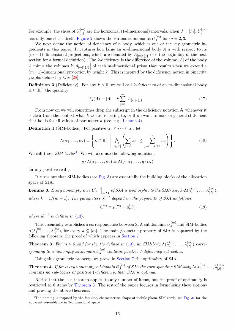
has only one slice: itself. Figure 2 shows the various subdomains U (m)J for m = 2, 3.

We next define the notion of deficiency of a body, which is one of the key geometric in-gredients in this paper. It captures how large an m-dimensional body A is with respect to its(m− 1)-dimensional projections, which are denoted by A[m]\{j} (see the beginning of the nextsection for a formal definition). The k-deficiency is the difference of the volume |A| of the bodyA minus the volumes k

∣∣∣A[m]\{j}

∣∣∣ of each m-dimensional prism that results when we extend a(m−1)-dimensional projection by height k. This is inspired by the deficiency notion in bipartitegraphs defined by Ore [28].

Definition 3 (Deficiency). For any k > 0, we will call k-deficiency of an m-dimensional bodyA ⊆ Rm+ the quantity

δk(A) ≡ |A| − km∑j=1

∣∣∣A[m]\{j}

∣∣∣ . (17)

From now on we will sometimes drop the subscript in the deficiency notation δk whenever itis clear from the context what k we are referring to, or if we want to make a general statementthat holds for all values of parameter k (see, e.g., Lemma 4).

Definition 4 (SIM-bodies). For positive α1 ≤ · · · ≤ αr, let

Λ(α1, . . . , αr) ≡

x ∈ Rr+

∣∣∣∣∣∣∧J⊆[r]

∑j∈J

xj ≤r∑

j=r−|J |+1αj

. (18)

We call these SIM-bodies4. We will also use the following notation:

q · Λ(α1, . . . , αr) ≡ Λ(q · α1, . . . , q · αr)

for any positive real q.

It turns out that SIM-bodies (see Fig. 3) are essentially the building blocks of the allocationspace of SJA:

Lemma 3. Every nonempty slice U (m)J

∣∣∣−J :t

of SJA is isomorphic to the SIM-body k·Λ(λ(m)1 , . . . , λ

(m)|J | ),

where k = 1/(m+ 1). The parameters λ(m)r depend on the payments of SJA as follows:

λ(m)r ≡ µ(m)

r − µ(m)r−1, (19)

where µ(m)r is defined in (13).

This essentially establishes a correspondence between SJA subdomains U (m)J and SIM-bodies

Λ(λ(m)1 , . . . , λ

(m)|J | ), for every J ⊆ [m]. The main geometric property of SJA is captured by the

following theorem, the proof of which appears in Section 7.

Theorem 3. For m ≤ 6 and for the λ’s defined in (13), no SIM-body Λ(λ(m)1 , . . . , λ

(m)|J | ) corre-

sponding to a nonempty subdomain U(m)J contains positive 1-deficiency sub-bodies.

Using this geometric property, we prove in Section 7 the optimality of SJA:

Theorem 4. If for every nonempty subdomain U (m)J of SJA the corresponding SIM-body Λ(λ(m)

1 , . . . , λ(m)|J | )

contains no sub-bodies of positive 1-deficiency, then SJA is optimal.

Notice that the last theorem applies to any number of items, but the proof of optimality isrestricted to 6 items by Theorem 3. The rest of the paper focuses in formalizing these notionsand proving the above theorems.

4The naming is inspired by the familiar, characteristic shape of mobile phone SIM cards; see Fig. 3a for theapparent resemblance in 2-dimensional space.

16

5 Bodies and Deficiencies

In this section we develop the geometric theory that captures the critical structural properties ofSJA mechanisms and use this to prove our main result, Theorem 2, that shows their optimality.First we will need to establish some notation and formally define some notions.

For any positive integer m, an m-dimensional body A is any compact subset of the nonnega-tive orthant A ⊆ Rm+ . We will denote its volume simply by |A| ≡ µ(A) (where µ is the standardm-dimensional Lebesgue measure). For any index set J ⊆ [m], the projection of A with respectto the J coordinates is defined as

A[m]\J ≡ {x−J | x ∈ A}

and is the remaining body of A if we “delete” coordinates J . For any r ∈ [m], index set J ⊆ [m]with |J | = m − r and t ∈ Rm−r+ we define the slice of A above the point t with respect tocoordinates J as

A|J :t ≡ {x−J | x ∈ A ∧ xJ = t} .

It is the remaining of the body A if we fix a vector t at coordinates J . The operations ofprojecting and slicing bodies commute with each other, that is, A[m]\I

∣∣∣J :t

= (A|J :t)[m]\I for alldisjoint sets of indices I, J ⊆ [m] and |J |-dimensional vector t.

For any set of points S ⊆ Rm+ we denote their convex hull by H(S) and for any vector x wewill denote by P(x) the set of all permutations of x. We will say that a body A is downwardsclosed if, for any point of A, all points below it are also contained in A: y ∈ A for all y ∈ Rm+with y ≤ x ∈ A. Body A will be called symmetric if it contains all permutations of its elements:P(x) ⊆ A for all x ∈ A. If an m-dimensional body A is symmetric then one can define its widthto be the length of its projection towards any axis: w(A) ≡ |A{j}| for any j ∈ [m]. In a similarway, if A ⊆ S we will say that A is upwards closed (with respect to S) if, for any x ∈ A, wehave y ∈ A for any x ≤ y ∈ S. For any set of points S ⊆ Rm+ , its downwards closure is definedto be all points below it: D(S) =

{x ∈ Rm+ | ∃y ∈ S : x ≤ y

}. Finally, we describe a property

that will play a key role in the following:

Definition 5 (p-closure). We will say that a body A is p-closed if it contains the convex hullof the permutations of any of its elements. Formally: H(P(x)) ⊆ A for all x ∈ A.

Notice that any p-closed body must be symmetric (but not necessarily convex) and that anyconvex symmetric body is p-closed.

A useful, trivial to prove property of the deficiency function (see Definition 3) is that it issupermodular :

Lemma 4. For any bodies A1, A2,

δ(A1 ∪A2) + δ(A1 ∩A2) ≥ δ(A1) + δ(A2).

The next lemma tells us that “leaving gaps” between the points of bodies and the orthant’sfaces can only reduce the deficiency.

Lemma 5. For any bodies A,B such that B ⊆ A and A is downwards closed, there exists adownwards closed sub-body B ⊆ A such that δ(B) ≥ δ(B).

Instead of proving this lemma, we provide a stronger construction, given by the followingLemma 6.

Lemma 6. Let Am be the set of m-dimensional bodies and Km ⊆ Am be the set of downwardsclosed ones. There is a mapping χ : Am → Km such that for any A,B ∈ Am:

1. |χ(A)| = |A| and, for every J ⊆ [m], |χ(A)J | ≤ |AJ |.

17

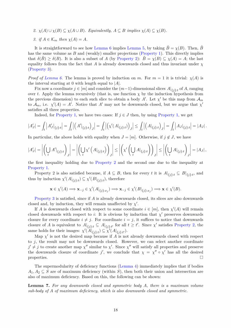
2. χ(A) ∪ χ(B) ⊆ χ(A ∪B). Equivalently, A ⊆ B implies χ(A) ⊆ χ(B).

3. if A ∈ Km then χ(A) = A.

It is straightforward to see how Lemma 6 implies Lemma 5, by taking B = χ(B). Then, Bhas the same volume as B and (weakly) smaller projections (Property 1). This directly impliesthat δ(B) ≥ δ(B). It is also a subset of A (by Property 2): B = χ(B) ⊆ χ(A) = A; the lastequality follows from the fact that A is already downwards closed and thus invariant under χ(Property 3).

Proof of Lemma 6. The lemma is proved by induction on m. For m = 1 it is trivial: χ(A) isthe interval starting at 0 with length equal to |A|.

Fix now a coordinate j ∈ [m] and consider the (m−1)-dimensional slices A|{j}:t of A, rangingover t. Apply the lemma recursively (that is, use function χ by the induction hypothesis fromthe previous dimension) to each such slice to obtain a body A′. Let χ′ be this map from Amto Am, i.e. χ′(A) = A′. Notice that A′ may not be downwards closed, but we argue that χ′satisfies all three properties.

Indeed, for Property 1, we have two cases: If j ∈ J then, by using Property 1, we get

∣∣A′J ∣∣ =∫t

∣∣∣A′J ∣∣{j}:t∣∣∣ =∫t

∣∣∣(A′∣∣{j}:t)J ∣∣∣ =∫t

∣∣∣(χ′(A|{j}:t))J ∣∣∣ ≤∫t

∣∣∣(A|{j}:t)J ∣∣∣ =∫t

∣∣∣AJ |{j}:t∣∣∣ = |AJ | .

In particular, the above holds with equality when J = [m]. Otherwise, if j 6∈ J , we have

∣∣A′J ∣∣ =∣∣∣∣∣(⋃

t

A′∣∣{j}:t

)J

∣∣∣∣∣ =∣∣∣∣∣(⋃

t

χ′(A|{j}:t

))J

∣∣∣∣∣ ≤∣∣∣∣∣(χ′(⋃

t

A|{j}:t

))J

∣∣∣∣∣ ≤∣∣∣∣∣(⋃

t

A|{j}:t

)J

∣∣∣∣∣ = |AJ | ,

the first inequality holding due to Property 2 and the second one due to the inequality atProperty 1.

Property 2 is also satisfied because, if A ⊆ B, then for every t it is A|{j}:t ⊆ B|{j}:t, andthus by induction χ′(A|{j}:t) ⊆ χ′(B|{j}:t), therefore

x ∈ χ′(A) =⇒ x−j ∈ χ′(A|{j}:xj) =⇒ x−j ∈ χ′(B|{j}:xj

) =⇒ x ∈ χ′(B).

Property 3 is satisfied, since if A is already downwards closed, its slices are also downwardsclosed and, by induction, they will remain unaffected by χ′.

If A is downwards closed with respect to some coordinate i ∈ [m], then χ′(A) will remainclosed downwards with respect to i: It is obvious by induction that χ′ preserves downwardsclosure for every coordinate i 6= j. For coordinate i = j, it suffices to notice that downwardsclosure of A is equivalent to A|{j}:t ⊆ A|{j}:t′ for all t ≥ t′. Since χ′ satisfies Property 2, thesame holds for their images: χ′(A|{j}:t) ⊆ χ′(A|{j}:t′).

Map χ′ is not the desired map because if A is not already downwards closed with respectto j, the result may not be downwards closed. However, we can select another coordinatej′ 6= j to create another map χ′′ similar to χ′. Since χ′′ will satisfy all properties and preservethe downwards closure of coordinate j′, we conclude that χ = χ′′ ◦ χ′ has all the desiredproperties.

The supermodularity of deficiency functions (Lemma 4) immediately implies that if bodiesA1, A2 ⊆ S are of maximum deficiency (within S), then both their union and intersection arealso of maximum deficiency. Based on this, the following can be shown:

Lemma 7. For any downwards closed and symmetric body A, there is a maximum volumesub-body of A of maximum deficiency, which is also downwards closed and symmetric.

18

Proof. Let B ⊆ A be of maximum deficiency. Then, by Lemma 5 there exists a downwardsclosed B ⊆ A such that δ(B) ≥ δ(B), and, due to the maximum deficiency of B, it must be thatδ(B) = δ(B). Now, let B1, B2, . . . , Bm! be all possible permutations of the body B (within them-dimensional space) and take their union B =

⋃m!i=1 Bi. This new body B is clearly symmetric.

Also, because of the symmetry of A, all Bi remain within A, so B ⊆ A.Now notice that all Bi’s have δ(Bi) = δ(B), so they also have maximum deficiency within A.

Remember that the deficiency function is supermodular (Lemma 4), so the union of maximumdeficiency sets must also be of maximum deficiency. Thus, B is indeed of maximum deficiency.Finally, it is not difficult to see that union preserves downwards closure and also, trivially,|B| ≥ |B|.

The next lemma describes how global maximum deficiency implies also a kind of local one:

Lemma 8. Let A ⊆ S be a maximum deficiency body (within S). Then, every slice of A musthave nonnegative deficiency and must not contain subsets with higher deficiency.

Proof. To get to a contradiction, suppose that there exists such a slice B = A|J :t of A, such thatδ(B) < 0. Then, let’s remove the entire slice B above t from body A, to get a new body A′. This(m− 1)-dimensional slice though is of measure 0 in the larger m-dimensional space, so what weshould really do is to remove an ε-neighborhood of B (around t) within A, of “parallel” slices.This neighborhood has a volume of positive measure and is arbitrarily close to the slice5. Thissection removed from the body had the property of having volume strictly less than k times itsprojections with respect to the coordinates not in J , i.e., the “active” coordinates in B (becausewe are working close to B for which δ(B) < 0). Regarding the other remaining projectionswith respect to the coordinates in J , by removing points they cannot possibly be increased.Since volumes have positive sign effect at the expression (17) of the deficiency function, andprojections have negative, we can deduce that the resulting body has strictly higher deficiencythan A, which contradicts the maximum deficiency of A within S.

The proof for subsets of the slice with higher deficiency is similar: replace the entire slicewith its subset of higher deficiency, and the total deficiency must increase.

As a consequence of Lemma 8 we get the following properties of maximum deficiency sub-bodies, which imply that these bodies must be “large enough” (Lemmas 10 and 11) and alsodemonstrate some kind of “symmetric convexity” (p-closure Lemma 12, Definition 5). But firstwe will need an inequality that brings together volumes and projections of bodies, due to Loomisand Whitney [21]. An easy proof of this can be found in [2].

Lemma 9 (Loomis–Whitney). For any m-dimensional body A,

|A|m−1 ≤m∏j=1

∣∣∣A[m]\{j}

∣∣∣ .Lemma 10. Let A 6= ∅ be an m-dimensional body with nonnegative k-deficiency. Then

|A| ≥ (km)m.

As a consequence, if A is also symmetric and downwards closed, its width must be at least

w(A) ≥ km.5For ease of presentation, in the following we will use that procedure without making explicit mention to the

underlying technicalities.

19

Proof. Since δk(A) ≥ 0, we know that |A| ≥ k∑mj=1

∣∣∣A[m]\{j}

∣∣∣ , or equivalently

m∑j=1

∣∣∣A[m]\{j}

∣∣∣ ≤ |A|k. (20)

Also, by the Loomis–Whitney inequality (Lemma 9), |A|m−1 ≤∏mj=1

∣∣∣A[m]\{j}

∣∣∣; so, by using the

arithmetic-geometric means inequality we can derive that |A|m−1 ≤(

1m

∑mj=1

∣∣∣A[m]\{j}

∣∣∣)m, orequivalently

m∑j=1

∣∣∣A[m]\{j}

∣∣∣ ≥ m |A|m−1m . (21)

Combining (20) and (21) we get m |A|m−1

m ≤ |A|k , which completes the proof of the lemma

(since |A| 6= 0). The inequality involving the body’s width follows immediately from the obser-vation that every symmetric and downwards closed body A is included in the m-dimensionalhypercube with edge length w(A).

Lemma 11. If A is a nonempty, symmetric, downwards closed body with nonnegative k-deficiency then it must contain the point (k, 2k, . . . ,mk). More generally, it must contain thepoint (k, 2k, . . . , (m− 1)k,w(A)).

Proof. We will recursively utilize Lemmas 8 and 10 to show that points

(mk,0m−1), (mk, (m− 1)k,0m−2), . . . , (mk, (m− 1)k, . . . , k)

belong to A, where A is a symmetric, downwards closed sub-body of A of maximum deficiency(see Lemma 7). By Lemma 10 it must be that that w(A) ≥ mk, thus (mk,0m−1) ∈ A bydownwards closure. For the next dimension, consider the slice A

∣∣∣{j}:mk

(for some j ∈ [m]). Itis (m − 1)-dimensional, of nonnegative deficiency by Lemma 8, and so it must have width atleast (m − 1)k (Lemma 10). That means that point (mk, (m − 1)k,0m−2) must be in A. Wecan continue like this all the way down to single-dimensional lines.

Lemma 12 (p-closure). Let A ⊆ S be a maximum volume sub-body of S of maximum deficiencyand let S be p-closed and downwards closed. Then every slice of A (including A itself) must bep-closed (see Definition 5).

Proof. Without loss (by Lemma 7) A can be assumed to be symmetric and downwards closed.We need to prove that, for any r ∈ [m] (r is the dimension of the slice) and any r-dimensionalvector x and z ∈ H(P(x)) in the convex hull of its permutations,

for all t : (x, t) ∈ A =⇒ (z, t) ∈ A.

The proof is by induction on r. For the base case of r = 1, it is H(P(x)) = {x} so theproposition follows trivially. For the induction step, assume the proposition is true for somer ≤ m− 1 and we will prove it for r+ 1. So, take (r+ 1)-dimensional vectors x and z such thatz ∈ H(P(x)) and fix some t ∈ Rm−r−1

+ . To complete the proof we need to show that the sliceof A above x, with respect to the first r + 1 coordinates, is included within the one above z,i.e. A|[r+1]:x ⊆ A|[r+1]:z. For simplicity, let’s abuse notation for the remaining of this proof andjust use Ax and Az for these slices.

So, to arrive at a contradiction, let’s assume that, Ax \ Az 6= ∅. First notice that sinceAx ∩ Az ⊆ Ax and Ax is a slice of a maximum deficiency body, by Lemma 8 it must be thatδ(Ax ∩Az) ≤ δ(Ax). So, by the supermodularity of deficiencies (Lemma 4) we get that

δ(Ax ∪Az) ≥ δ(Az).

20

This means that if we replace (an ε-neighborhood around z of) slice Az by its superset Ax ∪Azand we can also show that no new projections are created with respect to the first r + 1coordinates, then the overall deficiency of the body would not decrease and its volume wouldincrease strictly (since we have assumed that Ax \ Az 6= ∅), which is a contradiction to themaximum deficiency of A within S. Notice a subtle point here: How do we know that thisextension can fit within S above point z? It does, because we have assumed S to be p-closedand the new elements added are convex combinations of permutations of elements already knownto be in S. The remainder of the proof is dedicated to proving that this extension indeed doesnot create new projections with respect to the first r + 1 coordinates.

Without loss, due to symmetry, we can take x1 ≤ x2 ≤ · · · ≤ xr+1. We argue that, if weremove any one of the coordinates of the vector z, it can be dominated by a convex combinationof permutations of the vector x−1 (i.e., the vector x if we remove its smallest coordinate). To seethat, remember that z is at the convex hull of the permutations of x, so there exist nonnegativereal parameters {ξπ} such that

z =∑

π∈P(x)ξππ and

∑π∈P(x)

ξπ = 1.

But that means thatz−j =

∑π∈P(x)

ξππ−j (22)

for any coordinate j.Let’s define a transformation φ over all vectors {π−j | π ∈ P(x) and j ∈ [r + 1]} such that

φ(π−j) = π−j if the j-th coordinate removed from π to get π−j was x1, and otherwise φ(π−j)is the r-dimensional vector that we get if we replace x1 in π−j by the coordinate πj that wasremoved. It follows that for all j

π−j ≤ φ(π−j) and φ(π−j) ∈ P(x−1),

so by (22),z−j ≤

∑π∈P(x)

ξπφ(π−j) ∈ H(P(x−1)).

By the induction hypothesis and downwards closure for A it can be deduced that

(x−1, 0, t) ∈ A =⇒ (z−j , 0, t) ∈ A for all j ∈ [r + 1].

Thus in particular for every t ∈ Ax, due to symmetry of A, we have that ((z−j , 0), t) ∈ A,which means that indeed every projection of (z, t) with respect to a coordinate in [r + 1] wasalready included in A.

6 Decomposition of SJA into SIM-bodies

6.1 SIM-bodies

Remember that in Definition 4 we introduced the notion of a SIM-body Λ(α1, . . . , αr): forparameters α1 ≤ · · · ≤ αr, it is the set of all vectors x ∈ Rr+ satisfying conditions

∑j∈J xj ≤∑r

j=r−|J |+1 αj for all J ⊆ [r].The geometry of the allocation space of the SJA mechanisms (see Fig. 2) naturally gives

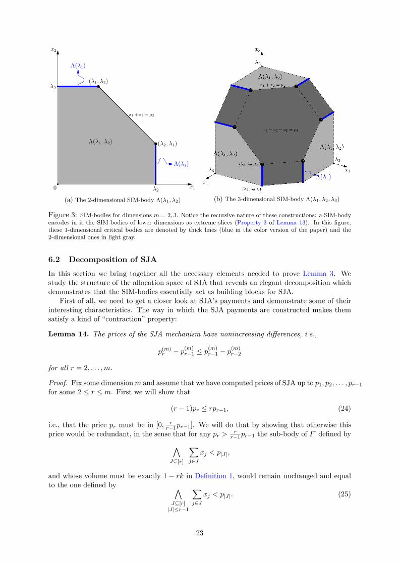
rise to this family of bodies. Their importance and connection with the structure of the SJAmechanisms will become evident in Section 6.2, where we prove Lemma 3. The intuition behindthe naming becomes obvious if one looks at Fig. 3a. By the way SIM-bodies are defined, one

21

can immediately see that they are downwards closed, symmetric, and convex polytopes. Thus,they are also p-closed. Each one of its faces corresponds to a defining hyperplane∑

j∈Jxj = αr+1−|J | + · · ·+ αr

for some J ⊆ [r] or, of course, to a side of the r-dimensional positive orthant Rm+ .SIM-bodies demonstrate some inherently recursive and symmetric properties, captured by

the following lemma. They are made clear in Fig. 3.

Lemma 13. For any SIM-body Λ = Λ(α1, . . . , αr):

1. w(Λ) = αr

2. Λ = D(H(P(α1, . . . , αr)))

3. Λ|{j}:αr= Λ(α1, . . . , αr−1) for any j ∈ [r]

4. Λ[r]\{j} = Λ(α2, . . . , αr) for any j ∈ [r]

5. δq·k(q · Λ) = qr · δk(Λ) for any q, k > 0

Proof. Property 1 is trivial: by the definition of SIM-bodies (18), a point (x,0r−1) ∈ Λ if andonly if x ≤ αr ∧ · · · ∧ x ≤ α1 + · · ·+ αr, i.e., x ≤ αr.

For Property 2, let E be the set of the extreme points of the polytope Λ. It is convex, thusΛ = H(E). But it is also downwards closed, so we can just focus on the extreme points E ⊆ Ethat belong to the “full” facet of the hyperplane x1 + . . . xr = α1 + · · · + αr, since the entirepolytope can be recovered as the downwards closure Λ = D(H(E)). By taking intersectionswith the other hyperplanes and keeping in mind that the αj ’s are nondecreasing, we get thatthese extreme points in E are (α1, α2, . . . , αr) and all its permutations. So, we can recover theentire SIM-body as Λ = D(H(P(α1, . . . , αr))).

For Property 3, notice that an (r − 1)-dimensional vector x belongs in the slice Λ|{j}:αrif

and only if (x, αr) ∈ Λ, which by using (18) is equivalent to

∧J⊆[r−1]

(∑i∈J

xi ≤ αr+1−|J | + · · ·+ αr

)and

∧J⊆[r−1]

(αr +

∑i∈J

xi ≤ αr−|J | + · · ·+ αr

).

The second set of conditions can be rewritten simply as∧J⊆[r−1]

∑i∈J

xi ≤ αr−|J | + · · ·+ αr−1, (23)

which makes the first set of constraints redundant since αr−|J |+ · · ·+αr−1 ≤ αr+1−|J |+ · · ·+αrfrom the monotonicity of the sequence of αr’s. The constraints (23) that we are left with,exactly define Λ(α1, . . . , αr−1) (see (18)).

Property 4 can be shown in a very similar way: due to downwards closure, any projectionΛ[r]\{j} is just the slice Λ|{j}:0.

Finally, Property 5 is a result of scaling: q · Λ and Λ are similar by a scaling factor of q, sothe ratio of their volumes is qr and the ratio of their projections is qr−1. In formula (17) thatdefines deficiencies, the volumes of the projections are also multiplied by the parameter k of thedeficiency, resulting in an overall ratio of qr between the two deficiencies.

22

x2

x1

Λ(λ1, λ2)

λ2

λ2

(λ2, λ1)

(λ1, λ2)

x1 + x2 = µ2

0

Λ(λ1)

Λ(λ1)

(a) The 2-dimensional SIM-body Λ(λ1, λ2) (b) The 3-dimensional SIM-body Λ(λ1, λ2, λ3)

Figure 3: SIM-bodies for dimensions m = 2, 3. Notice the recursive nature of these constructions: a SIM-bodyencodes in it the SIM-bodies of lower dimensions as extreme slices (Property 3 of Lemma 13). In this figure,these 1-dimensional critical bodies are denoted by thick lines (blue in the color version of the paper) and the2-dimensional ones in light gray.

6.2 Decomposition of SJA

In this section we bring together all the necessary elements needed to prove Lemma 3. Westudy the structure of the allocation space of SJA that reveals an elegant decomposition whichdemonstrates that the SIM-bodies essentially act as building blocks for SJA.

First of all, we need to get a closer look at SJA’s payments and demonstrate some of theirinteresting characteristics. The way in which the SJA payments are constructed makes themsatisfy a kind of “contraction” property:

Lemma 14. The prices of the SJA mechanism have nonincreasing differences, i.e.,

p(m)r − p(m)

r−1 ≤ p(m)r−1 − p

(m)r−2

for all r = 2, . . . ,m.

Proof. Fix some dimensionm and assume that we have computed prices of SJA up to p1, p2, . . . , pr−1for some 2 ≤ r ≤ m. First we will show that

(r − 1)pr ≤ rpr−1, (24)

i.e., that the price pr must be in [0, rr−1pr−1]. We will do that by showing that otherwise this

price would be redundant, in the sense that for any pr > rr−1pr−1 the sub-body of Ir defined by∧

J⊆[r]

∑j∈J

xj < p|J |,

and whose volume must be exactly 1− rk in Definition 1, would remain unchanged and equalto the one defined by ∧

J⊆[r]|J |≤r−1

∑j∈J

xj < p|J |. (25)

23

Indeed, the body defined from (25) is a downwards closed, symmetric convex polytopeand for the newly inserted hyperplane x1 + · · · + xr = pr to have any effect on it, i.e., tohave a nonempty intersection with it, it must be that this hyperplane’s “symmetric point”(pr/r, . . . , pr/r) belongs already to the interior of the body in (25) (this is due to the symmetryand convexity of the body). So, this point must satisfy the (r − 1)-dimensional conditionx1 + · · ·+ xr−1 ≤ pr−1, thus (r − 1)(pr/r) ≤ pr−1 which is exactly property (24).

To show that pr − pr−1 ≤ pr−1 − pr−2 for all 2 ≤ r ≤ m, or equivalently pr ≤ 2pr−1 − pr−2,by (24) it is enough to show that r

r−1pr−1 ≤ 2pr−1−pr−2. But this is equivalent to (r−1)pr−2 ≤(r − 2)pr−1 which we know holds, also from (24).

Normalized payments By the procedure of defining SJA payments (Definition 1), it canbe the case that price pr is smaller than pr−1, i.e., pr ∈ [pl, pl+1] for some l ≤ r − 2. This isperfectly acceptable, and it just means that essentially we render older prices that are abovepr redundant, in the sense that setting pj ← pr for all j < r with pj ≥ pr would not havean effect on the sub-body

∧J⊆[r]

∑j∈J xj < p|J | of Ir used in the definition of SJA in (10).

This because x1 + · · · + xr ≤ pr =⇒ x1 + · · · + xj ≤ pj (since j < r and pr ≤ pj), so oldconditions x1 + · · · + xj ≤ pj have become useless. In particular, notice how this is the casefor the full-bundle price p

(m)m when m = 5, 6: from Eqs. (14) and (15) we see that indeed

p(5)5 ≈ 1.9856 < 2.0005 ≈ p(5)

4 and p(6)5 ≈ 2.3774 < 2.4165 ≈ p(6)

6 . This means that no bundle ofm− 1 items is ever going to be sold under the SJA mechanism for m = 5 or m = 6:

U(5)[4] = U

(6)[5] = ∅. (26)

Furthermore, by the nonincreasing differences property of the SJA payments (Lemma 14),every new payment after r will continue to fall below the previous one. So, at the end thesituation will be in the form of

p1 ≤ · · · ≤ pl ≤ pm ≤ . . . (27)

for some l < m and, as we discussed above, there will be absolutely no effect on the mechanismif we update all older payments that have ended up above pm to “collapse” to pm, i.e.,

p1 ≤ · · · ≤ pl ≤ pm = pm−1 = pm−2 = · · · = pl+1. (28)

Rigorously, we redefine

p(m)j ← p(m)

m for all j ∈ [m− 1] with pj ≥ pm.

While this normalization has no effect on the SJA mechanism itself, it makes sure that paymentsare now given in a nondecreasing order, which is an elegant property that will simplify ourexposition later on.

An important observation is that this normalization of payments does not break the propertyof the nonincreasing differences of the payments of SJA, i.e. Lemma 14 continues to hold: havinga look at the transition before and after the normalization process from (27) to (28) we see thatall the differences up to the l-th payment remain unchanged, pl+1 − pl can only decrease andall differences above the (l + 1)-th payment have just collapsed to 0.

From now on and for the remaining of this paper we will assume that SJA payments arenormalized. The only difference that this makes, for up to m = 6 dimensions, to the values ofthe payments we have already computed at Eqs. (14) and (15) in Section 4 is that for m = 5, 6we have that

p(5)4 ← p

(5)5 and p

(6)5 ← p

(6)6 ,

which gives by (13) that also the µ(m)r parameters are updated to µ(m)

m−1 ← µ(m)m − (m+ 1):

µ(5)4 ≈ 12.0865 µ

(6)5 ≈ 18.3585.

24

Recall the definition λr ≡ µr − µr−1 from (19). These are the critical parameters of theSIM-bodies used in all the key theorems for the optimality of SJA. Equation (19) is equivalentto saying that µr = λ1 + · · ·+ λr. Taking the µ(m)

r values into account (see (13)) the λ(m)r ’s for

up to m = 6 items are, for m ≤ 4,

λ1 = 1 λ2 = 1 +√

2 λ3 ≈ 3.6830 λ4 ≈ 4.9000 (29)

and for m = 5, 6 the only modifications are

λ(5)4 ≈ 4.9894 λ

(5)5 = 6 λ

(6)5 ≈ 6.3613 λ

(6)6 = 7. (30)

The nonincreasing differences property of the SJA payments makes these parameters mono-tonic:

Lemma 15. The λ(m)r parameters are nondecreasing and upper-bounded by m+ 1, i.e.,

λ(m)r−1 ≤ λ

(m)r ≤ m+ 1,

for all r = 2, . . . ,m.

Proof. Using the transformations (13) and (19) we have

pr − pr−1 ≤ pr−1 − pr−2 =⇒ µr−1 − µr−2 ≤ µr − µr−1 =⇒ λr−1 ≤ λr

andpr−1 ≤ pr =⇒ µr − µr−1 ≤ m+ 1 =⇒ λr ≤ m+ 1,

which concludes the proof since the SJA payments are nondecreasing with nonincreasing differ-ences (Lemma 14).

An algebraic manipulation of (16), using the nonincreasing differences property of the SJApayments, can give us the following characterization:

Lemma 16. For any subset of items J ⊆ [m],

U(m)J =

x ∈ Im∣∣∣∣∣∣∧L⊆J

∑j∈L

xj ≥ p(m)|J | − p

(m)|J |−|L|

∧L⊆[m]\J

∑j∈L

xj ≤ p(m)|J |+|L| − p

(m)|J |

.Proof. Fix some positive integer m, J ⊆ [m] and an arbitrary x ∈ Im. We need to show thatx satisfies the constraints in the description of set U (m)

J at the statement of Lemma 16 if andonly if it satisfies the constraints in (16). To be more precise, and after moving all xj ’s in theconstraints of (16) at the left side of the inequalities and deleting the ones that cancel out, weneed to show that ∑

j∈J\Lxj −

∑j∈L\J

xj ≥ p|J | − p|L| for all L ⊆ [m] (31)

if and only if ∑j∈L1

xj ≥ p|J | − p|J |−|L1| for all L1 ⊆ J (32)

and ∑j∈L2

xj ≤ p|J |+|L2| − p|J | for all L2 ⊆ J , (33)

where for simplicity we drop the superscript (m) from the prices and denote J = [m] \ J .

25

Indeed, first assume that x satisfies (31) and pick any L1 ⊆ J , L2 ⊆ J . Then, sinceJ \ (J \ L1) = L1 and (J \ L1) \ J = ∅, by using L← J \ L1 in (31) we get∑

j∈L1

xj ≥ p|J | − p|J\L1| = p|J | − p|J |−|L1|,

which proves that x satisfies (32). In a similar way, since J \ (J ∪L2) = ∅ and (J ∪L2)\J = L2,if we use L← J ∪ L2 in (31) we get

−∑j∈L2

xj ≥ p|J | − p|J∪L2| = p|J | − p|J |+|L2|,

which is the same as (33).For the opposite direction, assume now that x satisfies (32) and (33), and pick any L ⊆ [m].

Since J \ L ⊆ J and L \ J ⊆ J , if we use L1 ← J \ L and L2 ← L \ J in (32) and (33),respectively, we get ∑

j∈J\Lxj ≥ p|J | − p|J |−|J\L|,

∑j∈L\J

xj ≤ p|J |+|L\J | − p|J |.

By subtracting these inequalities and taking into consideration that |J | − |J \ L| = |J ∩ L| and|J |+ |L \ J | = |J ∪ L| we have∑

j∈J\Lxj −

∑j∈L\J

xj ≥ 2p|J | − p|J∩L| − p|J∪L|.

So, in order to show that (31) holds and conclude the proof of the lemma, it is enough to showthat p|J | − p|J∩L| − p|J∪L| ≥ −p|L|, or equivalently that

p|J∪L| − p|J | ≤ p|L| − p|J∩L|.

But since |J ∪ L| − |J | = |L| − |J ∩ L| (they are both equal to |L \ J |) and |J ∪ L| ≥ |L|, theabove inequality indeed holds due to the nonincreasing differences property of the SJA payments(Lemma 14).

Notice here that, due to symmetry, every slice U(m)J

∣∣∣−J :t

with |J | = r ≤ m is isomorphic

to U(m)[r]

∣∣∣[r+1...m]:t

and so, from the characterization in Lemma 16, this slice is invariant withrespect to the specific value of the ((m−r)-dimensional) vector t. In particular, if it’s nonempty,then

U(m)J

∣∣∣−J :t

= U(m)J

∣∣∣−J :0m−|J|

. (34)

The following lemma essentially gives an alternative definition of SJA, in terms of the deficienciesof its allocation components U (m)

J . In particular, it requires every |J |-dimensional slice of anysubdomain U

(m)J to have zero deficiency:

Lemma 17. Every slice U(m)J

∣∣∣−J :t

of SJA has zero k-deficiency, where k = 1m+1 .

Proof sketch. Fix some dimension m and let k = 1/(m+ 1). By the definition of SJA (10), thedomain U∅ where at least one item is sold must have volume m/(m + 1): the probability ofselling at least an item is mk = m/(m + 1) which corresponds to the volume of this domainbecause the valuations’ space is the unit cube Im. Every projection (U∅){j} of this body towardsany coordinate j ∈ [m] has volume 1: it is the (m−1)-dimensional side of the cube; just set the

26

valuation of item j to xj = 1 and trivially notice that, no matter what the remaining valuationsx−j ∈ Im−1 are, at least one item is being sold by SJA, namely item j, since xj = 1 ≥ p1.Bringing the above together, this means that the k-deficiency of U∅ is m/(m+ 1)−k ·m ·1 = 0.

This valuations subdomain U∅ where at least one item is sold can be decomposed in itsvarious components UJ , where ∅ 6= J ⊆ [m]. Its volume is just the sum of the volumes ofthese components. Also, its projections (i.e. the sides of the unit cube Im) can be covered bytaking the projection of any such component UJ with respect to its “active” coordinates in J .This tells us that the deficiency of the entire body U∅ is essentially reduced to the sum of thedeficiencies of its subdomains. But this body has zero k-deficiency, so all its components mustalso have zero deficiencies (by using an inductive argument).

A complete, formal proof of this characterization can be found in Appendix A.

Now we are ready to prove Lemma 3, which makes rigorous the correspondence between thevarious components U (m)

J of the allocation space of SJA and SIM-bodies. It is the motivationbehind introducing SIM-bodies in the first place. Essentially, the entire allocation space of SJAis made up by slices of SIM-bodies:

Lemma (Lemma 3). Every nonempty slice U (m)J

∣∣∣−J :t

is isomorphic to the SIM-body k·Λ(λ(m)1 , . . . , λ

(m)|J | ),

where k = 1m+1 .

Proof. Let |J | = r. Then, due to symmetry, the slice UJ |−J :t is isomorphic to U[r]

∣∣∣[r+1...m]:t

.An r-dimensional vector y belongs to this slice if and only if (y, t) ∈ U[r], which by Lemma 16means that y ∈ Ir and ∧

L⊆[r]

∑j∈L

yj ≥ pr − pr−|L|.

By (13) this can be written as ∧L⊆[r]

∑j∈L

yj ≥ |L| − (µr − µr−|L|)k.

So this slice is an upwards closed body within the r dimensional unit-hypercube Ir, and if weapply the isomorphism y 7→ 1r − y it is flipped around and mapped to the downwards closedbody around the origin 0r defined by y ∈ Ir and

∧L⊆[r]

∑j∈L yj ≤ (µr − µr−|L|)k. By taking

into consideration (19) this becomes∧L⊆[r]

∑j∈L

yj ≤ λr−|L|+1k + · · ·+ λrk. (35)

It is easy to see that the extra condition y ∈ Ir can be replaced by the weaker one y ∈ Rr+,since the upper bounds yj ≤ 1 are already captured by (35): for L = {j} it gives

yj ≤ λrk = λrm+ 1 ≤ 1,

the last inequality holding from Lemma 14. So, we end up with exactly the definition ofΛ(kλ1, . . . , kλr). We must note here that this SIM-body is well-defined, since the λr’s arenondecreasing (Lemma 14).

7 Proof of Optimality

In this section we conclude the proof of our main result about the optimality of SJA (Theorem 2).We do that by showing Theorems 3 and 4.

In addition to the SIM-bodies Λ(λ1, . . . , λr) being essentially the building blocks of theallocation space of the SJA, the particular choice of the λr parameters makes them satisfyanother property: they have zero 1-deficiency:

27

Lemma 18. For any dimension m, if a subdomain U(m)J of SJA is nonempty then the corre-

sponding SIM-body Λ(λ(m)1 , . . . , λ

(m)|J | ) has zero 1-deficiency.

Proof. Fix some m and let k = 1/(m + 1). For any nonempty subdomain UJ , the sliceUJ |−J :0m−|J|

is nonempty (by downwards closure), so by Lemma 17 it has zero k-deficiency.

But from Lemma 3 it is also isomorphic to the SIM-body k · Λ(λ(m)1 , . . . , λ

(m)r ), thus δk(k ·

Λ(λ(m)1 , . . . , λ

(m)r )) = 0. By Property 5 of Lemma 13, this means that indeed δ1(Λ(λ(m)

1 , . . . , λ(m)r ))

= 0.

Now we are ready to prove Theorem 3. It is essentially the only ingredient of this paper whoseproof does not work for more than 6 items (condition (38), specifically). In a way it demonstratesthe maximality of the deficiency of the particular critical SIM-bodies Λ(λ1, . . . , λr), in the sensethat they cannot contain subsets that have greater deficiency than themselves.

Theorem (Theorem 3). For up to m ≤ 6, no SIM-body Λ(λ(m)1 , . . . , λ

(m)r ) corresponding to a

nonempty subdomain U(m)[r] contains positive 1-deficiency sub-bodies.

Proof. We will prove the stronger statement that for all r ≤ m ≤ 6 no SIM-body Λ(λ(m)1 , . . . , λ

(m)r )

contains a sub-body with nonnegative 1-deficiency greater than its own, i.e.,

∅ 6= A ⊆ Λ(λ(m)1 , . . . , λ(m)

r ) ∧ δ1(A) ≥ 0 =⇒ δ1(A) ≤ δ1(Λ(λ(m)1 , . . . , λ(m)

r )) (36)

This is enough to establish the theorem, because of Lemma 18. We will use induction on r. Atthe basis, whenever r = 1, for any number of items m the SIM-body is just the line segmentΛ(λ(m)

1 ) = [0, λ(m)1 ] and it is easy to see that every (nonempty) subset of it will have smaller

volume but the same projection, resulting in smaller deficiency.Moving on to the inductive step, for simplicity denote Λ = Λ(λ(m)

1 , . . . , λ(m)r ) and let A ⊆ Λ

be a maximum volume sub-body of maximum nonnegative deficiency within Λ. Without loss(by Lemma 7) A can be assumed to be symmetric and downwards closed. By Lemma 12, thistells us that every slice of it must be p-closed (since A is within Λ which is a SIM-body andthus p-closed). We will prove that A = Λ which is enough to establish (36).

We start by showing that the outmost (r − 1)-dimensional slice of A, namely A|{1}:w(Λ),cannot be empty. Notice that, by Property 1 of Lemma 13, w(Λ) = λ

(m)r . The choice of

coordinate 1 here is arbitrary; due to symmetry any slice A|{j}:w(Λ) with j ∈ [r] would workin exactly the same way. If this slice was empty, we could add in this free space of A (anε-neighborhood of) the (r − 1)-dimensional SIM-body B defined by

B = Λ(λ(m′)1 , . . . , λ

(m′)r−1 ) where m′ =

r − 1, if U (m)[r−1] = ∅,

m, otherwise.(37)

Observe here, that by taking into consideration the values of the λ(m)j parameters of the SJA

mechanism (see Eqs. (29) and (30)) we can see that the following properties are satisfied for allr ≤ m ≤ 6:

λ(m′)j ≤ λ(m)

j and λ(m′)j ≤ j + 1, for all j ∈ [r − 1] (38)

andλ

(m)j ≤ j + 1, for all j ∈ [r − 2]. (39)

In particular, for m = r = 6, notice that although λ(m)r−1 = λ

(6)5 ≈ 6.3613 > 6 = (r − 1) + 1

(and that is why Property (39) above cannot be extended to j = r− 1), it’s still the case6 that6Due to the fact that U (6)

[5] = ∅ (see (26)) and the definition of m′ in (37).

28

λ(m′)r−1 = λ

(r−1)r−1 = λ

(5)5 = 6 = (r − 1) + 1 and so (38) holds. So, it must be that

B ⊆ Λ(λ(m)1 , . . . , λ

(m)r−1) = Λ|{1}:λ(m)

r,

the first inclusion being a result of (38) and the last equality being from Property 3 of Lemma 13.This means that B indeed fits in the exterior space Λ at distance x1 = λ

(m)r , which is exactly

where we put it.We will now show that this addition caused no decrease at the 1-deficiency of A, which

would contradict the maximality of the volume of A. Equivalently, we need to show that theincrease we caused in the volume by extending A was at least equal to the increase in the totalvolume of its projections. First, we show that no new projections were created with respect tocoordinate 1, i.e., B was already included in A[r]\{1} = A|{1}:0. Indeed, it is

B = D(H(P(λ(m′)1 , . . . , λ

(m′)r−1 ))) ⊆ D(H(P(2, . . . , r))) ⊆ A|{1}:0 .

The first equality comes from Property 2 of the SIM-bodies in Lemma 13, the second inclusionis from (38), and the last inclusion is by Lemma 11 and the p-closure of A|{1}:0. What is left toshow is that the sum of the new projections created with respect to the remaining coordinates[2...r] was at most equal to the increase in the volume. But this comes directly from the factthat the slice B we added has zero 1-deficiency: it is a SIM-body corresponding to a subdomainU

(m′)[r−1] 6= ∅ (see Lemma 18).

So, in the following we can indeed assume that body A ⊆ Λ is of maximum width w(A) =λ

(m)r . Then we will show that, at x1 = w(A), A must in fact include the entire correspond-

ing slice of Λ. This slice is Λ|{1}:λmr

= Λ(λ(m)1 , . . . , λ

(m)r−1), so that would mean that the

extreme point (λ(m)1 , . . . , λ

(m)r−1, λ

(m)r ) is in A, and thus by p-closure (Lemma 12) the body

D(H(P(λ(m)1 , . . . , λ

(m)r ))) must be included within A. But from Property 2 of Lemma 13 this

body is exactly the entire external body Λ, which concludes the proof. So let’s show that indeedA|{1}:λm

r= Λ|{1}:λm

r. It is enough to show that removing this slice of A and replacing it with

the full slice of Λ would result in a non-decrease of the 1-deficiency: that would contradict themaximality of the volume of A.

First, notice that A|{1}:λmr

is within Λ|{1}:λmr

, where Λ|{1}:λmr

is the SIM-body Λ(λ(m1 , . . . , λ

(m)r−1)

and also slice A|{1}:λmr

must have nonnegative deficiency (by Lemma 8). So, by the inductionhypothesis it must be that the full slice Λ|{1}:λm

rhas at least the deficiency of the slice A|1:λm

r

it replaces. That means that, taking into consideration only projections in the directions [2...r],the overall change in the deficiency is indeed nonnegative. So, to conclude the proof it is enoughto show that no new projections with respect to coordinate 1 are created by this replacement,i.e. that Λ(λ(m

1 , . . . , λ(m)r−1) was already included in A[r]\{1} = A|{1}:0. Indeed,

Λ(λ(m1 , . . . , λ

(m)r−1) = D(H(P(λ(m)

1 , . . . , λ(m)r−1)))

⊆ D(H(P(λ(m)1 , . . . , λ

(m)r−2, λ

(m)r )))

⊆ D(H(P(2, . . . , r − 1, w(A)))),

by (39) and the fact that w(A) = λ(m)r , which concludes the proof since slice A|{1}:0 is p-

closed and (2, . . . , r − 1, w(A)) belongs to it, because (1, 2, . . . , r − 1, w(A)) belongs to A byLemma 11.

We now present our main tool to prove that SJA is optimal. It utilizes the fact that theallocation space of SJA has no positive deficiency subsets in a combinatorial way.

Theorem (Theorem 4). If for every nonempty subdomain U (m)J of SJA the corresponding SIM-

body Λ(λ(m)1 , . . . , λ

(m)|J | ) contains no sub-bodies of positive 1-deficiency, then SJA is optimal.

29

Figure 4: Proper colorings of the allocation space U∅ of the SJA mechanism for m = 2 items and differentdiscretization factors N = 18 (left) and N = 105 (right). Blue corresponds to the direction of the horizontal axisand red to the vertical axis. The zero region U∅ where no item is allocated (white region in Fig. 2) is colored inyellow. Notice how the entire region U{1} is colored blue and the entire U{2} red. The critical and technicallyinvolved part of the coloring for two items is the one of region U{1,2} where both items are allocated. Interpretingthis in the realm of the dual program and the language of the proof of Theorem 4, blue is color 1 and correspondsto the points where function z1 increases with “full” derivative m + 1 = 3 (with respect to the coordinate x1)while z2 remains constant (with respect to coordinate x2). Red is color 2 and denotes the reverse situation wherez2 increases with derivative 3 (with respect to coordinate x2) and z1 remains constant (with respect to variablex1). Yellow is color 0 where both z1 and z2 are constant.

Proof. The proof of Theorem 4 is done via a combinatorial detour to a discrete version ofthe problem, which is interesting in its own right and highlights the connection of the dualprogram with bipartite matchings. The nonpositive deficiencies property allows us to utilizeHall’s marriage condition. Let us denote by Ij ≡ {(x−j , 1) | x ∈ Im } the side on the boundaryof the Im cube which is perpendicular to axis j, for j ∈ [m].

We start by restricting the search for an appropriate feasible dual solution to those functionszj(x) that have the following form:

Fix some integer N which is a multiple of m+ 1 and let ε′ = 1/N . We discretize thespace by taking a fine grid partition of the hypercube Im into small hypercubes ofside ε′ and we require that inside each small hypercube the derivatives ∂zj(x)/∂xjare constant and take either value 0 or value m+ 1.

We must point out here that this discretization is used only in the analysis and it is not part ofthe optimal selling mechanism which is given just by its prices p(m)

r .With the discretization, the combinatorial nature of the dual solutions emerges: a dual

solution is essentially a coloring of all the ε′-hypercubes of Im into colors 0, 1, . . . ,m. Theinterpretation of the coloring is the following: the derivative ∂zj(x)/∂xj has a positive valuem+ 1 if and only if the corresponding hypercube (at which x belongs to) has color j, otherwiseit is zero (i.e., zj(x) is constant with respect to the direction of the j-axis); color 0 is usedexactly for the points where all zj functions are constant. A feasible dual solution correspondsto a coloring in which every line of hypercubes parallel to some axis, say axis j, contains atleast N/(m+ 1) hypercubes of color j. To see this, notice that function zj(x) must increase ina fraction of (at least) 1/(m+ 1) of those small hypercubes (because it starts at value 0 and hasto increase to a value of at least 1; see the dual constraints in Remark 1). Figure 4 illustratessuch a coloring for m = 2 items.

To formalize this let us discretize the unit cube Im in ε′-hypercubes [(i1−1) ·ε′, i1 ·ε′]×· · ·×[(im− 1) · ε′, im · ε′], where ij ∈ [N ] for all j ∈ [m] (see Fig. 5). To keep notation simple, we willsometimes identify hypercubes by their center points, i.e., refer to the ε′-hypercube x instead

30

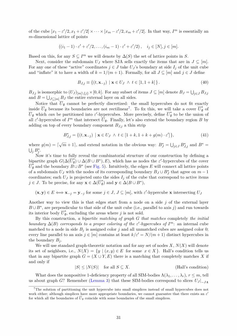
of the cube [x1− ε′/2, x1 + ε′/2]× · · · × [xm− ε′/2, xm + ε′/2]. In that way, Im is essentially anm-dimensional lattice of points(

(i1 − 1) · ε′ + ε′/2, . . . , (im − 1) · ε′ + ε′/2), ij ∈ [N ], j ∈ [m].

Based on this, for any S ⊆ Im we will denote by ∆(S) the set of lattice points in S.Next, consider the subdomain UJ where SJA sells exactly the items that are in J ⊆ [m].

For any one of these “active” coordinates j ∈ J take UJ ’s boundary at side Ij of the unit cubeand “inflate” it to have a width of k = 1/(m+ 1). Formally, for all J ⊆ [m] and j ∈ J define

BJ,j ≡ {(t,x−j) | x ∈ UJ ∧ t ∈ [1, 1 + k]} . (40)

BJ,j is isomorphic to (UJ)[m]\{j}× [0, k]. For any subset of items J ⊆ [m] denote BJ =⋃j∈J BJ,j

and B =⋃J⊆[m]BJ the entire external layer on all sides.

Notice that U∅ cannot be perfectly discretized: the small hypercubes do not fit exactlyinside U∅ because its boundaries are not rectilinear7. To fix this, we will take a cover U∗∅ ofU∅ which can be partitioned into ε′-hypercubes. More precisely, define U∗∅ to be the union ofall ε′-hypercubes of Im that intersect U∅. Finally, let’s also extend the boundary region B byadding on top of every boundary component BJ,j a thin strip

B∗J,j = {(t,x−j)∣∣ x ∈ UJ ∧ t ∈ [1 + k, 1 + k + g(m) · ε′]}, (41)

where g(m) = d√m + 1e, and extend notation in the obvious way: B∗J =

⋃j∈J B

∗J,j and B∗ =⋃

j B∗j .

Now it’s time to fully reveal the combinatorial structure of our construction by defining abipartite graph G(∆(U∗∅) ∪∆(B ∪ B∗), E), which has as nodes the ε′-hypercubes of the coverU∗∅ and the boundary B∪B∗ (see Fig. 5). Intuitively, the edges E will connect all lattice points

of a subdomain UJ with the nodes of its corresponding boundary BJ ∪B∗J that agree on m− 1coordinates; each UJ is projected onto the sides Ij of the cube that correspond to active itemsj ∈ J . To be precise, for any x ∈ ∆(U∗∅) and y ∈ ∆(B ∪B∗),

(x,y) ∈ E ⇐⇒ x−j = y−j for some j ∈ J , J ⊆ [m], with ε′-hypercube x intersecting UJ

Another way to view this is that edges start from a node on a side j of the external layerB ∪B∗, are perpendicular to that side of the unit cube (i.e., parallel to axis j) and run towardsits interior body U∗∅, excluding the areas where j is not sold.

By this construction, a bipartite matching of graph G that matches completely the initialboundary ∆(B) corresponds to a proper coloring of the ε′-hypercubes of Im: an internal cubematched to a node in side Bj is assigned color j and all unmatched cubes are assigned color 0;every line parallel to an axis j ∈ [m] contains at least k/ε′ = N/(m+ 1) distinct hypercubes inthe boundary Bj .

We will use standard graph-theoretic notation and for any set of nodes X, N(X) will denoteits set of neighbors, i.e., N(X) = {y | (x, y) ∈ E for some x ∈ X }. Hall’s condition tells usthat in any bipartite graph G = (X ∪ Y,E) there is a matching that completely matches X ifand only if

|S| ≤ |N(S)| for all S ⊆ X. (Hall’s condition)

What does the nonpositive 1-deficiency property of all SIM-bodies Λ(λ1, . . . , λr), r ≤ m, tellus about graph G? Remember (Lemma 3) that these SIM-bodies correspond to slices UJ |−J :t

7The solution of partitioning the unit hypercube into small simplices instead of small hypercubes does notwork either; although simplices have more appropriate boundaries, we cannot guarantee that there exists an ε′

for which all the boundaries of U∅ coincide with some boundaries of the small simplices.

31

g(m)ε′

k

k

g(m)ε′kk

x2

x1

U{1,2}

U∅

U{1}

U{2}

U∅⋆

B{1,2},1 B⋆{1,2},1

B{1},1 B⋆{1},1

B{1,2},2

B⋆{1,2},2

B{2},2

B⋆{2},2

Figure 5: The discretization of the allocation space and the structure of graph G used in the proof of Theorem 4,for m = 2 items. The space U∅ where SJA sells at least one item (colored gray) does not properly align withthe ε′-discretization grid so we have to take a cover U∗∅ (outlined with the thick line, green in the color versionof this paper). The boundaries Bj ∪ B∗j have width k + g(m)ε′. The one on the right (perpendicular to thevertical axis) consists of ε′-cubes holding color 1 (blue at the color version of the paper) and the one at the topcolor 2 (red). Edges run from every internal ε′-cube, vertically towards the red exterior and horizontally towardsthe blue exterior. Notice, however, how the cube within the allocation subspace U{1} has only horizontal (blue)edges running out of it, since it is not allowed to use color 2 (red). That is due to the fact that item 2 is not soldwithin U{1}.

32

of the allocation space, so (using also Property 5 of Lemma 13) for any J ⊆ [m], t ∈ Rm−|J |+and S ⊆ UJ |−J :t:

|S| ≤ k∑j∈J|Sj | , (42)

where Sj ≡ S[m]\{j}. Using the fact that every such slice UJ |−J :t has zero k-deficiency (Lemma 17),if we take complements S = UJ |−J :t \S and Sj =

(UJ |−J :t

)[m]\{j}

\Sj the above relation gives

k∑j∈J

∣∣∣Sj∣∣∣ ≤ ∣∣∣S∣∣∣ . (43)

First we will show that there is a matching on the bipartite graph G we defined, whichcompletely matches all nodes in ∆(U∅). By (42) and the fact that every (UJ)[m]\{j} × [0, k]is isomorphic to BJ,j , Hall’s theorem tells us that we can completely match ∆(UJ |−J :t) into∆(BJ). By the way we have constructed the edge set E, this directly means that there is acomplete matching of ∆(U∅) into ∆(B). So, to extend this into a complete matching of thecover ∆(U∗∅), using this time additional points in the extended thin-stripe boundary B∗ at theother side of the bipartite graph G, it is enough to show that the extra lattice points in U∗∅ \U∅of any line parallel to some axis j are at most g(m), the number of neighbors in B∗. Indeed,any point in U

∗∅ cannot have distance more than

√mε′ ≤ g(m)ε′ from a point in U∅, because

every ε′-hypercube of U∗∅ intersects with U∅ and the diameter of such a hypercube (with respectto the Euclidean metric) is exactly

√mε′. We will now show that there is also a complete

matching of ∆(B) into ∆(U∗∅). By the way we constructed the edge set, it is enough to showthat every slice ∆(BJ |−J :t) of the boundary can be completely matched into the correspondinginternal slice ∆(U∗∅|−J :t). Fix some nonempty J ⊆ [m] and t ∈ Rm−|J |+ . By Hall’s theorem itis enough to prove that, for any family of sets of {Tj}j∈J of lattice points Tj ⊆ ∆(BJ,j |−J :t),∑j∈J |Tj | ≤ |

⋃j∈J N(Tj)|. We will prove the stronger

∑j∈J |Tj | ≤ |

⋃j∈J N(Tj)∩U∅|−J :t|; that

is, we will just count neighbors in the initial set U∅ and not the cover U∗∅. The continuousanalogue of this is to take Tj ’s be subsets of BJ,j |−J :t and consider the natural extension of theneighbor function N when we now have a infinite graph of edges{

(x,y)∣∣∣ x ∈ UJ |−J :t ∧ y ∈ BJ |−J :t ∧ x−j = y−j for some j ∈ J

}Let S = UJ |−J :t \

⋃j∈J N(Tj) be the set of points not being neighbors of any node in

⋃j∈J Tj

of the boundary. Then by (43) it is enough to show that∑j∈J |Tj | ≤ k

∑j∈J

∣∣∣Sj∣∣∣, whereSj = S[m]\{j}. Every point in the boundary BJ,j |−J :t that has neighbors in

⋃j∈J N(Tj) projects

(with respect to j) inside Sj . But, for any point y in Tj the only other points that can havethe same projection with respect to coordinate j are all points of the line segment of BJ,j |−J :twhich is parallel to the j-axis and passes through y, and this segment has length k.

Combining the existence of the above two matchings, a straightforward use of the classicCantor–Bernstein theorem from Set Theory ensures the existence of a matching in graph G thatcompletely matches both ∆(U∗∅) and ∆(B). But, as we discussed before, this means that U∗∅is properly colorable and thus this coloring induces a feasible dual solution. Let’s denote thissolution by zj(x), j ∈ [m] and also let u(x) be the primal solution given by SJA, i.e., u is theutility function of the SJA mechanism. To prove the optimality of u, we will take advantage ofthe approximate complementarity: we claim that this primal-dual pair of solutions satisfies theapproximate complementarity conditions in Lemma 2 for ε = g(m)m(m+ 1) · ε′:

u(x) ·

m+ 1−∑j∈[m]

∂zj(x)∂xj

≤ ε (44)

−u(0,x−j) · zj(0,x−j) ≤ ε (45)

33

u(1,x−j) · (zj(1,x−j)− 1) ≤ ε (46)

zj(x) ·(

1− ∂u(x)∂xj

)≤ ε. (47)

If that is true, then the proof of Theorem 4 is complete, since by the approximate complementar-ity Lemma 2 the primal and dual objectives differ by at most (3m+ 1)ε = (3m+ 1)g(m)m(m+1)ε′, and if we take the limit of this as ε′ → 0, these values must be equal. So let’s prove that(44)–(47) indeed hold.

Condition (45) is satisfied trivially, since both the primal and the dual variables are nonneg-ative. Regarding (46), for any line parallel to some axis j the length of its segment intersectingthe boundary B ∪ B∗ (which is the one contributing the critical colors j to that direction) isk + g(m)ε′. So, given that the derivative of zj(x) in sections colored with j is m + 1 we canupper-bound the value of zj(1,xj) by (k+g(m)ε′)(m+1) = 1+g(m)(m+1)ε′. This means thatzj(1,xj)− 1 ≤ g(m)(m+ 1)ε′, and given the fact that the utility function has the property thatu(x) ≤ m (because its derivatives are at most 1 at every direction), we finally get the desiredu(1,x−j) · (zj(1,x−j)− 1) ≤ g(m)m(m+ 1)ε′ = ε.

For condition (44), assume that u(x) > 0 (otherwise it is satisfied). That means that SJAsells at least one item, thus x ∈ U∅ ⊆ U

∗∅; but U∗∅ is completely matched, thus all points of U∗∅

are colored with some color in [m] (not with color 0); this is equivalent to the fact that somederivative of the zj functions is m+ 1 and all others are zero, meaning that the correspondingslack variable m+ 1−

∑j∈[m] ∂zj(x)/∂xj is zero.

Finally, for condition (47), fix some direction j ∈ [m] and assume that ∂u(x)/∂xj 6= 1(otherwise the condition is satisfied). SJA is deterministic, so it must be that ∂u(x)/∂xj = 0,i.e., item j is not allocated. That means that x belongs to a subdomain UJ with j /∈ J , and thesame is true for all points before it parallel to axis j (that is, all points (t,x−j) with t ∈ [0, xj ]).Thus, by the way that the edge set E of the graph G was defined, x’s ε′-hypercube, as wellas all hypercubes before it and parallel to axis j, cannot have been colored with color j unlessthey happen to intersect with a neighboring subdomain UJ∗ with j ∈ J∗. But it is a simplegeometric argument to see that point (xj−ε′m,x−j) is at distance at least ε′m√

|J∗|≥ ε′m√

m=√mε′

below the boundary∑j∈J∗ xj = p|J∗| of UJ∗ (since we already know that x is below it), which

is exactly the diameter of the ε-hypercubes. So, at most m such hypercubes below x’s couldintersect with UJ∗ , and thus be colored with color j, meaning that zj(x) cannot have increasedmore than (m+1)ε′ ·(m+1) from zero. This proves that indeed zj(x)(1−∂u(x)/∂xj) = zj(x) ≤(m+ 1)2ε′ ≤ ε.

8 Conclusion

Our main goal in this paper was to design revenue maximizing auctions when many heteroge-neous items are to be sold to a buyer whose values are independently, uniformly distributedover the unit interval [0, 1]. This is the “canonical” multidimensional monopolist problem inEconomics that still remains unsolved, four decades after the seminal work of Myerson [26]for the special case of a single item. We design and analyze a natural mechanism (SJA), andprove its optimality for up to 6 items. Interestingly, it turns out that the optimal mechanism isdeterministic. Prior to our work only solutions for 2 or 3 items were known [23, 29], and theywere achieved mostly through a direct, case-specific optimization approach rather than a clear,unifying viewpoint that could help us towards a more fundamental understanding of multi-itemauction settings.

The cornerstone of our approach is the use of duality and complementarity. Towards thisend, we present a much more general weak duality theory framework that can be formulatedfor many buyers and arbitrary joint distributions which we hope will prove useful in futureattacks on generalizations of our problem: After the conference version of this paper, our

34

duality framework has already successfully been applied to deal with rather general classes ofdistributions [14, 10] and in the domain of approximately optimal auctions as well [12]. Oursolution illuminates the rich geometric ideas underlying the problem, and in the process weformally develop some novel geometric machinery that might be of independent interest.

The most obvious direction for future work is validating the conjecture that SJA is indeedoptimal for any number of items and not just up to 6. Another fundamental open problem is thatof finding exact optimal solutions, like the ones provided in this paper, for more than one bidder:for example, the seemingly simple case of two items and two buyers with i.i.d. uniform valuationsover [0, 1] is still wide open. Is determinism still powerful enough for revenue maximization whenmultiple bidders are involved? And if not, how well can deterministic auctions that generalizeSJA approximate the optimal revenue?

Acknowledgements: We thank Anna Karlin, Amos Fiat, Sergiu Hart, and ConstantinosDaskalakis for useful discussions. We are also very grateful to the anonymous reviewers fortheir careful and thorough reading of our manuscript and for their valuable feedback.

References

[1] R. Aharoni. Infinite matching theory. Discrete Mathematics, 95(1–3):5–22, 1991. URLhttp://dx.doi.org/10.1016/0012-365X(91)90327-X.

[2] G. R. Allan. An inequality involving product measures. In Radical Banach algebras andautomatic continuity, pages 277–279. Springer, 1983. URL http://dx.doi.org/10.1007/BFb0064557.

[3] M. Babaioff, N. Immorlica, B. Lucier, and S. M. Weinberg. A simple and approximatelyoptimal mechanism for an additive buyer. In Proceedings of the 55th Annual Symposium onFoundations of Computer Science, FOCS ’14, 2014. URL http://arxiv.org/abs/1405.6146.

[4] B. Bollobas and A. Thomason. Projections of bodies and hereditary properties of hy-pergraphs. Bulletin of the London Mathematical Society, 27(5):417–424, 1995. URLhttp://dx.doi.org/10.1112/blms/27.5.417.

[5] Y. Cai and Z. Huang. Simple and nearly optimal multi-item auctions. In Proceedings of the24th Annual ACM-SIAM Symposium on Discrete Algorithms, SODA ’13, pages 564–577,2013. URL http://epubs.siam.org/doi/abs/10.1137/1.9781611973105.41.

[6] S. Chawla, J. D. Hartline, and R. Kleinberg. Algorithmic pricing via virtual valuations. InProceedings of the 8th ACM Conference on Electronic Commerce, EC ’07, pages 243–251,2007. URL http://doi.acm.org/10.1145/1250910.1250946.

[7] C. Daskalakis and S. M. Weinberg. Symmetries and optimal multi-dimensional mechanismdesign. In Proceedings of the 13th ACM Conference on Electronic Commerce, EC ’12, pages370–387, 2012. URL http://doi.acm.org/10.1145/2229012.2229042.

[8] C. Daskalakis, A. Deckelbaum, and C. Tzamos. The complexity of optimal mechanismdesign. In Proceedings of the 25th Annual ACM-SIAM Symposium on Discrete Algorithms,SODA ’13, pages 1302–1318, 2013. URL http://epubs.siam.org/doi/abs/10.1137/1.9781611973402.96.

[9] C. Daskalakis, A. Deckelbaum, and C. Tzamos. Mechanism design via optimal transport. InProceedings of the 14th ACM Conference on Electronic Commerce, EC ’13, pages 269–286,2013. URL http://doi.acm.org/10.1145/2482540.2482593.

35

[10] A. Fiat, K. Goldner, A. R. Karlin, and E. Koutsoupias. The fedex problem. In Proceedingsof the 2016 ACM Conference on Economics and Computation, EC ’16, pages 21–22. ACMPress, 2016. doi: 10.1145/2940716.2940752. URL http://homes.cs.washington.edu/˜kgoldner/papers/fedex.pdf.

[11] Y. Giannakopoulos. A note on optimal auctions for two uniformly distributed items. CoRR,abs/1409.6925, 2014. URL http://arxiv.org/pdf/1409.6925.pdf.

[12] Y. Giannakopoulos. Bounding the optimal revenue of selling multiple goods. The-oretical Computer Science, 581(0):83–96, 2015. doi: 10.1016/j.tcs.2015.03.010. URLhttp://arxiv.org/abs/1404.2832.

[13] Y. Giannakopoulos and E. Koutsoupias. Duality and optimality of auctions for uniformdistributions. In Proceedings of the 15th ACM Conference on Economics and Computation,EC ’14, pages 259–276, 2014. URL http://doi.acm.org/10.1145/2600057.2602883.

[14] Y. Giannakopoulos and E. Koutsoupias. Selling two goods optimally. In Proceedings of the42nd International Colloquium on Automata, Languages, and Programming (ICALP’15),pages 650–662, 2015. doi: 10.1007/978-3-662-47666-6 52. URL http://arxiv.org/abs/1510.03399.

[15] S. Hart and N. Nisan. Approximate revenue maximization with multiple items. In Proceed-ings of the 13th ACM Conference on Electronic Commerce, EC ’12, pages 656–656, 2012.doi: 10.1145/2229012.2229061. URL http://arxiv.org/abs/1204.1846.

[16] S. Hart and N. Nisan. The menu-size complexity of auctions. In Proceedings of the 14thACM Conference on Electronic Commerce, EC ’13, pages 565–566, 2013. doi: 10.1145/2482540.2482544. URL http://arxiv.org/abs/1304.6116.

[17] S. Hart and P. J. Reny. Maximal revenue with multiple goods: Nonmonotonicity and otherobservations. Technical report, The Center for the Study of Rationality, Hebrew University,Jerusalem, 2012. URL http://www.ma.huji.ac.il/hart/abs/monot-m.html.

[18] J. D. Hartline and A. R. Karlin. Profit maximization in mechanism design. In N. Nisan,T. Roughgarden, E. Tardos, and V. Vazirani, editors, Algorithmic Game Theory, chap-ter 13. Cambridge University Press, 2007.

[19] V. Krishna. Auction Theory. Academic Press, 2nd edition, 2009.

[20] X. Li and A. C.-C. Yao. On revenue maximization for selling multiple independentlydistributed items. Proceedings of the National Academy of Sciences, 110(28):11232–11237,2013. URL http://dx.doi.org/10.1073/pnas.1309533110.

[21] L. H. Loomis and H. Whitney. An inequality related to the isoperimetric inequality. Bulletinof the American Mathematical Society, 55:961–962, 1949. URL http://dx.doi.org/10.1090/S0002-9904-1949-09320-5.

[22] L. Lovasz and M. D. Plummer. Matching theory. North-Holland, 1986.

[23] A. M. Manelli and D. R. Vincent. Bundling as an optimal selling mechanism for a multiple-good monopolist. Journal of Economic Theory, 127(1):1 – 35, 2006. URL http://dx.doi.org/10.1016/j.jet.2005.08.007.

[24] A. M. Manelli and D. R. Vincent. Multidimensional mechanism design: Revenue maxi-mization and the multiple-good monopoly. Journal of Economic Theory, 137(1):153 – 185,2007. URL http://dx.doi.org/10.1016/j.jet.2006.12.007.

36

[25] R. P. McAfee and J. McMillan. Multidimensional incentive compatibility and mechanismdesign. Journal of Economic Theory, 46(2):335 – 354, 1988. URL http://dx.doi.org/10.1016/0022-0531(88)90135-4.

[26] R. B. Myerson. Optimal auction design. Mathematics of Operations Research, 6(1):58–73,1981. URL http://dx.doi.org/10.1287/moor.6.1.58.

[27] N. Nisan. Introduction to mechanism design (for computer scientists). In N. Nisan,T. Roughgarden, E. Tardos, and V. Vazirani, editors, Algorithmic Game Theory, chap-ter 9. Cambridge University Press, 2007.

[28] O. Ore. Graphs and matching theorems. Duke Mathematical Journal, 22(4):625–639, 1955.URL http://dx.doi.org/10.1215/S0012-7094-55-02268-7.

[29] G. Pavlov. Optimal mechanism for selling two goods. The BE Journal of TheoreticalEconomics, 11(1), 2011. URL http://dx.doi.org/10.2202/1935-1704.1664.

[30] M. Pycia. Stochastic vs deterministic mechanisms in multidimensionalscreening. PhD thesis, MIT, 2006. URL http://pycia.bol.ucla.edu/pycia-multidimensional-screening.pdf. Chapter 3.

[31] J.-C. Rochet. The taxation principle and multi-time hamilton-jacobi equations. Journalof Mathematical Economics, 14(2):113 – 128, 1985. URL http://dx.doi.org/10.1016/0304-4068(85)90015-1.

[32] R. Rockafellar. Convex Analysis., volume 28 of Princeton landmarks in mathematics.Princeton University Press, 1997.

[33] J. Thanassoulis. Haggling over substitutes. Journal of Economic Theory, 117(2):217 – 245, 2004. URL http://www.sciencedirect.com/science/article/pii/S0022053103003351.

[34] R. V. Vohra. Mechanism Design: a linear programming approach. Cambridge UniversityPress, 2011.

[35] Z. Wang and P. Tang. Optimal mechanisms with simple menus. CoRR, abs/1311.5966,2013. URL http://arxiv.org/abs/1311.5966.

[36] A. C.-C. Yao. An n-to-1 bidder reduction for multi-item auctions and its applications.In Proceedings of the 26th Annual ACM-SIAM Symposium on Discrete Algorithms, pages92–109, 2015. doi: 10.1137/1.9781611973730.8. URL http://arxiv.org/abs/1406.3278.

A Full Proof of Lemma 17

Recall the definition of body V (p(m)1 , . . . , p

(m)r ) in (11). By the definition of SJA in (10), the

volume of this body must be equal to rk. Then, as we discussed in the proof sketch of Lemma 17in Section 6.2, this translates to its deficiency being zero:

δ 1m+1

(V (p(m)1 , . . . , p(m)

r )) = 0 for all r ≤ m. (48)

Before giving the formal proof of Lemma 17, we will need the following lemma that shows howthe deficiency of any such subdomain of the valuation space is the sum of the deficiencies of its“critical” subslices of lower dimensions:

37

Lemma 19. For any subset of items J ⊆ [m], the k-deficiency of any slice of the subdomainwhere at least one of the items in J is sold, when all other items’ bids are fixed to zero, is thesum of the k-deficiencies of all its sub-slices (U (m)

L |−J :0)|J\L:t, where ∅ 6= L ⊆ J and k = 1m+1 .

Formally,

δk(V (p(m)1 , . . . , p

(m)|J | )) =

∑∅6=L⊆J

∫I|J|−|L|

δk

((U

(m)L

∣∣∣−J :0

)∣∣∣∣J\L:t

)dt.

Proof. Fix some m. For the sake of clarity we will prove the proposition for J having fulldimension J = m. All the arguments easily carry on to the more general case where J ⊆ [m] ifone takes all valuations of items not in J to be 0, i.e., “slicing” ( · )|−J :0, since they are validfor any selling mechanism with nonincreasing price differences and SJA specifically; essentially,the case of |J | = m′ ≤ m directly translates to the case of an m′-dimensional mechanism.

So, it is enough to show that

|V | =∑

∅6=L⊆[m]

∫Im−|L|

∣∣∣UL|−L:t

∣∣∣ dt (49)

∣∣∣V[m]\{j}

∣∣∣ =∑

∅6=L⊆[m]j∈L

∫Im−|L|

∣∣∣∣(UL|−L:t

)[m]\{j}

∣∣∣∣ dt for all j ∈ [m], (50)

where for simplicity we have denoted the space V (p1, . . . , pm) where mechanism allocates atleast one item with V . Equation (49) is a result of the fact that V can be decomposed asV =

∑∅6=L⊆[m] UL and every allocation subspace UL is isomorphic to the disjoint union of all

its slices UL|−L:t. In a similar way, to prove that (50) holds, it is enough to show that for somefixed j ∈ [m], the projection V[m]\{j} can be covered by the union of all the projections of thesubspaces UL with respect to coordinate j and that all these projections (UL)[m]\{j} are disjointalmost everywhere, i.e., they can only intersect in a set of measure zero.

For the former, let x−j ∈ V[m]\{j}. Then (x−j , 1) ∈ V (by only increasing the componentsof a valuation profile, items that were sold to the buyer are still going to be sold). So, thereis a nonempty set of items L ⊆ [m] such that (x−j , 1) ∈ UL and j ∈ L (item j is sold sincexj = 1 ≥ p1), meaning that indeed x−j ∈ (UL)[m]\{j} with j ∈ L. For the latter, consider distinctsets L,L′ ⊆ [m] with j belonging to both L and L′, and let a valuation profile x ∈ UL ∩ UL′ .Then, by the characterization in Lemma 16 it must be that∑

l∈L′\Lxl ≥ p|L′| − p|L′|−|L′\L| and

∑l∈L′\L

xl ≤ p|L|+|L′\L| − p|L|,

the first inequality being from the fact that x ∈ UL′ and the second from x ∈ UL, taking intoconsideration that L′ \ L ⊆ L′ and L′ \ L 6⊆ L. As a result, the sum

∑l∈L′\L xl can range at

most over only a single value, namely p|L′| − p|L′|−|L′\L| = p|L|+|L′\L| − p|L| (and only if thesetwo values are of course equal), otherwise by merging these two inequalities together we wouldhave gotten that

p|L′| − p|L′|−|L′\L| < p|L|+|L′\L| − p|L|,

which contradicts the nonincreasing payment differences property, since both differences arebetween payments that differ at exactly |L′ \ L| “steps” but |L|+ |L′ \ L| ≥ |L′|.

Lemma (Lemma 17). Every slice U(m)J

∣∣∣−J :t

of SJA has zero k-deficiency, where k = 1m+1 .

Proof. Fix some m and let k = 1/(m + 1). We use induction on the cardinality of J . At thebase of the induction |J | = 1, and due to symmetry it is enough to prove the proposition forslices of the form U{1}

∣∣∣[2...m]:t

. By (34) this is equal to the slice U{1}

∣∣∣[2...m]:0m−1

, which is the

single-dimensional interval [p1, 1], thus having k-deficiency 1− p1 − 1m+1 · 1 = m

m+1 − p1 = 0.

38

For the inductive step, fix some r ≤ m and assume the proposition holds for all J ⊆ [m] with|J | ≤ r − 1. We will show that it is true also for |J | = r. Again, due to symmetry, it is enoughto prove that the k-deficiency of slice U[r]

∣∣∣[r+1...m]:0m−r

is zero (taking into consideration (34)).By Lemma 19 we deduce that the subdomain where at least one of items [r] is sold, given thatthe remaining [r + 1...m] bids are fixed to zero, has

δk(V (p1, . . . , pr)) =∑

∅6=L⊆[r]

∫Ir−|L|

δk

((UL|[r+1...m]:0

)∣∣∣[r]\L:t

)dt

= δk

(U[r]

∣∣∣[r+1...m]:0

)+

∑∅6=L⊆[r]|L|≤r−1

∫Ir−|L|

δk(UL|[m]\L:(t,0)

)dt

= δk

(U[r]

∣∣∣[r+1...m]:0

),

by the induction hypothesis. But from the definition of SJA, and in particular (48), we havethat δk(V (p1, . . . , pr)) = 0, which concludes the proof.

B Convexity and Duality

In this section we discuss the convexity constraint of the utility functions. For clarity, we focuson the simple case of a single bidder and a single item. We show that the convexity constraint isnot necessary for regular8 distributions. And in the opposite direction, we exhibit a nonregulardistribution for which the convexity constraint cannot be dropped without affecting optimality.

The primal Program (4) (taking into consideration (5)) for this case is

supu

u(H)Hf(H)− u(L)Lf(L)−∫ H

Lu(x)(f(x) + (xf(x))′) dx

subject to

u′(x) ≤ 1 (z(x))u′(x) ≥ 0 (s(x))u′′(x) ≥ 0 (w(x))u(x) ≥ 0

Notice that there is no reason to include u(L) = 0 since this holds for the optimal solution;that is because if u(x) and u(x) − c are both feasible solutions and c is a positive constant,then the corresponding objectives differ by cHf(H) − cLf(L) −

∫HL c(f(x) + (xf(x))′) dx =

−c(H · F (H)− L · F (L)) < 0; this shows that the optimal solution has u(x) = 0 for some x.In our treatment of the subject in the main text of the paper, we dropped the constraints

labelled by the dual variables w(x) and for the most part we also dropped the ones correspondingto s(x). We did this to keep the primal and dual systems simple. More importantly, there is astrong reason for ignoring the constraints corresponding to w(x) for multi-parameter domains:the convexity constraints ∇2u(x) � 0 (that is, the Hessian of u being positive semidefinite) arenot linear in u (unlike the one-dimensional case, in which the constraint u′′(x) ≥ 0 is linear inu).

In the rest of this subsection, we investigate when the simplified systems are optimal. Wefirst drop the constraints corresponding to convexity to get the dual

infz,s

∫ H

Lz(x) dx

8A distribution is called regular when x− 1−F (x)f(x) is nondecreasing.

39

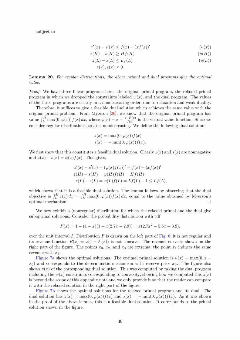
subject to

z′(x)− s′(x) ≤ f(x) + (xf(x))′ (u(x))z(H)− s(H) ≥ Hf(H) (u(H))z(L)− s(L) ≤ Lf(L) (u(L))z(x), s(x) ≥ 0.

Lemma 20. For regular distributions, the above primal and dual programs give the optimalvalue.

Proof. We have three linear programs here: the original primal program, the relaxed primalprogram in which we dropped the constraints labeled w(x), and the dual program. The valuesof the three programs are clearly in a nondecreasing order, due to relaxation and weak duality.

Therefore, it suffices to give a feasible dual solution which achieves the same value with theoriginal primal problem. From Myerson [26], we know that the original primal program hasvalue

∫HL max(0, ϕ(x))f(x) dx, where ϕ(x) = x− 1−F (x)

f(x) is the virtual value function. Since weconsider regular distributions, ϕ(x) is nondecreasing. We define the following dual solution:

z(x) = max(0, ϕ(x))f(x)s(x) = −min(0, ϕ(x))f(x).

We first show that this constitutes a feasible dual solution. Clearly z(x) and s(x) are nonnegativeand z(x)− s(x) = ϕ(x)f(x). This gives,

z′(x)− s′(x) = (ϕ(x)f(x))′ = f(x) + (xf(x))′

z(H)− s(H) = ϕ(H)f(H) = Hf(H)z(L)− s(L) = ϕ(L)f(L) = Lf(L)− 1 ≤ Lf(L),

which shows that it is a feasible dual solution. The lemma follows by observing that the dualobjective is

∫HL z(x) dx =

∫HL max(0, ϕ(x))f(x) dx, equal to the value obtained by Myerson’s

optimal mechanism.

We now exhibit a (nonregular) distribution for which the relaxed primal and the dual givesuboptimal solutions. Consider the probability distribution with cdf

F (x) = 1− (1− x)(1 + x(2.7x− 2.9)) = x(2.7x2 − 5.6x+ 3.9),

over the unit interval I. Distribution F is drawn on the left part of Fig. 6; it is not regular andits revenue function R(x) = x(1 − F (x)) is not concave. The revenue curve is shown on theright part of the figure. The points x0, x2, and x3 are extrema; the point x1 induces the samerevenue with x3.

Figure 7a shows the optimal solutions. The optimal primal solution is u(x) = max(0, x −x0) and corresponds to the deterministic mechanism with reserve price x0. The figure alsoshows z(x) of the corresponding dual solution. This was computed by taking the dual programincluding the w(x) constraints corresponding to convexity; showing how we computed this z(x)is beyond the scope of this appendix note and we only provide it so that the reader can compareit with the relaxed solution in the right part of the figure.

Figure 7b shows the optimal solutions for the relaxed primal program and its dual. Thedual solution has z(x) = max(0, ϕ(x))f(x) and s(x) = −min(0, ϕ(x))f(x). As it was shownin the proof of the above lemma, this is a feasible dual solution. It corresponds to the primalsolution shown in the figure.

40

0

1

2

3

0 0.5 1

F (x)

f(x)

(a) The distribution

0

0.01

0.02

0.03

0.04

0.05

0.06

0.07

0.08

0 0.5 1

R(x)

x0 x1 x2 x3

(b) The revenue curve R(x) = x(1− F (x))

Figure 6: The probability distribution in (a) is not regular and does not have concave revenue curve, i.e.,F (x) + xf(x)− 1 is not monotone (increasing). Its revenue curve is shown in (b). The points x0, x2, and x3 areextrema; the point x1 has the same revenue with x3.

The value of the dual solution is∫ 1

0z(x) dx =

∫ x2

x0−R′(x) dx+

∫ 1

x3−R′(x) dx = R(x0)−R(x2)+R(x3)−R(1) = R(x0)−R(x2)+R(x3).

It is straightforward to verify that the indicated primal solution gives the same value, whichshows that they are both optimal. However, the primal solution is not convex. Furthermore,its value R(x0) − R(x2) + R(x3) is strictly higher than the value R(x0) of the valid optimalsolution, because R(x3) > R(x2). Therefore the convexity constraint is essential to obtain theoptimal solution.

C Duality for Unbounded Domains

As we mentioned in the presentation of the duality framework in Section 3, for it to make senseas it is we need the integrals in the basic transformation of the primal revenue-maximizationobjective in expression (5) to be well-defined. This is definitely the case when we have boundeddomains, i.e., when the upper-boundary Hi,j of each interval Di,j = [Li,j , Hi,j ] is finite: allintegrals in (5) are finite and the integration by parts is valid. This of course includes thespecial case of uniform distributions which is the main topic in this paper. We will now discusshow one can still use this duality framework in cases where the domain D is not bounded.

For the sake of clarity, let’s assume for the remaining of this section that we have a singlebidder and that item valuations are i.i.d. from some distribution F with pdf f over an interval[L,H], L ≥ 0. First notice that, even for unbounded domains where H =∞, the critical integral

∫D−j

Hj u(Hj ,x−j) f(Hj ,x−j) dx−j = Hf(H)∫

[L,H]m−1u(H,x−j)

∏l 6=j

f(xl) dx−j (51)

in (5) may still converge as H →∞. In such a case, the duality framework from Section 3 can beapplied as it is: one just has to take the limit of H →∞ wherever H appears, and in particularthe Weak Duality Lemma 1 is still valid if one replaces condition zj(H,x−j) ≥ Hf(H,x−j) by

41

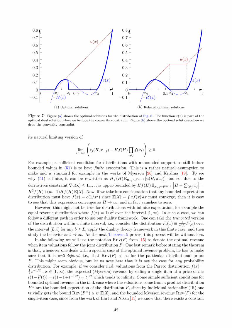
−0.1

0

0.1

0.2

0.3

0.4

0.5

0.6

0.7

0.8

0 0.5 1x0 x1 x3

u(x)

−R′(x)

z(x)

(a) Optimal solutions

−0.1

0

0.1

0.2

0.3

0.4

0.5

0.6

0.7

0.8

0 0.5 1x0 x2 x3

u(x)

z(x)

−R′(x)

(b) Relaxed optimal solutions

Figure 7: Figure (a) shows the optimal solutions for the distribution of Fig. 6. The function z(x) is part of theoptimal dual solution when we include the convexity constraint. Figure (b) shows the optimal solutions when wedrop the convexity constraint.

its natural limiting version of

limH→∞

zj(H,x−j)−Hf(H)∏l 6=j

f(xl)

≥ 0.

For example, a sufficient condition for distributions with unbounded support to still inducebounded values in (51) is to have finite expectation. This is a rather natural assumption tomake and is standard for example in the works of Myerson [26] and Krishna [19]. To seewhy (51) is finite, it can be rewritten as Hf(H)Ex−j∼Fm−1 [u(H,x−j)] and so, due to thederivatives constraint ∇u(x) ≤ 1m, it is upper-bounded by Hf(H)Ex−j∼Fm−1

[H +

∑l 6=j xj

]=

H2f(H)+(m−1)Hf(H)E[X]. Now, if we take into consideration that any bounded-expectationdistribution must have f(x) = o(1/x2) since E[X] =

∫xf(x) dx must converge, then it is easy

to see that this expression converges as H →∞, and in fact vanishes to zero.However, this might not be true for distributions with infinite expectation, for example the

equal revenue distribution where f(x) = 1/x2 over the interval [1,∞). In such a case, we canfollow a different path in order to use our duality framework. One can take the truncated versionof the distribution within a finite interval, i.e., consider the distribution Fb(x) ≡ 1

F (b)F (x) overthe interval [L, b] for any b ≥ L, apply the duality theory framework in this finite case, and thenstudy the behavior as b→∞. As the next Theorem 5 proves, this process will be without loss.

In the following we will use the notation Rev(F ) from [15] to denote the optimal revenuewhen item valuations follow the joint distribution F . One last remark before stating the theoremis that, whenever one deals with a specific case of the optimal revenue problem, he has to makesure that it is well-defined, i.e., that Rev(F ) < ∞ for the particular distributional priorsF . This might seem obvious, but let us note here that it is not the case for any probabilitydistribution. For example, if we consider i.i.d. valuations from the Pareto distribution f(x) =12x−3/2 , x ∈ [1,∞), the expected (Myerson) revenue by selling a single item at a price of t is

t(1−F (t)) = t(1−1+t−1/2) = t1/2 which tends to infinity. Some simple sufficient conditions forbounded optimal revenue in the i.i.d. case where the valuations come from a product distributionFm are the bounded expectation of the distribution F , since by individual rationality (IR) onetrivially gets the bound Rev(Fm) ≤ mE[X], and the bounded Myerson revenue Rev(F ) for thesingle-item case, since from the work of Hart and Nisan [15] we know that there exists a constant

42

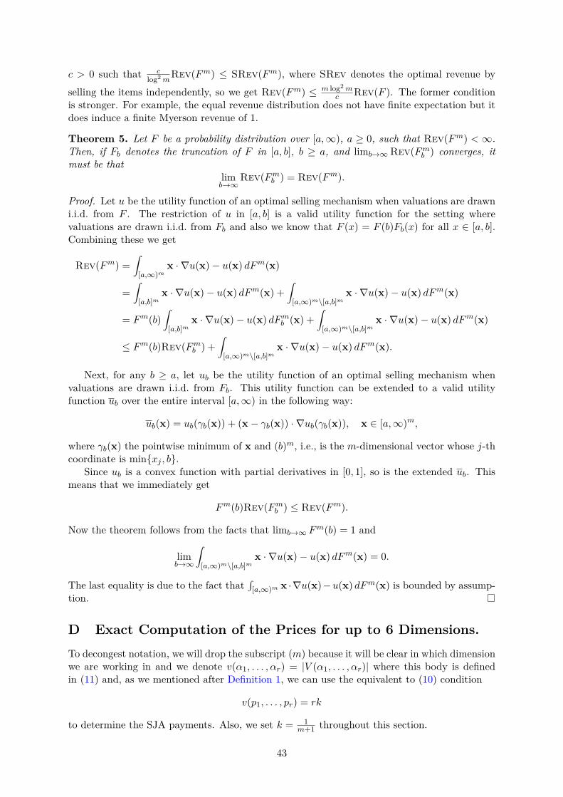
c > 0 such that clog2 m

Rev(Fm) ≤ SRev(Fm), where SRev denotes the optimal revenue by

selling the items independently, so we get Rev(Fm) ≤ m log2 mc Rev(F ). The former condition

is stronger. For example, the equal revenue distribution does not have finite expectation but itdoes induce a finite Myerson revenue of 1.

Theorem 5. Let F be a probability distribution over [a,∞), a ≥ 0, such that Rev(Fm) <∞.Then, if Fb denotes the truncation of F in [a, b], b ≥ a, and limb→∞Rev(Fmb ) converges, itmust be that

limb→∞

Rev(Fmb ) = Rev(Fm).

Proof. Let u be the utility function of an optimal selling mechanism when valuations are drawni.i.d. from F . The restriction of u in [a, b] is a valid utility function for the setting wherevaluations are drawn i.i.d. from Fb and also we know that F (x) = F (b)Fb(x) for all x ∈ [a, b].Combining these we get

Rev(Fm) =∫

[a,∞)mx · ∇u(x)− u(x) dFm(x)

=∫

[a,b]mx · ∇u(x)− u(x) dFm(x) +

∫[a,∞)m\[a,b]m

x · ∇u(x)− u(x) dFm(x)

= Fm(b)∫

[a,b]mx · ∇u(x)− u(x) dFmb (x) +

∫[a,∞)m\[a,b]m

x · ∇u(x)− u(x) dFm(x)

≤ Fm(b)Rev(Fmb ) +∫

[a,∞)m\[a,b]mx · ∇u(x)− u(x) dFm(x).

Next, for any b ≥ a, let ub be the utility function of an optimal selling mechanism whenvaluations are drawn i.i.d. from Fb. This utility function can be extended to a valid utilityfunction ub over the entire interval [a,∞) in the following way:

ub(x) = ub(γb(x)) + (x− γb(x)) · ∇ub(γb(x)), x ∈ [a,∞)m,

where γb(x) the pointwise minimum of x and (b)m, i.e., is the m-dimensional vector whose j-thcoordinate is min{xj , b}.

Since ub is a convex function with partial derivatives in [0, 1], so is the extended ub. Thismeans that we immediately get

Fm(b)Rev(Fmb ) ≤ Rev(Fm).

Now the theorem follows from the facts that limb→∞ Fm(b) = 1 and

limb→∞

∫[a,∞)m\[a,b]m

x · ∇u(x)− u(x) dFm(x) = 0.

The last equality is due to the fact that∫

[a,∞)m x ·∇u(x)−u(x) dFm(x) is bounded by assump-tion.

D Exact Computation of the Prices for up to 6 Dimensions.

To decongest notation, we will drop the subscript (m) because it will be clear in which dimensionwe are working in and we denote v(α1, . . . , αr) = |V (α1, . . . , αr)| where this body is definedin (11) and, as we mentioned after Definition 1, we can use the equivalent to (10) condition

v(p1, . . . , pr) = rk

to determine the SJA payments. Also, we set k = 1m+1 throughout this section.

43

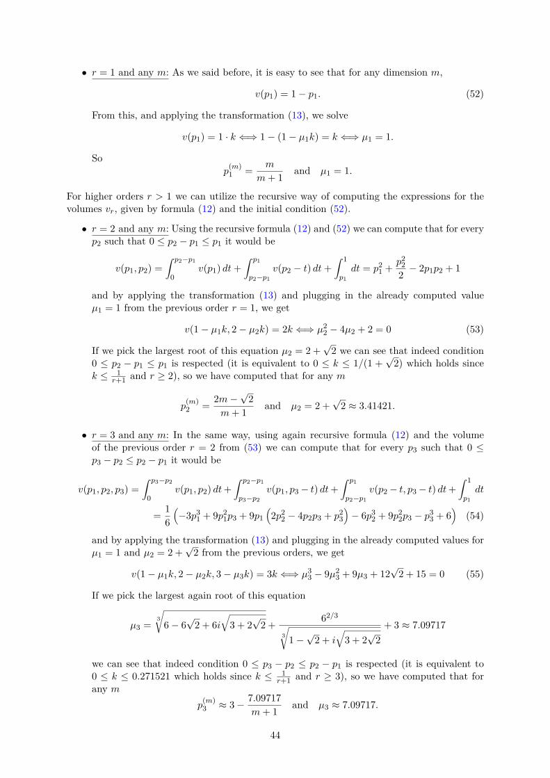
• r = 1 and any m: As we said before, it is easy to see that for any dimension m,

v(p1) = 1− p1. (52)

From this, and applying the transformation (13), we solve

v(p1) = 1 · k ⇐⇒ 1− (1− µ1k) = k ⇐⇒ µ1 = 1.

Sop

(m)1 = m

m+ 1 and µ1 = 1.

For higher orders r > 1 we can utilize the recursive way of computing the expressions for thevolumes vr, given by formula (12) and the initial condition (52).

• r = 2 and any m: Using the recursive formula (12) and (52) we can compute that for everyp2 such that 0 ≤ p2 − p1 ≤ p1 it would be

v(p1, p2) =∫ p2−p1

0v(p1) dt+

∫ p1

p2−p1v(p2 − t) dt+

∫ 1

p1dt = p2

1 + p22

2 − 2p1p2 + 1

and by applying the transformation (13) and plugging in the already computed valueµ1 = 1 from the previous order r = 1, we get

v(1− µ1k, 2− µ2k) = 2k ⇐⇒ µ22 − 4µ2 + 2 = 0 (53)

If we pick the largest root of this equation µ2 = 2 +√

2 we can see that indeed condition0 ≤ p2 − p1 ≤ p1 is respected (it is equivalent to 0 ≤ k ≤ 1/(1 +

√2) which holds since

k ≤ 1r+1 and r ≥ 2), so we have computed that for any m

p(m)2 = 2m−

√2

m+ 1 and µ2 = 2 +√

2 ≈ 3.41421.

• r = 3 and any m: In the same way, using again recursive formula (12) and the volumeof the previous order r = 2 from (53) we can compute that for every p3 such that 0 ≤p3 − p2 ≤ p2 − p1 it would be

v(p1, p2, p3) =∫ p3−p2

0v(p1, p2) dt+

∫ p2−p1

p3−p2v(p1, p3− t) dt+

∫ p1

p2−p1v(p2− t, p3− t) dt+

∫ 1

p1dt

= 16(−3p3

1 + 9p21p3 + 9p1

(2p2

2 − 4p2p3 + p23

)− 6p3

2 + 9p22p3 − p3

3 + 6)

(54)

and by applying the transformation (13) and plugging in the already computed values forµ1 = 1 and µ2 = 2 +

√2 from the previous orders, we get

v(1− µ1k, 2− µ2k, 3− µ3k) = 3k ⇐⇒ µ33 − 9µ2

3 + 9µ3 + 12√

2 + 15 = 0 (55)

If we pick the largest again root of this equation

µ3 =3√

6− 6√

2 + 6i√

3 + 2√

2 + 62/3

3√

1−√

2 + i√

3 + 2√

2+ 3 ≈ 7.09717

we can see that indeed condition 0 ≤ p3 − p2 ≤ p2 − p1 is respected (it is equivalent to0 ≤ k ≤ 0.271521 which holds since k ≤ 1

r+1 and r ≥ 3), so we have computed that forany m

p(m)3 ≈ 3− 7.09717

m+ 1 and µ3 ≈ 7.09717.

44

• r = 4 and any m: Continuing up the same way, we compute that for every p4 such that0 ≤ p4 − p3 ≤ p3 − p2 it is

v(p1, p2, p3, p4) =∫ p4−p3

0v(p1, p2, p3) dt+

∫ p3−p2

p4−p3v(p1, p2, p4 − t) dt

+∫ p2−p1

p3−p2v(p1, p3 − t, p4 − t) dt+

∫ p1

p2−p1v(p2 − t, p3 − t, p4 − t) dt+

∫ 1

p1dt

which equals

124(4p4

1 − 16p31p4 − 24p2

1

(3p2

3 − 6p3p4 + 2p24

)− 16p1

(3p3

2 − 9p22p4 − 9p2

(2p2

3 − 4p3p4 + p24

)+6p3

3 − 9p23p4 + p3

4

)+ 18p4

2 − 48p32p4 − 36p2

2

(2p2

3 − 4p3p4 + p24

)+ 12p4

3 − 16p33p4 + p4

4 + 24).

(56)

By applying the transformation (13), plugging in the already computed values for µ1 = 1and µ2 = 2 +

√2 and using the fact that µ3 is the root of Equation (55), we get that

equation v(1− µ1k, 2− µ2k, 3− µ3k, 4− µ4k) = 4k is equivalent to

µ44 − 16µ3

4 + 24µ24 + 96

√2µ4 + 128µ4 + 72µ2

3 − 144√

2µ3 − 288µ3 + 48√

2 + 88 = 0. (57)

If we pick the largest again root µ4 ≈ 11.9972 of this equation we can see that indeedcondition 0 ≤ p4 − p3 ≤ p3 − p2 is respected (it is equivalent to 0 ≤ k ≤ 0.204082 whichholds since k ≤ 1

r+1 and r ≥ 4), so we have computed that for any m

p(m)4 ≈ 4− 11.9972

m+ 1 and µ4 ≈ 11.9972.

• r = 5 and m = 5: At this point we need to modify a little bit our procedure of computingthe volumes in the usual recursive way, and consider the case where the new p5 price issuch that p3 ≤ p5 ≤ p4 instead of p5 ≥ p4 (and in fact the even stronger condition thatp5 − p4 ≤ p4 − p3). This is again a straightforward calculation, since as we argued before,v(p1, p2, p3, p4, p5) = v(p1, p2, p3, p5, p5) and so

v(p1, p2, p3, p4, p5) =∫ p5−p3

0v(p1, p2, p3, p5 − t) dt+

∫ p3−p2

p5−p3v(p1, p2, p5 − t, p5 − t) dt

+∫ p2−p1

p3−p2v(p1, p3 − t, p5 − t, p5 − t) dt+

∫ p1

p2−p1v(p2 − t, p3 − t, p5 − t, p5 − t) dt+

∫ 1

p1dt

which equals

1120

(−5p5

1 + 25p41p5 − 50p3

1p25 + 50p2

1

(6p3

3 − 18p23p5 + 18p3p

25 − 5p3

5

)+ 25p1

(4p4

2 − 16p32p5

+24p22p

25 − 16p2

(3p3

3 − 9p23p5 + 9p3p

25 − 2p3

5

)+ 18p4

3 − 48p33p5 + 36p2

3p25 − 3p4

5

)− 2

(20p5

2

−75p42p5 + 100p3

2p25 − 50p2

2

(3p3

3 − 9p23p5 + 9p3p

25 − 2p3

5

)+ 30p5

3 − 75p43p5 + 50p3

3p25 − 2p5

5 − 60))(58)

By applying the transformation (13), plugging in the already computed values for µ1 = 1and µ2 = 2 +

√2 and using the fact that µ3 is the root of Equation (55), we get that

equation v(1− µ1k, 2− µ2k, 3− µ3k, 5− µ5k, 5− µ5k) = 5k is equivalent to

4µ55−225µ4

5 +4350µ35 +800

√2µ2

5−34950µ25 +900µ5µ

23−1800

√2µ5µ3−3600µ5µ3−14600

√2µ5

+ 121175µ5 + 720√

2µ23 − 14220µ2

3 + 22680√

2µ3 + 49680µ3 + 41080√

2− 161215 = 0(59)

45

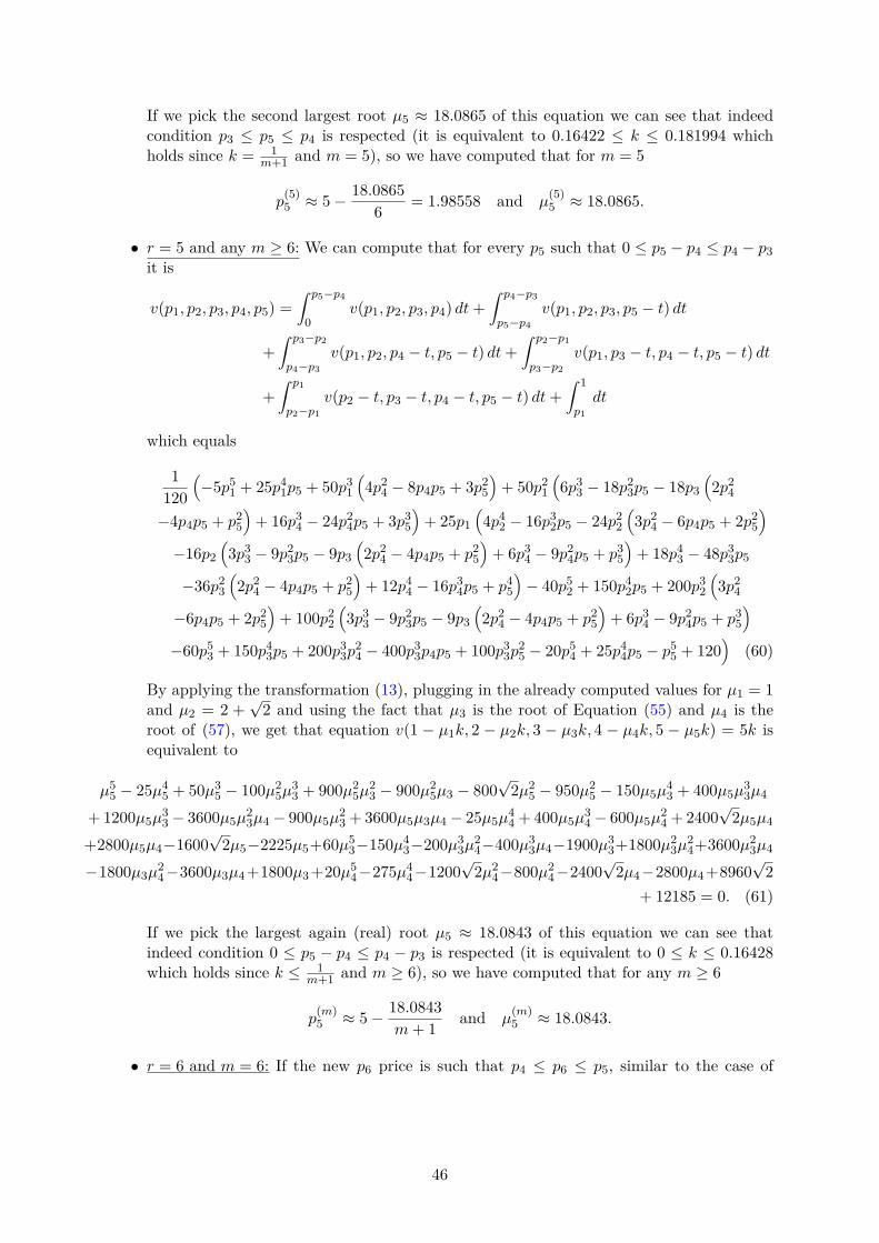
If we pick the second largest root µ5 ≈ 18.0865 of this equation we can see that indeedcondition p3 ≤ p5 ≤ p4 is respected (it is equivalent to 0.16422 ≤ k ≤ 0.181994 whichholds since k = 1

m+1 and m = 5), so we have computed that for m = 5

p(5)5 ≈ 5− 18.0865

6 = 1.98558 and µ(5)5 ≈ 18.0865.

• r = 5 and any m ≥ 6: We can compute that for every p5 such that 0 ≤ p5 − p4 ≤ p4 − p3it is

v(p1, p2, p3, p4, p5) =∫ p5−p4

0v(p1, p2, p3, p4) dt+

∫ p4−p3

p5−p4v(p1, p2, p3, p5 − t) dt

+∫ p3−p2

p4−p3v(p1, p2, p4 − t, p5 − t) dt+

∫ p2−p1

p3−p2v(p1, p3 − t, p4 − t, p5 − t) dt

+∫ p1

p2−p1v(p2 − t, p3 − t, p4 − t, p5 − t) dt+

∫ 1

p1dt

which equals

1120

(−5p5

1 + 25p41p5 + 50p3

1

(4p2

4 − 8p4p5 + 3p25

)+ 50p2

1

(6p3

3 − 18p23p5 − 18p3

(2p2

4

−4p4p5 + p25

)+ 16p3

4 − 24p24p5 + 3p3

5

)+ 25p1

(4p4

2 − 16p32p5 − 24p2

2

(3p2

4 − 6p4p5 + 2p25

)−16p2

(3p3

3 − 9p23p5 − 9p3

(2p2

4 − 4p4p5 + p25

)+ 6p3

4 − 9p24p5 + p3

5

)+ 18p4

3 − 48p33p5

−36p23

(2p2

4 − 4p4p5 + p25

)+ 12p4

4 − 16p34p5 + p4

5

)− 40p5

2 + 150p42p5 + 200p3

2

(3p2

4

−6p4p5 + 2p25

)+ 100p2

2

(3p3

3 − 9p23p5 − 9p3

(2p2

4 − 4p4p5 + p25

)+ 6p3

4 − 9p24p5 + p3

5

)−60p5

3 + 150p43p5 + 200p3

3p24 − 400p3

3p4p5 + 100p33p

25 − 20p5

4 + 25p44p5 − p5

5 + 120)

(60)

By applying the transformation (13), plugging in the already computed values for µ1 = 1and µ2 = 2 +

√2 and using the fact that µ3 is the root of Equation (55) and µ4 is the

root of (57), we get that equation v(1 − µ1k, 2 − µ2k, 3 − µ3k, 4 − µ4k, 5 − µ5k) = 5k isequivalent to

µ55 − 25µ4

5 + 50µ35 − 100µ2

5µ33 + 900µ2

5µ23 − 900µ2

5µ3 − 800√

2µ25 − 950µ2

5 − 150µ5µ43 + 400µ5µ

33µ4

+ 1200µ5µ33− 3600µ5µ

23µ4− 900µ5µ

23 + 3600µ5µ3µ4− 25µ5µ

44 + 400µ5µ

34− 600µ5µ

24 + 2400

√2µ5µ4

+2800µ5µ4−1600√

2µ5−2225µ5+60µ53−150µ4

3−200µ33µ

24−400µ3

3µ4−1900µ33+1800µ2

3µ24+3600µ2

3µ4

−1800µ3µ24−3600µ3µ4 +1800µ3 +20µ5

4−275µ44−1200

√2µ2

4−800µ24−2400

√2µ4−2800µ4 +8960

√2

+ 12185 = 0. (61)

If we pick the largest again (real) root µ5 ≈ 18.0843 of this equation we can see thatindeed condition 0 ≤ p5 − p4 ≤ p4 − p3 is respected (it is equivalent to 0 ≤ k ≤ 0.16428which holds since k ≤ 1

m+1 and m ≥ 6), so we have computed that for any m ≥ 6

p(m)5 ≈ 5− 18.0843

m+ 1 and µ(m)5 ≈ 18.0843.

• r = 6 and m = 6: If the new p6 price is such that p4 ≤ p6 ≤ p5, similar to the case of

46

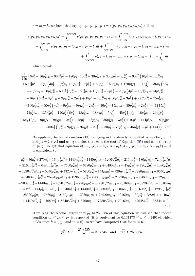
r = m = 5, we have that v(p1, p2, p3, p4, p5, p6) = v(p1, p2, p3, p4, p6, p6) and so

v(p1, p2, p3, p4, p5, p6) =∫ p6−p4

0v(p1, p2, p3, p4, p6− t) dt+

∫ p4−p3

p6−p4v(p1, p2, p3, p5− t, p5− t) dt

+∫ p3−p2

p4−p3v(p1, p2, p4 − t, p6 − t, p6 − t) dt+

∫ p2−p1

p3−p2v(p1, p3 − t, p4 − t, p6 − t, p6 − t) dt

+∫ p1

p2−p1v(p2 − t, p3 − t, p4 − t, p6 − t, p6 − t) dt+

∫ 1

p1dt

which equals

1720

(6p6

1 − 36p51p6 + 90p4

1p26 − 120p3

1

(10p3

4 − 30p24p6 + 30p4p

26 − 9p3

6

)− 90p2

1

(10p4

3 − 40p33p6

+60p23p

26 − 40p3

(3p3

4 − 9p24p6 + 9p4p

26 − 2p3

6

)+ 60p4

4 − 160p34p6 + 120p2

4p26 − 11p4

6

)− 36p1

(5p5

2

−25p42p6 + 50p3

2p26 − 50p2

2

(6p3

4 − 18p24p6 + 18p4p

26 − 5p3

6

)− 25p2

(4p4

3 − 16p33p6 + 24p2

3p26

−16p3(3p3

4 − 9p24p6 + 9p4p

26 − 2p3

6

)+ 18p4

4 − 48p34p6 + 36p2

4p26 − 3p4

6

)+ 2

(20p5

3 − 75p43p6

+100p33p

26 − 50p2

3

(3p3

4 − 9p24p6 + 9p4p

26 − 2p3

6

)+ 30p5

4 − 75p44p6 + 50p3

4p26 − 2p5

6

))+ 5

(15p6

2

−72p52p6 + 135p4

2p26 − 120p3

2

(6p3

4 − 18p24p6 + 18p4p

26 − 5p3

6

)− 45p2

2

(4p4

3 − 16p33p6 + 24p2

3p26−

16p3(3p3

4 − 9p24p6 + 9p4p

26 − 2p3

6

)+ 18p4

4 − 48p34p6 + 36p2

4p26 − 3p4

6

)+ 40p6

3 − 144p53p6 + 180p4

3p26

−80p33

(3p3

4 − 9p24p6 + 9p4p

26 − 2p3

6

)+ 30p6

4 − 72p54p6 + 45p4

4p26 − p6

6 + 144))

(62)

By applying the transformation (13), plugging in the already computed values for µ1 = 1and µ2 = 2+

√2 and using the fact that µ3 is the root of Equation (55) and µ4 is the root

of (57) , we get that equation v(1− µ1k, 2− µ2k, 3− µ3k, 4− µ4k, 6− µ6k, 6− µ6k) = 6kis equivalent to

µ66−36µ5

6 +270µ46−160µ3

6µ33 +1440µ3

6µ23−1440µ3

6µ3−1200√

2µ36−2160µ3

6−180µ26µ

43 +720µ2

6µ33µ4

+ 2160µ26µ

33 − 6480µ2

6µ23µ4 − 7560µ2

6µ23 + 6480µ2

6µ3µ4 + 6480µ26µ3 − 45µ2

6µ44 + 720µ2

6µ34 − 1080µ2

6µ24

+ 4320√

2µ26µ4 + 5040µ2

6µ4 + 4320√

2µ26 + 5760µ2

6 + 144µ6µ53− 720µ6µ

33µ

24− 2880µ6µ

33µ4− 8640µ6µ

33

+ 6480µ6µ23µ

24 + 25920µ6µ

23µ4 + 12960µ6µ

23 − 6480µ6µ3µ

24 − 25920µ6µ3µ4 − 6480µ6µ3 + 72µ6µ

54

−900µ6µ44−1440µ6µ

34−4320

√2µ6µ

24−720µ6µ

24−17280

√2µ6µ4−20160µ6µ4 +8928

√2µ6 +13104µ6

− 40µ63 − 144µ5

3 + 1440µ43 + 240µ3

3µ34 + 1440µ3

3µ24 + 2880µ3

3µ4 + 10560µ33 − 2160µ2

3µ34 − 12960µ2

3µ24

− 25920µ23µ4 − 7560µ2

3 + 2160µ3µ34 + 12960µ3µ

24 + 25920µ3µ4 − 2160µ3 − 30µ6

4 + 288µ54 + 1440µ4

4

+ 1440√

2µ34 + 1680µ3

4 + 8640√

2µ24 + 5760µ2

4 + 17280√

2µ4 + 20160µ4 − 42048√

2− 58344 = 0(63)

If we pick the second largest root µ6 ≈ 25.3585 of this equation we can see that indeedcondition p4 ≤ p6 ≤ p5 is respected (it is equivalent to 0.137473 ≤ k ≤ 0.149686 whichholds since k = 1

m+1 and m = 6), so we have computed that for m = 6

p(6)6 ≈ 6− 25.3585

7 = 2.37736 and µ(6)6 ≈ 25.3585.

47