january 2008 modelling of air pollution -why? magnuz engardt swedish meteorological and hydrological...
TRANSCRIPT
Janu
ary
2008
Modelling of air pollution
-Why?
Magnuz Engardt
Swedish Meteorological and Hydrological Institute
Janu
ary
2008
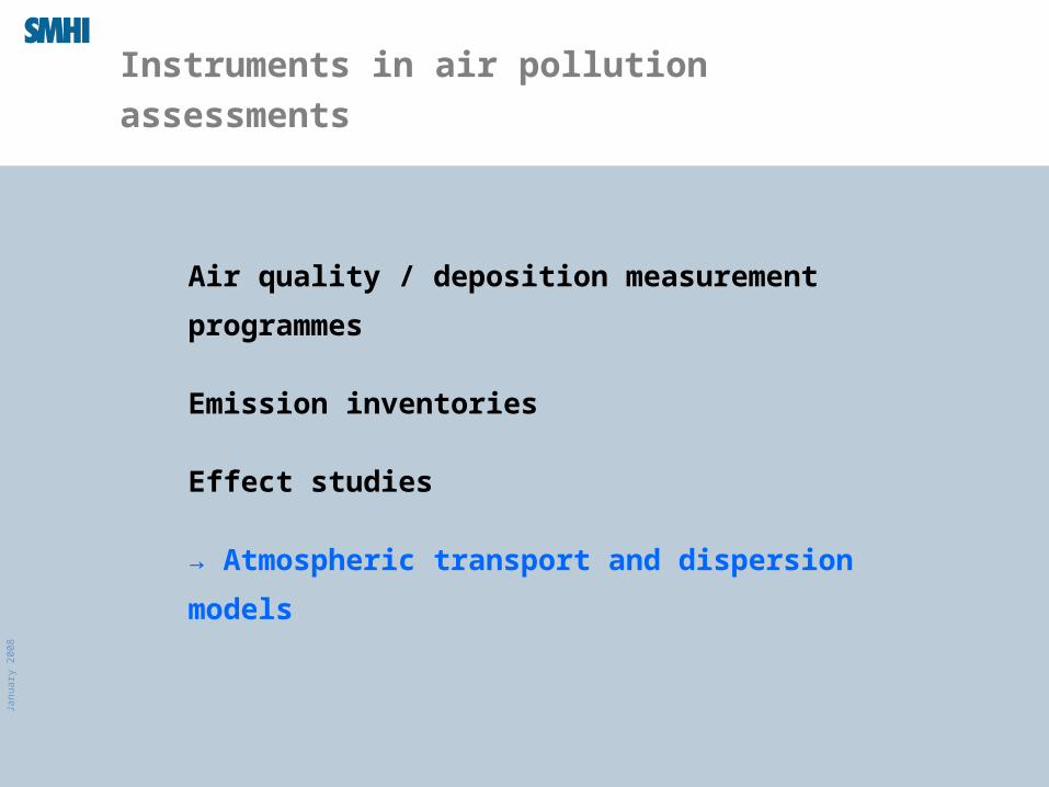
Instruments in air pollution assessments
Air quality / deposition measurement programmes
Emission inventories
Effect studies
→ Atmospheric transport and dispersion models
Janu
ary
2008
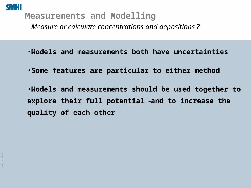
Measurements and Modelling
•Models and measurements both have uncertainties
•Some features are particular to either method
•Models and measurements should be used together to explore
their full potential and to increase the quality of each other
Measure or calculate concentrations and depositions ?
Janu
ary
2008
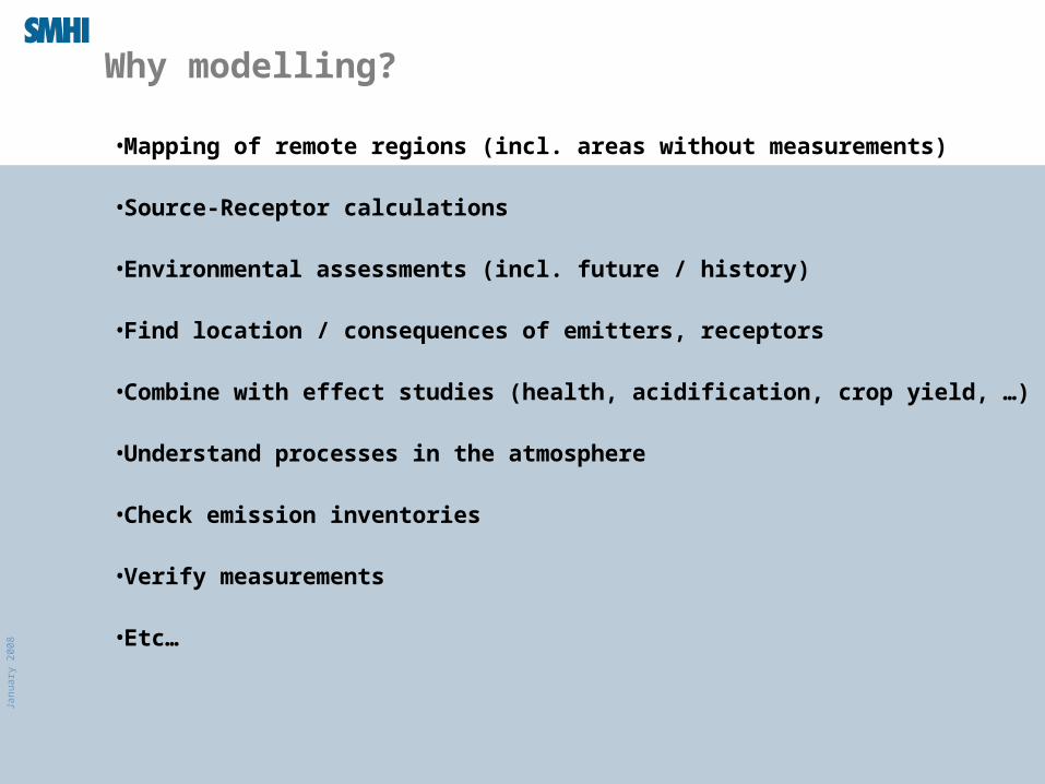
Why modelling?
•Mapping of remote regions (incl. areas without measurements)
•Source-Receptor calculations
•Environmental assessments (incl. future / history)
•Find location / consequences of emitters, receptors
•Combine with effect studies (health, acidification, crop yield, …)
•Understand processes in the atmosphere
•Check emission inventories
•Verify measurements
•Etc…

Janu
ary
2008
Some examples…
Janu
ary
2008
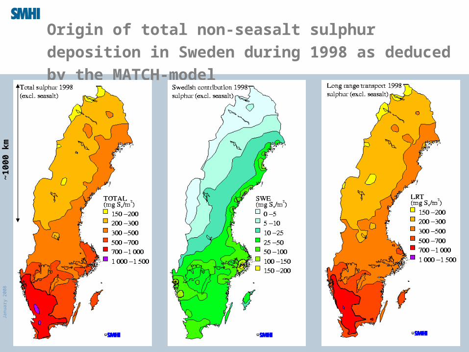
Origin of total non-seasalt sulphur deposition in Sweden
during 1998 as deduced by the MATCH-model
~10
00 k
m
Janu
ary
2008
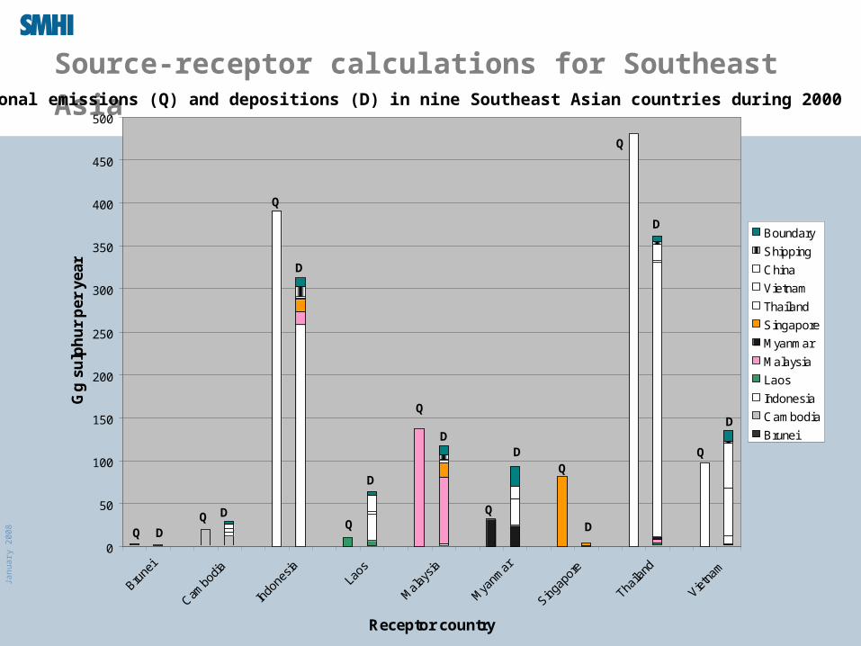
Source-receptor calculations for Southeast AsiaNational emissions (Q) and depositions (D) in nine Southeast Asian countries during 2000
0
50
100
150
200
250
300
350
400
450
500
Brune
i
Cambo
dia
Indo
nesia
Laos
Mal
aysia
Mya
nmar
Singap
ore
Thaila
nd
Vietna
m
Receptor country
Gg
su
lph
ur
per
yea
r
Boundary
Shipping
China
Vietnam
Thailand
Singapore
Myanmar
Malaysia
Laos
Indonesia
Cambodia
Brunei
Q
Q
Q
Q
Q
Q
QDD
D
D
D
D D
D
D
Janu
ary
2008
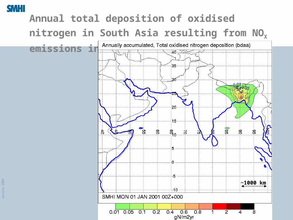
Annual total deposition of oxidised nitrogen in South
Asia resulting from NOX emissions in Bangladesh.
~1000 km
Janu
ary
2008
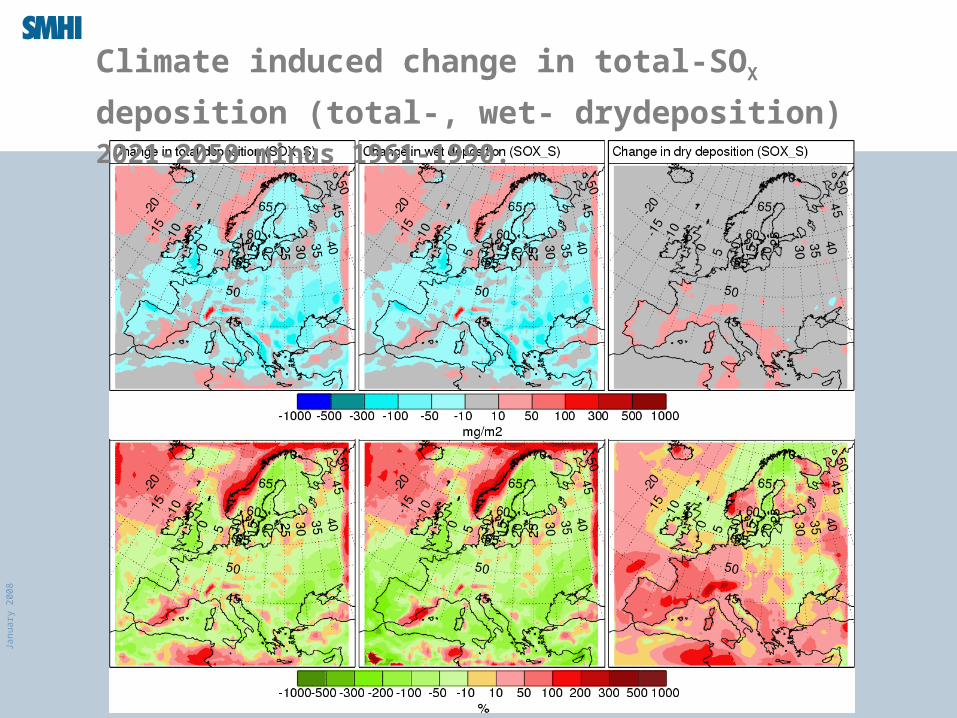
Climate induced change in total-SOX deposition
(total-, wet- drydeposition) 2021-2050 minus 1961-1990.
Janu
ary
2008
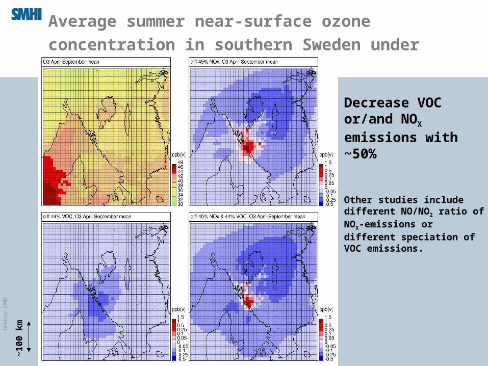
Average summer near-surface ozone concentration in
southern Sweden under different emission scenarios
Decrease VOC or/and NOX emissions with ~50%
Other studies include different NO/NO2 ratio of NOX-emissions or different speciation of VOC emissions.
~10
0 km
Janu
ary
2008
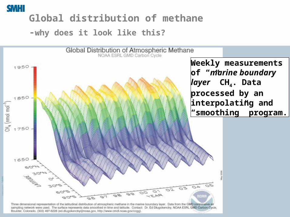
Global distribution of methane
-why does it look like this?
Weekly measurements of “marine boundary layer” CH4. Data processed by an interpolating and “smoothing” program.

Janu
ary
2008
Janu
ary
2008
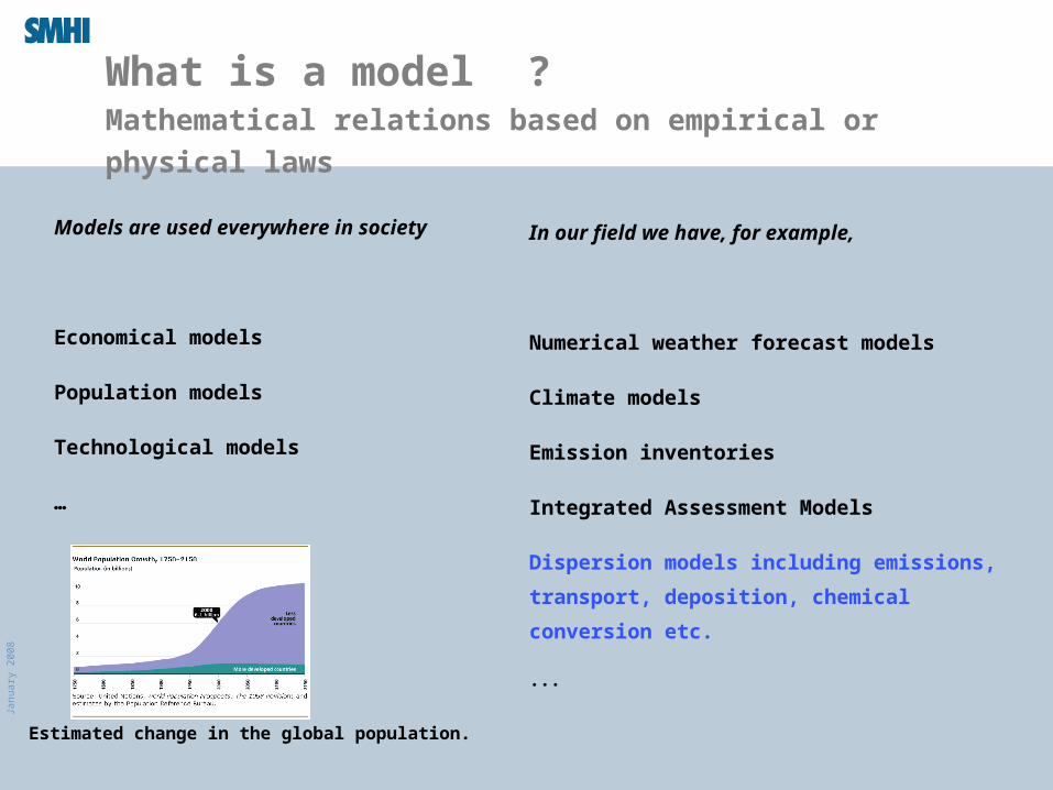
What is a model?Mathematical relations based on empirical or physical laws
In our field we have, for example,
Numerical weather forecast models
Climate models
Emission inventories
Integrated Assessment Models
Dispersion models including emissions, transport,
deposition, chemical conversion etc.
...
Models are used everywhere in society
Economical models
Population models
Technological models
…
Estimated change in the global population.
Janu
ary
2008
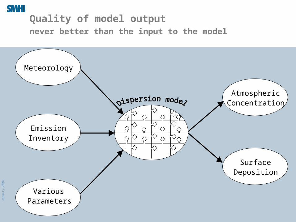
Quality of model outputnever better than the input to the model
VariousParameters
Meteorology
EmissionInventory
SurfaceDeposition
AtmosphericConcentration
Janu
ary
2008
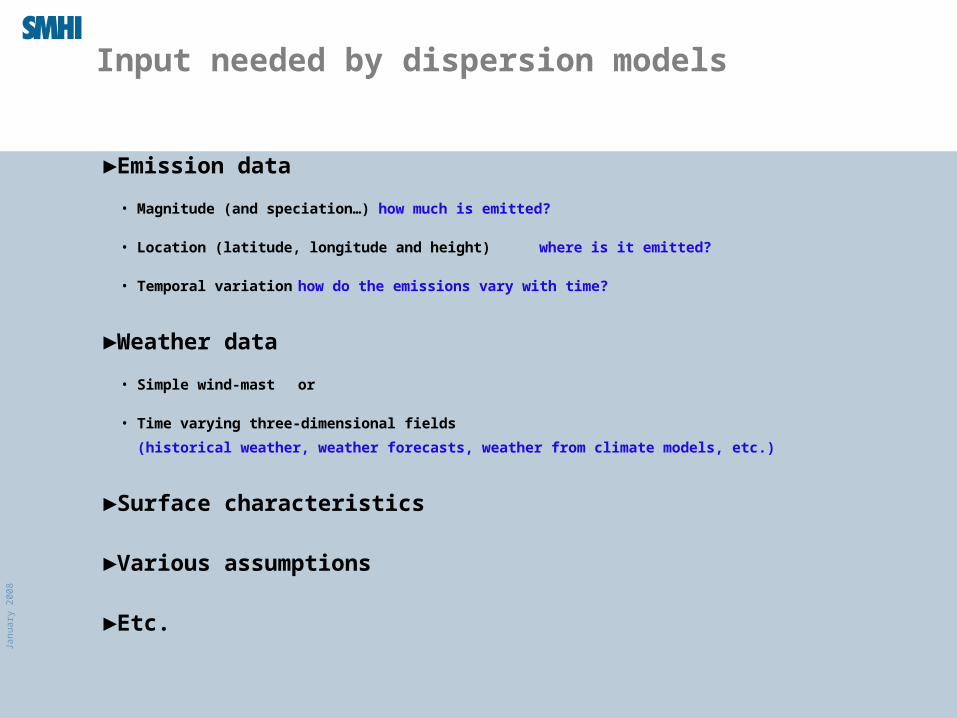
Input needed by dispersion models
►Emission data
• Magnitude (and speciation…) how much is emitted?
• Location (latitude, longitude and height) where is it emitted?
• Temporal variation how do the emissions vary with time?
►Weather data
• Simple wind-mast or
• Time varying three-dimensional fields
(historical weather, weather forecasts, weather from climate models, etc.)
►Surface characteristics
►Various assumptions
►Etc.
Janu
ary
2008
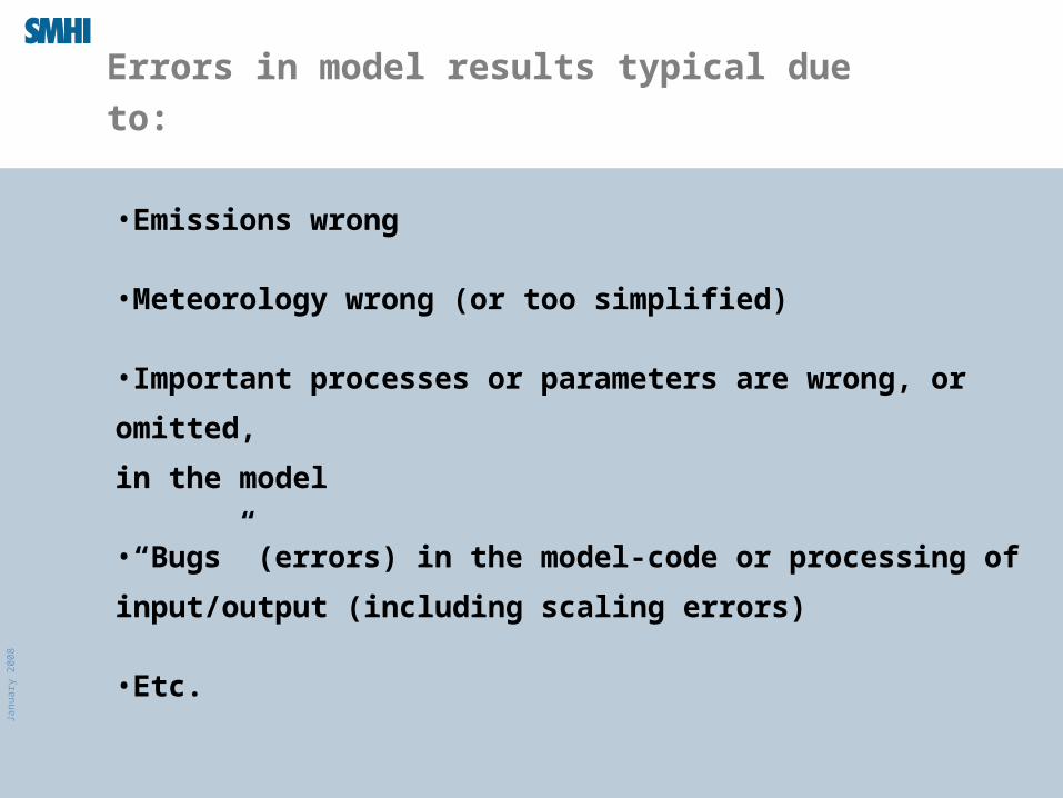
Errors in model results typical due to:
•Emissions wrong
•Meteorology wrong (or too simplified)
•Important processes or parameters are wrong, or omitted,
in the model
•“Bugs” (errors) in the model-code or processing of input/output
(including scaling errors)
•Etc.
Janu
ary
2008
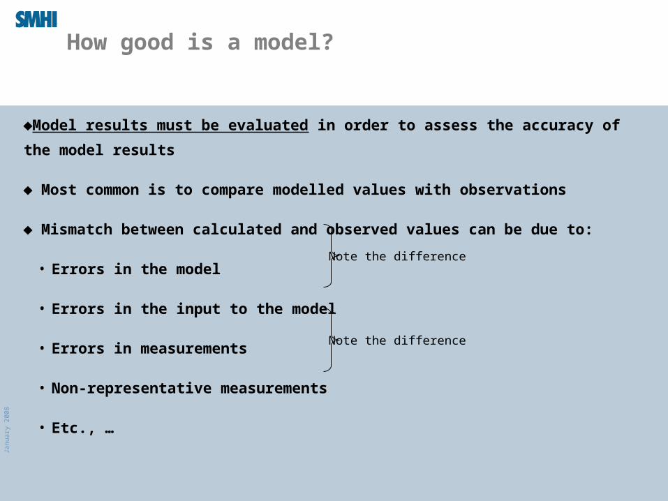
How good is a model?
Model results must be evaluated in order to assess the accuracy of the model results
Most common is to compare modelled values with observations
Mismatch between calculated and observed values can be due to:
• Errors in the model
• Errors in the input to the model
• Errors in measurements
• Non-representative measurements
• Etc., …
Note the difference
Note the difference
Janu
ary
2008
N
1i MC
ii )CC)(MM(
N
1r
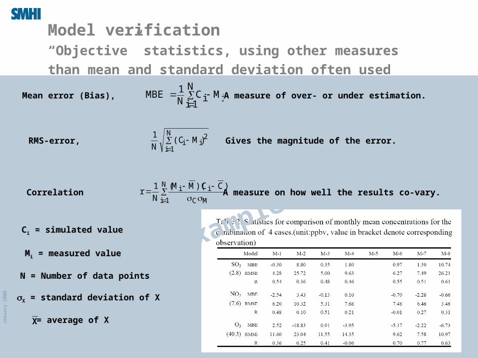
Model verification“Objective” statistics, using other measures than mean
and standard deviation often used
A measure on how well the results co-vary.
iMN
1iiC
N1MBE
A measure of over- or under estimation.Mean error (Bias),
N
1i
2ii )M(C
N
1Gives the magnitude of the error.RMS-error,
Correlation
Ci = simulated value
Mi = measured value
N = Number of data points
X = standard deviation of X
= average of XX
Example
Janu
ary
2008
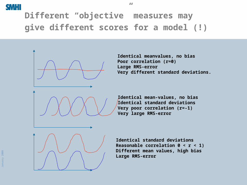
Different “objective” measures may give
different scores for a model (!)
Identical meanvalues, no biasPoor correlation (r≈0)Large RMS-errorVery different standard deviations.
Identical mean-values, no biasIdentical standard deviations Very poor correlation (r=-1)Very large RMS-error
Identical standard deviations Reasonable correlation 0 < r < 1)Different mean values, high biasLarge RMS-error
Janu
ary
2008
Model verification (cont’d)Visual inspection of results
“Subjective” inspection of the results by plotting them
should also be performed. Methods include:
• Timeseries
• Scatterplots
• Maps
Janu
ary
2008
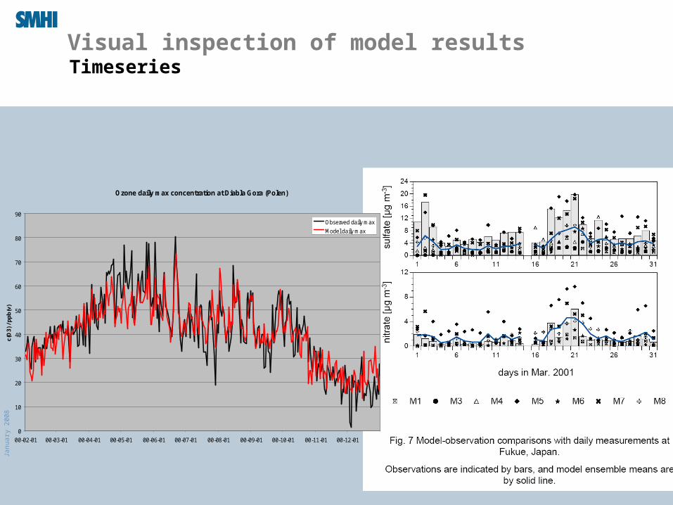
Visual inspection of model resultsTimeseries
Ozone daily max concentration at Diabla Gora (Polen)
0
10
20
30
40
50
60
70
80
90
00-02-01 00-03-01 00-04-01 00-05-01 00-06-01 00-07-01 00-08-01 00-09-01 00-10-01 00-11-01 00-12-01
c(O
3) /
pp
b(v
)
Observed daily max
Model daily max
Janu
ary
2008
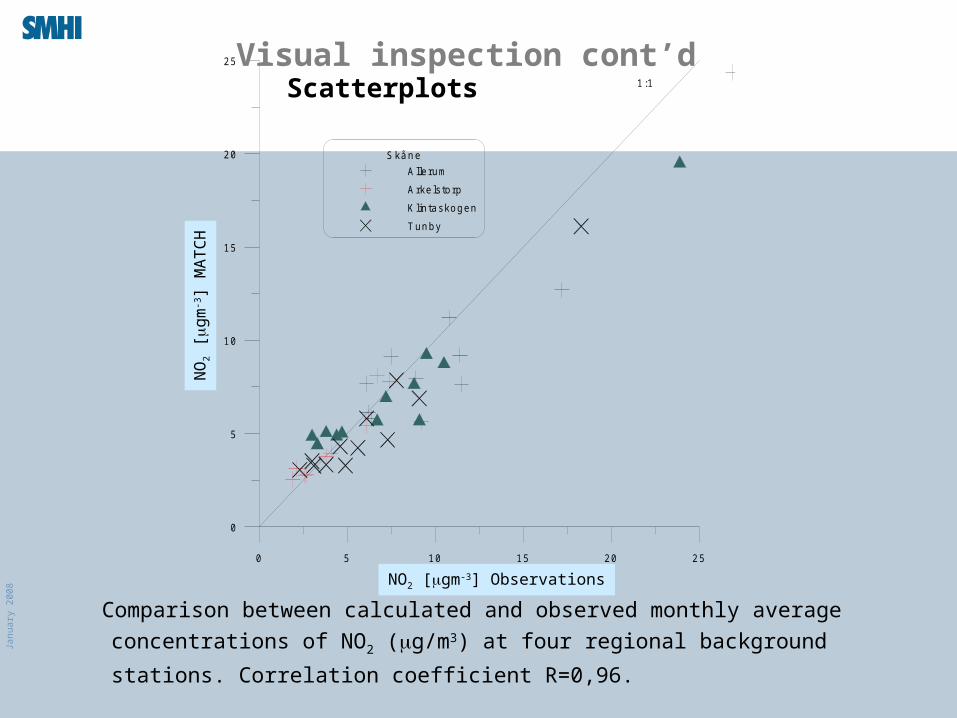
Comparison between calculated and observed monthly average concentrations of
NO2 (g/m3) at four regional background stations. Correlation coefficient R=0,96.
0 5 10 15 20 25N O 2 (µg /m 3) M ä td a ta
0
5
10
15
20
25
NO
2(µ
g/m
3 ) M
AT
CH
All
S kå n eA llerum
Arke lstorp
K lin taskogen
Tunby
1:1ScatterplotsVisual inspection cont’d
NO
2 [
gm
-3]
MA
TC
H
NO2 [gm-3] Observations
Janu
ary
2008
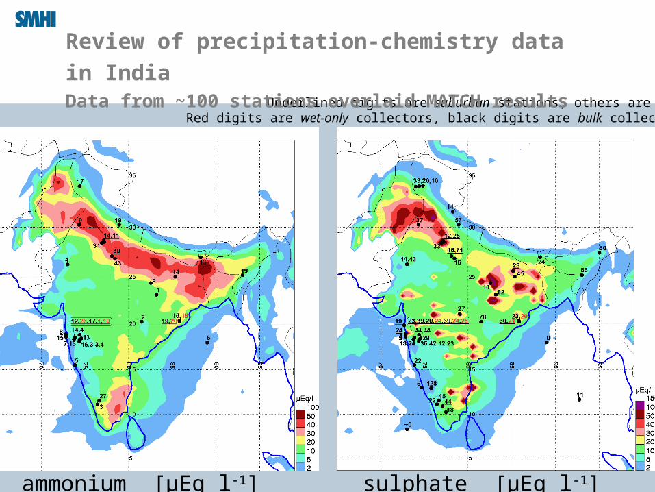
ammonium [μEq l-1] sulphate [μEq l-1]
Underlined digits are suburban stations, others are rural.Red digits are wet-only collectors, black digits are bulk collectors.
Review of precipitation-chemistry data in IndiaData from ~100 stations overlaid MATCH results
Janu
ary
2008
Can you use a model of limited quality?
(How “bad” performance is acceptable?)
Unrealistic data should never be accepted
A “factor of two” is often regarded as a very good correspondence
If there is little measured data available you may have to trust your model
results even if the discrepancy is relatively large.
Sometimes you are concerned with typical average levels, sometimes you
want to capture diurnal or day-to-day or seasonal variations
Note the problem of unrepresentative measurements
Keep uncertainty in input data in mind (model results could not be better
than the input)
Janu
ary
2008
Model quality (cont’d)
It’s good to check the model in different ways
• Both atmospheric concentrations and surface depositions
• Study vertical profiles (although you very seldom have any data
away from the surface…)
• Test both inert and reactive species…
• Both primary and secondary species
• Test the same model at different places and during different
periods
If you have discrepancies, try to understand what they are caused by!
Janu
ary
2008
Error propagation
Sometimes small errors in the input cause large errors in
the output
Sometimes it turns out that certain input data or model
formulations doesn’t matter much
Analyse the robustness of your results through sensitivity
tests
Janu
ary
2008
Atmospheric dispersion modelling
–basic concepts (Ch. 23 in Seinfeld and Pandis, 1998)
Magnuz Engardt
Swedish Meteorological and Hydrological Institute

Janu
ary
2008
Pollutants (gases and particles) are transported
with the three-dimensional wind
t=t0+t
t=t0
Janu
ary
2008
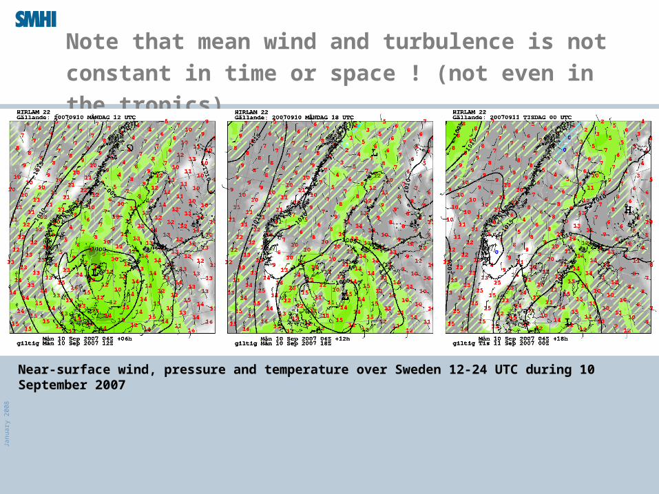
Note that mean wind and turbulence is not constant
in time or space ! (not even in the tropics)
Near-surface wind, pressure and temperature over Sweden 12-24 UTC during 10 September 2007
Janu
ary
2008
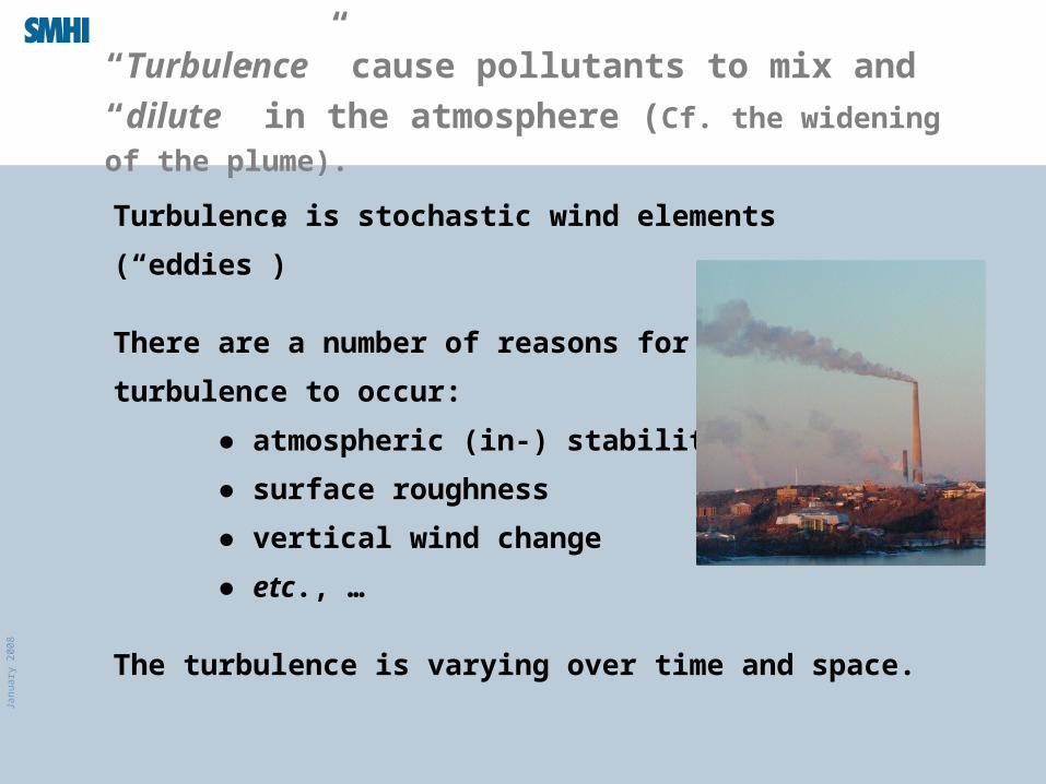
“Turbulence” cause pollutants to mix and “dilute”
in the atmosphere (Cf. the widening of the plume).
Turbulence is stochastic wind elements (“eddies”)
There are a number of reasons for
turbulence to occur:
● atmospheric (in-) stability
● surface roughness
● vertical wind change
● etc., …
The turbulence is varying over time and space.
Janu
ary
2008
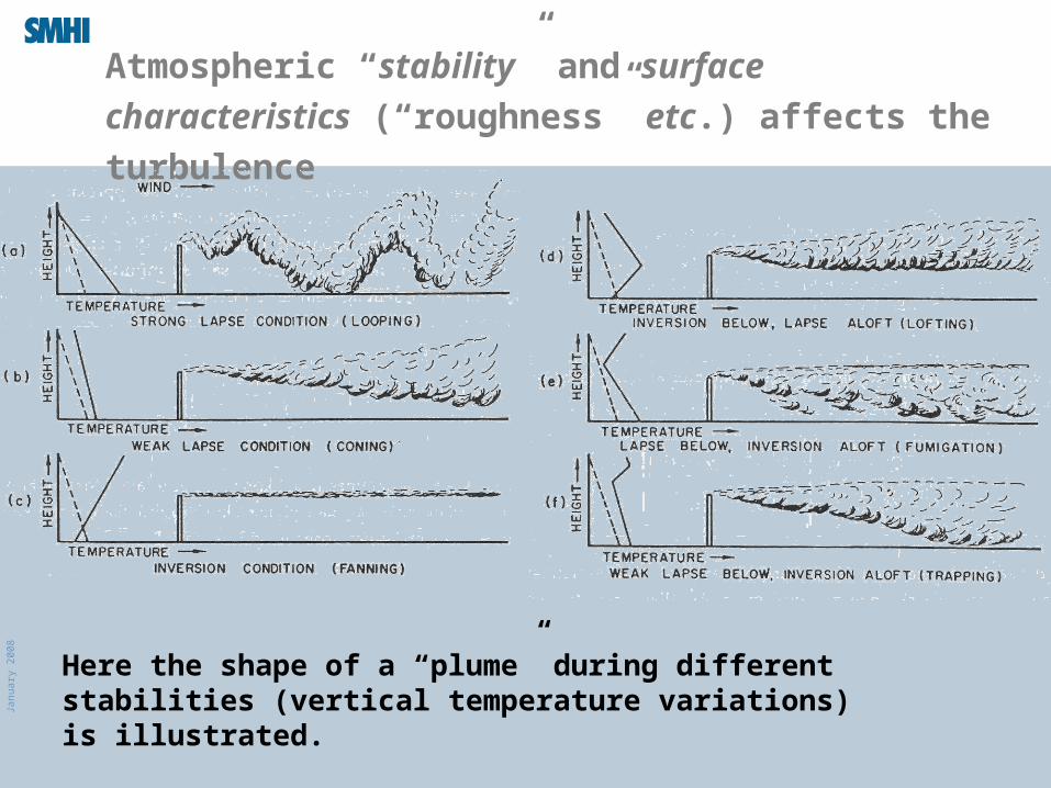
Atmospheric “stability” and surface characteristics
(“roughness” etc.) affects the turbulence
Here the shape of a “plume” during different stabilities (vertical temperature variations) is illustrated.
Janu
ary
2008
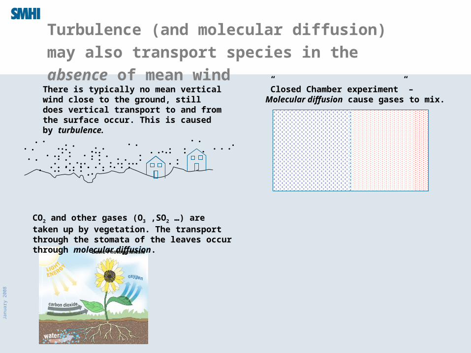
Turbulence (and molecular diffusion) may also
transport species in the absence of mean wind
... . . ..
... . . ..
... . . ....
. . . ..
... . . ..
... . . ..
.... .......
........
.... .... ... .
. .... ..
... .
. . ..
.. .
There is typically no mean vertical wind close to the ground, still does vertical transport to and from the surface occur. This is caused by turbulence.
”Closed Chamber experiment” – Molecular diffusion cause gases to mix.
CO2 and other gases (O3 ,SO2 …) are taken up by vegetation. The transport through the stomata of the leaves occur through molecular diffusion.
Janu
ary
2008
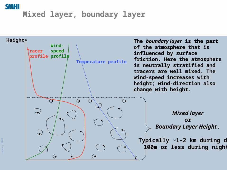
Mixed layer, boundary layer
The boundary layer is the part of the atmosphere that is influenced by surface friction. Here the atmosphere is neutrally stratified and tracers are well mixed. The wind-speed increases with height; wind-direction also change with height.
Mixed layeror
Boundary Layer Height.
Typically ~1-2 km during day,100m or less during night.
Temperature profile
Tracer profile
HeightWind-speedprofile
Janu
ary
2008
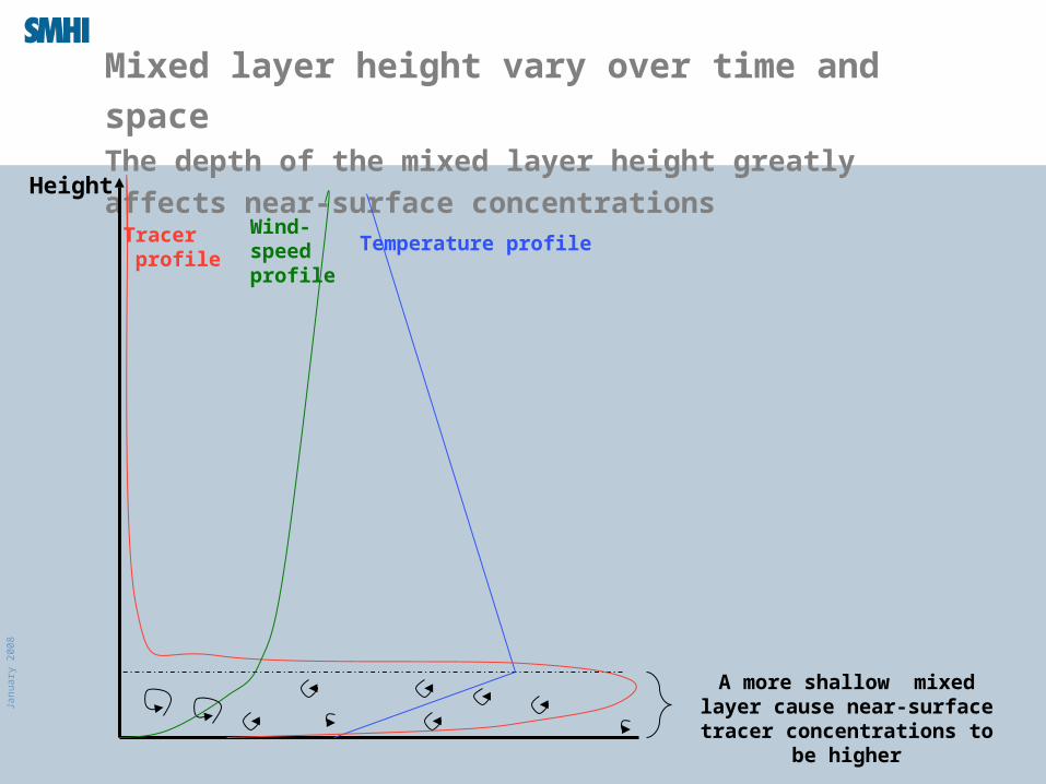
Mixed layer height vary over time and spaceThe depth of the mixed layer height greatly affects near-
surface concentrations
Temperature profileTracer profile
Height
Wind-speedprofile
A more shallow mixed layer cause near-surface tracer
concentrations to be higher
Janu
ary
2008
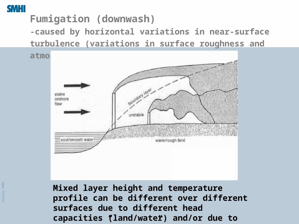
Fumigation (downwash)-caused by horizontal variations in near-surface turbulence
(variations in surface roughness and atmospheric stability)
Mixed layer height and temperature profile can be different over different surfaces due to different head capacities (land/water) and/or due to different ”roughness” of the surface.
Janu
ary
2008
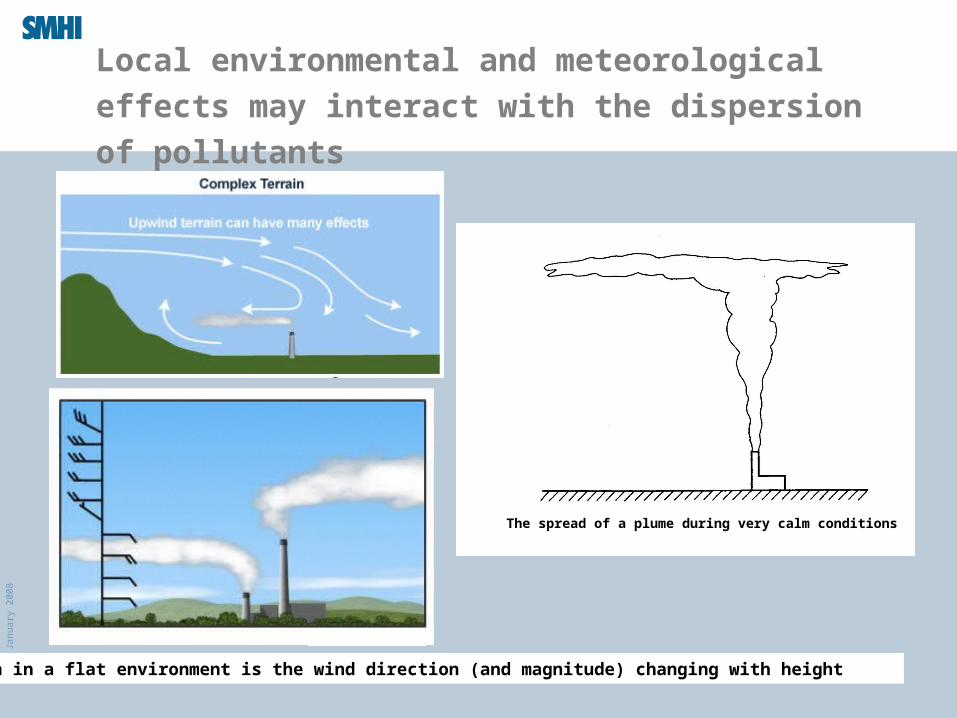
Local environmental and meteorological effects may
interact with the dispersion of pollutants
The spread of a plume during very calm conditions
Even in a flat environment is the wind direction (and magnitude) changing with height
Janu
ary
2008
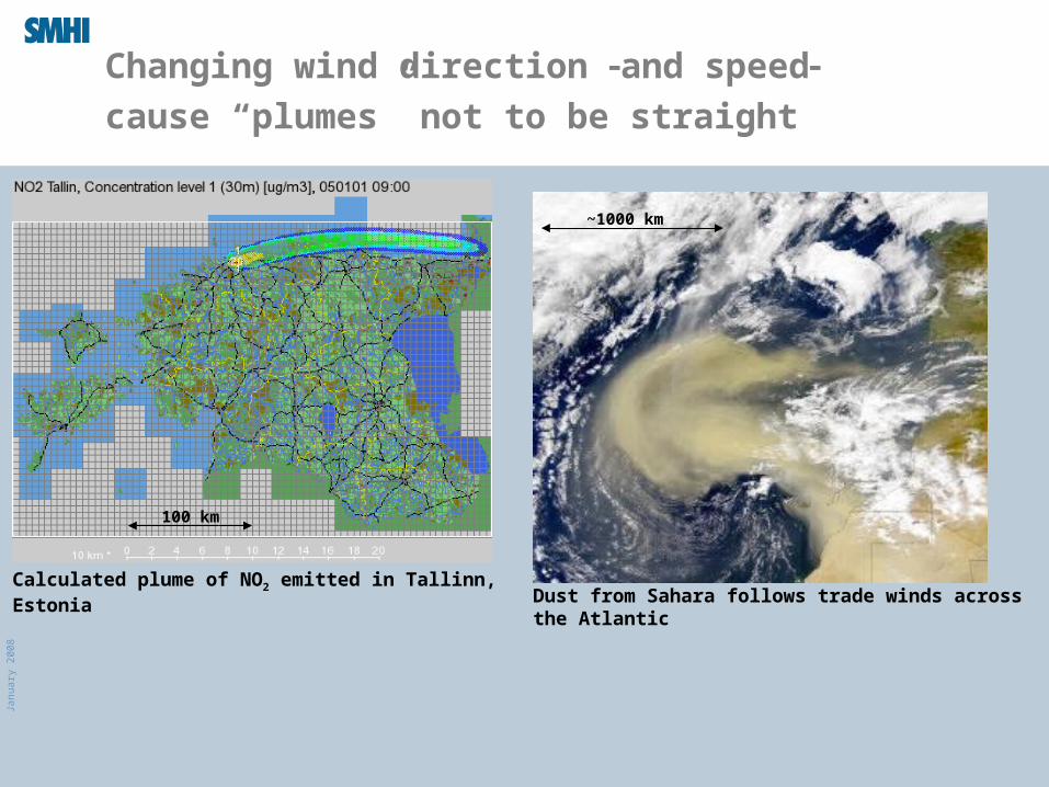
Changing wind direction and speed cause
“plumes” not to be straight
Calculated plume of NO2 emitted in Tallinn, EstoniaDust from Sahara follows trade winds across the Atlantic
~1000 km
100 km
Janu
ary
2008
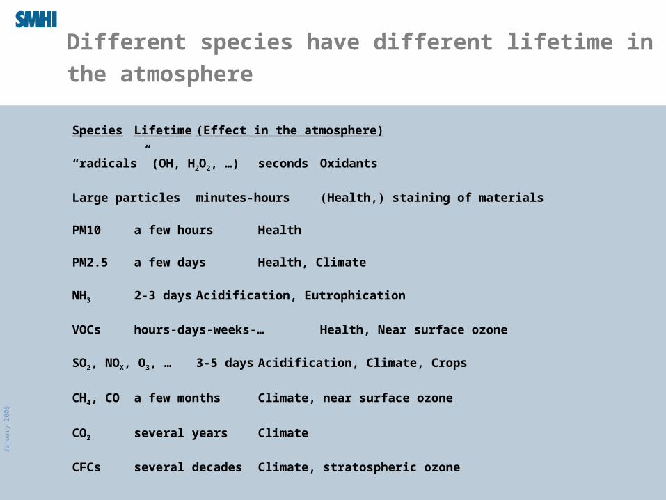
Different species have different lifetime in the
atmosphere
Species Lifetime (Effect in the atmosphere)
“radicals” (OH, H2O2, …) seconds Oxidants
Large particles minutes-hours (Health,) staining of materials
PM10 a few hours Health
PM2.5 a few days Health, Climate
NH3 2-3 days Acidification, Eutrophication
VOCs hours-days-weeks-… Health, Near surface ozone
SO2, NOX, O3, … 3-5 days Acidification, Climate, Crops
CH4, CO a few months Climate, near surface ozone
CO2 several years Climate
CFCs several decades Climate, stratospheric ozone
Janu
ary
2008
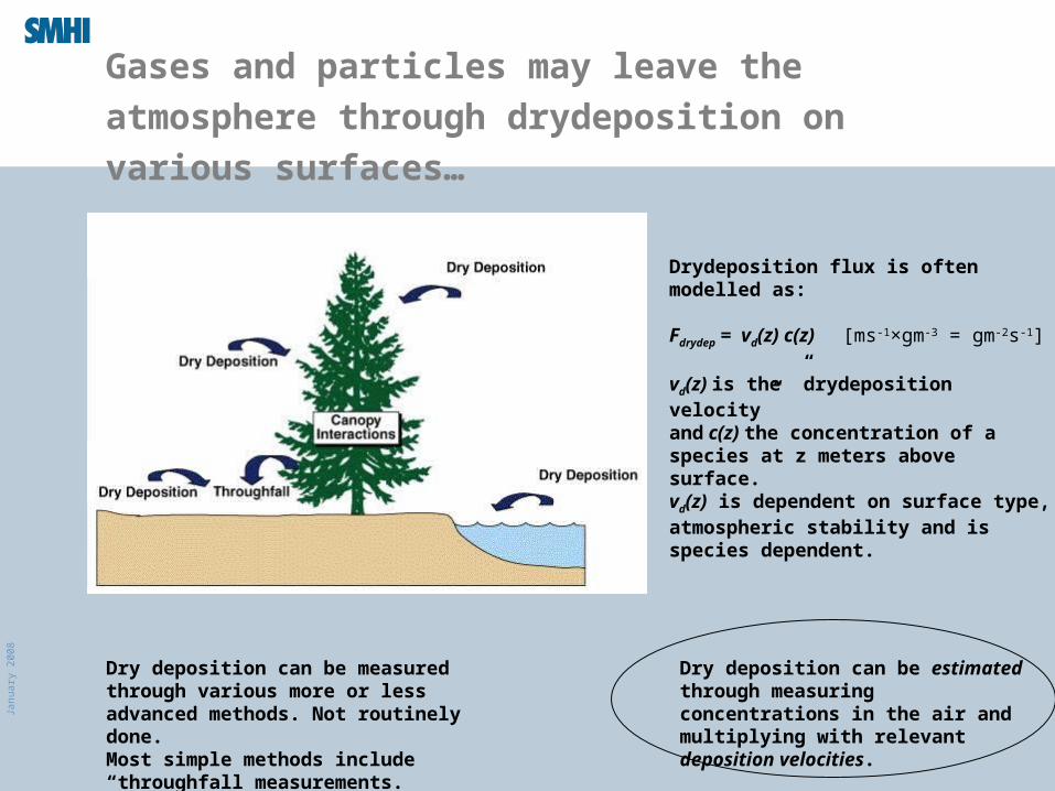
Gases and particles may leave the atmosphere
through drydeposition on various surfaces…
Drydeposition flux is often modelled as:
Fdrydep = vd(z) c(z) [ms-1×gm-3 = gm-2s-1]
vd(z) is the ”drydeposition velocity”and c(z) the concentration of a species at z meters above surface.vd(z) is dependent on surface type, atmospheric stability and is species dependent.
Dry deposition can be estimated through measuring concentrations in the air and multiplying with relevant deposition velocities.
Dry deposition can be measured through various more or less advanced methods. Not routinely done.Most simple methods include “throughfall measurements.
Janu
ary
2008
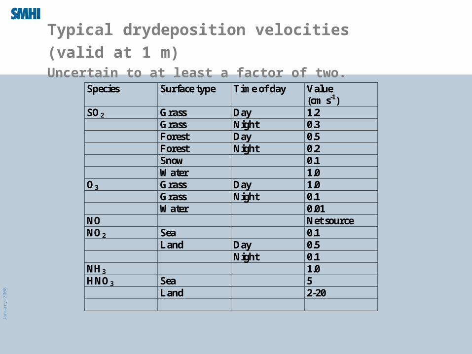
Typical drydeposition velocities (valid at 1 m)Uncertain to at least a factor of two.
Species Surface type Time of day Value (cm s-1)
SO2 Grass Day 1.2 Grass Night 0.3 Forest Day 0.5 Forest Night 0.2 Snow 0.1 Water 1.0 O3 Grass Day 1.0 Grass Night 0.1 Water 0.01 NO Net source NO2 Sea 0.1 Land Day 0.5 Night 0.1 NH3 1.0 HNO3 Sea 5 Land 2-20
Janu
ary
2008
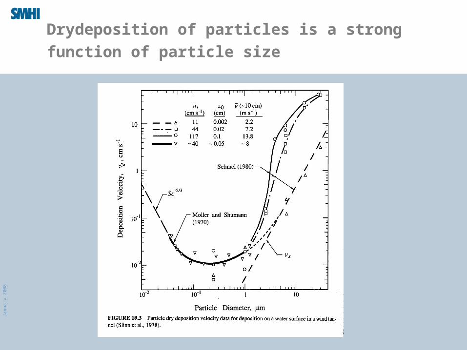
Drydeposition of particles is a strong function of
particle size
Janu
ary
2008
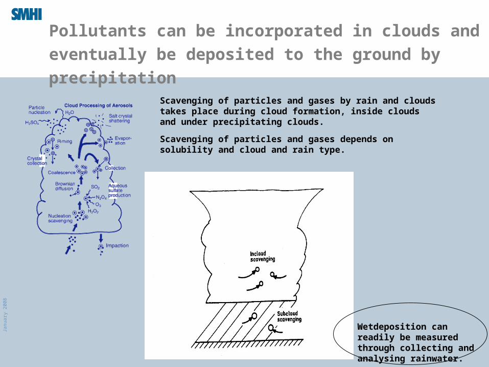
Pollutants can be incorporated in clouds and eventually
be deposited to the ground by precipitation
Scavenging of particles and gases depends on solubility and cloud and rain type.
Scavenging of particles and gases by rain and clouds takes place during cloud formation, inside clouds and under precipitating clouds.
Wetdeposition can readily be measured through collecting and analysing rainwater.
Janu
ary
2008
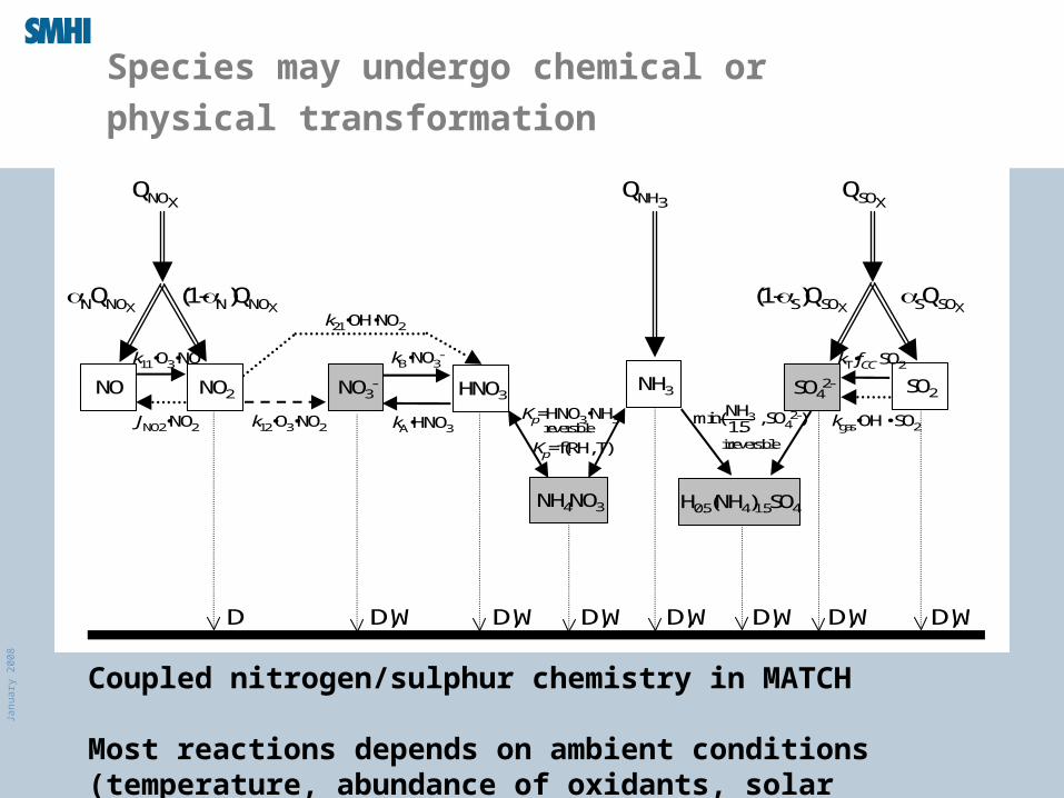
Species may undergo chemical or physical
transformation
NO NO2 HNO3NO3-
NH4NO3
NH3 SO42- SO2
H0.5(NH4)1.5SO4
QNOXQNH3
QSOX
JNO2•NO2
k11•O3•NO
k12•O3•NO2
k21•OH•NO2
Kp=HNO3•NH3kA•HNO3
kB•NO3- kT•fCC SO2
D D,W D,W D,W D,W D,W D,W D,W
kgas•OH • SO2
Kp=f(RH, T) irreversible
NQNOXSQSOX
(1-N)QNOX(1-S)QSOX
min( , SO42-)
1.5NH3
reversible
Coupled nitrogen/sulphur chemistry in MATCH
Most reactions depends on ambient conditions (temperature, abundance of oxidants, solar radiation, humidity etc.).
Janu
ary
2008
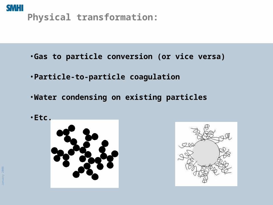
Physical transformation:
•Gas to particle conversion (or vice versa)
•Particle-to-particle coagulation
•Water condensing on existing particles
•Etc.
Janu
ary
2008
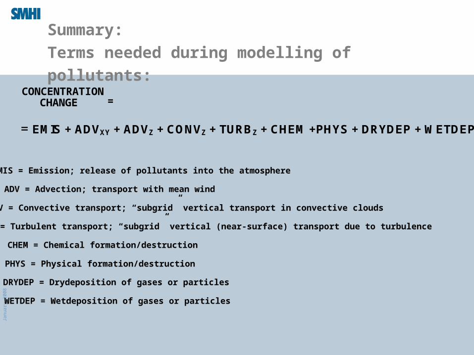
Summary:
Terms needed during modelling of pollutants:
= EMIS + ADVXY + ADVZ + CONVZ + TURBZ + CHEM +PHYS + DRYDEP + WETDEP
ADV = Advection; transport with mean wind
EMIS = Emission; release of pollutants into the atmosphere
CONV = Convective transport; “subgrid” vertical transport in convective clouds
TURB = Turbulent transport; “subgrid” vertical (near-surface) transport due to turbulence
CHEM = Chemical formation/destruction
DRYDEP = Drydeposition of gases or particles
WETDEP = Wetdeposition of gases or particles
PHYS = Physical formation/destruction
CONCENTRATIONCHANGE =

Janu
ary
2008
An example from real life:
Janu
ary
2008
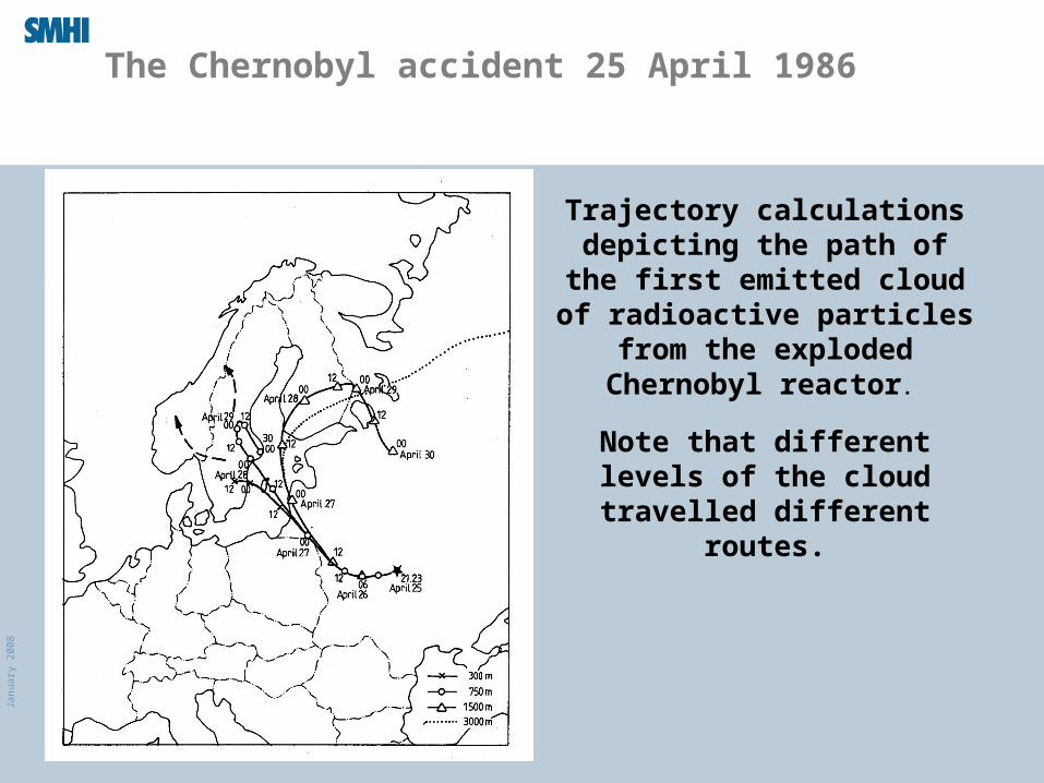
The Chernobyl accident 25 April 1986
Trajectory calculations depicting the path of the first emitted cloud of radioactive particles from the exploded
Chernobyl reactor.
Note that different levels of the cloud travelled different
routes.
Janu
ary
2008
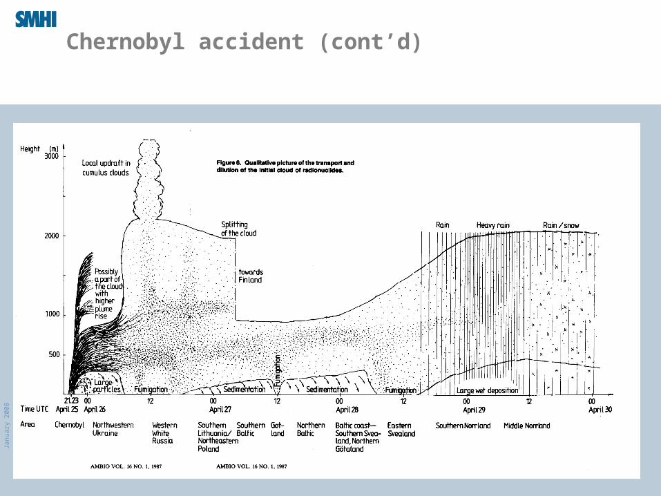
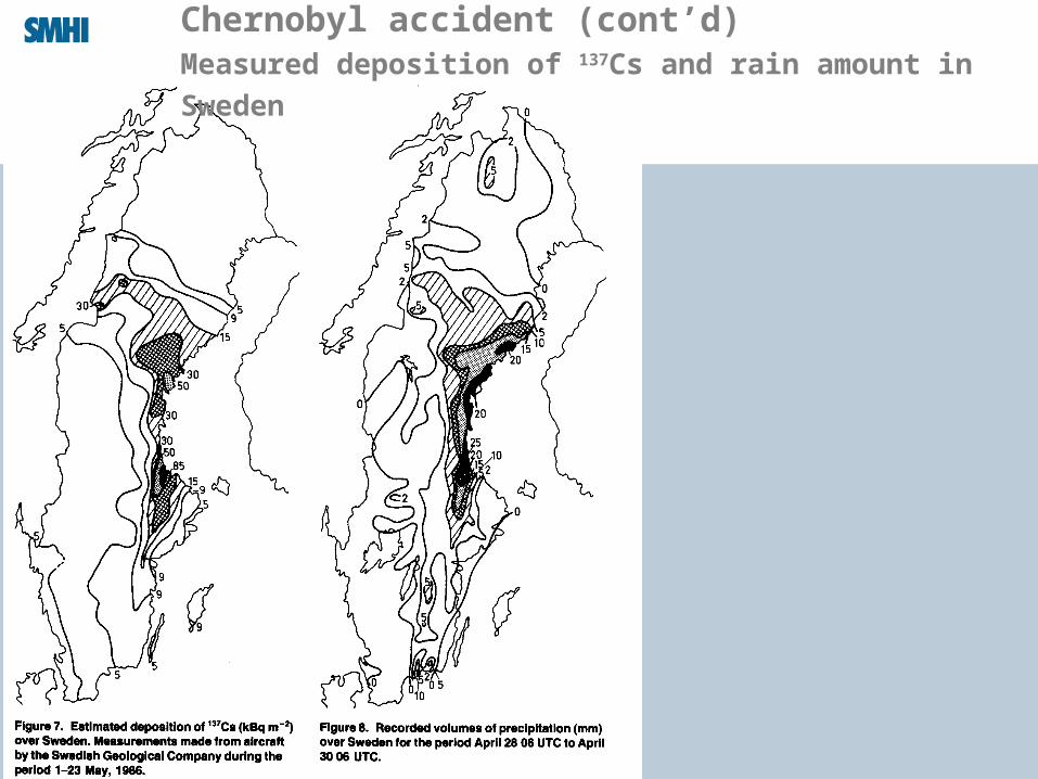
Chernobyl accident (cont’d)
Janu
ary
2008
Chernobyl accident (cont’d)Measured deposition of 137Cs and rain amount in Sweden
Janu
ary
2008
Different types of models…
Janu
ary
2008
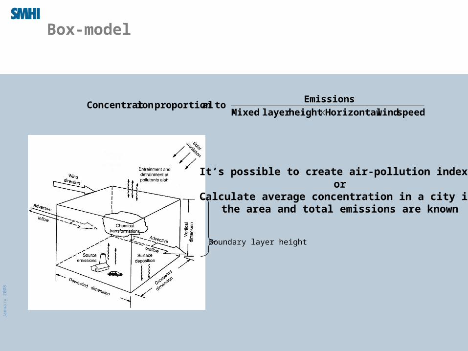
Box-model
speed windHorizontal height layer Mixed
Emissions to alproportion ionConcentrat
It’s possible to create air-pollution indexesor
Calculate average concentration in a city if the area and total emissions are known
Boundary layer height
Janu
ary
2008
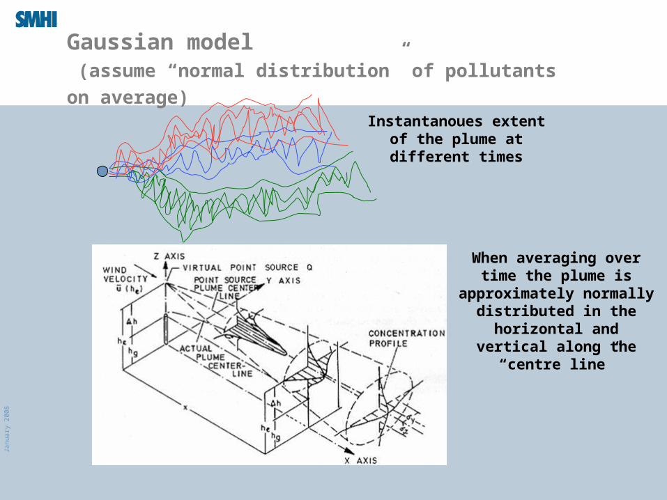
Gaussian model (assume “normal distribution” of pollutants on average)
Instantanoues extent of the plume at different times
When averaging over time the plume is approximately normally distributed in the
horizontal and vertical along the “centre line”
Janu
ary
2008
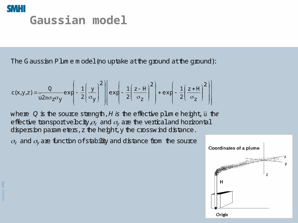
Gaussian model
The Gaussian Plume model (no uptake at the ground at the ground):
2
z
Hz
2
1exp
2
z
Hz
2
1exp
2
y
y
2
1exp
yz2u
Q)z,y,x(c
where Q is the source strength, H is the effective plume height, u the effective transport velocity,z and y are the vertical and horizontal dispersion parameters, z the height, y the crosswind distance.
z and y are function of stability and distance from the source
Janu
ary
2008
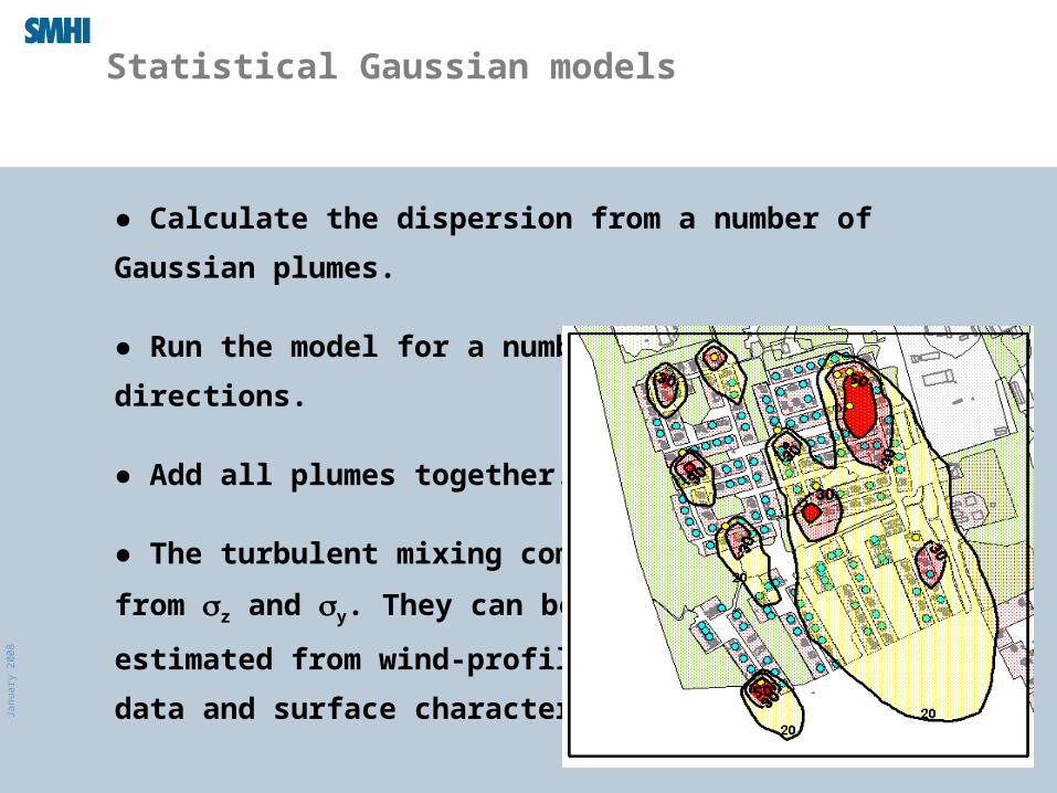
Statistical Gaussian models
● Calculate the dispersion from a number of Gaussian plumes.
● Run the model for a number of wind- speeds and directions.
● Add all plumes together.
● The turbulent mixing comes
from z and y. They can be
estimated from wind-profile
data and surface characteristics
Janu
ary
2008
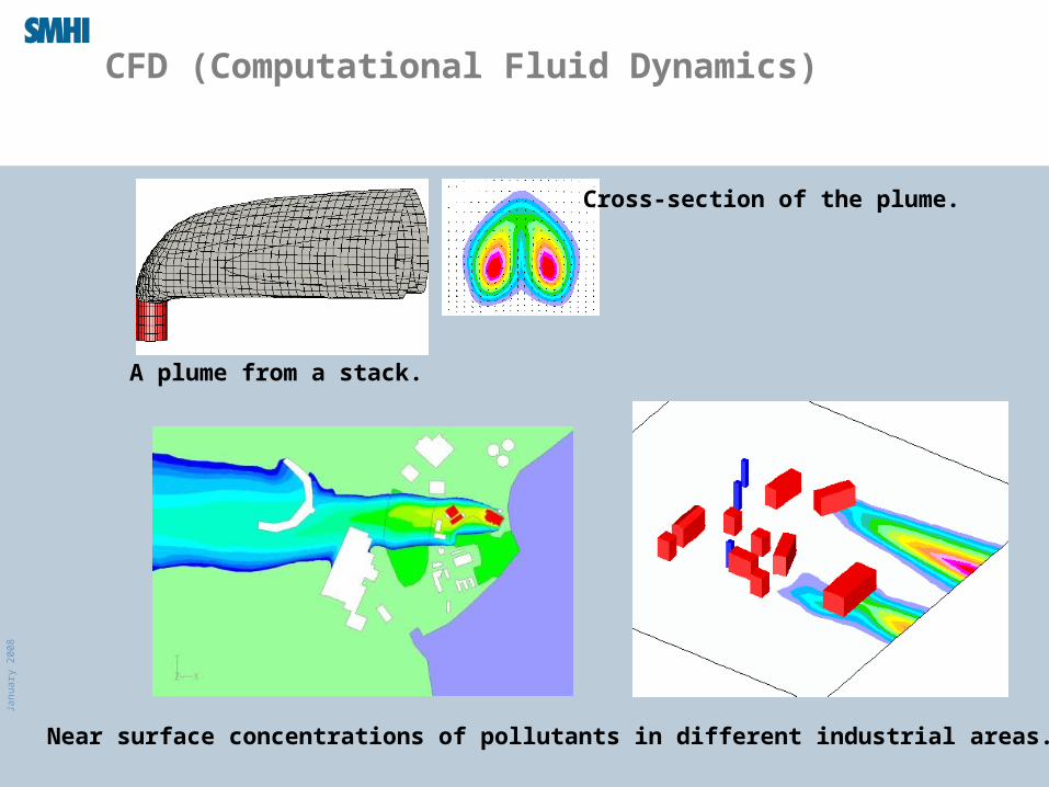
CFD (Computational Fluid Dynamics)
A plume from a stack.
Cross-section of the plume.
Near surface concentrations of pollutants in different industrial areas.
Janu
ary
2008
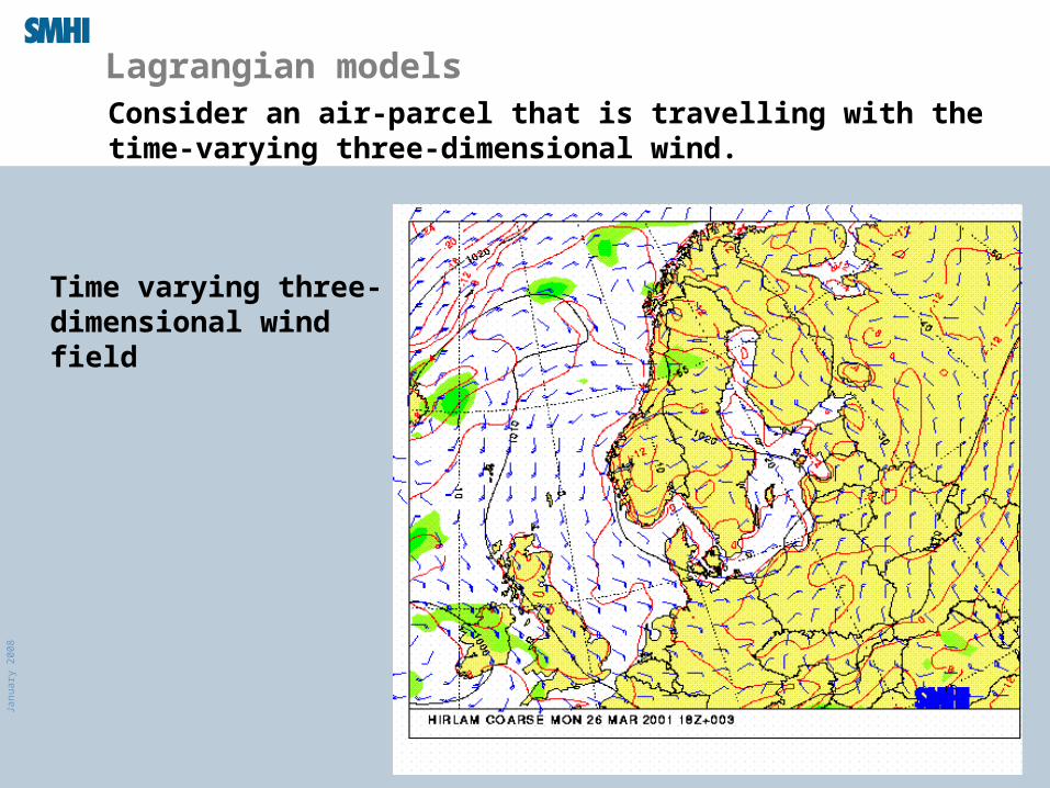
Lagrangian modelsConsider an air-parcel that is travelling with the time-varying three-dimensional wind.
Time varying three-dimensional wind field
Janu
ary
2008
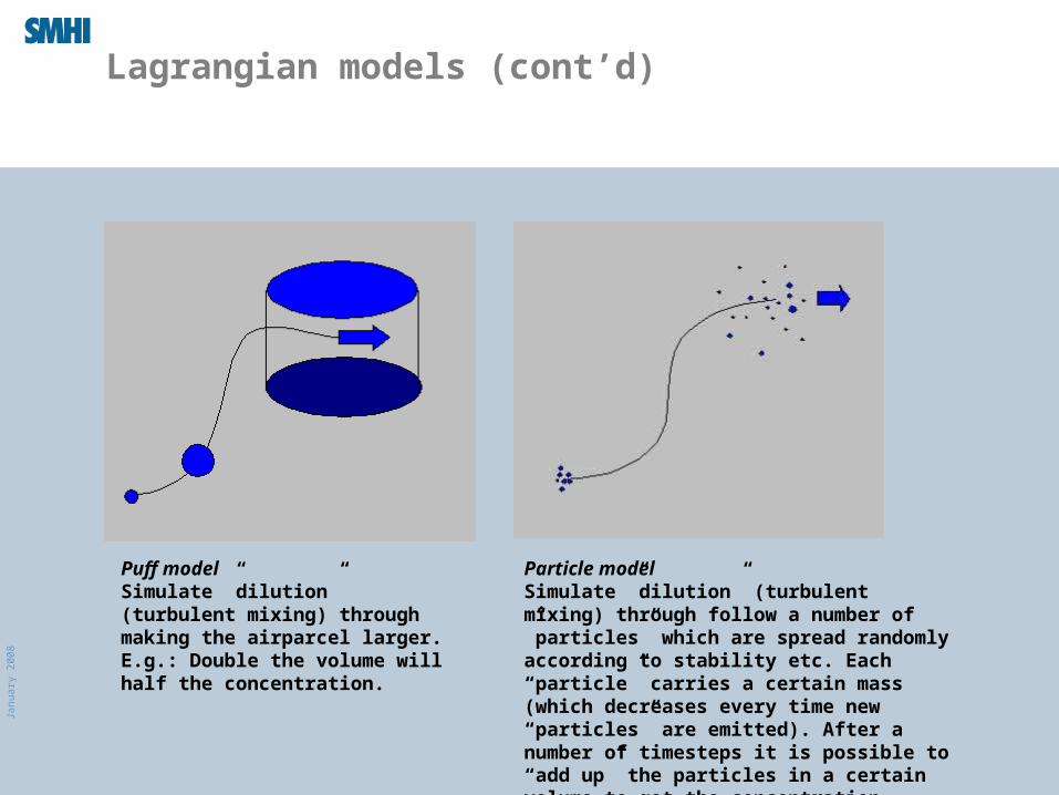
Lagrangian models (cont’d)
2
5.0exp),,(22 xy
xmzyxc
zxy
Puff modelSimulate ”dilution” (turbulent mixing) through making the airparcel larger.E.g.: Double the volume will half the concentration.
Particle modelSimulate ”dilution” (turbulent mixing) through follow a number of ”particles” which are spread randomly according to stability etc. Each “particle” carries a certain mass (which decreases every time new “particles” are emitted). After a number of timesteps it is possible to “add up” the particles in a certain volume to get the concentration.
Janu
ary
2008
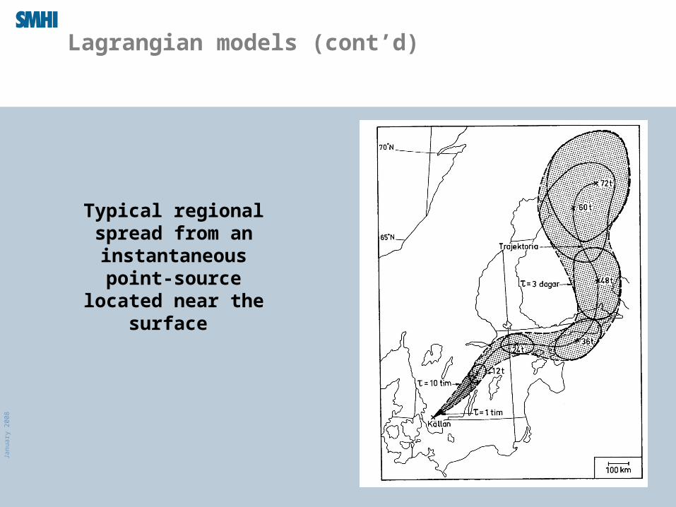
Lagrangian models (cont’d)
Typical regional spread from an instantaneous point-source located
near the surface
Janu
ary
2008
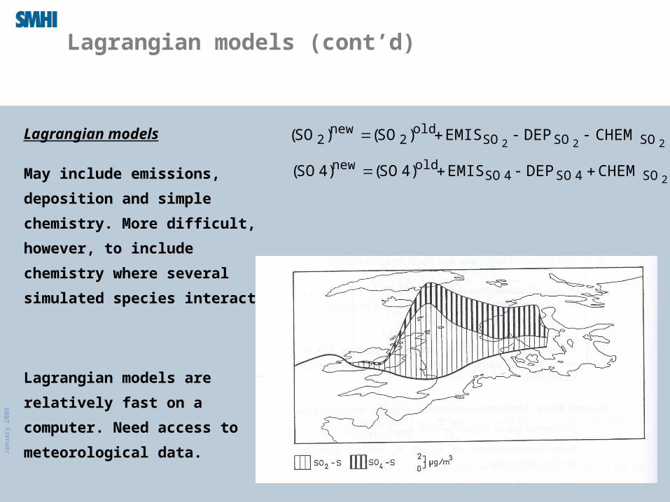
Lagrangian models (cont’d)
Lagrangian models
May include emissions, deposition
and simple chemistry. More
difficult, however, to include
chemistry where several simulated
species interact.
Lagrangian models are relatively
fast on a computer. Need access to
meteorological data.
222 SOSOSOold
2new
2 CHEMDEPEMIS)SO()SO(
2SO4SO4SOoldnew CHEMDEPEMIS)4SO()4SO(
Janu
ary
2008
Eulerian models (or gridpoint models)
Janu
ary
2008
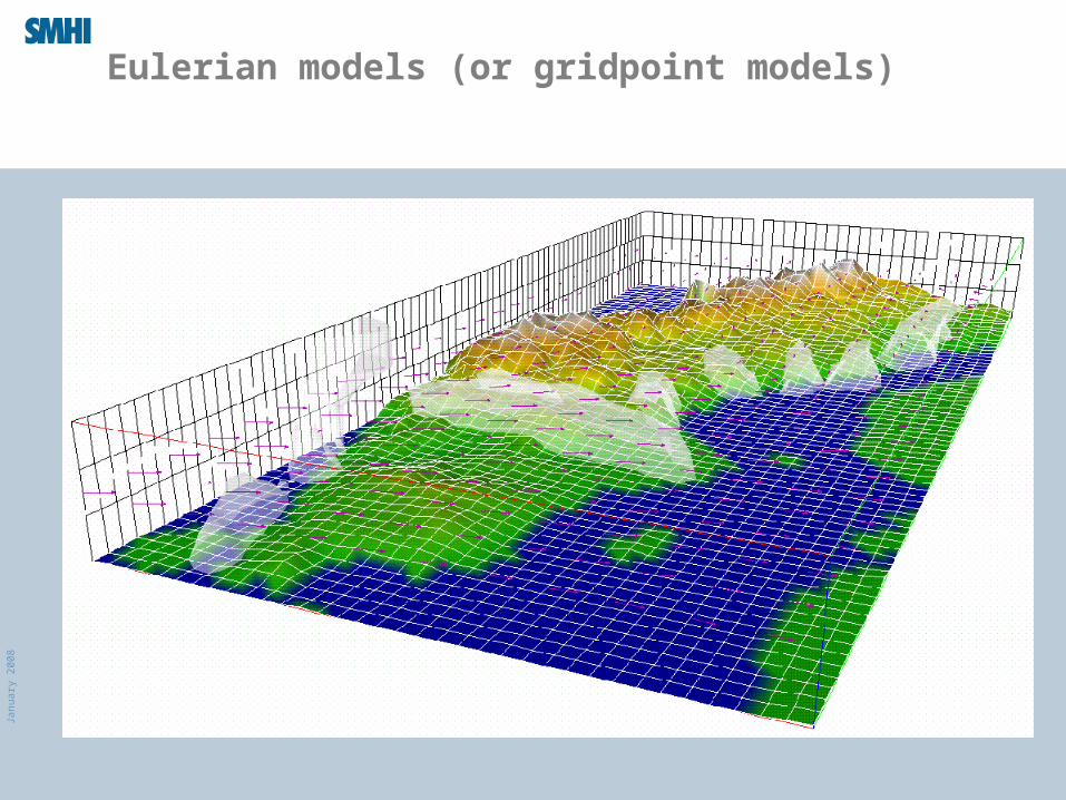
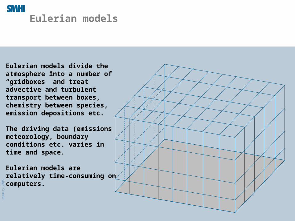
Eulerian models
Eulerian models divide the atmosphere into a number of “gridboxes” and treat advective and turbulent transport between boxes, chemistry between species, emission depositions etc.
The driving data (emissions meteorology, boundary conditions etc. varies in time and space.
Eulerian models are relatively time-consuming on computers.
Janu
ary
2008
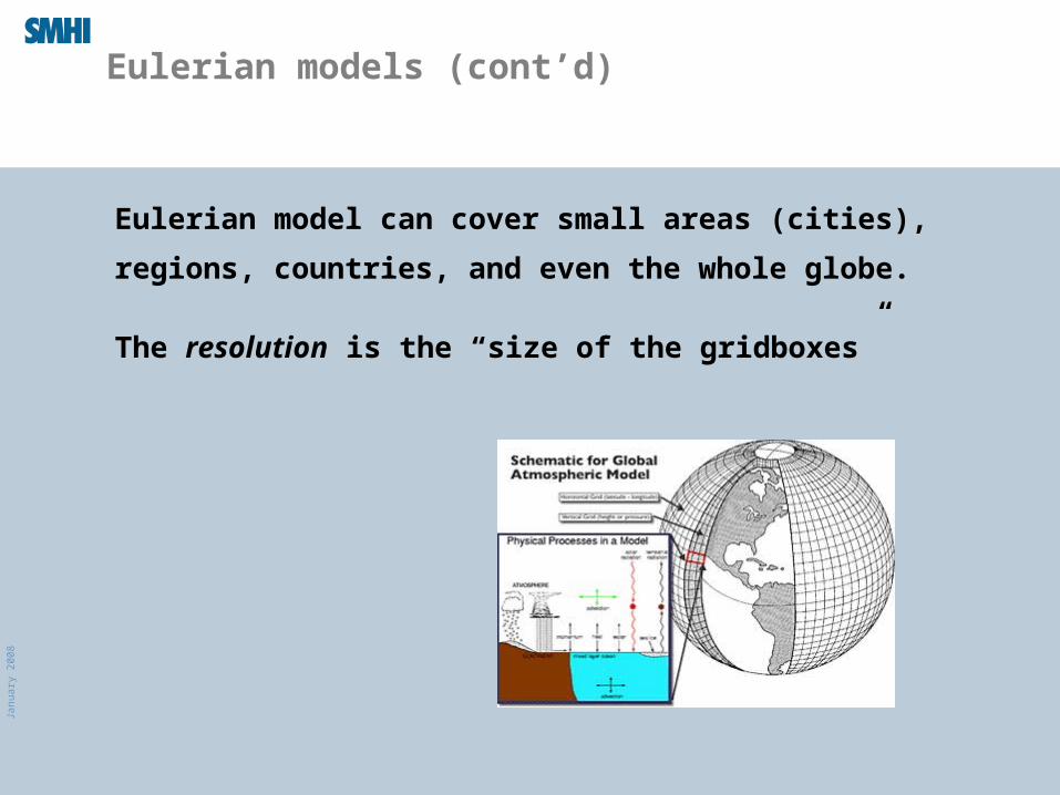
Eulerian models (cont’d)
Eulerian model can cover small areas (cities), regions,
countries, and even the whole globe.
The resolution is the “size of the gridboxes”
Janu
ary
2008
Eulerian models (cont’d)
Not straightforward to construct advection and chemistry
schemes that are shape and mass conservative etc.
A number of processes, that can not be explicitly
described needs to be “parameterised”
Janu
ary
2008
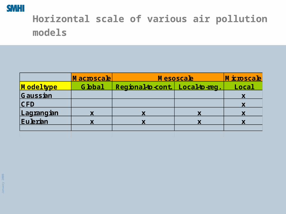
Macroscale Mesoscale MicroscaleModel type Global Regional-to-cont. Local-to-reg. LocalGaussian xCFD xLagrangian x x x xEulerian x x x x
Horizontal scale of various air pollution models
Janu
ary
2008
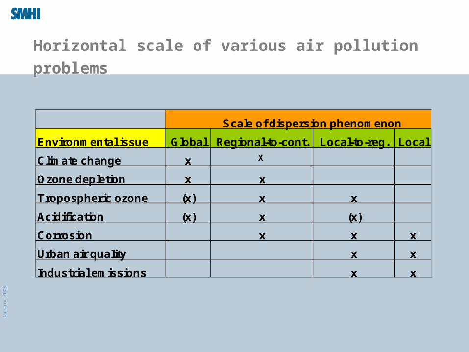
Horizontal scale of various air pollution problems
Scale of dispersion phenomenon
Environmental issue Global Regional-to-cont. Local-to-reg. Local
Climate change x
Ozone depletion x x
Tropospheric ozone (x) x x
Acidification (x) x (x)
Corrosion x x x
Urban air quality x x
Industrial emissions x x
X

Janu
ary
2008
Basic meteorology…Chapter 1. in Atmospheric Chemistry and Physics
(Seinfeld and Pandis, 1998)
Magnuz Engardt
Janu
ary
2008
Do you know…?
What the atmosphere is?
Why the is wind blowing?
Why does it rain?
Why is it colder at night than during day
Why do different regions have different climate?
Why is the sky blue?
How can it be possible to calculate what the weather will be like tomorrow?
Why are the forecasts not always right?
What does meteorology has to do with air quality and air pollution?
Janu
ary
2008
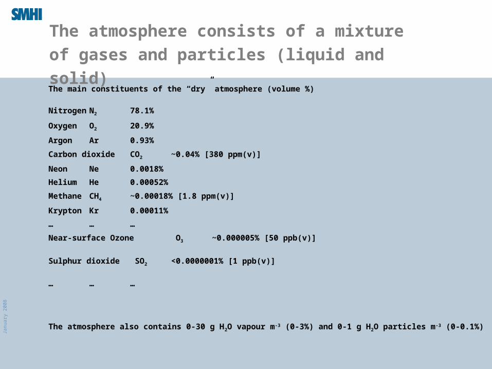
The atmosphere consists of a mixture of gases
and particles (liquid and solid)
The main constituents of the “dry” atmosphere (volume %)
Nitrogen N2 78.1%
Oxygen O2 20.9%
Argon Ar 0.93%
Carbon dioxide CO2 ~0.04% [380 ppm(v)]
Neon Ne 0.0018%
Helium He 0.00052%
Methane CH4 ~0.00018% [1.8 ppm(v)]
Krypton Kr 0.00011%
… … …
Near-surface Ozone O3 ~0.000005% [50 ppb(v)]
Sulphur dioxide SO2 <0.0000001% [1 ppb(v)]
… … …
The atmosphere also contains 0-30 g H2O vapour m-3 (0-3%) and 0-1 g H2O particles m-3 (0-0.1%)
Janu
ary
2008
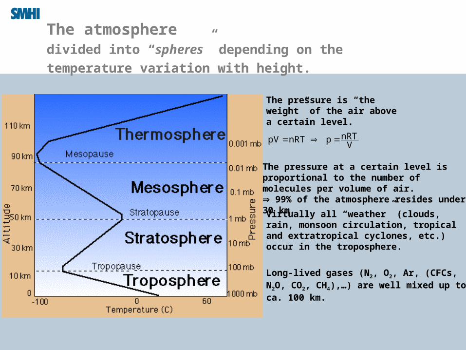
The atmospheredivided into “spheres” depending on the temperature
variation with height.
The pressure is “the weight” of the air above a certain level.
Long-lived gases (N2, O2, Ar, (CFCs, N2O, CO2, CH4),…) are well mixed up to ca. 100 km.
Virtually all “weather” (clouds, rain, monsoon circulation, tropical and extratropical cyclones, etc.) occur in the troposphere.
The pressure at a certain level is proportional to the number of molecules per volume of air. 99% of the atmosphere resides under 30 km.
VnRTp nRTpV
Janu
ary
2008
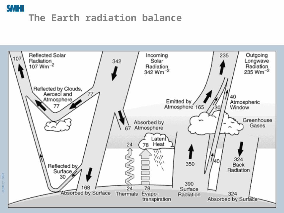
The Earth radiation balance
Janu
ary
2008
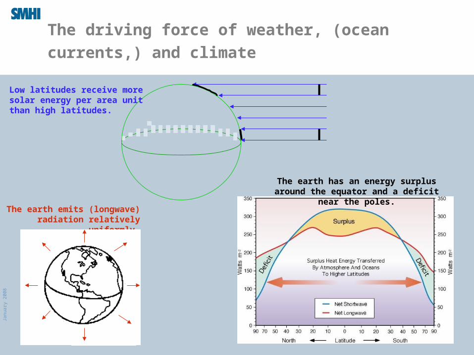
The driving force of weather, (ocean currents,)
and climate
Low latitudes receive more solar energy per area unit than high latitudes.
The earth has an energy surplus around the equator and a deficit near the poles.
The earth emits (longwave) radiation relatively uniformly.
Janu
ary
2008
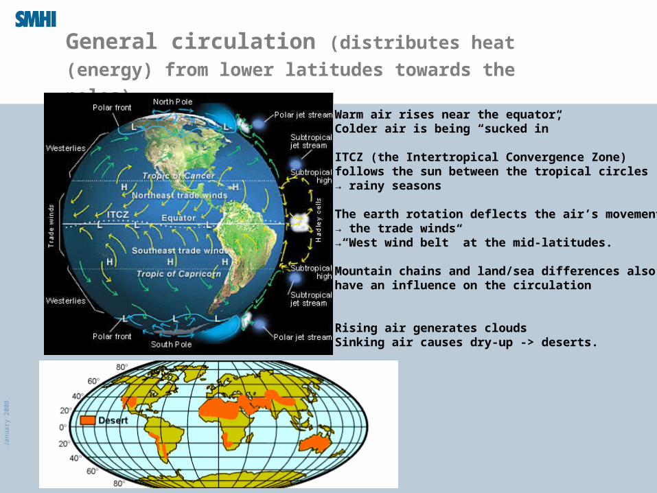
General circulation (distributes heat (energy) from
lower latitudes towards the poles)
Warm air rises near the equator,Colder air is being “sucked in”
ITCZ (the Intertropical Convergence Zone) follows the sun between the tropical circles→ rainy seasons
The earth rotation deflects the air’s movement→ the trade winds→“West wind belt” at the mid-latitudes.
Mountain chains and land/sea differences also have an influence on the circulation
Rising air generates cloudsSinking air causes dry-up -> deserts.
Janu
ary
2008
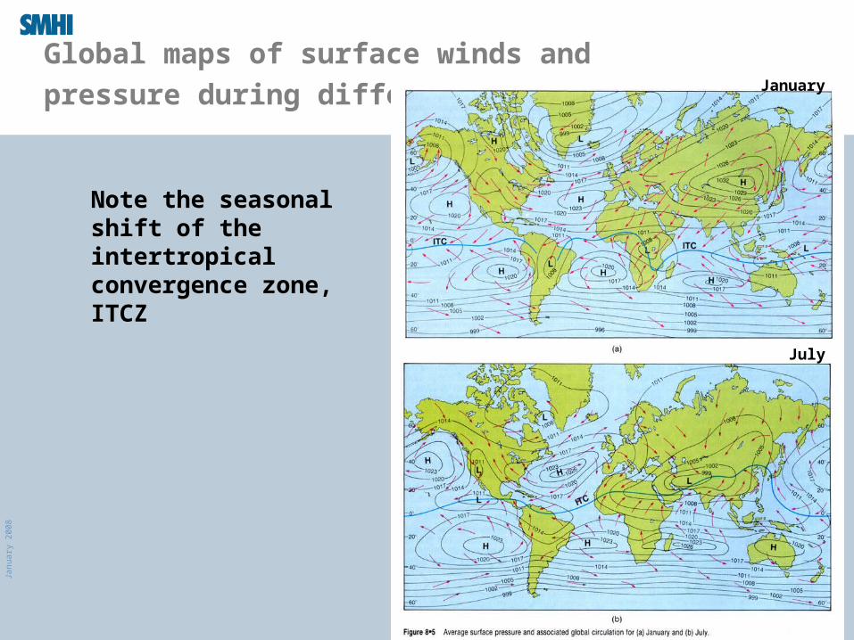
Global maps of surface winds and pressure
during different seasons
Note the seasonal shift of the intertropical convergence zone, ITCZ
July
January
Janu
ary
2008
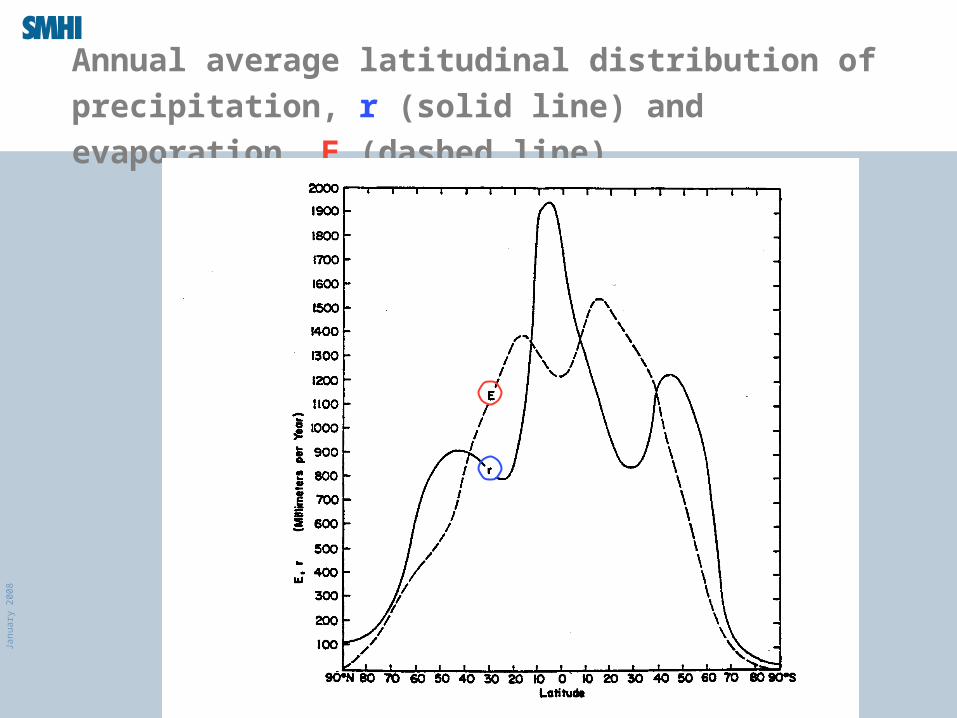
Annual average latitudinal distribution of precipitation, r
(solid line) and evaporation, E (dashed line)
Janu
ary
2008
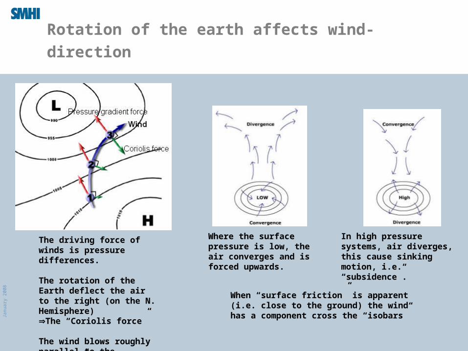
Rotation of the earth affects wind-direction
The driving force of winds is pressure differences.
The rotation of the Earth deflect the air to the right (on the N. Hemisphere)The “Coriolis force”
The wind blows roughly parallel to the “isobars” in the “free atmosphere”
Where the surface pressure is low, the air converges and is forced upwards.
In high pressure systems, air diverges, this cause sinking motion, i.e. “subsidence”.
When “surface friction” is apparent (i.e. close to the ground) the wind has a component cross the “isobars”
Janu
ary
2008
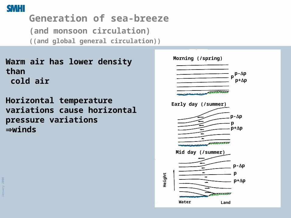
Generation of sea-breeze (and monsoon circulation) ((and global general circulation))
Warm air has lower density than cold air
Horizontal temperature variations cause horizontal pressure variationswinds
Morning (/spring)
Early day (/summer)
Mid day (/summer)
Water Land
Hei
gh
t
p+p
p-pp
p
p+p
p-p
pp-p
p+p
Janu
ary
2008
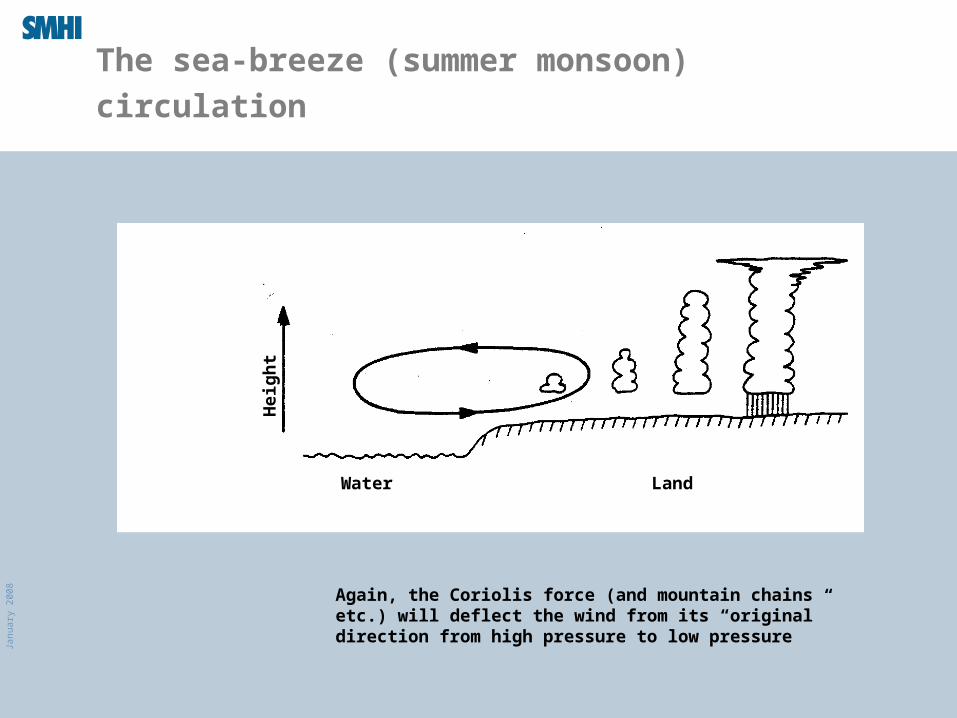
The sea-breeze (summer monsoon) circulation
Water
Land
Hei
gh
t
Again, the Coriolis force (and mountain chains etc.) will deflect the wind from its “original” direction from high pressure to low pressure
Janu
ary
2008
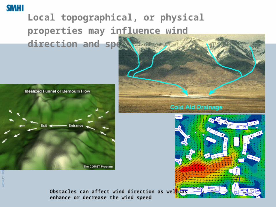
Local topographical, or physical properties may
influence wind direction and speed.
Obstacles can affect wind direction as well asenhance or decrease the wind speed
Janu
ary
2008
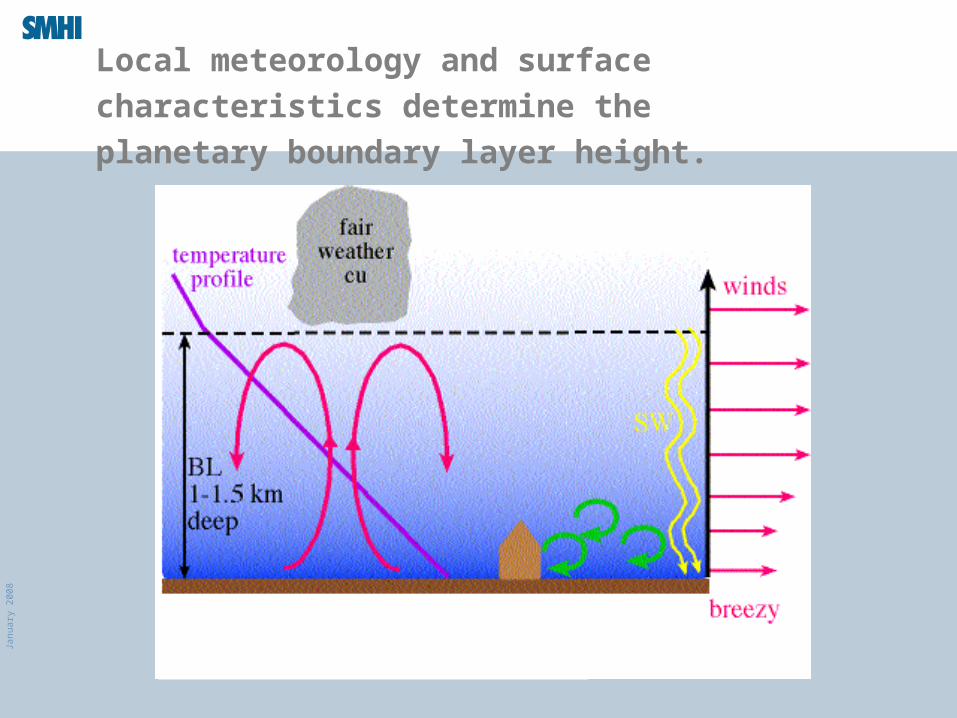
Local meteorology and surface characteristics
determine the planetary boundary layer height.
Janu
ary
2008
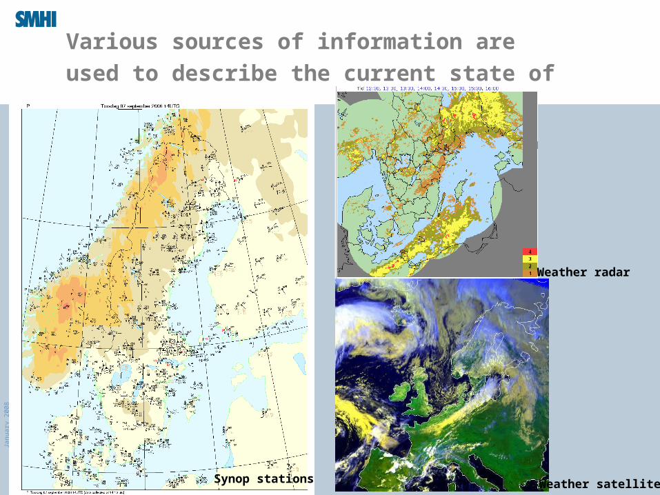
Various sources of information are used to
describe the current state of the atmosphere
Synop stations
Weather radar
Weather satellite
Janu
ary
2008
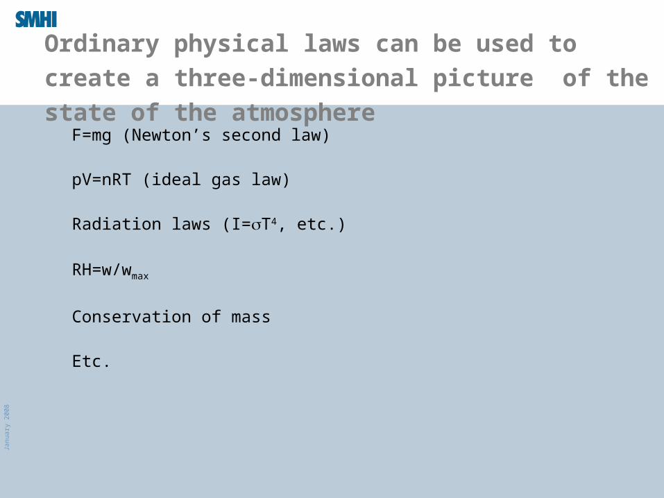
Ordinary physical laws can be used to create a three-
dimensional picture of the state of the atmosphere
F=mg (Newton’s second law)
pV=nRT (ideal gas law)
Radiation laws (I=T4, etc.)
RH=w/wmax
Conservation of mass
Etc.
Janu
ary
2008
Analysis and Forecast models
Models are used to fill the gaps between the observations
“Analysis”
Models can also be used to calculate the future state of
the atmosphere (weather forecasts)
Janu
ary
2008
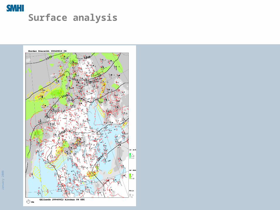
Surface analysis

Janu
ary
2008
The end…