Vietnamese-German University

Ruhr-University Bochum

Computational Engineering

Java Programming for Adaptive Finite

Element Method applied in two-dimensional

linear contact model

Nguyen Duy Khoi

under guidance of

Mr. Senthil Subramaniam

Dr. Karlheinz Lehner

A Thesis Submitted in Partial Fulfillment

of the Requirements for the Degree of Master of Science

in Computational Engineering

December 25

th 2012

2

3

Abstract Mesh generation is a fundamental step in finite element method since the quality of the

mesh has a great influence on the error of obtained approximated solution. To get a

desired precision, adaptive technique is used to improve the mesh. In this work, h-

refinement which is one of adaptive techniques is applied in linear contact model. Linear

contact model is simulated by Lagrange Multiplier method for non-matching mesh. To

avoid the complexities, linear two-dimensional contact model is only considered. Beside

the fundamental theory of finite element method, computational contact mechanics and

adaptive meshing, this work also tries to cover the practical programming algorithms

which are used during the theories implementation such as mesh generation algorithms,

global matrix assembly algorithm used in finite element method and refinement

algorithm used in adaptive meshing.

4

5

Acknowledgements First of all, I would like to express my deepest thank to Mr. Senthil Subramaniam who is

my industrial supervisor in Bosch company. He suggested the topic and gave me a lot of

research directions for this thesis. Without his help, I cannot finish my work.

In addition, I would like to thank Dr. Karlheinz Lehner who helped me in evaluating this

thesis.

Finally, it is my pleasure to give my special gratitude to Mr. Sudhakar Kunte who gave

me the golden opportunity to do my work in Robert Bosch Engineering and Business

Solutions Vietnam Ltd as well as my colleagues in this company who provided facility

and friendly atmosphere during my internship period.

6

7

Contents

Abstract ............................................................................................................................... 3 Acknowledgements ............................................................................................................. 5 1 Introduction ................................................................................................................. 9 2 Linear Continuum Mechanics ................................................................................... 11

2.1 Kinematics .......................................................................................................... 11 2.2 Stress and equilibrium ........................................................................................ 13

2.2.1 Cauchy’s Theorem ...................................................................................... 13 2.2.2 Balance equation: ........................................................................................ 14

2.3 Boundary conditions .......................................................................................... 15 2.3.1 Dirichlet boundary condition ...................................................................... 15 2.3.2 Newmann boundary condition .................................................................... 15

2.4 Constitutive equation for isotropic materials ..................................................... 16 2.5 Principle of Virtual Work ................................................................................... 17

3 Finite Element Method theory .................................................................................. 19 3.1 FEM in 2D problem ........................................................................................... 19

3.1.1 Plane stress .................................................................................................. 19

3.1.2 Plane strain .................................................................................................. 20 3.1.3 Weak form in two-dimensional problem .................................................... 20

3.2 Discretization ..................................................................................................... 22 3.3 Constant Strain Triangle..................................................................................... 23

3.3.1 Linear shape function .................................................................................. 24 3.3.2 Isoparametric element ................................................................................. 24

3.3.3 Jacobian transformation .............................................................................. 25 3.3.4 Local stiffness matrix .................................................................................. 26 3.3.5 Local load vector......................................................................................... 27

4 Meshing..................................................................................................................... 29 4.1 Delaunay triangulation ....................................................................................... 29

4.1.1 Definition .................................................................................................... 29

4.1.2 Algorithms .................................................................................................. 29 4.1.3 Flow chart ................................................................................................... 31

4.2 2D Triangular Mesh generation ......................................................................... 32 4.2.1 Introduction ................................................................................................. 32 4.2.2 Algorithm .................................................................................................... 32

4.2.3 Flow chart ................................................................................................... 35 5 Frictionless Contact Mechanic .................................................................................. 37

5.1 Gap function for planar contact .......................................................................... 37 5.2 Lagrange Multiplier Method .............................................................................. 39 5.3 Minimum potential energy ................................................................................. 39 5.4 Node to node contact .......................................................................................... 40 5.5 Non-matching mesh contact ............................................................................... 41

6 Adaptive Meshing ..................................................................................................... 45 6.1 Residual based error estimation ......................................................................... 45

8

6.1.1 Variational formulation for boundary value problem (BVP) ..................... 46

6.1.2 Priori error estimation: ................................................................................ 46 6.2 Recovery based error estimation ........................................................................ 47

6.2.1 Error in Constant Strain Element: ............................................................... 47

6.2.2 Recovery based error estimation in Constant Strain Triangle elements ..... 48 6.3 Rivara’s triangular refinement algorithm ........................................................... 50

6.3.1 Algorithm .................................................................................................... 50 6.3.2 Flow chart ................................................................................................... 52

7 Numerical Example .................................................................................................. 53

7.1 Plate with a hole ................................................................................................. 53 7.2 Planar contact model .......................................................................................... 57

8 Future Work .............................................................................................................. 63 References ......................................................................................................................... 65

9

1 Introduction This work presents theory, practice and programming of the adaptive finite element

method which is applied in linear contact model. To avoid the complexities of the three-

dimensional problem, two-dimensional model is only considered. Given an input planar

straight line graph (PSLG), Delaunay triangulation and two-dimensional mesh generation

algorithm are used to create the mesh for the input. Mesh generation is a foundation for

the next calculations where finite element method and computational contact theory are

implemented. Finite element method which is applied here is linear since the linear

material is used and the displacement of the model is very small as an assumption. In this

thesis, the non-matching mesh contact is covered so that the meshes of the two objects in

model are freely generated. The linear contact model is considered here since it does not

require the theory of non-linear continuum mechanics which is not an interest in this

work. To simulation this contact model, the Lagrange Multiplier for non-matching mesh

is applied. In next step, strain energy of each element is calculated base on the

displacement solution found from finite element calculations. Base on this information,

adaptive technique chooses elements which have smallest values and refined them based

on Rivara’s algorithm. The error estimation which is used in this adaptive technique is

recovery based one. This error is evaluated in energy norm.

The outline of the remainder of this thesis is as follows: The theory of linear

continuum mechanics will be reviewed in next section. Base on this theory, two-

dimensional linear finite element method is presented in the section three. In the section

4, meshing related algorithms which are Delaunay triangulation and Jim Ruppert’s two-

dimensional mesh generation are clarified. The Lagrange Multiplier method for non-

matching mesh contact model is introduced in sector 5. Section 6 covers the adaptive

techniques as well as Rivara’s algorithm for h-refinement. The results of programming

are shown in detail in section 7. Finally, some future works are discussed in section 8.

10

11

2 Linear Continuum Mechanics Mechanics is a subject studying motion of a physical object. This motion could be

belongs to one of the following categories:

Particle: the physical object is considered as a point and its motion is only

translation.

Rigid body: the body is not treated as the point anymore. However, it shape

changes during the movement. Mechanics studying this kind of object consider

not only translation but also rotation of the motion.

Deformable body: the shape of the object changes during the motion. Therefore,

relative distance of material points of the object can also change. This change

leads to the deformation in addition to the translation and rotation of the body.

Continuum mechanics covers the motion of deformable body. However, it neglects the

molecular effect of the object. The studying of this motion includes knowing the reason

why the object moves which is called kinetics and understanding the way how it moves

which is called kinematics.

2.1 Kinematics

Kinematics related to modeling the movement of an object in a space. The movement

includes translation, rotation and deformation is represented by displacement. Kinematics

requires the theory of tensor calculus and tensor algebra since displacement and some

quantities can be represented by tensor fields or tensor functions.

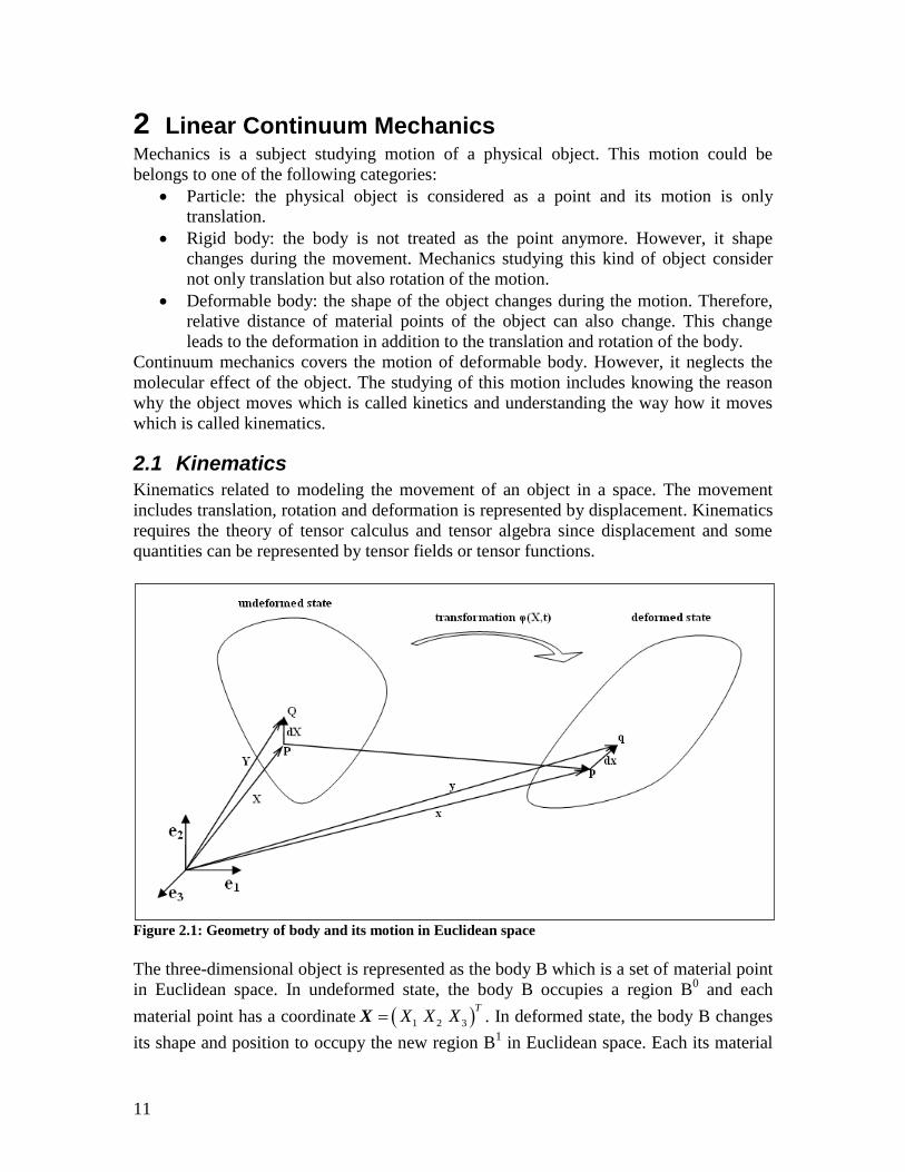
Figure 2.1: Geometry of body and its motion in Euclidean space

The three-dimensional object is represented as the body B which is a set of material point

in Euclidean space. In undeformed state, the body B occupies a region B0 and each

material point has a coordinate 1 2 3

TX X XX . In deformed state, the body B changes

its shape and position to occupy the new region B1 in Euclidean space. Each its material

12

point also changes to the new correspond coordinate 1 2 3

Tx x xx . The illustration of

Figure 2.1 shows that the two material point P and Q which have position vector X and Y

respectively move to new the position p and q which have position vector x and y in

deformed state. The line element dX defined by these two points also changes to new line

element dx. This change is described by the time-dependent mapping , tX

,tx X (2.1)

Base on this mapping, a displacement function which shows the motion of material points

of the body can be define as:

( , ) ( , ) ( ,0) ( , )t t t u x φ X φ X x X X (2.2)

The displacement functions can be written in a fully tensor field form:

1 2 3( , ) ( , ) ( , ) ( , )t u t u t u t 1 2 3u X X e X e X e (2.3)

Or it can be represented by a vector:

1 2 3( , ) , , ,T

t u t u t u t u X X X X (2.4)

Line element can be found:

,,

td d t d

x Xx X u X X X

X X (2.5)

With length of the line element defined as: 22

22

ds d d d

dX d d d

x x x

X X X (2.6)

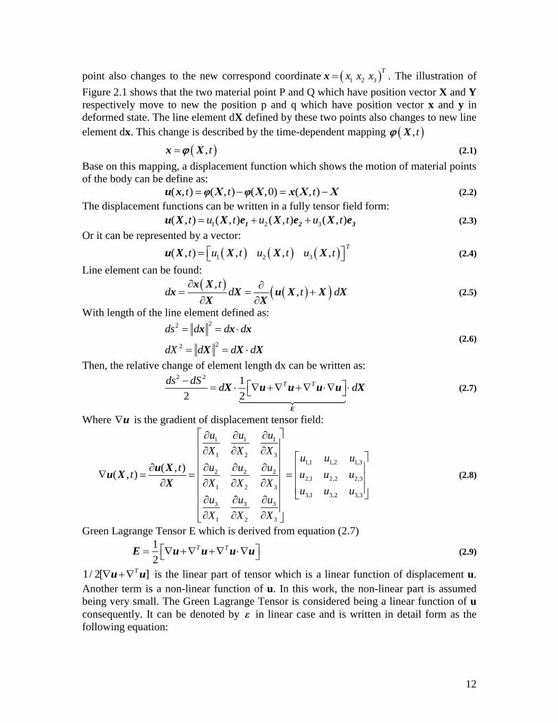
Then, the relative change of element length dx can be written as: 2 2 1

2 2

T Tds dSd d

E

X u u u u X (2.7)

Where u is the gradient of displacement tensor field:

1 1 1

1 2 3

1,1 1,2 1,3

2 2 22,1 2,2 2,3

1 2 3

3,1 3,2 3,3

3 3 3

1 2 3

( , )( , )

u u u

X X Xu u u

u u utt u u u

X X Xu u u

u u u

X X X

u Xu X

X (2.8)

Green Lagrange Tensor E which is derived from equation (2.7)

1

2

T T E u u u u (2.9)

1/ 2[ ]T u u is the linear part of tensor which is a linear function of displacement u.

Another term is a non-linear function of u. In this work, the non-linear part is assumed

being very small. The Green Lagrange Tensor is considered being a linear function of u

consequently. It can be denoted by ε in linear case and is written in detail form as the

following equation:

13

1,1 1,2 2,1 1,3 3,1

1,2 2,1 2,2 2,3 3,2 , ,

1,3 3,1 2,3 3,2 3,3

1 1

2 2

1 1 1 1

2 2 2 2

1 1

2 2

T

i j j i

u u u u u

u u u u u u u

u u u u u

ε u u (2.10)

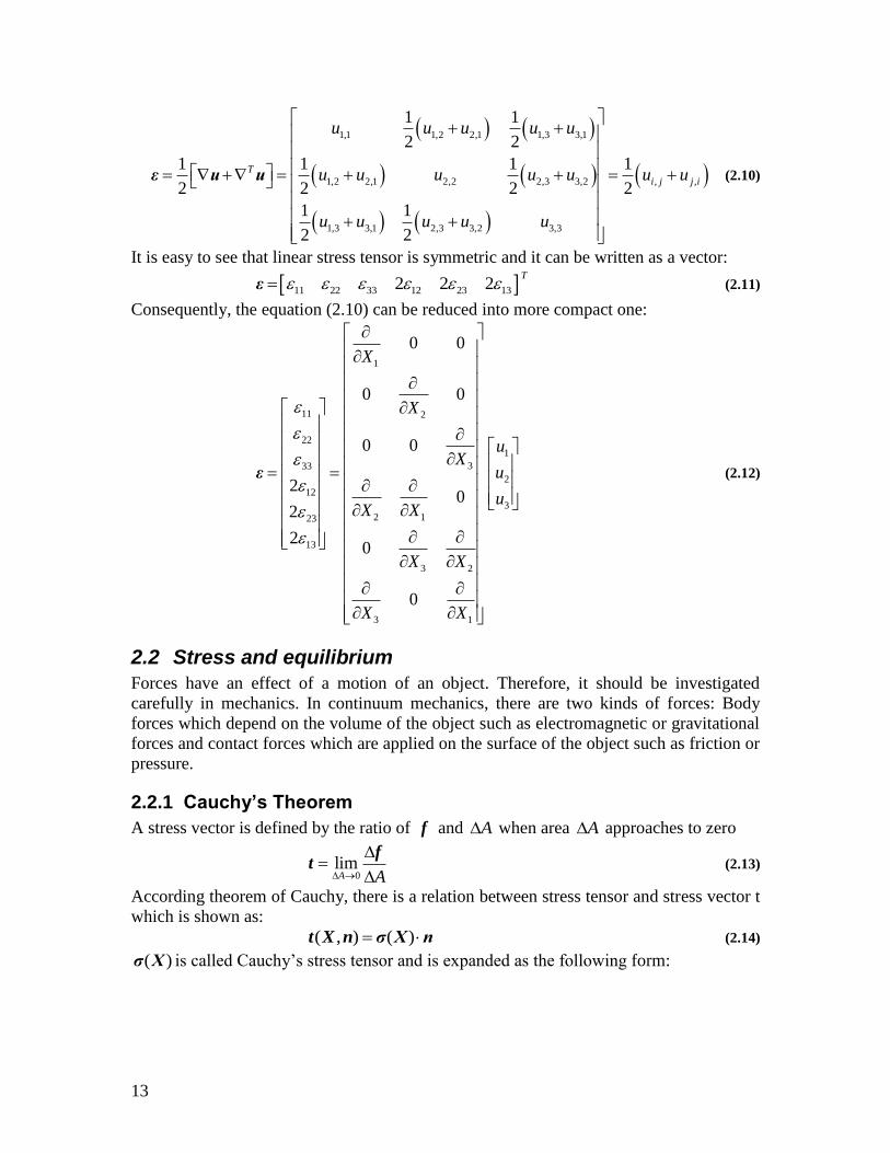
It is easy to see that linear stress tensor is symmetric and it can be written as a vector:

11 22 33 12 23 132 2 2T

ε (2.11)

Consequently, the equation (2.10) can be reduced into more compact one:

1

11 2

22

1

333

2

12

3

2 123

13

3 2

3 1

0 0

0 0

0 0

20

2

20

0

X

X

uX

u

uX X

X X

X X

ε (2.12)

2.2 Stress and equilibrium

Forces have an effect of a motion of an object. Therefore, it should be investigated

carefully in mechanics. In continuum mechanics, there are two kinds of forces: Body

forces which depend on the volume of the object such as electromagnetic or gravitational

forces and contact forces which are applied on the surface of the object such as friction or

pressure.

2.2.1 Cauchy’s Theorem

A stress vector is defined by the ratio of f and A when area A approaches to zero

0limA A

ft (2.13)

According theorem of Cauchy, there is a relation between stress tensor and stress vector t

which is shown as:

( , ) ( ) t X n σ X n (2.14)

( )σ X is called Cauchy’s stress tensor and is expanded as the following form:

14

11 12 13

21 22 23

31 32 33

σ (2.15)

According the moment equilibrium for stress components, stress tensor is symmetric:

11 12 13

12 22 23

13 23 33

T

σ σ σ (2.16)

2.2.2 Balance equation:

Motion is a result of forces when they are applied on the object. Therefore, this motion

has to satisfy some conditions which related forces. They are called equilibrium

conditions: *0 0dV dA dV

F b t u (2.17)

Where the first term is the total of body forces, the second term is the total of traction

forces and the final one is the total of inertia forces. Apply Cauchy’s theorem and Gauss

theorem to the second term:

dA dA dV

*t σ n σ (2.18)

Then,

0dV dA dV

b σ u (2.19)

It satisfies for all sub-domain of . Therefore,

0 b σ u (2.20)

It can be written in system of equations:

33,332,321,313

23,232,221,212

13,132,121,111

bu

bu

bu

(2.21)

Or in compact tensorial form

3

2

1

13

23

12

33

22

11

123

312

321

3

2

1

000

000

000

b

b

b

XXX

XXX

XXX

u

u

u

(2.22)

15

2.3 Boundary conditions

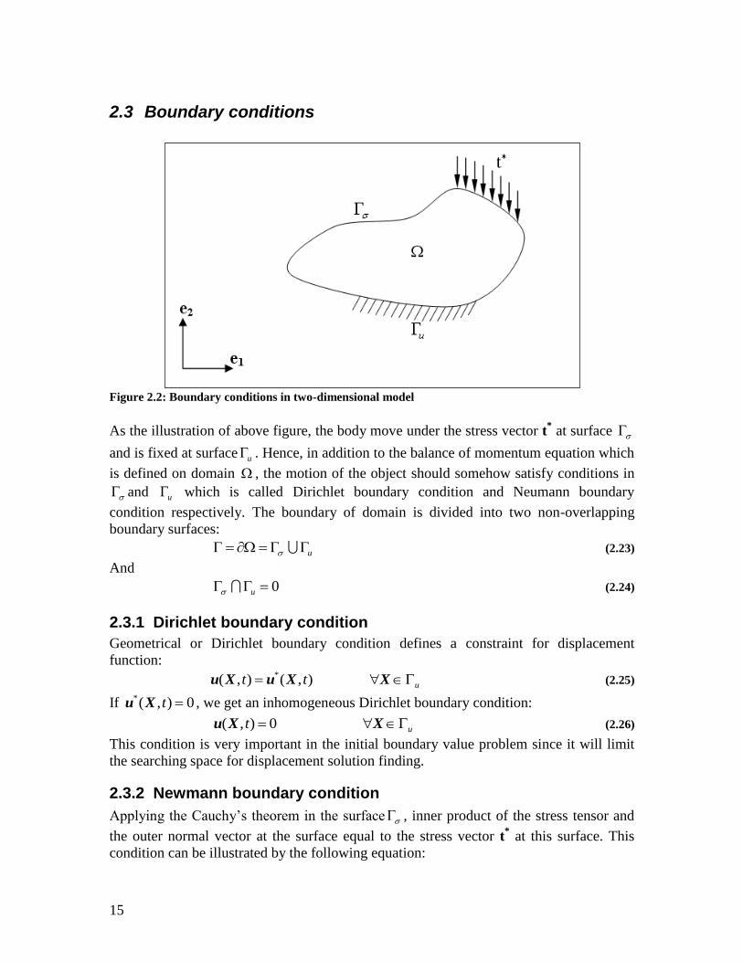
Figure 2.2: Boundary conditions in two-dimensional model

As the illustration of above figure, the body move under the stress vector t* at surface

and is fixed at surface u . Hence, in addition to the balance of momentum equation which

is defined on domain , the motion of the object should somehow satisfy conditions in

and u which is called Dirichlet boundary condition and Neumann boundary

condition respectively. The boundary of domain is divided into two non-overlapping

boundary surfaces:

u (2.23)

And

0 u (2.24)

2.3.1 Dirichlet boundary condition

Geometrical or Dirichlet boundary condition defines a constraint for displacement

function: *( , ) ( , ) ut t u X u X X (2.25)

If *( , ) 0t u X , we get an inhomogeneous Dirichlet boundary condition:

( , ) 0 ut u X X (2.26)

This condition is very important in the initial boundary value problem since it will limit

the searching space for displacement solution finding.

2.3.2 Newmann boundary condition

Applying the Cauchy’s theorem in the surface , inner product of the stress tensor and

the outer normal vector at the surface equal to the stress vector t* at this surface. This

condition can be illustrated by the following equation:

16

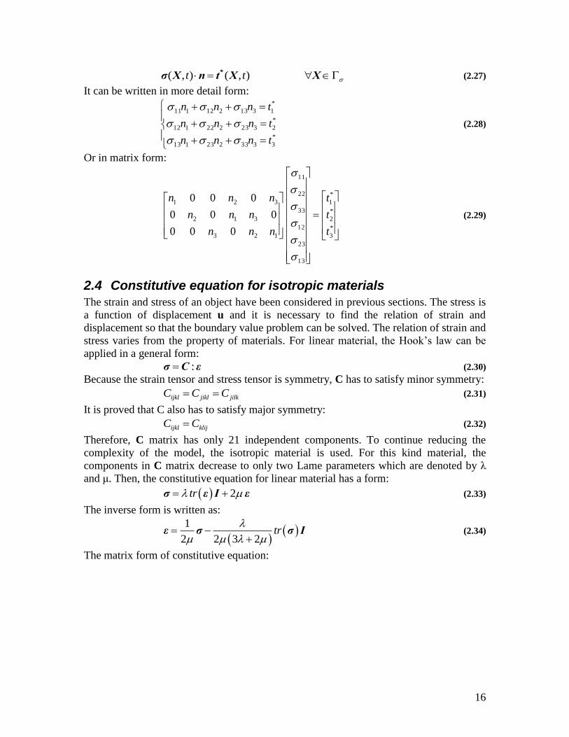
( , ) ( , )t t *σ X n t X X (2.27)

It can be written in more detail form:

*

3333223113

*

2323222112

*

1313212111

tnnn

tnnn

tnnn

(2.28)

Or in matrix form:

*

3

*

2

*

1

13

23

12

33

22

11

123

312

321

000

000

000

t

t

t

nnn

nnn

nnn

(2.29)

2.4 Constitutive equation for isotropic materials

The strain and stress of an object have been considered in previous sections. The stress is

a function of displacement u and it is necessary to find the relation of strain and

displacement so that the boundary value problem can be solved. The relation of strain and

stress varies from the property of materials. For linear material, the Hook’s law can be

applied in a general form:

:σ C ε (2.30)

Because the strain tensor and stress tensor is symmetry, C has to satisfy minor symmetry:

jilkjiklijkl CCC (2.31)

It is proved that C also has to satisfy major symmetry:

klijijkl CC (2.32)

Therefore, C matrix has only 21 independent components. To continue reducing the

complexity of the model, the isotropic material is used. For this kind material, the

components in C matrix decrease to only two Lame parameters which are denoted by λ

and μ. Then, the constitutive equation for linear material has a form:

2tr σ ε I ε (2.33)

The inverse form is written as:

1

2 2 3 2tr

ε σ σ I (2.34)

The matrix form of constitutive equation:

17

11 11

22 22

33 33

12 12

23 23

13 13

2 0 0 0

2 0 0 0

2 0 0 0

20 0 0 0 0

20 0 0 0 0

20 0 0 0 0

σ C ε

(2.35)

Or can be represented by a function of E and ν:

11 11

22 22

33 33

12 12

23 23

13 13

1 0 0 0

1 0 0 0

1 0 0 0

1 20 0 0 0 0

2 21 1 21 2

20 0 0 0 02

21 2

0 0 0 0 02

E

σ ε

C

(2.36)

Where E and ν are defined as:

)23(E (2.37)

)(2

(2.38)

2.5 Principle of Virtual Work

Test function for displacement which denoted as u is defined in domain and has to

satisfy the following conditions:

Test function satisfy the Dirichlet boundary condition

( ) 0 u u X X (2.39)

Test function satisfy the field condition sym u ε (2.40)

Test function is infinitesimal

Test function is arbitrary

From the previous section, the balance of force is:

0div u σ b (2.41)

Multiply with test function uand integral the result over the whole domain:

0dV div dV

u u b u σ (2.42)

To derive the second term of above equation, some tensor calculus equation is required:

18

: :

: :

div div div

div div div

u σ u σ u σ u σ u σ

u σ u σ u σ u σ u σ (2.43)

Replace it into the original strong form:

: 0

A B

dV dV div dV dV

u u u b u σ u σ (2.44)

For calculating A, applied the Gauss theorem for the divergence term

A div dV dA dA

u σ u σ n u σ n (2.45)

Apply Newmann boundary condition to this term:

0

A dA dA

*

*

σ n t

u σ n u t (2.46)

The term :u σ can be rewrite into another form and is replaced into B

: : : :

: :

sym sym

B dV dV

u σ u σ u σ ε σ

u σ ε σ (2.47)

Finally, the balance of momentum equation is written in a weak form as the following:

int

:

dyn extW W W

dV dV dV dA

*

u u ε σ u b u t (2.48)

dynW is the virtual work of dynamic forces, intW is the internal virtual work and extW is

the virtual work of external forces.

extdyn WWW int (2.49)

The weak form is equivalent to the strong form. In addition to, weak form can be

approximated by finite element method.

19

3 Finite Element Method theory Finite Element Method is Garlevkin method that reduces the function space of exact

solution to approximated function space where the solution of displacement is

approximated by polynomial functions. The basic function of this polynomial function

space is divided into many piecewise functions if the linear interpolation functions are

used.

3.1 FEM in 2D problem

Characterized by two properties:

The small thickness h compare to the other dimensions, the plane stress state

Infinite dimension of the direction x3, the plane strain state

3.1.1 Plane stress

Because the thickness h is too small, the stress related to the third direction is equal to

zero.

0332313 (3.1)

The strain in third direction:

02313 (3.2)

2211332

(3.3)

Then, the constitutive equation of plane stress is:

12

2211

11

11

12

22

11

22

000

02

02

02

0

(3.4)

It can be reduced to:

12

22

11

12

22

11

22

200

0)(2

0)(2

2

2

(3.5)

Or using the parameters E and :

20

12

22

11

2

12

22

11

22

100

01

01

1

E

(3.6)

3.1.2 Plane strain

0332313 (3.7)

The third direction related components of stress tensor can be determined:

02313 (3.8)

)()(2

221133

(3.9)

Then, the relation of stress and strain tensor is shown as:

12

22

11

12

22

11

200

02

02

(3.10)

Or

12

22

11

12

22

11

22

2100

01

01

211

E

(3.11)

3.1.3 Weak form in two-dimensional problem

:dV dV dV d

*

u u ε σ u b u t

The volume element dV is replaced by multiplying the area element dA by the line

element 3dX . Besides, the three-dimensional Neumann boundary also is divided into two-

dimensional one and thickness coordinate 3dX

2 2 2 2

3 3 3 3

2 2 2 2

:

h h h h

h h h hA A A

A B C D

dX dA dX dA dX dA dX d

*

u u ε σ u b u t (3.12)

The displacement vector, it’s variational and acceleration vector in plane strain and plane

stress are:

1 2 1 1 2 2 1 2

1 2 1 1 2 2 1 2

1 2 1 1 2 2 1 2

( , ) , ,

( , ) , ,

( , ) , ,

T

T

T

X X u X X u X X

X X u X X u X X

X X u X X u X X

u

u

u

(3.13)

Because they do not depend on coordinate 3X , the term A can be calculated:

21

2

3

2

h

hA A

A dX dA hdA u u u u (3.14)

The strain and stress is also independent of 3X since:

111

1

22

22

12

2 1

0

0

2

X

u

uX

X X

ε (3.15)

σ C ε (3.16)

Hence,

2

3

2

h

hA A

B dX dA hdA ε σ ε σ (3.17)

The vector 1 2

Tb bb and are constant to 3X , thus:

2

3

2

h

hA A

C dX dA hdA u b u b (3.18)

Because *

3 0t in two-dimensional model as plane strain or plane stress, the stress vector

at Newmann boundary can be presented by:

* *

1 2

T

t t *

t (3.19)

Then,

2

3

2

h

h

D dX d hd

* *

u t u t (3.20)

The terms A, B, C and D are replaced to original equation, then:

A A A

hdA hdA hdA hd

*

u u ε σ u b u t (3.21)

In more detail form:

dh

t

t

u

udAh

b

b

u

udAhdAh

u

u

u

u

AAA

*

2

*

1

2

1

2

1

2

1

12

22

11

12

22

11

2

1

2

1

2

(3.22)

22

3.2 Discretization

Figure 3.1: Discretization with triangular and quadrangular element

Instead of finding the exactly solution in the whole domain Ω, Finite Element Method is

used to find an approximate solution by dividing the original domain Ω into many

smaller domains Ωe which are triangles or quadrilaterals:

NE

e

e

1

(3.23)

In each element, the principle of virtual work is also satisfied: e

ext

ee

dyn WWW int (3.24)

The process in which the object is divided into element structure is call mesh generation.

There are many mesh generation algorithms which depend on the shape of element. In

this work, the triangular element is used in the finite element method. The triangular

mesh generation algorithm will be introduced in detail in later section.

23

3.3 Constant Strain Triangle

Figure 3.2: Constant Strain Triangle coordinates transformation

There are many kinds of triangular element which depend on the number of nodes and

shape functions of the element. Constant Strain Triangle (CST) is a very basic triangular

element. Its name come from the fact that the strain calculated at a point in this element is

independent to coordinate of the point. The CST has only three nodes and its shape

functions are linear. The transformation from arbitrary triangle in physical coordinate to

standard CST in natural coordinate is illustrated in Figure 3.2. The natural coordinate is

defined base on the areas of triangles iA , which are shown in Figure 3.2, divided by total

area of the triangle A

A

Aii (3.25)

There are some conditions of for the natural coordinate

1,0

11 213321

i

(3.26)

Then, these conditions are reduced to:

12

213

1

10

11010

10

(3.27)

24

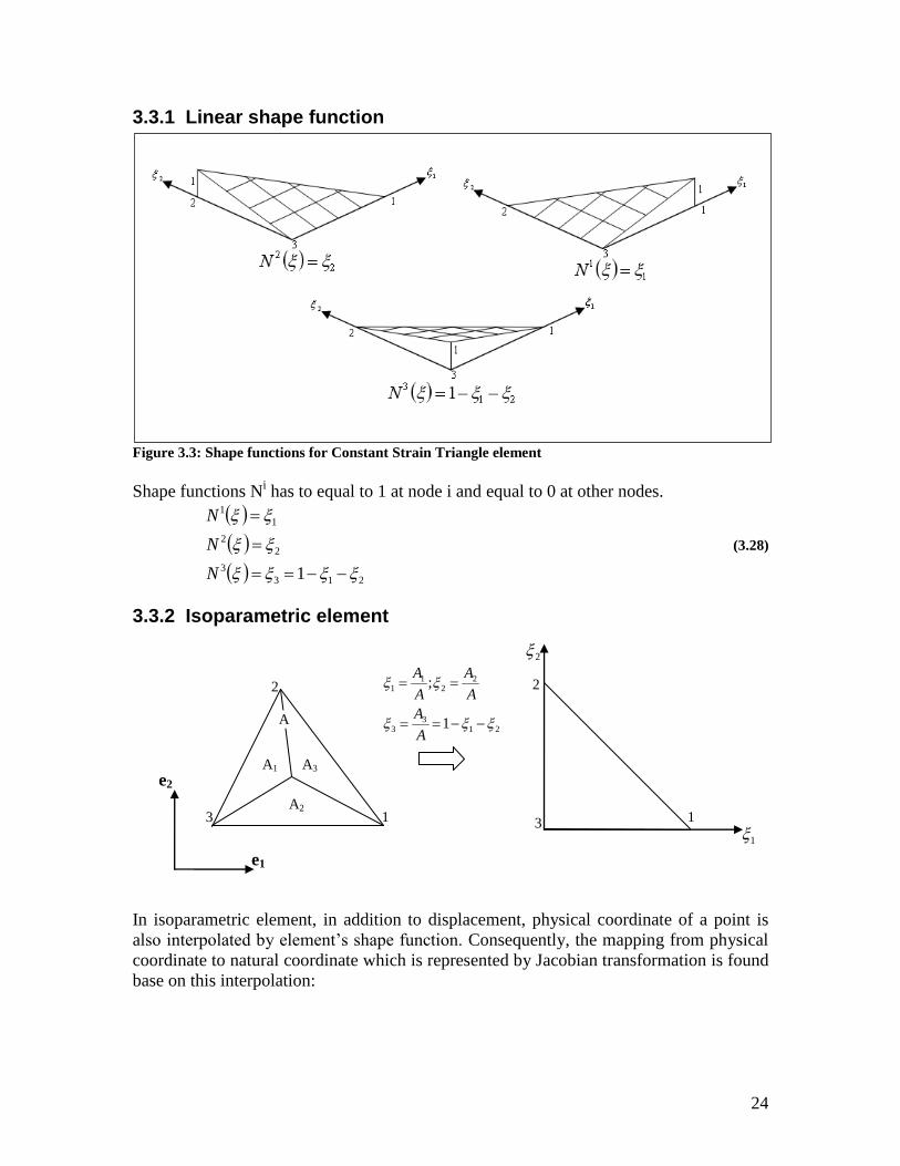
3.3.1 Linear shape function

Figure 3.3: Shape functions for Constant Strain Triangle element

Shape functions Ni has to equal to 1 at node i and equal to 0 at other nodes.

213

3

2

2

1

1

1

N

N

N

(3.28)

3.3.2 Isoparametric element

In isoparametric element, in addition to displacement, physical coordinate of a point is

also interpolated by element’s shape function. Consequently, the mapping from physical

coordinate to natural coordinate which is represented by Jacobian transformation is found

base on this interpolation:

e1

e2

1

2

3

1

2

1

2

3

A1 A3

A2

A 21

33

22

11

1

;

A

A

A

A

A

A

25

h e

h e

h e

h e

X ξ X ξ N ξ X

u ξ u ξ N ξ u

u ξ u ξ N ξ u

u ξ u ξ N ξ u

(3.29)

Applied for two dimensions problem with linear interpolation, the physical coordinate is

approximated as:

3

121

2

12

1

11

3

121

32

121

21

121

1

1

)1(

,,,

eee

eee

XXX

XNXNXNX

(3.30)

3

221

2

22

1

21

3

221

32

221

21

221

1

2

)1(

,,,

eee

eee

XXX

XNXNXNX

(3.31)

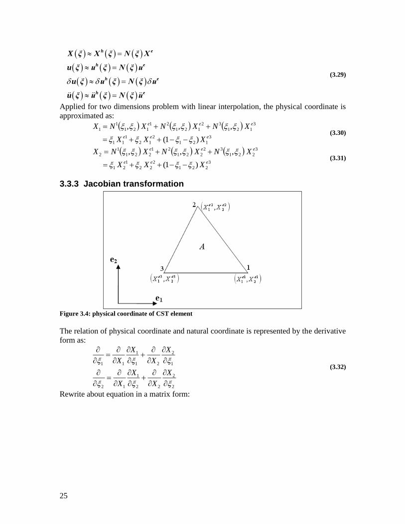
3.3.3 Jacobian transformation

Figure 3.4: physical coordinate of CST element

The relation of physical coordinate and natural coordinate is represented by the derivative

form as:

2

2

22

1

12

1

2

21

1

11

X

X

X

X

X

X

X

X (3.32)

Rewrite about equation in a matrix form:

26

X

J

X

X

XX

XX

2

1

2

2

2

1

1

2

1

1

2

1

(3.33)

Where J ξ is the Jacobian matrix which show the relation of physical coordinate and

natural coordinate. Its component can be calculated as the following:

3

2

2

2

2

222

3

1

2

1

2

121

3

2

1

2

1

212

3

1

1

1

1

111

eeee

eeee

XXX

JXXX

J

XXX

JXXX

J

(3.34)

Determinant of Jacobian matrix:

1 3 2 3 2 3 1 3

1 1 2 2 1 1 2 2 2e e e e e e e eX X X X X X X X A J ξ (3.35)

With A is the area of the considered triangle element 2 3 3 1

1 2 2 2 2 2 2 2

1 2 1 1

3 2 1 3

1 1 1 1 2 1 1 1

2 2 2 1

1 1

2 2

1 1

2 2

e e e e

e e e e

X X X X X X

X A X A

X X X X X X

X A X A

J J

J J

(3.36)

3.3.4 Local stiffness matrix

The element stiffness matrix or local stiffness matrix 211

1 2

0 0

T h d d

e

k B C B J (3.37)

Where:

iiii

ii

ii

i

NX

NX

NX

NX

NX

NX

NX

NX

B

2;

1

21;

1

12;

2

21;

2

1

2;

2

21;

2

1

2;

1

21;

1

1

0

0

(3.38)

Therefore,

1 2 1 2

1 1 1 1

1 2 1 2

2 2 2 2

1 1 2 2 1 2 1 2

2 1 2 1 2 2 1 1

0 0 0

0 0 0

X X X X

X X X X

X X X X X X X X

B (3.39)

Replace the Jacobian transformation to B matrix, we get:

27

2 3 3 1 1 2

2 2 2 2 2 2

3 2 1 3 2 1

1 1 1 1 1 1

3 2 2 3 1 3 3 1 2 1 1 2

1 1 2 2 1 1 2 2 1 1 2 2

0 0 01

0 0 02

e e e e e e

e e e e e e

e e e e e e e e e e e e

X X X X X X

X X X X X XA

X X X X X X X X X X X X

B (3.40)

Because:

2

11

0

2

1

0

1

2

dd (3.41)

Replacing this integral into the element stiffness equation leads to the result:

12

2

T Ah Ah e Tk B C B B C B (3.42)

In matrix form, the local matrix can be represented as:

11 12 13

21 22 23

31 32 33

e e e

e e e

e e e

k k k

k k k

k k k

ek (3.43)

The local stiffness matrix is symmetric due to the symmetry of B matrix

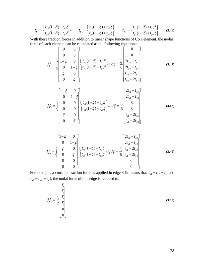
3.3.5 Local load vector

Figure 3.5: the components of the nodal forces of an element

In this part, the external element energy is considered: e

extW hd

*

e eu t u r (3.44)

With the local load vector is the total of nodal load of three edges of CST element:

1 2 3

e e e

e Γ Γ Γr f f f (3.45)

With the unit thickness h = 1, the edge nodal loads1

e

Γf , 2

e

Γf and 3

e

Γf depend on the shape

functions and traction forces applied in appropriate edge. The traction forces for each

edge are interpolated as:

28

2 3 1 3 1 2

2 3 1 3 1 2

(1 ) (1 ) (1 )

(1 ) (1 ) (1 )

x x x x x x

y y y y y y

t t t t t t

t t t t t t

1 2 3Γ Γ Γt t t (3.46)

With these traction forces in addition to linear shape functions of CST element, the nodal

force of each element can be calculated as the following equations:

12 3 2 31

1

2 3 2 30

2 3

2 3

00 0

00 0

(1 ) 21 0

(1 ) 20 1 6

20

20

x x x x

y y y y

x x

y y

t t t tll d

t t t t

t t

t t

1

e

Γf (3.47)

1 3

1 3

11 3 2

2

1 30

1 3

1 3

21 0

20 1

(1 ) 00 0

(1 ) 00 0 6

20

20

x x

y y

x x

y y

x x

y y

t t

t t

t t ll d

t t

t t

t t

2

e

Γf (3.48)

1 2

1 2

11 2 1 23

3

1 2 1 20

1 0 2

0 1 2

(1 )0 2

(1 )0 26

0 0 0

0 0 0

x x

y y

x x x x

y y y y

t t

t t

t t t tll d

t t t t

3

e

Γf (3.49)

For example, a constant traction force is applied in edge 3 (it means that xxx ttt 21 and

yyy ttt 21 ), the nodal force of this edge is reduced to:

3

2

0

0

x

y

x

y

t

t

tl

t

3

e

Γf (3.50)

29

4 Meshing As the previous section, a high quality mesh takes a very important role in Finite Element

Method. There are many algorithms as well as heuristics to find the good mesh such as

quadtree, advancing front or Delaunay triangulation. In this section, the Delaunay

triangulation is introduced as the first step of mesh generation which creates the “rough”

mesh for an input data. Then, a mesh generation based on maintaining Delaunay

triangulation is used to modify this mesh with a purpose that is improving the quality of

the mesh.

4.1 Delaunay triangulation

4.1.1 Definition

Was introduced by Boris Delaunay in 1934, Delaunay triangulation is used broadly for

many robust two-dimension mesh generators. As in the Figure 4.1, Delaunay

triangulation for a set of input point S is a set of triangles such that each circumcircle of

each its element does not contain any vertex of S inside.

Figure 4.1: input points, Delaunay triangulation and the corresponding empty circumcircle

Delaunay triangulation has many important characteristics that are valuable for finite

element method. The most interesting property is that this triangulation maximizes the

minimum angle of the output triangles. In other words, the minimum angle of the output

triangles which is shown in the middle figure in Figure 4.1 has a largest value.

4.1.2 Algorithms

Base on the definition of Delaunay triangulation, a basic algorithm for this triangulation

can be easily found. For a set of input point S, every possible triangle of triple of points

of S that contain no point in it’s interior will belong to Delaunay triangulation. However,

this original algorithm requires much time to be executed. For example, for an input

includes one hundred points, it will take 100 * 99 * 98 times to check if a triangle created

by the possible triple of points contains any input point or not. In this work, the authors

implement another algorithm which is illustrated in the following figures:

30

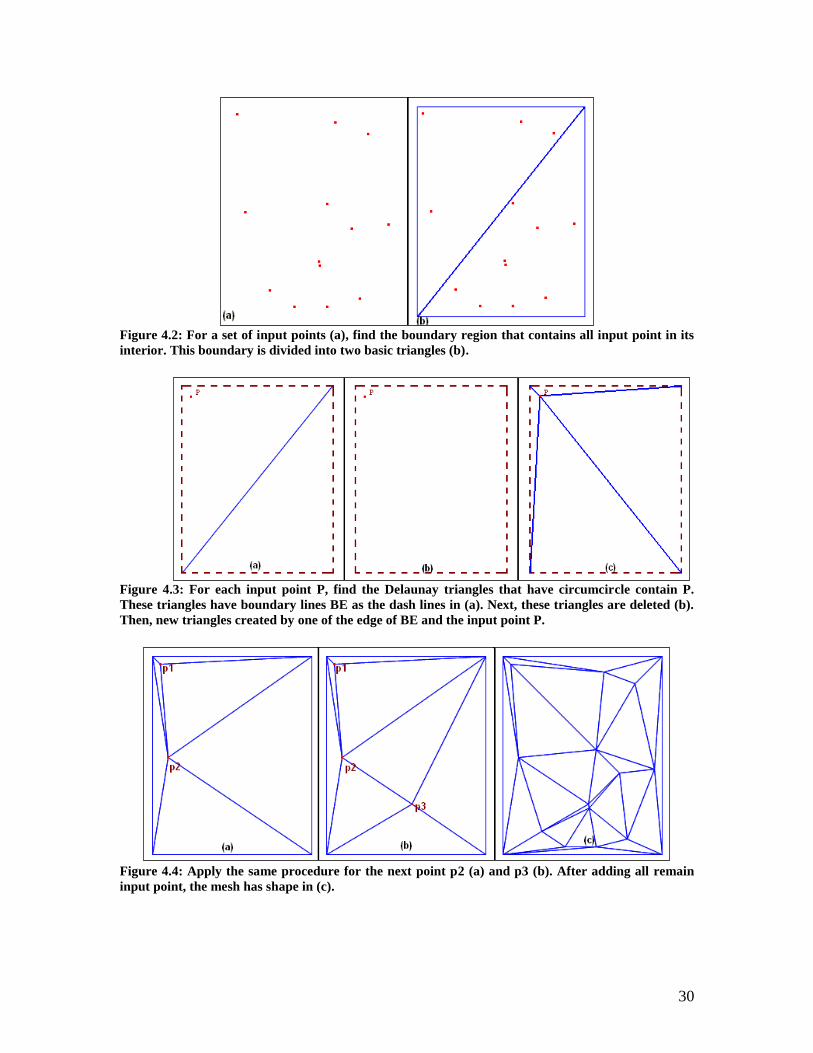
Figure 4.2: For a set of input points (a), find the boundary region that contains all input point in its

interior. This boundary is divided into two basic triangles (b).

Figure 4.3: For each input point P, find the Delaunay triangles that have circumcircle contain P.

These triangles have boundary lines BE as the dash lines in (a). Next, these triangles are deleted (b).

Then, new triangles created by one of the edge of BE and the input point P.

Figure 4.4: Apply the same procedure for the next point p2 (a) and p3 (b). After adding all remain

input point, the mesh has shape in (c).

31

Figure 4.5: The final mesh after removing boundary edges and related triangles.

4.1.3 Flow chart

Call S is the set of input point, T is the output triangles

Check if set

of input point

S is empty

N

Y

Start

Initialize T including

two boundary triangle

which contain all input

point

- Get and remove a point P from S

- Find the set of triangles I in T which

have circumcircles contain input point P

- Find the set of boundary edge E created

by I

- Remove I from T

- Create new triangles by an edge got

from E and P. Add these triangles to T

Finish

Remove boundary

triangles

32

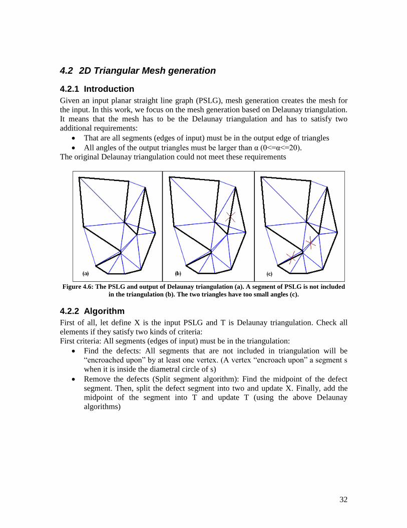
4.2 2D Triangular Mesh generation

4.2.1 Introduction

Given an input planar straight line graph (PSLG), mesh generation creates the mesh for

the input. In this work, we focus on the mesh generation based on Delaunay triangulation.

It means that the mesh has to be the Delaunay triangulation and has to satisfy two

additional requirements:

That are all segments (edges of input) must be in the output edge of triangles

All angles of the output triangles must be larger than α (0<=α<=20).

The original Delaunay triangulation could not meet these requirements

Figure 4.6: The PSLG and output of Delaunay triangulation (a). A segment of PSLG is not included

in the triangulation (b). The two triangles have too small angles (c).

4.2.2 Algorithm

First of all, let define X is the input PSLG and T is Delaunay triangulation. Check all

elements if they satisfy two kinds of criteria:

First criteria: All segments (edges of input) must be in the triangulation:

Find the defects: All segments that are not included in triangulation will be

“encroached upon” by at least one vertex. (A vertex “encroach upon” a segment s

when it is inside the diametral circle of s)

Remove the defects (Split segment algorithm): Find the midpoint of the defect

segment. Then, split the defect segment into two and update X. Finally, add the

midpoint of the segment into T and update T (using the above Delaunay

algorithms)

33

Figure 4.7: Because the vertex a, b encroach upon s, s have to be divided by the midpoint c in (a). For

adding new point c, apply the same adding point algorithm in Delaunay triangulation. It means that

finding the boundary edges of affected triangles and removing affected triangles (b). Then, the new

triangles are created by boundary edges and the mid point c (c).

Second criteria: All angles of triangles must be larger than α (0<=α<=20)

Find the defects: Calculate all angles of the triangulation, find the defect triangles

that have an angle smaller than α.

Remove the defects: Find the circumcenter p of the defect triangle. If p encroach

upon any segment, split the segment (using the algorithm of i), then update X and

T. If p does not encroach upon any segment, add p to T and update T

Figure 4.8: The dark triangle needs to be modified because it has too small angle (it is called skinny).

The circumcenter of defect triangle is c and c encroaches upon s1 and s2 which have mid point c1

and c2 respectively (a). Therefore, instead of adding new point c, the segment s1 and s2 should be

divided by c1 and c2 using the same algorithm of previous figure (b).

34

Figure 4.9: Another case of skinny triangle which is the dark color triangle in (a). However, this case

is different from the previous one because c does not encroach upon any segment. In this situation, c

can be added directly to the mesh by using the Denaulay adding point algorithm (b).

Figure 4.10: Execute the algorithm till there is no defect in the mesh (a). After removing the triangles

that are outside the PSLG region, the final result mesh for input PSLG is obtained in (b)

35

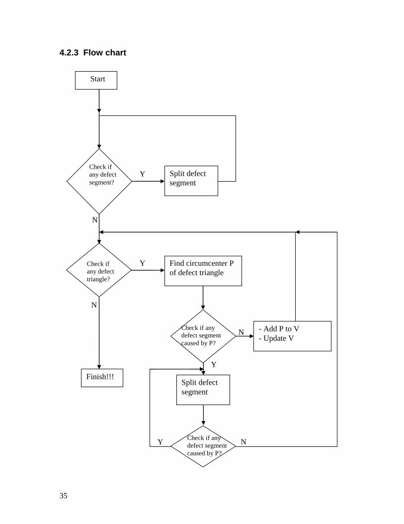
4.2.3 Flow chart

Check if

any defect

segment?

Split defect

segment Y

Check if

any defect

triangle?

Y

N

Find circumcenter P

of defect triangle

Check if any

defect segment

caused by P?

N - Add P to V

- Update V

Split defect

segment

Y

N

Finish!!!

Start

Check if any

defect segment

caused by P?

N Y

36

37

5 Frictionless Contact Mechanic

5.1 Gap function for planar contact

Figure 5.1: Deformation of two objects in two-dimensional space

At time t = 0, two bodies occupy the region 1 and 1 . After deforming, the two bodies

changed their shape and occupy the new regions 1 1φ and 22φ . A point of object 1

which has a position X1 at t = 0 and a point belong to object 2 which have position X

2

change to new position x1 and x

2 respectively at deformed state. c is the contact area

where all points of two objects have same position.

In contact model, one of these two object is chosen be a master object and another is

called slave object. x2 is arbitrary point in contact surface of master object. Then, we find

a point that belongs to slave object and has the minimum distance to x2, it is the point 1

x

which is illustrated in Figure 5.1. Then, the normal gap in contact surface is defined by:

( )Ng 2 1 1x x n (5.1)

1n is the normal vector of

1φ at point 1

x

Beside the normal gap function, we also have tangential gap function. However, it is

considered being very small and being neglected in this work.

The normal gap function can be represented as a function of displacement:

( ) ( ) (( ) ( ))

( ) 0

N

i

g

g

2 1 1 2 2 1 1 1

2 1 1

u x x n X u X u n

u u n (5.2)

ig is initial gap and ( )ig 2 1 1X X n

Base on that, the variation of the gap functions can be determined as:

( )Ng 2 1 1u u n (5.3)

2u is the test function or the variational of 2

u

38

1u is the test function or the variational of 1

u

Condition for gap function and normal pressure on contact area:

0

0

0

NN

N

N

pg

p

g

(5.4)

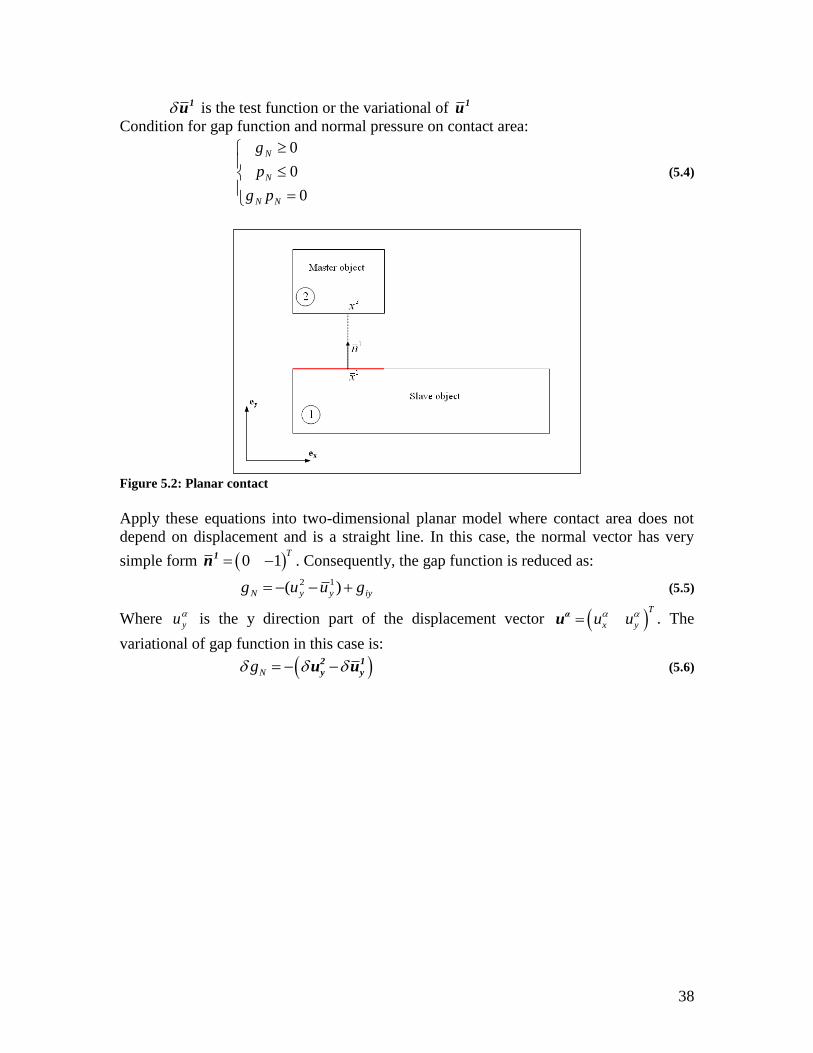
Figure 5.2: Planar contact

Apply these equations into two-dimensional planar model where contact area does not

depend on displacement and is a straight line. In this case, the normal vector has very

simple form 0 1T

1n . Consequently, the gap function is reduced as:

iyyyN guug )( 12 (5.5)

Where yu is the y direction part of the displacement vector

T

x yu u αu . The

variational of gap function in this case is:

Ng 2 1

y yu u (5.6)

39

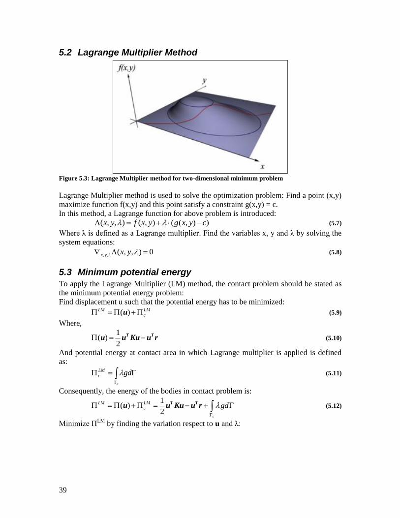
5.2 Lagrange Multiplier Method

Figure 5.3: Lagrange Multiplier method for two-dimensional minimum problem

Lagrange Multiplier method is used to solve the optimization problem: Find a point (x,y)

maximize function f(x,y) and this point satisfy a constraint g(x,y) = c.

In this method, a Lagrange function for above problem is introduced:

)),((),(),,( cyxgyxfyx (5.7)

Where λ is defined as a Lagrange multiplier. Find the variables x, y and λ by solving the

system equations:

0),,(,, yxyx (5.8)

5.3 Minimum potential energy

To apply the Lagrange Multiplier (LM) method, the contact problem should be stated as

the minimum potential energy problem:

Find displacement u such that the potential energy has to be minimized:

( )LM LM

c u (5.9)

Where,

1( )

2 T T

u u Ku u r (5.10)

And potential energy at contact area in which Lagrange multiplier is applied is defined

as:

c

gdLM

c (5.11)

Consequently, the energy of the bodies in contact problem is:

1( )

2c

LM LM

c gd

T T

u u Ku u r (5.12)

Minimize ПLM

by finding the variation respect to u and λ:

40

2 1

2 1

( ) 0

( ) 0

c c

c c

y y

y y iy

gd u u d

gd u u g d

T T T Tu Ku u r u Ku u r

(5.13)

The variations u and λ are found by solving above system of equation. The stiffness

global matrix K and load vector r can be determined by the method introduced in

previous sections. However, the remains require the interpolation of Lagrange multiplier

function and gap function which depends on the discretization of contact surface. There

are two types of contact surface:

Node to node contact

Non-matching mesh contact

5.4 Node to node contact

Figure 5.4: Node-to-node contact problem

In node-to-node contact, all nodes of the two meshes have to be in the same position in

contact area. Therefore, the surface domain and the discretization of these domains of

two objects is the same. This will be a big advantage for many calculations in contact

model which will be made clear later. However, in this contact, one mesh depends on

another mesh. Therefore, only one of two meshes is able to be refined in adaptive

technique. Because of the same discretization of two contact surefaces, function λ,

displacement functions and initial gap function are interpolated as:

P

iyPPiy

J

yJJy

I

yIIy

K

KK

J

yJJy

I

yIIy

K

KK

gNg

uNuuNuM

uNuuNuM

)(

)()()(

)()()(

1122

1122

(5.14)

Replace to the equation of variational of contact energy:

41

2

1

( ) ( )

( ) ( )

c

ii

c c

c

iic

n

K K T yI

i I K

n

K K J yJ

i J K

gd M N J d u

M N J d u

(5.15)

In node-to-node contact, the basic functions MK, NI, NJ are defined in the same domain

and same discretization. Therefore, the integral terms can be easily calculated. Because

the shape functions are chosen as linear functions, we get the following result:

2 12 1 2 1

1 2 1 26 6

c c

c

i i

n nT Ti i

i yi i yi

i i

M M

L Lgd u u

T T Tλ M u u M λ (5.16)

M is a global matrix which is assembled from Mi. Apply the same procedure for

constraint equation:

2 12 1 2 1 2 1

1 2 1 2 1 26 6 6

c c c

c

i i i

n n nT T Ti i i

i yi i yi i iyi

i i i

M M M

L L Lgd u u g

T T

iyλ Mu λ Gg

(5.17)

Replacing into the original system equation leads to:

0

0

c

c

gd

gd

T T T T T T

T T

iy

u Ku u r u Ku u r u M λ

λ Mu λ Gg (5.18)

Above system equation have to be satisfied for all u and λ . Finally, this system of

equation can be rewritten in the matrix form:

T

iy

ruK -M

-Ggλ-M 0 (5.19)

By solving this equation, we will get displacement vector u and Lagrange Multiplier

vector λ which also is the pressure at nodes.

5.5 Non-matching mesh contact

In non-marching mesh contact, the discretizations of the two contact surfaces are

different. Therefore, the gap function which depends on displacement of the both contact

surface cannot be determined by the way as in node-to-node contact. Mortar method is

used for this problem. In this method, an intermediate surface is defined and the Lagrange

multipliers function will be approximated on this surface.

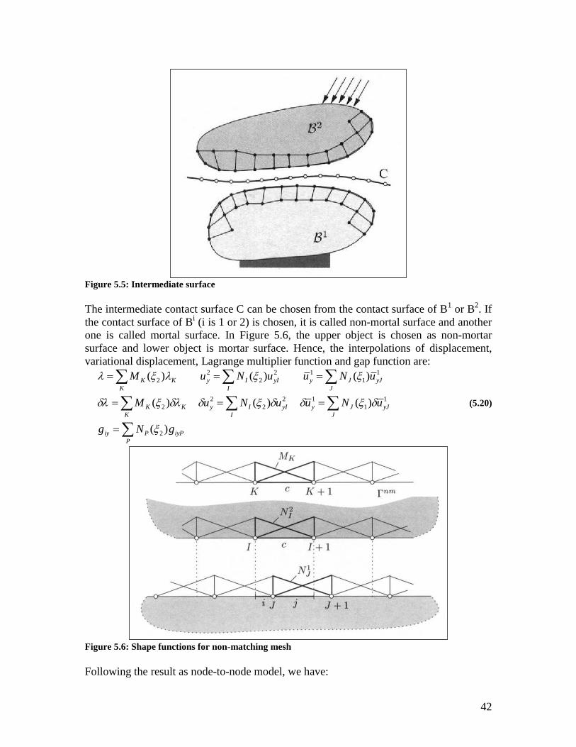
42

Figure 5.5: Intermediate surface

The intermediate contact surface C can be chosen from the contact surface of B1 or B

2. If

the contact surface of Bi (i is 1 or 2) is chosen, it is called non-mortal surface and another

one is called mortal surface. In Figure 5.6, the upper object is chosen as non-mortar

surface and lower object is mortar surface. Hence, the interpolations of displacement,

variational displacement, Lagrange multiplier function and gap function are:

P

iyPPiy

J

yJJy

I

yIIy

K

KK

J

yJJy

I

yIIy

K

KK

gNg

uNuuNuM

uNuuNuM

)(

)()()(

)()()(

2

1

1

12

2

2

2

1

1

12

2

2

2

(5.20)

Figure 5.6: Shape functions for non-matching mesh

Following the result as node-to-node model, we have:

43

c

ic

i

c

ic

i

c

n

i J K

yJJKK

n

i I K

yITKK

udJNM

udJNMgd

1

212

2

222

)()(

)()(

(5.21)

2 1c c

c

n nT T

i yi i yi

i i

gd u u

1 2 T T T

i iM M λ M u u M λ (5.22)

1

iM can be easily calculated because the shape function MK and NI are defined in the

same domain. With linear basic function, 1

iM in contact element i is determined as:

21 11 1 1 2 12

2 2 2 1 2 2 2

2 1 2 2 21 1

212 2 2 2 1

1 2 2 2

2 2 2 2 21

1( ) ( )

4 2

(1 )(1 ) (1 )(1 )1

(1 )(1 ) (1 )(1 )4 2

yi

K K I yI i i

I K yi

yi

i i

yi

N N N N uLM N J d u d

N N N N u

uLd

u

1iM

(5.23)

With: 1

2 2 2 2

2

2 2 2 21

(1 )(1 ) (1 )(1 ) 2 11

(1 )(1 ) (1 )(1 ) 1 24 2 6

L Ld

1

iM (5.24)

Calculating 2

iM is more complicated because the discretization of two domains is

different. For example, to calculate 2

iM in contact element c, we need to divide the

original element into two mortar segments i and j (please refer to above figure). Then, we

calculate 2

iM in each mortar segment and sum all results to get 2

iM :

J K

yJjjjJjKKj

J K

yJiiiJiKKi

J K

yJJKK

udJNM

udJNMudJNM

ij

iiic

i

1

1

1

12

1

1

1

12

1

212

))(())((

))(())(()()(

(5.25)

Apply the same procedure for constraint equation

2 2 12 1 2 1

1 2 1 26 6

c c c

c

n n nT T Ti i

i yi i i yi i iyi

i i i

L Lgd u M u g

1 1i iM M

(5.26)

Finally, we get the system of equation:

T

iy

ruK -M

-Ggλ-M 0 (5.27)

where global matrix M can be assembled from element matrix 1

iM and 2

iM and global

matrix G can be assembled from element matrix 1

iM

44

45

6 Adaptive Meshing Instead of finding the exact solution, FEM try to find an approximated solution with

minimum error. This error depends on the mesh of the model. The mesh should be

“good” enough so that the result with desired accuracy is obtained. The Adaptive Finite

Element techniques are used to find a quality mesh for finite element method with

minimized calculation cost. This technique should be automatic, efficient and robust so

that it can be applied for many models. The basis operations of Adaptive method is trying

to change the mesh by refining, coarsening or relocating it’s structure or adjust the

number of degree of freedom of basic function. Base on these procedures, adaptive

procedures can be classified into three categories:

P method: in this method, the polynomial degree of basic function is adjusted to

improve to precision of the finite element method.

R method: the number of element of the mesh is kept but its structure is relocated.

H method: the mesh is optimized due to refining or coarsening its element.

These methods can be applied in single or in combination for improving the accuracy of

approximated solution. P method is the most powerful in many models. Otherwise, h-

method is the most popular refinement.

In this work, H refinement is used due to its popularity. The simplest way to implement h

refinement is refining the whole mesh if the accuracy of solution has not reached to

desired value. However, it requires much calculation effort. In fact, there are some

regions of the mesh do not need to be refined. Therefore, the two basic operations of this

technique are finding the regions of element that need to be refined and refining these

regions. Both of these operations will be introduced in this section.

The first operation needs an error evaluation for elements. There are two kinds of error

evaluation:

Residual based: the error of the approximated solution is estimated directly by the

norm: e hu u .

Recovery based: was introduced by Zienkiewicz and Zhu in 1987. Instead of

estimating e hu u , the recovery solution *u which is better than hu is found

first. Then, the approximated error *e *

hu u is determined.

6.1 Residual based error estimation

Discretization is the key step for Finite Element Method. However, it leads to

interpolation error in approximated solution. There are two kinds of error: prior error and

posteriori error. Evaluation of this error is used to steer the adaptive meshing scheme.

Two important requirements of the error estimation are reliability and efficiency.

Reliability is that the estimation has to reach to desired precision and efficiency means

that the computational cost for this work should be acceptable. Normally, the error can

be calculated by hu u and it has to satisfy

toluue h (6.1)

Where u is the exact solution, uh is the approximate solution, tol is tolerance which is

chosen very small usually. In practical model, exact analytical solution u can not be

46

found. Therefore, in optimization problem, instead of minimize the error e, we try to

minimized the tolerance tol while keeping the constraint (6.1).

6.1.1 Variational formulation for boundary value problem (BVP)

For simplification, the two-dimensional model or Poisson’s equation with Dirichlet

boundary u and Newmann boundary is considered here. The model can be

represented as a boundary value problem

0 uand

u f x u x

n u g x (6.2)

Let define V as Sobolev space of functions which belong to function space H1 and

satisfies Dirichlet boundary condition:

: 0 uon 1V v H v (6.3)

Consequently, the variational formulation for above boundary value problem can be

represented as finding a function u in V such that:

( , ) ( )a l u v v v V (6.4)

Where a(u,v) is bilinear form of function u, v and l(v) is linear functional. Both of terms

are defined in H1 as:

( , )a d

u v u v (6.5)

( )l d d

v f v g v (6.6)

Then, energy norm based on bilinear form is defined as:

,E

av v v (6.7)

6.1.2 Priori error estimation:

Usually, we cannot solve BVP since V is very complicated. Therefore, in Galerkin

method, V is approximated by Vh. Now, our problem is finding the approximated

solution uh in Vh such that:

,a lh h hu v v (6.8)

This approximation will lead an interpolation error:

e hu u (6.9)

This error relate to bilinear form of elliptic linear model. As Lax-Milgram theorem, this

bilinear form has to be bounded as:

, ,V V

a M v w v w v w V V (6.10)

2

,V

a v v v v V (6.11)

Follow the Cea’s Lemma optimality condition for elliptic linear model:

infh h

V Vv V

M

h hu u u u (6.12)

With 1V H , the norm for error is defined as:

47

1 1p

p

H Hch

hu u u (6.13)

6.2 Recovery based error estimation

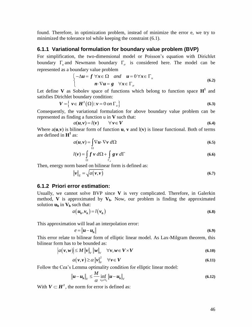
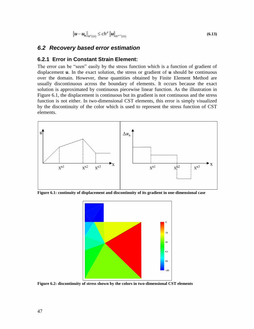
6.2.1 Error in Constant Strain Element:

The error can be “seen” easily by the stress function which is a function of gradient of

displacement u. In the exact solution, the stress or gradient of u should be continuous

over the domain. However, these quantities obtained by Finite Element Method are

usually discontinuous across the boundary of elements. It occurs because the exact

solution is approximated by continuous piecewise linear function. As the illustration in

Figure 6.1, the displacement is continuous but its gradient is not continuous and the stress

function is not either. In two-dimensional CST elements, this error is simply visualized

by the discontinuity of the color which is used to represent the stress function of CST

elements.

Figure 6.1: continuity of displacement and discontinuity of its gradient in one-dimensional case

Figure 6.2: discontinuity of stress shown by the colors in two-dimensional CST elements

48

Instead of trying to estimate an error huu which is very difficult in practical problem,

recovery-based error estimators find the post-processed solution u* which is expected

being better than uh then estimate a new defined error huu * . The approximated

solution uh is called non post-processed solution in this case.

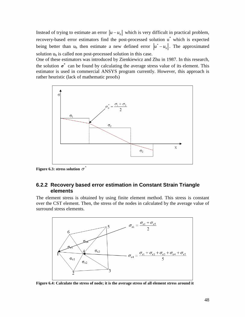
One of these estimators was introduced by Zienkiewicz and Zhu in 1987. In this research,

the solution *σ can be found by calculating the average stress value of its element. This

estimator is used in commercial ANSYS program currently. However, this approach is

rather heuristic (lack of mathematic proofs)

Figure 6.3: stress solution

*

6.2.2 Recovery based error estimation in Constant Strain Triangle elements

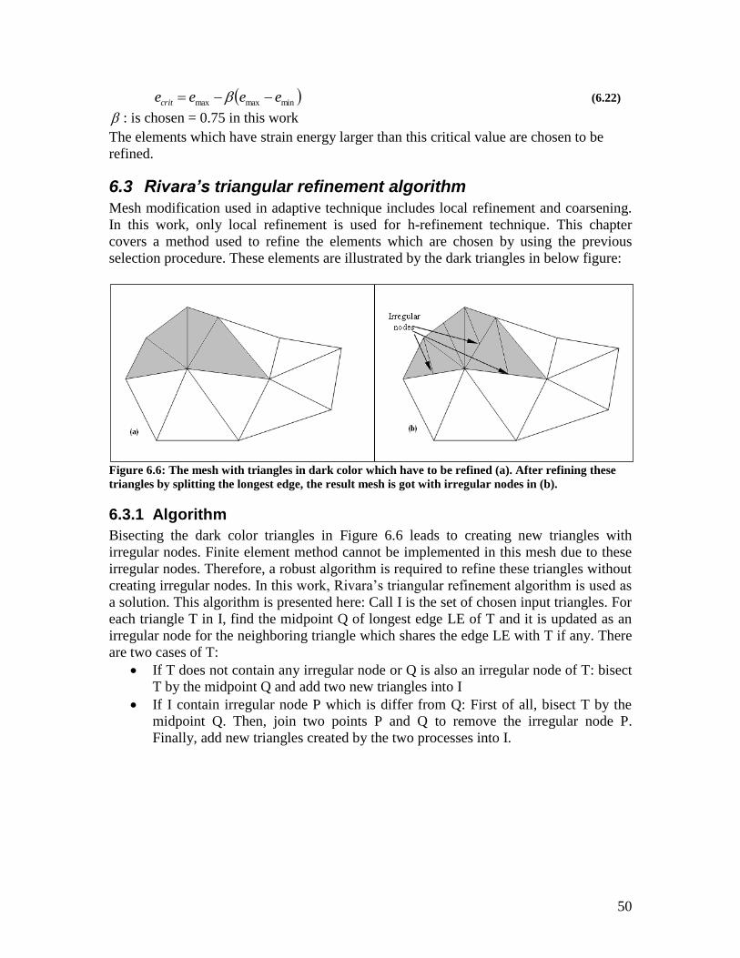
The element stress is obtained by using finite element method. This stress is constant

over the CST element. Then, the stress of the nodes in calculated by the average value of

surround stress elements.

Figure 6.4: Calculate the stress of node; it is the average stress of all element stress around it

49

Then, the post-processed stresses of the CST elements are determined by the average

value of its node stresses. This step is illustrated as in below figure:

Figure 6.5: Calculate the new value stress of element

Calculate the error of the element by using the energy norm of post-processed solution u*

and non post-processed solution uh:

1

2

,T

E Ee a dV

* * * * -1 *

h h hu u u u u u σ σ C σ σ (6.14)

2

,T

h Ee e a dV

* * * -1 *

h he e σ σ C σ σ (6.15)

With:

,T

a dV

* * * -1 *

h hu u u u σ σ C σ σ (6.16)

And

* *

he σ σ (6.17)

Hence,

2

,T

h Ee e a dV

* * * -1 *

h he e σ σ C σ σ (6.18)

n

ehEh Eee 222 (6.19)

Where

2T

e edV

* -1 *

e e e eσ σ C σ σ (6.20)

Strain energy can be also used

21 1

2 2

T

e ee dV

* -1 *

e e e eσ σ C σ σ (6.21)

Calculate strain energy of all elements in the mesh. Then, the maximum and minimum

strain energy is determined. The critical strain energy is defined base on these values as:

50

minmaxmax eeeecrit (6.22)

: is chosen = 0.75 in this work

The elements which have strain energy larger than this critical value are chosen to be

refined.

6.3 Rivara’s triangular refinement algorithm

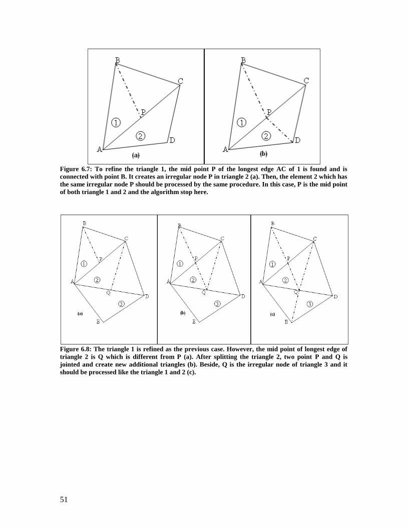
Mesh modification used in adaptive technique includes local refinement and coarsening.

In this work, only local refinement is used for h-refinement technique. This chapter

covers a method used to refine the elements which are chosen by using the previous

selection procedure. These elements are illustrated by the dark triangles in below figure:

Figure 6.6: The mesh with triangles in dark color which have to be refined (a). After refining these

triangles by splitting the longest edge, the result mesh is got with irregular nodes in (b).

6.3.1 Algorithm

Bisecting the dark color triangles in Figure 6.6 leads to creating new triangles with

irregular nodes. Finite element method cannot be implemented in this mesh due to these

irregular nodes. Therefore, a robust algorithm is required to refine these triangles without

creating irregular nodes. In this work, Rivara’s triangular refinement algorithm is used as

a solution. This algorithm is presented here: Call I is the set of chosen input triangles. For

each triangle T in I, find the midpoint Q of longest edge LE of T and it is updated as an

irregular node for the neighboring triangle which shares the edge LE with T if any. There

are two cases of T:

If T does not contain any irregular node or Q is also an irregular node of T: bisect

T by the midpoint Q and add two new triangles into I

If I contain irregular node P which is differ from Q: First of all, bisect T by the

midpoint Q. Then, join two points P and Q to remove the irregular node P.

Finally, add new triangles created by the two processes into I.

51

Figure 6.7: To refine the triangle 1, the mid point P of the longest edge AC of 1 is found and is

connected with point B. It creates an irregular node P in triangle 2 (a). Then, the element 2 which has

the same irregular node P should be processed by the same procedure. In this case, P is the mid point

of both triangle 1 and 2 and the algorithm stop here.

Figure 6.8: The triangle 1 is refined as the previous case. However, the mid point of longest edge of

triangle 2 is Q which is different from P (a). After splitting the triangle 2, two point P and Q is

jointed and create new additional triangles (b). Beside, Q is the irregular node of triangle 3 and it

should be processed like the triangle 1 and 2 (c).

52

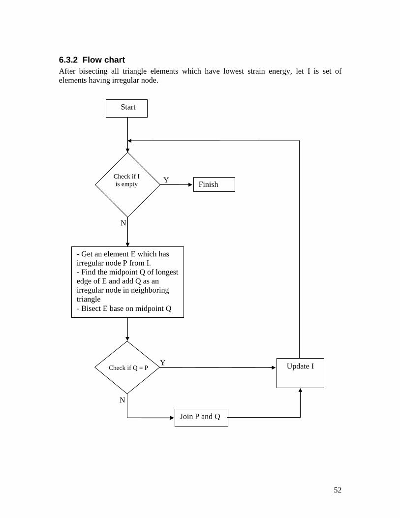
6.3.2 Flow chart

After bisecting all triangle elements which have lowest strain energy, let I is set of

elements having irregular node.

Check if I

is empty Finish Y

Y

N

- Get an element E which has

irregular node P from I.

- Find the midpoint Q of longest

edge of E and add Q as an

irregular node in neighboring

triangle

- Bisect E base on midpoint Q

Join P and Q

N

Start

Check if Q = P Update I

53

7 Numerical Example

7.1 Plate with a hole

Figure 7.1: Geometrical parameters of the model

Young modulus E = 210000

Poisson ratio 3.0

Thichness 1t

Figure 7.2: The mesh result after applying Delaunay triangulation and two-dimensional mesh

generation

54

Figure 7.3: This displacement result after multiplying by 100 times

Figure 7.4: the stress x result of the model before applying adaptive procedure

55

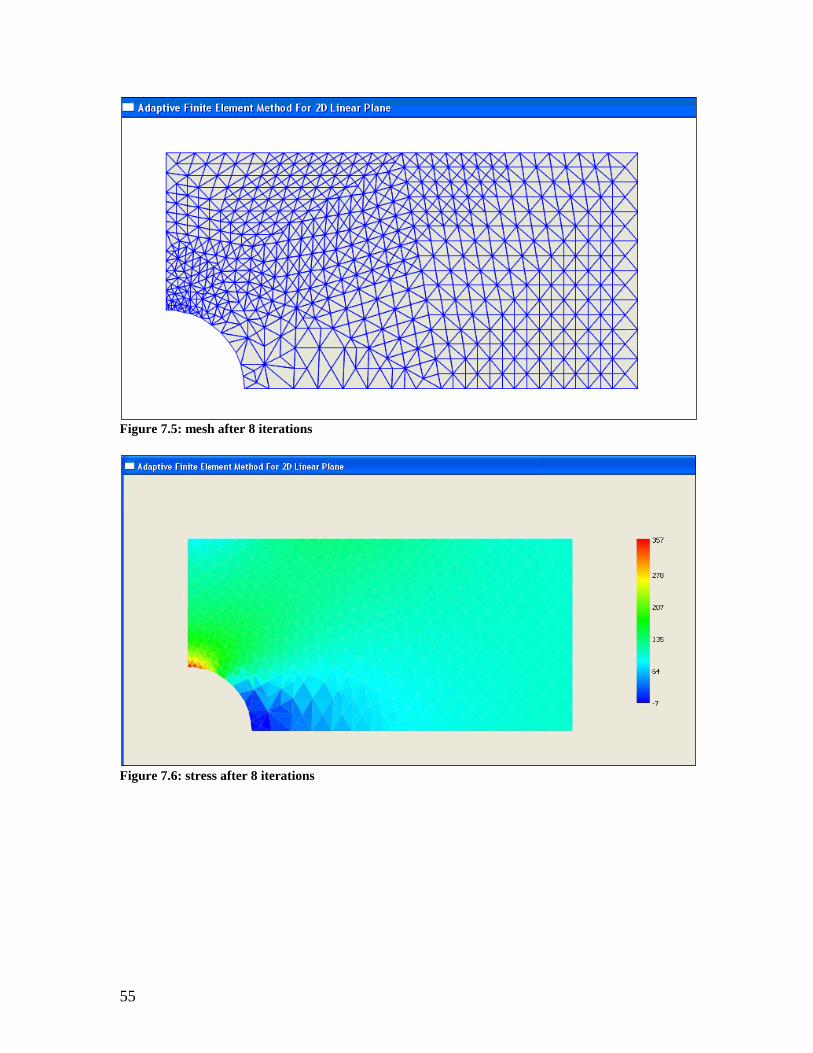
Figure 7.5: mesh after 8 iterations

Figure 7.6: stress after 8 iterations

56

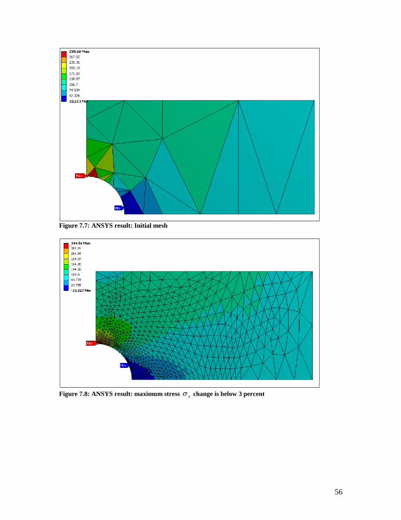
Figure 7.7: ANSYS result: Initial mesh

Figure 7.8: ANSYS result: maximum stress x change is below 3 percent

57

7.2 Planar contact model

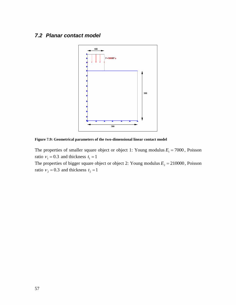
Figure 7.9: Geometrical parameters of the two-dimensional linear contact model

The properties of smaller square object or object 1: Young modulus 70001 E , Poisson

ratio 3.01 and thickness 11 t

The properties of bigger square object or object 2: Young modulus 2100002 E , Poisson

ratio 3.02 and thickness 12 t

58

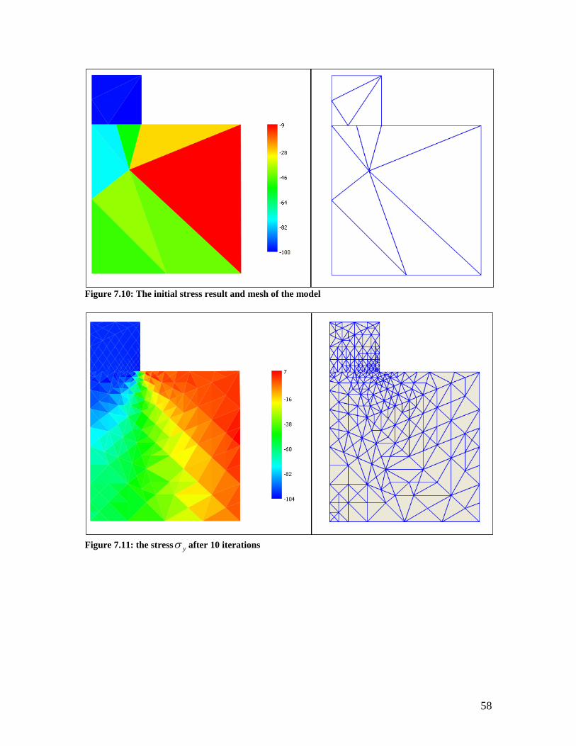
Figure 7.10: The initial stress result and mesh of the model

Figure 7.11: the stress y after 10 iterations

59

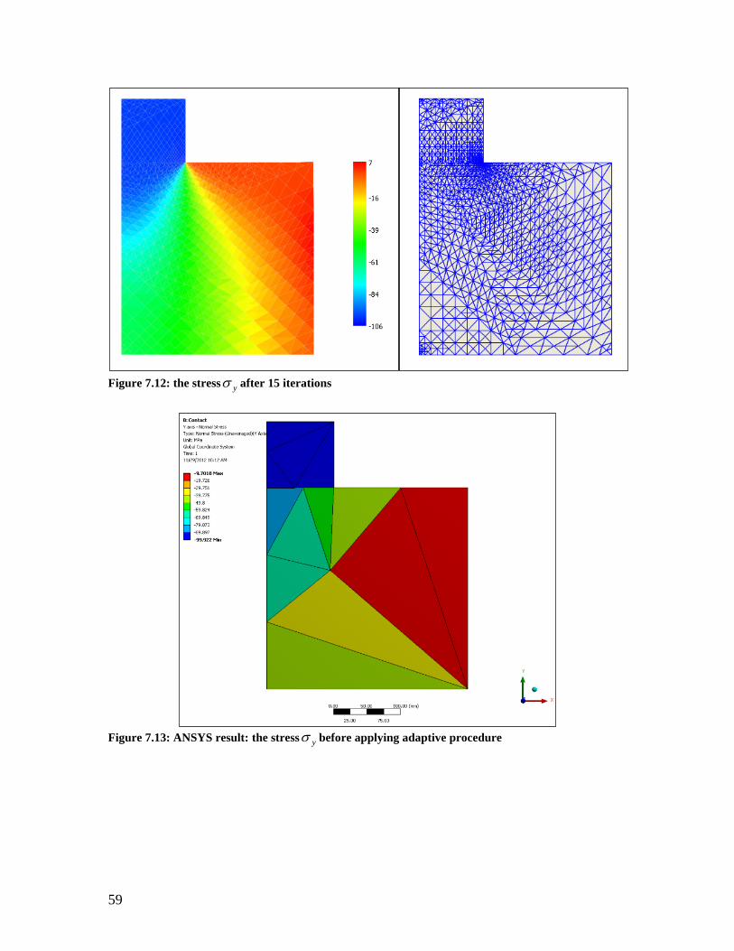
Figure 7.12: the stress y after 15 iterations

Figure 7.13: ANSYS result: the stress y before applying adaptive procedure

60

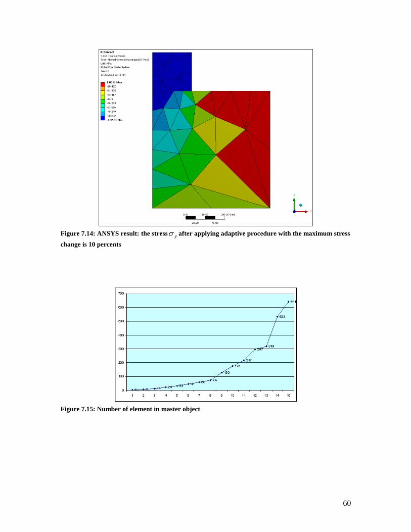
Figure 7.14: ANSYS result: the stress y after applying adaptive procedure with the maximum stress

change is 10 percents

Figure 7.15: Number of element in master object

61

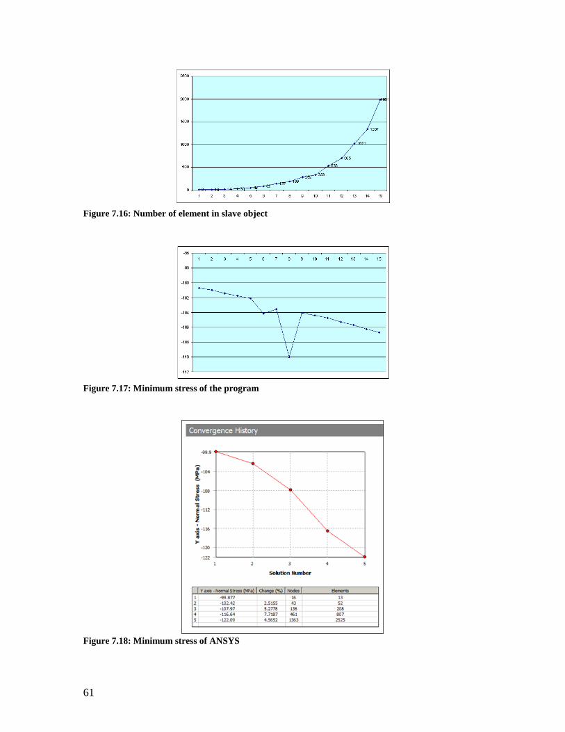
Figure 7.16: Number of element in slave object

Figure 7.17: Minimum stress of the program

Figure 7.18: Minimum stress of ANSYS

62

63

8 Future Work This work only considers the linear problem in which displacement is very small and

contact area does not depend on the displacement. However, in practical contact model,

the displacement is usually very large and contact area is a function of displacement. The

model for non-linear problem without contact has a form:

ir (u)=r (8.1)

Where )(uri is the internal force of model and it depends on displacement u. To solve

about equation, a non-linear solver such as Newton-Raphson method or arc-length

method is required.

The non-linear contact model which is illustrated as sphere contact in figure 8.1 is very

complicated since the contact area depends on displacement and the tangential gap

function consideration is a must. The system of equation which is the result of

implementation of Lagrange multiplier method for non-linear contact has a form:

T Tc c cT T

cc

K (u)+K u,λ C u Δu G u +C u λ=-

Δλ G uC u 0

(8.2)

This system of equation is derived very carefully in [6]. Solving this equation also need a

non-linear solver.

Figure 8.1: An example of symmetric sphere contact model

64

65

References [1] J. Ruppert. A new and simple algorithm for quality 2-dimensional mesh generation. In

Proc. 4th

ACM-SIAM Symp. On Disc. Algorithms, pages 83-92, 1993.

[2] L.P. Chew. Guaranteed-quality triangular meshes. Technical report, Cornell

University, 1989. No. TR89-983.

[3] L.P. Chew. Constrained Delaunay triangulation. Algorithmica, 4:97-108, 1989.

[4] Thomas Gratsch, Klaus-Jurgen Bathe. A posteriori error estimation techniques in

practical finite element analysis. Computers & Structures, 2004.

[5] O.C.Zienkiewicz, B. Boroomand, J.Z. Zhu. Recovery procedure in error estimation

and adaptivity. Part I: Adaptivity in linear problems. Comput. Methods Appl. Mech.

Engrg. 176 (1999) 111-125.

[6] Wriggers, P. (2002). Computational Contact Mechanics. Wiley, Chichester.

[7] Bin Yang, Tod A. Laursen, Xiaonong Meng. Two dimensional mortar contact

methods for large deformation frictional sliding. Int. J. Numer. International journal for

numerical methods in engineering, 2005, 62:1183-1225.

[8] G. Meschke. Finite Element Methods in Linear Structural Mechanics. Lecture notes,

Ruhr University Bochum, Institute for Structural Mechanics, November 2010.

[9] J.Fish and T Belytschko. A first Course in Finite Elements. John Wiley & Sons,

Chichester, 2006.