jawaharlal nehru engineering college network analysis
TRANSCRIPT
Jawaharlal Nehru Engineering College
Network Analysis & Synthesis
For
Second Year Students
Manual made by
Mr. Madhuresh Sontakke
LABORATORY MANNUAL CONTENTS
This manual is intended for the second year students of engineering branches in the subject of network theory. This manual typically contains practical/Lab Sessions related to Network Theory covering various aspects related the subject
to enhance understanding.
In this manual we have made the efforts to cover various experiments on network theory with detailed circuit diagrams, detailed procedure and graphs wherever required.
Students are advised to thoroughly go through this manual rather than only topics mentioned in the syllabus as practical aspects are the key to
understanding and conceptual visualization of theoretical aspects covered in the books.
Good Luck for your Enjoyable Laboratory Sessions
Ms. B.V.Pahade

FOREWORD
It is my great pleasure to present this laboratory manual for second year engineering students for the subject of Network Theory, keeping in view the vast coverage required to visualize the basic concepts of various networks using basic
components. NT covers designing a network for specific input/output requirements.
This being a core subject, it becomes very essential to have clear theoretical and practical designing aspects.
This lab manual provides a platform to the students for understanding the basic concepts of network theory. This practical background will help students to gain
confidence in qualitative and quantitative approach to electronic networks.
Good Luck for your Enjoyable Laboratory Sessions.
Prof. Dr. H.H.Shinde
Principal

MAHATMA GANDHI MISSION`S
JAWAHARLALNEHRUENGINEERINGCOLLEGE AURANGABAD.
Department of Electrical Electronics and Power
Vision of JNEC To create self-reliant, continuous learner and competent technocrats imbued with
human values. Mission of JNEC 1. Imparting quality technical education to the students through participative teaching
–learning process. 2. Developing competence amongst the students through academic learning and
practical experimentation. 3. Inculcating social mindset and human values amongst the students. JNEC Environmental Policy
1. The environmental control during its activities, product and services. 2. That applicable , legal and statutory requirements are met according to
environmental needs. 3. To reduce waste generation and resource depletion. 4. To increase awareness of environmental responsibility amongst its students and staff. 5. For continual improvement and prevention of pollution.
JNEC Quality Policy: Institute is committed to:
To provide technical education as per guidelines of competent authority.
To continually improve quality management system by providing additional resources required. Initiating corrective & preventive action & conducting management review meeting at periodical intervals.
To satisfy needs & expectations of students, parents, society at large. EEP Department
VISION:
To Develop competent Electrical Engineers with human values. MISSION:
• To Provide Quality Technical Education To The Students Through Effective
Teaching-learning Process.
• To Develop Student’s Competency Through Academic Learning, Practicals And
Skill Development Programs.
• To Encourage Students For Social Activities & Develop Professional Attitude
Along With Ethical Values.
SUBJECT INDEX
1. Do’s and Don’ts
2. Lab exercise:
1) To perform mesh analysis.
2) To perform nodal analysis.
3) To verify superposition theorem
4) To verify Thevnins theorem
5) To verify Nortans theorem.
6) To Study maximum Power transfer theorem.
7) To verify reciprocity theorem
8) Verification of Millmans equivalent circuit.
9) To Study analysis of RL circuit
10) To Study analysis of RC circuit.
11) Transient Analysis Of RLC for step voltage response.
12) Frequency Response of RLC circuit win sinusoidal voltage.
1. DOs and DON’T DOs in Laboratory :
1. Do not handle kits without reading the instructions from manual.
2. Go through the procedures given in the lab manual for performing practical’s.
3. Strictly observe the instructions given by teacher/lab instructor.
Instruction for Laboratory Teachers:
1. Submission related to whatever lab work has been completed should be done during the next lab session.
2. Students should be guided and helped whenever they face difficulties.
3. The promptness of submission should be encouraged by way of marking and evaluation patterns that will benefit the sincere students.
2. Lab Exercises:
Exercise No1: (2 Hours) – 1 Practical
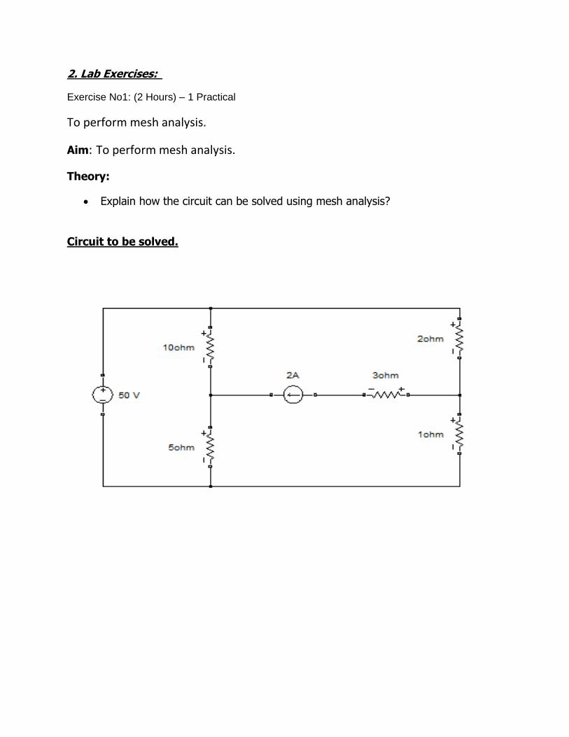
To perform mesh analysis.
Aim: To perform mesh analysis.
Theory:
Explain how the circuit can be solved using mesh analysis?
Circuit to be solved.
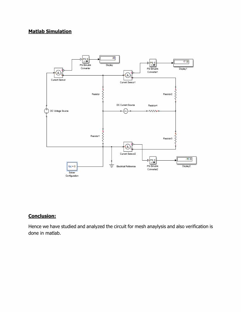
Matlab Simulation
Conclusion:
Hence we have studied and analyzed the circuit for mesh anaylysis and also verification is
done in matlab.
Exercise No 2: (2 Hours) – 1 Practical
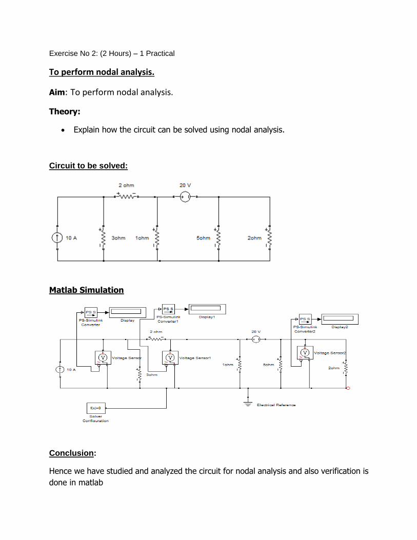
To perform nodal analysis.
Aim: To perform nodal analysis.
Theory:
Explain how the circuit can be solved using nodal analysis.
Circuit to be solved:
Matlab Simulation
Conclusion:
Hence we have studied and analyzed the circuit for nodal analysis and also verification is
done in matlab
Exercise No 3 : ( 2 Hours) – 1 Practical
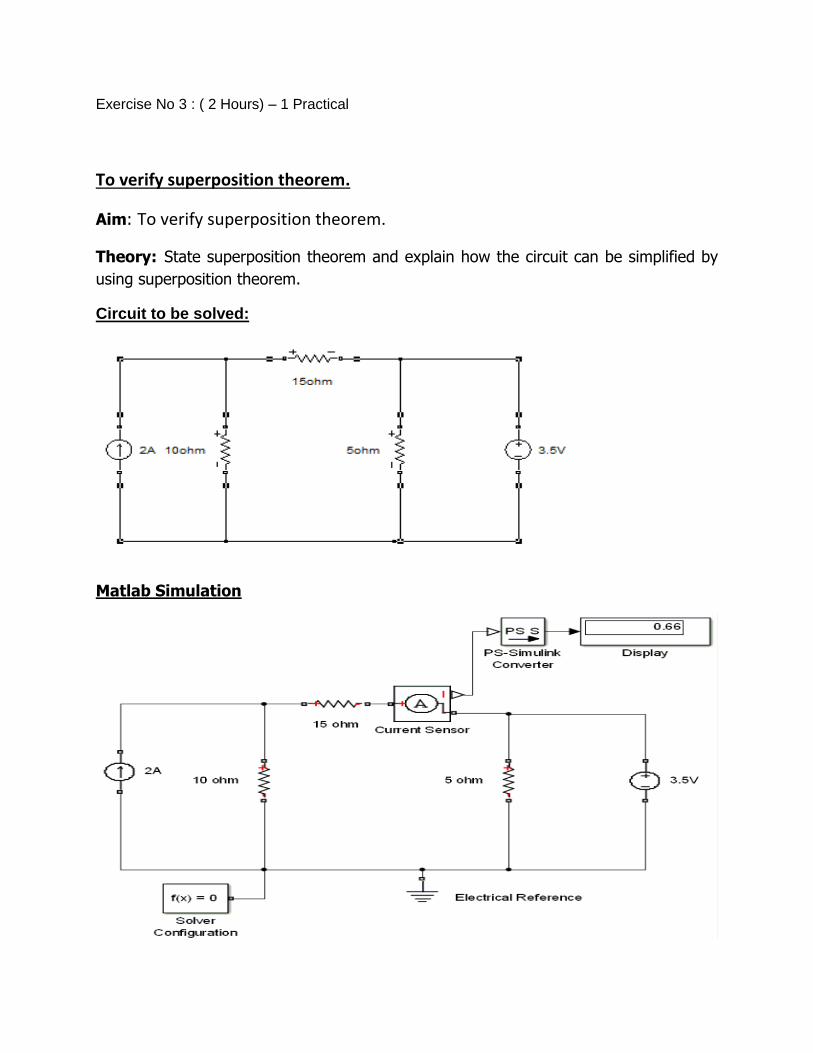
To verify superposition theorem.
Aim: To verify superposition theorem.
Theory: State superposition theorem and explain how the circuit can be simplified by
using superposition theorem.
Circuit to be solved:
Matlab Simulation
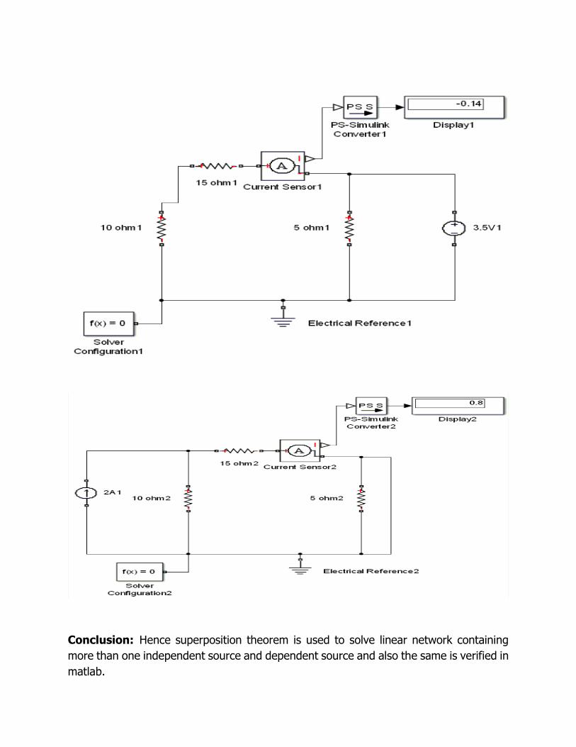
Conclusion: Hence superposition theorem is used to solve linear network containing
more than one independent source and dependent source and also the same is verified in
matlab.

Exercise No 4 : ( 2 Hours) – 1 Practical
To verify Thevnins theorem
Aim: To verify Thevnins theorem
Theory : State thevenins theorem and explain how the circuit can be simplified by using
thevnins theorem.
Circuit to be solved:
Matlab Simulation
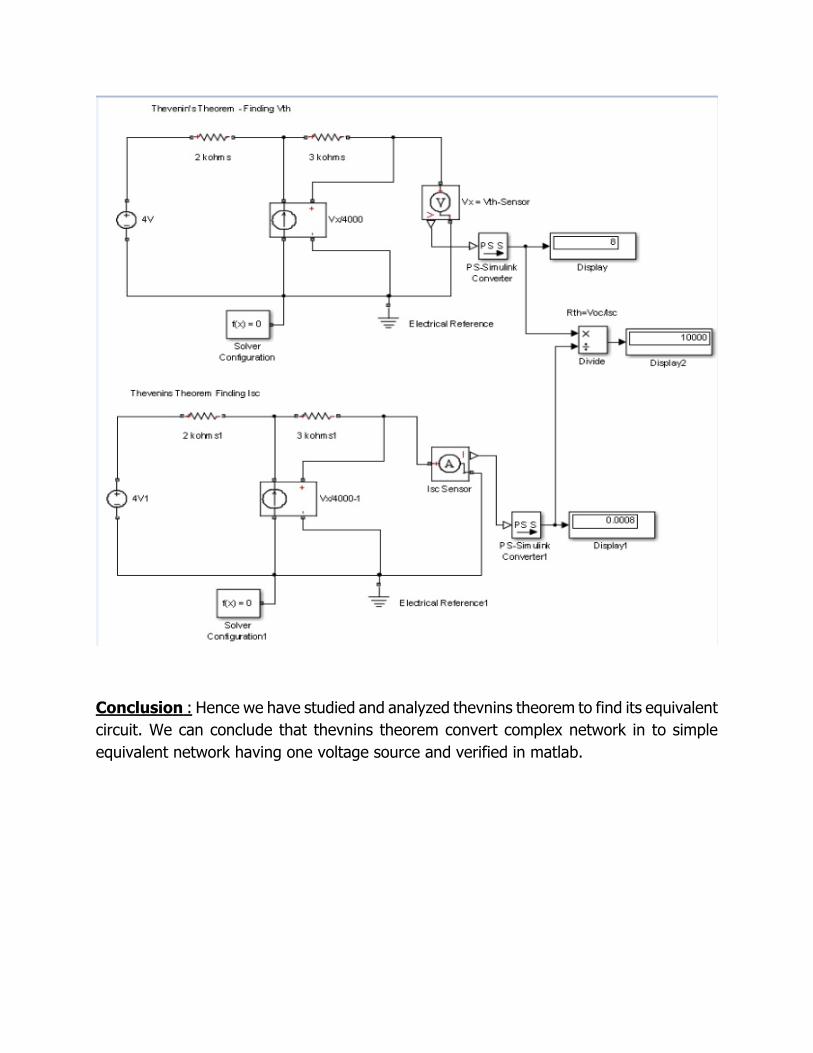
Conclusion : Hence we have studied and analyzed thevnins theorem to find its equivalent
circuit. We can conclude that thevnins theorem convert complex network in to simple
equivalent network having one voltage source and verified in matlab.
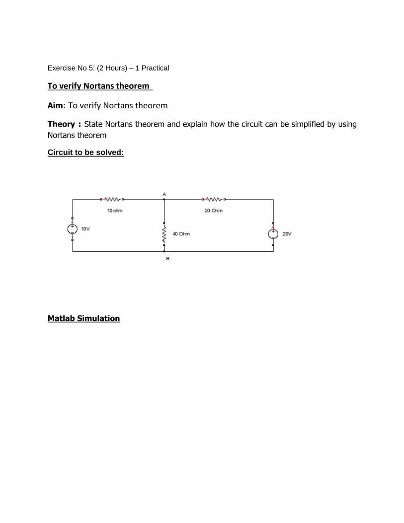
Exercise No 5: (2 Hours) – 1 Practical
To verify Nortans theorem
Aim: To verify Nortans theorem
Theory : State Nortans theorem and explain how the circuit can be simplified by using
Nortans theorem
Circuit to be solved:
Matlab Simulation
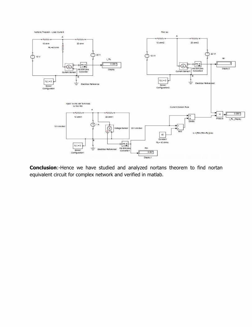
Conclusion:-Hence we have studied and analyzed nortans theorem to find nortan
equivalent circuit for complex network and verified in matlab.
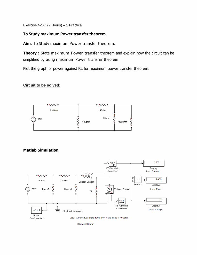
Exercise No 6: (2 Hours) – 1 Practical
To Study maximum Power transfer theorem
Aim: To Study maximum Power transfer theorem.
Theory : State maximum Power transfer theorem and explain how the circuit can be
simplified by using maximum Power transfer theorem
Plot the graph of power against RL for maximum power transfer theorem.
Circuit to be solved:
Matlab Simulation
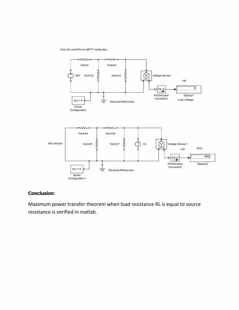
Conclusion:
Maximum power transfer theorem when load resistance RL is equal to source
resistance is verified in matlab.
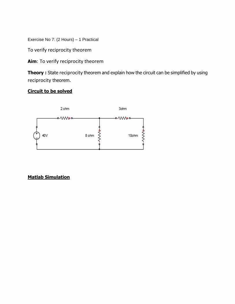
Exercise No 7: (2 Hours) – 1 Practical
To verify reciprocity theorem
Aim: To verify reciprocity theorem
Theory : State reciprocity theorem and explain how the circuit can be simplified by using
reciprocity theorem.
Circuit to be solved
Matlab Simulation
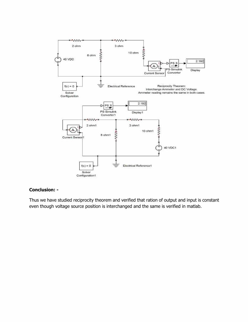
Conclusion: -
Thus we have studied reciprocity theorem and verified that ration of output and input is constant
even though voltage source position is interchanged and the same is verified in matlab.
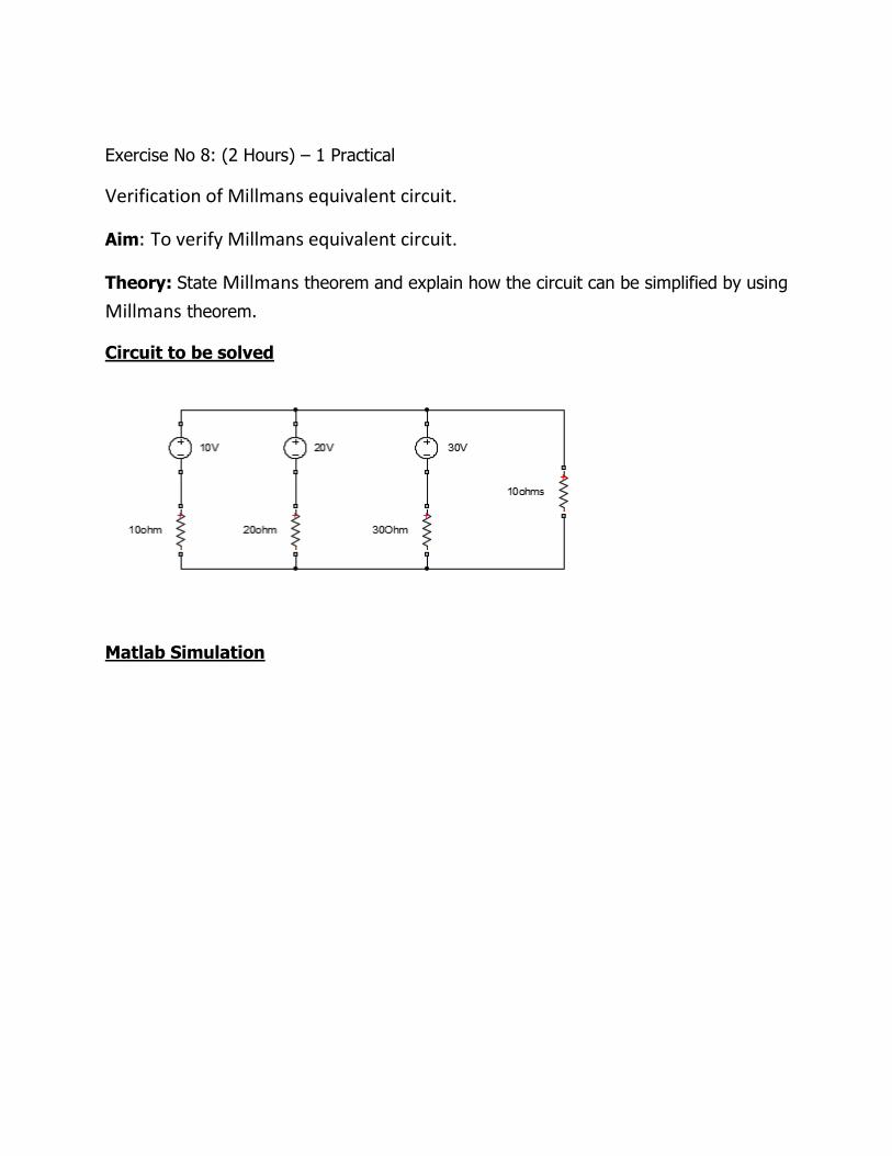
Exercise No 8: (2 Hours) – 1 Practical
Verification of Millmans equivalent circuit.
Aim: To verify Millmans equivalent circuit.
Theory: State Millmans theorem and explain how the circuit can be simplified by using
Millmans theorem.
Circuit to be solved
Matlab Simulation
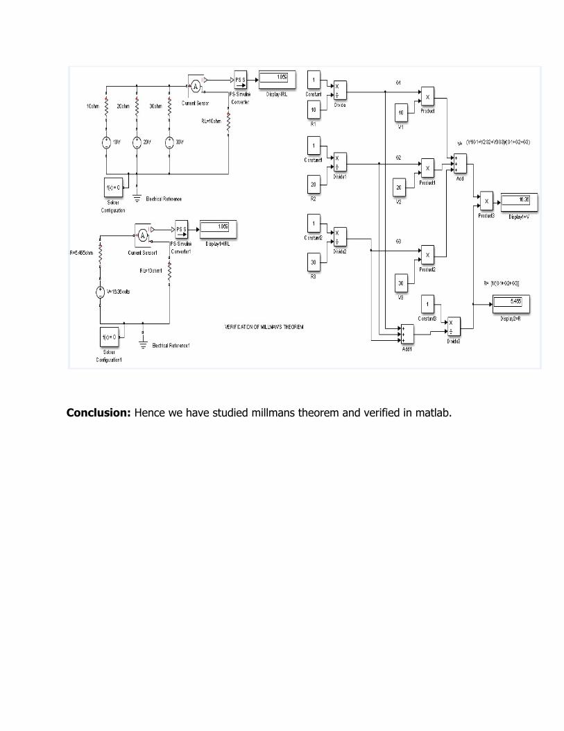
Conclusion: Hence we have studied millmans theorem and verified in matlab.
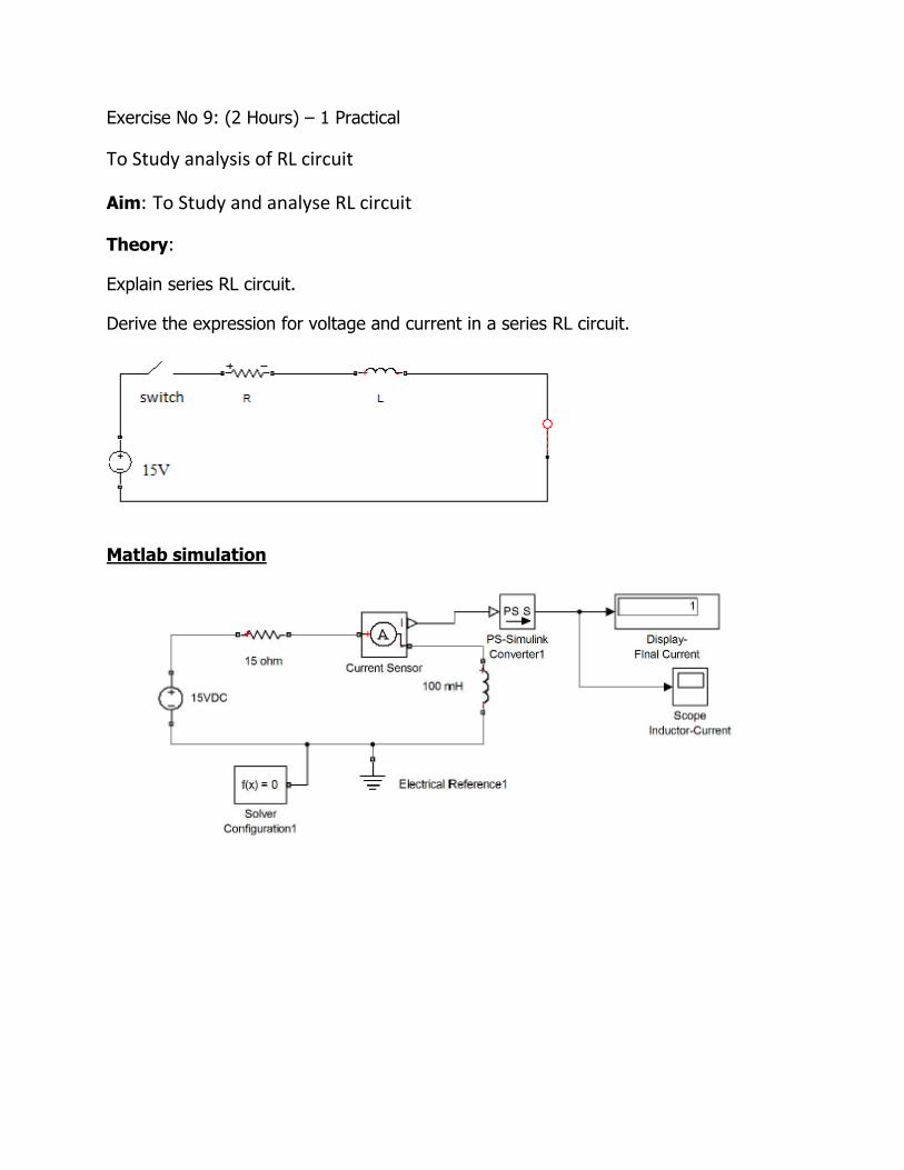
Exercise No 9: (2 Hours) – 1 Practical
To Study analysis of RL circuit
Aim: To Study and analyse RL circuit
Theory:
Explain series RL circuit.
Derive the expression for voltage and current in a series RL circuit.
Matlab simulation
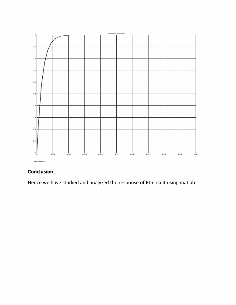
Conclusion:
Hence we have studied and analyzed the response of RL circuit using matlab.
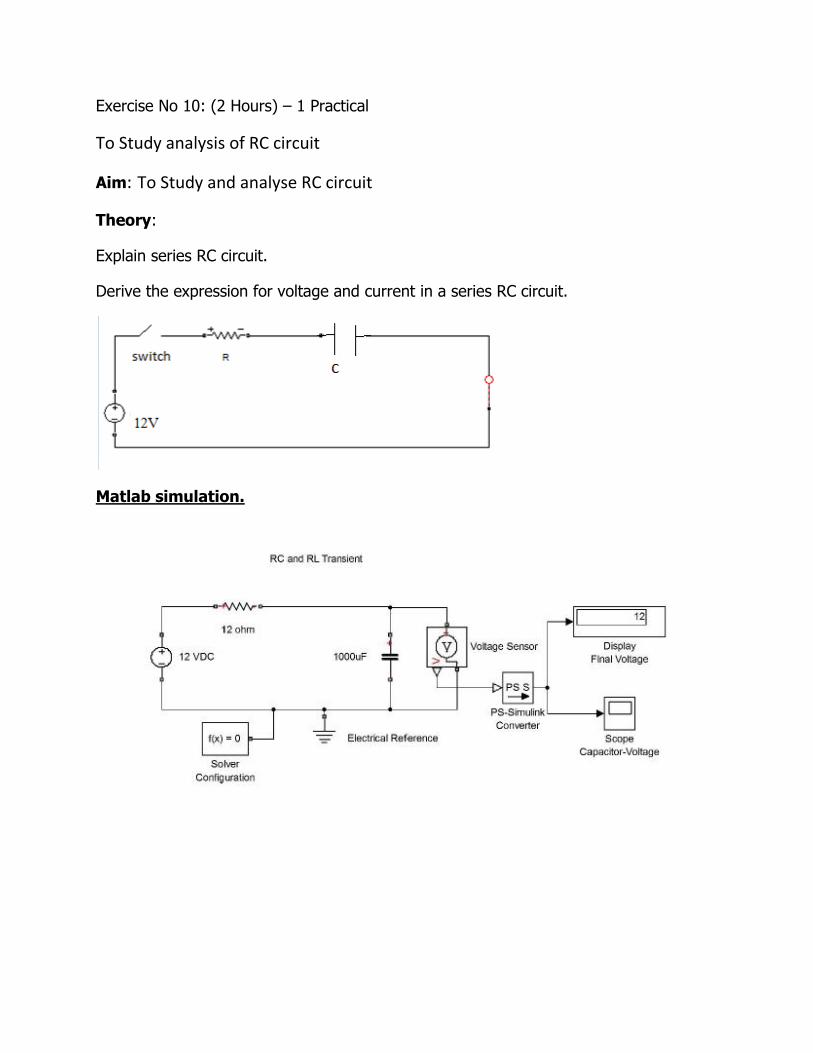
Exercise No 10: (2 Hours) – 1 Practical
To Study analysis of RC circuit
Aim: To Study and analyse RC circuit
Theory:
Explain series RC circuit.
Derive the expression for voltage and current in a series RC circuit.
Matlab simulation.
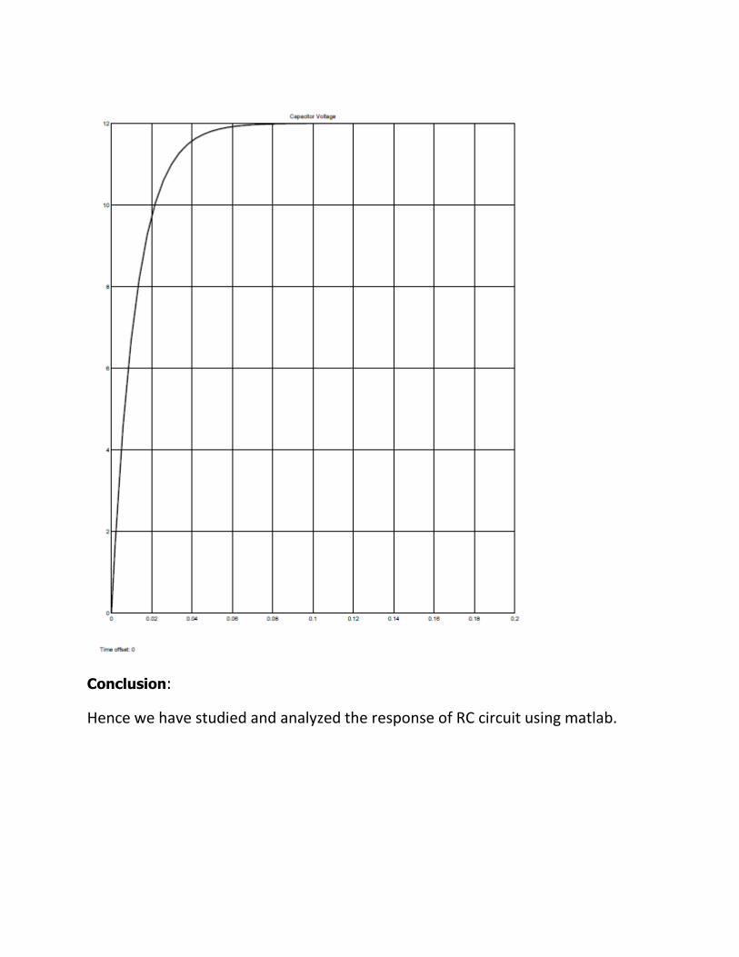
Conclusion:
Hence we have studied and analyzed the response of RC circuit using matlab.
Exercise No 11: (2 Hours) – 1 Practical
TRANSIENT RESPONSES OF SERIES RLC, RL, AND RC CIRCUITS WITH SINE AND STEP
INPUTS
AIM: To study the transient analysis of RLC, RL and RC circuits for sinusoidal and step inputs
Theory :
The transient response is the fluctuation in current and voltage in a circuit (after the application of
a step voltage or current) before it settles down to its steady state. This lab will focus on simulation
of series RL (resistor-inductor), RC (resistor-capacitor), and RLC (resistor inductor-capacitor)
circuits to demonstrate transient analysis.
Transient Response of Circuit Elements:
A. Resistors: As has been studied before, the application of a voltage V to a resistor (with
resistance R ohms), results in a current I, according to the formula: I = V/R
The current response to voltage change is instantaneous; a resistor has no transient response.
B. Inductors: A change in voltage across an inductor (with inductance L Henrys) does not result in
an instantaneous change in the current through it. The i-v relationship is described with the
equation: v=L di/ dt
This relationship implies that the voltage across an inductor approaches zero as the current
in the circuit reaches a steady value. This means that in a DC circuit, an inductor will eventually act
like a short circuit.
C. Capacitors: The transient response of a capacitor is such that it resists instantaneous change in
the voltage across it. Its i-v relationship is described by: i=C dv /dt
This implies that as the voltage across the capacitor reaches a steady value, the current through it
approaches zero. In other words, a capacitor eventually acts like an open circuit in a DC circuit.
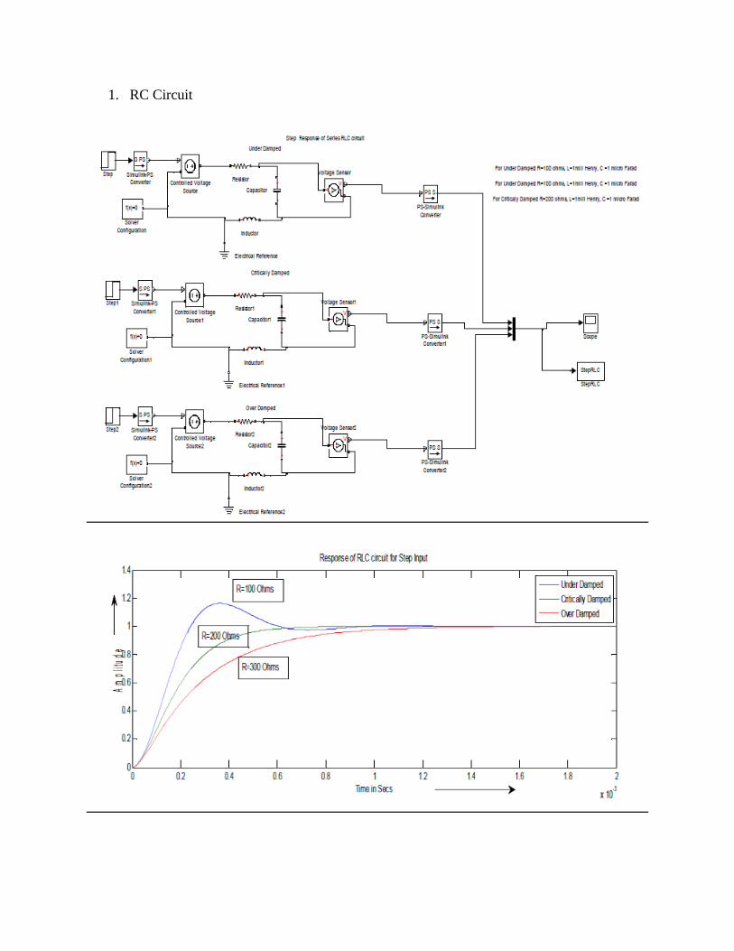
1. RC Circuit
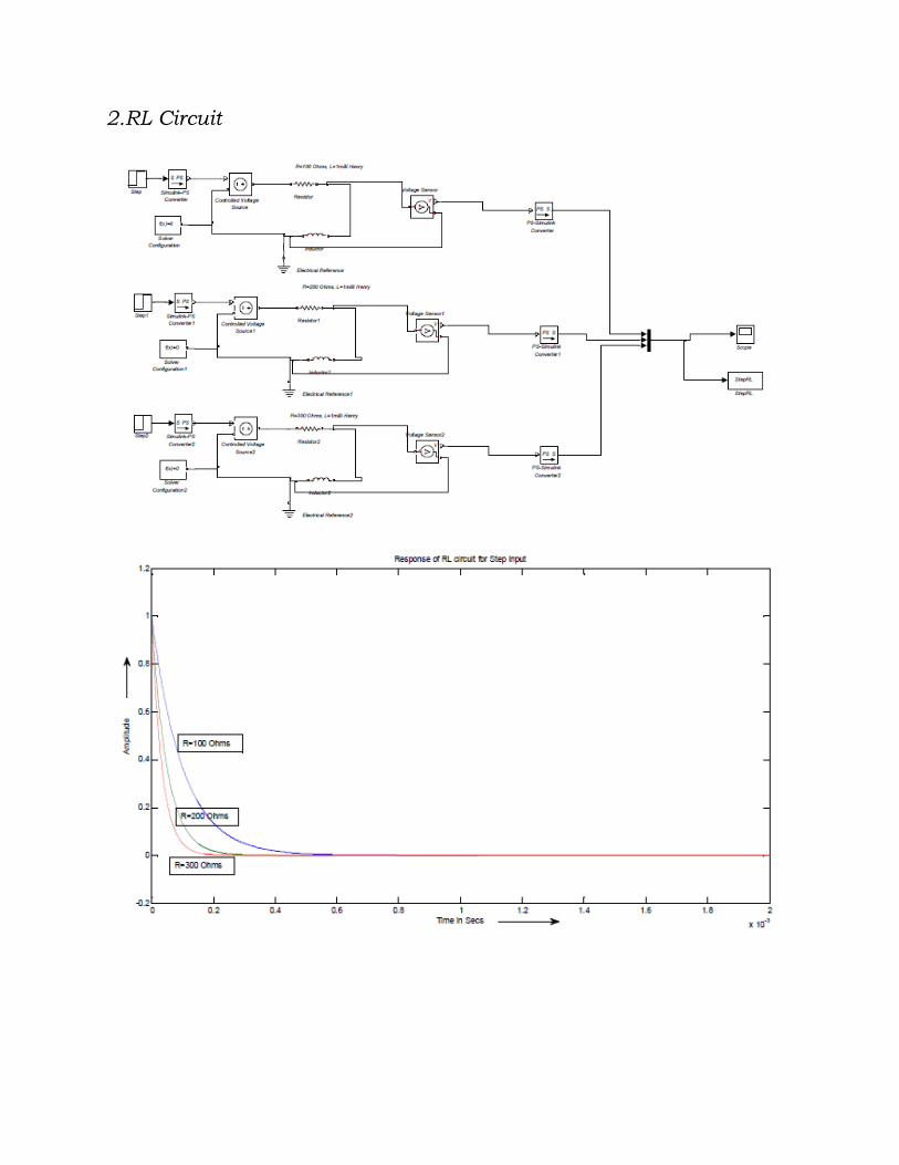
2.RL Circuit
Exercise No 11: (2 Hours) – 1 Practical
Frequency Response of RLC circuit win sinusoidal voltage.
AIM: To study the Frequency Response of RLC circuit win sinusoidal voltage
Theory :
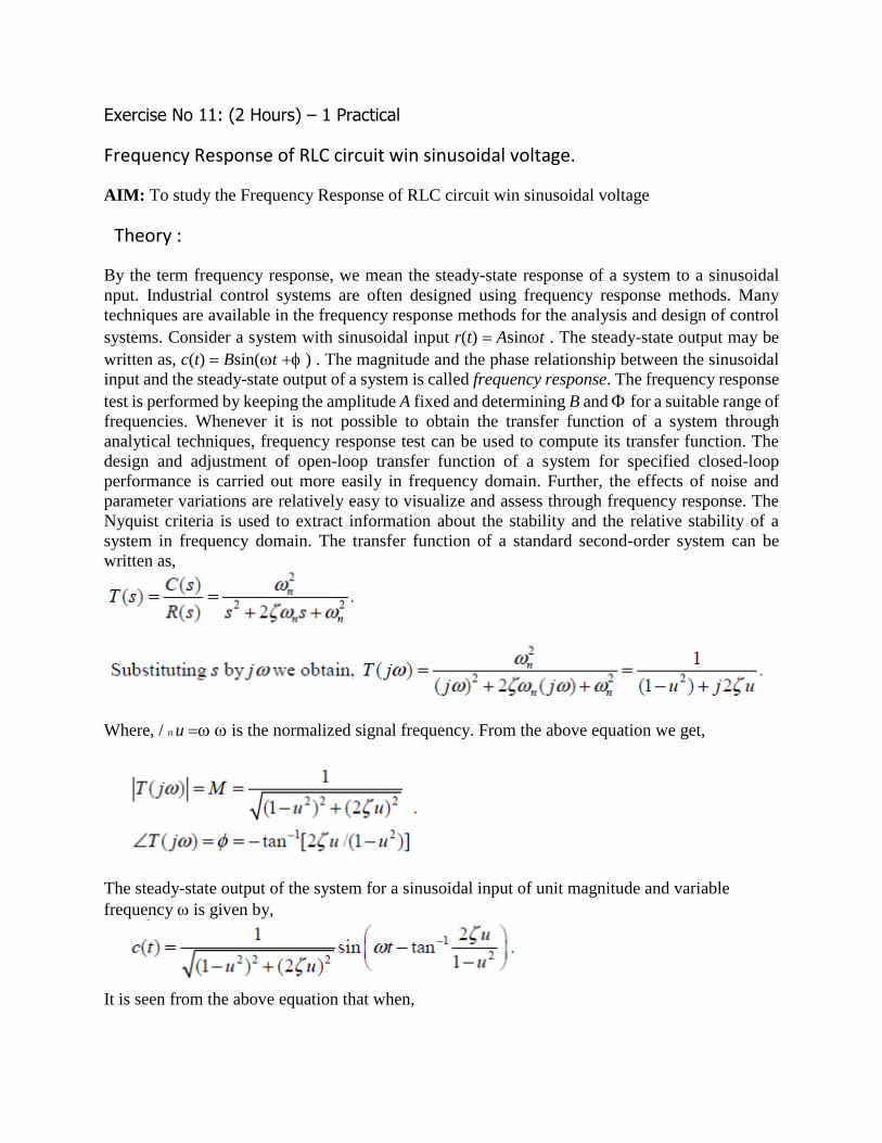
By the term frequency response, we mean the steady-state response of a system to a sinusoidal
nput. Industrial control systems are often designed using frequency response methods. Many
techniques are available in the frequency response methods for the analysis and design of control
systems. Consider a system with sinusoidal input r(t) Asint . The steady-state output may be
written as, c(t) Bsin(t ) . The magnitude and the phase relationship between the sinusoidal
input and the steady-state output of a system is called frequency response. The frequency response
test is performed by keeping the amplitude A fixed and determining B and for a suitable range of
frequencies. Whenever it is not possible to obtain the transfer function of a system through
analytical techniques, frequency response test can be used to compute its transfer function. The
design and adjustment of open-loop transfer function of a system for specified closed-loop
performance is carried out more easily in frequency domain. Further, the effects of noise and
parameter variations are relatively easy to visualize and assess through frequency response. The
Nyquist criteria is used to extract information about the stability and the relative stability of a
system in frequency domain. The transfer function of a standard second-order system can be
written as,
Where, / n u is the normalized signal frequency. From the above equation we get,
The steady-state output of the system for a sinusoidal input of unit magnitude and variable
frequency is given by,
It is seen from the above equation that when,
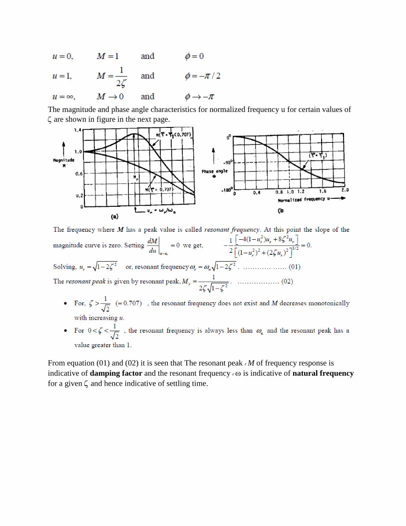
The magnitude and phase angle characteristics for normalized frequency u for certain values of
are shown in figure in the next page.
From equation (01) and (02) it is seen that The resonant peak r M of frequency response is
indicative of damping factor and the resonant frequency r is indicative of natural frequency
for a given and hence indicative of settling time.
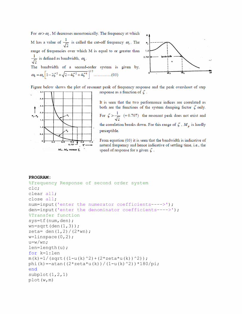
PROGRAM:
%Frequency Response of second order system
clc;
clear all;
close all;
num=input('enter the numerator coefficients---->');
den=input('enter the denominator coefficients---->');
%Transfer function
sys=tf(num,den);
wn=sqrt(den(1,3));
zeta= den(1,2)/(2*wn);
w=linspace(0,2);
u=w/wn;
len=length(u);
for k=1:len
m(k)=1/(sqrt((1-u(k)^2)+(2*zeta*u(k))^2));
phi(k)=-atan((2*zeta*u(k))/(1-u(k)^2))*180/pi;
end
subplot(1,2,1)
plot(w,m)
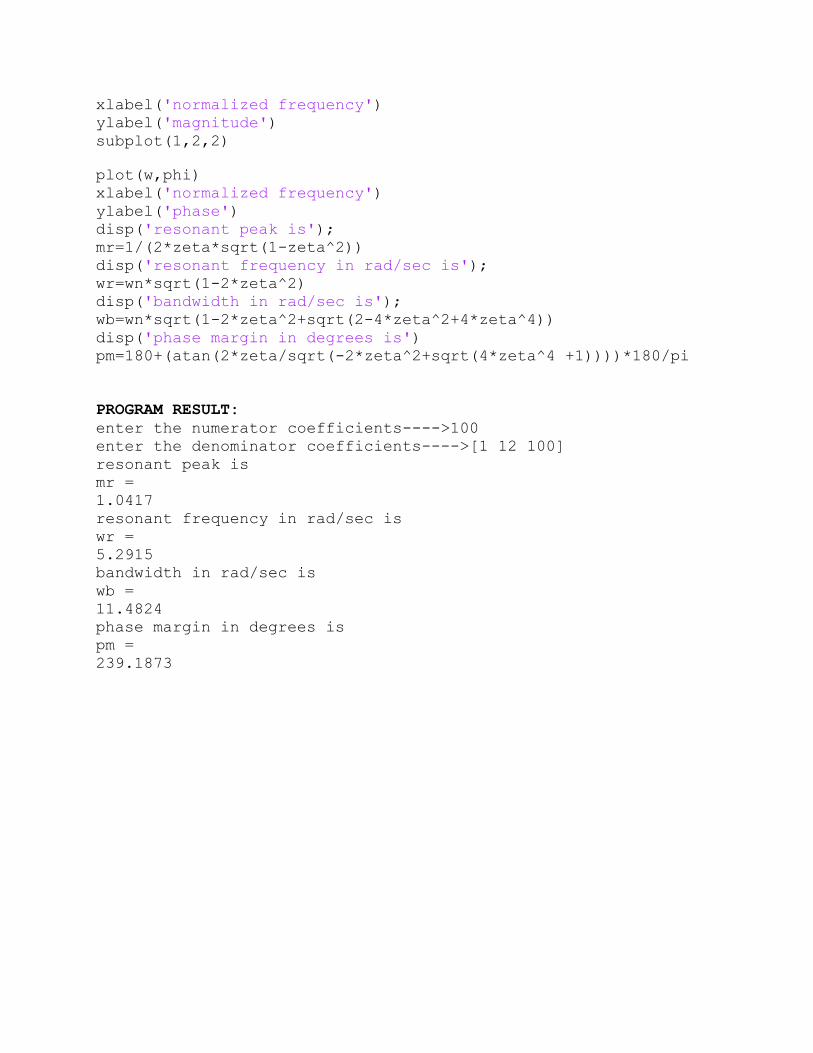
xlabel('normalized frequency')
ylabel('magnitude')
subplot(1,2,2)
plot(w,phi)
xlabel('normalized frequency')
ylabel('phase')
disp('resonant peak is');
mr=1/(2*zeta*sqrt(1-zeta^2))
disp('resonant frequency in rad/sec is');
wr=wn*sqrt(1-2*zeta^2)
disp('bandwidth in rad/sec is');
wb=wn*sqrt(1-2*zeta^2+sqrt(2-4*zeta^2+4*zeta^4))
disp('phase margin in degrees is')
pm=180+(atan(2*zeta/sqrt(-2*zeta^2+sqrt(4*zeta^4 +1))))*180/pi
PROGRAM RESULT:
enter the numerator coefficients---->100
enter the denominator coefficients---->[1 12 100]
resonant peak is
mr =
1.0417
resonant frequency in rad/sec is
wr =
5.2915
bandwidth in rad/sec is
wb =
11.4824
phase margin in degrees is
pm =
239.1873
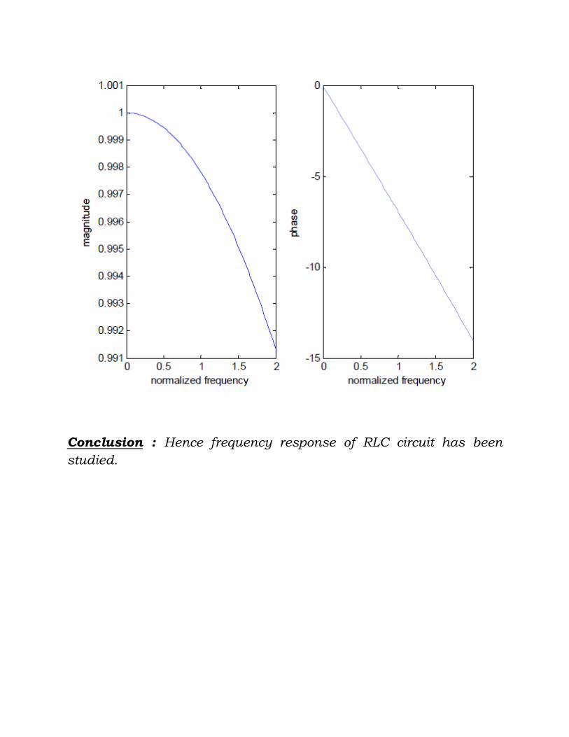
Conclusion : Hence frequency response of RLC circuit has been
studied.