jerome h. klotz february 25, 2006 · 8 contents 11.8 minimax estimation . . . . . . . . . . . . . ....
TRANSCRIPT

A Computational Approach to Statistics
Jerome H. Klotz
February 25, 2006

2
Copyright c© 2004 Jerome H. KlotzDepartment of StatisticsUniversity of Wisconsin at Madison
Acknowledgement
Great appreciation is expressed to my wife Barbara for her constant loveand support.
Sincere thanks goes to Professor Joseph L. Hodges, Jr, teacher, thesisdirector, mentor, and friend.
To professors at the University of California, Berkeley, also contributinggreatly to my education, I thank and remember with great respect: DavidBlackwell, Lucien LeCam, Erich Lehmann, Michael Loeve, Jerzy Neyman,Henry Scheffe, and Elizabeth Scott.
While writing, conversations with Rich Johnson were quite helpful.

3
Preface
GoalThe purpose of this book is to provide an introduction to statistics with an
emphasis on appropriate methods of computation with modern algorithms.We hope it will provide a useful introductory reference for persons with aneed to analyze data using computers.
Program listings are included in the appendices so that modifications andcorrections can be made as desired. Suggestions, corrections, and errors willbe appreciatively received at the e-mail address [email protected].
OrganizationTopics covered are as follows, namely:
(1) Descriptive Statistics.
(2) Discrete Probability.
(3) Random Variables
(4) Continuous Probability.
(5) The General Measure Theory Model
(6) Distribution Measures
(7) Multivariate Distributions.
(8) Characteristic Functions
(9) Asymptotics
(10) Sampling Theory for Statistics.
(11) Point Estimatiom.
(12) Hypothesis Testing.
(13) Interval Estimation.
(14) The General Linear Hypothesis.
(15) Nonparametric Methods.
Ends of proofs are labeled with .

4
Contents
1 Descriptive Statistics 151.1 Graphic Description of Data . . . . . . . . . . . . . . . . . . . 15
1.1.1 Histograms . . . . . . . . . . . . . . . . . . . . . . . . 151.1.2 Stem-and-Leaf Diagrams . . . . . . . . . . . . . . . . . 191.1.3 Boxplots . . . . . . . . . . . . . . . . . . . . . . . . . . 211.1.4 Dot Diagrams . . . . . . . . . . . . . . . . . . . . . . . 22
1.2 Measures of the Center . . . . . . . . . . . . . . . . . . . . . . 221.2.1 The Sample Median . . . . . . . . . . . . . . . . . . . 221.2.2 Some Robust Measures of the Center . . . . . . . . . . 231.2.3 The Sample Mean or Average. . . . . . . . . . . . . . . 24
1.3 Measures of Dispersion or Spread . . . . . . . . . . . . . . . . 251.3.1 The Sample Range and Interquartile Range . . . . . . 251.3.2 Mean Absolute Deviation . . . . . . . . . . . . . . . . 251.3.3 The Sample Variance . . . . . . . . . . . . . . . . . . . 25
1.4 Grouped Data . . . . . . . . . . . . . . . . . . . . . . . . . . . 271.5 Properties . . . . . . . . . . . . . . . . . . . . . . . . . . . . . 321.6 Problems . . . . . . . . . . . . . . . . . . . . . . . . . . . . . . 35
2 Discrete Probability 372.1 The Sample Space . . . . . . . . . . . . . . . . . . . . . . . . 372.2 Events . . . . . . . . . . . . . . . . . . . . . . . . . . . . . . . 38
2.2.1 Events Constructed From Other Events . . . . . . . . . 382.2.2 Event Relations . . . . . . . . . . . . . . . . . . . . . . 402.2.3 Venn Diagrams . . . . . . . . . . . . . . . . . . . . . . 422.2.4 Sigma Fields of Events . . . . . . . . . . . . . . . . . . 42
2.3 Probability . . . . . . . . . . . . . . . . . . . . . . . . . . . . 432.3.1 Defining Probability for Discrete Sample Spaces . . . . 472.3.2 Equal Probabilities in Finite Sample Spaces . . . . . . 48
5

6 CONTENTS
2.4 Conditional Probability . . . . . . . . . . . . . . . . . . . . . . 542.4.1 Independent Events . . . . . . . . . . . . . . . . . . . . 56
2.5 Problems . . . . . . . . . . . . . . . . . . . . . . . . . . . . . . 57
3 Random Variables 613.1 Discrete Random Variables . . . . . . . . . . . . . . . . . . . . 62
3.1.1 Binomial Random Variables . . . . . . . . . . . . . . . 633.1.2 Negative Binomial Random Variables . . . . . . . . . . 633.1.3 Poisson Distribution . . . . . . . . . . . . . . . . . . . 643.1.4 Hypergeometric Distribution . . . . . . . . . . . . . . . 643.1.5 Negative Hypergeometric Distribution . . . . . . . . . 653.1.6 Cumulative Distribution Functions . . . . . . . . . . . 65
3.2 Problems . . . . . . . . . . . . . . . . . . . . . . . . . . . . . . 68
4 Continuous Distributions 714.1 Continuous Density Examples . . . . . . . . . . . . . . . . . . 73
4.1.1 C.D.F. for Continuous random Variables . . . . . . . . 754.2 Problems . . . . . . . . . . . . . . . . . . . . . . . . . . . . . . 75
5 The General Case 775.1 Some Measure Theory . . . . . . . . . . . . . . . . . . . . . . 77
5.1.1 Measure Definition . . . . . . . . . . . . . . . . . . . . 775.1.2 Definition of the Integral of a Function . . . . . . . . . 785.1.3 Derivatives for Measures . . . . . . . . . . . . . . . . . 83
5.2 General Densities . . . . . . . . . . . . . . . . . . . . . . . . . 845.2.1 Conditional Expectation . . . . . . . . . . . . . . . . . 84
6 Distribution Measures 876.1 P.D.F. and C.D.F. Plots . . . . . . . . . . . . . . . . . . . . . 876.2 Measures of the Center . . . . . . . . . . . . . . . . . . . . . . 876.3 Variance . . . . . . . . . . . . . . . . . . . . . . . . . . . . . . 916.4 Problems . . . . . . . . . . . . . . . . . . . . . . . . . . . . . . 93
7 Several Random Variables 977.1 Bivariate Random Variables . . . . . . . . . . . . . . . . . . . 97
7.1.1 Marginal Densities . . . . . . . . . . . . . . . . . . . . 1027.1.2 Conditional Densities . . . . . . . . . . . . . . . . . . . 103
7.2 Several Random Variables . . . . . . . . . . . . . . . . . . . . 105

CONTENTS 7
7.2.1 Discrete Multivariate Distributions . . . . . . . . . . . 1057.2.2 Continuous Multivariate Distributions . . . . . . . . . 106
7.3 Problems . . . . . . . . . . . . . . . . . . . . . . . . . . . . . . 107
8 Characteristic Functions 1098.1 Univariate Characteristic Functions . . . . . . . . . . . . . . . 1098.2 Multivariate Characteristic Functions . . . . . . . . . . . . . 116
8.2.1 Conditional Characteristic Functions . . . . . . . . . . 1198.3 Problems . . . . . . . . . . . . . . . . . . . . . . . . . . . . . . 120
9 Asymptotics 1239.1 Random Variable Convergences . . . . . . . . . . . . . . . . . 1239.2 Laws of Large Numbers. . . . . . . . . . . . . . . . . . . . . . 1319.3 Central Limit Theorems. . . . . . . . . . . . . . . . . . . . . . 1379.4 Problems. . . . . . . . . . . . . . . . . . . . . . . . . . . . . . 139
10 Sampling Theory for Statistics 14110.1 Transformations of Variables . . . . . . . . . . . . . . . . . . . 141
10.1.1 The Continuous Case . . . . . . . . . . . . . . . . . . . 14110.1.2 The Discrete Case . . . . . . . . . . . . . . . . . . . . 146
10.2 Order Statistics . . . . . . . . . . . . . . . . . . . . . . . . . . 14710.3 Linear Transformations . . . . . . . . . . . . . . . . . . . . . . 14810.4 The Convolution Integral . . . . . . . . . . . . . . . . . . . . . 14810.5 Distribution of X and S2 for Xi Independent N (µ, σ2). . . . 14910.6 Student’s t and Fisher’s F Distribution . . . . . . . . . . . . . 15010.7 Noncentral Distributions . . . . . . . . . . . . . . . . . . . . . 15210.8 Chi square distribution of XTΣ−X . . . . . . . . . . . . . . . 15510.9 Problems . . . . . . . . . . . . . . . . . . . . . . . . . . . . . . 156
11 Point Estimation 15911.1 Sufficient Statistics . . . . . . . . . . . . . . . . . . . . . . . . 15911.2 Completeness . . . . . . . . . . . . . . . . . . . . . . . . . . . 16511.3 Exponential Families . . . . . . . . . . . . . . . . . . . . . . . 16611.4 Minimum Variance Unbiased Estimation . . . . . . . . . . . . 16811.5 Cramer-Rao-Frechet Information Lower Bound . . . . . . . . . 17811.6 Maximum Likelihood Estimation . . . . . . . . . . . . . . . . 183
11.6.1 Properties of Maximum Likelihood Estimators . . . . . 18411.7 Bayes Point Estimators . . . . . . . . . . . . . . . . . . . . . . 197

8 CONTENTS
11.8 Minimax Estimation . . . . . . . . . . . . . . . . . . . . . . . 20211.9 Problems . . . . . . . . . . . . . . . . . . . . . . . . . . . . . . 206
12 Hypothesis Testing 21112.1 Simple Hypotheses . . . . . . . . . . . . . . . . . . . . . . . . 21212.2 Composite Hypotheses . . . . . . . . . . . . . . . . . . . . . . 214
12.2.1 Distributions with Monotone Likelihood Ratio . . . . . 21412.2.2 U.M.P. One Sided Tests . . . . . . . . . . . . . . . . . 21412.2.3 P-Values . . . . . . . . . . . . . . . . . . . . . . . . . . 21712.2.4 Least Favorable Priors . . . . . . . . . . . . . . . . . . 21712.2.5 U.M.P.Unbiased Tests . . . . . . . . . . . . . . . . . . 21912.2.6 P-values for UMPU Tests . . . . . . . . . . . . . . . . 228
12.3 Generalized Likelihood Ratio Test −2 log(Λ). . . . . . . . . . . 23112.4 Conditional Generalized Likelihood Ratio Test . . . . . . . . . 24312.5 Problems . . . . . . . . . . . . . . . . . . . . . . . . . . . . . . 247
13 Interval Estimation 24913.1 Confidence Intervals . . . . . . . . . . . . . . . . . . . . . . . 24913.2 Bayesian Intervals . . . . . . . . . . . . . . . . . . . . . . . . . 25513.3 Problems . . . . . . . . . . . . . . . . . . . . . . . . . . . . . . 256
14 The General Linear Hypothesis 25714.1 Least Square, M.L.,and UMVU Estimates of β . . . . . . . . . 25714.2 The UMVU Estimator for σ2 . . . . . . . . . . . . . . . . . . 25914.3 The Linear Hypothesis . . . . . . . . . . . . . . . . . . . . . . 25914.4 Latin Squares . . . . . . . . . . . . . . . . . . . . . . . . . . . 26414.5 Unbalanced Multifactor ANOVA . . . . . . . . . . . . . . . . 265
14.5.1 An Example . . . . . . . . . . . . . . . . . . . . . . . . 27314.5.2 Scheffe’s Multiple Comparisons Method . . . . . . . . . 279
14.6 Analysis of Covariance . . . . . . . . . . . . . . . . . . . . . . 28114.6.1 An Example . . . . . . . . . . . . . . . . . . . . . . . . 283
14.7 Problems . . . . . . . . . . . . . . . . . . . . . . . . . . . . . . 285
15 Nonparametric Methods 28715.1 The Sign Test . . . . . . . . . . . . . . . . . . . . . . . . . . . 287
15.1.1 Confidence Interval for the Median . . . . . . . . . . . 28915.1.2 Point Estimate for the Median . . . . . . . . . . . . . . 29015.1.3 Small Sample Performance Comparisons . . . . . . . . 292

CONTENTS 9
15.1.4 Large Sample Performance Comparisons . . . . . . . . 29315.1.5 Efficiency of the Median Point Estimator . . . . . . . . 295
15.2 The Wilcoxon Signed Rank Test . . . . . . . . . . . . . . . . . 29715.2.1 Null Distribution of W+ . . . . . . . . . . . . . . . . . 29815.2.2 Zeros and Ties . . . . . . . . . . . . . . . . . . . . . . 29915.2.3 Wilcoxon Point Estimate for the Center of Symmetry . 30215.2.4 Efficiency of W+ . . . . . . . . . . . . . . . . . . . . . 303
15.3 The Two Sample Median Test . . . . . . . . . . . . . . . . . . 30415.3.1 Confidence Interval for a Difference in Location Pa-
rameters . . . . . . . . . . . . . . . . . . . . . . . . . . 30515.3.2 Efficiency of the Mood and Brown Test . . . . . . . . . 306
15.4 The Two Sample Wilcoxon Rank Test . . . . . . . . . . . . . 30715.4.1 Null Distribution of UY X . . . . . . . . . . . . . . . . . 30715.4.2 Distribution of UY X in the Presence of Ties . . . . . . 30915.4.3 Confidence Intervals for a Location Difference . . . . . 31215.4.4 Efficiency of the Two Sample Wilcoxon . . . . . . . . . 314
15.5 Mood and Brown Median Test for K Samples . . . . . . . . . 31515.5.1 The Exact Null Distrbution of B2 . . . . . . . . . . . . 31515.5.2 Large Sample Null Distribution Approxination . . . . . 31915.5.3 Liniting Pitman efficiency of B2 . . . . . . . . . . . . . 320
15.6 The Kruskal Wallis H Test . . . . . . . . . . . . . . . . . . . . 32015.6.1 Null Distribution of H . . . . . . . . . . . . . . . . . . 32115.6.2 Null Distribution of H with Ties . . . . . . . . . . . . . 32115.6.3 Limiting Pitman efficiency of the H test . . . . . . . . 326
15.7 Two Way Rank Tests . . . . . . . . . . . . . . . . . . . . . . . 32615.7.1 Benard and van Elteren test . . . . . . . . . . . . . . . 32615.7.2 Friedman’s test . . . . . . . . . . . . . . . . . . . . . . 32915.7.3 Durban’s test . . . . . . . . . . . . . . . . . . . . . . . 33115.7.4 Efficiency of V. . . . . . . . . . . . . . . . . . . . . . . 337
15.8 Problems . . . . . . . . . . . . . . . . . . . . . . . . . . . . . . 337
A Subroutine cdf.h. 339
B Program normal.h 345
C Program Regress.cpp 347
D Program test.cpp 353

10 CONTENTS
E Program Pvalue.cpp 355
F Program rxcIndep.cpp 363
G Program OneVar.cpp 369
H Program TwoVar.cpp 373
I Program multiway.cpp 377
J Subroutine Wilcox.h 397
K Program sRank.cpp 401
L Subroutine MannW.h 407
M Program RankSum.cpp 413
N Program Mood.cpp 419
O Program HTest.cpp 437
P Program BenVanElt.cpp 449
Q Program Friedman.cpp 461
R Durban.cpp 471

List of Figures
1.1 Histogram for Lake Mendota Freezing Data. . . . . . . . . . . 171.2 Histogram for Lake Mendota Thawing Data. . . . . . . . . . . 191.3 Boxplot . . . . . . . . . . . . . . . . . . . . . . . . . . . . . . 211.4 Boxplot for Mendota Thawing Data . . . . . . . . . . . . . . . 221.5 A Dot Diagram. . . . . . . . . . . . . . . . . . . . . . . . . . . 22
2.1 Venn Diagrams . . . . . . . . . . . . . . . . . . . . . . . . . . 422.2 Conditional Space . . . . . . . . . . . . . . . . . . . . . . . . . 55
3.1 Lot Partition for Hypergeometric . . . . . . . . . . . . . . . . 65
4.1 Discrete Triangular p.d.f. . . . . . . . . . . . . . . . . . . . . . 724.2 Continuous Triangular Density . . . . . . . . . . . . . . . . . . 724.3 Normal N (0, 1) Density . . . . . . . . . . . . . . . . . . . . . 76
6.1 Binomial p.d.f. . . . . . . . . . . . . . . . . . . . . . . . . . . 946.2 Hypergeometric p.d.f. . . . . . . . . . . . . . . . . . . . . . . . 946.3 Negative Binomial p.d.f. . . . . . . . . . . . . . . . . . . . . . 956.4 Poison p.d.f. . . . . . . . . . . . . . . . . . . . . . . . . . . . . 956.5 Negative Binomial c.d.f. . . . . . . . . . . . . . . . . . . . . . 966.6 Binomial c.d.f. . . . . . . . . . . . . . . . . . . . . . . . . . . . 96
7.1 Bivariate Hypergeometric p.d.f . . . . . . . . . . . . . . . . . . 997.2 Bivariate Normal N2(0, I2) Density. . . . . . . . . . . . . . . . 101
8.1 Complex Variable Path for Cauchy . . . . . . . . . . . . . . . 116
10.1 Jacobean Illustration . . . . . . . . . . . . . . . . . . . . . . . 14210.2 Example of a Transform Region . . . . . . . . . . . . . . . . . 144
11

12 LIST OF FIGURES

List of Tables
1.2 Lake Mendota Freezing Dates . . . . . . . . . . . . . . . . . . 161.3 Data for Freezing Dates Histogram . . . . . . . . . . . . . . . 161.4 Lake Mendota Thawing Dates . . . . . . . . . . . . . . . . . . 181.5 Data for Thawing Dates Histogram . . . . . . . . . . . . . . . 181.6 Stem-and-Leaf Diagram for Freezing Data . . . . . . . . . . . 201.7 Stem-and-leaf Diagram for Thawing Data . . . . . . . . . . . 20
12.1 Test Data . . . . . . . . . . . . . . . . . . . . . . . . . . . . . 245
14.1 5× 5 Latin Square . . . . . . . . . . . . . . . . . . . . . . . . 26514.2 Unbalanced 3 Factor Data . . . . . . . . . . . . . . . . . . . . 27314.3 Main Effects Calculation . . . . . . . . . . . . . . . . . . . . . 27414.4 V12 and Y·(i1, i2, ·). . . . . . . . . . . . . . . . . . . . . . . . . 27514.5 Contrast Coefficients . . . . . . . . . . . . . . . . . . . . . . . 280
15.1 Sign Test Efficiency . . . . . . . . . . . . . . . . . . . . . . . . 29315.2 Sign Test Limiting Efficiency . . . . . . . . . . . . . . . . . . . 29515.3 Median Efficiency . . . . . . . . . . . . . . . . . . . . . . . . . 29615.4 2nP [W+ = w] for n = 1(1)12, w = 0(1)15. . . . . . . . . . . . 29915.5 Limiting Efficiency of W+ . . . . . . . . . . . . . . . . . . . . 30415.6 Mood and Brown Test Limiting Efficiency . . . . . . . . . . . 307
13

14 LIST OF TABLES

Chapter 1
Descriptive Statistics
1.1 Graphic Description of Data
1.1.1 Histograms
Consider a data collection of size n and denote them by X1, X2, . . . , Xn.A graphical description, called a histogram, can be constructed by selectinga collection of class intervals of the form [ak−1, ak) = x : ak−1 ≤ x < akwhere a1 < a2 < . . . < aK are numbers, and plotting bars over the intervalsproportional to the number of data values nk in the kth interval. In case theclass intervals are not of equal length, we adjust the bar height hk for thekth interval to take that into account. To be precise, we can construct thefollowing table:
Table 1.1: Histogram Data
Class Interval Length Count Proportion Bar Height[a0, a1) L1 = a1 − a0 n1 p1 = n1/n h1 = p1/L1
[a1, a2) L2 = a2 − a1 n2 p2 = n2/n h2 = p2/L2
. . . . . . . . . . . . . . .[aK−1, aK) LK = aK − aK−1 nK pK = nK/n hK = pK/LK
Note that n1 +n2 + · · ·+nK = n the total number, provided all the data arebetween a0 and aK .
15

16 CHAPTER 1. DESCRIPTIVE STATISTICS
To illustrate, consider the following n = 111 data values in table 1 corre-sponding to coded freezing dates of Lake Mendota in Madison Wisconsin:
Table 1.2: 111 Freezing Dates for Lake Mendota 1855-1965.November 23 coded 0, . . ., January 30 coded 68.
25 13 2 15 14 21 9 33 25 15 21 25 19 17 9 3126 7 6 17 48 15 44 28 24 0 40 17 25 24 19 1231 40 52 33 34 23 11 35 43 28 24 16 34 32 22 3220 21 39 27 39 29 25 16 35 31 50 23 35 23 18 4116 32 32 23 39 26 23 13 24 28 10 23 68 17 32 3127 43 14 35 40 43 41 14 23 25 20 37 28 31 30 1823 37 37 40 19 21 37 16 36 26 23 19 27 22 49
If we select class intervals [0,10), [10,20), . . ., [60,70) we get the followingtable:
Table 1.3: Data for Freezing Dates Histogram
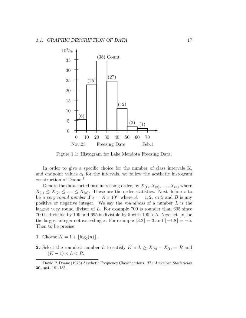
Class Interval Length Count Proportion Bar Height[ 0,10) 10 6 0.054 0.0054[10,20) 10 25 0.225 0.0225[20,30) 10 38 0.342 0.0342[30,40) 10 27 0.243 0.0243[40,50) 10 12 0.108 0.0108[50,60) 10 2 0.018 0.0018[60,70) 10 1 0.009 0.0009
1.1. GRAPHIC DESCRIPTION OF DATA 17
-
6
0 10 20 30 40 50 60 70
0
5
10
15
20
25
30
35
103hk
(6)
(25)
(38) Count
(27)
(12)
(2) (1)
Freezing DateNov.23 Feb.1
Figure 1.1: Histogram for Lake Mendota Freezing Data.
In order to give a specific choice for the number of class intervals K,and endpoint values ak for the intervals, we follow the aesthetic histogramconstruction of Doane.1
Denote the data sorted into increasing order, by X(1), X(2), . . . , X(n) whereX(1) ≤ X(2) ≤ . . . ≤ X(n). These are the order statistics. Next define x tobe a very round number if x = A × 10B where A = 1, 2, or 5 and B is anypositive or negative integer. We say the roundness of a number L is thelargest very round divisor of L. For example 700 is rounder than 695 since700 is divisible by 100 and 695 is divisible by 5 with 100 > 5. Next let ⌊x⌋ bethe largest integer not exceeding x. For example ⌊3.2⌋ = 3 and ⌊−4.8⌋ = −5.Then to be precise
1. Choose K = 1 + ⌊log2(n)⌋.
2. Select the roundest number L to satisfy K × L ≥ X(n) − X(1) = R and(K − 1)× L < R.
1David P. Doane (1976) Aesthetic Frequency Classifications. The American Statistician30, #4, 181-183.

18 CHAPTER 1. DESCRIPTIVE STATISTICS
3. Choose the roundest number a0 that satisfies a0 ≤ X(1) andX(n) < a0 +K × L.
4. Let ak = a0 + k × L for k = 0, 1, . . .K.
Consider the following n = 111 data values.
Table 1.4: 111 Thawing Dates for Lake Mendota 1855-1965. Nov. 23↔ 0.
143 164 123 111 124 138 141 137 150 133 146 148 129 144 140 130152 151 142 143 139 145 106 140 123 161 118 141 144 148 147 143144 128 127 144 131 135 112 136 134 138 124 146 145 139 127 121146 129 136 121 122 135 123 117 143 130 138 138 137 139 133 123126 113 128 148 143 147 147 116 130 124 117 121 133 132 123 125128 141 119 132 145 139 123 130 137 117 118 138 132 127 139 140137 149 122 132 133 132 132 142 141 134 140 131 140 142 114
We illustrate the above four rules for constructing an aesthetic histogramwith the data from table 1.3.
1. K = 1 + ⌊log2(111)⌋ .= 1 + ⌊6.794⌋ = 7.
2. The roundest L satisfying 7L ≥ 164− 106 = 58 and 6L < 58 is L = 9.
3. The roundest a0 satisfying a0 ≤ 106 and 164 < a0 + 63 is a0 = 105.
4. ak = 105 + 9k for k = 0, 1, . . . , 7.
Table 1.5: Data for Thawing Dates Histogram
Class Interval Length Count Proportion Bar Height[105,114) 9 4 0.0360 0.0040[114,123) 9 13 0.1171 0.0130[123,132) 9 25 0.2252 0.0250[132,141) 9 35 0.3153 0.0350[141,150) 9 29 0.2613 0.0290[150,159) 9 3 0.0270 0.0030[159,168) 9 2 0.0180 0.0020

1.1. GRAPHIC DESCRIPTION OF DATA 19
-
6
105 114 123 132 141 150 159 168
0
5
10
15
20
25
30103hk
(4)
(13)
(25)
(35) Count
(29)
(3) (2)
Thawing DateFeb.26 Apr.30
Figure 1.2: Histogram for Lake Mendota Thawing Data.
1.1.2 Stem-and-Leaf Diagrams
A stem-and-leaf diagram is a variation of the histogram in which the leadingdigits of the data values take the place of the class intervals and the loworder digit is used to build the bar height. The stem-and-leaf diagram canreconstruct the order statistics. To illustrate the stem-and-leaf diagram forthe freezing data, see table 1.6.
To subdivide the class intervals we can break the high order digits forthe stem in two parts by listing low order digits 0,1,2,3,4 on one line and5,6,7,8,9 on the next line. To illustrate for the thawing data, see table 1.7.
Subdivision into 5 parts uses 5 stems for 0,1, 2,3,4,5,6,7,and8,9 respectively.

20 CHAPTER 1. DESCRIPTIVE STATISTICS
Table 1.6: Stem-and-Leaf Diagram for Freezing Data
Stem Leaf0 0267991 01233444555666677778899992 00111122333333333444455555666777888893 0111112222233445555677779994 0000113334895 026 8
Table 1.7: Stem-and-leaf Diagram for Thawing Data
Stem Leaf1010 611 123411 677788912 1112233333344412 567778889913 00001122222233334413 55667777888889999914 00000111122233333444414 555666777888915 0121516 1416

1.1. GRAPHIC DESCRIPTION OF DATA 21
1.1.3 Boxplots
To define a boxplot, we first define sample percentiles.Definition. The 100p-th percentile is a value x such that the number of datavalues less than or equal x is at least n× p and the number of observationsgreater than or equal x is at least n× (1− p).
The 25th, 50th, and 75th percentiles are the lower (first) quartile, thesecond quartile (or median), and the upper (third) quartile. respectively.They are sometimes denoted Q1, Q2 (or X), and Q3.
We define percentiles in terms of order statistics where the 100p-th per-centile is, for integer r,
Zp =
X(r) if r > np and n− r + 1 > n(1− p)
(X(r) +X(r+1))/2 if r = np
The median, often denoted X, is defined by
X =
X(k+1) for odd n = 2k + 1
(X(k) +X(k+1))/2 for even n = 2k
to be the middle or the average of the two middle data values after sorting.It is the 50th percentile using the interpolated definition.
We now can define a boxplot in terms of X(1), Q1, X, Q3, and X(n).
u uX(1) Q1 X Q3 X(n)
Figure 1.3: Boxplot Using Quartiles.
To illustrate for the Mendota thawing data, we have X(1) = 106, Q1 = 126,
X = 135, Q3 = 142 and X(111) = 164 and the box plot is:

22 CHAPTER 1. DESCRIPTIVE STATISTICS
u u106 126 135 142 164
Figure 1.4: Boxplot for Mendota Thawing Data
1.1.4 Dot Diagrams
A dot diagram consists of dots placed on a line at locations correspondingto the value of each observation Xi for i = 1, 2, . . . , n. For example, if thesorted data values are:1.2, 2.3, 2.7, 2.7, 3.4, 3.6, 3.8, 3.8, 3.8, 3.8, 4.2, 4.2, 4.9, 5.4, 5.4, 6.1,7.2then the corresponding dot diagram is:
1 2 3 4 5 6 7 8
u u u
u
uuu
u
u
u
u
u
u u
u
u u
↑
Figure 1.5: A Dot Diagram.
1.2 Measures of the Center
1.2.1 The Sample Median
Recall, the median X is defined by
X =
X(k+1) for odd n = 2k + 1
(X(k) +X(k+1))/2 for even n = 2k
to be the middle or the average of the two middle data values after sorting.It is the 50th percentile using the percentile definition. At least 50% of the

1.2. MEASURES OF THE CENTER 23
data values are less than or equal the median and at least 50% are greaterthan or equal the median. It is a stable measure of the center in that it isnot much affected by an extreme value.
There are algorithms for calculating the median that are somewhat fasterthan a sorting algorithm (O(n) vs. O(n logn). However, because of readyaccess to sorting algorithms such as quicksort, it seems simpler to calculateby sorting to obtain the order statistics and then select the middle one(s).
1.2.2 Some Robust Measures of the Center
The r-trimmed mean is designed to protect against a few wild observationsand is defined by
Tr =X(r+1) +X(r+2) + · · ·+X(n−r−1) +X(n−r)
(n− 2r)
It trims r observations from of each end of the sorted observations and aver-ages the remaining values.
A modification is the r-Winsorized mean defined by
Wr =(r + 1)X(r+1) +X(r+2) + · · ·+X(n−r−1) + (r + 1)X(n−r)
n.
It replaces the r smallest observations by X(r+1) and the r largest values byX(n−r) and then averages.
Another robust estimator of the center is the Walsh sum median definedby first calculating all n(n + 1)/2 Walsh sums
(Xi +Xj)
2for 1 ≤ i ≤ j ≤ n
and then calculating the median
M = median(Xi +Xj)/2 : 1 ≤ i ≤ j ≤ n.The Walsh sums are obtained from the following triangular array
Xi+Xj
2X1 X2 X3 . . . Xn−1 Xn
X1 X1X1+X2
2X1+X3
2. . . X1+Xn−1
2X1+Xn
2
X2 X2X2+X3
2. . . X2+Xn−1
2X2+Xn
2
X3 X3 . . . X3+Xn−1
2X3+Xn
2...
. . ....
...
Xn−1 Xn−1Xn−1+Xn
2
Xn Xn

24 CHAPTER 1. DESCRIPTIVE STATISTICS
and then sorted to find the median M of these n(n+ 1)/2 values.To illustrate the calculation of these three robust estimators consider the
ten values4.7, 1.2, 10.2, 6.2, 10.9, 1.4, 5.8, 1.1, 10.8, 5.1Then the 2-trimmed mean is
T2 =1.4 + 4.7 + 5.1 + 5.8 + 6.2 + 10.2
6
.= 5.567 .
The 3-Winsorized mean is
W3 =4× 4.7 + 5.1 + 5.8 + 4× 6.2
10.= 5.450 .
To calculate the Walsh sum median we first calculate the 55 Walsh sums:
Xi+Xj
24.7 1.2 10.2 6.2 10.9 1.4 5.8 1.1 10.8 5.1
4.7 4.70 2.95 7.45 5.45 7.80 3.05 5.25 2.90 7.75 4.901.2 1.20 5.70 3.70 6.05 1.30 3.50 1.15 6.00 3.15
10.2 10.20 8.20 10.55 5.80 8.00 5.65 10.50 7.656.2 6.20 8.55 3.80 6.00 3.65 8.50 5.65
10.9 10.90 6.15 8.35 6.00 10.85 8.001.4 1.40 3.60 1.25 6.10 3.255.8 5.80 3.45 8.30 5.451.1 1.10 5.95 3.10
10.8 10.8 7.955.1 5.10
The sorted Walsh sums are1.1, 1.15, 1.2, 1.25, 1.3, 1.4, 2.9, 2.95, 3.05, 3.1, 3.15, 3.25, 3.45, 3.5, 3.6, 3.65,3.7, 3.8, 4.7, 4.9, 5.1, 5.25, 5.45, 5.45, 5.65, 5.65, 5.7, 5.8, 5.8, 5.95, 6, 6, 6,6.05, 6.1, 6.15, 6.2, 7.45, 7.65, 7.75, 7.8, 7.95, 8, 8, 8.2, 8.3, 8.35, 8.5, 8.55,10.2, 10.5, 10.55, 10.8, 10.85, 10.9and the Walsh sum median is the middle value M = 5.8.
1.2.3 The Sample Mean or Average.
The most commonly used measure of the center is the sample mean or sampleaverage defined by
X =X1 +X2 + · · ·+Xn
n=
∑ni=1Xi
n.

1.3. MEASURES OF DISPERSION OR SPREAD 25
If we put unit weights for each dot in the dot diagram, then the point ofbalance of the system of weights is at X. For the dot diagram in figure 1.5,X = 4.0294 as indicated by the arrow ↑. In contrast to the median andother robust estimators, the sample mean can be greatly affected by a singleextreme value.
1.3 Measures of Dispersion or Spread
1.3.1 The Sample Range and Interquartile Range
The sample range is defined as the difference of the largest and smallestvalues. In terms of the order statistics,
R = X(n) −X(1).
The interquartile range is defined by the difference of the third and firstquartiles,
IQR = Q3 −Q1.
The larger the range values, the more dispersed are the data values.
1.3.2 Mean Absolute Deviation
The mean absolute deviation about the sample median is defined by
D =1
n
n∑
i=1
|Xi − X|.
Sometimes the sample mean X is used instead of the sample median X butthen the measure is larger.
1.3.3 The Sample Variance
The most commonly used measure of spread is the sample variance definedby
S2 =
∑ni=1(Xi − X)2
n− 1. (1.1)

26 CHAPTER 1. DESCRIPTIVE STATISTICS
The square root S = (S2)1/2 is called the sample standard deviation.Other equations which are formally equivalent but have different numericalaccuracy are
S2 =(∑n
i=1X2i )− nX2
n− 1(1.2)
S2 =(∑n
i=1(Xi − C)2)− n(X − C)2
n− 1(1.3)
for any constant C.Finally, if we write S2 = S2[n] and X = X[n] to indicate the number ofvalues used in the calculation, we have update equations
S2[n] =(n− 2)
(n− 1)S2[n− 1] +
1
n(X[n− 1]−Xn)2 (1.4)
X[n] =Xn +
∑n−1i=1 Xi
n=Xn + (n− 1)X[n− 1]
n
with starting values S2[1] = 0, X[1] = X1.
Equation (1.1) is an accurate method of calculating S2 but requires twopasses through the data. The first pass is used to calculate X, and the secondto calculate S2 using X.
Equation (1.2) is often used by programmers to calculate S2 since it onlyrequires one pass through the data. Unfortunately, it can be inaccurate dueto subtraction of quantities with common leading digits (
∑X2
i and nX2).
A more accurate one pass method uses equation (1.4) although it isslightly more complicated to program.
Equation (1.3) is useful for data with many common leading digits. Forexample, using the values (1000000001, 1000000002, 1000000003), we can takeC = 1000000000 in (1.3) and calculate S2 = 1, Many pocket calculators failto get the correct answer for such values because of the use of equation (1.2).
To illustrate each calculation, consider the data (X1, X2, . . . , Xn) =(2.0, 1.0, 4.0, 3.0, 5.0).
For equation (1.1) we first calculate X = (2 + 1 + 4 + 3 + 5)/5 = 3 andthen
S2 =(2− 3)2 + (1− 3)2 + (4− 3)2 + (3− 3)2 + (5− 3)2
(5− 1)=
10
4= 2.5 .

1.4. GROUPED DATA 27
For equation (1.2) we have
S2 =(22 + 12 + 42 + 32 + 52)− (5× 32)
(5− 1)=
55− 45
4= 2.5 .
Using an arbitrary constant C = 4 equation (1.3) gives
S2 =[(2− 4)2 + (1− 4)2 + (4− 4)2 + (3− 4)2 + (5− 4)2]− [5× (3− 4)2]
(5− 1)
=15− 5
4= 2.5 .
For equation (1.4) starting with n = 1 and updating for n = 2, 3, 4, 5 weget
n = 1
X[1] = 2S2[1] = 0
n = 2
X[2] = (1 + 2)/2 = 1.5S2[2] = 0 + (1/2)(2− 1)2 = 0.5
n = 3
X[3] = (4 + 2× 1.5)/3 = 7/3S2[3] = (1/2)0.5 + (1/3)(1.5− 4)2 = 7/3
n = 4
X[4] = (3 + 3× 7/3)/4 = 2.5S2[4] = (2/3)7/3 + (1/4)(7/3− 3)2 = 5/3
n = 5
X[5] = (5 + 4× 2.5)/4 = 3S2[5] = (3/4)5/3 + (1/5)(2.5− 5)2 = 2.5
(1.5)
1.4 Grouped Data
Sometimes there are many repetitions of data values and it is more convenientto represent the data in a table that gives the values and their counts asfollows:
value x1 x2 . . . xK
counts n1 n2 . . . nK
where x1 < x2 < · · · < xK and n1 + n2 + · · ·+ nK = n. The sample medianis then
X =
xr if
∑ri=1 ni > n/2 and
∑Ki=r ni > n/2
(xr + xr+1)/2 if∑r
i=1 ni = n/2.(1.6)

28 CHAPTER 1. DESCRIPTIVE STATISTICS
To calculate the r-trimmed mean and r-Winsorized mean for grouped datadetermine integers (s, t) for r < n/2 where 0 ≤ s < t ≤ K,∑s
i=1 ni ≤ r <∑s+1
i=1 ni, and∑K
i=t+1 ni ≤ r <∑K
i=t ni. Then
Tr =[(∑s+1
i=1 ni)− r]xs+1 + ns+2xs+2 + · · ·+ nt−1xt−1 + [(∑K
i=t ni)− r]xt
n− 2r(1.7)
Wr =(∑s+1
i=1 ni)xs+1 + ns+2xs+2 + · · ·+ nt−1xt−1 + (∑K
i=t ni)xt
n. (1.8)
For the Walsh sum median for grouped data, we construct the uppertriangular table of Walsh sum values wij = (xi+xj)/2 : for 1 ≤ i ≤ j ≤ K
(xi + xj)/2 x1 x2 x3 . . . xK
x1 x1 (x1 + x2)/2 (x1 + x3)/2 . . . (x1 + xK)/2x2 x2 (x2 + x3)/2 . . . (x2 + xK)/2x3 x3 . . . (x3 + xK)/2...
. . ....
xK xK
These values are repeated with counts nij = ni(ni + 1)/2 for i = j andnij = ninj for i < j:
counts n1 n2 n3 . . . nK
n1 n1(n1 + 1)/2 n1n2 n1n3 . . . n1nK
n2 n2(n2 + 1)/2 n2n3 . . . n2nK
n3 n3(n3 + 1)/2 . . . n3nK...
. . ....
nK nK(nK + 1)/2
We then sort the N = K(K + 1)/2 Walsh sum values wij along with theircounts nij to get
sorted Walsh sums w(1) w(2) . . . w(N)
corresponding counts m1 m2 . . . mN
We then calculate the median M using equation (1.6) applied to this tableof values and counts. Note w(1) = x1, m1 = n1(n1 +1)/2, w(2) = (x1 +x2)/2,m2 = n1n2, . . . , w(N−1) = (xK−1 + xK)/2, mN−1 = nK−1nK , w(N) = xK ,mN = nK(nK + 1)/2. The rest of the values must be determined by sorting.

1.4. GROUPED DATA 29
We have the identity
K∑
i=1
ni(ni + 1)
2+
K−1∑
i=1
K∑
j=i
ninj =
K∑
i=1
ni
2+
1
2
K∑
i=1
K∑
j=1
ninj =n(n + 1)
2
so that the count of the total number of Walsh sums agrees with that for theungrouped case.
The sample mean for grouped data is the weighted average
X =n1x1 + n2x2 + · · ·+ nKxK
n. (1.9)
For measures of spread the sample range is R = xK − x1 and the in-terquartile range is IQR = Q3 −Q1 where Q1 is the 25th percentile and Q3
is the 75th percentile. For grouped data, we define a 100p-th percentile by
Zp =
xr if
∑ri=1 ni > np and
∑Ki=r ni > n(1− p)
(xr + xr+1)/2 if∑r
i=1 ni = np .
Then Q1 = Z.25 and Q3 = Z.75
The mean absolute deviation about the median for grouped data is
D =
∑Ki=1 |ni(xi − X)|
n
where X is calculated from equation (1.6).To calculate S2 for grouped data we have formulae corresponding to equa-
tions (1.1), (1.2), (1.3), and (1.4) for ungrouped data.
S2 =
∑Ki=1 ni(xi − X)2
n− 1(1.10)
S2 =(∑K
i=1 nix2i )− nX2
n− 1(1.11)
S2 =(∑K
i=1 ni(xi − C)2)− n(X − C)2
n− 1(1.12)
where X is calculated from equation (1.9).For the update equation, write
S2k =
∑ki=1 ni(xi − Xk)2
Nk − 1

30 CHAPTER 1. DESCRIPTIVE STATISTICS
where
Xk =
∑ki=1 nixi
Nk , Nk =k∑
i=1
ni .
Then S2 = S2K, X = XK, n = NK, and
Xk = (nkxk +Nk − 1Xk − 1)/Nk
S2k =
(Nk − 1 − 1
Nk − 1
)S2k − 1+
nkNk − 1Nk(Nk − 1)
(Xk − 1 − xk)2
(1.13)for k = 1, 2, . . . , K with starting values S21 = 0, X1 = x1, N1 = n1 .
To illustrate calculations for grouped data, consider the table
value 1.2 1.7 5.8 6.7 11.2 12.1count 3 4 8 10 6 2
Then the medianX = 6.7
from equation (1.6) with r = 4 since 3 + 4 + 8 + 10 = 25 > 33 × 0.5 and10 + 6 + 2 > 33× 0.5.
The 5-trimmed mean is
T5 =2× 1.7 + 8× 5.8 + 10× 6.7 + 3× 11.2
23.= 6.539
from equation (1.7).The 7-Winsorized mean is
W7 =15× 5.8 + 10× 6.7 + 8× 11.2
33.= 7.382
from equation (1.8).To calculate the Walsh sum median we set up the arrays of values and
countsxi+xj
21.2 1.7 5.8 6.7 11.2 12.1
1.2 1.2 1.45 3.5 3.95 6.2 6.651.7 1.7 3.75 4.2 6.45 6.95.8 5.8 6.25 8.5 8.956.7 6.7 8.95 9.4
11.2 11.2 11.6512.1 12.1

1.4. GROUPED DATA 31
counts 3 4 8 10 6 23 6 12 24 30 18 64 10 32 40 24 88 36 80 48 16
10 55 60 206 21 122 3
We then sort the values, carrying along the corresponding counts to get thetable
value 1.2 1.45 1.7 3.5 3.75 3.95 4.2 5.8 6.2 6.25 6.45count 6 12 10 24 32 30 40 36 18 80 24
value 6.65 6.7 6.9 8.5 8.95 8.95 9.4 11.2 11.65 12.1count 6 55 8 48 16 60 20 21 12 3
from which the median is M = 6.25 for these sorted Walsh sums.The sample mean is
X =3× 1.2 + 4× 1.7 + 8× 5.8 + 10× 6.7 + 6× 11.2 + 2× 12.1
33.= 6.521 .
For measures of spread we have
R = 12.1− 1.2 = 10.9
IQR = 6.7− 5.8 = 0.9
D =
K∑
i=1
ni|xi − X|/n .= 2.4697 .
To calculate S2 using equations (1.10), (1.11), or (1.12) we obtain
S2 .= 11.74985
32 CHAPTER 1. DESCRIPTIVE STATISTICS
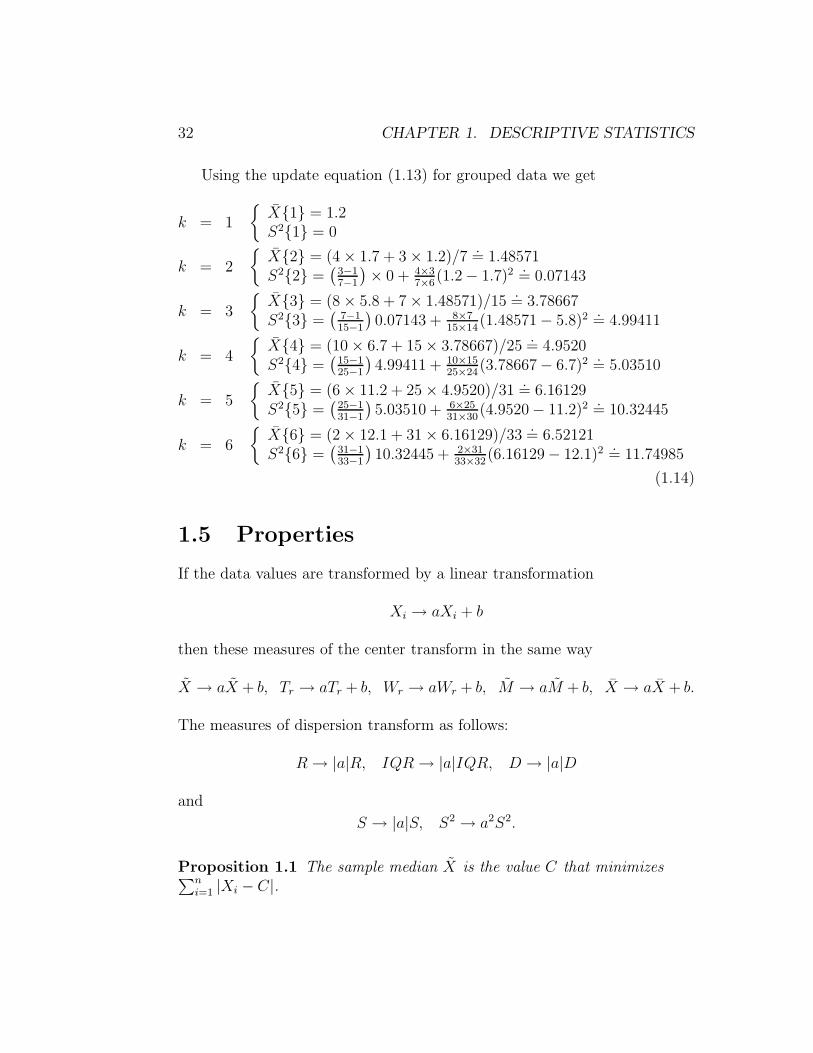
Using the update equation (1.13) for grouped data we get
k = 1
X1 = 1.2S21 = 0
k = 2
X2 = (4× 1.7 + 3× 1.2)/7
.= 1.48571
S22 =(
3−17−1
)× 0 + 4×3
7×6(1.2− 1.7)2 .
= 0.07143
k = 3
X3 = (8× 5.8 + 7× 1.48571)/15
.= 3.78667
S23 =(
7−115−1
)0.07143 + 8×7
15×14(1.48571− 5.8)2 .
= 4.99411
k = 4
X4 = (10× 6.7 + 15× 3.78667)/25
.= 4.9520
S24 =(
15−125−1
)4.99411 + 10×15
25×24(3.78667− 6.7)2 .
= 5.03510
k = 5
X5 = (6× 11.2 + 25× 4.9520)/31
.= 6.16129
S25 =(
25−131−1
)5.03510 + 6×25
31×30(4.9520− 11.2)2 .
= 10.32445
k = 6
X6 = (2× 12.1 + 31× 6.16129)/33
.= 6.52121
S26 =(
31−133−1
)10.32445 + 2×31
33×32(6.16129− 12.1)2 .
= 11.74985
(1.14)
1.5 Properties
If the data values are transformed by a linear transformation
Xi → aXi + b
then these measures of the center transform in the same way
X → aX + b, Tr → aTr + b, Wr → aWr + b, M → aM + b, X → aX + b.
The measures of dispersion transform as follows:
R→ |a|R, IQR→ |a|IQR, D → |a|D
and
S → |a|S, S2 → a2S2.
Proposition 1.1 The sample median X is the value C that minimizes∑ni=1 |Xi − C|.

1.5. PROPERTIES 33
Proof.Define X(0) = −∞ and X(n+1) = +∞.Let X(r) < C ≤ X(r+1) for r ∈ 0, 1, . . . n.Our proof considers two cases.Case I. X < C.For n = 2k + 1 we have X = X(k+1) < C ≤ X(r+1) and r > k.
For n = 2k, X = (X(k) +X(k+1))/2 < C ≤ X(r+1) and r ≥ k.Then
n∑
i=1
|Xi − C| −n∑
i=1
|Xi − X|
=
r∑
i=1
(C −X(i)) +
n∑
i=r+1
(X(i) − C)−k∑
i=1
(X −X(i))−n∑
i=k+1
(X(i) − X)
=
r∑
i=1
(C−X+X−C)+
n∑
i=r+1
(X(i)−X+X−C)−k∑
i=1
(X−X(i))−n∑
i=k+1
(X(i)−X)
= (2r − n)(C − X) + 2r∑
i=k+1
(X −X(i)) .
For n = 2k + 1, since (X − X(k+1)) = 0 we can sum from k + 2. UsingX(k+1) ≤ X(k+2) ≤ · · · ≤ X(r) < C
(2r − n)(C − X) + 2r∑
i=k+2
(X −X(i)) > (2k + 2− n)(C − X) > 0
For n = 2k similarly using X(r) < C replacing X(i) by C,
(2r − n)(C − X) + 2
r∑
i=k+1
(X −X(i)) > (2k − n)(C − X) = 0 .
Case II. C ≤ X.For n = 2k + 1, X(r) < C ≤ X = X(k+1) gives r < k + 1 or r ≤ k.
For n = 2k, X(r) < C ≤ X = (X(k) +X(k+1))/2 also gives r ≤ k.Then as in case I and using C ≤ X(i) for i = r + 1, r + 2, . . . , k we have
n∑
i=1
|Xi−C|−n∑
i=1
|Xi−X | = (2r−n)(C−X)+2
k∑
i=r+1
(X(i)−X) ≥ (n−2k)(X−C) ≥ 0
and C = X minimizes in both cases.

34 CHAPTER 1. DESCRIPTIVE STATISTICS
Proposition 1.2 The sample mean X is the value C that minimizes∑ni=1(Xi − C)2.
Proof.
n∑
i=1
(Xi − C)2 =
n∑
i=1
(Xi − X + X − C)2
=
n∑
i=1
(Xi − X)2 + 2(X − C)
n∑
i=1
(Xi − X) + n(X − C)2
and using∑n
i=1(Xi − X) = 0,
=
n∑
i=1
(Xi − X)2 + n(X − C)2 ≥n∑
i=1
(Xi − X)2.
Thus C = X minimizes.
Proposition 1.3 If C ≥ 1 then the proportion of observations outside theinterval (X − CD, X + CD) does not exceed 1/C.
Proof.Let A = i : Xi ≤ X−CD or Xi ≥ X+CD. Then the proportion outsidethe interval is
∑i∈A 1
n=
1
n
∑
i :
|Xi−X|/(CD)≥1
1 ≤ 1
n
n∑
i=1
|Xi − X|/(CD) =1
C.
Proposition 1.4 (Chebyshev’s Proposition for sample data).If C ≥ 1, then the proportion of observations outside the interval(X − CS, X + CS) does not exceed 1/C2.
Proof.Let B = i : Xi ≤ X −CS or Xi ≥ X +CS. Then the proportion outsidethe interval is∑
i∈B 1
n=
1
n
∑
i :
(Xi−X)2/(CS)2≥1
1 ≤ 1
n
n∑
i=1
(Xi − X)2/(CS)2 =
(n− 1
nC2
).

1.6. PROBLEMS 35
As an example, using C = 10, the proportion of data values outside of 10standard deviations S from the sample mean does not exceed 1/100. ThisChebyshev bound is usually quite crude and can be improved upon if thefrequency distribution for the data is known.
An excellent statistical software package that can calculate many of thedescriptive statistics as well as more complicated statistical procedures is Rdeveloped by Venables, Smith and the R Development Core Team. It can bedownloaded from the web address http:// www.r-project.org. Manuals2
are also available.
1.6 Problems
For problems (1)-(12) use the following data
12.5, 11.4, 10.5, 9.7, 15.2, 8.9, 7.6, 14.3,13.1, 6.5, 17.0, 8.8, 7.7, 10.4, 11.0, 12.3
1. Construct the aesthetic histogram.
2. Construct a stem-and-leaf diagram.
3. Construct a box-plot.
4. Construct the dot diagram.
5. Calculate the sample median.
5. Calculate the 3-trimmed mean.
6. Calculate the 5-Winsorized mean.
7. Write a computer program to calculate the Walsh sum median.
8. Calculate the sample range R.
9. Calculate the inter quartile range IQR.
10. Calculate the mean absolute deviation about the median D.
2Venables, W.N., Smith, D.M. and the R Development Core Team (2004). An Intro-duction to R. A .pdf file available from http:// www.r-project.org

36 CHAPTER 1. DESCRIPTIVE STATISTICS
11. Calculate the sample variance S2.
12. Write a computer program to calculate S2 using the update formula(1.4).
13. Write a computer program to calculate the Walsh sum median for table1.1.
For problems (14)-(17) use the following grouped data:
value 5.2 6.7 7.8 9.7 15.4count 4 6 10 12 5
14. Calculate the sample median.
15. Calculate the Walsh sum median.
16. Calculate the sample mean.
17. Calculate S2 using the update equation (1.13).
18. Prove formula (1.4).
19. Prove formula (1.13).
20. Prove D ≤ R/2.

Chapter 2
Discrete Probability
2.1 The Sample Space
Consider a random experiment which has a variety of possible outcomes. Letus denote the set of possible outcomes, called the sample space, by
S = e1, e2, e3, . . ..If the outcome ei belongs to the set S we write ei ∈ S. If the outcome doesnot belong to the set S we write e 6∈ S.
Ws say the sample space is discrete if either there is a finite number ofpossible outcomes
S = ei : i = 1, 2, . . . , nor there is a countably infinite number of possible outcomes (the outcomescan be put into one to one correspondence with the set of positive integers)
S = ei : i = 1, 2, . . . ,∞.To illustrate, consider the random experiment of tossing a coin 3 times
with each toss resulting in a heads (H) or a tail (T). Then the sample spaceis finite with
S = HHH,HHT,HTH, THH,HTT, THT, TTH, TTT.For another example, consider the random experiment of tossing a coin re-peatedly until a heads (H) come up. Then the sample space is countablyinfinite with
S = H, TH, TTH, TTTH, . . ..
37

38 CHAPTER 2. DISCRETE PROBABILITY
2.2 Events
Events are subsets of the sample space and we often use letters A, B, C, etc.to label them. For example in the finite sample space for the toss of a coin3 times we might consider the event
A = HHT,HTH, THH
that 2 heads came up in 3 tosses. For the countable example, let the eventB be an odd number of tosses occurred
B = H, TTH, TTTTH, TTTTTTH, . . ..
2.2.1 Events Constructed From Other Events
Since we are dealing with subsets, set theory can be used to form otherevents.
The complement of an event A is defined by
Ac = e : e ∈ S and e 6∈ A.
It is the set of all outcomes in S that are not in A.The intersection of two events A and B is defined by
A ∩B = e : e ∈ A and e ∈ B.
It is the set of all outcomes common to both A and B. In case there areno outcomes common to both we say the intersection is empty and use thesymbol φ = to represent the empty set (the set with no outcomes) andwrite A ∩ B = φ.
The union of two events is defined by putting them together
A ∪ B = e : e ∈ A or e ∈ B.
Here the word or is used in a non exclusive sense. The outcome in the unioncould belong to A, it could belong to B, or it could belong to both.
Intersections of multiple events such as a finite sequence of events or acountable sequence:
Ai : i = 1, 2, . . . , N or Ai : i = 1, 2, . . . ,∞

2.2. EVENTS 39
are denoted by
N⋂
i=1
Ai = e : e ∈ Ai for all i = 1, 2, . . . , N
for finite intersections, and
∞⋂
i=1
Ai = e : e ∈ Ai for all i = 1, 2, . . . ,∞
for countably infinite intersections. Similarly, we denote
N⋃
i=1
Ai = e : e ∈ Ai for some i, i = 1, 2, . . . , N
for finite unions, and
∞⋃
i=1
Ai = e : e ∈ Ai for some i, i = 1, 2, . . . ,∞
for countably infinite unions.To illustrate these definitions, consider the sample space for the roll of two
dice . The first die is red and the second die is green and each die has 1,2,3,4,5,6 on the faces. Then if we use the notation (i, j) where i, j ∈ 1, 2, 3, 4, 5, 6for an outcome with the first coordinate representing the up face for the reddie and the second coordinate the up face for the green die, the sample spaceis
S = (1, 1), (1, 2), (1, 3), (1, 4), (1, 5), (1, 6),(2, 1), (2, 2), (2, 3), (2, 4), (2, 5), (2, 6),(3, 1), (3, 2), (3, 3), (3, 4), (3, 5), (3, 6),(4, 1), (4, 2), (4, 3), (4, 4), (4, 5), (4, 6),(5, 1), (5, 2), (5, 3), (5, 4), (5, 5), (5, 6),(6, 1), (6, 2), (6, 3), (6, 4), (6, 5), (6, 6)
Let the event A be the 1st (red) die is 3 or less
A = (1, 1), (1, 2), (1, 3), (1, 4), (1, 5), (1, 6),(2, 1), (2, 2), (2, 3), (2, 4), (2, 5), (2, 6),(3, 1), (3, 2), (3, 3), (3, 4), (3, 5), (3, 6)

40 CHAPTER 2. DISCRETE PROBABILITY
Let B be the event the sum is divisible by 3
B = (1, 2), (2, 1), (1, 5), (2, 4), (3, 3), (4, 2), (5, 1),
(3, 6), (4, 5), (5, 4), (6, 3), (6, 6) .Then the complement of A is
Ac = (4, 1), (4, 2), (4, 3), (4, 4), (4, 5), (4, 6),(5, 1), (5, 2), (5, 3), (5, 4), (5, 5), (5, 6),(6, 1), (6, 2), (6, 3), (6, 4), (6, 5), (6, 6) .
The intersection of A and B is
A ∩ B = (1, 2), (2, 1), (1, 5), (2, 4), (3, 3), (3, 6) .
The union of A,B is
A ∪B = (1, 1), (1, 2), (1, 3), (1, 4), (1, 5), (1, 6),(2, 1), (2, 2), (2, 3), (2, 4), (2, 5), (2, 6),(3, 1), (3, 2), (3, 3), (3, 4), (3, 5), (3, 6),(4, 2), (4, 5), (5, 1), (5, 4), (6, 3), (6, 6) .
2.2.2 Event Relations
We say the event A is a subset of B and write A ⊂ B if and only if e ∈ Aimplies e ∈ B. That is B has all the outcomes that A has (and possiblyothers). In symbols
A ⊂ B ⇐⇒ e ∈ A =⇒ e ∈ B .
We say that two sets A, B are equal if both A ⊂ B and B ⊂ A.DeMorgan’s rules.
(a) (A ∪ B)c = (Ac) ∩ (Bc), (b) (A ∩ B)c = (Ac) ∪ (Bc) .
Proof. We show outcomes in the left set belong to the right set and con-versely.(a)
e ∈ (A ∪B)c ⇐⇒ e 6∈ (A ∪ B)⇐⇒ e 6∈ A and e 6∈ B⇐⇒ e ∈ Ac and e ∈ Bc ⇐⇒ e ∈ (Ac) ∩ (Bc).

2.2. EVENTS 41
(b)
e ∈ (A ∩ B)c ⇐⇒ e 6∈ (A ∩ B)⇐⇒ e 6∈ A or e 6∈ B
⇐⇒ e ∈ Ac or e ∈ Bc ⇐⇒ e ∈ (Ac) ∪ (Bc).
Distributive laws.
(a) A∩(B∪C) = (A∩B)∪(A∩C), (b) A∪(B∩C) = (A∪B)∩(A∪C) .
Proof.(a)
e ∈ A ∩ (B ∪ C)⇐⇒ e ∈ A and e ∈ (B ∪ C)⇐⇒ e ∈ A and e ∈ B or e ∈ C
⇐⇒ e ∈ A and e ∈ B or e ∈ A and e ∈ C⇐⇒ e ∈ A ∩B or e ∈ A ∩ C ⇐⇒ e ∈ (A ∩B) ∪ (A ∩ C).
(b)e ∈ A ∪ (B ∩ C)⇐⇒ e ∈ A or e ∈ (B ∩ C)⇐⇒ e ∈ A or e ∈ B and e ∈ C
⇐⇒ e ∈ A or e ∈ B and e ∈ A or e ∈ C⇐⇒ e ∈ A ∪ B and e ∈ A ∪ C ⇐⇒ e ∈ (A ∪B) ∩ (A ∪ C).
DeMorgan’s rules and the distributive laws also hold for finite or infinitecollections of events:
(N⋃
i=1
Ai)c =
N⋂
i=1
Aci , (
∞⋃
i=1
Ai)c =
∞⋂
i=1
Aci
(
N⋂
i=1
Ai)c =
N⋃
i=1
Aci , (
∞⋂
i=1
Ai)c =
∞⋃
i=1
Aci .
B ∩ (N⋃
i=1
Ai) =N⋃
i=1
(B ∩Ai) , B ∪ (N⋂
i=1
Ai) =N⋂
i=1
(B ∪ Ai) .
B ∩ (∞⋃
i=1
Ai) =∞⋃
i=1
(B ∩Ai) , B ∪ (∞⋂
i=1
Ai) =∞⋂
i=1
(B ∪ Ai) .

42 CHAPTER 2. DISCRETE PROBABILITY
&%'$
A
Ac6
S
&%'$
&%'$
A B
S
A ∩B
6
S
A ∪B
&%'$
&%'$
A B
6
AAK
Figure 2.1: Three Venn diagrams illustrating Ac, A ∩B, and A ∪ B.
2.2.3 Venn Diagrams
Venn diagrams are a graphical method to visualize set relations. We use abounding rectangle to represent the sample space S and closed curves such ascircles to represent events A, B, C, · · · . We can shade regions to representsets of interest. For example, the three Venn diagrams above illustrate Ac,A ∩ B, and A ∪ B shaded with vertical lines.
2.2.4 Sigma Fields of Events
Before defining probabilities for events we discuss the collection of events onwhich we define the probability. Such a collection is a class of sets A withthe following properties:
(i). S ∈ A.
(ii). If A ∈ A then Ac ∈ A.
(iii). if Ai ∈ A for i = 1, 2, . . . ,∞ then⋃∞
i=1Ai ∈ A.
Using (i) and (ii) we have φ = Sc ∈ A.If Ai ∈ A for i = 1, 2, . . . ,∞ then
⋂∞i=1Ai ∈ A using DeMorgan’s rule and
(ii),(iii)∞⋂
i=1
Ai = (
∞⋃
i=1
Aci)
c ∈ A .

2.3. PROBABILITY 43
Using the infinite sequence Ai : i = 1, 2, . . . ,∞ where Ai = φ fori = N + 1, N + 2, . . . ,∞ we have using (iii)
N⋃
i=1
Ai =
∞⋃
i=1
Ai ∈ A .
Then using this finite union, DeMorgan’s rule, and (ii),(iii) we have
N⋂
i=1
Ai = (
N⋃
i=1
Aci)
c ∈ A
and finite unions and intersections belong to A as well as countably infiniteunions and intersections. Thus our class of events A is a rich collection and wecannot get a set outside of it by taking complements unions, or intersections.This class is called a sigma field.
2.3 Probability
Intuitively, the probability of an event A, denoted P (A), is a number suchthat 0 ≤ P (A) ≤ 1 with 1 indicating that the event is certain to occur, and 0that it will not. There are several philosophical interpretations of probabil-ity. For the Bayesian school of probability, the probability represents theirpersonal belief of the frequency of occurence. Different Bayesians may assigndifferent probabilities to the same event. For the frequentist school, prob-ability represents the limiting average frequency of occurrence of the eventin repeated trials of identical random experiments as the number of trialsgoes to infinity. Other philosophies, use symmetry or other considerations toassign probability.
For any interpretation, we require that a probability is a measure forevents in a sigma field and satisfies the following axioms due to Kolmogorov,the late famous Russian probabilist:(i). 0 ≤ P (A) ≤ 1.(ii). If Ai : i = 1, 2, . . . ,∞, Ai ∩Aj = φ for i 6= j then
P (
∞⋃
i=1
Ai) =
∞∑
i=1
P (Ai) .

44 CHAPTER 2. DISCRETE PROBABILITY
This is called sigma additivity for disjoint events.(iii). P (S) = 1.From these axioms, all properties of a probability are derived.
Lemma 2.1 P (φ) = 0
Proof. If P (φ) > 0, then
P (φ) = P (∞⋃
i=1
φ) =∞∑
i=1
P (φ) =∞
by (ii), and gives the contradiction to (i) that P (φ) =∞.
Lemma 2.2 For a finite collection of events that are disjoint
Ai : i = 1, 2, . . . , N, Ai ∩ Aj = φ for i 6= j
P (N⋃
i=1
Ai) =N∑
i=1
P (Ai)
Proof. Consider the countable sequence of events
Ai : i = 1, 2, . . . ,∞, Ai ∩ Aj = φ for i 6= j
where Ai = φ for i = N + 1, N + 2, . . . ,∞ we have
P (
N⋃
i=1
Ai) = P (
∞⋃
i=1
Ai) =
∞∑
i=1
P (Ai) =
N∑
i=1
P (Ai)
and finite additivity holds for disjoint events.
Lemma 2.3 P (Ac) = 1− P (A).
Proof. Using S = A ∪ Ac, where A ∩Ac = φ, and finite additivity
1 = P (S) = P (A ∪ Ac) = P (A) + P (Ac) .
Subtracting P (A) from both sides gives the result.
Lemma 2.4 If A ⊂ B, then A = A ∩ B and P (A) ≤ P (B).

2.3. PROBABILITY 45
Proof.
e ∈ A =⇒ e ∈ A and e ∈ B =⇒ e ∈ A ∩ B .
Converseley
e ∈ A ∩B =⇒ e ∈ A and e ∈ B =⇒ e ∈ Aso that A = A ∩B.Next using the distributive law for events
P (B) = P (B ∩ S) = P (B ∩ (A ∪ Ac)) = P ((B ∩ A) ∪ (B ∩Ac))
and using A = A ∩B and finite additivity for disjoint A and B ∩ Ac
= P (A ∪ (B ∩ Ac)) = P (A) + P (B ∩Ac) ≥ P (A) .
Lemma 2.5 If A,B ∈ A are any two sets, not necessarily disjoint, then
P (A ∪ B) = P (A) + P (B)− P (A ∩ B) . (2.1)
Proof. Using the distributive law for events, let
A ∪ B = (A ∩ S) ∪ (B ∩ S) = (A ∩ (B ∪ Bc)) ∪ (B ∩ (A ∪Ac))
= (A∩B) ∪ (A∩Bc)∪ (B ∩A)∪ (B ∩Ac) = (A∩Bc)∪ (A∩B) ∪ (B ∩Ac)
Then by finite additivity for disjoint events
P (A ∪ B) = P (A ∩Bc) + P (A ∩B) + P (B ∩ Ac) .
Adding and subtracting P (A ∩B) and using finite additivity gives
= (P (A ∩Bc) + P (A ∩B)) + (P (B ∩ Ac) + P (A ∩ B))− P (A ∩ B)
= P (A) + P (B)− P (A ∩B) .
Lemma 2.6 For a finite sequence of not necessarily disjoint eventsAi : i = 1, 2, . . . , N, we have
P (
N⋃
i=1
Ai) =
N∑
i=1
(−1)i−1S(N)i (2.2)

46 CHAPTER 2. DISCRETE PROBABILITY
where
S(N)1 =
N∑
i=1
P (Ai)
S(N)2 =
∑∑
1≤i<j≤N
P (Ai ∩Aj)
S(N)3 =
∑∑∑
1≤i<j<k≤N
P (Ai ∩Aj ∩ Ak)
. . . = . . .
S(N)N = P (
N⋂
i=1
Ai)
Proof by induction. For N = 1 equation (2.2) reduces to the identityP (A1) = P (A1).For N = 2 we get P (A1 ∪ A2) = P (A1) + P (A2) − P (A1 ∩ A2) which holdsby equation (2.1).Now assume the induction hypothesis that (2.2) holds for N = m events, toshow that it also holds for N = m+ 1.
P (m+1⋃
i=1
Ai) = P ((m⋃
i=1
Ai)∪Am+1) = P (m⋃
i=1
Ai)+P (Am+1)−P (Am+1∩ (m⋃
i=1
Ai))
using (2.1). Applying the distributive law to the last term and (2.2) for mevents to the first and last terms we get
P (
m+1⋃
i=1
Ai) =
m∑
i=1
(−1)i−1S(m)i + P (Am+1)−
m∑
i=1
(−1)i−1S(m)i (m+ 1)
where
S(m)i (m+ 1) =
∑∑. . .
∑
1≤j1<j2<···<ji≤m
P (i⋂
k=1
(Am+1 ∩ Ajk)) .
Using
S(m+1)1 = S
(m)1 + P (Am+1) , (−1)mS
(m+1)m+1 = −(−1)m−1S(m)
m (m+ 1) ,
and
(−1)i−1S(m+1)i = (−1)i−1S
(m)i − (−1)i−2S
(m)i−1 (m+ 1) for i = 2, 3, . . . , m ,

2.3. PROBABILITY 47
we get (2.2) holds for N = m+ 1 events which completes the induction:
P (m+1⋃
i=1
Ai) =m+1∑
i=1
(−1)i−1S(m+1)i .
2.3.1 Defining Probability for Discrete Sample Spaces
For the discrete case S = e1, e2, e3, . . ., where there are a finite or count-ably infinite number of outcomes, we use the sigma field of all possible subsetsof S including φ,S. We assign numbers pi ≥ 0 to each outcome ei where∑
i : ei∈S pi = 1. We then define
P (A) =∑
i :ei∈A
pi
This definition satisfies the probability axioms.Axiom (i) holds since pi ≥ 0 and P (S) = 1, we have
0 ≤∑
i :ei∈A
pi = P (A) ≤∑
i :ei∈S
pi = P (S) = 1 .
Axiom (ii) holds since we can break up the sums for disjoint eventsAi : i = 1, 2, . . . ,∞ where Ai ∩ Aj = φ for i 6= j. Note, for finite samplespaces, all but a finite number of the sets are the empty set φ. For these weuse the convention that a sum over no outcomes is zero.
P (
∞⋃
i=1
Ai) =∑
j :
ej∈S
∞
i=1 Ai
pj =
∞∑
i=1
∑
ji :
eji∈Ai
pji=
∞∑
i=1
P (Ai) .
Finally, axiom (iii) holds since P (S) =∑
i : ei∈S pi = 1.
As an example, consider the sample space S = H, TH, TTH, TTTH, . . .of tossing a coin until it comes up heads. Suppose we assign correspondingprobabilities 1/2, 1/4, 1/8, . . . where pi = (1/2)i. Then if the event B isan odd number of tosses, B = H, TTH, TTTTH, . . ., we have
P (B) =∑
i :ei∈B
(1
2
)2i−1
=1
2+
1
8+
1
32+ . . .

48 CHAPTER 2. DISCRETE PROBABILITY
=1
2
∞∑
k=0
(1
4
)k
=1
2
1
(1− 14)
=2
3
using the geometric series identity∑∞
k=0 xk = 1/(1 − x), 0 < x < 1, for
x = 1/4.
2.3.2 Equal Probabilities in Finite Sample Spaces
An important special case is that of a finite sample space S = e1, e2, e3, . . . , eNwith associated probabilities pi = 1/N for all outcomes ei, i = 1, 2, . . . , N .Then if we denote the number of outcomes in the set A by ||A|| we have
P (A) =∑
i :ei∈A
1
N=
1
N
∑
i :ei∈A
1 =||A||||S|| .
For such probabilities, it is necessary to count the number of outcomes ||A||and ||S|| = N . We give some standard counting rules.
Rule 2.1 Product rule.If one operation can be done in n1 ways and the second operation can be donein n2 ways independently of the first operation then the pair of operations canbe done in n1 × n2 ways.If we have K operations, each of which can be done independently in nk waysfor k = 1, 2, . . . , K then the combined operation can be done inn1 × n2 × · · · × nK ways.
For example, a touring bicycle has a derailleur gear with 3 front chainwheelsand a rear cluster with 9 sprockets. A gear selection of a front chainwheeland a rear sprocket can be done in 3× 9 = 27 ways.A combination lock has 40 numbers on the dial 0, 1, 2, . . . , 39. A setting con-sists of 3 numbers. This can be done in 40× 40× 40 = 64, 000 ways.
Rule 2.2 Permutation rule.The number of different possible orderings of r items taken from a total ofn items is n(n − 1)(n − 2) · · · (n − r + 1). We denote this by (n)r. Othernotations are nPr and P n
r . For the special case of r = n we use the notationn! and read it n-factorial.

2.3. PROBABILITY 49
Proof. Applying the product rule, the first item can be chosen in n ways,then independently of this choice, there are (n − 1) ways to choose the 2nditem, (n− 2) ways for the third, . . ., (n− r + 1) ways for the rth choice.
For example, if the items are 1, 2, 3, 4, 5 the different arrangementsof 3 items are
(1,2,3), (1,3,2), (2,1,3), (2,3,1), (3,1,2), (3,2,1)(1,2,4), (1,4,2), (2,1,4), (2,4,1), (4,1,2), (4,2,1)(1,2,5), (1,5,2), (2,1,5), (2,5,1), (5,1,2), (5,2,1)(1,3,4), (1,4,3), (3,1,4), (3,4,1), (4,1,3), (4,3,1)(1,3,5), (1,5,3), (3,1,5), (3,5,1), (5,1,3), (5,3,1)(1,4,5), (1,5,4), (4,1,5), (4,5,1), (5,1,4), (5,4,1)(2,3,4), (2,4,3), (3,2,4), (3,4,2), (4,2,3), (4,3,2)(2,3,5), (2,5,3), (3,2,5), (3,5,2), (5,2,3), (5,3,2)(2,4,5), (2,5,4), (4,2,5), (4,5,2), (5,2,4), (5,4,2)(3,4,5), (3,5,4), (4,3,5), (4,5,3), (5,3,4), (5,4,3)
a total of 5× 4× 3 = 60 different orderings.
The value of n! can get very large. Some examples are
n 0 1 2 3 4 5 6 7 8 9n! 1 1 2 6 24 120 720 5040 40320 362880
To approximate the value for large n, a refined Stirlings’s approximation canbe used
n!.= (2π)1/2nn+1/2e−n+1/(12n) .
Next, consider the number of different subsets of size r from n different items,with the order of the items within the subset not distinguished.
Rule 2.3 Combination rule.The number of different subsets of size r chosen from a set of n differentitems is (
nr
)=
(n)r
r!
which is called the number of combinations of n things taken r at a time.Other notations are nCr and Cn
r . This is also the number of distinguishablearrangements of r elements of one type and n− r elements of another type

50 CHAPTER 2. DISCRETE PROBABILITY
Proof. Denote this number by x. Then if we consider the number of per-mutations of r items out of n total, we have the identity
(n)r = x× r!
since each unordered set of r items can be ordered in (r)r = r! ways toget the complete ordered collection. We divide by r! to solve for x. Forthe proof of the second proposition, there is a one to one correspondencebetween selecting a subset and a sequence of two types of elements (identifythe selected components in the subset with the position of the first type ofelement in the sequence).
For the previous permutation example with n = 5 and r = 3 we canchoose just one element from each line (e.g. in increasing order) to get thesubsets
1, 2, 3, 1, 2, 4, 1, 2, 5, 1, 3, 4, 1, 3, 5, 1, 4, 5,
2, 3, 4, 2, 3, 5, 2, 4, 5, 3, 4, 5 .
a total of
(53
)= (5)3/3! = 60/6 = 10 subsets. For two types of elements
(say 0 or 1) we have corresponding sequences
11100, 11010, 11001, 10110, 10101, 10011,
01110, 01101, 01011, 00111 .
We can also write (nr
)=
(n)r
r!=
n!
r!(n− r)!because of the cancellation of the last n − r terms in n! by (n − r)! to get(n)r = n!/(n− r)!. This shows the symmetry
(nr
)=
(n
n− r
)
and simplifies calculation by restricting to cases of min r, (n− r) ≤ n/2.The combination is also called a binomial coefficient from the identity for
powers of a binomial expression
(x+ y)n =
n∑
r=0
(nr
)xryn−r .

2.3. PROBABILITY 51
We use the conventions
(n0
)= 1, and
(na
)= 0 for a < 0.
There are many identities for binomial coefficients. One is
(nr
)+
(n
r − 1
)=
(n+ 1r
).
This identity yields Pascal’s triangle for building up a table of values:
(nr
)r
0 1 2 3 4 5 6 7 8 9n1 12 1 2 13 1 3 3 14 1 4 6 4 15 1 5 10 10 5 16 1 6 15 20 15 6 17 1 7 21 35 35 21 7 18 1 8 28 56 70 56 28 8 19 1 9 36 84 126 126 84 36 9 1
. . .
Rule 2.4 Multinomial Rule.If we have K different types of elements of which there are nk of type k fork = 1, 2, . . . , K and
∑Kk=1 nk = N , then there are
N !∏Kk=1(nk!)
=
(Nn1
)(N − n1
n2
)· · ·(N − n1 − n2 − · · · − nK−2
nK−1
)
distinguishable arrangements. It is called the multinomial coefficient andoccurs in powers of a multinomial (x1 + x1 + · · · + xK)N as coefficient ofxn1
1 xn22 · · ·xnK
K in the expansion.
Proof. We use the product rule and the combination rule for sequencesafter dividing the group into the first type and the non first types. Thendivide the non first types into the 2nd type and the non first or secondtypes, and continue this process to get the right side of the above expression.Cancellation gives the factorial expression.

52 CHAPTER 2. DISCRETE PROBABILITY
With these counting rules we consider a variety of examples.In the first deal of 5 cards in a poker hand, what is the probability of a
full house (3 of one kind and 2 of of another, e.g. 3 kings and 2 aces)?Using the product rule, permutation rule, and combination rule we have
P (full house) =
(13)2 ×(
43
)×(
42
)
(525
) =1872
2598960
.= 7.202881× 10⁻⁴
Order is important chosing 2 from the 13 card types A, 2, 3, 4, 5, 6, 7, 8, 9, 10, J, Q,K,(3 kings and 2 aces are different than 2 kings and 3 aces) but not within the4 suits ♣, ♠,♥,♦.
Assuming 365 days in a year, what is the probability of the event An thatno two people out of a total of n have the same birthday?
P (An) =(365)n
365n.
The following is a table of values calculated starting with P (A1) = 1 andupdating with P (An) = P (An−1)× (366− n)/365:
n : 1 2 3 4 5 6 7 8 9 10 11 12P (An) : 1 .9973 .9918 .9836 .9729 .9595 .9438 .9257 .9054 .8831 .8589 .8330
n : 13 14 15 16 17 18 19 20 21 22 23 24P (An) : .8056 .7769 .7471 .7164 .6850 .6531 .6209 .5886 .5563 .5243 .4927 .4617
This result that only 23 people make the probability less than 1/2 is surpris-ing to many.
A postman has n identical junk mail flyers to place in mail boxes anddoes it at random instead of by address. What is the probability that atleast one person gets the correct address?Let Ai be the event of a match for the ith mailbox. To calculate P (
⋃ni=1Ai).
P (n⋃
i=1
Ai) =n∑
i=1
(−1)i−1S(n)i
using (2.2). We have
P (Ai) = 1/n, P (Ai ∩ Aj) =1
(n)2, P (
jk⋂
i=j1
Ai) =1
(n)k

2.3. PROBABILITY 53
and
Sk =
(nk
)
(n)k
=1
k!
since there are
(nk
)terms in the sum each with value 1/(n)k. Then
P (
n⋃
i=1
Ai) = 1− 1
2!+
1
3!− . . .+ (−1)n−1 1
n!=
n∑
k=1
(−1)k−1 1
k!.
For large n, this is approximated by 1− e−1 .= 0.6321 using the Taylor series
expansion for e−1 =∑∞
k=0(−1)k
k!where e
.= 2.71828.
There are N different pairs of shoes in a dark closet. If 2K shoes areselected at random, 2K < N , what is the probability P (Am) of getting mcomplete pairs where 0 ≤ m ≤ K?
If we line up the N pairs of shoes there are
(Nm
)ways to select m pairs.
Among the remaining N −m pairs we select 2K − 2m single shoes, either a
left shoe or a right shoe. This can be done in
(N −m
2K − 2m
)× 22K−2m ways.
Thus
P (Am) =
(Nm
)×(
N −m2K − 2m
)× 22K−2m
(2N2K
) .
What is the probability of getting 2 pairs in the first deal of a 5 cardpoker hand?
P (2 pairs) =
(132
)(42
)2
11
(41
)
(525
) =123552
2598960.= 0.047539 .
Note, the order of selecting the pairs is unimportant.How many different arrangements are possible for the letters in the word
MISSISSIPPI? With type M we have n1 = 1, type I has n2 = 4, type S hasn3 = 4, and type P has n4 = 2. So there are
11!
1!4!4!2!= 11× 210× 15 = 34650 .

54 CHAPTER 2. DISCRETE PROBABILITY
Gamblers often quote probabilities in terms of odds. We say the odds infavor of an event A are m to n if P (A) = m/(m+ n).
2.4 Conditional Probability
Sometimes, the probability of an event is changed by knowing that anotherevent has occurred. To reflect this change we define the conditional proba-bility of an event A given that we know the event B has occurred and denotethis P (A|B). To illustrate the situation using Venn diagrams as in figure 2.2,we have the original sample space for the event A and then a reduced samplespace restricted to the event B as follows: We rescale the probabilities forA in the new sample space of B so that the probabilities are 0 outside of Band proportional to the original probabilities within B. We take
P (A|B) =∑
i :ei∈A∩B
(C × pi) = C × P (A ∩ B)
where the constant of proportionality C > 0. We determine C by the re-quirement that P (B|B) = 1 which gives
P (B|B) =∑
i :ei∈B∩B
(C × pi) = C × P (B) = 1 .
So C = 1/P (B) and our definition becomes
P (A|B) =P (A ∩ B)
P (B).
Note, we require P (B) > 0 for this definition.
For an example, in the first deal of a 5 card poker hand, let A be theevent of a flush (all 5 cards are from the same suit). Let B be the event thatall 5 cards are red ♥,♦. Then
P (A) =
4×(
135
)
(525
) =5148
2598960.= 0.0019808

2.4. CONDITIONAL PROBABILITY 55
A
S
-B occurs
'&
$%B
6
A ∩ B
Figure 2.2: Changing Sample Space for Conditional Probability.
and
P (A|B) =
2×(
135
)/
(525
)
(265
)/
(525
) =
2×(
135
)
(265
) =2574
65780.= 0.039130 .
The probability of A knowing B has occurred increases, in this case, sincemixtures with black cards have been ruled out.
An important theorem for conditional probabilities isBayes Theorem.Let the sample space be partitioned into disjoint subsets
S =K⋃
k=1
Bk where Bj ∩ Bk = φ for j 6= k .
Then for any event A we have
P (Bk|A) =P (A|Bk)P (Bk)∑Kj=1 P (A|Bj)P (Bj)
.
Proof.
P (Bk|A) =P (A ∩Bk)
P (A)=P (A|Bk)P (Bk)
P (A ∩ S)
=P (A|Bk)P (Bk)
P (A ∩ (⋃K
j=1Bj))=
P (A|Bk)P (Bk)∑Kj=1 P (A ∩Bj)
=P (A|Bk)P (Bk)∑Kj=1 P (A|Bj)P (Bj)
.
As an example, suppose the incidence of disease in a population is 0.0001 =1/10, 000. A screening test for the disease has a false positive error proba-bility of 0.05 and a false negative error probability of 0.04. An individual

56 CHAPTER 2. DISCRETE PROBABILITY
tests positive for the disease. What is the probability that the person hasthe disease?Let B1 be the event that the person has the disease, B2 that the person doesnot, and A the event of being positive for the disease on the screening test.Then
P (B1|A) =P (A|B1)P (B1)∑2j=1 P (A|Bj)P (Bj)
=(1− 0.04)× 0.0001
0.96× 0.001 + 0.05× 0.9999.= 0.001917 .
Note that the probability is still not large although it is a factor of 19.17larger than the population incidence. So don’t panic but follow it up.
2.4.1 Independent Events
For the case when P (A|B) = P (A), that is knowing B has occurred does notaffect the probability of A, we say that the events A and B are independent.This condition can also be written P (A ∩ B) = P (A)P (B) for A and Bindependent.
We say the events A1, A2, . . . , An are pairwise independent ifP (Ai ∩Aj) = P (Ai)P (Aj) for all i, j with i 6= j.
We say the events A1, A2, . . . , An are mutually independent if we have
P (
jk⋂
i=j1
Ai) =
jk∏
i=j1
P (Ai) for j1 < j2 < . . . < jk and all k = 2, 3, . . . , n .
It is possible to have pairwise independence but not mutual independence.As an example, consider the sample space for the roll of two dice with prob-ability 1/36 for each outcome. Let the event A1 be first die odd, A2 be thesecond die odd, and A3 be the sum is odd. Then
P (A1 ∩A2) =9
36=
(18
36
)(18
36
)= P (A1)P (A2)
P (A1 ∩A3) =9
36=
(18
36
)(18
36
)= P (A1)P (A3)
P (A2 ∩A3) =9
36=
(18
36
)(18
36
)= P (A2)P (A3)

2.5. PROBLEMS 57
And we have pairwise independence. Since the sum of two odd numbers iseven,
P (A1 ∩ A2 ∩ A3) = 0 6=(
18
36
)(18
36
)(18
36
)= P (A1)P (A2)P (A3)
and we do not have mutual independence.The most common structure for independence is that of a sample space
that is a product space. That is we have two sample collections S1,A1, P1and S2,A2, P2 of the sample space, sigma field of events, and probabilityand we form a compound S,A, P where the Cartesian product
S = (ei, ej) : ei ∈ S1, ej ∈ S2 def= S1 ⊗ S2
is the set of all pairs made up of outcomes from each individual sample space,
A = σA1 ⊗ A2 : A1 ∈ A1, A2 ∈ A2
is the smallest sigma field that contains product sets (e.g. rectangles) fromeach individual sigma field, and P is determined by
P (A1 ⊗ A2) = P1(A1)P2(A2) for A1 ∈ A1 , A2 ∈ A2 .
Events in A that are of the form A1⊗S2 where A1 ∈ A1 will be independentof events of the form S1 ⊗ A2 where A2 ∈ A2.
In the example with the roll of two dice let S1 = 1, 2, 3, 4, 5, 6, A1
be the class of all 26 = 16 subsets of S1 including φ,S1, P1(i) = 1/6 fori = 1, 2, . . . , 6 corresponding to the first die and similarly define S2, A2, P2for the second die. Then for the product space of the roll of the two dice
S = (i, j) : i ∈ S1, j ∈ S2 and P ((i, j)) =
(1
6
)(1
6
)=
1
36.
In this example, the structure says that the roll of one die does not affect theother.
2.5 Problems
1. A white rook is placed at random on a chessboard. A black rook isthen placed at random at one of the remaining squares. What is theprobability that the black rook can capture the white rook?

58 CHAPTER 2. DISCRETE PROBABILITY
2. Jack and Jill are seated randomly at a pair of chairs at an 11 chair roundtable. What is the probability that they are seated next to each other?
3. In a 7 game playoff series between team A and team B, the first to win 4games wins the series. For each team, the probability of a win at homeis 0.6 and away it is 0.4. Team A plays the first 2 games at home,then the next 3 away and then 2 at home if necessary. What is theprobability that team A wins the series?
4. An old Ford trimotor airplane has engines on the left wing (L), on theright wing (R) and in the nose (N). The palne will crash if at least onewing engine and the nose engine fail. If the probabilities of failure areP (L) = 0.05 = P (R) for the wing engines and P (N) = 0.04 for thenose engine, give the probability of a crash.
5. In 7 card stud poker, if only 5 cards can be used to make a poker hand,give the probability of a full house.
6. A soft drink case has 24 different slots. There are 3 coke bottles, 7 pepsibottles, and 8 Dr. Pepper bottles. How many distinguishable ways canthey be placed in the case?
7. How many distinguishable ways can 7 identical balls be placed in 11 dif-ferent cells?
8. How many dominos are there in a set?
9. In a family with two children, what is the probability that both childrenare girls given that at least one is a girl?
10. A die is rolled and then a coin is tossed the number of times that the diecame up. What is the probability that the die came up 5 given that 2heads were observed to occur?
11. Prove DeMorgan’s rules for an infinite collection of events.
12. Prove that the intersection of two sigma fields on the same sample spaceis a sigma field.

2.5. PROBLEMS 59
13. Prove by induction that the probability of exactly k of the eventsA1, A2, . . . , An occuring is given by
P[k] =
n∑
i=k
(−1)k−i
(ik
)S
(n)i .
14. A fair coin is tossed until the same result occurs twice. Give the proba-bility of an odd number of tosses.
15. A thick coin can come up heads (H), tails (T), or edge (E) with proba-bilities pH , pT , or pE where pH + pT + pE = 1.(a) If the coin is tossed 4 times, describe the sample space of possibleoutcomes and assign probabilities assuming independence.(b) Give the probability of getting 2 heads and 1 tail.

60 CHAPTER 2. DISCRETE PROBABILITY

Chapter 3
Random Variables
We now consider numerical features of outcomes in the sample space andintroduce the concept of a random variable.
Definition 3.1 A random variable X is a function from the sample space Sto the real line R = x ; −∞ < x <∞ = (−∞, ∞). For each outcome
e ∈ S we have X(e) = x where x is a number −∞ < x <∞ .
Because we want to define probabilities we have
Definition 3.2 A measurable random variable X is a random variable suchthat for each interval B = (a, b] = x : a < x ≤ b we have
A = X−1(B) = e : X(e) ∈ B ∈ A .
That is, the set of all outcomes A ⊂ S that are mapped by X into the intervalB on the real line belong to the sigma field A and so have a probability defined.
Definition 3.3 The probability distribution PX(B) for a measurable randomvariable X is defined by
PX(B) = P (A) where A = X−1(B) for B = (a, b] .
For general sets B in the Borel sigma field B, which is the smallest sigma fieldthat contains intervals, we define PX(B) = P (A) where A = X−1(B) ∈ Aby limits using the axioms.
61

62 CHAPTER 3. RANDOM VARIABLES
Definition 3.4 The sigma field A(X) of a measurable random variable isdefined by
A(X) = A : A = X−1(B) where B ∈ B .
Inverse inages of intervals in R determine the subsets A of A(X) ⊂ A.
To illustrate, consider the sample space of tossing a coin 3 times:
S = HHH,HHT,HTH, THH,HTT, THT, TTH, TTT.
with associated probability 1/8 for each outcome. Define X to be the numberof heads observed. Then
X(HHH) = 3, X(HHT ) = X(HTH) = X(THH) = 2,
X(HTT ) = X(THT ) = X(TTH) = 1, X(TTT ) = 0
and
P (X = x) =
(3x
)1
8for x = 0, 1, 2, 3.
For the example of rolling two dice, let X be the sum of the two up faces.Then X(i, j) = i+ j for i, j = 1, 2, . . . , 6 and
x 2 3 4 5 6 7 8 9 10 11 12P (X = x) 1
36236
336
436
536
636
536
436
336
236
136
For the example of tossing a coin until heads come up with P (H) = 1/2 =P (T ), if X is the nimber of tosses, P (X = x) = (1/2)x for x = 1, 2, . . . ,∞.
3.1 Discrete Random Variables
A discrete random variable takes on only a finite or countably infinite numberof values. The probability of such values is called the discrete probabilitydensity function (p.d.f.) and is often denoted by fX(x) = P (X = x) wherex ranges over the possible values.
We consider some important such random variables.

3.1. DISCRETE RANDOM VARIABLES 63
3.1.1 Binomial Random Variables
Consider the sample space of tossing a bent coin n times with outcome prob-abilites determined by P (H) = p and P (T ) = 1 − p = q where 0 < p < 1.Then
P (HHH · · ·H︸ ︷︷ ︸x
TTT · · ·T︸ ︷︷ ︸n−x
) = pxqn−x
and similarly for all outcomes with x H ’s and n − x T ’s. Then if X is thenumber of heads observed we have
P (X = x) =
(nx
)pxqn−x for x = 0, 1, 2, . . . , n
since there are
(nx
)such outcomes with probability pxqn−x. This distri-
bution is called the binomial distribution. The probabilities add to 1 since
n∑
x=0
(nx
)pxqn−x = (p+ q)n = 1n = 1 .
3.1.2 Negative Binomial Random Variables
For tossing a coin repeatedly until r heads come up where the outcomeprobabilities are determined by P (H) = p and P (T ) = 1−p = q let Y be thenumber of tails observed along the way. Then each outcome is of the form
HTTHH . . . T |H︸ ︷︷ ︸r H ’s and y T ’s
with the last outcome the final rth head. This sequence has probability prqy
and there are
(y + r − 1
y
)such outcomes applying the binomial counting
rule for sequences of two types of elements to the first r − 1 H ’s and y T ’s .Thus
P (Y = y) =
(y + r − 1
y
)prqy for y = 0, 1, 2, . . . ,∞ .
It gets its name from the coefficients in the negative binomial expansion(p+ q)−r. The probabilities add to 1 since
∞∑
y=0
(y + r − 1
y
)prqy = (p+ q)−r = 1−r = 1 .

64 CHAPTER 3. RANDOM VARIABLES
The special case where r = 1 is called the geometric distribution.
3.1.3 Poisson Distribution
For the binomial distribution with n large and p small but λ = np moderate,the following Poisson distribution is a good approximation.
P (X = x) =λx
x!e−λ for x = 0, 1, 2, . . . ,∞ .
In fact we can show that the binomial with n → ∞, p = pn → 0, npn → λconverges to the Poisson. Writing the binomial probability as follows andusing (n)xp
xn → λx and (1− pn)n−x → e−λ gives
(nx
)px
n(1− pn)n−x =(n)xp
xn
x!(1− pn)n−x → λx
x!e−λ .
3.1.4 Hypergeometric Distribution
The hypergeometric distribution often arises in a sampling situation wherethe sampling is done without replacement.
Consider an urn with a total of N items of which D are defective andN−D are nondefective. We take out n items and observe the random variableX the number of defectives among the n selected without replacement. As
in the binomial distribution there are
(nx
)sequences with x defectives and
n− x nondefectives among the n selected. However, since we do not replaceitems after selecting them, each such sequence has probability(D)x(N −D)n−x/(N)n. Thus
fX(x) =
(nx
)(D)x(N −D)n−x
(N)n=
n!D!(N − n)!(N −D)!
x!(n− x)!(D − x)!(N − n−D + x)!N !
=
(nx
)(N − nD − x
)
(ND
) =
(Dx
)(N −Dn− x
)
(Nn
) for x = L,L+ 1, . . . , U
where the limits are L = max0, n+D −N and U = minn,D.If we represent the urn items in figure 3.1, the last two expressions above can

3.1. DISCRETE RANDOM VARIABLES 65
'
&
$
%
N-n n
D
N-D
xD-x
n-xN-n-D+x
'
&
$
%
D N-D
n
N-n
x
D-x N-n-D+x
n-x
Figure 3.1: Division of Sample Space for Hypergeometric Distribution.
be viewed as partitioning into defectives and non defectives and then sam-pling and nonsampling for the left one and then partitioning into samplingand nonsampling then defective and nondefective selection for the right.
3.1.5 Negative Hypergeometric Distribution
For the urn with D defectives and N −D nondefectives we sample withoutreplacement until we get a total of r defectives. Let Y be the total nonde-fectives observed. Then the p.d.f. is
fY (y) =
(r + y − 1
y
)(D)r(N −D)y
(N)r+y=
(D
r − 1
)(N −Dy
)
(N
r + y − 1
) (D − (r − 1))
(N − y − (r − 1))
for y = 0, 1, . . . , N −D, and r ≤ D.
3.1.6 Cumulative Distribution Functions
The cumulative distribution function (c.d.f.) of a random variable X is de-fined by
FX(x) = P (X ≤ x) .
For discrete random variables, it is the sum of p.d.f. values up to and includ-ing x.
FX(x) =∑
y≤x
pX(y) .

66 CHAPTER 3. RANDOM VARIABLES
For integer valued random variables such as the binomial, negative binomial,Poisson, hypergeometric, and negative hypergeometric we have
P (a ≤ X ≤ b) = FX(b)− FX(a− 1) .
To evaluate the c.d.f. for the Binomial, we can use its relationship to thearea under the curve defined for a, b > 0 by
Ix(a, b) =Γ(a+ b)
Γ(a)Γ(b)
∫ x
0
ua−1(1− u)b−1du
which is called the incomplete beta function. The gamma function Γ(a) =∫∞0ua−1e−udu and satisfies Γ(n+1) = n!, for integer n, Γ(1/2) = (π)1/2, and
Γ(a+ 1) = aΓ(a) for a > 0. For the binomial, with parameters n and p
FX(x;n, p) =x∑
k=0
(nk
)pk(1− p)n−k = Iq(n− x, x+ 1)
The negative binomial c.d.f. can also be calculated using the incompletebeta function from
FY (y; r, p) =
y∑
k=0
(k + r − 1
k
)prqk = Ip(r, y + 1) .
For the Poisson c.d.f. we can use the incomplete gamma function givenby
G(x, a) =
∫ x
0
ua−1e−u
Γ(a)du
andx∑
k=0
e−λλk
k!= 1−G(λ, x+ 1) .
If we denote the hypergeometric c.d.f. by
FX(x;N,D, n) =
x∑
k=L
(nx
)(D)x(N −D)n−x
(N)n
where L = max0, n+D−N and integer x ≤ U = minn,D, then the neg-ative hypergeometric c.d.f. can be expressed in terms of the hypergeometricby
FY (y;N,D, r) =
y∑
k=0
(r + k − 1
k
)(D)r(N −D)k
(N)r+k= 1−FX(r−1;N,D, r+y) .

3.1. DISCRETE RANDOM VARIABLES 67
The C++ subroutines cdf.h in Appendix A gives programs that calcu-late these c.d.f.’s.
The incomplete beta function calculation uses an algorithm of Soper1.For x ≤ a/(a+ b) and a, b ≥ 1 it uses the identity
Ix(a, b) = xa(1− x)b−1 Γ(a+ b)
Γ(a+ 1)Γ(b)+ Ix(a + 1, b− 1)
a total of S = ⌊b+ (1− x)(a + b)⌋ times and then uses
Ix(a, b) = xa(1− x)b Γ(a+ b)
Γ(a+ 1)Γ(b)+ Ix(a + 1, b)
repeatedly until convergence is attained. For x > a/(a + b) and a, b ≥ 1 wefirst use Ix(a, b) = 1−I(1−x)(b, a) and then apply the algorithm to I(1−x)(b, a).For either a < 1 or b < 1 we use
Ix(a, b) = xa(1− x)b Γ(a+ b)
Γ(a+ 1)Γ(b)
(1− x(a + b)
b
)+ Ix(a+ 1, b+ 1)
and then apply the previous to Ix(a + 1, b+ 1).The incomplete gamma c.d.f. is calculated using the series
G(x, a) =xae−x
Γ(a)
∞∑
k=0
xk
(a + k)k+1
for small x and using
G(x, a) = 1− xae−x
Γ(a)c(x)
where the continued fraction
c(x) = 1/x+(1−a)/1+1/x+(2−a)/1+2/x+· · ·(k−a)/1+k/x+· · · .
for large x.
1Soper, H.E. (1921) The numerical evaluation of the incomplete beta function or ofthe integral
∫ x
0tp−1(1− t)q−1dt for ranges of x between 0 and 1.Tracts for Computers No.
VII, edited by Karl Pearson. Cambridge University Press, Cambridge, England.

68 CHAPTER 3. RANDOM VARIABLES
The hypergeometric c.d.f. is calculated with
FX(x;N,D, n) = p(x;N,D, n)
(1 +
x−L∑
k=1
(x)k(N −D − n+ x)k
(D − x+ k)k(n− x+ k)k
)
where L = max0, D + n−N and
p(x;N,D, n) =
(nx
)(D)x(N −D)n−x
(N)n
for x ≤ (D + 1)(n+ 1)/(N + 2) the mode. For x > (D + 1)(n + 1)/(N + 2)we use the identity
FX(x;N,D, n) = 1− FX(D − x− 1;N,D,N − n)
and apply the sum to FX(D − x− 1;N,D,N − n).
3.2 Problems
1. Let h(x) be a measurable function from R to R. That is for B the smallestsigma field generated by intervals in R, then h−1(B) ∈ B for B ∈ B.Prove that for X, a measurable random variable, A(Y ) ⊂ A(X) ifY = h(X).
2. Prove that the negative binomial c.d.f. can be expressed in terms of thebinomial c.d.f. by
FY (y; r, p) =
y∑
k=0
(r + k − 1
k
)prqk =
y+r∑
k=r
(y + rk
)pkqy+r−k = 1− FX(r − 1; y + r, p) .
3 Prove that for the binomial c.d.f. we have
FX(x;n, p) = 1− FX(n− x− 1;n, q) .
4. Prove for the hypergeometric c.d.f.
FX(x;N,D, n) = FX(x;N, n,D) = 1− FX(n− x− 1;N,N −D, n) .

3.2. PROBLEMS 69
5. Show for the negative binomial p.d.f. that
(r + y − 1
y
)prqy −→ λy
y!e−λ
as r →∞ and rq → λ > 0.
6. Show for the hypergeometric p.d.f.
(nx
)(D)x(N −D)n−x
(N)n
−→(nx
)pxqn−x
as N →∞ and D/N → p, 0 < q = 1− p < 1
7. Calculate FX(20; 49, 0.48) for the binomial c.d.f.
8. Calculate FY (20; 10, 0.37) for the negative binomial c.d.f.
9. Calculate FX(250; 1000, 500, 500) for the hypergeometric c.d.f.
10. Calculate FY (245; 1000, 500, 250) for the negative hypergeometric c.d.f.
11. Calculate FX(9; 10) for the Poisson c.d.f.

70 CHAPTER 3. RANDOM VARIABLES

Chapter 4
Continuous Distributions
Previously we have considered discrete random variables that can only takeon a finite or countably infinite number of values. We now consider randomvariables that take on a continuum of values such as in an interval on the realline. Distributions for such random variables are often obtained as limits ofdiscrete random variables.
To illustrate, consider a sequence of discrete random variablesXn : n = 1, 2, . . . where
P (Xn = k/n) =2
n− 1
(1− k
n
)for k = 1, 2, . . . , n.
This is a triangular shaped discrete density with c.d.f.
∑
k : k/n≤x
2
n− 1
(1− k
n
)=∑
k≤⌊nx⌋
2
n− 1
(1− k
n
)−→ x(2− x) for 0 < x ≤ 1
since for r = ⌊nx⌋ we have r/n→ x and∑r
k=1 k = r(r + 1)/2 andr(r + 1)/(n(n− 1))→ x2 as n→∞.
This c.d.f. limit takes values in the interval (0, 1] and can be viewedas the area under the function f(x) = 2(1 − x) from 0 to x ≤ 1. Notethat the probability of any value approaches zero but that the probabilityfor an interval goes to the area under the function over that interval. If wedefine X = limn→∞Xn as a random variable with the c.d.f. x(2 − x), it isa continuous random variable with continuous probability density fX(x) =2(1 − x) for 0 < x ≤ 1. The pictures are as follows for the discrete densitywith n = 20 and the limiting function f(x). Bars centered at each x = k/nare used here instead of lines for the p.d.f. plot.
71

72 CHAPTER 4. CONTINUOUS DISTRIBUTIONS
0.05 0.15 0.25 0.35 0.45 0.55 0.65 0.75 0.85 0.95
x
p(x)
0.00
0.02
0.04
0.06
0.08
0.10
Figure 4.1: Discrete density fXn(x) = 2(1 − x)/(n − 1) for x =1/n, 2/n, . . . , n/n = 1, n = 20.
0.0 0.2 0.4 0.6 0.8 1.0
0.00.5
1.01.5
2.0
x
f(x)
Figure 4.2: Limiting continuous density f(x) = 2(1− x) for 0 < x ≤ 1.

4.1. CONTINUOUS DENSITY EXAMPLES 73
In general, we can define a continuous random variable by assigning afunction fX(x) that is called a continuous density function. It is used tospread the unit of probability over the real line and has the properties
fX(x) ≥ 0 and
∫ ∞
−∞fX(x)dx = 1 .
Thus it is a nonnegative function that has area 1 and
P (a < X ≤ b) =
∫ b
a
fX(x)dx .
The continuous density function is not a probability. It must be integratedto find the area over a set to get the set’s probability. The expected valuefor a random variable with a continuous density is
E(g(X)) =
∫ ∞
−∞g(x)fX(x)dx .
Some properties are
E(g(X) + t(X)) = E(g(X)) + E(t(X))
E(aX + b) = aE(X) + b
E(C) = C
4.1 Continuous Density Examples
There are many examples of continuous densities. Some commonly used onesare:
The standard normal density fX(x) = e−x2/2/√
2π for −∞ < x < ∞ oftenrefered to as the N (0, 1) density.Figure 4.3 plots the density. The areabetween the two vertical lines under the density gives P (−1 < X < 2)
The general normal density with parameters −∞ < µ <∞, σ > 0 given by
fX(x) =e−
12(
x−µσ )
2
σ√
2π
for −∞ < x <∞. It is called the N (µ, σ2) density.

74 CHAPTER 4. CONTINUOUS DISTRIBUTIONS
The standard Cauchy density or Cauchy with location and scale parameters−∞ < µ <∞, σ > 0 for −∞ < x <∞
fX(x) =1
π(1 + x2), fX(x) =
1
σπ(1 +
(x−µ
σ
)2) .
The standard exponental density and exponential density with location andscale parameters −∞ < µ <∞, σ > 0
fX(x) =
e−x for 0 ≤ x <∞0 for x < 0.
, fX(x) =
1σe−(x−µ)/σ for µ ≤ x <∞
0 for x < µ.
The gamma density with shape and scale parameters α, σ > 0
fX(x) =xα−1e−x/σ
σαΓ(α), for x > 0, and fX(x) = 0, for x ≤ 0.
The chi-square density χ2n with density
fX(x) =xn/2−1e−x/2
Γ(n/2)2n/2for 0 < x∞
is a special case of the gamma with α = n/2 and σ = 2.
The beta density with shape parameters α, β > 0
fX(x) =Γ(α + β)
Γ(α)Γ(β)xα−1(1−x)β−1 for 0 < x < 1, and fX(x) = 0 elsewhere.
The Weibull density with parameters β, σ > 0
fX(x) =β
σβxβ−1e−(x/σ)β
for x > 0, and fX(x) = 0, for x ≤ 0.
The double exponential with parameters −∞ < µ <∞, σ > 0
fX(x) =1
2σe−|x−µ|/σ for −∞ < x <∞.

4.2. PROBLEMS 75
4.1.1 C.D.F. for Continuous random Variables
The c.d.f. for a continuous random variable is
FX(x) = P (−∞ < X ≤ x) =
∫ x
−∞fX(u)du .
To calculate P (a < X ≤ b) = P (a ≤ X < b) = P (a < X < b) = P (a ≤X ≤ b) which are all the same for a continuous random variable since theprobability of a single point is zero, we can use FX(b)− FX(a).
For the standard normal N (0, 1) density, the c.d.f. function is oftendenoted by Φ(x). For general normal N (µ, σ2) random variables we canexpress the c.d.f. in terms of Φ(z) as
FX(x) = Φ((x− µ)/σ) .
For a density symmetric about 0 we have FX(−x) = (1 − FX(x)). Wenote this holds for the N (0, 1) c.d.f. ( Φ(−x) = (1− Φ(x)) ).
Appendix B gives the C++ subroutine normal.h for the N (0, 1) c.d.f.For small x we use the series
Φ(x) =1
2+xe−x2/2
√2π
∞∑
k=0
x2k
1× 3× · · · (2k + 1).
For large positive or negative x we use the continued fraction
c(x) = 1/x+ 1/x+ 2/x+ 3/x+ · · ·k/x+ · · ·with
Φ(x) =
1− e−x2/2√2π
c(x) for x > 0
−e−x2/2√2π
c(x) for x < 0
4.2 Problems
1. For the standard normal N (0, 1) random variable, caculateP (−1 < X < 2) to 12 decimals.
2. For the gamma density with α = 3 and σ = 2, calculate P (5 < X < 8).
3. For the beta density with α = 3 and β = 7 calculate P (0.15 < X < 0.6).

76 CHAPTER 4. CONTINUOUS DISTRIBUTIONS
−4 −2 0 2 4
0.0
0.1
0.2
0.3
0.4
x
y
Figure 4.3: Normal N (0, 1) density showing area between vertical lines forP (−1 < X < 2).

Chapter 5
The General Case
5.1 Some Measure Theory
5.1.1 Measure Definition
A measure µ is a set function defined on a sample space and sigma field(Ω,A) that satisfies
(i) µ(A) ≥ 0 for A ∈ A.
(ii) If Ai : i = 1, 2, . . . ,∞ is an infinite collection of disjoint sets( Ai ∩Aj = φ for i 6= j ) then µ(
⋃∞i=1Ai) =
∑∞i=1 µ(Ai).
We say the measure µ is sigma finite if we can find a disjoint partition of thesample space Ω =
⋃∞i=1Ai such that µ(Ai) <∞ for all i = 1, 2, . . . ,∞.
An important example is counting measure on Rn. Here Ω is a set ofvectors in Rn with integer components A is the sigma field of all subsets ofΩ, and µ(A) is the count of the number of such vectors in A.
Another important example is Lebesgue measure. Here Ω is the n dimen-sional Euclidean space Rn = (x1, x2, . . . , xn) : −∞ < xi <∞, A = B(n) isthe Borel sigma field on Rn which is the smallest sigma field that containsall rectangles A = (x1, x2, . . . , xn) : ai < xi < bi for all ai < bi. Then themeasure µ is determined from the value for rectangles µ(A) =
∏ni=1(bi− ai).
Theorem 5.1 If An ∈ A, An ↑ A then µ(An)→ µ(A).
Proof.If µ(An) =∞ for some n, then
µ(A) = µ(An) + µ(A ∩Acn) =∞ .
77

78 CHAPTER 5. THE GENERAL CASE
Thus µ(Ak) =∞ for k ≥ n so limn µ(An) =∞ = µ(A).
Next assume µ(An) <∞ for all n.
A = A1 ∪∞⋃
i=2
(Ai ∩ Aci−1)
and using additivity for disjoint events and µ(Ai) = µ(Ai−1) + µ(Ai ∩ Aci−1)
for Ai−1 ⊂ Ai
µ(A) = µ(A1) +∞∑
i=2
(µ(Ai)− µ(Ai−1)) = limnµ(An) .
5.1.2 Definition of the Integral of a Function
Define an indicator function for an event A by
IA(x) =
1 if x ∈ A0 if x 6∈ A .
Next define a simple function (a function that takes a finite number of values)for Ω =
⋃ki=1Ai, where Ai ∈ A are disjoint, by
h(x) =k∑
i=1
aiIAi(x) so that h(x) = ai for x ∈ Ai .
Then for this simple function we define
∫
Ω
h(x)dµ(x) =k∑
i=1
aiµ(Ai)
Next, for measurable h(x) ≥ 0 define∫
Ω
h(x)dµ(x) = sup∫
Ω
s(x)dµ(x) : s simple, 0 ≤ s(x) ≤ h(x)
Finally, for measurable h(x) define
∫
Ω
h(x)dµ(x) =
∫
Ω
h+(x)dµ(x)−∫
Ω
h−(x)dµ(x)

5.1. SOME MEASURE THEORY 79
where h+(x) = max0, h(x) ≥ 0 and h−(x) = max0,−h(x)) ≥ 0. Theintegral is well defined and for Lebesgue measure it equals the more com-monly used Rieman integral when the Rieman integral exists. For countingmeasure, it reduces to a sum.
Theorem 5.2 Jensen’s Inequality. If h(x) is a continuous function de-fined on an open interval I = (a, b) and convex
h(λx+ (1− λ)y) ≤ λh(x) + (1− λ)h(y)
for 0 < λ < 1, a < x < y < b), and P (X ∈ (a, b)) = 1, then
h(E(X)) ≤ E(h(X)) .
For a proof see, for example, Ash1.
Theorem 5.3 Let h ≥ 0 be measurable and define
λ(B) =
∫
B
h(x)dµ(x) .
Then λ is a measure.
Proof.Let h be a nonnegative simple function. Then
λ(B) =
∫
B
h(x)dµ(x) =
k∑
i=1
xiµ(B ∩Ai)
and since µ is countably additive and h ≥ 0 gives λ(B) ≥ 0 it is a measure.Next let h be a nonnegative measurable function.
For simple s, 0 ≤ s ≤ h and B =⋃∞
i=1Bn where Bn ∈ A are disjoint
∫
B
s(x)dµ(x) =
∞∑
i=1
∫
Bn
s(x)dµ(x)
1Ash, Robert B. (1972) Real Analysis and Probability. Academic Press, Inc. HarcourtBrace Janovich Publishers, San Diego, California. pp. 286-288.
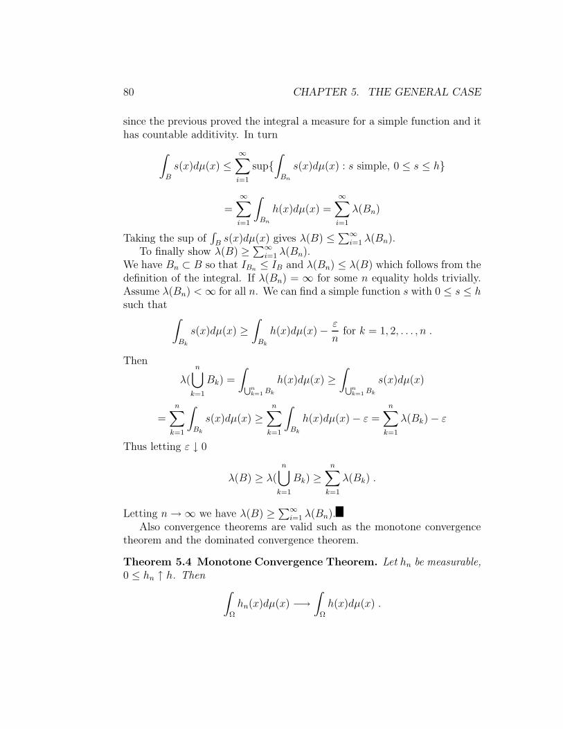
80 CHAPTER 5. THE GENERAL CASE
since the previous proved the integral a measure for a simple function and ithas countable additivity. In turn
∫
B
s(x)dµ(x) ≤∞∑
i=1
sup∫
Bn
s(x)dµ(x) : s simple, 0 ≤ s ≤ h
=
∞∑
i=1
∫
Bn
h(x)dµ(x) =
∞∑
i=1
λ(Bn)
Taking the sup of∫
Bs(x)dµ(x) gives λ(B) ≤∑∞
i=1 λ(Bn).To finally show λ(B) ≥∑∞
i=1 λ(Bn).We have Bn ⊂ B so that IBn ≤ IB and λ(Bn) ≤ λ(B) which follows from thedefinition of the integral. If λ(Bn) = ∞ for some n equality holds trivially.Assume λ(Bn) <∞ for all n. We can find a simple function s with 0 ≤ s ≤ hsuch that
∫
Bk
s(x)dµ(x) ≥∫
Bk
h(x)dµ(x)− ε
nfor k = 1, 2, . . . , n .
Then
λ(
n⋃
k=1
Bk) =
∫Sn
k=1 Bk
h(x)dµ(x) ≥∫
Snk=1 Bk
s(x)dµ(x)
=
n∑
k=1
∫
Bk
s(x)dµ(x) ≥n∑
k=1
∫
Bk
h(x)dµ(x)− ε =
n∑
k=1
λ(Bk)− ε
Thus letting ε ↓ 0
λ(B) ≥ λ(
n⋃
k=1
Bk) ≥n∑
k=1
λ(Bk) .
Letting n→∞ we have λ(B) ≥∑∞i=1 λ(Bn).
Also convergence theorems are valid such as the monotone convergencetheorem and the dominated convergence theorem.
Theorem 5.4 Monotone Convergence Theorem. Let hn be measurable,0 ≤ hn ↑ h. Then
∫
Ω
hn(x)dµ(x) −→∫
Ω
h(x)dµ(x) .

5.1. SOME MEASURE THEORY 81
Proof.
0 ≤ hn ≤ h =⇒∫
Ω
hn(x)dµ(x) ≤∫
Ω
h(x)dµ(x)
and
K = limn
∫
Ω
hn(x)dµ(x) ≤∫
Ω
h(x)dµ(x) .
Next, let 0 < b < 1 and let s be a non negative simple function with s ≤ h.Define
Bn = x : hn(x) ≥ bs(x) ↑ Ω
since hn ↑ h and s is finite valued. We have
K ≥∫
Ω
hn(x)dµ(x) ≥∫
Bn
hn(x)dµ(x) ≤∫
Ω
h(x)dµ(x) ≥ b
∫
Bn
s(x)dµ(x) .
Now λ(Bn) =∫
Bns(x)dµ(x) is a measure and so λ(Bn)→ λ(Ω) and
K ≥ b
∫
Ω
s(x)dµ(x) .
Letting b ↑ 1 and taking the sup of the integral for simple s, 0 ≤ s ≤ h gives
K ≥∫
Ω
h(x)dµ(x) .
Define
lim infn→∞
fn(x) = supn
infk≥n
fk(x), lim supn→∞
fn(x) = infn
supk≥n
fk(x) .
We have the following:
Lemma 5.1 Fatou’s Lemma. Let f1, f2, . . . , f be measurable functions.(a) If fn ≥ f for all n where
∫Ωf(x)dµ(x) > −∞, then
lim infn→∞
∫
Ω
fn(x)dµ(x) ≥∫
Ω
(lim infn→∞
fn(x))dµ(x) .
(b) If fn ≤ f for all n where∫Ωf(x)dµ(x) <∞, then
lim supn→∞
∫
Ω
fn(x)dµ(x) ≤∫
Ω
(lim sup
n→∞fn(x)
)dµ(x) .

82 CHAPTER 5. THE GENERAL CASE
Proof.(a) Let gn = infk≥n fk and g = lim infn fn. Then gn ≥ f for all n, and gn ↑ g.Thus by the monotone convergence theorem applied to 0 ≤ (gn−f) ↑ (g−f),
∫
Ω
gn(x)dµ(x) −→∫
Ω
(lim infn
fn(x))dµ(x) .
Since gn ≤ fn∫
Ω
(lim infn
fn(x))dµ(x) = limn
∫
Ω
gn(x)dµ(x)
= lim infn
∫
Ω
gn(x)dµ(x) ≤ lim infn
∫
Ω
fn(x)dµ(x) .
(b) Since lim supn fn = − lim infn(−fn) we can use (a)∫
Ω
lim supn
fn(x)dµ(x) = −∫
Ω
lim infn
(−fn(x)dµ(x)
≥ − lim infn
∫
Ω
(−fn(x))dµ(x) = lim supn
∫
Ω
fn(x)dµ(x) .
Theorem 5.5 Dominated Convergence Theorem.∫
Ω
fn(x)dµ(x) −→∫
Ω
f(x)dµ(x)
provided fn(x)→ f(x) and |fn(x)| ≤ g(x) as n→∞ where∫
Ω
g(x)dµ(x) <∞ .
Proof.Using Fatou’s lemma, since −g(x) ≤ fn(x) ≤ g(x),
∫Ω(−g(x))dµ(x) > −∞,
and∫Ωg(x)dµ(x) <∞,
∫
Ω
lim infn
fn(x)dµ(x) ≤ lim infn
∫
Ω
fn(x)dµ(x)
≤ lim supn
∫
Ω
fn(x)dµ(x) ≤∫
Ω
lim supn
fn(x)dµ(x) .
But f = limn fn = lim infn fn = lim supn fn so
limn
∫
Ω
fn(x)dµ(x) =
∫
Ω
f(x)dµ(x).

5.1. SOME MEASURE THEORY 83
5.1.3 Derivatives for Measures
We say a measure ν is absolutely continuous with respect to the measure µand write ν << µ if µ(A) = 0 implies ν(A) = 0 for A ∈ A.
The following Radon-Nikodym theorem is proved in courses on measuretheory. See, for example, Ash (1972)2.
Theorem 5.6 Radon-Nikodym Theorem. Let µ and ν be sigma finitemeasures. Then there exists a nonnegative A measurable function f suchthat
ν(A) =
∫
A
f(x)dµ(x) =
∫
Ω
IA(x)f(x)dµ(x) .
if and only if ν is absolutely continuous with respect to µ (ν << µ). If g isanother function satisfying the above equations, then g = f a.e. [µ].
The function f(x) is often denoted
f(x) =dν
dµ(x) .
Theorem 5.7 Chain Rule. If η << ν << µ then
dη
dµ=dη
dν
dν
dµ.
ProofWe first prove that if η(A) =
∫Af(x)dν(x) and ν(A) =
∫Ag(x)dµ(x) then
∫
Ω
f(x)dν(x) =
∫
Ω
f(x)g(x)dµ(x) .
If f(x) =∑k
i=1 xiIAi(x) is simple, then
∫
Ω
f(x)dν(x) =k∑
i=1
xiν(Ai) =k∑
i=1
xi
∫
Ai
g(x)dµ(x)
=
∫
Ω
k∑
i=1
xiIAi(x)g(x)dµ(x) =
∫
Ω
f(x)g(x)dµ(x) .
2Robert B. Ash (1972). Real Analysis and Probability. Academic Press, Inc. HarcourtBrace Janovich, Publishers. San Diego, California. pp. 63-65.
84 CHAPTER 5. THE GENERAL CASE
Next, if f ≥ 0 is measurable, let fn ↑ f where fn is simple. Then∫
Ω
fn(x)dν(x) =
∫
Ω
fn(x)g(x)dµ(x)
and using the monotone convergence theorem, n→∞,∫
Ω
f(x)dν(x) =
∫
Ω
f(x)g(x)dµ(x) .
Now let
η(A) =
∫
Ω
IA(x)f(x)dν(x), and ν(A) =
∫
Ω
IA(x)g(x)dµ(x)
by the Radon-Nikodym theorem where f = dη/dν, g = dν/dµ since η << νand ν << µ. Then by the above result
η(A) =
∫
Ω
IA(x)f(x)g(x)dµ(x)
anddη
dµ=dη
dν
dν
dµ.
5.2 General Densities
Throughout, we will use fX(x) as the density of a random variable withrespect to either counting measure for the discrete case or Lebesgue measurefor the continuous case. We will write
P (X ∈ A) =
∫
x∈A
fX(x)dµ(x)
where µ is either counting measure (discrete case) or Lebesgue measure (con-tinuous case) since (µ(A) = 0) =⇒ (P (X ∈ A) = 0) or PX << µ for thediscrete or continuous case.
5.2.1 Conditional Expectation
To define E(h(X)|T (X)) we first recall the sigma field A(T (X)) =A : A = T−1(B), B ∈ B for a measurable function T (X). It is the class

5.2. GENERAL DENSITIES 85
of all sets that are inverse images under T of Borel sets. It is a subset of Asince T is a measurable function.
Now we define E(h(X)|T (X)) as an A(T (X)) measurable function thatsatisfies∫
A0
h(x)fX(x)dµ(x) =
∫
A0
E(h(X)|T (x))fX(x)dµ(x) for all A0 ∈ A(T (X)) .
This definition uses the Radon-Nikodym theorem since
ν(A0) =
∫
A0
h(x)fX(x)dµ(x) <<
∫
A0
fX(x)dµ(x) for A(T (X)) .
The A(T (X)) measurable function that exists by the Radon-Nikodym theo-rem is called the conditional expectation E(h(X)|T (X)).
By setting A0 = Ω in the definition we have
E(E(h(X)|T (X)) = E(h(X)) .
We also have the following properties:
If Y = k a constant, a.e., then E(Y |T (X)) = k a.e..
If Y1 ≤ Y2 a.e., then E(Y1|T (X)) ≤ E(Y2|T (X)) a.e..
|E(Y |T (X))| ≤ E(|Y ||T (X)).
E(aY1 + bY2|T (X)) = aE(Y1|T (X)) + bE(Y2|T (X)).
If 0 ≤ Yn ↑ Y a.e., then E(Yn|T (X) ↑ E(Y |T (X)).
If |Yn| ≤ g(X) with E(g(X)) <∞ then E(Yn|T (X))→ E(Y |T (X)).

86 CHAPTER 5. THE GENERAL CASE

Chapter 6
Distribution Measures
There are various measures that help to describe the distribution of a randomvariable.
6.1 P.D.F. and C.D.F. Plots
The theoretical histogram or p.d.f. plot gives a visual display of the frequencyof the various outcomes plotting fX(x) versus x.Figure 6.1 gives the p.d.f. plot for the binomial with n = 10 and p = 0.5.Figures 6.2, 6.3, 6.4, 6.5 give plots for the hypergeometric, negative binomial,Poisson, and negative hypergeometric.
A cumulative form of graphical display plots the c.d.f FX(x) versus x.For example the c.d.f. plot for the binomial with n = 10 and p = 0.5 is givenin figure 6.6.
6.2 Measures of the Center
A theoretical median of the distribution is a number m for whichP (X ≤ m) ≥ 1/2 ≤ P (X ≥ m). Such a number always exists.For discrete random variables, if FX(x) = 1/2 on an interval a ≤ x ≤ b thenany value m, a ≤ m ≤ b can serve as a value for the median. The mediancan be read off the c.d.f. plot by looking at the horizontal line y = 1/2 andreading off the value(s) x where the line intersects the c.d.f. See the dottedline in figure 4.6.
87

88 CHAPTER 6. DISTRIBUTION MEASURES
Theorem 6.1 The value of the constant C that minimizes E|X − C| isC = m where m is the median of the distribution of X.
Proof.Let FX(x) be the c.d.f. for X and write
E|X − C| =∫ ∞
−∞|x− C|dFX(x)
where we define the integral
∫ b
a
h(x)dFX(x) =
∫
(a,b]
h(x)fX(x)dµ(x)
=
∑x:
a<x≤bh(x)fX(x) for the discrete case
∫ b
ah(x)fX(x)dx for the continuous case, fX(x) = dFX(x)
dx.
We note that the median m satisfies FX(m) ≥ 1/2 and FX(m−) ≤ 1/2 whereFX(m−) = limε↓0 FX(m− ε) sinceFX(m) = P (X ≤ m) ≥ 1/2 ≤ P (X ≥ m) = 1− P (X < m) = 1− FX(m−).Then
E|X − C| −E|X −m| =∫ C
−∞(C − x)dFX(x) +
∫ ∞
C
(x− C)dFX(x)
−∫ m
−∞(m− x)dFX(x)−
∫ ∞
m
(x−m)dFX(x)
=
∫ C
−∞(C −m+m− x)dFX(x) +
∫ ∞
C
(x−m+m− C)dFX(x)
−∫ m
−∞(m− x)dFX(x)−
∫ ∞
m
(x−m)dFX(x)
= (C −m)(2FX(C)− 1) + 2
∫ C
m
(m− x)dFX(x) .
If C ≥ m then replacing x by C gives
E|X − C| − E|X −m| ≥ (C −m)(2FX(C)− 1) + 2(m− C)(F (C)− F (m))
= (C −m)(2FX(m)− 1) ≥ 0 .

6.2. MEASURES OF THE CENTER 89
If C < m then replacing x by C for x < m and noting (x−m) = 0 for x = mgives
E|X −C| −E|X −m| ≥ (m−C)(1− 2FX(C) + 2(m−C)(F (m−)− F (C))
= (m− C)(1− 2FX(m−)) ≥ 0 .
Another measure of the center is the theoretical mean or expected value. Itis often denoted by µ or E(X) and, provided it is finite, it is defined by
E(X) =
∫ ∞
−∞xdFX(x) .
It is the probability weighted sum of the values of the random variable in thediscrete case and is the integral of the values multiplied by the continuousdensity in the continuous case. It is the center of balance of the p.d.f. plot inthe discrete case and the center of balance of the continuous density in thecontinuous case.
Theorem 6.2 The value of the constant C that minimizes E(X − C)2 isC = µ = E(X).
Proof.
E(X−C)2 = E(X−µ+µ−C)2 = E(X−µ)2 +2(µ−C)E(X−µ)+(µ−C)2
= E(X − µ)2 + (µ− C)2 ≥ E(X − µ)2 .
For the binomial we have
E(X) =n∑
k=0
k
(nk
)pkqn−k = np .
For the negative binomial
E(X) =
∞∑
k=0
k
(r + k − 1
k
)prqk =
rq
p.
For the Poisson
E(X) =
∞∑
k=0
kλk
k!e−λ = λ .

90 CHAPTER 6. DISTRIBUTION MEASURES
For the hypergeometric
E(X) =U∑
k=L
k
(nk
)(D)k(N −D)n−k
(N)n=nD
N
where L = max0, n+D −N and U = minn,D.For the negative hypergeometric
E(X) =N−D∑
k=0
k
(r + k − 1
k
)(D)r(N −D)k
(N)r+k=r(N −D)
(D + 1).
For the N (µ, σ2) density, E(X) = µ.For the exponential(µ, σ) density , E(X) = µ+ σ.For the gamma(α, σ) density, E(X) = ασ.For the beta(α, β) density , E(X) = α/(α+ β).For the Weibull(β, σ) density , E(X) = σ1/βΓ(1 + 1/β).For the double exponential(µ, σ) density, E(X) = µ.
The derivation of the expectation of the binomial is
E(X) =n∑
k=0
k
(nk
)pkqn−k = np
n∑
k=1
(n− 1k − 1
)pk−1qn−1−(k−1)
= npn−1∑
t=0
(n− 1t
)ptqn−1−t = np(p+ q)n−1 = np(1)n−1 = np .
The derivation for the N (µ, σ2) density is
E(X) =
∫ ∞
−∞x
1
σ√
2πe−(x−µ)2/(2σ2)dx
= µ+
∫ ∞
−∞(x− µ)
1
σ√
2πe−(x−µ)2/(2σ2)dx
= µ+ σ
∫ ∞
−∞t
1√2πe−t2/2dt = µ .
Derivations for other expectations are similar and use the fact that the prob-ability densities sum or integrate to one.

6.3. VARIANCE 91
In general, the expectation of a function of a random variable is definedby
E(h(X)) =
∫ ∞
−∞h(x)dFX(x).
provided that it is finite. Note E(C) = C for a constant C since the proba-bility density sums or integrates to 1.An example with an infinite expectation is given by the p.d.f.
fX(x) =6
π2x2for x = 1, 2, . . . ,∞.
since the expectation is
E(X) =
∞∑
x=1
x6
π2x2=
6
π2
∞∑
x=1
1
x=∞ .
6.3 Variance
A popular measure of spread of a distribution is the variance. It is oftendenoted by σ2 or Var(X) and defined by
Var(X) = E((X − µ)2) where µ = E(X) .
We haveE((X − µ)2) = E(X2)− µ2
and also= E(X(X − 1))− µ(µ− 1) . (6.1)
Proof.
E((X − µ)2) = E(X2 − 2µX + µ2) = E(X2)− 2µ2 + µ2 = E(X2)− µ2 .
Also
E(X(X−1))−µ(µ−1) = E(X2−X)−µ2+µ = E(X2)−µ−µ2+µ = E(X2)−µ2 .
For Y = aX + b we have V ar(Y ) = a2V ar(X).Using equation (6.1) we can derive σ2 for the various discrete distribu-
tions:

92 CHAPTER 6. DISTRIBUTION MEASURES
Binomial, σ2 = npq,
Negative binomial, σ2 = rq/p2.
Poisson, σ2 = λ.
Hypergeometric,
σ2 = n
(D
N
)(N −DN
)(N − nN − 1
).
Negative hypergeometric,
σ2 =r(N + 1)(N −D)(D − r + 1)
(D + 2)(D + 1)2.
For the various continuous densities the variances are as follows:
N (µ, σ2) density V ar(X) = σ2.
Exponential(µ, σ) density V ar(X) = σ2.
Gamma(α, σ) density V ar(X) = ασ2.
Beta(α, β) density V ar(X) = αβ/((α+ β)2(α+ β + 1)).
Weibull(β, σ) density V ar(X) = σ2/β(Γ(1 + 2/β)− Γ(1 + 1/β)).
Double exponential(µ, σ) density V ar(X) = 2σ2.
The variance gives a bound on the probability outside an interval aroundthe expectation.Chebyshev’s TheoremFor any constant C > 1
P (µ− Cσ < X < µ+ Cσ) ≥ 1− 1
C2
where µ = E(X) and σ2 = V ar(X).Proof.
P (|X − µ| ≥ Cσ) =
∫
|x−µ|/(Cσ)≥1fX(x)dµ(x)
≤∫ ∞
−∞
(x− µ)2
C2σ2fX(x)dµ(x) =
1
C2.

6.4. PROBLEMS 93
6.4 Problems
1. For the exponential distribution fX(x) = e−x/σ/σ for x > 0 give the c.d.f.and the median.
2. For the geometric distribution fX(x) = qxp where p + q = 1, 0 < p < 1and x = 0, 1, 2, . . . ,∞, give the c.d.f. and the median.
3. For the Weibull(β, σ) distribution, give the c.d.f. and the median.
4. Derive the expectation and variance for the Poisson(λ) distribution.
5. Derive the expectation and variance for the negative binomial(r, p).
6. Derive the expectation and variance for the hypergeometric(N,D, n).
7. Derive the expectation and variance for the beta(α, β) distribution.
8. Derive the expectation and variance for the gamma(α, σ) distribution.
9 Derive the variance for the N (µ, σ2) distribution.
10 Derive the expectation and variance for the continuous uniform(a, b) den-sity
fX(x) =1
(b− a) for a < x < b, 0, otherwise.

94 CHAPTER 6. DISTRIBUTION MEASURES
0 2 4 6 8 10
0.00
0.05
0.10
0.15
0.20
0.25
x
y
Figure 6.1: Binomial p.d.f. plot (n, p) = (10, 0.5) .
0 2 4 6 8 10
0.00
0.05
0.10
0.15
0.20
0.25
0.30
x
y
Figure 6.2: Hypergeometric p.d.f. plot (N,D, n) = (30, 15, 10).

6.4. PROBLEMS 95
0 2 4 6 8 10
0.00
0.05
0.10
0.15
0.20
x
y
Figure 6.3: Negative binomial p.d.f. plot (r, p) = (10, 0.8)
0 2 4 6 8 10
0.00
0.05
0.10
0.15
0.20
0.25
x
y
Figure 6.4: Poisson p.d.f. plot λ = 2.5.

96 CHAPTER 6. DISTRIBUTION MEASURES
0 2 4 6 8 10
0.00
0.05
0.10
0.15
0.20
0.25
x
y
Figure 6.5: Negative hypergeometric p.d.f. plot (N,D, r) = (30, 24, 10).
0 2 4 6 8 10
0.00.2
0.40.6
0.81.0
x
y
Figure 6.6: Binomial c.d.f. plot (n, p) = (10, 0.5), median=5.

Chapter 7
Several Random Variables
7.1 Bivariate Random Variables
We define the distribution for two random variables X, Y in a manner similarto that for a single random variable.
P ((X, Y ) ∈ B(2)) = P (A)
whereA = e : (X(e), Y (e)) ∈ B(2) and B(2) ∈ B(2)
where B(2) is the smallest sigma field generated by rectangles(a1, b1]⊗ (a2, b2] = (x, y) : a1 < x ≤ b1, a2 < y ≤ b2 in the plane.
For the discrete case where (X, Y ) take on finite or countably infinitenumbers of values the discrete joint density is
fX,Y (x, y) = P (X = x, Y = y) where∑
all x
∑
all y
fX,Y (x, y) = 1 .
In the jointly continuous case we assign probabilities as the volume underthe surface defined by a continuous 2 dimensional density fX,Y (x, y) and overthe set B(2) in the (x, y) plane where the density satisfies
fX,Y (x, y) ≥ 0 and
∫ ∞
−∞
∫ ∞
−∞fX,Y (x, y)dxdy = 1 .
Thus the probability is the volume
P ((X, Y ) ∈ B(2)) =
∫ ∫
(x,y)∈B(2)fX,Y (x, y)dxdy .
97

98 CHAPTER 7. SEVERAL RANDOM VARIABLES
For a discrete example, an urn contains R red, W white and B blue ballswhere R+W +B = N total. A sample of n is selected without replacementand we observe X the number of red balls in the sample and Y the numberof white balls in the sample. Then the bivariate hypergeometric p.d.f. is:
P (X = x, Y = y) = fX,Y (x, y) =
(Rx
)(Wy
)(B
n− x− y
)
(Nn
)
=
(n!
x!y!(n− x− y)!
)(R)x(W )y(B)(n−x−y)
(N)n
.
Some important bivariate discrete densities are:
Trinomial(m, p1, p2, p3):
fX,Y (x, y) =m!
x!y!(m− x− y)!px1p
y2p
m−x−y3
for 0 < p1, p2, p3 < 1, p1+p2+p3 = 1, and x, y,m integers, 0 ≤ x, y ≤ m,x+ y ≤ m.
Bivariate hypergeometric(N,D1, D2, D3, n)
fX,Y (x, y) =
(D1
x
)(D2
y
)(D3
n− x− y
)
(Nn
)
where D1, D2, D3, N, n, x, y are integers, D1 +D2 +D3 = N .
Bivariate negative binomial(r, p1, p2, p3):
fX,Y (x, y) =(r + x+ y − 1)!
x!y!(r − 1)!px
1py2p
r3
for 0 < p1, p2, p3 < 1, p1 + p2 + p3 = 1, and x, y, r integers.

7.1. BIVARIATE RANDOM VARIABLES 99
-y
6
1001287
2001287
3001287 fX,Y (x, y)
x
0 1 2 3 40
1
2
3
ss
ss
ss
ss
s
ss
s
s
ss s s
Figure 7.1: Plot of fX,Y (x, y) vs. (x, y) for bivariate hypergeometric disrti-bution (R,W,B) = (3, 4, 6) and n = 5.

100 CHAPTER 7. SEVERAL RANDOM VARIABLES
Bivariate negative hupergeometric(N,D1, D2, D3, r):
fX,Y (x, y) =(r + x+ y − 1)!
x!y!(r − 1)!
(D1)x(D2)y(D3)r
(N)x+y+r
where D1, D2, D3, N, r, x, y are integers, D1 +D2 +D3 = N .
Bivariate Poisson(λ1, λ2):
fX,Y (x, y) =λx
1λy2
x!y!e−λ1−λ2
where 0 < λ1, λ2 <∞, x, y = 0, 1, . . . ,∞.
For a continuous example let
fX,Y (x, y) =e−(x2+y2)/2
2πfor −∞ < x, y <∞ .
Figure 7.2 plots this continuous joint density. This is called the bivariate
normal N2(0, I2) density where 0 = (0, 0), and I2 =
(1 00 1
).
Some important bivariate densities are:
Bivariate normal N2(µ,Σ) where µ = (µ1, µ2), Σ =
(σ2 ρστρστ τ 2
)
fX,Y (x, y) =1
2πστ√
1− ρ2e− 1
2(1−ρ2)(x−µ1
σ )2−2ρ(x−µ1
σ )( y−µ2τ )+( y−µ2
τ )2
and −∞ < µ1, µ2 <∞, 0 < σ, τ , −1 < ρ < 1, −∞ < x, y <∞.
Bivariate beta or Dirichlet(α1, α2, α3):
fX,Y (x, y) =Γ(α1 + α2 + α3)
Γ(α1)Γ(α2)Γ(α3)xα1−1yα2−1(1− x− y)α3−1
for α1, α2, α3 > 0, 0 < x, y < 1, x+ y < 1.

7.1. BIVARIATE RANDOM VARIABLES 101
x
y
z
Figure 7.2: Bivariate Normal N2(0, I2) Density.

102 CHAPTER 7. SEVERAL RANDOM VARIABLES
7.1.1 Marginal Densities
The marginal density for a single discrete random variable can be obtainedfrom the joint discrete density by summing
fX(x) =∑
all y
pX,Y (x, y), fY (y) =∑
all x
fX,Y (x, y) .
The marginal density for a continuous random variable is similarly obtainedfrom the joint continuous density by integrating
fX(x) =
∫ ∞
−∞fX,Y (x, y)dy, fY (y) =
∫ ∞
−∞fX,Y (x, y)dx .
As examples, for the bivariate hypergeometric(N,D1, D2, D3, n) the marginalis
fX(x) =
U(x)∑
y=L(x)
(D1
x
)(D2
y
)(D3
n− x− y
)
(Nn
) =
(D1
x
)(D2 +D3
n− x
)
(Nn
)
where L(x) = max0, n− x−D3 and U(x) = minD2, n− x.This is a univariate hypergeometric(N,D1, n) discrete density.
For the trinomial(m, p1, p2, p3) the marginal is
fX(x) =
(mx
)px
1(1− p1)m−x
which is the univariate binomial(m, p1).The bivariate negative binomial(r, p1, p2, p3) has marginal
fX(x) =
(x+ r − 1
x
)(p1
p1 + p3
)x(p3
p1 + p3
)r
which is the univariate negative binomial(r, p1/(p1 + p3)).The bivariate negative hypergeometric(N,D1, D2, D3, r) has
fX(x) =
(x+ r − 1
x
)(D1)x(D3)r
(D1 +D3)x+r
which is the univariate negative hypergeometric(D1 +D3, D1, r).

7.1. BIVARIATE RANDOM VARIABLES 103
The marginal of the bivariate normal N2(0, I2) density is
fX(x) =
∫ ∞
−∞
1
2πe−(x2+y2)/2dy =
1√2πe−x2/2
which is the univariate normal N (0, 1) density.The marginal of the bivariate Dirichlet(α1, α2, α3) is
fX(x) =Γ(α1 + α2 + α3)
Γ(α1)Γ(α2 + α3)xα1−1(1− x)α2+α3−1
for 0 < x < 1 which is the univariate beta(α1, α2 + α3) density.
7.1.2 Conditional Densities
The conditional distribution of a random variable given the value of anotherrandom variable is defined for discrete random variables by
fX|Y (x|y) = P (X = x|Y = y) =P (X = x, Y = y)
P (Y = y)=fX,Y (x, y)
fY (y).
For example, for the negative binomial with p3 = 1 − p1 − p2, using thefact that negative binomial probabilities add to 1,
fY (y) =
∞∑
x=0
(r + x+ y − 1)!
x!y!(r − 1)!px
1py2p
r3
=(y + r − 1)!
y!(r − 1)!
(p2
(1− p1)
)y (p3
(1− p1)
)r ∞∑
x=0
(x+ y + r − 1)!
x!(y + r − 1)!px
1(1− p1)y+r
=(y + r − 1)!
y!(r − 1)!
(p2
(1− p1)
)y (p3
(1− p1)
)r
.
Then fX|Y (x|y) =
((r + x+ y − 1)!
x!y!(r − 1)!px
1py2p
r3
)/
((y + r − 1)!
y!(r − 1)!
(p2
(1− p1)
)y (p3
(1− p1)
)r)
=(x+ y + r − 1)!
x!(y + r − 1)!px
1(1− p1)y+r
which is the negative binomial(p1, y + r).

104 CHAPTER 7. SEVERAL RANDOM VARIABLES
For continuous random variables, the conditional density of X given Y isdefined by
fX|Y (x|y) =fX,Y (x, y)
fY (y).
For example, for the bivariate normal N2(µ,Σ), the marginal density
fY (y) =
∫ ∞
−∞
1
2πστ√
1− ρ2e− 1
2(1−ρ2)( x−µ1
σ )2−2ρ(x−µ1
σ )( y−µ2τ )+(y−µ2
τ )2dx
and setting u = (x− µ1)/(σ√
1− ρ2)
=e−(y−µ2)2/(2τ2)
τ√
2π
∫ ∞
−∞
1√2πe−
12u−ρ(y−µ2)/(τ
√1−ρ2)2
du =e−(y−µ2)2/(2τ2)
τ√
2π
which is the univariate normal N (µ2, τ2) density. Then fX|Y (x|y) =
(1
2πστ√
1− ρ2e− 1
2(1−ρ2)(x−µ1
σ )2−2ρ(x−µ1
σ )( y−µ2τ )+( y−µ2
τ )2)/
(1
τ√
2πe−
(y−µ2)2
2τ2
)
=1
σ√
1− ρ2√
2πe− 1
2σ2(1−ρ2)x−(µ1+ρσ(y−µ2)/τ)2
the univariate normal N (µ1 + ρσ(y − µ2)/τ, σ2(1− ρ2)) conditional density.
We say the random variables X, Y are independent if
P (X ∈ B1, Y ∈ B2) = P (X ∈ B1)P (Y ∈ B2) .
For discrete or continuous random variables, X, Y are independent if thediscrete or continuous densities factor:
fX,Y (x, y) = fX(x)fY (y) for all (x, y) .
Equivalently, if the conditional density of X|Y is the same as the marginaldensity of X, then X, Y are independent.
For example the bivariate Poisson satisfies the condition for independencesince
fX,Y (x, y) =λx
1λy2
x!y!e−λ1−λ2 =
λx1
x!e−λ1 × λy
2
y!e−λ2 = fX(x)fY (y) .

7.2. SEVERAL RANDOM VARIABLES 105
When ρ = 0 the bivariate normal N2(µ,Σ) factors since fX,Y (x, y) =
1
2πστe−
12(x−µ1)2/σ2+(y−µ2)2/τ2 =
(e−
12σ2 (x−µ1)2
σ√
2π
)(e−
12τ2 (y−µ2)2
τ√
2π
)= fX(x)fY (y)
and we have independence. The parameter ρ is called the correlation coeffi-cient and is a measure of dependence.
7.2 Several Random Variables
For several random variables X1, X2, . . . , Xn the joint discrete or continuousdensity is an n dimensional function
fX1,X2,...,Xn(x1, x2, . . . , xn)
that is non negative and sums or integrates to 1 over the n dimensional setof points (x1, x2, . . . , xn). There are 2n− 2 subsets of 2, 3, . . . , n− 1 variablesand that many possible marginal densities. For example if n = 3 there areunivariate marginals for X1, for X2, and for X3 and bivariate marginals for(X1, X2), for (X1, X3), and for (X2, X3).
7.2.1 Discrete Multivariate Distributions
Some discrete multivariate examples are
Multinomial(m, p1, p2, . . . , pk)
fX1,X2,...,Xk−1(x1, x2, . . . , xk−1) =
m!∏kj=1 xj !
k∏
j=1
pxj
j
for 0 < pi < 1, p1 +p2 + · · ·+pk = 1, and integer xi satisfy 0 ≤ xi ≤ m,x1 + x2 + · · ·+ xk−1 ≤ m, and xk = m−∑k−1
j=1 xj .
Multivariate hypergeometric(N,D1, D2, . . . , Dk, m)
fX1,X2,...,Xk−1(x1, x2, . . . , xk−1) =
m!(D1)x1(D2)x2 · · · (Dk−1)xk−1(Dk)xk
x1!x2! · · ·xk!(N)m
for D1 + D2 + · · · + Dk = N and integer xi satisfy 0 ≤ xi ≤ m,x1 + x2 + · · ·+ xk = m.

106 CHAPTER 7. SEVERAL RANDOM VARIABLES
Multivariate negative binomial(r, p1, p2, . . . pk)
fX1,X2,...,Xk−1(x1, x2, . . . , xk−1) =
(x1 + x2 + · · ·+ xk−1 + r − 1)!
x1!x2! · · ·xk−1!(r − 1)!px1
1 px22 · · · pxk−1
k−1 prk
for 0 < pi < 1, p1 +p2 + · · ·+pk = 1, and integer xi satisfy 0 ≤ xi <∞.
Multivariate negative hypergeometic(N,D1, D2, . . . , Dk, r)
fX1,X2,...,Xk−1(x1, x2, . . . , xk−1) =
(x1 + x2 + · · ·+ xk−1 + r − 1)!
x1!x2! · · ·xk−1!(r − 1)!
(D1)x1(D2)x2 · · · (Dk−1)xk−1(Dk)r
(N)(m+x1+x2+···+xk−1)
for integer Di > 0, D1 + D2 + · · · + Dk = N , and integer xi satisfy0 ≤ xi <∞.
7.2.2 Continuous Multivariate Distributions
Some continuous multivariate examples are
Multivariate normal Nn(µ, Σ),
µ = (µ1, µ2, . . . , µn)T , and Σ =
σ11 σ12 . . . σ1n
σ21 σ22 . . . σ2n...
.... . .
...σn1 σn2 . . . σnn
where Σ is symmetric and positive definite. The symmetric condition isσij = σji. In matrix notation Σ = ΣT where ΣT is the transpose matrixobtained by interchanging rows and columns. The positive definitecondition says that for all vectors (v1, v2, . . . , vn)T with some componentvj 6= 0, we have
n∑
i=1
n∑
j=1
viσijvj > 0 .
fX1,X2,...,Xn(x1, x2, . . . , xn) =1
(2π)n/2|Σ|1/2exp−1
2
n∑
i=1
n∑
j=1
(xi−µi)σ(ij)(xj−µj)

7.3. PROBLEMS 107
where Σ−1 = (σ(ij) : i, j = 1, 2, . . . , n) is the inverse matrix for Σ and|Σ| is the determinant of Σ. The inverse matrix satisfies
n∑
k=1
σikσ(kj) =
1 if i = j0 if i 6= j
or ΣΣ−1 = In
where the identity matrix with n rows and n columns is
In =
1 0 . . . 00 1 . . . 0...
.... . .
...0 0 . . . 1
.
Multivariate Dirichlet(α1, α2, . . . , αn, αn+1) where αi > 0
fX1,X2,...,Xn(x1, x2, . . . , xn) =Γ(∑n+1
i=1 αi)∏n+1i=1 Γ(αi)
(n∏
i=1
xαi−1i
)(1−
n∑
i=1
xi)αn+1−1
for 0 < xi < 1,∑n
i=1 xi < 1.
Many other examples are obtained by assuming X1, X2, . . . , Xn are inde-pendent identically distributed with density f so that
fX1,X2,...,Xn(x1, x2, . . . , xn) =
n∏
i=1
f(xi) .
7.3 Problems
1. Derive the marginal distribution ofX for the bivariate negative binomial(r, p1, p2, p3)distribution.
2. For the three dimensional multinomial(m, p1, p2, p3, p4) derive the marginaljoint distribution for X1, X2.
3. For the bivariate Dirichlet(α1, α2, α3) derive the marginal density for X.
4. For the bivariate Dirichlet, derive the conditional density for X givenY = y.

108 CHAPTER 7. SEVERAL RANDOM VARIABLES
5. For the multivariate normalNn(µ,Σ) show that if X = (X1×m1 ,X
1×(n−m)2 )
that X1 and X2 are independent if
Σ =
(Σ11 00 Σ22
)
by showing fX(x) = fX1(x1)fX2
(x2).

Chapter 8
Characteristic Functions
8.1 Univariate Characteristic Functions
A very convenient technical device is the complex valued characteristic func-tion
hX(t) = E(eitX) = E(cos(tX)) + iE(sin(tX))
where i =√−1. There is a 1-1 correspondence between a distribution and
its characteristic function. It always exists since
|eitX | = (cos2(tX) + sin2(tX))1/2 = 1 .
Theorem 8.1 If hX(u) is the characteristic function of the distribution func-tion FX(x), then
FX(b)− FX(a) =1
2πlimc→∞
∫ c
−c
(e−iua − e−iub)
iuhX(u)du
for all a, b at which FX is continuous.
Proof.Define
Ic =1
2π
∫ c
−c
(e−iua − e−iub)
iu
[∫ ∞
−∞eiuxdFX(x)
]du .
Since∣∣∣∣(e−iua − e−iub)
iueiux
∣∣∣∣ =
∣∣∣∣(e−iua − e−iub)
iu
∣∣∣∣ =
∣∣∣∣∫ b
a
e−iuxdx
∣∣∣∣ ≤ b− a
109

110 CHAPTER 8. CHARACTERISTIC FUNCTIONS
and ∫ c
−c
∫ ∞
−∞(b− a)dFX(x) = 2c(b− a) <∞
we can interchange the order of integration (Fubini’s theorem) to get
Ic =1
2π
∫ ∞
−∞
∫ c
−c
(e−iua − e−iub)
iueiuxdudFX(x) =
∫ ∞
−∞Jc(x)dFX(x)
where
Jc(x) =1
2π
∫ c
−c
(sin(u(x− a))− sin(u(x− b)))u
du
since ∫ c
−c
(cos(u(x− a))− cos(u(x− b)))iu
du = 0 .
Substituting v = u(x− a) and w = u(x− b) we get
Jc(x) =1
2π
∫ c(x−a)
−c(x−a)
sin(v)
vdv − 1
2π
∫ c(x−b)
−c(x−b)
sin(w)
wdw .
As c→∞ we have
Jc(x) −→ J(x) =
0 if x < a or x > b1/2 if x = a or x = b1 if a < x < b.
Using the dominated convergence, for a, b continuity points of FX ,
limc→∞
Ic =
∫ ∞
−∞J(x)dFX(x) = FX(b)− FX(a) .
For integer valued discrete random variables the p.d.f. satisfies
fX(x) =1
2π
∫ π
−π
hX(t)e−itxdt. (8.1)
For continuous random variables we have
fX(x) =1
2π
∫ ∞
−∞hX(t)e−itxdt (8.2)

8.1. UNIVARIATE CHARACTERISTIC FUNCTIONS 111
provided its characteristic function hX(t) satisfies∫∞−∞ |hX(t)|dt < ∞. As
examples, the characteristic function for a binomial random variable is
hX(t) =n∑
x=0
eitx
(nx
)pxqn−x = (peit + q)n
and equation (8.1) is verified(nx
)pxqn−x =
1
2π
∫ π
−π
n∑
k=0
eitk
(nk
)pkqn−ke−itxdt
since1
2π
∫ π
−π
eit(k−x)dt =
1 if k = x0 if k 6= x
The characteristic function for the density fX(x) = e−x2/2/√
2π is hX(t) =e−t2/2. To verify equation (8.2) in this case
fX(x) =1
2π
∫ ∞
−∞e−t2/2e−itxdt =
1
2π
∫ ∞
−∞e−t2/2 cos(tx)dt
since the imaginary part
−i 1
2π
∫ ∞
−∞e−t2/2 sin(tx)dt = 0
is the integral of an odd function with the integral on the negative axiscanceling the integral on the positive axis.If we differentiate with respect to x we get
f ′X(x) =
1
2π
∫ ∞
−∞e−t2/2(−t sin(tx))dt
and integrating by parts
=1
2πe−t2/2 sin(tx)|∞−∞ −
1
2π
∫ ∞
−∞e−t2/2x cos(tx)dt = −xfX(x) .
Solving the differential equation
f ′X(x) = −xfX(x) where fX(0) =
1√2π
we get after integrating, loge(fX(x)) = −x2/2 + C where C = loge(1/√
2π).Thus fX(x) = e−x2/2/
√2π.

112 CHAPTER 8. CHARACTERISTIC FUNCTIONS
Theorem 8.2 If E(|Xn|) = µn <∞ then for k ≤ n
h(k)X (u) = ik
∫eiuxxkdF (x), u ∈ R
and h(k)X is continuous and bounded by µk <∞. Also
hX(u) =n−1∑
k=0
mk(iu)k
k!+ un
∫ 1
0
(1− t)n−1
(n− 1)!h
(n)X (tu)dt =
n∑
k=0
mk(iu)k
k!+ o(un)
where mn = E(Xn).
Proof.First, since |X|k ≤ 1 + |X|n for k ≤ n, µn < ∞ gives µk < ∞. If wedifferentiate
∫eiuxdF (x) a total of k times, the integral is absolutely con-
vergent and by the dominated convergence theorem, we can interchange thedifferentiation limit and the integration:
h(k)X (u) =
d
duh
(k−1)X (u) = lim
δ↓0
h(k−1)X (u+ δ)− h(k−1)
X (u)
δ
=
∫(ix)k−1 lim
δ↓0
(eix(u+δ) − eixu)
δdF (x) = ik
∫eiuxxkdF (x) .
If we expand
eiux =n−1∑
k=0
(iux)k
k!+ un
∫ 1
0
(1− t)n−1
(n− 1)!(ix)neiutxdt
and integrate, we get
hX(u) =n−1∑
k=0
(iu)k
k!mk + un
∫ 1
0
(1− t)n−1
(n− 1)!h
(n)X (tu)dt .
Similarly, if we expand
eiux =
n∑
k=0
(iux)k
k!+
(iu)n+1
(n+ 1)!eiuξ where 0 ≤ ξ ≤ x

8.1. UNIVARIATE CHARACTERISTIC FUNCTIONS 113
then after integration, we get
hX(u) =n∑
k=0
(iu)k
k!mk + o(un) .
As an example, for the binomial(n, p)
h′X(0) =d
dt(peit + q)n|t=0 = n(peit + q)n−1ipeit|t=0 = inp
so E(X) = np.For the standard normal N (0, 1)
h′′X(0) =d2
dt2e−t2/2|t=0 = (t2 − 1)e−t2/2|t=0 = −1 = i21
so E(X2) = 1.The following is a list of some useful characteristic functions:
Binomial(n, p): hX(t) = (peit + q)n.
Negative binomial(r, p): hY (t) = (p/(1− qeit))r.
Poisson(λ): hX(t) = expλ(eit − 1)
Normal N (µ, σ2): hX(t) = expitµ− t2σ2/2.
Gamma(α, σ): hX(t) = (1− itσ)−α.
Cauchy(µ, σ): hX(t) = expitµ− σ|t|.
We note for the Cauchy, the derivative of hX(t) does not exist at t = 0 andE(X) does not exist since E(|X|) =∞.
The moment generating function, when it exists. is defined by
mX(t) = E(etX) .
Theorem 8.3 If the moment generating function exists and is finite in anopen interval (−a, a) about t = 0, then the characteristic function is
hX(t) = mX(it).

114 CHAPTER 8. CHARACTERISTIC FUNCTIONS
Proof.If z = u + iv is a complex variable with u ∈ (−a, a) and we substitute intomX to get the complex function
mX(z) =
∫ ∞
−∞ezxdFX(x)
then we first show mX(z) is an analytic function of z.We have
|mX(z)| ≤∫ ∞
−∞|ezx|dFX(x) =
∫ ∞
−∞euxdFX(x) = mX(u) <∞ .
Next(mX(z + δ)−mX(z))
δ=
∫ ∞
−∞ezx (eδx − 1)
δdFX(x) .
Using the inequality (which can be proved by a series argument)
∣∣∣∣(eδx − 1)
δ
∣∣∣∣ ≤eη|x|
η, for |δ| ≤ η
we have the integrand bounded in absolute value by
∣∣∣∣ezx (eδx − 1)
δ
∣∣∣∣ ≤1
η|expzx + η|x|| ≤ 1
η|exp(z + η)x+ exp(z − η)x|
for |δ| ≤ η. For η > 0 sufficiently small, this is an integrable function andthe dominated convergence theorem gives
lim|δ|→0
(mX(z + δ)−mX(z))
δ=
∫ ∞
−∞xezxdFX(x)
finite and mX(z) is analytic.Next, by the assumption, since mX(u) <∞ for real u ∈ (−a, a) where a > 0,we have mX(z) is analytic for complex z = u+ iv where−a < u < a, −∞ < v < ∞. By analytic continuation, mX(u) can beuniquely extended to the purely complex characteristic function
mX(iv) =
∫ ∞
−∞eivxdFX(x) = hX(v), for −∞ < v <∞ .

8.1. UNIVARIATE CHARACTERISTIC FUNCTIONS 115
As an example, for the gamma distribution, the moment generating functionis
mX(t) =
∫ ∞
0
etxxα−1e−x/σ
σαΓ(α)dx = (1− tσ)−α
which is obtained by a change of variable. Replacing t by it gives hX(t) =(1− itσ)−α.
Another method to derive characteristic functions uses the Cauchy residuetheorem for complex variables
2πif(z0) =
∫
z∈C
f(z)
(z − z0)dz
for a closed counter clockwise path C around the fixed point z0.
To illustrate for the Cauchy(0, 1) density, for t > 0,
e−t = 2πi
(eiti
π(i+ i)
)=
∫
z∈C
eitz/(π(z + i))
(z − i) dz
=
∫ R
−R
eitx
π(1 + x2)dx+
∫ π
0
eit(Reiθ)
π(1 + (Reiθ)2)Reiθidθ
−→∫ ∞
−∞
eitx
π(1 + x2)dx = hX(t) as R→∞
since ∣∣∣∣∣
∫ π
0
eit(Reiθ)
π(1 + (Reiθ)2)Reiθidθ
∣∣∣∣∣ ≤πR
|R2 − 1| → 0 as R→∞ .
The path C is illustrated in figure 8.1.
A similar argument with a path around z = −i can be used to get hX(t) =et for t < 0. Combining, gives hX(t) = e−|t| for−∞ < t <∞ since hX(0) = 1.We note that the moment generating function does not exist for the Cauchyso that we cannot use hX(t) = mX(it).
In general, for Y = aX + b we have hY (t) = eitbhX(at). Thus for theCauchy(µ, σ) the characteristic function is eitµe−|σt|.

116 CHAPTER 8. CHARACTERISTIC FUNCTIONS
−3 −2 −1 0 1 2 3
0.0
0.5
1.0
1.5
2.0
2.5
3.0
x
y
−R R
R
i
Figure 8.1: Counter clockwise path C used to calculate the Cauchy(0, 1)characteristic function hX(t) for t > 0.
8.2 Multivariate Characteristic Functions
The multivariate characteristic function is defined by
hX1,X2,...,Xn(t1, t2, . . . , tn) = E(ei(t1X1+t2X2+···+tnXn)) .
The inversion formula for discrete random vectors with integer valuedcomponents is
fX1,X2,...,Xn(x1, x2, . . . , xn) =(
1
2π
)n ∫ π
−π
∫ π
−π
. . .
∫ π
−π
e−i(t1x1+t2x2+···+tnxn)hX1,x2,...,Xn(t1, t2, . . . , tn)dt1dt2 · · · dtn .

8.2. MULTIVARIATE CHARACTERISTIC FUNCTIONS 117
For continuous random variables
fX1,X2,...,Xn(x1, x2, . . . , xn) =
(1
2π
)n ∫ ∞
−∞
∫ ∞
−∞. . .
∫ ∞
−∞e−i(t1x1+t2x2+···+tnxn)hX1,X2,...,Xn(t1, t2, . . . , tn)dt1dt2 · · · dtn
provided∫ ∞
−∞
∫ ∞
−∞. . .
∫ ∞
−∞|hX1,X2,...,Xn(t1, t2, . . . , tn)|dt1dt2 · · · dtn <∞ .
The general multivariate inversion formula is
Theorem 8.4 If a = (a1, a2, . . . an) and b = (b1, b2, . . . , bn), ai < bi, are con-tinuity points of FX1,X2,...,Xn(x1, x2, . . . , xn) then for X = (X1, X2, . . . , Xn),u = (u1, u2, . . . , un)
FX(b)− FX(a) = limc→∞
1
(2π)n
∫ c
−c
· · ·∫ c
−c
[n∏
k=1
(e−iukak − e−iukbk)
iuk
]hX(u)du .
Proof.Following the proof and notation of the univariate inversion theorem 8.1,
1
(2π)n
∫ c
−c
· · ·∫ c
−c
[n∏
k=1
(e−iukak − e−iukbk)
iuk
]hX(u)du =
∫ ∞
−∞· · ·∫ ∞
−∞
[n∏
k=1
Jc(xk)
]dFX(x)
−→∫ ∞
−∞· · ·∫ ∞
−∞
[n∏
k=1
J(xk)
]dFX(x) = FX(b)− FX(a) .
The multivariate moment generating function is
mX(u1, u2, . . . , un) = E(ePn
k=1 ukXk) .
An extension of theorem 8.3 to the multivariate case is
Theorem 8.5 If the multivariate moment generating mX(u) exists for u =(u1, u2, . . . , un) in a neighborhood of u = (0, 0, . . . , 0) then the multivariatecharacteristic function can be obtained by replacing uk by iuk in the momentgenerating function:
hX(u1, u2, . . . , un) = mX(iu1, iu2, . . . , iun) .

118 CHAPTER 8. CHARACTERISTIC FUNCTIONS
Proof.Consider the univariate moment generating function for a linear combination
E(etPn
k=1 akXk) = mX1,X2,...,Xn(ta1, ta2, . . . , tan) .
By the univariate theorem 8.3, the corresponding characteristic function is
E(eitPn
k=1 akXk) = mX1,X2,...,Xn(ita1, ita2, . . . , itan) .
But this is just the characteristic function
hX1,X2,...,Xn(ta1, ta2, . . . tan) .
For examples of characteristic functions, for the multinomial (m, p1, p2, . . . , pk)with xk = m−∑k−1
j=1 xj it is hX1,X2,...,Xk−1(t1, t2, . . . , tk−1) =
∑
xk−1
∑
xk−2
· · ·∑
x1
eiPk−1
j=1 tjxjm!∏k
j=1 xj !
k∏
j=1
pxj
j =
(pk +
k−1∑
j=1
pjeitj
)m
.
The multivariate negative binomial (r, p1, p2, . . . pk) characteristic func-tion is
hX1,X2,...,Xk−1(t1, t2, . . . , tk−1) =
(pk
1−∑k−1j=1 e
itjpj
)r
.
The characteristic function for the multivariate normal Nn(µ,Σ) is
hX1,X2,...,Xn(t1, t2, . . . , tn) = expin∑
j=1
µjtj −1
2
n∑
j=1
n∑
k=1
tjσjktk
= expitTµ− 1
2tTΣt
where tT = (t1, t2, . . . , tn).The multivariate characteristic function can be used to obtain the marginal
distribution for a subset of variables using
hX1,X2,...,Xm(t1, t2, . . . , tm) = hX1,X2,...,Xm,Xm+1,...,Xn(t1, t2, . . . , tm, 0, . . . , 0)
for m < n.

8.2. MULTIVARIATE CHARACTERISTIC FUNCTIONS 119
For example, the marginals of the multivariate normal are also multi-variate normal. If X1, X2, . . . , Xn are Nn(µ,Σ) we can partition (tn×1)T =
((tm×11 )T , (t
(n−m)×12 )T )
µ =
(µm×1
1
µ(n−m)×12
), and Σn×n =
(Σm×m
11 Σm×(n−m)12
Σ(n−m)×m
21 Σ(n−m)×(n−m)22
)
and get
hX1,X2,...,Xm(tm×11 ) = hX1,X2,...Xn(tT
1 , 0) = expitT1 µ1 −
1
2tT1 Σm×m
11 t1 .
The marginal is thus the multivariate normal Nm(µ1,Σ11).
8.2.1 Conditional Characteristic Functions
In the bivariate case, the conditional characteristic function is
hX|Y (t|y) =∑
all x
eitxpX|Y (x|y) and hX|Y (t|y) =
∫ ∞
−∞eitxfX|Y (x|y)dx (8.3)
for discrete and continuous distributions respectively. We can obtain themfrom the joint characteristic function by
hX|Y (t|y) =
∫ π
−πe−iyshX,Y (t, s)ds∫ π
−πe−iyshX,Y (0, s)ds
(8.4)
for discrete random vectors with integer components and
hX|Y (t|y) =
∫∞−∞ e−iyshX,Y (t, s)ds∫∞−∞ e−iyshX,Y (0, s)ds
for the continuous case.For the multivariate case, writing X1×n = (X1×m
1 ,X1×(n−m)2 ),
t1×n = (t1×m1 , t
1×(n−m)2 )
hX1|X2(t1|x2) =
∫∞−∞∫∞−∞ · · ·
∫∞−∞ e−i(t2xT
2)hX1,X2
(t1, t2)dtm+1dtm+2 · · · dtn∫∞−∞∫∞−∞ · · ·
∫∞−∞ e−i(t2xT
2)hX1,X2
(0, t2)dtm+1dtm+2 · · ·dtn

120 CHAPTER 8. CHARACTERISTIC FUNCTIONS
for the continuous case with a similar formula for the discrete integer valuedvector case with integration limits from −π to π instead of −∞ to ∞.
For an example, consider the bivariate trinomial(m, p1, p2, p3) distributionand its conditional characteristic function given Y = y. Using formula (8.4)for random vectors with integer component values
hX|Y (t|y) =
∫ π
−πe−isy(p1e
it + p2eis + p3)
mds∫ π
−πe−isy(p1 + p2eis + p3)mds
=
∫ π
−πe−isy
∑j
∑k
m!j!k!(m−j−k)!
(p1eit)j(p2e
is)kp(m−j−k)3∫ π
−πe−isy
∑j
m!j!(m−j)!
(p2eis)j(p1 + p3)(m−j)ds
=
12π
∑j
m!j!y!(m−y−j)!
(p1eit)j(p2e
is)yp(m−y−j)3
12π
m!y!(m−y)!
(p2eis)y(p1 + p3)(m−y)
=
∑j
(m−y)!j!(m−y−j)!
(p1eit)jp
(m−y−j)3
(p1 + p3)(m−y)=
(p1
p1 + p3eit +
p3
p1 + p3
)(m−y)
.
This is the binomial(m− y, p1/(p1 + p3)) characteristic function.For limit theorems of conditional distributions, see Steck (1957)1 and
Holst (1981)2.
8.3 Problems
1. Derive the characteristic functions for the binomial and the multinomialdistributions.
2. Derive the marginal distributions for the multinomial(n, p1, p2, p3, p4) wherep1 + p2 + p3 + p4 = 1.
3. Derive the characteristic function for the Poisson(λ) distribution.
4. For the multivariate normal Nn(µ,Σ), derive the conditional density
fX1,X2,...Xm|Xm+1,...,Xn(x1, x2, . . . , xm|xm+1, . . . , xn) .
1Steck, George (1957). Limit Theorems for Conditional Distributions. University ofCalifornia Publications in Statistics 2 235-284
2Holst, Lars (1981). Some conditional limit theorems in exponential families. Annalsof Probability 9, 818-830.

8.3. PROBLEMS 121
5. For the trinomial(n, p1, p2, p3), derive the conditional density fX1|X2(x1|x2).
6. Show that if fX(x) = fX(−x) then hX(t) is real (the complex part van-ishes).
7. Show that if hX(t) = 1 for some t 6= 0 that X has a discrete lattice distri-bution pX(a+mk) = P (X = a+mk), m an integer for appropriate aand k = 2π/t.
8. Show that if X1, X2 are independent, that hX1+X2(t) = hX1(t)hX2(t).
9. If X1 is binomial(n1, p) and X2 binomial(n2, p) and independent, give thedistribution of X1 +X2.
10. If X1 is negative binomial(r1, p) and X2 is negative binomial(r2, p) andindependent, give the distribution of X1 +X2.
11. If X1 is Poisson(λ1) and X2 Poisson(λ2) and independent, give the dis-tribution of X1 +X2.
12. Let (X, Y ) : N2((µ, η),
(σ2 ρστρστ τ 2
)). Using the bivariate characteris-
tic function, calculate E(X), E(Y ), V ar(X), V ar(Y ), Cov(X, Y ) =E(XY )− E(X)E(Y ).

122 CHAPTER 8. CHARACTERISTIC FUNCTIONS

Chapter 9
Asymptotics
9.1 Random Variable Convergences
Definition 9.1 We say a sequence of random variables Xn : n = 1, 2, . . .converges in distribution to a random variable X and write Xn
d−→ X if theprobability distribution FXn(x) converges to FX(x) for all continuity pointsx of FX(x). In this case, we say FXn converges weakly to FX and writeFXn
w=⇒ FX . If FXn
w=⇒ FX and FXn(±∞) → FX(±∞) we say FXn con-
verges completely to FX and write FXn
c=⇒ FX .
Definition 9.2 We say a sequence of Borel measurable random variablesXn : n = 1, 2, . . . on (Ω,A, P ) converges in probability to a random variable
X and write Xnp−→ X if
P (|Xn −X| > ε) −→ 0 as n −→∞for any ε > 0.
Definition 9.3 We say a sequence of Borel measurable random variablesXn : n = 1, 2, . . . on (Ω,A, P ) converges almost surely to a random variableX and write Xn
a.s.−→ X if
P (
∞⋃
m=n
|Xm −X| > ε) −→ 0 as n→∞ for any ε > 0 .
Theorem 9.1 If A = ω : Xn(ω) 6→ X(ω), then
Xna.s.−→ X =⇒ P (A) = 0 .
123
124 CHAPTER 9. ASYMPTOTICS
ProofLet
Bnδ = ω : |Xn(ω)−X(ω)| ≥ δ, Bδ =∞⋂
n=1
∞⋃
k=n
Bkδ .
We have ∞⋃
k=n
Bkδ ↓ Bδ and P (
∞⋃
k=n
Bkδ)→ P (Bδ) .
Now
A = ω : Xn(ω) 6→ X(ω) =⋃
δ>0
Bδ =∞⋃
m=1
B1/m
since if ω ∈ ⋃δ>0Bδ, then ω ∈ Bδ for some δ and hence ω ∈ B1/m for 1/m < δand ω ∈ ⋃∞
m=1B1/m.
Thus if Xna.s.−→ X we have P (
⋃∞k=nBkδ)→ 0 as n→∞ and
P (Bδ) = limnP (
∞⋃
k=n
Bkδ) = 0 and P (
∞⋃
m=1
B1/m) ≤∞∑
m=1
P (B1/m) = 0 .
Definition 9.4 We say a sequence of random variables Xn : n = 1, 2, . . .converges in the r-th mean to a random variable X and write Xn
r−→ X if
E(|Xn −X|r) −→ 0 as n −→∞ .
We have the following:
Theorem 9.2 Almost sure convergence implies convergence in probabilityimplies convergence in distribution:
Xna.s.−→ X =⇒ Xn
p−→ X =⇒ Xnd−→ X .
Also, convergence in the r-th mean implies convergence in probability:
Xnr−→ X =⇒ Xn
p−→ X =⇒ Xnd−→ X .
ProofXn
a.s.−→ X =⇒ Xnp−→ X:
P (|Xn −X| > ε) ≤ P (
∞⋃
m=n
|Xm −X| > ε) −→ 0 .

9.1. RANDOM VARIABLE CONVERGENCES 125
Xnp−→ X =⇒ Xn
d−→ X:Let x be a continuity point of FX (x ∈ C(FX)).If Xn > x and X −Xn ≥ −ε then X > x− ε. Consequently
P ([Xn > x] ∩ [X −Xn > −ε]) ≤ P (X > x− ε) .
Taking complements
P (X ≤ x−ε) ≤ P ([Xn ≤ x]∪[X−Xn ≤ −ε]) ≤ P (Xn ≤ x)+P (|Xn−X| ≥ ε) .
Similarly, if X > x+ ε and Xn −X ≥ −ε then Xn > x and
P ([X > x+ ε] ∩ [Xn −X > −ε]) ≤ P (Xn > x) .
Taking complements,
P (Xn ≤ x) ≤ P ([X ≤ x+ε]∪[Xn−X ≤ −ε]) ≤ P (X ≤ x+ε)+P (|Xn−X| ≥ ε) .
Combining these inequalities, we get
P (X ≤ x−ε)−P (|Xn−X| ≥ ε) ≤ P (Xn ≤ x) ≤ P (X ≤ x+ε)+P (|Xn−X| ≥ ε) .
As n→∞, P (|Xn −X| ≥ ε) −→ 0 and then letting ε→ 0 gives
P (X < x) ≤ lim infn
P (Xn ≤ x) ≤ lim supn
P (Xn ≤ x) ≤ P (X ≤ x)
and FXn(x) = P (Xn ≤ x) −→ P (X ≤ x) = FX(x) since P (X = x) = 0because x ∈ C(FX).
Xnr−→ X =⇒ Xn
p−→ X:Markov’s inequality is P (|Y | ≥ a) ≤ E(|Y |r)/ar. Setting Y = Xn −X givesP (|Xn −X| ≥ ε) ≤ E(|Xn −X|r)/εr −→ 0 as n→∞ since Xn
r−→ X.Example where Xn
a.s.−→ 0 but Xn 6 r−→ 0.Let P be Lebesgue measure on Ω = [0, 1], and
Xn(ω) =
en for 0 ≤ ω ≤ 1/n0 for 1/n < ω ≤ 1.
Then
P (
∞⋃
k=n
ω : |Xk(ω)| ≥ δ) = 1/n→ 0

126 CHAPTER 9. ASYMPTOTICS
and Xna.s.−→ 0. However,
E(|Xn|r) = enr/n→∞ and Xn 6 r−→ 0 .
Example where Xmnp, r−→ 0 but Xmn 6 a.s.−→ 0 as n→∞.
Let P be Lebesgue measure on Ω = [0, 1], and
Xmn(ω) =
1 for (m− 1)/n < ω ≤ m/n, m = 1, 2, . . . , n0 elsewhere.
Then E(|Xmn|r) = (1/n)r → 0 and we have convergence in the r-th meanand probability, but
P (⋃
k≥n
k⋃
m=1
[|Xmk| > ε]) = P ((0, 1/n]∪(1/n, 2/n]∪· · ·∪((n−1)/n, 1]) = 1 6→ 0
and we do not have a.s. convergence.
Theorem 9.3 Helly Bray theorem. Let Fnw
=⇒ F , then
∫ ∞
−∞g(x)dFn(x) −→
∫ ∞
−∞g(x)dF (x)
for every bounded continuous function g.
Proof.Assume |g(x)| ≤ c and choose a < b such that
|∫ a
−∞g(x)d(Fn(x)− F (x))| ≤ c[Fn(a) + F (a)] < ε
and
|∫ ∞
b
g(x)d(Fn(x)− F (x))| ≤ c[(1− Fn(b)) + (1− F (b))] < ε .
Next, partition the interval (a, b) into K intervals using continuity pointsx1, x2, . . . , xK−1 of F where x0 = a < x1 < x2 < · · · < xK−1 < b = xK aresuch that
|g(x)− g(xi)| < ε for xi ≤ x < xi+1 .

9.1. RANDOM VARIABLE CONVERGENCES 127
DefinegK(x) = g(xi) for xi ≤ x < xi+1 .
We have, as n→∞,
∫ b
a
gK(x)dFn(x) =K−1∑
i=0
g(xi)(Fn(xi+1)− Fn(xi))
−→K−1∑
i=0
g(xi)(F (xi+1)− F (xi)) =
∫ b
a
gK(x)dF (x)
so that for n sufficiently large,
|∫ b
a
gK(x)d(Fn(x)− F (x))| < ε .
Then
|∫ b
a
g(x)d(Fn(x)− F (x))|
= |∫ b
a
(g(x)−gK(x))dFn(x)+
∫ b
a
gK(x)d(Fn(x)−F (x))+
∫ b
a
(gK(x)−g(x))dF (x)|
<
∫ b
a
εdFn(x) + ε+
∫ b
a
εdF (x) < 3ε .
Combining these results, we have
|∫ ∞
−∞g(x)d(Fn(x)− F (x))|
≤ |∫ a
−∞g(x)d(Fn(x)−F (x))|+|
∫ b
a
g(x)d(Fn(x)−F (x))|+|∫ ∞
b
g(x)d(Fn(x)−F (x))| < 5ε .
Theorem 9.4 Let continuous gn(x)→ g(x) uniformly in x as n→∞.
If Xna.s.→ X then gn(Xn)
a.s.→ g(X). If Xnp→ X then gn(Xn)
p→ g(X).
Proof.Almost sure convergence follows by a pointwise argument. For convergencein probability, let ε > 0 be given. Then
P (|gn(Xn)− g(X)| ≥ ε) ≤ P (|gn(Xn)− g(Xn)|+ |g(Xn)− g(X)| ≥ ε)

128 CHAPTER 9. ASYMPTOTICS
≤ P (|gn(Xn)− g(Xn)| ≥ ε/2) + P (|g(Xn)− g(X)| ≥ ε/2) .
Since g(x) is continuous, for any δ > 0, there exists N(1)δ so that
P (|g(Xn)− g(X)| ≥ ε/2) < δ/2
provided n ≥ N(1)δ since Xn
p→ X. Also since gn(x) → g(x) uniformly in x,we have
P (|gn(Xn)− g(Xn)| ≥ ε/2) ≤ P (supXm
|gn(Xm)− g(Xm)| ≥ ε/2) < δ/2
for n ≥ N(2)δ . Thus for n ≥ maxN (1)
δ , N(2)δ we have
P (|gn(Xn)− g(X)| ≥ ε) < δ .
A useful theorem for proving convergence in distribution is
Theorem 9.5 Continuity Theorem of Paul LevyIf Fn(x) are distribution functions with characteristic functions hn(t) suchthat limn hn(t) exists for every t and limn hn(t) = h(t) is continuous at t = 0,then there is a distribution function F such that Fn → F as n → ∞ and his the characteristic function of F .
Proof.We first prove a lemma:
Lemma 9.1 Every sequence of distribution functions contains a subsequencethat converges to a function continuous from the right.
Proof of lemma.Let D = rn be the set of rationals. All terms of the sequence Fn(r1)are between 0 and 1. Thus there is a subsequence Fn1(r1) that converges.Next for r2 there is a subsequence n2 ⊂ n1 such that Fn2(r2) converges.Continuing in this way, we have Fnν(rk) converges for all rk ∈ D. Let thediagonal sequence
ci = limFni(ri) for i = 1, 2, . . .
and define
F (x) = infri>x
ci

9.1. RANDOM VARIABLE CONVERGENCES 129
which is continuous from the right. To show that for every x a continuitypoint of F (x ∈ C(F )) we have
F (x) = limν→∞
Fnν(x) .
For x ∈ C(F ) we can find a value δ > 0 such that
|F (x+ δ)− F (x− δ)| < ε .
Let ri < rk be rationals such that
x− δ < ri < x < rk < x+ δ .
ThenF (x− δ) ≤ ci ≤ F (x) ≤ ck ≤ F (x+ δ) .
Furthur,Fnν (ri) ≤ Fnν(x) ≤ Fnν(rk)
and letting ν →∞ci ≤ lim
νFnν(x) ≤ ck .
Consequently,| lim
νFnν (x)− F (x)| < ε
and letting ε→ 0 gives
limνFnν(x) = F (x) .
Now to prove the theorem it remains to show F (∞)−F (−∞) = 1 whichimplies F (−∞) = 0 and F (∞) = 1. From the uniqueness theorem forcharacteristic functions
Fnν (x+ t)− Fnν (x− t) = limu→∞
1
2π
∫ u
−u
(e−iu(x−t) − e−iu(x+t))
iuhnν (u)du .
Then∫ a
0
(Fnν (x+t)−Fnν (x−t))dt = limu→∞
1
2π
∫ u
−u
∫ a
0
(e−iu(x−t) − e−iu(x+t))
iuhnν (u)dtdu
= limu→∞
1
2π
∫ u
−u
2(1− cos(ua))
u2e−iuxhnν(u)du .

130 CHAPTER 9. ASYMPTOTICS
Setting x = 0 gives∫ a
0
(Fnν(t)− Fnν (−t))dt = limu→∞
1
π
∫ u
−u
(1− cos(ua))
u2hnν (u)du .
Letting nν →∞ and dividing by a we get
1
a
∫ a
0
(F (t)− F (−t))dt = limu→∞
1
πa
∫ u
−u
(1− cos(ua))
u2h(u)du
=1
π
∫ ∞
−∞
(1− cos(t))
t2h(t/a)dt .
Letting a→∞ using the continuity of h(t) at t = 0, gives
F (∞)− F (−∞) =1
π
∫ ∞
−∞
(1− cos(t))
t2dt = 1.
Note
F (w)(a− w)
a≤ 1
a
∫ a
w
F (t)dt ≤ 1
a
∫ a
0
F (t)dt ≤ F (a)
and letting a→∞ gives
F (w) ≤ lima→∞
1
a
∫ a
0
F (t)dt ≤ F (∞) .
Now let w →∞ to get
lima→∞
1
a
∫ a
0
F (t)dt = F (∞) .
Similarly,
lima→∞
1
a
∫ a
0
F (−t)dt = F (−∞) .
Now consider another convergent subsequence of Fn(x) and denote thelimit of the new subsequence by F ∗(x). Applying the previous proof, thecharacteristic functions of the new subsequence have the same limit h(t). Bythe inversion theorem, and the consequent uniqueness, we have F ∗(x) = F (x)for all x. Thus every convergent ubsequence of Fn(x) has the same limitF (x) which is the c.d.f.
Theorem 9.6 If Xnd−→ X and g(x) is continuous, then g(Xn)
d−→ g(X).

9.2. LAWS OF LARGE NUMBERS. 131
Proof. Writing the characteristic function for g(Xn) and using the Helly-Bray theorem (9.3) on the bounded continuous real and imaginary parts ofeitg(x),
E(eitg(Xn)) =
∫ ∞
−∞eitg(x)dFn(x) −→
∫ ∞
−∞eitg(x)dF (x) = E(eitg(X)) .
Using Paul Levy’s continuity theorem (9.5) gives the result.
9.2 Laws of Large Numbers.
Theorem 9.7 Borel Cantelli Lemma.If∑
n P (An) converges, then
P (
∞⋂
n=1
∞⋃
k=n
Ak) = P (lim supn
An) = 0 .
Proof.
[lim supn
An] ⊂∞⋃
k=m
Ak =⇒ P (lim supn
An) ≤ P (
∞⋃
k=m
Ak) ≤∞∑
k=m
P (Ak)→ 0
as m→∞ since∑
n P (An) converges.
Theorem 9.8 Kolmogorov’s Inequality.Let X1, X2, . . . , Xn be independent with E(Xi) = 0 and Var(Xi) = σ2
i < ∞.If Sn =
∑ni=1Xi, then for ε > 0,
P ( max1≤k≤n
|Sk| ≥ ε) ≤ V ar(Sn)
ε2.
Proof.Let the event
Ak = ω : |Sk(ω)| ≥ ε, |Sj(ω)| < ε for j < k .
The Ak are disjoint and
E(S2n) ≥
n∑
k=1
∫
Ak
S2ndP =
n∑
k=1
∫
Ak
(S2k + 2Sk(
n∑
j=k+1
Xj) + (
n∑
j=k+1
Xj)2)dP .

132 CHAPTER 9. ASYMPTOTICS
Since, by independence, E(SkIAkXj) = E(SkIAk
)E(Xj) = 0 for j > k,
V ar(Sn) = E(S2n) ≥
n∑
k=1
∫
Ak
S2kdP ≥
n∑
k=1
ε2P (Ak) = ε2P ( max1≤k≤n
|Sk| ≥ ε) .
Theorem 9.9 Toeplitz LemmaIf ank k = 1, 2, . . . , kn satisfy ank → 0 for every fixed k and
∑k |ank| ≤
c < ∞, then xn → 0 gives sn =∑
k ankxk → 0. If∑
k ank → 1 thenxn → x implies sn → x. If bn =
∑nk=1 ak ↑ ∞, then xn → x finite implies∑n
k=1 akxk/bn → x.
Proof.If xn → 0 then for given ε > 0, n ≥ nεwe have |xn| < ε/c. Then
|sn| ≤∑
k≤nε
|ankxk|+ ε .
Letting n→∞ and then ε ↓ 0 gives sn → 0.Next
sn =∑
k
ankx+∑
k
ank(xk − x)→ x
using the previous part. Finally, setting ank = ak/bn for k ≤ n completes theproof.
Theorem 9.10 Kolmogorov’s Theorem.Let Xn : n = 1, 2, . . . ,∞ be independent with E(Xi) = µi and Var(Xi) =σ2
i . Then∞∑
i=1
σ2i
i2<∞ =⇒
∑ni=1Xi
n−∑n
i=1 µi
n
a.s.−→ 0 .
Proof.Without loss of generality, assume µi = 0 and let Sn = X1 +X2 + · · ·+Xn.To show
P (∞⋃
k=n
[|Sk|/k > ε])→ 0
or P (lim supn[|Sn| > nε]) = 0.Let
Bk =2k+1−1⋃
n=2k
[|Sn| > nε] .

9.2. LAWS OF LARGE NUMBERS. 133
We have
Bk ⊂2k+1⋃
n=1
[|Sn| > 2kε]
and by Kolmogorov’s inequality,
P (Bk) ≤ P ( max1≤n<2k+1
[|Sn| > 2kε]) ≤ 1
ε2
2k+1∑
n=1
σ2n
(2k)2.
Thus ∞∑
k=0
P (Bk) ≤1
ε2
∞∑
n=1
σ2n
∑
k:
2k+1≥n
1
22k.
If we define an = ⌈log2(n)⌉ − 1 then
∑
k:
2k+1≥n
1
22k=
1
22an
1
(1− 1/4)
and since an ≥ log2(n)− 1
∞∑
k=0
P (Bk) ≤1
ε2
∞∑
n=1
σ2n
1
22(log2(n)−1)
4
3=
1
ε2
∞∑
n=1
σ2n
16
3n2<∞ .
By the Borel-Cantelli Lemma, P (lim supnBn) = 0 andP (lim supn[|Sn| > nε]) = 0.
Theorem 9.11 Kolmogorov’s Strong Law of Large Numbers.Let Xn : n = 1, 2, . . . ,∞ be independent, identically distributed, withE(Xn) = µ where |µ| <∞. Then
∑nk=1Xk
n
a.s.−→ µ .
Proof.By the assumption, |µ| <∞ gives E(|X1|) <∞. Let
Yk = XkI[|Xk| ≤ k] =
Xk for |Xk| ≤ k0 for |Xk| > k

134 CHAPTER 9. ASYMPTOTICS
If An = [|Xn| ≥ n] then∑
n
P (Xn 6= Yn) ≤∑
n
P (An) ≤ E(|X1|) <∞
and by the Borel-cantelli lemma,
P (lim supn
[Xn 6= Yn]) = 0
and∑n
k=1Xk/n and∑n
k=1 Yk/n have the same a.s. limit. It suffices to showas n→∞ that ∑n
k=1 Yk
n
a.s.−→ µ .
By the dominated convergence theorem,
E(Yn) −→ E(X1) = µ
and by the Toeplitz lemma, E(∑n
k=1 Yk/n)→ µ. It remains to prove
n∑
k=1
Yk/n− E(n∑
k=1
Yk/n)a.s.−→ 0 .
This follows using Kolmogorov’s theorem, since
∑
n
V ar(Yn)
n2≤∑
n
E(Y 2n )
n2=∑
n
E(X2
1
n2I[|X1| < n]) =
∑
n
1
n2
n∑
k=1
E(X21I[k−1 ≤ X1 < k])
=
∞∑
k=1
∞∑
n=k
1
n2E(X2
1I[k−1 ≤ X1 < k]) ≤∞∑
k=1
2
kE(X2
1I[k−1 ≤ X1 < k]) ≤ 2E(|X1|) <∞
using the identity∑∞
n=k1n2 < 2/k for k ≥ 1.
The following theorem will be useful for proving convergences of estima-tors.
Theorem 9.12Herman Rubin’s1 Uniform Strong Law of Large Numbers.Let X1,X2, . . . ,Xn be independent, identically distributed random vectorswith c.d.f. F (x). Let Θ be a compact subset of RK and let g(x, θ) be mea-surable in x ∈ X for each θ ∈ Θ. Assume
1Rubin, Herman (1956). Uniform convergence of random functions with applicationsto statistics Annals of Mathematical Statistics 27, 200-203.

9.2. LAWS OF LARGE NUMBERS. 135
(a) there is a function G(x) such that for all x ∈ X and all θ ∈ Θ
|g(x, θ)| ≤ G(x), where
∫
XG(x)dF (x) <∞ ,
(b) there is an increasing sequence of measurable sets Si such that
P (X −∞⋃
i=1
Si) = 0
and for each i, g(x, θ) is equicontinuous in θ for x ∈ Si.That is for every ε > 0 there is a δ > 0 such that
|g(x, θ1)− g(x, θ2)| < ε for ||θ1 − θ2|| < δ
where ε does not depend on x ∈ Si.
Then1
n
n∑
k=1
g(Xk, θ)a.s.−→
∫
Xg(x, θ)dF (x)
uniformly for θ ∈ Θ and the limit is continuous in θ.
Proof.By the dominated convergence theorem 5.5, and assumptions (a) and (b),for any ε > 0 we can choose i sufficiently large so that
∫
X−Si
G(x)dF (x) < ε/5 since
∫G(x)I[X−Si](x)dF (x)→ 0 as i→∞ .
Define
Zk =
G(Xk) for Xk 6∈ Si
0 for Xk ∈ Si .
Since g(x, θ) is equicontinuous in θ for x ∈ Si and Θ is compact, there existsa finite collection of open sets V1, V2, . . . , Vm for which Θ ⊂ ⋃m
j=1 Vj and afinite set of points θj ∈ Vj such that for the ε > 0 above (that is independentof x)
|g(x, θ)− g(x, θj)| < ε/4 for θ ∈ Vj .

136 CHAPTER 9. ASYMPTOTICS
By the strong law of large numbers (theorem 9.8), we can select Nε sufficientlylarge so that for any δ > 0
P (| 1n
n∑
k=1
g(Xk, θj)−∫g(x, θj)dF (x)| ≥ ε/4 for some n ≥ Nε) <
δ
2m
for j = 1, 2, . . . , m and also
P (| 1n
n∑
k=1
Zk| > ε/4 for some n ≥ Nε) <δ
2
since1
n
n∑
k=1
Zka.s.−→ E(Zk) =
∫
X−Si
G(x)dF (x) <ε
5<ε
4.
For θ ∈ Vj
|g(Xk, θ)− g(Xk, θj)| <ε
4+ 2Zk
since
|g(Xk, θ)− g(Xk, θj)| <ε/4 for Xk ∈ Si
2G(Xk) < 2Zk + ε/4 for Xk 6∈ Si .
Then
P (| 1n
n∑
k=1
g(Xk, θ)− E(g(X, θj))| ≥ ε for some n ≥ Nε, some θj , θ ∈ Vj)
≤ P (| 1n
n∑
k=1
(g(Xk, θ)− g(Xk, θj))|+ |1
n
n∑
k=1
g(Xk, θj)−E(g(X, θj))| ≥ ε
for some n ≥ Nε, some θj , θ ∈ Vj)
≤ P (ε/4 + | 1n
n∑
k=1
2Zk|+ |1
n
n∑
k=1
g(Xk, θj)−E(g(X, θj))| ≥ ε
for some n ≥ Nε, some θj ∈ Vj)
≤ P (| 1n
n∑
k=1
2Zk|+ |1
n
n∑
k=1
g(Xk, θj)−E(g(X, θj))| ≥3ε
4

9.3. CENTRAL LIMIT THEOREMS. 137
for some n ≥ Nε, some θj ∈ Vj)
≤ P (| 1n
n∑
k=1
Zk| > ε/4 for some n ≥ Nε)+
P (| 1n
n∑
k=1
g(Xk, θj)−E(g(X, θj))| ≥ ε/4 for some n ≥ Nε, some θj ∈ Vj)
≤ δ
2+
m∑
j=1
δ
2m= δ .
Thus∑n
k=1 g(Xk, θ)/n, which is continuous in θ, converges uniformly in θ(since Nε does not depend on θ). As the limit of a sequence of continu-ous functions that converge uniformly is continuous, we have the limit of∑n
k=1 g(Xk, θ)/n is continuous. By the strong law of large numbers, that
limit is E(g(X, θ)) =∫X g(x, θ)dF (x).
9.3 Central Limit Theorems.
Theorem 9.13 Central Limit Theorem for I.I.D. Random Variables.If X1, X2, . . . , Xn are independent, identically distributed with E(Xi) = µ andVar(Xi) = σ2 <∞ then as n→∞,
Zn =
∑nk=1Xk − nµσ√n
d−→ Z
where Z : N (0, 1) has the standard normal distribution.
Proof.Since σ2 <∞ we can use the expansion in theorem 8.1 for the characteristicfunction to prove convergence in distribution by showing the characteristicfunction converges to the characteristic function of a standard normal randomvariable:
hZn(u) =n∏
k=1
h(Xk−µ)/(σ√
n)(u) = (1− σ2
2nσ2u2 + o(u2/n))n → e−u2/2 .
We now apply Paul Levy’s continuity theorem 9.3.

138 CHAPTER 9. ASYMPTOTICS
Theorem 9.14 Liapounov’s Central Limit Theorem.
If Xi are independent with E(Xi) = µi and Var(Xi) = σ2i < ∞ then if
δ > 0 and ∑nk=1E(|Xk|2+δ)
[(∑n
i=1 σ2i )
1/2]2+δ→ 0 as n→∞
we have
Zn =
∑nk=1(Xk − µi)
(∑n
i=1 σ2i )
1/2
d−→ Z
where Z : N (0, 1) has the standard normal distribution.
For a proof see Loeve2, pages 287-288.
As an example, if Xn has a binomial(n, p) distribution, then
Xn − np√np(1− p)
d−→ Z : N (0, 1)
as n → ∞ since we can think of Xn as a sum of independent identicallydistributed Bernoulli random variables:
Xn =n∑
i=1
Wi where Wi =
1 with probability p0 with probability 1− p.
The following Beery Esseen theorem is useful for applying the normalapproximation.
Theorem 9.15 Beery Esseen Normal Approximation Theorem.IfX1, X2, . . . , Xn are independent, E(Xi) = 0,with Sn =
∑ni=1Xi, σ
2n =Var(Sn),
E|Xi|3 <∞ then
∣∣∣∣P[Sn
σn≤ x
]− Φ(x)
∣∣∣∣ ≤K
σ3n
n∑
i=1
E|Xi|3 . (9.1)
where the constant K <∞.
For a proof, see, for example, Loeve (1977)1, page 300.
2M. Loeve Probability Theory I, Fourth Edition Springer-Verlag 1977.

9.4. PROBLEMS. 139
9.4 Problems.
1. If Xnd−→ c where c is a finite constant, prove that Xn
a.s.−→ c.
2. If Xnd−→ X then if g is a continuous function g(Xn)
d−→ g(X).
3. Let
Xk =
k with probability 1/20 with probability 1/2.
Determine constants an and bn and prove that as n→∞,
Zn =
∑nk=1Xk − an
bn
d−→ Z : N (0, 1)
4. If X1, X2, . . . , Xn are independent Cauchy(0, 1) random variables, givethe distribution for X =
∑ni=1Xi/n as n → ∞ using characteristic
functions.
5. If X1, X2, . . . , Xn are independent identically distributed with Var(Xi) =σ2 <∞, prove that
S2 =1
(n− 1)
n∑
i=1
(Xi − X)2 a.s.−→ σ2 .
6. Let X1, X2, . . . , Xn be independent Poisson(λ). Determine constants an
and bn such that
Zn =
∑ni=1Xi − an
bn
d−→ Z : N (0, 1).

140 CHAPTER 9. ASYMPTOTICS

Chapter 10
Sampling Theory for Statistics
10.1 Transformations of Variables
10.1.1 The Continuous Case
In the continuous univariate case, to derive the distribution of a randomvariable obtained by a 1-1 differentiable transformation from another, wecan use the change of variable formula for integrals with U = g(X)
P (X ∈ A) =
∫
x∈A
fX(x)dx =
∫
u∈g(A)
fX(g−1(u))
∣∣∣∣∂g−1(u)
∂u
∣∣∣∣ du
where x = g−1(u) is the inverse transform and the absolute value takes a(+) sign for a locally increasing transformation and a (-) sign for a locallydecreasing transformation to keep the probability nonnegative. Thus
fU(u) = fX(g−1(u))
∣∣∣∣dg−1(u)
du
∣∣∣∣ .
As an example, consider the exponential(0, 1) density fX(x) = e−x for x > 0and let U = e−X . Then
fU(u) = u
∣∣∣∣∂(− ln u)
∂u
∣∣∣∣ = u/u = 1
for 0 < u < 1 and 0 elsewhere (the uniform density on (0, 1)).For the bivariate continuous case with 1-1 differentiable transformations
we give the intuition behind the formula for the transformation U = g1(X, Y ), V =g2(X, Y )
141

142 CHAPTER 10. SAMPLING THEORY FOR STATISTICS
:
(u, v) u+ du
v + dv A
-
6
-
6
(x,y) x+ du∂s1
∂u+ dv ∂s1
∂v
y + du∂s2
∂u+ dv ∂s2
∂v
B1 B2
B3
S
B4B5
B6
Figure 10.1: Parallelogram illustrating Jacobean calculation.
Consider small values du, dv and
P ((U, V ) ∈ (u, u+ du)⊗ (v, v + dv)).= fU,V (u, v)dudv
.= fX,Y (s1(u, v), s2(u, v))
∣∣∣∣∣
∣∣∣∣∣∂s1(u,v)
∂u∂s1(u,v)
∂v∂s2(u,v)
∂u∂s2(u,v)
∂v
∣∣∣∣∣
∣∣∣∣∣ dudv
where x = s1(u, v), y = s2(u, v) is the inverse transformation foru = g1(x, y), v = g2(x, y).
The absolute value of the determinant arises from the transformed areaA as illustrated in figure 10.1.
Area A = S −∑6i=1Bi.
Writings1(u, v) = x, s2(u, v) = y,
s1(u+ du, v).= s1(u, v) +
∂s1
∂udu, s2(u+ du, v)
.= s2(u, v) +
∂s2
∂udu,
s1(u, v + dv).= s1(u, v) +
∂s1
∂vdv, s2(u, v + dv)
.= s2(u, v) +
∂s2
∂vdv,
s1(u+ du, v + dv).= s1(u, v) +
∂s1
∂udu+
∂s1
∂vdv,
s2(u+ du, v + dv).= s2(u, v) +
∂s2
∂udu+
∂s2
∂vdv
we approximate the transformed area by the parallelogram

10.1. TRANSFORMATIONS OF VARIABLES 143
A =
(∂s1
∂udu+
∂s1
∂vdv
)(∂s2
∂udu+
∂s2
∂vdv
)− 1
2
(∂s1
∂udu
)(∂s2
∂udu
)
−(∂s2
∂udu
)(∂s1
∂vdv
)− 1
2
(∂s1
∂vdv
)(∂s2
∂vdv
)− 1
2
(∂s1
∂vdv
)(∂s2
∂vdv
)
−(∂s1
∂vdv
)(∂s2
∂vdv
)− 1
2
(∂s1
∂udu
)(∂s2
∂udu
)
=
(∂s1
∂u
∂s2
∂v− ∂s1
∂v
∂s2
∂u
)dudv =
∣∣∣∣∂s1
∂u∂s1
∂v∂s2
∂u∂s2
∂v
∣∣∣∣ dudv .
Thus taking the absolute value to insure nonnegative probabilities we havein the limit as du, dv→ 0
fU,V (u, v) = fX,Y (s1(u, v), s2(u, v))
∣∣∣∣∣∣∣∣
∂s1
∂u∂s1
∂v∂s2
∂u∂s2
∂v
∣∣∣∣∣∣∣∣
in the 1-1 differentiable case.For the continuous differentiable multivariate case where the inverse trans-
formations are many to one (say k to 1) the formula extends to
fU1,U2,...,Un(u) =k∑
i=1
fX1,X2,...,Xn(s(i)(u))
∣∣∣∣∣∣∣∣∂g(i)
∂u
∣∣∣∣∣∣∣∣
where u = (u1, u2, . . . , un), s(i)(u) = (s(i)1 (u), s
(i)2 (u), . . . , s
(i)n (u)) and
∣∣∣∣∣∣∣∣∂s(i)
∂u
∣∣∣∣∣∣∣∣ =
∣∣∣∣∣∣∣∣∣∣∣
∣∣∣∣∣∣∣∣∣∣∣
∂s(i)1
∂u1
∂s(i)1
∂u2· · · ∂s
(i)1
∂un
∂s(i)2
∂u1
∂s(i)2
∂u2· · · ∂s
(i)2
∂un...
.... . .
...∂s
(i)n
∂u1
∂s(i)n
∂u2· · · ∂s
(i)n
∂un
∣∣∣∣∣∣∣∣∣∣∣
∣∣∣∣∣∣∣∣∣∣∣
is the absolute value of the determinant of the Jacobean for the ith inversen dimensional transformation.
We note that the inverse can have different multiplicities in different re-gions. For example, consider the uniform density on the unit square:
fX,Y (x, y) =
1 for 0 < x, y < 10 elsewhere

144 CHAPTER 10. SAMPLING THEORY FOR STATISTICS
-1 2 3 u
6v
1
12
(0, 0)
qp p p p p p p p p p p p p p p p p p pp p p p p p p p
p p p p p p pp p p p p
p p p p pp p p p p
p p p pp p p p
p p pp p p q
A1A2
?
v = u2
8
?
v = (u−1)2
?v = u− 2
Figure 10.2: Region A2 of 2-1 inverse transform and region A1 of 1-1 inversetransform.
and let U = X + 2Y , V = XY . Then
x = s(1)1 (u, v) =
u+√u2 − 8v
2, y = s
(1)2 (u, v) =
u−√u2 − 8v
4
x = s(2)1 (u, v) =
u−√u2 − 8v
2, y = s
(2)2 (u, v) =
u+√u2 − 8v
4.
Using s(1)1 ≤ 1 and the values are not imaginary gives the region A2 =
(u, v) : u2 ≥ 8v, u ≤ 2v + 1, v ≤ 1/2 .
Also s(2)1 ≤ 1 and s
(2)2 ≤ 1 gives the region A1 ∪A2 =
(u, v) : u2 ≥ 8v & 0 < v < 1/2, u ≥ 2v+1 & v ≥ 1/2, u ≤ v+2 & 0 < v < 1 .
Then calculating both Jacobeans of the inverse transforms to be 1/√u2 − 8v
we have
fU,V (u, v) =
2√
u2−8vfor (u, v) ∈ A2 = (u, v) :
√8v ≤ u ≤ 2v + 1, 0 < v < 1/2
1√u2−8v
for (u, v) ∈ A1 = (u, v) : 0 < v < 1, 2v + 1 ≤ u ≤ v + 2 .
For an example with many inverse transformations let X1, X2, X3 be in-dependent normal N (0, σ2) and
U1 =X2
1
X21 +X2
2
, U2 =X2
1 +X22
X21 +X2
2 +X23
, U3 = X21 +X2
2 +X23 .

10.1. TRANSFORMATIONS OF VARIABLES 145
There are 8 inverse transformations
X1 = ±√U1U2U3, X2 = ±
√(1− U1)U2U3, X3 = ±
√(1− U2)U3
corresponding to all 8 possible sign assignments. The joint density is then
fU1,U2,U3(u1, u2, u3) =8∑
i=1
fX(s(i))
∣∣∣∣∣∣∣∣∂s(i)
∂u
∣∣∣∣∣∣∣∣
where the Jacobean of the first inverse transformation s(1) (all + signs) is
∣∣∣∣∣∣∣∣∂s(1)
∂u
∣∣∣∣∣∣∣∣ =
∣∣∣∣∣∣
∣∣∣∣∣∣
12(u2u3/u1)
1/2 12(u1u3/u2)
1/2 12(u1u2/u3)
1/2
−12(u2u3/(1− u1))
1/2 12((1− u1)u3/u2)
1/2 12((1− u1)u2/u3)
1/2
0 −12(u3/(1− u2))
1/2 12((1− u2)/u3)
1/2
∣∣∣∣∣∣
∣∣∣∣∣∣
=
√u3
8√u1(1− u1)(1− u2)
and is the same for the other 7 transformations. Then
fU1,U2,U3(u1, u2, u3) =8
(2πσ2)3/2e−u3/(2σ2)
√u3
8√u1(1− u1)(1− u2)
=
(Γ(1)u
1/2−11 (1− u1)
1/2−1
Γ(1/2)Γ(1/2)
)(Γ(3/2)u1−1
2 (1− u2)1/2−1
Γ(1)Γ(1/2)
)(u
3/2−13 e−u3/(2σ2)
Γ(3/2)(2σ2)3/2
)
which is the product of a beta(1/2, 1/2), beta(1, 1/2) and gamma(3/2, 2σ2),density so that U1, U2, U3 are statistically independent. The gamma(3/2, 2σ2)is also called the σ2χ2
3 density.An often useful way to calculate the Jacobean of the inverse transforma-
tion is to calculate the Jacobean of the direct transform U = g(X) evaluatedat the inverse and then take the recriprocal of the determinant’s absolutevalue:
∣∣∣∣∣∣∣∣∂s(i)(u)
∂u
∣∣∣∣∣∣∣∣ =
∣∣∣∣∣∣∣∣∣∣∣
∣∣∣∣∣∣∣∣∣∣∣
∂s(i)1
∂u1
∂s(i)1
∂u2· · · ∂s
(i)1
∂un
∂s(i)2
∂u1
∂s(i)2
∂u2· · · ∂s
(i)2
∂un...
.... . .
...∂s
(i)n
∂u1
∂s(i)n
∂u2· · · ∂s
(i)n
∂un
∣∣∣∣∣∣∣∣∣∣∣
∣∣∣∣∣∣∣∣∣∣∣
=

146 CHAPTER 10. SAMPLING THEORY FOR STATISTICS
∣∣∣∣∣∣∣∣∂g(x)
∂x
∣∣∣∣∣∣∣∣−1
x=s(i)(u)
=
∣∣∣∣∣∣∣∣∣∣
∣∣∣∣∣∣∣∣∣∣
∂g1(x)∂x1
∂g1(x)∂x2
· · · ∂g1(x)∂xn
∂g2(x)∂x1
∂g2(x)∂x2
· · · ∂g2(x)∂xn
......
. . ....
∂gn(x)∂x1
∂gn(x)∂x2
· · · ∂gn(x)∂xn
∣∣∣∣∣∣∣∣∣∣
∣∣∣∣∣∣∣∣∣∣
−1
x=s(i)
.
The proof uses the chain rule for differentiation. In is the n × n identitymatrix.
In =∂u
∂uT=
(∂g(x)
∂uT
)
x=s(u)
=
((∂g(x)
∂xT
)(∂x
∂uT
))
x=s(u)
=
(∂g(x)
∂xT
)
x=s(u)
(∂s(u)
∂uT
).
Taking the absolute value of the determinant, using the determinant of theproduct matrix is the product of the matrix determinants, and ||In|| = 1
1 =
∣∣∣∣∣∣∣∣∂g(x)
∂xT
∣∣∣∣∣∣∣∣x=s(u)
∣∣∣∣∣∣∣∣∂s(u)
∂uT
∣∣∣∣∣∣∣∣ .
As an example consider the transform U = X/Y , V = X2 + Y 2. TheJacobean of the first inverse transform (+sign)
s(1)1 (u, v) =
√v
1 + u2, s
(1)2 = u
√v
1 + u2
is ∣∣∣∣∣
∣∣∣∣∣v1/2
(1+u2)3/2uv−1/2
2√
1+u2
−uv1/2
(1+u2)3/2v−1/2
2√
1+u2
∣∣∣∣∣
∣∣∣∣∣ =1
2(1 + u2)
The Jacobean of the direct transform is∣∣∣∣∣∣∣∣y−1 −xy−2
2x 2y
∣∣∣∣∣∣∣∣ = 2(1 +
x2
y2) .
Taking the recriprocal after substituting s(1) gives 1/(2(1+u2)) also but withless difficulty.
10.1.2 The Discrete Case
For transformations of discrete random variables, we simply substitute in the1-1 case:
fU(u) = fX(s(u)) .

10.2. ORDER STATISTICS 147
For inverse transformations with k to 1 multiplicity we sum over the inversetransforms:
fU(u) =
k∑
i=1
fX(s(i)(u)) .
Consider the discrete example with X, Y independent geometric(p):
fX,Y (x, y) = p2qx+y where 0 < q = 1− p < 1
and U = minX, Y , V = maxX, Y . For u < v the inverse transform is2-1 and for u = v it is 1-1. We have
fU,V (u, v) =
2p2qu+v for u = 0, 1, 2, . . . , v − 1p2q2v for u = v
v = 0, 1, 2, . . . ,∞ .
The marginals, obtained by summing, are
fU(u) = q2u(1− q2), fV (v) = 2pqv(1− qv)+ p2q2v = (1− qv+1)2− (1− qv)2 .
10.2 Order Statistics
The order statistics X(1), X(2), . . . , X(n) where X(1) < X(2) < · · · < X(n) arethe sorted values of X1, X2, . . . , Xn. If Xi are independent with c.d.f. F (x)and continuous density f(x), then the joint density is
fX(1),X(2),...,X(n)(x(1), x(2), . . . , x(n)) =
n!∏n
i=1 f(x(i)) for x(1) < x(2) < · · · < x(n)
0 otherwise
using the n! multiplicity of the inverse transforms with Jacobeans 1 (thedeterminant of a permutation matrix). If j1 < j2 < · · · < jk, where ji ∈1, 2, . . . , n, then the marginal density
fX(j1),X(j2),...,X(jk)(z1, z2, . . . , zk) =
n!f(z1)f(z2) · · ·f(zk)
(j1 − 1)!(j2 − j1 − 1)! · · · (jk − jk−1 − 1)!(n− jk)!×
F j1−1(z1)(F (z2)−F (z1))j2−j1−1 · · · (F (zk)−F (zk−1))
jk−jk−1−1(1−F (zk))n−jk
for z1 < z2 < · · · < zk, and 0 otherwise. For the transformation U(i) =F (X(i)) for i = 1, 2, . . . , n we have
fU(j1),U(j2),...,U(jk)(u1, u2, . . . , uk) =
n!
(j1 − 1)!(j2 − j1 − 1)! · · · (jk − jk−1 − 1)!(n− jk)!×
uj1−11 (u2 − u1)
j2−j1−1 · · · (uk − uk−1)jk−jk−1−1(1− uk)
n−jk .

148 CHAPTER 10. SAMPLING THEORY FOR STATISTICS
10.3 Linear Transformations
If we have a linear transformation for a continuous distribution
Ui =
n∑
j=1
aijXj for i = 1, 2, . . . , n or in matrix notation U = AX
then since this is a 1-1 transformation for ||A|| > 0
fU(u) =fX(A−1u)
||A|| .
As a special application, if X has a multivariate normal Nn(µ,Σ) densityand U = AX then
fU(u) =e−
12(uTA−T−µT)Σ−1(A−1u−µ)
||A||(2π)n/2|Σ|1/2=e−
12(uT−µTAT)A−TΣ−1A−1(u−Aµ)
(2π)n/2|AΣAT|1/2
where A−T = (A−1)T is the transpose of the inverse matrix andA−TΣ−1A−1 = (AΣAT)−1. This is the multivariate normalNn(Aµ,AΣAT)distribution.
10.4 The Convolution Integral
For X, Y independent with continuous densities, the density of the sum
fX+Y (s) =
∫ ∞
−∞fX(s− y)fY (y)dy .
Proof.
FX+Y (s) =
∫ ∞
−∞P (X ≤ s− y|Y = y)fY (y)dy =
∫ ∞
−∞FX(s− y)fY (y)dy
using independence of X, Y . Differentiating under the integral
fX+Y (s) =dFX+Y (s)
ds=
∫ ∞
−∞fX(s− y)fY (y)dy .
As an application we have the following

10.5. DISTRIBUTION OF X AND S2 FORXI INDEPENDENTN (µ, σ2). 149
Proposition 10.1 If Xi for i = 1, 2, . . . , n are independent normal N (0, σ2)then the density for Un =
∑ni=1X
2i is the σ2χ2
n or gamma(n/2, 2σ2) density:
fUn(s) =sn/2−1e−s/(2σ2)
Γ(n/2)(2σ2)n/2.
Proof.Using complete induction on n and writing Un = Un−1 + U1 where U1 = X2
1
and Un−1 =∑n
i=2X2i
fUn(s) =
∫ s
0
(s− y)(n−1)/2−1e−(s−y)/(2σ2)
Γ((n− 1)/2)(2σ2)(n−1)/2
y1/2−1e−y/(2σ2)
Γ(1/2)(2σ2)1/2dy
=sn/2−1e−s/(2σ2)
Γ(n/2)(2σ2)n/2
∫ s
0
Γ(n/2)(s− y)(n−1)/2−1y1/2−1
Γ((n− 1)/2)Γ(1/2)sn/2−1dy
and substituting v = y/s
=sn/2−1e−s/(2σ2)
Γ(n/2)(2σ2)n/2
∫ 1
0
Γ(n/2)v(n−1)/2−1(1− v)1/2−1
Γ((n− 1)/2)Γ(1/2)dv =
sn/2−1e−s/(2σ2)
Γ(n/2)(2σ2)n/2× 1
using the beta((n− 1)/2, 1/2) density integrates to 1.
10.5 Distribution of X and S2 for Xi Indepen-
dent N (µ, σ2).
Let X1, X2, . . . , Xn be independent N (µ, σ2) and consider
Z =
Z1
Z2
Z3...Zn
=
1√n
1√n
1√n
· · · 1√n
1√2
−1√2
0 · · · 01√3·2
1√3·2
−2√3·2 · · · 0
......
.... . .
...1√
n·(n−1)
1√n·(n−1)
1√n·(n−1)
· · · −(n−1)√n·(n−1)
X1
X2
X3...Xn
.
In matrix notation Z = AX where A is the above n × n matrix. We cancheck that AAT = In = ATA and
n∑
i=1
Z2i = ZTZ = XTATAX = XTInX =
n∑
i=1
X2i .

150 CHAPTER 10. SAMPLING THEORY FOR STATISTICS
Since X has a multivariate normal Nn(µ1, σ2In) distribution where 1 =
(1, 1, . . . , 1)T it follows that Z has a multivariate normal Nn(η, σ2In) sinceσ2AInA
T = σ2In and
η = µA1 =
µ√n
00...0
T
.
Thus
(n− 1)S2 =
n∑
i=1
X2i − nX2 =
n∑
i=1
Z2i − Z2
1 =
n∑
i=2
Z2i
has a σ2χ2(n−1) distribution since Z2, Z3, . . . , Zn are independent N (0, σ2).
Also√nX = Z1 is independent and N (µ
√n, σ2). Rescaling, it follows that
X and S2 are independent N (µ, σ2/n) and σ2
(n−1)χ2
n−1.
10.6 Student’s t and Fisher’s F Distribution
Proposition 10.2 If Z : N (0, σ2) and U : σ2χ2n are independent, then
T =Z√U/n
has Student’s tn density given by
fT (t) =Γ((n+ 1)/2)
(πn)1/2Γ(n/2)(1 + t2/n)(n+1)/2.
Proof.
fT,U(t, u) = fZ,U(t√u/n, u)||
√u/n|| = e−t2u/(2nσ2)
σ√
2π
un/2−1e−u/(2σ2)
Γ(n/2)(2σ2)n/2
√u/n .
Then
fT (t) =
∫ ∞
0
fT,U(t, u)du =
∫ ∞
0
e−t2u/(2nσ2)
σ√
2π
u(n+1)/2−1e−u/(2σ2)
√nΓ(n/2)(2σ2)n/2
du

10.6. STUDENT’S T AND FISHER’S F DISTRIBUTION 151
and letting v = u(1 + t2/n)/(2σ2)
=
∫ ∞
0
e−v/2
σ√
2nπΓ(n/2)(2σ2)n/2
(v2σ2
(1 + t2/n)
)(n+1)/2−1dv(2σ2)
(1 + t2/n)
=Γ((n + 1)/2)√
nπΓ(n/2)(1 + t2/n)(n+1)/2.
Proposition 10.3 If U : σ2χ2m and V : σ2χ2
n are independent, then
F =U/m
V/n
has Fisher’s Fm,n distribution with density
fF(w) =(m/n)m/2Γ((m+ n)/2)wm/2−1
Γ(m/2)Γ(n/2)(1 + wm/n)(m+n)/2
for 0 < w <∞.
Proof.
fF ,V (w, v) = fU,V (wvm/n, v)||vm/n||
=(wvm/n)m/2−1e−wvm/(n2σ2)
Γ(m/2)(2σ2)m/2
vn/2−1e−v/(2σ2)
Γ(n/2)(2σ2)n/2vm/n .
Then
fF (w) =
∫ ∞
0
fF ,V (w, v)dv
=
∫ ∞
0
(wvm/n)m/2−1e−wvm/(n2σ2)
Γ(m/2)(2σ2)m/2
vn/2−1e−v/(2σ2)
Γ(n/2)(2σ2)n/2vm/ndv
and making the change of variable s = v(1 + wm/n)/σ2
=wm/2−1(m/n)m/2
(1 + wm/n)(m+n)/2
∫ ∞
0
s(m+n)/2−1e−s/2
Γ(m/2)Γ(n/2)2(m+n)/2ds
=(m/n)m/2Γ((m+ n)/2)wm/2−1
Γ(m/2)Γ(n/2)(1 + wm/n)(m+n)/2.

152 CHAPTER 10. SAMPLING THEORY FOR STATISTICS
Proposition 10.4 If U : σ2χ2m and V : σ2χ2
n are independent, then
X =U
U + V
has the beta(m/2, n/2) density
fX(x) =Γ((m+ n)/2)
Γ(m/2)Γ(n/2)xm/2−1(1− x)n/2−1 .
Proof.For W = nU/(mV ) we have X = (m/n)W/(1 + (m/n)W ) soW = (n/m)X/(1−X) and using the Fm,n density
fX(x) = fW ((n/m)x/(1− x))||(n/m)(1− x)−2||
=Γ((m+ n)/2)
Γ(m/2)Γ(n/2)xm/2−1(1− x)n/2−1(m/n)m/2(n/m)m/2 .
10.7 Noncentral Distributions
Proposition 10.5 Let Xi be independent normal N (µi, σ2). The distribu-
tion ofU = X2
1 +X22 + · · ·+X2
n
is the noncentral σ2χ2n(δ2
n/σ2) where δ2
n =∑n
i=1 µ2i with density
fU(u) =
∞∑
k=0
e−δ2n/(2σ2) (δ
2n/(2σ
2))k
k!
u(2k+n)/2−1e−u/(2σ2)
Γ((2k + n)/2)(2σ2)(2k+n)/2
for u > 0.
Proof.Define δ2
k =∑k
i=1 µ2i for k = 1, 2, . . . , n and set
Z =
Z1
Z2
Z3...Zn
=
µ1
δn
µ2
δn
µ3
δn· · · µn
δn
µ2µ1
δ2δ1
−δ21
δ2δ10 · · · 0
µ3µ1
δ3δ2
µ3µ2
δ3δ2
−δ22
δ3δ2· · · 0
......
.... . .
...µnµ1
δnδn−1
µnµ1
δnδn−1
µnµ1
δnδn−1· · · −δ2
n−1
δnδn−1
X1
X2
X3...Xn
.

10.7. NONCENTRAL DISTRIBUTIONS 153
In matrix notation Z = AX where A is the previous n×nmatrix and satisfiesAAT = ATA = In. It follows from X : Nn(µ, σ2In) whereµ = (µ1, µ2, . . . , µn)
T that Z : Nn(η, σ2In) with η = (δn, 0, 0, . . . , 0)T . Also
n∑
i=1
Z2i = ZTZ = XTATAX = XTX =
n∑
i=1
X2i = U .
The density
fZ21(u) = fZ1(
√u)
∣∣∣∣∣∣∣∣d√u
du
∣∣∣∣∣∣∣∣ + fZ1(−
√u)
∣∣∣∣∣∣∣∣d(−√u)du
∣∣∣∣∣∣∣∣
=12u−1/2e(
√u−δn)2/(2σ2)
σ√
2π+
12u−1/2e(−
√u−δn)2/(2σ2)
σ√
2π
=u1/2−1e−u/(2σ2)
Γ(1/2)(2σ2)1/2e−δ2
n/(2σ2)
(eδn
√u/σ2
+ e−δn√
u/σ2
2
)
=
∞∑
k=0
e−δ2n/(2σ2) (δ
2n/(2σ
2))k
k!
u(2k+1)/2−1e−u/(2σ2)
Γ((2k + 1)/2)(2σ2)(2k+1)/2.
Forming the convolution Z21 +
∑ni=2 Z
2i term by term and using the convolu-
tion of σ2χ22k+1 and σ2χ2
n−1 is σ2χ22k+n gives
fU(u) = fPni=1 Z2
i(u) =
∞∑
k=0
e−δ2n2σ2
(δ2n
2σ2
)k
k!
u(2k+n)/2−1e−u/(2σ2)
Γ((2k + n)/2)(2σ2)(2k+n)/2.
Thus the noncentral σ2χ2n(δ2
n/σ2) density is a Poisson(δ2
n/(2σ2)) probability
mixture of central σ2χ22k+n(0) densities.
Proposition 10.6 Let U : σ2χm(δ2) and V : σ2χ2n(0) be independent.
W =U
U + V
has the noncentral beta(δ2, m/2, n/2) density given by
fW (w) =
∞∑
k=0
e−δ2
2
(δ2
2
)k
k!
Γ((2k +m+ n)/2)
Γ((2k +m)/2)Γ(n/2)w(2k+m)/2−1(1− w)n/2−1 .

154 CHAPTER 10. SAMPLING THEORY FOR STATISTICS
Proof.
fW,V (w, v) = fU,V (wv/(1− w), v)
∣∣∣∣v
(1− w)2
∣∣∣∣
=
∞∑
k=0
e−δ2
2
(δ2
2
)k
k!
(wv
1−w
) 2k+m2
−1e− wv
(1−w)2σ2
Γ(2k+m2
)(2σ2)2k+m
2
vn/2−1e−v/(2σ2)
Γ(n/2)(2σ2)n/2
v
(1− w)2
Integrating to obtain the marginal
fW (w) =
∫ ∞
0
fW,V (w, v)dv =
∞∑
k=0
e−δ2
2
(δ2
2
)k
k!
(w
1−w
) 2k+m2
−1 1(1−w)2
Γ(2k+m2
)Γ(n2)(2σ2)
2k+m+n2
∫ ∞
0
v2k+m+n
2−1e−
v2σ2 (1+ w
(1−w))dv .
Making the change of variable t = v/(σ2(1− w)) gives
fW (w) =∞∑
k=0
e−δ2
2
(δ2
2
)k
k!
w2k+m
2−1(1− w)
n2−1
Γ(2k+m2
)Γ(n2)2
2k+m+n2
∫ ∞
0
t2k+m+n
2−1e−t/2dt
=
∞∑
k=0
e−δ2
2
(δ2
2
)k
k!
Γ(
2k+m+n2
)w
2k+m2
−1(1− w)n2−1
Γ(
2k+m2
)Γ(
n2
) .
This is a Poisson(δ2/2) probability mixture of beta((2k+m)/2, n/2) densities.The noncentral tn(δ) distribution is defined by
T =Z + δ√U/n
where Z : N (0, 1) and U : χ2n(0) are independent. There seems to be no nice
closed form expression for the density. The c.d.f. can be calculated from
FT (t) =
∫ ∞
0
Φ(t
√u
n− δ)u
n/2−1e−u/2
Γ(n/2)2n/2du
where Φ(x) is the c.d.f. for the N (0, 1) distribution.

10.8. CHI SQUARE DISTRIBUTION OF XTΣ−X 155
10.8 Chi square distribution of XTΣ−X
Proposition 10.7 Let X : NK(0,Σ) where ΣK×K is symmetric, positivesemidefinate of rank r ≤ K. Then the quadratic form
XTΣ−X
has a noncentral χ2r(0) distribution where Σ− is a generalized inverse of Σ
that satisfies ΣΣ−Σ = Σ.
Proof.Let AΣAT = D where A is K ×K nonsingular, and the diagonal matrix
DK×K =
(Ir×rr 0r×(K−r)
0(K−r)×r 0(K−r)×(K−r)
).
Ir is the r × r identity matrix and 0 is a matrix of zeros. See for examplepage 344, theorem 6 of Anderson (1958)1. Let Σ−
0 = ATDA. Then it is ageneralized inverse of Σ using D2 = D
ΣΣ−0 Σ = (A−1DA−T )(ATDA)(A−1DA−T ) = A−1DA−T = Σ .
Also, any generalize inverse Σ− of Σ is of the form
Σ− = Σ−0 + (W−Σ−
0 ΣWΣΣ−0 )
where WK×K is arbitrary, since
ΣΣ−Σ = ΣΣ−0 Σ + (ΣWΣ−ΣΣ−
0 ΣWΣΣ−0 Σ)
= Σ + (ΣWΣ−ΣWΣ) = Σ .
Then
XTΣ−X = XTΣ−0 X + ZT (W −Σ−
0 ΣWΣΣ−0 )Z .
Let
U =
(Ur×1
1
U(K−r)×12
)= AX : NK(0,D)
1Anderson, T.W. (1958). An Introduction to Multivariate Statistical Analysis. JohnWiley, New York

156 CHAPTER 10. SAMPLING THEORY FOR STATISTICS
so that U1 : Nr(0, Ir) and P (U2 = 0) = 1. Substituting, with U and
A−TWA−1 = BK×K =
(Br×r
11 B12
B21 B22
)
we obtain
XTΣ−X = UTA−T (ATDA)A−1U+(UT (A−TWA−1)U−UT D(A−TWA−1)DU)
= UT1 U1 + (UTBU−UTDBDU)
= UT1 U1 + UT
1 B12U2 + UT2 B21U1 + UT
2 B22U2 = UT1 U1 : χ2
r(0) .
Proposition 10.8 Let X : NK(µ,Σ) where ΣK×K is symmetric, positivesemidefinate of rank r ≤ K. Define Σ− to be a K ×K matrix which
(a) is a generalized inverse (ΣΣ−Σ = Σ),
(b) is symmetric (Σ− = (Σ−)T ),
(c) is reflexive (Σ−ΣΣ− = Σ−).
Then
XTΣ−X
has a noncentral χ2r(δ
2) distribution, with noncentrality parameter
δ2 = µTΣ−µ .
For a proof, see Rao and Mitra (1971)2, page 173, theorem 9.3.2.
10.9 Problems
1. Let X, Y be independent with continuous density f(x) = e−x for x > 0and 0 elsewhere. Derive the joint density for U = X+Y and V = X−Yand give the marginal densities fU(u) and fV (v).
2. Let X1, X2 be independent N (0, 1). Derive the density for U = X1/X2.
2Rao, C. R. and Mitra, S. K. (1971). Generalized Inverse of Matrices and its Applica-tions. John Wiley, New York.

10.9. PROBLEMS 157
3. Let Xi be Bernoulli(p) random variables (P (Xi = 1) = p = 1−P (Xi = 0)for 0 < p < 1) . If N :Binomial(n, p), give the discrete density fS,N(s, k)
and fS(s) for the random sum S =∑N
i=1Xi
4. Let Xi be independent with discrete density pXi(xi) = qxi−mp
for xi = m,m + 1, m + 2, . . . ,∞, q = 1 − p, 0 < p < 1. AssumeU =
∑ni=1(Xi − X(1)) and V = X(1) are independent. Give fU,V (u, v)
and fU(u), pV (v).
5. Let X, Y be independent with density
f(x) =
α
xα+1 for x ≥ 10 for x < 1
Derive the density for U =√XY .
6. Let (X, Y ) : N2((0, 0), σ2
(1 ρρ 1
)). Derive the joint density for U =
X + Y, V = X − Y .
7. Let X, Y be independent N (0, 1).Using the convolution integral, derivethe density for U = X + Y .
8. Let XK×1 : NK(0,Σ) where
Σ =
ρ1 0 · · · 00 ρ2 · · · 0...
.... . .
...0 0 · · · ρK
−
ρ1
ρ2...ρK
(ρ1 , ρ2 , · · · , ρK
),
0 < ρi, and∑K
i=1 ρi = 1. Give the distribution of∑K
i=1X2
i
ρi.

158 CHAPTER 10. SAMPLING THEORY FOR STATISTICS
9. Let XK×1 : NK(λ,Σ) where
λ =
λ1
λ2...λK
, Σ =
ρ1 0 · · · 00 ρ2 · · · 0...
.... . .
...0 0 · · · ρK
−
ρ1
ρ2...ρK
(ρ1, ρ2, · · · , ρK
),
λi, ρi > 0 for i = 1, 2, . . . , K, with∑K
i=1 λi = 1 =∑K
i=1 ρi.For
Σ− =
1/ρ1 0 · · · 00 1/ρ2 · · · 0...
.... . .
...0 0 · · · 1/ρK
−
11...1
(
1 , 1 , · · · , 1)1×K
,
(i) Verify conditions (a),(b), and (c) of proposition 10.8.
(ii) Give the distribution of
XTΣ−X =
K∑
i=1
(Xi − ρi
K∑
k=1
Xk
)2
.
(iii) What is the distribution if λi = ρi for i = 1, 2, . . . , K ?

Chapter 11
Point Estimation
11.1 Sufficient Statistics
For a set of observations X = (X1, X2, . . . , Xn) it is of interest to find func-tions of this data that can be used for making inferences about unknownparameters of the distribution.
We consider a family of distributions P = Pθ : θ ∈ Θ where θ is avector of unknown parameters and Pθ is a probability distribution for thedata X. The idea of a sufficient statistic S(X), a function of the data whichmay be vector valued, is that any inference using the full data set X can justas well be made using S(X) provided the family of distributions P for whichS(X) is sufficient is the correct distribution for X.
Definition 11.1 We say S(X) is sufficient for P = Pθ : θ ∈ Θ if for allA ∈ B(n), the Borel sigma field on Rn,
Pθ(X ∈ A|S(X) = s)
does not depend on θ for almost every1 s.
The idea behind this definition is that we can use the conditional distri-bution which is known, since it does not depend on the unknown parameterθ, to reconstruct another sample with the same distribution as X. Since thisreconstructed sample has the same distribution as X, it is equally useful formaking statistical inferences.
1It holds for every s except possibly for s ∈ N where Pθ(N) = 0 for all θ ∈ Θ.
159

160 CHAPTER 11. POINT ESTIMATION
As an example, let X1, X2 be independent Poisson(θ) for unknownθ ∈ (0,∞). Consider S(X1, X2) = X1 +X2. We have
P (X1 = x1, X2 = s−x1|X1+X2 = s) =θse−2θ
x1!(s− x1)!/(2θ)se−2θ
s!=
(sx1
)1
2s.
Thus the conditional distribution is the binomial(n, 1/2) distribution and wecould reconstruct another sample X
′
1, X′
2 by tossing a coin s times and lettingX
′
1 be the number of heads and X′
2 the number of tails.To identify the sufficient statistic for a family of distributions we can use
Theorem 11.1 Neyman-Fisher Factorization Theorem. Let X have adistribution which belongs to P = Pθ : θ ∈ Θ where Pθ << µ for all θ ∈ Θ.Then S(X) is sufficient for P if and only if the joint density is of the form
fX(x) =dPθ
dµ(x) = g(S(x), θ)h(x)
where g depends on θ and on x only through the function S(x) and h doesnot depend on θ.
We first prove a lemma.
Lemma 11.1 A family P of probability measures satisfies P << µ for allP ∈ P for some µ if and only if there is a countable familyPi : i = 1, 2, . . . ,∞, Pi ∈ P such that P <<
∑i ciPi where ci > 0,∑
i ci = 1 for all P ∈ P.
Proof of lemma 11.1.If such a subset Pi : i = 1, 2, . . . ,∞ exists take µ =
∑i ciPi.
Conversely, assume P << µ for all P ∈ P. To show that there exists such acollection Pi : i = 1, 2, . . . ,∞.Define Q to be the class of all probability measures of the form Q =
∑i ciPi
where Pi ∈ P, ci > 0, and∑
i ci = 1. Q << µ implies there exists a densityq(x) = dQ
dµ(x) by the Radon-Nikodym theorem. Since P ⊂ Q it suffices to
prove there exists a Q0 ∈ Q such that Q0(A) = 0 implies Q(A) = 0 for allQ ∈ QDefine the class C of sets C ∈ A for which there exists Q ∈ Q such thatq(x) > 0 a.e.[µ]2 for x ∈ C and Q(C) > 0. We have C is not empty since
2q(x) > 0 for all x except possibly for x ∈ D where µ(D) = 0.

11.1. SUFFICIENT STATISTICS 161
1 = Q(Ω) =∫x:q(x)>0 q(x)dµ(x) = Q(C) where C = x : q(x) > 0.
Let µ(Ci) → supC∈C µ(C). For C ∈ C, Q(C) > 0 and q(x) > 0 for x ∈ C sowe have µ(C) > 0, supC∈C µ(C) > 0, and µ(Ci) > 0 for i sufficiently large(i ≥ N).Since Ci ∈ C, Qi(Ci) > 0 for some Qi ∈ Q and qi(x) > 0 a.e. [µ] for x ∈ Ci.Denote C0 =
⋃∞i=N Ci and q0(x) =
∑∞i=N ciqi(x), Q0 =
∑∞i=N ciQi. We have
Q0(C0) > 0 and q0(x) > 0 a.e. [µ] for x ∈ C0 so C0 ∈ C.Suppose Q0(A) = 0 and let Q be any member of Q. To show Q(A) = 0.
Q0(A) = 0 =⇒ Q0(A ∩ C0) = 0 =⇒ µ(A ∩ C0) = 0 =⇒ Q(A ∩ C0) = 0
since q0(x) > 0 for x ∈ A ∩ C0 ⊂ C0 and Q << µ.Next for C = x : q(x) > 0, Q(A ∩ Cc
0 ∩ Cc) = 0 since q(x) = 0 for x ∈ Cc.Finally, Q(A ∩ Cc
0 ∩ C) = 0 since if not
Q(A∩Cc0 ∩C) > 0 =⇒ µ(A∩Cc
0 ∩C) > 0 =⇒ µ(C0∪ (A∩Cc0 ∩C)) > µ(C0)
which is a contradiction to µ(C0) = supC∈C µ(C) since A ∩ Cc0 ∩ C ∈ C and
C0 ∪ (A ∩ Cc0 ∩ C) ∈ C
Thus
Q(A) = Q(A ∩ C0) +Q(A ∩ Cc0 ∩ Cc) +Q(A ∩ Cc
0 ∩ C) = 0 + 0 + 0 = 0 .
Proof of theorem 10.1.Using lemma 10.1 let Q0 =
∑i ciPθi
satisfy Pθ(A) = 0 for all θ if and only ifQ0(A) = 0. Suppose S is sufficient for θ. Then for A0 ∈ A(S(X)), A ∈ Aand all θ ∫
A0
P (A|S(x))dPθ(x) = Pθ(A ∩A0)
and for Q0 =∑
i ciPθi
∫
A0
P (A|S(x))dQ0(x) = Q0(A ∩A0) .
Let
g(S(x), θ) =dPθ
dQ0
(x)
be the Radon-Nikodym derivative for (A(S(X)), Q0). To show that g(S(x), θ)is the Radon-Nikodym derivative for (A, Q0). Setting A = Ω we have

162 CHAPTER 11. POINT ESTIMATION
Pθ(A) =
∫
Ω
P (A|S(x))dPθ(x) =
∫
Ω
EQ0(IA(X)|S(x))dPθ(x)
=
∫
Ω
EQ0(IA(X)|S(x))g(S(x), θ)dQ0(x) =
∫
Ω
EQ0(g(S(x), θ)IA(X)|S(x))dQ0(x)
=
∫
Ω
g(S(x), θ)IA(x)dQ0(x) =
∫
A
g(S(x), θ)dQ0(x) .
SodPθ
dQ0
(x) = g(S(x), θ) on A .
Conversely, suppose
dPθ
dQ0(x) = g(S(x), θ)
to show PQ0(A|S(x)) is a conditional probability function for all Pθ ∈ P.Let g(S(x), θ) = dPθ
dQ0(x) on A. For fixed A and θ define
ν(A) =
∫
A
dPθ(x) .
Then on A(S(X)) we have
dν
dPθ(x) = Eθ(IA(X)|S(x))
anddν
dQ0
(x) = Eθ(IA(X)|S(x))dPθ
dQ0
(x) = Pθ(A|S(x))g(S(x), θ) .
Next, on Adν
dQ0(x) =
dν
dPθ(x)
dPθ
dQ0(x) = IA(x)g(S(x), θ)
and
dν
dQ0(x) = EQ0(IA(X)g(S(X), θ)|S(x)) = PQ0(A|S(x))g(S(x), θ)
on A(S(X)). Thus
PQ0(A|S(x))g(S(x), θ) = Pθ(A|S(x))g(S(x), θ)

11.1. SUFFICIENT STATISTICS 163
and since g(S(x), θ) 6= 0 a.e. A(S(X)), Pθ) we have
PQ0(A|S(x)) = Pθ(A|S(x))
a.e. (A(S(X)), Pθ) and PQ0(A|S(x)) is a determination of the conditionalprobability that does not depend on θ so we have S(X) is sufficient.To finish the theorem we must show
dPθ
dµ(x) = g(S(x), θ)h(x)
if and only ifdPθ
dQ0(x) = g(S(x), θ)
for some h(x).If Q0 =
∑i ciPθi
satisfy Pθ(A) = 0 for all θ if and only if Q0(A) = 0 then
dPθ
dµ(x) = g(S(x), θ)h(x)
with
h(x) =dQ0
dµ(x) .
Converseley, ifdPθ
dµ(x) = g(S(x), θ)h(x)
thendQ0
dµ(x) =
∑
i
cig(S(x), θi)h(x) = K(S(x))h(x)
anddPθ
dQ0
(x) = g∗(S(x), θ)
where g∗(S(x), θ) = g(S(x), θ)/K(S(x)) when K(S(x)) > 0 and 0 otherwise.
Theorem 11.2 A 1-1 function of a sufficient statistic is also sufficient.

164 CHAPTER 11. POINT ESTIMATION
Proof.Let U(x) = t(S(X)) where t is a 1-1 function. Then by the factorizationtheorem, the joint density is
g(S(x), θ)h(x) = g(t−1(U(x)), θ)h(x)
where t−1 is the inverse function. Thus U(X) is sufficient.
As an example, let X1, X2, . . . , Xn be independent N (µ, σ2).Then (
∑ni=1Xi,
∑ni=1X
2i ) is sufficient for θ = (µ, σ2) ∈ (−∞,∞) ⊗ (0,∞)
since
fX1,X2,...,Xn(x1, x2, . . . , xn) =n∏
i=1
1
σ√
2πe−(xi−µ)2/(2σ2)
=e−nµ2/(2σ2)
(σ22π)n/2exp−
n∑
i=1
x2i /(2σ
2) +n∑
i=1
xi(µ/σ2) .
Theorem 11.3 If S(X) is sufficient for θ and ϕ is a 1-1 function of θ thenS(X) is sufficient for η = ϕ(θ)
Proof.Using the factorization theorem,
g(S(x), θ)h(x) = g(S(x), ϕ−1(η))h(x)
where ϕ−1 is the inverse function.
Applying these theorems, if X1, X2, . . . , Xn are independent N (µ, σ2),then
X =
∑ni=1Xi
n, S =
(∑ni=1(Xi − X)2
n− 1
)1/2
is sufficient for (µ, σ) since
S =
((∑n
i=1X2i )− (
∑ni=1Xi)
2/n
n− 1
)1/2
and (X, S) is a 1-1 function of (∑n
i=1Xi,∑n
i=1X2i ) and (µ, σ) is a 1-1 function
of (µ, σ2) since σ > 0.

11.2. COMPLETENESS 165
11.2 Completeness
We say a distribution of a statistic S is complete if the equation
Eθ(h(S)) = 0 for all θ ∈ Θ
only has the solution h(s) = 0 for almost all3 s.For example if X:binomial(n, p) for 0 < p < 1 then it is complete. Con-
sidern∑
x=0
h(x)
(nx
)px(1− p)n−x = 0 for all p ∈ (0, 1).
This is an nth degree polynomial in p/(1− p) that vanishes for more than nvalues of p/(1− p)-in fact for a continuoum of values. Thus the coefficientsmust all be zero, namely
h(x)
(nx
)= 0 for x = 0, 1, 2, . . . , n.
Since
(nx
)6= 0 we have h(x) = 0 for x = 0, 1, 2, . . . , n and completeness
holds.For another example, let X = (X1, X2, . . . , Xn) be independent with a
uniform(0, θ) density
fXi(xi) =
1
θfor 0 < xi < θ, 0 < θ <∞ .
Then the distribution of S(X) = maxX1, X2, . . . , Xm is complete.
P (S ≤ s) =n∏
i=1
P (Xi ≤ s) =(sθ
)n
I[0 ≤ s ≤ θ]
and
fS(s) =nsn−1
θnI[0 ≤ s ≤ θ] .
The equation for completeness is
∫ θ
0
h(s)nsn−1
θnds = 0 for all θ ∈ (0,∞) .
3It holds for every s except possibly for s ∈ N where Pθ(N) = 0 for all θ ∈ Θ.

166 CHAPTER 11. POINT ESTIMATION
Multipling by θn/n gives ∫ θ
0
h(s)snds = 0
and differentiating with respect to θ gives
h(θ)θn = 0 for all θ ∈ (0,∞).
Thus h(s) = 0 for all s ∈ (0,∞) and completeness holds.
11.3 Exponential Families
We say a family P = Pθ : θ ∈ Θ belongs to a k parameter exponentialfamily if the density with respect to µ (e.g. counting or Lebesgue measure)is of the form
fX(x) = C(θ) expk∑
i=1
Ti(x)ηi(θ)h(x)
where x = (x1, x2, . . . , xn), θ = (θ1, θ2, . . . , θk). We assume that neither theTi nor the ηi satisfy a linear constraint.
As an example, if X = (X1, X2, . . . , Xn) are independent N (µ, σ2) then
fX(x) =
n∏
i=1
1
σ√
2πe−(xi−µ)2/(2σ2)
=e−nµ2/(2σ2)
(σ22π)n/2exp−
n∑
i=1
x2i /(2σ
2) +n∑
i=1
xi(µ/σ2)
which is a 2 parameter exponential family.If X = (X1, X2, . . . , Xs−1) is multinomial(n, p1, p2, . . . , ps) then
fX(x) =n!
x1!x2! · · ·xs!px1
1 px22 · · · pxs
s
where∑s
i=1 pi = 1, and xs = n−∑s−1i=1 xi, with 0 ≤ xi ≤ n. We can write
fX(x) = expn loge(ps) exps−1∑
i=1
xi loge(pi/ps)n!
x1!x2! · · ·xs!
which is an s− 1 parameter exponential family.

11.3. EXPONENTIAL FAMILIES 167
Another form of the exponential family uses the natural parameters η =(η1, η2, . . . , ηk)
fX(x) = C∗(η) expk∑
i=1
Ti(x)ηih(x) .
The natural parameter space is
Λ = η :
∫ ∞
−∞exp
k∑
i=1
Ti(x)ηih(x)dµ(x) <∞ .
We have the following theorem:
Theorem 11.4 Let X have density
fX(x) = C∗(η) expk∑
i=1
Ti(x)ηih(x)
for η ∈ Λ, the natural parameter space. The sufficient statistic T = (T1, T2, . . . , Tk)iT
is complete provided the natural parameter space contains a k-dimensionalrectangle.
Proof. See also Lehmann4.Without loss of generality, assume the rectangle contains the origin (since wecan make a linear translation and absorb the correction into h(x). Considerthe equation
Eη(g(T)) =
∫(g+(T(x))− g−(T(x))fT(T(x))dµ(x) = 0
for all η ∈ Λ where g+ = max0, g and g− = max0,−g. Then
∫exp
k∑
i=1
Ti(x)ηih(x)g+(T(x))dµ(x) =
∫exp
k∑
i=1
Ti(x)ηih(x)g−(T(x))dµ(x)
(11.1)and for η = 0
∫h(x)g+(T(x))dµ(x) =
∫h(x)g−(T(x))dµ(x) . (11.2)
4E.L. Lehmann, Testing Statistical Hypotheses, Second Edition. Wadsworth &Brooks/Cole 1991 pages 132-133.

168 CHAPTER 11. POINT ESTIMATION
If we divide equation (11.1) by the common value of equation (11.2) we get
∫exp
k∑
i=1
Ti(x)ηidP+(T(x)) =
∫exp
k∑
i=1
Ti(x)ηidP−(T(x))
where
P+(T(x) ∈ A) =
∫
T(x)∈A
h(x)g+(T(x))dµ(x)/
∫h(y)g+(T(y))dµ(y),
P−(T(x) ∈ A) =
∫
T(x)∈A
h(x)g−(T(x))dµ(x)/
∫h(y)g−(T(y))dµ(y) .
Thus the moment generating funcion for P+ equals that for P− for η in a kdimensional interval that contains 0. Hence by theorem 8.5, the characteristicfunctions are equal. By uniqueness of multivariate characteristic functions,(theorem 8.4), P+ = P− and so g+ = g− and g = 0 proving completeness.
11.4 Minimum Variance Unbiased Estimation
For point estimation the problem is that of finding a statistic that is closein some sense to a function τ(θ) of the unknown parameter θ. In genereal,there is no uniformly best estimator, since, for example, the estimator that isconstantly equal 7 is a great estimator if τ(θ) = 7 but not so good otherwise.One approach is to find estimators T (X) that are unbiased for τ(θ) in that
Eθ(T (X)) =
∫T (x)fX(x|θ)dµ(x) = τ(θ) for all θ ∈ Θ .
Then among such estimators, find one that minimizes
Eθ(T (X)− τ(θ))2 = V arθ(T (X))
if such exists.
In many cases, there exists a complete sufficient statistic S(X) and afunction of it that is unbiased and it will prove to be a uniformly minimumvariance unbiased estimator.

11.4. MINIMUM VARIANCE UNBIASED ESTIMATION 169
Theorem 11.5 Blackwell-Rao Theorem. Let X have distribution Pθ ∈P = Pθ : θ ∈ Θ with sufficient statistic S(X) and let T (X) be an unbiasedestimator for τ(θ). If E(T (X)− τ(θ))2 <∞ and if
U(S(X)) = E(T (X)|S(X))
then U(S(X)) is an unbiased estimator for τ(θ) and
E(U(S(X))− τ(θ))2 ≤ E(T (X)− τ(θ))2; .
Proof.By Jensen’s inequality, with E(X) = E(T (X)|S(X)), X = T (X), sinceh(x) = (x− θ)2 is convex, we have
(E(T (X)|S(X))− τ(θ))2 ≤ E((T (X))− τ(θ))2|S(X))
and taking expectations using E(E((T (X)− τ(θ))2|S(X))) =E(T (X)− τ(θ))2
E(U(S(X))− τ(θ))2 ≤ E(T (X))− τ(θ))2 .
Thus for minimizing variance among unbiased estimators, we can restrictattention to unbiased functions of the sufficient statistic.
Theorem 11.6 Let X have distribution Pθ ∈ P = Pθ : θ ∈ Θ with suffi-cient statistic S(X) that is complete. Then if U(S(X)) is unbiased for τ(θ), itis the uniformly minimum variance unbiased (U.M.V.U.) estimator for τ(θ).
Proof.By the Blackwell-Rao theorem let U1(S(X)) and U2(S(X)) be unbiased forτ(θ). Then for all θ ∈ Θ
Eθ(U1(S(X))− U2(S(X)) = τ(θ)− τ(θ) = 0
and g(S(X)) = U1S(X))− U2(S(X)) = 0 a.e. Thus
U1(S(X)) = U2(S(X)) a.e. P
and there is only one such unbiased estimator that is a function of S(X) (upto sets of Pθ measure zero.
Thus if there is a complete sufficient statistic, to obtain the U.M.V.U.estimator we look for a function of S(X) that is unbiased for τ(θ).
There are basically two ways to find such a function.

170 CHAPTER 11. POINT ESTIMATION
1. Find any unbiased estimator T (X). Then calculate U(S(X)) = E(T (X)|S(X))which is unique by completeness.
2. Solve the functional equation for U(s)
Eθ(U(S)) =
∫U(s)fS(s)dµ(s) = τ(θ) for all θ ∈ Θ .
For an example, let X = (X1, X2, . . . , Xn) where Xi are independentN (µ, σ2). Let θ = (µ, σ2). To find the U.M.V.U. estimator for (a) τ(θ) = µand (b) τ(θ) = σ2. By exponential family theory, S(X) = (
∑ni=1Xi,
∑ni=1X
2i )
is sufficient and complete since the natural parameter space contains a 2 di-mensional rectangle.(a) Using the second method above we have
Eθ(
n∑
i=1
Xi) = nµ, so EθX = τ(θ) = µ
and X =∑n
i=1Xi/n is a function of S(X) that is unbiased and henceU.M.V.U. for estimating µ.(b) We have
Eθ(S2) = Eθ(
σ2
(n− 1)χ2
(n−1)) =σ2
(n− 1)(n− 1) = τ(θ) = σ2
and S2 = [∑n
i=1X2i − (
∑ni=1Xi)
2/n]/(n − 1) is a function of S(X) that isunbiased and U.M.V.U. for estimating σ2.
For another example, let X = (X1, X2, . . . , Xn) where Xi are independentwith discrete density
PM(Xi = k) =1
2M + 1for k an integer, −M ≤ k ≤M
where θ = M is an unknown integer parameter M ∈ 0, 1, 2, . . . ,∞. Toderive the U.M.V.U. estimator for τ(θ) = M .
P (X = (x1, x2, . . . , xn)) =1
(2M + 1)nI[maxn
i=1|xi|≤M ](x)I[0≤minni=1|xi|](x)
so by the Neyman-Fisher factorization theorem S(X) = maxni=1|Xi| is suf-
ficient for M .
P (n
maxi=1|Xi| ≤ s) =
(2s+ 1
2M + 1
)n
for s = 0, 1, 2, . . . ,M

11.4. MINIMUM VARIANCE UNBIASED ESTIMATION 171
and
P (n
maxi=1|Xi| = 0) =
(1
2M + 1
)n
P (n
maxi=1|Xi| = s) =
(2s+ 1
2M + 1
)n
−(
2(s− 1) + 1
2M + 1
)n
for s = 1, 2, . . . ,M .
To show completeness
EM(h(S)) = 0 for all M ∈ 0, 1, 2, . . . ,∞
For M = 0 this gives
h(0)× 1 = 0 and h(0) = 0 .
Using induction, assume h(s) = 0 for s = 1, 2, . . . , N − 1, to show h(N) = 0.Let M = N then the equation for completeness gives
h(0)P (S = 0)+h(1)P (S = 1)+· · ·+h(N−1)P (S = N−1)+h(N)P (S = N) = 0
and using the induction hypothesis
h(N)P (S = N) = 0 and h(N) = 0 .
Thus by induction h(s) = 0 for s = 0, 1, 2, . . . ,∞ and completeness is proved.Using the first method, we find a simple unbiased estimator based on |X1|
EM(T (|X1|)) = M for all M = 0, 1, 2, . . . ,∞
Now first, playing around, we find an estimator R(|X1|) that is linear in M
R(k) =
1 for k = 04k for k = 1, 2, . . . ,M.
E(R(|X1|) = 11
2M + 1+
M∑
k=1
4k2
2M + 1=
1 + 4M(M + 1)
2M + 1= 2M + 1
so
T (|X1|) =(R(|X1|)− 1)
2=
0 for |X1| = 02|X1| − 1/2 for |X1| > 0
is unbiased for M . We now compute the U.M.V.U estimator
U(s) = E(T (|X1|)|S = s) .

172 CHAPTER 11. POINT ESTIMATION
The conditional distribution is
P (|X1| = k|S = s) =P (|X1| = k, S = s)
P (S = s)
=
P (|X1| = 0,maxni=2|Xi| = 0)/P (S = 0) for k = s = 0
P (|X1| = 0,maxni=2|Xi| = s)/P (S = s) for 0 = k < s
P (|X1| = k,maxni=2|Xi| = s)/P (S = s) for 1 ≤ k < s
P (|X1| = s,maxni=2|Xi| ≤ s)/P (S = s) for 1 ≤ k = s .
and after canceling (2M + 1)n from numerator and denominator
=
1 for k = s = 0(2s+1)n−1−(2(s−1)+1)n−1
(2s+1)n−(2(s−1)+1)n for 0 = k < s
2(2s+1)n−1−(2(s−1)+1)n−1(2s+1)n−1−(2(s−1)+1)n−1 for 1 ≤ k < s
2 (2s+1)n−1
(2s+1)n−1−(2(s−1)+1)n−1 for 1 ≤ k = s
Then for s > 0
U(s) =s∑
k=1
2kP (|X1| = k|S = s)) =
s−1∑
k=1
(2k − 1/2)2(2s+ 1)n−1 − (2(s− 1) + 1)n−1(2s+ 1)n − (2(s− 1) + 1)n
+(2s− 1/2)2(2s+ 1)n−1
(2s+ 1)n − (2(s− 1) + 1)n
=(2s(s− 1)− (s− 1))(2s+ 1)n−1 − (2(s− 1) + 1)n−1+ (4s− 1)(2s+ 1)n−1
(2s+ 1)n − (2(s− 1) + 1)n
=s(2s+ 1)n − (s− 1)(2(s− 1) + 1)n
(2s+ 1)n − (2(s− 1) + 1)nfor s = 1, 2, . . . ,M
and for s = 0,
U(0) = E(T (|X1|)|S = 0) = 0× 1 = 0 .
As a check, canceling (2s+1)n− (2(s−1)+1)n from numerator and denom-inator
EM(U(S)) = 0+
M∑
s=1
s(2s+ 1)n − (s− 1)(2(s− 1) + 1)n
(2M + 1)n=M(2M + 1)n
(2M + 1)n= M

11.4. MINIMUM VARIANCE UNBIASED ESTIMATION 173
from the telescoping sum. It is the unbiased estimator for M based on thecomplete sufficients statistic S and is U.M.V.U.
For another example, let Y1, Y2, . . . , Yn be independent normal with
Eθ(Yi) =
p∑
j=1
xijβj and V arθ(Yi) = σ2 (11.3)
where θ = (β1, β2, . . . , βp, σ2).
First, let τ(θ) = ψ =∑p
j=1 ajβj for given aT = (a1, a2, . . . , ap). The jointdistribution is
(1
σ22π
)n/2
exp−n∑
i=1
(Yi −p∑
j=1
xijβj)2/(2σ2)
= C(θ) exp−n∑
i=1
Y 2i /(2σ
2) +
p∑
j=1
(βj/σ2)
n∑
i=1
Yixij
where C(θ) is a constant. Thus
n∑
i=1
Y 2i , and
n∑
i=1
Yixij for j = 1, 2, . . . , p
is sufficient for θ. It is complete by exponential family theory since theparameter space contains a k = p+ 1 dimensional rectangle provided
Xn×p =
x11 x12 . . . x1p
x21 x22 . . . x2p...
.... . .
...xn1 xn2 . . . xnp
is of rank p. Then if Y = (Y1, Y2, . . . , Yn)T and β = (β1, β2, . . . , βp)
T , we haveY has a Nn(Xβ, σ
2In) distribution where In is the n×n identity matrix and
YTY and XTY
are the sufficient statistics. Using
E(XTY) = XTXβ,

174 CHAPTER 11. POINT ESTIMATION
the U.M.V.U. estimator for ψ = aTβ is
ψ = aT (XTX)−1XTY .
If we form the QR decomposition for X (see for example Golub and VanLoan5 (1989) pages 211-233)
Xn×p = Qn×nRn×p
where Q is orthogonal, (QTQ = In = QQT ), and
Rn×p =
r11 r12 r13 . . . r1p
0 r22 r23 . . . r2p
0 0 r33 . . . r3p...
......
. . ....
0 0 0 . . . rpp
0 0 0 . . . 0...
......
. . ....
0 0 0 . . . 0
=
(Rp×p
11
0
)
and R11 is upper triangular of rank p. If we partition QT
QT =
(QT
1
QT2
)
where QT1 is of dimension p× n then we can solve for β in the equation
R11β = Z where Z = QT1 Y
and then calculate the estimate ψ = aT β.Next, let τ(θ) = σ2 and consider
(Y −Xβ)T (Y −Xβ) = YTY − βTXTXβ
which is a function of the sufficient statistic. Substituting QR for X gives
YTQ
(In −
(Ip 00 0
))QT Y = YTQ
(0 00 I(n−p)
)QTY .
5Golub, G.H. and C.F. Van Loan, 1989, Matrix Computations, Second Edition. JohnsHopkins University Press, Baltimore.

11.4. MINIMUM VARIANCE UNBIASED ESTIMATION 175
From
E(QTY) = QTQR = R =
(Rp×p
11
0
)
we have
YTQ
(0 00 I(n−p)
)QTY = WTW = σ2χ2
(n−p)(0)
where W = QT2 Y has a N(n−p)(0, σ
2I(n−p)) distribution. Since σ2χ2(n−p)(0)
has expectation σ2(n− p),
S2 =(Y −Xβ)T (Y −Xβ)
(n− p) =WTW
(n− p)
is the U.M.V.U. estimator for σ2.For
β = (XTX)−1XTY
the variance covariance matrix is
σ2(XTX)−1 = σ2R−111 R−T
11
which is estimated by
S2(XTX)−1 = S2R−111 R−T
11 .
To calculate these estimators, we can obtain the QR decomposition byHouseholder transformations and then
(ZW
)= QT Y .
The C++ code Regress.cpp in Appendix C can be compiled to producean executable program. For example, using the gnu C++ compiler underLINUX, we compile it as follows:% g++ -o Regress Regress.cppWe then execute it using the data file named data1 as follows:
% Regress data1

176 CHAPTER 11. POINT ESTIMATION
If the input file Regress.data is:4 22 14 1 25 1 39 1 58 1 4Then the program output is:
(n,p)=(4,2)
(a[1],a[2])=(2,1)
Y[i] : X[i,j] i=1,2,...,n, j=1,2,...,p
________________________________________
4 : 1 2
5 : 1 3
9 : 1 5
8 : 1 4
b=( 0.200000, 1.800000 )’
Cov(b) estimate
1.080000 -0.280000
-0.280000 0.800000
a’b= 2.200000
Estimate of Var(a’b)=3.280000
S^2= (Y-Xb)’(Y-Xb)/(n-p)= 0.400000
For the important special case of simple linear regression
Yi = β0 + xiβ1 + εi
where εi are independent N (0, σ2) for i = 1, 2, . . . , n, we have closed formexpressions for the U.M.V.U. estimators. In particular,
β1(n) =SxY (n)
S2x(n)
, β0(n) = Yn − β1(n)xn

11.4. MINIMUM VARIANCE UNBIASED ESTIMATION 177
and
σ2 =S2
e (n)
(n− 2)
where
SxY (n) =n∑
i=1
(xi − xn)(Yi − Yn), S2X(n) =
n∑
i=1
(xi − x)2
S2e (n) =
n∑
i=1
(Yi − Yn − β1(n)(xi − xn))2 .
and
xn =
∑ni=1 xi
n, Yn =
∑ni=1 Yi
n.
We can calculate these terms by updating using the formulae6
SxY (n+ 1) = SxY (n) +n
(n + 1)(xn+1 − xn)(Yn+1 − Yn)
S2x(n + 1) = S2
x(n) +n
(n+ 1)(xn+1 − xn)2
S2e (n+ 1) = S2
e (n) +n
(n + 1)(Yn+1 − Yn − β1(n)(xn+1 − xn))2 S2
x(n)
S2x(n+ 1)
with starting values S2x(1) = 0, SxY (1) = 0, S2
e (1) = 0 and x1 = x1, Y1 = Y1.We can also remove an incorrect entry using
S2e (n) = S2
e (n+1)− (n + 1)
n(Yn+1−Yn+1−β1(n+1)(Xn+1−Xn+1))
2S2x(n+ 1)
S2x(n)
where
S2x(n) = S2
x(n+ 1)− (n + 1)
n(xn+1 − xn+1)
2 .
Golub and Styan (1973) 7 give update formulae for general linear regres-sion.
6Klotz, J.H.(1995) Updating Simple Linear regression. Statistica Sinica 5, 399-403.7Golub, G.H. and Styan, G.P.H. (1973). Numerical computations for univariate linear
models. Journal of Statistical Computation and Simulation 2, 256-274.

178 CHAPTER 11. POINT ESTIMATION
11.5 Cramer-Rao-Frechet Information Lower
Bound
Theorem 11.7 Let X have density f(x|θ) for θ ∈ Θ with respect to a mea-sure µ(x) and assume1. The set A = x : f(x|θ) > 0 does not depend on θ and for all x ∈ A,θ ∈ Θ, (∂/∂θ) ln(f(x|θ)) exists and is finite.2. If T (X) is a statistic such that Eθ|T (X)| <∞ for all θ ∈ Θ, then
∂
∂θ
∫T (x)f(x|θ)dµ(x) =
∫∂
∂θT (x)f(x|θ)dµ(x) .
3. The information matrix
I(θ) = −Eθ
(∂2
∂θ∂θTln(f(X|θ))
)= Eθ
(∂
∂θln(f(X|θ)) ∂
∂θTln(f(X|θ))
)
is positive definite.Then if δ(X) is any estimator with Eθ(δ
2(X)) <∞ we have
V arθ(δ(X)) ≥ αTI−1(θ)α
where
α =∂
∂θEθ(δ(X)) .
We first prove some lemmas.
Lemma 11.2 For any random variables X1, X2, . . . , Xr with finite secondmoments, the covariance matrix C = (Cov(Xi, Xj)) is positive semidefinite.It is positive definite if there do not exist constants a = (a1, a2, . . . , ar)
T andb such that P (
∑ri=1 aiXi = b) = 1.
Proof of lemma.
V arθ(r∑
i=1
aiXi) = aTCa ≥ 0
and it is strictly positive if no such constants a and b exist.

11.5. CRAMER-RAO-FRECHET INFORMATION LOWER BOUND 179
Lemma 11.3 Let X1, X2, . . . , Xr, Y be random variables with finite secondmoments and define the multiple correlation coefficient ρ∗ = supaCorr(
∑ri=1 aiXi, Y ).
If γ = (γ1, γ2, . . . , γr)T where γi = Cov(Xi, Y ) and Σ = Cov(X1, X2, . . . , Xr)
is positive definite, then
(ρ∗)2 = γTΣ−1γ/V ar(Y ) .
Proof of lemma.Since the correlation coefficient is invariant under scale changes, the vectora that maximizes Corr(
∑ri=1 aiXi, Y ) is not uniquely defined. Without loss
of generality, assume V arθ(∑r
i=1 aiXi) = aT Σa = 1. Then to maximize aT γ
subject to aTΣa = 1 using LaGrange multipliers, we can maximize
aT γ − λ
2aTΣa .
Differentiating with respect to a and setting it equal 0 gives
γ − λΣa = 0r×1
or
a = Σ−1λ−1γ .
Substituting into the side condition aT Σa = 1 gives
(γTλ−1Σ−1)Σ(Σ−1λ−1γ) = λ−2γTΣ−1γ = 1
and
λ = ±√
γTΣ−1γ and (aT γ)2 =
(γTΣ−1γ√γTΣ−1γ
)2
= γTΣ−1γ .
From this
(ρ∗)2 = Corr2(
r∑
i=1
aiXi, Y ) =Cov2(
∑ri=1Xi, Y )
V ar(∑r
i=1 aiXi)V ar(Y )
=(aT γ)2
V ar(∑r
i=1 aiX1)V ar(Y )=
γTΣ−1γ
V ar(∑r
i=1 aiXi)V ar(Y )=
γTΣ−1γ
V ar(Y )

180 CHAPTER 11. POINT ESTIMATION
since we set V ar(∑r
i=1 aiXi) = 1.Proof of theorem (11.7).Replacing Y by δ(X), Xi by
∂
∂θiln(f(X|θ))
and γi by
αi = Cov(δ(X),∂
∂θi
ln(f(X|θ)))
in the lemmas gives the result since
Σij = Cov(∂
∂θi
ln(f(X|θ), ∂∂θj
ln(f(X|θ)))) = Iij(θ)
and
1 ≥ (ρ∗)2 =αTI−1(θ)α
V arθ(δ(X)).
As an example, let X1, X2, . . . , Xn be independent with density
fXi(xi|θ) =
xα−1i e−xi/σ
σαΓ(α)for xi > 0, 0 elsewhere
where θ = (α, σ)T . We calculate for a single observation
−E(∂2 ln(fX(x|θ))
∂θ∂θT
)=
(ψ′(α) 1/σ1/σ α/σ
)= I(θ)
where ψ(α) = d ln(Γ(α))/dα is the digamma function. For a sample, theinformation is nI(θ). For estimating g(θ) = σ we have
αT =
(∂g(θ)
dα,∂g(θ)
dσ
)= (0, 1) .
For unbiased estimators δ(X1, X2, . . . , Xn) of σ we have
V arθ(δ(X1, X2, . . . , Xn)) ≥ (0, 1)(nI(θ))−1
(01
)=
σ2
n(α− (ψ′(α))−1).
Since Γ(α) = Γ(1 + α)/α we have ψ′(α) = 1/α2 + ψ′(1 + α) and
0 <1
α=
∞∑
k=0
1
(α + k)(α + k + 1)<
∞∑
k=0
1
(α + k)2= ψ′(α) .

11.5. CRAMER-RAO-FRECHET INFORMATION LOWER BOUND 181
The univariate information lower bound for unbiased estimation of σ is
V arθ(δ(X1, X2, . . . , Xn)) ≥ σ2
nα
which is smaller than the above bivariate information lower bound.
Theorem 11.8 If we have calculated the information I(θ) in terms of aparameter θ = (θ1, θ2, . . . , θK)T and we wish to calculate it for a differentparameterization η = (η1, η2, . . . , ηK)T then, provided the derivatives exist,
I(η) =
(∂θT
∂η
)I(θ)
(∂θ
∂ηT
)
where
(∂θ
∂ηT
)=
∂θ1/∂η1 ∂θ1/∂η2 . . . ∂θ1/∂ηK
∂θ2/∂η1 ∂θ2/∂η2 . . . ∂θ2/∂ηK...
.... . .
...∂θK/∂η1 ∂θK/∂η2 . . . ∂θK/∂ηK
=
(∂η
∂θT
)−1
=
(∂θT
∂η
)T
.
Proof.By the chain rule,
∂L(η|x)
∂ηj=
K∑
i=1
∂L(θ|x)
∂θi
∂θi
∂ηj
or in terms of vectors(∂L(η|x)
∂ηT
)1×K
=
(∂L(θ|x)
∂θT
)1×K (∂θ
∂ηT
)K×K
.
Then I(η) =
E
(∂L(η|X)
∂η
∂L(η|X)
∂ηT
)= E
((∂θT
∂η
)(∂L(θ|X)
∂θ
)(∂L(θ|X)
∂θT
)(∂θ
∂ηT
))
=
(∂θT
∂η
)E
((∂L(θ|X)
∂θ
)(∂L(θ|X)
∂θT
))(∂θ
∂ηT
)=
(∂θT
∂η
)I(θ)
(∂θ
∂ηT
).
Finally, the K ×K identity matrix
IK =
(∂η
∂ηT
)=
(∂η
∂θT
)(∂θ
∂ηT
)

182 CHAPTER 11. POINT ESTIMATION
using the chain rule. Inverting gives
(∂η
∂θT
)−1
=
(∂θ
∂ηT
).
For an example, let Xi be independent for i = 1, 2, . . . , n with
fXi(xi|θ) = pxi1
1 pxi22 · · ·pxik
K
where xij ∈ 0, 1,∑K
j=1 xij = 1 and θ = (ln(p1/pK), ln(p2/pK), . . . , ln(pK−1/pK))T .The information
I(θ) =
p1(1− p1) −p1p2 . . . −p1pK−1
−p2p1 p2(1− p2) . . . −p2pK−1...
.... . .
...−pK−1p1 −pK−1p2 . . . pK−1(1− pK−1)
.
To calculate the information for the parameter η = (p1, p2, . . . , pK−1)T we
have
I(η) =
(∂θT
∂η
)I(θ)
(∂θ
∂ηT
)
=
1p1
+ 1pK
1pK
. . . 1pK
1pK
1p2
+ 1pK
. . . 1pK
......
. . ....
1pK
1pK
. . . 1pK−1
+ 1pK
and also
I−1(η) =
p1(1− p1) −p1p2 . . . −p1pK−1
−p2p1 p2(1− p2) . . . −p2pK−1...
.... . .
...−pK−1p1 −pK−1p2 . . . pK−1(1− pK−1)
since
(∂θT
∂η
)=
1p1
+ 1pK
1pK
. . . 1pK
1pK
1p2
+ 1pK
. . . 1pK
......
. . ....
1pK
1pK
. . . 1pK−1
+ 1pK
.

11.6. MAXIMUM LIKELIHOOD ESTIMATION 183
11.6 Maximum Likelihood Estimation
Another approach to point estimation involves adjusting the parameters ofthe joint density (with respect to a dominating measure µ) to make it a maxi-mum at the observed values of the random variables. The joint density, whenviewed as a function of the parameters θ for fixed x is called the likelihood.
L(θ|x) = fX(x|θ) for θ ∈ Θ
where fX(x|θ) is the joint density function of x for fixed θ. The value θ(X)that maximizes L(θ|X) for θ ∈ Θ, if it exists, is called the maximum likeli-hood estimator.
For example, let X have the binomial(n, p) distribution. Then
L(p|x) = px(1− p)n−x
(nx
)for p ∈ [0, 1] .
To find the maximum likelihood estimator of pwe can differentiate loge(L(p|x)),set it to zero, and solve for p, since loge(L(p|x)) is a unimodal differentiablefunction of p and an increasing function of L(p|x) so that a value of p maxi-mizing loge(L(p|x)) maximizes L(p|x):
d
dploge(L(p|x)) =
d
dp
(x loge(p) + (n− x) loge(1− p) + loge
(nx
))
=x
p− (n− x)
(1− p) = 0 .
Thenx(1− p)− p(n− x) = 0 and p(x) =
x
n
is the maximum likelihood estimator.The maximum likelihood estimator may not be unique.
Let X1, X2, . . . , Xn be independent Uniform(θ − 1/2, θ + 1/2) with
fXi(xi|θ) = I[θ − 1/2 < xi < θ + 1/2] for −∞ < θ <∞ .
ThenL(θ|x1, x2, . . . xn) = I[x(n) − 1/2 < θ < x(1) + 1/2]
and θ is any value between X(n) − 1/2 and X(1) + 1/2.

184 CHAPTER 11. POINT ESTIMATION
The maximum likelihood estimator may not exist.Let X1, X2, . . . , Xn be independent with density
fXi(xi|θ) = (1− λ)
e−(xi−µ)2/2
√2π
+ λe−(xi−µ)2/(2σ2)
σ√
2π
for θ = (µ, σ2) ∈ θ : −∞ < µ <∞, σ2 > 0 with λ known. For µ = x1 thelikelihood
L(θ|x1, x2, . . . , xn) =
n∏
i=1
fXi(xi|θ) =
((1− λ)√
2π+
λ
σ√
2π
) n∏
i=2
fXi(xi|θ)→∞
as σ2 → 0.The maximum likelihood estimator may not be consistent.
Definition 11.2 A consistent estimator θ(X1, X2, . . . , Xn) for θ satisfies
P (|θ(X1, X2, . . . , Xn)− θ| > ε)→ 0 as n→∞
for any ε > 0. That is, we have convergence in probability:
θ(X1, X2, . . . , Xn)p−→ θ as n→∞.
For example, let Xi, Yi both be independent N (µi, σ2) for i = 1, 2, . . . , n.
The maximum likelihood estimator for σ2 is
σ2 =
∑ni=1(Xi − Yi)
2
4n=
2σ2χ2n
4n
p−→ σ2
2
using E(σ2) = σ2/2, Var(σ2) = σ4/(2n) and Chebyshev’s theorem.
11.6.1 Properties of Maximum Likelihood Estimators
Invariance under transformations.Suppose we have a 1-1 transformation ξ = g(θ) of the parameter θ. If wewrite
L∗(ξ|x) = L(g−1(ξ)|x)
then if θ maximizes L(θ|x) then ξ = g(θ) maximizes L∗(ξ|x) since
supξL∗(ξ|x) = sup
ξL(g−1(ξ)|x) = sup
θL(θ|x) = L(θ|x) = L∗(g(θ)|x) .

11.6. MAXIMUM LIKELIHOOD ESTIMATION 185
If the function ξ = g(θ) is not 1-1, then we define the induced likelihoodby
L∗(ξ|x) = supθ:g(θ)=ξ
L(θ|x) .
We then have the following
Theorem 11.9 If θ is the maximum likelihood estimator of θ, then for anyfunction g(θ), the maximum likelihood estimator of g(θ) is g(θ).
Proof.
L∗(ξ|x) = supξL∗(ξ|x) = sup
ξsup
θ:g(θ)=ξ
L(θ|x) = L(θ|x) .
Furthur,L(θ|x) = sup
θ:g(θ)=g(θ)
L(θ|x) = L∗(g(θ)|x) .
From these we get L∗(ξ|x) = L∗(g(θ)|x) and we can take ξ = g(θ) tomaximize.Sufficiency.Generally, the maximum likelihood estimator is a function of the sufficientstatistic.
Lemma 11.4 If the maximum likelihood estimator θ(x) exists and is unique,and if T(x) is a sufficient statistic, then θ(x) is a function of T(x).
Proof.Using the Neyman-Fisher factorization theorem,
L(θ|x) = g(T(x), θ)h(x) .
Thus supθ L(θ|x) is equivalent to supθ g(T(x), θ) and θ is a function of T(x).When the maximum likelihood estimator is not unique, m.l.e.’s can be con-structed that are not finctions of the sufficient statistic. For example, ifX1, X2, . . . , Xn are independent Uniform(θ − 1/2, θ + 1/2) then
1
(1 +X21 )
(X(n) − 1/2) +X2
1
(1 +X21 )
(X(1) + 1/2)
maximizes but is a function of X1 as well as the sufficient statistics
X(1) = minXi, and X(n) = maxXi .

186 CHAPTER 11. POINT ESTIMATION
However, we can always select a m.l.e. that is a function of the sufficientstatistic. In the previous example we could take
θ = (X(1) +X(n))/2 .
Maximum likelihood estimators as solutions to likelihood derivativeequations.Define the log likelihood function
L(θ|x) = ln(L(θ|x)) .
We have the following
Theorem 11.10 If the parameter space Θ is an open set in Rk, L(θ|x) existsand is continuous, then sufficient conditions for θ to be a local maximumare
L(θ|x) =
(∂L(θ|x)
∂θ
)K×1
|θ=θ = 0K×1
and
−L(θ|x) = −(∂2L(θ|x)
∂θ∂θT
)K×K
|θ=θ is positive definite.
Note, positive definite means
−aT L(θ|x)a > 0 for aK×1 6= 0K×1 .
Proof.Write the univariate function g(λ) = L(θ + λa|x) for λ ∈ [0, 1]. Then usinga Taylor expansion
g(λ) = g(0) + λg′(0) +λ2
2g′′(ξ)
where ξ ∈ [0, λ] and a = (a1, a2, . . . , aK). Since
g′(λ) =K∑
k=1
ak∂L(θ + λa|x)
∂θk
= aT L(θ + λa|x)
and
g′′(ξ) =K∑
j=1
K∑
k=1
ajak∂2L(θ + ξa|x)
∂θj∂θk= aT L(θ + ξa|x)a

11.6. MAXIMUM LIKELIHOOD ESTIMATION 187
we have setting λ = 1
L(θ + a|x) = L(θ|x) + aT L(θ|x) +1
2aT L(θ + ξa|x)a
where ξ ∈ [0, 1]. Since L(θ|x) = 0 and for a 6= 0 sufficiently small
aT L(θ + ξa|x)a < 0
by the positive definite condition and continuity, we have
L(θ + a|x) < L(θ|x)
and a relative maximum occurs at θ.For an example, let X = (X1, X2, . . . , XK) and
P (X = x) =n!
x1!x2! · · ·xK !px1
1 px22 · · · pxK
K
where∑K
k=1 xk = n and pk > 0,∑K
k=1 pk = 1. Define
θk = ln(pk/pK) for k = 1, 2, . . . , K − 1 .
Then
pk(θ) =eθk
1 +∑K−1
j=1 eθj
and pK(θ) = 1−K−1∑
j=1
pj =1
1 +∑K−1
j=1 eθj
.
We have
L(θ|x) =K−1∑
k=1
xkθk − n ln(1 +K−1∑
j=1
eθj ) + ln(n!)−K∑
k=1
ln(xk!)
and
∂L(θ|x)
∂θk= xk −
neθk
1 +∑K−1
j=1
= xk − npk = 0 for k = 1, 2, . . .K − 1 .
From thispk(θ) =
xk
nfor k = 1, 2, . . .K

188 CHAPTER 11. POINT ESTIMATION
is the unique solution since
−L(θ|x) = n
p1(1− p1) −p1p2 . . . −p1pK−1
−p2p1 p2(1− p2) . . . −p2pK−1...
.... . .
...−pK−1p1 −pK−1p2 . . . pK−1(1− pK−1)
is positive definite everywhere (not just at θ) since
−aT L(θ|x)a = n(
K−1∑
k=1
a2kpk − (
K−1∑
k=1
akpk)2) > 0
for a 6= 0.Another example is the general exponential family with natural parameter
η = (η1, η2, . . . , ηK)T and density with respect to a measure µ(x) given by
fX(x|η) = C(η) expK∑
i=1
Ti(x)ηih(x) .
The log likelihood can be written
L(η|x) = ηTT(x)− A(η) + ln(h(x))
where A(η) = − ln(C(η)). The derivative equation is
L(η|x) =∂L(η|x)
∂η= T(x)− ∂A(η)
∂η= 0K×1
and
−L(η|x) =∂2A(η)
∂η∂ηT= Cov(T(X))
is positive definite everywhere. We also have
Eη(T(X)) =∂A(η)
∂η
so the m.l.e. η satisfies
T(x) = Eη(T(X)) .

11.6. MAXIMUM LIKELIHOOD ESTIMATION 189
A particular case is a sample from a bivariate normal where
Xi =
(Xi1
Xi2
): N2
((µ1
µ2
),
(σ2
1 ρσ1σ2
ρσ1σ2 σ22
))
are independent vectors for i = 1, 2, . . . , n. The log likelihood is
L(η|x) = ln
n∏
i=1
1
σ1σ2
√1− ρ22π
×
exp
−1
2(1− ρ2)
[(xi1 − µ1
σ1
)2
− 2ρ
(xi1 − µ1
σ1
)(xi2 − µ2
σ2
)+
(xi2 − µ2
σ2
)2]
.
Then
T(x) = (
n∑
i=1
xi1,
n∑
i=1
xi2,
n∑
i=1
x2i1,
n∑
i=1
xi1xi2,
n∑
i=1
x2i2)
T
η =
(µ1 − µ2ρσ1/σ2
(1− ρ2)σ21
,µ2 − µ1ρσ2/σ1
(1− ρ2)σ22
,−1
2(1− ρ2)σ21
,ρ
(1− ρ2)σ1σ2
,−1
2(1− ρ2)σ22
)T
and
Eη(T(X)) = (nµ1, nµ2, n(σ21 + µ2
1), n(ρσ1σ2 + µ1µ2), n(σ22 + µ2
2))T .
Solving the equation T(x) = Eη(T(X)) gives
µ1 =
∑ni=1 xi1
n= x1, µ2 =
∑ni=1 xi2
n= x2, (11.4)
σ12 =
∑ni=1(xi1 − x1)
2
n, σ2
2 =
∑ni=1(xi2 − x2)
2
n, ρ =
∑ni=1(xi1 − x1)(xi2 − x2)
nσ1σ2.
For a multivariate generalization, let X1,X2, . . . ,Xn be independent mul-tivariate normal Np(µ,Σ) where
µ =
µ1
µ2...µp
, Σ =
σ11 σ12 . . . σ1p
σ21 σ22 . . . σ2p...
.... . .
...σp1 σp2 . . . σpp
= (σij)

190 CHAPTER 11. POINT ESTIMATION
with Σ symmetric, positive definite. The joint density is
fX1,X2,...,Xn(x1,x2, . . . ,xn|η) =
n∏
i=1
1
(2π)p/2|Σ|1/2exp
−1
2(xi − µ)T Σ−1(xi − µ)
and the log likelihood is
L(η|x1,x2, . . . ,xn) = −np2
ln(2π)− n
2ln(|Σ|)− 1
2
n∑
i=1
(xi − µ)T Σ−1(xi − µ)
= −np2
ln(2π)− n
2ln(|Σ|)− n
2
p∑
j=1
p∑
k=1
µjσjkµk
−p∑
j=1
σjj
2(
n∑
i=1
x2ij)−
p−1∑
j=1
p∑
k=j+1
σjk(
n∑
i=1
xijxik) +
p∑
j=1
(
p∑
k=1
µkσjk)
n∑
i=1
xij
where Σ−1 = (σij) = (σji) is also symmetric. This is in the exponentialfamily with dimension K = 2p+ p(p− 1)/2 and
T(x) = (n∑
i=1
x2i1, . . . ,
n∑
i=1
x2ip,
n∑
i=1
xi1xi2, . . . ,n∑
i=1
xi(p−1)xip,n∑
i=1
xi1, . . . ,n∑
i=1
xip)T
η =
(−σ11
2, . . . ,
−σpp
2, σ12, . . . , σ(p−1)p,
p∑
j=1
µjσj1, . . . ,
p∑
j=1
µjσjp
)T
Eη(T(X)) =
(n(σ11+µ21), . . . , n(σpp+µ
2p), n(σ12+µ1µ2), . . . , n(σ(p−1)p+µ(p−1)µp), nµ1, . . . , nµp)
T .
Solving the equation T(x) = Eη(T(X)) gives m.l.e.
µj =
∑ni=1 xij
n= xj for j = 1, 2, . . . , p
σjj =1
n
n∑
i=1
(xij − xj)2 for j = 1, 2, . . . , p
σjk =1
n
n∑
i=1
(xij − xj)(xik − xk) for 1 ≤ j < k ≤ p.
Consistency of the m.l.e.

11.6. MAXIMUM LIKELIHOOD ESTIMATION 191
Theorem 11.11 Let X1,X2, . . . ,Xn be a sequence of independent identi-cally distributed random vectors with c.d.f. F (x|θ), θ ∈ Θ a parameter spacethat is a compact subset of RK . Let the family of distributions be dominatedby a sigma finite measure µ(x) and let f(x|θ) = dF (x|θ)/dµ be the densitywith respect to µ(x). Assume
(a) ln(f(x|θ)) is measurable in x for each θ ∈ Θ and equicontinuous in θ,
(b) there exists an x measurable function G(x) such that
| ln(f(x|θ))| ≤ G(x) where
∫
XG(x)dF (x|θ) <∞ .
If θn is any value that maximizes
Ln(θ|x1,x2, . . . ,xn) =
n∑
i=1
ln(f(xi|θ))
then the m.l.e. θn is a strongly consistent estimator:
θna.s.−→ θ0
where θ0 is the true value of the parameter.
Proof.Using Rubin’s uniform strong law of large numbers (theorem 9.12) we have
1
nLn(θ|X1,X2, . . . ,Xn) =
1
n
n∑
i=1
ln(f(Xi|θ)) a.s.−→ Eθ0(ln(f(X|θ)) .
Applying Jensen’s inequality (theorem 5.2) gives
Eθ0(ln
(f(X|θ)f(X|θ0)
)) =
∫ln
(f(x|θ)f(x|θ0)
)f(x|θ0)dµ(x) ≤ ln
(∫f(x|θ)f(x|θ0)
f(x|θ0)dµ(x)
)
≤ ln
(∫f(x|θ)dµ(x)
)= ln(1) = 0
with equality if and only if f(x|θ) = f(x|θ0) a.e. µ. Thus
Eθ0(ln(f(X|θ)) ≤ Eθ0(ln(f(X|θ0))

192 CHAPTER 11. POINT ESTIMATION
with equality if and only if f(x|θ) = f(x|θ0) a.e. µ. Since the limit functionis continuous (by theorem 9.12), has a unique maximum at θ0, and Θ iscompact, the expected value is bounded away from its maximum when θ isbounded away from θ0. Thus for δ > 0 there exists an ε > 0 such that
Eθ0(ln(f(X|θ)) ≤ Eθ0(ln(f(X|θ0))− ε (11.5)
for ||θ − θ0|| ≥ δ.Now assume to the contrary that there exists a set of positive probabilityin the space of points x∞ = (x1,x2, . . .) where θn(x1,x2, . . . ,xn) does notconverge to θ0. Then there exists a subsequence m ⊂ n and a limit pointθx∞ such that
θm → θx∞ where θx∞ 6= θ0 .
Because θm produces a maximum for every m
1
m
m∑
i=1
ln(f(xi|θm)) ≥ 1
m
m∑
i=1
ln(f(xi|θ0)) .
By uniform convergence and continuity of the limit
Eθ0(ln(f(X|θ)|θ=θx∞) ≥ Eθ0(ln(f(X|θ0))
which contradicts equation (11.5). Thus θn is strongly consistent.
Limiting normal distribution of the m.l.e. Let f(x|θ) for θ ∈ Θ bedensities with respect to a measure µ(x).Consider the following assumptions:Assumption 1. ln(f(x|θ)) is measurable in x for each θ ∈ Θ and equicon-tinuous in θ.Assumption 2.There exists an x measurable function G(x) such that
| ln(f(x|θ))| ≤ G(x) where
∫
XG(x)f(x|θ)dµ(x) <∞ .
Assumption 3. There exists an open subset Vε(θ0) of Θ containing the trueparameter θ0 such that for almost all x, independent of θ, the density has all(measurable in x) first and second order partial derivatives with respect tothe components of θ ∈ Vε(θ0).Assumption 4.The first order partial derivatives of ln(f(x|θ)) satisfy
Eθ
(∂ ln(f(X|θ))
∂θ
)=
∂
∂θEθ(ln(f(X|θ))) = 0K×1

11.6. MAXIMUM LIKELIHOOD ESTIMATION 193
and the positive definite information matrix satisfies
I(θ) = −Eθ
(∂2 ln(f(X|θ))
∂θ∂θT
)= Eθ
(∂ ln(f(X|θ))
∂θ
∂ ln(f(X|θ))∂θT
).
Assumption 5. For θ0 ∈ Θ there exists an x measurable function H(x)such that
∣∣∣∣∣
∣∣∣∣∣∂2 ln(f(x|θ))
∂θ∂θT
∣∣∣∣θ0
∣∣∣∣∣
∣∣∣∣∣ ≤ H(x),
∫
XH(x)f(x|θ0)dµ(x) <∞
and∂2 ln(f(x|θ))
∂θ∂θT
is measurable in x and equicontinuous in θ.
Theorem 11.12 Let X1,X2, . . . ,Xn be independent identically distributedrandom vectors with density f(x|θ), θ ∈ Θ, with respect to a measure µ(x)satisfying assumptions (1) through (5) with Θ an open subset of a compactsubset of RK. If the maximum likelihood estimator θn satisfies the derivativeequation
L(θn|X1,X2, . . . ,Xn) = 0K×1
then, as n→∞,
√n(θn − θ0) d−→ Z : NK(0, I−1(θ0)) .
Proof.Assumptions (1) and (2) give a.s. consistency of the m.l.e. by theorem (11.11).Using assumption (3) and expanding L(θn|X1,X2, . . . ,Xn) in a Taylor seriesabout θ0 we get
1√nL(θn|X1,X2, . . . ,Xn) =
1√nL(θ0|X1,X2, . . . ,Xn)
+
∫ 1
0
1
nL(θ0 + η(θn − θ0)|X1,X2, . . . ,Xn)dη
√n(θn − θ0) .
Since the left side is zero, (θn is a root of the derivative equation), we have
1√nL(θ0|X1,X2, . . . ,Xn) =
∫ 1
0
(−1
nL(θ0+η(θn−θ0)|X1,X2, . . . ,Xn))dη
√n(θn−θ0) .

194 CHAPTER 11. POINT ESTIMATION
Taking the limit as n→∞
Z =
∫ 1
0
I(θ0)dη limn
√n(θn − θ0) .
Here the limit in distribution
Z = limn
1√nL(θ0|X1,X2, . . . ,Xn) : NK(0, I(θ0))
using the central limit theorem and assumption (4). Using assumption (5),θn
a.s.−→ θ0, uniform equicontinuity of L(θ|X1,X2, . . . ,Xn) on the open subsetΘ of a compact subset of RK (since a continuous function on a compact setis uniformly continuous), theorem (9.4), and Rubin’s strong law of largenumbers (theorem 9.12) we have
−1
nL(θ0 + η(θn − θ0)|X1,X2, . . . ,Xn)
a.s.−→ I(θ0) .
Thus
I(θ0) limn
√n(θn − θ0) = Z
and inverting the positive definite I(θ0) (assumption (4)) gives
√n(θn − θ0) d−→ I−1(θ0)Z : NK(0, I−1(θ0)) .
We note the components asymptotically attain the information lowerbound for unbiased estimators. However, for finite n the exact variance-covariance matrix could be infinite.
As an example, let
Xi =
(Xi1
Xi2
): N2
((µ1
µ2
),
(σ2
1 ρσ1σ2
ρσ1σ2 σ22
))for i = 1, 2, . . . , n
be independent bivariate normal with θ = (µ1, µ2, σ21, σ
22, ρ)
T ∈ Θ where
Θ = (µ1, µ2, σ21, σ
22, ρ)
T : −∞ < aj1 < µj < aj2 <∞, 0 < bj1 < σ2j < bj2 <∞,
−1 < c1 < ρ < c2 < 1, j = 1, 2 .

11.6. MAXIMUM LIKELIHOOD ESTIMATION 195
The m.l.e. (from equations (11.4))
θn =
µ1
µ2
σ21
σ22
ρ
=
∑ni=1Xi1/n∑ni=1Xi2/n∑n
i=1(Xi1 − X1)2/n∑n
i=1(Xi2 − X2)2/n∑n
i=1(Xi1 − X1)(Xi2 − X2)/(nσ1σ2)
where Xj =∑n
i=1Xij/n for j = 1, 2, satisfies as n→∞√n(θn − θ0) d−→ Z : N5(0, I−1(θ0))
for the true value θ0 ∈ Θ and I(θ) =
1
(1− ρ2)
1/σ2
1−ρ/(σ1σ2) 0 0 0
−ρ/(σ1σ2) 1/σ22 0 0 0
0 0 (2− ρ2)/(4σ4
1) −ρ2/(4σ2
1σ2
2) −ρ/(2σ2
1)0 0 −ρ2/(4σ2
1σ2
2) (2− ρ2)/(4σ4
2) −ρ/(2σ2
2)
0 0 −ρ/(2σ21) −ρ/(2σ2
2) (1 + ρ2)/(1− ρ2)
,
I−1(θ) =
σ21 ρσ1σ2 0 0 0
ρσ1σ2 σ22 0 0 0
0 0 2σ41 2ρ2σ2
1σ22 ρ(1− ρ2)σ2
1
0 0 2ρ2σ21σ
22 2σ4
2 ρ(1− ρ2)σ22
0 0 ρ(1− ρ2)σ21 ρ(1− ρ2)σ2
2 (1− ρ2)2
.
Theorem 11.13 The Delta Method.If√n(Xn−µ)
d−→ Np(0,Σ) and g(x)K×1 has continuous derivatives, K ≤ p,then √
n(g(Xn)− g(µ))d−→ NK(0,Λ)
where
Λ =
(∂g(µ)
∂µT
)Σ
(∂g(µ)T
∂µ
).
Proof.Using a vector Taylor expansion
g(Xn) = g(µ) +
(∂g(ξn)
∂µT
)(Xn − µ)

196 CHAPTER 11. POINT ESTIMATION
where ξn is between Xn and µ. Then
√n(g(Xn)− g(µ))
d−→(∂g(µ)
∂µT
)Z
where Z = limn
√n(Xn − µ) : Np(0,Σ) since
(∂g(ξn)
∂µT
)d−→(∂g(µ)
∂µT
)
using theorem (9.6) since√n(Xn − µ)
d−→ Np(0,Σ) gives Xnd−→ µ and
ξnd−→ µ. The result follows from the linear transformation, -see section
(10.3).As an example of the use of this theorem, if
√n(θn − θ) d−→ Z : NK(0, I(θ)−1)
then if g = (g1, g2, . . . , gr)T has continuous derivatives where r ≤ K, we have
√n(g(θn)− g(θ)) d−→W : Nr(0,Λ(θ))
where
Λ(θ)r×r =
(∂g(θ)
∂θT
)r×K
(I(θ)−1)K×K
(∂g(θ)T
∂θ
)K×r
.
Applying this to X1, X2, . . . , Xn : N (µ, σ2) we have for θ = (µ, σ2)T , themaximum likelihood estimators satisfy
√n(θn − θ)
=√n
(X − µ∑n
i=1(Xi − X)2/n− σ2
)d−→ Z : N2
((00
),
(1/σ2 0
0 1/(2σ4)
)−1)
where X =∑n
i=1Xi/n. Then if g(θ) = µ/σ we have
√n
(X/(
n∑
i=1
(Xi − X)2/n)1/2 − µ/σ)
d−→W : N1(0, λ)
where
λ = (1/σ,−µ/(2σ3))
(σ2 00 2σ4
)(1/σ
−µ/(2σ3)
)=
(1 +
µ2
2σ2
).

11.7. BAYES POINT ESTIMATORS 197
11.7 Bayes Point Estimators
We consider a distribution Λ(θ) over the parameter space Θ called the priordistribution. We introduce a loss function
L(δ(X), θ) ≥ 0
that measures the cost of estimating g(θ) using the estimator δ(X). Theaverage or expected loss is called the risk function and we denote it by
Rδ(θ) = Eθ(L(δ(X), θ)) .
The Bayes risk of the estimator δ(X) is then the average of the risk withrespect to the prior
rδ(Λ) =
∫
θ∈Θ
Rδ(θ)dΛ(θ) .
The Bayes estimator δB(X) is an estimator that minimizes the Bayes risk.That is
rδB(Λ) =
∫
θ∈Θ
Eθ(L(δB(X), θ))dΛ(θ) ≤∫
θ∈Θ
Eθ(L(δ(X), θ))dΛ(θ) = rδ(Λ)
for all δ(X).For an example, let X have a binomial(n, p) distribution, let the loss for
estimating g(p) = p be squarred error
L(δ(X), p) = (δ(X)− p)2
and consider the prior with density
dΛ(p)
dp= λ(p) =
Γ(α+ β)
Γ(α)Γ(β)pα−1(1− p)β−1 for 0 < p < 1
where α, β are known. Then the Bayes estimator δB(X) minimizes
∫ 1
0
n∑
x=0
(δ(x)− p)2
(nx
)px(1− p)n−x Γ(α + β)
Γ(α)Γ(β)pα−1(1− p)β−1dp
=
n∑
x=0
∫ 1
0
(δ(x)− p)2 Γ(n+ α + β)
Γ(x+ α)Γ(n− x+ β)px+α−1(1− p)n−x+β−1dp

198 CHAPTER 11. POINT ESTIMATION
×(nx
)Γ(x+ α)Γ(n− x+ β)Γ(α+ β)
Γ(n+ α + β)Γ(α)Γ(β).
Thus the Bayes estimator is
δB(x) =
∫ 1
0
pΓ(n + α + β)
Γ(x+ α)Γ(n− x+ β)px+α−1(1−p)n−x+β−1dp = E(p|x) =
x+ α
n+ α + β
which is the mean of the posterior density
λ(p|x) =Γ(n+ α + β)
Γ(x+ α)Γ(n− x+ β)px+α−1(1− p)n−x+β−1 .
In general, for squarred error loss, the Bayes estimator is the posteriormean. If we can interchange the order of integration,∫
θ∈Θ
∫
X(δ(x)−g(θ))2dFX|θ(x|θ)dΛ(θ) =
∫
X
∫
θ∈Θ
(δ(x)−g(θ))2dFθ|X(θ|x)dFX(x)
and
δB(x) =
∫
θ∈Θ
g(θ)dFθ|X(θ|x)
minimizes. If the loss is absolute error L(δ(X), θ) = |δ(X)− g(θ)| then theBayes estimator is the median of the posterior distribution of g(θ).
A useful class of prior distributions is the conjugate8 family that has thesame form as the joint density of X|θ but viewed as a function of θ. A wayto derive the class is to write the joint density for fictitous sample values x∗
then replace corresponding sufficient statistics S(x∗) by parameters for theprior and then rescale so the prior integrates to 1.
For example, let X = (X1, X2, . . . , Xn) whereXi are independent Poisson(θ)where 0 < θ <∞. The joint density of a fictitious sample is
fX∗(x∗|θ) =
n∗∏
i=1
θx∗
i
x∗i !e−θ =
θs∗e−n∗θ
∏n∗
i=1 x∗i !
where s∗ =∑n∗
i=1 x∗i . Setting α = s∗+1, 1/β = n∗, the conjugate prior family
is
λ(θ) =θα−1e−θ/β
Γ(α)βαfor 0 < θ <∞
8Raiffa, Howard and Schlaiffer, Robert (1961) Applied Statistical Decision Theory.Cambridge: MIT Press.

11.7. BAYES POINT ESTIMATORS 199
which is the gamma(α, β) family.For another example, let X = (X1, X2, . . . , Xn) where Xi are independent
N (µ, σ2). The joint density for a fictitious sample is
fX∗(x∗|µ, σ2) =1
(2πσ2)n∗/2exp−
n∗∑
i=1
(x∗i − µ)2/(2σ2)
which is proportional to
hn∗/2e−n∗h(µ−x∗)2/2e−h(P
x∗
i2−n∗x∗2)/2
where h = 1/σ2. Then a conjugate prior family for θ = (µ, h) is
λ(θ) =(αh)1/2e−αh(µ−γ)2/2
√2π
h(α+1)/2−1e−h/(2β)
Γ((α + 1)/2)(2β)(α+1)/2
setting α = n∗, 1/β =∑n∗
i=1 x∗2i − nx∗2, γ = x∗ =
∑n∗
i=1 x∗i /n
∗. This isthe normal-gamma(α, β, γ) family. That is, the prior density of µ given h isN (γ, 1/(αh)) and the marginal prior density of h is gamma((α + 1)/2, 2β).
The nice feature of a conjugate prior is that the posterior ditributionbelongs to the same class and the parameters of the posterior distribution (theconditional distribution of θ|X) can be obtained by identifying the sufficientstatistics for the combined fictitous and observed sample S(x∗,x).
For the Poisson(θ) example, the posterior density for x = (x1, x2, . . . , xn)is
λ(θ|x) =θα′−1e−θ/β′
β ′αΓ(α′)
where α′ = α +∑n
i=1 xi and 1/β ′ = (1/β) + n. The Bayes estimator forsquarred error loss is then
θB(x) = E(θ|x) = α′β ′ =α +
∑ni=1 xi
β−1 + n.
For the normal-gamma(α, β, γ) family, the posterior is also a normal-gamma( α′, β ′, γ′) family where
α′ = α+ n,1
β ′ =1
β+ (
n∑
i=1
x2i − nx2) +
nα(γ − x)2
(n+ α), γ′ =
(αγ + nx)
(α + n).

200 CHAPTER 11. POINT ESTIMATION
The marginal distributions of µ and of h = 1/σ2 are
λ(µ) =Γ(α/2 + 1)(αβ)1/2
Γ((α+ 1)/2)Γ(1/2)(1 + αβ(µ− γ)2)α/2+1for −∞ < µ <∞
λ(h) =h(α+1)/2−1e−h/(2β)
Γ((α + 1)/2)(2β)(α+1)/2for 0 < h <∞ .
For estimating µ using squarred error loss, the posterior mean gives
µB(x) = E(µ|x) = γ′ =(αγ + nx)
(α+ n)
and for estimating σ2 with squarred error loss
σ2B(x) = E(h−1|x) =
1
(α′ − 1)β ′ =1
(α + n− 1)
(1
β+
n∑
i=1
x2i − nx2 +
nα(γ − x)2
(n+ α)
).
The binomial(n, p) has conjugate prior density
λ(p) =Γ(α + β)
Γ(α)Γ(β)pα−1(1− p)β−1 for 0 < p < 1
which is a beta(α, β) density. The posterior is also a beta(α′, β ′) where
α′ = α+ x, β ′ = β + n− x .
For squarred error loss the Bayes estimator of p is
pB(x) = E(p|x) =α′
α′ + β ′ =α + x
α+ β + n. (11.6)
If X:Hypergeometric(N,D, n) or for integer x, n,D,N , x ≤ n,D ≤ N ,
P (X = x|D) =
(nx
)(N − nD − x
)
(ND
) for max(0, n+D−N) ≤ x ≤ min(n,D),
then a mathematically convenient family of priors for the parameter D withinteger a, b known is for d = 0, 1, . . . , N
P (D = d) =
∫ 1
0
(Nd
)pd(1− p)N−d Γ(a+ b)
Γ(a)Γ(b)pa−1(1− p)b−1dp

11.7. BAYES POINT ESTIMATORS 201
=
(d+ a− 1a− 1
)(N − d+ b− 1
b− 1
)
(N + a + b− 1a+ b− 1
) =
(d+ a− 1
d
)(N)d(a+ b− 1)a
(N + a+ b− 1)(a+d)
.
(11.7)If we call a negative hypergeometric(M,A, r) distribution for Y with
P (Y = y) =
(r + y − 1
y
)(A)r(M − A)y
(M)(r+y)
for y = 0, 1, . . . ,M −A,
which has expectation r(M −A)/(A+ 1), then the prior for D is a negativehypergeometric(N + a + b − 1, a + b − 1, a) prior with E(D) = Na/(a + b).The posterior distribution is
P (D = d|x) =P (X = x|d)P (D = d)
P (X = x)=
∫ 1
0
(N − nd− x
)pd−x(1−p)N−n−(d−x) Γ(a+ b+ n)
Γ(a + x)Γ(b+ n− x)pa+x−1(1−p)b+(n−x)−1dp
=
(d+ a− 1a + x− 1
)(N − d+ b− 1b+ (n− x)− 1
)
(N + a + b− 1n+ a + b− 1
)
=
(d+ a− 1d− x
)(N − n)(d−x)(n+ a + b− 1)(a+x)
(N + n+ a+ b− 1)(a+d)
for d = x, x+1, . . . , N−n+x
which is a negative hypergeometric(N + n + a + b − 1, n + a + b − 1, a + x)for D − x. For squarred error loss, the Bayes estimator for D is
DB(x) = E(D|x) = x+(N − n)(a + x)
(a+ b+ n)=x(a + b+N) + a(N − n)
(a+ b+ n).
If Y :negative hypergeometric(N,D, r) with
P (Y = y) =
(r + y − 1
y
)(D)r(N −D)y
(N)(r+y)for y = 0, 1, . . . , N −D,
then for the negative hypergeometric(N + a+ b− 1, a+ b− 1, a) prior
P (D = d) =
(d+ a− 1
d
)(N)d(a+ b− 1)a
(N + a+ b− 1)(a+d)
for d = 0, 1, . . . , N

202 CHAPTER 11. POINT ESTIMATION
the posterior for d = r, r + 1, . . . , N − y is
P (D = d|y) =
(d+ a− 1d− r
)(N − r − y)d−r(a + b+ r + y − 1)a+r
(N + a + b− 1)(a+d)
.
This is a negative hypergeometric(N + a + b − 1, a + b + r + y − 1, a + r)distribution for D-r. For squarred error loss, the Bayes estimator is then
DB(y) = E(D|y) = r +(a+ r)(N − r − y)
(a+ b+ r + y).
11.8 Minimax Estimation
This approach to point estimation desires to minimize the maximum risk.Thus a minimax estimator δM(X) of g(θ) satisfies
supθRδM
(θ) ≤ supθRδ(θ)
for all estimators δ(X) of g(θ).This approach guards against the worst case value of θ. It is a game theory
approach with the statistician and nature as adversaries. Thus the statis-tician assumes that nature is trying select the true value of θ to maximizethe risk. The statistician’s strategy is that of selecting the estimator δM(X)to minimize this maximum risk. It is a conservative approach and guardingagainst the worst case parameter may degrade the estimator’s performancefor other parameter values.
There are several approaches to finding the minimax estimator.
Theorem 11.14 Let Λ(θ) be a prior distribution over the parameter spaceΘ such that its Bayes estimator δB(X) satisfies
rδB(Λ) =
∫
θ∈Θ
RδB(θ)dΛ(θ) = sup
θRδB
(θ)
Then(i) δB = δM is minimax.(ii) If δB is the unique Bayes estimator for the prior Λ(θ), then it is theunique Minimax estimator.(iii) The prior distribution Λ(θ) is least favorable.

11.8. MINIMAX ESTIMATION 203
A prior Λ(θ) is said to be least favorable if its Bayes risk is maximum
rδB(Λ) ≥ rδ′B
(Λ′)
for all prior distributions Λ′(θ).Proof.(i) Let δ be any estimator. Then
supθRδ(θ) ≥
∫
θ∈Θ
Rδ(θ)dΛ(θ) ≥∫
θ∈Θ
RδB(θ)dΛ(θ) = sup
θRδB
(θ) .
(ii) If δB is the unique Bayes estimator, then, if δ is any other estimator,
supθRδ(θ) ≥
∫
θ∈Θ
Rδ(θ)dΛ(θ) >
∫
θ∈Θ
RδB(θ)dΛ(θ) = sup
θRδB
(θ) .
(iii) Let Λ′(θ) be any other prior. Then
rδ′B(Λ′) =
∫
θ∈Θ
Rδ′B(θ)dΛ′(θ) ≤
∫
θ∈Θ
RδB(θ)dΛ′(θ) ≤ sup
θRδB
(θ) = rδB(Λ) .
Corollary 11.1 If a Bayes estimator δB(X) has constant risk, then it isminimax.
Proof.If RδB
(θ) = C then theorem (11.14) holds since
rδB(Λ) =
∫
θ∈Θ
CdΛ(θ) = C = supθC = sup
θRδB
(θ) .
For an example of the use of the corollary, consider X:binomial(n, p). Thebayes estimator (11.6) has risk
RδB(p) = E
((α+X)
(n+ α + β)− p)2
=npq
(n+ α + β)2+
((α + np)
(n + α + β)− p)2
.
When α = β =√n/2 this risk is constant and equals
1
4n(1 + 1/√n)

204 CHAPTER 11. POINT ESTIMATION
and the minimax estimator is
pM(x) =x+√n/2
n+√n
.
Note the U.M.V.U. estimator p(x) = x/n has risk p(1− p)/n and
supp
p(1− p)n
=1
4n>
1
4n(1 + 1/√n)
.
However,p(1− p)
n<
1
4n(1 + 1/√n)
for
p 6∈(
1−√
1− (1 + 1/√n)−2
2,1 +
√1− (1 + 1/
√n)−2
2
)
which is all but a small interval about 1/2. The minimax estimator guardsagainst the worst case parameter p = 1/2 at the expense of parametersoutside of a small interval about 1/2.
Another example is X:hypergeometric(N,D, n) where D is the parame-ter, N, n known, and the loss is squarred error for estimating D. Then theestimator D(x) = αx+ β has risk
RD(D) = α2nD(N −D)(N − n)
N2(N − 1)+
(αnD
N+ β −D
)2
.
This is a constant β2 when
α =N
n(1 +√
N−nn(N−1)
), β =
N√
N−nn(N−1)
2(1 +√
N−nn(N−1)
).
This corresponds to the Bayes estimator for the prior (11.7) with
a =β
α− 1, b =
N − nα− βα− 1
.
Thus
DM(x) =N
n(1 +√
N−nn(N−1)
)x+
N
n(1 +√
N−nn(N−1)
)

11.8. MINIMAX ESTIMATION 205
is minimax with risk
(N
n
)2 n(
N−nN−1
)
4(1 +
√N−n
n(N−1)
)2 .
The U.M.V.U. estimator D(x) = Nx/n has risk
RD(D) =
(N
n
)2nD(N −D)(N − n)
N2(N − 1)
with maximum value
supDRD(D) =
(N
n
)2n(N − n)
4(N − 1)>
(N
n
)2 n(
N−nN−1
)
4(1 +
√N−n
n(N−1)
)2 = RDM(D) .
Although the maximum risk is larger that that for the minimax estimator,the risk of D(x) is smaller than that for DM(x) when D is outside of arelatively small interval about N/2.
Another approach to finding minimax estimators uses the following the-orem:
Theorem 11.15 Let Λm(θ) be a sequence of priors with Bayes risk
rδB(Λm) −→ r
and δ is an estimator with
supθRδ(θ) = r .
Then δ is minimax and for every prior Λ(θ) we have
rδB(Λ) ≤ r .
Proof.If δ∗ is any other estimator,
supθRδ∗(θ) ≥
∫
θ∈Θ
Rδ∗(θ)dΛm(θ) ≥ rδB(Λm) −→ r = sup
θRδ(θ) .

206 CHAPTER 11. POINT ESTIMATION
Finally, for Λ(θ) is any prior,
rδB(Λ) =
∫
θ∈Θ
RδB(θ)dΛ(θ) ≤
∫
θ∈Θ
Rδ(θ)dΛ(θ) ≤ supθRδ(θ) = r .
For an example, let X = (X1, X2, . . . , Xn) where Xi : N (θ, σ2) with σ2
known. Consider the prior distribution Λ(θ) where θ : N (µ,m2) with µ,mknown. Then the Bayes estimator is
δB(x) =nx/σ2 + µ/m2
n/σ2 + 1/m2.
As m→∞, the Bayes risk
rδB(Λ) =
1
(n/σ2 + 1/m2)→ r = σ2/n .
Thus δ(x) = x has
Rδ(θ) =σ2
n= r
and is minimax.
11.9 Problems
1. Let X1, X2, . . . , Xn be independent with density
fXi(xi|θ) =
1
(θ2 − θ1)for θ1 ≤ xi ≤ θ2
where θ = (θ1, θ2). Derive the U.M.V.U. estimators for θ1 and for θ2.
2. Let Xi be independent Np(µ,Σ) for i = 1, 2, . . . , n where
µ = (µ1, µ2, . . . , µp)T and Σ = (σjk : j, k = 1, 2, . . . , p) .
Derive the U.M.V.U. estimators for µj and σjk for 1 ≤ j ≤ k ≤ p.
3. Let X = (X1, X2, . . . , Xn) have joint distribution
fX(x|M) =1
(M)nfor 0 ≤ xi ≤M
with integer xi all different for i = 1, 2, . . . , n. Derive the U.M.V.U.estimator for the integer parameter M .
4. If X:Poisson(θ). Show that the U.M.V.U. estimator for θ attains theCramer-Rao-Frechet information lower bound for unbiased estimation.

11.9. PROBLEMS 207
5. Let Y = (Y1, Y2, . . . , YK) have joint distribution
P (Y = y) =(r + y1 + y2 + · · ·+ yK − 1)!
(r − 1)!y1!y2! · · · yK !pr
0py1
1 py2
2 · · · pyK
K
yi = 0, 1, 2, . . . ,∞, i = 1, 2, . . . , K where p0 + p1 + p2 + · · ·+ pK = 1and 0 < pi < 1. Derive the maximum likelihood estimators for pi fori = 1, 2, . . . , K. Prove that as r →∞,
√r
p1 − p1
p2 − p2...
pK − pK
d−→ NK(0,Σ)
and give Σ.
6. Let X have a hypergeometric(N,D, n) distribution where N, n are known.Derive the maximum likelihood estimator for D and give its meansquare error.
7. Let X = (X1, X2, . . . , XK) where
P (X = x) =n!
x1!x2! · · ·xK !px1
1 px22 · · · pxK
K
where x1 + x2 + · · ·+ xK = n and
pj =
(Kj
)pj(1− p)K−j for 0 < p < 1 .
Derive the maximum likelihood estimator for p and give its exact dis-tribution. Show that as n→∞ we have
√n(p− p) d−→ N (0, σ2)
and give σ2.
8. Let X1, X2, . . . , Xn be independent with
P (Xi = xi|θ) =
(r + (xi − ν)− 1
r − 1
)pr(1− p)xi−ν
for xi = ν, ν+1, . . . ,∞, θ = (p, ν), 0 < p < 1, ν ∈ 0,±1,±2, . . . ,±∞.Derive the U.M.V.U. estimators for p and ν. Also derive the maximumlikelihood estimators for p and ν.

208 CHAPTER 11. POINT ESTIMATION
9. Let X1, X2, . . . , Xn be independent N (−σ2/2, σ2). Derive the maximum
likelihood estimator for σ2. Show√n(σ2 − σ2)
d−→ N (0, τ 2) and showτ 2 < 2σ4. Note for S2 =
∑ni=1(Xi − X)2/(n− 1) we have
√n(S2 − σ2))
d−→ N (0, 2σ4) .
10. Let Xi, X2, . . . , Xn be independent with
fXi(xi|θ) =
αx−α+1i
θαfor xi > θ, 0 elsewhere
and α > 0 known. For the prior density
λ(θ) =(m− 1)
θmfor 1 < θ <∞, and 0 elsewhere,
give the Bayes estimator of θ using squarred error loss.
11. Let X1, X2, . . . , Xm be independent with continuous uniform densityR(0, θ1) and Y1, Y2, . . . , Yn independent R(0, θ2). Derive the U.M.V.U.estimator for ρ = θ1/θ2 and compare the mean square error with thatof the maximum likelihood estimator ρ.
12. Let X = (X1, X2, . . . , Xn) have joint distribution for sampling withoutreplacement given by
P (X = x) =1
(M)nfor all different xi ∈ 1, 2, . . . ,M
i = 1, 2, . . . , n, and (M)n = M(M − 1) · · · (M − n + 1). Derive theU.M.V.U. estimator for M .
13. Let X = (X1, X2, . . . , XK−1) have joint discrete distribution
P (X = x) =n!
x1!x2! · · ·xK !px1
1 px22 · · ·pxK
K
where∑K
i=1 pi = 1, 0 < pi < 1,∑K
i=1 xi = n, and integerxi ∈ 0, 1, . . . , n. Give the class of conjugate prior densities λ(p1, p2, . . . , pK−1)and give the corresponding Bayes estimator for
∑Ki=1 aipi, where ai are
known, using squarred error loss.

11.9. PROBLEMS 209
14. LetX:Poisson(θ). Derive the minimax estimator for θ using loss function
L(δ(x), θ) =(δ(x)− θ)2
θ.
15. Let X1, X2, . . . , Xn be independent N (0, σ2) Using loss
L(δ(x), σ2) =
(δ(x)− σ2
σ2
)2
derive the minimax estimator for σ2.

210 CHAPTER 11. POINT ESTIMATION

Chapter 12
Hypothesis Testing
We next consider the hypothesis testing problem for observations X withdistribution Pθ(x), θ ∈ Θ of deciding between the hypothesis θ ∈ ΘH or thealternative hypothesis θ ∈ ΘA where Θ = ΘH ∪ ΘA. Neyman and Pearsonconsidered error probabilities for a possibly randomized decision rule. Letφ(x) be the probability of deciding θ ∈ ΘA given x. Then the type I errorprobability
α = supθ∈ΘH
Eθ(φ(X))
and the type II error probabilities
β(θ) = Eθ(1− φ(X)) for θ ∈ ΘA .
Because one type of error may be of more concern than the other, the nullhypothesis ΘH is labeled so that the type I error is the more serious withthe type II error for the alternative hypothesis ΘA the less serious. Then theNeyman-Pearson formulation puts a bound on the type I error probabilityα and subject to this bound, tries to select a decision rule to minimize thetype II error probabilities β(θ) for θ ∈ ΘA.
The power function of a test φ is defined by
γ(θ) = Eθ(φ(X)) for θ ∈ Θ .
Then the type I errorα = sup
θ∈ΘH
γ(θ)
and the type II error
β(θ) = 1− γ(θ) for θ ∈ ΘA .
211

212 CHAPTER 12. HYPOTHESIS TESTING
12.1 Simple Hypotheses
For the case where ΘH = θ0 and ΘA = θ1 each have just one element(simple null hypothesis and simple alternative hypothesis) the Neyman -Pearson fundamental lemma gives a solution for the best decision rule basedon the likelihood ratio statistic
L(x) =f(x|θ1)f(x|θ0)
where f(x|θ) is the density of Pθ(x) with respect to a measure µ(x). Note,since Pθ0 and Pθ1 << Pθ0 + Pθ1 such densities exist by the Radon-Nikodymtheorem.
Lemma 12.1 Neyman-Pearson fundamental lemma.(i) For testing the simple null hypothesis against the simple alternative hy-pothesis
H : θ = θ0 vs. A : θ = θ1
the decision rule
φ(x) =
1 for L(x) > Cξ for L(x) = C0 for L(x) < C
(12.1)
where C, ξ are determined so that
Eθ0(φ(X)) = α (12.2)
minimizes the type two error β(θ1) (is most powerful).(ii) If a test with type I error α has smallest type II error for testing θ0 vs.θ1 then it satisfies
φ(x) =
1 for L(x) > C0 for L(x) < C
unless there exists a test with Eθ0(φ(X)) < α and β(θ1) = 0.
Proof.(i) For α = 0 take C =∞. For α = 1 take C = −∞.Next assume 0 < α < 1 and define
α(C) = Pθ0(f(X|θ1) > Cf(X|θ0)) .

12.1. SIMPLE HYPOTHESES 213
Then 1− α(C) is the c.d.f. for L(X) and
(1− α(C))− (1− α(C − 0)) = Pθ0(L(X) = C),
α(−∞) = 1, α(∞) = 0, and α(C) ↓. Let C0 satisfy α(C0) ≤ α ≤ α(C0 − 0)and define
φ(x) =
1 for L(x) > C0
ξ0 for L(x) = C0
0 for L(x) < C0
where ξ0 =α− α(C0)
α(C0 − 0)− α(C0).
If α(C0) = α(C0 − 0) take ξ0 = 0. Then
Eθ0(φ(X)) = 1P (L(X) > C0) + ξ0P (L(X) = C0)
= α(C0) +
(α− α(C0)
α(C0 − 0)− α(C0)
)(α(C0 − 0)− α(C0)) = α
and C = C0 ≥ 0 satisfies (12.1) and (12.2).(ii) Now let φ∗(x) be any other decision rule with type I error α∗ ≤ α anddefine
S+ = x : φ(x)− φ∗(x) > 0 and S− = x : φ(x)− φ∗(x) < 0 .
Then ∫
x∈X(φ(x)− φ∗(x))(f(x|θ1)− C0f(x|θ0))dµ(x)
=
∫
x∈S+∪S−
(φ(x)− φ∗(x))(f(x|θ1)− C0f(x|θ0))dµ(x) ≥ 0
since for x ∈ S+, φ(x) > 0 and f(x|θ1)−C0f(x|θ0) ≥ 0, for x ∈ S−, φ(x) < 1and f(x|θ1)− C0f(x|θ0) ≤ 0. Thus in both cases the the integrand productis non negative and
∫
x∈X(φ(x)− φ∗(x))f(x|θ1)dµ(x)
≥∫
x∈X(φ(x)− φ∗(x))C0f(x|θ0)dµ(x) = C0(α− α∗) ≥ 0 .
(ii) Let φ∗(x) be a type I error α test with smallest type II error β∗and define
S = x : f(x|θ1) 6= C0f(x|θ0) ∩ (S+ ∪ S−) .

214 CHAPTER 12. HYPOTHESIS TESTING
Then
(φ(x)− φ∗(x))(f(x|θ1)− C0f(x|θ0)) > 0 for x ∈ Sand if µ(S) > 0 then
∫
x∈S+∪S−
(φ(x)− φ∗(x))(f(x|θ1)− C0f(x|θ0))dµ(x)
=
∫
x∈S(φ(x)− φ∗(x))(f(x|θ1)− C0f(x|θ0))dµ(x) > 0 .
Thus for φ we have 1−β ≥ 1−β∗ for φ∗ which is a contradiction and µ(S) = 0.If φ∗ has type I error < α then we can add points x to the rejection region(increase φ(x)) until either Eθ0(φ(X)) = α or Eθ1(φ(X)) = 1− β∗ = 1.
12.2 Composite Hypotheses
12.2.1 Distributions with Monotone Likelihood Ratio
We say the distribution f(x|θ) has monotone likelihood ratio if there existsa statistic T (x) such that
f(x|θ1)f(x|θ0)
for all θ0 < θ1
is increasing in T (x).For example if X1, X2, . . . , Xn are independent N (0, σ2) then for
x = (x1, x2, . . . , xn) we have
f(x|σ2) =
(1
σ√
2π
)n
exp− 1
2σ2
n∑
i=1
x2i
has monotone likelihood ratio with T (x) =∑n
i=1 x2i .
12.2.2 U.M.P. One Sided Tests
Theorem 12.1 For testing composite one sided hypotheses
H: θ ≤ θ0 vs. A: θ > θ0

12.2. COMPOSITE HYPOTHESES 215
for distributions with monotone likelikood ratio there exists a uniformly mostpowerful (U.M.P.) test given by
φ(x) =
1 for T (x) > Cξ for T (x) = C0 for T (x) < C
where C, ξ satisfy Eθ0(φ(X)) = α .
Proof.We consider the most powerful test of the simple H: θ = θ0 vs. simple A:θ = θ1 where θ1 > θ0. Then using the Neyman-Pearson fundamental lemma,the most powerful likelihood ratio test is
φ(x) =
1 for L(x) > C0
ξ0 for L(x) = C0
0 for L(x) < C0
where C0, ξ0 satisfy Eθ0(φ(X)) = α .
Using the monotone likelihood ratio property, this (for appropriate C, ξ) isequivalent to
φ(x) =
1 for T (x) > Cξ for T (x) = C0 for T (x) < C
where C, ξ satisfy Eθ0(φ(X)) = α . (12.3)
Next we show the power function of the test γ(θ) is strictly increasing in θfor all γ(θ) > 0 so that γ(θ) ≤ α for θ ≤ θ0 and the test has type I error α.Consider θ′ < θ′′ and let α′ = Eθ′(φ(X)). Then φ is most powerful fortesting θ′ vs. θ′′ and considering the trivial test φ∗ ≡ α′ which has powerEθ′′(φ
∗(X)) = α′ ≤ Eθ′′(φ(X)) since φ is most powerful.Finally, since the test φ of type I error α for H is most powerful against θ1and does not depend on the choice of θ1, it is uniformly most powerful.
If FT (t) is the c.d.f., then the condition that C, ξ satisfy Eθ0(φ(X)) = αis equivalent to
FT (C−) ≤ 1− α, FT (C) > 1− α
ξ =FT (C)− (1− α)
FT (C)− FT (C−). (12.4)
As an example, let X have a binomial(n, p) distribution and considerH: p ≤ p0 vs. A: p > p0. Then, since the binomial distribution has a mono-tone likelihood ratio with T (x) = x, the U.M.P. test is given by (12.3) and

216 CHAPTER 12. HYPOTHESIS TESTING
(12.4) where, expressing the binomial c.d.f. in terms of the incomplete betafunction,
FX(C) =C∑
x=0
(nx
)px
0(1−p0)n−x = I(1−p0)(n−C,C+1), FX(C−) = FX(C−1).
For another example, if X: hypergeometric(N,D, n) testing H: D ≤ D0
vs. A: D > D0, the U.M.P. test is given by (12.3) and (12.4) with T (x) = xand for L = max(0, n+D0 −N),
FX(C) = FX(C;N,D0, n) =C∑
x=L
(nx
)(N − nD0 − x
)/
(ND0
),
FX(C−) = FX(C − 1) .
If X: Poisson(λ), the U.M.P. test of H: λ ≤ λ0 vs. A: λ > λ0 is given by(12.3) and (12.4) with T (x) = x where the Poisson c.d.f. expressed in termsof the incomplete gamma function is
FX(C) =
C∑
x=0
λx0
x!e−λ0 = 1−G(λ0, C + 1), FX(C−) = FX(C − 1) .
If X: negative binomial(r, p) testing H: p ≤ p0 vs. A: p > p0, then wehave monotone likelihood ratio with T (x) = −x and the U.M.P. test is
φ(x) =
1 if x < Cξ if x = C0 if x > C
where C, ξ satisfy
FX(C) =
C∑
x=0
(r + x− 1
x
)pr
0(1−p0)x = Ip0(r, C+1) > α, FX(C−1) ≤ α,
ξ =α− FX(C − 1)
FX(C)− FX(C − 1).
The C++ program Test.cpp in Appendix D calculates C, ξ given α andthe parameters for these examples.

12.2. COMPOSITE HYPOTHESES 217
12.2.3 P-Values
For a test that rejects the hypothesis for large values of a statistic (T (X) ≥ Cα)a convenient decision rule is one using the P-value
α(t) = PH(T (X) ≥ t)
where t is the observed value of T (X). Then if we reject if
α ≥ α(t)
it is equivalent to rejecting if t = T (x) ≥ Cα where α = PH(T (X) ≥ Cα).The P-value is the smallest value of α for which we can reject the hypothesisfor the given value of the data t = T (x).
To illustrate, let X1, X2, . . . , Xn be independent N (0, σ2). For testingH: σ2 ≤ 2.5 vs. A: σ2 > 2.5 the U.M.P. test rejects if
n∑
i=1
X2i /2 ≥ χ2
n,α
where P (χ2n ≥ χ2
n,α) = α. For a sample of size n = 12 with∑12
i=1X2i = 53.7,
the P-value, using the incomplete gamma for the chi square distribution, is
α = P (χ212 ≥ 53.7/2.5) = 1−G(53.7/(2× 2.5), 12/2) = 0.0437782
and we can reject using type I error α for any α ≥ α = 0.0437782.
12.2.4 Least Favorable Priors
Another method to derive a most powerful test of a composite hypothesisversus a simple alternative uses a least favorable prior over the parametersin the composite null hypothesis when such exist.
Definition 12.1 Let the composite null hypothesis H: θ ∈ ΘH have a priordistribution Λ(θ) for θ ∈ ΘH . Then if X has density f(x|θ), define
gΛ(x) =
∫
θ∈ΘH
f(x|θ)dΛ(θ) . (12.5)
We say Λ(θ) is least favorable if, for the simple alternative h(x), the max-imum power βΛ for testing gΛ(x) vs. h(x) satisfies βΛ ≤ βΛ′ for any otherprior Λ′(θ), θ ∈ ΘH . Here βΛ′ is the maximum power for testing gΛ′(x) vs.h(x).

218 CHAPTER 12. HYPOTHESIS TESTING
We then have the following
Theorem 12.2 If φΛ(x) is most powerful for testing HΛ: gΛ(x) vs. A: h(x),where gΛ(x) is given by (12.5), and has type I error α for H: f(x|θ), θ ∈ ΘH ,then it is most powerful for testing H vs. A and Λ is least favorable.
Proof.Let φ∗(x) be a test of H vs. A with type I error Eθ(φ
∗(X)) ≤ α for θ ∈ ΘH .Then, interchanging the order of integration,
∫
x∈Xφ∗(x)gΛ(x)dµ(x) =
∫
θ∈ΘH
Eθ(φ∗(X))dΛ(θ) ≤ α
and φ∗(x) is a test with type I error at most α for testing HΛ vs. A. Thusφ(x) is at least as powerful as φ∗(x). Next, if Λ′(θ) is any other prior on ΘH ,then φΛ(x) has type I error α for testing HΛ′ vs. A. Thus βΛ ≤ βΛ′ since thepower of φ(x) cannot exceed the power of the most powerful test of HΛ′ vs.A.
We use the Neyman-Pearson fundamental lemma to derive the most pow-erful test of gΛ(x) vs h(x) based on the likelihood ratio for an appropriateleast favorable prior Λ(θ).
For an example, let X1, X2, . . . , Xn be independent N (µ, σ2) where θ =(µ, σ2). To derive the U.M.P. test of H: σ2 ≤ σ2
0 , −∞ < µ < ∞ vs. A:σ2 > σ2
0, −∞ < µ < ∞, consider the simple alternative (µ1, σ21) where
σ20 < σ2
1. Reducing the problem by sufficiency, we have (X, S2) is sufficientfor θ = (µ, σ2) where
X =
n∑
i=1
Xi/n, S2 =
n∑
i=1
(X1 − X)2/(n− 1) .
which are independent N (µ, σ2/n) and (σ2/(n− 1))χ2(n−1)(0) respectively. If
we consider the prior Λ(θ) that puts probability 1 on the line σ2 = σ20 and
µ : N (µ1, (σ21 − σ2
0)/n) then forming the convolution of a N (0, σ20/n) and a
N (µ1, (σ21 − σ2
0)/n) random variable gives a N (µ1, σ21/n) result and
gΛ(x, s2) =(s2)(n−1)/2−1e−(n−1)s2/(2σ2
0)
Γ((n− 1)/2)2(n−1)/2(σ20/(n− 1))(n−1)/2
√n
σ1
√2πe−n(x−µ1)2/(2σ2
1) .
The likelihood ratio test then rejects for large values of
h(X, S2)
gΛ(X, S2)=
(σ1
σ0
)n−1
e(n−1)S2(1/(2σ20 )−1/(2σ2
1 ))

12.2. COMPOSITE HYPOTHESES 219
which is equivalent to rejecting if
(n− 1)S2
σ20
≥ χ2n−1,α .
Since this test has type I error α for H and does not depend on µ1 and σ21, it
is U.M.P. for H vs. A.
12.2.5 U.M.P.Unbiased Tests
When no U.M.P. test exists, we can consider restricting attention to teststhat are unbiased and then finding the uniformly most powerful test withinthis class.
Definition 12.2 We say a test φ(x) is unbiased if
Eθ(φ(X)) ≤ α for θ ∈ ΘH , Eθ(φ(X)) ≥ α for θ ∈ ΘA .
If we denote the boundary ω = ΘH ∩ ΘA (the intersection of the closuresof ΘH and ΘA) then, if the power function of an unbiased test is continuous,we have β(θ) = Eθ(φ(X)) = α for θ ∈ ω. The test is then said to be similaron the boundary ω.
For a one parameter exponential family with density
dPθ
dµ(x = C(θ)eθT (x)h(x)
the power function of a test φ(x) is continuous. For testing
(1) H1: θ ≤ θ0 vs. A1: θ > θ0(2) H2: θ ≤ θ1 or θ ≥ θ2 vs. A2: θ1 < θ < θ2(3) H3: θ1 ≤ θ ≤ θ2 vs. A3: θ < θ1 or θ > θ2(4) H4: θ = θ0 vs. A4: θ 6= θ0

220 CHAPTER 12. HYPOTHESIS TESTING
there exists U.M.P. unbiased tests given by
φ1(t) =
1 if t > c0ξ1 if t = c00 if t < c0
where Eθ0(φ1(T )) = α
φ2(t) =
1 if c1 < t < c2ξ2 if t = ci where Eθi
(φ2(T )) = α, i = 1, 20 if t < c1 or t > c2
φ3(t) =
1 if t < c1 or t > c2ξ3 if t = ci where Eθi
(φ3(T )) = α, i = 1, 20 if c1 < t < c2
φ4(t) =
1 if t < c1 or t > c2ξ4 if t = ci i = 1, 20 if c1 < t < c2
where Eθ0(φ4(T )) = α, Eθ0(Tφ4(T )) = αEθ0(T ) .
Proofs are given by Lehmann1 using the folowing extension of the Neyman-Pearson fundamental lemma.
Lemma 12.2 Let f0, f1, . . . , fm be real valued functions that are integrablewith respect to a measure µ. Let φ be a critical function such that
∫φ(x)fi(x)dµ(x) = ci for i = 1, 2, . . . , m. (12.6)
If C is the class of critical functions satisfying (12.6) there exists a φ ∈ Cthat maximizes ∫
φ(x)f0(x)dµ(x) .
A sufficient condition to maximize is the existance of constants k1, k2, . . . , km
such that
φ(x) = 1 if f0(x) >
m∑
i=1
kifi(x)
φ(x) = 0 if f0(x) <
m∑
i=1
kifi(x) . (12.7)
1E.L.Lehmann (1991),Testing Statistical Hypotheses, Second Edition Wadsworth &Brooks/Cole, Pages 135-137.

12.2. COMPOSITE HYPOTHESES 221
If φ ∈ C satisfies (12.7) with ki ≥ 0 for i = 1, 2, . . . , m then it maximizes∫φ(x)f0(x)dµ(x) among all φ such that
∫φ(x)fi(x)dµ(x) ≤ ci for i = 1, 2, . . . , m.
For an example, let X have a Poisson(θ) distribution and consider H:θ = θ0 vs. A: θ 6= θ0 then the U.M.P unbiased test is given by φ4 withT (x) = x and c1, c1, ξ1, ξ2 determined by
c2−1∑
x=c1+1
θx0e
−θ0
x!+ (1− ξ1)
θc10 e
−θ0
c1!+ (1− ξ2)
θc20 e
−θ0
c2!= 1− α
c2−2∑
y=C1
θx0e
−θ0
x!+ (1− ξ1)
θc1−10 e−θ0
(c1 − 1)!+ (1− ξ2)
θc2−10 e−θ0
(c2 − 1)!= 1− α .
This requires trial and error so that for
FX(x) =
x∑
y=0
θy0e
−θ0
y!
we have c1 and c2 satisfy
FX(c2)− FX(c1 − 1) > 1− α, FX(c2 − 1)− FX(c1) ≤ 1− αFX(c2 − 1)− FX(c1 − 2) > 1− α, FX(c2 − 2)− FX(c1 − 1) ≤ 1− α .
We then solve the following linear equations for ξ1, ξ2
(1− ξ1)θc10 e
−θ0
(c1)!+ (1− ξ2)
θc20 e
−θ0
(c2)!= (1− α)− (FX(c2 − 1)− FX(c1))
(1− ξ1)θc1−10 e−θ0
(c1 − 1)!+ (1− ξ2)
θc2−10 e−θ0
(c2 − 1)!= (1− α)− (FX(c2− 2)− FX(c1 − 1)).
If the constraints 0 ≤ ξ1, ξ2 ≤ 1 are not satisfied, then iteration continues onthe choice of c1, c2 until they are.
Another important class of distributions for which the power function ofa test is continuous is the exponential family with parameter θ and nuisanceparameters ν = (ν1, ν2, . . . , νk) given by
dPθ
dµ(x) = C(θ, ν) expθu(x) +
k∑
i=1
νiti(x) . (12.8)

222 CHAPTER 12. HYPOTHESIS TESTING
For testing hypotheses and alternatives about θ, such as H: θ = θ0, wehave
ω = (θ0, ν) : ν ∈ Υwhere Υ is the natural parameter space of dPθ0,ν/dµ. The sufficient statisticfor ω is T(X) = (t1(X), t2(X), . . . , tk(X)) and we can construct a similar testif
E(φ(X)|T(X) = t) = α
since thenEω(E(φ(X)|T(X)) = Eω(α) = α .
Such conditional tests are called tests of Neyman structure.
Theorem 12.3 All similer tests to have Neyman structure if and only if(⇐⇒) the sufficient statistic T(X) for ω is boundedly complete.
Proof.(⇐=) If T(X) is boundedly complete, let φ(X) be a similar test. Then
Eω(φ(X)− α) = 0 .
Then for ψ(t) = E(φ(X)− α|T(X) = t) we have
Eω(ψ(T)) = Eω(E(φ(X)− α|T)) = Eω(φ(X)− α) = 0 .
Since ψ(t) is bounded, we have ψ(t) = 0 by bounded completeness and wehave Neyman structure since
E(φ(X)− α|T(X) = t) = 0 .
(=⇒) Let all similar tests have Neyman structure and let ψ(t) be bounded,|ψ(t)| ≤ K, with
Eω(ψ(T)) = 0 .
Then Cψ(t) + α where C = minα, 1 − α/K is a similar test since it isbetween 0 and 1 and
Eω(Cψ(T) + α) = 0 + α for θ ∈ ω .
Thus by the assumption, it has Neyman structure and
E(Cψ(T(X)) + α|T(X) = t) = Cψ(t) + α = α .

12.2. COMPOSITE HYPOTHESES 223
So ψ(t) = 0 since C > 0 and we have bounded completeness.
Applying Neyman structure and the extension of the fundamental lemmato the exponential family with density with respect to a measure µ(x) givenby (12.8) we have the following
Theorem 12.4 For the exponential distribution (12.8) with parameter spacecontaining a k + 1 dimensional rectangle, testing
(1) H1: θ ≤ θ0 vs. A1: θ > θ0(2) H2: θ ≤ θ1 or θ ≥ θ2 vs. A2: θ1 < θ < θ2(3) H3: θ1 ≤ θ ≤ θ2 vs. A3: θ < θ1 or θ > θ2(4) H4: θ = θ0 vs. A4: θ 6= θ0
there exist uniformly most powerful unbiased tests given by
φ1(u, t) =
1 if u > c0(t)ξ1(t) if u = c0(t)0 if u < c0(t)
where Eθ0(φ1(U,T)|T = t) = α
φ2(u, t) =
1 if c1(t) < u < c2(t)ξ2(t) if u = ci(t) where Eθi
(φ2(U,T)|T = t) = α, i = 1, 20 if u < c1(t) or u > c2(t)
φ3(u, t) =
1 if u < c1(t) or u > c2(t)ξ3(t) if u = ci(t) where Eθi
(φ3(U,T)|T = t) = α, i = 1, 20 if c1(t) < u < c2(t)
φ4(u, t) =
1 if u < c1(t) or u > c2(t)ξ4(t) if u = ci(t) i = 1, 20 if c1(t) < u < c2(t)
where Eθ0(φ4(U,T)|T = t) = α, Eθ0(Uφ4(U,T)|T = t) = αEθ0(U |T = t) .
For a proof see Lehmann2
For an application, consider the test of independence in a 2×2 contingencytable
X11 X12 X1+
X21 X22 X2+
X+1 X+2 N
2E.L.Lehmann (1991),Testing Statistical Hypotheses, Second Edition Wadsworth &Brooks/Cole, Pages 145-149.

224 CHAPTER 12. HYPOTHESIS TESTING
where for integer xij
P (X11 = x11, X12 = x12, X21 = x21) =N !
x11!x12!x21!x22!px11
11 px1212 p
x2121 p
x2222
(12.9)and
2∑
j=1
xij = xi+
2∑
i=1
xij = x+j
2∑
j=1
pij = pi+
2∑
i=1
pij = p+j for i, j = 1, 2,
xij ≥ 0, pij ≥ 0,2∑
i=1
2∑
j=1
xij = N, and2∑
i=1
2∑
j=1
pij = 1.
The hypothesis is H : pij = pi+p+j for all i, j = 1, 2 vs. A : pij 6= pi+p+j forsone i, j ∈ 1, 2. If we write
θ = ln
(p21p12
p11p22
)
then
p11 = p1+p+1 +(1− p21p12/(p11p22))
p21p12/(p11p22)p21p12 = p1+p+1 +
(1− eθ)
eθp21p12
and
pij = pi+p+j + (−1)i+j (1− eθ)
eθp21p12 for i, j = 1, 2.
Then we can rewrite equation (12.9) as
exp−x11θ + x+1 ln(p12/p22) + x+1 ln(p21/p22) +N ln(p22)and the hypothesis is equivalent to H : θ = 0 vs. A : θ 6= 0. The U.M.P.unbiased test then rejects with probability
φ4 =
1 if x11 < c1(x1+, x+1) or x11 > c2(x1+, x+1)ξi if x11 = ci(x1+, x+1) for i = 1, 20 if c1(x1+, x+1) < x11 < c2(x1+, x+1)
where the conditional probability under the hypothesis is
PH(X11 = x11|x1+, x+1) =
(x1+
x11
)(x2+
x+1 − x11
)
(Nx+1
)

12.2. COMPOSITE HYPOTHESES 225
and c1, c2, ξ1, and ξ2 satisfy
EH(φ4|x1+, x+1) = α , EH(X11φ4|x1+, x+1) = αEH(X11|x1+, x+1).
We solve the following 2 equations for c1, c2, ξ1, and ξ2 by trial and error
∑
x11
φ4
(x1+
x11
)(x2+
x+1 − x11
)
(Nx+1
) = α
∑
x11
φ4
(x1+ − 1x11 − 1
)(x2+
x+1 − x11
)
(N − 1x+1 − 1
) = α .
If F (x|N,D, n) is the hypergeometric c.d.f., p(x|N,D, n) is the p.d.f. given inchapter 3, and F ((a, b]|N,D, n) = F (b|n,D, n)−F (a|N,D, n) is the intervalprobability, then we solve for c1, c2 by trial and error to satisfy
F ((c1, c2 − 1]|N, x1+, x+1) ≤ 1− α
F ((c1 − 1, c2]|N, x1+, x+1) > 1− αF ((c1 − 1, c2 − 2]|N − 1, x1+ − 1, x+1 − 1) ≤ 1− αF ((c1 − 2, c2 − 1]|N − 1, x1+ − 1, x+1 − 1) > 1− α
and then solve for ξ1, ξ2 from
(1− ξ1)p(c1|N, x1+, x+1) + (1− ξ2)p(c2|N, x1+, x+1) =
1− α− F ((c1, c2 − 1]|N, x1+, x+1))
(1−ξ1)p(c1−1|N−1, x1+−1, x+1−1)+(1−ξ2)p(c2−1|N−1, x1+−1, x+1−1) =
1− α− F ((c1 − 1, c2 − 2]|N − 1, x1+ − 1, x+1 − 1).
If the constraints that 0 ≤ ξ1, ξ2 ≤ 1 are not satisfied, iteration continues onc1, c2 until they are.
For the case of a continuous distribution, if there exists a statistic V forthe uniformly most powerful test of theorem (12.4) that is monotone in U

226 CHAPTER 12. HYPOTHESIS TESTING
and statistically independent of T under the hypothesis H , then V can beused for an unconditional test.
Basu’s3 theorem can be used in many cases to show statistical indepen-dence.
Theorem 12.5 Let T be sufficient for P = Pθ : θ ∈ Θ with PT bound-edly complete. If V is any statistic that does not depend on θ then V isindependent of T .
Proof. By assumption Eθφ(V ) is independent of θ for any critical functionφ. By bounded completeness, all similar tests have Neyman structure usingtheorem 12.3. Thus E(φ(V )|T ) is constant for every bounded function φ andwe have independence.
As an illustration, consider the regression model Y = Xβ + ε given inequation (11.3) and the problem of testing H : ψ =
∑pi=1 aiβi = ψ0 vs. A :
ψ 6= ψ0. Using the X = QR decomposition where Qn×n = (Qn×p1 ,Q
n×(n−p)2 )
is orthogonal and
Rn×p =
r11 r12 r13 . . . r1p
0 r22 r23 . . . r2p
0 0 r33 . . . r3p...
......
. . ....
0 0 0 . . . rpp
0 0 0 . . . 0...
......
. . ....
0 0 0 . . . 0
=
(Rp×p
11
0
)
where rii > 0 we form the orthogonal matrix
Dp×p =
dT1
dT2...
dTp
wheredT
1 = aTR−111 /(a
TR−111 R−T
11 a)1/2, DTD = Ip = DDT .
3Basu, D. (1955). On statistics independent of a complete sufficient statistic. Sankhya15, 577-580.

12.2. COMPOSITE HYPOTHESES 227
Making the transformations
Zp×1 = QT1 Y, W(n−p)×1 = QT
2 Y
U = DZ =
U1
U2...Up
=
ψ/(aTR−111 R−T
11 a)1/2
dT2 Z...
dTp Z
we have the joint density
fU,W(u,w) =1
(σ√
2π)nexp
− 1
2σ2[(u− E(U))T (u− E(U)) + wTw]
= C exp
ψψ
σ2(aT R−111 R−T
11 a)+
p∑
i=2
νiui −1
2σ2(uT u + wTw)
where νi = dTi R11β/σ
2 for i = 2, 3, . . . , p and uTu + wTw = yTy.Applying theorem (12.4) part (4) using θ = ψ/(σ2aT R−1
11 R−T11 a) the U.M.P.
unbiased test is
φ4 =
1 if ψ < c1(t) or ψ > c2(t)
ξ4i(t) if ψ = ci(t) i = 1, 2
0 if c1(t) < ψ < c2(t)
where t = ((u2, u3, . . . , up),yTy) and
Eθ0(φ4|t) = α, Eθ0(ψφ4|t) = αEθ0(ψ|t) .
Equivalently, the U.M.P. unbiased test rejects if V =
[U1 − ψ0/(aT R−1
11 R−T11 a)1/2]
(1
(n−p)YTY − U2
1 −∑p
i=2 U2i )1/2
=(ψ − ψ0)
σ(aTR−111 R−T
11 a)1/2/∈ (−tn−p,α/2(0), tn−p,α/2(0))
since V is monotone in ψ and statistically independent of t under H . Heretn−p,α/2(0)) is the upper α/2 percentage point of the central Student t distri-bution with degrees of freedom parameter n− p.

228 CHAPTER 12. HYPOTHESIS TESTING
12.2.6 P-values for UMPU Tests
Definition 12.3 The P-value, for a test based on the statistic T , is thesmallest value of α for which the observed value of T always leads to therejection of the null hypothesis.
Equivalently, this extended P-value is the smallest value of the significancelevel α for which the observed value of T rejects with probability 1. Forconditional tests, we use the conditional significance levels in the definition,given the value of the complete sufficient statistic under the null hypothesis.
Under our definition, in a two-sided setting, we do not allow randomiza-tion at the observed value of the test statistics but do allow possible random-ization in the other tail for discrete distributions.
To illustrate, consider X binomial(n, p) and H : p = p0 versus A : p 6= p0.Then the equations determining φ4 for the UMPU test reduce to
C1−1∑
x=0
fB(x|n, p0) + ξ1fB(C1|n, p0) + ξ2fB(C2|n, p0) +n∑
x=C2+1
fB(x|n, p0) = α
(12.10)C1−1∑
x=0
xfB(x|n, p0)+ξ1C1fB(C1|n, p0)+ξ2C2fB(C2|n, p0)+
n∑
x=C2+1
xfB(x|n, p0) = αnp0
(12.11)where the binomial discrete density is
fB(x|n, p) =
(nx
)px(1− p)n−x for x = 0, 1, . . . , n, 0 < p < 1 .
To solve these two equations for (C1, C2), (ξ1, ξ2) we first iterate on C1, C2
so that both
C2−1∑
x=C1+1
fB(x|n, p0) ≤ 1− α,C2∑
x=C1
fB(x|n, p0) > 1− α
and
C2−1∑
x=C1+1
fB(x− 1|n− 1, p0) ≤ 1− α,C2∑
x=C1
fB(x|n, p0) > 1− α

12.2. COMPOSITE HYPOTHESES 229
and then solve the two linear equations for ξ1, ξ2) from
(1− ξ1)fB(C1|n, p0) + (1− ξ2)fB(C2|n, p0) = 1− α−C2−1∑
x=C1+1
fB(x|n, p0)
(1−ξ1)fB(C1−1|n−1, p0)+(1−ξ2)fB(C2−1|n−1, p0) = 1−α−C2−2∑
x=C1
fB(x|n−1, p0) .
(12.12)If ξ1 or ξ2 /∈ [0, 1] we iterate again on C1, C2 until 0 ≤ ξ1, ξ2 ≤ 1. Somecare must be taken in obtaining the numerical solutions to the two equations(12.12). We found multiple solutions but only one where 0 ≤ ξ1, ξ2 ≤ 1.
For the P-value calculation, definem to be the mode of the binomial(n, p0)distribution where m = ⌊(n + 1)p0⌋ is the greatest integer not exceeding(n+ 1)p0. Then for observed value X = x we calculate
α(x) = PH(X < C1) + ξ1PH(X = C1) + ξ2PH(X = C2) + PH(X > C2)
where Ci = Ci(x), and ξi = ξi(x), i = 1, 2, are determined as follows:If x < m set C1 = x, ξ1 = 1 and solve for C2 and ξ2 from
1− ξ2 =
∑C2−2x=C1
fB(x|n− 1, p0)−∑C2−1
x=C1+1 fB(x|n, p0)
(fB(C2|n, p0)− fB(C2 − 1|n− 1, p0))
We start iterating with C2 = n and decerment it until 0 ≤ ξ2 ≤ 1.If x = m we set α(m) = 1.If x > m set C2 = 1, ξ2 = 1 and solve for C1 and ξ1 from
1− ξ1 =
∑C2−2x=C1
fB(x|n− 1, p0)−∑C2−1
x=C1+1 fB(x|n, p0)
(fB(C1|n, p0)− fB(C1 − 1|n− 1, p0)).
We start with C1 = 0 and increment it until 0 ≤ ξ1 ≤ 1.For example, with (x, n, p0) = (3, 10, 0.6) we find (C1, C2) = ((3, 8),
(ξ1, ξ2) = (1, 0.13745), and the P-value α(3) = 0.11774.If X has a Poisson(λ) density
fP(x|λ) =λxe−λ
x!for x = 0, 1, 2, . . . ,∞
for testing H : λ = λ0 versus A : λ 6= λ0 using the UMPU test, we proceedas in the binomial but with fB(x|n, p0) and fB(x − 1|n − 1, p0) replaced by

230 CHAPTER 12. HYPOTHESIS TESTING
fP(x|λ0) and fP(x− 1|λ0) and m = ⌊λ0⌋.For x < m we can start iteration with C2 = 3m and decrement it until0 ≤ ξ2 ≤ 1.
For example, if (x, λ0) = (13, 7.0) then (C1, C2) = (3, 13), (ξ1, ξ2) =(0.134575, 1), and the P-value α(13) = 0.063651.
If X has the negative binomial(r, p) distribution with density
fNB(x|r, p) =
(r + x− 1
x
)pr(1−p)x for x = 0, 1, 2, . . . ,∞, 0 < p < 1, r ≥ 1
for testing Hp = p0 versus A : p 6= p0 using the UMPU test we proceedsimilarly replacing fB(x|n, p0) and fB(x − 1|n − 1, p0) by fNB(x|r, p0) andfNB(x − 1|r + 1, p0) with mode m = ⌊(r − 1)(1 − p0)/p0⌋. We iterate as inthe Poisson.
For example, for (x, r, p0) = (14, 10, 0.6) we get (C1, C2) = (2, 14), (ξ1, ξ2) =(0.53209, 1) and P-value α(14) = 0.093468.
If X has a binomial(n1, p1) distribution and Y has a binomial(n2, p2)distribution and X, Y are independent, then the P-value for the UMPU test(conditional on X + Y = s) of H : p1 = p2 versus A : p1 6= p2 is obtainedfrom the hypergeometric conditional distribution
fH(x|N, s, n1) =
(n1
x
)(s)x(N − s)(n1−x)
(N)n1
for x = L,L+ 1, . . . , U
where N = n1 + n2, (a)k =∏k−1
i=0 (a − i), L = max(0, s − n2), and U =min(n1, s). We replace fB(x|n, p0) and fB(x − 1|n− 1, p0) by fH(x|N, s, n1)and fH(x− 1|N − 1, s− 1, n1− 1) with mode m = ⌊(n1 + 1)(s+ 1)/(N + 2)⌋.For x < m, we start iteration with C2 = U and decrement it until 0 ≤ ξ2 ≤ 1.For x > m, we start iteration with C1 = L and increment it until 0 ≤ ξ1 ≤ 1.
For example, if (x, n1) = (5, 15) and (y, n2) = (8, 9) then (C1, C2) =(5, 11), (ξ1, ξ2) = (1, 0.51793) and the P-value is α(5) = 0.02333.
The C++ program Pvalue.cpp in Appendix E calculates P-values forsome discrete UMPU tests.
For a one sided test or a test that rejects for a statistic T (X) ≥ C theP-value α(t) = PH(T (X) ≥ t) where t is the observed value of T (X).
For continuous distributions, the P-value can usually be reduced to thatof rejection for a statistic T (X) ≥ C.For example, let X1, X2, . . . , Xm N (µ, σ2) and Y1, Y2, . . . , Yn N (η, τ 2) all be

12.3. GENERALIZED LIKELIHOOD RATIO TEST −2 LOG(Λ). 231
independent. For testing H : σ2 = τ 2 versus A : σ2 6= τ 2 the UMPU testrejects for
V =
∑mi=1(Xi − X)2
∑mi=1(Xi − X)2 +
∑nj=1(Yj − Y )2
/∈ [C1, C2]
where
Γ((m+ n− 2)/2)
Γ((m− 1)/2)Γ((n− 1)/2)
∫ C2
C1
v(m−1)/2−1(1− v)(n−1)/2−1dv = 1− α
andCm−1
1 (1− C1)n−1 = Cm−1
2 (1− C2)n−1
Then for v the observed value of V we have the P-value
α(v) = PH(V m−1(1− V )n−1 ≤ vm−1(1− v)n−1) .
12.3 Generalized Likelihood Ratio Test−2 log(Λ).
In situations with composite hypotheses where no UMP or UMPU test exists,the generalized likelihood ratio test of Wilks(1938)4 is often used. If theparameter space is Θ and the hypothesis space is Θ0 then the statistic is
−2 loge(Λ) = 2[ln(supθ∈Θ
fX(x|θ))− ln( supθ∈Θ0
fX(x|θ))]
where fX(x|θ) is the joint density of the observations with respect to a mea-sure.
For example, consider the r × c contingency table
X =
X11 X12 . . . X1c
X21 X22 . . . X2c...
.... . .
...Xr1 Xr2 . . . Xrc
with joint density
fX(x|p) =N !
x11!x12! · · ·xrc!px11
11 px1212 · · · pxrc
rc
4Wilks, S.S.(1938) The large sample distribution of the likelihood ratio for testingcomposite hypotheses. Annals of Mathematical Statistics 9, 60-62.

232 CHAPTER 12. HYPOTHESIS TESTING
where pij ∈ [0, 1] and∑r
i=1
∑cj=1 pij = 1. For testing the hypothesis H : pij =
pi+p+j for all i, j versus A : pij 6= pi+p+j for some i, j where pi+ =∑c
j=1 pij
and p+j =∑r
i=1 pij , the generalized likelihood ratio statistic is
−2 ln(Λ) = 2[
r∑
i=1
c∑
j=1
Xij ln(Xij/N)−r∑
i=1
Xi+ ln(Xi+/N)−c∑
j=1
X+j ln(X+j/N)] .
The limiting distribution of −2 ln(λ) under suitable regularity conditions isthat of a chi square random variable. Davidson and Lever (1970) 5 giveconditions and a proof of the asymptotic chi square distribution.
Let Xi, i = 1, 2, . . . , n be independent, identically distributed with densityf(xi|θ) with respect to a measure µ.
Xi =
Xi1
Xi2...Xip
, θ =
θ1θ2...θs
∈ Θ
where Θ is an s-dimensional parameter space.Assumptions.
A1 ∂ ln(f)∂θj
, ∂2 ln(f)∂θj∂θk
, and ∂3 ln(f)∂θj∂θk∂θt
exist for almost all x ∈ Rp and all θ ∈ Θ.
A2 For almost all x and all θ ∈ Θ∣∣∣∣∂f
∂θj
∣∣∣∣ < Fj(x),
∣∣∣∣∂2f
∂θj∂θk
∣∣∣∣ < Fjk(x)
where Fj(x) and Fjk(x) are integrable over Rp for j, k = 1, 2, . . . , s.
A3 For every θ ∈ Θ, the information matrix
I(θ) = Eθ
(∂ ln(f(X|θ))
∂θ
∂ ln(f(X|θ))∂θT
)
is positive definite with finite determinant.
5Davidson and Lever (1970). The limiting distribution of the likelihood ratio statisticunder a class of local alternatives. Sankhya Ser. A 32, 209-224.

12.3. GENERALIZED LIKELIHOOD RATIO TEST −2 LOG(Λ). 233
A4 For almost all x ∈ Rp and all θ ∈ Θ∣∣∣∣∂3 ln(f(x|θ))∂θj∂θk∂θt
∣∣∣∣ < Hjkt(x)
where E(Hjkt(X)) < M <∞ for some M > 0, j, k, t = 1, 2, . . . , s.
B There exist positive numbers ν and T such that whenever
||θ′′ − θ′|| =s∑
j=1
|θ′′j − θ′j | < ν
for θ′, θ′′ ∈ Θ we have
Eθ′
(∂2 ln(f(X|θ′′))
∂θ′′j ∂θ′′k
)2
< T
for j, k = 1, 2, . . . , s.
C There exist positive numbers η, K such that
Eθ
∣∣∣∣∂ ln(f(X|θ))
∂θj
∣∣∣∣η
< K
for all θ ∈ Θ, j = 1, 2, . . . , s.
D There exist δ > 0 and L > 0 such that
Eθ(|Hjkt(X)− Eθ(Hjkt(X))|1+δ) < L <∞
for all θ ∈ Θ.
We consider a test of the composite hypothesis
H : θ =
(ξη
)=
(ξ0η
)= θ∗
where
ξ0 =
ξ01ξ02...ξ0r
, η =
η1
η2...
ηs−r

234 CHAPTER 12. HYPOTHESIS TESTING
with ξ0 completely specified, against near-by alternatives
A(n) : θ = θ(n) =
(ξ(n)
η
)
where ξ(n) = ξ0 + δ(n)/√n and
δ(n) =
δ(n)1
δ(n)2...
δ(n)r
→
δ1δ2...δr
as n→∞.
Define
I(θ) =
(Cr×r
11 (θ) C12(θ)
C21(θ) C(s−r)×(s−r)22
)= (cjk(θ) : j, k = 1, 2, . . . s)
I−1(θ) =
(C11(θ) C12(θ)C21(θ) C22(θ)
), Cr×r
11 (θ) = (C11(θ))−1 .
Under the assumptions A,B,C,D we have the following
Theorem 12.6 For testing the hypothesis H : θ = θ∗ versus A(n) the gener-alized likelihood ratio statistic
−2 ln(Λ)L−→ χ2
r(λ2) as n→∞
for a sequence of near-by alternatives θ = θ(n) where the limiting non cen-trality patameter λ2 = δT C11(θ
∗)δ.
Sketch of proof.Write the log likelihood
L(θ|X1, X2, . . . , Xn) =
n∑
i=1
ln(f(Xi|θ))
and its derivatives
(∂L(θ|X1, X2, . . . , Xn)
∂θ
)s×1
= L(θ|X1, X2, . . . , Xn)

12.3. GENERALIZED LIKELIHOOD RATIO TEST −2 LOG(Λ). 235
(∂2L(θ|X1, X2, . . . , Xn)
∂θ∂θT
)s×s
= L(θ|X1, X2, . . . , Xn)
Forming a limited Taylor expansion up to second order for θ∗ ∈ ω (thehypothesis space), and expanding about the maximum likelihood estimateunder the general model gives
L(θ∗|X1, X2, . . . , Xn) = L(θ|X1, X2, . . . , Xn) + (θ − θ∗)T L(θ|X1, X2, . . . , Xn)
+1
2((θ − θ∗)T L(θ|X1, X2, . . . , Xn)(θ − θ∗) (12.13)
where θ lies on a line between θ∗ and θ.Because of the continuity of the likelihood (differentiable), we have the
maximum likelihood estimate is a root of the likelihood equation andL(θ|X1, X2, . . . , Xn) = 0 so that equation (12.13) reduces to
L(θ∗|X1, X2, . . . , Xn) = L(θ|X1, X2, . . . , Xn)
+1
2(θ − θ∗)T L(θ|X1, X2, . . . , Xn)(θ − θ∗) (12.14)
Next expand L(θ∗|X1, X2, . . . , Xn) about θω, the MLE under the hypothesis,
θω =
(ξ0ηω
)
and we similarly get
L(θ∗|X1, X2, . . . , Xn) = L(θω|X1, X2, . . . , Xn)
+1
2(ηω − η)T
(L(θ|X1, X2, . . . , Xn)
)22
(ηω − η) (12.15)
where
(L(θ|X1, X2, . . . , Xn)
)22
=
(∂2L(θ|X1, X2, . . . , Xn)
∂θj∂θk: j, k = 1, 2, . . . , s− r
)∣∣∣∣θ=θ
and θ lies between θ∗ and θω.Subtracting equation (12.15) from equation (12.14), multiplying by 2 and
transposing quadratic terms we get
−2 ln(Λ) = 2L(θ|X1, X2, . . . , Xn)− 2L(θH |X1, X2, . . . , Xn) =

236 CHAPTER 12. HYPOTHESIS TESTING
√n(θ − θ∗)T
(−1
nL(θ|X1, X2, . . . , Xn)
)√n(θ − θ∗)
−√n(ηH − η)T
(−1
nL(θ|X1, X2, . . . , Xn)
)
22
√n(ηH − η) (12.16)
If θ = θ(n) is the true value of the parameter vector for the near-by alterna-tives, we have θ(n) → θ∗ and using consistency of the maximum likelihoodestimators, we have θ → θ∗ and θH → θ∗ in probability as n → ∞. By theuniform strong law of large numbers,
−1
nL(θ|X1, X2, . . . , Xn)
P−→ I(θ∗) =
(C11(θ
∗) C12(θ∗)
C21(θ∗) C22(θ
∗)
)
= (cjk(θ∗) : j, k = 1, 2, . . . , s)
and (−1
nL(θ|X1, X2, . . . , Xn)
)
22
P−→ C22(θ∗) .
Then −2 ln(Λ) will have the limiting distribution of
s∑
j=1
s∑
k=1
ZjZkcjk(θ∗)−
s∑
j=r+1
s∑
k=r+1
ZωjZωkcjk(θ∗) (12.17)
where √n(θj − θ∗j )
D−→ Zj for j = 1, 2, . . . , s
and √n(ηωj − ηj)
D−→ Zωj+r for j = 1, 2, . . . , s− r .We next show that equation (12.17) is equivalent to
r∑
j=1
r∑
k=1
ZjZkcjk(θ∗) = ZT
11C11(θ∗)Z11
where
Z11 =
Z1
Z2...Zr
: Nr(δ, C
11(θ∗))

12.3. GENERALIZED LIKELIHOOD RATIO TEST −2 LOG(Λ). 237
We do this using two more limited expansions about θ and θω with θ betweenθ and θ, θω between θ and θω,
− 1√n
n∑
i=1
∂ ln(f(Xi|θ∗))∂θj
= 0 +s∑
k=1
√n(θk − θ∗k)
(−1
n
n∑
i=1
∂2 ln(f(Xi|θ))∂θj∂θk
)
and
− 1√n
n∑
i=1
∂ ln(f(Xi|θ∗))∂θj
= 0+
s∑
k=r+1
√n(θωk−θ∗k)
(−1
n
n∑
i=1
∂2 ln(f(Xi|θω))
∂θj∂θk
).
As n→∞ these equations become
Yj =
s∑
k=1
Zkcjk(θ∗) for j = 1, 2, . . . , s
and
Yj =
s∑
k=r+1
Zωkcjk(θ∗) for j = r + 1, r + 2, . . . , s
where
Y =
Y1
Y2...Yn
: Ns(0, I(θ∗))
using the central limit theorem.Equation (12.17) can then be written
ZTI(θ∗)Z− ZTω22C22Zω22 (12.18)
whereZT = YTI−1(θ∗)
and for YT22 = (Yr+1, Yr+2, . . . , Ys) = YT (0, Is−r),
ZTω22 = (Zωr+1, Zωr+2, . . . , Zωs) = YT
22C−122 .
Substituting into equation (12.18) gives
YT
(I−1 −
(0 00 C−1
22
))Y = ZTI
(I−1 −
(0 00 C−1
22
))IZ

238 CHAPTER 12. HYPOTHESIS TESTING
= ZT
(C11 − C12C
−122 C21 0
0 0
)Z = ZT
11(C11)−1Z11 .
Now Zr×111 = (Z1, Z2, . . . , Zr)
T : Nr(δ, C11) for the sequence of near-by alter-
natives so thatZT
11(C11)−1Z11 : χ2
r(λ2)
where the limiting noncentrality parameter
λ2 = δT (C11)−1δ = δT C11δ .
For an example, let Xi for i = 1, 2, . . . , n be independent bivariate normal
Xi =
(Xi1
Xi2
): N2
((µ1
µ2
),
(σ2
1 ρσ1σ2
ρσ1σ2 σ22
)).
Consider the hypothesis
H :
(µ1
µ2
)=
(µ01
µ02
)versus A :
(µ1
µ2
)6=(µ01
µ02
).
The maximum likelihood estimators under the general model are
µj = Xj =
∑ni=1Xi1j
n, σ2
j =
∑ni=1(Xij − Xj)
2
nfor j = 1, 2
and
ρ =
∑ni=1(Xi1 − X1)(Xi2 − X2)(∑n
i=1(Xi1 − X1)2∑n
i=1(Xi2 − X2)2)1/2
The maximum likelihood estimators under the hypothesis are
σ2ωj =
∑ni=1(Xij − µ0j)
2
nfor j = 1, 2
and
ρω =
∑ni=1(Xi1 − µ01)(Xi2 − µ02)
(∑n
i=1(Xi1 − µ01)2∑n
i=1(Xi2 − µ02)2)1/2
The generalized likelihood ratio statistic
−2 ln(Λ) = n ln
(σ2
ω1σ2ω2(1− ρ2
ω)
σ21 σ
22(1− ρ2)
).

12.3. GENERALIZED LIKELIHOOD RATIO TEST −2 LOG(Λ). 239
For θ = (µ1, µ2, σ1, σ2, ρ)T , the Fisher information matriz is
I(θ) =
(C11 00 C22
)
where
C11 =
(1/(σ2
1(1− ρ2)) −ρ/(σ1σ2(1− ρ2))
−ρ/(σ1σ2(1− ρ2)) 1/(σ22(1− ρ2))
)
and
C22 =
(2− ρ2)/(4σ41(1− ρ2)) −ρ2/(4σ2
1σ22(1− ρ2)) −ρ/(σ2
1(1− ρ2))−ρ2/(4σ2
1σ22(1− ρ2)) (2− ρ2)/(4σ4
2(1− ρ2)) −ρ/(σ22(1− ρ2))
−ρ/(σ21(1− ρ2)) −ρ/(σ2
2(1− ρ2)) (1 + ρ2)/(1− ρ2)2
.
The inverse is
I−1(θ) =
σ21 ρσ1σ2 0 0 0
ρσ1σ2 σ22 0 0 0
0 0 2σ41 2ρ2σ2
1σ22 ρ(1− ρ2)σ2
1
0 0 2ρ2σ21σ
22 2σ4
2 ρ(1− ρ2)σ22
0 0 ρ(1− ρ2)σ21 ρ(1− ρ2)σ2
2 (1− ρ2)2
.
Thus because C12 = 0 = C21 we have
C11 = C11 =
(1/(σ2
1(1− ρ2)) −ρ/(σ1σ2(1− ρ2))−ρ/(σ1σ2(1− ρ2)) 1/(σ2
2(1− ρ2))
)
and−2 ln(Λ)
L−→ χ22(λ
2)
as n→∞ where the noncentrality parameter
λ2 =
[δ21
σ21(1− ρ2)
− 2δ1δ2ρ
σ1σ2(1− ρ2)+
δ22
σ22(1− ρ2)
]
for the near-by alternatives µ1 = µ01 + δ1/√n and µ2 = µ02 + δ2/
√n .
We can write (see for example Anderson (1958)6)
−2 ln(Λ) = n ln(1 + T 2/(n− 1))
6Anderson, T.W. (1958) An Introduction to Multivariate Statistical Analysis. J. Wileyand Sons, Inc. New York pages 102-103.
240 CHAPTER 12. HYPOTHESIS TESTING
where Hotelling’s
T 2 = n2(n− 1)(X1 − µ01, X2 − µ02)
(σ2
1 ρσ1σ2
ρσ1σ2 σ22
)−1(X1 − µ01
X2 − µ02
)
= n((X− µ0)TS−1(X− µ0) .
Here
S =1
n− 1
( ∑ni=1(Xi1 − X1)
2∑n
i=1(Xi1 − X1)(Xi2 − X2)∑ni=1(Xi1 − X1)(Xi2 − X2)
∑ni=1(Xi2 − X2)
2
)
and T 2(n− 1)/(2n) has the noncentral F2,n−1(λ2) distribution with noncen-
trality parameter
λ2 = n(µ1−µ01, µ2−µ02)1
(1− ρ2)
(1/σ2
1 −ρ/(σ1σ2)−ρ/(σ1σ2) 1/σ2
2
)(µ1 − µ01
µ2 − µ02
)
= n
[(µ1 − µ01)
2
σ21(1− ρ2)
− 2(µ1 − µ01)(µ2 − µ02)ρ
σ1σ2(1− ρ2)+
(µ2 − µ02)2
σ22(1− ρ2)
]
which is the same as λ2 given above with δj =√n(µj − µ0j), j = 1, 2.
We note that the exact distribution converges to the asymptotic distribution
n ln
(1 +
T 2
n− 1
)=
n
n− 1T 2 +Op(
1
n)
=n
n− 1
[F2,n−1(λ
2)2n
n− 1
]+Op(
1
n)
L−→ χ22(λ
2)
as n→∞.Often the hypothesis is not stated in the form H : θ = (ξ0, η)
T but canbe brought into this form by a transformation that gives
H : ζ(θ) = ζ∗ =
(ξ0η
).
Davidson and Lever4 give the following conditions for
−2 ln(Λ)L−→ χ2
r(λ2)
for near-by alternatives ξ = ξ0 + δ(n)/√n , δ(n) → δ = (δ1, δ2, . . . , δr)
T .Assumptions

12.3. GENERALIZED LIKELIHOOD RATIO TEST −2 LOG(Λ). 241
(a) The inverse
θ(ζ) =
θ1(ζ)θ2(ζ)
...θr(ζ)η1(ζ)
...ηs−r(ζ)
exists where ζ = ζ(θ) =
ξ1(θ)ξ2(θ)
...ξr(θ)η1(θ)
...ηs−r(θ)
.
(b) The first and second partial derivatives ∂θ(ζ)/(∂ζj), ∂2θ(ζ)/(∂ζj∂ζk)
exist and are bounded.
(c) infθ∈Θ
∣∣∂ζ/(∂θT )∣∣ > 0.
The noncentrality parameter
λ2 = δT C11(ζ∗)δ
where
I(ζ∗) =
(−E
(∂2 ln(f)
∂ζj∂ζk
)∣∣∣∣ζ=ζ∗
: j, k = 1, 2, . . . , s
)=
(Cr×r
11 (ζ∗) C12(ζ∗)
C21(ζ∗) C
(s−r)×(s−r)22 (ζ∗)
)
I−1(ζ∗) =
(C11(ζ∗) C12(ζ∗)C21(ζ∗) C22(ζ∗)
)and C11(ζ
∗) = (C11(ζ∗))−1 .
If we have already calculated the information matrix I(θ) then we can cal-culate
I(ζ) =
(∂θT
∂ζ
)I(θ)
(∂θ
∂ζT
)
where
∂θ
∂ζT=
∂θ1
∂ζ1· · · ∂θ1
∂ζs
.... . .
...∂θs
∂ζ1· · · ∂θs
∂ζs
and
∂θT
∂ζ=
(∂θ
∂ζT
)T
.
Consider the example of testing the hypothesis H : µ1 = µ2 and σ21 = σ2
2
versus the alternative A : µ1 6= µ2 or σ21 6= σ2
2 with independent(Xi1
Xi2
): N2
((µ1
µ1
),
(σ2
1 00 σ2
2
))for i = 1, 2, . . . , n .

242 CHAPTER 12. HYPOTHESIS TESTING
The maximum liklihood estimators under the general model are
µj =1
n
n∑
i=1
Xij = Xj , σ2j =
1
n
n∑
i=1
(Xij − Xj)2 for j = 1, 2 .
Under the hypothesis,
µω = (X1 + X2)/2, σ2ω =
1
2n
(n∑
i=1
[(Xi1 − µω)2 + (Xi2 − µω)2]
)
and
−2 ln(Λ) = 2n ln
(σ2
ω
σ1σ2
).
Using the transformation
ζ(θ) =
µ1 − µ2
σ21 − σ2
2
µ2
σ22
for θ =
µ1
µ2
σ21
σ22
,
the information matrix is
I(ζ) =∂θT
∂ζI(θ) ∂θ
∂ζT
=
1 0 0 00 0 1 01 1 0 00 0 1 1
1/σ21 0 0 0
0 1/σ22 0 0
0 0 1/(2σ41) 0
0 0 0 1/(2σ42)
1 0 1 00 0 1 00 1 0 10 0 0 1
=
1/σ21 0 1/σ2
1 00 1/(2σ4
1) 0 1/(2σ41)
1/σ21 0 1/σ2
1 + 1/σ22 0
0 1/(2σ41) 0 1/(2σ4
1) + 1/(2σ42)
.
With σ21 = σ2
2 we have
I(ζ∗) =
1/σ22 0 1/σ2
2 00 1/(2σ4
2) 0 1/(2σ42)
1/σ22 0 2/σ2
2 00 1/(2σ2
2) 0 1/σ42
.

12.4. CONDITIONAL GENERALIZED LIKELIHOOD RATIO TEST 243
I−1(ζ∗) =
2σ22 0 −σ2
2 00 4σ4
2 0 −2σ42
−σ22 0 σ2
2 00 −2σ4
2 0 2σ42
and
C11(ζ∗) =
(1/(2σ4
2) 00 1/(4σ4
2)
).
Then
−2 ln(Λ)L−→ χ2
2(λ2) where λ2 =
δ21
2σ22
+δ22
4σ42
and µ1 − µ2 = δ1/√n, σ2
1 − σ22 = δ2/
√n.
The result can be extended to the problem of several independent samples
Xij for i = 1, 2, . . . , K, j = 1, 2, . . . , ni
where fi(xij |θ) is the density for Xij , the same for the ith sample forj = 1, 2, . . . , ni and all Xij independent.We assume that assumptions A,B,C,D hold and that
I(θ) =
K∑
i=1
ρiEθ
(∂ ln(fi)
∂θ
∂ ln(fi)
∂θT
)= −
n∑
i=1
ρiEθ
(∂2 ln(fi)
∂θ∂θT
)
where ρi = ni/N , N =∑K
i=1 ni. Then the result is as given in theorem 12.5.
12.4 Conditional Generalized Likelihood Ra-
tio Test
To obtain a test with an exact null distribution, if a sufficient statistic existsunder the hypothesis, we can condition on it to obtain a distribution that isfree of unknown parameters. In many cases, the properties of the conditionalLR test are asymptotically the same as the optimal properties of the general-ized LR test. Bahadur and Raghavachari7 discuss efficies for the conditionaland unconditional tests.
7Bahadur, R.R. and Raghavachari (1972) Some Asymptotic Properties of LikelihoodRatios on General Sample Spaces. Proceedings of the Sixth Berkeley Symposium on Math-ematical Statistics and Probability. Berkeley and Los Angeles. University of CaliforniaPress 1 129-152.

244 CHAPTER 12. HYPOTHESIS TESTING
For an example, Let X = (X11, X12, . . . , Xrc) and
P (X = x) =n!
x11!x12! · · ·xrc!px11
11 px1212 · · · pxrc
rc
where
r∑
i=1
c∑
j=1
pij = 1 and
r∑
i=1
c∑
j=1
xij = n .
For testing H : pij = pi+p+j where pi+ =∑c
j=1 pij and p+j =∑c
i=1 pij forall i, j versus A : pij 6= pi+p+j for some i, j the sufficient statistics under Hare Xi+ : i = 1, 2, . . . , r and X+j : j = 1, 2, . . . , c where Xi+ =
∑cj=1Xij
and X+j =∑r
i=1Xij .The conditional distribution
PH(X = x)|Xi+ = xi+, X+j = x+j , i = 1, 2, . . . , r, j = 1, 2, . . . , c)
=
∏ri=1 (xi+!/(xi1!xi2! · · ·xic!))
n!/(x+1!x+2! · · ·x+c!)(12.19)
does not depend on pi+ or p+j under H .The generalized likelihood ratio statistic is
−2 ln(Λ) = 2
[r∑
i=1
c∑
j=1
Xij ln (nXij/(Xi+X+j))
]. (12.20)
The P-value of this test which rejects for large values of −2 ln(Λ) condition-ally given Xi+, X+j can be obtained by enumerating all r × c matrices thathave row margins Xi+ and column margins X+j. For each such matrix wecalculate the statistic (12.20) and add the conditional probability (12.19) ifthe statistic is equal or greater than the observed value of −2 ln(Λ).
This is a straightforward but inefficient way to do the calculation. TheC++ program rxcIndep.cpp in Appendix F calculates exact P-values forsmall counts. For the UNIX system we compile the program (using gnu C++)with the with the command g++ -o rxcIndep rxcIndep.cpp. Using thefile rxc.dat, with r=3, and c=4, we execute it with the command
rxcIndep rxc.dat
and get the following output:

12.4. CONDITIONAL GENERALIZED LIKELIHOOD RATIO TEST 245
Table 12.1: Test Data rxc.dat for rxcIndep Program
3 410 9 7 38 4 6 70 2 12 9
Likelihood ratio test conditional on the margins X[i,+],X[+,j]
for an rxc table X[i,j] i=1,2,...,r, j=1,2,...,c with multinomial
dist. testing independence H: p[i,j]=p[i,+]p[+,j] for all i,j.
The program generates all non negative integer component matrices u
with margins equal to X[i,+],X[+,j]. The P-value is computed by adding
up P(u|X[i,+],X[+,j]) for each matrix u with T(u)>=T(X) where X is
the data matrix & T is equivalent to the LR statistic -2ln(lambda).
Data Matrix X
| 10 9 7 3 |29
| 8 4 6 7 |25
| 0 2 12 9 |23
|______________________|
18 15 25 19 |77
-2ln(lambda)=24.8408
Starting Matrix
| 18 11 0 0 |29
| 0 4 21 0 |25
| 0 0 4 19 |23
|______________________|
18 15 25 19 |77
Ending Matrix
| 0 0 10 19 |29
| 0 10 15 0 |25
| 18 5 0 0 |23
|______________________|
18 15 25 19 |77
P-value: P[-2ln(lambda)>=24.8408|X[i,+],X[+,j]]=0.000740365

246 CHAPTER 12. HYPOTHESIS TESTING
Total matrices enumerated=3084350.
We note the large number of matrices enumerated, even for a fairly smallcontingency table. An improved algorithm is given by Seung-Ho Kang 8 thatcovers larger cases. However, the chi-square approximation
PH(−2 ln(Λ) > x|xi+, x+j).= P (χ2
(r−1)(c−1)(0) > x)
is used for cases that are too large for the exact calculation.For another example, consider the multinomial genetic model
P (Xijk = xijk 1 ≤ i ≤ r, 1 ≤ j ≤ k ≤ m) = n!r∏
i=1
m∏
j=1
m∏
k=j
pxijk
ijk
xijk!
for integer 1 ≤ i ≤ r, 1 ≤ j ≤ k ≤ m. Here the index i corresponds to anattribute Bi and the indices j, k correspond to genotypes AjAk of a diploidgenetic system with m different genes in one locus.
The hypothesis for testing independence of attributes and genotype aswell as if the genotype follows the Hardy-Weinberg equilibrium law is
H : pijk = γiρjρk(2− δjk) for all i, j, k
where∑r
i=1 γi = 1,∑m
j=1 ρj = 1, δjk = 1 if j = k, and δjk = 0 if j 6= k.Under the hypothesis
PH(Xijk = xijk for all i, j, k) =n!2x∗
+++
∏ri=1
∏mj=1
∏mk=j xijk!
(r∏
i=1
γxi++
i
)(m∏
j=1
ρx∗
+j+
j
)
where
x+jk =
r∑
i=1
xijk, x∗+++ =
m−1∑
j=1
m∑
k=j+1
x+jk,
and for i = 1, 2, . . . , r, j = 1, 2, . . . , m
Xi++ =m∑
j=1
m∑
k=j
Xijk, X∗+j+ =
j∑
t=1
X+tj +m∑
k=j
X+jk,
8Kang, Seung-Ho (1997). The Conditional Likelihood Ratio Test of Independence inTwo-Way Contingency Tables. University of Wisconsin, Madison Ph.D. Thesis (Statis-tics).

12.5. PROBLEMS 247
are the sufficient statistics for γi, ρj under H.We have,
PH(Xi++ = xi++ : 1 ≤ i ≤ r) = n!
r∏
i=1
γxi++
i
xi++!
PH(X∗+j+ = x∗+j+ : 1 ≤ j ≤ m) = (2n)!
m∏
j=1
ρx∗
+j+
j
x∗+j+!
with Xi++ i = 1, 2, . . . , r :M(n, (γ1.γ2, . . . , γm)), and X∗+j+ j = 1, 2, . . . , m :
M(2n, (ρ1, ρ2, . . . , ρm)) independent under H .The generalized likelihood ratio statistic −2 ln(Λ) =
2
r∑
i=1
m∑
j=1
j∑
k=1
Xijk ln
(Xijk
n
)−
r∑
i=1
Xi++ ln
(Xi++
n
)−
m∑
j=1
X∗+j+ ln
(X∗
+j+
2n
)−X∗
+++ ln(2)
and
PH(Xijk = xijk|xi++, x∗+j+ : ∀i, j, k) =
(∏r
i=1 xi++!)(∏m
j=1 x∗+j+!)2x∗
+++
(∏r
i=1
∏mj=1
∏mk=j xijk!)(2n)!
.
The P-value of the conditional generalized likelihood ratio test could be ob-tained by enumerating all possible tables of Xijk which have valuesxi++, x∗+j+ the same as the data and adding up the tables probabilityPH(Xijk = xijk|xi++, x
∗+j+ : ∀i, j, k) if its value of −2 ln(Λ) is greater or equal
the data’s statistic (a difficult task).
12.5 Problems
1. Let X1, X2, . . . , Xn be independent Uniform(0, θ). Derive the UMP testof H : θ = θ0.
2. Let X1, X2, . . . , Xm be independent N (µ, σ2) and Y1, Y2, . . . , Yn be inde-pendent N (η, σ2) where σ2 is known. Derive the UMP test of H : µ =η versus A : µ > η.
3. Let X1, X2, . . . , Xn be independent Poisson(θ) and Y1, Y2, . . . , Yn indepen-dent Poisson(η). Derive the UMP unbiased test of H : θ = η versusA : θ > η. Is this test also UMP?

248 CHAPTER 12. HYPOTHESIS TESTING
4. Let Xijk : i, j = 1, 2 be independent for k = 1, 2 with
P (Xijk = xijk : i, j = 1, 2) = nk!2∏
i=1
2∏
j=1
pxijk
ijk
xijk!
where xijk ∈ 0, 1, . . . , nk,∑2
i=1
∑2j=1 xijk = nk
∑2i=1
∑2j=1 pijk = 1,
0 ≤ pijk ≤ 1. Derive the UMP unbiased test of H : p111 = p112 versusA : p111 > p112.
5. Let X = Xij : i, j = 1, 2, . . . , m have the multinomial joint distributionM(n, pij : i, j = 1, 2, . . . , m) given by
P (X = x) = n!m∏
i=1
m∏
j=1
pxij
ij
xij !
where integer xij ∈ 0, 1, . . . , n,∑m
i=1
∑mj=1 xij = n, 0 ≤ pij ≤ 1,and∑m
i=1
∑mj=1 pij = 1. Consider the hypothesis and alternative
H : pij = ρ1ρj for all i, j = 1, 2, . . .m and A : pij 6= ρiρj for some i, j
where 0 ≤ ρi ≤ 1 and∑m
i=1 ρi = 1.Derive the generalized likelihood ratio statistic −2 ln(Λ). Give the con-ditional generalized likelihood ratio statistic for testing H and discusshow to calculate its exact P-value.
6. Let Xi, i = 1, 2, . . . , n be independent N (aiµ, b2iσ
2) where (ai, b2i ) are
known, (µ, σ2) unknown. Derive the UMP unbiased test of H : µ = µ0
versus A : µ > µ0 where µ0 is known.
7. LetXjk = µ+ aj + εjk for j = 1, 2, . . . , J, k = 1, 2, . . . , K
where aj are independent N (0, σ2a) and εjk are independent N (0, σ2
e).Derive the UMP unbiased test of H : σ2
a = 0 versus A : σ2a > 0.

Chapter 13
Interval Estimation
13.1 Confidence Intervals
We define a comfidence interval for a parameter θ with confidence probability1− α based on the observations X with distribution in P = pθ(x) : θ ∈ Θas a pair of random variables (L(X), U(X)) that satisfy
Pθ(L(X) ≤ θ, and U(X) ≥ θ) ≥ 1− α for all θ ∈ Θ .
For example, let X = (X1, X2, . . . , Xn) where Xi : N (θ, 1) are independent.Then a 1− α confidence interval for θ is
(L(X), U(X)) = (X − zα/2√n, X +
zα/2√n
)
where, for the standard normal cdf, Φ(zα/2) = 1−α/2. and X =∑n
i=1Xi/n.This follows from Pθ(L(X) ≤ θ, and U(X) ≥ θ) =
P (−zα/2 ≤√n(X − θ) ≤ zα/2) = Φ(zα/2)− Φ(−zα/2) = 1− α
for all θ ∈ (−∞,∞) = Θ.More generally, we say that the random set S(X) is a 1 − α confidence
set for θ ifPθ(θ ∈ S(X)) = 1− α for all θ ∈ Θ
(the random set S(X) covers the fixed parameter θ with probability 1− α).We can construct confidence sets from tests of hypotheses. Let A(θ0) be
the acceptance region for testing the hypothesis Hθ0 : θ = θ0 versus the
249

250 CHAPTER 13. INTERVAL ESTIMATION
alternative Aθ0 where
Pθ0(X ∈ A(θ0)) = 1− α for every θ0 ∈ Θ .
If we define S(X) = θ : X ∈ A(θ), θ ∈ Θ then S(X) is a 1− α confidenceset for θ since
Pθ(θ ∈ S(X)) = Pθ(X ∈ A(θ)) = 1− α .
As an example, consider the t-test for testing Hµ0 : µ = µ0 versus thealternative Aµ0 : µ 6= µ0 based on X1, X2, . . . , Xn independent N (µ, σ2).Then the acceptance region for the UMP unbiased test is
A(µ0) = (X1, X2, . . . , Xn) : −tα/2,n−1 ≤√n(X − µ0)
S≤ tα/2,n−1
where X =∑n
i=1Xi/n, S = [∑n
i=1(Xi−X)2/(n−1)]1/2 and the correspondingconfidence set is
S(X1, X2, . . . , Xn) = µ : X − tα/2,n−1S√n≤ µ ≤ X + tα/2,n−1
S√n .
For confidence sets generated from tests with optimality properties, thereis a corresponding optimality property. For example, if the confidence setis generated from a UMP test, then the probability that the confidence setcovers false values of θ is a minimum since
Pθ(θ0 ∈ S(X)) = Pθ(X ∈ A(θ0)) is a minimum for θ ∈ Aθ0 .
For confidence sets generated from UMP unbiased tests, we have
Pθ(θ0 ∈ S(X)) = Pθ(X ∈ A(θ0)) ≤ 1− α for θ ∈ Aθ0
and the probability of covering a false parameter value is smaller than theprobability of covering the true parameter value.
The confidence interval for σ2 with X1, X2, . . . , Xn independent N (µ, σ2)corresponding to the UMP unbiased test of H : σ2 = σ2
0 versus A : σ2 6= σ20
has the acceptance region
A(σ20) = (X1, X2, . . . , Xn) : C1 ≤
n∑
i=1
(Xi − X)2/σ20 ≤ C2

13.1. CONFIDENCE INTERVALS 251
and associated unbiased confidence interval
S(X) = σ2 :
∑ni=1(Xi − X)2
C2
≤ σ2 ≤∑n
i=1(Xi − X)2
C1
.
Here U =∑n
i=1(Xi − X)2/σ2 has the chi-square distribution with degrees offreedom parameter ν = n− 1 and critical values (C1, C2) satisfy equations
P (C1 ≤ U ≤ C2) =
∫ C2
C1
fχ2ν(u)du = 1− α (13.1)
∫ C2
C1
fχ2ν+2
(u)du = 1− α. (13.2)
To solve for (C1, C2), we integrate equation (13.2) by parts and obtain theequation
Cν1 e
−C1 = Cν2 e
−C2 .
Writing r = C1/C2 this can be written as
C2 = νln(r)
(r − 1).
We iterate on r ∈ (0, 1) by means of a half interval search with lower boundr = 0 and upper bound r = 1 and starting values C2 = ν ln(r)/(r − 1)),C1 = rC2 for r = 1/2. The C++ program OneVar.cpp in Appendix Gsearches until equation (13.1) is satisfied to within ε = 10−10. m For the caseof µ known, the program uses U =
∑ni=1(Xi−µ)2/σ2 and degrees of freedom
parameter ν = n.For X1, X2, . . . , Xm independent N (µ, σ2) and Y1, Y2, . . . , Yn independent
N (η, σ2) the UMP unbiased test of H : δ = µ − η = δ0 versus A : δ 6= 0with σ2 unknown has acceptance region for type I error α given by
A(δ0) = X,Y : −tνα/2 ≤(X − Y − δ0)
S√
(1/m) + (1/n)≤ −tνα/2
and the corresponding 1− α probability confidence set is S(X,Y) =
δ : (X−Y )−tνα/2S√
(1/m) + (1/n) ≤ δ ≤ (X−Y )+tνα/2S√
(1/m) + (1/n) .
Here T = (X − Y − δ)/(S√
(1/m) + (1/n)) has the Student t distribution,tν,α/2 is the upper α/2, percentage point of the t distribution

252 CHAPTER 13. INTERVAL ESTIMATION
(P (T > tν,α/2) = α/2), the degrees of freedom parameter is ν = m + n − 2,and
S2 =m∑
i=1
(Xi − X)2 +n∑
j=1
(Yj − Y )2, S =√S2.
For X1, X2, . . . , Xm independent N (µ, σ2) and Y1, Y2, . . . , Yn independentN (η, τ 2) the UMP unbiased test of ρ = σ2/τ 2 = ρ0 versus A : ρ 6= ρ0 hastype I error α acceptance region given by
A(ρ0) = X,Y : C1 ≤S2
X
S2X + ρ0S
2Y
≤ C2
and 1− α probability confidence interval
S(X,Y) = ρ :S2
X(1− C2)
S2YC2
≤ ρ ≤ S2X(1− C1)
S2yC1
.
Here U = S2X/(S
2X +ρS2
y) has the incomplete beta distribution Iu(ν1/2, ν2/2)with degrees of freedom (ν1, ν2) = (m− 1, n− 1),
S2X =
m∑
i=1
(Xi − X)2, S2Y =
n∑
j=1
(Yj − Y )2,
and the critical values (C1, C2), where 0 < C1 < C2 < 1 satisfy
∫ C2
C1
Γ((ν1 + ν2)/2)
Γ(ν1/2)Γ(ν2/2)uν1/2(1− u)ν2/2du = 1− α (13.3)
and∫ C2
C1
Γ((ν1 + 2 + ν2)/2)
Γ((ν1 + 2)/2)Γ(ν2/2)u(ν1+2)/2(1− u)ν2/2du = 1− α (13.4)
Manipulating equation (13.4) we reduce it to
ν1 ln(C1) + ν2 ln(1− C1) = ν1 ln(C2) + ν2 ln(1− C2) .
If we write r = ν1/ν2 and F1 = C1/(r(1−C1), F2 = C2/(r(1−C2) then the1− α confidence interval is
S2X/(m− 1)
F2S2Y /(n− 1)
≤ ρ ≤ S2X/(m− 1)
F1S2Y /(n− 1)

13.1. CONFIDENCE INTERVALS 253
in terms of critical values (F1, F2) for the Fν1,ν2 distribution of
F =S2
X/(m− 1)
ρS2Y /(n− 1)
.
The C++ program TwoVar.cpp in Appendix H calculates the value ofthe confidence interval iterating on C1 and C2 to satisfy the equations. Forthe case where (µ, ν) is known we input (ν1, ν2) = (m,n) for the degrees offreedom parameter and
S2X =
m∑
i=1
(Xi − µ)2, S2Y =
n∑
j=1
(Yj − ν)2
for the sums of squares.Often, because of simplicity, equal tail confidence intervals are used
instead of UMP unbiased condidence intervals. For example, we use
S(X) = σ2 :
∑ni=1(Xi − X)2
C2≤ σ2 ≤
∑ni=1(Xi − X)2
C1
where ∫ C1
0
fχ2ν(u)du = α/2 =
∫ ∞
C2
fχ2ν(u)du
for a confidence interval for σ2 whenX1, X2, . . . , Xn are independentN (µ, σ2).For two independent samplesX1, X2, . . . , Xm : N (µ, σ2), and Y1, Y2, . . . , Yn :
N (ν, τ 2), with ρ = σ2/τ 2, we use
S(X,Y) = ρ :S2
X/(m− 1)
F2S2Y /(n− 1)
≤ ρ ≤ S2X/(m− 1)
F1S2y/(n− 1)
where, using the Fν1,ν2 distribution,
∫ F1
0
fFν1,ν2(v)dv = α/2 =
∫ ∞
F2
fFν1,ν2(v)dv .
For discrete distributions, the equal tail test is often modified to an ap-proximate conservative equal tail test. Consider the acceptance interval withprobability at least 1−α for a parameter θ in an interval based on the statisticT (X) with monotone likelihood given by
A(θ0) = X : C1 < T (X) < C2

254 CHAPTER 13. INTERVAL ESTIMATION
with C1, C2 satisfying
α1 =∑
T (x)≤C1
Pθ0[T (X) = T (x)] ≤ α/2, α2 =∑
T (x)≥C2
Pθ0 [T (X) = T (x)] ≤ α/2 .
We choose α1, α2 as close as possible but les than or equal to α/2 and theacceptance probability is 1− α1 − α2 ≥ 1− α. The conservative confidenceinterval with confidence coefficient at least 1− α for an observed value x isthen often of the form
S(x) = θ : X ∈ A(θ) = θ : θL(x) ≤ θ ≤ θU (x)
where θL(x), θU(x) satisfy∑
T (y)≥T (x)
PθL[T (X) = T (y)] = α/2,
∑
T (y)≤T (x)
PθU[T (X) = T (y)] = α/2 .
We define the confidence coefficient as the infimum over the θ parameterspace of the probability that S(X) covers θ.
As an example, let X have a binomial(n, p) distribution. The equal tailconfidence interval with confidence coefficient 1− α for an observed value xsatisfies
S(x) = p : pL(x) ≤ p ≤ pU(x)where
n∑
y=x
(ny
)py
L(1− pL)n−y = α/2,x∑
y=0
(ny
)py
U(1− pU)n−y = α/2 .
The solutions, pL(X), pU(x), can be obtained from the inverse of the incom-plete beta function by solving
∫ pL
0
Γ(n+ 1)
Γ(x)Γ(n− x+ 1)ux−1(1− u)n−xdu = IpL
(x, n− x+ 1) = α/2,
IpU(x+ 1, n− x) = 1− α/2
using the relation between the incomplete beta function and the binomialdistribution (chapter 3).
For X distributed as Poisson(λ), the equal tail confidence interval for λwith confidence coefficient 1− α is obtained similarly
S(x) = λ : λL(x) ≤ λ ≤ λU(x)

13.2. BAYESIAN INTERVALS 255
where∞∑
y=x
λyL
y!e−λL = α/2,
x∑
y=0
λyU
y!e−λU = 1− α/2 .
Using the relation of the Poisson cdf and the incomplete gamma function(chapter 3), we can solve for λL(x), λU(x) from
∫ λL
0
ux−1e−u
Γ(x)du = G(x, λL) = α/2, G(x+ 1, λU) = 1− α/2 .
13.2 Bayesian Intervals
If X has a distribution P (x|θ) for θ ∈ Θ with a prior distribution Λ(θ) overthe parameter space Θ, we define a Bayesian confidence set or γ probabilitycredible region S(x) as a set that satisfies the posterior probability
P [θ ∈ S(x)|X = x) ≥ γ
for all x.
For example, let X have a binomial(n, p) distribution, and consider theprior density
λ(p) =Γ(α + β)
Γ(α)Γ(β)pα−1(1− p)β−1 for 0 < p < 1 .
Then a γ probability cedible interval for p is
S(x) = p : pL(x) < p < pU(x)
where α, β, and γ are given, and pL(x), pU(x) satisfy the posterior probability
∫ pU (x)
pL(x)
Γ(n+ α + β)
Γ(x+ α)Γ(n− x+ β)px+α−1(1− p)n−x+β−1dp = γ .
Usually, pL(x), pU(x) are chosen to make the interval as short as possible forthe specified value of γ forming the highest (posterior) probability density(HPD) region.

256 CHAPTER 13. INTERVAL ESTIMATION
13.3 Problems
1. Let X1, X2, . . . , Xn be independent with gamma density
f)Xi(xi) =xα−1
i e−xi/σ
σαΓ(α)for 0 < xi <∞
where (α, σ) are unknown.Derive the UMPU confidence interval for σ.
2. Let (X11, X12, X21, X22) have the multinomial( n, p11, p12, p21, p22) distri-bution, p11 + p12 + p21 + p22 = 1. Construct the UMPU confidenceinterval for p11.
3. Let X, Y have joint density
P (X = x, Y = y) =(x+ y + r − 1)!
x!y!(r − 1)!px
1py2p
r3 for x, y = 0, 1, 2, . . . ,∞
where r is known, (p1, p2) unknown, p1 + p2 + p3 = 1, 0 ≤ p1, p2 ≤ 1.Construct the UMPU confidence interval for p1.
4. Let X, Y be independent with Gamma (α, σ) and Gamma (β, τ) densitiesrespectively. Derive the equal tail confidence interval for ρ = σ/τ .
5. LetYn×1 = Xn×pβp×1 + εn×1
where ε is multivariate normal Nn(0, σ2In) for the n×n identity matrix
In with β and σ unknown. Here n > p ≥ r where r is the rank of X.Construct the UMPU confidence interval for
ψ =
p∑
i=1
aiβi
where (a1, a2, . . . , ap) are known. Also give the UMPU confidence in-terval for σ2.
6. Let X have Poisson(λ) density. For the conjugate Gamma prior
fΛ(λ) =λαe−λ/σ
σαΓ(α)for 0 < λ <∞
where (α, σ) are known, give the HPD Bayesian credible interval for λ.

Chapter 14
The General Linear Hypothesis
We consider the model
Yi =
p∑
j=1
xijβj + εi for i = 1, 2, . . . , n
where εi are indepndent N (0, σ2). In matrix notation,
Yn×1 = Xn×pβp×1 + εn×1
where ε is multivariate normal Nn(0, σ2In) for the n× n identity matrix In
with β and σ unknown and n > p ≥ r, with r the rank of X.
14.1 Least Square, M.L.,and UMVU Estimates
of β
The least square estimates of β are defined to be a solution to the problemof minimizing
S2(β) =
n∑
i=1
(Yi −p∑
j=1
xijβj)2
with respect to β. The solution, which need not be unique, satisfies thenormal equations
∂S(β)
∂β= 0p×1 .
257

258 CHAPTER 14. THE GENERAL LINEAR HYPOTHESIS
If X is of full rank p, that is
X =
x11 x12 . . . x1p
x21 x22 . . . x2p...
.... . .
...xn1 xn2 . . . xnp
where the rows(xi1, xi2, . . . , xip)
are linearly independent
n∑
i=1
ci(xi1, xi2, . . . , xip) = 0 if and only if ci = 0 for all i = 1, 2, . . . , n,
then the solution is unique and is
β =(XTX
)−1XTY
although this is not the best way to calculate it. Following the discussion inchapter 11, for the full rank case, we can use the QR decomposition
X = QR
where Qn×n is orthogonal and
Rn×p =
r11 r12 . . . r1p
0 r22 . . . r2p...
.... . .
...0 0 . . . rpp
0 0 . . . 0...
.... . .
...0 0 . . . 0
=
(Rp×p
11
0(n−p)×p
)
with rii > 0. Thenβ = R−1
11 QT1 Y
is obtained by solving backward the triangular linear equation
R11β = QT1 Y

14.2. THE UMVU ESTIMATOR FOR σ2 259
where the partition
QT =
(QT
1
QT2
)
and QT1 and QT
2 are of dimension p× n and (n− p)× n respectively.The QR decomposition can be obtained by Householder transformations
as illustrated in program Regress.cpp..Since β is a function of the complete sufficient statistic XTY and YTY
and has the normal distribution
β : Np(β, σ2(RT
11R11)−1) = Np(β, σ
2(XTX)−1)
it is unbiased and is the UMVU estimator of β. It is also the m.l.e. estimatorof β.
14.2 The UMVU Estimator for σ2
From chapter 11, we have the U.M.V.U. estimator for σ2 is
S2(β) =WTW
(n− p)
where W = QT2 Y has the normal distribution N(n−p)(0, σ
2I(n−p)) so that
S2(β) is distributed as (σ2/(n− p))χ2(n−p)(0).
We note that β is a function of V = QT1 Y and S2(β) is a function of
W = QT2 Y so that β and S2(β) are statistically independent since V,W
have normal distributions and
Cov(V,W) = 0
because QT1 Q2 = 0 from the orthogonality of Q.
14.3 The Linear Hypothesis
For the full rank case (r = p) we next consider the hypothesis
H : A0β = c0 versus the alternative A : A0β 6= c0

260 CHAPTER 14. THE GENERAL LINEAR HYPOTHESIS
where Am×p0 , of full rank m (m < p < n), and for
A0 =
a11 a12 . . . a1p
a21 a22 . . . a2p...
.... . .
...am1 am2 . . . amp
we have the rows of A0 are linear combinations of the rows of X, that is
(ai1, ai2, . . . , aip) =
n∑
j=1
dij(xi1, xi2, . . . , xip)
for some constants dij, i = 1, 2, . . . , m, not all zero. A0 and cm×10 are both
known.Consider the problem of finding the β = β0 that minimizes
S2(β) =
n∑
i=1
(Yi −p∑
j=1
xijβj)2
subject to A0β = c0. We can differentiate the Lagrange Multiplier
L(β) = (Y −Xβ)T (Y −Xβ)− 2λT (A0β − c0)
and solve the equation set to zero to obtain the constrained minimizing value
β0 = β − (XTX)−1AT0 (A0(X
TX)−1AT0 )−1(A0β − c0) .
Using XTXβ = XTY to simplify, we obtain the value
S2(β0) = S2(β) + S2H
where
S2H = (A0β − c0)
T (A0(XTX)−1AT
0 )−1(A0β − c0) . (14.1)
The generalized likelihood ratio test then can be reduced to rejecting thehypothesis H in favor of the alternative A if
F =S2
H/m
S2(β)/(n− p)> Fα,m,(n−p)

14.3. THE LINEAR HYPOTHESIS 261
where Fα,m,(n−p) is the upper α probability point of the central F distribu-
tion with degrees of freedom (m,n − p). We note that S2ω and S2(β) are
statistically independent since they are functions of V and W respectively.
The distribution of F under the alternative is that of a noncentral F withnoncentrality parameter
δ2 =(A0β − c0)
T (A0(XTX)−1AT
0 )−1(A0β − c0)
σ2
and degrees of freedom (m,n− p). Equivalently,
U =S2
ω
S2ω + S2(β)
has the noncentral beta(m/2, (n− p)/2, δ2) distribution with the same non-centrality parameter δ2.
As an example, consider the two-way layout with equal numbers per cell:
Yjkl = µjk + εjkl for j = 1, 2, . . . , J, k = 1, 2, . . . , K, l = 1, 2, . . . , L (14.2)
where εjkl are independent N (0, σ2). Here
βT = (µ11, µ12 . . . , µ1K , µ21 . . . , µ2K , . . . , µJ1, . . . , µJK),
n = JKL, p = JK. and X is the Kronecker product
XJKL×JK =
1 0 . . . 01 0 . . . 0...
.... . .
...1 0 . . . 00 1 . . . 0...
.... . .
...0 1 . . . 0...
.... . .
...0 0 . . . 1...
.... . .
...0 0 . . . 1
= IJK ⊗ 1L

262 CHAPTER 14. THE GENERAL LINEAR HYPOTHESIS
where IJK is the JK × JK identity matrix and 1L is the column vector of1’s of length L. Note the Kronecker product A⊗B is
Am×n ⊗ Br×s = Cmr×ns =
a11B a12B . . . a1nBa21B a22B . . . a2nB
......
. . ....
am1B am2B . . . amnB
.
If
A3×2 =
(a11 a12 a13
a21 a22 a23
)and B2×2 =
(b11 b12b21 b22
)
then
A⊗ B =
a11b11 a11b12 a12b11 a12b12 a13b11 a13b12a11b21 a11b22 a12b21 a22b12 a13b21 a13b22a21b11 a21b12 a22b11 a22b12 a23b11 a23b12a21b21 a21b22 a22b21 a22b22 a23b21 a23b22
6×4
.
For the hypothesis for the row effects
H1 : µj· − µ·· = 0 versus A1 : µj· − µ·· 6= 0 for j = 1, 2, . . . , J − 1
(note under H1 we also have µJ · − µ·· = 0 since∑J
j=1(µj· − µ·· = 0) where
µj· =
K∑
k=1
µjk/K, µ·· =
J∑
j=1
K∑
k=1
µjk/(JK)
we have A(J−1)×JK0 =
1K− 1
JK. . . 1
K− 1
JK− 1
JK. . . − 1
JK. . . − 1
JK. . . − 1
JK
− 1JK
. . . − 1JK
1K− 1
JK. . . 1
K− 1
JK. . . − 1
JK. . . − 1
JK...
. . ....
.... . .
.... . .
.... . .
...
− 1JK
. . . − 1JK
− 1JK
. . . − 1JK
. . . − 1JK
. . . − 1JK
=1
K
1 0 . . . 0 00 1 . . . 0 0...
.... . .
......
0 0 . . . 1 0
(J−1)×J
⊗ 1TK −
1
JK1(J−1)1
TJK

14.3. THE LINEAR HYPOTHESIS 263
and c(J−1)×10 = 0. Then we obtain
(XTX)−1 =1
LIJK
(A0((XTX)−1AT
0 ) =
(1
KLIJ−1 −
1
J1(J−1)1
T(J−1)
)
(A0((XTX)−1AT
0 )−1 = KL(I(J−1) + 1(J−1)1
T(J−1)
).
S2H1
= (A0β − c0)T (A0(X
TX)−1AT0 )−1(A0β − c0) = KL
J∑
j=1
(Yj·· − Y···)2
(14.3)with degrees of freedom ν1 = (J − 1). The F statistic is then
F =S2
H1/(J − 1)
S2e/(JK(L− 1))
=KL
∑Jj=1(Yj·· − Y···)2/(J − 1)
∑Jj=1
∑Kk=1
∑Ll=1(Yjkl − Yjk·)2/(JK(L− 1))
.
Similarly for the hypotheses for the column effects and interactions
H2 : µ·k − µ·· = 0 for k = 1, 2, . . .K − 1
H12 : µjk − µj· − µ·k + µ·· = 0 for j = 1, 2, . . . J − 1, k = 1, 2, . . . , K − 1
we have the sums of squares S2 and degrees of freedom ν are respectively
S2H2
= JL
K∑
k=1
(Y·k· − Y···)2, ν2 = (K − 1)
S2H12
= L
J∑
j=1
K∑
k=1
(Yjk· − Yj·· − Y·k· + Y···)2, ν12 = (J − 1)(K − 1)
The denominator sum of squares and degrees of freedom are
S2e =
J∑
j=1
K∑
k=1
L∑
l=1
(Yjkl − Yjk·)2, νe = JK(L− 1) . (14.4)
The computations are often presented in an analysis of variance table

264 CHAPTER 14. THE GENERAL LINEAR HYPOTHESIS
Source SS d.f. MS F P-value
Rows S2H1
ν1 MS1 MS1/MSe P (Fν1,νe >MS1
MSe)
Columns S2H2
ν2 MS2 MS2/MSe P (Fν2,νe >MS2
MSe)
Interactions S2H12
ν12 MS12 MS12/MSe P (Fν12,νe >MS12
MSe)
Error S2e νe MSe
Total S2T νT MST
Here SS stands for the sum of squares, d.f. for the degrees of freedom, andMS for the mean squares (SS/d.f.). The total sum of squares and degreesof freedom are
S2T =
J∑
j=1
K∑
k=1
L∑
l=1
(Yjkl − Y···)2, νT = JKL− 1
and, for this balanced case, are calculated as a check sum of all the SS anddegrees of freedom.
For specific linear models, more direct methods are often used to moreeasily calculate the sums of squares.
14.4 Latin Squares
Consider the latin square design with M2 observations
Yi,j,k(ij) = µ+ αi + βj + γk(ij + εi,j,k(ij)
where εi,j,k are independent N (0, σ2), α· = β· = γ· = 0 with indices i =1, 2, . . . ,M , j = 1, 2, . . . ,M and k = k(ij) determined by a Latin squaredesign from an array of k(ij) values. In the ith row k(ij) has all the values1, 2, . . . ,M and in the jth column k(ij) also has all the values 1, 2, . . . ,M .For example, with M = 5 table 14.1 is a 5× 5 latin square:
Hypotheses of interest are HA : αi = 0 for all i = 1, 2, . . . ,M ,HB : βj = 0 for all j = 1, 2, . . . ,M and HC : γk = 0 for all k = 1, 2, . . . ,M .After minimizing the sums of squares directly, we get the ANOVA table

14.5. UNBALANCED MULTIFACTOR ANOVA 265
Table 14.1: A Latin Square 5× 5.
k ji 1 2 3 4 5
2 3 4 5 13 4 5 1 24 5 1 2 25 1 2 3 4
Source SS D.F. MS F
A S2A = M
∑Mi=1(Yi·· − Y···)2 M − 1 MSA =
S2A
M−1MSA
MSe
B S2B = M
∑Mj=1(Y·j· − Y···)2 M − 1 MSB =
S2B
M−1MSB
MSe
C S2C = M
∑Mk=1(Y··k − Y···)2 M − 1 MSC =
S2C
M−1MSC
MSe
Error S2e DFe MSe = S2
e
DFe
Total S2T =
∑Mi=1
∑Mj=1(Yi,j,k(ij) − Y···)2 M2 − 1 MST =
S2T
M2−1
where DFe = M2 − 3M + 2, Y··· =∑M
i=1
∑Mj=1 Yi,j,k(ij)/M
2,
S2e =
m∑
i=1
M∑
j=1
(Yi,j,k(ij) − Yi·· − Y·j· − Y··k(ij) + 2Y···)2 ,
and
Y··k =1
M
∑
(i,j)∈Dk
Yi,j,k(ij) , Dk = (i, j) : k(ij) = k .
14.5 Unbalanced Multifactor ANOVA
We consider a contrast algorithm following Scheffe (1959) 1 and extended byJorn and Klotz (1989)2 3
1Scheffe, H.(959) The Analysis of Variance, John Wiley and Sons, New York section3.5
2H. Jorn and J. Klotz (1989) The contrast algorithm for unbalanced multifactor analysisof variance. Journal of the American Statistical Association 84, pages 318-324.
3H. Jorn An Algorithm for Unbalanced Multifactor ANOVA Models with Contrasts.1986 PhD thesis, University of Wisconsin, Department of Statistics.

266 CHAPTER 14. THE GENERAL LINEAR HYPOTHESIS
Consider the multifactor analysis of variance model with treatment fac-tors 1, 2, . . . , p, each of which has levels L1, L2, . . . , Lp. Let i = (i1, i2, . . . ip)where ir ∈ 1, 2, . . . , Lr be a vector of integers that represent a particularcombination of treatment levels or cell. Assume there are n(i) > 0 observa-tions there and write the j-th observation as
Yj(i) = µ(i) + ε(i) for j = 1, 2, . . . , n(i) .
The parameter µ(i) is the cell expectation and the random variable ε(i) isthe error term assumed to be independent N (0, σ2) for all i and j.
We define overall effect, main effects, and higher order interactions asweighted combinations of cell expectations. For the r-th factor, define weightwr(ir) for level ir, where
∑Lr
ir=1wr(ir) = 1. Equal weights wr(ir) = 1/Lr aremost commonly used but unequal weights can emphasize certain levels of afactor.
Define constant, main, and higher order interactions by
m = µ(·, ·, . . . , ·) =∑
i1
∑
i2
. . .∑
ip
w1(i1)w2(i2) . . . wp(ip)µ(i1, i2, . . . , ip),
mr(ir) = µ(·, . . . , ·, ir, ·, . . . , ·)−mmrs(ir, is) = µ(·, . . . , ·, ir, ·, . . . , is, ·, . . . , ·)−m−mr(ir)−ms(is)
. . .
m12...p(i1, i2, . . . , ip) = µ(ii, i2, . . . , ip)−m−p∑
r=1
mr(ir)−∑
i≤r
∑
<s≤p
mrs(ir, is)−. . .−etc.
where the (·) notation in the r-th position indicates weighted averaging onthe r-th factor. The main effects and interactions satisfy side conditions
mr(·) =
Lr∑
ir=1
wr(ir)mr(ir) = 0, mrs(ir, ·) = mr(·, is) = 0
mrst(ir, is, ·) = mrst(ir, ·, it) = mrst(·, is, it) = 0, etc.
This provides a reparameterization with
µ(i) = m+
p∑
r=1
mr(ir) +∑
i≤r
∑
<s≤p
mrs(ir, is) + . . .+m12...p(i1, i2, . . . , ip) .

14.5. UNBALANCED MULTIFACTOR ANOVA 267
Hypotheses of interest are
Hr1r2...rk: mr1r2...rk
(ir1 , ir2 , . . . , irk) = 0 for all ir1 , ir2 , . . . , irk
. (14.5)
To calculate the numerator sums of squares for these hypotheses, many algo-rithms solve linear equations XTXβ = XTY to minimize the sum of squaresand then subtract an error sum of squares. While this approach is quite gen-eral for many different models, it lacks efficiency in our specific case and canlead to floating point inaccuracy when subtracting the error sum of squaresif there are common leading digits. We propose a more efficient algorithmbased on Scheffe’s method of multiple comparisons which does not requirethe error sum of squares subtraction.
Hypotheses (14.5) hold if and only if all linear combinations of the pa-rameters are zero. In particular, Hr holds if and only if linear combinations
ψr =
Lr∑
ir=1
c(ir)mr(ir) = 0
for all c(ir) : ir = 1, 2, . . . Lr. The hypotheses Hrs hold if and only if
ψrs =Lr∑
ir=1
Ls∑
is=1
c(ir, is)mrs(ir, is) = 0
for all c(ir, is) : ir = 1, 2, . . . Lr, is = 1, 2, . . . , Ls with similar zero linearcombinations for higher order interactions.
Scheffe (1959), section 3.5, proves that the numerator sum of squarescorresponding to a general linear hypothesis is equivalent to the square ofthe maximal linear combination estimate among those that satisfy a varianceconstraint:
S2H = ψ2
max, where Var(ψ2max) = σ2 .
To describe the calculation of ψ2max, consider the k-th order interaction where
we simplify notation by choosing the first k factors. Calculations for othersubsets are similar. For H12...k defined in (14.5) consider
ψ12...k =
L1∑
i1=1
L2∑
i2=1
· · ·LK∑
ik=1
c(i1, i2, . . . , ik)m12...k(i1, i2, . . . , ik) .

268 CHAPTER 14. THE GENERAL LINEAR HYPOTHESIS
Since m12...k(i1, i2, . . . , ik) is a linear combination of cell means, we can writeψ12...k as
ψ12...k =
L1∑
i1=1
L2∑
i2=1
· · ·LK∑
ik=1
d(i1, i2, . . . , ik)µ(i1, i2, . . . , ik) (14.6)
which we call a contrast. The coefficients d(i1, i2, . . . , ik) =
c(i1, i2, . . . , ik)− w1(i1)c(+, i2, . . . , ik)− . . .− wk(ik)c(i1, i2, . . . , ik−1,+)
+w1(i1)w2(i2)c(+,+, i3, . . . , ik) + w1(i1)w3(i3)c(+, i2,+, i4, . . . , ik) + . . .
+wk−1(ik−1)wk(ik)c(i1, i2, . . . , ik−2,+,+) + . . .
p+(−1)kw1(i1)w2(i2) . . . wk(ik)c(+,+, . . . ,+) (14.7)
where c(+, i2, . . . , ik) =∑Li
i1=1 c(i1, i2, . . . , ik). In matrix notation,
d = ((IL1 −w11TL1
)⊗ (IL2 −w21TL2
)⊗ . . .⊗ (ILk−wk1
TLk
))c
where wr is the column vector of weights for factor r and c and d are columnvectors in lexical order of their arguments (i1, i2, . . . , ik).
The rank of (ILr −wr1TLr
) is (Lr − 1) so the linear space of vectors d has
rank∏k
r−1(Lr − 1) using the rank of a Kronecker product is the product ofthe ranks.
It follows from (14.7) for s = 1, 2, . . . , k we have
Ls∑
is=1
d(i1, i2, . . . , ik) = 0 for all ir with r 6= s . (14.8)
Although there are a total of∑k
s=1∏k
r=1 Lr/Ls equations in (14.8), only atotal of
ν = (
k∏
r=1
Lr)− (
k∏
r=1
(Lr − 1)) (14.9)
constraints can be independent because of the rank of the d space. Wereplace equations (14.8) by an equivalent independent subset of equations
L1∑
i1=1
d(i1, i2, . . . , ik) = 0 for all it = 1, 2, . . . , Lt, for t > 1,

14.5. UNBALANCED MULTIFACTOR ANOVA 269
Ls∑
is=1
d(i1, i2, . . . , ik) = 0 for all ir = 1, 2, . . . , Lr − 1, and
for all it = 1, 2, . . . , Lt where 1 ≤ r < s < t ≤ k,
Lk∑
ik=1
d(i1, i2, . . . , ik) = 0 for all ir = 1, 2, . . . , Lr − 1 where r < k . (14.10)
The total number of constraints in equations (14.10) is
ν =
k∏
t=2
Lt +
k−1∑
s=2
(
s−1∏
r=1
(Lr − 1)(
k∏
t=s+1
Lt) +
k−1∏
r=1
(Lt − 1) . (14.11)
The equality of (14.9) and (14.11) can be shown by induction on k.To estimate ψ12...k replace µ(i) by the cell average Y·(i) to obtain
ψ12...k =
L1∑
i1=1
L2∑
i2=1
· · ·Lk∑
ik=1
d(i1, i2, . . . , ik)Y·(i1, i2, . . . , ik, ·, . . . , ·) . (14.12)
Define V12...k by
Var(Y·(i1, i2, . . . , ik, ·, . . . , ·)) = σ2/V12...k(i1, 12, . . . , ik)
or
V12...k(i1, 12, . . . , ik) = (
Lk+1∑
ik+1=1
· · ·Lp∑
ip=1
w2k+1(ik+1) · · ·w2
p(ip)/n(i1, i2, . . . , ip))−1
with V12...k(i) = n(i). Then
Var(ψ12...k) = σ2
L1∑
i1=1
L2∑
i2=1
· · ·Lk∑
ik=1
d2(i1, i2, . . . , ik)/V12...k(i1, i2, . . . , ik) (14.13)
To obtain S212...k = ψ2
max we calculate ψmax by maximizing (14.12) with re-spect to choice of d subject to constraints (14.10) and
L1∑
i1=1
L2∑
i2=1
· · ·Lk∑
ik=1
d2(i1, i2, . . . , ik)/V12...k(i1, i2, . . . , ik) = 1 (14.14)

270 CHAPTER 14. THE GENERAL LINEAR HYPOTHESIS
from Var(ψmax) = σ2 and (14.13). The Lagrange multiplier equation for thisconstrained maximization problem is:
L =
L1∑
i1=1
L2∑
i2=1
· · ·Lk∑
ik=1
d(i1, i2, . . . , ik)Y·(i1, i2, . . . , ik, ·, . . . , ·)
−λ0
2
L1∑
i1=1
L2∑
i2=1
· · ·Lk∑
ik=1
d2(i1, i2, . . . , ik)/V12...k(i1, i2, . . . , ik)− 1
−L2∑
i2=1
· · ·Lk∑
ik=1
λ1(i2, . . . , ik)
L1∑
i1=1
d(i1, . . . , ik)
−L1∑
i1=1
L3∑
i3=1
· · ·Lk∑
ik=1
λ2(i1, i3, . . . , ik)L2∑
i2=1
d(i1, . . . , ik)− . . .
−L1−1∑
i1=1
· · ·Lk−1−1∑
ik−1=1
λk(i1, . . . , ik−1)
Lk∑
ik=1
d(i1, . . . , ik) . (14.15)
Note for values of d(i1, . . . , ik) that maximize (14.12) subject to (14.14) and(14.10), the resulting value of L gives ψmax since all but the first term in(14.15) vanish. If we use the convention that λs(i1, . . . , is−1, is+1, . . . , ik) = 0for ir = Lr with r < s, since these terms are absent in (14.15), and drop thearguments (i1, . . . , ik) to save space, we can write
L =∑
i1
· · ·∑
ik
d(Y·− λ1 − λ2 − · · · − λk)− (λ0/2)(∑
i1
· · ·∑
ik
d2/V12...k − 1) .
Differentiating L with respect to d(i1, . . . , ik) and equating to zero gives
d = (Y· − λ1 − λ2 − · · · − λk)V12...k/λ0 .
Substituting d into (14.14) gives
λ20 =
∑
i1
· · ·∑
ik
V12...k(Y· − λ1 − λ2 − · · · − λk)2 .
Finally, replacing d and λ0 in L gives
ψmax = L =∑
i1
· · ·∑
ik
V12...k(Y· − λ1 − λ2 − · · · − λk)2/λ0

14.5. UNBALANCED MULTIFACTOR ANOVA 271
= (∑
i1
· · ·∑
ik
V12...k(Y· − λ1 − λ2 − · · · − λk)2)1/2
for values λ1, λ2, . . . , λk that satisfy (14.10). The resulting interaction sumof squares is
S212...k = ψ2
max =
L1∑
i1=1
· · ·Lk∑
ik=1
V12,...k(i1, . . . , ik)Y·(i1, . . . , ik, ·, . . . , ·)−λ1(i2, . . . ik)−· · ·− k(i1, . . . , ik−1)2
(14.16)where the Lagrange multipliers λ1, λ2, . . . , λk areobtained by substituting dvalues into (14.10) or equivalently by solving
Ls∑
is=1
V12...k(i1, . . . , ik)Y·(i1, . . . , ik, ·, . . . , ·)i−λ1(i2, . . . ik)−· · ·− k(i1, . . . , ik−1) = 0
(14.17)for s = 1 and it = 1, 2, . . . Lt, t > 1 and 1 < s < k, ir = 1, 2, . . . , Lr − 1,it = 1, 2, . . . , Lt, 1 ≤ r < s < t ≤ k, and s = k, ir = 1, 2, . . . , Lr − 1, r < k.
For 1 < s < k let λs be the column vector of Lagrange multipliers with ele-ments λs(i
(s)) written in lexical order of the arguments i(s) = (i1, . . . , is−1, is+1, . . . , ik):
λTs = (λs(1, . . . , 1, 1, . . . , 1), . . . , λs(L1 − 1, . . . , Ls−1 − 1, Ls+1, . . . , Lk)) .
Similarly letλT
1 = (λ1(1, . . . , 1), . . . , λ1(L2, . . . , Lk))
λTk = (λ1(1, . . . , 1), . . . , λ1(L1 − 1, . . . , Lk−1 − 1)) .
These equations can be written in symmetric matrix form
Aλ =
A11 A12 · · · A1k
A22 · · · A2k
. . .
Akk
λ1
λ2...
λk
=
b1
b2...
bk
= b (14.18)
where the block Ass′ is a νs × νs′ submatrix with
νs = (
s−1∏
r=1
(Lr−1))(
k∏
t=s+1
Lt) for 1 < s < k, and ν1 =
k∏
t=2
Lt, νk =
k−1∏
r=1
(Lr−1) .

272 CHAPTER 14. THE GENERAL LINEAR HYPOTHESIS
Define the integer j to be the position corresponding to the argument i(s) inthe lexical ordering of λs. Similarly, let j′ correspond to i(s
′). Then the (j, j′)element of Ass′ is defined as follows for diagonal blocks
Ass = diag(V12...(s−1)+(s+1)...k(i(s)) : j = 1, 2, . . . , νs; j ↔ i(s))
where
V12...(s−1)+(s+1)...k(i(s)) =
Ls∑
is=1
V12...k(i1, . . . , is, . . . , ik)
For off diagonal blocks
Ass′ = (ajj′ : j = 1, 2, . . . , νs, j′ = 1, 2, . . . , νs′)
where we define ajj′ as follows:
ajj′ =
V12...k(i1, i2, . . . , ik), if i(s) and i(s
′) are compatible0 otherwise
(14.19)
where j corresponds to i(s) and j′ corresponds to i(s′). In the vector (i1, i2, . . . , ik)
for V12...k in equation (14.19) the value for is is determined by its value in i(s′)
and the value for is′ is determined by its value in i(s). The remaing values ofir are determined by the common values in i(s) and i(s
′).For (i1, i2, . . . , ik), i
(s) = (i1, . . . , is−1, is+1, . . . , ik), i(s′) = (i1, . . . , is′−1, is′+1, . . . , ik),
we say i(s) and i(s′) are compatible if the common k − 2 coordinates of
(i1, i2, . . . , ik) excluding is and is′ have the same values in i(s) as in i(s′).
For example, for (i1, i2, i3, i4) = (1, 2, 4, 7) we have i(3) = (1, 2, 7), andi(2) = (1, 4, 7) are compatible since i1 and i4 are the same. The vectorsbs in (14.18) are defined by
bsj =Ls∑
is=1
V12...kY·(i1, . . . , ik, ·, . . . , ·)
where again j corresponds to i(s) in the lexical order of λs.For large systems, most of the vectors i(s) and i(s
′) are not compatibleyielding a sparse matrix. Algorithms for sparse matrices are appropriate forsuch systems45.
4Shu-Yen Ho (1990). Sparse Matrix Methods for Unbalanced Multifactor ANCOVA.PhD thesis, Department of Statistics, University of Wisconsin at Madison.
5Ho, S.H. and Klotz, J.H. (1992). Sparse matrix methods for unbalanced multifactoranalysis of variance and covariance. J. Statistical Computation and Simulation 41 55-72

14.5. UNBALANCED MULTIFACTOR ANOVA 273
Table 14.2: Unbalanced 3 factor data with (L1, L2, L3) = (4, 3, 2).i1i2i3 n(i) Yj(i) Y·(i) i1i2i3 n(i) Yj(i) Y·(i)111 2 1.11 0.97 1.040 311 2 1.22 1.13 1.175112 2 1.52 1.45 1.485 312 2 1.38 1.08 1.230121 2 1.09 0.99 1.040 321 2 1.34 1.41 1.375122 2 1.27 1.22 1.245 322 2 1.40 1.21 1.305131 1 1.21 1.210 331 2 1.34 1.19 1.265132 1 1.24 1.240 332 2 1.46 1.39 1.425211 2 1.30 1.00 1.150 411 2 1.19 1.03 1.110212 2 1.55 1.53 1.540 412 1 1.29 1.290221 2 1.03 1.21 1.120 421 2 1.36 1.16 1.260222 2 1.24 1.34 1.290 422 2 1.42 1.39 1.405231 2 1.12 0.96 1.040 431 2 1.46 1.03 1.245232 1 1.27 1.270 432 1 1.62 1.620
The error sum of squares and degrees of freedom are
S2e =
L1∑
i1=1
L2∑
i2=1
· · ·Lp∑
ip=1
n[i]∑
j=1
(Yj(i)− Y·(i))2, and νe = N − L1L2 · · ·Lp .
14.5.1 An Example
We illustrate the calculations using equal weights for the data of Snedecor6
Table 12.10.1) as modified by Federer and Zelen7 (1966 Table 1). See Table14.2 above.
For example, in the main effect calculations for factor 1,
V1(2) = 3∑
i2=1
2∑
i3=1
w22(i2)w
23(i3)
n(2, i2, i3)−1
= (
1
3
)2(1
2
)2(1
2+
1
2+
1
2+
1
2+
1
2+
1
2+
1
1
)−1 = 10.2857,
6G.W. Snedecor (1956) Statistical Methods. Iowas State College Press, Ames, Iowa.7W.T. Federer and M. Zelen (1966). Analysis of multifactor classifications with unequal
numbers of observations. Biometrics 22, 525-552.

274 CHAPTER 14. THE GENERAL LINEAR HYPOTHESIS
Table 14.3: Main effect computation summary.r ir = 1 2 3 4 A b λ S2
r
W1 0.25 0.25 0.25 0.251 V1 9 10.2857 12 9 40.2857 51.0377 1.2699 0.07665
Y·(i1, ·, ·) 1.2100 1.2350 1.2958 1.3219W2 0.3333 0.3333 0.3333
2 V2 14.2222 16 10.6667 40.8889 51.6469 1.2631 0.01001Y·(·, i2, ·) 1.2525 1.2550 1.2894W3 0.5 0.5
3 V3 22.1538 18 40.1538 50.4200 1.2557 0.3960Y·(·, ·, i3) 1.1692 1.3621
Y·(2, ·, ·) =3∑
i2=1
2∑
i3=1
w2(i2)w3(i3)Y·(2, i2, i3) =
(1
3
)(1
2
)(1.150 + 1.540 + 1.120 + 1.290 + 1.040 + 1.270) = 1.2350,
A1×1 =
4∑
i1=1
V1(i1) = 9 + 10.2857 + 12 + 9 = 40.2857,
b1×1 =
4∑
i1=1
V1(i1)Y·(i1, ·, ·) =
9× 1.21 + 10.2857× 1.2350 + 12× 1.2958 + 9× 1.3217 = 51.0377,
λ1 = A−1b = (40.2857)−1(57.0377) = 1.2669
S21 =
4∑
i1=1
V1(i1)(Y·(i1, ·, ·)− λ1)2 =
9(1.2100− 1.2669)2 + 10.2875(1.235− 1.2669)2+
12(1.2958− 1.2669)2 + 9(1.3217− 1.2669)2 = 0.07665.
For the (1, 2) interaction, table 3 summarizes the calculation of V12 andY·(i1, i2, ·).

14.5. UNBALANCED MULTIFACTOR ANOVA 275
Table 14.4: Values of V12 and Y·(i1, i2, ·).i1i2 11 12 13 21 22 23 31 32 33 41 42 43
V12(i1, i2) 4 4 2 4 4 2.6667 4 4 4 2.6667 4 2.6667Y·(i1, i2, ·) 1.2625 1.1425 1.225 1.345 1.205 1.155 1.2025 1.34 1.345 1.2 1.3325 1.4325
For the (1, 2) interaction, the equation Aλ = b from (14.18) is
1423
0 0 4 4 40 16 0 4 4 40 0 111
32 22
34
4 4 2 10 0 04 4 22
30 102
30
4 4 4 0 0 12
λ1(1)λ1(2)λ1(3)λ2(1)λ2(2)λ2(3)
=
18.4420.0814.7312.0713.2815.55
For example, with s = 2, j = 3, i(s) = (3) and
b23 =3∑
i2=1
V12(3, i2)Y·(3, i2, ·) = 4× (1.2025 + 1.34 + 1.345) = 15.55 .
The solution
λT = (1.3175, 1.3102, 1.3485,−0.1138,−0.0775,−0.0296) .
Substituting into equation (14.16) with λ2(4) = 0 gives
S212 =
4∑
i1=1
3∑
i2=1
V12(i1, i2)(Y·(i1, i2, ·)− λ1(i2)− λ2(i1))2 = 0.21232 .
Similar calculations give S213 = 0.0897 and S2
23 = 0.04557.
For the single 3 factor interaction (1, 2, 3), we have V123(i) = n(i) andY·(i) given in table 1.
We have
Aλ = b =
A11 A12 A13
A22 A23
A33
λ1
λ2
λ3
=
b1
b2
b3
=

276 CHAPTER 14. THE GENERAL LINEAR HYPOTHESIS
8 0 0 0 0 0 2 0 2 0 2 0 2 0 2 0 2 00 7 0 0 0 0 0 2 0 2 0 2 2 0 2 0 2 00 0 8 0 0 0 2 0 2 0 2 0 0 2 0 2 0 20 0 0 8 0 0 0 2 0 2 0 2 0 2 0 2 0 20 0 0 0 7 0 1 0 2 0 2 0 0 0 0 0 0 00 0 0 0 0 5 0 1 0 1 0 2 0 0 0 0 0 0
5 0 0 0 0 0 2 2 0 0 0 00 5 0 0 0 0 2 2 0 0 0 00 0 6 0 0 0 0 0 2 2 0 00 0 0 5 0 0 0 0 2 2 0 00 0 0 0 6 0 0 0 0 0 2 20 0 0 0 0 6 0 0 0 0 2 2
4 0 0 0 0 00 4 0 0 0 00 0 4 0 0 00 0 0 4 0 00 0 0 0 4 00 0 0 0 0 4
1.06791.37431.26211.40291.28511.5399−0.2055−0.1694−0.2654−0.2293
0.0254−0.1603
0.2289−0.0025
0.37130.11980.04890.0750
=
8.959.809.5910.498.316.985.376.706.626.937.637.925.054.575.384.824.815.36
.
Substituting λ2(4, i3) = 0, λ3(4, i2) = 0, λ3(i1, 3) = 0 gives
S2123 =
4∑
i1=1
3∑
i2=1
2∑
i3=1
n(i)(Y·(i)− λ1(i2, i3)− λ2(i1, i3)− λ3(i1, i2))2 = 0.08362 .
Table 4 gives the summary ANOVA table.
Table 4. ANOVA table for the data of table 1.Source SS d.f. MS F P-value
Main effectsFactor 1 0.07665 3 0.02555 1.5830 0.2264Factor 2 0.01001 2 0.00501 0.3102 0.7370Factor 3 0.36960 1 0.36960 22.9010 0.0001
2-way interactionsFactor 1×2 0.21232 6 0.03539 2.1926 0.0893Factor 1×3 0.08097 3 0.02699 1.6723 0.2066Factor 2×3 0.04557 2 0.02279 1.4118 0.2681
3-way interactionFactor 1×2×3 0.08362 6 0.01394 0.8635 0.5389
Error 0.30665 19 0.01614Total 1.2429 42
The C++ program multiway.cpp in Appendix I, calculates the ANOVAtable for a data file which has the number of factors (p) on the first line,

14.5. UNBALANCED MULTIFACTOR ANOVA 277
the levels L1 L2 . . . Lp on the second line, and then data values Yj(i) forj = 1, 2, . . . , n(i) one line per cell i = (i1i2 . . . ip) with the lines in lexicalorder of the cells: i=(1 1 . . . 1), (2 1 . . . 1), . . . , (L1 L2, . . . Lp).
If n[i] ≥ 1 for all cells and n[i] > 1 for some cell i then all interactionsums of squares are calculated. If n[i] = 1 for all cells i, the error sum ofsquares is calculated assuming m12···p(i) = 0 for all i using S2
e = S212···p. To
illustrate, the data of table 1 is entered as follows:34 3 21.11 0.971.30 1.001.22 1.131.19 1.031.09 0.991.03 1.211.34 1.411.36 1.161.211.12 0.961.34 1.191.46 1.031.52 1.451.55 1.531.38 1.081.291.27 1.221.24 1.341.40 1.211.42 1.391.241.271.46 1.391.62
← corresponding to →
pL1 L2 L3
Y [111][1] Y [111][2]Y [211][1] Y [211][2]Y [311][1] Y [311][2]Y [411][1] Y [411][2]Y [121][1] Y [121][2]Y [221][1] Y [221][2]Y [321][1] Y [321][2]Y [421][1] Y [421][2]Y [131][1]Y [231][1] Y [231][2]Y [331][1] Y [331][2]Y [431][1] Y [431][2]Y [112][1] Y [112][2]Y [212[1] Y [212][2]Y [312][1] Y [312][2]Y [412][1]Y [122][1] Y [122][2]Y [222][1] Y [222][2]Y [322][1] Y [322][2]Y [422][1] Y [422][2]Y [132][1]Y [232][1]Y [332][1] Y [332][2]Y [432][1]
If we call the above file multiway.data and the C++ program multi-way.cpp we can compile the C++ program under LINUX using the gnuC++ compiler as follows:

278 CHAPTER 14. THE GENERAL LINEAR HYPOTHESIS
g++ -o multiway multiway.cppand then execute it with
multiway multiway.dataThe program output is then
Do you want equal weights? Enter Y)es or N)o y:
Do you want to print out the data? Enter Y)es or N)o y:
Data:-a total of 43 observations. 3 factors with levels (4, 3, 2).
j cell n(j) Y.[j] | Y[j][k] for k=1,2,...,n[j]
__________________________________________________________________
1 (1,1,1) 2 1.0400 | 1.1100 0.9700
2 (2,1,1) 2 1.1500 | 1.3000 1.0000
3 (3,1,1) 2 1.1750 | 1.2200 1.1300
4 (4,1,1) 2 1.1100 | 1.1900 1.0300
5 (1,2,1) 2 1.0400 | 1.0900 0.9900
6 (2,2,1) 2 1.1200 | 1.0300 1.2100
7 (3,2,1) 2 1.3750 | 1.3400 1.4100
8 (4,2,1) 2 1.2600 | 1.3600 1.1600
9 (1,3,1) 1 1.2100 | 1.2100
10 (2,3,1) 2 1.0400 | 1.1200 0.9600
11 (3,3,1) 2 1.2650 | 1.3400 1.1900
12 (4,3,1) 2 1.2450 | 1.4600 1.0300
13 (1,1,2) 2 1.4850 | 1.5200 1.4500
14 (2,1,2) 2 1.5400 | 1.5500 1.5300
15 (3,1,2) 2 1.2300 | 1.3800 1.0800
16 (4,1,2) 1 1.2900 | 1.2900
17 (1,2,2) 2 1.2450 | 1.2700 1.2200
18 (2,2,2) 2 1.2900 | 1.2400 1.3400
19 (3,2,2) 2 1.3050 | 1.4000 1.2100
20 (4,2,2) 2 1.4050 | 1.4200 1.3900
21 (1,3,2) 1 1.2400 | 1.2400
22 (2,3,2) 1 1.2700 | 1.2700
23 (3,3,2) 2 1.4250 | 1.4600 1.3900
24 (4,3,2) 1 1.6200 | 1.6200

14.5. UNBALANCED MULTIFACTOR ANOVA 279
ANALYSIS OF VARIANCE TABLE
================================================================
Source SS D.F. MS F P-value
================================================================
Main Effects____________________________________________________
Factor (1) 0.0766 3 0.0255 1.5830 0.2264
Factor (2) 0.0100 2 0.0050 0.3102 0.7370
Factor (3) 0.3696 1 0.3696 22.9005 0.0001
2-way Interactions______________________________________________
Factors (1,2) 0.2123 6 0.0354 2.1926 0.0893
Factors (1,3) 0.0810 3 0.0270 1.6723 0.2066
Factors (2,3) 0.0456 2 0.0228 1.4118 0.2681
3-way Interactions______________________________________________
Factors (1,2,3) 0.0836 6 0.0139 0.8635 0.5389
________________________________________________________________
Error 0.3066 19 0.0161
================================================================
Total 1.2429 42 0.0296
14.5.2 Scheffe’s Multiple Comparisons Method
When one of the main effect or interaction hypotheses is rejected, it is oftenof interest to explore reasons for rejections by exhibiting linear combinationsof hypothesis parameter estimates that are significantly different from zero.See, for example the discussion in sections 3.4, 3.5 of Scheffe (1959) 8 Weillustrate the method for the multifactor analysis of variance.
The estimate of the variance of the contrast (14.12) is
V ar(ψ12...k) = MSe
∑
i1
· · ·∑
ik
d2(i1, . . . , ik)/V12...k(i1, . . . , ik)
where MSe = S2e/νe is the error mean square estimate of σ2 with
S2e =
∑
i1
· · ·∑
ip
∑
j
(Yj(i1, . . . , ip)− Y·(i1, . . . , ip))2, νe = N − L1L2 · · ·Lp
8Scheffe, H. (1959) The Analysis of Variance, John Wiley and Sons, New York.
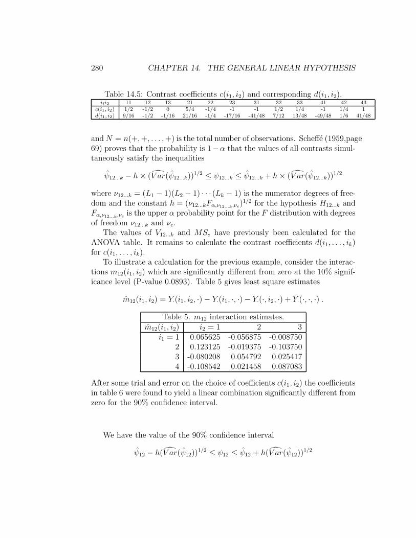
280 CHAPTER 14. THE GENERAL LINEAR HYPOTHESIS
Table 14.5: Contrast coefficients c(i1, i2) and corresponding d(i1, i2).iii2 11 12 13 21 22 23 31 32 33 41 42 43
c(i1, i2) 1/2 -1/2 0 5/4 -1/4 -1 -1 1/2 1/4 -1 1/4 1d(i1, i2) 9/16 -1/2 -1/16 21/16 -1/4 -17/16 -41/48 7/12 13/48 -49/48 1/6 41/48
andN = n(+,+, . . . ,+) is the total number of observations. Scheffe (1959,page69) proves that the probability is 1−α that the values of all contrasts simul-taneously satisfy the inequalities
ψ12...k − h× (V ar(ψ12...k))1/2 ≤ ψ12...k ≤ ψ12...k + h× (V ar(ψ12...k))
1/2
where ν12...k = (L1 − 1)(L2 − 1) · · · (Lk − 1) is the numerator degrees of free-dom and the constant h = (ν12...kFα,ν12...k,νe)
1/2 for the hypothesis H12...k andFα,ν12...k,νe is the upper α probability point for the F distribution with degreesof freedom ν12...k and νe.
The values of V12...k and MSe have previously been calculated for theANOVA table. It remains to calculate the contrast coefficients d(i1, . . . , ik)for c(i1, . . . , ik).
To illustrate a calculation for the previous example, consider the interac-tions m12(i1, i2) which are significantly different from zero at the 10% signif-icance level (P-value 0.0893). Table 5 gives least square estimates
m12(i1, i2) = Y·(i1, i2, ·)− Y·(i1, ·, ·)− Y·(·, i2, ·) + Y·(·, ·, ·) .
Table 5. m12 interaction estimates.m12(i1, i2) i2 = 1 2 3
i1 = 1 0.065625 -0.056875 -0.0087502 0.123125 -0.019375 -0.1037503 -0.080208 0.054792 0.0254174 -0.108542 0.021458 0.087083
After some trial and error on the choice of coefficients c(i1, i2) the coefficientsin table 6 were found to yield a linear combination significantly different fromzero for the 90% confidence interval.
We have the value of the 90% confidence interval
ψ12 − h(V ar(ψ12))1/2 ≤ ψ12 ≤ ψ12 + h(V ar(ψ12))
1/2

14.6. ANALYSIS OF COVARIANCE 281
= 0.638698− (19× 2.10936)1/2(0.031800)1/2 ≤ ψ12 ≤0.638698 + (19× 2.10936)1/2(0.031800)1/2
= 0.00429 ≤ ψ12 ≤ 1.27310
does not contain zero (F0.10,6,19 = 2.10936).
14.6 Analysis of Covariance
Consider the model
Ω : Yn×1 = Un×rγr×1 + Vn×sδs×1 + εn×1
where ε is multivariate normal Nn(0, σ2In) for the n× n identity matrix In
with γ, δ, and σ unknown and n > r+ s, with r+ s the rank of (U,V). Theparameters δ are covariates with V known. Hypotheses of interest are
Hω : Bm×r0 γ = cm×1
0
where B0 and c0 are given.If we write X = (U,V), βT = (γT , δT ), p = r + s, and
Am×p0 = (Bm×r
0 , 0m×s) then the previous linear model (14.1) applies with γΩ
and δΩ satisfying
XTXβΩ = XTY
orUTUγΩ + UTVδΩ = UT Y
VTUγΩ + VTVδΩ = VTY
Solving, we obtain
γΩ = (UTU)−1(UTY −UTVδΩ) .
If we write the modelΩ : Yn×1 = Uγ + ε
then following Scheffe (page 204)9, we can express the sum of squares for Ωin terms of the sums of squares for Ω.
9Scheffe, H. (1959) The Analysis of Variance, John Wiley and Sons, New York.

282 CHAPTER 14. THE GENERAL LINEAR HYPOTHESIS
DefineP(Ω)Y = UγΩ + VδΩ
= U(UTU)−1UTY + (I−U(UTU)−1U)VδΩ
= P(Ω)Y + Q(Ω)VδΩ
whereP(Ω) = U(UTU)−1U, and Q(Ω) = I−U(UTU)−1U .
Then using
||Z||2 = ZTZ, Q(Ω)T Q(Ω) = Q(Ω), and VTQ(Ω)VδΩ = VTQ(Ω)Y
we haveS2
e (Ω) = ||Y −P(Ω)Y||2
= ||Y −P(Ω)Y −Q(Ω)VδΩ||2
= ||Y −P(Ω)Y||2 − 2YT (I−P(Ω))Q(Ω)VδΩ + ||+ ||Q(Ω)VδΩ||2
= S2e (Ω)− δ
T
ΩVTQ(Ω)Y .
If we write
δΩ =
δ1Ωδ2Ω...
δsΩ
and V = (v1,v2, . . . ,vs) where vj =
v1j
v2j...vnj
then with S2e (Ω) = YTQ(Ω)Y we have
S2e (Ω) = S2
e (Ω)−s∑
j=1
δjΩvTj Q(Ω)Y (14.20)
andδΩ = (VTQ(Ω)V)−1VTQ(Ω)Y .
For calculating the numerator sum of squares for the hypothesis Hω wecan use equation (14.1)
S2Hω
= S2(ω)− S2(Ω) = (A0βΩ − c0)T (A0(X
TX)−1AT0 )−1(A0βΩ − c0)

14.6. ANALYSIS OF COVARIANCE 283
= (B0γΩ − c0)T (B0(U
T RU)−1BT0 )−1(B0γΩ − c0)
where R = I−V(VTV)−1VT and γΩ = (UTRU)−1UTRY.If we consider the model Ω and the hypothesis Hω : B0γ = c0 and we find
that S2(ω) is a quadeatic form YQ(ω)Y, which is the case when c0 = 0, thenwe can also calculate the numerator sum of squares S2
Hω= S2(ω) − S2(Ω)
using equation (14.20) and
S2(ω) = S2(Ω)−s∑
j=1
δjωvTj Q(ω)Y .
Here the vector δω (as well as γω) minimizes
||Y −Uγ −Vδ||2 subject to B0γ = c0
orδω = (VTQ(ω)V)−1VTQ(ω)Y
14.6.1 An Example
For an example, consider the balanced two-way layout with two covariates:
Ω : Yjkl = µjk + v(1)jklδ1 + v
(2)jklδ2 + εjkl
for j = 1, 2, . . . , J , k = 1, 2, . . . , K, and l = 1, 2, . . . , L with independentεjkl : N (0, σ2).
Write
α(1)j = µj· − µ··, α
(2)k = µ·k − µ··, α
(12)jk = µjk − µj· − µ·k + µ··
and consider the hypotheses
H1 : α(1)j = 0 for all j = 1, 2, . . . , J,
H2 : α(2)k = 0 for all k = 1, 2, . . . , K,
H12 : α(12)jk = 0 for all j = 1, 2, . . . , J, k = 1, 2, . . . , K .
From equations (14.3) and (14.4) we have
S2H1
(ω) = KLJ∑
j=1
(Yj·· − Y···)2

284 CHAPTER 14. THE GENERAL LINEAR HYPOTHESIS
and
S2e (Ω) =
J∑
j=1
K∑
k=1
L∑
l=1
(Yjkl − Yjk·)2 = YTQ(Ω)Y
S2(ω1) = S2e (Ω) + S2
H1(ω) = YTQ(ω1)Y
=J∑
j=1
K∑
k=1
L∑
l=1
(Yjkl − Yjk·)2 +KL
J∑
j=1
(Yj·· − Y···)2 .
Then
S2e (Ω) = S2
e (Ω)− δ1Ωv(1)Q(Ω)Y − δ2Ωv(2)Q(Ω)Y
where, in lexical order,
YT = (Y111, Y112, · · · , Y11L, Y121, · · · , Y12L, · · · , YJK1, · · · , YJKL)
and
(v(i))T =(v
(i)111, v
(i)112, · · · , v(i)
11L, v(i)121, · · · , v(i)
12L, · · · , v(i)JK1, · · · , v(i)
JKL
)for i = 1, 2 .
The covariate parameter estimates are obtained as solutions to the symmetriclinear equations
VTQ(Ω)VδΩ = VTQ(Ω)Y
or
((v(1))TQ(Ω)v(1) (v(1))TQ(Ω)v(2)
(v(2))TQ(Ω)v(1) (v(2))TQ(Ω)v(2)
)(δ1,Ω
δ2,Ω
)=
((v(1))TQ(Ω)Y(v(2))TQ(Ω)Y
)
Similarly,
S2(ω1) = S2(ω1)− δ1ω1v(1)Q(ω1)Y − δ2ω1v
(2)Q(ω1)Y
with the hypothesis covariate estimates solutions to
((v(1))TQ(ω)v(1) (v(1))TQ(ω)v(2)
(v(2))TQ(ω)v(1) (v(2))TQ(ω)v(2)
)(δ1,ω
δ2,ω
)=
((v(1))TQ(ω)Y(v(2))TQ(ω)Y
).
Then
S2H1
(ω1) = S2(ω1)− S2e (Ω) .

14.7. PROBLEMS 285
The F statistic is then
F =S2
H1(ω1)/(J − 1)
S2e (Ω)/(JK(L− 1)− 2)
which has the F(J−1),JK(L−1)−2 distribution.A Pascal program that calculates the analysis of covariance (ANCOVA)
table for multifactor designs with P-values is given by Shu-Yen Ho10
14.7 Problems
1. LetYjklm = µ+ αj + βk + γl + δjk + ηjl + ξkl + λjkl + εjklm
for j = 1, 2, . . . , J , k = 1, 2, . . . , K, l = 1, 2, . . . , L, m = 1, 2, . . . ,Mwhere εjklm : N (0, σ2) are independent and
J∑
j=1
αj =K∑
k=1
βk =L∑
l=1
γl = 0,
J∑
j=1
δjk =K∑
k=1
δjk =J∑
j=1
ηjl =L∑
l=1
ηjl =K∑
k=1
ξkl =L∑
l=1
ξkl = 0
J∑
j=1
λjkl =K∑
k=1
λjkl =L∑
l=1
λjkl = 0 .
Derive closed form expressions for sums of squares in the ANOVA tablefor testing main effects and higer order interactions are zero. Giveexpressions for Scheffe’s method of multiple comparisons to explainany effects significantly different from zero.
10Ho, Shu-Yen (1990). Sparse Matrix Methods for the Unbalanced Multifactor ANCOVA.University of Wisconsin at Madison Ph.D. Thesis, Department of Statistics. See alsoS.H.Ho and J.H. Klotz (1992). Sparse matrix methods for unbalanced multifactor analysisof variance and covariance. Journal of Statistical Computation and Simulation 41 55-72.

286 CHAPTER 14. THE GENERAL LINEAR HYPOTHESIS
2. Let
Yjklm = µ+αj + βk + γl + δjk + ηjl + ξkl + λjkl + ρtjklm +φujklm + εjklm
with side conditions and errors εjklm as in problem 1 and tjklm, ujklm
given. Give formulae for the ANCOVA table for testing main effectsand higer order interactions are zero.
3. Consider the following linear model
Yi = β0 + β1c1i + β2x2i + β3x3i + εi for i = 1, 2, . . . , n
with εi independent N (0, σ2) for the data
i x1i x2i x3i Yi
1 1.0 2.0 1.5 122 1.5 2.0 2.1 133 1.0 3.7 0.9 254 2.5 0.3 6.0 185 0.5 2.5 4.0 176 0.8 3.0 6.5 20
Test the hypothesis H : β1 + β3 = 0 versus A : β1 + β3 6= 0 and give a90% confidence interval for β1 + β3.

Chapter 15
Nonparametric Methods
Nonparametric or distribution free methods are designed to make inferenceswith few assumptions on the underlying distribution of the observations.Instead of a parametric model, for example N (µ, σ2), minimal assumptionssuch as X1, X2, . . . , Xn are independent with distribution F (x) continuousare considered.
15.1 The Sign Test
One of the simplest nonparametric methods is the sign test. Assume thatX1, X2, . . . , Xn are independent with c.d.f. F (x) with median m. That is mis a value such that
P [Xi ≤ m] = F (m) ≥ 1
2≤ 1− F (m−) = P [Xi ≥ m]
where F (m−) = limε↓0 F (m − ε) If F is continuous then F (m) = 12. We
consider one-sided hypotheses
H∗1 : m ≤ m0 vs A∗
1 : m > m0
H∗2 : m ≥ m0 vs A∗
2 : m < m0
or the two-sided hypothesis
H∗12 : m = m0 vs A∗
12 : m 6= m0 .
287

288 CHAPTER 15. NONPARAMETRIC METHODS
Consider the statistics
S+ =n∑
i=1
I[Xi > m0], S0 =n∑
i=1
I[Xi = m0], and S− =n∑
i=1
I[Xi < m0]
which are the number of observations that exceed, equal, or are less than m0.The joint distribution of (S+, S0, S−) is that of the multinomial
P [S+ = s+, S0 = s0, S− = n−s+−s0] =n!
s+!s0!(n− s+ − s0)!p
s+
+ ps00 p
(n−s+−s0)−
where
p+ = P [Xi > m0], p0 = P [Xi = m0], and p− = P [Xi < m0] = 1− p+− p0 .
We consider the hypotheses
H1 : p+ ≤ p−, H2 : p+ ≥ p−, and H12 : p1 = p2
and the corresponding alternatives
A1 : p+ > p−, A2 : p+ < p−, and A12 : p1 6= p2 .
H1 =⇒ H∗1
p+ ≤ p− gives p+ + p− ≤ 2p− or 1 − p0 ≤ 2p−. Thus p− ≥ (1 − p0)/2and P [Xi ≤ m0] = p− + p0 ≥ (1− p0)/2 + p0 ≥ 1/2 and m ≤ m0.
H2 =⇒ H∗2
p+ ≥ p− gives p+ ≥ (1− p0)/2 and P [Xi ≥ m0] = p+ + p0 ≥(1− p0)/2 + p0 ≥ 1/2 and m ≥ m0.
H12 =⇒ H∗12
p+ = p− gives 2p+ + p0 = 1 = 2p− + p0 or p+ = (1− p0)/2 = p−. ThenP [Xi ≥ m0] = p++p0 = (1−p0)/2+p0 ≥ 1/2 <= p−+p0 = P [Xi ≤ m0]and m = m0.
If F is continuous, so that p0 = 0 then the hypotheses H are equivalent tothe H∗ hypotheses.
To eliminate the nuisance parameter p0 we condition on S0. When p+ =p−, then p+/(1− p0) = 1/2 and
PH [S+ = s+|S0 = s0] =n!p
s+
+ ps00 p
(n−s+−s0)+
s+!s0!(n− s+ − s0)!/
(n
s0
)ps0
0 (1− p0)(n−s0)
15.1. THE SIGN TEST 289
=
(n− s0
s+
)1
2n−s0.
For the one-sided composite hypotheses, we use a least favorable distributionthat puts probability one for p+ = p−.
For testing H1 versus A1 we reject H1 in favor of A1 if S+ ≥ C1, givenS0 = s0, where the type I error α and C1 satisfy
n−s0∑
x=C1
(n− s0
x
)1
2(n−s0)= α . (15.1)
The power of the test for H1 is given for the alternative A1 : p+ > p− by
γ =
n−s0∑
x=C1
(n− s0
x
)(p+
1− p0
)x(p−
1− p0
)n−s0−x
.
For testing H2 versus A2, given S0 = s0, we reject if S+ ≤ C2 where αand C2 satisfy
C2∑
x=0
(n− s0
x
)1
2(n−s0)= α . (15.2)
For the two-sided hypothesis, given S0 = s0, we reject H12 in favor of A12
if S+ ≤ C12 or S+ ≥ n− s0 − C12 where
C12∑
x=0
(n− s0
x
)1
2(n−s0)= α/2 .
15.1.1 Confidence Interval for the Median
We consider the case where the distribution F (x) = G(x − m) where G iscontinuous with G(0) = 1/2 so thatm is the median of F . The acceptance re-gion for the two-sided test based on X = (X1, X2, . . . , Xn) in this continuousdistribution case is
A(m0) = X : C12 < S+ < n− C12
whereC12∑
x=0
(n
x
)1
2n= α/2 . (15.3)

290 CHAPTER 15. NONPARAMETRIC METHODS
The associated confidence set for m with confidence coefficient 1− α is
S(X) = m : C12 < S+(m) < n− C12
where S+(m) =∑n
i=1 I[Xi > m].To simplify the confidence set, let X(1) ≤ X(2) ≤ . . . ≤ X(n) be the order
statistics. Then X(r) ≤ m if and only if S+(m) ≤ n− r and
S(X) = m : C12 < S+(m) < n− C12 = m : C12 < S+(m) ≤ n− C12 − 1
= m : S+(m) ≤ C12c ∩ m : S+(m) ≤ n− C12 − 1= m : X(n−C12) ≤ mc ∩ m : X(C12+1) ≤ m
= m : X(C12+1) ≤ m < X(n−C12)) = [X(C12+1), X(n−C12))
Corresponding one-sided confidence bounds for the median m, with con-fidence coefficient 1− α, are
m : X(n−C1+1) ≤ m, and m : m < X(n−C2)
for the lower and upper bounds. Here C1, C2, and C12 satisfy equations(15.1), (15.2), and (15.3) with s0 = 0.
15.1.2 Point Estimate for the Median
If the sample size is odd (n = 2r + 1) then the 50% upper confidence boundfor the median is (−∞, X(r+1)) since (−∞, X(n−C2)) is the upper bound wherefrom equation (15.2)
C2∑
x=0
(2r + 1
x
)1
22r+1= 0.5
and C2 = r so that n − C2 = 2r + 1 − r = r + 1. Similarly the 50% lowerconfidence bound is [X(r+1),∞) and it seems reasonable to take the pointestimate for m to be X(r+1) =median(X1, X2, . . . , Xn). For even sample size(n = 2r) the upper bound with confidence coefficient at least 50% and closestto it is (−∞, X(r)) since
r∑
x=0
(2r
x
)1
22r>
1
2>
r−1∑
x=0
(2r
x
)1
22r.

15.1. THE SIGN TEST 291
To prove this
r∑
x=0
(2r
x
)1
22r=
r∑
x=0
(2r
2r − x
)1
22r=
2r∑
u=r
(2r
u
)1
22r.
So
2r∑
x=0
(2r
x
)1
22r=
r∑
x=0
(2r
x
)1
22r+
2r∑
u=r
(2r
u
)1
22r= 1 +
(2r
r
)1
22r.
Dividing by 2 we get
r∑
x=0
(2r
x
)1
22r=
1
2+
(2r
r
)1
22r+1>
1
2.
A similar proof shows
r−1∑
x=0
(2r
x
)1
22r=
1
2−(
2r
r
)1
22r+1<
1
2.
Thus C2 = r, n− C2 = 2r − r = r and (−∞, X(r)) is the upper bound withconfidence coefficient
1
2+
(2r
r
)1
22r+1.
Similarly, [X(r+1),∞) is the lower bound with the same confidence coefficient.We average these two bounds to get the point estimate
X(r) +X(r+1)
2= X = median(X1, X2, . . . , Xn) .
In both cases it is the median of the sample.To calculate the binomial probability we can use the incomplete beta
c.d.f. with the identity
x∑
k=0
(n
k
)1
2n= I1/2(n− x, x+ 1)
and use the subroutine in cdf.h, Appendix A.

292 CHAPTER 15. NONPARAMETRIC METHODS
15.1.3 Small Sample Performance Comparisons
We compare the performance of the sign test with that of parametric tests.Consider first the N (µ, σ2) distribution where σ2 is known. Here the medianm = µ and we test H1 : µ ≤ µ0 versus A1 : µ > µ0. The parametric X testbased on n2 observations rejects H1 in favor of A1 if
Z =
√n2(X − µ0)
σ≥ zα
where
α = 1− Φ(zα), Φ(x) =
∫ x
−∞
1√2πe−t2/2dt .
A measure of efficiency of the sign test based on n1 observations relative tothe X test based on n2 observations is e12(α, β, n1) = n2/n1. Here the samplesizes are chosen for a fixed alternative µ so that the type I error α and typeII error β are the same for each test. The problem with this definition is thatthe sample size is a discrete variable and it is often impossible to exactlymatch both error probabilities. If we choose a sample size n1 and a criticalvalue C1 that gives type I error for the sign test αS+ = α then we can adjustzα so that the type I error for the X test satisfies αX = α. However it maynot be possible to adjust n2 so that βX = βS+ = β. It is possible to findintegers n∗
2 < n∗∗2 such that
Φ(zα −√n∗∗
2 (µ− µ0)/σ) ≤ β ≤ Φ(zα −√n∗
2(µ− µ0)/σ) .
Thus we need some kind of interpolation between n∗2, n
∗∗2 to define n2. In this
example, the easiest interpolation is to pretend n2 is a continuous variablewith
Φ(zα −√n2(µ− µ0)/σ) = β .
Solving, we obtain
n2 =
[(zα + zβ)σ
µ
]2
For example, with n1 = 50, C1 = 30,
αS+ =
50∑
x=30
(50
x
)1
250
.= 0.10319 .

15.1. THE SIGN TEST 293
Table 15.1: Efficiency of the sign test relative to the X test.
n1 α β µ n2 e1211 0.1133 0.1013 0.9542 6.771 0.61616 0.1051 0.1188 0.7722 9.935 0.62123 0.1050 0.1177 0.6434 14.39 0.62650 0.1013 0.1156 0.4399 31.55 0.63176 0.1034 0.1105 0.3585 48.12 0.633
106 0.1032 0.1073 0.3055 67.24 0.634125 0.1052 0.1085 0.2793 79.33 0.634150 0.1103 0.1061 0.2534 95.08 0.634
For µ0 = 0, µ = 0.43991, σ2 = 1, we have p+ = 1−Φ(µ0−µ).= Φ(0.43991)
.=
0.67 and
βS+
.=
29∑
x=0
(50
x
)(0.67)x(0.33)50−x .
= 0.115641 .
Then
zα = Φ−1(1− 0.101319).= 1.27407, zβ
.= Φ−1(1− 0.115641) = 1.19706
n2 =
[1.27407 + 1.19706
0.43991
]2.= 31.5547, and e12
.= 31.5547/50
.= 0.63109 .
Table 15.1 gives additional such efficiency values.
Thus the nonparametric test relative to the parametric test requires abouta 37% larger sample size for the protection against the parametric model notbeing valid in this example.
15.1.4 Large Sample Performance Comparisons
As the sample sizes get large, it is also of interest to compare nonparametricand parametric tests. We look at asymptotic efficiency as n1 → ∞ withαS+(n1)→ α and βS+(n1)→ β where 0 < α, β < 1.

294 CHAPTER 15. NONPARAMETRIC METHODS
Using the central limit theorem for the binomial distribution we musthave C1 = C1(n1) satisfying
(C1(n1)− n1/2)√n1/4
−→ zα = Φ−1(1− α) (15.4)
with −∞ < zα <∞ since 0 < α < 1.Next, for n1 →∞, αS+(n1)→ α, in order for βS+(n1)→ β with
0 < α, β < 1 we must have the alternative µ = µn2 → µ0 since if not therewould be a subsequence converging to a limit value for µ greater than µ0.Because the X test is consistent, we would have βX → 0 for this subsequencecontradicting βX(n2)→ β > 0. This also implies
p+ = Φ((µn2 − µ0)/σ)→ 1/2
using the continuity of Φ(x).Using the normal approximation to the binomial under the alternative,
the Berry-Esseen approximation (9.1) gives
∣∣∣∣∣βS+(n1)− Φ
(C1(n1)− n1p+√n1p+(1− p+)
)∣∣∣∣∣ ≤ K((1− p+)3p+ + p3
+(1− p+))√n1p+(1− p+)
−→ 0
and since βS+(n1)→ β where 0 < β < 1 we have
Φ
(C1(n1)− n1p+√n1p+(1− p+)
)−→ β . (15.5)
Thus equations (15.4) and (15.5) give
αS+ −→ α =⇒ C1(n1) = n1/2 + zα
√n1/4(1 + o(1)) (15.6)
βS+ −→ β =⇒ C1(n1) = n1p+ + zβ
√n1p+(1− p+)(1 + o(1)) (15.7)
where o(1)→ 0 as n1 →∞. Subtracting (15.6) from (15.7) gives
n1(p+ − 1/2) +√n1(−zβ
√p+(1− p+)− zα/2)(1 + o(1))
and dividing by√n1/4 we get
zα + zβ = (2p+ − 1)√n1(1 + o(1)) .

15.1. THE SIGN TEST 295
Table 15.2: Limiting Pitman efficiencies of S+ relative to X.
Density ψ(t) ePS+,X
Uniform I[|t| < .5] 1/3 0.333
Normal e−t2/2/√
2π 2/π 0.637Logistic et/(1 + et)2 π2/12 0.822Double Exp. e−|t|/2 2 2.000Cauchy 1/[π(1 + t2)] ∞ ∞
Similarly, for the X test we get
zα + zβ =√n2(µn2 − µ0)/σ
and equating zα + zβ gives
n2
n1=
(2p+ − 1
(µn2 − µ0)/σ
)2
.
Taking the limit as n1 →∞ gives the limiting efficiency, due to Pitman, as
ePs+,X = lim
n1→∞n2
n1
=
(lim
n1→∞2Φ((µn2 − µ0)/σ)− 1
(µn2 − µ0)/σ
)2
=2
π.= 0.637 .
Consider a distribution function Ψ(t) with density ψ(t) and median att = 0 with finite variance σ2. If the distribution F (x) = Ψ(x − µ), belongsto a location parameter family, then for testing H : µ = 0 versus A : µ > 0we can similarly derive the limiting Pitman efficiency as
ePs+,X = 4σ2ψ2(0) (15.8)
using the central limit theorem for S+ and for X. Table 15.1.2 gives valuesfor several such distributions.
If we compare S+ against the t test when σ2 is unknown, the limits arethe same as for comparing against X.
15.1.5 Efficiency of the Median Point Estimator
If we calculate the variances of the sample median and sample mean for anormal N (µ, σ2) distribution we get the following table:

296 CHAPTER 15. NONPARAMETRIC METHODS
Table 15.3: Efficiency of X relative to X for N (µ, σ2).
n Var(X) Var(X) eX,X
1 1.0 1.0 1.0003 0.449 0.333 0.7425 0.287 0.200 0.6967 0.210 0.143 0.6819 0.1661 0.1111 0.668
11 0.1370 0.0909 0.66413 0.1661 0.0769 0.65815 0.1017 0.06667 0.65617 0.09004 0.05882 0.65319 0.08079 0.05263 0.651∞ 0 0 0.637
J.L. Hodges1 suggests
Var(X).=
2
π
(1− 0.4324
n
)
is a good approximation for the variance of the median for the N (0, 1) dis-tribution. Var(X) = 1/n for N (0, 1).
To get limiting efficiency, as n → ∞, let F (x) = Ψ(x − µ), Ψ(0) = 1/2,and dΨ(t)/dt = ψ(t). We have, for X =median(X1, X2, . . . , Xn),
√n(X − µ)
d−→ N (0, [4ψ2(0)]−1) as n→∞ .
To see this, let n = 2k + 1 so that the sample medianX = X(k+1). Then
Pµ[√n(X(k+1) − µ) ≤ u] = P0[X(k+1) ≤ u/
√n]
where Pµ indicates the probability is calculated for F (x) = Ψ(x − µ). Thisin turn equals
P0[#(Xi ≤ u/√n) ≥ k + 1] = P0[#(Xi − u/
√n ≤ 0) ≥ k + 1]
1Personal communication.

15.2. THE WILCOXON SIGNED RANK TEST 297
= P−u/√
n[#(Xi ≤ 0) ≥ k + 1] = P−u/√
n[#(Xi > 0) < k + 1]
= P−u/√
n[S+ < k+1] = P−u/√
n
[(S+ − np)/
√np(1− p) < (k + 1− np)/
√np(1− p)
]
where p = P−u/√
n[Xi > 0] = 1−H(u/√n). Using
k + 1− np√np(1− p)
=
((n + 1)/2− n(1−H(u/
√n))√
n/2
) √n/2√
np(1− p)−→ 2uh(0)
as n→∞ since p→ 1/2. The central limit theorem then gives
P−u/√
n
[(S+ − np)/
√np(1− p) < (k + 1− np)/
√np(1− p)
]−→ Φ(2uψ(0)) .
Using the central limit theorem for X we have for E(Xi) = µn, Var(Xi) = σ2
√n(X − µ)
d−→ N (0, σ2) .
If we define the limiting efficiency for these point estimators as the ratio ofthe variances of the limiting distributions then
eX,X =σ2
[4ψ2(0)]−1= 4σ2ψ2(0) .
This limit is the same as the limiting Pitman efficiency for the test of S+
relative to X and gives 2/π.= 0.637 for the N (µ, σ2) distribution.
15.2 The Wilcoxon Signed Rank Test
We note that the efficiency of the sign test is not particularly high whencompared to the X or t test forN (µ, σ2) alternatives. If we are willing to alsoassume that under the null hypothesis the distribution is symmetric aboutthe median then there is a nonparametric test with much better efficiency.
Let the sample X1, X2, . . . , Xn be independent with continuous c.d.f.F (x). For the hypothesis
H1 : F (x) is symmetric about the median µ = 0 versus A1 : µ > 0
the Wilcoxon2 signed rank statistic is
W+ =n∑
k=1
kzk where zk =
1 if X[k] > 00 if X[k] < 0
2Wilcoxon, Frank (1945). Individual comparisons by ranking methods. Biometrics 1,80-83

298 CHAPTER 15. NONPARAMETRIC METHODS
and X[k] is the k th largest in magnitude of the sample:
|X[1]| < |X[2]| < · · · < |X[n]| .
Thus W+ is the sum of the magnitude ranks for those observations that arepositive. We reject H1 in favor of A1 if W+ ≥ C1 where PH [W+ ≥ C1] = α
We note that if Xi = X ′i−X ′′
i where (X ′i, X
′′i ) are both independent with
the same distribution under H then Xi have a symmetric null distributionin this paired comparisom case.
15.2.1 Null Distribution of W+
If F is symmetric about µ = 0 then
PH [Z1 = z1, Z2 = z2, . . . , Zn = zn] =1
2nwhere zk ∈ 0, 1 .
Then
PH [W+ = w] =a(w, n)
2n
where a(w, n) is the number of vectors (z1, z2, . . . , zn) for which∑n
k=1 kzk = w.We can calculate a(w, n) from the recursion equation
a(w, n) = a(w, n− 1) + a(w − n, n− 1)
with a(−k, n) = 0 = a(n(n+1)/2+k, n) for integer k ≥ 1 and a(0, 1) = 1 = a(1, 1).This equation is shown as follows by adding numbers for zn = 1 and zn = 0:
a(w, n) = #(z1, z2, . . . , zn) :n∑
k=1
kzk = w
= #(z1, z2, . . . , zn−1, 0) :n−1∑
k=1
kzk = w
+#(z1, z2, . . . , zn−1, 1) :
n−1∑
k=1
kzk = w − n
= a(w, n− 1) + a(w − n, n− 1) .

15.2. THE WILCOXON SIGNED RANK TEST 299
Table 15.4: 2nP [W+ = w] for n = 1(1)12, w = 0(1)15.
w 0 1 2 3 4 5 6 7 8 9 10 11 12 13 14 15n=1 1 1
2 1 1 1 13 1 1 1 2 1 1 14 1 1 1 2 2 2 2 2 1 1 15 1 1 1 2 2 3 3 3 3 3 3 2 2 1 1 16 1 1 1 2 2 3 4 4 4 5 5 5 5 4 4 47 1 1 1 2 2 3 4 5 5 6 7 7 8 8 8 88 1 1 1 2 2 3 4 5 6 7 8 9 10 11 12 139 1 1 1 2 2 3 4 5 6 8 9 10 12 13 15 17
10 1 1 1 2 2 3 4 5 6 8 10 11 13 15 17 2011 1 1 1 2 2 3 4 5 6 8 10 12 14 16 19 2212 1 1 1 2 2 3 4 5 6 8 10 12 15 17 20 24
If we define W− =∑n
k=1 k(1 − zk) then the distribution of W− is the sameas that of W+ under the hypothesis of symmetry about µ = 0. Thus since
W+ +W− =n∑
k=1
k =n(n + 1)
2
we have a(w, n) = a(n(n + 1)/2 − w, n) and the distribution is symmetricabout n(n + 1)/4. Table 15.4 gives the distribution of 2nP [W+ = w] forn ≤ 12.
15.2.2 Zeros and Ties
When zeros and ties are present, Prat(1959)3 recommends using the zeros inranking the magnitudes and using average ranks for the magnitude ties. If0 < z1 < z2 < · · · < zK are the distinct magnitudes then the counts for theobservations X1, X2, . . . , Xn can be set up in a table:
3Prat, J.W. (1959) Remarks on zeros and ties in the Wilcoxon signed rank procedures.Journal of the American Statistical Association 54, 655-667.

300 CHAPTER 15. NONPARAMETRIC METHODS
Magnitudes 0 z1 z2 · · · zK
#(Xi > 0) u1 u2 · · · uK
#(Xi < 0) v1 v2 · vK
Total t0 t1 t2 · · · tK
Then with ai(t) the average ranks for the observations with tied magnitudezi, the statistic
W+ =
K∑
i=1
uiai(t), W− =
K∑
i=1
viai(t)
where t = (t0, t1, . . . , tK) and ai(t) = t0 + t1 + · · ·+ ti−1 + (ti + 1)/2.Klotz (1992)4 gave an algorithm for calculating the exact distribution and
later improved it using linked lists5
For large samples, a normal approximation can be used with
Z =W+ − E(W+|t)√
V ar(W+|t)
where
E(W+|(t0, t1, . . . , tK)) =n(n+ 1)− t0(t0 + 1)
2
andV ar(W+|(t0, t1, . . . , tK)) =
n(n + 1)(2n+ 1)− t0(t0 + 1)(2t0 + 1)
24−∑K
i=1 ti(ti − 1)(ti + 1)
48.
A subroutine Wilcox.h uses a linked list to calculate the Wilcoxon signedrank distribution with provision for ties in appendix J. Th program sRank.cppin appendix K uses the subroutine to calculate P-values for the test with in-put a set of numbers in a file. If the sample size n ≤ 200 exact P-valuses aregiven in addition to P-values from the normal approximation. For exampleif the data in file sRank.data is (X1, X2, . . . , X15) =
(5.0, −4.0, 0, 3.0, 2.0, −5.0, −1.0, −3.0, 4.0, 0, −4.0, 2.0, −3.0, −3.0, −2.0)
with the table of counts
4Klotz, J.H.(1992) Exact computation of the Wilcoxon signed rank distribution withzeros and ties. Computing Science and Statistics (Interface 90). Proceedings of the 22ndSymposium on the Interface. Springer-Verlag. N.Y. 397-400.
5Klotz, Jerome (1998) A linked list for the Wilcoxon signed rank test. NonparametricStatistics 9 88-93.

15.2. THE WILCOXON SIGNED RANK TEST 301
Magnitudes 0 1.0 2.0 3.0 4.0 5.0#(Xi > 0) 0 2 1 1 1#(Xi < 0) 1 1 3 2 1Total 2 1 3 4 3 2
and average ranks a = (3, 5, 8.5, 12, 14.5), then compiling the program sRank.cppg++ -o sRank sRank.cppand then executing it withsRank sRank.datagives the following output:
Wilcoxon signed rank test for data in Test.data .
Average magnitude ranks are used with zeros and ties.
Zeros are used to form average magnitude ranks with
W+ the sum of these ranks for positive observations.
W+=45 for sample size n= 15.
Lower tail P-value P(W+<=45 |5,t)= 0.22998046875
Upper tail P-value P(W+>=45 |5,t)= 0.78173828125
Two sided P-value= 0.4599609375 .
Normal approximation with zeros and ties correction:
approximate lower tail P-value 0.2203
approximate upper tail P-value 0.7797
approximate two tailed P-value 0.4405.
E(W+)= 58.5 , Var(W+)= 306.375, z= -0.77127 .
The limiting normal distribution of W+ under the hypothesis as n→∞ canbe established using the Liapounov form of the central limit theorem (seeTheorem 9.14).

302 CHAPTER 15. NONPARAMETRIC METHODS
15.2.3 Wilcoxon Point Estimate for the Center of Sym-
metry
Let X1, X2, . . . , Xn be independent with c.d.f F (x) = Ψ(x − µ) where Ψ(t)is continuous and symmetric about t = 0 (Ψ(−t) = 1−Ψ(t)). The statistic
W+ =∑∑
1≤i≤k≤n
I[Xi +Xj
2> 0]
since if we define X[1], X[2], . . . , X[n] to be the observations sorted by magni-tude, |X[1]| < |X[2]| < · · · < |X[n]|, then
∑∑
1≤i≤k≤n
I[Xi +Xj
2> 0] =
n∑
k=1
k∑
r=1
I[X[r] +X[k]
2> 0]
=n∑
k=1
kI[X[k] > 0] =n∑
k=1
kzk = W+
where zk = 1 if X[k] > 0 and 0 otherwise. Recall the values (Xi +Xj)/2 fori ≤ j are Walsh sums. Thus W+ is the number of positive Walsh sums outof the total n(n+ 1)/2.
For testing H : µ = µ0 versus A : µ 6= µ0 consider the acceptance regionusing W+(µ0) which is the Wilcoxon signed rank test statistic calculated forthe observations Xi − µ0 for i = 1, 2, . . . , n. The 1− α probability region is
A(µ0) = (X1, X2, . . . , Xn) : C < W+(µ0) < n(n + 1)/2− C
where the critical value C satisfies
P [W+ ≤ C] =α
2.
The associated confidence set is
S(X1, X2, . . . , Xn) = µ : C < W+(µ) < (n(n + 1)/2)− C .
Using
W+(µ) =∑∑
1≤i≤k≤n
I[Xi +Xj
2> µ]

15.2. THE WILCOXON SIGNED RANK TEST 303
and the event[C < W+(µ)] = [µ < w(n(n+1)/2−C)]
where w(1) < w(2) < · · · < w(n(n+1)/2) are the sorted Walsh sums. We haveW+(µ) < C implies at least C+1 of the ordered Walsh sums exceed µ namelythe C + 1 Walsh sums w(n(n+1)/2−C), w(n(n+1)/2−C+1), . . . , w(n(n+1)/2). Thus
S(X1, X2, . . . , Xn) = µ : w(C+1) ≤ µ < w(n(n+1)/2−C) .
For an example, consider the 12 data values
4.9 6.0 6.9 17.6 4.5 12.3 5.7 5.3 9.6 13.5 15.7 1.7
The 12× 13/2 = 78 sorted Walsh sums are
1.70 3.10 3.30 3.50 3.70 3.85 4.30 4.50 4.704.90 4.90 5.10 5.10 5.25 5.30 5.30 5.45 5.505.65 5.65 5.70 5.70 5.85 5.90 6.00 6.10 6.306.45 6.90 7.00 7.05 7.25 7.45 7.60 7.65 7.808.25 8.40 8.60 8.70 8.80 9.00 9.00 9.15 9.209.40 9.60 9.60 9.60 9.65 9.75 10.10 10.20 10.3011.65 11.80 12.25 12.30 12.65 12.90 13.50 13.60 14.0014.60 14.95 15.55 15.70 16.65 17.60
To construct a confidence interval with confidence coefficient just excceding0.95 we have from table 15.4, PH [W+ ≤ 13|n = 12] = 87/212 .
= 0.0212402and the exact confidence coefficient is 1−α = 1− 174/212 .
= 0.9575196. Thevalue of the confidence interval is
[w(14), w(65)) = [5, 25, 11, 80) .
The point estimator for µ is the median of the sorted Walsh sums. Forthe example it is (8.60+8.70)/2=8.65 .
15.2.4 Efficiency of W+
The limiting Pitman efficiency for ”near-by” location alternatives (F (x) =Ψ(x− µn)) where µn = O(1/
√n)) relative to the t-test is given by
ePW+,t = 12σ2
[∫ ∞
−∞ψ2(t)dt
]2
(15.9)

304 CHAPTER 15. NONPARAMETRIC METHODS
Table 15.5: Limiting Pitman efficiencies of W+ relative to X or t.
Density ψ(t) ePW+,t
Parabolic 3(5− t2)I[t2 < 5]/(20√
5) 108/125 0.864
Normal e−t2/2/√
2π 3/π 0.955Uniform I[|t| < .5] 1 1.000Logistic et/(1 + et)2 π2/9 1.097Double Exp. e−|t|/2 3/2 1.500Cauchy 1/[π(1 + t2)] ∞ ∞
where ψ(t) is the density of Ψ(t) and σ2 is the variance for Ψ. Table (15.5)gives values for various densities.
Hodges and Lehmann (1956)6, using a calculus of variations argument,show that eP
W+,t(H) ≥ 0.864 for all distributions. This lower bound is attainedfor the patabolic density. Klotz (1963)7, using a computation scheme ofHodges, showed that small sample efficiency for normal shift alternatives isclose to the limiting Pitman efficiency value.
The limiting efficiency of the Walsh sum median point estimator relativeto X, by an argument similar to that for the sign test and median, is is alsogiven by equation (15.9) where σ2/n is the variance of X.
15.3 The Two Sample Median Test
Let X1, X2, . . . , Xm be independent with c.d.f. F (x) and Y1, Y2, . . . , Yn beindependent with c.d.f. G(x). For testing the hypothesis
H : G = F versus A : G > F (15.10)
6Hodges, J.L. and E.L. Lehmann (1956) Efficiencies of some nonparametric competitorsof the t-test. Annals of Mathematical Statistics 27, 324-335.
7Klotz, J.H. (1963) Small sample power and efficiency for the one sample Wilcoxonand normal scores tests. Annals of Mathematical Statistics 34 624-632.

15.3. THE TWO SAMPLE MEDIAN TEST 305
Mood and Brown (1950)8 proposed the two sample median test. Let Z bethe median of the combined sample X1, X2, . . . , Xm, Y1, Y2, . . . , Yn and define
B =m∑
i=1
I[Xi > Z]
the number of Xi that exceed Z. If B is large, we reject H in favor of A (ashift of the X sample to the right of the Y sample).
The null distribution of B is the hypergeometric(N,m, a)
PH [B = b] =
(m
b
)(n
a− b
)/
(N
a
)for b = L,L+ 1, . . . , U
where N = m+ n, L = max(0, m+ a−N), U = min(m, a), and
a =
m∑
i=1
I[Xi > Z] +
n∑
j=1
I[Yj > Z]
is the number of observations in the pooled sample greater than Z.If N is even and there are no ties, then a = N/2.
15.3.1 Confidence Interval for a Difference in Location
Parameters
If F (x) = Ψ(x− µ) and G(x) = Ψ(x− η), with ∆ = µ − η, then for testingH : ∆ = ∆0 we can use the statistic
B(∆0) =
m∑
i=1
I[Xi −∆0 > Z(∆0)]
where Z(∆0) is the median for the combined sample
X1 −∆0, X2 −∆0, . . . , Xm −∆0, Y1, Y2, . . . , Yn .
The acceptance region with probability 1 − α for the approximately equaltailed two sided test is
A(∆0) = (X1, X2, . . . , Xm, Y1, Y2, . . . , Yn) : C1 < B(∆0) < C28Mood, A.M. (1950) Introduction to the Theory of Statistics. McGraw-Hill, New York.

306 CHAPTER 15. NONPARAMETRIC METHODS
wherePH(B ≤ C1) = α1, PH(B ≥ C2) = α2, α = α1 + α2
and α1, α2 ≤ α∗/2 are both as close to α∗/2 as possible where 1− α∗ is thenominal confidence coefficient. The associated confidence set for ∆ is
S(X1, X2, . . . , Xm, Y1, Y2, . . . , Yn) = ∆ : C1 < B(∆) < C2 .
Using the relation
[B(∆) ≥ b] = [Y(n−(a−b)) < X(m−b+1) −∆] = [∆ < X(m−b+1) − Y(n−(a−b))]
since at least b of the Xi −∆, namely the sorted values
X(m−b+1) −∆, X(m−b+2) −∆, . . . , X(m) −∆,
must be greater than the observations that contain the median Z(∆) whichinclude at least
X(1) −∆, X(2) −∆, . . . , X(m−b) −∆, Y(1), Y2), . . . , Y(n−(a−b)) .
Note (m − b) + (n − (a − b)) = N − a which is the number of observationsless than or equal Z. Thus
[C1 < B(∆) < C2] = [B(∆) ≥ C2]c ∩ [B(∆) ≥ C1 + 1]
= [∆ < X(m−C2+1) − Y(n−a+C2)]c ∩ [∆ < X(m−C1) − Y(n−a+C1+1)]
= [X(m−C2+1) − Y(n−a+C2) ≤ ∆ < X(m−C1) − Y(n−a+C1+1)]
= [X(m−C2+1) − Y(n−a+C2), X(m−C1) − Y(n−a+C1+1)) .
15.3.2 Efficiency of the Mood and Brown Test
For F (x) = Ψ(x − µ) and G(x) = Ψ(x − η) where Ψ(x) has density ψ(x)then using asymptotic theory for ”near-by” altermatives ∆ = µ− η = ∆N =O(1/
√N) we obtain the limiting Pitman efficiency of B relative to the two
sample t test for these location parameter distributions as N → ∞, λN =m/N → λ where 0 < λ < 1 is
4σ2ψ2(0)
where σ2 is the variance of the distribution Ψ(x). Table 15.6 gives values forvarious densities as in table 15.2 for the sign test.

15.4. THE TWO SAMPLE WILCOXON RANK TEST 307
Table 15.6: Limiting Pitman efficiencies of B relative to t.
Density ψ(t) ePB,t
Uniform I[|t| < .5] 1/3 0.333
Normal e−t2/2/√
2π 2/π 0.637Logistic et/(1 + et)2 π2/12 0.822Double Exp. e−|t|/2 2 2.000Exponential e−tI[t > 0] 4 4.000Cauchy 1/[π(1 + t2)] ∞ ∞
15.4 The Two Sample Wilcoxon Rank Test
Another test for the hypothesis (15.10) is that of the Wilcoxon two samplerank sum test 9. For the two samples (X1, X2, . . . , Xm) and (Y1, Y2, . . . , Yn)from continuous distributions (so there are no ties), let R(Xi) be the rank inthe pooled sample of N = m+ n observations. We reject H in favor of A if
WX =
m∑
i=1
R(Xi)
is large. An alternate equivalent statistic due to Mann and Whitney10 is
UY X =m∑
i=1
n∑
j=1
I[Yj < Xi] = WX −m(m+ 1)
2.
To show this we have
UY X = R(X(1))− 1 +R(X(2))− 2 + · · ·+R(X(m))−m = WX −m(m+ 1)/2 .
15.4.1 Null Distribution of UY X
The null distribution of UY X is the same as that for UXY . To prove this letW ∗
X ,W∗Y be the values of the statistics where we rank the observations in
9Wilcoxon, Frank (1945). Individual comparisons by ranking methods. Biometrics 1,80-83
10Mann, H. B. and Whitney, D.R. (1947). On a test of whether one of two randomvariables is stochastically larger than another. Annals of Mathematical Statisticsis 18,50-60.

308 CHAPTER 15. NONPARAMETRIC METHODS
reverse order (from largest to smallest). Then
W ∗X =
m∑
i=1
R∗(Xi) =
m∑
i=1
(N + 1− R(Xi)) = m(N + 1)−WX
where R∗(Xi) is the rank in decreasing order of Xi and R(Xi) is the rank inincreasing order. Thus
WX −m(N + 1)/2 = m(N + 1)/2−W ∗X
Since the joint null distribution of the ranks R∗(Xi) is the same as that forR(Xi), namely 1/
(Nm
), we have
PH [WX −m(N + 1)/2 = w] = PH [m(N + 1)/2−WX = w] . (15.11)
Now using WX + WY = N(N + 1)/2 we have WX −m(N + 1)/2 = m(N +1)/2−WY so from (15.11) we get
PH(UY X = u] = PH [(WX −m(N + 1)/2) +mn/2 = u]
= PH [(m(N + 1)/2−WX) +mn/2 = u] = P [WY − n(N + 1)/2 +mn/2 = u]
= PH [WY − n(n + 1)/2 = u] = PH [UXY = u] .
Since UY X = mn − UXY the distribution of UY X is symmerric about mn/2for the case of no ties.
Let U = UXY or UY X . If we define
PH [U = u] =a(u|N,m)(
Nm
) ,
we have the recursion equation
a(u|N, n) = a(u|N − 1, m) + a(u− n|N − 1, m− 1)
since the largest value in the pooled sample is either a Y value or an X valuefor U = UY X . If A(u|N,m) =
∑uk=0 a(k|N,m) is the cumulative, then also
A(u|N, n) = A(u|N − 1, m) + A(u− n|N − 1, m− 1)
with side conditions
A(u|N, n) = 0 for u < 0, and A(u|N, n) =
(N
m
)for u ≥ mn.

15.4. THE TWO SAMPLE WILCOXON RANK TEST 309
A variety of tables exist. In particular Milton (1964)11 gives critical values.Fix and Hodges (1955)12 use this recursion formula and partition theory toextend the calculation of exact probabilities.
15.4.2 Distribution of UY X in the Presence of Ties
Consider the discrete case where the observations can only take on the valuesz1 < z2 < · · · < zK . Let
P [Xi = zk] = pk and P [Yj = zk] = rk
where∑K
k=1 pk = 1 =∑K
k=1 rk. The hypothesis is then H : pk = rk and thedistributions under H are
PH(X = x) = pu11 p
u22 · · · puk
K , PH(Y = y) = pv11 p
v22 · · · pvk
K
and for X = (X1, X2, . . . , Xm), x = (x1, x2, . . . , xm) Y = (Y1, Y2, . . . , Yn),y = (y1, y2, . . . , ym)
PH(X = x,Y = y) = pt11 p
t22 · · · ptk
K
where the counts
uk =m∑
i=1
I[xi = zk], vk =n∑
j=1
I[yj = zk], and tk = uk + vk .
Thus Tk = Uk +Vk =∑m
i=1 I[Xi = zk]+∑n
j=1 I[Yj = zk] for k = 1, 2, . . . , K issufficient for p = (p1, p2, . . . , pK) under H . We can construct a distributionfree test by conditioning on T = (T1, T2, . . . , TK). We have
PH(U = u|T = t) =
(m!
K∏
k=1
pukk
uk!
)(n!
K∏
k=1
pvkk
vk!
)/
(N !
K∏
k=1
ptkk
tk!
)=
K∏
k=1
(tkuk
)/
(N
m
).
11Milton, R.(1964) An extended table of critical values for the Mann-Whitney(Wilcoxon) two sample statistic. Journal of the American Statistical Association 59,925-934.
12Fix, E. and Hodges, J.L.,Jr.(1955). Significance probabilities of the Wilcoxon test.Annals of Mathematical Statistics 26, 301-312.

310 CHAPTER 15. NONPARAMETRIC METHODS
Putter (1955)13 recommends using average ranks R∗(Xi) for the Wilcoxonrank sum statistic
W ∗X =
m∑
i=1
R∗(Xi) =
K∑
k=1
ukr∗k
where the k-th largest average rank is
r∗k = t1 + t2 + · · ·+ tk−1 +tk + 1
2for k = 2, 3, . . . , K
and r∗1 = (t1 + 1)/2. The equivalent Mann Whitney form is
UY X = (U1, U2, . . . , UK)
1/2 0 · · · 01 1/2 · · · 0...
.... . .
...1 1 · · · 1/2
V1
V2...VK
= UQVT
which satisfies
UY X =
m∑
i=1
n∑
j=1
(I[Yj < Xi] +
1
2I[Yj = Xi]
)= W ∗
X −m(m+ 1)
2.
The exact distribution is given by
PH(UY X ≤ x|T = t] =∑
u∈R(x)
K∏
k=1
(tkuk
)/
(N
m
)
whereR(x) = u : uQ(t − u)T ≤ x .
Klotz (1966)14 developed an early program using this scheme by generatingall possible vectors (u1, u2, . . . , uK) with
∑Kk=1 uk = m and 0 ≤ uk ≤ tk for
k = 1, 2, . . . , K. Mehta et. al.(1984)15 improved this scheme by eliminat-ing some unnecessary vectors in the generation. Cheung and Klotz (1997)16
13Putter, J.(1955). The treatment of ties in some nonparametric tests. Annals ofMathematical Statistics 26, 368-386.
14Klotz, J.H. (1966) The Wilcoxon, ties, and the computer. Journal of the AmericanStatistical Association 61, 772-787.
15Mehta, C.R., Patel, N.R. and Tsiatis, A.A. (1984). Exact significance testing toestablish treatment equivalence with ordered categorical data. Biometrics 40, 819-825.
16Cheung, Y.K. and Klotz, J.H. (1997). The Mann Whitney Wilcoxon distributionusing linked lists. Statistica Sinica 7, 805-813.

15.4. THE TWO SAMPLE WILCOXON RANK TEST 311
furthur improved the distribution calculation by using a linked list. The sub-routine MannW.h in appendix L calculates the distribution for given valuesof t andm. The program RankSum.cpp in appendix M gives exact P-valuesfor N ≤ 100 and approximate P-values using the normal approximation for
Z =UY X −EH(UY X |t)√
V arH(UY X |t)
where
EH(UY X |t) =mn
2, V arH(UY X |t) =
mn(N + 1)
12
(1− γ
N3 −N
),
and γ =∑K
k=1(t3k − tk) is the correction for ties. Note γ = 0 if there are no
ties (ti = 1 for all i = 1, 2, . . . , K = N).For example if the file dataX contains the values
18 14.5 13.5 12.5 23 24 21 17 18.5 9.5 14
and the file dataY contains the values
27 34 20.5 29.5 20 28 20 26.5 22 24.5 34 35.5 19
then compiling the program using the gnu C++ compiler withg++ -o RankSum RankSum.cpp and executing the program withRankSum dataX dataY we obtain the following output:
P-values for the Wilcoxon Mann Whitney two sample rank sum test for the
X sample data in file ‘dataX’ and the Y sample data in file ‘dataY’.
Using the exact distribution:
UYX = 14, m= 11, n= 13
Lower tail P-value is P(UYX<=14|m, t)= 0.000184284
Upper tail P-value is P(UYX>=14|m, t)= 0.999839
For the two sided test which rejects for |UYX-E(UYX)|>=C
the P-value is P(UYX<=14|m,t)+P(UYX>=129|m,t)= 0.000371773 .
Using the normal approximation with
UYX = 14, m= 11, n= 13
E(UYX)=71.5, Var(UYX)=297.658, sigma(UYX)=17.2528
Z=(UYX-E(UYX))/sigma(UYX)=-3.3328

312 CHAPTER 15. NONPARAMETRIC METHODS
Approximate lower tail P-value is 0.000429882
Approximate upper tail P-value is 0.99957
Approximate P-value for the two sided test is 0.000859765
for ties
t=(1, 1, 1, 1, 1, 1, 1, 1, 1, 2, 1, 1, 1, 1, 1, 1, 1, 1, 1, 1, 2, 1).
K= 22, sum(t[i]^3-t[i])= 12 .
15.4.3 Confidence Intervals for a Location Difference
If F (x) = Ψ(x − µ) and G(x) = Ψ(x − η), are continuous with ∆ = µ − η,then for testing H : ∆ = ∆0 we can use the statistic
UY X(∆0) = #Xi −∆0 < Yj : for i = 1, 2, . . . , m; j = 1, 2, . . . , n .
If the acceptance region for the two sided test is
A(∆0) = (X1, X2, . . . , Xm, Y1, Y2, . . . , Yn) : C1 < UY X(∆0) < C2
then the corresponding confidence interval for ∆ is
S(X1, X2, . . . , Xm, Y1, Y2, . . . , Yn) = ∆ : C1 < UY X(∆) < C2 .
Let W(1) < W(2) < · · · < W(mn) be the sorted values of Xi − Yj fori = 1, 2, . . . , m and j = 1, 2, . . . , n. Then we have the relation
[UY X(∆) ≥ k] = [W(mn−k+1) > ∆]
since if at least k of the differences Xi − Yj are greater than ∆, they areW(mn−k+1),W(mn−k+2), . . . ,W(mn). Thus
S(X1, X2, . . . , Xm, Y1, Y2, . . . , Yn) = ∆ : W(mn−C2+1) ≤ ∆ < W(mn−C1)
If we use an equal tail test, with C1 chosen such that
α
2= PH(UY X ≤ C1)
then using the symmetry for the distribution without ties, C2 = mn − C1
and the confidence interval for ∆ is then [W(C1+1),W(mn−C1)). We count inC1 + 1 values from both ends of W(1) < W(2) < · · · < W(mn).

15.4. THE TWO SAMPLE WILCOXON RANK TEST 313
If Ψ(x) is not continuous then the confidence interval that includes bothendpoints
∆ : W ∗(mn−C2+1) ≤ ∆ ≤W ∗
(mn−C1)where W ∗
(1) ≤W ∗(2) ≤ · · · ≤W ∗
(mn) are sorted values of Yj−Xi, has probabilityof covering ∆ at least 1− α. Here α = α1 + α2 and
α1 = PH(UY X ≤ C1), α2 = PH(UY X ≥ C2)
is computed using the null distribution without ties. For a proof, see Randalesand Wolfe (1979)17 pages 182,183.
For example, if the X sample values are
2.7 3.2 4.5 7.6 8.1
and the Y sample values are
0.8 1.6 1.9 2.2 3.7 4.3 8.0
then the sarted differences are
-5.3 -4.8 -3.5 -1.4 -1.0 -0.9 -0.5-0.4 0.1 0.2 0.5 0.8 0.8 1.01.1 1.3 1.6 1.9 2.3 2.4 2.62.9 3.3 3.7 3.8 3.9 4.4 5.45.7 5.9 6.0 6.2 6.5 6.8 7.3
.
If we use C1 = 6 and C2 = 29 then P (UY X ≤ 6) = P (UY X ≥ 29) = 29/792.=
0.0366162 and P (6 < UY X < 29) = 734/792.= 0.9267677. Thus counting in
7 from each end, the value of the confidence interval with probability at least0.9267677 is [W(7),W(29)] = [−0.5, 5.7].
Hodges and Lehmann (1963)18 recommend the point estimator for ∆given by
∆ = medianYj −Xi : i = 1, 2, . . . , m; j = 1, 2, . . . , n .
In the example above, ∆ = 1.9.
17Randals, R.H. and Wolfe, D.A. (1979). Introduction to the Theory of NonparametricStatistics. John Wiley & Sons, New York.
18Hodges, J.L.,Jr. and Lehmann, E.L. (1962). Estimates of location based on ranktests. Annals of Mathematical Statistics 34, 598-611.

314 CHAPTER 15. NONPARAMETRIC METHODS
15.4.4 Efficiency of the Two Sample Wilcoxon
Noether (1955)19 presented a theoren for comparing the efficiency of two testsfor a sequence of alternative distributions converging to the null hypothesis(so called near by alternatives). The theorem established the relative effi-ciency under several assumptions, including the common limiting distribu-tion such as the normal, as a ratio of the squares of the efficacies of the twotests.
For the two sample Wilcoxon Mann Whitney test, the Hoeffding (1948)20
paper on U statistics proved the asymptotic normality of UY X . It can alsobe shown for WX using the theory of Chernoff and Savage (1958)21.
For F (x) = Ψ(x − ∆N), G(x) = Ψ(x) with ∆N = O(1/√N), and λN =
m/N → λ where 0 < λ < 1 as N →∞, the efficacy for UY X is
EUY X= lim
N→∞
dE∆(UY X)/d∆|∆=0√NV ar0(UY X)
=√
12λ(1− λ)
∫ ∞
−∞ψ2(x)dx .
Similarly, for the two sample t test the efficacy is
Et =√λ(1− λ)/σ2
and the limiting Pitman efficiency for these shift alternatives is
ePUY X ,t =
E2UY X
E2t
= 12σ2
[∫ ∞
−∞ψ2(x)dx
]2
where ψ(x) = dΨ(x)/dx is the density for Ψ. This is the same expression asin equation (15.9), (see table 15.5), for the one sample Wilcoxon signed ranktest Pitman efficiency relative to the one sample t test.
This efficiency is also the limiting ratio of variances for the point estimate∆ relative to X − Y as shown by Hodges and Lehmann (1963)18.
19Noether, G.E. (1955) On a theorem of Pitman. Annals of Mathematical Statistics26,64-68
20Hoeffding, W. (1948). A class of statistics with asymptotically normal distribution.Annals of Mathematical Statistics 19, 293-325.
21Chernoff, H. and Savage, I.R. (1958). Asymptotic normality and efficiency of certainnonparametric test statistics. Annals of Mathematical Statistics 29,972-994.

15.5. MOOD AND BROWN MEDIAN TEST FOR K SAMPLES 315
15.5 Mood and Brown Median Test for K
Samples
Let samples Xij : j = 1, 2, . . . , ni be independent with distribution func-tion Fi(x) for i = 1, 2, . . . , K. To test the hypothesis
H : F1 = F2 = · · · = FK versus A : not all Fi equal, (15.12)
Brown and Mood (1948)22, (1951)23 proposed the K sample median testwhich rejects H in favor of A for large values of
B2(M) =N(N − 1)
a(N − a)K∑
i=1
(Mi −
nia
N
)2
/ni
where N =∑K
i=1 ni, and M = (M1,M2, . . . ,MK) are the numbers in each
sample that exceed the median of the pooled sample, a =∑K
i=1Mi .
15.5.1 The Exact Null Distrbution of B2
To take into account the possibility of ties, consider the discrete case wherethe samples take on the values z1 < z2 < · · · < zc with probabilities
PH(Xij = zr) = pr, r = 1, 2, . . . , c (15.13)
where∑c
r=1 pr = 1. We can construct a distribution free test of H by condi-tioning on the sufficient statistic T = (T1, T2, . . . , Tc) where
Tr =K∑
i=1
ni∑
j=1
I[Xij = zr, ] r = 1, 2, . . . , c
is the total number of observations equal to zr. Given T = (t1, t2, . . . , tc) = t,define the pooled sample median by
z =
zs if
∑sr=1 tr ≥ N/2 and
∑cr=s tr ≥ N/2
(zs + zs+1)/2 if∑s
r=1 tr = N/2 and∑c
r=s+1 tr = N/2.
22Brown, G.W. and Mood, A.M. (1948). Homogenity of several samples. The AmericanStatistician 2 22.
23Brown, G.W. and Mood, A.M. (1951). On median tests for linear hypotheses. Pro-ceedings of the Second Berkeley Symposium on Mathematical Statistics and ProbabilityUniversity of California Press, Berkeley, California, pp 159-166.

316 CHAPTER 15. NONPARAMETRIC METHODS
Then the counts above the median are Mi =∑ni
j=1 I[Xij > z]. We have for
a =∑K
i=1mi ,
PH(M = (m1, m2, . . . , mK)|T = (t1, t2, . . . , tc)) =
(n1
m1
)(n2
m2
)· · ·(
nK
mK
)(
Na
) .
We can calculate the exact P-value by enumeration
α =∑
u∈R
K∏
i=1
(ni
ui
)(
Na
)
where u = (u1, u2, . . . uK) and
R = u : ui integer, 0 ≤ ui ≤ ni,
K∑
i=1
ui = a, B2(u) ≥ B2(M) .
The more efficient approach of Jorn and Klotz (2002)24 uses the equivalentstatistic
V (M) =
K∑
i=1
M2i /ni
where
B2(M) =N(N − 1)
a(N − a)
(V (M)− a2
N
).
If we write Nk =∑k
i=1 ni, Vk =∑k
i=1M2i /ni, and ak =
∑ki=1Mi for
k = 1, 2, . . . , K then for
Qk(vk|ak) = PH(Vk ≥ vk|t)
we have the convolution formula
Qk(vk|ak) =
Lk∑
mk=Lk
Qk−1(vk −m2k/nk|ak −mk)
(nk
mk
)(Nk−1
ak−mk
)(
Nk
ak
)
where Lk = max(0, ak − Nk−1) and Lk = min(ak, nk). For k = 1 we startwith the indicator function Q1(v1|a1) = I[a2
1/n1 ≥ v1].
24Jorn, H. and Klotz, J. (2002). Exact distribution of the K sample Mood and Brownmedian test. Nonparametric Statistics 14, 249-257.

15.5. MOOD AND BROWN MEDIAN TEST FOR K SAMPLES 317
For contrasts, we can adapt the multiple comparison method of Scheffe(1959)25 using contrasts of the form
φ =
K∑
i=1
CiMi/ni, where
K∑
i=1
Ci = 0 .
We have the following
Theorem 15.1 Under the hypothesis, the probability is 1− α that simulta-neously for all contrasts
−[hαVar(φ)
]1/2
< φ <[hαVar(φ)
]1/2
where
Var(φ) =a(N − a)N(N − 1)
K∑
i=1
C2i
ni, a =
K∑
i=1
Mi, N =
K∑
i−1
ni
and hα satisfies PH(B2 ≥ hα |t) = α.
Proof: Since∑K
i=1Ci = 0, by Schwartz inequality
φ2 =
(K∑
i=1
CiMi
ni
)2
=
(K∑
i=1
Ci√ni
((Mi − nia/N)√
ni
)2)
≤(
K∑
i=1
C2i
ni
)(K∑
i=1
(Mi − nia/N)2
ni
)
=
(a(N − a)N(N − 1)
K∑
i=1
C2i
ni
)(N(N − 1)
a(N − a)K∑
i=1
(Mi −
nia
N
)2
/ni
)= Var(φ)B2
and
PH(φ2 < hαVar(φ) |t) ≥ PH(B2Var(φ) < hαVar(φ) |t) = 1− α .
The program Mood.cpp in appendix N calculates the P-value for theMood and Brown test with an options for contrasts and methods for dataentry.
25Scheffe, H. (1959). The Analysis of Variance. John Wiley and Sons, New York.

318 CHAPTER 15. NONPARAMETRIC METHODS
For eaample if we compile the file Mood.cpp with the commandg++ -o Mood Mood.cpp for the gnu C++ compiler and then execute itwith Mood then, for the choices made, we obtain the following output fordata in file Mood.dat, which has 8 lines for the 8 samples, and selecting acontrast with coefficients (0, 0, 2, 0,−1, 0,−1, 0) :
Do you wish to enter data vaues or counts?
Type V for data values or C for counts : v
Do you wish to enter data from the keyboard or from a file?
Type K for keyboard or F for file : f
Enter input data file name: Mood.dat
Data matrix:
2 2.8 3.3 3.2 4.4 3.6 1.9 3.3 2.8 1.1
3.5 2.8 3.2 3.5 2.3 2.4 2 1.6
3.3 3.6 2.6 3.1 3.2 3.3 2.9 3.4 3.3 3.2
3.2 3.3 3.2 2.9 3.3 2.5 2.6 2.8
2.6 2.6 2.9 2 2 2.1
3.1 2.9 3.1 2.5
2.6 2.2 2.2 2.5 1.2 1.2
2.5 2.4 3 1.5
Sample counts m[i] of values above pooled median,
and sample sizes n[i], for i=1,2,...,8.
#i | 1 2 3 4 5 6 7 8 | Total
_______________________________________________________
m[i]| 5 3 9 5 1 3 0 1 | 27
_______________________________________________________
n[i]| 10 8 10 8 6 4 6 4 | 56
_______________________________________________________
Median of pooled sample is 2.8 .
Do you wish to write answers to a file?
Type y)es or n)o : n
The Mood & Brown chi square statistic Chi^2= 17.696
Equivalently, V=M[1]^2/n[1]+...+M[K]^2/n[K]= 17.517

15.5. MOOD AND BROWN MEDIAN TEST FOR K SAMPLES 319
The P-value P[V>=17.517]= 0.0068961050168
for K=8, n=(10, 8, 10, 8, 6, 4, 6, 4), and a=27.
count=384847
Program time : 0 seconds.
Program ticks: 290000 ticks.
Do you wish to enter a contrast?
Please enter y)es or n)o : y
The values of M[i]-a*n[i]/N are :
0.1786 -0.8571 4.179 1.143 -1.893 1.071 -2.893 -0.9286
Enter 8 constants that add to zero : 0 0 2 0 -1 0 -1 0
phi= 1.633
Confidence probability for this contrast is : 0.965755
Do you wish to enter a contrast?
Please enter y)es or n)o : n
15.5.2 Large Sample Null Distribution Approxination
As N →∞ with ni/N → λi, where 0 < λi < 1 and∑K
i=1 λi = 1, we have
B2(M) =N(N − 1)
a(N − a)K∑
i=1
(Mi −
nia
N
)2
/nid−→ χ2
K−1(0)
under the hypothesis. This follows from the limiting normal distribution of
Z =
((M1 − n1a/N)√
n1
,(M2 − n2a/N)√
n2
, . . . ,(MK − nKa/N)√
nK
)Td−→ NK(0,Σ)
where the K ×K matrix of rank K − 1 is
Σ =1
4
1− λ1 −√λ1λ2 · · · −√λ1λK
−√λ2λ1 1− λ2 · · · −
√λ2λK
......
. . ....
−√λKλ1 −√λKλ2 · · · 1− λK

320 CHAPTER 15. NONPARAMETRIC METHODS
since
VarH
(Mi√ni
)=a(N − a)(N − ni)
N2(N − 1)−→ 1
4(1− λi) ,
and
CovH
(Mi√ni,Mj√nj
)= − a(N − a)
N2(N − 1)
√ninj −→ −
1
4
√λiλj .
Then using proposition 10.7 in section 10.8, and 14Σ− = IK , the K × K
identity matrix, we have
B2 =
(N(N − 1)
a(N − a)
)ZT IKZ =
(N(N − 1)
a(N − a)
)1
4ZT Σ−Z
d−→ 41
4χ2
K−1(0) .
15.5.3 Liniting Pitman efficiency of B2
If we compare B2 against the F test for the analysis of variance one waylayout for shift alternatives Fi(x) = Ψ(x− µi), i = 1, 2, . . . , K withµi = O(1/
√N) as N → ∞, we obtain the same expression as for the two
sample comparison, namely
ePB2,F = 4σ2ψ2(0)
where ψ is the density for Ψ. See table 15.6.
15.6 The Kruskal Wallis H Test
As in the discussion for the Mood and Brown K sample test, let the samplesXij : j = 1, 2, . . . , ni be independent with c.d.f Fi(x) for i = 1, 2, . . . , K.Kruskal (1952)26 and Kruskal and Wallis (1952)27 proposed a test for the Ksample hypothesis (15.12) based on rejection for large values of the statistic
H =12
N(N + 1)[1− γ/(N3 −N)]
K∑
k=1
(Rk+ − ni
(N + 1)
2
)2
/ni
26Kruskal, W.H. (1952). A nonparametric test for the several sample problem. Annalsof Mathematical Statistics 23, 525-540
27Kruskal, W.H. and Wallis, W.A. (1952). Use of ranks on one criterion analysis ofvariance. Journal of the American Statistical Association 47, 583-621.

15.6. THE KRUSKAL WALLIS H TEST 321
where
Rk+ =
ni∑
i=1
R(Xij), γ =
c∑
r=1
(t3r − tr) ,
R(Xij) is the rank of Xij in the pooled sample of size N =∑K
i=1 ni, and tris the number tied for the rth largest observation with c distinct values.
When K = 2 the test reduces to the two sided two sample Wilcoxon ranksum test.
15.6.1 Null Distribution of H
Kruskal and Wallis (1952)27 discuss the exact distribution and gave tablesfor K = 3 and n1, n2, n3 ≤ 5. More extensive tables are given by Iman et. al.(1975)28.
For large samples, Kruskal an Wallis (1952)27 also discuss the χ2K−1(0)
approximation of the null distribution.
15.6.2 Null Distribution of H with Ties
If the distribution is discrete with sample values taking on the valuesz1 < z2 < · · · < zc with probability
P (Xij = zr) = pir for j = 1, 2, . . . , ni and r = 1, 2, . . . , c .
The hypothesis is then pir = pr for i = 1, 2, . . . , K as in equation (15.13) forthe Mood and Brown K sample test. Then for the counts
Uir =
ni∑
j=1
I[Xij = zr] for i = 1, 2, . . . , K and r = 1, 2, . . . , c
and the K × c matrix of these counts
U =
U(1)
U(2)
...U(K)
=
U11 U12 · · · U1c
U21 U22 · · · U2c...
.... . .
...UK1 UK2 · · · UKc
28Iman, R.L., Quade, D., and Alexander, D.A. (1975). Exact probability levels for theKruskal-Wallis Test. Selected Tables in Mathematical Statistics 3 329-384.

322 CHAPTER 15. NONPARAMETRIC METHODS
we have
PH(U = u) =
[K∏
i=1
ni!
ui1!ui2! · · ·uic!
]pt1
1 pt22 · · ·ptc
c
where tr =∑K
i=1 uir. Under the hypothesis T = (T1, T2, . . . , Tc) where Tr =∑Ki=1 Uir is sufficient for p = (p1, p2, . . . , pc),
PH(T = t) =N !
t1!t2! · · · tc!pt1
1 pt22 · · · ptc
c
and we can condition on T to obtain a parameter free distribution
PH(U = u|T = t) =
[K∏
i=1
ni!
ui1!ui2! · · ·uic!
]/
N !
t1!t2! · · · tc!.
If we use average ranks for the rth largest value given by
ar = t1 + t2 + · · ·+ tr−1 + (tr + 1)/2
then the value of the Kruskal Wallis statistic is
H(u) =12
N(N + 1)[1− γ/(N3 −N)]
K∑
k=1
(Rk+(u(k))− nk(N + 1)/2)2/ni
where the value of the sum of the average ranks for the ith sample is
Rk+(u(k)) =
c∑
r=1
ukrar , and γ =
c∑
r=1
(t3r − tr) .
If we observe U = u0 then the exact P-value for the test is
α(u0) =∑
u∈RI[H(u) ≥ H(u0)]
[K∏
i=1
ni!
ui1!ui2! · · ·uic!
]/
N !
t1!t2! · · · tc!
where
R = u : 0 ≤ uij integer,K∑
i=1
uir = tr,c∑
r=1
uir = ni
with t and (n1, n2, . . . , nK) the column and row margins of u0.

15.6. THE KRUSKAL WALLIS H TEST 323
Klotz and Teng (1977)29 devloped a program that enumerated all possiblecount matrices u with the given margins to calculate P-values. More recently,Jorn and Klotz slightly improved the calculation by using a convolution.
Define the equivalent statistic
VK =
K∑
i=1
R2i+/ni
where
H =12
N(N + 1)[1− γ/(N3 −N)]
[VK −N(N + 1)2/4
].
LetQK(vK |t) = PH(Vk ≥ vK |T = t) .
Denoting
t(k)r =
k∑
i=1
uir, t(k) = (t(k)1 , t
(k)2 , . . . , t(k)
c )
u(k) = (uk1, uk2, . . . , ukc), Nk = n1 + n2 + · · ·+ nk, for k = 1, 2, . . . , K
we have
Qk(vk|t(k)) =∑
u(k)∈S(nk,t(k))
Qk−1(vk − R2k+(u(k))/nk|t(k) − u(k))
∏cr=1
(t(k)r
ukr
)(
Nk
nk
)
(15.14)where we use the average ranks for t = t(K) (not t(k)),
Rk+(u(k)) =
c∑
r=1
ukra(K)r , a(K)
r = t(K)1 + t
(K)2 + · · ·+ t
(K)r−1 + (t(K)
r + 1)/2 ,
and
S(nk, t(k)) = u(k) : ukr integer, 0 ≤ ukr ≤ t(k)
r ,c∑
r=1
ukr = nk .
29Klotz, J. and Teng, J. (1977). One-way layout for counts and the exact enumera-tion of the Kruskal-Wallis H distribution with ties. Journal of the American StatisticalAssociation 72, 165-169.

324 CHAPTER 15. NONPARAMETRIC METHODS
We start with
Q1(v1|t(1)) = I[c∑
r=1
u1ra(K)r ≥ v1] where t(1) = u(1) . (15.15)
Setting up a vector A[1, 2, . . . , K] of nodes of the form
(vk, Qk(vk|t(k)), t(k),u(k)) for k = 1, 2, . . . , K
we initially set the node A[K] to
(vK , 0, t(K),u(K))
where vK is the observed value of VK and u(K) is the starting vector in lexicalorder in the set S(nK , t
(K)). Nodes A[k] for k = K−1, K−2, . . . , 1 are theninitially set to
(vk, 0, t(k),u(k))
where
vk = vk+1 −R2k+1,+/nk+1 , R2
k+1,+ =
c∑
r=1
uk+1,ra(K)r , t(k) = t(k+1) − u(k+1)
and u(k+1) and t(k+1) are obtained from A[k + 1] and u(k) is the startingvector in lexical order in the set S(nk, t
(k)).After this initialization we set Q1(v1|t(1)) in A[1] using (15.15) and then
add to Qk(vk|t(k)) in A[k] for k = 2, 3, . . . , K using equation (15.14). Aftereach addition to Qk(vk|t(k)), the value of u(k) is changed to the next largestin lexical order in S(nk, t
(k)) and then u(k−1),u(k−2), . . . ,u(1) are reset tothe smallest in lexical order. When u(k) is at its largest in lexical order andcannot be changed, then Qk+1(vk+1|t(k+1) is added to using (15.14) and nodesA[k], A[k − 1], . . . , A[1] reset in a similar way. The process ends when u(K)
is the largest in lexical order and then QK(vK |t) is the P-value.Program HTest.cpp in appendix O calculates exact P-values for an array
of counts U. For eaample, compiling with
g++ -o HTest HTest.cpp
and then executing with
HTest
we get the following output:

15.6. THE KRUSKAL WALLIS H TEST 325
Exact P-value for the Kruskal-Wallis H test with ties
Program for small arrays of counts.
Copyright (C) Jerome Klotz and Hongsuk Jorn
University of Wisconsin and Inha University.
Enter number of rows K : 4
Enter number of columns C : 5
Enter counts by rows (4 rows, 5 columns):
Enter U[1]: 15 0 1 1 0
Enter U[2]: 15 1 1 0 1
Enter U[3]: 9 3 1 0 2
Enter U[4]: 17 1 0 0 0
4x5 Data Matrix & Margins
| 15 0 1 1 0 | 17
| 15 1 1 0 1 | 18
| 9 3 1 0 2 | 15
| 17 1 0 0 0 | 18
________________________________
| 56 5 3 1 3 | 68
Average Ranks:
28.5 59 63 65 67
Test statistics using average ranks:
Kruskal Wallis statistic with ties H=7.20629
R[1,+]^2/n[1]+...+R[K,+]^2/n[K]= V=82179.6
P-value: P[ H>=7.20629 |t]= 0.0590693
Node Count = 89600
Program time : 0 seconds.
Program ticks: 100000 ticks.
We note that the program generates the same number of nodes as ||R||, thenumber of matrices U with these margins.
The program can take a very large amount of time for larger matrices. For

326 CHAPTER 15. NONPARAMETRIC METHODS
example, a 4×5 array of counts with (n1, n2, n2, n4) = (22, 29, 27, 28) and t =(4, 11, 37, 36, 18) has ||R|| = 63, 646, 854, 206 so that the χ2
3(0) approximationshould be used. The Benard van Elteren test in the next section can be usedto calculate this by setting the number of blocks b = 1.
15.6.3 Limiting Pitman efficiency of the H test
If we compare H against the F test for the analysis of variance one waylayout for shift alternatives Fi(x) = Ψ(x − µi), i = 1, 2, . . . , K with densityψ(u) = dΨ(u)/du and µi = O(1/
√N) as N → ∞, we obtain the same
expression as for the comparison of the two sample Wilcoxon and the t test,namely
12σ2
[∫ ∞
−∞ψ2(u)du
]2
.
15.7 Two Way Rank Tests
15.7.1 Benard and van Elteren test
Let Xijk : ı = 1, 2, . . . , K, j = 1, 2, . . . , b, k = 1, 2, . . . , nij be independentwith c.d.f. Fij(x). We consider the hypothesis of no difference between thetreatments i = 1, 2, . . . , K :
H : Fij(x) = Fj(x) versus not all equal for some i.
The test of Benard and van Elteren (1953)30 generalizes the tests of Fried-man (1937)31, Cochran (1950)32, Kruskal and Wallace (1952)33 and Durban(1951)34. Let Rijk be the average rank in the jth block over the K treatments
30Benard, A.A. and van Elteren, Ph. (1953). A generalization of the method of mrankings. Proceedings Koninklijke Akademie van Wetenschappen Amsterdam, 56, 358-369.
31Friedman, M. (1937). The use of ranks to avoid the the assumption of normalityimplicit in the analysis of variance. Journal of the American Statistical Association 32,675-701.
32Cochran, W. (1950). The comparison of percentages in matched samples. Biometrika37, 256-266.
33Kruskal, W.H. and Wallis, W.A. (1952). Use of ranks on one criterion analysis ofvariance. Journal of the American Statistical Association 47, 583-621.
34Durban, J. (1951). Incomplete blocks in ranking experiments. British Journal ofPsychology (Statistical Section), 4, 85-90.

15.7. TWO WAY RANK TESTS 327
for the n+j =∑K
i=1 nij observations. Define
Ri++ =b∑
j=1
nij∑
k=1
Rijk
EH(Ri++) =
b∑
j=1
nij(nj+ 1)/2
Ui = (Ri++ − EH(Ri++)), U = (U1, U2, . . . , UK)T ,
σii = VarH(Ri++) =b∑
j=1
nij(n+j − nij)(n+j + 1)(1− γj/(n3+j − n+j))/12,
σii′ = CovH(Ri++, Ri′++) = −b∑
j=1
nijni′j(n+j + 1)(1− γj/(n3+j − n+j))/12,
The tie correction factors are γj =∑cj
r=1(t3jr − tjr) with tjr the total number
in the j th block tied for the r th largest value among the cj distinct blockvalues and
Σ = (σii′ : i, i′ = 1, 2, . . .K) .
The statistic, which is invariant under the choice of a generalized inverseΣ− that satisfies ΣΣ−Σ = Σ, is symmetric (Σ− = (Σ−)T ), and reflexive(Σ−ΣΣ− = Σ−), is
V = UTΣ−U .
We use a χ2K−1(0) approximation to the null distribution using a limiting
joint normal distribution for normalized U and proposition 10.7 in section10.8. We reject H if V ≥ χ2
K−1,α(0) where χ2K−1,α(0) is the upper α proba-
bility point.Since Σ is of rank K−1, a particular and convenient generalized inverse is
obtained by deleting the last row and column of Σ to get the (K−1)×(K−1)nonsingular matrix Σ11. Inverting it, we can use
Σ− =
(Σ−1
11 00 0
), where Σ =
(Σ11 σ12
σ21 σ22
).
Since the determinant |Σ| = 0, we get∣∣∣∣
Σ11 σ12
σ21 σ22
∣∣∣∣∣∣∣∣
Σ−111 00 1
∣∣∣∣ =
∣∣∣∣IK−1 σ12
σ21Σ−111 σ22
∣∣∣∣ = σ22 − σ21Σ−111 σ12 = 0 .

328 CHAPTER 15. NONPARAMETRIC METHODS
Thus σ22 = σ21Σ−111 σ12 and
ΣΣ−Σ =
(Σ11 σ12
σ21 σ21Σ−111 σ12
)= Σ .
Then
V = (U1, U2, . . . , UK−1)Σ−111
U1
U1...
UK−1
.
For an example, consider the values
Xijk j = 1 2 3 4
i = 1335
21
337
221
2463
52
17
3
5124
7681
435
89
.
We calculate
Rijk nij j = 1 2 3 4 Ri++ E(Ri++) Ui
i = 144
8.53
31.5
2338
33.53.51.5
3 43.5 49 −5.5
26.5104
3 − 06.51
21.55
2 34.5 35.5 1.0
3
8.512
6.5
4
546
1.5
453
6.53
67
2 62.0 57.5 4.5
γj, n+j || sum 36, 10 6, 6 30, 8 12, 7 140 140 0
.

15.7. TWO WAY RANK TESTS 329
Then
Σ11.=
(41.37797615 −16.03928572−16.03928572 33.44285714
), U =
−5.51.04.5
,
and
V.= (−5.5, 1.0)
(41.37797615 −16.03928572−16.03928572 33.44285714
)−1( −5.51.0
).= 0.77813 .
The P-value, using a χ22(0) approximation, is
α.= P (χ2
2(0) ≥ 0.77813).= 0.67769
which is not significant.If nij = 1 for all i = 1, 2, . . . , K and j = 1, 2, . . . , b, then V reduces to the
Friedman statistic
V =12
bK(K + 1)1− γ/(b(K3 −K))K∑
i=1
(Ri+ −
b(K + 1)
2
)2
where γ =∑b
j=1 γj.
15.7.2 Friedman’s test
Appendix Q gives a program to calculate approximate and small sampleexact P-values for Friedman’s test. For example, if we compile the program(g++ -o Friedman Friedman.cpp) and execute it (Friedman) and typethe file name Leh.data with the following values:
4 7251 126 49 45 233 291 1385207 180 123 85 232 208 1204167 104 63 147 233 158 1611301 120 186 100 250 183 1913
.

330 CHAPTER 15. NONPARAMETRIC METHODS
Then the output is:
Exact and approximate P-value for Friedman’s test by Jerome Klotz.
Enter input data file name: Leh.data
Input Data X[i,j] for i=1,2,...,4 (treatments), j=1,2,...,7 (blocks).
251 126 49 45 233 291 1385
207 180 123 85 232 208 1204
167 104 63 147 233 158 1611
301 120 186 100 250 183 1913
Average Ranks R[i,j] | R[i+]
3 3 1 1 2.5 4 2 | 16.5
2 4 3 2 1 3 1 | 16
1 1 2 4 2.5 1 3 | 14.5
4 2 4 3 4 2 4 | 23
Friedman statistic (corrected for ties) :3.69565
Tie correction factor gamma=sum(gamma[j]) :6
Approximate P-value : P[Chi Square > 3.69565 | 3 d.f. ]=0.296259
Permuting Product(K!)/(t[j][1]!...t[j][c[j]]!) : j=1,...,b-1=95551488
columns and calculating statistics.
If this number is large, it may take a while.
Tie counts t[j][r] :r=1,2,...,c[j] for columns 1,2,...,7 :
(1, 1, 1, 1),(1, 1, 1, 1),(1, 1, 1, 1),(1, 1, 1, 1),(1, 2, 1),
(1, 1, 1, 1),(1, 1, 1, 1) .
Permutation counts for columns 1,2,...,6 :(24, 24, 24, 24, 12, 24) .
Equivalent Statistic Q=1267.5
Exact P-value : 30121268/95551488=0.315236 .
The Friedman test furthur reduces to Cochran’s statistic for dichotomousresponses (Xij ∈ 0, 1). For this case tj1 = K −X+j , tj2 = X+j,
(1− γ
b(K3 −K)
)=
3
b(K2 − 1)
b∑
j=1
X+j(K −X+j)
Ri++ =b(K + 1)
2+K
2(Xi+ −X++/K)2

15.7. TWO WAY RANK TESTS 331
and V simplifies to Cochran’s form
V =K(K − 1)
∑bj=1X+j(K −X+j)
K∑
i=1
(Xi+ −X++/K)2 .
15.7.3 Durban’s test
For the balanced incomplete block test of Durban (1951)35 define
K the number of treatments.
b the number of blocks.
d the number of observations per block, d < K.
a the number of times each treatment occurs
λ the number of blocks in which the i-th and i′-th treatments occur together(the same for all pairs (i, i′), with i 6= i′).
The treatment and value matrices are respectively
T = (Tij : i = 1(1)d, j = 1(1)b ) , and X = (Xi,j : i = 1(1)d, j = 1(1)b ) .
For block j, if there is a treatment i, let Ri,j be the average rank of thevalue among that block’s existing treatment values and 0 if there is no suchtreatment. We define Ri,+ =
∑bj=1Ri,j and Ui = Ri,+ − a(d+ 1)/2.
The variance, covariance matrix is
ΣK×K = (σi,i′ : i, i′ = 1(1)K)
where
V ar(Ri,+) = σi,i =
b∑
j=1
ni,j(d− ni,j)(d+ 1)(1− γj/(d3 − d))/12
Cov(Ri,+, Ri′,+) = σi,i′ = −b∑
j=1
ni,jni′,j(d+ 1)(1− γj/(d3 − d))/12
35Durban, J. (1951). Incomplete blocks in ranking experiments. British Journal ofPsychology (Statistical Section) 4, 85-90.

332 CHAPTER 15. NONPARAMETRIC METHODS
with tk for k = 1, 2, . . . , cj the numbers tied in block j, a total of cj differentvalues, and γj =
∑cj
k=1(t3k− tk) is the tie correction factor. The value ni,j = 1
if treatment i is in block j with ni,j = 0 otherwise, i = 1(1)K, j = 1(1)b.To define Durban’s statistic, let
UK×1 = (U1, U2, . . . , UK)T , V(K−1)×1 = (U1, U2, . . . , UK−1)T
Σ(K−1)×(K−1)1,1 = (σi,i′ : i, i′ = 1(1)(K − 1))
Σ1,1 = LLT
where L(K−1)×(K−1) is the lower triangular Choleski decomposition of Σ1,1
given by
L =
r1,1 0 0 . . . 0r2,1 r2,2 0 . . . 0...
......
. . ....
r(K−1),1 r(K−1),2 r(k−1),3 . . . r(K−1),(K−1)
and
ri,i = (σi,i −i−1∑
k=1
r2i,k)
1/2, ri,i′ = (σi,i′ −i′−1∑
k=1
ri,kri′,k)/ri′,i′
with W obtained by solving the equation
LW = V.
Then Durban’s statistic is
Q = UTΣ−U = VTΣ−11,1V = WTW (15.16)
where Σ− is a generalized inverse of Σ that satisfies ΣΣ−Σ = Σ.We can verify equation (15.16) by showing that a generalized inverse
Σ− =
(Σ−1
1,1 00T 0
)
where 0(K−1)×1 = (0, 0, . . . , 0)T . We have ΣΣ−Σ =
(Σ1,1 σ1,2
σ2,1 σ2,2
)(Σ−1
1,1 00T 0
)(Σ1,1 σ1,2
σ2,1 σ2,2
)=
(Σ1,1 σ1,2
σ2,1 σ2,1Σ−11,1σ1,2
)= Σ .

15.7. TWO WAY RANK TESTS 333
provided σ2,2 = σ2,1Σ−11,1σ1,2. Here σ2,1 = σT
1,2. Since Σ is singular
0 =
∣∣∣∣Σ1,1 σ1,2
σ2,1 σ2,2
∣∣∣∣∣∣∣∣Σ−1
1,1 −Σ−11,1σ1,2
0T 1
∣∣∣∣ =
∣∣∣∣I 0
Σ−11,1σ2,1 (σ2,2 − σ2,1Σ
−11,1σ1,2)
∣∣∣∣
= (σ2,2 − σ2,1Σ−11,1σ1,2) |I|
completing the proof since, for the identity, |I| = 1.For the case of no ties (γj = 0 for all j = 1(1)b), Durban’s statistic
simplifies to
Q =12(K − 1)
aK(d− 1)(d+ 1)
K∑
i=1
(Ri,+ −
a(d+ 1)
2
)2
. (15.17)
Equation (15.16) reduces to equation (15.17) for no ties since the (K − 1)× (K − 1)matrix
Σ1,1 =a(d− 1)(d+ 1)
12
1 −1/(K − 1) . . . −1/(K − 1)−1/(K − 1) 1 . . . −1/(K − 1)
......
. . ....
−1/(K − 1) −1/(K − 1) . . . 1
Σ−11,1 =
12(K − 1)
a(d− 1)(d+ 1)K
1 0 . . . 00 1 . . . 0...
.... . .
...0 0 . . . 1
+
11...1
(1, 1, . . . , 1)
and
VTΣ−11,1V =
12(K − 1)
a(d− 1)(d+ 1)K(K−1∑
i=1
U2i +(
K−1∑
i=1
Ui)2) =
12(K − 1)
a(d− 1)(d+ 1)K
K∑
i=1
U2i
since∑(K−1)
i=1 Ui = −UK . To show this
K∑
i=1
Ui =
K∑
i=1
(Ri,+ − a(d+ 1)/2) = bd(d+ 1)/2−Ka(d + 1)/2 = 0
because bd = Ka is the number of observations.

334 CHAPTER 15. NONPARAMETRIC METHODS
We use a χ2K−1 distribution for the approximate P-value:
α(Q).= P [χ2
K−1 > Q] .
The program Durban.cpp in appendix R calculates exact and approximateP-values for Durban’s test. We can compile it (using, for example the gnuC++ compiler) with the command
g++ -o Durban Durban.cpp
and then execute it with
Durban T X
where T is a treatment assignment matrix with the first row values of d andb and X is the corresponding value matrix. For example, if the matrices T,X are respectively
3 71 1 3 1 2 2 42 3 4 6 3 5 54 5 7 7 6 7 6
0.465 0.602 0.875 0.423 0.652 0.536 0.6090.343 0.873 0.325 0.987 1.142 0.409 0.4170.396 0.634 0.330 0.426 0.989 0.309 0.931
then the output is
P-values for Durban’s nonparametric balanced incomplete block
test by Jerome Klotz.
Treatment matrix. Entries are treatments, columns are blocks.
1 1 3 1 2 2 4
2 3 4 6 3 5 5
4 5 7 7 6 7 6
Value matrix. Entries are values, columns are blocks.
0.456 0.602 0.875 0.423 0.652 0.536 0.609
0.343 0.873 0.325 0.987 1.142 0.409 0.417
0.396 0.634 0.330 0.426 0.989 0.309 0.931
Value of Durban statistic is Q=7.71429 .
Approximate P-value: P[ChiSquare(6)>7.71429]=0.259792 .
For calculating the exact P-value, the total number of
permutations is 46656.
Do you wish to continue? Type Y)es or N)o :y
The exact P-value is: 14224/46656=0.30487 .

15.7. TWO WAY RANK TESTS 335
The C++ program BenVanElt.cpp in appendix P calculates the valueof V . If we compile it (using, for example, the gnu C++ compiler) with thecommand
g++ -o BenVanElt BenVanElt.cpp
and then execute it with
BenVanElt test.data
where test.data is the data file for the previous example:
3 4
3 2 3 3
3 0 2 2
4 4 3 2
3 3 5 2 1 3 3 7 2 2 1
4 6 3 5 2 1 7
5 1 2 4 7 6 8 1 4 3 5 8 9
then the output is:

336 CHAPTER 15. NONPARAMETRIC METHODS
Benard van Elteren test program by Jerome Klotz.
It generalizes the Friedman, Cochran, and Durban two way rank tests.
Cell counts n[i,j] for treatment row i=1,..,3, and block j=1,..,4 .
___________________________
3 2 3 3
3 0 2 2
4 4 3 2
___________________________
n[+,j] 10 6 8 7
Average ranks:(a[j,r] : r=1,..,c[j]), j=1,..,4
_______________________________________________
(1, 2, 4, 6.5, 8.5, 10), (1.5, 3, 4, 5, 6), (1, 3, 5, 6.5, 8),
(1.5, 3.5, 5, 6, 7)
Values of (R[i++],E(R[i++]),R[i++]-E(R[i++])) for i=1,..,3.
__________________________________________________________
R[i++] 43.5 34.5 62
E(R[i++]) 49 33.5 57.5
R[i++]-E(R[i++]) -5.5 1 4.5
Row :(Xijk, Rijk):k=1,..,n[ij],i=1,..,3, j=1,..,4.
____________________________________________________
1: (3, 4), (3, 4), (5, 8.5), (1, 1.5), (2, 3), (3, 3),
(3, 3), (7, 8), (1, 1.5), (2, 3.5), (2, 3.5)
2: (3, 4), (4, 6.5), (6, 10), , (2, 1), (5, 6.5), (1, 1.5),
(7, 5)
3: (1, 1), (2, 2), (4, 6.5), (5, 8.5), (1, 1.5), (6, 4),
(7, 5), (8, 6), (3, 3), (4, 5), (5, 6.5), (8, 6), (9, 7)
Value of Benard van Elteren statistic V= 0.778129 .
P-value by a central Chi-square approximation with K-1=2 degrees of freedom:
P[ChiSquare(2)>0.778129]=0.677691.

15.8. PROBLEMS 337
The data file has K and b as the first entries, followed by nij in lexicalorder i = 1, 2, . . . , K, and j = 1, 2, . . . , b, and then the Xijk values for i =1, 2, . . . , K, j = 1, 2, . . . , b, and k = 1, 2, . . . , nij in lexical order. Whitespaceis ignored.
15.7.4 Efficiency of V.
Mehra and Sarangi (1967)36 calculate the efficiency for location alternatives.
Fij(x) = Ψ(x− µi − ηj)
when nij = ni. Then for L =∑K
i=1 ni, the limiting Pitman efficiency relativeto the F test for the two way layout as b→∞ is
ePV,F =
12σ2L
L+ 1
(∫ ∞
−∞ψ2(u)du
)2
where σ2 =∫∞−∞ x2ψ(u)du− (
∫∞−∞ xψ(u)du)2 and ψ(u) = dΨ(u)/du.
For the normal distribution and nij = 1 for the Friedman test,
ePV,F =
3K
π(K + 1).
When K = 2 the test reduces to the sign test and ePS+,t = 2/π for the normal
distribution as given in equation (15.8) or table 15.2.
15.8 Problems
1. Another type of limiting efficiency, Bahadur efficiency, compares the ratioof sample sizes for two tests with limiting type II error β, 0 < β < 1for a fixed alternative with type I errors α→ 0 at an exponential rate.Derive the Bahadur efficiency of the sign test relative to the t-test ifXi : F (x) = Φ(x− µ) testing H : µ = 0 versus A : µ > 0.
2. Calculate E(W+) and V ar(W+) for a continuous alternative F (x).
3. Calculate E(UY X) and V ar(UY X) for continuous alternatives (F (x), G(x)).
36Mehra, K.L. and Sarangi, J.(1967). Efficiency of certain rank tests for comparativeexperiments. Annals of Mathematical Statistics 38, 90-107.

338 CHAPTER 15. NONPARAMETRIC METHODS
4. Derive PH(B = b) for the two sample Mood and Brown test.
5. Derive EH(UY X |t) and V arH(UY X |t) for the case of ties.
6. If we modify the two sample median statistic to be the number of Xobservations that are greater than or equal the pooled sample median,give the corresponding confidence interval for the difference in locationparameters.
7. If X1, X2, . . . , Xm : F (x) and Y1, Y2, . . . , Yn : G(x) are independent, fortesting H : F (x) = G(x), the control quantile statistic, for a specifiedinteger d, 0 ≤ d ≤ m, rejects in favor of A : F (x) < G(x) for largevalues of
Ud =n∑
j=1
I[Yj < X(d)] .
Give PH(Ud = u), EH(Ud), and V arH(Ud) for F (x) = G(x) continuous.
8. Derive the confidence interval for a location difference ∆ = ξ − η whereF (x) = Ψ(x − ξ) and G(x) = Ψ(x − η) associated with the controlquantile statistic.
9. Calculate the value of the Kruskal-Wallis H test statistic for the 8 samplesof sizes (10, 8, 10, 8, 6, 4, 6, 4) in file Mood.data using the Benard vanElteren program with one block b = 1.

Appendix A
Subroutine cdf.h.
Programs to calculate the incomplete beta, incomplete gamma, and hyper-geometric c.d.f.’s.
//cdf.h file. Use #include "cdf.h" to add this file to a program.
//incomplete beta, incomplete gamma, & hypergeometric subroutines
#include <cmath> //for log(x) and exp(x) functions
#define min(a,b) ((a)<(b)? (a):(b))
#define max(a,b) ((a)<(b)? (b):(a))
#define abs(a) ((a)<0? -(a):(a))
#define sqr(a) ((a)*(a))
namespace cdf
double cfrac(const double *a, int n, double z)
// a[0]/(z+a[1]/(z+a[2]/(z+...+(z+a[n]/z)...))) continued fraction
double s=0;
for(int k=n-1; k>=0; k--) s=a[k]/(z+s);
return s;
double Binet(double z)// Stirling’s formula error term:
// uses continued fraction from Jones, William B. and W.J. Thron(1980)
//Continued Fractions: Analytic Theory and Applications. Encyclopedia of
// Mathematics and Applications Vol II, Addison Wesley, Reading New York.
//Binet(z)=ln(gamma(z))-(z-1/2)ln(z)+z-0.5*ln(2pi), pi=3.141592...
339

340 APPENDIX A. SUBROUTINE CDF.H.
double a[ ]=1/12.0, 1/30.0, 53/210.0, 195/371.0, 22999/22737.0,
29944523/19733142.0, 109535241009/48264275462.0;
return cfrac(a,7,z);
double G(double u)
//ln(1+u)-u with accuracy on [-1/2,1]
if((u<-0.5)||(u>1.0)) return log(1.0+u)-u;
double s=0; //on [-1/2,1] do continued fraction
for(int k=10; k>0; k--)
double dk=(double)k, dk2=2.0*dk;
s=sqr(dk+1.0)*u/(dk2+1.0+sqr(dk)*u/(dk2+2.0+s));
return -sqr(u)/(2.0+s);
double lngamma(double x)
//ln(gamma(x)) by Stirling’s approximation with error term
const double n=7, lnsq2pi=0.918938533204673;//0.5*ln(2pi)
double c=x, s=1.0;
while(c<n) s*=c; c+=1.0;
s=-log(s);
return s+(c-0.5)*log(c)-c+lnsq2pi+Binet(c);
double perm(double a,int k)
// evaluates a(a-1)...(a-k+1)
double p=a;
for(int i=1; i<k; i++) p*=--a;
return p;
double f(double x, double a, double b)
//x^a(1-x)^b*Gamma(a+b)/(Gamma(a+1)Gamma(b))
double s=a*log(x)+b*log(1-x)+lngamma(a+b)-lngamma(a+1)
-lngamma(b);
return exp(s);
double Soper(double x, double a, double b)
// Soper’s (1921) algorithm for incomplete Beta Ix(a,b)
const double epsilon=1.0e-14;

341
double x1=1-x, sum=0, ai=1, ck, as, v=x/x1, ab1=a+b-1;
double a12=perm(a+2,2),b2=perm(b+1,2), ab4=perm(a+b+3,4);
int S=(int)(b+x1*(a+b)), i=0, k;
if (S>0) do sum+=ai; i++; ai*=v*(b-i)/(a+i);
while((abs(ai/sum)>epsilon)&&(i<S));
if(i==S) k=0; ck=ai*x1; as=a+S;
do sum+=ck; k++; ck*=x*(ab1+k)/(as+k);
while(abs(ck/sum)>epsilon);
return sum*f(x,a+2,b+2)*a12*b2/ab4/sqr(x*x1)/x1;
double icbeta(double x, double a, double b)
//incomplete beta function Ix(a,b)
if(x<=0) return 0;
if(x>=1.0) return 1.0;
if((a>1.0)&&(b>1.0))
if(x<=a/(a+b)) return Soper(x,a,b);
else return 1.0-Soper(1-x,b,a);
else
double c=perm(a+2,3)*perm(b+1,2)/perm(a+b+3,4);
double fxab=c*f(x,a+2,b+2)/sqr(x*(1-x));
return fxab*(1-x*(a+b)/b)/a+icbeta(x,a+1,b+1);
double lnxf(double x, double a)
// ln(x^ae^-x/gamma(a))
double u=(x-a)/a;
return a*G(u)+G(a)+(a+1)*log(a)-lngamma(2+a);
double icgamma(double x, double a) //incomplete gamma
// integral(0,x] (x^a-1e^-xdx/Gamma(a)
double d0=-708.41, epsilon=1.0e-14s,d,c,uk,ak,fk;
if(x<=0) return 0;
else
d=lnxf(x,a);
if(d<d0) d=0; else d=exp(d);
if((x<a)||(x<1.0)) //do series
ak=a; uk=1; s=1;
while(abs(uk/s)>epsilon) ak++; uk*=x/ak; s+=uk;

342 APPENDIX A. SUBROUTINE CDF.H.
return (s*d/a);
else //do continued fraction
c=0;
for(int k=30; k>0; k--)
fk=(double)k; c=fk/(x+c); c=(fk-a)/(1.0+c);
c=1.0/(x+c);
return (1.0-c*d);
double p_(double x, double N, double D, double n)
//hypergeometric density
const double epsilon=1.0e-10;
double L=max(0,n+D-N),U=min(n,D);
if(((x+epsilon)<L)||((x-epsilon)>U) return 0;
double s=lngamma(N-D+1)-lngamma(N+1)+lngamma(D+1)-lngamma(D-x+1);
s+=lngamma(N-n+1)-lngamma(x+1)+lngamma(n+1)
-lngamma(n-x+1)-lngamma(N-n-D+x+1);
return exp(s);
double sum(double x, double N, double D, double n)
const double epsilon=1.0e-14;
double dk=1, s=1, ak=1;
double L=max(0,n+D-N);
while((dk<(x-L+0.5))&&((ak/s)>epsilon))
ak*=(1+x-dk)/(n-x+dk)*(N-D-n+x+1-dk)/(D-x+dk);
s+=ak; dk++;
return s;
double HyperG(double x, double N, double D, double n)
//hypergeometric c.d.f
double L=max(0,n+D-N), U=min(n,D);
if (x<L) return 0;
if (x>=U) return 1;
if(x>(n+1)/(N+1)*(D+1)) return 1-HyperG(D-x-1,N,D,N-n);

343
else return p_(x,N,D,n)*sum(x,N,D,n);
//end namespace cdf

344 APPENDIX A. SUBROUTINE CDF.H.

Appendix B
C++ subroutine normal.h
The following C++ subroutine calculates the standard normal c.d.f.
//normal.h file. Use #include "normal.h" to add to a C++ program.
//Subroutines for the standard normal N(0,1) c.d.f. Phi(x) .
#include <cmath>
#define abs(a) ((a)<0? -(a):(a))
#define sqr(a) ((a)*(a))
double f(double x) // Standard normal N(0,1) p.d.f.
const double lnsq2pi=0.918938533204673; //0.5*ln(2pi)
return exp(-0.5*sqr(x)-lnsq2pi);
double Phi(double x) // Standard normal N(0,1) c.d.f.
int k, n=40;
const double a=2.8, L=5.566E-16, U=8.13;
double s=1, c=0,x2=sqr(x),u=1;
if(abs(x)<L) return 0.5;
if(x<-U) return 0;
if(x>U) return 1.0;
if(abs(x)<a) //do series
for(k=1; k<=n; k++) u*=x2/(2.0*k+1.0); s+=u;
return 0.5+x*f(x)*s;
345

346 APPENDIX B. PROGRAM NORMAL.H
else //do continued fraction
for(k=n; k>=1; k--) c=k/(x+c);
c=f(x)/(x+c);
if(x>0) return 1.0-c; else return -c;

Appendix C
C++ ptogram Regress.cpp
C++ Program Estimating aTβ and σ2.
\indexprogram!Regress.cpp
//Regress.cpp
#include <stdio.h>
#include <iostream.h>
#include <fstream.h>
#include <stdlib.h>
#include <math.h>
#define sqr(x) ((x)*(x))
#define sign(x) (((x)<0)? -1 : 1)
#define abs(x) (((x)<0)? (-(x)):(x))
int n,p;
double *a,*Y,**X,*b,aTb,sigma2, Var_aTb, **S,**A;
void GetData(char *filename)
int i,j;
ifstream infile;
infile.open(filename);
if(!infile)
cout<<"Cannot open "<<filename<<" for input.\n";
exit(1);
infile>>n>>p;
347

348 APPENDIX C. PROGRAM REGRESS.CPP
a=new double[p+1];
Y=new double[n+1];
X=new (double*)[n+1];
for(i=1; i<=n; i++) X[i]=new double[p+1];
for(j=1; j<=p; j++) infile>>a[j];
for(i=1; i<=n; i++)
infile>>Y[i];
for(j=1; j<=p; j++) infile>>X[i][j];
infile.close();
void PrintData()
int i,j;
cout<<"\n\n(n,p)=("<<n<<", "<<p<<")\n\n";
cout<<"(a";
if(p==1) cout<<"[1])=";
else if(p==2) cout<<"[1],a[2])=(";
else cout<<"[1],...,a["<<p<<"])=(";
for(j=1; j<p; j++) cout<<a[j]<<", ";
cout<<a[p]<<")\n\n";
cout<<"Y[i]: X[i,j] i=1,2,...,n, j=1,2,...,p. \n";
cout<<"__________________________\n";
for(i=1; i<=n; i++)
cout<<Y[i]<<" : ";
for(j=1; j<=p; j++) cout<<X[i][j]<<" ";
cout<<"\n";
cout<<"\n";
void XtoQR() //Householder method changes X=QR to R11,v1,v2,...,vp
// Q=Q1*Q2*...*Qp where Qi=I-2vi*vi’/(vi’*vi).
int i,j1,j2;
const double epsilon=1.0E-12;
double norm, C, *v=new double[n+1], *w=new double[p+1];
for(j1=1; j1<=p; j1++)

349
norm=0; //do house(X[j1:n,j1])
for(i=j1; i<=n; i++) norm+=sqr(X[i][j1]); v[i]=X[i][j1];
if(norm>epsilon)
norm=sqrt(norm);
C=X[j1][j1]+sign(X[j1][j1])*norm;
for(i=j1+1; i<=n; i++) v[i]/=C;
else cout<<"Singular case, exit.\n"; exit(1);
v[j1]=1; //end of house(X[j1:n,j1])
C=0; //do row.house(X[j1:n, j1:p],v[j1:n])
for(i=j1; i<=n; i++) C+=sqr(v[i]);
C=-2.0/C;
for(j2=j1; j2<=p; j2++)
w[j2]=0;
for(i=j1; i<=n; i++) w[j2]+=X[i][j2]*v[i];
w[j2]*=C;
for(i=j1; i<=n; i++)
for(j2=j1; j2<=p; j2++) X[i][j2]+=v[i]*w[j2];
for(i=j1+1; i<=n; i++) X[i][j1]=v[i];
//end row.house(X[j1:n, j1:p),v[j1:n])
delete[ ] v;
delete[ ] w;
// The matrix X[i,j] now has triangular R11 on or above the diagonal.
// The vector vj[j+1:n] is stored in column j below the diagonal, with
// vj[i]=0 for i<j and vj[j]=1 understood and not stored.
void YtoQTY()// Y is changed to Q’*Y=Qp*...*Q2*Q1*Y where
// Q1*Y=Y-C*v1,and C=2v1’*Y/(v1’*v1).
int i,j;
double C1,C2,C;
for(j=1; j<=p; j++)
C1=Y[j]; C2=1; //since vj[i]=0 for i<j, and vj[j]=1,

350 APPENDIX C. PROGRAM REGRESS.CPP
for(i=j+1; i<=n; i++) //we start at vj[j+1]... .
C1+=X[i][j]*Y[i];//get vj’*Y
C2+=sqr(X[i][j]);//get vj’*vj
C=2.0*C1/C2;
for(i=j; i<=n; i++)//get Y-C*vj
if(i==j) Y[i]-=C;
else Y[i]-=C*X[i][j];
//Qj*...Q2*Q1*Y calculated
void bSolve() // Solve R11*b=(Q’*Y)[1:p] for b, calculate a’*b, and S^2
// where a’*b=a[1]b[1]+...+a[p]b[p], S^2=(Y-Xb)’*(Y-Xb)/(n-p).
int i,j;
const double epsilon=1.0E-12;
b=new double[p+1]; //regression coefficient space
for(i=p; i>=1; i--)
if(abs(X[i][i])>epsilon)
b[i]=Y[i]; //Y[1:p] stores (Q’*Y)[1:p]
for(j=i+1; j<=p; j++) b[i]-=X[i][j]*b[j];
b[i]/=X[i][i]; //X[i][j] stores R11[i][j], i<=j
//R11 is pxp upper triangular
else cout<<"Singular case.\n"; exit(1);
aTb=0; for(i=1; i<=p; i++) aTb+=a[i]*b[i];
sigma2=0; for(i=p+1; i<=n; i++) sigma2+=sqr(Y[i]);
sigma2/=(double)(n-p);
void GetVar() // Calculates estimate of Var(a’b)=a’(R11’R11)^-1a
double *v=new double[p+1];
int i,j;
for(i=1; i<=p; i++)
v[i]=a[i];
for(j=1; j<i; j++) v[i]-=X[j][i]*v[j];

351
v[i]/=X[i][i];
Var_aTb=0;
for(i=1; i<=p; i++) Var_aTb+=sqr(v[i]);
Var_aTb*=sigma2;
delete[ ] v;
void Cov()
int i,j,k;
S=new (double*)[p+1];//S for R11 inverse
A=new (double*)[p+1];//A for R11^-1*R11^-T
for(i=1; i<=p; i++)
S[i]=new double[p+1];
A[i]=new double[p+1];
for(j=1; j<=p; j++)
for(i=j; i>=1; i--)
if(i==j) S[i][i]=1;
else S[i][j]=0;
for(k=i+1; k<=j; k++) S[i][j]-=X[i][k]*S[k][j];
S[i][j]/=X[i][i];
//S=Inverse(R11) calculated
for(i=1; i<=p; i++)
for(j=i; j<=p; j++)
A[i][j]=0;
for(k=j; k<=p; k++) A[i][j]+=S[i][k]*S[j][k];
A[i][j]*=sigma2;
//symmetric A=Cov(b) estimate calculated
for(i=1; i<=p; i++) for(j=1; j<i; j++) A[i][j]=A[j][i];
//end of Cov( )
void PrintAnswers()
int i,j;
cout<<"b=(";

352 APPENDIX C. PROGRAM REGRESS.CPP
for(i=1; i<p; i++) cout<<b[i]<<", ";
cout<<b[p]<<")’\n\n";
cout<<"Cov(b) estimate\n";
for(i=1; i<=p; i++)
for(j=1; j<=p; j++) cout<<setw(10)<<A[i][j]<<" ";
cout<<"\n";
cout<<"\n"<<"a’b= "<<aTb<<"\n\n";
cout<<"S^2=(Y-Xb)’(Y-Xb)/(n-p)= "<<sigma2<<"\n\n";
void CleanUpData()
int i;
delete[ ] a;
delete[ ] b;
delete[ ] Y;
for(int i=1; i<=n; i++) delete[ ] X[i];
delete[ ] X;
for(i=1; i<=p; i++) delete[ ] S[i]; delete[ ] A[i];
delete[ ] S; delete[ ] A;
int main(int argc, char *argv[ ])
// argv[1] is datafile name
GetData(argv[1]);
PrintData();
XtoQR();
YtoQTY();
bSolve();
GetVar();
Cov();
PrintAnswers();
CleanUpData();
return 0;

Appendix D
C++ program test.cpp forU.M.P. tests
The following C++ program calculates critical values and randomizationconstants for binomial, Poisson, or hypergeometric U.M.P. tests.
//Critical values program test.cpp.
//For binomial, hypergeometric, or Poisson.
#include <iostream.h>
#include "cdf.h" //(from chapter 3)
bool OK;
double n, p0, N, D0, lambda0, alpha, C=-1, xi;
char ch;
void getdata()
do
cout<<"Enter b, h, or p for ";
cout<<"binomial, hypergeometric, or Poisson:"; cin>>ch;
OK=(ch==’b’)||(ch==’h’)||(ch==’p’);
if (!OK) cout<<"Error, enter again.\n"
while (!OK);
if(ch==’b’) cout<<"Enter n and p0 :"; cin>>n>>p0;
if(ch==’h’) cout<<"Enter N, n, and D0 :"; cin>>N>>n>>D0;
if(ch==’p’) cout<<"Enter lambda0 :"; cin>>lambda0;
cout<<"Enter alpha, 0<alpha<1 :"; cin>>alpha;
353

354 APPENDIX D. PROGRAM TEST.CPP
double F(double C)
if(ch==’b’) return cdf::icbeta(1.0-p0,n-C,C+1.0);
if(ch==’h’) return cdf::HyperG(C,N,D0,n);
if(ch==’p’) return 1.0-cdf::icgamma(lambda0,C+1.0);
void getCxi()
double FC=0, FC1;
do FC1=FC; C++; FC=F(C); while (FC<=(1.0-alpha));
xi=(FC-(1.0-alpha))/(FC-FC1);
int main()
getdata();
getCxi();
cout<<"(C,xi)=("<<C<<", "<<xi<<").\n";
return 0;

Appendix E
C++ program Pvalue.cpp forsome U.M.P.U. tests
//Pvalue.cpp
//UMPU test P-value program for the one sample binomial, Poisson,
//negative binomial, and the two sample binomial, Poisson,
//negative binomial distributions. Also the test.of independence
//for a 2x2 table with a multinomial(N,p11,p12,p21,p22) distribution
//Copyright (C) 2003 Jerome Klotz, Department of Statistics,
//University of Wisconsin, 1210 W. Dayton St.,Madison 53706.
#include <iostream.h>
#include <stdlib.h>
#include "cdf.h" //(from chapter 3)
double x,n,p0,lambda0, r;
double y,n1,n2,K0,s,r1,r2;
double N,x11,x12,x21,x22,x1p,xp1;
double L,U,L1,U1;
double c1,c2,gam1,gam2;
double m,alpha, epsilon=1.0e-10;
int k;
bool OK;
void PrintHeading(void)
cout<<"P-value program for some discrete UMPU tests.\n\n";
355

356 APPENDIX E. PROGRAM PVALUE.CPP
void GetDist(void)
char ch;
do
cout<<"\nEnter an integer k where 0<=k<=7\n";
cout<<"Enter 0 to exit\n";
cout<<"One sample: enter 1 binomial, 2 Poisson,";
cout<<" 3 negative binomial\n";
cout<<"Two samples: enter 4 binomial, 5 Poisson,";
cout<<" 6 negative binomial\n";
cout<<"Independence in a 2x2 table: enter 7 :"; cin>>ch;
k=(int)(ch-’0’); //convert character to integer
OK=(0<=k)&&(k<=7);
if(!OK) cout<<"Incorrect entry. Please reenter:\n";
while(!OK);
if(k==0) exit(0);
double F(double x)
switch(k)
case 1: if(x<-epsilon) return 0;
if(x>(n-epsilon)) return 1;
return cdf::icbeta(1-p0,n-x,x+1);
case 2: if(x<-epsilon) return 0;
return 1-cdf::icgamma(lambda0,x+1);
case 3: if(x<-epsilon) return 0;
return cdf::icbeta(p0,r,x+1);
case 4: L=max(0,s-n2); U=min(n1,s);
if(x<(L-epsilon)) return 0;
if(x>(U-epsilon)) return 1;
return cdf::HyperG(x,n1+n2,s,n1);
case 5: if (x<-epsilon) return 0;
if(x>(s-epsilon)) return 1;
return cdf::icbeta(1/(K0+1),s-x,x+1);
case 6: if(x<-epsilon) return 0;
return (1-cdf::HyperG(r1-1,r1+r2+s-1,r1+r2-1,r1+x));
case 7: L=max(0,x1p+xp1-N); U=min(x1p,xp1);
if(x<(L-epsilon)) return 0;

357
if(x>(U-epsilon)) return 1;
return cdf::HyperG(x,N,x1p,xp1);
double F1(double x)
switch(k)
case 1: if(x<-epsilon) return 0;
if(x>(n-1-epsilon)) return 1;
return cdf::icbeta(1-p0,n-1-x,x+1);
case 2: if(x<-epsilon) return 0;
return 1-cdf::icgamma(lambda0,x+1);
case 3: if(x<-epsilon) return 0;
return cdf::icbeta(p0,r+1,x+1);
case 4: L=max(0,s-1-n2); U=min(n1,s)-1;
if(x<(L-epsilon)) return 0;
if(x>(U-epsilon)) return 1;
return cdf::HyperG(x,n1+n2-1,s-1,n1-1);
case 5: if (x<-epsilon) return 0;
if (x>(s-1-epsilon)) return 1;
return cdf::icbeta(1/(K0+1),s-1-x,x+1);
case 6: if(x<-epsilon) return 0;
return (1-cdf::HyperG(r1,r1+r2+s-1,r1+r2,r1+1+x));
case 7: L1=max(0,x1p+xp1-N-1); U1=min(x1p,xp1)-1;
if(x<(L1-epsilon)) return 0;
if(x>(U1-epsilon)) return 1;
return cdf::HyperG(x,N-1,x1p-1,xp1-1);
double f0(double x)
return F(x)-F(x-1);
double f1(double x)
return (F1(x)-F1(x-1));
void GetData(void)
cout<<"\n";

358 APPENDIX E. PROGRAM PVALUE.CPP
switch(k)
case 1:
do
cout<<"One sample X:binomial(n,p) testing H:p=p0.\n";
cout<<"Enter x n p0: "; cin>>x>>n>>p0;
OK=(x>-epsilon)&&(x<(n+epsilon));
OK=OK&&(n>(1-epsilon))&&(p0>epsilon);
if(!OK) cout<<"Incorrect entry. Reenter.\n";
while(!OK); break;
case 2:
do
cout<<"One sample X:Poisson(lambda"<<") ";
cout<<"testing H:lambda =lambda0 .\n";
cout<<"Enter x lambda0 :"; cin>>x>>lambda0;
OK=(x>-epsilon)&&(lambda0>epsilon);
if(!OK) cout<<"Incorrect entry. Reenter.\n";
while(!OK); break;
case 3:
do
cout<<"One sample X:negative binomial(r,p) ";
cout<<"testing H:p=p0 .\n";
cout<<"Enter x r p0 :"; cin>>x>>r>>p0;
OK=(x>-epsilon)&&(r>epsilon)&&(p0>epsilon);
if(!OK) cout<<"Incorrect entry. Reenter.\n";
while(!OK); break;
case 4:
do
cout<<"Two samples, independent X:binomial(n1,p1)";
cout<<" and Y:binomial(n2,p2)\n";
cout<<"testing H:p1=p2 .\n";
cout<<"Enter x n1 y n2 :"; cin>>x>>n1>>y>>n2;
OK=((x>-epsilon)&&(y>-epsilon));
if(!OK) cout<<"Incorrect entry. Reenter.\n";
while(!OK); break;
case 5:
do
cout<<"Two samples, ";
cout<<"independent X:Poisson(lambda1)";

359
cout<<"and Y:Poisson(lambda2),\n";
cout<<"testing H: lambda1=K*lambda2 .\n";
cout<<"Enter x y K :"; cin>>x>>y>>K0;
OK=((x>-epsilon)&&(y>-epsilon)&&(K0>epsilon));
if(!OK) cout<<"Incorrect entry. Reenter.\n";
while(!OK); break;
case 6:
do
cout<<"Two samples, independent X:negative ";
cout<<"binomial(r1,p1) and\n";
cout<<"Y:negative binomial(r2,p2) testing H:p1=p2 .\n";
cout<<"Enter x r1 y r2 :"; cin>>x>>r1>>y>>r2;
OK=((x>-epsilon)&&(y>-epsilon));
OK=OK&&((r1>(1-epsilon))&&(r2>(1-epsilon)));
if(!OK) cout<<"Incorrect entry. Reenter.\n";
while(!OK); break;
case 7:
do
cout<<"Test of independence in a 2x2 table.\n";
cout<<"X=(X11,X12,X21,X22):multinomial";
cout<<"(N, p[1,1],p[1,2],p[2,1],p[2,2])\n";
cout<<"testing H:p[i,j]=p[i,+]*p[+,j] for all i,j=1,2\n";
cout<<"where p[i,+]=p[i,1]+p[i,2], p[+,j]=p[1,j]+p[2,j].\n";
cout<<"Enter x11 x12 :"; cin>>x11>>x12;
cout<<"Enter x21 x22 :"; cin>>x21>>x22;
OK=(x11>-epsilon)&&(x12>-epsilon);
OK=OK&&(x21>-epsilon)&&(x22>-epsilon);
if(!OK) cout<<"Incorrect entry. Reenter.\n";
while(!OK); break;
//end GetData
void SetParameters(void)
switch(k)
case 1: case 2: case 3: break;
case 4: s=x+y; N=n1+n2; break;
case 5: case 6: s=x+y; break;
case 7: x=x11; x1p=x11+x12; xp1=x11+x21;
N=x11+x12+x21+x22; break;

360 APPENDIX E. PROGRAM PVALUE.CPP
double mode()
switch(k)
case 1: return floor((n+1)*p0+epsilon);
case 2: return floor(lambda0+epsilon);
case 3: return floor((r-1)*(1-p0)/p0+epsilon);
case 4: return floor((n1+1)*(s+1)/(N+2)+epsilon);
case 5: return floor((s+1)*K0/(1+K0)+epsilon);
case 6: if(abs(r1+r2-1)<epsilon) return 0;
return floor((r1-1)*(s+1)/(r1+r2-2)+epsilon);
case 7: return floor((x1p+1)*(xp1+1)/(N+2)+epsilon);
double LowerValue(void)
switch(k)
case 1: case 2: case 3: case 5: case 6: return 0;
case 4: return max(0,s-n2);
case 7: return max(0,x1p+xp1-N);
double UpperValue(void)
switch(k)
case 1: return n;
case 2: case 3: return 3*mode();
case 4: return min(n1,s);
case 5: case 6: return s;
case 7: return min(x1p,xp1);
void GetPval(void)
bool OK,LowerTail;
double gam1bar,gam2bar;
m=mode();
if(abs(x-m)<epsilon)
cout<<"x=mode="<<m<<" .\n"; alpha=1;
if(m<(UpperValue()-epsilon))

361
c1=m; gam1=1; c2=m+1; gam2=1;
else c2=m; gam2=1; c1=m-1; gam1=1;
else
LowerTail=(x<(m+epsilon));
if(LowerTail)
cout<<"Lower tail.\n";
gam1=1; c1=x; c2=UpperValue();
do
gam2bar=(F1(c2-2)-F1(c1-1)-(F(c2-1)-F(c1)))/(f0(c2)-f1(c2-1));
OK=(gam2bar<(1+epsilon))&&(gam2bar>=-epsilon);
if(!OK) c2--;
if(c2<(x+epsilon)) cout<<"No convergence.\n"; exit(0);
while(!OK);
gam2=1-gam2bar;
else //upper tail
cout<<"Upper tail.\n";
gam2=1; c2=x; c1=LowerValue();
do
gam1bar=(F1(c2-2)-F1(c1-1)-F(c2-1)+F(c1))/(f0(c1)-f1(c1-1));
OK=(gam1bar<(1+epsilon))&&(gam1bar>-epsilon);
if(!OK) c1++;
if(c1>(x-epsilon)) cout<<"No convergence.\n"; exit(0);
while(!OK);
gam1=1-gam1bar;
if(abs(gam1)<epsilon) gam1=0;//round to zero
if(abs(gam2)<epsilon) gam2=0;
alpha=F(c1-1)+gam1*f0(c1)+gam2*f0(c2)+1-F(c2);
//end GetPval
void PrintData(void)
switch(k)

362 APPENDIX E. PROGRAM PVALUE.CPP
case 1: cout<<"(x,n,p0)=("<<x<<", "<<n<<", "<<p0<<").\n"; break;
case 2: cout<<"(x,lambda0)=("<<x<<", "<<lambda0<<").\n"; break;
case 3: cout<<"(x,r,p0)=("<<x<<", "<<r<<", "<<p0<<").\n"; break;
case 4: cout<<"(x,n1)=("<<x<<", "<<n1<<"),";
cout<<" (y,n2)=("<<y<<", "<<n2<<").\n"; break;
case 5: cout<<"(x,y)=("<<x<<", "<<y<<"), K="<<K0<<" .\n"; break;
case 6: cout<<"(x,r1)=("<<x<<", "<<r1<<"),";
cout<<"(y,r2)=("<<y<<", "<<r2<<").\n"; break;
case 7: cout<<"(x11,x12,x21,x22)=("<<x11<<", "<<x12<<", ";
cout<<x21<<", "<<x22<<").\n"; break;
void PrintAns(void)
cout<<"Pvalue("<<x<<")= "<<alpha<<"\n";
cout<<"Critical values (C1,C2)=("<<c1<<", "<<c2<<").\n";
cout<<"Randomization probabilities (gamma1,gamma2)=(";
cout<<gam1<<", "<<gam2<<"). \n";
int main()
PrintHeading();
do
GetDist();
GetData();
SetParameters();
GetPval();
PrintData();
PrintAns();
while(true);
return 1;

Appendix F
C++ program rxcIndep.cpptesting independence
The following C++ program calculates the exact P-value for the conditionallikelihood ratio test of independence in an rxc contingency table for smallcases.
//rxcIndep.cpp
#include <iostream.h>
#include <fstream.h>
#include <math.h>
#define min(x,y) (((x)<(y))? (x):(y))
int r,c,i,j;
const double epsilon=1.0e-10;
int **X, *Xrow, *Xcol, **U, *Urow, *Ucol, n;
long MatrixCount;
double m2lnLam; //-2ln(lambda)
double Pval;
double s0; //constant parts of prob
void PrintHeading(void)
cout<<"Likelihood ratio test conditional on the ";
cout<<"margins X[i,+],X[+,j]\n";
cout<<"for an rxc table X[i,j] i=1,2,...,r, ";
cout<<"j=1,2,...,c with multinomial\n";
363

364 APPENDIX F. PROGRAM RXCINDEP.CPP
cout<<"dist. testing independence H: p[i,j]=p[i,+]p[+,j]";
cout<<" for all i,j.\n\n";
cout<<"The program generates all non negative integer ";
cout<<"component matrices u \n";
cout<<"with margins equal to X[i,+],X[+,j]. ";
cout<<"The P-value is computed by adding\n";
cout<<"up P(u|X[i,+],X[+,j]) for each matrix u with ";
cout<<"T(u)>=T(X) where X is \n";
cout<<"the data matrix & T is equivalent to the LR";
cout<<"statistic -2ln(lambda).\n\n";
//end PrintHeading
void GetData(char *filename)
ifstream infile;
infile.open(filename);
if(!infile) cout<<"Cannot open "<<filename<<" for input.\n"; exit(1);
infile>>r>>c;
X=new (int*)[r+1];
for(i=1; i<=r; i++) X[i]=new int[c+1];
for(i=1; i<=r; i++) for(j=1; j<=c; j++) infile>>X[i][j];
infile.close();
//end GetData
void SetUMatrix(void)
U=new (int*)[r+1];
for(i=1; i<=r; i++) U[i]=new int[c+1];
Urow=new int[r+1]; Ucol=new int[c+1];
//end SetUMatrix
void SetMargins(void) //sets row, col margins and n
Xrow=new int[r+1]; Xcol=new int[c+1];
for(i=1; i<=r; i++)
Xrow[i]=0;
for(j=1; j<=c; j++) Xrow[i]+=X[i][j];
if(Xrow[i]==0) cout<<"Zero row margin, exit.\n"; exit(0);
for(j=1; j<=c; j++)

365
Xcol[j]=0;
for(i=1; i<=r; i++) Xcol[j]+=X[i][j];
if(Xcol[j]==0) cout<<"Zero column margin, exit.\n"; exit(0);
n=0; for(i=1; i<=r; i++) n+=Xrow[i];
//end SetMargins
void PrintCounts(int **x, char *name)
cout<<"\n"<<name;
for(i=1; i<=r; i++)
cout<<"\n| ";
for(j=1; j<=c; j++) cout.width(4); cout<<x[i][j]<<" ";
cout<<" |"<<Xrow[i];
cout<<"\n|_";
for(j=1; j<=c; j++) cout<<"_____";
cout<<"_|\n ";
for(j=1; j<=c; j++) cout.width(4); cout<<Xcol[j]<<" ";
cout<<" |"<<n<<"\n";
//end PrintCounts
double lnfac(int n)
//log(n!) by Stirling’s formula and Binet cont. frac.error funct.
if (n<2) return 0.0;
double r, dn=n, lnsq2pi=0.918938533204673; // 0.5*log(2*pi)
double a1=1.0/12.0, a2=1.0/30.0, a3=53.0/210.0, a4=195.0/371.0;
double a5=22999.0/22737.0, a6=29944523.0/19733142.0;
double a7=109535241009.0/48264275462.0;
r=dn+a7/dn; r=dn+a6/r; r=dn+a5/r; r=dn+a4/r; r=dn+a3/r; r=dn+a2/r;
return (lnsq2pi-dn +(dn+0.5)*log(dn)+a1/r);
//end lnfac
void InitProb(void)
s0=-lnfac(n);
for(i=1; i<=r; i++) s0+=lnfac(Xrow[i]);
for(j=1; j<=c; j++) s0+=lnfac(Xcol[j]);
//end InitProb

366 APPENDIX F. PROGRAM RXCINDEP.CPP
double Prob(void)
double s=s0; //constant terms from InitProb
for(i=1; i<=r; i++)
for(j=1; j<=c; j++) s-=lnfac(U[i][j]);
return exp(s);
//end Prob
double LRStat(int **x)
double stat=0;
for(i=1; i<=r; i++)
for(j=1; j<=c; j++)
if(x[i][j]>0)
stat+=x[i][j]*log((double)(x[i][j]*n)/(double)(Xrow[i]*Xcol[j]));
return 2*stat;
//end LRStat
double T(int **x) //equivalent statistic
double stat=0;
for(i=1; i<=r; i++) for(j=1; j<=c; j++)
if(x[i][j]>0) stat+=x[i][j]*log(x[i][j]);
return stat;
//end T
void LexOrd(int i1)
//rows i1,i1+1,...,r of U set to "smallest" order
for(j=1; j<=c; j++) Ucol[j]=Xcol[j];
for(i=1; i<=r; i++) Urow[i]=Xrow[i];
if(i1>1) for(j=1; j<=c; j++) for(i=1; i<i1; i++) Ucol[j]-=U[i][j];
for(i=i1; i<=r; i++) for(j=1; j<=c; j++)
U[i][j]=min(Urow[i],Ucol[j]);
Urow[i]-=U[i][j]; Ucol[j]-=U[i][j];
//end LexOrd
bool ChangeRow(int i1) //changes the i1-th row of U to the next largest
//then resets rows i1+1,...,r & returns true else returns false at end.
int j0, s;
bool cellfull;

367
for(j=1; j<=c; j++) Ucol[j]=Xcol[j];
if(i1>1) for(j=1; j<=c; j++) for(i=1; i<i1; i++) Ucol[j]-=U[i][j];
s=-1; j=0;
do j++; while (U[i1][j]==0);
if(j==c) return false;
else
do
s+=U[i1][j]; j++;
cellfull=(U[i1][j]==min(Xrow[i1],Ucol[j]));
while (cellfull&&(j<c));
if(cellfull) return false;
else //modify row
U[i1][j]++; j0=j-1;
for(j=1; j<=j0; j++) U[i1][j]=min(s,Ucol[j]); s-=U[i1][j];
return true;
//end ChangeRow
bool Next(void) // returns true if U modified to next largest,
// otherwise returns false at end.
bool done;
int i1=r;
do i1--; done=ChangeRow(i1); while((!done)&&(i1>1));
if(done) LexOrd(i1+1);
return done;
//end Next
void PrintTestStat(void)
m2lnLam=LRStat(X);
cout<<"-2ln(lambda)="<<m2lnLam<<"\n";
//end PrintTestStat
void SetPval(void)
MatrixCount=0; Pval=0;
LexOrd(1); //sets starting matrix U

368 APPENDIX F. PROGRAM RXCINDEP.CPP
PrintCounts(U,"Starting Matrix"); //smallest in lexical order
InitProb(); //set constants in probabilities
double T0=T(X); //T0 is equivalent statistic for data X
do MatrixCount++; if(T(U)>(T0-epsilon)) Pval+=Prob(); while(Next());
//Next() changes U matrix to next largest in lexical order
PrintCounts(U,"Ending Matrix"); //largest in lexical order
//end SetPval
void PrintAnswers(void)
cout<<"\nP-value:\n";
cout<<"P[-2ln(lambda)>="<<m2lnLam<<"|X[i,+],X[+,j]]="<<Pval<<"\n";
cout<<"\nTotal matrices enumerated="<<MatrixCount<<".\n";
//end PrintAnswers
void DeleteArrays(void)
for(i=1; i<=r; i++) delete[] X[i];delete[] U[i];
delete[] X; delete[] Xrow; delete[] Xcol;
delete[] U; delete[] Urow; delete[] Ucol;
//end DeleteArrays
int main(int argc, char* argv[])
//argv[] is name of file with r, c, and X[i,j] values
PrintHeading();
GetData(argv[1]);
SetUMatrix();
SetMargins();
PrintCounts(X,"Data Matrix X");
PrintTestStat();
SetPval();
PrintAnswers();
DeleteArrays();
return 1;

Appendix G
C++ program OneVar.cpp forthe confidence interval for σ2
The following C++ program gives the unbiased confidence interval for thevariance using a sample from a normal distribution.
//OneVar.cpp Unbiased confidence interval program for a normal variance.
#include <stdlib.h>
#include <iostream.h>
#include <math.h>
#include "cdf.h" // see chapter 3 page 60
const double epsilon=1.0e-10; // equation tolerance for integral
double df; // degrees of freedom nu=n-1 or n
double U; // chi square value
double rLower, rUpper, r; // r=C1/C2
double C1, C2; // critical values
double d1, d2, alphabar; // integrals, 1-alpha
double LowerBound, UpperBound; // bounds for sigma^2
double F(double m, double u) // F(m,u)=P[U<u], U is chi-square m=df.
// Incomplete gamma is used.
return cdf::icgamma(u/2.0,m/2.0);
void GetData(void)
cout<<"Enter integer degrees of freedom df>0: ";
369

370 APPENDIX G. PROGRAM ONEVAR.CPP
cin>>df;
cout<<"Enter chi square value U>0: ";
cin>>U;
cout<<"Enter confidence coefficient 0<1-alpha<1: ";
cin>>alphabar;
if((df<1)||(U<0)||(alphabar<epsilon)||(alphabar>(1.0-epsilon)))
cout<<"Invalid data, (df,U,1-alpha)="<<df<<", ";
cout<<U<<", "<<alphabar<<") exit.\n"; exit(0);
void GetC1C2(void)
rLower=0; rUpper=1.0;
do
r=(rLower+rUpper)/2.0;
C2=df*log(r)/(r-1);
C1=r*C2;
d1=F(df,C2)-F(df,C1);
if(d1<alphabar) rUpper=r;
else if(d1>alphabar) rLower=r;
while(fabs(d1-alphabar)>epsilon);
void PrintAnswers(void)
cout<<"r=C1/C2= "<<r<<"\n";
d2=F(df+2.0,C2)-F(df+2.0,C1); LowerBound=U/C2; UpperBound=U/C1;
cout<<"(C1, C2)=("<<C1<<", "<<C2<<")\n";
cout<<"F("<<df<<","<<C2<<")-F("<<df<<","<<C1<<")="<<d1<<"\n";
cout<<"F("<<df+2.0<<","<<C2<<")-F("<<df+2.0<<","<<C1<<")="<<d2<<"\n";
cout<<"The "<<100.0*alphabar<<" percent confidence interval for the";
cout<<" variance is ("<<LowerBound<<", "<<UpperBound<<").\n";
int main(void)
GetData();
GetC1C2();
PrintAnswers();

371
return 1;

372 APPENDIX G. PROGRAM ONEVAR.CPP

Appendix H
C++ program for the unbiasedconfidence interval for σ2/τ2
The following C++ program calculates the confidence interval for the ratioof two variances given the degrees of freedom and the sums of squares fromtwo normal samples.
//TwoVar.cpp program to calculate the confidence interval for the
//ratio of two variances of samples from two normal distributions.
#include <iostream.h>
#include <math.h>
#include <stdlib.h>
#include "cdf.h" //see chapter 3 page 60
double alphabar;
double df1, df2;// degrees of freedom (m-1,n-1) or (m,n)
double Sx2, Sy2;
// sums of squares (sum(Xi-ave(X))^2, sum(Yj-ave(Y))^2)
double C1, C2, C1Lower, C1Upper, C2Lower, C2Upper;
//beta critical values, bounds
double d1, d2, e1, e2; //integral values, values of h function
const double epsilon=1.0e-10; //tolerance for convergence
double h(double x)
return df1*log(x)+df2*log(1.0-x);
373

374 APPENDIX H. PROGRAM TWOVAR.CPP
void GetData(void)
bool bad;
cout<<"Unbiased confidence interval for the ratio of ";
cout<<two variances.\n\n";
cout<<"Enter confidence coefficient 1-alpha: ";
cin>>alphabar;
cout<<"Enter degrees of freedom df1 and df2: ";
cin>>df1>>df2;
cout<<"Enter sums of squares Sx2 and Sy2: ";
cin>>Sx2>>Sy2;
bad=(alphabar<epsilon)||(alphabar>(1-epsilon));
bad=bad||(df1<1)||(df2<1)||(Sx2<epsilon)||(Sy2<epsilon);
if(bad)
cout<<"Invalid data (1-alpha, df1, df2, Sx2, Sy2)=("<<alphabar;
cout<<", "<<df1<<", "<<df2<<", "<<Sx2<<", "<<Sy2<<"), exit.\n";
exit(0);
void GetC1C2(void)
double bound=df1/(df1+df2);
C1Lower=0; C1Upper=bound;
do
C1=(C1Lower+C1Upper)/2.0;
e1=h(C1);
C2Lower=bound; C2Upper=1.0;
do
C2=(C2Lower+C2Upper)/2.0;
e2=h(C2);
if(e2>e1) C2Lower=C2;
else if(e2<e1) C2Upper=C2;
while(fabs(e2-e1)>epsilon);
d1=cdf::icbeta(C2,df1/2.0,df2/2.0)-cdf::icbeta(C1,df1/2.0,df2/2.0);

375
if(d1<alphabar) C1Upper=C1;
else if(d1>alphabar) C1Lower=C1;
while(fabs(d1-alphabar)>epsilon);
d2=cdf::icbeta(C2,(df1+2.0)/2.0,df2/2.0)-cdf::icbeta(C1,(df1+2.0)/2.0,df2/2.0);
void PrintAnswers(void)
double r=df1/df2, x1=C1/(r*(1-C1)), x2=C2/(r*(1-C2)), x=Sx2/(r*Sy2);
cout<<"\nBeta dist. critical values: (C1,C2)=("<<C1<<","<<C2<<").\n";
cout<<"I("<<C2<<", "<<df1/2.0<<", "<<df2/2.0<<")-I("<<C1<<", ";
cout<<df1/2.0<<", "<<df2/2.0<<")="<<d1<<" .\n";
cout<<"I("<<C2<<", "<<(df1+2.0)/2.0<<", "<<df2/2.0<<")-I("<<C1;
cout<<", "<<(df1+2.0)/2.0<<", "<<df2/2.0<<")="<<d2<<" .\n";
cout<<"F ratio (Sx2/df1)/(Sy2/df2)="<<x<<" .\n";
cout<<"F distribution critical values: (F1,F2)=("<<x1<<", "<<x2<<").\n";
cout<<"The variance ratio "<<100*alphabar<<" percent confidence ";
cout<<"interval value is ("<<x/x2<<", "<<x/x1<<").\n\n";
int main(void)
GetData();
GetC1C2();
PrintAnswers();
return 1;

376 APPENDIX H. PROGRAM TWOVAR.CPP

Appendix I
C++ program for unbalancedmultiway ANOVA
The following C++ program, multiway.cpp, calculates an ANOVA table.
//multiway.cpp a program for multifactor analysis of variance.
//Copyright (C) 2003, Jerome H. Klotz. University of Wisconsin.
#include <stdlib.h>
#include <iostream>
#include <fstream>
#include <iomanip>
#include <cmath>
#include <list>
#include <iterator>
#include "cdf.h"
using namespace std;
const int nmax=50;//maximum cell count
int M, N, p; // cell count, total observations, # factors
int *L, *n; // L[i]=levels i-th factor, n[j] # in cell j
double **Y; // data Y[i][j],0<i<=M, 0<j<=n[i]
double *Ybar; // Ybar[i]=Y[i][*] weighted averages
double **w; // w[i][j] are weights
double **A,*b; // A ,b are for solving for lambda
double *lambda; // lambda- LaGrange multiplier values
int *nu; // nu[k]=size k-th block of b
377

378 APPENDIX I. PROGRAM MULTIWAY.CPP
int *NuSum; // NuSum[i]=nu[1]+...+nu[i]
int Nu; // Nu=sum nu[i]: for i=1,2,...k
list<int> Dp; // Dp=(1, L[1], L1]*L[2],..., L[1]*L[2]*..*.L[p])
list<int> Hp; // Hp=(1, 2,..., p)
void GetData(char *filename)
int i,j;
char ch;
double buffer[nmax+1];
ifstream infile;
infile.open(filename);
if(!infile)
cout<<"Cannot open "<<filename<<" for input.\n";
exit(1);
infile>>p;
if(p<1)
cout<<"Number of factors is less than 1, exit.\n";
exit(1);
L=new int[p+1];
for(i=1; i<=p; i++)
infile>>L[i];
if(L[i]<2)
cout<<"There exists a level less than 2, exit.\n";
exit(1);
do ch=infile.get(); while(!isdigit(ch));//move to next line
infile.putback(ch);
M=L[1];
for(i=2; i<=p; i++) M*=L[i];
n=new int[M+1];

379
Y=new (double*)[M+1];
for(i=1; i<=M; i++)
n[i]=0;
while((ch=infile.get())!=’\n’)
if(isdigit(ch))
infile.putback(ch);
n[i]++;
infile>>buffer[n[i]];
Y[i]=new double[n[i]+1];
for(j=1; j<=n[i]; j++) Y[i][j]=buffer[j];
void SetWeights(void)
int i,j;
double sum;
char ch;
w=new (double*)[p+1];
for(i=1; i<=p; i++) w[i]=new double[L[i]+1];
cout<<"Do you want equal weights? Enter Y)es or N)o :";
cin>>ch;
if((ch==’y’)||(ch==’Y’))
for(i=1; i<=p; i++) for(j=1; j<=L[i]; j++) w[i][j]=1.0/L[i];
else
cout<<"Enter weights w[i][j] for i=1,...,"<<p;
cout<<", j=1,...,L[i]\n";
for(i=1; i<=p; i++)
cout<<"i="<<i<<" Enter "<<L[i];
cout<<" weights that add to 1.0 :\n";
for(j=1; j<=L[i]; j++)

380 APPENDIX I. PROGRAM MULTIWAY.CPP
cout<<"w["<<i<<"]["<<j<<"]=";
cin>>w[i][j];
for(i=1; i<=p; i++)//make weights add to one.
sum=0;
for(j=1; j<=L[i]; j++) sum+=w[i][j];
if(sum>0) for(j=1; j<=L[i]; j++) w[i][j]/=sum;
else // if zero, exit
cout<<"Zero weights, exit. \n";
exit(1);
void SetYbar_N(void)
int i,j;
N=0;
for(i=1; i<=M; i++) N+=n[i];
Ybar=new double[M+1];
for(i=1; i<=M; i++)
Ybar[i]=0;
for(j=1; j<=n[i]; j++) Ybar[i]+=Y[i][j];
Ybar[i]/=(double)n[i];
void SetDD(list<int> &DD, int s, list<int> hh)
//for address calculation
int j,K;
list<int>::iterator is,it;
DD.erase(DD.begin(),DD.end());
if(s!=0)
is=hh.begin(); advance(is,s-1);

381
hh.erase(is);
is=hh.begin();
K=hh.size();
DD.push_back(1);
it=DD.begin();
for(j=1; j<K; j++)
if(j<s) DD.push_back((L[(*is)]-1)*(*it));
else DD.push_back(L[(*is)]*(*it));
is++; it++;
void SetStorage(void)//M=L[1]*L[2]*...*L[p]>Nu
int i;
nu=new int[p+1];
NuSum=new int[p+1];
A=new (double*)[M+1];//triangular storage A[i,j]=A[j,i]
for(int i=1; i<=M; i++) A[i]=new double[i+1];
b=new double[M+1];
lambda=new double[M+1];
Hp.erase(Hp.begin(),Hp.end());
for(i=1; i<=p; i++) Hp.push_back(i);
SetDD(Dp,0,Hp);
int Address(list<int> ii, list<int> DD)
//sets address from list ii using DD
int j=0;
list<int> ::iterator s,t;
t=DD.begin();
for(s=ii.begin(); s!=ii.end(); s++)
j+=((*s)-1)*(*t);
t++;
return ++j;

382 APPENDIX I. PROGRAM MULTIWAY.CPP
void Initialize(list<int> &hh)
// sets starting list (1)
hh.erase(hh.begin(),hh.end());
hh.push_back(1);
bool Change(list<int> &hh)//changes list hh to next largest in
// lexical order. Returns true if possible, otherwise false.
int k=hh.size(),k2=0,j,r,pmax=p;
if(k==p) return false; //no modification
list<int> ::reverse_iterator ri;
list<int> ::iterator fi1,fi2 ;
ri=hh.rbegin();
while(((*ri)==pmax)&&(ri!=--hh.rend()))
pmax--; ri++;
if((*ri)!=pmax) //increment value < pmax and reset
r=(*ri);
fi2=find(hh.begin(),hh.end(),r);
for(fi1=fi2; fi1!=hh.end(); fi1++) k2++;
hh.erase(fi2,hh.end());
for(j=r+1; j<=(r+k2); j++) hh.push_back(j);
else //set beginning subset with one more element
hh.erase(hh.begin(),hh.end());
for(j=1; j<=k+1; j++) hh.push_back(j);
return true;
void PrintList(list<int> LL, char ch)
//prints list LL followed by a character
list<int>::iterator fi;
cout<<"(";
if(LL.empty()) cout<<")"<<ch;
else
for(fi=LL.begin(); fi!=LL.end(); fi++)

383
cout<<*fi<<( (fi==(--LL.end())) ? ")":",");
cout<<ch;
void SetComplement(list<int> &hc, list<int> hh )
// sets complement list hc=hp -hh
int j;
list<int>::iterator s;
hc.erase(hc.begin(), hc.end());
for(j=1; j<=p; j++)
s=find(hh.begin(),hh.end(),j);
if(s==hh.end()) hc.push_back(j);
void SetList(list<int> &ii, int j, int s, list<int> hh)
//sets list (i1,i2,...,ik)<--> j using hh and block s
list<int> DD;
list<int>::reverse_iterator ri;
list<int>::iterator it;
ii.erase(ii.begin(),ii.end());
if((hh.size()>1)||(s==0))
SetDD(DD,s,hh);
int R=j-1; //cout<<"R="<<R<<"\n";
for(ri=DD.rbegin(); ri!=DD.rend(); ri++)
ii.push_front(R/(*ri));
it=ii.begin();
R-=(*it)*(*ri);
for(it=ii.begin(); it!=ii.end(); it++) (*it)++;
void PrintData(void)
int j,k;
list<int> ii;

384 APPENDIX I. PROGRAM MULTIWAY.CPP
char ch;
cout<<"Do you want to print out the data? Enter Y)es or N)o :";
cin>>ch;
if((ch==’y’)||(ch==’Y’))
cout<<"\nData:-a total of "<<N<<" observations. ";
cout<<p<<((p==1)?" factor":" factors")<<" with ";
if(p==1) cout<<L[1]<<" levels.\n";
else
cout<<"levels (";
for(j=1; j<=p; j++) cout<<L[j]<<((j==p)?").\n":", ");
cout<<" j cell";
cout<<setfill(’ ’)<<setw(2*p)<<" ";
cout<<"n(j) Y.[j] | Y[j][k] for k=1,2,...,n[j] \n";
cout<<setfill(’_’)<<setw(3*p+56)<<"_"<<"\n";
for(j=1; j<=M; j++)
cout<<setfill(’ ’)<<setw(3)<<j<<" ";
SetList(ii,j,0,Hp);
PrintList(ii,’ ’);
cout<<setw(4)<<n[j]<<" ";
cout<<fixed<<setw(9)<<setprecision(4)<<Ybar[j]<<" | ";
for(k=1; k<=n[j]; k++)
cout<<fixed<<setw(9)<<setprecision(4)<<Y[j][k]<<" ";
cout<<"\n";
void InitializeList(list<int> &ii, list<int> hh)
//sets starting list ii=(1,1,...,1) from hh=(h1,h2,...,hk)
int j,k=hh.size();
ii.erase(ii.begin(),ii.end());
for(j=1; j<=k; j++) ii.push_back(1);
bool IncrementList(list<int> &ii, list<int> hh)
//increments (i1,i2,...,ik) if possible

385
int j,k1=0;
list<int>::iterator t1,t2,t3;
t3=hh.begin();
for(t1=ii.begin(); t1!=ii.end(); t1++)
if((*t1)<L[(*t3)])
(*t1)++;
for(t2=ii.begin(); t2!=t1; t2++) k1++;
ii.erase(ii.begin(), t1);
for(j=1; j<=k1; j++) ii.push_front(1);
return true;
else t3++;
return false;
void Merge(list<int> ii, list<int> ic, list<int> &ip, list<int> hh)
// puts lists ii and ic together to form list ip
int j;
list<int>::iterator sii, sic;
ip.erase(ip.begin(),ip.end());
sii=ii.begin(); sic=ic.begin();
for(j=1; j<=p; j++)
if(find(hh.begin(),hh.end(),j)==hh.end())
ip.push_back((*sic)); sic++;
else
ip.push_back((*sii)); sii++;
double V(list<int> hh, int j)
int i,jj;
double v=0, WW=1.0;
list<int> LL,Lc,DD,Dc,hc,ii,ic,ip;
list<int>::iterator itic,itHc;
SetComplement(hc,hh); //hc set

386 APPENDIX I. PROGRAM MULTIWAY.CPP
SetList(ii,j,0,hh);
if(!hc.empty())
InitializeList(ic,hc);
do
Merge(ii,ic,ip,hh);
jj=Address(ip,Dp);
WW=1.0;
itHc=hc.begin();
for(itic=ic.begin(); itic!=ic.end(); itic++)
WW*=sqr(w[(*itHc)][(*itic)]);//sqr(x)=x*x
itHc++;
v+=WW/n[jj];
while(IncrementList(ic,hc));
return 1.0/v;
else return n[j]; //case hh=(1,2,...p)
void SetNus(list<int> hh)
int k,s,t,K=hh.size();
list<int>:: iterator it;
for(k=1; k<=K; k++)
nu[k]=1; it=hh.begin();
for(s=1;s<k; s++)
nu[k]*=(L[(*it)]-1); it++;
it++;
for(t=(k+1); t<=K; t++)
nu[k]*=L[(*it)]; it++;

387
NuSum[0]=0;
for(k=1; k<=K; k++) NuSum[k]=NuSum[k-1]+nu[k];
void SetBlockIndices(int j, int &kk, int &jj)
// kk is block, jj is index in block
kk=1;
while (j>NuSum[kk]) kk++;
jj=j-NuSum[kk-1];
double Ybar_dot(list<int> hh, int j)
int i,jj;
double Y_dot=0, WW; //WW is product of weights for hc
list<int> ic,ii,ip,hc;
list<int>::iterator it,is;
SetList(ii,j,0,hh);
SetComplement(hc,hh); //hc set
InitializeList(ic,hc);
do
Merge(ii,ic,ip,hh);
jj=Address(ip,Dp);
WW=1.0; it=ic.begin();
for(is=hc.begin(); is!=hc.end(); is++)
WW*=w[(*is)][(*it)]; it++;
Y_dot+=Ybar[jj]*WW;
while(IncrementList(ic,hc));
return Y_dot;
bool Compatible(list<int> iis1,list<int> iis2,int s1, int s2)
bool same=true;
int i,r=min(s1,s2),s=max(s1,s2),K=iis1.size()+1;
list<int>::iterator it1,it2;
it1=iis1.begin(); it2=iis2.begin();
for(i=1; i<r; i++)

388 APPENDIX I. PROGRAM MULTIWAY.CPP
same=same&&((*it1)==(*it2));
it1++; it2++;
if(s1<s2) it2++; else it1++;
for(i=r; i<(s-1); i++)
same=same&&((*it1)==(*it2));
it1++; it2++;
if(s1<s2) it1++; else it2++;
for(i=s; i<K; i++)
same=same&&((*it1)==(*it2));
it1++; it2++;
return same;
void SetAb(list<int> hh)
list<int> ii1,ii2,iis1,iis2,DD;
list<int>::iterator itii1,itii2,its1,its2,ith;
int i,i1,i2,s1,s2,j1,j2,jj1,jj2,K=hh.size();
SetNus(hh);
Nu=NuSum[K];
SetDD(DD,0,hh);
for(i1=1; i1<=Nu; i1++)
SetBlockIndices(i1,s1,j1);
SetList(iis1,j1,s1,hh);
ii1.erase(ii1.begin(),ii1.end());
copy(iis1.begin(),iis1.end(),inserter(ii1,ii1.begin()));
itii1=ii1.begin(); advance(itii1,s1-1);
ii1.insert(itii1,0); itii1--;
b[i1]=0;
ith=hh.begin(); advance(ith,s1-1);
for(i=1; i<=L[(*ith)]; i++)//set b

389
(*itii1)=i;
jj1=Address(ii1,DD);
b[i1]+=V(hh,jj1)*Ybar_dot(hh,jj1);
for(i2=1; i2<=i1; i2++)
SetBlockIndices(i2,s2,j2);
SetList(iis2,j2,s2,hh);
ii2.erase(ii2.begin(),ii2.end());
copy(iis2.begin(),iis2.end(),inserter(ii2,ii2.begin()));
itii2=ii2.begin(); advance(itii2,s2-1);
ii2.insert(itii2,0); itii2--;
ith=hh.begin(); advance(ith,s2-1);
if(s1==s2)//set diagonal block element
if(j1!=j2) A[i1][i2]=0;
else
A[i1][i2]=0;
for(i=1; i<=L[(*ith)]; i++)
(*itii2)=i;
jj2=Address(ii2,DD);
A[i1][i2]+=V(hh,jj2);
else //set off diagonal block element
if(!Compatible(iis1,iis2,s1,s2)) A[i1][i2]=0;
else
its1=iis1.begin();
its2=iis2.begin();
advance(its2,s2-1);
(s1<s2)? advance(its1,s2-2):advance(its1,s2-1);
iis2.insert(its2,(*its1));
jj2=Address(iis2,DD);

390 APPENDIX I. PROGRAM MULTIWAY.CPP
A[i1][i2]=V(hh,jj2);
//end for(i2
//end for(i1
//end SetAb
void SolveLambda(void) //A is symmetric of dimension Nu x Nu
// use Choleski decomposition A=GG’ to solve A*lambda=b for lambda
// First solves Gx=b for x and then solves x=G’lambda for lambda
// x overwrites b, and G[i,j] overwrites A[i,j] for j<=i.
int i,j,k;
double sum;
for(j=1; j<=Nu; j++)
for(i=j; i<=Nu; i++)
sum=0;
for(k=1; k<j; k++) sum+=A[i][k]*A[j][k];
if(i==j) A[i][i]=sqrt(A[i][i]-sum);
else A[i][j]=(A[i][j]-sum)/A[j][j];
//lower triangular G[i,j] overwrites A[i,j] for j<=i
for(i=1; i<=Nu; i++)
sum=0;
for(k=1; k<=(i-1); k++) sum+=b[k]*A[i][k];
b[i]=(b[i]-sum)/A[i][i];
// b overwritten by x
for(i=Nu; i>=1; i--)
sum=0;
for(k=(i+1); k<=Nu; k++) sum+=A[k][i]*lambda[k];
lambda[i]=(b[i]-sum)/A[i][i];
bool InRange(list<int> is, int k, list<int> h)
//returns true if is(k) is in range, otherwise false
bool inLimit=true;
int i, Lim, K=h.size();
list<int>::iterator its, ith;

391
ith=h.begin(); its=is.begin();
for(i=1; i<K; i++)
if(i==k) ith++;
Lim=((i<k)? L[(*ith)]-1 : L[(*ith)]);
inLimit=inLimit&&((*its)<=Lim);
its++; ith++;
return inLimit;
double LambdaSum(list<int> hh, int j)
int jj,k,K=hh.size(),Lim;
double LamSum=0;
list<int> DDk,ii,iis;
list<int>::iterator its,ith;
SetList(ii,j,0,hh);
SetAb(hh);
SolveLambda();
for(k=1; k<=K; k++)
iis.erase(iis.begin(),iis.end());
copy(ii.begin(),ii.end(),inserter(iis,iis.begin()));
its=iis.begin(); advance(its,k-1);
iis.erase(its);
SetDD(DDk,k,hh);
if(InRange(iis,k,hh))
jj=NuSum[k-1]+Address(iis,DDk);
LamSum+=lambda[jj];
return LamSum;
double SS(list<int> hh)
int j,MM=1;
list<int>::iterator it;

392 APPENDIX I. PROGRAM MULTIWAY.CPP
list<int> ii;
double ssh=0;
InitializeList(ii,hh);
for(it=hh.begin(); it!=hh.end(); it++) MM*=L[(*it)];
for(j=1; j<=MM; j++)
ssh+=V(hh,j)*sqr(Ybar_dot(hh,j)-LambdaSum(hh,j));
return ssh;
int DF(list<int> hh)
int df=1;
list<int>::iterator it;
for(it=hh.begin(); it!=hh.end(); it++) df*=(L[(*it)]-1);
return df;
int DFe(void)
if(N==M) return DF(Hp);
return N-M;
double SSe(void)
double sse=0;
int i,j;
if(N>M)
for(i=1; i<=M; i++)
for(j=1; j<=n[i]; j++) sse+=sqr(Y[i][j]-Ybar[i]);
else sse=SS(Hp);
return sse;
double SST(void)
double Ysum=0,Ydotdot,sst=0;
int i,j;
for(i=1; i<=M; i++) for(j=1; j<=n[i]; j++) Ysum+=Y[i][j];
Ydotdot=Ysum/N;
for(i=1; i<=M; i++)
for(j=1; j<=n[i]; j++) sst+=sqr(Y[i][j]-Ydotdot);

393
return sst;
void PrintANOVA(void)
bool start=true;
list<int> H;
cout<<"\n\n ";
cout<<"ANALYSIS OF VARIANCE TABLE\n";
if(N==M)
cout<<"One observation per cell. ";
cout<<" The error sum of squares is\n";
cout<<"calculated assuming the ";
PrintList(Hp,’ ’); cout<<"interaction is zero.\n";
double ssH,sse,ssT,msH,mse,msT,FF,x,Pval;
int i, k, dfH, dfe, dfT, last_i=(1<<p)-1;
dfe=DFe(); sse=SSe(); mse=sse/dfe;
dfT=N-1; ssT=SST(); msT=ssT/dfT;
cout<<"\n";
cout<<setfill(’=’)<<setw(58+2*p)<<"="<<"\n"<<setfill(’ ’);
cout<<" Source "<<setw(2*p)<<" ";
cout<<" SS D.F. MS F P-value \n";
cout<<setfill(’=’)<<setw(58+2*p)<<"="<<"\n"<<setfill(’ ’);
Initialize(H);
k=0; i=0;
do //main effect and interaction entries
i++;
if((i!=last_i)||(N>M))
start=(k<H.size());
if(start)
k=H.size();
if(k==1) cout<<"Main Effects______";
else cout<<k<<"-way Interactions";
cout<<setfill(’_’)<<setw(40+2*p)<<"_"<<"\n";

394 APPENDIX I. PROGRAM MULTIWAY.CPP
cout<<setfill(’ ’);
cout<<((k==1) ? "Factor ":"Factors ");
PrintList(H,’ ’);
ssH=SS(H); dfH=DF(H); msH=ssH/dfH;
FF=msH/mse; x=sse/(ssH+sse);
Pval=cdf::icbeta(x,dfe/2.0,dfH/2.0);
cout<<setprecision(4)<<fixed<<setw(2*(p-k)+2)<<" ";
cout<<setw(11)<<ssH<<" ";
cout<<setw(3)<<dfH<<" "<<setw(10)<<msH<<" ";
cout<<setw(8)<<FF<<" "<<setw(6)<<Pval<<"\n";
while(Change(H));//next do error and total entries
cout<<setfill(’_’)<<setw(58+2*p)<<"_"<<"\n"<<setfill(’ ’);
cout<<"Error "<<setw(2*p)<<" "<<setw(11)<<sse<<" ";
cout<<setw(3)<<dfe;
cout<<" "<<setw(10)<<mse<<"\n";
cout<<setfill(’=’)<<setw(58+2*p)<<"="<<"\n"<<setfill(’ ’);
cout<<"Total "<<setw(2*p)<<" "<<setw(11)<<ssT<<" ";
cout<<setw(3)<<dfT;
cout<<" "<<setw(10)<<msT<<"\n";
void CleanUp(void)
int i;
for(i=1; i<=M; i++)
delete[] Y[i]; delete[] A[i];
delete[] A; delete[] b; delete[] lambda;
delete[] Y; delete[] Ybar; delete[] n;
delete[] L; delete[] nu; delete[] NuSum;
int main(int argc, char *argv[])
GetData(argv[1]);
SetWeights();
SetStorage();
SetYbar_N();
PrintData();

395
PrintANOVA();
CleanUp();
return 0;

396 APPENDIX I. PROGRAM MULTIWAY.CPP

Appendix J
C++ program for the Wilcoxonsigned rank distribution
//Wilcox.h Subroutines for Wilcoxon one sample signed rank test
#include <cmath>
#include <vector>
#include <list>
#include <iterator>
#include <algorithm>
using namespace std;
namespace sRank
class node
public:
int w;
double pr;
node(int c=0, double d=0):w(c),pr(d)
bool operator ==(const node &y) const
return w==y.w;
bool operator < (const node &y) const
return w<y.w;
;
397

398 APPENDIX J. SUBROUTINE WILCOX.H
int n,K,*a;
list<node> *sRankList;
double bin(int x, int m) // binomial(x,m,1/2)=mCx/2^m density
double r, dx=(double)x, dm=(double)m, sum=-dm*log(2.0);
for(r=dx; r>0; r--) sum+=log(dm--/r);
return exp(sum);
void Set_nKa(vector<int> t)
int k;
K=t.size()-1;
n=0; for(k=0; k<=K; k++) n+=t[k];
a=new int[K+1];
a[0]=t[0]+1; for(k=1; k<=K; k++) a[k]=a[k-1]+t[k-1]+t[k];
void SetNodes(int W, vector<int> t)
node nd;
int nk,w,uk,k,wk,Mk,Bk;
list<node>::iterator it,itf;
Set_nKa(t);
Bk=n*(n+1)-t[0]*(t[0]+1);
Mk=Bk/2;
nd.w=W; nd.pr=0;
sRankList=new list<node>[K+1];
sRankList[K].push_back(nd);
nk=n;
for(k=K-1; k>=0; k--)
nk-=t[k+1];
Bk=nk*(nk+1)-t[0]*(t[0]+1); Mk=Bk/2;
for(it=sRankList[k+1].begin(); it!=sRankList[k+1].end(); it++)

399
w=it->w;
for(uk=0; uk<=t[k+1]; uk++)
wk=w-a[k+1]*uk;
if(wk>Mk) wk=Bk-wk-1;
nd.w=wk;
itf=find(sRankList[k].begin(),sRankList[k].end(),nd);
if((wk>=0)&&(itf==sRankList[k].end())) sRankList[k].push_back(nd);
//end SetNodes
double Prob(int W, vector<int> t)
bool complement;
int k,w,uk,wk,Mk,Bk,nk;
double sum, Prob;
list<node>::iterator it,it1;
SetNodes(W,t);
for(it=sRankList[0].begin(); it!=sRankList[0].end(); it++) it->pr=1.0;
nk=0;
for(k=0; k<K; k++)
nk+=t[k]; Bk=nk*(nk+1)-t[0]*(t[0]+1); Mk=Bk/2;
for(it=sRankList[k+1].begin(); it!=sRankList[k+1].end(); it++)
w=it->w; sum=0;
for(uk=0; uk<=t[k+1]; uk++)
wk=w-uk*a[k+1];
if(wk>Mk)
wk=Bk-wk-1;
complement=true;
else complement=false;
if(wk>=0)

400 APPENDIX J. SUBROUTINE WILCOX.H
for(it1=sRankList[k].begin(); it1!=sRankList[k].end(); it1++)
if((it1->w)==wk) break;
if(!complement) sum+=(it1->pr)*bin(uk,t[k+1]);
else sum+=(1.0-it1->pr)*bin(uk,t[k+1]);
else if(complement) sum+=bin(uk,t[k+1]);
it->pr=sum;
it=sRankList[K].begin();
Prob=it->pr;
delete[] sRankList;
return Prob;
//end Prob
//end namespace sRank

Appendix K
C++ program to calculate theP-value using the Wilcoxonsigned rank test
// sRank.cpp Program to compute W+ the Wilcoxon signed rank statistic.
// It calculates the value w for W+ from a given set of data. It has
// provision for zeros and ties (t[0] is the number of zeros
// and t[1],t[2],...,t[K] are the number tied for the magnitude
// ranks in increasing order 1,2,...,K. u[k] are the number of
// postiive observations with magnitude rank k). The statistic
// W+ =u[1]a[1]+u[2]a[2]+...u[K]a[K]
// where a[k]=t[0]+...+a[k-1]+(a[k]+1)/2 are average ranks.
// If the sample size n<=200 it calculates the exact P-values
// P(W+<=w |K,(t[0],t[1],...,t[K) and P(W+>=w|K,t).
// Approximate P-values are calculated using the normal approximation.
// Copyright (C) 2004 Jetrome H. Klotz, University of Wisconsin.
#include <iostream>
#include <fstream>
#include <stdlib.h>
#include <cmath>
#include <vector>
#include <list>
#include <iterator>
#include <algorithm>
#include <iomanip>
401

402 APPENDIX K. PROGRAM SRANK.CPP
#include "normal.h"
#include "Wilcox.h"
using namespace std;
int i,j,W,K,n;
vector<int> u,t,a;
class pairtype
public:
double x; //for Xi i=1,2,...,n
double z; //for|Xi|
pairtype(double r=0, double s=0): x(r),z(s)
bool operator == (const pairtype &y) const
return z==y.z; //for sorting on |Xi|
bool operator < (const pairtype &y) const
return z<y.z;
;
vector<pairtype> XZ;
void GetData(char *filename)
double V;
pairtype R;
ifstream infile;
infile.open(filename);
if(!infile)
cout<<"Cannot open "<<filename<<" for input.\n";
exit(1);
do
XZ.push_back(R);
infile>>V;

403
R=pairtype(V,fabs(V));
while(!infile.eof());
n=XZ.size()-1;
sort(XZ.begin(),XZ.end());
void Set_ut()
i=1;
for(j=0; j<=n; j++)
t.push_back(0);
u.push_back(0);
if(j==0)
while((i<n)&&(XZ[i].z==0))
t[0]++; i++;
else
t[j]++;
if(XZ[i].x>0) u[j]++;
while((i<n)&&(XZ[i].z==XZ[i+1].z))
t[j]++;
if(XZ[i+1].x>0) u[j]++;
i++;
i++;
if(i>n) break;
K=t.size()-1;
void Set_a()

404 APPENDIX K. PROGRAM SRANK.CPP
a.push_back(t[0]+1);
for(i=1; i<=K; i++) a.push_back(a[i-1]+t[i-1]+t[i]);
void SetW()
W=0;
for(i=1; i<=K; i++) W+=a[i]*u[i];
void ApproxPval()
int k,sum0=0;
double z, EW, VarW, sum1=0;
double alpha0,alpha1,alpha2;
EW=(double)(n*(n+1)-t[0]*(t[0]+1))/2;
for(k=1; k<=K; k++) sum0+=t[k]*(t[k]-1)*(t[k]+1);
sum1=(double)(n*(n+1)*(2*n+1)-t[0]*(t[0]+1)*(2*t[0]+1));
VarW=(sum1/6.0) -((double)sum0)/12.0;
z=((double)W-EW)/sqrt(VarW);
alpha0=Phi(z);
alpha1=1-Phi(z);
alpha2=2*min(alpha0,alpha1);
cout<<"Normal approximation with zeros and ties correction \n\n";
cout<<"Approximate lower tail P-value "<<setprecision(4)<<alpha0<<".\n\n";
cout<<"Approximate upper tail P-value "<<alpha1<<".\n\n";
cout<<"Approximate two tailed P-value "<<alpha2<<".\n\n";
cout<<"E(W+)= "<<setw(7)<<EW/2.0<<" , Var(W+)= "<<setw(7)<<VarW/4.0<<", ";
cout<<"z= "<<setprecision(5)<<z<<" .\n\n";
void PrintHeading(char *filename)
double Wplus=(double)W/2.0;
cout<<"\n\nWilcoxon signed rank test for data in "<<filename<<" .\n\n";
cout<<"Average magnitude ranks are used with zeros and ties.\n";
cout<<"Zeros are used to form average magnitude ranks with\n";

405
cout<<"W+ the sum of these ranks for positive observations.\n\n";
cout<<"W+="<<Wplus<<" for sample size n= "<<n<<".\n\n";
void PrintAnswers()
double PWKt,PBk_WKt;
int W2=n*(n+1)-t[0]*(t[0]+1)-W;
PWKt=sRank::Prob(W,t);
PBk_WKt=sRank::Prob(W2,t);
double Wplus=(double)W/2.0;
double alpha2=2.0*min(PWKt,PBk_WKt);
cout<<"Lower tail P-value P(W+<="<<Wplus<<" |"<<K<<",t)= ";
cout<<setprecision(12)<<PWKt<<"\n\n";
cout<<"Upper tail P-value P(W+>="<<Wplus<<" |"<<K<<",t)= ";
cout<<setprecision(12)<<PBk_WKt<<"\n\n";
cout<<"Two sided P-value= "<<alpha2<<" .\n\n";
int main(int argc, char *argv[])
GetData(argv[1]);
Set_ut();
Set_a();
SetW();
PrintHeading(argv[1]);
if(n<=200)
PrintAnswers();
ApproxPval();
return 1;

406 APPENDIX K. PROGRAM SRANK.CPP

Appendix L
C++ subroutine to calculatethe Mann Whitney Wilcoxondistribution with ties
// MannW2.h Subroutine for Mann Whitney Wilcoxon two sample rank test distribution
#include <vector>
#include <list>
#include <iterator>
#include <algorithm>
#include "cdf.h"
using namespace std;
namespace MannW
class type3
public:
int m; // X sample size
int u2; // statistic value
double pr; // probability value
type3(int c=0, int d=0, int e=0):m(c),u2(d),pr(e)
bool operator == (const type3 &y) const
return (m==y.m)&&(u2==y.u2); //for finding (m,u2) values
407

408 APPENDIX L. SUBROUTINE MANNW.H
bool operator < (const type3 &y) const
return ((m<y.m)||((m==y.m)&&(u2<y.u2)));
;
list<type3> *A;
int *a, K, N;
void Set_aKN(vector<int> t)
int i;
K=t.size()-1;
a=new int[K+1];
N=t[1]; a[1]=t[1];
for(i=2; i<=K; i++)
N+=t[i]; a[i]=a[i-1]+t[i-1]+t[i];
void PrintList(list<type3> L)
int count=0;
list<type3>::iterator it3;
cout<<"(m,u2,pr)) values:\n";
for(it3=L.begin(); it3!=L.end(); it3++)
count++;
cout<<"("<<it3->m<<", "<<it3->u2<<", "<<it3->pr<<"), ";
if(count%8==0) cout<<"\n";
cout<<"\n";
int Umin(int k, int m, vector<int> t)
int ui, U2=-m*m, mk=m;
for(int i=1; i<=k; i++)

409
ui=min(mk,t[i]);
mk-=ui;
U2+=ui*a[i];
return U2;
int Umax(int k, int m, vector<int> t)
int ui, U2=-m*m, mk=m;
for(int i=k; i>0; i--)
ui=min(mk,t[i]);
mk-=ui;
U2+=ui*a[i];
return U2;
void SetList(int U2, int m, vector<int> t)
int k,mk,mk1,rk,Lower_k,Upper_k,sum_tk;
int u2k, u2k1;
list<type3>::iterator it3,it30;
Set_aKN(t);
A=new list<type3>[K+1];
type3 T3;
T3.m=m; T3.u2=U2; T3.pr=0;
A[K].push_back(T3);
sum_tk=N;
for(k=K-1; k>1; k--)
sum_tk-=t[k+1];
for(it3=A[k+1].begin(); it3!=A[k+1].end(); it3++)
mk=it3->m; u2k=it3->u2;
Lower_k=max(0,mk-sum_tk); Upper_k=min(mk,t[k+1]);
for(rk=Lower_k; rk<=Upper_k; rk++)

410 APPENDIX L. SUBROUTINE MANNW.H
u2k1=u2k-rk*(a[k+1]-2*mk+rk);
mk1=mk-rk; T3.m=mk1; T3.u2=u2k1;
if((u2k1>=Umin(k,mk1,t))&&(u2k1<=Umax(k,mk1,t)))
it30=find(A[k].begin(),A[k].end(),T3);
if(it30==A[k].end()) A[k].push_back(T3);
void CleanUp(void)
int k;
for(k=0; k<=K; k++) A[k].erase(A[k].begin(),A[k].end());
delete[]A;
double Prob(int U2, int m, vector<int> t)
int x, k, u20, u2k, rk, m0, mk;
int sum_tk1, N2, Nk, Lower_k, Upper_k;
double ProbSum;
type3 T3;
list<type3>::iterator it3,it31;
SetList(U2,m,t);
if(K<2) cout<<"K<2, exit.\n"; exit(0);
if(K==2)
x=(U2-m*(t[1]-m))/N;
return CDF::HyperG(x,N,t[2],m);
N2=t[1]+t[2];
for(it3=A[2].begin(); it3!=A[2].end(); it3++)
m0=it3->m; u20=it3->u2;

411
x=(u20-m0*(t[1]-m0))/N2;
it3->pr=CDF::HyperG(x,N2,t[2],m0);
sum_tk1=t[1];
for(k=3; k<=K; k++)
sum_tk1+=t[k-1]; Nk=sum_tk1+t[k];
for(it3=A[k].begin(); it3!=A[k].end(); it3++)
m0=it3->m; u20=it3->u2;
ProbSum=0;
Lower_k=max(0,m0-sum_tk1); Upper_k=min(m0,t[k]);
for(rk=Lower_k; rk<=Upper_k; rk++)
u2k=u20-rk*(a[k]-2*m0+rk); mk=m0-rk;
T3.m=mk; T3.u2=u2k;
if( (Umin(k-1,mk,t)<=u2k)&&(u2k<=Umax(k-1,mk,t)) )
it31=find(A[k-1].begin(),A[k-1].end(),T3);
ProbSum+=(it31->pr)*CDF::p(rk,Nk,t[k],m0);
else if(Umax(k-1,mk,t)<u2k) ProbSum+=CDF::p(rk,Nk,t[k],m0);
it3->pr=ProbSum;
it3=A[K].begin();
ProbSum=it3->pr;
CleanUp();
return ProbSum;
//end namespace MannW

412 APPENDIX L. SUBROUTINE MANNW.H
Appendix M
C++ program to calculateapproximate and exact(N ≤ 100) P-values for theWilcoxon two sample rank test.
//RankSum.cpp Program to compute the P-value for the two
//sample Wilcoxon Mann Whitney rank sum test.
#include <iostream>
#include <fstream>
#include <iomanip>
#include <cmath>
#include <vector>
#include <iterator>
#include <algorithm>
#include "MannW.h" //Appendix M
#include "normal.h" //Appendix G
using namespace std;
int m,n,N,K,U2;
double UYX;
vector<double> X,Y;
vector<int> u,t,a;
413

414 APPENDIX M. PROGRAM RANKSUM.CPP
class pairtype
public:
int z;
double Z;
pairtype(int c=0, double d=0): z(c), Z(d)
bool operator == (const pairtype &y) const
return Z==y.Z;
bool operator < (const pairtype &y) const
return Z<y.Z;
T2;
vector<pairtype> zZ;
int ReadFile(char *filename, vector<double> &W)
double V=0;
ifstream infile;
infile.open(filename);
if(!infile)
cout<<"Cannot open "<<filename<<" for input.\n"; exit(0);
do
W.push_back(V);
infile>>V;
while(!infile.eof());
infile.close();
return W.size()-1;
void GetData_mn(char *filename1, char *filename2)
m=ReadFile(filename1,X);
n=ReadFile(filename2,Y);
void SetNzZ()

415
int k;
N=m+n;
for(k=1; k<=N; k++)
if(k<=m) T2.z=1; T2.Z=X[k];
else T2.z=0; T2.Z=Y[k-m];
zZ.push_back(T2);
void SetKtua()
int i,k=1;
sort(zZ.begin(), zZ.end());
u.push_back(0); t.push_back(0);
u.push_back(zZ[0].z); t.push_back(1);
for(i=1; i<N; i++)
if(zZ[i-1].Z==zZ[i].Z)
t[k]++; u[k]+=zZ[i].z;
else
k++; t.push_back(1);
u.push_back(zZ[i].z);
K=t.size()-1;
a.push_back(0);
for(i=1; i<=K; i++) a.push_back(a[i-1]+t[i-1]+t[i]);
void SetU2()
int k;
U2=-m*m;
for(k=1; k<=K; k++) U2+=u[k]*a[k];
UYX=((double)U2)/2.0;

416 APPENDIX M. PROGRAM RANKSUM.CPP
void PrintHeading(char *filename1, char *filename2)
cout<<"P-values for the Wilcoxon Mann Whitney two sample ";
cout<<"rank sum test for the \n";
cout<<"X sample data in file ‘"<<filename1<<"’ and the ";
cout<<"Y sample data in file ‘"<<filename2<<"’.\n\n";
void PrintExact()
int i, C1=min(U2,2*m*n-U2),C2=max(U2,2*m*n-U2), count=0;
double dC1=((double)C1)/2.0, dC2=((double)C2)/2.0;
double alphaL=MannW::Prob(U2,m,t);
double alphaU=1.0-MannW::Prob(U2-1,m,t);
double alpha2=MannW::Prob(C1,m,t)+1.0-MannW::Prob(C2-1,m,t);
cout<<"Using the exact distribution: \n";
cout<<"UYX = "<<UYX<<", m= "<<m<<", n= "<<n<<"\n";
cout<<"Lower tail P-value is P(UYX<="<<UYX<<"|m, t)= ";
cout<<alphaL<<"\n";
cout<<"Upper tail P-value is P(UYX>="<<UYX<<"|m, t)= ";
cout<<alphaU<<"\n";
cout<<"For the two sided test which rejects for ";
cout<<"|UYX-E(UYX)|>=C \n";
cout<<"the P-value is P(UYX<="<<dC1<<"|m,t)+P(UYX>=";
cout<<dC2<<"|m,t)= "<<alpha2<<" .\n";
void PrintApprox()
int i, count=0, c=0;
double EUYX, VarUYX,sigmaUYX, Z;
double dm=(double)m, dn=(double)n, dN=(double)N, dc;
double alphaL,alphaU, alpha2;
EUYX=dm*dn/2.0;
for(i=1; i<=K; i++) c+=(t[i]-1)*t[i]*(t[i]+1);
dc=(double)c; // tie correction factor
VarUYX=dm*dn*(dN+1.0)*(1.0-dc/((dN-1.0)*dN*(dN+1)))/12.0;

417
sigmaUYX=sqrt(VarUYX);
Z=(UYX-EUYX)/sigmaUYX;
alphaL=Phi(Z); alphaU=1.0-alphaL;
alpha2=2.0*min(alphaL,alphaU);
cout<<"\nUsing the normal approximation with\n";
cout<<"UYX = "<<UYX<<", m= "<<m<<", n= "<<n<<"\n";
cout<<"E(UYX)="<<EUYX<<", Var(UYX)="<<VarUYX<<;
cout<<", sigma(UYX)="<<sigmaUYX<<"\n";
cout<<"Z=(UYX-E(UYX))/sigma(UYX)="<<Z<<"\n";
cout<<"Approximate lower tail P-value is ";
cout<<setw(7)<<alphaL<<"\n";
cout<<"Approximate upper tail P-value is ";
cout<<setw(7)<<alphaU<<"\n";
cout<<"Approximate P-value for the two sided test is ",
cout<<setw(7)<<alpha2<<"\n";
cout<<"for ties\nt=(";
for(i=1; i<K; i++)
count++; cout<<t[i]<<", ";
if(count%30==0) cout<<"\n";
cout<<t[K]<<").\n";
cout<<"K= "<<K<<", sum(t[i]^3-t[i])= "<<c<<" .\n";
int main(int argc, char *argv[])
PrintHeading(argv[1],argv[2]);
GetData_mn(argv[1],argv[2]);
SetNzZ();
SetKtua();
SetU2();
if(N<=100) PrintExact();
PrintApprox();
return 1;

418 APPENDIX M. PROGRAM RANKSUM.CPP

Appendix N
C++ program to calculate theP-value for the Mood andBrown K sample Median Test.
//Mood.cpp Program for the Mood and Brown test.
//Copyright (C) 2002 H.S. Jorn and J.H. Klotz
#include<iostream>
#include<fstream>
#include<string>
#include<vector>
#include<algorithm>
#include<iomanip>
#include<cmath>
#include<ctime>
#define sqr(x) ((x)*(x))
using namespace std;
//global variables
vector<int> n_vec; //for sample sizes
vector<int> m_vec; //for counts above median
vector<double> z; //for data values
int K,a; //number of samples, total observations, sum m[i]
double da; //double version of a
int *n,*m,*N; //n[i] sample sizes, m[i] counts above median,
419

420 APPENDIX N. PROGRAM MOOD.CPP
double *dN,*dm,*dn;//double versions of N[i],m[i],n[i]
double **X,median; //X[i][j] are data values, median of pooled samples
bool data_entered; //true if values entered, false if counts entered
double V0,Chi2; //statistics for data
double *lnInt; //(ln(1), ln(2),...,ln(N[K])
long counts=0; //number of nodes modified
bool writeFile; //true if output file desired, false otherwise
bool valuedata; //true if values entered
string fname; //name of output file
ofstream ofile; //output file
time_t startTime, endTime;//for timing the calculation in seconds
clock_t startTick, endTick;//for timing clock ticks of the computer
class node
public:
double vk, Qk;
int ak,mk;
node(double v0=0, double Q0=0, int a0=0, int m0=0):
vk(v0), Qk(Q0), ak(a0), mk(m0)//constructor
node& node::operator=(const node &r)
//to set one node = another
if(&r!=this)
vk=r.vk; Qk=r.Qk; ak=r.ak; mk=r.mk;
return *this;
*A;//for Array[1,...,K] of nodes
void getKeyData()
int i,j, nival;
double x;
cout<<"Enter the number of rows K :";
cin>>K;
cout<<"Enter the number of data values per row :";
n_vec.push_back(0);

421
for(i=1; i<=K; i++)
cin>>nival;
n_vec.push_back(nival);
cout<<"Enter data matrix (X[i,j]) by rows #i=1,2";
if(K>3) cout<<",...,";
if(K==3) cout<<",";
if(K>2) cout<<K<<"\n";
for(i=1; i<=K; i++)
cout<<"row #"<<i<<": ";
for(j=1; j<=n_vec[i]; j++)
cin>>x;
z.push_back(x);
void getFileData()
int i, j, nival;
string filename;
double x;
cout<<"Enter input data file name: ";
cin>>filename;
cout<<"File name "<<filename<<" obtained\n";
ifstream infile(filename.c_str());
if(!infile)
cout<<"Cannot open input file "<<fname<<"\n";
exit(0);
infile>>K;
n_vec.push_back(0);
for(int i=1; i<=K; i++)

422 APPENDIX N. PROGRAM MOOD.CPP
infile>>nival;
n_vec.push_back(nival);
for(i=1; i<=K; i++)
for(j=1; j<=n_vec[i]; j++)
infile>>x;
z.push_back(x);
infile.close();
void getData()
char ch;
cout<<"Do you wish to enter data from the keyboard or from a file?\n";
do
cout<<"Type K for keyboard or F for file : ";
cin>>ch;
if(ch==’K’||ch==’k’) getKeyData();
else if(ch==’F’||ch==’f’) getFileData();
while(!(ch==’K’||ch==’k’||ch==’F’||ch==’f’));
void getKeyCounts()//for entering counts by keyboard
int i,ni,mi;
cout<<"Enter the number of samples K : ";
cin>>K;
cout<<"Enter counts above median m[i] for i=1,2";
if(K>3) cout<<",...,";
if(K==3) cout<<",";
if(K>2) cout<<K;
cout<<"\n: ";
m_vec.push_back(0);
for( i=1; i<=K; i++)

423
cin>>mi;
m_vec.push_back(mi);
cout<<"Enter sample sizes n[i], i=1,2";
if(K>3) cout<<",...,";
if(K==3) cout<<",";
if(K>2) cout<<K;
cout<<"\n: ";
n_vec.push_back(0);
for( i=1; i<=K; i++)
cin>>ni;
n_vec.push_back(ni);
void getFileCounts()
int ci, i, j;//counts
string filename;
cout<<"For a count file (first row number of samples, second row counts above median,";
cout<<"third row sample sizes),\n";
cout<<"enter input count file name : ";
cin>>filename;
ifstream infile(filename.c_str());
if(!infile)
cout<<"Cannot open input file "<<filename<<"\n";
exit(0);
infile>>K;
m_vec.push_back(0);
n_vec.push_back(0);
for(i=1; i<=2; i++)
for(j=1; j<=K; j++)
infile>>ci;
if(i==1) m_vec.push_back(ci);

424 APPENDIX N. PROGRAM MOOD.CPP
else n_vec.push_back(ci);
cout<<"Counts entered.\n";
infile.close();
void getCounts()
char ch;
cout<<"Do you wish to enter counts from the keyboard or from a file?\n";
do
cout<<"Type K for keyboard or F for file : ";
cin>>ch;
if(ch==’K’||ch==’k’) getKeyCounts();
else if(ch==’F’||ch==’f’) getFileCounts();
while(!(ch==’K’||ch==’k’||ch==’F’||ch==’f’));
void printData()
cout<<"\nData matrix:\n";
for(int i=1; i<=K; i++)
for(int j=1; j<=n[i]; j++) cout<<X[i][j]<<" ";
cout<<"\n";
cout<<"\n\n";
void printCounts(bool valdata)
int i;
cout<<"Sample counts m[i] of values above pooled median,\n";
cout<<"and sample sizes n[i], for i=1,2";
if(K>3) cout<<",...,";
if(K==3) cout<<",";
if(K>2) cout<<K<<".\n\n";

425
if(K==2) cout<<".\n\n";
cout<<" #i |";
for(i=1; i<=K; i++) cout<<setw(4)<<i<<" ";
cout<<" | Total\n";
for(i=0; i<=K+2; i++) cout<<"_____";
cout<<"\n";
cout<<"m[i]|";
for(i=1; i<=K; i++) cout<<setw(4)<<m[i]<<" ";
cout<<" | "<<setw(4)<<a<<"\n";
for(i=0; i<=K+2; i++) cout<<"_____";
cout<<"\n";
cout<<"n[i]|";
for(i=1; i<=K; i++) cout<<setw(4)<<n[i]<<" ";
cout<<" | "<<setw(4)<<N[K]<<"\n";
for(i=0; i<=K+2; i++) cout<<"_____";
cout<<"\n\n";
if(valdata) cout<<"Median of pooled sample is "<<median<<" .\n\n";
void getInput()
char ch;
cout<<"Do you wish to enter data vaues or counts?\n";
do
cout<<"Type V for data values or C for counts : ";
cin>>ch;
if(ch==’V’||ch==’v’)
data_entered=true;
getData();
valuedata=true;
else if(ch==’C’||ch==’c’)
data_entered=false;
getCounts();
valuedata=false;

426 APPENDIX N. PROGRAM MOOD.CPP
while(!(ch==’V’||ch==’v’||ch==’C’||ch==’c’));
void writeData(ostream &file)
int i,j;
file<<"The data values are :\n";
for(i=1; i<=K; i++)
for(j=1; j<=n[i]; j++) file<<X[i][j]<<" ";
file<<"\n";
file<<"The combined samples median is : "<<median<<"\n";
void writeCounts(ostream &file)
int i;
file<<"Sample sizes for "<<K<<" samples : n=( ";
for(i=1; i<K; i++) file<<setw(3)<<n[i]<<", ";
file<<setw(3)<<n[K]<<").\n";
file<<"Corresponding Counts above median : m=( ";
for(i=1; i<K; i++) file<<setw(3)<<m[i]<<", ";
file<<setw(3)<<m[K]<<").\n";
void printInput()
char ch;
bool ok;
if(data_entered) printData();
printCounts(valuedata);
cout<<"Do you wish to write answers to a file?\n";
do
cout<<"Type y)es or n)o :";
cin>>ch;

427
ok=(ch==’y’)||(ch==’Y’)||(ch==’n’)||(ch==’N’);
while (!ok);
if (ch==’y’||ch==’Y’) writeFile=true;
else writeFile=false;
if(writeFile)
cout<<"Enter output data file name: ";
cin>>fname;
ofile.open(fname.c_str());// ,ios::app); to append
if(!ofile)
cout<<"Can’t open "<<fname<<" for writing.\n";
exit(0);
if(data_entered) writeData(ofile);
writeCounts(ofile);
ofile.close();
void print_K_n()
int j;
vector<int>::iterator itn,ite=n_vec.end();
cout<<"K="<<K<<" rows. Row size vector n=(";
if(K>0)
for(j=1; j<K; j++)
cout<<n_vec[j-1]<<",";
cout<<n_vec[K-1];
else cout<<0;
cout<<").\n\n";
void Allocate()
n=new int[K+1];

428 APPENDIX N. PROGRAM MOOD.CPP
dn=new double[K+1];
m=new int[K+1];
dm=new double[K+1];
N=new int[K+1];
dN=new double[K+1];
A=new node[K+1];
void setLnInt()
lnInt=new double[N[K]+1];
for(int i=1; i<=N[K]; i++) lnInt[i]=log((double)i);
void initialize()
int i,j;
vector<int>::iterator itn=n_vec.begin();
vector<int>::iterator itm=m_vec.begin();
vector<double>::iterator itz=z.begin();
N[0]=0;
itn++;
for(i=1; i<=K; i++)
n[i]=*itn;
dn[i]=(double)n[i];
itn++;
N[i]=N[i-1]+n[i];
dN[i]=(double)N[i];
if(!data_entered)
a=0; itm++;
for(i=1; i<=K; i++)
m[i]=*itm;
dm[i]=(double)m[i];
itm++;

429
a+=m[i];
else
X=new (double*)[K+1];
for(i=1; i<=K; i++) X[i]=new double[n[i]+1];
for(i=1; i<=K; i++)
for(j=1; j<=n[i]; j++)
X[i][j]=*itz; itz++;
sort(z.begin(),z.end());
int t=(N[K]/2)-1; //t is integer floor(N/2)-1 since z[0] is sorted X[1][1]
if(N[K]%2) median=z[t+1];
else median=(z[t]+z[t+1])/2.0; //overall median calculated
a=0;
for(i=1; i<=K; i++)
m[i]=0;
for(j=1; j<=n[i]; j++)
if(X[i][j]>median) m[i]++;
dm[i]=(double)m[i];
a+=m[i];
da=(double)a;
setLnInt();
void DeAllocate()
delete[]n;
delete[]dn;
delete[]m;
delete[]dm;
delete[]N;
delete[]dN;

430 APPENDIX N. PROGRAM MOOD.CPP
if(data_entered)
for(int i=1; i<=K; i++) delete[] X[i];
delete[] X;
delete[] A;
delete[] lnInt;
template <class T>
double Vstat(int k, T *u, int *n)
//returns v=u[1]^2/n[1]+...+u[k]^2/n[k]
double v=0,du, dn;
for(int i=1; i<=k; i++)
du=(double)u[i];
dn=(double)n[i];
v+=du*du/dn;
return(v);
double Chi2stat()
double sum=0;
for(int i=1; i<=K; i++) sum+=(sqr(dm[i]-da*dn[i]/dN[K]))/dn[i];
sum*=dN[K]*(dN[K]-1)/(da*(dN[K]-da));
return sum;
void setStats()
V0=Vstat(K,m,n);
Chi2=Chi2stat();
double Vmin(int k, int ak)

431
return sqr(ak)/dN[k];
double lnP(int r, int k) // calculates ln(r_P_k) where r_P_k
// is the number of permutations of r things taken k at a time
double sum=0;
for(int i=k; i>0; i--) sum+=lnInt[r--];
return sum;
double hyperG(int x, int n, int D, int N)//hypergeometric
// h(x;(n,D,N))=(n_C_x)*((N-n)_C_(D-x))/N_C_D probability
double sum=lnP(n,x)+lnP(D,x)+lnP(N-D,n-x)-(lnP(x,x)+lnP(N,n));
return exp(sum);
void printNodes()
cout<<"Nodes:";
for(int i=1; i<=K; i++)
cout<<"("<<A[i].vk<<","<<A[i].Qk<<","<<A[i].ak<<","<<A[i].mk<<") ";
cout<<"\n";
void setStartA()
double vk=V0;
int ak=a,mk;
for(int i=K; i>0; i--)
mk=max(0,ak-N[i-1]);
A[i].vk=vk;
A[i].Qk=0;
A[i].ak=ak;
A[i].mk=mk;
vk-=sqr(mk)/dn[i];

432 APPENDIX N. PROGRAM MOOD.CPP
ak-=mk;
void resetA(int k)
//resets A[1,2,...,k] using A[k+1]
for(int i=k; i>0; i--)
A[i].vk=A[i+1].vk-sqr(A[i+1].mk)/dn[i+1];
A[i].Qk=0;
A[i].ak=A[i+1].ak-A[i+1].mk;
A[i].mk=max(0,A[i].ak-N[i-1]);
void setProb()
int k=1;
double epsilon=1.0e-8;
do
if(k==1)
if(A[1].vk-epsilon<(sqr(A[1].ak)/dn[1])) A[1].Qk=1;
else A[1].Qk=0;
k++;
counts++;
else
if(A[k].vk-epsilon<Vmin(k,A[k].ak)) A[k++].Qk=1;
else
if(A[k-1].Qk>0)
A[k].Qk+=A[k-1].Qk*hyperG(A[k].mk, A[k].ak, n[k], N[k]);
if((A[k].mk)==(min(n[k],A[k].ak))) k++;
else

433
A[k].mk++;
resetA(k-1);
k=1;
while(k<=K);
void printAnswers()
cout<<"\nThe Mood & Brown chi square statistic Chi^2= ";
cout<<setprecision(5)<<Chi2<<"\n";
cout<<"Equivalently, V=M[1]^2/n[1]+...+M[K]^2/n[K]= ";
cout<<setprecision(5)<<V0<<" \n\n";
cout<<setprecision(5)<<"The P-value P[V>="<<V0<<"]= ";
cout<<setprecision(12)<<A[K].Qk<<"\n";
cout<<"for K="<<K<<", n=(";
for(int j=1; j<K; j++) cout<<n[j]<<", ";
cout<<n[K]<<"), and a="<<a<<".\n\n";
cout<<"count="<<counts<<"\n\n";
void writeAnswer()
int i;
ofile.open(fname.c_str(),ios::app); //to append
if(!ofile)
cout<<"Can’t open "<<fname<<" for writing.\n";
exit(0);
ofile<<"\n\nThe Mood & Brown chi square statistic Chi^2= ";
ofile<<setprecision(5)<<Chi2<<"\n";
ofile<<"Equivalently, V= M[1]^2/n[1]+...+M[K]^2/n[k]=";
ofile<<setprecision(5)<<V0<<" \n \n";
ofile<<setprecision(5)<<"The P-value P[V>="<<V0<<"]= ";
ofile<<setprecision(12)<<A[K].Qk<<"\n";

434 APPENDIX N. PROGRAM MOOD.CPP
ofile<<"for K="<<K<<", n=(";
for( i=1; i<K; i++) ofile<<n[i]<<", ";
ofile<<n[K]<<"), and a="<<a<<".\n";
ofile<<"count= "<<counts<<"\n";
ofile.close();
void contrasts()
int i;
bool yes, ok;
char ch;
double phi, Cbar, prob, var;
double* C=new double[K+1];
do
start: cout<<"Do you wish to enter a contrast?\n";
do
cout<<"Please enter y)es or n)o ";
cin>>ch;
yes=(ch==’y’)||(ch==’Y’);
ok=yes||(ch==’n’)||(ch==’N’);
while (!ok);
if(yes)
cout<<"The values of M[i]-a*n[i]/N are :\n";
for(i=1; i<=K; i++)
cout<<setw(7)<<setprecision(4)<<dm[i]-dn[i]*a/dN[K]<<" ";
cout<<"\n";
phi=0; Cbar=0;
cout<<"\nEnter "<<K<<" constants that add to zero :\n";
for(i=1; i<=K; i++) cin>>C[i];
for(i=1; i<=K; i++) Cbar+=C[i];
Cbar/=(double)K;
for(i=1; i<=K; i++) C[i]-=Cbar; //replace C[i] by C[i]-Cbar
for(i=1; i<=K; i++) phi+=(C[i]*m[i])/dn[i];
cout<<"phi= "<<phi<<"\n";

435
var=Vstat(K,C,n);
if(var>0) V0=sqr(phi)/var+sqr(da)/dN[K];
else
cout<<"All zero contrast, start over:\n";
goto start;
setStartA();
setProb();
prob=1.0-A[K].Qk;
cout<<"Confidence probability for this contrast is : ";
cout<<setprecision(6)<<prob<<"\n";
if(writeFile)
ofile.open(fname.c_str(),ios::app);
if(!ofile)
cout<<"Can’t open "<<fname<<" for writing.\n";
exit(0);
ofile<<"\n\nContrast Coefficients C=(";
for(i=1; i<K; i++) ofile<<C[i]<<", ";
ofile<<C[K]<<").\n";
ofile<<"Value of contrast ";
ofile<<"C[1]m[1]/n[1]+...+C[K]m[k]/n[K]=";
ofile<<setprecision(5)<<phi;
ofile<<"\nConfidence probability : ";
ofile<<setprecision(5)<<prob<<" \n\n";
ofile.close();
else delete[] C;
while(yes);
void outputAnswers()
printAnswers();

436 APPENDIX N. PROGRAM MOOD.CPP
if(writeFile) writeAnswer();
void PrintProgramTime(time_t startT, time_t endT,
clock_t startC,clock_t endC)
cout<<"Program time : "<<difftime(endT,startT)<<" seconds.\n";
cout<<"Program ticks: "<<endC-startC<<" ticks.\n";
int main()
getInput();
Allocate();
initialize();
printInput();
setStats();
startTime=time(NULL);
startTick=clock();
setStartA();
setProb();
outputAnswers();
endTime=time(NULL);
endTick=clock();
PrintProgramTime(startTime,endTime, startTick, endTick);
contrasts();
DeAllocate();
return 1;

Appendix O
C++ program to calculate theP-value for the H test.
//HTest.cpp . C++ program to calculate the exact P-value of the Kruskal
//Wallis H test for a small matrix of counts using a convolution.
//Copyright (C) 2001, Jerome Klotz and Hongsuk Jorn
//University of Wisconsin and Inha University
#include <iostream>
#include <math.h>
#include <float.h>
#include <iomanip>
#include <ctime>
#define min(a,b) (((a)<(b))? (a):(b))
using namespace std;
//global values
int K, C; //K rows, C columns in count matrix
int N; //Total counts
int cnt=0; //number of nodes set
int *n,*t,*u; //n[i] is ith sample size ,t[j] ties, u row of matrix
int **U0; //U0[i][j] is data matrix of counts
double *a; //(a[1],a[2],...,a[C]) are average ranks
double H0, V0;//statistics for data
double *lnFac;//lnFac[m]=log(m!)
time_t startTime, endTime;//for timing the calculation in seconds
clock_t startTick, endTick;//for timing clock ticks of the computer
437

438 APPENDIX O. PROGRAM HTEST.CPP
class node
//a node has v,p,(t[1],t[2],...,t[C]),(u[1].u[2],...,u[C])
public:
double v,p;//node double values
int *t, *u;//node vector values
node(double v0=0, double p0=0, int *t0=NULL, int *u0=NULL)
//for constructing a node from values (v0,p0,t0,u0)
v=v0; p=p0;
if(t0!=NULL)
t=new int[C+1];
for(int j=1; j<=C; j++) t[j]=t0[j];
else t=NULL;
if(u0!=NULL)
u=new int[C+1];
for(int j=1; j<=C; j++) u[j]=u0[j];
else u=NULL;
node& node::operator=(const node &r)
//to set one node = another
int j;
if(&r!=this)
v=r.v;
p=r.p;
delete[] t;
t=new int[C+1];
for(j=1; j<=C; j++) t[j]=r.t[j];
delete[] u;
u=new int[C+1];
for(j=1; j<=C; j++) u[j]=r.u[j];

439
return *this;
~node()
//for deleting a node
delete[] t;
delete[] u;
*Array;//for Array[1,...,K] of nodes
void PrintHeading()
cout<<"Exact P-value for the Kruskal-wallis H test with ties\n";
cout<<"Program for small arrays of counts.\n";
cout<<"Copyright (C) Jerome Klotz and Hongsuk Jorn\n";
cout<<"University of Wisconsin and Inha University.\n";
void SetKC()
//sets dimensions of count matrix
cout<<"\nEnter number of rows K : ";
cin>>K;
cout<< "Enter number of columns C : ";
cin>>C;
void Allocate()
//allocates storage depending on K,C
U0=new int*[K+1];
for(int i=0; i<=K; i++) U0[i]=new int[C+1];
n=new int[K+1];
t=new int[C+1];
u=new int[C+1];
a=new double[C+1];
Array=new node[K+1];//allocate space (array of default nodes)

440 APPENDIX O. PROGRAM HTEST.CPP
void DeAllocate()
//deletes vectors to free storage when finished
for(int i=0; i<=K; i++) delete [] U0[i];
delete [] U0; delete [] n; delete [] t;
delete [] u; delete [] a; delete [] lnFac;
delete [] Array;
void SetCounts()
//gets initial count matrix
int i,j;
cout<<"Enter counts by rows ("<<K<<" rows, "<<C<<" columns):\n";
for(i=1; i<=K; i++)
cout<<"Enter U["<<i<<"]: ";
for(j=1; j<=C; j++) cin>>U0[i][j];
cout<<"\n";
void SetMargins()
//sets margins, & N from initial count matrix
int i,j;
N=0;
for(i=1; i<=K; i++)//row margins
n[i]=0;
for(j=1;j<=C; j++) n[i]+=U0[i][j];
N+=n[i];
for(j=1; j<=C; j++)//column margins
t[j]=0;
for(i=1; i<=K; i++) t[j]+=U0[i][j];
441
void PrintCounts(int **U)
//prints array (U[i,j]) and margin totals
int i,j;
cout<<"\n"<<K<<"x"<<C<<" Data Matrix & Margins\n";
for(i=1; i<=K; i++)
cout<<"|";
for (j=1; j<=C; j++)
cout.width(4);
cout<<U[i][j]<<" ";
cout<<"|";
cout.width(4);
cout<<n[i]<<"\n";
cout<<"_";
for(j=1; j<=C; j++)
cout<<"_____";
cout<<"______\n"<<"|";
for(j=1; j<=C; j++)
cout.width(4);
cout<<t[j]<<" ";
cout<<"|";
cout.width(4);
cout<<N<<"\n\n";
void SetLnFac()
//sets log(m!) for m=0,1,...,N
int i;
double sum=0;
lnFac=new double[N+1];
lnFac[0]=lnFac[1]=0;

442 APPENDIX O. PROGRAM HTEST.CPP
for(i=2; i<=N; i++)
sum+=log((double)i);
lnFac[i]=sum;
void SetStartVec(int* u, const int ni , const int* t)
//sets a lexical "smallest" single vector (u[1],...,u[C]),
//so that 0<=u[i]<=t[i] and u[1]+...+u[C]=ni
int i,sum=ni;
for(i=1; i<=C; i++)
u[i]=min(sum,t[i]);
sum-=u[i];
bool NextVec(int* u, int ni, int* t)
//if possible, changes vector (u[1],u[2],...,u[C]) to next "largest"
//vector and returns true. Otherwise returns false if vector is
//already "largest" and vector remains unchanged.
int i=0,j,sum=-1;
bool cellfull;
do i++; while(u[i]==0);//skip initial zeros
if(i==C) return false; //trivial case of all zeros
do
sum+=u[i];
i++;
cellfull=(u[i]==min(ni,t[i]));
while(cellfull &&(i<C));//i is index of first non full cell
if(cellfull) return false;//already "largest" case (no change)
u[i]++;
for(j=1; j<i; j++)
u[j]=min(sum,t[j]);
sum-=u[j];

443
return true;//(u[1],u[2],...,u[C]) changed to next "largest"
void SetRanks()
//sets average rank values in (a[1],a[2],...,a[C])
int j;
a[1]=((double)(t[1]+1))/2.0;
for(j=2; j<=C; j++)
a[j]=a[j-1]+((double)(t[j-1]+t[j]))/2.0;
double Statistic(int **U)
//calculates V for the KxC array (U[i,j])
int i,j;
double R,V=0;
for(i=1; i<=K; i++)
R=0;
for(j=1; j<=C; j++) R+=a[j]*((double)U[i][j]);
V+=R*R/((double)n[i]);
return V;
double HStatistic(double V)
//calculates H test statistic using V
int j;
double H, dN=(double)N, dt, dC=dN*(dN+1.0);
double gamma=0;//tie correction factor
for(j=1; j<=C; j++)
dt=(double)t[j];
gamma+=(dt+1)*dt*(dt-1);
H=(12.0/( dC*(1-gamma/(dC*(dN-1))) ))*(V-dC*(dN+1)/4.0);
return H;

444 APPENDIX O. PROGRAM HTEST.CPP
void SetH0_V0()
//sets H and V for the data
V0=Statistic(U0);
H0=HStatistic(V0);
void PrintH0_V0()
//prints H and V for the data
cout<<"\nTest statistics using average ranks:\n";
cout<<"Kruskal Wallis statistic with ties H="<<H0<<"\n";
cout<<" R[1,+]^2/n[1]+...+R[K,+]^2/n[K]= V="<<V0<<"\n\n";
void PrintRanks()
//prints average ranks a[j], j=1,2,...,C
int j;
cout<<"Average Ranks:\n";
for(j=1; j<=C; j++) cout<<a[j]<<" ";
cout<<"\n";
void SetStartArray()
//sets initial Array[1,2,...,K] of nodes starting at K
int i,j;
double v,R;
int *t0=new int[C+1];
v=V0;
for(j=1; j<=C; j++) t0[j]=t[j];
SetStartVec(u,n[K],t0);
Array[K]=*new node(v,0,t0,u);
for(i=K-1; i>0; i--)
R=0;
for(j=1; j<=C; j++)
R+=a[j]*Array[i+1].u[j];
t0[j]-=Array[i+1].u[j];

445
v-=R*R/((double)n[i+1]);
SetStartVec(u,n[i],t0);
Array[i]=*new node(v,0,t0,u);
void ResetArray(int k)
//resets Array[k,k-1,...,1] using Array[k+1]
int i,j;
double R;
for(i=k; i>0; i--)
R=0;
for(j=1; j<=C; j++)
Array[i].t[j]=Array[i+1].t[j]-Array[i+1].u[j];
R+=(Array[i+1].u[j])*a[j];
Array[i].v=Array[i+1].v-R*R/((double)n[i+1]);
Array[i].p=0;
SetStartVec(Array[i].u,n[i],Array[i].t);//set u vector
void PrintArray()
//prints Array[1,2,...,K] for checking
int i,j;
for(i=1; i<=K; i++)
cout<<"i="<<i<<", ("<<Array[i].v<<", "<<Array[i].p<<", t=(";
for(j=1; j<=C; j++) cout<<Array[i].t[j]<<", ";
cout<<"), u=(";
for(j=1; j<=C; j++) cout<<Array[i].u[j]<<", ";
cout<<").\n";

446 APPENDIX O. PROGRAM HTEST.CPP
double Prob(int *u, int *t)
//calculates binomial (product t[j]_C_u[j]: j=1,2,...,C )/(N0_C_n0)
//using log factorials where N0=t[1]+t[2]+...t[C], n0=u[1]+...+u[C]
int j,n0=0,N0=0;
double lnP=0;
for(j=1; j<=C; j++)
lnP+=(lnFac[t[j]]-lnFac[u[j]]-lnFac[t[j]-u[j]]);
N0+=t[j]; n0+=u[j];
lnP-=(lnFac[N0]-lnFac[n0]-lnFac[N0-n0]);
return exp(lnP);
void SetProb()
//sets probabilities for k=1,2,...,K
double V1,R1,epsilon=1.0e-8;
bool done;
int i=1,j;
do
if(i==1)
R1=0;
for(j=1; j<=C; j++) R1+=Array[1].u[j]*a[j];
V1=R1*R1/((double)n[1]);
if(V1>=Array[1].v-epsilon) Array[1].p=1;
else Array[1].p=0;
i++; cnt++;
else
Array[i].p+=Array[i-1].p*Prob(Array[i].u,Array[i].t);
done=!NextVec(Array[i].u,n[i],Array[i].t);//try to change u
if(!done) //reset lower array if changed
ResetArray(i-1);//from i-1 downto 1
i=1;//now start at 1 and build up

447
else i++;//go up one stage and add lower stage prob.
while (i<=K);
void PrintProb()
cout<<"\nP-value:\n";
cout<<"P[ H>="<<H0<<" |t]= "<<Array[K].p<<"\n";
cout<<"\nNode count="<<cnt<<".\n\n";
void PrintProgramTime(time_t startT, time_t endT, clock_t startC,clock_t endC)
cout<<"Program time : "<<difftime(endT,startT)<<" seconds.\n";
cout<<"Program ticks: "<<endC-startC<<" ticks.\n";
int main()
PrintHeading();
SetKC();
Allocate();
SetCounts();
SetMargins();
PrintCounts(U0);
startTime=time(NULL);
startTick=clock();
SetRanks();
PrintRanks();
SetLnFac();
SetH0_V0();
PrintH0_V0();
SetStartArray();
SetProb();
PrintProb();
endTime=time(NULL);

448 APPENDIX O. PROGRAM HTEST.CPP
endTick=clock();
PrintProgramTime(startTime,endTime, startTick, endTick);
DeAllocate();
return 1;

Appendix P
C++ P-value program for theBenard van Elteren test.
//BenVanElt.cpp Benard-van Elteren test calculation.
#include <iostream>
#include <fstream>
#include <stdlib.h>
#include <cmath>
#include <vector>
#include <list>
#include <iterator>
#include <algorithm>
#include <iomanip>
#include "cdf.h"
using namespace std;
class Dta
public:
int i; //row index
double Xijk, Rijk; // data values and ranks
Dta(int c=0, double d=0, double e=0): i(c),Xijk(d),Rijk(e)
bool operator == (const Dta &y) const return Xijk==y.Xijk;
bool operator < (const Dta &y) const return Xijk<y.Xijk;//sorts Xijk
;
bool sorti(const Dta &x, const Dta &y) return x.i<y.i; //to sort i
449

450 APPENDIX P. PROGRAM BENVANELT.CPP
vector<Dta> *Block; //for Block[j].i and Blocj[j].Xijk values
vector<int> *t; //for t[j][r] values, r=1,2,...,c[j]
vector<double> *a; //a[j][r] is the average rank
int *c; //for c[j] counts
int **n; //for n[i][j] values
int *n_2; //for n+j=n_2[j] values
double *gam; //for gamma[j] values
int i,i1,i2,j,k,r; //indices i,i1 rows, i2,j columns, k,r sum indices
int K,b; //number of treatments, blocks
double **sigma11; //for (sigma11[i1][12]:i1,i2=1,2,...K-1) matrix
double **L; //lower triangular matrix for Sigma11=LL’
double *R; //for (R1++,R2++,...RK++)
double *U; //for (U[1],U[2],...,U[K])
double *ER; //for (E(R[1]),E(R[2]),...,E(R[K]))
double *W; //for quadratic form
double V; //value of U’(Inveres(Sigma11)U
double alpha; //P-value
ifstream infile; //file for data
void PrintHeading(void)
cout<<"\n\nBenard van Elteren test program by Jerome Klotz.\n";
cout<<"It generalizes the Friedman, Cochran, and ";
cout<<"Durban two way rank tests.\n\n";
void OpenDataFile(char *filename)
infile.open(filename);
if(!infile)
cout<<"Cannot open for input the file named \n"<<filename;
cout<<"\n\n";
exit(0);

451
void GetKb(void)
infile>>K>>b;
if((K<2)||(b<1))
cout<<"Data too small, exit\n"; exit(0);
void SetStorage(void)
Block=new vector<Dta>[b+1];
t=new vector<int>[b+1];
a=new vector<double>[b+1];
c=new int[b+1];
n=new (int*)[K+1];
for(i=1; i<=K; i++) n[i]=new int[b+1];
n_2=new int[b+1];
gam=new double[b+1];
sigma11=new (double*)[K];
for(i=1; i<K; i++) sigma11[i]=new double[K];
L=new (double*)[K];
for(i=1; i<K; i++) L[i]=new double[i+1]; //Lower triangular
W=new double[K];
R=new double[K+1];
U=new double[K+1];
ER=new double[K+1];
void Get_nij()
for(i=1; i<=K; i++) for(j=1; j<=b; j++) infile>>n[i][j];
for(j=1; j<=b; j++)
n_2[j]=0;
for(i=1; i<=K; i++) n_2[j]+=n[i][j];

452 APPENDIX P. PROGRAM BENVANELT.CPP
void Print_nij(void)
cout<<"Cell counts n[i,j] for treatment row i=1,..,"<<K;
cout<<", and block j=1,..,"<<b<<" .\n";
cout<<setfill(’_’)<<setw(5*b+7)<<"_"<<"\n"<<setfill(’ ’);
for(i=1; i<=K; i++)
cout<<" ";
for(j=1; j<=b; j++) cout<<setw(5)<<n[i][j];
cout<<"\n";
cout<<setfill(’_’)<<setw(5*b+7)<<"_"<<"\n"<<setfill(’ ’)<<"n[+,j] ";
for(j=1; j<=b; j++) cout<<setw(5)<<n_2[j];
cout<<"\n\n";
void GetXijk(void)
Dta Value; //for setting up data structure
double Xijk;
for(i=1; i<=K; i++) for(j=1; j<=b; j++) for(k=1; k<=n[i][j]; k++)
infile>>Xijk;
Value.Xijk=Xijk; Value.i=i; Block[j].push_back(Value);
void CloseDataFile(void)
infile.close();
void Set_tj_aj_gamj(void)
//for ties, average ranks, and tie correction
vector<Dta>::iterator itd, itd1, itd2;
vector<int>::iterator itr;

453
vector<double>::iterator ita;
for(j=1; j<=b; j++)
sort(Block[j].begin(),Block[j].end()); //sorts Block[j] on Xijk
a[j].push_back(1); t[j].push_back(0); t[j].push_back(1);
i=1; r=1;
itd2=Block[j].end(); itd2--;
for(itd=Block[j].begin(); itd!=itd2; itd++) //set t[j][r] values
itd1=itd; itd1++;
if((itd->Xijk)==(itd1->Xijk)) t[j][r]++;
else r++; t[j].push_back(1);
c[j]=t[j].size()-1;
for(r=1; r<=c[j]; r++)
//set integer a[j]=2*(j-th largest average rank value)
a[j].push_back(a[j][r-1]+t[j][r-1]+t[j][r]);
gam[j]=0;
for(r=1; r<=c[j]; r++) //set gam[j] values
gam[j]+=(double)((t[j][r]-1)*t[j][r]*(t[j][r]+1));
void SetRijk()
vector<Dta>::iterator itd;
for(j=1; j<=b; j++)
k=1; r=1;
for(itd=Block[j].begin(); itd!=Block[j].end(); itd++)
//set Rijk values to ave. ranks
itd->Rijk=a[j][r]/2.0; k++;
if(k>t[j][r]) k=1; r++;

454 APPENDIX P. PROGRAM BENVANELT.CPP
void SetU(void)
vector<Dta>::iterator itd;
for(j=1; j<=b; j++) sort(Block[j].begin(),Block[j].end(),sorti);
//sorts on i
for(i=1; i<=K; i++)
R[i]=0; ER[i]=0;
for(j=1; j<=b; j++)
ER[i]+=n[i][j]*(n_2[j]+1.0)/2.0;
for(itd=Block[j].begin(); itd!=Block[j].end(); itd++)
if(itd->i==i) R[i]+=itd->Rijk;
U[i]=R[i]-ER[i];
void SetSigma11(void)
vector<Dta>::iterator itd;
double Const;
for(i1=1; i1<K; i1++)
for(i2=1; i2<K; i2++)
sigma11[i1][i2]=0;
for(j=1; j<=b; j++)
Const=( 1.0-gam[j]/((n_2[j]-1.0)*n_2[j]*(n_2[j]+1.0)) )/12.0;
if(i1==i2) sigma11[i1][i1]+=
n[i1][j]*(n_2[j]-n[i1][j])*(n_2[j]+1.0)*Const;
else sigma11[i1][i2]-=n[i1][j]*n[i2][j]*(n_2[j]+1.0)*Const;
void SetCholeski(void) //Sets lower triangular Choleski factor L
// where Sigma11=LL’ is positive definite, symmetric.

455
const double epsilon=1.0E-10; //for singularity test.
double sum, lamMin=1.0E25, lamMax=0;
for(i1=1; i1<=K-1; i1++)
for(i2=1; i2<=i1; i2++)
sum=0;;
L[i1][i2]=sigma11[i1][i2];
for(k=1; k<i2; k++)
sum+=L[i1][k]*L[i2][k];
L[i1][i2]-=sum;
if(i1==i2)
lamMin=min(L[i1][i1],lamMin);
lamMax=max(L[i1][i1],lamMax);
if((lamMax<epsilon)||(lamMin/lamMax)<epsilon)
cout<<"Singular covariance matrix. Incorrect design.";
cout<<"Program exit.\n\n"; exit(0);
L[i1][i1]=sqrt(L[i1][i1]);
else L[i1][i2]/=L[i2][i2];
void PrintCholeski(void)
cout<<"\n\nL[i1,i2] :\n";
for(i1=1; i1<K; i1++)
for(i2=1; i2<=i1; i2++) cout<<L[i1][i2]<<", ";
cout<<"\n";
cout<<"\n\n";
void SetQuadForm()

456 APPENDIX P. PROGRAM BENVANELT.CPP
double sum;
for(i1=1; i1<K; i1++)
sum=0;
for(k=1; k<i1; k++) sum+=L[i1][k]*W[k];
W[i1]=(U[i1]-sum)/L[i1][i1];
V+=sqr(W[i1]);
void PrintSigma11(void)
cout<<"Sigma11[i1,i2] for i1,i2=1,..,K-1="<<K-1<<"\n";
for(i1=1; i1<K; i1++)
for(i2=1; i2<K; i2++)
cout<<sigma11[i1][i2];
if(i2<K-1) cout<<", ";
cout<<"\n";
cout<<"\n\n";
void PrintData(void)
vector<Dta>::iterator itd;
cout<<"Average ranks:(a[j,r] : r=1,..,c[j]), j=1,..,"<<b<<"\n";
cout<<setfill(’_’)<<setw(47)<<"_"<<"\n"<<setfill(’ ’);
for(j=1; j<=b; j++)
cout<<"(";
for(r=1; r<=c[j]; r++)
cout<<a[j][r]/2.0;
if (r==c[j]) cout<<")";
else cout<<", ";

457
if(j<b) cout<<", ";
else cout<<" ";
if(j%6==0) cout<<"\n ";
cout<<"\n\n";
cout<<"Values of (R[i++],E(R[i++]),R[i++]-E(R[i++])) for i=1,..,"<<K<<".\n";
cout<<setfill(’_’)<<setw(58)<<"_"<<"\n"<<setfill(’ ’);
for(k=1; k<=3; k++)
switch(k)
case 1: cout<<"R[i++] "; break;
case 2: cout<<"E(R[i++]) "; break;
case 3: cout<<"R[i++]-E(R[i++]) "; break;
switch(k)
case 1: for(i=1; i<=K; i++) cout<<setw(7)<<R[i]<< " "; break;
case 2: for(i=1; i<=K; i++) cout<<setw(7)<<ER[i]<<" "; break;
case 3: for(i=1; i<=K; i++) cout<<setw(7)<<U[i]<< " "; break;
cout<<"\n";
cout<<"\n\n";
cout<<"Row :(Xijk, Rijk):k=1,..,n[ij],i=1,..,"<<K<<", j=1,..,"<<b<<".\n";
cout<<setfill(’_’)<<setw(52)<<"_"<<"\n"<<setfill(’ ’);
for(i=1; i<=K; i++)
cout<<i<<": "; r=0;
for(j=1; j<=b; j++)
k=0;
for(itd=Block[j].begin(); itd!=Block[j].end(); itd++)
if((k==0)&&(itd==Block[j].begin()))
cout<<"";

458 APPENDIX P. PROGRAM BENVANELT.CPP
if(n[i][j]==0) cout<<((j<b)?", ":" ");
if(itd->i==i)
k++;
cout<<"("<<itd->Xijk<<", "<<itd->Rijk<<")";
if(k<n[i][j]) cout<<", ";
else
if(j<b) cout<<", ";
else cout<<" ";
if((r+1)%6==0) cout<<"\n "; r++;
cout<<"\n";
cout<<"\n\n";
void SetAlpha(void)
alpha=1.0- cdf::icgamma(V/2.0, (K-1)/2.0);
void PrintAnswers()
cout<<"Value of Benard van Elteren statistic V= "<<V<<" .\n\n";
cout<<"P-value by a central Chi-square approximation ";
cout<<"with K-1="<<K-1<<" degrees of freedom:\n\n";
cout<<" P[ChiSquare("<<K-1<<")>"<<V<<"]="<<alpha<<".\n\n";
void CleanUp(void)
delete[] Block; delete[] t;
delete[] a; delete[] c;
for(i=0; i<=K; i++) delete[] n[i];
delete[] n; delete[] n_2;

459
delete[] gam;
for(i=1; i<K; i++) delete[] sigma11[i];
delete[] sigma11;
for(i=1; i<K; i++) delete[] L[i];
delete[] L;
delete[] U; delete[] W;
delete[] R; delete[] ER;
int main(int argc, char *argv[])
PrintHeading();
OpenDataFile(argv[1]);
GetKb();
SetStorage();
Get_nij();
Print_nij();
GetXijk();
CloseDataFile();
Set_tj_aj_gamj();
SetRijk();
SetU();
SetSigma11();
SetCholeski();
SetQuadForm();
PrintData();
SetAlpha();
PrintAnswers();
CleanUp();
return(1);

460 APPENDIX P. PROGRAM BENVANELT.CPP

Appendix Q
C++ program for exact andapproximate P-values forFriedman’s test with ties.
#include <iostream>
#include <string>
#include <fstream>
#include <iomanip>
#include <vector>
#include <algorithm>
#include "cdf.h" //includes #define sqr(a) ((a)*(a)) and icbeta for chi sq
using namespace std;
float **X,Q,alpha,g0, *gammaj; //Xij values, Statistic, tie factor,
int K,b,*c; //number of rows, columns, ties
long countN,countD,Kfac; //numerator, denometer counts, K!
long *cnt,*PermLim; // permutation count and total for column R[j]
vector<int> *t;
class Dta
public:
int i;
float Xij, Rij;
461

462 APPENDIX Q. PROGRAM FRIEDMAN.CPP
~Dta()
Dta &operator=(const Dta &r)
if (&r!=this) i=r.i; Xij=r.Xij; Rij=r.Rij;
return *this;
bool operator == (const Dta &y) const return Xij==y.Xij;
bool operator < (const Dta &y) const return Xij<y.Xij; //for sorting Xij
;
bool sorti(const Dta &x, const Dta &y) return x.i<y.i; //for sorting i
vector<Dta> *Block; //for Block[j].i, Block[j].Xij, Block[j].Rij
vector<float> *R;
void GetFileData() //Sets storage also
int i,j;
string filename;
cout<<"\nEnter input data file name: ";
cin>>filename;
ifstream infile(filename.c_str());
if(!infile)
cout<<"Cannot open input file "<<filename<<"\n";
exit(0);
infile>>K>>b;
X=new float *[K];
for(i=0; i<K; i++) X[i]=new float[b];
for(i=0; i<K; i++) for(j=0; j<b; j++) infile>>X[i][j];
infile.close();
cnt=new long[b-1];
c=new int[b];
PermLim=new long[b-1];
Block=new vector<Dta>[b];
R=new vector<float>[b];
gammaj=new float[b];
t=new vector<int>[b];
463
long Factorial(int n) //calculates n!
long fac=1, nL=(long)n;
for(long r=2; r<=nL; r++) fac*=r;
return fac;
long Multinomial(long n, vector<int>s)
long denom=1;
for(int r=0; r<s.size(); r++) denom*=Factorial(s[r]);
return Factorial(n)/denom;
void PrintX() //Prints X matrix and sets K!
int i,j;
cout<<"Input Data X[i,j] for i="<<"1,2,...,"<<K;
cout<<" (treatments), j=1,2,...,"<<b<<" (blocks).\n";
for(i=0; i<K; i++)
for(j=0; j<b; j++)
cout<<setw(6)<<X[i][j]<<((j<(b-1))? " ":"\n");
cout<<"\n";
Kfac=Factorial(K); //sets K!
void SetBlocks(void) //Sets Block[j], j=0,1,...,b-1
int i,j,k,r;
vector<float>a;
vector<int> t;
int ct;
Dta Z;
vector<Dta>::iterator itd,itd1,itd2;
for(j=0; j<b; j++)

464 APPENDIX Q. PROGRAM FRIEDMAN.CPP
k=1;
a.push_back(1);
t.push_back(0);
t.push_back(1);
for(i=0; i<K; i++)
Z.i=i; Z.Xij=X[i][j]; Z.Rij=0;
Block[j].push_back(Z);
sort(Block[j].begin(), Block[j].end());
itd2=Block[j].end(); itd2--;
for(itd=Block[j].begin(); itd!=itd2; itd++)
itd1=itd; itd1++;
if((itd->Xij)==(itd1->Xij)) t[k]++;
else k++; t.push_back(1);
ct=t.size()-1;
for(r=1; r<=ct; r++) a.push_back(a[r-1]+t[r-1]+t[r]);
k=1; r=1;
for(itd=Block[j].begin(); itd!=Block[j].end(); itd++)
itd->Rij=a[r]/2.0; k++;
if(k>t[r]) k=1; r++;
a.erase(a.begin(),a.end()); t.erase(t.begin(),t.end());
sort(Block[j].begin(), Block[j].end(),sorti);
void PrintBlocks() //Prints Blocks
int i=0,j;
cout<<"\n";
vector<Dta>::iterator itd;
for(j=0;j<b; j++)

465
for(itd=Block[j].begin(); itd<Block[j].end(); itd++)
cout<<setw(6)<<itd->i<<" "<<setw(6)<<itd->Xij<<" "<<setw(6)<<itd->Rij<<"\n";
cout<<"____________________\n";
i++;
void SetR() //Sets R matrix
int j;
vector<Dta>::iterator itd;
for(j=0; j<b; j++)
for(itd=Block[j].begin(); itd!=Block[j].end(); itd++)
R[j].push_back(itd->Rij);
void PrintR() //Prints R matrix
int i,j,r;
float SumRj;
cout<<"Average Ranks R[i,j]";
cout<<setw(6+((b-1)*7)-19)<<" "<<"| R[i+]\n";
for(i=0; i<K; i++)
SumRj=0;
for(r=0; r<b; r++) SumRj+=R[r][i];
for(j=0; j<b; j++)
cout<<setw(6)<<R[j][i]<<" ";
cout<<"| "<<SumRj<<"\n";
cout<<"\n";

466 APPENDIX Q. PROGRAM FRIEDMAN.CPP
float FriedStat() //calculates Friedman statistic with tie factor
int i,j,r;
float V,W;
vector<Dta>::iterator itd,itd1,itd2;
W=0; //compute sum sum(R[i,j]-b(K+1)/2) : 0<=j<K ^2 : 0<=i<b
for(i=0; i<K; i++)
V=0;
for(j=0; j<b; j++) V+=R[j][i];
V-=((float)(b*(K+1)))/2.0;
W+=sqr(V);
g0=0; //now compute tie correction g0=sum(gamma[j])
for(j=0; j<b; j++) //set t[j][r], PermLim[j], and get gamma
sort(Block[j].begin(),Block[j].end());
t[j].push_back(1);
r=0;
itd2=Block[j].end(); itd2--;
for(itd=Block[j].begin(); itd!=itd2; itd++)
itd1=itd; itd1++;
if((itd->Xij)==(itd1->Xij)) t[j][r]++;
else r++; t[j].push_back(1);
c[j]=t[j].size();
gammaj[j]=0;
for(r=0; r<c[j]; r++)
gammaj[j]+=(float)(t[j][r]-1)*t[j][r]*(t[j][r]+1);
g0+=gammaj[j];
PermLim[j]=Multinomial(K,t[j]);
W*=12.0/(((float)b*K*(K+1))*(1.0-g0/((float)b*(K+1)*K*(K-1))));
return W;
float Statistic() //Calculate statistic sum sum(R[i,j] : 0<=j<K ^2 : 0<=i<b

467
int i,j;
float V,stat=0;
for(i=0; i<K; i++)
V=0;
for(j=0; j<b; j++) V+=R[j][i];
stat+=sqr(V);
return stat;
double GetPvalue()
float epsilon=1.0E-3;
int r,k,s;
countN=0; countD=0;
for(r=0; r<(b-1); r++) cnt[r]=0;
do //while k<(b-1)
k=0;
while (cnt[k]<PermLim[k])
next_permutation(R[k].begin(),R[k].end());
if(Statistic()>(Q-epsilon)) countN++; countD++;
cnt[k]++;
;
A0: k++;
cnt[k]++;
if(k<(b-1)) if(cnt[k]<PermLim[k])
for(r=0; r<k; r++) cnt[r]=0;
next_permutation(R[k].begin(),R[k].end());
else goto A0;
while(k<(b-1));
alpha=((double)countN)/((double)countD);
return alpha;

468 APPENDIX Q. PROGRAM FRIEDMAN.CPP
void PrintPvalue()
long no=1; int j,r;
float W=FriedStat();
cout<<"Friedman statistic (corrected for ties) :"<<W<<"\n";
cout<<"Tie correction factor gamma=sum(gamma[j]) :"<<g0<<"\n";
cout<<"Approximate P-value : P[Chi Square > "<<W<<" | "<<K-1;
cout<<" d.f. ]="<<1.0-cdf::icgamma(W/2.0,(K-1)/2.0)<<"\n";
for(j=0; j<(b-1); j++) no*=PermLim[j];
cout<<"\nPermuting Product(K!)/(t[j][1]!...t[j][c[j]]!) :";
cout<<" j=1,...,b-1="<<no<<" columns and calculating statistics.\n";
cout<<"If this number is large, it may take a while.\n\n";
cout<<"Tie counts t[j][r] :r=1,2,...,c[j] for columns 1,2";
if(b==3) cout<<",3 :";
if(b>3) cout<<",...,"<<b<<" :";
for(j=0; j<b; j++)
if(j%8==0) cout<<"\n";
cout<<"(";
for(r=0; r<c[j]; r++)
cout<<t[j][r];
if(j<(b-1)) cout<<((r<(c[j]-1))?", ":"),");
else cout<<((r==(c[j]-1))?") ":", ");
cout<<".\n";
cout<<"Permutation counts for columns 1,2";
if(b==3) cout<<" : ";
if(b==4) cout<<",3 : ";
if(b>4) cout<<",...,"<<(b-1)<<" :";
cout<<"(";
for(j=0; j<(b-1); j++) cout<<PermLim[j]<<((j<(b-2))? ", ":") .\n");
alpha=GetPvalue();
cout<<"Equivalent Statistic Q="<<Q<<"\n";
cout<<"Exact P-value : "<<countN<<"/"<<countD<<"="<<alpha<<"\n";

469
void Heading()
cout<<"\nExact and approximate P-value for Friedman’s test by Jerome Klotz.\n";
void CleanUp()
for(int i=0; i<K; i++) delete[]X[i];
delete[]X;
delete[]R;
delete[]cnt;
delete[]c;
delete[]PermLim;
delete[]gammaj;
delete[]t;
int main()
Heading();
GetFileData();
PrintX();
SetBlocks();
SetR();
PrintR();
Q=Statistic();
PrintPvalue();
CleanUp();
return 1;

470 APPENDIX Q. PROGRAM FRIEDMAN.CPP

Appendix R
P-values for Durban’snonparametric incompleteblock test.
//Program to calculate the exact P-value for Durban’s test.
#include <iostream>
#include <string>
#include <fstream>
#include <iomanip>
#include <vector>
#include <algorithm>
#include "cdf.h" //includes #define sqr(a) ((a)*(a)) and icbeta for chi sq
using namespace std;
const double epsilon=1.0E-10;
int **D, **n; //Balanced incomplete block treatments, value indicator
double **R; //Balanced incomplete block average ranks
int K,d,b; //dimensions: treatments, obs./block, blocks
double **Sigma, EV, *Ri, *U;
//Covariance, EV= E(R[i,+]), R[i,+], U[i]=R[i,+]-EV
double *W, **L, Q, sum; //U=LW, Sigma=LL’, Q=W’W,
long countN, countD, *PermCount ,*t, *PermLim;
vector<int> gammaj; //tie factors: gamma[j]=(t[j]-1)*t[j]*(t[j]+1)
vector<double> *Z;
471

472 APPENDIX R. DURBAN.CPP
class Dta
public:
int i;
double Xij, Rij;
bool operator == (const Dta &y) const return Xij==y.Xij;
bool operator < (const Dta &y) const return Xij<y.Xij; //for sorting Xij
;
vector<Dta> s;
void Heading()
cout<<"\nP-values for Durban’s nonparametric balanced ";
cout<<"incomplete block test by Jerome Klotz.\n\n";
long Factorial(int m)
long fac=1, mL=(long)m;
for(long i=2; i<=mL; i++) fac*=i;
return fac;
long Multinomial(int N, vector<int> p)
// calculates N!/(p[0]!p[1]!...p[k]!)
long denom=1;;
for(int i=0; i<p.size(); i++) denom*=Factorial(p[i]);
return Factorial(N)/denom;
void GetDMatrix(char *filename)
ifstream infile;
infile.open(filename);
if(!infile)

473
cout<<"Cannot open "<<filename<<" for input.\n";
exit(0);
infile>>d>>b; //First line has row, column dimensions
D=new int*[d];
for(int i=0; i<d; i++) D[i]=new int[b];
for(int i=0; i<d; i++) for(int j=0; j<b; j++) infile>>D[i][j];
infile.close();
K=0;
for(int i=0; i<d; i++) for(int j=0; j<b; j++) K=max(K,D[i][j]);
void SetStorage()
Z=new vector<double>[b];
R=new double*[K+1];
for(int i=0; i<=K; i++) R[i]=new double[b+1];
n=new int*[K+1];
for(int i=0; i<=K; i++) n[i]=new int[b+1];
Sigma=new double*[K];
for(int i=0; i<=K; i++) Sigma[i]=new double[K];
L=new double*[K+1];
for(int i=0; i<=K; i++) L[i]=new double[K+1];
Ri=new double[K+1];
U=new double[K+1];
W=new double[K+1];
PermCount=new long[b-1];
PermLim=new long[b-1];
void PrintDMatrix()
cout<<"Treatment matrix. Entries are treatments, columns are blocks.\n";
for(int i=0; i<d; i++)
for(int j=0; j<b; j++) cout<<right<<setw(9)<<D[i][j]<<" ";
cout<<"\n";

474 APPENDIX R. DURBAN.CPP
void PrintZVector()
cout<<"Value matrix. Entries are values, columns are blocks.\n";
for(int i=0; i<d; i++)
for(int j=0; j<b; j++) cout<<right<<setw(9)<<Z[j][i]<<" ";
cout<<"\n";
void GetZMatrix(char *filename)
double ZZ;
ifstream infile;
infile.open(filename);
if(!infile)
cout<<"Cannot open "<<filename<<" for input.\n";
exit(0);
for(int i=0; i<d; i++) for(int j=0; j<b; j++)
infile>>ZZ; Z[j].push_back(ZZ);
infile.close();
void SetRMatrix() //R[i,j] and tie factors gamma[j] using ties t
Dta ss;
vector<Dta>::iterator itd,itd1,itd2,itd3;
vector<int> rr,t;
int k,ct,e,h=1,jj=0,g0;
vector<double> a;
for(int i=1; i<=K; i++) for(int j=1; j<=b; j++) R[i][j]=0;
for(int j=1; j<=b; j++)
k=1;

475
for(int i=1; i<=d; i++)
int p=D[i-1][j-1];
ss.i=p; ss.Xij=Z[j-1][i-1]; ss.Rij=0; s.push_back(ss);
sort(s.begin(),s.end());
a.push_back(1); t.push_back(0), t.push_back(1);
itd2=s.end()-1;
for(itd=s.begin(); itd!=itd2; itd++)
itd1=itd; itd1++;
if((itd->Xij)==(itd1->Xij)) t[k]++;
else k++; t.push_back(1);
g0=0;
for(h=1; h<t.size(); h++) g0+=(t[h]-1)*t[h]*(t[h]+1);
gammaj.push_back(g0);
ct=t.size();
for(e=1; e<ct; e++) a.push_back(a[e-1]+t[e-1]+t[e]);
k=1; e=1;
for(int i3=0; i3<ct; i3++)
a[i3]=a[i3]/2.0; k++;
if(k>t[e]) k=1; e++;
int c=1, g=1;
for(itd3=s.begin(); itd3!=s.end(); itd3++)
if(c<=t[g]) itd3->Rij=a[g]; c++;
else c=1; g++; itd3->Rij=a[g]; c++;
c=1;
for(itd3=s.begin(); itd3!=s.end(); itd3++)
for(int i4=1; i4<=K; i4++) if(itd3->i==i4)
R[i4][j]=itd3->Rij;
PermLim[j-1]=Multinomial(d,t);
a.erase(a.begin(),a.end());
t.erase(t.begin(),t.end());

476 APPENDIX R. DURBAN.CPP
s.erase(s.begin(),s.end());
void Setn()
for(int i=1; i<=K; i++) for(int j=1; j<=b; j++) n[i][j]=0;
for(int i=0; i<d; i++) for(int j=0; j<b; j++)
int k=D[i][j]; n[k][j+1]=1;
void SetSigma() //Cov(R[i1,+],R[i2,+])
double TieFactor;
for(int i1=1; i1<K; i1++) for(int i2=1; i2<K; i2++)
Sigma[i1][i2]=0;
for(int j=1; j<=b; j++)
TieFactor=(1.0-gammaj[j-1]/((d-1.0)*d*(d+1.0)))/12.0;
if(i1==i2) if(n[i1][j]==1)
Sigma[i1][i1]+=(d-1.0)*(d+1.0)*TieFactor;
else if(n[i1][j]==1 && n[i2][j]==1)
Sigma[i1][i2]-=(d+1.0)*TieFactor;
void SetCholeski() //Sigma=LL’ where L is lower triangular
double lamMin=1.0E25, lamMax=0;
for(int i1=1; i1<=K-1; i1++)
for(int i2=1; i2<=i1; i2++)
sum=0;
L[i1][i2]=Sigma[i1][i2];
for(int j1=1; j1<i2; j1++) sum+=L[i1][j1]*L[i2][j1];
L[i1][i2]-=sum;

477
if(i1==i2)
lamMin=min(L[i1][i1],lamMin);
lamMax=max(L[i1][i1],lamMax);
if(lamMax<epsilon||(lamMin/lamMax)<epsilon)
cout<<"The covariance matrix Sigma is singular. ";
cout<<"Program exit.\n";
exit(0);
L[i1][i1]=sqrt(L[i1][i1]);
else L[i1][i2]/=L[i2][i2];
void SetU()
for(int i=1; i<=K; i++)
Ri[i]=0;
for(int j=1; j<=b; j++) Ri[i]+=R[i][j];
int a0=0; //number of times each treatment occurs
for(int i=0; i<d; i++) for(int j=0; j<b; j++)
if(D[i][j]==1) a0++;
double ERi=a0*(d+1.0)/2.0;
for(int i=1; i<=K; i++) U[i]=Ri[i]-ERi;
double DurbanStat() // U=LW, Sigma=LL’, Q=W’W
double sum;
double Q1=0;
for(int i1=1; i1<K; i1++)
sum=0;
for(int k=1; k<i1; k++) sum+=L[i1][k]*W[k];

478 APPENDIX R. DURBAN.CPP
W[i1]=(U[i1]-sum)/L[i1][i1];
Q1+=sqr(W[i1]);
return Q1;
void ApproxPvalue()
Q=DurbanStat();
cout<<"Value of Durban statistic is Q="<<Q<<" .\n";
cout<<"Approximate P-value: P[ChiSquare("<<K-1<<")>"<<Q<<"]=";
cout<<1.0-cdf::icgamma(Q/2.0,(K-1.0)/2.0)<<" .\n";
bool PermuteZ()
int k=0;
for(k=0; k<(b-1); k++)
if(PermCount[k]<(PermLim[k]-1)) break;
if(k<(b-1))
next_permutation(Z[k].begin(),Z[k].end());
PermCount[k]++;
for(int i=0; i<k; i++) PermCount[i]=0;
return true;
else return false;
void ExactPvalue()
const double delta=1.0E-5;
char ch;
long PermTotal=1;
for(int i=0; i<(b-1); i++) PermTotal*=PermLim[i];
cout<<"For calculating the exact P-value, the total ";
cout<<"number of permutations is "<<PermTotal<<".\n";
cout<<"Do you wish to continue? Type Y)es or N)o :"; cin>>ch;

479
if(ch==’N’||ch==’n’) exit(0);
else while(ch!=’N’&&ch!=’n’&&ch!=’Y’&&ch!=’y’)
cout<<"Please type Y,y,N,or n :"; cin>>ch;
if(ch==’N’||ch==’n’) exit(0);
double Q0;
countN=0, countD=0;
for(int i=0; i<(b-1); i++) PermCount[i]=0;
do
SetRMatrix();
SetU();
Q0=DurbanStat();
if(Q0>=(Q-delta)) countN++; countD++;
while(PermuteZ());
cout<<"The exact P-value is: "<<countN;
cout<<"/"<<countD<<"="<<((double)countN)/((double)countD)<<" .\n";
void CleanUp()
for(int i=0; i<d; i++) delete[]D[i]; delete[]D;
for(int i=0; i<=K; i++) delete[]R[i]; delete[]R;
for(int i=0; i<=K; i++) delete L[i]; delete[]L;
for(int i=0; i<=K; i++) delete n[i]; delete[]n;
delete[]U; delete[]W; delete[]Ri; delete[]Z;
delete[]PermLim; delete[]PermCount;
int main(int argc, char *argv[])
int count=0;
Heading();
GetDMatrix(argv[1]);
PrintDMatrix();
SetStorage();
GetZMatrix(argv[2]);
PrintZVector();
SetRMatrix();

480 APPENDIX R. DURBAN.CPP
Setn();
SetSigma();
SetCholeski();
SetU();
ApproxPvalue();
ExactPvalue();
CleanUp();
return 0;

Bibliography
[1] Anderson, T.W. (1958). An Introduction to Multivariate StatisticalAnalysis. John Wiley, New York
[2] Ash, Robert B. (1972). Real Analysis and Probability. Academic Press,Inc. Harcourt Brace Janovich, Publishers. San Diego, California.
[3] Bahadur, R.R. and Raghavachari (1972). Some Asymptotic Propertiesof Likelihood Ratios on General Sample Spaces. Proceedings of the SixthBerkeley Symposium on Mathematical Statistics and Probability. Berke-ley and Los Angeles Press 1, 129-152. University of California.
[4] Basu, D. (1955). On statistics independent of a complete sufficient statis-tic. Sankhya 15, 577-580.
[5] Benard, A.A. and van Elteren, Ph. (1953). A generalization of themethod of m rankings. Proceedings Koninklijke Akademie van Weten-schappen Amsterdam, 56, 358-369.
[6] Brown, G.W. and Mood, A.M. (1948). Homogenity of several samples.The American Statistician 2, 22.
[7] Brown, G.W. and Mood, A.M. (1951). On median tests for linear hy-potheses. Proceedings of the Second Berkeley Symposium on Mathemat-ical Statistics and Probability University of California Press, Berkeley,California, pages 159-166.
[8] Chernoff, H. and Savage, I.R. (1958). Asymptotic normality and effi-ciency of certain nonparametric test statistics. Annals of MathematicalStatistics 29, 972-994.
[9] Cochran, W. (1950). The comparison of percentages in matched samples.Biometrika 37, 256-266.
481

482 BIBLIOGRAPHY
[10] Cheung, Y.K. and Klotz, J.H. (1997). The Mann Whitney Wilcoxondistribution using linked lists. Statistica Sinica 7, 805-813.
[11] Davidson and Lever (1970). The limiting distribution of the likelihoodratio statistic under a class of local alternatives. Sankhya, Ser. A 32,209-224.
[12] Doane, David P. (1976). Aesthetic Frequency Classifications. The Amer-ican Statistician 30, #4, 181-183.
[13] Federer, W.T. and M. Zelen (1966). Analysis of multifactor classifica-tions with unequal numbers of observations. Biometrics 22, 525-552.
[14] Durban, J. (1951). Incomplete blocks in ranking experiments. BritishJournal of Psychology (Statistical Section) 4, 85-90.
[15] Fix, E. and Hodges, J.L.,Jr. (1955). Significance probabilities ofthe.Wilcoxon test. Annals of Mathematical Statistics 26, 301-312.
[16] Friedman, M. (1937). The use of ranks to avoid the the assumption ofnormality implicit in the analysis of variance. Journal of the AmericanStatistical Association 32, 675-701.
[17] Golub, G.H. and Van Loan, C.F. (1989) Matrix Computations, SecondEdition. Johns Hopkins University Press, Baltimore.
[18] Ho, Shu-Yen (1990).Sparse Matrix Methods for Unbalanced MultifactorANCOVA. PhD thesis, Department of Statistics, University of Wiscon-sin at Madison.
[19] Ho, S.H. and Klotz, J.H. (1992). Sparse matrix methods for unbalancedmultifactor analysis of variance and covariance. Journal of StatisticalComputation and Simulation 41, 55-72.
[20] Hodges, J.L. and E.L. Lehmann (1956). Efficiencies of some nonpara-metric competitors of the t-test. Annals of Mathematical Statistics 27,324-335.
[21] Hodges, J.L.,Jr. and Lehmann, E.L. (1962). Estimates of location basedon rank tests. Annals of Mathematical Statistics 34, 598-611.

BIBLIOGRAPHY 483
[22] Hoeffding, W. (1948). A class of statistics with asymptotically normaldistribution. Annals of Mathematical Statistics 19, 293-325.
[23] Holst, Lars (1981). Some conditional limit theorems in exponential fam-ilies. Annals of Probability 9, 818-830.
[24] Jorn, H. (1986). An Algorithm for Unbalanced Multifactor ANOVA Mod-els with Contrasts. PhD thesis, University of Wisconsin, Department ofStatistics.
[25] Jones, William B. and Thron, W.J. (1980). Continued Fractions: Ana-lytic Theory and Applications. Encyclopedia of Mathematics and Appli-cations Vol II. Addison Wesley, Reading, New York.
[26] Jorn, H and Klotz, J.H. (1989) The contrast algorithm for unbalancedmultifactor analysis of variance. Journal of the American Statistical As-sociation 84, 318-324.
[27] Jorn, H. and Klotz, J. (2002). Exact distribution of the K sample Moodand Brown median test. Nonparametric Statistics 14, 249-257.
[28] Kang, Seung-Ho (1997). The Conditional Likelihood Ratio Test of Inde-pendence in Two-Way Contingency Tables. Ph.D. Thesis, University ofWisconsin at Madison, Department of Statistics.
[29] Klotz, J.H. (1966). The Wilcoxon, ties, and the computer. Journal ofthe American Statistical Association 61, 772-787.
[30] Klotz, J.H. (1963) Small sample power and efficiency for the one sampleWilcoxon and normal scores tests Annals of Mathematical Statistics 34,624-632.
[31] Klotz, J. and Teng, J. (1977). One-way layout for counts and the exactenumeration of the Kruskal-Wallis H distribution with ties. Journal ofthe American Statistical Association 72, 165-169.
[32] Klotz, J.H. (1992) Exact computation of the Wilcoxon signed rank dis-tribution with zeros and ties. Computing Science and Statistics (Inter-face 90).Proceedings of the 22nd Symposium on the Interface. Springer-Verlag N.Y., 397-400.

484 BIBLIOGRAPHY
[33] Klotz, Jerome (1998). A linked list for the Wilcoxon signed rank test.Nonparametric Statistics 9, 88-93.
[34] Klotz, J.H. (1995). Updating Simple Linear regression. Statistica Sinica5, 399-403.
[35] Kruskal, W.H. (1952). A nonparametric test for the several sample prob-lem. Annals of Mathematical Statistics 23, 525-540.
[36] Kruskal, W.H. and Wallis, W.A. (1952). Use of ranks on one criterionanalysis of variance. Journal of the American Statistical Association 47,583-621.
[37] Lehmann, E.L. (1991). Testing Statistical Hypotheses,Second Edition.Wadsworth & Brooks/Cole.
[38] Loeve, M. (1977). Probability Theory I, Fourth Edition. Springer-Verlag.
[39] Mann, H. B. and Whitney, D.R. (1947). On a test of whether one oftwo random variables is stochastically larger than another. Annals ofMathematical Statisticsis 18, 50-60.
[40] Mehra, K.L. and Sarangi, J. (1967). Efficiency of certain rank tests forcomparative experiments. Annals of Mathematical Statistics 38, 90-107.
[41] Mehta, C.R., Patel, N.R. and Tsiatis, A.A. (1984). Exact significancetesting to establish treatment equivalencewith ordered categorical data.Biometrics 40, 819-825.
[42] Milton, R. (1964). An extended table of critical values for the Mann-Whitney (Wilcoxon) two sample statistic. Journal of the American Sta-tistical Association 59, 925-934.
[43] Mood, A.M. (1950).Introduction to the Theory of Statistics. McGraw-Hill, New York.
[44] Noether, G.E. (1955). On a theorem of Pitman. Annals of MathematicalStatistics 26, 64-68.
[45] Prat, J.W. (1959). Remarks on zeros and ties in the Wilcoxon signedrank procedures. Journal of the AmericanStatistical Association 54, 655-667.

BIBLIOGRAPHY 485
[46] Putter, J. (1955). The treatment of ties in some nonparametric tests.Annals of Mathematical Statistics 26, 368-386.
[47] Raiffa, Howard and Schlaiffer, Robert (1961). applied Statistical DecisionTheory. Cambridge: MIT Press.
[48] Randals, R.H. and Wolfe, D.A. (1979). Introduction to the Theory ofNonparametric Statistics. John Wiley & Sons, New York.
[49] Rubin, Herman (1956). Uniform convergence of random functions withapplications to statistics. Annals of Mathematical Statistics 27, 200-203.
[50] Steck, George (1957). Limit Theorems for Conditional Distributions Uni-versity of California Publications in Statistics 2, 235-284..
[51] Rao, C. R. and Mitra, S. K. (1971). Generalized Inverse of Matrices andits Applications. John Wiley, New York.
[52] Scheffe, H.(959). The Analysis of Variance, John Wiley and Sons, NewYork.
[53] Snedecor, G.W. (1956) Statistical Methods. Iowas State College Press,Ames, Iowa.
[54] Soper, H.E. (1921). The numerical evaluation of the integral∫ x
0tp−1(1 − t)q−1dt for ranges of x between 0 and 1. Tracts for Com-
puters No. VII, edited by Karl Pearson. Cambridge University Press,Cambridge, England.
[55] Wilcoxon, Frank (1945). Individual comparisons by ranking methods.Biometrics 1, 80-83.
[56] Wilks, S.S. (1938). The large sample distribution of the likelihood ratiofor testing composite hypotheses. Annals of Mathematical Statistics 9,60-62.

Index
αshape parameter, 74type I error, 211
βlinear model parameter, 173shape parameter, 74type II error, 211
δnoncentrality parameter, 152
γpower function, 211
almost sure convergence, 123alternative hypothesis, 211ANCOVA, 272
sparse matrix methods, 285ANOVA, 259, 261
Latin square, 264table, 263two-way layout, 261unbalanced 3 way layout exam-
ple, 273unbalanced multifactor, 265
Basu’s theorem, 226Bayes estimator, 197Bayes risk, 197Bayes theorem, 55Bayesian intervals, 255Beery Esseen theorem, 138Benard van Elteren test, 326
binomial coefficients, 51Blackwell Rao theorem, 169Borel Cantelli lemma, 131boxplot, 21
c.d.f, 65symmetric, 75
c.d.f and p.d.f plots, 87c.d.f.
binomial, 66continuous, 75
normal, 75hypergeometric, 66negative binomial, 66Poisson, 66
central limit theorem, 137Liapounov, 138
characteristic function, 109binomial, 113Cauchy, 113conditional, 119
trinomial, 120gamma, 113multinomial, 118multivariate, 116multivariate negative binomial, 118multivariate normal, 118negative binomial, 113normal, 113Poisson, 113
Chebyshev’s proposition, 34
486
INDEX 487
Chebyshev’s theorem, 92chi-square, 150, 155
gamma, 74, 149combination rule, 49complete, 165composite hypothesis, 214conditional densitiy, 103
bivariate normal, 104negative binomial, 103
conditional distributionlimit theorems, 120
conditional expectation, 84conditional generalized likelihood ra-
tio test, 243conditional probability, 54confidence interval, 249
binomial, 254difference of means, 251equal tail, 253mean, 250Poisson, 255U.M.P. unbiased
ratio of variances, 252U.M.P.unbiased, 250
variance, 251variance, 250
confidence set, 249continuity theorem, 128continuous density
beta, 74Cauchy, 74double exponential, 74exponential, 74gamma, 74normal, 73Weibull, 74
contrast, 279Mood and Brown test, 317
contrast algorithm, 265countably infinite, 37counting rules, 52Cramer-Rao-Frechet information lower
bound, 178cumulative distribution function, 65
DeMorgan’s rules, 40density, 73distribution
betanoncentral, 261
noncentral F, 261distribution of X andS2, 149distribution of XTΣ−X, 155dominated convergence theorem, 82dot diagram, 22
eventcomplement, 38intersections, 38multiple intersections, 38multiple unions, 39sigma field, 42union, 38
events, 38independent, 56
mutually, 56pairwise, 56
expected value, 89beta, 90binomial, 89exponential, 90hypergeometric, 90negative binomial, 89negative hypergeometric, 90Poisson, 89Weibull, 90

488 INDEX
exponental familycomplete, 167
exponential family, 166natural parameter space, 167
Fatou’s lemma, 81Fisher’s F distribution, 151function, 78
indicator, 78measurable, 78
non negative, 78simple, 78
gammachi-square, 74, 149incomplete gamma function, 67Poisson cdf, 66
general linear hypothesis, 257generalized inverse, 155generalized likelihood ratio test, 231,
260conditional, 243limiting distribution, 232
grouped data, 27sample mean, 29sample median, 27, 28sample variance, 29
update equation, 32trimmed mean, 28Walsh sum median, 28Winsorized mean, 28
Helley Bray theorem, 126histogram, 15
aesthetic, 17very round number, 17
Hotelling’s T 2, 238hypothesis testing, 211
incomplete beta function, 67incomplete gamma function, 67independent events, 56inter quartile range, 25interquartile range
grouped data, 29interval estimation, 249
Jacobian, 143Jensen’s inequality, 79
Klomogorov’s inequality, 131Kolmogorov’s strong law of large num-
bers, 133Kolmogorov’s theorem, 132Kruskal Wallis test, 320
limiting efficiency, 326null distribution, 321
ties, 321
lagrange multiplier, 260Lagrange multipliers
multiway, 271lake Mendota freezing dates, 16lake Mendota thawing dates, 18largest integer not exceeding, 17
left, right floor, 17laws of large numbers, 131Lebesgue integral, 78linear hypothesis, 259
Mann Whitney Wilcoxon rank sumtest, 307
confidence interval, 312limiting efficiency, 314null distribution, 307recursion equation, 308ties, 310
marginal density, 102

INDEX 489
bivariate negative binomial, 102bivariate negative hypergeometric,
102bivariate normal, 103Dirichlet, 103hypergeometric, 102trinomial, 102
maximum likelihood estimation, 183consistency, 190limiting distribution, 192
maximum likelihood estimation1properties,184
mean absolute deviation, 25grouped data, 29
measure, 77counting, 77Lebesgue, 77sigma finite, 77
median, 21limiting efficiency, 295
minimax estimation, 202moment generating function, 113
multivariate, 117monotone convergence theorem, 80monotone likelihood ratio, 214Mood and Brown test, 315
exact null distribution, 315limiting efficiency, 320
multinomial rule, 51multivariate normal, 106
conditional distribution, 107
near-by alternatives, 239Neyman Fisher factorization theorem,
160, 170Neyman-pearson fundamental lemma,
212noncentral distribution, 152
chi square, 152, 156t, 154
nonparametric, 287null hypothesis, 211
one sided hypothesis, 214one sided test, 214order statistics, 17
P-value, 217percentile
grouped data, 29percentiles, 21permutation rule, 48point estimation, 159
Bayes, 197maximum likelihood, 183minimax, 202minimum variance unbiased esti-
mation, 168U.M.P.U. estimator
regression variance, 259positive definite, 186posterior distribution, 198
mean, 198median, 198
power function, 211prior distribution, 197
congugate, 198least favorable, 217normal-gamma, 199
probability, 43Bayesian, 43conditional, 54continuous, 71discrete, 47equally likely outcomes, 48frequentest, 43

490 INDEX
probabiliycontinuous
density, 73product rule, 48product space, 57program
BenVanElt.cpp, 330, 445Htest.cpp, 324, 433Mood.cpp, 317, 415multiway.cpp, 373OneVar.cpp, 251, 365Pvalue.cpp, 230RankSum.cpp, 311, 409Regress.cpp, 175regress.cpp, 259rxcIndep.cpp, 244, 359sRank.cpp, 397Test.cpp, 216test.cpp, 349TwoVar.cpp, 253, 369
Pvalue.cpp, 351
QR decomposition, 258
Radon Nikodym theorem, 83random variable, 61
convergence, 123almost sure, 123in probability, 123r-th meam, 124
distributionbinomial, 62hypergeometric, 64negative binomial, 63negative hypergeometric, 65Poisson, 64
measurable, 61probability distribution, 61
random variable convergencein distribution, 123
random variables, 97bivariate, 97
beta, 100hypergeometric, 98negative binomial, 98negative hypergeometric, 100normal, 100Poisson, 100trinomial, 98
random vectors, 105multinomial, 105multivariate Dirichlet, 107multivariate hypergeometric, 105multivariate negative binomial, 106multivariate negative hypergeomet-
ric, 106multivariate normal, 106
rao Blackwell theorem, 169regression program, 175risk
Bayes, 197risk function, 197
sample mean, 24grouped data, 29
sample range, 25grouped data, 29
sample space, 37discrete, 37subsets, 38
sample variance, 25grouped data, 29update equation, 26
grouped data, 29sigma field
axioms, 61

INDEX 491
Borel, 61sign test, 287
efficiency, 293limiting Pitman efficiency, 295median
confidence interval, 290simple hypothesis, 212sparse matrix, 272stem-and-leaf, 19Student’s t distribution, 150subroutine
cdf.h, 67, 335MannW.h, 311, 403normal.h, 341Wilcox.h, 393
sufficient statistic, 159complete, 169one to one function, 163
Toeplitz lemma, 132transform of dispersion measures, 32transformation
Householder, 259transformations, 141
continuous, 141discrete, 146
transformations of measures of cen-ter, 32
trimmed mean, 23grouped data, 28
two sample median test, 304confidence interval, 306limiting efficiency, 307null distribution, 305
two way rank tests, 326Benard van Elteren test, 326Cochran’s test, 326Durban’s test, 326
Friedman’s test, 326Kruskal Wallis test, 326
type I error, 211type II error, 211
U.M.V.U. estimation, 168uniform strong law of large numbers,
134uniformly most powerful unbiased test,
219P-value, 228
update algorithmgeneral linear regression, 177sample variance, 26
grouped data, 29simple linear regression, 177
variance, 91beta, 92binomial, 92double exponential, 92exponential, 92gamma, 92hypergeometric, 92negative binomial, 92negative hypergeometric, 92normal, 92Poisson, 92Weibull, 92
Venn diagrams, 42
Walsh sum median, 23grouped data, 28
Wilcoxon Mann Whitney rank sumtest, 307
confidence interval, 312limiting efficiency, 314null distribution, 307ties, 310

492 INDEX
Wilcoxon signed rank test, 297confidence interval, 303linkedlist, 300null distribution, 298point estimator, 302
limiting efficiency, 304zeros and ties, 299
Winsorized mean, 23