Jets from Spinning Black Holes

in Active Galactic Nuclei

Dissertation

zur

Erlangung des Doktorgrades (Dr. rer. nat.)

der

Mathematisch-Naturwissenschaftlichen Fakultat

der

Rheinischen Friedrich-Wilhelms-Universitat Bonn

vorgelegt von

Ioana Dutan

aus

Bukarest, Rumanien

Bonn, im Oktober 2010

Angefertigt mit Genehmigung der Mathematisch-Naturwissenschaftlichen Fakultatder Rheinischen Friedrich-Wilhelms-Universitat Bonn

Promotionskommission:

1. Erstgutachter und Betreuer: Prof. Dr. Peter L. Biermann,Max Planck Institute for Radio Astronomy, Bonn

2. Zweitgutachter: Prof. Dr. Uli Klein,Argelander Institute for Astronomy, Bonn

3. Fachnahes Mitglied: PD Dr. Jorg Pretz,Institute of Physics, Bonn

4. Fachangrenzendes Mitglied: Prof. Dr. Jens Franke,Mathematical Institute of the University of Bonn

Tag der Promotion: 31 Januar 2011

Diese Dissertation ist auf dem Hochschulschriftenserver der ULB Bonnhttp : //hss.ulb.uni− bonn.de/diss−online

elektronisch publiziert. Das Erscheinungsjahr ist 2011.

To my parents.

iii

iv

.

Acknowledgments

This thesis could not have been completed without the generosity and assistanceof a large number of people to whom I would like to express my gratitude.

I am grateful to Peter L. Biermann, my thesis adviser, for the possibility he gave meto work on a subject I like and for his support that he made available in a number of ways.In particular, I would like to thank him for comprehensive and stimulating discussions,valuable suggestions and comments on this thesis and on my other manuscripts.

I am also grateful to the second referee, Uli Klein, for reviewing this thesis. I alsothank Jorg Pretz and Jens Franke, who kindly agreed to join the examination committee.

I would like to thank my thesis committee (Peter L. Biermann, Uli Klein, Anton J.Zensus, and Frank Bertoldi) for offering suggestions to solve several problems encounteredin my research.

This work was supported by the International Max Planck Research School (IM-PRS) for Astronomy and Astrophysics at the Universities of Bonn and Cologne, beingperformed at the Max Planck Institute for Radio Astronomy, Bonn, in the Theory group.I am also grateful to Gerd Weigelt, the director of the Infrared Astronomy Department, forproviding me with financial support during the final stage of this work.

Furthermore, I would like to thank Ken-Ichi Nishikawa, Yosuke Mizuno, and ShinjiKoide, my collaborators on General Relativistic Magnetohydrodynamic Simulations of JetFormation, for providing me with their simulation code and for their scientific supportand encouragement. The simulations were performed on a machine at the National Centerfor Supercomputing Applications at the University of Illinois at Urbana-Champaign, USA,through a research project whose principal investigator is Ken-Ichi Nishikawa. The resultsof this collaboration are presented in Chapter 4.

I would like to thank Laurentiu Caramete, my office mate, for providing me witha complete sample of active galactic nuclei, which is a part of the work for his PhD thesis.This has made it possible for me to extend the application of the model for Ultra-high-energy Cosmic Rays developed in Chapter 3 to observational data. I also thank him for hisfriendship, patience, and help in ways too numerous to mention.

I thank Alex Curutiu for his expertise whenever I was stuck with a problem in myprograms, as well as for his friendship.

I also thank Alan Roy, Ivan Aguido, and Manuel Peruchio (from the VLBI group)for insights into observational research of active galactic nuclei.

I am grateful to Michelle Fekety for proofreading this thesis and my other manu-scripts, as well as for her friendship and kind assistance in dealing with bureaucratic pro-cedures and many hassles.

It is a pleasure to thank my colleagues and friends for a lot of help, for numerousdiscussions either related to science or just about life itself, and for creating a friendlyatmosphere in which I could enjoy the work at this thesis. Beside those already mentioned,I thank Hyunjoo Kim, Laura Gomez, Sınziana Paduroiu, Leonardo Castaneda, and TraianPopescu, with whom I spent a longer time in Bonn. There are Petru Ghenuche and ValeriuTudose, abroad, who were there when I needed most. I would also like to thank my bestfriend back in Romania, Melania Chiciuc, for her never-ending support.

I also acknowledge my Master’s thesis co-adviser at the University of Bucharest,Mircea Rusu, for his influence on my studies and more. It is quite difficult to catch in a few

v

vi Acknowledgments

words his qualities as a professor, and as a person in general. It was a real privilege for meto have him as a mentor.

At the end, I would like to thank my father especially for encouraging me inkeeping my way and trying harder. I also thank my mother, in memoriam. Many of herwords have been guiding me through life.

Contents

Abstract . . . . . . . . . . . . . . . . . . . . . . . . . . . . . . . . . . . . . . . . ix

Acronyms . . . . . . . . . . . . . . . . . . . . . . . . . . . . . . . . . . . . . . . xiMost Used Mathematical Symbols . . . . . . . . . . . . . . . . . . . . . . . xii

Preface . . . . . . . . . . . . . . . . . . . . . . . . . . . . . . . . . . . . . . . . . xiii

1 Introduction to Kerr Black Holes 1

1.1 Introduction . . . . . . . . . . . . . . . . . . . . . . . . . . . . . . . . . . . . 1

1.2 Kerr solution . . . . . . . . . . . . . . . . . . . . . . . . . . . . . . . . . . . 41.3 Kerr black holes in Boyer-Lindquist coordinates . . . . . . . . . . . . . . . . 5

1.4 Orbits in the Kerr metric . . . . . . . . . . . . . . . . . . . . . . . . . . . . 8

1.5 Stretched horizon – membrane paradigm . . . . . . . . . . . . . . . . . . . . 10

2 Magnetic Connection Model for Launching Relativistic Jets from KerrBlack Holes 11

2.1 Introduction . . . . . . . . . . . . . . . . . . . . . . . . . . . . . . . . . . . . 122.2 Basic assumptions . . . . . . . . . . . . . . . . . . . . . . . . . . . . . . . . 17

2.3 Mass flow rate into the jets . . . . . . . . . . . . . . . . . . . . . . . . . . . 21

2.4 Angular momentum and energy conservation laws . . . . . . . . . . . . . . 24

2.5 Launching power of the jets . . . . . . . . . . . . . . . . . . . . . . . . . . . 252.6 Rate of the disk angular momentum removed by the jets . . . . . . . . . . 32

2.7 Efficiency of jet launching . . . . . . . . . . . . . . . . . . . . . . . . . . . . 33

2.8 Spin evolution of the black hole . . . . . . . . . . . . . . . . . . . . . . . . . 34

2.9 Relevance to the observational data . . . . . . . . . . . . . . . . . . . . . . . 362.9.1 Maximum lifetime of the AGN from the black hole spin-down power 36

2.9.2 On the relation between the spin-down power of a black hole and theparticle maximum energy in the jets . . . . . . . . . . . . . . . . . . 38

2.9.3 On the relation between the spin-down power of a black hole and theobserved radio flux-density from flat-spectrum core source . . . . . . 39

2.10 Summary and conclusions . . . . . . . . . . . . . . . . . . . . . . . . . . . . 40

3 Ultra-High-Energy Cosmic Ray Contribution from the Spin-Down Powerof Black Holes 45

3.1 Introduction . . . . . . . . . . . . . . . . . . . . . . . . . . . . . . . . . . . . 45

3.2 Model description . . . . . . . . . . . . . . . . . . . . . . . . . . . . . . . . . 52

3.2.1 Model conditions . . . . . . . . . . . . . . . . . . . . . . . . . . . . . 523.2.2 Magnetic field scaling along a steady jet . . . . . . . . . . . . . . . . 52

3.2.3 Electron and proton number densities . . . . . . . . . . . . . . . . . 54

3.2.4 Particle energy distribution . . . . . . . . . . . . . . . . . . . . . . . 55

vii

viii Contents

3.2.5 Self-absorbed synchrotron emission of the jets . . . . . . . . . . . . . 563.3 Luminosity and flux of the ultra-high-energy cosmic rays . . . . . . . . . . . 613.4 Maximum particle energy of ultra-high-energy cosmic rays . . . . . . . . . . 62

3.4.1 Spatial limit . . . . . . . . . . . . . . . . . . . . . . . . . . . . . . . 623.4.2 Synchrotron loss limit . . . . . . . . . . . . . . . . . . . . . . . . . . 63

3.5 Application to M87 and Cen A . . . . . . . . . . . . . . . . . . . . . . . . . 633.6 Predictions for nearby galaxies as ultra-high-energy cosmic ray sources . . . 653.7 Summary and conclusions . . . . . . . . . . . . . . . . . . . . . . . . . . . . 66

4 General Relativistic Magnetohydrodynamics Simulation of Jet Formationfrom Kerr Black Holes 694.1 Introduction . . . . . . . . . . . . . . . . . . . . . . . . . . . . . . . . . . . . 704.2 General relativistic magnetohydrodynamics equations in conservation form 75

4.2.1 3+1 decomposition of the space-time (in the Eulerean formulation) . 754.2.2 3+1 decomposition of the energy-momentum tensor . . . . . . . . . 794.2.3 Perfect fluid approximation . . . . . . . . . . . . . . . . . . . . . . . 804.2.4 Evolution of the electromagnetic fields . . . . . . . . . . . . . . . . . 804.2.5 Conservation Equations . . . . . . . . . . . . . . . . . . . . . . . . . 82

4.3 General relativistic magnetohydrodynamics simulation code (Koide et al.) . 854.3.1 Metric and coordinates . . . . . . . . . . . . . . . . . . . . . . . . . 854.3.2 General relativistic magnetohydrodynamics equations in zero angular

momentum observer’s frame . . . . . . . . . . . . . . . . . . . . . . . 864.3.3 Description of the code . . . . . . . . . . . . . . . . . . . . . . . . . 88

4.4 Simulation of jet formation from a Kerr black hole . . . . . . . . . . . . . . 944.4.1 Initial conditions . . . . . . . . . . . . . . . . . . . . . . . . . . . . . 944.4.2 Numerical results . . . . . . . . . . . . . . . . . . . . . . . . . . . . . 954.4.3 Comparison with the RAISHIN simulation code (Mizuno et al.) . . . 1084.4.4 Comparison with other work . . . . . . . . . . . . . . . . . . . . . . 110

4.5 Summary and conclusions . . . . . . . . . . . . . . . . . . . . . . . . . . . . 111Outlook . . . . . . . . . . . . . . . . . . . . . . . . . . . . . . . . . . . . . . . . 113References . . . . . . . . . . . . . . . . . . . . . . . . . . . . . . . . . . . . . . . 115Appendix 1 . . . . . . . . . . . . . . . . . . . . . . . . . . . . . . . . . . . . . . 127Appendix 2 . . . . . . . . . . . . . . . . . . . . . . . . . . . . . . . . . . . . . . 129List of Publications . . . . . . . . . . . . . . . . . . . . . . . . . . . . . . . . . 133

Abstract

Relativistic jets are highly collimated plasma outflows that can be present in extra-galactic radio sources, which are associated with active galactic nuclei (AGN). Observationsgive strong support for the idea that a supermassive black hole (BH), surrounded by anaccretion disk, is harbored in the center of an AGN. The jet power can be generally providedby the accretion disk, by the BH rotation, or both. Such powerful jets can also be sitesof the origin of ultra-high-energy cosmic rays (UHECRs). In this work, we study the jetformation from rapidly-spinning BHs in the framework of General Relativity and GeneralRelativistic Magnetohydrodynamics, as well as the acceleration of UHECRs in AGN jets.

Magnetic connection model for launching relativistic jets from a Kerrblack hole: Despite intense efforts to understand the processes responsible for formationof the AGN jets, we still face the problem of exactly how to explain them. Here, we presenta model for launching relativistic jets in active galactic nuclei (AGN) from an accretingKerr black hole (BH) through the rotation of the space-time in the BH ergosphere, wherethe gravitational energy of the accretion disk, which can be increased by the BH rotationalenergy transferred to the ergospheric disk via closed magnetic field lines that connect the BHto the disk (BH-disk magnetic connection), is converted into jet energy. The main role of theBH-disk magnetic connection is to provide the source of energy for the jets when the massaccretion rate is very low. We assume that the jets are launched from the ergospheric disk,where the rotational effects of the space-time become much stronger. The rotation of thespace-time channels a fraction of the disk energy (i.e., the accreting rest mass-energy plusthe BH rotational energy deposited into the disk by magnetic connection) via a magneticflow into a population of particles that escape from the disk surfaces, carrying away mass,energy, and angular momentum in the form of jets and allowing the remaining disk gas toaccrete. We use general-relativistic conservation laws for the structure of the ergosphericdisk to calculate the mass flow rate into the jets, the launching power of the jets, and theangular momentum transported by the jets. As far as the BH is concerned, it can (i) spinup by accreting matter and (ii) spin down due to the magnetic counter-acting torque on theBH. We found that a stationary state of the BH (a∗ = const) can be reached if the massaccretion rate is larger than m ∼ 0.001. For m < 0.001, the BH spins down continuously,unless a large amount of matter is provided. In this picture, the maximum AGN lifetimecan be much longer than ∼ 107 yr when using the BH spin-down power. Next, we derive (i)the relation between the BH spin-down power and the particle maximum energy in the jetsand (ii) the relation between the BH spin-down power and the observed radio flux-densityfrom flat-spectrum core sources. In the limit of the spin-down power regime, the modelproposed here can be regarded as a variant of the Blandford-Znajek mechanism, wherethe BH rotational energy is transferred to the ergospheric disk and then used to drive thejets rather than transported, via Poynting flux, to remote astrophysical loads from wherematter-dominated jets can form. As a result, the jets driven from an ergospheric disk canhave a relatively strong power for low mass accretion rates.

Ultra-high-energy Cosmic Ray contribution from the spin-down powerof black holes: The possibility to trace sources of UHECRs is of crucial importance toparticle astronomy, as it can improve constraints on Galactic and extragalactic magneticfields, set upper limits on Lorentz invariance, and probe the AGN engine as an accelerationmechanism. A considerable improvement was achieved by trying to identify the nature of

ix

x Abstract

UHECRs using ground detector arrays’ data as, for instance, Auger data. We propose amodel for the UHECR contribution from the spin-down power of BHs in low-luminosityactive galactic nuclei (LLAGN) with energy flow along the jet Ljet 6 1046 erg s−1. This isin contrast to the opinion that only powerful AGN can accelerate particles of energy > 100EeV. Assuming that the UHECRs (protons) are accelerated (with a power-law energy dis-tribution) by shocks in the AGN jets, one can evaluate the maximum energy of the particlesunder both the spatial limit and synchroton emission losses. Under the conditions of theproposed model, we rewrite the equations which describe the synchrotron self-absorbedemission of a non-thermal particle distribution to obtain the observed radio flux-densityfrom flat-spectrum core sources. In general, the jet power provides the UHECR luminosityand so, its relation to the observed radio flux-density. As a result, we obtain the expres-sions for the minimum luminosity and flux of the UHECR as a function of the observedradio flux-density and jet parameters. First, we apply the model to Cen A and M87, twopossible sources of UHECRs, and then use a complete sample of 29 steep-spectrum radiosources (Caramete 2010), with a total flux density greater than 0.5 Jy at 5 GHz, to makepredictions for the maximum particle energy, luminosity, and flux of the UHECRs. Wefound that the particles can be accelerated to energies higher than 100 EeV, despite thefact that the jet power is 6 1046 erg s−1. The present Auger data indicate that Cen A isa noteworthy source of UHECRs, and our model calculations suggest that Cen A is indeeda very strong candidate. However, the UHECR-AGN correlation should be substantiatedwith further statistics, from Auger and other observatories.

General relativistic magnetohydrodynamics simulation of jet formationfrom Kerr black holes: The first general relativistic magnetohydrodynamics (GRMHD)code for numerically simulating jet formation from accreting BHs was developed by Koideet al. (1999) using the conservation form of the ideal GRMHD equations on fixed geometry(either Schwarzschild or Kerr). Using the GRMHD code of Koide et al., we present numer-ical results of jet formation from a thin accretion disk co-rotating with a rapidly-spinningBH (a∗ = 0.95). We found that the jet consists of (i) a gas pressure-driven component and(ii) an electromagnetically-driven component which is developed inside the former. Thisis different from the previous results obtained by Koide et al., where the jet has two sep-arately components (the pressure-driven and electromagnetically-driven components). Asthe time evolves, the disk plasma loses angular momentum by the magnetic field torqueand falls towards the BH. When the rapid infall of plasma encounters the disk plasma thatis decelerated by centrifugal forces near the BH, a shock is produced inside the disk at∼ 3 rS (rS denotes the Schwarzschild radius). The high pressure behind the shock pushesthe plasma outward by gas-pressure forces and pinches it into a collimated jet. As a re-sult, a gas pressure-driven component of the jet is produced. On the other hand, theelectromagnetically-driven component of the jet has two origins: one associated with theextraction of the BH rotational energy in the BH ergosphere and the other one with thetwisting of the magnetic field far from the BH. The maximum velocity of the plasma in thejet is ∼ 0.4 c, which is considerable lower than the velocity of the inner parts of some AGNjets for which the observations indicate relativistic speeds. However, the outer parts of thejet can have mildly- and sub-relativistic speeds. Despite this low velocity in the inner partof the jet, the electromagnetically-driven component of the jet is important by itself as itshows that the extraction of the rotational energy from the BH via a Penrose-like process inthe BH ergosphere is possible, though for transient jets. Further development of the codemay accomplish the attempt to fully match the AGN observational data.

Acronyms

ADM: Arnowitt-Deser-Misner (formalism)AGN: Active Galactic NucleiBLRG: Broad-Line Radio GalaxyBH: Black HoleCFL: Courant-Friedrichs-Lewy (stability condition)CR: Cosmic RayFIDO: FIDucial ObserverGR: General RelativityGRB: Gamma-Ray BurstsGRMHD: General Relativistic MagnetoHydroDynamicsGZK: Greisen-Zatsepin-Kuzmin (cutoff)HiRes: High Resolution (Fly’s Eye experiment)LLAGN: Low Luminosity Active Galactic NucleiMHD: MagnetoHydroDynamicsMRI: MagnetoRotational InstabilityLINER: Low-Ionization Nuclear Emission-line Region (galaxy)NLRG: Narrow-Line Radio GalaxyOVV: Optically Violent Variable (quasars)PDE: Partial Differential EquationQUASARS: QUAuasiStellar Radio SourceSED: Spectral Energy DistributionSTVD: Simplified Total Variation Diminishing (method)TVD: Total Variation Diminishing (method)UHE: Ultra High EnergyUHECR: Ultra-High-Energy Cosmic RayVCV: Veron-Cetty & Veron CatalogVLBI: Very Long Baseline InterferometryZAMO: Zero Angular Momentum Observer

xi

Most Used Mathematical Symbols

a: BH spin (angular momentum)a∗ = a/rg: BH spin parameterα: lapse function in 3+1 splitB: strength of magnetic fieldβ = v/c: velocity in units of speed of lightβ = pgas/pmag: plasma betaβi: shift vector in 3+1 splitc: speed of lightD: general-relativistic correction functionDj: Doppler factor of the jetE: particle’s energyE†: particle’s specific energyη: efficiency of jet launchingFCR: CR fluxgµν : metric tensorG: Newtonian gravitational constantγ: Lorentz factor of the jetγij: spatial 3-metricΓ: specific heat ratioh: specific enthalpyL: energy flow along the jetLCR: CR luminosityL†: particle’s specific angular momentumM : BH mass

M : mass accretion rate

MEdd: Eddington mass accretion rate

Mjets: mass outflow rate (in the jets)

m = M/MEdd: mass accretion rate in units of MEdd

ΩD: angular velocity of the accretion diskΩH: angular velocity of the BHp: spectral indexp: gas pressurePjets: power of the jetsqjets: mass outflow parameterr: radial coordinaterg = GM/c2: gravitational radiusrH: radius of the BH horizonrms: radius of the innermost stable (circular) orbitrsl: radius of the stationary limit surfacerS = 2GM/c2: Schwarzschild radiusρ: gas densityT µν : energy-momentum tensorτν : optical depth

xii

Preface

Active galactic nuclei are galaxies whose nucleus (or central core) spectrum cannotbe explained by standard stellar physics, e.g., a dense stellar cluster of massive stars or astellar mass BH. The most successful general interpretation is now a spinning supermassiveBH (M ∼ 107 − 109 M⊙), as a result of the discovery of compact X-ray sources (in thelate sixties and early seventies), which was followed by a large amount of work on BHsand accretion onto BHs from both theoretical and observational point of views. The BH issupposed to be surrounded by a rotating accretion disk, which supplies the BH with gas andmagnetic fields. A distinctive feature of an AGN is the jet, which can extend far beyond thehost galaxy, in some cases as much as a few Mpc (e.g., ∼ 4.38 Mpc for 3C 236 and ∼ 4.69Mpc for J1420 – 0545). Curtis (1918) was the first to observe a jet in the M87 galaxy, whichhe described as a “curious straight ray” being “apparently connected with the nucleus by athin line of matter. The ray is brightest at its inner edge, [...].”

One of the major processes at the center of an AGN is the accretion of disk matteronto the BH. The disk matter is heated and the excessive radiation energy is emitted, dueto the viscosity of the accretion disk. Close to the BH, the accretion disk can convert therest mass-energy of the infalling matter onto the BH into output energy of either radiationor jets. Theoretically, up to 42 percent of the rest mass-energy of the accreting matter canbe converted into radiation if the BH rotates at its maximum spin (Bardeen 1970). Thefact that quasars1 are more abundant in the early universe suggests that, when the BH hashad little matter available in the host galaxy to consume, they stop shining (i.e., the ratiobetween their nucleus luminosity and the Eddington luminosity2 becomes less than about0.01). The jet formation is usually associated with a mass accretion rate onto the BH (M )that is less than the Eddington accretion rate [MEdd = LEdd/(εc

2), where ε is the efficiencyof converting the accretion disk energy into radiation, usually being taken as 0.1]. Whenthe mass accretion rate is 10−2MEdd . M . MEdd, the jet production in AGN might beintermittent [i.e., it might be in a flaring mode (e.g., Ulvestad & Ho 2001)], as it has beenobserved in microquasars for more than one decade (Pooley & Fender 1997; Rodrıguez &

1Quasars point to an early epoch in the history of the universe when the universe was less than a billionyears old and a sixth of its current size. At the beginning of the sixties, observations of certain radio-emitting objects, thought to be stars, resulted in spectra which showed unusual properties for a star. In1963, these spectra were explained by very large Doppler-shifted emission lines. This amount corresponds toa receding velocity which is a large fraction of the speed of light, therefore these objects must have emittedthe now-a-days observed radiation a very long time ago. Since in a short exposure optical image one sawonly the compact nucleus, these objects were indistinguishable from a star, and they were, therefore, termedquasistellar radio sources (quasars). Later on, it became clear that only a small fraction of quasars, about10 percent, have hundreds to thousands of times stronger radio emission than optical emission. Historically,the first identification of an object (3C 295) with a member of a galaxy cluster at an unusual redshift wasobtained by Minkowski (1960). In 1962-1963, independent studies of the objects 3C 273 and 3C 48 byHazard et al. (1963), Oke (1963), Schmidt (1963), and Greenstein & Matthews (1963) suggested that theseobjects can be of extragalactic origin, with redshifts reflecting the Hubble expansion. It turns out that theseobjects were the first quasars ever discovered.

2For a system with a spherical accretion, the Eddington luminosity represents a theoretical upper limitto its luminosity, and it is obtained by equating the outward nuclear continuum radiation pressure with theinward gravitational force. This procedure yields: LEdd = 1.3 × 1047(M/109M⊙) erg s−1. Though, super-Eddington luminosities were observed in some accreting binary systems [e.g., King (2010) and referencestherein].

xiii

xiv Preface

UltravioletVisibleRadio/Infrared

synchrotronradiation

blackbodyradiation

blue bump

absorption lines

lum

inos

ity

wavelengthFigure 0.1: Schematic representation ofthe typical spectrum of a quasar.

Mirabel 1997). The jets have the most obvious observational effects in the radio band,where radio interferometry arrays can be used to study the synchrotron radiation emittedby the jets down to sub-parsec scales. However, they radiate in all wavelengths from radioto γ-ray via the synchrotron and inverse-Compton processes. The synchrotron emissionobserved from the AGN jets implies that magnetic fields must be present in the jets as well.From radio polarization observations, the magnetic field in the jets looks relatively ordered.

Over the last four decades or so, a considerable amount of theoretical work hasbeen aimed at explaining the role of the BH and its accretion disk in the mechanism of jetformation in AGN, with particular emphasis on the power source of such a jet. The AGNjets are believed to be powered by (i) the accretion disk, (ii) the BH rotation, or (iii) both. Inthe first case, the jets may either be launched only electromagnetically (e.g., Blandford 1976;Lovelace 1976) or by (General Relativistic) Magnetohydrodynamics processes at the innerregion of the accretion disk (e.g., Blandford & Payne 1982; Koide et al. 1999; McKinney& Gammie 2004). In the second case, the jets may be powered by the Blandford-Znajekmechanism (Blandford & Znajek 1977); that is, the energy flux of the jets is provided byconversion of the BH rotational energy into Poynting flux, which is then dissipated at largedistances from the BH by current instabilities, as these instabilities become important whenthe jet slows down (Lyutikov & Blandford 2002). For the third case, we developed a modelthat is presented in Chapter 2. [But also see Wang et al. (2008).] Despite intense effortsto understand the AGN jets by either theoretical modeling and numerical simulation or byobservation, clear answers to numerous questions have not been found yet, such as thoserelated to the processes responsible for their formation, acceleration, and collimation, aswell as their composition of normal or pair plasma and magnetic fields.

The majority of AGN shows broad emission over the entire electromagnetic spec-trum. Their broad-band spectrum [or spectral energy distribution (SED)] is a combinationof thermal and non-thermal synchrotron emission and is by far wider than that of a normalgalaxy. The spectra can provide clues about the physical processes taking place in the AGNand help distinguish different types among the AGN. Furthermore, many AGN show strongemission lines and variability of their radiation flux. AGN spectra can show (i) strong opti-cal emission lines (in many cases with abnormal line-intensity ratios); (ii) patterns of highor low-ionization, (iii) a power-law (of different slopes) in the radio/infrared band due tothe synchrotron emission of the jets (which can extend to optical and X-ray bands for verypowerful jets), (iv) an infrared excess from the thermal radiation, which is re-emitted by

Preface xv

dust grains in the torus (see below), (v) an unusual ultraviolet excess (called the “big bluebump”) that ranges from the visual to ultraviolet band and peaks at about 3000 A , whichis produced by thermal radiation from the accretion disk, (vi) a soft X-ray excess, whoseorigin is under debate (e.g., Miniutti et al. 2008), or (vii) very densely distributed narrowabsorption lines in the quasar spectra which are thought to be produced by intervening,tenuous intergalactic clouds at various redshifts (see Fig. 0.1 for the typical spectrum of aquasar). Furthermore, a good indicator of an AGN is the presence of a compact radio core,when available.

Observations give strong support for a unification scheme of the AGN. This unifi-cation is based (i) on the bolometric luminosity of the source (Lbol), (ii) on the Eddingtonratio (Lbol/LEdd), (iii) on the radio properties of the source, and (iv) on the orientation ofthe source with respect to the line of sight, provided that the symmetry axis of the AGN isidentified with the symmetry axis of the jet3 (Antonucci 1993; Urry & Padovani 1995). Sinceall these objects present quite heterogenous properties, it is difficult to construct a singlescheme to unify them. However, they still can be separated into classes, and some of theseclasses might share the same underlying physics, looking different just because they areseen from other angles of view. In a simple manner, the AGN can be (i) of high-luminosityor low-luminosity,4 (ii) of Type 1 (unobscured) or Type 2 (obscured), or (iii) radio-loud orradio-quiet. These classes will be discussed further in this section. One should keep in mindthat we do not know with certainly whether the low-luminosity AGN are or not scaled-downversions of the high-luminosity ones. They might be separated by different physical andspectroscopical properties. Figure 0.2 shows a schematic representation of the AGN fromthe unification point of view.

The bolometric luminosity of a source is derived directly from its SED, when themeasurements are available. Otherwise, Lbol is estimated by applying some bolometriccorrections derived from a set of well-observed calibrator sources (Ho 2008). This is usuallyobtained by taking the optical B-band (which is centered at the wavelength λ = 4400 A)as a reference point, which, in the case of low-luminosity AGN, is not a suitable technique.This is in part because their optical continuum measurements are scarce and the optical/UVregion of the SED depends on the source extinction; in this case an extrapolation from thebolometric luminosity in the X-band is typically used. Based on the bolometric luminosity,AGN are classified as (i) high-luminosity AGN (e.g., quasars) with Lbol ∼ 1046 − 1048

erg s−1 or (ii) low-luminosity AGN (LLAGN) with Lbol < 1045 erg s−1, going as fardown as ∼ 1037 erg s−1 (Ho 2009). From lower to higher luminosity, the LLAGN are,for instance, absorption-line nuclei, transition objects, low-ionization nuclear emission-lineregion galaxies (LINERs),5 and Seyfert galaxies (see below). Radio galaxies are also foundamong the LLAGN (e.g., M87 and Centaurus A). In the spectra of LLAGN, the big bluebump is very weak or absent, which is in contrast to the high-luminosity AGN. LLAGNare much more common as they are associated with nearby AGN, and therefore easier to

3If every AGN episode involves a spin-flip of the central BH, then there is a third axis.

4Sometimes the highest luminosity is in a waveband which we do not know. Until rather recently we didnot know that there were AGN which emit most in gamma rays. It can be possible that there are AGN thatemit most in neutrinos.

5Here, we include the LINERs in discussion, although newer interpretations of the LINER ionizationmechanism indicate that galaxies with LINER spectra might not be AGN at all [e.g., Schawinski et al.(2010) and references therein].

xvi Preface

Figure 0.2: AGN unification scheme. Many ofthe differences among the AGN may be only dueto a different orientation of the source with re-spect to the observer. Grey arrow indicates theviewing angle.

sample. By comparison, a normal galaxy has a bolometric luminosity . 1042 erg s−1, wherethe bulk of its luminosity is emitted in the optical band and is mainly produced by stars.Therefore, for very low-luminosity AGN, good techniques must be employed in order toseparate the optical emission of the nucleus from that of its host galaxy.

The distinctive features of AGN are the broad-line regions (BLRs), as well asthe narrow-line regions (NLRs), whose major ionization mechanism is the photoionizationby the continuum radiation produced by the accretion disk. Consequently, these regionsproduce broad lines (with widths up to 104 km s−1) and narrow lines (with a width ∼ 100km s−1), respectively, in the AGN spectra. A key element in the unification scheme is theobscuring dusty torus, or other geometrical form. A direct view to the central BH andto the BLRs results in type 1 AGN, whereas a blocked view of the BLRs yields type2 AGN. In the latter case, the existence of hidden BLRs can be revealed in polarizedlight (Antonucci 1993), as well as through X-ray spectroscopy Mushotzky (1982); Lawrence& Elvis (1982). Therefore, the two types of AGN might be the same phenomenon, butthey look different only because the observer orientation with respect to the dusty torusis not the same. The size of the obscuring torus was originally predicted by theoreticalcalculations to be hundreds of parsecs, where the (compact) torus was associated with adusty, optically thick region of a hydromagnetic wind flowing outward from the middle partof the accretion disk. However, high-resolution infrared observations indicate that the torussize is just about a few parsecs (Elitzur 2006). Elitzur explained that this difference occursas a result of the clumpy nature of the torus.

Very low-luminosity AGN lack BLRs (Laor 2003). This might occur as a resultof the underlying physics, which may impose an upper limit to the line width. A possibleexplanation might be provided through the model developed by Elitzur & Shlosman (2006).Their model predicts that for a bolometric luminosity below ∼ 1042 erg s−1, the dusty torusdisappears and the release of the accreting rest mass-energy switches from hydromagneticdisk winds to radio jets.

AGN can also be classified as radio quiet or radio loud based on their radioproperties, which are, in fact, due to the synchrotron emission of the jets. This classificationis usually made based on the value of the radio loudness parameter (R), which is defined asthe ratio of observed radio-to-optical flux density.6 In many studies of the radio loudness

6The observed flux density (Fν) is defined as the observed flux (F ) per observing frequency interval (∆ν).

Preface xvii

of AGN, the radio flux was measured at 5 GHz and the optical flux in the B-band. Theradio-quiet AGN (R ∼ 0.1 − 1) are much more numerous than the radio-loud AGN (R ∼100− 1000), where a deficit of sources is shown in between of them (e.g., Kellermann et al.1989; Barvainis et al. 2005). Another criterion for the radio loudness of AGN was proposedby Miller et al. (1990), which is based only on the radio luminosity of the source; i.e., thedelimitation between radio-quiet and radio-loud AGN is set to the radio luminosity at 5GHz of P5GHz ∼ 1025 W Hz−1 sr−1 (1032 erg s−1 Hz−1 sr−1).

Powerful jets usually end in a strong shock against the intergalatic medium atthe so-called hotspot, and then the outflow plasma inflates the lobes of the source. Forradio-loud AGN, the contribution from the jets and lobes dominates the luminosity of theAGN, at least in the radio band. In the case of radio-quiet AGN, the radio emission israther weak and the morphology of the jet is different from that of the radio-loud sources,in the sense that the jet usually does not end in a strong shock at the hotspot but it israther disrupted relatively close to the host galaxy. The reason for observing these twotypes of AGN may not necessarily imply just a weak jet; in principle, it could also be due toa unusual cosmic-ray electron spectrum. Under the assumption that the jets are poweredby the Blandford-Znajek mechanism, Blandford (1990) suggested that the observed radioloud/quiet dichotomy might be explained based on the hypothesis that the jets in radio-loudAGN could be driven by rapidly-spinning BHs, whereas the jets in radio-quiet AGN aredriven by slowly-rotating BHs. This is also known as the “spin paradigm.” It is known thatthe radio galaxies (which are radio-loud AGN) reside in giant ellipticals and Seyfert galaxies(which are radio-quiet) in disk (spiral and lenticular) galaxies [e.g., Ho & Peng (2001) andreferences therein]. Sikora et al. (2007) studied the population of radio loud/quiet AGN andshowed that, when the total radio emission of the AGN is considered, the AGN split intotwo different populations. Specifically, the AGN hosted by giant elliptical galaxies can beabout 1000 times louder than the AGN hosted by disk galaxies. This “spin paradigm” canalso be related to the cosmological evolution of BHs (i.e., merging and accretion histories)in their host galaxies (Volonteri et al. 2007), since the galaxies themselves (ellipticals ordisks) evolved in a different manner.

Radio-quiet AGN have (i) high bolometric luminosity like radio-quiet quasars,which usually reside in giant elliptical galaxies, and (ii) low bolometric luminosity likeSeyfert galaxies (Seyfert 1943), which are mainly found in spirals, as well as LINERs.There are two types of Seyfert galaxies: Type 1 Seyfert galaxies, which have two sets ofemission lines in their optical spectra, narrow and broad lines, and Type 2 Seyfert galaxies,which show only the narrow line component. Seyfert 1s are predominantly more luminousradio sources than Seyfert 2s (Ulvestad & Ho 2001), and their upper bolometric luminosityis ∼ 1045 erg s−1. By analogy with Seyfert galaxies, radio-quiet quasars are of (i) type1, which are optically-unobscured and their spectra show the blue bump, as well as thebroad emission lines, and (ii) type 2, which are obscured having quasar-like luminosities

The observed radio flux represents the rate of flow of radio waves, being equal to F = L/4πd2, where L is thesource luminosity and d is the distance to the source. If L refers to the observed monochromatic luminosityat one specific frequency, it has the units erg s−1 Hz−1. Instead, if L refers to the integrated luminosityover a corresponding frequency band, it has the units erg s−1. Observationally, the AGN radio emissioncan be either extended or core-dominated, the latter being specified by the radio flux at an intermediatefrequency (∼ 1 GHz) which is dominated by that of a single radio emission component whose size is ∼ 1 kpc(Blandford & Konigl 1979). For beamed emission, the observed flux is enhanced by the Doppler factor toa power which depends on the structure of the jet (see Chapter 3). If the source is extended, the observedflux is also taken per steradian.

xviii Preface

but not strong optical nuclear continuum or broad line emission. Type 2 quasars might bethe evolutionary precursors of type 1 quasars; however, they are intrinsically different [e.g.,Vir Lal & Ho (2010) and references therein]. An intriguing question is whether there aretype 2 quasars at high luminosity as well.

Radio-loud AGN have (i) high bolometric luminosity like radio-loud quasars, op-tically violent variable (OVV) quasars, and broad-line radio galaxies7 (BLRGs), and (ii)low-luminosity like the narrow-line radio galaxies (NLRGs), which have emission-line spec-tra similar to those of Seyfert 2s (e.g., M87 and Centaurus A) and the BL Lac objects. BLLac objects show a lack of strong optical emission or absorption lines in their spectra. Onthe other hand, the OVVs show large variations (> 0.1mag) in their optical flux on shorttimescales (e.g., a day). Collectively, BL Lac objects, OVVs, and highly polarized quasarsare called blazars. They are mainly described as rapidly variable, having polarized optical,radio, and X-ray emission. All known blazars are radio sources which have a high radioluminosity combined with a flatness of their radio spectrum and show apparent superlumi-nal motions. Eddington ratios of the BL Lac objects are generally lower than those of theradio-loud quasars, with a rough separation at Lbol/LEdd ∼ 0.01.

In the view of the standard unification scheme of AGN, Seyfert 1s and BLRGsmay differ from Seyfert 2s and NLRGs, respectively, only by the orientation of the obscur-ing torus. BL Lac objects and OVVs are both face-on versions of radio sources. In otherwords, the compact radio sources are extended radio sources viewed along their relativisticjets, where the relativistically Doppler-boosted emission from the innermost parts of the jetexceeds the unboosted emission from the surrounding extended radio source. Furthermore,LLAGN do not seem to follow the unification scheme since the BLR, as well as the obscur-ing torus, is actually missing and not just hidden (Elitzur & Ho 2009). However, furthercharacteristics of AGN will continue to be revealed as theoretical models and observationaltechniques improve. Nevertheless, whatever difficulties are posed when constructing a uni-fication scheme of AGN, the presence of BHs in the heart of AGN and their spectacularjets which mark the dynamics of AGN is well established.

In this work, we try to provide new insights into the physics of jet formation fromspinning BHs at the center of an AGN, as well as into the UHECR acceleration processby such a jet. In the beginning, we give a short introduction to rotating (Kerr) BHs. InChapter 2, we present a model for launching relativistic jets in AGN from the ergosphericregion of an accretion disk surrounded a Kerr BH, as a fraction of the disk energy (i.e., theaccreting rest mass-energy plus the BH rotational energy transferred to the ergospheric diskvia BH-disk magnetic connection) is converted into jet energy. In Chapter 3, we proposea model for ultra-high-energy cosmic ray contribution from the spin-down power of BHs inLLAGN. In Chapter 2, we present General Relativistic Magnetohydrodynamics numericalresults of jet formation from a rapidly-spinning BH. In the end, we present an outlook anddescribe future plans.

7The radio galaxies were first observed in the forties and have become well known since the mid-fifties,by which time the Third Cambridge Catalog (3C) had been released. Radio galaxies can be extended (e.g.,Cygnus A) or core-dominated (e.g., blazars). Fanaroff & Riley (1974) classified extended radio galaxiesaccording to their radio morphology. They determined the ratio between the two brightest peaks and thetotal extent of the source, and then classified the sources having a ratio lower than 0.5 as class I and thesources with a ratio greater than 0.5 as class II. These classes have been called FR-I and FR-II ever since.More specifically, the brightest radio-emitting region is located near the center of the source in FR-Is (e.g.,Centaurus A), but at the extremities of the sources in FR-IIs (e.g., Cygnus A). Furthermore, in FR-I theextended emission is usually not easily detected, since its surface brightness is so weak.

Chapter 1

Introduction to Kerr Black Holes

1.1 Introduction

Albert Einstein’s theory of general relativity is the extension of the special rela-tivity to non-inertial frames. Its formulation has its root in the so-called weak principleof equivalence (Galileo principle of equivalence); that is, in a gravitational field, all bodiesfall with the same acceleration. In general relativity, the Minkowski space-time (of spe-cial relativity) is replaced with a curved (pseudo-)Riemannian space-time, in which thereare generally no preferred coordinate systems. There are two results of special relativityimportant for general relativity: (i) the intrinsic properties of space-time are described bythe metric and (ii) the trajectories of the free-falling test particles1 are time-like geodesicsof that metric. But in a curved space-time, initially parallel geodesics do not remain par-allel. The same thing happens to two free-falling observers who are initially at rest in anon-uniform gravitational field. They will not remain at rest with respect to each other;therefore, their geodesics will not remain parallel. This observation is the key idea in gen-eral relativity, which is to identify the free-falling test particles in a gravitational field withthe inertial observers of special relativity. Consequently, in general relativity the metricdescribes the gravitational field by specifying (through its time-like geodesics) the motionof the free-falling observers.

The space-time of general relativity is a four-dimensional differentiable manifoldendowed with a metric. Generally, manifolds are mathematical tools for analyzing a surfaceby describing it as a collection of overlapping, simple surfaces smoothly related to each other.The overlapping of simple surfaces makes it easier to move from one surface to another.Therefore, in curved space-time, one needs to consider coordinate patches (sub-regions ofspace-time which can be covered by one coordinate system) with overlap transition functionsthat cover the entire space. Let us consider two events, say A and B, very close to eachother, where the difference in each of their four generalized coordinates (xµ, µ = 0, 1, 2, 3)is an infinitesimal quantity. The “distance” between these events is given by

ds2 = gµνdxµdxν , (1.1)

where the quantities gµν are the components of the metric tensor. The metric tensor

1A test particle is defined as having no charge, negligible gravitational binding energy compared to itsrest mass, and negligible angular momentum, being small enough that inhomogeneities of the gravitationalfield within its volume have a negligible effect on its motion.

1

2 Chapter 1: Introduction to Kerr Black Holes

space− like

null

t

x

time−like

time−likeFigure 1.1: The space-time dia-gram for generalized coordinates.

at each point of the space-time is covariant, symmetric (gµν = gνµ), and nondegenerate(det gµν 6= 0), with a signature of either -2 or +2, depending on convention.

For any vector vµ, the metric assigns the real number ||v||2 = gµνvµvν , where ||v||

is the norm of the vector. Since the space-time in general relativity is a pseudo-Riemannianmanifold, the vector squared norm can be positive, negative, or null, and consequently,the vector is called time-like, space-like, or null.2 The space-time diagram for generalizedcoordinates is shown in Fig. 1.1.

In Riemannian geometry, a key notion is the connection (or parallel transport),which allows one to compare what happens at two distant points of a curved space. Theconnection coefficients (or Christoffel symbols) can be calculated directly from the metricand its first derivatives, though they are not the components of a tensor themselves. Thederivative of a tensor on a differentiable manifold is called the covariant derivative andrepresents the generalization of the ordinary partial derivative in the Euclidean space to anarbitrary manifold.

The theory of general relativity is a result of Einstein’s attempt to find the relativis-tic equivalent of Poisson’s equation ∇2ϕ = −4πGρ, where ϕ is the gravitational potentialof a distribution of matter with the density ρ and G is the constant of gravitation. Heuris-tically, the first step is to replace the mass density with the time-time component of thetensor describing a physical system, in the limit of a weak field. The tensor in question isthe stress energy-momentum tensor of the matter, T µν . The second step is to look for atensor whose components involve the metric tensor and its first and second derivative, as-suring a second-order partial differential equation generalizing the Poisson equation, whosedivergence vanishes. The quantity which distinguishes between a flat and curved space-timeis the Riemann tensor, whose trace is the Ricci tensor Rµν . In covariant form, Einstein’sequations read

Rµν −1

2gµνR =

8πG

c2Tµν , (1.2)

where c is the speed of light. The left hand side of the Eq. 1.2 represents the so-calledEinstein tensor Gµν , and R = Rµ

µ = gµνRµν is the curvature scalar. The covariant derivativeof both tensors Gµν and Tµν vanishes. Equation 1.2 shows that the gravitational field canbe described by a purely geometric quantity, its source being the matter tensor.

2The metric can have the signature -2, i.e., the signs of the diagonal components are, in order, (+ - --), thus, the squared norm is positive for time-like vectors and negative for space-like vectors. When themetric has the signature +2 (- + + +), the squared norm is negative for time-like vectors and positive forspace-like vectors.

Chapter 1: Introduction to Kerr Black Holes 3

In general relativity, there is complete freedom in choosing the coordinate system;i.e., a given space-time can be represented by different coordinates. Even though the metrictensor components depend on the coordinate system, the space-time itself does not. Thephysical events happen independently of our observations, as Einstein stated; therefore, itmust be possible to express physical laws that take the same form whatever coordinatesystem one chooses. The laws are called covariant, and Einstein’s principle is the principleof general covariance. Furthermore, all physical laws that hold in flat space-time can beexpressed in terms of vectors and tensors, provided that the derivatives are replaced withthe covariant derivatives.

Schwarzschild solution

The first solution of the Einstein’s vacuum field equations was found by Schwarz-schild (1916). It is assumed that the field outside of a distribution of mass M does notchange with time and has a spherical symmetry. Schwarzschild started from a general lineelement for the assumed symmetry and, then, determined the metric coefficients by inte-grating the field equations. He then found the line element that forms the exact solution ofEinstein’s equation with a suitable transformation of the rectangular-like coordinates to thespherical-like coordinates (r, θ, φ, and t). The latter coordinates are called the Schwarzschildcoordinates, and the frame of reference that they form is called the Schwarzschild referenceframe. The frame is static and non-deformable, and it can be thought as a coordinate latticeformed by weightless rigid robes which fill the whole space-time. The robes intersectionsgive spatial positions, and at each intersection there is a clock which can be synchronizedwith all the others by sending and receiving light signals. The radial coordinate r is de-fined through the surface area 4πr2 of the sphere of constant r. The point given by r = 0represents the center of the symmetry. The metric can be rewritten as

ds2 = −(

1− rsr

)

dt2 +(

1− rsr

)−1dr2 + r2

(

dθ2 + sin2 θ dφ)

, (1.3)

where rs = 2MG/c2 is the Schwarzschild radius. The factor (1− rs/r) in the second termreflects the curvature of the three-dimensional space-time. The rate of the flow of thephysical (proper) time, τ , at a given point does not coincide with the t-coordinate. It isspecified by dτ =

√−gtt dt. Far from the gravitational source (r → ∞), gtt → 1 and,therefore, dτ = dt; that is, t is the physical time measured by an observer removed toinfinity. The parameterization t = const for the events means simultaneity in the entirereference frame for the observers being at rest in this frame.

Schwarzschild’s solution becomes singular at r = rs or r = 0. On the surfacer = rs, the norm of the time-like Killing vector is gtt = 0, so that the world lines of theparticles becomes null (or light-like). These world lines coincide with the photon worldline, thus the light cones of all events on the surface r = rs are tangent to the surface.Therefore, this surface can be crossed only in one direction, and it is called the eventhorizon. The world lines are time-like for r > rs and space-like for r < rs. The accelerationof free-falling particles goes to infinity as they approach the event horizon. All particlespassing through the horizon will be falling in towards r = 0, but to an observer outsidethe horizon, it appears to take an infinite amount of time. The singularity at r = rs is aphysical singularity only in the Schwarzschild reference frame; that is, it is just not possibleto extend the Schwarzschild reference frame as a rigid and non-deformable reference frame

4 Chapter 1: Introduction to Kerr Black Holes

beyond r = rs. The singularity at r = 0 is, however, a true singularity of the space-timefor which the curvature tensor diverges itself. The singularities of coordinate systems aretypical in general relativity. In general, they can be removed by suitable transformationsto another set of coordinates. Therefore, to solve the Einstein’s field equations, specialcoordinate systems must be chosen, though the chosen coordinates may not cover the entirespace-time.

1.2 Kerr solution

Kerr solution (Kerr 1963, 2007) of Einstein’s vacuum field equations describes theexternal field of an isolated source at rest having non-zero angular momentum.3 The solutiondiscovered by Kerr is not a result of an attempt to directly solve the general equationsfor a stationary axisymmetric space-time. The solution is a consequence of studying thevacuum space-times that have algebraically special curvature tensors. An example of analgebraically special metric is the Kerr-Schild metric (Kerr & Schild 1965a,b; Kerr 2007).Kerr metric itself belongs to the Kerr-Schild algebraical class and, consequently, it can bewritten in a Kerr-Schild form. This form was used by Kerr to show that the Kerr space-timeis asymptotically flat and rotates. By applying the Kerr-Schild formalism, one can constructnew solutions of the Einstein field equations from the Minkowski space-time and its nullgeodesic vector fields, which can then be applied to some energy momentum content, likethe vacuum or the electromagnetic field. Schwarzschild solution can be also written in aKerr-Schild form.

To find the solution, Kerr looked for the symmetries of the space-time. The metricadmits two Killing vectors, which are associated with the time translations and rotationsabout the axis of the symmetry. The space-time is stationary and one can choose a time-independent reference frame, which can be transformed in the Lorentz frame at infinity.Kerr found such a reference frame and expressed the Kerr-Schild form of the metric in thiscoordinates as

ds2 =

(

1− 2Mr

Σ

)

dt2 +

(

1 +2Mr

Σ

)

dr2 +Σdθ2 +

[

(

r2 + a2)

+2Mr

Σa2 sin2 θ

]

sin2 θ dφ2

+4Mr

Σdt dr − 4Mra sin2 θ

Σdt dφ− 2a sin2 θ

(

1 +2Mr

Σ

)

dr dφ

,

(1.4)where Σ = r2 + a2 cos2 θ. Since the metric is asymptotically flat, the parameter M can beidentified with the mass of the field source and the parameter a with its angular momentum.The metric of Eq. 1.4 resembles the Boyer-Lindquist form of the Kerr metric, the lattermetric being simpler, though. For a = 0, the Kerr metric is reduced to the Schwarzschildmetric.

The Kerr geometry is believed to be the late-time limit reached by gravitationalcollapse of any rotating body (Novikov & Thorne 1973a; Hawking & Ellis 1973; Frolov& Novikov 1998). If the body contracts to a size less than its gravitational radius, ablack hole4 is formed. The velocity required to leave the boundary of the BH (or the

3Throughout the rest of the chapter, we use geometrical units: c = G = 1.

4The term “black hole” was popularized by Wheeler (1968). It is not clear who actually invented this

Chapter 1: Introduction to Kerr Black Holes 5

event horizon) equals the speed of light. Since the speed of light is an absolute limit on thepropagation speed for any physical signal, nothing can escape from the region inside the BH.All the properties of the matter that formed the BH are gone except for the mass, angularmomentum, and electric charge (which is known as the “no hair” theorem). They are justslightly smaller than those the body had before the collapse, because the gravitational wavescarry off a part of the total energy and angular momentum of the body during the collapse.

1.3 Kerr black holes in Boyer-Lindquist coordinates

In this section, we describe the Kerr space-time outside of a rotating and unchargedBH in the most commonly used coordinates of Boyer & Lindquist (1967). Even though themetric in these coordinates has a pathological behavior at the event horizon, its structure issimpler and describes the space-time exterior to the event horizon very well. As we shall seein Chapter 4, in the case of the General Relativistic Magnetohydrodynamics simulations ofjets formation from Kerr BHs, using the Kerr-Schild coordinates may be a better choice toovercome the numerical problems that occur when approaching the BH event horizon.

In the Boyer-Lindquist coordinates (t, r, θ, φ), the Kerr metric reads

ds2 = −(

1− 2Mr

Σ

)

dt2 − 4Mar sin2 θ

Σdtdφ

+Σ

∆dr2 +Σdθ2 +

(

r2 + a2 +2Ma2r sin2 θ

Σ

)

sin2 θdφ2

, (1.5)

where M is the BH mass, a is the BH angular momentum per unit mass per speed of light(|a| ≤ M), and the metric functions are defined by

∆ = r2 − 2Mr + a2 , Σ = r2 + a2 cos2 θ. (1.6)

Since the metric coefficients in Boyer-Lindquist coordinates are independent of tand φ, both ξt = (∂t)r,θ,φ and ξφ = (∂φ)r,θ,φ are the Killing vectors for the metric. InBoyer-Lindquist coordinates, their components are (1, 0, 0, 0) and (0, 0, 0, 1), respectively.The vector ξφ generates rotations about the axis of symmetry z. On the other hand, thevector ξt corresponds asymptotically to time translation; that is, the Killing vector fieldwhich is directed along the lines of time t shifts the three-dimensional space to anotheridentical to it. Thus, the coordinate t, the time of the distant observers, can be thought asthe universal time enumerating the three-dimensional slices. In other words, the space-timeis split into a family of three-dimensional slices of constant t plus the universal time t whichenumerates these slices. This is called the 3+1 decomposition of the space-time. In theSchwarzschild reference frame, the condition t = const meant simultaneity in the entireexternal space. In the Kerr space-time this condition does not hold anymore because themetric has non-vanishing off-diagonal components. The Killing vector ξt becomes space-likeat points close to the event horizon, and the grid of the three-dimensional space would moveat superluminal speed with respect to any observer. The scalar products5 of the Killing

term. It seems that the first recorded use of the term was through a report by Ewing (1962).

5The scalar product of any two (tangent) vectors is v ·w = gµνvµwν .

6 Chapter 1: Introduction to Kerr Black Holes

vectors with themselves and each other are (Misner et al. 1973)

ξt · ξt = gtt , ξφ · ξφ = gφφ , and ξt · ξφ = gtφ. (1.7)

The Killing vectors are geometric properties of the space-time, so that they are indepen-dent of the coordinate system in which the metric is written. The fact that these scalarproducts are equal to the metric components is a result of a good choice of Boyer-Lindquistcoordinates. Therefore, the metric components gtt, gφφ, and gtφ keep the information aboutthe space-time symmetry, being responsible for different features of Kerr space-time, suchas the time dilation, the stationary limit surface, or the dragging of inertial frames.

The standard metric form valid for any stationary, axisymmetric, and asymptoti-cally flat space-time is (Bardeen 1970)

ds2 = −e2νdt2 + e2Ψ (dφ− ωdt)2 + e2µ1dr2 + e2µ2dθ2 , (1.8)

which is reduced to the Kerr metric in Boyer-Lindquist coordinates if

e2ν =Σ∆

A= α2 , e2Ψ =

A

Σsin2 θ , e2µ1 =

Σ

∆, e2µ2 = Σ , ω =

2Mar

A, ω =

√A

Σ, (1.9)

with the metric function A =(

r2 + a2)2 − a2∆sin2 θ.

The physical and geometrical interpretation of the terms in the metric equation(Eq. 1.8) is as follows: the lapse function α relates the proper time of zero-angular-momentum observers (see below) τ to the universal time t, time of the distant observers(gravitational redshift factor); ω is the frame-dragging angular velocity; ω is the cylindricalradius such that 2πω = 2π

√gφφ is the circumference of a circle around the axis of the

symmetry; and ∆ and Σ are geometrical functions which introduce the event horizon andthe stationary limit surface, respectively.

The Kerr metric has coordinate singularities at ∆ = 0 and Σ = 0 (see later inthis section). For ∆ = 0, there are three possibilities: M2 < a2, M2 = a2, and M2 > a2.Only for the last one, the space-time allows an event horizon. The equation ∆ = 0 has twosolutions, the outer or the event horizon r+ and the inner r− horizon,

r± = M ±√

M2 − a2 , (1.10)

see Fig. 1.2. The difference between the Schwarzschild and Kerr geometry is the existenceof the ergosphere (or stationary limit surface) in the Kerr case, which is caused bythe dragging of inertial reference frames due to a non-vanishing angular momentum. Thetime-like Killing vector becomes null at the stationary limit surface rsl, rather than at theevent horizon. First, we consider

ξt · ξt = gtt = −(

1− 2Mr

Σ

)

= 0, (1.11)

for (Σ− 2Mr) = 0. This gives two surfaces of infinite red-shift:

r = M ± (M2 − a2 cos2 θ)1/2. (1.12)

The inner surface of infinite red-shift is located inside of the event horizon. The outersurface of infinite red-shift,

rsl = M + (M2 − a2 cos2 θ)1/2 , (1.13)

Chapter 1: Introduction to Kerr Black Holes 7

Figure 1.2: Schematic representation of aKerr BH.

is called the stationary limit surface, and coincides with the event horizon only at the poles(θ = 0, π). For r < rsl, the Killing vector ξt becomes space-like (ξt · ξt > 0). The regionbetween the stationary limit surface and the event horizon defines the ergoregion. Stationaryobservers moves along world lines (r, θ) = const with constant angular velocity relative tothe local geometry. For them, the space-time geometry is unchanged in their neighborhood.If their angular velocity is zero, so that they move only in time along world lines (r, θ, φ)= const, they can be though as being static with respect to the asymptotic rest frame (theframe of distant observers at rest in the Boyer-Lindquist coordinates). Static observers,whose world lines would have ξt as tangent vectors, cannot exist inside the ergosphere sinceξt is space-like there. The angular velocity relative to distant observers is Ω = dφ/dt > 0for a > 0 and r < rsl; that is, an observer moving along a non-spacelike world line insidethe ergosphere must co-rotate with BH. Nothing inside the ergosphere can remain at restwith respect to distant observers. This process is called dragging of inertial frames, orin short frame dragging. Stationary observers cannot have angular velocities of any value.The angular velocity is constrainted by the condition that the four-velocity of stationaryobservers must lie inside the future cone; that is,

gtt + 2Ωgtφ +Ω2gφφ > 0. (1.14)

This gives the limits of angular velocity,

Ω− 6 Ω 6 Ω+, where Ω± = ω ± α

ω. (1.15)

Figure 1.3 shows the angular velocity of the frame dragging in comparison withits prograde (Ω+) and retrograde (Ω−) limits.6 At the stationary limit surface Ω− = 0.Inside this limit, all stationary observers must orbit the BH with positive angular velocity,so that static observers cannot exist there. The frame-dragging “strength” increases as theobservers approach the event horizon. At the event horizon, all angular velocities are thesame, that is, the BH forces everything to rotate with it.

To study the motion of particles, one must introduce a reference frame which doesnot rotate. This frame is called the locally non-rotating frame of zero angular momentumobservers (ZAMOs). In the picture of 3+1 decomposition of the space-time, the frame ischosen such that its world lines are orthogonal to the slices of constant t; that is, the world

6We use the normalization to the gravitational radius rg = GM/c2; thus, the BH spin parameter isa∗ = a/rg and the radius is r∗ = r/rg.

8 Chapter 1: Introduction to Kerr Black Holes

g = r/r*radius r2 4 6 8 10

)-1

M-1

G3 c×

angu

lar

velo

city

(

-0.2

0

0.2

0.4 = 0.95*a

(prograde limit)+Ω (frame dragging)ω (retrograde limit)-Ω

Figure 1.3: Frame-dragging process fora BH with a spin parameter of a∗ =0.95. The middle curve is the frame-dragging angular velocity ω, whereasthe upper and lower curves are the pro-grade and retrograde limits, Ω+ andΩ−, respectively. Note that Ω− changessigns at the stationary limit surface,which is 2 rg in the equatorial plane ofthe BH. At the horizon, which is locatedat rH ≃ 1.3 rg, all curves coincide (foran angular velocity of ∼ 0.36 c3 G−1

M−1); that is, everything must rotatewith the angular velocity of the BH.

lines are time-like lines which are not twisted. The ZAMOs are at rest in this frame, andmove with respect with the Boyer-Lindquist coordinate system. So that, they move in theabsolute space at constant r and θ, and at constant, in time, angular velocity in φ.

Both Killing vectors ξt and ξφ are tangent to the horizon, and are space-like there.The null geodesic generators of the horizon are tangent to the null vectors ξ = ξt + ΩHξφ,where ΩH is called the BH angular velocity,

ΩH ≡ ω(rH) =a

2MrH=

a

r2H + a2. (1.16)

The BH angular velocity is constant over the horizon, so that the event horizon rotatesrigidly.

Now, we go back to the coordinate singularity for Σ = 0. This gives r2+a2 cos2 θ =0, so that r2 = 0 for θ = π/2. The Boyer-Lindquist coordinates were obtained from the Kerrcoordinates (x, y, z, t) applying a set of transformations. In this picture, the singularity atr = 0 corresponds to a ring of radius a: x2 + y2 = a2 for z = 0.

1.4 Orbits in the Kerr metric

In the case of a thin accretion disk, the disk particles orbit around the BH andlose energy and angular momentum in some processes (e.g., viscosity). The particle orbitsin Kerr space-time can be described by three constants of motion (Carter 1968). Theyare: the particle specific energy, the particle angular momentum, and the so-called Carter’sconstant. The motion of particles, if it was initially in the equatorial plane of the BH,remains in the equatorial plane the whole time if Carter’s constant vanishes. Using Carter’sformalism, Bardeen et al. (1972) derived the equations governing the particle trajectory fororbits in the equatorial plane of the BH. For circular motion, the particle specific energyand angular momentum are

E† = E/m =r3/2 − 2Mr1/2 ± aM1/2

r3/4(r3/2 − 3Mr1/2 ± 2aM1/2)1/2, (1.17)

L† = L/m =±M1/2(r2 ∓ 2aM1/2r1/2 + a2)

r3/4(r3/2 − 3Mr1/2 ± 2aM1/2)1/2, (1.18)

Chapter 1: Introduction to Kerr Black Holes 9

and the particle angular velocity is

Ω =dφ

dt= ± M1/2

r3/2 ±M1/2a, (1.19)

where the upper sign refers to direct orbits, whereas the lower sign refers to retrogradeorbits. At large radii, both direct and retrograde orbits are bound, with nearly equalbinding energies (Bardeen 1973a). A spin-orbit coupling effect, which increases the bindingenergy of the direct orbit and decreases the binding energy of the retrograde orbit relativeto the Schwarzschild value, becomes important at small radii. Nonetheless, circular orbitsdo not exist for all radii. The denominator of equations (1.17) and (1.18) must have a realvalue,

r3/2 − 3Mr1/2 ± 2aM1/2 ≥ 0. (1.20)

Next, we mention the particle orbits that are possible around a Kerr BH. They can be foundin more detail in (Bardeen et al. 1972; Chandrasekhar 1983).

Photon orbits: The photon orbit is obtained from the limiting condition in Eq.1.20,

rph∗ = 2

1 + cos[

2/3 cos−1 (∓a∗)]

, (1.21)

where the normalization to the gravitational radius was used (see the footnote on page 8).At r = rph∗ the specific particle energy (Eq. 1.17) becomes infinity, therefore it is a photonorbit. This photon orbit represents the innermost boundary of the circular orbits, but itis unstable (it can also be seen in Fig. 1.4, where the photon orbit is inside the innermoststable orbit). The envelope of the photon orbits represents the so-called photon sphere.

Marginally bound orbits: An unbound circular orbit is an orbit with E† > 1.A small outward perturbation to the particles in such an orbit can produce an escape ofthe particles to infinity. The marginally bound orbits correspond to E† = 1, for particlesfalling towards the BH from rest, as seen at infinity,

rmb∗ = 2∓ a∗ + 2 (1∓ a∗)1/2 . (1.22)

A particle with an orbit r < rmb falls directly into the BH.Innermost stable (circular) orbits: Bound circular orbits are not all stable.

The condition of stability implies a maximum binding energy of the particles in the BHgravitational potential (1− E†), which gives a minimum particle angular momentum of

rms∗ = 3 + z2 ∓ [(3− z1) (3 + z1 + 2z2)]1/2 , (1.23)

z1 = 1 +(

1− a2∗)1/3

[

(1 + a∗)1/3 + (1− a∗)

1/3]

, z2 =(

3a2∗ + z21)1/2

.

In the theory of thin accretion disks (Shakura & Sunyaev 1973), or its generalrelativistic approach (Novikov & Thorne 1973a; Page & Thorne 1974), the inner edge of thedisk is located at the innermost stable radius. When the disk particles reach this radius,they drop out of the disk and go directly into the BH.

Figure 1.4 shows the orbit radii as a function of BH spin parameter for the wholeinterval −1 6 a∗ 6 1. The left side corresponds to retrograde orbits, the right side to directorbits, and the middle to a Schwarzschild BH (a∗ = 0). The radii from top to bottom are:the marginally stable orbit, the marginally bound orbit, the photon radius, the stationary

10 Chapter 1: Introduction to Kerr Black Holes

g = a/r*

spin parameter a-1 -0.5 0 0.5 1

g =

r/r

*ra

dius

r

0

5

10

ms*r

mb*r

ph*r

sl*r

H*rFigure 1.4: Characteristic orbit radii asa function of BH spin parameter for thewhole interval −1 6 a∗ 6 1. The radiifrom top to bottom are: the marginallystable orbit rms∗, the marginally boundorbit rmb∗, the photon orbit rph∗, thestationary limit surface in the equato-rial plane rsl∗, and the event horizonrH∗. Note that the stationary limit sur-face is 2 rg for any value of the BH spinparameter.

limit radius in the equatorial plane, and the event horizon. Note that the stationary limitsurface is 2 rg for any value of the spin parameter. For a maximal rotating BH (a∗ = 1),there is an apparent coincidence of the first three orbits with the BH event horizon. This isinduced by general relativistic effects. To calculate the proper distance between any of thethree radii and the BH radius, one needs to include the square root of the metric componentgrr. This implies a non-zero limit for the proper distance between the orbits.

1.5 Stretched horizon – membrane paradigm

The BH can be surrounded by a boundary surface, so that the interaction of theBH with the outside world can be described in terms of special boundary conditions atthis boundary surface. Znajek (1978) and Damour (1978) developed a formalism in whichthe BH horizon is identified with such a boundary surface. There is a physical distinctionbetween the horizon and the boundary of an ordinary body; the BH horizon is a nullsurface, while the boundary of an ordinary body is a time-like surface. To overcome thisproblem, Thorne & Macdonald (1982); Thorne et al. (1986), chose the boundary surfacerepresenting the BH slightly outside of the event horizon. The horizon is then stretchedto cover up this boundary surface; this is known as stretched horizon. In this way, thenull horizon is replaced with a physical membrane endowed with electrical, mechanical,and thermodynamical properties. For example, Macdonald & Thorne (1982) presented, indetails, the electrodynamics of Kerr BHs from the membrane paradigm point of view byusing the 3+1 decomposition of space-time. The motion of coordinates within a surface isdescribed by the shift vector, whose φ component is the reverse sign of the frame-draggingangular velocity.

Blandford & Znajek (1977) proposed a mechanism for extracting the rotationalenergy of the BH, where the angular momentum and rotational energy of the BH are trans-ferred to a large-scale magnetic field and transported out as a Poynting flux. They derivedthe equations for a stationary and axisymmetric force-free magnetosphere in curved space-time and reduced the set of equations to a constraint equation relating the toroidal magneticfield to the charge density and toroidal current density. The mechanism is explained fromthe membrane paradigm point of view, where the equations were written using the elec-tric and magnetic three-vectors in absolute space whose time dependence is governed byMaxwell-type equations. We will refer to the membrane paradigm in the following chapter.

Chapter 2

Magnetic Connection Model forLaunching Relativistic Jets fromKerr Black Holes

In this chapter, we present a model for launching relativistic jets in active galacticnuclei (AGN) from an accreting Kerr black hole (BH) as an effect of the rotation of thespace-time, where the gravitational energy of the accretion disk inside the ergosphere, whichcan be increased by the BH rotational energy transferred to the disk via closed magneticfield lines that connect the BH to the disk (BH-disk magnetic connection), is convertedinto jet energy. The main role of the BH-disk magnetic connection is to provide the sourceof energy for the jets when the mass accretion rate is very low. We assume that the jetsare launched from the disk inside the BH ergosphere, where the rotational effects of thespace-time become much stronger, being further accelerated by magnetic processes. Insidethe ergosphere, we consider a split topology of the magnetic field, where parts of the diskconnect to the BH and other parts to the jets via magnetic field lines. The rotation ofthe space-time channels a fraction of the disk energy (i.e., the gravitational energy of thedisk plus the rotational energy of the BH which is deposited into the disk by magneticconnection) into a population of particles that escape from the disk surfaces, carrying awaymass, energy and angular momentum in the form of jets, allowing the remaining disk gas toaccrete. Since the accretion disk can be cooled very efficiently as its energy is taken awayby jets, the accretion disk beneath the jets is left non-radiant. In this picture, the BH canundergo recurring episodes of its activity with: (i) a first phase when the accretion powerdominates and (ii) a second phase when the BH spin-down power dominates. In the limitof the spin-down power regime, the model proposed here can be regarded as a variant ofthe Blandford-Znajek mechanism, where the BH rotational energy is transferred to the diskinside the ergosphere and then used to drive the jets. As a result, the jets driven from adisk inside the BH ergosphere can have a relatively strong power for low mass accretionrates. We use general-relativistic conservation laws to calculate the mass flow rate into thejets, the launching power of the jets and the angular momentum transported by the jetsfor BHs with a spin parameter a∗ > 0.95. As far as the BH is concerned, it can (i) spin upby accreting matter and (ii) spin down due to the magnetic counter-acting torque on theBH. We found that a stationary state of the BH (a∗ = const) can be reached if the massaccretion rate is larger than m ∼ 0.001. The maximum value of the BH spin parameter

11

12Chapter 2: Magnetic Connection Model for Launching Relativistic Jets from Kerr Black

Holes

depends on m being less but close to 0.9982 (Thorne’s model). For m < 0.001, the BH spinsdown continuously, unless a large amount of matter is provided. In addition, the maximumAGN lifetime can be much longer than ∼ 107 yr when using the BH spin-down power.We also study the relation between the BH spin-down power and the particle maximumenergy in the jets and the relation between the BH spin-down power and the observed radioflux-density from flat-spectrum core source.

2.1 Introduction

Relativistic jets are highly collimated plasma outflows present in extragalacticradio sources, which are associated with many AGN. The radio emission from the jets issynchrotron radiation produced by relativistic electrons and positrons in the jets. Theparticles interact with their own synchrotron photons by inverse Compton process, whichleads to a boosting of the self-generated synchrotron photons to higher energies like X-and γ-rays. Therefore, the jets can be observed over a wide range of the electromagneticspectrum. Moreover, the observed radio emission from the jets proves the presence ofmagnetic fields and particles accelerated to the relativistic regime. The magnetic fields canaccelerate plasma by magnetic gradient forces, and then collimated it by hoop stresses.1

If the matter accreted by a BH has enough angular momentum compared to thatof a particle moving in a circular orbit around and near the BH, an accretion disk can beformed.

The launching power of the jet can generally be provided by the accretion disk,by the BH rotation, or both. Moreover, as the jet is launched, the BH can evolve towardsa stationary state with a spin parameter whose maximum value is less but close to one(a∗ . 1, where theoretically −1 6 a∗ 6 +1). One can consider the launching power of thejet to be a fraction of the disk power. A number of questions come to mind: Is this fractiongenerally valid for astrophysical jets from BHs with the same mass and spin? Can the diskmanage to launch the jet by itself as the BH accretes at low rates? How does the magneticfield get involved? Can the BH take over and support the disk to launch the jet as the massaccretion rate goes down? How does the BH spin evolve while the jet is launched, and whatis the maximum spin parameter in this case? We try to answer these questions using themodel proposed in this chapter.

A supermassive BH (M ∼ 109M⊙) can be fed and spun up by accreting matterwith a consistent sense of the angular momentum [the first calculations for a Kerr BH wereperformed by Bardeen (1970)] or by merging with another BH (e.g., Berti & Volonteri 2008;Gergely & Biermann 2009).

The disk luminosity is generated by the release of accreting rest mass-energy inthe BH gravitational field. The accretion process is usually described by (i) the efficiencyof converting the accreting rest mass-energy into radiation energy ε (which also establishesthe relation between the AGN bolometric luminosity and the BH growth rate) and (ii) theEddington ratio m, which relates the bolometric luminosity to the Eddington luminosity.The Eddington luminosity describes the balance between the gravitational force and theradiation pressure on the accreting matter. If the radiation pressure dominates, that is, the

1By ‘hoop’ stress, a large-scale and predominantly toroidal magnetic field exerts an inward force on thejet particles. The hoop stress is balanced either by the gas pressure of the jet or by centrifugal force if thejet is spinning.

Chapter 2: Magnetic Connection Model for Launching Relativistic Jets from Kerr Black

Holes 13

accretion rate is larger than the Eddington limit (m > 1), the accretion stops. Jet formationis usually associated with a radiatively-inefficient accretion flow (m < 1). Among the firstproposed models of accretion onto supermassive BHs were those of Prendergast & Burbidge(1968) and Lynden-Bell (1969). Lust (1952) developed the first mathematical descriptionof an optically thin accretion disk.

The general relativistic effects on the structure of the inner regions of an accretiondisk surrounding a Kerr BH were first studied by Novikov & Thorne (1973a) and Page &Thorne (1974) using Bardeen et al.’s (1972) orthonormal frames of the locally nonrotatingobservers. These studies resulted in a geometrically thin, optically thick accretion diskmodel [see also Shakura & Sunyaev (1973) for a quasi-Newtonian approach to the descriptionof the disk accretion onto a Schwarzschild BH]. This is known as the standard, thin-accretiondisk model. The model assumes that the disk is quasi-Keplerian (i.e., the radial pressure isnegligible and the radial velocity of the flow is much smaller than its azimuthal component),and extends to the innermost stable (circular) orbit. The disk is driven by internal viscoustorque, which transports the angular momentum of the disk outwards, allowing the diskmatter to be accreted onto the BH. It is assumed that the torque vanishes at the innermoststable orbit, so that the disk matter plunges into the BH carrying the specific energy andangular momentum that it has had at the innermost stable orbit. In the general relativisticregime, accretion onto the BH implies the conversion of the rest mass-energy of the infallingmatter in the BH potential wall into kinetic and thermal energy of the accreting mass flow.If the thermal energy is efficiently radiated away, the orbiting gas becomes much cooler thanthe local virial temperature, and the disk remains geometrically thin. In the inner regionsof the disk, the radiation pressure dominates the gas pressure. The opacity is dominated byelectron scattering; i.e., the photons random-walk before leaving the disk as they scatter offof electrons. Since the half-thickness of the disk at a given radius, r, is much smaller than theradius itself, h(r) ≪ r, the disk structure can be described through one-dimensional (1-D)hydrodynamic equations which are integrated in the vertical direction. Donea & Biermann(1996) developed a model of thin accretion disk driven jets, which can explain the shape ofUV spectra from an AGN when the disk is sub-Eddington. Models of jet/wind formationfrom an accretion disk typically invoke specific magnetic field structures, as the synchrotronradio emission observed in (extra)galactic jets is possible only if magnetic fields are present.The jet can be launched and collimated, for instance, by centrifugal and magnetic forces(e.g., Blandford & Payne 1982). A possible condition for centrifugal launching of jets from athin accretion disk is that the coronal particles, which are found just above the disk, shouldgo into unstable orbits around the BH (Lyutikov 2009). The jets/winds can also be launchedfrom either (i) a geometrically thick disk with, e.g., an advection-dominated accretion flow(e.g., Narayan & Yi 1994; Armitage & Natarajan 1999), a convection-dominated flow (Meier2001), or an advection-dominated inflow and outflow (Blandford & Begelman 1999), or (ii)a layer located between the accretion disk and the BH corona which consists of a highlydiffusive, super-Keplerian rotating and thermally dominated by virial-hot and magnetizedion-plasma (Hujeirat et al. 2002). [See also the work by Kuncic & Bicknell (2004) for thefirst fully analytic description of a turbulent magnetohydrodynamics (MHD) accretion diskcoupled to a corona.] Falcke & Biermann (1995, 1999) proposed a jet-disk symbiosis modelfor powering jets; starting from the assumption that radio jets and accretion disks aresymbiotic features present in radio quasars, these objects consist of a maximal jet powerwith a total equipartition (i.e., the magnetic energy flow along the jet is comparable to thekinetic jet power), and the total jet power is a particular fraction of the disk power. This

14Chapter 2: Magnetic Connection Model for Launching Relativistic Jets from Kerr Black

Holes

fraction can be found by fitting the jet parameters to the observational data.

The energy and angular momentum of a BH can be electromagnetically extractedin the presence of a strong magnetic field threading the BH and supported by externalcurrents flowing in the accretion disk, as shown by Blandford & Znajek (1977). In thiscase, the energy flux of the jets is provided by conversion of the BH rotational energyinto Poynting flux, which is then dissipated at large distances from the BH by currentinstabilities (Lyutikov & Blandford 2002). The Blandford–Znajek mechanism has beenwidely applied to jet formation in AGN, as well as to microquasar jets and gamma raybursts, in an attempt to match a number of observational data. Macdonald & Thorne(1982) explained this mechanism in terms of the BH membrane paradigm, in which casean imaginary stretched horizon (a conducting surface located just outside of the BH eventhorizon) mimics the BH electrodynamics as seen by outside observers. The electric chargethat falls into the stretched horizon do not cross it. Instead, it circulates on the stretchedhorizon, being conserved, until a charge of opposite sign falls into the stretched horizonto annihilate it. The electric current can flow into the stretched horizon, stay there, andthen flow out again. The charge and the current on the stretched horizon are fictitiousto an observer which falls through the stretched horizon, whereas they look perfectly realto an observer who stays outside of the stretched horizon. From the viewpoint of Thorneet al. (1986), the membrane paradigm implies not only the existence of a stretched horizon,but also a 3+1 split of space-time into (absolute) space and (universal) time. Therefore,the stretched horizon is regarded as a 2-D space-like surface that resides in 3-D space andevolves in response to driving forces from the external universe (Price & Thorne 1986). As aresult, outside observers can make measurements at the stretched horizon and describe thephysical properties of the horizon using modified pre-relativistic equations, such as Ohm’slaw. As another possibility, Poynting jets can be driven by an ergospheric disk, as a resultof gravitohydromagnetics processes (i.e., interactions between a large-scale magnetic fieldand the plasma inside the BH ergosphere), which were first described by Punsly & Coroniti(1990).

Different theoretical models of jet formation have been tested already by usingnumerical simulations. For instance, general relativistic magnetohydrodynamics (GRMHD)simulation results are consistent with models of gas pressure and magnetically driven jets(e.g., Koide et al. 1999; Mizuno et al. 2004a; Nishikawa et al. 2005b; Hawley & Krolik2006), as well as with the Blandford–Znajek mechanism (e.g., Komissarov 2001; Koide2003; McKinney & Gammie 2004). On the other hand, Punsly et al. (2009) performed fullyrelativistic 3-D MHD simulations of jets driven through the interaction of the magnetic fieldwith the accreting gas in the BH ergosphere. Once again, the BH ergosphere is a part ofthe stationary asymptotically flat space-time (as the Kerr space-time) in which the Killing2

vector that corresponds asymptotically to time translation becomes space-like (Friedman1978). The ergosphere lies outside of the BH event horizon, and its boundary intersectsthe event horizon only at the poles. At the stationary limit surface, an observer must moveat the speed of light opposite the rotation of the BH just in order to stay still. Inside theergosphere, the space-time itself is dragged in the direction of the BH rotation; i.e., nothingcan stay there at rest with respect to distant observers, but it must orbit the BH in the samedirection in which the BH rotates. This process is called the dragging of inertial frames

2Since the Kerr space-time is stationary (i.e., time-independent) and axially symmetric, there are twoKilling vectors associated with these two symmetries (e.g., Kerr 2007).

Chapter 2: Magnetic Connection Model for Launching Relativistic Jets from Kerr Black

Holes 15

(e.g., Misner et al. 1973).

The BH-disk magnetic connection, first mentioned by Zeldovich & Schwartzmanand quoted in Thorne (1974), can occur and change the energy-angular-momentum bal-ance of the accreting gas in the disk (e.g., Macdonald & Thorne 1982; Thorne et al. 1986;Blandford 1999; van Putten 1999). Li (2000a,b, 2002a) derived the equations for the energyand angular momentum transferred from a Kerr BH to a geometrically-thin accretion disk(which consists of a highly-conducting ionized gas) by magnetic connection, and we shalluse these equations. [But also see the work by Wang et al. (2003).] As the BH rotatesrelative to the disk, an electromotive force is generated. This drives a poloidal electric cur-rent flowing through the BH and the disk and produces an additional power on the disk.From the conservation laws of energy and angular momentum for a thin Keplerian accre-tion disk torqued by a BH, Li (2002a) calculated the radiation flux, the internal viscoustorque, and the total power of the disk, and found that the disk can radiate even with-out accretion. Li (2002b) also looked for observational signatures of the BH-disk magneticconnection as more energy is radiated away from the disk and showed that the magneticconnection can produce a steeper emissivity compared to the standard, thin-accretion diskmodel. Uzdensky (2004, 2005) obtained the numerical solution of the Grad-Shafranov equa-tion for a BH-disk magnetic-connection configuration in the case of both Schwarzschild andKerr BHs. The Grad-Shafranov equation is a non-linear, partial differential equation thatdescribes the magnetic flux distribution of plasma in an axisymmetric system. Uzdenskyfound that the BH-disk magnetic connection can only be maintained very close to the BH(see in the next section). In recent years, a number of models that also include the BH-diskmagnetic connection have been developed. A BH magnetic field configuration with bothopen and closed magnetic field lines was considered by Lei et al. (2005), who described thefield configuration by the half-opening angle of the magnetic flux on the horizon, whichcan evolve to zero in some range of the power-law index of the radial distribution of themagnetic field on the disk. Wang et al. (2007) proposed a toy model for the magneticconnection, in which case a poloidal magnetic field is generated by a single electric currentflowing in the equatorial plane around a Kerr BH. Ma et al. (2007) derived the energy andangular momentum fluxes for a Kerr BH surrounded by an advection-dominated accretiondisk. To solve the equations of the accretion flow, they used a pseudo-Newtonian potential.Gan et al. (2009) solved the dynamic equations for a disk-corona system and simulated itsX-ray spectra by using the Monte Carlo method. Zhao et al. (2009) studied the magneticfield configuration generated by a toroidal distributed continuously in a thin accretion disk,as well as the role of magnetic reconnection in the disk to produce quasi-periodic oscil-lations in BH binaries. In the context of GRMHD, Koide et al. (2006) presented a 2-DGRMHD result of jet formation driven by a magnetic field produced by a current loop neara rapidly-rotating BH, in which case the magnetic flux tubes connect the region betweenthe BH ergosphere and a co-rotating accretion disk. Furthermore, relativistic Poynting jetsdriven from the inner region of an accretion disk that is initially threaded by a dipole-likemagnetic field were studied by Lovelace & Romanova (2003). Their model is derived fromthe special relativistic equation for a force-free electromagnetic field. [See also Lynden-Bell(1996, 2003).]

In this chapter, we propose a model for launching relativistic jets from a (geometrical-ly-thin) disk inside the ergosphere as an effect of the rotation of the space-time. We considerhere the BH-disk magnetic connection, whose main role is to provide the source of energy

16Chapter 2: Magnetic Connection Model for Launching Relativistic Jets from Kerr Black

Holes

for the jets when the mass accretion rate is very low. We use the general relativistic form ofthe conservation laws for the matter in a thin accretion disk to describe the disk structurewhen both the BH-disk magnetic connection and the jet formation are considered. Themodel is based on the calculations of Novikov & Thorne (1973a), Page & Thorne (1974),and Li (2002a), being mainly influenced by the work of Znajek (1978) and Macdonald &Thorne (1982). [Some incipient ideas which are at the base of this model were exposed inDutan & Biermann (2005).] This is the first work that studies the process of jet launchingfrom a (geometrically-thin) accretion disk inside the BH ergosphere when the energy andangular momentum are transferred from the BH to the disk via closed magnetic field lines,whithin the framework of general relativity. An important result of the model proposedhere, with impact on observation of the AGN jets, is that the power of the jets does notdepend linearly on the mass accretion rate all the way down to very low accretion rates forBHs of a given mass. This result is different from that of Allen et al. (2006), who found alinear dependence between the power of the jet and the mass accretion rate by consideringa spherical Bondi-type accretion onto BHs (in which case the accreting matter has zero orvery low angular momentum). In their calculations, the power of the jet is estimated fromthe energy and time scale required to inflate the cavity observed in the surrounding X-rayemitting gas. The model proposed here combines two regimes associated with the driving ofthe jets, an accretion power regime and a (BH) spin-down power regime, where the switchfrom the former to the latter regime corresponds to a mass accretion rate of m ∼ 10−1.8. Inthe accretion power regime, the power of the jets is linearly dependent on the mass accretionrate, whereas in the spin-down power regime the power of the jets depends very weakly onthe mass accretion rate. In the accretion power regime, the energy and angular momentumare extracted and transported away from the disk inside the BH ergosphere by both the ki-netic flux of particles and Poynting flux in the form of jets. Instead, in the spin-down powerregime the energy and angular momentum are extracted and carried away from the diskinside the ergosphere predominantly in the form of Poynting flux with just little amount ofkinetic flux of particles. The work presented in this chapter is different from that of Wanget al. (2008), in which the production of Poynting flux jets is associated with a combinationof the Blandford–Znajek mechanism, the BH-disk connection, and the Blandford–Paynemechanism. Furthermore, we argue that the accretion, which is initially at either close tothe Eddington rate or at low rates, can be driven in a non-radiant, geometrically thin, andquasi-Keplerian disk inside the BH ergosphere by the external jet torque. This is distinctlydifferent from optically thin, advection-dominated accretion flow models (e.g., Narayan &Yi 1994), in which the accretion at low rates is advection-dominated (i.e., the thermal en-ergy generated via viscous dissipation is mostly retained by the accreting mass flow ratherthan being radiated, and the energy is advected in towards the BH) and quasi-radial (i.e.,the flow is geometrically thick, having roughly a spherical structure), which results from theincrease of the gas temperature. Our first goal in the present work is to obtain estimationsfor jet-related quantities, in particular the mass loading, power and Lorentz factor of thejet, when the BH rotational energy is transferred to the disk inside the ergosphere and thento compare them with those derived from the Blandford-Znajek mechanism. In the limitof the spin-down power regime, the model proposed here can be regarded as a variant ofthe Blandford-Znajek mechanism, where the BH rotational energy is transferred to the diskinside the ergosphere rather than transported to remote astrophysical loads. Our secondgoal is to determine the upper limit of the spin attained by a stationary Kerr BH whenboth jet formation and BH-disk magnetic connection are considered and to investigate how

Chapter 2: Magnetic Connection Model for Launching Relativistic Jets from Kerr Black

Holes 17

the value of the mass accretion rate can influence the departure of the BH spin parameterfrom its theoretical maximum limit of a∗ = 1.

Chapter outline

In Section 2.2, we describe the assumptions of the model. In Section 2.3, we derivethe mass flow rate into the jets. Using the general-relativistic conservation laws for energyand angular momentum of the matter in the accretion disk (Section 2.4), we derive thelaunching power of the jets (Section 2.5) and the angular momentum removed by the jets(Section 2.6). In Section 2.7, we calculate the efficiency of launching the jets and show thatwhen the BH accretes at low rates, the spin-down of the BH is an efficient mechanism tolaunch the jets via the accretion disk. In Section 2.8, we study the spin evolution of the BHand discuss conditions of BH stationary states for given mass accretion rates. In Section2.9, we refer to the long lifetime of an AGN from the BH spin-down power as a particularrelevance of the proposed model to the observational data. In Section 2.10, we present asummary of the key points, as well as our conclusions, and suggest further work to be done.

2.2 Basic assumptions

• We consider that matter outside of the BH has negligible gravitational effects com-pared to the BH gravity and that an

• We consider that matter outside of the BH has negligible gravitational effects com-pared to the BH gravity and that an accretion disk settles down in the equatorialplane of a Kerr BH. We assume that the accretion disk is geometrically thin andquasi-Keplerian, therefore the physical quantities integrated over the vertical direc-tion can be used in order to describe the radial structure of the disk. The inner part ofthe accretion disk is located inside the BH ergosphere, extending from the stationarylimit surface (or ergosphere) inward to the innermost stable orbit (see Fig. 2.1). Inthe BH equatorial plane, the stationary limit surface is located at rsl = 2 rg and doesnot depend on the BH spin parameter, whereas the radius of the innermost stableorbit depends on a∗ [cf. eq. 2.21 of Bardeen (1970)]; so that, rms(a∗) = 2 rg fora∗ = 0.95 and ∼ 1.2 rg for a∗ ∼ 1. Here, rg = GM/c2 is the gravitational radius

[rg = r†g(M/109M⊙) = 1.48× 1014(M/109M⊙) cm], G is the Newtonian gravitationalconstant, M is the BH mass and c is the speed of light.

• We adopt the viewpoint of the BH membrane paradigm of Thorne et al. (1986) andrepresent the BH by the stretched horizon.

• We consider the case of rapidly-spinning BHs with a spin parameter a∗ > 0.95, basedon the argument by Bardeen (1973b) that a strong preference for a particle to orbitin the equatorial plane requires the BH spin parameter to be close to its maximumvalue.

• We consider that closed magnetic field lines connect the BH to the accretion disk (e.g.,Blandford 1999; Li 2000b). The poloidal component of the magnetic field transfersangular momentum and energy (in the form of Poynting flux) from the BH to thedisk, thereby increasing the amount of the gravitational energy which is released from

18Chapter 2: Magnetic Connection Model for Launching Relativistic Jets from Kerr Black

Holes

*

slr r

a

B

BH

jet

ms

spin parameter

innermoststable orbit

p

stationary limit

ΩΗ >

surfaceBH ergospheredisk inside the

locus of frame draggingD Ω

Figure 2.1: Schematic representation of the in-ner part of the accretion disk-BH-jet system,where the BH is represented by the stretchedhorizon (Thorne et al. 1986). Above the sur-face of the disk inside the BH ergosphere, theclosed magnetic field lines (solid lines) do notcross the open magnetic field lines (dashedlines); they overlap only in the line-of-sightprojection. For some explanation on the struc-ture of the magnetic field in the ergosphericdisk, the reader is referred to the text below.

the accretion disk. This energy is liberated very close to the BH, where most ofthe gravitational energy of the accretion disk is available (in our case, from the diskinside the BH ergosphere). Next, we assume that the disk energy (which, once again,represents the disk gravitational energy plus the BH rotational energy deposited intothe disk by magnetic connection) is used to launch the jets. In this way, the diskremains cool and geometrically thin. By comparison, in a standard, thin accretiondisk, the thermal energy is efficiently radiated away, so that the orbiting gas becomesmuch cooler than the local virial temperature, and the disk remains geometricallythin.

• As the numerical results obtained by Uzdensky (2005) indicate, a closed magneticfield configuration can only be maintained in a region close to the BH. This region islimited to the radius of ∼ 12 rms = 72 rg for a static BH (a∗ = 0) and decreases to∼ 6 rms = 20.4 rg as the BH spin parameter increases to a∗ = 0.7. Therefore, it mightbe possible that, for a BH with a∗ > 0.95, the closed magnetic field configuration toexist only in the region bounded by the BH ergosphere.

• We constrain the jet formation to the disk inside the ergosphere, where the rotationaleffects of the space-time become much stronger. The slope of the specific energy of diskparticles (Eq. 2.13) for a∗ > 0.95 steepens in the BH ergosphere, indicating that mostof the gravitational energy of the accretion disk is realeased from there. Moreover,inside the ergosphere, the space-time is dragged in the direction of the BH rotationand everything must co-rotate with the BH. (We shall ignore the possibility for theplasma inside the BH ergosphere to have negative mechanical energy at infinity.)Outside the ergosphere, it is plausible that patches of the disk gas may counter-rotatewith the BH due to some instability or turbulence in the disk. If some magnetic fieldlines are frozen in such patches, they likely reconnect with the co-rotating magneticfield lines, and the closed magnetic field configuration can be destroyed. On the otherhand, as discussed above, it seems that a closed magnetic field configuration mightexist only in the region bounded by the BH ergosphere. And it is this magnetic fieldthat transferres rotational energy from the BH to the accretion disk.

• A more general magnetic field threading the BH would consist of a combination of

Chapter 2: Magnetic Connection Model for Launching Relativistic Jets from Kerr Black

Holes 19

closed magnetic field lines, as discussed above, and open magnetic field lines (extendingfrom the BH to infinity), which can enable the extraction of BH rotational energythrough the Blandford–Znajek mechanism. Now, one can wonder: (i) How muchof the rotational energy of the BH is directly extracted by jets and how much istransferred to the disk, and (ii) under which specific conditions? These questions canbe addressed in some future work. We limit the present work to the case of a BHthreaded only by closed magnetic field lines and compare the values of some basicphysical quantities (such as the power) of a jet driven solely from the disk inside theBH ergosphere with those of a jet powered by the Blandford-Znajek mechanism.

• We assume that the jets remove angular momentum from the disk, enabling theaccretion process. The external torques acting on the disk inside the BH ergosphere(i.e., magnetic BH-disk torque and jet torque) can dominate over the internal viscoustorque of the disk (Blandford 2001), where the internal torque can be produced bymagneto-rotational instability (e.g., Balbus & Hawley 1991), which is driven by thefree energy available from the differential rotation of the gas flow. This is based onthe fact that the magnetic BH-disk and jet torques have lever arms that are externalto the accretion disk, and therefore potentially very large[see, e.g., the discussion onthe winds from accretion disks in Pudritz (2000)].

• To form the jet, at some point, the particles must cross the magnetic field lines.One can picture this as being due to drifts and instabilities inside the disk (Balbus& Hawley 1994, 1996, 1998). In addition to the closed magnetic field lines thatconnect the BH to the disk inside the ergosphere, the magnetic field in the disk canbe represented similar to the magnetic field on the Sun surface. In a direct top-downview, it looks mottled, with arcs of magnetic fields connecting different regions andother magnetic flux tubes extending into free space and allowing matter to flow out[see also fig. 36 of Thorne et al. (1986)]. [An accretion disk with a magnetic fieldconfiguration similar to that of the Sun was studied by Yuan et al. (2009) for drivingepisodic magnetohydrodynamic (MHD) jets.] However, the closed (BH-disk) and open(disk-infinity) magnetic field lines are supposed to be dominant in the model proposedhere.

• To examine the fate of the magnetic field in the space around the BH, we followthe ideas of Thorne et al. (1986) on the ‘cleaning’ of the magnetic field by the BHstretched horizon to maintain an ordered magnetic field [see fig. 36 of Thorne et al.(1986)]. Since the magnetic field is frozen into the accretion disk, the field linesare transported in toward the BH by the accretion flow. Once the flow reaches theinnermost stable orbit, it drops out of the disk and falls directly into the BH, andbecomes causally disconnected from the field lines to which it was attached. However,the flux conservation law assures that the field lines, although disconnected from theirsource, will be pushed onto the BH by the Maxwell pressure of the adjacent field linesor thread through the near-vacuum region between the accretion disk and the BHor pushed back into the disk via Rayleigh-Taylor instabilities. If this cleaning worksefficiently enough, an approximately stationary and axisymmetric magnetic field of thetype described in the paragraph above can be formed [see also Li (2000c)], otherwisethe process discussed in this chapter is not continuous and a different description thanthat presented here must be employed. Furthermore, our approach here is simple in

20Chapter 2: Magnetic Connection Model for Launching Relativistic Jets from Kerr Black

Holes

the sense that with the assumption of an approximately stationary and axisymmetricmagnetic field, the outflow near the launching region is thereby taken to be quasi-stationary (∂/∂t = 0). Therefore, we are limited by not being able to specify time-dependent effects in the outflow. We concentrate here on the launching region of thejets, determining the mass flow rate into the jets and other conserved quantities ofthe outflow, and discuss the importance of the magnetic field in accelerating the jetson sub-parsec scales without solving the entire flow problem (see Section 2.5).

• To allow for jet formation, we assume that the surface density of the disk and the meanradial velocity combine themselves in such a way to keep their product constant overthe disk inside the BH ergosphere (see Section 2.3). This can be thought of as being aneffect of the BH rotation. By comparison, in the model of Blandford & Payne (1982)the disk particles are driven upwards by the gradient of the pressure in the disk tofill the corona around the disk. The plasma should be sufficient to produce whatevercharge and current densities are required for an MHD flow. The magnetic field linesthat pass through the corona will be bent from near vertical to make a certain anglewith the disk surface. If this angle is greater than 60, the particles will fling outwardsunder centrifugal forces. Then, as magnetic stresses become important, the particleswill be further accelerated by the gradient of the magnetic pressure. Far from the disk,the particles inertia will cause the magnetic field to become increasingly toroidal. Asa result, the flow will be collimated by the magnetic hoop stresses to a cylindricalshape outside the (outer) light cylinder. In the model proposed here, the rotation ofthe space-time is responsible for ejecting particles in the direction perpendicular tothe disk. The escape particles then slide along the open magnetic field lines (dashedlines in Fig. 2.1), being accelerated by magnetic forces (see Section 2.5).

• Due to the motion of the disk plasma in which magnetic field lines are frozen, it isalso possible that magnetic reconnection will take place at the interface of closed andopen magnetic field lines. (Such a non-ideal MHD effect, which is common to impul-sive and gradual flares, can convert magnetic energy into kinetic energy and thermalenergy, and topologically change field lines; this can have significant consequences forthe global evolution of a system. This effect is also connected with a violation of themagnetic flux conservation.) Such a magnetic reconnection that allows outflows to bedriven has been observed in time-dependent resistive MHD simulations of jet/windformation from neutron stars performed by Romanova et al. (2009). This role of mag-netic reconnection in driving outflows can also be extended to accreting BH systems.To estimate the rate of the magnetic energy that can be extracted through recon-nection, we follow the work by de Gouveia dal Pino & Lazarian (2005); de GouveiaDal Pino et al. (2010). If we apply eq. 12 of de Gouveia dal Pino & Lazarian (2005)to a BH of 109 M⊙, we obtain a value of ∼ 1043 erg s−1, which is about two orders ofmagnitude smaller than the minimum value of the power of the jet that we obtain inthe model proposed here.

• We use the Kerr metric (Kerr 1963) in cylindrical coordinates. In and near the BHequatorial plane, the metric is given by

ds2 = −e2νdt2 + e2ψ (dφ− ωdt)2 + e2µdr2 + dz2, (2.1)

where r, φ and z are defined as the cylindrical coordinates in the asymptotic restframe, and t is the physical time of an observer removed to infinity (Page & Thorne

Chapter 2: Magnetic Connection Model for Launching Relativistic Jets from Kerr Black

Holes 21

1974). The components of the metric tensor in (2.1) are specified by

e2ν =r2∆

A, e2ψ =

A

r2, e2µ =

r2

∆, ω = 2rgaA

−1, (2.2)

where the metric functions read

∆ = r2 − 2rgr + a2, A = r4 + r2a2 + 2rgra2, (2.3)

where a = J/(Mc) is the angular momentum of the BH about the spinning axis(J) per unit mass and per speed of light. The BH spin parameter is defined asa∗ ≡ J/Jmax (= a/rg), where Jmax = GM2/c is the maximal angular momentum ofthe BH.

To describe the structure of a thin accretion disk (Novikov & Thorne 1973a), thereference frames used in their calculations are: (i) the frame of Boyer-Lindquist coordinatesfor the space-time outside of a Kerr BH (in our case, the Boyer-Lindquist coordinates aretransformed to cylindrical coordinates); (ii) the orbiting orthonormal frames of zero angularmomentum observers (ZAMOs), and (iii) the mean local rest frame of gas particles.

The Boyer-Lindquist coordinates (and the cylindrical coordinates) are, to somedegree, unphysical in the BH ergosphere because physical observers cannot stay at rest, dueto the frame-dragging effect of the BH rotation. Therefore, the physical processes arounda Kerr BH must be studied in a reference frame which does not rotate with respect to thereference frame of the Boyer-Lindquist coordinates (or the cylindrical coordinates). Thereference frame in question is the frame of ZAMOs (Bardeen et al. 1972). The observerscarry with them an orthonormal tetrad of 4-vectors, their locally Minkowskian coordinatebasis vectors, so that the physical quantities are described by their projections on theorthonormal tetrad.

Novikov & Thorne (1973a) proved that the mean local rest frame of the gas par-ticles is nearly identical to the orbiting orthonormal frame of ZAMOs if the motion of gasparticles is nearly geodesical. Since the disk is assumed to be in a quasi-steady state, thegas-related quantities are averaged on a scale comparable to the thickness of the disk. Allphysical quantities (vectors, tensors, etc.) related to the matter in the accretion disk aredescribed in ZAMO’s reference frame.

2.3 Mass flow rate into the jets

First, let us explain the terms used for the (rest-)mass flow rates, which are mea-sured by observers at infinity. The term mass accretion rate refers to the mass flow ratethrough the disk up to the ergosphere (MD = mMEdd). In the ergosphere, MD is dividedinto the mass outflow rate into the jets (Mjets) and the mass inflow rate onto the BH (Min).Now, we can write the mass outflow rate as

Mjets = Min(rsl)− Min(rms), (2.4)

where Min(rsl) and Min(rms) denote the mass inflow rate at the stationary limit surface andat the innermost stable orbit, respectively. The mass outflow rate can also be expressed as

Mjets = qjetsMin, (2.5)

22Chapter 2: Magnetic Connection Model for Launching Relativistic Jets from Kerr Black

Holes

jetM

innermoststable orbit

stationary

BHMms Msl

limit surface

Figure 2.2: Schematic repre-sentation of the mass flowthrough the disk inside the BHergosphere.

where the parameter qjets indicates the fraction of the mass of the disk inside the BHergosphere that goes into the jets. Figure 2.2 shows a schematic representation of the massflow in the disk inside the BH ergosphere.

The amount of mass that flows inward across a cylinder of radius r during acoordinate time interval ∆t, when averaged by the method in Novikov & Thorne (1973a),is

M = −2π√

|g|Σ vr D1/2, (2.6)

where√

|g| = eν+ψ+ν = r is the square root of the metric determinant (Eqs. 2.1 and2.2), Σ = 2h < ρ0 > is the surface density of the disk (with h being the half-thicknessof the disk and < ρ0 > the density of rest mass), vr is the mass-averaged radial velocity,and D = (1 − 2/r∗ + a2∗/r

2∗) is one of the functions used to calculate general relativistic

corrections to the Newtonian accretion disk structure. Here, r∗ = r/rg is the dimensionlessradius. We mention that Eq. 2.6 does not include the jet outflow, yet.

Next, we estimate the mass inflow rate at one specific radius of the disk inside theBH ergosphere using Eq. 2.6, so that the mass outflow rate becomes

Mjets =[

−2πrΣ vr D1/2]

rsl−[

−2πrΣ vr D1/2]

rms

. (2.7)

The mass inflow rate at the stationary limit surface is also given by mMEdd. Then,

Mjets = mMEdd

[

1− M(rms)

M(rsl)

]

. (2.8)

By analogy with a standard, thin accretion disk [eqs. 5.9.5 and 5.9.10 of Novikov& Thorne (1973a)], the product of the surface density and the mass-averaged radial velocitycan depend on the disk radius as Σvr ∝ rp. One can recover a standard, thin accretion diskby setting p = −1, in which case the mass accretion rate [Eq. 2.6, also eq. 5.6.2 of Novikov& Thorne (1973a)] is independent of the radius. Now, instead of trying to obtain an exactcondition for jet launching, let us simply take p = 0, as this gets rid of the requirement toknow Σ and vr precisely. Let us examine the consequences of this choice. Clearly, p = 0corresponds to a product Σvr constant for any radius of the disk inside the ergosphere,and consequently the mass inflow rate on to the BH decreases with radius as Min(r) ∼ r,and the difference flows into the jets. Then, Min(r) at a given radius is specified by thegeneral relativistic factor D1/2, which depends on the BH spin parameter. For an ADAFdisk that allows outflows, Min(r) ∼ rq, where 0 6 q < 1 [eq. 13 of Blandford & Begelman(1999)]. Therefore, our choice of q = 1 (or p = 0 ) represents a limiting case in the modelby Blandford & Begelman (1999).

Chapter 2: Magnetic Connection Model for Launching Relativistic Jets from Kerr Black

Holes 23

Figure 2.3: Mass outflow parameter(qjets) as a function of the BH spinparameter (a∗). For a∗ ∼ 1, almostthe whole material of the disk insidethe BH ergosphere flows into the jets(qjets ≃ 0.98); that is, the BH almoststops being fed by accreting matter. *

spin parameter a0.95 0.96 0.97 0.98 0.99 1

je

ts m

ass

outfl

ow p

aram

eter

q0

0.2

0.4

0.6

0.8

1

)*

= f(ajets

q

g = 2 routr

Figure 2.4: Mass outflow parameter asa function of the BH spin parameterif the inner disk would have been ex-tended beyond the stationary limit sur-face. The jet formation occurs for a∗ >0.755, which corresponds to qjets > 0.

* spin parameter a

0.7 0.75 0.8 0.85 0.9 0.95 1

je

ts m

ass

outfl

ow p

aram

eter

q

-0.2

0

0.2

0.4

0.6

0.8

1

)*

= f(ajets

q

g = 30 routr

Using equations (2.5) and (2.8), as well as the expression of D, we obtain thefraction of the mass inflow that goes into the jets (or the mass outflow parameter) as

qjets(a∗) = 1− rms∗

rsl∗

(

1− 2/rms∗ + a2∗/r2ms∗

1− 2/rsl∗ + a2∗/r2sl∗

)1/2

, (2.9)

where rms∗ = rms/rg and rsl∗ = rsl/rg.

Figure 2.3 shows the mass outflow parameter as a function of the BH spin param-eter. For a∗ = 0.95, the mass outflow into the jets is only about 8 percent of the availablemass inflow through the disk inside the BH ergosphere. Instead, for the extreme value of thespin parameter a∗ ∼ 1, the mass outflow is about 98 percent of the available mass inflow.This means that in the case of extreme spin, the BH almost stops being fed by accretingmatter.

Suppose the inner disk would have been extended beyond the stationary limitsurface. In this case, the disk particles can form the jets (qjets > 0) if and only if the BHspin parameter were a∗ > 0.755 (Fig. 2.4).

We mention that the results presented in this section are valid for our choice ofp = 0. This, of course, need not be a necessary condition for jet launching, since we haveexamined the mass outflow parameter for just one value of p, that which makes Σvr constant

24Chapter 2: Magnetic Connection Model for Launching Relativistic Jets from Kerr Black

Holes

for any radius of the disk inside the BH ergosphere and qjets dependent only on the BH spinparameter, but it is certainly sufficient. The BH rotation causes an outflow of particlesfrom the disk, where the energy (and angular momentum) carried by the escape particlesis taken from the accretion disk. The escape particles then slide along the open magneticfield lines, being accelerated by magnetic forces (see Section 2.5).

2.4 Angular momentum and energy conservation laws

To describe the structure of the disk inside the BH ergosphere, we use the angularmomentum and energy conservation laws derived by Page & Thorne (1974) and include boththe BH-disk magnetic connection and the jet formation. When deriving the conservationlaws, Page & Thorne (1974) do not make any assumption about the type of stress-energypresent (e.g., magnetic fields, viscous stresses, etc.). The calculations performed by Page& Thorne (1974) are valid even if the disk is highly dynamical, but can also be applied tosteady-state and quasi-steady-state disks, in which case the mass accretion rate is constantthroughout the disk. Here, we consider that the removal of the angular momentum of thedisk inside the BH ergosphere can be produced by the external jet torque and that theexternal torques acting on the disk inside the BH ergosphere (i.e., BH-disk magnetic torqueand jet torque) dominate over the internal viscous torque of the disk. In this case, we canwrite the angular momentum conservation law3 as

d

dr

[

(1− qjets) MDcL†]

+ 4πrH = 4πrJL† , (2.10)

where on the left-hand side, the first term describes the angular momentum carried by theaccreting mass of the disk inside the BH ergosphere, and the second term describes theangular momentum transferred from the BH to the disk inside the ergosphere. The termon the right describes the angular momentum carried away by the jets. L† is thespecific angular momentum of a gas particle orbiting in the accretion disk, J is the totalflux of energy (of particle and magnetic origin) carried away by jets, and H is the flux ofangular momentum transferred from the BH to the disk inside the ergosphere. H is definedthrough the magnetic torque produced by the BH on both surfaces of the accretion diskTHD (Li 2002a)

THD = 2

∫ r2

r1

2πrHdr, (2.11)

where the limits of integration are two radii of the accretion disk with r1 < r2.

Similar to the angular momentum conservation law, we can write the energy con-servation law as

d

dr

[

(1− qjets) MDc2E†

]

+ 4πrHΩD = 4πrJE† , (2.12)

where on the left hand-side, the first term describes the rate of the energy flow through thedisk inside the BH ergosphere, and the second term is the magnetic torque per unit areaof the disk inside the ergosphere THDΩD (here ΩD is the Keplerian angular velocity of thegas particles in the disk). The third term describes the energy flow along the jets. E†

3The equation describing the angular momentum conservation is derived in Appendix 1.

Chapter 2: Magnetic Connection Model for Launching Relativistic Jets from Kerr Black

Holes 25

Figure 2.5: Difference between the an-gular velocities of the BH and the in-ner edge of the accretion disk. WhenΩH > ΩD, energy and angular momen-tum are transferred from the BH to theaccretion disk. When ΩH < ΩD, en-ergy and angular momentum are trans-ferred from the accretion disk to theBH. For a∗ = 0.35, ΩH = ΩD, and thereis no transfer of energy (or angular mo-mentum) in either direction. For a∗ =0.999999, ΩH−ΩD = 0.0052 c3G−1M−1.The turning point corresponds to a∗ =0.9275. *

spin parameter a0 0.2 0.4 0.6 0.8 1

-1M

-1G3

c×) D

Ω-H

Ω (

-0.05

0

0.05

0.1

is the specific energy of a gas particle having mass µ and orbiting in the same direction asthe BH rotation (Bardeen et al. 1972):

E† ≡ E

µ=

r3/2 − 2rgr1/2 + r

1/2g a

r3/4(

r3/2 − 3rgr1/2 + 2r1/2g a

)1/2. (2.13)

The flux of angular momentum transferred from the BH to the disk inside theergosphere by magnetic connection has the following expression (Li 2002a):

H =1

8π3r

(

dΨD

c dr

)2 ΩH − ΩD

(−dRH/dr), (2.14)

where ΨD is the flux of the poloidal magnetic field lines which thread the surface of thedisk inside the BH ergosphere, and ΩH is the BH angular velocity. The derivation of Eq.(2.14) is based on the supposition that the accretion disk consists of a highly conductingionized gas. This implies that (i) the accretion disk resistance is neglected in comparisonwith the BH surface resistance and (ii) the magnetic field lines are frozen in the accretiondisk, being transported by the disk gas and rotating with ΩD. On the other hand, theangular velocity of the magnetic field lines threading the horizon is ΩH, due to the effectof the frame-dragging at the BH horizon. For a∗ > 0.35 and r ≥ rms, one obtainsΩH > ΩD, so that the BH transfers energy (and angular momentum) to thedisk (Fig. 2.5). For a∗ < 0.35, one obtains ΩH < ΩD, and this time the accretion disktransfers energy (and angular momentum) to the BH. For a∗ = 0.35, it yields ΩH = ΩD; thiscondition implies that there is no energy (nor angular momentum) transfer between the BHand the accretion disk by magnetic connection. The maximum value of the flux of angularmomentum transferred from the BH to the accretion disk corresponds to a∗ = 0.9275.

2.5 Launching power of the jets

We are now in the position to calculate the launching power of the jets with thehelp of the conservation laws previously derived. First, we define the launching power ofboth jets as

Pjets = 2

∫ rsl

rms

2πJE†rdr . (2.15)

26Chapter 2: Magnetic Connection Model for Launching Relativistic Jets from Kerr Black

Holes

Integrating the equation of the energy conservation law (Eq. 2.12) over the disk inside theBH ergosphere, we find the launching power of the jets:

Pjets = (1− qjets) MDc2(

E†sl − E†

ms

)

+ 4π

∫ rsl

rms

rHΩDdr . (2.16)

The first term describes the rest energy of the accreting matter onto the BH, and the secondterm describes the energy transfer from the rotating BH to the disk inside the ergosphere.E†

sl and E†ms are the specific energy of the gas particle (Eq. 2.13) evaluated at the stationary

limit surface and at the innermost stable orbit, respectively.Using Eq. (2.14), we obtain the launching power of the jets as

Pjets = (1− qjets) MDc2(

E†sl − E†

ms

)

+1

2π2

∫ rsl

rms

(

dΨD

c dr

)2 ΩH − ΩD

(−dRH/dr)ΩDdr, (2.17)

where the angular velocities of the BH and the accretion disk, respectively, are

ΩH ≡ c

2rg

a∗

1 + (1− a2∗)1/2

=c

rgΩH∗, (2.18)

ΩD ≡ c

rg

1

r3/2∗ + a∗

=c

rgΩD∗. (2.19)

To calculate the launching power of the jets, we need to evaluate both ΨD and(−dRH/dr). First, we write the magnetic flux that threads the accretion disk surface,

ΨD =

∫

BD(dS)z=0, (2.20)

where BD is the poloidal component of the magnetic field that threads the disk. The surfacearea between two equatorial surfaces in a Kerr space-time can be calculated from

(dS)z=0 =√

det g(rφ) dr dφ, (2.21)

where the determinant of the surface metric is

det g(rφ) =

∣

∣

∣

∣

grr grφgφr gφφ

∣

∣

∣

∣

=

∣

∣

∣

∣

e2µ 00 e2ψ

∣

∣

∣

∣

=A

∆. (2.22)

This result follows from Eqs. (2.1), (2.2), and (2.3). With these, the surface area in Eq.(2.21) reads

(dS)z=0 =

(

A

∆

)1/2

2π dr. (2.23)

The poloidal component of the magnetic field that threads the BH horizon, BH,and the poloidal component of the magnetic field at the inner edge of the accretion disk,BD(rms), can be of the same order (e.g., Livio et al. 1999) and related by

BH = ζBD(rms) , where ζ ≥ 1. (2.24)

On the other hand, the poloidal component of the magnetic field that threads the accretiondisk surface scales as BD ∝ r−n, where 0 < n < 3 (Blandford 1976). Consequently,

BD = BD(rms)

(

r

rms

)−n

=BH

ζ

(

r

rms

)−n

. (2.25)

Chapter 2: Magnetic Connection Model for Launching Relativistic Jets from Kerr Black

Holes 27

Since the BH horizon behaves, in some aspects, like a rotating conducting surface(e.g., Damour 1978; Znajek 1978; Thorne et al. 1986), it can be thought of as being a“battery” driving currents around a circuit. The energy for this comes from the BH rotation(Znajek 1978). The internal resistance of the battery in the horizon, i.e., the resistancebetween two magnetic surfaces that thread the horizon, is

dRH = RHdl

2πrH, (2.26)

where RH = 4π/c = 377 ohm, dl is the horizon distance between two magnetic surfaces (seeFig. 2.1), 2πrH is the cylindrical circumference at r = rH, and rH = rg[1+(1−a2∗)

1/2] = rgrH∗

is the radius of the BH horizon (Thorne et al. 1986).The voltage difference generated by the BH has a maximum magnitude of V =

ΩHΨH, where ΨH = BHAH is the magnetic flux threading the BH, and AH = 8πrgrH =8πr2grH∗ is the surface area of the BH.

Assuming that the magnetic field is carried into the BH by the accretingdisk gas, we set the BH potential drop to the energy of the gas particles carriedinto the BH, the latter being the particle specific energy at the innermost stableorbit. Suppose that during a first epoch, the BH accretes at a rate approximately equal tothe Eddington rate.4 This supposition provides V 2 = MaccE

†msc2. Therefore, the maximum

value of the magnetic field that threads the BH horizon is

(BmaxH )2 =

MEddcE†ms,lim

4πr2g(a∗,lim)2

, (2.27)

where a∗,lim = 0.9982 is the BH limiting spin in the case of a radiatively-efficient accretiondisk (Thorne 1974), and the corresponding particle specific energy at the innermost stable

orbit is E†ms,lim = 0.6759. Although this limit of the BH spin may be even closer to its

maximum value a∗ ∼ 1, it produces a negligible variation in the maximum value of the BHmagnetic field. Using the expression of the gravitational radius (see page 18), the maximumvalue of the magnetic field that threads the BH horizon (Eq. 2.27) becomes

(BmaxH )2 =

M †EddcE

†ms,lim

4π εlim(r†g)2(a∗,lim)2

(

M

109M⊙

)−1

, (2.28)

or

BmaxH = 0.56 × 104

(

M

109M⊙

)−1/2

gauss. (2.29)

This result is similar to the calculation performed by Znajek (1978). [See also Lovelace(1976).] The only difference is that we set the BH potential drop to the specific energy ofthe particles at the innermost stable orbit, whereas Znajek (1978) makes use of the factthat the Eddington luminosity sets an upper bound on the radiation pressure (as the diskis radiatively efficient), and thus V 2 ∼ LEdd.

4The Eddington accretion rate is defined from the Eddington luminosity as MEdd = LEdd/(εc2) =

4πGM/(εκTc), where ε is the efficiency of converting the accreting rest mass-energy into radiation energy,and κT denotes the Thomson opacity. ε depends on the BH spin parameter as ε = 1− E†

ms (Thorne 1974),so that ε = 0.06 for a Schwarzschild BH and ε = 0.42 for an extremely spinning Kerr BH. We scale the BHmass to 109M⊙, so that MEdd = M†

Eddε−1(M/109M⊙), where M†

Edd = 1.38 × 1026 g s−1.

28Chapter 2: Magnetic Connection Model for Launching Relativistic Jets from Kerr Black

Holes

)Sun M9 10× M ( -210 -110 1 10

gau

ss)

4 1

0×

(

H B

-110

1

10

= 0.9982*a

Figure 2.6: BH magnetic field strengthestablished during the early epoch whenthe BH accretes at the Eddington limitand reaches a stationary state with thespin parameter a∗ = 0.9982. It is givenfor a BH mass in the (107 − 1010)M⊙

range.

The dependence of BH on the BH mass is shown in Figure 2.6, given the limitingBH spin parameter a∗ = 0.9982 for a BH of mass in the range of (107 − 1010)M⊙. Fora∗ > 0.95, the magnetic field is weakly dependent on the spin parameter for a given massof the BH.

The continuum of the magnetic field within a narrow strip between two magneticsurfaces, which connect the BH to the disk inside the ergosphere, dΨH = dΨD (e.g., Wanget al. 2007), gives

BH2πrH dl = −BD

(

A

∆

)1/2

2π dr. (2.30)

Making use of Eqs. (2.25), (2.26), and (2.30), we obtain

(−dRH/dr) =2

c r2H

1

ζ

(

r

rms

)−n (A

∆

)1/2

. (2.31)

Next, we write the particle specific energy (Eq. 2.13) using the dimensionlessradius and the spin parameter. Then, we substitute this equation (evaluated at rsl∗ andrms∗ , respectively) together with (2.18) – (2.27), (2.30), and (2.31) for Eq. (2.17). So, thelaunching power of the jets becomes

Pjets = mM †Eddc

2ε−1(1− qjets)(

E†sl∗

− E†ms∗

)

(

M

109M⊙

)

+ M †Eddc

2 C∗

(

BH

BmaxH

)2( M

109M⊙

)∫ rsl∗

rms∗

r1−n∗ R1/2∗ (ΩH∗ − ΩD∗)ΩD∗dr∗

, (2.32)

where

C∗ =r2H∗

rnms∗E†ms∗,lim

4πζ(a∗,lim)2εlim, R∗ =

1 + a2∗r−2∗ + 2a2∗r

−3∗

1− 2r−1∗ + a2∗r

−2∗

. (2.33)

For the following calculations, we consider the strength of the magnetic field in Eq. (2.32)to be as high as its maximum value BH

∼= BmaxH . On the right-hand side, the first term

represents the accretion power of the disk inside the BH ergosphere, and the second termrepresents the BH spin-down power transferred to the disk inside the ergosphere by magneticconnection. So, Eq. (2.32) can also read:

Pjets = P accjets + P rot

jets . (2.34)

Chapter 2: Magnetic Connection Model for Launching Relativistic Jets from Kerr Black

Holes 29

Figure 2.7: Launching power of the jetsas a function of the mass accretion ratem (Eq. 2.32) for a given BH spin pa-rameter a∗ = 0.99. The switch from anaccretion power regime to a spin-downpower regime corresponds to a mass ac-cretion rate m ≃ 10−1.8. EddM/DM = m accretion rate

-410 -310 -210 -110)

-1 e

rg s

45 1

0×(

jets

jets

laun

chin

g po

wer

P1

10 ) = 1maxH/B

H, (BSun M9 = 10BHM

= 0.99*a

Figure 2.8: Launching power of the jetsas a function of ζ given that a∗ = 0.99and m = 0.1; its maximum correspondsto ζ = 1. The same behavior is obtainedfor any a∗ ∈ [0.95, 1] and m; thus, we setζ for our calculations by taking its valuecorresponding to the maximum of thelaunching power of the jets; i.e., ζ = 1. )

ms(rD / B

H = Bζ

2 4 6 8 10

) -1

erg

s45

10

×( je

ts la

unch

ing

pow

er o

f the

jets

P

0.964

0.966

0.968

0.970

) = 1maxH/B

H, (BSun M9 = 10BHM

= 0.99*

= 0.1, am

In Fig. 2.7, we plot the launching power of the jets as a function of the massaccretion rate. The plot shows that a transition from an accretion power regime to a spin-down power regime is produced for m ≃ 10−1.8. So, we have: (1) an accretion powerregime in which case m > 10−1.8 and the dominating term in the launching power ofthe jets is P acc

jets, and (2) a spin-down power regime in which case m < 10−1.8 and thedominating term in the launching power of the jets is P rot

jets. This is an important result,which can directly be related to observations. As we mention in the introduction of thischapter, the dependence of the power of the jet on the mass accretion rate differs for the tworegimes; that is, in the accretion power regime, the power of the jets is linearly dependenton the mass accretion rate (see Eq. 2.32), whereas in the spin-down power regime the powerof the jets depends very weakly on the mass accretion rate.

In Eq. (2.32), the launching power of the jets depends on: (i) the mass accretionrate m, (ii) the BH mass M , (iii) the BH spin parameter a∗, (iv) the power-law index n,and (v) the ratio of the magnetic field strengths ζ. We chose the last two parameters asfollows: the power-law index n is taken to be ‘2’ as for a frozen magnetic field (Alfven 1963),and ζ is set by taking its value corresponding to the maximum of the launching power ofthe jet, which is one (see Fig. 2.8). Therefore, for the following calculations, we consider

n = 2 and ζ = 1 .

In Fig. 2.9, we plot the launching power of the jets as a function of the BH

30Chapter 2: Magnetic Connection Model for Launching Relativistic Jets from Kerr Black

Holes

* spin parameter a

0.95 0.96 0.97 0.98 0.99

) -1

erg

s45

10

×( je

ts la

unch

ing

pow

er o

f the

jets

P

0

2

4

6

8

10

12 ) = 1maxH/B

H, (BSun M9 = 10BHM

= 1m = 0.5m = 0.1m = 0.01mjetsrotP

Figure 2.9: Launching power of the jetsas a function of a∗ (Eq. 2.32) for fourvalues of the mass accretion rate. Themass accretion rates from top to bot-tom are 1, 0.5, 0.1, and 0.01. The bot-tom curve represents the power of thejets given by the BH spin-down P rot

jets.Note that there is a slight difference be-tween the two bottom curves (red andturquoise curves). In the case of verylow mass accretion rates, m < 10−1.8,Pjets is approximately equal to the BHspin-down power.

spin parameter, for a BH mass of 109M⊙, given four values of the mass accretion rate(m = 1, 0.5, 0.1, and 0.01), as well as the BH spin-down power contribution to the jetspower (bottom curve). Since the area of the disk inside the BH ergosphere increases withan increase of a∗, there is a dominating trend of the jet power to increase as well, exceptfor a∗ close to the extreme value. The turn-over of the curve is produced due to the generalrelativistic factor that appears in the term (1 − qjets) of the accretion power. In the caseof the spin-down power regime, the jet power is ∼ 1045 erg s−1, which is only 10−2 ofthe Eddington luminosity of a 109 solar mass BH. This value of P rot

jets is comparable to the

maximum rate of energy extraction by the Blandford–Znajek mechanism, which is ∼ 1045

erg s−1 for a BH mass of 109M⊙ and a∗ close to the extreme value [Eq. 4.50 of Thorneet al. (1986)]. For a lower mass of the BH, the jet power decreases, as the launching powerof the jets is proportional to the BH mass.

On sub-parsec scales, the jets are likely to be dominated by electromagnetic pro-cesses (MHD or pure electrodynamic), where the energy is transported along the jets viaPoynting flux, and are potentially unstable if significant thermal mass load is present (Meier2003). Next, we estimate the magnetization parameter of the jet plasma at the launchingpoints, σ, which reflects the effect of a rotating magnetic field on accelerating the jet plasmaby measuring the Poynting flux in terms of particle flux (e.g., Michel 1969; Camenzind 1986;Fendt & Greiner 2001). The initial magnetization parameter of the jets (denoted by an index‘0’) is given by

σ0 =Ψ2Ω2

D

4πMjetsc3, (2.35)

where Ψ =∫

B dS and ΩD is here taken as the angular velocity of the magnetic field linesfrozen in the disk. For illustration, we evaluate σ0 for three values of the mass accretionrate (m = 1, 0.1, 0.01 and 0.001) in the case of a BH with the spin parameter of a∗ = 0.99(see Fig. 2.10). The magnetization parameter increases with decreasing mass accretion rate(σ0 ∼ m−1), as well as with decreasing radius. When σ0 > 1, the Poynting flux dominatesin the jets and the energy can be transferred from the magnetic field to the particles. Asa result, the jets can be accelerated on the expense of the stored energy in the magneticfield as the Poynting flux is converted into kinetic energy flux by magnetic forces (e.g.,Fendt 2004). The magnetic force can be split in two components: the magnetic pressureforce (∼ ∇B2

φ ), which points in positive outward direction, and the magnetic tension

Chapter 2: Magnetic Connection Model for Launching Relativistic Jets from Kerr Black

Holes 31

Figure 2.10: Initial magnetization pa-rameter of the jet plasma as a functionof the disk radius for three values ofthe mass accretion rate when the BHspin parameter is a∗ = 0.99. The massaccretion rates from top to bottom are0.01, 0.1 and 1. For σ > 1, the jets arePoynting flux-dominated outflows; i.e.,the energy content of the jets is mainlyin the magnetic part. For σ < 1, the jetsare particle-dominated outflows. Notethat σ0 ∼ m−1. g = r/r*radius r

1.5 1.6 1.7 1.8 1.9 20σ

mag

netiz

atio

n pa

ram

eter

1

10

210

= 0.99*

, aSun M9 = 10BHM = 0.001m = 0.01m = 0.1m = 1m

force (∼ B2φ ), which points in negative inward direction. (Bφ denotes the strength of the

toroidal component of the magnetic field.) In the case of a ballistic jet, which expandswith a constant speed, the two forces cancel each other and the toroidal component of themagnetic field decreases as Bφ ∼ z−1 due to the magnetic flux conservation. (z denotes thedistance along the jet.) To accelerate the flow, the magnetic pressure gradient must prevailover the magnetic tension force. This can be possible, in principle, due to the decrease in thestrength of the toroidal magnetic field as the jet propagates away from the source, but onehas to solve the full problem to verify whether the magnetic pressure gradient dominatesover the magnetic tension force. The magnetic acceleration process is limited by the freeenergy available in the magnetic field, and saturation must occur at some point. When thekinetic energy flux becomes dominant in the jet, strong shocks can occur. These shockscan further accelerate the jet. However, if the magnetic field becomes highly twisted, themagnetic field itself will not be able to explain the acceleration of the jet, as the magneticreconnection or other instability in the jet can lead to magnetic energy dissipation andshock formation. (Strong toroidal magnetic fields are subject to the kink instability, whichexcites large-scale helical motions that can distort or even disrupt the jet [e.g., Mizuno et al.(2009a) and references therein]. However, the growth rate of the kink mode may be reduced,for instance, by increasing the magnetic pinch or by including a gradual shear, an externalwind or relativistic bulk motion.) How far the magnetic acceleration of the jets can occurdepends from one case to another, and the ambient medium into which jets propagate canplay a significant role. On parsec scales, relativistic shocks are expected to be prominent(Lobanov 2007). A first stationary, strong shock can be produced in the approximate range(3 − 6) × 103 rg (Markoff et al. 2001; Marscher et al. 2008), whereas moving shocks canoccur between 20 and 200 rg. For very large values of the magnetization parameter, theMHD approximation breaks down (Mizuno et al. 2009a). For σ0 = 1 the Poynting flux andthe particle kinetic energy flux are in equipartition, whereas for σ0 < 1 the jets are kineticenergy flux-dominated outflows. For given mass accretion rate and BH spin parameter, thevalue of σ0 is not much less than one, being only within one order or magnitude smallerthan one. Therefore, it is possible that the jets will be stable and propagate initially witha constant speed. However, plasma processes can become more important in this case.

For given mass accretion rate and radius, σ0 increases with the BH spin parameter;i.e., the Poynting flux in the jets increases as the BH rotates faster. For m = 1 (Fig. 2.10),the maximum value of σ0 is 0.993, which is obtained at the innermost stable orbit for a

32Chapter 2: Magnetic Connection Model for Launching Relativistic Jets from Kerr Black

Holes

EddM/DM = m accretion rate -310 -210 -110 1

γ L

oren

tz fa

ctor

of t

he je

ts

-110

1

10

210Sun M9 = 10BHM

= 0.99*a

Figure 2.11: Lorentz factor of the jetsas a function of m (Eq. 2.36). Thejets have a bulk Lorentz factor γ >2 when the mass accretion rate m <10−1.8, which corresponds to the spin-down power regime. In the case of theaccretion power regime, m > 10−1.8,the jets are mildly- and sub-relativistic,γ < 2.

BH spin parameter of 0.9982. (However, σ0 increases for higher spins but we limit here thevalue of the BH spin parameter to that of Thorne’s model.) For m = 10−1.8, which delimitsthe accretion power regime from the spin-down power regime, the initial magnetizationparameter is larger than ∼ 5 for any a∗ > 0.95.

One can consider a relation between the magnetization parameter (Eq. 2.35) and

the initial Lorentz factor of the jets of the form γ0 = σ1/q0 , where the value of the power low

index depends on the magnetic field configuration. For a radial outflow with negligible gaspressure, q = 3 (Michel 1969). For a collimated MHD jet, the value of q is also 3 if the fluxdistribution is the same (Fendt & Greiner 2001). With the power low above, the jets canpresent a radial distribution of the initial Lorentz factor, which increases with decreasingradius. Note that γ0 differs from the bulk Lorentz factor of the jets (γ) that is defined below(Eq. 2.36), where it is assumed that the Poynting flux in the jets has been fully convertedinto kinetic energy flux.

The bulk Lorentz factor of the jets γ, defined by

Pjets = γMjetsc2 = γqjetsmMEddc

2, (2.36)

[which follows, e.g., from Falcke & Biermann (1995); see also Vila & Romero (2010)] isdrawn in Fig. 2.11 as a function of the mass accretion rate. The jets have a relativisticspeed of 0.9 − 0.995 c (or γ = 2 − 10, which is the typical bulk Lorentz factor for an AGNjet) when the mass accretion rate m ∈ [10−2.5, 10−1.8]; i.e., these jets correspond to thespin-down power regime. In the case of the accretion power regime, the jets are mildly- andsub-relativistic (γ < 2). There is no significant variation of γ with the BH spin parameter(a∗ > 0.95) for a given mass accretion rate.

2.6 Rate of the disk angular momentum removed by the jets

Now, we define the rate of the disk angular momentum removed by the jets as

Jjets = 2

∫ rsl

rms

2πJL†rdr . (2.37)

Chapter 2: Magnetic Connection Model for Launching Relativistic Jets from Kerr Black

Holes 33

Figure 2.12: Rate of the disk angu-lar momentum removed by the jets(Eq. 2.40) as a function of the BHspin parameter a∗ for four values of themass accretion rate. The mass accre-tion rates from top to bottom are 1, 0.5,0.1, and 0.01. The bottom curve repre-sents the BH spin-down transferred tothe disk inside the ergosphere by mag-netic connection. Note that there is aslight difference between the two bot-tom curves (red and turquoise curves).

* spin parameter a

0.95 0.96 0.97 0.98 0.99 e

rg )

50 1

0×(

jets

rat

e of

jets

ang

ular

mom

entu

m J

0

0.5

1

1.5

2) = 1max

H/BH

, (BSun M9 = 10BHM = 1m = 0.5m = 0.1m = 0.01mjetsrotP

Using the angular momentum conservation law (Eq. 2.10), the rate of the disk angularmomentum removed by the jets can be written as

Jjets = (1− qjets) MDc(

L†sl − L†

ms

)

+ 4π

∫ rsl

rms

rHdr , (2.38)

where the dimensionless specific angular momentum of the gas particle orbiting in theaccretion disk is

J†(r∗) = r−1/2∗

1− 2a∗r−3/2∗ + a2∗r

−2∗

(

1− 3r−1∗ + 2a∗r

−3/2∗

)1/2. (2.39)

Combining equation (2.38) with equations (2.18) – (2.27) and (2.30) – (2.31), therate of the disk angular momentum removed by the jets becomes

Jjets = mM †Eddc rgε

−1(1− qjets)(

L†sl∗

− L†ms∗

)

(

M

109M⊙

)

+ M †Eddc rgC∗

(

BH

BmaxH

)2( M

109M⊙

)∫ rsl∗

rms∗

r1−n∗ R1/2∗ (ΩH∗ − ΩD∗) dr∗,

, (2.40)

where C∗ and R∗ are defined by equation (2.33). We can also write the disk angularmomentum removed by the jets as the sum of two components, the accretion and therotation parts,

Jjets = Jaccjets + J rot

jets . (2.41)

Figure 2.12 shows the rate of the disk angular momentum removed by the jets asa function of the spin parameter of the BH, given four values of the mass accretion rate(m = 1, 0.5, 0.1, and 0.01), as well as the BH spin-down J rot

jets (bottom curve). To knowhow this angular momentum is transported by the jets, further models must be employed.

2.7 Efficiency of jet launching

We define the efficiency of jet launching as the ratio of the launching power ofthe jets to the total power that comes from the accreting rest mass-energy and from the

34Chapter 2: Magnetic Connection Model for Launching Relativistic Jets from Kerr Black

Holes

* spin parameter a

0.95 0.96 0.97 0.98 0.99 1

η e

ffici

ency

of l

aunc

hing

the

jets

0

0.2

0.4

0.6

0.8

1

) = 1maxH/B

H, (BSun M9 = 10BHM

= 0.0001m = 0.001m = 0.01m = 0.1m = 1m

Figure 2.13: Efficiency of jet launching(Eq. 2.42) as a function of the BH spinparameter a∗ for different mass accre-tion rates. The mass accretion ratesfrom the top to bottom are 0.0001,0.001, 0.01, 0.01, and 1. For very lowmass accretion rates, m < 0.001, theBH spin-down becomes a very efficientmechanism of launching the jets via theaccretion disk.

rotational energy of the BH. Thus,

η =Pjets

mMEddc2 + P rotjets

. (2.42)

In Figure 2.13, we plot the efficiency of jet launching for the range of the massaccretion rate m ∈ [0.0001, 1]. For very low mass accretion rates, m < 0.001, the efficiency ofjet launching reaches values close to unity, in which case the spin-down of the BH becomes avery efficient mechanism to launch the jets via the accretion disk. For the spin-down powerregime, the efficiency of jet launching is higher than the maximal efficiency of converting thegravitational energy of the accretion disk into radiation (ε = 0.42), as a result of transferringthe BH rotational energy to the accretion disk via BH-disk magnetic connection.

2.8 Spin evolution of the black hole

Theoretically, a Kerr BH can be spun up to a state with a spin parameter whosemaximum value is a∗ = 1. As the spin evolves, a Kerr BH can achieve a stationary state.A theorem established by Hawking (1972) states that a BH is in a stationary state if andonly if the BH is either static or axisymmetric. Suppose we have a Kerr BH. Perturbatingfields can, however, deflect the spin orientation away from the symmetry axis. In this case,the BH must either spin down until a static (Schwarzschild) BH is reached or evolve in sucha way that it aligns its spin with the perturbative field orientation. This can be the case ofan warped accretion disk, which is, for instance, directly observed in NGC 4258 [see Moran(2008)].

Next, we study the BH spin evolution and seek the maximum spin parameter thatcorresponds to a stationary state of the BH, when both the BH-disk magnetic connectionand the jet formation are considered. Thorne (1974) calculated the influence of photoncapture on the spin evolution of the BH and found a limiting state of a∗,lim ≃ 0.9982. Thislimit does not apply to our model since the disk inside the BH ergosphere is not radiative,as in the case of Thorne’s model. Instead, it drives the jets. We consider this limit onlyto determine the maximum value of the BH magnetic field, given at the time when the BHaccretes at near the Eddington limit.

Chapter 2: Magnetic Connection Model for Launching Relativistic Jets from Kerr Black

Holes 35

Bardeen (1970) showed that the mass and angular momentum of the BH can bechanged by the specific energy and angular momentum of the particles carried into theBH. The BH mass (and the angular momentum) variation equals the value of the particlespecific energy (and angular momentum) at the innermost stable orbit multiplied by therest mass accreted (dM0) if no other stress energy is allowed to cross the horizon. That is,

dM = E†ms dM0 and dJ = J†

ms dM0, (2.43)

where E†ms and J†

ms are the specific energy and angular momentum of the particles evaluatedat the innermost stable orbit. Using Eq. (2.43), one can obtain the differential equationthat describes the spin evolution of the BH due to matter accretion:

(

da∗d lnM

)

matter

=c

GM

(

dJ

dM

)

− 2a∗ . (2.44)

Now, we consider the magnetic extraction of the BH rotational energy through theBH-disk magnetic connection. The spin evolution law (Eq. 2.44) will be changeddue to the counter-acting torque exerted on the BH by the magnetic fieldthat connects the BH to the disk inside the ergosphere. The energy and angularmomentum lost (or gained, depending on the angular velocities of the BH and disk, cf. Eq.2.14) by the BH through the BH-disk magnetic connection are (see, e.g., Li 2002a):

c2(

dM

dt

)

HD

= 2PHD and

(

dJ

dt

)

HD

= 2THD, (2.45)

where PHD = ΩHTHD, and the factor ‘2’ comes from the fact that the accretion disk has twosurfaces, as well as two jets. Adding the effects of the BH spin-up by accretion (Eq. 2.43)and the BH spin-down by magnetic connection (Eq. 2.45), the equations for evolution ofthe BH mass and the BH angular momentum become:

c2(

dM

dt

)

= (1− qjets) MDc2E†

ms + c2(

dM

dt

)

HD

, (2.46)

(

dJ

dt

)

= (1− qjets) MDL†ms +

(

dJ

dt

)

HD

. (2.47)

Using these two equations, we can express the BH spin evolution as

(

da∗d lnM

)

total

=c

GM

(1− qjets)MDL†ms +

(

dJdt

)

HD

(1− qjets)MDE†ms +

(

dMdt

)

HD

− 2a∗ , (2.48)

when both the BH spin-up by accreting matter and the BH spin-down due to the angularmomentum transferred from the BH to the disk inside the ergosphere are considered. FromEqs. (2.44) and (2.48), the spin-down of the BH by means of BH-disk magnetic connectionis described by

(

da∗d lnM

)

HD

=

(

da∗d lnM

)

total

−(

da∗d lnM

)

matter

. (2.49)

36Chapter 2: Magnetic Connection Model for Launching Relativistic Jets from Kerr Black

Holes

* spin parameter a

0.95 0.96 0.97 0.98 0.99

/dln

M*

spi

n ev

olut

ion

da

0

0.2

0.4

0.6

0.8

1

spin-up of BH by accreting matter = 0.01mmagnetic counter-acting torque, = 0.1mmagnetic counter-acting torque, Figure 2.14: Spin evolution of a Kerr

BH. The purple line represents the driv-ing torque by which the matter spinsup the BH (Eq. 2.44). The blue andgreen lines represent the counter-actingtorque on the BH due to transfer of ro-tational energy from the BH to the disk(Eq. 2.49) for m = 0.1 and m = 0.01,respectively. For these two cases of themass accretion rate, the stationary stateof the BH corresponds to a∗ ≃ 0.9944and a∗ ≃ 0.9762, respectively.

Figure 2.14 shows the spin evolution of a Kerr BH for two values of the massaccretion rate m = 0.1 and m = 0.01, respectively. The purple line represents the drivingtorque by which the matter spins up the BH [Eq. 2.44; see also fig. 6 in Thorne (1974)],and the blue and green lines represent the counter-acting torque on the BH due to transferof rotational energy from the BH to the disk (Eq. 2.49) for m = 0.1 and m = 0.01,respectively. The crossing point of the plots corresponds to the spin parameter for whichthe BH is in a stationary state. For m = 0.1, if the BH initially rotates with a∗ = 0.9982, theBH may spin down to a stationary state with a maximum spin parameter of a∗ = 0.9944.For m = 0.01, the maximum spin parameter is a∗ = 0.9762, whereas for m = 0.001, themaximum spin parameter is a∗ = 0.9525. Thus, as the mass accretion rate decreases, themaximum spin parameter corresponding to a stationary BH decreases as well. On the otherhand, as the mass accretion rate decreases, the magnetic torque reaches values close tounity, so it is greater than 0.43, which is the maximum value of the matter torque. Thisimplies deviations from pure Keplerian orbits, and so the possibility to drive away theexcess angular momentum of the disk in the form of jets when the BH spin-down power isconsidered. A further analysis of the spin evolution (which is not explicitly shown in Fig.2.14) suggests that a BH needs a mass accretion rate of at least m ∼ 0.001 for its spin tostay high (a∗ > 0.95). For lower mass accretion rates (m < 0.001), the BH may spin downcontinuously until the BH reaches a static state. It can spin-up again to a∗ > 0.95 if a largeamount of matter is provided by accretion (or by merging, which is not discussed here). Inthis case, the amount of accreting mass should be a factor of about 1.84 from the initialmass of the BH (Thorne 1974).

2.9 Relevance to the observational data

2.9.1 Maximum lifetime of the AGN from the black hole spin-down power

In this section, we calculate the time-scale needed for a Kerr BH to spin down froma∗ ∼ 1 to 0.95, which can then be related to the maximum lifetime of the AGN, providedthat the BH was spun up to nearly its maximum spin during a phase when the AGN wasactive. The AGN can be active as long as the accreting rest mass-energy is converted intoobserved radiation energy. Such an AGN can have a longer lifetime through the additionaluse of its BH spin-down power, despite having a very-low mass-accretion rate (m < 0.1).

Chapter 2: Magnetic Connection Model for Launching Relativistic Jets from Kerr Black

Holes 37

Figure 2.15: Lifetime of the AGN fromthe BH spin-down power as a functionof the mass accretion rate. The lifetimeof the AGN is ∼ 3 × 107 yr when us-ing the accretion power. The BH spin-down power adds to the lifetime of theAGN, for instance, 2.8×108 yr, 3.9×108

yr, and ∼ 4 × 108 yr when m = 10−2,m = 10−3, and m < 10−4, respectively(while the BH spin parameter decreasesfrom a∗ ∼ 1 to 0.95). maccretion rate

-410 -310 -210 -110 1 y

ears

)7

10

×A

GN

tim

e ev

olut

ion

(

10

Following the well-known work by Salpeter (1964), the time needed to fuel the AGN to abolometric luminosity Lbol ∼ 1045 erg s−1 can be ∼ 107 yr for a typical radiative efficiencyof ε = 0.1. Moreover, the lifetime of high accreting AGN (and quasars) was constrainedby recent observations to the range ∼ 107 − 108 yr (e.g., Porciani et al. 2004; Hopkins &Hernquist 2009). These numbers have been essentially the same since the 1960s, just a bitsmaller now than originally.

Next, we estimate the maximum lifetime of the AGN. Differentiating the BHangular momentum J = Mca = (GM2/c) a∗ with respect to time t, the BH time evolutionis specified by

(

da∗dt

)

=c

GM2

(

dJ

dt

)

− 2a∗M

(

dM

dt

)

. (2.50)

Integrating this equation, the time interval over which the BH spin evolves between twogiven values of a∗ is

t =

∫ a∗2

a∗1

[

c

GM2

(

dJ

dt

)

− 2a∗M

(

dM

dt

)]−1

da∗ , (2.51)

where (dJ/dt) can be obtained from Eqs. (2.47) and (2.49), and (dM/dt) from Eqs. (2.46)and (2.49). With the above equation, we can estimate the lifetime of the AGN. We specifythat the time interval (Eq. 2.51) is not dependent on the BH mass.

In Fig. 2.15, we plot the time evolution of the AGN as a function of the massaccretion rate (Eq. 2.51), when the BH spin parameter decreases from a∗ ∼ 1 to 0.95. For amass accretion rate close to the Eddington limit, the lifetime of the AGN is about 3×107 yr.The lifetime curve moves toward lower mass accretion rates for another ∼ 108 yr, when theAGN uses its BH spin-down power to launch the jets. Therefore, the total lifetime of theAGN can be much longer than the Hubble time (tH ∼ 1010.14 yr). The maximum lifetime ofthe AGN is, however, dependent on the mass accretion rate. The maximum lifetime of theAGN from the BH spin-down power is, for instance, ∼ 2.8×108 yr, ∼ 3.9×108 yr, ∼ 4×108

yr for m = 10−2, m = 10−3, and m < 10−4, respectively. In the latter case, the BH maynot attain a stationary state and spins down until a static BH is reached. The lifetime ofthe AGN scales with the strength of the BH magnetic field relative to its maximum value ast ∼ (BH/B

maxH )−2. Therefore, if the BH is a factor of k lower than Bmax

H , then the maximumlifetime of the AGN will be a factor of k2 larger. For instance, when k = 7 and m = 10−2,one obtains the exact Hubble time.

38Chapter 2: Magnetic Connection Model for Launching Relativistic Jets from Kerr Black

Holes

Now, we compare our results to the lifetime of an AGN powered by the Blandford–Znajek mechanism. The total energy that can be extracted by the Blandford–Znajek mech-anism is (e.g., Li 2000a):

EBZ ≃ 0.09Mc2 ≃ 1.6× 1062 erg

(

M

109M⊙

)

. (2.52)

The maximum rate of energy extraction by the Blandford–Znajek mechanism is [Eq. 4.50of Thorne et al. (1986)]:

PBZ ≃ 1045 ergs−1

(

BH

104G

)2( M

109M⊙

)2

, (2.53)

for a BH with a∗ ∼ 1. Therefore, the lifetime of an AGN powered by the Blandford–Znajekmechanism is:

tBZ =EBZ

PBZ≃ 5× 109 yr

(

BH

104G

)−2( M

109M⊙

)−1

, (2.54)

which is not dependent of the BH mass, as BH scales with (M/109M⊙)−1/2. Except for the

exact time scale, our result (Eq. 2.51) scales with the magnetic field and with the BH massexactly the same way as for the Blandford-Znajek mechanism.

Moving back to our results, if the mass accretion rate changes over the whole lifeof the AGN from m ∼ 10−1.8 to m < 10−4, the maximum lifetime of the AGN can be evenlonger than that of an AGN powered by the Blandford–Znajek mechanism. In summary, themaximum lifetime of the AGN can be much longer than ∼ 107 yr when using the BH spin-down power. The lifetime is dependent on the mass accretion rate, as well as on the factor(BH/B

maxH ). We mention that the results presented here refer only to rapidly-spinning BHs

(a∗ > 0.95).

2.9.2 On the relation between the spin-down power of a black hole andthe particle maximum energy in the jets

Particles (electrons/positrons and protons) can be accelerated by shocks in thejets to the relativistic regime and then produce the synchrotron spectrum observed fromradio jets. Cosmic ray protons can survive the radiative cooling, propagate through theintergalatic medium, and produce secondary particles through interaction with Earth’s at-mosphere. A model for the ultra-high-energy cosmic ray contribution from the spin-downpower of BHs is discussed in Chapter 3.

In this section, we seek the relation between the BH spin-down power and theparticle maximum energy in the jets. From Eq. 2.32, the BH spin-down power contributionto the jet power is

P rotjets = M †

Eddc2C∗

(

M

109M⊙

)

·∫ rsl∗

rms∗

r−1∗ R

1/2∗ (ΩH∗ − ΩD∗)ΩD∗dr∗, (2.55)

where C∗ and R∗ are specified by equation 2.33.

In the case of the spatial (geometrical) limit, which means that the jet particleorbits must fit into the Larmor radius, the particle maximum energy is derived in Section

Chapter 2: Magnetic Connection Model for Launching Relativistic Jets from Kerr Black

Holes 39

Figure 2.16: Factor k =(P rot

jets/1045 erg s−1)/(Esp

max/1020 eV)2

as a function of the BH spin parameter.A maximum particle energy of 1020 eVcorresponds to a jet power of ∼ 3×1045

erg s−1 for an spin parameter close tothe maximum allowed value. Therefore,particles can be accelerated to ultra-high-energy regime in low-luminosityAGN. *

spin parameter a0.95 0.96 0.97 0.98 0.99

fact

or K

0

1

2

3

3.4. The equation reads

Espmax = 5× 1020

(

M

109M⊙

)1/2

(eV) , (2.56)

for a jet launched from within the ergosphere, r0 = 2 rg.

The BH spin-down power and the particle maximum energy are related throughthe equation

(

P rotjets

1045 erg s−1

)

= K

(

Espmax

1020 eV

)2

, (2.57)

where

K = (4× 10−47)M †Eddc

2C∗

∫ rsl∗

rms∗

r−1∗ R

1/2∗ (ΩH∗ − ΩD∗)ΩD∗dr∗. (2.58)

Figure 2.16 shows that factor K is weakly dependent on the BH spin parameter, when thelatter varies in the [0.95, 0.9982] range. Therefore, a maximum particle energy of 1020 eVcorresponds to a jet power of ∼ 3×1045 erg s−1 for a spin parameter close to the maximumallowed value. This means that a jet with an energy flow of 1045 erg s−1, which is poweredby the BH spin-down, can be a site of particle acceleration to ultra-high energies of > 100EeV. Since the jet luminosity is the lower limit of the energy flow along the jet, Lbol

jets 6 Pjets,we can conclude that ultra-high-energy cosmic rays can be produced in low-luminosity AGN(Lbol < 1045 erg s−1).

2.9.3 On the relation between the spin-down power of a black hole andthe observed radio flux-density from flat-spectrum core source

Blandford & Konigl (1979) showed that the flat-spectrum radio synchrotron emis-sion of a compact jet core can be produced by superposition of self-absorbed synchrotronspectra at different positions of the jet. In their model, the observed radio flux-densitydepends on the jet power and the distance to the jet source Ds:

Fν ∼ P17/12jet D−2

s . (2.59)

40Chapter 2: Magnetic Connection Model for Launching Relativistic Jets from Kerr Black

Holes

This ‘luminosity’ reflects the radiative property of the jet, in which case the radiated energyis replaced by dissipation of the jet kinetic energy. In comparison with the disk emission,the jet luminosity in Eq. 2.59 does not depend on the BH mass.

Falcke & Biermann (1995) found that for radio-loud AGN, the jet luminositydepends non-linearly on the BH mass:

Fν ∼ M17/12D2.2jet γ

−1.8jet , (2.60)

where Djet is the Doppler factor of the jet, and γjet is the bulk Lorentz factor of the jet.The result is obtained for the case of an accretion-dominated jet, i.e., Pjet ∼ Ldisk, whereLdisk is the luminosity of the disk (also see Falcke et al. 1995).

Heinz & Sunyaev (2003) obtained a generalization of Eq. 2.59, for any scale-invariant jet model producing a power-law synchrotron spectrum with an index α in theform of:

Fν ∼ P(17+8α)/12jet M−α, (2.61)

where M is the BH mass. Because of the large mass difference between AGN and micro-quasars, this non-linearity function of the observed radio flux-density with the BH massindicates that the AGN jets are more radio-loud that the microquasar jets.

In Chapter 3, we derive the expression of the observed radio flux-density (seeequation 3.46) for a conical jet, where the magnetic field along the jet scales with thedistance, B ∼ z−1, and the electron number density in the jet scales as C ′ ∼ z−2. Weshowed that the observed radio flux-density is dependent on the energy flow along the jet,the distance to the jet source, and the BH mass as

Fν ∼ P5/6jet D−2

s M7/12 D−3jet γ

33/5jet (tan θ)6/5 , (2.62)

where θ is the half-opening angle of the jet. Therefore, in the BH spin-down powerregime, the jet luminosity is dependent on the BH mass, but with a differentexponent than in the case of the accretion-dominated regime. Similar to Eqs.2.59, 2.60, and 2.61, the expression of observed radio flux-density in equation 2.62 is notdependent on the distance along the jet; thus, it can be applied to microquasars as well.

2.10 Summary and conclusions

Starting from the general-relativistic conservation laws for matter in a thin accre-tion disk, we included both the BH-disk magnetic connection and the jet formation. Thejets are launched from the disk inside the BH ergosphere, where the rotational effects of thespace-time become much stronger. In the BH ergosphere, the frame-dragging effect ensuresthat the magnetic field lines frozen in the disk co-rotate everywhere with the BH, reducingthe effect of magnetic reconnection and keeping the magnetic field configuration globallythe same. Furthermore, the jets can extract mass, energy, and angular momentum fromthe disk inside the BH ergosphere. For this situation, we derived the mass flow rate intothe jets, the launching power of the jets, the angular momentum removed by the jets, theefficiency of launching the jets, the maximum spin parameter attained by a stationary BH,and the maximum lifetime of an AGN.

Chapter 2: Magnetic Connection Model for Launching Relativistic Jets from Kerr Black

Holes 41

• We found that the mass flow rate into the jets is dependent on the BH spin parameter,where the mass outflow into the jets can be associated with the rotation of the space-time itself. For the extreme value of the spin parameter a∗ ∼ 1, the mass outflowinto the jets is about 98 percent of the available mass flow through the disk insidethe BH ergosphere, whereas for a∗ = 0.95 this is only about 8 percent. This meansthat in the case of extreme spin, the BH stops being fed by accreting matter. As apossible alternative, the jets may have no matter right at the beginning (i.e., theyare Poynting flux jets) and get it only very quickly from drifts just above the disk orthe surrounding wind (i.e., indirectly from the disk). This may only be relevant forextremely low accretion rates.

• In this work, we considered the case of rapidly-spinning BHs with a spin parameterof a∗ > 0.95 and a mass of 109M⊙, and we assumed that the power of the disk insidethe BH ergosphere is used to drive the jets. This fraction is specified by mass outflowinto the jets through the parameter qjets, which in turn depends on the BH spinparameter, as well as on the mass accretion rate 2.42. The efficiency of jet launchingis higher at low mass accretion rates, reaching values close to unity for m ∼ 10−4, inwhich case, the jet power can be supplied by the BH rotational energy via the diskinside the ergosphere. The switch from an accretion power regime to a spin-downpower regime corresponds to a mass accretion rate of m ≃ 10−1.8. In the case of thespin-down power regime (m < 10−1.8), the jet power is ∼ 1045 erg s−1, which is only10−2 of the Eddington luminosity of a 109 solar mass BH. This is comparable to themaximum rate of energy extraction by the Blandford–Znajek mechanism, which is∼ 1045 erg s−1 for a BH mass of 109M⊙ and a∗ ∼ 1. This implies that, in principle,both the Blandford–Znajek mechanism and launching the jets from the disk insidethe ergosphere via the BH-disk magnetic connection can operate. We intend to studythe driving of the jets when the BH is threaded by a combination of open and closedmagnetic field lines in future work.

• The jets can have a relativistic speed, 0.9−0.995 c (or γ = 2−10, which is the typicalbulk Lorentz factor for an AGN jet), when the mass accretion rate m ∈ [10−2.5, 10−1.8].In the case of the accretion power regime, the jets are mildly- and sub-relativistic.However, after launching the jets can be accelerated through magnetic processes. Thejets remove the angular momentum of the disk inside the BH ergosphere at a ratewhich is dependent on the BH spin parameter. To know how this angular momentumis transported by the jets, further models have to be employed. The efficiency ofjet launching is higher at low mass accretion rates, reaching values close to unity form ∼ 10−4. In this case, the BH spin-down power is efficiently used to launch the jets.

• Considering the balance between the BH spin-up by accreting matter and the BHspin-down due to the magnetic counter-acting torque on the BH, we determined themaximum spin parameter which corresponds to a stationary state of the BH. Themaximum spin value shifts towards a∗ = 0.95 as the mass accretion rate decreases.For instance, the maximum spin parameter corresponding to m = 0.1, m = 0.01, andm = 0.001 is a∗ = 0.9944, a∗ = 0.9762, and a∗ = 0.9525, respectively. At lower massaccretion rates (m < 0.001), the BH may undergo a spin-down process towards astatic BH. The BH never reaches a stationary state unless a large amount of matteris provided (perhaps by star capture or by merging) to spin up the BH again to

42Chapter 2: Magnetic Connection Model for Launching Relativistic Jets from Kerr Black

Holes

a∗ > 0.95.

• We showed that an AGN can have a much longer lifetime than ∼ 107 yr when using theBH spin-down power, and the maximum lifetime is dependent on the mass accretionrate, as well as on the factor (BH/B

maxH ). After an accretion-dominated phase of

about 3× 107 yr, the AGN can live off of the BH spin-down power for another 108 yr.The BH spin-down power adds to the lifetime of the AGN, for instance, ∼ 2.8 × 108

yr, ∼ 3.9× 108 yr, ∼ 4× 108 yr for m = 10−2, m = 10−3, and m < 10−4, respectively.Moreover, if the BH is a factor of k lower that Bmax

H , then the lifetime of the AGNwill be a factor of k2 larger. For k = 7 and m = 10−2, one obtains the exact Hubbletime. Another possibility is that the mass accretion rate changes over the whole lifeof the AGN from m ∼ 10−1.8 to m < 10−4. In this case, the maximum lifetime ofthe AGN can be even longer than that of an AGN powered by the Blandford–Znajekmechanism, which is∼ 5×109 yr for a BH with a∗ close to the extreme value. However,it will be difficult to predict a maximum lifetime of the AGN for this case, since thereis no mechanism, to date, to control the change of the mass accretion rate over longintervals of time.

• We determined the relation between the BH spin-down power and the particle maxi-mum energy in the jets. Considering the production of ultra-high-energy cosmic rays(> 100 EeV) by shocks in AGN jets, we found that low-luminosity AGN can be sitesof particle acceleration to such high energies.

• We obtained the relation between the BH spin-down power and the observed radioflux-density from flat-spectrum core source, and found that the observed radio flux-density depends non-linearly on the BH mass and energy flux along the jet.

In the limit of the BH spin-down regime, the model proposed here can be thoughtof as being a variant of the Blandford-Znajek mechanism. It is a variant of to the Blandford-Znajek mechanism if an insignificant fraction of the rotational energy is transported awayby jets through open magnetic field lines that might thread the BH. If we were to considerthe open magnetic field lines in addition to the closed magnetic field lines that threadthe BH, our calculations would have been completed such that they would include theBlandford-Znajek mechanism.

The results presented in this chapter are dependent on our assumptions that aBH-disk magnetic connection exists. Closed magnetic field lines in the BH ergosphere maybe produced by a current ring in the vicinity of the BH. Models for the magnetic connectionwhere a poloidal magnetic field is generated by a single electric current flowing in the BHequatorial plane or at the inner edge of the accretion disk were proposed, for instance, byLi (2002c) and Wang et al. (2007). The key parameters of our model are, however, the BHmass, the BH spin, and the mass accretion rate.

One indirect way to test whether this mechanism operates in reality is to study therelation between the observed radio flux density from AGN (e.g., from flat-spectrum coresources) and their mass accretion rates in order to fit the model prediction with respect tothe relation between the power of the jet and the mass accretion rate (see Fig. 2.7). Thelatter shows that the power of the jet does not depend linearly on the mass accretion rateall the way down to very low accretion rates, so that there can be sources with relativelystrong jet power but low mass accretion rate. In this case the jet power is mainly dependenton the BH parameters, such as the mass and the spin of the BH. The first step is to find

Chapter 2: Magnetic Connection Model for Launching Relativistic Jets from Kerr Black

Holes 43

a relation between the power of the jets and the observed radio flux density, Fobs. For aconical jet (where the magnetic field along the jet scales with the distance, B ∼ z−1, andthe electron number density in the jet scales as C ′ ∼ z−2) from a flat-spectrum core source,

we found the dependence: Pjets ∼ F6/5obs D

12/5M−7/10, where D is the distance to the AGNand M is the BH mass (see Chapter 3). The second step is to produce a complete sampleof AGN with known jet parameters, as the Doppler factor, and whose mass accretion ratecan be constrained by observational data, and then to fit the model prediction.

Furthermore, if AGN were in the Poynting flux limit disregarding the mass accre-tion rate, then one might expect that the power in the jet from a large sample runs into alower limit, which is given by the minimum Poynting flux.

The model presented here can also be extended to microquasars considering thatphysical quantities (e.g., BH magnetic field, jet power, etc.) scale with the BH mass.

Although numerical simulations of jet formation from the ergosphere of a rapidly-spinning BH with closed magnetic field lines that connect the BH to the disk inside theergosphere has not been performed yet, this can be one of the challenges to be faced bynumerical relativists.

44Chapter 2: Magnetic Connection Model for Launching Relativistic Jets from Kerr Black

Holes

.

Chapter 3

Ultra-High-Energy Cosmic RayContribution from the Spin-DownPower of Black Holes

We propose a model for the ultra-high-energy cosmic ray (UHECR) contributionfrom the spin-down power of BHs in low-luminosity active galactic nuclei (LLAGN), whichpresent a jet power Pj 6 1046 erg s−1. This is in contrast to the general opinion thatonly powerful AGN can accelerate particles to energies > 100 EeV.1 The jet launched fromthe ergospheric disk propagates along a cylinder of length z0 (a few gravitational radii),using the spin-down power of the BH, and then opens in a conical shape. Due to thelateral expansion, the internal pressure drops rapidly below the outside pressure and arecollimation shock is produced. A first strong shock, which accelerates the jet particleswith a power-law energy distribution, can be produced at z ∼ 3 × 103 gravitational radii.Under the conditions of the proposed model, we rewrite the equations which describe thesynchrotron self-absorbed emission of such a non-thermal particle distribution to obtainthe observed radio flux-density from flat-spectrum core sources. In general, the jet powerprovides the UHECR luminosity and so, its relation to the observed radio flux-density. Asa result, we obtain the expressions for the minimum luminosity and flux of the UHECR as afunction of the observed radio flux-density and jet parameters. We apply the model to M87and Cen A, two possible sources of UHECRs whose jet parameters can be inferred fromobservational data. In addition, both sources are LLAGN with an accretion rate relativeto the Eddington accretion rate < 10−2.5, therefore they can be powered by the BH spindown. We use a complete sample of 29 steep-spectrum radio sources (Caramete 2010) witha total flux density greater than 0.5 Jy at 5 GHz to make predictions for the maximumparticle energy, luminosity, and flux of the UHECRs. They indicate that, although the jetpower is 6 1046 erg s−1, the jet particles can be accelerated to energies > 100 EeV.

3.1 Introduction

Cosmic rays (CRs) are relativistic particles of extraterrestrial origin, consistingmainly of protons, alpha particles, and other atomic nuclei but also including some high-

1EeV = 1018 eV, where 1 eV = 1.6× 10−19 J.

45

46Chapter 3: Ultra-High-Energy Cosmic Ray Contribution from the Spin-Down Power of

Black Holes

energy electrons and photons. They enter Earth’s atmosphere, collide with atomic nuclei,and produce many secondary particles, principally pions, muons, electrons, neutrinos, aswell as gamma rays, which all together form the so-called CR air shower.

CR astrophysics began with a discovery by Victor Hess, who in 1912 made mea-surements of radiation levels at different altitudes with electroscopes aboard a balloon. Hefound that the radiation levels increased with altitude and concluded that such radiationmust enter the atmosphere from outer space, therefore the name “cosmic radiation.”2 Sincethen, questions about from where these particles come and how they are accelerated havenot yet been answered. The study of CR secondaries, as “little” showers in cloud chambers,has led to great discoveries in physics of new particles such as positrons and muons.

At first, CRs were believed to be photons, and later on, based on the so-calledlatitude effect (the intensity of radiation at equator is less than the intensity of radiationat higher latitudes), it was established that CRs consist of charged particles as well. Thisresult was an essential ingredient in the theory by Baade & Zwicky (1934), who were the firstto propose that CRs are produced in supernova explosions. A stronger indication for thecharged CR came from the East-West effect (see, e.g., the review by Gaisser & Stanev 2008).Furthermore, using broadly separated detectors, Auger et al. (1939) observed extended airshowers generated by CRs, with energies of the primary particles up to 1014 eV, which wasquite unexpected. The energy spectrum, which is usually taken to be the number of particleswithin some energy interval dE and counted per surface area per time per solid angle canbe expressed as a power-law ∼ E−p with a spectral index p = 2.7.3 Later, the primaryparticles at GeV energies were identified as mostly protons and, with a lesser abundance,heavier nuclei (e.g., helium).

The present-day understanding of the CR acceleration process has its roots in theseminal papers by Fermi (1949, 1954). In his first paper, Fermi proposed a mechanismby which particles injected into the interstellar medium with energy above a particularthreshold are accelerated randomly by collisions with magnetic irregularities in movingclouds. In his second paper, Fermi proposed specific models for the magnetic field whichwould imply an increase in the energy gain. Fermi’s idea led to the development of thediffusive shock acceleration theory by various authors in the late 1970s (see, e.g.,Axford et al. 1977; Krymsky 1977; Bell 1978a,b; Blandford & Ostriker 1978). The theoryof diffusive acceleration at shock fronts describes the interaction of (test) particles with anon-relativistic fluid flow at a given parallel shock front (where the normal to the shockfront is parallel to both the direction of fluid flow and magnetic field). In the initial form ofthe theory, the particles were considered reactionless, i.e., the back-reaction of acceleratedparticles on the shock structure was neglected. Furthermore, the theory assumed thatparticles undergo scattering off magnetic irregularities (waves), with a scattering mean pathlarger than the shock thickness. In this way, the particles can cross the shock many timesand gain momentum at each crossing cycle as a result of the velocity difference betweenthe upstream (ahead of the shock) and downstream (behind the shock) scatters, which iscaused by the shock compression. For an isotropic particle distribution, in the shock frame,the mean energy4 gain (∆E/E) depends linearly on the shock velocity (βsh): ∆E/E ∼ βsh,

2The term “cosmic rays” was introduced by Millikan (1926).

3Latest data on the CRs energy spectrum are presented later in this section.

4Here, we use energy and later momentum. One should bare in mind that the shock acceleration theory

Chapter 3: Ultra-High-Energy Cosmic Ray Contribution from the Spin-Down Power of

Black Holes 47

where βsh ≤ 10−1. The energy gain differs, however, when different background conditionsare imposed at the shock front, such as the particle back-reaction on the shock, the shockvelocity, perturbations of the magnetic field, or the obliquity of the shock (see, e.g., Drury1983; Jokipii 1987; Gallant & Achterberg 1999; Kirk et al. 2000; Keshet & Waxman 2005;Meli et al. 2008). After crossing the shock many times, the particles lose the informationabout the initial momentum, and without a momentum scale, their distribution becomesa power-law in momentum f ∼ P−s (here, P is the particle momentum and s is thepower-law index of the phase-space density of the injected particles with some Lorentzfactor). Due to being scale-free in particle momentum, the acceleration process can producea power-law spectrum in particle energy, at least for ultrarelativistic particles, whose velocityis nearly independent of the energy (Kirk 2005). The estimated value of the power-lawindex of the accelerated particle density [N(E) ∼ E−p] matches the observed spectralslope of the synchrotron emission from a non-thermal electron distribution (Iν ∼ ν−α), forexample, in AGN (see, e.g., Wiita 1985). The slopes are related through α = (p − 1)/2with s = 2 + p. Now, if we refer to radio galaxies, a flat-spectrum core source has aspectral index which is typically α 6 0.5 at the very center and α ≃ 0.5 − 0.7 at a largerradius (the compact radio core can be extremely weak compared with the very bright andluminous radio lobes, suggesting that the radio core might suffer absorption). The latterspectral index corresponds to a power-law index of the accelerated particle of p ≃ 2.0− 2.4.The power-law index of the accelerated particle can be considered, in different models,as that of the injection spectrum of UHECR. To determine the formation of the UHEspectrum after propagation from the acceleration region (which is here considered to be anAGN) to the outer Earth atmosphere, one needs to consider the followings: (i) UHECRsource distribution; (ii) cosmic ray source luminosity, (iii) cosmic ray injection (acceleration)spectrum, (iv) maximum acceleration energy, (v) cosmic ray chemical composition, and(vi) cosmic ray source cosmological evolution (Stanev 2008). Berezinsky et al. (2006) haveargued that the injection spectrum of (pure proton composition) UHECR is E−2.7. Theirmodel fits the observed UHECR HiRes spectrum, but it does not appear to fit the Augerspectrum (some details on the cosmic-ray research projects, such as Hires and Auger, aregiven later in this section).

Hillas (1984) identified possible sites of accelerating particles to UHEs in either aone-shot process by electric fields, along large-distance, strong magnetic fields of neutronstars or BH accretion disks, or at parallel shock waves. The maximum energy of a particleof charge eZ accelerated within a region of size L was found by balancing the accelerationtime with the escape time from the acceleration region, when the diffusion mean free pathis comparable to the particle gyro-radius. Hence,

Emax = βZBL, (3.1)

where B is the magnetic field inside the acceleration region and β is the velocity of the shockwave. For oblique shocks, the β term is replaced with a geometrical factor of order unity. 1 (Jokipii 1987). The magnetic field needs to be strong enough to confine the particleswithin their acceleration region, and the acceleration region must be large enough so thatthe particles can gain sufficient energy before they escape. This criterion was used to selectpossible acceleration sites, which are plotted in a Log(B) vs. Log(L) diagram (known as

uses momentum only. Just for relativistic energies, energy and momentum are equivalent [see later in thesame paragraph or in Kirk (2005)].

48Chapter 3: Ultra-High-Energy Cosmic Ray Contribution from the Spin-Down Power of

Black Holes

the Hillas diagram). Using the acceleration versus available times, the hot spots in radiogalaxies were considered to be the only possible sites for accelerating UHECR. Biermann(1994) was the first to introduce γ-ray bursts (GRBs) as possible accelerators for UHECR,and later Waxman (1995) and Vietri (1995) developed quantitative theories. Particles withenergies below 100 EeV may originate from within our Galaxy [for e.g., supernova remnants(SNRs) or Galactic disk].

After taking into account the transport through the interstellar medium, particleacceleration in diffusive parallel shock waves implies a power-law index which matches theslope of the galactic CR spectrum (∼ 2.7). Thus, this mechanism has been largely consideredfor accelerating cosmic rays in SNRs. Even so, the particles can achieve a maximum energyas high as ∼ 1 PeV (see, e.g., Lagage & Cesarsky 1983; van der Swaluw & Achterberg 2004).Therefore, to explain the production of UHECRs (> 100 EeV), one must look for differentmechanisms. Relativistic shock acceleration, unipolar induction, and magnetic flares arethe most plausible acceleration mechanisms, and oblique shocks can help a great deal (see,e.g., Meli & Biermann 2006). Alternative scenarios are given by “top-down” models; thatis, UHECRs are generated through the decay of some supermassive particles released fromtopological defects (relics of cosmological phase transitions which might have been producedin the early universe). This is only valid if the UHECRs are protons. We note that Augernow publicly claims that the particles are heavy nuclei, while HiRes claims the opposite(see, e.g., Abraham et al. 2010; Abbasi et al. 2010).

The magnetic field plays an important role for the particle acceleration mecha-nism. The field should be strong enough to confine the particles in the acceleration region,but at the same time, weak enough to avoid too much loss by radiative cooling. In AGNjets of kpc scales, the magnetic field strength is typically ∼ 10−2 − 10−4 G, which providesa maximum energy up to Emax ∼ 1 ZeV for a particle (Biermann & Strittmatter 1987).The requested value may not be reachable in GRBs if the particles are accelerated at super-luminal, ultrarelativistic shocks (see, e.g., Meli et al. 2008). Nonetheless, the detection ofhigh-energy (> 1 TeV) neutrinos can be used as an indicator for acceleration sites of UHE-CRs, either AGN or GRBs, since neutrino production is expected to occur when UHECRsinteract with matter or radiation fields. Since neutrinos are not deflected by magnetic fieldsin the interstellar and intergalatic space, they can point back directly to their sources. Forcharged particles, models of particle propagation from the acceleration region to the outerEarth atmosphere must be taken into account.

A first identification of a CR with energy 1020 eV was reported by Linsley (1963),as a result of observing the fluorescent light from an air shower with the Volcano RanchArray. Soon after the discovery of the cosmic microwave background (CMB, Penzias &Wilson 1965), Greisen (1966) and Zatsepin & Kuzmin (1966) realized that the universeis not empty at all; it is filled with photon gas, so that the universe is not transparentto UHECRs. They showed that UHE particles, if they are protons with energy larger orabout equal to 50 EeV, cannot propagate freely. (50 EeV is not the threshold but the defacto feature in the resulting spectrum.) The particles are subject to energy loss by pionphoto-production by scattering off of the CMB photons: pγ → pπ0(nπ−), with subsequentdecays in neutrinos, electrons, and γ-rays. The mean free path collisions (of protons withrespect to CMB photons) is less than 10 Mpc, but since the energy loss in a single collisionis about 20 percent only, the mean free path for losing a significant amount of energy is oforder 50 Mpc; that is, the effective radius of free penetration of protons from a source tothe observer is ∼ 50 Mpc. The mean free path is a function of energy beyond the threshold

Chapter 3: Ultra-High-Energy Cosmic Ray Contribution from the Spin-Down Power of

Black Holes 49

Figure 3.1: CR energy spectrum (fromhttp://www.telescopearray.org). Thespectrum is formed from measurementsof different instruments to cover theenergy range from 108 to 1021 eV.The spectrum steepens around 1 PeV(the “knee”), as the power-law index αchanges from 2.7 to about 3.1, and thenflattens around 3 EeV (the “ankle”). TheGZK effect implies a suppression of thespectrum beyond 50 EeV.

(see, e.g., Allard et al. 2008). Therefore, the energy of CR protons is highly unlikely to be> 1020 eV, unless their sources are within a few tens of Mpc. This is known as the GZKcutoff. The CR energy spectrum is shown in Fig. 3.1. It needs to be stressed that: (i) theGZK is not really a cutoff, only a strong turn-off of the spectrum (it does continue); (ii) itwas obvious from the beginning that the nearby few sources (of UHECRs) would dominate(see, e.g., Ginzburg & Syrovatskii 1963; Cunningham et al. 1980); (iii) since the argumenton the GZK cutoff uses ∆-resonances in the pγ interaction, then arguments change whenheavy nuclei are taken into account; and (iv) the GZK cutoff becomes a paradox if oneconsiders that there are no really powerful radio galaxies in our neighborhood as sources ofUHECRs.

With the introduction of new techniques for observing the air fluorescence anddetecting e−/e+, muons, and Cerenkov photons with ground-based detectors, as well as theconstruction of large arrays,5 new UHECR were detected in the 1990s. The data releasedfrom a number of experiments has been widely discussed, because they show discrepantresults with respect to the GZK cutoff. As of the year 2001, the HiRes spectrum showed aGZK cutoff, whereas the AGASA spectrum did not. Moreover, data from AGASA showedan intriguing feature (at that time): a small angle anisotropy in angular distribution ofthe arrival direction of the primary particles. The arrival direction of the primary particlesis not expected to point to their sources. One can obtain a weak correlation with thedistribution of the sources only if the particles are protons (see, e.g., Das et al. 2008; Ryu

5Since the flux of particles with energy exceeding 1020 eV is 1 particle/km2/per century/steradian, verylarge ground-based air-shower arrays are needed to study the energy spectrum, chemical composition, orlarge-scale (an)isotropy of the UHECR.

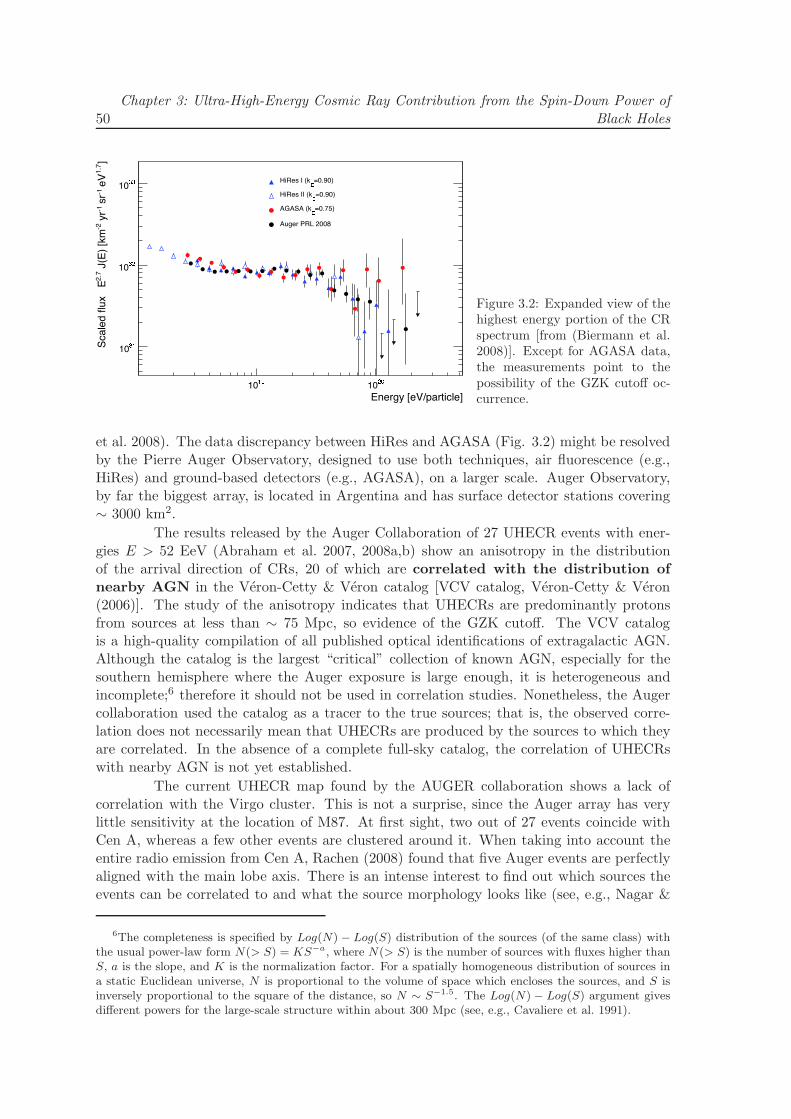
50Chapter 3: Ultra-High-Energy Cosmic Ray Contribution from the Spin-Down Power of

Black Holes

Figure 3.2: Expanded view of thehighest energy portion of the CRspectrum [from (Biermann et al.2008)]. Except for AGASA data,the measurements point to thepossibility of the GZK cutoff oc-currence.

et al. 2008). The data discrepancy between HiRes and AGASA (Fig. 3.2) might be resolvedby the Pierre Auger Observatory, designed to use both techniques, air fluorescence (e.g.,HiRes) and ground-based detectors (e.g., AGASA), on a larger scale. Auger Observatory,by far the biggest array, is located in Argentina and has surface detector stations covering∼ 3000 km2.

The results released by the Auger Collaboration of 27 UHECR events with ener-gies E > 52 EeV (Abraham et al. 2007, 2008a,b) show an anisotropy in the distributionof the arrival direction of CRs, 20 of which are correlated with the distribution ofnearby AGN in the Veron-Cetty & Veron catalog [VCV catalog, Veron-Cetty & Veron(2006)]. The study of the anisotropy indicates that UHECRs are predominantly protonsfrom sources at less than ∼ 75 Mpc, so evidence of the GZK cutoff. The VCV catalogis a high-quality compilation of all published optical identifications of extragalactic AGN.Although the catalog is the largest “critical” collection of known AGN, especially for thesouthern hemisphere where the Auger exposure is large enough, it is heterogeneous andincomplete;6 therefore it should not be used in correlation studies. Nonetheless, the Augercollaboration used the catalog as a tracer to the true sources; that is, the observed corre-lation does not necessarily mean that UHECRs are produced by the sources to which theyare correlated. In the absence of a complete full-sky catalog, the correlation of UHECRswith nearby AGN is not yet established.

The current UHECR map found by the AUGER collaboration shows a lack ofcorrelation with the Virgo cluster. This is not a surprise, since the Auger array has verylittle sensitivity at the location of M87. At first sight, two out of 27 events coincide withCen A, whereas a few other events are clustered around it. When taking into account theentire radio emission from Cen A, Rachen (2008) found that five Auger events are perfectlyaligned with the main lobe axis. There is an intense interest to find out which sources theevents can be correlated to and what the source morphology looks like (see, e.g., Nagar &

6The completeness is specified by Log(N) − Log(S) distribution of the sources (of the same class) withthe usual power-law form N(> S) = KS−a, where N(> S) is the number of sources with fluxes higher thanS, a is the slope, and K is the normalization factor. For a spatially homogeneous distribution of sources ina static Euclidean universe, N is proportional to the volume of space which encloses the sources, and S isinversely proportional to the square of the distance, so N ∼ S−1.5. The Log(N) − Log(S) argument givesdifferent powers for the large-scale structure within about 300 Mpc (see, e.g., Cavaliere et al. 1991).

Chapter 3: Ultra-High-Energy Cosmic Ray Contribution from the Spin-Down Power of

Black Holes 51

Matulich 2008; Moskalenko et al. 2009). Moskalenko et al. (2009) found eight additionalAGN within θ 6 3.2 with z 6 0.018 (the same criteria used by Auger). The sources aremainly LLAGN with a bolometric luminosity of Ljet 6 1043 erg s−1 (Zaw et al. 2009), andjust a few of them have known jets.

Poynting flux models for the origin of jets from force-free magnetosphere above athin accretion disk were first proposed by Lovelace (1976) and Blandford (1976). A rotat-ing magnetic field sweeps ambient matter and, consequently, feels a strong induced poloidalelectric field. Since the magnetic field (which is predominantly toroidal at large distancesin the jet) has a poloidal component, angular momentum and energy are carried away by aPoynting flux. In the model by Lovelace, the accreting protons are accelerated in the poten-tial drop across the disk by an electric force, which exceeds the BH gravitational attractionby a factor of ∼ 1012. It is assumed that particles can form two high-current, aligned, andopposite proton beams. The output electrical power in the beams is proportional to theprotons’ maximum energy squared: L ∼ E2

max. The maximum energy to which the accretiondisk can accelerate the proton beams is set by the Eddington luminosity. If one takes thePoynting flux as a lower limit to the energy flux along a relativistic jet, UHECR productionin LLAGN cannot be explained. Biermann et al. (2008) rewrote Lovelace’s equation as

LP =c

4πfflare

(

Emax

eZγsh

)2

, (3.2)

where Z is the mass number of the nuclei, γsh is the Lorentz factor of the shock, andfflare(< 1) is the jet intermittency. As the authors state, probably all three elements arerequired if one considers UHECR production by sources like M87 and Cen A, whose energyflow along the jet are < 1045 erg s−1 and < 1043 erg s−1, respectively (Whysong & Antonucci2003). The energy flow along the jet for Cen A is confirmed by Abdo et al. (2010).

Boldt & Ghosh (1999) suggested that particles with energies > 1020 eV may beaccelerated near the event horizon of spinning BHs associated with presently inactive quasarremnants. The required electromagnetic force is generated by the BH induced rotation ofexternally supplied magnetic field lines threading the horizon. The BH behaves as a battery,driving currents around a circuit, with an electromagnetic force of up to 1021 eV (for a BHwith a mass of 109M⊙). In this case, the production of observed flux of the highest energycosmic rays would constitute a negligible drain on the BH dynamo. That is, replenishingthe particle ejected at high energies (> 1020 eV) would require a minimal mass input; aluminosity of 1042 erg s−1 in such particles (if protons) corresponds to a rest mass loss< 10−5M⊙ in a Hubble time.

In this chapter, we propose a model for UHECR contribution from the spin-downpower of BHs in LLAGN. The particles in the jet manage to tap the spin-down powerof the BH, and then they are accelerated at relativistic shocks and reached energies upto the UHE domain. The electrons lose their energy through synchroton emission (andalso through inverse-Compton emission), whereas the protons are capable of surviving theradiative cooling and perhaps of propagating through the intergalatic medium. Since bothparticles undergo the same acceleration process, there must be a correlation between theelectron synchrotron emission and the UHECR proton energy. We seek this correlation tomake predictions for UHECRs from nearby LLAGN.

52Chapter 3: Ultra-High-Energy Cosmic Ray Contribution from the Spin-Down Power of

Black Holes

Chapter outline

In Section 3.2, we provide a description of the model. In Section 3.3, we derivethe relation between the luminosity (and flux) of the UHECRs and the observed radio flux-density for a flat-spectrum core source. In Section 3.4, we calculate the particle maximumenergy taking into account the spatial limit and synchroton emission losses. In Section 3.5,we present the application of the model to M87 and Cen A. In Section 3.6 we provide thepredictions for nearby galaxies as UHECR sources, with specific emphasis on the UHECRcontribution from the spin-down power of BHs in LLAGN. In Section 3.7, we present asummary of the key points and discuss the implication of this model for further studies ofthe UHECRs.

3.2 Model description

3.2.1 Model conditions

• We assume that the UHECRs are accelerated by shocks in AGN jets, which arelaunched from the ergospheric disk (see Chapter 2). The ergospheric disk extendsfrom the stationary limit surface rsl inward to the innermost stable orbit rms. Whenthe accretion rate relative to the Eddington accretion rate is < 10−1.8 (which is thecase of LLAGN), the jets can be powered by the spin down of the BH via the accretiondisk, where the rotational energy of the BH is transferred to the ergospheric disk byclosed magnetic field lines that connect the BH to the disk. The jet propagates alonga cylinder of length z0 (see Fig. 3.3) using the BH spin-down power and then extendsinto a conical shape with a constant opening angle 2 θ, as a consequence of the freeadiabatic expansion of the jet plasma. (The tip of the cone is located at some z < z0.)A similar geometry of the jet was considered by Markoff et al. (2001).

• We assume that the UHECRs are proton-dominated. This is based on the measure-ment of a suppression of the CR flux at energies larger than 50 EeV, which indicatesthat the UHECRs are of extragalactic origin and have a light mass spectrum that isdominated by protons.

• In the observer frame, the magnetic field along the jet varies as B ∼ γ−1j z−1 and the

electron number density in the jet scales as ∼ γjz−2, where γj is the bulk Lorentz

factor of the jet. (See discussions below.)

• We set the slope of the particle density distribution to p = 2 (which corresponds toflat-spectrum core sources with a spectral index α = 0.5) and the strength of theBH magnetic field to its maximum value (Bmax

H ). The latter condition provides, inturn, the minimum value for the particle maximum energy, luminosity, and flux of theUHECRs.

3.2.2 Magnetic field scaling along a steady jet

To describe the jet physics, we use the following reference frames: (i) the framecomoving with the matter in the jet and (ii) the (rest) frame of the observer, in which therelativistic jet moves with the bulk Lorentz factor.

Chapter 3: Ultra-High-Energy Cosmic Ray Contribution from the Spin-Down Power of

Black Holes 53

Figure 3.3: Schematic representation ofthe jet geometry. The jet is launched fromthe ergospheric disk and propagates alonga cylinder up to a distance z0. Then, itexpands freely into a conical shape witha constant opening angle 2 θ. The openmagnetic field that threads the ergosphericdisk (dashed line) is wound up, far fromthe BH, into a toroidal magnetic field Bφ

which collimates the jet. In the region ofthe ergospheric disk, the closed magneticfield connects the BH to the ergosphericdisk (solid line). In addition, the magneticfield structure in the ergospheric disk con-tains magnetic field lines similar to thoseon the Sun surface; i.e., it contains mag-netic loops which connect distant regionsof the inner disk and field lines which ex-tend out very far from the disk and allowmatter to flow out. The closed magneticfield lines do not cross the open magneticfield lines.

z0

z

0r= slr

rms

B

ϕB

p

θ

In a frame comoving with the jet, the poloidal component of the magnetic field isconsidered to vary as Bp ∼ z−2. This variation follows from the conservation of magneticflux along the axis z. To keep the field divergence-free, the toroidal component mustvary as Bφ ∼ z−1. This topology of Bφ ∼ z−1 was first derived by Parker (1958) forthe magnetohydrodynamics solution of a spherical-symmetric flow (so that, a jet can beconsidered a conical cut along the flow surfaces). [See also Blandford & Konigl (1979).]The observational support to this variation of Bφ is specified later on in this section. Ata distance, say, z0, the poloidal and toroidal components of the comoving magnetic fieldbecome approximately equal Bp0 ≃ Bφ0. We consider z0 of a few gravitational radii, basedon the fact that the VLBI observation, for instance, of the jet in M87 at 7 mm gives evidenceon the jet collimation (by the toroidal magnetic field) on scales of 60− 200 rg (Biretta et al.2002) and the global 3.5 mm VLBI observations have resolved sizes for the compact radiosources of ∼ 10 rg (see, e.g., Lee et al. 2008). A large-scale and predominantly toroidalmagnetic field can exert an inward force (hoop stress), confining and collimating the jet(see, e.g., Bisnovatyi-Kogan & Ruzmaikin 1976; Blandford & Payne 1982). The magnetichoop stress is balanced either by the gas pressure of the jet or by centrifugal force if the jetis spinning. From z0 upward, the poloidal component of the magnetic field becomes weaker,so that the field lines are soon wound up in the azimuthal direction by the jet rotation.Thus, above z0, the magnetic field along the jet is nearly azimuthal B ∼ Bφ (for a steadyjet) and varies inversely proportional to the distance along the jet,

B = B0

(

z

z0

)−1

, (3.3)

where B0 ≡ Bφ0 ≃ Bp0 is the strength of the magnetic field at the height z = z0 abovethe equatorial plane of the BH. This z-dependence of the magnetic field appears to becontradicted by radio-polarization observations (Bridle & Perley 1984). These observationsstrongly suggest that the magnetic field is predominantly parallel to the jet axis initially and

54Chapter 3: Ultra-High-Energy Cosmic Ray Contribution from the Spin-Down Power of

Black Holes

only later becomes perpendicular to the jet axis, with some parallel magnetic field left over.Becker & Biermann (2009) argued that the basic pattern of the magnetic field is indeedBφ ∼ z−1, and that the observational evidence for a parallel magnetic field is due to highlyoblique shocks. Their argument is based on the observations of the jet structure whichindicate the occurrence of moving shocks between 20 and 200 rg, while the first stationary,strong shock can be produced in the approximate range of (3− 6)× 103 rg (Markoff et al.2001, 2005; Marscher et al. 2008).

The strength of the magnetic field in the comoving frame B0 can be related to thepoloidal magnetic field in the BH frame BH (see, e.g., Drenkhahn 2002) as

B0 =1

γjBH =

BmaxH

γj

(

BH

BmaxH

)

, (3.4)

where the maximum value of the BH magnetic field is given by

BmaxH ≃ 0.56 × 104

(

M

109M⊙

)−1/2

gauss, (3.5)

(Eq. 2.29) which is obtained in a similar manner as the calculation performed by Znajek(1978), with the difference that the BH potential drop (V ) is set to the specific energy ofthe particles at the innermost stable orbit, whereas Znajek (1978) makes use of the factthat the Eddington luminosity sets an upper bound on the radiation pressure (as the diskis radiatively efficient), and thus V 2 ∼ LEdd. The maximum value of the BH magnetic fieldcorresponds to the time when the accretion rate was as high as the Eddington accretionrate. In this case, the BH spin parameter is limited to a∗ = 0.9982 (Thorne 1974). Althoughthis limit might be even closer to the maximal value of the spin parameter ∼ 1, this willintroduce just a small variation of the maximum value of the BH magnetic field.

3.2.3 Electron and proton number densities

The jet is assumed to be composed mainly of electrons, positrons, and protons.We denote by fep ≡ ne/np the ratio of the electron to proton number densities, wherethe number densities are measured in a frame comoving with the jet plasma. Unless oth-erwise noted, ne should be assumed to include the positron number density as well. Itis straightforward to generalize to a mixed chemical composition, including many heavynuclei. Furthermore, both electrons and protons can have thermal and non-thermal popu-lations before being accelerated at a shock front. There may also be a substantial numberof positrons from pion production and decay processes (also called secondaries).

Now, we look for the expression of the proton and electron number densities in-jected into the accelerating region. First, we consider the mass flow rate into the jets, whichin the observer frame is given by

Mj =d

dt(ρjVj) =

d

dt[nmz(S)z=0] = γjnmvj(S)z=0, (3.6)

where ρj is the rest-mass density of the jet, Vj is the comoving volume of the jet, (S)z=0 isthe launching area of the jet, z is the length of the cylinder along which the jet propagatesbefore expanding freely in a conical geometry, and vj = βjc is the bulk velocity of the jet.

Chapter 3: Ultra-High-Energy Cosmic Ray Contribution from the Spin-Down Power of

Black Holes 55

The surface area between two equatorial surfaces of a Kerr BH can be calculatedas

(dS)z=0 =

(

A

∆

)1/2

2πdr, (3.7)

where the Kerr metric functions are

∆ = r2 − 2rgr + a2 and A = r4 + r2a2 + 2rgra2, (3.8)

where r is the coordinate radius. Next, we use normalizations to the gravitational radius,so that r∗ = r/rg is the dimensionless radius. The surface area is then

(S)z=0 = 2πr2g

rsl∗∫

rms∗

r∗

√

1 + r−2∗ a2∗ + 2r−3

∗ a2∗1− r−1

∗ + r−2∗ a2∗

dr∗ ≡ 2πr2gk0, (3.9)

where the factor k0 increases from ∼ 2 to ∼ 80 as the BH spin parameter increases from 0.95to ∼ 1. For the first equality, we use the fact that the ergospheric disk, from where the jetis launched, has its inner and outer radii at the innermost stable orbit rms and stationarylimit surface rsl = 2rg ≡ r0, respectively.

The comoving density of the jet can be expressed in terms of the ratio of theelectron to proton number densities as

nm = npmp + neme = npmp

(

1 + fepme

mp

)

≡ npmpf0. (3.10)

If one assumes, in average, one electron/positron for each proton in the jet, fep = 1 andf0 ≃ 1. For protons dominating over the electrons, fep < 2 × 103, where electrons andpositrons can partially occur as secondaries.

Substituting Eqs. (3.9) and (3.10) for (3.6), we obtain the mass flow rate into thejet,

Mj = γjβjcnpmpf02πr2gk0. (3.11)

This expression provides the proton number density, which in turn we use to derive theelectron number density,

ne = fepMj

γjβjcmpf02πr2gk0. (3.12)

We shall use this result later for evaluating the self-absorbed synchrotron emission of thejets (Section 3.2.5).

3.2.4 Particle energy distribution

We suppose that a recollimation shock (Sanders 1983) is produced at the jet height∼ z0. As a result, a power-law energy distribution of the particles is established. For agiven frequency, the emission from the synchrotron process for electrons and protons givesa factor (mp/me)

3 ≃ 1010 in favor of electrons (see, e.g., Novikov & Thorne 1973b). Inaddition, Biermann & Strittmatter (1987) showed that the proton synchrotron emissioncan be competitive if one considers that the proton emission ranges to much higher photonenergy. Moreover, it is also not at all obvious that they have the same normalization at the

56Chapter 3: Ultra-High-Energy Cosmic Ray Contribution from the Spin-Down Power of

Black Holes

same Lorentz factor of the particle and that the particles have a continuous power-law fromrest mass to UHE. The number density of the electrons in the energy interval E, E + dE[or mec

2γ, mec2(γ + dγ)] has the power-law form

N(E)dE = CE−pdE, (3.13)

or, in terms of the Lorentz factor,

N(γ)dγ = C ′γ−pdγ, (3.14)

where γ ∈ [γmin, γmax] is the Lorentz factor of the electrons and p is the power-law index(see, e.g., Rybicki & Lightman 1979). The normalization coefficients of the electron numberdensity in Eqs. 3.13 and 3.14 are related by

C = C ′(mec2)p−1. (3.15)

The normalization of the electron number density C ′ follows the pressure in a reheating flow(∼ z−2), whereas an adiabatic flow would give a steeper dependence, which leads to shocks(see, e.g., Sanders 1983). Adiabatic behavior implies P ∼ ργad , where γad is the adiabaticindex. Since a relativistic fluid usually has γad = 4/3, in an adiabatic flow the temperatureruns as z−2/3. Furthermore, one can have a conical flow only if the temperature of the flowis approximately constant. The energy for reheating can be taken from the flow throughhighly oblique shocks. The normalization of the electron number density, in the case of aconical jet, is therefore

C ′ = C ′0

(

z

z0

)−2

(cm−3). (3.16)

Possible values of the power-law distribution indices p of the electrons acceleratedby the relativistic shock are discussed later in Section 3.5.

3.2.5 Self-absorbed synchrotron emission of the jets

The spectra from compact radio sources can be explained by self-absorbed syn-chrotron emission of the jets produced by electrons with a power-law energy distribution.In this section, we rewrite the quantities which describe the self-absorbed synchrotron emis-sion, derived in Rybicki & Lightman (1979), and express them under our model considera-tions. We first introduce the absorption coefficient, optical depth, synchrotron emissivity,and source function in order to calculate the flux density of the synchrotron emission fromradio sources with a flat-spectrum core. (The quantities which describe the self-absorbedsynchrotron emission are in cgs units.)

The specific intensity of radiation Iν is defined as the radiative energy flux perunit frequency, per unit solid angle (i.e., the energy per time, per unit area, per unitfrequency, per unit solid angle). The radiative transfer equation for the specific intensity ofthe radiation Iν along a distance ds through a medium combines both the absorption andemission effects as

dIνds

= −ανIν + jν , (3.17)

where αν is the absorption coefficient and jν is the emission coefficient. Instead of using theradiative transfer equation of the form in Eq. 3.17, it becomes more convenient to introduce

Chapter 3: Ultra-High-Energy Cosmic Ray Contribution from the Spin-Down Power of

Black Holes 57

another variable, the optical depth τν , which is measured along the direction of propagatingradiation, as

dτν = ανds. (3.18)

Therefore, τν can be obtained by integrating Eq. 3.18 along a path through the medium.For τν > 1 the medium is called optically thick (or opaque), whereas for τν < 1 the mediumis called optically thin (or transparent), in which case a photon of a given frequency ν cantravel without being absorbed by the medium itself. If one divides the radiative transferequation by αν and uses the definition of the optical depth, then

dIνdτν

= −Iν + Sν , (3.19)

where Sν ≡ jν/αν is called the source function.To find how the specific intensity varies as radiation travels through a medium,

one needs to specify the coefficients αν and jν , or alternatively Sν and τν , for every pointalong the path length. The solution of the transfer equation (Eq. 3.19), for a constantsource function, is written as

Iν = Iν,0e−τν + Sν(1− e−τν ), (3.20)

where the first term on the right-hand side describes the amount of radiation left over fromthe intensity after it has passed through an optical depth τν , and the second term representsthe contribution of the intensity from the radiation emitted along the path. When there isonly emission from a specific region, then

Iν = Sν(1− e−τν ). (3.21)

Lind & Blandford (1985) showed that the phase space distribution of the emitting particlesis not isotropic in any frame of reference, given a relativistic shock. It helps, however, toassume that there is such a frame (to assume that this is approximately true leads to a smallerrors only in the derived quantities). On the other hand, in the case of weak sources, thebeaming could go backwards under special circumstances, whereas for strong superluminalsource, the beaming propagates towards us. Next, we also neglect the flux from componentsmoving away from the observer.

For an optically thick case, e−τν ≃ 0 and Iν = Sν . Thus, when looking at anopaque medium, it does not matter what radiation sources are behind this, the specificintensity is given by the source function of the medium which faces the observer.

The power radiated per unit volume per unit frequency dP/(dV dν) ∼ ν−p+12 has

a high-frequency cutoff at the highest frequency produced by the highest energy electronsin the emitting region. There is also a low-frequency cutoff due to the self-absorption ofthe synchrotron radiation. Computing the absorption and emission of radiation is rathercomplicated, because the synchrotron emission is not necessarily isotropic since the magneticfield imposes a preferred direction. A way out of this situation is to look at the region inwhich the magnetic field is chaotic, so it has no net direction. (This looks like a contradictionwith the other assumption of B ∼ z−1, since in a chaotic regime we have B ∼ z−4/3 fordensity ∼ z−2. Of course, the observations show that there is some fraction of regularity, andso the earlier assumption is justified. One could also argue, that in each shock the magneticfield is re-regularized.) Therefore, the emission coefficient can be set as the angle-averagedsynchrotron power per unit volume per unit frequency.

58Chapter 3: Ultra-High-Energy Cosmic Ray Contribution from the Spin-Down Power of

Black Holes

The absorption coefficient is dependent on the emitting frequency as αν ∼ ν−p+42 .

If p = 2, the absorption coefficient will be αν ∼ ν−3. This steep dependence on frequencyimplies that the emission region will be optically thick to synchrotron radiation at sufficientlylow frequencies. Instead, at high frequency, the region will be transparent to the synchrotronradiation.

Absorption coefficient

In a frame comoving with the jet plasma, the absorption coefficient of the syn-chrotron radiation can be calculated as

αν =

√3e3B sinα0

8πme

(

3eB sinα0

2πm3ec

5

)p2

C Γ

(

3p + 2

12

)

Γ

(

3p+ 22

12

)

ν−p+42 (cm−1), (3.22)

where e is the electric charge of the electron, me is the electron mass, p is the power-lawindex of the particles distribution, C is the normalization factor for the power-law electronenergy distribution (Eq. 3.13), B is the magnetic field in the frame comoving with thejet, Γ(x) is the Gamma function of argument x, and ν is the frequency of the synchrotronradiation [eq. 6.26 in Rybicki & Lightman (1979)]. To average over the pitch angle α, for alocal randomly oriented magnetic field with a probability distribution 1

2 sinαdα, one needsto evaluate the following integral (Longair 1994)

∫ π

0

1

2sinα(sinα)

p+22 dα =

√πΓ(

p+64

)

2Γ(

p+84

) . (3.23)

Including the values of the physical constants and using the expressions for thenormalization of the electron distribution function, C and C ′ (Eqs. 3.15 and 3.16), as wellas for comoving magnetic field along the jet (Eq. 3.3), the absorption coefficient becomes

αν = K1C′0

(

z

z0

)− p+62

Bp+22

0 ν−p+42 , (3.24)

where

K1 = 8.4× 10−3(1.25 × 1019)p2(

8.2× 10−7)p−1

√π

2Γ

(

3p+ 2

12

)

Γ

(

3p+ 22

12

)

Γ

(

p+ 6

4

)

Γ−1

(

p+ 8

4

)

.(3.25)

Optical depth of the self-absorbed region

To calculate the observed distance along the jet where the jet becomes self-absorbed,we first determine the optical depth τν of the jet material. The averaged path of a photonthrough the jet has the length r(z), which is a reasonable approximation for a jet observedat large inclination angle (see, e.g., Kaiser 2006). This is not in contradiction to the ideathat some jets point towards us (see the footnote on page 63). We introduce a factor l0 inthe expression of the path length to account for a small inclination angle. Thus, we canwrite the optical depth as

τν = ανr(z)l0. (3.26)

Chapter 3: Ultra-High-Energy Cosmic Ray Contribution from the Spin-Down Power of

Black Holes 59

For conical jets, the intrinsic half-opening angle is given by tan θ = r/z ∼= r0/z0. With theabsorption coefficient specified through Eq. (3.24), the optical depth can be written as

τν = K1C′0r0l0

(

z

z0

)−p+42

Bp+22

0 ν−p+42 . (3.27)

The distance along the jet where the jet becomes self-absorbed (zssa) is defined asthe distance z for which τν = 1. Using Eq. (3.27), we obtain

zssa =(

K1C′0l0)

2p+4 (tan θ)−1 r

p+6p+4

0 Bp+2p+4

ν−1

0 . (3.28)

Synchrotron emissivity

The total power radiated per unit volume per unit frequency by a non-thermalparticle distribution equals

Pω =

√3e3

2πmec2C ′B sinα0

p+ 1

(

mecω

3eB sinα0

)−p−12

Γ

(

p

4+

19

12

)

Γ

(

p

4− 1

12

)

, (3.29)

where ω = 2πν [Eq. 6.36 in Rybicki & Lightman (1979)]. Using Eqs. (3.3) and (3.16), aswell as the method to calculate the averaged pitch angle employed in Longair (1994), theexpression of the total power becomes

Pν = 2πPω = K2C′0

(

z

z0

)−p+52

Bp+12

0 ν−p−12 , (3.30)

where

K2 = 3.7× 10−23(

1.2× 10−7)−

p−12 (p + 1)−1

√π

2Γ

(

p

4+

19

12

)

Γ

(

p

4− 1

12

)

Γ

(

p+ 5

4

)

Γ−1

(

p+ 7

4

)

.(3.31)

Next, we derive (z/z0) from Eq. 3.27 when τν = 1. With this, the expression for the totalpower takes the form

P ′ν = K2 (K1r0l0)

−p+5p+4 (C ′

0)− 1

p+4B− p+3

p+4

0 ν3, (3.32)

and the emission coefficient is simply: jν = Pν/4π.

Source function

The emission coefficient is defined as the product between the absorption coef-ficient αν and the source function Sν . At low frequencies, the emitting region is opaqueto synchrotron radiation and the observed intensity of radiation Iν is proportional to thesource function, while at high frequencies, the region is transparent and the observed inten-sity is proportional to the emission coefficient. The two dependences should be matched atthe transition from opaque to transparent regime. This transition corresponds to an opticaldepth τν = 1. The source function in the self-absorbed limit is then

Sν =1

4π

Pναν

=1

4π

K2

K1

(

z

z0

) 12

B− 1

20 ν

52 (erg s−1cm−2Hz−1), (3.33)

60Chapter 3: Ultra-High-Energy Cosmic Ray Contribution from the Spin-Down Power of

Black Holes

where the last equality was obtained using Eqs. (3.24) and (3.30). Note that in the sourcefunction, the emitting frequency does not depend on the power-law index of the electronenergy distribution. For τν = 1, the source function becomes

S′ν = K3

(

C ′0r0l0

)−1p+4 B

− 1p+4

0 ν2 (erg s−1cm−2Hz−1), (3.34)

where K3 = K−

p+3p+4

1 K2.

Flux density of the synchrotron emission

To obtain the emission spectrum, one needs to solve the equation for the radiativetransfer through a homogeneous medium. Because the angular sizes of the jets are small,instead of the specific intensity of the radiation, one usually measures the flux density Fν(energy per unit time, per unit frequency interval, that passes through a surface of unitarea). Thus,

dFν = IνdΩ = Sν [1− exp(−τν)] dΩ. (3.35)

Since the frequency shift of the approaching photons, specified by the Doppler factor,7 isνobs = Djν, the transformation of the specific intensity to the observer frame is

Iν,obs = D3j Iν , (3.36)

where the relativistic invariant quantity Iν/ν3 was used. The solid angle corresponding to

the source is

dΩ =2πrdz

D2s

, (3.37)

where Ds is the distance from the observer to the jet source, and r = z tan θ. If we insertEq. (3.37) into Eq. (3.35) and integrate it from z0 to z, we obtain the flux density of thesynchrotron emission in the case of τν = 1 as

F ′ν = S′

ν [1− exp(−1)]π(tan θ)D−2s z2

[

1−(z0z

)2]

, (3.38)

where the second term in the last squared bracket can be neglected with respect to the firstterm for z ≫ z0 (where the jet emission becomes self-absorbed). Using Eqs. (3.28) and(3.34), the flux density is then

F ′ = K4(C′0l0)

5p+4 r

2p+13p+4

0 B2p+3p+4

0 D−2s (tan θ)−1 , (3.39)

where K4 = 0.16K− p−1

p+4

1 K2. The radio flux density in Eq. (3.39) does not depend on theemitted frequency of the radiation since we already adopted the case of flat-spectrum coresources when τν = 1.

7The Doppler factor of the jet is Dj = γ−1j (1−βj cosϕ)

−1, where ϕ is the inclination angle of the jet axiswith respect to the line of sight (which is Lorentz transformed through sinϕobs = Dj sinϕ). The angles arerotated by the Lorentz transformation, so that a jet seen at angle γ−1

j is rotated basically to a transverse

view for large γj.

Chapter 3: Ultra-High-Energy Cosmic Ray Contribution from the Spin-Down Power of

Black Holes 61

For a power-law synchrotron spectrum of the form Fobs ∼ ν−αobs , the observed fluxdensity is related to the intrinsic flux density as

Fobs = D3+αj F ′, (3.40)

where Eq. (3.36) was used. Equation (3.40) is valid for a single blob emission (see, e.g.,Blandford & Konigl 1979). For a continuous jet consisting of uniformly-spaced blobs, oneneeds to consider the emission per unit length in the observer frame. Therefore,

Fobs = D2+αj F ′, (3.41)

due to the fact that the number of the blobs observed per unit length is ∼ 1/Dj.

3.3 Luminosity and flux of the ultra-high-energy cosmic rays

In this section, we look to find the UHECR luminosity flux FCR specified as afunction of the observed radio flux-density Fobs. First, we consider the kinetic luminositydefined as

LCR = ǫCRγ2j Mjc

2 , (3.42)

where we assume that the spin-down power of the BH drives the jet, and the UHECRluminosity is a fraction of the jet power, therefore LCR ∼ ǫCRLj = ǫCR(Lkin+Lmagn+LCR).If we were to adopt the point of view that the jet power is shared equally in a comovingframe between the baryonic matter, magnetic field and cosmic rays extending to the highestenergy, then εCR ≃ 1/3. In the jet-disk model of Falcke & Biermann (1995), the energyequipartition in the comoving frame appears to be a good approximation. If it were alsotrue here, it would determine the Lorentz factor and would suggest that AGN driven by theBH spin-down power, and suffering from a low accretion rate, may attain a higher Lorentzfactor, consistent with some observations.

An upper limit for the electron density is given by ne 6 C ′0. Next, we use this result

(Eq. 3.12) in the expression for the observed radio flux-density (Eq. 3.40 and Eq. 3.41) andfind the mass flow rate into the jet Mj. On the other hand, the magnetic field B0 followsfrom equations 3.4 and 3.5. After performing these calculations, we obtain the UHECRluminosity

LCR = K5fβjD−hj

(γj5

)2p+13

5

(

tan θ

0.05

)p+45(

r02rg

)− 2p+135(

BH

BmaxH

)− 2p+35

Fp+45

obs D2(p+4)

5s

(

M

109M⊙

)−2p+310

ergs−1, (3.43)

where

K5 =π

6mpc

3K−

p+45

4 (5)2p+13

5+h(2.96 × 1014)−

2p+35 (0.56 × 104)−

2p+35 (0.05)

p+45 , (3.44)

where h = [(p + 5)(p + 4)]/10 for single blob emission (Eq. 3.40) or [(p + 3)(p + 4)]/10for continuous blob emission (Eq. 3.41), and f = f0k0(l0fep)

−1. We use a normalizationvalue for the jet Lorentz factor, say 5, although the jet Lorentz factor can range from ∼ 2to ∼ 100, as observational data suggest. We adopt fep ∼ 1− 10 (and f0 ≃ 1), which means

62Chapter 3: Ultra-High-Energy Cosmic Ray Contribution from the Spin-Down Power of

Black Holes

that there is one electron for at least one proton in a jet powered by a rapidly-spinning BH(a∗ > 0.95) and observed at a large angle (> 10). Sadly, there is a very poor constraint onthe BH spin parameter from the UHECR luminosity.

Given the UHECR luminosity, one can easily obtain the UHECR flux,

FCR =LCR

4πD2s

. (3.45)

Mildly-relativistic shocks (1 . γs . 10) are believed to occur in the AGN jets.Gallant & Achterberg (1999) have shown that at relativistic shocks, the particles typicallyperform a fraction ∼ γ−1

s of the Larmor orbit upstream before recrossing the shock, andthe particle energy gain increases by a factor of γ2sh in the first shock-crossing cycle. Inthe subsequent shock-crossing cycles, the energy gain is of the order of 2. The predictedspectral index is ≃ 2. A series of Monte Carlo simulations,8 performed under a widerange of background conditions at the shock front, indicate a value p ≃ 2.2 − 2.3 forthe slope (see, e.g., Bednarz & Ostrowski 1998; Achterberg et al. 2001; Kirk et al. 2000;Keshet & Waxman 2005). It follows that in the regime of arbitrarily high Lorentz factorshocks, the acceleration process generates particle spectra which are quasi-independent ofthe considered background conditions, leading to a quasi-universal slope of ∼ 2.2. Thepicture can be changed when one considers more realistic conditions in the vicinity of theshock. For example, Niemiec & Ostrowski (2006) studied possible models for perturbedmagnetic field upstream of the shock and found that for superluminal mildly-relativisticshocks (γsh ∼ 5 − 30), a flattening of the spectrum occurs, p ≃ 1.5, with a cutoff at lowerenergies than as expected for UHECRs. A flattening of the spectrum, p ∼ 2.1− 1.5, is alsoobserved in simulation results obtained by Meli et al. (2008) for the case of superluminalultra-relativistic shocks (100 < γsh < 1000), with a turbulent magnetic field and variousshock obliquity; however, for subluminal mildly-relativistic shocks, the spectral slope hasvalues between 2.0 < p < 2.3.

We adopt p = 2 , which is the upper value of the spectral index for flat-spectrum

core sources. The cosmic ray luminosity (Eq. 3.43) becomes

LCR =3.6× 1038βjD−3j

(γj5

)17/5(

tan θ

0.05

)6/5( r02rg

)−17/5( BH

BmaxH

)−7/5

(

Fobs

mJy

)6/5( Ds

Mpc

)12/5( M

109M⊙

)−7/10, (3.46)

where a continuous jet was considered (h = 3). For p . 2, the results for the CR luminosityare slightly reduced.

3.4 Maximum particle energy of ultra-high-energy cosmic

rays

3.4.1 Spatial limit

Now, we look for the maximum energy of the UHECR in the case of the spatial(geometrical) limit (Falcke & Biermann 1995); i.e., the jet particle orbits must fit into the

8Monte Carlo simulations are meant to find a way of constructing the trajectories of particles whosedistribution obey the desired transport equation.

Chapter 3: Ultra-High-Energy Cosmic Ray Contribution from the Spin-Down Power of

Black Holes 63

Larmor radius. Following Gallant & Achterberg (1999), the maximum particle energy inthe downstream rest frame can be written as

Espmax = γseZBr, (3.47)

where γs is the shock Lorentz factor, Z the particle mass number, and B is the magneticfield in the comoving frame. Using the expression for the magnetic field along the jet (Eqs.3.3 and 3.4) and the fact that tan θ = r0/z0, the CRs maximum energy (in the observerframe) becomes

Espmax = eZBmax

H r0

(

γsγj

)(

BH

BmaxH

)

, (3.48)

where BH is the magnetic field in the BH frame. For protons,

Espmax = 5× 1020

(

BH

BmaxH

)(

r02rg

)(

M

109M⊙

)1/2

(eV) , (3.49)

where γs ≃ γj was used.

3.4.2 Synchrotron loss limit

Setting synchrotron losses equal to diffusive shock acceleration gains, Biermann& Strittmatter (1987) showed that a ubiquitous cutoff in the non-thermal emission spectraof AGN, knots and hot spots in the jets can be explained. This requires that protonsto be accelerated near 1021 eV. The cutoff frequency, ν∗, might be produced at about3000 − 6000 rg. Rewriting their expression for the maximal proton energy,

Elossmax ≃ 1.4× 1020

(

ν∗3× 1014Hz

)1/2

B−1/2 (eV), (3.50)

and using the expression for the magnetic field, we obtain the maximal proton energy inthe loss limit:

Elossmax ≃ 4.2× 1018

(

ν∗3× 1014Hz

)1/2 (γj5

)1/2(

BH

BmaxH

)−1/2( M

109M⊙

)1/2 ( z

z0

)1/2

(eV) .(3.51)

3.5 Application to M87 and Cen A

In this section, we investigate the UHECR luminosity flux for two possible sourcesof UHECR, M87 and Cen A, whose jet parameters can be inferred from observational data.

M87 (NGC 4486) is a giant elliptical galaxy located at ∼ 16 Mpc, perhaps thedominant galaxy in the closest big galaxy cluster to us, the Virgo Cluster. Although thegalaxy hosts a supermassive BH with mass of (3.2± 0.9)× 109M⊙ (Macchetto et al. 1997),its radio morphology places it near the FR-I/FR-II division.9 Its giant optical jet was

9The Fanaroff-Riley classification (Fanaroff & Riley 1974) of a galaxy depends on its radio luminosity.The definition of FR-I and FR-II follows from the radio morphology, FR-I have the lobe emission center-brightened, whereas FR-II have the lobe emission edge-brightened. The radio morphology strongly correlateswith the radio luminosity at low radio frequency (see, e.g., the review by Miley 1980). Most galaxies thatare brighter than 2× 1025h−2

100WHz−1str−1 at 178 MHz are of the FR-II type, while less luminous galaxiesbelong mainly to the FR-I class. The division between the two classes becomes sharper if the distribution asa function of the radio luminosity, as well as of the absolute optical magnitude, is taken into account (see,e.g., Barthel 1989).

64Chapter 3: Ultra-High-Energy Cosmic Ray Contribution from the Spin-Down Power of

Black Holes

discovered by Curtis (1918) and was the first extragalactic large-scale jet ever observed.Since then, the jet has been observed over a wide range of the electromagnetic spectrum.The radio map at 7 mm with VLBI (Biretta et al. 2002) reveals the structure of the jeton the sub-parsec scale and indicates a jet (apparent) opening angle of approximately 60

on scales of about 0.04 pc. On large scales, the jet shows apparent superluminal motion of∼ 6c, which implies a small angle to the line of sight, of just a few degrees. Whysong &Antonucci (2003) have estimated an energy flow along the jet of Ljet ∼ 1045 erg s−1.

Cen A (NGC 5128) is the nearest active galactic nucleus at a distance of ∼ 3.5Mpc. There are quite a few distance measurements with values in the 3.4− 4.4 Mpc range(see, e.g., Tonry et al. 2001; Rejkuba 2004; Ferrarese et al. 2007). The giant elliptical galaxyfeatures a dark lane and a twisted edge-on disk of gas and dust which contain H II regionsobscuring the nucleus at optical wavelengths. They are believed to be remnants of a mergerof a giant elliptical galaxy with a smaller spiral galaxy, which has occurred about 107 − 108

years ago (Malin et al. 1983). Due to its radio morphology, Cen A has been classified as aFR-I radiogalaxy. The radio maps show jet structures extending from the core on pc andkpc scales to giant outer lobes which extend to an apparent diameter of 10 on the sky. Thejets point in a very different direction from the overall lobes (Junkes et al. 1993a,b), and thismay have two reasons: (i) there may have been a spin-flip, so that the big radio lobes referto the old spin direction and the jets to the new spin direction; or (ii) a cosmologically largescale structure (LSS) shear flow (Ryu et al. 1998, 2008) pulls the relativistic gas ejectedby the active BH along the local LSS shear. A general relativistic approach for the spin-flip of the BH was described by Gergely & Biermann (2009). A recent determination ofits BH mass of M = (5.5 ± 3.0) × 107M⊙ (Cappellari et al. 2009) was obtained by usinghigh-resolution integral-field observations of the stellar kinematics.

Taking r = 2 rg and BH ≃ BmaxH , the equations for the maximum particle energy

in the spatial (Eq. 3.49) and loss (Eq. 3.51) limits, as well as for the UHECR luminosity(Eq. 3.46), become

Espmax = 5× 1020

(

M

109M⊙

)1/2

(eV),

Elossmax ≃ 4.2× 1018

(

ν∗3× 1014Hz

)1/2(γj5

)1/2(

M

109M⊙

)1/2( z

z0

)1/2

(eV),

LCR = 3.65× 1038βj (1− βj cosϕ)3(γj5

)32/5(

tan θ

0.05

)6/5

(

Fobs

mJy

)6/5( Ds

Mpc

)12/5( M

109M⊙

)−7/10

(erg s−1).

(3.52)

This set of equations is used for the following estimations on UHECR contribution fromthe BH spin-down power. For the expression of Eloss

max in Eq. (3.52), we use (z/z0) ∼ 103.Our choice is based on the results obtained by Becker & Biermann (2009), which show thata first large steady shock can be produced at about z ∼ 3 × 103 rg [following the work byMarkoff et al. (2001)]. This is confirmed by observations of a blazar inner jet as revealed bya radio-to-γ-ray outburst (Marscher et al. 2008). The same conclusion was reached earlierby Biermann & Strittmatter (1987) using the observed cutoff in the radio emission of AGN.

Table 3.1 contains our estimations for the UHECR maximum particle energy, lu-minosity, and flux in the case of M87 and Cen A, whose jet parameters can be obtainedfrom observational data. The observed radio-core flux-density corresponds to the frequency

Chapter 3: Ultra-High-Energy Cosmic Ray Contribution from the Spin-Down Power of

Black Holes 65

Table 3.1: The jet parameters for M87 and Cen A, and the corresponding maximum particle energy(spatial and loss limits), UHECR luminosity and flux. Here, the quantities assume that the particlesare protons.

Source γj ϕ θ Ds M F 5GHzcore Esp

max Elossmax LCR FCR

() () (Mpc) (×109M⊙) (mJy) (ZeV) (ZeV) (erg s−1) (erg s−1cm−2)

(1) (2) (3) (4) (5) (6) (7) (8) (9) (10) (11)

M87 6 10 19 16 3 2875.1 0.86 0.25 2.03× 1043 7.03× 10−10

Cen A 2 65 5 3.5 0.055 6984 0.11 0.21 3.16× 1042 2.28× 10−9

NOTE: Col. (1) Source name; Col. (2) Jet Lorentz factor; Col. (3) Angle to the line of sight; Col. (4) Jetsemi-opening angle; Col. (5) Distance to the source; Col. (6) BH mass; Col. (7) Core flux density at 5 GHz; Col.(8) maximum particle energy (spatial limit); Col (9) maximum particle energy (loss limit); Col. (10) UHECRluminosity for a power-law index of particle distribution p = 2; Col. (11) UHECR flux. REFERENCES: JetLorentz factor: Biretta et al. (1999) and Meisenheimer et al. (2007); Angle to the line of sight: Biretta et al.(1999) and Tingay et al. (1998); Distance to the source for M87 Macri et al. (1999) and for Cen A we assumea distance Ds = 3.5 Mpc to be consistent with the BH mass determination; BH mass: Macchetto et al. (1997)and Cappellari et al. (2009); Core flux density at 5 GHz: Nagar et al. (2001) and Slee et al. (1994). The valueof the quantities inferred from observational data are the median ones, which we use in our estimations.

of GHz. For comparison, the energy along the jet estimated by Whysong & Antonucci(2003), is ∼ 1045 erg s−1 and ∼ 1043 erg s−1 for M87 and Cen A, respectively. [The energyflow along the jet for Cen A is confirmed by Abdo et al. (2010).] The estimations of theluminosity and flux of the UHECR correspond, however, to the slope of the particle densitydistribution of p = 2. For a steeper slope of the particle density distribution, both the lu-minosity and flux of the UHECR increase. Although the sources have a low power jet, theyare powerful enough to provide the environment for particles to be accelerated to ultra-highenergies of ∼ 1 ZeV. In this case, the jet power is supplied by the BH spin-down power.

Eliminating the BH mass using the expressions of Espmax and LCR (Eq. 3.52), the

UHECR luminosity and the maximum particle energy are related through the followingequation

(

LCR

1045erg/s

)−10/7

= K

(

Espmax

1020eV

)2

, (3.53)

where

K = 6.27×107β−10/7j (1− βj cosϕ)

−30/7

(

tan θ

0.05

)−12/7(γj5

)−64/7(

Fobs

mJy

)−12/7 ( Ds

Mpc

)−24/7

.

(3.54)Equation (3.53) is, therefore, not dependent on the BH mass, instead it is dependent onthe jet-related quantities.

3.6 Predictions for nearby galaxies as ultra-high-energy cos-mic ray sources

We apply the model to a complete sample of steep-spectrum radio sources (Bier-mann et al. 2008; Caramete 2010), at redshift z < 0.025 (about 100 Mpc), with a totalradio flux density larger than 0.5 Jy. The numbers for the estimated flux and maximalenergy exclude the GZK effect, but they include the dilution with distance. The selectioncriteria used by the authors are presented in more detail in their papers. Table 3.2 lists thepredictions for the UHECR particle maximum energy, luminosity, and flux. We emphasize

66Chapter 3: Ultra-High-Energy Cosmic Ray Contribution from the Spin-Down Power of

Black Holes

M87CR/FCRf = F

-210 -110 1 10

inte

gral

cou

nts

N(>

f)

1

10

Figure 3.4: Integral source counts of thecomplete sample of steep-spectrum ra-dio sources (see Table 3.2.), where theirUHECR flux is estimated relative tothat of M87.

that there could be a common scaling limit, such as a condition that the Larmor radius hasto fit three times or five times into the jet. The scaling limit is not critical to our predictionsas long as we refer the quantities to, say, M87; therefore, the jet parameters are assumedto be the same as for M87, all scaled by mass, radio power, and distance. That can be seenwhen comparing the estimated values of the UHECR maximum particle energy and fluxfor Cen A in Tables 3.1 and 3.2; the differences are within one order of magnitude. Usinga scaling relative to M87, one implicitly allows for the possibility that all sources produceheavier nuclei (Z > 1). Of course this again assumes that all sources are the same in thisrespect. We argue that although the sources are LLAGN, they can be sites of acceleratingparticles to ultra-high energies ∼ 1 ZeV with an UHECR luminosity < 1043 erg s−1.

In Fig. 3.4, we show the plot of integral source counts (N) versus relative UHECRflux (last column in Table 3.2.), where the data points are split in 8 bins of variable widthwith the bin upper edge three times larger than the bin lower edge. Although the datapoints are too sparse to discriminate models of the flux distribution, we estimate the mostlikely model parameters that could generate those data points. We fit a power-law model(N = C fκ) to the mean values of the data in each bin forN(> 0.405) (see Fig. 3.5) using thelog-likelihood method.10 The errors for the data points are estimated by

√N . For the best

fit that we obtained, the model parameters are: C = 4.88±1.74 and κ = 0.86±0.45. (Sincethe source counts for each bin is too low, especially in the tail of the assumed power-lowdistribution, we cannot perform a χ2-test.) Within the errors, we can consider a power-lawmodel with κ > 1, which implies that weak sources can dominate over the strong sources.In this view, LLAGN (powered by the BH spin down) can make a large contribution tothe integrated UHECR flux in the local universe, as the density of LLAGN is significantlyhigher than the density of powerful AGN.

3.7 Summary and conclusions

In this work we developed a new model for UHECR contribution from BH spin-down power. We relate the observed radio flux-density to the cosmic ray luminosity andflux, and calculate the maximum particle energy in both spatial and loss limits. This model

10For plotting numerical results and for data analyzing, we use ROOT, which is an open source, dataanalysis program developed at CERN.

Chapter 3: Ultra-High-Energy Cosmic Ray Contribution from the Spin-Down Power of

Black Holes 67

Figure 3.5: Integral source counts of thesame sample as in Fig. 3.4. The modelparameters for the best fit of a power-law model (N = C fκ) with N(> 0.405)are: C = 4.88±1.74 and κ = 0.86±0.45.

M87CR/FCRf = F

-210 -110 1 10in

tegr

al c

ount

s N

(>f)

1

10

0.45± = 0.86 κ 1.74, ±C = 4.88

is relevant for many radio galaxies, where the accretion rate is very low, and therefore theBH spin-down power is a better option for powering their jets. Our predictions can be usedin various propagation codes for UHECR, which typically use the maximal energy and fluxof the cosmic rays scaled relative to a canonical radio galaxy, as well as the slope of the CRspectrum. The only difficulty is that the predicted quantities scale a bit differently if someof the UHECRs are heavy nuclei at the origin. That is because for heavy nuclei, the energyscales up with Z. For a middling FIR/Radio ratio,11 as Cen A has, a starburst may haveprovided all the necessary pre-accelerated nuclei. Nonetheless, this is not the case for M87.We would like to point out that our model is just an extension of associating sites of theorigin of UHECRs to AGN with low accretion rates, beside those of high accretion rates.

Table 3.2. NOTE: Col. (1) Source name; Col. (2) Distance to the source; Col. (3) BH mass; Col. (4) Core

flux density at 5 GHz; Col (5) Maximum particle energy (spatial limit); Col. (6) Maximum particle energy

relative to the corresponding value for M87; Col. (7) UHECR luminosity; (8) UHECR flux; (8) UHECR

flux relative to the corresponding value for M87.

11“FIR” is the flux density at 60 µ and “Radio” is the flux density at 5 GHz.

68Chapter3:Ultra

-High-E

nergyCosm

icRayContrib

utio

nfro

mtheSpin-D

ownPowerof

BlackHoles

Table 3.2: UHECR predictions for a complete sample of 29 steep-spectrum radio sources (Biermann et al. 2008; Caramete 2010). The numbers forthe estimated flux and maximal energy exclude the GZK effect, but include the dilution with distance.

Source D M F 5GHzcore Esp

max Espmax/ Eloss

max Elossmax/ LCR FCR FCR/

(Mpc) (×109M⊙) (mJy) (1020 eV) Esp,M87max (1020 eV) Eloss,M87

max (erg s−1) (erg s−1 cm−2) FM87CR

(1) (2) (3) (4) (5) (6) (7) (8) (9) (10) (11)

ARP 308 69.7 0.1 67.8 1.57 0.18 0.45 0.18 8.39×1043 1.52×10−10 0.21CGCG 114-025 67.4 0.19 443.39 2.16 0.25 0.63 0.25 4.70×1044 9.15×10−10 1.30ESO 137-G006 76.2 0.92 631.32 4.76 0.55 1.38 0.55 3.19×1044 4.87×10−10 0.69

IC 4296 54.9 1 214 4.97 0.57 1.44 0.57 3.75×1043 1.10×10−10 0.15IC 5063 44.9 0.2 29 2.22 0.25 0.64 0.25 6.49×1042 2.84×10−11 0.04

NGC 0193 55.5 0.2 40 2.22 0.25 0.64 0.25 1.58×1043 4.55×10−11 0.06NGC 0383 65.8 0.55 92 3.68 0.42 1.07 0.42 3.19×1043 6.52×10−11 0.09NGC 1128 92.2 0.2 39 2.22 0.25 0.64 0.25 5.20×1043 5.41×10−11 0.07NGC 1167 65.2 0.46 243 3.37 0.39 0.98 0.39 1.13×1044 2.36×10−10 0.33NGC 1316 22.6 0.92 26 4.76 0.55 1.38 0.55 3.76×1041 6.51×10−12 0.01NGC 1399 15.9 0.3 10 2.72 0.31 0.79 0.31 1.12×1041 3.94×10−12 0.005NGC 2663 32.5 0.61 160 3.88 0.45 1.13 0.45 1.06×1043 8.89×10−11 0.12NGC 3801 50 0.22 635 2.33 0.27 0.67 0.27 3.19×1044 1.12×10−9 1.60NGC 3862 93.7 0.44 1674 3.29 0.38 0.96 0.38 2.83×1045 2.85×10−9 4.06NGC 4261 16.5 0.52 390 3.58 0.41 1.04 0.41 6.80×1042 2.20×10−10 0.31NGC 4374 16 1 168.7 4.97 0.57 1.44 0.57 1.46×1042 5.05×10−11 0.07NGC 4486 16 3 2875.1 8.61 1 2.50 1 2.03×1043 7.03×10−10 1NGC 4651 18.3 0.04 15 0.99 0.11 0.28 0.11 1.05×1042 2.78×10−11 0.03NGC 4696 44.4 0.3 55 2.72 0.31 0.79 0.31 1.02×1043 4.59×10−11 0.06NGC 5090 50.4 0.74 268 4.27 0.49 1.24 0.49 4.94×1043 1.72×10−10 0.24NGC 5128 3.5 0.055 6984 1.16 0.13 0.33 0.13 2.53×1043 1.82×10−8 25.95NGC 5532 104.8 1.08 77 5.16 0.6 1.50 0.6 4.92×1043 3.96×10−11 0.05NGC 5793 50.8 0.14 95.38 1.86 0.21 0.54 0.21 4.67×1043 1.60×10−10 0.22NGC 7075 72.7 0.25 20 2.48 0.28 0.72 0.28 1.13×1043 1.89×10−11 0.02UGC 01841 84.4 0.1 182 1.57 0.18 0.45 0.18 4.34×1044 5.39×10−10 0.76UGC 02783 82.6 0.42 541 3.22 0.37 0.93 0.37 5.58×1044 7.23×10−10 1.02UGC 11294 63.6 0.29 314 2.67 0.31 0.78 0.31 2.01×1044 4.39×10−10 0.62VV 201 66.2 0.1 88 1.57 0.18 0.45 0.18 1.01×1044 2.04×10−10 0.29WEIN 45 84.6 0.27 321.6 2.58 0.3 0.75 0.3 4.31×1044 5.33×10−10 0.75

Chapter 4

General RelativisticMagnetohydrodynamics Simulationof Jet Formation from Kerr BlackHoles

The first GRMHD code for simulating jet formation from accreting BHs was de-veloped by Koide et al. (1999) using the conservation form of the ideal GRMHD equationson fixed geometry (either Schwarzschild or Kerr). Using the simulation code by Koide etal., we present numerical results of jet formation from a rapidly-spinning BH (a∗ = 0.95),when the accretion disk co-rotates with the BH rotation and the coronal plasma falls freelytowards the BH.1 The main result of the numerical simulation presented here consists ofan electromagnetically-driven component of the jet which, near the BH, is developed insidethe gas pressure-driven component of the jet. This is different from the previous resultsobtained by Koide et al., where the jet has two separately components (the pressure-drivenand magnetically-driven components). The jet consists of plasma coming from the disk, aswell as from the BH corona. Far from the BH, the jet is basically driven by electromag-netic forces, whereas the gas-pressure forces of the coronal plasma, which decelerate the jet,are somewhat weaker than the driving electromagnetic forces. The maximum velocity ofthe plasma in the jet is ∼ 0.4 c (i.e., the jet is sub-relativistic). This is considerable lowerthan the velocity of the inner parts of some AGN jet for which the observations indicaterelativistic speeds. However, the outer parts of the jet can have mildly- and sub-relativisticspeeds. Despite this low velocity in the inner part of the jet, the electromagnetically-drivencomponent of the jet is important by itself as it shows that the extraction of the rotationalenergy from the BH via a Penrose-like process in the BH ergosphere is possible, althoughfor transient jets. Further development of the code may accomplish the attempt to fullymatch the AGN observational data.

1The simulations using the code by Koide et al., as well as the tests with the RAISHIN code by Mizuno etal., were performed on a machine at the National Center for Supercomputing Applications at the Universityof Illinois at Urbana-Champaign, USA, through the collaboration with Ken-Ichi Nishikawa and YosukeMizuno.

69

70Chapter 4: General Relativistic Magnetohydrodynamics Simulation of Jet Formation from

Kerr Black Holes

4.1 Introduction

General relativistic magnetohydrodynamics (GRMHD) describes the dynamics ofrelativistic, electrically conducting fluids, when magnetic fields are present, in the gravi-tational field of compact objects. Connecting magnetohydrodynamics (MHD) to generalrelativity, the GRMHD provides a suitable framework to study time-dependent accretionflow and jet formation from the region near BHs or neutron stars (NSs). Here, we makeuse of the GRMHD laws written in 3+1 language for a general space-time. The laws areexpressed in terms of quantities (magnetic field, flow velocity, etc.) which are measured bythe fiducial observers2 whose world lines are orthogonal to the hypersurfaces of constanttime (see Section 4.2.1 for details).

The formation of relativistic jets in AGN and microquasars, explained (i) by mag-netohydrodynamical effects as in the jet model of Blandford & Rees (1974), (ii) by MHDcentrifugal acceleration as in the Blandford-Payne mechanism (Blandford & Payne 1982), or(iii) by electromagnetic extraction of energy as in the Blandford-Znajek mechanism (Bland-ford & Znajek 1977), involves an accretion disk around rotating BHs. The discovery ofquasi-periodic oscillations in X-ray binaries extended the frequency range over which theseoscillations occur into timescales associated with the relativistic, innermost regions of ac-cretion disks (e.g., Mirabel & Rodriguez 1999). A relativistic description is also necessaryin scenarios involving the explosive collapse of massive stars to a BH (collapsar model, see,e.g., Woosley 1993) or during the last phases of the coalescence of neutron star binaries.These catastrophic events are believed to exist at the central engine of highly energeticgamma-ray bursts (GRBs, see, e.g., Piran 2000). In addition, non-spherical gravitationalcollapse leading to BH formation or to a supernova explosion, and neutron star binarycoalescence are among the most promising sources of short GRBs.

Powerful tools to improve our understanding of these astrophysical phenomenaare accurate, large-scale, 3-D numerical simulations. Nowadays, computational general-relativistic astrophysics is an increasingly important field of research. In addition to thelarge amount of observational data by X- and gamma-ray satellites such as BATSE, Bep-poSAX, Chandra, XMM-Newton, INTEGRAL, SWIFT, FERMI, formerly GLAST (e.g.,Abdo et al. (2009) and also http://fermi.gsfc.nasa.gov/], or in the future IXO (http://ixo.gsfc.nasa.gov/), and EXIST (http://exist.gsfc. nasa.gov/)], and the new generation ofgravitational wave detectors [LIGO and LISA (http://www.ligo.org/ and http://www.lisa.org/)], the rapid increase in computing power through parallel supercomputers and theassociated advance in software technologies is making large-scale numerical simulations inthe framework of general relativity possible.

Recent observations and theoretical research suggest that magnetic fields play acrucial role in determining the evolution of many astrophysical objects. In any highly con-ducting astrophysical plasma, a frozen-in magnetic field can be amplified appreciably bygas compression or shear. Even when an initial seed field is weak, the field can grow inthe course of time to significantly influence the gas dynamical behavior of the system. Thisprocess is called the magnetorotational instability [MRI, e.g., Balbus & Hawley (1998) andreferences therein], and it is an efficient mechanism to magnetically induce the transportof angular momentum in a thick torus-like accretion disk (with H/r > 0.1, where H is the

2Also known as the Eulerean observers, which are the zero angular momentum observers in the case ofKerr space-time.

Chapter 4: General Relativistic Magnetohydrodynamics Simulation of Jet Formation from

Kerr Black Holes 71

half-thickness of the disk at the disk radius r) around a BH. Perturbations in a differentiallyrotating disk grow when the magnetic pressure is smaller than the gas pressure. As a result,weak magnetic fields are amplified on dynamic time scales. In fact, the angular momentumin a GRMHD disk can generally be transported by either the MRI or the magnetic braking.The latter is observed in the GRMHD jet formation obtained by Koide et al. (1998) whena thin accretion disk is considered. In this case, the differential rotation of the accretiondisk winds up a toroidal magnetic field, which then begins to transport angular momentumfrom the inner to the outer part of the accretion disk. The MRI does not grow in a thinaccretion disk since the wavelength at the maximum grow rate is larger than the height ofthe disk (Mizuno et al. 2006a). If, in addition, the gravitational field is strong and dynam-ical, magnetic fields can even affect the entire geometry of space-time, according to generalrelativity. In this situation, terms involving magnetic and electric fields are important notonly as electromagnetic forces acting on the matter in the equations of relativistic hydro-dynamics but also as stress-energy sources governing the metric in Einstein’s gravitationalfield equations.

In the most general case, the equations governing the dynamics of relativisticastrophysical systems form a coupled system of time-dependent partial differential equa-tions comprised of the MHD equations and the Einstein gravitational-field equations. Toinvestigate the dynamics of accretion disks and the associated jet formation in AGN orin microquasars, GRMHD simulation codes have been developed (e.g., the review by Font2008). The first distinction between the GRMHD codes is the way the equations are written:in a conservation or non-conservation form.

In short, a conservation GRMHD code3 is based on: (i) the choice of coordi-nates (e.g., Boyer-Lindquist coordinates or Kerr-Schild coordinates); (ii) the discretizationof the system (the finite difference methods, the finite element methods, or the finite vol-ume methods); (iii) the scheme to integrate the non-linear hyperbolic system of GRMHDequations and handle the discontinuities [e.g., a (Godunov-type4) high-resolution shock-capturing schemes]; (iv) the scheme to keep the magnetic field divergence-free (e.g., con-strained transport); (v) the recovery scheme to derive primitive variables from the conservedones (see later in this chapter); and (vi) the validation tests (e.g., 1-D tests in Minkowskispace-time that include Alfven wave propagation, fast and slow magnetosonic shocks, ornon- and relativistic shock tubes).

As long as the electric resistivity is negligible, the electric and displacement cur-rents do not need to be explicity calculated when the conservation form of the GRMHDequations is applied. Therefore, the numerical errors that can occur when calculate theelectric current density are eliminated. This is one advantage of using the GRMHD equa-tions in conservation form in comparison with using forms of the GRMHD equations thatinclude explicity the electric current density (Koide 2003).

For non-conservation forms, a ZEUS-like (Stone & Norman 1992) approach is em-ployed. De Villiers & Hawley (2003) numerically simulated an accretion disk by considering

3Some details on the GRMHD code used in this chapter are given in Section 4.3.

4Godunov-type scheme, encouraged by successful applications to the Euler equations, are considered tobe highly effective in resolving discontinuities, such as shock waves, for high-speed flow problems (Myong& Roe 1998). Godunov (1959) used the local characteristic structure obtained from solving a Riemannproblem to define an upwind method. The Riemann problem concerns the evolution of an arbitrary initialdiscontinuity, which can be described by various self-similar waves and contact discontinuity, as well as shockwaves.

72Chapter 4: General Relativistic Magnetohydrodynamics Simulation of Jet Formation from

Kerr Black Holes

a magnetized gas disk and the ideal MHD equations. They developed a scheme to permitthe integration of an internal energy equation rather than a total energy equation (as for theconservation schemes), which is, however, suitable in regions of a flow where the internalenergy is small compared to the total energy (highly supersonic flows). As a result, thekinetic energy, as well as the magnetic energy, can be lost at the grid scale. Therefore,an artificial viscosity term which is added in the internal energy equation enables some ofthe kinetic energy to be captured as heat. As the authors state, the shortcoming of theirsimulation code revealed by the validation tests is due to the artificial viscosity algorithm ofthe underlying hydrodynamic solver. Nevertheless, their numerical code can be applied tothe study of the MRI thick tori evolution for both the Schwarzschild and Kerr BHs. Theirnumerical simulation also shows significant outflow driven by the accretion disk (see alsoDe Villiers et al. 2005; Hawley & Krolik 2006).

Unless otherwise noted, the next numerical GRMHD codes which are next men-tioned are based on conservation schemes.

The first GRMHD simulations of jet formation were performed by Koide et al.(1998, 1999, 2000a) using the 3+1 formalism of general relativistic conservation laws ofmass, momentum, and energy, and Maxwell equations with infinite electric conductivity(ideal MHD approximation) with the static metrics. These conditions are the base of moststudies of jet formation. The GRMHD equations are solved in the test-fluid approximation,5

using the simplified total variation diminishing (TVD) method.6 The background geometryis either Schwarzschild or Kerr space-time with Boyer-Lindquist coordinates. In particu-lar, Koide et al. (1999) investigated (in 2-D) the dynamics of an accretion disk initiallythreaded by a uniform magnetic field [described by the vacuum solution of Wald (1974)]in a non-rotating corona (either in a state of steady fall or in hydrostatic equilibrium)around a Schwarzschild BH. The GRMHD numerical results show that matter in the diskloses angular momentum by magnetic braking, and then it falls into the BH. The disk fallsfaster in this simulation than in the non-relativistic case because of the general-relativisticeffects that are important below 3 rS, where rS ≡ 2GM/c2 is the Schwarzschild radius. Acentrifugal barrier at r = 2 rS strongly decelerates the infalling material. Plasma near theshock at the centrifugal barrier is accelerated by the J × B force (where J and B denotethe current density vector and the magnetic field vector, respectively) and forms bipolarjets. Inside this magnetically driven jet, the gradient of gas pressure also generates a jetabove the shock region (gas-pressure driven jet). This two-layered jet structure is formedboth in a hydrostatic corona and in a steady-state falling corona. Koide et al. (2000a)also developed a GRMHD code using the Kerr geometry and found that with a rapidly-rotating BH magnetosphere of a spin parameter a∗ = 0.95, the maximum velocity of thejet is (0.3 − 0.4) c. The simulations show how the BH drags the inertial frames around inthe ergosphere. Simulations with free-falling corona and initial uniform magnetic field asinitial conditions were performed also by Koide (2003, 2004) and Nishikawa et al. (2005b).

3-D GRMHD simulation results of jet formation from a Schwarzschild BH obtained

5In this case, the self-gravity of the fluid is neglected in comparison with the background gravitationalfield, so that the energy-momentum of the fluid does not couple to the metric and does not deform the Kerrgeometry.

6The code represents an extension of the jet formation in the case of non-steady Newtonian MHD (Shibata& Uchida 1986; Uchida & Shibata 1985). MHD formation of the jet (in 2-D and 3-D) has been obtained forrelativistic regime, for instance, by Koide et al. (1996), Nishikawa et al. (1997), and Nishikawa et al. (1998).

Chapter 4: General Relativistic Magnetohydrodynamics Simulation of Jet Formation from

Kerr Black Holes 73

by Nishikawa et al. (2003, 2005b) show a bipolar jet with velocity ∼ 3 c. In the later stage,a wind with a much wider angle than the early-stage jet’s angle and a thick disk are formed.The jet is formed from the initially accreting matter and, since at the outer boundary ofthe disk no matter is further injected, the power to generate the jet is dissipated and thejet is transformed into a wind. Compared to the previous 2-D numerical results, due to alonger simulation time, a thickening of the disk is also observed by the end of simulationrun.

Mizuno et al. (2004a) presented results of jet propagation through progenitor stel-lar models of collapsar. In this case, 2.5-D GRMHD simulations of the gravitational collapseof a rotating magnetized massive star with a Kerr BH at the center are performed [for aSchwarzschild BH see Mizuno et al. (2004b)]. These simulations show the formation ofa disk-like structure and the generation of a mildly relativistic jet (∼ 0.3 c). The jet-likeoutflow is accelerated mainly by the magnetic field; when the rotation of the BH is faster,the magnetic field is twisted strongly owing to the frame-dragging effect. The magneticenergy stored by the twisting magnetic field is directly converted into kinetic energy of thejet rather than propagating as an Alfven wave. Thus, as the rotation of the BH becomesfaster, the poloidal velocity of the jet becomes faster. The obtained kinetic energy of thejet is about 1054 erg, which is large enough to explain the standard energy in GRBs (∼ 1051

erg). The jet velocity is, however, too low to account for the jet velocity in GRBs, thereforenew mechanisms need to be considered, perhaps neutrino-annihilation or shock accelerationof particles. Nonetheless, these results can be applied to baryon-rich outflows associatedwith failed GRBs, which may be observed as hypernovae (e.g., SN 2002ap).

More GRMHD simulations were developed (e.g., Gammie et al. 2003; Komissarov2004; Anninos et al. 2005; McKinney 2006; Mizuno et al. 2006a; Del Zanna et al. 2007;Giacomazzo & Rezzolla 2007; McKinney & Blandford 2009). In the paper series by Gam-mie et al. (2003), McKinney & Gammie (2004), or McKinney (2006), the numerical schemeHARM (High Accuracy Relativistic Magnetohydrodynamics) was employed, in which case aconservation, shock-capturing scheme is applied. The Kerr metric is written in Kerr-Schildcoordinates, such that the inner radial computational boundary can be placed inside thehorizon and so out of causal contact with the flow. The jets have two components: (i) amatter-dominated outflow moving at about 0.3 c along the centrifugal barrier surroundingan evacuated axial funnel and (ii) a highly-relativistic Poynting-flux-dominated jet, withinthe funnel, which is accelerated and collimated by magnetic and gas pressure forces in theinner torus and the surrounding corona. The latter paper is an extention of the previ-ous ones to study the Poynting-flux-dominated jets, which are accelerated by continuousmass-loading from the disk. In this case, large Lorentz factors are obtained, Γ ∼ 10, witha maximum terminal Lorentz factor of Γ∞ . 103 (McKinney 2006). Komissarov (2004)obtained the first numerical results of a magnetically-dominated monopole BH magneto-sphere. He found that the numerical solution evolves towards a stable steady-state solution,which corresponds to the Blandford-Znajek force-free solution. Furthermore, Anninos et al.(2005) developed a code (Cosmos++) to solve the GRMHD equations in fixed backgroundspace-times using time-explicit, finite-volume discretization. The code has options for solv-ing the GRMHD equations using traditional artificial viscosity or non-oscillatory, centraldifference methods, or a new extended artificial viscosity scheme using artificial viscositytogether with a dual energy/flux-conserving formulation. This code is applied, for instance,

74Chapter 4: General Relativistic Magnetohydrodynamics Simulation of Jet Formation from

Kerr Black Holes

by Fragile & Meier (2009) to investigate how the hard-state objects7 behave if they wouldradiate efficiently. Giacomazzo & Rezzolla (2007) presented a new code (WhiskyMHD) de-veloped to solve the full set of GRMHD equations in a dynamical and arbitrary space-timewith high-resolution shock-capturing techniques on domains with adaptive grid refinements.

Mizuno et al. (2006a) developed a new code, RAISHIN,8 which is based on a3+1 formalism of the general-relativistic conservation laws of particle number and energymomentum, Maxwell equations, and Ohm’s law with no electrical resistance (ideal MHDcondition). In the RAISHIN code, a conservation, high-resolution shock-capturing scheme isemployed. The numerical fluxes are calculated using the Harten et al. (1983) approximateRiemann solver scheme. The flux-interpolated, constrained transport scheme is used tomaintain a divergence-free magnetic field. The RAISHIN code has proven to be accurate tothe second order and has passed a number of numerical tests, including highly relativisticcases and highly magnetized cases in both special and general relativity. The RAISHINcode has been used in its relativistic MHD configuration (Mizuno et al. 2007) to study theeffects of strong magnetic fields and weakly relativistic sheath motion, c/2, on the Kelvin-Helmholtz instability associated with a relativistic, γ = 2.5, jet spine-sheath interaction,as well as the development of current-driven kink instability through 3-D relativistic MHDsimulations (Mizuno et al. 2009b).

In many cases, equations which describe non-adiabatic processes (such as viscosity,resistivity, or radiative transfer) or sophisticated microphysics (e.g., realistic equations ofstate for nuclear matter), which can be important contributors to the dynamics of theaccretion flows, must be added to the GRMHD equations. Radiative transfer calculationsin general relativity were considered, for instance, by Fuerst & Wu (2004), Nishikawa et al.(2005a), De Villiers (2008), and Wu et al. (2008).

In this chapter, we present the numerical results of jet formation from rapidly-spinning BHs (a∗ = 0.95), surrounded by a thin accretion disk with a free-falling corona,using the GRMHD code developed by Koide et al. (1998, 1999, 2000a) and Mizuno et al.(2004a). The results are compared to the numerical simulations performed with the RAISHINcode (Mizuno et al. 2006a), as well as with other work. Geometrized units (G = c = 1) areused throughout this chapter, except where explicitly indicated. The signature of 4-metricis +2 and Greek (Latin) indices run from 0 to 3 (1 to 3); the Einstein summation conventionis used. Four-vectors are denoted through index notation or boldface letters, e.g., vµ or v.

For the theoretical part exposed on this chapter, we generally follow Baumgarte &Shapiro (2003) and Wilson & Mathews (2003) for 3+1 decomposition of the space-time, aswell as Koide (2003), Nishikawa et al. (2005b), Mizuno et al. (2006b), Camenzind (2007),Font (2008), and Nishikawa9 for specific aspects of GRMHD.

7In X-ray binaries (BH-BH or BH-NS), the hard X-ray state (10-20 keV) is usually observed when thesource is faint, having a photon spectrum index of about 1.7; thus, the name low/hard state (e.g., Remillard& McClintock 2006). This state is associated with emission from all three components: the accretion disk,the hot corona, and the jet. Objects in hard-state usually produce jets with speeds of ∼ 0.3 c.

8RAISHIN stands for RelAtIviStic magnetoHydrodynamics sImulatioN; it is also the ancient Japanesegod of lightning.

9Nishikawa, K.-I.: book on “Black Hole Simulations,” which is work in progress.

Chapter 4: General Relativistic Magnetohydrodynamics Simulation of Jet Formation from

Kerr Black Holes 75

Chapter outline

In Section 4.2 we assemble the complete set of GRMHD equations in conservationform using the 3+1 decomposition of space-time. They determine the self-consistent evolu-tion of a relativistic MHD fluid in Kerr space-time. In Section 4.3, we describe the GRMHDsimulation code (Koide et al. 1998, 1999, 2000a; Mizuno et al. 2004a) employed further inthis chapter. In Section 4.4 we present the numerical results of jet formation from rapidly-spinning BHs (a∗ = 0.95). The simulation results show that a jet with velocity of about 0.4 cis formed. By the end of simulations and far from the BH, the jet is accelerated mainly byelectromagnetic forces, where the simulations ran over one hundred light-crossing time units(τS = rS/c). A comparison with the code developed by Mizuno et al. (2006a), RAISHIN, aswell as other work, is also presented. A summary and conclusions are presented in Section4.5.

4.2 General relativistic magnetohydrodynamics equations in

conservation form

The set of GRMHD equations are obtained from the local conservation laws of theenergy-momentum tensor,10 the continuity equation (conservation of the matter density),and the Maxwell equations. In addition, an equation of state for the fluid must be specified.Here, we consider only ideal MHD; that is, the fluid is a perfect conductor with no resistivityand no viscous loss. Effects due to viscosity, as well as radiation transport, are neglected.

In the case of numerical relativity, an appropriate formalism to study the timeevolution of a system is, among others [e.g., characteristic methods (Gomez et al. 1998)],the Cauchy approach in 3+1 decomposition of the space-time. This formalism, which isapplied to a large extent in GRMHD numerical simulations, is described in the followingsection.

4.2.1 3+1 decomposition of the space-time (in the Eulerean formulation)

In the standard covariant form, Einstein equations (e.g., Misner et al. 1973),

Gµν = 8πTµν , (4.1)

do not explicitly describe the time evolution of a system. To produce numerical solutionsof the Einstein equations, the equations are recast into a so-called 3+1 formulation (inwhich the coordinate time is split from the three spatial coordinates) and reformulated asan initial value (or Cauchy) problem; that is, the gravitational field is considered to be thetime history of the geometry of a space-like 3-D hypersurface on which the initial valueproblem is solved, and the evolution equations are integrated along the trajectories of achosen reference frame.

The usual 3+1 decomposition of the Einstein equations is the Arnowitt-Deser-Misner (ADM, Arnowitt et al. 1962) formalism, by which the space-time is foliated into afamily of space-like 3-D hypersurfaces Σ(t), labeled by the time coordinate t. This time

10In general relativity, the distribution of the mass, momentum, and stress due to matter, and to anynon-gravitational fields, is described by the energy-momentum tensor T µν .

76Chapter 4: General Relativistic Magnetohydrodynamics Simulation of Jet Formation from

Kerr Black Holes

Σ(t)

Σ(t+dt)

x

y

observer

Eulerian

Coordinateobserver

Fluid observer

x

tFigure 4.1: Schematic represen-tation of observer frames in theADMmetric [adapted fromWilson& Mathews (2003)].

coordinate is chosen along a normal unit vector to the 3-D hypersurfaces. These hypersur-faces are separated by differential displacements in coordinate time, dt (see Fig. 4.1). Thedata on each space-like hypersurface is specified by both γµν and Kµν , where

γµν = gµν + nµnν , (4.2)

is the spatial metric induced by the space-time metric gµν onto each slice Σ(t), and n isthe future directed unit vector normal to Σ(t). This unit vector satisfies the normalizationrelation nµn

µ = −1. The extrinsic curvature, Kµν , can be written in terms of the Liederivatives11 of the spatial metric along the unit normal vector, Kµν = −(1/2)Lnγµν .

Since n is a unit time-like vector, the vector cn (c is the speed of light12) canbe interpreted as the 4-velocity field of the observers that are instantaneously at rest inthe spatial slices Σ. These observers are usually referred to as the Eulerean observers.In the case of Kerr space-time, the Eulerean observers are called zero angular momentumobservers (ZAMOs). They move through space-time in a direction orthogonal to the spatialslices with clocks showing the proper time τ . This implies that from the point of view of theEulerean observer, the hypersurface Σ(t) can be locally regarded as a set of simultaneousevents. The frame of a Eulerean observer is an appropriate frame in which to measurephysical quantities such us the fluid velocity, etc., since this frame is defined independentlyof the choice of coordinates.

The general covariance of general relativity provides four degrees of freedom, whichare used to adjust the coordinate system as desired. This freedom is embodied in fourfunctions: the lapse function α and the spatial shift vector βµ (which has, at most, threenon-zero components).

The orthogonal proper time interval between two slices is α dτ , so that one canchoose Nµ = αnµ as the (orthogonal) vector field connecting the slices and then α =(−gµνN

µNν)1/2. So that, any 4-vector field t can be decomposed into a part proportionalto n (the time-like part) and the other part tangent to the hypersurface Σ (the spatial part)as

tµ = αnµ + βµ, (4.3)

where βµnµ = 0 (since the shift vector is tangent to the hypersurface Σ, whereas the vectorn is normal to Σ). The lapse function and the shift vector determine how the coordinates

11An introduction to Lie derivatives can be found, for example, in Schutz (1980).

12Here, we include c in the 4-velocity definition, but later we shall drop it.

Chapter 4: General Relativistic Magnetohydrodynamics Simulation of Jet Formation from

Kerr Black Holes 77

Figure 4.2: Schematic representation ofthe ADM metric [adapted from Wilson &Mathews (2003)].

Σ(t)

Σ(t+dt)

x

y x

n α−(dtα

dtβi

+ β2 ) dt1/22

evolve from one slice to the next, in the sense that the lapse function determines howmuch proper time elapses between slices along the unit normal vector, while the shift vectordetermines by how much the spatial coordinates are shifted with respect to the normalvector (see Figs. 4.2 and 4.3).

Similarly, any 4-D tensor can be decomposed into a spatial part and a time-likepart. The spatial part is obtained by contracting the tensor with the projection operator,

γµν = gµσγσν = gµν + nµnν = δµν + nµnν, (4.4)

and the time-like part by contracting it with −nµnν . For example, the 3+1 decompositionof a 4-D tensor can be applied to the energy-momentum tensor of a magnetized fluid, whichgives, in fact, the GRMHD equations (see later in this chapter).

To describe a system in the 3+1 approach, the following reference frames are used:(i) the coordinate frame, (ii) the Eulerean frame, and (iii) the fluid frame (see Fig. 4.1).

The coordinate frame is defined by the coordinate basis eµ, whose time legis the vector t, so that the scalar products of the tangent vectors constitute the metriceµ · eν = gµν . The components of the coordinate basis vectors are (eµ)

ν = δ νµ and (eµ)ν =gµν .

For any vector V, the following holds: nµVµ = ntV

t = −αV t. By definition, thecontraction of any spatial vector with the unit normal vector is zero, so if V is spatial,we then have nµV

µ = 0. Using Eq. 4.6, the time component of the contravariant spatialvector is then zero, V t = 0. Since the shift vector is spatial, we have βt = 0, and thusβµ = (0, βi). From Eq. 4.6 and taking into account that nµn

µ = −1, we have nt = α−1.The contravariant component of the unit normal vector is then obtained from the definitionin Eq. 4.3, together with βµ = (0, βi), as

nµ =1

α(1,−βi). (4.5)

Since nµnµ = −1, the components of the unit normal vector n in the coordinate frame are

nµ = (−α, 0, 0, 0), (4.6)

which, when inserted into the definition of the spatial metric (Eq. 4.2), gives γij = gij . Inaddition, γµt = 0, which follows from the fact that the time components of contravariant,spatial tensors are zero. With these ingredients, the inverse of the 4-metric can be writtenas

(

gtt gtj

git gij

)

=

(

− 1α2

βj

α2

βi

α2 γij − βiβj

α2

)

. (4.7)

78Chapter 4: General Relativistic Magnetohydrodynamics Simulation of Jet Formation from

Kerr Black Holes

dx

dτ=αdt

βidt

uP

Q R

Σ(t)

Σ(t+dt)

µ

P’

ix = consti x +dx = consti

i

Figure 4.3: Geometrical interpretationof the lapse function α and the shift vec-tor βi.

Using ni = 0, γij = gij , γµt = 0, and γikγkj = δij , the components of the 4-metric

with respect to a coordinate system, xµ, can be written in terms of the lapse function α,the shift vector βi, and the 3-metric γij as

(

gtt gtjgit gij

)

=

(

βkβk − α2 βjβi γij

)

. (4.8)

So, the line element between any two points in a 3+1-dimensional space-time (also calledthe ADM metric) is

ds2 = gµνdxµdxµ = −(α2 − βiβ

i)dt2 + 2βidxidt+ γijdxidxj

= −α2dt2 + γij(dxi + βidt)(dxj + βjdt).

(4.9)

Figure 4.2 shows a schematic representation of the ADM metric.A coordinate observer moves through space-time in a direction such that the spatial

coordinates xi on slice Σ(t) are equal to the space coordinates of his location at time t+ dt(the blue curves in Fig. 4.3). Besides this, one has complete freedom to choose where thosecoordinates connect to the next spatial slice, i.e., where the point P ′ should be located.Though, this freedom is restricted by causality if causality is automatically obeyed. Theshift of the space coordinates from one 3-D hypersurface to the next one is then specifiedby βi (the green line in Fig. 4.3). If point Q, where the normal to the slice Σ(t) connectswith the slice Σ(t+ dt), has the coordinate yi, one can write

xi(t) = xi(t+ dt) = yi + βidt. (4.10)

Thus, the length of the space-time vector stretching from the coordinate observer’s positionat point P to point P ′ is the one specified by the observer’s watch,

(ds2)c.o. = (−α2 + βiβi)dt2, (4.11)

so that the lapse of proper time shown by a clock moving in the coordinate observer’s frameis given by

dτ =√

α2 − β2 dt. (4.12)

Let us consider the points P (t, xi), Q(t + dt, xi − βidt), and R(t + dt, xi + dxi)in the coordinate frame. In this frame, the 4-velocity of a particle u, normalized so thatuµu

µ = −1, has the components

uµ =(dt, dxi)

dτ= (ut, ui) =

(

dt

dτ,dxi

dτ

)

, (4.13)

Chapter 4: General Relativistic Magnetohydrodynamics Simulation of Jet Formation from

Kerr Black Holes 79

which, in the Eulerean reference frame,13 reads

u′µ =(αdt, dxi + βidt)

dτ= (αut, ui + βiut) = αut

(

1,ui

αut+

βi

α

)

. (4.14)

The Lorentz factor between the Eulerean frame and the coordinate frame is givenby W = −nµu

µ = αut = (1 − v2)−1/2, where v2 = γijvivj is the squared modulus of the

3-velocity of the particle with respect to the Eulerean observer. From the last term inEq. 4.14, one can define the particle’s 3-velocity in the Eulerean frame as

vi =ui

αut+

βi

α, (4.15)

with the covariant component vi = γijvj = ui/(αu

t) = ui/W .

When the 3+1 metric in Eq. 4.9 is applied to the Einstein equations, these equa-tions are decomposed into evolution and constraint equations [for a full description of theseequations, see, for example, Wilson &Mathews (2003)]. The constraint equations come fromprojecting the Einstein equations along the unit normal vector. There is a similar decom-position in the case of electromagnetism; Maxwell equations are split into time-independent(divergence) equations that constrain the electric and magnetic fields at an instant timeand time-dependent (curl) equations that determine their evolution from one instant timeto the next. For both gravitation and electromagnetism, if the constraint equations aresatisfied at some initial time, the evolution equations guarantee that they will be satisfiedat subsequent times. However, the decomposition of Einstein equations is not unique, thusvarious 3+1 methods have been developed (e.g., Font 2008). Nevertheless, all those methodsshould produce the same result. In many cases, the evolution equations are replaced withan evolution system which is specialized to the matter being described. This is also the caseof GRMHD, where the evolution equations of GRMHD are based on the 3+1 decompositionof the energy-momentum tensor (fluid plus electromagnetic field tensor).

4.2.2 3+1 decomposition of the energy-momentum tensor

The energy-momentum tensor can be decomposed into quantities which refer tothe slice alone. These quantities, which are measured by an Eulerean observer, are:

• the total energy density,

E = T µνnµnν , (4.16)

which follows from the fact that the 4-velocity of the Eulerean observer is the unitnormal vector n;

• the momentum density in the λ direction, tangent to Σ(t),

Sλ = −T µνnµγνλ ; and (4.17)

• the spatial stress tensor,

Sλσ = Tµνγµλγ

νσ. (4.18)

13In the Eulerean reference frame, the coordinates of the points P , Q, and R read: P (t′, x′i), Q(t′ +αdt, x′i), and R(t′ + αdt, x′i + βidt+ dxi).

80Chapter 4: General Relativistic Magnetohydrodynamics Simulation of Jet Formation from

Kerr Black Holes

4.2.3 Perfect fluid approximation

A perfect fluid is defined as having no forces between the particles and no heatconduction or viscosity in the fluid rest frame. In this approximation, the matter is char-acterized by various thermodynamic quantities, such as the rest-mass density ρ (ρ = nmB,where n is the baryon number density and mB is the average rest mass of the baryons),the specific internal energy ε, the average pressure p, and the average 4-velocity of the fluidu. These quantities are defined in the rest frame of a fluid element at a point xµ. It isconvenient to use the relativistic specific enthalpy defined as

h = 1 + ε+p

ρ. (4.19)

With these ingredients, the energy-momentum tensor for a perfect fluid can bewritten as

T µνfluid = ρhuµuν + pgµν . (4.20)

The energy-momentum tensor must be boosted from the fluid frame into the Eulerean framewhen the Einstein equations are written in the Eulerean frame.

If the fluid is assumed to be in local thermodynamic equilibrium, one can write anequation of state of the form p = p(ρ, ε), which relates the pressure with ρ and ε.

In the case of a magnetized fluid, the energy-momentum tensor is obtained byadding the electromagnetic tensor to the fluid tensor (elaborated on later in this chapter).

4.2.4 Evolution of the electromagnetic fields

In this section, the evolution equation of the magnetic field is derived. This equa-tion enters into the GRMHD conservation system of equations. In general relativity, theelectromagnetic field is described by the Faraday electromagnetic tensor Fµν . This tensoris expressed by the electric field Eµ and the magnetic field Bµ, which are measured by anEulerean observer (having the 4-velocity nµ), as

Fµν = nµEν − nνEµ + nλǫλµνσBσ, (4.21)

where ǫλµνσ is the antisymmetric Levi-Civita tensor density.14 Both electric and magneticfields are orthogonal to nµ (Eµnµ = Bµnµ = 0), and they are given by

Eµ = Fµνnν and Bµ =1

2ǫµνκλnνFκλ = nν

∗F νµ, (4.22)

where the quantity

∗Fµν =1

2ǫµνκλFκλ (4.23)

denotes the dual of electromagnetic field tensor.

14The components of the Levi-Civita tensor density are the same in any coordinate system. Antisymmetrymeans that the tensor changes sign if any two indices are exchanged; e.g., ǫλµνσ = −ǫµλνσ. This tensordensity has the values +1 for an even permutation of the reference sequence, −1 for an odd permutationof the reference sequence, and 0 if any two indices are the same. One can form an ordinary contravarianttensor by multiplying ǫλµνσ by |g|1/2, where g = det gµν is the determinant of 4-metric (Weinberg 1972).

Chapter 4: General Relativistic Magnetohydrodynamics Simulation of Jet Formation from

Kerr Black Holes 81

In ideal MHD, the fluid is considered to be a perfect conductor; that is, the fluidhas infinite conductivity, and in order to keep the current finite, the conduction currentmust vanish,

Fµνuν = 0, (4.24)

which means that the electric field in the rest frame of the fluid is zero. The electric andmagnetic fields measured by a comoving observer are

Eµ = Fµνuν and Bµ = uν∗F νµ. (4.25)

The ideal MHD condition (Eq. 4.24) implies that the electric field measured by a comovingobserver becomes zero (Eµ = 0). Moreover, Bµ is orthogonal to uµ, i.e. uµB

µ = 0. Boththe electromagnetic tensor and its dual can be expressed in terms of Bµ as

Fµν = uλǫλµνσBσ and ∗Fµν = Bµuν − Bνuµ. (4.26)

Using the spatial metric in Eq. 4.2 and the fact that Bµ is orthogonal to uµ, we haveγµν Bν = Bµ . From Eqs. 4.22 and 4.26, one can obtain

γµνBν = −nλu

λBµ. (4.27)

Therefore, the magnetic field measured by a comoving observer becomes

Bµ = −γµνBν

nνuν, (4.28)

whose time and space components are given by

Bt =WviB

i

αand Bi =

Bi + αBtui

αut. (4.29)

The evolution equation for the magnetic field can be obtained in conservation formfrom the dual of Maxwell’s equation,

Fµν,λ + Fλµ,ν + Fνλ,µ = 0, (4.30)

which in a coordinate basis reads

∗Fµν;ν =

1√

|g|∂

∂xν(√

|g| ∗Fµν) = 0. (4.31)

Since√

|g| = α√γ and ∗F it = Bi/α, the time component of Eq. 4.31 gives the divergence-

free magnetic field constraint,1√

|g|∂

∂xi(√γ Bi) = 0, (4.32)

whereas the spatial components give the induction equation,

1√

|g|∂

∂t(√γ Bi) +

1√

|g|∂

∂xi[√

|g| (ujBi − uiBj)] = 0. (4.33)

From the spatial part of the comoving magnetic field in Eq. 4.29, one can obtain

ujBi − uiBj = (vjBi − viBj), (4.34)

82Chapter 4: General Relativistic Magnetohydrodynamics Simulation of Jet Formation from

Kerr Black Holes

where vi = vi − βi/α. Therefore, the induction equation can be written as

1√

|g|∂

∂t(√γ Bi) +

1√

|g|∂

∂xi[√

|g| (vjBi − viBj)] = 0 . (4.35)

Generally, the electromagnetic tensor reads

T µνEM =1

4π

(

FµλF νλ − 1

4gµνFαβF

αβ

)

, (4.36)

which in the ideal MHD condition, can be simply expressed in terms of the magnetic 4-vectorbµ = Bµ/

√4π as

T µνEM = b2uµuν +b2

2gµν − bµbν , (4.37)

where b2 = bµbµ.

4.2.5 Conservation Equations

The evolution equations for matter can be expressed as the local conservation lawsfor particle number and energy-momentum. The particle number conservation equation iswritten as

(ρuµ);µ = 0, (4.38)

where ρ is the rest-mass density of the fluid and uµ is its 4-velocity. Equation 4.38 can bewritten in a coordinate basis as

1√

|g|∂

∂xµ(√

|g| ρuµ) = 0. (4.39)

On the other hand, the energy-momentum conservation equation is given by T µν;ν =0, which in a coordinate basis can be written as

1√

|g|∂

∂xµ(√

|g|T µν) = 0, (4.40)

and1√

|g|∂

∂t(√

|g|T tν) + 1√

|g|∂

∂xi(√

|g|T iν)− ΓνµσTµσ = 0, (4.41)

where Γνµσ is the Christoffel symbol.

For a magnetized fluid, the energy-momentum tensor is obtained by adding theenergy-momentum tensor of the fluid to that of the electromagnetic field,

T µν = T µνfluid + T µνEM. (4.42)

Now, if we consider Eqs. 4.20 and 4.37, the total energy-momentum tensor be-comes

T µν = (ρh+ b2)uµuν +

(

p+b2

2

)

gµν − bµbν . (4.43)

Chapter 4: General Relativistic Magnetohydrodynamics Simulation of Jet Formation from

Kerr Black Holes 83

In the case of 3+1 formalism, one can define the following conserved variables:15

D = −Jµnµ = −ρuµnµ = ρW ,

Sj = αT tj = (ρh+ b2)W 2vj ,

E = T µνnµnν = α2T tt = (ρh+ b2)W 2 −(

p+b2

2

)

, (4.44)

where Jµ = ρuµ denotes the rest-mass flux. For numerical calculations, it is useful toinclude a derived conserved variable,

τ = E −D , (4.45)

instead of the total energy density E.

Using the conserved variables, one can obtain the conservation laws of

• the baryon number conservation,

1√

|g|∂

∂t(√γ D) +

1√

|g|∂

∂xi(√

|g|Dvi) = 0 ; (4.46)

• the momentum equation, from the spatial components of the energy-momentum con-servation equation,

1√

|g|∂

∂t(√γ Sj) +

1√

|g|∂

∂xi(√

|g|T ij ) = T µν(

∂gνj∂xµ

− Γσνµgσj

)

; (4.47)

• the energy equation, from the time component of the energy-momentum conservationequation,

1√

|g|∂

∂t(√γ τ) +

1√

|g|∂

∂xi[√

|g| (αT ti −Dvi)] = α

(

T µt∂ lnα

∂xµ− T µνΓtνµ

)

. (4.48)

To form the GRMHD system of equations, the equations 4.46, 4.47, and 4.48 areaugmented by the induction equation (Eq. 4.35). To complete the system of equations, oneneeds to specify the fluid equation of state (EOS); a Γ-law EOS is assumed next, thus

p = (Γ− 1)ρu, (4.49)

where Γ is the adiabatic index.In a compact form, the evolution equations of GRMHD can be written as

1√

|g|∂(√γU)

∂t+

1√

|g|∂(√

|g|F)∂xi

= S , (4.50)

15The derivation of the conserved variables as well as the conservation equations are provided in Appendix2.

84Chapter 4: General Relativistic Magnetohydrodynamics Simulation of Jet Formation from

Kerr Black Holes

where the quantities U (conserved variables), F (fluxes), and S (source terms) are

U =

DSjτBi

, (4.51)

F =

Dvi

T ijαT ti −Dvi

viBj − vjBi

, (4.52)

and

S =

0

T µν(

∂gνj∂xµ − Γσνµgσj

)

α(

T µt ∂ lnα∂xµ − T µνΓtνµ)

0i

, (4.53)

where 0i ≡ (0, 0, 0)T.

The GRMHD system of equations (Eq. 4.50) is a set of eight non-linear hyperbolicpartial differential equations (PDEs) written in conserved form.16 In general, the hyperbolicequations represent wave propagation. The main difficulty to be encountering when solvingnon-linear hyperbolic PDEs is the spontaneous development of discontinuous solutions evenfor smooth initial data (e.g, when a supersonic flow has shock waves). Numerical methodsin conservation form are likely to be employed in GRMHD for the following reason: theconservation form is preserved during the integration of the equations and assures the cor-rect jump conditions across discontinuities (but only if there are no phase transitions, likein an ionization front). The behavior of the conservation form is based on the theorem byLax & Wendroff (1960), which states that if the numerical solution converges, it convergesto a weak solution (solution with shocks and contact discontinuities) of the original systemof equations. However, weak solutions are not uniquely determined by their initial values,so in order to find a physically admissible solution an additional condition must be satisfiedsuch as the entropy condition.17 A wide variety of different methods have been employedto obtain numerical solutions to the systems of non-linear hyperbolic PDEs. Among them,we mention two classes of shock-capturing methods: (i) high-resolution shock-capturingschemes which are based on Riemann solvers18 and make use of the characteristic informa-tion of the system, so that the schemes take into account the direction of signal propagation(or wave propagation), e.g., McKinney & Gammie (2004), Mizuno et al. (2006a); and (ii)high-order methods which do not explicitly use the information on wave propagation. The

16Strict conservation law is possible only in flat space-time. For Minkowski metric, the source term S

vanishes itself.

17The entropy of any fluid element should increase when running through a discontinuity.

18An exact (and an approximate) solution to the Riemann problem on the cell interfaces describes theevolution of an initial discontinuity at these interfaces which is then used to evaluate the numerical fluxes.To compute the fluxes, one must differ between the left-going and right-going waves with respect to the cellinterface, which can be regarded as an upwind procedure. For details on Riemann solvers see, e.g., Toro(2009).

Chapter 4: General Relativistic Magnetohydrodynamics Simulation of Jet Formation from

Kerr Black Holes 85

methods of the first class are said to be upwind-based methods.19 The schemes of the secondclass are based on either high-order central TVD20 schemes as the Lax-Wendroff schemewith an additional diffusion term (e.g., Koide et al. 1999), or on non-oscillatory high-orderextensions of first-order central schemes as the Lax-Friedrichs scheme (see Font 2008, andreference therein).

Any conserved GRMHD scheme updates the vector of conserved variables (U,Eq. 4.51), which contains eight variables (D,Sj , τ , and Bi). However, to model the flow the“primitive” (or physical) variables (density, pressure, and velocity components of the flow)must be known. There is no analytic solution to the problem of deriving primitive variablesfrom the conserved variables, therefore root-finding algorithms must be employed.

The wave property of the GRMHD equations is intimately related to the con-struction, analysis, and implementation of the corresponding discrete approximations, al-though the eigenstructure of the problem, i.e., the characteristic decomposition of the fluxF, may not be explicitly known. This approach is also specific to Davis’ simplified total-variation-diminishing (STVD) method, which is employed by Koide et al. for their GRMHDsimulation code (Section 4.3.3).

4.3 General relativistic magnetohydrodynamics simulationcode (Koide et al.)

As we already mentioned, the first GRMHD code for simulating jet formation fromaccreting BHs was developed by Koide et al. (1999) using the conservation form of the idealGRMHD equations on fixed geometry (either Schwarzschild or Kerr). The code can beapplied to the study of jets propagation through a magnetized corona, as well as the earlystages of jet formation from (non-)rotating BHs. The code is very stable when jets with aLorentz factor less than 10 are simulated.

Using Koide et al. simulation code, we present numerical results of jet formationfrom rapidly-spinning BHs, a∗ = 0.95, focusing on the effect of the BH rotation when sim-plified microphysics is used; i.e., processes such as neutrino cooling and photodisintegrationare ignored.

4.3.1 Metric and coordinates

As the accreting mass is sufficiently small on the simulation timescale, the space-time metric does not evolve with time. The space-time is described by the metric tensorgµν , which is expressed in Boyer-Lindquist coordinates (x0, x1, x2, x3) = (ct, r, θ, φ), with amodified tortoise coordinate in the radial direction, x = ln(r/rS). This coordinate transfor-mation compensates to some degree the Boyer-Lindquist coordinate singularity at the BHhorizon by increasing the numerical spatial resolution as one approaches the BH horizon.The line element can be written as

ds2 = gµνdxµdxν = −h20(cdt)

2 +

3∑

i=1

[h2i (dxi)2 − 2h2iωidtdx

i], (4.54)

19The term upwind schemes, as well as central (or symmetric) schemes, refers to spatial discretization.

20The order of accuracy for time-accurate calculations refers to both the time and spatial discretization.Once again, TVD stands for total variation diminishing, and it will be discussed later.

86Chapter 4: General Relativistic Magnetohydrodynamics Simulation of Jet Formation from

Kerr Black Holes

where

g00 = −h20 , gii = h2i , gi0 = g0i = −h2iωi/c. (4.55)

Using the definition of the lapse function α and the shift velocity βi as

α =

√

√

√

√h20 +3∑

i=1

(

hiωic

)2

, (4.56)

βi =hiωic α

, (4.57)

the line element becomes

ds2 = −α2(cdt)2 +3∑

i=1

(hidxi − cβαdt)2. (4.58)

The contravariant metric components are then

g00 = − 1

α2, gi0 = g0i = − 1

α2

ωic, gij =

1

hihj(δij − βiβj), (4.59)

where δij is the Kronecker’s δ symbol.

In the Boyer-Lindquist coordinates, the metric of Kerr space-time is written as

h0 =

√

1− 2rgr

Σ, h1 =

√

Σ

∆, h2 =

√Σ, h3 =

√

A

Σsin θ, (4.60)

ω1 = ω2 = 0, ω3 =2cr2ga∗r

A, (4.61)

where ∆ = r2 − 2rgr + (a∗rg)2 cos2 θ, Σ = r2 + (a∗rg)

2 cos2 θ, and A = r2 + (a∗rg)22 −

∆(a∗rg)2 sin2 θ are the metric functions (Section 1.3). The lapse function is α =

√

∆Σ/A

and the radius of the event horizon is rH = rg(1 +√

1− a2∗).

4.3.2 General relativistic magnetohydrodynamics equations in zero an-gular momentum observer’s frame

Now, using the notations that were introduced in the previous section, the GRMHDequations (Eq. 4.50) in the fiducial observer (FIDO) frame, which once again is a locallyinertial frame, are rewritten following Koide (2003) and Koide et al. (2006). Once again,FIDOs are the ZAMOs in the case of the Kerr metric. Therefore, the GRMHD equationsare expressed in a form based on fluid and field quantities which are measured by ZAMOsdirectly, the ZAMO-measured magnetic field and fluid velocity, and the mass density andpressure as seen in the comoving frame.21

21An observer in the comoving frame rides on the fluid and sees events locally. Since any quantity observedin this frame is by nature a fluid characteristic, it is usually called proper value.

Chapter 4: General Relativistic Magnetohydrodynamics Simulation of Jet Formation from

Kerr Black Holes 87

The conserved variables22 (Eq. 4.44) are defined as a function of the variablesmeasured in the ZAMO’s frame (denoted with hat):

D = γρ ,

P i =1

c2hγ2vi +

1

c2

(

E× B)

i,

ǫ = hγ2 − p−Dc2 +B2

2+

E2

2c2, (4.62)

where P i is the momentum density and ǫ is the total energy density. The boosting Lorentzfactor from the coordinate frame to the ZAMO’s frame is γ ≡ γ = [1 −

∑3i=1(v

i/c)2]−1/2,where vi is the three-velocity and the relativistic enthalpy density is h = ρc2+Γp/(Γ−1) =eint+p. The electric charge density is ρe ≡ ρe = c−1αJ0, where J0 is the time component ofthe electric four-current density, Jµ = (J0, J1, J2, J3). The total energy-momentum tensor(fluid + electromagnetic field) is

T ij = pδij +h

c2γ2vivj +

(

B2

2+

E2

2c

)

δij − BiBj −EiEjc2

, (4.63)

where δij is the Kronecker symbol.With these ingredients, the GRMHD equations in ZAMO’s frame become

∂D

∂t= − 1

h1h2h3

∑

i

∂

∂xi

[

αh1h2h3hi

D(

vi + cβi)

]

, (4.64)

∂P i

∂t= − 1

h1h2h3

∑

j

∂

∂xj

[

αh1h2h3hj

(

T ij + cβjP i)

]

−(

ǫ+Dc2) 1

hi

∂α

∂xi

+ αf icurv −∑

j

P jσji +∑

cαβj(

GijPi −GjiP

j)

, (4.65)

∂ǫ

∂t= − 1

h1h2h3

∑

i

∂

∂xi

[

αh1h2h3hi

c2(

P i −Dvi +βi

cǫ

)]

−∑

i

c2P i 1

hi

∂α

∂xi−∑

i,j

T ijσij −∑

i

cαβif icurv , (4.66)

∂Bi

∂t= − hi

h1h2h3

∑

j,k

ǫijk∂

∂xj

αhk

Ek −∑

l,m

ǫklmcβlBm

. (4.67)

The system of equations consists of eight conservation laws. To them, the constraint equa-tion for the magnetic field must be added,

∑

i

1

h1h2h3

∂

∂xi

(

h1h2h3hi

Bi

)

= 0. (4.68)

22Here, we use the notations by Koide (2003) for the conserved variables.

88Chapter 4: General Relativistic Magnetohydrodynamics Simulation of Jet Formation from

Kerr Black Holes

The electric field, the electric charge density, and the electric current density arecalculated using the following expressions:

Ei = −∑

j,k

ǫijkvjBk, (4.69)

ρe =∑

i

1

c21

h1h2h3

∂

∂xi

(

h1h2h3hi

Ei

)

, (4.70)

α(

J i + ρecβi)

+1

c2∂Ei∂t

=∑

j,k

hih1h2h3

ǫijk∂

∂xj

αhk

Bk +∑

l,m

ǫklmβl Ekc

, (4.71)

where f icurv ≡∑i(Gij Tij −GjiT

ji), Gij ≡ − 1hihj

∂hi∂xj

, and σij ≡ 1hi

∂∂xj

(cαβi).

4.3.3 Description of the code

The scheme employed by Koide et al. to solve the system of GRMHD equationsbelongs to the class of high-order central schemes. It is a two-step Lax-Wendroff schemewith a TVD diffusion term. The algorithm, which is known as the simplified total-variation-diminishing (STVD) method, was developed by Davis (1984) as a shock capturing schemefor hydrodynamics, and adapted to jet formation from accreting BHs by Koide et al. Forthe STVD method to work, only the maximum speed of the waves is required, no Jacobianand characteristic decompositions are needed. For this reason, the STVD method is simpleand less expensive, especially when it is applied to multi-dimensional problems. More onthe advantages as well as the disadvantages of applying the STVD method see towards theend of the chapter.

Coordinate system

The code can be used in a wide variety of coordinate systems: (i) Cartesian coor-dinates; (ii) cylindrical coordinates (also in the general relativistic case); (iii) spherical co-ordinates; (iv) Boyer-Lindquist coordinates for Schwarzschild BH; and (v) Boyer-Lindquistcoordinates for Kerr BH. Evidently, the last two coordinate systems are specific to jetformation from accreting BHs. The code written in Kerr-Schild coordinates is work inprogress.

Discretization of the GRMHD equations and the STVD method

The GRMHD system of equations (Eq. 4.50) is a set of non-linear hyperbolic PDEswritten in conserved form. Let us consider the conservation equation in one dimension,

∂u(x, t)

∂t+

∂f(u, t)

∂x= 0, (4.72)

where u and f are the state and flux vectors, and let unj be the numerical approximationof u(x, t) at x = j∆x and t = n∆t. The subscript index j runs in the spatial direction, thesuperscript index n runs for time, ∆x is the grid size, and ∆t is the time step (see Fig. 4.4).

Chapter 4: General Relativistic Magnetohydrodynamics Simulation of Jet Formation from

Kerr Black Holes 89

Any numerical solution to systems of PDEs is based on discretization of the system.For a finite-difference discretization, one must replace the derivatives with approximate, al-gebraic difference quotients, which are expressed in terms of the state variables at two ormore grid points, unj . To build a numerical scheme, it is necessarily to construct the numeri-cal fluxes (starting from the grid point values unj ), which must be consistent approximationsto the physical fluxes f across the cell interfaces. Since the problem is time dependent, atime-marching procedure must be used to advance the solution from one time level to thenext, such that the solution at a new time can be obtained from the approximations in theprevious time steps. To march the solution in time, Koide et al. used a variation of thetwo-step Lax-Wendroff scheme, which is second-order accurate (in space and time).

Numerical methods are devised with specific properties of accuracy, efficiency, sta-bility (in particular, lack of spurious oscillations), etc. Non-linear hyperbolic equationsadmit discontinuous solutions (called weak solutions), which can arise spontaneously aftera finite time even for smooth initial data. Finite differencing across shock and contactdiscontinuities will inevitably cause oscillations, which can lead to inaccuracies, spuriousphysical effects, and numerical instabilities. Therefore, numerical schemes must be able tocapture any discontinuity that might arise in the solution. By means of difference equations,finite-difference solutions represent, in fact, inexact solutions to the governing PDEs, butexact solutions to the slightly modified PDEs. Such equations are called modified equa-tions, and they contain second, third, or higher-order derivatives of the state variables.For first-order solutions (or monotone schemes), the truncation error contains second-orderderivatives in the state variables which act as dissipative terms. These dissipative termsare responsable for producing smooth numerical solutions free of the spurious oscillations.Therefore, the dissipation is needed for the stability of the scheme, but at the same timeone may wish to get rid of this dissipation for obtaining good quality solutions. Unfor-tunately, the first-order schemes usually create too much dissipation which smooth thesolution excessively, and cannot produce accurate solutions for complex flow problems. Incontrast, higher-order accurate schemes have too little numerical dissipation, and many ofthem have third derivatives in the modified equation which cause numerical dispersion. Thenumerical dispersion produces a distortion of the propagation of different phases of a wave,which shows up as wiggles in front of and behind the wave (e.g., Anderson 1995). Theerror can propagate to smooth regions of the flow and corrupt the accuracy of the solutionon a global level. The combined effect of dissipation and dispersion is often referred toas diffusion. Whereas the first-order methods produce physically plausible solutions withpoor accuracy, the higher-order methods, on the other hand, may produce solutions in thesmooth regions with non-physical fluctuations caused by discontinuities (e.g., reflection atboundaries). A way out of this situation was to design higher-order shock-capturing meth-ods, which are higher-order in the smooth part of the flow with numerical dissipation onlyin the neighborhood of a discontinuity. Higher-order TVD methods are based on non-lineardissipation terms, which means that the diffusion coefficient depends on the local behaviorof the solution, so that the amount of dissipation varies from one grid point to another andusually consists of automatic feedback mechanism without adjustable parameters.23 These

23For classical schemes, the dissipation term (also called artificial viscosity) is either linear, such that thesame amount is applied at all grid points, or contain of adjustable parameters (see Yee 1989, and referencetherein). In this case, it is difficult to find an appropriate form that introduces just enough dissipation topreserve monotonicity without causing unnecessary smearing of the solutions. For this reason, it is usuallynot applied to problems with very strong shocks. Another difficulty is the reflection of weak waves from the

90Chapter 4: General Relativistic Magnetohydrodynamics Simulation of Jet Formation from

Kerr Black Holes

methods often use limiters which impose constraints on the gradient of the state variables(slope limiters) or on the flux function (flux limiters).

The class of TVD methods originated in a series of papers by Harten (1983, 1984),Davis (1984), Roe (1984), Sweby (1984), Osher & Chakravarthy (1984), Yee (1985), whichare based on the modified flux approach. Although Harten (1983) has introduced theconcept of TVD to characterize oscillation-free systems, Harten’s method has little in com-mon with other TVD methods (Laney 1998). The stability condition for the flux-limitedmethod design by Harten is, in fact, a stronger stability condition than the TVD condi-tion. The TVD condition is a non-linear stability condition, so that the total variation ofa discrete solution is controlled in a non-linear way in order to prevent the appearance ofany new extremum. The total variation of the solution, defined as the summed differencesTV (un) =

∑

j |unj+1 − unj |, is a measure of the overall amount of oscillations in solution.This can be seen in the equivalent definition TV (un) = 2(

∑

j umax −∑

j umin), where eachmaximum is counted positively twice and each minimum is counted negatively twice. Theformation of spurious oscillations can contribute with new maxima and minima, so thatthe total variation will increase. So, the TVD condition specifies that, in order to haveoscillation-free solutions, the total variation should not grow for any initial condition. Itreads

∑

j

|un+1j+1 − un+1

j | 6∑

j

|unj+1 − unj |. (4.73)

The smaller the decrease is in the total variation, the smaller the error is. Nevertheless,the term “TVD” refers to a wide range of modern methods, such as the already mentionedflux-limited methods, and do not necessarily focus on the TVD stability condition, butusually on stronger non-linear stability conditions. These methods were developed after theinvention of the term TVD in 1983 (Laney 1998). For more hints on the TVD methods see,for instance, van Leer (2006).

Taking the two-step Lax-Wendroff scheme as an example, the flow tends to bediscontinuous at the time-centered cell interfaces, posing particular problems to the com-putation of the numerical fluxes. These can be avoided using a variant of the two-step Lax-Wendroff scheme such as the MacCormack (1971) method, which is a two-step predictor-corrector algorithm. The MacCormack method reduces to the original Lax-Wendroff schemein the linear case f(u) = au, with a a constant matrix. Although the MacCormack methodsuffers as well from oscillatory behavior of the solution near discontinuities and points ofextrema, the oscillations can be suppressed when using a TVD method. The MacCormackmethod can be easily implemented for non-linear problems since it does not require thecalculation of the Jacobian matrix of f , ∂f/∂u.

The STVD method developed by Davis (1984) for strong shocks is a variationof the two-step Lax-Wendroff scheme with an additional non-linear term, usinga flux-limited approach (Eq. 4.78). Therefore, the solution is free of spurious oscillationswithout losing the scheme accuracy in other regions of the flow. The time step is constrainedby the Courant-Friedrichs-Lewy [CFL, Courant et al. (1928)] stability condition c∆t/∆x <1. [See also Courant & Friedrichs (1977) and Richtmyer & Morton (1994)]. A descriptionof the STVD scheme can be also find in Koide et al. 1999 (Appendix D). The following isa presentation of the STVD scheme.

boundary of the simulation box, which then get strengthened on axis.

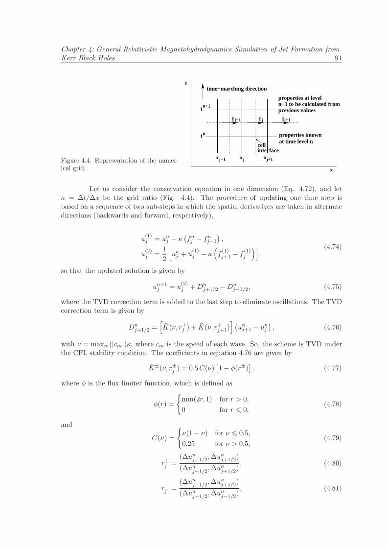
Chapter 4: General Relativistic Magnetohydrodynamics Simulation of Jet Formation from

Kerr Black Holes 91

Figure 4.4: Representation of the numer-ical grid.

t

x x x

t

t

n

jj−1 j+1

n+1

j j+1j−1

time−marching direction

properties knownat time level n

properties at level

previous valuesn+1 to be calculated from

x

interfacecell

f f f

Let us consider the conservation equation in one dimension (Eq. 4.72), and letκ = ∆t/∆x be the grid ratio (Fig. 4.4). The procedure of updating one time step isbased on a sequence of two sub-steps in which the spatial derivatives are taken in alternatedirections (backwards and forward, respectively),

u(1)j = unj − κ

(

fnj − fnj−1

)

,

u(2)j =

1

2

[

unj + u(1)j − κ

(

f(1)j+1 − f

(1)j

)]

,(4.74)

so that the updated solution is given by

un+1j = u

(2)j +Dn

j+1/2 −Dnj−1/2, (4.75)

where the TVD correction term is added to the last step to eliminate oscillations. The TVDcorrection term is given by

Dnj+1/2 =

[

K(ν, r+j ) + K(ν, r+j+1)]

(

unj+1 − unj)

, (4.76)

with ν = maxm(|cm|)κ, where cm is the speed of each wave. So, the scheme is TVD underthe CFL stability condition. The coefficients in equation 4.76 are given by

K±(ν, r±j ) = 0.5C(ν)[

1− φ(r±)]

, (4.77)

where φ is the flux limiter function, which is defined as

φ(r) =

min(2r, 1) for r > 0,

0 for r 6 0,(4.78)

and

C(ν) =

ν(1− ν) for ν 6 0.5,

0.25 for ν > 0.5,(4.79)

r+j =(∆unj−1/2,∆unj+1/2)

(∆unj+1/2,∆unj+1/2), (4.80)

r−j =(∆unj−1/2,∆unj+1/2)

(∆unj−1/2,∆unj−1/2), (4.81)

92Chapter 4: General Relativistic Magnetohydrodynamics Simulation of Jet Formation from

Kerr Black Holes

where (.,.) denotes the inner product in Rm, and ∆unj+1/2 = unj+1 − unj .

Koide et al. extended the STVD method to a 2-D scheme through the use ofthe splitting method. This procedure introduces a weak checkerboard numerical instability,which is avoid when the two coefficients K+ and K− are combined into a single coefficientK defined as

K(ν, r+, r−) = 0.5C(ν)[

1− φ(r+, r−)]

, (4.82)

with

φ(r+, r−) = max[0,min(2r+, r−, 1),min(2r−, r+, 1)]. (4.83)

Method to keep the magnetic field divergence-free

Regarding the evolution of the magnetic field, the induction equation is alreadypart of the GRMHD equation system (Eq. 4.51). The number of the GRMHD equations isreduced from eight to five when the components of the magnetic field are obtained analyt-ically. Here, the magnetic field is initially uniform, as seen by observers at infinity, beingrepresented by Wald’s solution (1974). However, the divergence free condition must bemaintained throughout the whole computation. Koide et al. uses the so-called magnetic-field cleaning method, a procedure through which the components of the magnetic field arere-defined at each time step.

Method to recover the primitive variables from the conserved variables

The quantities that are updated during the integration of GRMHD equations arethe conserved variables. However, one must know the primitive variables in order to describethe flow, and so the primitive variables must be computed as a function of conserved vari-ables at each time step. All conservation GRMHD schemes require methods to transformfrom primitive variables to conserved variables and vice-versa. The direct transformation(primitive variables → conserved variables) is easily obtained using the set of equations 4.62.Instead, the inverse transformation (conserved variables → primitive variables) usually in-volve the numerical solutions of non-linear algebraic equations. There is more than one wayto do this. The method which is used by Koide et al. to recover the primitive variables fromthe conserved variables solves numerically two non-linear, simultaneous algebraic equationswith unknown variables x ≡ γ − 1 and y ≡ γ(v ·B)/c2,

x (x+ 2)[

ΓRx2 + (2ΓR− d)x+ ΓR− d+ u+ Γ2 y

2]2

=(

Γx2 + 2Γx+ 1)2 [

f2(x+ 1)2 + 2σy + 2σxy + b2y2]

and (4.84)

[

Γ(

R− b2)

x2 +(

2ΓR − 2Γb2 − d)

x+ ΓR− d+ u− b2 + Γ2 y

2]

y

= σ (x+ 1)(

Γx2 + 2Γx+ 1)

, (4.85)

where R = D + ǫ/c2, d = (Γ − 1)D, u = (1 − Γ/2)B2/c2, f = P/c, b = B/c, andσ = B · P/c2. Equations 4.84 and 4.85 are solved at each cell using a two-variable Newton-Raphson iteration method.

Chapter 4: General Relativistic Magnetohydrodynamics Simulation of Jet Formation from

Kerr Black Holes 93

Validation tests

The code is checked by undergoing various test calculations: (i) the steady stateinfall of a finite pressure gas into the BH (Bondi flow), which is approximately in free falland presents a transonic solution; (ii) the transonic solution with a shock; (iii) the Keplerianmotion in a free-fall corona; (iv) the sub-Keplerian motion in a free-fall corona; and (v) theKeplerian motion in a hydrostatic corona (Koide et al. 1999).

Transonic solution for a free-fall flow

Following Koide et al. (1999), a steady state infall of a finite pressure gas onto theBH (which, in approximation, is a free-fall flow) can be described by the solution of Bondi& Hoyle (1944). The gas inflow is supposed to be spherical symmetric with a polytropicequation of state, p ∝ ρΓ. The gas equation of motion can be written as a function oftwo constant of motion, F (a sort of adiabatic invariant) and respectively H (∼ specificenthalpy):

F =

(

H

αγ− 1

)

(

αr2γv

c

)Γ−1, (4.86)

where, once again, α is the lapse function and γ is the Lorentz factor, and

H = α0γ0

(

1 +Γ

Γ− 1

p0ρ0c2

)

, F =Γ

Γ− 1

p0ρ0c2

(

α0r20γ0

v0c

)Γ−1, (4.87)

where α0, γ0, p0, ρ0, and v0 are evaluated at an arbitrary point r = r0.

For a given H and Γ, the equation of motion F (v, r) admits a transonic solution,which in a radial distribution of the flow velocity passes through the sonic point from thesubsonic to supersonic regions. The sonic point is obtained by solving

∂F

∂γ= 0,

∂F

∂α= 0. (4.88)

From the first equation, one obtains the sonic flow condition: v = vs = (Γp/h)1/2c, whereh, once again, denotes the relativistic enthalpy, h ≡ ρc2 + Γp/(Γ − 1). When solving forboth equation, one can obtain the following reduced equation

(

H2 − 1)

x3 +

(

9

4− 2gH2

)

x2 +

(

H2g2 − 33

42

)

x+

(

3

4

)3

= 0, (4.89)

where x ≡ r/rS and g ≡ (3Γ− 2)/4(Γ− 1). Therefore, the velocity of the flow at a specificr = x rS is determined by v = vs with α = H(γ−2 + Γ− 2)/[(Γ − 1)γ].

Normalizations

For the thermal, magnetic, and rotational energy, the following non-dimensionalparameters are used:

Eth =v2s0v2K0

, Emag =v2A0

v2K0

, Erot =v2φv2K0

, (4.90)

94Chapter 4: General Relativistic Magnetohydrodynamics Simulation of Jet Formation from

Kerr Black Holes

where vs0 is the relativistic sound speed,

vs0 = c

√

Γp0ρ0c2 + Γp0/(Γ− 1)

, (4.91)

vA0 is the Alfven velocity,

vA0 = cB0

√

ρ0c2 + Γp0/(Γ− 1) +B20

, (4.92)

and vK0 is the relativistic Keplerian velocity,

vK0 =c

√

2(r0/rS − 1), (4.93)

which is reduced to the Newtonian Keplerian velocity, vK = (GM/r)1/2, when the non-relativistic limit is considered, rS/r ≪ 1. Here, all velocities are evaluated at the innermoststable orbit by ZAMOs, being denoted with the subscript “0.”

4.4 Simulation of jet formation from a Kerr black hole

We perform 2.5-D simulations of jet formation from a Kerr BH surrounded by athin Keplerian accretion disk in the numerical domain 1.5 rS 6 R 6 15rS, 0 6 θ 6 π/2 with128 × 128 grid points.

4.4.1 Initial conditions

• The simulations are performed for a BH spin parameter of a∗ = 0.95.

• The coordinates are set to: (x1min = 1.5, x1max = 30) in the radial direction, (x2min =0 rad, x2max = 6.28 rad) for the azimuthal angle, and (x3min = 0.03 rad, x3max = 1.57rad) for the polar angle.

• A free boundary condition at the inner and outer boundaries is used, so that waves,fluids, and magnetic fields can pass through freely.

• The numerical computation is scale free (i.e., they do not depend on the BH mass),where the physical quantities are normalized as follows:

physical quantity normalization unit

time (τS) rS/clength (r) rSdensity (ρ) ρ0pressure (P ) ρ0c

2

velocity (v) c

magnetic field√

ρ0c2

For a BH with mass of 3M⊙, the Schwarzschild radius is ∼ 8× 105 cm and the timeunit τS = 3× 10−5 s. The normalization unit of density ρ0 is the initial proper massdensity of the corona density at (r, z) = (3 rS, 0). For a density unit of ρ0 = 1010 gcm−3, the magnetic field strength unit is 3×1014 G and the pressure unit is P = 1029

dyn cm−2.

Chapter 4: General Relativistic Magnetohydrodynamics Simulation of Jet Formation from

Kerr Black Holes 95

• The coronal plasma is considered to be a transonic free-fall flow with the specificenthalpy h/ρc2 = 1 + Γp/[(Γ − 1)ρc2] = 1.3, where the specific heat ratio is set toΓ = 5/3.

• The magnetic field is initially uniform, as seen by observers at infinity, being repre-sented by Wald’s solution (Wald 1974). The vector potential24 of the Wald solutionis

Aµ =B0

2(gµ3 + 2a∗rggµ0), (4.94)

where B0 denotes the magnetic field strength. When the metric is written in Boyer-Lindquist coordinates, the components of the magnetic field measured by a comovingobserver are (Koide 2003)

Br = B0cos θ√

A

∆+2rgr

[

r4 − (a∗rg)4]

Σ2

, (4.95)

Bθ = −B0

√

∆

Asin θ

r − rg +rgΣ2

[

r2 + (a∗rg)2]

Σ+ 2(a∗rg)2[

r2 − (a∗rg)2]

cos2 θ

.

(4.96)

In the simulations, the magnetic field strength B0 is set by comparing the magneticenergy density, uB ∼ B2

0 , to the rest-mass energy density of the plasma, um ∼ ρ0c2.

For a magnetic-field-dominating case (uB > um), the Alfven velocity is close to thespeed of light (Koide 2003). The magnetic field strength can be written as B0 =b0√

ρ0c2, where b0 is a simulation parameter.

• The inner edge of the disk is at r = 3 rS.

• The disk inclination angle with respect to the BH equatorial plane is 15.

• In the disk, the azimuthal component of the velocity is assumed to be the relativisticKeplerian velocity (Eq. 4.93), and the poloidal component vanishes.

• The ratio of the disk mass density to the coronal mass density is 100.

4.4.2 Numerical results

The simulation of jet formation is initiated with a large-scale uniform magneticfield passing through a thin (Keplerian) accretion disk, with the magnetic field being setas for b0 = 0.1 and the pressure of plasma around the BH being set to p0 = 1.0ρ0c

2. Amagnetic field with b0 = 0.1 is considered to be weak. (Strong fields are those for whichb0 > 1.)

Times for various snapshots were chosen to cover the entire computed evolutionof the plasma density (Fig. 4.5), the plasma being divided in two parts: (i) the coronaaround the BH and (ii) the thin accretion disk that co-rotates with the BH (Fig. 4.5a).The rest-mass density is represented in a logarithmic scale. The solid line shows the poloidal

24The covariant component of the electromagnetic field tensor can be witten in terms of the four-vectorpotential as Fµν = ∂µAν − ∂νAµ, where Aµ = (Φe, A

1, A2, A3) is the four-vector potential (Φe is the electro-static potential).

96Chapter 4: General Relativistic Magnetohydrodynamics Simulation of Jet Formation from

Kerr Black Holes

component of the magnetic field (Bp), and the arrow represents the plasma poloidal velocityas seen in the ZAMO frame normalized to the speed of light (vp/c). As the simulationevolves, the disk plasma losses angular momentum by the magnetic field torque and fallstoward the BH. Figure 4.5b shows the state at t = 64 tS, when the inner edge of the diskhas rotated 1.6 cycles. The centrifugal force decelerates the disk plasma at r ∼ 3 rS, andthe rapid infall of the plasma in front of this produces a shock inside the disk. The highpresure behind the shock begins to produce the jet (we will refer to this as the formationof the pressure-driven component of the jet).

The gas pressure and electromagnetic forces that are used to accelerate (or decel-erate) the plasma are, in the ZAMO frame,

Wgp = −v · ∇(αp), (4.97)

WEM = αv · (E+ J×B) , (4.98)

where α is, once again, the lapse function.

The disk plasma carries the frozen magnetic field with it, causing a considerabledeformation of the field lines. As there is no stable orbit at r 6 3 rS, the accretion diskcontinues to fall rapidly toward the BH, enters the ergosphere, and then crosses the horizon.This is shown by the crowded magnetic field lines near the BH. Figure 4.5c shows the stateat t = 120 tS, by which time the inner edge of the disk has rotated 3 cycles. In the shockregion, the matter is accelerated by the electromagnetic force and the increased gas pressure.Figure 4.5d shows the final state at t = 186 tS when the inner edge of the disk has rotated4.7 cycles. The jet is formed almost along the poloidal magnetic field lines. The maximumtotal velocity of the jet is ∼ 0.4 c. The time evolution of rest-mass density indicates thatthe jet consists of:

1. a gas pressure-driven component and

2. a magnetically-driven component which is developed inside the gas pressure-driven jet.

The former comes from the region of the disk near the shock r 6 3 rS. The latter comeson one hand from the extraction of the BH rotational energy in the ergosphere, and on theother hand from the twisting of the magnetic field far from the BH.

For a better illustration of the distribution of the regions of acceleration (or decel-eration) of the plasma by gas-pressure and electromagnetic forces, in Figs. 4.6 and 4.7 weplot these forces in the z direction, (- W z

gp) and W zEM (color), overlapped with the poloidal

component of the magnetic field (solid line), and in Figs. 4.8 and 4.9 overlapped with the(negative) toroidal component of the magnetic field, Bφ (solid line). The magnetic fieldlines are twisted counter to the accretion disk rotation, therefore we plot −Bφ. In Figs. 4.6and 4.8, the light green-orange color shows the region were the plasma is accelerated by thegas-pressure force, whereas the blue color shows the region where the plasma is decelerated.The gas-presure force accelerates the plasma (orange) in the region of the disk where theshock is produced, as well as in the region very close to the BH where the coronal plasma ispresent. This high gas-pressure force acting on the plasma near the BH reflects the generalrelativistic effects which are introduced in the system by the lapse function. The gradient(in the z direction) of the lapse function increases about one order of magnitude in the re-gion close to the BH (Fig. 4.10), and then it decreases as one approaches the event horizon.

Chapter 4: General Relativistic Magnetohydrodynamics Simulation of Jet Formation from

Kerr Black Holes 97

Figure 4.5: Time evolution of the jet formation in the magnetosphere of a BH with a spin parametera∗ = 0.95. The black circle indicates the BH. Solid line represents the poloidal component of themagnetic field, Bp. Color shows the logarithm of the proper mass density, ρ. Arrows representthe plasma poloidal velocity as seen in ZAMO frame normalized to the speed of light, vp/c. Thedistance and the time are in units of rS and τS ≡ rS/c, respectively. (a) For the initial conditions,a coronal plasma distribution, which is given by a transonic solution with Γ = 5/3 and H = 1.3,and a Keplerian accretion disk around the BH are set up. The density of the disk is 100 greaterthan that of the corona. (b) t = 64 tS. The disk plasma falls towards the BH. The magnetic fieldlines are twisted through the plasma motion and through the frame dragging effect that occurs inthe BH ergosphere. A shock is produced in the accretion disk at ∼ 3 rS. (c) t = 112 tS. In the shockregion, the matter is accelerated by the Lorentz force and the increased gas pressure, leading to jetformation. (d) t = 186 tS. The jet is formed almost along the magnetic field lines. The maximumpoloidal velocity of the jet is ∼ 0.4 c.

98Chapter 4: General Relativistic Magnetohydrodynamics Simulation of Jet Formation from

Kerr Black Holes

Figure 4.6: Magnitude of the gas-pressure force in the z direction, W zgp (color), that accelerates (or

decelerates) the plasma. Solid line shows the poloidal component of the magnetic field and arrowrepresents the plasma poloidal velocity. Light green-orange color shows the region were the plasmais accelerated, whereas blue color shows the region where the plasma is decelerated.

Chapter 4: General Relativistic Magnetohydrodynamics Simulation of Jet Formation from

Kerr Black Holes 99

Figure 4.7: Magnitude of the electromagnetic force in the z direction that accelerates the plasma,W z

EM (color). Solid line shows the poloidal component of the magnetic field and arrow represents theplasma poloidal velocity. The plot shows the magnetically-driven jet component which is associatedwith the twisting of the magnetic field (blue region), as well as with the electromagnetic extractionof the BH rotation energy (red-yellow region close to the BH).

100Chapter 4: General Relativistic Magnetohydrodynamics Simulation of Jet Formation from

Kerr Black Holes

Figure 4.8: Magnitude of the gas-pressure force in the z direction (color) that accelerates (or de-celerates) the plasma. Solid line shows the toroidal component of the magnetic field and arrowrepresents the plasma poloidal velocity. Light green-orange color shows the region were the plasmais accelerated, whereas blue color shows the region where the plasma is decelerated.

Chapter 4: General Relativistic Magnetohydrodynamics Simulation of Jet Formation from

Kerr Black Holes 101

Figure 4.9: Magnitude of the electromagnetic force in the z direction that accelerates the plasma,W z

EM (color). Solid line shows the toroidal component of the magnetic field and arrow represents theplasma poloidal velocity. The plot shows the magnetically-driven jet component which is associatedwith the twisting of the magnetic field (blue region), as well as with the electromagnetic extractionof the BH rotation energy (red-yellow region close to the BH).

102Chapter 4: General Relativistic Magnetohydrodynamics Simulation of Jet Formation from

Kerr Black Holes

Sradius r/r2 4 6

grad

ient

of t

he la

pse

func

tion

0.02

0.04

0.06

0.08

0.10

= 0.95*a

Sz = 0.5 rSz = 1.0 rSz = 1.5 r

Figure 4.10: Radial distribution of thegradient (in the z direction) of the lapsefunction in the Boyer-Lindquist refer-ence frame on the three different sur-face: z = 0.5 rS, z = 1.0 rS, and z =1.5 rS.

This decrease of the gradient towards a null value close to the BH is explained throughthe fact that the lapse function in Boyer-Lindquist coordinates becomes null at the eventhorizon. The horizon is located behind our boundary at r = 1.5 rS, therefore we cannotfollow the profile of the gradient of the lapse function very close to the event horizon. (Thehorizon is located at rH ∼ 0.65 rS for a BH spin parameter of a∗ = 0.95.) If we compareFig. 4.8 with Fig. 4.9, we can observe that the region of electromagnetic acceleration of theplasma is clearly associated with the twisting of the magnetic field lines far from the BH,where there is a lack of plasma accelerated by gas pressure.

In Fig. 4.7, the electromagnetic power (color) increases over one order of magni-tude from the blue to the light red-yellow. The plot shows the electromagnetically-drivenjet component which is associated with the twisting of the magnetic field (blue region inFigs. 4.7c and d), as well as with the electromagnetic extraction of the BH rotation energy(red-yellow region close to the BH). In the BH ergosphere, the electromagnetically-drivenjet is accelerated by the magnetic field which is frozen into the accretion disk. Due to theframe dragging effect, the disk is forced to rotate in the same direction as the BH rotation.As a result, both the azimuthal component of the magnetic field and the magnetic tensionincrease, therefore the plasma is accelerated by the magnetic pressure. Such mechanism ofjet production can be thought of as being a MHD Penrose process that uses the magneticfields to extract rotational energy of the BH and eject a collimated outflow from very nearthe horizon (Koide et al. 2000a). In contrast, running long-term simulations, Komissarov(2005) concluded that his results can be explained if the rotational energy is extracted fromthe BH through the purely electromagnetic mechanism of Blandford and Znajek (1977).In the numerical simulations of Komissarov (2005), no regions of negative hydrodynamic“energy at infinity” are seen inside the ergosphere, and therefore the MHD Penrose processdoes not operate. This might suggest that an MHD Penrose process can be observed onlyfor transient jets. This conclusion might be revised when long-term simulations using thecode of Koide et al. (1998, 2000a) and Koide (2003) will be performed.

We refer to the region of stronger acceleration of the plasma by the gas-pressureand electromagnetic forces as the jet-forming region. For a better understanding of thephysics of the jet formation mechanism, in Fig. 4.11 we plot the plasma beta, β = pgas/pmag

(color), and the toroidal component of the magnetic field (contour). The blue color showsthe region where the magnetic pressure dominates the gas pressure and light red-yellow-green shows where the gas pressure is dominant. Initially, the dominant component of the

Chapter 4: General Relativistic Magnetohydrodynamics Simulation of Jet Formation from

Kerr Black Holes 103

Figure 4.11: Time evolution of the plasma beta β = pgas/pmag (color). Solid line shows the toroidalcomponent of the magnetic field and arrow represents the plasma poloidal velocity. In the regionwhere the magnetic field is twisted stronger, the magnetic pressure is higher.

104Chapter 4: General Relativistic Magnetohydrodynamics Simulation of Jet Formation from

Kerr Black Holes

jet is the gas pressure-driven component (blue-green regions in Fig. 4.11b). By the end ofthe simulation, t = 186 tS, a magnetically-driven jet component had begun to be developedinside the pressure-driven component of the jet (dark blue regions in Fig. 4.11d), as thetoroidal component of the magnetic field has increased about five times the initial value(Fig. 4.12d). This amplification is caused by the shear of the plasma flow in the Boyer-Lindquist frame due to the frame dragging effect of the rotating BH, and the magnetic fieldamplification energy comes from the rotation of the BH itself (Koide et al. 2000a). Themagnetic tension accelerates the plasma by the magnetic pressure. The region of the jetwhere the magnetic pressure dominates (Fig. 4.11d) is clearly associated with the region ofelectromagnetic extraction of the BH rotation energy (Fig. 4.7d).

To illustrate the physical processes that occur during the simulation, we plot thex-profiles of various physical quantities first on the surface of z = 0.7 rS, which is close to theBH equatorial plane, at t = 64 tS (Fig. 4.12). (Here, the coordinate x denotes the coordinater.) In Fig. 4.12a, the density profile shows the presence of a shock at r ∼ 3 rS. Behindthe shock, the increased gas pressure dominates the magnetic pressure. This dominance isalso shown in Fig. 4.12f, where the plasma beta in the region r ∈ [1.5, 3.8] rS is over unity.In this region, the acceleration of the plasma is, therefore, produced by the gas-pressureforce (the dotted line in Fig. 4.12e). The azimuthal components of the velocity and ofthe magnetic field are dominant (Figs. 4.12b and d), suggesting that the disk plasma isalso accelerated by centrifugal forces. However, at the shock front, the azimuthal velocityof the plasma decreases (Fig. 4.12b). The total velocity of the plasma is less that theKeplerian velocity, being supersonic and super-Alfvenic. Behind the shock the plasmabecomes, however, subsonic and sub-Alfvenic (Fig. 4.12c). Both the sonic and Alfvenicvelocities drop from ∼ 0.3 c to zero at the shock front and then increase to ∼ 0.6 c behindthe shock. The Keplerian velocity in the shock region is ∼ 0.6 c. The jet from the disk hasnot been formed yet by the time of t = 64 tS. The plasma accelerated in the z-directioncorresponding to the region r < 3 rS, where the poloidal component of the plasma velocityincreases (Fig. 4.12b), comes from the BH corona. By the end of the simulation, t = 186 tS(Fig. 4.13), all components of the magnetic field have been increased to values greater thanten times the initial value of the magnetic field and the total velocity of the plasma hasreached a value close to the Keplerian velocity. Note that the plasma motion is here studiedon a surface close to the BH equatorial plane. The fact that the radial magnetic field isstrongly amplified near the BH reflects the dragging of the magnetic field lines by the diskplasma.

In Fig. 4.14, we plot the x-profiles of various physical quantities on the surface ofz = 5.15 rS by the end of the simulation (t = 186 tS). By this time, the total velocity ofthe plasma flowing in the region r ∈ [4, 9] rS has reached a value greater than the Keplerianvelocity of the disk (Fig. 4.14c). On the other hand, the plasma in the very same region hasa positive component of the velocity in the z direction (Fig. 4.14b), therefore the disk andcoronal plasma is likely to flow out in the z direction and form a jet. The plasma is, on onehand, decelerated by the gas-pressure force (see the corresponding blue-green region in Fig.4.6) and, on the other hand, accelerated by the electromagnetic force (see the correspondingorange-blue region in Fig. 4.7), the latter being stronger though (see also Fig. 4.14e).

To show the structure of the jet, we plot the z-profiles of various physical quantitieson the surface of x = 4.73 rS at t = 186 tS which corresponds to the maximum value of theplasma velocity (Fig. 4.15). On this surface, the magnetic pressure dominates the gaspressure up to about z = 10 rS (Figs. 4.15a and f). The dominant component of the

Chapter 4: General Relativistic Magnetohydrodynamics Simulation of Jet Formation from

Kerr Black Holes 105

Figure 4.12: The x-profiles of various physical quantities on the surface of z = 0.7 rS at t = 64 tS,the time at which the shock in the disk starts to be developed. (a) Density ρ (solid line), gaspressure pgas (dashed line), and magnetic pressure pmag (dot-dashed line). (b) Components of theplasma velocity, vr (solid line), vz (doted line), vφ (dashed line), and vp (3-dot-dashed line). (c)Total velocity vtot = (v2r +v2z +v2φ)

1/2 (solid line), Alfven velocity vA (dashed line), sound velocity cs(dot-dashed line), and Keplerian velocity vK (3-dot-dashed line). (d) Components of the magneticfield, Br (solid line), Bz (dot-dashed line), and Bφ (dashed line). (e) Vertical component of theelectromagnetic force W z

EM (solid line) and the gas-pressure force W zgp (doted line). (f) Plasma beta

β = pgas/pmag.

106Chapter 4: General Relativistic Magnetohydrodynamics Simulation of Jet Formation from

Kerr Black Holes

Figure 4.13: The x-profiles of various physical quantities on the surface of z = 0.7 rS at the end ofthe simulation t = 186 tS. (a) Density ρ (solid line), gas pressure pgas (dashed line), and magneticpressure pmag (dot-dashed line). (b) Components of the plasma velocity, vr (solid line), vz (dotedline), vφ (dashed line), and vp (3-dot-dashed line). (c) Total velocity vtot = (v2r + v2z + v2φ)

1/2 (solidline), Alfven velocity vA (dashed line), sound velocity cs (dot-dashed line), and Keplerian velocityvK (3-dot-dashed line). (d) Components of the magnetic field, Br (solid line), Bz (dot-dashed line),and Bφ (dashed line). (e) Vertical component of the electromagnetic force W z

EM (solid line) and thegas-pressure force W z

gp (doted line). (f) Plasma beta β = pgas/pmag.

Chapter 4: General Relativistic Magnetohydrodynamics Simulation of Jet Formation from

Kerr Black Holes 107

Figure 4.14: The x-profiles of various physical quantities on the surface of z = 5.1 rS (which cor-responds to the base of the jet) at the end of the simulation t = 186 tS. (a) Density ρ (solid line),gas pressure pgas (dashed line), and magnetic pressure pmag (dot-dashed line). (b) Components ofthe plasma velocity, vr (solid line), vz (doted line), vφ (dashed line), and vp (3-dot-dashed line). (c)Total velocity vtot = (v2r +v2z +v2φ)

1/2 (solid line), Alfven velocity vA (dashed line), sound velocity cs(dot-dashed line), and Keplerian velocity vK (3-dot-dashed line). (d) Components of the magneticfield, Br (solid line), Bz (dot-dashed line), and Bφ (dashed line). (e) Vertical component of theelectromagnetic force W z

EM (solid line) and the gas-pressure force W zgp (doted line). (f) Plasma beta

β = pgas/pmag.

108Chapter 4: General Relativistic Magnetohydrodynamics Simulation of Jet Formation from

Kerr Black Holes

velocity still remains the azimuthal component (Fig. 4.15b). However, as Fig. 4.15c shows,the jet is likely to be produced from about z = 3 rS all the way up, becoming subsonicand sub-Alfvenic from about z = 4 rS though. The total velocity of the particles has themaximum value of about ∼ 0.4 c. The dominant component of the magnetic field is thetoroidal component (Fig. 4.15d), which increases in the jet-forming region. The ratio ofthe toroidal to the poloidal component of the magnetic field, Bφ/Bp, represents the twistof the magnetic field. This twist increases strongly in the jet-forming region (Fig. 4.15e),where the magnetic energy stored by the twisting magnetic field is converted into kineticenergy of the jet. Such a large twist of the magnetic field implies a large magnetic pressureas well, which is also reflected by a low plasma beta in this region (Fig. 4.15f).

We would like to point out that the main result of the simulation presented inthis chapter is the presence of an electromagnetically-driven component of the jet which,close to the BH, is developed inside the gas pressure-driven jet component. In the regionsfar from the BH, the jet is accelerated by electromagnetic forces. Similar to the previoussimulations performed by Koide et al., where the accretion disk co-rotates with the BHrotation in a free-falling corona, the maximum value of the jet velocity is ∼ 0.4 c, i.e., thejet is sub-relativistic.

4.4.3 Comparison with the RAISHIN simulation code (Mizuno et al.)

The critical problem of Koide et al. GRMHD code is that the schemes can notmaintain a divergence-free magnetic field automatically. Therefore, Mizuno et al. (2006b,2007, 2009b) have developed a new 3-D GRMHD code, RAISHIN, which is a conservative,high-resolution shock-capturing scheme. A Harten-Lax-van Leer approximate Riemannsolver is employed to compute the numerical fluxes. In order to maintain the divergence-free condition, a flux-interpolated, constrained transport scheme is applied. As far as thenumerical accuracy and the numerical costs are concerned, one can select a method, whichis more computationally efficient, from the following four reconstruction algorithms: thepiecewise linear methods with either Minmod or MC slope-limiter function, the convexessentially non-oscillatory method, and the piecewise parabolic method, where a multistepTVD Runge-Kutta method either with second or third-order time accuracy can be appliedto advance the solution in time.

Simulations of jet formation from non-rotating (a∗ = 0) and rapidly-rotating (a∗ =0.95) BHs were performed, when a thin accretion disk and a uniform magnetic field areconsidered initially. The simulation results indicate that mildly relativistic jets (v & 0.4 c)are driven by the Lorentz force and the gas pressure gradients. In the case of the rotatingBH, an additional, faster, and more collimated matter-dominated inner jet (v & 0.5 c) isproduced and accelerated through the twisting of the magnetic field that occurs in theBH ergosphere. The jet kinematic structure depends mainly on the BH spin and on themagnetic field configuration and strength. The simulations were carried out for Boyer-Lindquist coordinates. Nevertheless, the RAISHIN code with the Kerr-Schild coordinatesis subject to further work by Mizuno et al. This approach may provide a way to overcome thenumerical problems that occur when approaching the BH event horizon, as for the boundaryconditions. The expected results would be longer term simulations (∼ 103 − 104 tS) whenstrong magnetic fields are considered (b0 > 1).

To show the behavior of the Kerr-Schild coordinates at the BH event horizon,which is a physical singularity in the Boyer-Lindquist reference frame, in Fig. 4.16 we plot

Chapter 4: General Relativistic Magnetohydrodynamics Simulation of Jet Formation from

Kerr Black Holes 109

Figure 4.15: The z-profiles of various physical quantities on the surface of x = 4.73 rS at the end ofthe simulation t = 186 tS. (a) Density ρ (solid line), gas pressure pgas (dashed line), and magneticpressure pmag (dot-dashed line). (b) Components of the plasma velocity, vr (solid line), vz (dot-dashed line), and vφ (dashed line). (c) Total velocity vtot = (v2r + v2z + v2φ)

1/2 (solid line), Alfvenvelocity vA (dashed line), sound velocity cs (dot-dashed line), and Keplerian velocity vK (double-dot-dashed line). (d) Components of the magnetic field, Br (solid line), Bz (dot-dashed line), andBφ (dashed line). (e) Ratio of toroidal to poloidal magnetic components Bφ/Bp. (f) Plasma betaβ = pgas/pmag.

110Chapter 4: General Relativistic Magnetohydrodynamics Simulation of Jet Formation from

Kerr Black Holes

Figure 4.16: Radial distribution of thelapse function in the Boyer-Lindquistreference frame (purple line) and inthe Kerr-Schild reference frame (greenline). The lapse function in the Boyer-Lindquist frame becomes singular atthe event horizon (rH ∼ 0.65 rS fora∗ = 0.95), whereas the lapse func-tion in the Kerr-Schild frame is a well-behaved function all the way down tothe true singularity of the space-time atr = 0. We use the normalized radiusr/rS.

the radial distribution of the lapse function (which in turn gives the acceleration of free-falling particles, the external magnetic field strength, etc.) in the two reference frames:Kerr-Schild (green line) and Boyer-Lindquist (purple line), respectively. We consider herethe case when the BH spins at a∗ = 0.95, so that the horizon radius is ≃ 0.65 rS. Thelapse function in the Boyer-Lindquist reference frame, αBL =

√

Σ∆/A (Eq. 1.9), becomessingular as one approaches the BH horizon. Instead, the lapse function in the Kerr-Schildreference frame [αKS = 1/

√1 + Z with Z = 2r2gr∗/Σ = r2Sr∗/(2Σ), e.g., Font et al. (1999)]

stays finite. Moreover, the lapse function in the Kerr-Schild frame is a well-behaved functionall the way down to the true singularity of the space-time at r = 0.

4.4.4 Comparison with other work

The results presented in this chapter are obtained for a geometrically thin accre-tion disk. Nevertheless, numerical simulations of jet formation for a thick accretion diskwere performed, for instance, by McKinney & Gammie (2004); McKinney (2006); Hawley &Krolik (2006). As we already mentioned in the introduction, McKinney & Gammie (2004);McKinney (2006) have developed a conservative shock-capturing scheme (called HARM) foraxisymmetric simulations of jet formation. The code uses modified Kerr-Schild coordinates.In one of their models, large-scale magnetic fields are created self-consistently by a thickaccretion disk with hight to radius ratio H/R & 0.1. The jets formed in their simulationsalso present two components: (i) a highly-relativistic, Poynting flux-dominated “funnel,”originating from around the BH poles, and (ii) a “wind,” which consists of a cone of ma-terial near the edge of the funnel and moves at sub-relativistic speeds (v ∼ 0.3 c). Thefunnel region is nearly force-free and consistent with the Blandford-Znajek mechanism, forwhich the authors presented a self-contained derivation in Kerr-Schild coordinates. Theirresults indicate that the rotational energy of the BH is extracted via the Blandford-Znajekmechanism, but not through an MHD Penrose process. Instead, their second componentof the jet is similar to the gas pressure-driven component of the jet in our simulations.Hawley & Krolik (2006) also obtained two components of the jet [similarly to McKinney &Gammie (2004) and McKinney (2006)] using a GRMHD code that resembles the algorithmsemployed in the ZEUS code used for non-relativistic astrophysical MHD simulations, withBoyer-Lindquist coordinates. In the numerical simulations performed by McKinney (2006)and Hawley & Krolik (2006), poloidal-loop magnetic fields inside the torus are considered

Chapter 4: General Relativistic Magnetohydrodynamics Simulation of Jet Formation from

Kerr Black Holes 111

initially. This magnetic field is then twisted and expands from the torus (i.e., the thickdisk) as a magnetic tower, which fills the funnel region. In our case, the magnetic field isinitially vertical, threading the disk and the BH ergosphere, which is then twisted by theframe dragging effect and form a magnetically-driven component of the jet. Although thesame basic mechanism of jet formation is used in the work by McKinney & Gammie (2004);McKinney (2006); Hawley & Krolik (2006) as in our work, the jets show different features.These differences can be attributed to a different type of the magnetic field and accretiondisk used initially for simulations.

4.5 Summary and conclusions

After an introduction to the GRMHD equations in 3+1 formalism, we presentedthe results of GRMHD simulation of jet formation from a thin accretion disk that co-rotateswith a rapidly-spinning BH (a∗ = 0.95) in a free-falling corona, using the code developedby Koide et al. (1998, 2000a); Koide (2003).

• For the numerical results presented in this chapter, we set the simulation parametersin such a way to perform a longer term simulation. We used a weak magnetic fieldof 0.1(ρ0c

2)1/2 and an inner boundary at 1.5 rS, so that the final stage of the jetformation corresponds to t = 186 tS. Koide et al. have performed simulations of jetformation from a Kerr BH using a variety of parameter set, including the strength ofthe magnetic field as strong as 5.57(ρ0c

2)1/2.

• The numerical results show that, as the time evolves, the disk plasma loses angularmomentum by the magnetic field torque and falls toward the BH. When the rapidinfall of plasma encounters the disk plasma that is decelerated by centrifugal forcesnear the BH, a shock is produced inside the disk at ∼ 3 rS. The high pressure behindthe shock pushes the plasma outward by gas-pressure forces and pinches it into acollimated jet. As a result, a gas pressure-driven component of the jet is produced.On the other hand, the magnetic field is frozen in the accretion disk. Therefore,the infalling plasma bends the magnetic field inward, creating a significant radialcomponent of the field which is then twisted by the differential disk rotation into anazimuthal component. As the azimuthal component of the magnetic field increases,and so the magnetic tension, the plasma is accelerated by the magnetic pressure. Thiselectromagnetically-driven component of the jet has two origins: one associated withthe extraction of the BH rotational energy in the ergosphere and the other one withthe twisting of the magnetic field far from the BH.

• Similar to Koide et al., the maximum jet velocity obtained in this numerical simulationis ∼ 0.4 c. This is considerable lower than the velocity of the inner parts of someAGN jet for which the observations indicate relativistic speeds (e.g., Ghisellini et al.2005). However, the outer parts of the jet can have mildly- and sub-relativistic speeds.Nevertheless, the jet can be accelerated further out at shock fronts. This accelerationmight eventually be seen in longer term simulations. A relativistic jet of ∼ 0.9 c hasbeen obtained in the numerical simulations performed by Koide et al. (2000b), in thecase of a non-rotating disk around a rapidly-rotating BH though.

• The previous simulations performed by Koide et al. show a two-component jet: (i)an inner, low density, fast, electromagnetically-driven jet and (ii) an outer, high den-

112Chapter 4: General Relativistic Magnetohydrodynamics Simulation of Jet Formation from

Kerr Black Holes

sity, slow, gas pressure-driven jet. In the case of the simulation results presentedin this chapter, the dominant component of the jet in the region close to the BH isinitially the gas pressure-driven component, which becomes weaker compared to theelectromagnetically-driven component as the time goes on. So that, by the end ofthe simulation, the electromagnetically-driven component of the jet has already beendeveloped inside the gas pressure-driven jet. On the other hand, in the region far fromthe BH, the jet is mainly driven by electromagnetic forces. There, the gas-pressureforces of the coronal plasma which decelerate the jet are somewhat weaker than thedriving electromagnetic forces.

• To illustrate the dependence of jet formation on the BH spin (for a rapidly-rotatingBH, a∗ > 0.95), we also performed simulations in the case of a higher spin of a∗ =0.9982 (not shown in this chapter). The physical quantities obtained as a resultof the simulation do not differ between the two cases of the BH spin, therefore weconclude that the eventual differences between them might be revealed when longerterm simulations are performed.

The results presented here are strongly dependent on the strength of the magneticfield, as well as on the location of the inner boundary. For stronger magnetic fields, thejet should be totally electromagnetically driven, and we can study the Penrose-like processin the BH ergosphere for the extraction of the BH rotational energy for this case as well.On the other hand, choosing an inner boundary closer to the BH can reveal some physicalprocesses which might not be shown by the numerical results presented here. As statedbefore, the development of the code for Kerr-Schild coordinates is expected to producelonger term simulations when strong magnetic fields are considered.

Despite intense efforts to understand the processes responsible for formation, ac-celeration, and collimation of the jets from BHs, we still face the problem of exactly howto explain these processes. The numerical results of jet formation presented in this chapterindicate how outflows from a thin accretion disk co-rotating with a rapidly-spinning BHmight be produced within the framework of the GRMHD. The main purpose of these time-dependent simulations was to study the initial transient effects associated with accelerationof the jets. The results presented here, using the code by Koide et al. (1998, 2000a); Koide(2003), are able to shed light on how the jets can be accelerated thanks to the gas-pressureand electromagnetic forcess and to show that the extraction of the rotational energy fromthe BH via a Penrose-like process in the BH ergosphere is possible, as found by Koide et al.(2000a), but see Komissarov (2005).

Outlook

In this thesis, we have studied some aspects of the physics of jets from spinningBHs that regard their formation, as well as the acceleration of UHECRs. Our main findingswere summarized at the beginning of this thesis. Here, we give an outlook and describefuture plans.

In Chapter 2, we proposed a model through which AGN jets can be launched fromthe ergospheric disk surrounded a Kerr BH, when closed magnetic field lines connect theBH to the ergospheric disk. Through such a BH-disk magnetic connection, the BH transfersenergy and angular momentum to the disk, and the available accreting rest mass-energyincreases. Furthermore, the jets can extract and transport away mass, energy, and angularmomentum from the ergospheric disk. A more general magnetic field threading the BHwould consist of a combination of closed magnetic field lines and open magnetic field lines,extending from BH to infinity, which can enable the extraction of BH rotational energythrough the Blandford–Znajek mechanism. As part of our future work, we plan to extendthe work presented in this thesis by including the open magnetic field configuration anddevelop a self-consistent physical model that may fully describe the energy extraction fromthe BH.

Turning to the Chapter 3, the possibility to trace sources of UHECRs is of crucialimportance to particle astronomy, as it can improve constraints on Galactic and extragalac-tic magnetic fields, set upper limits on Lorentz invariance through GZK considerations, andprobe the AGN engine as an acceleration mechanism. A considerable improvement wasachieved by trying to identify the nature of UHECRs using ground-detector arrays’ dataas, for instance, Auger data. Although the present Auger data indicate that Cen A is anoteworthy source of UHECRs, the UHECR-AGN correlation should be substantiated withfurther statistics, either from Auger or other observatories. In this context, the contributionof the spin-down power of BHs in LLAGN to the UHECRs may help to understand betterthis UHECR-AGN correlation by applying the model developed in Chapter 3 to a largercomplete sample of AGN.

In Chapter 4, we presented numerical results of jet formation from a thin accre-tion disk co-rotating with a rapidly-spinning BH within the framework of the GRMHD. Adifficulty encountered by us was the short term of the present calculations (∼ 200 tS) dueto numerical problems that occur when approaching the BH event horizon. We plan toimprove the results by using the code with the Kerr-Schild coordinates, which may allowfor longer term simulations (∼ 103 − 104 tS), to further test and clarify the mechanism ofenergy extraction from the BH via a Penrose-like process in the BH ergosphere, as well as toperhaps reveal new relevant features of jet formation. Moreover, the Lorentz factor of thejet obtained by our calculations has a lower value than that of the inner jet, as indicated bysome observations. An obvious solution is further acceleration along the jet (e.g., Blandford& Konigl 1979; Falcke & Biermann 1995).

113

114 Outlook

.

References

Abbasi, R. U., Abdou, Y., Abu-Zayyad, T., et al. 2010, Phys. Rev. Lett., 104, id. 161101

Abdo, A. A., Ackermann, M., Arimoto, M., et al. 2009, Science, 323, 1688

Abdo, A. A., Ackermann, M., Arimoto, M., et al. 2010, Published online 1 April 2010;10.1126/Science.1184656

Abraham, J., Abreu, P., Aglietta, M., et al. 2007, Science, 318, 939

Abraham, J., Abreu, P., Aglietta, M., et al. 2008a, Astropart. Phys., 29, 188

Abraham, J., Abreu, P., Aglietta, M., et al. 2008b, Phys. Rev. Lett., 101, id. 061101

Abraham, J., Abreu, P., Aglietta, M., et al. 2010, Phys. Rev. Lett., 104, id. 091101

Achterberg, A., Gallant, Y. A., Kirk, J. G., & Guthmann, A. W. 2001, MNRAS, 328, 393

Alfven, H. 1963, Cosmical Electrodynamics (Clarendon, Oxford)

Allard, D., Busca, N. G., Decerprit, G., Olinto, A. V., & Parizot, E. 2008, JCAP, 10, 33

Allen, S. W., Dunn, R. J. H., Fabian, A. C., Taylor, G. B., & Reynolds, C. S. 2006, MNRAS,372, 21

Anderson, J. D. J. 1995, Computational Fluid Dynamics: The Basics with Applications(McGraw-Hill, Inc.)

Anninos, P., Fragile, C. P., & Salmonson, J. D. 2005, ApJ, 635, 723

Antonucci, R. 1993, ARA&A, 31, 473

Armitage, P. J. & Natarajan, P. 1999, ApJ, 523, L7

Arnowitt, R., Deser, S., & Misner, C. W. 1962, Gravitation: An Introduction to CurrentResearch (Wiley, New York, USA), 227

Auger, P. V., Ehrenfest, P., Maze, R., Daudin, J., & Freon, R. A. 1939, Rev. Mod. Phys.,11, 288

Axford, W. I., Leer, E., & McKenzie, J. F. 1977, in Proceedings of the 15th InternationalCosmic Ray Conference, Plovdiv, Vol. 11, 132

Baade, W. & Zwicky, F. 1934, in Proceedings of the National Academy of Sciences of theUnited States of America, Vol. 20, 259

115

116 References

Balbus, S. A. & Hawley, J. F. 1991, ApJ, 376, 214

Balbus, S. A. & Hawley, J. F. 1994, MNRAS, 271, 197

Balbus, S. A. & Hawley, J. F. 1996, ApJ, 467, 76

Balbus, S. A. & Hawley, J. F. 1998, Rev. Mod. Phys., 70, 1

Bardeen, J. M. 1970, Nature, 226, 64

Bardeen, J. M. 1973a, in Black Holes Les Astres Occlus, ed. C. DeWitt & B. S. DeWitt(New-York: Gordon & Breach), 215

Bardeen, J. M. 1973b, in Black Holes Les Astres Occlus, ed. C. DeWitt & B. S. DeWitt(New-York: Gordon & Breach), 221

Bardeen, J. M., Press, W. H., & Teukolsky, S. A. 1972, ApJ, 178, 347

Barthel, P. D. 1989, ApJ, 336, 606

Barvainis, R., Lehar, J., Birkinshaw, M., Falcke, H., & Blundell, K. 2005, ApJ, 618, 108

Baumgarte, T. W. & Shapiro, S. L. 2003, Phys. Rep., 376, 41

Becker, J. K. & Biermann, P. L. 2009, Astropart. Phys., 31, 138

Bednarz, J. & Ostrowski, M. 1998, Phys. Rev. Lett., 80, 3911

Bell, A. R. 1978a, MNRAS, 182, 147

Bell, A. R. 1978b, MNRAS, 182, 443

Berezinsky, V., Gazizov, A., & Grigorieva, S. 2006, Phys. Rev. D, 74, id. 043005

Berti, E. & Volonteri, M. 2008, ApJ, 684, 822

Biermann, P. B., Becker, J. K., Caramete, L., et al. 2008, in Nuclear Physics B ProceedingsSupplements: Proceedings of the Origin, Mass, Composition and Acceleration Mecha-nisms of UHECRs (CRIS 2008), held in Malfa, Italy, Vol. 190, 61, also astro-ph/0811.1848

Biermann, P. L. 1994, in Proceedings of the High Energy Astrophysics. Models and Obser-vations from MeV to EeV, ed. J. M. Matthews (Singapore: World Scientific), 217

Biermann, P. L. & Strittmatter, P. A. 1987, ApJ, 322, 643

Biretta, J. A., Junor, W., & Livio, M. 2002, New Astron. Rev., 46, 239

Biretta, J. A., Sparks, W. B., & Macchetto, F. 1999, ApJ, 123, 351

Bisnovatyi-Kogan, G. S. & Ruzmaikin, A. A. 1976, Ap&SS, 42, 401

Blandford, R. D. 1976, MNRAS, 176, 465

Blandford, R. D. 1990, in 20 Saas-Fee Advanced Course of the Swiss Society for Astrophysicsand Astronomy: Active galactic nuclei, ed. T. J.-L. Courvoisier & M. Mayor (Berlin:Springer), 161

References 117

Blandford, R. D. 1999, in Proceedings of the Astrophysical Discs - An EC Summer School,Astronomical Society of the Pacific Conference series, ed. J. A. Sellwood & J. Goodman,Vol. 160, 265

Blandford, R. D. 2001, Prog. Theor. Phys. Suppl., 143, 182

Blandford, R. D. & Begelman, M. C. 1999, MNRAS, 303, L1

Blandford, R. D. & Konigl, A. 1979, ApJ, 232, 34

Blandford, R. D. & Ostriker, J. P. 1978, ApJ, 221, L29

Blandford, R. D. & Payne, D. G. 1982, MNRAS, 199, 883

Blandford, R. D. & Rees, M. J. 1974, MNRAS, 169, 395

Blandford, R. D. & Znajek, R. L. 1977, MNRAS, 179, 433

Boldt, E. & Ghosh, P. 1999, MNRAS, 307, 491

Bondi, H. & Hoyle, F. 1944, MNRAS, 104, 273

Boyer, R. H. & Lindquist, R. W. 1967, J. Math. Phys., 8, 265

Bridle, A. & Perley, A. 1984, ARA&A, 22, 319

Camenzind, M. 1986, A&A, 162, 32

Camenzind, M. 2007, Compact Objects in Astrophysics: White Dwarfs, Neutron Stars, andBlack Holes (Springer-Verlag Berlin Heidelberg New York)

Cappellari, M., Neumayer, N., Reunanen, J., et al. 2009, MNRAS, 394, 660

Caramete, L. 2010, PhD thesis, in preparation

Carter, B. 1968, Phys. Rev, 174, 1559

Cavaliere, A., Colafrancesco, S., & Scaramela, R. 1991, ApJ, 380, 15

Chandrasekhar, S. 1983, The Mathematical Theory of Black Holes (Oxford UniversityPress), 316

Courant, R. & Friedrichs, K. O. 1977, Supersonic Flow and Shock Waves, Applied Mathe-matical Sciences, v. 21 (Springer), first published in 1948

Courant, R., Friedrichs, K. O., & Lewy, H. 1928, Mathematische Annalen, 100, 32 (Englishtranslation in IBM J. 1967, 11, 215)

Cunningham, G., Lloyd-Evans, J., Pollock, A. M. T., Reid, R. J. O., & Watson, A. A. 1980,ApJ, 236, L71

Curtis, H. D. 1918, Publications of Lick Observatory, 13, 31

Damour, T. 1978, Phys. Rev. D, 18, 3598

Das, S., Kang, H., Ryu, D., & Cho, J. 2008, ApJ, 682, 29

118 References

Davis, S. F. 1984, ICASE Rep. 84-20, NASA CR-172373, NASA Langley Research Center

de Gouveia dal Pino, E. M. & Lazarian, A. 2005, A&A, 441, 845

de Gouveia Dal Pino, E. M., Piovezan, P. P., & Kadowaki, L. H. S. 2010, A&A, 518, 5

De Villiers, J.-P. 2008, astro-ph/0802.0848

De Villiers, J.-P. & Hawley, J. F. 2003, ApJ, 589, 458

De Villiers, J.-P., Hawley, J. F., Krolik, J. H., & Hirose, S. 2005, ApJ, 620, 878

Del Zanna, L., Zanotti, O., Bucciantini, N., & Londrillo, P. 2007, A&A, 473, 11

Donea, A. C. & Biermann, P. L. 1996, A&A, 315, 43

Drenkhahn, G. 2002, A&A, 387, 714

Drury, L. O. 1983, Rep. Prog. Phys., 46, 973

Dutan, I. & Biermann, P. L. 2005, in Proceedings of the 40th Rencontres de Moriond: VeryHigh Energy Phenomena in the Universe, held in La Thuile, Italy, 12-19 March 2005, alsoastro-ph/0505403

Elitzur, M. 2006, New Astron. Rev., 50, 728

Elitzur, M. & Ho, L. C. 2009, ApJ, 701, L91

Elitzur, M. & Shlosman, I. 2006, ApJ, 648, L101

Ewing, A. 1962, Science News Letter, 82, 32

Falcke, H. & Biermann, P. L. 1995, A&A, 293, 665

Falcke, H. & Biermann, P. L. 1999, A&A, 342, 49

Falcke, H., Malkan, M. A., & Biermann, P. L. 1995, A&A, 298, 375

Fanaroff, B. L. & Riley, J. M. 1974, MNRAS, 167, 31

Fendt, C. 2004, ApJ, 608, 378

Fendt, C. & Greiner, J. 2001, A&A, 369, 308

Fermi, E. 1949, Phys. Rev., 75, 1169

Fermi, E. 1954, ApJ, 119, 1

Ferrarese, L., Mould, J. R., Stetson, P. B., et al. 2007, ApJ, 654, 186

Font, J. A. 2008, Living Rev. Relativity (http://www.livingreviews.org/lrr-2008-7), 11, 7

Font, J. A., Ibanez, J. M., & Papadopoulos, P. 1999, MNRAS, 305, 920

Fragile, C. P. & Meier, D. L. 2009, ApJ, 693, 771

Friedman, J. L. 1978, Commun. Math. Phys., 63, 243

References 119

Frolov, V. P. & Novikov, I. D. 1998, Black Hole Physics (Kluwer Academic Publishers)

Fuerst, S. V. & Wu, K. 2004, A&A, 424, 733

Gaisser, T. K. & Stanev, T. 2008, http://pdg.lbl.gov/2008/reviews/rpp2008-rev-cosmic-rays.pdf

Gallant, Y. A. & Achterberg, A. 1999, MNRAS, 305, L6

Gammie, C. F., McKinney, J. C., & Toth, G. 2003, ApJ, 589, 444

Gan, Z.-M., Wang, D.-X., & Lei, W.-H. 2009, MNRAS, 394, 2310

Gergely, L. A. & Biermann, P. L. 2009, ApJ, 697, 1621

Ghisellini, G., Tavecchio, F., & Chiaberge, M. 2005, A&A, 432, 401

Giacomazzo, B. & Rezzolla, L. 2007, Classical and Quantum Gravity, 24, 235

Ginzburg, V. L. & Syrovatskii, S. I. 1963, Astron. Zh., 40, 466, transl. in Sov. Astron. A.J.,7, 357

Godunov, S. K. 1959, Mat. Sb., 47, 271

Gomez, R., Lehner, L., Marsa, R. L., et al. 1998, Phys. Rev. Lett., 80, 3915

Greenstein, J. L. & Matthews, T. 1963, Nature, 197, 1041

Greisen, K. 1966, Phys. Rev. Lett., 16, 748

Harten, A. 1983, J. Comput. Phys., 9, 357

Harten, A., Lax, P. D., & van Leer, B. 1983, SIAM Rev., 25, 35

Hawking, S. & Ellis, G. 1973, The Large Scale Structure of Spacetime (Cambridge Univ.Press)

Hawking, S. W. 1972, Comm. Math. Phys., 25, 152

Hawley, J. F. & Krolik, J. H. 2006, ApJ, 641, 103

Hazard, C., Mackey, M. B., & Schimmins, A. J. 1963, Nature, 197, 1037

Heinz, S. & Sunyaev, R. A. 2003, MNRAS, 343, L59

Hillas, A. M. 1984, ARA&A, 22, 425

Ho, L. C. 2008, ARA&A, 46, 475

Ho, L. C. 2009, ApJ, 699, 626

Ho, L. C. & Peng, C. Y. 2001, ApJ, 555, 650

Hopkins, P. F. & Hernquist, L. 2009, ApJ, 698, 1550

Hujeirat, A., Camenzind, M., & Livio, M. 2002, A&A, 394, L9

120 References

Jokipii, J. R. 1987, ApJ, 313, 842

Junkes, N., Haynes, R. F., Harnett, J. I., & Jauncey, D. L. 1993a, A&A, 269, 29

Junkes, N., Haynes, R. F., Harnett, J. I., & Jauncey, D. L. 1993b, A&A, 274, 1009

Kaiser, C. R. 2006, MNRAS, 367, 1083

Kellermann, K. I., Sramek, R., Schmidt, M., Shapper, D. B., & Green, R. 1989, AJ, 98,1195

Kerr, R. P. 1963, Phys. Rev. Lett., 11, 237

Kerr, R. P. 2007, To appear in “The Kerr Spacetime”, Eds D.L. Wiltshire, M. Visser, andS.M. Scott, Cambridge Univ. Press, also arXiv: gr-qc/0706.1109

Kerr, R. P. & Schild, A. 1965a, in Atti del Congregno Sulla Relativita Generale: GalileoCentenario

Kerr, R. P. & Schild, A. 1965b, in Proc. Sym. in Applied Math. XVII, Ed. R. Finn (AmericanMath. Soc, Providence, Rhode Island), 199

Keshet, U. & Waxman, E. 2005, Phys. Rev. Lett., 94, id. 111102

King, A. R. 2010, MNRAS, 402, 1516

Kirk, J. G. 2005, Invited talk at 22nd Texas Symposium on Relativistic Astrophysics,Stanford, 2004 (with video presentation), also astro-ph/050331

Kirk, J. G., Guthmann, A. W., Gallant, Y. A., & Achterberg, A. 2000, ApJ, 542, 235

Koide, S. 2003, Phys. Rev. D, 67, id. 104010

Koide, S. 2004, ApJ, 606, L45

Koide, S., Kudoh, T., & Shibata, K. 2006, Phys. Rev. D, 74, id. 044005

Koide, S., Meier, D. L., Shibata, K., & Kudoh, T. 2000a, ApJ, 536, 668

Koide, S., Meier, D. L., Shibata, K., & Kudoh, T. 2000b, in Nuclear Physics B ProceedingsSupplements, Vol. 80, Proceedings of the Texas Symposium on Relativistic Astrophysicsand Cosmology, held in Paris, France, 14-18 December 1998, ed. E. Aubourg, T. Mont-merle, & J. Paul (World Scientific Press, Paris), 1

Koide, S., Nishikawa, K.-I., & Mutel, R. L. 1996, ApJ, 463, L71

Koide, S., Shibata, K., & Kudoh, T. 1998, ApJ, 495, L63

Koide, S., Shibata, K., & Kudoh, T. 1999, ApJ, 522, 727

Komissarov, S. S. 2001, MNRAS, 326, L41

Komissarov, S. S. 2004, MNRAS, 350, 1431

Komissarov, S. S. 2005, MNRAS, 359, 801

References 121

Krymsky, G. F. 1977, Dokl. Akad. Nauk. SSSR Ser. Fiz., 45, 461

Kuncic, Z. & Bicknell, G. V. 2004, ApJ, 616, 669

Lagage, P. O. & Cesarsky, C. J. 1983, A&A, 125, 249

Laney, C. B. 1998, Computational Gasdynamics (Cambridge University Press), 506, 463,491

Laor, A. 2003, ApJ, 590, 86

Lawrence, A. & Elvis, M. 1982, ApJ, 256, 410

Lax, P. D. & Wendroff, B. 1960, Commun. Pure Appl. Math., 13, 217

Lee, S.-S., Lobanov, A. P., Krichbaum, T. P., et al. 2008, ApJ, 136, 159

Lei, W.-H., Wang, D.-X., & Ma, R.-Y. 2005, ApJ, 619, 420

Li, L.-X. 2000a, ApJ, 533, L115

Li, L.-X. 2000b, Phys. Rev. D, 61, id. 084016

Li, L.-X. 2000c, ApJ, 531, L111

Li, L.-X. 2002a, ApJ, 567, 463

Li, L.-X. 2002b, A&A, 392, L469

Li, L.-X. 2002c, Phys. Rev. D, 65, id. 084047

Lind, K. R. & Blandford, R. D. 1985, ApJ, 295, 358

Linsley, J. 1963, Phys. Rev. Lett., 10, 146

Livio, M., Ogilvie, G. I., & Pringle, J. E. 1999, ApJ, 512, 100

Lobanov, A. 2007, Invited review at the 8th European VLBI Network Symposium.Published electronically by Proeedings of Science (http://pos.sissa.it), arXiv: astro-ph/0708.4280

Longair, M. 1994, High Energy Astrophysics, Vol. 2 (Cambridge Uni. Press), 259

Lovelace, R. V. E. 1976, Nature, 262, 649

Lovelace, R. V. E. & Romanova, M. M. 2003, ApJ, 596, L159

Lust, R. 1952, Z. Naturforschg., 7a, 87

Lynden-Bell, D. 1969, Nature, 223, 690

Lynden-Bell, D. 1996, MNRAS, 279, 389

Lynden-Bell, D. 2003, MNRAS, 341, 1360

Lyutikov, M. 2009, MNRAS, 396, 1545

122 References

Lyutikov, M. & Blandford, R. D. 2002, in Proceedings of the 1st Niels Bohr SummerInstitute on Beaming and Jets in Gamma Ray Bursts, held in Copenhagen, Denmark,12-30 Aug 2002, ed. R. Ouyed, 146, also astro-ph/0210671

Ma, R.-Y., Yuan, F., & Wang, D.-X. 2007, ApJ, 671, 1981

Macchetto, F., Marconi, A., Axon, D. J., et al. 1997, ApJ, 489, 579

MacCormack, R. W. 1971, in Proceedings of the 2nd Inter. Conf. on Numerical Methods inFluid Dynamics (Springer: Berlin, Germany), 151

Macdonald, D. A. & Thorne, K. S. 1982, MNRAS, 198, 345

Macri, L. M., Huchra, J. P., Stetson, P. B., et al. 1999, ApJ, 521, 155

Malin, D. F., Quinn, P. J., & Graham, J. A. 1983, ApJ, 272, L5

Markoff, S., Falcke, H., & Fender, R. 2001, A&A, 372, L25

Markoff, S., Nowak, M. A., & Wilms, J. 2005, ApJ, 635, 1203

Marscher, A. P., Jorstad, S. G., D’Arcangelo, F. D., et al. 2008, Nature, 452, 966

McKinney, J. C. 2006, MNRAS, 368, 1561

McKinney, J. C. & Blandford, R. D. 2009, MNRAS, 394, L126

McKinney, J. C. & Gammie, C. F. 2004, ApJ, 611, 977

Meier, D. L. 2001, ApJ, 548, L9

Meier, D. L. 2003, NewAR, 47, 667

Meisenheimer, K., Tristram, K. R. W., Jaffe, W., et al. 2007, A&A, 471, 453

Meli, A., Becker, J. K., & Quenby, J. J. 2008, A&A, 492, 323

Meli, A. & Biermann, P. L. 2006, A&A, 454, 687

Michel, F. C. 1969, ApJ, 158, 727

Miley, G. K. 1980, ARA&A, 18, 165

Miller, L., Peacock, J. A., & Mead, A. R. G. 1990, MNRAS, 244, 207

Millikan, R. A. 1926, Popular Astronomy, 34, 232

Miniutti, G., Ponti, G., Greene, J. E., et al. 2008, MNRAS, 394, 443

Minkowski, R. 1960, ApJ, 132, 908

Mirabel, I. F. & Rodriguez, L. F. 1999, ARA&A, 37, 409

Misner, C. W., Thorne, K. S., & Wheeler, J. A. 1973, Gravitation (Freeman and Co.), 879

Mizuno, Y., Hardee, P., & Nishikawa, K.-I. 2007, ApJ, 662, 835

References 123

Mizuno, Y., Lyubarsky, Y., Nishikawa, K.-I., & Hardee, P. E. 2009a, ApJ, 700, 684

Mizuno, Y., Lyubarsky, Y., Nishikawa, K.-I., & Hardee, P. E. 2009b, ApJ, 700, 684

Mizuno, Y., Nishikawa, K.-I., Koide, S., Hardee, P., & Fishman, G. J. 2006a, in Proceedingsof the VI Microquasar Workshop: Microquasars and Beyond, ed. T. Belloni (Trieste:SISSA), 45

Mizuno, Y., Nishikawa, K. I., Koide, S., Hardee, P. E., & Fishman, G. J. 2006b, astro-ph/0609004

Mizuno, Y., Yamada, S., Koide, S., & Shibata, K. 2004a, ApJ, 615, 389

Mizuno, Y., Yamada, S., Koide, S., & Shibata, K. 2004b, ApJ, 606, 395

Moran, J. M. 2008, in Frontiers of Astrophysics: A Celebration of NRAO’s 50th AnniversaryASP Conference Series, Vol. 395, Proceedings of the conference held 18-21 June, 2007,at the National Radio Astronomy Observatory, Charlottesville, Virginia, USA, ed. A. H.Bridle, J. J. Condon, & G. C. Hunt, 87

Moskalenko, I. V., Stawarz, L., Porter, T. A., & Cheung, C. C. 2009, ApJ, 693, 1261

Mushotzky, R. F. 1982, ApJ, 256, 92

Myong, R. S. & Roe, P. L. 1998, J. Comput. Phys., 147, 545

Nagar, N. & Matulich, J. 2008, A&A, 488, 879

Nagar, N. M., Wilson, A. S., & Falcke, H. 2001, ApJ, 559, L87

Narayan, R. & Yi, I. 1994, ApJ, 428, L13

Niemiec, J. & Ostrowski, M. 2006, ApJ, 641, 984

Nishikawa, K.-I., Koide, S., Sakai, J.-I., et al. 1997, ApJ, 483, L45

Nishikawa, K.-I., Koide, S., Sakai, J.-I., et al. 1998, ApJ, 498, 166

Nishikawa, K.-I., Koide, S., Shibata, K., Kudoh, T., & Sol, H. 2003, in Proceedings of theNew Views on MICROQUASARS, ed. P. Durouchoux, Y. Fuchs, & J. Rodriguez (Centerfor Space Physics, Kolkata), 109

Nishikawa, K.-I., Mizuno, Y., Fuerst, S., et al. 2005a, in Proceedings of the AstrophysicalSources of High Energy Particles and Radiation, ed. T. Bulik, B. Rudak, & G. Madejski(AIP Conf. Proc.), 184

Nishikawa, K.-I., Richardson, G., Koide, S., et al. 2005b, ApJ, 625, 60

Novikov, I. D. & Thorne, K. S. 1973a, in Black Holes Les Astres Occlus, ed. C. DeWitt &B. S. DeWitt (New-York: Gordon & Breach), 343

Novikov, I. D. & Thorne, K. S. 1973b, in Black Holes Les Astres Occlus, ed. C. DeWitt &B. S. DeWitt (New-York: Gordon & Breach), 359

Oke, J. B. 1963, Nature, 197, 1040

124 References

Osher, S. & Chakravarthy, S. R. 1984, SIAM J. Num. Anal., 21, 955

Page, D. N. & Thorne, K. S. 1974, ApJ, 191, 499

Parker, R. D. 1958, ApJ, 128, 664

Penzias, A. A. & Wilson, R. W. 1965, ApJ, 142, 419

Piran, T. 2000, Phys. Rep., 333, 529

Pooley, G. G. & Fender, R. P. 1997, MNRAS, 292, 925

Porciani, C., Magliocchetti, M., & Norberg, P. 2004, MNRAS, 355, 1010

Prendergast, K. H. & Burbidge, G. R. 1968, ApJ, 151, L83

Price, R. H. & Thorne, K. S. 1986, Phys. Rev. D, 33, 915

Pudritz, R. E. 2000, Royal Society of London Transactions Series A, 358, 741

Punsly, B. & Coroniti, F. V. 1990, ApJ, 354, 585

Punsly, B., Igumenshchev, I. V., & Hirose, S. 2009, ApJ, 704, 851

Rachen, J. P. 2008, astro-ph/0808.0349

Rejkuba, M. 2004, A&A, 413, 903

Remillard, R. A. & McClintock, J. E. 2006, ARA&A, 44, 49

Richtmyer, R. D. & Morton, K. W. 1994, Difference Methods for Initial-Value Problems(Krieger Pub Co; 2 edition)

Rodrıguez, L. F. & Mirabel, I. F. 1997, ApJ, 474, L123

Roe, P. L. 1984, ICASE Rep. 84-53, NASA CR-172478, NASA Langley Research Center

Romanova, M. M., Ustyugova, G. V., Koldoba, A. V., & Lovelace, R. V. E. 2009, MNRAS,399, 1802

Rybicki, G. B. & Lightman, A. P. 1979, Radiative Processes in Astrophysics (John Wiley& Sons)

Ryu, D., Kang, H., & Biermann, P. L. 1998, A&A, 335, 19

Ryu, D., Kang, H., Cho, J., & Das, S. 2008, Science, 320, 909

Salpeter, E. E. 1964, ApJ, 140, 796

Sanders, R. H. 1983, ApJ, 266, 73

Schawinski, K., Urry, C. M., Virani, S., et al. 2010, ApJ, 711, 284

Schmidt, M. 1963, Nature, 197, 1040

Schutz, B. F. 1980, Geometrical Methods of Mathematical Physics (Cambridge Uni. Press,Cambridge)

References 125

Seyfert, C. K. 1943, ApJ, 97, 28

Shakura, N. I. & Sunyaev, R. A. 1973, A&A, 24, 337

Shibata, K. & Uchida, Y. 1986, PASJ, 38, 631

Sikora, M., Stawarz, L., & Lasota, J.-P. 2007, ApJ, 658, 815

Slee, O. B., Sadler, E. M., Reynolds, J. E., & Ekers, R. D. 1994, MNRAS, 269, 928

Stanev, T. 2008, To appear in the Focus Issue ‘High Energy Cosmic Rays’ of New Journalof Physics, ed. M. Teshima and A.A. Watson

Stone, J. M. & Norman, M. L. 1992, ApJS, 80, 753

Sweby, P. K. 1984, SIAM J. Num. Anal., 21, 995

Thorne, K. S. 1974, ApJ, 191, 507

Thorne, K. S. & Macdonald, D. A. 1982, MNRAS, 198, 339

Thorne, K. S., Price, A. A., & Macdonald, D. A. 1986, Black Holes: The MembraneParadigm (Yale Univ. Press, New Haven)

Tingay, S. J., Jauncey, D. L., Reynolds, J. E., & et.al. 1998, AJ, 115, 960

Tonry, J. L., Dressler, A., Blakeslee, J. P., & et.al. 2001, ApJ, 546, 681

Toro, E. F. 2009, Riemann Solvers and Numerical Methods for Fluid Dynamics: A PracticalIntroduction (Springer)

Uchida, Y. & Shibata, K. 1985, PASJ, 37, 515

Ulvestad, J. S. & Ho, L. C. 2001, ApJ, 558, 561

Urry, C. M. & Padovani, P. 1995, PASP, 107, 803

Uzdensky, D. A. 2004, ApJ, 603, 652

Uzdensky, D. A. 2005, ApJ, 620, 889

van der Swaluw, E. & Achterberg, A. 2004, A&A, 421, 1021

van Leer, B. 2006, Commun. Comput. Phys., 1, 192

van Putten, M. H. P. M. 1999, Science, 284, 115

Veron-Cetty, M. P. & Veron, P. 2006, A&A, 455, 773

Vietri, M. 1995, ApJ, 453, 883

Vila, G. S. & Romero, G. E. 2010, MNRAS, 403, 1457

Vir Lal, D. & Ho, L. C. 2010, AJ, 139, 1089

Volonteri, M., Sikora, M., & Lasota, J.-P. 2007, ApJ, 667, 704

126 References

Wald, R. M. 1974, Phys. Rev. D, 10, 1680

Wang, D.-X., Lei, W.-H., & Ma, R.-Y. 2003, MNRAS, 342, 851

Wang, D.-X., Ye, Y.-C., Li, Y., & Ge, Z.-J. 2008, MNRAS, 385, 841

Wang, D. X., Ye, Y. C., Li, Y., & Liu, D. M. 2007, MNRAS, 374, 647

Waxman, E. 1995, Phys. Rev. Lett., 75, 386

Weinberg, S. 1972, Gravitation and Cosmology (John Wiley & Sons, Inc.), 360

Wheeler, J. A. 1968, Am. Sci., 59, 1

Whysong, D. & Antonucci, R. 2003, New Astron. Rev., 47, 219

Wiita, P. J. 1985, Phys. Rep., 123, 117

Wilson, J. R. & Mathews, G. J. 2003, Relativistic Numerical Hydrodynamics (CambridgeUni. Press)

Woosley, S. E. 1993, ApJ, 405, 273

Wu, K., Fuerst, S. V., Mizuno, Y., et al. 2008, ChJAS, 8, 226

Yee, H. C. 1985, in Proceedings of the 6th GAMM Conference on Numerical Methods inFluid Mechanics (Braunschweig: Vieweg), 399

Yuan, F., Lin, J., Wu, K., & Ho, L. C. 2009, MNRAS, 395, 2183

Zatsepin, G. T. & Kuzmin, V. A. 1966, Pis’ma Zh. Eksp. Teor. Fiz., 4, 114, [Englishtranslation in JETP Lett., 4, 78 (1966)]

Zaw, I., Farrar, G. R., & Greene, J. E. 2009, ApJ, 696, 1218

Zhao, C.-X., Wang, D.-X., & Gan, Z.-M. 2009, MNRAS, 398, 1886

Znajek, R. L. 1978, MNRAS, 185, 833

Appendix 1

Derivation of the angular momentum conservation law (Eq. 2.10)

Here, we present the derivation of the angular momentum conservation law forthe matter that flows in the ergospheric region of the accretion disk (Eq. 2.10). Thisderivation is based on the general-relativistic angular-momentum conservation law thatdescribes the structure of a geometrically-thin accretion disk (Page & Thorne 1974). Basedon this conservation law, Li (2002) derived the conservation law that includes the BH-disk magnetic connection, and Donea & Biermann (1996) derived the conservation law thatincludes the jet. In a slightly different manner, our result is obtained when both the BH-diskmagnetic connection and the jet formation are considered.

The angular-momentum conservation law can be obtained by contracting theenergy-momentum tensor of the matter in the disk with the axial Killing vector of Kerrspace-time (∂/∂φ). The energy-momentum tensor T can be decomposed with respect tothe 4-velocity field u as (Page & Thorne 1974)

T = ρ0(1 + Π)u⊗ u+ t+ u⊗ q+ q⊗ u, (4.99)

where ρ0 is, again, the density of rest mass, Π is the specific internal energy, t is the stresstensor in the averaged rest frame (which is a second-rank, symmetric tensor orthogonal tou, t · u = u · t = 0), and q is the energy-flow vector, which is a 4-vector orthogonal to u,q · u = 0. Here, geometrical units are used: c = G = k (Boltzmann constant) = 1.

For a geometrically thin accretion disk, the internal energy is negligible comparedto the gravitational potential energy, Π ≪ 1− E†.

Page & Thorne (1974) assumed that the only energy flow is in the vertical direction,and the angular momentum is transported mechanically by torques in the disk (by magneticstress, viscous stress, etc.). This means that: < tzφ >=< tzt >=< tzr >=< qφ >=< qt >=<qr >= 0, at z = ±h.

The quantity F (r) =< qz(r, z = h) >=< −qz(r, z = −h) > represents the energyper unit proper time (τ) per unit proper area (A) flowing out of upper face of disk, asmeasured by an observer on the upper face who orbits with the time-averaged motion ofthe disk matter (or the time-averaged flux flowing out of lower face), and W r

φ ≡∫ +h−h <

trφ > dz = (grr)1/2× (time-averaged torque per unit circumference acting across a cylinderat radius r, due to the stresses in the disk).

In differential form, the angular-momentum conservation law reads

∇ · J = 0, J ≡ T · ∂/∂φ = (density-flux 4-vector for angular momentum). (4.100)

This conservation law can be simplified to a useful form as in equation (23) of Page & Thorne(1974), where the differential form of the conservation law is converted to an integral formby integrating over the 3-volume of the disk between radius r and r +∆r. Gauss theorem

127

128 Appendix 1

is then applied to convert the volume integral to a surface integral. Thus,

0 =

∫

V

∇ · J√

|g|dtdrdzdφ =

∫

∂VJ · d3Σ =

∫

∂VTαφ d

3Σα

=

h∫

−h

t+∆t∫

t

2π∫

0

[

ρ0(1 + Π)uφur + trφ + uφq

r + qφur]

(−g)1/2 dφ dt dz

r+∆r

r

+

r+∆r∫

r

t+∆t∫

t

2π∫

0

[

ρ0(1 + Π)uφuz + tzφ + uφq

z + qφuz]

(−g)1/2 dφ dt dr

h

−h

+ total angular momentum in the 3-volumet+∆tt ,

(4.101)

which is equation (23) of Page & Thorne (1974). In the first brace, one can neglect Π(negligible specific heat), as well as the terms uφq

r and qφur by comparison with the term

uφqz of the second brace (negligible heat transport along the plane of the disk). Therefore,

the first brace reduces to

H∫

−H

(2π∆t)(

< ρ0 > uφur+ < trφ >

)√

|g|dz

r+∆r

r

. (4.102)

Now, we calculate this brace taking into account the jet formation as

(2π∆t)(ΣL†ur +W rφ)√

|g|r+∆r

r= ∆t∆r

[

−(MD − Mjets)L† + 2πrW r

φ

]

,r, (4.103)

where we made use of the rest-mass conservation law that includes the mass flow into thejets , MD − Mjets = −2πrΣur.

In the second brace of equation 4.101, we keep the term uz that accounts for theparticle motion in the vertical direction and obtain

2 (2π∆t)(Σuz + F )L†√

|g|∆r = 2 (2πr∆t∆r)JL†, (4.104)

where J = Σuz + F denotes the total flux of energy (of particle and magnetic origin)transported by jets.

The third brace of equation 4.101 is negligible compared with the first brace since,by assumption (Page & Thorne 1974), the time interval ∆t is small enough that during thisinterval the external geometry of the BH changes negligibly.

Combining equations 4.103 and 4.104, equation (23) of Page & Thorne becomes[

(MD − Mjets)L† − 2πrW r

φ

]

,r= 4πJL†. (4.105)

Using the definition of the magnetic torque produced by the BH on both surfaces ofthe accretion disk given by Li (see Eqs. 2.11 and 2.14), the angular momentum conservationlaw (Eq. 4.105), including c, becomes

d

dr

[

(1− qjets) MDcL†]

+ 4πrH = 4πrJL†, (4.106)

when both the BH-disk magnetic connection and the jet formation are considered.

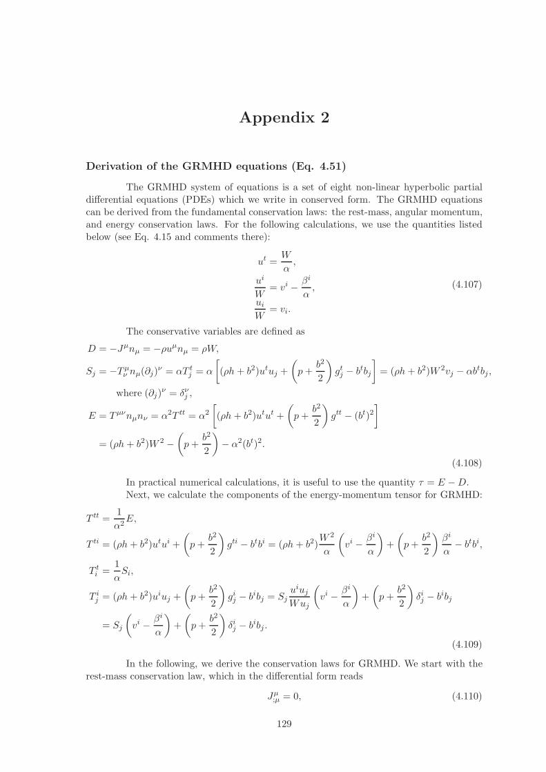
Appendix 2

Derivation of the GRMHD equations (Eq. 4.51)

The GRMHD system of equations is a set of eight non-linear hyperbolic partialdifferential equations (PDEs) which we write in conserved form. The GRMHD equationscan be derived from the fundamental conservation laws: the rest-mass, angular momentum,and energy conservation laws. For the following calculations, we use the quantities listedbelow (see Eq. 4.15 and comments there):

ut =W

α,

ui

W= vi − βi

α,

uiW

= vi.

(4.107)

The conservative variables are defined as

D = −Jµnµ = −ρuµnµ = ρW,

Sj = −T µν nµ(∂j)ν = αT tj = α

[

(ρh+ b2)utuj +

(

p+b2

2

)

gtj − btbj

]

= (ρh+ b2)W 2vj − αbtbj ,

where (∂j)ν = δνj ,

E = T µνnµnν = α2T tt = α2

[

(ρh+ b2)utut +

(

p+b2

2

)

gtt − (bt)2]

= (ρh+ b2)W 2 −(

p+b2

2

)

− α2(bt)2.

(4.108)

In practical numerical calculations, it is useful to use the quantity τ = E −D.Next, we calculate the components of the energy-momentum tensor for GRMHD:

T tt =1

α2E,

T ti = (ρh+ b2)utui +

(

p+b2

2

)

gti − btbi = (ρh+ b2)W 2

α

(

vi − βi

α

)

+

(

p+b2

2

)

βi

α− btbi,

T ti =1

αSi,

T ij = (ρh+ b2)uiuj +

(

p+b2

2

)

gij − bibj = SjuiujWuj

(

vi − βi

α

)

+

(

p+b2

2

)

δij − bibj

= Sj

(

vi − βi

α

)

+

(

p+b2

2

)

δij − bibj .

(4.109)

In the following, we derive the conservation laws for GRMHD. We start with therest-mass conservation law, which in the differential form reads

Jµ;µ = 0, (4.110)

129

130 Appendix 2

where Jµ = ρuµ denotes the rest-mass flux. The above can be evaluated as

Jµ;µ =1√−g

(√−gJµ),µ =

1√−g(√−gρuµ),µ =

=1√−g

(

α√γρ

W

α

)

,t

+1√−g

(√−gρW (vi − βi

α)

)

,i

=

=1√−g

(√γD),t +

1√−gD

(

vi − βi

α

)

,i

= 0

, (4.111)

which represents the first GRMHD equation. Let us obtain the remaining seven. To recap,the Eulerean basis consists of four vectors eµ = n, ∂i. Consider now the expression

(T µν(eγ)ν);µ = T µν;µ(eγ)

ν + T µν(eγ)ν;µ = T µν(

(eγ)ν,µ − Γλνµ(eγ)λ

)

, (4.112)

where T µν;µ = 0 from the conservation law of the energy-momentum tensor.

Next, we obtain the angular-momentum and energy conservation laws by evaluat-ing the above expression. First, we consider the left-hand side of equation( 4.112) for theindex γ = t,

(T µν(et)ν);µ = (T µνnν);µ = (−αT µt);µ = − 1√−g

(√−gαT tt),t + (

√−gαT it),i

= − 1√−g

(√γα2T tt),t +

(√−gα

[

(ρh+ b2)W 2

α

(

vi − βi

α

)

+

(

p+b2

2

)

βi

α2− bibt

])

,i

= − 1√−g

(√γE),t +

(√−g

[(

E +

(

p+b2

2

))(

vi − βi

α

)

+

(

p+b2

2

)

βi

α− αbibt

])

,i

= − 1√−g

(√γE),t +

(√−g

[

E

(

vi − βi

α

)

+

(

p+b2

2

)

vi − αbibt])

,i

,

(4.113)

where we used the fact that (ρh+ b2)W 2 = E +(

p+ b2

2

)

.

The right-hand side of equation (4.112) reads

T µν(

(et)ν,µ − Γλνµ(et)λ

)

= −T µtα,µ + αΓtνµTµν = α

(

−T µt(lnα),µ + ΓtνµTµν)

. (4.114)

Substituting equations (4.113) and (4.114) for equation (4.112), we obtain the secondGRMHD equation (energy conservation law)

1√−g

(√γE),t +

(√−g

[

E

(

vi − βi

α

)

+

(

p+b2

2

)

vi − αbibt])

,i

= α(

−T µt(lnα),µ + ΓtνµTµν)

. (4.115)

Appendix 2 131

Next, we consider the left-hand side of Eq. (4.112) for the index γ = j,

(T µν(ej)ν);µ = (T µj);µ =

1√−g

(√−gT µj)

,µ

=1√−g

(√−gT tj),t + (

√−gT ij),i

=1√−g

(√−γSj),t +

(√−g

[

Sj

(

vi − βi

α

)

+

(

p+b2

2

)

δij − bibj

])

,i

.

(4.116)

The right-hand side of equation reads

T µν(

(ej)ν,µ − Γλνµ(ej)λ

)

= T µν(

[

gνλ(ej)λ]

,µ− Γλνµgλσ(ej)

σ

)

= T µν(

gνj,µ − Γλνµgλj

)

.

(4.117)Substituting equations (4.116) and (4.117) for equation (4.112), we obtain the

other three GRMHD equations (angular-momentum conservation law),

1√−g

(√−γSj),t +

(√−g

[

Sj

(

vi − βi

α

)

+

(

p+b2

2

)

δij − bibj

])

,i

= T µν(

gνj,µ − Γλνµgλj

)

. (4.118)

The remaining three GRMHD equations are the three components of the inductionequation, which was derived in Section 4.35. The GRMHD equations can be written in acompact form

1√

|g|∂(√γU)

∂t+

1√

|g|∂(√

|g|F)∂xi

= S , (4.119)

where the quantities U (conserved variables), F (fluxes), and S (source terms) are

U =

DSjτBi

, (4.120)

F =

Dvi

Sj vi +(

p+ b2

2

)

δij − bibj

τ vi +(

p+ b2

2

)

vi − α2(bt)2 +Dvi

viBj − vjBi

, (4.121)

S =

0

T µν(

∂gνj∂xµ − Γσνµgσj

)

α(

T µt ∂ lnα∂xµ − T µνΓtνµ)

0i

, (4.122)

where vi =(

vi − βi

α

)

and 0i ≡ (0, 0, 0)T.

132 Appendix 2

.

List of Publications

1. Ultra-High-Energy Cosmic Ray Contribution from the Spin-Down Power of Black

Holes, Dutan, I., 2010, to be submitted to MNRAS

2. Magnetic Connection Model for Launching Relativistic Jets from a Kerr Black Hole,Dutan, I., 2010, submitted to MNRAS (astro-ph/1001.5434)

3. Relativistic Jets in Active Galactic Nuclei: Importance of Magnetic Fields, Dutan,I. and Biermann, P. L., 2008, in Proceedings of the Relativistic Astrophysics andCosmology - Einstein’s Legacy, held in Munich, Germany, 07-11 November 2005.ESO Astrophysics Symposia, p. 431-432

4. High Energy Phenomena in Active Galactic Nuclei: Relativistic Jets, Dutan, I. andBiermann, P. L., 2005, in Proceedings of the Astrophysical Sources of High EnergyParticles and Radiation, held in Torun, Poland, 20-24 June 2005. Eds. T. Bulik, B.Rudak, and G. Madejski. AIP Conference Proceedings, vol. 801, p. 212-213

5. Jets Driven by Accretion onto Rotating Black Holes, Dutan, I. and Biermann, P.L.,2005, in Proceedings of the 40th Rencontres de Moriond: Very High Energy Phenom-ena in the Universe, held in La Thuile, Italy, 12-19 March 2005 (also astro-ph/0505403)

6. The Efficiency of Using Accretion Power of Kerr Black Holes, Dutan, I. and Bier-mann, P.L., 2005, in Proceedings of the 14th Course of the International School ofCosmic Rays Astrophysics, a NATO Advanced Study Institute, held in Erice, Italy,2-13 July 2004. Eds. M. M. Shapiro, T. Stanev, and J. P. Wefel. NATO science seriesII: Mathematics, physics and chemistry, vol. 209, p. 175-181 (also astro-ph/0410194)

133