Bancheri

LINKERS

JGrass-NewAge: WaterBudget componentMarialaura Bancheri

Correspondence:

marialaura.bancheri@unitn.it

Dipartimento di Ingegneria Civile

Ambientale e Meccanica, Trento,

Mesiano di Povo, Trento, IT

Full list of author information is

available at the end of the article

Abstract

These pages teach how to run the WaterBudget component inside the OMS 3console. Some preliminary knowledge and installation of OMS is mandatory (see @Alsouseful). This component deals with the water budget solution, for a defined layer. Giventhe time series of the rainfall and of the potential evapotranspiration, the componentsis able to estimate the water storage, to simulate the runoff and the actualevapotranpiration for the considered layer, at different time-step. It also simulate thepossible drainage toward deeper layer. The package is perfectly integrated in theJGrass-NewAge, and can be fed by other components, like the one providing thepotential evapotranspiration and connected to calibration algorithms. Once parametersare assigned according to the selected model, it can be used for the forecasting waterstorage in a selected point.

@Version:0.1

@License:GPL v. 3

@Inputs:• Rainfall (mm);• Potential evapotranspiration (mm);• Discharge (if required) (m3/s);• Solver model (String);• Q model (String);• AET model (String);• Area of the basin (A) (km2);• Non-linear reservoir parameter (a) (-);• Non-linear reservoir exponent (b) (-);• Maximum storage (mm);• Pore volume in the root zone (nZ) (mm);• Recharge rate (Re) (mm);

@Outputs:• Water storage [mm];• Total discharge [m3/m2];• Actual evapotranspiration [mm];• Quick runoff [m3/m2];• Drainage from the layer [m3/m2].

@Doc Author: Marialaura Bancheri

@References:• See References section below

Keywords: OMS; JGrass-NewAGE Component Description; Water budget

Bancheri Page 2 of 11

Code Information

Executables

This link points to the jar file that, once downloaded can be used in the OMS console:

https://github.com/GEOframeOMSProjects/OMS_Project_WB/tree/master/lib

Developer Info

This link points to useful information for the developers, i.e. information about the code

internals, algorithms and the source code

https://github.com/geoframecomponents

Also useful

To run JGrass-NewAGE it is necessary to know how to use the OMS console. Information

at: ”How to install and run the OMS console”,

https://alm.engr.colostate.edu/cb/project/oms).

JGrasstools are required for preparing some input data (information at:

http://abouthydrology.blogspot.it/2012/11/udig-jgrasstools-resources-in-italian.

html

To visualize results you need a GIS. Use your preferred GIS, following its installation

instructions. To make statistics on the results, you can probably get benefits from R:

http://www.r-project.org/ and follow its installation instruction.

To whom address questions

marialaura.bancheri@unitn.it

Authors of documentation

Marialaura Bancheri (marialaura.bancheri@unitn.it)

This documentation is released under Creative Commons 4.0 Attribution International

Bancheri Page 3 of 11

Component DescriptionThis component solves the water budget, simulates the discharge and the actual evapo-

transpiration, according to the model chosen. The equation solved is:

dS(t)

dt= J(t) −Q(t) −AET (t) (1)

where S [mm] is the water storage, J [mm] is the precipitation, Q the discharge [m3/m2]

and AET [mm] is the actual evapotranspiration. Both the discharge and the actual evepo-

transpiration can be given values or estimated from the S, according to different models,

i.e.:

Q(t) = aS(t)b (2)

AET =S(t)

SmaxET (t) (3)

where ET is the potential evapotranspiration. Also the soil moisture can be modeled,

considering the porosity (n) and the depth of the root zone (Z). In this case, the equation

solved is:

nZds(t)

dt= J(t) −Q(t) −AET (t) (4)

The component, given the maximum recharge rate of the lower layer (Re), is also able

to estimate the drainage toward the deeper layers, eq. 5 and the direct runoff from the

considered layer, eq. 6

R(t) = min(Q(t), Re) (5)

Qquick(t) = Q(t) −R(t) (6)

Detailed Inputs description

The input file is a .csv file containing a header and one or more time series of input data,

depending on the number of stations involved. Each column of the file is associated to a

different station.

The file must have the following header:

• The first 3 rows with general information such as the date of the creation of the file

and the author;

• the fourth and fifth rows contain the IDs of the stations (e.g. station number 8:

value 8, ID, ,8);

• the sixth row contains the information about the type of the input data (in this

case, one column with the date and one column with double values);

• the seventh row specifies the date format (YYYY-MM-dd HH:mm).

All the previous information shown in the figure 1.

Bancheri Page 4 of 11

Figure 1 Heading of the .csv input file

Rainfall

The rainfall is given in time series of (mm) for the investigated station .

Evapotranpiration

The evapotranpiration is given in time series of (mm) for the investigated station.

Discharge

The discharge is given in time series for the investigated station in (m3/s). The discharge

values are directly converted in to (mm), given the value of the area of the basin. This

values are needed in the case the user wants to solve the water balance only using external

values, otherwise the component simulates the discharge, using the previous models, eq.

2.

Solver model

The Solver model field is a string in which the user specifies the integrator to use of the

solution of the ODE 1. There are two options :”dp853” which is the Dormand-Prince

8(5,3) integrator and ”Eulero”, which is the Euler integrator.

Q model

The Q model field is a string in which the user specifies the model for the discharge:

”NonLinearResevoir” or ”ExternalValues”.

AET model

The AET model field is a string in which the user specifies the model for the evapotran-

spiration: ”AET” or ”ExternalValues”.

Area of the basin

A is the area of the basin expressed in (km2).

Non-linear reservoir parameter (a)

Non-linear reservoir parameter is the a parameter in eq. 2

Non-linear reservoir exponent (b)

Non-linear reservoir exponent is the b exponent in eq. 2

Maximum storage

Maximum storage is the variable Smax in eq. 3. It is expressed in (mm)

Bancheri Page 5 of 11

Pore volume in the root zone

The pore volume in the root zone is the variable nZ in eq. 4 and it is the product of the

soil porosity n and the depth of the root zone Z.

Recharge rate(mm)

The Recharge rate is the variable Re in eq. 5 and it is the maximum recharge rate towards

the lower layer.

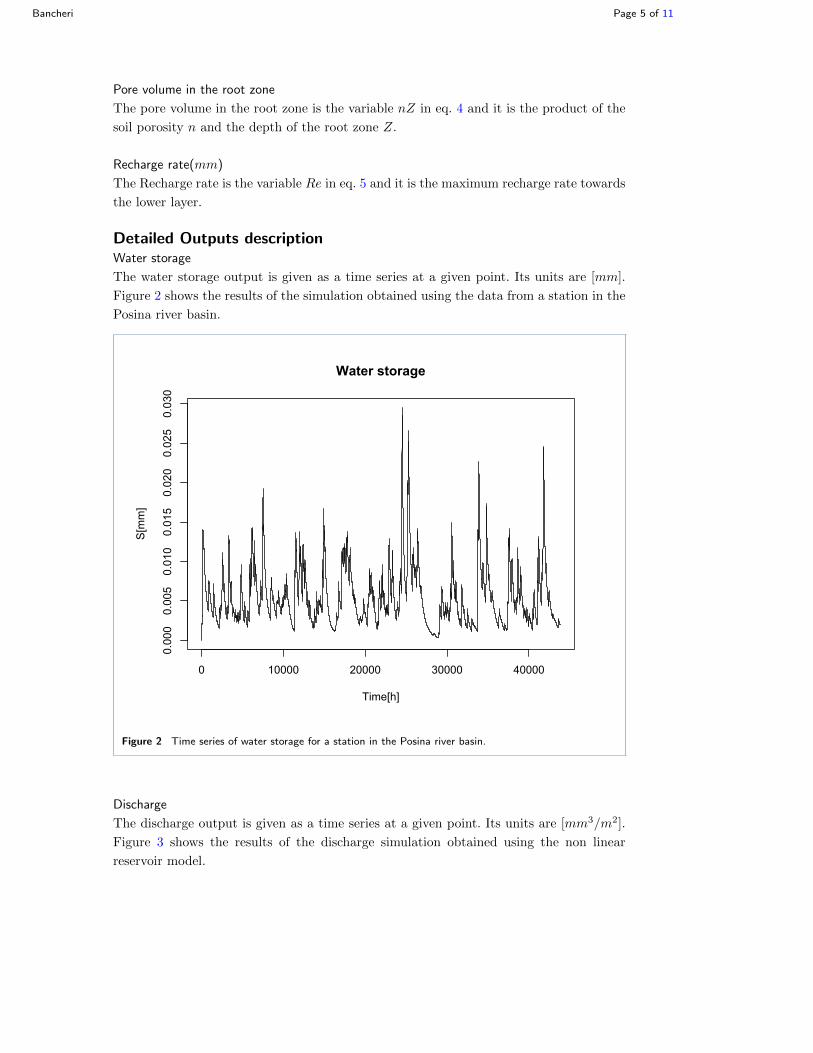
Detailed Outputs descriptionWater storage

The water storage output is given as a time series at a given point. Its units are [mm].

Figure 2 shows the results of the simulation obtained using the data from a station in the

Posina river basin.

0 10000 20000 30000 40000

0.000

0.005

0.010

0.015

0.020

0.025

0.030

Water storage

Time[h]

S[mm]

Figure 2 Time series of water storage for a station in the Posina river basin.

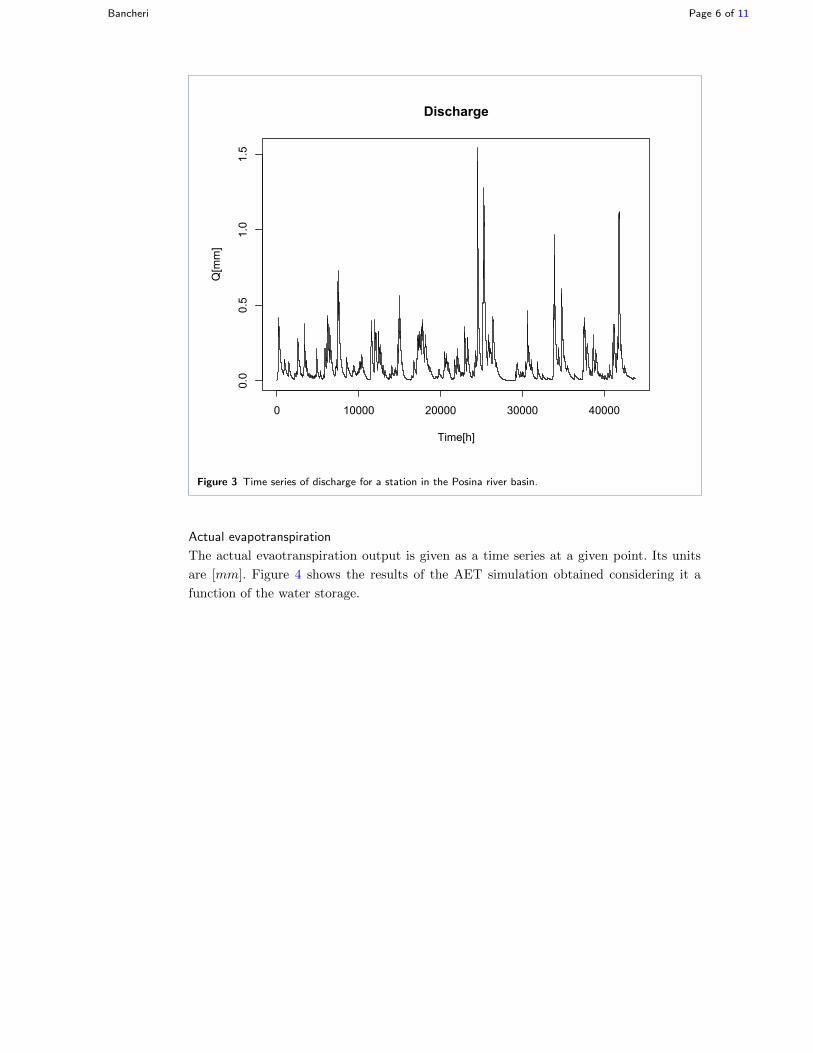
Discharge

The discharge output is given as a time series at a given point. Its units are [mm3/m2].

Figure 3 shows the results of the discharge simulation obtained using the non linear

reservoir model.

Bancheri Page 6 of 11

0 10000 20000 30000 40000

0.0

0.5

1.0

1.5

Discharge

Time[h]

Q[mm]

Figure 3 Time series of discharge for a station in the Posina river basin.

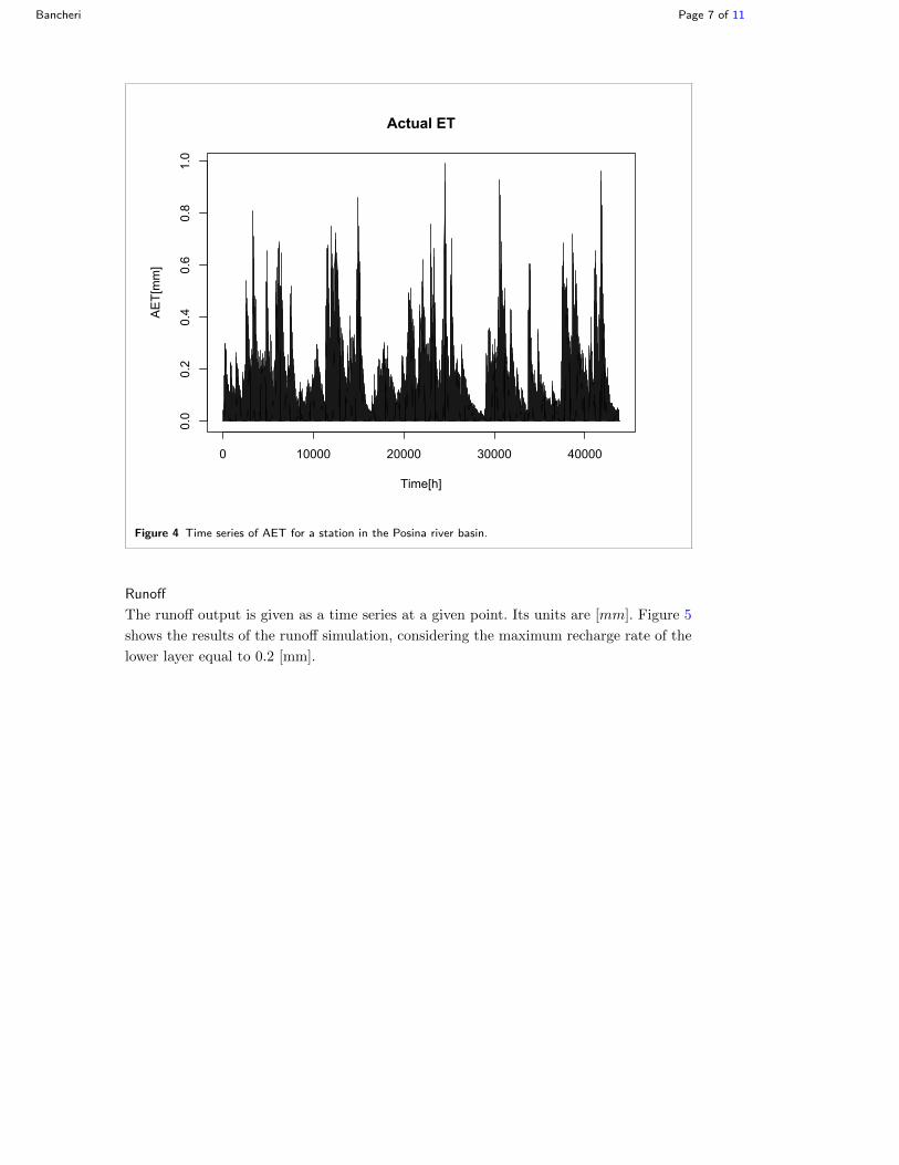
Actual evapotranspiration

The actual evaotranspiration output is given as a time series at a given point. Its units

are [mm]. Figure 4 shows the results of the AET simulation obtained considering it a

function of the water storage.

Bancheri Page 7 of 11

0 10000 20000 30000 40000

0.0

0.2

0.4

0.6

0.8

1.0

Actual ET

Time[h]

AET[mm]

Figure 4 Time series of AET for a station in the Posina river basin.

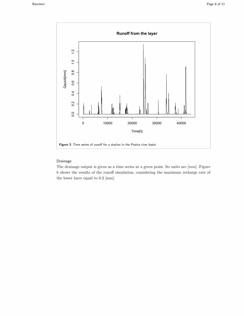
Runoff

The runoff output is given as a time series at a given point. Its units are [mm]. Figure 5

shows the results of the runoff simulation, considering the maximum recharge rate of the

lower layer equal to 0.2 [mm].

Bancheri Page 8 of 11

0 10000 20000 30000 40000

0.0

0.2

0.4

0.6

0.8

1.0

1.2

Runoff from the layer

Time[h]

Qquick[mm]

Figure 5 Time series of runoff for a station in the Posina river basin.

Drainage

The drainage output is given as a time series at a given point. Its units are [mm]. Figure

6 shows the results of the runoff simulation, considering the maximum recharge rate of

the lower layer equal to 0.2 [mm].

Bancheri Page 9 of 11

0 10000 20000 30000 40000

0.00

0.05

0.10

0.15

0.20

Drainage toward the lower layers

Time[h]

R[mm]

Figure 6 Time series of drainage toward a deeper layer for a station in the Posina river basin.

ExamplesThe following .sim file is customized for the use of the WaterBudget component. The .sim

file can be downloaded from here:

https://github.com/GEOframeOMSProjects/OMS_Project_WB/tree/master/simulation

import static oms3.SimBuilder.instance as OMS3def home = oms_prjdef startDate= "1994 -01 -01 00:00"def endDate= "1998 -12 -31 00:00"OMS3.sim {

resource "$oms_prj/lib/waterbudget -0.0.1 - SNAPSHOT -jar -with -dependencies.jar"

model(while:"reader_data_J.doProcess") {components {

"reader_data_J" "org.jgrasstools.gears.io.timedependent.OmsTimeSeriesIteratorReader"

"reader_data_ET" "org.jgrasstools.gears.io.timedependent.OmsTimeSeriesIteratorReader"

"ws" "waterBudget.WaterBudget""writer_S" "org.jgrasstools.gears.io.timedependent.

OmsTimeSeriesIteratorWriter""writer_Q" "org.jgrasstools.gears.io.timedependent.

OmsTimeSeriesIteratorWriter""writer_ET" "org.jgrasstools.gears.io.timedependent.

OmsTimeSeriesIteratorWriter""writer_Quick" "org.jgrasstools.gears.io.timedependent.

OmsTimeSeriesIteratorWriter""writer_R" "org.jgrasstools.gears.io.timedependent.

OmsTimeSeriesIteratorWriter"}

Bancheri Page 10 of 11

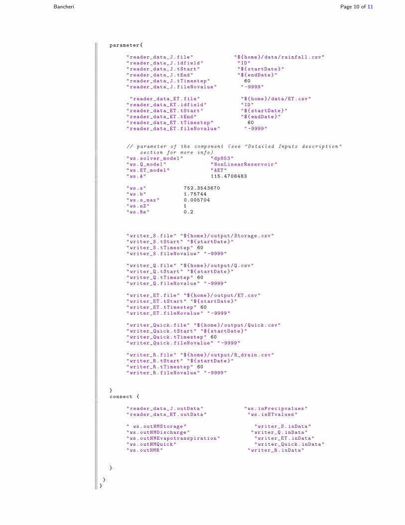
parameter{

"reader_data_J.file" "${home}/data/rainfall.csv""reader_data_J.idfield" "ID""reader_data_J.tStart" "${startDate}""reader_data_J.tEnd" "${endDate}""reader_data_J.tTimestep" 60"reader_data_J.fileNovalue" " -9999"

"reader_data_ET.file" "${home}/data/ET.csv""reader_data_ET.idfield" "ID""reader_data_ET.tStart" "${startDate}""reader_data_ET.tEnd" "${endDate}""reader_data_ET.tTimestep" 60"reader_data_ET.fileNovalue" " -9999"

// parameter of the component (see "Detailed Inputs description "section for more info)

"ws.solver_model" "dp853""ws.Q_model" "NonLinearReservoir""ws.ET_model" "AET""ws.A" 115.4708483

"ws.a" 752.3543670"ws.b" 1.75744"ws.s_max" 0.005704"ws.nZ" 1"ws.Re" 0.2

"writer_S.file" "${home}/ output/Storage.csv""writer_S.tStart" "${startDate}""writer_S.tTimestep" 60"writer_S.fileNovalue" " -9999"

"writer_Q.file" "${home}/ output/Q.csv""writer_Q.tStart" "${startDate}""writer_Q.tTimestep" 60"writer_Q.fileNovalue" " -9999"

"writer_ET.file" "${home}/ output/ET.csv""writer_ET.tStart" "${startDate}""writer_ET.tTimestep" 60"writer_ET.fileNovalue" " -9999"

"writer_Quick.file" "${home}/ output/Quick.csv""writer_Quick.tStart" "${startDate}""writer_Quick.tTimestep" 60"writer_Quick.fileNovalue" " -9999"

"writer_R.file" "${home}/ output/R_drain.csv""writer_R.tStart" "${startDate}""writer_R.tTimestep" 60"writer_R.fileNovalue" " -9999"

}connect {

"reader_data_J.outData" "ws.inPrecipvalues""reader_data_ET.outData" "ws.inETvalues"

" ws.outHMStorage" "writer_S.inData""ws.outHMDischarge" "writer_Q.inData""ws.outHMEvapotranspiration" "writer_ET.inData""ws.outHMQuick" "writer_Quick.inData""ws.outHMR" "writer_R.inData"

}

}}

Bancheri Page 11 of 11

Data and ProjectThe following link is for the download of the input data necessaries to execute the WB

component (as shown in the .sim file in the previous section ) :

https://github.com/GEOframeOMSProjects/OMS_Project_WB/tree/master/data

The following link is for the download of the OMS project for WB component:

https://github.com/GEOframeOMSProjects/OMS_Project_WB

%

References