JHEP05(2014)057

Published for SISSA by Springer

Received: March 17, 2014

Accepted: April 5, 2014

Published: May 13, 2014

Is it possible to embed a 4D, N = 4 supersymmetric

vector multiplet within a completely off-shell adinkra

hologram?

Mathew Calkins, D.E.A. Gates, S. James Gates Jr. and Brian McPeak

Center for String and Particle Theory, Department of Physics, University of Maryland,

College Park, MD 20742-4111, U.S.A.

E-mail: mathewpcalkins@gmail.com, deagates@terpmail.umd.edu,

gatess@wam.umd.edu, bmcpeak@terpmail.umd.edu

Abstract: We present evidence of the existence of a 1D, N = 16 SUSY hologram that

can be used to understand representation theory aspects of a 4D, N = 4 supersymmetrical

vector multiplet. In this context, the long-standing “off-shell SUSY” problem for the 4D,

N = 4 Maxwell supermultiplet is precisely formulated as a problem in linear algebra.

Keywords: Supersymmetric gauge theory, Extended Supersymmetry, Gauge Symmetry

ArXiv ePrint: 1402.5765

Open Access, c© The Authors.

Article funded by SCOAP3.doi:10.1007/JHEP05(2014)057

JHEP05(2014)057

Contents

1 Introduction 1

2 The SUSY holography conjecture 2

3 Adinkra matrices and information conservation 5

4 Valise 1D, N = 16 supermultiplet formulation 6

5 Extracting 1D, N = 16 valise adinkra matrices 7

6 Previous results about off-shell vs. on-shell 9

6.1 On-shell chiral supermultiplet 10

6.2 On-shell vector supermultiplet 11

6.3 The 0-brane reduced algebra 13

7 Conclusion, summary & prospectus 14

A 4D supersymmetry results 16

B 4D, N = 1 L-matrices & R-matrices 18

C 4D, N = 4 L-matrices & R-matrices 19

1 Introduction

The utility of the extra dimension concept underwent a reassessment due to the construc-

tion of 11D supergravity [1, 2]. Since then, the concept has received much attention even

to the point of producing a broadly studied approach [3–5] (e. g. ‘brane-world scenarios’)

that dominated phenomenological discussion for a decade. The 11D approach was the

solution to a difficult problem as Cremmer and Julia used it to present the first complete

description of 4D, N = 8 supergravity [6].

Thus, for perhaps the first time in the literature associated with supergravity, it was

shown that a higher dimensional approach contained information about a lower dimensional

theory that could be more easily accessed from the higher dimensional starting point. This

same idea can be seen in the relation of 10D, N = 1 SUSY YM theories to 4D, N = 4 SUSY

YM theories. The key point to note is that the information necessary for the construction

of both the higher dimensional and lower dimensional theories is conserved by either the

dimensional reduction or dimensional extension processes. The lower dimensional theory

acts as a hologram for the higher dimensional one. These facts are well known.

– 1 –

JHEP05(2014)057

Starting in 1994 [7], we began to find evidence [8–11] that this well known result ex-

tends all the way from supersymmetric quantum field theories to supersymmetric quantum

mechanical models and more unexpectedly the conservation of the information may be so

robust that it might allow the former to be re-constructed from the latter in some limits.

Eventually we gave this idea a name “SUSY holography” [12, 13].

The topic of the 4D, N = 4 Yang-Mills supermultiplet [14–16] has been a fruitful one

for many years. Almost from the instant of its first presentation, the unusual properties of

this model have generated a steady stream of inspirations concluding most recently with

the introduction of the “amplituhedron” [17, 18]. Thus, this theory has long been one of

our objectives to study via the tools that have been developed for SUSY holography.

Stated another way, it is our goal to follow a path similar to that of Cremmer and Julia,

but to use the idea of “SUSY holography” in the reverse route of using a lower dimensional

construct, at least at the level of representation theory, to gain greater understanding of a

higher dimensional construct. One of our previous works [19], presented (what may be the

most) detailed results on the nature of the non-closure of the SUSY algebra for the 4D, N= 4 supermultiplet in the context of an equivalent N = 1 superfield formulation solely in

four dimensions. In this current work, we will begin the process of studying its projection

(or shadow) into the sea of one dimensional N = 16 adinkra networks known to exist.

2 The SUSY holography conjecture

On first reflection, the proposal of “SUSY holography” would seem untenable. There is an

easy example to show why this conclusion might be reached. For a four dimensional field

theory (supersymmetrical or not), the starting point for a reduction to one dimension can

be implemented by making the replacement

∂µ = Tµ∂

∂τ, Tµ ≡ (1, 0, 0, 0) , (2.1)

in actions. As well, all field variables are assumed to depend only on the real parameter

τ and all gauge fields are restricted to the Coulomb gauge. In the context of a non-

supersymmetrical theory, such a reduction can lead to an ambiguity involving a loss of

spin-bundle information. Let us consider two distinct four dimensional theories:

(a.) an action involving three parity-even massless spin-0 fields φI , (where I= 1, 2, and 3)

LSpin−0 = −1

2

(∂µφ

I) (∂µφI) , (2.2)

so that under the prescription of (2.1) leads to

LSpin−0 =1

2

(∂τφ

1) (∂τφ

1)

+1

2

(∂τφ

2) (∂τφ

2)

+1

2

(∂τφ

3) (∂τφ

3), and (2.3)

(b.) an action for a spin-1 gauge field given by

LSpin−1 = −1

4FµνF

µν = −1

2F0 iF

0 i , (2.4)

– 2 –

JHEP05(2014)057

(since all spatial derivatives vanish in our reduction scheme) and following the pre-

scription above this becomes,

LSpin−1 =1

2

[(∂τ A1)

2 + (∂τ A2)2 + (∂τ A3)

2]. (2.5)

As is seen above, the forms of (2.3) and (2.5) are exactly the same. Thus, starting from

a non-supersymmetrical one dimensional theory involving three bosonic fields there is no

way to distinguish which of the four dimensional actions were its origin. Specifically, the

information on the 4D spin-bundle of the fields was lost. This is an example of what we refer

to as loss of information under non-supersymmetric 0-brane reduction described by (2.1).

Remarkably, within the context of supersymmetrical theories, this information can be

conserved. . . if one looks into the “correct” structure.

While it is true that the information about the 4D origins of the actions does not

appear in either 1D action, if these non-supersymmetrical theories are embedded within

1D, N = 4 theories at one extreme and 4D, N = 1 theories on the other, the information

can be subtly encoded in the SUSY variations!

We begin with the spin-0 field and for the sake of simplicity, we only need to consider a

single such field. Since it has parity-even, it becomes the A-field in a chiral supermultiplet

as part of the collection of fields (A, B, ψa, F, G). In a similar manner, the spatial vector~A can be combined with its temporal component A0 to form a 4-vector Aµ and becomes

the gauge field in a vector supermultiplet among the collection of fields (Aµ, λa, d). So

these are the relevant 4D supermultiplets.

In 1D, a valise formulation that is off-shell is one where a set of bosonic variables Φi(τ)

and fermionic variables Ψk(τ) locally satisfy the following realization under the action of a

set of supercovariant derivatives DI

DIΦi = i (LI)ikΨk and DIΨk = (RI)ki (∂τΦi) , (2.6)

with L-matrices and R-matrices satisfying

(LI)i (RJ)

k + (LJ)i (RI)

k = 2 δIJ δik ,

(RJ)ıj (LI)j

k + (RI)ıj (LJ)j

k = 2 δIJ δık .

(2.7)

(RI)k δik = (LI)i

k δk , (2.8)

and where the indices range as I, J, etc. = 1, . . . , N ; i, j, etc. = 1, . . . , d; and ı, , etc. =

1, . . . , d for integers d, and N .

Implementation of the reduction process described at the beginning of this section is

not sufficient to arrive at a valise formulation of these 4D, N = 1 supermultiplets. In order

to obtain a valise will also require that we make the ‘field redefinitions’

F I → ∂τFI , GI → ∂τG

I , d→ ∂τd , (2.9)

after the reduction. In a subsequent section, we will obtain the valise formulation of the

4D, N = 4 theory as the main new result of this work.

– 3 –

JHEP05(2014)057

Applying all of this machinery to the components of a chiral supermultiplet we find

DaA = ψa , DaB = i(γ5)abψb ,

DaF = (γ · T )ab ψb , DaG = i

(γ5γ · T

)ab ψb ,

Daψb = i (γ · T )ab (∂τA)−(γ5γ · T

)ab

(∂τB)− iCab (∂τF ) +(γ5)ab

(∂τG) , (2.10)

and in a similar manner for the components of the vector supermultiplet, one is led to

DaAi = (γi)abλb , Dad = i

(γ5γ · T

)ab λb ,

Daλb = − i2

([γ · T , γi

])ab

(∂τAi) +(γ5)ab

(∂τd) . (2.11)

All the equations in (2.10) and (2.11) have exactly the form of (2.6).

Under the reduction described above, there is a way to begin solely with a one di-

mensional supersymmetrical theory as shown in (2.3) or (2.5) and determine which of the

two four-dimensional theories could provide the starting point. The way this is done is

to note that for a one dimensional supersymmetrical theory, with at least four worldline

SUSY charges, any action is also accompanied by an associated set of 4×4 ‘L-matrices’ and

‘R-matrices’ [20] as defined by the equations in (2.6)

All three chiral supermultiplets will have the same set of L-matrices and R-matrices

as first derived before in the work of [20]. This same work derived the L-matrices and

R-matrices for the vector supermultiplet also. The work of [21] noted each L-matrix and R-

matrix can be expressed in terms of a ‘Boolean factor’ denoted by(S(I)

)i

ˆwhich appears via

(LI)ik =

(S(I)

)i

ˆ(P(I))ˆ k, for each fixed I = 1, 2, . . . , N. (2.12)

(S(I)

)i

ˆ=

(−1)b1 0 0 · · ·

0 (−1)b2 0 · · ·0 0 (−1)b3 · · ·...

......

. . .

↔

(RI =

d∑i=1

bi 2i−1

)b

(2.13)

(a diagonal matrix with real entries that squares to the identity) times an element of

the permutation group(P(I))ˆk. The matrices above can be associated with a class of

topological objects given the name of “adinkras” [22] which are graphs that capture (with

complete fidelity) the information in the matrices and nodal heights. In fact, if the adinkras

are regarded as graphs or networks, the permutation factor within the L-matrices and

R-matrices are the ‘adjacency matrices’ from graph theory.

The adinkras associated with the chiral and the vector supermultiplets, respectively,

are shown in figure 1. These are the graphs associated solely with the equations that appear

in (A.1) and (A.4).

On the other hand, the adinkra graphs associated with the valise equations of (2.10)

and (2.11) are different and given in figure 2.

Written solely in the form of valise adinkras or their associated matrices in appendix B,

it is not at all clear how the spin-bundle information to distinguish the chiral supermultiplet

from the vector supermultiplet has been retained. The question becomes, “What structure

in the graphs or their associated matrices holographically stores the information about the

distinction?”

– 4 –

JHEP05(2014)057

(a.) (b.)

Figure 1. Adinkra graphs for the chiral (a.) and vector (b.) supermultiplets.

3 Adinkra matrices and information conservation

The work of [21] has offered a proposal for identifying such a mechanism: the information

may be accessed via the elements of the permutation group. To see most transparently

how the permutation group elements contain the information we are seeking, it is useful to

describe these elements in terms of cycles.1

To show this approach clearly, we will give an explicit demonstration using the L1

matrix of the chiral multiplet.

(L1) i k =

1 0 0 0

0 0 0 −1

0 1 0 0

0 0 −1 0

=

1 0 0 0

0 −1 0 0

0 0 1 0

0 0 0 −1

1 0 0 0

0 0 0 1

0 1 0 0

0 0 1 0

(L1) i k = (10)b

1 0 0 0

0 0 0 1

0 1 0 0

0 0 1 0

, (3.1)

where the Boolean factor (10)b is defined according to the conventions of [21]. We next

note that the element of the permutation group above obviously satisfies1 0 0 0

0 0 0 1

0 1 0 0

0 0 1 0

1

2

3

4

=

1

4

2

3

(3.2)

which implies

1→ 1 , 2→ 4 , 3→ 2 , 4→ 3 , (3.3)

and this reveals the cycle (2 4 3). We then can write L1 = (10)b (2 4 3).

Upon applying such considerations to all the L-matrices and the R-matrices, we find

L1 = (10)b (2 4 3) , L2 = (12)b (1 2 3) , L3 = (6)b (1 3 4) , L4 = (0)b (1 4 2) ,

R1 = (12)b(2 3 4) , R2 = (9)b (1 3 2) , R3 = (10)b(1 4 3) , R4 = (0)b (1 2 4) , (3.4)

1We acknowledge conversations with Kevin Iga who emphasized this point.

– 5 –

JHEP05(2014)057

(a.) (b.)

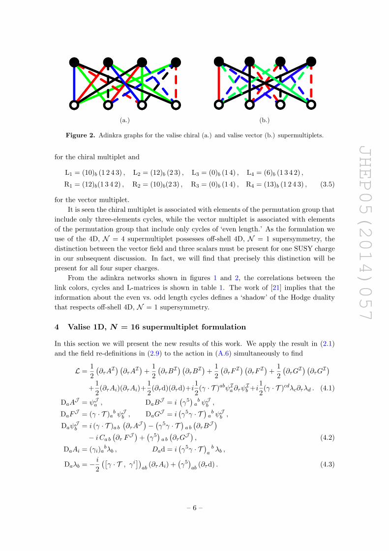
Figure 2. Adinkra graphs for the valise chiral (a.) and valise vector (b.) supermultiplets.

for the chiral multiplet and

L1 = (10)b (1 2 4 3) , L2 = (12)b (2 3) , L3 = (0)b (1 4) , L4 = (6)b (1 3 4 2) ,

R1 = (12)b(1 3 4 2) , R2 = (10)b(2 3) , R3 = (0)b (1 4) , R4 = (13)b (1 2 4 3) , (3.5)

for the vector multiplet.

It is seen the chiral multiplet is associated with elements of the permutation group that

include only three-elements cycles, while the vector multiplet is associated with elements

of the permutation group that include only cycles of ‘even length.’ As the formulation we

use of the 4D, N = 4 supermultiplet possesses off-shell 4D, N = 1 supersymmetry, the

distinction between the vector field and three scalars must be present for one SUSY charge

in our subsequent discussion. In fact, we will find that precisely this distinction will be

present for all four super charges.

From the adinkra networks shown in figures 1 and 2, the correlations between the

link colors, cycles and L-matrices is shown in table 1. The work of [21] implies that the

information about the even vs. odd length cycles defines a ‘shadow’ of the Hodge duality

that respects off-shell 4D, N = 1 supersymmetry.

4 Valise 1D, N = 16 supermultiplet formulation

In this section we will present the new results of this work. We apply the result in (2.1)

and the field re-definitions in (2.9) to the action in (A.6) simultaneously to find

L =1

2

(∂τA

I) (∂τAI)+1

2

(∂τB

I) (∂τBI)+1

2

(∂τF

I) (∂τF I)+1

2

(∂τG

I) (∂τGI)+

1

2(∂τAi)(∂τAi)+

1

2(∂τd)(∂τd)+i

1

2(γ · T )abψIa∂τψ

Ib +i

1

2(γ · T )cdλc∂τλd . (4.1)

DaAJ = ψJa , DaB

J = i(γ5)ab ψJb ,

DaFJ = (γ · T )a

b ψJb , DaGJ = i

(γ5γ · T

)ab ψJb ,

DaψJb = i (γ · T )a b

(∂τA

J )− (γ5γ · T ) a b (∂τBJ )− i Ca b

(∂τ F

J )+(γ5)a b

(∂τG

J ) , (4.2)

DaAi = (γi)abλb , Dad = i

(γ5γ · T

)ab λb ,

Daλb = − i2

([γ · T , γi

])ab

(∂τAi) +(γ5)ab

(∂τd) . (4.3)

– 6 –

JHEP05(2014)057

CM VM

BLUE (243) (1243)

RED (123) (23)

BLACK (134) (14)

GREEN (142) (1342)

Table 1. Adinkra link color & cycles in L-matrices.

However, for the SU(2) triplet supercovariant derivatives the realization takes the forms

DIaAJ = δI J λa − εI JK ψ

Ka , DIaB

J = i(γ5)ab[δIJλb + εI JK ψ

Kb

],

DIaFJ = (γ · T )a

b[δI J λb − εI JK ψ

Kb

],

DIaGJ = i

(γ5γ · T

)ab[−δIJ λb + εI JK ψ

Kb

],

DIaψJb = δI J

[i

1

2

([γ · T , γi

])ab (∂τ Ai) +

(γ5)a b (∂τd)

]+ εI JK

[i (γ · T )a b

(∂τA

K)+(γ5γ · T

)a b

(∂τB

K)−i Ca b

(∂τF

K)− (γ5) a b (∂τGK)] , (4.4)

for the fields in the valise adinkra formulation of the three chiral supermultiplets and

DIa Ai = −(γi)ab ψIb , DIa d = i (γ5γ · T )a

b ψIb ,

DIaλb = i (γ · T )a b(∂τA

I)− (γ5γ · T ) a b (∂τBI) (4.5)

− i Ca b(∂τF

I)− (γ5) a b (∂τGI) ,for the fields of the valise adinkra formulation of the vector supermultiplet. The equations

in this section that involve the D-operators are clearly of the same form as in (2.6) with

the indices now ranging as I, J, etc. = 1, . . . , 16; i, j, etc. = 1, . . . , 16; and ı, , etc. = 1,

. . . , 16.

5 Extracting 1D, N = 16 valise adinkra matrices

With the results of the previous section in hand, we are now able to extract the L-matrices

and R-matrices of the 1D, N = 16 adinkra matrices associated with the discussion of

the previous section. In order to present our results coherently, we use the following

notation conventions that are the most obvious appropriate generalizations of (2.6). We

now introduce the 1D covariant derivatives D[0]I and D[I]

I to act as the holographic images

of Da and DaI . Their realizations on the valise fields may be expressed in the forms

D[0]IΦi = i

(L[0]I

)ik

Ψk , D[0]IΨk =

(R

[0]I

)ki

(∂τΦi) ,

D[I]IΦi = i

(L[I]I

)ik

Ψk , D[I]IΨk =

(R

[I]I

)ki

(∂τΦi) ,(5.1)

where above the bosonic and fermionic quantities Φi and Ψk respectively take the forms of

two sixteen component quantities

Φi =(A1, B1, F 1, G1, A2, B2, F 2, G2, A3, B3, F 3, G3, ~A, d

), (5.2)

Ψk = −i(ψ1

1, ψ12, ψ

13, ψ

14, ψ

21, ψ

22, ψ

23, ψ

24, ψ

31, ψ

32, ψ

33, ψ

34, λ1, λ2, λ3, λ4

),

– 7 –

JHEP05(2014)057

(where ~A corresponds to the spatial components of the gauge field) as is appropriate in the

context of this section.

Explicitly we find for the(

L[0]I

)ik

matrices

(L[0]1

)ik =

(10)b(243) 0 0 0

0 (10)b(243) 0 0

0 0 (10)b(243) 0

0 0 0 (10)b(1243)

,

(L[0]2

)ik =

(12)b(123) 0 0 0

0 (12)b(123) 0 0

0 0 (12)b(123) 0

0 0 0 (4)b(23)

,

(L[0]3

)ik =

(6)b(134) 0 0 0

0 (6)b(134) 0 0

0 0 (6)b(134) 0

0 0 0 (0)b(14)

,

(L[0]4

)ik =

(0)b(142) 0 0 0

0 (0)b(142) 0 0

0 0 (0)b(142) 0

0 0 0 (6)b(1342)

, (5.3)

and these L-matrices are simply reaffirming relations of colors to eight distinct cycles seen

before in section 3. In a similar manner the(

R[0]I

)k i

matrices take the forms

(R

[0]1

)k i =

(12)b(234) 0 0 0

0 (12)b(234) 0 0

0 0 (12)b(234) 0

0 0 0 (12)b(1342)

(

R[0]2

)k i =

(9)b(132) 0 0 0

0 (9)b(132) 0 0

0 0 (9)b(132) 0

0 0 0 (10)b(23)

(

R[0]3

)k i =

(10)b(143) 0 0 0

0 (10)b(143) 0 0

0 0 (10)b(143) 0

0 0 0 (0)b(14)

(

R[0]4

)k i =

(0)b(124) 0 0 0

0 (0)b(124) 0 0

0 0 (0)b(124) 0

0 0 0 (9)b(1243)

(5.4)

in the basis defined by (5.2).

This brings us to the explicit results for the triplet L-matrices and R-matrices.

– 8 –

JHEP05(2014)057

One of the most obvious features about these is that the holographical mechanism

for conserving the spin-bundle information of the four dimensional related theory is still

present in the 1D, N = 16 valise formulation! The explicit way this occurs is by making

three observations:

(a.) examination of the matrices in (5.3) and (5.4) shows a 3:1 ratio of odd-length

cycles/even-length cycle within each L-matrix and R-matrix,

(b.) examination of the matrices in appendix C continues to show a 3:1 ratio of three

odd-length cycles/even-length cycle within each L-matrix and R-matrix cycle, and

(c.) examination of the matrices in appendix C shows that only the same eight cycles

within the permutation group appear within the triplet L-matrices as do appear in

the singlet L-matrices.

The first of these observations was expected as it follows from the fact that the first

supersymmetry generated by the singlet Da-operator obviously acts on three 1D, N = 4

chiral multiplet adinkras and one 1D, N = 4 vector multiplet adinkra.

The second and third observations, however, are striking evidence that the mechanism

of using the lengths of cycles of the permutation elements embedded with the L-matrices

and R-matrices apparently continues to work as the transformation laws associated with

the hologram of the triplet DIa -operators possesses the same property and there was no

a priori reason to expect this conservation of information among all four supercharges.

Furthermore, it is seen that in all four sets of L-matrices associated with the supercharges,

the same 3:1 ratio of odd-length three-cycles/even cycles is present.

We are thus fortified in our assertion that the 1D, N = 16 SUSY quantum mechanical

model described by the equations in section 5 constitutes a SUSY hologram of the 4D,

N = 4 model described in section 4.

But is it an off-shell valise adinkra hologram?

6 Previous results about off-shell vs. on-shell

In order to answer this question, it is useful to both review some previous work [20] that

can be used as a foundation upon which an expanded discussion can be built. In this

section we use the on-shell versus off-shell valise adinkra formulations of the 4D, N = 1

chiral scalar and the vector supermultiplets as our jumping off points.

From the perspective of valise adinkra formulations, L-matrices and R-matrices con-

tinue to exist for on-shell theories but with the main distinctions:

(a.) the i, j, etc. indices have a range according to 1, . . . , dL, the ı, , etc. indices have a

range according to 1, . . . , dR, where dL may be distinctly different from dR, and

(b.) the algebras for the L-matrices and R-matrices are changed to:

(LI)i (RJ)

k + (LJ)i (RI)

k = 2 δIJ δik +

(∆L

I J

)ik ,

(RJ)ıj (LI)j

k + (RI)ıj (LJ)j

k = 2 δIJ δık +

(∆R

I J

)ık .

(6.1)

The quantities(∆L

I J

)ik and

(∆R

I J

)ık respectively measure the non-closure of the SUSY

algebra on the bosons and fermions of the supermultiplet.

– 9 –

JHEP05(2014)057

Figure 3. Adinkra for on-shell chiral supermultiplet.

6.1 On-shell chiral supermultiplet

The fields (A, B, ψa) of the on-shell valise version of the 4D, N = 1 chiral are shown in

figure 3, which correspond to the D-algebra equations

DaA = ψa , DaB = i(γ5)ab ψb,

Daψb = i (γ · T ) a b ∂τA−(γ5γ · T

)a b ∂τB .

(6.2)

Using (6.2), calculations yield the follow super-commutator algebra

{Da , Db}A = i 2 (γ · T )a b ∂τ A , {Da , Db}B = i 2 (γ · T )a b ∂τ B ,

{Da , Db}ψc = i 2 (γ · T )a b ∂τ ψc − i (γµ)a b (γµγ · T )cd∂τ ψd .

(6.3)

The first two of these equations have the expected form for a supersymmetry algebra, but

the third term immediately above can be re-expressed as

{Da , Db}ψc = i 2 (γ · T )a b ∂τ ψc + i 2 (γµ)a b (γµ)cdKd(ψ) ,

Kc(ψ) = −1

2(γ · T )c

d∂τ ψd ,(6.4)

where Kc measures the ‘non-closure’ of the algebra. From the adinkra in figure 3, we define

the (2 × 1) bosonic “field vector” and (4 × 1) fermionic “field vector”

Φi = (A, B ) , Ψk = −i (ψ1, ψ2, ψ3, ψ4) , (6.5)

as appropriate for such the adinkra shown in 3. This permits us to obtain the following

L-matrices and R-matrices.

(L1) i k =

[1 0 0 0

0 0 0 −1

], (L2) i k =

[0 1 0 0

0 0 1 0

],

(L3) i k =

[0 0 1 0

0 −1 0 0

], (L4) i k =

[0 0 0 1

1 0 0 0

], (6.6)

(R1) i k =

1 0

0 0

0 0

0 −1

, (R2) i k =

0 0

1 0

0 1

0 0

,

(R3) i k =

0 0

0 −1

1 0

0 0

, (R4) i k =

0 1

0 0

0 0

1 0

. (6.7)

– 10 –

JHEP05(2014)057

Figure 4. Adinkra for on-shell chiral supermultiplet.

Given the matrices in (6.6) and (6.7) we find the following relations hold

(LI)i (RJ)

k + (LJ)i (RI)

k = 2 δIJ δik ,

(RJ)ıj (LI)j

k + (RI )ıj (LJ)j

k = δIJ (I)ık +

[~αβ1

]IJ·(~αβ1

)ık .

(6.8)

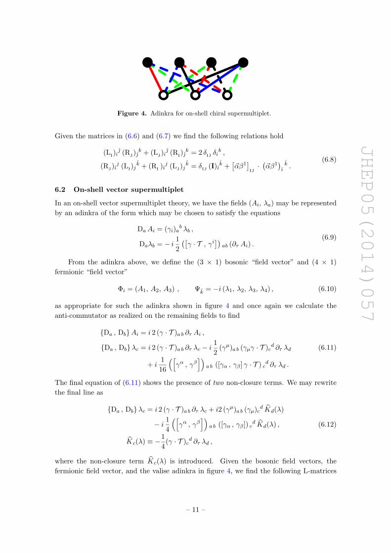
6.2 On-shell vector supermultiplet

In an on-shell vector supermultiplet theory, we have the fields (Ai, λa) may be represented

by an adinkra of the form which may be chosen to satisfy the equations

DaAi = (γi)ab λb ,

Daλb = − i 1

2

([γ · T , γi

])ab (∂τ Ai) .

(6.9)

From the adinkra above, we define the (3 × 1) bosonic “field vector” and (4 × 1)

fermionic “field vector”

Φi = (A1, A2, A3) , Ψk = −i (λ1, λ2, λ3, λ4) , (6.10)

as appropriate for such the adinkra shown in figure 4 and once again we calculate the

anti-commutator as realized on the remaining fields to find

{Da , Db}Ai = i 2 (γ · T )a b ∂τ Ai ,

{Da , Db}λc = i 2 (γ · T )a b ∂τ λc − i1

2(γµ)a b (γµγ · T )c

d ∂τ λd (6.11)

+ i1

16

([γα , γβ

])a b ([γα , γβ] γ · T ) c

d ∂τ λd .

The final equation of (6.11) shows the presence of two non-closure terms. We may rewrite

the final line as

{Da , Db}λc = i 2 (γ · T )a b ∂τ λc + i2 (γµ)a b (γµ)cd Kd(λ)

− i 1

4

([γα , γβ

])a b ([γα , γβ]) c

d Kd(λ) , (6.12)

Kc(λ) ≡ −1

4(γ · T )c

d ∂τ λd ,

where the non-closure term Kc(λ) is introduced. Given the bosonic field vectors, the

fermionic field vector, and the valise adinkra in figure 4, we find the following L-matrices

– 11 –

JHEP05(2014)057

and R-matrices below.

(L1) i k =

0 1 0 0

0 0 0 −1

1 0 0 0

, (L2) i k =

1 0 0 0

0 0 1 0

0 −1 0 0

,(L3) i k =

0 0 0 1

0 1 0 0

0 0 1 0

, (L4) i k =

0 0 1 0

−1 0 0 0

0 0 0 −1

, (6.13)

(R1) k i =

0 0 1

1 0 0

0 0 0

0 −1 0

, (R2) k i =

1 0 0

0 0 −1

0 1 0

0 0 0

,

(R3) k i =

0 0 0

0 1 0

0 0 1

1 0 0

, (R4) k i =

0 −1 1

0 0 0

1 0 0

0 0 −1

. (6.14)

Given the matrices in (6.13) and (6.14) we find the following relations hold

(LI)i (RJ)

k + (LJ)i (RI)

k = 2 δIJ δik ,

(RJ)ıj (LI)j

k + (RI)ıj (LJ)j

k =3

2δIJ (I4)ı

k − 1

2

[~α β2

]IJ·(~α β2

)ık

+1

2

[~α β1

]IJ·(~α β1

)ık

+1

2

[~α β3

]IJ·(~α β3

)ık .

(6.15)

The results in (6.3), (6.8), (6.11), and (6.15) once more are beautiful examples of SUSY

holography. In the cases of (6.3), and (6.11) the SUSY commutator algebra closes on

the bosons. In the corresponding algebra of the L-matrices and R-matrices, the quantity(∆L

I J

)ik is identically zero.

However, a careful examination of(∆R

I J

)ık in each of the respective cases (6.8)

and (6.15) reveals an even more striking exhibition of SUSY holography.

In the case of (6.4), if we look at the non-closure terms, it is seen that there appear four

linearly independent matrices (γµ)ab on the right hand side of the equation. In a similar

manner, if we look at(∆R

I J

)ık (as defined by the second line of (6.8)), we see there appear

precisely four independent matrices δI J , and(~αβ1

)I J

.

In the case of (6.12), if we look at the non-closure terms, it is seen that there appear

ten linearly independent matrices (γµ)ab, and ([ γα , γβ ])ab on the right hand side of the

equation. In a similar manner, if we look at(∆R

I J

)ık (as defined by the second line of (6.15)),

we see there appear precisely ten independent matrices δI J ,(~αβ2

)I J

,(~αβ1

)I J

,(~αβ3

)I J

on

the right hand side of the equation.

Finally, by looking at the results in (6.4), and (6.12), it is seen that the concept of an

“off-shell central charge” collapses for one dimensional SUSY theories! In higher dimensions

imposing the conditions Kc(ψ) = 0 or Kc(λ) = 0 is equivalent to imposition of a equation

– 12 –

JHEP05(2014)057

of motion restrictions on fermions. However, for a one dimensional SUSY theory, this is

also equivalent to demanding that all fermionic fields are constants and by consistency all

bosonic field can be at most linear functions of τ .

6.3 The 0-brane reduced algebra

Here we present the form of the super-commutator algebra of the supercovariant derivatives

whose realizations are given in (4.2)–(4.5).{DIa ,D

Jb

}AK = i 2δI J (γ · T )ab∂τA

K − 2εI J K(γ5)ab∂τd

− 2κI J KM[iCab∂τF

M +(γ5)ab∂τG

M] ,{DIa ,D

Jb

}BK = i 2δI J (γ · T )ab∂τB

K + 2 iεI J KCab ∂τd ,{DIa ,D

Jb

}FK = i 2δI J (γ · T )ab∂τF

K + 2εI J K(γ5γ · T

)ab∂τd

+ 2κI J KM[−iCab∂τAM +

(γ5γ · T

)ab∂τG

M] ,{DIa ,D

Jb

}GK = i 2δI J (γ · T )ab∂τG

K + 2εI J K(γ5γi

)ab∂τAi

− 2κI J KM[(γ5)ab∂τA

M +(γ5γ · T

)ab∂τF

M] ,{DIa ,D

Jb

}d = i 2δI J (γ · T )ab∂τd

+ 2εI J K[(γ5)ab∂τA

K − iCab∂τBK +(γ5γ · T

)ab∂τF

K] ,{DIa ,D

Jb

}Ai = i 2δI J (γ · T )ab∂τAi − 2εI J K (γ5γi)ab∂τG

K ,{DIa ,D

Jb

}λc = i 2δI J (γ · T )ab∂τλc − iεI J K

[Cab(γ · T ) d

c −(γ5)ab

(γ5γ · T

)cd

−(γ5γν

)a b

(γ5γνγ · T )cd]∂τψ

Kd ,{

DIa ,DJb

}ψKc = i 2δI J (γ · T )ab∂τψ

Kc + iεI J K

[Cab(γ · T ) d

c −(γ5)ab

(γ5γ · T

)cd

−(γ5γν

)a b

(γ5γνγ · T

)cd]∂τλd

− iκI J KM[Cab(γ · T )c

d +(γ5)ab

(γ5γ · T

)cd

+(γ5γν

)ab

(γ5γνγ · T

)cd]∂τψ

Md ,

(6.16)

where the quantity is defined by κI J KM ≡ δIMδJK − δIKδJM . We should mention

that these were obtained by applying the 0-brane reduction procedure to the the results

presented in [19].

The super-commutator for the singlet-supercovariant Da with the triplet-supercovariant

DIa takes the form {Da,D

Ib

}AJ = i 2 εI J K Cab ∂τF

K{Da,D

Ib

}BJ = i 2 εI J K Cab ∂τG

K{Da,D

Ib

}FJ = i 2 εI J K Cab ∂τA

K{Da,D

Ib

}GJ = i 2 εI J K Cab ∂τB

K{Da,D

Ib

}ψJc = i 2 εI J K Cab (γ · T )c

d∂τψKd{

Da,DIb

}d = 0{

Da,DIb

}~A = 0{

Da,DIb

}λc = 0 .

(6.17)

– 13 –

JHEP05(2014)057

The first five of these equations inform us that there is a triplet central charge ZI that

appears algebraically as {Da,D

Ib

}= i 2CabZI (6.18)

and that acts on the fields of the chiral multiplet according to:

ZI(AJ)

= εI J K ∂τ FK , ZI

(BJ)

= εI J K ∂τ GK ,

ZI(FJ)

= εI J K ∂τ AK , ZI

(GJ)

= εI J K ∂τ BK , (6.19)

ZI(ψJa)

= εI J K (γ · T )cd∂τψ

Kd . (6.20)

This same triplet central charge acts very differently on the fields of the vector supermul-

tiplet where we see

ZI (λa) = ZI(~A)

= ZI (d) = 0 . (6.21)

So based on the experience of previous examinations based on valise adinkras, the 1D,

L-matrices and R-matrices derived in section 6 do not correspond to an off-shell valise.

7 Conclusion, summary & prospectus

In the work, we have reached a milestone of establishing a 1D, N = 16 formulation of

the 4D, N = 4 abelian vector supermultiplet realized as a valise. At the level of repre-

sentation theory, the formulation is expected to capture faithfully properties of the four

dimensional theory.

We have explicitly seen that the distinction between 4D, N = 1 chiral and 4D, N = 1

vector supermultiplets as characterized by the length of cycles in related L-matrices and

R-matrices is retained even though only one of four SUSY charges is realized in an off-

shell manner.

This work establishes a new platform from which to explore a very old problem, “Do

there exist a set of fields that contain those of the on-shell 4D, N = 4 abelian vector super-

multiplet as a subset and allow for the off-shell realization of four spacetime supercharges?”

There is a widely held view that the answer to this question is negative. One of the

most cited reason given for supporting this viewpoint is a ‘no-go theorem’ [23]. We do not

disagree with this result. However, we have long asserted that one of the assumptions at

its foundation is a priori about dynamics. In particular, the authors observe:

since all spinor auxiliary fields come in pairs (one as the Lagrange multiplier

of the other), the total Fermi dimensionality of the off-shell representation is

thus determined modulo 2d (=8N) by the total dimensionality of the physical

Fermi fields.

If this assumption is dropped, would the result of the no-go theorem change? This possi-

bility is held out even in this work itself. It is in this domain of relaxing this assumption

we wish to probe using adinkra-enabled methodology.

We have arrived at a rather precise reformulation of the off-shell problem strictly in

terms of linear algebra. The problem is to find the smallest integer p for which sixteen

distinct (16 + 4p)× (16 + 4p) L-matrices can be constructed that satisfy two conditions:

– 14 –

JHEP05(2014)057

(a.) they must contain the 16 × 16 L-matrix sub-blocks of (5.3)–(5.4), and

(b.) realize the “Garden Algebra” conditions” in (2.6)–(2.8).

We strongly suspect the result for the no-go theorem will change, at least at the level

of valise adinkras, if the assumption mentioned above is dropped. Superspace methods

imply that there is necessarily a solution for p = 131,068, but the challenge is to find

smaller solutions.

Firstly, as seen in our discussion of the 4D, N = 1 chiral and vector supermultiplets,

the problem of auxiliary fields is equivalent to adding more nodes to the adinkra corre-

sponding to the on-shell theory. In the example of the 4D, N = 1 supermultiplets, the

addition of such nodes corresponds to enlarging the L-matrices and R-matrices (analogous

to starting with those of (6.6), (6.7), (6.13), (6.14)) in such a way as to satisfy the conditions

in (2.6), (2.7), and (2.8).

This is a problem that has similarities to a problem in cryptography and is familiar to

anyone who has seen the television game show, “Wheel of Fortune” or in some versions of a

crossword puzzle. Some letters, but not all, in words are given, and the point is reconstruct

the complete words. The “Garden Algebras” in this context serves as the dictionary of

acceptable words.

In our 1D, N = 4 examples, the matrices of (6.6), (6.7), (6.13), and (6.14) act as the

initial letters and the complete matrices (given in appendix B) satisfying the conditions

in (2.7)–(2.8) play the role of the completed words. Apparently for the 1D, N = 16

supermultiplet, the matrices of section 6 play the role of the initial letters, and the quest

should be to complete them so that their augmentation into even larger square arrays

satisfy the conditions in (2.7)–(2.8).

Even if there is a solution for the valise adinkra, there would remain the problem of

lifting of the nodes and the restoration of 4D Lorentz invariance. So success at the level of

adinkras is no guarantee for the full field theory. However, even in this case, the nature of

any obstruction would be clarified.

In future works, we will report on our continuing efforts.

“The world will never be the same once you’ve seen it through the eyes of Forrest

Gump.” — Forrest Gump

“Everything should be made as simple as possible, but not simpler.” —

Attributed to A. Einstein

Added note in proof. During the course of this work, it became apparent that the

color assignments to two of the adinkra graphs in the work of [20] are inconsistent with the

rest of that work. To obtain a consistent assignment, whenever the vector supermultiplet

adinkras are illustrated there, the follow color reassignments need to be made:

(a.) orange links → purple links,

(b.) green links → orange links, and

(c.) purple links → green links.

In our current work this inconsistency has been eliminated.

– 15 –

JHEP05(2014)057

Acknowledgments

We would like to acknowledge Professors Kevin Iga and Kory Stiffler for helpful conver-

sations. This work was partially supported by the National Science Foundation grants

PHY-0652983 and PHY-0354401. This research was also supported in part the University

of Maryland Center for String & Particle Theory. Additional acknowledgment is given by

M. Calkins, D. E. A. Gates, and B. McPeak to the Center for String and Particle Theory,

as well as recognition for their participation in 2013 SSTPRS (Student Summer Theoretical

Physics Research Session). Adinkras were drawn with the aid of the Adinkramat c© 2008

by G. Landweber.

A 4D supersymmetry results

In our conventions, in the set of equations describing the chiral supermultiplet in four

dimensions take the forms,

DaA = ψa , DaB = i(γ5)ab ψb ,

Daψb = i (γµ)a b (∂µA)−(γ5γµ

)a b (∂µB)− i Ca b F +

(γ5)a bG , (A.1)

DaF = (γµ)ab (∂µ ψb) , DaG = i

(γ5γµ

)ab (∂µ ψb) ,

which imply the supersymmetry property

{Da , Db} = i 2 (γµ)a b ∂µ . (A.2)

Finally, the action given by

LCM = −1

2∂µA∂

µA− 1

2∂µB∂

µB + i1

2(γµ)bcψb∂µψc +

1

2F 2 +

1

2G2 , (A.3)

possesses a symmetry (up to a surface term) under the variations implied by (A.1).

The analogous the set of equations describing the vector supermultiplet in four dimen-

sions take the forms,

DaAµ = (γµ)ab λb ,

Daλb = − i 1

4([γµ , γν ]) ab (∂µAν − ∂ν Aµ) +

(γ5)a b d , (A.4)

Da d = i(γ5γµ

)ab (∂µλb) .

Up to a gauge transformation on the spin-1 field these also satisfy the algebra described

by (2.7) and (2.8). The action given by

LVM = −1

4FµνF

µν + i1

2(γµ)bcλb∂µλc +

1

2d2 , (A.5)

possesses a symmetry (up to a surface term) under the variations implied by (A.4).

A common treatment of the 4D, N = 4 vector supermultiplet [16, 24, 25] is one

where the supersymmetry derivatives are not treated symmetrically. In this asymmetrical

treatment, one of the supersymmetric covariant derivatives (that can be denoted by Da) is

realized in an off-shell manner, while the remaining three (denoted by DIa with I = 1, 2,

and 3) are not treated in an off-shell manner.

– 16 –

JHEP05(2014)057

At the level of component fields, the action for a Υ(1) 4D, N = 4, supersymmetric

vector supermultiplet includes six spin-0 bosons (AI and BI), one spin-1 gauge boson (Aµ),

four spin-1/2 fermions (λa and ψIa ), and seven auxiliary spin-0 fields (d, F I , and GI) and

takes the form

L = −1

2

(∂µA

I) (∂µAI)− 1

2

(∂µB

I) (∂µBI)+ i

1

2(γµ)ab ψIa∂µψ

Ib +

1

2

(F I)2

+1

2

(GI)2

(A.6)

− 1

4FµνF

µν + i1

2(γµ)cdλc∂µλd +

1

2d2,

where the gamma matrices throughout our discussion are defined as in appendix A of [20].

This Lagrangian is invariant up to surface terms with respect to the global supersymmetric

transformations define in (A.1) which are here modified to take into account there are now

three independent chiral supermultiplets. So we have

DaAI = ψIa ,

DaBI = i

(γ5)ab ψIb ,

DaψIb = i(γµ)a b

(∂µA

I)− (γ5γµ) a b (∂µBI)− i Ca b F I +

(γ5)a bG

I ,

DaFI = (γµ)a

b(∂µ ψ

Ib

),

DaGI = i

(γ5γµ

)ab(∂µ ψ

Ib

),

(A.7)

under the singlet D-operator acting on the three 4D, N = 1 chiral supermultiplets. For the

4D, N = 1 vector supermultiplet, the realization of the action of the singlet D-operator is

given by (A.4) still. In order to realize 4D, N = 4, a triplet DaI-operators is required.

There is a well-known realization of the triplet DaI-operators

DIa Aµ = −(γµ)ab ψIb ,

DIaλb = i(γµ)a b(∂µA

I)− (γ5γµ) a b (∂µBI)− i Ca b F I −

(γ5)a bG

I ,

DIa d = i (γ5γµ)ab(∂µψ

Ib

). (A.8)

DIaAJ = δI J λa − εI JK ψ

Ka ,

DIaBJ = i

(γ5)ab[δI J λb + εI JK ψ

Kb

],

DIaψJb = δI J

[i

1

4([γµ , γν ]) ab (∂µAν − ∂ν Aµ) +

(γ5)a b d

]+ εI JK

[i (γµ)a b

(∂µA

K)+(γ5γµ

)a b

(∂µB

K)−i Ca b FK −

(γ5)a bG

K] ,DIaF

J = (γµ)ab ∂µ

[δI J λb − εI JK ψ

Kb

],

DIaGJ = i

(γ5γµ

)ab ∂µ

[−δI J λb + εI JK ψ

Kb

], (A.9)

that also leaves the action (A.6) invariant up to surface terms. This applies to the compo-

nent fields of the chiral supermultiplets and for the component fields of the vector super-

multiplet we utilize.

– 17 –

JHEP05(2014)057

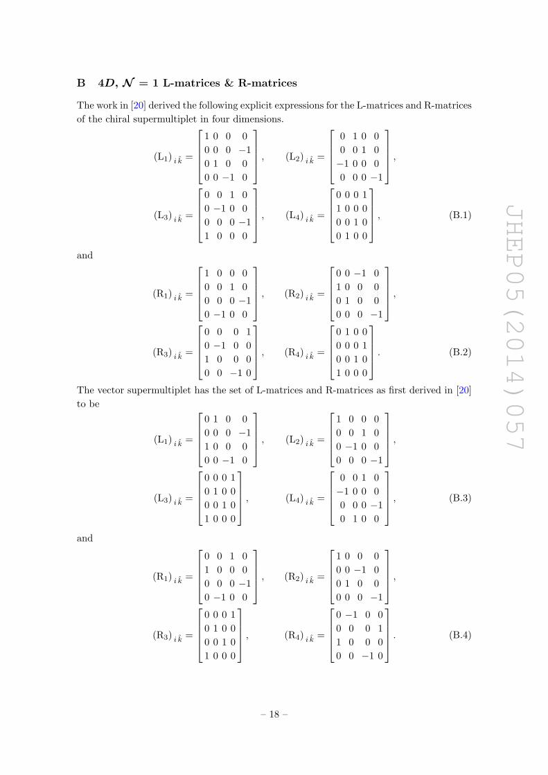
B 4D, N = 1 L-matrices & R-matrices

The work in [20] derived the following explicit expressions for the L-matrices and R-matrices

of the chiral supermultiplet in four dimensions.

(L1) i k =

1 0 0 0

0 0 0 −1

0 1 0 0

0 0 −1 0

, (L2) i k =

0 1 0 0

0 0 1 0

−1 0 0 0

0 0 0 −1

,

(L3) i k =

0 0 1 0

0 −1 0 0

0 0 0 −1

1 0 0 0

, (L4) i k =

0 0 0 1

1 0 0 0

0 0 1 0

0 1 0 0

, (B.1)

and

(R1) i k =

1 0 0 0

0 0 1 0

0 0 0 −1

0 −1 0 0

, (R2) i k =

0 0 −1 0

1 0 0 0

0 1 0 0

0 0 0 −1

,

(R3) i k =

0 0 0 1

0 −1 0 0

1 0 0 0

0 0 −1 0

, (R4) i k =

0 1 0 0

0 0 0 1

0 0 1 0

1 0 0 0

. (B.2)

The vector supermultiplet has the set of L-matrices and R-matrices as first derived in [20]

to be

(L1) i k =

0 1 0 0

0 0 0 −1

1 0 0 0

0 0 −1 0

, (L2) i k =

1 0 0 0

0 0 1 0

0 −1 0 0

0 0 0 −1

,

(L3) i k =

0 0 0 1

0 1 0 0

0 0 1 0

1 0 0 0

, (L4) i k =

0 0 1 0

−1 0 0 0

0 0 0 −1

0 1 0 0

, (B.3)

and

(R1) i k =

0 0 1 0

1 0 0 0

0 0 0 −1

0 −1 0 0

, (R2) i k =

1 0 0 0

0 0 −1 0

0 1 0 0

0 0 0 −1

,

(R3) i k =

0 0 0 1

0 1 0 0

0 0 1 0

1 0 0 0

, (R4) i k =

0 −1 0 0

0 0 0 1

1 0 0 0

0 0 −1 0

. (B.4)

– 18 –

JHEP05(2014)057

C 4D, N = 4 L-matrices & R-matrices

Here we give the explicit results for the triplet(

L[0]I

)ik

L-matrices related to the N = 4

supermultiplet that are analogous to those appearing in (5.3) for the singlet L-matrices.

(L[1]1

)ik =

0 0 0 (2)b(243)

0 0 (15)b(243) 0

0 (0)b(243) 0 0

(13)b(1243) 0 0 0

,

(L[1]2

)ik =

0 0 0 (4)b(123)

0 0 (9)b(123) 0

0 (6)b(123) 0 0

(11)b(23) 0 0 0

,

(L[1]3

)ik =

0 0 0 (14)b(134)

0 0 (3)b(134) 0

0 (12)b(134) 0 0

(7)b(14) 0 0 0

,

(L[1]4

)ik =

0 0 0 (8)b(142)

0 0 (5)b(142) 0

0 (10)b(142) 0 0

(1)b(1342) 0 0 0

, (C.1)

with their associated R-matrices given by

(R

[1]1

)k i =

0 0 0 (7)b(1342)

0 0 (0)b(234) 0

0 (15)b(234) 0 0

(8)b(234) 0 0 0

(

R[1]2

)k i =

0 0 0 (13)b(23)

0 0 (5)b(132) 0

0 (10)b(132) 0 0

(1)b(132) 0 0 0

(

R[1]3

)k i =

0 0 0 (14)b(14)

0 0 (9)b(143) 0

0 (6)b(143) 0 0

(11)b(143) 0 0 0

(

R[1]4

)k i =

0 0 0 (4)b(1243)

0 0 (3)b(124) 0

0 (12)b(124) 0 0

(2)b(124) 0 0 0

. (C.2)

– 19 –

JHEP05(2014)057

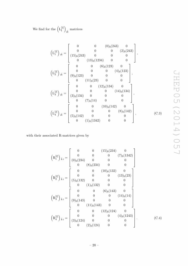
We find for the(

L[2]I

)ik

matrices

(L[2]1

)ik =

0 0 (0)b(243) 0

0 0 0 (2)b(243)

(15)b(243) 0 0 0

0 (13)b(1234) 0 0

,

(L[2]2

)ik =

0 0 (6)b(123) 0

0 0 0 (4)b(123)

(9)b(123) 0 0 0

0 (11)b(23) 0 0

,

(L[2]3

)ik =

0 0 (12)b(134) 0

0 0 0 (14)b(134)

(3)b(134) 0 0 0

0 (7)b(14) 0 0

,

(L[2]4

)ik =

0 0 (10)b(142) 0

0 0 0 (8)b(142)

(5)b(142) 0 0 0

0 (1)b(1342) 0 0

, (C.3)

with their associated R-matrices given by

(R

[2]1

)k i =

0 0 (15)b(234) 0

0 0 0 (7)b(1342)

(0)b(234) 0 0 0

0 (8)b(234) 0 0

(

R[2]2

)k i =

0 0 (10)b(132) 0

0 0 0 (13)b(23)

(5)b(132) 0 0 0

0 (1)b(132) 0 0

(

R[2]3

)k i =

0 0 (6)b(143) 0

0 0 0 (14)b(14)

(9)b(143) 0 0 0

0 (11)b(143) 0 0

(

R[2]4

)k i =

0 0 (12)b(124) 0

0 0 0 (4)b(1243)

(3)b(124) 0 0 0

0 (2)b(124) 0 0

. (C.4)

– 20 –

JHEP05(2014)057

We find for the(

L[3]I

)ik

matrices

(L[3]1

)ik =

0 (15)b(243) 0 0

(0)b(243) 0 0 0

0 0 0 (2)b(243)

0 0 (13)b(1243) 0

,

(L[3]2

)ik =

0 (9)b(123) 0 0

(6)b(123) 0 0 0

0 0 0 (4)b(123)

0 0 (11)b(23) 0

,

(L[3]3

)ik =

0 (3)b(134) 0 0

(12)b(134) 0 0 0

0 0 0 (14)b(134)

0 0 (7)b(14) 0

,

(L[3]4

)ik =

0 (5)b(142) 0 0

(10)b(142) 0 0 0

0 0 0 (8)b(142)

0 0 (1)b(1342) 0

, (C.5)

with their associated R-matrices given by

(R

[3]1

)k i =

0 (0)b(234) 0 0

(15)b(234) 0 0 0

0 0 0 (7)b(1342)

0 0 (8)b(234) 0

(

R[3]2

)k i =

0 (5)b(132) 0 0

(10)b(132) 0 0 0

0 0 0 (13)b(23)

0 0 (1)b(132) 0

(

R[3]3

)k i =

0 (9)b(143) 0 0

(6)b(143) 0 0 0

0 0 0 (14)b(14)

0 0 (11)b(143) 0

(

R[3]4

)k i =

0 (3)b(124) 0 0

(12)b(124) 0 0 0

0 0 0 (4)b(1243)

0 0 (2)b(124) 0

. (C.6)

Open Access. This article is distributed under the terms of the Creative Commons

Attribution License (CC-BY 4.0), which permits any use, distribution and reproduction in

any medium, provided the original author(s) and source are credited.

– 21 –

JHEP05(2014)057

References

[1] E. Cremmer, B. Julia and J. Scherk, Supergravity Theory in Eleven-Dimensions, Phys. Lett.

B 76 (1978) 409 [INSPIRE].

[2] L. Brink and P.S. Howe, Eleven-Dimensional Supergravity on the Mass-Shell in Superspace,

Phys. Lett. B 91 (1980) 384 [INSPIRE].

[3] L. Randall and R. Sundrum, Out of this world supersymmetry breaking, Nucl. Phys. B 557

(1999) 79 [hep-th/9810155] [INSPIRE].

[4] L. Randall and R. Sundrum, A large mass hierarchy from a small extra dimension, Phys.

Rev. Lett. 83 (1999) 3370 [hep-ph/9905221] [INSPIRE].

[5] L. Randall and R. Sundrum, An alternative to compactification, Phys. Rev. Lett. 83 (1999)

4690 [hep-th/9906064] [INSPIRE].

[6] E. Cremmer and B. Julia, The SO(8) Supergravity, Nucl. Phys. B 159 (1979) 141 [INSPIRE].

[7] S.J. Gates Jr. and L. Rana, On Extended Supersymmetric Quantum Mechanics,

UMDEPP-93-194 (1994), unpublished.

[8] S.J. Gates Jr. and L. Rana, Ultramultiplets: a new representation of rigid 2-d, N = 8

supersymmetry, Phys. Lett. B 342 (1995) 132 [hep-th/9410150] [INSPIRE].

[9] S.J. Gates and L. Rana, A theory of spinning particles for large-N extended supersymmetry,

Phys. Lett. B 352 (1995) 50 [hep-th/9504025] [INSPIRE].

[10] S.J. Gates Jr. and L. Rana, A theory of spinning particles for large-N extended

supersymmetry. 2., Phys. Lett. B 369 (1996) 262 [hep-th/9510151] [INSPIRE].

[11] S.J. Gates Jr. and L. Rana, Tuning the RADIO to the off-shell 2−D Fayet hypermultiplet

problem, hep-th/9602072 [INSPIRE].

[12] S.J. Gates Jr., I. Linch, William Divine, J. Phillips and L. Rana, The fundamental

supersymmetry challenge remains, Grav. Cosmol. 8 (2002) 96 [hep-th/0109109] [INSPIRE].

[13] S.J. Gates Jr., I. Linch, William Divine and J. Phillips, When superspace is not enough,

University of Md Preprint UMDEPP-02-054, Caltech Preprint CALT-68-2387,

hep-th/0211034 [INSPIRE].

[14] L. Brink, J.H. Schwarz and J. Scherk, Supersymmetric Yang-Mills Theories, Nucl. Phys. B

121 (1977) 77 [INSPIRE].

[15] F. Gliozzi, J. Scherk and D.I. Olive, Supersymmetry, Supergravity Theories and the Dual

Spinor Model, Nucl. Phys. B 122 (1977) 253 [INSPIRE].

[16] M.T. Grisaru, W. Siegel and M. Rocek, Improved Methods for Supergraphs, Nucl. Phys. B

159 (1979) 429 [INSPIRE].

[17] N. Arkani-Hamed and J. Trnka, The Amplituhedron, Caltech Preprint CALT-68-2872,

arXiv:1312.2007 [INSPIRE].

[18] N. Arkani-Hamed and J. Trnka, Into the Amplituhedron, Caltech Preprint CALT-68-2873,

arXiv:1312.7878 [INSPIRE].

[19] S.J. Gates Jr., J. Parker, V.G.J. Rodgers, L. Rodriguez and K. Stiffler, A Detailed

Investigation of First and Second Order Supersymmetries for Off-Shell N = 2 and N = 4

Supermultiplets, University of MD Preprint UMDEPP-11-009, arXiv:1106.5475 [INSPIRE].

– 22 –

JHEP05(2014)057

[20] S.J. Gates Jr. et al., 4D, N = 1 Supersymmetry Genomics (I), JHEP 12 (2009) 008

[arXiv:0902.3830] [INSPIRE].

[21] I. Chappell, Isaac, S.J. Gates and T. Hubsch, Adinkra (in)equivalence from Coxeter group

representations: A case study, UMD-PP-012-014 Int. J. Mod. Phys. A 29 (2014) 1450029

[arXiv:1210.0478] [INSPIRE].

[22] M. Faux and J. Gates, S. J., Adinkras: A graphical technology for supersymmetric

representation theory, Phys. Rev. D 71 (2005) 065002 [hep-th/0408004] [INSPIRE].

[23] W. Siegel and M. Rocek, On off-shell supermultiplets, Phys. Lett. B 105 (1981) 275

[INSPIRE].

[24] M.T. Grisaru, M. Rocek and W. Siegel, Zero Three Loop β-function in N = 4 Super

Yang-Mills Theory, Phys. Rev. Lett. 45 (1980) 1063 [INSPIRE].

[25] M.T. Grisaru, M. Rocek and W. Siegel, Superloops 3, Beta 0: A Calculation in N = 4

Yang-Mills Theory, Nucl. Phys. B 183 (1981) 141 [INSPIRE].

– 23 –