Instance-aware Semantic Segmentation via Multi-task Network Cascades

Jifeng Dai Kaiming He Jian Sun

Microsoft Research{jifdai,kahe,jiansun}@microsoft.com

AbstractSemantic segmentation research has recently witnessed

rapid progress, but many leading methods are unable toidentify object instances. In this paper, we present Multi-task Network Cascades for instance-aware semantic seg-mentation. Our model consists of three networks, respec-tively differentiating instances, estimating masks, and cat-egorizing objects. These networks form a cascaded struc-ture, and are designed to share their convolutional features.We develop an algorithm for the nontrivial end-to-end train-ing of this causal, cascaded structure. Our solution is aclean, single-step training framework and can be general-ized to cascades that have more stages. We demonstratestate-of-the-art instance-aware semantic segmentation ac-curacy on PASCAL VOC. Meanwhile, our method takes only360ms testing an image using VGG-16, which is two ordersof magnitude faster than previous systems for this challeng-ing problem. As a by product, our method also achievescompelling object detection results which surpass the com-petitive Fast/Faster R-CNN systems.

The method described in this paper is the foundation ofour submissions to the MS COCO 2015 segmentation com-petition, where we won the 1st place.

1. Introduction

Since the development of fully convolutional networks(FCNs) [23], the accuracy of semantic segmentation hasbeen improved rapidly [5, 24, 6, 31] thanks to deeplylearned features [20, 27], large-scale annotations [22], andadvanced reasoning over graphical models [5, 31]. Nev-ertheless, FCNs [23] and improvements [5, 24, 6, 31] aredesigned to predict a category label for each pixel, but areunaware of individual object instances. Accurate and fastinstance-aware semantic segmentation is still a challengingproblem. To encourage the research on this problem, the re-cently established COCO [22] dataset and competition onlyaccept instance-aware semantic segmentation results.

There have been a few methods [10, 13, 7, 14] address-ing instance-aware semantic segmentation using convolu-

sh

are

d fe

atu

re

s

task 1

task 2

task 3sh

are

d fe

atu

re

s

task 1

task 2

task 3

Figure 1. Illustrations of common multi-task learning (left) and ourmulti-task cascade (right).

tional neural networks (CNNs) [21, 20]. These methods allrequire mask proposal methods [29, 3, 1] that are slow atinference time. In addition, these mask proposal methodstake no advantage of deeply learned features or large-scaletraining data, and may become a bottleneck for segmenta-tion accuracy.

In this work, we address instance-aware semantic seg-mentation solely based on CNNs, without using externalmodules (e.g., [1]). We observe that the instance-aware se-mantic segmentation task can be decomposed into three dif-ferent and related sub-tasks. 1) Differentiating instances. Inthis sub-task, the instances can be represented by boundingboxes that are class-agnostic. 2) Estimating masks. In thissub-task, a pixel-level mask is predicted for each instance.3) Categorizing objects. In this sub-task, the category-wiselabel is predicted for each mask-level instance. We expectthat each sub-task is simpler than the original instance seg-mentation task, and is more easily addressed by convolu-tional networks.

Driven by this decomposition, we propose Multi-taskNetwork Cascades (MNCs) for accurate and fast instance-aware semantic segmentation. Our network cascades havethree stages, each of which addresses one sub-task. Thethree stages share their features, as in traditional multi-tasklearning [4]. Feature sharing greatly reduces the test-timecomputation, and may also improve feature learning thanksto the underlying commonality among the tasks. But unlikemany multi-task learning applications, in our method a laterstage depends on the outputs of an earlier stage, forminga causal cascade (see Fig. 1). So we call our structures“multi-task cascades”.

Training a multi-task cascade is nontrivial because of the

1

arX

iv:1

512.

0441

2v1

[cs

.CV

] 1

4 D

ec 2

015

for each RoI

for each RoI

CONVs

conv feature map

FCs

FCs

RoI warping,

pooling

masking

CONVs

box instances (RoIs)

mask instances

categorized instances

sh

are

d fe

atu

re

s

stage 1

stage 2

stage 3

B

M

C

L1

L2

L3

person

personperson

horse

Figure 2. Multi-task Network Cascades for instance-aware semantic segmentation. At the top right corner is a simplified illustration.

causal relations among the multiple outputs. For example,our mask estimating layer takes convolutional features andpredicted box instances as inputs, both of which are out-puts of other layers. According to the chain rule of back-propagation [21], the gradients involve those with respectto the convolution responses and also those with respectto the spatial coordinates of predicted boxes. To achievetheoretically valid backpropagation, we develop a layer thatis differentiable with respect to the spatial coordinates, sothe gradient terms can be computed.

Our cascade model can thus be trained end-to-end via aclean, single-step framework. This single-step training al-gorithm naturally produces convolutional features that areshared among the three sub-tasks, which are beneficial toboth accuracy and speed. Meanwhile, under this trainingframework, our cascade model can be extended to morestages, leading to improvements on accuracy.

We comprehensively evaluate our method on the PAS-CAL VOC dataset. Our method results in 63.5% mean Av-erage Precision (mAPr), about 3.0% higher than the previ-ous best results [14, 7] using the same VGG network [27].Remarkably, this result is obtained at a test-time speed of360ms per image, which is two orders of magnitudes fasterthan previous systems [14, 7].

Thanks to the end-to-end training and the independenceof external modules, the three sub-tasks and the entiresystem easily benefit from stronger features learned bydeeper models. We demonstrate excellent accuracy on thechallenging MS COCO segmentation dataset using an ex-tremely deep 101-layer residual net (ResNet-101) [16], andalso report our 1st-place result in the COCO segmentationtrack in ILSVRC & COCO 2015 competitions.

2. Related Work

Object detection methods [10, 15, 9, 26] involve predict-ing object bounding boxes and categories. The work of R-

CNN [10] adopts region proposal methods (e.g., [29, 32])for producing multiple instance proposals, which are usedfor CNN-based classification. In SPPnet [15] and Fast R-CNN [9], the convolutional layers of CNNs are shared onthe entire image for fast computation. Faster R-CNN [26]exploits the shared convolutional features to extract regionproposals used by the detector. Sharing convolutional fea-tures leads to substantially faster speed for object detectionsystems [15, 9, 26].

Using mask-level region proposals, instance-aware se-mantic segmentation can be addressed based on the R-CNNphilosophy, as in R-CNN [10], SDS [13], and Hypercol-umn [14]. Sharing convolutional features among mask-level proposals is enabled by using masking layers [7]. Allthese methods [10, 13, 14, 7] rely on computationally ex-pensive mask proposal methods. For example, the widelyused MCG [1] takes 30 seconds processing an image, whichbecomes a bottleneck at inference time. DeepMask [25]is recently developed for learning segmentation candidatesusing convolutional networks, taking over 1 second per im-age. Its accuracy for instance-aware semantic segmentationis yet to be evaluated.

Category-wise semantic segmentation is elegantly tack-led by end-to-end training FCNs [23]. The output of anFCN consists of multiple score maps, each of which is forone category. This formulation enables per-pixel regressionin a fully-convolutional form, but is not able to distinguishinstances of the same category. The FCN framework hasbeen further improved in many papers (e.g., [5, 31]), butthese methods also have the limitations of not being able topredict instances.

3. Multi-task Network Cascades

In our MNC model, the network takes an image of arbi-trary size as the input, and outputs instance-aware semanticsegmentation results. The cascade has three stages: propos-

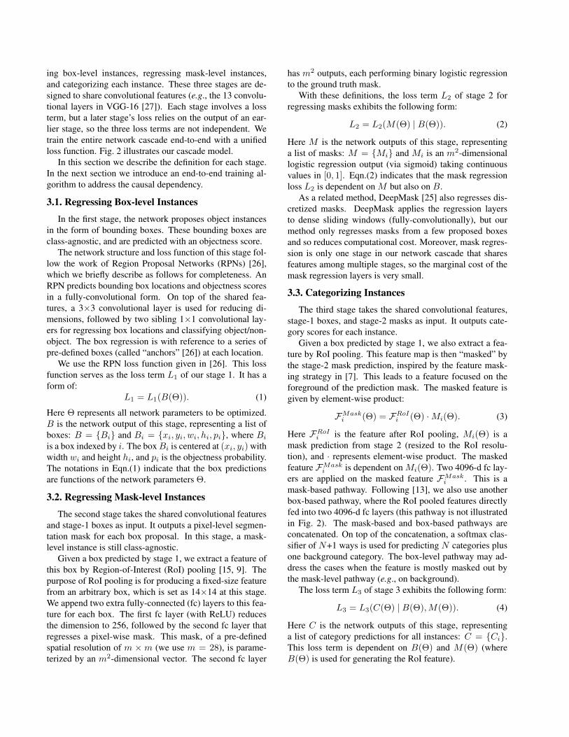
ing box-level instances, regressing mask-level instances,and categorizing each instance. These three stages are de-signed to share convolutional features (e.g., the 13 convolu-tional layers in VGG-16 [27]). Each stage involves a lossterm, but a later stage’s loss relies on the output of an ear-lier stage, so the three loss terms are not independent. Wetrain the entire network cascade end-to-end with a unifiedloss function. Fig. 2 illustrates our cascade model.

In this section we describe the definition for each stage.In the next section we introduce an end-to-end training al-gorithm to address the causal dependency.

3.1. Regressing Box-level Instances

In the first stage, the network proposes object instancesin the form of bounding boxes. These bounding boxes areclass-agnostic, and are predicted with an objectness score.

The network structure and loss function of this stage fol-low the work of Region Proposal Networks (RPNs) [26],which we briefly describe as follows for completeness. AnRPN predicts bounding box locations and objectness scoresin a fully-convolutional form. On top of the shared fea-tures, a 3×3 convolutional layer is used for reducing di-mensions, followed by two sibling 1×1 convolutional lay-ers for regressing box locations and classifying object/non-object. The box regression is with reference to a series ofpre-defined boxes (called “anchors” [26]) at each location.

We use the RPN loss function given in [26]. This lossfunction serves as the loss term L1 of our stage 1. It has aform of:

L1 = L1(B(Θ)). (1)

Here Θ represents all network parameters to be optimized.B is the network output of this stage, representing a list ofboxes: B = {Bi} and Bi = {xi, yi, wi, hi, pi}, where Bi

is a box indexed by i. The boxBi is centered at (xi, yi) withwidth wi and height hi, and pi is the objectness probability.The notations in Eqn.(1) indicate that the box predictionsare functions of the network parameters Θ.

3.2. Regressing Mask-level Instances

The second stage takes the shared convolutional featuresand stage-1 boxes as input. It outputs a pixel-level segmen-tation mask for each box proposal. In this stage, a mask-level instance is still class-agnostic.

Given a box predicted by stage 1, we extract a feature ofthis box by Region-of-Interest (RoI) pooling [15, 9]. Thepurpose of RoI pooling is for producing a fixed-size featurefrom an arbitrary box, which is set as 14×14 at this stage.We append two extra fully-connected (fc) layers to this fea-ture for each box. The first fc layer (with ReLU) reducesthe dimension to 256, followed by the second fc layer thatregresses a pixel-wise mask. This mask, of a pre-definedspatial resolution of m ×m (we use m = 28), is parame-terized by an m2-dimensional vector. The second fc layer

has m2 outputs, each performing binary logistic regressionto the ground truth mask.

With these definitions, the loss term L2 of stage 2 forregressing masks exhibits the following form:

L2 = L2(M(Θ) | B(Θ)). (2)

Here M is the network outputs of this stage, representinga list of masks: M = {Mi} and Mi is an m2-dimensionallogistic regression output (via sigmoid) taking continuousvalues in [0, 1]. Eqn.(2) indicates that the mask regressionloss L2 is dependent on M but also on B.

As a related method, DeepMask [25] also regresses dis-cretized masks. DeepMask applies the regression layersto dense sliding windows (fully-convolutionally), but ourmethod only regresses masks from a few proposed boxesand so reduces computational cost. Moreover, mask regres-sion is only one stage in our network cascade that sharesfeatures among multiple stages, so the marginal cost of themask regression layers is very small.

3.3. Categorizing Instances

The third stage takes the shared convolutional features,stage-1 boxes, and stage-2 masks as input. It outputs cate-gory scores for each instance.

Given a box predicted by stage 1, we also extract a fea-ture by RoI pooling. This feature map is then “masked” bythe stage-2 mask prediction, inspired by the feature mask-ing strategy in [7]. This leads to a feature focused on theforeground of the prediction mask. The masked feature isgiven by element-wise product:

FMaski (Θ) = FRoI

i (Θ) ·Mi(Θ). (3)

Here FRoIi is the feature after RoI pooling, Mi(Θ) is a

mask prediction from stage 2 (resized to the RoI resolu-tion), and · represents element-wise product. The maskedfeature FMask

i is dependent on Mi(Θ). Two 4096-d fc lay-ers are applied on the masked feature FMask

i . This is amask-based pathway. Following [13], we also use anotherbox-based pathway, where the RoI pooled features directlyfed into two 4096-d fc layers (this pathway is not illustratedin Fig. 2). The mask-based and box-based pathways areconcatenated. On top of the concatenation, a softmax clas-sifier of N+1 ways is used for predicting N categories plusone background category. The box-level pathway may ad-dress the cases when the feature is mostly masked out bythe mask-level pathway (e.g., on background).

The loss term L3 of stage 3 exhibits the following form:

L3 = L3(C(Θ) | B(Θ),M(Θ)). (4)

Here C is the network outputs of this stage, representinga list of category predictions for all instances: C = {Ci}.This loss term is dependent on B(Θ) and M(Θ) (whereB(Θ) is used for generating the RoI feature).

4. End-to-End Training

We define the loss function of the entire cascade as:

L(Θ) =L1(B(Θ)) + L2(M(Θ) | B(Θ))

+ L3(C(Θ) | B(Θ),M(Θ)),(5)

where balance weights of 1 are implicitly used among thethree terms. L(Θ) is minimized w.r.t. the network param-eters Θ. This loss function is unlike traditional multi-tasklearning, because the loss term of a later stage depends onthe output of the earlier ones. For example, based on thechain rule of backpropagation, the gradient of L2 involvesthe gradients w.r.t. B.

The main technical challenge of applying the chain ruleto Eqn.(5) lies on the spatial transform of a predicted boxBi(Θ) that determines RoI pooling. For the RoI poolinglayer, its inputs are a predicted box Bi(Θ) and the convolu-tional feature map F(Θ), both being functions of Θ. In FastR-CNN [9], the box proposals are pre-computed and fixed,and the backpropagation of RoI pooling layer in [9] only in-volves F(Θ). However, this is not the case in the presenceof B(Θ). Gradients of both terms need to be considered ina theoretically sound end-to-end training solution.

In this section, we develop a differentiable RoI warpinglayer to account for the gradient w.r.t. predicted box posi-tions and address the dependency on B(Θ). The depen-dency on M(Θ) is also tackled accordingly.

Differentiable RoI Warping Layers. The RoI poolinglayer [9, 15] performs max pooling on a discrete grid basedon a box. To derive a form that is differentiable w.r.t. thebox position, we perform RoI pooling by a differentiableRoI warping layer followed by standard max pooling.

The RoI warping layer crops a feature map region andwarps it into a target size by interpolation. We use F(Θ) todenote the full-image convolutional feature map. Given apredicted box Bi(Θ) centered at (xi(Θ), yi(Θ)) with widthwi(Θ) and height hi(Θ), an RoI warping layer interpolatesthe features inside the box and outputs a feature of a fixedspatial resolution. This operation can be written as lineartransform on the feature map F(Θ):

FRoIi (Θ) = G(Bi(Θ))F(Θ). (6)

Here F(Θ) is reshaped as an n-dimensional vector, withn = WH for a full-image feature map of a spatial sizeW × H . G represents the cropping and warping opera-tions, and is an n′-by-n matrix where n′ = W ′H ′ cor-responds to the pre-defined RoI warping output resolutionW ′ ×H ′. FRoI

i (Θ) is an n′-dimensional vector represent-ing the RoI warping output. We note that these operationsare performed for each channel independently.

The computation in Eqn.(6) has this form:

FRoIi (u′,v′) =

W×H∑(u,v)

G(u, v;u′, v′|Bi)F(u,v), (7)

where the notations Θ in Eqn.(6) are omitted for simplifyingpresentation. Here (u′, v′) represent a spatial position in thetarget W ′ × H ′ feature map, and (u, v) run over the full-image feature map F .

The function G(u, v;u′, v′|Bi) represents transforminga proposed box Bi from a size of [xi −wi/2, xi +wi/2)×[yi−hi/2, yi+hi/2) into another size of [−W ′/2,W ′/2)×[−H ′/2, H ′/2). Using bilinear interpolation, G is sep-arable: G(u, v;u′, v′|Bi) = g(u, u′|xi, wi)g(v, v′|yi, hi)where:

g(u, u′|xi, wi) = κ(xi +u′

W ′wi − u), (8)

where κ(·) = max(0, 1 − | · |) is the bilinear inter-polation function, and xi + u′

W ′wi maps the position ofu′ ∈ [−W ′/2,W ′/2) to the full-image feature map do-main. g(v, v′|yi, hi) is defined similarly. We note that be-cause κ is non-zero in a small interval, the actual computa-tion of Eqn.(7) involves a very few terms.

According to the chain rule, for backpropagation involv-ing Eqn.(6) we need to compute:

∂L2

∂Bi=

∂L2

∂FRoIi

∂G

∂BiF (9)

where we use ∂Bi to denote ∂xi, ∂yi, ∂wi, and ∂hi forsimplicity. The term ∂G

∂Biin Eqn.(9) can be derived from

Eqn.(8). As such, the RoI warping layer can be trained withany preceding/succeding layers. If the boxes are constant(e.g., given by Selective Search [29]), Eqn.(9) is not needed,which becomes the case of the existing RoI pooling in [9].

After the differentiable RoI warping layer, we append amax pooling layer to perform the RoI max pooling behavior.We expect the RoI warping layer to produce a sufficientlyfine resolution, which is set as W ′ ×H ′ = 28 × 28 in thispaper. A max pooling layer is then applied to produce alower-resolution output, e.g., 7×7 for VGG-16.

The RoI warping layer shares similar motivations withthe recent work of Spatial Transformer Networks [18]. In[18], a spatial transformation of the entire image is learned,which is done by feature interpolation that is differentiablew.r.t. the transformation parameters. The networks in [18]are used for image classification. Our RoI warping layeris also driven by the differentiable property of interpolatingfeatures. But the RoI warping layer is applied to multipleproposed boxes that are of interest, instead of the entire im-age. The RoI warping layer has a pre-defined output sizeand arbitrary input sizes, in contrast to [18].

sh

are

d fe

atu

res

stage 1

stage 2

stage 3

B

M

C, B'

stage 4

stage 5

M'

C'

Figure 3. A 5-stage cascade. On stage 3, bounding boxes updatedby the box regression layer are used as the input to stage 4.

Masking Layers. We also compute the gradients involvedin L3(C(Θ) | B(Θ),M(Θ)), where the dependency onB(Θ) and M(Θ) is determined by Eqn.(3). With thedifferentiable RoI warping module (FRoI

i ), the operationsin Eqn.(3) can be simply implemented by an element-wiseproduct module.

In summary, given the differentiable RoI warping mod-ule, we have all the necessary components for backpropa-gation (other components are either standard, or trivial toimplement). We train the model by stochastic gradient de-scent (SGD), implemented in the Caffe library [19].

5. Cascades with More StagesNext we extend the cascade model to more stages within

the above MNC framework.In Fast R-CNN [9], the (N+1)-way classifier is trained

jointly with class-wise bounding box regression. Inspiredby this practice, on stage 3, we add a 4(N+1)-d fc layer forregression class-wise bounding boxes [9], which is a siblinglayer with the classifier layer. The entire 3-stage networkcascade is trained as in Sec. 4.

The inference step with box regression, however, isnot as straightforward as in object detection, because ourultimate outputs are masks instead of boxes. So during in-ference, we first run the entire 3-stage network and obtainthe regressed boxes on stage 3. These boxes are then con-sidered as new proposals1. Stages 2 and 3 are performedfor the second time on these proposals. This is in fact 5-stage inference. Its inference-time structure is illustrated inFig. 3. The new stages 4 and 5 share the same structuresas stages 2 and 3, except that they use the regressed boxesfrom stage 3 as the new proposals. This inference processcan be iterated, but we have observed negligible gains.

Given the above 5-stage cascade structure (Fig. 3), it iseasy to adopt our algorithm in Sec. 4 to train this cascadeend-to-end by backpropagation. Training the model in thisway makes the training-time structure consistent with the

1To avoid multiplying the number of proposals by the number of cat-egories, for each box we only use the highest scored category’s boundingbox regressor.

inference-time structure, which improves accuracy as willbe shown by experiments. It is possible to train a cascadewith even more stages in this way. But due to concerns onfast inference, we only present MNCs with up to 5 stages.

6. Implementation DetailsNon-maximum suppression. On stage 1, the network pro-duces ∼104 regressed boxes. For generating the propos-als for stage 2, we use non-maximum suppression (NMS)to reduce redundant candidates. The threshold of theIntersection-over-Union (IoU) ratio for this NMS is 0.7 asin [26]. After that, the top-ranked 300 boxes [26] will beused for stage 2. During training, the forward/backwardpropagated signals of stages 2 and 3 only go through the“pathways” determined by these 300 boxes. NMS is sim-ilar to max pooling, maxout [11], or other local compet-ing layers [28], which are implemented as routers of for-ward/backward pathways. During inference, we use thesame NMS strategy to produce 300 proposals for stage 2.

Positive/negative samples. (i) On stage 1, their definitionsfollow [26]. (ii) On stage 2, for each proposed box we findits highest overlapping ground truth mask. If the overlap-ping ratio (IoU) is greater than 0.5, this proposed box is con-sidered as positive and contributes to the mask regressionloss; otherwise is ignored in the regression loss. The maskregression target is the intersection between the proposedbox and the ground truth mask, resized to m × m pixels.(iii) On stage 3, we consider two sets of positive/negativesamples. In the first set, the positive samples are the in-stances that overlap with ground truth boxes by box-levelIoU ≥ 0.5 (the negative samples are the rest). In the sec-ond set, the positive samples are the instances that overlapwith ground truth instances by box-level IoU ≥ 0.5 andmask-level IoU≥ 0.5. The loss function of stage 3 involvestwo (N+1)-way classifiers, one for classifying mask-levelinstances and the other for classifying box-level instances(whose scores are not used for inference). The reason forconsidering both box-level and mask-level IoU is that whenthe proposed box is not a real instance (e.g., on the back-ground or poorly overlapping with ground truth), the re-gressed mask might be less reliable and thus the box-levelIoU is more confident.

Hyper-parameters for training. We use the ImageNet pre-trained models (e.g., VGG-16 [27]) to initialize the sharedconvolutional layers and the corresponding 4096-d fc lay-ers. The extra layers are initialized randomly as in [17].We adopt an image-centric training framework [9]: theshared convolutional layers are computed on the entire im-age, while the RoIs are randomly sampled for computingloss functions. In our system, each mini-batch involves 1image, 256 sampled anchors for stage 1 as in [26]2, and 64

2Though we sample 256 anchors on stage 1 for computing the loss

ZF net VGG-16 nettraining strategies (a) (b) (c) (d) (a) (b) (c) (d)shared features? X X X X X X

end-to-end training? X X X Xtraining 5-stage cascades? X X

mAPr@0.5 (%) 51.8 52.2 53.5 54.0 60.2 60.5 62.6 63.5

Table 1. Ablation experiments on PASCAL VOC 2012 validation. For (a), (b), and (c), the cascade structures for training have 3 stages.The inference process (5-stage, see 5) is the same for all cases; the models are only different in the training methods. The pre-trainedmodels are ZF net [30] (left) and VGG-16 net [27] (right).

sampled RoIs for stages 2 and 3. We train the model using alearning rate of 0.001 for 32k iterations, and 0.0001 for thenext 8k. We train the model in 8 GPUs, each GPU holding1 mini-batch (so the effective mini-batch size is ×8). Theimages are resized such that the shorter side has 600 pixels[9]. We do not adopt multi-scale training/testing [15, 9], asit provides no good trade-off on speed vs. accuracy [9].

Inference. We use 5-stage inference for both 3-stage and5-stage trained structures. The inference process gives us alist of 600 instances with masks and category scores (300from the stage 3 outputs, and 300 from the stage 5 outputs).We post-process this list to reduce similar predictions. Wefirst apply NMS (using box-level IoU 0.3 [10]) on the listof 600 instances based on their category scores. After that,for each not-suppressed instance, we find its “similar” in-stances which are defined as the suppressed instances thatoverlap with it by IoU ≥ 0.5. The prediction masks of thenot-suppressed instance and its similar instances are mergedtogether by weighted averaging, pixel-by-pixel, using theclassification scores as their averaging weights. This “maskvoting” scheme is inspired by the box voting in [8]. The av-eraged masks, taking continuous values in [0, 1], are bina-rized to form the final output masks. The averaging step im-proves accuracy by∼1% over the NMS outcome. This post-processing is performed for each category independently.

7. Experiments7.1. Experiments on PASCAL VOC 2012

We follow the protocols used in recent papers [13, 7, 14]for evaluating instance-aware semantic segmentation. Themodels are trained on the PASCAL VOC 2012 training set,and evaluated on the validation set. We use the segmenta-tion annotations in [12] for training and evaluation, follow-ing [13, 7, 14]. We evaluate the mean Average Precision,which is referred to as mean APr [13] or simply mAPr. Weevaluate mAPr using IoU thresholds at 0.5 and 0.7.

Ablation Experiments on Training Strategies. Table1 compares the results of different training strategies forMNCs. We remark that in this table all results are obtained

function, the network of stage 1 is still computed fully-convolutionally onthe entire image and produces all proposals that are used by later stages.

via 5-stage inference, so the differences are contributed bythe training strategies. We show results using ZF net [30]that has 5 convolutional layers and 3 fc layers, and VGG-16net [27] that has 13 convolutional layers and 3 fc layers.

As a simple baseline (Table 1, a), we train the threestages step-by-step without sharing their features. Threeseparate networks are trained, and a network of a later stagetakes the outputs from the trained networks of the earlierstages. The three separate networks are all initialized by theImageNet-pre-trained model. This baseline has an mAPr of60.2% using VGG-16. We note that this baseline result iscompetitive (see also Table 2), suggesting that decomposingthe task into three sub-tasks is an effective solution.

To achieve feature sharing, one may follow the step-by-step training in [26]. Given the above model (a), the sharedconvolutional layers are kept unchanged by using the laststage’s weights, and the three separate networks are trainedstep-by-step again with the shared layers not tuned, follow-ing [26]. Doing so leads to an mAPr of 60.5%, just on parwith the baseline that does not share features. This suggeststhat sharing features does not directly improve accuracy.

Next we experiment with the single-step, end-to-endtraining algorithm developed in Sec. 4. Table 1 (c) showsthe result of end-to-end training a 3-stage cascade. ThemAPr is increased to 62.6%. We note that in Table 1 (a),(b), and (c), the models have the same structure for train-ing. So the improvement of (c) is contributed by end-to-endtraining this cascade structure. This improvement is simi-lar to other gains observed in many practices of multi-tasklearning [4]. By developing training algorithm as in Sec. 4,we are able to train the network by backpropagation in atheoretically sound way. The features are naturally sharedby optimizing a unified loss function, and the benefits ofmulti-task learning are witnessed.

Table 1 (d) shows the result of end-to-end training a 5-stage cascade. The mAPr is further improved to 63.5%.We note that all results in Table 1 are based on the same5-stage inference strategy. So the accuracy gap between (d)and (c) is contributed by training a 5-stage structure that isconsistent with its inference-time usage.

The series of comparisons are also observed when usingthe ZF net as the pre-trained model (Table 1, left), showingthe generality of our findings.

method mAPr@0.5 (%) mAPr@0.7 (%) time/img (s)O2P [2] 25.2 - -SDS (AlexNet) [13] 49.7 25.3 48Hypercolumn [14] 60.0 40.4 >80CFM [7] 60.7 39.6 32MNC [ours] 63.5 41.5 0.36

Table 2. Comparisons of instance-aware semantic segmentation onthe PASCAL VOC 2012 validation set. The testing time per image(including all steps) is evaluated in a single Nvidia K40 GPU, ex-cept that the MCG [1] proposal time is evaluated on a CPU. MCGis used by [13, 14, 7] and its running time is about 30s. The run-ning time of [14] is our estimation based on the description fromthe paper. The pre-trained model is VGG-16 for [14, 7] and ours.O2P is not based on deep CNNs, and its result is reported by [13].

conv stage 2 stage 3 stage 4 stage 5 others total0.15 0.01 0.08 0.01 0.08 0.03 0.36

Table 3. Detailed testing time (seconds) per image of our methodusing 5-stage inference. The model is VGG-16. “Others” includepost-processing and communications among stages.

Comparisons with State-of-the-art Methods. In Table 2we compare with SDS [13], Hypercolumn [14], and CFM[7], which are existing CNN-based semantic segmentationmethods that are able to identify instances. These papers re-ported their mAPr under the same protocol used by our ex-periments. Our MNC has∼3% higher mAPr@0.5 than pre-vious best results. Our method also has higher mAPr@0.7than previous methods.

Fig 4 shows some examples of our results on the valida-tion set. Our method can handle challenging cases wheremultiple instances of the same category are spatially con-nected to each other (e.g., Fig 4, first row).

Running Time. Our method has an inference-time speedof 360ms per image (Table 2), evaluated on an Nvidia K40GPU. Table 3 shows the details. Our method does not re-quire any external region proposal method, whereas the re-gion proposal step in SDS, Hypercolumn, and CFM costs30s using MCG. Furthermore, our method uses the sharedconvolutional features for the three sub-tasks and avoids re-dundant computation. Our system is about two orders ofmagnitude faster than previous systems.

Object Detection Evaluations. We are also interested inthe box-level object detection performance (mAPb), so thatwe can compare with more systems that are designed forobject detection. We train our model on the PASCAL VOC2012 trainval set, and evaluate on the PASCAL VOC 2012test set for object detection. Given mask-level instancesgenerated by our model, we simply assign a tight boundingbox to each instance. Table 4 shows that our result (70.9%)compares favorably to the recent Fast/Faster R-CNN sys-tems [9, 26]. We note that our result is obtained with fewertraining images (without the 2007 set), but with mask-level

system training data mAPb (%)R-CNN [10] VOC 12 62.4Fast R-CNN [9] VOC 12 65.7Fast R-CNN [9] VOC 07++12 68.4Faster R-CNN [26] VOC 12 67.0Faster R-CNN [26] VOC 07++12 70.4MNC [ours] VOC 12 70.9MNCbox [ours] VOC 12 73.5MNCbox [ours]† VOC 07++12 75.9

Table 4. Evaluation of (box-level) object detection mAP on thePASCAL VOC 2012 test set. “12” denotes VOC 2012 trainval, and“07++12” denotes VOC 2007 trainval+test and 2012 trainval. Thepre-trained model is VGG-16 for all methods.†: http://host.robots.ox.ac.uk:8080/anonymous/NUWDYX.html

network mAP@[.5:.95] (%) mAP@.5 (%)VGG-16 [27] 19.5 39.7

ResNet-101 [16] 24.6 44.3Table 5. Our baseline segmentation result (%) on the MS COCOtest-dev set. The training set is the trainval set.

annotations. This experiment shows the effectiveness of ouralgorithm for detecting both box- and mask-level instances.

The above detection result is solely based on the mask-level outputs. But our method also has box-level outputsfrom the box regression layers in stage 3/5. Using thesebox layers’ outputs (box coordinates and scores) in place ofthe mask-level outputs, we obtain an mAPb of 73.5% (Ta-ble 4). Finally, we train the MNC model on the union setof 2007 trainval+test and 2012 trainval. As the 2007 set hasno mask-level annotation, when a sample image from the2007 set is used, its mask regression loss is ignored (but themask is generated for the later stages) and its mask-levelIoU measure for determining positive/negative samples isignored. These samples can still impact the box proposalstage and the categorizing stage. Under this setting, we ob-tain an mAPb of 75.9% (Table 4), substantially better thanFast/Faster R-CNN [9, 26].

7.2. Experiments on MS COCO Segmentation

We further evaluate on the MS COCO dataset [22]. Thisdataset consists of 80 object categories for instance-awaresemantic segmentation. Following the COCO guidelines,we use the 80k+40k trainval images to train, and report theresults on the test-dev set. We evaluate the standard COCOmetric (mAPr@IoU=[0.5:0.95]) and also the PASCAL met-rics (mAPr@IoU=0.5). Table 5 shows our method usingVGG-16 has a result of 19.5%/39.7%.

The end-to-end training behavior and the independenceof external models make our method easily enjoy gainsfrom deeper representations. By replacing VGG-16 with anextremely deep 101-layer network (ResNet-101) [16], weachieve 24.6%/44.3% on the MS COCO test-dev set (Ta-

personperson

person

person person

person

person

person

person person

person

potted plant

chair

sheep

sheep

sheep

sheep sheep

sheep

carcar

carcar

car

personperson

person

table

input our result ground truth

table

chair

chair

chair

input our result input our result ground truth

dogdog

ground truth

potted plant

personperson

motobike

potted plant

Figure 4. Our instance-aware semantic segmentation results on the PASCAL VOC 2012 validation set. One color denotes one instance.

ble 5). It is noteworthy that ResNet-101 leads to a relativeimprovement of 26% (on mAPr@[.5:.95]) over VGG-16,which is consistent to the relative improvement of COCOobject detection in [16]. This baseline result is close tothe 2nd-place winner’s ensemble result (25.1%/45.8% byFAIRCNN). On our baseline result, we further adopt globalcontext modeling and multi-scale testing as in [16], andensembling. Our final result on the test-challenge set is28.2%/51.5%, which won the 1st place in the COCO seg-mentation track3 of ILSVRC & COCO 2015 competitions.Fig. 5 shows some examples.

3http://mscoco.org/dataset/#detections-challenge2015

8. ConclusionWe have presented Multi-task Network Cascades for fast

and accurate instance segmentation. We believe that theidea of exploiting network cascades in a multi-task learn-ing framework is general. This idea, if further developed,may be useful for other recognition tasks.

Our method is designed with fast inference in mind, andis orthogonal to some other successful strategies developedpreviously for semantic segmentation. For example, onemay consider exploiting a CRF [5] to refine the boundariesof the instance masks. This is beyond the scope of this paperand will be investigated in the future.

Figure 5. Our instance-aware semantic segmentation results on the MS COCO test-dev set using ResNet-101 [16].

References

[1] P. Arbelaez, J. Pont-Tuset, J. T. Barron, F. Marques, andJ. Malik. Multiscale combinatorial grouping. In CVPR,

2014.

[2] J. Carreira, R. Caseiro, J. Batista, and C. Sminchisescu. Se-mantic segmentation with second-order pooling. In ECCV.2012.

[3] J. Carreira and C. Sminchisescu. Cpmc: Automatic ob-ject segmentation using constrained parametric min-cuts.TPAMI, 2012.

[4] R. Caruana. Multitask learning. Machine learning,28(1):41–75, 1997.

[5] L.-C. Chen, G. Papandreou, I. Kokkinos, K. Murphy, andA. L. Yuille. Semantic image segmentation with deep con-volutional nets and fully connected crfs. In ICLR, 2015.

[6] J. Dai, K. He, and J. Sun. Boxsup: Exploiting boundingboxes to supervise convolutional networks for semantic seg-mentation. In ICCV, 2015.

[7] J. Dai, K. He, and J. Sun. Convolutional feature masking forjoint object and stuff segmentation. In CVPR, 2015.

[8] S. Gidaris and N. Komodakis. Object detection via a multi-region & semantic segmentation-aware cnn model. In ICCV,2015.

[9] R. Girshick. Fast R-CNN. In ICCV, 2015.[10] R. Girshick, J. Donahue, T. Darrell, and J. Malik. Rich fea-

ture hierarchies for accurate object detection and semanticsegmentation. In CVPR, 2014.

[11] I. J. Goodfellow, D. Warde-Farley, M. Mirza, A. Courville,and Y. Bengio. Maxout networks. arXiv:1302.4389, 2013.

[12] B. Hariharan, P. Arbelaez, L. Bourdev, S. Maji, and J. Malik.Semantic contours from inverse detectors. In ICCV, 2011.

[13] B. Hariharan, P. Arbelaez, R. Girshick, and J. Malik. Simul-taneous detection and segmentation. In ECCV. 2014.

[14] B. Hariharan, P. Arbelaez, R. Girshick, and J. Malik. Hyper-columns for object segmentation and fine-grained localiza-tion. In CVPR, 2015.

[15] K. He, X. Zhang, S. Ren, and J. Sun. Spatial pyramid poolingin deep convolutional networks for visual recognition. InECCV, 2014.

[16] K. He, X. Zhang, S. Ren, and J. Sun. Deep residual learningfor image recognition. arXiv:1512.03385, 2015.

[17] K. He, X. Zhang, S. Ren, and J. Sun. Delving deep intorectifiers: Surpassing human-level performance on imagenetclassification. In ICCV, 2015.

[18] M. Jaderberg, K. Simonyan, A. Zisserman, andK. Kavukcuoglu. Spatial transformer networks. InNIPS, 2015.

[19] Y. Jia, E. Shelhamer, J. Donahue, S. Karayev, J. Long, R. Gir-shick, S. Guadarrama, and T. Darrell. Caffe: Convolu-tional architecture for fast feature embedding. arXiv preprintarXiv:1408.5093, 2014.

[20] A. Krizhevsky, I. Sutskever, and G. E. Hinton. Imagenetclassification with deep convolutional neural networks. InNIPS, 2012.

[21] Y. LeCun, B. Boser, J. S. Denker, D. Henderson, R. E.Howard, W. Hubbard, and L. D. Jackel. Backpropagationapplied to handwritten zip code recognition. Neural compu-tation, 1989.

[22] T.-Y. Lin, M. Maire, S. Belongie, J. Hays, P. Perona, D. Ra-manan, P. Dollar, and C. L. Zitnick. Microsoft COCO: Com-mon objects in context. In ECCV. 2014.

[23] J. Long, E. Shelhamer, and T. Darrell. Fully convolutionalnetworks for semantic segmentation. In CVPR, 2015.

[24] G. Papandreou, L.-C. Chen, K. Murphy, and A. L. Yuille.Weakly- and semi-supervised learning of a dcnn for semanticimage segmentation. In ICCV, 2015.

[25] P. O. Pinheiro, R. Collobert, and P. Dollar. Learning to seg-ment object candidates. In NIPS, 2015.

[26] S. Ren, K. He, R. Girshick, and J. Sun. Faster R-CNN: To-wards real-time object detection with region proposal net-works. In NIPS, 2015.

[27] K. Simonyan and A. Zisserman. Very deep convolutionalnetworks for large-scale image recognition. In ICLR, 2015.

[28] R. K. Srivastava, J. Masci, S. Kazerounian, F. Gomez, andJ. Schmidhuber. Compete to compute. In NIPS, 2013.

[29] J. R. Uijlings, K. E. van de Sande, T. Gevers, and A. W.Smeulders. Selective search for object recognition. IJCV,2013.

[30] M. D. Zeiler and R. Fergus. Visualizing and understandingconvolutional neural networks. In ECCV, 2014.

[31] S. Zheng, S. Jayasumana, B. Romera-Paredes, V. Vineet,Z. Su, D. Du, C. Huang, and P. Torr. Conditional randomfields as recurrent neural networks. In ICCV, 2015.

[32] C. L. Zitnick and P. Dollar. Edge boxes: Locating objectproposals from edges. In ECCV, 2014.