j.ijheatmasstransfer.2015.01.068 a simple method to calculate shell side fluid pressure drop in a...

International Journal of Heat and Mass Transfer 84 (2015) 700–712

Contents lists available at ScienceDirect

International Journal of Heat and Mass Transfer

journal homepage: www.elsevier .com/locate / i jhmt

A simple method to calculate shell side fluid pressure drop in a shelland tube heat exchanger

http://dx.doi.org/10.1016/j.ijheatmasstransfer.2015.01.0680017-9310/� 2015 Elsevier Ltd. All rights reserved.

⇑ Corresponding author.E-mail addresses: [email protected] (B. Parikshit), [email protected]

(K.R. Spandana), [email protected] (V. Krishna), [email protected](T.R. Seetharam), [email protected] (K.N. Seetharamu).

B. Parikshit ⇑, K.R. Spandana, V. Krishna, T.R. Seetharam, K.N. SeetharamuDepartment of Mechanical Engineering, PES Institute of Technology, 100 ft. Ring road, Banashankari III stage, Bangalore 560 085, India

a r t i c l e i n f o a b s t r a c t

Article history:Received 19 September 2014Received in revised form 12 December 2014Accepted 9 January 2015

Keywords:Shell and tube heat exchangerPressure dropFEM modelFriction factorsNo tube in window section

Pressure drop predictions on the shell side of a shell and tube heat exchanger (STHX) are investigatedusing the concept of Finite Element Method (FEM). In this model the shell side region is discretised intoa number of elements and by taking into account the effect of flow pattern, the pressure drop on the shellside of a STHX is determined. The present method is simple to apply and the predictions agree reasonablywell with a large number of experimental data available in the literature. The range of applicability of thepresent method extends beyond that used by others in the literature. The earlier predictions wererestricted to tubes in the window region, however, the predictions of the present method are extendedto the cases of no tubes in the window (NTIW) region also.

� 2015 Elsevier Ltd. All rights reserved.

1. Introduction

Shell and tube heat exchangers are very widely used in anumber of industries and its applications include transformer oilcooling, exhaust gas heat recovery, solvent distillate process,ethanol mash-stillage, power plants, air-conditioning units, etc.This heat exchanger (HX) comprises of one fluid flowing throughthe tubes and the other fluid flowing in the shell across the tubebundle. The flow in the shell side of a shell and tube heat exchan-ger (STHX) with segmented baffles is quite complex. The flow inbaffle region is illustrated in Fig. 1, in terms of main stream SH,leakage stream between tubes and baffle SL and bypass streambetween tube bundle and shell SB. The gaps between a baffle andthe tube cause leakage stream SL, which may modify the mainstream SH significantly. As the tubes cannot be placed very closeto the shell, bypass streams SB may be formed, which also influ-ences the main stream. The flow direction of the main stream rel-ative to the tubes is different in the window sections created by thebaffle cut from that in the cross flow sections existing between thesegmental baffles. This necessitates the use of different equationsto calculate the pressure drop in the window sections to those usedin the cross flow sections. The spacing between the tube plates andthe first and the last baffle differs in many cases from the spacing

between two adjacent baffles. Some of the afore mentionedstreams are not present in the first and the last section of theHX. A large number of investigations which describe methods tocalculate the shell side pressure drop in a STHX have beenpublished [1–5]. A critical review of these methods is given byPalen and Taborek [6]. They have compared the differentcalculation procedures against a large number of experimentalmeasurements on small units and on industrial HXs. Accordingto them, the methods of Tinker [3,4] and of Delaware [5] gavethe best result as compared to the other methods. The method ofTinker [3,4] has been criticized as it is relatively complicated.

Gaddis and Gnielinski [7] have followed the Delaware method[5] to calculate the shell side pressure drop, except that, insteadof using diagrams – as in the Delaware method – to calculate thepressure drop in the ideal tube bank, they have used equations pre-viously presented by them in [8,9]. Correction factors are thenused, as in the Delaware method, to take into account the deviationof the flow inside the shell from that in the ideal case of a tubebank. They have compared pressure drops predicted by theirmodel with those obtained experimentally by different investiga-tors. The comparison is represented by the ratio, Dpm/Dpc for allavailable experimental points, as a function of Reynolds number(Re). The comparison shows that for large number of experimentalpoints the deviations between measurements and theoretical pre-dictions are as high as ±35% for Reynolds number range from 10 to105. Further, about one third of the experimental points have devi-ations more than ±35%. They also found that in extreme cases, themeasured pressure drop is as low as one fifth or as high as four

http://crossmark.crossref.org/dialog/?doi=10.1016/j.ijheatmasstransfer.2015.01.068&domain=pdf

http://dx.doi.org/10.1016/j.ijheatmasstransfer.2015.01.068

mailto:[email protected]





http://dx.doi.org/10.1016/j.ijheatmasstransfer.2015.01.068

http://www.sciencedirect.com/science/journal/00179310

http://www.elsevier.com/locate/ijhmt

Nomenclature

a relative transverse pitch of tube bundle, a = xt/do

Abmin minimum cross- sectional area at the baffle tip (m2)Amin minimum area of flow of fluid in a cross section (m2)Anozzle nozzle cross-section area (m2)b relative longitudinal pitch of tube bundle, b = xl/do

c relative diagonal pitch of tube bundle, c = xd/do

d0 outer tube diameter (m)Dotl diameter of the circle encompassing the end tubes (m)Ds inner diameter of shell (m)Eu Euler number (friction factor), Eu ¼ 2DPA2

min

nqQ2

Euc corrected friction factor after using angular correctionfactor

Kw correction for angular flowkn nozzle pressure drop coefficient for each nozzlelc baffle cut in (m)N number of rows in a particular element, if it is inter-

baffle element it is necf and if it is window element itis new

Nc number of elements in inter-baffle regionnecf number of rows in inter-baffle element = Ds�2lc

xlNc

new number of rows in window section = 0:8lc�Ds�Dotl

2Nw

2 xl

Ntw number of tubes in window sectionNw total number of elements in upper and lower window

sectionPi pressure at ith node

p tube pitch, p ¼ ptdo

pt tube pitch (m)Q volume flow rate in (m3/s)

Re Reynolds number, Re ¼ qQd0Aminl

S baffle spacing (m)xd diagonal pitch of tube bundle (m)xi distance between outer most tubes at cross section

(Fig. 2(b)) at the end of ith element (m)xe space between the outer most tube in a shell and shell

outer diameter (m): Ds � Dotlxl longitudinal pitch of tube bundle (m)xt transverse pitch of tube bundle (m)x(i) net distance at the exit of ith element within the tube

outer limit (m), xðiÞ ¼ xiþxi�12

l viscosity of the fluid (in Pa s)q density of shell side fluid (kg/m3)wm acute angle the fluid makes with the tube in the

mid-section in radiansww acute angle the fluid makes with the tube in the window

section in radiansDP pressure drop (Pa)DPc calculated shell side pressure dropDPexp experimental pressure dropDPfem pressure drop predicted by Finite element modelDPm measured shell side pressure drophb angle subtended by the baffle cut

B. Parikshit et al. / International Journal of Heat and Mass Transfer 84 (2015) 700–712 701

times the calculated values. This clearly indicates that the methodof Gaddis and Gnielinski [7] cannot be applied safely in the formsuggested by them. Kapale et al. [10] have proposed a theoreticalmodel to calculate the shell side pressure drop. Their model incor-porates the effect of pressure drop in inlet and out let nozzles alongwith the losses in the segments created by baffles. For the range ofReynolds number between 103 and 105, they found that theirresults match more closely (deviation between +2.4% and �4%)with the available experimental results. But they have not shownthe validity of their model to predict pressure drop in HXs withNTIW. The calculation adopted by Kapale et al. [10] is complex.They have not predicted pressure drop for all the cases for whichexperimental data is available. Thus, there is a need to develop asimple model to calculate pressure drop on the shell side of STHXs.All the theoretical models reported in literature to calculate theshell-side pressure drop in a STHX require a lot of calculations with

Fig. 1. Flow through shell of shell and tube heat exchanger with segmental bafflewith leakage streams. [7].

a number of variables involved in the calculations. Further thesemodels use different correlations for window section and crossflow section. In all the above mentioned references, the methodol-ogy to find pressure drop coefficient involves tedious calculationswhich include various geometrical parameters and is time con-suming. These pressure drop coefficients have been changed timeand again, yet no coefficient has been found which works satisfac-torily for all cases.

Friction factors for flow over rectangular tube banks have beengiven by Zukauskas [11] and Gunter and Haw [12]. A Finite ele-ment model of STHX for determining amount of heat transfer hasbeen developed by Ravikumaur et al. [13] in 1988 but applicationof such a model to determine pressure drop in STHX has not beencarried out so far.

Yonghua et al. [14], experimentally investigated the shell-sidethermo-hydraulic performance of a shell and tube HX with trefoilhole baffles under turbulent flow regime. Based on the experimentalresults, empirical correlations of the Nusselt number and pressureloss as a function of the Reynolds number are obtained. To analyzethe mechanisms of these thermo-hydraulic characteristics, numer-ical computation is carried out. Ender and Ilker [15], investigatedthe baffle spacing, baffle cut and shell diameter dependencies ofthe heat transfer coefficient and the pressure drop by numericallymodeling a small HX. The authors refer to the Bell-Delaware [5]method as a very detailed and an accurate method to estimate theoutlet parameters and have compared their results to that method,but Bell-Delaware method itself does not predict pressure drop val-ues close to the experimental values. The authors have also com-pared the pressure drop results to Kapale’s [10] model and havefound a deviation of up to 34%. Results obtained from the CFD sim-ulations show that the existing analytical methods under predictthe pressure drop in many cases. Vera et al. [16], present a modelto determine the outlet conditions of a shell and tube HX workingin a refrigeration cycle either as a condenser or evaporator only.The model does not take the internal geometrical information into

b. Cross section of the baffle space

c. Circular cross section split intoRectangular elements

Upper Window

Mid-Sec�on

Lower Window

a. One baffle space divided into elements (1, 2, 3, 4)

1

2

3

4

d. Flow direc�on and associated pitches

Flow

dir

ec�o

n(L

ongi

tudi

nal d

irec

�on)

Transverse direc�on

Fig. 2. Element model of the shell and tube heat exchanger.

702 B. Parikshit et al. / International Journal of Heat and Mass Transfer 84 (2015) 700–712

account and as a result requires special types of correlations toestimate the heat transfer coefficients and the pressure drop. Thepressure drop model of Vera et al. [16] is much simpler than theearlier published works on pressure drop models, but this modelis restricted to refrigerator systems. This model uses Zukauskasfriction factor [11] to determine the influence of geometrical factorson pressure drop (according to the expression proposed by Hewittet al. [17]). But these correlations are not explicitly used as a methodby itself elsewhere to find pressure drop in shell and tube HXs.Rajagapal and Srikanth [18] have studied the effect of baffle inclina-tion angles of 0�, 10� and 20�. The pressure drop decreases by 4% forHXs with a 10� baffle inclination angle and by 16% for HX with 20�baffle inclination angle. Prithiviraj and Andrews [19] have devel-oped a three-dimensional CFD numerical code, HEATX, to simulateflow and heat transfer in shell and tube heat exchangers. The modelpresented by Prithiviraj and Andrews [19] uses ideal tube bankcorrelations of Zukauskas [11] to find the distributed resistancesfor shell side cross flow pressure drop and heat transfer. The CFDanalysis is carried out only for a 30� tube bundle and the validationfor other cases are not presented. Problem set up and calculationtime for executing the Bell [5] and Kern [2] method is about20 min. The typical computational time taken to run the HEATX[19] three-dimensional simulations are about 20 h on a Pentium133. However, the HEATX results are fairly accurate and a deviationup to 10% is observed when verified against the experimental workof Halle [20].

In the present work, an attempt has been made to formulate anew and simple method to predict the pressure drop on the shellside of a shell and tube HX using the concept of FEM. Initially themodel is tested with friction factors given by Gunter et al. [12],

but is found to be deviating up to 85% from the experimental worksof Halle et al. [20]. In the proposed model, the correlation for fric-tion factor as suggested by Zukauskas [11] is used for each ele-ment. The overall pressure drop is computed after assembly ofall elements. The novelty of the present model lies in the fact thatthe pressure drop on the shell side of the STHX can be determinedin a simple way with limited data of HX geometry provided bymanufacturers. The predicted pressure drop is compared to exper-imental work for 240 cases. In order to limit the number of pages,130 cases are presented here. The configuration codes usedthroughout this paper for an abbreviated description of the config-urations of HXs tested are as presented in Table 1.

2. New pressure drop model

Fluid flows when there is a pressure drop between 2 regions.The pressure drop encountered between the 2 sections for a givenflow quantity is connected in the form of an element (as in the case

of FEM) 1R

1 �1�1 1

� �Pi

Pj

� �¼ Qi

Q j

� �, where R is the flow resistance

encountered during the flow between the 2 sections. Thus, the ele-ment relates the pressure drop encountered to the flow quantitythrough the resistance encountered by the fluid. When the frictionfactor varies along the length of the fluid flow as in the developingsection of a pipe, this method helps to incorporate such variationsin the model. This method of representation allows us to determinethe total pressure drop by summing up the pressure drop in each ofthe sub regions.

The steps in the FEM involve geometric representation of thedomain, discretization of the domain into elements and nodes,

Table 1Explanation of heat exchanger configuration code [20].

Position Symbols Definition

1st letter F Full tube bundleN No-tube-in-window bundle

2nd letter P Plain tube1st number 6 or 8 Number of cross passes2nd number 10 or 14 in Nominal size of nozzles

10 in. size: 0.241 m (9.50 in.)14 in. size: 0.337 m (13.25 in.)

3rd number 30 to 90 deg Tube layout patternLast digit 15.5 to 29.8 percent Baffle cut as percentage of inside

diameter


obtaining the characteristics of an element, assembly of allelements, incorporating boundary conditions and solving thesystem of equations.

In FEM, to obtain the characteristics of the entire domain forany variables like temperature, pressure etc., a small region isselected which has typical characteristics of the entire domain.Using variational or weighted residual method, characteristic ofthe sub-region is obtained. After obtaining the characteristic ofthe element, all the elements are assembled. Nodal values liketemperature, pressure are then determined by inserting theboundary conditions and solving the system of equations.

2.1. Geometrical model

The model requires the shell side of STHX to be discretised intomany elements, with elements in window section, mid-section,and inlet–outlet section as shown in Fig. 2. In the present model,Zukauskas friction factor has been used. The discretization andthe number of elements taken should be such that, it should reflectthe situation (in rectangular tube bundles) Zukauskas [11] hasused for determining the friction factor. In this way 4 elementsgives satisfactory results. These 4 elements in one cross flowsection are distributed with 1 element in each window sectionand 2 elements in the mid-section to find pressure drop across thatsection.

The longitudinal and transverse pitches for various tube arraysare as given by Shah et al. [21] and are illustrated in Table 2.

For inline tube arrangement, the minimum cross flow area usedis given by

Amin ¼ðxt � doÞSxðiÞ

xtþ Sxe ð1Þ

whereas for staggered arrangement, the minimum cross flow area isgiven by

Amin ¼xt � doð ÞSxðiÞ

xtþ Sxe for xt � do 6 2 xd � doð Þ ð2aÞ

or

Amin ¼2ðxd � doÞSx ið Þ

xtþ Sxe for xt � do > 2 xd � doð Þ ð2bÞ

Table 2Properties of tube banks [21].

30� Triangular staggered array 60� Rotated triangular

Transverse tube pitch (xt) ptffiffiffi3p

pt

Longitudinal tube pitch (xl)ffiffi3p

2 ptpt2

2.2. Yaw correction factor

In most of the investigations so far reported in literature, theactual flow direction of fluid has not been taken into account forcalculation of pressure drop. Most of the authors have assumed amodel wherein, fluid flow is perpendicular to tube bundles. How-ever Kapale et al. [10] have proposed a model which takes intoaccount direction of fluid flow. They consider fluid flow in the win-dow region to be parallel to the tubes and that in the mid-sectionto be flowing at an angle. In the present investigation the fluid flowdirection adopted is different from that of the model of Kapaleet al. [10].

The flow pattern for this model for inter-baffle region and inletand outlet sections are shown in Figs. 3–5. Figs. 3 and 4 representthe flow in inter-baffle region, while Fig. 5 represents flow in bothinlet and outlet sections. The flow patterns in inter-baffle regiondiffer from that for inlet and outlet section as depicted in Figs. 3–5.

These flow patterns decide the angle w (Appendix A) at whichthe fluid crosses the tube bundle. The correction factor given byZukauskas [11], which is in the form of a graph is correlated bySchlunder [22], Eqs. (3a) and (3b) give correlations to obtain yawcorrection factors.

Yaw correction factor for inline tube arrangement:

Kw ¼ 1:107 expð�0:301w�2:412Þ ð3aÞ

Yaw correction factor for staggered tube arrangement:

Kw ¼ 1:245 expð�0:478w�1:733Þ ð3bÞ

The Euler number (Eu) as obtained from [11] is multiplied bycorrection factor Kw and the corrected Euler number (Euc) iscalculated:

Euc ¼ KwEu ð4Þ

The shell-side fluid flow is found to vary depending on the Shelldiameter, baffle spacing and tubes in window section.

2.3. FEM model

In the case of a STHX, the fluid flow on its shell side is complex.The flow path of a shell side fluid is first determined as it decidesthe characteristics of the element (shown in Section 2.2). Thefriction factor required to find the pressure drop is selected (inthe present case Zukauskas correlations) for each of the sections.Stiffness matrix for each of the element is then determined. Thesestiffness matrices are assembled to obtain the global stiffnessmatrix. On the load vector, known boundary conditions areinserted and pressure at each of the nodes is determined (seeFig. 6). Typical example for pressure drop in a pipe network isavailable in Lewis et al. [23].

In the present model the whole HX is discretised into a numberof elements depending on the number of baffles. Between the baf-fles, it is discretised into 4 elements in the direction of flow as illus-trated in Fig. 2(a) and the evaluation for pressure drop is performedelement by element using Zukauskas correlation for rectangulartube bundles [11]. The formula to be used for calculating pressuredrop is discussed in reference [24]. Using Euc, the pressure drop for

staggered array 90� Square inline array 45� Rotated square staggered array

ptffiffiffi2p

pt

ptptffiffi

2p

a. With tubes in window section b. No tubes in window section

ψw

ψm

ψwψm = ψwψm = ψw

Fig. 3. Flow in Inter-baffle region when DsS 6 1.

a. With tubes in window section

ψm

ψw

ψw

b. No tubes in window section

ψw

ψw

ψm

Fig. 4. Flow in Inter-baffle region when DsS > 1.

ψw

ψm

ψw

Fig. 5. Flow in Inlet or outlet section.

Table 3Correction factors for 60� and 45� tube arrangement.

K45 = 0.97 for Re < 104K45 = �9.289 Re�0.2203 + 2.289 for 104

6 Re 6 106

K45 = 1.834 for Re > 106

K60 = 0.85 for Re < 3 � 104

K60 = 1 for 3 � 1046 Re < 5 � 104

K60 = 1.05 for 5 � 1046 Re 6 105

K60 = 1.1 for Re P 105


flow over a rectangular tube bank is calculated. The coefficient k ofstiffness matrix for each element within the shell and tube HX isgiven by

k ¼ 2A2min

EucqQnð5aÞ

Eq. (5b) gives the pressure drop coefficient in nozzles, these ele-ments are added at the beginning of the inlet section and at theend of exit section. These elements are added to take into account

pressure drop due to sudden expansion at inlet nozzle and suddencontraction at the exit nozzle as discussed by Gaddis et al. [7]:

k ¼ 2A2nozzle

knqQð5bÞ

The value of kn is taken as 1 for each nozzle as suggested by Gaddiset al.

The pressure element is given by,

k �k

�k k

� �Pi

Pj

� �¼

Q

�Q

� �ð6Þ

Using the coefficient of stiffness matrix for each element, the coef-ficient for overall stiffness matrix is obtained and then the equa-tions are solved to get overall pressure drop.

For a window section with no tubes, the pressure drop is negli-gible. Hence, the nodal pressure value at the exit (Pj) can safely beapproximated to the nodal pressure value at the inlet (Pi) of theelement. The pressure element of the NTIW region is given by

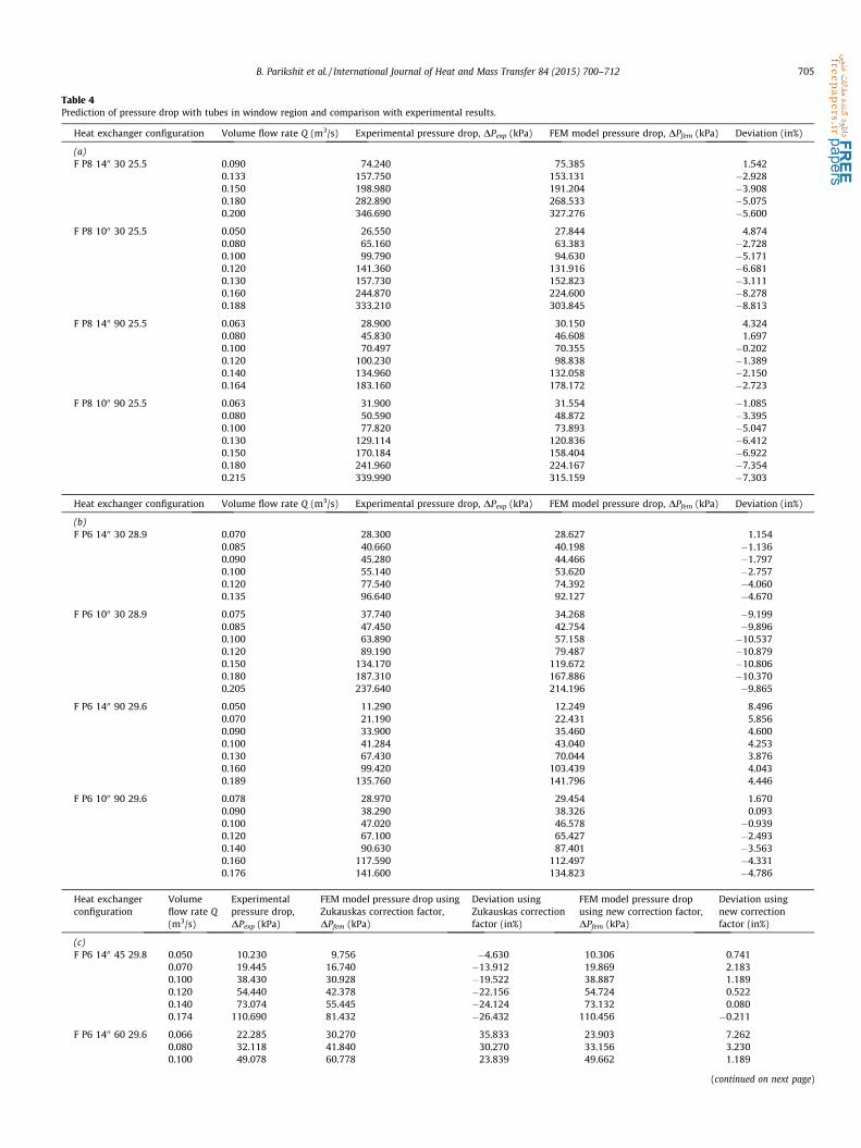
Table 4Prediction of pressure drop with tubes in window region and comparison with experimental results.

Heat exchanger configuration Volume flow rate Q (m3/s) Experimental pressure drop, DPexp (kPa) FEM model pressure drop, DPfem (kPa) Deviation (in%)

(a)F P8 1400 30 25.5 0.090 74.240 75.385 1.542

0.133 157.750 153.131 �2.9280.150 198.980 191.204 �3.9080.180 282.890 268.533 �5.0750.200 346.690 327.276 �5.600

F P8 1000 30 25.5 0.050 26.550 27.844 4.8740.080 65.160 63.383 �2.7280.100 99.790 94.630 �5.1710.120 141.360 131.916 �6.6810.130 157.730 152.823 �3.1110.160 244.870 224.600 �8.2780.188 333.210 303.845 �8.813

F P8 1400 90 25.5 0.063 28.900 30.150 4.3240.080 45.830 46.608 1.6970.100 70.497 70.355 �0.2020.120 100.230 98.838 �1.3890.140 134.960 132.058 �2.1500.164 183.160 178.172 �2.723

F P8 1000 90 25.5 0.063 31.900 31.554 �1.0850.080 50.590 48.872 �3.3950.100 77.820 73.893 �5.0470.130 129.114 120.836 �6.4120.150 170.184 158.404 �6.9220.180 241.960 224.167 �7.3540.215 339.990 315.159 �7.303


(b)F P6 1400 30 28.9 0.070 28.300 28.627 1.154

0.085 40.660 40.198 �1.1360.090 45.280 44.466 �1.7970.100 55.140 53.620 �2.7570.120 77.540 74.392 �4.0600.135 96.640 92.127 �4.670

F P6 1000 30 28.9 0.075 37.740 34.268 �9.1990.085 47.450 42.754 �9.8960.100 63.890 57.158 �10.5370.120 89.190 79.487 �10.8790.150 134.170 119.672 �10.8060.180 187.310 167.886 �10.3700.205 237.640 214.196 �9.865

F P6 1400 90 29.6 0.050 11.290 12.249 8.4960.070 21.190 22.431 5.8560.090 33.900 35.460 4.6000.100 41.284 43.040 4.2530.130 67.430 70.044 3.8760.160 99.420 103.439 4.0430.189 135.760 141.796 4.446

F P6 1000 90 29.6 0.078 28.970 29.454 1.6700.090 38.290 38.326 0.0930.100 47.020 46.578 �0.9390.120 67.100 65.427 �2.4930.140 90.630 87.401 �3.5630.160 117.590 112.497 �4.3310.176 141.600 134.823 �4.786

Heat exchangerconfiguration

Volumeflow rate Q(m3/s)

Experimentalpressure drop,DPexp (kPa)

FEM model pressure drop usingZukauskas correction factor,DPfem (kPa)

Deviation usingZukauskas correctionfactor (in%)

FEM model pressure dropusing new correction factor,DPfem (kPa)

Deviation usingnew correctionfactor (in%)

(c)F P6 1400 45 29.8 0.050 10.230 9.756 �4.630 10.306 0.741

0.070 19.445 16.740 �13.912 19.869 2.1830.100 38.430 30.928 �19.522 38.887 1.1890.120 54.440 42.378 �22.156 54.724 0.5220.140 73.074 55.445 �24.124 73.132 0.0800.174 110.690 81.432 �26.432 110.456 �0.211

F P6 1400 60 29.6 0.066 22.285 30.270 35.833 23.903 7.2620.080 32.118 41.840 30.270 33.156 3.2300.100 49.078 60.778 23.839 49.662 1.189

(continued on next page)


Table 4 (continued)


Volumeflow rate Q(m3/s)

Experimentalpressure drop,DPexp (kPa)

FEM model pressure drop usingZukauskas correction factor,DPfem (kPa)

Deviation usingZukauskas correctionfactor (in%)

FEM model pressure dropusing new correction factor,DPfem (kPa)

Deviation usingnew correctionfactor (in%)

0.120 69.395 82.600 19.028 69.530 0.1950.140 93.010 107.370 15.439 94.542 1.6470.157 115.640 130.778 13.090 115.249 �0.338


Volume flow rate Q (m3/s) Experimental pressure drop, DPexp (kPa) FEM model pressure drop, DPfem (kPa) Deviation (in%)

(d)F P6 1400 45 15.5 0.050 24.240 24.928 2.838

0.070 48.170 48.332 0.3360.090 79.230 79.091 �0.1760.100 97.610 97.154 �0.4680.130 164.090 162.096 �1.2150.150 217.840 214.411 �1.5740.174 292.260 286.789 �1.872

F P6 1400 60 15.5 z0.050 28.996 28.898 �0.3360.070 55.696 56.178 0.8650.090 90.690 89.388 �1.4360.100 111.260 109.782 �1.3290.125 171.530 172.778 0.7280.140 213.710 213.297 �0.193


1 �1�1 1

� �Pi

Pj

� �¼

00

� �ð7Þ

Apart from the elements defined as shown in Fig. 2 STHXs with lowbaffle cuts will also have spring elements just at the baffle space totake into account the minor losses which will be discussed in Sec-tion 3.2. The coefficient k for the stiffness matrix of this spring ele-ment is given by

k ¼ A2bmin

klqQð8Þ

3. Results and discussions

3.1. Comparison with experimental value and new correction factors

Zukauskas [11] suggested friction factors are used for staggered(30�) with a/b ratio as 1.155 and inline (90�) tube bundles with(a � 1)/(b � 1). For any other tube configuration Zukauskas [11]have proposed correction factors to be multiplied with correspond-ing friction factor of staggered (30�) and inline (90�) configuration.But when Zukauskas friction factor, along with his correction factorwas applied to 45� and 60� tube bundle, this model gave a devia-tion of +27% and �36% respectively (Table 4c). Additional correc-tion factors k45 and k60 are proposed respectively for 45�and 60�tube bundles as given in Table 3, on lines similar to Kapale et al.who modified the friction factors presented by Kern [2].

The present method with 4 elements in a cross flow path, isapplied to most of the cases presented by Halle et al. [20]. Theresults are shown in Tables 4 and 5. The experimental results givenby Halle [20], has innate error of about 5% as discussed by Kistlerand Chenoweth [25]. It is found that, for 30� and 90� tube bundlesas shown in Tables 4a,b and Tables 5a,b, the pressure drops arecompared with values reported by Halle et al. [20] and the devia-tion is less than ±5% for most of the cases. Therefore, the use of fric-tion factors proposed by Zukauskas [11] in the present modelyields good results.

The correction factors are to be multiplied with the standardfriction factors given by Zukauskas [11] for staggered (30�) tubebundles with a/b ratio of 1.155 and inline (90�) tube bundles with(a � 1)/(b � 1) as 1. Using these correction factors, the pressure

drop for STHXs with tubes in window agree well with experimen-tal values with a deviation of �0.5% to +7.3% as seen from Table 4c.

The friction factors with their correction factors when appliedto a low baffle cut of 15.5% gave a deviation of more than 50% fromexperimental values. The reason for this deviation being, the minorlosses encountered at the baffle end in the 15.5% baffle cut due toorifice effect. The effect of minor losses increases for lower bafflecuts and this is also evident from the pressure drop distributionillustrated by Halle et.al [20], where the pressure drop at 15.5% baf-fle cut is 60% higher than other baffle cuts. The minor loss coeffi-cients (kl) for 15.5% baffle cut are represented in Eqs. (9) and (10):

Kl ¼ 0:315 For 60� tube bundle ð9Þ

Kl ¼ 0:415 For 45� tube bundle ð10Þ

The minimum cross flow area at the baffle is calculated using Eq.(11), and the pressure drop due to minor loss is determined byEqs. (6) and (8):

Abmin ¼12

Ds2

� �2

ðhb � sinhbÞ � Ntwpdo2

4ð11Þ

The pressure drop in HX with tubes in window section (Table 4)mostly deviated by less than ±6%. However, the maximum deviation(�10.9%) is found in cases with nozzle diameter of 10 inches, prob-ably, by the use of the nozzle pressure drop coefficient as suggestedby Gaddis et al. [7] which is 2 (for both the nozzles combined). HXwith NTIW (Table 4) deviated by less than ±7% in most of the cases.

3.2. Present prediction of DP and its comparison with available values

The present predictions of DP are compared with those avail-able in literature (Table 6). The present method predicts the pres-sure drop with greater accuracy when compared to most of theother models. Zukauskas [11] has already provided well estab-lished results for friction factors for Reynolds number ranging 10to 106. The earlier authors have applied their models for Reynoldsnumber 103 to 105. However, Gaddis et al. [7], have used the fric-tion factors for Reynolds number range from 10 to 105 with devi-ations in predicted pressure drops up to ±35% and in some casesbeyond that. Thus, in the present model, the predictions areextended beyond the Reynolds number 105 upto 106, in view ofthe friction factors of Zukauskas used in the present method.

Table 5Prediction of pressure drop with no NTIW region and comparison with experimental results.


(a)N P8 1400 30 25.5 0.100 46.070 45.123 �2.056

0.130 73.690 72.159 �2.0780.160 106.860 105.307 �1.4540.200 159.320 159.008 �0.1960.240 220.800 223.571 1.2550.280 290.960 298.994 2.7610.316 361.295 376.161 4.115

N P8 1000 30 25.5 0.075 29.110 29.254 0.4940.090 40.280 40.335 0.1370.120 67.210 67.563 0.5250.150 99.980 101.540 1.5600.180 138.320 142.264 2.8510.210 181.985 189.735 4.2580.251 249.980 265.521 6.217


(b)N P8 1400 90 25.5 0.064 18.540 17.031 �8.137

0.090 35.320 31.576 �10.6000.120 60.840 53.624 �11.8610.150 92.750 81.310 �12.3350.170 117.510 102.898 �12.4350.200 159.760 139.978 �12.3820.230 208.058 182.694 �12.1910.251 245.420 215.948 �12.009

N P6 1000 90 29.6 0.037 3.426 3.105 �9.3590.060 8.378 7.489 �10.6100.090 17.740 15.733 �11.3150.120 30.200 26.822 �11.1860.160 51.430 46.028 �10.5040.200 77.710 70.283 �9.5570.230 100.640 91.788 �8.7950.251 118.300 108.532 �8.257


(c)N P6 1000 30 28.9 0.102 24.281 23.966 �1.298

0.130 37.574 37.058 �1.3730.160 54.601 54.121 �0.8790.200 81.591 81.755 0.2020.230 104.929 106.143 1.1570.261 131.747 134.640 2.196

N P6 1400 45 15.5 0.050 14.465 14.298 �1.1540.080 36.170 36.337 0.4600.100 55.890 56.188 0.5340.130 93.220 93.344 0.1330.150 123.220 123.067 �0.1240.177 170.160 169.550 �0.359


Volume flow rate Q(m3/s)

Experimental pressure drop, DPexp

(kPa)FEM model pressure drop using new correction factor,DPfem (kPa)

Deviation(in%)

(d)N P6 1400 60 29.6 0.051 5.498 4.955 �9.881

0.080 12.420 11.222 �9.6430.100 18.600 16.448 �11.5710.130 29.910 29.665 �0.8210.170 48.600 46.502 �4.3170.203 67.000 64.377 �3.915

N P6 1400 60 15.5 0.054 17.130 18.034 5.2770.070 28.130 29.268 4.0470.090 45.460 46.150 1.5180.130 91.750 98.218 7.0490.160 136.410 142.498 4.4630.189 187.510 198.329 5.770


Pressure drop predicted for the case of Reynolds number of 106,deviates from the experimental value by the order of �9%. Thusextending the validity of the present model beyond the Reynoldsnumber of 105 to the case of Reynolds number of 106.

The methods provided by Bell [5] and Kern [2] show deviationsup to 40% in calculating pressure drop, as mentioned in the workby Prithviraj and Andrews [19]. This deviation is observed becausetheir methods are unable to predict nozzle pressure drop. Also,

Determine geometrical variables for each element:

xl, xt, x(i), Amin(i), necf, new

Find Reynolds number at each element and corresponding Euler number (Eu)

Determine Yaw angle at window section (ψw) using Fig 3a, Fig 4a

and Fig 5 Appendix 1.

Determine Yaw angle at mid section (ψm) using Fig 3b, Fig 4b

and Fig 5

Determine yaw correction factor (Kψ) and corrected Euler number (Euc )

Construct all Element stiffness matrix

Calculate Abmin and determine the spring element stiffness matrix coefficient

Low baffle cut ?

Determine the stiffness matrix coefficient to account for nozzle losses

Assemble element matrices to find Global stiffness matrix and load vector

Apply boundary condition

If yes

If no

Pressure distribution and pressure drop

Solve for the system of equations

For window section elements For mid-section elements

Fig. 6. Algorithm for the present model.


Kern’s [2] method as pointed out by Prithviraj and Andrew [19], isspecifically designed for units with a baffle cut of 25%. Kern’smethod does not have a provision to account for NTIW bundlesand so cannot be used to predict the pressure drop for NTIW bun-dles. Bell’s [5] method rightly predicts the trend of the number ofbaffle on the overall pressure drop. Although, Kern’s method hasfewer calculation steps compared to that of Bell-Delaware, thecomplexity still persists. This can be seen in the published worksof Kapale et al. [10] and Prithviraj and Andrews [19], the valuesof pressure drop calculated using Kern’s method yields differentresults, for the same HX and with the same mass flow rates. Thisclearly shows that the analytical methods of Bell [5] and Kern [2]are difficult to implement.

It can also be seen that the method by Gaddis et al. [7], which iscurrently the widely accepted pressure drop model, predicts pres-sure drop with lower accuracy compared to the present model.

HEATX results are promising, but since it’s a CFD simulation,and time consuming it cannot be applied to new cases in theabsence of the availability of CFD tools and complete geometricdetails.

Although Kapale et al. [10] model gives better results, the pro-cess of calculation using [10] is time consuming and tedious. Also,Kapale et al. [10] have not shown the validity of their model for allthe configurations presented by Halle et.al [20]. Just like Bell [5]and Gaddis [7], Kapale’s [10] method involves cumbersome calcu-lations to arrive at pressure drop coefficient. Kapale’s method alsoinvolves referring to works of Gaddis et al. [7] to find various fac-tors and hence, involves quite a lot of work in obtaining variousparameters required to calculate the pressure drop. Friction factorsproposed by Kern [2] have been modified by Kapale et al. [10] byintroducing a correction factor to develop a new empirical formula.But their correction factors to Kern’s friction factor are applicableonly for 3 tube pitches, 1.25, 1.33 and 1.50.

Table 6b presents the prediction of DP and its comparison withother works for the case of NTIW. For the 2 cases considered, it canbe observed that FEM predictions are quite close to the experimen-tal values. It can also be observed that the present method predictsthe pressure drop in the NTIW better than the predictions of Belland Gaddis. However, the predictions from HEATX are close tothe experimental values with a penalty of taking very large timeof the order of 20 h for the predictions.

4. Conclusion

The proposed model in this paper predicts the shell side pres-sure drop of a shell and tube heat exchanger using the concept ofFinite Element Method. This method is simple to apply and thepredictions are quite close to the experimental values. The modelhas been successfully tested for shell and tube heat exchangerswith baffle cut in the range of 25% to 30%. And also, for a minimumbaffle cut of 15.5% the predictions are quite good. From this inves-tigation the following conclusions can be drawn:

� The present model is simple and is able to predict pressure dropwith minimum geometrical details.� The model has been successfully tested for shell and tube Heat

Exchangers with baffle cut from 25 to 30%, and can be appliedwith confidence up to a minimum baffle cut of 15.5%.� This model takes considerably less computation time to predict

the pressure drop compared to all other available models.� The pressure drop can be predicted up to any point, along the

flow, on the shell side of a shell and tube Heat Exchanger.� The present model is applicable to the case of no tubes in win-

dow section which many other models do not have a provisionto calculate. Flow directions predicted in this shell and tubeHeat Exchanger take into account the effects of baffle spacing,baffle cut and no tubes in window section. By using these flowdirections, the predictions of pressure drop are quite close tothe experimental values for 240 cases.� It was found out that for 30� and 90� tube bundles, Zukauskas

friction factor gave agreeable results but for 45� and 60� correc-tion factors had to be proposed. These correction factors wereverified after applying the same for 130 experimental points.

Conflict of interest

None declared.

Table 6aPrediction of DP and validation for shell and tube heat exchangers with tubes in window section.


Volume flow rateQ (m3/s)

Exp. pressure dropDPexp (kPa)

FEM model pressure drop,DPfem (kPa)

Percentage (%) deviation from experimental values

Presentmodel

Kapale’smodel [10]

HEATX[19]

Taborek[21]

Gaddis[7]

Kern[2]

F P6 1400 30 28.9% 0.08 36.32 36.14 �0.5 �3.1 �6.3 4.1 14.8 26.5F P6 1400 30 28.9% 0.1 55.14 53.62 �2.8 �1.4 �5.6 5.8 15.4 25.2F P6 1400 30 28.9% 0.12 77.54 74.39 �4.1 0.0 �7.1 7.2 16 17.6F P6 1400 30 28.9% 0.133 93.97 89.66 �4.6 0.8 �7.4 8 28 20.5F P8 1400 30 25.5% 0.133 157.75 153.13 �2.9 2.4 �3.1 20.1 9.2 59F P6 1000 30 28.9% 0.133 107.65 95.91 10.9a �3.9 2.8 9.5 10.4 �5.1F P6 1400 45 29.8% 0.05 10.19 10.31 1.2 �4.0 � 1.5 27.5 22.9F P6 1000 90 25.5% 0.215 339.99 315.16 �7.3 2.3 � 19.5 27.9 18.1

a Low nozzle diameter case.

Table 6bPrediction of DP and validation for shell and tube heat exchangers with no tubes in the window section and comparison of CFD simulation [19].


Volume flow rate Q(m3/s)

Exp. Pressure drop DPexp

(kPa)FEM model pressure drop, DPfem

(kPa)Percentage (%) deviation from experimentalvalues

Presentmodel

HEATX[19]

Bell[6]

Gaddis[7]

N P8 1400 30 25.5% 0.133 39.9 38.62 �3.2 1.5 �5.4 14.4N P6 1000 30 28.9% 0.133 77.1 75.20 �2.5 �4.7 �12 13.8


Acknowledgment

This work is supported in part by the TEQIP 1.2.1 research grant(World Bank), for the Centre of Excellence in Knowledge Analyticsand Ontological Engineering (KAnOE) at PES Institute of Technol-ogy, Bangalore 560085, India.

Appendix A

Calculation of Ww and Wm.

Heatexchangercase

Heat exchangersection type

Ww

(radians)
wm (radians)
DsS 6 1
Tubes in window
section
tan�1 Ds
S
tan�1 Ds
S
No tubes in windowsection
tan�1 4lc3S

� �
tan�1 Ds�2lc
S4

� �
Inlet andoutletsection
Whenfluidenterssection

tan�1 2lcSe

� �
p2
Whenfluidexitssection

p2

DsS > 1
Tubes in window
section
tan�1 3lc
2S

� �
tan�1 Ds�2lc
S4

� �
No tubes in windowsection
tan�1 2lcS

� �
tan�1 Ds�2lc
S2

� �
Inlet andoutletsection
Whenfluidenterssection

tan�1 2lcSe

� �
p2
Whenfluidexitssection

p2

Appendix B. Example problem

HX configuration – HX with Tubes in window sectionInner diameter of the shell (Ds) – 0.59 mDiameter of outer tube limit (Dotl) – 0.568 mOuter diameter of tubes (do) – 0.191 mTube pitch (p) – 1.25Tube bundle array angle – 30�Baffle cut – 28.9%Number of baffles – 5Length of each cross path (S) – 0.597 mInlet and outlet nozzle diameter – 0.337 mVolume flow rate (Q) – 0.085 m3/sq – 997.0479 kg/m3

l – 8.9 � 10�4 Pa s

Here, the elements are labeled in each section according todirection of fluid flow, i.e. when the fluid enters the section, theelement it encounters first is the first element and the elementfrom which it leaves that section is the 4th element.

Step 1. Determination of geometrical variables from the givengeometrical data

lc ¼ Baffle cut percentage� Ds ¼ 0:289� 0:59 ¼ 0:1705 m

a ¼ 1:25; b ¼ 1:0825

xt ¼ 0:0239 m; xl ¼ 0:0207 m

x1 ¼ 2�

ffiffiffiffiffiffiffiffiffiffiffiffiffiffiffiffiffiffiffiffiffiffiffiffiffiffiffiffiffiffiffiffiffiffiffiffiffiffiffiffiffiffiffiffiffiffiffiffiffiffiffiffiffiffi� Ds � 2lc

2

� �2

þ Dotl2

� �2s

¼ 0:5105 m

x2 ¼ 0:5680 m

xe ¼ Ds � Dotl ¼ 0:0220 m

xð1Þ ¼ 0:5105þ 02

¼ 0:2553 m


xð2Þ ¼ 0:5680þ 0:51052

¼ 0:5393 m

Since, the array is staggered, then depending on the case eitherEq. (2a) or Eq. (2b) is used to calculate the minimum area of flow.

Here, xt � do 6 2ðxd � doÞ therefore Eq. (2a) is used.

Aminð1Þ ¼ 0:0436 m2

Aminð2Þ ¼ 0:0775 m2

Step 2. Determination of Reynolds number for the given volumetricflow and Euler number

Euler number (Eu) for the Reynolds number is either deter-mined from the correlations presented in Schlunder [22] or directlyfrom the Zukauskas graphs [11,23].

Re(1) = qQd0Aminð1Þl

= 41703.3108, for which Euler number Eu(1) is

found to be 0.320811 from Zukauskas correlationRe(2) = qQd0

Aminð2Þl= 23461.4357, for which Euler number Eu(2) is

found to be 0.372618 from Zukauskas correlation

Step 3. Determination of Yaw angle and corrected Euler number

From Eu the value of Euc is calculated using Eq. (4). For stag-gered array Eq. (3b) has to be used to determine the yaw correctionfactor Kw.

Since, S > Ds the problem is the case of Fig. 3, the values of yawangle are determined using the relations depicted in Appendix A.

Step 3(a) At sections between baffles (inter-baffle regions)

Fig. 7.

ww ¼ wm ¼ tan�1 Ds

S¼ 0:7795 rad

So; Kw ¼ 0:596356

Therefore, at the inter-baffle regions,

Eucð1Þ ¼ Eucð4Þ ¼ 0:19132 ðwindow sectionÞ

Eucð2Þ ¼ Eucð3Þ ¼ 0:222213 ðmid sectionÞ

Step 3(b) At the inlet and outlet sections

wm ¼p2

rad; so; Kw ¼ 1:000585

wm ¼ tan�1 2lc

S¼ 0:518991 rad; Kw ¼ 0:280714

Therefore, at the inlet and outlet regions,

Eucð1Þ ¼ 0:09006

Eucð2Þ ¼ Eucð3Þ ¼ 0:372836

P5

P2P1

P4

P3

∆P1

∆P2

∆P3

∆P4

Elements of inter-baffle region. P1, P2, P3, P4, P5 are the pressures at nodal points 1 to 5, a

Eucð4Þ ¼ 0:320999

The Euler numbers are multiplied with the correction factors K45 orK60 if the given tube bundle is a 45� or 60� tube bundlerespectively.

Step 4. Determination of stiffness matrix and pressure drop

For calculating pressure drop, stiffness matrix (6) is first calcu-lated using Eqs. (5a), (5b) and (8).

Step 4(a) For inter-baffle region

n(1) and n(4) correspond to number of rows of tubes in win-dow sections (new)n(1) = n(4) = 6.17Using Eq. (5a),k(1) = k(4) = 3.8014 � 10�5

n(2) and n(3) correspond to number of rows of tubes in win-dow sections (necf)n(2) = 6.020887Using Eq. (5a),k(2) = k(3) = 1.06 � 10�4

The pressure drop for one inter baffle region is calculated asfollows:

k �k�k k

� �Pi

Pj

� �¼

Q

�Q

� �

Assembly of the elements give:

10�4�

0:38014 �0:38014 0 0 0

�0:38014 1:44014 �1:06 0 0

0 �1:06 2:12 �1:06 0

0 0 �1:06 1:44014 �0:38014

0 0 0 �0:38014 0:38014

266666664

377777775

P1

P2

P3

P4

P5

8>>>>>>><>>>>>>>:

9>>>>>>>=>>>>>>>;

¼

0:085

0

0

0

�0:085

8>>>>>>><>>>>>>>:

9>>>>>>>=>>>>>>>;

Let P5 be 0.Solving the above matrix, we obtain the pressure distribu-tion in one inter-baffle region and the result is as follows:

P1

P2

P3

P4

P5

8>>>>>><>>>>>>:

9>>>>>>=>>>>>>;¼

6:0758� 103

3:8398� 103

3:0379� 103

2:236� 103

0� 103

8>>>>>><>>>>>>:

9>>>>>>=>>>>>>;

Therefore, the net pressure drop in all inter-baffle regions(DPibr)=4 � 6.0758 = 24.3032 kPa (see Fig. 7).

nd DP1, DP2, DP3, DP4 are the pressure drop in the elements of the section.

P2

P4

P3

∆P1

∆P2

∆P3

∆P4

P1

P5

Fig. 8. Elements of inlet–outlet region. P1, P2, P3, P4, P5 are the pressures at nodal points 1 to 5, and DP1, DP2, DP3, DP4 are the pressure drop in the elements of the section.

P2P1 ∆P1

Fig. 9. Entry and exit Nozzle element. P1, P2 are the pressures at nodal points 1 and 2 respectively, and DP1 is the pressure drop in the element of one nozzle section.


Step 4(b) For Inlet and exit sectionn(1) and n(4) correspond to number of rows of tubes in win-dow sections (new)n(1) = n(4) = 6.17Using Eq. (5a),k(1) = 8.0755 � 10�5

k(4) = 2.2657 � 10�5

n(2) and n(3) correspond to number of rows of tubes in win-dow sections (necf)n(2) = n(3) = 6.021Using Eq. (5a),k(2) = k(3) = 6.3178 � 10�5

k �k

�k k

� �Pi

Pj

� �¼

Q

�Q

� �

Assembly of the elements give:

10�4

0:80755 �0:80755 0 0 0

�0:80755 1:43933 �0:63178 0 0

0 �0:63178 1:26356 �0:63178 0

0 0 �0:63178 0:85835 �0:22657

0 0 0 �0:22657 0:22657

266666664

377777775

P1

P2

P3

P4

P5

8>>>>>>><>>>>>>>:

9>>>>>>>=>>>>>>>;

¼

0:085

0

0

0

�0:085

8>>>>>>><>>>>>>>:

9>>>>>>>=>>>>>>>;

Let P5 be 0.Solving the above matrix, we obtain the pressure distribu-tion in one Inlet/outlet region and the results are as follows:

P1

P2

P3

P4

P5

8>>>>>><>>>>>>:

9>>>>>>=>>>>>>;¼

7:4950� 103

6:4424� 103

5:097� 103

3:7516� 103

0� 103

8>>>>>><>>>>>>:

9>>>>>>=>>>>>>;

The net pressure drop in inlet and outlet region (DPior) =2 � 7.495 � 103 Pa = 14.99 kPa (see Fig. 8).

Step 4(c) Nozzle pressure dropThe nozzle pressure drop is determined using Eq. (5b) in (6),

k �k

�k k

� �Pi

Pj

� �¼

Q

�Q

� �

10�4 �1:87756 �1:87756�1:87756 1:87756

� �P1

P2

� �¼

0:085�0:085

� �

P1

P2

� �¼

452:71460

� �

Therefore, net pressure drop from inlet and outlet noz-zles = (DPnz) = 2 � 0.4527 = 0.9054 kPa (see Fig. 9).

Step 4(d) Low baffle cut pressure drop

If the baffle cut is low, then the sudden-expansion and con-traction losses should be taken into account by using Eq. (8)in (6).Here, baffle cut is not low, hence pressure drop due to bafflecut of 28.9%, (DPbl) = 5 � 0 = 0

Net pressure drop determined by FEM model ðDPfemÞ¼ DPibr þ DPior þ DPnz þ DPbl

¼ 24:3032þ 14:99þ 0:9054þ 0 ¼ 40:1986 kPa

Experimental pressure drop ðDPexpÞ ¼ 40:66 kPa:

References

[1] D.A. Donohue, Heat transfer and pressure drop in heat exchangers, Ind. Eng.Chem. Res. 41 (1949) 499–2511.

[2] D.Q. Kern, Process Heat Transfer, McGraw-Hill, New York, 1950.[3] T. Tinker, Shell-Side Characteristics of Shell and Tube Heat Exchangers, Parts I,

II, III, General Discussion on Heat Transfer, Institution of Mechanical Engineers,London, 1951. pp. 97–116.

[4] T. Tinker, Shell-side characteristics of shell and tube heat exchangers: asimplified rating system for commercial heat exchangers, Trans. ASME 80(1958) 36–52.

[5] K.J. Bell, Final report of the cooperative research program on shell and tubeheat exchangers, University of Delaware, Engineering Experimental Station,Bulletin No. 5, 1963.

[6] J.W. Palen, J. Taborek, Solution of shell side flow pressure drop and heattransfer by stream analysis method, Chem. Eng. Prog. Symp. Ser. 65 (1969) 53–63.

[7] E.S. Gaddis, V. Gnielinski, Pressure drop on the shell side of shell and-tube heatexchangers with segmental baffles, Chem. Eng. Process. 36 (1997) 149–159.

[8] E.S. Gaddis, V. Gnielinski, Druckverlust in querdurchstriimten Rohrbiindeln,vt.verfahrenstechnik 17 (1983) 410–418.

http://refhub.elsevier.com/S0017-9310(15)00076-9/h0005



















[9] E.S. Gaddis, V. Gnielinski, Pressure drop in cross flow across tube bundles, Ind.Eng. Chem. Res. 25 (1985) 1–15.

[10] Uday C. Kapale, Satish Chand, Modeling for shell-side pressure drop for liquidflow in shell-and-tube heat exchanger, Int. J. Heat Mass Transfer 49 (2006)601–610.

[11] A.A. Zukauskas, Heat transfer from tubes in cross flow, Adv. Heat Transfer 18(1987) 87–159.

[12] A.Y. Gunter, W.A. Haw, A general correlation of friction factors for varioustypes of surfaces in cross flow, Trans. ASME 67 (1945) 643–660.

[13] S.G. Ravikumaur, K.N. Seetharamu, P.A. Aswatha Narayana, Finite elementanalysis of shell and tube heat exchangers, Int. Commun. Heat Mass Transfer15 (2) (1988) 151–163.

[14] Yonghua You, Aiwu Fan, Xuejiang Lai, Suyi Huang, Wei Liu, Experimental andnumerical investigations of shell-side thermo-hydraulic performances forshell-and-tube heat exchanger with trefoil-hole baffles, Appl. Therm. Eng. 50(1) (2013) 950–956.

[15] Ender. Ozden, Ilker. Tari, Shell side CFD analysis of a small shell-and-tube heatexchanger, Energy Convers. Manage. 51 (5) (2010) 1004–1014.

[16] F. Vera-García, J.R. García-Cascales, J. Gonzálvez-Maciá, R. Cabello, R. Llopis, D.Sanchez, E. Torrella, A simplified model for shell-and-tubes heat exchangers:practical application, Appl. Therm. Eng. 30 (10) (2010) 1231–1241.

[17] G. Hewitt, G. Shires, T. Bott, Process Heat Transfer, CRC Press Inc., 1994.

[18] Rajagapal Thundil Karuppa Raj, Srikanth Ganne, Shell side numerical analysisshell and tube heat exchanger considering the effects of baffle inclinationangle on fluid flow, Therm. Sci. 16 (4) (2012) 1165–1174.

[19] M. Prithiviraj, M.J. Andrews, Comparison of a three-dimensional numericalmodel with existing methods for prediction of flow in shell-and-tube heatexchangers, Heat Transfer Eng. 20 (2) (1999) 15–19.

[20] H. Halle, J.M. Chenoweth, M.W. Wambsganss, Shell-side water flow pressuredrop distribution measurements in an industrial-sized test heat exchanger,ASME J. Heat Transfer 110 (1988) 60–67.

[21] R.K. Shah, Dus�an P. Sekulic, Fundamentals of Heat Exchanger Design, Wiley,New York, 2003.

[22] E.U. Schlunder, Heat Exchanger Design Handbook, vols. 1–4, Hemisphere, NewYork, 1983, http://dx.doi.org/10.2514/3.60159.

[23] Roland W. Lewis, Perumal Nithiarasu, Kankanhalli N. Seetharamu,Fundamentals of Finite elements for Heat and Fluid flow, John Wiley & Sons,UK, 2004.

[24] Frank P. Incropera, David P. Dewitt, Theodore L. Bergman, Adrienne S. Lavine,K.N. Seetharamu, T.R. Seetharam, Fundamentals of Heat and Mass Transfer,Wiley India Private Ltd., 2013.

[25] R.S. Kistler, J.M. Chenoweth, Heat exchanger shellside pressure drop:comparison of predictions with experimental data, ASME J. Heat Transfer110 (1988) 68–76.





































http://dx.doi.org/10.2514/3.60159












j.ijheatmasstransfer.2015.01.068 a simple method to calculate shell side fluid pressure drop in a...

Documents

theno tube

throughe shell

window sections

tube plates andthe

tube heat exchanger

ideal tube bank

themeasured pressure

international journal