jindao sun investigation of the application of adhesively
TRANSCRIPT

Jindao Sun
Investigation of the application of
adhesively bonded lifting lugs in ship
building
Thesis number:
SDPO.17.002.m


Investigation of the Application of
adhesively bonded lifting lugs in ship
building
By
Jindao Sun
For the degree of Master in MT-DPO
at Delft University of Technology
to be defended publicly on Tuesday January 31, 2017 at 2:00 PM.
Supervisor : Dr.ir. J.F.J. (Jeroen) Pruijn
Thesis committee: Prof.ir. JJ Hopman TU Delft
Dr.ir. Arie Romeijn TU Delft
Faculty of Mechanical, Maritime and Materials Engineering (3mE)
Delft University of Technology


Contents
I. Background ............................................................................................................................. 1
1. Introduction ......................................................................................................................... 1
1.1 Background ......................................................................................................... 1
1.2 Define questions ................................................................................................. 4
1.3 Research plan ..................................................................................................... 5
II. Setting up the knowledge stage ........................................................................................... 8
2. Introduction of basic knowledge ................................................................................... 8
2.1 Introduction of adhesives .................................................................................. 8
2.2 Introduction rules for welded lifting lugs ........................................................ 13
2.3 Discussing evaluation methods ...................................................................... 18
2.4 Summary and finding ....................................................................................... 19
III. Adaptation rules and Evaluation ........................................................................................... 23
3. Adaptation: Dimensions definition and stress calculation ...................................... 24
3.1 Classification and Load analysis .................................................................... 24
3.2 Stress calculation ............................................................................................. 25
3.3 Designing lifting lugs and Define original dimensions ................................. 30
3.4 Summary ............................................................................................................ 37
4. Adaptation: Feasible fixing position selection .......................................................... 38
4.1 Analyses for position requirements................................................................ 38
4.2 Influences of strength in potential positions ................................................. 41
4.3 Summary ............................................................................................................ 43
5. Building and simulating FEM models ........................................................................ 45
5.1 Introduction of FEM model .............................................................................. 45
5.2 Discussing the boundary conditions .............................................................. 50
5.3 Discussing the results ...................................................................................... 52
5.4 Summary ............................................................................................................ 57
IV. Improvement and verification ................................................................................................ 59
6. Improving lifting lugs and verification of improvements .......................................... 59
6.1 Adjusting bonding layer’s shape .................................................................... 59
6.2 Arrange position ................................................................................................ 65
6.3 Adhesive properties ......................................................................................... 71
6.4 Improvement summary .................................................................................... 74
6.5 Summary ................................................................................................................. 75
V. Turning analysis ....................................................................................................................... 77
7. Lifting lugs in turning .................................................................................................... 77
7.1 Load analysis for turning ................................................................................. 77
7.2 Position selection .............................................................................................. 80
7.3 Stress calculation and shape definition ......................................................... 81
7.4 FEM simulation and results discussing ......................................................... 87
7.5 Summary ............................................................................................................ 90
VI. Conclusion ............................................................................................................................... 92

8. Conclusion and further research ................................................................................ 92
8.1 Conclusion ......................................................................................................... 92
8.2 Further research ............................................................................................... 94
References .................................................................................................................................... 96
Acknowledgements ...................................................................................................................... 98

Abstract
Defects are produced when lifting lugs being welded on ship sections during the building
process. The large amount of heat produced in the welding work causes “heat affected
zone” in the base metal on sections and destroys painted coatings on the plates; and
residual stress decreases the mechanical performance of the steel plates. To eliminate
the defects, it is hypothesized that “structural adhesive bonding” can replace welding for
installing lifting lugs to some extent. An investigation of the application of adhesively
bonded lifting lugs in ship building is processed to give methods for the application and
check the feasibility of replacing welded lifting lugs with adhesively bonded lifting lugs.
In the research, a serious of rules for adhesively bonded lifting lugs is adapted from rules
for welded lifting lugs; “structural adhesives”, “adhesive bonding joints”, “the shape and
geometry of lifting lugs” and “positions for installation” are investigated. Then adhesively
bonded lifting lugs are designed based on the adapted rules; and then improved after the
evaluation by FEM simulation.
The results show that adhesively bonded lifting lugs can replace welding lifting lugs with
high probability when the capacity is less than 20ton; when the capacity is between 20ton
and 30ton, limitations such as “not enough bonding area” and “no positions for installation”
constrain the replacement. When the capacity of a lifting lug is above 30ton, adhesively
bonded lifting lugs cannot replace welded lifting lugs.


1
I. Background
1. Introduction
Currently, “sectional method of hull construction” is used in the ship building process.
Wikipedia [1]
describes it as: “Modern shipbuilding makes considerable use of
prefabricated sections. Entire multi-deck segments of the hull or superstructure will be
built elsewhere in the yard, transported to the building dock or slipway, and then lifted into
place”. When lifting sections in the building process, lifting lugs are used to connect the
cable from cranes; and most lifting lugs are welded on ship sections. Figure 1.0.1 shows a
section lifted by a crane in the building process and Figure 1.0.2 shows a welded lifting
lug.
Figure 1.0.1 A lifted section in building
process (World maritime news [2]
)
Figure 1.0.2 A welded lifting lug
(AUTODESK.COMMUNITY [3]
)
Welding lifting lugs on ship sections causes extra big problems to the sections. Adhesive
bonding can eliminate the defects according to its advantages; so using adhesively
bonded lifting lugs might be a good solution. Adhesive bonding and welding are different
in application and requirements; so the application of adhesively bonded lifting lugs will be
investigated and research is going to be processed to judge the feasibility and give some
basic advice for the potential application. In this part, an overview of the research is given.
1.1 Background
1.1.1 Defects of welded lifting lugs
In the beginning, defects caused by welded lifting lugs are given to show how welded
lifting lugs affect the performance of the base metal on ship sections. Damages are

2
produced mainly in the installing process caused by the welding work; while in the
removing process (for lifting lugs must be removed after lifting work), gas cutting or
gouging leads to damages. To find out the exactly damages and their harm to the sections,
an interview was made with Adriaan Visser, who works as the Production Manager in IHC
IQIP. Three main kinds of damages are concluded in the interview, they are Heat Affected
Zone (HAZ), residual stress and coating damages; the following parts will talk about these
aspects.
Firstly, the most obvious damage provided by welded lifting lugs is the HAZ; HAZ is
caused by large amount of heat produced in the welding, gouging or gas cutting process;
the HAZ appears around the welding seam or area experiencing gas cutting or gouging
work. Figure 1.1.1 shows the distribution of a HAZ around a welding seam.
Figure 1.1.1 Heat Affected Zone around welding seam (SlideShare [4]
)
The HAZ is defined as “the portion of the base metal that was not melted during brazing
and cutting/welding, but whose microstructure and mechanical properties were altered by
the heat.” The properties of the metal in the HAZ are hard for prediction; mostly the
metal in the HAZ becomes brittle which shows less extensibility than the normal.
Therefore, the HAZ will cause decreasing in the fatigue ability of ship sections.
Furthermore, some lifting lugs are welded on the hull of the ship; HAZs around these lifting
lugs become a potential hazard to the ship and be harmful to the safety.
The second damage is the residual stress; it is created after the welding work. The most
direct influence of the residual stress is the metal plate’s deformation. To the appearance,
the metal plates become curved and unsmooth, the ship’s exterior is influenced.
Figure1.1.2 shows the deformation caused by residual stress after welding.
Figure 1.1.2 Deformation caused by residual stress (TWI Group websites
[5])

3
To the interior, the residual stress decreases the mechanical behaviors of the base metal,
such as decreasing the stiffness, the stabilities of components and the fatigue ability.
The third damage relates to the coating. Lifting lugs are generally installed on places
where the panting work is finished; when the lifting lugs are welded, the coating on the
welding joint should be removed to ensure the quality of the welding. In addition, coating
around the welding joint is destroyed by the high temperature created in the welding work.
The damaged coating needs to be re-painted so that the work load in the building process
is increased.
1.1.2 Advantages of adhesive bonding joints
Adhesive bonding joints are widely used in the fabrication industry and different types of
adhesively bonding joints are used to connect components for producing machines,
vehicles and aircrafts. Adhesive bonding joints show some unique and outstanding
advantages in some aspects comparing with other connecting methods.
Different with welding, adhesive bonding can avoid the defects of welding in the operating
process. Firstly, adhesive bonding does not produce large amount of heat in the operating
process; so no HAZ is produced. Secondly, welding residual stress in the base metal is
also avoided because adhesive bonding does not influence the base metal. Thirdly,
adhesive bonding is slightly destructive to the coating comparing with welding. The
coating may also be removed for bonding but no heat will be produced to destroy the
coating around the bonding joints.
Besides the characteristics listed above, adhesive bonding has other characteristics that
benefit for installing lifting lugs; such as easy to bond dissimilar materials and remove.
Firstly, because an adhesive bonding joint uses adhesive’s viscosity to connect
components; the components’ materials are not required such severe like welding.
Secondly, most adhesives become poor in strength performances when the temperature
increases above 100℃; which make the bonded components easy to disassemble and
the lifting lugs needs to be removed after lifting will be benefit from this characteristic.
1.1.3 Sub conclusion
Comparing with welding, adhesive bonding cannot provide same mechanical properties
for the connecting joints but adhesive bonding does not influence the steel negatively;
therefore, it has potentials to be used for temporary structures during the ship building
process, such as lifting lugs or structures. In the ship building process, installing and
cutting welded lifting lugs on ship sections or some facilities causes troubles for base
metals used in building. While adhesive bonding joints are harmless to the base metal and
more easily removed; therefore, using adhesively bonded joints for fixing lifting lugs is a
good attempt in the ship production process. As a result, it can be hypothesized that

4
adhesive bonding joints can replace welding joints in installation of lifting lugs to
some extent. In the next part, questions for the research are given.
1.2 Define questions
Even adhesive bonding joints have been successfully applied in other fabrication
industries, whether it can be used for connecting lifting lugs and sections in ship building
industry is still uncertain. Analysis and investigation need to be processed, and main
questions are defined as:
1. Whether adhesively bonded lifting lugs can be applied in ship
building?
2. If it is applied, what are the rules for the application?
To solve the main question, several sub-questions are defined and shortly explained
below.
A. What kinds of adhesives will be feasible for bonding lifting lugs?
Adhesives are the main medium connecting two components in a bonding joint, so their
performances become factors need to be considered. Mostly, the ship sections and lifting
lugs are made of metal; so kinds of adhesives for metal to metal bonding are needed in
the application and the adhesive should also has enough strength to carry the load in the
building process.
B. What types of bonding joints can be used?
As most adhesives perform better in defensing shear strength than normal strength, the
bonding joints need to be designed to make adhesives sustain loads in the shear direction.
For selecting bonding joints, it should also consider the shape of positions for installation
on the ship sections. A good bonding joint can completely use adhesives’ advantages to
make the bonding joints have high strength and feasible for operation and production.
C. How to define the shape and geometrical attribute of lifting lugs?
The area of the bonding joints will determine the load a bonding joint can bear. So an
appropriate shape for a bonding joint will make it have enough strength. To analyze the
shape aims to decrease the stress concentration in the joints to avoid too high stress in a
point so that the reliability of the bonding joints can be increased. The research will find
out requirements (e.g. size of lifting lugs) constrain the shape and formulas to calculate
the stresses with given geometries.
D. What is the state of stress of the bonding joint with load?
After setting the shape and theoretical formulas for calculating critical stresses for bonding

5
joints, the performances of the bonding joints needs to be known. For some unregularly
shape joints, theoretical formulas hardly give exactly results for the stresses. To simulate
the real situation of bonding joints to see the value, direction and description of stresses
will help to find the defects of designs; and modifying them to get a better application.
E. Where is the optimal position for installing lifting lugs?
After solving the strength problems, the next step turns to installing lifting lugs on sections
in appropriate places. A place suitable for fixing lifting lugs is the main issue needs to be
solved for this part of research. To give a reasonable solution, there are sub problems
need to be considered, such as which places have enough strength for fixing and lifting
lugs, which places are able to use the selected bonding joints and what are the influences
of the structures in the fixing position.
F. How to evaluate the feasibility of the application?
After a serious of research for the application of adhesively bonded lifting lugs, plans for
the application are given and their feasibility needs to be evaluated. So evaluation
methods are needed in the research as well as criterion used for evaluation.
G. How bonding joints perform in turning?
Lifting work is one part of the lifting lugs’ function; the other part is the turning work. The
main difference between turning work and lifting work is the change of the load; both value
and direction. To find out performances of bonding joints in turning work is important for
judging whether adhesively bonded joints can be applied in ship building.
1.3 Research plan
Based on the “sub research questions A to F” listed above, eight topics about the
research are concluded and they are listed in table 1.3.1.
Table 1.3.1 Topics concluded from sub questions
Number of sub research
questions
Topics
A Adhesive
B Adhesive bonding joint
C Geometry
D Load, Stress
E Position
F Simulation, Strength
Based on the topics, a “research spiral” is designed and it is used to guide the research;

6
the “research spiral” is shown in Figure 1.3.1.
Strength
Adhesive
Joint
Load
Stress
Geometry
Position
FEM model
Figure 1.3.1 Research Spiral
There are three research circles in the research spiral and they are in different colors. The
first research circle is colored in blue and knowledge about the research is going to be set
up; sub questions “A to F” will be answered globally. The work will be done in the first
research circle is listed below:
(1) Collecting information about metal to metal adhesive and adhesive bonding joints
(2) Understanding rules of welded lifting lugs in ship building
(3) Defining methods for evaluation
Then in the second research circle, sub questions “A to F” will be answered further. The
rules of welded lifting lugs are going to be adapted to rules of adhesively bonded lifting
lugs. In the adaption work, requirements about load, stress, geometry and position for
installing lifting lugs will be given combining with characteristics of adhesive bonding; and
adapted rules should be given. After that, the application based on the adapted rules of
adhesively bonded lifting lugs will be evaluated by some methods to see the feasibility and
defects.
In the last research circle, the aim of the work is to make the application feasible and sub
questions “A to F” will be answered adequately. According to the defects found in the
second research circle, the adapted rules of adhesively bonded lifting lugs will be
improved and new plans for the application will be given. And then verification about the
new application plans is going to be processed to check the feasibility. In the real-life

7
research, the improvement for making the application feasible may take several turns of
research, so a dashed line to stand for several times of improvement is added in the end
of the third research circle before the conclusion.
The application of adhesively bonded lifting lugs contains two processes: “lifting process”
and “turning process”. The research starts with the “lifting process”, which means the
“transportation work” in the building; useful information and feasibility of part of the
application are concluded from the first part of research. Then the “turning process” is
researched in the seconded part of the research; useful information and data can be used
from the conclusions in the “lifting process” research. After the second part of the research,
sub question “G” will be answered adequately; and final conclusions can be given.
8
II. Setting up the knowledge stage
Strength
Adhesive
Joint
Load
Stress
Geometry
Position
FEM model
Figure 2.0.1 Research Spiral
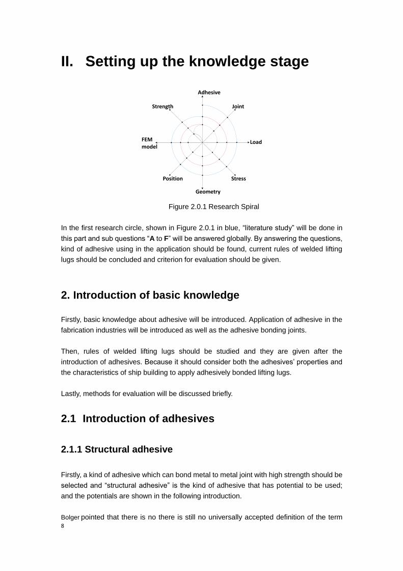
In the first research circle, shown in Figure 2.0.1 in blue, “literature study” will be done in
this part and sub questions “A to F” will be answered globally. By answering the questions,
kind of adhesive using in the application should be found, current rules of welded lifting
lugs should be concluded and criterion for evaluation should be given.
2. Introduction of basic knowledge
Firstly, basic knowledge about adhesive will be introduced. Application of adhesive in the
fabrication industries will be introduced as well as the adhesive bonding joints.
Then, rules of welded lifting lugs should be studied and they are given after the
introduction of adhesives. Because it should consider both the adhesives’ properties and
the characteristics of ship building to apply adhesively bonded lifting lugs.
Lastly, methods for evaluation will be discussed briefly.
2.1 Introduction of adhesives
2.1.1 Structural adhesive
Firstly, a kind of adhesive which can bond metal to metal joint with high strength should be
selected and “structural adhesive” is the kind of adhesive that has potential to be used;
and the potentials are shown in the following introduction.
Bolger pointed that there is no there is still no universally accepted definition of the term

9
"structural adhesive"; and he proposes the definition: thermosetting resin compositions
used to form permanent, load-bearing, joints between two rigid, high-strength,
adherends[6]
. The ASTM1 defines structural adhesive as: “a bonding agent used for
transferring required loads between adherends exposed to service environments typical
for the structure involved”. And the characteristics of structural adhesives are calculated
by Hartshorn[7]
in his book, and they are listed below.
1. High-strength adherends are involved (metal, wood, ceramic, reinforced plastic).
2. The adhesive is capable of transferring stress between the adherends without loss of
structural integrity, within the design limits for the bonded structure.
3. The bonded structure maintains integrity over long periods of time in typical service
environments.
Hartshorn studied the structures further and he listed the advantages and limitations of
structural adhesive bonding in his book and shown in table 2.1.1 [8]
.
Table 2.1.1 Advantages and limitations of structural adhesive bonding
Advantages limitations
1. Outstanding fatigue resistance.
2. Light-gauge materials may be joined.
3. Suitable for dissimilar materials.
4. Integrity of materials maintained.
5. Joints are completely sealed.
6. Only practical method for certain
applications.
7. Provides thermal and electrical
insulation.
8. Smooth surfaces obtained.
9. Can reduce manufacturing costs.
1. Joints must be designed to eliminate
peel and cleavage stresses.
2. Careful surface preparation often
required.
3. Performance may be degraded by
hostile environments.
4. Simple nondestructive test methods are
not available.
5. Limited high-temperature resistance.
6. Equipment costs can be high.
The research of Bolger and Hartshorn can show the potentials to apply structural
adhesives preliminary and the application of structural adhesives in fabrication industries
will explain the potential further.
Structural adhesives have been applied successfully within many sectors of industry, such
as automobile and aerospace industries [9]
, which have similar situation with ship building
industry for bonding metal components; and the application in those industries can
provide reasonable help and experiences for applying adhesively bonded lifting lugs.
For producing automobiles, adhesives with high strength were produced in 1990s and
they started to be used for bonding structure elements of automobiles [10]
. Firstly,
manufactures glued windscreens and rear windows; then components like front bonnet,
boot lid or roof were bonded with adhesives. In recently years, adhesive bonding plays a
more important role in automobile industry because multi-material design becomes
1 American Society for Testing and Materials

10
popular. R. D. Adams gives examples in his book, the new S-Class Coup6 of
DaimlerChrysler has more than 100 m of structural bonds in body in white applications; in
the “series 7 BMW” have more than 10 kg of structural adhesives applied.
In the aircraft industry, the application of adhesively bonding can date to the time in WW II;
“de Havilland” used epoxy adhesives to bond the wooden structures for warplane
“Mosquito” (Dan Gleich, 2002). This application fully proves that structural adhesives have
enough strength, even for weapons in the war; Figure 1.1.3 shows the warplane
“Mosquito”.
Figure 1.1.3 “de Havilland Mosquito war plane” (fennerschool [12]
)
The techniques for bonding aluminum was fully developed in 1950s and adhesive bonding
becomes the more favoring joining option because the development of composite
materials [13]
. Adhesive bonding joints are also used to bond components such as control
surfaces, tail structures and fuselages. Other aircraft companies such as “SAAB”, “Fokker”
and “Cessna” also used adhesive bonding in their aircraft widely; “SAAB” has made a type
of aircrafts using adhesive bonding with the properties of the structure cannot be achieved
with conventional riveted structures [14]
. The application of structural adhesives in
automobile industry and airplane industry can further prove that structural adhesive
bonding has great potential for bonding lifting lugs.
Weitzenbock showed some current application of structural adhesive in ship building,
such as “joining lightweight structures made of composite or aluminium to the steel hull [15]
”; the application shows that adhesive bonding make it possible to bond lifting lugs and
sections made of different materials. Weitzenbock also showed that adhesive bonding is
needed by the ship building industry in the future. He said that multi materials or
lightweight materials are required for joining to build ships such as “low energy ship”,
“green-fueled ship” and “The Arctic ship” which are needed in the future; and adhesive
bonding is relevant for the connecting of the materials used in those ships [16]
. So the
application of adhesively bonded lifting lugs can solve both the defects of the current
welded lifting lugs and it will also help build ships with new materials in the future.
Then the concentration moves to select specific structural adhesives that can be used in
the application. Based on the chemical composition, adhesives are separated as five
categories [17]
: Epoxy, Phenolic, Acrylic, Cyanoacrylate, and Urethane (or Polyurethane).
Their performances for bonding are concluded in table 2.1.2.
11
For bonding lifting lugs for ship sections in current ship building industry, the basic
requirement is that the adhesive should have high performance for bonding metal
substrates. According to this requirement, the Polyurethane adhesive and Cyanoacrylate
adhesive are excluded from the application.
Table 2.1.2 Performances of kinds of adhesives
Available bonding substrates
Epoxy Metal, glass, wood
Acrylic Metals, wood, organic glass
Polyurethane Wood
Cyanoacrylate Wood and medical
Phenolic Wood, metal, glass
Bouwman did further research on application of adhesives in shipbuilding [18]
. He tested
kinds of adhesives in the view of their appropriate substrates, strength and operation
conditions. In his test, an important factor is considered; that is the performance of
adhesives bonding substrates with premium painting. The results shows that the epoxy
adhesives are the most appropriate structural adhesives for bonding metal with or without
premium painting and the acrylic adhesive works a little worse but still acceptable.
Therefore, the adhesives used as specimen for calculation are selected from structural
epoxy adhesives and structural acrylic adhesives.
From main adhesive manufactures, two kinds of structural adhesives are selected as
specimen for calculation. They are “Epibond 100 A/B High-temperature Epoxy Structural
Adhesive [19]
” from Company Huntsman and “3M Scotch-Weld™ Acrylic Adhesives
DP8410NS Green [20]
” from Company 3M. Some basic data of their properties are shown
in table2.2.2.
Table 2.2.2 Properties of the two selected adhesives
Category Type Lap shear
strength for
bonding metal
Young’s
modulus
Poisson’s ratio
Epoxy Epibond 100 34.5 mpa 2178.7 mpa 0.22
Acrylic DP8410NS
Green
24.6 mpa 1301.5 mpa 0.3
2.1.2 Bonding joints
Adhesive bonding joints have been studied for a period of time and a certain number of
books and researches have introduced them. Adams and Wake [21]
and Straalen [22]
described kinds of adhesive bonding joints in detail. Hartshorn [23]
generalized bonding
joints into three main categorizes: “Butt joints”, “Lap joints” and “Scarf and Modified Joints”.

12
“Although the butt joint has a simple design, it is probably one of the least popular”, says in
Hartshorn’s research.
In butt joints, contact area of the adhesive and substrates are small and it is determined
by the cross-sectional area of the adherends; furthermore, butt joints will produce tensile
stress and peel stress in large values, which are the weak points of adhesively bonding
joint. Even increasing the area of the joint can increase the strength; the application for
carrying large mass ship sections is difficult. Therefore, butt joints will not be selected for
analyzing in the thesis.
Figure 2.1.1 Butt joint
Lap or overlap joints are the most common bonding type and there are many variations of
overlap joints, such as single lap joints and double lap joints.
Figure 2.1.2 A single lap and a double Lap joint
Single lap joint is the simplest type of overlap joint; stress concentration will occur in the
edges of the joints, however, by increasing the joints’ width and overlap length will make
the strength higher. Double lap joint is another useful type of lap joint. Comparing with
single lap joint, it can significantly decrease stress concentration and increase the
strength; but the application condition is more complicated. Both single lap and double lap
joints can have high strength for connection, so they should be options for the application.
Scarf joint is similar with lap joint in the connection form; both of them have overlap area in
the joint. However, scarf joint works better than lap joint; it is even regarded as the most
efficient joint design.
Figure 2.1.3 Scarf joint [24]
There are other types of joints design such as tapered, stepped and joggle lap joint, all of
them have improved performance, but the complicated shape makes them more difficult
to be applied for connecting lifting lugs.

13
To sum up, lap joints are the most appropriate types of joints for the lifting lugs connection
work in ship building. In the thesis, both single lap joints and double lap joints will be
analyzed for the application; and a serious of modification will be processed for the joints
contrary to the characteristics in ship building.
At last, other types of bonding joints are shown in Figure2.1.4. Some of them may be
feasible for some special conditions. The joints are concluded by Dan Gleich in the
research [25]
.
Figure 2.1.4 Kinds of bonding joints [25]
2.2 Introduction rules for welded lifting lugs
The rules for welded lifting lugs [26]
are provided by IHC ship yard; it describes critical
factors for welded lifting lugs in the lifting work in detail. The documents introduce rules in
two parts; the former part mainly talked about lifting lugs in lifting process and the turning
process is given in the second part. The basic requirements for lifting work, requirements
of lifting lugs’ strength and geometries and critical stress calculation are introduced in the

14
first part; in the second part, the load analysis and requirements for turning sections are
provided. All the requirements and precautions are concluded and listed in the following
parts.
I. Components in the lifting process
Components for lifting a section include steel cable, shackle, green pin and lifting lugs.
Steel cable is the link between crane and section, in the end near the section it is
connected with the shackle. The shackle connects the lifting lug with the green pin which
is a steel stick inserts through a hole (named “padeye”) on the lifting lug. The green pin
and the shackle’s sizes influence the dimensions of the lifting lug; the details will be given
later.
II. Classification for lifting lugs
The lifting lugs are classified into three categories according to the load they carry; the
categories are “less than 20ton”, “between 20ton and 30ton” and “more than 30ton”.
Except the difference in the dimensions, lifting lugs in each level have different
requirements for installation modes and positions, they are listed below:
A. Lifting lugs carrying load less than 20ton do not need to pierce the plate of the
structure
B. Lifting lugs carrying load from 20ton to 30ton need to pierce the plate, but can be
welded against a bulkhead or web frame
C. Lifting lugs carrying load more than 30ton must pierce the plate and need to be
integrated into the bulkhead or web frame
III. Position for installation
The positions for fixing lifting lugs should fulfill some requirements. As mentioned before,
kinds of components are used in the lifting process; when installing lifting lugs on sections,
there should be enough space for fixing lifting lugs and arranging the other components
that connected with lifting lugs. The arrangement of lifting lugs should also consider the
stabilities when the section is moving, which means the lifting lugs need to be bilateral
symmetry; it relates to the load calculation.
IV. Load calculation
The load on each lifting lug should be kept under the strength requirements, however,
loads on each lifting lug may not be separated averagely, their values depends on the
mass distribution of a section. The method to calculate the load is shown with an example
below.
Example:
The total load for lifting is given as 𝐹𝑡, the number of lifting lugs is set as 4 (the load on 2
lifting lugs in one symmetry side is 𝐹𝑡
2), and it is assumed that "𝐹1 = 𝐹3, 𝐹2 = 𝐹4". The load
on each lifting lug depends on the shape of the section and the position of the gravity
center.

15
�1
�2
�3
�4
�1 = �3,�2 = �4
�
�
�
Figure 2.1.1 A brief view for calculating loading in lifting
{𝐹1 ∙ 𝐿1 = 𝐹2 ∙ 𝐿2
𝐹1 + 𝐹2 =𝐹𝑡
2
(2.1.1)
{𝐹1 =
𝐹𝑡∙𝐿1
2(𝐿1+𝐿2)
𝐹2 =𝐹𝑡∙𝐿2
2(𝐿1+𝐿2)
(2.1.2)
V. Strength and shape of the lifting lug
The shape of a lifting lug depends on the load it bears and the dimensions of lifting
accessories it connects with; a lifting lug’s shape (the joint part is not in) is shown in
Figure2.1.2.
A
B
W
�2
�1
Figure 2.1.2 A brief view of the top part of a lifting lug
The hole in the lifting lug is used to assemble with a green pin; the green pin will be
inserted through the hole and connected with the shackle. The Diameter of the hole in a
lifting lug is generally 3mm larger than the Diameter of the green pin. The green pin’s

16
radius is set as “r”, and then the diameter of the hole on the lifting lug will be:
𝑅1 = 𝑟 + 1.5 (𝑚𝑚) (2.1.3)
The radius of the lifting lug is influenced by the radius of the hole, the thickness of the
lifting lug and the load. The requirement is the stress in the area (perpendicular to the
shown surface in Figure 2.1.2) above the top point of the “pad eye” should be smaller than
1ton 𝑐𝑚2.
If the load is set as “T ton”, then the area (perpendicular to the shown surface in Figure
2.1.2) above the top point isT
1ton
𝑐𝑚2 = T 𝑐𝑚2. And if the thickness of the lifting lug is set as “t”,
then the height above the top point isA = T t, so the radius of the lifting lug
𝑅2 = 𝑅1 + 𝐴 (2.1.4)
The width of the lifting lug is twice as the radius of the semi-circle in the top, that is:
W = 𝑅2 (2.1.5)
The height above the bottom board and the circle of the hole is influenced by the width of
the lifting lug. It is:
B = W + 50(𝑚𝑚) (2.1.6)
The area of the cross section is also required; the stress in the area cannot be larger
than1𝑐𝑚2 𝑡𝑜𝑛. So t × W ≥ T 1𝑐𝑚2 𝑡𝑜𝑛.
VI. Stress and strength of the joint
There are two kinds of welding joints introduced in the rules, butt welding joint and lap
welding joint. For a welded lifting lug with a butt welding joint, the bending stress and a
composite stress (formed by a bending stress and a shear stress) are required. The
maximum bending stress should be smaller than 2.4 ton/𝑐𝑚2 and the composite stress
should be smaller than 1.2 ton/𝑐𝑚2. An example of a butt welded lifting lug is used to show
critical stresses and the calculation methods.
W
B
T
W
t
Figure 2.1.3 A brief of a welded lifting lug with butt joint
As shown in Figure2.1.3, the lifting lug is welded on the side surface of a section with a
butt welding joint, the load “T” acts on the lifting lug in vertical direction. Therefore, in the

17
joint there will be shear stress and normal stress caused by a bending moment. The
normal stress is calculated firstly.
The bending moment𝑀𝑏𝑒𝑛𝑑𝑖𝑛𝑔:
𝑀𝑏𝑒𝑛𝑑𝑖𝑛𝑔 = T × B (2.1.7)
The moment of resistance𝑀𝑟𝑒𝑠𝑖𝑠𝑡𝑎𝑛𝑐𝑒:
𝑀𝑟𝑒𝑠𝑖𝑠𝑡𝑎𝑛𝑐𝑒 =1
6× 𝑡 ×𝑊2 (2.1.8)
Then the maximum bending stress 𝜎𝑚𝑎𝑥is:
𝜎𝑚𝑎𝑥 =𝑀𝑏𝑒𝑛𝑑𝑖𝑛𝑔
𝑀𝑟𝑒𝑠𝑖𝑠𝑡𝑎𝑛𝑐𝑒=
T×B1
6×𝑡×𝑊2
(2.1.9)
Then the shear stress is calculated and it is used to calculate a composite stress which is
used to judge the strength of the joint.
The shear stress τ:
τ =𝑇
𝐴=
𝑇
𝑊×𝑡 (2.1.10)
“A” is the area of the cross section of the lifting lug
Then the composite stress δ:
δ = √𝜎𝑚𝑎𝑥2 + 𝜏2 (2.1.11)
Then turns to the lap welded lifting lug; Figure2.1.4 shows a welded lifting lug with lap
joint.
W
H
L
L
�0
T
Figure 2.1.4 A brief view of a welded lifting lug with lap joint
In a lap welding joint, the shear stress is required. The width of the welded seam is “d” per
side and the length is “H”; so the welding area per side 𝐴0 is: 𝐴0 = 𝐻 × 𝑑
The load on the lifting lug is “T”, and then the shear stress per side is :
𝜏0 =𝑇 2⁄
𝐴0=
𝑇
2×𝐻×𝑑 (2.1.12)

18
The shear stress should be less than 1ton/𝑐𝑚2.
There is also a requirement for the width of the lifting lug. When the lifting lug is lap welded
on the plate of a section, the stress transfers from the top of the welding seam with an
angle of �0 till the end creating a distance “L” per side. The stress acts on the line is
required and it should be less than 1ton/𝑐𝑚2. If the thickness of the plate is defined as “𝑡𝑏”,
the stress “𝜎𝑏” is:
𝜎𝑏 =𝑇
(0.577×𝐻×2+𝑊)×𝑡𝑏 (2.1.13)
And 𝜎𝑏 should be less than 1ton/𝑐𝑚2.
2.3 Discussing evaluation methods
In the research, evaluation needs to be processed to discover defects of the adapted rules
for applying adhesively bonded lifting lugs and check the feasibility of the specific
application after improvements; therefore, criterion and methods for evaluation should be
given.
Same with rules of welded lifting lugs, the strength of adhesive bonding joints is used as
the criterion for evaluation; when an adhesively bonded lifting lug is carrying load, the
stress in the bonding joint should be no more than the strength of the bonding joint can
provide. The strength of the bonding joint relates to adhesives’ properties in specific kinds
of bonding joints. In the research lap joints are used; so the adhesives’ overlap strength
and strength in the normal direction should be used as the criterion. Shear stress and
normal stress need to be calculated.
The stress can be calculated from two ways; one is test and the other is FEM simulation.
Bouwman introduced tests for measuring strength of adhesive bonding joints in the
research [27]
; which can be also used for measuring stress in bonding joints. This method
needs severe requirements for laboratory equipment and specimens which are hard to be
processed in the current situation; so FEM simulation should be the evaluation method
used in the research. In the FEM simulation, models are built based on the specimens and
simulated with the same situation in the real-life. By using FEM simulation software, the
needed results, such as stress, can be read. FEM simulation have been used and
discussed in lot of research about adhesive bonding joints, such as Yuping Yang’s
research [28]
about “Composite-to-Steel Adhesive Joints” and Dan Gleich’s research [29]
about “Structural Bonded Joints”. For the selection of specific FEM software, it will be
given in Chapter 5.

19
2.4 Summary and finding
2.4.1 Summary
Sub questions A to F (listed below) can now be answered globally.
A. What kinds of adhesives will be feasible for bonding lifting lugs?
Epoxy structural adhesives and Acrylic structural adhesives are selected for bonding
adhesively bonded lifting lugs; Epoxy adhesives “Epibond 100” and Acrylic adhesives
“DP8410NS Green” are selected as specimens in the research.
B. What types of bonding joints can be used?
Lap joints, contains both single lap joints and double lap joints are selected as the joints’
type in the application; but which ones performs better will be analyzed in the following
parts.
C. How to define the shape and geometrical attribute of lifting lugs? D. What is the
state of stress of the bonding joint with load? E. Where is the optimal position for
installing lifting lugs?
Rules of welded lifting lugs are introduced in the 2.2; shape and geometry of lifting lugs,
load, stress and positions for installation are introduced. The rules can be concluded in six
aspects shown below.
1.Components in the lifting process
4.Load calculation
5.Strength and shape of the lifting lug
2.Classification for lifting lugs
3.Positions for installation Adaptation of
Rules
6. Strength and stress of the joint
F. How to evaluate the feasibility of the application?
The strength of the adhesive bonding joint is used as the criterion for the evaluation and to
make the application feasible the stress in the joint should be no more than the strength.
FEM simulation is used as the method to calculate the needed stress.
2.4.2 Finding
The strength of adhesives is used for the adaptation and evaluation, such as defining the
original dimensions of lifting lugs and checking whether a bonded lifting lug is feasible for
20
application; so the strength should be given. In the research, the focus is put on shear
strength and normal strength regarding to the characteristics of lifting lugs’ fixing type. It is
found that in a data sheet provided by an adhesive manufacture, shear strength is easily
got but it is hard to get information of normal strength. So a method to calculate the normal
strength should be defined.
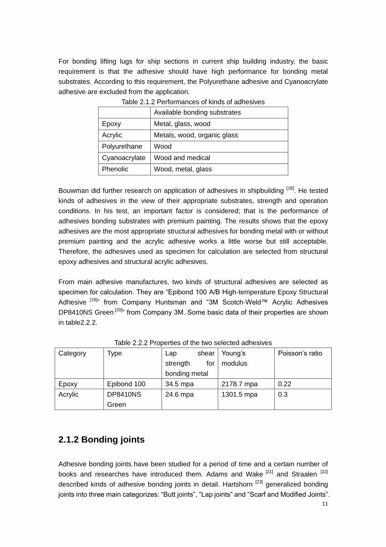
Before calculating the normal strength, the method to define shear strength is introduced.
For lap joints with two metal substrates, the shear strength of an adhesive is got from a
test named “ASTM D1002”. In the test, specimens are tested on a “tensile testing machine”
which is shown in Figure 2.3.1. The specimen is pulled from its two sides by the tensile
testing machine; and when the specimen is broken, the force is recorded and defined as
breaking load. Then the break load is divided by the value of the bonding area, the result
is the shears strength of the adhesive. And the data provided by the manufactures are
usually measured from this test.
Figure2.3.1. A tensile testing machine and a specimen (ADMET [30]
)
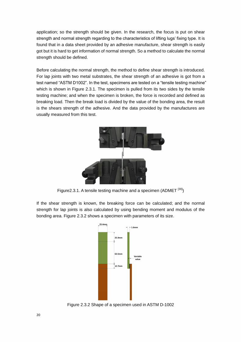
If the shear strength is known, the breaking force can be calculated; and the normal
strength for lap joints is also calculated by using bending moment and modulus of the
bonding area. Figure 2.3.2 shows a specimen with parameters of its size.
25.4mm
25.4mm
63.5mm
12.7mm
1.6mm
Variable value
Figure 2.3.2 Shape of a specimen used in ASTM D-1002
21
All the dimensions of a specimen is ruled in “ASTM D1002” data sheet [31]
; while the
thickness of the bonding layer can be a variable value and in the theoretical calculation it
is set as a very small value which can be neglected in the calculation; and the thickness of
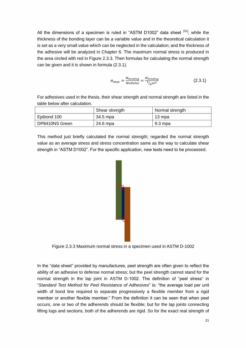
the adhesive will be analyzed in Chapter 6. The maximum normal stress is produced in
the area circled with red in Figure 2.3.3. Then formulas for calculating the normal strength
can be given and it is shown in formula (2.3.1).
σ𝑚𝑎𝑥 =𝑀𝑏𝑒𝑛𝑑𝑖𝑛𝑔
𝑀𝑜𝑑𝑢𝑙𝑢𝑠=
𝑀𝑏𝑒𝑛𝑑𝑖𝑛𝑔
16⁄ 𝑤𝑙2
(2.3.1)
For adhesives used in the thesis, their shear strength and normal strength are listed in the
table below after calculation.
Shear strength Normal strength
Epibond 100 34.5 mpa 13 mpa
DP8410NS Green 24.6 mpa 9.3 mpa
This method just briefly calculated the normal strength; regarded the normal strength
value as an average stress and stress concentration same as the way to calculate shear
strength in “ASTM D1002”. For the specific application, new tests need to be processed.
Figure 2.3.3 Maximum normal stress in a specimen used in ASTM D-1002
In the “data sheet” provided by manufactures, peel strength are often given to reflect the
ability of an adhesive to defense normal stress; but the peel strength cannot stand for the
normal strength in the lap joint in ASTM D-1002. The definition of “peel stress” in
“Standard Test Method for Peel Resistance of Adhesives” is: “the average load per unit
width of bond line required to separate progressively a flexible member from a rigid
member or another flexible member.” From the definition it can be seen that when peel
occurs, one or two of the adherends should be flexible; but for the lap joints connecting
lifting lugs and sections, both of the adherends are rigid. So for the exact real strength of

22
adhesives, some tests like ASTM D-1002 need to be processed, and the tests should be
more close to the real condition. Bouwman (2011) did a serious of this kind of tests in his
research and he got some reasonable data for some adhesives’ performance. Therefore,
in the future research the tests for measuring adhesives’ strength can use both theoretical
calculation like ASTM D-1002 or tests same as Bouwman did.
23
III. Adaptation rules and Evaluation
Strength
Adhesive
Joint
Load
Stress
Geometry
Position
FEM model
Figure 3.0.1 Research Spiral
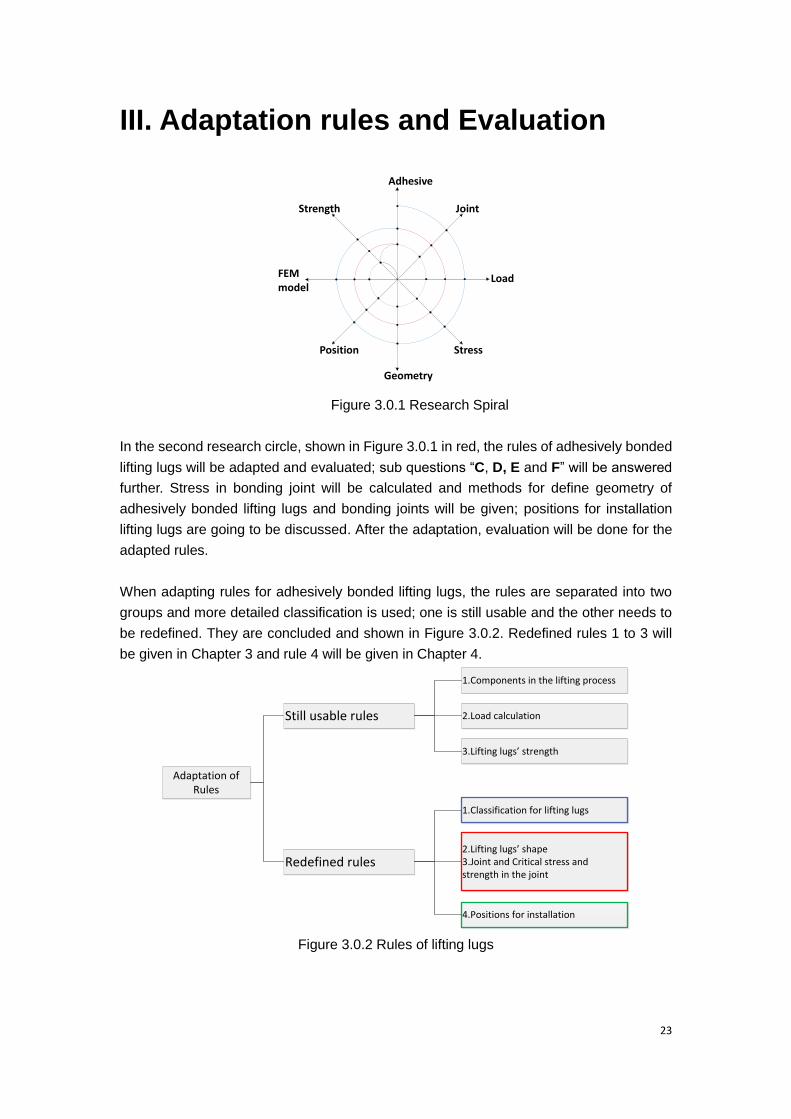
In the second research circle, shown in Figure 3.0.1 in red, the rules of adhesively bonded
lifting lugs will be adapted and evaluated; sub questions “C, D, E and F” will be answered
further. Stress in bonding joint will be calculated and methods for define geometry of
adhesively bonded lifting lugs and bonding joints will be given; positions for installation
lifting lugs are going to be discussed. After the adaptation, evaluation will be done for the
adapted rules.
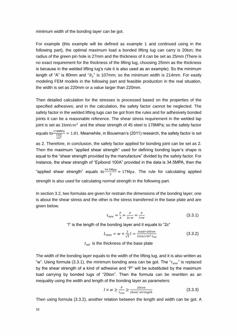
When adapting rules for adhesively bonded lifting lugs, the rules are separated into two
groups and more detailed classification is used; one is still usable and the other needs to
be redefined. They are concluded and shown in Figure 3.0.2. Redefined rules 1 to 3 will
be given in Chapter 3 and rule 4 will be given in Chapter 4.
1.Components in the lifting process
2.Load calculation
3.Lifting lugs’ strength
Still usable rules
1.Classification for lifting lugs
2.Lifting lugs’ shape3.Joint and Critical stress and strength in the joint
4.Positions for installation
Redefined rules
Adaptation of Rules
Figure 3.0.2 Rules of lifting lugs

24
3. Adaptation: Dimensions definition and stress
calculation
This chapter aims to translate the rules for welded lifting lugs to rules for adhesively
bonded lifting lugs; such as define preliminary shape and dimensions of lifting lugs and
bonding layers. Firstly, the shape and dimensions of lifting lugs are given; and then the
concentration is moved to the bonding joints. Secondly, the stress in the bonding layer is
going to be calculated with theoretical formulas. At last, the method to define the shape
and dimensions of the bonding layer will be given.
3.1 Classification and Load analysis
In the rules of welded lifting lugs, lifting lugs carrying load more than 20ton need to be
inserted into the structures when they are installed; while those carrying load less than
20ton are not required. So lifting lugs carry load less than 20ton are able to use adhesive
bonding for installation. For lifting lugs carry load between 20ton and 30ton, to avoid
damaging the section, they can only be used when no plate is above the installation
structures; the application of adhesively bonded lifting lugs is further limited. For lifting
lugs carrying load above 30ton, they need to pierce the plate and be integrated with the
structures for installation; which means adhesive bonding cannot be used for their
installation. So 20ton is defined as the optimal load for applying adhesively bonded lifting
lugs and the thesis will concentrate on lifting lugs with capacity less than 20ton; lifting lugs
with capacity from 20ton to 30ton are not ideal for using adhesive bonding joints and less
attention is paid on them in the research.
Except load, the adhesively bonded lifting lugs can be classified according to the bonding
joint, “single lap joint” and “double lap joint”; and the classification is shown below.
Carrying load less than 20ton
Carrying load between 20ton and 30ton (Constrained for application)
Adhesively bonded lifting lugs(Classified by load)
Single lap lifting lugs
Double lap lifting lugs
Adhesively bonded lifting lugs(Classified by bonding joint)
The method for calculating load on adhesively bonded lifting lugs is the same with that for
welded lifting lugs which is given in Chapter 2; but there is something should be taken

25
attention. For welded lifting lugs, the essential is calculating load they carrying on; while
for adhesively bonded lifting lugs, the essential should be changed to control the load on
each lifting lug under the requirement (optimal maximum load: 20ton, maximum load with
constrains: 30ton). For example, if a section uses 4 adhesively bonded lifting lugs in the
lifting process, and the structures for installation have plates on them. If the whole mass of
the section is set as 80ton, so each lifting lug carry no more than 20ton load and the 80
ton load must be distributed to every lifting lug averagely. The discussion for the
positioning will be discussed in the chapter 4.
Because the poor performance for defensing normal stress of bonded lap joints, the
direction of the load should be kept vertical to the ground and parallel with the adhesive
layer to avoid producing normal stress. In the real-life situation, when ship sections are
transported, the steel cables are difficultly to be kept vertical and angle exists between the
steel cable and the vertical line; and the direction of the load changes with the steel cable
which causes extra normal stress or torque. Figure 3.1.1 shows the situation.
Vertical line
Steel cable
Steel cable
Vertical line
Steel cable
Steel cable
Figure 3.1.1 Situations of load directions in the transportation process
The situations shown above should be avoided in the building process. To ensure the
strength of the bonding joints when the situation happens, safety factor are used in the
stress calculation and lifting lugs design process; the safety factor is talked in 3.3 in this
chapter. In the research, steel cables on lifting lugs are hypothesized vertical to the
ground to stand for the ideal situation.
3.2 Stress calculation
3.2.1 Failure mode introduction
Figuring out the failure modes in a lap joint is necessary because it prevents wrong
application and operation; and it is discussed in this part. A basic adhesively bonded
single lap joint is composed by two adherends and an adhesive bonding layer, Figure3.2.1
shows the composition of a lap joint with the names of parts mentioned in the introduction

26
of failure modes.
Substrate’s surface
Substrate/Adherend
Adhesive bonding layer
Figure 3.2.1 components in a bonded lap joint
The failures occur in a bonded lap joint happen in three places, the adherends, the
bonding layer and the substrates. The failure modes for adhesively bonded joints are
calculated in researches and Hartshorn’s (1986) concluded three basic failure modes [32]
in his book: “adhesive failure” “cohesive failure” and “substrate failure”. They are defined
as:
“Cohesive failure” occurs when the specimen fails within the adhesive layer;
“Adhesive failure” occurs when the specimen fails at the interface between the adhesive
and adherend;
“Substrate failure”: refers to the damages appearing in the substrate or adherend.
Figure3.2.2 explains how the failures occur in adhesive bonding joints. These three kinds
of failure modes are also used by manufactures for giving the properties of adhesives in
data sheets. In the research, the “substrate failure” is about the strength of lifting lugs
which is introduced in Chapter 2; while “cohesive failure” and “adhesive failure” are about
the adhesive bonding layer which are the concentration in this chapter.
Figure3.2.2 Failure modes in bonded lap joints (SubsTech
[33])
Bouwman (2011) gave the differences between “Cohesive failure” and “Adhesive failure”
in detail in his research [34]
and Figure3.2.3 shows it.

27
Figure3.2.3 Failure modes in tests [34]
Therefore, combining with the characteristics of a lap bonding joint, the critical stresses
can be pointed: the shear stress in the adhesive layer and the interface between substrate
and adhesive layer, the normal stress in the adhesive layer and the interface between
substrate and adhesive layer. These stresses are going to be analyzed in the following
part.
3.2.2 Theoretical calculation of stresses in bonding joints
Shear stress and normal stress in the bonding joint are the stresses need to be calculated
in the application. And for lap joints, shear stress should be taken attention in the first
place; then is the normal stress. Figure3.2.4 shows a single lap bonding joint with
dimensions used for calculating shear and normal stresses.
�
�
Figure 3.2.4 A Lap joint with dimensions
For the average shear stress in a lap bonded joint, the formula for calculating can be given
as:
𝜏𝑎𝑣𝑒 =𝑃
𝐴=
𝑃
2𝑐∙𝑤 (3.2.1)
P-the load acts on the joint
A-the bonding layer’s area
2c-length of the bonding layer
w-width of the bonding layer
𝜏𝑎𝑣𝑒-the average shear stress
But in this formula, the result only shows the average stress which cannot reflect the real

28
situation of an adhesively bonded lap joint; because the uniform distribution shear stress
occurs only when the adherends are rigid and the adhesive deforms only in shear [35]
. For
the real distribution of shear stress in a bonded lap joint, both Hartshorn (1986) and
Adams gave their views; the difference between their views is the decrease speed of the
stress from the edge to the middle, but they both believed that stress concentration occurs
in the edge of the bonding layer [36]
.
To calculate the value of the stress concentration, stress concentration factor n is used to
explain the relationship between the maximum stress 𝜏𝑚𝑎𝑥 and the average shear
stress 𝜏𝑎𝑣𝑒.
𝜏𝑚𝑎𝑥 = n ∙ 𝜏𝑎𝑣𝑒 (3.2.2)
𝜏𝑚𝑎𝑥- maximum stress in the bonding layer
n-stress concentration factor
In the calculation of the stress concentration factor, “Volkersen’s theory ” and “Goland and
Reissner’s (1944) theory” are recognized; both Hartshorn and Adams used their theory in
their books. “Volkersen’s theory” does not consider the bending of the adherends from the
eccentricity of the loading path, so “predictions based on Volkersen's work is more valid
for double-lap joints where bending is minimized [37]
(Hartshorn, 1986)”. Volkersen’s work
of stress concentration factor is shown below.
n =𝜏𝑚𝑎𝑥
𝜏=
𝛿(2 2−1+cosh2 𝛿
sinh2 𝛿) (3.2.3)
𝜏𝑚𝑎𝑥 = n ∙ τ =𝛿(2 2−1+cosh2 𝛿
sinh2 𝛿) ∙ 𝜏 (3.2.4)
δ and ε are factors which are calculated in formulas(3.2.5)and (3.2.6).
δ2 =2𝑐2𝐺𝑎
𝐸𝑠2𝑡𝑠2𝑡𝑎 (3.2.5)
ε2 =𝐸𝑠1𝑡𝑠1+𝐸𝑠2+𝑡𝑠2
2𝐸𝑠1𝑡𝑠1 (3.2.6)
𝑡𝑠1 and 𝑡𝑠2- the thickness of the two adherends
𝑡𝑎- the thickness of the bonding layer
𝐸𝑠1 and 𝐸𝑠2- the Young’s modulus of the two adherends
𝐺𝑎- the shear modulus of the adhesive
While Goland and Reissner considered bending in their work, and the results are given
as:
n =𝜏𝑚𝑎𝑥
𝜏=
1+3𝐾
4(𝛽𝑐
𝑡𝑠cosh
𝛽𝑐
𝑡𝑠) +
3
4(1 − 𝐾) (3.2.7)
𝜏𝑚𝑎𝑥 = τ ∙ [1+3𝐾
4(𝛽𝑐
𝑡𝑠cosh
𝛽𝑐
𝑡𝑠) +
3
4(1 − 𝐾)] (3.2.8)
β, K, 𝑢1 and 𝑢2 are factors and they are listed in formulas (3.2.9) to (3.2.12).
β = √ (𝐺𝑎𝑡𝑠
𝐸𝑠𝑡𝑎)12⁄ (3.2.9)

29
K =cosh𝑢2𝑐 sinh𝑢1𝑙
sinh𝑢1𝑙 cosh𝑢2𝑐+2√2cosh𝑢1𝑙 sinh𝑢2𝑐 (3.2.10)
𝑢1 =2
𝑡𝑠[�(1 − 𝜈2)
𝑃
𝐸𝑠𝑡𝑠]12⁄ (3.2.11)
𝑢2 =√2
4𝑢1 (3.2.12)
𝜈- the Poisson’s’s ratio of the adhesive
For the normal stress in a single lap joint, the simplified calculation of maximum normal
stress can use the formula same with the welded joint, they are shown below:
𝜎0 =𝑀𝑏𝑒𝑛𝑑𝑖𝑛𝑔
𝐼𝑅=
(𝑡𝑠2+𝑡1)×𝑃
1
6𝑊×(2𝑐)2
(3.2.13)
In Goland and Reissner’s theory, the normal stress is got in the process when they
calculated the stress concentration factor, it is shown in formula.
σ =𝑃𝑡𝑠𝑐2
[(𝑅2𝜆2𝐾
+ 𝜆𝐾′ cosh𝜆 cos 𝜆) cosh 𝜆
𝑥
𝑐cos 𝜆
𝑥
𝑐
+ (𝑅1𝜆2𝐾
+ 𝜆𝐾′ sinh𝜆 sin 𝜆) sinh𝜆
𝑥
𝑐sin 𝜆
𝑥
𝑐]
(3.2.14)
For lap joints, the calculation for normal stress contains more factors and more steps than
the calculation for shear stress; and the formulas are more appropriate for calculating
regular lap joint specimens. In the real application, the situation will become more
complicated such as the shape of lap joint becomes irregular and the properties of
adherends may not the same; therefore, calculating theoretical normal stress becomes
difficult based on the pure formula. However, the theory for calculating normal stress
“using bending moment” and “modulus” is used again for calculating the normal stress
and the next part (3.3, chapter 3) will show the method in detail.
In conclusion for the stresses calculation for bonded lap joints:
In the shear direction, “Goland and Reissner’s theory” is used for single lap joints and
“Volkersen’s theory” theory is used for double lap joints to calculate the stress
concentration factor. And in the normal direction, the situation becomes more complicated
and the theoretical calculation formulas are hard to be applied and the results may
become unreliable; the calculation formulas provided in the rules of welded lifting lugs are
used as a primary method. To get the exact results, using software to do FEM simulation
is a good method; and in the FEM software the distribution of the stresses can be shown
as well. So FEM simulation is chosen as the method to measure the stress in the bonding
joint and it is talked in Chapter 5 of the thesis.

30
3.3 Designing lifting lugs and Define original
dimensions
3.3.1 Selecting installation type
Firstly in the design of adhesively bonded lifting lugs is to ensure the installation type. As
lap joints are decided to be used for the application, several plans arranging lifting lugs are
provided and they are shown in Figure3.3.1.
Plan 1
Plan 2
Plan 3
Plan 4
Figure 3.3.1 pictures of different lap bonding plans
The plans given above all have potentials to be applied for the lifting lugs installation, but
the lifting lugs’ design should be processed based on the lap joints’ properties; so some of
them should be abandoned. Bouwman (2011), Hartshron (1986) and also Adams(1984)
said in their researches, the lap joints design should avoid peel and cleavage stress to
increase the strength of the joint; Bouwman also gave a picture for explain it.

31
Figure 3.3.2 Types should be avoided and applied for bonded joints (Bouwman 2011)
Based on the view given by the authors, the first plan should be canceled, because
cleavage stress is created. Then comparing with the last three plans, the second plan will
have a shear stress in the vertical direction and another stress caused by a bending
moment in horizontal direction; while the third and fourth plan only have shear stress in
the perpendicular direction. And normal stress in the horizontal direction perpendicular to
the adhesive layer exists in all plans. Therefore the second plan’s strength is lower than
the third and fourth; the third and fourth plan will be chosen for the lifting work during the
production process. Actually, the second plan is a transformation of the third plan which
can be used in the turning process; and it will be analyzed in the chapter about turning
process.
3.3.2 Define Dimensions
The first thing for design a bonded lifting lug is to guarantee the lifting lug’s strength for its
self; which means the lifting lug should not be broken under the maximum load it can carry.
This problem mainly relates to the area above the pad eye in the lifting lug which is talked
in 2.1.1, chapter 2; Figure 3.3.3 shows a lifting lug in the front view and the dimensions of
it has been talked in 2.1, Chapter 2.
A
B
W
�2
�1
Figure 3.3.3 Top part of a single lap lifting lug
In the requirement, the stress in the area (perpendicular to the papaer) above the hole for
inserting the green pin must be smaller than 1ton/𝑐𝑚2; so when the thickness is given, a
32
minimum width of the bonding layer can be got.
For example (this example will be defined as example 1 and continued using in the
following part), the optimal maximum load a bonded lifting lug can carry is 20ton; the
radius of the green pin hole is 27mm and the thickness of it can be set as 25mm (There is
no exact requirement for the thickness of the lifting lug, choosing 25mm as the thickness
is because in the welded lifting lug’s rule it is also used as an example). So the minimum
length of “A” is 80mm and “𝑅2” is 107mm; so the minimum width is 214mm. For easily
modeling FEM models in the following part and feasible production in the real situation,
the width is set as 220mm or a value larger than 220mm.
Then detailed calculation for the stresses is processed based on the properties of the
specified adhesives; and in the calculation, the safety factor cannot be neglected. The
safety factor in the welded lifting lugs can be got from the rules and for adhesively bonded
joints it can be a reasonable reference. The shear stress requirement in the welded lap
joint is set as 1ton/𝑐𝑚2 and the shear strength of 45 steel is 178MPa; so the safety factor
equals to178MPa
1ton
𝑐𝑚2
= 1.81. Meanwhile, in Bouwman’s (2011) research, the safety factor is set
as 2. Therefore, in conclusion, the safety factor applied for bonding joint can be set as 2.
Then the maximum “applied shear strength” used for defining bonding layer’s shape is
equal to the “shear strength provided by the manufacture” divided by the safety factor. For
instance, the shear strength of “Epibond 100A” provided in the data is 34.5MPA, then the
“applied shear strength” equals to34.5Mpa
2≈ 17Mpa . The rule for calculating applied
strength is also used for calculating normal strength in the following part.
In section 3.2, two formulas are given for restrain the dimensions of the bonding layer; one
is about the shear stress and the other is the stress transferred in the base plate and are
given below.
𝜏𝑎𝑣𝑒 =𝑃
𝐴=
𝑃
2𝑐∙𝑤=
𝑃
𝑙×𝑤 (3.3.1)
“l” is the length of the bonding layer and it equals to “2c”
𝐿𝑚𝑖𝑛 = 𝑤 +2
√3𝑙 =
𝑙𝑜𝑎𝑑=20𝑡𝑜𝑛
1𝑡𝑜𝑛 𝑐𝑚2∙𝑡𝑎𝑑 (3.3.2)
𝑡𝑎𝑑 is the thickness of the base plate
The width of the bonding layer equals to the width of the lifting lug, and it is also written as
“w”. Using formula (3.3.1), the minimum bonding area can be got. The “𝜏𝑎𝑣𝑒” is replaced
by the shear strength of a kind of adhesive and “P” will be substituted by the maximum
load carrying by bonded lugs of “20ton”. Then the formula can be rewritten as an
inequality using the width and length of the bonding layer as parameters:
𝑙 × 𝑤 ≥𝑃
𝜏𝑎𝑣𝑒≥
20𝑡𝑜𝑛
𝑠ℎ𝑒𝑎𝑟 𝑠𝑡𝑟𝑒𝑛𝑔𝑡ℎ (3.3.3)
Then using formula (3.3.2), another relation between the length and width can be got. A

33
new inequality is given below:
𝑤 +2
√3𝑙 ≥
𝑙𝑜𝑎𝑑=20𝑡𝑜𝑛
1𝑡𝑜𝑛 𝑐𝑚2∙𝑡𝑎𝑑 (3.3.4)
Using inequalities (3.3.3) and (3.3.4), a smaller range for measuring the shape of the
bonding layer can be got; and example is shown below.
Continue using the example 1 given in PART A, even there is no parameter that has been
given will influence inequalities (3.3.3) and (3.3.4). The “Epibond 100” epoxy adhesive is
chosen for calculating and the applied shear strength after dealing with safety factor is
defined as 17mpa; and the thickness of base plate is defined a 8mm (the thickness can be
adjusted according to the real situation). Then new inequalities for the example are given:
𝑙 × 𝑤 ≥𝑃
𝜏𝑎𝑣𝑒≥
20𝑡𝑜𝑛
17𝑚𝑝𝑎= 11765𝑚𝑚2 (3.3.5)
𝑤 +2
√3𝑙 ≥
𝑙𝑜𝑎𝑑=20𝑡𝑜𝑛1𝑡𝑜𝑛
𝑐𝑚2 ∙8𝑚𝑚= 50𝑚𝑚 (3.3.6)
Thirdly, for the normal stress, the theoretical calculation method is two complicated and it
needs to define other unknown parameters in the formula; that causes it is not suitable for
restricting the bonding layer’s dimensions. While, for general calculation, it can refer the
method using in the welded lifting lug’s rule-using “bending moment” and “modulus (Dutch:
weerstands moment tegen buiging)”. Figure3.3.4 shows the parameters for calculation.
Arm
Figure3.3.4. Shape for calculating normal stress
Then the calculations for them are given:
𝑀𝑏𝑒𝑛𝑑𝑖𝑛𝑔 = 𝑃 × 𝑎𝑟𝑚 (3.3.7)
𝑎𝑟𝑚 = 0.5𝑡ℎ𝑖𝑐𝑘𝑛𝑒𝑠𝑠 + 𝑏𝑜𝑛𝑑𝑖𝑛𝑔 𝑙𝑎𝑦𝑒𝑟 𝑡ℎ𝑖𝑐𝑘𝑛𝑒𝑠𝑠 (3.3.8)
Modulus =1
6× 𝑤 × 𝑙2 (3.3.9)
𝜎𝑚𝑎𝑥 =𝑀𝑏𝑒𝑛𝑑𝑖𝑛𝑔
Modulus=
𝑃×𝑎𝑟𝑚1
6×𝑤×𝑙2
(3.3.10)

34
𝜎𝑚𝑎𝑥 is the normal stress, it can also stand for the normal strength
Transferring formula (3.3.9) to an inequality to restrict the shape, the new inequality can
be got and shown below.
𝑤 × 𝑙2 ≥𝑃×𝑎𝑟𝑚
1
6×𝑛𝑜𝑟𝑚𝑎𝑙 𝑠𝑡𝑟𝑒𝑛𝑔𝑡ℎ
(3.3.11)
Then use inequality (3.3.11) in example 1. The normal strength of “Epibond 100” epoxy
adhesive is 6.5mpa; the thickness of the bonding layer is set as 1mm. A new inequality
with the given parameters can be given:
𝑤 × 𝑙2 ≥20ton×(12.5mm+1mm)
1
6×6.5mpa
= 49 �07𝑚𝑚3 (3.3.12)
3.3.3 Sub conclusion
With inequalities (3.3.3), (3.3.4) and (3.3.11), using width “w” and length “l” as axis of a
coordinate, three curves can be drawn to give a range for defining shape. And the rules for
measuring the minimum width can also be seen as a restricting condition and the
description in inequality is:
𝑤 ≥ 𝑅2𝑚𝑖𝑛 (3.3.13)
And in example 1 it is:
𝑤 ≥ 14mm (3.3.14)
If maximum values of the width and length are ruled based on the feasible fixing position
can provide, the range for defining the bonding layer’s dimensions can be got.
Then moving to example 1, if the feasible position can provide 400mm×400mm area, and
using inequalities (3.3.5),( 3.3.6),( 3.3.12) and (3.3.14), a range is got; shown in Figure
3.3.5 (a).
�+
√ ≥
= �
� ∙
=
�(mm)
(mm)
� ≥
�× ≥
× ( . + )
× .
=
×� ≥
≥
�
=
Figure3.3.5 (a) Range in a coordinate for defining dimension with 20ton load
So the width and length of the bonding layer can be chosen from the shadowed area in
the coordinate shown in the Figure 3.3.5 (a). For the example 1, the final width is chosen
as 220mm, and the length is 330mm. The shape is set bigger than the theoretical one for
against the stress concentration, so the length is chosen much bigger than the theoretical.
Figure 3.3.5 (b) shows the coordinate for defining dimension when the load increases to
30ton; the area for available value becomes smaller.

35
�× ≥
× ( . + )
× .
=
×� ≥
≥
�
=
�+
√ ≥
= �
� ∙
=
�(mm)
(mm)
� ≥
Figure3.3.5 (b) Range in a coordinate for defining dimension with 30ton load
In example 1, all the basic dimensions are guaranteed; and two fillets are set to decrease
the stress concentration in the two bottom corners, as the radius of the fillets, it is
analyzed in chapter 6, and it is set as 50mm firstly. Figure3.3.6 shows the basic design of
a single lap bonded lifting lug, in the following part it will be modified if defects appear or
the performance cannot fulfill the requirements.
w
�
B
l
l
w
t
Bonding layer
Front view
Side view
Figure3.3.6. A single lap lifting and its dimensions

36
So the final dimension for the basic single lap is given as:
Width: w=220mm
Length of bonding layer: l=330mm
Length: L=l+B+R2=330+160+110=600mm
Thickness: t=25mm
Radius of each fillet: 𝑟𝑓 = 50𝑚𝑚
This example of basic single lap lifting lug model will be used as an original model for
setting FEM model in following parts, monitoring the stress distribution, value and stress
concentration in the bonding layer.
3.3.4 Double lap lifting lugs dimensioning
For double lap lifting lugs, the thought for define bonding layer’s dimensions is same with
that of single lap lifting lugs; while there is one thing different and should be taken care of
for guarantee the self-strength.
w
�
B
l
l
w
t
�
Figure3.3.7 A double lap lifting lug
Figure3.3.7 shows the shape of a double lap lifting with a basic design, the thing should
be concerned is the thickness of the lifting lug for two side parts, the thickness is defined
as 𝑡𝑙. Following the requirements of welded lifting lug, the stress in the cross section are
of the side parts of a double lap lifting lug should be less than 1ton/𝑐𝑚2; which means:

37
𝑡𝑙 ×w ≥10𝑡𝑜𝑛1𝑡𝑜𝑛
𝑐𝑚2
= 10𝑐𝑚2.
For example, if the width of the lifting lug uses the same width with example 1, the
minimum 𝑡𝑙 is 10𝑐𝑚2
220𝑚𝑚= 4.55𝑚𝑚.
In the thesis, the general shape of a model of a double lap lifting lug is set as the same as
a single lap one; The occupied volumes on the section for fixing the two kinds of lifting
lugs are the same; then comparison between the two kinds of lifting lugs is processed.
So example 2 will provide dimensions of a basic double lap lifting lug:
Width: w=220mm
Length: L=l+B+R2=330+160+110=600mm
Thickness in the top part: t=25mm
Side part thickness: 𝑡𝑙 =1
2(𝑡 − 𝑏𝑎𝑠𝑒 𝑝𝑙𝑎𝑡𝑒 𝑡ℎ𝑖𝑐𝑘𝑛𝑒𝑠𝑠 − 𝑏𝑜𝑛𝑑𝑖𝑛𝑔 𝑙𝑎𝑦𝑒𝑟 𝑡ℎ𝑖𝑐𝑘𝑛𝑒𝑠𝑠 × ) =
0.5( 5 − 8 − 1 × ) = 7.5𝑚𝑚 > 4.55𝑚𝑚
Radius of each fillet: 𝑟𝑓 = 50𝑚𝑚
The double lap lifting lug provided in example 2 is also used for building original FEM
model in following chapters.
3.4 Summary
In Chapter 3, the sub questions “C” and “D” are primarily and partially answered:
C. How to define the shape and geometrical attribute of lifting lugs?
Based on the theoretical calculation formulas, the method for defining primary shape and
dimensions of lifting lugs and bonding layers is given. The dimensions of the bonding
layer and lifting lug must fulfill the stress requirements firstly; and all the limitation factors
can be transferred into mathematical formulas and given in a coordinate as a “selection
Figure”. Dimensions are defined with the “selection Figure” combining other requirements,
such as easily production and installation position.
D. What is the state of stress of the bonding joint with load?
Stresses are not distributing averagely in the bonding layer and stress concentration
occurs in the edge of the bonding layer; formulas for theoretically calculating shear and
normal stress are given.
The discussion of installation position is given in Chapter 4.

38
4. Adaptation: Feasible fixing position selection
After the design of the shape and dimensions of adhesively bonded lifting lugs, the places
to install them will be discussed in this chapter. In the thesis, the positions that have
potentials to be used for bonding lifting lugs are defined as “potential positions”; but not all
the potential positions can be used for the installation. The feasible fixing positions are
selected from potential positions; and there are several levels for the selection. In the
chapter, differences between kinds of potential positions are talked; and the final fixing
positions are selected after the analysis.
4.1 Analyses for position requirements
In the first part of this chapter, the requirements for the potential positions on sections are
translated from the rules of welded lifting lugs or drafted based on the properties of
adhesive bonding. The positions for fixing lifting lugs influence the performances of the
bonded lifting lugs in both macro and micro aspects; and both aspects should be
considered in the selection. The macro view refers to “how the whole section mass
distributes on each lifting lug”, “whether the potential position is strong enough” and
“whether the area is suitable for adhesive bonding”. The micro view refers to how the
stresses and the stress concentration are produced in the joint. The selection for potential
positions will be processed in several levels from macro view to micro view, progressively.
In the first level for selecting potential positions, the task is to find positions that can
distribute the whole section mass to each lifting lug under their carrying capacities. As
required in the former chapter, the load acts on each lifting lug should be less than 20ton;
and the calculating method is given in chapter 2. In the rules for welded lifting lugs, lifting
lugs carrying load less than 20ton need not to be inserted into the skin of the section but
only bulkheads or web frames can be the positions for fixing. So in the first selecting level,
bulkheads and web frames that distributes load on each lifting lug under their carrying
capacity are selected as the potential positions.
In the second level, requirements about bonding area are considered. The requirements
relate to both the shape and the value of the area for bonding. For the adhesively bonded
joints, the bonding plane needs to be kept as flat as possible to ensure the strength and
the surface for bonding joints should have no protrusion; such as welding seam is allowed
in the region in the bonding joint. Then the value of the surface used for the bonding
should be large enough for the bonding joint needs and fulfill the requirements for both the
length and width. Therefore, in the second level, the potential positions are re-defined as:
“appropriate bulkheads and web frames with flat plane and enough bonding area for the
bonding joints but without any protrusions that obstruct the lugs’ installation”.
In the third level, the space requirements are considered. In this level, the coordination
between lap joints’ type and potential position is discussed. The single lap joint and the

39
double lap joint are different in the bonding requirements; the single lap joint needs one
surface for bonding while the double lap joint needs two symmetrical surfaces.
Furthermore, the single lap joint causes bigger bending moment than the double lap joint
because its asymmetry structure; and the bending moment causes bending deformation
in both the lifting lug and the base plate which increases the normal stress. While, the
double lap joint is a symmetry structure which causes no bending for the adherends; so it
can decrease the normal stress caused by bending. Besides of that, double lap joint
distributes the total loads to both of the two bonding layers which decrease the value of
stress. Therefore, it can be regarded that the double lap joint is more reliable than the
single lap joint; the priority of applying double lap joints should be higher than single lap
joints. For applying double lap joints, the potential positions should have two symmetrical
surfaces for bonding and there should be spaces on the top surface. While, for single lap
joint, one appropriate bonding surface in the potential position is needed. Except for the
number of bonding surfaces, the space provided by the potential position for the
accessories combined with a lifting lug should be enough. A lifting lug in lap joint needs to
have a part (shown in Figure 2.1.2) higher than the top surface of the section to be
assembled with other lifting accessories; therefore, there should be no obstacles
influencing the accessories during the lifting process. So in the third level, the potential
positions are defined more detailed as: “Appropriate bulkheads and web frames with flat
plane and enough bonding area for the bonding joints but without any protrusion that
obstruct the lugs’ installation; the bulkhead or web frames should have enough bonding
surfaces for the applied lap joints and enough space for other lifting accessories”.
In the fourth level, the concentration moves to factors in the micro view; such as the
deformation of bending. Compared with the shape of a section, the deformation produced
in the lifting process can be seen as micro changes; and it influences the joints’ strength,
considerably. As Hartshorn (1986) said in the book, the adherends’ bending will influence
single lap bonding joints’ strength []; the different stress concentration factors calculated by
“Volkersen” and “Goland and Reissner” also explains it. The bending of the adherends
increases the shear stress concentration and the normal stress; even peel can be caused
in the metal to metal bonding joint. Therefore, potential positions that have small
deformation of bending should be selected preferentially. Finally, the definition of the
potential positions can be given as: “Appropriate bulkheads and web frames with flat
plane and enough bonding area for the bonding joints but without any protrusion that
obstruct the lugs’ installation; the bulkhead or web frames should have enough bonding
surfaces for the applied lap joints and enough space for other lifting accessories; the
potential position should make the deformation of bending as small as possible”. Feasible
fixing positions are selected from the potential positions referring some specific
requirements, such as which type of lap joints is used or operation requirements.
An example is shown below to explain how to select potential positions in a section based
on the “4 levels requirements” given above; the example can show the former three levels
and the last level selection will be discussed in 4.2.

40
A sectional view of a section provided by IHC Ship Yard is shown in Figure 4.1.1 (lifting
plan 1301 [39]
); it shows the overview of the lifting plan using welded lifting lugs which are
highlighted in red circles. Six lifting lugs are arranged in the top side, the bottom side and
one of the flank sides of the section, and all of them are welded on frames.
Firstly, appropriate bulkheads or web frames will be found. In the top side, the plate has
been welded and bonded lifting lugs cannot be applied. Therefore, bonded lifting lugs can
only be fixed on the other side, choosing frames that no plates welded on the frames. The
selected frames are the same as the frames used in plan for welded lifting lugs; shown in
Figure 4.1.2 highlighting with blue blocks.
Figure 4.1.1 Overview of the lifting plan
Figure 4.1.2 Frames for bonded lifting lugs

41
Then appropriate area on the frame will be selected. Figure 4.1.3 shows the front view of
the frame selected in the frame. The areas in the green blocks are not welded with
stiffeners or other longitudinal structures, so it can be regarded as flat area which is
suitable for bonding. And the areas’ length and width restrain the bonding joints’ size, such
as the length and width, shown with black lines in Figure 3.3.5, Chapter 3. If the values of
the areas are assumed big enough for the bonding joints’ requirement, the areas for
bonding are got.
Figure 1.1.3 Front view of the web frame
Then the process comes to judge the space requirement. Combining with Figure 4.2 and
4.3, there is no top plate on the selected areas on the web fame so both single lap and
double lap joints can be applied. And also there are no obstacles to the lifting work around
the selected areas; so the final area for bonding is chosen from them.
At last, the ability for defense bending deformation is analyzed. FEM models for the
selected structures and lifting lugs will also be built in “Part III” to simulate the influences in
the micro view and the results will show the exact strength of the bonding joints. The
explanation of the influences in the micro view is discussed in the section 4.2.
4.2 Influences of strength in potential positions
The performance of the bonding joints is influenced by some factors form the micro view;
deformation of bending is the main reason for decreasing the joints’ strength. In the
potential positions, the support structures assembled on the bonding plates will influence
the deformation of bending. Combining with the characteristics of ship sections, different
kinds of support structures are discussed.
The bending in the potential positions mainly influences single lap joints, because the load
acts on the lifting lug is eccentric; while the double lap joint distributes load to each side
equally, bending does not occur in the base plate during the lifting process if the load is
kept vertical. So the analysis focuses on positions for installing single lap joints.
A bonded lifting lug with single lap joints is fixed on one surface of the structure in sections;
and the structure must be selected from bulkheads or web frames which are made of
plates. The properties of plate structures provides one big area surface to for bonding and
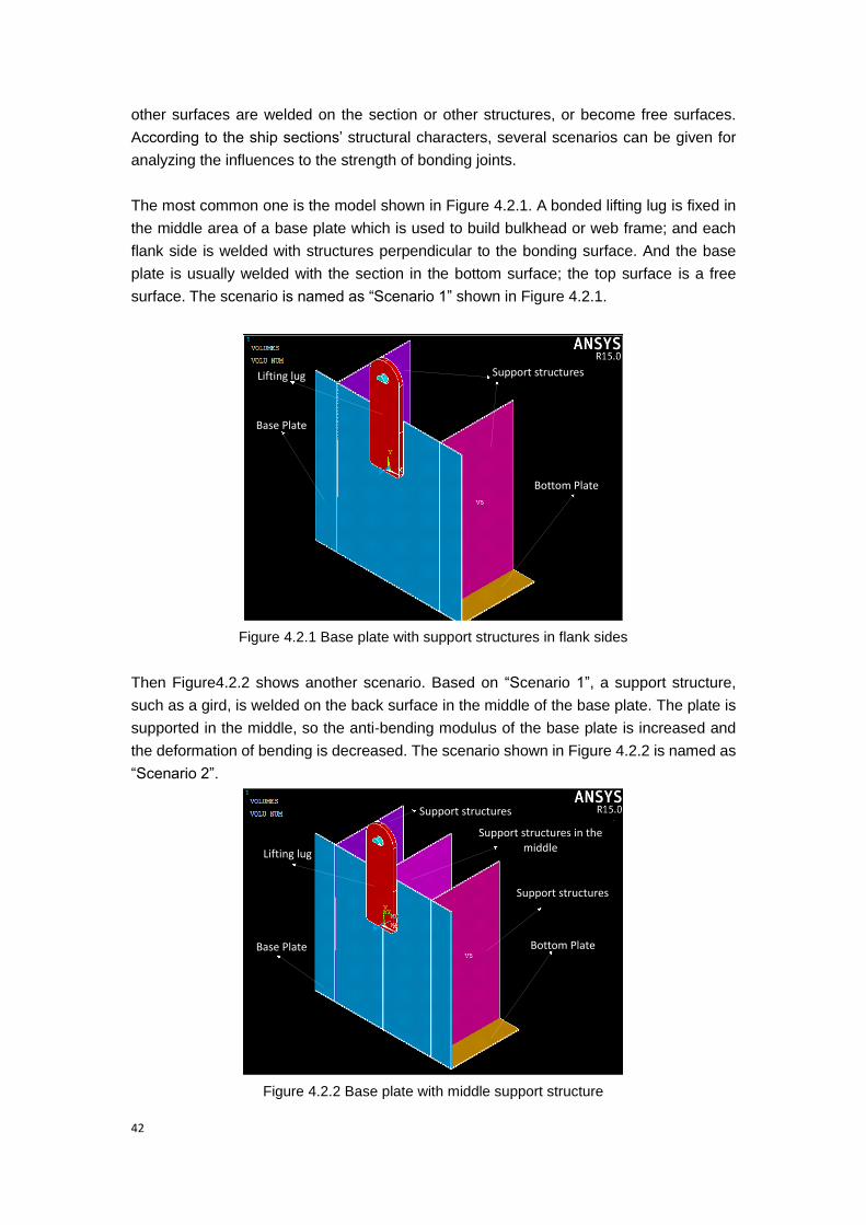
42
other surfaces are welded on the section or other structures, or become free surfaces.
According to the ship sections’ structural characters, several scenarios can be given for
analyzing the influences to the strength of bonding joints.
The most common one is the model shown in Figure 4.2.1. A bonded lifting lug is fixed in
the middle area of a base plate which is used to build bulkhead or web frame; and each
flank side is welded with structures perpendicular to the bonding surface. And the base
plate is usually welded with the section in the bottom surface; the top surface is a free
surface. The scenario is named as “Scenario 1” shown in Figure 4.2.1.
Base Plate
Lifting lug
Support structures
Bottom Plate
Figure 4.2.1 Base plate with support structures in flank sides
Then Figure4.2.2 shows another scenario. Based on “Scenario 1”, a support structure,
such as a gird, is welded on the back surface in the middle of the base plate. The plate is
supported in the middle, so the anti-bending modulus of the base plate is increased and
the deformation of bending is decreased. The scenario shown in Figure 4.2.2 is named as
“Scenario 2”.
Support structures in the
middle
Support structures
Support structures
Bottom Plate
Base Plate
Lifting lug
Figure 4.2.2 Base plate with middle support structure

43
In Figure 4.2.3, a more complicated scenario named “Scenario 3” is shown. Different with
“Scenario 2”, the support structure in the middle is instead by several stiffeners. The
stiffeners are distributed in the whole area of the base plate in the back surface; the
stiffeners increase the stiffness of the whole base plate.
Bottom Plate
Support structures
Lifting lug
Base Plate
Stiffeners
Figure 4.2.3 Base plate with stiffeners
The first scenario experiences the largest bending among the three scenarios; while the
second and third scenario make the base plate have higher stiffness to defense bending.
The exact results will be simulated in FEM models and the differences between each
scenario can be given; by comparing the differences the priority to select positions for
bonding lifting lugs can be got. Chapter 5 will introduce FEM simulation and the results.
4.3 Summary
The chapter concludes requirements for positions for fixing lifting lugs; and sub question
“E” is answered further:
E. Where is the optimal position for installing lifting lugs?
the potential fixing positions with requirements can be concluded as “Bulkheads and web
frames with flat plane and enough bonding area for the bonding joints but without any
protrusion that obstruct the lugs’ installation; the bulkhead or web frames should have
enough bonding surfaces for the applied lap joints and enough space for other lifting
accessories; the potential position should make the deformation of bending as small as
possible”.
The selection of potential positions with macro view requirements is explained by an
example; and the micro view is talked in the second part. The support structures on the
potential positions’ structures are the main factors influencing the performance for

44
defensing bending; three kinds of scenarios are given and they will be simulated by FEM
models in Chapter 5.
45
5. Evaluation: Building and simulating FEM models
In this chapter, items of FEM simulation are introduced. Firstly, the basic FEM model of
bonded lifting lug’s system is given. Then boundary conditions for different kinds of the
potential positions are discussed, corresponding to the scenarios given in 4.2, chapter 4.
Lastly, the results of the FEM simulation will be analyzed and discussed to Figure out
probable defects.
5.1 Introduction of FEM model
5.1.1 Software selection
In the finite element analysis simulation, the software ANSYS is used; the mode
“mechanical APDL” for solving structure problems in the software is used. For analyzing
finite element problems, FEM software such as ANSYS and ABAQUS are both suitable for
dealing with problems about adhesive bonding joints; and they have been already used
for analyzing bonding joints in lectures by lots of researchers. Fan-rong Kong [40]
(2006)
introduced some methods for analyzing cleavage stress in lap bonded joints using ANSYS;
the specimens have commons with bonded lifting lugs structures in the research. So
ANSYS will be selected to be applied in the thesis for the FEM simulation.
The official website of ANSYS introduce the software for structure calculation as: “The
strength of components is a key requirement in understanding a product’s performance,
lifecycle and possible failure modes. Mechanical loading, thermal stress, bolt tension,
pressure conditions and rotational acceleration are just some of the factors that will dictate
strength requirements for materials and designs. ANSYS Mechanical ensures your
product’s viability and safety by predicting the strength required for the loads your design
will experience in service [41]
.” And combined with the research results of FEM analysis, it
can believe that ANSYS provides reasonable solutions for problems about adhesively
bonded joints. Then FEM models are gonging to be built based on “ANSYS”.
The general process for FEM simulation with ANSYS in this research is concluded as
eight steps shown in Figure 5.1.1. The first five steps in the box are steps for building the
basic model which will be used for the calculation later; they will be introduced in part
5.1.2. Then in the sixth step, boundary conditions are set based on the scenarios provided
in 4.2, chapter 4; and it is discussed in section 5.2. The last two steps will deal with the
results and they will be given in section 5.3.
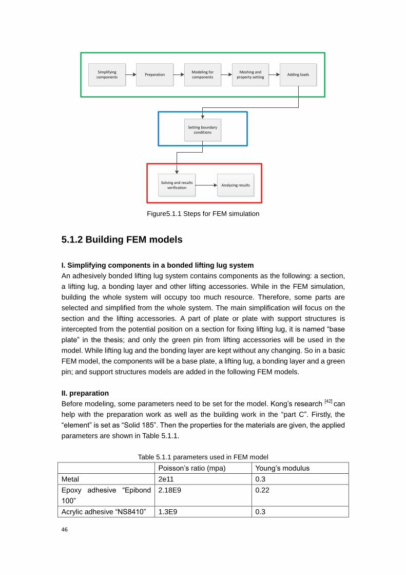
46
Simplifying components
PreparationModeling for components
Meshing and property setting
Adding loads
Setting boundary conditions
Solving and results verification
Analyzing results
Figure5.1.1 Steps for FEM simulation
5.1.2 Building FEM models
I. Simplifying components in a bonded lifting lug system
An adhesively bonded lifting lug system contains components as the following: a section,
a lifting lug, a bonding layer and other lifting accessories. While in the FEM simulation,
building the whole system will occupy too much resource. Therefore, some parts are
selected and simplified from the whole system. The main simplification will focus on the
section and the lifting accessories. A part of plate or plate with support structures is
intercepted from the potential position on a section for fixing lifting lug, it is named “base
plate” in the thesis; and only the green pin from lifting accessories will be used in the
model. While lifting lug and the bonding layer are kept without any changing. So in a basic
FEM model, the components will be a base plate, a lifting lug, a bonding layer and a green
pin; and support structures models are added in the following FEM models.
II. preparation
Before modeling, some parameters need to be set for the model. Kong’s research [42]
can
help with the preparation work as well as the building work in the “part C”. Firstly, the
“element” is set as “Solid 185”. Then the properties for the materials are given, the applied
parameters are shown in Table 5.1.1.
Table 5.1.1 parameters used in FEM model
Poisson’s ratio (mpa) Young’s modulus
Metal 2e11 0.3
Epoxy adhesive “Epibond
100”
2.18E9 0.22
Acrylic adhesive “NS8410” 1.3E9 0.3

47
III. Modeling
The FEM model starts with a single lap bonded lifting lug; the FEM model contains an
adhesively bonded lifting lug, a bonding layer, a base plate and a green pin; Figure 5.1.2
shows it with an overview in picture (a) and “front and side view” in picture (b).
Base plate
Bonding layer
Bonded lifting lug
Green pin
(a)
(b)
Figure5.1.2 FEM model of a single lap lifting lug
All components in the model are built as “VOLUME” in ANSYS. The base plate is
simplified with dimension of 1m×1m in length and width, 8mm in thickness. The
dimension of the base plate uses data from the “liftingplan 1301” and values of the
dimension are simplified to make the model to be built. In the future research, the base
plate can be built with other dimensions to make the simulation more close to specific
applications. The lifting lug’s and bonding area’s dimensions are used data calculated
before in “example 1”, section 3.3, Chapter 3; and they are placed in the middle of the
plate. The green pin is cut in the middle and deleted the lower half part, this measurement
aims to make the load easily added on and exactly simulate the force transferring. The
lifting lug, bonding area and the base plate are connected using the operation “glue” in
ANSYS to simulate adhesive bonding.
Similar with the single lap lifting lug, the FEM model of a double lap lifting lug is shown in

48
Figure 5.1.3; dimensions are used data from “Example 2” provided in section 3.3, Chapter
3.
Bonded lifting lug
Base plate
Green pin
(a)
(b)
Figure 5.1.3 FEM model of a double lap lifting lug
Then for decreasing the calculation burden for the computer, the FEM models are further
simplified; because they are both in symmetry structures. And ANSYS can provide a
function that using a symmetry part of the model to simulate a complete system by setting
appropriate boundary conditions. The single lap lifting lug model is symmetry to the middle
plane perpendicular to the bonding layer; so half of the whole model will be used. While
double lap lifting lug model is symmetry to both the middle plane perpendicular to the
bonding layer and the middle plane parallel to the bonding layer; and finally a symmetry
structure of 1/4 of the whole model is used. Figure 5.1.4 shows and briefly explains the
further simplified model.

49
(a) Further simplified single lap FEM model
(b) Further simplified double lap FEM model
Figure5.1.4 Further simplified FEM models
IV. Meshing and properties setting
In this step, mesh will be set to the model. To ensure the accuracy of the calculating
results, elements are defined as “hexahedral” for all the components. The mesh density is
set as an appropriate number at first and then they will be arranged to make the results
accurate; the discussion will be introduced in the third section in this chapter.
Then the components in the model will be defined with different properties based on their
own properties. The bonding layer is defined with properties of selected adhesives and
the lifting lug, base plate and green pin are defined with properties of metal.
V. Adding load
The load added on the model is 20ton, the maximum value an adhesively bonded lifting
can carry. The load is added on the bottom surface of the green pin in pressure; to transfer
load to pressure, the formula is given in Formula (5.1.1).
𝑃𝑟𝑒𝑠𝑠𝑢𝑟𝑒 =𝐿𝑜𝑎𝑑𝑠
𝑟×𝑙𝑔𝑝 (5.1.1)
And the dimensions of the area for adding load of a 20ton-green pin is 54mm in width and

50
80mm in length, then the pressure is calculated as:
pressure =20𝑡𝑜𝑛
0.054𝑚×0.08𝑚= 4.6� × 107𝑝𝑎 (5.1.2)
So the pressure applied in the FEM is 4.63× 10⁷Pa.
5.2 Discussing the boundary conditions
Boundary conditions are something to constrain the FEM model that make the model can
simulate the real situation, and they will influence the results. Because the FEM model
used in the research is cut from the whole system, setting correct boundary conditions to
make the model have the same situation with the original system is important. For FEM
models used in the research, the support structures on the base plate are the main factors
influence the setting of boundary conditions, and several different boundary conditions are
discussed based on the scenarios provided in chapter 4.
Similar with the former parts, the discussion starts with the simplest single lap bonded
lifting lug. The whole model can be regarded as being fixed on the ground and a force acts
on the lifting lug, this can simulate the balance situation of the whole system. In
Figure5.2.1, it shows how the base plate is cut and simplified from its original structure in
a ship section. It can be seen that the two flank surfaces are not exist in the reality; they
are abstracted after the simplification. Therefore, these two surfaces should be
constrained with totally fixed in x, y and z directions. The bottom surface is welded with
the bottom plate of the section and it is not pulled to separate from the bottom plate of the
section; the bottom surface is not moved in the directions in the horizontal plane. So the
boundary condition set on the bottom surface should be in x, y and z directions. In sum,
the boundary conditions for the basic FEM model used in the research is set by
constraining the surfaces’ displacement; the surfaces which are constrained by other
structures based on the real condition are selected.
Selected frame
Areas to be simplified
Figure 5.2.1 Selection of simplified base plate
For the lifting lug with double lap joint, the situation of the base plate experiences the

51
same with the simple single lap lifting lug. So boundary conditions are also the same.
Then the discussion moves to the setting for different scenarios of lifting lugs with single
lap joints. “Scenario 1” (shown in Figure 4.2.1) has the same boundary conditions with the
basic single lap lifting lugs.
In Scenario 2 (shown in Figure 4.2.2), the situation becomes different from the basic one.
In Scenario 2, there is a support structure in the middle of the base plate. The support
structure can increase the stiffness of the base plate; the middle area will have the largest
stiffness in the whole base plate and bending in this area will be effectively defensed.
While the two areas besides the support structure in the base plate will experience larger
bending deformation with the increasing of the distance away from the support structure.
So for setting boundary conditions for Scenario 2, the support structure will be totally fixed
and the base plate is the same with that in the simple single lap lifting lug. Figure5.2.2
shows the setting of the boundary condition for Scenario 2.
Figure5.2.2 Boundary condition for Scenario 2
In Scenario 3, the support structures become stiffeners distributing averagely on the back
side of the base plate. The stiffness of the whole base plate is increased largely and
bending of the base plate is decreased significantly. So it can be assumed that a base
plate with a serious of stiffeners will not experience bending in the lifting process; and the
FEM model for Scenario 3 can use the same with the basic single lap lifting lug; but
different in the setting of boundary conditions. Then in the setting of the boundary
conditions for the model, the back surface of the base plate is set with fixed in the direction
perpendicular to the back surface; and the other surfaces’ displacements are the same
with the basic single lap model. Figure 5.2.3 shows the conditions in detail.

52
Figure5.2.3 Boundary condition for Scenario 3
5.3 Discussing the results
The FEM model will be solved after the preparation work being finished in the former part;
and the results of stresses in the bonding joints will be analyzed. Before the analysis of
the stress results, the accuracy of the results will be discussed firstly.
For calculation FEM model with ANSYS in the solution part, the density of the mesh on the
model is one of the factors that influence the accuracy of results. The density of the mesh
influences the number of the elements used for calculation in the FEM model. The results’
accuracy will increase with the increase of the density of mesh and number of elements;
and the accuracy will be stable when the density increases to a value. Because the
performance of adhesively bonded joints using for fixing lifting lugs is the focus for the
investigation in the research; the concentration of the mesh density should be on the
bonding layers in the FEM models.
In the operation of setting mesh density in the FEM models, the mesh density is controlled
by dividing the sides on the bonding layer and mapped mesh method is applied for the
meshing to get regular hexahedral elements.
The original mesh density starts with dividing each side on the bonding surface into 50
parts; which means the elements’ size of the bonding layer is 220
50= 4.4𝑚𝑚 in width and
330
50= 6.6𝑚𝑚 in length; and the thickness was divided into 5 parts averagely. Then the
elements’ size in the bonding surface of the bonding layer will be decreased to increase
the mesh density to check whether the elements’ size is small enough to provide accuracy
results. Simulation will be repeated until reasonable results are got; the shear stress and
deformation in the shear in the direction same with the load in the concentration part will
be monitored as factors for judging. In table 5.1, a serious of simulation results of the
basic single lap model with epoxy adhesive joints in different mesh density are shown.

53
Table 5.3.1 Results of simulations with different mesh densities
Element size of
bonding surface
(width*length, mm)
Deformation in the
direction same
with the load
(10−3mm)
Changing ratio Maximum shear
stress (Mpa)
Changing
ratio
4.4*6.6 1.67 - 30.5 -
2.2*3.3 1.94 13.9% 51.9 41.2%
1.1*1.65 1.71 -13.5% 41.7 -24.5%
0.55*0.825 1.72 0.58% 43.8 4.8%
Comparing with results shown in table 5.3.1, when the element size is controlled around
1.1~1.6mm, changings of results become smaller and results become stable; so this
element size will be used in the following simulations.
The simulation results can be got after the system running in the software; the results
show the values of different stresses exist in the bonding layer and their distribution. Then
a group of simulation results are given in Figure 5.3.1.
(a) Front side of shear stress
(b)Back side of shear stress
(c) Front side of normal stress
(d) Back side of normal stress
Figure5.3.1 stresses’ distribution in a lap bonded joint in “Scenario1”
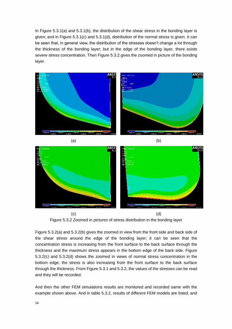
54
In Figure 5.3.1(a) and 5.3.1(b), the distribution of the shear stress in the bonding layer is
given; and in Figure 5.3.1(c) and 5.3.1(d), distribution of the normal stress is given. It can
be seen that, in general view, the distribution of the stresses doesn’t change a lot through
the thickness of the bonding layer; but in the edge of the bonding layer, there exists
severe stress concentration. Then Figure 5.3.2 gives the zoomed in picture of the bonding
layer.
(a) (b)
(c)
(d)
Figure 5.3.2 Zoomed in pictures of stress distribution in the bonding layer
Figure 5.3.2(a) and 5.3.2(b) gives the zoomed in view from the front side and back side of
the shear stress around the edge of the bonding layer; it can be seen that the
concentration stress is increasing from the front surface to the back surface through the
thickness and the maximum stress appears in the bottom edge of the back side. Figure
5.3.2(c) and 5.3.2(d) shows the zoomed in views of normal stress concentration in the
bottom edge; the stress is also increasing from the front surface to the back surface
through the thickness. From Figure 5.3.1 and 5.3.2, the values of the stresses can be read
and they will be recorded.
And then the other FEM simulations results are monitored and recorded same with the
example shown above. And in table 5.3.2, results of different FEM models are listed; and

55
they are used to compare with the adhesive’s strength to judge the feasibility for applying
bonded joints. The strength of the selected adhesives is shown in Table 5.3.3.
Table 5.3.2 Results in different FEM models after simulation
Single lap joints Double lap joints
Scenario 1 Scenario 2 Scenario 3 -
Adhesive EP AC EP AC EP AC EP AC
Shear
concentration
stress
41.7mpa 32.5mpa 12.9mpa
Fillet
corner
8.98mpa
10.5mpa
Fillet
corner
8.9mpa
16.8mpa 12.00mpa 18.8mpa 12.7mpa
Location
description
At the
fillet
Corner
and the
bottom
edge
At the
fillet
Corner
and the
bottom
edge
At the
middle of
the
bottom
edge and
two top
edge
corners
At the
middle
of the
bottom
edge
and two
top edge
corners
At the top
edge
At the top
edge
At the top
corner of
two
edges
At the top
corner of
two
edges
Max Normal
stress pull
82.7mpa 65.4mpa 27.4mpa 19.0mpa 15.0mpa 10.1mpa 17.5mpa 11.6mpa
Max Normal
stress
compress
75.1mpa 58.9mpa 15.6mpa 12.9mpa 16.4mpa 11.7mpa 16.6mpa 11mpa
Tips for table 5.2: EP=epoxy adhesive “Epibond 100” AR=acrylic adhesive “DP8410NS Green”
Scenario 1: Base plate without any support structures.
Scenario 2: Base plate with a support structure in the interior area.
Scenario 3: Base plate with a strong support structures such as a serious of stiffeners.
Table 5.3.3 Strength of selected adhesives
Adhesive name Category Shear strength Normal strength
Epibond 100 Epoxy 34.5 mpa 13 mpa DP8410 Acrylic 24.6 mpa 9.3 mpa
From the table it can be seen that adhesively bonded lifting lugs in Scenario 1 suffers the
largest concentration shear stress among all scenarios. The base plate in Scenario 1 will
suffer the most serious bending because there is no anti-bending structure; the
simulations are same with the theories given in Hartshorn’s (1986) book. Figure 5.8 uses
Epoxy adhesive’s joints’ performance in Scenario 1 to show the situation of the lifting lug
and the base plate. In Figure5.3.3 (a) the general deformation of the whole model is
shown2, the base plate suffers a large bending; the deformation in with is much larger than
that in length which means the width of the base plate influences the stress more and in
2 The deformation is zoomed by a scale factor of 4.65 for monitoring it clearly

56
the future the width of the base plate should be taken more concentration to be
researched. Figure5.3.3 (b) gives the distribution of the shear stress in the bonding layer.
In sum, the shear stress concentration is much larger than the adhesive’s strength and the
joints in Scenario 1 cannot be used.
(a)
(b)
Figure 5.3.3 Results in Scenario 1
Results in Scenario 2 and Scenario 3 show smaller shear stress concentration compared
with Scenario 1; and their shear stress concentration are similar and both of the maximum
shear stress can be accepted by the requirements of the strength. Scenario 2 suffers a
much larger normal stress; because the supporting structures in Scenario 2 provide fewer
efforts against bending than those in Scenario 3.
In the double lap joints’ simulation, there will be no bending in the base plate; the shear
stress concentration is a little larger than that in Scenario 3 which also suffers no bending
in the base plate, but the area with concentration stress becomes smaller. Figure 5.3.4(a)
and 5.3.4(b) show the distribution of shear stress in Scenario 3 and the Scenario of double
lap. While the area that carrying loads in the double lap bonding layer is smaller than that
in Scenario 3, because double lap joint separates the total load into two bonding layers.

57
(a) Distribution of shear stress in Scenario
3
(b) Distribution of shear stress in a double
lap scenario
(c) Distribution of normal stress in
Scenario 3
(d)Distribution of normal stress in a
double lap scenario
Figure 5.3.4 Distribution of stresses in Scenario 3 and double lap scenario
Figure 5.3.4(c) and 5.3.4(d) gives the distribution of the normal stress in the two scenarios.
The values of the maximum normal stresses are similar, but the average normal stresses
(stresses not in the concentration areas) are much different in the two scenarios; the value
in the double lap layer is nearly half of that in Scenario 3 with single lap joint.
5.4 Summary
The adapted rules are evaluated in this chapter and sub question “F. How to evaluate the
feasibility of the application?” can be answered. FEM models are built and simulated in
software “ANSYS”; values and distribution of shear stress and normal stress in the
bonding joints are read from the simulation results. The stress is compared with the
selected adhesives’ strength to check the feasibility.
From the FEM simulation results, It can conclude a rule for choosing fixing positions for
lifting lugs with single lap joints: lifting lugs with single lap joints should be placed in
positions that have supporting structures for defensing bending and they can never be
placed in the interior area of a base plate without any support structures.

58
Then for the stresses, it can be seen that bending is the factor that will cause a sharp
increase in stress concentration and areas that suffer stress concentration. Scenario 1,
Scenario 2 and Scenario 3 can show that decreasing the bending deformation can
contribute to decrease the stress concentration in both value and area. Shear stress can
be decreased within allowable value in the area suffering stress concentration of shear
stress; but the normal stress cannot fulfill the strength requirements. Therefore, the
modification will be processed in the next chapter to make the normal stress concentration
allowable. Because in Scenario 3, the bonding joint performs the best with stress
concentration, so the focus of the modification will be put on Scenario 3 for single lap; and
“Scenario for double lap” will be used continually for lifting lugs with double lap joint.

59
IV. Improvement and verification
The third research circle is shown in green in Figure 4.0.1. In the third research circle, the
application of adhesively bonded lifting lugs based on adapted rules in “Part III” will be
improved and the improved application will be verified.
Strength
Adhesive
Joint
Load
Stress
Geometry
Position
FEM model
Figure 4.0.1 Design Spiral
After the researches in this part, sub questions “C, D and E” will be answered fully; the
final answers to these sub questions can be given based on the results shown in FEM
simulations.
6. Improving lifting lugs and verification of
improvements
The FEM simulations in Chapter 5 show shear stress and normal stress in the bonding
layers in different situations; and in most part of a bonding layer, stress can fulfill the
requirements. But there is still area experiencing stress concentration with much larger
stress which may cause failure in the bonding layer. Firstly, investigation of modifying “the
shape and dimensions of the bonding layer” and “fixing methods” will be processed to
decrease the stress concentration. Then performances of different adhesives are
researched to discover the influences caused by different adhesives’ properties. Finally,
there provides a feasible plan for bonded lifting lugs.
6.1 Adjusting bonding layer’s shape
First in this chapter, shape of the bonding layer will be analyzed. Shape such as the
bonding area size, the thickness of the bonding layer and the fillet’s radius size are
defined as critical factors that will influence the performance for resisting stress
concentration. They will be verified in a serious of values in FEM models to monitor how
they influence concentration stresses in the bonding layer; and the results are used for

60
modifying the bonding layer. The Single lap simulation with “Scenario 3” is used for
analyzing in this part, because Scenario1 and Scenario2 are proofed not suitable for
adhesive bonding.
6.1.1 Influences of bonding area
Increasing the bonding area is the most direct way to decrease the average stress in the
bonding layer; and according to the theoretical calculating formula 𝜏𝑚𝑎𝑥 = 𝑛 ∙ 𝜏𝑎𝑣𝑒, it is
also useful for decreasing concentration stresses.
To increase the bonding area, it can be achieved by increasing only the width or length of
the bonding layer, or increasing both of them; and in this analysis, it will analyze the width
or length separately. The new models will be increased with bonding area, in each model
only the width or the length is going to be changed to increase the bonding area; Figure
6.1.1 shows what is changed in the bonding layer.
In Chapter 5, the results show that stress concentration appears in two parts in a bonding
layer; one is the edge of the fillet in the bottom side, another is the corner in the top side.
Figure 6.1.2 shows the areas with highlighted in red circles in a picture of the bonding
layer in front view. So the monitored results from the simulations are maximum shear and
normal stress in both the top corner and the filet in the bottom; the stresses are recorded
separately and compared with the same results simulated in “Scenario 3”; epoxy adhesive
“Epibond 100” is used for building the bonding layer. Table 6.1.1 gives the data.
Increased bonding area in same value
Width increased
Length increased
Figure 2.1.1 Different ways of increasing bonding area

61
Stress concentration areas
Figure 6.1.2 Bonding layer and its stress concentration areas
From the results shown in Table 6.1.1, by changing the size of the length to increase the
bonding area is more efficient than changing the width to decrease “shear and normal
stress concentration” in fillet area and “normal stress concentration” in the top corner area;
but by only changing the length cannot decrease the shear stress in the top corner
efficiently. The phenomenon is caused by the transfer of the force. When the force
transferring from the top to the bottom, the area carrying load is a triangle, shown in
Figure 6.1.3; the stress starts from a point and then spread to the two sides of the bonding
layer. The angle between the vertical and the spreading direction should be�0 ; and the
value of the angle can be predicted from the rules for lap welded lifting lugs, given in
Figure 2.1.4, chapter 2. So increasing the width makes the bonding area carry more loads
in the top area.
Another thing should be taken care is that only the shear stress concentration can be
controlled in the range of the strength requirements by increasing the bonding area; the
normal stress concentration is still much larger than the requirements. Therefore, new
methods need to be found out to control the normal stress.
Original bonding layer
Width added bonding layer
Length added bonding layer 30º
Figure 6.1.3 Load transferring in the bonding layer

62
Table 6.1.1 Changed parameters and stresses
Increased
bonding
area
10000𝑚𝑚2 20000𝑚𝑚2 Original results
Increasin
g width
Size
value(mm)
250×330 280×330 220×330
Shear
stress(mpa
)
Fillet Top corner Fillet Top
corner
Fillet Top
corner
10.5 15.5 9.9 14.5 11.1 16.8
Normal
stress
(mpa)
Fillet Top corner Fillet Top
corner
Fillet Top
corner
12.3 14.3 11.6 13.8 13.1 15
Increasin
g length
Size
value(mm)
220×375 220×420 220×330
Shear
stress(mpa
)
Fillet Top
corner
Fillet Top
corner
Fillet Top
corner
10.2 16.3 9.41 16 11.1 16.8
Normal
stress
(mpa)
Fillet Top
corner
Fillet Top
corner
Fillet Top
corner
12.1 14 11.1 13.5 13.1 15
6.1.2 Thickness influences
The bonding layer’s thickness has been discussed in some literatures; but the literatures
show different opinions about it. In a theoretical research processed by PK Shaoo (2006)
using FEM analysis, the thickness of the layer is set as 0.0126 inch [43]
(0.32004mm);
while in another research of a real application simulation processed by Yang (2011), the
thickness of the bonding layer is set from 2mm to 4mm [44]
. There is a big difference
between the two analyses for the bonding layer’s thickness, and it is hard to judge which
one can help the analysis of this thesis. So for this research, the appropriate value of
bonding layer’s thickness is given by processing a serious of FEM simulations.
The thickness analysis in this part will use the model of a lifting lug with single lap joint
with boundary conditions in “scenario 3” as the basic model and epoxy adhesive “Epibond
100” will be used for building the bonding layer. New simulations with different bonding
layer’s thickness are processed and the thickness is set as 0.5mm, 2mm, 3mm and 4mm
in new FEM models. Maximum shear stress and normal stress in the concentration areas
(shown in Figure 6.1.2) are monitored.

63
After processing the simulation, results in FEM models with different thickness of bonding
layers are listed and compared in table 6.1.2.
Table 6.1.2 stresses in bonding layer with different thickness
Stress
Thickness
Shear concentration (MPa) Normal concentration (MPa)
Top corner Fillet Top corner Fillet
0.5mm 26.7 14.8 12.8 14.2
1mm 16.8 11.1 15 13.1
2mm 11.3 8.44 13.0 13.2
3mm 8.86 7.24 11.6 12.9
4mm 7.58 6.54 10.8 12.6
From the table, it can be seen that the shear stress concentration decreases with the
increasing of the thickness; while after 2mm thickness; the changes in shear stress
become smaller, both in the fillet and the top corner. The normal stress starts to decrease
from thickness of 1mm in the top corner and 2mm in the fillet; but it doesn’t change a lot
with the thickness increasing after 2mm. Though bonding layer with 0.5mm thickness can
decrease normal stress concentration but the shear stress concentration is enlarged
several times comparing with bonding layers of other thickness.
With the increasing of bonding layers’ thickness the difficulty for producing perfect bonding
layer is increased, air bladders may exist with larger probability. After 2mm thickness, the
shear stress concentration fulfills the strength requirement and doesn’t change a lot; so
2mm for the bonding layer thickness is used in the modification. But the normal stress
concentration still cannot be solved by increase thickness; researches need to be
continued.
6.1.3 Fillet radius’ influences
Fillets are used to eliminate corners in structures for decreasing stress concentration; and
they are also used in the thesis for eliminating stress concentration in the bonding layer.
The radius of the fillets becomes a critical factor for decreasing the stress concentration
and several simulations are processed to monitor changes in fillets with different radius.
In the former research, the fillet radius was set as 5cm and simulation results have been
got. And the new simulation model will increase the radius to 8cm, monitoring the stressed
around the fillet; and then another new model will be built with a semi-circle bottom line to
stand for the maximum fillet radius can be, stresses are monitored in the bottom line. All
the models will set the bonding layer thickness at 2mm. Figure 6.1.4 shows the different
bonding layers in front view. There is one thing should be noticed, the larger the radius,
the more area will be decreased from the whole bonding area. In table 6.1.4 the bonding
decreased area is listed with the changing of stresses.

64
(a) Bonding layer with 5cm fillet
(b) Bonding layer with 8cm fillet
(c) Bonding layer with circle bottom line with 11cm radius
Figure 6.1.4 Bonding layers with different fillet radius
Table 6.1.3 stresses and decreased bonding area in models with different fillet radius
Shear concentration
stress (mpa)
Normal
concentration stress
(mpa)
Area
decreased(𝑚𝑚2)
Comparing with 50mm
50mm 8.44 13.2 -
80mm 8.12 11.4 838.5
110mm(semi-circle) 8.02 11.7 2064
The data in Table 6.1.3 shows that increasing the fillet radius can decrease shear stress
concentration in small extend; while the normal stress decreasing ratio is a little higher,
and a semi-circle bottom line cannot decrease the normal stress concentration efficiently,
it is caused by the large decreased bonding area. So increasing the fillet radius can be
defined as an inefficient method to decrease stress concentration for the optimization, and
change the whole bottom line of the bonding layer to a semi-circle is not advised for the
modification.
In sum, to decrease the stress concentration by arranging the shape of bonding layer: the
bonding area should be increased by increasing both the width and length; the bonding

65
layer’s thickness should be arranged to an appropriate value (that depends on the specific
requirement and production process); radius of fillet in the bottom corner should be big
enough to resist stress concentration.
6.2 Arrange position
Except the shape and dimensions of the bonding layer, the bonding position (the places
for bonding on potential position) also influences stress concentration in the bonding layer.
The top corner is the most severe part experiences stress concentration in the bonding
layer and by adjusting the bonding layer’s shape it is hard to decrease the stress
concentration under the strength requirement; because the top corner locates in the area
where sudden change in shape happens. Different with the bottom corner which can be
transferred in fillet to eliminate stress concentration; the shape of the bonding layer and
the lifting lug in the top corner cannot be changed. So changing the bonding position to
make the bonding layer avoid to be positioned at the edge is a method for eliminating
stress concentration in the top corner.
Then the new modified plan can be given and Figure 6.2.1 shows it briefly. Firstly, the
bonding layer’s position on the base plate is moved, the top edge of the bonding layer is
lower than the top edge of the base plate; therefore the sudden change in the top edge
can be avoided. Secondly, the bonding layer’s position in the lower part of the lifting lug is
also changed; it is moved to the middle area of the lower part of the lifting lug so the
sudden change caused by other edges are avoided. Lastly, the top corners of the bonding
layer are transferred into fillets to eliminate stress concentration.
In this plan, a modification of the lifting lug is added to help solve bending problem. Figure
6.2.2 shows the plan in zoom. For single lap joint, when the load is added on the lifting lug,
because there is a distance between the load and the bonding area, a bending moment
“𝑀𝑏𝑒𝑛𝑑𝑖𝑛𝑔” is provided and the lifting lug is bent. So in the new plan, a metal gasket is
added in the new created gap between the base plate and the lifting lug to decrease the
influence of bending. The gasket is fixed on the lifting lug by welding or other method but
not fixed with the base plate.
Then FEM model for the new single lap lifting lug is built and the exact shape and
dimensions are given in Figure 6.2.3. The new FEM model will also be simplified into a
symmetry model and its boundary condition of the base plate is the same with “Scenario
3”; Figure 6.2.4 shows the FEM model.

66
Bonding layer
New lifting lug
Base plate
(a)
(b)
(c)
(d)
Gasket
Figure 6.2.1 Modified lifting lugs installation plan
�
Base plate
Bonding layer
New lifting lug
Gasket
Figure 6.2.2
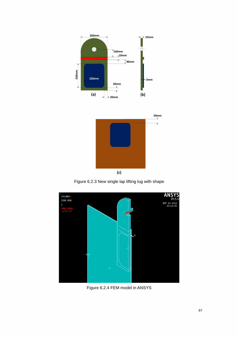
67
(a)
(b)
(c)
220mm
33
0m
m
20mm
20mm
40mm
10mm
160mm
260mm
25mm
2mm
50mm
Figure 6.2.3 New single lap lifting lug with shape
Figure 6.2.4 FEM model in ANSYS

68
Then the simulation is processed. The distribution of stresses is shown in Figure 6.2.5 and
the exact value is shown in table 6.2.1.
(a) Shear stress distribution in front side
(c) Normal stress distribution in front side
(b) Shear stress distribution in back side
(d) Normal stress distribution in back side
Figure 6.2.5 stresses distribution in the bonding layer
From the distribution of stresses in the bonding layer shown in Figure 6.2.5 (a) and (b), the
shear stress concentration locates in the top and bottom fillets; and the value of the stress
listed in Table 6.2.1 indicates that they are all less than 9 Mpa which is less than the
applied shear strength of 17Mpa. Figure 6.2.5 (c) and (d) gives the normal stress
distribution in the bonding layer, it can be seen that the normal stress in most of the area is
in low value and in the bottom fillet there appears stress concentration. When zooming in
the top fillet, it can be seen that there still exists stress concentration in the edge of the
bonding layer, shown in Figure 6.2.6. The maximum value of normal stress concentration
is under the applied normal strength. So it can be concluded that the new plan for single
lap lifting lugs can decrease the stress concentration and control the maximum stresses
under the strength requirements.
Table 6.2.1 stresses in the bonding layer of a single lap lifting lug
Shear stress (mpa) Normal stress (mpa)
Top fillet 8.16 6.32
Bottom fillet 7.34 5.16

69
Figure 6.2.6 zooming in view of the stress distribution
The thought for modifying single lap joints is also helpful for the optimization for double lap
lifting lugs. In the new plan for a double lap lifting lug, the bonding area is also moved both
in the lifting lug and the base plate same as what is done in a single lap lifting lug;
because bending does not influence double lap joint, the gasket is canceled. The brief
view of a modified double lap lifting lug is shown in Figure 6.2.7 with shape.
(a)
(b)
(c)
220mm
33
0m
m
20mm
20mm
40mm
160mm
260mm
25mm
2mm
50mm
6.5mm
Figure 6.2.7 New double lap lifting lug with shape
Then simulation is processed to see the results. The stress distribution is shown in Figure
6.2.8; and the stress values are shown in Table 6.2.2. The shear stress distribution in the
bonding layer is similar with that in single lap joint; but the stress concentration area

70
become smaller as well as the maximum value. The normal stress concentration appears
around the top and bottom fillet. Comparing with the single lap, the stress concentration
area around top fillet increases in area value but decreases in stress value; while the
normal stress around the bottom fillet decreases in both area and stress value. All
stresses are controlled under the applied strength so the new plan of double lap fulfills the
strength requirement.
(a) Shear stress distribution in front side
(b) Shear stress distribution in back side
(c) Normal stress distribution in front side
(d) Normal stress distribution in front side
Figure 6.2.8 stresses distribution in the bonding layer of a double lap lifting lug
Table 6.2.2 stresses in one of the bonding layer of a double lap lifting lug
Shear stress (mpa) Normal stress (mpa)
Top fillet 7.99 4.86
Bottom fillet 5.37 5.48
From now on, lifting lugs using epoxy adhesive “Epibond 100” are modified to fulfill the
strength requirements and another selected adhesive’s performance needs to be tested.
So in the next part, adhesives with different properties are discussed with their
performance.

71
6.3 Adhesive properties
According to the research in Chapter 5, the performances of the two selected adhesives
are different in the same bonding joint, see Table 5.2. The acrylic adhesive make the
maximum stress value less than the epoxy adhesive in the bonding joint; the young’s
modulus and the Poisson’s ratio may be the reasons for this phenomenon. Therefore, the
influences caused by these two factors (young’s modulus and the Poisson’s ratio) are
going to be analyzed in this part. Then some advises for selecting adhesives are
concluded.
6.3.1 Simulations for different young’s modulus and Poisson’s
ratio
In the results provided in table 5.2, with FEM models in same shape and boundary
conditions, the acrylic adhesive bonding layer has stresses in smaller value than the
epoxy adhesive layer. The main differences between the two adhesives are their strength,
young’s modulus and Poisson’s ratio; and the young’s modulus and Poisson’s ratio may
be critical factors that influence stresses in the bonding layer. But there is one thing should
be taken care, the bonding joints is carrying load in the shear direction, so the shear
modulus must be considered. The shear modulus is a value relates to the young’s
modulus and Poisson’s ratio; and formula (6.3.1) gives the relation. So a calculation form
between the two adhesives’ properties can be given in table 6.3.1. These properties show
the factor (or factors) influences the stress value in the bonding joint.
G =𝐸
2(1+𝜈) (6.3.1)
Table 6.3.1 properties of selected adhesives
Young’s modulus Poisson’s ratio Shear modulus
EP 2178.7 mpa 0.22 892.9 mpa
AC 1301.5 mpa 0.3 500.6 mpa
The epoxy adhesive has higher Young’s modulus and Poisson’s ration than the acrylic
adhesive; so the shear modulus is also higher. But only the two selected adhesives
cannot show all the influence caused by adhesive’s properties; it needs 4 comparisons to
see the of the adhesive’s properties influences.
1. Adhesives with same Poisson’s ratio and different Young’s modulus, and adhesive “A1”
is supposed.
2. Adhesives with same Young’s modulus and different Poisson’s ratio, and adhesive “A2”
is supposed.
3. Adhesives with same shear modulus and different in Young’s modulus and different

72
Poisson’s ratio, and adhesive “A3” is supposed.
4. Adhesives with different shear modulus, Young’s modulus and different Poisson’s ratio,
the two selected adhesives can do this test.
If epoxy adhesive “Epibond 100” is selected as the basic specimen in the comparison
tests and other specimens’ properties are set based on the “Epibond 100”. The first
comparison test is about different Young’s modulus, the comparison is between “Epibond
100” and a supposed adhesive named as “A1”; “A1” has the same Poisson’s ratio but
different Young’s modulus with the epoxy adhesive. The second comparison test is about
different Poisson’s ratio and the comparison is between “Epibond 100” and a supposed
adhesive named as “A2”; “A2” has the same Young’s modulus but different Poisson’s ratio
with the epoxy. In the third comparison test, the comparison is between “Epibond 100” and
a supposed adhesive named as “A3”; “A3” has the same shear modulus with the epoxy
adhesive; the Young’s modulus and Poisson’s ratio are both increased. At last the fourth
comparison test is about different young’s modulus and Poisson’s ratio which can use the
selected epoxy adhesive and acrylic adhesive as the two specimens. All the properties of
the supposed adhesives are listed in Table 6.3.2.
Table 6.3.2 properties of supposed adhesives
A1 1301.5 mpa 0.22 533.4
A2 2178.7 mpa 0.44 756.5 mpa
A3 2571.5 mpa 0.44 892.9 mpa
6.3.2 Results analyzing
The new simulation models will use the same with Scenario 3 in shape and boundary
conditions, but different in property setting of bonding layers. Then new simulations are
processed and results are collected. To simulation results and the stresses used for
comparison, only the maximum stresses in the fillet area are concerned; the stresses in
the corner are neglected because the corner is changed into fillet in the new plan given in
6.2. Figure 6.3.1 shows which area in the bonding layer is concerned with pointing in red
circle; and Table 6.3.3 lists the exact values of shear and normal stresses for both the
selected adhesive and the supposed adhesives.
Mornitoring areas
Figure 6.3.1 monitoring areas

73
T6.3.3 stresses in the comparison models
I.
Normal stress (MPA) Shear stress (MPA)
EP 13.1 11.1
A1 10.2 8.78
II.
Normal stress (MPA) Shear stress (MPA)
EP 13.1 11.1
A2 13.1 12.4
III.
Normal stress (MPA) Shear stress (MPA)
EP 13.1 11.1
A3 14.2 13.3
IV.
Normal stress (MPA) Shear stress (MPA)
EP 13.1 11.1
AC 10.1 8.87
From the results of the first two comparison tests (see Table 6.3.3-I and 6.3.3-II), it can be
concluded that: high value of Young’s modulus will increase the normal stress; while
Poisson’s ration do not influence the normal stress, it will decrease the shear modulus as
well as the maximum shear stress. Then in the fourth comparison (Table 6.3.3-IV), the
results show that high modulus will cause high stress to both normal and shear. In the
second comparison test (Table 6.3.3-II), the two specimens have the same shear modulus
but different in the results in shear stress; the supposed adhesive with higher Young’s
modulus experiences higher normal and shear stress than the selected epoxy adhesive.
So the young’s modulus should be the main factor which influence the maximum stresses
in the bonding joint.
It can be concluded that maximum stress in both shear and normal directions is
decreased by decreasing the young’s modulus and shear modulus, but young’s modulus
is the main factor that influences the maximum stresses.
While, small value of modulus causes large strain in the bonding layer which causes
failure to the bonding joint. In the report provided by U.S. Department of Transportation
(2002), it gives Figures of some structural adhesives’ stress-strain curves; which shows
the adhesives can only keep their ideal modulus in small strain and after a specific point
their modulus decreases obviously. Figure 6.3.2 gives a curve of a kind of structural
adhesive from the report.
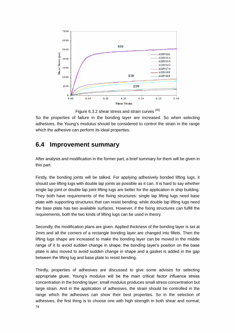
74
Figure 6.3.2 shear stress and strain curves [45]
So the properties of failure in the bonding layer are increased. So when selecting
adhesives, the Young’s modulus should be considered to control the strain in the range
which the adhesive can perform its ideal properties.
6.4 Improvement summary
After analysis and modification in the former part, a brief summary for them will be given in
this part.
Firstly, the bonding joints will be talked. For applying adhesively bonded lifting lugs, it
should use lifting lugs with double lap joints as possible as it can. It is hard to say whether
single lap joint or double lap joint lifting lugs are better for the application in ship building.
They both have requirements of the fixing structures: single lap lifting lugs need base
plate with supporting structures that can resist bending; while double lap lifting lugs need
the base plate has two available surfaces. However, if the fixing structures can fulfill the
requirements, both the two kinds of lifting lugs can be used in theory.
Secondly, the modification plans are given. Applied thickness of the bonding layer is set at
2mm and all the corners of a rectangle bonding layer are changed into fillets. Then the
lifting lugs shape are increased to make the bonding layer can be moved in the middle
range of it to avoid sudden change in shape; the bonding layer’s position on the base
plate is also moved to avoid sudden change in shape and a gasket is added in the gap
between the lifting lug and base plate to resist bending.
Thirdly, properties of adhesives are discussed to give some advises for selecting
appropriate glues. Young’s modulus will be the main critical factor influence stress
concentration in the bonding layer; small modulus produces small stress concentration but
large strain. And in the application of adhesives, the strain should be controlled in the
range which the adhesives can show their best properties. So in the selection of
adhesives, the first thing is to choose one with high strength in both shear and normal;

75
then coordinate the stresses and strain with appropriate modulus and Poisson’s ratio.
At last the performances of the two selected adhesives in the modified single lap and
double lap lifting lugs are listed in the Table 6.4.1 and strength of selected adhesives is
shown in Table 6.4.2. Because the results in the models provided in 6.2 can fulfill the
requirements, the final models will continue using the same shape provided in Figure
6.2.3 and 6.2.7. Strain in the bonding layer is added in the table as well.
Table 6.4.1 Results in the modified lifting lugs for lifting process
Epibond 100 DP8410NS Green
Shear stress Top fillet (mpa) 8.16 6.06
Bottom fillet (mpa) 7.34 5.86
Normal stress Top fillet(mpa) 6.32 2.18
Bottom fillet (mpa) 5.16 5.22
Strain Shear 3.75E-4 3.94E-4
Normal 2.28E-3 2.87E-3
(a) Single lap lifting lug
Epibond 100 DP8410NS Green
Shear stress Top fillet (mpa) 7.99 6.08
Bottom fillet (mpa) 5.37 4.11
Normal stress Top fillet(mpa) 4.86 3.77
Bottom fillet (mpa) 5.48 4.2
Strain Shear 3.8E-4 3.9E-4
Normal 2E-3 2.3E-3
(b) Double lap lifting lug
Table 6.4.2 Strength of selected adhesives
Adhesive name Category Shear strength Normal strength
Epibond 100 Epoxy 34.5 mpa 13 mpa DP8410 Acrylic 24.6 mpa 9.3 mpa
From the results given in 6.1 to 6.3, it can be predicted that lifting lugs with capacity from 20ton
to 30ton can be applied with adhesive bonding joints; the bonding layer should have large
enough bonding area, appropriate shape and be built with appropriate adhesive. The
improvement of the bonding layer should be researched in further research.
6.5 Summary
To sum up the results in this part, the application of adhesively bonded lifting lugs based
on the adapted rules is improved and results shows the improved plans for application are
feasible for applying. Sub question “C, D and E” are fully answered.
C. How to define the shape and geometrical attribute of lifting lugs?

76
The final plans of the shape and geometry of adhesively bonded lifting lugs are given in
6.2 in this chapter; examples are used to shown the feasibility.
D. What is the state of stress of the bonding joint with load?
The values of stress in the bonding joints in improved plans are shown in Table 6.4.1 and
the distribution of the stress is shown in Figure 6.2.5 and Figure 6.2.8.
E. Where is the optimal position for installing lifting lugs?
The positions for installation should be kept the same with that concluded in “Part III”; but
the bonding layer is moved to the interior area on both the base plate and the lifting lugs to
avoid sudden change of shape and stress concentration.
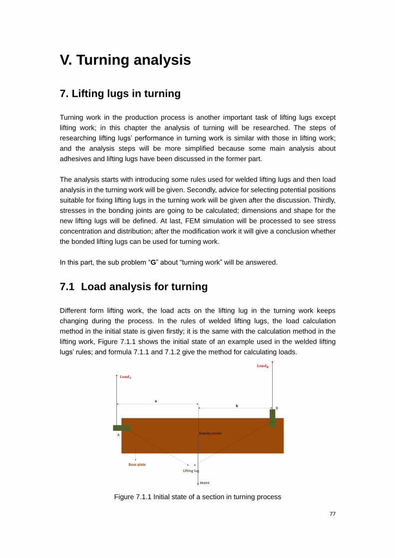
77
V. Turning analysis
7. Lifting lugs in turning
Turning work in the production process is another important task of lifting lugs except
lifting work; in this chapter the analysis of turning will be researched. The steps of
researching lifting lugs’ performance in turning work is similar with those in lifting work;
and the analysis steps will be more simplified because some main analysis about
adhesives and lifting lugs have been discussed in the former part.
The analysis starts with introducing some rules used for welded lifting lugs and then load
analysis in the turning work will be given. Secondly, advice for selecting potential positions
suitable for fixing lifting lugs in the turning work will be given after the discussion. Thirdly,
stresses in the bonding joints are going to be calculated; dimensions and shape for the
new lifting lugs will be defined. At last, FEM simulation will be processed to see stress
concentration and distribution; after the modification work it will give a conclusion whether
the bonded lifting lugs can be used for turning work.
In this part, the sub problem “G” about “turning work” will be answered.
7.1 Load analysis for turning
Different form lifting work, the load acts on the lifting lug in the turning work keeps
changing during the process. In the rules of welded lifting lugs, the load calculation
method in the initial state is given firstly; it is the same with the calculation method in the
lifting work, Figure 7.1.1 shows the initial state of an example used in the welded lifting
lugs’ rules; and formula 7.1.1 and 7.1.2 give the method for calculating loads.
Gravity center
a
b
Lifting lug
Base plate
A
B
�
�
Figure 7.1.1 Initial state of a section in turning process

78
𝐿𝑜𝑎𝑑𝐴 =𝑏
𝑎+𝑏𝑚𝑎𝑠𝑠 (7.1.1)
𝐿𝑜𝑎𝑑𝐵 =𝑎
𝑎+𝑏𝑚𝑎𝑠𝑠 (7.1.2)
Then the rules show the state when the optimal load acts on a lifting lug; the state will
happen when the direction of the load moves and coincides with the line of the gravity of
the section. Figure 7.1.2 shows the state using the same example shown in Figure 7.1.1;
in this situation, the whole load is concentrated on the lifting lugs on the top. In the former
part, the optimal load a bonded lifting lug can carry is defined as 20ton, therefore, if a
section uses four lifting lugs in the production process and only two of them will carry load
in the situation shown in Figure 7.1.2. As a result of that, the optimal maximum mass of a
section adhesively bonded lifting lugs can carry is limited as 40ton in theory; much less
than 80ton, the theoretical optimal maximum load for lifting.
Gravity center
a
b
A
B
Figure 7.1.2 The state lifting lug A hold the whole section’s mass
From Figure 7.1.2, it can be seen that the state the maximum load appears on the top two
lifting lugs are influenced by some factors of the section, the gravity center and position of
the lifting lugs; Figure 7.1.3 gives the shape of these factors.

79
Figure 7.1.3 Shape of factors
So the angle when maximum load appears is related to the length and height between the
lifting lug and the gravity center; and the formula to calculate the angle is given below.
tanα =𝑎
ℎ𝑎 (7.1.3)
For finding a suitable value ofα, some supposed situations are given; and the calculation
and discussion of the stresses is given in 7.3.
However, the rules for welded lifting lugs don’t give how the load on each lifting lug
changes from the initial state to the maximum load appears on the top lifting lugs; but
changes should be noticed. Figure 7.1.4 shows a section and related shape in a state
during the turning process and calculation formulas are given from 7.1.4 to 7.1.7.
Gravity center
a
b
A
B
�
�
′
′
Figure 7.1.4 A state during the turning process
80
𝑎′ = 𝑎 cos𝛼 − ℎ𝑎 sin 𝛼 (7.1.4)
𝑏′ = 𝑏 cos𝛼 + ℎ𝑏 sin 𝛼 (7.1.5)
𝐿𝑜𝑎𝑑𝐴 =𝑏′
𝑎′+𝑏′=
𝑏 cos𝛼+ℎ𝑏 sin𝛼
(𝑎+𝑏)cos𝛼+(ℎ𝑏−ℎ𝑎) sin𝛼×
𝑚𝑎𝑠𝑠
2 (7.1.6)
𝐿𝑜𝑎𝑑𝐵 =𝑎′
𝑎′+𝑏′=
𝑎 cos𝛼−ℎ𝑎 sin𝛼
(𝑎+𝑏) cos𝛼+(ℎ𝑏−ℎ𝑎) sin𝛼×
𝑚𝑎𝑠𝑠
2 (7.1.7)
The value of the load a lifting lug carries in the initial state relates to the position of the
gravity center, but the exact value is influenced by shape of a specific model; the only
thing that can be determined is that the maximum load is not beyond 20 ton for a bonded
lifting lug. For adhesively bonded lifting lugs, the whole mass should be separated on
each lifting lug averagely to avoid the load concentrating on one or some of them; so in
the calculation below, the gravity center of section is set in the middle of the section. Then
in the initial state, the load on each lifting lug is 10ton.
7.2 Position selection
For selecting position for adhesively bonded lifting lugs in turning process, it is similar with
that in the lifting process. Firstly, structures with potential positions are selected, and then
they are judged which kind of bonding joint they are suitable for. In the former parts, the
requirements were given in 6.4, chapter 6. While, in the turning process there are some
differences for selecting fixing positions.
In the initial state during the turning process, lifting lugs cannot be all fixed in one surface;
they need to be fixed in three surfaces on a section. There should be three lifting lugs
installed on the section in three different surfaces; in the first stage for turning, the section
is turned from the initial state by hoisting lifting lug A; when the direction of the load acts
on A coincides with the gravity line of the section, lifting lug A will carry the whole mass
and lifting B starts contributing nothing to the turning. Then in the second stage, a cable is
linked with lifting lug in the opposite surface with Lifting lug B and the section continues
turning until it is turned 180 degrees. If the lifting lugs are still distributed in same type with
the lifting process, the second stage cannot be processed.
So in turning process, the selection for fixing positions should obey the rules given in
Chapter 4 firstly; and then they should be positioned in three different surfaces on the
section.

81
7.3 Stress calculation and shape definition
7.3.1 Stress calculation and joints design
The change of load acts on lifting lugs causes change of the stresses produced in the
bonding layer during the turning process. And in the whole process, the load acts on the
lifting lug changes in two states; one is the initiate state shown in Figure 7.1.1 and another
is the state during turning, shown in Figure 7.1.4.
In the state during turning, the load on lifting lug A keeps increasing and load on lifting lug
B keeps decreasing; so lifting lug A will be the critical lifting lug of the analysis and the
following research focuses on lifting lug A. From Figure 7.1.4, the load on lifting lug A can
be separated into two directions, one is perpendicular to the lifting lug and the other is in
the axis line of the lifting lug; the perpendicular will produce a moment and the other one
produces shear stress in the axis direction.
To define the shape and calculate the theoretical stresses, it starts with the initial state. In
the initiate state, the load is perpendicular to the lifting lug and a moment is provided;
while in the bonding joint there will appear a torque to defense the moment. Figure 7.3.1
shows a lifting lug in the initial state with shape.
LOAD
ARM
�
10MM
B
Figure 7.3.1 A lifting lug in the initial state with shape
The bonding layer is designed as a circle which is the best shape to defense torque and it
is arranged in the middle part of the lifting to avoid sudden change in shape in the edge;
10mm is set from the edge of the bonding layer to the edge of the base plate. The bonding
layer’s radius is 𝑅𝐵𝐿 and the distance between the center of the lifting eye and the center
of the bonding layer is defined as the arm.
So the torque in the section cross section of the bonding layer is:
Torque = Load × Arm = Load × (B + 𝑅𝐵𝐿 + 10mm) (7.3.1)

82
The “polar moment of inertia𝐼𝑝” of the bonding layer is:
𝐼𝑝 =𝜋
2𝑅𝐵𝐿
4 (7.3.2)
The maximum shear stress appears in the edge of the bonding layer which is:
𝜏𝑇 =𝑇𝑜𝑟𝑞𝑢𝑒×𝑅𝐵𝐿
𝐼𝑝=
Load×(B+𝑅𝐵𝐿+10mm)𝜋
2𝑅𝐵𝐿
3 (7.3.3)
Then an example is shown to discuss how to define the radius of the bonding layer in the
initial state; and this example is named “example 3”. In example 3, a 40ton section is
given; the shape of the section is similar to a cuboid. In the cross section fixing with lifting
lugs of the section, the distance between two lifting lugs is 10m and the height is 1.6m and
it is supposed that the distances between the gravity center to the two lifting lugs are
equal and the gravity center is in the middle of the height. Figure 7.3.2 shows a brief view
of it.
Gravity center
a
b
10m
1.6m
Lifting lug
Base plate
A
B
Figure 7.3.2 Brief view of a cross section from a section
It is set “a=b”, so the load acts on lifting lug A is 10 ton. In the former part, the value of “B”
in the lifting lug is calculated as 160mm, so the “Arm” is “170mm+𝑅𝐵𝐿”. Then substituting
exact value, the formula can be written as:
𝜏𝑇 =10ton×(170mm+𝑅𝐵𝐿)
𝜋
2𝑅𝐵𝐿
3 (7.3.4)
Then a curve about 𝜏𝑇 and 𝑅𝐵𝐿 can be given and it is shown in Figure 7.3.3.
� �
. mm
Figure 7.3.3 Curve for 𝜏𝑇 and 𝑅𝐵𝐿

83
From the curve, it can be seen that the shear stress decreases with the increase of the
radius of the bonding layer; the speed for decreasing becomes slow with the increase of
the radius. The shear stress decreases 70% when the radius increases to 160mm and 82%
when the radius increases to 200mm. The shear strength of Epoxy adhesive “Epibond
100” is 17Mpa, so the maximum radius of the bonding layer is 105.76mm. As the
experience in the former part, the stress concentration is much higher than the theoretical
value; so in the example the radius can be selected as 200mm.
Then the stresses during the turning process will be analyzed and defined shape of the
bonding layer is checked if it can fulfill the requirements in the process. A brief view of the
cross section from a section during the turning process is shown in Figure 7.3.4 with
shape.
Gravity center
a
b
A
B
�
�
�
�
Figure 7.3.4 the cross section from a section during the turning process
When the section is in the turning process, the load keeps in the vertical direction; and it
can be separated into two sub loads, 𝐿𝑜𝑎𝑑𝐴𝑥 and 𝐿𝑜𝑎𝑑𝐴𝑦; shown in the Figure. 𝐿𝑜𝑎𝑑𝐴𝑥
is in the axis direction of the section which will produce shear stress; and 𝐿𝑜𝑎𝑑𝐴𝑦 is
perpendicular to the lifting lug which will produce torque to the bonding layer. The
maximum stress in this phenomenon is the composite stress of the shear stress produced
by 𝐿𝑜𝑎𝑑𝐴𝑦 and the shear stress provided by the torque, the maximum composite shear
stress will in the axis direction of the section which is same with𝐿𝑜𝑎𝑑𝐴𝑦. Then the
calculation formulas are given below.

84
𝐿𝑜𝑎𝑑𝐴 =𝑏 cos𝛼+ℎ𝑏 sin𝛼
(𝑎+𝑏) cos𝛼+(ℎ𝑏−ℎ𝑎) sin𝛼×
𝑚𝑎𝑠𝑠
2 (7.3.5)
𝐿𝑜𝑎𝑑𝐴𝑦 =𝑏 cos𝛼+ℎ𝑏 sin𝛼
(𝑎+𝑏)cos𝛼+(ℎ𝑏−ℎ𝑎) sin𝛼× sin𝛼 ×
𝑚𝑎𝑠𝑠
2 (7.3.6)
𝐿𝑜𝑎𝑑𝐴𝑥 =𝑏 cos𝛼+ℎ𝑏 sin𝛼
(𝑎+𝑏)cos𝛼+(ℎ𝑏−ℎ𝑎) sin𝛼× cos𝛼 ×
𝑚𝑎𝑠𝑠
2 (7.3.7)
𝜏𝑦 =𝐿𝑜𝑎𝑑𝐴𝑦
𝐴𝑏𝑙=
𝐿𝑜𝑎𝑑𝐴𝑦
𝜋𝑅𝐵𝐿2 (7.3.8)
𝜏𝑇 =𝑇𝑜𝑟𝑞𝑢𝑒×𝑅𝐵𝐿
𝐼𝑝=
𝐿𝑜𝑎𝑑𝐴𝑦×Arm𝜋
2𝑅𝐵𝐿
3 (7.3.9)
𝜏𝑐𝑜𝑚 = 𝜏𝑦 + 𝜏𝑇 (7.3.10)
Then use “example 3” to discuss the trend of the stress changing during the turning
process. In example 3, a 40ton section is given; the shape of the section is similar to a
cuboid. In the cross section fixing with lifting lugs of the section, the distance between two
lifting lugs is 10m and the height is 1.6m and it is supposed that the distances between the
gravity center to the two lifting lugs are equal and the gravity center is in the middle of the
height. Figure 7.3.2 shows a brief view of it.
From Figure 7.3.4 and 7.3.6 it can be inferred that the value of ℎ𝑏 is a constant value
which equals to “0.5height + 10mm+ B” and in the example it is 970mm; while the value
of ℎ𝑎 is a variable value which can change between 0 to 600mm. The value of ℎ𝑎 will
also influence the maximum angle a section can be turned in the first stage as well as the
maximum stress when the whole load acts on lifting lug A. Therefore, several values of ℎ𝑎
are set and the values are 0, 300mm and 600mm. Then inferring exact value to the
formula for calculating the maximum composite shear stress, three formulas with different
ℎ𝑎 value can be got.
𝜏𝑐𝑜𝑚 = 1.59(cos𝛼+0.194sin𝛼
2 cot𝛼+0.074) + 5.89 (
cos𝛼+0.12sin𝛼
2 cot𝛼+0.074 tan𝛼) (7.3.11)
𝜏𝑐𝑜𝑚 = 1.59(cos𝛼+0.194sin𝛼
2 cot𝛼+0.134) + 5.89 (
cos𝛼+0.06sin𝛼
2 cot𝛼+0.134 tan𝛼) (7.3.12)
𝜏𝑐𝑜𝑚 = 1.59(cos𝛼+0.194sin𝛼
2 cot𝛼+0.194) + 5.89 (
cos𝛼
2 cot𝛼+0.194tan𝛼) (7.3.13)
Figure 7.3.5 shows the curves for the three formulas shown above.

85
�
( )
=
=
=
Figure 7.3.5 curves for different value of ℎ𝑎
From the three curves’ trend in the coordinate; smaller value of ℎ𝑎makes the composite
stress smaller during the whole turning process until the load coincides with the gravity
line. And the curves also show that the smaller ℎ𝑎 is, the lower shear stress there will be
in the state when the section stops turning. Therefore, it can be concluded that lifting lug in
the side surface should be fixed to make the distance between it and the gravity center in
the vertical direction as small as possible.
Then in “example 3”, the lifting lug in the side surface is fixed in the same horizontal plane
with the gravity center, which means ℎ𝑎 equals to 0 and the blue curve in Figure 7.3.7
shows the trend of stress’ variation. The general trend of the blue curve shows that the
shear stress will not higher than 3.2mpa in theoretical, so the radius defined in the initial
state can fulfill the requirements during the turning process. The curves also show that the
shear stress increases when the section starts turning and reach a maximum value at an
angle; after that the shear stress starts decreasing. The value of the angle create the
maximum shear stress can be read and this state in the turning process is defined as the
“critical state”, and this state will be simulated in the FEM software to monitor the stress
concentration for judging feasibility. And the initial state is also selected for FEM
simulation.
7.3.2 Lifting lug design
In the previous part, new bonding joint type is given for turning and the shape and shape
of the new bonding joint is quite different from the one used in the lifting process; therefore
the lifting lug used in the lifting work needs to be modified to adapt the new bonding joint
and turning work.
There will be some modifications in the new lifting lugs. Firstly, the area of the lower part of
the lifting lug for arranging bonding layer should be increased; as the new bonding layer is

86
a circle, the lower part will be redesigned as a square. The length of the sides of the
square is a little longer than the diameter of the bonding layer to avoid sudden change in
shape.
Secondly, because a torque is created in the bonding layer during the turning process, the
lifting lug should be modified to decrease the value of the torque. The torque equals load
times arm in theoretical calculation, the load can’t be changed, so to decrease the torque
the “arm” should be decreased. In the modified lifting, the distance between the top point
of the bonding layer to the edge of the base plate is decreased to 10mm; and the gasket is
cancelled to save the distance.
The upper part of the lifting lug is kept the same with the one using in the lifting process.
Figure 7.3.6 shows a brief of the modified lifting lug with shape.
10mm
� = 00
�2 = 110
10mm
1 = 110
2 = 4 0
=160
= 5
=
Figure 7.3.6. A brief view of the modified single lap lifting lug for turning
In Figure 7.3.8, the modified lifting lug is shown and there is a part circled with red in the
Figure; this part should be taken care and checked with bending. The applied modulus of
that part is:
cm × cm× .5cm÷ 6 = 01.7𝑐𝑚3
While the minimum modulus the part needs to have is :
10ton × 16cm ÷1ton
𝑐𝑚2= 160𝑐𝑚3
The applied modulus is bigger than the minimum modulus, so the modified lifting lug
fulfills the strength requirement for itself.
Then base on the single lap modified lifting lug, a double lap modified lug for turning is
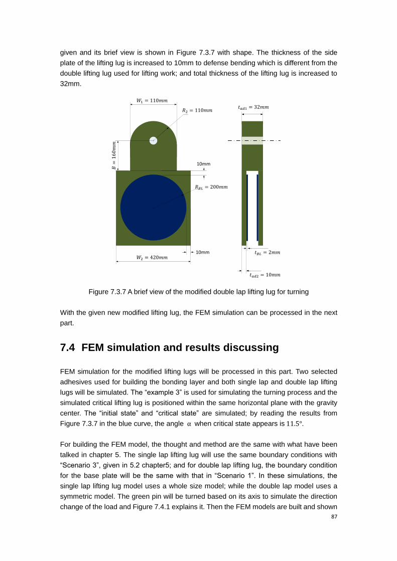
87
given and its brief view is shown in Figure 7.3.7 with shape. The thickness of the side
plate of the lifting lug is increased to 10mm to defense bending which is different from the
double lifting lug used for lifting work; and total thickness of the lifting lug is increased to
32mm.
10mm
� = 00
�2 = 110
10mm
1 = 110
2 = 4 0
=160
=
1 = �
2 = 10
Figure 7.3.7 A brief view of the modified double lap lifting lug for turning
With the given new modified lifting lug, the FEM simulation can be processed in the next
part.
7.4 FEM simulation and results discussing
FEM simulation for the modified lifting lugs will be processed in this part. Two selected
adhesives used for building the bonding layer and both single lap and double lap lifting
lugs will be simulated. The “example 3” is used for simulating the turning process and the
simulated critical lifting lug is positioned within the same horizontal plane with the gravity
center. The “initial state” and “critical state” are simulated; by reading the results from
Figure 7.3.7 in the blue curve, the angle α when critical state appears is 11.5 .
For building the FEM model, the thought and method are the same with what have been
talked in chapter 5. The single lap lifting lug will use the same boundary conditions with
“Scenario 3”, given in 5.2 chapter5; and for double lap lifting lug, the boundary condition
for the base plate will be the same with that in “Scenario 1”. In these simulations, the
single lap lifting lug model uses a whole size model; while the double lap model uses a
symmetric model. The green pin will be turned based on its axis to simulate the direction
change of the load and Figure 7.4.1 explains it. Then the FEM models are built and shown

88
in Figure 7.4.2.
(a) Position of green pin in initial state
(b) Position of green pin in state during
turning
Figure 7.4.1 Green pin’s position in the turning process
(a) Single lap lifting lug
(b) Double lap lifting lug
Figure 7.4.2 FEM model of lifting lugs and base plates
Then the results in a single lap lifting lug are shown in Figure 7.4.3 to explain the stress
distribution. In Figure 7.4.3(a) and (b), shear stress caused by the torque, the distribution
basically meets the theoretical distribution. In the edge of the bonding layer the value of
the shear stress is bigger than that in the inner area; and the value of the shear stress
near the load is bigger than that far from the load, because the stress weakens through
the bonding layer. Figure 7.4.3 (c) shows the normal stress, it can been seen in most of
the bonding layer the normal stress is in small value; when zooming in the edge, shown in
Figure 7.4.3(d), it can been seen there still exists stress concentration in some areas.

89
(a) Shear stress in the axis direction (yz)
(b) Shear stress in the perpendicular axis
direction (xz)
(c) Normal stress distribution
(d) Zoom in the edge for normal stress
Figure 7.4.3 Stress distribution in a modified single lap lifting lug’s bonding layer
In table 7.4.1(a) and 7.4.1(b), all values of results in different models are listed; it contains
models with two selected adhesives used in single and double lap lifting lugs in the “initial
state” and “critical state” during the turning process. Strength of selected adhesives is
shown in 7.4.2.
Table 7.4.1(a) results in the initial state
Epibond 100 DP8410NS Green
Single lap Shear stress in axis
(mpa)
6.73 5.41
Shear perpendicular to
axis (mpa)
8.08 6.36
Normal stress (mpa) 5.04 4.25
Double lap Shear stress in axis
(mpa)
4.94 3.81
Shear perpendicular to
axis (mpa)
5.89 4.56
Normal stress (mpa) 4.17 2.88

90
Table 7.4.1(b) results in the critical state
Epibond 100 DP8410NS Green
Single lap Shear stress in axis
(mpa)
7.25 5.81
Shear perpendicular to
axis (mpa)
8.41 6.58
Normal stress (mpa) 5.18 4.36
Double lap Shear stress in axis
(mpa)
5.14 3.95
Shear perpendicular to
axis (mpa)
6.4 4.88
Normal stress (mpa) 3.47 2.55
Table 7.4.2 Strength of selected adhesives
Adhesive name Category Shear strength Normal strength
Epibond 100 Epoxy 34.5 mpa 13 mpa DP8410 Acrylic 24.6 mpa 9.3 mpa
From the results, it can be seen that the stresses in the bonding layer are controlled under
the strength requirements; which can prove that the adhesively bonded lifting lugs have
the abilities for being applied in the turning process.
7.5 Summary
To conclude the analysis processed in this chapter: adhesively bonded lifting lugs and can
be used in the turning process, but the bonding joint are different from that used in the
lifting process; limitations also exists for application. The sub question “G. How bonding
joints perform in turning?” is answered.
Firstly, the total mass of the section is limited; because the optimal maximum load a
bonded lifting lug can carry is 20ton and only two lifting lugs hold the whole mass of the
section in a state during the turning process. Secondly, the positions for fixing lifting lugs
are difficult to find, the skins welded on the frames are obstacles for the installation; and
the requirements for value of area is increased. Thirdly, the bonding layers are difficult to
be produced; a round bonding layer make the production more complicated than a
rectangle bonding layer. The discussion of producing the bonding layer will be given in the
last part.
Therefore, even the bonded lifting lugs are proved feasible for turning sections; several
limitations restrict its application in the real production. For the real application, problems
still need to be solved.

91

92
VI. Conclusion
8. Conclusion and further research
In the end of the research, conclusions of the analysis are summarized and advice for the
further research is also listed.
8.1 Conclusion
Then the sub questions asked in the beginning of the thesis will be answered.
A. What kinds of adhesives will be feasible for bonding lifting lugs?
In general, structural adhesives should be used for bonding lifting lugs in the application;
“epoxy structural adhesives” and “acrylic structural adhesives” are suitable for the
application. Requirements for selecting appropriate adhesives are also concluded: firstly,
the adhesive should have enough strength to hold the loads, usually the higher the better;
secondly, the Young’s modulus and the Poisson’s ratio should be considered to control the
strain of the adhesive in adhesive elastic deformation under the applied load.
B. What types of bonding joints can be used?
“Lap joints” are the best adhesively bonding joints for installing lifting lugs in the
application; both “single lap joints” and “double lap joints” can be used. “Single lap joints”
need the fixing positions supported with structures to decrease bending; while “double lap
joints” need the fixing structures with two available bonding surfaces for arranging
bonding joints. Both of the joints can make the adhesively bonded lifting lugs feasible for
the application with enough supporting structures and appropriate bonding layers.
“Double lap joints” are advised for application because it can release the bending in
minimum level.
C. How to define the shape and geometrical attribute of lifting lugs?
To define the shape and dimension of bonded lifting lugs, it is processed in two parts. The
first part is to ensure the strength of the lifting lug itself, it relates to the load and other
accessories used in the lifting process; the detail methods are given in 2.1, Chapter 2.
20ton is defined as the optimal maximum load a lifting lug carries because minimal
installation requirements are required with this load.
The second part is to make the bonding layers performances fulfill the strength
requirements. The bonding layers are different in lifting process and turning process. In
the lifting process, bonding layers are designed as a rectangle with fillets in four corners

93
and located in the inner area of the lifting lug; details for defining the original shape are
given in 3.3, Chapter 3; and the improvements are provided in 6.1 and 6.2, Chapter 6. In
the turning process, the bonding layer is redesigned as a circle to defense torque and
value of the area are increased; details are provided in chapter 7.
D. What is the state of stress of the bonding joint with load?
“Shear stress” is the main stress in the bonding joints and large in value; normal stress
also exists in the bonding layer. Stress concentrations appear in the edges of the bonding
layer and they are sharply increased by bending of the base plate. For calculating shear
stress and normal stress theoretically, formulas are given in 3.2, Chapter 3 and 7.3,
Chapter 7; while FEM simulations are provided in part III and part IV. In the FEM models,
the stress concentration values are got, and the value is several times higher than the
theoretical average values of the stresses. After modification, the value of concentration
stresses can be controlled within the strength requirements of the selected adhesives in
specific applications.
E. Where are the best places for fixing lifting lugs on a section?
Generally, the bonded lifting lugs can only be fixed on structures of web frames or
bulkheads which have enough value of available area for bonding in sections; the
requirements for fixing single lap bonding joints and double lap joints are also different.
For single lap joints, the fixing structures should have enough modulus to defense
bending; while double lap joints need two surfaces available for bonding. Details about
requirements are talked and given in Chapter 4.
F. How to evaluate the feasibility of the application?
The strength of the bonding layer and bonding joint is used as a criterion for evaluation
and verification. Adhesively bonded lifting lugs are designed based on the rules adapted
from rules of welded lifting lugs; shear stress and normal stress in the bonding joint are
calculated and in feasible applications they cannot be larger than the strength of the
bonding joint. FEM is chosen to simulate for calculating stress in the bonding joints and
software “ANSYS” is used in the research.
G. How bonding joints perform in turning?
In the turning process, the load causes torque in the bonding layer and stress distribution
is different from that in the lifting process; the changes in the distribution cause the
stresses increasing in value and stress concentration increasing. Therefore, the bonding
layer used in lifting process cannot be continually used in the turning process; a round
bonding layer with larger bonding area is provided to instead the rectangle bonding layer.
With the new bonding layer, shear stress and normal stress can be controlled within the
adhesives’ requirements as well as the stress concentration. However, in the turning

94
process, the maximum mass of a section are decreased to 40ton, because of the applying
limitation of bonded lifting lugs; Chapter 7 gives the details.
After answering the sub questions, the final conclusions are given.
The main questions of the investigation are:
1. Whether adhesively bonded lifting lugs can be applied in ship
building?
2. If it is applied, what are the rules for the application?
And the final conclusions are shown below:
Adhesively bonded lifting lugs can replace welded lifting lugs when the
capacity of the lifting lugs is lower than 20ton.
The application of the adhesively bonded lifting lugs should consider the
defined calculations for: “the load a lifting lug can carry”, “the strength
of adhesives”, “the positions of installation”, “the shape of bonding
layer” and “stress in the bonding layer”.
8.2 Further research
The thesis processes some basic investigation for the feasibility of applying adhesively
bonded lifting lugs in ship building; the results show the application is able to use
theoretically, but for the further application, more researches should be processed and
practiced. In this part, some advice for the further research is given.
Firstly, the research for the lifting lugs with capacity from 20ton to 30ton should be
processed in the future. In the research, lifting lugs with capacity from 20ton to 30ton are
not regarded as ideal subjects for investigation because they have more requirements for
installation and suffer higher risks; the concentration for the research is put on lifting lugs
with capacity of 20ton. While, making adhesively bonded lifting lugs carry heavier load can
expand the application of adhesively bonded lifting lugs and solve more problems in the
ship building process; research needs to be taken to optimize the application of
adhesively bonded lifting lugs with capacity from 20ton to 30ton.
Secondly, the data about the adhesives information should be completed. In the thesis,
the applied strength of adhesives is calculated from the data sheet provided by
manufactures and standard test ASTM D1002 is also used for calculation. The data can
show some properties of the adhesives, but they are more close to theoretical results. For
the real production, tests like what Bouwman (2011) did in his researches should be
advised to be processed in the further research; giving exact estimation for adhesives
using in condition close to real production.
Thirdly, the production of the bonding layer should be analyzed. In the research, the
bonding layers are designed smaller than the lifting lugs and with special shapes. So in

95
the production it is hard to operate. To solve this problem, molds should be used in the
production process to help the adhesive curdle into specific shape; then the molds can be
moved. Another advice is to use adhesive films to produce bonding layer, but it is the work
more related to adhesive manufactures.
Lastly, the economy problems should be analyzed. The adhesively bonded lifting lugs can
help improve the performances of the ship, but whether the costs deserve the benefits
may be different in views among shipyards, ship owners and ship designers. While for
some non-metallic materials ships, adhesively bonded lifting lugs is a good choice; but for
traditional steel structure ships the application’s benefit-cost ratio deserves to be
analyzed.

96
References
1. https://en.wikipedia.org/wiki/Shipbuilding#Industrial_Revolution, January, 2017
2.http://worldmaritimenews.com/archives/179125/shipbuilding-industry-set-to-pick-up-afte
r-2017/, January, 2017
3. http://forums.autodesk.com/t5/inventor-forum/fea-lifting-problem/td-p/5111638,
January, 2017
4. http://www.slideshare.net/nasihatbunda/me-328-welding-metallurgy, November, 2016
5.http://www.twi-global.com/technical-knowledge/job-knowledge/distortion-types-and-cau
ses-033/, November, 2016
6. J. C. Bolger, Adhesives in Manufacturing (G. L. Schneberger, ed.), p. 133, 1983
7. S. R. Hartshorn, Structural Adhesives Chemistry and Technology, P. 2, 1986
8. S. R. Hartshorn, Structural Adhesives Chemistry and Technology, P. 9~10, 1986
9. Ijsbrand J. Van Straalen and Michel J.L. van Tooren, Development of Design Rules for
Strutural Adhesive Bonded Joints, P263~264, 2001
10. R. D. Adams, Adhesive bonding-Science, technology and applications, P 357, 2014
11. Dan Gleich, Stress Analysis of Structural Bonded Joints, P6, 2002
12.http://fennerschool-associated.anu.edu.au/fpt/nwfp/mosquito/Mosquito.html,
December, 2016
13. Dan Gleich, Stress Analysis of Structural Bonded Joints, P6, 2002
14. R. D. Adams, Adhesive bonding-Science, technology and applications, P 522~526,
2014
15. Jan R. Weitzenbock , Adhesives in marine engineering, P4, 2012
16. Jan R. Weitzenbock , Adhesives in marine engineering, P2~3, 2012
17. S. R. Hartshorn, Structural Adhesives Chemistry and Technology, P. 4, 1986
18. P.C. Bouwman, The potential of adhesive bonding in shipbuilding, P51~66, 2010
19. HUNTSMAN, Epibond® 100 A/B High-temperature Epoxy Structural Adhesive,
May, 2013
20. 3M, Scotch-Weld™ Acrylic Adhesives DP8405NS Green • DP8410NS Green
Technical Data Sheet, February, 2014
21. R. D. Adams and W. C. Wake, Structural adhesive joints in engineering,1984
22. Ijsbrand J. Van Straalen and Michel J.L. van Tooren, Development of Design Rules for
Strutural Adhesive Bonded Joints, P265~272, 2001
23. S. R. Hartshorn, Structural Adhesives Chemistry and Technology, P441~445, 1986
24. S. R. Hartshorn, Structural Adhesives Chemistry and Technology, P444, 1986
25. Dan Gleich, Stress Analysis of Structural Bonded Joints, P12, 2002
26. Hans Bink, Secties keren, April, 2016
27. P.C. Bouwman, The potential of adhesive bonding in shipbuilding, P56, 2010
28. Yu-Ping Yang, George W. Ritter and David R. Speth, Finite Element Analyses of
Composite-to-Steel Adhesive Joints, P25~27, ADVANCED MATERIALS & PROCESSES,
June, 2011
29. Dan Gleich, Stress Analysis of Structural Bonded Joints, P67~72, 2002
30.http://www.admet.com/testing-applications/testing-standards/astm-d1002-adhesive-la

97
p-joint-shear-testing/, August, 2016
31. Standard test method for apparent shear strength of single-lap-joint adhesively
bonded metal specimens by tension loading (metal-to-metal)
32. S. R. Hartshorn, Structural Adhesives Chemistry and Technology, P411, 1986
33. http://www.substech.com/dokuwiki/doku.php?id=fundamentals_of_adhesive_bonding,
October, 2016
34. P.C. Bouwman, The potential of adhesive bonding in shipbuilding, P66, 2010
35. R. D. Adams and W. C. Wake, Structural adhesive joints in engineering, 1984
36. S. R. Hartshorn, Structural Adhesives Chemistry and Technology, P427, 1986
37. S. R. Hartshorn, Structural Adhesives Chemistry and Technology, P428~432, 1986
38. S. R. Hartshorn, Structural Adhesives Chemistry and Technology, P429, 1986
39, Liftingplan 1301, IHC HOLLAND B.V. 2014
40. Fan-Rong Kong, Min You, Xiao-Ling Zheng and Hai-Zhou Yu, Three-dimensional
stress analysis of adhesive-bonded joints under cleavage loading, P298~305,
International Journal of Adhesion & Adhesives 27 (2007)
41. http://www.ansys.com/products/structures/Strength-Analysis, November, 2016
42. Fan-Rong Kong, Min You, Xiao-Ling Zheng and Hai-Zhou Yu, Three-dimensional
stress analysis of adhesive-bonded joints under cleavage loading, P299, International
Journal of Adhesion & Adhesives 27 (2007)
43. PK Sahoo, B. Dattaguru and CRL Murthy, Finite element analysis of adhesively
bonded lap joints, P331, XIIV NASA: Fatigue, Fracture and Ageing Structures,
January, 2006
44. Yu-Ping Yang, George W. Ritter and David R. Speth, Finite Element Analyses of
Composite-to-Steel Adhesive Joints, P26~27, ADVANCED MATERIALS & PROCESSES,
June, 2011
45. U.S. Department of Transportation, Shear Stress-Strain Data for Structural Adhesives,
A-2, 2002
98
Acknowledgements
First of all, I would like to extend my sincere gratitude to my supervisor Dr.ir. J.F.J. (Jeroen)
Pruijn, who guides me throughout the research and helps me solve problems in the
research.
I would like to thank for Mr. Adriaan Visser, the production manager from IHC IQIP, who
gives me advice about defects of welding. I am deeply thankful for Mr. Hans Bink from IHC
Holland BV, who provides me useful information and rules of welded lifting lugs. I would
also give my thanks to Ir. Reinier Bos, who gives me advice on stress analysis and guide
on ANSYS.
Finally, I would like to thank my parents, who do their best to support me study for a
master degree in TU Delft and continually give me encouragement. And I’d like to give
special thanks for my friends who help and support me during the research.
Jindao Sun
18/01/2017
Delft