jochen schanz, bank of england disclaimer: the views expressed in this presentation are my own and...
TRANSCRIPT

Jochen Schanz, Bank of England
Disclaimer: The views expressed in this presentation are my own and my not coincide with the views of the Bank of England.
A joint calibration of banks’ capital and liquidity ratios
“International competition in banking: theory and practice”, Sumy, Ukraine, May 2012
1
Background
Policy initiatives following the start of the banking crisis: • Revision of prudential regulation: higher capital requirements,
new liquidity requirements, possibly varying across time and instiutions
• Creation of a more robust bank insolvency regime and early intervention rights
• Proposals to change the structure of the banking sector and of trading and settlement activities (eg, central counterparties).
• Increased information requirements, also for non-bank sector, to reduce opaqueness of financial system.
2
Background
This paper: revision of prudential regulation• Could think of two ways to avoid bank failure
– Permit investment in risky, illiquid assets but require 100% equity
– Permit debt funding but only invest in safe, liquid assets
• What would be a good intermediate choice? optimal combination of capital and liquidity ratios
• Paper compares benefits and costs of varying capital and liquidity ratios
• Objective: inform prudential debate. So keep framework simple; allow different calibrations; rather than present point estimates, show which parameters / assumptions matter.
3
Related literature
• Barrell et al (2009), Kato et al (2010: Regression-based models. Find some degree of substitutability between capital and liquidity ratios in ensuring a bank’s safety.
• Gauthier, He, and Souissi (2010): large network model of Canadian banks. Find some degree of substitutability. Focus on risk, not costs: initial balance sheet is exogenous, deposit rate exogenous; risk-neutral depositors.
• De Nicoló, Gamba and Lucchetta (2012): multi-period model, endogenous issuance of claims. However: view only disadvantages of liquidity requirements but not benefits (short-term debt is insured).
• Morris and Shin (2008): uncalibrated bank run model with explicit consideration of both liquidity and solvency risk. Find substitutability. No cost/benefit analysis.
4
Setup
• Simple three-period single-bank bank run model with some extensions:– Some aspects of balance sheet composition endogenous
(chosen by bank / by regulator);
– deposit rate endogenous;
– depositors may be risk averse.
• Players:– One bank: risk neutral, maximises expected profits.
– Continuum of depositors: risk averse, maximise expected utility
• Balance sheet items:– 2 assets: 1 safe=liquid asset; 1 risky=illiquid asset
– 3 liabilities: uninsured, unsecured deposits; bonds; equity.
5

Timing
1. Bank (or regulator) chooses some features of balance sheet:– Liquidity ratio (liquid asset / deposits)
– Capital ratio (equity / illiquid asset)
where costs of funds are given.
2. Partly observable shock to risky asset return– Depositors may withdraw. Compare expected utility from rolling
deposits over with safe return of outside investment
– In-crisis deposit rate endogenous! Bank varies deposit rate in attempt to avoid bank run. Trade off: high deposit rate is costly reduces profits higher solvency risk. Low deposit rate lowers solvency risk but higher liquidity risk.
– If bank cannot accommodate all withdrawal requests, it fails.
3. Solvency check & payouts to claimholders.
6
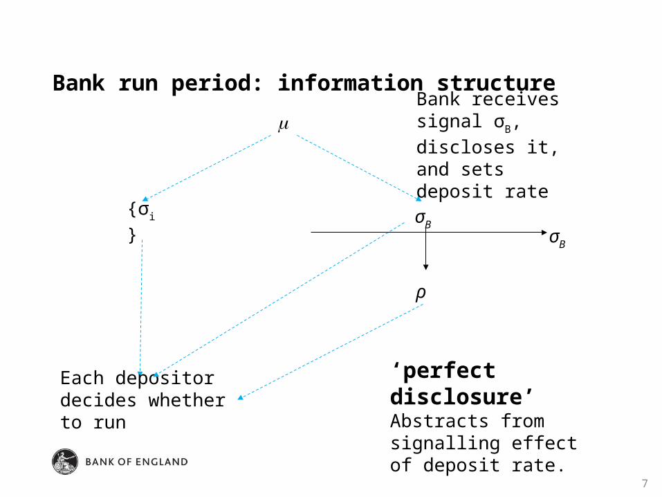
Bank run period: information structure
7
σB
ρ
{σi}
Each depositor decides whether to run
Bank receives signal σB, discloses it, and sets deposit rate σB
‘perfect disclosure’Abstracts from signalling effect of deposit rate.
Bank run period: Equilibrium
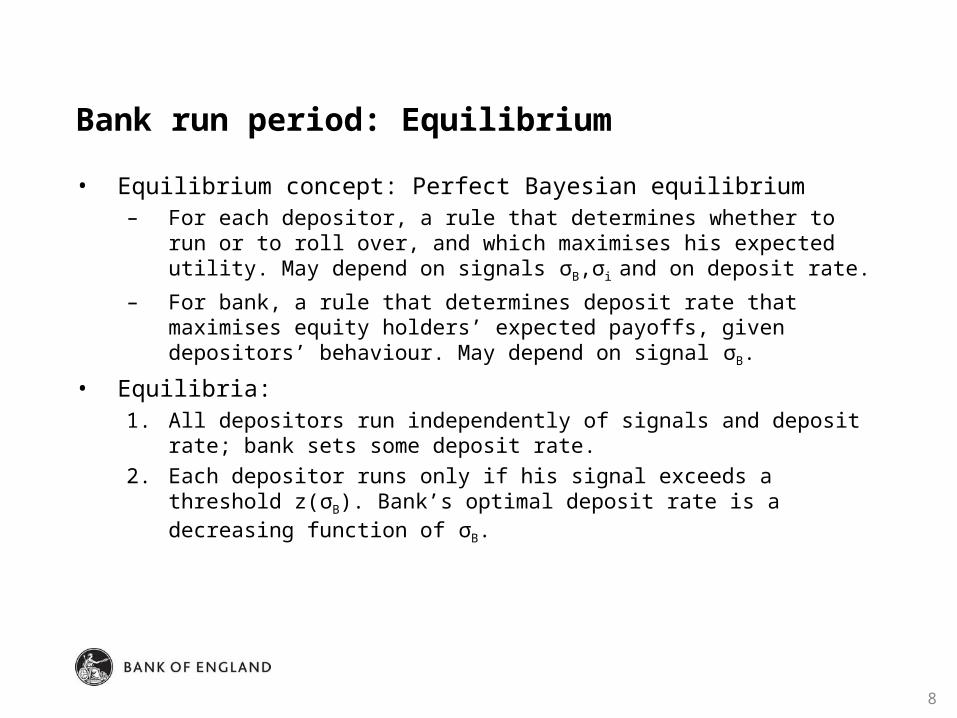
• Equilibrium concept: Perfect Bayesian equilibrium– For each depositor, a rule that determines whether to run or to
roll over, and which maximises his expected utility. May depend on signals σB,σi and on deposit rate.
– For bank, a rule that determines deposit rate that maximises equity holders’ expected payoffs, given depositors’ behaviour. May depend on signal σB.
• Equilibria:1. All depositors run independently of signals and deposit rate; bank
sets some deposit rate.
2. Each depositor runs only if his signal exceeds a threshold z(σB). Bank’s optimal deposit rate is a decreasing function of σB.
8

Bank run period: ex-ante likelihood of bank’s failure
• For given capital and liquidity ratios, compute ex-ante likelihood of failure via simulation:– Generate risky asset returns
– Check whether more deposits withdrawn than bank has liquid assets. If so, bank fails. If not, check whether bank nevertheless fails in final period because it is insolvent.
• Do this for different combinations of capital and liquidity ratios• Capital and liquidity ratios that lead to same likelihood of failure
are collected in iso-risk curves.
9
Key determinants of iso-risk curves
10
Capital ratio (e)
Liq
uid
ity r
atio
(m
/s)
Risk-averse depositors, normal returns
Lower recovery value
Risk-neutral depositors
Greater risk aversion
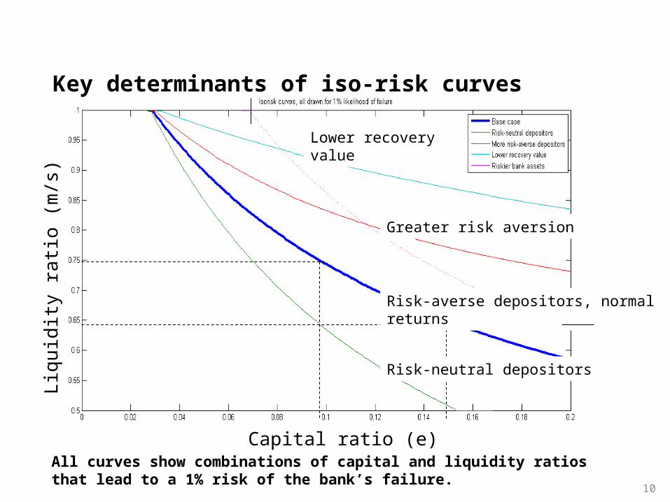
All curves show combinations of capital and liquidity ratios that lead to a 1% risk of the bank’s failure.
Results
Some degree of substitutability between capital and liquidity ratios:
• A well capitalised bank can afford to pay a high interest rate to attract depositors in a crisis without putting its solvency at risk. So its liquidity risk is smaller.
Key determinants of iso-risk curves are:
• Depositors’ risk-aversion: the more risk-averse, the greater liquidity risk, and the more capital and liquidity are required to meet a given failure risk target.
• Distribution of asset returns: the greater the volatility, the more capital and liquidity are required.
• Recovery value: the larger depositors’ recovery value, the less capital and liquidity are required.
11

First period: Choice of capital and liquidity ratios
• Recall: cost of funds are exogenous in first period. Different types of funding have different costs.
• Less elegant than endogenising cost of funding instruments... • ...but avoids complications of explicitly modelling departures
from Modigliani/Miller...• ... and facilitates testing the effect of different funding cost
assumptions on trade offs (source of disagreement in Basel III negotiations, in particular cost of equity)
12
Costs of adjusting capital and liquidity ratios
• Adjustment method: Aim is to separate effect of adjusting capital ratio from adjusting liquidity ratio.
• Capital ratio = equity / risky assets. Adjustment: replace bonds by equity (balance sheet size constant; liquidity ratio unchanged).
• Liquidity ratio = Liquid assets / unstable (short-term) liabilities (‘deposits’). Adjustment: purchase government bonds financed by bonds, keeping deposits constant (balance sheet expansion; capital ratio unchanged).
• Adjustments are costly only if bank’s funding costs do not fully adjust to changes in risk; or if government bonds ‘special’: preferred habitat for some investors.
13

Cost scenarios
14
# Funding costs adjust to bank’s risk
Return on gilts
Costs of higher capital ratios
Costs of higher liquidity ratios
1 No Constant Tax-adjusted difference between return on equity and bank bonds
Spread of bank bonds over government bonds
2 Yes, to changes in credit risk (s.t. taxes)
Constant Lost tax benefit of debt finance
As #1
3 As #2 Variable As #2 As #1 but spread rises with bank purchases of gilts

Calibration choices for key parameters
15
Parameter Value
Long-term bank debt 5%Equity 10%, 15%Liquid asset = risk-free outside investment option 3%
Risky asset distribution: 5% Gross mean return (ex funding cost) 5% Standard deviation: from structural credit risk model 0.9% Standard deviation: from Miles et al (2011) 2.5%
Tax rate 28%Recovery value of depositors’ claims 50%, 10%Exogenous components of bank’s balance sheet in period 1 Investment in risky asset: normalised to 100% Short-term debt 25%
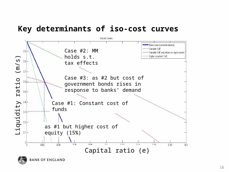
Key determinants of iso-cost curves
16
Capital ratio (e)
Liq
uid
ity r
atio
(m
/s)
Case #1: Constant cost of funds
Case #2: MM holds s.t. tax effects
as #1 but higher cost of equity (15%)
Case #3: as #2 but cost of government bonds rises in response to banks’ demand

Key determinants of cost-minimal combinations for failure risk levels from 20% to 0.05%
17
Capital ratio (e)
Liq
uid
ity r
atio
(m
/s) Constant costs of funding
instruments, normal returns
3.5%
Constant costs of funding instruments, fat-tailed returns
7%
Cost of equity funding adjusts to risk and return on government bonds falls with bank’s demand; normal returns.
Cost of equity funding adjusts to risk; normal returns

Optimal capital and liquidity ratios
• Expansion paths only shows cost-minimal combinations of capital and liquidity ratios for given risk.
• Need to quantify cost of bank failure to compare costs and benefits of higher capital and liquidity ratios.
18
Model Sector-wide interpretation
Cost of higher capital and liquidity ratios
Increase in funding costs and negative carry from holdings gilts
Decline in investment and GDP due to higher bank lending rates
Benefits of higher capital and liquidity ratios
Reduced likelihood of bank’s failure higher payments to equity holders
Reduced likelihood of banking crises and associated decline in GDP
Welfare benefits and costs
• Benefits: Assume GDP falls by 10% in response to each crisis, 2.5pp of which are permanent.
can compute marginal welfare benefit (as a % of GDP) of a financial crisis, and of reducing the probability of that crisis when banks’ capital and liquidity ratios are increased.
• Costs: Assume that banks pass on most of cost increase in normal times (but not in crisis times) to borrowers
Bank-dependent borrowers’ cost of capital rises
Reduction in investment and production capacity
Reduction in level of long-run GDP
Can compute marginal welfare cost of reducing probability of banking crisis from impact of higher capital and liquidity ratios on banks’ cost.
19
Welfare benefits and costs: results and discussion
• Across cases, crisis probability of less than 1% balances costs and benefits of higher capital and liquidity ratios
• However:– Welfare calculation takes many shortcuts
– In particular, interdependencies between banks are ignored – but so is imperfect correlation between banks’ portfolios – net effect uncertain.
– Discrepancy between assumption that return on illiquid asset is exogenous (bank run model) and assumption that banks pass on increased funding costs to clients in normal times (welfare loss through tighter regulation)
– No justification for why funding costs don’t correspond to banks’ risk not clear which private costs are welfare costs, and not just redistributions of banks’ private costs.
20

Discussion: External insurance against illiquidity
• In practice, central bank offers liquidity insurance to solvent banks
• In a world in which banks rely on CB liquidity insurance, model overestimates required liquid asset holdings.
• If CB offers liquidity insurance at a pre-announced interest rate (eg, policy rate + 100bps at DW), model also overestimates marginal benefit of higher capital ratios: no need to pay high deposit rates in crisis.
• Under what conditions should CB provide liquidity insurance (price, collateral requirements, commitment)?
21

Discussion: Variation of prudential requirements and monetary policy implementation
• Interactions between monetary policy and variations in capital and liquidity ratios
• Liquidity: Increased demand by banks for safe, liquid assets
– Reduces yield of liquid asset shifts down risk-free yield curve
– Reduces bank’s profits some increase in cost of bank lending.
Would these factors have opposite impact on real activity?
• Cost of higher liquidity ratio may depend on way in which monetary policy is implemented.
• If haircuts on assets that count towards regulatory liquid asset buffer are larger than haircuts on assets that CB sets, banks may pledge these assets to CB.
22

Conclusion
• Capital and liquidity ratios can substitute for each other in ensuring that the bank is resilient to the threat of runs.
• A high liquidity ratio appears appropriate
– If the return on equity is unresponsive to changes in the bank’s solvency risk AND credit intermediation via banks matters;
– If depositors are very risk-averse in periods in which we care about banking stability;
– If there is ample supply of almost risk-free liquid assets.
• Base case suggests that desirable probability of bank failure is less than 1% p.a.
23

ANNEX

Annex
• Marginal costs and benefits of lower probability of bank failure• Convenience yield of Treasuries• Modeling of liquidity risk• Imperfect disclosure• More on the calibration of asset returns
25

Marginal welfare costs and benefits of lowering probability of bank failure
26
00.020.040.060.080.10.120.140.160.180.20
10
20
30
40
50
60
70
Risk of crisis (inverted scale) p.a.
% o
f G
DP
Cumulated discounted cost and benefit of reducing the probability of crises by 1pp
High benefits
Low benefits
Cost case 1: fixed returnsCase 2: CoE responds
Case 3: CoE and return on GovBonds respond
Risk of bank failure
% o
f GD
P

Cost of purchases of gilts
• Simplest approach: cost = normal-time difference in yield of bank bonds and gilts times amount.
• But keeps yields constant. How might they change?• Decompose yield difference into two components
– Default risk premium
– Convenience premium: due to (1) greater liquidity of gilts; and (2) investor preference for ‘absolute safety’ of gilts: avoids credit risk assessment costs etc.
27

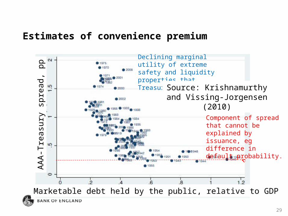
Estimates of convenience premium
• Gilts have desirable attributes which bank bonds don’t have. • When banks absorb greater amount of outstanding gilts, fewer
gilts are available for non-bank investors • Both price of gilts and convenience premium over bank bonds
will rise. • But by how much?• Consider the following link between the supply of US Treasuries
and the spread of AAA corporate bonds over US Treasuries.
28
Marketable debt held by the public, relative to GDP
AA
A-T
rea
sury
sp
rea
d, p
pEstimates of convenience premium
Declining marginal utility of extreme safety and liquidity properties that Treasuries offer.
Component of spread that cannot be explained by issuance, eg difference in default probability.
29
Source: Krishnamurthy and Vissing-Jorgensen (2010)

Estimates of convenience yield of US Treasuries
Costs
30
0
50
100
150
200
250
300
20% 40% 60% 80% 100% 120%
bps
Marketable debt held by the public, % of GDP
Range of point estimates: various specifications and samples
Estimates of convenience premium of Gilts
Why choose the lower bound estimates?• US Treasuries probably demand a greater convenience yield
than gilts• Lessons from effect of QE on gilt yields:
– £200bn in bond purchases gilt yields fall by 100bps.
– But not entirely clear how comparable to KV
– KV considered permanent effects in normal times ( underestimate). However, QE replaced gilts with (liquid & safe) CB reserves.
– £200bn corresponded to reduction in supply of gilts from 40% to 25% of GDP in 2009/10 KV would suggest gilt yields down 35bps.
Costs
31

Modeling of liquidity risk (Morris and Shin, 2008)
• Assumption: Given some information about banks’ profitability, depositors choose on the basis of expected returns whether or not to withdraw their deposits.
• Requires an assessment of what other depositors do. – Informally: depositor does not know what his fellow depositors will
do, so assumes that share of fellow depositors who withdraw is uniformly distributed.
• Result: ‘Risk-dominant’ equilibrium selected.• Supported by experimental evidence.
32

Risk-dominant equilibrium
• Two equilibria: (Run, Run) and (Don’t run, Don’t run)• Payoff from running when uncertain about opponent’s behaviour:
(1/2) * 1 + (1/2) * 2 = 1.5. • Payoff from not running: (1/2) * (-1) + (1/2) * 3 = 1• So (Run, Run) is the risk-dominant equilibrium• If ‘Don’t run’ becomes more profitable in expectation – for
example, because the bank has more capital and liquidity – then don’t run could be the risk-dominant equilibrium.
Run Don’t run
Run (1,1) (2,-1)
Don’t run (-1,2) (3,3)
33
1/2 1/2
Overview Analytical framework
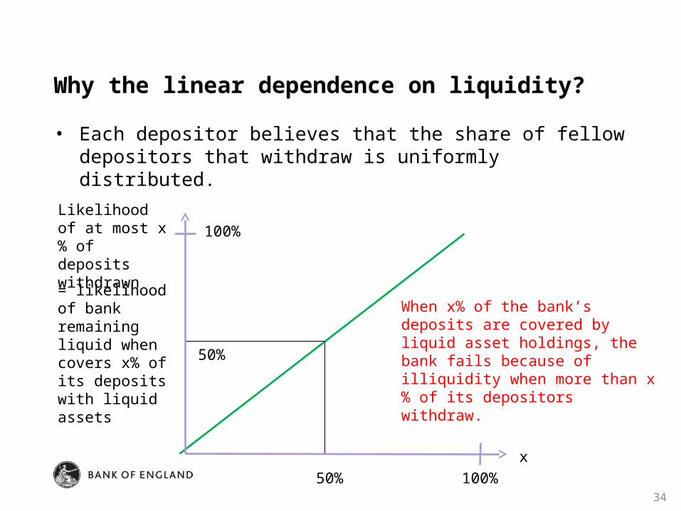
Why the linear dependence on liquidity?
• Each depositor believes that the share of fellow depositors that withdraw is uniformly distributed.
100%50%
= likelihood of bank remaining liquid when covers x% of its deposits with liquid assets
50%
When x% of the bank’s deposits are covered by liquid asset holdings, the bank fails because of illiquidity when more than x% of its depositors withdraw.
x
Likelihood of at most x% of deposits withdrawn
100%
34
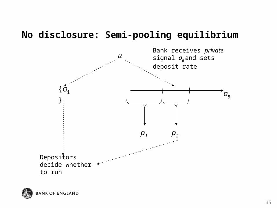
No disclosure: Semi-pooling equilibrium
35
σB
ρ1 ρ2
{σi}
Depositors decide whether to run
Bank receives private signal σB and sets deposit rate
Semi-pooling equilibrium for precise signals
Dependence on precision of depositors’ signals• Bank sets interest rate to avoid that withdrawals exceed liquid
asset holdings. Assume parameters / balance sheet are such that that higher interest rate attracts deposits.
• When depositor signals are imprecise, depositors rely on deposit rate as source of information bank with bad signal has incentive to deviate from equilibrium, set a lower interest rate, and mimic better bank need wide pooling interval to avoid that deviation profitable.
• When depositor signals are very precise, they ignore information provided via deposit rate bad bank has little incentive to mimic better bank intervals narrow
36

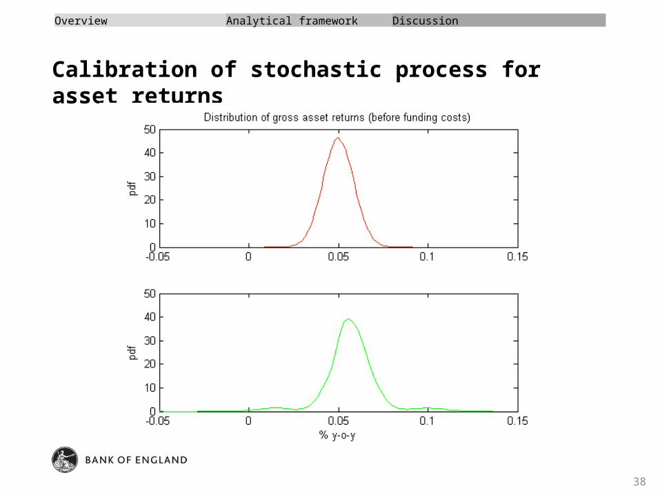
Calibration of asset returns
• Distribution of bank’s asset returns in absence of liquidity risk = distribution of major UK banks’ assets using Merton-type network model.
– Questionable interpretation: Merton model assumes risk-free debt and no liquidity risk.
– Mean asset return set such that likelihood of bank’s failure due to solvency risk only = likelihood of ‘systemic crisis’ in structural credit risk model.
– Works if equity prices only reflect solvency risk – otherwise would overestimate failure risk.
• Alternative: Calibration following Miles et al (2011)
– Non-parametric estimate inferred from volatility of GDP
– Substantially higher volatility estimates and fat tails.
37
Calibration of stochastic process for asset returns
38
Overview Analytical framework Discussion

Calibration of stochastic process for asset returns
39

Decomposition of DM estimate of asset return
-0.4 -0.2 0 0.2 0.4 0.60
0.02
0.04
0.06
0.08
0.1
0.12
GDP and bank asset returns: % y-o-y changes
Distribution of GDP realisations. Source: Miles et al (2011)
-0.2 -0.1 0 0.1 0.20
0.02
0.04
0.06
0.08
0.1
0.12
Bank asset returns: % y-o-y changespdf
Implied distribution of bank asset returns. Source: Miles et al (2011)
-0.1 0 0.1 0.2 0.30
5
10
15
20
25
30
35
40Density estimate for sampled returns
Bank asset returns: % y-o-y changes
-0.1 -0.05 0 0.05 0.10
5
10
15
20
25
30
35
40Density estimate for predictable part of returns
Predictable returns: % y-o-y changes
-0.15 -0.1 -0.05 0 0.05 0.10
5
10
15
20
25
30
35
40Density estimate for unpredictable part of returns
Unpredictable returns: % y-o-y changes
0 0.05 0.1 0.15 0.20.97
0.975
0.98
0.985
0.99
0.995
1
1.005
leverage ratio (equity relative to unweighted assets)
Liq
uid
ity r
atio (
Liq
uid
resourc
es r
ela
tive t
o s
hort
-term
debt)
Isorisk curve for 0.5% likelihood of failure
40