NBER WORKING PAPER SERIES

SHOCKS

John H. Cochrane

Working Paper No. 4698

NATIONAL BUREAU OF ECONOMIC RESEARCH1050 Massachusetts Avenue

Cambridge, MA 02138April 1994

This research is partially supported by a grant from the NSF. I thank Alexander Reyfman foroutstanding research assistance, participants at the Fall 1993 Carnegie-RocheSter conference.Olivier Blanchard, Charles Plosser. Julio Rotemberg. and Michael Woodford for many helpfulcomments, and Charlie Evans for comments and several data series. This paper is part of theNBER's research program in Economic Fluctuations. Any opinions expressed arc those ofthe author and not those of the National Bureau of Economic Research.

NBER Working Paper #4698April 1994

SHOCKS

AB&IRACF

What are the shocks that drive economic fluctuations? I examine technology and money

shocks in some detail, and briefly review the evidence on oil price and credit shocks. I conclude

that none of these popular candidates accounts for the bulk of economic fluctuations. I then

examine whether consumption shocks." news that agents see but we do not, can account for

fluctuations. I find that it may be possible to conswuct models with this feature, though it is

more difficult than is commonly realized, If this view is correct, we will forever remain ignorant

of the fundamental causes of economic fluctuations.

John H. CochraneDepartment of EconomicsUniversity of Chicago1126 East 59th StreetChicago, IL 60637and NBER

1. Introduction

What shocks are responsible for economic fluctuations? Despite at least two hundred years

in which economists have observed fluctuations in economic activity, we still are not sure.

For example, a session of prominent macroeconomists at the 1993 AEA meetings ad-

dressed the question "what caused the 1990 recession?" (Blanchard (1993), Hall (1993),and Hansen and Prescott (1993).) They examined a long list of candidates—factor prices,

especially oil, monetary policy, government purchases, tax increases, technology shocks,bank regulation, international factors, and sectoral shifts. They came up empty-handed.

Prescott and Hansen claimed technology shocks, but interpreted these so broadly to en-compass any of the above and more (see below). Blanchard and Hall favored "consumption

shocks." Since consumption is an endogenous variable, the ultimate source of variabilitymust be news about future values of any of the above. But what news and about what

future event is not identified.

It is tempting to offer up a mixture of shocks in a spirit of compromise, so thatrecessions are sums of many small negative impulses, or to speculate that different shocks

caued different historical episodes. However, there are good reasons to try to limitourselves to a small number of recurring shocks. Business cycles are "all alike" in many

ways (Lucas 1977). Investment and durables fall by more than output, hours fall by

about as much as output, nondurable consumption by much less than output. Different

shocks are unlikely to produce such similar responses. For example, if a shock (saya credit crunch) is temporary, it should cause a small reduction in consumption, anda big decline in investment, If it is permanent (say a tax increase) it should cause amuch larger decline in consumption, and may not change investment at all. The need to

produce roughly similar dynamics severely constrains the dynamic structure of the shocks,

and hence argues for a common sourc& Similarly, shocks in different places—preferences,

technology, money, government spending, etc.—yield different correlations between series.In explicitly dynamic models, it is no longer true that any source of aggregate demand

decline is as good as another, and kicks off the same dynamic pattern.

After an extensive review of technology and money shocks, and a brief review ofoil and credit shocks, I conclude that we havcnt found large, identifiable, exogenousshocks to account for the bulk of output fluctuations. Monetary policy shock account

1

for at most 20% of the variation in output. Statistics that focus on predictability findalmost no contribution of technology shocks to business-cycle output variation. Shocks

to consumption and output—endogenous variables—explain a robust 50-70% of output

variation. Specification uncertainty, choice of statistic, and sampling variation are asmuch of the story as point estimates. Plausible variations can generate numbers from 0

to 100% for both money and technology shocks.

I then ask whether we can account for fluctuations by "consumption shocks," newsconsumers see but we do not see. This is an attractive view, and at least explains our

persistent ignorance of the underlying shocks. But it is not as easy as it seems to specify

a consistent dynamic model in which such consumption shocks generate business cycle

fluctuations.

My review of the evidence for various shocks stresses four themes:

Theme 1: Despite the fact that empirical work assessing the contribution of shocks is

often conducted in an atheoretical context, one's view of the propagation mechanism, or

economic theory, is crucially important for identifying shocks and evaluating their effect

on output. The results can change drastically as one views the data in the perspective ofmore or different theoretical views.

Theme 2: The statistic one chooses is crucially important as well. Variance decompo-

sitions, variance of Hodrick-Prescott filtered output, variance of Beveridge-Nelson filtered

output, etc. all can give drastically different results.

Theme 8: Economic agents have a lot more information than we do. What is a shock

to us may be known by them.

Theme 4: There are 'level' variables, including the consumption/output ratio, M2velocity, term spreads, and hours, that indicate the state of the economy, and hence can

forecast long-horizon output with huge (60% or more) ft2.

2. Some Warnings

1) Exogeneity. We traditionally search for exogenous shocks. Any VAR mechanicallyaccounts for 100% of the variance of output by unforecastable movements in endogenous

variables. To say that such a shock causes fluctuations just leads to the question, "why

did the endogenous variable move?" and a search for a deeper, exogenous shock. There is

also an econometric reason to search for exogenous shocks: only responses to an exogenous

2

variable can measure the effects of policy-induced changes in that variable.

But exogenous shocks are rare, and the imperialistic march of economics makes events

truly outside the economic system rarer every day. We are used to thinking of govern-

ment policy as exogenous, but a glance at the newspaper shows that policy-makers watch

the economy and economic forecasts obsessively. Monetary VARs recognize that policy

responds to the economy, and try to isolate the exogenousshocks as residuals to a policy

rule. But why should a policy-maker deliberately introduce a random component to itsdecisions? Any maximization objective in a nonstrategic environment leads to detenriin-

istir rules for setting controls as a function of state. The Fed always describes its actions

as responses to events, not randomized experiments.'

Technology shocks sound nicely exogenous. However, the growth literature is workinghard to make technology endogenous, and the real business cycle literature seems to have

abandoned the technology interpretation of the residual anyway. Prices are of course

endogenous economic variables. Only the weather remains exogenous2, but business cycles

seem to have nothing to do with the weather.

It would be nice to point to recognizable events, of the type that are reported in news-

papers, as the source of economic fluctuations, rather than residuals from some equation.

This search has been even more fruitless. Of course, Monday morning quarterbacks al-

ways attribute fluctuations to a long list of events, typically an undigested summary of

business section headlines. But the fingers pointed at these events are seldom attached

to a serious explanation how the headline events are quantitatively capable of producinga large and protracted decline in output, or why similar headlines often do not have any

effects. Finally, in expectational models, times when the Fed does nothing but it was

expected to are just as mudi a shock as times in which it did something unexpected; butthese times rarely wind up in the newspaper. In the context of these models, it is not

embarrassing that residuals to a forecasting equation are the underlying shocks -

2) Propagation Many papers try to study "shocks" without specifying much aboutthe "propagation mechanism." But the study of shocks and propagation mechanisms are

Of course, neither we nor economic agents have enough information to forecast policy perfectly.Residuals to agent's forcasting model can count as exogenous shocks if only unanticipated money matters.Unfortunately, we have even less inkrmation than agents, so the innovation measured by our forecastingmodel is not likely to be the same as the innovation measured by agents' models. Furthermore, ifanticipated money matters, or in investigating other shocks, then rponses to "shocks" that really reflect

superior information may not be meaningful.2For the moment. Advocates of economic policy to affect globaL warming and chaos theonste are

trying hard to make the weather endogenous as welt!

3

of course not separate enterprises. Shocks are only visible if we specify something about

how they propagate to observable variables. More importantly, we can't really believethat a shock affects the economy unless we understand how it does so.

Real business cycle models produce artificial time series, so we can use a lot of infor-

mation about the propagation mechanism to identify and quantify the importance of itsshocks. Dynamic monetary economics is at a much more primitive stage. The responsepatterns of cash-in-advance models are so far from the data that they are not much used

in the empirical analysis of monetary shocks. Many other monetary models do not give

any explicit dynamic predictions. Therefore, empirical researchers typically fish for VAR

specifications to produce impulse-responses that capture qualitative monetary dynamics,for example as described in Friedman (1968). Other shocks, such as oil price, credit, etc.

are not associated with well spelled out dynamic theories of their effects on the economy,

so identification and evaluation is even more tenuous. For this reason, shock identification

is often based on simplified stylized features rather than the predictions of explicit models

—"demand" shocks have no long-run effect on output, "monetary" shocks are representedby unforecastable movements in the federal funds rate, and so forth3

3) Who cares? The answer to question, "what exogenous shocks account for outputfluctuations?" has more limited implications than is usually recognized.

First, it may not have immediate policy implications. For example, suppose thatoil prices have small direct effects on the economy, but they induce monetary policy-makers to cause recessions. (Darby 1982 argues for this view.) In this case, oil prices arethe exogenous shock, and the Federal Reserve is just part of the propagation mechanism.

However, to say "oil shocks account for fluctuations" is a misleading description; monetary

policy caused the recessions. We don't have to worry about middle east politics to insulate

the economy from fluctuations, we have to worry about the Fed.

Second, the point of most shock accounting papers is really a comparison of broadclasses of as-yet-incomplete models of the propagation mechanism. They want toanswer

questions such as "can any competitive equilibrium model account for fluctuations inoutput, or will we need monetary, sticky price, or noncompetitive models?" But it's hardto come up with some behavior that a whole class of models, as yet not investigated,is incapable of producing. Furthermore, most classes of modelare not, in fact, tied tospecific shocks. Technology shocks could account for all of the fluctuations inoutput, yet

3 don't mean to sound criticaLThese identif'ing procedures are the state of the art.

4

do so through channels specified by imperfectly competitive models. Monetary shocks

could account for fluctuations, through a intertemporal market clearing mechanism (saya real business cycle model with a cash-in-advance constraint), as well as through a sticky

price mechanism.

Thus shock accounting does not really say that much about the plausibility of broad

classes of economic model. They say even less about modeling methodologies, which is

really at stake. I don't think Prescott would feel vindicated if the profession converged

on the view that technology shocks account for 80% (or all) of output fluctuations, yetdo so through fluctuations in the aggregate supply curve of an IS-LM model!

4) Information advantages. Shock identification procedures are sensitive to the factthat economic agents and policy makers base their forecasts on more variables than we

include in our VARs. The weather forecast Cranger-causes the weather, but shooting the

weatherman won't produce a sunny weekend.

5) Linearity. The central question in this paper is whether each candidate shockcan explain a large fraction of output variance (either variance of growth rates or forecast

error variance). A lot of assumptions go even into this statement of the question.

First, are recessions any different from other times? In virtually all economic models

and in VAR representations, booms and busts are just different draws from the same dis-

tribution. Recessions may represent an interesting combination of large negative shocks,

but they are not draws from a different process. But in thinking qualitatively about theeconomy, we often study recessions as if they are a distinct phenomenon. The above cited

AEA session was not organized around "What accounts for the forecast error variance of

output?" but "What caused the last recession?"

Second, does the economy respond to shocks in an importantly nonlinear way? Mostqualitative discussions reflect such a belief, for example, the need for a "booster shot" to

keep the economy from "sliding into a recession." But real business cycle models and VAR

techniques are decidedly linear, and there is little lolid evidence for important nonlinear

structure in the data.

With these warnings and the themes they motivate in mind, I turn to a quantitative

examination of the evidence for some shocks.

5

3. Monetary shocks

Shock-s to the quantity of money or other measures of Federal Reserve policy have long

been suspected to influence output. The central question for us is: how much outputvariation is due to monetary shocks? Even if the Fed can influence output, it does notfollow that most fluctuations in output are in fact due to monetary policy shocks.

Ideally, we would address this question by using a well-specified model that identifies

monetary shocks and predicts the economy's response, as real business cycle models do

for technology shocks. However, we don't have any empirically successful models of this

sort, so most evidence for the effects of monetary shocks comes via vector autoregressions

(VARs). Three issues guide our evaluation of these VARs.

1) Shape of impulse-responses. In the absence of an empirically useful dynamic mon-

etary theory, at least we can require the impulse-response functions to conform to qual-

itative theory such as Friedman (1968). Most VARs do not conform to this standard.

Prices may go down, real interest rates up, and output may be permanently affected byan expansionary shock. It is not very convincing to claim that money accounts for x%of the variance of output in such a VAR, since we have no idea how money produces its

alleged effect.

2) Shock identification. This is obviously a crucial decision, but theory offers little help.

First, one has to pick which variable to use as an indicator of money supply disturbances.

I will examine the popular choices, Ml, M2, the federal funds rate, and nonborrowedreserves.

Second, one must specify the ordering, or which variables are contemporaneously un-

affected by shocks to other variables. The monetary variable often goes first—it is assumed

not to be contemporaneously affected by any of the other variables. This is sometimesjustified by the (false) assumption that the Fed and the money supply process do notrespond to within-period values of the other variables. Of course, the opposite assump-ion that monetary aggregates do not contemporaneously affect economic variables is even

worse! Nonrecursive identification schemes are also possible. The true shocks may linear

combinations of the innovations, to any single variable. These schemes take linear combi-

nations of the impulse-response functions, so they can have a major effect on the results,

even when the error varjance-covariance matrix is diagonal.

The results often depend on the identification scheme. In practice, researchers clearly

experiment with orderings, and present the scheme that gives the "best" results. If "best"

6

• means "responses that most closely correspond to the predictions of monetary theory"this is not so bad, and can almost be defended as a theory-based identification procedure.

3) Specification. Much VAR evidence also turns out not to be robust to variable

definitions, lags, unit root structure, trends, variables included in the VAR, at what

horizon variance decompositions are calculated, and sampling error. (See Todd 1993.)My baseline VARs use log-levels, quarterly data and one year of lags. I have corroboratedmost results in monthly data and with two years of lags. Most but not all results are

robust.

A preview of the results. I examine M2, Ml, federal funds and nonborrowed reserve

shocks in turn. A common pattern emerges. In simple VARs, each shock seems to accountfor a large fraction of output variation. When more variables are introduced and as the

specification is refined (fished) so that the responses are broadly consistent with monetary

theory, we find that monetary shocks explain lower and lower fractions of output variance.

In the end, I find evidence that monetary policy can affect the economy roughly the wayFriedman said it would, though with suspiciously long lags, but I do not find evidencethat monetary policy shocks did account for more than at most 20% of the variance of

output, and likely much less.

3.1. M2

3.1.1. A simple M2, y, p VAR

I start with a simple VAR consisting of the logs of M2, output, and the price level, in the

spirit of the first VARs run by Sims (1980). In the impulse-response functions, Figure3.1, M2 shocks are persistent, and lead to substantial rises in output and then prices.However, the output response is surprisingly drawn out. It peaks two to three yearsafter

the shock, and output seems to be permanent. The price response is also very sluggish.4

Table 3.1 shows variance decompositions for this VAR, and Table 3.2 summarizes

output variance decompositions for all of the M2 VARs. The M2 shock accounts for

dramatic fractions of the variance of output at long horizons, increasing from 32% at a

one year horizon to 82% (!) at a 3 year horizon. The M2 shock also accounts for 21%

40f course, one should be cautious in evaluating estimated long-horizon responses in this (any) VAR.Since the VAR is run in levels1 and I happened not to estimate explosive roots in this VAR, the estimatedresponses to all shocks are transitory, but take 100-200 years to die out. Many of theVARs I estimatebelow have impulse-responses that oscillate with periods of 20-40 years. For this reason, the graphs stopat a 5 year response.

7

ml—).*2 n2—)% I,

T2 3TVTTt"TFigure 3.1: Response to 1 a m2 shocks, m2 y p VAR. Horizontal axis in years, verticalaxis in %.

of quarterly output growth, and 45% annually. Note how sensitive the results are to the

horizon. This is far from an innocuous choice! This VAR is not sensitive to the order of

orthogonalization (as long as one maintains some recursive scheme), and to the inclusion

of trends.

Shock and horizonlYear 2Year1 Qtr. 3 Year

Var.of m2 y p1m2 y pjm2 y p1m2 y pm2 100 0 0 99 1 0 98 0 2 94 1 5

y 1 99 0 32 68 0 70 30 0 82 17 1

p 1 3 96 0 7 92 1 17 83 3 24 73

Table 3.1: Variance decomposition from rn2-y-p VAR. Table entries are percent of horizonstep ahead forecast error variance of the row variable explained by the column shock.VARs in log.levels with 4 lags, orthogonalized in the given order (m2, y, p). Quarterlydata 1959:1-1992:4.

However, we obtain very small output effects if we view this VAR through the eyes of

a simple rational expectations or cash.in-advance model in which money can have only

one-period effects5, or if non-neutral effects of money must come through price shocks as

in Lucas (1972). M2 shocks account for 1% of one-quarter ahead output variance, andprice shocks for less than 0.5%; price shocks account for less than 10% of output variance

at any horizon, in any orthogonalization.

Also in line with a traditional monetarist view,virtually all M2 variance (94-99%) is

due to M2 shocks. However, M2 shocks explain tiny fractions of price variance (0-3%);

virtually all of the variance of prices is due to price shocks. Since price shocks do not have

large effects on M2, we cannot understand this feature as Fed accommodation. Inflation

is certainly not always and everywhere a monetary phenoknenon in this VAR! These facts

are common to most of the VARs that follow, so I concentrate on the central question of

'"Simple" here means that agents can find out the value of aggregates with a one quarter lag.

8

this paper, output variance decompositions.

Forecast error 2 Var yVAR 1Q 1Y 2Y 3Y 1Q 1Ym2yp 1 32 70 82 21 45

cyp 18 60 78 77 29 47m2ffcyp 1 20 39 41 11 21

m2ffcyp;e.c. 0 16 28 25 11 21

(s. e. of above) (8) (11)ffcypm2 0 5 12 14 4 6

m2ffch/popyp,trend 0 8 11 7 7 5

Table 3.2: Summary of output variance decompositions in M2 VARs. All VARS runlog-levels with 4 lags, unless otherwise indicated.

3.1.2. Level variables

VARs are all about forecasting. The best long-horizon output forecasting variables are'level' variables; stationary variables that tell you if output is 'below trend' and hencemust grow over several quarters. M2 velocity is such a level variable. It is stable over

time (real M2 and output are cointegrated). Hence, if velocity is high, output must growor M2 must decline to reestablish velocity. As it turns out, real output does the adjusting.

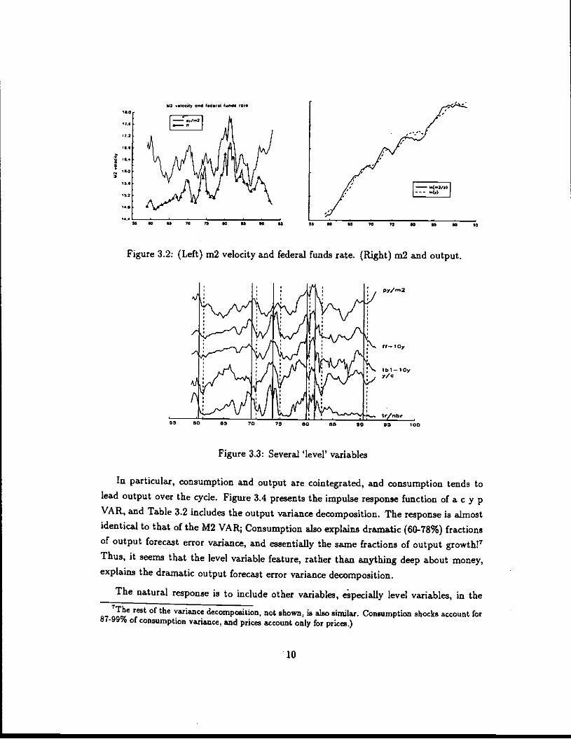
Figure 3.2 plots M2 velocity to make this point. In the left hand panel, we see that

M2 velocity is stable over time. Its fluctuations are surprisingly correlated with the level

of the federal funds rate. Thus, M2 velocity will forecast output much as the funds rate

does. However, variations in M2 velocity are tiny (note the vertical scale)6. The righthand panel plots real M2 and output. As you can see, the level of real M2 does not stray

far from that of output and M2 leads output, especially in the late 1970's and 1980's.

But there are many other level variables, including the consumption/output ratio,hours or unemployment rate, and term spreads. Figure 3.3 presents several of these level

variables. As the Figure shows, they are all highly correlated, and any one seems to pickout NBER peaks and troughs as well as the others.

6The interest elasticity of m2/(py) is only about -0.03. Here is an OLS regression, 1059:1-1992:4:

ln(rn2) = —5.07 + 1.002 ln(pp) — 0.025 ln(ff)

Since most of m2 pays interest, and since m2 velocity seems not to respond to the trend in interest rates,it is probably not wise to interpret the correlation between m2 velocity and interest rates in traditionalmoney demand terms.

9

it.u-I

'U..

'U..

11.0

I"It,It.•4.

Figure 3.2: (Left) m2 velocity and federal funds rate. (Right) m2 and output.

Figure 3.3: Several 'level' variables

*00

In particular, consumption and output are cointegrated, and consumption tends tolead output over the cycle. Figure 3.4 presents the impulse response function of a c y pVAR, and Table 3.2 includes the output variance decomposition. Theresponse is almostidentical to that of the M2 VAR; Consumption also explains dramatic (60-78%) fractionsof output forecast error variance, and essentially the same fractions of output growth!7Thus, it seems that the level variable feature, rather than anything deep about money,explains the dramatic output forecast error variance decomposition.

The natural response is to include other variables, apecially level variables, in thetThe rest of the variance decomposition, not shown, is also similar. Consumption shocks account (or

87-99% of consumption variance, and prices account only for prices.)

•lo

Ifl .•iacity and I.d.r, ('s.d. rol•

I"—'—fl

'a o Us II 75 Ia IS IC U

— ln(n3/p)

10 US 00 IS

c—c c—)y c—Ip

Figure 3.4: Responses to consumption shock, c y p VAR

VAR, and see whether money retains marginal forecast power.

3.1.3. A 5 variable VAR

I first run a five-variable VAR with M2, federal funds, consumption, output and prices.

Figure 3.5 presents the impulse-response function, and Table 3.2 includes the output

variance decomposition.

m2—). m2—)v n'Z—p0.I

0.U.,

UI

U-U •

Figure 3.5: Responses to m2 shock

This impulse-response function starts to look more like a monetary VAR should. M2

shocks have an initial liquidity effect on nominal interest rates, and then an inflation

effect. They have a hump-shaped effect on output and send prices upward. The impliedreal interest rate response also shows a transitory liquidity effect. However, the responsesare still surprisingly drawn out, and money still seems to have a permanent effect on

output and certainly on consumption.

As the impulse-responses start to look more reasonable, the output variance decom-position starts to fall. At every horizon and in differences, M2 shocks account for about

half of the variance of output that they did in the M2 y p VAR.. This is still a sizable

fraction, however, 20-40% rather than 40-80%.

U

3.1.4. Imposing velocity and c/y stability

Next, I impose the fact that M2 velocity and the consumption/output ratios are stable.To do this, I run the VAR in error-correction form, i.e. I run growth rates of all variables

except federal funds on their lags and the lagged log c/y and log M2/(py) ratios8. Figure3.6 presents the impulse-response function and Table 3.2 includes the output variance

decomposition. The responses look even more like monetary responses should. We now

get transitory responses of consumption, output and interest rates (the long-run outputand consumption responses are less than one standard error from zero) along with the

right signs on all the other variables.

The variance decompositions, reported in Table 3.2, show that the fractions of output

variance explained have dropped by another half to a third. The forecast error variances

due to M2 are 16%, 18% and 25% at 1, 2, and 3 year horizons, and 11%, 21% of onequarter and one year output variance. Furthermore, standard errors are large; a 2 aconfidence interval extends to nearly zero percent of output variance explained.

w.3—)m2 m2—)V m2—>ca. ,2—) m2—)R.oir

Figure 3.6: Responses to m2 shocks, error-correction VAR using c/y and m2/py as fore-casting variables.

3.1.5. Using long-run restrictions to identify monetary policy shocks

A further refinement: perhaps one should identify a money supply shock as a combination

of federal funds and money innovations rather than one or the other. A money supplyshock should work back up the money demand curve. To this end, and in order to impose

the desirable feature that money supply shocks should have transitory effects on realvariables, I identify a money supply shock as that combination of M2 and federal funds

shocks that has exactly no long-run effect on output (and hence consumption, since they

51t is important that the imposed cointegrating vectors m —y — pand c — y really are stationary, orone estimates explosive roots. For this reason, the error-correction VAR uses total GDP for output, andconsumption + 0.65 times government purchases for consumption.

12

are assumed cointegrated). Since the long-run effect of a M2 shock on output is small and

statistically insignificant in the previous VAR, this should be a small refinement to the

results.9

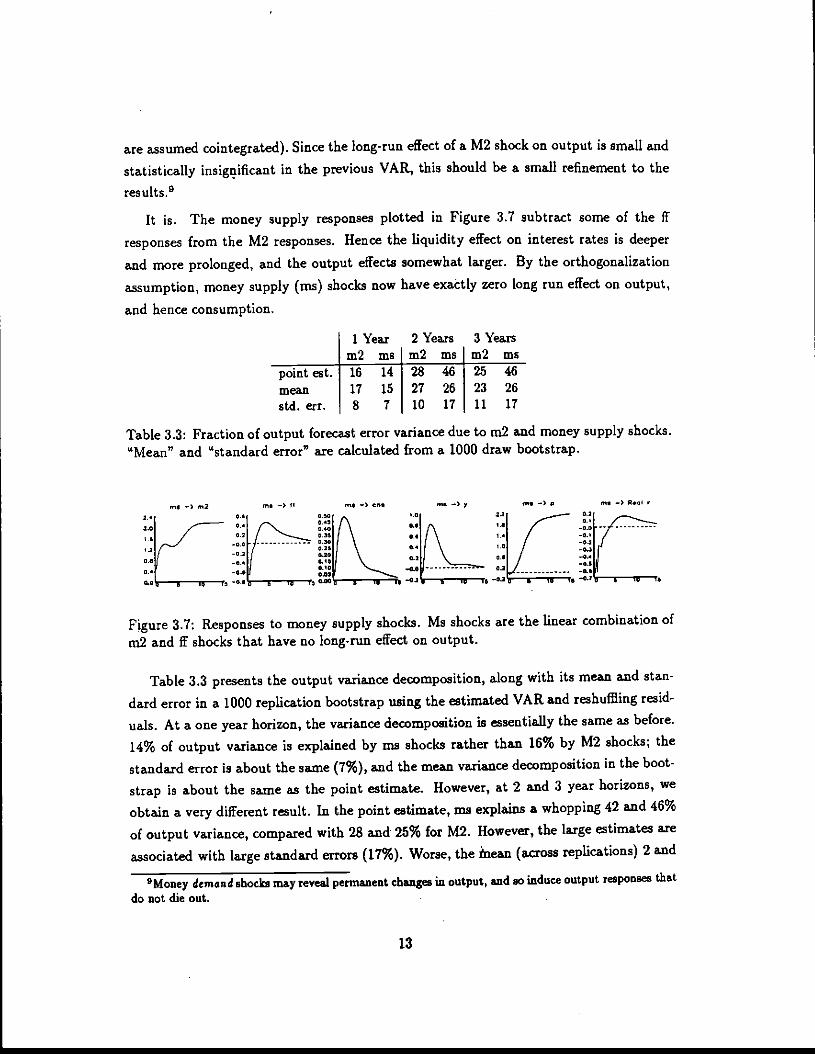
It is. The money supply responses plotted in Figure 3.7 subtract some of the ifresponses from the M2 responses. Hence the liquidity effect on interest rates is deeper

and more prolonged, and the output effects somewhat larger. By the orthogonalizationassumption, money supply (ms) shocks now have exactly zero long run effect on output,

and hence consumption.

lYear 2Years 3Yearsm2 ms m2 ms m2 ins

46

Figure 3.7: Responses to money supply shocks. Ms shocks are the linear combination of

m2 and if shocks that have no long-nm effect on output.

Table 3.3 presents the output variance decomposition, along with its mean and stan-

dard error in a 1000 replication bootstrap using the estimated VAR and reshuffling resid-uals. At a one year horizon, the variance decomposition is essentially the same as before.14% of output variance is explained by ma shocks rather than 16% by M2 shocks; thestandard error is about the same (7%), and the mean variance decomposition in the boot-

strap is about the same as the point estimate. However, at 2 and 3 year horizons, we

obtain a very different result. In the point estimate, ma explains a whopping 42 and 46%

of output variance, compared with 28 and 25% for M2. However, the large estimates are

associated with large standard errors (17%). Worse, the Mean (across replications) 2 and

9Money demand shocks may reveal pennanent changes in output, and so induce output responsesthatdo not die out.

13

point est. 16 14 28 46 25mean 17 15 27 26 23 26std.err. 8 7 10 17 11 17

Table 3.3: Fraction of output forecast error variance due to m2 and money supply shocks."Mean" and "standard error" are calculated from a 1000 draw bootstrap.

no .) m2 Ins —, II me — y me —) p0.500.450.400.350.300.205.200.i20.50

020.505 5 55 Is

3 year variance decomposition is only about 26%, about the same as M2. Similarly, the

mean response of output to the money supply shock peaks at 0.5, about the same value

as the M2 shock, while the point estimate shown in Figure 3.7 peaks at 0.8. One can

take the means as easily as the point estimates a consistent estimates of the true variance

decomposition.

There are two reasons for this strange sampling behavior. First, the if responses aremuch less precisely estimated than the M2 responses. The ms responses are a linear com-

bination of the M2 and if responses, and so inherit some of the larger sampling variation of

the if responses. Second, long-run responses are notoriously hard to estimate, since theyinvolve sums of coefficients or an estimate of the spectral density at frequency zero. Even

if the true long-run response is zero, the unconstrained estimate will not be zero in every

sample. Forcing it to be equal to zero in each sample is the heart of the sampling problem.

(Canova, Faust and Leeper (1993) discuss the difficulties of long-run VAR identification

in detail.)

In summary, though the long-run restrictions are an attractive refinement, the sam-pling distribution is substantially worse when they are imposed. When we take this fact

into account, the VAR with long run restrictions does not provide solid evidence for an

effect of monetary shocks larger than the 15-25 %, with 7.12% standard errors, provided

by the M2 VAR.

3.1.6. But.. More variables and orthogonalization

Plausible variations can destroy the pretty pattern of the impulse response functionsand bring the variance decomposition down below 10%. This specification uncertaintyis perhaps a reason even stronger than sampling uncertainty to doubt the 15-25% figure

given above.

For example, I also include hours per capita and a trend in the VAR. Detrendedhours are also a business cycle 'level' variable: output is high when hours are high. (See

Rotemberg and Woodford 1993.) Figure 3.8 shows the output response. M2 shocks now

die out after 5 years, and have a transitory and much shorter effect on output. But prices

go off in the wrong direction. Table 3.2 includes the output variance decomposition. M2

shocks now account for less than 10% of the variance of output at any horizon.

The five-variable VAR is sensitive to the order of orthogonali2ation. Figure 3.9 presents

the response of output when M2 is orthogonaflzed last (all shocks can affect M2 within

14

m2 —, ml040.70.I0.10.40.30.I0.t0.0

ml —) • ml —) r.cIr

Figure 3.8: Responses to m2 shocks, VAR with hours/per capita

a quarter), and Table 3.2 again presents the output variance decomposition. The liq-uidity/inflation effects disappear, M2 has permanent output effects, and no price effect.

M2 shocks again account for less than 10% of the variance of output. My procedure of

choosing the ordering to produce the "right" pattern of responses is not innocuous.

ml —} s'2 ) p m3 —, ml ml — r.&,

0.400.' 046 0.6I.0.-SO 0.4

0.8 t4

O.8V L02

04 04 O20.110.100.060.I00 IS •3 I IS

3.2. Ml

Figure 3.9: Responses to m2 shocks, when m2 is orthogonalized last

Ml corresponds more closely to the idea of a non- interest paying transactions balance.

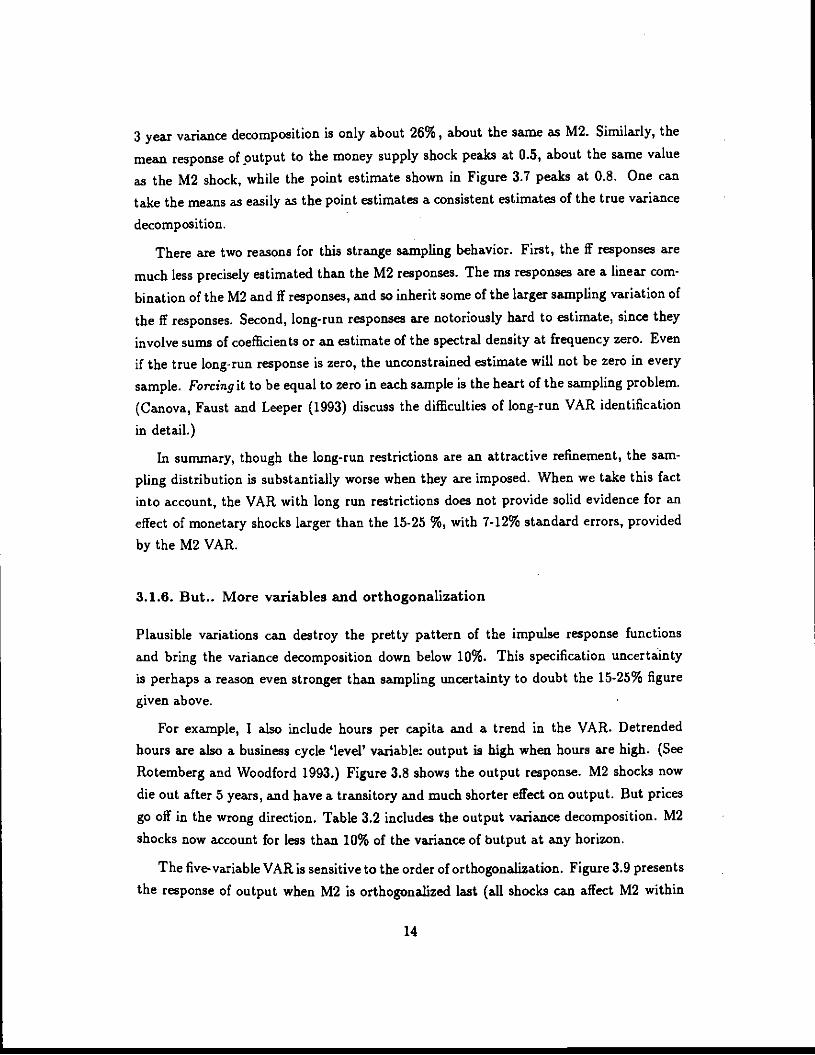
Figure 3.10 presents Ml velocity and the federal funds rate. In contrast to M2, Ml

velocity responds sensibly to the rise in the federal funds rate. The interest elasticity is

between1° -0.15 and -0.35 depending on specification, compared to -0.03 for M2. However,Ml velocity does not respond to cyclical variations in the federal funds rate, at least until

the mid-1980's. Ml does not lead output, either directly or via an interest elasticity and

101 estimated the following regressions from 1959:1-1992:4:

ajid, imposing a unit income elasticity,

ln(vnl) = —3.71 + 0.81 ln(.-py) — 0.151n(ff)

ln(ml/ptj) = —5.69— 0.34 ln(ff)

15

"2 —) C m2—-In m2—),

the fact that interest rates lead output. As a result, it is less useful than M2 for forecasting

output, and contributes less to output variance, as we will see.

However, these facts do not mean we should throw Ml out. The theory of moneydemand refers to a transactions balance for which one pays at least an interest spread; if

Ml shocks explain less output variance than M2 shocks, so much the worse for M2. Onecan simply read this fact as another case in which imposing theory sharpens (lowers) our

estimates.

hil nIociI, and l.d.r. lund.•0

I,5

S -

'S

Figure 3.10: ml velocity and federal funds rate

3.2.1. A simple Ml y p VAR

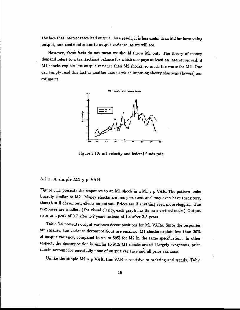
Figure 3.11 presents the responses to an Ml shock in a Ml y p VAR. The pattern looksbroadly similar to M2. Money shocks are less persistent and may even have transitory,though still drawn out, effects on output. Prices are if anything even more sluggish. The

responses are smaller. (For visual clarity, each graph has its own vertical scale.) Outputrises to a peak of 0.7 after 1-2 years instead of 1.4 after 2-3 years.

Table 3.4 presents output variance decompositions for Ml VARs. Since the responsesare smaller, the variance decompositions are smaller. Ml shocks explain less than 20%of output variance, compared to up to 80% for M2 in the same specification. In otherrespect, the decomposition is similar to M2: Ml shocks are still largelyexogenous, priceshocks account for essentially none of output variance and all price variance.

Unlike the simple M2 y p VAR, this VAR is sensitive to ordering and trends. Table

16

— —I'—'— It

SO 55 10 15 SO - 95 5* 55

mi—Omi m1—07 mi—Op0.22.2t II.0

LOS

L01-0.020.2

2 3 4 I

Figure 3.11: Response to ml shocks in ml y p VAR

Forecast error a2 Var yVAR IQ 1,1 2Y 3Y 1Q 1Ymlyp 3 16 20 20 11 19

ymip 3 1 1 1 9 9

mlyp;trend 2 8 7 8 10 16

rnlffcyp 3 2 3 8 S 10

rnlffcyp,errorcorr. 2 6 5 4

mlffcyp;e.c.;msshocks 5 7 5 4

Table 3.4: Percent of output variance explained by ml shocks.

3.4 presents variance decompositions with Ml ordered last, and when a trend is included.

Now less than 10% of output variance is explained by Ml shocks at any horizon. These

changes destroy the pretty impulse-response pattern as well.

3.2.2. A five variable VAR

Figure 3.12 presents the responses in a Ml if c y p VAR, the same specification thatprovided such nicely shaped responses for M2. Here, the responses look nothing like what

we expect of a monetary shock. As shown in Table 3.4, the fractions of output variance

explained are tiny.

ml —)ml mi—OfF mI—)c mi—Op mi)r.,lt0.120.060.04•00

—0.04-0.04.0.12—0.,.—0.20 i 1 3 45

Figure 3.12: Responses to ml shocks.

17

ml —> P

3.2.3. Imposing cointegrating vectors and long run restrictions

As with M2, we thay get better looking response functions by imposing long run restric-tions. Though the level of interest rates is probably stable in the long-enough run, it has

moved slowly in our sample. Thus, Mi velocity does not appear stationary. Rather, Midemand, Mi — p — y — off, is a better candidate for a stationary variable. I also includec — y as a stationary variable. Also as a result of the slow movement of federal funds, the

specification with stationary levels of interest rates leads to explosive responses. There-

fore, I run a VAR of differences of Mi, ff, c, y, p on their lags and the lagged valueof c — y and Mi — p — y — 0.75ff. I use -0.75 for the interest elasticity of Mi demand,

rather than -0.35 as suggested by the OLS regression presented above; -0.35 minimizesthe sum of squared residuals, but the resulting Mi —p — y — 0.35ff series still has atrend in our sample. The higher interest elasticity produces a series without a trend, and

hence non-explosive responses".

The top panel of Figure 3.13 presents responses to Ml shocks from this VAR. The

bottom panel presents responses to money supply shocks, identified as above as the combi.

nation of Mi and if shocks that leave output unchanged in the long run. These responses

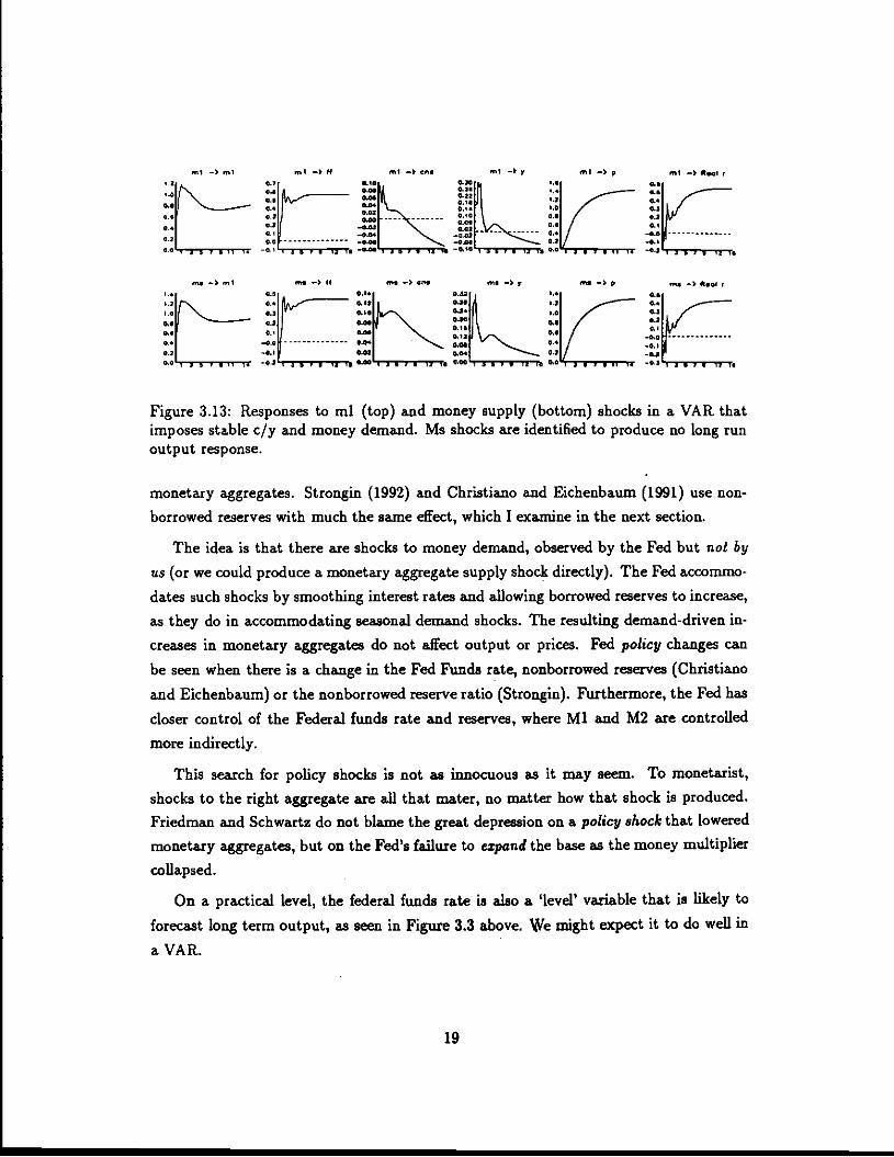
are consistent with what we expect for monetary shocks. Mi or ins shocks lead to ashort liquidity effect, and then a permanent rise in federal funds. (The level of ff isnot stationary in this specification, so there is no reason for this response to return tozero.) Mi or ms shocks lead to brief, transitory output and consumption responses, andto increases in prices. The real rate shows a short liquidity effect as well. Since inflation

eventually stops, the nonstationarity of ff is accounted for by a long-run increase in thereal interest rate. The brevity of Ml shocks' non-neutral effects is noteworthy, since itmore closely corresponds with theory.

Table 3.4 includes the variance decomposition. Despite (or maybe because of) theattractive pattern of impulse responses, Ml or Mi money supply shocks account fortrivial fractions of output variance, around 5% at all horizons.

3.3. Federal Funds

Bernanke and Blinder (1991) and Sims (1988), following a suggestion of McCallum (1982),

argue that federal funds rate forecast errors measure monetary policy shocks better than

If all of this seems a little strained, it i5. The point is to find aspecilication that produces teh "right"pattern of Impulse-responses, not to follow the dicta of atheoretical time-series specification.

18

el—)ca. TiI—)y mI—)ptict'I0.fltI•0.11ticto.Sn -

—cal-Ca.—tic •,,,, ' ,

..cc

Figure 3.13: Responses to ml (top) and money supply (bottom) shocks in a VAR thatimposes stable c/y and money demand. Ms shocks are identified to produce no long runoutput response.

monetary aggregates. Strongin (1992) and Christiano and Eichenbaum (1991) use non-

borrowed reserves with much the same effect, which I examine in the next section.

The idea is that there are shocks to money demand, observed by the Fed but not by

us (or we could produce a monetary aggregate supply shock directly). The Fed accommo-

dates such shocks by smoothing interest rates and allowing borrowed reserves to increase,

as they do in accommodating seasonal demand shocks. The resulting demand-driven in-

creases in monetary aggregates do not affect output or prices. Fed policy changes canbe seen when there is a change in the Fed Funds rate, nonborrowed reserves (Christiano

and Eichenbaum) or the nonborrowed reserve ratio (Strongin). Furthermore, the Fed has

closer control of the Federal funds rate and reserves, where Ml and M2 are controlled

more indirectly.

This search for policy shocks is not as innocuous as it may seem. To inonetarist,shocks to the right aggregate are all that mater, no matter how that shock is produced.Friedman and Schwartz do not blame the great depression on a policy shock that lowered

monetary aggregates, but on the Fed's failure to expand the base as the money multiplier

collapsed.

On a practical level, the federal funds rate is also a 'level' variable that is likely to

forecast long term output, as seen in Figure 33 above. We might expect it to do well in

a VAR.

19

.i,t —, nil in —, If on. — CO. — —) p _ — s

3.3.1. Simple if y p VARs

The top panel of Figure 3.14 presents the responses to if shocks in a simple if y p VAR.Federal funds shocks are persistent. A rise in federal funds gives rise to an initial sixmonth rise in output, and then a permanent decline. Last, there is a "price puzzle". Inresponse to a contractionary federal funds shock, prices increase for 2 years, and onlycome back to where they started after 5 years.

It .10 1111 It—I..&—) F II —, p Ii —I It

It—,, It—,.

Figure 3.14: Responses to federal funds rate shocks. Top panel: ify p VAR. Middle panel:y p if VAR (if orthogonalized last). Bottom panel: y p if VAR with trend.

Table 3.5 presents output variance decompositions. Federal funds shocks explain be-

tween 6 and 32% of output forecast error variance, as the horizon lengthens, and 24-28%

of output growth variance at iquarter and 1 year horizon.

This VAR turns out to be somewhat sensitive to ordering and trends. The middle panel

of Figure 3.14 presents the response to federal funds shocks when they are orthogonalized

last. This deepens the output response, removes the troublesome initial rise in output, and

reduces the price puzzle somewhat. Summing and squaring the larger output response, we

find a much larger output variance decomposition. 50% of the 3year output forecast erroris due to the if shock, though somewhat more modest fractions at shorter horizons—14%

and 30% at 1 and 2 year horizons, and 20-27% in growth rates.

The bottom panel of Figure 3.14 includes a trend in the VAR. Now the price puzzle is

20

Forecast error a2 Var iy VARIQ 1Y 2Y 3Y 1Q 1Y6 6 20 320 15 37 500 14 30 38

24 2821 3120 27

flypypifypff;trend

7 4 25 38

0 11 41 5420 2720 39

tblsypyptbls;trend

o 13 26 20 12 16 cypcpmlffo 11 21 16 11 15 cypcpmlff;trend0 3 3 2 3 3 ch/popypcpznlff

Table 3.5: Percentage of output variance explained by federal funds rate shocks. All VARsin log levels with 4 lags.

reduced even more, to a 2 year pauSe before prices start to decline. However, the output

response is not as deep. This improvement in the shape of the VAR lowers the variance

decomposition by about a third, as shown in Table 3.5.

Nothing is particularly special about the federal funds rate in this VAR. Thesecond

block of Table 3.5 includes results that use the one month t.bill rate in place of the federal

funds rate. The variance decomposition and response functions (not shown) are almost

identical to those of federal funds.

3.3.2. Larger VARs

We need to put the federal funds shock in competition with other level variables asabove. I follow Christiano, Eichenbaum and Evans (1993) in adding an index of sensitive

commodity prices to the VAR and orthogonalizing federal funds last. The price puzzle

may be due to the fact that the Fed watches commodity prices and contracts on news of

future inflation. As a result, part of the contractionary if shock reflects news of rises in

prices. By including commodity prices, we may control for an important part of the Fed's

information set. (The warning about left out variables and information sets is clearly at

work here!) More practically, these modifications reduce the price puzzle and so produce

better looking pictures; this alone may be enough justification. I also include Ml to see

how a monetary aggregate responds to the federal funds shock.

The top panel of Figure 3.15 presents the responses to federal funds shocks from thissix

variable VAR. The responses are fairly sensible: there is :transitory output effect. Prices

as measured by the GDP deflator still go slightly the wrong way for a year; however the

commodity price index falls immediately and attains its permanent valueafter only two

21

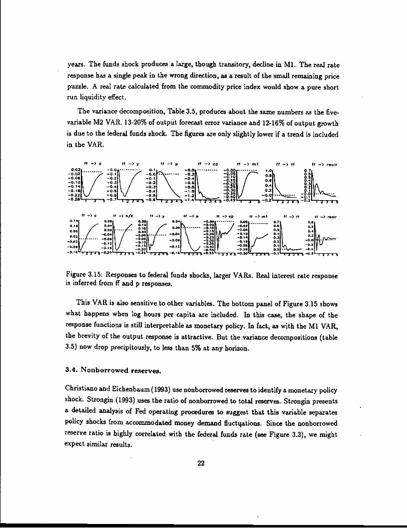
years. The funds shock produces a large, though transitory, decline in Ml. The real rate

response has a single peak in the wrong direction, as a result of the small remaining price

puzzle. A real rate calculated from the commodity price index would show a pure shortrun liquidity effect.

The variance decomposition, Table 3.5, produces about the same numbers as the five-variable M2 VAR. 13-20% of output forecast error variance and 12-16% of output growth

is due to the federal funds shock. The figures are only slightly lower if a trend is includedin the VAR.

ff—)y ll—)p tJ—)ep Jt—)n,I ff_)ff It—)reoI,

O-02V

—0.0 1.0, 0.7.—0.02

—0.2k—0.051 T 0.61

o —oo • 0.5K

—Os —0.251 / O.flfl

—0.06

O.III

0.411—0.10

:Q:I

-.020• I 9-IIA—0.16 —'.0 °0R / °L 'v—0.22 1 2 °•35ItJ —0.0 ---'.c__._____________ —0.401, __________ ____________________ _________ __________ —0.I__________—0.26 :,:, , , 0.2 ijs,s0.2

,,—c fl—)h/c U) If—)p Il—Sop II—)',' ff)tt Vl—)r.ol,- 0.081 - 0.201 - —0.00 0.02. 0.7l 0.5.

0.101 / °°b 7 0.151 / F\ .0osR / —0.02 o.I \ —0.1• OSj 0.211A — —

00•I I I /

o.I

/ —0.0.1002 , _::..7 —0.0.! :j Ik#t

0.41 ________

-045 _0.221,K 0.1o.o. / :j 0.08 040 —o.,. 02

_______ ::i v —-' r..0.1210J0 '...d 0.45 0.24w 0.0 -

—0.10 23.5—030 ,2J—2—50.25 l2j450.l6 12J45-0.'O I33.50.30 Ira—.—,—°' ,z.p0.6 'gj

Figure 3.15: Responses to federal funds shocks, larger VARs. Real interest rate responseis inferred from ff and p responses.

This VAR is also sensitive to other variables. The bottom panel of Figure 3.15 shows

what happens when log hours per capita are included. In this case, the shape of theresponse functions is still interpretable as monetary policy. In fact, as with the Ml VAR,

the brevity of the output response is attractive. But the variance decompositions (table3.5) now drop precipitously, to less than 5% at any horizon.

3.4. Nonborrowed reserves.

Christiano and Eichenbaum (1993) use nonborrowed reserves to identify a monetary policy

shock. Strongin (1993) uses the ratio of nonborrowed to total reserves. Strongin presents

a detailed analysis of Fed operating procedures to suggest that this variable separatespolicy shocks from accommodated money demand fiuct4ations. Since the nonborrowed

reserve ratio is highly correlated with the federal funds rate (see Figure 3.3), we mightexpect similar results.

22

In fact, the results using the nonborrowed reserve ratio are almost identical to the

federal funds results. Figure 3.16 presents responses to nbr/tr shocks in three variableVARs. The pattern is almost identical to federal funds, Figure 3.16. With nbr/tr first,there is a small output movement in the wrong direction followed by a sustained decline

and a big price puzzle. With nbr/tr last, the output decline is continuous, and the pricepuzzle is reduced.

nbr/tr—.lnbt/t( itt/It —) y nbc/ti —, p

InIt/U -)

Figure 3.16: Responses to nonborrowed reserve/total reserve ratio shocks. Top panel:nbr/tr y p VAR; bottom panel: y p nbr/tr VAR. Both VARs in levels without trends

The output variance decompositions sinnmarized in Table 3.6 axe also almost identical

to their federal funds counterparts. With nbr/tr orthogonalized its shocks explain

up to 52% of output variance at a three year horizon, and a substantial 32% of annual

output growth.

Forecast error 2 Var AyVAR 1Q 1Y 2Y 3Y 1Q 1Ynbr/trypypnbr/tr

7 4 20 340 9 36 52

23 3416 32

cypcpmlnbr/tr 0 10 28 28 11 18

c y p cp ml nbr/tr; trend 0 10 27 27 11 18ch/popypcpmlnbr/tr 0 4 8 5 4 6

Table 3.6: Percent of output variance explained by nonborroweed/total reserve shocks.AU VAR.s in log levels with 4 lags.

Figure 3.17 presents responses from the usual five varibleVAR. The pattern is almost

exactly the same as ttie federal funds pattern, and conforms roughly to the pattern we

expect of a monetary shock. As before, the output variance decomposition declines, to

a maximum of 28% at two and three year horizons, and 18% of annual output growth.

23

ct/ti —) pU,

-to

nbc/It —, nbc/ti

Adding hours has the same effect as with federal funds. The impulse-response pattern is

not that badly affected, but nbr/tr shocks now account for less than 8%of the variance

of output.

nbr/tr —) C flbt/tr —) y nbr/tr —> p nbr/tr —) cp nbr/tr —> ml nbr/tf —) nbr/t

2.23k'C'T. 07N4C"T5 ___________

nb./Ir —, C nbrIIr —) h/c nb./it —) v nbt/tt —) P nOr/It .—) nbt/t

:Li :Btj/ E°gl':N\J ____—0-Ia •jt.0•2I TsJ.i•. i4345—O.' lA3S0 0.2

Figure 3.17: Responses to nonborrowed reserve/total reserve shocks. Vars in log levelswithout trends.

3.5. Long horizon output forecasts

In each of the above VARs, adding consumption substantially reduced the fraction ofoutput variance explained by the monetary shocks. Here I look at the relative forecast

power of consumption and monetary variables directly, to see if consumption drives the

monetary variables out.

Table 3.7 compares forecasts of 3 year output growth using federal funds, the realM2/output ratio, and the consumption /output ratio.'2 The top panel starts with singlevariable regressions. All variables significantly forecast output growth, The R2 are high,

as often happens in multi-period forecasts with serially correlated right hand variables.

The consumption / output ratio has the highest t-statistic and, more importantly, R2,0.63.

The second panel of Table 3.7 presents multiple regressions, which are the horse race.

The first row compares federal funds and M2, out of curiosity over which is the "better"

monetary variable. Recalling the correlation of federal funds and M2, the fact that both

13A11 the regressions contain a trend. This significantly improves the krecast performance of theinterest rate variables. There is a secular decline in output growth, visible in figure 3.18. The interestrate spreads have no trend, so are not significant and have tiny H2 in regressions with no trend, while theinterest rate levels do better simply becaazae they have some trend.

24

nbr/it —) co abt/tt —) ni0.01

—0.03—0.0*—0.10—tie—0.i*.0.Z2

0.3.—0.20

I. Single regressionsif if-by m2/py c/y

cod.t.

k2

-0.35 -0.95 0.43 1.70-2.08 -4.76 2.38 8.400.26 0.34 0.31 0.63

II. Multiple regressionsif if-bOy m2/py c/y A2

coef.t.

0.19 0.54 0.310.43 1.42

coef.t.

-0.73 0.20 0.35-5.40 1.04

coef.t.

-0.01 1.70 0.63-0.06 7.32

cott.

-0.14 1.64 0.63-0.45 6.23

cod. 0.16 L62 0.64t. 0.87 6.45

Table 3.7: Ols forecasting regressions of three-year log output growth. All regressionsinclude a time trend, Yt+3 — = a + i+ $g + Cg.f 3. Standard errors corrected for error

overlap and heteroskedasticity.

are individually insignificant suggests that they capture the same information about out-

put growth. But the second row, which compares the fed funds spread and M2 suggests

that the spread does have significant information beyond that contained in M2. (In a

VAR, the spread gives a very similar results as the leveh)

The third and fourth rows run a horse race between federal funds and the consump-tion/output ratio. The fed funds variables are insignificant, and the coefficients are sub-

stantially lower than in the single variable regressions. The consumption coefficient and

significance is hardly affected by the inclusion of either fed funds variable. Thus, consump-

tion drives out federal funds as a forecaster of output. The fifth row runs a similar race

between the real M2/output and consumption /output ratios. Again, whether measuredby the coefficient or the t-statistics, consumption drives out M2.

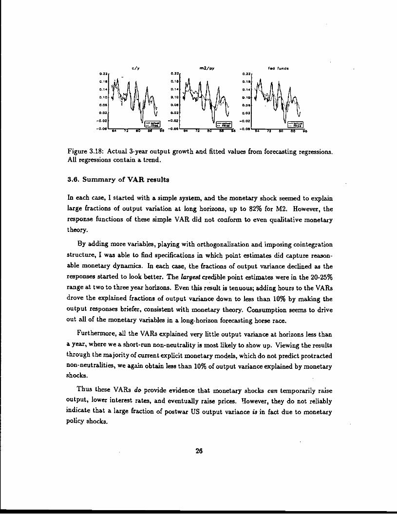
Figure 3.18 also suggests that consumption does a better job of forecasting outputgrowth than the monetary variables. Not only is the 112 higher, but the consumptionforecasts seem contemporaneous with output growth, where the Fed funds rate forecast

lags.

25

dy rn2/py I.d funds0.22 0.22 0.22

010

_________________ _________________________________ I.- mi..I Zttal.-o.oe - - - ..._0.06 Q • 95OO6 64 72 60 06 96

Figure 3.18: Actual 3-year output growth and fitted values from forecasting regressions.All regressions contain a trend.

3.6. Summary of VAR results

In each case, I started with a simple system, and the monetary shock seemed to explain

large fractions of output variation at long horizons, up to 82% for M2. However, theresponse functions of these simple VAR did not conform to even qualitative monetary

theory.

By adding more variables, playing with orthogonalization and imposing cointegrationstructure, I was able to find specifications in which point estimates did capture reason-

able monetary dynamics. In each case, the fractions of output variance declined as theresponses started to look better. The largest credible point estimates were in the 20-25%range at two to three year horizons. Even this result is tenuous; adding hours to the VARs

drove the explained fractions of output variance down to less than 10% by making the

output responses briefer, consistent with monetary theory. Consumption seems to driveout all of the monetary variables in a long-horizon forecasting horse race.

Furthermore, all the VAR.s explained very little output variance at horizons less than

a year, where we a short-rim non-neutrality is most likely to show up. Viewing the results

through the majority of current explicit monetary models, which do not predict protracted

non-neutralities, we again obtain less than 10% of output variance explained by monetaryshocks.

Thus these VARs do provide evidence that monetary shocks can temporarily raise

output, lower interest rates, and eventually raise prices. However, they do not reliablyindicate that a large fraction of postwar US output variance is in fact due to monetarypolicy shocks.

26

6.4 #4 #14 CC VC

Even the largest figures are certainly an overstatement, for several reasons. 1) Otherreal variables can help forecast output and drive down the contribution of monetary

variables. 2) The Fed and private agents are likely to have information advantages, sothat M2 or federal funds move in anticipation of news about the economy that we donot include in a VAR'3. In addition, monetary aggregates and the economy undoubtedly

react to each other within a period. For both reasons, the identification of a moneysupply shock is tenuous. 3) Very little theory is used to restrict the form of the VAR.Believing that money even accounts for 15-25% of output variation at a 2-3 year horizon

(and virtually zero at a 1 quarter horizon) requires us to understand how it produces

such a response. 4) Once we recognize sampling uncertainty and (more importantly)specification uncertainty (the reader can easily see how much fishing went into producing

good-looking impulse responses), the range of estimates consistent with the data is very

large.

3.7. Systematic Monetary Policy

Variance decompositions can answer the question "how much output variance is due tomonetary policy shocks?" This is a different question than "how much output varianceis due to monetary policy?" unless one imposes the view that systematic policy has no

C

effect whatsoever.

For example, many economists believe that postwar output is more stable than prewar

output because the Fed learned to systematically offset real shocks. Similarly, outputmight be much more variable if the Fed stopped accommodating seasonal and other shifts

in money demand (such as after the 1987 stock market crash). If so, a negative fraction

of output variance is due to monetary policy.

These examples presume that systematic or anticipated monetary policy can havereal effects. But variance decompositions and impulse-responses are poorly suited toaddressing these issues; Variance decompositions cannot be negative! When we read

impulse-response function as a measure of the effects of a monetary shock, we implicitly

'3Sims (1992) puts it nicely: ...becuase interest rates and money are closely linked to investmentportfolio decisions, they tend to react quicliy to new information, as other asset market variables do.Money and interest rates have strong predictive value for aggregate activity for the same reason thatstock prices do...One can imagine, in other words, that the historical pattern of monetary tightnesspreceding recessions is misleading. High interest rates might 'produce' contractions in activity the waythe cock's crow produces the sunrise." This is at heart the same point made by King and Flosser (1984)as well as Tobin (1970): money that really responds to output can look like it causes output.

27

assume that anticipated money has no real effect.14 If anticipated money has real effects,

then the response function measures the response of y to the current in shock, and the

path of future m's that the shock sets in motion.'5

Does anticipated money matter? It is hard to. swallow the persistent responses of

output to monetary shocks found above as delayed responses to unanticipated money.However, since the monetary variables also have protracted responses to the shocks, theoutput responses are consistent with a view that money has short-lived effects on output,

if anticipated money does matter.

If we accept this view, then the study of systematic monetary policy (accommodationof seasonal and other shifts in money demand, systematic stabilization of other shocks),

or monetary institutions (deposit insurance, lender of last resort) may be more importantto macroeconomics than an assessment of how much output can be further stabilized bymaking monetary policy more predictable. It may not be the answers that are wrong; We

may simply be asking the wrong question.

4. Technology shocks

The real business cycle literature is dominated by the assumption that "technologyshocks" drive economic fluctuations. A typical production function is

Z =

"And that the VAR has isolated shocks to agents' information sets.'5To make this point explicitly, suppose that the "structural" model is

= a,(L)(rn — E,_1(mt)) + czpnrn(L)m. + n

= anq,(L)yt + Cmt

inverting this model to find the moving average representation, the y response to the mshock is

—' . a,nnt(L)amn.(L) + aijma(L)lit — + Lint.

— apms(L)amy(L)

As you can see, the parameters a,,rn.(L) and a,,,,,(L) affect this response. In the special case that p doesnot respond to anticipated m, = 0, so the true rponse is the same as the impulse.response,

a,,(L)

which is independent of the money supply rule.

28

and A is the shock'6. Of course, the models are capable of producing responses to many

shocks, including government spending, financing and monetary shocks (when appropriate

frictions are introduced.) However, technology shocks—shocks to current period marginalproductivity—are centrally important for obtaining realistic artificial time-series in cur-

rent models. Other shocks have not been found to contribute much to output variation

or cyclical co-movement in the real business cycle paradigm.

Obviously, technology contains some stochastic element, so the crucial question is

"how much variation in output can technology shocks explain?" Prescott (1986) presents

a famous calculation that 70% of the volatility of GNP is due to technology shocks. This

calculation is made by calibrating a model economy, i-c. choosing values for preference and

technology parameters and for the variance and autocorrelation of the technology shock.

Then, "70%" refers to the variance of Hodrick-Prescott filtered model output divided by

Hodrick -Prescott filtered actual output.

This calculation is obviously sensitive to the calibrated value of the variance of thetechnology shock, and possibly other parameters as well. Double the standard deviation

of the technology shock, and you double the predicted standard deviation of output. The

fraction can come out over 100% if you're not careful! It is not a variance decomposition.

Eichenbaum (1991) uses (3MM to quantify the sampling uncertainty of the calibration

procedure, and finds that the estimate of var(ymoijej)/var(y.g.,gs) is 0.78 with a standard

error of 0.64! Sensibly enough, virtually all of this uncertainty comes from uncertaintyin the calibrated variance and autocorrelation of the technology shock.

I will concentrate on a different source of "whimsy" (Eichenbaum's terminology), how

the point estimates are affected by the choice of statistic.

To start with, Eichenbaum only considers sampling variation given a set of moments

that we pick model parameters to match. The figure is also obviously sensitive to thecalibration procedure: if one included only var(y) in the list of moments to be matched,

then the calibration procedure will "explain" 100% of the variance of output, by picking

a suitable variance of the technology shock.

Furthermore, consider the effect of correlation between output and productivity. Real

business cycle models have one shock and many series. They are stochastically singular,

i.e. functions of each series are perfectly correlated. In tl4e data, they are not. Instead of

'6Up until now, we have been using the word "shock" for "innovation", all "shocks" were unpredictable.The real business cycle literature uses the word "shock" to describe the Solow residual $AS$ even if it ispredictable. I'll conform to this unfortunate terminology.

29

just counting model variance / data variance, we could insist that the model only explains

the variance of a single dynamic factor of output, Solow residuals, labor, consumption,investment, etc., or the projection of output on Solow residuals. These calculation will

yield smaller numbers.

As an extreme example, Gordon (1993) argues that when one accounts for measure-

ment error in capital and hours, there is no correlation left between productivity and

output. He exploits the model's prediction of an almost perfect correlation (see below) to

conclude that productivity shocks explain 0% of the variance of output. Note that Gor-

don's productivity series still has plenty of variance, and so might still produce a high

number using Prescott's statistic.

The next section shows how statistics that focus on the predictability of output can

give numbers much smaller than Prescott's.

4.1. Forecastability and calculations that technology shocks explain very little.

4-1.1. A simple VAR.

£ start with a simple characterization of the data. Blanchard and Quah (1989), Shapiro

and Watson (1988) and Cochrane (1994) present VARs that decompose output into per-

manent and transitory shocks. Figure 4.1 presents the impulse-response function of aconsumption . output VAR in this spirit (it is closest, obviously, to Cochrane (1994),

but the message of other specifications is similar). I regress log conswnption and output

growth on the log consumption/output ratio and two lagged growths17. In the left hand

panel of Figure 4.1 the shocks are identified by forcing the long-run output response ofthe transitory shock to zero, following Blanchard and Quah. It happens that this or-thogonalization is almost exactly the same as the conventional y-first orthogonalization.

Orthogonalizing with consumption first, shown in the right hand panel of 4.1 produces a

similar picture.

The impulse-response functions reveal a large transitory component to output. Asshown in Table 4.1, the transitory shock accounts for 89% of the variance of output growth

and 89%, 73%, 63% of the 1, 2, and 3 year output forecast error variance respectively.

'7The VAR uses log nondurable plus services consumption and. log private GDP —GDP less gov-ernment purchases — for output. The use of private GDP is a minor refinement, suggested by KingPlosser Stock and Watson (1991). the consumption/private GOP ratio is more stable than the con-sumption/GD? ratio, and hence better forecasts business-cycle variation in output. Also, models are

designed to explain private sector GDP.

30

.2

1.2 è—fll*.—14 '.0

.0___________ 1 ••• 1' 'N _________

a.. _:.,_ fl" 04 £

O24SSIQU IS I 0 2Q,,,i.a I.IIoaq a ubaak O..a,W. Ia0..I.q a nk

Figure 4.1: Impulse-response function from nondurable + services consumption—privateoutput VAR. Right hand panel is orthgonalized with consumption first (y shock does notaffect c contemporaneously). Left hand panel is orthogonalized so that the transitoryshock ha

Shock and horizonlYear 2 Years 3 Years Differences

Var of perm trans penn trans perm trans petit transconsumption 78 22 86 15 90 10 77 23

output 12 89 27 73 37 63 11 89

Table 4.1: Variance decomposition. Table entries give the percent of the forecast errorvariance of the row variable due to the column shock at the indicated horizon. The VARconsists of a regression of zXc and y on c — y and two laggs of & and Ay. The shocksare orthogonalized so that the transitory shock has no long-run effect on output.

We can compare the implied c-y VAR representation predicted by models to Figure 4.1and Table 4.1 to see how well the models reproduce the second moments of consumption

and output. This use of the VAR does not require us to find structural interpretationsof the shocks, which is a contentious issue. (See Hansen and Sargent (1991), Lippi and

Reichlin (1993), Blanchard and Quah (1993), Cassou and Mittnik (1990) and Coclirane(1994) for some of the debate.)

4.1.2. A model, and Blanchard and Quali's small number.

Now, let;s see what impulse-response function a standard model doespredict. Figure 4.2

shows the response to a 1% technology shock of the King, Plosser and Rebelo (1988)model with linear utility for leisure as in Hansen (1985) and Rogerson (1988). The model

31

is

max EE$t(ln(Cg) +8(1 — Ne)) .5.2.nO

Z = (AN)°K° = C + I= (1 — J)JI + It

lnA =g+InA_i +ftParameters are calibrated as in Campbell (1992) to produce a nonstochastic steady state

with growth g = 2% and rate of return = 6%. a = 2/3, 6 = 0.1, N = 1/3.

I

S40oj0t.d Iim. n.j.,

$ 0 II 20 3$ 2$ 24 40 40 40 4$ N 2) 40Q*..dn

Raoo.n all I.ct.aoS 4040*

cz111

11111111 11111 11111 11111 :

0-n-s

Figure 4.2: Artificial time series and response to 1% technology shock in King PlosserRebelo model.

It turns out that consumption and output are invertible functions of the technology

shock, so a c-y VAR should recover the technology shock, and should find no other shock.

Thus, the responses to a technology shock are also the model's predictions for the VAR

impulse-response function.

Comparing Figure 4.2 with Figure 4.1, this standard real business cycle model produces

time series that look something like the permanent shock in the data. The transitory shock

and its response are absent from the model's impulse-response function. In this way, we

reproduce Blanchard and Quali's result:

Small fractions of the variance of output are due to technology (permanent)shocks.

From the above variance decomposition, about 12% 27% and 37% at 1, 2, and 3 year

horizons, and 11% in annual growth rates. (Mechanically, the number rises to 100% asthe horizon increases.)

32

32

I.

l0

10

I•5

4.1.3. Predictability and a small number inspired by R.otemberg and Wood-ford.

The essential message of the VAR is that output contains a large predictable component.

This is good news. If a recession is a period in which output is "below trend", we must

expect output to grow more in the future, and vice-versa in a boom. The predictability

of long-run output growth verifies that there are such periods. The left hand panel of

Table 4.2 makes this predictability point directly: regressions of output growth on theconsumption/output ratio yield R2 values up to 0.4 at a two year horizon. R2 above 0.6

can be obtained by adding a trend, as in Figure 3.7, interest rates, unemployment, hours,or other variables.

Output Solow ResidualHorizon 1Q 1Y 2Y 3Y 1Q 1Y 2Y 3Ycoeffficient 0.15 0.85 1.37 1.53 0.23 0.83 1.07 1.07

t-statistic 3.76 6.64 6.71 5.62 7.93 9.95 8.55 6.610.06 0.31 0.45 0.48 0.27 0.60 0.53 0.45

Table 4.2: Regressions of output growth and Solow residual on consumption/output ratio,— = /I(c — y) + cj+,i. c=log nondurable plus services consumption. y = log (gdp-

government purchases). Solow residual = y - 1/3*ln(k) - 2/Stln(hours), k inferred fromgross fixed investment with 6 = 0.1. Coefficients estimated by OLS; t-statistics correctedfor serial correlation due to overlapping data, and for conditional heteroskedsticity.

This observation suggests another calculation: Define the "business cycle" component

of output as the forecastable or transitory component of output. Since model outputis basically unforecastable, we expect to find that the model explains small fractions of

the variance of the business cycle component of output. This point is emphasized byRotemberg and Woodford (1993); it can also be seen in the flat model spectral densities

reported by Watson (1994).

One such calculation is the ratio of k-period forecastable output growth to that pre-

dicted by the model,var(Etyg+ —

var(Eiyt+4 — y) -

If we divide both numerator and denominator by var(yg+k —y) and calibrate the model

(variance of technology shock) so that var(yg+I, — vt),,wda: = var(ys+k — ydut4,, the above

statistic is the same as the ratio of long-horizon 112

02 — var(Etyt+k — Vt)ALE —

var(y(+k — Vt)

33

in the data and in the model Table 4.3 presents forecasting J?2 in the data (from Table

4.2) and in several models. The Table just presents the B2; the results of division are

pretty obvious.

Model IQ 1Y 2Y 3Y var(BN)/var(Ay)

Data (c-y VAR) 0.06 0.31 0.45 0.48 17.0

std. model: at = at_i + c 3.5E.06 1.IE-05 1.7E-05 2.OE-05 0.0007

differenced estimate 0.997 0.45 0.14 0.09 2.6

trend estimate 0.74 0.42 0.39 0.44 19.2

random walk a + smooth news 0.12 0.36 0.51 0.58 20.6

news from a, y, c, hrs VAR 0.76 0.57 0.46 0.44 70.6

Table 4.3: Long-horiozon output growth forecast W and ratio of Beveridge-Nelsonde.

trended output variance to variance of output growth.

For the standard model (identified by the technology process Ug = a_+et in the table),

output forecasting P2 is pitifully small. In the data, we see the subflantial forecast B2

Dividing the two, we obtain:

Technology shocks explain 0.002% or less of business cycle variation in output!

4.1.4. Beveridge Nelson detrending in place of the Hodrick Prescott Filter.

What if Prescott had detrended output using the Beveridge-Nelson detrending method in

place of the Hodrick-Prescott filter? The Beveridge-Nelson (1981) trend is defined as the

level output will reach when all dynamics have worked themselves out'8. It formalizes the

idea that the cyclical compoient is the part that is forecast to die out. The Beveridge-

Nelson trend is visually indistinguishable from the Hodrick-Prescott trend in the plots of

data and trend used to justify Hodrick-Prescott detrending (see Cochrane 1994for a plot

of the B-N trend, and Prescott (1986) for the HP filtered trend.)

The variance of Beveridge-Nelson detrended data is var(yt — limk_,a. Etyt÷k) and so is

the limit of the numerator of the long-horizon R. The denominator of long-horizon Rexplodes as k — , however. For that reason, the last column of Table 4.3 presents the

variance of Beveridge-Nelson detrended output divided by the variance of output growth.

'8Formally, the Beveridge-Nelson trend is

4rend = lim(E,y,÷b — icE(Ay)) = y, ÷L — E(Ay)j=1

I work from VARs and ignore the constants, so I ignore the E(y) terms.

34

Dividing the "model" number by the "data" number, we obtain the fraction of Beveridge-

Nelson detrended output due to technology shocks. (This calculation is still a littlegenerous to technology shocks. I allow the calibrator to freely assume counterfactually

large variation of Solow residuals to match output growth variance. It's devastatingenough; but one can divide by another third or so by scaling to the variance of Solowresiduals rather than output.)

For the standard model, the Beveridge Nelson detrended output has a variance 0.07%

that of output growth. In the data, Beveridge-Nelson detrended output variance is 17

times the variance of output growth. Dividing the two, we find again that

Technology shocks explain 0.009% or less of Beveridge-Nelson detrended outputvariance!

A seemingly minor change in the detrending method produces a dramatic change inthe result. The standard model, while a useful stochastic growth model, does not seem

to produce any business cycles!

4.1.5. Endogenous dynamics; a small number inspired by Christiano

Output and technology are so close in Figure 4.2 that they are barely distinguishable.All the dynamics of output come from the assumed dynamics of the shock. (Christiano

(1988) and Eichenbauzn (1993) emphasize this point.) This observation suggests that we

define the fraction of output variance explained by the model as the variation generated

by the propagation mechanism, rather than simply assumed in the external shocks.

To quantify this point, Table 4.4 presents the correlation of long run output growthwith Solow residual growth and the ratio of the variance of output growth to the variance

of the Solow residual, in the data and several models. As the Table shows, the correlation

between output and Solow residual is nearly perfect in this standard model, and there isessentially no amplification of shocks.

The model explains essentially 0% of output fluctuations.

4.2. Forecastable technology shocks

Of course, all of the above calculations depend on the structure and parameterization

of the real business cycle model, as well as the nature of its shocks. A first repair is

35

1Q if 2Y 3YModel Correlation: corr(y — y, at÷k — at)Data

-

Std. model aj = ti + Et

Differenced estimateTrend estiamteRandom walk a + smooth newsNews from a, y, c,hrs VAR

0.85 0.79 0.75 0.74

1-(2E-06) l-(6E-06) 1-(9E-06) 1-(1E-05)0.95 0.99 0.99 0.990.69 0.93 0.97 0.980.90 0.91 0.92 0.920.97 0.96 0.97 0.98

Amplification: var(yt+k — yt) / vaz(at+k — at)Data 1.68 2.01 1.96 1.91

Std. model at = at_i + 0.98 0.98 0.99 0.99Differenced estimate 1.30 1.27 1.13 1.07

Trend estimate 1.89 2.17 2.20 2.21Random walk a + smooth news 1.40 1.44 1.40 1.33News from a, y, c, hrs VAR 2.46 2.20 2.05 1.92

Table 4.4: Correlation of long-na output growth with solow residual, and ratio of outputgrowth variance to solow residual variance

obvious enough that it is worth pursuing here: Since output dynamics look a lot like

shock dynamics, put in some interesting technology shock dynamics.

This path isn't as innocuous as it seems. Hall (1988) and Evans (1992) attack the idea

that Solow residuals represent technology shocks by showing that they are forecastable by

a number of variables, including military spending, government purchases, and monetary

aggregates. Table 4.2 shows that Solow residuals are about as predictable as output from

the c/y ratio. Rotemberg and Woodford (1993) argue that changes in technology should

not be forecastable. On a priori grounds, then, these authors argue that we shouldn't try

to repair the technology shock view by allowing forecastable technology shocks.

Of course, some components of government spending (infrastructure, military R&D,

NASA, etc.) may actually cause increases in technology. Proponents of such spending cer-

tainly advocate this view loudly enough! Also, government spending, even in wars, must

respond to forecasted tax revenues, and monetary policy may accommodate predictedexpansions in real activity. Since policy-makers and private agents have more informa-

tion than our VAR, spurious (hanger-causality is likely. Finally, many real business cycleadvocates have abandoned the pure technology shock view of the Solow residual (see be-

low), in which case forecastable movements are more plausible. I take a pragmatic view

and investigate the consequences of forecastable technology shocks; purists are free to

disregard the results.

What dynamic structure should we put in for the technology shock? A natural idea is

36

to use the structure found in the data. To this end, I ran two autoregressions of Solow

residuals on lagged Solow residuals:

Differences: & = p + Ef)Aa_ + ct

and

Levels with trend: at = a0 + bt + E $a_ + c.

(As one would expect, a specification in levels without a trend produced almost exactly the

same result as with differences. Below, I consider multivariate Solow residual forecasts.)

Figure 4.3 presents the estimated impulse-responses for the Solow residuals, together

with the responses of output, consumption, and labor when technology shocks with theestimated dynamics are fed through the RBC model. The differenced specification pro-

duces a very persistent shock, while the trend specification produces, a transitory shock.

You still get out what you put in: the shape of both output responses is essentially thatof the shock response. The stationary shock is amplified somewhat as investment risesto smooth the transitory shock forward and labor supply increases to take advantage of

transitorily higher wages. The transitory shock produces a transitory output response,like the response to the transitory shock in the data; the permanent shock produces apermanent output response like that of the permanent shock in the data.

Tables 4.3 and 4.4 include forecastability and correlation/amplification statistics forthese models, marked "Differenced estimate" and "Trend estimate". As we might suspect

from the graph, the permanent technology shock produces low output 112 once the initial

rise in output has passed, high correlation of output and technology shock, and small

amplification. It only explains about 2.6/17 = 15% of Beveridge-Neison detrended outputvariance. The stationary shock does much better: the forecast W are similar to thosefound in the data, and shocks are amplified. It explains a little more than all of Beveridge-

Nelson detrended output variance. Thus, we can get transitory output variation and

athplification out of a real business cycle model, by assuming a transitory technologyshock.

The data will not be helpful in determining which shock process is correct, however.

The stationary shock process has a very slowly declining response function, so no testcould tell it from the unit root shock process. Conveisely, the examples warn us to

beware empiricists who make seemingly innocuous detrending assumptions; they havemajor effects on the properties of the real business cycle model.

37

Figure 4.3: Estimated impulse-response function for Solow residuals and KPR modelresponses to technology shocks with the estimated structure.

The transitory shock model still predicts far too much correlation, so almost all output

dynamics are due to the assumed shock dynamics. Most importantly, there is now nostochastic growth, no permanent shock as found in the data. Making the assumed shock

process have a response that does not go to zero doesn't help much. The series arestill correlated, output has the same response as the shock, and correspondingly less

forecastability and amplification.

The real business cycle model needs more shocks. The problem we are having is thatit is hard to match a single shock model to a multiple shock world. To decide how much of

the variance of output is due to technology shocks, it would help a lot to have somemodel

of the other shocks. Real business cycle modelers have tended to ignore the stochasticsingularity in their model's predictions, citing measurement error. However, it seems that

one of the babies — either transitory, business cycle dynamics or stochastic growth —

get thrown out with the bath water by doing so. Below, I examine whether news about

future technology shocks can account for the extra shock.

.3

U

S.

52

__.._ _.

I

S.. — 1* I—..—e —

n I. It It0s

38

4.3. Production function, labor hoarding

The estimated teéhnology shock depends crucially on the assumed form of the production

function. Labor and capital hoarding have recently been examined, in part to explain thelorecastability of Solow residuals. (Burnside, Eichenbaum and Rebelo 1993, Eichenbaum

1993, Sbordone 1993). For example, suppose the production function is

Y2 = (441NE)°(KU1)'°

where E represents effort and U represents capital utilization. The Solow residual is

(AE)°u1, so variables that Changer-cause endogenous effort and capital utiliza-

tion will Granger-cause the residual, even maintaining the assumption that they do notGranger-cause the true technology shock A1.

Indeed, Burnside, Eichenbaum and Rebelo find that when variable effort is added,

the model predicts forecastable Solow residuals. They also find that adding labor effort

drops the Prescott-style calculation of the explained variance of output from 80% to 31%.

Eichenbaum (1993) finds even stronger results when capital hoarding is introduced.

These calculations suggest that variations on the structure and parazneterization of theRBC model will also have important effects on the estimated importance of technologyshocks.

4.4. Interpreting technology shocks-

Much of the controversy over real business cycles stems from common-sense resistanceto the idea that variations in the state of knowledge drive fluctuations. In particular, it

is hard to interpret declines, and some authors argue against forecastability or dynamicstructure in technology;

From the point of view of measurement, anyihing that causes output to vary givencapital and labor will result in a Solow residual, and hence will be identified as a "tech-

nology shock." Labor or capital hoarding, money, taxes or any other friction that causesoutput to be less then N°K1 will have the same effect. Plosser (1989) argues for this

interpretation of technology shocks. Recently, Hansen and Prescott (1993) seem to haveadopted the latter interpretation.

Every nation has a set of rules and regulations that govern the conduct of

business. These have consequences for the incentives to adopt more advanced

39

technologies and for the resources required to operate existing ones. ...Systerns

that divert entrepreneurial talent from improving technologies to rent-seeking

activities...[andj changes in the legal and regulatory system within a countryoften induce negative as well as positive changes in technology.

In a separate discussion, they liken technology shocks to small perturbations in all the

factors that make the US a better place to do business than India. In short, technology

shock3 are changes in the inefficiencies induced by policy!

In cataloguing views on the source of fluctuations, real business cycle theorists are

now fishing in the same pond as all other macroeconomists, though with a well-specified

rod consisting of explicit dynamic models. Any of the items in the list on the first page

of this paper would cause a measured "technology shock." In fact, the thrust of muchrecent real business cycle research has been to explicitly include tax and other stochastic,

real distortions. This is good news for the real business cycle methodology, since it now

can produce explicit dynamic models with the kind of distortions economists have beeninterested in for generations. Eventually, we should be able to make calculations likethe above to quantify the impact of government spending, taxation, monetary and credit

shocks in the context of explicit dynamic models. However, it is obviously bad news for

the view that technology shocks, narrowly defined, are the source of fluctuations: it says

that the calculations we have made do not bear on the issue.

4.5. Summary

Table 4.5 summarizes a few calculations of the importance of technology shocks. Westarted with Prescott's calculation that 70% of the variance of output is explained bytechnology shocks. However, this calculation turns out to be subject to enormous sam-pling error. Perhaps more importantly, the statistic one uses turns out to matter verymuch. The fact that standard stochastic growth models produce little output forecasta-bility and output dynamics very dose to shock dynamics, suggest numbers as low as 0%.

Modifications to the production function can have a similar effect. Mean-reverting (i.e.forecastable) technology shocks can give rise to mean-reverting and hence forecastable

output, but this fix is controversial, and puts us in danger of losing stochastic growth.

Finally, the concept of technology shocks seems to have melted away. It is now inter-preted so broadly that it can stand for essentially any distortion that causes a measured

Solow residual. With this interpretation, it is vacuous to say that technology shocks cause

40

Author Statistic or observation Fraction

i tt fihlered vmoaei)resco e3(HP filtered vt. ) 70 %

Eichenbaum Sampling error (&.4k, Pahock ) 78% +1- 64%

Blanchard-Quah a2(y) from perm. shock 12% 27% 37%Rotemberg-Woodford 0.002 %

Christiano '2t771 1—corr(y, a) tiny

Beveridge-Nelson B-N trend not HF filter 0.003 %

Gordon corr(shock,output) 0

Burnside, Eichenbaum, Itebelo Labor hoarding 31 %

Table 4.5: Summary of calculations of the contribution of technology shocks to outputvariability. Author column gives the inspiration for the calculation. Numbers are mycalculations, not theirs.

fluctuations.

5. Some new contenders

Sd. Oil Prices and reallocation

Hamilton (1983) suggested that oil price shocks account for postwar recessions. Every

postwar recession was preceded by an oil price increase. VARs suggest that oil prices are

econometrically exogenous, and, since the big increases are due to OPEC or the Texas

Raihoad Commission, exogeneity rings true. However, big technology, monetary andfederal funds shocks also occur around the beginning of every postwar recession, and can

appear exogenous in VARs.

I run two simple VARs using the producer price index for crude petroleum. The first

just includes output, the second includes both output and consumption, in the style ofthe monetary VARs examined above. Figure 5.1 presents the responses of output to

the oil price shocks, and Table 5.1 presents the output variance decompositions. As the

figure shows, innovations in oil prices do produce sustaiped output declines. However,the magnitude of the declines is much smaller than the declines produced by output or

consumption shocks. Summing and squaring, less than 10% of the variance of output is

41

explained by oil price shocks. (Oil prices account for 80% or more, and usually 99%, of

oil price variance, confirming Hamilton's exogeneity tests.) The problem is simple. There

are only a few large oil price changes. Yes, they were followed by recessions, but the rest

of the fluctuations in output are not accounted for by oil price changes, and the severity

of the recessions does not occur in strict proportion to the oil price innovation. Giventhis evidence, it does not seem worth the space required to sort out whether this small

contribution remains when put into competition with monetary variables or technology

shocks.

TI F

Figure 5.1: Output responses in oil price VARs. Top: oil price output VAR. Bottom: oilprice, consumption, output VAR. VARs in log levels, 4 lags.

HorizonVAR 1Q 1Y 2Y 3Y DifferencesOil,y 1 4 7 8 4

Oil,y,c 0 0 2 5 1

Table 5.1: Output variance decomposition, oil price VARs. Table entries give the per-centage of output variance accounted for by oil price shocks.

The biggest sticking point for oil price advocates is the propagation mechanism. Im-

ported oil is a small fraction of GDP, so traditional production theory suggests that evenlarge increases in its price should have small effects on output. A general equilibrium

model might generate a larger response, for example if labor supply declines when thereis an oil shock. But Kim and Lougani (1992) construct such a model, and find that oil

shocks only account for 18% of the variance of output with a CES production function.

Finn (1993) constructs a real business cycle model witlf varying capital utilization that

explains the forecastability of Solow residuals from energy price increases. She also finds

42

S..., , —, ,

rr3

7-19% of output variance explained. Furthermore, standard models predict symmetriceffects, so that real oil price declines should cause booms.

Of course, the small input problem applies to money as well. The cost of holdingreserves plus cash (the money "imported" into the economy) is the interest cost, on theorder of 1/10% of GDP. Thus, viewing money services as an input to production, the same

classical theory says that variations in the money stock should have tiny effects on output.

In response to this problem, theorists are working hard on models with frictions in whichvariations in this small money stock can have large effects. Similarly, work is underwayon models in which oil price changes can have large and possibly asymmetric effects on

output. Hamilton (1988) examines a two period multi-sector model with fixed costs toreallocating labor across sectors. Atkeson and Kehoe (1993) add putty-clay capital whose

energy usage built in forever once installed. Rotemberg and Woodford (1993) advocate

imperfectly competitive models.

An emerging empirical literature supports some of these stories. Bresnahan and Ramey

(1992) show that when oil prices rise, plants that produce small cars operate at capacity;

plants that produce large cars are idle. Over the long run, more small car plants arecreated, but a short run decline in output and employment results. Davis and Haltiwanger

(1990) show that job churning is countercyclical.

5.2. Credit Shocks

There is much descriptive evidence that problems in credit allocation are a part of eco-

nomic fluctuations. Bernanke (1983) argued that the disappearance of bank intermedi-aries, rather than a scarcity of the medium of exchange, accounted for falling output in

the great depression. Wojnilower (1980) (1985) argues that the beginning of recessions,like pre-wa.r financial panics, were often accompanied by "credit crunches" in which therewas much nonpirce rationing of credit.

However, credit shocks do not seem to explain a large part of postwar US outputfluctuations. As Bernanke's (1994) review makes clear, most credit research is aimed atdemonstrating a credit channelor amplification mechanism for open market operations orother shocks. Credit shocksmay have been important in pre-war recessions accompanied

by banking panics, and it is perhaps a success story of postwar macroeconomic policythat such shocks have been avoided or that the economy has been insulated from theireffects.

43

Current empirical work on credit imperfections (for example, Fazzari Hubbard and

Peterson 1988, Geytler and Gilchrist 1992 or Kashyap, Stein and Wilcox 1991) essentially

documents a small firm residual in investment. The smallest of firms either pay a few

percent more for credit than estimated betas or q predict, or they face constraints whose

shadow values are of the same order of magnitude. This evidence mirrors evidence in

finance that small firm stocks pay a few percentage points more risk premium than thestatic CAPM and regression beta estimates predict. Since small firms are small, it is

hard to imagine that these effects are central reasons why large firm or aggregate output

goes down in recessions. In a nice survey, Ramey (1993) showsthat monetary aggregatesdrive credit indicators out of VARs similar to those discussed above. (However, Bernanke

(1994) responds by arguing that wide monetary aggregates may be good indicators of

credit conditions.)

6. Consumption or news shocks

We have examined popular candidates for shocks, and found little solid evidence that

they account for the bulk of business cycle fluctuations. Shocks to consumption, output,or other endogenous variables dominate most calculations. Other contenders, such as

government spending or financing shocks are not quantitatively plausible.

One response to this observation is to advocate models with nonlinear dynamics,chaos, etc. Such models can enormously amplify small shocks, or display dynamics with

no external shocks at all. However, standard economic models seem very resistant tochaos. So far, either very stylized environments or extreme parameter values must beinvoked (see Boldrin and Woodford 1990 for a survey).

Since we can't seem to find observable exogenous shocks, how about unobservableshocks? Surely agents have much more information than we do. Suppose they getbad news about the future. Then, consumption declines and sets off a recession. Weeconomists, like Hall (1993) and Blanchard (1993), conclude that consumption shocks or

declines in consumer confidence "caused" the recession.

One might doubt that agents in the economy can forecast so much better thaneconomists. We too are consumers, and we spend more time reading the paper andporing over the data than most. But thi8 argument fotgts aggregation. Each personhas information about his own prospects, most of which is idiosyncratic. Total consump-

tion aggregates all this information about aggregate activity. Ask a consumer about next

44

year's CDP and he will answer "I don't know." But he may know that his factory isclosing, and hence he is consuming less. This idiosyncratic shock is correlated with future

CDP. Summing over consumers, aggregate consumption can reveal information aboutfuture aggregate activity, although neither consumers in the economy nor economists who

study it can name what the crucial pieces of information are.

6.1. Response to a simple news shock

To make consumption shocks more than an exercise in residual-naming, we need to specify

what news is about and verify that the series we see behave as they do. Unfortunately,

standard intertemporal models do not produce consumption-led recessions. One mightthink that good news about the future would increase cOnsumption through the wealth

effect, and set off a surge in investment to build up the capital stock to the new higherdesired level. (See Fazna 1992 for an articulation of this view.) But increasing bothconsumption and investment requires an increase in output. In standard equilibriummodels, output does not respond to such shifts in "demand." if consumption increases,investment must go down; if the rate of return rises enough to make investment increase,

it must come at the expense of consumption.

To be specific, Figure 6.1 plots the response of the King Plosser Rebelo model tonews that a 1% permanent technology shock will happen in one year. Consumption rises

instantly, and then varies slowly due to intertempora.l substitution effects. Labor declines.

There is no current technology shock, and capital has not changed, so there is no wage rate

increase to induce more labor supply. At higher consumption levels, consumers choose

to work less. Since labor diminishes, and technology and capital are unchanged, current

output (Y = (AN)°K'°) also goes down. Investment, the residual between decliningoutput and rising consumption, declines so much I couldn't fit it on the graph. The boom

only comes when the technology shock actually happens.

Thus, news of a future improvement in technology sets off a recession (or, perhapsmore appropriately, a binge and a vacation) in the standard real business cycle model.This behavior is robust to parameterization and to variations on the model, including

adjustment costs to investment, varying labor effort, and varying capital utilization (Itried all three). In the remainder of this section, I explore several ways of getting around

this problem, and implementing the consumption shock view.

45

R••po.fl4 to a..s 01 IX i.chnoloty 01.0th

Figure 6.1: Response of King Plosser Rebelo model to news of a 1 percent technology

shock.

6.2. Smooth news + technology shocks

Recall that the data show more than one shock. Large fractions of the variance of out-

put are attributed to shocks that are orthogonalto consumption. Perhaps we don't need

"consumption1ed" recessions after all. Perhaps a model with a news shock and a tech-

nology shock can mimic the consumption-output VAR of Figure 4.1.

To pursue this idea, I modify the standard real business cycle model to include a

random walk technology shock as well as a shock that carries news of a small but very

persistent long-term rise in technology. Letting ag denote the log technology shock and

z the news variable, the shock process is

[ae][l 0(L)1{ati1+[CtlztilO p flzt_ij 8twith parameter values 0(L) = 1+L+L2+..+L'2, p = 0.8, c = 1, co 0.05, E(qfit) = 0.

The left panel of Figure 6.2 presents responses to the news shock ö. The shock

is constructed to forecast a long slow increase in technology, which can be seen in the

Figure. Output, labor supply and consumption behave as smoothed versions of the news

shock discussed above.

The right hand panel of Figure 6.2 presents the impulse-response function of the

implied consumption-output VAR. The VAR shocks are orthogonalized so that a transi-

tory shock has no permanent effect on output. As in the estimated c-y VAR, Figure 4.1,

there is a strong transitory component to output. Consumption responds very little to

46

l.2

IC&

.1.2

O,jofl.r•'8

this transitory shock. The permanent shock causes a delayed rise in output, as in thedata, though the rise here is slower. Consumption rises more slowly in response to thepermanent shock than in the data.

—-——

II

Figure 6.2: Left panel: Response of King-Plosser-Rebelo model to news shock. Rightpanel: Impluse-response of implied consumption-output VAR, with transitory shock de-fined to have no permanent effect on output.

The VAR successfully hides the fact that consumption and output move in oppositedirections in response to the news shock. Consumption and output both rise in response

to both permanent and transitory VAR shocks. (The VAR shocks do not recover theoriginal news and technology innovations, but linear combinations of them.) In fact, model

consumption and output innovations have a 0.61 correlation coefficient, which is higherthan 0.41 found in the data.

Table 6.1 presents the variance decomposition of the implied c-y VAR. As in the data,

transitory shocks account for the vast majority of output fluctuations at one to three year

horizons, while the variance of consumption is mostly due to the permanent shock. Table

6.2 presents the implied coefficients and 112 in long-horizon output forecasting regressions,

based on the c/p ratio. As in the data, Table 4.2, the coefficients are positive (low output

relative to consumption means high future output growth). The coefficients rise withhorizon, as does the 112, up to a maximum of about 0.4. The rise is a little slower in thisexample than in the data, but the pattern is the same. As shown in Table 4.3, the entire

time-t information set (not just c/y) gives even higher long-horizon 112, up to 0.6, and aBeveridge-Nelson detrended output variance almost exactly that of the data. And thismodel does display stochastic growth.

47

— t_.., _a

0

Shock and horizon1 Year 2 Years 3 Years

- Var of perm trans penn trans perm transc 74 26 70 30 71 29

y 5 95 10 90 25 75

Table 6.1: Decomposition of variance from c-y var implied by real business cycle model

with smooth news about future technology shocks. The VAR shocks are orthogonalized

so that the transitory shock has no long-nm effect on output.

Horizon 1/4 1 2 5 7

b 0.03 0.23 0.65 1.98 2.68R2 0.001 0.02 0.08 0.28 0.39

Table 6.2: Coefficients and R2 in regression of horizon output growth on consump-

tion/output ratio, Yt+k — = a + ,3(ct — Vt) + 6+k. implied by King Plosser Rebelomodel with smooth news and random walk technology shocks.

6.3. News from a VAR

Instead of dreaming up joint processes for news and technology, an alternative procedure

(suggested by King and Watson 1993) is to send the RBCmodel technology shock forecasts

from a VAR. One VAR that gives plausible results (not all do) uses Solow residuals,

output, consuruption, and hours, estimated in log levels. The top panel of Figure 6.3

presents the response of Solow residuals to each shock in the VAR. As you can see, there

are permanent and transitory components and an interesting dynamic structure.

Now, feed this shock structure through the real business cycle model'9, and what comes

out? The bottom panel of Figure 6.3 presents the response to the technology innovation(remember, there are four more shocks in this model!) and the response function of the

consumption-output VAR implied by the model. That VAR has a pattern similar to that

found in the data, Figure 4.1.

6.4. Comments on the approach.

These models are obviously not the last word. Certainly, the number and dynamic spec-

ification of the news shocks and the paraxneterization and structure of the real business

cycle model can be varied to make the model's implied c-y VAR fit more closely to that

'9Consumption, output and hours in the VAR are not held the same as the model's predictionsin

making the simulation. They act inearelyas information variables, like the variable z in the smooth news

model above.

48

sob. —, sob. •1 •It Ivo — Ia

I. It aoI.v .0.40

a..'A

a..

GA

Jo-a.3

—00- .oa

-0-2 .0.'0111211 14 1 14 0

Figure 6.3: Top: response function from estimated VAR of solow residual, y, c, hours.Bottom: response to technology shock and implied c-y impulse response from RBC model.

seen in the data.

One hungers for a theorem, which I don't know how to prove or disprove: given aparticular real stochastic growth model, can one always dream up a model for information

about technology shocks to generate an arbitrary c-y VAR? Or is there some discipline in

the exercise?-

On the other hand, (or if not) one can imagine changes to the structure of the model

that would make it easier to generate business cycle dynamics from consumption shocks.

The proportional technology shock in the real business cycle model is carefully crafted to

give a wealth effect, raising consumption, and a transitorily higher wage, to induce higherlabor supply. It is not necessary that news be of such a variable; in fact, as we have seen,

it hurts the model for it to be so. Thus, news about, say government spending shocks,that have wealth effects but no interetemporal substitution effects, may much more easily

generate business cycle type dynamics.

However, there are differences between model and data that news shocks cannot repair.

News shocks cannot remove the stochastic singularity from every VAR. For example, with

a production function Z = (ANt)"K1'" and utility u(Cg) + v(1 — Ne), one first order

49

•i'ipIOsl_'llplliIi ti.1iso loll"a OAk Ia'llld 00

lias 50 140

condition states that ' , — ___________V tL — —ax.;

Given two of output, labor and consumption, this equation determines the third exactly.

Hence, a VAR with consumption, output and labor will have two shocks, not three.

6.5. Summary

News shocks can repair some of the defects of the technology shock viewdiscussed above.

The model with news shocks predicts a substantial transitory movement in output; it

captures both growth and cycles, and it removes the stochastic singularity in the c-y

VAR. Since output moves on news with no contemporaneous change in the technology

shock, output and technology are no longer perfectly correlated. An econometrician faced

with data from this economy would conclude that "consumption shocks" are an important

source of transitory variation in output.

Of course, "technology shocks" still axe the driving variable in a fundamental sense.

However, as before, one can interpret these shocks broadly. News that taxes are likely to

be raised, or some other long-lasting distortion is likely to come about, will function as

well as news of true productivity.

7. Conclusions

I find that none of the popular candidates for observable shocks robustly accounts for the

bulk of business cycle fluctuations in output. What does this mean?

One of the new candidates, such as oil-reallocation, credit shocks, or nonlinear dy-narnics may be fleshed out and deliver an explanation for fluctuations. New propagation

mechanisms, such as noncompetitive models or a lending channel may help us to see thattraditional technology money or other shocks do in fact have large and frequent effects.

Since these models are in their infancy, it is hard to speculate what they will produce.

On the other hand, real business cycle theorists may refine their models to producemore business-cycle type (forecastable) dynamics and more amplification of technology

shocks. Dynamic monetary theory and shock identification may improve so that monetary

policy shocks can credibly account for a large fraction of utpt4 variation.

The other possibility is that consumption and output move on news that we do not

see. This view at least explains our persistent ignorance, but it means that we may forever

50

be ignorant of the true shocks that drive fluctuations. The surprise is that this view isnot true by construction. Models that explain business cycle dynamics with news shocksmust be construcbed and matched to data just like other models. And real businesscyclemodels do not easily generate business cycle dynamics with shocks that do not affectcurrent period marginal productivity.

51

8. References

Atkeson, Andrew, and Patrick Kehoe (1993) "Notes for a Model of Putty-Clay Capital

and The Effect of Energy Price Shocks on the Economy" Manuscript, University of

Pennsylvania.

Beveridge, Stephen, and Charles R. Nelson, "A New Approach to Decomposition ofEconomic Time Series into Permanent and Transitory Components with Particular

Attention to Measurement of the 'Business Cycle'," Journal of Monetary Economics

VII (1981), 151-174.

Bak, Per, Kan Chen, José Scheinkman and Michael Woodford (1993), "Aggregate Fluc-

tuations from Independent Sectoral Shocks: Self-Organized Criticality in a Model

of Production and Inventory Dynamics" Richerche Economiche 47, 3-30.

Bernanke, Ben S. (1983) "Nonmonetary Effects of the Financial Crisis in the Propagation

of the Creat Depression" American Economic Review 73 257-276.

Bernanke, Ben S. and Alan S. Blinder (1988) "The Federal Funds Rate and the Channels

of Monetary Transmission" American Economic Review 82, 901-921.

Bernanke, Ben S. (1994) "Credit in the Macroeconomy" Federal Reserve Bank of New

York Quarterly Review Forthcoming.

Blanchard, Olivier Jean (1993) "Consumption and the Recession of 1990-91" American

Economic Review 83, 270-74.

Blanchard, Olivier Jean and Danny Quah (1989), "The Dynamic Effects of AggregateDemand and Supply Disturbances," The American Economic Review, 79, 655-673.

Blanchard, Olivier Jean and Danny Quah (1993), "The Dynamic Effects of AggregateDemand and Supply Disturbances: Reply," The American Economic Review, 83,653-658.

Boidrin, Michele and Michael Woodford, (1990) "Endogenous Fluctuations and Chaos:

a Survey" Journal of Monetary Economics 25, 182-222-

Bresnahan, T. and Valerie Rainey (1992), "Output Fluctuations at the Plant Level"

NBER Working Paper 4105.

52

Burnside, Craig, Martin Eichenbaum and Sergio Rebelo (1993) "Labor Hoarding andthe Business Cycle" Journal of Political Economy" 101 245273.

Campbell, John Y. (1992), "Inspecting the Mechanism: An Analytical Approach to theStochastic Growth Model." NBER Working Paper 4188

Canova, Fabio, Jon Faust and Eric M. Leeper (1993), "Do Long-Run Identifying Re-strictions Identify Anything?"Manuscript, Federal Reserve Board.

Cassou, Steven P and Stefan Mittinik (1990) "Causal Relationships in Real Business

Cycle Models" Manuscript, Department of Economics, SUNY Stony Brook.

Christiano, Lawrence J. (1988) "Why Does Inventory Investment Fluctuate so Much?"Journal of Monetary Economics 21, 247-280.

Christiano, Lawrence J. and Martin Eichenbauin (1992), "Current Real Business Cy-cle Theories and Aggregate Labor-Market Fluctuations," The American EconomicReview, 82, 431-450.

Christiano, Lawrence J. and Martin Eichenbaum (1991), "Identification and theLiquid-ity Effect of a Monetary Policy Shock," NBER Working Paper No. 3920.

Cochrane, John II. (1991) "Volatility Tests and Efficient Markets: A Review Essay"Journal of Monetary Economics 27 463-485.

Cochrane, John H. (1994), "Permanent and Transitory Components of GNP and StockPrices." Forthcoming, Quarterly Journal of Economics

Darby Michael (1982), "The Price of Oil and World Inflation and Depression" AmericanEconomic Review 72, 738-751.

Davis, Steven J. (1987) "Allocative Disturbances and Specific Capital in Real BusinessCycle Theories" American Economic Review 77, 326-332.

Davis, Steven J. and John Haltiwanger (1990) "Gross Job Creation and Destruction:Microeconomic Evidence and Macroeconomic Implications" in Blanchard, Olivierand Stanley Fisher, Edt NBER Macroeconomics Annual (Cambridge: MIT Press)123-168.

Eichenbaum, Martin 5. (1991) "Real Business Cycle Theory; Wisdom of Whimsy?"Journal of Economic Dynamics and Control 15, 607-626.

53

Eichenbaum, Martin 5. (1993) "Some Comments on the Role of Econometrics in Theory"

Manuscript, Northwestern University.

Evans, Charles L. (1992), "Productivity Shocks and Real Business Cycles," Journal of

Monetary Economics, 29.

Evans, George and Lucrezia Reichuin (1993), "Information, Forecasts and Measurement

of the Business Cycle," Discussion Paper Series No. 756, Centrefor Economic Policy

Research.

Fama, Eugene F. (1992), "Transitory Variation in Investment and Output," Journal of

Monetary Economics, 30, 467-480.

Fay, Jon A. and James L. Medoff (1985), "Labor and Output Over the Business Cycle:

Some Direct Evidence," The American Economic Review, 75, 638-655.

Fa2zari, S. Hubbard, It. and B. Peterson (1988) "Financing Constraints and COrporate

Investment" Brookings Papers on Economic Activity: 141-195

Fisher, Mark E. and John J. Seater (1993) "Long Run Neutrality and Superneutrality

in an ARIMA Framework" American Economic Review 83, 402-414.

Finn, Mary G. (1993), "Variance Properties of Solow's Productivity Residual," Manuscript,

Federal Reserve Bank of Richmond.

Gordon, David B. and Eric M. Leeper, (1993) "The Dynamic Impactsof Monetary Policy:

An Exercise in Tentative Identification" Working Paper 93-5, Federal Reserve Bank

of Atlanta

Gordon, Robert J. (1993) "Are Procydlical Productivity Fluctuations a Figment of Mea-

surement Error?" Manuscript, Northwestern University.

Hall, Robert E., (1988) "The Relation between Price and Marginal Cost inU.S. Industry"

Journal of Politico) Economy 96, 921-947.

Hall, Robert E. (1993) "Macroeconomic Theory and the Recession of1990-91" American

Economic Review 83, 275-279.

Hall, Robert E. "Invariance Properties of Solow Residuals"

Hamilton, James D. (1983) "Oil and the Macroeconomy since World War II," Journal

of Political Economy 91, 228-248.

54

Hamilton, James D. (1988) "A Neoclassical Model of Unemployment and the Business

Cycle" Journal of Political Economy 96, 593-617.

Hamilton, James D. (1989) "A New Approach to the Economic Analysis of Nonstationary

Time Series and the Business Cycle" Econometrica 57, 357-384.

Hansen, Gary D. (1985) "Indivisible Labor and the Business Cycle" Journal of Monetary

Economics 16, 309-328.

Hansen, Gary D. and Edward C. Prescott (1990), "Recursive Methods for Computing

Equilibria of Business Cycle Models."

Hansen, Gary D. and Edward C. Prescott (1993), "Did Technology Shocks Cause the1990-1991 Recession?" The American Economic Review, 83, 280-6.

Hansen, Gary D. and Thomas J. Sargent (1988), "Straight Time and Overtime in Equi-

librium," Journal of Monetary Economics, 21, 281-308.

Hansen, Lars Peter and Thomas J. Sargent (1991), "Two Difficulties in InterpretingVector Autoregressions" Ch. 4 of Rational Expectations Econometrics. WestviewPress.

Ingram, Beth Fisher, Narayana Kocherlakota, and N. E. Savin, (1993) "Explaining Busi-

ness Cycles: a Multiple Shock Approach," Manuscript, Department of Economics,University of Iowa.

Kashyap, Anil, and Jeremy C. Stein (1993) "Monetary Policy and Bank Lending" NBER

Working Paper 4317

Ka.shyap, Anil, Jeremy C. Stein and David Wilcox, (1992) "Monetary Policy and CreditConditions:Evidence from the composition of External Finance" Forthcoming, Amer-

ican Economic Review

Kennan, John (1988), "An Econometric Analysis of Fluctuations in Aggregate Labor

Supply and Demand," Econometrica, 56, 317-333.

Kim, In-Moo and Prakash Loungani (1992) "The role of energy in real business cycle

models" Journal of Monetary Economics 29 173-189.

King, Robert G. and Charles I. Plosser (1984), "Money, Credit, and Prices in a Real

Business Cycle," The American Review, 74, 363-80.

55

King, Robert C., Charles I. Plosser and Sergio T. Rebelo (1988), "Real Business Cycles:

I. Introduction," Journal of Monetary Economics, 21.

King, Robert G., Charles I. Plosser and Sergio T. Rebelo (1983), "Real Business Cycles:

II. New Directions," Journal of Monetary Economics, 21.

King, Robert C. Charles I. Plosser, James H. Stock and Mark W. Watson (1991)"Stochastic Trends and Economic Fluctuations" American Economic Review 81

81 9-840.

King, Robert C., and Mark W. Watson (1992) "Testing Long-Run Neutrality" Working

Paper.

Kydla.nd, Finn E. and Edward C. Prescott (1988), "The Workweek of Capital and Its

Cyclical Implications," Journal of Monetary Economics, 21, 343- 360.

Lippi, Marco and Reichuin Lucrezia (1993), "The Dynamic Effects of Aggregate Demand

and Supply Disturbances: Comment," American Economic Review, 83, 644-652.

Lippi, Marco and Reichlin Lucrezia (1993), "Diffusion of Technical Change and theDecomposition of Output into Trend and Cycle."

Litterman, Robert and Lawrence Weiss (1985) "Money, Real Interest Rates and Output:

A Reinterpretation of Postwar US Data" Econometrica 53, 129-156.

Long, John B. Jr. and Charles I. Plosser (1983) "Real Business Cycles" Journal ofPolitical Economy 91 39-69.

Lucas, Robert E. Jr., (1977) "Understanding Business Cycles"

McCailum, Bennett (1983), "A Reconsideration of Sims' Evidence Concerning Mone-tarism" Economics Letters 13, 167-71.

Meek, Paul (1982), "U.S. Monetary Policy and Financial Markets," Federal ReserveBank of New York.

Mork, Knut (1987), "Oil and the Macroeconomy When Prices Go Up and Down: an

Extension of Hamilton's Results" Journal of Political Economy 97 740-744.

Plosser, Charles I (1990) "Understanding Real Business Cycles" Journal of EconomicPerspectives Summer 1990

56

Prescott, Edward C. (1986), "Theory Ahead of Business Cycle Measurement," CarnegieRochester Conference Series on Public Policy

Ramey, Valerie, (1993) "How Important is the Credit Channel in the Transmission of

Monetary Policy?" 1992 Carnegie Rochester Conference Series and NBER WorkingPaper 4285 1993.

Rogerson, Richard, (1988) "Indivisible Labor, Lotteries and Equilibrium" Journal ofMonetary Economics 21 3-17.

Rotemberg, Julio and Michael Woodford (1993) "Can the Real Business Cycle Model

Explain Forecastable Movements in GNP?" Manuscript, University of Chicago.

Rudebusch, Glenn, D. (1988), "Are Productivity Fluctuations Due to Real SupplyShocks?" Economics Letters, 27, 327-331.

Sbordone, Argia M. (1993), "Is Procyclical Productivity Due to Externalities?" Manuscript,Federal Reserve Bank of Chicago.

Sbordone, Argia M. (1993), "A Dynamic Model of Labor Hoarding." Manuscript, FederalReserve Bank of Chicago.

Shapiro, Matthew and Mark Watson (1988) "Sources of Business Cycle Fluctuations"NBER Macroeconomics Annual 111-148.

Shiller, Robert "The Ultimate Sources of Aggregate Shocks."

Sims, Christopher A. (1980) "Comparison of Interwar and Postwar Business Cycles:Monetarism Reconsidered," American Economic Review 70, 250-257.

Sims, Christopher A. (1980), "Macroeconomics and Reality," Econometrica 48, 1-48.

Sims, Christopher A. (1988) "Identifying Policy Effects" in Bryant R.C., D.W. Hender-

son, C. Holthaxn, P. Hooper, S.A. Symansky, eds., Empirical Macroeconomics forInterdependent Economies (Washington DC: The Brookings Institution), 305-21.

Sims, Christopher A. (1992) "Interpreting the Macroeconomic Time Series Facts" Euro-

pean Economic Review 36, 975-1011.

Strongin, Steven (1992), "The Identification of Mouciary Policy Disturbances: Ex-

plaining the Liquidity Puzzle," Working Paper wp-92-27, Federal Reserve Bankof Chicago.

57

Todd, Richard M. (1990) "Vector Autoregression Evidence on Monetarism: AnotherLook at the Robustness Debate," Federal Reserve Bank of Minneapolis QuarterlyReview Spring 19-27. -

Williamson, Stephen D. (1987), "Financial Intermediation, Business Failures, and RealBusiness Cycles," Journal of Political Economy, 95, 1196- 1216.

Wojnilower, Albert M. (1980) "The Central Role of Credit Crunches in Recent Financial

History" Brookings Papers on Economic Activity 2 277-339.

Wojnilower, Albert M. (1985) "Private Credit Demand, Supply and Crunches—HowDifferent are the 1980's?" American Economic Review 75 351-356.

58