1

Joint Dynamic Pricing and Radio ResourceAllocation Framework for IoT Services in 5G

Mohammad Moltafet, Atefeh Rezaei, Nader Mokari, Mohammad Reza Javan, Hamid Saeedi, and HosseinPishro-Nik

Abstract—In this paper, we study the problem of resourceallocation as well as pricing in the context of Internet of things(IoT) for fifth generation (5G) networks. We provide a novelpricing model for IoT services where all the parties involvedin the communication scenario as well as their revenue andcost are determined. We formulate the resource allocation inthe considered model as a multi-objective optimization problemwhere in addition to the resource allocation variables, the pricevalues are also optimization variables. To solve the proposedmulti-objective optimization problem, we use the scalarizationmethod which gives different Pareto optimal solutions. We solvethe resulting problems using the alternating approach basedon the successive convex approximation (SCA) method whichconverges to a local solution with few iterations. We also considera conventional approach where each entity tries to maximize itsown revenue independently. Simulation results indicate that byapplying the proposed joint framework, we can increase the totalrevenue compared to the conventional case while providing analmost complete fairness among the players. This is while theconventional approach fails to provide such a fairness.Index Terms– IoT, Resource Allocation, Pricing, SCMA, Het-Nets.

I. INTRODUCTION

A. Motivation

Internet of Things (IoT) is a framework that allows billionsof smart devices to be connected to the Internet [1]. Suchdevices are able to operate and transmit data to other systemswith minimal or without any human interaction. The devel-opment of IoT has greatly influenced many areas, and manyIoT applications have been implemented to improve qualityof life in different aspects such as health care, transportation,and manufacturing [2].

The core of most IoT systems contains smart wirelesssensors that can collect data from the environment and conveysuch data to the central controllers, referred to as IoT serviceprovider (ISP), for further processing [1]. The entity that ownssuch sensors is referred to as the sensor device owner (SDO).In addition to SDO and ISP, we can generally consider 4 otheressential units: infrastructure providers (InPs), the regulatory,power supplier, and end users. InP provides the requiredinfrastructures and equipments for the communications ofdifferent ISPs and lends bandwidth to them, regulatory lendsbandwidth to different InPs, and power supplier provides thenecessary electrical power in base stations (BS) and sensors.

Mohammad Moltafet, Atefeh Rezaei, Nader Mokari, and Hamid Saeedi arewith the Department of Electrical and Computer Engineering, Tarbiat ModaresUniversity, Tehran, Iran. Mohammad R. Javan is with the Department ofElectrical and Robotics Engineering, Shahrood University, Shahrood, HosseinPishro-Nik is with University of Massachusetts, Amherst, MA, USA.

Finally, the ISP processes the raw data transmitted by sensorsand sells them to end users.

As all of these mentioned entities in an IoT networkhave their own technical and financial interests, reaching afinancial resource sharing agreement among them is usually achallenging task. Moreover, most small SDO’s and ISPs maynot have enough knowledge on the technical and financialdetails of the service provided by the large InPs and maybe billed by the InP’s at unreasonable rates. The lack of atransparent market and solid pricing model is one of the mainbarriers that prevent IoT from becoming pervasive. Therefore,a solid trading/pricing model is necessary to regulate suchdeals among InPs, ISPs, SDO, and end users.

Moreover, IoT in fifth generation (5G) network required tobe able support massive machine type communication. Mas-sive machine type communication requires enormous amountsof connectivity capability and high spectral efficiency. Inorder to enhance the spectral efficiency and also increase thecapability of system connectivity, ISPs and SDO can exploitthe sparse code multiple access (SCMA) technique. Thisaccess technique, is proposed as an appropriate technique for5G networks [3]–[5]. With the SCMA technique, a subcarriercan be used more than once in the coverage area of a BS,which can improve the spectral efficiency and capability ofconnectivity.

B. Related Work

There are a number of works in wireless networking liter-ature that use pricing methods to model the trade-offs amongdifferent entities [6], [7]. Examples include secondary andprimary operators in cognitive radio networks [8], device todevice (D2D) communications [9], and different base stationsin heterogeneous networks [10]. The existing literature focuseson bandwidth as the resource to be traded [11].

In D2D communication, user equipments transmit data sig-nals to each other over a direct link using the cellular resourcesrather than the BS to improve bandwidth efficiency. In fact,existing cellular users can sustain their network resources byswitching to the D2D mode. Therefore, there must be someincentive or reward for the D2D users to make them interestedto do so. This requires proper pricing strategies for operatorsto obtain maximum possible profit as shown in [12]–[15].

In a cognitive radio network, the primary cellular networkowns the licensed spectrum while the secondary users attemptto dynamically utilize the spectrum. In most cases, such dy-namic occupation requires users to pay for the services they getfrom the primary network through direct billing or by serving

2

as primary users’ (PU) relays. Thus, the spectrum becomes aspecial kind of commodity in a CRN [16]. Consequently, alarge amount of research has been done to provide differentpricing strategies to accommodate efficient spectrum sharing[17]–[25].

The idea of heterogeneous networks in which low-cost smallcells (e.g., microcells, picocells, and femtocells) with smallcoverage areas and low transmission powers are deployed isa promising one for improving the efficiency of spectrumutilization in cellular networks. In this regard, pricing schemeshave been considered in [26]–[33].

Few papers in the literature have considered pricing schemesfor resources other than spectrum. In D2D communications,power has been considered as a subject of trading in [34]. In[35] a D2D communication framework is considered in whichthe authors design a power-pricing framework based on theprinciple of the Stackelberg game. In [36], relay servers are asubject of pricing where sellers offer cooperative services atthe cost of resources such as power by way of auction.

As far as pricing in IoT is concerned, only few worksexist in the literature [37]–[40]. As a simple market, [37]investigates the pricing scheme in a business model of IoTwith three participants: multiple sensing data owners, serviceproviders, and users. With similar market components, [38]proposes an economic model in big data and IoT in whichthe authors use the classification-based machine learning al-gorithms to define the generic utility function of data. Then,using a Stackelberg game, the optimal raw data selling priceis obtained. Service management of an IoT device has beeninvestigated in [39] where the Markov decision process is usedto model an optimization framework in order to obtain anoptimal policy for the device owner. This policy considersenergy transfer and bid acceptance, and attempts to maximizethe reward, defined as the revenue from a winning bid and thecosts paid for energy transfer.

Despite its necessity, there is no pricing platform in theIoT literature that can comprehensively address the idea ofresource sharing/trading which can happen at multiple levels.Motivated by the aforementioned discussion, the objectiveof this paper is to provide an end to end dynamic pricingframework in IoT systems that facilitates reaching of anagreement between the network elements and in particular,SDO, InPs, ISPs, and end users, and to create transparency insuch agreements.

C. Our ContributionsTo address the conflicting interests of different players, we

have to take into account each entity’s objective. Consequently,there are multiple objectives in the network design processwhich should be optimized simultaneously. Multi-objectiveoptimization is a powerful tool that can address such ascenario.

The novelty of the proposed model is two-fold:• A novel comprehensive framework including all the ma-

jor players and different levels of resource sharing isprovided. To the best of our knowledge, no prior workexists that addresses this complex and multilevel pricingstructure of IoT systems.

• Due to the complexity of the formulated problems, sev-eral tools including multi-objective optimization, convexoptimization and relaxation methods are combined in theframework of wireless communications to analyze thesystem.

We evaluate the performance of the proposed model fordifferent values of the network parameters using simulations.Moreover, we compare the performance of the proposedalgorithm to the conventional approach, in which resourceallocation and pricing are disjointly performed by each IoTplayer.

D. Paper Organization

The organization of the paper is as follows: In Section II,the system model and the pricing scheme are presented. InSection III, problem formulation is provided. Solution of theproposed problem is provided in Section V and simulationresults are in Section VII. Finally, the paper is concluded inSection VIII.

II. SYSTEM MODEL

A. Network Model

Consider a scenario with U users, each of which belongsto one ISP and acts as an IoT service consumer, and I InPs,where InP i has Bi BSs. On the other hand, there are Sbi

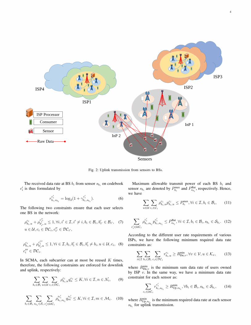
sensors in the coverage area of BS bi who sell the raw data toISPs. In this paper, we focus on both the uplink transmissionof raw data from sensors to BSs and downlink transmissionof processed data from BSs to users. The data processing isperformed at the private cloud of each ISP which is connectedto all BSs.

Figures 1 and 2 illustrate the downlink and uplink trans-missions in the network, respectively, where each InP frame-work contains one macro base station (MBS) and few femtobase stations (FBSs). We denote the set of InPs by I ={1, 2, . . . , I}, set of BSs in InP i by Bi = {1, 2, . . . , Bi},and set of sensors by S =

∪bi∈Bi

Sbi , where Sbi is the set of

sensors in cell bi whose cardinality is Sbi . Besides, there areU users with the set of U = {1, 2, . . . , U}, each of whichcan be associated to only one BS in the network. Moreover,each user is served by one ISP. The set of ISPs is denoted byV = {1, 2, . . . , V }. Furthermore, the set of users served byISP v is denoted by Kv. Hence, we have U =

∪v∈V

Kv.

The frequency bandwidth of downlink and uplink wirelesschannels in each InP i are denoted by WDn

i and WUpi , re-

spectively. We assume that different InPs use non-overlappingbandwidth. Within each InPi, the bandwidth is divided be-tween downlink and uplink transmission, denoted by WDn

i andWUp

i , respectively. These available spectrum are divided intoNi and Mi subcarriers, respectively. It is assumed that eachsubcarrier has bandwidth of WS. The set of downlink and up-link subcarriers in InP i are indicated by Ni = {1, 2, . . . , Ni}and Mi = {1, 2, . . . ,Mi}, respectively.

We utilize the SCMA technique which is one of the maincandidates for 5G multiple access techniques [3]–[5]. Weassume that the set of downlink and uplink codebooks are

3

Direct Transmission Link of FBS

Consumer

Sensor

InP 1

InP 2

Sensors

ISP2

ISP3ISP4

ISP Processor

ISP1

Fig. 1: Downlink transmission from BSs to users.

shown by DCi = {1, . . . , Ci} and UCi = {1, . . . , C ′i},

respectively, where Ci and C ′i are the number of downlink

and uplink codebooks, respectively. Moreover, the mappingbetween downlink subcarriers and codebooks is shown by qcin ,where qcin = 1 if codebook ci consists of subcarrier n, and oth-erwise qcin = 0. In a same way, for uplink case we define q′c

′i

m toshow the mapping between uplink subcarriers and codebooks.It should be noted that for both uplink and downlink cases, weassume that the mapping between codebooks and subcarriersis known and fixed.

Let pcibi,u denote the downlink transmit power of BS bi ∈ Bi

to user u on codebook ci ∈ DCi, and p′c′i

bi,sbidenotes the uplink

transmit power of sensor sbi to BS bi on codebook c′i. Thechannel gain between BS bi and user u on subcarrier n, andbetween BS bi and sensor sbi on subcarrier m are determinedby hnbi,u and hmbi,sbi

, respectively. The codebook assignment

indicators are expressed by ρcibi,u, ρ′c′ibi,sbi

∈ {0, 1}. Note thatpcibi,u is assigned to subcarrier n based on a given proportion0 ≤ λbin,ci ≤ 1, indicated based on codebook design whichsatisfies

∑n∈Ci

λbin,ci = 1 where Ci is the set of subcarriers in

codebook ci. In a same way, p′c′i

bi,sbiis assigned to subcarrier

m based on a given proportion λ′bim,ci . The received SINR at

user u from BS bi on codebook ci is given by

γcibi,u =ρcibi,u

∑n∈Ni

qcin λbin,cip

cibi,u

|hnbi,u|2

Icibi,u + (σcibi,u

)2, (1)

where Icibi,u is obtained by

Icibi,u =∑

b′i∈Bi/{bi}

∑u′∈U

∑n∈Ni

ρcib′i,u′qcin λ

b′in,cip

cib′i,u

′ |hnb′i,u|2. (2)

Accordingly, the data rate at user u from BS bi on codebookci is formulated by

rcibi,u = log2(1 + γcibi,u). (3)

The uplink SINR from sensor sbi to BS bi on subcarrier mcan be expressed by

γc′ibi,sbi

=ρ′c′ibi,sbi

∑m∈Mi

q′mbi λ′bin,c′i

p′c′ibi,sbi

|hmbi,sbi |2

I′c′ibi,sbi

+ (σ′c′ibi,sbi

)2, (4)

where I ′c′i

bi,sbiis given by

I′c′ibi,sbi

=∑

b′i∈Bi/{bi}

∑s′b′i∈Sbi

∑m∈Mi

ρ′c′ib′i,s

′b′i

qc′imλ

′b′im,c′i

p′c′ib′i,s

′b′i

(5)

|hmbi,s′b′i

|2.

4

ConsumerInP 1

InP 2

ISP1

Sensor

Sensors

ISP2

ISP3

ISP4

ISP Processor

Fig. 2: Uplink transmission from sensors to BSs.

The received data rate at BS bi from sensor sbi on codebookc′i is thus formulated by

rc′ibi,sbi

= log2(1 + γc′ibi,sbi

). (6)

The following two constraints ensure that each user selectsone BS in the network:

ρcibi,u + ρc′′i′

b′i′ ,u

≤ 1, ∀i, i′ ∈ I, i′ ̸= i, bi ∈ Bi, b′i′ ∈ Bi′ , (7)

u ∈ U , ci ∈ DCi, c′′i′ ∈ DCi′ ,

ρcibi,u + ρc′′′i

b′i,u≤ 1, ∀i ∈ I, bi, b′i ∈ Bi, b

′i ̸= bi, u ∈ U , ci, (8)

c′′′i ∈ DCi.

In SCMA, each subcarrier can at most be reused K times,therefore, the following constraints are enforced for downlinkand uplink, respectively:∑

bi∈Bi

∑u∈U

∑ci∈DCi

ρcibi,uqcin ≤ K, ∀i ∈ I, n ∈ Ni, (9)

∑bi∈Bi

∑sbi∈Si

∑c′i∈UCi

ρ′c′ibi,sbi

q′c′im ≤ K, ∀i ∈ I,m ∈ Mi. (10)

Maximum allowable transmit power of each BS bi andsensor sbi are denoted by Pmax

biand PBat

sbi, respectively. Hence,

we have ∑u∈U

∑ci∈Ci

ρcibi,upcibi,u

≤ Pmaxbi , ∀i ∈ I, bi ∈ Bi, (11)

∑c′i∈UCi

ρc′ibi,sbi

pc′ibi,sbi

≤ PBatsbi, ∀i ∈ I, bi ∈ Bi, sbi ∈ Sbi . (12)

According to the different user rate requirements of variousISPs, we have the following minimum required data rateconstraints as:∑

i∈I

∑bi∈Bi

∑ci∈DCi

rcibi,u ≥ RminDn,v, ∀v ∈ V, u ∈ Kv, (13)

where RminDn,v is the minimum sum data rate of users owned

by ISP v. In the same way, we have a minimum data rateconstraint for each sensor as:∑

ci∈UCi

rc′ibi,sbi

≥ RminUp,sbi

, ∀bi ∈ Bi, sbi ∈ Sbi , (14)

where RminUp,sbi

is the minimum required data rate at each sensorsbi for uplink transmission.

5

B. Pricing Scheme

In the proposed pricing model, each sensor sells its rawsensed data to ISPs. In other words, each ISP collects datafrom different sensors. Then, ISPs perform a processing basedon the determined sets of collected data and sell it to users.Fig. 3 illustrates the proposed pricing model of the consideredsystem. Based on Fig. 3, there are four major players in theproposed IoT pricing scheme: InPs, sensors, ISPs and users.In the following, we present the pricing model of each player.

1) InPs: Each InP leases power and bandwidth from apower supplier and regulatory, respectively, and lends themto ISPs. In addition, each InP i lends its bandwidth to the setof sensors owned by BSs in Bi. Assume that LPower,BS

bilet the

unit of price of power consumption at BS bi, per Watt. Theincome of InP i from lending power to ISPs can be obtainedas

ϕInP,Poweri =

∑bi∈Bi

∑u∈U

∑ci∈DCi

LPower,BSbi

ρcibi,upcibi,u

. (15)

Let LBWi denote the unit price for lending downlink and

uplink transmission bandwidths, per Hz, to ISPs and sensors.Therefore, the income of InP i from lending spectrum to ISPsand sensors are given by

ϕInP,BWi =

∑bi∈Bi

∑u∈U

∑ci∈DCi

∑n∈Ni

qcin LBWi ρcibi,uWS+ (16)

∑bi∈Bi

∑sbi∈Sbi

∑c′i∈UCi

∑m∈Mi

q′mbi LBWi ρ

c′ibi,sbi

WS.

The cost of InP i for buying power from power suppliers witha unit price CPower,Sup (per Watt) is obtained by

ψInP,Poweri =

∑bi∈Bi

∑u∈U

∑ci∈Ci

ρcibi,upcibi,u

CPower,Sup, ∀i ∈ I, (17)

and the cost of buying bandwidth from regulatory with unitprice CBW

i (per Hz) can be formulated by

ψInP,BWi =WDn

i CBWi +WUp

i CBWi , ∀i ∈ I. (18)

The revenue of InP i is thus given by

ΦInPi = ϕInP,Power

i + ϕInP,BWi − ψInP,Power

i − ψInP,BWi . (19)

Hence, the total revenue of InPs in the network is formulatedas follows:

ΦInPtot =

∑i∈I

ΦInPi . (20)

2) Sensors: Each sensor sbi has a reservation wage costCSens,Reserv

sbito obtain the raw data. Moreover, it leases power

from the power supplier and bandwidth from InPs with unitsprice CPower,Sup (per Watt) and LBW

i (per Hz), respectively, tosell the raw data with the price LSens,Data

v,sbiwhich is offered by

ISP v to sensor sbi in uplink transmission to ISPs. In doingso, the uplink data rate of each sensor sbi is the income ofthe sensor with unit of price LUp,Rate

sbi(1/bps). Accordingly, the

revenue of each sensor sbi can be obtained by

ΦSenssbi

=∑v∈V

min{∑u∈Kv

αsbi ,u, 1}LSens,Data

v,sbi+ (21)

∑v∈V

∑c′i∈UCi

min{∑u∈Kv

αsbi ,u, 1}rc

′i

bi,sbiLUp,Ratesbi

−min{∑u∈U

αsbi ,u, 1}CSens,Reserv

sbi−∑

c′i∈UCi

ρc′ibi,sbi

pc′ibi,sbi

CPower,Sup −∑

c′i∈UCi

∑m∈Mi

q′mbi ρc′ibi,sbi

WSLBWi ,

where the binary indicator αsbi ,u∈ {0, 1} takes value 1 when

the raw data of sensor sbi is used in the processing data ofuser u at the cloud of ISP. Note that each ISP buys the data ofsensor sbi at most once. The total revenue of sensors is thusgiven by

ΦSenstot =

∑sbi∈Sbi

ΦSenssbi

. (22)

3) ISPs: Each ISP buys power and downlink bandwidthfrom InP with unit price LPower,BS

biand LBW

i , respectively.Moreover, it leases the raw data of sensors with price LSens,Data

v,sbiand gives money to sensors for their uplink data rate with theunit price LUp,Rate

sbi. The income of each ISP is composed of two

components. Firstly, they get money for their downlink datarate servicing to users with the unit of price LDn,Rate

v (per bit/s).Secondly, they lend their processed data to users. The priceof the processed data which is served to user u from ISP v is

QuLReserv,Userv,u , where Qu = q log(1+

I∑i=1

∑bi∈Bi

∑sbi

∈Sbi

αsbi,u

I∑i=1

∑bi∈Bi

Sbi

) is

the service quality function of a set of sensors whose data isused by user u [6], and LReserv,User

v,u is the maximum reservationprice that ISP v takes from user u. In addition, q is a sensingquality of player that is used to tune service quality receivedby the users. In doing so, the income of ISP v originating fromthe data service given to the its subscribing users is given by

ϕISP,ratev =

∑i∈I

∑bi∈Bi

∑u∈Kv

∑ci∈DCi

∑n∈Ni

qcin LDn,Ratev WSr

cibi,u

.

(23)

Moreover, the income of ISP v from selling the processed datato users in Kv is obtained by

ϕISP,datav =

∑u∈Kv

QuLReserv,Userv,u . (24)

The cost of buying power from InPs at ISP v is given by

ψISP,Powerv =

∑i∈I

∑bi∈Bi

∑u∈Kv

∑ci∈DCi

LPower,BSbi

ρcibi,upcibi,u

, (25)

and the cost of buying bandwidth from InPs at ISP v is givenby

ψISP,BWv =

∑i∈I

∑bi∈Bi

∑u∈Kv

∑ci∈DCi

∑n∈Ni

qcin LBWi ρcibi,uWS. (26)

The price of buying the raw data from sensors at each ISP vcan be formulated by

ψISP,datav =

∑sbi∈Sbi

min{∑u∈Kv

αsbi ,u, 1}LSens,Data

v,sbi. (27)

6

Regulatory Power Supplier

Uplink and

Downlink

Bandwidth

Transmit Power of SensorsTransmit Power of BSs

InP

ISP

IoT User

Uplink Bandwidth

Downlink Bandwidth Transmit Power of BSs Raw Data

Uplink Data Rate

Downlink Data Rate Processed Data

𝐶𝑖BW

𝐿𝑣Dn ,Rate 𝑄𝑢𝐿𝑣,𝑢

Reserv ,User

𝐿𝑖BW 𝐿𝑏𝑖

Power ,BS

𝐿𝑣,𝑠𝑏𝑖

Sens ,Data

𝐿𝑠𝑏𝑖Up ,Rate

𝐶Power ,Sup

𝐶Power ,Sup

𝐿𝑖BW

SDO

Fig. 3: IoT Pricing Scheme.

Moreover, each ISP v gives money to sensors for their uplinkdata rates with the total price of

ψISP,Uplinkv =

∑i∈I

∑bi∈Bi

∑sbi∈Sbi

min{∑u∈Kv

αsbi ,u, 1}rc

′i

bi,sbi

(28)

LUp,Ratesbi

.

The revenue of each ISP v is thus formulated as follows:

ΦISPv = ϕISP,rate

v + ϕISP,datav − ψISP,Power

v − ψISP,BWv (29)

− ψISP,datav − ψISP,Uplink

v .

Therefore, the total revenue of ISPs is given by

ΦISPtot =

∑v∈V

ΦISPv . (30)

4) Users: Each user is willing to achieve the high qualityIoT and high data rate services with low power and spectrumconsumption. Therefore, for each user, rewards and costs aremodeled as follows:

• Reward 1: IoT service (the processed data) is receivedby users with unit price CReserv,User

u . Therefore, reward ofuser u for IoT service is given by

ϕUser,datau = QuC

Reserv,Useru , ∀u ∈ Kv. (31)

• Cost 1: The received data rate by users which is offeredby ISP v with unit cost LDn,Rate

v is given by

ψUser,rateu = (32)

∑i∈I

∑bi∈Bi

∑ci∈DCi

∑n∈Ni

qcin LDn,Ratev WSr

cibi,u

, ∀u ∈ Kv.

• Cost 2: IoT service price at user u with unit costLReserv,Userv,u which is offered by ISP v to user u, can be

obtained by QuLReserv,Userv,u , ∀u ∈ Kv.

The revenue of each user u ∈ Kv is formulated as follows:

ΦUseru = ϕUser,data

u − ψUser,rateu −QuL

Reserv,Userv,u , ∀u ∈ Kv. (33)

Therefore, the total revenue of users is obtained by

ΦUsertot =

∑u∈U

ΦUseru . (34)

III. PROPOSED PRICING MODEL

In this paper, we aim to design a joint uplink/downlink datadelivery policy with BS selection at users and determine the ef-ficient value of pricing units offered by each player. Moreover,we obtain the efficient raw data subset selection for processingthe collected raw data for each user. Let us denote p =

[pBS,pSens], pBS = [pcibi,u], pSens = [p

c′ibi,sbi

], ρ = [ρBS,ρSens],

ρBS = [ρcibi,u], ρSens = [ρ′c′ibi,sbi

], LPower,BS = [LPower,BSbi

],

LBW = [LBWi ], LSens,Data = [LSens,Data

v,sbi], LUp,Rate = [LUp,Rate

sbi],

LDn,Rate = [LDn,Ratev ], α = [αsbi ,u

], LReserv,User = [LReserv,Userv,u ],

L = [LPower,BS,LBW,LSens,Data,LUp,Rate,LDn,Rate,LReserv,User].In order to jointly maximize the revenues of major playersin the proposed pricing model, we use the multi-objective

7

approach. The multi-objective optimization problem of theproposed system model is formulated as

maxρ,p,L,α

{ΦISPtot ,Φ

InPtot ,Φ

Senstot ,Φ

Usertot }, (35a)

s.t. : (7)-(14).

The proposed optimization problem in (35) is intractable. Totackle this issue, we adopt the scalarization method. By usingthis method, a multi-objective function can be transformedinto a simple, tractable, and single objective function [41]–[43]. Note that there are many cases in the scalarizationmethods resulting in different Pareto optimal solutions. Theresult of solution of each single objective problem forms apoint of Pareto boundary. In the following, we exploit twoapproaches within the scalarization method, namely, max-min and weighted-one algorithms, to solve the multi-objectiveoptimization problem. The main reasons behind selection ofthese methods are that the weighted-one is very simple andthe max-min method achieves the best fairness in the system.For more clarification please refer to Appendix A.

A. Max-Min Approach

ISPs, InPs, and SDO are three players which work togetherto provide IoT services for end users. In this approach, ourgoal is to maximize the fairness index among these threeplayers. Consequently, our max-min optimization problem isformulated as follows:

maxρ,p,L,α

minISP,InP,Sens,

{ΦISPtot ,Φ

InPtot ,Φ

Senstot }+ΦUser

tot , (36a)

(36b)s.t. : (7)-(14).

B. Weight-One Approach

In this approach, our goal is to maximize the summationof weighted utilities of ISPs, InPs, sensors, and users. Themax-min optimization problem is formulated as follows:

maxρ,p,L,α

∑v∈V

ωISPv ΦISP

v +∑u∈U

ωUseru ΦUser

u (37a)

+∑i∈I

ωInPi ΦInP

i +∑i∈I

∑bi∈Bi

∑sbi∈Sbi

ωSenssbi

ΦSenssbi

s.t. (7)-(14).

where ωISPv , ωUser

u , ωInPi and ωSens

sbiare the weights tuned based

on the priority of ΦISPv , ΦUser

u , ΦInPi and ΦSens

sbi, respectively.

IV. CONVENTIONAL APPROACH IN IOT PRICING

Based on a conventional approach, each player by con-sidering a minimum utility requirement for the other play-ers maximizes its utility. Then, the calculated results of itscorresponding price variables are reported to a central unit.Central unit by considering the reported price variables solvesa comprehensive joint power and codebook allocation problemfor all of the players. Consequently, by the conventional

method, price variables are determined by players and powerand codebook are assigned centrally. In the following, theoptimization problems which should be solved by differentplayers and the optimization problem which should be solvedby the central unit are presented. It should be noted thateach InP can play the role of the central unit to solve thecomprehensive joint power and codebook allocation problem.

A. InP Optimization Problem

Each InP maximizes its utility function by consideringminimum utilities ΦISP

0 , ΦUser0 and ΦSDO

0 for ISPs, users andSDO, respectively. Moreover, for other InPs it considers min-imum utility ΦEInP

0 . The corresponding optimization problemis formulated as:

maxρ,p,L,α

ΦInPi , (38a)

s.t. : (7)-(14),

ΦISPtot ≥ ΦISP

0 , (38b)

ΦUsertot ≥ ΦUser

0 , (38c)

ΦInPi′ ≥ ΦEInP

0 , i′ ∈ I/i, (38d)

ΦSDOtot ≥ ΦSDO

0 . (38e)

B. ISP Optimization Problem

Each ISP maximizes its utility function by consideringminimum utilities ΦInP

0 , ΦUser0 and ΦSDO

0 for InPs, users andSDO, respectively. Moreover, for other ISPs, each ISP con-siders minimum utility ΦEISP

0 . The corresponding optimizationproblem is formulated as:

maxρ,p,L,α

ΦISPv , (39a)

s.t. : (7)-(14),

ΦInPtot ≥ ΦInP

0 , (39b)

ΦUsertot ≥ ΦUser

0 , (39c)

ΦISPv′ ≥ ΦEISP

0 , ∀v′ ∈ V/v, (39d)

ΦSDOtot ≥ ΦSDO

0 . (39e)

C. SDO Optimization Problem

SDO maximizes its utility function by considering minimumutilities ΦInP

0 , ΦUser0 and ΦISP

0 for InPs, users, and ISPs, respec-tively. The corresponding optimization problem is formulatedas:

maxρ,p,L,α

ΦSDOtot , (40a)

s.t. : (7)-(14),

ΦInPtot ≥ ΦInP

0 , (40b)

ΦUsertot ≥ ΦUser

0 , (40c)

ΦISPtot ≥ ΦISP

0 . (40d)

8

D. Central Unit Optimization Problem

As we mentioned, central unit by considering the reportedprices, solves a joint power and codebook allocation problem.Therefore, optimization problem which should be solved bythe central unit is presented as follows:

maxρ,p,α

{ΦISPtot ,Φ

InPtot ,Φ

Senstot ,Φ

Usertot }, (41a)

(41b)s.t. : (7)-(14).

V. SOLUTION

A. Solution of the Weight-One Approach

In order to solve the optimization problem (37), the alternat-ing algorithm is used [44]. Based on the alternating method,in each iteration, each set of variables are calculated assumingother variable sets are fixed.

The main solution steps are presented in Algorithm 1. In

Algorithm 1 ITERATIVE RESOURCE ALLOCATION AL-GORITHM

• STEP1: Initialization:– Set t = 0 (iteration number),– Find α(0), P(0), L(0), and ρ(0)

• STEP2:– Set P = P(t), α = α(t), and ρ = ρ(t),– Solve the optimization problem with variable L,– Set the result of optimization problem solution to

L(t+ 1),• STEP3:

– Set P = P(t), L = L(t+ 1), and ρ = ρ(t),– Solve the optimization problem with variable α,– Set the result of optimization problem solution to

α(t+ 1),• STEP4:

– Set L = L(t+ 1), α = α(t+ 1), and ρ = ρ(t),– Solve the optimization problem with variable P,– Set the result of optimization problem solution to

P(t+ 1),• STEP5:

– Set L = L(t+1), α = α(t+1), and P = P(t+1),– Solve the optimization problem with variable ρ,– Set the result of optimization problem solution to

ρ(t+ 1),• STEP6:

– If convergencestop and return α, P, L, and ρ as the suboptimalsolution,

– Elseset t = t+ 1 and go back to STEP 2,

– Output: Suboptimal value of α, P, L, and ρ.

Step 2, the problem of finding L is solved by assuming theother variables being fixed. This problem is a non-constrainedlinear programming which can be solved by using the CVX

toolbox [45]. The optimization problem with variable L isformulated as follows:

maxL

∑v∈V

ωISPv ΦISP

v +∑u∈U

ωUseru ΦUser

u (42)

+∑i∈I

ωInPi ΦInP

i +∑i∈I

∑bi∈Bi

∑sbi∈Sbi

ωSenssbi

ΦSenssbi

.

In Step 3, with assumption of other optimization variablesbeing fixed, the problem of finding α is solved. By using theepigraph technique and relaxing the variable α to have thecontinuous value between 0 and 1, the optimization problem(42) is reformulated as:

maxα,δ,β

∑i∈I

∑bi∈Bi

∑sbi∈Sbi

ωSenssbi

(∑v∈V

δv,sbiLSens,Datav,sbi

+ (43a)

∑v∈V

∑c′i∈UCi

δv,sbi rc′ibi,sbi

LUp,Ratesbi

− βsbiCSens,Reservsbi

)+

∑v∈V

ωISPv

( ∑u∈Kv

q log(1 +

I∑i=1

∑bi∈Bi

∑sbi∈Sbi

αsbi ,u

I∑i=1

∑bi∈Bi

Sbi

)

LReserv,Userv,u −

∑sbi∈Sbi

δv,sbiLSens,Datav,sbi

−

∑i∈I

∑bi∈Bi

∑sbi∈Sbi

δv,sbi rc′ibi,sbi

LUp,Ratesbi

)+

∑v∈V

∑u∈Kv

ωUseru

(q log(1 +

I∑i=1

∑bi∈Bi

∑sbi∈Sbi

αsbi ,u

I∑i=1

∑bi∈Bi

Sbi

)

(CReserv,Useru − LReserv,User

v,u )

),

s.t. δv,sbi ≤∑u∈Kv

αsbi ,u, (43b)

δv,sbi ≤ 1, (43c)

βsbi ≤∑u∈U

αsbi ,u, (43d)

βsbi ≤ 1, (43e)

0 ≤ αsbi ,u≤ 1, (43f)

where δ = [δv,sbi ] and β = [βsbi ] are the auxiliary variablescorresponding to the epigraph algorithm. The optimizationproblem (43) is convex which can be solved by applyingthe CVX toolbox. The aim of Step 4 is finding p. Thecorresponding optimization problem is formulated as:

maxp

∑v∈V

ωISPv

(∑i∈I

∑bi∈Bi

∑u∈Kv

∑ci∈DCi

LDn,Ratev WSr

cibi,u

(44a)

−∑i∈I

∑bi∈Bi

∑u∈Kv

∑ci∈DCi

LPower,BSbi

ρcibi,upcibi,u

−

∑i∈I

∑bi∈Bi

∑sbi∈Sbi

min{∑u∈Kv

αsbi ,u, 1}rc

′i

bi,sbiLUp,Ratesbi

)−

9

∑v∈V

∑u∈Kv

ωUseru

(∑i∈I

∑bi∈Bi

∑ci∈DCi

LDn,Ratev WSr

cibi,u

)+

∑i∈I

ωInPi

( ∑bi∈Bi

∑u∈U

∑ci∈DCi

LPower,BSbi

ρcibi,upcibi,u

)+

∑i∈I

∑bi∈Bi

∑sbi∈Sbi

ωSenssbi

(∑v∈V

∑c′i∈UCi

min{∑u∈Kv

αsbi ,u, 1}

rc′ibi,sbi

LUp,Ratesbi

−∑

c′i∈UCi

ρc′ibi,sbi

pc′ibi,sbi

CPower,Sup),

s.t. (11)-(14).

Due to the non-convex rate function in uplink and downlinktransmissions, the optimization problem (44) is non-convex.To tackle the non-convexity issue of the considered problem, asuccessive convex approximation (SCA) approach with differ-ence of two concave functions (D.C.) approximation methodis used. In order to apply this method, at first the downlinkrate function is written as

rcibi,u = f cibi,u − gcibi,u, (45)

where

f cibi,u = log2(ρcibi,u

∑n∈Ni

qcin λbin,cip

cibi,u

|hnbi,u|2 + Icibi,u (46)

+ (σcibi,u

)2),

gcibi,u = log2(Icibi,u

+ (σcibi,u

)2). (47)

By applying the D.C. approximation, we have

gcibi,u(pBS,t) ≈ gcibi,u(p

BS,t−1) +∇gcibi,u(pBS,t−1) (48)

(pBS,t − pBS,t−1),

where

∇gcibi,u(pBS) = (49)

0, ∀i′ ̸= i,∑n∈Ni

ρcib′i,u′q

cin λ

b′in,ci

|hnb′i,u

|2

ln(2)(Icibi,u

+(σcibi,u

)2) , ∀u′ ̸= u, b′i ̸= bi.

The uplink data rate function is written as

rc′ibi,sbi

= f′c′ibi,sbi

− g′c′ibi,sbi

, (50)

where

fc′ibi,sbi

= log2(ρ′c′ibi,sbi

∑m∈Mi

q′mbi,sbiλ′bin,c′i

p′c′ibi,sbi

|hmbi,sbi |2+

(51)

I′c′ibi,sbi

+ (σ′c′ibi,sbi

)2),

gc′ibi,sbi

= log2(I′c′ibi,sbi

+ (σ′c′ibi,sbi

)2). (52)

By applying the D.C. approximation, we have

gc′ibi,sbi

(pSens,t) ≈ gc′ibi,sbi

(pSens,t−1) +∇gc′i

bi,sbi(pSens,t−1)

(53)

(pSens,t − pSens,t−1).

where

∇gc′i

bi,sbi(pSens) = (54)

0, ∀i′ ̸= i,∑m∈Mi

ρ′c′ib′i,s′

b′i

qc′imλ

′b′im ,c′i

| hmbi,s

′b′i

|2

I′c′ibi,sbi

+ (σ′c′ibi,sbi

)2. b′i ̸= bi.

By applying the D.C. approximation, the optimization problem(44) is approximated by a convex function which can be solvedby CVX toolbox. In Step 5, the problem of finding ρ is solvedwhich is an integer non-linear optimization problem. To solveit, we initially relax the integer variables to continuous valuesbetween zero and one. The same steps that are applied in theprevious step are applied here as well.

B. Solution of the Max-Min Approach

To solve the max-min approach optimization problem, atfirst we apply the epigraph method as:

maxρ,p,L,α,t

t+ΦUsertot , (55a)

s.t. : (7)-(14),

ΦISPtot ≥ t, (55b)

ΦInPtot ≥ t, (55c)

ΦSenstot ≥ t, (55d)

where t is an auxiliary variable. Then, we continue similar tothe weight-one approach algorithm.

C. Solution of the Conventional Approach Problems

Each of the presented optimization problem in the conven-tional approach can be solved by the iterative algorithm shownin Algorithm 1.

VI. CONVERGENCE OF THE PROPOSED SOLUTIONALGORITHM

The alternating method exploits an iterative algorithm inwhich in each iteration each set of variables is calculated bysupposing that the other variable sets are fixed and processis continued until convergence. The necessary and sufficientconditions to ensure the algorithm convergence is that in eachiteration the objective function increases or stays unalteredcompared to the previous iteration [46], [47]. In our solution,we have

· · · ≤ U(ρt,pt,Lt,αt)a≤ U(ρt,pt,Lt+1,αt)

b≤ (56)

U(ρt,pt,Lt+1,αt+1)c≤ U(ρt,pt+1,Lt+1,αt+1)

d≤

U(ρt+1,pt+1,Lt+1,αt+1) ≤ . . .

which indicates that after each iteration, the objective functionincreases or stays unaltered compared to the previous iteration.

Inequality (a) in (56) follows from the fact that optimizationproblem with variables L and constant ρ,p and α (ρ =ρt,p = pt,α = αt) is a linear program whose worst solutionis L = Lt, therefore, based on the worst solution, we have

10

Lt+1 = Lt. Consequently, we have U(ρt,pt,Lt,αt) ≤1

U(ρt,pt,Lt+1,αt). For inequalities (b), (c) and (d), the sameargument as for inequality (a) can be used. Since for a finite setof transmit powers and subcarrier assignment, the summationof utilities is bounded, the procedure must converge.

VII. SIMULATION RESULTS

In order to evaluate the performance of the proposed endto end pricing and radio resource allocation approach, wefirst depict the utility of each of the players versus variousparameters. Moreover, we compare the performance of theproposed approach to the conventional one.

A. Parameters

The considered parameters for numerical results are sum-marized as follows: Pmax

1i= 50 (Watts) for all i ∈ I,

Pmaxbi

= 1 (Watts) for all i ∈ I and b ∈ {2, . . . , B},I = 2, B = 2, V = 2, Rmin

Up,sbi= 0.01 (bps/Hz) for

all bi ∈ Bi, sbi ∈ Sbi , and RminDn,v = 0.1 (bps/Hz) for all

v ∈ V, v ∈ Kv, hnbi,u = xnbi,u(Dbi,u)ξ where ξ indicates the

path loss exponent and ξ = −3, xnbi,u represents the Rayleighfading, and Dbi,u demonstrates the distance between user uand BS bi. Moreover, to scale the price of the power, data ofsensor, and user reservation of player, we define a parameteras scale of player with value SF = 105. By defining this scaleof player, the maximum and minimum prices of each of theparameters is defined as follows: 0 ⪯ LPower,BS ⪯ SF ×Lmax,0 ⪯ LBW ⪯ Lmax, 0 ⪯ LSens,Data ⪯ SF×Lmax, 0 ⪯ LUp,Rate ⪯Lmax, 0 ⪯ LDn,Rate ⪯ Lmax and 0 ⪯ LReserv,User ⪯ SF × Lmaxwhere ⪯ denotes vector inequality or componentwise inequal-ity. Moreover, there are some common settings in the most ofthe results which are as follows: Sbi = 3 and the number ofsubcarriers for both of UL and DL transmission are set to 4.Furthermore, we assume that each ISP serves 4 users.

B. Results

Figs. 4, 5, 6, respectively, depict the utility of all players inthe max-min, weight-one, and conventional approach versusdifferent values of Lmax where the number of sensors is set to3. From these figures we can see that by increasing the utility(revenue) of InPs, ISPs, and SDO, the total utility of the usersis decreased. This is due to the fact that users are the endconsumer of the network and the other players income comesfrom their payments. Moreover, as can be seen, the utility ofInPs is more than that of the other players. This is becauseInPs sell their resources to SDO and ISPs, simultaneously (seethe details of pricing model of InPs in n in Fig. 3).

Now using the results in the above figures we obtain Figs. 7and 8 which depict total revenue and fairness for the max-min,conventional, and weight-one methods.

In general, we look for a setting which has the best totalrevenue. However, such revenue has to be divided in a fairfashion among the stakeholders. To quantify this fact, weexploit the Jain fairness index [48]. The Jain fairness index

3 3.5 4 4.5 5 5.5 6 6.5 7

LMax

-1.5

-1

-0.5

0

0.5

1

Util

ity

108

ISPUserInPSensTotal

Fig. 4: Utility of each players in the max-min approach versusdifferent values of Lmax.

for utilities of ISPs, InPs, and SDO is calculated as follows[48]:

J(ΦISPtot ,Φ

InPtot ,Φ

Senstot ) =

(ΦISPtot +ΦInP

tot +ΦSenstot )2

3((ΦISPtot )

2 + (ΦInPtot )

2 + (ΦSenstot )2)

.

(57)

With the Jain fairness index, when ΦISPtot = ΦInP

tot = ΦSenstot ,

the best fairness (i.e., J(ΦISPtot ,Φ

InPtot ,Φ

Senstot ) = 1) is achieved.

As the figures show, if we go with the conventional ap-proach, we are in fact cutting the total revenue. Moreover,the degree of fairness is not also acceptable. By using theweight-one approach, the total revenue is drastically increased.Nevertheless, the resulting fairness is still far from beingacceptable. Finally, if we use the max-min approach, we getclose to the complete fairness. This is while the total revenueis also increased compared to the conventional approach.

The results prove how the proposed end to end joint pricingand radio resource allocation approach can provide fairnessand at the same time, increase the revenue. This is achievedthrough jointly optimizing the parameters corresponding to allplayers.

VIII. CONCLUSIONS

In this paper, we provided a novel comprehensive pricingmodel for IoT services in 5G networks. We considered all theparties involved in the communication scenario and determinedthe revenue and cost of each party. We formulated the resourceallocation in the considered model as a multi-objective opti-mization problem where in addition to the resource allocation,the pricing variables were also the optimization variables. Wesolved the resulting problem using the alternating approachand evaluated the performance of the proposed model fordifferent network scenarios using simulations. Moreover, wepresented the conventional approach for pricing and radioresource allocation. Simulation results indicate that by apply-ing the proposed joint framework, we can increase the totalrevenue compared to the conventional case while providing

11

3 3.5 4 4.5 5 5.5 6 6.5 7L

Max

-4

-3

-2

-1

0

1

2

3U

tility

108

ISPUserInPSDOTotal

Fig. 5: Utility of each player in the weight-one approach versusdifferent values of Lmax.

3 3.5 4 4.5 5 5.5 6 6.5 7L

Max

-4

-2

0

2

4

6

8

10

12

Util

ity

107

ISPUserInPSDOTotal

Fig. 6: Utility of each player in the conventional approach versusdifferent values of Lmax.

3 3.5 4 4.5 5 5.5 6 6.5 7

LMax

0.5

1

1.5

2

2.5

3

3.5

4

4.5

5

Uti

lity

108

ConventionalWeight-One

Max-Min

Fig. 7: Summation of players utilities for the proposed methods.

3 3.5 4 4.5 5 5.5 6 6.5 7

LMax

0.45

0.5

0.55

0.6

0.65

0.7

0.75

0.8

0.85

0.9

Fac

tor

of

Fai

rnes

s

ConventionalWeight-one

Max-Min

Fig. 8: Fairness index for the proposed methods.

an almost complete fairness among the players. This pavesthe way to reach the stated goal of the paper: removing oneof the barriers that prevent IoT from becoming pervasive.

APPENDIX

Appendix A: Suppose that we have a multi-objectivemaximization problem with objective functions F and G, andvariable vector ϱ formulated as follows

maxϱ

{F (ϱ), G(ϱ)}, (58a)

s.t. : C1-CK ,

where C1, . . . , CK are the constraints of the optimizationproblem.

In order to solve (58), one method is scalarization wherethe original multi-objective problem is transformed into asingle objective problem. There are various methods whichtransform the original problem into a single objective opti-mization problem. Each single objective optimization problemgives a Pareto optimal solution of the original multi-objectiveproblem. Each of the solutions is determined by a point in thePareto solution set of the original problem. For example, Fig.9 shows the Pareto solution set of the maximization problemin which the bold line determines the Pareto boundary. Eachof the points can be interpreted as the solution of a specifictransformed single objective optimization problem. Supposethat the weighted method is used to transfer the multi-objectiveinto a single objective problem. With the weighted method, theoptimization problem (58) is reformulated as

maxϱ

WF (ϱ) + (1−W )G(ϱ), (59a)

s.t. : C1-CK .

The weighted method is an approach of the scalarizationmethod in which with different values of W , various singleobjective optimization problem can be achieved. When thePareto solution set is a convex set, such as Fig. 9, with theweighted method all of the points in the Pareto boundary

12

can be achieved. For example, point S1 can be interpretedas a weighted single objective problem in which the weightof function F is W = 1. Point S2 can be interpreted as aweighted single objective optimization problem in which themain goal is maximizing the fairness between functions F andG. Point S3 can be interpreted as a weighted single objectiveoptimization problem in which the weight of function G is 1or (W = 0). As we mentioned, with the weighted approach,all points of the Pareto boundary of a convex Pareto solutionset can be achieved. However, finding a value of W whichgives the best fairness between F and G is so complicated,while by exploiting the max-min approach as

maxϱ

{minF,G

{F (ϱ), G(ϱ)}} (60a)

s.t. : C1-CK ,

the best fairness can be easily achieved. Moreover, if thePareto solution set not be a convex set, such as Fig. 10, theweighted approach can not achieve all of the Pareto boundarypoints. For example, in Fig. 10, point S2 (consider that S2gives the best fairness) can not be achieved with the weightedapproach. In this case, the max-min method can be applied toachieve the best fairness between F and G. From the aboveexplanation, we can find that in a multi-objective optimizationproblem, considering the main goal of the multi-objectiveoptimization problem, a single objective optimization problemcan be formulated from the main multi-objective problem.It should be noted that, in addition to the main goal of thetransformed optimization problem, its solution complexity canhave essential role in selecting the form of the transformedoptimization problem.

The proposed max-min approach in (36) comes from thisfact that the fairness among ISPs, SDO and InPs has themaximum values, and also, the utility function of users hasthe maximum value. It should be noted that, due to the thisfact that the user utility has a negative value, it is not possibleto consider it as an entry of the max-min approach.

REFERENCES

[1] A. Kamilaris and A. Pitsillides, “Mobile phone computing and theinternet of things: A survey,” IEEE Internet of Things Journal, vol. 3,no. 6, pp. 885–898, Dec 2016.

[2] S. Vashi, J. Ram, J. Modi, S. Verma, and C. Prakash, “in proc. internetof things (IoT): A vision, architectural elements, and security issues,”in 2017 International Conference on I-SMAC (IoT in Social, Mobile,Analytics and Cloud) (I-SMAC), Feb 2017, pp. 492–496.

[3] H. Nikopour and H. Baligh, “Sparse code multiple access,” in Proc.2013 IEEE 24th Annual International Symposium on Personal, Indoor,and Mobile Radio Communications (PIMRC), Sept 2013, pp. 332–336.

[4] S. Zhang, X. Xu, L. Lu, Y. Wu, G. He, and Y. Chen, “Sparse codemultiple access: An energy efficient uplink approach for 5G wirelesssystems,” in Proc. 2014 IEEE Global Communications Conference, Dec2014, pp. 4782–4787.

[5] M. Moltafet, N. M. Yamchi, M. R. Javan, and P. Azmi, “Comparisonstudy between PD-NOMA and SCMA,” IEEE Transactions on VehicularTechnology, vol. 67, no. 2, pp. 1830–1834, Feb 2018.

[6] D. Niyato, D. T. Hoang, N. C. Luong, P. Wang, D. I. Kim, and Z. Han,“Smart data pricing models for the internet of things: a bundling strategyapproach,” IEEE Network, vol. 30, no. 2, pp. 18–25, Mar 2016.

[7] D. Niyato, M. A. Alsheikh, P. Wang, D. I. Kim, and Z. Han, “Marketmodel and optimal pricing scheme of big data and internet of things(IoT),” in Proc 2016 IEEE International Conference on Communications(ICC), May 2016, pp. 1–6.

F

G

F = G

S1

S2

S3

W = 1

W = 0

W = w

Pareto Boundary for Max-Max

Fig. 9: Convex Pareto boundary of a multi-objective maximizationproblem with two objective functions.

F

G

F = GS1

S3

S4

Pareto Boundary for Max-Max

W = 1

S2

W = 0

W = w

Fig. 10: Non-convex Pareto boundary of a multi-objective maximiza-tion problem with two objective functions.

[8] J. Denis, M. Pischella, and D. L. Ruyet, “Energy-efficiency-basedresource allocation framework for cognitive radio networks withfbmc/ofdm,” IEEE Transactions on Vehicular Technology, vol. 66, no. 6,pp. 4997–5013, Jun. 2017.

[9] A. Sultana, L. Zhao, and X. Fernando, “Efficient resource allocationin device-to-device communication using cognitive radio technology,”IEEE Transactions on Vehicular Technology, vol. 66, no. 11, pp. 10 024–10 034, Nov 2017.

[10] D. T. Ngo, S. Khakurel, and T. Le-Ngoc, “Joint subchannel assignmentand power allocation for OFDMA femtocell networks,” IEEE Transac-tions on Wireless Communications, vol. 13, no. 1, pp. 342–355, Jan.2014.

[11] J. Li, Q. Sun, and G. Fan, “Resource allocation for multiclass service inIoT uplink communications,” in Proc. 2016 3rd International Conferenceon Systems and Informatics (ICSAI), Nov 2016, pp. 777–781.

13

[12] H. Kebriaei, B. Maham, and D. Niyato, “Bandwidth price optimizationfor D2D communications underlaying cellular networks,” in Proc. IEEEWCNC’14, Apr. 2014, pp. 1608–1614.

[13] P. Li, S. Guo, and I. Stojmenovic, “A truthful double auction fordevice-to-device communications in cellular networks,” IEEE Journalon Selected Areas in Communications, vol. 34, no. 1, pp. 71–81, Jan.2016.

[14] C. Xu, L. Song, Z. Han, D. Li, and B. Jiao, “Resource allocation usinga reverse iterative combinatorial auction for device-to-device underlaycellular networks,” in Proc. IEEE GLOBECOM’12, Dec. 2012, pp.4542–4547.

[15] C. Xu, L. Song, Z. Han, Q. Zhao, X. Wang, and B. Jiao, “Interference-aware resource allocation for device-to-device communications as anunderlay using sequential second price auction,” in Proc. IEEE ICC,2012, pp. 445–449.

[16] C. Jiang, Y. Chen, K. R. Liu, and Y. Ren, “Network economics incognitive networks,” IEEE Communications Magazine, vol. 53, no. 5,pp. 75–81, May 2015.

[17] Y. Xing, R. Chandramouli, and C. Cordeiro, “Price dynamics in com-petitive agile spectrum access markets,” IEEE Journal on Selected Areasin Communications, vol. 25, no. 3, pp. 613–621, Apr. 2007.

[18] O. Ileri, D. Samardzija, T. Sizer, and N. B. Mandayam, “Demandresponsive pricing and competitive spectrum allocation via a spectrumserver,” in Proc. IEEE DySPAN05, Nov. 2005, pp. 194–202.

[19] D. Niyato and E. Hossain, “Competitive pricing for spectrum sharing incognitive radio networks: Dynamic game, inefficiency of nash equilib-rium, and collusion,” IEEE Journal on Selected Areas in Communica-tions, vol. 26, no. 1, pp. 192–202, Jan. 2008.

[20] S. Gandhi, C. Buragohain, L. Cao, H. Zheng, and S. Suri, “A generalframework for wireless spectrum auctions,” in Proc. IEEE DySPAN’07,Apr. 2007, pp. 22–33.

[21] D. Niyato and E. Hossain, “Hierarchical spectrum sharing in cognitiveradio: A microeconomic approach,” in Proc. IEEE WCNC’07, Mar.2007, pp. 3822–3826.

[22] O. Simeone, I. Stanojev, S. Savazzi, Y. Bar-Ness, U. Spagnolini, andR. Pickholtz, “Spectrum leasing to cooperating secondary ad hoc net-works,” IEEE Journal on Selected Areas in Communications, vol. 26,no. 1, pp. 203–213, Jan. 2008.

[23] D. Niyato and E. Hossain, “Market equilibrium, competitive, and coop-erative pricing for spectrum sharing in cognitive radio networks: analysisand comparison,” IEEE Transactions on Wireless Communications,vol. 7, no. 11, pp. 4273–4283, Nov. 2008.

[24] H. Sartono, Y. H. Chew, W. H. Chin, and C. Yuen, “Joint demand andsupply auction pricing strategy in dynamic spectrum sharing,” in Proc.IEEE PIMRC, Sep. 2009, pp. 833–837.

[25] C. Jiang, Y. Chen, K. R. Liu, and Y. Ren, “Optimal pricing strategyfor operators in cognitive femtocell networks,” IEEE Transactions onWireless Communications, vol. 13, no. 9, pp. 5288–5301, Sep. 2014.

[26] D. Niyato and E. Hossain, “Wireless broadband access: WiMax andbeyond-integration of WiMax and WiFi: Optimal pricing for bandwidthsharing,” IEEE Communications Magazine, vol. 45, no. 5, pp. 140–146,May 2007.

[27] S.-Y. Yun, Y. Yi, D.-H. Cho, and J. Mo, “The economic effects of shar-ing femtocells,” IEEE Journal on Selected Areas in Communications,vol. 30, no. 3, pp. 595–606, Apr. 2012.

[28] X. Kang, R. Zhang, and M. Motani, “Price-based resource allocation forspectrum-sharing femtocell networks: A stackelberg game approach,”IEEE Journal on Selected Areas in Communications, vol. 30, no. 3, pp.538–549, Apr. 2012.

[29] N. Shetty, S. Parekh, and J. Walrand, “Economics of femtocells,” inProc. IEEE GLOBECOM’09, Dec. 2009, pp. 1–6.

[30] L. Duan, J. Huang, and B. Shou, “Economics of femtocell serviceprovision,” IEEE Transactions on Mobile Computing, vol. 12, no. 11,pp. 2261–2273, Nov. 2013.

[31] Y. Yi, J. Zhang, Q. Zhang, and T. Jiang, “Spectrum leasing to femtoservice provider with hybrid access,” in Proc. IEEE INFOCOM’12, Mar.2012, pp. 1215–1223.

[32] Y. Chen, J. Zhang, and Q. Zhang, “Utility-aware refunding frameworkfor hybrid access femtocell network,” IEEE Transactions on WirelessCommunications, vol. 11, no. 5, pp. 1688–1697, May 2012.

[33] K. Zhu, E. Hossain, and D. Niyato, “Pricing, spectrum sharing, andservice selection in two-tier small cell networks: A hierarchical dynamicgame approach,” IEEE Transactions on Mobile Computing, vol. 13,no. 8, pp. 1843–1856, Aug. 2014.

[34] J. Wang, C. Jiang, Z. Bie, T. Q. Quek, and Y. Ren, “Mobile datatransactions in device-to-device communication networks: pricing and

auction,” IEEE Communications Letters, vol. 5, no. 3, pp. 300–303,Jun. 2016.

[35] Q. Xu, Y. Chen, and K. J. R. Liu, “Optimal pricing for interference con-trol in time-reversal device-to-device uplinks,” in Proc. IEEE GlobalSIP,2015, pp. 1096–1100.

[36] D. Yang, X. Fang, and G. Xue, “Truthful auction for cooperativecommunications,” in Proc. ACM International Symposium on MobileAd Hoc Networking and Computing, 2011, pp. 1–10.

[37] D. Niyato, D. T. Hoang, N. C. Luong, P. Wang, D. I. Kim, and Z. Han,“Smart data pricing models for the internet of things: a bundling strategyapproach,” IEEE Network, vol. 30, no. 2, pp. 18–25, Apr.-Mar. 2016.

[38] D. Niyato, M. A. Alsheikh, P. Wang, D. I. Kim, and Z. Han, “Marketmodel and optimal pricing scheme of big data and internet of things(IoT),” arXiv preprint arXiv:1602.03202, 2016.

[39] D. Niyato, P. Wang, and D. I. Kim, “Optimal service auction for wirelesspowered internet of things (IoT) device,” in Proc IEEE GLOBECOM’15,2015, pp. 1–6.

[40] A. E. Al-Fagih, F. M. Al-Turjman, W. M. Alsalih, and H. S. Hassanein,“A priced public sensing framework for heterogeneous IoT architec-tures,” IEEE Transactions on Emerging Topics in Computing, vol. 1,no. 1, pp. 133–147, Jun. 2013.

[41] J. H. Cho, Y. Wang, I. R. Chen, K. S. Chan, and A. Swami, “Asurvey on modeling and optimizing multi-objective systems,” IEEECommunications Surveys Tutorials, vol. 19, no. 3, pp. 1867–1901,thirdquarter 2017.

[42] K. Deb, “Solving goal programming problems using multi-objectivegenetic algorithms,” in Proc. Congress on Evolutionary Computation-CEC99 (Cat. No. 99TH8406), vol. 1, 1999, p. 84 Vol. 1.

[43] E. Bjornson, E. A. Jorswieck, M. Debbah, and B. Ottersten, “Multiob-jective signal processing optimization: The way to balance conflictingmetrics in 5G systems,” IEEE Signal Processing Magazine, vol. 31,no. 6, pp. 14–23, Nov 2014.

[44] R. Hooke and T. A. Jeeves, “Direct search solution of numerical andstatistical problems,” Journal of the ACM (JACM), vol. 8, no. 2, pp.212–229, 1961.

[45] I. C. Research, “CVX: Matlab software for disciplined convex program-ming,” http://cvxr.com/cvx, Aug 2012.

[46] L. Venturino, N. Prasad, and X. Wang, “Coordinated scheduling andpower allocation in downlink multicell OFDMA networks,” IEEE Trans-actions on Vehicular Technology, vol. 58, no. 6, pp. 2835–2848, July2009.

[47] R. C. de Lamare and R. Sampaio-Neto, “Adaptive reduced-rank equal-ization algorithms based on alternating optimization design techniquesfor mimo systems,” IEEE Transactions on Vehicular Technology, vol. 60,no. 6, pp. 2482–2494, July 2011.

[48] A. B. Sediq, R. H. Gohary, R. Schoenen, and H. Yanikomeroglu,“Optimal tradeoff between sum-rate efficiency and jain’s fairness indexin resource allocation,” IEEE Transactions on Wireless Communications,vol. 12, no. 7, pp. 3496–3509, July 2013.