joint integrated production-maintenance policy with
TRANSCRIPT

HAL Id: hal-01493305https://hal.archives-ouvertes.fr/hal-01493305
Submitted on 21 Mar 2017
HAL is a multi-disciplinary open accessarchive for the deposit and dissemination of sci-entific research documents, whether they are pub-lished or not. The documents may come fromteaching and research institutions in France orabroad, or from public or private research centers.
L’archive ouverte pluridisciplinaire HAL, estdestinée au dépôt et à la diffusion de documentsscientifiques de niveau recherche, publiés ou non,émanant des établissements d’enseignement et derecherche français ou étrangers, des laboratoirespublics ou privés.
Joint integrated production-maintenance policy withproduction plan smoothing through production rate
controlSofiene Dellagi, Anis Chelbi, Wajdi Trabelsi
To cite this version:Sofiene Dellagi, Anis Chelbi, Wajdi Trabelsi. Joint integrated production-maintenance policy withproduction plan smoothing through production rate control. Journal of Manufacturing Systems,Elsevier, 2017, 42, pp.262-270. �10.1016/j.jmsy.2016.12.013�. �hal-01493305�

JOINT INTEGRATED PRODUCTION-MAINTENANCE
POLICY WITH PRODUCTION PLAN SMOOTHING
THROUGH PRODUCTION RATE CONTROL
Sofiene Dellagi
LGIPM, Université de Lorraine, Metz, France
Email: [email protected] Anis Chelbi
University of Tunis, Ecole Nationale Supérieure d’Ingénieurs de Tunis, CEREP, Tunis, Tunisia
Email: [email protected] Wajdi Trabelsi
LGIPM, ICN Business School, Nancy Metz, France
Email: [email protected]
Abstract We consider a production system that has to satisfy a random demand during a finite planning horizon
under a required service level. This study consists in developing an analytical model in order to
determine a near-optimal integrated maintenance-production plan which takes into consideration the
influence of the production rate on the system’s failure rate while attempting in the same time to
smooth the production plan through the production rate control between periods of the planning
horizon. A numerical example is presented in order to illustrate the contribution of the proposed
modelling approach and discuss the different trade-offs that are considered.
Key Words: Integrated production-maintenance strategies, Optimization, Variable production rates,
Degradation, and Smoothing production rate.
1. INTRODUCTION AND LITTERATURE REVIEW
Manufacturing companies must manage several functional areas successfully, such as
production, maintenance, quality and marketing. One of the keys to success consists in
treating all these services simultaneously. In order to ensure an efficient coordination between
them, managers and decision makers have to consider a global systemic approach integrating
the interactions between parts or all of those complementary functions. In this perspective,
several researchers have investigated ways of integrating maintenance and production after
decades during which those two functions had been studied separately. Works on
maintenance policies started with Barlow et al. [1] and continued with a huge number of
contributions as it can be seen in a survey on maintenance models by Wang [2]. During the
last two decades, several companies have realized that strategies dissociating maintenance and
production were ineffective. The need for developing new integrated maintenance-production
strategies became evident. Brandolese et al. [3] proposed a strategy for maintaining a multiple
machines production system. The planning consists in programming the execution date of
each task and the machine that should perform it. They integrated preventive maintenance
tasks in the planning placing them as close as possible to the optimal maintenance periods.

2
Chelbi et al. [4] developed a mathematical model in order to determine both the buffer stock
size and the preventive maintenance period for an unreliable production unit which is subject
to regular preventive maintenance of random duration. The optimization of the preventive
maintenance period and the buffer size was also the problem addressed by Pal et al. [5] in the
context of an imperfect production system that may shift to an ‘out-of-control’ state after a
random time. Non-conforming products are reworked incurring an additional cost. They also
considered the situation where both the buffer size and the production rate are the decision
variables. Rezg et al. [6] developed an analytical model and a numerical procedure which
allow determining a joint optimal inventory control and age-based preventive maintenance
policy for a randomly failing production system. Recently, Tambe and Kulkarni [7] developed
a selective maintenance and quality control decision optimization framework considering the
production schedule of the machine. They derive an optimal maintenance decision, consisting
in one of three actions (repair, replace or do-nothing) for the system components along with
the optimal sample size, the acceptance number and the time between samples, taking into
account the optimal production schedule. The authors used a genetic algorithm in order to
solve the problem.
In the same framework, some researchers have taken into account several external constraints.
In fact, integrated maintenance-production strategies which take into consideration
subcontracting have been studied by Dellagi et al. [8]. They developed and optimized a
maintenance policy incorporating subcontractor constraints. They demonstrated through a
case study, the influence of the subcontractor constraints on the optimal integrated
maintenance-production strategy. Dealing also with the same subject, Dahane et al. [9]
studied analytically the problem of the integration of subcontracting activities and determined
the optimal number of subcontracting tasks to be performed during a maintenance cycle.
Recently, Nourelfath et al. [10] dealt also with the same problem of integrating preventive
maintenance and production planning, for a production system composed of a set of parallel
components. A subsequent work by Nourelfath and Châtelet [11] assumed the presence of
economic dependence and common cause failures in the production system. Mifdal et al. [12]
considered the same problem in the case of multiple-products manufacturing systems.
Looking at the literature on integrated maintenance-production policies, we noticed that the
influence of the production rate on the system degradation in presence of a random demand
over a finite planning horizon was rarely addressed in depth. Very few works dealt with this
issue. For example, the study of Hajej et al. [13] which presents an analytical stochastic
optimization model based on the operational age concept, revealed the significant influence of
the production rate on the deterioration of the manufacturing system and consequently on the
integrated production-maintenance policy. Later, Hajej et al. [14] dealt with the same problem
by integrating a subcontracting constraint in order to recycle a certain quantity of returned
products. In these two studies, the authors started by establishing an optimal production plan
which minimizes the total inventory and production cost taking into consideration the
subcontractor constraint. Then, using this optimal production plan, they derived an optimal
maintenance schedule which minimizes the total maintenance cost. Their approach is
sequential. Moreover, they do not consider the influence of having differences between
quantities produced in successive periods and the impact of such differences on labour and
set-up related costs.
The approach adopted in this study favours the fact of smoothing the production rate between
periods in order to avoid the disadvantages of a significant variation (mainly in terms of set-
up costs).

3
This paper is organized as follows: In the next section we specify the targeted contributions of
this work. Then the problem and the working assumptions are described in section 3. Section
4 is dedicated to the working assumptions and the development of the analytical model. A
numerical example is presented in section 5 to illustrate the proposed modelling approach and
discuss different trade-offs that are considered. Finally, conclusions and potential future work
are provided in Section 6.
2. TARGETED CONTRIBUTIONS
Several industries such as steel production exhibit fluctuation of the production rate between
production periods. This yields a great deal of set-up and preparation work like unloading and
loading raw materials using special equipment and human resources. Moreover, in the case of
production lines, generally buffers with finite capacities are present between machines. The
variation of the production rate between periods brings the necessity of changing the buffers’
levels involving a certain handling and logistics cost. Hence, it is clear that the production rate
fluctuation between periods may have a significant impact on the set-up cost incurred at the
beginning of each period. To the best of our knowledge, this issue has not been considered in
the literature. The adopted approach in this study favors the fact of smoothing the production
rate between periods in order to avoid the disadvantages of a significant variation (mainly in
terms of set-up costs). We also propose an integrated (and not sequential) optimization of the
maintenance schedule and the production plan in order to derive a near-optimal integrated
maintenance-production strategy taking into account the penalty induced by excessive varia-
tion of the production rate between periods of the planning horizon. To do so, we express the
set-up cost as being proportional to the production rate variation between successive periods
of the production plan. Besides, we propose new modelling features in the total integrated
cost modelling, particularly when dealing with the shortage and inventory holding costs by
considering them separately contrarily to the previous studies mentioned above.
The proposed model allows the investigation of different trade-offs. The first one is between
the smoothing penalty and the production plan, the inventory, and the preventive maintenance
schedule. We also consider the effect of the demand variability on the smoothing penalty, the
production and maintenance plans, and on the total expected cost.
3. PROBLEM STATEMENT
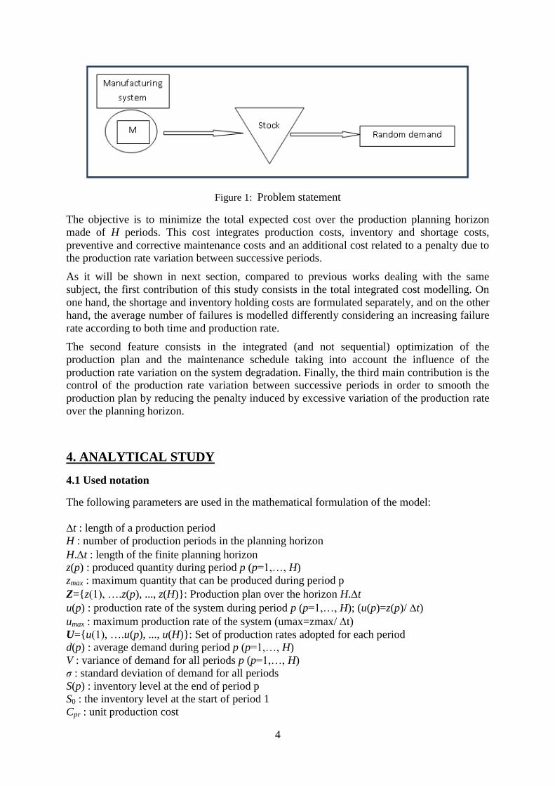
We consider a single machine M subject to degradation and random failures. It produces one
type of product whose demand is random and characterized by a Normal probability
distribution with known average and standard deviation. The demand is satisfied from a stock
(Fig. 1). Production is planned over a finite horizon divided in H production periods of equal
length t. It is assumed that the quantity produced at every period is added to the stock at the
end of the period and the demand of every period is satisfied at the end of the period. The
machine failure rate increases with both time and the production rate. Periodic preventive
maintenance actions have to be scheduled to reduce the probability of failure.
We are in presence of a production control problem with a state variable, namely the
inventory level, together with the following control variables: the production rates for every
period and the number of preventive maintenance actions to be performed over the time
horizon Ht.
4
Figure 1: Problem statement
The objective is to minimize the total expected cost over the production planning horizon
made of H periods. This cost integrates production costs, inventory and shortage costs,
preventive and corrective maintenance costs and an additional cost related to a penalty due to
the production rate variation between successive periods.
As it will be shown in next section, compared to previous works dealing with the same
subject, the first contribution of this study consists in the total integrated cost modelling. On
one hand, the shortage and inventory holding costs are formulated separately, and on the other
hand, the average number of failures is modelled differently considering an increasing failure
rate according to both time and production rate.
The second feature consists in the integrated (and not sequential) optimization of the
production plan and the maintenance schedule taking into account the influence of the
production rate variation on the system degradation. Finally, the third main contribution is the
control of the production rate variation between successive periods in order to smooth the
production plan by reducing the penalty induced by excessive variation of the production rate
over the planning horizon.
4. ANALYTICAL STUDY
4.1 Used notation
The following parameters are used in the mathematical formulation of the model:
∆t : length of a production period
H : number of production periods in the planning horizon
H.t : length of the finite planning horizon
z(p) : produced quantity during period p (p=1,…, H)
zmax : maximum quantity that can be produced during period p
Z={z(1), ….z(p), ..., z(H)}: Production plan over the horizon H.t
u(p) : production rate of the system during period p (p=1,…, H); (u(p)=z(p)/ t)
umax : maximum production rate of the system (umax=zmax/ t)
U={u(1), ….u(p), ..., u(H)}: Set of production rates adopted for each period
d(p) : average demand during period p (p=1,…, H)
V : variance of demand for all periods p (p=1,…, H)
σ : standard deviation of demand for all periods
S(p) : inventory level at the end of period p
S0 : the inventory level at the start of period 1
Cpr : unit production cost

5
Cs : inventory holding cost of one product unit per time unit.
Cl : shortage cost of one product unit.
CTS : expected total cost of production, shortage and inventory holding over the time horizon
Ht
Cv : unit set-up cost
CM : total average maintenance cost
Cpm : preventive maintenance action cost
Ccm : corrective maintenance action cost
SC : penalty cost relative to production rate variation
mu : monetary units
: probability to satisfy the demand (service level).
f(t) : probability density function associated with the time to failure of M
F(t) : probability distribution function associated with the time to failure of M
R(t) : reliability function: 1- F(t)
n(t) : nominal failure rate corresponding to the maximum production rate (depends only on
time)
λ(t,u(p)) : machine failure rate function during period p (p= 1,…, H) (depends on time and on
the production rate during period p)
tu : time units
The cost model to be developed corresponds to a production/maintenance planning problem
with constraints related to inventory, production and preventive maintenance.
4.2 Woking Assumptions
The following assumptions are considered:
- The machine failure rate increases with both time and production rate
- Preventive maintenance actions restore the machine to an “as-good-as-new” state.
- The planning time horizon starts with a new or as good as new machine. However, it
doesn’t end necessarily with a perfect preventive maintenance action. The equipment could
be replaced by a different one or maintained differently after the end of the planning
period.
- The quantity z(p) produced in period p is added to the inventory at the end of the period
and then the demand d(p) is satisfied.
- Preventive maintenance and repair actions durations are negligible.
- The units short are lost (no backorders) and a shortage cost is incurred.
4.3 Formulation of the integrated production-maintenance total expected cost
We develop in what follows the expressions of the three major components of the total
expected cost incurred over the planning horizon. These costs are: the production and
inventory cost, the maintenance cost, and the set-up cost (smoothing penalty). Recall that the
decision variables are the production rates for every period and the number of preventive
maintenance actions to be performed over the planning horizon.
4.3.1 Production, shortage and inventory costs formulation
The constraints related to inventory balance, service level satisfaction, and maximum produc-
tion quantity per period, are expressed as follows:

6
Inventory balance:
10,....)1()1()()1( H,=p +pd+pz+pS=+pS (1)
With: )1()1()1( 0 dz+S=S
Service level satisfaction:
1...0,0)1(Prob H,=p pS (2)
Production capacity:
H=p zpz 1,...,)(0 max (3)
Accordingly, the inventory evolves as shown in the example below in Fig. 2:
Figure 2: Inventory evolution over the planning horizon Ht
Thus, the expression of the total cost of production, shortage and inventory over the finite
horizon Ht is given by:
0 0
1 1 1
1 1
H H H
prS p S p
p p p
CTS Cs t S p Cl S p C z p
(4)
With: 1S(p)>0 is equal to 1 if S(p)>0 and equal to zero otherwise
1S(p)<0 is equal to 1 if S(p)<0 and equal to zero otherwise
It is worth noticing here that most of the papers dealing with the same subject such as Hajej et
al. [13,14,15] and Ayed et al. [16] consider a quadratic model (known as HMMS (Holt,
Madigliani, Muth, and Simon) [17]) integrating shortage and excess of stock considering
however the same unitary cost for shortage and for inventory holding.
S(t)
t
t
S(1)
2t
kt Ht
S0
S(2)
Shortage quantity for p=2
d(2)
d(1)
z(2)
z(1) d(p)
z(p)
S(p
)

7
Our approach (Eq. 4) makes this important distinction between these unitary costs that are not
the same in practice.
The constraint relative to the service level is stochastic. It is possible to transform this
constraint to a deterministic one (Hajej et al. [13]). In fact, it provides the minimal quantities
to produce at each period p in order to satisfy the service level.
1,...,0)1(0)1(Prob ),( Hp zpzpS pS (5)
Where ),( pSz represents a minimum cumulative production quantity expressed as follows:
10,...)()1()()( 1
1
1),( H,p pS+pd+V=z +p+ppS (6)
With:
Vp+1 : variance of demand at period p+1;
p+1 : cumulative Gaussian distribution function with mean d(p+1) and finite variance Vp+1.
-1p+1 : inverse Gaussian distribution function
4.3.2. The maintenance cost formulation
We consider a periodic preventive maintenance (PM) policy with minimal repair at failure.
The interval [0, Ht] is partitioned into N equal parts each of length kt plus a possible
remaining duration shorter than kt. Perfect preventive maintenance actions are performed
periodically at times i× kt, i=1,…,N.
For a given production plan Z (Z={z(1), ..., z(p), ..., z(H)}), and a given PM period kt, the
total maintenance cost is given by:
kU,C+kNC=kU,CM cmpm (7)
N(k) represents the integer part of (H/k), which corresponds to the number of PM actions. k is
the decision variable through which the maintenance policy can be defined. (U,k) stands for
the average number of failures (minimal repairs) over the horizon Ht.
The lemma below provides the expression of the average number of failures:
Lemma
)1()(1))(()()(
)1()(
)())1(()()()(
1)(
)(
2 max
)()1(
0 max
)(
0 max
)(1
1))((
0 max
)(1
1)(
0 2 max
)1(
0 max0 max
1
>kkNH
kkNH
=i
n
kNiΔt
n
kiNΔt
n
kN
=kkNH
Δt
n
kN
kN
=j
k
=i
n
jiΔt
n
ijΔt
n
j
ΔtΔtλu
uik+dttλ
u
u+dttλ
u
u+
dttλu
u+
ΔtΔtλu
uik+dttλ
u
u+dttλ
u
u=kU,
(8)
uij represents the production rate during period i after the jth
PM action.

8
Proof
Recall that PM actions are performed every k production periods, which means every kt
restoring the system to as good as new state.
The planning horizon Ht is divided into (N(k) +1) periods, each one is noted j, j{0,1,2….
,(N(k))}. Hence, j=0 corresponds to the first PM interval [0, kt], the second PM period [kt,
2kt] corresponds to period j=1, etc. Note that the last PM action is performed at instant
(N(k).k.t), and the interval (N(k)-1).k.t), (N(k).k.t) corresponds to j = (N(k)-1).
To illustrate this decomposition, Fig. 3 below shows an example with the following values:
H = 13 periods; k = 3 periods, N = 4, Δt = 1 tu. Hence, N(k) = 4. (N(k).k.t) = 12 tu.
t
3t
Ht =13 t
J=0 J=1 J=2 J=3
0
3t 3t 3t
PM PM PM PM
Figure 3: Example of PM periods over a planning horizon Ht =13 time units
The average number of failures over the planning horizon H.t is the sum of the average
number of failures during periods j=0 to (N(k) -1), to which should be added the average
number of failures during the last interval (N(k).k.t, HΔt corresponding to j= (N(k)).
Average number of failures during a PM period j
Recall that the system failure rate evolves according to time and to the production rate which
varies from one period to another. In order to take into account the influence of the production
rate variation on the system degradation, we use Cox model [18]. Formally, the failure rate is
expressed according to the production rate during each period and the nominal failure rate.
The following expression is proposed (Hajej et al. [13]):
,p nt u p t g u p
Where λp(t,u(p)) represents the instantaneous failure rate function at period p as a function of
the production rate u(p). λn(t) is the failure rate for nominal conditions which corresponds to
the failure rate when the production system is operating with its maximum production rate,
and
max
u pg u p
u .
Although this linear relationship between the production rate and the failure rate does not
necessarily hold for any type of systems, it is adopted here like in (Hajej et al. [13], [14], [15])
as an approximation.
Let uij represent the production rate during period i after the jth
PM action.
)(,...,0,,...,1),( kNkjiwithuij
Hence, the failure rate during period i after the jth PM action is given by:
)(,...,0,,...,1),()(),(max
kNkjiu
utut
ij
nijij

9
The evolution of the production system’s failure rate within any preventive maintenance cycle
period j = h is presented in Fig. 4 below:
t
λ(t,u)
t
(uih/umax)λn(t)
S1h
Sih
S2h
(h+1)kt J=h
hkt
PM PM
Figure 4: Evolution of the production system failure rate within a preventive maintenance
cycle (period j = h)
Let S1j be the average number of failures during the first production period after the jth
PM
action:
1
1
max0
t
j
j n
uS t dt
u
In the same way, S2j, corresponding to the average number of failures during the second
production period after the jth
PM action, is given by:
2 1
2
max max0
t
j j
j n n
u uS t dt t t
u u
Generalizing this to all production periods after the jth
PM actions, we obtain:
1
max max0
1 for 2,3...
ti jij
ij n n
uuS t dt k i t t i k
u u
Hence, the average number of failures during any period j is expressed as follows:

10
)(,...,0)())1(()()(2 max
)1(
0 max0 max
1kNjtt
u
uikdtt
u
udtt
u
u k
i
n
jit
n
ijt
n
j
Average number of failures over the period 0, (N(k).k.t
Considering all periods j (j=0 to N(k)-1), the total average number of failures over the interval
0, (N(k).k.t is expressed as follows:
1)(
0 2 max
)1(
0 max0 max
1)())1(()()(
kN
j
k
i
n
jit
n
ijt
n
jtt
u
uikdtt
u
udtt
u
u
Average number of failures over the interval (N(k).k.t, HΔt
Looking at the remaining period N(k).k.t, Ht after the last PM action is performed during
the planning horizon, one can distinguish three possible cases:
Case 1: this period doesn’t exist. This means that the last preventive maintenance action
coincides with H. t, the end of the planning horizon.
Formally: H-(N(k).k) = 0
Case 2: we have only one production period of length t, in the interval N(k).k.t, Ht.
Formally: H-(N(k).k) = 1
Case 3: we have more than one production period in the interval N(k).k.t, Ht
Formally: H-(N(k)*k) > 1
Taking into account these three possible situations, the average number of failures in the in-
terval N(k).k.t, Ht is given by:
)1()())1(()()(
)1()(
1)(
)(
2 max
)()1(
0 max
)(
0 max
)(1
1))((
0 max
)(1
kkNH
kkNH
i
n
kNit
n
kiNt
n
kN
kkNH
t
n
kN
ttu
uikdtt
u
udtt
u
u
dttu
u
The first term of this sum corresponds to case 2, and the second and third terms correspond to
case 3. Obviously, in the first case (case 1), the number of failures is equal to zero.
Average number of failures over the planning horizon H.t
Summing up the obtained average number of failures for all periods, we obtain:

11
)1()())1(()()(
)1()(
)())1(()()(),(
1)(
)(
2 max
)()1(
0max
)(
0max
)(1
1))((
0max
)(1
1)(
0 2 max
)1(
0max
0max
1
kkNH
kkNH
i
nkNi
t
nkiN
t
nkN
kkNH
t
nkN
kN
j
k
i
nji
t
nij
t
nj
ttu
uikdtt
u
udtt
u
u
dttu
u
ttu
uikdtt
u
udtt
u
uk
U
End of the proof
4.4 Penalty cost relative to the production rate variation: variable set-up cost
As mentioned earlier, one of the objectives of this study is to smooth the production rate
between periods. To do so, we consider a variable set-up cost, which is proportional to the
difference of the quantity produced from one period to the next one. Indeed, reducing or
increasing the quantity to produce may induce in many situations labour related costs
(overtime, or hiring/firing costs) and more or less complexity of the set-up.
We define Cv as unit set-up cost. It corresponds to the direct cost of resources needed to adapt
the production unit to the production quantity change between successive periods.
Hence, the penalty cost relative to production rate variation is given by:
1
1
1H
v
p
SC C z p z p
(9)
4.5 The total integrated maintenance/ production/inventory cost taking into account the
set up cost
Using the developed mathematical expressions above in this section, the total cost
optimization problem can be formulated as follows:
)(),(
SCCMCTSMink
Z
(10)
Subject to:
10,...,)1(1)()()1( H=p +pd+pz+pS=+pS
1...0,0)1(Prob H,=p pS
H=p zpz 1,...,)(0 max
4.6 Solution method
Formally, solving the constrained minimization problem stated above (Eq. 10), yields the
determination of optimal production quantity for every period {z(1)*, z(2)*, ..., z(p)*, …,
z(H)*} and the optimal period (k*t) of PM actions to be performed over the finite horizon
Ht. Due to the obvious complexity of the model, we developed an iterative search procedure
to find a near-optimal solution. It is presented below in four steps.

12
Step 1: Use Eqs. (5) and (6) to determine the minimum cumulative production quantity to
produce in each period in order to satisfy the service level constraint given by Eq. (2).
Step 2: Perform a simple enumeration by varying the production quantity for each period p
(using a relatively small step) between the minimum value obtained in step 1 and the
maximum one zmax given in constraint (3) in order to consider all possible production
plans.
Step 3: For every production plan established in step 2, vary k, number of production
periods between preventive maintenance actions, between 1 and H, and calculate each time
the corresponding total cost (Eq. 10).
Step 4: Determine the values of the decision variables ((z(1)*, z(2)*, ... z(p)*, …, z(H)*),
k*) which yielded the minimal total cost.
MATHEMATICA®
software was used to perform the calculations and obtain a near-optimal
solution for all instances of the problem considered in this paper.
5. NUMERICAL EXAMPLE AND TRADE-OFFS ANALYSIS
5.1 Reference example
A numerical example is presented in this section in order to illustrate the use of the analytical
model developed in the previous sections. We assume that the finite planning horizon is made
of 36 periods of one month each (t = 1 month). The other input data are summarized in
Table 1 below (‘mu’ stands for ‘monetary units):
Reliability data
System time to failure distribution F(t): Weibull distribution with :
Scale parameter : β = 16 & Shape parameter : = 3
Corrective maintenance cost Ccm = 3000 mu
Preventive maintenance cost Cpm = 500 mu
Inventory data
Shortage cost per unit Cl = 1 mu/unit short
Inventory holding cost per unit per time unit Cs = 0.65 mu/unit/tu
Initial inventory level S(0) = 0
Service level = 0.9
Production data
Unit production cost Cpr = 7 mu/unit
Maximum production rate
Maximum production quantity per period
umax = 500 units per month
zmax = 500 units
Nominal set-up cost Cv = 5 mu
Table 1: Numerical data

13
As for the demand, the variance is supposed to be equal for all periods: V = 4.52. The average
demand per period is presented in Table 2 below:
Jan Feb Mar Apr May Jun Jul Aug Sep Oct Nov Dec
350 420 340 392 431 444 442 340 392 375 392 400
350 370 395 415 431 444 442 340 392 375 400 420
350 340 392 370 431 392 500 350 320 420 365 480
Table 2: Monthly mean demand
Solving the problem using the procedure described in section 3, we obtain the following near-
optimal maintenance/production plan presented in Table 3 below:
Near-optimal production plan over the finite horizon Ht = 36 months N* k*
Jan Feb Mar Apr May Jun Jul Aug Sep Oct Nov Dec
500 500 439 500 500 269 434 352 500 500 395 470
500 438 485 400 400 127 400 500 465 193 400 370
65 438 500 200 400 400 499 323 407 351 166 400
6
6
N*: Optimal number of preventive maintenance actions over Ht
k*: Optimal number of production periods between preventive maintenance actions
Table 3: Near-optimal maintenance/production plan
The total cost related to this plan is equal to : 5.24429×10⁷ mu.
5.2 Sensitivity analyses
Effect of Cv on the production plan, the inventory, and the preventive maintenance
schedule
In the perspective of smoothing the production plan through the production rate control
between periods of the planning horizon, we studied the impact of the variation of the unit
set-up cost between successive periods, Cv, on the obtained solution.
Considering the same input data, we obtained the following results presented in Table 4:

14
Cv: Unit set-up cost
between successive
periods
Average production quantity
variation between successive
periods
N* k* Average end of
month inventory
2 143.71 4 9 156.94
5 126.17 6 6 464.56
7 75.31 7 5 955.58
8 74.57 7 5 1200.53
10 58.34 9 4 1221.47
Table 4: Effect of the variation of the unit set-up cost
Fig. 5 below shows the trade-off between the unit-setup cost and the average production
quantity variation between successive periods, the optimal number of preventive maintenance
actions, and the average end of month inventory.
Figure 5: Evolution of the average production quantity variation between successive periods,
and the average end of month inventory according to the unit set-up cost Cv
First, one can easily notice that, as expected, when the unit set-up cost between successive
periods increases, the average variation of the production quantity, between successive
periods, decreases. This clearly illustrates the effect of production smoothing.

15
Furthermore, it is interesting to notice that the decrease of the average variation of the
production quantity between successive periods yields an increase of the quantity to be
produced in some periods, and consequently a higher average end of month inventory. Indeed,
we know that the quantity to be produced in each period should be between a certain
minimum given by the service level constraint (Eqs. 5 and 6) and a given maximum
corresponding to the capacity of the machine (Eq. 3). These limits are considered in the first
two steps of the solving procedure. Hence, as the smoothing penalty increases, reducing the
average variation of the production quantity between successive periods can be achieved
either by increasing or by decreasing successive production quantities between the two limits.
This is achieved using the model considering simultaneously the trade-off between inventory
and shortage costs. The near-optimal solutions, for this specific example, display an increase
of the quantities to be produced and therefore an increase of the average end of month
inventory. In the same time, the increase of the production rate through the production periods
affects the system degradation and induces the need for a more frequent preventive
maintenance as it can also be seen in Fig. 5.
The above observations illustrate the fact that the developed model allows the simultaneous
consideration of the different trade-offs between the smoothing penalty, the production plan,
the inventory, and the preventive maintenance schedule.
We performed several other numerical experiments with different input parameters settings to
check the smoothing effect. We present below a sample of the obtained results corresponding
to a situation involving a higher shortage cost. While keeping the original combination of
input parameters, we increased the shortage cost Cl from 1 mu to 5 mu. A priori, for such a
situation, the quantities to be produced should be higher throughout the production periods
since shortages are more costly while production and inventory holding costs remain the
same.
The following near-optimal maintenance/production plan has been obtained (Table 5):
Near-optimal production plan over the finite horizon Ht = 36 months N* k*
Jan Feb Mar Apr May Jun Jul Aug Sep Oct Nov Dec
500 500 392 422 481 500 500 500 500 444 481 404
388 500 322 321 443 132 434 480 467 500 438 500
437 330 500 500 479 377 0 500 450 500 500 200
7
5
Table 5: Near-optimal maintenance/production plan with Cl = 5 mu and Cv = 5 mu
The total cost related to this near-optimal plan is equal to : 7.38×10⁸ mu.
Compared to the situation with a lower shortage cost (Cl = 1 mu), one can easily observe
comparing Tables 3 and 5 that, in total, more products are produced in the second situation (a
total of 15782, compared to a total of 14186 items). Moreover, this increase of total
production over the same horizon yielded an increase of the number of preventive
maintenance actions that have to be performed (from 6 to 7 actions). This is due to the fact
that the machine failure rate increases with the production rate.

16
Again, in this situation, we studied the impact of the smoothing penalty on the optimal
strategy and on the inventory.
The following results were obtained (Table 6):
Cv: Unit set-up cost
between successive
periods
Average production quantity
variation between successive
periods
N* k* Average end of
month inventory
2 116.74 4 9 592.22
5 75.14 7 5 950.42
8 63.97 7 5 967.5
10 60 9 4 1296.22
Table 6: Effect of the variation of the unit-setup cost with Cl = 5 mu
One can easily notice the same trade-offs as in the case of (Cl=1 mu) discussed above. The
increase of Cv induces a decrease of the average production quantity variation between
successive periods, the need for more preventive maintenance (higher N*) and the increase of
inventory.
Effect of demand variability on the production and maintenance plans, and on the total
expected cost
While keeping the original set of input parameters (Table 1) as well as the monthly average
demand (Table 2), we ran experiments varying the demand variance. The following near-
optimal maintenance/production plans have been obtained (Tables 7, 8 and 9):
Near-optimal production plan over the finite horizon Ht = 36 months N* k*
Jan Feb Mar Apr Ma Jun Jul Aug Sep Oct Nov Dec
500 500 439 500 500 369 434 352 500 500 395 470
500 438 485 500 500 127 490 500 465 393 500 370
365 438 500 200 500 500 499 323 407 351 366 500
7
5
Table 7: Near-optimal maintenance/production plan with demand variance V=8

17
Near-optimal production plan over the finite horizon Ht = 36 months N* k*
Jan Feb Mar Ap May Jun Jul Aug Sep Oct Nov Dec
500 500 500 500 500 500 500 500 449 500 305 500
500 500 500 500 500 500 500 500 500 500 500 500
500 500 500 500 500 500 500 377 269 318 500 500
7
5
Table 8: Near-optimal maintenance/production plan with demand variance V=10
Near-optimal production plan over the finite horizon HΔt = 36 months N* k*
Jan Feb Mar Ap May Jun Jul Aug Sep Oct Nov Dec
500 500 500 500 500 500 500 500 500 500 500 500
500 500 500 500 500 500 500 500 500 500 500 500
500 500 500 500 500 500 500 500 500 500 500 500
12
3
Table 9: Near-optimal maintenance/production plan with demand variance V =20
We summarize the obtained results V in table 10 below:
V: Demand
Variance N* k*
Average production quantity
variation between successive
periods
Average end of
month inventory
Total Cost
(mu)
4.52 6 6 126.17 464.56 5.25×10⁷
8 7 5 90.8 987.33 5.77×10⁷
10 7 5 27.25 1741.83 6.07×10⁷
20 12 3 0 1980.25 6.57×10⁷
Table 10: Effect of the variation of the demand
One can clearly see that a demand with a higher variability causes the system to produce more
and generate higher levels of inventory. Hence, because of higher production rates yielding a
faster degradation of the machine, more frequent preventive maintenance is needed (N* in-
creases). We also note that higher variability of demand yields an increase of the total ex-
pected cost.
In fact, as the demand variance increases, obviously, the minimum quantity determined in
Step 1 increases in order to satisfy the required service level. The system is then forced to

18
produce more per period without exceeding the machine capacity. Here comes the trade-off
between the smoothing penalty, the inventory, and the maintenance policy. Going further with
a relatively high variance (V= 20), the obtained near-optimal integrated policy consists in pro-
ducing at the maximum production rate for all periods. In this situation, smoothing is perfect-
ly achieved (set-up cost, SC, is null).
6. CONCLUSION
In this paper we considered a manufacturing system made of a single machine that is subject
to random failures. In order to reduce the failure frequency, a periodic preventive maintenance
policy with minimal repair at failure is adopted. The production system must satisfy a random
product demand over a finite planning horizon with a given required service level. The finite
horizon is divided into equal periods. A mathematical model has been developed in order to
derive a joint near-optimal production plan and preventive maintenance schedule minimizing
the total cost of production, maintenance and inventory, taking into account constraints
related to the production system capacity, the service level to be satisfied and the inventory
balance.
Compared to previous works, a different cost modelling approach has been proposed.
Furthermore, an integrated (not sequential) optimization of the production plan and the
maintenance schedule has been proposed. It takes into account the influence of the production
rate variation on the production system failure rate. Finally, expressing the set-up cost as
being proportional to the production rate variation between successive periods, allowed
reducing the penalty induced by excessive variation of the production rate over the planning
horizon.
The proposed modelling approach has been illustrated through a numerical example. A
sensitivity study with respect to the set-up cost has been performed in order to show the
impact of the production plan smoothing on the obtained solution.
The trade-off between the smoothing penalty and the production plan, the inventory, and the
preventive maintenance schedule has also been discussed. We finally studied the effect of the
demand variability on the smoothing penalty, the production and maintenance plans, and on
the total expected cost.
Extensions to this work are under consideration. One of them consists in the investigation of
more realistic situations in which preventive maintenance actions are imperfect and have non-
negligible durations. Another extension of this work would consist in going beyond the
limitation imposed by the linear relationship between the production rate and the failure rate
of the system. More general expressions should be investigated empirically and analytically.
REFERENCES
[1] Barlow RE and Hunter LC (1960) “Optimum Preventive Maintenance Policies”. Operations
Research, vol. 8, pp 90-100.
[2] Wang H (2002) “A survey of maintenance policies of deteriorating systems”. European Journal
of Operational Research, vol. 139(3), pp. 469–489.
[3] Brandolese M, Fransi M and Pozzeti A (1996) “Production and maintenance integrated
planning”. International Journal of Production Research, vol. 34(7), pp.2059-2075.

19
[4] Chelbi A and Rezg N (2006) “Analysis of a production/inventory system with randomly failing
production unit subjected to a minimum required availability level”. International Journal of
Production Economics, vol. 99, pp. 131-143.
[5] Pal B, Sana SS and Chaudhuri KS (2013) “A mathematical model on EPQ for stochastic
demand in an imperfect production system”. Journal of Manufacturing Systems, vol. 32, pp
260-270.
[6] Rezg N, Dellagi S and Chelbi A (2008) “Optimal strategy of inventory control and preventive
maintenance”. International Journal of Production Research, vol. 46(19), pp. 5349–5365.
[7] Tambe PP and Kulkarni MS (2015) “A superimposition based approach for maintenance and
quality planoptimization with production schedule, availability, repair time anddetection time
constraints for a single machine”. Journal of Manufacturing Systems, vol. 37, pp 17-32.
[8] Dellagi S, Rezg N and Xie X (2007) “Preventive maintenance of manufacturing systems under
environmental constraints”. International Journal of Production Research, vol. 45(5), pp.1233–
1254.
[9] Dahane M, Clementz C and Rezg N (2010) “Effects of extension of subcontracting on a
production system in a joint maintenance and production context”. Computers & Industrial
Engineering, vol. 58(1), pp. 88–96.
[10] Nourelfath M, Fitouhi MC and Machani M (2010) “An integrated model for production and
preventive maintenance planning in multi-state systems”. IEEE Transactions on Reliability, vol.
59(3), pp. 496–506.
[11] Nourelfath M and Châtelet E (2012) “Integrating production, inventory and maintenance
planning for a parallel system with dependent components”. Reliability Engineering and System
Safety, vol. 101, pp. 59–66.
[12] Mifdal L, Hajej Z and Dellagi S (2015) “Joint Optimization Approach of Maintenance and
Production Planning for a Multiple-Product Manufacturing System”. Mathematical Problems in
Engineering, vol. 2015, Article ID 769723, 17 pages, 2015. doi:10.1155/2015/769723
[13] Hajej Z, Rezg N and Dellagi S (2011) “Optimal integrated maintenance/production policy for
randomly failing systems with variable failure rate”. International Journal of Production
Research, vol. 49(19), pp. 5695-5712.
[14] Hajej Z, Dellagi S and Rezg N (2011) “Production/Maintenance Policies Optimization with
Operational Age Concept in a Subcontracting Constraint”.18th IFAC World Congress, vol.
18(1), pp. 5213-5218, Milan, Italy.
[15] Hajej Z, Dellagi S and Rezg N (2014) “Joint optimization of maintenance and production
policies with subcontracting and product returns”. Journal of Intelligent Manufacturing, vol.
25(3), pp. 589-602.
[16] Ayed S, Dellagi S and Rezg N (2012) “Joint optimisation of maintenance and production
policies considering random demand and variable production rate”. International Journal of
Production Research, vol. 50(23), pp. 6870-6885.
[17] Holt CC, Modigliani F, Muth JF and Simon HA (1960) ”Planning Production, Inventory and
Work Force”. Prentice Hall, Englewood Cliffs, NJ.
[18] Cox D (1972) “Regression models and life-tables”. Journal of the royal statistical society, vol.
34(2), pp187-220.