joint learning of measurement matrix and signal
TRANSCRIPT
818 IEEE TRANSACTIONS ON COMPUTATIONAL IMAGING, VOL. 6, 2020
Joint Learning of Measurement Matrix and Signal
Reconstruction via Deep LearningRobiulhossain Mdrafi , Student Member, IEEE, and Ali Cafer Gurbuz , Senior Member, IEEE
Abstract—In this work, we propose an automatic sensing andreconstruction scheme based on deep learning within the compres-sive sensing (CS) framework. Classical CS utilizes pre-determinedlinear projections in the form of random measurements and con-vex optimization with a known sparsity basis to reconstruct sig-nals. Here, we develop a data-driven approach to learn both themeasurement matrix and the inverse reconstruction scheme for agiven class of signals, such as images. The developed deep learningapproach paves the way for end-to-end learning and reconstructionof signals with the aid of cascaded fully connected and multistageconvolutional layers with a weighted loss function in an adver-sarial learning framework. Results obtained over the CIFAR-10image database show that the proposed deep learning architec-tures provide higher peak signal-to-noise ratio (PSNR) levels, and,hence, learn better measurement matrices than that of randomlyselected, specifically designed to reduce average coherence with agiven basis, or state-of-the-art data driven approaches. The learnedmeasurement matrices achieve higher PSNR compared to randomor designed matrices not only when they are utilized in the proposeddata-driven approach but also when used in �1 based recovery. Thereconstruction performance on the test dataset improves as moretraining samples are utilized. Quantitative results for sparsity levelanalysis, incremental measurement design, and various trainingscenarios are provided.
Index Terms—Measurement matrix design, deep learning,compressive sensing, learning sparse representation, convolutionalneural networks, inverse problem.
I. INTRODUCTION
THE generalized set of linear measurements defined by a
measurement matrix (MM) plays a very crucial role in
diverse areas of data science and sensing applications, such
as imaging systems, radar and remote sensing, and wireless
communications networks, where the compressed sensing (CS)
[1]–[3] framework enables theoretical guarantees for sparse
signal reconstruction. CS relies on two fundamental principles;
namely, sparsity and incoherent sampling. The sparsity principle
is built on the assumption that we can express a signalx ∈ RN×1
as a linear combination of K columns from an exactly known
basis Ψ ∈ RN×N as x = Ψs, where ‖s‖0 = K and K � N .
Classical CS acquires random linear projections of the signal
Manuscript received July 21, 2019; revised December 9, 2019 and February28, 2020; accepted March 15, 2020. Date of publication March 30, 2020; dateof current version April 27, 2020. This work was supported in part by NationalScience Foundation CPS program under Grant 1931861. The associate editorcoordinating the review of this manuscript and approving it for publication wasDr. Singanallur Venkatakrishnan. (Corresponding author: Ali Cafer Gurbuz.)
The authors are with the Department of Electrical and Computer Engi-neering, Mississippi State University, Mississippi, MS 39762 USA (e-mail:[email protected]; [email protected]).
Digital Object Identifier 10.1109/TCI.2020.2983153
as y = Φx, with y ∈ RM×1 and M � N , while entries of the
MM Φ can be randomly selected from a given distribution, such
as Gaussian or Bernoulli. In [4], a sufficient condition for the
recovery of aK-sparse signal using orthogonal matching pursuit
(OMP) [5] in terms of the mutual coherence of systemA = ΦΨ
is provided as
µ(A) ≤1
2K − 1, (1)
where the mutual coherence µ(A) is defined as
µ(A) = maxk �=l
|aTk al|
‖ak‖2 ‖al‖2, (2)
representing the worst case coherence between any two columns
of A. Although fixed random linear MMs can be referred as
universal in the sense that they can provide incoherence with
many known basis, they are not specific and optimal to the
underlying structure of the observed class of signals defined
by the sparsity basis Ψ.
The upper bound in (1) shows that for the same measurement
number, we can obtain a better reconstruction of the observed
signal, hence a larger K, by minimizing the mutual coherence
µ(A). To achieve such a goal, there have been studies on the
design of the MM, Φ. While some studies focus on constructing
deterministic linear embedding using nuclear norm minimiza-
tion with max-norm constraints [6], many studies have been
focused on minimizing the averaged mutual coherence instead
of the worst case coherence, defined in (2), under the assumption
that the averaged metric will reflect an average signal recovery
performance [7]–[9]. To this end, an iterative procedure was
detailed in [7] to reduce the average mutual coherence of system
A and results showed that the optimization of the projection
matrix could provide improved recovery performance compared
to a randomly generated MM. A similar goal is formulated to
make the Gram matrixG = ATA as close to the identity matrix
as possible in terms of the Frobenius norm,
minΦ
‖I−ΨTΦTΦΨ‖2F . (3)
An iterative technique was proposed in [8] to solve (3), while
a closed form solution to (3) was given in [9], which can be
expressed as,
Φ = ΓΛ−1/2UT (4)
with the assumption of Ψ being full rank. where Γ is any
matrix with orthonormal rows such as Γ = [IM 0] and UΛUT
is the eigenvalue decomposition of AAT . In [10], the result in
2333-9403 © 2020 IEEE. Personal use is permitted, but republication/redistribution requires IEEE permission.See https://www.ieee.org/publications/rights/index.html for more information.
Authorized licensed use limited to: Mississippi State University Libraries. Downloaded on August 14,2020 at 03:49:26 UTC from IEEE Xplore. Restrictions apply.

MDRAFI AND GURBUZ: JOINT LEARNING OF MEASUREMENT MATRIX AND SIGNAL RECONSTRUCTION VIA DEEP LEARNING 819
(4) is extended for a wider range of dictionaries. Mainly, we
can obtain a specifically designed MM by utilizing one of the
mentioned MM design techniques for an assumed sparsity basis
Ψ to achieve a system with lower average mutual coherence as
compared to that attainable with randomly selected MMs.
However, it might not always be possible to know the sparsity
basis exactly since the inverse transform between the sensor
data and the signal/image domain is not fully known due to sen-
sor modelling errors and non-idealities, unknown propagation
mediums, noise, and off-grid effects for different applications.
In addition, generally, the signals are not exactly sparse in the
assumed basis but only compressible. Moreover, MM design
techniques try to minimize an average coherence metric, but this
does not necessarily guarantee better signal reconstruction. Once
the MMs and the sparsity dictionaries are chosen CS inherently
defines a fixed assumed linear relation between the measurement
and the signal domains. The main goal of an inversion technique
is to use this assumed relation, which might come from prior
domain knowledge, to reconstruct the signals.
Another possible approach to derive the actual unknown in-
verse relation from measurement to signal spaces is through ex-
ploiting the large, available, signal datasets. Recently, advances
in data science, especially automatic feature learning with deep
neural networks (DNNs) and its variants [11]–[14], have resulted
in improved performance across many applications, including
computer vision [15]–[17], and has prompted researchers to
apply DNNs for a variety of inverse problems [18]. While
analytical methods like CS require prior domain knowledge
that can be incorporated into the solution, in contrast, DNNs
exploit large datasets to derive the unknown solution to the
inverse problem. In this work, we propose a data-driven ap-
proach inspired from sparse data acquisition and reconstruction
techniques to learn both the MM and the DNN-based inverse re-
construction scheme for a given class of signals. The developed
DNN features cascaded fully connected and multistage convo-
lutional layers with a weighted loss function from each stage
in an adversarial learning framework. Next, we briefly present
the background on DNN-based reconstruction techniques and
introduce the proposed ideas in learning of MM and signal
reconstruction scheme with the novel main contributions of the
work.
Studies into data driven learning of signal reconstruction has
only recently been considered in the literature. One of the first
studies in this area is presented in [19] implementing a stacked
denoising autoencoder (SDA). However, the architecture of
SDA involves cascaded sets of fully connected (FC) layers that
make the training process computationally expensive with the
increment of signal size. In addition, it also runs the risk of
overfitting the testing set. To avoid the shortcomings of SDA,
several improvements to the network structure are proposed
in [20]–[24] mainly to reduce the high number of parameters of
SDAs. In [20], a convolutional neural network (CNN) structure
is learned between the image proxy obtained through the adjoint
operator on the compressed measurements, i.e., ΦTy, and the
actual image, where a fixed random MM is used to create the
measurements. In [21], a FC layer followed by a CNN structure,
namely Reconnet is proposed to reconstruct signals directly
from their compressed measurements, again obtained from a
fixed random MM. The study in [22] modifies the Reconnet
architecture in [21] by adding residual blocks and obtains im-
proved performance by using the residual error between the
ground truth and the preliminary reconstructed image. However,
it works on image blocks, which may produce block effects in the
reconstructed images. While these techniques have a common
goal of learning to reconstruct an image from its compressed
measurements using a neural network, the sensing matrix for all
of these works are assumed to be known and in general taken as
having random Gaussian entries.
In [23], an auto-encoder framework, namely DeepCodec is
used to learn a transformation from the original signals to the
compressed measurements allowing measurements to collect
more information from the image. This is a form of dimension
reduction. The measurements generated by the architecture are
later used to recover the given class of signals. An extension of
this work [25] is deep sparse signal representation and recovery
(DeepSSRR). Both approaches learn their sensing mechanisms
from the data. The method in [26] discusses adding a fully
connected layer to the Reconnet architecture in [21] to learn
the measurements from the given image patches. While learning
sensing mechanisms from data are discussed in [25], [26], the
embedding from original signal to the measurements could be
nonlinear. Although nonlinear embedding could provide high
performance, many applications and data acquisition systems
work with linear measurements as in CS.
In this work, we propose a supervised deep learning technique
with a novel architecture and loss function to jointly learn a linear
MM and the sparse reconstruction scheme for a given class of
signals i.e., images. Prior versions of this work with different
DNN structures and analysis can be found in [27], [28]. In CS,
the sensing process is linearly modelled as y = Φx. In this
work, the MM, Φ, that results in the compressed measurements,
y, from the original signal, x, is modelled as an FC network
layer with linear activation functions as illustrated in Fig. 1.
Hence, the linear measurement process, y = Φx in classical
data acquisition can be directly modelled by the weights of this
FC layer that can be a part of data-driven learning.
The sparse reconstruction process in general utilizes the CS
measurements and an initial starting point (proxy image) to
iteratively reconstruct the image. Our goal is also to model such
a process using a DNN structure. To do so the output of the
first FC layer, which is generating compressed measurements,
is followed by another FC layer to generate a proxy image and
a set of convolutional layers with nonlinear activation functions
to achieve the reconstruction of the signal in multiple stages.
More detail on the selection of DNN structure is provided in
Section II. The proposed end-to-end DNN learns jointly both
the MM to be used to sense the signal class and a DNN structure
to reconstruct images from these CS measurements. In this
work, we also utilized a novel loss function. Instead of only
minimizing the Euclidean loss between the input label image
and the final reconstructed output image, we have also included
losses between output of each reconstruction stage and the label
as shown in Fig. 2, mainly to force the learning system to create
enhanced mid-stage reconstructions, which also reflect in the
Authorized licensed use limited to: Mississippi State University Libraries. Downloaded on August 14,2020 at 03:49:26 UTC from IEEE Xplore. Restrictions apply.

820 IEEE TRANSACTIONS ON COMPUTATIONAL IMAGING, VOL. 6, 2020
Fig. 1. (Top) Classical CS data acquisition, y = Φx. (Bottom) A fully con-nected layer with linear activation functions modeling the CS measurements inthe top figure.
final reconstruction output. Use of this loss function resulted in
better reconstructions as compared to minimizing the Euclidean
loss between final reconstructed and true images.
The proposed structure is trained and tested on CIFAR-10
dataset [29]. The obtained results are compared with the ran-
domly generated MMs with Gaussian entries, designed MM
using (4) assuming the sparsity basis Ψ as the discrete cosine
transform (DCT) basis, and data-driven approaches [20], [25],
[26]. Results show increased performance against all compared
techniques. Since the dataset contains images of various target
classes, DCT is a suitable sparsity basis for the image class.
The reconstruction performance is evaluated through the peak
signal-to-noise ratio (PSNR) between the reconstructed and the
true images and it is compared with �1 minimization based
sparse recovery. Additionally, we have also incorporated the
proposed DNN architecture into the generative adversarial net-
work (GAN) [14] framework to achieve increased performance
through discriminator capability. GANs mainly consist of two
essential parts, namely the generator and the discriminator, both
of which are DNNs themselves. However, the generator takes
a set of real number in terms of a vector as the input, while, in
contrast, the discriminator takes an image as the input. The aim
of generator is to produce an image so that the discriminator
cannot distinguish it from the real image. In this problem,
the proposed DNN architecture acts as a generator, while the
discriminator is created from a cascaded set of convolutional
layers with a softmax layer to estimate the probability of whether
the generated image is fake or not. By using such framework,
we can also give rise to adversarial Euclidean loss. By using this
GAN framework with the proposed form of loss, we showed
that we can retain more information in terms of PSNR than that
of using the proposed DNN architecture under the traditional
framework with Euclidean losses.
The main contributions of this work can be stated as follows:� A data-driven approach for learning the MM is proposed,
including several new DNN structures inspired by sparse
data acquisition and reconstruction techniques.� A novel weighted multistage Euclidean error loss is uti-
lized in the total loss function to both learn the MM and
reconstruction process weights.� A GAN framework utilizing the novel multistage end-to-
end generator DNN is proposed with the adversarial loss
function, resulting in enhanced reconstruction.� Detailed performance analysis on the learned MM in com-
parison to the random, designed MMs and data-driven
approaches are provided in terms of input image sparsity
levels, number of measurements, and resulting mutual
coherence levels of MMs.� An incremental learning approach is proposed, where the
system learns the next set of optimal measurements in
addition to a fixed measurement set to minimize the defined
cost.� Comparisons to previously proposed DNNs in the litera-
ture and �1 minimization based techniques are provided.
Learned MMs provide increased performance when they
are utilized with sparse recovery with �1 minimization.
The rest of the paper is organized as follows: The proposed
DNN structure is detailed in Section II. The dataset, experi-
mental settings, and training and testing results of the proposed
method with the compared techniques have been presented in
Section III. Finally, conclusions are drawn in Section IV.
II. PROPOSED LEARNING STRUCTURE
The proposed multistage DNN architecture for joint learning
of MM and signal reconstruction scheme is illustrated in Fig. 2.
The illustrated architecture presents an end-to-end learning pro-
cess, where both the measurements from an input label image
and reconstructions from these compressed measurements to an
output image are learned. Next, the parts of the proposed DNN
structure are detailed.
A. Data Acquisition
The first part of the DNN shown in Fig. 2, including a reshap-
ing and a fully connected layer (FC1) models the sensing system
to acquire the data from the original signal to the compressed do-
main i.e., the collection of the compressed linear measurements
from the given class of signal. In this paper, we work on the
images; hence, the input signal to the system will beX ∈ RN×N .
Since, the FC1 layer is used for mapping the original signal
into the linear compressed measurements; the input signal is
vectorized via reshaping i.e., X → x : RN×N → RN2×1. After
reshaping, the vectorized original signal is fed into FC1 layer to
give compressed linear measurements y ∈ RM×1. This FC1
layer models the y = Φx sensing process, where entries of
Φ are the weights used in FC1 layer, as illustrated in Fig. 1.
In FC1, linear activation functions are used since the data
Authorized licensed use limited to: Mississippi State University Libraries. Downloaded on August 14,2020 at 03:49:26 UTC from IEEE Xplore. Restrictions apply.

MDRAFI AND GURBUZ: JOINT LEARNING OF MEASUREMENT MATRIX AND SIGNAL RECONSTRUCTION VIA DEEP LEARNING 821
Fig. 2. Illustration of the proposed DNN structure (ConvMMNet) for joint learning of MM and sparse signal reconstruction.
acquisition process in CS systems are linear. Therefore, each
measurement obtained in the compressed measurement vector
y can be expressed as a weighted linear combination of values
from x. The dimension (M ×N2) of the weights in FC1 also
denotes the dimension of the MM.
B. Construction of the Proxy Image
Typically, sparse reconstruction approaches require an initial
point to start with, such as a proxy image. The adjoint oper-
ator, ΦT , normally is one way to form such a proxy output
via p = ΦTy. In the DNN structure, to create such a proxy
image we have used another FC layer, which we call FC2.
The dimension of the weight in FC2 is (N2 ×M ), so that
the output dimension is equal to the dimension of the input
image. In our experiments, we also tested a non-trainable FC2
to exactly model the adjoint operation ΦT using the weights
of FC1 layer; however, a trainable FC2 layer that included
nonlinear activations resulted in better performance. Hence, a
trainable FC2 is utilized in the general DNN structure. The
output vector of the layer p ∈ RN2×1 is then reshaped to get
the approximate image X1 ∈ RN×N . Next, the obtained proxy
signal is fed into the reconstruction part of the architecture.
C. Multistage Signal Reconstruction
The remaining parts of the architecture followingFC2 mainly
deals with the reconstruction of the image from the proxy image
X1. To achieve this, a series of DNN modules are used in
each reconstruction stage. The final predicted output XS after
passing through S stages of DNN modules is deemed as the
reconstructed version of the original signalX. The convolutional
filters produces hierarchical representation of the obtained rough
TABLE IPROPOSED DNN AND GAN NETWORK STRUCTURE
image to find the appropriate features that can map the estimated
image closer to the true pixel values. N stages of CNNs with the
same structure is utilized, where each stage uses three layers
of 32, 16, and 1 convolutional filter, respectively. In between
convolutional filters, ReLu are utilized. While a kernel size
of 5× 5 is used for all convolutional layers. The structure of
the proposed DNN is detailed in Table-I. Previously, in [20],
[27], [28], a DNN module having convolutional filters cascaded
with rectified linear unit (ReLu), and average pooling (AP)
layers have been used. But including average pooling layers
mainly smooths the resultant image, which may be a source
Authorized licensed use limited to: Mississippi State University Libraries. Downloaded on August 14,2020 at 03:49:26 UTC from IEEE Xplore. Restrictions apply.

822 IEEE TRANSACTIONS ON COMPUTATIONAL IMAGING, VOL. 6, 2020
TABLE IIAVERAGE PSNR FOR DIFFERENT SET OF TESTED MULTISTAGE WEIGHTS
of underfitting to the data in case of such multi-stage DNNs.
Instead, in this work, in each stage, convolutional filters cascaded
with only ReLu units have been used. Better reconstruction
performances are obtained with excluding AP layers. Multi-
ple stages are used to simulate the multistage approaches in
sparse reconstructions. Similar approaches are also taken in
DNN based approaches such as [22], [30] where each stage
learns the residual error between stages. Our multistage ap-
proach together with the novel loss function provides better
reconstruction performance in comparison to a single stage as
shown in Table II. The classical approach is to create a loss
function between the true image and final DNN output. In this
case, this corresponds to a weighting of (0,0,1) for the three
stage output weights (w1, w2, w3) in ConvMMNet as shown in
Fig. 2. The hypothesis we wanted to test was whether forcing the
intermediate stage outputs of ConvMMNet to be closer to the
true image by adding a weighted share from their loss to the total
loss would help the final image reconstruction performance. To
test this hypothesis, we simulated a set of weights; from not
including intermediate stage outputs at all to equally weighting
all stage outputs. It can be seen that using a learned weight
combination of (w1 = 0.15, w2 = 0.68, w3 = 0.17) resulted the
highest PSNR levels for all tested number of measurements. This
weight combination also provides approximately 3 dB higher
PSNR compared to the case where only end-to-end loss term
is considered. Performance change with number of stages is
discussed in Section III.
The goal of the DNN is to reconstruct an image that is as close
to the ground truth image X as possible in mean squared sense.
However, the proposed multistage DNN provides the additional
advantage by producing intermediate image outputs, which are
then used in the calculation of the loss to be minimized. To force
the DNN to create better intermediate images, and through that
a better final output, we propose to use a weighted mean squared
loss as
LW (Θ) =1
T
T∑
i=1
(S∑
k=1
wk‖Xk,i(Θ)−Xi‖F
). (5)
The total weighted loss LW (Θ) in (5) is calculated over the
the total number of T training samples and it is backpropagated
to optimize the weights in the associated convolutional and FC
layers to minimize LW (Θ). The reconstructed image Xk,i is
a function of the learned parameters Θ and the weights wk
represents the importance of the loss for the corresponding stage
k. In this work, instead of making the wk as hyperparameter, we
have also make it learnable so that set of weights that produce
the most optimum intermediate reconstruction of the images
can be obtained. Model based reconstruction approaches such
Fig. 3. Block diagram of the GAN using the proposed DNN as generator.
as [31] have utilized data consistency layers, which effectively
requires outputs of stages to be close to the measurements
through unrolling the classical sparsity constraint optimization
algorithms. Data consistency layers in [31] use proxy conjugate
gradient steps in an iterative fashion to recover sparse signals.
The presented weighted loss function also provides a similar
consistency effect through forcing intermediate stage outputs to
be closer to the true data sample along with learning the weights
used after each stage from data. Our results showed that using a
properly weighted total loss produces enhanced reconstructions
in average compared to only minimizing the loss between the
final output and true images. This process creates a learned DNN
structure, where the first fully connected layer FC1 will corre-
spond to the learned linear MM to sense the class of signal. The
remaining layers of the DNN take compressed measurements
and output the reconstructed image. The overall structure of the
proposed DNN is shown in Fig. 2 and is henceforth referred to
as ‘ConvMMNet’ throughout the remainder of the paper.
D. Multistage Signal Reconstruction in
Adversarial Framework
In addition to the multistage DNN shown in Fig. 2, we have
also used the adversarial losses in tandem with the multistage
Euclidean loss to learn both the MM and the reconstruction
network. For the adversarial loss, we have modified the loss
function by introducing the proposed DNN into the GAN
framework shown in Fig. 3. The GAN is comprised of two
networks: the generator, and the discriminator. The generator
network G(.) accepts as input the vector x ∈ RN2×1, which
is the vectorized version of the input image X ∈ RN×N and
then uses the proposed ConvMMNet architecture to estimate
the reconstructed image X. Then, this estimated reconstruction,
along with the original image, X is passed to the discriminator
network D(.) to classify whether the obtained image is real or
fake. The main motivation here is to improve the performance of
the generator network such that the reconstructed image can fool
the original image, which is fed into the discriminator network.
The discriminator network D(.) takes a two dimensional signal
of size N ×N as its input. It has a CNN structure with a kernel
Authorized licensed use limited to: Mississippi State University Libraries. Downloaded on August 14,2020 at 03:49:26 UTC from IEEE Xplore. Restrictions apply.
MDRAFI AND GURBUZ: JOINT LEARNING OF MEASUREMENT MATRIX AND SIGNAL RECONSTRUCTION VIA DEEP LEARNING 823
size of 4× 4 in each layer with ReLu activations. Then, the
output of the CNN stage is reshaped into a vector, which is fed
into aFC layer with a dropout rate of 0.5 to get the classification
accuracy that corresponds to the probability of the output image
being real or fake.
The loss term in the discriminator of the GAN measures how
well it can classify the true image (real) and the reconstructed
images (fake) generated by the ConvMMNet model, and may
be expressed as,
LD =1
T
T∑
i=1
LCE(D(Xi), 1) + LCE(D(G(xi)), 0), (6)
where LCE denotes the cross entropy calculated for both real
and fake images with ground truth labels being assigned to one
and zero respectively. LCE is expressed in (7) as
LCE(z, z) = −zlogz + (1− z)log(1− z). (7)
The generator loss LG is defined as the combination of
Euclidean loss in (5) and adversarial loss in (6). Therefore, the
total loss in the generator network can be expressed as
LG(ΘD,ΘG) =λG
TLW (ΘG) +
λD
T
×
T∑
i=1
LCE(D(G(xi,ΘG),ΘD), 1). (8)
The hyperparameters λG, λD are selected to be 1 and 0.0001,
respectively in order to regularize the parameters from the gen-
erator and the discriminator networks. The learning rate for both
G and D has been set as 10−4. The update ΘG is done at twice
the rate of ΘD because the discriminator converges much faster
than the generator [14]. In this way, we can update the parameters
via the combination of Euclidean and adversarial loss functions.
This adversarial framework is shown in Fig. 3 and is referred to
as ‘ConvMMNet-GAN’ in the remainder of the paper. Details
on its structure are provided in Table I.
III. SIMULATION RESULTS
A. Experimental Settings
For training, validating, and testing of the proposed end-to-
end DNN structures utilizing joint learning of the MM and image
reconstruction as described in Section II, we have exploited the
publicly available dataset, CIFAR-10 [29]. This dataset is widely
exploited for computer vision tasks like object detection and
classification [32]. It contains a total of 60000 color images of
size 32× 32× 3 from ten different object classes. Since our
main goal is image reconstruction rather than classification; we
only use image class information to design the train and test
datasets. For the simulations. two different train/validation/test
dataset setups are developed. In the first case, which we call
Training-1, the whole dataset is split into six batches, where five
of them are used for training and validating and remaining one
is used for testing. Test set consists of 10000 images, mainly
1000 examples from each of the ten objects. The remaining set
is shuffled so that number of examples are varying in each batch
and 80% of them are used for training and 20% of them are
used for validation. Hence in Training-1 40000 images are used
for training, 10000 for validation, and 10000 for testing. In the
second configuration (Training-2), we have excluded all images
of one object class from the training and used these samples as
test dataset where training dataset is formed using samples from
all object classes except the excluded one. Hence, in this case,
we have 6000 test set images from one single object class and
54000 of images from all other object classes. 80% images out
of 54000 have been used for training and rest of them are used as
validation data. The color images in the dataset are converted to
grayscale and all learning and simulations are done on grayscale
images. For evaluating the reconstruction performance of the
proposed DNN structures we opt to use the peak to signal noise
ratio (PSNR) [33] metric defined as,
PSNR = 10 log10max2
X
‖X− Xi‖22(9)
where, maxX is the maximum intensity value of the given
image X.
The backpropagation of the proposed DNNs is done by using
a mini-batch gradient descent routine. To accelerate correct
learning process we split the dataset into a set of batches. We
have set the mini-batch size to 32 for our simulations and run the
backpropagation for 500 epochs with an exponentially decaying
learning rate from 0.1 to 0.0001 to find the optimized parameters
to reconstruct the final image. We have used Tensorflow [34], the
open source deep learning framework, in this work for training
and testing purposes.
B. Simulations on the Design of ConvMMNet Structure
To achieve the DNN architectures presented in Section II,
several simulations are carried out both to evaluate the perfor-
mance and determine the choice of structure to be used in the
final DNN. In all simulations to determine the structure of the
network, only validation datasets are used. Test datasets are only
used for the final network. In Fig. 2, the second fully connected
layer (FC2) is designed to create an initial rough image. In sparse
reconstruction, an initial starting point could be constructed
through the adjoint operator as x = ΦTy where Φ is the MM.
We first tested on a non-trainable FC2 with weights obtained as
transpose of FC1 weights, and compared this with a trainable
FC layer. We observed that a trainable FC2 layer was resulting
in 0.9 dB more average PSNR performance as compared to
the former case. Hence a trainable FC2 layer is used in the
final architecture. In terms of initialization of DNN weights,
all layers are initialized with randomly selected weights. We
tested initializing the FC1 layer with the weights obtained
from the designed MM for the DCT basis. We observed that
the resultant difference between initializing FC1 randomly and
using designed weights was less than 0.3 dB, hence we selected
random initialization to keep it more general. Another test is
done on the number of stages used in the reconstruction part of
the DNN. Compared to a single stage system as presented in our
initial study [27], using multiple reconstruction stages improved
Authorized licensed use limited to: Mississippi State University Libraries. Downloaded on August 14,2020 at 03:49:26 UTC from IEEE Xplore. Restrictions apply.

824 IEEE TRANSACTIONS ON COMPUTATIONAL IMAGING, VOL. 6, 2020
Fig. 4. Testing performance as a function of different number of DNN stages.
the average PSNR results approximately 2 dB. However, using
more stages may only result in almost the same reconstruction
performance on the validation data. The fact is evident in Fig. 4.
It is seen that using more than three stages the average PSNR
didn’t bring further performance increase and hence a three stage
system is used in the final DNN architecture.
C. Compared Approaches and Qualitative Results
To analyze the performance of the learned MM and the
reconstruction networks, we have compared the proposed ap-
proaches with other MMs and recovery techniques. The learned
MMs from ConvMMNet and ConvMMNet-GAN structures are
compared with random MM with entries selected from the stan-
dard normal distribution and designed MM as described in [9]
assuming DCT as the sparsity basis, adaptive or learned MMs as
obtained from using DeepSSRR [25], learned Reconnet and its
GAN version [26]. These MMs are utilized in both DNN based
reconstructions and constraint �1 minimization based sparse
recovery. In �1 minimization, sparsity basis is used as the DCT
basis. For DNN based reconstruction, two proposed networks
in this work are also compared with DeepInverse (DI) [20] and
original Reconnet [21] approaches, where both networks use
compressed measurements from random MM as their inputs.
In [21], [26], [30], mainly a 33× 33 overlapping blocks are
used to represent the image. Here, instead we have used 32× 32images from the CIFAR-10 dataset to reimplement the DNN ar-
chitecture in [21], [26], [30]. In these comparisons, the goal is to
understand the effectiveness of MMs in terms of signal recovery
under different recovery approaches and to compare DNN and
�1 minimization based techniques under the same framework.
Although there are many other sparse recovery approaches [5],
[35]–[37], their performance compared to �1-recovery is well
established. Hence comparison of the performance of learned
MMs with other sparse recovery techniques is not discussed
in this paper. However, the learned MMs and the resultant
compressed measurements can be used with any sparse recovery
technique to achieve an enhanced result. The reconstruction
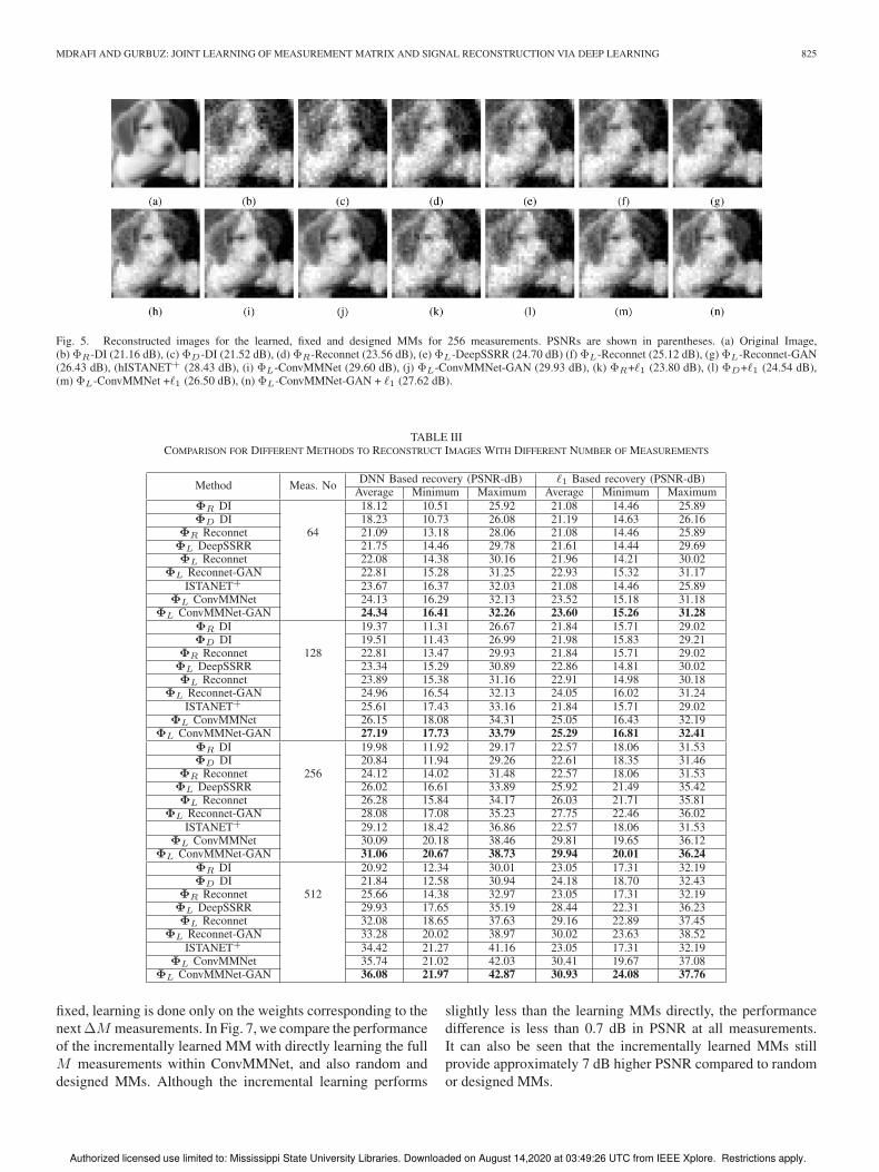
result for an example test set image is shown in Fig. 5 for all
compared approaches along with the obtained PSNR values. All
compared approaches use 256 measurements for this 32× 32
image. The highest PSNR for this qualitative analysis is obtained
by the learned MM obtained via the proposed ConvMMNet-
GAN. While �1-recovery performs comparably better than some
DNN reconstructions for random MM cases, the joint learning
of MM and DNN reconstruction achieves better reconstruction
performance as classical CS recovery scenario of random MM
and �1-recovery. The images shown in Fig. 5 are results on a sin-
gle example image. Next subsections provide more quantitative
analysis on average performances over the full test dataset as a
function of number of measurements, incremental measurement
designs, effect of signal sparsity on DNN based reconstructions,
and coherence analysis on the learned MMs.
D. Quantitative Analysis
For quantitative evaluation, all the DNN architectures are
run over the testing dataset, for varying number of compressed
measurements from M = 64 to M = 512. After obtaining the
outputs, the reconstruction performance of compared techniques
are evaluated in terms of the PSNR metric. The average, max-
imum and minimum PSNRs obtained over the test dataset
have been reported on Table III and the average PSNRs are
illustrated in Fig. 6. From both visual and quantitative per-
spectives, it can be seen that for all the measurement cases,
the proposed ConvMMNet-GAN architecture produces the best
MM resulting the highest PSNR levels. The learned MMs by
the proposed architectures outperform the randomly created and
designed MMs by around 6−16 dB in PSNR levels when it is
used in DNN based reconstruction, or 3−7 dB when employed
in �1-based recovery. In addition, the designed MM that is
defined as optimal in the sense of minimizing average mutual
coherence for the given sparsity basis is not optimal in terms of
average reconstruction performance and the learned MM from
ConvMMNet-GAN provides 6−13 dB more PSNR than this
designed MM. In addition, we also see that both ConvMMNet
and ConvMMNet-GAN structures outperform the concurrent
state-of-the-art learned MMs (Reconnet and its gan version,
DeepSSRR, and ISTANET) by having 1−5 dB more average
PSNR than them. Moreover, DNN based reconstruction with
learned MMs outperform �1 based reconstruction, when these
learned MMs are utilised in �1 recovery indicating the supremacy
of data driven reconstruction. However, in case of �1 based re-
construction, the MMs learned through proposed ConvMMNet
and ConvMMNet-GAN outperform all compared MM cases by
having 1−2 dB more PSNR. It is also seen that the learned MM
by the ConvMMNet-GAN results around 1 dB higher PSNR
than ConvMMNet.
E. Incremental Measurement Design Results
The proposed ConvMMNet learns the MM for a fixed given
number of measurements, M . While MMs can be learned
independently for different number of measurements, another
way is incremental learning. In this incremental learning ap-
proach, given a fixed number of measurements M0, we learn
the next ∆M number of measurements to have a total of M =M0 +∆M measurements. In this approach, while the weights
on FC1 that corresponds to the initial M measurements are
Authorized licensed use limited to: Mississippi State University Libraries. Downloaded on August 14,2020 at 03:49:26 UTC from IEEE Xplore. Restrictions apply.
MDRAFI AND GURBUZ: JOINT LEARNING OF MEASUREMENT MATRIX AND SIGNAL RECONSTRUCTION VIA DEEP LEARNING 825
Fig. 5. Reconstructed images for the learned, fixed and designed MMs for 256 measurements. PSNRs are shown in parentheses. (a) Original Image,(b) ΦR-DI (21.16 dB), (c) ΦD-DI (21.52 dB), (d) ΦR-Reconnet (23.56 dB), (e) ΦL-DeepSSRR (24.70 dB) (f) ΦL-Reconnet (25.12 dB), (g) ΦL-Reconnet-GAN(26.43 dB), (hISTANET+ (28.43 dB), (i) ΦL-ConvMMNet (29.60 dB), (j) ΦL-ConvMMNet-GAN (29.93 dB), (k) ΦR+�1 (23.80 dB), (l) ΦD+�1 (24.54 dB),(m) ΦL-ConvMMNet +�1 (26.50 dB), (n) ΦL-ConvMMNet-GAN + �1 (27.62 dB).
TABLE IIICOMPARISON FOR DIFFERENT METHODS TO RECONSTRUCT IMAGES WITH DIFFERENT NUMBER OF MEASUREMENTS
fixed, learning is done only on the weights corresponding to the
next∆M measurements. In Fig. 7, we compare the performance
of the incrementally learned MM with directly learning the full
M measurements within ConvMMNet, and also random and
designed MMs. Although the incremental learning performs
slightly less than the learning MMs directly, the performance
difference is less than 0.7 dB in PSNR at all measurements.
It can also be seen that the incrementally learned MMs still
provide approximately 7 dB higher PSNR compared to random
or designed MMs.
Authorized licensed use limited to: Mississippi State University Libraries. Downloaded on August 14,2020 at 03:49:26 UTC from IEEE Xplore. Restrictions apply.
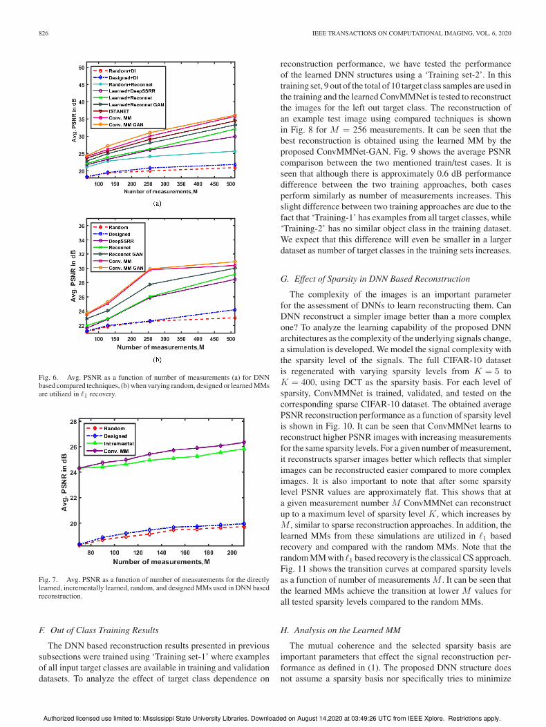
826 IEEE TRANSACTIONS ON COMPUTATIONAL IMAGING, VOL. 6, 2020
Fig. 6. Avg. PSNR as a function of number of measurements (a) for DNNbased compared techniques, (b) when varying random, designed or learned MMsare utilized in �1 recovery.
Fig. 7. Avg. PSNR as a function of number of measurements for the directlylearned, incrementally learned, random, and designed MMs used in DNN basedreconstruction.
F. Out of Class Training Results
The DNN based reconstruction results presented in previous
subsections were trained using ‘Training set-1’ where examples
of all input target classes are available in training and validation
datasets. To analyze the effect of target class dependence on
reconstruction performance, we have tested the performance
of the learned DNN structures using a ‘Training set-2’. In this
training set, 9 out of the total of 10 target class samples are used in
the training and the learned ConvMMNet is tested to reconstruct
the images for the left out target class. The reconstruction of
an example test image using compared techniques is shown
in Fig. 8 for M = 256 measurements. It can be seen that the
best reconstruction is obtained using the learned MM by the
proposed ConvMMNet-GAN. Fig. 9 shows the average PSNR
comparison between the two mentioned train/test cases. It is
seen that although there is approximately 0.6 dB performance
difference between the two training approaches, both cases
perform similarly as number of measurements increases. This
slight difference between two training approaches are due to the
fact that ‘Training-1’ has examples from all target classes, while
‘Training-2’ has no similar object class in the training dataset.
We expect that this difference will even be smaller in a larger
dataset as number of target classes in the training sets increases.
G. Effect of Sparsity in DNN Based Reconstruction
The complexity of the images is an important parameter
for the assessment of DNNs to learn reconstructing them. Can
DNN reconstruct a simpler image better than a more complex
one? To analyze the learning capability of the proposed DNN
architectures as the complexity of the underlying signals change,
a simulation is developed. We model the signal complexity with
the sparsity level of the signals. The full CIFAR-10 dataset
is regenerated with varying sparsity levels from K = 5 to
K = 400, using DCT as the sparsity basis. For each level of
sparsity, ConvMMNet is trained, validated, and tested on the
corresponding sparse CIFAR-10 dataset. The obtained average
PSNR reconstruction performance as a function of sparsity level
is shown in Fig. 10. It can be seen that ConvMMNet learns to
reconstruct higher PSNR images with increasing measurements
for the same sparsity levels. For a given number of measurement,
it reconstructs sparser images better which reflects that simpler
images can be reconstructed easier compared to more complex
images. It is also important to note that after some sparsity
level PSNR values are approximately flat. This shows that at
a given measurement number M ConvMMNet can reconstruct
up to a maximum level of sparsity level K, which increases by
M , similar to sparse reconstruction approaches. In addition, the
learned MMs from these simulations are utilized in �1 based
recovery and compared with the random MMs. Note that the
random MM with �1 based recovery is the classical CS approach.
Fig. 11 shows the transition curves at compared sparsity levels
as a function of number of measurements M . It can be seen that
the learned MMs achieve the transition at lower M values for
all tested sparsity levels compared to the random MMs.
H. Analysis on the Learned MM
The mutual coherence and the selected sparsity basis are
important parameters that effect the signal reconstruction per-
formance as defined in (1). The proposed DNN structure does
not assume a sparsity basis nor specifically tries to minimize
Authorized licensed use limited to: Mississippi State University Libraries. Downloaded on August 14,2020 at 03:49:26 UTC from IEEE Xplore. Restrictions apply.

MDRAFI AND GURBUZ: JOINT LEARNING OF MEASUREMENT MATRIX AND SIGNAL RECONSTRUCTION VIA DEEP LEARNING 827
Fig. 8. Reconstructed images for the learned, fixed and optimal sensing matrix for 256 measurements using samples from class that is not used for training(a) Original Image, (b) ΦR-DI (23.59 dB), (c) ΦD-DI (24.29 dB), (d) ΦR-Reconnet (26.27 dB), (e) ΦL-DeepSSRR (26.51 dB), (f) ΦL-Reconnet (27.78 dB),(g) ΦL-Reconnet-GAN (29.02 dB), (h) ISTANET+ (30.47 dB), (i) ΦL-ConvMMNet (31.68 dB), (j) ΦL-ConvMMNet-GAN (32.79 dB), (k) ΦR + �1 (26.09 dB),(l) ΦD + �1 (26.80 dB), (m) ΦL-ConvMMNet + �1 (28.52 dB), (n) ΦL-ConvMMNet-GAN + �1 (29.30 dB).
Fig. 9. Avg. PSNR as a function of number of measurements for Training-1and Training-2 cases.
Fig. 10. Average PSNR for different measurement numbers M as a functionof sparsity level K.
Fig. 11. Transition curves at different different sparsity levels (K = 5, K =
55, and K = 200) as a function of number of measurements.
a parameter like mutual coherence. Nevertheless, we made a
simulation to understand the coherence properties of the learned
MMs. The sparsity basis Ψ is assumed to be DCT basis and the
mutual coherence of the system A = ΦΨ is calculated for the
MM Φ. We tested random MM, learned MMs for ConvMMNet,
DeepSSRR, Reconnet, and the designed MM for the assumed
basis. We show the average mutual coherence as a function
of number of measurements in Fig. 12. It can be seen that
the designed MM has the lowest average coherence since it is
designed specifically for that purpose. The learned MMs have
more average coherence compared to random MMs. On the other
hand, it can be seen from the histogram plots of the coherence
shown in Fig. 13 that the designed MM almost has the highest
maximum absolute coherence while learned MMs from Con-
vMMNet and Reconnet have similar values with that of designed
one. On the contrary, learned MM in DeepSSRR and random
MM have similar lower values of absolute coherence. Presented
results in this paper show that the learned MM provides the
Authorized licensed use limited to: Mississippi State University Libraries. Downloaded on August 14,2020 at 03:49:26 UTC from IEEE Xplore. Restrictions apply.
828 IEEE TRANSACTIONS ON COMPUTATIONAL IMAGING, VOL. 6, 2020
Fig. 12. Average mutual coherence of the tested learned, designed and randomMMs with the DCT basis as a function of number of measurements M .
Fig. 13. Histogram for the coherence values of tested MMs at M = 128, [A:Random, B: ConvMMNet, C: Reconnet, D: DeepSSRR, E: Designed].
best reconstruction performance of compared MMs although not
necessarily minimizing average or absolute coherence values.
We think that this is because first average mutual coherence
is not directly guarantee better reconstruction performance and
secondly the assumed DCT basis may not be the best basis for
the tested image dataset.
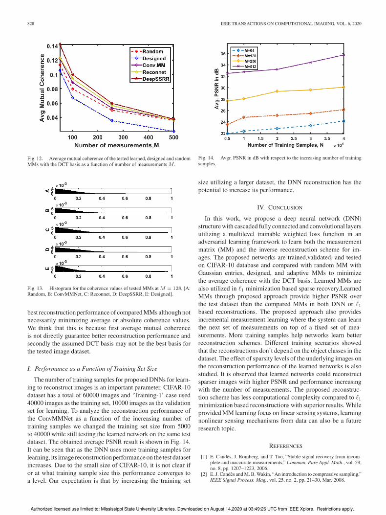
I. Performance as a Function of Training Set Size
The number of training samples for proposed DNNs for learn-
ing to reconstruct images is an important parameter. CIFAR-10
dataset has a total of 60000 images and ‘Training-1’ case used
40000 images as the training set, 10000 images as the validation
set for learning. To analyze the reconstruction performance of
the ConvMMNet as a function of the increasing number of
training samples we changed the training set size from 5000
to 40000 while still testing the learned network on the same test
dataset. The obtained average PSNR result is shown in Fig. 14.
It can be seen that as the DNN uses more training samples for
learning, its image reconstruction performance on the test dataset
increases. Due to the small size of CIFAR-10, it is not clear if
or at what training sample size this performance converges to
a level. Our expectation is that by increasing the training set
Fig. 14. Avgr. PSNR in dB with respect to the increasing number of trainingsamples.
size utilizing a larger dataset, the DNN reconstruction has the
potential to increase its performance.
IV. CONCLUSION
In this work, we propose a deep neural network (DNN)
structure with cascaded fully connected and convolutional layers
utilizing a multilevel trainable weighted loss function in an
adversarial learning framework to learn both the measurement
matrix (MM) and the inverse reconstruction scheme for im-
ages. The proposed networks are trained,validated, and tested
on CIFAR-10 database and compared with random MM with
Gaussian entries, designed, and adaptive MMs to minimize
the average coherence with the DCT basis. Learned MMs are
also utilized in �1 minimization based sparse recovery.Learned
MMs through proposed approach provide higher PSNR over
the test dataset than the compared MMs in both DNN or �1based reconstructions. The proposed approach also provides
incremental measurement learning where the system can learn
the next set of measurements on top of a fixed set of mea-
surements. More training samples help networks learn better
reconstruction schemes. Different training scenarios showed
that the reconstructions don’t depend on the object classes in the
dataset. The effect of sparsity levels of the underlying images on
the reconstruction performance of the learned networks is also
studied. It is observed that learned networks could reconstruct
sparser images with higher PSNR and performance increasing
with the number of measurements. The proposed reconstruc-
tion scheme has less computational complexity compared to �1minimization based reconstructions with superior results. While
provided MM learning focus on linear sensing systems, learning
nonlinear sensing mechanisms from data can also be a future
research topic.
REFERENCES
[1] E. Candès, J. Romberg, and T. Tao, “Stable signal recovery from incom-plete and inaccurate measurements,” Commun. Pure Appl. Math., vol. 59,no. 8, pp. 1207–1223, 2006.
[2] E. J. Candès and M. B. Wakin, “An introduction to compressive sampling,”IEEE Signal Process. Mag., vol. 25, no. 2, pp. 21–30, Mar. 2008.
Authorized licensed use limited to: Mississippi State University Libraries. Downloaded on August 14,2020 at 03:49:26 UTC from IEEE Xplore. Restrictions apply.

MDRAFI AND GURBUZ: JOINT LEARNING OF MEASUREMENT MATRIX AND SIGNAL RECONSTRUCTION VIA DEEP LEARNING 829
[3] D. L. Donoho, A. Maleki, and A. Montanari, “Message-passing algo-rithms for compressed sensing,” Proc. Nat. Acad. Sci., vol. 106, no. 45,pp. 18914–18919, 2009.
[4] J. Tropp, “Greed is good: Algorithmic results for sparse approximation,”IEEE Trans. Inf. Theory, vol. 50, no. 10, pp. 2231–2242, Oct. 2004.
[5] J. A. Tropp and A. C. Gilbert, “Signal recovery from random measurementsvia orthogonal matching pursuit,” IEEE Trans. Inf. Theory, vol. 53, no. 12,pp. 4655–4666, Dec. 2007.
[6] C. Hegde, A. C. Sankaranarayanan, W. Yin, and R. G. Baraniuk, “Numax:A convex approach for learning near-isometric linear embeddings,” IEEE
Trans. Signal Process., vol. 63, no. 22, pp. 6109–6121, Nov. 2015.[7] M. Elad, “Optimized projections for compressed sensing,” IEEE Trans.
Signal Process., vol. 55, no. 12, pp. 5695–5702, Dec. 2007.[8] J. M. Duarte-Carvajalino and G. Sapiro, “Learning to sense sparse signals:
Simultaneous sensing matrix and sparsifying dictionary optimization,”IEEE Trans. Image Process., vol. 18, no. 7, pp. 1395–1408, Jul. 2009.
[9] L. Zelnik-Manor, K. Rosenblum, and Y. C. Eldar, “Sensing matrix opti-mization for block-sparse decoding,” IEEE Trans. Signal Process., vol. 59,no. 9, pp. 4300–4312, Sep. 2011.
[10] G. Li, Z. Zhu, D. Yang, L. Chang, and H. Bai, “On projection matrix opti-mization for compressive sensing systems,” IEEE Trans. Signal Process.,vol. 61, no. 11, pp. 2887–2898, Jun. 2013.
[11] Y. LeCun, Y. Bengio, and G. Hinton, “Deep learning,” Nature, vol. 521,no. 7553, pp. 436–444, 2015.
[12] A. Krizhevsky, I. Sutskever, and G. E. Hinton, “Imagenet classificationwith deep convolutional neural networks,” in Proc. Adv. Neural Inf. Pro-
cess. Syst., 2012, pp. 1097–1105.[13] P. Vincent, H. Larochelle, I. Lajoie, Y. Bengio, and P.-A. Manzagol,
“Stacked denoising autoencoders: Learning useful representations in adeep network with a local denoising criterion,” J. Mach. Learn. Res.,vol. 11, pp. 3371–3408, 2010.
[14] I. Goodfellow et al., “Generative adversarial nets,” in Proc. Adv. Neural
Inf. Process. Syst., 2014, pp. 2672–2680.[15] F. N. Iandola, S. Han, M. W. Moskewicz, K. Ashraf, W. J. Dally, and
K. Keutzer, “Squeezenet: Alexnet-level accuracy with 50x fewer parame-ters and < 0.5 mb model size,” 2016, arXiv:1602.07360.
[16] S. Zagoruyko and N. Komodakis, “Wide residual networks,” 2016,arXiv:1605.07146.
[17] K. Simonyan and A. Zisserman, “Very deep convolutional networks forlarge-scale image recognition,” in 3rd Int. Conf. Learn. Representations,2015.
[18] A. Lucas, M. Iliadis, R. Molina, and A. K. Katsaggelos, “Using deep neuralnetworks for inverse problems in imaging: Beyond analytical methods,”IEEE Signal Process. Mag., vol. 35, no. 1, pp. 20–36, Jan. 2018.
[19] A. Mousavi, A. B. Patel, and R. G. Baraniuk, “A deep learning approachto structured signal recovery,” in Proc. IEEE 53rd Annu. Allerton Conf.
Commun., Control, Comput. (Allerton), 2015, pp. 1336–1343.[20] A. Mousavi and R. G. Baraniuk, “Learning to invert: Signal recovery via
deep convolutional networks,” in Proc. IEEE Int. Conf. Acoust., Speech,
Signal Process., 2017, pp. 2272–2276.[21] K. Kulkarni, S. Lohit, P. Turaga, R. Kerviche, and A. Ashok, “Reconnet:
Non-iterative reconstruction of images from compressively sensed mea-surements,” in Proceedings IEEE Conf. Comput. Vision Pattern Recognit.,2016, pp. 449–458.
[22] H. Yao et al., “Dr2-net: Deep residual reconstruction network for imagecompressive sensing,” Neurocomputing, vol. 359, pp. 483–493, 2019.
[23] A. Mousavi, G. Dasarathy, and R. G. Baraniuk, “Deepcodec: Adaptivesensing and recovery via deep convolutional neural networks,” 2017,arXiv:1707.03386.
[24] X. Xie, Y. Wang, G. Shi, C. Wang, J. Du, and X. Han, “Adaptive mea-surement network for cs image reconstruction,” in Proc. CCF Chin. Conf.
Comput. Vision, 2017, pp. 407–417.[25] A. Mousavi, G. Dasarathy, and R. G. Baraniuk, “A data-driven and
distributed approach to sparse signal representation and recovery,” in Proc.
Int. Conf. Learn. Representations, 2019.[26] S. Lohit, K. Kulkarni, R. Kerviche, P. Turaga, and A. Ashok, “Convo-
lutional neural networks for noniterative reconstruction of compressivelysensed images,” IEEE Trans. Comput. Imag., vol. 4, no. 3, pp. 326–340,Sep. 2018.
[27] R. MdRafi and A. C. Gurbuz, “Learning to sense and reconstruct a classof signals,” in Proc. IEEE Radar Conf., Apr. 2019, pp. 1–5.
[28] R. MdRafi and A. C. Gurbuz, “Data driven measurement matrix learningfor sparse reconstruction,” in Proc. IEEE Data Sci. Workshop, Jun. 2019,pp. 253–257.
[29] A. Krizhevsky, I. Sutskever, and G. E. Hinton, “Imagenet classificationwith deep convolutional neural networks,” in Advances in Neural Infor-
mation Processing Systems 25, F. Pereira, C. J. C. Burges, L. Bottou, andK. Q. Weinberger, Eds., Red Hook, NY, USA: Curran Associates, Inc.,2012, pp. 1097–1105.
[30] J. Zhang and B. Ghanem, “Ista-net: Iterative shrinkage-thresholding algo-rithm inspired deep network for image compressive sensing,” in Proc.
IEEE Conf. Comput. Vision and Pattern Recognit. (CVPR), 2018, pp.1828–1837.
[31] H. K. Aggarwal, M. P. Mani, and M. Jacob, “MoDL: Model based deeplearning architecture for inverse problems,” IEEE Trans. Med. Imag., vol.38, no. 2, pp. 394–405, Feb. 2019.
[32] G. Huang, Z. Liu, L. Van Der Maaten, and K. Q. Weinberger, “Denselyconnected convolutional networks,” in Proc. Conf. Comput. Vision Pattern
Recognit., 2017, pp. 2261–2269.[33] R. C. Gonzalez and R. E. Woods, Digital Image Processing. Englewood
Cliffs, NJ, USA: Prentice-Hall, 2008.[34] M. Abadi et al., “TensorFlow: Large-scale machine learning on heteroge-
neous systems,” 2015. Software available from tensorflow.org[35] T. Blumensath and M. E. Davies, “Iterative hard thresholding for
compressed sensing,” Appl. Comput. Harmonic Anal., vol. 27, no. 3,pp. 265–274, 2009.
[36] D. Needell and J. A. Tropp, “CoSaMP: Iterative signal recovery fromincomplete and inaccurate samples,” Appl. Comp. Harmonic Anal., vol. 26,no. 3, pp. 301–321, 2009.
[37] D. L. Donoho, A. Maleki, and A. Montanari, “Message passing algorithmsfor compressed sensing: I. motivation and construction,” in Proc. IEEE Inf.
Theory Workshop Inf. Theory, Jan. 2010, pp. 1–5.
Robiulhossain Mdrafi (Student Member, IEEE) re-ceived the B.Sc. degree in electrical, electronic, andcommunication engineering from the BangladeshUniversity of Professionals, Dhaka, Bangladesh, in2010. He is currently working toward the Ph.D. de-gree in electrical and computer engineering with Mis-sissippi State University, Starkville, MS, USA. He isa Research Assistant working with the InformationProcessing and Sensing (IMPRESS) Lab, MS-State.His research interests include deep learning basedinverse problems such as sparse signal/image recon-
struction, physics aware deep learning and learning in radar and remote sensingapplications.
Ali Cafer Gurbuz (Senior Member, IEEE) receivedthe B.S. degree in electrical engineering from BilkentUniversity, Ankara, Turkey, in 2003, and the M.S. andPh.D. degrees from the Georgia Institute of Technol-ogy, Atlanta, GA, USA, in 2005 and 2008, both inelectrical and computer engineering. From 2003 to2009, he researched compressive sensing based com-putational imaging problems with Georgia Tech. Heheld faculty positions with TOBB University and theUniversity of Alabama between 2009 and 2017. He iscurrently an Assistant Professor with the Department
of Electrical and Computer Engineering, Mississippi State University, Starkville,MS, USA, where he is the Co-Director of Information Processing and Sensing(IMPRESS) Lab. His active research program on the development of sparsesignal representations, compressive sensing theory and applications, radar andsensor array signal processing, and machine learning. He is the recipient ofThe Best Paper Award for Signal Processing Journal in 2013 and the TurkishAcademy of Sciences Best Young Scholar Award in Electrical Engineering in2014. He was an Associate Editor for several journals such as Digital Signal
Processing, EURASIP Journal on Advances in Signal Processing, and Physical
Communications. He is a member of Sigma Xi.
Authorized licensed use limited to: Mississippi State University Libraries. Downloaded on August 14,2020 at 03:49:26 UTC from IEEE Xplore. Restrictions apply.