joint program in oceanography/ applied ocean … doctoral dissertation by vicente i. fernandez june...

2011-13

DOCTORAL DISSERTATION

by

Vicente I. Fernandez

June 2011

Performance Analysis for Lateral-Line-Inspired

Sensor Arrays

MIT/WHOI

Joint Programin Oceanography/

Applied Ocean Scienceand Engineering

Massachusetts Institute of Technology

Woods Hole Oceanographic Institution

Performance Analysis for Lateral-Line-Inspired Sensor Arrays

by


Submitted to the Department of Mechanical Engineeringon May 20, 2011, in partial fulfillment of the

requirements for the degree ofDoctor of Philosophy

AbstractThe lateral line is a critical component of the fish sensory system, found to affect numerousaspects of behavior including maneuvering in complex fluid environments, schooling, preytracking, and environment mapping. This sensory organ has no analog in modern oceanvehicles, despite its utility and ubiquity in nature, and could fill the gap left by sonar andvision systems in turbid cluttered environments. Yet, while the biological sensory systemsuggests the broad possibilities associated with such a sensor array, nearly nothing is knownof the input processing and what information is available via the real lateral line. This thesisdemonstrates and characterizes the ability of lateral-line-inspired linear pressure sensorarrays to perform two sensory tasks of relevance to biological and man-made underwaternavigation systems, namely shape identification and vortex tracking.

The ability of pressure sensor arrays to emulate the ”touch at a distance” feature ofthe lateral line, corresponding to the latter’s capability of identifying the shape of objectsremotely, is examined with respect to moving cylinders of different cross sections. Usingthe pressure distribution on a small linear array, the position and size of a cylinder is trackedat various distances. The classification of cylinder shape is considered separately, using alarge database of trials to identify two classification approaches: One based on differencesin the mean flow, and one trained on a subset which utilizes information from the wake.The results indicate that it is in general possible to extract specific shape information frommeasurements on a linear pressure sensor array, and characterize the classes of shapeswhich are not distinguishable via this method.

Identifying the vortices in a flow makes it possible to predict and optimize the perfor-mance of flapping foils, and to identify imminent stall in a control surface. Vortices inwakes also provide information about the object that generated the wake at distances muchlarger than the near-field pressure perturbations. Experimental studies in tracking a vortexpair and an individual vortex interacting with a flat plate demonstrate the ability to trackvortices with a linear pressure sensor array from both small streamlined bodies and largeflat bodies. Based on a theoretical analysis, the relationship between the necessary arrayparameters and the range of vortices of interest is established.

Thesis Supervisor: Michael S. TriantafyllouTitle: Professor of Mechanical and Ocean Engineering

3

Acknowledgments

First of all, I would like to gratefully acknowledge my advisor Prof. Michael Triantafyllou

for his support, insight, and guidance on this work. I would like to also acknowledge

Prof. Jeffrey Lang for his advice and aid, especially on the topics of electrical experimental

design and noise reduction. Prof. Franz Hover I would like to acknowledge for his direct

and insightful questions as well as his advice, which frequently contributed to keeping this

project well grounded. I would like to acknowledge several towing tank graduate students

and post-docs that helped in experimental work or by lending moral support: Stephen Licht,

Jason Dahl, Brad Simpson, Pradya Prempraneerach, and Stephen Hou. And last, but not

least, I would like to acknowledge Natasha Blitvic, a keen probabilist who also happens to

be my wife, for her persistent support and stimulating discussions.

I would also like to acknowledge the support of the NOAA’s Sea Grant, the Singapore-

MIT Alliance for Research and Technology, and the National Defense Science and Engi-

neering Graduate (NDSEG) Fellowship for their support throughout my thesis work.

5

Contents

1 Introduction 27

1.1 Research Motivation . . . . . . . . . . . . . . . . . . . . . . . . . . . . . 27

1.2 Chapter Overviews . . . . . . . . . . . . . . . . . . . . . . . . . . . . . . 32

2 Biological Foundation 35

2.1 Lateral Line Structure . . . . . . . . . . . . . . . . . . . . . . . . . . . . . 35

2.1.1 Superficial Subsystem . . . . . . . . . . . . . . . . . . . . . . . . 36

2.1.2 Canal Subsystem . . . . . . . . . . . . . . . . . . . . . . . . . . . 38

2.2 Lateral-Line-Mediated Fish Behavior . . . . . . . . . . . . . . . . . . . . 40

2.2.1 Approach to Lateral Line Modeling . . . . . . . . . . . . . . . . . 41

2.2.2 The Lateral Line and Dipole Stimuli . . . . . . . . . . . . . . . . . 42

2.2.3 The Lateral Line and Solid Objects . . . . . . . . . . . . . . . . . 43

2.2.4 The Lateral Line and Vortices . . . . . . . . . . . . . . . . . . . . 45

2.3 Conclusions . . . . . . . . . . . . . . . . . . . . . . . . . . . . . . . . . . 47

3 Tracking a Cylinder in Motion 49

3.1 Strategy and Motivation . . . . . . . . . . . . . . . . . . . . . . . . . . . . 50

3.2 Model Evaluation and Selection . . . . . . . . . . . . . . . . . . . . . . . 51

3.2.1 General Model Form and State Transition . . . . . . . . . . . . . . 52

3.2.2 Measurement Models . . . . . . . . . . . . . . . . . . . . . . . . . 53

3.2.3 Measurement Model Frame Equivalence . . . . . . . . . . . . . . 55

3.3 Experimental Setup . . . . . . . . . . . . . . . . . . . . . . . . . . . . . . 61

3.3.1 Cylinder Motion . . . . . . . . . . . . . . . . . . . . . . . . . . . 61

7

3.3.2 Sensing Platform . . . . . . . . . . . . . . . . . . . . . . . . . . . 62

3.3.3 Test Matrix . . . . . . . . . . . . . . . . . . . . . . . . . . . . . . 65

3.3.4 Noise Analysis and Data Preparation . . . . . . . . . . . . . . . . 65

3.4 Results . . . . . . . . . . . . . . . . . . . . . . . . . . . . . . . . . . . . . 68

3.5 Cylinder State Estimation . . . . . . . . . . . . . . . . . . . . . . . . . . . 70

3.5.1 Cylinder Tracking via a Kalman Filter . . . . . . . . . . . . . . . . 71

3.5.2 Cylinder Tracking Via Particle Filter . . . . . . . . . . . . . . . . . 77

3.6 Discussion . . . . . . . . . . . . . . . . . . . . . . . . . . . . . . . . . . . 90

4 Object Identification and Classification 95

4.1 Introduction . . . . . . . . . . . . . . . . . . . . . . . . . . . . . . . . . . 95

4.2 Experimental Procedure . . . . . . . . . . . . . . . . . . . . . . . . . . . . 96

4.2.1 Experimental Layout . . . . . . . . . . . . . . . . . . . . . . . . . 98

4.2.2 Test Matrix . . . . . . . . . . . . . . . . . . . . . . . . . . . . . . 99

4.2.3 Data Pre-Processing . . . . . . . . . . . . . . . . . . . . . . . . . 100

4.3 Results . . . . . . . . . . . . . . . . . . . . . . . . . . . . . . . . . . . . . 102

4.4 Analysis . . . . . . . . . . . . . . . . . . . . . . . . . . . . . . . . . . . . 109

4.4.1 Heuristically Selected Features . . . . . . . . . . . . . . . . . . . . 109

4.4.2 Principal Component Analysis . . . . . . . . . . . . . . . . . . . . 112

4.4.3 Discussion and Comparison . . . . . . . . . . . . . . . . . . . . . 115

4.5 Conclusion . . . . . . . . . . . . . . . . . . . . . . . . . . . . . . . . . . 123

5 Vortex Tracking 127

5.1 Introduction . . . . . . . . . . . . . . . . . . . . . . . . . . . . . . . . . . 127

5.1.1 Variable Definitions . . . . . . . . . . . . . . . . . . . . . . . . . 129

5.1.2 Vortex Modeling . . . . . . . . . . . . . . . . . . . . . . . . . . . 130

5.2 Experimental Procedure . . . . . . . . . . . . . . . . . . . . . . . . . . . . 131

5.2.1 Particle Image Velocimetry . . . . . . . . . . . . . . . . . . . . . . 132

5.2.2 Experimental Layout: Streamlined Body . . . . . . . . . . . . . . 132

5.2.3 Experimental Layout: Flat Body . . . . . . . . . . . . . . . . . . . 136

5.3 Data Processing . . . . . . . . . . . . . . . . . . . . . . . . . . . . . . . . 139

8

5.3.1 Pressure Data Pre-Processing . . . . . . . . . . . . . . . . . . . . 139

5.3.2 PIV Processing . . . . . . . . . . . . . . . . . . . . . . . . . . . . 142

5.3.3 Independent Vortex Identification . . . . . . . . . . . . . . . . . . 143

5.4 Real Time Vortex Tracking . . . . . . . . . . . . . . . . . . . . . . . . . . 147

5.4.1 Experimental Vortex Forward Models . . . . . . . . . . . . . . . . 148

5.4.2 Estimation Methods . . . . . . . . . . . . . . . . . . . . . . . . . 158

5.4.3 Streamlined Body Results . . . . . . . . . . . . . . . . . . . . . . 163

5.4.4 Flat Plate Results . . . . . . . . . . . . . . . . . . . . . . . . . . . 178

5.5 Vortex Tracking Dependence on Array Parameters . . . . . . . . . . . . . . 184

5.5.1 Reflected Vortex Model . . . . . . . . . . . . . . . . . . . . . . . 185

5.5.2 Vortex Pair Model . . . . . . . . . . . . . . . . . . . . . . . . . . 194

5.6 Discussion . . . . . . . . . . . . . . . . . . . . . . . . . . . . . . . . . . . 200

5.7 Conclusions . . . . . . . . . . . . . . . . . . . . . . . . . . . . . . . . . . 208

6 Conclusions 211

6.1 Overview . . . . . . . . . . . . . . . . . . . . . . . . . . . . . . . . . . . 211

6.2 Principal contributions of the thesis . . . . . . . . . . . . . . . . . . . . . 212

6.2.1 Passive cylinder tracking . . . . . . . . . . . . . . . . . . . . . . . 212

6.2.2 Passive cylinder shape classification . . . . . . . . . . . . . . . . . 214

6.2.3 Vortex tracking . . . . . . . . . . . . . . . . . . . . . . . . . . . . 216

6.3 Recommendations for future work . . . . . . . . . . . . . . . . . . . . . . 218

6.3.1 Improved sensor array density for multiple vortex tracking . . . . . 219

6.3.2 Vortex street tracking . . . . . . . . . . . . . . . . . . . . . . . . . 219

6.3.3 Numerical forward models for wakes . . . . . . . . . . . . . . . . 219

6.3.4 Biological object discrimination . . . . . . . . . . . . . . . . . . . 220

6.3.5 Active object identification . . . . . . . . . . . . . . . . . . . . . . 220

6.3.6 Two-dimensional sensor arrays . . . . . . . . . . . . . . . . . . . . 220

6.3.7 Local flow models for large objects . . . . . . . . . . . . . . . . . 221

9

List of Figures

1-1 Photograph of Finnegan the Roboturtle, a flapping foil autonomous under-

water vehicle, undergoing tests in a pool. . . . . . . . . . . . . . . . . . . . 30

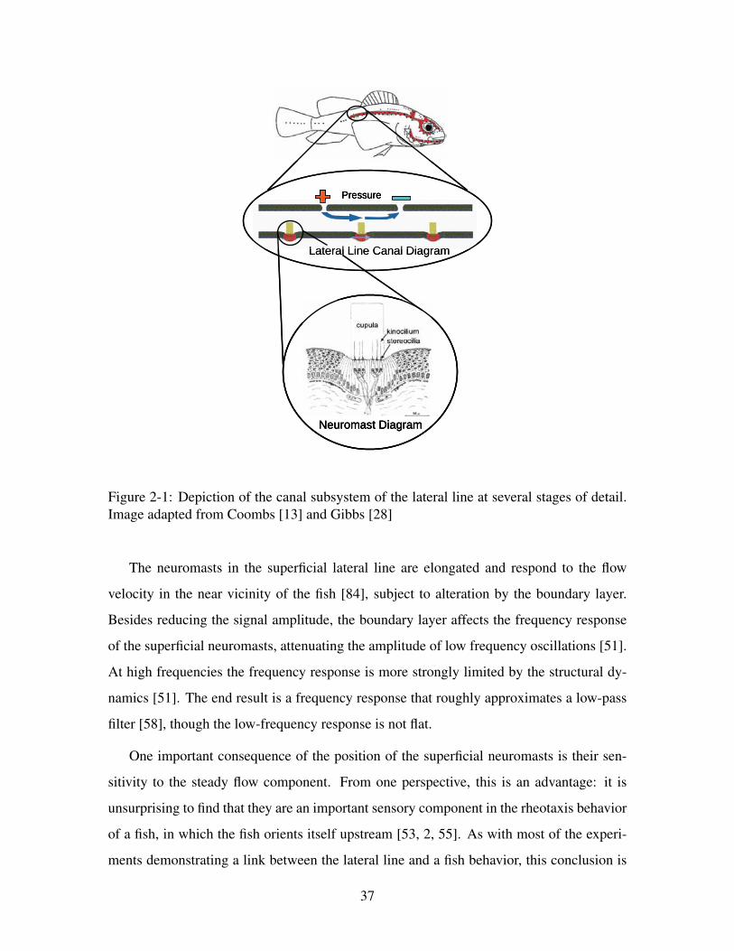
2-1 Depiction of the canal subsystem of the lateral line at several stages of

detail. Image adapted from Coombs [13] and Gibbs [28] . . . . . . . . . . 37

2-2 Comparison of varieties of cephalic canal lateral lines (left four images)

and truck canal lateral lines (right four images). The canals are highlighted

in red. Image modified from Gibbs [28] . . . . . . . . . . . . . . . . . . . 40

3-1 Hidden Markov model undirected graph. The diagram describes the rela-

tion between a series of random variables with edges denoting direct de-

pendence between the random variables. . . . . . . . . . . . . . . . . . . 52

3-2 Model wake boundaries. The wakes for each model are superposed around

the outline of the actual cylinder for comparison. The wakes are depicted

near a wall and in open water with the solid black line denoting the location

of the wall. . . . . . . . . . . . . . . . . . . . . . . . . . . . . . . . . . . 57

3-3 Pressure comparison between models and CFD simulation in open water.

The simulated CFD pressure over a ghost sensor array is displayed at reg-

ular intervals over multiple shedding periods in blue. The mean of these

simulated pressure traces (in black) is compared to the results from the

analytical models. . . . . . . . . . . . . . . . . . . . . . . . . . . . . . . . 58

11

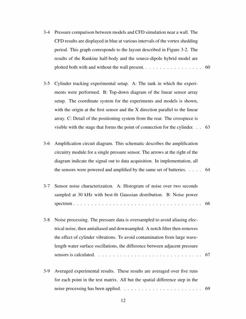
3-4 Pressure comparison between models and CFD simulation near a wall. The

CFD results are displayed in blue at various intervals of the vortex shedding

period. This graph corresponds to the layout described in Figure 3-2. The

results of the Rankine half-body and the source-dipole hybrid model are

plotted both with and without the wall present. . . . . . . . . . . . . . . . . 60

3-5 Cylinder tracking experimental setup. A: The tank in which the experi-

ments were performed. B: Top-down diagram of the linear sensor array

setup. The coordinate system for the experiments and models is shown,

with the origin at the first sensor and the X direction parallel to the linear

array. C: Detail of the positioning system from the rear. The crosspiece is

visible with the stage that forms the point of connection for the cylinder. . . 63

3-6 Amplification circuit diagram. This schematic describes the amplification

circuitry module for a single pressure sensor. The arrows at the right of the

diagram indicate the signal out to data acquisition. In implementation, all

the sensors were powered and amplified by the same set of batteries. . . . . 64

3-7 Sensor noise characterization. A: Histogram of noise over two seconds

sampled at 30 kHz with best-fit Gaussian distribution. B: Noise power

spectrum . . . . . . . . . . . . . . . . . . . . . . . . . . . . . . . . . . . . 66

3-8 Noise processing. The pressure data is oversampled to avoid aliasing elec-

trical noise, then antialiased and downsampled. A notch filter then removes

the effect of cylinder vibrations. To avoid contamination from large wave-

length water surface oscillations, the difference between adjacent pressure

sensors is calculated. . . . . . . . . . . . . . . . . . . . . . . . . . . . . . 67

3-9 Averaged experimental results. These results are averaged over five runs

for each point in the test matrix. All but the spatial difference step in the

noise processing has been applied. . . . . . . . . . . . . . . . . . . . . . . 69

12

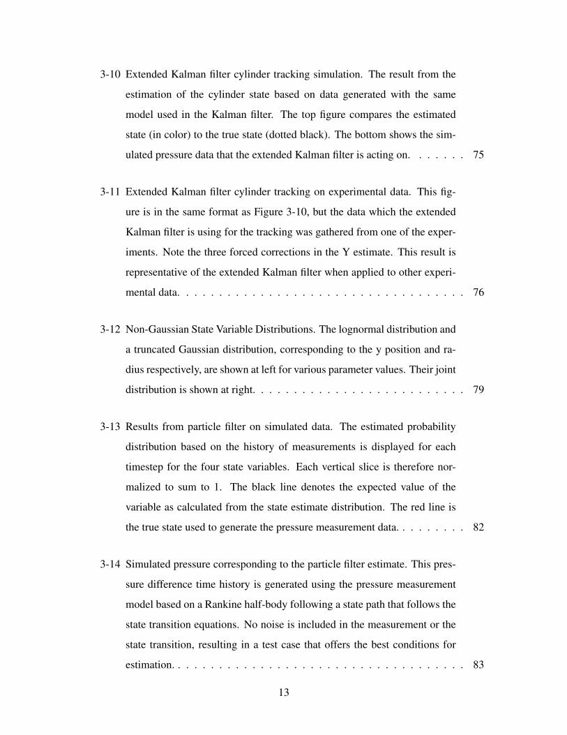
3-10 Extended Kalman filter cylinder tracking simulation. The result from the

estimation of the cylinder state based on data generated with the same

model used in the Kalman filter. The top figure compares the estimated

state (in color) to the true state (dotted black). The bottom shows the sim-

ulated pressure data that the extended Kalman filter is acting on. . . . . . . 75

3-11 Extended Kalman filter cylinder tracking on experimental data. This fig-

ure is in the same format as Figure 3-10, but the data which the extended

Kalman filter is using for the tracking was gathered from one of the exper-

iments. Note the three forced corrections in the Y estimate. This result is

representative of the extended Kalman filter when applied to other experi-

mental data. . . . . . . . . . . . . . . . . . . . . . . . . . . . . . . . . . . 76

3-12 Non-Gaussian State Variable Distributions. The lognormal distribution and

a truncated Gaussian distribution, corresponding to the y position and ra-

dius respectively, are shown at left for various parameter values. Their joint

distribution is shown at right. . . . . . . . . . . . . . . . . . . . . . . . . . 79

3-13 Results from particle filter on simulated data. The estimated probability

distribution based on the history of measurements is displayed for each

timestep for the four state variables. Each vertical slice is therefore nor-

malized to sum to 1. The black line denotes the expected value of the

variable as calculated from the state estimate distribution. The red line is

the true state used to generate the pressure measurement data. . . . . . . . . 82

3-14 Simulated pressure corresponding to the particle filter estimate. This pres-

sure difference time history is generated using the pressure measurement

model based on a Rankine half-body following a state path that follows the

state transition equations. No noise is included in the measurement or the

state transition, resulting in a test case that offers the best conditions for

estimation. . . . . . . . . . . . . . . . . . . . . . . . . . . . . . . . . . . . 83

13

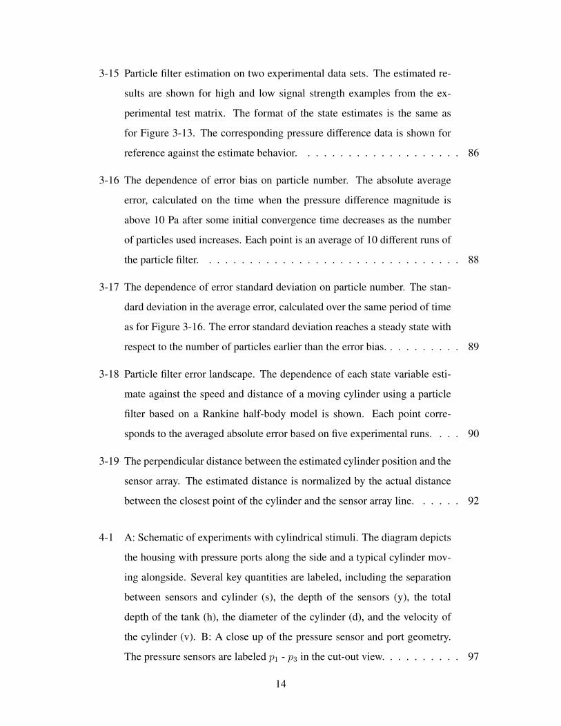
3-15 Particle filter estimation on two experimental data sets. The estimated re-

sults are shown for high and low signal strength examples from the ex-

perimental test matrix. The format of the state estimates is the same as

for Figure 3-13. The corresponding pressure difference data is shown for

reference against the estimate behavior. . . . . . . . . . . . . . . . . . . . 86

3-16 The dependence of error bias on particle number. The absolute average

error, calculated on the time when the pressure difference magnitude is

above 10 Pa after some initial convergence time decreases as the number

of particles used increases. Each point is an average of 10 different runs of

the particle filter. . . . . . . . . . . . . . . . . . . . . . . . . . . . . . . . 88

3-17 The dependence of error standard deviation on particle number. The stan-

dard deviation in the average error, calculated over the same period of time

as for Figure 3-16. The error standard deviation reaches a steady state with

respect to the number of particles earlier than the error bias. . . . . . . . . . 89

3-18 Particle filter error landscape. The dependence of each state variable esti-

mate against the speed and distance of a moving cylinder using a particle

filter based on a Rankine half-body model is shown. Each point corre-

sponds to the averaged absolute error based on five experimental runs. . . . 90

3-19 The perpendicular distance between the estimated cylinder position and the

sensor array. The estimated distance is normalized by the actual distance

between the closest point of the cylinder and the sensor array line. . . . . . 92

4-1 A: Schematic of experiments with cylindrical stimuli. The diagram depicts

the housing with pressure ports along the side and a typical cylinder mov-

ing alongside. Several key quantities are labeled, including the separation

between sensors and cylinder (s), the depth of the sensors (y), the total

depth of the tank (h), the diameter of the cylinder (d), and the velocity of

the cylinder (v). B: A close up of the pressure sensor and port geometry.

The pressure sensors are labeled p1 - p3 in the cut-out view. . . . . . . . . . 97

14

4-2 A: Resting noise distribution of the Honeywell 242PC15M pressure sensor.

the normalized histogram is generated from a 3 second sample at 300kHz.

B: The corresponding power spectrum to the noise sample. High frequency

electrical noise peaks are evident in the power spectrum. . . . . . . . . . . 101

4-3 Results from two sets of tests comparing pressure traces obtained from two

different cross sections. Both cross sections had a diameter of two inches,

velocity of 0.75 m/s, and separation of 0.51 cm (0.2 in). The mean value

of all four sensors in each set of 100 runs is shown. The corresponding

standard deviation is offset by -2 kPa, but on the same scale as the mean

pressure traces. . . . . . . . . . . . . . . . . . . . . . . . . . . . . . . . . 103

4-4 Pressure traces for a single run with a round cylinder are depicted, showing

the variability accross measurements from individual sensors. These traces

were filtered with a cut-off frequency of 100 Hz but not aligned. The low

pressure spike marked with an arrow has the signature of a vortex imping-

ing on the sensor port. . . . . . . . . . . . . . . . . . . . . . . . . . . . . . 104

4-5 The mean value of the pressure as function of time. Eight data sets are

presented, cross-compared to assess the effect of cylinder size. Each data

set is composed of 100 runs. . . . . . . . . . . . . . . . . . . . . . . . . . 105


presented, cross-compared to assess the effect of cylinder velocity. Each

data set is composed of 100 runs. . . . . . . . . . . . . . . . . . . . . . . . 106


presented, cross-compared to assess the effect of cylinder shape. Each data

set is composed of 100 runs. . . . . . . . . . . . . . . . . . . . . . . . . . 107

4-8 Diagram of selected features. The three features initially chosen for anal-

ysis are marked on a sample pressure trace. The pressure data has been

filtered with a cutoff frequency of 60 Hz. . . . . . . . . . . . . . . . . . . . 110

15

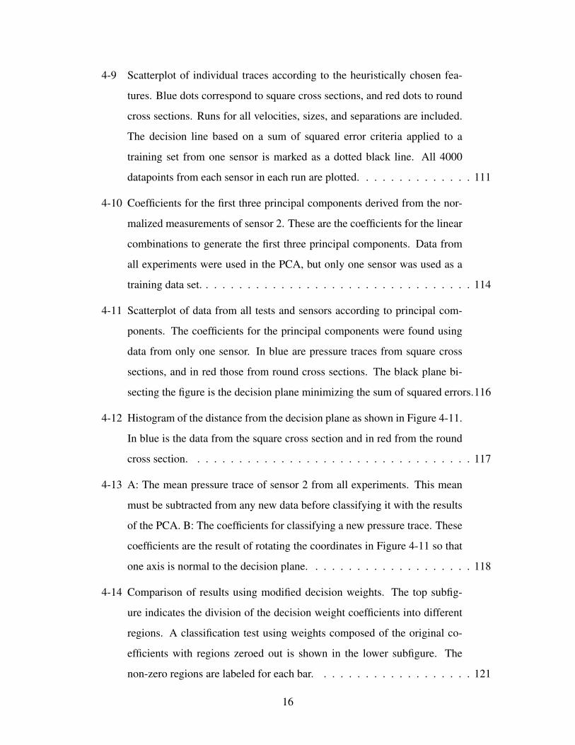
4-9 Scatterplot of individual traces according to the heuristically chosen fea-

tures. Blue dots correspond to square cross sections, and red dots to round

cross sections. Runs for all velocities, sizes, and separations are included.

The decision line based on a sum of squared error criteria applied to a

training set from one sensor is marked as a dotted black line. All 4000

datapoints from each sensor in each run are plotted. . . . . . . . . . . . . . 111

4-10 Coefficients for the first three principal components derived from the nor-

malized measurements of sensor 2. These are the coefficients for the linear

combinations to generate the first three principal components. Data from

all experiments were used in the PCA, but only one sensor was used as a

training data set. . . . . . . . . . . . . . . . . . . . . . . . . . . . . . . . . 114

4-11 Scatterplot of data from all tests and sensors according to principal com-

ponents. The coefficients for the principal components were found using

data from only one sensor. In blue are pressure traces from square cross

sections, and in red those from round cross sections. The black plane bi-

secting the figure is the decision plane minimizing the sum of squared errors.116

4-12 Histogram of the distance from the decision plane as shown in Figure 4-11.

In blue is the data from the square cross section and in red from the round

cross section. . . . . . . . . . . . . . . . . . . . . . . . . . . . . . . . . . 117

4-13 A: The mean pressure trace of sensor 2 from all experiments. This mean

must be subtracted from any new data before classifying it with the results

of the PCA. B: The coefficients for classifying a new pressure trace. These

coefficients are the result of rotating the coordinates in Figure 4-11 so that

one axis is normal to the decision plane. . . . . . . . . . . . . . . . . . . . 118

4-14 Comparison of results using modified decision weights. The top subfig-

ure indicates the division of the decision weight coefficients into different

regions. A classification test using weights composed of the original co-

efficients with regions zeroed out is shown in the lower subfigure. The

non-zero regions are labeled for each bar. . . . . . . . . . . . . . . . . . . 121

16

5-1 Depiction of the experimental layout for tracking a vortex pair near a stream-

lined body. The red box marks the imaged region for PIV, which is lit by

the laser in green. The location of the sensors are marked by red dots. . . . 133

5-2 Simulation of the path of counter-rotating vortices of equal magnitude near

a wall. Dots are placed at equal time intervals along the path to depict the

speed. The wall is marked by a dotted line at the y = 0 axis. . . . . . . . . 135

5-3 Depiction of the experimental layout for tracking a vortex pair near a flat

plate. The red box marks the imaged region for PIV, which is lit by the

laser in green. The location of the sensors are marked by red dots. A rough

approximation to the path of the vortices is also shown. . . . . . . . . . . . 137

5-4 Typical pressure data set from streamlined body experiments. The surface

wave effects are clearly visible. . . . . . . . . . . . . . . . . . . . . . . . . 141

5-5 Depiction of the results using the optimization of an analytical model to

identify the state of a vortex pair. The tracking results (solid colored dots)

are overlaid on an intermediate frame and corresponding velocity field. . . . 144

5-6 Comparison of the estimated state of a vortex based on PIV vector fields.

Results for the vortex closest to the sensor body of a vortex pair are shown.

In black filled dots are the estimates based on a least-squares fit using an

analytical vortex pair model. In open colored circles are directly identi-

fied estimates based on the location of the peak vorticity and area vorticity

integrals. . . . . . . . . . . . . . . . . . . . . . . . . . . . . . . . . . . . . 146

5-7 A general model for the two vortices near the streamlined body. . . . . . . 149

5-8 Reconstructed pressure from different forward models based on PIV vortex

states for streamlined body experiments. The raw measured pressure is

plotted in color. The thin black lines represent the reconstructed pressure

predicted by the forward models. . . . . . . . . . . . . . . . . . . . . . . . 153

5-9 Reconstructed pressure differences from different forward models based

on PIV vortex states for streamlined body experiments. The raw measured

pressure is plotted in color. The thin black lines represent the reconstructed

pressure predicted by the forward models. . . . . . . . . . . . . . . . . . . 154

17

5-10 A general model for a single vortex near sensors mounted on a flat plate.

The dotted line represents the plane of the plate. . . . . . . . . . . . . . . . 155

5-11 Reconstructed pressure differences from a forward model with a single vor-

tex and its image based on PIV vortex states for the flat plate body experi-

ments. The raw measured pressure is plotted in color. The thin black lines

represent the reconstructed pressure predicted by the forward model. . . . . 157

5-12 Simulated extended Kalman filter application for tuning internal parame-

ters. The upper subfigure plots the simulated pressure (dotted black line)

and the reconstructed pressure (color) based on the Kalman filter state es-

timate. The lower subfigure displays the convergence of the state estimate

(color) to the true state (dotted black line). . . . . . . . . . . . . . . . . . . 162

5-13 Results of a streamlined body vortex estimation trial. The estimated state

variables (black line) are compared against the values from the PIV data

in the upper left. In the upper right, the position traces of the pressure-

estimated (black points) versus PIV-estimated (red points) vortices are shown

against the background of the vorticity distribution at an intermediate time.

The edge of the sensor body and sensor locations are marked at the left

edge of the image. At the bottom, the measured pressure is shown, filtered

with a 20 Hz cutoff frequency. . . . . . . . . . . . . . . . . . . . . . . . . 164

5-14 Results of a streamlined body vortex estimation trial. The results corre-

spond to the same data as Figure 5-13. The position estimate based on the

PIV data (red circle) is compared against that based on the pressure data

only (black circle) at different stages in the time series. Each of the smaller

subfigures, proceeding vertically from the top left, corresponds to the time

marked by a dotted line in the top subfigure. . . . . . . . . . . . . . . . . . 166

18






The edge of the sensor body and sensor locations are marked at the right























19





























20

5-23 Results of a vortex estimation trial with the sensors on a flat plate. The es-

timated state variables (black line) are compared against the values from

the PIV data at the left. In the upper right, the position traces of the

pressure-estimated (black points) versus PIV-estimated (red points) vor-

tices are shown against the background of the vorticity distribution at an

intermediate time. The edge of the sensor body and sensor locations are

marked at the top edge of the image. At the lower right, the unfiltered

measured pressure is shown. . . . . . . . . . . . . . . . . . . . . . . . . . 178

5-24 Results of a vortex estimation trial with the sensors on a flat plate. The

results correspond to the same data as Figure 5-23. The position estimate

based on the PIV data (red circle) is compared against that based on the

pressure data only (black circle) at different stages in the time series. Each

of the smaller subfigures, proceeding vertically from the top left, corre-

sponds to the time marked by a dotted line in the top subfigure. . . . . . . . 181

5-25 Results of a vortex estimation trial with the sensors on a flat plate. The es-

timated state variables (black line) are compared against the values from

the PIV data at the left. In the upper right, the position traces of the

pressure-estimated (black points) versus PIV-estimated (red points) vor-

tices are shown against the background of the vorticity distribution at an

intermediate time. The edge of the sensor body and sensor locations are

marked at the top edge of the image. At the lower right, the unfiltered

measured pressure is shown. . . . . . . . . . . . . . . . . . . . . . . . . . 182

5-26 Results of a vortex estimation trial with the sensors on a flat plate. The

results correspond to the same data as Figure 5-25. The position estimate

based on the PIV data (red circle) is compared against that based on the

pressure data only (black circle) at different stages in the time series. Each

of the smaller subfigures, proceeding vertically from the top left, corre-

sponds to the time marked by a dotted line in the top subfigure. . . . . . . . 183

21

5-27 Instantaneous inversion based on a single pressure sensor for the reflected

vortex model. Part A shows the spatial map of the cost function generated

with one sensor. The small x at (0,0.1) denotes the true location of the

vortex. Part B depicts the pressure distribution on the wall at the y = 0 axis. 187

5-28 Maps of the cost function for a reflected vortex model with the vortex at

various lateral locations. The x in each image with a y position of 0.1 and

an x position labeled in the subfigure title denotes the true location of the

vortex. The black lines correspond to level sets generated by the assump-

tion of noise with standard deviations of 1, 5, and 10% of the maximum

measured pressure. . . . . . . . . . . . . . . . . . . . . . . . . . . . . . . 190

5-29 Maps of the cost function for a reflected vortex model with an increasing

array length but constant sensor spacing. The x at (0,0.1) in each image

denotes the true location of the vortex. The black lines correspond to level

sets generated by the assumption of noise with standard deviations of 1, 5,

and 10% of the maximum measured pressure. . . . . . . . . . . . . . . . . 191

5-30 Maps of the cost function for a reflected vortex model with an increasing

array length and fixed number of sensors. The x at (0,0.1) in each image

denotes the true location of the vortex. The black lines correspond to level

sets generated by the assumption of noise with standard deviations of 1, 5,

and 10% of the maximum measured pressure. . . . . . . . . . . . . . . . . 193

5-31 The pressure distribution on a linear array due to an external vortex pair.

The separation between the vortices is given in the legend with respect to

the perpendicular distance between the sensor array and the closest vortex. . 195

5-32 Maps of the cost function for a vortex pair model with the vortices at vari-

ous lateral locations. The x in each image denotes the true locations of the

vortices. The black lines correspond to level sets generated by the assump-

tion of noise with standard deviations of 1, 5, and 10% of the maximum

measured pressure. . . . . . . . . . . . . . . . . . . . . . . . . . . . . . . 196

22

5-33 Maps of the cost function for a vortex pair model with an increasing array

length but constant sensor spacing. The x in each image denotes the true

location of the vortex. The black lines correspond to level sets generated

by the assumption of noise with standard deviations of 1, 5, and 10% of the

maximum measured pressure. . . . . . . . . . . . . . . . . . . . . . . . . 198

5-34 Maps of the cost function for a vortex pair model with an increasing array

length fixed number of sensors. The x in each image denotes the true lo-

cation of the vortex. The black lines correspond to level sets generated by

the assumption of noise with standard deviations of 1, 5, and 10% of the

maximum measured pressure. . . . . . . . . . . . . . . . . . . . . . . . . 199

5-35 Simulated setup for a pressure sensor array similar to the one on a stream-

lined body being applied to a foil in order to track an external vortex. . . . . 203

5-36 Dependence of foil lift on the position of an external vortex. In the top sub-

figure, the foil is plotted with horizontal lines indicating the range of posi-

tions of the external vortex. The lower subfigure demonstrates the effect of

a vortex at the positions marked in the top subfigure on the normalized lift

of the foil. . . . . . . . . . . . . . . . . . . . . . . . . . . . . . . . . . . . 204

5-37 Dependence of foil moment on the position of an external vortex. In the top

subfigure, the foil is plotted with horizontal lines indicating the range of po-

sitions of the external vortex. The lower subfigure demonstrates the effect

of a vortex at the positions marked in the top subfigure on the normalized

moment of the foil. . . . . . . . . . . . . . . . . . . . . . . . . . . . . . . 207

23

List of Tables

3.1 Experimental matrix for cylinder tracking. The range of velocities and

distances was determined by the signal strength and by the abilities and

noise of the experimental setup. . . . . . . . . . . . . . . . . . . . . . . . 65

4.1 Table of tests performed for identifying a moving object. Not included in

the table are two sets of 100 runs (one for each cross section shape) at 0.75

m/s, 5.08 cm diameter, and 1.27 cm separation. . . . . . . . . . . . . . . . 100

4.2 Table of the Strouhal numbers associated with the cylinder identification

experiments. . . . . . . . . . . . . . . . . . . . . . . . . . . . . . . . . . . 123

5.1 Error statistics for tracking vortices from a streamlined body. The statistics

are calculated while the vortex is in front of the sensor array, allowing for

a brief window of convergence. . . . . . . . . . . . . . . . . . . . . . . . . 201

5.2 Error statistics for tracking vortices from a flat plate. The statistics are

calculated while the vortex is in front of the sensor array, allowing for a

brief window of convergence. . . . . . . . . . . . . . . . . . . . . . . . . . 202

25

Chapter 1

Introduction

The fish lateral line is a versatile short-range sensor organ, involved in mapping environ-

ments [76], identifying objects [75, 82], tracking prey [16, 20], and conserving energy

while swimming in wakes [43]. Despite its utility in the natural underwater world, there

is currently no analog to the sensor for ships or underwater vehicles. Translated to ships

and autonomous underwater vehicles (AUV’s), this sensory system would provide sub-

stantial benefits in maneuvering and object detection in difficult environments. Although

many behaviors have been associated with the lateral line in fish, the type of processing

and information extracted by the fish has yet to be discovered. It is unknown whether fish

are obtaining specific information about stimuli, such as the exact location of a vortex, or

whether they are simply responding to broader trends, such as the indication of the pres-

ence of a vortex on one side. The extent to which velocity measurements play a role in fish

responses is also unclear. Without understanding the extent to which spatial information

can be derived via the lateral line organ, it is impossible to transfer the sensor to man-made

vehicles.

1.1 Research Motivation

The primary goal of this research is to establish whether the position, size, and shape of

moving cylinders and their wake structures can be extracted in real time solely from pres-

sure measurements linearly distributed on the surface of a submerged body. The question

27

of identifying solid objects in a flow is of particular interest to underwater vehicles oper-

ating near shore, where obstacles are common and the turbid, cluttered environment are

problematic for vision and sonar systems. AUV’s are largely used in open volumes of wa-

ter due to these limitation, but there is increasing interest in operating them in littoral zone,

requiring increased maneuverability and improved sensing. For example, many underwater

inspection tasks are currently still carried out by divers, despite the tedious and dangerous

nature of the task. These inspection are done for maintenance and security reasons, and in-

clude structures such as oil platforms and extraction networks, bridges, and harbor pilings.

These inspections are frequently necessary in areas that are regularly turbid with external

currents, and the entire purpose is to inspect cluttered structures. For this reason, this the-

sis focuses on tracking and identifying a moving cylindrical object and it’s wake based on

pressure measurements emulating the fish lateral line. The wake is a significant factor in

this scenario. It obscures information about the shape of the object, but it also extends

the range in which the object can be detected due to the longevity of the vortices that are

shed from the cylinder, overcoming the inherent range limitations of distributed pressure

sensors.

The primary sensory systems available to AUVs for navigation, vision and sonar, fail

in the difficult environments encountered in littoral zones and for underwater inspection.

Due to the multiple targets and frequently relatively shallow water depth, sonar frequently

suffers from multipath issues which lead to false positives and make navigation difficult.

Similarly, the turbidity of the water directly limits the function of vision systems by the

reducing the visibility range. In contrast, a sensor that functioned along the lines of the

lateral line organ in fish would naturally bypass these issues. Such a sensor would naturally

emphasize the closest stimuli providing both it’s advantages and limitations. It would not be

affected by turbidity since it does not use light, and would disregard complicated structures

not in the vicinity, thus focusing on the objects necessary for immediate navigation. The

caveat for such a sensor would be that its range of operation is limited by the array length

and the noise floor, as discussed in Chapter 5. In addition to the differences in functionality,

both vision and sonar systems are active, requiring the emission of energy, acoustic or light,

into the fluid. This leads to substantial power consumption on platforms that tend to have

28

a strict power budget (e.g. 20 W for Didson Sonar and more than 50W for Remote Ocean

Systems vision system). In contrast, a lateral-line-like array is passive apart from any

flow disturbances caused by the motion of the AUV. The comparable power consumption

depends on the exact parameters of the sensor array, but would be on the order of 0.7 W,

more than an order of magnitude smaller than the traditional systems. This makes a lateral-

line-like sensor array an attractive addition for AUVs working in difficult environments,

potentially providing detailed aid in navigation with little additional cost.

The identification of vortices is of significant interest on its own merit, apart from what

it implies about solid bodies in the flow. The pressure field generate by one or several

vortices is what allows their detection from a lateral-line-like sensor, but it also affects the

operation of any nearby control surface or foil. This is particularly true in the cases when

the vortices are generated on the surface of interest, for example when the angle of attack

of a rudder is too large or during the normal operation of a flapping foil. In these cases,

the location and strength of the vortex affect the performance of the structure by altering

the lift and drag characteristics. Figure 1-1 shows a vehicle designed to use four flapping

foils for highly maneuverable locomotion (see [47, 86]). In this configuration, the rear pair

of foils operate directly in the wake of the front pair, and therefore frequently interact with

shed vortices. While a uniform steady flow maybe an adequate flow model for the front

foils, the rear foils operate in a more complicated environment and it is difficult to predict

the lift and thrust that will be generated for any particular motion. Knowing the location of

vortices as they approach and pass near the foils would greatly aid in improving the flow

model for these rear foils.

Even more than on rudders, knowledge of the local vortices would be particularly use-

ful if implemented on control surfaces that can undergo rapid changes in angle of attack. In

this situation, a dynamic stall occurs which differs in a number of respects from the steady

state stall frequently considered. One difference is that due to the dynamics of the flow, the

angle at which stall occurs is higher than in the static case, and dependant on the rate of

change of the angle of attack [9, 26]. In addition, the final loss of lift in dynamic stall is

preceded by a strong leading edge vortex that travels over the surface of the foil. These fea-

tures make detecting imminent dynamic stall a promising flow monitoring application for

29

vortex detection with a lateral-line-like sensor array. One particular example in which this

could be applied is the roll stabilization of ships. This is accomplished using a pair of foils

at approximately the midpoint of the ship hull which are actuated in pitch to control against

the roll of ships interested in steadier motion. The system typically works well unless a se-

ries of large waves suddenly increase the effective angle of attack, leading to dynamic stall

and loss of control in roll stabilization. Current approaches to dealing with these concerns

involve reducing the feedback gain when stall is detected and attempting to estimate the

angle of attack based on the response to the stabilizer pitch [61]. An alternative to these

global modeling approaches would be possible with the proposed lateral-line-inspired sen-

sor array, which could detect the leading edge vortex with time to provide a corrective

action before stall. This approach would allow more aggressive control under difficult sea

states.

Figure 1-1: Photograph of Finnegan the Roboturtle, a flapping foil autonomous underwatervehicle, undergoing tests in a pool.

In addition, there has been interest in extracting energy from currents using a flapping

foil device [89]. In this scenario, self-generated vortices are of critical importance to

maximizing the lift and energy efficiency. The formation and shedding of the leading edge

vortices in a flapping foil depend on the heave and pitch of the foil [71]. Monitoring the

30

leading edge vortices would allow the motion parameters to be changed and optimized as

external conditions vary.

Researchers have only lightly considered the topic of a lateral-line-like sensor for man-

made vehicles up to this point. Much work has been done by biologists in examining the

function of the lateral line and connecting it to the behaviors and abilities of the fish (see

[13] and Chapter 2). However, only recently have scientists looked to translate the abilities

of the lateral line for applications to man-made vehicles. These approaches have varied

substantially in method, using hot wire anemometers [87] and replica hair cells [49] to

recreate the measurements of the lateral line. Even then, the focus has been on identifying

and tracking an oscillating dipole stimulus, which roughly models small prey for fish.

In this work, the focus on the study on inference with a lateral-line-like sensor is for ap-

plications to ships and underwater vehicles. For this reason, the lateral line is approximated

by a linear array of pressure sensors. This approximates the information gathered by the

trunk canal portion of the lateral line organ, which has been shown to respond to pressure

gradients in fish [79], and is responsible for the majority of fish behaviors discussed so

far. The one-dimensional nature of the sensor array means that there is limited information

about an object perpendicular to the plane formed by a point on the object and the linear

array. As a result, only stimuli that are broadly two-dimensional are used. This reduces the

complexity of the problem while preserving its biological and engineering relevance.

In addition to examining the ability of an implementation of a lateral-line-like sensor

array for object and vortex tracking, this thesis will consider some basic questions about

the nature sensor array. In particular, the questions of whether absolute pressure mea-

surements are sufficient in comparision to pressure gradient measurements, and whether

velocity measurements are superfluous for the considered applications, will be addressed.

These questions are derived from differences between the abstraction of the biological lat-

eral line for AUV applications and the original biological sensory organ. In addition, the

relationship between the parameters of a linear pressure sensor array and the accuracy of

the estimation, particularly in the case of vortex tracking, will be examined.

31

1.2 Chapter Overviews

Chapter 2 covers background information on the fish lateral line, including the basic struc-

ture and performance of the lateral line, differences between the trunk and cephalic portions

of the lateral line, behaviors attributed to the lateral line, and stimuli used in research with

the fish lateral line. This background further motivates the specifics of the problem ad-

dressed in this thesis of estimating the position, size, and shape of a moving cylinder and

its wake based on a pressure sensor array.

Chapter 3 answers the question of whether the position and size of a moving circular

cylinder can be tracked using a linear pressure sensor array. This consists of identifying

a model that captures the dominant features of the moving cylinder and its wake on the

pressure sensing array, experiments realizing the test problem under a number of velocities

and distances, and an analysis of the results of estimation algorithms on the data.

In Chapter 4, the question of identifying the shape of a moving cylinder is addressed.

A separate experimental setup is described for distinguishing a circular cross section from

a square cross section, emphasizing the repeatability of the experiment with accumulating

noise over precision in some of the experimental parameters. The results are considered on

average, leading to a feature set that reliably classifies the moving object. The consideration

of a non-parametric feature extraction method, principal component analysis, results in

considerably higher classification success.

Chapter 5 considers the wake of a moving object specifically, focusing on tracking

vortices using the same linear pressure sensor array. Using the experimental apparatuses

from both they cylinder tracking and cylinder shape experiments, it is demonstrated that

externally generated vortices can be tracked in position and strength using a linear pressure

sensor array. The body one which the sensor array is mounted has a substantial effect on

vortex tracking. Two types of structures are examined: a fish-like body and a hull-like body,

demonstrating changes in the model that are sufficient to adapt to the different situations.

In addition, results describing the relation between vortex tracking and the sensor array

parameters are discussed.

Chapter 6 concludes the thesis with a discussion of the primary contributions. Sugges-

32

tions for further work are also discussed.

33

Chapter 2

Biological Foundation

This chapter surveys aspects of the work done in investigating the structure and function

of the lateral line organ in fish. Although the lateral line organ is a complicated sensory

system with multiple parts, a complete mimicry of the lateral line is unnecessary to achieve

the goals of translating certain lateral-line-like abilities for AUV’s and ships. The distinc-

tion between the critical and the likely superfluous components to a lateral-line-like sensor

given the stated goals can only be developed via an understanding of the operation of the

biological lateral line. As will be discussed, there remain significant gaps in the knowledge

of the workings of the lateral line, particularly in the information processing, which will

need to be overcome in order to track cylinders and vortices.

The first portion of this chapter describes the lateral line organ, discussing the structure

of the two subsystems of the lateral line and their associated functionality, with the goal

of identifying an appropriate analog which can be used for tracking moving cylinders and

vortices. Subsequently, research into the lateral line response to three types of artificial

stimuli will be discussed in detail. These stimuli are an oscillating dipole, physical objects

in the environment, and vortices.

2.1 Lateral Line Structure

All aspects of the lateral line system rely on a single fundamental sensory element: the

neuromast. The structure of the neuromast is consistent for all fish, though the proportions

35

and shapes of the different elements may vary. Broadly speaking, a neuromast is a hair-

cell-based deflection sensor that works roughly like a cantilever extended into the flow. The

drag generated by the flow around the neuromast structure causes bending and translation

of the extended structure which is converted into electrical signals for the fish.

A neuromast is composed primarily of three critical components: kinocilia, stereocilia,

and the cupula (see [28, 51] for reviews). A diagram of a representative neuromast is shown

in the lowest portion of Figure 2-1. In a neuromast, several hair cells together each extend

a long kinocilium out from the surface. These long hairs move in response to the local

flow, but fundamentally act as mechanical amplifiers. The signal transduction occurs via

the short stereocilia which are connected to each kinocilium near the base. In order to

extend the size of the kinocilia bundle and move them all together, the entire structure is

encased in a gelatinous cupula. All together, the bundle of hair cells and cupula form the

sensory element referred to as a neuromast. The resulting sensing element does not respond

directly to pressure, but instead responds to flow velocity via a drag-like mechanism. Due

to the relative positions and connections between the kinocilia and stereocilia, neuromasts

are directional sensors flow velocity sensors. The stimulation of a neuromast with respect

to flow angle roughly follows a cosine distribution [55].

In the following, we shall discuss the two subsystems of the lateral line: the superficial

lateral line and the canal lateral line. While both subsystems rely on the neuromasts as the

fundamental building blocks, they provide drastically different functionalities.

2.1.1 Superficial Subsystem

A number of neuromasts are distributed over the surface of the fish body, in configurations

that greatly vary with species, forming the superficial lateral line subsystem (small dots in

Figure 2-1). These neuromasts interact directly with the external flow, governing the nature

of the stimuli and behaviors that associate with it. Although there are similarities between

the superficial neuromasts in all fish, there is also a large amount of variability in the size,

number, and distribution between different fish species, and even between different fish

within a species (sighted and blind, for example) [55, 77].

36

Pressure

Lateral Line Canal Diagram

Neuromast Diagram

PressurePressure

Lateral Line Canal Diagram

Neuromast DiagramNeuromast Diagram

Figure 2-1: Depiction of the canal subsystem of the lateral line at several stages of detail.Image adapted from Coombs [13] and Gibbs [28]

The neuromasts in the superficial lateral line are elongated and respond to the flow

velocity in the near vicinity of the fish [84], subject to alteration by the boundary layer.

Besides reducing the signal amplitude, the boundary layer affects the frequency response

of the superficial neuromasts, attenuating the amplitude of low frequency oscillations [51].

At high frequencies the frequency response is more strongly limited by the structural dy-

namics [51]. The end result is a frequency response that roughly approximates a low-pass

filter [58], though the low-frequency response is not flat.

One important consequence of the position of the superficial neuromasts is their sen-

sitivity to the steady flow component. From one perspective, this is an advantage: it is

unsurprising to find that they are an important sensory component in the rheotaxis behavior

of a fish, in which the fish orients itself upstream [53, 2, 55]. As with most of the experi-

ments demonstrating a link between the lateral line and a fish behavior, this conclusion is

37

reached by examining changes in behavior when the lateral line component is deactivated.

The steady direct component of the flow identified for rheotaxis generates problems when

attempting to identify small oscillatory stimuli such as a dipole (discussed in more detail

below). In particular, the sensitivity of the superficial neuromasts to oscillatory stimuli was

found to be severely degraded in the presence of steady flow [25].

It is also of interest to note that the superficial neuromasts appear to be utilized in small

groups by fish. Each neuromast on the surface is not innervated individually, but a group

of 5 to 10 are innervated jointly [14, 59]. This implies that the flow velocity information is

effectively averaged over a small region on the fish surface before any further processing.

The averaging is likely connected to the reduced reliability of the superficial neuromasts in

steady flow.

Although there remain open questions on the importance and utility of superficial neu-

romasts. The primary associated behavior with this subsystem of the lateral line remains

rheotaxis. As such, it implies a limited utility for the purposes of a lateral-line-like sensor

focused on identifying solid objects and flow structures.

2.1.2 Canal Subsystem

In contrast to the superficial neuromasts, the neuromasts forming the canal subsystem of

the lateral line are removed from the direct external flow. These neuromasts are instead

enclosed in sub-dermal canals which regularly open to the flow through pores. Between

each pair of pores is a neuromast [28]. A model depiction of the canal system is shown

in Figure 2-1. In the top image, the canal system of the lateral line in a representative fish

is highlighted in red. Both experimentally and theoretically, it has been shown that the

canal neuromasts of the lateral line respond to pressure gradients over the surface of the

fish [23]. The manner in which this occurs is depicted in the middle diagram of Figure 2-1.

Although the neuromast in the canal still responds to the fluid velocity, the flow in the canal

is driven by pressure differences across the adjacent pores. Thus a gradient in the pressure

on the surface of the fish will cause a mismatch between the pressure in adjacent pores, and

stimulate in the underlying canal neuromast. Besides altering the nature of the stimulus, the

38

canals also appear to have frequency-shaping properties, which compensate for the natural

frequency of the neuromast to generate a fairly flat sensitivity up to 100 Hz [79, 42].

As a result of being driven by the pressure gradient across the body of the fish, the

canal neuromasts are not effected by the boundary layer on the fish body. Perhaps more

importantly, the steady flow signal which saturates the superficial neuromasts is substan-

tially reduced for the canal neuromasts. The steady flow develops a consistent pressure

distribution over the surface of the fish which likely forms the baseline for perturbations

due to nearby stimuli [33, 34].

In contrast to the superficial neuromasts, each individual canal neuromast is indepen-

dently innervated [59]. This emphasis on the importance of each individual canal neuro-

mast is also evident in the shape of the canals, which are frequently irregularly shaped in

order to magnify the fluid velocity at the location of the neuromasts [28] (see lower left

cephalic canal system in Figure 2-2 for example). This difference in treatment when com-

pared to the superficial neuromasts indicates that the details of the pressure distribution are

important to the functioning of the canal portion of the lateral line, as opposed to global or

ensemble measurements.

The canal system in the lateral line is typically divided further into two types of canals:

the cephalic (near the head) and trunk canals. These two sections of the canal system are

differentiated by their location on the fish and the structure of the canals. Both types of

canals are present in all fish, though there is significant variation in the form (Figure 2-2).

The cephalic canal system is typically composed of several interconnected lengths on the

jaw and around the eye, while the trunk canals are typically very linear and extend the

length of the fish body from just behind the head to the tail [55]. The practical result from

this is that the cephalic canals cover a curved surface, potentially extracting information

about the three dimensional pressure gradient in the vicinity of the fish head. In contrast,

the trunk canal is frequently a single linear array which can only measure the pressure gra-

dient along the axis of the canal. Although the details of the canal system vary substantially

between species, a typical inter-pore spacing of the trunk canal is 2 mm [17]. This corre-

sponds specifically to the mottled sculpin species, a sit-and-wait predator with a length

ranging from 7 to 9.5 cm [15] (which gives an upper bound to the trunk canal length).

39

Figure 2-2: Comparison of varieties of cephalic canal lateral lines (left four images) andtruck canal lateral lines (right four images). The canals are highlighted in red. Imagemodified from Gibbs [28]

2.2 Lateral-Line-Mediated Fish Behavior

Through a large number of experiments with many fish species, a number of behaviors

have been definitively connected to the lateral line organ. In many of the fish behaviors, the

lateral line is not necessarily the only relevant sensory input, but the removal of the lateral

line results in a significant degradation or alteration of the behavior. The most frequent

overlap with the lateral line sensory system is the inner ear [19, 7], but vision [43] can

also play a role. For this reason, naturally blind cavefish have played a critical role in

investigating the specific capabilities of the lateral line [55]. In these fish, the lateral line

effectively takes the place of vision.

Among the many behaviors that have associated with the lateral line are many that fall

under predator-prey relationships, including escape responses [50], plankton feeding [57],

bivalve feeding [56], and ambush feeding [54]. In many of these cases, the fish that exhibit

these behaviors will do so when the environment inhibits other sensory cues, such as the

stargazer fish ambushing prey in the dark.

When one considers naturally blind or nocturnal fish, a number of further behaviors

in locomotion are associated with the lateral line, such as collision avoidance [75], the

ability to map environments [76, 8], and to identify detailed characteristics of different

physical structures [32]. In general the strong tie between these behaviors and the lateral

40

line is not as noticeable in other sighted fish. For sighted fish, there are still behaviors that

cannot exclusively rely on sight and must still utilize the lateral line. These are behaviors

in which the motion of the fish depends on the invisible local flow structures, such as when

schooling [62] or exploiting the flow behind a rock in a stream [43]. In both of those cases,

a normally sighted fish that artificially blinded is able to accomplish the task relying solely

on the lateral line inputs. As already mentioned, many species of fish also utilize the lateral

line for alignment with the surrounding flow [53].

A few other behaviors have been discovered to depend on the lateral line which do not

fall under the subjects of underwater predator-prey relations and locomotion. For exam-

ple, certain species of salmon have been found to communicate via the lateral line during

spawning [69]. In addition, some fish species are able to locate sources of disturbances in

on the surface based on ripples [4].

Based on these observations, the following section outlines the general philosophy and

approach to lateral line modeling taken in this thesis, followed by discussions of the three

stimuli that will be considered, namely the dipole, rigid bodies, and vortices. The dipole

stimulus is the most researched artificial stimulus for the lateral line, and the remaining two

have distinct non-biological applications for AUV’s and ocean vehicles.

2.2.1 Approach to Lateral Line Modeling

Of all the previously-mentioned behaviors, all but rheotaxis are either exclusively or pre-

dominantly associated with the canal neuromasts as opposed to the superficial neuromasts.

For this reason, it is reasonable to interpret that pressure gradients are the primary sensory

input necessary for these behaviors, as opposed to the flow velocity information obtained

by the superficial neuromasts. The details of the cephalic versus trunk canal portions are

less well understood, but it is likely that most of the prey tracking or locating behaviors

utilize the cephalic canals. In contrast, based on the fish behavior in experiments such as

those by Hassan [32], that many of the object and fluid structure discrimination behaviors

rely on the trunk canals.

This thesis focuses on examining and reproducing the ability to passively detect mov-

41

ing solid objects and vortices, which fall under the trunk canal behaviors. Therefore, we

employ a linear array of pressure sensors to obtain the same quality of information as the

trunk canal neuromasts. Although the fish lateral line is stimulated by the difference in

pressure across a region, common microelectromechanical sensors (MEMS) pressure sen-

sors are readily available to measure pressure over a large range and the pressure difference

can be extracted easily from an array of these sensors. Note that there is no attempt to

recreate the structure of the canal system or the neuromasts. Rather, this thesis is focused

on the inference that can be accomplished based on the information available to a lateral-

line-like sensor array. Based on what is known of the function of the canal system of the

lateral line, an array of pressure sensors will capture that information. It is possible that

there are details, such as in the frequency response shaping of the canal system, which are

evolutionarily optimized for lateral line behaviors in fish, but such subtleties will not be

captured in an engineering approximation to the lateral line until they are well understood

in fish. Also, it is possible that the canal neuromast is a repurposing of an existing sensory

unit and therefore an evolutionary local minimum. For these reasons, the lateral line is an

important guide and inspiration for this thesis, identifying the type of measurements to be

used and the possible information to be extracted, but the thesis does not attempt to recreate

or mimic the fish lateral line.

2.2.2 The Lateral Line and Dipole Stimuli

By far the most attention in artificial stimuli for the lateral line in fish has been devoted

to the dipole stimulus (See for example [55, 57, 14, 18, 20, 21, 11]). The dipole stimulus

is generated by mechanically vibrating a small bead with a sinusoidal displacement at a

constant frequency, typically on the order of 60 Hz [13, 21]. The general motivation for

this stimulus type is that it mimics certain aspects of invertebrate prey such as plankton [56,

57, 55]. This is primarily supported by the way in which a vibrating sphere can induce a

feeding response in fish such as the mottled sculpin, where the fish will approach the sphere

and occasionally strike at the sphere [13]. A substantial amount of the preference for the

dipole stimulus in lateral line experiments is likely also due to it’s ease of implementation

42

and simulation, since measurements of the frequency distribution of planktonic prey have

shown an upper bound at approximately 50 Hz [57, 56]

However, as a result of the well-defined, repeatable stimulus, many details have been

learned about the lateral line’s response to a dipole. Using the feeding response of the

fish, it has been possible to associate the detection of a dipole stimulus exclusively with

the canal portion of the lateral line, by sequentially selectively deactivating the canal and

superficial neuromasts [14]. In addition, numerous studies have established the sensitivity

of the lateral line with respect to the dipole distance and frequency.

Although little is definitively known about how a fish determines the location, or at least

relative angle, of a vibrating bead, recently there have been several attempts to recreate the

analysis. Wavelets have been used to successfully locate a dipole in simulation, utiliz-

ing the canonical pressure distribution formed on a linear truck-like canal as the mother

wavelet [21]. This approach is attractive due to its ease of implementation and potential

biological implementation. Experimental approaches using a hot wire anemometer have

demonstrated that it is also possible to locate a dipole using an instantaneous least-squares

minimization [87].

2.2.3 The Lateral Line and Solid Objects

Ever since the lateral line was originally described as an organ with the ability to “touch at

a distance” [24], one of the most intriguing aspects of the lateral line has been its mapping

of the environment and rigid objects. This phrase has been used to describe how a fish

appears able to obtain information about rigid objects in the flow without coming into

physical contact. The majority of the experimental results in this area with the lateral line

come from blind or nocturnal fish, which have an increased reliance on the lateral line.

The most basic level of interaction between the fish lateral line and solid objects is

collision avoidance. The lateral line plays an active role in collision avoidance for blind

fish [85]. Interestingly, the approach is not foolproof, and blind fish will commonly collide

with a wall if they are in the middle of a tail beat as opposed to a glide phase. This has

implications on self generated noise which may mask external stimuli.

43

A more notable behavior associated with the lateral line in blind fish is the ability to

map out a new environment using the lateral line [76]. Blind cave fish have a particular

behavior when introduced into a novel environment: they swim at elevated speeds for a

period of up to a day, after which they swim more slowly. This behavior appears to be

an exploration and familiarization of the surroundings. If a fish is removed from such an

environment, but returned to it within 2 days, it will spend significantly less time exploring

it the second time. This has been taken as an indication that the fish generates a spatial map

of the environment through exploration.

Experiments with in which moving objects are passed near a stationary fish have been

used to examine non-oscillatory object stimuli [52, 80]. While these experiments are very

suggestive that a fish is able to extract detailed information about the shape, size, and veloc-

ity of the passing object, they cannot confirm that there is knowledge or information about

the object itself as opposed to a change in the measured patters of the lateral line inputs.

For example, if there was a true understanding of the passing object, then a rotation of the

object should not elicit a startle response. This is the difference between accustomization

to a particular lateral line input versus knowledge of the object generating that signal.

A more conclusive set of experiments was accomplished by Weissert and von Campen-

hausen [82] and later by Hassan [32] in which a fish was required to identify and recall a

pattern of vertical bars in order to obtain food. A fish was given two choices of holes to en-

ter, surrounded by different patters of vertical bars. The correct choice of pattern resulted in

a food reward. In these experiments, the location of the bars changed in order to avoid other

factors influencing memory. After some training blind fish were able to regularly identify

the correct pattern by swimming past each entrance. In this experiment, the free swimming

fish interrogates each bar pattern several times and remembers the correct pattern across

different trials. This implies at minimum that the fish has a sense of the lateral line pattern

associated with an object that can change location. Again, whether the excitation pattern

is translated into a detailed model of the vertical bars is unknown. However, due to the

changing location and the ability of the fish to approach the bar pattern from any direction,

this experiment confirms that a fish extracts more abstract knowledge about an object than

we could conclude from the moving object experiments.

44

Based on all of these results, there is a substantial amount of evidence pointing to the

possibility that a lateral-line-like sensor can locate and identify solid objects. However, the

level of detail of the information available about the objects is unknown. For example, is it

possible to distinguish all shapes? If not, what shapes are indistinguishable and how much

information can be extracted about them? Given the interest in using a lateral-line-like

array for filling the gap left by vision and sonar systems in complex environments and the

lack of answer from studies of the fish lateral line, it is important to address these questions

directly.

The biological experiments discussed on object identification have fallen into two cat-

egories: active and passive object detection. This thesis focuses on the passive detection of

objects, in which the stimulus is generated completely by the object. In passive detection,

the magnitude of stimulus can be increased as needed by altering the size and speed of the

object. In contrast, the signal corresponding to the active identification is generally weaker

since the flow is generated by the motion of the sensing body, which additionally has the

issue of self-generated noise due to the motion. For these reasons, the initial research in

object detection covered in this thesis will focus on passive object detection.

2.2.4 The Lateral Line and Vortices

Vortices are long-lived flow structures that generate regular pressure distributions and are

therefore a likely target for interaction with the fish lateral line. Vortices are generated in

fluid flow in a number of ways, but the primary methods of biological relevance are via the

motion of a fish’s tail when generating thrust and in the interaction between a bluff body

and a free stream (such as the flow in a river). In both of these scenarios, some fish species

have learned to make use of their lateral line to take advantage of the vortices.

All fish generate persistent vortices in their wake when they swim with a caudal fin.

This fact has allowed predators to track and capture prey even when they are unable to see

the prey, by following the wake left in the fluid. This behavior was shown conclusively

by Pohlmann et al. in catfish [64, 63] which could track prey wakes up to ten seconds

after they passed. Additionally, it is clear based on those experiments that the lateral line

45

is a critical component in the behavior. Without a functional lateral line, the method of

prey capture shifted from predominantly wake following (55%) to almost entirely chance

encounter (6% wake following). This research demonstrates the lateral line’s use in wake

following, which is most likely associated with vortices in the wake as they are an important

persistent component of the wake. However, it does not demonstrate that the lateral line is

used to identify individual vortices.

Certain fish, such as trout, have been observed to adopt unique gaits when swimming

behind cylinders in steady flow in order to take advantage of the alternating vortices shed-

ding from the cylinder in order to reduce the energy needed to maintain position in the

flow [46, 45]. This motion by the fish requires tuning to the position of the vortices with

respect to the fish body [44]. While the behavior is complex and depends on more than just

the lateral line, the removal of the lateral line causes a clear alteration in the motion of the

fish when trying take advantage of the wake [43]. In addition, it has been found that the

vortex shedding frequency is encoded in the nerve fibers connected to the lateral line [10],

indicating that at least some high level information about vortices is being captured. The

response of fish to the wake of a cylinder is a clearer indication of vortex tracking via the

lateral line, since the relative position of the vortices to the fish body is of importance for

minimizing the energy expenditure of swimming. However, as of yet there is no confirma-

tion that the fish lateral line is used to extract the position of individual vortices.

Similar to the conclusions with the lateral line and object identification, there are many

factors that indicate that a lateral-line-like sensor can estimate detailed real-time informa-

tion about nearby vortices. This is based on the complementary nature of vortices with

respect to the measured signals and the fish behaviors that appear to utilize vortices and in

some cases the particular location of vortices. However, in order to use a lateral-line-like

sensor to track vortices, questions about the limits of the information available will need to

be addressed as well as the actual implementation. So far, the knowledge of the biological

lateral line is unable to contribute to these goals.

It is interesting to note that vortices play a role in tracking prey for other species that

do not have a lateral line, specifically harbor seals. Using their specially shaped whiskers,

which may dampen self-generated vibrations [31], these seals have been shown able to

46

track the path of a small mechanical submarine while blindfolded, sevearl seconds after the

submarine had gone [22]. The only method of achieving this feat requires tracking the path

via the wake, which is most significantly composed of vortices. While this does not have a

direct impact on the implementation of a lateral-line-like sensor array, it further reinforces

the importance and the detectability of vortices under similar situations.

2.3 Conclusions

The fish lateral line is a versatile sensory organ that enables some surprising behaviors

in fish. This thesis is focused on the abilities of the lateral line to identify rigid bodies

and vortices, which have been associated with the trunk canal neuromasts of the lateral

line. This canal section of the lateral line responds to pressure gradients on the surface of

the fish along a horizontal line. Based on these observations, the sensory system chosen to

implement similar abilities on man-made objects is a linear array of pressure sensors. While

a two dimensional array may improve the ability to estimate three dimensional stimuli, the

lateral line model provides an indication of a sufficient yet simple sensory arrangement for

the tasks of interest.

In examining the ability of fish to identify rigid bodies and vortices, there is plenty of

circumstantial evidence that suggests a lateral-line-like sensor would be able to accomplish

both tasks. However, there remain significant unanswered questions, particularly with re-

spect to the level of detail of information available via the lateral line. These questions need

to be answered experimentally from the engineering perspective, and this is the principal

goal of this thesis.

47

Chapter 3

Tracking a Cylinder in Motion

This chapter focuses on the question of whether it is possible to identify in real time the

position and size of a moving cylinder based solely on an array of pressure sensors. Since

the cylinder is moving relative to the fluid, it generates a wake which is significant factor in

the ability to track a cylinder. While, Chapter 5 of this thesis separately addresses the ques-

tion of tracking the individual vortices generated in the wake of a cylinder, in the present

chapter, the wake will be dealt with more abstractly. Specifically it will be considered as

a part of the whole pressure field generated by a moving cylinder. On a separate note, al-

though the focus is on a moving cylinder coupled with stationary sensors, the results will

be applicable to situations such as a stationary cylinder in a current.

The question of the position and size of a cylinder deserves separate consideration from

the question of identifying the shape of a cylinder. The position and size can be considered

the most fundamental elements of a moving cylinder. The position is necessary if the shape

of the cylinder is going to be estimated in real time. Similarly the size of the cylinder cross-

section can be considered the lowest order information about the shape. While information

about the shape in the pressure field will decay with distance in potential flow, the size of

the cylinder is one of the slowest decaying signals. Given the relevance of the position and

size, it is important to characterize the conditions under which it is possible to accurately

estimate them. This is a precursor to investigating the question of identifying the shape of

a cylinder.

Although the inspiration for the question of whether an array of pressure measurements

49

captures sufficient information to track a cylinder in real time originates with the lateral

line organ in fish, there is little information available on whether fish are able to extract this

specific information (see Chapter 2). From the evolutionary perspective, there is reason to

believe that such information would be relevant to a fish. In particular, fish that sit and wait

on a lake floor for prey to pass above, such as the mottled sculpin [16], may benefit from

the ability to locate nearby fish and classify them as predator or prey depending on the size.

However, whether this occurs is only speculation at this point. As with the rest of the thesis,

the pressure sensor array considered in this chapter is restricted to a linear and horizontally

aligned arrangement, much like the trunk lateral line in fish. In this sense, results of the

present investigation provide an indication of whether it would be possible for a fish to use

its trunk lateral line in such a manner.

3.1 Strategy and Motivation

A round cylinder is the most appropriate starting point for approaching the question of

tracking a cylinder with a general cross section. As seen in the parameterization by Bouf-

fanais et al [6], the shape of a cylinder can be easily expressed as a series of perturbations

of increasing complexity based on a conformal map. As the complexity increases, the order

of the pole needed to represent the perturbation in potential flow also increases, resulting

in a faster decay of the pressure generated by the perturbation. The lowest-order shape, a

circle, therefore has the largest applicability to other shapes, especially when the cylinder is

a some distance from the sensors. Though the presence of the wake implies that the lessons

from potential flow cannot be directly applied, the relationship between small complicated

perturbations in a shape and quickly decaying contributions to the near field pressure will

still hold.

There are several stages in evaluating whether a linear array of pressure sensors can be

used to estimate the position and size of a moving cylinder in real time. These are: choosing

an adequate model for the cylinder motion and pressure measurements; choosing, adapting,

and testing an estimation algorithm; and, finally, evaluating the performance of the cylinder

state estimation. While there are many different possibilities for modeling the pressure gen-

50

erated by a moving cylinder, the focus here is on a constant analytic model in the interest of

reduced computation for real-time estimation. The choice of estimation algorithm depends

on the model and the measurement noise, but many well-known inference techniques are

available given the format of the problem. Once a successful estimation technique has been

identified, it is of interest to determine whether the estimation is equally accurate under all

conditions, or whether certain types of moving cylinders are better estimated.

In order to investigate the question of tracking a moving cylinder in an open environ-

ment in a realistic setting, it is necessary to apply estimation techniques to experimentally

acquired data. In particular, the problem must also be considered from an experimental

point of view in order to account for the effect of realistic non-electrical noise. A priori, it

is unknown what noise sources are the most significant from the point of view of tracking

a cylinder. For instance, the unwanted signals may be generated from persistent eddies in

the experimental tank or from surface oscillations. By experimentally characterizing the

noise sources and testing the estimation algorithms on physically generated data, it will be

possible to develop a robust implementation.

3.2 Model Evaluation and Selection

In order to track the position and size of a circular cylinder, two components are necessary:

a model of the physical situation and an algorithm for estimation. These two parts are

distinct, and while the estimation technique depends on the specific characteristics of the

measurements and experiment, such as the noise, the model does not. The model represents

the forward problem which turns an initial set of conditions such as the initial location,

speed, and size of the cylinder, and predicts the entire subsequent set of measurements.

The inverse problem, going from the measurements to the current state of the cylinder, is

dealt with through the estimation algorithm. In this chapter, the scenario to be modeled is

that of a circular cylinder undergoing a steady translation at a reasonably high Reynolds

number near a wall on which the sensors will be mounted. This is an idealization of the

scenario in which an object passes near the hull of a ship.

51

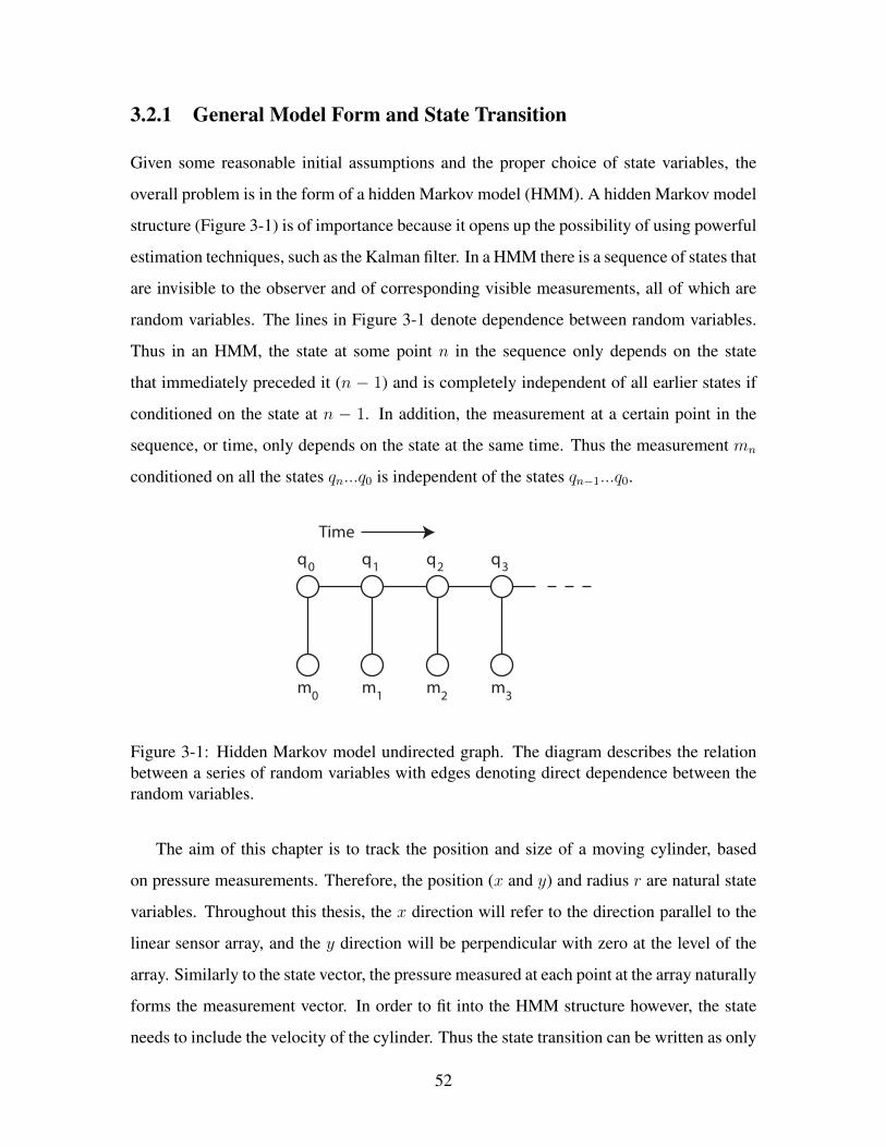
3.2.1 General Model Form and State Transition

Given some reasonable initial assumptions and the proper choice of state variables, the

overall problem is in the form of a hidden Markov model (HMM). A hidden Markov model

structure (Figure 3-1) is of importance because it opens up the possibility of using powerful

estimation techniques, such as the Kalman filter. In a HMM there is a sequence of states that

are invisible to the observer and of corresponding visible measurements, all of which are

random variables. The lines in Figure 3-1 denote dependence between random variables.

Thus in an HMM, the state at some point n in the sequence only depends on the state

that immediately preceded it (n − 1) and is completely independent of all earlier states if

conditioned on the state at n − 1. In addition, the measurement at a certain point in the

sequence, or time, only depends on the state at the same time. Thus the measurement mn

conditioned on all the states qn...q0 is independent of the states qn−1...q0.

Time

q q q q

m m mm0 1 2 3

0 1 2 3

Figure 3-1: Hidden Markov model undirected graph. The diagram describes the relationbetween a series of random variables with edges denoting direct dependence between therandom variables.

The aim of this chapter is to track the position and size of a moving cylinder, based

on pressure measurements. Therefore, the position (x and y) and radius r are natural state

variables. Throughout this thesis, the x direction will refer to the direction parallel to the

linear sensor array, and the y direction will be perpendicular with zero at the level of the

array. Similarly to the state vector, the pressure measured at each point at the array naturally

forms the measurement vector. In order to fit into the HMM structure however, the state

needs to include the velocity of the cylinder. Thus the state transition can be written as only

52

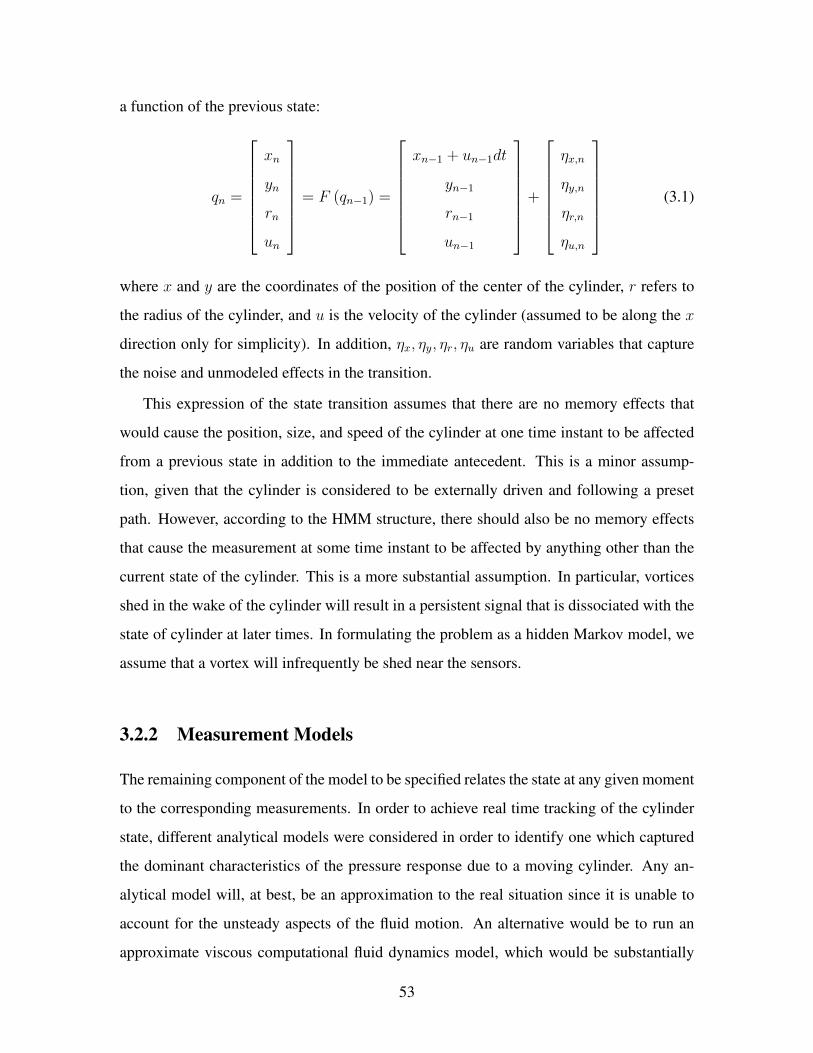
a function of the previous state:

qn =

xn

yn

rn

un

= F (qn−1) =

xn−1 + un−1dt

yn−1

rn−1

un−1

+

ηx,n

ηy,n

ηr,n

ηu,n

(3.1)

where x and y are the coordinates of the position of the center of the cylinder, r refers to

the radius of the cylinder, and u is the velocity of the cylinder (assumed to be along the x

direction only for simplicity). In addition, ηx, ηy, ηr, ηu are random variables that capture

the noise and unmodeled effects in the transition.

This expression of the state transition assumes that there are no memory effects that

would cause the position, size, and speed of the cylinder at one time instant to be affected

from a previous state in addition to the immediate antecedent. This is a minor assump-

tion, given that the cylinder is considered to be externally driven and following a preset

path. However, according to the HMM structure, there should also be no memory effects

that cause the measurement at some time instant to be affected by anything other than the

current state of the cylinder. This is a more substantial assumption. In particular, vortices

shed in the wake of the cylinder will result in a persistent signal that is dissociated with the

state of cylinder at later times. In formulating the problem as a hidden Markov model, we

assume that a vortex will infrequently be shed near the sensors.

3.2.2 Measurement Models

The remaining component of the model to be specified relates the state at any given moment

to the corresponding measurements. In order to achieve real time tracking of the cylinder

state, different analytical models were considered in order to identify one which captured

the dominant characteristics of the pressure response due to a moving cylinder. Any an-

alytical model will, at best, be an approximation to the real situation since it is unable to

account for the unsteady aspects of the fluid motion. An alternative would be to run an

approximate viscous computational fluid dynamics model, which would be substantially

53

more computationally expensive.

The standard analytical model for a cylinder in a steady uniform flow in an invis-

cid, irrotational fluid is created with a dipole, where the complex potential is Φ (z) =

u(z + a2

z−z0

). In this equation, z = x + iy and z0 refers to the complex location of the

center of the cylinder. The radius of the modeled cylinder is denoted by a. The complex

potential Φ is a combination of the velocity potential and stream function, Φ = φ + Iψ,

and the flow velocity can be obtained by: u − Iv = ∂Φ∂z

. The dipole model is severely

inadequate for tracking a moving cylinder, due to its complete lack of a wake. This not

only affects the pressure once the cylinder has passed a sensor, but changes the complete

near-field pressure distribution including ahead of the cylinder, as demonstrated shortly.

Three models were considered which would capture aspects of the wake of the cylinder

better than a dipole. The first model is an analytical potential flow model similar to the

dipole model, in which a source is instead used as the singularity for forming the structure.

The corresponding complex potential is:

Φ (z) = u (z + a log (z − z0)) (3.2)

As previously, z0 refers to the center of the cylinder. Also a is the radius of the cylinder,

which is taken to be the distance between the stagnation point and the center. This model is

commonly referred to as a Rankine half-body [60]. The second model under consideration

is a hybrid of the rankine half body with a dipole. The combination of the two allows the

width of the wake to be altered independently from the radius of the cylinder, unlike in the

case of the Rankine half-body. The corresponding complex potential for this hybrid model

is

Φ (z) = u

(z +

β2

z − z0

+a2 − β2

alog (z − z0)

)(3.3)

Here, a is still the radius of the cylinder, and β is a weighting factor that ranges from 0

to a corresponding to the range between just a source and just a dipole. The final model

is based on a slightly different approach, in which a shadow of the cylinder was manually

extended downstream from the furthest lateral points on the cylinder in order to simulate a

thin wake. The flow was evaluated around this extended cylinder using a panel method. A

54

depiction of the streamlines passing through the stagnation point for each model is shown

in Figure 3-2 for situations both near and far from a wall.

These potential models were used to obtain the near field pressure via the unsteady

Bernoulli equation [60]:

P (z) +1

2ρ

∣∣∣∣∂Φ (z)

∂z

∣∣∣∣2 + ρ∂φ (x, y)

∂t= P∞ +

1

2ρu2∞ (3.4)

Note that the derivative in time is with respect to the velocity potential only (the real com-

ponent of Φ), and is therefore always real and a function of x and y separately rather than

of z = x + iy alone.1 Also, this unsteady form of the Bernoulli equation applies to every

instant in time separately, but considering the pressure at a spatially distant points constant

enables the comparison across time.

3.2.3 Measurement Model Frame Equivalence

Although the problem scenario is that of a cylinder steadily translating through still water

next to a flat plate, this is equivalent to the scenario in which the cylinder is stationary under

a steady uniform flow next to a flat plate with the position of the sensors translating on the

plate. This equivalence holds due to the assumption that the flat plate extends infinitely,

and thus there is no difference in the potential model except the change in location. It is

similarly valid if there is no sensing body included in the model. The equivalence can be

seen explicitly by considering the Bernoulli equation applied to the two scenarios with a

general complex potential model. Let z0 refer to a fixed position for the cylinder corre-

sponding to the case with the moving sensor frame of reference, and zn = z0 − utn be the

position of the moving cylinder at time-step n in the physical scenario. For the purpose of

demonstrating the equivalency, let both the velocity and perpendicular distance from the

sensors be constant: un = u and yn = y0. Correspondingly, consider a general complex

potential Φ (z − zn) for the moving cylinder in still water, which is related to the complex

potential of the stationary cylinder in a steady flow by Φ (z − z0) = Φ (z − z0) + uz. The

1The distinction made here is between, for instance, xex+iy and (x+iy)ex+iy . The latter can be expressedin terms of the z = x+ iy variable alone, yielding zez , whereas the former cannot.

55

argument of the complex potential is written explicitly as z− z0 in order to denote the rela-

tionship between the point of evaluation, z, and the center of the cylinder z0. Note that all

the complex potentials discussed so far have this form (except the shadow wake generated

by the panel method, which is similar but without all the singularities centered at z0). In

the case of the stationary cylinder, the Bernoulli equation reduces as:

P (z) +1

2ρ

∣∣∣∣∂Φ (z − z0)

∂z

∣∣∣∣2 + ρ∂φ (x− x0, y − y0)

∂t= P∞ +

1

2ρu2∞

P (z) +1

2ρ

∣∣∣∣∂(

Φ (z − z0) + uz)

∂z

∣∣∣∣2 = P∞ +1

2ρu2

P (z)− P∞ = −1

2ρ

∣∣∣∣∂Φ (z − z0)

∂z+ u

∣∣∣∣2 +1

2ρu2

P (z)− P∞ = −1

2ρ

(∣∣∣∣∂Φ (z − z0)

∂z

∣∣∣∣2 + 2u<

[∂Φ (z − z0)

∂z

]+ u2

)+

1

2ρu2

P (z)− P∞ = −1

2ρ

(∣∣∣∣∂Φ (z − z0)

∂z

∣∣∣∣2 + 2u∂φ (x− x0, y − y0)

∂x

)(3.5)

Considering the case of a moving cylinder passing the same point as the stationary

cylinder, without external flow:

P (z) +1

2ρ

∣∣∣∣∂Φ (z − zn)

∂z

∣∣∣∣2 + ρ∂φ (x− xn, y − y0)

∂t= P∞ +

1

2ρu2∞

P (z) +1

2ρ

∣∣∣∣∂Φ (z − zn)

∂z

∣∣∣∣2 + ρ∂φ (x− xn, y − yn)

∂xn

∂xn∂t

= P∞ +1

2ρ02

P (z) +1

2ρ

∣∣∣∣∂Φ (z − zn)

∂z

∣∣∣∣2 + ρ∂φ (x− xn, y − y0)

∂xu = P∞

P (z)− P∞ = −1

2ρ

∣∣∣∣∂Φ (z − zn)

∂z

∣∣∣∣2 − ρ∂φ (x− xn, y − y0)

∂xu

P (z)− P∞ = −1

2ρ

(∣∣∣∣∂Φ (z − zn)

∂z

∣∣∣∣2 + 2u∂φ (x− xn, y − y0)

∂x

)(3.6)

Since zn (t = 0) = z0, both frames of reference give the same results. For compactness, the

stationary cylinder frame is preferred since there is no time derivative in the corresponding

in the Bernoulli equation.

56

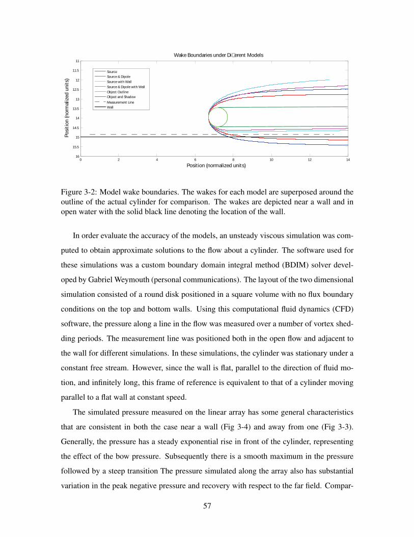
Position (normalized units)

Po

siti

on

(n

orm

ali

ze

d u

nit

s)

Wake Boundaries under Dierent Models

0 2 4 6 8 10 12 14

11

11.5

12

12.5

13

13.5

14

14.5

15

15.5

16

Source

Source & Dipole

Source with Wall

Source & Dipole with Wall

Object Outline

Measurement Line

Wall

Object and Shadow

Figure 3-2: Model wake boundaries. The wakes for each model are superposed around theoutline of the actual cylinder for comparison. The wakes are depicted near a wall and inopen water with the solid black line denoting the location of the wall.

In order evaluate the accuracy of the models, an unsteady viscous simulation was com-

puted to obtain approximate solutions to the flow about a cylinder. The software used for

these simulations was a custom boundary domain integral method (BDIM) solver devel-

oped by Gabriel Weymouth (personal communications). The layout of the two dimensional

simulation consisted of a round disk positioned in a square volume with no flux boundary

conditions on the top and bottom walls. Using this computational fluid dynamics (CFD)

software, the pressure along a line in the flow was measured over a number of vortex shed-

ding periods. The measurement line was positioned both in the open flow and adjacent to

the wall for different simulations. In these simulations, the cylinder was stationary under a

constant free stream. However, since the wall is flat, parallel to the direction of fluid mo-

tion, and infinitely long, this frame of reference is equivalent to that of a cylinder moving

parallel to a flat wall at constant speed.

The simulated pressure measured on the linear array has some general characteristics

that are consistent in both the case near a wall (Fig 3-4) and away from one (Fig 3-3).

Generally, the pressure has a steady exponential rise in front of the cylinder, representing

the effect of the bow pressure. Subsequently there is a smooth maximum in the pressure

followed by a steep transition The pressure simulated along the array also has substantial

variation in the peak negative pressure and recovery with respect to the far field. Compar-

57

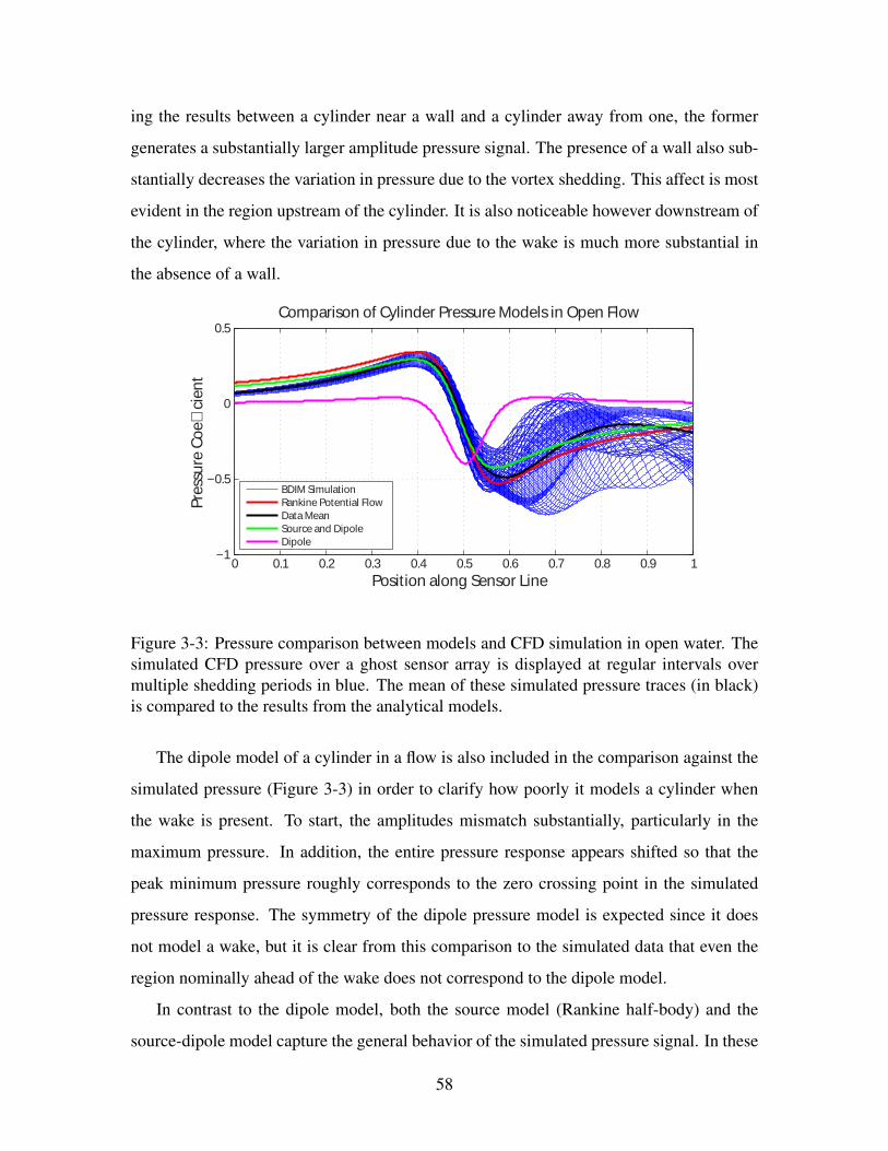
ing the results between a cylinder near a wall and a cylinder away from one, the former

generates a substantially larger amplitude pressure signal. The presence of a wall also sub-

stantially decreases the variation in pressure due to the vortex shedding. This affect is most

evident in the region upstream of the cylinder. It is also noticeable however downstream of

the cylinder, where the variation in pressure due to the wake is much more substantial in

the absence of a wall.

0 0.1 0.2 0.3 0.4 0.5 0.6 0.7 0.8 0.9 1−1

−0.5

0

0.5

Position along Sensor Line

Pre

ssu

re C

oe

ci

en

t

BDIM Simulation

Rankine Potential Flow

Data Mean

Source and Dipole

Dipole

Comparison of Cylinder Pressure Models in Open Flow

Figure 3-3: Pressure comparison between models and CFD simulation in open water. Thesimulated CFD pressure over a ghost sensor array is displayed at regular intervals overmultiple shedding periods in blue. The mean of these simulated pressure traces (in black)is compared to the results from the analytical models.

The dipole model of a cylinder in a flow is also included in the comparison against the

simulated pressure (Figure 3-3) in order to clarify how poorly it models a cylinder when

the wake is present. To start, the amplitudes mismatch substantially, particularly in the

maximum pressure. In addition, the entire pressure response appears shifted so that the

peak minimum pressure roughly corresponds to the zero crossing point in the simulated

pressure response. The symmetry of the dipole pressure model is expected since it does

not model a wake, but it is clear from this comparison to the simulated data that even the

region nominally ahead of the wake does not correspond to the dipole model.

In contrast to the dipole model, both the source model (Rankine half-body) and the

source-dipole model capture the general behavior of the simulated pressure signal. In these

58

comparisons, the parameter determining the width of the wake was set to the value mini-

mizing the least-squares difference with respect to the mean simulated pressure trace away

from a wall. Both the source and the tuned source and dipole model approximately match

the mean simulated data’s amplitude in the pressure response and are closely aligned in

position at the point were the pressure transitions from positive to negative. However,

both models share the same faults at either extreme of the pressure response. Upstream of

the cylinder, the decay in pressure is dominated by the source singularity and decays too

slowly with respect to the simulated results. As expected, downstream of the cylinder, the

two models only roughly match the average decay from the simulated data. This is unsur-

prising, since there is a large amount of variation in the pressure corresponding to the wake

region which cannot be captured by a single steady analytical model.

The primary difference between the source and the source and dipole models is in the

amplitude of the pressure response near the transition region. At the positive pressure peak,

the model with the dipole thinning the wake matches the mean simulated results very well,

while the rankine model overestimates the maximum pressure. For the peak minimum

pressure, both models differ from the mean simulated response by about an equal amount,

but with the source and dipole model making an overestimate while the rankine model

underestimates. Although there are differences between the pressure predicted by the two

models, they are small with respect to the variation in pressure that occurs within one vortex

shedding period.

The results from the panel method model in which only the shadow of the cylinder was

projected to simulate a wake resulted in pressure whose amplitude fell below the projected

values by a substantial margin, remaining at less than half the amplitude of the simulated

results. This clearly indicates that the wake in this model is too small. Since both the

Rankine and the source-dipole models predict a pressure distribution that is much closer to

the CFD results, the directly specified panel method wake will not be considered further.

In the case of a simulated cylinder away from a wall, both the Rankine and the source

dipole mixture capture the appropriate transition behavior in pressure. Near a wall, the

situation changes only slightly (Figure 3-4). The effect of the wall increases the amplitude

pressure measured in the sensor array. Using the same wake thickness as for the no-wall

59

simulations, the source and dipole model still captures the maximum pressure very well

and now is much closer to the minimum peak pressure. The model with the source alone

over estimates the magnitude of the pressure throughout the transition area. Beyond these

differences, the agreement with the simulated pressure results is no different than in the no-

wall case. When a wall is present, the source-dipole model predicts the correct amplitude

in pressure on the sensor array, while the Rankine model consistently overestimates it.

One important note is that when a wall is present, the Rankine model will result in

pressure that nearly overlaps the source-dipole model if the radius of the Rankine model

cylinder is reduced ten percent. This implies that there are few significant differences

between the overall shape of the pressure response from the two models, but there is a

difference in the modeling of the size of the cylinder. If the Rankine half-body model is

used for solving the inverse problem, it should be expected that the size of the cylinder will

be under-estimated.

0 0.1 0.2 0.3 0.4 0.5 0.6 0.7 0.8 0.9 1

−1.2

−1

−0.8

−0.6

−0.4

−0.2

0

0.2

0.4

0.6

0.8

Position along Sensor Line

Pre

ssu

re C

oe

ci

en

t

Comparison of Pressure Measurements between Models

BDIM Simulation

Simulation Average

Rankine Potential Flow

Source & Dipole

Rankine with Wall

Source & Dipole with Wall

Figure 3-4: Pressure comparison between models and CFD simulation near a wall. TheCFD results are displayed in blue at various intervals of the vortex shedding period. Thisgraph corresponds to the layout described in Figure 3-2. The results of the Rankine half-body and the source-dipole hybrid model are plotted both with and without the wall present.

The conclusions from the CFD simulations of a cylinder in a steady flow indicate that

an analytical model based on a source and dipole will predict the pressure on a linear

sensor array well in the vicinity of the cylinder, but with less accuracy and some systematic

bias both up and downstream of the cylinder. The Rankine model behaves similarly, with

60

slightly worse performance in the open water case compared to the source-dipole model,

and an underestimate of the cylinder size when near the wall. However, the purpose of

examining these models is to obtain a basis for the tracking of a cylinder in real time in

a real environment. For that purpose, the Rankine model is better suited than the source-

dipole model if there is a wall near. Due to the image of the cylinder needed to represent

the wall, the stagnation point used to define the size of the cylinder migrates towards the

wall, and modeling a cylinder of a specified radius requires further costly calculations. In

comparison, the Rankine model has a similar migration of the stagnation point, but the

model can still be analytically expressed as a function of the cylinder diameter. The cost of

using the Rankine model would be predicted to be a slight underestimate of the radius of

the cylinder, but since there is no difference between the responses when using a smaller

radius, it should not affect the ability to track a cylinder.

In order to evaluate ability to track a cylinder based on a Rankine model, data was col-

lected from a series of experiments representing the scenario of interest. The fundamental

characteristic of the experiment was to pass a circular cylinder moving at constant velocity

past an array of pressure sensors with a precise specified distance, matching the scenario

used for the model.

3.3 Experimental Setup

The experiments were conducted in the CENSAM Singapore experimental tank. The CEN-

SAM tank is 3.6 m long by 1.2 m wide and approximately 1 m deep. Two separate com-

ponents are involved in the experiment: a method for moving a cylinder along a precise

path and a sensing platform that reproduces the ability of a lateral-line like sensor array

embedded in an infinite wall.

3.3.1 Cylinder Motion

On the top of the tank, a two-dimensional positioning system allows accurate position

and velocity specification over the water. The positioning system is composed of an ”H”

configuration of belt-driven linear actuators (Parker LCB-40). Two 3.6 meter long actuators

61

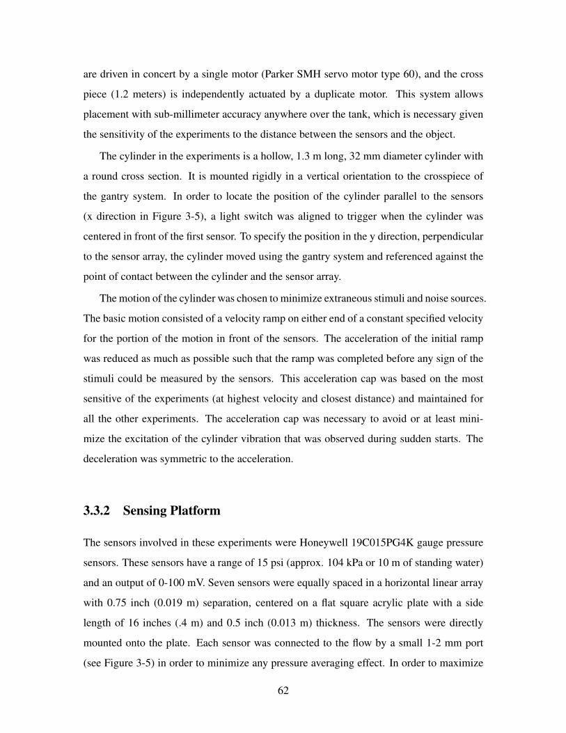
are driven in concert by a single motor (Parker SMH servo motor type 60), and the cross

piece (1.2 meters) is independently actuated by a duplicate motor. This system allows

placement with sub-millimeter accuracy anywhere over the tank, which is necessary given

the sensitivity of the experiments to the distance between the sensors and the object.

The cylinder in the experiments is a hollow, 1.3 m long, 32 mm diameter cylinder with

a round cross section. It is mounted rigidly in a vertical orientation to the crosspiece of

the gantry system. In order to locate the position of the cylinder parallel to the sensors

(x direction in Figure 3-5), a light switch was aligned to trigger when the cylinder was

centered in front of the first sensor. To specify the position in the y direction, perpendicular

to the sensor array, the cylinder moved using the gantry system and referenced against the

point of contact between the cylinder and the sensor array.

The motion of the cylinder was chosen to minimize extraneous stimuli and noise sources.

The basic motion consisted of a velocity ramp on either end of a constant specified velocity

for the portion of the motion in front of the sensors. The acceleration of the initial ramp

was reduced as much as possible such that the ramp was completed before any sign of the

stimuli could be measured by the sensors. This acceleration cap was based on the most

sensitive of the experiments (at highest velocity and closest distance) and maintained for

all the other experiments. The acceleration cap was necessary to avoid or at least mini-

mize the excitation of the cylinder vibration that was observed during sudden starts. The

deceleration was symmetric to the acceleration.

3.3.2 Sensing Platform

The sensors involved in these experiments were Honeywell 19C015PG4K gauge pressure

sensors. These sensors have a range of 15 psi (approx. 104 kPa or 10 m of standing water)

and an output of 0-100 mV. Seven sensors were equally spaced in a horizontal linear array

with 0.75 inch (0.019 m) separation, centered on a flat square acrylic plate with a side

length of 16 inches (.4 m) and 0.5 inch (0.013 m) thickness. The sensors were directly

mounted onto the plate. Each sensor was connected to the flow by a small 1-2 mm port

(see Figure 3-5) in order to minimize any pressure averaging effect. In order to maximize

62

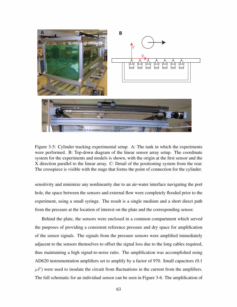
X

Y

A B

C

Figure 3-5: Cylinder tracking experimental setup. A: The tank in which the experimentswere performed. B: Top-down diagram of the linear sensor array setup. The coordinatesystem for the experiments and models is shown, with the origin at the first sensor and theX direction parallel to the linear array. C: Detail of the positioning system from the rear.The crosspiece is visible with the stage that forms the point of connection for the cylinder.

sensitivity and minimize any nonlinearity due to an air-water interface navigating the port

hole, the space between the sensors and external flow were completely flooded prior to the

experiment, using a small syringe. The result is a single medium and a short direct path

from the pressure at the location of interest on the plate and the corresponding sensor.

Behind the plate, the sensors were enclosed in a common compartment which served

the purposes of providing a consistent reference pressure and dry space for amplification

of the sensor signals. The signals from the pressure sensors were amplified immediately

adjacent to the sensors themselves to offset the signal loss due to the long cables required,

thus maintaining a high signal-to-noise ratio. The amplification was accomplished using

AD620 instrumentation amplifiers set to amplify by a factor of 970. Small capacitors (0.1

µF ) were used to insulate the circuit from fluctuations in the current from the amplifiers.

The full schematic for an individual sensor can be seen in Figure 3-6. The amplification of

63

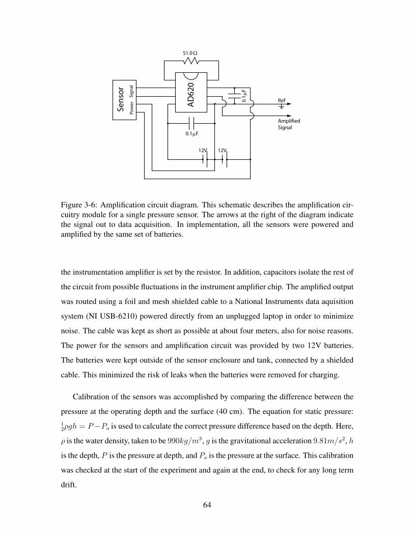
AD

620

Sens

or

12V 12V

0.1 Fµ

0.1

F µ

Ref

AmpliedSignal

51.0 Ω

Pow

erSi

gnal

Figure 3-6: Amplification circuit diagram. This schematic describes the amplification cir-cuitry module for a single pressure sensor. The arrows at the right of the diagram indicatethe signal out to data acquisition. In implementation, all the sensors were powered andamplified by the same set of batteries.

the instrumentation amplifier is set by the resistor. In addition, capacitors isolate the rest of

the circuit from possible fluctuations in the instrument amplifier chip. The amplified output

was routed using a foil and mesh shielded cable to a National Instruments data aquisition

system (NI USB-6210) powered directly from an unplugged laptop in order to minimize

noise. The cable was kept as short as possible at about four meters, also for noise reasons.

The power for the sensors and amplification circuit was provided by two 12V batteries.

The batteries were kept outside of the sensor enclosure and tank, connected by a shielded

cable. This minimized the risk of leaks when the batteries were removed for charging.

Calibration of the sensors was accomplished by comparing the difference between the

pressure at the operating depth and the surface (40 cm). The equation for static pressure:12ρgh = P−Po is used to calculate the correct pressure difference based on the depth. Here,

ρ is the water density, taken to be 990kg/m3, g is the gravitational acceleration 9.81m/s2, h

is the depth, P is the pressure at depth, and Po is the pressure at the surface. This calibration

was checked at the start of the experiment and again at the end, to check for any long term

drift.

64

3.3.3 Test Matrix

To quantify the dependence of the tracking accuracy on the motion parameters, a series of

experiments were performed with the same cylinder and experimental setup. The first of

the two variables of interest is the speed of the cylinder, which affects the strength of the

pressure field and the Reynolds number. The wake characteristics and Reynolds number are

closely tied. The second variable of interest is the minimum distance from the sensors in the

path of the cylinder (in the y direction according to Figure 3-5). The specific matrix of tests

is described in Table 3.1 The velocity ranges from 125 mm/s to 313 mm/s, corresponding

to a range of Reynolds numbers between 4,000 and 10,000. At the upper end of signal

strength, the range of the two variables was limited by the speed of the gantry system and

the minimum distance for which there was complete confidence in avoiding collisions. At

the other extreme of the testing matrix, at a velocity of 125 mm/s and distance of 20 mm,

the measured signal is on the order of 10 Pa which is comparable to the unprocessed noise

levels. Due to the variability of the wake, five runs were carried out for each element of the

testing matrix.

2 mm 5 mm 10 mm 15 mm 20 mm0.31 m/s 5 Runs0.25 m/s 5 Runs 5 Runs 5 Runs 5 Runs 5 Runs0.19 m/s 5 Runs 5 Runs 5 Runs 5 Runs 5 Runs0.13 m/s 5 Runs 5 Runs 5 Runs 5 Runs 5 Runs

Table 3.1: Experimental matrix for cylinder tracking. The range of velocities and distanceswas determined by the signal strength and by the abilities and noise of the experimentalsetup.

3.3.4 Noise Analysis and Data Preparation

The signals of interest in these experiments are of very small magnitude. In the case of a

strong response they are on the order of 200 Pa, but for weaker stimuli they are on the order

of 20 Pa or less. As a result, managing noise and inteference from external sources was

of extreme importance in the experiments. Many aspects of the experimental setup were

chosen in order to minimize noise, as described in section 3.3, but others had to be managed

65

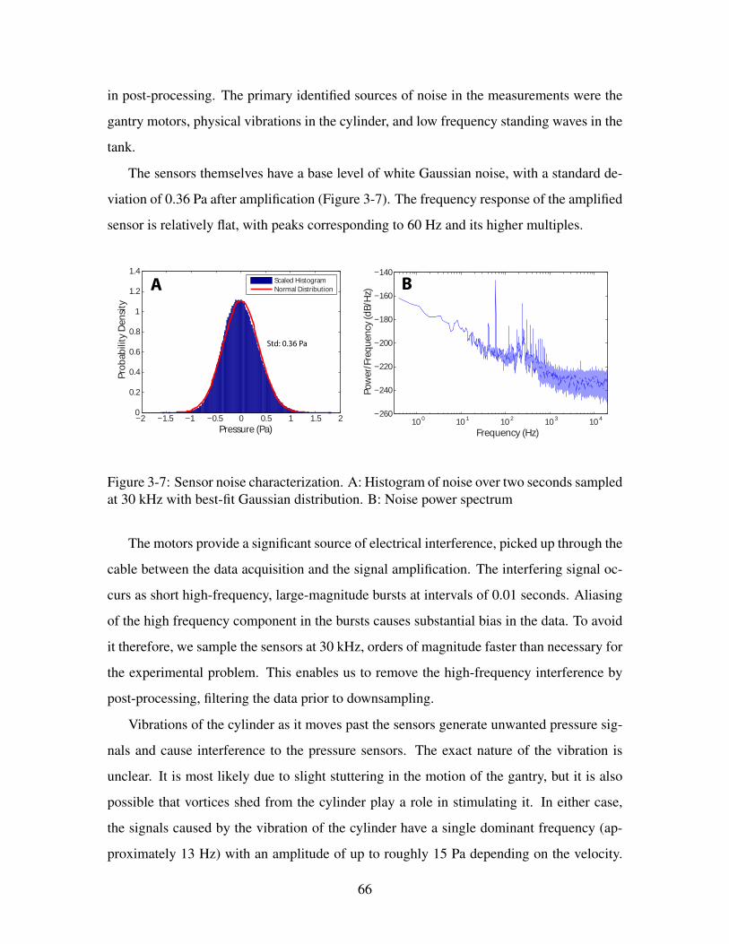
in post-processing. The primary identified sources of noise in the measurements were the

gantry motors, physical vibrations in the cylinder, and low frequency standing waves in the

tank.

The sensors themselves have a base level of white Gaussian noise, with a standard de-

viation of 0.36 Pa after amplification (Figure 3-7). The frequency response of the amplified

sensor is relatively flat, with peaks corresponding to 60 Hz and its higher multiples.

−2 −1.5 −1 −0.5 0 0.5 1 1.5 20

0.2

0.4

0.6

0.8

1

1.2

1.4

Pressure (Pa)

Pro

ba

bil

ity

De

nsi

ty

Scaled Histogram

Normal Distribution

100

101

102

103

104

−260

−240

−220

−200

−180

−160

−140

Frequency (Hz)

Po

we

r/F

req

ue

ncy

(d

B/H

z)

Std: 0.36 Pa

A B

Figure 3-7: Sensor noise characterization. A: Histogram of noise over two seconds sampledat 30 kHz with best-fit Gaussian distribution. B: Noise power spectrum

The motors provide a significant source of electrical interference, picked up through the

cable between the data acquisition and the signal amplification. The interfering signal oc-

curs as short high-frequency, large-magnitude bursts at intervals of 0.01 seconds. Aliasing

of the high frequency component in the bursts causes substantial bias in the data. To avoid

it therefore, we sample the sensors at 30 kHz, orders of magnitude faster than necessary for

the experimental problem. This enables us to remove the high-frequency interference by

post-processing, filtering the data prior to downsampling.

Vibrations of the cylinder as it moves past the sensors generate unwanted pressure sig-

nals and cause interference to the pressure sensors. The exact nature of the vibration is

unclear. It is most likely due to slight stuttering in the motion of the gantry, but it is also

possible that vortices shed from the cylinder play a role in stimulating it. In either case,

the signals caused by the vibration of the cylinder have a single dominant frequency (ap-

proximately 13 Hz) with an amplitude of up to roughly 15 Pa depending on the velocity.

66

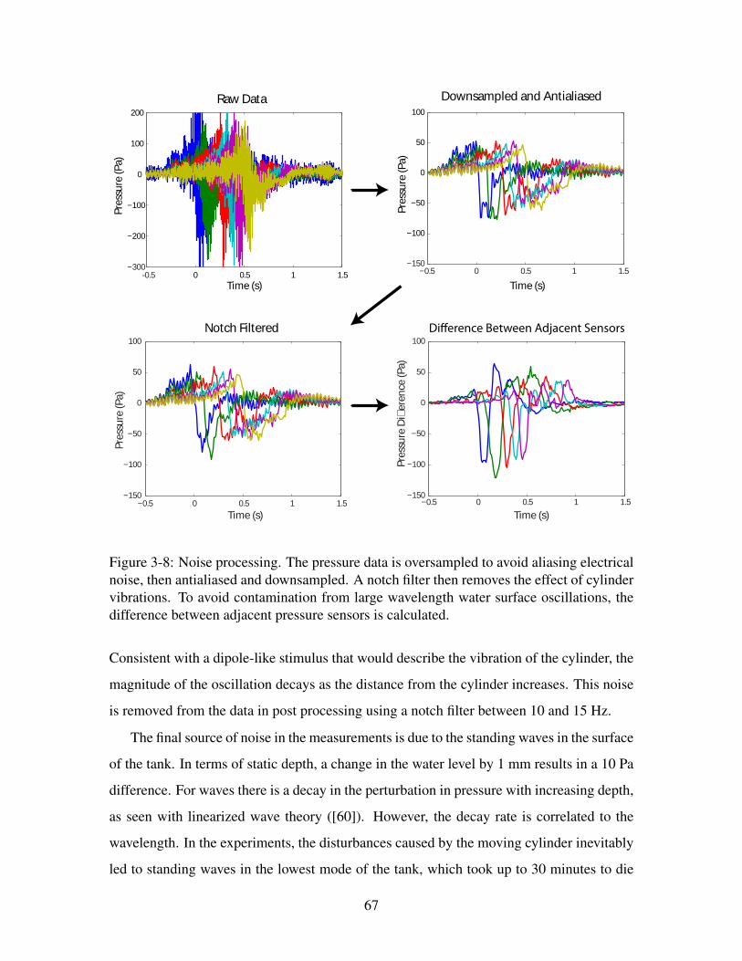
-0.5 0 0.5 1 1.5−300

−200

−100

0

100

200

Time (s)

Pre

ssu

re (

Pa

)

Raw Data

−0.5 0 0.5 1 1.5−150

−100

−50

0

50

100

Time (s)

Pre

ssu

re D

ie

ren

ce (

Pa

)

Dierence Between Adjacent Sensors

−0.5 0 0.5 1 1.5−150

−100

−50

0

50

100

Time (s)

Pre

ssu

re (

Pa

)

Notch Filtered

−150

−100

−50

0

50

100

Time (s)

Pre

ssu

re (

Pa

)

Downsampled and Antialiased

−0.5 0 0.5 1 1.5

Figure 3-8: Noise processing. The pressure data is oversampled to avoid aliasing electricalnoise, then antialiased and downsampled. A notch filter then removes the effect of cylindervibrations. To avoid contamination from large wavelength water surface oscillations, thedifference between adjacent pressure sensors is calculated.

Consistent with a dipole-like stimulus that would describe the vibration of the cylinder, the

magnitude of the oscillation decays as the distance from the cylinder increases. This noise

is removed from the data in post processing using a notch filter between 10 and 15 Hz.

The final source of noise in the measurements is due to the standing waves in the surface

of the tank. In terms of static depth, a change in the water level by 1 mm results in a 10 Pa

difference. For waves there is a decay in the perturbation in pressure with increasing depth,

as seen with linearized wave theory ([60]). However, the decay rate is correlated to the

wavelength. In the experiments, the disturbances caused by the moving cylinder inevitably

led to standing waves in the lowest mode of the tank, which took up to 30 minutes to die

67

out. Considering the difference in pressure between adjacent pressure sensors, which can

be interpreted as a simple spatial low-pass filtering scheme, effectively removes this noise

source. The success of the scheme is owed to the fact that, since only the large-wavelength

waves generate the disturbance, the disturbance is equal across all the sensors and therefore

vanishes in the differential.

The final result of the combined post-processing is a data set consisting of the difference

in pressure between adjacent sensors, sampled at 100 Hz. In general, the processing is suf-

ficiently cost-effective for expected applications outside of the laboratory, as the described

filtering techniques can be realized through efficient algorithms in both software and hard-

ware. Moreover, several of the post-processing steps are an artifact of the experimental

setup and are unnecessary in an application setting. In particular, the first two filtering

steps are necessary solely due to the noise introduced by the two dimensional gantry and

not due to extra fluid stimuli (such as wake vortices). In either a biological or naval set-

ting, one would not expect a moving object to generate noise comparable to the cylinder

vibration or motor electrical interference. Signal contamination due to surface waves is

still a concern in both applications, but it is notable that the fish lateral line also measures

pressure differences.

3.4 Results

The results of the experiments match the CFD results in form. Generally described, the

signal of a cylinder passing a sensor results in an initial increase in pressure relative to

when there is no cylinder, followed by a sharp transition to negative pressure and a slower

recovery to zero. The maximum pressure is generally smaller in magnitude than the mini-

mum pressure after the sharp transition. This trace is similarly replicated, if shifted in time,

for each sensor in a single run.

The averaged results for each point in the test matrix are visible in Figure 3-9. Based

on these results, it is clear that there is a strong relationship between the velocity of the

cylinder and the magnitude of the pressure signals, but a much weaker one between the

magnitude and the distance of the cylinder. Instead, the distance of the cylinder appears

68

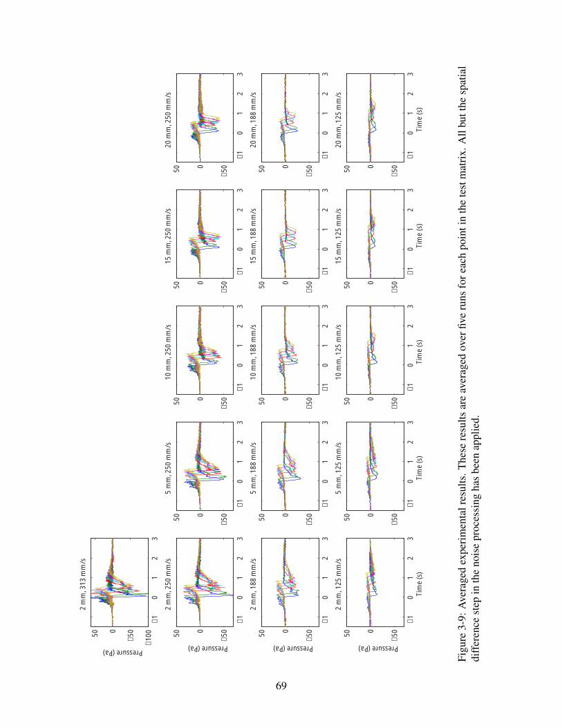
−1

01

23

−5

00

50

2 m

m, 1

25

mm

/s

Tim

e (

s)

Pressure (Pa)

−1

01

23

−5

00

50

2 m

m, 1

88

mm

/s

Pressure (Pa)

−1

01

23

−5

00

50

2 m

m, 2

50

mm

/s

Pressure (Pa)

−1

01

23

−1

00

−5

00

50

2 m

m, 3

13

mm

/sPressure (Pa)

−1

01

23

−5

00

50

5 m

m, 1

25

mm

/s

Tim

e (

s)

−1

01

23

−5

00

50

5 m

m, 1

88

mm

/s

−1

01

23

−5

00

50

5 m

m, 2

50

mm

/s

−1

01

23

−5

00

50

10

mm

, 12

5 m

m/s

Tim

e (

s)

−1

01

23

−5

00

50

10

mm

, 18

8 m

m/s

−1

01

23

−5

00

50

10

mm

, 25

0 m

m/s

−1

01

23

−5

00

50

15

mm

, 12

5 m

m/s

Tim

e (

s)

−1

01

23

−5

00

50

15

mm

, 18

8 m

m/s

−1

01

23

−5

00

50

15

mm

, 25

0 m

m/s

−1

01

23

−5

00

50

20

mm

, 12

5 m

m/s

Tim

e (

s)

−1

01

23

−5

00

50

20

mm

, 18

8 m

m/s

−1

01

23

−5

00

50

20

mm

, 25

0 m

m/s

Figu

re3-

9:A

vera

ged

expe

rim

enta

lres

ults

.The

sere

sults

are

aver

aged

over

five

runs

fore

ach

poin

tin

the

test

mat

rix.

All

butt

hesp

atia

ldi

ffer

ence

step

inth

eno

ise

proc

essi

ngha

sbe

enap

plie

d.

69

to primarily affect the speed at which the pressure recovers to it’s ambient state after the

cylinder has passed.

One important note is that the third pressure sensor from the left in the array was not

available during the experiments due to electronic problems. This sensor is disregarded for

the purposes of analysis and estimation. When considering the difference between adjacent

sensors, this implies that one of these differences is taken over twice the distance of the

others. However, this small anomaly requires no modifications in the model or estimation

of the cylinder state, as the model is valid for a general number of sensors. Moreover, the

loss of one sensor is very unlikely to have an effect on the overall results beyond decreased

noise-reduction performance due to a loss of redundancy in measurement.

3.5 Cylinder State Estimation

With a promising model identified using CFD simulations and an experimental data set

to use for evaluating effectiveness, it is possible to identify and test estimation techniques

for tracking a cylinder position and size based on the measurements of a pressure sensor

array. The HMM structure of the problem implies that many powerful estimation strategies,

such as the Kalman filter, will apply. However, the nonlinear form of the model and the

constrained relationships between the state variables mean that not all approaches will be

equal and some exploration is required.

For the model described in this chapter (Section 3.2), the portion of the model dealing

with the state transition (equation 3.1) is already linear. However, the other half of the

model, using a Rakine half-body potential flow model to describe the measurements on the

sensor array given a cylinder state (equation 3.2) is not linear. Many estimation techniques,

such as the Kalman filter, work directly on linear models. For these techniques, the success

of local linear approximations to the model, such as those in the extended Kalman filter,

depends on the type and extent of the nonlinearity. Considering the experimental setup in

which the sensors are imbedded in a flat wall, the relation between the measurements and

the state is:

P (s)− P∞ =1

2ρu2

n

∣∣∣∣1 +kn

s− zn+

kns− zn

∣∣∣∣2 (3.7)

70

Both the pressure P and sensors location s are vectors in these equations. Also, since the

sensors are imbedded in the flat plate that forms the axis of symmetry, s is a real vector. The

overbar on zn denotes the complex conjugate. Note that the pressure is given as a pressure

difference with respect to the far-field pressure P∞. Also, the variable kn is related to the

radius of the modeled cylinder, but due to the presence of an image, it also depends on the

distance of the center from the sensors, yn. The exact relation is:

kn =1

2

√4y2

n − r2na

yn(3.8)

As expected, the variable kn approaches the radius rn as the distance yn increases. Al-

though the radius, speed, and perpendicular distance are constant in the experiments, the

model allows for changes as might occur under different circumstances. The combina-

tion of these equations fully describe the measurement model, and result from the Rankine

half-body model, equation 3.2, applied to the Bernoulli equation, equation 3.4. Based on

equations 3.7 and 3.8, it is clear that the pressure measurements are nonlinear in all of the

state variables.

3.5.1 Cylinder Tracking via a Kalman Filter

The Kalman filter is a form of a predictor-corrector estimator which chooses a gain for the

correction which is optimal for a linear system with white Gaussian noise. It operates on

a hidden Markov model or its continuous state equivalent. To estimate the hidden state

based on the measurements, the Kalman filter tracks both the state estimate and the error

covariance matrix of the estimate. In dealing with nonlinear transition and measurement

models, the most common approach is to linearize the equations in a first order taylor series

approximation, referred to as the extended Kalman filter. Another more recent extension of

the Kalman filter, the unscented Kalman filter, effectively keeps higher order terms of the

approximation with the added advantage of not having to compute the Jacobian each time.

As a very flexible and robust estimation technique, the Kalman filter and its variants are the

first logical estimation approaches for consideration. The details of the Kalman filter and

its nonlinear variants are described in [27] among many other texts.

71

As it relates to the problem of tracking the state of a moving cylinder, a key component

of the Kalman filter approach is that it approximates all noise variables as zero mean Gaus-

sian random variables. There are two sets of noise variables. The first set is associated with

the measurement equations. In this case, the distribution can be matched to the electrical

noise inherent in the measurement. The second set of noise variables is those represented

in equation 3.1 which capture any uncertainty in the transition between states and are in-

dependent from the measurement noise variables. While the transition between states is

nominally known exactly, this noise allows for some flexibility due to a potential misalign-

ment in the axis of motion or the influence of unmodeled factors. The variance of these

noise variables also affects the gain used during the Kalman filter correction step. In tuning

the relative weight of the transition noise variance to the measurement noise variance, it is

possible to adjust the confidence in new measurements of the Kalman filter relative to the

predicted trajectory based on the state transition model.

The state variables in this problem are not independent. In particular, both the radius

and the perpendicular distance must be positive, and the radius of the cylinder cannot be

greater than the perpendicular distance: 0 < rn < yn. These constraints are physically

intuitive, since the cylinder cannot pass behind the sensors and a negative radius is non-

sensical. Similarly, if the radius is larger than the perpendicular distance, this implies that

a collision will take between the cylinder and the plate on which the sensors are mounted.

Unfortunately, the potential flow model used to predict the pressure measurements along

the linear sensor array cannot account for these physical boundaries. The boundary that

defines the the surface of the cylinder is a hypothetical one, matching a streamline in the

flow model at the stagnation point only. As a result, the equations described in 3.7 and 3.8

result in predicted pressures of similar magnitude regardless of the signs of the radius and

distance, and more importantly, regardless of the relative values of the two variables. This

implies that there is no substantially increasing error that will drive the estimate of the

Kalman filter away from these boundaries in the correction phase of the filter, and as a

result the estimated state may stray into non-physical regions. These occurrences can be

crudely prevented by testing the state variable relations each iteration and forcing the state

back into a legitimate physical region when a violation occurs. This can work if it occurs

72

rarely, but for the most part does not lead a good result as it does not stop the underlying

cause.

The extended Kalman filter was tested first on data simulated using the model from sec-

tion 3.2 and subsequently using data gathered in the experiments. For the model described

in this chapter (Section 3.2), the portion of the model dealing with the state transition (equa-

tion 3.1) is already linear. The measurement equation is linearized using the corresponding

Jacobian matrix. The simulated data was generated by first generating a sequence of states

using the state transition model initialized to a state in line with the experiments. For exam-

ple, with an initial state of 35mm perpendicular distance, 15mm radius, 250mm/s velocity,

and -50mm x position, the sequence of states would progress in the x direction with con-

stant increments determined by the sampling rate, with the other variables held constant.

Based on these states, the measurements are generated using equation 3.7, again without

the addition of any noise. This noiseless simulated data set is the most favorable initial

test for an estimation algorithm, since the model used in the algorithm exactly matches the

model used to generated the data and there is no noise. As such, it provides an opportunity

to tune the various noise and initialization parameters of the Kalman filter. Although efforts

were made to accurately reflect the noise parameters of the experiment, little information

is available for the process noise in the state transition, and so the sensitivity of the mea-

surements to the state variable can be used to influence the choice. A typical result of the

extended Kalman filter application to simulated data can be seen in Figure 3-10. In this ex-

ample, it is evident that the extended Kalman filter converges to fairly accurate estimates of

the position and radius, but underestimates the velocity. The exact behavior of the estimate

convergence in extended Kalman filter depends heavily on the initial state. In particular, it

was found that severly underestimating the initial guess for the radius, and overestimating

the initial perpendicular distance, are important for the accurate convergence of the state

in the extended Kalman filter. However, with a reasonable choice of initial condition, the

extended Kalman filter reasonably extracted the state of a moving cylinder from simulated

data.

The experience with the simulated data sets also allowed the fine tuning of the noise

model used in the transition equations. Although the overall ratio of transition noise vari-

73

ance to measurement noise variance affects the confidence applied to new measurements,

there are still relative weights in the noise variables to consider. In the case of the mea-

surement noise, there is no reason to believe that any of the off the shelf sensors behave

differently once they have been calibrated. In addition, following the data preparation de-

scribed in 3-7, there is no correlation between the noise of individual sensors remaining.

Therefore the noise covariance matrix for the measurements is in the form of a constant

times the identity matrix. It is slightly more complicated in the case of the covariance ma-

trix for the state variables. In this case, there is no guiding physical intuition, since the

noise does not represent a physical uncertainty in the state transition. In fact, it is possi-

ble to set the noise variance of the state variables to zero and have results very similar to

those of figure 3-10. However, this leads to some very undesirable behavior if the cylinder

does not pass the pressure sensors shortly after the Kalman filter is initialized. With zero

noise variance in the state variables, the reliance on the measurements will decrease with

time to the point that new measurements will be effectively ignored. This is a problem if

it occurs when the sensors are effectly only measuring noise since a large range of state

configurations can achieve this result. By the time the sensors pick up the effect of the

cylinder, the estimate may have hardened into a very small cylinder, a cylinder far away,

or a stationary cylinder, which all could have resulted in no measurement. By including

a nonzero noise covariance matrix for the state transition equation, one effect there is an

upper limit induced on the confidence of the estimate, so that the filter will respond to new

measurements. Given that the state covariance should be non-zero, I assumed the covari-

ance matrix to be diagonal. It was observed from the responses to simulated data that the

variance of the y position and the radius should be smaller than that of the x position and

velocity, in order to converge well under a variety of conditions while avoiding the nearby

boundaries. Based on the experience with the simulated data, a ratio of 0.5 between the

state noise variances worked well.

Complications due to the firm relationships between the state variables are not clear

until the estimation algorithm is applied to experimental data. In the experimental data,

the Rankine model used as the base of the Kalman filter is only an approximation to the

physical relation between the cylinder state and the pressure measurements. As earlier de-

74

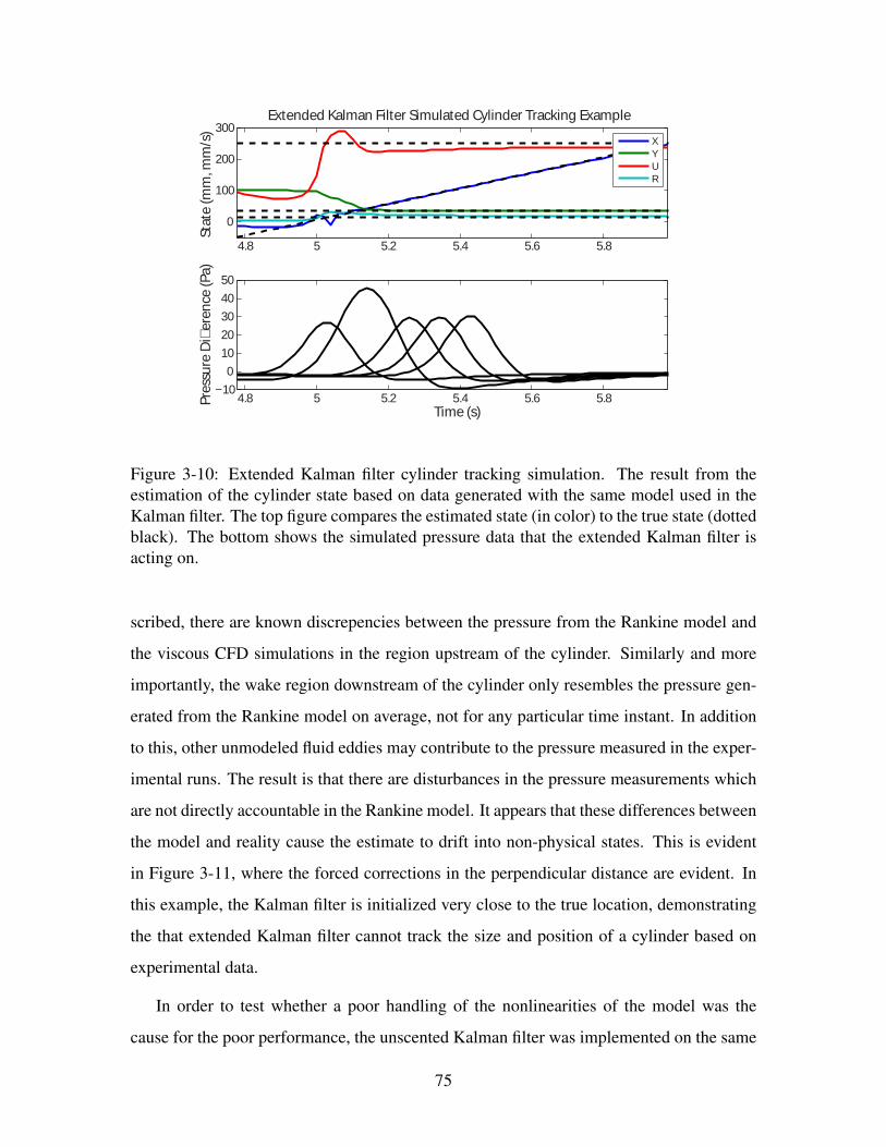
4.8 5 5.2 5.4 5.6 5.8

0

100

200

300

Sta

te (

mm

, mm

/s)

Extended Kalman Filter Simulated Cylinder Tracking Example

X

Y

U

R

4.8 5 5.2 5.4 5.6 5.8−10

0

10

20

30

40

50

Time (s)

Pre

ssu

re D

ie

ren

ce (

Pa

)

Figure 3-10: Extended Kalman filter cylinder tracking simulation. The result from theestimation of the cylinder state based on data generated with the same model used in theKalman filter. The top figure compares the estimated state (in color) to the true state (dottedblack). The bottom shows the simulated pressure data that the extended Kalman filter isacting on.

scribed, there are known discrepencies between the pressure from the Rankine model and

the viscous CFD simulations in the region upstream of the cylinder. Similarly and more

importantly, the wake region downstream of the cylinder only resembles the pressure gen-

erated from the Rankine model on average, not for any particular time instant. In addition

to this, other unmodeled fluid eddies may contribute to the pressure measured in the exper-

imental runs. The result is that there are disturbances in the pressure measurements which

are not directly accountable in the Rankine model. It appears that these differences between

the model and reality cause the estimate to drift into non-physical states. This is evident

in Figure 3-11, where the forced corrections in the perpendicular distance are evident. In

this example, the Kalman filter is initialized very close to the true location, demonstrating

the that extended Kalman filter cannot track the size and position of a cylinder based on

experimental data.

In order to test whether a poor handling of the nonlinearities of the model was the

cause for the poor performance, the unscented Kalman filter was implemented on the same

75

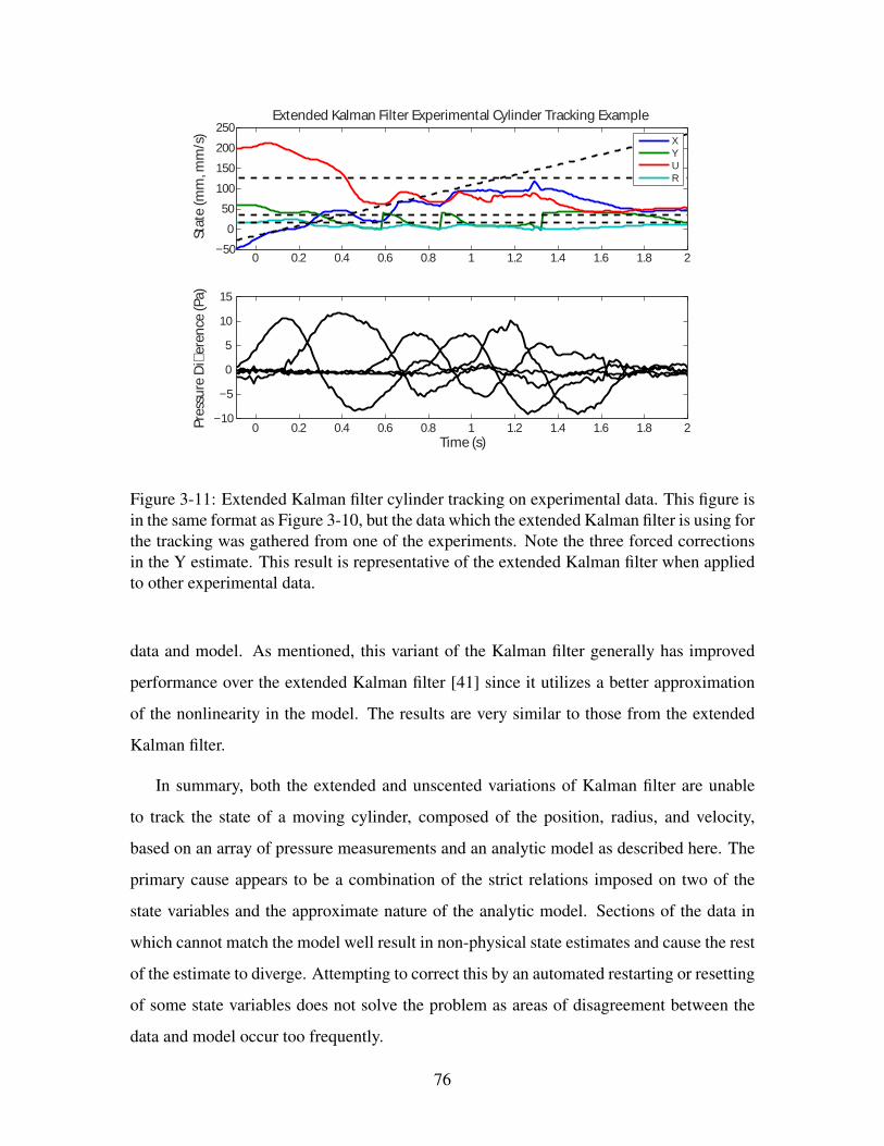
0 0.2 0.4 0.6 0.8 1 1.2 1.4 1.6 1.8 2−50

0

50

100

150

200

250

Sta

te (

mm

, mm

/s)

Extended Kalman Filter Experimental Cylinder Tracking Example

X

Y

U

R

0 0.2 0.4 0.6 0.8 1 1.2 1.4 1.6 1.8 2−10

−5

0

5

10

15

Time (s)

Pre

ssu

re D

ie

ren

ce (

Pa

)

Figure 3-11: Extended Kalman filter cylinder tracking on experimental data. This figure isin the same format as Figure 3-10, but the data which the extended Kalman filter is using forthe tracking was gathered from one of the experiments. Note the three forced correctionsin the Y estimate. This result is representative of the extended Kalman filter when appliedto other experimental data.

data and model. As mentioned, this variant of the Kalman filter generally has improved

performance over the extended Kalman filter [41] since it utilizes a better approximation

of the nonlinearity in the model. The results are very similar to those from the extended

Kalman filter.

In summary, both the extended and unscented variations of Kalman filter are unable

to track the state of a moving cylinder, composed of the position, radius, and velocity,

based on an array of pressure measurements and an analytic model as described here. The

primary cause appears to be a combination of the strict relations imposed on two of the

state variables and the approximate nature of the analytic model. Sections of the data in

which cannot match the model well result in non-physical state estimates and cause the rest

of the estimate to diverge. Attempting to correct this by an automated restarting or resetting

of some state variables does not solve the problem as areas of disagreement between the

data and model occur too frequently.

76

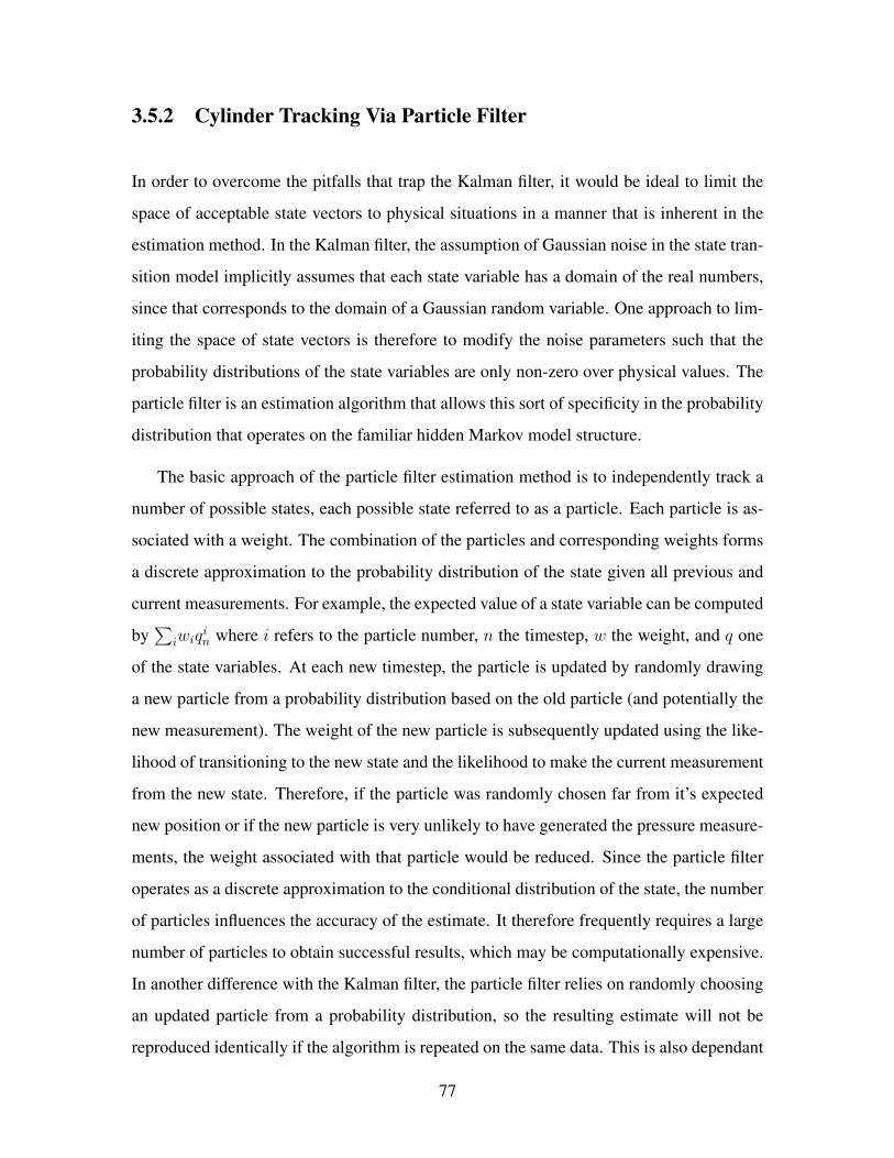
3.5.2 Cylinder Tracking Via Particle Filter

In order to overcome the pitfalls that trap the Kalman filter, it would be ideal to limit the

space of acceptable state vectors to physical situations in a manner that is inherent in the

estimation method. In the Kalman filter, the assumption of Gaussian noise in the state tran-

sition model implicitly assumes that each state variable has a domain of the real numbers,

since that corresponds to the domain of a Gaussian random variable. One approach to lim-

iting the space of state vectors is therefore to modify the noise parameters such that the

probability distributions of the state variables are only non-zero over physical values. The

particle filter is an estimation algorithm that allows this sort of specificity in the probability

distribution that operates on the familiar hidden Markov model structure.

The basic approach of the particle filter estimation method is to independently track a

number of possible states, each possible state referred to as a particle. Each particle is as-

sociated with a weight. The combination of the particles and corresponding weights forms

a discrete approximation to the probability distribution of the state given all previous and

current measurements. For example, the expected value of a state variable can be computed

by∑

iwiqin where i refers to the particle number, n the timestep, w the weight, and q one

of the state variables. At each new timestep, the particle is updated by randomly drawing

a new particle from a probability distribution based on the old particle (and potentially the

new measurement). The weight of the new particle is subsequently updated using the like-

lihood of transitioning to the new state and the likelihood to make the current measurement

from the new state. Therefore, if the particle was randomly chosen far from it’s expected

new position or if the new particle is very unlikely to have generated the pressure measure-

ments, the weight associated with that particle would be reduced. Since the particle filter

operates as a discrete approximation to the conditional distribution of the state, the number

of particles influences the accuracy of the estimate. It therefore frequently requires a large

number of particles to obtain successful results, which may be computationally expensive.

In another difference with the Kalman filter, the particle filter relies on randomly choosing

an updated particle from a probability distribution, so the resulting estimate will not be

reproduced identically if the algorithm is repeated on the same data. This is also dependant

77

on the number of particles, with the effect reduced if there are many particles covering the

state vector space.

There are many different variants to the particle filter algorithm, just as for the Kalman

filter. However, because of the Monte Carlo foundation of the particle filter these variants

are unrelated to the non-linearity of the problem which is handled without trouble. Instead,

the variations of the particle filter are related to the sampling method when transitioning

from one state to the next. New particles are drawn from a probability distribution termed

the proposal distribution which is ideally equal to the conditional probability of the new

state conditioned on the previous state and new measurements p (qn|qn−1,mn). Given the

complicated relation between the measurements and the state, this conditional probability is

difficult to know. The most common variant of the particle filter uses a proposal distribution

based only on the state transition equations p (qn|qn−1) called the bootstrap method. Other

approaches use an extended or unscented Kalman filter to approximate p (qn|qn−1,mn)

for the proposal distribution. The focus on this chapter will be on the bootstrap particle

filter. The unscented particle filter was also implemented, but it led to increased errors and

computation time without any compensating benefit. The details of the bootstrap particle

filter method are further described in [67].

The key difference between the Kalman filter approaches and the particle filter, as far

as tracking a moving cylinder is concerned, is that the range of boundaries in the state

variables can be explicitly included. This is through the specification of the distribution

of the noise random variables in the state transition equation (3.1). The distribution of

the noise for the x position and velocity state variables is the same as was implied for the

Kalman filter: zero mean Gaussian distributions with some specified variance. Both the y

position and the radius need different distributions for their corresponding noise variables

since they have restricted ranges.

In the case of the y position, the probability distribution needs to be positive, but one

would expect that if the current state is sufficiently far from zero relative to the standard

deviation, then the distribution would be roughly Gaussian. That is to say, the desire is

that, far from zero, the distribution would be symmetric and zero mean with a single peak

and long tails. The log normal distribution fits these characteristics well. The log normal

78

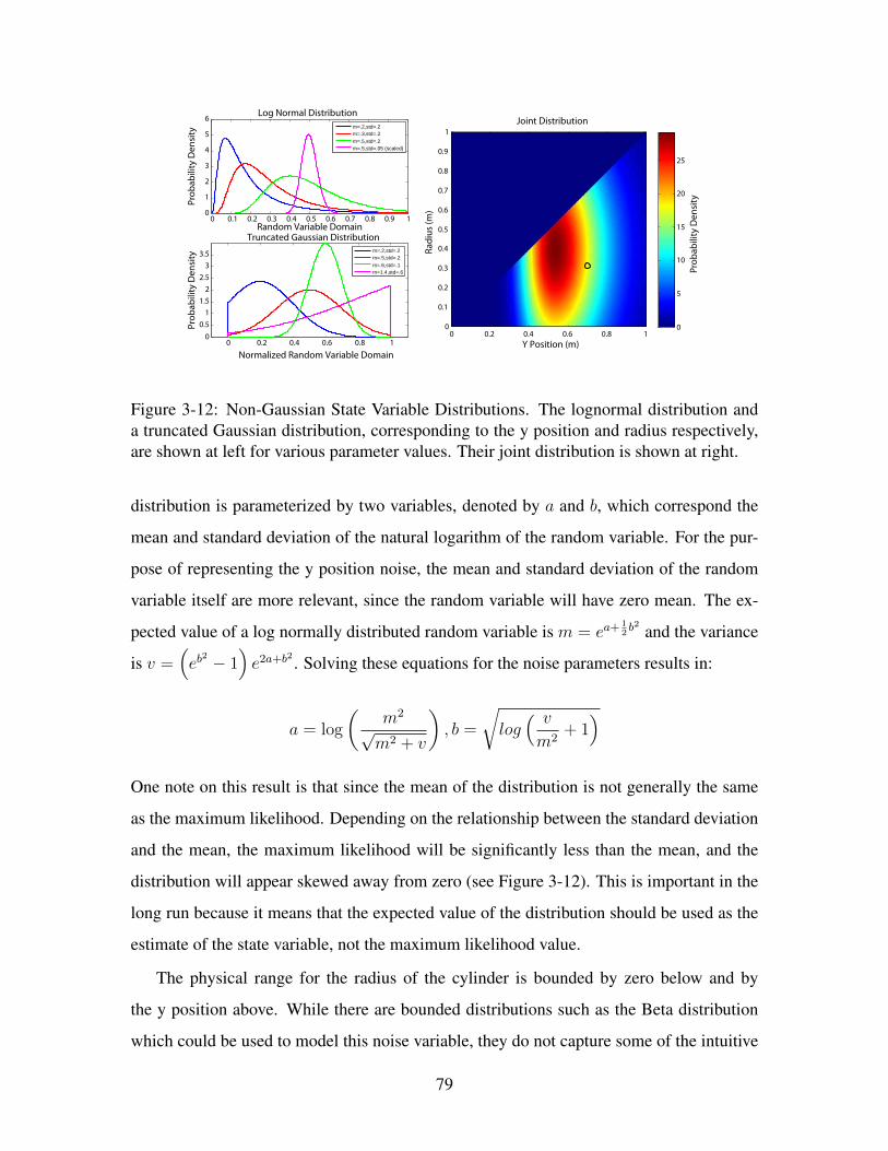
0 0.1 0.2 0.3 0.4 0.5 0.6 0.7 0.8 0.9 10

1

2

3

4

5

6

Random Variable Domain

Prob

abili

ty D

ensi

ty

Log Normal Distributionm=.2,std=.2m=.3,std=.2m=.5,std=.2m=.5,std=.05 (scaled)

0 0.2 0.4 0.6 0.8 10

0.51

1.52

2.53

3.5

Normalized Random Variable Domain

Prob

abili

ty D

ensi

ty

Truncated Gaussian Distributionm=.2,std=.2m=.5,std=.2m=.6,std=.1m=1.4,std=.6

Y Position (m)

Radi

us (m

)

0 0.2 0.4 0.6 0.8 10

0.1

0.2

0.3

0.4

0.5

0.6

0.7

0.8

0.9

1

0

5

10

15

20

25

Joint Distribution

Prob

abili

ty D

ensi

ty

Figure 3-12: Non-Gaussian State Variable Distributions. The lognormal distribution anda truncated Gaussian distribution, corresponding to the y position and radius respectively,are shown at left for various parameter values. Their joint distribution is shown at right.

distribution is parameterized by two variables, denoted by a and b, which correspond the

mean and standard deviation of the natural logarithm of the random variable. For the pur-

pose of representing the y position noise, the mean and standard deviation of the random

variable itself are more relevant, since the random variable will have zero mean. The ex-

pected value of a log normally distributed random variable is m = ea+ 12b2 and the variance

is v =(eb

2 − 1)e2a+b2 . Solving these equations for the noise parameters results in:

a = log

(m2

√m2 + v

), b =

√log( v

m2+ 1)

One note on this result is that since the mean of the distribution is not generally the same

as the maximum likelihood. Depending on the relationship between the standard deviation

and the mean, the maximum likelihood will be significantly less than the mean, and the

distribution will appear skewed away from zero (see Figure 3-12). This is important in the

long run because it means that the expected value of the distribution should be used as the

estimate of the state variable, not the maximum likelihood value.

The physical range for the radius of the cylinder is bounded by zero below and by

the y position above. While there are bounded distributions such as the Beta distribution

which could be used to model this noise variable, they do not capture some of the intuitive

79

behavior required. Clearly the expectation is that the cylinder radius does not change.

Therefore if the previous cylinder radius estimate is not near either boundary in comparison

to the standard deviation, the noise variable associated with the update should be zero mean

and confined. In this situation, a Beta distribution or Gaussian would work effectively and

the boundaries would not come into play. If the estimate of the radius is very small or near

the estimated y position compared to the standard deviation, then the distribution should to

be asymmetric with a bias away from boundary, but it would be logical if the most likely

value was still the previous radius. Again the Beta distribution is flexible enough to capture

this well. One further issue stems from the choice that the y position is free to be updated

over it’s complete range instead of being limited below by the radius. This implies the

possibility of an updated y position that is smaller than the previous radius. In this case, the

reasonable form of the probability distribution would be to have the maximum likelihood at

the upper boundary of the distribution, and to have the rest of the distribution monotonically

decrease. Here the Beta distribution has more difficulty. One solution that achieves all

of the desired behaviors is a truncated Gaussian distribution. This corresponds to using

a Gaussian distribution centered at the previous value with a fixed variance, but fixed at

zero outside the physical values and normalized so that it integrates to one (Figure 3-12).

In addition, this approach implies that the farther the physical range is from the previous

value, the flatter the distribution will be.

Much like in the case of the Kalman filter, the determination of the state transition

equations with their noise random variable distributions still leaves some parameters gov-

erning the width of the distributions free. As for the Kalman filter, these parameters are not

representative of any actual stochastic behavior in the state transition. However, the effect

of these parameters is substantially different than for the Kalman filter. The particle filter

works best with a lot of particles of equal weight, but the tendency is to converge in weight

to just a few particles which offer the best estimate. The standard approach to dealing with

this, used here, is to resample the particles from the estimated posterior distribution when

the number of effective particles falls to low (See [67]). An important consequence is that

after resampling, many of the particles have the same state until the next update. The speed

at which the particles subsequently disperse is governed by the variance of the noise vari-

80

ables. If the variance is too high, the particles will disperse too quickly and the effective

number of particles will drop immediately again, leading to a very inconsistent estimate.

If the variance is too low, then it may take a long time for the filter to sample an adjacent

space that may offer a better estimate. Therefore the noise variance should in general be as

small as reasonable such that the estimate converges quickly.

Using simulated data in the same way as for the Kalman filter, the noise variance asso-

ciated with each of the four state variables was tuned using experimental runs on idealized

data. In this case, the sensitivity of the pressure measurements to the state variable was

used as a guide for the variance associated with that variable. This is because the more

sensitive the measurements are, the more likely the possibility of converging strongly to an

incorrect value during resampling, especially once it is applied to experimental data where

there is some model mismatch. Both the x position and the velocity were found to be the

most influential on the pressure measurements. The radius is also fairly influential, but is

confined between zero and the y position and therefore does not need to explore as large a

sample space. Based on many test runs with simulated data, the standard deviations of 5

Pa, 2 Pa, 5 Pa, and 2 Pa for the x position, y position, velocity, and radius respectively were

found to work well.

In addition to the state transition noise characteristics, the noise variance for the pres-

sure measurement model was also specified using the simulated data as a test case. In the

simulated data, no measurement noise was used to examine the convergence under opti-

mal conditions. For the actual pressure sensors, the amount of noise after processing for

electrical and static pressure effects (Figure 3-8) is very small in comparison to the mean-

ingful signals. Using a measurement noise standard deviation that matches the data leads

to problems with the Kalman filter algorithm, since it quickly causes the effective num-

ber of particles to decrease. Since the model being used is not perfect, it is a problem if

during a timestep in which the model does not fit the measurements well due to either ex-

ternal factors or inadequacies of the model, the entire particle distribution converges during

resampling on a single particle that does fit the measurements. This situation effectively

derails the estimate. To avoid this, the standard deviation of the measurement noise is set

to 15 Pa, which is sufficiently broad that the effective particle number collapse is reduced

81

while still increasing the weight of particles that correspond well with measurements.

-0.5 0 0.5 1 1.5

-0.2

0

0.2

0.4

XPo

sitio

n (m

)

-0.5 0 0.5 1 1.5

0.05

0

0.2

0.15

Y

Posi

tion

(m)

0.2

-0.5 0 0.5 1 1.5

0.2

0

0.4

0.6

Time (s)

U

Velo

city

(m/s

)

-0.5 0 0.5 1 1.5

0.02

0

0.04

0.06

Time (s)

R

Radi

us (m

)

0.1

0.08

Figure 3-13: Results from particle filter on simulated data. The estimated probability dis-tribution based on the history of measurements is displayed for each timestep for the fourstate variables. Each vertical slice is therefore normalized to sum to 1. The black line de-notes the expected value of the variable as calculated from the state estimate distribution.The red line is the true state used to generate the pressure measurement data.

A representative result of the particle filter applied to simulated data is seen in Fig-

ure 3-13. Since the particle filter tracks a discrete approximation to the probability density

function (pdf) of the state conditioned on all the previous measurements, this figure dis-

plays the full pdf for each timestep. The color scale of blue to red corresponds to zero to

high probability density. Since each vertical slice must integrate to one, the maxima are

not comparable in value from one timestep to the next. On the other hand, viewing the full

pdf gives a complete sense of the confidence in the estimate. For the example discussed

here, one thousand particles were used in the particle filter. The expected value of the state

82

−0.5 0 0.5 1 1.5−10

0

10

20

30

40

50

Time (s)

Pres

sure

Di

eren

ce (P

a)

Simulated Pressure Dierence

Figure 3-14: Simulated pressure corresponding to the particle filter estimate. This pressuredifference time history is generated using the pressure measurement model based on aRankine half-body following a state path that follows the state transition equations. Nonoise is included in the measurement or the state transition, resulting in a test case thatoffers the best conditions for estimation.

variable at each time instant is shown in black. The estimated cylinder state depicted in

Figure 3-13 is based on the data shown in Figure 3-14. As with the Kalman filter, this

data was generated from a known state path using the same measurement model as in the

particle filter. That known state path is depicted in red in Figure 3-13. Since the data is

noiseless in both the state transitions and the measurements, it represents an idealization

of the problem in which the filter can be tested under its optimal conditions. To match

the experimental data later, the third pressure sensor in the linear array is removed before

computing the pressure difference.

The results depicted in Figure 3-13 show that a particle filter successfully tracks posi-

tion, radius, and velocity of a moving cylinder in the optimal simulated case. There is no

strong dependence on a single initial condition as in the case of the Kalman filter, and by

the underlying noise model there is no chance of a non-physical state being reached. Given

this ideal test case, there are a number of features evident in the way the cylinder is tracked

by the particle filter. First, the a priori probability distributions for the state variable were

initialized to be uniformly distributed over a generous range (-0.5-0.5m for the x direction,

83

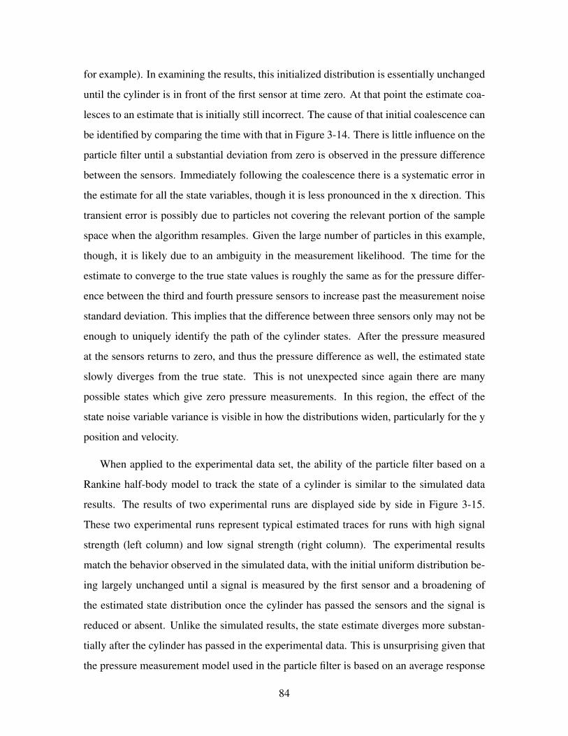
for example). In examining the results, this initialized distribution is essentially unchanged

until the cylinder is in front of the first sensor at time zero. At that point the estimate coa-

lesces to an estimate that is initially still incorrect. The cause of that initial coalescence can

be identified by comparing the time with that in Figure 3-14. There is little influence on the

particle filter until a substantial deviation from zero is observed in the pressure difference

between the sensors. Immediately following the coalescence there is a systematic error in

the estimate for all the state variables, though it is less pronounced in the x direction. This

transient error is possibly due to particles not covering the relevant portion of the sample

space when the algorithm resamples. Given the large number of particles in this example,

though, it is likely due to an ambiguity in the measurement likelihood. The time for the

estimate to converge to the true state values is roughly the same as for the pressure differ-

ence between the third and fourth pressure sensors to increase past the measurement noise

standard deviation. This implies that the difference between three sensors only may not be

enough to uniquely identify the path of the cylinder states. After the pressure measured

at the sensors returns to zero, and thus the pressure difference as well, the estimated state

slowly diverges from the true state. This is not unexpected since again there are many

possible states which give zero pressure measurements. In this region, the effect of the

state noise variable variance is visible in how the distributions widen, particularly for the y

position and velocity.

When applied to the experimental data set, the ability of the particle filter based on a

Rankine half-body model to track the state of a cylinder is similar to the simulated data

results. The results of two experimental runs are displayed side by side in Figure 3-15.

These two experimental runs represent typical estimated traces for runs with high signal

strength (left column) and low signal strength (right column). The experimental results

match the behavior observed in the simulated data, with the initial uniform distribution be-

ing largely unchanged until a signal is measured by the first sensor and a broadening of

the estimated state distribution once the cylinder has passed the sensors and the signal is

reduced or absent. Unlike the simulated results, the state estimate diverges more substan-

tially after the cylinder has passed in the experimental data. This is unsurprising given that

the pressure measurement model used in the particle filter is based on an average response

84

in the CFD simulations. For a single experimental run, pressure measured in the wake re-

gion is expected to differ from the model therefore causing a change in the estimate. There

is some indication of the delayed convergence that was observed with the simulated data,

particularly in the Y position and radius of the low signal example. In that case, it appears

that after signals are initially measured by the first two pressure sensors there is a period

in which the Y position and radius are significantly over-estimated. This changes at about

the time pressure difference between the third and fourth pressure sensors increases. In

contrast, the strong signal example has a much smaller shift, if any.

The particle filter based on Rankine half-body tracks the cylinder well in general, but

there are differences in the estimation accuracy for each state variable. The x position

state, parallel to the direction of the linear sensor array, is tracked best. However, unlike

the simulated results, the estimate of the x position shows a step-like progression which is

substantially more pronounced in the strong signal example. The level portions correspond

in number and location to the peaks in the pressure difference measurements. Another

notable observation is that both the y position and the radius are under-estimated. This is

somewhat expected for the radius since in choosing the simpler potential flow model of

the Rankine half-body, it was noted earlier that the response of the slightly more accurate

dipole-source model could be reproduced by reducing the radius in the Rankine half-body.

The under-estimation of the y position is a little more surprising. It appears to be more

significant in the example with a smaller signal strength, but it is unclear whether this is

associated with the underlying model or a lack of sensitivity in the measurements due to

the y position. There is some error in the velocity estimate, though in general probability

distribution for the velocity is broad. Keep in mind that the velocity is not being calculated

based on a cross-correlation of the signals, which would provide a much more accurate

velocity estimate after the fact, but would not be able to attempt to track changes in velocity

in real time.

The results displayed in Figure 3-15 are based on a particle filter with one thousand

particles. This amount is useful for obtaining a good image of the conditional state distri-

butions, as shown in the figure. However, it also generates an excessive amount of compu-

tation time (order 15 sec). Reducing the number of particles will not immediately effect the

85

Far Distance Pass Close Distance Pass

0 0.2 0.6 0.7Time (s)

0.3 0.4 0.5 0.8 0.90.1-0.1-500

500

0

X

Posi

tion

(mm

)

0 0.2 0.6 0.7Time (s)

0.3 0.4 0.5 0.8 0.90.1-0.1

Posi

tion

(mm

)

0

20

40

60

80

100Y

0 0.2 0.6 0.7Time (s)

0.3 0.4 0.5 0.8 0.90.1-0.1

Velo

city

(mm

/s)

0

100

200

300

400

500

600U

0 0.2 0.6 0.7Time (s)

0.3 0.4 0.5 0.8 0.90.1-0.1

Radi

us (m

m)

0

20

40

60

80

100R

-40

-20

0

20

40

60

0 0.2 0.6 0.7Time (s)

0.3 0.4 0.5 0.8 0.90.1-0.1

X

0 0.1 0.8Time (s)

0.2 0.4 0.5

0

-300

400

Posi

tion

(mm

)Ve

loci

ty (m

m/s

)

0

100

200

300

400

500

600U

Radi

us (m

m)

0

20

40

60

80

100R

Posi

tion

(mm

)

0

20

40

60

80

Y100

Time (s)

Pres

sure

Di

eren

ce (P

a)

-200

-100

100

200

300

-0.1 0.3 0.6 0.7 0.9

0 0.1 0.8Time (s)

0.2 0.4 0.5-0.1 0.3 0.6 0.7 0.9

0 0.1 0.8Time (s)

0.2 0.4 0.5-0.1 0.3 0.6 0.7 0.9

0 0.1 0.8Time (s)

0.2 0.4 0.5-0.1 0.3 0.6 0.7 0.9

−0.1 0 0.1 0.2 0.3 0.4 0.5 0.6 0.7 0.8 0.9−100

−50

0

50

100

150 Measured Pressure Measured Pressure

Pres

sure

Di

eren

ce (P

a)

Figure 3-15: Particle filter estimation on two experimental data sets. The estimated resultsare shown for high and low signal strength examples from the experimental test matrix. Theformat of the state estimates is the same as for Figure 3-13. The corresponding pressuredifference data is shown for reference against the estimate behavior.

86

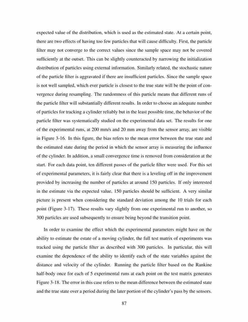
expected value of the distribution, which is used as the estimated state. At a certain point,

there are two effects of having too few particles that will cause difficulty. First, the particle

filter may not converge to the correct values since the sample space may not be covered

sufficiently at the outset. This can be slightly counteracted by narrowing the initialization

distribution of particles using external information. Similarly related, the stochastic nature

of the particle filter is aggravated if there are insufficient particles. Since the sample space

is not well sampled, which ever particle is closest to the true state will be the point of con-

vergence during resampling. The randomness of this particle means that different runs of

the particle filter will substantially different results. In order to choose an adequate number

of particles for tracking a cylinder reliably but in the least possible time, the behavior of the

particle filter was systematically studied on the experimental data set. The results for one

of the experimental runs, at 200 mm/s and 20 mm away from the sensor array, are visible

in Figure 3-16. In this figure, the bias refers to the mean error between the true state and

the estimated state during the period in which the sensor array is measuring the influence

of the cylinder. In addition, a small convergence time is removed from consideration at the

start. For each data point, ten different passes of the particle filter were used. For this set

of experimental parameters, it is fairly clear that there is a leveling off in the improvement

provided by increasing the number of particles at around 150 particles. If only interested

in the estimate via the expected value, 150 particles should be sufficient. A very similar

picture is present when considering the standard deviation among the 10 trials for each

point (Figure 3-17). These results vary slightly from one experimental run to another, so

300 particles are used subsequently to ensure being beyond the transition point.

In order to examine the effect which the experimental parameters might have on the

ability to estimate the estate of a moving cylinder, the full test matrix of experiments was

tracked using the particle filter as described with 300 particles. In particular, this will

examine the dependence of the ability to identify each of the state variables against the

distance and velocity of the cylinder. Running the particle filter based on the Rankine

half-body once for each of 5 experimental runs at each point on the test matrix generates

Figure 3-18. The error in this case refers to the mean difference between the estimated state

and the true state over a period during the later portion of the cylinder’s pass by the sensors.

87

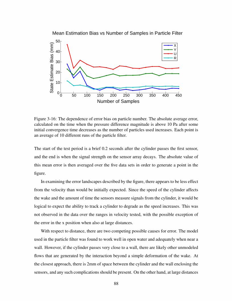
0 50 100 150 200 250 300 350 400 4500

10

20

30

40

50

Mean Estimation Bias vs Number of Samples in Particle Filter

Number of Samples

Sta

te E

stim

ate

Bia

s (m

m)

XYUR

Figure 3-16: The dependence of error bias on particle number. The absolute average error,calculated on the time when the pressure difference magnitude is above 10 Pa after someinitial convergence time decreases as the number of particles used increases. Each point isan average of 10 different runs of the particle filter.

The start of the test period is a brief 0.2 seconds after the cylinder passes the first sensor,

and the end is when the signal strength on the sensor array decays. The absolute value of

this mean error is then averaged over the five data sets in order to generate a point in the

figure.

In examining the error landscapes described by the figure, there appears to be less effect

from the velocity than would be initially expected. Since the speed of the cylinder affects

the wake and the amount of time the sensors measure signals from the cylinder, it would be

logical to expect the ability to track a cylinder to degrade as the speed increases. This was

not observed in the data over the ranges in velocity tested, with the possible exception of

the error in the x position when also at large distances.

With respect to distance, there are two competing possible causes for error. The model

used in the particle filter was found to work well in open water and adequately when near a

wall. However, if the cylinder passes very close to a wall, there are likely other unmodeled

flows that are generated by the interaction beyond a simple deformation of the wake. At

the closest approach, there is 2mm of space between the cylinder and the wall enclosing the

sensors, and any such complications should be present. On the other hand, at large distances

88

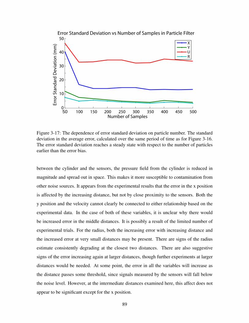
50 100 150 200 250 300 350 400 450 5000

10

20

30

40

50Error Standard Deviation vs Number of Samples in Particle Filter

Number of Samples

XYUR

Erro

r Sta

ndar

d D

evia

tion

(mm

)

Figure 3-17: The dependence of error standard deviation on particle number. The standarddeviation in the average error, calculated over the same period of time as for Figure 3-16.The error standard deviation reaches a steady state with respect to the number of particlesearlier than the error bias.

between the cylinder and the sensors, the pressure field from the cylinder is reduced in

magnitude and spread out in space. This makes it more susceptible to contamination from

other noise sources. It appears from the experimental results that the error in the x position

is affected by the increasing distance, but not by close proximity to the sensors. Both the

y position and the velocity cannot clearly be connected to either relationship based on the

experimental data. In the case of both of these variables, it is unclear why there would

be increased error in the middle distances. It is possibly a result of the limited number of

experimental trials. For the radius, both the increasing error with increasing distance and

the increased error at very small distances may be present. There are signs of the radius

estimate consistently degrading at the closest two distances. There are also suggestive

signs of the error increasing again at larger distances, though further experiments at larger

distances would be needed. At some point, the error in all the variables will increase as

the distance passes some threshold, since signals measured by the sensors will fall below

the noise level. However, at the intermediate distances examined here, this affect does not

appear to be significant except for the x position.

89

Velocity (mm/s)

Dis

tanc

e (m

m)

X Position Error (mm)

150 200 250 300

20

25

30

35

0

5

10

15

20

25

Velocity (mm/s)

Dis

tanc

e (m

m)

Y Position Error (mm)

150 200 250 300

20

25

30

35

0

2

4

6

8

10

Velocity (mm/s)

Dis

tanc

e (m

m)

Velocity Error (mm/s)

150 200 250 300

20

25

30

35

0

10

20

30

Velocity (mm/s)

Dis

tanc

e (m

m)

Radius Error (mm)

150 200 250 300

20

25

30

35

0

2

4

6

8

10

Error Dependence on Distance and Velocity

Figure 3-18: Particle filter error landscape. The dependence of each state variable estimateagainst the speed and distance of a moving cylinder using a particle filter based on a Rank-ine half-body model is shown. Each point corresponds to the averaged absolute error basedon five experimental runs.

3.6 Discussion

The results of the particle filter in estimating the position and size of a moving cylinder

demonstrate that the state of a moving round cylinder can be tracked in real time using a

fix analytic model as the base. They also provide the framework for accomplishing the

cylinder tracking in real time. The error in the state estimation follow some predictable

relationships with the speed and distance, but not all variables are affected equally.

The model was chosen to capture the dominant characteristics in the pressure response

of a moving round cylinder and its wake as predicted by computational fluid dynamics.

The simple potential flow model of a Rankine half-body, generated by a source in a steady

90

uniform flow, matches the shape and amplitude of the pressure distribution over a line

parallel to the flow (and thus motion of the cylinder). In addition, the transition from high

to low pressure is correctly located and reproduced. The model deviates slightly the decay

rate in front of the peak pressure, decaying to slowly. In the wake region, the model roughly

captures the mean pressure recovery, but the unsteady nature of the wake means that there

are significant differences between the model and any instantaneous pressure distribution.

Based on the relationship between the state variables of interest, and an analysis of the

Kalman filter and particle filter estimation results, approaches that rely only on Gaussian

noise models are unsuitable for tracking a moving cylinder. A method without a priori

noise parameterization, such a particle filter, is better suited for tracking a cylinder size and

position. The Kalman filter implementations were only successful in tracking a cylinder

from simulated data with accurate initial states and were unable to track a cylinder from

experimental results, whereas the particle filter was able to accurately track cylinders based

on experimental data. The failure mechanisms in tracking the cylinder of the Kalman filter,

such as running off a boundary, are consistent with the use of a Gaussian model for non-

Gaussian noise.

A particle filter has been used to track the cylinder position and size given a history

of pressure measurements. Based on the analysis of the number of particles needed for

the reliable behavior of the particle filter in this application, as low as 200 particles could

be used with a reasonable expectation of consistency. At that level (200-300 particles) a

sampling rate of 20 Hz is needed for the particle filter to run in real time in a MATLAB

implementation on a 2.66 GHz laptop. This speed could likely be improved. However, 20

Hz is sufficient to capture the relevant features of the pressure signals and is sufficiently

fast for changes in the state that might be expected if the y position or velocity shifts.

By applying the particle filter based on the Rankine model to the full test matrix of ex-

perimental data, it is possible to get a sense of how reliable the cylinder tracking estimate

is, and how it depends on the distance and speed of the moving cylinder. The expectation

was that the error in tracking a cylinder increases slowly with increasing distance and de-

creasing velocity. The error was also expected to increase rapidly below some lower limit

in distance. Based on the results from the experimental data, the error in tracking was found

91

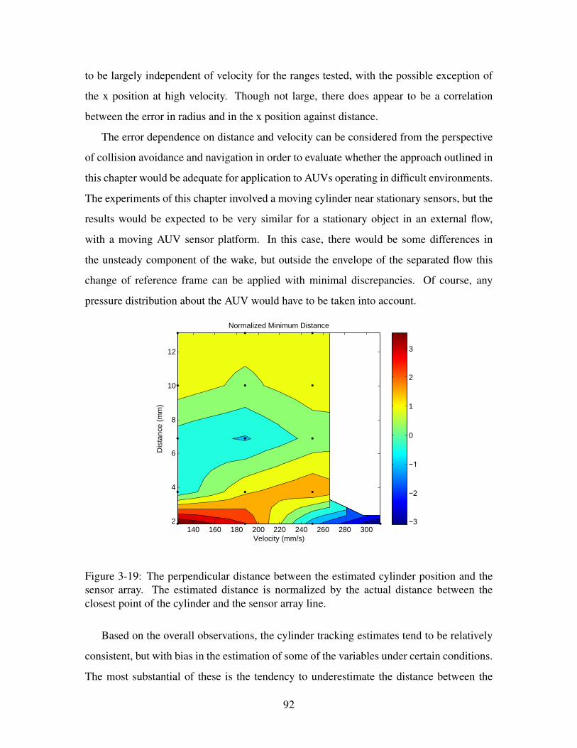
to be largely independent of velocity for the ranges tested, with the possible exception of

the x position at high velocity. Though not large, there does appear to be a correlation

between the error in radius and in the x position against distance.

The error dependence on distance and velocity can be considered from the perspective

of collision avoidance and navigation in order to evaluate whether the approach outlined in

this chapter would be adequate for application to AUVs operating in difficult environments.

The experiments of this chapter involved a moving cylinder near stationary sensors, but the

results would be expected to be very similar for a stationary object in an external flow,

with a moving AUV sensor platform. In this case, there would be some differences in

the unsteady component of the wake, but outside the envelope of the separated flow this

change of reference frame can be applied with minimal discrepancies. Of course, any

pressure distribution about the AUV would have to be taken into account.

Velocity (mm/s)

Dis

tanc

e (m

m)

Normalized Minimum Distance

140 160 180 200 220 240 260 280 3002

4

6

8

10

12

−3

−2

−1

0

1

2

3

Figure 3-19: The perpendicular distance between the estimated cylinder position and thesensor array. The estimated distance is normalized by the actual distance between theclosest point of the cylinder and the sensor array line.

Based on the overall observations, the cylinder tracking estimates tend to be relatively

consistent, but with bias in the estimation of some of the variables under certain conditions.

The most substantial of these is the tendency to underestimate the distance between the

92

sensors and the cylinder. However, at very small distances, the radius of the cylinder was

also substantially underestimated. In terms of the position along the sensor array, the error

increased with velocity at large distances. From the point of view of collision avoidance

and navigation however, the minimum distance between the object being tracked and the

sensor array is the primary concern. If this minimum distance is underestimated, then it

implies that an AUV will be more conservative in maneuvering near the object. If the

distance is overestimated, the vehicle may collide with the cylinder. Clearly it is preferable

to err on the side of underestimation. The results based on the y and r estimates from

the experimental matrix are shown in Figure 3-19 with the estimated minimum distance

normalized by the true minimum distance. This implies that a value less than 1 corresponds

to an estimate that reduces the likelihood of collision, whereas a value greater than one

implies that the estimate creates a risk of collision. A value of zero or below implies that

the estimate indicates a collision is occurring in the simulation. In examining the figure, it

is evident that the collision distance is only overestimated for the closest distances in which

the separation is 2mm, which is due to the underestimation of the radius that was remarked

upon earlier. With the distance so small, the reduced radius estimate results in an error

that could lead to real collisions. However, practically speaking, this separation distance

between the cylinder and array of 2 mm is already effectively a collision, since maneuvering

with that degree of precision is difficult in unpredictable environments. At slightly larger

experimental distances, the separation underestimated (with a few false collisions where

the y position is most severely underestimated). These errors are not as significant as

overestimating the distance, since they lead to more conservative navigation but do not

result in collisions. Beyond the intermediate distances, it appears that the estimate of the

separation settles to a reasonable approximation of the true separation. The results therefore

are promising, indicating that for all but the closest distances, a lateral-line-like pressure

sensor array could be used for object avoidance in environments with currents.

93

Chapter 4

Object Identification and Classification

4.1 Introduction

This chapter addresses the ability pressure sensor arrays, emulating the lateral line organ,

to distinguish the shapes of physical objects when they move within their stimulus range.

While the workings of the lateral line organ itself are progressively better understood, there

is still comparatively little known about the information extracted from the lateral line by

the fish, outside of that corresponding to the dipole stimulus.

As discussed in Chapter 2, hydrodynamic stimuli from aquatic animals other than small

prey has received the least attention in biological studies. Larger fish, potentially predatory,

are not well modeled by small oscillatory dipoles and instead would be better approximated

by blunt moving objects. Experiments by Vogel and Bleckmann [80] have demonstrated

that goldfish use their lateral line to respond to changes in size, velocity and shape of

passing rods in still water. The results of Chapter 3 have shown that there is sufficient

information to track the size and position of a passing rod, but did not address the question

of shape.

Two studies ([70] and [6]) have considered parameterizations of the shape of an arbi-

trary object suitable for modeling flow and pressure distributions in potential flow. The

authors have used these parameterizations to demonstrate how a simulated fish swimming

in a potential flow could identify the shape of an object by swimming past or around it.

However, these models are not able to take into account the wake that forms behind a

95

moving object which is a significant factor in lateral line measurements when the object is

moving. Despite the simulation results estimating the shape of an object in potential flow,

it is unclear how much of the shape information is altered when a wake is present.

Through the experiments presented in this chapter, we investigate the information con-

cerning the shape of non-oscillatory stimuli that can be obtained through a pressure sensor

array. As a representative problem, the study concentrates on whether it is possible to dis-

tinguish between cylinders with square and round cross-sections. These stimuli are similar

in basic structure and size, but the presence of sharp corners and the bluntness of the front

face may distinguish the shape of the square. Similar to the earlier behavioral experiments

by Vogel and Bleckmann [80], the objects are moved past stationary sensors to generate

the signals.

After a description of the relevant experiments, the chapter first examines the average

response of a lateral-line-like sensor to a passing cylinder of different shapes. Individual

pressure traces generated by the time history of a single sensor as a cylinder passes by will

vary greatly from one trial to the next due to the wake of the cylinder. By inspecting the

averaged results, differences in the pressure response due to shape will be revealed, leading

to features that can be used to distinguish the shape of a cylinder based on a single pass.

This approach succeeds in distinguishing the cylinder shapes, but as will be shown, it is

limited since the features are connected to only a few points in the pressure response. A

second approach for feature extraction is subsequently discussed and evaluated, using a

principal component analysis to generate a single decision criterion that incorporates the

entire pressure response. This is much more successful, but requires interpretation in order

to understand what it may be using as a basis of the decision.

4.2 Experimental Procedure

The experiments described in this chapter are similar to those of the previous chapter in

that both are focused on a vertical cylinder passing by a stationary horizontal linear pres-

sure sensor array in still water. However, whereas the previous chapter focused on demon-

strating that the size and position of a moving cylinder could be tracked in real time, the

96

presenta chapter is concerned with extracting the shape of the moving cylinder based on the

near-field pressure. As a result of the change in experimental focus, there are substantial

differences in the experimental setup. Unlike the experiments from Chapter 3, the exper-

iments in this chapter are designed with a heavier emphasis on repeated measurements.

This is accomplished at the cost of reduced precision in maintaining some of the free ex-

perimental parameters constant. The experiments completed in the Singapore towing tank

allowed the very precise placement and motion of the cylinder, but, due largely to the small

dimensions of the tank, standing waves would develop after a single experimental pass that

would influence the measurements. For this reason, large numbers of trials were imprac-

tical. In contrast, the large dimensions of the MIT towing tank coupled with the artificial

beach at one end significantly dampen surface waves and therefore allow for repeated tri-

als with minimal delays. Unfortunately, the positioning of the cylinder is less precise due

to the large distance between the carriage and the test section (approximately 1.5 vertical

meters) and to difficulties in the precise placement of the sensors.

sy

h

v

dA B

p

p

p

1

2

3

Figure 4-1: A: Schematic of experiments with cylindrical stimuli. The diagram depicts thehousing with pressure ports along the side and a typical cylinder moving alongside. Severalkey quantities are labeled, including the separation between sensors and cylinder (s), thedepth of the sensors (y), the total depth of the tank (h), the diameter of the cylinder (d), andthe velocity of the cylinder (v). B: A close up of the pressure sensor and port geometry.The pressure sensors are labeled p1 - p3 in the cut-out view.

97

4.2.1 Experimental Layout

The fundamental aspects of the layout of the experiments described in this chapter are the

same as in Chapter 3. A vertical cylinder was passed in front of an array of stationary

pressure sensors, much in the same manner. The experiments were performed in the MIT

Towing Tank, where the water tank has dimensions 40 m by 2.5 m by 1.3 m equipped with

an overhead carriage capable of towing at speeds up to 1.5 m/s. The housing containing

the sensors was fixed near the center of the tank and aligned with the motion of a movable

carriage. Vertical cylinders attached to the carriage were towed at constant velocity past the

sensors. The specific configuration can be seen in Figure 4-1A. The motion of the cylinders

began five meters upstream from the sensors, reached its final velocity within 0.5 meters

from the start, and continued up to two meters past the sensors. Six seconds of pressure

data were recorded at 2 kHz.

Besides the tank size, the housing that contained the pressure difference was signifi-

cantly different than the one used for the cylinder tracking experiments. The sensor hous-

ing for the cylinder shape detection was based on a cylindrical body with a diameter of 11.4

cm (4.5 in), and a streamlined nose and tail (Figure 4-1). The sensors are ported to the side

of the cylinder, aligned with the main cylinder axis.

The pressure sensors used in the experiments were gauge pressure sensors made by

Honeywell, part 242PC15M, with a nominal sensitivity of 48 µV/Pa and response time

of 1 µs. These sensors included internal amplification, which meant they could not be

grouped closely in an array. The four sensors were enclosed in a streamlined housing as

shown in Figure 4-1 and were connected to the outside flow through ports spaced 6.35 cm

(2.5 in) apart. The sensor port geometry can be seen in Figure 4-1B. The density of this

linear array was limited by the size of the pressure sensors. However, since the stimuli

in the experiments were moving at constant velocity, the time series from each sensor can

be used to approximate the spatial response sampled at intervals d = V/fs, where V is the

velocity of the stimulus and fs is the sampling frequency. This is an accurate approximation

wherever the flow is steady in the frame of the moving stimulus, but does not hold as well

in the wake region of the cylinders, where the distribution and location of vortices is time

98

dependent. The sensors were connected to a rigid tube with a 0.472 cm (0.186 in) inner

diameter. A small hole 1.3 mm (.050 in) in diameter and 3.2 mm (0.13 in) deep connected

the tube to the outside fluid. This layout was chosen to minimize the noise, given that it

was not possible to mount the pressure sensors flush.

In order to minimize any additional electrical noise picked up through interference, the

signals were further amplified using a similar circuit as in Chapter 3 (Figure 4-2. Since the

sensors used in these experiments already have some internal amplification, a gain of 10

was used. A single voltage divider with a potentiometer was used to remove the common

zero offset generated by the static pressure from all of the sensors. This was necessary in

order to avoid the saturation of the data acquisition system (NI USB-6210). Due to the

comparative sizes of the amplification circuitry and the sensor housing, the amplification

in these experiments occurred outside of the water, connected by a foil-shielded cable. As

with the other experiments, the data acquisition was coupled with an unconnected laptop

in order to minimize electrical noise from building electrical sources.

4.2.2 Test Matrix

The difference between square and circular cylinder cross sections is of primary inter-

est, but it is also important to test the dependence of the results on the towing speed, the

cylinder diameter, and the distance from the cylinder to the sensors. This is necessary in

order to have some confidence that the results demonstrate that different shapes are being

distinguished, instead of different particular experiments. In all of the experiments, the ori-

entation of the square cross section was kept constant with the leading face perpendicular

to the oncoming flow. Two sizes for each cross section were tested: 5.08 cm (2 in) and 7.62

cm (3 in). For the round cross section, size refers to the diameter, and for the square cross

sections it refers to the side length.

Two carriage velocities were also tested at 0.50 m/s and 0.75 m/s. Most of the tests

were performed at a separation of 0.51 cm (0.2 in), but two sets were also done at a larger

separation of 1.27 cm (0.5 in). A total of ten sets of experiments were run with different

combinations of these variables as shown in (Table 4.1). Each set consisted of one hundred

99

5.1 mm Separation7.62 cm Diameter 5.08 cm Diameter

0.50 m/s 0.75 m/s 0.50 m/s 0.75 m/sSquare 100 Runs 100 Runs 100 Runs 100 RunsRound 100 Runs 100 Runs 100 Runs 100 Runs

Table 4.1: Table of tests performed for identifying a moving object. Not included in thetable are two sets of 100 runs (one for each cross section shape) at 0.75 m/s, 5.08 cmdiameter, and 1.27 cm separation.

passes of the cylinder past the sensors. These experiments correspond to Reynolds numbers

between 2 ·104 to 6 ·104 and to ratios of the separation between sensors and object (labeled

s in Figure 4-1) to object size between 0.1 and 0.3. These conditions and the geometric

arrangements were chosen in order to be relevant to the situation of a fish exploring a new

environment (see [82]), and to a vehicle operating within a cluttered environment.

4.2.3 Data Pre-Processing

Calibration of the sensors was done immediately after testing without removing the setup

from the water. In order to calibrate all of the sensors at the same time and in situ, a

wave machine was used to generate waves at approximately 1.5 Hz. The amplitude of the

waves was measured above the position of the sensors at the same time as the pressure

oscillations from the waves were recorded. The calibration was calculated using linearized

surface wave theory [60], in which

Ap = ρgcosh [k (y + h)]

cosh [kh]· Aw (4.1)

determines the amplitude Ap of the pressure oscillation a distance y below the surface in

water of depth hwhen the wave amplitudeAw is measured. In the equation, ρ is the density

of water, g is the gravitational acceleration, and k is the wave number. The wavenumber of

the surface waves is calculated from the dispersion relation w2 = gk tanh [kh], where the

frequency w was calculated by fitting a sine to the recorded pressure.

The Honeywell sensors used in these experiments have a substantial amount of white

noise in their measurements. In tests using a manometer to apply a constant measureable

100

Pressure (Pa) Frequency (Hz)

Noise Power Spectrum

Pow

er S

pect

ral D

ensi

ty (d

B)

Noise Distribution for 3 Second Sample

Prob

abili

ty D

ensi

tyA B

Std: 17.0 Pa

-83.84 -37.26 -13.97 9.32 32.61 55.90-60.56 79.190

100

200

300

400

500

600

10 10 10 10 10101 2 3 4 5 6

-130

-125

-120

-115

-110

-105

-100

-95

-90

Figure 4-2: A: Resting noise distribution of the Honeywell 242PC15M pressure sensor. thenormalized histogram is generated from a 3 second sample at 300kHz. B: The correspond-ing power spectrum to the noise sample. High frequency electrical noise peaks are evidentin the power spectrum.

pressure, it was found that the sensor noise had a standard deviation of approximately 17

Pa, based on a measured sensitivity of 42µVPa

which is below the specified 48µVPa

. Figure 4-2

shows the clearly Gaussian noise distribution, as well as the corresponding power spectrum

which does not contain much notable electrical interference until very high frequencies.

These tests demonstrate the character of the sensors only, as the tests did not include the

additional external amplification and utilized very short (less than a foot) cabling.

Since the experiments were done in a much larger tank which was not susceptible to

establishing long wavelength standing waves, it is unnecessary to consider the difference

between pressure sensors in this Chapter, unlike Chapter 3. Instead, the raw data were

processed as follows: First the hydrostatic pressure, taken as the mean pressure before the

cylinder approached (where the pressure signal is flat), was subtracted from the data of

each sensor for every run; all pressures shown in the figures and discussed in the text are

pressure differences with respect to the hydrostatic pressure. The cylinder stimuli were

run at two velocities (0.5 m/s and 0.75 m/s) past the sensors, but the data was collected

at 2 kHz in all cases; this is equivalent to sampling the slow tests more closely in space.

For this reason, the data from slower velocity runs were then downsampled by a factor of

3/2, making them comparable to the higher speed data. Following this, each pressure trace

101

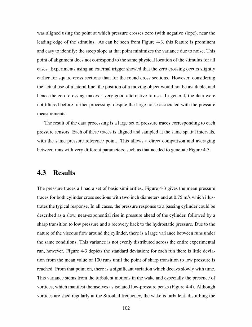
was aligned using the point at which pressure crosses zero (with negative slope), near the

leading edge of the stimulus. As can be seen from Figure 4-3, this feature is prominent

and easy to identify: the steep slope at that point minimizes the variance due to noise. This

point of alignment does not correspond to the same physical location of the stimulus for all

cases. Experiments using an external trigger showed that the zero crossing occurs slightly

earlier for square cross sections than for the round cross sections. However, considering

the actual use of a lateral line, the position of a moving object would not be available, and

hence the zero crossing makes a very good alternative to use. In general, the data were

not filtered before further processing, despite the large noise associated with the pressure

measurements.

The result of the data processing is a large set of pressure traces corresponding to each

pressure sensors. Each of these traces is aligned and sampled at the same spatial intervals,

with the same pressure reference point. This allows a direct comparison and averaging

between runs with very different parameters, such as that needed to generate Figure 4-3.

4.3 Results

The pressure traces all had a set of basic similarities. Figure 4-3 gives the mean pressure

traces for both cylinder cross sections with two inch diameters and at 0.75 m/s which illus-

trates the typical response. In all cases, the pressure response to a passing cylinder could be

described as a slow, near-exponential rise in pressure ahead of the cylinder, followed by a

sharp transition to low pressure and a recovery back to the hydrostatic pressure. Due to the

nature of the viscous flow around the cylinder, there is a large variance between runs under

the same conditions. This variance is not evenly distributed across the entire experimental

run, however. Figure 4-3 depicts the standard deviation; for each run there is little devia-

tion from the mean value of 100 runs until the point of sharp transition to low pressure is

reached. From that point on, there is a significant variation which decays slowly with time.

This variance stems from the turbulent motions in the wake and especially the presence of

vortices, which manifest themselves as isolated low-pressure peaks (Figure 4-4). Although

vortices are shed regularly at the Strouhal frequency, the wake is turbulent, disturbing the

102

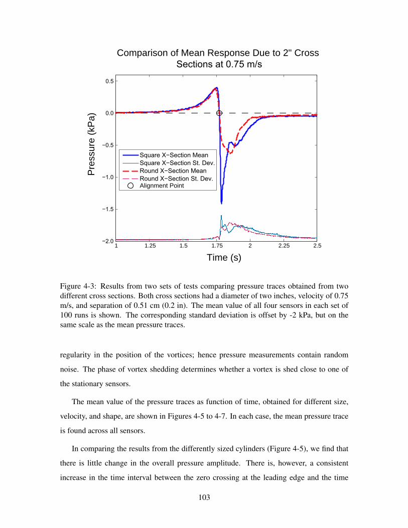
1 1.25 1.5 1.75 2 2.25 2.5−2.0

−1.5

−1.0

−0.5

0.0

0.5

Time (s)

Pre

ssur

e (k

Pa)

Comparison of Mean Response Due to 2" Cross Sections at 0.75 m/s

Square X−Section MeanSquare X−Section St. Dev.Round X−Section MeanRound X−Section St. Dev.Alignment Point

Figure 4-3: Results from two sets of tests comparing pressure traces obtained from twodifferent cross sections. Both cross sections had a diameter of two inches, velocity of 0.75m/s, and separation of 0.51 cm (0.2 in). The mean value of all four sensors in each set of100 runs is shown. The corresponding standard deviation is offset by -2 kPa, but on thesame scale as the mean pressure traces.

regularity in the position of the vortices; hence pressure measurements contain random

noise. The phase of vortex shedding determines whether a vortex is shed close to one of

the stationary sensors.

The mean value of the pressure traces as function of time, obtained for different size,

velocity, and shape, are shown in Figures 4-5 to 4-7. In each case, the mean pressure trace

is found across all sensors.

In comparing the results from the differently sized cylinders (Figure 4-5), we find that

there is little change in the overall pressure amplitude. There is, however, a consistent

increase in the time interval between the zero crossing at the leading edge and the time

103

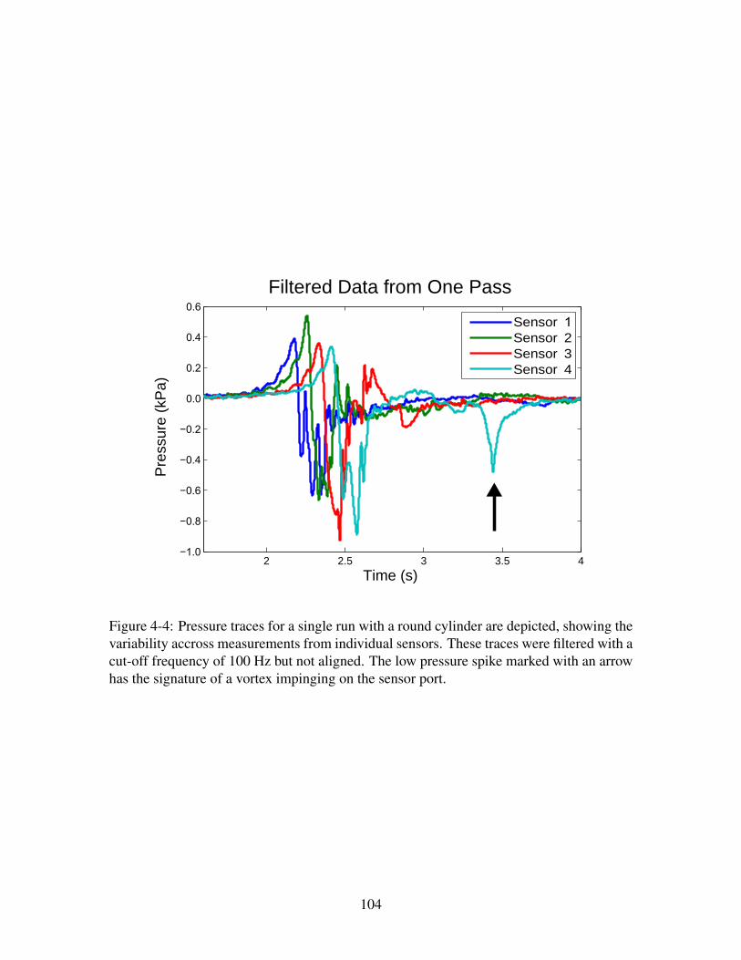
2 2.5 3 3.5 4−1.0

−0.8

−0.6

−0.4

−0.2

0.0

0.2

0.4

0.6Filtered Data from One Pass

Time (s)

Pre

ssur

e (k

Pa)

Sensor 1Sensor 2Sensor 3Sensor 4

Figure 4-4: Pressure traces for a single run with a round cylinder are depicted, showing thevariability accross measurements from individual sensors. These traces were filtered with acut-off frequency of 100 Hz but not aligned. The low pressure spike marked with an arrowhas the signature of a vortex impinging on the sensor port.

104

1 1.5 2 2.5−1.5

−1.0

−0.5

0.0

0.5

Pre

ssur

e (k

Pa)

Square Cross Section 0.50 m/s

Size Comparison of Mean Pressure Traces

1 1.5 2 2.5

Square Cross Section 0.75 m/s

1 1.5 2 2.5−1.5

−1.0

−0.5

0.0

0.5

Time (s)

Pre

ssur

e (k

Pa)

Round Cross Section 0.50 m/s

2"3"

1 1.5 2 2.5Time (s)

Round Cross Section 0.75 m/s

−1.5

−1.0

−0.5

0.0

0.5

−1.5

−1.0

−0.5

0.0

0.5

Figure 4-5: The mean value of the pressure as function of time. Eight data sets are pre-sented, cross-compared to assess the effect of cylinder size. Each data set is composed of100 runs.

105

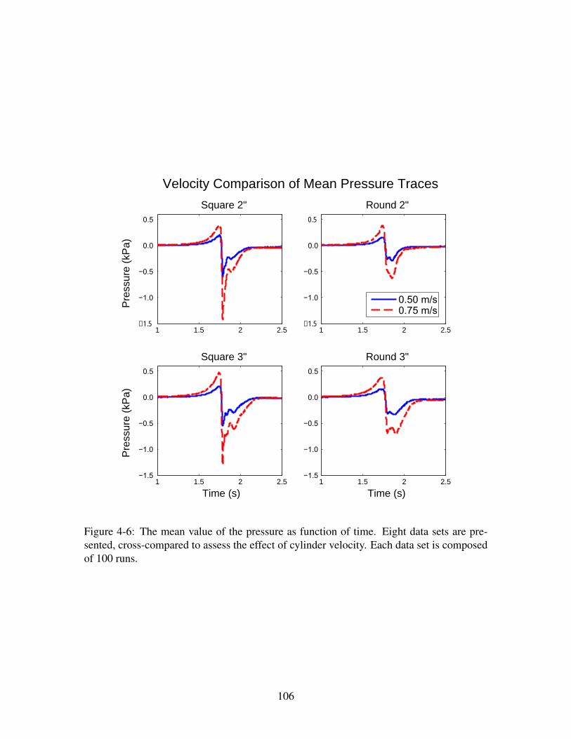
1 1.5 2 2.5−1.5

−1.0

−0.5

0.0

0.5

Pre

ssur

e (k

Pa)

Square 2"

Velocity Comparison of Mean Pressure Traces

1 1.5 2 2.5

Round 2"

1 1.5 2 2.5−1.5

−1.0

−0.5

0.0

0.5

Time (s)

Pre

ssur

e (k

Pa)

Square 3"

1 1.5 2 2.5

Time (s)

Round 3"

0.50 m/s0.75 m/s

−1.5

−1.0

−0.5

0.0

0.5

−1.5

−1.0

−0.5

0.0

0.5

Figure 4-6: The mean value of the pressure as function of time. Eight data sets are pre-sented, cross-compared to assess the effect of cylinder velocity. Each data set is composedof 100 runs.

106

1 1.5 2 2.5−1.5

−1.0

−.5

0.0

0.5

Pre

ssur

e (k

Pa)

2" at 0.50 m/s

Comparison of Cross Sections in Mean Pressure Traces

Square X−SectionRound X−Section

1 1.5 2 2.5

2" at 0.75 m/s

1 1.5 2 2.5−1.5

−1.0

−0.5

0.0

0.5

Time (s)

Pre

ssur

e (k

Pa)

3" at 0.50 m/s

1 1.5 2 2.5

Time (s)

3" at 0.75 m/s

−1.5

−1.0

−.5

0.0

0.5

−1.5

−1.0

−0.5

0.0

0.5

Figure 4-7: The mean value of the pressure as function of time. Eight data sets are pre-sented, cross-compared to assess the effect of cylinder shape. Each data set is composed of100 runs.

107

when the pressure returns to the hydrostatic pressure value. While this change is evident

in the mean pressure traces, it is much more difficult to pick out in the individual pressure

responses due to the large flow variability in that region, which corresponds to the wake

region.

A cylinder moving at a higher velocity creates a larger amplitude pressure response.

Recall that due to the resampling of the lower speed data, this is an effective comparison of

the spatial pressure fields and not the time histories. The increased amplitude is evident in

Figure 4-6 and is expected from potential flow. Indeed, a potential flow model of a circular

cylinder in steady flow predicts that the pressure is given as:

P − P∞ = U2 · C(x, r, ρ). (4.2)

where U is the velocity of the cylinder, x is the position vector from the center of the

cylinder, r is the radius of the cylinder, and ρ is the density of water (refer to [60]). The

model is not quantitatively accurate because it is based on a round cross section and cannot

take into account the wake region; however, it provides qualitatively the correct velocity

dependence. For example, the model predicts that the pressure at 0.75 m/s should be 94

(2.25) times larger than the pressure trace at 0.50 m/s. The ratios found by fitting least

squares in the experimental traces were found to be 2.09, 2.12, 2.13, and 2.15, in clockwise

order, according to Figure 4-6. There does not seem to be any systematic dependence

on the shape or size of the cylinder on this quantity. The scaling effect of velocity is

particularly convenient because it is possible to accurately determine the velocity of the

stimulus by comparing the time lag between sensors. The effects of velocity can, therefore,

be immediately removed from further analysis of the shape of the cylinder.

Finally, the results from different cylinder cross-sectional shapes are compared in Fig-

ure 4-7. Qualitatively, there are a number of apparent differences between the mean traces.

The most striking difference is that the square cross section is characterized by a sharp

peak of low pressure following immediately after the zero cross point. This is true for all

sizes and velocities tested. On the other hand, other differences depend on the size of the

cylinder. In particular, there is a wake length difference for the smaller cylinders that is not

108

present for the larger cylinders. Also, the initial peak, before the zero crossing point, seems

larger and sharper for the square cross sections at 0.75 m/s, but there is little difference with

the round cross section at the lower velocity.

4.4 Analysis

The goal of the analysis is to obtain a reliable approach to classify the cross-sectional shape

of the cylinder stimulus from the pressure signature measured by the pressure sensors in a

single pass. Preferably, the classification should be insensitive to velocity, size, and separa-

tion, indicating that it is truly distinguishing shape. Also, the classification should ideally

be simple to apply to new pressure traces. We consider two approaches to classifying the

cylinder shape: one based on a few features chosen from specific regions in the pressure

traces; and the other based on features extracted with a principal component analysis which

are formed from linear combinations of the entire pressure traces. In the first, the features

are chosen directly as a result of the averaged results shown in Figure 4-7. In the second,

there is no direct influence on which features are utilized.

4.4.1 Heuristically Selected Features

Given the observed differences on average between the pressure measured when a square

versus circular cross section passes the sensors, the simplest approach to classification is to

pick out features among those differences and to assume that they will hold for individual

traces. In this way, the maximum before the zero crossing point (Max), the minimum

immediately following the zero crossing point (Min), and the slope at the zero crossing

point (Slope) were chosen as the characteristic features (Figure 4-8). The slope at the

zero crossing point was determined on data filtered with a cutoff frequency of 60 Hz. The

length of the wake region was not chosen as a feature, despite the fact that it was identified

as a possible source of distinction in the pressure response to the different cross sectional

shapes. This was due to its high variability and difficulty in quantifying the feature from

individual runs.

The effects of the chosen features are heavily correlated. For example, an increase in the

109

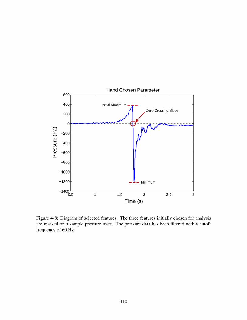
0.5 1 1.5 2 2.5 3−1400

−1200

−1000

−800

−600

−400

−200

0

200

400

600

Time (s)

Pre

ssur

e (P

a)

Hand Chosen Parameters

Initial Maximum

Minimum

Zero-Crossing Slope

Figure 4-8: Diagram of selected features. The three features initially chosen for analysisare marked on a sample pressure trace. The pressure data has been filtered with a cutofffrequency of 60 Hz.

110

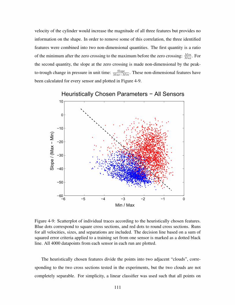
velocity of the cylinder would increase the magnitude of all three features but provides no

information on the shape. In order to remove some of this correlation, the three identified

features were combined into two non-dimensional quantities. The first quantity is a ratio

of the minimum after the zero crossing to the maximum before the zero crossing: MinMax

. For

the second quantity, the slope at the zero crossing is made non-dimensional by the peak-

to-trough change in pressure in unit time: SlopeMax−Min

. These non-dimensional features have

been calculated for every sensor and plotted in Figure 4-9.

−6 −5 −4 −3 −2 −1 0−60

−50

−40

−30

−20

−10

0

10

Min / Max

Slo

pe /

(Max

− M

in)

Heuristically Chosen Parameters − All Sensors

Figure 4-9: Scatterplot of individual traces according to the heuristically chosen features.Blue dots correspond to square cross sections, and red dots to round cross sections. Runsfor all velocities, sizes, and separations are included. The decision line based on a sum ofsquared error criteria applied to a training set from one sensor is marked as a dotted blackline. All 4000 datapoints from each sensor in each run are plotted.

The heuristically chosen features divide the points into two adjacent “clouds”, corre-

sponding to the two cross sections tested in the experiments, but the two clouds are not

completely separable. For simplicity, a linear classifier was used such that all points on

111

one side of the decision line are considered to be square and those on the other side to be

round (Figure 4-9). The classifier was chosen to minimize the sum of squared errors from

a training data subset, where the error for a single run is the difference between a desired

distance from the line and the actual normal distance to the line. The magnitude of the

desired distance was arbitrarily set to one, since the distinguishing key that the desired dis-

tance is positive for one class in the training set and negative for the other class of objects.

The decision line is then found from:

w =(XTX

)−1XT y (4.3)

in which w is a vector of weights that define the decision boundary by w · x = 0; X is

a matrix made from the features such that each column corresponds to one feature and

each row to one test; the vector y is the set of desired distances, with elements of ±1

corresponding to the class of corresponding test. See [78] for details and a derivation of

the result. Minimizing the sum of squared errors makes it possible to obtain a classifier on

a set that is not separable without knowing the probability distributions of the features for

each class. The percentage of misclassified runs (9.8%) gives an estimate of the probability

of error in the classifier.

These heuristically chosen features are straightforward to identify and do not require

any alignment of the data. Given a new time series or spatial distribution of pressure, the

zero crossing point is easy to identify, and all other features follow directly from it. This

classification approach is also fairly insensitive to different sampling rates, as long as they

are high enough to be able to estimate accurately the slope at the zero crossing point. The

difficulty with this approach is that there is a fairly large mis-classification rate (9.8%),

which is likely a result of relying on individual points in a noisy measurement.

4.4.2 Principal Component Analysis

An alternative approach to obtaining features is provided by Principal Component Analy-

sis (PCA) (see [78, 40, 38]). This technique, closely related to the Karhunen-Loeve trans-

form and singular value decomposition, obtains optimal features from noisy data. The fea-

112

tures are linear combinations of the pressure traces with coefficients that are determined by

PCA. The resulting features can in turn be analyzed in a similar manner to the heuristically

chosen-features in order to classify the cross sections of the cylinder stimuli.

Principal Component Analysis interprets each pressure trace, obtained from a single

run on a single sensor, to be a collection of highly correlated features. Each sample is

considered to be a feature. Since there is data from multiple runs, once they are aligned,

there are multiple observations of each feature. The purpose of PCA is to compress the data

so that a small number of linear combinations of the original features (individual samples)

best represent the entire set of data. These new features, which are linear combinations

of the sampled points in a pressure trace, are the principal components. They are found

so that each principal component has the maximum possible variance, subject to having

unit area, and being uncorrelated with all the previous principal components. Implicit

in this procedure is the assumption that the information of interest in the data set is that

which has the largest variance. For example, it assumes that the difference in pressure

traces generated by the different cross sections is larger than the variance in the data due to

noise or turbulence. If this is not the case, the analysis would attempt to provide a compact

representation of the noise. The constraint of uncorrelated principal components is ideal for

feature generation, since it removes redundancy. The variance of the principal components

typically drops off steeply, so that the data are well represented by considering only the

first few components.

In implementation, PCA works as a singular value decomposition of the sample covari-

ance matrix of the data ([40, 38]). One important detail in the implementation is that the

mean of each initial feature (a sample point in the pressure trace) must be removed. This

mean is taken across all training data, not over each class. With the means removed, the

sample covariance is straightforward to calculate.

Several PCAs were performed on the pressure traces. As mentioned, PCA does not

optimize the features for classification. Ideally, the variation in the data would be due

exclusively to the difference in cross section shape. In that case, a Principal Component

Analysis would produce features well suited for classifying the data by stimulus shape;

however, this is not the case. In particular, the variation in the data due to velocity (Fig-

113

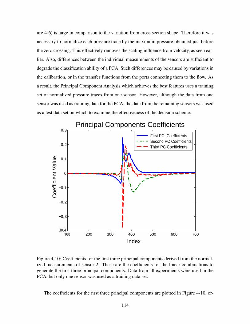
ure 4-6) is large in comparison to the variation from cross section shape. Therefore it was

necessary to normalize each pressure trace by the maximum pressure obtained just before

the zero crossing. This effectively removes the scaling influence from velocity, as seen ear-

lier. Also, differences between the individual measurements of the sensors are sufficient to

degrade the classification ability of a PCA. Such differences may be caused by variations in

the calibration, or in the transfer functions from the ports connecting them to the flow. As

a result, the Principal Component Analysis which achieves the best features uses a training

set of normalized pressure traces from one sensor. However, although the data from one

sensor was used as training data for the PCA, the data from the remaining sensors was used

as a test data set on which to examine the effectiveness of the decision scheme.

100 200 300 400 500 600 700−0.4

−0.3

−0.2

−0.1

0

0.1

0.2

0.3

Index

Coe

ffici

ent V

alue

Principal Components Coefficients

First PC CoefficientsSecond PC CoefficientsThird PC Coefficients

Figure 4-10: Coefficients for the first three principal components derived from the normal-ized measurements of sensor 2. These are the coefficients for the linear combinations togenerate the first three principal components. Data from all experiments were used in thePCA, but only one sensor was used as a training data set.

The coefficients for the first three principal components are plotted in Figure 4-10, or-

114

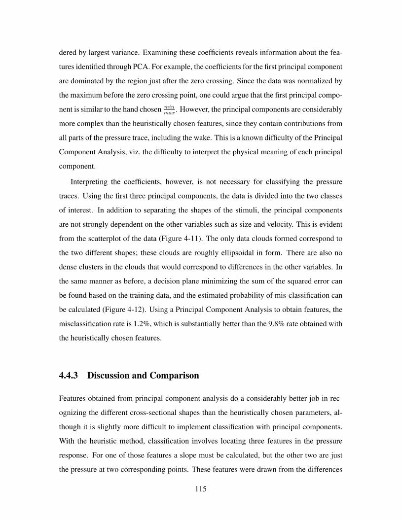
dered by largest variance. Examining these coefficients reveals information about the fea-

tures identified through PCA. For example, the coefficients for the first principal component

are dominated by the region just after the zero crossing. Since the data was normalized by

the maximum before the zero crossing point, one could argue that the first principal compo-

nent is similar to the hand chosen minmax

. However, the principal components are considerably

more complex than the heuristically chosen features, since they contain contributions from

all parts of the pressure trace, including the wake. This is a known difficulty of the Principal

Component Analysis, viz. the difficulty to interpret the physical meaning of each principal

component.

Interpreting the coefficients, however, is not necessary for classifying the pressure

traces. Using the first three principal components, the data is divided into the two classes

of interest. In addition to separating the shapes of the stimuli, the principal components

are not strongly dependent on the other variables such as size and velocity. This is evident

from the scatterplot of the data (Figure 4-11). The only data clouds formed correspond to

the two different shapes; these clouds are roughly ellipsoidal in form. There are also no

dense clusters in the clouds that would correspond to differences in the other variables. In

the same manner as before, a decision plane minimizing the sum of the squared error can

be found based on the training data, and the estimated probability of mis-classification can

be calculated (Figure 4-12). Using a Principal Component Analysis to obtain features, the

misclassification rate is 1.2%, which is substantially better than the 9.8% rate obtained with

the heuristically chosen features.

4.4.3 Discussion and Comparison

Features obtained from principal component analysis do a considerably better job in rec-

ognizing the different cross-sectional shapes than the heuristically chosen parameters, al-

though it is slightly more difficult to implement classification with principal components.

With the heuristic method, classification involves locating three features in the pressure

response. For one of those features a slope must be calculated, but the other two are just

the pressure at two corresponding points. These features were drawn from the differences

115

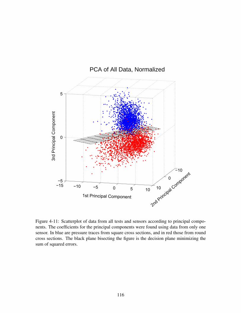
−15 −10 −5 0 5 10

−10

0

10−5

0

5

2nd Princip

al Component

PCA of All Data, Normalized

1st Principal Component

3rd

Prin

cipa

l Com

pone

nt

Figure 4-11: Scatterplot of data from all tests and sensors according to principal compo-nents. The coefficients for the principal components were found using data from only onesensor. In blue are pressure traces from square cross sections, and in red those from roundcross sections. The black plane bisecting the figure is the decision plane minimizing thesum of squared errors.

116

−4 −3 −2 −1 0 1 2 3 4 5 60

10

20

30

40

50

60

70

80

90

100

Error in Classifying Square: 0.20 % Error in Classifying Round: 2.20 % Total Classification Error: 1.20 %

Distance to Decision Boundary

Num

ber o

f Poi

nts

Histogram of Normalized Data Using the PCA

Figure 4-12: Histogram of the distance from the decision plane as shown in Figure 4-11.In blue is the data from the square cross section and in red from the round cross section.

observed in the average pressure traces for each shape. Then, the classification of a new

pressure trace can be made based on the sign of the distance d, defined by:

d = w2 ·(Min

Max

)new

+ w1 ·(

Slope

Max−Min

)new

+ w0 (4.4)

where the constants w2, w1, and w0 come from the equation of the decision line in Figure 4-

9, which is w2 · MinMax

+w1 · SlopeMax−Min

+w0 = 0. The distance will be positive for square cross

sections and negative for round cross sections. The main downside to this approach appears

to be closely tied to it’s ease in calculation. The features used to classify the shape are very

localized quantities, therefore susceptible to noise. Low pass filtering is necessary in order

to remove some of the worst noise issues and it is telling that this effectively spreads out

the number of data points used to calculate the feature.

In the case of the principal components the approach is the complete opposite, relying

on differently weighted contributions from the entire pressure data set. There are essentially

three steps for classifying a new pressure trace using the PCA results. First the zero crossing

point must be located, just as in the other method. Second, the same mean pressure trace

117

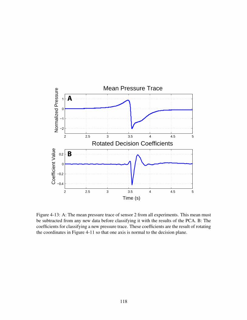
2 2.5 3 3.5 4 4.5 5

−2

−1

0

1

Nor

mal

ized

Pre

ssur

e Mean Pressure Trace

2 2.5 3 3.5 4 4.5 5

−0.4

−0.2

0

0.2

Time (s)

Coe

ffici

ent V

alue

Rotated Decision Coefficients

A

B

Figure 4-13: A: The mean pressure trace of sensor 2 from all experiments. This mean mustbe subtracted from any new data before classifying it with the results of the PCA. B: Thecoefficients for classifying a new pressure trace. These coefficients are the result of rotatingthe coordinates in Figure 4-11 so that one axis is normal to the decision plane.

118

that was subtracted from all the normalized data in the analysis (Figure 4-13A) must be

removed from the new trace. Then, the distance to the decision plane can be found through

a linear combination with the coefficients shown in Figure 4-13B, which are a combination

of the coefficients for the principal components rotated such that they form a coordinate

normal to the decision plane. Thus only one linear combination is performed with the

new data, and the result is compared to the intersection of the decision plane on that axis.

Besides the added complexity, the fact that the mean from the training data must be kept in

memory may limit the extent to which this procedure may be generalized.

The primary question remaining on the topic of the PCA results is what information is

being used to make the accurate decisions. By rotating the principal components to align

an axis with the decision plane, it was possible to condense the decision metric into a single

test depicted in Figure 4-13. By examining the weights of this test (part B of the Figure 4-

13) and in particular comparing them against the mean pressure trace (part A), one can

extract some intuition on the information being used.

The linear combination weights have three main sections of interest. The first of these

is the small positive peak observed just after the 3.5s mark in Figure 4-13B. When com-

pared against the mean pressure trace, this peak is situated between the peak maximum

pressure and the zero crossing point. It is expected that the zero crossing point would have

zero weight in the classification test, since all the pressure traces were aligned at that point

and therefore it is a constant across all the data sets. Similarly, the magnitude of the max-

imum pressure has been normalized for all the pressure traces, which may be why the test

coefficients are small at that location. One explanation for this first peak is that it is tied

to the slight rearward shift in the location of that first peak that is observed for the square

cross section. It is also possible that the important component is not necessarily the peak of

the coefficients, but instead perhaps it is the constant slope in the coefficients through the

zero crossing point which approximates the derivative at the zero crossing point. The exact

nature of this bump in the decision test weights is still unclear.

The second region of interest in the decision weights is also the most dominant one: the

large negative peak in the weights (labeled as III in Figure 4-14). The minimum peak in

the weights corresponds to the location of the minimum peak in the average pressure trace.

119

This matches the observations in the earlier results section, in which the minimum pressure

was the most clear indicator of the shape of the cylinder on average. Since the pressure

is negative in this region, the large negative pressure aligned with the weights that occurs

with the square cylinder will result in a large positive contribution to the decision metric.

The peak in the decision coefficients is sharp in this region, which appears to indicate that

the location of the minimum pressure is critical. This is a bit surprising given that the

individual traces such as those seen in Figure 4-4 seemed to display a range in positions

for the minimum pressure. Despite this, the meaning behind the large weights in this area

is fairly clear.

The third region of interest in the decision weights is the most surprising overall. This

area is the relatively broad area of positive weights located completely in the wake of

the cylinder (see section IV in Figure 4-14). While there are definitely differences that

were observed on average in this region of the pressure field, it is also a region of high

variability between one trace and the next (see Figure 4-3). As a result, it was unexpected

that information from this area would be used to judge the shape of the cylinder. Based

on the positive decision weights, this region in the decision weights implies that a smaller

or more positive wake region is associated with the square cylinder. It is difficult to see

from the averaged pressure traces why this is associated with the square shape. According

to the mean traces, the low pressure region for the square cylinder generally takes longer

to recover to zero. This would imply the opposite association as is seen is the decision

weights, and is also counter to the manner that the decision weights taper off. In any case,

the different size cylinders have a much larger effect on the length of the wake than the

shape. The only possible feature observed in the averaged pressure traces that might be

associated with this region in the decision weights is the slight rebound in the pressure seen

after the primary negative peak for the square cylinders. In Figure 4-7, there is a consistent

region just after the main negative peak in which the pressure for the square cylinder is

larger than that of the round cylinder. It is a brief period and not a large effect when viewed

on average, but that may be what the weights from the PCA approach are using.

These three regions describe the main sections of non-zero weights in the classification

test. The regions before and after these three sections appear to be largely zero. However,

120

300 350 400 450

−0.4

−0.2

0

0.2

Coecient Number

Coe

cien

t Wei

ght

0

10

20

30

40

50

Prob

abili

ty o

f Mis

scla

ssi

catio

n

I II III IV V

I II III IV V I-V III-V II-III I-IIIII-IVII-IVCoecient Sections

PCA Decision Components

Figure 4-14: Comparison of results using modified decision weights. The top subfigureindicates the division of the decision weight coefficients into different regions. A classifi-cation test using weights composed of the original coefficients with regions zeroed out isshown in the lower subfigure. The non-zero regions are labeled for each bar.

since they span a large area, they may still contribute to the final decision. In addition,

although each of the three primary sections can be tied to possible differences between

the shape pressure fields, it is important to recall that the PCA methods used to create the

decision weights did not necessarily prioritize the shape. In particular, it is possible that the

third region described, found in the volatile wake are of the pressure field, does not affect

the shape classification but was instead included in the principal components simply due

to the high variability. In order to examine the importance of the various sections of the

weights in the classification test, the misclassification rate was recalculated based on tests

different sections of the decision weights set to zero. The results are visible in Figure 4-14.

In the lower figure, the first five bars indicate the results when each section individually is

non-zero. Compared to the full result (the sixth bar at 1.2% error), all the individual sections

are substantially worse at classifying the shapes. Keep in mind that a fully random decision

metric would give approximately 50% error. Therefore sections I and V individually are

fairly close to providing no information about the shape of the cylinder. This confirms the

121

expectation that the small variations in the weights in these sections do not substantially

effect the classification. When considered individually, the best classification region is

region III, which again matches expectations. It is interesting to note further, however, that

region II more accurately predicts the shape than region IV. Upon further investigation, the

simple relationships implied by the performance of the individual sections is substantially

complicated. First of all, it appears that the information utilized in section II is redundant

with that of section III, where as the information in section IV is crucial to an accurate

classification. These statements come from the observation that classification based on

sections II and III jointly result in fairly poor accuracy, where as the inclusion of section IV

improves the result to slightly worse than that of the full set of coefficients. On the other

hand, when including section IV, there is very little difference in the results when section

II is included or excluded. It is also interesting to note that the inclusion of the final section

of coefficients in the III-V result provides the best result by a small margin. In comparing

the results of the III-V section to the I-II section, it is clear that the coefficients beyond the

zero crossing point are much more important than those before. In summary, it appears that

sections III and IV are critical in producing an accurate classification, where as section II

is redundant with III, and section V still provides a very modest benefit.

Having established that the pressure distribution in the wake is a vital component in the

decision to classify the shape of the passing object, it is still unclear how the information

about the shape is encoded in the wake. One possibility that deserves exploration is that

the structure of the shed vortices changes between one shape and the next. It is well known

that the shape of the cylinder affects the Strouhal number [5], which governs the vortex

shedding frequency. It is possible that the spacing in the shed vortices consistently effects

the measurements, even if the phase of the vortex shedding is random. For the range of

Reynolds numbers used in the experiments, the Strouhal numbers for both cylinder shapes

are fairly flat at 0.2 and approximately 0.14 for the round and square cross sections respec-

tively. This means that the vortices are spaced at approximately every 2.5 diameters for the

round cylinder and 3.6 diameters for the square cylinder. When considering the different

diameters included in the test data, the results are shown in the following table:

Note for reference that the length of the sensor array is about 20 cm. Therefore, in most

122

7.62 cm Diameter 5.08 cm DiameterRound 19 cm 12.8 cmSquare 27.1 cm 18.2 cm

Table 4.2: Table of the Strouhal numbers associated with the cylinder identification exper-iments.

of the experimental runs a vortex was shed near at least one of the sensors. However, the

more important observation from the table is that the effect of the two different diameters

on the Strouhal number is large compared to the effect of the shape on it. Although for a

given diameter, the vortex spacing is much larger for the square cylinder, the vortex spacing

of the small square cylinder is nearly equivalent to the at of the large round cylinder. This

means that half of the data would be ambiguous or even potentially misclassified if the test

was based solely on the vortex spacing. When in addition to this, the random phase of the

vortex shedding is factored in, is unlikely that the vortex spacing is a contributing factor in

the cylinder shape identification. The cause for the difference in Strouhal numbers with the

cylinder shape is related to the distance between the two separated shear layers[5]. This

width is in turn increased for bluffer bodies such as the flat face of the square used in these

experiments. It is possible that this difference in wake size and structure is responsible for

the information utilized in section IV of Figure 4-14. The wake thickness would have the

same dependence on shape and size as the Strouhal number, but would not rely on the added

random timing of the vortices. When considered alone, the decision coefficients in section

IV resulted in approximately 30% error in classification. This matches the hypothesis that

the wake thickness would distinguish approximately half of the data and be ambiguous on

the other half.

4.5 Conclusion

This chapter has shown that the shape of a cylinder can be distinguished between two

known shapes using the information from a linear array of pressure sensors. Although

this does not go the entire way to demonstrating that an arbitrary shape can be identified

based on a lateral-line-like sensor array, it has established that detailed information on

123

the shape is available and indicated what aspects of the pressure response are the most

relevant. Two successful approaches for distinguishing the cylinder shape were described

in this chapter, overcoming the large variation observed in repeated trials with the same

cylinder. The first utilized differences observed in the averaged responses to each shape in

order to select features that could identify the shape in an individual pressure trace. The

second approach, with an error rate less than 2% utilized a principal component analysis

to identify the modes of most significant variation in a set of training data. By ensuring

that the difference in shape was the primary cause of consistent differences in the data,

this approach was directed towards generating a single test which evaluates the shape of

the cylinder. The result from the PCA approach utilizes the entire pressure data set of the

cylinder after is has passed to make a decision.

The accuracy in the classification based on the PCA-derived test is all the more sur-

prising given the range of velocities, sizes, and distances of the cylinders used. Although

the primary interest is in the shape of the cylinders, it is important to include this range

of parameters in any attempt to demonstrate that it is the shape that is being distinguished

instead of two experiments. For example, the importance of the Strouhal number could not

be evaluated without the variety of sizes in the cylinders tested. The two tests described

in this chapter were both able to identify the shape of a cylinder after it had passed the

sensor array using a single test to determine the shape in a range of conditions. While this

should not be generalized into concluding that the tests work for all sizes and velocities, it

is important to know that a test will be robust to small errors in the estimate of the size or

velocity that might be predicted ahead of time via strategies from Chapter 3.

The results from the classification test developed with the principal component analysis

makes it clear that the pressure corresponding to the wake region in the pressure field

contains significant information about the shape of the cylinder. In fact, it appears that the

PCA results were equally effective in identifying the shape if no information forward of

the zero-crossing point was used. This is an interesting result in that it runs counter to the

implicit assumptions of potential flow studies that portions of the flow, such as that ahead

of the cylinder, may be well represented by the potential flow about an object. Given the

importance of the wake in identifying the shape between two known possibilities, it will be

124

necessary in order to identify an arbitrary shape to have a good flexible model for the wake

and its relationship to the shape. This may call for numerical estimation methods. From

looking into possible sources of information in the wake, the results have reinforced the

importance of first estimating the size of the cylinder in order to be able to distinguish the

cause for a large wake width.

125

Chapter 5

Vortex Tracking

5.1 Introduction

From the results in Chapter 3, it was found that the immediate wake of a moving cylinder

contained a substantial amount of information for distinguishing the shape of that cylinder.

In this chapter, the wake is considered on its own, with an emphasis on a well developed

wake further from the body that have generated it than in the moving cylinder case. Within

the wake, vortices are a critical long-lived component that forms due to instability in the

separated shear layers [5]. When considering the strict range limitations due to the decay of

the near field pressure distribution, vortices present an opportunity to extend the footprint

of a moving object much further. For example, a seal has been shown to be able to trace

the motion of remote underwater vehicle based on the wake with a delay of up to five

seconds [29]. Information gathered about vortices in the wake of an object can be used

to infer certain features of the original object, such as speed and size based on the vortex

spacing and strength.

Completely separate from their relevance to detecting and identifying a moving object,

vortices are of interest in themselves. As persistent coherent fluid structures, vortices affect

the flow and pressure distributions about nearby objects. Besides being the basis for the

entire idea of using an artificial lateral line, this also means that vortices affect the function

of flapping foils or control surfaces which rely on generating a pressure difference between

opposing surfaces. Therefore, self generated vortex can have substantial effects on maneu-

127

vering vehicles. As one example, the leading edge vortex that forms in a foil at high angles

of attack strongly influences the amount of lift generated, critically important for the flight

of insects such as the Hawkmoth [1].

In addition to the background described in Chapter 2 on how a fish is theorized to locate

and utilize vortices in the wake of an object to decrease its energy expenditure, there have

been a few studies examining the problem of tracking vortices based on distributed pres-

sure sensors or artificial lateral lines. In the first of these, Ren and Mohseni [66] examined

the detection of a vortex wake from a fish-like body in two dimensions. Their study, using

potential flow in two dimensions with a Joukowski foil model for the fish body, was largely

focused on the conditions for identifying a regular convecting vortex street based on the

pressure and pressure differences on a sensor array distributed over the boundary of the

foil. However, the spacing between the vortices considered in this work is much smaller

than the array length, so that five or more vortices are contributing substantially to the mea-

surements at any particular time. The focus is correspondingly on the effect of array density

in capturing the oscillatory pressure gradients of the problem. This work differs from that

presented in this chapter since this chapter is concerned with identifying the precise state

of one and two vortices, as opposed to the global characterization (such as frequency) of a

vortex wake, which can be subsequently extracted from the detailed information.

Suzuki and Colonius [74], consider the inverse problem of identifying a vortex in an

air channel from a numerical perspective. The estimation was accomplished via an instan-

taneous least squares optimization, with a small discussion of a fixed estimator-corrector

mechanism between timesteps. The enclosed channel with known flow velocity considered

in the paper is a substantially different environment, particularly in terms of the convention

of the vortices. The paper also tackles the question of tracking multiple vortices simultane-

ously, finding that the accuracy of the vortex tracking based on the least squares inversion

degrades substantially when two vortices are in sufficiently close proximity to affect the

each other’s measurements.

Both Suzuki and Colonius, and Ren and Mohseni demonstrate that in a potential flow

formulation, information on vortices in the flow is theoretically available to a lateral-line-

like sensor array. However, it is still unclear to what extent these theoretical results extend

128

to real environments. This is particularly true given the ignored viscous affects and other

background fluid flow which may lead to highly correlated noise in the measurements.

This chapter develops a slightly different theoretical base from both previous works, using

the same potential flow assumptions, in order to solve the inverse problem for an artificial

lateral line tracking a vortex in an open environment from both a fish (or AUV) and ship hull

perspective. This model base and estimation method is tested on experimental data using

single vortices and vortex pairs, using particle image velocimetry (PIV) to independently

verify the accuracy of the inversion. The use of experimental data also makes it possible to

verify the accuracy of the forward model, which predicts the pressure distribution based on

a known vortex state. In addition, the questions of tracking two interacting vortices and the

relation between sensor array parameters and accuracy are considered.

5.1.1 Variable Definitions

For consistency throughout multiple experiments in tracking vortices, similar variables and

coordinate systems will be used in each case. The general problem formulation consists

of one or several vortices moving in a plane, with some points of measurement in a linear

array on that plane. The axes are defined with the origin at one of the sensors in the linear

array, with the X axis parallel to the linear array and the Y axis pointing away. The fluid

domain in which vortices may be is limited to the half plane defined by the positive Y axis.

Each vortex is defined by a state vector of three variables: (xi, yi, ki) where xi and yi are

the position of the ith vortex, and ki refers to its strength which is related to the circulation

of the vortex by Γi = 2πki. Frequently the position of a vortex is depicted as the complex

zi = xi+ ıyi. The position of each sensor is denoted by sj , where s marks a location on the

x axis. The pressure measured at one of the sensors is Pj , with the subscript corresponding

to the sensor number, as for sj .

When considering models for the vortices, the vortex state vector will be referred to as

qi(t), where the subscript refers which state formulation is being used. All cost functions

are denoted by J , and are positive functions of vortex parameters. For a general variable, a

superscript of “meas” refers to the measured quantity, as opposed to the modeled quantity

129

(denoted by a “model” superscript) or a true quantity (superscript “true”) in the case it is

being compared directly against a simulation with a defined true value.

5.1.2 Vortex Modeling

The vortex tracking described in this chapter is founded on a general set of models using

potential flow in two dimensions to represent the real fluid domain. The two major assump-

tions involved in these representations, that of an inviscid and largely two dimensional flow,

fit well for this problem as long as a few restrictions are placed on the vortices.

Unlike the situations described for cylinder tracking and identification, the fluid flow

involved with measuring vortices is very well captured by potential flow models. The

inviscid assumption is substantially less onerous. Due to the simple streamlined geometries

of the sensing bodies, there is no flow separation on the bodies based on the flow induced

by vortices at a reasonable distance. For the vortices themselves, since they are purely fluid

structures there is no wake or flow separation as there is with a moving cylinder. Therefore,

in a two dimensional plane, a line vortex described by the complex potential Φ (z) =

−ık log (z − zo) accurately predicts the flow distribution beyond a minimum distance from

center of the vortex. A core region of the vortex must be exempted as the line vortex model

predicts that the velocity is unbounded. Instead, viscous effects dominate close to the vortex

center, and the rotation is close to a solid body rotation. Several models are commonly used

to account for the vortex core, such as the Rankine vortex model which inserts a solid body

rotation within some boundary radius, and the Oseen vortex [68], which further smooths

the transition between the solid body and irrotational flow.

In large part however, the vortex core can be ignored for the purposes of tracking vor-

tices. The vortices considered here are generally well separated, with the distance between

vortex centers substantially larger than a vortex core diameter. In addition, as long as the

vortices do not approach too closely to the sensing body, the vortex cores do not affect the

pressure measurements. This is the case generally for all the experiments in this chapter.

The only remaining concern in terms of viscous effects is the generation of secondary

vorticity from the interaction of a vortex with the sensing body. This will occur if the pri-

130

mary vortex approaches the sensing body structure too closely and causes flow separation.

Based on observations, this did not occur except at distances in which the influence of the

core on the measurements might also be suspected (based on PIV results). Therefore, the

experiments and analysis of vortex tracking were limited to trials in which the vortices

maintained sufficient distance.

The two dimensional limitation of the models used in this chapter is a potential source

of error when estimating the vortex state. In order to minimize the discrepancies caused

by this assumption, long vertical vortices were generated using extended foils. While tech-

nically vortex rings, this approach maximizes the distance between the horizontal portions

of the ring and the sensors. In addition to the vortices themselves, the shape of the sensing

body affects the amount of flow out of the modeled plane. This affect will be considered

later, as it affects the experiments differently.

5.2 Experimental Procedure

In all of the experiments involving tracking a vortex or vortex pair based on a linear pressure

sensor array, the basic layout is the same. The experiments consist of two parts: measuring

the pressure generated by vortices with a lateral-line-like sensor embedded in an enclosure,

and completely independently collecting information to locate and measure the strength of

the vortices. These two components allow the estimation of the vortex state based on the

pressure measurements to be compared against a ground truth. The independent determi-

nation of the vortex state is done using particle image velocimetry (PIV), which provides

a quantitative description of fluid flow in a plane. The primary difference between the two

sets of experiments is in the shape of the body which encloses the sensors. One set of

experiments uses a streamlined cylindrical body, much like the shape of the Remus AUV

[37] and the other uses a flat plate in order to approximate the effect of sensors mounted on

a ship hull.

131

5.2.1 Particle Image Velocimetry

Particle image velocimetry (PIV) is a common fluid visualization technique that has de-

veloped many variants since its introduction. In general it provides a quantitative estimate

of the velocity field of a fluid. In these experiments, PIV is used in both experimental

setups to provide the control information for the vortices being tracked. Although the de-

tails of the implementation differ slightly for each setup, the fundamental technique of PIV

is the same. In each case, a very thin laser sheet is used to illuminate a horizontal two-

dimensional plane in the flow, in line with the sensor array axis. Inside this plane, neutrally

buoyant small particles reflect the light while effectively traveling with the fluid. A camera

located perpendicular to the laser sheet captures images of the position of these particles

in rapid succession. The change in location of the particles between frames then forms the

basis for the calculation of the velocity field. Instead of tracking individual particles, the

velocity field is determined by comparing the cross correlation of small windows in each

frame. This makes use of multiple particles to estimate the velocity direction, and is more

robust against particles traveling out of the imaged plane. The size of these interrogation

windows is an important factor in the processing of the PIV data.

The planar particle image velocimetry used in these experiments provides an estimate

of the velocity field in the illuminated plane. From the velocity field, it is possible to

identify the location vortices (discussed further in 5.3.2). One important constraint is that

no information is available on velocity components out of the illuminated plane. In order

to minimize the importance of this velocity component, the experiments, particularly with

respect to the vortex generation, were designed in order to maximize the two-dimensional

nature of the flow.

5.2.2 Experimental Layout: Streamlined Body

The primary characteristic of the first experiment for tracking vortices is that it utilizes a

streamlined body to enclose the pressure sensor array. The basic geometry of the sensing

body consists of a cylindrical body with a 10.16 cm (4 inch) outer diameter. The front and

back of the tube are capped using sealed plywood attached to high density polyethylene

132

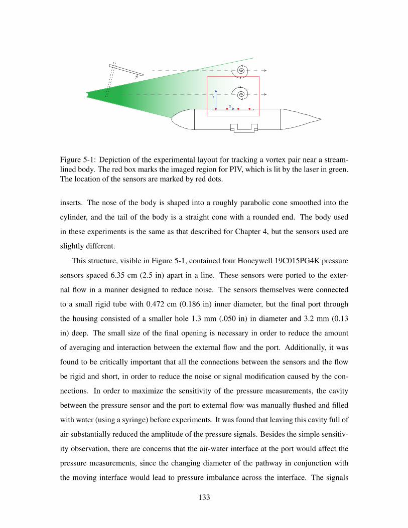
X

Y

Figure 5-1: Depiction of the experimental layout for tracking a vortex pair near a stream-lined body. The red box marks the imaged region for PIV, which is lit by the laser in green.The location of the sensors are marked by red dots.

inserts. The nose of the body is shaped into a roughly parabolic cone smoothed into the

cylinder, and the tail of the body is a straight cone with a rounded end. The body used

in these experiments is the same as that described for Chapter 4, but the sensors used are

slightly different.

This structure, visible in Figure 5-1, contained four Honeywell 19C015PG4K pressure

sensors spaced 6.35 cm (2.5 in) apart in a line. These sensors were ported to the exter-

nal flow in a manner designed to reduce noise. The sensors themselves were connected

to a small rigid tube with 0.472 cm (0.186 in) inner diameter, but the final port through

the housing consisted of a smaller hole 1.3 mm (.050 in) in diameter and 3.2 mm (0.13

in) deep. The small size of the final opening is necessary in order to reduce the amount

of averaging and interaction between the external flow and the port. Additionally, it was

found to be critically important that all the connections between the sensors and the flow

be rigid and short, in order to reduce the noise or signal modification caused by the con-

nections. In order to maximize the sensitivity of the pressure measurements, the cavity

between the pressure sensor and the port to external flow was manually flushed and filled

with water (using a syringe) before experiments. It was found that leaving this cavity full of

air substantially reduced the amplitude of the pressure signals. Besides the simple sensitiv-

ity observation, there are concerns that the air-water interface at the port would affect the

pressure measurements, since the changing diameter of the pathway in conjunction with

the moving interface would lead to pressure imbalance across the interface. The signals

133

from the pressure sensors were amplified immediately within the sensing body, using the

amplification circuit described in Chapter 3. The resulting amplified signals were transmit-

ted through a short shielded cable to a NI-DAQ USB 6210 data acquisition system powered

directly by an unplugged laptop. The data was collected at 30 kHz via a custom LabView

program. Besides the pressure data, an additional signal from the PIV system correspond-

ing to the camera trigger was also recorded, in order to later match the timing between the

two data sets. To calibrate the sensors, the change in static pressure between the operating

depth and the surface was used, based on both the initial setup and the final removal.

In order to generate vortices easily detectable by the pressure sensor array, a vortex pair

was generated by the sweep of a thin rigid flat plate (roughly 23cm (9 in) by 28 cm (11 in)

with the axis of rotation 2 inches from the rear). Figure 5-1 depicts the rough orientation

of the plate at the beginning and end of the motion used to generate the vortices. In order

to provide the torque to generate large vortices, it was found that driving the plate by

hand was much more effective than all attempts to mechanize the process. This required

some training in order to properly direct the vortex pair, which was accomplished using

the illumination PIV laser sheet at very low power to provide feedback and visualization

of the fluid motions. The end result, as shown in Figure 5-1, is that a pair of vortices was

regularly generated which would travel in straight line roughly parallel to the direction of

the sensor array.

These experiments were carried out in a small fluid visualization tank at the MIT towing

tank with dimensions of 2.4 m by 0.75 m by 0.7 m, with the last dimension of height

varying slightly depending on the water level. The depth of the line of pressure sensors

below the water level was approximately 30 cm in all cases. The calibration of the sensors

was checked each day of experimentation by comparing the pressure difference from the

surface to the final operating depth. The sensor body was mounted in the tank using a stand

which extended slightly behind the streamlined body. In order to minimize any motions,

the stand connected to the tank in three non-collinear locations forming a rigid connection.

The PIV setup used to independently image the vortex state utilized a Quantronix Dar-

win 527 Series Nd:YLF laser mounted on an optical table at one end of the tank. This is a

pulsed laser with an optimal frequency of 1 kHz for maximizing the output power. In these

134

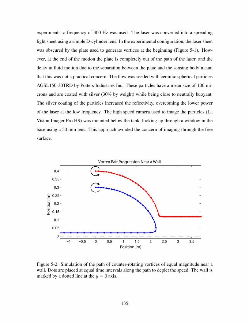
experiments, a frequency of 300 Hz was used. The laser was converted into a spreading

light sheet using a simple D-cylinder lens. In the experimental configuration, the laser sheet

was obscured by the plate used to generate vortices at the beginning (Figure 5-1). How-

ever, at the end of the motion the plate is completely out of the path of the laser, and the

delay in fluid motion due to the separation between the plate and the sensing body meant

that this was not a practical concern. The flow was seeded with ceramic spherical particles

AGSL150-30TRD by Potters Industries Inc. These particles have a mean size of 100 mi-

crons and are coated with silver (30% by weight) while being close to neutrally buoyant.

The silver coating of the particles increased the reflectivity, overcoming the lower power

of the laser at the low frequency. The high speed camera used to image the particles (La

Vision Imager Pro HS) was mounted below the tank, looking up through a window in the

base using a 50 mm lens. This approach avoided the concern of imaging through the free

surface.

−1 −0.5 0 0.5 1 1.5 2 2.5 3 3.50

0.05

0.1

0.15

0.2

0.25

0.3

0.35

0.4

Position (m)

Posi

tion

(m)

Vortex Pair Progression Near a Wall

Figure 5-2: Simulation of the path of counter-rotating vortices of equal magnitude near awall. Dots are placed at equal time intervals along the path to depict the speed. The wall ismarked by a dotted line at the y = 0 axis.

135

5.2.3 Experimental Layout: Flat Body

In the case of the sensor array being embedded in a flat plate, which more closely reflects

the situation on a ship hull than the streamlined sensor body, the same experiment cannot

physically be carried out. With a flat plate sensor enclosure, the interaction between the

vortices and the plate alters the path of the vortices. Although the setup of the second set

of experiments (Figure 5-3) uses a flat plate of limited size, it effects the vortices in much

the same way as a flat plate of infinite span. Using the potential flow line vortex model,

the flat plate can be accounted for by reflecting the two real vortices over the plane of the

plate. This four-vortex system now interacts very differently than a two-vortex system. In

particular, if the two real vortices begin with equal and opposite circulation, the velocity

of the two vortices will not be equal: The vortex closest to the wall will be affected by

the image vortices more strongly. Since the closest image vortex is it’s own reflection, the

dominant influence is to slow down with respect to the outer physical vortex. This implies

that the case of linear translation for the vortex pair parallel to the wall in an unstable

scenario. It can be accomplished in potential flow by just the right balance of circulation

between the vortices, but it would be very unlikely to occur in experiments.

Figure 5-2 demonstrates the type of path that results from a vortex pair with equal

circulation magnitude and initially located perpendicular to the wall. As seen in the figure,

the two vortices first rotate and converge on the wall. At a certain point in the approach to

the wall, the distance of the closest vortex to its image becomes smaller than the distance

to the second physical vortex, resulting in a change in direction. Fairly quickly after this,

the two physical vortices proceed as if nearly independent of each other, following paths

parallel to the wall in opposite directions, at speeds corresponding to their distance from

the wall. Experimentally, based on PIV observations, the vortices were verified to carry out

this prediction. In order to generated data to test the tracking of vortices near a hull-like

body, an alternative configuration was used, where the initial vortex pair is arranged parallel

to the wall. In this case, the two vortices approach the wall directly and split evenly, both

final vortex trajectories having the same distance from the wall, but moving in opposite

directions. The rough observed trajectories are sketched in the layout diagram (Figure 5-

136

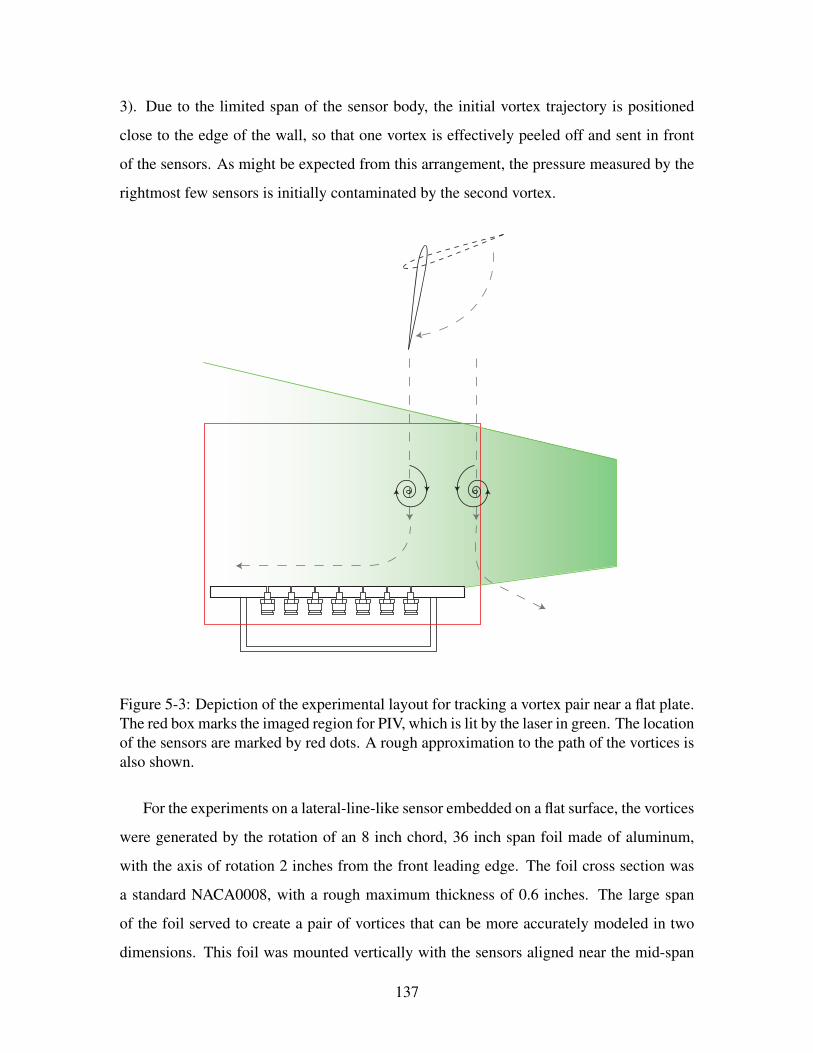
3). Due to the limited span of the sensor body, the initial vortex trajectory is positioned

close to the edge of the wall, so that one vortex is effectively peeled off and sent in front

of the sensors. As might be expected from this arrangement, the pressure measured by the

rightmost few sensors is initially contaminated by the second vortex.

Figure 5-3: Depiction of the experimental layout for tracking a vortex pair near a flat plate.The red box marks the imaged region for PIV, which is lit by the laser in green. The locationof the sensors are marked by red dots. A rough approximation to the path of the vortices isalso shown.

For the experiments on a lateral-line-like sensor embedded on a flat surface, the vortices

were generated by the rotation of an 8 inch chord, 36 inch span foil made of aluminum,

with the axis of rotation 2 inches from the front leading edge. The foil cross section was

a standard NACA0008, with a rough maximum thickness of 0.6 inches. The large span

of the foil served to create a pair of vortices that can be more accurately modeled in two

dimensions. This foil was mounted vertically with the sensors aligned near the mid-span

137

level. A rod connected to the foil forming the axis of rotation was held in the motor mount

above the water in order to allow for persistence in the location of the foil. However, the

actual motion of the foil was hand driven, using a small bar attached obliquely to the foil to

apply torque. This apparatus was necessary to provide sufficient torque to generate clearly

visible and measurable vortices. Unfortunately, as a result of the hand driven motion, an

exact description of the motion of the foil is unavailable and subject to a certain degree

of variability between trials. The results, as observed through PIV images, corresponded

with well defined measurable vortices most when the foil initially rotated counter the final

motion. Roughly speaking, the foil would begin from rest at approximately 80 degrees from

the axis pointing perpendicularly to the linear array, slowly sweep back to approximately

100 degrees, then smoothly but quickly rotate to its final position of 10 degrees.

The sensor body and data acquisition setup used in these experiments is identical to

the one described in Chapter 3, in the experiments in cylinder tracking. In short, seven

Honeywell 19C015PG4K sensors formed a linear sensor array, spaced apart by 0.75 inches.

The linear array was embedded in the center of a 16 inch square flat plate, representing a

ship hull or section of another large flat object. The same amplification circuit was used to

amplify the pressure signals 970 times before collecting the data via a NI-DAQ USB6210

analog to digital converter. Pressure data was collected at 30 kHz.

The flat surface vortex estimation experiments were done in a different tank compared

to the streamlined body experiments. This tank is the same as that discussed for the ex-

periments in Chapter 3, with dimensions 3.6 m by 1.2 m by 1.2 m. The calibration of the

sensors was again done by comparing the difference between the pressure at the operating

depth and the surface to the operating depth (approximately 40 cm). This calibration was

checked at the start of the experiment and again at the end, to check for any long term drift

or other malfunction.

The PIV setup for the flat body experiments is also substantially different than that of

the streamlined body, due to the different locations. The rough arrangement is similar: a

horizontal laser sheet with the vertically mounted camera capturing images from below.

However, for these experiments, a continuous wave Coherent Verdi V10 laser was used,

mounted on an optical table on top of a rolling cart. As in the case of the streamlined body,

138

the laser beam was converted to a flat sheet using a d-cylinder. In this case, the optics were

also augmented by a set of two ninety degree mirrors to adjust the height of the sheet. The

same particles were used to seed the tank as in the streamlined body experiments. The

camera used to capture the particles lit by laser light, however, was a high-speed Phantom

V10 camera with a 50 mm prime Nikon lens. The camera was again mounted below the

tank, and a rough depiction of the field of view is shown in Figure 5-3. In the case of the

flat plate, care needed to be taken in the positioning of the camera. Although ideally the

sensors would be at the edge of the field of view in order to maximize the visualization of

the fluid, this leads to an oblique view of the flat plate on which the sensors are mounted.

The result is a ghost image of the sensor structure illuminated by the diffuse laser light

which is present in all the images. This complicates the PIV calculations, as it is essentially

a stationary image that contradicts information from moving particles. In order to reduce

this effect, the camera needs to be position as close to the plane of the flat plate as possible.

It is therefore a trade off between maximizing the field of view of the flow and maximizing

the quality of the velocity approximation in the region very close to sensors. This trade off

was improved as much as possible by reducing the amount of diffuse laser light. A certain

amount of the laser sheet diffuses due to the particles, but the reflection of light off of the

sensor structure was minimized by covering the areas in contact with the laser with black

tape. The result allowed to the sensors to be offset from the center of the frame without

substantial ghost images of the structure appearing. As in the previous case, the trigger

signal for the camera was also captured in the pressure data acquisition, in order to provide

a time reference between the PIV and pressure data.

5.3 Data Processing

5.3.1 Pressure Data Pre-Processing

In both experimental setups, the ambient electrical noise was of a low amplitude, as no ex-

ternal motors were running at the time of data collection. Therefore, the pressure measure-

ments required little filtering. No low pass filtering beyond that necessary for antialiasing

139

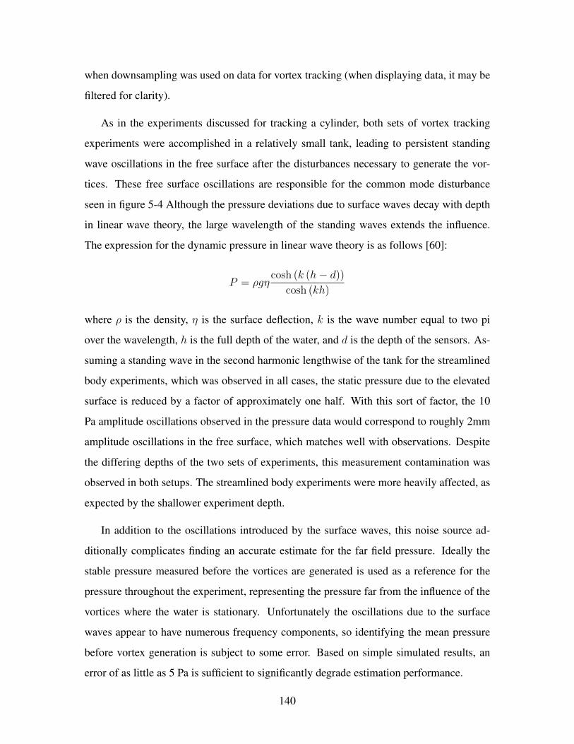
when downsampling was used on data for vortex tracking (when displaying data, it may be

filtered for clarity).

As in the experiments discussed for tracking a cylinder, both sets of vortex tracking

experiments were accomplished in a relatively small tank, leading to persistent standing

wave oscillations in the free surface after the disturbances necessary to generate the vor-

tices. These free surface oscillations are responsible for the common mode disturbance

seen in figure 5-4 Although the pressure deviations due to surface waves decay with depth

in linear wave theory, the large wavelength of the standing waves extends the influence.

The expression for the dynamic pressure in linear wave theory is as follows [60]:

P = ρgηcosh (k (h− d))

cosh (kh)

where ρ is the density, η is the surface deflection, k is the wave number equal to two pi

over the wavelength, h is the full depth of the water, and d is the depth of the sensors. As-

suming a standing wave in the second harmonic lengthwise of the tank for the streamlined

body experiments, which was observed in all cases, the static pressure due to the elevated

surface is reduced by a factor of approximately one half. With this sort of factor, the 10

Pa amplitude oscillations observed in the pressure data would correspond to roughly 2mm

amplitude oscillations in the free surface, which matches well with observations. Despite

the differing depths of the two sets of experiments, this measurement contamination was

observed in both setups. The streamlined body experiments were more heavily affected, as

expected by the shallower experiment depth.

In addition to the oscillations introduced by the surface waves, this noise source ad-

ditionally complicates finding an accurate estimate for the far field pressure. Ideally the

stable pressure measured before the vortices are generated is used as a reference for the

pressure throughout the experiment, representing the pressure far from the influence of the

vortices where the water is stationary. Unfortunately the oscillations due to the surface

waves appear to have numerous frequency components, so identifying the mean pressure

before vortex generation is subject to some error. Based on simple simulated results, an

error of as little as 5 Pa is sufficient to significantly degrade estimation performance.

140

The remedy for this noise source is the same as was implemented for the cylinder track-

ing experiments: considering the difference between adjacent pressure sensors. While the

long wavelength of the surface waves are responsible for the contamination of the pressure

measurements, they also allow for a straightforward solution. The wavelength is large in

comparison to the array length, therefore all sensors are influenced in phase by nearly the

same noise magnitude (See Figure 5-4). Using the inter-sensor pressure difference effec-

tively removes any information about the mean pressure which both takes care of the com-

mon mode oscillations due to the free surface and the ambiguity of the pressure reference.

In the case of the far field reference, it is only necessary to identify a common reference

when there is no nearby stimulus. Therefore, it is sufficient to normalize the mean of sev-

eral oscillations for each sensor when the vortices have not yet been generated or have long

past. This solution is similar to the actual function of the biological lateral line, which mea-

sures pressure gradients through the canal system. Although there are many more factors

at play in the biological system, such as the need to convert a flow velocity sensor into a

pressure sensor using a system of canals, it is possible that the differential nature of the

lateral line also addresses a similar problem in fish.

4 6 8 10 12 14 16-70

-60

-50

-40

-30

-20

-10

0

10

20

30

Time (s)

Pre

ssu

re (

Pa

)

Example Pressure Data, Streamlined Body Experiment

Figure 5-4: Typical pressure data set from streamlined body experiments. The surface waveeffects are clearly visible.

141

5.3.2 PIV Processing

A key element necessary for the use of the experiments to test vortex tracking elements is

an independent estimate of the vortex position and strength. This is the primary reason for

the particle image velocimetry used in conjunction with the experiments, as described in

the experimental setup. In order to obtain estimates of the vortex states, the images of the

particles are first processed to generate an estimate of the vector field in the imaged plane,

and the vortices are subsequently located based on the velocity field.

For the PIV data gathered at the MIT towing tank, the data processing to obtain the

velocity fields was done using DaVis v.7 software by LaVision, which corresponded to

the PIV equipment in those experiments. The image files were lightly pre-processed prior

to cross correlation, by masking the portion of the image in which the sensing body was

visible. The cross correlation processing used the routines in DaVis based on a two di-

mensional fast Fourier transform. The final interrogation window size was 32x32 pixels.

However, due to the large variety in the amplitude and direction of the fluid motion when

vortices were present, the vector field was computed over multiple passes, starting with an

interrogation window size of 64x64 pixels before the 32 pixel window, with two passes for

each window size. This repetition was necessary in order to locate the correct region of the

flow for cross correlation. No weighting was applied to the interrogation windows.

The PIV data gathered in the Singapore CENSAM tank, which corresponds to the flat

plate sensor experiments, was processed in a very similar manner. However, the software

used to process the images was Insight 3G. The procedure for evaluating the velocity fields

based on the particle images remained the same. First light pre-processing was done to

mask out a rectangle enclosing the sensing body. Since the shape of the sensing body is

also rectangular, this fit closely to the boundary of the structure. In processing the images,

the interrogation window size was increased by one step for this experimental setup, due

to a combination of a higher resolution camera and a larger distance from the image plane

to the camera. The initial interrogation window size was 128x128 pixels, moving down to

64x64.

In both cases, a raw image was additionally kept with the processed PIV data, in order

142

to obtain a physical reference. From these images, the location of an individual sensor

port can be accurately identified, relating the spatial distribution of the velocity field to the

coordinates in the pressure data estimates.

5.3.3 Independent Vortex Identification

In order to locate the vortices based on the velocity field generated by the PIV processing,

an automated approach was developed and used. This approach was found to accurately

identify vortices which had their core within the imaged area of the PIV (and therefore

within the velocity field). At the same time, it also estimated the location of the second

vortex which was generally outside the field of view. Unfortunately, the accuracy of the

estimate of the second vortex could not be confirmed in all cases, but in the cases where the

second vortex eventually entered the field of view, the results were consistent and smooth.

Besides the information provided on the vortex not captured in the PIV directly, the

main motivation for using an approach based on an analytical model is the robustness to

noise in the PIV vector field. Unfortunately, the nature of a pair of strong vortices in still

water poses challenges for calculating the vector field, since there are important regions

of both high and low velocity, and the direction of the vectors vary greatly. A certain

degree of compromise is necessary between accurately estimating velocity near the center

of the vortices and accurately capturing the flow field further away. The end result is that,

particularly near the vortex core, it is slightly more likely for a vector to be the result of

a faulty correlation. For direct methods in identifying a vortex from a vector field, only

the vector field in a small area about the vortex is used, making it susceptible to the error

of a single vector in that region. In contrast, fitting an analytical model makes use of the

entire vector field for estimating each vortex, making it substantially more robust to errors

in single vectors.

The automated approach works by fitting an analytical model to the velocity field cal-

culated by PIV, similar to that described by Vollmers [81]. When applying an analytical

model to the velocity field in order to identify the vortices, it is critical to use a model which

accounts for the core. Although an inviscid, irrotational flow model is generally accurate

143

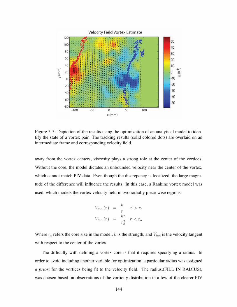
y (m

m)

120

100

80

60

40

20

0

-20

-40

-60

-80

x (mm)-100 -50 0 50 100

Velocity Field Vortex Estimate

Figure 5-5: Depiction of the results using the optimization of an analytical model to iden-tify the state of a vortex pair. The tracking results (solid colored dots) are overlaid on anintermediate frame and corresponding velocity field.

away from the vortex centers, viscosity plays a strong role at the center of the vortices.

Without the core, the model dictates an unbounded velocity near the center of the vortex,

which cannot match PIV data. Even though the discrepancy is localized, the large magni-

tude of the difference will influence the results. In this case, a Rankine vortex model was

used, which models the vortex velocity field in two radially piece-wise regions:

Vtan (r) =k

rr > ro

Vtan (r) =kr

r2o

r < ro

Where ro refers the core size in the model, k is the strength, and Vtan is the velocity tangent

with respect to the center of the vortex.

The difficulty with defining a vortex core is that it requires specifying a radius. In

order to avoid including another variable for optimization, a particular radius was assigned

a priori for the vortices being fit to the velocity field. The radius,(FILL IN RADIUS),

was chosen based on observations of the vorticity distribution in a few of the clearer PIV

144

velocity fields. It was found that the vortex tracking results were not strongly dependent on

the specified radius as long as it was within a reasonable range.

The actual optimization of the analytical model parameters is accomplished by mini-

mizing a least squares cost function defined over the velocity field:

J =∑i

∣∣∣V meas

i − V model

i

∣∣∣2This cost function is based on the vector differences between the velocity field measured

via PIV and the velocity field based on the analytical model for some combination of pa-

rameters. The optimization was implemented in Matlab using the gradient-based fmincon

function, which also allowed the inclusion of a minimum y distance constraint. The only

extra piece of information needed to run the algorithm is the initial guess for the vortex

state. This was accomplished by manually picking the location of peak vorticity corre-

sponding to the nearest vortex, in one of the first frames in which the circular streamlines

are visible. The initial strength of this vortex was set to a unit magnitude with the correct

sign. For the tow-tank experiments, the location of the second free vortex was chosen to

have the same initial X position as the primary visible one, and an initial spacing of 20

cm in the Y direction. The strength of the second vortex was fixed to be equal in mag-

nitude but opposite in sign to the near vortex. This was found to be necessary not just as

an initialization for the algorithm, but throughout in order to maintain a smoothly varying

estimate for the second vortex. In the case of the Singapore experiments, where the sec-

ond vortex is an image, only one vortex needed initialization. At each timestep, the initial

vortex state was used to begin the least squares optimization, and the result was propagated

by one timestep to generate the initialization values for the next PIV frame. This approach

generated consistent results that were robust to reasonable changes in the initialization.

The automated approach for extracting and independent estimate of the vortex state

from the PIV was validated against more direct traditional methods for this particular ap-

plication. In both sets of experiments with vortices, the vortices were generated by the

motion of a foil or plate sweeping an arc, but the imaged area was substantially apart from

the foil. This means that in the imaged area, the flow was dominated by a few large vortices,

145

56.5 57 57.5 58-0.2

-0.15

-0.1

-0.05

0

0.05

0.1

0.15

Time (s)

Vo

rte

x S

tate

Strength Dir

X Position Dir

Y Position Dir

Strength LS

X Position LS

Y Position LS

Comparison of PIV Vortex Estimates

Figure 5-6: Comparison of the estimated state of a vortex based on PIV vector fields.Results for the vortex closest to the sensor body of a vortex pair are shown. In black filleddots are the estimates based on a least-squares fit using an analytical vortex pair model.In open colored circles are directly identified estimates based on the location of the peakvorticity and area vorticity integrals.

and very little shear flow. Given this situation, the local maximum in vorticity magnitude

is a good measure of the location of a vortex [39]. A comparison of the X and Y position

of the vortex estimated via the maximum in vorticity against the analytic model fitting is

shown in Figure 5-6. The maximum vorticity only provides an estimate when the center

of the vortex is within the image. Over that region, the two estimation methods agree con-

siderably, with the algorithm based on the analytical model having slightly less variation

from image to image, as might be expected since many more vectors are involved in the

estimate.

Estimating the vortex strength directly from the PIV vector field for comparison was

accomplished using both a line integral and a surface integral to compute the circulation

over a region encompassing the vortex core.

Γ =

∫C

v · ds =

∫ ∫A

w · n dA

where A is a surface enclosing the vortex in the two dimensional PIV plane, and C is the

146

corresponding closed boundary to that surface. ds is a differential length element along the

boundary of the surface, and w is the vorticity. Both approaches were implemented using

a rectangular region centered about the local extremum in vorticity. Although a single

integral was used in each case, several sizes were tested in order to find the maximum

circulation. The maximum circulation was taken to be an accurate representation of the true

vortex circulation, as the inclusion of the vortex core would reduce it if the region is too

small, and other vortices or fluid interactions would reduce it if the area is too large. Both

integral methods were found to provide nearly identical results when applied in this manner.

In comparison, the analytical model method (Figure 5-6) matches the direct integral method

results reasonably well in vortex strength. Unlike the comparison in position however, the

analytical model is consistently below the direct method estimate during the later portion

of the data set. It is unclear which of the two approaches is in error. However, given the

reduced information used to calculate the direct approximation, it is the more likely option.

Overall, automatically fitting the analytical model to the PIV velocity fields generates

consistent estimates of the location and strength of the nearest vortex. As shown, this

estimate also matches well with local direct estimates of the strength and position of the

vortex. There is also a slight improvement in the estimate consistency from one time-step

to the next for the analytical model compared to the direct methods. The key point however,

is that the automated PIV estimates based on fitting an analytic model generally agree very

closely to the direct approach which assumes no model. Therefore, there is no concern that

the line vortex model used as the analytical model for the PIV will generate results that are

favorably inclined to the estimates based on pressure data, regardless of similarities in the

analytical model.

5.4 Real Time Vortex Tracking

In order to solve the inverse problem of tracking a vortex in real time based on the data

provided by an artificial lateral line, several components must be addressed. First, an ac-

curate forward model is needed to predict the pressure measurements based on the state

of a vortex (or vortices). Second, depending on the characteristics of the forward model,

147

an appropriate estimation technique needs to be identified. Using the estimation technique

and the forward model together, the results can be optimized for the problem and the results

compared to the true vortex state directly based on the PIV data.

It is important to recognize at the outset that the problem of tracking a vortex based

on pressure measurements is ill-posed when one considers a certain maximum of precision

or noise in the measurements. This can be most clearly seen in an extreme case where

the pressure sensors all measure the same reference pressure, there is no unique vortex

state that corresponds to it. For example, it could be that there are no vortices present in

the fluid, or it could be that there is a vortex, or many vortices, but that they are all too

far away to affect the sensors significantly in comparison to the noise floor. This issue

of range is well known for the lateral line, since near field pressure disturbances decay

quickly with distance. The implication on the inverse problem is that there will be certain

types of measurements scenarios in which tracking a vortex will be impossible, and others

in which certain aspects of the vortex are ambiguous. This is considered in more detail

later in section 5.5.

5.4.1 Experimental Vortex Forward Models

This section addresses the question of identifying a good forward model which relates the

vortex states of interest to the pressure measurements. Due to the differences in the flow for

the two experimental setups (streamlined body and flat plate body), different forward mod-

els will be needed. The main measure of quality for a forward model is the ability to predict

the measured pressure given the known relevant vortex states. This will be evaluated us-

ing the vortex states estimated from the PIV data and compared against the experimentally

measured pressure for a representative data set. However, since we are interested in solv-

ing the inverse problem, we also desire a simple forward model with the fewest number

of parameters. Excessive parameters describing the flow that do not substantially alter the

pressure measurements will be very difficult to estimate from the pressure measurements

due to the low sensitivity.

148

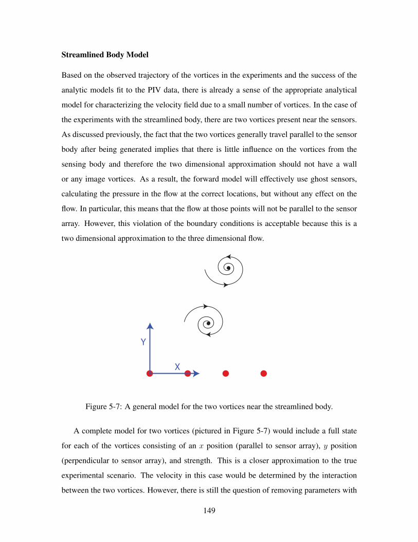
Streamlined Body Model

Based on the observed trajectory of the vortices in the experiments and the success of the

analytic models fit to the PIV data, there is already a sense of the appropriate analytical

model for characterizing the velocity field due to a small number of vortices. In the case of

the experiments with the streamlined body, there are two vortices present near the sensors.

As discussed previously, the fact that the two vortices generally travel parallel to the sensor

body after being generated implies that there is little influence on the vortices from the

sensing body and therefore the two dimensional approximation should not have a wall

or any image vortices. As a result, the forward model will effectively use ghost sensors,

calculating the pressure in the flow at the correct locations, but without any effect on the

flow. In particular, this means that the flow at those points will not be parallel to the sensor

array. However, this violation of the boundary conditions is acceptable because this is a

two dimensional approximation to the three dimensional flow.

X

Y

Figure 5-7: A general model for the two vortices near the streamlined body.

A complete model for two vortices (pictured in Figure 5-7) would include a full state

for each of the vortices consisting of an x position (parallel to sensor array), y position

(perpendicular to sensor array), and strength. This is a closer approximation to the true

experimental scenario. The velocity in this case would be determined by the interaction

between the two vortices. However, there is still the question of removing parameters with

149

low sensitivity. One simple reduction in the parameters is immediately apparent given the

particular experimental setup here. Since the vortex pair stimulus consists of the starting

and stopping vortices of a foil, the strength of these vortices should be equal in magnitude

but opposite in sign. This assumption will be used throughout whenever a vortex pair is

being considered.

The forward model consists of two components. The primary interest is in the relation-

ship between the vortex pair state and the pressure, but there is also a component of the

model that describes the state progression. For the current description of the vortex pair,

the state vector would consist of five variables: one strength and four positions. Along

with the boundary conditions discussed, this is sufficient to define the complex potential

describing the flow:

Φ (z) = −ik log (z − z1) + ik log (z − z2) (5.1)

where z1 and z2 are the complex representations of the center for each vortex. The induced

velocity that governs the motion of the vortices can be calculated by considering the veloc-

ity (derivative of the complex potential with respect to z) at the center of one of the vortices

with only the other one acting. The result is u − iv = ikz1−z2 . As a result, the description

of the state progression is fairly straightforward. We assume that the vortex strengths do

not decay (on the timescale of the experiment), and that the first derivative of the position

is given by the induced velocity just described.

The second part of the forward model with unconstrained position relates the vortex pair

state at a time instant to the pressure. This is derived directly from the unsteady Bernoulli

equation [3]:

P (z)− P∞ = −1

2ρ

∣∣∣∣∂Φ(z)

∂z

∣∣∣∣2 − ρ∂ < (Φ(z))

∂t(5.2)

P (s)− P∞ = −1

2ρ

∣∣∣∣ −iks− z1

+ik

s− z2

∣∣∣∣2 + ρk y1

(s− x1)2 + y21

u+ ...

−ρ k y2

(s− x2)2 + y22

u+ ρk

(s− x1)2 + y21

v − ρ k

(s− x2)2 + y22

v (5.3)

150

Here we make use of the fact that the pressure sensors are defined on the x axis and so

have no imaginary component. The position of the sensors is therefore given by the real

scalar s. Also, note that the real part of the complex potential is the angle that the point

of evaluation makes with the center of each vortex, scaled by the vortex strength. This

model for the pressure uses the vortex state at one time instant only, since it makes use

of the instantaneous estimate of the vortex velocities based on the their relative position.

For brevity, this model will be referred to as the 1.6 model, as it has one vortex entirely

specified, and two thirds of the parameters specified for the second vortex.

A second parameter which should be considered for removal is the relative x position

of the second (more distant) vortex. Given the direction of motion, the separation in the y

direction is critical to the two-vortex model since it produces the velocity in the x direction.

However, the vortex pair generally have a very small velocity component in the y direction,

and therefore the x position of the two vortices should be very similar. This is confirmed

via the estimates of the vortex locations provided by the PIV. Therefore, one logical simpli-

fication would be to assume that the x positions of the two vortices are equal. This model

is very similar to the one described above, except that the velocity component v = 0 for

both the state progression and the pressure equation (5.3), as well as x1 = x2. Since this

model effectively has one and a third of the parameters of a single vortex (without velocity

specified), it will be referred to in brief as the 1.3 vortex model.

Another possibility in modeling the flow near the streamlined body, for the purposes

of predicting the pressure, is to focus on the closest vortex only. Due to the proximity of

this vortex, it will cause the majority of the contribution to the pressure measurements.

For a single vortex, the vortex state under the two dimensonal constraint being used in this

chapter can be fully defined with three parameters: two for the position of the vortex and

one for the strength or circulation. However, a single vortex would be stationary in still

water without an image vortex due to interactions with nearby bodies or fluid structures.

Clearly this is not the case in either of the experimental setups (as observed in the PIV

results). Therefore, if we approximate the scenario by a single vortex in this situation,

the state needs to be augmented by a velocity. For the general experimental setup in this

chapter, the primary direction of motion is along the axis of the sensor array, so only one

151

velocity component will be used: U along the x axis. In this model, the state progression

is defined by a constant vortex strength and y position, and with the derivative of the x

position equal to U . The equation of pressure is given as follows:

P (s)− P∞ = −1

2ρ

∣∣∣∣ −iks− z1

∣∣∣∣2 + ρk y1

(s− x1)2 + y21

U (5.4)

To test the accuracy of these three forward models, they are used to predict the pressure

in an experimental setting given a vortex trajectory that is extracted from the corresponding

PIV. The results of this comparison for representative data set which had a good, complete

set of PIV-extracted states is displayed in Figure 5-8. In examining the first two parts of

this figure, which correspond to the 1.3 and 1.6 vortex models, it is clear that there are

very strong similarities and that they capture a substantial portion of the actual measured

pressure. Both the 1.3 and 1.6 models capture the negative pressure peak at the tail end

of the time series. At the beginning of the time series, the 1.3 model which assumes the x

position of the two vortices are equal, is more consistent in recreating the pressure in the

first large negative pressure peak. In between these two large peaks, the pressure recreation

is similar for both models, and underestimates the actual measured pressure for some of the

sensors, while matching the others. One substantial difference between these two models

is that the 1.6 model more readily recreates pressure greater than the reference. Looking

at the results of the single vortex model, where the velocity U was estimated based on the

smoothed derivative of the x position extracted from the PIV data, the pressure is generally

heavily over estimated in magnitude. This is particularly true in the later parts of the time

series.

The reconstruction of the pressure is improved when considering the difference between

adjacent sensors (Figure 5-9). As discussed earlier, this removes the effect of a drifting

reference pressure, primarily the effect of small amplitude, large wavelength, oscillations

in the free surface. Based on this figure, it is even clearer that the two vortex models

outperform the single vortex model, and that there is no obvious benefit to allowing the

second vortex to differ in the x position from the first. As a result, we shall identify the 1.3

vortex model as the most appropriate forward model for solving the inverse problem for

152

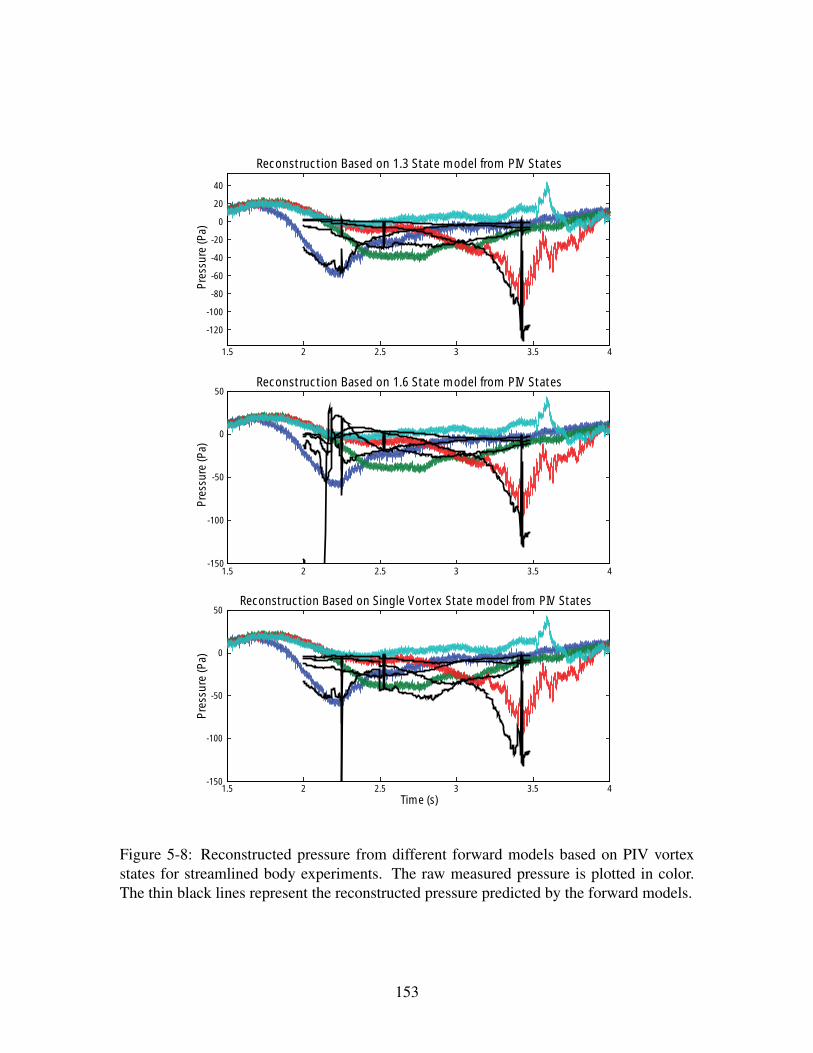
1.5 2 2.5 3 3.5 4

-120

-100

-80

-60

-40

-20

0

20

40

Pre

ssu

re (

Pa

)

Reconstruction Based on 1.3 State model from PIV States

1.5 2 2.5 3 3.5 4-150

-100

-50

0

50

Time (s)

Pre

ssu

re (

Pa

)

Reconstruction Based on Single Vortex State model from PIV States

1.5 2 2.5 3 3.5 4-150

-100

-50

0

50

Pre

ssu

re (

Pa

)


Figure 5-8: Reconstructed pressure from different forward models based on PIV vortexstates for streamlined body experiments. The raw measured pressure is plotted in color.The thin black lines represent the reconstructed pressure predicted by the forward models.

153

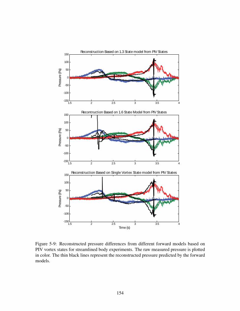
1.5 2 2.5 3 3.5 4-150

-100

-50

0

50

100

150

Pre

ssu

re (

Pa

)


1.5 2 2.5 3 3.5 4-150

-100

-50

0

50

100

150

Pre

ssu

re (

Pa

)

Recontruction Based on 1.6 State Model from PIV States

1.5 2 2.5 3 3.5 4-150

-100

-50

0

50

100

150

Time (s)

Pre

ssu

re (

Pa)

Reconstruction Based on Single Vortex State model from PIV States

Figure 5-9: Reconstructed pressure differences from different forward models based onPIV vortex states for streamlined body experiments. The raw measured pressure is plottedin color. The thin black lines represent the reconstructed pressure predicted by the forwardmodels.

154

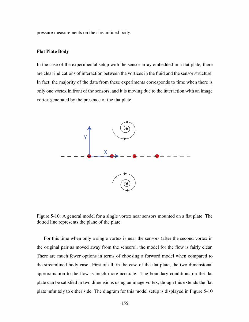
pressure measurements on the streamlined body.

Flat Plate Body

In the case of the experimental setup with the sensor array embedded in a flat plate, there

are clear indications of interaction between the vortices in the fluid and the sensor structure.

In fact, the majority of the data from these experiments corresponds to time when there is

only one vortex in front of the sensors, and it is moving due to the interaction with an image

vortex generated by the presence of the flat plate.

X

Y

Figure 5-10: A general model for a single vortex near sensors mounted on a flat plate. Thedotted line represents the plane of the plate.

For this time when only a single vortex is near the sensors (after the second vortex in

the original pair as moved away from the sensors), the model for the flow is fairly clear.

There are much fewer options in terms of choosing a forward model when compared to

the streamlined body case. First of all, in the case of the flat plate, the two dimensional

approximation to the flow is much more accurate. The boundary conditions on the flat

plate can be satisfied in two dimensions using an image vortex, though this extends the flat

plate infinitely to either side. The diagram for this model setup is displayed in Figure 5-10

155

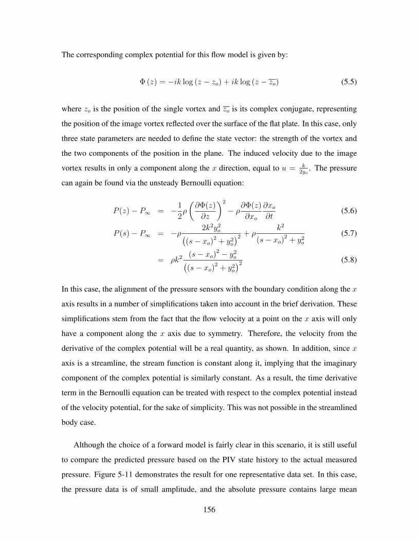
The corresponding complex potential for this flow model is given by:

Φ (z) = −ik log (z − zo) + ik log (z − zo) (5.5)

where zo is the position of the single vortex and zo is its complex conjugate, representing

the position of the image vortex reflected over the surface of the flat plate. In this case, only

three state parameters are needed to define the state vector: the strength of the vortex and

the two components of the position in the plane. The induced velocity due to the image

vortex results in only a component along the x direction, equal to u = k2yo

. The pressure

can again be found via the unsteady Bernoulli equation:

P (z)− P∞ = −1

2ρ

(∂Φ(z)

∂z

)2

− ρ∂Φ(z)

∂xo

∂xo∂t

(5.6)

P (s)− P∞ = −ρ 2k2y2o(

(s− xo)2 + y2o

)2 + ρk2

(s− xo)2 + y2o

(5.7)

= ρk2 (s− xo)2 − y2o(

(s− xo)2 + y2o

)2 (5.8)

In this case, the alignment of the pressure sensors with the boundary condition along the x

axis results in a number of simplifications taken into account in the brief derivation. These

simplifications stem from the fact that the flow velocity at a point on the x axis will only

have a component along the x axis due to symmetry. Therefore, the velocity from the

derivative of the complex potential will be a real quantity, as shown. In addition, since x

axis is a streamline, the stream function is constant along it, implying that the imaginary

component of the complex potential is similarly constant. As a result, the time derivative

term in the Bernoulli equation can be treated with respect to the complex potential instead

of the velocity potential, for the sake of simplicity. This was not possible in the streamlined

body case.

Although the choice of a forward model is fairly clear in this scenario, it is still useful

to compare the predicted pressure based on the PIV state history to the actual measured

pressure. Figure 5-11 demonstrates the result for one representative data set. In this case,

the pressure data is of small amplitude, and the absolute pressure contains large mean

156

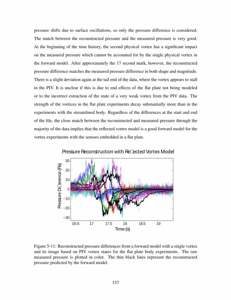
pressure shifts due to surface oscillations, so only the pressure difference is considered.

The match between the reconstructed pressure and the measured pressure is very good.

At the beginning of the time history, the second physical vortex has a significant impact

on the measured pressure which cannot be accounted for by the single physical vortex in

the forward model. After approximately the 17 second mark, however, the reconstructed

pressure difference matches the measured pressure difference in both shape and magnitude.

There is a slight deviation again at the tail end of the data, where the vortex appears to stall

in the PIV. It is unclear if this is due to end effects of the flat plate not being modeled

or to the incorrect extraction of the state of a very weak vortex from the PIV data. The

strength of the vortices in the flat plate experiments decay substantially more than in the

experiments with the streamlined body. Regardless of the differences at the start and end

of the file, the close match between the reconstructed and measured pressure through the

majority of the data implies that the reflected vortex model is a good forward model for the

vortex experiments with the sensors embedded in a flat plate.

16.5 17 17.5 18 18.5 19

−30

−20

−10

0

10

20

30

Time (s)

Pre

ssu

re D

ie

ren

ce (

Pa

)

Pressure Reconstruction with Reected Vortex Model

Figure 5-11: Reconstructed pressure differences from a forward model with a single vortexand its image based on PIV vortex states for the flat plate body experiments. The rawmeasured pressure is plotted in color. The thin black lines represent the reconstructedpressure predicted by the forward model.

157

5.4.2 Estimation Methods

The goal of the experiments and the identification of a forward model is to be able to solve

the inverse problem and verify that it has been accurately resolved. In order to tackle the

inverse problem, the primary requirements are to be robust to noise and changes in the

model while using as much of the data history as possible. While it is possible to attempt

to invert the pressure measurements separately for each time instant, this would guarantee

a sub-optimal result. For example, the pressure described by equation (5.8) is a function

of the strength squared only, and therefore the direction of rotation of a vortex would be

impossible to determine from the measurements at a single time instant. However, the

rotation of the vortex also determines the direction it moves, resolving the ambiguity if

data across multiple time instances is used. In addition, the solutions to the inverse problem

need to be limited to certain conditions, implicitly or explicitly, since the inverse problem

is technically ill-posed under certain conditions (for example, small signals).

Similarly to Chapter 3, the problem as it has been described for tracking a vortex via

pressure sensors naturally fits into the hidden Markov model structure where the measure-

ments only depend on the current vortex state, and a new vortex state depends only on the

one directly before it. The actual model for the vortex progression is continuous in time as

opposed to the discrete time description just given, but the HMM concept can be extended.

This model structure makes it possible to use a number of estimation algorithms, including

the Kalman and particle filters among others. Both the Kalman and particle filters satisfy

the desired characteristics for an estimation algorithm.

Estimation Algorithm & Implementation

Among the different possibilities for an estimation technique, the Kalman filter was cho-

sen for this problem due to its ability to tune the length of the memory of the process and

its widespread application to many problems in engineering. Restricting the length of the

memory of the Kalman filter allows the estimate to change if the model changes or drifts

due to external influences. For example, in the case of a single vortex that can only move in

the x direction, the limited memory allows the y position to change even after a substantial

158

amount of time has passed with one y position. As a result of its wide use, many different

variations of the original Kalman filter are available for different degrees of nonlinearity

and different types of models. As is evident from equations (5.3) and (5.8), the equations

relating the vortex state vectors to the vector of pressure measurements are not linear. Mul-

tiple approaches are known to apply the Kalman filter to nonlinear problems [41, 27]. In

this case, a simple first order approximation of the nonlinear pressure function is used via

the extended Kalman filter algorithm. In addition, the continuous time state progression

was coupled with a discrete time measurement update. The details of the implementation

are described in [27].

The Kalman filter and it’s nonlinear variants, including the extended Kalman filter being

used in this chapter, model the noise in the system as being white and having a Gaussian

distribution. The Gaussian distribution is not a concern in tracking vortices as it was in

Chapter 3 for tracking a cylinder. The measurement noise is reasonably described by a

Gaussian distribution already. However, modeling noise in the state transition model as

Gaussian is an approximation, since this noise term stands in for a number of effects that

are not included in the flow model such as other vortices or any external flow. The state

transition noise terms also play an important role in the convergence and adaptation of the

Kalman filter algorithm (see next section). The vortex tracking problem differs significantly

from the cylinder tracking problem in that there is a natural boundary that corresponds to

the physical sensor body. Specifically, if the vortex strength estimate is not zero, then

the pressure corresponding to an estimate in which the y position is very small will be

very large and therefore substantially different from the measured pressure. This large

increase in error as the vortex approaches to close to the sensors acts to repel the estimate

from having the vortex cross behind the sensing plane (leading to a non-physical situation).

There are two exceptions in which it is still possible to have the vortex estimate cross

the x axis. First, if the vortex estimate places the vortex far from the sensors in the x

direction, then the cost of crossing the sensor array is strongly reduced. Second, during the

initial stages of the Kalman filter, the magnitude of the state estimate corrections is large

to compensate for the lack of information, which may lead to crossing the x axis without

evaluating an intermediate point with small y position. These possible exceptions both

159

relate to the initialization of the Kalman filter. By not initializing the estimation algorithm

before the sensor array registered a signal from the vortices, and by limiting the magnitude

of the initialization of the estimate error covariance matrix, the issue of a vortex crossing

behind the sensor array plane was non-existent in practice.

Parameter Determination

The extended Kalman filter has a number of internal parameters that need to be specified.

These include the initial state estimate covariance matrix, the transition covariance matrix,

and the measurement covariance matrix. As a general rule, values for these internal knobs

in the extended Kalman filter were kept the same for all the vortex tracking experiments,

regardless of whether streamlined body or flat plate was used to measure the pressure. This

was done in order to keep from overtuning the estimation method to each data set. Due to

the different state vectors in the two cases, there are still slight differences. The result is a

rough general set of covariance matrices for estimating vortices.

The first of these internal parameters to consider is the initial state covariance matrix.

The Kalman filter produces real time estimates of the distribution of the state vector (as-

suming a Gaussian form), which corresponds to the mean value of the state and its error

covariance matrix. The confidence in the state estimate, represented by the covariance ma-

trix, is instrumental in determining the magnitude of the correction applied in response to

discrepancies between the measured and predicted pressure at the next measurement up-

date. In all of the experiments in tracking vortices, little information is used to provide the

initial state value, and therefore there is almost no confidence in it. It is preferable that the

state estimate be heavily corrected once the first measurements are used. For these reasons,

the initial values of the state covariance matrix need to be fairly large. In addition, since

there is no a priori reason to introduce dependence between the variables, the initial state

error covariance is diagonal. The actual values of the diagonal elements were chosen based

on the dimensions of the variables and the problem. All the length variables in the state

were initialized to have a variance of (0.1m)2. The strength variable in the state vector has

units of m2/s. Given the fundamental length scale of the problem is in mm, and that a

typical value for the strength is 0.01m2/s, the initial variance was set to 1e-5 (m2/s)2.

160

The choice of the measurement and state transition noise covariance matrices are inter-

related as they strongly affect the behavior of the Kalman filter. In particular, the relative

magnitudes of the two matrices determines the reliance of the algorithm on the new mea-

sured information versus the previously estimated state. If the measurement noise variance

is small with respect to the state transition noise variance, then the estimate of the state

will approach the instantaneous inverse estimate of the state given the measurements. If

the measurements still have substantial noise, this means that the state estimate will vary

wildly. The extreme case of zero measurement noise is not valid for the variants of the

Kalman filter. In the opposing situation, when the state transition noise variance is very

small with respect to the measurement noise variance, the state estimate is much slower

to respond to discrepancies between the predicted and measured pressure. It is possible to

have zero transition noise variance, implying that the state transition is known exactly. This

typically leads to a “hardening” of the state estimate where, after a certain amount of time

in which the transients due to the initial state error covariance die out, the state estimate

may progress via the state transition rules only and be completely independent of new mea-

surements. In this context, one effective way to think of the state transition noise variance

is as a lower bound to the state error covariance. By upper bounding the confidence in the

state estimate, the algorithm is always able to change its estimate based on new informa-

tion. For this reason, it is frequently beneficial to model some noise in the state transition,

even if there is no physical source for the noise.

The ratio of the measurement noise variance to the process (or state transition) noise

variance was chosen based on a combination of experimentation and relative signal mag-

nitude. The actual measurement noise corresponding to the Honeywell pressure sensors

being used is very small, with a standard deviation of just a few Pascals. For the state

transition, there is no noise of the same sort which is easily quantifiable, but it is possible

to examine the amount of drift in the y position component from the PIV estimate of the

position. This can be about 1 cm over the entire data set, and closer to 1 mm on a more

local scale. This is sufficient to give a rough magnitude level for each of the covariance

matrices, with the measurement covariance having elements with magnitude of 10 Pa2 and

the state transition covariance having elements with magnitude on the order of 10−6 m2.

161

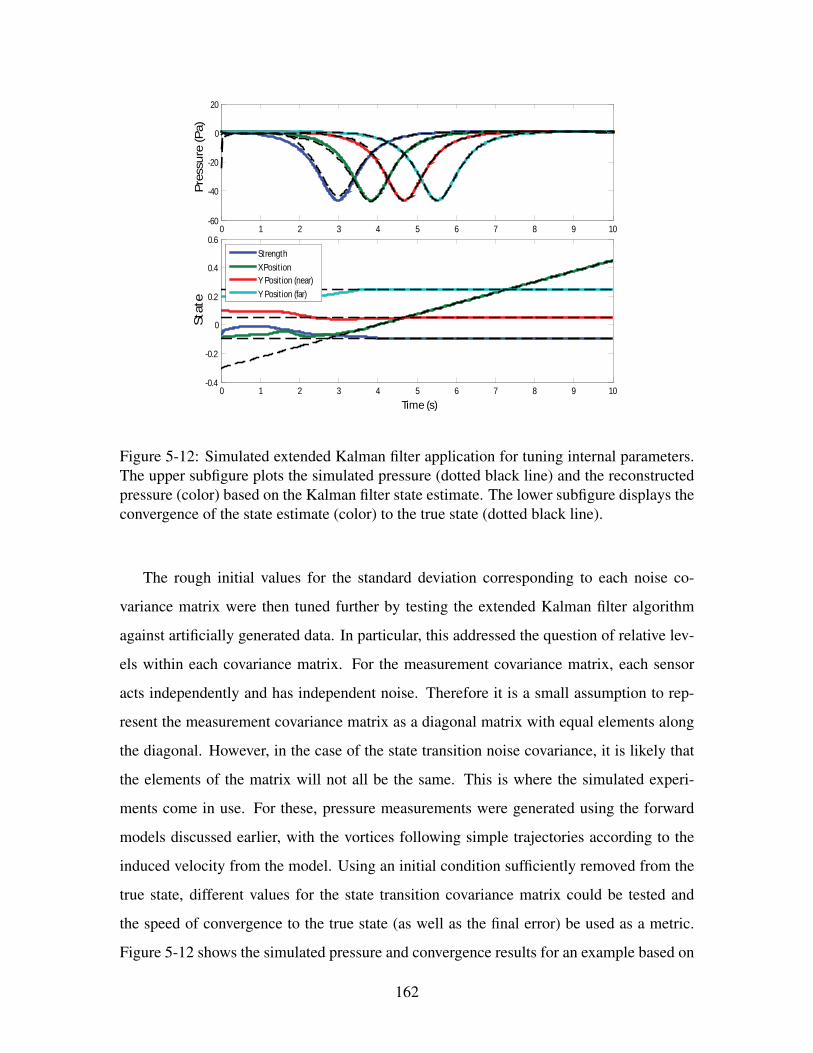
0 1 2 3 4 5 6 7 8 9 10-60

-40

-20

0

20

Pre

ss

ure

(P

a)

0 1 2 3 4 5 6 7 8 9 10-0.4

-0.2

0

0.2

0.4

0.6

Time (s)

Sta

te

Strength

X Position

Y Position (near)

Y Position (far)

Figure 5-12: Simulated extended Kalman filter application for tuning internal parameters.The upper subfigure plots the simulated pressure (dotted black line) and the reconstructedpressure (color) based on the Kalman filter state estimate. The lower subfigure displays theconvergence of the state estimate (color) to the true state (dotted black line).

The rough initial values for the standard deviation corresponding to each noise co-

variance matrix were then tuned further by testing the extended Kalman filter algorithm

against artificially generated data. In particular, this addressed the question of relative lev-

els within each covariance matrix. For the measurement covariance matrix, each sensor

acts independently and has independent noise. Therefore it is a small assumption to rep-

resent the measurement covariance matrix as a diagonal matrix with equal elements along

the diagonal. However, in the case of the state transition noise covariance, it is likely that

the elements of the matrix will not all be the same. This is where the simulated experi-

ments come in use. For these, pressure measurements were generated using the forward

models discussed earlier, with the vortices following simple trajectories according to the

induced velocity from the model. Using an initial condition sufficiently removed from the

true state, different values for the state transition covariance matrix could be tested and

the speed of convergence to the true state (as well as the final error) be used as a metric.

Figure 5-12 shows the simulated pressure and convergence results for an example based on

162

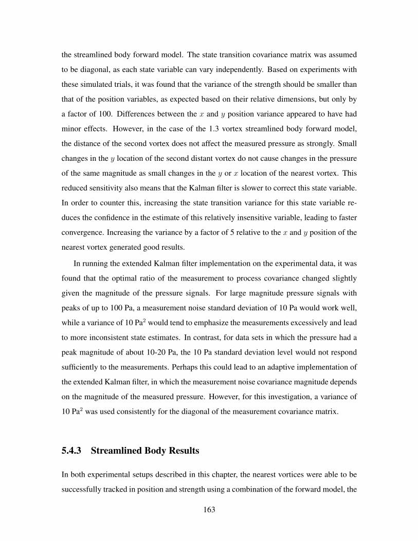
the streamlined body forward model. The state transition covariance matrix was assumed

to be diagonal, as each state variable can vary independently. Based on experiments with

these simulated trials, it was found that the variance of the strength should be smaller than

that of the position variables, as expected based on their relative dimensions, but only by

a factor of 100. Differences between the x and y position variance appeared to have had

minor effects. However, in the case of the 1.3 vortex streamlined body forward model,

the distance of the second vortex does not affect the measured pressure as strongly. Small

changes in the y location of the second distant vortex do not cause changes in the pressure

of the same magnitude as small changes in the y or x location of the nearest vortex. This

reduced sensitivity also means that the Kalman filter is slower to correct this state variable.

In order to counter this, increasing the state transition variance for this state variable re-

duces the confidence in the estimate of this relatively insensitive variable, leading to faster

convergence. Increasing the variance by a factor of 5 relative to the x and y position of the

nearest vortex generated good results.

In running the extended Kalman filter implementation on the experimental data, it was

found that the optimal ratio of the measurement to process covariance changed slightly

given the magnitude of the pressure signals. For large magnitude pressure signals with

peaks of up to 100 Pa, a measurement noise standard deviation of 10 Pa would work well,

while a variance of 10 Pa2 would tend to emphasize the measurements excessively and lead

to more inconsistent state estimates. In contrast, for data sets in which the pressure had a

peak magnitude of about 10-20 Pa, the 10 Pa standard deviation level would not respond

sufficiently to the measurements. Perhaps this could lead to an adaptive implementation of

the extended Kalman filter, in which the measurement noise covariance magnitude depends

on the magnitude of the measured pressure. However, for this investigation, a variance of

10 Pa2 was used consistently for the diagonal of the measurement covariance matrix.

5.4.3 Streamlined Body Results

In both experimental setups described in this chapter, the nearest vortices were able to be

successfully tracked in position and strength using a combination of the forward model, the

163

extended Kalman filter, and its tuned internal parameters. In looking into the details, it will

be possible to further understand under what conditions vortices can be tracked.

The experiments which enclosed a linear array of pressure sensors in a streamlined

tubular body required a 1.3 vortex forward model, which recreated the pressure at the sen-

sors accurately by not modeling the presence of the body. In looking at the results of the

inverse problem applied to this situation, the state of the nearest vortex is tracked surpris-

ingly well under a number of conditions. In the presence of substantial unmodeled signal

sources, the state estimate would robustly return to an accurate value after the unexplained

pressure signal abated.

Position (mm)

Po

siti

on

(m

m)

Vortex Tracking

−50 0 50 100 150 200

−150

−100

−50

0

50

100

−50

−40

−30

−20

−10

0

10

20

30

40

50

Pressure Estimate

PIV Estimate

Vort

icity

(1/s

)

56.4 56.6 56.8 57 57.2 57.40

0.05

0.1

Strength

56.4 56.6 56.8 57 57.2 57.4

0

100

200

300X

56.4 56.6 56.8 57 57.2 57.40

50

100

Y

Time (s)

(mm

)(m

m)

(m /s

)2

56.4 56.6 56.8 57 57.2 57.4

-50

-40

-30

-20

-10

0

10

Pres

sure

(Pa)

Time (s)

Measured Pressure

Figure 5-13: Results of a streamlined body vortex estimation trial. The estimated statevariables (black line) are compared against the values from the PIV data in the upper left.In the upper right, the position traces of the pressure-estimated (black points) versus PIV-estimated (red points) vortices are shown against the background of the vorticity distribu-tion at an intermediate time. The edge of the sensor body and sensor locations are markedat the left edge of the image. At the bottom, the measured pressure is shown, filtered witha 20 Hz cutoff frequency.

164

The first two examples of the state estimation for a streamlined body are examples of

data sets without substantial aberrations in the pressure. Figure 5-13 shows the results of

the vortex estimation from the linear pressure sensor array, compared against the estimate

independently derived from the PIV data. The estimates of each state represent the mean of

the conditional probability for each state variable conditioned on all the pressure measure-

ments up to and including the time of the estimate. Focusing first on the upper left section

of the figure, each state estimate based on pressure follows the behavior of the true state

as derived from the PIV closely. The best of these is the x position, denoting the location

of the vortex along the length of the array. The estimate of the x position matches the PIV

data almost exactly. In contrast, the y position estimate based on pressure tracks the true

position of the vortex very well throughout the majority of the data set, but smoothly drifts

apart at the tail end. The strength estimate appears to have a constant bias, overestimating

the strength of the vortex in comparison to the PIV results, but does capture the slight de-

cay in strength throughout the data set. Unfortunately the PIV that corresponds to this run

decays in quality slightly at the tail end, making the the drift away from the sensors slightly

suspect. This is visible in the righthand plot, where the PIV estimate of the location begins

to lose cohesion. However, the main cause of the failure to track the small drift is likely

within the parameters of the Kalman filter. It is possible that by that point, the data had

been consistent with the model to the point that the influence of new measurements was

reduced. Another visualization of the results for this example is shown in Figure 5-14, in

which the location of the vortex estimates from the pressure and PIV are shown against the

corresponding vorticity distribution at different points in time.

In comparing the state estimate results with the measured pressure, there is a clear ad-

justment in the estimate of the y position that occurs at approximately 56.4 seconds. This

corresponds to the time where the first sensor is beginning to differ significantly in com-

parison to the others. This behavior is expected, as before that point in time there is little

information available that may not be attributed to noise in the measurements. However, it

does also bring up an important point. The approach used here to track a vortex makes sub-

stantial use of the initialization transients of the Kalman filter. Since very little is assumed

known about the location and size of the vortices, the initial period in which the estimate

165

0 100 200

−100

0

100

−50

0

50

56 56.2 56.4 56.6 56.8 57 57.2 57.4 57.6 57.8 58−60

−40

−20

0

0 100 200

−100

0

100

−50

0

50

0 100 200

−100

0

100

−50

0

50

0 100 200

−100

0

100

−50

0

50

0 100 200

−100

0

100

−50

0

50

0 100 200

−100

0

100

−50

0

50

Position (mm) Position (mm)

Posi

tion

(mm

)Po

sitio

n (m

m)

Posi

tion

(mm

)

1

2

3

4

5

6Vo

rtic

ity (1

/s)

Vort

icity

(1/s

)Vo

rtic

ity (1

/s)

Time (s)

Pres

sure

(Pa)

Streamlined Body Estimation Results

Figure 5-14: Results of a streamlined body vortex estimation trial. The results correspondto the same data as Figure 5-13. The position estimate based on the PIV data (red circle)is compared against that based on the pressure data only (black circle) at different stagesin the time series. Each of the smaller subfigures, proceeding vertically from the top left,corresponds to the time marked by a dotted line in the top subfigure.

166

is more sensitive to the measurements than the steady state behavior is very important in

locating the vortices.

The second of the clean examples demonstrates a scenario that is slightly different from

the first, in which the extended Kalman filter implementation does follow a signification

change in the motion of the nearest vortex. These results are visible in Figure 5-15 and

Figure 5-16. Although in general the vortex state is tracked very well in both the examples

so far, there are some substantial differences. Unlike the first example, this second one

tracks the vortex strength well, without overestimating it. Additionally, as mentioned, the

Kalman filter results track a substantial change in direction as the vortex approaches the

sensor array in the y axis after initially maintaining roughly constant. However, in further

contrast to the previous results, the y position estimate based on the pressure exhibits small

oscillations about the true value. It is unclear what causes this behavior. One difference

between this example and the previous is that the strength of the vortex is larger. This could

be responsible for the improved tracking of the vortex strength, but would be unlikely

to cause the oscillations. The most likely remaining cause is that some small secondary

unmodeled vortices were present near the sensors, which were not sufficient to corrupt the

vortex tracking, but did alter it.

It is important to note that in the discussion of the two examples so far, only the state

of the closest vortex is being tracked. The 1.3 vortex model being used at the base of

the extended Kalman filter is a model that includes two vortices, with the second vortex

limited to one free variable representing the distance between the two vortices. However,

in implementation, it was observed that this separation variable is greatly inconsistent and

strongly underestimated in comparison to the observed (via PIV) location of the second

vortex. This is most likely due to the greatly reduced sensitivity to the position of the

furthest vortex when there is a closer one in the flow field. This difference in sensitivity

had been previously observed in the simulated tests of the extended Kalman filter, but

it was trackable at that stage. With the inclusion of realistic noise and unmodeled fluid

structures, it was determined that while this second vortex is necessary in order to obtain

a good forward model, there can be no confidence in the inverse problem estimate of the

second vortex. As a result, the vortex tracking is focused on the issue of accurately tracking

167

Position (mm)

Po

siti

on

(m

m)

Vortex Tracking Results

−100 −50 0 50 100−80

−60

−40

−20

0

20

40

60

80

100

120

−40

−30

−20

−10

0

10

20

30

40

PIV Estimate

Pressure Estimate

Vort

icity

(1/s

)

93.8 94 94.2 94.4 94.6 94.8 95 95.2

-0.04

-0.02

0Strength

-150

-100

-50

0

50

X Position

0

50

Y Position

(mm

)(m

m)

93.8 94 94.2 94.4 94.6 94.8 95 95.2

93.8 94 94.2 94.4 94.6 94.8 95 95.2

(m /s

)2

Time (s)

93.5 94 94.5 95 95.5 96-80

-60

-40

-20

0

20

40

Pres

sure

(Pa)

Time (s)

Measured Pressure

Figure 5-15: Results of a streamlined body vortex estimation trial. The estimated statevariables (black line) are compared against the values from the PIV data in the upper left.In the upper right, the position traces of the pressure-estimated (black points) versus PIV-estimated (red points) vortices are shown against the background of the vorticity distribu-tion at an intermediate time. The edge of the sensor body and sensor locations are markedat the right edge of the image. At the bottom, the measured pressure is shown, filtered witha 20 Hz cutoff frequency.

168

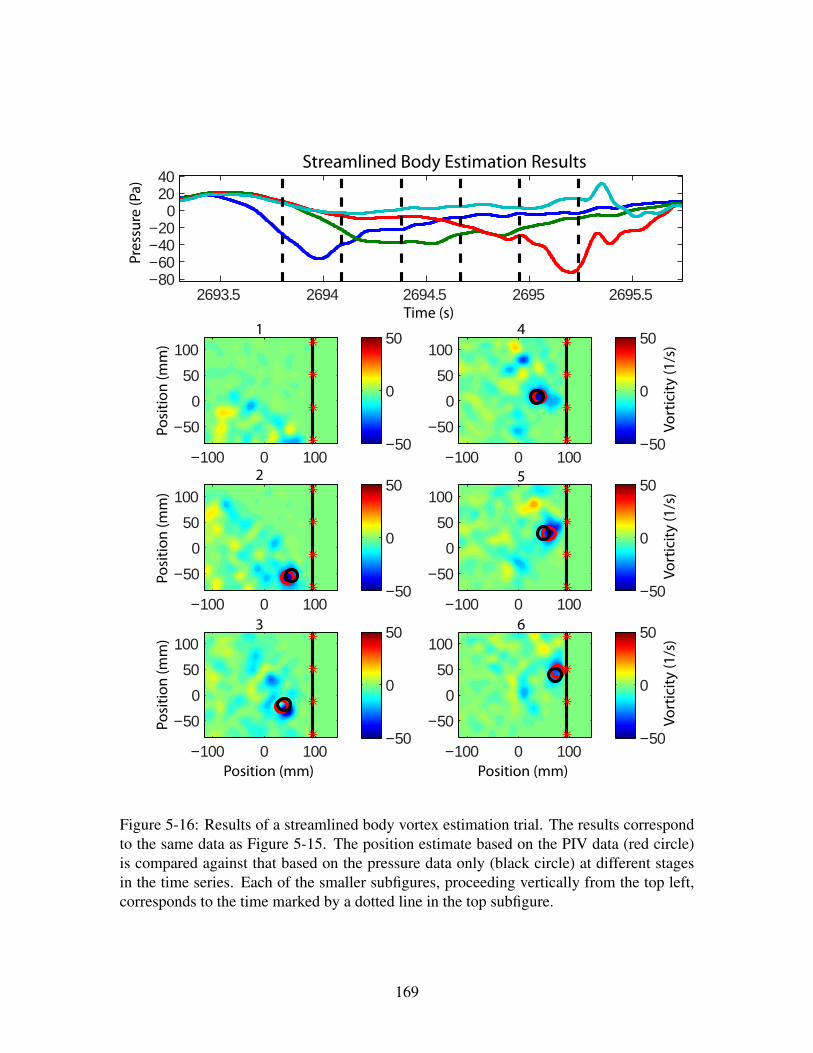
2693.5 2694 2694.5 2695 2695.5−80−60−40−20

02040

−100 0 100

−50

0

50

100

−50

0

50

−100 0 100

−50

0

50

100

−50

0

50

−100 0 100

−50

0

50

100

−50

0

50

−100 0 100

−50

0

50

100

−50

0

50

−100 0 100

−50

0

50

100

−50

0

50

−100 0 100

−50

0

50

100

−50

0

50


Posi

tion

(mm

)Po

sitio

n (m

m)

Posi

tion

(mm

)

1

2

3

4

5

6

Vort

icity

(1/s

)Vo

rtic

ity (1

/s)

Vort

icity

(1/s

)

Time (s)

Pres

sure

(Pa)



169

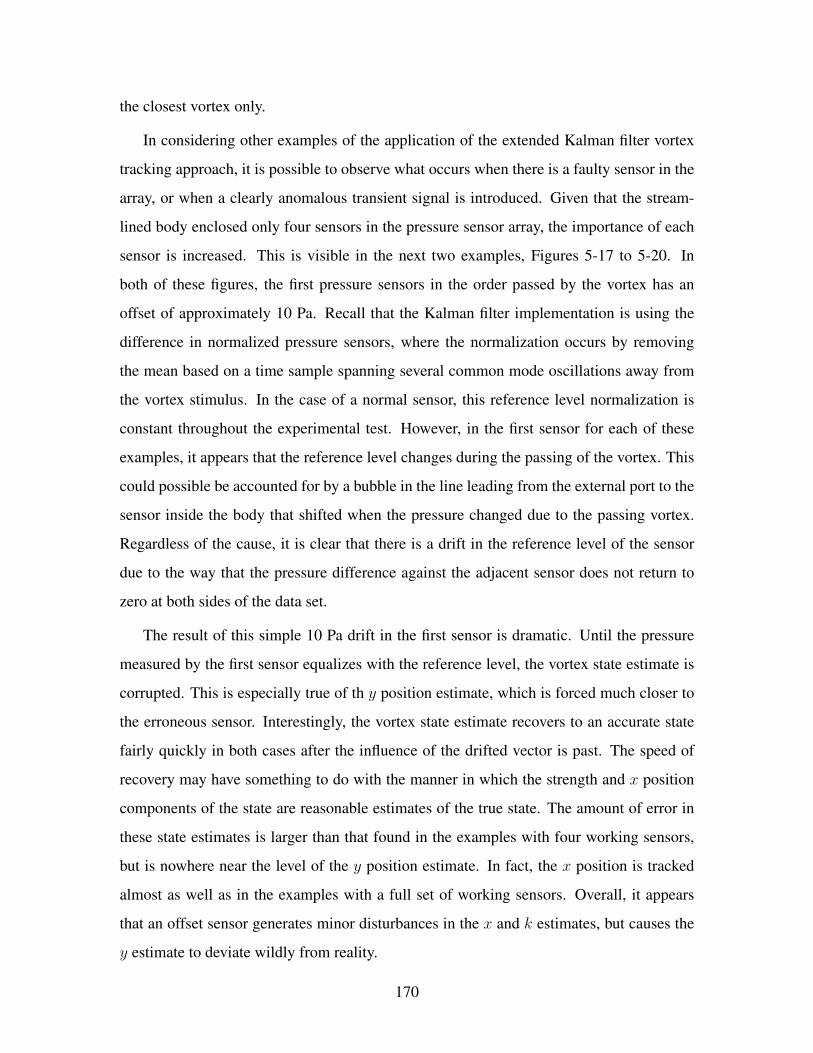
the closest vortex only.

In considering other examples of the application of the extended Kalman filter vortex

tracking approach, it is possible to observe what occurs when there is a faulty sensor in the

array, or when a clearly anomalous transient signal is introduced. Given that the stream-

lined body enclosed only four sensors in the pressure sensor array, the importance of each

sensor is increased. This is visible in the next two examples, Figures 5-17 to 5-20. In

both of these figures, the first pressure sensors in the order passed by the vortex has an

offset of approximately 10 Pa. Recall that the Kalman filter implementation is using the

difference in normalized pressure sensors, where the normalization occurs by removing

the mean based on a time sample spanning several common mode oscillations away from

the vortex stimulus. In the case of a normal sensor, this reference level normalization is

constant throughout the experimental test. However, in the first sensor for each of these

examples, it appears that the reference level changes during the passing of the vortex. This

could possible be accounted for by a bubble in the line leading from the external port to the

sensor inside the body that shifted when the pressure changed due to the passing vortex.

Regardless of the cause, it is clear that there is a drift in the reference level of the sensor

due to the way that the pressure difference against the adjacent sensor does not return to

zero at both sides of the data set.

The result of this simple 10 Pa drift in the first sensor is dramatic. Until the pressure

measured by the first sensor equalizes with the reference level, the vortex state estimate is

corrupted. This is especially true of th y position estimate, which is forced much closer to

the erroneous sensor. Interestingly, the vortex state estimate recovers to an accurate state

fairly quickly in both cases after the influence of the drifted vector is past. The speed of

recovery may have something to do with the manner in which the strength and x position

components of the state are reasonable estimates of the true state. The amount of error in

these state estimates is larger than that found in the examples with four working sensors,

but is nowhere near the level of the y position estimate. In fact, the x position is tracked

almost as well as in the examples with a full set of working sensors. Overall, it appears

that an offset sensor generates minor disturbances in the x and k estimates, but causes the

y estimate to deviate wildly from reality.

170

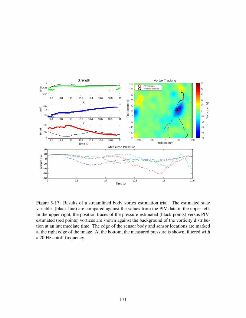
Position (mm)

Po

siti

on

(m

m)

Vortex Tracking

−100 −50 0 50 100−80

−60

−40

−20

0

20

40

60

80

100

120

−50

−40

−30

−20

−10

0

10

20

30

40

50

PIV Estimate

Pressure Estimate

Vort

icity

(1/s

)

9.6 9.8 10 10.2 10.4 10.6 10.8 11

-0.04

-0.02

0Strength

-100

0

100

X

0

50

100Y

Time (s)

9 9.5 10 10.5 11 11.5-80

-60

-40

-20

0

20

40

9.6 9.8 10 10.2 10.4 10.6 10.8 11

9.6 9.8 10 10.2 10.4 10.6 10.8 11

Time (s)

Measured Pressure

(mm

)(m

m)

(m /s

)2

Pres

sure

(Pa)


171

1509.2 1509.4 1509.6 1509.8 1510 1510.2 1510.4 1510.6 1510.8 1511 1511.2−80

−60

−40

−20

0

20

−100 0 100

−50

0

50

100

−50

0

50

−100 0 100

−50

0

50

100

−50

0

50

−100 0 100

−50

0

50

100

−50

0

50

−100 0 100

−50

0

50

100

−50

0

50

−100 0 100

−50

0

50

100

−50

0

50

−100 0 100

−50

0

50

100

−50

0

50


Posi

tion

(mm

)Po

sitio

n (m

m)

Posi

tion

(mm

)

1

2

3

4

5

6

Vort

icity

(1/s

)Vo

rtic

ity (1

/s)

Vort

icity

(1/s

)

Time (s)

Pres

sure

(Pa)



172

Position (mm)

Po

siti

on

(m

m)

Vortex Tracking

−100 −50 0 50 100−80

−60

−40

−20

0

20

40

60

80

100

120

−50

−40

−30

−20

−10

0

10

20

30

40

50PIV Estimate

Pressure Estimate

Vort

icity

(1/s

)

6.4 6.6 6.8 7 7.2 7.4 7.6

-0.04

-0.02

0Strength

-100

0

100

X

0

50

100Y

6.4 6.6 6.8 7 7.2 7.4 7.6

6.4 6.6 6.8 7 7.2 7.4 7.6

6 6.5 7 7.5 8 8.5-80

-60

-40

-20

0

20

40

Time (s)

Time (s)

Measured Pressure

(mm

)(m

m)

(m /s

)2

Pres

sure

(Pa)


173

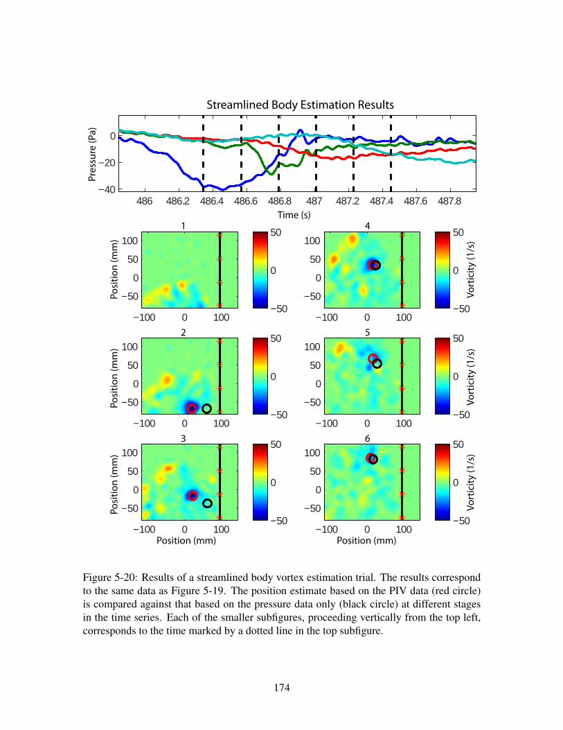
486 486.2 486.4 486.6 486.8 487 487.2 487.4 487.6 487.8−40

−20

0

−100 0 100

−50

0

50

100

−50

0

50

−100 0 100

−50

0

50

100

−50

0

50

−100 0 100

−50

0

50

100

−50

0

50

−100 0 100

−50

0

50

100

−50

0

50

−100 0 100

−50

0

50

100

−50

0

50

−100 0 100

−50

0

50

100

−50

0

50


Posi

tion

(mm

)Po

sitio

n (m

m)

Posi

tion

(mm

)

1

2

3

4

5

6

Vort

icity

(1/s

)Vo

rtic

ity (1

/s)

Vort

icity

(1/s

)

Time (s)

Pres

sure

(Pa)



174

Another example of vortex tracking from a streamlined body in the face of suboptimal

operating conditions is displayed in Figures 5-21 and 5-22. In this experimental result, the

measured pressure has an aberration at approximately 961.8 seconds, where the pressure

in the third sensor suddenly increases for a brief period of time. The cause of this increase

is unknown, the it appears from the PIV that the near vortex in this case was closer to

the sensors than the others considered so far, so it’s possible that secondary vortices may

have formed at the interface with the sensory body. Regardless of the cause, the vortex

tracking algorithm is unable to accurately track the nearest vortex while one of the sensors

is measuring a large stimulus that is not due to the vortex in question. Again however, once

the transient unexplained signal passes, the estimate based on pressure data appears to

recover to track the PIV estimate once again (Note that the PIV estimate becomes sporadic

afterwards due to the proximity of the solid body).

As demonstrated by a number of examples, a small linear sensor array of four pressure

sensors is sufficient to track a nearby vortex from a small streamlined body, such as a fish

or AUV. These results also validate the 1.3 vortex model, with the assumption that the

streamlined body does not influence the flow for the purposes of predicting the pressure

measurements. The level of detail available to a lateral-line-like sensor is as high as could

be desired. With a full set of functioning sensors, the position of a vortex center was tracked

with a mean error of a few millimeters, smaller than the viscous core of the vortices in

question. These successful results also confirm that a fish would have sufficient information

to extract this detailed information from a flow, focusing on the size and position of the

nearest vortex to the lateral line. Whether a fish requires and uses this level of detailed

inference over nearby vortices is unknown and a question to be addressed by experiments

with the fish itself.

With only four sensors, it is evident that there is little redundancy in the measurements,

and therefore even small discrepancies in the measurements of a single sensor can throw off

the vortex tracking. However, it is also clear that the vortex tracking estimate can recover

from a faulty sensor after the vortex passes beyond that sensor. In the case of a larger

number of sensors, it would likely be possible to correctly estimate the state of a vortex

while a single sensor provides faulty readings.

175

Position (mm)

Po

siti

on

(m

m)

Vortex Tracking

−100 −50 0 50 100−80

−60

−40

−20

0

20

40

60

80

100

120

−50

−40

−30

−20

−10

0

10

20

30

40

50

PIV Estimate

Pressure Estimate

961.2 961.4 961.6 961.8 962 962.2 962.4 962.6 962.8

-0.04

-0.02

0Strength

961.2 961.4 961.6 961.8 962 962.2 962.4 962.6 962.8

-100

0

100

X

961.2 961.4 961.6 961.8 962 962.2 962.4 962.6 962.80

50

100Y

961.2 961.4 961.6 961.8 962 962.2 962.4 962.6 962.8-80

-60

-40

-20

0

20

40

(mm

)(m

m)

(m /s

)2

Pres

sure

(Pa)

Time (s)

Time (s)

Vort

icity

(1/s

)

Measured Pressure


176

960.8 961 961.2 961.4 961.6 961.8 962 962.2 962.4 962.6 962.8−80

−60

−40

−20

0

20

−100 0 100

−50

0

50

100

−50

0

50

−100 0 100

−50

0

50

100

−50

0

50

−100 0 100

−50

0

50

100

−50

0

50

−100 0 100

−50

0

50

100

−50

0

50

−100 0 100

−50

0

50

100

−50

0

50

−100 0 100

−50

0

50

100

−50

0

50


Posi

tion

(mm

)Po

sitio

n (m

m)

Posi

tion

(mm

)

1

2

3

4

5

6

Vort

icity

(1/s

)Vo

rtic

ity (1

/s)

Vort

icity

(1/s

)

Time (s)

Pres

sure

(Pa)



177

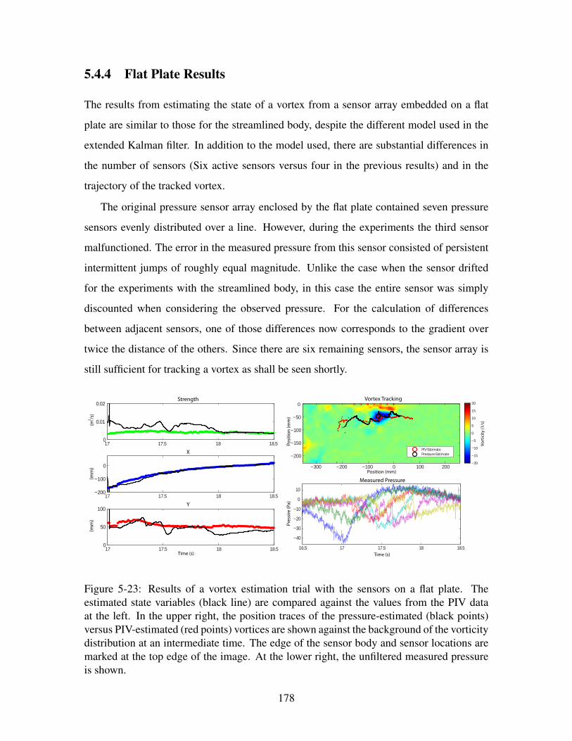
5.4.4 Flat Plate Results

The results from estimating the state of a vortex from a sensor array embedded on a flat

plate are similar to those for the streamlined body, despite the different model used in the

extended Kalman filter. In addition to the model used, there are substantial differences in

the number of sensors (Six active sensors versus four in the previous results) and in the

trajectory of the tracked vortex.

The original pressure sensor array enclosed by the flat plate contained seven pressure

sensors evenly distributed over a line. However, during the experiments the third sensor

malfunctioned. The error in the measured pressure from this sensor consisted of persistent

intermittent jumps of roughly equal magnitude. Unlike the case when the sensor drifted

for the experiments with the streamlined body, in this case the entire sensor was simply

discounted when considering the observed pressure. For the calculation of differences

between adjacent sensors, one of those differences now corresponds to the gradient over

twice the distance of the others. Since there are six remaining sensors, the sensor array is

still sufficient for tracking a vortex as shall be seen shortly.

16.5 17 17.5 18 18.5

−40

−30

−20

−10

0

10

17 17.5 18 18.50

0.01

0.02

−200

−100

0

0

50

100

Time (s)

Pres

sire

(Pa)

17 17.5 18 18.5

17 17.5 18 18.5Time (s)

(mm

)(m

m)

(m /s

)2

Strength

X

Y

−300 −200 −100 0 100 200

−200

−150

−100

−50

0

Position (mm)

PIV Estimate

Pressure Estimate

Posi

tion

(mm

)

−20

−15

−10

−5

0

5

10

15

20

Vort

icity

(1/s

)

Vortex Tracking

Measured Pressure

Figure 5-23: Results of a vortex estimation trial with the sensors on a flat plate. Theestimated state variables (black line) are compared against the values from the PIV dataat the left. In the upper right, the position traces of the pressure-estimated (black points)versus PIV-estimated (red points) vortices are shown against the background of the vorticitydistribution at an intermediate time. The edge of the sensor body and sensor locations aremarked at the top edge of the image. At the lower right, the unfiltered measured pressureis shown.

178

A number of details due to the difference in experimental setup are worth discussing

before examining the accuracy of the resulting vortex estimates. First of all, due to the

path of the initial vortex pair, there is a large signal measured by the first sensor in all the

data sets which does not contribute towards the tracking of the single nearby vortex. This

first sensor is strongly influence by the presence of the second vortex which subsequently

moves away from the sensors in the opposite direction. This is evident in the blue pressure

trace in Figure 5-23. This scenario is somewhat artificial from the point of view of tracking

externally generated vortices. The focus of these tests is to evaluate whether a lateral-

line-like array can identify and track a single vortex near a hull-like body, so the extended

Kalman filter is initialized slightly late, removing some of the initial data in which the

single vortex model is completely invalid. Besides the initial vortex pair, the pressure data

obtained from the flat plate experiments tended to be of a smaller magnitude than those

from the streamlined body. This is likely more related to the manner in which the vortices

were generated, which required a larger distance and weaker torques.

Finally, another major difference between the streamlined body experiments and those

with the flat plate is the level of interaction between the vortices and the sensing body. This

difference is in part the entire reason for the two different sets of experiments. However, it

appears that the level of interaction between the vortex and flat plate goes slightly beyond

that captured in the reflected-vortex model. In both cases, the vortex centers appear to

approximately 50 mm from the sensor array. However, with the streamlined body, there

appeared to be no secondary vorticity generated by an interaction between the vortex and

the boundary layer on the body. In contrast, with the flat plate body, a noticeable shear layer

does develop on the plate surface (vorticity distribution in Figure 5-23), and eventually

small counter-rotating vortices are shed into the flow (frames 4 and 6 in Figure 5-24).

A typical result for the flat-plate-embedded sensors is shown in Figure 5-23. As men-

tioned, the extended Kalman filter is initialized slightly after the first disturbances in pres-

sure due to vortices are felt. However, this does not completely bypass the influence of the

second physical vortex. At the 17 s mark, where the estimation begins, the first sensor is at

its peak measurement. The vortex tracking result demonstrate that, despite the initial sec-

ond vortex and the later secondary vortices, the estimate of the x position along the length

179

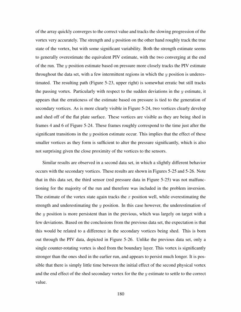
of the array quickly converges to the correct value and tracks the slowing progression of the

vortex very accurately. The strength and y position on the other hand roughly track the true

state of the vortex, but with some significant variability. Both the strength estimate seems

to generally overestimate the equivalent PIV estimate, with the two converging at the end

of the run. The y position estimate based on pressure more closely tracks the PIV estimate

throughout the data set, with a few intermittent regions in which the y position is underes-

timated. The resulting path (Figure 5-23, upper right) is somewhat erratic but still tracks

the passing vortex. Particularly with respect to the sudden deviations in the y estimate, it

appears that the erraticness of the estimate based on pressure is tied to the generation of

secondary vortices. As is more clearly visible in Figure 5-24, two vortices clearly develop

and shed off of the flat plate surface. These vortices are visible as they are being shed in

frames 4 and 6 of Figure 5-24. These frames roughly correspond to the time just after the

significant transitions in the y position estimate occur. This implies that the effect of these

smaller vortices as they form is sufficient to alter the pressure significantly, which is also

not surprising given the close proximity of the vortices to the sensors.

Similar results are observed in a second data set, in which a slightly different behavior

occurs with the secondary vortices. These results are shown in Figures 5-25 and 5-26. Note

that in this data set, the third sensor (red pressure data in Figure 5-25) was not malfunc-

tioning for the majority of the run and therefore was included in the problem inversion.

The estimate of the vortex state again tracks the x position well, while overestimating the

strength and underestimating the y position. In this case however, the underestimation of

the y position is more persistent than in the previous, which was largely on target with a

few deviations. Based on the conclusions from the previous data set, the expectation is that

this would be related to a difference in the secondary vortices being shed. This is born

out through the PIV data, depicted in Figure 5-26. Unlike the previous data set, only a

single counter-rotating vortex is shed from the boundary layer. This vortex is significantly

stronger than the ones shed in the earlier run, and appears to persist much longer. It is pos-

sible that there is simply little time between the initial effect of the second physical vortex

and the end effect of the shed secondary vortex for the the y estimate to settle to the correct

value.

180

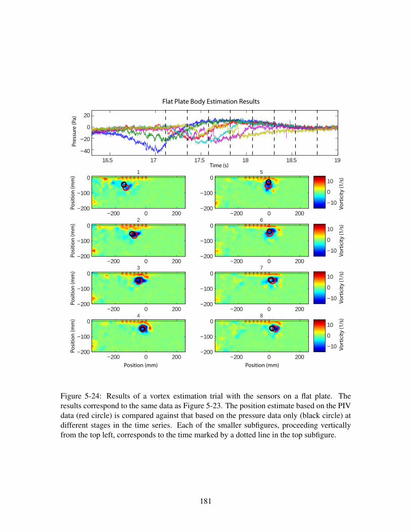
16.5 17 17.5 18 18.5 19

−40

−20

0

20

1

−200 0 200−200

−100

0

2

−200 0 200−200

−100

0

3

−200 0 200−200

−100

0

4

−200 0 200−200

−100

0

5

−200 0 200−200

−100

0

6

−200 0 200−200

−100

0

7

−200 0 200−200

−100

0

8

−200 0 200−200

−100

0

−10

0

10

−10

0

10

−10

0

10

−10

0

10

Vort

icity

(1/s

)Vo

rtic

ity (1

/s)

Vort

icity

(1/s

)Vo

rtic

ity (1

/s)

Posi

tion

(mm

)Po

sitio

n (m

m)

Posi

tion

(mm

)Po

sitio

n (m

m)


Time (s)

Pres

sure

(Pa)

Flat Plate Body Estimation Results

Figure 5-24: Results of a vortex estimation trial with the sensors on a flat plate. Theresults correspond to the same data as Figure 5-23. The position estimate based on the PIVdata (red circle) is compared against that based on the pressure data only (black circle) atdifferent stages in the time series. Each of the smaller subfigures, proceeding verticallyfrom the top left, corresponds to the time marked by a dotted line in the top subfigure.

181

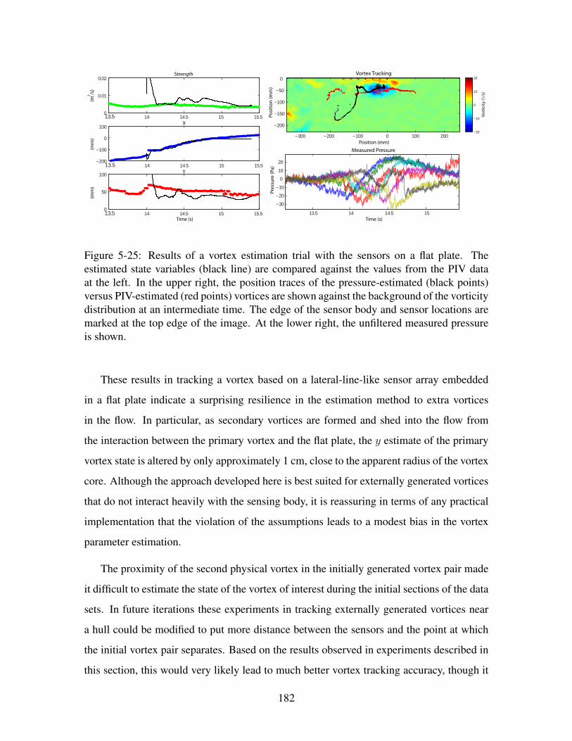
13.5 14 14.5 15

−30

−20

−10

0

10

20

−300 −200 −100 0 100 200

−200

−150

−100

−50

0

−20

−10

0

10

20

Time (s)

Pres

sure

(Pa)

Position (mm)

Posi

tion

(mm

)

Measured Pressure

Vortex Tracking

Vort

icity

(1/s

)

13.5 14 14.5 15 15.50

0.01

0.02

−200

−100

0

100

0

50

100

13.5 14 14.5 15 15.5

13.5 14 14.5 15 15.5

(mm

)(m

m)

(m /s

)2

Time (s)

Strength

X

Y

Figure 5-25: Results of a vortex estimation trial with the sensors on a flat plate. Theestimated state variables (black line) are compared against the values from the PIV dataat the left. In the upper right, the position traces of the pressure-estimated (black points)versus PIV-estimated (red points) vortices are shown against the background of the vorticitydistribution at an intermediate time. The edge of the sensor body and sensor locations aremarked at the top edge of the image. At the lower right, the unfiltered measured pressureis shown.

These results in tracking a vortex based on a lateral-line-like sensor array embedded

in a flat plate indicate a surprising resilience in the estimation method to extra vortices

in the flow. In particular, as secondary vortices are formed and shed into the flow from

the interaction between the primary vortex and the flat plate, the y estimate of the primary

vortex state is altered by only approximately 1 cm, close to the apparent radius of the vortex

core. Although the approach developed here is best suited for externally generated vortices

that do not interact heavily with the sensing body, it is reassuring in terms of any practical

implementation that the violation of the assumptions leads to a modest bias in the vortex

parameter estimation.

The proximity of the second physical vortex in the initially generated vortex pair made

it difficult to estimate the state of the vortex of interest during the initial sections of the data

sets. In future iterations these experiments in tracking externally generated vortices near

a hull could be modified to put more distance between the sensors and the point at which

the initial vortex pair separates. Based on the results observed in experiments described in

this section, this would very likely lead to much better vortex tracking accuracy, though it

182

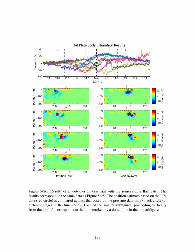
13.4 13.6 13.8 14 14.2 14.4 14.6 14.8 15 15.2 15.4−40

−20

0

20

40

1

−200 0 200−200

−100

0

2

−200 0 200−200

−100

0

3

−200 0 200−200

−100

0

4

−200 0 200−200

−100

0

5

−200 0 200−200

−100

0

6

−200 0 200−200

−100

0

7

−200 0 200−200

−100

0

8

−200 0 200−200

−100

0

−10

0

10

−10

0

10

−10

0

10

−10

0

10

Vort

icity

(1/s

)Vo

rtic

ity (1

/s)

Vort

icity

(1/s

)Vo

rtic

ity (1

/s)

Position (mm)Position (mm)

Posi

tion

(mm

)Po

sitio

n (m

m)

Posi

tion

(mm

)Po

sitio

n (m

m)

Time (s)

Pres

sure

(Pa)

Flat Plate Body Estimation Results

Figure 5-26: Results of a vortex estimation trial with the sensors on a flat plate. Theresults correspond to the same data as Figure 5-25. The position estimate based on the PIVdata (red circle) is compared against that based on the pressure data only (black circle) atdifferent stages in the time series. Each of the smaller subfigures, proceeding verticallyfrom the top left, corresponds to the time marked by a dotted line in the top subfigure.

183

would still not remove the effect of the secondary vortices.

5.5 Vortex Tracking Dependence on Array Parameters

Based on the experimental estimation results, it has been demonstrated that it is possible to

track a vortex in an experimental setting under different conditions roughly corresponding

to that of a fish and a ship hull. However, it is still unclear where the limits are to the vor-

tex tracking approach described in this chapter. In particular, it is virtually certain that the

ability to track a vortex using a linear array of pressure sensors will depend on the param-

eters of that sensor array: its overall length and sensor spacing. Considering the extreme

case, a sensor array composed of a single sensor would clearly perform differently than

the several-sensor arrays used in the experiments. It is critical to establish and understand

the connection between the sensor array parameters and the ability to sense vortices in or-

der to design appropriate and efficient lateral-line like sensor arrays using MEMS or other

technologies, as is being done by a number of groups [35, 88].

In order to examine the relationship between the estimation of the vortex state and the

sensor array parameters, the instantaneous estimate of the vortex state will be used. We will

consider the best estimate of the vortex state given a single instantaneous set of measure-

ments and no knowledge of the measurements or vortex state before and after. Considering

the instantaneous inverse problem will make it possible to examine and identify the mech-

anisms which are responsible for affecting the performance of the vortex estimation. These

mechanisms will then be extrapolated to estimation on the entire time series and compared

to behaviors observed in the Kalman filter estimation. The procedure for this will first in-

volve examining the effect of vortex location based on a single sensor and a representative

small linear array in order to derive intuition on what motivates the spatial localization of

a vortex. Then the effect of sensor array length and density will be examined for a vortex

centered along the length of the array.

The instantaneous estimate of a vortex state is based on the minimization of a least

squares cost function, in which J (x, y, k) ∝∑

i (Pi (x, y, k)− P truei )

2. In this equation,

the cost J represents a penalty based on the difference between the actual measured pressure

184

and the simulated pressure of a vortex at position (x, y) with strength k. The summation

variable i refers to a sum over the number of sensors used in the measurement. The least

squares cost function is an appropriate choice for this analysis since it is at the heart of the

Kalman filter, as well as being an intuitive cost function. Minimizing the cost function J

corresponds to finding the vortex state that best generates the measured data.

5.5.1 Reflected Vortex Model

The two models used in the experimental vortex tracking will be considered separately. The

first of these is the reflected vortex model, in which a single physical vortex is modeled in

potential flow, with an imaginary vortex reflected over the sensor array line. Recall that the

complex potential of the reflected vortex model is described by:

Φ (z) = −ik log (z − zo) + ik log (z − zo) (5.9)

where zo = xo + iyo represents the location of the physical vortex. The pressure associated

with this model is derived using the unsteady Bernoulli equation in the same manner as

discussed earlier.

With this model, it is possible to specify the cost function in more detail. The least

squares cost function for this particular model can be written as follows:

J (xo, yo, ko) =1

(P trueo )2

N∑i=1

(Pi (xo, yo, ko)− P true

i

)2 (5.10)

Where P truei is the measured pressure at sensor i obtained by the model based on the “cor-

rect” state of the vortex. If the test vortex state, denoted by the triplet (xo, yo, ko) is equal

to the true state, it is clear that the cost J will be zero and that this is the minimum value

possible for the cost function. The constant P trueo in the cost function is a normalization

constant that refers to the measurement with maximum magnitude based on the true vortex

state. For a reflected vortex centered in the middle of an array, this will always correspond

to the sensor location closest to the vortex.

Recall that the pressure at a point on the “wall” or plane of reflection is given by the

185

following formula derived from the unsteady Bernoulli equation:

P (z)− P∞ = −1

2ρ

(∂Φ(z)

∂z

)2

− ρ∂Φ(z)

∂xo

∂xo∂t

(5.11)

P (s)− P∞ = ρk2 (s− xo)2 − y2o(

(s− xo)2 + y2o

)2 (5.12)

Note that, as before, several shortcuts have been used implicitly due to the symmetry of

the problem and the fact that the points of measurement are restricted to the real axis.

For example, the complex potential is being used directly in the time derivative since the

real axis forms a streamline. The variable s, a real scalar denoting the position of the

measurement point on the real axis, is substituted in place of the complex z.

As evident from the end result, equation (5.12), the pressure measured at any point has a

simple squared relationship with the strength of the vortex. This implies that the only effect

of the vortex strength is on the magnitude of the signal, not its spatial distribution. As the

main question being addressed is how the spatial relationships between the sensor array

and the vortex position affect the ability to track the vortex state, the effect of the vortex

strength is of secondary importance. Of course, if a vortex is too weak in comparison to

the noise floor of the sensors, any attempts to estimate the vortex state will fail as there is

effectively no information in the measurements. For this section, it will be assumed that

the true vortex strength is sufficiently large compared to the noise amplitude.

When considering the cost of estimating a vortex to be at a particular location, the

estimate of the vortex strength is unspecified and will therefore be chosen as the strength

that minimizes the cost function at that point. This approach is intuitive in that two potential

locations for a vortex will be compared by the most accurate pressure measurements that

can be generated from those locations. It is also possible to consider the problem when

the vortex strength is assumed known. This would correspond to having good a priori

knowledge of the vortex strength due to either accurate earlier tracking or knowledge of

the vortex formation mechanisms. In this case, the results look very different, but there is

still ambiguity in the spatial position under certain conditions.

The optimization of the vortex strength for a given location follows directly from equa-

186

tions (5.10) and (5.12). From equation (5.12), the pressure at a point is proportional to the

strength squared: P truei = k2ai, where ai is the constant that depends on the location of the

measurement and of course the location of the vortex. From this, the equation for the cost

function can be rewritten and the root of its derivative with respect to k found.

J (k) =1

(P trueo )2

N∑i=1

(k2ai − P true

i

)2 (5.13)

dJ (k)

dk=

2

(P trueo )2

N∑i=1

(k2ai − P true

i

)2kai (5.14)

0 =N∑i=1

k2a2i − aiP true

i (5.15)

= k2

N∑i=1

a2i −

N∑i=1

aiPtruei (5.16)

The solution to the remaining quadratic equation gives the optimal vortex strength. In the

instantaneous case, there is no information on the sign of the vortex, so by convention the

positive strength will be used. In the experimental case of course, the motion of the vortex

over time reveals the direction of rotation. At times, the quadratic equation (5.16) does not

have real valued solutions. This corresponds to an impossible match between the measured

pressure and the location of the test vortex. In these cases, the optimal strength is zero.

Least Squares Cost Map

−0.2 −0.1 0 0.1 0.20

0.05

0.1

0.15

0.2

0.25

−0.4 −0.1 0 0.1 0.4−8

−6

−4

−2

0

2

−2

−1.5

−1

−0.5

0

Log

N

orm

aliz

ed C

ost

10

Distance Units

Dis

tanc

e U

nits

Distance Units

Nor

mal

ized

Pre

ssur

e

Instantaneous Least Squares Inversion Based on a Single Sensor

A B

Figure 5-27: Instantaneous inversion based on a single pressure sensor for the reflectedvortex model. Part A shows the spatial map of the cost function generated with one sensor.The small x at (0,0.1) denotes the true location of the vortex. Part B depicts the pressuredistribution on the wall at the y = 0 axis.

187

First consider the estimation of a vortex state for a vortex near a wall using only one

sensor and a single measurement. Clearly one would expect a number of positions to be

equally viable, since the strength of the vortex can be adjusted for a candidate position

in order to recreate the measured pressure at the solitary point. For this particular model

however, it turns out that not all points in the half plane (the fluid side of the plane bi-

sected by the linear array) are valid. This is displayed in Figure 5-27, which demonstrates

in subfigure A that only a vortex within a cone emanating at a 45 degree angle from the

measurement point can generate the pressure measurement similar to that of a vortex di-

rectly in front of the sensor (marked by an small cross in the figure). The reason for this

is clear from the distribution of pressure on the sensor line, shown at the right in Figure 5-

27B. In the case of the reflected vortex model, the lines of zero pressure (compared to the

far field stationary flow, as always) pass through the vortex location and form 45 degree

angles with the reflection plane. This can also be observed directly from the numerator in

equation (5.12). In the particular case shown in Figure 5-27, the vortex is 0.1 units away

from the wall and the zero crossing points of the pressure on the wall are at 0.1 and -0.1

units. Within this range, the pressure is below the far-field pressure, but outside this range

the pressure is above the far-field pressure. This spatial distribution is fixed relative to the

center of the vortex, regardless of the location of the vortex or its strength. As a result,

the sign of the pressure measured at a single point limits the possible range of the vortex

that generated it. In the case of a single vortex, this restriction evidently does not aid the

estimation much, as there is still a large region of ambiguity. However, the same principle

plays a large role when there are multiple sensors.

A map of the cost function, as seen in Figure 5-27A and in the following figures, visu-

ally presents the spatial components of estimating the vortex position in an intuitive manner.

In general, the cost function ranges from zero, at the exact location of the true vortex, to an

upper limit that is typically Jmax = 1(P true

o )2

∑Ni=1 (P true

i )2, which corresponds to locations

that cannot generate the same sign of pressure measurements as the true vortex. Although

these maps of the cost function depict the difference between noiseless, simulated measure-

ments, it is possible to relate the results to a more realistic measurement with random noise.

Consider the cost when the noiseless measurement of the true vortex state is compared to

188

a noisy measurement of the true vortex state: J = 1(P true

o )2

∑Ni=1 (P true

i − (P truei + ηi))

2

where ηi is the noise variable for each sensor. This is the situation that would occur if the

correct vortex state was hypothesized, but only noisy measurements were available. The

result is J = 1(P true

o )2

∑Ni=1 (ηi)

2. If ηi are normally distributed with variance σ2, then J

becomes a Chi-Squared random variable J = σ2

(P trueo )2

χ2. This expression relates the cost

function J to the maximum pressure and measurement noise variance. For example, as-

suming that the noise variance is ten percent of the maximum pressure magnitude, which

is a typical moderate noise scenario, it is possible to calculate a value for J such that with

95% confidence, the true state will be contained in the region with lower cost. This means

that in general the regions of low cost in a spatial map of the cost function can be inter-

preted as being more easily confused through noise, and the relevant level sets of the cost

map depend on the signal-to-noise ratio.

To examine the multiple sensor case with the reflected vortex model, first consider

the effect of the position of the vortex with respect to a modest linear sensor array of

five sensors. The location of the vortex perpendicular to the axis of the linear array is

kept constant, and several positions parallel to the axis of the linear array (the x axis) are

considered. The results are displayed in Figure 5-28. The position in the y direction of the

vortex in each frame of Figure 5-28 is the same as Figure 5-27, 0.1 normalized distance

units. The sensors are spaced at a distance of 1/30th (0.033) of a distance unit, chosen as a

combination of spacing and array length that is known to result in good localization for a

centered vortex at 0.1 units perpendicular distance, as will be discussed shortly. The black

curves in each subfigure represent the level sets for which the noise standard deviation

is 1%, 5%, and 10% of the maximum pressure magnitude. Also, note that each frame

in Figure 5-28 shows the map of the cost normalized for that particular instant. These

normalization constants are different from one time to the next, even though the resulting

surfaces are plotted with the same color map. In the first few frames of Figure 5-28, the

actual vortex position is outside the 45 degree line for all of the sensors implying that they

all measure a positive pressure. The nature of the region of ambiguity is not a surprise in

these cases, with a broad low-cost region that grows with distance. Between images D and

E in the figure, the vortex passes the x-position 0.166 which takes it past the zero crossing

189

0.27 Vortex Position

0 0.2 0.40

0.1

0.2


0 0.2 0.40

0.1

0.2


0 0.2 0.40

0.1

0.2


0 0.2 0.40

0.1

0.2


0 0.2 0.40

0.1

0.2


0 0.2 0.40

0.1

0.2


0 0.2 0.40

0.1

0.2


0 0.2 0.40

0.1

0.2


0 0.2 0.40

0.1

0.2

0 Vortex Position

0 0.2 0.40

0.1

0.2

−2

−1

0

Log

N

orm

aliz

ed C

ost

10

Dis

tanc

e U

nits

Dis

tanc

e U

nits

Dis

tanc

e U

nits

Dis

tanc

e U

nits

Dis

tanc

e U

nits

Distance UnitsDistance Units

A F

B

C

D

E

H

I

J

G

Figure 5-28: Maps of the cost function for a reflected vortex model with the vortex at vari-ous lateral locations. The x in each image with a y position of 0.1 and an x position labeledin the subfigure title denotes the true location of the vortex. The black lines correspond tolevel sets generated by the assumption of noise with standard deviations of 1, 5, and 10%of the maximum measured pressure.

190

point of the first sensor. This is marked by a radical reduction in the possible region for

the vortex estimate. Interestingly, the region of ambiguity subsequently grows again, until

image I. At that point, the vortex is still within the negative region of the first sensor, but

has just crossed the 45 degree boundary for the last sensor. Based on this progression,

it appears the localization of a vortex under a reflected model as it moves parallel to the

sensor array is largely a function of the position relative to the 45 degree lines from each

sensor. Also, under the reflected model, it is clear that even under good conditions, it is

difficult to locate a vortex that is off to the side of the sensor array. This is particularly true

if the vortex is outside the 45 degree line of all the sensors, as in B-D, but it still appears

difficult up until the vortex is approximately in front of the first sensor.

5 Distance Ratio

−0.1 0 0.10

0.05

0.1

0.15

3.13 Distance Ratio

−0.1 0 0.10

0.05

0.1

0.15

1.56 Distance Ratio

−0.1 0 0.10

0.05

0.1

0.15

0.758 Distance Ratio

−0.1 0 0.10

0.05

0.1

0.150.5 Distance Ratio

−0.1 0 0.10

0.05

0.1


−0.1 0 0.10

0.05

0.1

0.15


−0.1 0 0.10

0.05

0.1

0.2 Distance Ratio

−0.1 0 0.10

0.05

0.1

0.1 Distance Ratio

−0.1 0 0.10

0.05

0.1

−2

−1

0

Log

N

orm

aliz

ed C

ost

10

Distance UnitsDistance UnitsDistance Units

Dis

tanc

e U

nits

Dis

tanc

e U

nits

Dis

tanc

e U

nits

0.15 0.15 0.15

A

D

H

B

E

I

C

F

J

Figure 5-29: Maps of the cost function for a reflected vortex model with an increasing arraylength but constant sensor spacing. The x at (0,0.1) in each image denotes the true locationof the vortex. The black lines correspond to level sets generated by the assumption of noisewith standard deviations of 1, 5, and 10% of the maximum measured pressure.

191

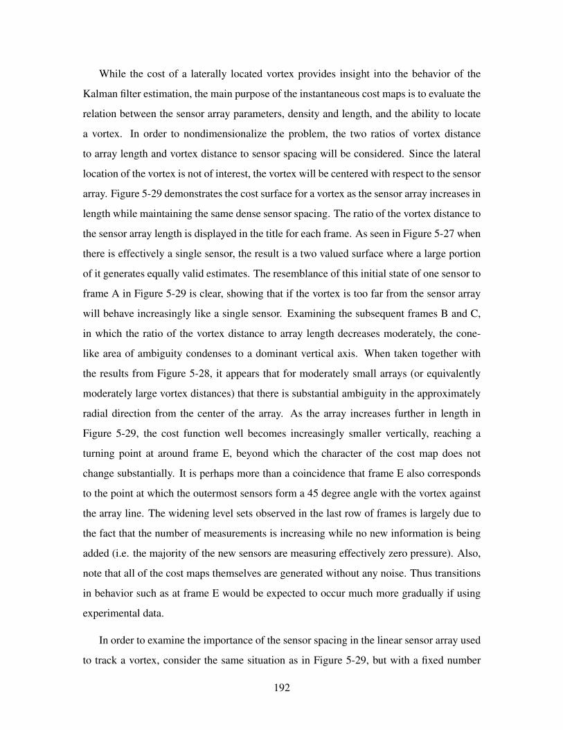
While the cost of a laterally located vortex provides insight into the behavior of the

Kalman filter estimation, the main purpose of the instantaneous cost maps is to evaluate the

relation between the sensor array parameters, density and length, and the ability to locate

a vortex. In order to nondimensionalize the problem, the two ratios of vortex distance

to array length and vortex distance to sensor spacing will be considered. Since the lateral

location of the vortex is not of interest, the vortex will be centered with respect to the sensor

array. Figure 5-29 demonstrates the cost surface for a vortex as the sensor array increases in

length while maintaining the same dense sensor spacing. The ratio of the vortex distance to

the sensor array length is displayed in the title for each frame. As seen in Figure 5-27 when

there is effectively a single sensor, the result is a two valued surface where a large portion

of it generates equally valid estimates. The resemblance of this initial state of one sensor to

frame A in Figure 5-29 is clear, showing that if the vortex is too far from the sensor array

will behave increasingly like a single sensor. Examining the subsequent frames B and C,

in which the ratio of the vortex distance to array length decreases moderately, the cone-

like area of ambiguity condenses to a dominant vertical axis. When taken together with

the results from Figure 5-28, it appears that for moderately small arrays (or equivalently

moderately large vortex distances) that there is substantial ambiguity in the approximately

radial direction from the center of the array. As the array increases further in length in

Figure 5-29, the cost function well becomes increasingly smaller vertically, reaching a

turning point at around frame E, beyond which the character of the cost map does not

change substantially. It is perhaps more than a coincidence that frame E also corresponds

to the point at which the outermost sensors form a 45 degree angle with the vortex against

the array line. The widening level sets observed in the last row of frames is largely due to

the fact that the number of measurements is increasing while no new information is being

added (i.e. the majority of the new sensors are measuring effectively zero pressure). Also,

note that all of the cost maps themselves are generated without any noise. Thus transitions

in behavior such as at frame E would be expected to occur much more gradually if using

experimental data.

In order to examine the importance of the sensor spacing in the linear sensor array used

to track a vortex, consider the same situation as in Figure 5-29, but with a fixed number

192

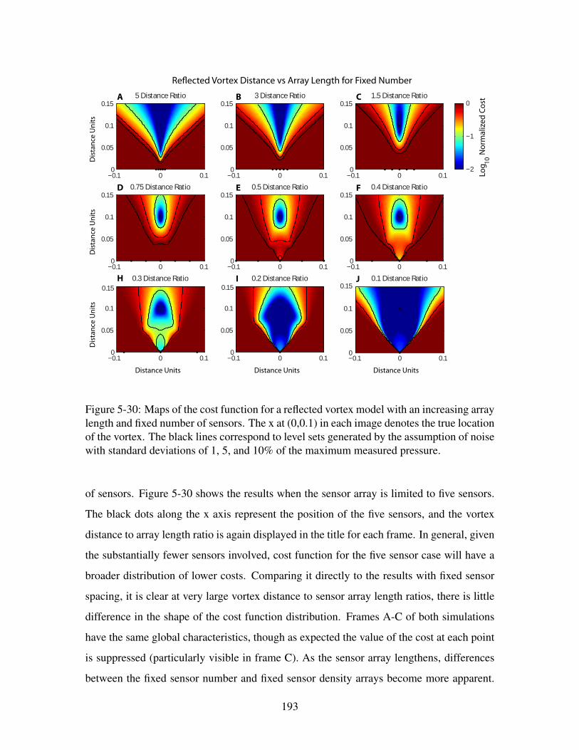
5 Distance Ratio

−0.1 0 0.10

0.05

0.1

0.15

3 Distance Ratio

−0.1 0 0.10

0.05

0.1

0.15

1.5 Distance Ratio

−0.1 0 0.10

0.05

0.1

0.15

0.75 Distance Ratio

−0.1 0 0.10

0.05

0.1


−0.1 0 0.10

0.05

0.1


−0.1 0 0.10

0.05

0.1

0.15

0.3 Distance Ratio

−0.1 0 0.10

0.05

0.1

0.2 Distance Ratio

−0.1 0 0.10

0.05

0.1

0.1 Distance Ratio

0.150.15

−0.1 0 0.10

0.05

0.1

0.15

−2

−1

0

Log

N

orm

aliz

ed C

ost

10

Distance UnitsDistance UnitsDistance Units

Dis

tanc

e U

nits

Dis

tanc

e U

nits

Dis

tanc

e U

nits

A

D

H

B

E

I

C

F

J

Figure 5-30: Maps of the cost function for a reflected vortex model with an increasing arraylength and fixed number of sensors. The x at (0,0.1) in each image denotes the true locationof the vortex. The black lines correspond to level sets generated by the assumption of noisewith standard deviations of 1, 5, and 10% of the maximum measured pressure.

of sensors. Figure 5-30 shows the results when the sensor array is limited to five sensors.

The black dots along the x axis represent the position of the five sensors, and the vortex

distance to array length ratio is again displayed in the title for each frame. In general, given

the substantially fewer sensors involved, cost function for the five sensor case will have a

broader distribution of lower costs. Comparing it directly to the results with fixed sensor

spacing, it is clear at very large vortex distance to sensor array length ratios, there is little

difference in the shape of the cost function distribution. Frames A-C of both simulations

have the same global characteristics, though as expected the value of the cost at each point

is suppressed (particularly visible in frame C). As the sensor array lengthens, differences

between the fixed sensor number and fixed sensor density arrays become more apparent.

193

Interestingly, in frames D and E of Figure 5-30, the regions near the true vortex position are

effectively undeformed in comparison to the case with constant sensor spacing. Around the

periphery, some differences are beginning to show however. In particular, the lower cost

region begins to spread towards the array and then outward. Although the limit in the end

is the same as the starting point, the area of low cost is originally limited to the immediate

vicinity of the closes sensor (frame I). This implies that as a vortex gets too close to a sparse

array, the ability to locate it identifying it’s closest sensor, is significantly degraded.

5.5.2 Vortex Pair Model

The primary practical difference that results from the vortex pair model, not found in the

reflected vortex model, is that there is an extra parameter to determine. Following the same

line of reasoning as with the vortex strength for the reflected vortex, in order to evaluate

the cost of estimating a vortex at a particular location, the cost function is optimized for the

vortex strength and vortex separation with the primary vortex at the point of interest. The

complex potential for the vortex pair is fundamentally very similar to the reflected vortex

(the location of the second vortex is not reflected, but there are still two vortices forming a

line perpendicular to the sensor array):

Φ (z) = −ik log (z − zo) + ik log (z − z1) (5.17)

with the additional constraint that if zo = x + iy then z1 = x + i (y + d). Therefore,

the function for the pressure measurements is still proportional to the strength squared,

and, for any combination of position and vortex pair separation, the optimal strength is a

straightforward calculation. In order to identify the optimal vortex separation however, the

cost function J (do) (with ko no longer a free variable, and xo, yo specified) was minimized

numerically.

In the case of the reflected vortex model, the 45 degree angle lines emanating from

the vortex marked important transitions from positive to negative pressure with respect

to the far field. In the case of the vortex pair, where the distance between the vortices

is unconstrained, this behavior is no longer present. In the limit of a very large distance

194

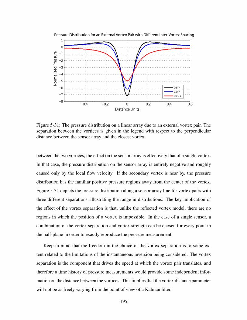
−0.4 −0.2 0 0.2 0.4 0.6−8

−7

−6

−5

−4

−3

−2

−1

0

1

0.5 Y

1.0 Y

10.0 Y

Distance Units

Nor

mal

ized

Pre

ssur

e

Pressure Distribution for an External Vortex Pair with Dierent Inter-Vortex Spacing

Figure 5-31: The pressure distribution on a linear array due to an external vortex pair. Theseparation between the vortices is given in the legend with respect to the perpendiculardistance between the sensor array and the closest vortex.

between the two vortices, the effect on the sensor array is effectively that of a single vortex.

In that case, the pressure distribution on the sensor array is entirely negative and roughly

caused only by the local flow velocity. If the secondary vortex is near by, the pressure

distribution has the familiar positive pressure regions away from the center of the vortex.

Figure 5-31 depicts the pressure distribution along a sensor array line for vortex pairs with

three different separations, illustrating the range in distributions. The key implication of

the effect of the vortex separation is that, unlike the reflected vortex model, there are no

regions in which the position of a vortex is impossible. In the case of a single sensor, a

combination of the vortex separation and vortex strength can be chosen for every point in

the half-plane in order to exactly reproduce the pressure measurement.

Keep in mind that the freedom in the choice of the vortex separation is to some ex-

tent related to the limitations of the instantaneous inversion being considered. The vortex

separation is the component that drives the speed at which the vortex pair translates, and

therefore a time history of pressure measurements would provide some independent infor-

mation on the distance between the vortices. This implies that the vortex distance parameter

will not be as freely varying from the point of view of a Kalman filter.

195


0 0.2 0.40

0.1

0.2


0 0.2 0.40

0.1

0.2


0 0.2 0.40

0.1

0.2


0 0.2 0.40

0.1

0.2


0 0.2 0.40

0.1

0.2


0 0.2 0.40

0.1

0.2


0 0.2 0.40

0.1

0.2


0 0.2 0.40

0.1

0.2


0 0.2 0.40

0.1

0.2

0 Vortex Position

0 0.2 0.40

0.1

0.2

Dis

tanc

e U

nits

Dis

tanc

e U

nits

Dis

tanc

e U

nits

Dis

tanc

e U

nits

Dis

tanc

e U

nits

Distance UnitsDistance Units

−3

−2

−1

0

Log

N

orm

aliz

ed C

ost

10

A F

B

C

D

E

H

I

J

G

Figure 5-32: Maps of the cost function for a vortex pair model with the vortices at variouslateral locations. The x in each image denotes the true locations of the vortices. The blacklines correspond to level sets generated by the assumption of noise with standard deviationsof 1, 5, and 10% of the maximum measured pressure.

196

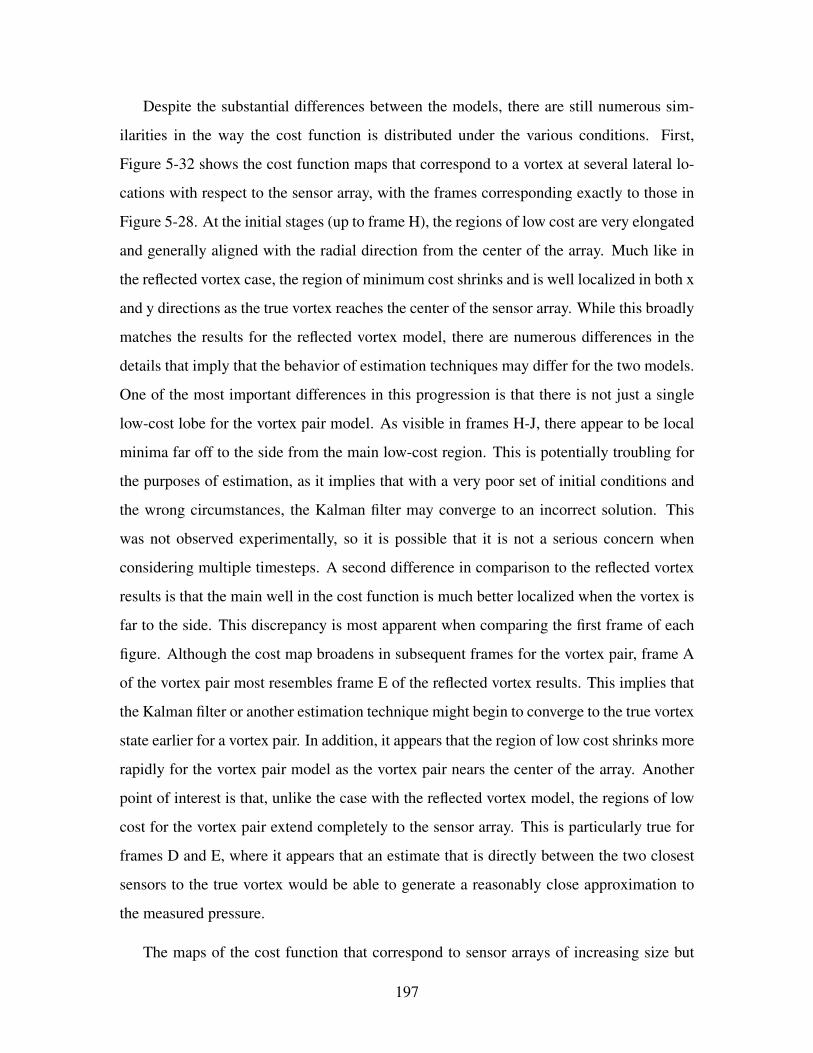
Despite the substantial differences between the models, there are still numerous sim-

ilarities in the way the cost function is distributed under the various conditions. First,

Figure 5-32 shows the cost function maps that correspond to a vortex at several lateral lo-

cations with respect to the sensor array, with the frames corresponding exactly to those in

Figure 5-28. At the initial stages (up to frame H), the regions of low cost are very elongated

and generally aligned with the radial direction from the center of the array. Much like in

the reflected vortex case, the region of minimum cost shrinks and is well localized in both x

and y directions as the true vortex reaches the center of the sensor array. While this broadly

matches the results for the reflected vortex model, there are numerous differences in the

details that imply that the behavior of estimation techniques may differ for the two models.

One of the most important differences in this progression is that there is not just a single

low-cost lobe for the vortex pair model. As visible in frames H-J, there appear to be local

minima far off to the side from the main low-cost region. This is potentially troubling for

the purposes of estimation, as it implies that with a very poor set of initial conditions and

the wrong circumstances, the Kalman filter may converge to an incorrect solution. This

was not observed experimentally, so it is possible that it is not a serious concern when

considering multiple timesteps. A second difference in comparison to the reflected vortex

results is that the main well in the cost function is much better localized when the vortex is

far to the side. This discrepancy is most apparent when comparing the first frame of each

figure. Although the cost map broadens in subsequent frames for the vortex pair, frame A

of the vortex pair most resembles frame E of the reflected vortex results. This implies that

the Kalman filter or another estimation technique might begin to converge to the true vortex

state earlier for a vortex pair. In addition, it appears that the region of low cost shrinks more

rapidly for the vortex pair model as the vortex pair nears the center of the array. Another

point of interest is that, unlike the case with the reflected vortex model, the regions of low

cost for the vortex pair extend completely to the sensor array. This is particularly true for

frames D and E, where it appears that an estimate that is directly between the two closest

sensors to the true vortex would be able to generate a reasonably close approximation to

the measured pressure.

The maps of the cost function that correspond to sensor arrays of increasing size but

197

constant sensor spacing (Figure 5-33) demonstrate a very similar behavior to that of the

reflected vortex model. Interestingly, when the length of the array is very small (frame A)

the distribution of the cost function still generates a cone-like region of low cost extending

vertically, much like in Figure 5-33A. This region of ambiguity narrows quickly into a ver-

tical strip (frame C, D) before becoming localized to a small ellipse. Despite the different

model, it appears that the map of the cost function is relatively unchanged for ratios larger

than 0.5 of the distance to the first vortex versus the array length. This is the same point at

which the behavior changed for the reflected vortex model.

5 Distance Ratio

−0.1 0 0.10

0.1

0.2

3.13 Distance Ratio

−0.1 0 0.10

0.1

0.2

1.56 Distance Ratio

−0.1 0 0.10

0.1

0.2


−0.1 0 0.10

0.1

0.2

0.5 Distance Ratio

−0.1 0 0.10

0.1

0.2

0.3


−0.1 0 0.10

0.1

0.2

0.3


−0.1 0 0.10

0.1

0.2

0.3

0.2 Distance Ratio

−0.1 0 0.10

0.1

0.2

0.3


−0.1 0 0.10

0.1

0.2

0.3

0.1 Distance Ratio

−0.1 0 0.10

0.1

0.2

0.3

−3

−2

−1

00.30.30.30.3

Log

N

orm

aliz

ed C

ost

10

Distance UnitsDistance UnitsDistance Units Distance Units Distance Units

Dis

tanc

e U

nits

Dis

tanc

e U

nits

Vortex Pair Distance vs Array Length for Fixed Spacing

A B C D E

F G H I J

Figure 5-33: Maps of the cost function for a vortex pair model with an increasing arraylength but constant sensor spacing. The x in each image denotes the true location of thevortex. The black lines correspond to level sets generated by the assumption of noise withstandard deviations of 1, 5, and 10% of the maximum measured pressure.

While the broad similarities between the reflected vortex model and the vortex pair

model remain in the case of the lengthening array with constant number of sensors, there

are more differences in the details. Generally speaking, following the progression in Fig-

ure 5-34, at a high distance-to-length ratio the estimation begins with low sensitivity in the

y direction, and at a low distance-to-length ratio the estimate has low sensitivity to position

within a small region about the closest sensor. However, the areas for a low cost estimate

198

for the vortex location generally extend much closer to the sensor array for all ratios when

compared to the reflected vortex model. Much like what was observed when the consid-

ering the question of lateral vortex position, tendrils of low cost extend all the way to the

sensor array between some of the sensors (particularly in frames E-G). These tendrils of

low cost begin to become visible quite early, at a ratio of vortex distance to sensor spac-

ing of 3. At the extreme depicted in the figure, where the sensor array was very sparse in

relation to the vortex position (frame J), it is interesting to note that region of low cost is

still quite limited in the y direction. This is true in comparison to the results of the reflected

vortex, but perhaps unsurprising given the observations in Figure 5-32 which found the cost

map surprisingly narrow for a vortex at a distance. From the point of view of interpreting

the implications on vortex tracking for a Kalman filter or another estimation technique,

these results imply that for a sparse sensor array, or for a vortex overly close to the array,

the results will possibly underestimate the distance of the vortex.

5 Distance Ratio

−0.1 0 0.10

0.1

0.2

3 Distance Ratio

−0.1 0 0.10

0.1

0.2

1.5 Distance Ratio

−0.1 0 0.10

0.1

0.2

0.75 Distance Ratio

−0.1 0 0.10

0.1

0.2

0.5 Distance Ratio

−0.1 0 0.10

0.1

0.2

0.4 Distance Ratio

−0.1 0 0.10

0.1

0.2

0.3

0.3 Distance Ratio

−0.1 0 0.10

0.1

0.2

0.3

0.2 Distance Ratio

−0.1 0 0.10

0.1

0.2

0.3

0.15 Distance Ratio

−0.1 0 0.10

0.1

0.2


−0.1 0 0.10

0.1

0.2

0.3

−3

−2

−1

0

Log

N

orm

aliz

ed C

ost

10

0.30.30.30.30.3

Distance UnitsDistance UnitsDistance Units Distance Units Distance Units

Dis

tanc

e U

nits

Dis

tanc

e U

nits

Vortex Pair Distance vs Array Length for Fixed Number

A B C D E

F G H I J

Figure 5-34: Maps of the cost function for a vortex pair model with an increasing arraylength fixed number of sensors. The x in each image denotes the true location of the vortex.The black lines correspond to level sets generated by the assumption of noise with standarddeviations of 1, 5, and 10% of the maximum measured pressure.

From the point of view of designing a linear sensor array for the purposes of tracking a

199

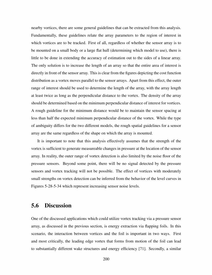
nearby vortices, there are some general guidelines that can be extracted from this analysis.

Fundamentally, these guidelines relate the array parameters to the region of interest in

which vortices are to be tracked. First of all, regardless of whether the sensor array is to

be mounted on a small body or a large flat hull (determining which model to use), there is

little to be done in extending the accuracy of estimation out to the sides of a linear array.

The only solution is to increase the length of an array so that the entire area of interest is

directly in front of the sensor array. This is clear from the figures depicting the cost function

distribution as a vortex moves parallel to the sensor arrays. Apart from this effect, the outer

range of interest should be used to determine the length of the array, with the array length

at least twice as long as the perpendicular distance to the vortex. The density of the array

should be determined based on the minimum perpendicular distance of interest for vortices.

A rough guideline for the minimum distance would be to maintain the sensor spacing at

less than half the expected minimum perpendicular distance of the vortex. While the type

of ambiguity differs for the two different models, the rough spatial guidelines for a sensor

array are the same regardless of the shape on which the array is mounted.

It is important to note that this analysis effectively assumes that the strength of the

vortex is sufficient to generate measureable changes in pressure at the location of the sensor

array. In reality, the outer range of vortex detection is also limited by the noise floor of the

pressure sensors. Beyond some point, there will be no signal detected by the pressure

sensors and vortex tracking will not be possible. The effect of vortices with moderately

small strengths on vortex detection can be inferred from the behavior of the level curves in

Figures 5-28-5-34 which represent increasing sensor noise levels.

5.6 Discussion

One of the discussed applications which could utilize vortex tracking via a pressure sensor

array, as discussed in the previous section, is energy extraction via flapping foils. In this

scenario, the interaction between vortices and the foil is important in two ways. First

and most critically, the leading edge vortex that forms from motion of the foil can lead

to substantially different wake structures and energy efficiency [71]. Secondly, a similar

200

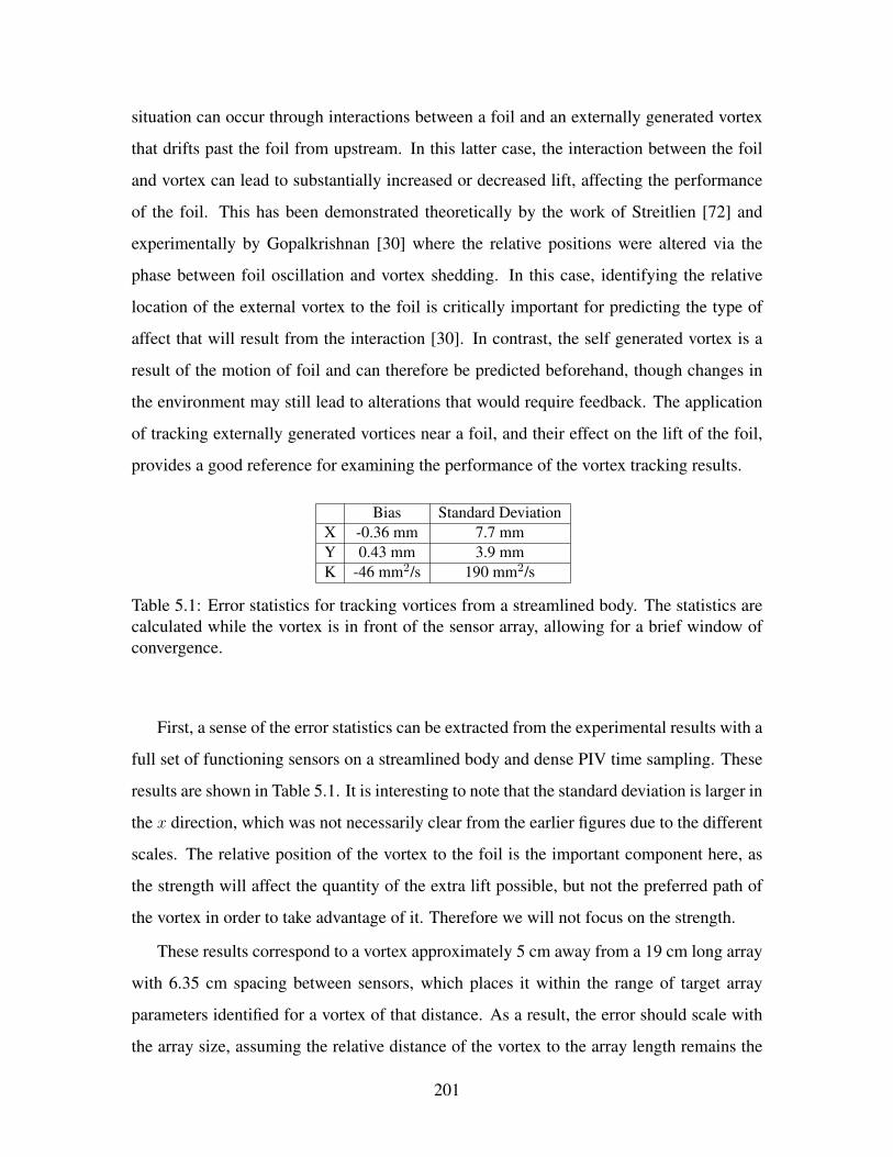
situation can occur through interactions between a foil and an externally generated vortex

that drifts past the foil from upstream. In this latter case, the interaction between the foil

and vortex can lead to substantially increased or decreased lift, affecting the performance

of the foil. This has been demonstrated theoretically by the work of Streitlien [72] and

experimentally by Gopalkrishnan [30] where the relative positions were altered via the

phase between foil oscillation and vortex shedding. In this case, identifying the relative

location of the external vortex to the foil is critically important for predicting the type of

affect that will result from the interaction [30]. In contrast, the self generated vortex is a

result of the motion of foil and can therefore be predicted beforehand, though changes in

the environment may still lead to alterations that would require feedback. The application

of tracking externally generated vortices near a foil, and their effect on the lift of the foil,

provides a good reference for examining the performance of the vortex tracking results.

Bias Standard DeviationX -0.36 mm 7.7 mmY 0.43 mm 3.9 mmK -46 mm2/s 190 mm2/s

Table 5.1: Error statistics for tracking vortices from a streamlined body. The statistics arecalculated while the vortex is in front of the sensor array, allowing for a brief window ofconvergence.

First, a sense of the error statistics can be extracted from the experimental results with a

full set of functioning sensors on a streamlined body and dense PIV time sampling. These

results are shown in Table 5.1. It is interesting to note that the standard deviation is larger in

the x direction, which was not necessarily clear from the earlier figures due to the different

scales. The relative position of the vortex to the foil is the important component here, as

the strength will affect the quantity of the extra lift possible, but not the preferred path of

the vortex in order to take advantage of it. Therefore we will not focus on the strength.

These results correspond to a vortex approximately 5 cm away from a 19 cm long array

with 6.35 cm spacing between sensors, which places it within the range of target array

parameters identified for a vortex of that distance. As a result, the error should scale with

the array size, assuming the relative distance of the vortex to the array length remains the

201

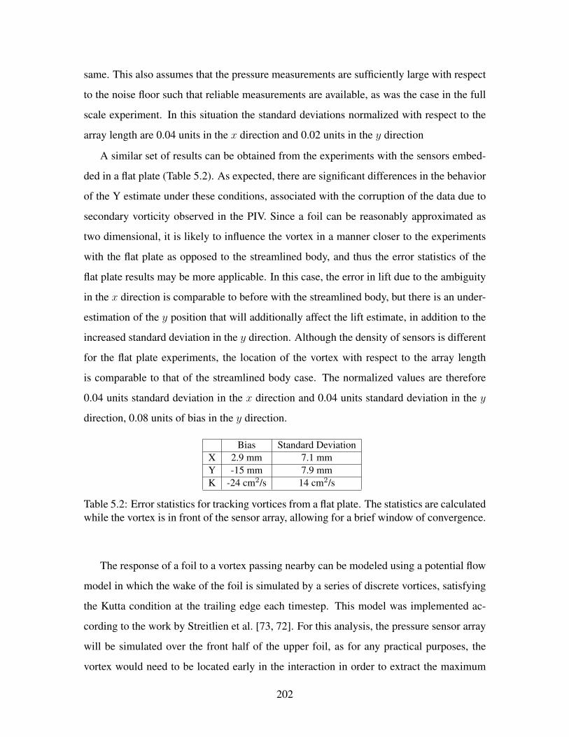
same. This also assumes that the pressure measurements are sufficiently large with respect

to the noise floor such that reliable measurements are available, as was the case in the full

scale experiment. In this situation the standard deviations normalized with respect to the

array length are 0.04 units in the x direction and 0.02 units in the y direction

A similar set of results can be obtained from the experiments with the sensors embed-

ded in a flat plate (Table 5.2). As expected, there are significant differences in the behavior

of the Y estimate under these conditions, associated with the corruption of the data due to

secondary vorticity observed in the PIV. Since a foil can be reasonably approximated as

two dimensional, it is likely to influence the vortex in a manner closer to the experiments

with the flat plate as opposed to the streamlined body, and thus the error statistics of the

flat plate results may be more applicable. In this case, the error in lift due to the ambiguity

in the x direction is comparable to before with the streamlined body, but there is an under-

estimation of the y position that will additionally affect the lift estimate, in addition to the

increased standard deviation in the y direction. Although the density of sensors is different

for the flat plate experiments, the location of the vortex with respect to the array length

is comparable to that of the streamlined body case. The normalized values are therefore

0.04 units standard deviation in the x direction and 0.04 units standard deviation in the y

direction, 0.08 units of bias in the y direction.

Bias Standard DeviationX 2.9 mm 7.1 mmY -15 mm 7.9 mmK -24 cm2/s 14 cm2/s

Table 5.2: Error statistics for tracking vortices from a flat plate. The statistics are calculatedwhile the vortex is in front of the sensor array, allowing for a brief window of convergence.

The response of a foil to a vortex passing nearby can be modeled using a potential flow

model in which the wake of the foil is simulated by a series of discrete vortices, satisfying

the Kutta condition at the trailing edge each timestep. This model was implemented ac-

cording to the work by Streitlien et al. [73, 72]. For this analysis, the pressure sensor array

will be simulated over the front half of the upper foil, as for any practical purposes, the

vortex would need to be located early in the interaction in order to extract the maximum

202

Figure 5-35: Simulated setup for a pressure sensor array similar to the one on a streamlinedbody being applied to a foil in order to track an external vortex.

benefit. In addition, when the vortex is near the trailing edge of the foil, it interacts with the

vortex trail being shed. This means that the history of the vortex is important at that point,

and a simple sensitivity analysis becomes more complex. In the case of the four sensor

implementation used in the streamlined body experiments, a depiction of the sensor array

on the Joukowski foil used in the simulation is shown in Figure 5-35. Both the lift and the

moment on the foil will be considered, using a full unsteady model that takes into account

the motion of the external vortex.

The focus is on the location of the vortex, but the strength of the external vortex needs

to be specified for the simulations. In this analysis, the external vortex has a circulation

equal to half that of the circulation about the foil required to maintain the Kutta condition

when there is no external vortex. All of the distances and positions will be normalized by

twice the chord length of the foil. Additionally, all of the lifts will be normalized by the

natural lift of the foil in the absence of a vortex. In the case of the moments, the moment

will be normalized by a nominal moment equivalent to that required to rotate the foil at a

constant angular velocity (1 radian per second) in a steady flow but with no vortex present.

Lift

With respect to the lift without a vortex present, the vortex depresses the lift when it is ahead

of the foil and augments it when the vortex is directly above the foil(Figure 5-36). The

maximum change in the lift with respect to the lateral position occurs in the rough location

leading edge of the foil. At this point, the sensitivity of the lift is 1.64 normalized lift per

normalized x position. This implies that the error in the lift estimate due to ambiguity in

203

-1.5 -1 -0.5 0 0.5

0

0.2

0.4

0.6

Y P

osi

tio

n

-1.5 -1 -0.5 0 0.5 10.8

1

1.2

1.4

1.6

X Position

No

rma

liz

ed

Lif

t

Figure 5-36: Dependence of foil lift on the position of an external vortex. In the topsubfigure, the foil is plotted with horizontal lines indicating the range of positions of theexternal vortex. The lower subfigure demonstrates the effect of a vortex at the positionsmarked in the top subfigure on the normalized lift of the foil.

204

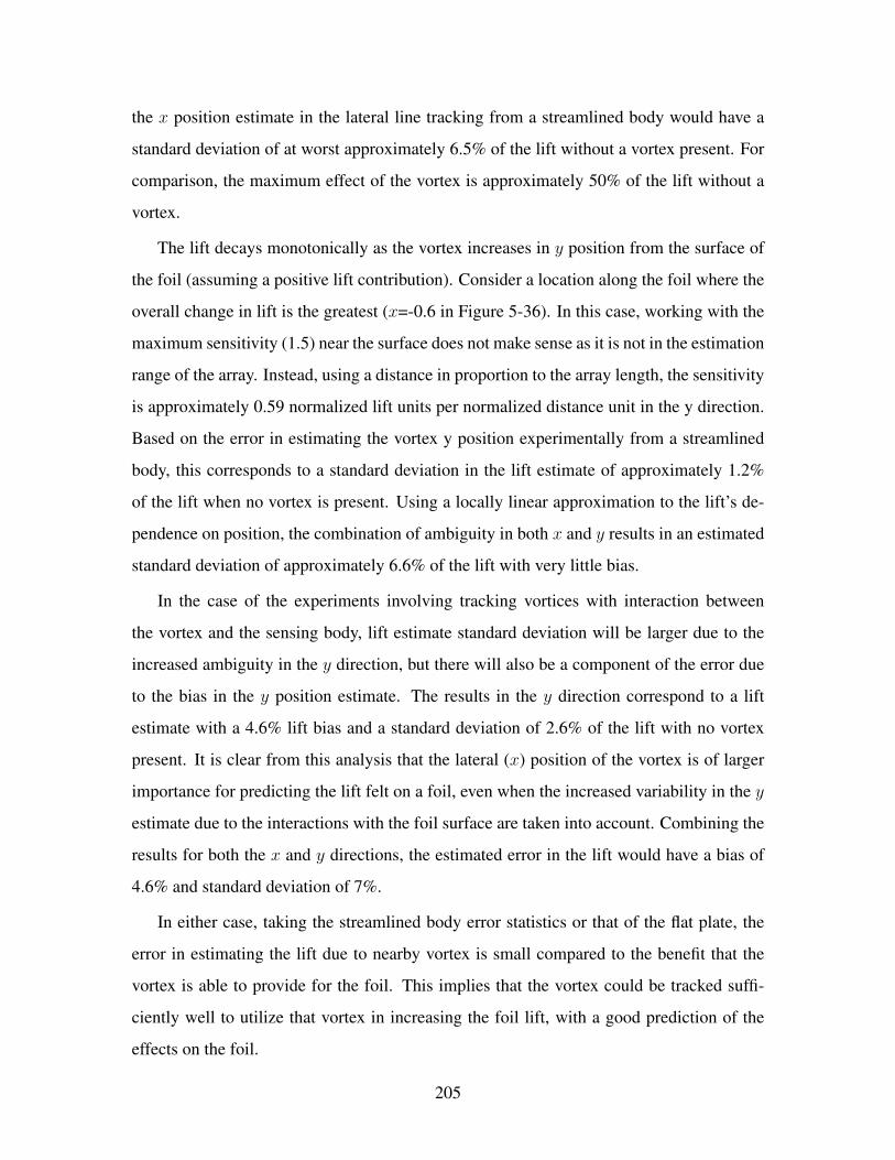
the x position estimate in the lateral line tracking from a streamlined body would have a

standard deviation of at worst approximately 6.5% of the lift without a vortex present. For

comparison, the maximum effect of the vortex is approximately 50% of the lift without a

vortex.

The lift decays monotonically as the vortex increases in y position from the surface of

the foil (assuming a positive lift contribution). Consider a location along the foil where the

overall change in lift is the greatest (x=-0.6 in Figure 5-36). In this case, working with the

maximum sensitivity (1.5) near the surface does not make sense as it is not in the estimation

range of the array. Instead, using a distance in proportion to the array length, the sensitivity

is approximately 0.59 normalized lift units per normalized distance unit in the y direction.

Based on the error in estimating the vortex y position experimentally from a streamlined

body, this corresponds to a standard deviation in the lift estimate of approximately 1.2%

of the lift when no vortex is present. Using a locally linear approximation to the lift’s de-

pendence on position, the combination of ambiguity in both x and y results in an estimated

standard deviation of approximately 6.6% of the lift with very little bias.

In the case of the experiments involving tracking vortices with interaction between

the vortex and the sensing body, lift estimate standard deviation will be larger due to the

increased ambiguity in the y direction, but there will also be a component of the error due

to the bias in the y position estimate. The results in the y direction correspond to a lift

estimate with a 4.6% lift bias and a standard deviation of 2.6% of the lift with no vortex

present. It is clear from this analysis that the lateral (x) position of the vortex is of larger

importance for predicting the lift felt on a foil, even when the increased variability in the y

estimate due to the interactions with the foil surface are taken into account. Combining the

results for both the x and y directions, the estimated error in the lift would have a bias of

4.6% and standard deviation of 7%.

In either case, taking the streamlined body error statistics or that of the flat plate, the

error in estimating the lift due to nearby vortex is small compared to the benefit that the

vortex is able to provide for the foil. This implies that the vortex could be tracked suffi-

ciently well to utilize that vortex in increasing the foil lift, with a good prediction of the

effects on the foil.

205

Moment

The moment that a vortex produces on a flapping foil is of interest because it might be

able to be utilized to reduce the energy expenditure in driving the foil. Since flapping

foils for extracting energy from flow are frequently actuated in pitch, any reduction the

torque necessary to actuate the foil would automatically translate to improved efficiency.

In addition, when the vortex is upstream of the pivot point being considered, the vortex

generates a moment that counters the desired motion of the foil (assuming the vortex is

towards the outside of the foil), which would result in a waste of energy if the pitch were

actuated at that time.

Figure 5-37 illustrates the dependence of the foil moment on the position of the external

vortex. As in the model by Streitlien, the moments are computed about a point at the mid-

chord of a cambered foil. As mentioned already, the moment is normalized by the torque

required to rotate the foil at a constant angular velocity of 1 radian per second in a steady

flow in the absence of a vortex. Also note that the moment depicted in Figure 5-37 is

positive when clockwise.

Similar to when considering the lift, this evaluation will be restricted to the front half of

the foil, where the interaction between the externally generated vortex and the trailing edge

vortices is minimized. Not surprisingly, the moments generated in response to the vortex

are reduced when the vortex is directly over the foil, due to the decreased moment arm.

The maximum sensitivity to the y position occurs in front of the leading edge of the foil,

while the maximum sensitivity to the x position occurs slightly behind the leading edge.

In the case of the sensitivity in the moment estimate with respect to the x position of

the vortex, the maximum sensitivity for a vortex near the surface is approximately 3.55

moment units per distance unit. Although this location is too close to the foil surface for

adequate tracking given the array parameters, it provides a good upper bound for the error

in estimating the moment. Both the streamlined body experimental results and the experi-

mental results with a vortex interacting with a flat plate provided similar error statistics for

the x position estimate. The corresponding error in the moment estimate would be have

standard deviation of approximately 14.2% of the reference moment.

206

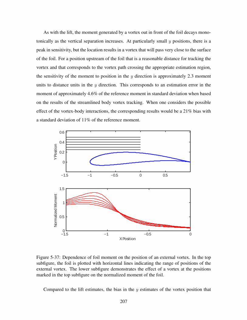
As with the lift, the moment generated by a vortex out in front of the foil decays mono-

tonically as the vertical separation increases. At particularly small y positions, there is a

peak in sensitivity, but the location results in a vortex that will pass very close to the surface

of the foil. For a position upstream of the foil that is a reasonable distance for tracking the

vortex and that corresponds to the vortex path crossing the appropriate estimation region,

the sensitivity of the moment to position in the y direction is approximately 2.3 moment

units to distance units in the y direction. This corresponds to an estimation error in the

moment of approximately 4.6% of the reference moment in standard deviation when based

on the results of the streamlined body vortex tracking. When one considers the possible

effect of the vortex-body interactions, the corresponding results would be a 21% bias with

a standard deviation of 11% of the reference moment.

−1.5 −1 −0.5 0 0.5

0

0.2

0.4

0.6

Y P

osi

tio

n

−1.5 −1 −0.5 00

0.5

1

1.5

X Position

No

rma

lize

d M

om

en

t

Figure 5-37: Dependence of foil moment on the position of an external vortex. In the topsubfigure, the foil is plotted with horizontal lines indicating the range of positions of theexternal vortex. The lower subfigure demonstrates the effect of a vortex at the positionsmarked in the top subfigure on the normalized moment of the foil.

Compared to the lift estimates, the bias in the y estimates of the vortex position that

207

occurs due to the foil-vortex interactions results in more substantial error. However, in

the context of the overall moment that vortex can cause to act against the desired pitching

motion (about 80%), this still provides information which can be used to predict the effects

of the interaction on the foil. In addition, the nature of the bias causes the estimated adverse

affects to be exaggerated, which will not lead to an excess expenditure of energy.

5.7 Conclusions

One of the primary motivations for identifying in detail the state of a vortex is its influence

over foils and control surfaces. The vortex is a persistent fluid structure which affects the

pressure distribution over the surface of nearby objects. By nature, a lateral-line-like sensor

array of the sort used in this chapter already gives the pressure distribution over a region of

the body surface. However, by identifying the vortex itself instead stopping at the pressure

distribution over a measured line, there are two substantial advantages. The first of these

is that using a limited sensor array to develop an accurate model of the local flow removes

the need to instrument the entire surface with pressure sensors. Instead, a small artificial

lateral line provides a description of the flow that can be extended to provide the pressure

distribution over the entire nearby surface. Secondly, by knowing the state of the vortex, it

is possible to predict how the pressure will change in the near future due to the motion of

the vortex (via advection and interaction with the body) and thus plan for how the vortex

will affect the structure. The results of the vortex tracking on the streamlined body and the

flat body demonstrate that a small pressure sensor array is sufficient for this purpose, and

the simulated results on array parameters give a starting point for the adequate design of

such a sensor array.

One important conclusion from the experimental results on estimating vortices with

the streamlined body is that in two dimensions it is a much closer approximation to use

an invisible body than a solid one. This has been remarked previously (for example see

[65]). However, it also implies that studies such as Ren and Mohseni [66] overestimate the

effect of the fish body on the flow. In addition to the effects on the global flow, this lack

of interaction appears to extend to the question of generating secondary vortices due to the

208

interactions between the primary vortex and the sensing body. This effect was observed

in the case of the flat plate experiments with substantial implications on vortex tracking,

but was completely absent in the streamlined body experiments. The result shows that the

simplified two dimensional inviscid flow model fits very well for fish-like small streamlined

bodies, and the corresponding vortex estimates tracked the nearest vortex accurately under

a variety of conditions.

In the context of fish, the results of the experiments described in this chapter on track-

ing vortices from a streamlined body clearly indicate that it is possible to obtain specific

information on the state of a nearby vortex based solely on a lateral-line-like sensor. Previ-

ously, experiments with live fish have tied the lateral line to energy-saving gaits that require

interaction with vortices [46, 43], but it has been unclear how much information was being

extracted via the lateral line and how it is used. While the demonstration of vortex tracking

in the streamlined body experiments do not answer this question, they do make it clear that

it is possible that a fish obtains information about individual vortices, as opposed to only

global characteristics such as shedding frequency.

It is still questionable whether it is possible to extract specific information for two or

more vortices that are not spread out along the length of a pressure sensor array. The

results with a streamlined sensing body, in which a vortex pair was used as the stimulus,

were not able to accurately reconstruct the position of the second, further, vortex. It was

found that the position of this vortex was insensitive to the pressure measurements, and

therefore did not converge in the time (roughly 2 seconds) of available measurable signals.

While the relative insensitivity is unlikely to change, it is likely that with a larger number of

sensors the estimation of the second vortex would improve since it effectively improves the

reliability of the measurements. In addition, a longer sensor array that therefore measures

the vortex pair for a larger period of time would likely improve the final estimate of the

vortex pair.

This extra difficulty in tracking multiple vortices does not necessarily hinder a fish in

a Karman vortex street. During the energy saving swimming, the fish swims between the

alternating vortices. Besides each vortex being spaced out in the direction of the lateral

line, this also means only a single vortex is is directly in front each face of the lateral line

209

at a time. It is likely that the vortices on either side of the fish can’t be treated completely

independently from the point of the lateral line, but it will not be the same as the vortex

pair scenario considered here.

The results with the sensor array embedded in a flat plate have shown that it is similarly

possible to track an individual vortex when interactions with the sensing body are more

substantial. However, it was clear that under these conditions secondary vorticity is a con-

cern and will affect the estimation. The affect appears to be manageable in that it causes

an underestimation in the y position and overestimation in the strength, but does not cause

the problem inversion to fail into an unrecoverable state. Based on the simulation results

considered in the later part of the chapter, the sensor array is not dense enough with respect

to the y distance of secondary vortices as they form. With a denser sensor array, it is likely

that the primary vortex would be tracked more accurately using the same method.

Besides the relevance to tracking externally generated vortices near a hull, the resilience

to secondary vorticity of the estimation based on a sensor on a flat plate implies that a

similar approach could be extended for self-generated vortices. Self generated vortices,

such as the leading edge vortex in a foil, generate from the separation of the flow on a body

and are therefore always in close proximity to the sensing surface. As long as the body of

the sensors is taken into account, it appears that any secondary vorticity that occurs in the

interaction between the vortex and surface can be considered a secondary issue that can

perhaps be addressed by increased density.

When the vortex estimation results are viewed from the context of specific applications,

it is possible to evaluate the degree of error in the estimation. In this case, the error in the

position estimate of the vortex tracking was analyzed in the context of generating lift and

moments on a foil. It was found that the error in the lift prediction due to the ambiguity in

vortex position is substantially less than the maximum lift the can be generated between the

foil and the external vortex, leading to the conclusion that the vortex tracking could be used

to improve the performance of a flapping foil energy extraction device. A similar situation

was observed with respect to the moment that is generated on a foil due to an external

vortex, though the effect of the bias from secondary vorticity has a more substantial effect.

210

Chapter 6

Conclusions

6.1 Overview

The fish lateral line organ presents a completely novel approach to sensing and interpreting

the local flow environment in the non-biological world of AUV’s and ships. Sensors based

on the lateral line have the potential, based on biological observations, to fill a gap left

by other sensory systems in complex environments and enhance the abilities of vehicles

to avoid collisions, identify unknown objects, and react to local flow. However, much is

still unknown about the workings of the lateral line and how well it would translate to

man-made vehicles.

The goal of this thesis has been to evaluate the realizable potential of lateral-line in-

spired sensors in two specific applications: tracking and identifying a cylinder and tracking

a vortex. Due to the lack of information about the actual lateral line processing, the first

essential task consisted of identifying appropriate estimation techniques for extracting the

desired tracking information from the pressure data. Moreover, since the linear pressure

sensor array used in this study approximates the function of a specific subsection of the

biological lateral line, it was necessary to determine whether further information (such as

velocity sensors or out-of-plane pressure sensors) would benefit the estimation task. Deriv-

ing combined insight from statistical estimation theory, theoretical fluid dynamics, and fish

studies, this work has taken a primarily experimental approach towards examining these

questions. While in many cases these experiments were not the first to examine the sig-

211

nals on a lateral-line-like array from and object or vortex stimulus (see for example Mog-

dans [52]), there are few if any precedents for utilizing the signals to estimate the original

stimulus (the closest being the numerical study by Suzuki [74]).

The following section describes the principal contributions of this thesis for each chap-

ter. This includes observations from the experiments as well as a successful demonstration

of the wealth of the information achievable and of the limitations of this sensing approach.

As this is the first major study using a pressure-based lateral-line-like sensor array to ex-

amine reproducing hypothesized abilities of the biological lateral line, this work opens a

large set of further questions to be studied. The final section contains recommendations for

future work, including a discussion of improvements and refinements to the current studies,

as well as a discussion of topics that build from the results of this study.

6.2 Principal contributions of the thesis

6.2.1 Passive cylinder tracking

The study in passively tracking a cylinder utilized a data set generated by passing a round

cylinder at constant velocity ranging between 0.2-0.5 m/s past a linear array of seven pres-

sure sensors embedded in a flat plate, passing at a distance between 2-20 mm from the

array. The cylinder radius, position, and velocity were tracked using a particle filter as

the nonlinear Kalman filter variants were shown to be inadequate. In order to tackle the

problem inversion, an approximate analytic forward model was identified through compar-

isons against numerical viscous simulations. The pressure distribution about a cylinder in a

steady flow is a well-known case and is a common validation tool for numerical simulation

codes [48, 12], but the question of identifying the cylinder position and size from a small

subset of the pressure field has never been previously addressed.

Characterization of the relative state estimate accuracy

The cylinder tracking (size and position) based on a linear pressure array was successfully

accomplished using a particle filter that included a joint distribution for the dependent ra-

212

dius and distance variables. The nature of the estimates, and in particular the error in the

estimates, varies for each state variable. The x position estimate, parallel to the linear sen-

sor array, varies about the true value but shows little consistent bias. In contrast, the y

position estimates, perpendicular to the linear sensor array, consistently underestimate the

distance between the sensors and the cylinder. In some cases the radius is also underes-

timated, though to a less extent than the y position. This seems to occur only when the

cylinder is very close to the sensors. This error behavior is likely particular to the analytic

forward model being used. However, for the purposes of collision avoidance, the bias in

the y position is not of significant concern as it always works to increase the safety factor.

Evaluation of tracking dependence on distance and speed

The results of the cylinder tracking were examined for dependence on distance and speed

of the cylinder, using a large series of experiments. The trends in estimation error are sur-

prisingly mild in most cases. Although the experiments ranged from an effective pressure

signal magnitude of 150 Pa to less than 10 Pa, many of the cylinder variables did not show

a noticeable dependence on these parameters. In the distant limit of small velocities and

large distances, the measurements available to the sensor array approach the noise floor of

the sensors and the inverse problem becomes insolvable. Based on the estimation results,

the radius estimate appears to degrade for very small distances, but be roughly indepen-

dent of velocity. The only other noticeable trends deal with the x position estimate, which

appears to worsen steadily but slowly with increasing velocity and distance.

Velocity information is not necessary for tracking a cylinder

The successful tracking of the moving cylinder based solely on the pressure from a linear

array of seven sensors indicates that augmentation with velocity data is unnecessary. The

specific problem scenario of the cylinder moving in still water is one in which velocity

measurements would not be at a disadvantage (there is no steady flow to saturate the sen-

sors), but there is no indication that their inclusion would add anything beyond redundancy

to the flow measurements. In this experimental scenario, the direction of flow and motion

is strongly encoded in both the asymmetry of the pressure distribution and it’s translation.

213

Importance of Pressure differences between adjacent sensors

While the pressure sensor array used to track a moving cylinder measures the pressure

along a line with respect to a fixed (atmospheric) reference, the estimation results in this

experiment, and in the others of this thesis, were impossible without considering the dif-

ference between pressure sensors and removing the fixed reference point. Although this

removes some information, primarily about the depth of the sensors, it also removes sig-

nificant common-mode drift that occurs due to influences of the surface. In the laboratory

environment, large wavelength standing waves of the free surface with an amplitude of a

few millimeters are a regular occurrence (excitable after a single cylinder pass) and gener-

ate oscillations in all the pressure sensors on the order of 10 Pa. While standing waves may

not be a common occurrence in an open environment, large wavelength surface oscillations

of even larger amplitude are likely and would cause similar problems for absolute pressure

measurements in shallow water. It is likely not coincidental that the fish lateral line canal

system responds to pressure differences across adjacent pores in the canal.

6.2.2 Passive cylinder shape classification

In order to examine the ability to identify the shape of a moving cylinder that has passed

a linear array of pressure sensors, experiments were done to test the ability to accurately

classify trials from two cylinders of two similar cross sections. Cylinders with square and

round cross sections with 5.1 and 7.6 cm diameters, velocities of 0.5 and 0.75 m/s, and

separations from the sensors of 0.5 and 1.3 cm. The pressure sensor array consisted of

four sensors spaced horizontally 2.5 inches apart (6.4 cm). In total, data from 1000 passes

were collected in order to closely examine the average differences and individual variation

between trials. Two classification tests were developed, with one based on features from a

principal component analysis trained on a data subset outperforming the alternative based

on average differences. The results establish that certain similar shapes can be distinguished

via a linear pressure sensor array, but also characterize a class of shapes that cannot be

differentiated.

214

Average pressure response features poorly discriminate cylinder shapes

Substantial variation in the data was observed across repeated trials of cylinders passing

a streamlined body. This variation was almost entirely restricted to the period following

the transition from high to low pressure which roughly corresponds to the leading edge of

the cylinder. Ahead of this transition, the pressure increases steadily in a near-exponential

ramp. After the transition, a large dip in the pressure is followed by a generally oscillatory

(but not sinusoidal) recovery to the far field pressure. Repeated trials differ in particu-

lar with respect to these oscillations. Distinct differences between the two tested cylinder

shapes are visible between the averaged pressure responses, with the most dramatic differ-

ences occurring after the pressure transition. A simple set of features based on these av-

erage differences results in a rate of approximately 10% misclassification. In many cases,

this classification test is unable to overcome the natural variation in the data.

Pressure dominated by the wake substantially contributes to discriminating cylinder

shapes

Shape classification based on principal component analysis features resulted in a high suc-

cess rate for classifying a moving cylinder with square or round cross section (98.8%). An

analysis of the decision criterion determined that the pressure measured directly behind

cylinder and thus alongside the wake is the second most informative region of the pressure

response for distinguishing the shapes. The most informative region corresponds to the

area near the point of minimum pressure, which matches the substantial differences in the

average pressure responses in this region. The relative importance of the wake region is

surprising, as the wake was primarily expected to obscure information about the shape due

to the separation of the flow from the moving cylinder. While the range in sizes tested rules

out vortex spacing being a factor, it is possible that the wake width, affected by the location

and angle of flow separation, is the vehicle for information.

215

Shape classification is robust to variations in size, distance, and speed

The decision criteria for classifying the shape of a cylinder after it has passed a linear array

of pressure sensors were tested against cylinders of different sizes, separations from the

sensors, and speeds. As mentioned, the decision criterion based on features from a princi-

pal component analysis was highly successful in distinguishing the shape of the cylinders

regardless of the experimental parameters, indicating that the criterion is resilient against

changes in parameters other than shape. For extreme changes in the size and distance the

performance is certain to degrade. The combination of sizes, speeds, and distances is crit-

ical in establishing a criterion that is truly based on shape as opposed to other differences

between experimental trials, as well as for establishing the robustness of the criterion.

Velocity information is not necessary for distinguishing cylinder shapes

As with tracking the cylinder position and size, there is no indication that concurrent ve-

locity measurements would improve shape classification and identification. The decision

criterion based on a principal component analysis already classifies 99% of the test cases

correctly.

6.2.3 Vortex tracking

The ability to track vortices using a linear array of pressure sensors, emulating a lateral line,

was examined from the perspective of a small streamlined body which roughly models a

fish or small AUV, and from a flat plate which is a closer approximation to the hull of larger

vehicles. The experiments with the streamlined body used a linear array of four pressure

sensors spaced at 2.5 in (6.4 cm) to track the nearest vortex of a vortex pair generated by

a swiveled foil. With seven sensors embedded on a flat plate (0.75 in. separation, 1.9 cm),

the experiments consisted of a single vortex passing in front of the array, separated from

the initial vortex pair generated at a distance.

216

Estimation of vortex position and strength from a small body

It was shown that with a linear pressure sensor array embedded in a small streamlined

(fish-like) body can track the position and strength of the nearest vortex accurately. The

two dimensional line vortex pair model was found sufficient for tracking the nearest vortex,

with any extra unmodeled vortices or external fluid effects being included as Gaussian noise

in the state transition model. The vortex tracking itself used a Kalman filter implementation

taking advantage of the Gaussian noise model.

Analysis of estimation with vortex-body interactions

The experimental results from tracking a single vortex in the proximity of a flat plate repre-

sent an example of the behavior when the vortex-body interactions are not negligible. The

induced velocity on the vortex itself is taken into account via a modification of the vortex

model, leading to successful tracking overall. However, the proximity of the vortex and

body leads to viscous effects that are not modeled: the development of secondary vorticity

from the boundary layer on the wall. These secondary vortices form near the sensor array

and are shed into the flow, causing perturbations to the measurements that are not accounted

for in the vortex model. The result leads to extra variability in the distance estimate for the

primary vortex, without substantially affecting the estimate of its position parallel to the

sensor array.

Sensor array design for vortex tracking

Based on an examination of the estimation of a simulated vortex or vortex pair at a single

time instant, relationships between the range of the vortices of interest and the pressure

sensor array length and density were established. In both cases of a vortex pair near a

streamlined body and a single vortex near a flat plate, the array length maximum distance

for tracking a vortex was found to be tied to the array length, with the array length as

roughly twice the vortex distance. Similarly, the closest distance for resolving the position

of a vortex was connected to the sensor density, with a minimum spacing of approximately

twice the minimum distance. For arrays with parameters outside these specifications, the

217

resolution of the position of the vortex degrades, leading to increased convergence times

and possible bias, but not into a complete inability to estimate the vortex. In the case of the

array length, it should be emphasized that the relationship serves as the minimum necessary

for tracking a vortex up to a given distance.

Velocity information is not necessary for tracking vortices, but may be beneficial

As in the case of the cylinder tracking and identification, the analysis of the vortex tracking

successfully achieved its goal without requiring extra velocity measurements. However,

unlike the other cases, it may be beneficial to augment the pressure array with velocity

measurements. The pressure field due to a vortex pair is symmetric in front and behind the

position of the vortex. The sign of the vortex strength determines the direction of motion

between measurements, and thus was able to be estimated successfully from the pressure

data, but at a single instant in time the sign of the vortex strength is unresolvable based

on pressure. Augmenting the data set by a reliable velocity measurement indicating the

direction of fluid motion would likely result in much faster convergence, particularly for

the vortex strength, but is not necessary for vortex tracking.

6.3 Recommendations for future work

This study is the first description of inference and signal processing with a pressure-based

lateral-line-like array that is not focused on detecting an oscillating dipole. While it is

always possible to improve the experimental setups and equipment, the successful results

of this study open up many avenues of further applications of a lateral-line-like sensor

array for AUV’s and ocean vehicles. Given that the fish lateral line is still an active area of

research, the results of the current study also suggest behaviors of the lateral line that can

be tested in order to further its understanding.

218

6.3.1 Improved sensor array density for multiple vortex tracking

In the vortex pair tracking experiments and estimation results, it was found at that an accu-

rate estimate of the state of the nearest vortex was available but that the low sensitivity of

the pressure measurements to the second, further, vortex made it difficult to track. These

experiments used a linear array of four pressure sensors spaced 2.5 in (6.4 cm) apart. A

high-density array of sufficient length for the distance of the second vortex would likely

result in an improved estimate of the second vortex due to the increased reliability of the

measurements. High density arrays of pressure sensors are difficult to achieve (but not un-

precedented [36]) using off-the-shelf pressure sensors as was done in this study, but would

be feasible if constructed directly with MEMS technology [35].

6.3.2 Vortex street tracking

The study in tracking vortices from a small streamlined body demonstrated that it was

possible to track the state of the closest vortex in a vortex pair. In natural environments,

vortices are frequently found in an alternating series spaced with regular intervals, as the

vortex streets forming behind blunt flow obstructions or oscillating thrust-producing foils.

The study of vortex tracking based on a lateral-line-like array could be straightforwardly

extended to examine the ability to track individual vortices in such a regular vortex street.

Although multiple vortices would be present, their spacing would distribute them along the

length of the arrays and likely not lead to the same ambiguities as for the vortex pair.

6.3.3 Numerical forward models for wakes

The potential flow models discussed in Chapter 3 for tracking a moving cylinder have

proved adequate for the task. However, the resulting state estimates exhibited variability

during individual runs, possibly due to the steady analytic approximation to the wake be-

ing used. In order to improve the forward model, a future approach may directly utilize

approximate real-time numerical models such as those by Weymouth [83].

219

6.3.4 Biological object discrimination

Based on the results of the study on cylinder shape identification, it is likely that there is a

class of object shapes which would not be distinguishable when moving past a lateral line

or similarly inspired sensor. These similar shapes would have similar wake widths based

on the size and bluntness of their forward faces. This suggests a very simple test along the

lines of the experiments by Mogdans and Bleckmann [52], in which the hypothesis can be

tested with live fish.

6.3.5 Active object identification

The cylinder tracking study described in this thesis corresponds to the passive object iden-

tification scenario, in which the interaction between the cylinder and a steady fluid flow

externally generate the pressure field signal. This scenario corresponds to some potential

AUV situations, but is also useful as a test case for object detection since the amplitude of

stimulus can be easily manipulated. In contrast, the active object identification scenario, in

which the fluid flow is driven purely by the motion of the sensing platform itself, presents

a less favorable noise environment due to the reduced signal amplitude and increased vi-

brations of the sensors. Despite the increased measurement difficulty this sort of object

detection and identification would be of great benefit to an AUV, which would not be de-

pendent on an external flow to interrogate an object of interest.

6.3.6 Two-dimensional sensor arrays

Particularly in the case of object detection and identification, current MEMS technology

makes it possible to use regular dense two-dimensional arrays of pressure sensors to map

the pressure distribution over a surface instead of the linear array considered in this study.

This additional information provides the opportunity to extend the inference beyond two-

dimensional cross sections of objects as was considered in the present study. This adds

considerable complication to the problem, but in conjunction with the active object iden-

tification could lead to forming complete three dimensional maps of arbitrary unknown

objects, making it the ultimate goal of touch-at-a-distance lateral-line-like sensors.

220

6.3.7 Local flow models for large objects

The present discussion of cylinder tracking and identification via a distributed linear pres-

sure sensor array is applicable to cross sections with length scales on the order of the

length of the array. In contrast, particularly for applications in navigation and maneuver-

ing, it would also be beneficial to extend the object identification studies to objects with

much larger length scales. In this regime, it would not necessarily be preferable to attempt

to obtain or model a full description of the object. In the very large extreme, for exam-

ple, a small vehicle searching for mines on a tanker hull would not benefit greatly from

having a flow model around the entire tanker as long as it had an adequate local model. Ex-

tending the object identification to very large objects with local perturbations would likely

require a completely new approach to the forward model. One concern with local modeling

approaches is the possible ambiguity of the fluid-solid boundary. As an initial note on re-

solving this ambiguity, it should be noted that fish have been observed to periodically make

contact with walls using their pectoral fins [85], which may be the biological approach to

dealing with this issue.

221

Bibliography

[1] S. A. Ansari, N. Phillips, G. Stabler, P. C. Wilkins, R. Zbikowski, and K. Knowles.

Experimental investigation of some aspects of insect-like flapping flight aerodynam-

ics for application to micro air vehicles. In G. K. Taylor, M. S. Triantafyllou, and

C. Tropea, editors, Animal Locomotion, pages 215–236. Springer, 2010.

[2] C. F. Baker and J. C. Montgomery. The sensory basis of rheotaxis in the blind mexican

cave fish, astyanax fasciatus. Journal of Comparative Physiology A-Sensory Neural

and Behavioral, 184(5):519–527, 1999.

[3] G. K. Batchelor. An introduction to fluid dynamics. Cambridge University Press, New

York, NY, 2000.

[4] H. Bleckmann, G. Tittel, and E. Blubaum-Gronau. The lateral line system of surface-

feeding fish: anatomy, physiology, and behavior. In S. Coombs, P. Gorner, and

H. Munz, editors, The mechanosensory lateral line: Neurobiology and evolution,

pages 501–526. Springer, 1989.

[5] R. D. Blevins. Flow-Induced Vibration. Van Nostrand Reinhold, New York, NY,

1990.

[6] R. Bouffanais, G. D. Weymouth, and D. K. P. Yue. Hydrodynamic object recognition

using pressure sensing. Proceedings of the Royal Society A: Mathematical, Physical

and Engineering Science, 2010.

223

[7] C. B. Braun and S. Coombs. The overlapping roles of the inner ear and lateral line:

the active space of dipole source detection. Philosophical Transactions of the Royal

Society of London, 355:1115–1119, 2000.

[8] T. Burt de Perera. Spatial parameters encoded in the spatial map of the blind mexican

cave fish, astyanax fasciatus. Animal Behaviour, 68(2):291–295, 2004.

[9] L. W. Carr. Progress in analysis and prediction of dynamic stall. Journal of Aircraft,

25(21):6–17, 1987.

[10] B. P. Chagnaud, H. Bleckmann, and M. H. Hofmann. Karman vortex street detection

by the lateral line. Journal of Comparative Physiology A, 193(7):753–763, 2007.

[11] B. P. Chagnaud, M. H. Hofmann, and J. Mogdans. Responses to dipole stimuli of

anterior lateral line nerve fibres in goldfish, carassius auratus, under still and running

water conditions. Journal of Comparative Physiology A, 193(2):249–263, 2006.

[12] N.R. Clarke and O.R. Tutty. Construction and validation of a discrete vortex method

for the two-dimensional incompressible navier-stokes equations. Computers & Flu-

ids, 23(6):751 – 783, 1994.

[13] S. Coombs. Smart skins: Information processing by lateral line flow sensors. Au-

tonomous Robotics, 11:255–261, 2001.

[14] S. Coombs, C. B. Braun, and B. Donovan. The orienting response of lake michigan

mottled sculpin is mediated by canal neuromasts. Journal of Experimental Biology,

204(2):337 –348, 2001.

[15] S Coombs and R. A. Conley. Dipole source localization by mottled sculpin. i. ap-

proach strategies. Journal of Comparative Physiology A: Neuroethology, Sensory,

Neural, and Behavioral Physiology, 180(4):387–399, 1997.

[16] S. Coombs and R. R. Fay. Dipole source localization by mottled sculpin, Cottus

bairdi. Journal of the Acoustical Society of America, 93:2116–2123, 1993.

224

[17] S. Coombs, J. J. Finneran, and R. A. Conley. Hydrodynamic image formation by

the peripheral lateral line system of the lake michigan mottled sculpin, cottus bairdi.

Philosophical Transactions: Biological Sciences, 355(1401):1111–1114, 2000.

[18] S. Coombs and J. Janssen. Behavioral and neurophysiological assessment of lateral

line sensitivity in the mottled sculpin, cottus bairdi. Journal of Comparative Physiol-

ogy A, 167(4), 1990.

[19] S. Coombs, J. Janssen, and J. C. Montgomery. Functional and evolutionary implica-

tions of peripheral diversity in lateral line systems. In D. B. Webster, R. R. Fay, and

A. N. Popper, editors, The evolutionary biology of hearing, pages 267–294. Springer,

New York, NY, 1992.

[20] S. Coombs and P. Patton. Lateral line stimulation patterns and prey orienting behavior

in the lake michigan mottled sculpin (Cottus bairdi). Journal of Comparative Physiol-

ogy A: Neuroethology, Sensory, Neural, and Behavioral Physiology, 195(3):279–297,

2009.

[21] B. Curcic-Blake and S. M. van Netten. Source location encoding in the fish lateral

line canal. Journal of Experimental Biology, 209(8):1548–1559, 2006.

[22] G. Dehnhardt, B. Mauck, W. Hanke, and H. Bleckmann. Hydrodynamic Trail-

Following in harbor seals (Phoca vitulina). Science, 293(5527):102 –104, July 2001.

[23] E. J. Denton and J. Gray. Mechanical factors in the excitation of clupeid lateral

lines. Proceedings of the royal society of London series B-Biological sciences,

218(1210):1–26, 1983.

[24] S. Dijkgraaf. The functioning and significance of the lateral line organs. Biological

Reviews, 38:51–105, 1963.

[25] J. Englemann, W. Hanke, J. Mogdans, and H. Bleckmann. Hydrodynamic stimuli and

the fish lateral line. Nature, 408:51–52, 2000.

225

[26] L. E. Ericsson and J. P. Reding. Fluid mechanics of dynamic stall: Part 1. unsteady

flow concepts. Journal of Fluids and Structures, 2:1–33, 1989.

[27] A. Gelb, editor. Applied Optimal Estimation. MIT Press, Cambridge, Massachusetts,

1974.

[28] M. A. Gibbs. Lateral line receptors: Where do they come from developmentally and

where is our research going? Brain, Behavior, and Evolution, 64:163–181, 2004.

[29] N. Glaeser, S. Wieskotten, C. Otter, G. Dehnhardt, and W. Hanke. Hydrodynamic

trail following in a California sea lion (Zalophus californianus). Journal of Com-

parative Physiology A-Neuroethology: Sensory Neural and Behavioral Physiology,

197(2):141–151, 2011.

[30] R. Gopalkrishnan, M. S. Triantafyllou, G. S. Triantafyllou, and D. Barrett. Active

vorticity control in a shear flow using a flapping foil. Journal of Fluid Mechanics,

274:1–21, 1994.

[31] W. Hanke, M. Witte, L. Miersch, M. Brede, J. Oeffner, M. Michael, F. Hanke,

A. Leder, and G. Dehnhardt. Harbor seal vibrissa morphology suppresses vortex-

induced vibrations. Journal of Experimental Biology, 213(15):2665 –2672, 2010.

[32] E. S. Hassan. On the discrimination of spatial intervals by the blind cave fish (Anop-

tichthys jordani). Journal of Comparative Physiology A, 159:701–710, 1986.

[33] E. S. Hassan. Mathematical description of the stimuli to the lateral line system of fish

derived from a 3-dimensional field analysis: I. the cases of moving in open water and

of gliding towards a plane surface. Biological Cybernetics, 66:443–452, 1992.

[34] E. S. Hassan. Mathematical description of the stimuli to the lateral line system of fish

derived from a 3-dimensional field analysis: II. the case of gliding alongside or above

a plane surface. Biological Cybernetics, 66:453–461, 1992.

[35] S.M. Hou, V.I. Fernandez, F.S. Hover, J. Lang, , and M.S. Triantafyllou. Development

and application of distributed mems pressure sensor array for auv object avoidance. In

226

Proceedings of the International Symposium on Unmanned Untethered Submersible

Technology (UUST), August 2009.

[36] L. M. Hudy, A. M. Naguib, and W. M. Humphreys. Wall-pressure-array measure-

ments beneath a separating/reattaching flow region. Physics of Fluids, 15(3):706–717,

March 2003.

[37] Inc. Hydroid, 2011. http://www.hydroidinc.com/remus100.html.

[38] J. E. Jackson. A User’s Guide to Principal Components. Wiley, Hoboken, New Jersey,

2003.

[39] J. Jeong and F. Hussain. On the identification of a vortex. Journal of Fluid Mechanics,

285:69–94, 1994.

[40] I. T. Jolliffe. Principal Component Analysis. Springer, New York, New York, second

edition, 2002.

[41] S. J. Julier and J. K. Uhlmann. Unscented filtering and nonlinear estimation. Pro-

ceedings of the IEEE, 92(3):401–422, 2004.

[42] A. J. Kalmijn. Functional aspects of the evolution of the auditory system of

actinopterygian fish. In J. Atema, R. R. Fay, A. N. Popper, and W. N Tavolga, ed-

itors, Sensory biology of aquatic animals, pages 83–130. Springer-Verlag, 1988.

[43] J. C. Liao. The role of the lateral line and vision on body kinematics and hydrody-

namic preference of rainbow trout in turbulent flow. Journal of Experimental Biology,

209(20):4077–4090, 2006.

[44] J. C. Liao. A review of fish swimming mechanics and behaviour in altered

flows. Philosophical Transactions of the Royal Society B - Biological Sciences,

362(1487):1973–1993, 2007.

[45] J. C. Liao, D. N. Beal, G. V. Lauder, and M. S. Triantafyllou. Fish exploiting vortices

decrease muscle activity. Science, 302(5650):1566 –1569, 2003.

227

[46] J. C. Liao, D. N. Beal, G. V. Lauder, and M. S. Triantafyllou. The Karman gait:

novel body kinematics of rainbow trout swimming in a vortex street. Journal of

Experimental Biology, 206(6):1059–1073, 2003.

[47] S. Licht, V. Polidoro, M. Flores, F. S. Hover, and M. S. Triantafyllou. Design and

projected performance of a flapping foil auv. IEEE Journal of Oceanic Engineering,

29(3):786–794, 2004.

[48] K. Mahesh, G. Constantinescu, and P. Moin. A numerical method for large-eddy

simulation in complex geometries. Journal of Computational Physics, 197(1):215–

240, 2004.

[49] M. E. McConney, K. D. Anderson, L. L. Brott, R. R. Naik, and V. V. Tsukruk. Bioin-

spired material approaches to sensing. Advanced Functional Materials, 19(16):2527–

2544, 2009.

[50] M. J. McHenry, K. E. Feitl, J. A. Strother, and W. J. Van Trump. Larval zebrafish

rapidly sense the water flow of a predator’s strike. Biology Letters, 5(4):477 –479,

2009.

[51] M. J. McHenry, J. A. Strother, and S. M. van Netten. Mechanical filtering by the

boundary layer and fluid-structure interaction in the superficial neuromast of the fish

lateral line system. Journal of Comparative Physiology A: Neuroethology, Sensory,


[52] J. Mogdans and H. Bleckmann. Responses of the goldfish trunk lateral line to moving

objects. Journal of Comparative Physiology A: Neuroethology, Sensory, Neural, and

Behavioral Physiology, 182(5):659–676, 1998.

[53] J. C. Montgomery, C. F. Baker, and A. G. Carton. The lateral line can mediate rheo-

taxis in fish. Nature, 389(6654):960–963, 1997.

[54] J. C. Montgomery and S. Coombs. Peripheral encoding of moving sources by the

lateral line system of a sit-and-wait predator. Journal of Experimental Biology,

201(1):91–102, 1998.

228

[55] J. C. Montgomery, S. Coombs, and C. F. Baker. The mechanosensory lateral line

system of the hypogean form of Astyanax fasciatus. Evolutionary Biology of Fishes,

62:87–96, 2001.

[56] J. C. Montgomery, S. Coombs, and M. Halstead. Biology of the mechanosensory

lateral line in fishes. Reviews in Fish Biology and Fisheries, 5(4):399–416, 1995.

[57] J. C. Montgomery and J. A. MacDonald. Sensory tuning of lateral line receptors in

antartic fish to the movements of planktonic prey. Science, 235(4785):195–196, 1987.

[58] J. C. Montgomery, S. P. Windsor, and D. K. Bassett. Behavior and physiology of

mechanoreception: separating signal and noise. Integrative Zoology, 4(1):3–12, 2009.

[59] H. Munz. Single unit activity in the peripheral lateral line system of the chichlid

fish Sarotherodon niloticus l. Journal of Comparative Physiology A, 157(5):555–568,

1986.

[60] J. N. Newman. Marine Hydrodynamics. MIT Press, Cambridge, Massachusetts, 1977.

[61] T. Perez and G. C. Goodwin. Constrained predictive control of ship fin stabilizers to

prevent dynamic stall. Control Engineering Practice, 16:482–494, 2008.

[62] T. J. Pitcher, B. L. Partridge, and C. S. Wardle. A blind fish can school. Science,

194(4268):963 –965, 1976.

[63] K. Pohlmann, J. Atema, and T. Breithaupt. The importance of the lateral line in noc-

turnal predation of piscivorous catfish. Journal of Experimental Biology, 207:2971–

2978, 2004.

[64] K. Pohlmann, F. W. Grasso, and T. Breithaupt. Tracking wakes: The nocturnal preda-

tory strategy of piscivorous catfish. Proceedings of the National Academy of Sciences

of the United States of America, 98(13):7371–7374, 2001.

[65] M. A. Rapo, H. Jiang, M. A. Grosenbaugh, and S. Coombs. Using computational fluid

dynamics to calculate the stimulus to the lateral line of a fish in still water. Journal of

Experimental, 212(10):1494–1505, 2009.

229

[66] Z. Ren and K. Mohseni. A model of lateral line of fish for vortex sensing. In 40th

Fluid Dynamics Conference and Exhibit. AIAA, 2010.

[67] B. Ristic, S. Arulampalam, and N. Gordon. Beyond the Kalman filter: Particle filters

for tracking applications. Artech house, New York, NY, 2004.

[68] P. G. Saffman. Vortex Dynamics. Cambridge University Press, New York, NY, 1995.

[69] M. Satou, A. Shiraishi, T. Matsushima, and N. Okumoto. Vibrational communication

during spawning behavior in the hime salmon (landlocked red salmon,Oncorhynchus

nerka). Journal of Comparative Physiology A, 168(4):417–428, 1991.

[70] A. Sichert, R. Bamler, and J. van Hemmen. Hydrodynamic object recognition: When

multipoles count. Physical Review Letters, 102(5), 2009.

[71] B. J. Simpson. Experimental studies of flapping foils for energy extraction. PhD

thesis, Massachusetts Institute of Technology, 2009.

[72] K. Streitlien. Extracting energy from unsteady flows through vortex control. PhD

thesis, Massachusetts Institute of Technology, 1994.

[73] K. Streitlien and M. S. Triantafyllou. Force and moment on a Joukowski profile in

the presence of point vortices. American Institute of Aeronautics and Astronautics

Journal, 33(4):603–610, 1995.

[74] T. Suzuki and T. Colonius. Inverse-imaging method for detection of a vortex in a

channel. American Institute of Aeronautics and Astronautics Journal, 41:1743–1751,

2003.

[75] T. Teyke. Collision with and avoidance of obstacles by blind cave fish Anoptichthys

jordani (characidae). Journal of Comparative Physiology A, 157:837–843, 1985.

[76] T. Teyke. Learning and remembering the environment in the blind cave fish anop-

tichthys jordani. Journal of Comparative Physiology A: Neuroethology, Sensory,


230

[77] T. Teyke. Morphological differences in the neuromasts of the blind cave fish Astyanax

Hubbsi and the sighted river fish Astyanax Mexicanus. Brain Behavior and Evolution,

35(1):23–30, 1990.

[78] S. Theodoridis and K. Koutroumbas. Pattern Recognition. Academic Press, San

Diego, California, third edition, 2006.

[79] S. M. van Netten. Hydrodynamic detection by cupulae in a lateral line canal: Func-

tional relations between physics and physiology. Biological Cybernetics, 94:67–85,

2006.

[80] D. Vogel and H. Bleckmann. Behavioral discrimination of water motions caused by

moving objects. Journal of Comparative Physiology A, 186:1107–1117, 2000.

[81] H. Vollmers. Detection of vortices and quantative evaluation of their main parameters

from experimental velocity data. Measurement Science and Technology, 12:1199–

1207, 2001.

[82] R. Weissert and C. von Campenhausen. Discrimination between stationary objects

by the blind cave fish Anoptichthys jordani (characidae). Journal of Comparative

Physiology A, 143:375–381, 1981.

[83] G. Weymouth, 2011. http://web.mit.edu/weymouth/www/.

[84] S. P. Windsor and M. J. McHenry. The influence of viscous hydrodynamics on the

fish lateral-line system. Integrative and Comparative Biology, 49(6):691–701, 2009.

[85] SP Windsor, D Tan, and JC Montgomery. Swimming kinematics and hydrodynamic

imaging in the blind mexican cave fish (Astyanax fasciatus). Journal of Experimental

Biology, 211(18):2950–2959, 2008.

[86] Malima I. Wolf, Stephen C. Licht, Franz Hover, and Michael S. Triantafyllou. Open

loop swimming performance of ‘Finnegan’ the Biomimetic Flapping Foil AUV. In

Wong, P. C. and Uchida, K. and Chung, J. S. and Sayed, M. and Moshagen, H. and

Fontaine, E., editor, Proceedings of the Sixteenth (2006) International Offshore and

231

Polar Engineering Conference, Vol. 2, International Offshore and Polar Engineering

Conference Proceedings, pages 247–253, 2006.

[87] Y. Yang, J. Chen, J. Engel, S. Pandya, N. Chen, C. Tucker, S. Coombs, and C. Liu.

Distant touch hydrodynamic imaging with an artificial lateral line. Proceedings of the

National Academy of Science, 103(50):18891–18895, 2006.

[88] Y. C. Yang, N. Chen, C. Tucker, S. Pandya, D. Jones, and C. Liu. Biomimetic flow

sensing using artificial lateral lines. Proceedings of the ASME International Mechan-

ical Engineering Congress, pages 1331–1338, 2008.

[89] Q. Zhu, M. Haase, and C. H. Wu. Modeling the capacity of a novel flow-energy

harvester. Applied Mathematical Modelling, 33(5):2207–2217, 2009.

232

1. REPORT NO.

4. Title and Subtitle

7. Author(s)

9. Performing Organization Name and Address

12. Sponsoring Organization Name and Address

15. Supplementary Notes

16. Abstract (Limit: 200 words)

17. Document Analysis a. Descriptors

b. Identifiers/Open-Ended Terms

c. COSATI Field/Group

18. Availability Statement

REPORT DOCUMENTATION

PAGE

2. 3. Recipient's Accession No.

5. Report Date

6.

8. Performing Organization Rept. No.

10. Project/Task/Work Unit No.

11. Contract(C) or Grant(G) No.

(C)

(G)

13. Type of Report & Period Covered

14.

50272-101

19. Security Class (This Report)

20. Security Class (This Page)

21. No. of Pages

22. Price

OPTIONAL FORM 272 (4-77)

(Formerly NTIS-35)Department of Commerce

(See ANSI-Z39.18) See Instructions on Reverse

UNCLASSIFIED

2011-13

June 2011Performance Analysis for Lateral-Line-Inspired Sensor Arrays


2011-13MIT/WHOI Joint Program in Oceanography/Applied Ocean Science & Engineering

Ph.D. Thesis

The lateral line is a critical component of the fish sensory system, affecting aspects of behavior including maneuvering in complex fluid environments, schooling, and prey tracking. This sensory organ has no analog in ocean vehicles and could fill thegap for navigation left by sonar and vision systems in turbid cluttered environments. This thesis demonstrates and characterizes the ability of lateral-line-inspired pressure sensor arrays to perform two sensory tasks of relevance to biological and man-made underwater vehicles, namely object and vortex tracking.

The ability of pressure sensor arrays to emulate the lateral line's "touch at a distance" feature, corresponding to the capability of identifying the shape of objects remotely, is examined for moving cylinders of different cross sections. Using the pressure distribution on a small linear array, the position and size of a cylinder is also tracked.

Identifying the vortices in a flow makes it possible to predict and optimize the performance of flapping foils and to identify imminent stall on a control surface. Experimental studies demonstrate the ability to track vortices with a pressure sensor array from both small streamlined and large flat bodies. In addition, the relationship between array parameters and the range of trackable vortices is established.

Lateral lineObject TrackingVortex Tracking

232Approved for publication; distribution unlimited.

This thesis should be cited as: Vicente I. Fernandez, 2011. Performance Analysis for Lateral-Line-Inspired Sensor Arrays. Ph.D.Thesis. MIT/WHOI, 2011-13.

NOAAMITNDSEG

MIT/WHOI

MIT/WHOI

joint program in oceanography/ applied ocean … doctoral dissertation by vicente i. fernandez june...

Documents