joint retinal layer and fluid segmentation in oct scans of ... retinal layer and fluid segmentation...

Joint retinal layer and fluid segmentation in OCTscans of eyes with severe macular edema usingunsupervised representation and auto-context

ALESSIO MONTUORO,1,2,* SEBASTIAN M. WALDSTEIN,1,2

BIANCA S. GERENDAS,1,2 URSULA SCHMIDT-ERFURTH,1,2 ANDHRVOJE BOGUNOVIC2

1Vienna Reading Center, Department of Ophthalmology and Optometry,Medical University of Vienna, Austria2Christian Doppler Laboratory for Ophthalmic Image Analysis,Department of Ophthalmology, Medical University of Vienna, Austria*[email protected]

Abstract: Modern optical coherence tomography (OCT) devices used in ophthalmology acquiresteadily increasing amounts of imaging data. Thus, reliable automated quantitative analysis ofOCT images is considered to be of utmost importance. Current automated retinal OCT layersegmentation methods work reliably on healthy or mildly diseased retinas, but struggle with thecomplex interaction of the layers with fluid accumulations in macular edema. In this work, wepresent a fully automated 3D method which is able to segment all the retinal layers and fluid-filledregions simultaneously, exploiting their mutual interaction to improve the overall segmentationresults. The machine learning based method combines unsupervised feature representation andheterogeneous spatial context with a graph-theoretic surface segmentation. The method wasextensively evaluated on manual annotations of 20,000 OCT B-scans from 100 scans of patientsand on a publicly available data set consisting of 110 annotated B-scans from 10 patients, all withsevere macular edema, yielding an overall mean Dice coefficient of 0.76 and 0.78, respectively.

c© 2017 Optical Society of America

OCIS codes: (100.6890) Three-dimensional image processing; (100.0100) Image processing; (170.4470) Ophthalmol-ogy; (170.4500) Optical coherence tomography.

References and links1. R. D. Jager, W. F. Mieler, and J. W. Miller, “Age-related macular degeneration,” New Engl. J. Med. 358, 2606–2617

(2008).2. J. A. Davidson, T. A. Ciulla, J. B. McGill, K. A. Kles, and P. W. Anderson, “How the diabetic eye loses vision,”

Endocrine 32, 107–116 (2007).3. P. A. Campochiaro, L. P. Aiello, and P. J. Rosenfeld, “Anti-vascular endothelial growth factor agents in the treatment

of retinal disease: From bench to bedside,” Ophthalmology 123, S78–S88 (2016).4. K. A. Rezaei and T. W. Stone, “2016 Global Trends in Retina Survey,” American Society of Retina Specialists,

Chicago, IL. (2016).5. U. Schmidt-Erfurth, S. M. Waldstein, G.-G. Deak, M. Kundi, and C. Simader, “Pigment epithelial detachment

followed by retinal cystoid degeneration leads to vision loss in treatment of neovascular age-related maculardegeneration,” Ophthalmology 122, 822–832 (2015).

6. S. M. Waldstein, J. Wright, J. Warburton, P. Margaron, C. Simader, and U. Schmidt-Erfurth, “Predictive value ofretinal morphology for visual acuity outcomes of different ranibizumab treatment regimens for neovascular AMD,”Ophthalmology 123, 60–69 (2016).

7. C. K. Hitzenberger, P. Trost, P.-W. Lo, and Q. Zhou, “Three-dimensional imaging of the human retina by high-speedoptical coherence tomography,” Opt. Express 11, 2753–2761 (2003).

8. A. Salinas-Alamán, A. García-Layana, M. J. Maldonado, C. Sainz-Gómez, and A. Alvárez-Vidal, “Using opticalcoherence tomography to monitor photodynamic therapy in age related macular degeneration,” Am. J. Ophthalmol.140, 23.e1 (2005).

9. S. M. Waldstein, A.-M. Philip, R. Leitner, C. Simader, G. Langs, B. S. Gerendas, and U. Schmidt-Erfurth, “Correlationof 3-dimensionally quantified intraretinal and subretinal fluid with visual acuity in neovascular age-related maculardegeneration,” JAMA Ophthalmol. 134, 182–190 (2016).

10. S. J. Chiu, X. T. Li, P. Nicholas, C. A. Toth, J. A. Izatt, and S. Farsiu, “Automatic segmentation of seven retinallayers in SDOCT images congruent with expert manual segmentation,” Opt. Express 18, 19413–19428 (2010).

Vol. 8, No. 3 | 1 Mar 2017 | BIOMEDICAL OPTICS EXPRESS 1874

#279865 https://doi.org/10.1364/BOE.8.001874 Journal © 2017 Received 2 Nov 2016; revised 1 Feb 2017; accepted 10 Feb 2017; published 27 Feb 2017

11. A. A. Taha and A. Hanbury, “Metrics for evaluating 3D medical image segmentation: analysis, selection, and tool”,BMC Med Imaging 15, 29 (2015).

12. S. J. Chiu, M. J. Allingham, P. S. Mettu, S. W. Cousins, J. A. Izatt, and S. Farsiu, “Kernel regression basedsegmentation of optical coherence tomography images with diabetic macular edema,” Biomed. Opt. Express 6,1172–1194 (2015).

13. X. Chen, M. Niemeijer, L. Zhang, K. Lee, M. D. Abramoff, and M. Sonka, “Three-dimensional segmentation offluid-associated abnormalities in retinal OCT: Probability constrained graph-search-graph-cut,” IEEE Trans. Med.Imaging 31, 1521–1531 (2012).

14. M. K. Garvin, M. D. Abramoff, X. Wu, S. R. Russell, T. L. Burns, and M. Sonka, “Automated 3-D intraretinal layersegmentation of macular spectral-domain optical coherence tomography images,” IEEE Trans. Med. Imaging 28,1436–1447 (2009).

15. T. Schlegl, S. M. Waldstein, W.-D. Vogl, U. Schmidt-Erfurth, and G. Langs, “Predicting semantic descriptions frommedical images with convolutional neural networks” Inf. Process. Med. Imaging 24, 437–448 (2015).

16. Q. Chen, T. Leng, L. Zheng, L. Kutzscher, J. Ma, L. de Sisternes, and D. L. Rubin, “Automated drusen segmentationand quantification in SD-OCT images,” Med. Image Anal. 17, 1058–1072 (2013).

17. I. Oguz, L. Zhang, M. D. Abrámoff, and M. Sonka, “Optimal retinal cyst segmentation from OCT images,” in“Medical Imaging 2016: Image Processing,” M. A. Styner and Elsa D. Angelini, eds., Proc. SPIE 9784, 97841E(2016)

18. J. Wang, M. Zhang, A. D. Pechauer, L. Liu, T. S. Hwang, D. J. Wilson, D. Li, and Y. Jia, “Automated volumetricsegmentation of retinal fluid on optical coherence tomography,” Biomed. Opt. Express 7, 1577-1589 (2016).

19. S. P. K. Karri, D. Chakraborthi, and J. Chatterjee, “Learning layer-specific edges for segmenting retinal layers withlarge deformations,” Biomed. Opt. Express 7, 2888–28901 (2016).

20. M. Zhang, J. Wang, A. D. Pechauer, T. S. Hwang, S. S. Gao, L. Liu, Li Liu, S. T. Bailey, D. J. Wilson, D. Huang, andY. Jia, “Advanced image processing for optical coherence tomographic angiography of macular diseases,” Biomed.Opt. Express 6, 4661–4675 (2015).

21. Z. Tu and X. Bai, “Auto-context and its application to high-level vision tasks and 3D brain image segmentation,”IEEE Trans. Pattern Anal. Mach. Intell. 32, 1744–1757 (2010).

22. L. Breiman, “Random forests,” Mach. Learn. 45, 5–32 (2001).23. A. Montuoro, C. Simader, G. Langs, and U. Schmidt-Erfurth, “Rotation invariant eigenvessels and auto-context for

retinal vessel detection,” in “Medical Imaging 2015: Image Processing,” S. Ourselin and M. A. Styner, eds., Proc.SPIE 9413 94131F (2015)

24. D. A. Ross, J. Lim, R.-S. Lin, and M.-H. Yang, “Incremental learning for robust visual tracking,” Int. J. Comput.Vision 77, 125–141 (2008).

1. Introduction

Macular edema is a swelling or thickening of the macula, the area of the retina responsible forcentral vision. It occurs frequently as secondary to age-related macular degeneration (AMD),diabetic retinopathy (DR) or retinal vein occlusion (RVO). AMD alone is the leading cause ofirreversible blindness in people over 50 years in the developed world [1] while diabetic macularedema (DME) is one of the leading causes of blindness in the United States [2]. The swelling ismainly the result of the accumulation of fluid inside (intraretinal fluid - IRF) and underneath theneurosensory retina (subretinal fluid - SRF), which severely affects the otherwise well definedlayered structure of the retina and can lead to profound loss of vision. An example of an opticalcoherence tomography (OCT) slice of a retina with macular edema is shown in Fig. 1, with IRFdepicted in white and SRF depicted in blue.

Intravitreal anti-vascular endothelial growth factor (anti-VEGF) therapy is an effective andsafe treatment option for patients suffering from these conditions [3]. Most physicians employ anindividualized therapeutic regimen, which aims at treating as little as possible to avoid associatedmorbidity and cost, but as much as needed to control the chronic disease [4]. Recent studies haveshown that individual retinal morphology has predictive value for treatment requirements andprognosis, which could lead the way to personalized treatment regimes, reducing the burdenon patients and the health care system [5, 6]. This highlights the need for robust and sensitivequantitative imaging biomarkers, on which treatment decisions could be reliably based.

Spectral domain OCT [7] is a powerful and widely used modality for 3D imaging of the retinain vivo with µm resolution. Due to its capability to visualize the retina and its layers with fluidpockets in fine detail, it plays a vital role in clinical decision making as well as in large scale


0 50 100 150 200

X axis

0

100

200

300

400

500

600

700

Z a

xis

0 50 100 150 200

X axis

0

100

200

300

400

500

600

700

Z a

xis

fovea

L0 - VITREOUS

L1 - ILM - RNFL-GCL

L2 - RNFL-GCL - GCL-IPL

L3 - GCL-IPL - IPL-INL

L4 - IPL-INL - INL-OPL

L5 - INL-OPL - OPL-HFL

L6 - OPL-HFL - BMEIS

L7 - BMEIS - IS#OSJ

L8 - IS#OSJ - IB_OPR

L9 - IB_OPR - IB_RPE

L10 - IB_RPE - OB_RPE

L11 - BELOW OB_RPE

V0 - IRF

V1 - SRF

UNKNOWN

Fig. 1. Left: B-scan of a SD-OCT volume of a patient with pronounced macular edema.Note the loss of OCT signal below highly absorbing regions such as fluid. Right: Voxel-wisemanual annotation of 14 regions.

clinical trials. Nevertheless, the ever growing amount of image acquisitions together with thesteadily increasing spatial resolution of OCT scans produce an amount of data that makes theirmanual analysis prohibitively time-consuming. This creates an unmet need for the developmentof fully automated image segmentation methods to quantify the status of retinal layers and fluidin a streamlined, objective and repeatable way.

An imaging biomarker that has already been proven to be linked with retinal function andtreatment response is the thickness of individual retinal layers [8]. Likewise, the quantification ofIRF and SRF volumes has recently been shown to be clinically relevant [9]. However, while theretinal layers are easily discernible in healthy and moderately diseased retinas, the presence ofIRF and SRF disrupts their visibility. In addition, highly absorbing materials in the retina (suchas hemorrhage and lipid exudation) result in further degradation of OCT image quality belowsuch lesions (Fig. 1), making the retinal layers barely distinguishable. Thus, the segmentationof patients with macular edema remains a very challenging task both for expert readers andparticularly for automated methods.

In terms of related work, both retinal layer segmentation algorithms and fluid segmentation al-gorithms have been previously proposed. However, up until recently these algorithms segmentedthe imaging biomarkers either individually or consecutively (e.g. the retinal layers first and thenIRF in the volume bounded by certain retinal layers). Thus, the simultaneous segmentation offluid and layers could exploit their complex interaction and yield improved segmentation resultson severely diseased cases. Nevertheless, the high degree of variability in the appearance ofsuch cases makes the accurate modeling of this fluid-layer interaction challenging. The layersegmentation approach proposed in [10] has recently been extended to additionally perform fluidsegmentation [12] in an iterative fashion. However it is performed in 2D, does not differentiatebetween the fluid types, and it is limited to eight main layers only. Another notable method isthe graph-theoretic approach proposed in [13] that combines a graph-search layer segmentationapproach [14] with graph-cut fluid segmentation. However, it segments only the inner and outerboundaries of the retina and does not differentiate between the fluid types. In a similar fashion, anumber of fluid segmentation approaches have been proposed that either require or perform aprior layer segmentation in order to improve the overall segmentation accuracy [15–18]. Thedynamic programming based approach presented in [19] uses a machine learning algorithmto predict the cost function for the final segmentation and is evaluated on the same data set asused in [12]. However, the method does not segment fluid, hence for the validation the layersinside the fluid areas were created using a linear interpolation, making it hard to compare withmethods that segment both fluid and layers. The method proposed in [20] uses a directional


graph search with a manually constructed cost function for the retinal layer segmentation andemploys a semi-automatic segmentation in cases with large morphologic deformations.

The aim of this work is to develop a fully automated segmentation of retinal structures in thepresence of macular edema using a data-driven approach by learning image and spatial featuresfrom a training set of manually labeled OCT images. In contrast to the related work, in thispaper we propose a method that performs a simultaneous 3D segmentation of all eleven retinallayers together with the two fluid regions (IRF and SRF). After an initial voxel classificationstep the retinal layers are segmented using a graph-theoretic approach [14], and the results arethen iteratively refined by exploiting the complex interaction between different retinal structuresusing auto-context methodology [21].

2. Method

2.1. Definitions

OCT acquires a single axial scan (A-scan, Z axis in Fig. 2) at a time and reconstructs a series ofcross sectional slices (B-scans, X/Z axis) by scanning through the volume. We define a surface Sto be a terrain like, continuous boundary that splits the OCT volume into two parts, one abovethe surface (called foreground F) and one below the surface (called background B). We furtherdefine a layer (L) to be the volume enclosed by two surfaces (e.g. L5 = [S4, S5]), and two fluidfilled volumes (V0 and V1 corresponding to IRF and SRF, respectively). The definition of theused surfaces, regions and their structural relationship is determined by the anatomy of the retinaand is provided in Table 1, resulting in 14 regions in total.

X

Z

Y

B − scan

A − scan

Fig. 2. OCT acquisition and the coordinate system. 1D axial scans (A-scan, purple) arecombined to form a 2D cross sectional slice (B-scan, red) by scanning through the volumein a raster scan pattern (blue). Multiple B-scans are then combined to form a complete OCTvolume.

2.2. Workflow overview

The overall workflow (Fig. 3) of the proposed method consists of the following steps: First,image-based features are extracted from the raw OCT data and are used together with manuallabels to train a base voxel classifier. The resulting probability map is then used to performthe initial surface segmentation and to extract various context-based features. Second, thesefeatures are used in conjunction with the image-based features to train another classifier. Suchcontext-based feature extraction and additional classifier training is then iteratively repeatedmultiple times in auto-context loop.


Table 1. Structural relationship between surfaces and regions (layers and fluids), where Fdenotes the foreground and B the background.

surface regi

ons

L0

L1

L2

L3

L4

L5

L6

L7

L8

L9

L10

L11

V0

V1

S0 – ILM F B B B B B B B B B B B B BS1 – RNFL-GCL F F B B B B B B B B B B B BS2 – GCL-IPL F F F B B B B B B B B B BS3 – IPL-INL F F F F B B B B B B B B BS4 – INL-OPL F F F F F B B B B B B B BS5 – OPL-HFL F F F F F F B B B B B B BS6 – BMEIS F F F F F F F B B B B B F BS7 – IS_OSJ F F F F F F F F B B B B FS8 – IB_OPR F F F F F F F F F B B B FS9 – IB_RPE F F F F F F F F F F B B F FS10 – OB_RPE F F F F F F F F F F F B F F

PCA image features

manual labels

voxelclass.(base)

prob.map

fovea estimation

distance features

prob. map convolution

context locations

Auto-context loop

voxelclass.

(context)

surfaceseg.

prob.map

surfaceseg.

Base voxel classification

training training

OCT

Fig. 3. Overview of the workflow of the proposed method consisting of a base voxelclassification stage and a subsequent auto-context loop.

0 5 10 15 20 25 30 35 400.0

0.2

0.4

0.6

0.8

1.0

scale 53

selected: 27

0 5 10 15 20 25 30 35 400.0

0.2

0.4

0.6

0.8

1.0

scale 113

selected: 15

0 5 10 15 20 25 30 35 400.0

0.2

0.4

0.6

0.8

1.0

scale 213

selected: 13

0 5 10 15 20 25 30 35 400.0

0.2

0.4

0.6

0.8

1.0

scale 413

selected: 16

0 5 10 15 20 25 30 35 400.0

0.2

0.4

0.6

0.8

1.0

scale 613

selected: 21

number of PCA components

cum

mula

tive

expla

ined v

ari

ance

Fig. 4. The amount of variance in the original data that can be explained by a given numberof PCA components. Markers show the number of components used for various scales inthe proposed method.

2.3. Base voxel classification using unsupervised representation

In order to predict for each voxel in the OCT volume the probability that it belongs to each ofthe 14 regions we use a random forest machine learning algorithm [22]. The individual surfacesare then extracted from the resulting probability maps using a 3D graph-theoretic segmentationapproach. A voxel-wise binary segmentation of the fluid volumes is achieved by assigning avoxel to the fluid class if the probability provided by the classifier was the maximum for thatclass. In the following paragraphs the method used to find suitable image feature descriptors andperform the 3D surface segmentation are described.


scale

53

PC

A 0

scale

11

3

PC

A 4

scale

41

3

PC

A 1

Fig. 5. PCA eigenvectors, rows: 3 eigenvectors at various scales, columns: slices of eigen-vectors and the corresponding 3D representation.

PCA image features In contrast to other methods (e.g. [12]) we did not manually define imagefeatures, instead we generated convolution kernels in an unsupervised manner similar to theapproach shown in [23]. We randomly pick voxels out of each OCT volume in the training set(approx. 10,000 voxels per volume, equally distributed among the regions) and extract a cubicpatch around them at various scales (53, 113, 213, 413 and 613). For each scale an incrementalprincipal component analysis (IPCA [24]) is then performed and the first 40 eigenvectors arecomputed. In order to reduce the amount of convolution kernels only the first n PCA componentswere used. We reconstructed the patches by using all 40 eigenvectors and then chose n so that95% of the variability in the patches could be explained by the first n eigenvectors (Fig. 4). Theselected eigenvectors are used as convolution kernels on the raw intensity data to compute theimage features. As can be seen in Fig. 5 these kernels extracted from the training data resembleGaussian and edge detection kernels.

Surface segmentation The surfaces are extracted by summing up the probabilities of theforeground regions and background regions, and using these two volumes as region costs in thegraph-theoretic approach proposed in [14]. We only use this regional information and do notinclude any edge information or explicit feasibility constraints. Given the non-negativity of proba-bility maps the topological ordering of the surfaces is preserved due to the foreground/backgrounddefinition seen in Table 1. We do not impose constraints on the minimum/maximum distancebetween surfaces and we use a smoothness constraint of ±10 px between neighboring A-scans.This rather loose constraint allows the graph-search to segment along the edges of fluid regionswhile relying on the smoothness of the probability maps to ensure a smooth inter-layer boundary.

2.4. Auto-context loop

In order to improve the results of the method described in the previous subsection we implementedan auto-context loop. Auto-context, first proposed in [21], is an iterative approach that includesspatial context extracted from previous classifications to refine the prediction result in the nextiteration.

The first iteration step is to train a classifier Cbase on image based features f img and thecorresponding labels (Fig. 1). The resulting probability map Pbase is then used to extract spatialcontext features fctxbase

. This context features are then used together with the image features totrain a new classifier Cctx0 . This process is then repeated for further improvements.

In order to be able to use auto-context we need a realistic probability prediction for eachsample A in our training set. If we would simply use the trained classifier Cbase to make thisprediction we would get unrealistic results since A would be part of the data on which Cbase


was trained. In order to avoid this, we trained a temporary classifier Ctemp on all samples in thetraining set, except A and used Ctemp to get a prediction Pbase for A. We repeated this step foreach sample in our training set and thus got a realistic prediction for each sample. This processhas to be repeated for each iteration of the auto-context loop as seen in Eq. (1).

Cbase : train( f img , labels) → predict(Cbase ) → extract( fctxbase)

Cctx0 : train( f img + fctxbase, labels) → predict(Cctx0 ) → extract( fctx0 )

Cctx1 : train( f img + fctx0 , labels) → predict(Cctx1 ) → extract( fctx1 )...

Cctxn : train( f img + fctxn−1 , labels) → predict(Cctxn ) → extract( fctxn )

(1)

The following paragraphs explain the two generic methods and the two methods specific tothe retinal layer segmentation task we used to extract fctxn from Pn−1.

Context locations One approach to include the probability maps of one stage into the featurevector of the next stage is to use the raw probability around each training example as a feature.In [21] this is done by extending eight rays in 45◦ intervals around each pixel and samplingthe probability map at given intervals yielding between 5,000 and 20,000 additional contextfeatures. Instead of extending 45◦ rays we randomly selected 150 sample locations following a3D Gaussian distribution (Fig. 6) around each pixel resulting in a denser sampling closer to thepixel and sparser sampling farther away.

δX [px]

40

20

0

20

δY [p

x]

40

20

0

20

δZ [

px]

40

20

0

20

Fig. 6. 150 relative context locations sampled using a Gaussian distribution (σ = 15 px).For each voxel the samples are taken from the probability map and used as context features.

Probability map convolution Instead of only using the sampled probability, Tu et al. alsoused the mean of a 3 × 3 window around each sample. This operation can be expressed as aconvolution of the probability map with a 3 × 3 uniform convolution kernel. Rather than usinguniform kernels we compute convolution kernels using the ground truth labels by taking samplesfrom region class A and counting how often region class B appears at each position in a smallwindow around the sample. In Fig. 7 this counts are shown for the pair L10 and L8 in which itcan be seen that the latter appears mostly a certain distance above the former. After normalizationthese maps are used as convolution filters on the probability maps generated by the classifier.

Distance features In addition to the general context information described above we includedcontext information specific to the retinal layer segmentation problem. For each surface we


-30 -25 -20 -15 -10 -5 5 10 15 20 25 30

-30

-25

-20

-15

-10

-5

5

10

15

20

25

30

Fig. 7. Example of convolution kernel encoding the probability of R8 relative to a R10sample at scale 613 px. Given that a voxel belongs to the class R8 the highest probability forfinding a voxel of class R10 is approx. 15 px above it.

calculated the distance of each voxel to the corresponding foreground and background (both in1D along the Z axis and in 3D) and the minimum 3D distance to the fluid regions.

0 50 100 150 200

X axis [px]

0

50

100

150

200

Y label [p

x]

prediction

ground truth

0

15

30

45

60

75

90

105

120

135

150

pre

dic

ted f

ovea d

ista

nce

[px]

0 50 100 150 200

X axis [px]

0

50

100

150

200

Y label [p

x]

prediction

ground truth

agreeing samples

0

15

30

45

60

75

90

105

120

135

150

cone m

odel [p

x]

Fig. 8. Fovea position estimation. Left: Fovea distance prediction; Right: Predicted foveaposition, with highlighted points in the distance map that are agreeing with the predictedposition.

Fovea estimation Within the foveal region the configuration of the layers is vastly differentfrom other regions of the retina. In order to encode this property in our training features, wecompute the distance of each voxel to the fovea in the XY plane. To get an estimate of the foveaposition, we calculate for each A-scan the thickness of each region and use this as a featurevector to train a random forest regressor on the XY distance to the manually annotated fovealocation. On the test set we then predict the fovea distance for each A-scan resulting in a distanceprediction map (Fig. 8). While the majority of the predicted distance map shows only smallprediction errors, some parts are predicted incorrectly. In order to find the fovea center we used arandom sample consensus (RANSAC) algorithm that is robust to such outliers. We randomlychoose an A-scan as the fovea position and count the amount of points in the distance map thatwould agree with this fovea position (i.e. whose predicted distance matches the actual distanceto the chosen fovea position). After repeating this step a number of times the fovea position forwhich most of the A-scans agree with is chosen as the final position.


3. Evaluation and results

The proposed approach is first evaluated on a very large data set consisting of 100 OCT volumes(macula centered, 1024 × 200 × 200 voxels, covering 2 × 6 × 6 mm3, Cirrus, Carl Zeiss Meditec,Inc., Dublin, CA) of patients with central and branch RVO. To generate the ground truth, theretinal scans were segmented using the method described in [14] and each B-scan was thenmanually corrected by trained graders resulting in a total of 20,000 annotated B-scans. In additionto the layers, the graders also annotated the IRF and SRF voxel regions as reported previously [9]and marked the location of the fovea.

In addition to the RVO data set, the algorithm was also evaluated on a publicly available dataset (see [12]) containing 10 OCT volumes (macula centered, 496 × 768 × 61 voxels, coveringapprox. 1.9 × 8.6 × 7.4 mm3, Spectralis, Heidelberg Engineering, Heidelberg, Germany) ofpatients with diabetic macular edema (DME). In each of the 10 volumes, manual annotation of 8retinal layers is available in 11 B-scans within the central 6 mm. For the same set of B-scans,manual fluid annotation (containing both IRF and SRF as one class) is available as well. Thus,110 fully annotated B-scans are used. Given the different nature of the data sets, the evaluationwas performed on each set individually as described below.

Lastly, we inspect the role of the individual features used by the method on the results. Weuse the importance measure implemented within the random forest classifier, which relies onpermuting the values of a feature and measuring how much the permutation decreases theclassification accuracy of the model. Important features can then be detected as those where thepermutation decreases the classification accuracy the most.

3.1. Retinal vein occlusion data set

Fig. 9. Qualitative results on example image shown in Fig. 1. Left: Segmentation result ofthe proposed method after one auto-context iteration. Right: Corresponding 3D visualization(data was processed for visualization purposes)

For the segmentation evaluation, the data set was split into 10 subsets, one of which was usedas test set, the rest alternating for training the auto-context loop as described in Section 2.4.Examples of results are shown qualitatively in Fig. 9 and Fig. 10. It can be observed thatthe correct layer ordering is preserved and that the resulting layers are smooth despite loosesegmentation constraints.

Performance of the layer segmentation was measured using the unsigned distance from theground truth along the Z axis (Fig. 11). It can be seen that the errors on the training data arecomparable to the errors on the dedicated test set, since due to the way the auto-context classifieris trained one sample is never used to train the classifier which is used to segment it. Furthermoreit can be seen that auto-context improved the segmentation result for each surface when comparedto the base classifier.


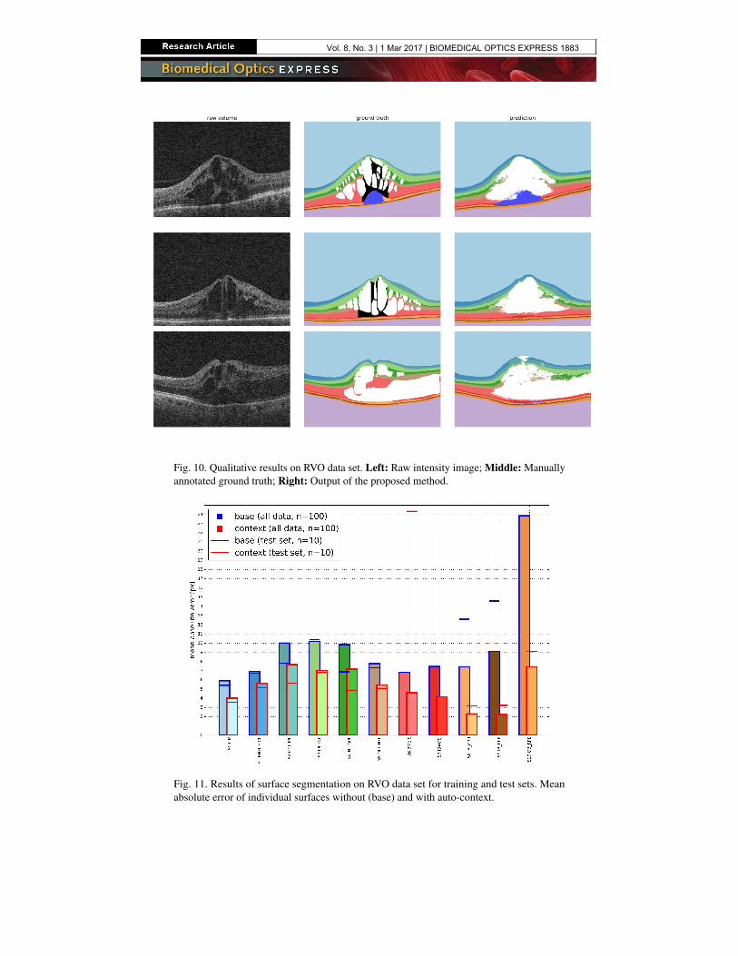
Fig. 10. Qualitative results on RVO data set. Left: Raw intensity image; Middle: Manuallyannotated ground truth; Right: Output of the proposed method.

Fig. 11. Results of surface segmentation on RVO data set for training and test sets. Meanabsolute error of individual surfaces without (base) and with auto-context.


Table 2. Results of region segmentation on RVO data set. Dice coefficients (mean ± std)without (base) and with auto-context.

L0 L1 L2 L3 L4 L5 L6base 0.99±0.01 0.72±0.09 0.61±0.08 0.65±0.09 0.62±0.09 0.68±0.09 0.84±0.08context 0.99±0.00 0.79±0.09 0.69±0.09 0.76±0.08 0.71±0.09 0.75±0.07 0.89±0.06

L7 L8 L9 L10 L11 V0 V1base 0.66±0.12 0.71±0.15 0.62±0.18 0.40±0.13 0.98±0.01 0.34±0.25 0.10±0.13context 0.74±0.08 0.80±0.07 0.73±0.11 0.62±0.10 0.99±0.00 0.41±0.25 0.24±0.20

In order to evaluate the region segmentation performance, we calculated the Dice coefficientfor each region as defined in Eq. (2)

Dice =2 ∗ TP

|true| + |predicted |=

2 ∗ TP

(TP + FN ) + (TP + FP )=

2 ∗ TP

2 ∗ TP + FN + FP

(2)

with TP and TN being the true positives and negatives (i.e. the correctly classified voxels), FP

and FN being the false positives and negatives (i.e. the incorrectly classified voxels), |true| thenumber of voxels that belong to the region according to the ground truth and |predicted | thenumber of voxels belonging to the region according to the algorithm. Dice is the most usedmetric in validating medical volume segmentations [11] and takes into account equally the falsepositive and the false negatives as defined by Eq. (2). The quantitative results can be seen inTable 2. Even though the coefficients for the fluid filled regions (i.e. V0 and V1) are relativelylow it can be seen that the segmentation does improve due to the auto-context approach.

Finally, in order to quantitatively evaluate the fovea position estimation we computed theabsolute Euclidean distance from the ground truth resulting in a mean error of µ = 10.0 px,σ = 5.5 px, median= 8.4 px (results of 10-fold cross validation, Fig. 12).

1 3 5 7 9 11 13 15 17 19 21 23

absolute error [px]

0

5

10

15

20

count

Fig. 12. Result of fovea estimation. Histogram of the absolute Euclidean distance betweenthe predicted fovea position and the manually annotated fovea position on 100 OCT volumesin the RVO data set.

3.2. Diabetic macular edema data set

The data set provided by [12] has only 8 surfaces and one fluid class annotated, hence thesurface/region definitions given in Table 1 had to be adapted accordingly (Table 3). Furthermoresince the provided scans have a highly anisotropic voxel size (i.e. approx 3.9 × 11.3 × 125 µm3

in contrast to 1.9 × 30.2 × 30.2 µm3 in the RVO data set) the PCA image features described insection 2.3 were recomputed in 2D (see Fig. 13). Since the manual annotation was not availablefor every B-scan, the probability map convolution described in section 2.4 could not be performedfor this evaluation. Finally, since a manual fovea position annotation is not available on this dataset, the fovea position was computed in an unsupervised manner as described in [12].


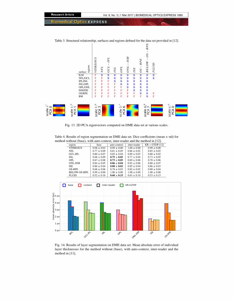
Table 3. Structural relationship, surfaces and regions defined for the data set provided in [12].

surface regi

ons

VI T

REOUS

NFL

GCL−

IPL

INL

OPL

ONL−

ISM

ISE

OS−

RPE

BELOW

−OS−

RPE

FLUID

ILM F B B B B B B B B BNFL/GCL F F B B B B B B B BIPL/INL F F F B B B B B BINL/OPL F F F F B B B B BOPL/ONL F F F F F B B B BISM/ISE F F F F F F B B BOS/RPE F F F F F F F B B FBM F F F F F F F F B F

Fig. 13. 2D PCA eigenvectors computed on DME data set at various scales.

Table 4. Results of region segmentation on DME data set. Dice coefficients (mean ± std) formethod without (base), with auto-context, inter-reader and the method in [12].

region base auto-context inter-reader KR + GTDP [12]VITREOUS 0.98 ± 0.02 0.99 ± 0.00 1.00 ± 0.00 0.99 ± 0.00NFL 0.77 ± 0.09 0.81 ± 0.05 0.86 ± 0.02 0.85 ± 0.02GCL-IPL 0.80 ± 0.07 0.85 ± 0.04 0.89 ± 0.03 0.88 ± 0.02INL 0.68 ± 0.09 0.75 ± 0.05 0.77 ± 0.04 0.73 ± 0.05OPL 0.67 ± 0.08 0.73 ± 0.05 0.69 ± 0.06 0.70 ± 0.06ONL-ISM 0.84 ± 0.05 0.86 ± 0.04 0.82 ± 0.06 0.80 ± 0.07ISE 0.86 ± 0.04 0.88 ± 0.02 0.85 ± 0.04 0.86 ± 0.03OS-RPE 0.68 ± 0.06 0.78 ± 0.03 0.82 ± 0.02 0.80 ± 0.04BELOW-OS-RPE 0.99 ± 0.00 1.00 ± 0.00 1.00 ± 0.00 1.00 ± 0.00FLUID 0.52 ± 0.16 0.60 ± 0.15 0.63 ± 0.10 0.53 ± 0.15

NFL

GCL-IPL

INL

OPL

ONL-IS

M ISE

OS-RPE

0 px

1 px

2 px

3 px

4 px

5 px

mean a

bso

lute

err

or

[px]

base context inter-reader KR+GTDP

Fig. 14. Results of layer segmentation on DME data set. Mean absolute error of individuallayer thicknesses for the method without (base), with auto-context, inter-reader and themethod in [11].


We computed the Dice coefficients for each region in the parts of the volumes where manualannotations were available. As shown in Table 4, the proposed method performs comparablyto the method proposed in [12] for most regions and even outperforms it in some (in bold). Inaddition, we computed the mean region thickness as in [12] and compared the absolute differenceto the manual annotation. It can be observed from Fig. 14 that the methods show comparableperformance. Similarly to the RVO data set, an improvement due to the auto-context loop isevident in all cases.

It is interesting to note that the performance on the DME data set is consistently better than onthe RVO data set even though fewer auto-context features and only 2D PCA features were used(Fig. 15). This can be attributed to the better signal to noise ratio in Spectralis scans (achievedthrough temporal oversampling) and the slightly less demanding segmentation task (RVO patientsgenerally have higher volumes of SRF present than DME patients).

Fig. 15. Segmentation results of subject #1 in the DME data set. Top: Central B-scan andthe manual annotations; Bottom: Results of the proposed method and the method presentedin [12].

3.3. Feature importance

Results in Tables 2 and 4 show that auto-context loop consistently improves the segmentations. Inthe evaluation of the feature importance reported by the random forest shown in Fig. 16, it can beseen that the newly proposed context-based features have a high impact on the final result. In ouranalysis, the distance features show up as the most important ones, even outperforming the imagebased features after one auto-context loop. Similarly, the fovea distance and the probability mapconvolution filter also demonstrate a high impact. In contrast, the random sampling of contextlocations does not show consistently good results. While some highly informative locations arerandomly chosen, the vast majority of sampled locations convey only limited information.

4. Discussion

Automated segmentation of retinal layers and fluid is a fundamental task for quantifying andcharacterizing macular edema in an objective and repeatable way. The main problem whensegmenting severely diseased scans is the high variability in the shape and location of fluid filledregions. As can be seen in Fig. 10, fluid can appear in most retinal layers, but can also span


0.0

0.25

0.5

0.75

1.0

rela

tive f

eatu

re im

port

ance PCA image features

Fovea position estimation

Distance features

Probability map convolution

Context locations

Fig. 16. Relative feature importance reported by the random forest classifier after oneauto-context iteration.

multiple layers and/or be “stacked” above other fluid filled regions. This makes it very difficultto manually encode or model all the possible interactions between fluids and retinal layers.

The main contribution of this work is that the proposed method is able to learn this interactionfrom the training data set using a machine learning approach. In addition to simultaneouslyobtaining both layer and fluid segmentations the two fluid types were also differentiated. Incontrast to other layer segmentation methods (e.g. [14]) the proposed method requires onlyhigh level information about the known anatomical ordering of the retinal layers (see Tables 1and 3). As a consequence, it can be trained on data sets of different (albeit similar) pathologieswithout the need for manual adaptation. Similarly, the computation of the convolutional filtersused as image features obtained with unsupervised representation (PCA) enables the applicationof the same method on different data sets with different spatial resolutions, image to noiseratios, and acquisition modes (with and without spatial oversampling), without the need of priornormalization.

Even though the proposed method achieved moderate performance in segmenting fluid regions,the segmentation still helps to “push” the surface segmentation closer to the correct position.This surface segmentation could later be used for an improved fluid segmentation - in much thesame way as a pre-existing fluid segmentation could be used to improve the surface segmentation.Such a pre-existing segmentation could be used as input for the auto-context approach whichenables the classifier to learn the long range spatial relations between objects in the image beyondthe size of the convolution filters.

The problem of accurately segmenting retinal fluid in severely diseased cases is challengingeven for qualified human readers, as noted in [12] and seen in the relatively poor inter-readeroverlap shown in Table 4. Further difficulties are caused by the poor signal to noise ratio in theRVO scans used for the validation, and by the presence of large SRF volumes obscuring theretinal layers as well as the distinction between the two fluid classes. Nevertheless, while the fluidsegmentation on the low-quality Cirrus scans in the RVO data set is relatively poor, the proposedmethod shows comparable or better performance to other methods on the Spectralis scans inthe DME data set. The results could be further improved by using e.g. a more sophisticatedgraph-cut segmentation instead of the voxel-wise estimation, or a morphological post-processingof the segmentation results.

A limitation of our machine-learning method is the reliance on large amounts of manuallylabeled ground truth data in order to accurately learn the high variability present in OCT scanswith severe macular edema. Nevertheless the extensive effort invested in obtaining such labeleddata was rewarded with increased segmentation performance. Providing more training dataespecially for regions that are represented by relatively few samples in the training data (e.g. NFLin the vicinity of the fovea) would help the machine learning algorithm to learn their variance inappearance and further improve the segmentation performance. Lastly, the voxel-wise estimationof the fluid classes in the proposed method tends to oversegment the retinal fluid (Fig. 10),


leading to a lower performance in the segmentation of the surrounding layers.Regarding the computational resources, due to the way the auto-context loop is trained the

algorithm requires a significant amount of processing time during the training phase (in order ofa few days). For the segmentation, the algorithm requires on average 7.2 minutes for the PCAimage feature extraction and 6.6 minutes per auto-context loop, on an Intel Core i7 (3770K @3.50GHz x 8) with 32GB RAM.

5. Conclusion

In this work we have introduced a novel fully automated 3D layer and fluid segmentationmethod based on unsupervised representation, auto-context and graph-theoretic segmentation.The proposed method simultaneously segments the layers and the two fluid related regions andlearns their mutual interaction to aid the retinal segmentation. To the best of our knowledge, thisis the first retinal layer and fluid segmentation to employ an iterative improvement approachyielding reasonable results even on highly pathologic cases. Furthermore, we have shown thatthe introduction of spatial context using auto-context and the domain specific context featuresimprove the segmentation results. In particular the distances to surface segmentations of theprevious iteration were shown to be important new features that improved the segmentationaccuracy. Such a methodology has further potential to be adapted to other medical imagesegmentation problems.

The method’s performance was extensively evaluated on a very large real world data setconsisting of 100 fully annotated OCT volumes that show signs of severe macular edema,yielding a mean unsigned surface position error of only 5.26 ± 18.75 px and a mean overallDice coefficient of 0.76. A second evaluation was performed on a publicly available data set,yielding a mean absolute thickness error of 2.87 ± 3.60 px and a mean overall Dice coefficient of0.78 on the retinal regions. Such an accurate automated segmentation of retinal layers in highlypathological SD-OCT scans can be used as starting point for more accurate fluid segmentationsor as an important imaging biomarker in itself.

Funding

The financial support by the Austrian Federal Ministry of Economy, Family and Youth and theNational Foundation for Research, Technology and Development is gratefully acknowledged.

Acknowledgments

The authors would like to thank Prof. Sina Farsiu and his group at Duke University for providingthe DME data set.


joint retinal layer and fluid segmentation in oct scans of ... retinal layer and fluid segmentation...

Documents