journal of agricultural science and practice - irj - · pdf fileara, jannatul fatema and...
TRANSCRIPT

First Quarter E-Book January-March 2016
Journal of Agricultural Science and Practice

ABOUT JASP
Journal of Agricultural Science and Practice (JASP) is an Open Access, Peer-Reviewed Journal that publishes Original and high-quality research articles in all areas of Agricultural Science. The Journal is committed to advancing and sharing creative, innovative and emerging ideas that will influence Agricultural policy and improve food sufficient around the world. The articles published in JASP will be of interest to Researchers, Government agencies and International organizations. JASP publishes per article and e-books every quarter. All published articles and e-books are freely accessible on our website. Editorial Office: [email protected] Customer Care: [email protected] Submit Articles: [email protected] Website: http://www.integrityresjournals.org

Dr. Roslan bin Ismail Department of Land Management Faculty of Agriculture Universiti Putra Malaysia 43400 UPM Serdang, Selangor,Malaysia Dr. Lee Seong Wei Faculty Agro Based Industry Universiti Malaysia Kelantan Jeli Campus Jeli, 17600, Kelantan, Malaysia Prof. Ehab Abdel Haleem Elsayad Soils & Water Department Fayoum Faculty of Agriculture Fayoum University, Egypt Dr. Nagham Rafeek Ibrahim El Saidy Department of Hygiene & Preventive Medicine Faculty of Veterinary Medicine Kafer Elshikh university, Egypt Dr. Josiah Chidiebere Okonkwo Department of Animal Science and Technology Faculty of Agriculture Nnamdi Azikiwe University P.M.B 5025 Awka, Anambra State, Nigeria
Editors

Table of Content: Volume 1: January – March 2016
Articles No.
Detection of Salmonella infection in slaughter cattle using meat juice and serum Abdulkadir A., Adamu N. A., Bitrus S., Gana L. L., Habibu S., Mohammed Y. Y., Alao E. A. and Mohammed F. I.
1-5
Isolation of Escherichia coli o157:h7 from water sources in the livestock complex, Mando, Kaduna Abdulkadir A., Muhammad T. I., El Yakub I., Taru I. A., Abba M., Enesi L., Bello L. and Mohammed F. I.
6-9
Impacts of Community Based Fisheries Management (CBFM) on the Livelihood of Fishers at Sherudanga beel in Rangpur District, Bangladesh Mst. Kaniz Fatema, Most. Jannatun Nahar, Motia Gulshan Ara, Jannatul Fatema and Muhammad Shahidul Haq
10-22
Estimating properties of unconsolidated sand-clay from spectral-induced polarization Mohammad Abdul Mojid, Hiroyuki Cho and Hideki Miyamoto
23-39

Journal of Agricultural Science and Practice
Volume 1. Page 1-5. Published 8th March, 2016 www.integrityresjournals.org/jasp/index
Full Length Research
Detection of Salmonella infection in slaughter cattle using meat juice and serum
Abdulkadir A.*, Adamu N. A., Bitrus S., Gana L. L., Habibu S., Mohammed Y. Y., Alao E. A. and Mohammed F. I.
Department of Animal Health, College of Agriculture and Animal Science, Mando: Division of Agricultural Colleges,
Ahmadu Bello University, Zaria, Nigeria.
*Corresponding author. Email: [email protected].
Copyright © 2016 Abdulkadir et al. This article remains permanently open access under the terms of the Creative Commons Attribution License 4.0, which permits unrestricted use, distribution, and reproduction in any medium, provided the original work is properly cited.
Received 26th January, 2016; Accepted 27th February, 2016
Abstract: Monitoring for Salmonella in slaughter cattle is important to enable targeted control measures to be applied on problem farms and at the abattoir. The aim of this study was to determine whether meat juice could be used as much as serum to identify slaughter cattle with a high prevalence of infection. Samples of meat juice & serum were taken from 100 slaughter cattle and comparisons were made between the results of individual Enzyme-linked immunosorbent assay (ELISA) tests on serum and meat juice. The ELISA tests showed a statistically significant Serum mean optical density (O.D.) with meat juice mean optical density (O.D.) from seven animals. All but one of the seven positive individual sample serum O.D. and sample/positive control (S/P) ratio results correlated significantly with the results of the meat juice O.D. ELISA. The results show a generally good correlation between serological results of individual serum and meat juice samples in slaughter cattle. Thus, ELISA could be used to flag up potentially hazardous Salmonella contaminated meat from slaughter cattle or herds which are more likely to be in need of improved Salmonella control. This can then be confirmed by bacteriological sampling at the abattoir or farm level and a control plan imposed. Key words: Enzyme-linked immunosorbent assay; meat juice; slaughter cattle; Salmonella; serum; test sample correlation.
INTRODUCTION Salmonella is a genus of bacteria that are a major cause of foodborne outbreaks in humans throughout the world (Waldvogel, 2000; Hirose et al., 2001). Due to genetic and environmental diversity Salmonella serotypes are adapted to live in a various range of hosts and habitats using pathogenic and non-pathogenic means of surviving (Callaway, et al, 2008). The prevalence of this pathogen presents major challenges in the food production and public health sectors in their efforts to supply safe foods as consumers’ food safety awareness is also on the increase.
Salmonella is a cause of acute and subclinical disease in cattle (Wray and Davies, 2000). It can cause disease in cattle of all ages, though the most commonly clinically affected group is calves aged 2 weeks to 3 months (Nielsen, 2003). Salmonella infections are still one of the most important foodborne diseases in humans and beef is one of the major sources for Salmonella infections in
humans (Hutwagner et al., 1997). The Salmonellae bacteria are generally transmitted to humans through consumption of mainly contaminated food of animal origin like beef and milk (Mead et al., 1999). Animals may also become infected from other Salmonella infected animals, directly or via a contaminated environment, including contaminated feed (European Food Safety Authority, 2011). Septicaemic cases due to Salmonella typhi are being reported in Africa especially in Kenya and Ghana (Mills-Robertson et al., 2002; Kariuki et al., 2004).
The importance of cattle as vectors of Salmonella have been shown by several abattoir studies where the prevalence of Salmonella in cattle caecal samples collected was high (8.34%) in Sango-Ota, Nigeria, and low for cattle and sheep (1.4% and 1.1% respectively) in Great Britain (Milnes, 2007). Infection in cattle can cause a range of clinical signs, from scouring to fever and death, but is often sub-clinical and so, is difficult for

J. Agric. Sci. Pract. 2 farmers to monitor and detect. Although it is unknown how many cases of human salmonellosis are attributed to eating cattle products, most cases are suspected to be related to the serovars S. Typhimurium, S. Dublin, S. Typhi, S. Paratyphi, and S. Newport which are all predominant types detected in samples from cattle (DEFRA, 2007). In the cattle industry, Salmonella Dublin causes economic losses in the form of death among calves and young animals, abortions and reproductive disorders among adult cattle, extra labor and increased veterinary expenses (Liza and Annette, 2004).
The starting point for control is monitoring to define the extent and distribution of infection. Bacteriological monitoring gives the best indication of the distribution of Salmonella on farms and facilitates the introduction and monitoring of control measures (Bager and Baggesen, 1993), but this must be carried out sufficiently rigorously to be meaningful, which may be expensive. Serological testing is less expensive for each individual sample, whereas bacteriological samples can be pooled. Pooled bacteriological samples have been very effective for monitoring large groups of poultry (Kradel and Miller, 1991; Aho, 1992), but are more difficult to achieve in a representative way for routine use on cattle farms/herds. Serology may provide a more sensitive indication of persistent cattle herd infection than limited bacteriology (Wiuff et al., 2002).
Many studies have tried to ascertain the factors that influence Salmonella prevalence, and identify on-farm control measures to reduce the Salmonella burden in livestock. Controlling Salmonella infections in cattle herds can provide economic, health and welfare benefits in the cattle industry, and may reduce the zoonotic risk. Risk factor identification is a necessary prerequisite to identifying suitable on-farm control measures to reduce the Salmonella burden, through precise and targeted approach. However, in order to study the infections dynamics within herds and risk factors affecting the spread of the infection, more knowledge about the prevalence for individual animals is required, and approaches for using these test over time and in combination need to be ascertained.
MATERIAL AND METHODS
The 200 samples were all collected in Kaduna from two abattoirs (Tudun Wada & Kawo Abattoirs) which were all from the central zone of Kaduna State.
The Tudun Wada Abattoir was established in 1959 by British colonials. It is the oldest and also the first abattoir in Nigeria to be established. About 200 cattle are slaughtered daily. The Kawo Abattoir was established in 1994. About 200 cattle are slaughtered daily.
This was a cross sectional study involving a systematic random sample of slaughter cattle, 10% of the daily slaughter cattle was selected and the 10th cattle in the
slaughter line were randomly selected for sampling. Thus 20 samples were collected daily. Animals were sampled only after owner’s consent was given. Blood and meat of each selected cattle was collected. Blood was collected directly immediately after slaughter in 20ml sterile sample bottle which were transported in cool boxes to the microbiology/parasitology laboratory of College of Agriculture and Animal Science, Ahmadu Bello University Mando Road, Kaduna. The samples were centrifuged at 1,000g for 15 minutes, after which the supernatant (serum) was decanted into sterile serum bottle and was refrigerated at – 20
0C until further processing. Meat
samples were collected form brisket of each selected cattle, wrapped into a sterile polythene bag, placed on ice in a cool box and immediately transported to the microbiology/parasitology laboratory of the College of Agriculture and Animal Science, Ahmadu Bello University, Mando Road, Kaduna. The meat samples were frozen for 24hours after which the samples were removed from the freezer and were kept to thaw into sterile sample bottle for the meat juice. All samples were identified by appropriate labeling. ELISA test procedure The Lipopolysaccharide (LPS) coated plate (Porcine Salmonella Antibody Test Kit; LPS B, C1, & D combined, BioChek, Burg Bracklaan 57, 2811 BP Reeuwijk. Holland) was removed from scaled bag and location of samples on template was recorded.
100µ1 of Negative Control and Positive Control were added into wells A1, B1, C1 and D1. 100µ1 of diluted samples were added into the appropriate wells and the plates were covered with lid and incubated at room temperature (22-27
0C) for 30 minutes. The contents of
wells were aspirated and washed 4 times with wash buffer (300µ1 per well). Plates were inverted and tapped firmly on absorbent paper. 100µ1 of conjugate reagents were added into the appropriate wells. Plates were covered with lid and incubated at room temperature (22-27
0C) for 30 minutes. Wash procedure was repeated as
earlier described. 100µ1 of prepared substrate reagents were added into the appropriate wells. Plates were covered with lid and incubated at room temperature 22-27
0C) for 15 minutes. 100µ1 of stop solution were added
to the appropriate wells to stop reaction. The micro titer plate was blanked in the air and the absorbance of control and samples was recorded by reading at 405nm using an ELISA reader (MC Jefferson KC-100 microplate reader, 4 Dunton Road, SE1 5SJ, London, United Kingdom).
Questionnaire
A brief questionnaire was administered at the time of

Abdulkadir et al. 3
Table 1. ELISA Result Comparison for Serum and Meat Juice
Sample ID SERUM ELISA MJ ELISA
Location S/P OD% S/P OD%
Kw6 0.4 10 0.92 23 Kawo
Kw7 0.4 10 0.88 22 Kawo
Kw8 0.4 10 0.76 19 Kawo
Kw11 0.292* 7.3* 0.52 13 Kawo
Tw16 0.68 17 4.8 119.8 Tudun Wada
Tw36 0.68 17 3.44 86 Tudun Wada
Tw42 0.6 15 1.4 35 Tudun Wada
ELISA: enzyme linked immunosorbent assay, MJ: meat juice, S/P; sample o positive ratio, OD: optical density. *Negative result
sample collection to investigate factors potentially associated with Salmonella in cattle such as source of animal, age, sex, breed, body condition score and previous antimicrobial usage.
Statistical analysis Data collected from the study area were analyzed using Chi square test at 95% confidence interval with values of P ≤ 0.05 considered significant. All analysis was done using statistical package for social sciences (SPSS) version 17.0.
RESULT
A total of 100 duplicate samples (serum and meat juice) were taken from slaughter cattle at the two (2) abattoirs located at Kawo and Tudun Wada, Kaduna metropolis. The animals originate from several sources within Kaduna State; including Anchau, Zaria, Birnin, Gwari, Kasuwan Magani, Kwai, Kauru, and livestock stations adjacent the abattoir (Zango). Sources outside Kaduna State include: Niger, Katsina State, Bauchi State, and Sokoto State. Antibodies against salmonella spp. were detected in 6 serum and 7 meat juice samples (7%, p ≤ 0.05). In all 6 serum samples (100% of positives) and 2 meat juice samples only low positive results (OD% 10% - 20%) were detected. High positive samples (OD% > 40%) were found in 2 samples of meat juice (15% of positives) while 3 meat juice samples had OD% between 20%-35% (Table 1). All serum positive samples were also positive with meat juice from same animal. All positive samples were detected only in animals that were sourced or originated from the ‘Zango’. All positive samples were also animals aged between 3-6yrs, had a body condition score of 3-5, and were all White Fulani breeds of cattle. Kawo abattoir had a higher prevalence of 4% (7/200) while Tudun Wada abattoir had a prevalence of 3% (6/200).
DISCUSSION
The ELISA kit used in this survey allows detection of antibodies to a broad range of Salmonella serogroups (B, C1, and D) indicating the exposure of cattle to the bacterium. The data presented in this study demonstrate the presence of antibodies specific to salmonella spp. In cattle presented for slaughter at the abattoir. About 7% of the animals tested were positive for antibodies against Salmonella spp., which is an agreement with previous works done on farms (Alao et al., 2012) where a prevalence of 8.28% was established. Although the individual serum or meat juice Salmonella ELISA test has a poor correlation with bacteriology on an individual basis (Christensen et al., 1999; Clouting and Davies, 2001; Davies et al., 2001; Corre´ge´, 2002), this study indicates that infection with Salmonella spp. does not only occur in herds but also in slaughter cattle. So slaughter cattle should be considered as potential source of Salmonella and thus constitute a public health hazard. This approach has been adopted in several other countries worldwide (Ludewig and Fehlhaber, 2001) and in other target species (Hoorfar et al., 1997; Feld et al., 2000; Nollet and Maes, 2005). However, this result cannot be compared to the results from monitoring of herds, which aim to categorize the health status of the herds.
Although in other studies, higher number of livestock collections might indicate that the abattoir have a greater amount of health condition problems, possibly caused by Salmonella or from health conditions associated with Salmonella infection, these factors may also be a risk simply because the increased number of vehicles entering the abattoir can facilitate the spread of Salmonella (Pritchard et al., 2005; Beloeil et al., 2007; Shilangale, 2014). No significant risk factor was identified in this study. This may be because only a small number of variables were analyzed and thus more important risk factors may have been missed or the true effect of variables underestimated. However, body condition score (BCS) of 4-5 was identified as a significant risk factor (OR

J. Agric. Sci. Pract. 4 2.4, Cl; 1.23-2.89). This may be a reflection of risk associated with latent carrier animals, whom look apparently healthy with a good body condition score (BCS) but have either subclinical disease and/or are shading the organism.
Conclusion and Recommendation
Serological examination provides a powerful tool to monitor infections with salmonella, when the diagnostic cut-off value of the ELISA >10% OD is used, and meat juice has proven to be a better sample than serum for serological monitoring/screening of slaughter cattle. This will not only raise awareness of infections with salmonella spp. in cattle, but also provide a basis for effective disease control. The individual serum or meat juice Salmonella ELISA test here has shown an unusual good correlation, hence, it should be used to flag up herds which are more likely to be in need of improved Salmonella control or slaughter cattle that may pose a public health risk. It is also possible to organize logistic slaughter based on herd ELISA result to reduce carcass contamination and thus recommended as a routine procedure for the abattoir to adopt. To decrease the risk from deliveries and visitors, biosecurity measures such as wearing protective clothing and footwear; the routine use of bootdips; ensuring deliveries are only made at the abattoir perimeter, and closing the abattoir to all but essential external vehicles should be utilized. REFERENCES
Aho, M. (1992) Problems of Salmonella sampling. International Journal of Food Microbiology. 15, 225-235.
Alao F., Kester C., Gbagba, B., & Fakilede, F. (2012). Comparison of prevalence and antimicrobial sensitivity of Salmonella Typhimurium in apparently healthy cattle and goats in Sango-Ota, Nigeria. The Internet Journal of Microbiology. 10(2). http://ispub.com/ijmb/10/2/14221.
Bager, N. & Baggesen, D. (1993). The Serological Response to Salmonella Serovar and Infant in Experimentally Infected Pigs the time Course Followed with an Indirect Ant – LPS ELISA & Bacteriological Examination. Pp. 205-218
Beloeil, P. A., Chauvin, C., Proux, K., Fablet, C., Madec, F., & Alioum, A. (2007). Risk factors for Salmonella seroconversion of fattening pigs in farrow-to-finish herds. Veterinary Research. 38, 835-848.
Callaway, T. R., Edrington, T. S., Anderson, R. C., Byrd, J. A. & Nisbet, D. J. (2008). Gastrointestinal microbial ecology and the safety of our food supply as related to Salmonella. Journal of Animal Science. 86(14), E163-E172.
Christensen, J., Baggesen, D.L., Sørensen, V., & Svensmark, B.(1999). Salmonella level of swine herds based on
serological examination of meat-juice samples and Salmonella occurrence measured by bacteriological follow up. Preventive Veterinary Medicine. 40, 277–292.
Clouting, C., & Davies, R. H. (2001). Evaluation of the
Salmonella meat-juice ELISA in the UK situation. Proceedings of Salinpork 2001. 4th International Symposium on Epidemiology and Control of Salmonella and Other Foodborne Pathogens in Pork. 2–5 September 2001, Leipzig, Germany, pp. 496-498.
Corre´ge´, I. (2002). Salmonella in pig farms: characterisation and epidemiological importance of the Salmonella status of gilts. Techni Porc., 25, 13-17.
Davies, R.H., Dalziel, R., Wilesmith, J.M., Ryan, J., Evans, S. J., Paiba, G. A., Byrne, C. & Pascoe, S. (2001). National survey for Salmonella in pigs at slaughter in Great Britain. Proceedings of Salinpork 2001. 4th International Symposium on Epidemiology and Control of Salmonella and Other Foodborne Pathogens in Pork. 2–5 September 2001, Leipzig, Germany, pp. 162-173.
Feld, N.C., Ekeroth, L., Gradel, K.O., Kabell, S. and Madsen, M. (2000) Evaluation of a serological Salmonella Mix-ELISA for poultry used in a national surveillance programme. Epidemiology and Infection, 125, 263-268.
Department of Environment, Food, and Rural Affairs (DEFRA) (2007). Zoonoses Report United Kingdom, 16-17.
European Food Safety Authority (EFSA) (2011). Analysis of the baseline survey on the prevalence of Campylobacter in broiler batches and of Campylobacter and Salmonella on broiler carcasses in the EU; Part B: Analysis of factors associated with Salmonella contamination of broiler carcasses. EFSA Journal. 9(2), 2017
Hirose, K., Tamura, K., Sagara, H. & Watnbe, H. (2001). Antibiotic susceptibility of Salmonella enterica serovar typhi and S. enterica serovar paratyphi A isolated from patients in Japan. Antimicrobial Agents and Chemotherapy. 45(3), 956-
958. Hutwagner, L. C., Maloney, E. K., Bean, N. H., Slutsker, L. &
Martin, S. M. (1997). Using laboratory-based surveillance data for prevention: an algorithm for detecting Salmonella outbreaks. Emerging Infectious Disease. 3, 395-400.
Kariuki, S., Revathi, G., Muyodi, J., Mwitura, J., Munyalo, A., Mirza, S., & Hart, C.A. (2004). Characterization of multidrug-resistant typhoid in Kenya. Journal of Clinical Microbiology.
42, 1477-1482. Liza, R. N. & Annette, K. E. (2004). Age-Stratified Validation of
an Indirect Salmonella Dublin Serum Enzyme-Linked Immunosorbent Assay for Individual Diagnosis in Cattle. Journal of Veterinary Diagnostic Investigation. 16, 212
Mead, P. S., Slutsker, L., Dietz, V., McCaig, L. F., Bresee, J. S., Shapiro, C., Griffin, P. M. & Tauxe R. B. (1999). Food-related illness and death in the United States. Emerging Infectious Disease. 5, 607-625.
Mills-Robertson, F., Addy, M. E., Mensah, P. & Crupper, S. S. (2002). Molecular characterization of antibiotic resistance in clinical Salmonella Typhi isolated in Ghana. FEMS Microbiology Letters. 215(2), 249-253.
Milnes, A. S., Stewart, I., Clifton-Hadley, F. A., Davies, R. H., Newell, D. G., Sayers, A. R., Cheasty, T., Cassar, C., Ridley, A., Cook, A. J. & Evans, S. J. (2007). Intestinal carriage of verocytotoxigenic Escherichia coli O157, Salmonella, thermophilic Campylobacter and Yersinia enterocolitica, in cattle, sheep and pigs at slaughter in Great Britain during 2003. Epidemiology of Infection. 136, 739-751.
Nielsen, J. (2003). Salmonella Dublin in cattle; use of diagnostic
tests for investigation of risk factors and infection dynamics. PhD Thesis. The Royal Veterinary and Agricultural University,

London, Pp. 205-218. Nollet, N., & Maes, D. (2005). Discrepancies between the
Isolation of Salmonella from Mesenteric Lymph Nodes and the Result of Serological Screening in Slaughter Pigs. Veterinary Research. Pp. 544-555.
Pritchard, D. G. (1982). Social and Management Factor involved in Respiratory Disease of Calves. Applied Animal Ethnology. Pp. 198-199.
Shilangale, R. P. (2014). Prevalence, Serotypes and Antimicrobial Resistance of Salmonella Isolated from Beef and Animal Feeds in Namibia. PhD Thesis, University of Namibia.
Wray C., Davies, R. H. (2000). Salmonella infections in cattle. In: Salmonella in domestic animals, ed. Wray, C., Wray, A., 1st ed., CABI Publishing. New York. pp.169-190
Hoorfar, J., Wedderkopp, A., & Lind, P. (1997). Detection of antibodies to Salmonella lipopolysaccharide in muscle fluid from cattle. American Journal of Veterinary Research, 58, 334-337.
Kradel, D. C. & Miller, W. L. (1991). Salmonella Enteritidis observations on field related problems. Proceedings of 40th Western Poultry Disease Conference. 24–27 April 1991, Acapulco, Guerrero, Mexico, Pp. 146-147.
Abdulkadir et al. 5 Ludewig, M., & Fehlhaber, K. (2001). Prevalence of Salmonella
in the pork production chain in the Federal State of Sachsen. 2: Serological investigation of slaughtered animals. Fleischwirtschaft, 81, 96-98.
Wiuff, C., Thorberg, B. M., Engvall, A. & Lind, P. (2002). Immunochemical analyses of serum antibodies from pig herds in a Salmonella non-endemic region. Veterinary Microbiology. 85, 69-82.
Waldvogel, F. A. (2000): Staphylococcus aureus (including staphylococcal toxic shock) In: Principles and practice of
infectious diseases (Mandell, G.L., Bennett, J.L. & Dolin, R. eds.) Churchill and Livingstone, New York. Pp. 2069-2100.

Journal of Agricultural Science and Practice
Volume 1. Page 6-9. Published 8th March, 2016 www.integrityresjournals.org/jasp/index
Full Length Research
Isolation of Escherichia coli o157:h7 from water sources in the livestock complex, Mando, Kaduna
Abdulkadir A.*, Muhammad T. I., El Yakub I., Taru I. A., Abba M., Enesi L., Bello L. and Mohammed F. I.
Department of Animal Health, College of Agriculture and Animal Science, Mando. Division of Agricultural Colleges,
Ahmadu Bello University, Zaria, Nigeria.
*Corresponding author. Email: [email protected].
Copyright © 2016 Abdulkadir et al. This article remains permanently open access under the terms of the Creative Commons Attribution License 4.0, which permits unrestricted use, distribution, and reproduction in any medium, provided the original work is properly cited.
Received 26th January, 2016; Accepted 28th February, 2016
Abstract: Failure in understanding the importance of water quality exposes humans and animals to the risk of diseases. Microbial contamination remains a critical risk factor in useable water in many parts of the world. This study was aimed at investigating Escherichia coli contamination of water samples. Fifty water samples were analysed to detect the occurrence of potentially pathogenic bacteria of Enterobacteriaceae family. All isolates detected were screened biochemically using Microbact GNB 12E and serotyped for the virulence antigens O and H. The results showed 14% (7/50) of the samples were positive for Escherichia coli, Salmonella arizonae, Enterobacter gergoviae, Enterobacter aerogenes, and Hafnia alvei. Out of which 3 samples were positive for Escherichia coli isolates which were collected from borehole (2 samples) and well water (1 sample) sources. All 2 isolates were serotyped for virulence antigen O157: H7 in which only 2 serotypes were identified for O157:H7 (2%) and O157:H
- (4%). Hence, it could be concluded that
water may be an important reservoir for E. coli infection and thus, the risk of contracting Enterohaemorrhagic Escherichia coli (EHEC) infection from contaminated water have been clearly established. Key words: EHEC, Enterobacteriaceae, reservoir, water, O157:H7.
INTRODUCTION Water plays a significant role for the sound pathogen that has emerged as a major cause of health of every person and is essential for plant life. About 75% of the earth’s crust is covered with water and the human body comprises approximately 70 % of water (Pant, 2004). Therefore, water is the most urgent for life and essential for good health of human beings. In Europe and America, much attention has been paid to the problem of water purity (Pant, 2004). The people of developing countries are attacked by water-borne diseases than those in developed countries (Simpson et al., 2002). Fecal pollution in water system is expected to originate from human and animal sources and multiple pollution control measures may be necessary to meet the requirement of the Clean Water Act and its amendments (Simpson et al., 2002). E. coli is one of the indicator organisms for freshwater systems which have been recommended by the U.S. Environmental Protection Agency (EPA) and it is a sensitive measure for fecal pollution since it is common
to almost all warm-blooded animals, including humans (U.S. EPA., 1986). Both Enterotoxigenic E. coli (ETEC) and Enterohaemorrhagic E. coli (EHEC) infections have been associated with the ingestion of food or water contamination with these organisms (Gannon et al., 1992). E. coli O157: H7 is a food-borne pathogen that has emerged as a major cause of hemorrhagic colitis. The reservoirs for EHEC O157:H7 are ruminants, particularly cattle and sheep, which are infected asymptomatically and shed the organism in feces. Other animals such as rabbits and pigs can also carry this organism. Humans acquire EHEC O157:H7 by direct contact with animal carriers, their feces, and contaminated soil or water, or via the ingestion of undercooked ground beef, other animal products, and contaminated vegetables and fruit. The infectious dose is very low, which increases the risk of disease (Alam and Zurek, 2006). Escherichia coli are serotyped based on the O (somatic lipopolysaccharide), H (flagellar) and K
Abdulkadir et al. 7
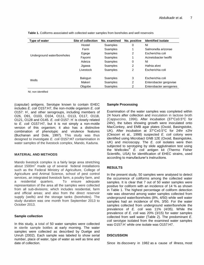
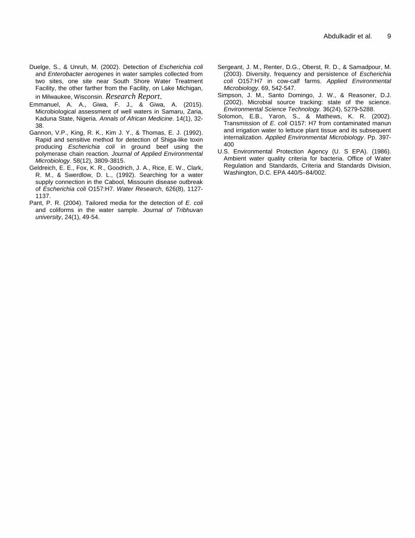
Table 1. Coliforms associated with collected water samples from boreholes and well reservoirs
Type of water Site of collection No. examined No. positive Identified isolate
Underground water/boreholes
Hostel 5samples 0 NI
Farm 5samples 1 Salmonella arizonae
Egege 5samples 2 Escherichia coli
Fayomi 5samples 1 Acinetobacter lwoffii
Adeiza 5samples 0 NI
Jigawa 5samples 2 Hafnia alvei
Livestock 5samples 2 Escherichia coli
Wells
Balogun 5samples 3 Escherichia coli
Makeri 5samples 2 Enterobacter gergoviae
Obgobe 5samples 2 Enterobacter aerogenes
NI; non identified
(capsular) antigens. Serotype known to contain EHEC includes E. coli O157:H7, the non-motile organism E. coli O157: H
-, and other serogroups, including members of
O26, O91, O103, O104, O111, O113, O117, O118, O121, O128 and O145. E. coli O157: H
- is closely related
to E. coli O157:H7, but it is not simply a non-motile version of this organism; it also has a distinctive combination of phenotypic and virulence features (Buchanan and Dole, 1997). This study was thus designed to investigate E. coli O157:H7 contamination in water samples of the livestock complex, Mando, Kaduna. MATERIAL AND METHODS Mando livestock complex is a fairly large area stretching about 1500m
2 made up of several federal installations
such as the Federal Ministry of Agriculture, College of Agriculture and Animal Science, school of pest control services, an integrated livestock farm, a poultry farm, and a residential quarters. To ensure adequate representation of the area all the samples were collected from all sub-divisions; which includes residential, farm and official areas; and also from the direct reservoir supply (wells) and the storage tanks (boreholes). The study duration was one month from September 2013 to October 2013. Sample collection In this study, a total of 50 water samples were collected in sterile sample bottles at early morning. The water samples were collected as described by Duelge and Unruh (2002). Each sample was labeled to show serial number, place of water, type of water as well as time and date of collection.
Sample Processing
Examination of the water samples was completed within 24 hours after collection and inoculation in lactose broth (Cappuccino, 1996). After incubation (37°C±0.5°C for 24hr), the tubes showing growth were inoculated onto MacConkey, and EMB agar plates (Oxoid, Basingstoke, UK). After incubation at 37°C±0.5°C for 24hr ±2hr (Clesceri et al., 1998) suspected E. coli colony were identified using Microbact GNB 12E (Oxoid, Basingstoke, UK) and microscopy. The E. coli isolates were then subjected to serotyping by slide agglutination test using the Wellcolex
® E. coli antigen kit (Thermo Fisher
Scientific, USA) for identification of EHEC strains, used according to manufacturer’s instructions.
RESULTS
In the present study, 50 samples were analysed to detect the occurrence of coliforms among the collected water samples. It is clear that 7 out of 50 water samples were positive for coliform with an incidence of 14 % as shown in Table 1. The highest percentage of coliform detection rate was observed among water samples collected from underground water/boreholes (8%, 4/50) while well water samples had an incidence of 6%, 3/50. For the water samples collected from underground water/borehole the prevalence of E. coli was 11% (4/35). While the prevalence of E. coli was 20% (3/15) for water samples collected from well water (Table 2). The predominant E. coli serotype isolated from the examined water samples was O157:H
- while one isolate was O157:H7.
DISCUSSION Since its discovery in 1982 as a cause of illness, most

J. Agric. Sci. Pract. 8
Table 2. Prevalence of E.coli serotypes among the examined water samples
Type of water No. examined E. coli positive E. coli positive (%) Sources Serotype No.
O157:H- 2 Underground 35 4 11% Egege O157:H- 1
O157:H7 1
O157:H- 1 Wells 15 3 20% Balogun O157:H- 1
O157:H- 1
infections from E. coli O157:H7 are believed to have come from eating undercooked ground beef. However, some have been water borne, as WHO estimates that 80% of all sickness in the world can be attributed to inadequate portable water supplies and poor sanitation. Water borne disease attributable to the ingestion of E. coli O157:H7 contaminated water has been reported (Geldreich et al., 1992). This study has demonstrated the potential risk of E. coli O157:H7 infection through contaminated water consumption with an isolation rate of 2% which is in agreement with the works of Aminu and Saidu, 2015 (3.03%), Chigor et al., 2010 (2.1%), and Sergeant, 2003 (1.5%). Highest proportion of coliform contamination obtained from wells may come from the animal reservoirs (ruminants) within the complex, as has been demonstrated by Emmanuel et al. (2015) and Solomon et al. (2002). These animals are allowed on free grazing and search for water within the complex with no restriction on contact with water sources/reservoirs used by humans (wells and boreholes). The reservoir hosts and epidemiology may vary with the organism. Ruminants, particularly cattle and sheep, are the most important reservoir hosts for E. coli O157:H7 (Bidet et al., 2005). A small proportion of the cattle in a herd can be responsible for shedding more than 95% of the organisms. These animals, which are called super-shedders, are colonized at the terminal rectum, and can remain infected much longer than other cattle. Super-shedders might also occur among sheep. Animals that are not normal reservoir hosts for E. coli O157:H7 may serve as secondary reservoirs after contact with ruminants (CDC, 2008).
Conclusion In conclusion, the strain of E. coli identified in this study from both the wells and underground water samples are consistent with the strains potentially pathogenic for humans. Identifying the major contributing source of contamination is the critical component for accurate assessment and successful control. Detection of potentially pathogenic E. coli O157:H7 in the examined water samples is alarming as many if not all the residents
of the livestock complex depend on these water sources daily for bathing, washing, laundry, and for cooking. These individuals are at great risk of contracting E. coli O157:H7 infection.
ACKNOWLEDGEMENT The technical staff of the Microbiology Laboratory, CAAS, Mando, Kaduna and Veterinary Public Health and Preventive Medicine laboratory, Ahmadu Bello University, Zaria, Nigeria. REFERENCES
Alam M. J., & Zurek, L. (2006). Seasonal prevalence of Escherichia coli O157:H7 in beef cattle feces. Journal of Food Protection. 69(12),3018-3020.
Aminu, M., & Saidu, B. B. (2015). Isolation of E. coli O157: H7 from vegetables and water used to irrigate vegetable farms within Sabon Gari, Zaria, Kaduna State. Proceedings of the Nigerian Society for Microbiology, held at the Department of Microbiology, Faculty of Science, Ahmadu Bello University, Zaria-Nigeria.
Bidet, P., Mariani-Kurkdjian, P., Grimont, F., Brahimi, N., Courroux, C., Grimont, P., & Bingen, E., (2005). Characterization of E. coli O157: H7 isolates causing haemolytic uraemic syndrome in France. Journal of Medical Microbiology, 54, 71-75.
Buchanan, R. L., & Doyle, M. P. (1997). “Foodborne disease significance of Escherichia coli 0157:H7 and other enterohemorrhagic E coli.” The Institute of Food Technologists’ Expert Panel on Food Safety and Nutrition. Food Technology, 51(10), 69-76.
Cappuccino, S. (1996). Microbiology: A Laboratory Manual. 4th edition. p.464.
Centers for Disease Control and Prevention [CDC] (2008). Division of Foodborne, Bacterial and Mycotic Diseases [DFBMD]. Escherichia coli [online]. CDC DFBMD. Accessed 20 August 2014.
Chigor, V. N., Umoh, V. J., & Smith, S.I. (2010). Occurrence of E. coli O157 in a river used for fresh produce irrigation in Nigeria. African Journal of Biotechnology. 9(2):178-182.
Clesceri, L.S., Greenberg, A. E., & Trussell, R. R. (1998). Standard method for the examination of water and waste water, 7th Ed. American public health association. Washington, DC.
Duelge, S., & Unruh, M. (2002). Detection of Escherichia coli
and Enterobacter aerogenes in water samples collected from two sites, one site near South Shore Water Treatment Facility, the other farther from the Facility, on Lake Michigan,
in Milwaukee, Wisconsin. Research Report. Emmanuel, A. A., Giwa, F. J., & Giwa, A. (2015).
Microbiological assessment of well waters in Samaru, Zaria, Kaduna State, Nigeria. Annals of African Medicine. 14(1), 32-38.
Gannon, V.P., King, R. K., Kim J. Y., & Thomas, E. J. (1992). Rapid and sensitive method for detection of Shiga-like toxin producing Escherichia coli in ground beef using the polymerase chain reaction. Journal of Applied Environmental Microbiology. 58(12), 3809-3815.
Geldreich, E. E., Fox, K. R., Goodrich, J. A., Rice, E. W., Clark, R. M., & Swerdlow, D. L., (1992). Searching for a water supply connection in the Cabool, Missourin disease outbreak of Escherichia coli O157:H7. Water Research, 626(8), 1127-1137.
Pant, P. R. (2004). Tailored media for the detection of E. coli and coliforms in the water sample. Journal of Tribhuvan university, 24(1), 49-54.
Abdulkadir et al. 9 Sergeant, J. M., Renter, D.G., Oberst, R. D., & Samadpour, M.
(2003). Diversity, frequency and persistence of Escherichia coli O157:H7 in cow-calf farms. Applied Environmental Microbiology. 69, 542-547.
Simpson, J. M., Santo Domingo, J. W., & Reasoner, D.J. (2002). Microbial source tracking: state of the science. Environmental Science Technology. 36(24), 5279-5288.
Solomon, E.B., Yaron, S., & Mathews, K. R. (2002). Transmission of E. coli O157: H7 from contaminated manun and irrigation water to lettuce plant tissue and its subsequent internalization. Applied Environmental Microbiology. Pp. 397-400
U.S. Environmental Protection Agency (U. S EPA). (1986). Ambient water quality criteria for bacteria. Office of Water Regulation and Standards, Criteria and Standards Division, Washington, D.C. EPA 440/5–84/002.

Journal of Agricultural Science and Practice
Volume 1. Page 10-22. Published 24th March, 2016 www.integrityresjournals.org/jasp/index
Full Length Research
Impacts of Community Based Fisheries Management (CBFM) on the Livelihood of Fishers at Sherudanga
beel in Rangpur District, Bangladesh
Mst. Kaniz Fatema1*, Most. Jannatun Nahar1, Motia Gulshan Ara1, Jannatul Fatema2 and Muhammad Shahidul Haq1
1Department of Fisheries Management, Bangladesh Agricultural University, Mymensingh-2202.
2Department of Agricultural Economics, Bangladesh Agricultural University, Mymensingh-2202.
*Corresponding author. Email: [email protected], [email protected]
Copyright © 2016 Fatema et al. This article remains permanently open access under the terms of the Creative Commons Attribution License 4.0,
which permits unrestricted use, distribution, and reproduction in any medium, provided the original work is properly cited.
Received 26th January, 2016; Accepted 13th March, 2016
Abstract: Community Based Fisheries Management (CBFM) approach appears to be an important factor in managing fisheries successfully. Thus, this study aims to investigate and evaluate the fisheries management practices and its impact on the livelihood of the fisheries community of Sherudanga beel in Rangpur district (Bangladesh) for a period of 12 months, from March 2010 to February 2011. The study was conducted based on Community Based Fisheries Management (CBFM) practices, beel biodiversity, fish production, socio-economic and livelihood condition of the fishermen community. The studied beel is 83 acre seasonal floodplain, which was mainly used by a community consisting of 80 families for their livelihood, where the CBFM approach was introduced by the community. At pre-CBFM, there was no controlled management system from any NGO or even Government for the proper management of the beel. Recently, community fishers leased out this beel from the government in year 2000 for 12 years and started to manage it. The CBFM project works for the development of fishery system, the fishermen community and the general society. The yearly gross fish production was higher than pre-CBFM period, implying that average abundance and fish biodiversity were significantly higher in the CBFM implemented beel. Majority of the fishermen had primary level education (37.5%) compared to 27.5% and 16.5% having secondary level and above secondary level education respectively, while 18.75% of them could sign their name only, indicating the improvement of education level among fishers. About 43.75% of them had small size family, while 40.0% and 16.25% had middle and large size families respectively. The prevalence of unconstructed house was the highest (77.5%) while few of them (22.5%) had semi constructed house. About 68.75% of the fishermen had medium income, while 12.5% and 18.75% had small and large income respectively. More than half (56.25%) of the fishermen received credits from different sources while rest (43.75%) of them did not get any credits. In conclusion, the overall findings showed that community based fisheries management has significantly increased annual fish production, lifted household income levels, improved access to credit from a wide range of sources and enabled livelihood diversification. Key words: Beel, Fisheries, CBFM, Livelihood
INTRODUCTION Although fisheries management in inland open water bodies of Bangladesh is critical but attention in recent years has received on Community Based Fisheries Management (CBFM) to empower fishing communities and improving the sustainability of management of inland water bodies. Full participation of the local communities living in the beel area has been recognized to be a pre-
requisite for the successful implementation of any fisheries development programs. CBFM is an alternative management scheme that is based on a participatory approach and calls for direct involvement and contri-bution of the community into the management of local fisheries resources. Thus, Community Based Fisheries Management (CBFM) has become a common strategy

for managing open water bodies and empowering local communities by involving community stakeholders, recognizing local needs, using local knowledge and establishing common property regiment (Berkes et al. 1998; Ostrom, 1990; Pomeroy and Berkes, 1997). It is a process by which people themselves have responsibility to manage their own resources, define their own needs, goals and aspirations and make decisions affecting their socio-economic welfare where government most often plays a minor role (Sajise, 1995). It also offers an opportunity to develop conservation approaches at local level and shift towards more sustainable fisheries and surrounding communities. As a result, CBFM has secured fisheries access for poor fisher’s community and improved nutrition, health, education, social status, standard of housing and sanitation of fisher communities. In a word, a possible solution to empowering fishing communities and improving the sustainability of manage-ment is Community Based Fisheries Management (CBFM).
Among the vast inland fishery resources of Bangladesh, beels are more potential for fish production. The beel is considered as biologically sensitive habitats as they play a vital role in the recruitment of fish populations in the riverine ecosystems and provide nursery grounds for commercially important fishes. Beel is an important source of cheap animal protein for the local population and also provides opportunities of full and part-time employment for the traditional fish farming communities living in the vicinity of the beel, providing them with additional household income and animal protein supplements. But, this beel fishery has been continuing degradations in the recent years due to roads, embankments, drainage, flood control and natural siltation along with overfishing (Ali, 1997; Haque et al. 1999).
Sherudanga beel is located in Mithapukur upazila of Rangpur district, Bangladesh covering rich reserve of aquatic fauna. This would provide great potential for the development of beel fisheries if appropriate management measures are carefully taken. Conventional fisheries management has not been effective for the beel thus CBFM approach has been introduced in 2000 and community has formed consisting of 80 families. CBFM aims to involve the participation of community stakeholders to ensure that future generations of Sherudanga beel will continue to have access to the benefits associated with sustainable fisheries and healthy ecosystems. Due to well-developed community involved in the beel for their livelihood, socio-economic condition of the fishermen, fisheries status, geographical situation and beel structure, the Sherudanga has been identified as the most important and promising area for freshwater fish culture for this study.
However, published research works on the socio-economic condition of fishermen and management
Fatema et al. 11 aspects of CBFM in the Sherudanga beel are relatively scanty. Therefore, a great requirement in socio-economic studies of fishermen livelihood concentrating on the development of CBFM models for effective management of Sherudanga beel is needed. This paper explored the role of existing institutional structures and types of organizations that directly affected the management of fisheries as well as discusses the impacts of CBFM on the livelihood of the fishermen. In addition, this study also examined the existing status of fish composition and fish production; to assess the diversity of fish and other aquatic species; and to make recommendations for the policy guidelines for the future development of the fishermen. We think, this study would be used for further studies as baseline information for developing appro-priate fisheries managements for Sherudanga beel.
Considering the importance of fish biodiversity for sustainable management of beel fisheries, an assessment was made of the present management system of the fisheries in the Sherudanga beel to investigate the existing potentials of the local communities to be involved in and to participate in the development of a community-based fisheries manage-ment system on beneficiary’s livelihood of the said beel.
MATERIALS AND METHODS
Study Area
The study was conducted in Sherudanga beel situated in the northern part of Bangladesh under Mithapukur upazila of Rangpur district (Figure 1 and 2). The area of the beel is about 83 acres, while it becomes about 500 acres during rainy season. The beel is located in Mithapukur upazila of Rangpur district, Bangladesh. Its geographical coordinates are 25° 34' 30" North, 89° 16' 00" East. There are several beels are scattered in this upazila including Chatra beel, Salinir beel, Chaitali beel, Boro Phaliar beel, Boro ruher beel, 26-bigha Dubla Chori beel, Tulshi Danga beel and Sherudanga beel. Among them, Sherudanga beel is largest which is situated to the western side from the Upazila office having 8 km distance. The beel area usually flooded every year. It remained under water most time of the year. From the month of June to September, the depth of water of the beel becomes 3.5 to 4.5 m. At the dry season (January to April), some portion of the beel was dried.
Data collection Methods
Field research was done for a calendar year from March 2010 to February 2011. The research was based on both primary and secondary data, comprehensive literature

J. Agric. Sci. Pract. 12
Figure 1. The map of Mithapukurupazila under Rangpur district where the study area, the Sherudangabeel, is indicated by an arrow.Rangpur district is shown in gray color in the inset map picture of Bangladesh. The beel is marked by blue color.
review and extracts of local knowledge and information. Collection of primary data was made by field observations and different methods viz. Questionnaire interview, Questionnaire survey, Participatory Rural Appraisal (PRA) tool (Figure 3). The PRA tool like focus group discussion (FGD) was conducted with members of beel fishing communities including women and children. Survey of operation of different fishing gears, catch trends, survey of fish market adjacent to beel, survey of biological resources of the beel and survey of socio-economic condition of fishermen was also done. Cross-check interviews were conducted with key informants,
such as district and sub-district fisheries officers, researchers, relevant project staff, and non-governmental organization (NGO) workers. At the same time, the researchers directly visited and gathered knowledge about physical environment of the beel fishing practice and household’s role as well as livelihood strategy, power relation’s socio-cultural norm and institutional, economic and demographic conditions. Secondary data was collected through literature and publication available from Upazila Fisheries Officer, local administration, Water Development Board (WDB), Department of Fisheries (DoF), Bangladesh Fisheries Research Institute (BFRI)

Fatema et al. 13
Figure 2. Magnified satellite view of the portion of Mithapukur upazila where Sherudanga beel is
indicated by an arrow (upper picture). Photograph was collected from Google Earth. The appearance of the study area (Sherudanga beel) (A) and a board describing the name & address of the CBFM community in Bengali (B) are shown in the down picture.
and related NGOs. Assistance also taken from quarterly and annual reports of fisheries, reports and books from Community Development and Settlement Program (CDSP) office and books of Bangladesh bureau of statistics. Sampling of water Water samples were collected from six different sites of the beel for plankton abundance study. In every case five liters of water samples were filtered through plankton net of 55 µm mesh size. Then the samples were concentrated to a volume of 50 ml and preserved in plastic vials with 5% formalin. For analysis, a sub-sample at 1ml was quickly drawn with a wide mouthed pipette and poured into a Sedgewick Rafter counting chamber of 1 ml capacity and organisms were counted as outlined by Boyd (1979). The S-R counting cell was placed under a
binocular microscope (Olympus BH 2 with phase contrast facilities; magnification 40x) and the plankton was identified and recorded. Fish sampling Identification of fishes was done through collection of different species directly from fishers, fishing through different types of gears, fishing through enclosure with bana, kua fishing, kata fishing and surveying from local fish markets. Identification of non-piscine species was done simultaneously. Aquatic weeds were collected from the beel and identification was made in the laboratory. Analysis of findings The collected data were coded, summarized and
Figure 2. Magnified satellite view of the portion of Mithapukur upazila where Sherudanga beel
is indicated by an arrow (upper picture). Photograph was collected from Google
Earth.
A
B

J. Agric. Sci. Pract. 14
Figure 3. A: Collection of data by questionnaire interview and B: Sherudanga beel community based fisheries management
office along with a member of the CBFM committee.
processed for analysis. These data were verified to eliminate all possible errors and inconsistencies by some criteria and standards for evaluation of the overall significance. Tabular technique was applied for the analysis of data by using simple statistical tools like average and percentages. Collected data was analyzed by using Microsoft Excel. RESULTS At the pre-CBFM time in Sherudanga beel community, the livelihood status, socio-economic condition and beel management performance were unpleasant. Anomalies in fish culture and lack of organization and supervision of the beel resulted in reduction of fish production that affected their livelihood. Serudanga beel is being managed since 2000 under the CBFM project which is implemented by the partnership of DoF and BRAC, a
non-government organization. With the help of participating NGOs, the community fishermen of the study area formed a beel management committee (BMC) (Figure 4). This committee properly manages the beel by the following continuous process introduced by CBFM system. Biodiversity of the Sherudanga beel Sherudanga beel is rich with fish and other aquatic biodiversity. During the study period, a total of 31 resident species were recorded (Table 1) from the beel of which 21 species were common, 6 rare and 4 species were highly endangered. A total of 9 non-resident species also were recorded of which seven are stocked species and the other two are non-stocked (Table 2). Otherwise, six species were identified as extinct species (Table 3). Of the 40 fish species, 12 species belong to the family of
Figure 3. A: Collection of data by questionnaire interview and B: Sherudanga beel community based fisheries management office
along with a member of the CBFM committee.
A
B

Fatema et al. 15
Table. 1. List of resident species recorded in Sherudanga beel during study period.
Sl. No. Family Local name Common name/ English name
Scientific name Comment
1 Anabantidae Koi Climbing perch Anabas testudineus
(Bloch, 1792) common
2 Anabantidae khalisha Goramy Colisa fasciatus
(Bloch and Schneider, 1801) Common
3 Anabantidae Ranga Khalisha
Goramy Colisa laliuis
(Hamilton, 1822)
Highly endangered
4 Bagridae Gulsha Catfish Mystus cavasius
(Hamilton, 1822)
Highly endangered
5 Bagridae Tengra Catfish Mystus vittatus
(Bloch, 1794) Common
6 Belonidae Kakila Needle fish Xenentodon cancila
(Hamilton, 1822) Common
7 Belonidae Lamba chanda
Elongate glass perchlet
Chanda nama
(Hamilton, 1822) Common
8 Channidae Taki/ Lati Snakehead Channa punctatus
(Bloch, 1793) Common
9 Channidae Shoal Snakehead Channa striatus
(Bloch, 1793) Common
10 Channidae Gajar Giant snakehead Channa marulius
(Hamilton, 1822) Common
11 Channidae Cheng Asiatic snakehead Channa orientalis
(Bloch and Schneider, 1801) Common
12 Clariidae Magur Catfish Clarias batrachus
(Linnaeus, 1758) Common
13 Clupedae Chapila Shad/Herring Gudusia chapra
(Hamilton, 1822)
Dominant resident sp.
14 Clupedae Kachki Shad/Herring Corica soborna
(Hamilton, 1822) Rare
15 Cobitidae Gutum Loach Lepidocephalus guntea
(Hamilton, 1822) Rare
16 Cyprinidae Mola Barb Amblypharyngodon mola
(Hamilton, 1822) Common
17 Cyprinidae Jatpunti Spot fin swamp barb Puntius sophore
(Hamilton, 1822) Common
18 Cyprinidae Tit punti Barb Puntius ticto
(Hamilton, 1822) Common
19 Cyprinidae Darkina Barb Rasboradani conius
(Hamilton, 1822) Common
20 Cyprinidae Narkali Chela
Minnow/ Barb Salmostoma bacaila
(Hamilton, 1822) Common
21 Gobiidae Baila/Bele Goby Glossogobius guiris
(Hamilton, 1822) Common
22 Heteropneustidae Shing Stinging catfish Heteropneustes fossilis
(Bloch, 1794) Common
23 Mastacembelidae Guchibaim Striped spiny eel Mastacembelus pancalus
(Hamilton, 1822) Common
24 Mastacembelidae Shalbaim Spiny eel Mastacembelus armatus
(Lacepède, 1800) Rare
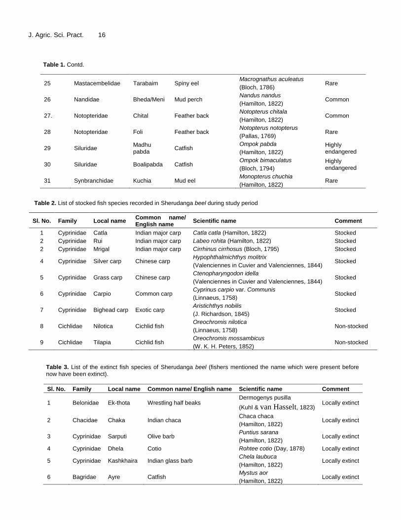
J. Agric. Sci. Pract. 16
Table 1. Contd.
25 Mastacembelidae Tarabaim Spiny eel Macrognathus aculeatus
(Bloch, 1786) Rare
26 Nandidae Bheda/Meni Mud perch Nandus nandus
(Hamilton, 1822) Common
27. Notopteridae Chital Feather back Notopterus chitala
(Hamilton, 1822) Common
28 Notopteridae Foli Feather back Notopterus notopterus
(Pallas, 1769) Rare
29 Siluridae Madhu pabda
Catfish Ompok pabda
(Hamilton, 1822)
Highly endangered
30 Siluridae Boalipabda Catfish Ompok bimaculatus
(Bloch, 1794)
Highly endangered
31 Synbranchidae Kuchia Mud eel Monopterus chuchia
(Hamilton, 1822) Rare
Table 2. List of stocked fish species recorded in Sherudanga beel during study period
Sl. No. Family Local name Common name/ English name
Scientific name Comment
1 Cyprinidae Catla Indian major carp Catla catla (Hamilton, 1822) Stocked
2 Cyprinidae Rui Indian major carp Labeo rohita (Hamilton, 1822) Stocked
2 Cyprinidae Mrigal Indian major carp Cirrhinus cirrhosus (Bloch, 1795) Stocked
4 Cyprinidae Silver carp Chinese carp Hypophthalmichthys molitrix
(Valenciennes in Cuvier and Valenciennes, 1844) Stocked
5 Cyprinidae Grass carp Chinese carp Ctenopharyngodon idella
(Valenciennes in Cuvier and Valenciennes, 1844) Stocked
6 Cyprinidae Carpio Common carp Cyprinus carpio var. Communis
(Linnaeus, 1758) Stocked
7 Cyprinidae Bighead carp Exotic carp Aristichthys nobilis
(J. Richardson, 1845) Stocked
8 Cichlidae Nilotica Cichlid fish Oreochromis nilotica
(Linnaeus, 1758) Non-stocked
9 Cichlidae Tilapia Cichlid fish Oreochromis mossambicus
(W. K. H. Peters, 1852) Non-stocked
Table 3. List of the extinct fish species of Sherudanga beel (fishers mentioned the name which were present before
now have been extinct).
Sl. No. Family Local name Common name/ English name Scientific name Comment
1 Belonidae Ek-thota Wrestling half beaks Dermogenys pusilla
(Kuhl & van Hasselt, 1823) Locally extinct
2 Chacidae Chaka Indian chaca Chaca chaca
(Hamilton, 1822) Locally extinct
3 Cyprinidae Sarputi Olive barb Puntius sarana
(Hamilton, 1822) Locally extinct
4 Cyprinidae Dhela Cotio Rohtee cotio (Day, 1878) Locally extinct
5 Cyprinidae Kashkhaira Indian glass barb Chela laubuca
(Hamilton, 1822) Locally extinct
6 Bagridae Ayre Catfish Mystus aor
(Hamilton, 1822) Locally extinct

Fatema et al. 17
Table 4. List of planktons with their generic and family name recorded from the beel
Class name Genus Class name Genus
Phytoplankton
Euglenophyceae Euglena Dipodascaceae Coccidiascus
Chlorophyceae
Ankistrodesmus Micractiniaceae Golenkenia
Chlorella Cymbellaceae Cymbella
Cosmarium Selenastraceae Monoraphidium
Gonadojygon Tabellariaceae Tabellaria
Pediastrum Biddulphiaceae Biddulphia
Tetradron Stephanodiscaceae Cyclotella
Ulothrix Nostocaceae Anabaena
Cyanophyceae Oscillatoria Cocconeidaceae Coconeis
Naviculaceae Navicula Chaetophoraceae Pleurococcus
Zooplankton
Monogononta Asplanchna Synuraceae Mallomonas
Maxillopoda Cyclops and Sida Coscinodiscophyceae Fragilaria
Cyprinidae, 4 species belong to the family of Channaidae, 3 species belong to the family of Cobitidae, Anabantidae and Mastacembelidae each, 2 species belong to Bagridae, Clupedae, Belonidae, Siluridae, Notopteridae, and Cichlidae families each and only 1 species belong to Clariidae, Gobiidae, Cobitidae, Heteropneustidae, Nandidae, and Synbranchidae family each.
The stocked species were catla (Catla catla), rui (Labeo rohita), silver carp (Hypophthalmichthys molitrix), mrigel (Cirrhinus cirrhosus), carpio (Cyprinus carpio), grass carp (Ctenopharyngodon idella) and bighead carp (Aristichthys nobilis). Moreover, two non-stocked and non-resident species found include nile tilapia (Oreochromis niloticus) and mozambique tilapia (Oreochromis mossambicus). Of the resident species, 21 species were common and most dominant of them includes Puntius sophore, Puntius ticto, Channa punctatus, Channa striatus, Mystus vittatus, Clarias batrachus, Mastacembelus armatus, Heteropneustes fossilis, Wallago attu, Macrobrachium lamerrii, and Macrobrachium malcolmsonii, 6 were rare including Corica soborna, Lepidocephalus guntea, Mastacembelus armatus, Macrognathus aculeatus, Notopterus notopterus, and Monopterus chuchia, 4 were highly endangered including Colisa laliuis, Mystus cavasius, Ompok pabda, and Ompok bimaculatus, and 6 were extinct from the beel including Darmogenys pussilus, Chaca chaca, Puntius sarana, Rohtee cotio, Chela laubuca, and Mystus aor.
The non-piscine biodiversity of Sherudanga beel
comprises 2 species of prawn including Macrobrachium lamerii and Macrobrachium malcolmsonii, 6 species of molluscs including Pila globosa, Planorbis sp., Viviparus bengalensis, Melanoides tuberculatus, Lamillidens marginalis and Corbiculata sp., 6 species of arthropods (aquatic insects) including Potamon sp., Belostoma sp., Abedus sp., Ranatra sp., Nepa sp., and Gerirs sp., 4 species of amphibians including Euphlyctis cyanophlyctis, Hoplobatra chustigerinus, Rhacophorus leucomystax and Bufomelanos tictus. Among 4 species of reptiles, two species of bivalves Lamillidens marginalis and Corbicu lata sp. and in reptiles Kachuga tecta (Kochchop) were abundant before but very rare or highly endangered at present.
Other than fish diversity, following type of planktons were observed in the study area including Navicula, Pleurococcus, Cyclotella, Anabaena, Gonadojygon, Oscillatoria, Chlorella, Pediastrum, Euglena, Ulothrix, Fragellaria, Asplanchna, Coconeis, Monoraphidium, Tabellaria, Biddulphia, Sida, Tetradon, Coscinodiscus, Nitzchia, Cyclops, Ankistrodesmus, Cosmarium, Golenkenia, Mallomonas and Cymbella (Table 4). Moreover, rich aquatic plant diversity were also observed including Eichhornia crassipes, Pistia stratiotes, Lemna minor, Azolla pinnata, Nymphaea rubra, Nymphaea nouchali, Nymphaea lotus, Nelumbo nucifera, Vallisneria spiralis, Potamogeton sp., Ipomoea fistulosa, Leersia hexandra, Ipomoea aquatic, Marsilea quadrifolia in the studied beel.
In this study, average fish production for one year was calculated from the cumulative data of large harvest and
J. Agric. Sci. Pract. 18
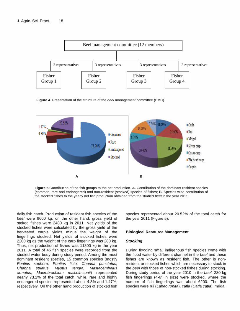
Figure 4. Presentation of the structure of the beel management committee (BMC).
Figure 5.Contribution of the fish groups to the net production. A. Contribution of the dominant resident species (common, rare and endangered) and non-resident (stocked) species of fishes; B. Species wise contribution of the stocked fishes to the yearly net fish production obtained from the studied beel in the year 2011.
daily fish catch. Production of resident fish species of the beel were 9600 kg, on the other hand, gross yield of stoked fishes were 2480 kg in 2011. Net yields of the stocked fishes were calculated by the gross yield of the harvested carp’s yields minus the weight of the fingerlings stocked. Net yields of stocked fishes were 2200 kg as the weight of the carp fingerlings was 280 kg. Thus, net production of fishes was 11800 kg in the year 2011. A total of 46 fish species were recorded from the studied water body during study period. Among the most dominant resident species, 15 common species (mostly Puntius sophore, Puntius ticto, Channa punctatus, Channa striatus, Mystus tengra, Mastacembelus armatus, Macrobrachium malcolmsonii) represented nearly 73.2% of the total catch, while, rare and highly endangered species represented about 4.8% and 1.47%, respectively. On the other hand production of stocked fish
species represented about 20.52% of the total catch for the year 2011 (Figure 5). Biological Resource Management Stocking During flooding small indigenous fish species come with the flood water by different channel in the beel and these fishes are known as resident fish. The other is non-resident or stocked fishes which are necessary to stock in the beel with those of non-stocked fishes during stocking. During study period of the year 2010 in the beel, 280 kg fish fingerlings (4-6" in size) were stocked, where the number of fish fingerlings was about 6200. The fish species were rui (Labeo rohita), catla (Catla catla), mrigal
Figure 4. Presentation of the structure of the beel management committee (BMC)
Beel management committee (12 members)
Fisher
Group 1
Fisher
Group 2
Fisher
Group 3
Fisher
Group 4
3 representatives 3 representatives 3 representatives 3 representatives
A B
Figure 5.Contribution of the fish groups to the net production. A. Contribution of the dominant resident species (common, rare and endangered) and non-resident (stocked) species of fishes; B. Species wise contribution of the stocked fishes to the yearly net fish production obtained from the studied beel in the year 2011.

Fatema et al. 19
Table 5. Stocking of the non-resident fish fingerlings in 2010 at the beel (area of the beel is about 80 acre, while about 500 acre
during flooding).
Sl. No. Species Size Stocking No. Stocking weight (kg) Stocking value (USD kg-1
) Total USD
1 Labeo rohita 4-5" 1000 40 1.4 56.2
2 Catla catla 5-6" 800 40 1.6 63.86
3 Cirrhinus cirrhosus 4-5" 1200 40 1.15 45.98
4 Cyprinus carpio 5.5-6.5" 600 40 1.92 76.63
5 Ctenopharyngodon idella 5-6" 600 40 1.60 63.86
6 Hypophthalmichthys molitrix 5-6" 1200 40 0.96 38.32
7 Hypophthalmichthys nobilis 4-5" 800 40 0.83 33.21
Total 6200 280 - 378.06
(Cirrhinus mrigala), grass carp (Ctenopharyngodon idella), silver carp (Hypophthalmichthys molitrix), bighead carp (Aristichthys nobilis) and common carp (Cyprinus carpio). Fish fingerlings were released during July, 2010 and harvested on March, 2011. The stocking density of the fingerlings in the beel for the year 2010 is summarized in the Table 5. Nursery management The BMC collected fish fry of selected species (Labeo rohita, Catla catla, Cirrhinus cirrhosus, Hypophthalmichthys molitrix, Hypophthalmichthys nobilis, Ctenopharyngodon idella and Cyprinus carpio) and managed them in a nursery pond. Two nursery ponds were used at the corner of the beel having an area of 20 and 23 decimal. They collected fish fry from nearest government hatchery.
Establishment of Sanctuary To overcome any endangered situation, community fishermen established two sanctuaries in this beel. Establishment of aquatic sanctuary is one of the effective tools for conserving fish stock, preserving biodiversity and increasing fish production. After the establishment of the sanctuary, fishermen of the studied beel reported a dramatic change of fish species such as Nandus nandus, Channa marulius, Barbodes gonionotus which were in endangered condition during pre-CBFM period become abundant in their density resulting the improvement of fish production and increment of fish biodiversity as well as production of Labeo rohita, Catla catla and Cirrhinus cirrhosus become elevated than the before.
Maintenance of fishing banned period For regular recruitment of resident species, BMC maintains a minimum three months of fishing banned
period (closed fishing season) during breeding season (June-September). At that time BRAC provided loans for the fishermen. Implementation of fish act Fishers got training from BRAC to protect environment and now they are more aware for protecting their own resources. Various types of fishing gears were found to operate in the study area. They were mostly traditional type and some of them were unique for the particular locality. From the survey it was found that nets, traps and wounding gears were operated by the fishermen in Sherudanga beel (Table 6). Besides these, fishermen also practiced dewatering and hand picking fisheries. Due to the vastness of the water body nets are operated more frequently. BMC discourage to catch undersized stock fish and strictly prohibited use of destructive fishing gear (current jal). In case of any violation of rules, BMC take necessary steps as may impose fine and even cancellation of membership. Fish marketing channel The price of fish depends on market structure, species, quality, size and weight. All traders in markets made a considerable amount of profit. However, concerns arises about the sustainable system of market due to higher transport costs, poor road and transport facilities, poor supply of ice, lack of money and poor institutional support. It was observed that, three types of fish marketing channel exist in the studied area. These were: i) Fishermen → Consumer ii) Fishermen → Retailer → Consumer iii) Fishermen → Arotdar → Wholesaler → Retailer → Consumer. Results of the present study indicated that 15% of the fishermen directly sold their fish to the consumers, while, 37% of them disposed their fish to the retailer and 48% of the fishermen handed over their fish to the wholesaler.

J. Agric. Sci. Pract. 20
Table 6. Different kinds of fishing gear used in Sherudanga beel
Group name Name of gears
Nets
Lift net (Dharma jal) Cast net (Jhakijal) Gill net (Current jal) Push net (Thelajal) Seine net (Berjal)
Traps Bair (Darki)
Wounding gears Hook (Borshi) Koch, Ekkata etc.
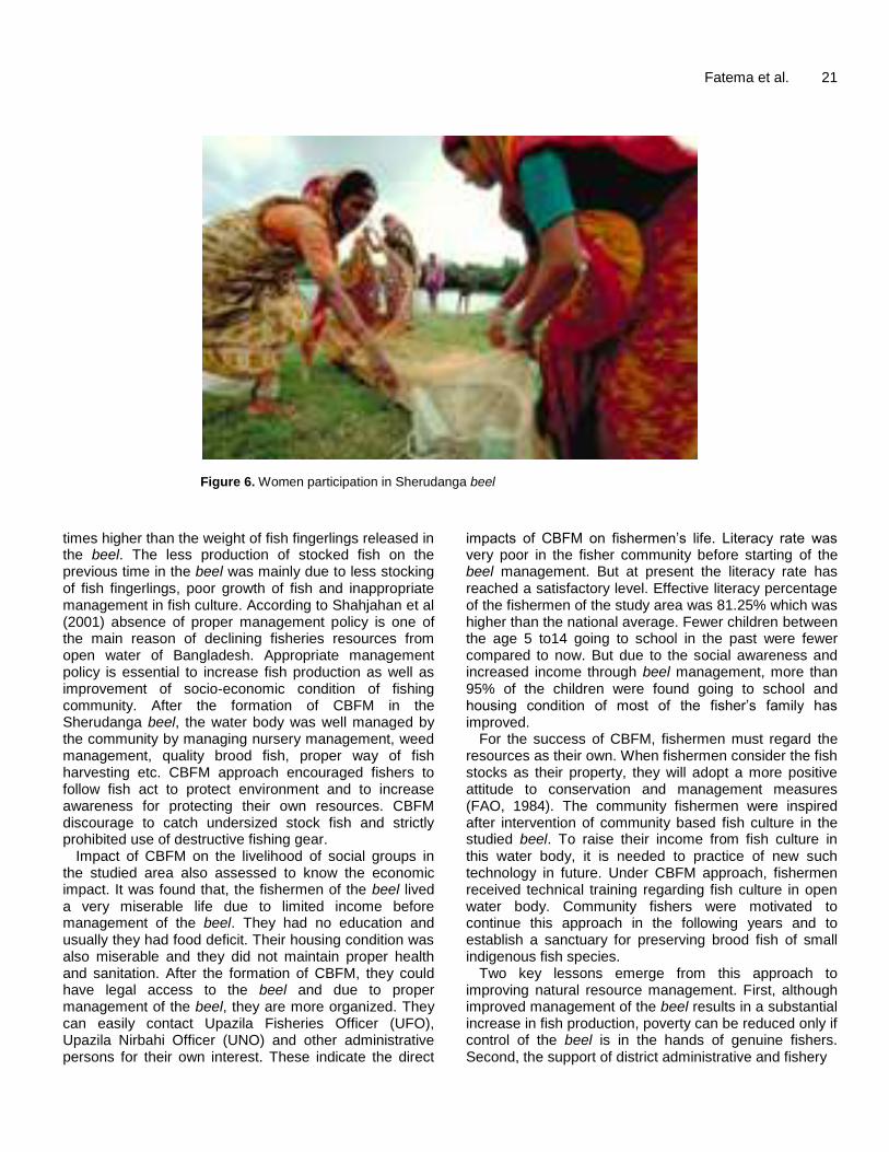
Socio economic condition of the fishermen Socio economic condition of the fishermen also studied to know the impact of CBFM approach because fishers are one of the most vulnerable communities in Bangladesh. At present, most of the fishermen have middle sized family (5-6 members). Majority (37.5%) of fishermen had primary level education compared to 27.5% and 16.3% having secondary and above secondary level education respectively, while about 18.75% of them could sign their names only. The prevalence of unconstructed house was the highest (77.5%) among the fishermen, while a few of them (22.5%) had semi-constructed house. Drinking water facilities, use of sanitary latrines and prevalence of different diseases was observed in good condition. The annual income of the fishermen varied from USD 459.792 to 753.55. Above three fourth (68.75%) of the fishermen had medium income, while the proportion of small and large income earning fishermen are 12.5% and 18.75%, respectively. Thus the overwhelming majority of the fishermen had medium to large income which might have been helpful for the management of their families and the beel. As regards to receipt of credit facilities more than half (56.25%) of the fishermen indicated that they had received credit from different sources such as banks (33.33%), NGOs (22.22%), money lenders (22.22%), relatives and friends (11.12%) and others (11.12%). The rest 43.75% of them said that they either did not require any credit or they did not get any credit. Most of the families of the fishermen had comparatively fairly well food security status. Dramatic awareness has been achieved after implementation of CBFM approach. Women participation in beel management activities found in progress. Women help in net making, fish harvesting, fish marketing and involved in decision making processes which led to a dramatic social change across Bangladesh (Figure 6). The CBFM has had considerable impact on poverty reduction and has improved food security. Before the CBFM, more than half of the households were classified as poor. The figure has now decreased to less
than half. Although the fishermen of Sherudanga beel enjoying CBFM’s positive impact on reducing poverty, improvement of natural resources by sustainable management of the resources but they are facing some problems during management of the beel including unavailability of quality seeds at reasonable prices and at due time, theft of fish by miscreants, recurring flooding of the beel, political pressure, occupying the beel edges by the nearby land owner during dry season, inadequate monitoring from fisheries officer, shortage of capital and inadequate credit facilities of the society etc. DISCUSSIONS After the implementation of CBFM system in the beel the dramatic changes has occurred regarding various aspects of the beel and beel fishery. Sherudanga beel is rich in its fish diversity, where 7 stocked, 31 resident and 6 extinct species were identified. During study period, a total number of 40 species of fish, 2 species of prawn, 6 species of molluscs, 6 species of arthropods, 4 species of amphibia and 3 species of reptiles were recorded in Sherudanga beel. Some species, which were highly endangered, found available during study period: For example, foli (Notopterus notopterus), boali pabda (Ompok bimaculatus), bheda/meni (Nandus nandus), baila/bele (Glossogobius guiris) etc. that might be due to good environment, sanctuary establishment as well as good management system for the beel. The common resident species like guizza (Mystus seenghala), and vedha (Nandus nandus) was rare before. At present these two species are abundant due to the biological and social management of the beel. In case of floral diversity, Eichhornia crassipes was most common in the beel periphery. Besides, a huge diversity of planktons was observed in the studied beel which were the primary food for the fish. Fishers applied urea to increase primary food production. Ahmed et al. (2004) recorded a total of 52 fish species belonging to 36 genera under 20 families and 1 species of prawn during the study period in Shakla beel under Brahamanbaria district. Siddiquee (2001) recorded a total of 14 non-resident fish and 43 resident species were identified of which 30 were common, 9 rare and 5 were highly endangered in Rajdhala beel under Netrokona district. Trivedi and Das (2006) reported that the phytoplankton and zooplankton composition, total count and species diversity in the Kulia beel, Nadia district, West Bengal, India, were determined to assess the ecological status of this floodplain wetland. Results showed that among phytoplankton, Cyanophyceae and Euglenophyceae were observed, while Rotifera, Cladocera and Copepoda were observed among zooplankton. CBFM maintained rules and regulations that is why fish production increased manifold in the beel. In the studied beel the weight of harvested fishes was 8.85
Fatema et al. 21
Figure 6. Women participation in Sherudanga beel
times higher than the weight of fish fingerlings released in the beel. The less production of stocked fish on the previous time in the beel was mainly due to less stocking of fish fingerlings, poor growth of fish and inappropriate management in fish culture. According to Shahjahan et al (2001) absence of proper management policy is one of the main reason of declining fisheries resources from open water of Bangladesh. Appropriate management policy is essential to increase fish production as well as improvement of socio-economic condition of fishing community. After the formation of CBFM in the Sherudanga beel, the water body was well managed by the community by managing nursery management, weed management, quality brood fish, proper way of fish harvesting etc. CBFM approach encouraged fishers to follow fish act to protect environment and to increase awareness for protecting their own resources. CBFM discourage to catch undersized stock fish and strictly prohibited use of destructive fishing gear.
Impact of CBFM on the livelihood of social groups in the studied area also assessed to know the economic impact. It was found that, the fishermen of the beel lived a very miserable life due to limited income before management of the beel. They had no education and usually they had food deficit. Their housing condition was also miserable and they did not maintain proper health and sanitation. After the formation of CBFM, they could have legal access to the beel and due to proper management of the beel, they are more organized. They can easily contact Upazila Fisheries Officer (UFO), Upazila Nirbahi Officer (UNO) and other administrative persons for their own interest. These indicate the direct
impacts of CBFM on fishermen’s life. Literacy rate was very poor in the fisher community before starting of the beel management. But at present the literacy rate has reached a satisfactory level. Effective literacy percentage of the fishermen of the study area was 81.25% which was higher than the national average. Fewer children between the age 5 to14 going to school in the past were fewer compared to now. But due to the social awareness and increased income through beel management, more than 95% of the children were found going to school and housing condition of most of the fisher’s family has improved.
For the success of CBFM, fishermen must regard the resources as their own. When fishermen consider the fish stocks as their property, they will adopt a more positive attitude to conservation and management measures (FAO, 1984). The community fishermen were inspired after intervention of community based fish culture in the studied beel. To raise their income from fish culture in this water body, it is needed to practice of new such technology in future. Under CBFM approach, fishermen received technical training regarding fish culture in open water body. Community fishers were motivated to continue this approach in the following years and to establish a sanctuary for preserving brood fish of small indigenous fish species.
Two key lessons emerge from this approach to improving natural resource management. First, although improved management of the beel results in a substantial increase in fish production, poverty can be reduced only if control of the beel is in the hands of genuine fishers. Second, the support of district administrative and fishery

J. Agric. Sci. Pract. 22 officials, as well as NGO facilitators, are essential in helping the group to reduce the influence of local or external power elites and in establishing norms of cooperative behavior and democratic functioning of beel fishing groups. CONCLUSION The results of this study indicated that the livelihood and socio-economic conditions of the fishermen improved than before the implementation of CBFM approach. The beel is a promising source for different kinds of native fish species as well as a crucial venue for improvement of socio-economic status of fishermen. This approach benefits the landless poor fishers by involving wide range of original fishermen in fish culture activities. Thus it ensures raise in average household incomes by 13% and average fish consumption of participating fishermen increased by 23.70% over the project period and helps in better sharing of benefits among the fishermen. Increasing access to various credit sources such as Grameen bank, ASA, BRAC and local co-operatives, suggest that the best approach may be to create strong links between fisher groups and existing NGOs. Fishers have changed their attitude and have greater awareness of fisheries rules and compliance through community based co-management policy and enforcement of Fish Regulation Act-1950. It is expected that CBFM approach will be able to restrict exploitation of the poor original fishers by money lender and other elite influential in this open water bodies by strengthening the bonding within fishermen society and by making them commercially strong. REFERENCES
Ahmed, K. K. U., Hasan, K. R., Ahmed, S. U., Ahmed, T., & Mustafa, M. G. (2004). Ecology of Shakla beel (Bramhmonbaria). Bangladesh Journal of Fisheries 9,101-110.
Ali, M. Y. (1997). Fish, water and people: Reflection on inland open water fisheries resources of Bangladesh. University press Ltd. Dhaka, Bangladesh. 127p.
Berkes, F., Feeny, D., McCay, B. J., & Acheson, J. M., (1998).
The benefit of the common. Nature 340, 91-93.
FAO (1984) Report of consultation on the regulation of fishing effort (fishing mortality). FAO Fisheries Report No. 289, Rome. 1993.
Haque, A. K. M. A, Middendorp, H. A. J., & Hasan, M. R., (1999). Impact of carp stocking on the abundance and biodiversity of non-stock indigenous fish species in culture based fisheries: A case study of from oxbow lakes. In: Middendorp, H. A. J., Thompson, P.M., & Pomeroy, R. S. (eds.) Sustainable Inland Fisheries Management in Bangladesh.ICLARM Corf. Proc. 58, 141-148.
Ostrom, E., (1990). Governing the Commons: The Evolution of Institutions for Collective Action. Cambridge University Press, Cambridge.
Pomeroy, R. S., & Berkes, F. (1997). Two to tango: The role of government in fisheries co management. Marine Policy, 21, 465-480.
Sajise, P. (1995). Community-based resource management in the Phillipines: perspective and experiences. A paper presented at the Fisheries co-management Workshop at North sea center, 29-31 may, Hirtshals, Dernmark.
Shahjahan, M., Miah, M. I., Haque, M. M., (2001). Present status of fisheries in the Jamuna river. Pak. J. Biol. Sci., 4(9), 1173-1176.
Siddiquee, M. J. A. (2001). Biological and social management of Rajdhalabeel at Netrokona district and its impacts on Biodiversity and poverty alleviation. MS Thesis, Department of Fisheries Management, Bangladesh Agricultural University. 78p.
Trivedi, R. K, & Das, S. K., (2006). Plankton as a tool for the ecological assessment of a floodplain wetland. Department of Fisheries Environment, Faculty of Fisheries Science, W.B.U.A.F.S. J. Inter. acad. 10(4), 573-577.

Journal of Agricultural Science and Practice
Volume 1. Page 23-39. Published 31st March, 2016 www.integrityresjournals.org/jasp/index
Full Length Research
Estimating properties of unconsolidated sand-clay from spectral-induced polarization
Mohammad Abdul Mojid1*, Hiroyuki Cho2 and Hideki Miyamoto2
1Department of Irrigation and Water Management, Bangladesh Agricultural University, Mymensingh − 2202,
Bangladesh. 2Department of Agricultural Sciences, Saga University, Saga 840-8502, Japan.
*Corresponding author. Email: [email protected]
Copyright © 2016 Mojid et al. This article remains permanently open access under the terms of the Creative Commons Attribution License 4.0,
which permits unrestricted use, distribution, and reproduction in any medium, provided the original work is properly cited.
Received 22nd January, 2016; Accepted 26th March, 2016
Abstract: Spectral-induced polarization (SIP) of glass beads, gravel, sand and sandclay mixtures (5, 10 and 20%
clay by weight) was measured over 10 mHz to 100 Hz by employing an SR810 DSP lock-in amplifier. Phase shift (),
and real part () and imaginary part () of complex electrical conductivity of the materials were calculated from the measured voltage and its x- and y-components to link them to physico-chemical properties of the materials. The phase shift decreased with the increase in salt concentration in pore water and diminished above a material-specific limiting salt concentration. The imaginary part of electrical conductivity was strongly correlated with clay content of
the samples. For gravel and sand, was strongly sensitive to pore-water content at 0.1 Hz, and there was a
material-specific correlation between and pore-water content. The ratio of the real part of electrical conductivity of the unsaturated samples to that of the saturated samples increased linearly with the increasing degree of pore-water saturation (ratio of water content of a sample to its water content at saturation) except for sand+20% clay mixture, in
which the real part of electrical conductivity ratio first increased linearly and then leveled off at high ( 0.6) water saturation. The real part of electrical conductivity ratio versus the degree of pore-water saturation relationship was different for sand+10% clay and sand+20% clay samples but unique for sand and sand+5% clay samples. Such relationships of real part of electrical conductivity ratio of soils to their pore-water saturation provide prospects of predicting important soil properties such as soil salinity. Key words: spectral induced polarization (SIP), phase shift, electrical conductivity, pore water, soil. INTRODUCTION Natural soils being consisted of a number of particles of different shapes and sizes, among other variables in soils, in various orientations have made it very difficult to measure many of their properties accurately (Samouëlian et al., 2005). In addition to this, the changes caused on soil by intensive agricultural activities are variable in space and time. Consequently, a continuous spatial and temporal follow-up of the soil physical and chemical properties is required. Geophysical methods can play a vital role in this regard. The general principle of geophysical methods is to study a physical property (e.g., electrical conductivity) in earth media; the study of the behavior of this property leads to the indirect and, usually, non-invasive collection of information for the earth media under investigation
(Scollar et al., 1990). Among the geophysical methods, those based on the electric properties are particularly promising since soil materials and their properties (e.g., particle size distribution, mineralogy, porosity, pore size distribution, connectivity, water content, solute concentration, electrical conductivity) are strongly correlated and can be quantified through the geo-electrical properties. Indeed, the flux of electrical charges through a soil permits conductor materials like metals and electrolytes to be distinguished from insulating materials like air (Samouëlian et al., 2005). According to these investigators, the soil materials (soil grains) exhibit intermediate electrical properties depending on their physical and chemical properties such as texture, salinity and water content. The air
J. Agric. Sci. Pract. 24 medium is an insulator (i.e., infinitively resistive), the resistivity of pore water is a function of the ionic concentration, and the resistivity of the solid grains is related to the electric charge density at the surface of the constituents. All these factors affect the electrical resistivity of a soil, but in different ways and to different extents.
Electrical resistivity method is increasingly getting importance since electrical conductivity (reciprocal of resistivity) can delineate some properties (e.g., water content, salinity) of soils (Logsdon and Laird, 2004; Samouëlian et al., 2005). It is based on the fact that conduction of electricity occurs in soils by the movement of ions through the bulk saturating electrolyte and by the movement of adsorbed ions, which remain in the electrical double layers (EDLs). The inner layer of an EDL is typically negatively charged mineral surface, attracting positively charged ions contained in the pore water to form the firmly attached Stern layer (Stern, 1924; Leroy and Revil, 2004). Beyond the Stern layer, positively charged ions continue to be attracted by the negatively charged mineral surface, but, at the same time, are repelled by each other and, also, by the Stern layer. The resulting dynamic equilibrium is referred to as the diffuse layer and represents the transition zone between the Stern layer and the neutral part of the pore water. The purpose of electrical resistivity surveys is to determine resistivity distribution of the sounding soil volume. For this, artificially generated electric currents are supplied to the soil and the resulting potential differences are measured. The patterns of potential difference provide information on the form of sub-surface heterogeneities and of their electrical properties (Kearey et al., 2013). The greater the electrical contrast between the soil matrix and heterogeneity, the easier is the detection. Consequently, the electrical resistivity of a soil can be considered as a proxy for the variability of soil physical properties (Banton et al., 1997). It is, however, noted that the electrical resistivity methods cannot measure the movement of adsorbed ions in the EDLs. The movement of adsorbed ions is measured only with induced polarization (IP) and spectral-induced polarization (SIP) methods.
The real part of the complex electrical conductivity of a soil is frequency independent below 1 kHz while the imaginary part is frequency dependent; both the real and imaginary parts are dependent on soil-water content (Ulrich and Slater, 2004). So, the variation of these electrical conductivities with water content may contain information about porosity, texture, pore geometry and, hence, water transmission properties (e.g., hydraulic conductivity) of the soil, and the properties of the pore water (Knight and Endres, 1990; Boadu and Seabrook, 2000). Electrical conductivity, although depends on porosity and tortuosity, among other factors like type of soil minerals present, pore-water electrical conductivity and pore-water content
(Revil, 1999; Binley and Kemna, 2005), is, however, less sensitive to detect small concentration of toxic contaminants (Olhoeft, 1985; SEG, 1990; Sumner, 2012). Induced polarization, IP, on the other hand, is more sensitive than electrical conductivity to the interfacial properties of rocks and soils (Lesmes and Frye, 2001). In IP method, an electric current is induced into the materials to be investigated through two electrodes, called current electrodes, and voltage is monitored through two other electrodes, called potential electrodes. IP methods are of two types: time domain and frequency domain. Time domain IP methods measure the voltage decay over a specified time interval after the induced voltage is removed; the integrated voltage is used as the measurement. Frequency domain IP methods use alternating currents (ac) to induce electric charges into the materials, and the apparent resistivity is measured at different ac frequencies. Spectral induced polarization, SIP, is an extension of the IP method; it measures frequency-dependent (spectral) complex impedance, which is equivalent to the amount of resistance and phase shift between the electric current and voltage. IP methods have shown some good prospects for mapping sub-surface contamination in cases where direct current (dc) resistivity methods are ineffective (Sadowski, 1988; Cahyna et al., 1990; Börner et al., 1993). Polarization in soils and sediments is caused by charged mineral surfaces and constrictions in the pore space, which lead to zones of unequal ionic transport properties in the pore space (Börner et al., 1996; Leroy et al., 2008). Several investigators (Börner et al., 1996; Sturrock, 1999; Binley et al., 2005; Kemna et al., 2005; Tong et al., 2006; Zisser et al., 2010) found good correlations between IP parameters and hydraulic properties of sub-surface formations. It is not possible to extract information on the variations in porosity (controlling factor on electrolytic conduction) and grain size (controlling factor on surface conduction) from a single resistivity measurement. But, IP data can be acquired in conjunction with resistivity measurements using time- or frequency-domain IP instrumentation. The IP measurements directly sense the polarization of the mineral-fluid interface and are primarily related to the surface electrical conductivity and surface area of the interconnected pore network (Weller et al., 2015). Electric models to describe IP data have evolved to use a complex surface electrical conductivity term, where the real part of the surface electrical conductivity represents electro-migration of charges along the mineral-fluid interface and the imaginary part represents the polarization of charges at the mineral-fluid interface (Vinegar and Waxman, 1984; Lesmes and Frye, 2001; Revil and Florsch, 2010).
The polarization response of non-metallic minerals has potential in engineering and environmental appli-cations (Olhoeft, 1985; Vanhala and Soininen, 1995; Börner et al., 1996). The dependency of polarization

upon lithological composition and hydrological properties of soils and rocks has raised the prospect of applying the SIP method in hydro-geological and
engineeringgeologic investigations (Binley et al., 2005; Hördt et al., 2007; Grunat et al., 2013). The SIP parameters were found to be dependent on the surface charge density, surface ionic mobility, particle size distribution, porosity, pore-water content, pore-water salinity and temperature of the soils (Ogilvy and Kuzmina, 1972; de Lima and Sharma, 1992; Revil et al., 2012; Weller et al., 2015). A number of previous studies demonstrated strong relationships between (i) the imaginary part of electrical conductivity and surface electrical conductivity (Vinegar and Waxman, 1984; Börner et al., 1996; Revil, 2012; Weller et al., 2013) and (ii) the imaginary part of electrical conductivity and surface area normalized to the pore volume (Börner et al., 1996; Weller et al., 2010b; Revil, 2012). By using simplified relations between the imaginary and real parts of the spectral electrical response, Börner et al. (1996), Weller and Börner (1996), Hördt et al. (2007), and Attwa and Günther (2013) predicted hydraulic conductivity of aquifers. Waxman and Smits (1968) showed a positive correlation between the cation exchange capacity (CEC) of sand and imaginary part of electrical conductivity, and Vinegar and Waxman (1984) proposed a linear relation between these two soil properties. Similar positive relation between soil CEC and low-frequency polarization was also reported by other researchers (e.g. Slater and Lesmes, 2002; Revil and Florsch, 2010; Revil, 2013). By analyzing 114 samples from 10 independent data sets, Weller et al. (2010b) showed linear relation between the imaginary part of electrical conductivity and ratio of surface area to pore volume.
Leroy and Revil (2009), Weller and Slater (2012) and Revil (2013) found dependency of low-frequency
imaginary part of electrical conductivity of claysand mixtures on their specific surface area and surface charge density or alternatively on their CEC. Okay et al. (2014) reported steadily increasing real and imaginary
parts of electrical conductivity of claysand mixtures with clay content of the mixtures. These investigators also found the imaginary part fairly independent of the pore fluid salinity but proportional to the CEC of the
claysand mixtures. Cosenza et al. (2008) and Ghorbani et al. (2009), however, reported poor correlations between polarization and CEC for clayey rock. In most of the studies mentioned here, the surface electric charge of the soil was considered to be solely related to the mineral fraction of the solid phase and mostly to the clay content. Schwartz and Furman (2015), however, showed that natural organic matter (OM), despite its high CEC, reduced soil polarization and that the contribution of OM to the total CEC of soil was of great importance. The relationships between the characteristics of SIP response, and lithological and
Mojid et al. 25 pedological parameters, such as grain size distribution (Lesmes and Morgan, 2001), pore size distribution (Scott and Barker, 2003), specific surface area (Börner et al., 1996; Slater and Lesmes, 2002), presence of clay minerals (Klein and Sill, 1982; Slater and Lesmes, 2002) and permeability (Börner et al., 1996; Binley et al., 2005; Revil and Florsch, 2010) were investigated in several studies. Most of these studies were, however, conducted on fully saturated samples. From the SIP measurements on variably saturated sand-clay mixtures, Breede et al. (2012) indicated that the polarization processes were plausibly related to pore sizes and not to grain sizes.
The SIP method, although increasingly becoming popular for geophysicists as a non-invasive geophysical method, has yet to be familiarized to soil scientists and other agricultural scientists. Texture, water content, salinity, pollutant content and hydraulic conductivity are some of the important soil properties with which various agricultural scientists are always concerned. Non-invasive real-time measurement of these soil properties are important for many practical applications such as irrigation scheduling, calculating leaching requirements, planning land reclamation, managing saline soils and determining land suitability for crop production. The SIP methods have potential to provide such measurements. But, accurate estimate of the soil properties from the SIP parameters relies on good understanding of the physico-chemical processes that control the SIP response of soils and of correlations between the SIP parameters and soil properties. This study therefore evaluated the SIP parameters of variably saturated glass beads, gravels, sand, clay, and sand–clay mixtures for estimating some physico-chemical properties of these materials.
THEORETICAL BACKGROUND
Induced polarization is related to ion diffusion produced by an electric current flowing through porous media. Due to the flow of electric current, gradients in ion concentration are produced in the regions where interfaces between solid and liquid phases are curved (Fixman, 1980), such as in pore constrictions. The ion concentration gradients, in turn, give rise to ion flows, which represent secondary electric currents within the pores (Marshall and Madden, 1959). These electric currents give rise to the secondary voltage, which is the manifestation of IP. When an alternating electric field is applied to a wet soil, the electrical double layers coating the soil grains are polarized (Schwarz, 1962; Leroy et al., 2008). The important part of polarization occurs in the Stern layer, usually over 1 mHz to 100 Hz of the applied electric field (Revil and Florsch, 2010), and corresponds to the electrochemical polarization of the medium. Indeed, Koch et al. (2011), based on strong evidence, suggested that the most important processes

J. Agric. Sci. Pract. 26 associated with the observed SIP response take place in the Stern layer. The polarization of the Stern layer leads to a frequency-dependent dielectric permittivity and phase shift. The other main polarization process is the Maxwell–Wagner polarization, which is associated with accumulation of electrical charges in the pore space of the soil, and usually occurs above 10 Hz (Chen and Or, 2006). The electrochemical and Maxwell–Wagner polarization mechanisms superimpose together and result in an overall polarization in a soil below 100 Hz of the applied electric field.
The frequency-domain IP measurements consist of imposing a harmonic current, I (A), into a material at a given frequency and measuring the resulting electric potential difference, V (V), between two non-polarizing
voltage electrodes. The impedance, Z*(ω) (), is expressed by (Okay et al., 2014).
𝑍∗(𝜔) =𝑉
𝐼= |𝑍∗(𝜔)|𝑒𝑖𝜑(𝜔) (1)
where ω is the angular frequency (rad s1; ω = 2f with f
being the frequency in Hz or s1), ί ( = √−1 ) is the
imaginary unit and φ is the phase shift (rad). The
complex resistivity ρ*(ω) ( m) is related to Z*(ω) by a geometric factor K (m) as 𝜌∗(𝜔) = 𝐾𝑍∗(𝜔) (2) The geometric factor, K, takes into account the position of the electrodes, size and shape of the samples, and the boundary conditions on their surface. The complex
electrical conductivity, σ*(ω) (S m1), of the material can
be expressed in polar form by (Weller et al., 1996; Breede et al., 2012; Koch et al., 2012; Okay et al., 2014)
𝜎∗(𝜔) =1
𝜌∗(𝜔)= 𝜎′(𝜔) + 𝑖𝜎′′(𝜔) (3)
where σ'(ω) is the real part and σ˝(ω) is the imaginary part of the complex electrical conductivity (both in S
m1), respectively. The real part, which is the in-phase
component and corresponds to the intrinsic electrical conductivity, is related to porosity, tortuosity, pore fluid electrical conductivity and pore-fluid saturation (Revil, 1999). The imaginary part, which is the quadrature component, corresponds to polarization effects of the Stern layer. The phase angle, caused by polarization, that defines phase shift, φ, between the injected current signal and the measured voltage, is expressed by (Weller et al., 1996; Breede et al., 2012; Okay et al., 2014)
𝜑(𝜔) = 𝑡𝑎𝑛−1 (𝜎′′(𝜔)
𝜎′(𝜔)) ≈
𝜎′′(𝜔)
𝜎′(𝜔) (4)
In Equation 4, 𝑡𝑎𝑛1(𝜎′′(𝜔)/𝜎′(𝜔)) ≈ 𝜎′′(𝜔)/𝜎′(𝜔)
remains valid for small values of φ (<100 mrad; Okay et al., 2014) obtained at low frequency (10
−3 to 10
3 Hz;
Koch et al., 2012; Weller et al., 2015), where IP phenomena are typically measured in the field. MATERIALS AND METHODS Materials Glass beads, gravel, sand and sand-clay Eight experiments were done using glass beads,
gravels, sand, clay and three sandclay mixtures with 5, 10 and 20% (by weight) clay content. Table 1 records some details of these materials with a summary of experimental conditions. Quartz sand used in the samples had a median grain size of 0.23 mm and a
specific surface area of 0.101 m2
g1. The clay (actual
clay content of 0.77 kg kg1) was smectite dominated
and contained, predominantly, sodium cations. The other elements of the clay mineralogy were kaolinite, vermiculite, mica, chlorite, quartz and feldspar. The CEC of the clay was 48.5 meq per 100 g and the
specific surface was 305 m2 g1
. Sample holder The sample holder (Figure 1) consisted of a transparent acrylic cylinder; 13 cm long, 6 cm inner diameter and 6.8 cm outer diameter; with both ends open. An acrylic ring; 1 cm thick, 6 cm inner diameter and 10 cm outer diameter; was fitted at both ends so that the total length of the sample holder was 15 cm. Two 2.5-cm thick acrylic plates of 6.8 cm diameter were used as end caps to close the ends of the sample holder. The inner side of the end caps was depressed to accommodate a current electrode plate inside it. Two porous bronze plates, with 6 cm diameter, 3.1 mm thickness and 15 µm effective pore diameter, were used as current electrodes; the bronze plates formed the upper and lower boundaries of the sample volume. Koch et al. (2011) also used similar bronze plates as current electrodes. The end cap and the lower ring could be fixed with six plastic screws. There were two small holes on each end cap: one hole was used for the passage of a thin electric cable to connect the current electrode with the current source, and the other hole was used as the passage for water and/or salt solution into and out of the sample holder. Both holes could be closed with cork screws. There were two other holes, both of diameter 8 mm, on the sample holder that were fitted with a 2.5-cm long glass tubes. The holes, 7 cm apart and 4 cm away from the ends, were used to insert potential electrodes. As found by Zimmermann et al. (2008), this positioning of the potential electrodes on

Mojid et al. 27 Table 1. Composition of the samples and conditions of the experiments in two different groups. Note that the water contents at
different steps of group 2 were controlled manually by draining the samples. Sometimes, after several saturation steps, water could not be drained out easily. So, it was not possible to keep the number of saturation steps equal for different solution concentrations of the samples.
Group no.
Expt. no.
Sample material
Grain diameter (mm)
Dry bulk density
(g cm3)
Porosity (%)
Solution conc.
(mol L1)
Pore-water content b/
measurement step
1
1 glass beads
6.00 - - C1C12
a
saturated
2 gravel 2.003.00 1.62 39 C1, C2, C5, C6, C8, C9, C10, C12
saturated
3 sand 0.23 1.59 40 C1, C2, C5, C6, C8, C9, C11, C12
saturated
4 clay (0.160.73)103 1.14 57
C1, C2, C5, C6, C8, C9, C11, C12
saturated
2
1 sand 0.23 1.59 40 C1, C2, C5, C6 47 steps
2 sand + 5% clay
sandclay mixture
1.78 33 C1, C5, C6, C9 57 steps
3 sand +
10% clay sandclay
mixture 1.83 31 C1, C2, C5, C8 6 steps
4 sand +
20% clay sandclay
mixture 1.91 28 C1, C2, C5, C8 56 steps
a
C1: 0.0001, C2: 0.001, C3: 0.002, C4: 0.003, C5: 0.005, C6: 0.01, C7: 0.02, C8: 0.05, C9: 0.1, C10: 0.2, C11: 0.5, C12: 1.0 (The
corresponding electrical conductivities are: 0.11, 0.17, 0.27, 0.40, 0.73, 1.39, 2.80, 6.68, 11.90, 22.64, 51.69 and 96.52 dS m1)
b sand: 0.33, 0.32, 0.29, 0.24, 0.19; sand + 5% clay: 0.32, 0.27, 0.22, 0.17, 0.15, 0.09; sand + 10% clay: 0.32, 0.27, 0.22, 0.17,
0.15, 0.13; sand + 20% clay: 0.32, 0.27, 0.22, 0.17, 0.15 (The clay content in the samples refers to its percentage of weight of the samples).
Figure 1. Schematic diagram of a sample holder for
SIP measurement in laboratory.
the sample holder avoided common mode errors. Two platinum rods, each 1.5 cm long and 2 mm in diameter,
were used for potential electrodes. SIP measurement system with a lock-in amplifier The spectral-induced polarization technique generally involves measurement of the magnitude and phase shift (or the components from which they can be calculated) of the polarization voltage (relative to a reference voltage) that results from the injection of an ac into a sample. The applied current polarizes the sample and induces polarization voltage. In this study, an SR810 DSP lock-in amplifier (Stanford Research Systems, Inc., USA) was employed as the signal source as well as the measurement unit for a frequency-domain SIP method. As described by Mojid et al. (2012; their Figure 2), the lock-in amplifier excited the sample by a sinusoidal wave from its SINE OUT port through a pair of current electrodes. The two input terminals of the lock-in amplifier received electrical response from the samples through two potential electrodes. A known current (with a current to voltage ratio of 1 mA : 1 V) was applied to the samples. It is noted that, with the SR810 DSP lock-in amplifier, it is possible to apply a selected current to a sample for any given current to voltage ratio, which depends on the resistance of the sample. The voltage response in the two potential electrodes was fed to the input terminals of the lock-in amplifier through two pre-

J. Agric. Sci. Pract. 28 amplifiers without gain. The high input impedance of the pre-amplifiers prevented current leakage (Vanhala and Soininen, 1995) and minimized polarization of the potential electrodes. The low output impedance of the pre-amplifiers reduced capacitive coupling effects in the cables. The amplitude of voltage and its x (real)- and y (imaginary)-components over the samples of different experiments were measured by the lock-in amplifier over the frequency range from 10 mHz to 100 kHz. Considering the accuracy of our measurement system (described below), the results of this study were reported for the frequency range from 10 mHz to 100 Hz. The phase shift as well as the real and imaginary parts of electrical conductivity was calculated from the measured voltages. Accuracy of the SIP measurement system The performance of the SIP measurement system/ experimental set-up was evaluated by conducting a benchmark test. This test also provided the measure-ment uncertainties with the system. The sample
holderelectrodes arrangement for measuring SIP was tested by employing the SR810 DSP lock-in amplifier and the results were reported, in detail, by Mojid et al. (2012); only a brief summary is presented here. Mojid et al. (2012) calibrated the SIP measurement system with
known resistors, and tested it for a resistivecapacitive circuit, which closely simulated a soil sample in terms of its electrical properties. The system imparted negligible influence of capacitive coupling below 100 Hz frequency of the applied electric field, and provided
voltage phase, , within 1-mrad accuracy; the noise level in the measurement was the least below 10 Hz.
An input current density of 0.35 A m2 induced
negligible noise in the measured and, consequently, was found optimum for application of the method (Mojid et al., 2012).
The sample holder–electrodes configuration was evaluated by measuring amplitude of electrical conductivity and phase spectra of 0.001, 0.01 and 0.1
mol L1 KCL solutions. The potential electrodes were
kept only within the side tubes of the sample holder by just touching the sample material in the column to minimize polarization of the electrodes by keeping them outside of the electric field associated with the current electrodes. The electrical connection to the potential electrodes was naturally provided through the conducting pore fluid, which wetted the sample into the cylinder (Zimmermann et al., 2008) and also through the soil mineral. Filling the sample holder with a KCl solution, a suitable current, based on solution resistivity, to get an appreciable magnitude of voltage was applied through the current electrodes from the lock-in amplifier. The employed lock-in amplifier displayed the in-phase (along x-axis) and quadrature (along y-axis) compo-
nents of the voltage along with voltage amplitude between the two potential electrodes. This voltage amplitude and its x- and y-components were recorded over 10 mHz to 100 kHz. As reported by Mojid et al. (2012), the effect of capacitive coupling of the cables of our SIP measurement system was negligible below 100 Hz, but it increased monotonously at higher frequency. Also, considering the frequency range of interest for field IP data sets (Ulrich and Slater, 2004; Weller et al., 2010a; Koch et al., 2012; Weller et al., 2015), this study, however, reported SIP results over 10 mHz to 100 Hz. The geometric factor of the sample–electrodes arrangement, K (Equation 2) was determined from the ratio of resistivity of the solutions and amplitudes of impedance. The phase error, defined by the difference between the measured and calculated phase spectra was determined for the solutions. The expected (theoretical) phase spectra in the solutions were
calculated from the ratio of the imaginary part (r o) to
the real part (o) of their conductivity amplitudes. The conductivity amplitude is expressed by ()=σo+iεrεoω,
in which o is the dc electrical conductivity of the
solution that was measured by a conductivity meter, r
is the dielectric constant of the solution at the
temperature of measurement, o is the dielectric
permittivity of free space (8.851012
F m1), i is the
imaginary unit (= √−1), and ω is the angular frequency
(rad s1; ω = 2f with f being the frequency in Hz).
Figure 2 illustrates the amplitude and phase spectra
of 0.001 mol L1 KCl solution for the sample holder–
electrodes configuration over 10 mHz to 100 Hz. The impedance first decreased with increasing frequency up to 0.1 Hz and then increased slightly before it leveled off at 100 Hz; the cause of the increase was not clear to
us. The measured phase showed a low peak of 0.18 mrad at 10 Hz. The cause of this was not clear to us. However, the measured phase closely approximated the expected phase with a small noise that ranged from
0 to 0.18 mrad. Such a small error in , obtained with
the bronzeplatinum electrodes combination, implied
that this is a suitable sample holderelectrodes configuration for our SIP measurement method by employing the lock-in amplifier. Methods Scheme of experiments
The experiments were classified into two groups, each consisting of four experiments. The first group of experiments with glass beads, gravel, sand and clay were designed to evaluate the effects of frequency of the applied voltage and salt concentration of pore-water on the phase shift, and real and imaginary parts of electrical conductivity of these materials. Although

Figure 2. Impedance spectra, measured phase spectra,
expected phase spectra and error in phase
measurement in 0.001 mol L1 KCl solution with current
electrodes of Bronze in combination with potential electrodes of platinum
sodium chloride (NaCl) solution was used in wetting the samples for SIP measurements in most of the previous studies, we used potassium chloride (KCl) solutions of different concentrations (Table 1) to wet the samples in our SIP measurements. Due to very specific radius of K-ions, the CECs of the samples wetted with KCl solutions might be different than the CECs of the samples wetted with NaCl solutions in the previous studies. So, the use of KCl solutions instead of NaCl solutions was a limitation for a better comparison of our results with previous studies. In the second group, one experiment was with sand and the rest three were with
sandclay mixtures. KCl solutions of four different concentrations (Table 1) were used to wet the sample in each experiment. The pore-water content of the samples was varied in four to seven steps for each salt concentration of the wetting solution. The water content of the samples was varied by draining out some water at the end of each step by applying suction at the bottom by a hanging water column. It was difficult to maintain equal number of equidistant steps for each salt concentration, and we thought that it would not be a major problem in analyzing our data and presenting the results. Therefore, the number of steps varied for most of the salt concentrations. The purposes of these experiments were to evaluate the effects of salt concentration in pore water, clay content and pore-water content on the SIP parameters. The details of
Mojid et al. 29 sample preparation and their conditioning are given later under sample preparation. Sample preparation The glass beads, gravels and sand listed in Table 1 were washed separately with sufficient quantity of
distilled water (electrical conductivity = 1.36103 dS
m1) in polyvinyl chloride (PVC) columns to remove their
background salts and other washable impurities. Note that, in geophysics, the commonly used unit for
electrical conductivity is either µS cm1 or S m1
, but, in soil science, electrical conductivity is a widely used
measure of soil salinity, which is expressed in dS m1.
So, in this study electrical conductivity of different samples (both soil and solution) was expressed in dS
m1. The washed materials were air-dried in laboratory.
Samples were prepared for different experiments (Table 1) by taking adequate quantities of the dry materials so that each sample could completely fill the sample holder. Each sample was mixed thoroughly by manual means to make it as much as a homogeneous mixture. Closing one end of the sample holder with a current electrode and an end cap (Figure 1), it was filled with the sample by incrementally packing same mass of material in approximately 4.25 cm layers. The sample materials were transferred into the sample holder with a spoon. The sample was compacted by applying same number of approximately identical pressure strokes at each filling step with a flat-tipped wooden rod, which was of nearly the same diameter as the interior of the sample holder. In between each filling step of the sample, the formed upper layer of the material was broken by using a sharp knife edge. Also, after each filling step, the sample holder was shaken vertically on its lower end. The open end of the sample holder was then closed with another current electrode and end cap. Two potential electrodes were inserted in the glass tubes of the sample holder by keeping their ends just within the tubes, but touching the sample in the column, and kept fixed by using plastic screws. At this stage, the sample holder was again given a few mild vertical shakes on both ends. We assumed that this procedure of sample preparation made the samples approximately homogeneous. However, the homogeneity of the samples by any sort of measurements was not checked. Koch et al. (2011) obtained consistent phase spectra through repeated measurements in sand with very small random errors when elapsed time between the measurements was small. Long elapsed time may affect SIP measurements since the SIP readings are affected by temperature, carbon dioxide levels, and any
reactions occurring inside the sample. Over 110 mHz frequency range, Koch et al. (2012) found inconsistent phase spectra through repeated measurements in sand, likely, due to inherently very long measurement times

J. Agric. Sci. Pract. 30 associated with the low end of the SIP frequency spectrum. The frequency range in the SIP measurements was above this range. However, no identical set of measurements was repeated, but the same sample column for different pore-water contents and concentrations in a particular experiment was used. Keeping the sample holder (with the sample inside) vertical with a stand and clamp, it was saturated slowly by passing the intended KCl solution through the hole at the bottom by a peristaltic pump for 24 hours. Closing the holes on the end caps, the sample was kept undisturbed for the next 24 hours to attain uniform distribution of the salt solution throughout. From the experience it is assumed that wetting the samples by slow upward flow of the solution maximized saturation level of the samples. However, some air bubbles might be entrapped in the samples. Ustra et al. (2012) and Personna et al. (2013) reported time dependence of SIP measurements following sample preparation. In their investigations, clay samples containing toluene took significant time to reach an equilibrium electrical response; for the state of electrical equilibrium after 40 days, they did not notice any clay–salt solution reaction kinetics trending towards equilibrium. So, during the 24-hour incubation period for the samples, chemical equilibrium was not most possibly attained, but a physical homogeneity in salt distribution in the sample might occur.
For the first group of experiments, after the measurement of SIP data (will be described in the next section), the major part of salt solution was drained out from the samples by opening the holes on the two end caps and by applying suction through the lower hole with a hanging water column and, finally, with a hand pump. The next solution was passed through the samples as before until the new solution had completely displaced the old one that was verified by intermittent measurement of electrical conductivity of the exiting solution and comparing it to the applying solution. After attaining homogeneous distribution of salt solution in the samples in the 24-hour incubation period, the required SIP data were measured. Following the same procedure, data were recorded for saturating solutions of different concentrations as indicated in Table 1. For the second group of experiments, the SIP data were measured for four to seven pore-water contents of the samples for each KCl solutions. First, the SIP data were measured in the saturated samples conditioned as before. Then, removing some pore water from the samples by applying suction, they were kept undisturbed for 72 hours to attain uniform distribution of the remaining pore water before next measurements were done. The remaining water in the samples was measured by weighing them on a balance. During redistribution of solution, the sample holder was always kept horizontal and rotated, intermittently, along its longitudinal axis in order to avoid accumulation of pore water at the lower part of the sample. Although not
Figure 3(a). Variation of phase shift with frequency
(0.01100 Hz) of the applied voltage in glass beads, sand and clay for different pore-water salt concentrations under saturated condition.
verified, considering the salt concentration of pore water (Table 1) in the samples, it was presumed that the salt would not move preferentially by gravity. Following this procedure, the SIP data were measured for four to seven pore-water contents of the samples. It was noted that the sample preparation and conditioning, and all
measurements were done in laboratory at 251o
C. At the end of each experiment, the sample was oven-dried to obtain the water content. This information was combined with the measured water outflow to obtain the water content of the sample at different steps. RESULTS AND DISCUSSION Effects of frequency and pore-water concentration on SIP parameters
Figure 3a illustrates variation of phase shift, (Equation 4), observed in glass beads, sand and clay over 10 mHz to 100 Hz for different salt concentrations of pore water. Because of considerable capacitive coupling effects of the cables of our SIP measurement system above 100 Hz (Mojid et al., 2012), the SIP results were

limited to this frequency range. The frequency range normally used for laboratory SIP measurements by other investigators was 0.1–10 Hz (Ulrich and Slater, 2004), 1–100 Hz (Koch et al., 2012) and 1 mHz to 1 kHz (Kemna et al., 2012; Weller et al., 2015). However, for field IP data measurements, the usable frequencies are usually restricted to <10 Hz due to excessive electromagnetic coupling at higher frequencies (Weller et al., 2010a). The variation of phase shift was different
for different materials; was 0 to 1.3 mrad for glass beads, 0 to 23 mrad for sand and 0 to 8 mrad for clay.
For any particular material, was attributed to the variation of pore-water salt concentration. The phase shift is a ratio of capacitive to conductive properties of materials and was influenced by the frequency of the applied electric field. Glass beads are exclusively inert insulating dielectrics with electrical conductivity and dielectric permittivity independent of frequency at their dry state. The phase shift in glass beads was negligible
below 10 Hz. The small obtained above 10 Hz resulted mainly from polarization of the saline pore
water (MaxwellWagner polarization) and generally decreased with the increasing salt concentration of pore water. Like glass beads, sand is also an almost inert insulating dielectric. The phase shift in sand decreased with the increase in pore-water salt concentration. For the lowest salt concentration (C1) in pore water, sand provided 10 to 21 mrad phase shift over the considered frequency range (Figure 3a) having a decreasing trend with increasing frequency. A similar nature of variation
of over frequency was also obtained at different pore-water contents in sand (discussed later). But, there was an inconsistency in the magnitude of the phase shifts for the two low concentrations (C1 and C2) of pore water. The unsaturated sand provided considerably lower phase shift than the saturated sand, the source of this discrepancy was not however clear. As depicted in
Figure 3a, decreased with the increase in pore-water
salt concentration up to 0.005 mol L1 (C5), after which
diminished at higher concentrations. The polarizations of EDLs coating the soil particles and of pore water superimposed, and resulted in the phase shift in clay that had power-law dependence on frequency. Slater et
al. (2006) also reported similar dependence of on
frequency for kaolinitesand mixtures. Below 20 Hz, decreased linearly with the increase in salt concentration of pore water and effectively diminished
above 0.005 mol L1. There was an exception to this
trend with C7 and C8 for which increased again strongly with decreasing frequency over 0.01 to 0.02 Hz. These results were due to the fact that the surface electrical conduction of clay particles increased with the increase in ionic strength of pore water (Revil and Glover, 1997) up to a limiting high concentration that was specific to a material. The surface electrical conduction then decreased with further increase in ionic strength of pore water because of close packing of the
Mojid et al. 31 counter ions on the mineral surface at high salinity. The maximum surface electrical conductivity was attributed to a trade-off between the increasing surface charge density and decreasing surface ionic mobility with the increase in ionic strength of pore water. The
MaxwellWagner polarization that represents blocking of ions at dielectric boundary layers in porous media might also play a role in the variation of phase shift in the upper part of the frequency range under consideration. The phase shift for clay over higher frequencies, especially above 100 Hz, is attributed, along with Maxwell-Wagner polarization, to the very small pore sizes in the clay (Breede et al., 2012). Actually, induced polarization arises from the superposition of various types of polarization mechanisms, which overlap in the frequency domain (Olhoeft, 1985; Cosenza et al., 2008; Leroy et al., 2008; Leroy and Revil, 2009; Jougnot et al., 2010). In metal-free and bacteria-free porous media, three main mechanisms control induced polarization: polarization of the Stern layer coating the soil mineral, Maxwell–Wagner polarization and membrane polarization. The polarization of the Stern layer arises in a wide frequency range from 1 mHz to 100 Hz and is controlled by the pore size distribution (Revil et al., 2012) while the Maxwell–Wagner polarization occurs at higher frequencies, usually above 10 Hz (Chen and Or, 2006), and is controlled by the formation factor, surface electrical conductivity and dielectric properties of different phases. Following Leroy et al. (2008), this study considered only the polarization of Stern layer assuming that electrochemical polarization of the Stern layer is the main polarization mechanism in the frequency band from 1 mHz to10 Hz.
The polarization of glass beads, sand and clay was evaluated by the imaginary part of their electrical
conductivity, , which was generated due to surface electrical conduction of these materials. Both the surface electrical conductivity and pore-water electrical conductivity contributed to the real part of electrical
conductivity, . However, the glass beads and sand being almost inert had negligible surface electrical conductivity and hence exerted negligible contribution
to . The electrolytic conduction in pore water primarily controlled the conductive component of current making the surface electrical conductivity a negligible contributor. As delineated in Figure 3b, the real part of electrical conductivity thus remained practically frequency independent below 100 Hz for the three materials; it increased, in a few cases, only by <2% over this frequency range. Lesmes and Frye (2001)
also reported similar nature of with frequency for Berea sandstone saturated with NaCl solution of
concentration 0.1 mol L1 and pH 8.
In accordance with Equation 4, the trends of variation of the imaginary part of electrical conductivity (Figure
3b), , and phase shift (Figure 3a) of the materials with

J. Agric. Sci. Pract. 32
Figure 3b. Variation of real and imaginary parts of electrical conductivity
with frequency (0.01100 Hz) of the applied voltage in glass beads, sand and clay for different pore-water salt concentrations under saturated condition.
frequency were similar. The magnitude of was zero except for its few very small values at high frequency
for glass beads, and 2.3104 dS m1
for sand, for
pore-water salt concentrations <0.2 mol L1. The pore-
water salt concentration >0.2 mol L1 suppressed the
surface electrical conductivity by reducing ionic mobility because of close packing of the counter ions on the
mineral surface and reduced to zero. For clay, increased with the increase in frequency following power law; the exponent of power law was 0.225. Since polarization of the Stern layer occurs over 1 mHz to 100 Hz (Revil et al., 2012) while the Maxwell–Wagner polarization occurs at higher frequencies, usually above
10 Hz (Chen and Or, 2006), the observed spectra in clay beyond 10 Hz was due to superposition of the two
polarization mechanisms. Below 10 Hz, occurred due to polarization of the Stern layer only. Under very
high pore-water concentrations (C10C12; Table 1), the real part of electrical conductivity dominates, rendering the imaginary part very small. There was a strong
dependence of on the surface electrical conductivity of clay at negligible pore-water salt concentration. Glass beads provided no surface electrical conductivity, sand containing only 1% (by weight) clay showed only a small effect of surface electrical conduction, but clay resulted in the highest surface electrical conductivity.
So, the imaginary part of electrical conductivity, at low frequency, is a strong function of clay content in a soil, and hence is regarded as an indicator of soil texture (Ghorbani et al., 2008). Dependency of SIP parameters on pore-water content
Several distinct features in the variation of phase shift, ,
of sand and sandclay mixtures with their pore-water content were observed. As revealed in Figure 4 for the lowest salt concentration of pore water (C1 = 0.0001
mol L1), increased with a decrease in pore-water
content from 0.33 to 0.19 m3
m3 in sand. Since the
sand contained only 1% clay, the contribution of clay to the real part of electrical conductivity was very small; the pore water primarily contributed to this electrical conductivity. Consequently, with the decrease in pore water, the real part of electrical conductivity of sand
also decreased (Figure 5) with a resulting increase in . Yoon and Park (2001) also reported that the electrical conductivity of sandy soils depends largely on pore-water content and its electrical properties rather than types of the soils. The nature of variation of phase shift in sand over frequency was similar to that for the

Mojid et al. 33
Figure 4. Variation of phase shift with frequency (0.01100 Hz) of the applied voltage at
different pore-water contents for sand, sand+5% clay, sand+10% clay and sand+20% clay mixture.
Figure 5. Real part of electrical conductivity of sand, sand+5%
clay, sand+10% clay and sand+20% clay mixtures wetted with
0.0001 mol L1 (C1; Table 1) KCl solution obtained at 1 Hz
frequency of the applied voltage as a function of pore-water content.
saturated sand for the two low salt concentrations (C1 and C2) of pore water (Figure 3a), but, as described
before, there was an inconsistency in their magnitudes. In sand+20% clay mixture, phase shift increased with
increasing pore-water content over 0.150.32 m3 m3
; in this sample, the real part of electrical conductivity also increased with increasing pore-water content (Figure 5). The considerable number of clay particles in this sample, compared to sand having only 1% clay, formed increased number of continuous electrically conductive paths through their EDLs. Actually, the real part of electrical conductivity was very small in the dry state of the sample, but it increased to a maximum value at some large water content, after which the real part of electrical conductivity decreased. At low salt concentration of pore water (e.g., C1), the EDLs expanded considerably (Mojid and Cho, 2008; their Equation 1) and a large fraction of the current flow occurred through the EDLs, giving rise to a large magnitude of electrical conductivity (Waxman and Smits, 1968). At very small water content, however, the EDLs were very thin and only a few clay particles remained in electrical contact with each other, resulting in small electrical conductivity of the samples (Nye, 1979). The EDLs continued expanding with increasing water content and made more continuous conductive pathways, with a consequent increase in electrical conductivity. Depending on the clay content of the samples, the EDLs expanded fully at some large water content, bringing all clay particles into electrical contact and resulting in the largest electrical conductivity for the samples. The EDLs started dissociating from each
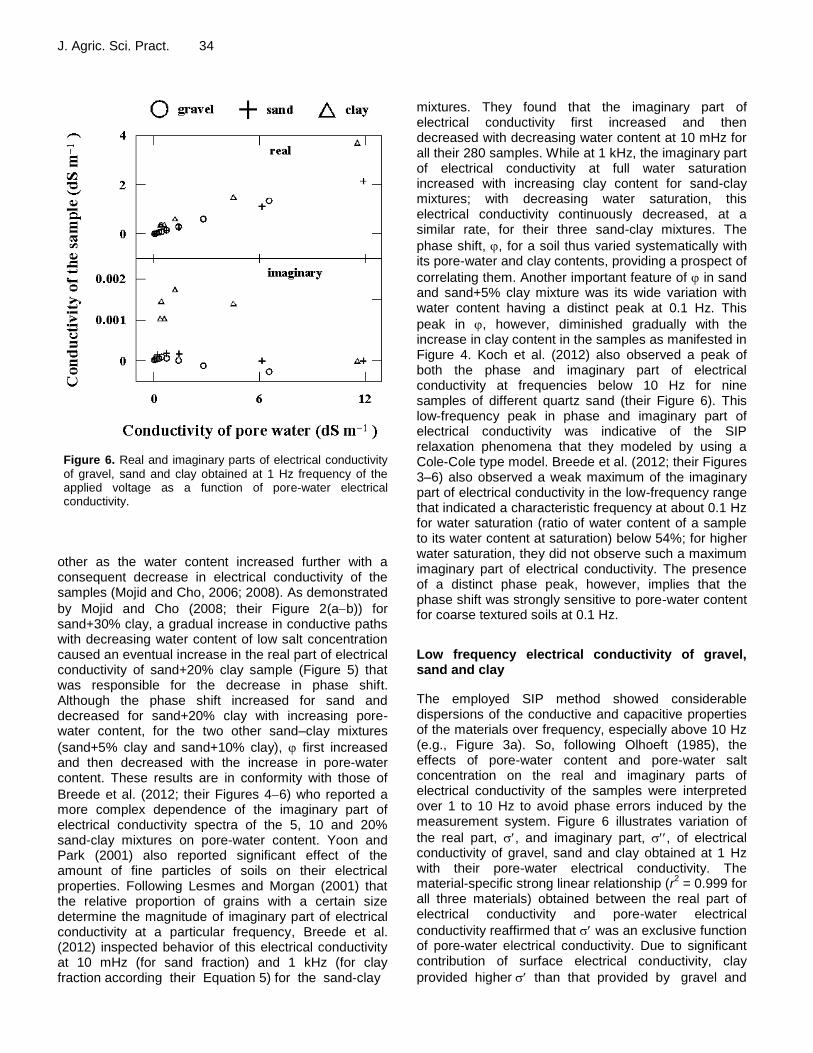
J. Agric. Sci. Pract. 34
Figure 6. Real and imaginary parts of electrical conductivity
of gravel, sand and clay obtained at 1 Hz frequency of the applied voltage as a function of pore-water electrical conductivity.
other as the water content increased further with a consequent decrease in electrical conductivity of the samples (Mojid and Cho, 2006; 2008). As demonstrated
by Mojid and Cho (2008; their Figure 2(ab)) for sand+30% clay, a gradual increase in conductive paths with decreasing water content of low salt concentration caused an eventual increase in the real part of electrical conductivity of sand+20% clay sample (Figure 5) that was responsible for the decrease in phase shift. Although the phase shift increased for sand and decreased for sand+20% clay with increasing pore-water content, for the two other sand–clay mixtures
(sand+5% clay and sand+10% clay), first increased and then decreased with the increase in pore-water content. These results are in conformity with those of
Breede et al. (2012; their Figures 46) who reported a more complex dependence of the imaginary part of electrical conductivity spectra of the 5, 10 and 20% sand-clay mixtures on pore-water content. Yoon and Park (2001) also reported significant effect of the amount of fine particles of soils on their electrical properties. Following Lesmes and Morgan (2001) that the relative proportion of grains with a certain size determine the magnitude of imaginary part of electrical conductivity at a particular frequency, Breede et al. (2012) inspected behavior of this electrical conductivity at 10 mHz (for sand fraction) and 1 kHz (for clay fraction according their Equation 5) for the sand-clay
mixtures. They found that the imaginary part of electrical conductivity first increased and then decreased with decreasing water content at 10 mHz for all their 280 samples. While at 1 kHz, the imaginary part of electrical conductivity at full water saturation increased with increasing clay content for sand-clay mixtures; with decreasing water saturation, this electrical conductivity continuously decreased, at a similar rate, for their three sand-clay mixtures. The
phase shift, , for a soil thus varied systematically with its pore-water and clay contents, providing a prospect of
correlating them. Another important feature of in sand and sand+5% clay mixture was its wide variation with water content having a distinct peak at 0.1 Hz. This
peak in , however, diminished gradually with the increase in clay content in the samples as manifested in Figure 4. Koch et al. (2012) also observed a peak of both the phase and imaginary part of electrical conductivity at frequencies below 10 Hz for nine samples of different quartz sand (their Figure 6). This low-frequency peak in phase and imaginary part of electrical conductivity was indicative of the SIP relaxation phenomena that they modeled by using a Cole-Cole type model. Breede et al. (2012; their Figures 3–6) also observed a weak maximum of the imaginary part of electrical conductivity in the low-frequency range that indicated a characteristic frequency at about 0.1 Hz for water saturation (ratio of water content of a sample to its water content at saturation) below 54%; for higher water saturation, they did not observe such a maximum imaginary part of electrical conductivity. The presence of a distinct phase peak, however, implies that the phase shift was strongly sensitive to pore-water content for coarse textured soils at 0.1 Hz.
Low frequency electrical conductivity of gravel, sand and clay
The employed SIP method showed considerable dispersions of the conductive and capacitive properties of the materials over frequency, especially above 10 Hz (e.g., Figure 3a). So, following Olhoeft (1985), the effects of pore-water content and pore-water salt concentration on the real and imaginary parts of electrical conductivity of the samples were interpreted over 1 to 10 Hz to avoid phase errors induced by the measurement system. Figure 6 illustrates variation of
the real part, , and imaginary part, , of electrical conductivity of gravel, sand and clay obtained at 1 Hz with their pore-water electrical conductivity. The material-specific strong linear relationship (r
2 = 0.999 for
all three materials) obtained between the real part of electrical conductivity and pore-water electrical
conductivity reaffirmed that was an exclusive function of pore-water electrical conductivity. Due to significant contribution of surface electrical conductivity, clay
provided higher than that provided by gravel and
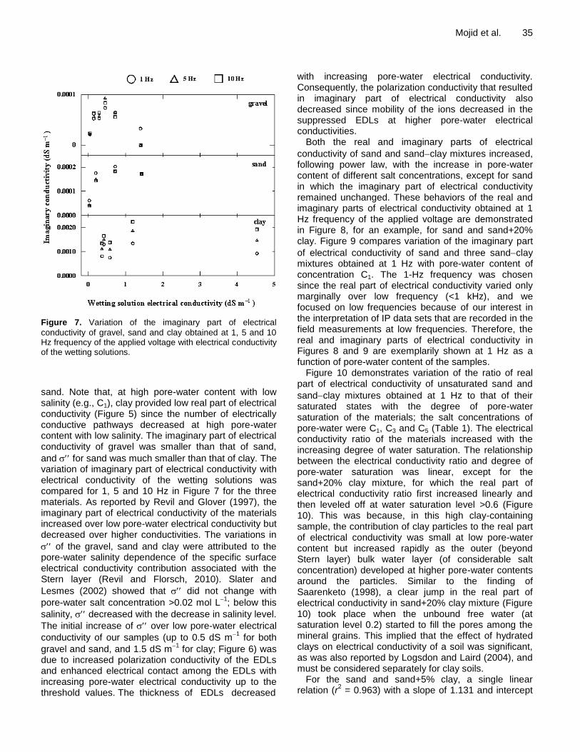
Figure 7. Variation of the imaginary part of electrical
conductivity of gravel, sand and clay obtained at 1, 5 and 10 Hz frequency of the applied voltage with electrical conductivity of the wetting solutions.
sand. Note that, at high pore-water content with low salinity (e.g., C1), clay provided low real part of electrical conductivity (Figure 5) since the number of electrically conductive pathways decreased at high pore-water content with low salinity. The imaginary part of electrical conductivity of gravel was smaller than that of sand,
and for sand was much smaller than that of clay. The variation of imaginary part of electrical conductivity with electrical conductivity of the wetting solutions was compared for 1, 5 and 10 Hz in Figure 7 for the three materials. As reported by Revil and Glover (1997), the imaginary part of electrical conductivity of the materials increased over low pore-water electrical conductivity but decreased over higher conductivities. The variations in
of the gravel, sand and clay were attributed to the pore-water salinity dependence of the specific surface electrical conductivity contribution associated with the Stern layer (Revil and Florsch, 2010). Slater and
Lesmes (2002) showed that did not change with
pore-water salt concentration >0.02 mol L1; below this
salinity, decreased with the decrease in salinity level.
The initial increase of over low pore-water electrical
conductivity of our samples (up to 0.5 dS m1 for both
gravel and sand, and 1.5 dS m1 for clay; Figure 6) was
due to increased polarization conductivity of the EDLs and enhanced electrical contact among the EDLs with increasing pore-water electrical conductivity up to the threshold values. The thickness of EDLs decreased
Mojid et al. 35 with increasing pore-water electrical conductivity. Consequently, the polarization conductivity that resulted in imaginary part of electrical conductivity also decreased since mobility of the ions decreased in the suppressed EDLs at higher pore-water electrical conductivities.
Both the real and imaginary parts of electrical
conductivity of sand and sandclay mixtures increased, following power law, with the increase in pore-water content of different salt concentrations, except for sand in which the imaginary part of electrical conductivity remained unchanged. These behaviors of the real and imaginary parts of electrical conductivity obtained at 1 Hz frequency of the applied voltage are demonstrated in Figure 8, for an example, for sand and sand+20% clay. Figure 9 compares variation of the imaginary part
of electrical conductivity of sand and three sandclay mixtures obtained at 1 Hz with pore-water content of concentration C1. The 1-Hz frequency was chosen since the real part of electrical conductivity varied only marginally over low frequency (<1 kHz), and we focused on low frequencies because of our interest in the interpretation of IP data sets that are recorded in the field measurements at low frequencies. Therefore, the real and imaginary parts of electrical conductivity in Figures 8 and 9 are exemplarily shown at 1 Hz as a function of pore-water content of the samples.
Figure 10 demonstrates variation of the ratio of real part of electrical conductivity of unsaturated sand and
sandclay mixtures obtained at 1 Hz to that of their saturated states with the degree of pore-water saturation of the materials; the salt concentrations of pore-water were C1, C3 and C5 (Table 1). The electrical conductivity ratio of the materials increased with the increasing degree of water saturation. The relationship between the electrical conductivity ratio and degree of pore-water saturation was linear, except for the sand+20% clay mixture, for which the real part of electrical conductivity ratio first increased linearly and then leveled off at water saturation level >0.6 (Figure 10). This was because, in this high clay-containing sample, the contribution of clay particles to the real part of electrical conductivity was small at low pore-water content but increased rapidly as the outer (beyond Stern layer) bulk water layer (of considerable salt concentration) developed at higher pore-water contents around the particles. Similar to the finding of Saarenketo (1998), a clear jump in the real part of electrical conductivity in sand+20% clay mixture (Figure 10) took place when the unbound free water (at saturation level 0.2) started to fill the pores among the mineral grains. This implied that the effect of hydrated clays on electrical conductivity of a soil was significant, as was also reported by Logsdon and Laird (2004), and must be considered separately for clay soils.
For the sand and sand+5% clay, a single linear relation (r
2 = 0.963) with a slope of 1.131 and intercept
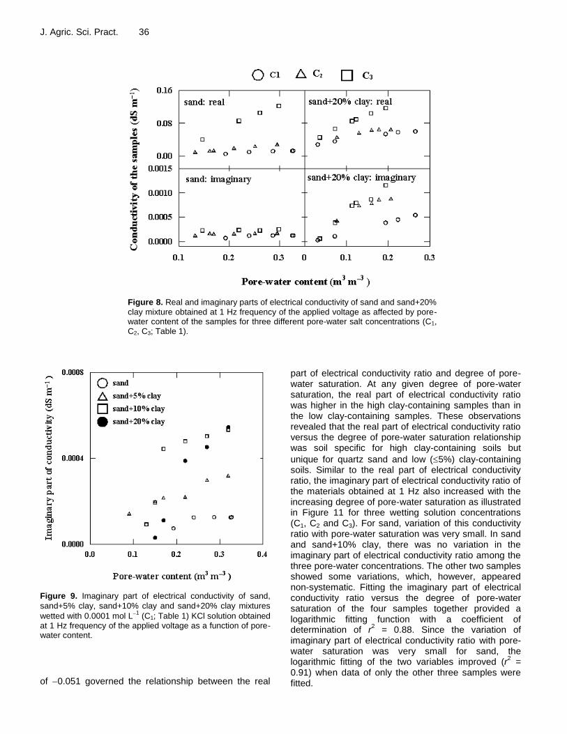
J. Agric. Sci. Pract. 36
Figure 8. Real and imaginary parts of electrical conductivity of sand and sand+20%
clay mixture obtained at 1 Hz frequency of the applied voltage as affected by pore-water content of the samples for three different pore-water salt concentrations (C1, C2, C3; Table 1).
Figure 9. Imaginary part of electrical conductivity of sand,
sand+5% clay, sand+10% clay and sand+20% clay mixtures
wetted with 0.0001 mol L1 (C1; Table 1) KCl solution obtained
at 1 Hz frequency of the applied voltage as a function of pore-water content.
of 0.051 governed the relationship between the real
part of electrical conductivity ratio and degree of pore-water saturation. At any given degree of pore-water saturation, the real part of electrical conductivity ratio was higher in the high clay-containing samples than in the low clay-containing samples. These observations revealed that the real part of electrical conductivity ratio versus the degree of pore-water saturation relationship was soil specific for high clay-containing soils but
unique for quartz sand and low (5%) clay-containing soils. Similar to the real part of electrical conductivity ratio, the imaginary part of electrical conductivity ratio of the materials obtained at 1 Hz also increased with the increasing degree of pore-water saturation as illustrated in Figure 11 for three wetting solution concentrations (C1, C2 and C3). For sand, variation of this conductivity ratio with pore-water saturation was very small. In sand and sand+10% clay, there was no variation in the imaginary part of electrical conductivity ratio among the three pore-water concentrations. The other two samples showed some variations, which, however, appeared non-systematic. Fitting the imaginary part of electrical conductivity ratio versus the degree of pore-water saturation of the four samples together provided a logarithmic fitting function with a coefficient of determination of r
2 = 0.88. Since the variation of
imaginary part of electrical conductivity ratio with pore-water saturation was very small for sand, the logarithmic fitting of the two variables improved (r
2 =
0.91) when data of only the other three samples were fitted.
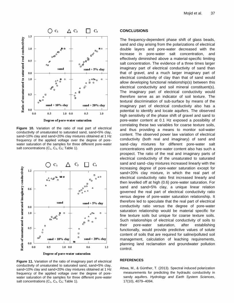
Figure 10. Variation of the ratio of real part of electrical
conductivity of unsaturated to saturated sand, sand+5% clay, sand+10% clay and sand+20% clay mixtures obtained at 1 Hz frequency of the applied voltage over the degree of pore-water saturation of the samples for three different pore-water salt concentrations (C1, C3, C5; Table 1).
Figure 11. Variation of the ratio of imaginary part of electrical
conductivity of unsaturated to saturated sand, sand+5% clay, sand+10% clay and sand+20% clay mixtures obtained at 1 Hz frequency of the applied voltage over the degree of pore-water saturation of the samples for three different pore-water salt concentrations (C1, C3, C5; Table 1).
Mojid et al. 37 CONCLUSIONS
The frequency-dependent phase shift of glass beads,
sand and clay arising from the polarizations of electrical
double layers and pore-water decreased with the
increase in pore-water salt concentration, and
effectively diminished above a material-specific limiting
salt concentration. The evidence of a three times larger
imaginary part of electrical conductivity of sand than
that of gravel, and a much larger imaginary part of
electrical conductivity of clay than that of sand would
allow developing functional relationship(s) between this
electrical conductivity and soil mineral constituent(s).
The imaginary part of electrical conductivity would
therefore serve as an indicator of soil texture. The
textural discrimination of sub-surface by means of the
imaginary part of electrical conductivity also has a
potential to identify and locate aquifers. The observed
high sensitivity of the phase shift of gravel and sand to
pore-water content at 0.1 Hz exposed a possibility of
correlating these two variables for coarse texture soils,
and thus providing a means to monitor soil-water
content. The observed power law variation of electrical
conductivity (both real and imaginary) of sand and
sandclay mixtures for different pore-water salt
concentrations with pore-water content also has such a
prospect. The ratio of the real and imaginary parts of
electrical conductivity of the unsaturated to saturated
sand and sandclay mixtures increased linearly with the
increasing degree of pore-water saturation except for
sand+20% clay mixture, in which the real part of
electrical conductivity ratio first increased linearly and
then levelled off at high (0.6) pore-water saturation. For
sand and sand+5% clay, a unique linear relation
governed the real part of electrical conductivity ratio
versus degree of pore-water saturation relationship. It
therefore led to speculate that the real part of electrical
conductivity ratio versus the degree of pore-water
saturation relationship would be material specific for
fine texture soils but unique for coarse texture soils.
Such relationships of electrical conductivity of soils to
their pore-water saturation, after establishing
functionally, would provide predictive values of solute
content of soils that are required for saline/polluted soil
management, calculation of leaching requirements,
planning land reclamation and groundwater pollution
control.
REFERENCES
Attwa, M., & Günther, T. (2013). Spectral induced polarization
measurements for predicting the hydraulic conductivity in
sandy aquifers. Hydrology and Earth System Sciences,
17(10), 4079–4094.
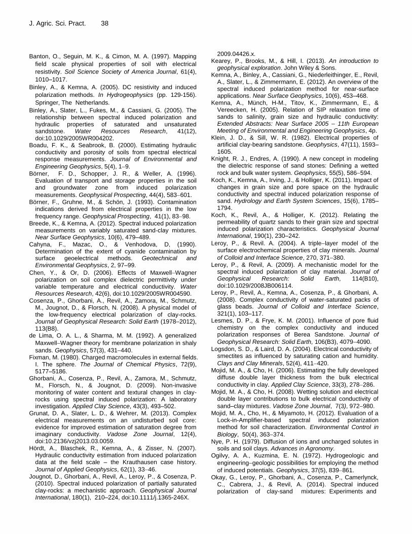
J. Agric. Sci. Pract. 38
Banton, O., Seguin, M. K., & Cimon, M. A. (1997). Mapping
field scale physical properties of soil with electrical
resistivity. Soil Science Society of America Journal, 61(4),
1010–1017.
Binley, A., & Kemna, A. (2005). DC resistivity and induced
polarization methods. In Hydrogeophysics (pp. 129-156).
Springer, The Netherlands.
Binley, A., Slater, L., Fukes, M., & Cassiani, G. (2005). The relationship between spectral induced polarization and hydraulic properties of saturated and unsaturated sandstone. Water Resources Research, 41(12), doi:10.1029/2005WR004202.
Boadu, F. K., & Seabrook, B. (2000). Estimating hydraulic conductivity and porosity of soils from spectral electrical response measurements. Journal of Environmental and
Engineering Geophysics, 5(4), 19.
Börner, F. D., Schopper, J. R., & Weller, A. (1996). Evaluation of transport and storage properties in the soil and groundwater zone from induced polarization
measurements. Geophysical Prospecting, 44(4), 583601.
Börner, F., Gruhne, M., & Schön, J. (1993). Contamination indications derived from electrical properties in the low
frequency range. Geophysical Prospecting, 41(1), 8398.
Breede, K., & Kemna, A. (2012). Spectral induced polarization measurements on variably saturated sand-clay mixtures. Near Surface Geophysics, 10(6), 479–489.
Cahyna, F., Mazac, O., & Venhodova, D, (1990). Determination of the extent of cyanide contamination by surface geoelectrical methods. Geotechnical and Environmental Geophysics, 2, 97–99.
Chen, Y., & Or, D. (2006). Effects of MaxwellWagner polarization on soil complex dielectric permittivity under variable temperature and electrical conductivity. Water Resources Research, 42(6), doi:10.1029/2005WR004590.
Cosenza, P., Ghorbani, A., Revil, A., Zamora, M., Schmutz, M., Jougnot, D., & Florsch, N. (2008). A physical model of the low-frequency electrical polarization of clay-rocks. Journal of Geophysical Research: Solid Earth (1978–2012), 113(B8).
de Lima, O. A. L., & Sharma, M. M. (1992). A generalized
MaxwellWagner theory for membrane polarization in shaly
sands. Geophysics, 57(3), 431440. Fixman, M. (1980). Charged macromolecules in external fields.
I. The sphere. The Journal of Chemical Physics, 72(9), 5177–5186.
Ghorbani, A., Cosenza, P., Revil, A., Zamora, M., Schmutz, M., Florsch, N., & Jougnot, D. (2009). Non-invasive monitoring of water content and textural changes in clay-rocks using spectral induced polarization: A laboratory investigation. Applied Clay Science, 43(3), 493–502.
Grunat, D. A., Slater, L. D., & Wehrer, M. (2013). Complex electrical measurements on an undisturbed soil core: evidence for improved estimation of saturation degree from imaginary conductivity. Vadose Zone Journal, 12(4), doi:10.2136/vzj2013.03.0059.
Hördt, A., Blaschek, R., Kemna, A., & Zisser, N. (2007). Hydraulic conductivity estimation from induced polarization data at the field scale – the Krauthausen case history.
Journal of Applied Geophysics, 62(1), 3346.
Jougnot, D., Ghorbani, A., Revil, A., Leroy, P., & Cosenza, P. (2010). Spectral induced polarization of partially saturated clay-rocks: a mechanistic approach. Geophysical Journal International, 180(1), 210–224, doi:10.1111/j.1365-246X.
2009.04426.x. Kearey, P., Brooks, M., & Hill, I. (2013). An introduction to
geophysical exploration. John Wiley & Sons. Kemna, A., Binley, A., Cassiani, G., Niederleithinger, E., Revil,
A., Slater, L., & Zimmermann, E. (2012). An overview of the spectral induced polarization method for near-surface applications. Near Surface Geophysics, 10(6), 453–468.
Kemna, A., Münch, H-M., Titov, K., Zimmermann, E., & Vereecken, H. (2005). Relation of SIP relaxation time of sands to salinity, grain size and hydraulic conductivity: Extended Abstracts: Near Surface 2005 – 11th European Meeting of Environmental and Engineering Geophysics, 4p.
Klein, J. D., & Sill, W. R. (1982). Electrical properties of artificial clay-bearing sandstone. Geophysics, 47(11), 1593–
1605. Knight, R. J., Endres, A. (1990). A new concept in modeling
the dielectric response of sand stones: Defining a wetted
rock and bulk water system. Geophysics, 55(5), 586594.
Koch, K., Kemna, A., Irving, J., & Holliger, K. (2011). Impact of changes in grain size and pore space on the hydraulic conductivity and spectral induced polarization response of sand. Hydrology and Earth System Sciences, 15(6), 1785–1794.
Koch, K., Revil, A., & Holliger, K. (2012). Relating the permeability of quartz sands to their grain size and spectral induced polarization characteristics. Geophysical Journal International, 190(1), 230–242.
Leroy, P., & Revil. A. (2004). A triplelayer model of the surface electrochemical properties of clay minerals. Journal
of Colloid and Interface Science, 270, 371380.
Leroy, P., & Revil, A. (2009). A mechanistic model for the spectral induced polarization of clay material. Journal of Geophysical Research: Solid Earth, 114(B10), doi:10.1029/2008JB006114.
Leroy, P., Revil, A., Kemna, A., Cosenza, P., & Ghorbani, A. (2008). Complex conductivity of water-saturated packs of glass beads. Journal of Colloid and Interface Science, 321(1), 103–117.
Lesmes, D. P., & Frye, K. M. (2001). Influence of pore fluid chemistry on the complex conductivity and induced polarization responses of Berea Sandstone. Journal of
Geophysical Research: Solid Earth, 106(B3), 40794090.
Logsdon, S. D., & Laird, D. A. (2004). Electrical conductivity of smectites as influenced by saturating cation and humidity.
Clays and Clay Minerals, 52(4), 411420. Mojid, M. A., & Cho, H. (2006). Estimating the fully developed
diffuse double layer thickness from the bulk electrical
conductivity in clay. Applied Clay Science, 33(3), 278286.
Mojid, M. A., & Cho, H. (2008). Wetting solution and electrical double layer contributions to bulk electrical conductivity of
sand–clay mixtures. Vadose Zone Journal, 7(3), 972980.
Mojid, M. A., Cho, H., & Miyamoto, H. (2012). Evaluation of a Lock-in-Amplifier-based spectral induced polarization method for soil characterization. Environmental Control in
Biology, 50(4), 363374.
Nye, P. H. (1979). Diffusion of ions and uncharged solutes in soils and soil clays. Advances in Agronomy.
Ogilvy, A. A., Kuzmina, E. N. (1972). Hydrogeologic and
engineeringgeologic possibilities for employing the method
of induced potentials. Geophysics, 37(5), 839861.
Okay, G., Leroy, P., Ghorbani, A., Cosenza, P., Camerlynck, C., Cabrera, J., & Revil, A. (2014). Spectral induced polarization of clay-sand mixtures: Experiments and

modeling. Geophysics, 79(6), E353–E375.
Olhoeft, G. R. (1985). Low-frequency electrical properties.
Geophysics, 50(12), 24922503.
Personna, Y. R., Slater, L., Ntarlagiannis, D., Werkema, D., & Szabo, Z. (2013). Complex resistivity signatures of ethanol in sand–clay mixtures. Journal of Contaminant Hydrology,
149, 7687. Revil, A. (1999). Ionic diffusivity, electrical conductivity,
membrane and thermoelectric potentials in colloids and granular porous media: A unified model. Journal of Colloid
and Interface Science, 212(2), 503522.
Revil, A. (2012). Spectral induced polarization of shaly sands: Influence of the electrical double layer. Water Resources Research, 48(2), W02517.
Revil, A. (2013). Effective conductivity and permittivity of unsaturated porous materials in the frequency range 1 mHz–1GHz. Water Resources Research, 49(1), 306–327.
Revil, A., & Florsch, N. (2010). Determination of permeability from spectral induced polarization in granular media.
Geophysical Journal International, 181(3), 14801498.
Revil, A., Glover, P. W. J. (1997). Theory of ionic-surface electrical conduction in porous media. Physical Review B, 55(3), 1757.
Revil, A., Koch, K., & Holliger, K. (2012). Is it the grain size or the characteristic pore size that controls the induced polarization relaxation time of clean sands and sandstones?. Water Resources Research, 48(5), W05602. doi: 10.1029/2011WR011561.
Saarenketo, T. (1998). Electrical properties of water in clay
and silty soils. Journal of Applied Geophysics, 40(1), 7388. Sadowski, R. M. (1988). Clay-organic interactions: M.Sc.
Thesis, Dept. of Geochemistry, Colo. School of Mines, Golden, CO, 209p.
Samouëlian, A., Cousin, I., Tabbagh, A., Bruand, A., & Richard, G. (2005). Electrical resistivity survey in soil
science: a review. Soil and Tillage research, 83(2), 173193.
Schwartz, N., & Furman, A. (2015). On the spectral induced polarization signature of soil organic matter. Geophysical Journal International, 200(1), 589–595.
Schwarz, G. (1962). A theory of the low-frequency dielectric dispersion of colloidal particles in electrolyte solution 1, 2.
The Journal of Physical Chemistry, 66(12), 2636264.
Scollar, I., Tabbagh, A., Hesse, A., Herzog, I. (1990). Archaeological prospecting and remote sensing, Cambridge University Press, 674p.
Scott, J. B., & Barker, R. D. (2003). Determining pore‐throat
size in Permo‐Triassic sandstones from low‐frequency electrical spectroscopy. Geophysical Research Letters, 30(9).
Slater, L., Lesmes, D. (2002). Electrical-hydraulic relationships observed for unconsolidated sediments. Water Resources Research, 38(10), doi:10.1029/2001WR00107.
Slater, L., Ntarlagiannis, D., & Wishart, De. (2006). On the
relationship between induced polarization and surface area
in metalsand and claysand mixtures. Geophysics, 71(2),
A1-A5, doi:10.1190/1.2187707.
Stern, O. (1924). Zur Theorie der elektrolytischen
Doppelschicht. Zeitschrift für Elektrochemie und
Angewandte Physikalische Chemie, 30(21‐22), 508516.
Sturrock, J. T. (1999). Estimates of permeability from broadband (spectral) induced polarization measurements, M. S. thesis, Boston College, Chestnut Hill, Mass.
Sumner, J. S. (2012). Principles of induced polarization for
Mojid et al. 39
geophysical exploration (Vol. 5). Elsevier.
Tong, M., Li, L., Wang, W., & Jiang, Y. (2006). A time-domain induced polarization method for estimating permeability in a shaly sand reservoir. Geophysical Prospecting, 54(5), 623–631.
Ulrich, C., & Slater, L. (2004). Spectral-induced polarization measurements on unsaturated unconsolidated sediments.
Geophysics, 69(3), 762771.
Ustra, A., Slater, L., Ntarlagiannis, D., & Elis, V. (2012). Spectral induced polarization (SIP) signatures of clayey soils containing toluene. Near Surface Geophysics, 10(6),
503515. Vanhala, H., & Soininen, H. (1995). Laboratory technique for
measurement of spectral induced polarization response of
soil samples. Geophysical Prospecting, 43(5), 655676.
Vinegar, H. J., & Waxman, M. H. (1984). Induced polarization of shaly sands. Geophysics, 49(8), 1267–1287.
Society of Exploration Geophysicists (SEG). (1990). Geotechnical and environmental geophysics (Vol. 1, Pp. 147-189). Ward, S. H. (Ed.). Tulsa, Oklahoma: Society of Exploration Geophysicists.
Waxman, M. H., & Smits, L. J. M. (1968). Electrical conductivities in oil-bearing shaly sands. Society of Petroleum Engineers Journal, 8(2), 107–122.
Weller, A., & Börner, F. D. (1996). Measurements of spectral induced polarization for environmental purposes.
Environmental Geology, 27(4), 329334.
Weller, A., Nordsiek, S., & Debschütz, W. (2010a). Estimating permeability of sandstone samples by nuclear magnetic resonance and spectral-induced polarization. Geophysics, 75(6), E215–E226.
Weller, A., Seichter, M., & Kampke, A. (1996). Induced-polarization modelling using complex electrical conductivities. Geophysical Journal International, 127(2),
387398. Weller, A., & Slater, L. (2012). Salinity dependence of
complex conductivity of unconsolidated and consolidated materials: Comparisons with electrical double layer models. Geophysics, 77(5), D185–D198.
Weller, A., Slater, L., Huisman, J. A., Esser, O., & Haegel, F. H. (2015). On the specific polarizability of sands and sand-clay mixtures. Geophysics, 80(3), A57–A61.
Weller, A., Slater, L., & Nordsiek, S. (2013). On the relationship between induced polarization and surface conductivity: Implications for petrophysical interpretation of electrical measurements. Geophysics, 78(5), D315–D325.
Weller, A., Slater, L., Nordsiek, S., & Ntarlagiannis, D. (2010b). On the estimation of specific surface per unit pore volume from induced polarization: A robust empirical relation fits multiple data sets. Geophysics, 75(4), WA105–WA112.
Yoon, G. L., & Park, J. B. (2001). Sensitivity of leachate and fine contents on electrical resistivity variations of sandy
soils. Journal of Hazardous Materials, 84(2), 147161.
Zimmermann, E., Kemna, A., Berwix, J., Glaas, W., Münch, H-M., & Huisman, J. A. (2008). A high-accuracy impedance spectrometer for measuring sediments with low polarizability. Measurement Science and Technology, 19(10), 105603, doi:10.1088/0957-0233/19/10/105603.
Zisser, N., Kemna, A., & Nover, G. (2010). Relationship between low-frequency electrical properties and hydraulic permeability of low-permeability sandstones. Geophysics, 75(3), 75, E131–E141.

Journal of Bioscience and Biotechnology Discovery Research Journal of Food Science and Nutrition Journal of Practical Medicine and Medical Science Journal of Public Health and Diseases Global Journal of Earth and Environmental Science Journal of Drugs and Pharmaceutical Science Journal of Animal Science and Veterinary Medicine Journal of Engineering Innovations and Applications Applied Journal of Physical Science Integrity Journal of Education and Training Research Journal of Business and Economic Management
Other Journals

Journal of Agricultural
Science and Practice
First Quarter E-Book January-March 2016