journal of computational...
TRANSCRIPT

Journal of Computational Physics 321 (2016) 776–796
Contents lists available at ScienceDirect
Journal of Computational Physics
www.elsevier.com/locate/jcp
A Hamiltonian preserving discontinuous Galerkin method
for the generalized Korteweg–de Vries equation
Hailiang Liu a,∗, Nianyu Yi b,∗a Iowa State University, Mathematics Department, Ames, IA 50011, United Statesb School of Mathematics and Computational Science, Xiangtan University, Xiangtan 411105, PR China
a r t i c l e i n f o a b s t r a c t
Article history:Received 11 January 2015Received in revised form 4 March 2016Accepted 6 June 2016Available online 9 June 2016
Keywords:Discontinuous Galerkin methodKorteweg–de Vries equationConservationStability
The invariant preserving property is one of the guiding principles for numerical algorithms in solving wave equations, in order to minimize phase and amplitude errors after long time simulation. In this paper, we design, analyze and numerically validate a Hamiltonian preserving discontinuous Galerkin method for solving the Korteweg–de Vries (KdV) equation. For the generalized KdV equation, the semi-discrete formulation is shown to preserve both the first and the third conserved integrals, and approximately preserve the second conserved integral; for the linearized KdV equation, all the first three conserved integrals are preserved, and optimal error estimates are obtained for polynomials of even degree. The preservation properties are also maintained by the fully discrete DG scheme. Our numerical experiments demonstrate both high accuracy of convergence and preservation of all three conserved integrals for the generalized KdV equation. We also show that the shape of the solution, after long time simulation, is well preserved due to the Hamiltonian preserving property.
© 2016 Elsevier Inc. All rights reserved.
1. Introduction
This paper is the continuation of our project, initiated in [40], of developing a high order discontinuous Galerkin (DG) method to preserve some key invariants for the generalized Korteweg–de Vries (gKdV) [18] equation:
ut + f (u)x + εuxxx = 0, x ∈R, t > 0, (1)
where the subscript t (or x, respectively) denotes the differentiation with respect to time variable t (or x), ε is a given constant, and f is a smooth function. This is a nonlinear, dispersive partial differential equation for u of two real variables. The original form of the KdV equation corresponds to (1) with ε = 1 and f = 3u2.
The KdV equation has several connections to physical problems. In addition to being the governing equation of the string in the Fermi–Pasta–Ulam problem in the continuum limit, it approximately describes the evolution of long, one-dimensional waves in many physical settings, including shallow-water waves with weakly non-linear restoring forces, long internal waves in a density-stratified ocean, ion-acoustic waves in a plasma, acoustic waves on a crystal lattice, and more.
Dispersion and non-linearity can interact to produce permanent and localized wave forms; It can be shown that any sufficiently fast decaying smooth solution will eventually split into a finite superposition of solitons traveling to the right
* Corresponding authors.E-mail addresses: [email protected] (H. Liu), [email protected] (N. Yi).
http://dx.doi.org/10.1016/j.jcp.2016.06.0100021-9991/© 2016 Elsevier Inc. All rights reserved.

H. Liu, N. Yi / Journal of Computational Physics 321 (2016) 776–796 777
plus a decaying dispersive part traveling to the left. This was first observed numerically by Zabusky & Kruskal (1965) [41], long after John Scott Russell’s experimental observation of solitons in 1834. One appealing feature of the KdV equation is that it has infinitely many integrals of motion (Miura, Gardner & Kruskal 1968) [27], which do not change with time. This is also accounted by the fact that the KdV equation can be reformulated into the Lax system, called Lax pairs [20].
The KdV equation is rich in conserved integrals; the first three for (1) are classical:
E1 =∫R
udx, E2 =∫R
u2dx, and E3 =∫R
⎛⎝ε
2u2
x −u∫
f (ξ)dξ
⎞⎠dx. (2)
The quality of the numerical approximation hence hinges on how well the conserved integrals can be preserved at the discrete level. The objective of this work is to develop a novel DG method to preserve these three conserved integrals at the discrete setting.
The conservation law structure of many PDEs is considered fundamental to their derivation, their behavior, and their dis-cretization. For conservative PDEs, numerical methods preserving their invariants are often advantageous: besides the high accuracy of numerical solutions, an invariant preserving scheme can maintain good stability properties over a long-time pe-riod. Numerical methods without this property may result in substantial phase and shape errors after long time integration. There are many numerical works in the literature to solve the KdV equation, ranging from finite difference methods [10,12,13,19,32,41], finite element methods [1,29,31], spectral methods [9,14,23,25,26,30], operator splitting methods [16,15], and discontinuous Galerkin methods [3,22,34,35,39]. However, the majority of the developed methods is designed to preserve only E1, not other invariants.
The earlier effort of inheriting some invariants as characteristic properties followed mainly the symplectic method for Hamiltonian ODEs; for instance, Furihata [10] designed a finite difference scheme to preserve both E1 and E3. Preservation of E1 and E2 in the context of the DG method has been recently investigated by Bona et al. [2] and the authors [40].
Discovered by Gardner [11] and also by Faddeev and Zakharov [8], the KdV equation is a Hamiltonian system, allowing for an infinite sequence of Hamiltonians. For the generalized KdV equation (1), E3 is still a Hamiltonian since (1) is equivalent to
ut =(
δE3
δu
)x.
This Hamiltonian structure sets the basis to construct an E3 preserving discretization for (1). In the case f (u) = u2/2, E2 is also a Hamiltonian since the KdV equation can be written as
ut =N(
δE2
δu
),
where the Lenard operator N = −(∂2x + 2
3 u∂x + 13 ∂xu) is linear and anti-symmetric. The main novelty in this work is the
preservation of E3 by our method, which we call the Hamiltonian preserving DG method. Indeed, the proposed method is shown to preserve all three conserved integrals for the linearized KdV equation, and preserve both E1 and E3 for the gen-eralized nonlinear KdV equation (1). The preservation of E2 is investigated with care: we observe that E2 is still preserved numerically, though its preservation is only shown in approximation sense. As illustrated in our numerical comparison (see Fig. 3), the E3-preserving scheme performs clearly better than the E2-preserving scheme introduced in [40]. Moreover, we observe large oscillations in the temporal evolution of E3 when testing the E2-preserving scheme (see Fig. 3(c)). To our best knowledge, the present DG method is the first one that can preserve all three invariants Ei (i = 1, 2, 3) numerically.
As for the numerical convergence, we should mention that the common feature of these central fluxes based DG methods is that the optimal order of accuracy can be achieved only for polynomials of even degree, as proved for the linearized KdV equation and numerically observed for the generalized KdV equation.
The DG method we discuss in this paper is a class of finite element methods using completely discontinuous piecewise-polynomial space for the numerical solution and the test functions in the spatial variables. The application of DG methods to hyperbolic problems has been quite successful, e.g., Reed and Hill [28] for solving linear equations, and Cockburn et al. [4–7] for solving nonlinear equations, and the DG methods have been extended to various higher order PDEs by many authors, including the KdV type equations; see, e.g., [39,37,2,38,40], the Camassa–Holm equation [36] and the Degasperis-Procesi equation [33,21]. These DG methods have several attractive properties. For instance, it can be easily designed for any order of accuracy, with the order of accuracy locally determined in each cell, thus allowing for efficient p adaptivity. The advantage of invariants preserving methods is to solve smooth wave problems, with the attempt to resolve all wave patterns for long time periods.
Obtaining a priori error estimates for various DG methods has been a main subject of research. The L2 a priori error estimates for nonlinear PDEs with high order derivatives such as the KdV equations have been obtained [39,35,3] using certain special local projections. For the conservative DG method for the generalized KdV equation in [2], a global projection was used in obtaining error estimates in some cases. Optimal L2 error estimates of the LDG method for the linearized KdV equation were obtained by Xu and Shu [38], where authors take advantage of stability estimates for auxiliary variables. The way of using error equations in the present work is closely related to that in [38].

778 H. Liu, N. Yi / Journal of Computational Physics 321 (2016) 776–796
This paper is organized as follows. In Section 2, we present the semi-discrete DG method for the generalized KdV equation, and prove its invariant preserving properties. The optimal error estimate is also analyzed for the linearized KdV equation in Section 2 when polynomials are of even degree, and therein, the upper bound of errors is proved to grow linearly in time. In Section 3, we present the fully discrete DG method with invariants preserving properties. Section 4contains numerical experiments that demonstrate the optimal convergence rates and invariants conservation of the proposed DG method. Finally, we give the concluding remarks in Section 5.
2. DG for the generalized KdV equation
We consider the generalized KdV equation of the form
ut = −( f (u) + uxx)x,
subject to initial data u(x, 0) = u0(x) and periodic boundary conditions. In order to design a DG method preserving three invariants, we reformulate this form into the following system
ut = qx, (3a)
q = − rx − f (u), (3b)
r = ux. (3c)
The third conservation law for the generalized KdV equation can be expressed as
E3 =∫ (
1
2r2 − F (u)
)dx, F (u) =
u∫0
f (ξ)dξ. (4)
2.1. DG formulation
Let us denote the computational mesh of the domain I by
I j = (x j−1/2, x j+1/2), j = 1, . . . , N.
The cell center is x j = (x j−1/2 + x j+1/2)/2, with h j = x j+1/2 − x j−1/2, and h = max1≤ j≤N h j . We assume that the mesh is regular, namely there is a constant c > 0 independent of h such that
ch ≤ h j, j = 1, · · · , N.
When c = 1, the mesh is uniform. We denote by w+j+1/2 the value of w at x j+1/2 evaluated from the right element I j+1,
and w−j+1/2 the value of w at x j+1/2 evaluated from the left element I j . [w] = w+ − w− denotes the jump of w at cell
interfaces, and {w} = 12 (w+ + w−) denotes the average of the left and right interface values. We then define the piecewise
polynomial space Vh as the space of polynomials of degree k in each cell I j , i.e.,
Vh = {w : w ∈ Pk(I j) for x ∈ I j, j = 1, . . . , N}.The DG method is formulated as follows: find uh, qh, rh ∈ Vh , such that ∀ξ, η, ρ ∈ Vh ,∫
I j
uhtξdx = −∫I j
qhξxdx + (qhξ)|∂ I j , (5a)
∫I j
qhηdx =∫I j
rhηxdx − (rhη)|∂ I j −∫I j
f (uh)ηdx, (5b)
∫I j
rhρdx +∫
uhρxdx − (uhρ)|∂ I j = 0, (5c)
with the numerical fluxes
(qh, rh, uh) = ({qh}, {rh}, {uh}). (6)
Here we have used the notation ξ |∂ I j = ξ(x− ) − ξ(x+ ) to denote interface terms.
j+1/2 j−1/2
H. Liu, N. Yi / Journal of Computational Physics 321 (2016) 776–796 779
The global form of the DG formulation may be obtained by summing (5) over all j’s,∫uhtξdx = −
∫qhξxdx −
∑j
(qh[ξ ]) j+1/2, (7a)
∫qhηdx =
∫rhηxdx +
∑j
rh[η] j+1/2 −∫
f (uh)ηdx, (7b)
∫rhρdx +
∫uhρxdx +
∑j
uh[ρ] j+1/2 = 0, (7c)
where ∫ =∑N
j=1
∫I j
, and the periodic boundary conditions have been used.
2.2. Conservative properties
We now turn to establish the conservation properties.
Theorem 2.1. Let (qh, rh, uh) be obtained from the DG scheme (7). Then both invariants E1 and E3 are preserved in the sense that
d
dt
∫uhdx = 0,
d
dt
∫ (1
2r2
h − F (uh)
)dx = 0. (8)
E2 is preserved for f (u) = αu. For nonlinear flux, we have
d
dt
∫u2
h
2dx =
∑j
⎛⎜⎜⎝{ f (uh)}(u+h − u−
h ) −u+
h∫u−
h
f (u)du
⎞⎟⎟⎠x j+1/2
, (9)
where denotes the piecewise L2-projection on space Pk:∫I j
f (u)vdx =∫I j
f (u)vdx, ∀v ∈ Pk(I j), j = 1,2, · · · , N.
Proof. To see the scheme preserves E1 we simply take ξ = 1 in (7a) to obtain ddt
∫uhdx = 0. To show the conservation
of E3, we take ξ = qh in (7a), η = −uht in (7b) and ρ = rh in ∂t (7c) to obtain∫uhtqhdx = −
∫qhqhxdx −
∑j
(qh[qh]) j+1/2,
−∫
qhuhtdx = −∫
rhuhtxdx −∑
j
rh[uht] j+1/2 +∫
f (uh)uhtdx,
∫rhtrhdx +
∫uhtrhxdx +
∑j
uht[rh] j+1/2 = 0.
Adding the above together and integrating the complete derivative out, we obtain
d
dt
∫ (r2
h
2− F (uh)
)dx = −
N∑j=1
(rh[uht] + uht[rh] − [uhtrh]
)j+1/2 = 0.
We next derive temporal change rate of E2.Take ξ = uh , η = rh , ρ = qh in (7) we get∫
uht uhdx = −∫
qhuhxdx −∑
j
(qh[uh]) j+1/2,∫qhrhdx =
∫rhrhxdx +
∑j
rh[rh] j+1/2 −∫
f (uh)rhdx,
∫rhqhdx +
∫uhqhxdx +
∑j
uh[qh] j+1/2 = 0.

780 H. Liu, N. Yi / Journal of Computational Physics 321 (2016) 776–796
Adding the above together and integrating the complete derivative out, we obtain
d
dt
∫u2
h
2dx =
∫f (uh)rhdx =
∑j
∫I j
f (uh)rhdx.
Set ρ = f (uh) in (7c) we have
d
dt
∫u2
h
2dx =
∑j
∫I j
f (uh)rhdx
= −∑
j
∫I j
uh( f (uh))xdx −∑
j
uh[ f (uh)] j+1/2
=∑
j
({ f (uh)}[uh]) j+1/2 +∑
j
∫I j
f (uh) · uhxdx
=∑
j
⎛⎜⎝{ f (uh)} −∫ u+
h
u−h
f (u)du
u+h − u−
h
⎞⎟⎠ [uh].
Note that for linear equation f (u) = −αu, we have
{ f (uh)} −∫ u+
h
u−h
f (u)du
u+h − u−
h
= 0,
hence E2 is also exactly preserved. This finishes the proof of the theorem. �Remark 2.1. For nonlinear flux, the change rate of E2 is in general non-vanishing, but can be quite small. For instance, if uh|I j ∈ P 0(I j), the change rate reduces to∣∣∣∣∣∣∣∣
∑j
⎛⎜⎜⎝ f (u+h ) + f (u−
h )
2[uh] −
u+h∫
u−h
f (u)du
⎞⎟⎟⎠j+1/2
∣∣∣∣∣∣∣∣≤max | f ′′|
12
∑j
|u+h − u−
h |3j+1/2 ∼ h2,
at least for approximating smooth solutions.
Remark 2.2. In the DG formulation (7), the nonlinear term ∫
f (uh)ηdx is calculated by quadratures with accuracy of order bigger than O (hk+2). For instance, if we use a Gauss quadrature with L ≥ k
2 + 1 points, it has accuracy of order at least O (hk+2). The evaluation of E3 involves the calculation of
∫F (uh)dx, for which we need to use quadratures with sufficient
accuracy. In our numerical examples, f (u) = u2/2, then F (uh) is a polynomial of degree 3k, for which we use a Gauss quadrature with L points, L ≥ 3k−1
2 , so that the numerical evaluation of E3 is exact.
2.3. Error estimation for the linearized KdV equation
In the following, we derive the error estimation of the discontinuous Galerkin method for the linearized KdV equation of the form
ut − αux + uxxx = 0, (10)
subject to initial data u0(x) and periodic boundary conditions.The corresponding DG method for (10) is formulated as follows: find uh, qh, rh ∈ Vh , such that ∀ξ, η, ρ ∈ Vh ,∫
I j
uhtξdx +∫I j
qhξxdx − qhξ |∂ I j = 0, (11a)
∫I
qhηdx −∫I
rhηxdx + rhη|∂ I j − α
∫I
uhηdx = 0, (11b)
j j j

H. Liu, N. Yi / Journal of Computational Physics 321 (2016) 776–796 781
∫I jrhρdx +∫
uhρxdx − uhρ|∂ I j = 0, (11c)
with the central numerical fluxes
(qh, rh, uh) = ({qh}, {rh}, {uh}). (12)
For the error estimates, we introduce a special global projection P as follows. For any u, P u|I j ∈ Pk(I j) satisfies
(P u, v)I j = (u, v)I j , ∀v ∈ Pk−1(I j), (13a)
{P u}|xj+ 1
2= u(x j+ 1
2), j = 1,2, · · · , N. (13b)
Lemma 2.2. Suppose the mesh is regular, and u is sufficiently smooth and periodic. Assume that k is even and that the number of cells N is odd. Then the projection P defined in (13) exists, and has the approximation property,
‖u − P u‖L2(I) ≤ Chk+1, (14)
for a constant C independent of the mesh size h.
Proof. Step 1. We first show the existence of such a projection. Let {Li(ξ)}ki=0 be the Legendre polynomials on I = [−1, 1]
with ‖Li(ξ)‖2L2( I)
= 22i+1 , and φ j
i (x) = Li(2(x − x j)/h j), then the projection of u can be expressed as
P u(x)|I j =k∑
i=0
u ji φ
ji (x), 1 ≤ j ≤ N.
From (13a) with v = {φ ji }k−1
i=0 , it follows that for 1 ≤ j ≤ N ,
u ji = 2i + 1
2
∫I
u j(ξ)Li(ξ)dξ, i = 0,1, · · · ,k − 1,
where u j(ξ) = u(x j + h j2 ξ). It remains to determine u j
k by using the interface conditions (13b), which leads to
u jk + (−1)ku j+1
k = b j := 2u(x j+1/2) −k−1∑i=0
(u ji + (−1) ju j+1
i ), j = 1,2, · · · , N.
The above equations can be written in matrix form as follows,⎡⎢⎢⎢⎢⎣1 (−1)k
1. . .
. . . (−1)k
(−1)k 1
⎤⎥⎥⎥⎥⎦⎡⎢⎢⎢⎣
u1k
u2k...
uNk
⎤⎥⎥⎥⎦=
⎡⎢⎢⎢⎣b1b2...
bN .
⎤⎥⎥⎥⎦ (15)
It is clear that the determinant of coefficient matrix of (15) is nonzero if and only if k is even and N is odd. Then the existence of global projection (13) follows.
Step 2. We now show the projection error. For i = 0, 1, · · · , k − 1, j = 1, 2, · · · , N , we have
|u ji |2 = (2i + 1)2
4
⎛⎜⎝∫I
u j(ξ)Li(ξ)dξ
⎞⎟⎠2
≤ 2i + 1
2‖u j(·)‖2
L2( I). (16)
For {u jk}N
j=1, from (15) and (16) we have
N∑j=1
(u jk)
2 ≤ CN∑
j=1
|b j|2 ≤ CN∑
j=1
(|u(x j+1/2)|2 +k−1∑i=0
|u ji |2)
≤ CN∑
(‖u j(ξ)‖2L∞( I)
+ k2‖u j(·)‖2L2( I)
) ≤ CN∑
‖u j(·)‖2H1( I)
.
(17)
j=1 j=1

782 H. Liu, N. Yi / Journal of Computational Physics 321 (2016) 776–796
From (16) and (17), we obtain
N∑j=1
k∑i=0
|u ji |2 =
N∑j=1
k−1∑i=0
|u ji |2 +
N∑j=1
|u jk|2 (18)
≤ k2
2
N∑j=1
‖u j(·)‖2L2( I)
+ CN∑
j=1
‖u j(·)‖2H1( I)
≤ CN∑
j=1
‖u j(·)‖2H1( I)
.
Then we get the following stability property for the projection P :
‖P u‖2L2(I) =
N∑j=1
h j
2
∫I
(k∑
i=0
u ji Li(ξ)
)2
dξ (19)
≤ hN∑
j=1
k∑i=0
(u ji )
2 ≤ ChN∑
j=1
‖u j(·)‖2H1( I)
.
Using (19) and (18), we derive the L2-error estimation (14) as follows.
‖u − P u‖2L2(I) = inf
v∈Vh
‖(I − P )(u + v)‖2L2(I) ≤ Ch
N∑j=1
infv∈Pk( I)
‖u j + v‖2H1( I)
≤ ChN∑
j=1
|u j|2Hk+1( I)
= ChN∑
j=1
(h j
2
)2k+1
|u|2Hk+1(I j)
≤ Ch2k+2|u|2Hk+1(I)
. �In order to obtain the error estimate to smooth solutions for the semi-discrete DG scheme (11), we first write the global
form obtained by summing over all j’s in (11),
(uht, ξ) + (qh, ξx) +∑
j
(qh[ξ ]) j+1/2 = 0, (20a)
(qh, η) − (rh, ηx) −∑
j
(rh[η]) j+1/2 − α(uh, η) = 0, (20b)
(rh,ρ) + (uh,ρx) +∑
j
(uh[ρ]) j+1/2 = 0, (20c)
where the periodic boundary conditions have been used. The consistency of the DG scheme implies that the exact solution u, with r = ux , q = −uxx + αu also satisfies (20). Hence for
(eu, eq, er) = (u − uh,q − qh, r − rh),
we have the following error equations:
((eu)t, ξ) + (eq, ξx) +∑
j
(eq[ξ ]) j+1/2 = 0, (21a)
(eq, η) − (er, ηx) −∑
j
(er[η]) j+1/2 − α(eu, η) = 0, (21b)
(er,ρ) + (eu,ρx) −∑
j
(eu[ρ]) j+1/2 = 0. (21c)
Let P be the global projection defined in (13), we use the following decomposition:
eu = (u − P u) + (P u − uh) = ePu + eD
u ,
eq = (q − Pq) + (Pq − qh) = ePq + eD
q ,
e = (r − Pr) + (Pr − r ) = eP + eD .
(22)
r h r r

H. Liu, N. Yi / Journal of Computational Physics 321 (2016) 776–796 783
First we have the following.
Lemma 2.3. Let (u, q, r) and (uh, qh, rh) be the exact solutions and their numerical approximations, respectively, then
(er, eDu ) = 0, ((er)t, (eD
u )t) = 0. (23)
Proof. Take ρ = eDu in equation (21c) to get
(er, eDu ) + (eP
u , (eDu )x) + (eD
u , (eDu )x) +
∑j
(e Pu [eD
u ]) j+1/2 +∑
j
(eDu [eD
u ]) j+1/2 = 0. (24)
With
(eDu , (eD
u )x) +∑
j
(eDu [eD
u ]) j+1/2 = 0,
and the definition of the global projection (13), we have
(er, eDu ) = 0. (25)
In a similar manner, we take the time derivative in (21c), and choose ρ = (eDu )t , to get
((er)t, (eDu )t) = 0. �
We proceed to derive the energy equations for eu , eq and er , from which the error estimates follow. Take the test functions ξ = eD
u , η = −eDr , and ρ = eD
q in (21) to get
((eu)t, eDu ) + (eq, (eD
u )x) +∑
j
(eq[eDu ]) j+1/2 = 0,
− (eq, eDr ) + (er, (eD
r )x) +∑
j
(er[eDr ]) j+1/2 + α(eu, eD
r ) = 0,
(er, eDq ) + (eu, (eD
q )x) +∑
j
(eu[eDq ]) j+1/2 = 0.
(26)
These in virtue of decomposition (22) and the projection properties yield
((eu)t, eDu ) + (eD
q , (eDu )x) +
∑j
(eDq [eD
u ]) j+1/2 = 0,
α(eu, eDr ) − (eP
q , eDr ) − (eD
q , eDr ) = 0,
(eDu , (eD
q )x) +∑
j
(eDu [eD
q ]) j+1/2 + (er, eDq ) = 0.
(27)
In the second equation we have used (eDr , (eD
r )x) +∑j(eD
r [eDr ]) j+1/2 = 0. Note that
(eDq , (eD
u )x) + (eDu , (eD
q )x) +∑
j
(eDq [eD
u ]) j+1/2 +∑
j
(eDu [eD
q ]) j+1/2 = 0,
so that the sum of all three equations in (27) gives
((eu)t , eDu ) + α(eu, eD
r ) − (ePq , eD
r ) + (ePr , eD
q ) = 0. (28)
From the first equation of (23), we have (eDu , eD
r ) + (eDu , eP
r ) = 0. Hence (28) reduces to
((ePu )t, eD
u ) + ((eDu )t, eD
u ) + α(ePu , eD
r ) − α(eDu , eP
r ) − (ePq , eD
r ) + (ePr , eD
q ) = 0. (29)
We take the time derivative in (21b)–(21c), with (21a), to obtain
((eu)t , ξ) + (eq, ξx) +∑
j
(eq[ξ ]) j+1/2 = 0, (30a)
− α((eu)t , η) + ((eq)t, η) − ((er)t, ηx) −∑
j
((er)t[η]) j+1/2 = 0, (30b)
((eu)t ,ρx) +∑
j
((eu)t[ρ]) j+1/2 + ((er)t,ρ) = 0. (30c)

784 H. Liu, N. Yi / Journal of Computational Physics 321 (2016) 776–796
Taking the test functions ξ = −(eDr )t , η = eD
q , and ρ = (eDu )t in (30), we get
− ((eu)t, (eDr )t) − (eq, ((eD
r )tx) −∑
j
(eq[(eDr )t]) j+1/2 = 0,
− α((eu)t, eDq ) + ((eq)t, eD
q ) − ((er)t, (eDq )x) −
∑j
((er)t[eDq ]) j+1/2 = 0,
((eu)t, (eDu )tx) +
∑j
((eu)t[(eDu )t]) j+1/2 + ((er)t, (eD
u )t) = 0.
(31)
Using the notation in (22) and the projection properties, we have
− ((eu)t, (eDr )t) − (eD
q , ((eDr )tx) −
∑j
(eDq [(eD
r )t]) j+1/2 = 0,
− α((eu)t, eDq ) + ((eq)t, eD
q ) − ((eDr )t, (eD
q )x) −∑
j
((eDr )t[eD
q ]) j+1/2 = 0,
((eDu )t, (eD
u )tx) + ((ePr )t, (eD
u )t) + ((eDr )t, (eD
u )t) +∑
j
((eDu )t[(eD
u )t]) j+1/2 = 0.
(32)
Note that
((eDu )t, (eD
u )tx) +∑
j
((eDu )t[(eD
u )t]) j+1/2 = 0,
(eDq , (eD
r )tx) + (eDr , (eD
q )tx) +∑
j
(eDq [(eD
r )t]) j+1/2 +∑
j
((eDr )t[eD
q ]) j+1/2 = 0,
so that the sum of all three equations in (32) leads to
((ePq )t, eD
q ) + ((eDq )t, eD
q ) − ((ePu )t, (eD
r )t) − α((ePu )t, eD
q ) − α((eDu )t, eD
q ) + ((ePr )t, (eD
u )t) = 0. (33)
We take the time derivative in (21c), with (21b), to obtain
− α(eu, η) + (eq, η) − (er, ηx) −∑
j
((er)[η]) j+1/2 = 0, (34a)
((eu)t,ρx) +∑
j
((eu)t[ρ]) j+1/2 + ((er)t,ρ) = 0. (34b)
Taking the test functions η = −(eDu )t , and ρ = eD
r in (34), we get
α(eu, (eDu )t) − (eq, (eD
u )t) + (er, ((eDu )tx) +
∑j
(er[(eDu )t]) j+1/2 = 0,
((eu)t, (eDr )x) +
∑j
((eu)t[eDr ]) j+1/2 + ((er)t, eD
r ) = 0.
(35)
Using the notation in (22) and the projection properties, we have
α(eu, (eDu )t) − (eq, (eD
u )t) + (eDr , (eD
u )tx) +∑
j
(eDr [(eD
u )t]) j+1/2 = 0,
((eDu )t, (eD
r )x) + ((er)t, eDr ) +
∑j
((eDu )t[eD
r ]) j+1/2 = 0.
(36)
Note that
(eDr , (eD
u )tx) + ((eDu )t, (eD
r )x) +∑
j
(eDr [(eD
u )t]) j+1/2 +∑
j
((eDu )t[eD
r ]) j+1/2 = 0,
then adding two equations in (36) gives
α(ePu , (eD
u )t) + α(eDu , (eD
u )t) + ((ePr )t, eD
r ) + ((eDr )t, eD
r ) − (ePq , (eD
u )t) − (eDq , (eD
u )t) = 0. (37)

H. Liu, N. Yi / Journal of Computational Physics 321 (2016) 776–796 785
Similar in deriving the equation (29), we take the time derivative in (21c) and choose the test functions ξ = (eDu )t , η =
−(eDr )t , and ρ = (eD
q )t . After some algebraic manipulation, we get
((ePu )tt, (eD
u )t) + ((eDu )tt, (eD
u )t) + α((ePu )t , (eD
r )t) + α((eDu )t, (eD
r )t) − ((ePq )t, (eD
r )t) + ((ePr )t , (eD
q )t) = 0. (38)
From the second equation of (23), we have
((eDu )t, (eD
r )t) + ((eDu )t, (eP
r )t) = 0.
Then we get
((ePu )tt, (eD
u )t) + ((eDu )tt, (eD
u )t) + α((ePu )t , (eD
r )t) − α((eDu )t, (eP
r )t) − ((ePq )t, (eD
r )t) + ((ePr )t, (eD
q )t) = 0. (39)
Summing all the four equations (29), (33), (37) and (39) together, after some algebraic manipulation, we obtain
(1 + α)((eDu )t, eD
u ) + ((eDq )t, eD
q ) + ((eDr )t, eD
r ) + ((eDu )tt, (eD
u )t) + I P + I D = 0, (40)
where
I P = ((ePu )t, eD
u ) + α(ePu , eD
r ) − α(ePr , eD
u ) − (ePq , eD
r ) + (ePr , eD
q )
+ ((ePq )t, eD
q ) − α((ePu )t, eD
q ) + (α − 1)((ePu )t, (eD
r )t) + (1 − α)((ePr )t, (eD
u )t)
+ α(ePu , (eD
u )t) + ((ePr )t, eD
r ) − ((ePq , (eD
u )t)
+ ((ePu )tt, (eD
u )t) − ((ePq )t, (eD
r )t) + ((ePr )t, (eD
q )t)
and
I D = −(1 + α)((eDu )t, eD
q ).
Integration of (40) with respect to time between 0 and t gives
1 + α
2‖eD
u (t)‖2 + 1
2‖eD
q (t)‖2 + 1
2‖eD
r (t)‖2 + 1
2‖(eD
u (t))t‖2
= 1 + α
2‖eD
u (0)‖2 + 1
2‖eD
q (0)‖2 + 1
2‖eD
r (0)‖2 + 1
2‖(eD
u (0))t‖2 −t∫
0
(I P + I D)dτ .
We now estimate the terms in ∫ t
0 I P dt and ∫ t
0 I Ddt , respectively. Using the approximation property of the projection in (14), we have
‖∂ it (eP
φ )‖ ≤ Chk+1, 0 ≤ i ≤ 2
for φ ∈ {u, q, r}. Upon further integration by parts in time for 3 out of 15 terms in I P and further using the Cauchy–Schwartz inequality, we have
−t∫
0
I P dτ ≤t∫
0
Chk+1(‖eDu (τ )‖ + ‖eD
q (τ )‖ + ‖eDr (τ )‖ + ‖(eD
u (τ ))t‖)dτ
+[(α − 1)((eP
u )t, eDr ) − ((eP
q )t, eDr )) + ((eP
r )t, eDq )]|t0
≤ Ch2k+2 +t∫
0
F (τ )dτ + 1
4
[‖eD
q (t)‖2 + ‖eDr (t)‖2) + (‖eD
q (0)‖2 + ‖eDr (0)‖2
],
where F (t) = ‖eDu (t)‖2 + ‖eD
q (t)‖2 + ‖eDr (t)‖2 + ‖(eD
u (t))t‖2. And
−t∫
0
I Ddτ ≤ 1 + α
2
t∫0
F (τ )dτ .
By the Grownwall inequality, we obtain
F (t) ≤ C F (0) + Ch2k+2. (41)
786 H. Liu, N. Yi / Journal of Computational Physics 321 (2016) 776–796
Similar as in [17], we choose the initial condition such that
qh(x,0) = Pq(x,0), q(x,0) = −u0xx(x) + αu0(x). (42)
From (11b) we find rh(x, 0) and further from (11c) we find uh(x, 0) so that they satisfy (see [38])
‖u(x,0) − uh(x,0)‖ + ‖q(x,0) − qh(x,0)‖ + ‖r(x,0) − rh(x,0)‖ + ‖ut(x,0) − (uh)t(x,0)‖ ≤ Chk+1. (43)
The triangle inequality with the estimate (43) and (14) implies F (0) ≤ Ch2k+2; hence F ≤ Ch2k+2, which using (14) again implies the following result.
Theorem 2.4. Assume that the linear KdV equation (10) with initial data and periodic boundary conditions admits a smooth solution u. Let (u, q, r) = (u, −uxx + αu, ux), and (uh, qh, rh) be the numerical approximation. Then
‖(u − uh)(t)‖ + ‖(q − qh)(t)‖ + ‖(r − rh)(t)‖ + ‖(u − uh)t(t)‖ ≤ Chk+1 (44)
holds for k even and N odd.
Remark 2.3. The error estimate for nonlinear f (u) appears difficult with the above analysis, since the scheme has no extra numerical dissipation for controlling the trouble terms from the nonlinear effect.
3. Time discretization
We now turn to time discretization of (7). Let {tn}, n = 0, 1, . . . , M be a uniform partition of the time interval [0, T ]. Let u0
h = u0 be the piecewise L2 projection of u0(x).
3.1. Algorithm
Let us give details related to the implementation of the method.
1. First, from (7c), we obtain rh in the following matrix form
Rh = MUh, (45)
where Uh denotes the vector containing the degree of freedom for uh .2. From (7b) we obtain
Q h = −M Rh − (( f (uh)))h, (46)
where is the piecewise L2 projection on Vh .3. We then substitute (45) and (46) into (7a) to obtain
d
dtUh = M Q h. (47)
4. We use a time discretization method to solve the obtained semi-discrete system (47).
The differential matrix M is a sparse block matrix, hence its multiplication with vectors involving it as the coefficient matrix, can be implemented efficiently.
In our numerical simulation, we use a semi-implicit time discretization so that two quantities E1 and E3 remain con-served in time.
We define the following operator
Dt unh = un+1
h − unh
�t, Aun
h = un+1h + un
h
2,
so that the fully discrete scheme has the form∫Dt un
hξdx = −∫
Aqnhξxdx −
∑j
( Aqnh[ξ ]) j+1/2, (48a)
∫Aqn
hηdx =∫
Arnhηxdx +
∑j
Arnh[η] j+1/2 −
∫F (un+1
h ) − F (unh)
un+1h − un
h
ηdx, (48b)
∫rn
hρdx +∫
unhρxdx +
∑j
unh[ρ] j+1/2 = 0, (48c)
where ∫ =∑N
j=1
∫, and the periodic boundary conditions have been used.
I j
H. Liu, N. Yi / Journal of Computational Physics 321 (2016) 776–796 787
Theorem 3.1. Let (qnh, r
nh, un
h) be obtained from the DG formulation (48). Then both invariants E1 and E3 are preserved for the DG scheme in the sense that
Dt
∫un
hdx = 0, Dt
∫ (1
2(rn
h)2 − F (unh)
)dx = 0.
Proof. To see the scheme preserves E1 we simply take ξ = 1 in (48a) to obtain Dt∫
unhdx = 0.
To show the conservation of E3, we take ξ = Aqnh in (48a), η = −Dt un
h in (48b) and ρ = Arnh in Dt (48c) to obtain∫
Dt unh Aqndx = −
∫Aqn
hqnhxdx −
∑j
( Aqnh[qn]) j+1/2,
−∫
Aqn Dt unhdx = −
∫Arn
h Dt unhxdx −
∑j
Arnh[Dt un
h] j+1/2 + Dt
∫F (un
h)dx,
∫Dtrn
h Arnhdx +
∫Dt un
h(Arnh)xdx +
∑j
Dt unh[Arn
h] j+1/2 = 0.
Adding these together and integrating the complete spatial derivatives out, we obtain
d
dt
∫ ((rn
h)2
2− F (un
h)
)dx = −
N∑j=1
(Arn
h[Dt unh] + Dt un
h[Arnh] − [Dt un
h Arnh])
j+1/2= 0. �
We compute numerical solutions for the KdV equation using our scheme (48). To solve the implicit scheme (48) numer-ically we use the Newton iteration.
4. Numerical results
In this section we provide numerical examples to illustrate the accuracy and capability of the method. With the aid of successive mesh refinements we have verified that, in all cases, the results shown are numerically convergent.
Example 4.1. We consider the IVP of the KdV equation{ut + uux + εuxxx = 0, x ∈ (0,1), t > 0,
u(x,0) = u0(x), x ∈ (0,1),(49)
with periodic boundary conditions. The exact solution is the so-called cnoidal-wave solution,
u(x, t) = acn2(4K (m)(x − vt − x0)),
Table 1Errors for Example 4.1 when using Pk polynomials on a uniform mesh of N cells. Final time T = 1.
k = 0
�t 1.0e−2 2.5e−3 6.25e−4 1.5625e−4
N 20 40 80 160
‖u − uh‖ 4.60e−1 2.00e−2 5.63e−2 2.04e−2
order – 1.20 1.83 1.47
k = 1
�t 1.0e−2 2.5e−3 6.25e−4 1.5625e−4
N 20 40 80 160
‖u − uh‖ 1.01e−1 3.71e−2 8.95e−3 3.60e−3
order – 1.44 2.05 1.31
k = 2
�t 1.0e−2 2.5e−3 6.25e−4 1.5625e−4
N 20 40 80 160
‖u − uh‖ 4.36e−3 3.76e−4 3.18e−5 3.60e−6
order – 3.54 3.56 3.14
k = 3
�t 6.25e−4 1.5625e−4 3.90625e−05 9.765625e−06
N 80 160 320 640
‖u − uh‖ 2.11e−5 2.10e−6 1.55e−07 1.03e−08
order – 3.33 3.76 3.91
788 H. Liu, N. Yi / Journal of Computational Physics 321 (2016) 776–796
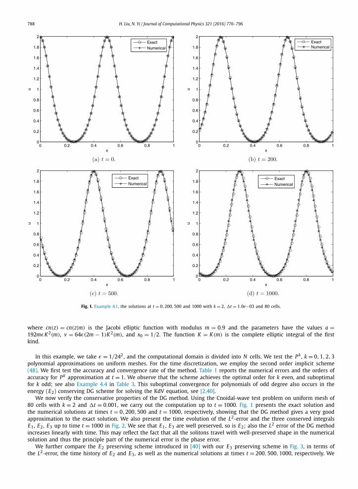
Fig. 1. Example 4.1, the solutions at t = 0,200,500 and 1000 with k = 2, �t = 1.0e−03 and 80 cells.
where cn(z) = cn(z|m) is the Jacobi elliptic function with modulus m = 0.9 and the parameters have the values a =192mεK 2(m), v = 64ε(2m − 1)K 2(m), and x0 = 1/2. The function K = K (m) is the complete elliptic integral of the first kind.
In this example, we take ε = 1/242, and the computational domain is divided into N cells. We test the P k , k = 0, 1, 2, 3polynomial approximations on uniform meshes. For the time discretization, we employ the second order implicit scheme (48). We first test the accuracy and convergence rate of the method. Table 1 reports the numerical errors and the orders of accuracy for Pk approximation at t = 1. We observe that the scheme achieves the optimal order for k even, and suboptimal for k odd; see also Example 4.4 in Table 3. This suboptimal convergence for polynomials of odd degree also occurs in the energy (E2) conserving DG scheme for solving the KdV equation, see [2,40].
We now verify the conservative properties of the DG method. Using the Cnoidal-wave test problem on uniform mesh of 80 cells with k = 2 and �t = 0.001, we carry out the computation up to t = 1000. Fig. 1 presents the exact solution and the numerical solutions at times t = 0, 200, 500 and t = 1000, respectively, showing that the DG method gives a very good approximation to the exact solution. We also present the time evolution of the L2-error and the three conserved integrals E1, E2, E3 up to time t = 1000 in Fig. 2. We see that E1, E3 are well preserved, so is E2; also the L2 error of the DG method increases linearly with time. This may reflect the fact that all the solitons travel with well-preserved shape in the numerical solution and thus the principle part of the numerical error is the phase error.
We further compare the E2 preserving scheme introduced in [40] with our E3 preserving scheme in Fig. 3, in terms of the L2-error, the time history of E2 and E3, as well as the numerical solutions at times t = 200, 500, 1000, respectively. We

H. Liu, N. Yi / Journal of Computational Physics 321 (2016) 776–796 789
Fig. 2. Example 4.1, time history of the L2 error, E1, E2 and E3 plots using the DG methods with k = 2, �t = 1.0e−03 and 80 cells.
Table 2The E2 and E3 of E2 preserving and E3 preserving schemes for Example 4.1 when using P 2 polynomials on a uniform mesh of 80 cell.
E2 preserving scheme t = 0 t = 200 t = 500 t = 900 t = 1000
E2(u) 1.00729302749 1.00729302749 1.00729302749 1.00729302749 1.00729302749
E2(uh) 1.00729302690 1.00729302690 1.00729302690 1.00729302690 1.00729302690|E2(uh )−E2(u)|
E2(u)5.8573e−10 5.8573e−10 5.8573e−10 5.8573e−10 5.8573e−10
E3 preserving scheme t = 0 t = 200 t = 500 t = 900 t = 1000
E2(uh) 1.00729302691 1.00729302692 1.00729302691 1.00729302692 1.00729302691|E2(uh )−E2(u)|
E2(u)5.7580e−10 5.6587e−10 5.7580e−10 5.6587e−10 5.7580e−10
E2 preserving scheme t = 0 t = 200 t = 500 t = 900 t = 1000
E3(uh) −0.18912751410 −0.19031815943 −0.19004235096 −0.18995786446 −0.19051454372
E3 preserving scheme t = 0 t = 200 t = 500 t = 900 t = 1000
E3(uh) −0.18925223716 −0.18925223716 −0.18925223716 −0.18925223716 −0.18925223716
clearly see that our E3 preserving scheme induces smaller L2 error and smaller phase errors. Moreover, it preserves both E2and E3, while the E2 preserving scheme only preserves E2, with large oscillations observed in the time history of E3. The corresponding comparison data are listed in Table 2.

790 H. Liu, N. Yi / Journal of Computational Physics 321 (2016) 776–796
Fig. 3. Example 4.1, the performance of the E2 preserving and E3 preserving schemes comparisons with k = 2, �t = 1.0e−03 and 80 cells.
Example 4.2. Consider again the KdV equation (49) with ε = 1, and u(x, 0) as the initial data, the exact solution is of the two soliton waves
u(x, t) = 12k2
1eθ1 + k22eθ2 + 2(k2 − k1)
2eθ1+θ2 + a2(k22eθ1 + k2
1eθ2)eθ1+θ2
θ1 θ2 2 θ1+θ2 2, (50)
(1 + e + e + a e )

H. Liu, N. Yi / Journal of Computational Physics 321 (2016) 776–796 791
Fig. 4. Example 4.2, the solutions at t = 0,40,80 and 120 with k = 2, �t = 0.1 and 400 cells.
Fig. 5. Example 4.3, the solutions at t = 0,1/π and 3.6/π with k = 2, �t = 0.005/π and 400 cells.

792 H. Liu, N. Yi / Journal of Computational Physics 321 (2016) 776–796
Table 3Errors for Example 4.4 when using Pk polynomials on a uniform mesh of N cells. Final time T = 1.
k = 0
�t 4.0e−2 1.0e−2 2.5e−3 6.25e−4 1.5625e−4N 10 20 40 80 160‖u − uh‖ 4.69e−1 1.97e−1 8.54e−2 4.08e−2 2.02e−2order – 1.25 1.21 1.06 1.02
k = 1
�t 4.0e−2 1.0e−2 2.5e−3 6.25e−4 1.5625e−4N 10 20 40 80 160‖u − uh‖ 1.18e−1 2.44e−2 8.13e−3 5.35e−3 2.84e−3order – 2.23 1.59 0.61 0.91
k = 2
�t 4.0e−2 1.0e−2 2.5e−3 6.25e−4 1.5625e−4N 10 20 40 80 160‖u − uh‖ 2.41e−3 2.13e−4 2.30e−5 2.7e−6 3.0e−7order – 3.50 3.21 3.09 3.17
k = 3
�t 4.0e−2 1.0e−2 2.5e−3 6.25e−4 1.5625e−4N 10 20 40 80 160‖u − uh‖ 1.90e−3 1.24e−4 7.55e−6 8.15e−7 3.28e−08order – 3.93 4.01 3.21 4.64
Fig. 6. Example 4.4, the solutions at t = 0,200,500 and 1000 with k = 1, �t = 6.25e−04 and 80 cells.
H. Liu, N. Yi / Journal of Computational Physics 321 (2016) 776–796 793
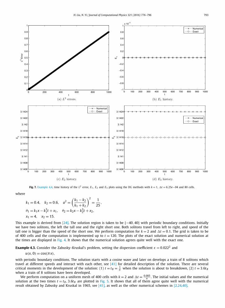
Fig. 7. Example 4.4, time history of the L2 error, E1, E2 and E3 plots using the DG methods with k = 1, �t = 6.25e−04 and 80 cells.
where
k1 = 0.4, k2 = 0.6, a2 =(
k1 − k2
k1 + k2
)2
= 1
25,
θ1 = k1x − k31t + x1, θ2 = k2x − k3
2t + x2,
x1 = 4, x2 = 15.
This example is derived from [24]. The solution region is taken to be [−40, 40] with periodic boundary conditions. Initially we have two solitons, the left the tall one and the right short one. Both solitons travel from left to right, and speed of the tall one is bigger than the speed of the short one. We perform computation for k = 2 and �t = 0.1. The grid is taken to be of 400 cells and the computation is implemented up to t = 120. The plots of the exact solution and numerical solution at the times are displayed in Fig. 4. It shows that the numerical solution agrees quite well with the exact one.
Example 4.3. Consider the Zabusky–Kruskal’s problem, setting the dispersion coefficient ε = 0.0222 and
u(x,0) = cos(πx),
with periodic boundary conditions. The solution starts with a cosine wave and later on develops a train of 8 solitons which travel at different speeds and interact with each other, see [41] for detailed description of the solution. There are several critical moments in the development of the solution: (1) t = tB = 1
π when the solution is about to breakdown, (2) t = 3.6tBwhen a train of 8 solitons have been developed.
We perform computation on a uniform mesh of 400 cells with k = 2 and �t = 0.005π . The initial values and the numerical
solution at the two times t = tB , 3.6tB are plotted in Fig. 5. It shows that all of them agree quite well with the numerical result obtained by Zabusky and Kruskal in 1965, see [41], as well as the other numerical schemes in [2,24,40].
794 H. Liu, N. Yi / Journal of Computational Physics 321 (2016) 776–796
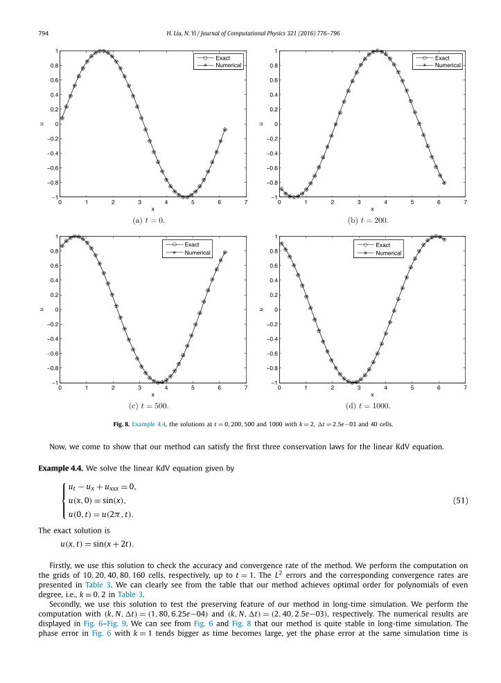
Fig. 8. Example 4.4, the solutions at t = 0,200,500 and 1000 with k = 2, �t = 2.5e−03 and 40 cells.
Now, we come to show that our method can satisfy the first three conservation laws for the linear KdV equation.
Example 4.4. We solve the linear KdV equation given by⎧⎪⎨⎪⎩ut − ux + uxxx = 0,
u(x,0) = sin(x),
u(0, t) = u(2π, t).
(51)
The exact solution is
u(x, t) = sin(x + 2t).
Firstly, we use this solution to check the accuracy and convergence rate of the method. We perform the computation on the grids of 10, 20, 40, 80, 160 cells, respectively, up to t = 1. The L2 errors and the corresponding convergence rates are presented in Table 3. We can clearly see from the table that our method achieves optimal order for polynomials of even degree, i.e., k = 0, 2 in Table 3.
Secondly, we use this solution to test the preserving feature of our method in long-time simulation. We perform the computation with (k, N, �t) = (1, 80, 6.25e−04) and (k, N, �t) = (2, 40, 2.5e−03), respectively. The numerical results are displayed in Fig. 6–Fig. 9. We can see from Fig. 6 and Fig. 8 that our method is quite stable in long-time simulation. The phase error in Fig. 6 with k = 1 tends bigger as time becomes large, yet the phase error at the same simulation time is

H. Liu, N. Yi / Journal of Computational Physics 321 (2016) 776–796 795
Fig. 9. Example 4.4, time history of the L2 error, E1, E2 and E3 plots using the DG methods with k = 2, �t = 2.5e−03 and 40 cells.
almost invisible when using k = 2, see Fig. 8. Fig. 7 and Fig. 9 show that the L2 error increases linearly with time, and the three qualities E1, E2, E3 are all preserved.
5. Concluding remarks
In this paper, we developed and analyzed a Hamiltonian preserving DG method for solving the generalized KdV equa-tion. Both semi-discrete and fully discrete DG schemes are shown to preserve E1 and E3. The better performance of the E3-preserving scheme than the E2-preserving scheme is shown through numerical comparison.
For wave equations, usually it is difficult to obtain DG schemes which can preserve more conservative integrals while still maintaining optimal high order of accuracy. Our scheme when applied to the linearized KdV equation preserves all the first three conserved integrals and has the proven optimal error estimates for polynomial elements of even degree. Our numerical experiments have demonstrated both high accuracy of convergence and preservation of all three conserved integrals for the generalized KdV equation. It is confirmed by numerical simulations that the Hamiltonian preserving property is important for minimizing phase and amplitude errors after long time simulation.
Acknowledgements
This research was partially supported by the National Science Foundation under grant DMS-1312636 and by NSF Grant RNMS-1107291 (KI-Net). Yi’s research was supported by NSFC Project (11201397, 91430213) and Hunan Provincial NSF Project (2015JJ2145).

796 H. Liu, N. Yi / Journal of Computational Physics 321 (2016) 776–796
References
[1] D.N. Arnold, R. Winther, A superconvergent finite element method for the Korteweg–de Vries equation, Math. Comput. 38 (1982) 23–36.[2] J. Bona, H. Chen, O. Karakashian, Y. Xing, Conservative, discontinuous-Galerkin methods for the generalized Korteweg–de Vries equation, Math. Comput.
82 (283) (2013) 1401–1432.[3] Y. Cheng, C.W. Shu, A discontinuous Galerkin finite element method for time dependent partial differential equations with higher order derivatives,
Math. Comput. 77 (2008) 699–730.[4] B. Cockburn, C.W. Shu, TVB Runge–Kutta local projection discontinuous Galerkin finite element method for conservation laws II: general framework,
Math. Comput. 52 (1989) 411–435.[5] B. Cockburn, S.Y. Lin, C.W. Shu, TVB Runge–Kutta local projection discontinuous Galerkin finite element method for conservation laws III: one dimen-
sional systems, J. Comput. Phys. 84 (1989) 90–113.[6] B. Cockburn, S. Hou, C.W. Shu, The Runge–Kutta local projection discontinuous Galerkin finite element method for conservation laws IV: the multidi-
mensional case, Math. Comput. 54 (1990) 545–581.[7] B. Cockburn, C.W. Shu, The Runge–Kutta discontinuous Galerkin method for conservation laws V: multidimensional systems, J. Comput. Phys. 141
(1998) 199–224.[8] L. Faddeev, V.E. Zakharov, Korteweg–de Vries equation as completely integrable Hamiltonian system, Funkc. Anal. Prilozh. 5 (1971) 18–27 (in Russian).[9] B. Fornberg, G.B. Whitham, A numerical and theoretical study of certain nonlinear wave phenomena, Philos. Trans. R. Soc. Lond. Ser. A, Math. Phys. Sci.
289 (1978) 373–404.[10] D. Furihata, Finite difference schemes for ∂u
∂t = (∂∂x
)α δgδu that inherit energy conservation or dissipation property, J. Comput. Phys. 156 (1999) 181–205.
[11] C.S. Gardner, Korteweg–de Vries equation and generalizations. IV: the Korteweg–de Vries equation as a Hamiltonian system, J. Math. Phys. 12 (1971) 1548–1551.
[12] K. Goda, Numerical studies on recurrence of the Korteweg–de Vries equation, J. Phys. Soc. Jpn. 42 (1977) 1040–1046.[13] I.S. Greig, J.L. Morris, A hopscotch method for the Korteweg–de Vries equation, J. Comput. Phys. 20 (1976) 64–80.[14] B. Guo, J. Shen, On spectral approximations using modified Legendre rational functions: application to the Korteweg–de Vries equation on the half line,
Indiana Univ. Math. J. 50 (2001) 181–204.[15] Helge Holden, Kenneth H. Karlsen, Nils Henrik Risebro, Terence Tao, Operator splitting for the KdV equation, Math. Comput. 80 (274) (2011) 821–846.[16] H. Holden, K.H. Karlsen, N.H. Risebro, Operator splitting methods for generalized Korteweg–de Vries equations, J. Comput. Phys. 153 (1999) 203–222.[17] L. Ji, Y. Xu, Optimal error estimates of the local discontinuous Galerkin method for Willmore flow of graphs on Cartesian meshes, Int. J. Numer. Anal.
Model. 8 (2011) 252–283.[18] D.J. Korteweg, G. de Vries, On the change of form of long waves advancing in a rectangular canal, and on a new type of long stationary waves, Philos.
Mag. 39 (1895) 422–443.[19] J. Li, M.R. Visbal, High-order compact schemes for nonlinear dispersive waves, J. Sci. Comput. 26 (2006) 1–23.[20] P. Lax, Integrals of nonlinear equations of evolution and solitary waves, Commun. Pure Appl. Math. 21 (1968) 467–490.[21] H. Liu, Y.Q. Huang, N.Y. Yi, A direct discontinuous Galerkin method for the Degasperis–Procesi equation, Methods Appl. Anal. 21 (2014) 83–106.[22] H. Liu, J. Yan, A local discontinuous Galerkin method for the Korteweg–de Vries equation with boundary effect, J. Comput. Phys. 215 (2006) 197–218.[23] W. Huang, D.M. Sloan, The pseudospectral method for third-order differential equations, SIAM J. Numer. Anal. 29 (1992) 1626–1647.[24] Y.F. Cui, D.K. Mao, Numerical method satisfying the first two conservation laws for the Korteweg–de Vries equation, J. Comput. Phys. 227 (2007)
376–399.[25] H. Ma, W. Sun, A Legendre–Petrov–Galerkin and Chebyshev collocation method for third-order differential equations, SIAM J. Numer. Anal. 38 (2001)
1425–1438.[26] H. Ma, W. Sun, Optimal error estimates of the Legendre–Petrov–Galerkin method for the Korteweg–de Vries equation, SIAM J. Numer. Anal. 39 (2002)
1380–1394.[27] R.M. Miura, C.S. Gardner, M.D. Kruskal, Korteweg–de Vries equation and generalizations ii: existence of conservation laws and constants of motion,
J. Comput. Phys. 9 (1968) 1204–1209.[28] W. Reed, T. Hill, Triangular mesh methods for the neutrontransport equation, La-ur-73-479, Los Alamos Scientific Laboratory, 1973.[29] J.M. Sanz-Serna, I. Christie, Petrov–Galerkin methods for nonlinear dispersive wave, J. Comput. Phys. 39 (1981) 94–102.[30] J. Shen, A new dual-Petrov–Galerkin method for third and higher odd-order differential equations: application to the KdV equation, SIAM J. Numer.
Anal. 41 (2004) 1595–1619.[31] R. Winther, A conservative finite element method for the Korteweg–de Vries equation, Math. Comput. 34 (1980) 23–43.[32] X.L. Xie, Large time-stepping methods for higher order time-dependent evolution equations, PhD thesis, Iowa State University, Ames, IA, 2008.[33] Y. Xu, C.W. Shu, Local discontinuous Galerkin methods for the Degasperis–Procesi equation, Commun. Comput. Phys. 10 (2) (2011) 474–508.[34] Y. Xu, C.W. Shu, Local discontinuous Galerkin methods for two classes of two-dimensional nonlinear wave equations, Physica D 208 (2005) 21–58.[35] Y. Xu, C.W. Shu, Error estimates of the semi-discrete local discontinuous Galerkin method for nonlinear convection-diffusion and KdV equations,
Comput. Methods Appl. Mech. Eng. 196 (2007) 3805–3822.[36] Y. Xu, C.W. Shu, A local discontinuous Galerkin method for the Camassa–Holm equation, SIAM J. Numer. Anal. 46 (2008) 1998–2021.[37] Y. Xu, C.W. Shu, Local discontinuous Galerkin method for higher order time-dependent partial differential equations, Commun. Comput. Phys. 7 (2010)
1–46.[38] Y. Xu, C.-W. Shu, Optimal error estimates of the semi-discrete local discontinuous Galerkin methods for high order wave equations, SIAM J. Numer.
Anal. 50 (1) (2012) 79–104.[39] J. Yan, C.W. Shu, A local discontinuous Galerkin method for KdV type equations, SIAM J. Numer. Anal. 40 (2002) 769–791.[40] N. Yi, Y. Huang, H. Liu, A direct discontinuous Galerkin method for the generalized Korteweg–de Vries equation: energy conservation and boundary
effect, J. Comput. Phys. 242 (2013) 351–366.[41] N.J. Zabusky, M.D. Kruskal, Interactions of “solitons” in a collisionless plasma and the recurrence of initial states, Phys. Rev. Lett. 15 (1965) 240–243.