Journal of Computational Physics 390 (2019) 306–322

Contents lists available at ScienceDirect

Journal of Computational Physics

www.elsevier.com/locate/jcp

A mesh-free pseudospectral approach to estimating the

fractional Laplacian via radial basis functions

Joel A. Rosenfeld a,∗, Spencer A. Rosenfeld b, Warren E. Dixon c

a Department of Electrical Engineering and Computer Science, Vanderbilt University, Nashville, TN, United States of Americab Department of Physics, University of Florida, Gainesville, FL, United States of Americac Nonlinear Controls and Robotics (NCR) Laboratory, Department of Mechanical and Aerospace Engineering, University of Florida, Gainesville, FL, United States of America

a r t i c l e i n f o a b s t r a c t

Article history:Received 19 January 2017Received in revised form 17 February 2019Accepted 24 February 2019Available online 15 March 2019

Keywords:Mesh-free methodsFractional LaplacianWendland RBFsFractional calculusPseudospectral methodsFractional Poisson equation

This paper investigates the use of radial basis function (RBF) interpolants to estimate a function’s fractional Laplacian of a given order through a mesh-free pseudospectral method. The mesh-free approach yields an algorithm that can be implemented in high dimensional settings without adjustment. Moreover, the fractional Laplacian is defined in terms of the Fourier transform, and the symmetry of RBFs can be exploited to simplify the estimation problem. Convergence rates are established for RBFs when the function whose fractional Laplacian to be estimated is compactly supported. Further results demonstrate convergence when a function is in the native space for a Wendland RBF (i.e. a Sobolev space) and satisfies a certain L1 condition. Numerical experiments demonstrate the developed method by estimating the fractional Laplacian of several functions and by solving a fractional Poisson equation with extended Dirichlet condition in one and two dimensions.

© 2019 Elsevier Inc. All rights reserved.

1. Introduction

Many complex phenomena can be accurately modeled by integer order (typically nonlinear) differential equations. How-ever, evidence suggests that for some complex systems the use of a generalized, fractional order, derivative more accurately represents physical behaviors [1,2]. For example, a heavily cited work by Paul Clavin demonstrated that a version of the Cauchy problem, regularized with a fractional Laplacian, was a better model for over driven detonations in gases [2]. Other work has investigated the fractional Laplacian in describing the viscoacoustic wave equation in geophysics [3,4], a fraction-alized version of the Schrödinger equation [5–8], the fractional Poisson equation [9,10], in hydrology [11,1] and many other applications [12–14]. The growing number of applications for the fractional Laplacian motivates novel approaches for the estimation of the operator, as well as solutions to related fractional order partial differential equations (PDEs), that can eas-ily extend to high dimensional problems. The fractional Laplacian (of order α > 0) can be represented in several equivalent forms [9]. The simplest representation is given by

(−�)α/2 f (x) := F−1[‖ξ‖αF[ f ]](x), (1)

* Corresponding author.E-mail addresses: joel.rosenfeld@vanderbilt.edu (J.A. Rosenfeld), spencerrosenfeld@ufl.edu (S.A. Rosenfeld), wdixon@ufl.edu (W.E. Dixon).

https://doi.org/10.1016/j.jcp.2019.02.0150021-9991/© 2019 Elsevier Inc. All rights reserved.

J.A. Rosenfeld et al. / Journal of Computational Physics 390 (2019) 306–322 307

where f :Rn →R, x ∈Rn , F is the n-dimensional Fourier transform,1

F[ f ](ξ) := f (ξ) =∫

Rn

f (x)e−ix·ξ dx (2)

with ξ ∈Rn , and � := d2

dx21

+ d2

dx22

+ · · · + d2

dx2n

is the Laplacian operator.

The numerical implementation of the fractional Laplacian is difficult due to its definition as an integral over all of Rn . Computational challenges associated with the fractional Laplacian have motivated various results in literature. For example, a finite difference approach was introduced in [9] to estimate the fractional Laplacian in one dimension. Other works utilize fast Fourier methods to discretize the fractional Laplacian [15,16]. These results demonstrate that numerically estimating the fractional Laplacian is difficult even in the single dimensional case, and where numerical methods that can be easily adapted to high dimensional problems present an even greater challenge.

The flexibility of collocation methods using radial basis functions (RBFs) for high dimensional problems has been demon-strated thoroughly for the integer order case, where RBFs are frequently used to numerically estimate solutions to elliptic boundary value problems and PDEs in general (cf. [17–22] and references therein). These methods hold appeal for the fractional Laplacian since only minor adjustments to existing algorithms are required to transport them to the fractional order case. The challenge to implementing collocation methods is in the computation of the fractional Laplacian of the basis functions themselves.

The n-dimensional Fourier transform of a RBF over Rn can be expressed in terms of a single dimensional integral against a Bessel function as discussed in Section 5.1, which is a key advantage that motivates the use of RBFs for the purpose of estimating solutions to fractional differential equations. Specifically, only a one dimensional integral must be estimated to produce an estimate of the fractional Laplacian of a RBF.

Estimation of this integral governs the RBF choice. For instance, Gaussians are excellent candidates, since both the Gaus-sian and its Fourier transform (another Gaussian) decay quickly. However, in some circumstances (e.g., for the homogeneous solution of a fractional Poisson equation with an extended Dirichlet condition) the use of a compactly supported basis function, such as the Wendland RBFs, may be advantageous. The drawback of using compactly supported basis functions is that the Fourier transform of a compactly supported function has unbounded support and does not decay as quickly as a Gaussian’s Fourier transform. This drawback can be mitigated through the choice of compactly supported basis functions. Smoother functions have Fourier transforms that decay faster than less smooth functions. In [23], Wendland developed an algorithm that yields compactly supported RBFs with a desired finite order of smoothness. Moreover, since the Wendland basis functions are polynomials on their support, the Fourier transform of these functions can be explicitly determined in many cases. Therefore, in many situations, the only error resulting from estimating the fractional Laplacian of a basis function occurs from inverting the Fourier transform in (1). The numerical experiments presented in this paper use the Wendland compactly supported basis functions.

The introduction of the fractional Laplacian naturally leads to questions about fractional order PDEs; such as the fractional Schrödinger equation [5–8] or the fractional order Poisson equation over a set � ⊂Rn with the extended Dirichlet condition

(−�)α/2u(x) = f (x) for x ∈ � ⊂Rn and u(x) = g(x) for x ∈Rn \ � (3)

with α > 0, f : � →R, g :Rn \ � →R, and u :Rn →R [9,10].Two main methods have been employed for collocation with RBFs in the theory of elliptic PDEs: the Kanza method

[24,25] and the symmetric collocation method [26,25]. For integer order systems, both methods converge to the solution of the elliptic partial differential equation as the collocation nodes increase. The Kanza method has been reported to converge faster, whereas symmetric collocation guarantees an invertible collocation matrix.

Over the past two years, others have begun work on integrating radial basis functions and collocation methods with fractional order operators. In particular, [27] uses a Kansa approach for the space-fractional advection-dispersion equations, which has a fractional operator in the form of a fractional directional derivative. In the setting of [27], the fractional direc-tional derivative specializes to the fractional Laplacian over a restricted range of fractional powers, α ∈ (1, 2]. In [28,29], RBFs are used for a Galerkin method to solve problems pertaining to nonlocal diffusion. In particular, the algorithms contained in [29] rely on local Lagrange functions to act as interpolants and to establish convergence results.

The contribution of this paper is the development of a pseudospectral method for the estimation of the fractional Lapla-cian using RBF interpolation; this is the first algorithm that focuses on establishing convergence results for the fractional Laplacian specifically and for the class of compactly supported RBFs. The advantage of using RBF interpolation is that few, if any, adjustments need to be made to the algorithm to facilitate the estimation of fractional derivatives over any dimen-sion, which is demonstrated by evaluating the fractional Laplacian of functions in one and two dimensions in Section 4.1and Section 4.4. Moreover, when evaluating the pseudospectral method, the Fourier transform of a RBF can be determined through the evaluation of a one dimensional integral (cf. [25] and Section 5.1), and the resulting fractional Laplacian is shift

1 Throughout this paper, the two notations for the Fourier transform defined as F[ f ] and f , will be used interchangeably.

308 J.A. Rosenfeld et al. / Journal of Computational Physics 390 (2019) 306–322

invariant, which reduces the amount of preprocessing required to evaluate the algorithm (Section 5). Finally, the developed approach leverages results on RBF interpolation such as [25] to yield the convergence results in Section 3.

RBF-based discretization of the fractional Laplacian enables the development of mesh-free methods for numerical so-lutions of fractional order PDEs. As an example, a numerical solution to a fractional order Poisson equation is given in Section 4.2 using a Kansa type approach. It is interesting to note that the symmetric method does not perform as well as the Kansa approach, even when the number of collocation points is much greater. For a discussion of the symmetric approach, see Section 4.3.

2. Review of interpolation by RBFs

For a function φ :R →Rn a RBF is defined as �(x) = φ(‖x‖2) where x ∈Rn . An advantage of approximating a function defined over a set � ⊂Rn , f : � →R, by RBFs is that a function in the native space of a RBF, which is denoted by N�(�), can be uniformly well approximated over compact sets by interpolants of the form

sX, f (x) :=m∑

i=1

wiφ(‖x − xi‖2), (4)

where X = {x1, ..., xm} ⊂ � and sX, f (xi) = f (xi) for i = 1, ..., m, when φ is continuous. Specific convergence rates can be determined for many RBFs based on the fill distance, hX,� := supx∈� minx j∈X ‖x − x j‖2. The RBFs used in this paper are the Wendland RBFs of order n ∈N and k ∈N , defined in [25,23,30]

Kn,k(x, y) := �n,k(x − y) = φn,k(‖x − y‖2). (5)

The native space for an RBF, � can be described in terms of L2 spaces and Fourier transforms. In particular,

Theorem 2.1 (Fourier representation of the native space). [30, Theorem 10.12] Suppose that � ∈ C(Rn) ∩ L1(Rn) is a real-valued positive definite function. Define G :=

{f ∈ L2(Rn) ∩ C(Rn) : f /

√� ∈ L2(Rn)

}and equip this space with the bilinear form

( f , g)G := (2π)−n/2(

f /√

�, g/

√�

)L2(Rn)

= (2π)−n/2∫

Rn

f (ω)g(ω)

�(w)dω.

Then G is a real Hilbert space with inner product (·, ·)G and reproducing kernel φ(· − ·), i.e. G = N�(Rn). In particular, every f ∈N�(Rn) can be recovered from its Fourier transform.

Theorem 2.2 (Native spaces for the Wendland RBFs). [30] The native space for the Wendland RBF with parameters n, k is Hn/2+k+1/2(Rn). For s > 0 the space

Hs(Rn) :=⎧⎨⎩ f ∈ C(Rn) ∩ L1(Rn) :

∫

Rn

| f (ω)|2(1 + ‖ω‖2)sdω < ∞

⎫⎬⎭ .

Approximation theorems utilizing RBFs establish convergence rate estimates over functions in the native spaces. As can be seen by Theorem 2.2, these native spaces may be Sobolev spaces, which are used extensively for solving PDEs [31]. However, since numerical methods for the fractional Laplacian can be directly applied to computing numerical solutions to the fractional Poisson equation it should be noted that for some choices of the parameter α, the solution to the fractional Poisson equation is guaranteed regularity up to Cα/2(Rn) [10]. For α < 1, the spaces in Theorem 2.2 do not have the required regularity. Consequently, in some cases it is implicitly assumed that the approximation problem may be estimating a weak solution to the fractional Poisson equation, where additional regularity is assumed.

Interpolation theorems using RBFs are frequently posed over sets, �, that satisfy the interior cone condition [25,30]. For the purposes of this paper, the convergence results are established over a ball. A ball in Rn satisfies the interior cone condition. Moreover, there is no fixed subset for which the convergence must be established over, since the approximation must be established over Rn by the nonlocal nature of the fractional Laplacian.

The following lemma, based on Theorem 14.5 in [25], will be used extensively for establishing the convergence of the fractional Laplacian of interpolants to the fractional Laplacian of f ∈Nφ .

Lemma 2.3. Suppose � ⊂Rn is bounded and satisfies an interior cone condition. Suppose φ ∈ C2k(� × �) is symmetric and strictly positive definite. Then there exists positive constants h0 and C (independent of x, f , and φ) such that for d ∈N with 2d < k,

|(−�)d f (x) − (−�)dsX, f (x)| ≤ ndChk−2dX,� ‖ f ‖Nφ(�) (6)

is the provided hX,� < h0 . Here ‖ · ‖Nφ(�) is the Hilbert space norm of the native space Nφ(�), and hX,� := supy∈� minx∈X ‖x − y‖2 .

J.A. Rosenfeld et al. / Journal of Computational Physics 390 (2019) 306–322 309

3. Estimation of the fractional Laplacian by RBF interpolants

The numerical methods presented in this paper rely on positive definite RBFs. To discuss the convergence of the fractional Laplacian, this section uses the native space of the RBFs. Both the native space and the fractional Laplacian are defined in terms of Fourier transforms, which facilitate the results in this paper.

The development in this section establishes convergence of the fractional Laplacian of interpolants to the fractional Laplacian of the sampled function. As is standard for approximation results involving RBFs, the convergence estimates will be demonstrated on functions in the RBF’s native space. Specifically, Theorem 3.1 shows that if two functions are compactly supported, then the difference between the two fractional Laplacians is controlled pointwise by the norm of the functions in the native Hilbert space of the RBF (i.e. the error is upper bounded by a scaled version of the norm).

Theorem 3.1. Suppose � ∈ C2k(Rn × Rn) is symmetric and strictly positive definite. Suppose that f , g ∈ N�(Rn) are compactly supported. Let d ∈N satisfy 2d < k and let α be a positive real number that satisfies 2d −n > α. Then there is a set � ⊂Rn and C > 0for which

∣∣∣(−�)α/2 f (x) − (−�)α/2 g(x)∣∣∣ ≤ C‖ f − g‖N�(�) ≤ C‖ f − g‖N�(Rn)

for all x ∈Rn.

Proof. Suppose that f and g are compactly supported in N�(Rn), then

∣∣∣(−�)α/2 f (x) − (−�)α/2 g(x)∣∣∣ =

∣∣∣∣∣∣∫

Rn

‖ξ‖αeix·ξ (F[ f ](ξ) −F[g](ξ))dξ

∣∣∣∣∣∣

=

∣∣∣∣∣∣∣∫

B1(0)

‖ξ‖αeix·ξ (F[ f ](ξ) −F[g](ξ))dξ +∫

Rn\B1(0)

‖ξ‖αeix·ξ (F[ f ](ξ) −F[g](ξ))dξ

∣∣∣∣∣∣∣

=

∣∣∣∣∣∣∣∫

B1(0)

‖ξ‖αeix·ξ (F[ f ](ξ) −F[g](ξ))dξ

+∫

Rn\B1(0)

‖ξ‖α

‖ξ‖2deix·ξ (

F[(−�)d f ](ξ) −F[(−�)d g](ξ))

dξ

∣∣∣∣∣∣∣. (7)

Let � be an open ball that contains the support of f and g . The Fourier transform of (−�)d f and (−�)d g can then be written as

∣∣∣F[(−�)d f ](ξ) −F[(−�)d g](ξ)

∣∣∣

=∣∣∣∣∣∣∫

�

[(−�)d f (x) − (−�)d g(x)

]eix·ξdx

∣∣∣∣∣∣ ≤ C0m(�)‖ f − g‖N�(�) (8)

where C0 is a positive constant, and m(·) is Lebesgue measure. Similarly,

|F[ f ](ξ) −F[g](ξ)| < C1m(�)‖ f − g‖N�(�). (9)

By inserting (8) and (9) into (7),∣∣∣(−�)α/2 f (x) − (−�)α/2 g(x)

∣∣∣

≤ Cm(�)‖ f − g‖N�(�)

⎛⎜⎝

∫

B1(0)

‖ξ‖αdξ+∫

Rn\B1(0)

1

‖ξ‖2d−αdξ

⎞⎟⎠ (10)

for some C > 0. The unbounded integral in (10) converges iff 2d − α > n. �

310 J.A. Rosenfeld et al. / Journal of Computational Physics 390 (2019) 306–322

For all of the results presented in this section, it is essential that the functions have either a fast rate of decay (i.e. the function is in L1(Rn)) or are compactly supported. The compact support or decay of the functions in these theorems is necessary to maintain the finiteness of bounds such as (8). The next proposition establishes that even if a function f ∈ N�(Rn) is compactly supported and the RBF is also compactly supported, there is still a finite error that cannot be controlled through standard interpolation theorems. Specifically, most convergence results for RBFs are framed in terms of a bounded subset � ⊂Rn , and convergence is shown over that subset. Once x ∈Rn leaves that subset, then there is no direct control over the error in terms of the separation constant, hX,� . In fact, results given in [32] indicate that the functions may get very large once x leaves �.

Proposition 3.2. Suppose � ∈ C2k(Rn × Rn) is symmetric and strictly positive definite. Suppose that f ∈ N�(Rn) is compactly supported. Let d ∈ N satisfy 2d < k and α > 0 satisfying 2d − α > n. Then there is a set � ⊂Rn, C > 0, and E > 0 for which given any X = {x1, ..., xm} ⊂ � the following holds

|(−�)α/2 f (x) − (−�)α/2sX, f (x)| ≤(

Chk−2dX,� ‖ f ‖N�(�) + E

)∫

Rn

1

‖ξ‖2d−αdξ

for all x ∈Rn where

hX,� = supx∈�

minx j∈X

‖x − x j‖2.

Proof. Let � ⊂ Rn be an open ball containing the support of f . Define �r := {x ∈ Rn : d(x, y) < r for some y ∈ �}, where r > 0 is the radius of the support of the RBF, �(x) = φ(‖x‖).

Let X = {x1, ..., xm} ⊂ �. Invoking Lemma 2.3, provides

|(−�)d f (x) − (−�)dsX, f (x)| ≤ ndChk−2dX,�r

√Cφ(x)‖ f ‖N�(�)

for all x ∈ �, and since both f and sX, f are zero outside of �r , the inequality holds for all x ∈ � ∪ (Rn \ �r). Subsequently, for ξ ∈Rn ,

∣∣∣F[(−�)d f − (−�)dsX, f ](ξ)

∣∣∣ =∣∣∣∣∣∣∫

Rn

[(−�)d f (x) − (−�)dsX, f (x)

]e−iξ ·xdx

∣∣∣∣∣∣

=∣∣∣∣∣∣∫

�

[(−�)d f (x) − (−�)dsX, f (x)

]e−iξ ·xdx

∣∣∣∣∣∣ +

∣∣∣∣∣∣∣∫

�r\�(−�)dsX, f (x)e−iξ ·xdx

∣∣∣∣∣∣∣≤ ndChk−2d

X,�

√Cφ(x)m(�)‖ f ‖N�(�r) + E, (11)

where E > 0 is a residual error where the size of sX, f can be arbitrarily large.2 An identical argument holds when consid-

ering F [ f − sX, f ](ξ) and results in the same bound except with hkX,� . Since hk

X,� < hk−2dX,� for sufficiently small hX,� , the

same bound as in (11) holds for F [ f − sX, f ](ξ) with possibly an adjustment to the constant C .To extend the estimate to include the fractional Laplacian of compactly supported functions in N�(Rn), consider

|(−�)α/2 f (x) − (−�)α/2sX, f (x)| = ∣∣F−1[‖ξ‖αF( f − sX, f )(ξ)](x)∣∣

=∣∣∣∣∣∣∫

Rn

‖ξ‖α(F[ f ](ξ) −F[sX, f ](ξ)

)eix·ξdξ

∣∣∣∣∣∣

=

∣∣∣∣∣∣∣∫

B1(0)

‖ξ‖α(F[ f ](ξ) −F[sX, f ](ξ)

)eix·ξdξ

∣∣∣∣∣∣∣

+

∣∣∣∣∣∣∣∫

Rn\B1(0)

‖ξ‖α

‖ξ‖2d

(F[(−�)d f ](ξ) −F[(−�)dsX, f ](ξ)

)eix·ξdξ

∣∣∣∣∣∣∣

2 The size of E can be bounded in terms of a reciprocal power of the separation constant hX,� . A method for obtaining an accurate estimation of the fractional Laplacian of f despite E is addressed in Theorem 3.3.

J.A. Rosenfeld et al. / Journal of Computational Physics 390 (2019) 306–322 311

≤(

Cd,n,�hk−2dX,� ‖ f ‖N�(�) + E

)⎛⎜⎝

∫

B1(0)

‖ξ‖αdξ +∫

Rn\B1(0)

1

‖ξ‖2d−αdξ

⎞⎟⎠ ,

where Cd,n,� is a constant depending only on d, n, and �. The unbounded integral after the last inequality converges provided 2d − α > n. �

To mitigate the error, E , in Proposition 3.2, a cutoff function is introduced for the Theorem 3.3. The cutoff function, G R/2 :Rn →R is a radial function that is identically 1 over B R/2(0) = {x ∈Rn|‖x‖2 < R/2} and G R/2(x) = 0 when ‖x‖2 > R . If the cutoff function is selected to be smooth enough over the annulus B R(0) \ B R/2(0), then the decay of the Fourier transform of the resulting function will be fast enough for numerical implementation. However, it was observed in numerical experiments, such as that of Section 4.1, that there was no measurable difference in the resulting estimations when utilizing the cutoff function as compared to when the cutoff function was not used. Therefore, the cutoff function is used here to establish convergence rate estimates.

Theorem 3.3 establishes that an estimate of the fractional Laplacian of a function can be achieved though the fractional Laplacian of an interpolant multiplied by a cutoff function. Proposition 3.2 indicates that obtaining convergence through the fractional Laplacian of interpolants alone may not be possible. Instead, the cutoff function is used to ensure that the global error between the interpolants and the compactly supported function remains small. The use of a cutoff function differs from the rest of the RBF literature and is necessary for establishing a theoretically supported estimate of the fractional Laplacian.

Theorem 3.3. Assume the hypothesis of Theorem 3.1, and let f ∈N�(Rn) be a function whose support lies inside of B R/2(0) for some R > 0. Let G R/2 : Rn → R be as described above. Assume also that G R/2 ∈ C2d(Rn). Then there exists positive constants h0 and C(independent of x, f , and φ) such that for d ∈N with 2d < k,∣∣∣(−�)α/2 f (x) − (−�)α/2(G R/2 · sX, f )(x)

∣∣∣ ≤ Chk−2dX,B R (0)‖ f ‖Nφ(�)

where hX,� < h0 and X = {x1, ..., xm} ⊂ B R(0) is a collection of sample points.

Proof. Let � = B R(0) be the ball of radius R > 0. Let X = {x1, ..., xm} ⊂ � be a collection of collocation points. Since G R/2(x) = 1 on B R/2(0),∣∣∣(−�)d f (x) − (−�)d(G R/2 · sX, f )(x)

∣∣∣ =∣∣∣(−�)d f (x) − (−�)dsX, f (x)

∣∣∣ (12)

for all x ∈ B R/2(0). Thus, the estimate in Lemma 2.3 holds on B R/2(0), and for hX,� sufficiently small, (12) is bounded by ndChk−2d

X,� ‖ f ‖Nφ(�) for some C > 0.

Since d ∈N , for x ∈ � \ B R/2(0) we have f (x) = 0, (−�)d f (x) = 0 and (−�)d(G R/2 · f

)(x) = 0. Consider

|(−�)d f (x) − (−�)d(G R/2 · sX, f )(x)| ≤∣∣∣(−�)d f (x) − (−�)d (

G R/2 · f)(x)

∣∣∣+

∣∣∣(−�)d (G R/2 · f

)(x) − (−�)d (

G R/2 · sX, f)(x)

∣∣∣=

∣∣∣(−�)d (G R/2 · f

)(x) − (−�)d (

G R/2 · sX, f)(x)

∣∣∣=

∣∣∣(−�)d [G R/2(x) · ( f (x) − sX, f (x)

)]∣∣∣over that set. The function (−�)d

[G R/2(x) · ( f (x) − sX, f (x)

)]has a large, but constant, number of terms due to the product

rule. Moreover, G R/2 ∈ C2d(Rn), so the derivatives of G R/2 of every order are bounded over � by some constant M . For a sufficiently small hX,� , the derivatives of every order of f − sX,� all have magnitude less than ndChk−2d

X,� ‖ f ‖Nφ(�) , since s f ,X is approximating f over �. Thus, for all x ∈ � \ B R/2(0),∣∣∣(−�)d [

G R/2(x) · ( f (x) − sX, f (x))]∣∣∣ = |(−�)d(G R/2 · sX, f )(x)|

< MN(ndChk−2dX,� ‖ f ‖Nφ(�)) := Chk−2d

X,� ‖ f ‖Nφ(�) (13)

for some integer N , the number of terms from the product rule, and

|(G R/2 · f )(x) − G R/2 · sX, f )(x)| = |(G R/2 · sX, f )(x)| < ChkX,�‖ f ‖Nφ(�) (14)

for some C > 0. Finally, combining the above estimates yields

312 J.A. Rosenfeld et al. / Journal of Computational Physics 390 (2019) 306–322

∣∣∣(−�)α/2 f (x) − (−�)α/2(G R/2 · sX, f )(x)∣∣∣ =∣∣∣∣∣∣∣

∫

B1(0)

‖ξ‖αeix·ξ [F[ f ](ξ) −F[(G R/2 · sX, f )](ξ)

]dξ

+∫

Rn\B1(0)

‖ξ‖α

‖ξ‖2deix·ξ [

F[(−�)d f ](ξ) −F[(−�)d(G R/2 · sX, f )](ξ)]

dξ

∣∣∣∣∣∣∣

=

∣∣∣∣∣∣∣∫

B1(0)

‖ξ‖αeix·ξ∫

Rn

[f (y) − (G R/2 · sX, f )(y)

]dydξ

+∫

Rn\B1(0)

‖ξ‖α

‖ξ‖2deix·ξ

∫

Rn

[(−�)d f (y) − (−�)d(G R/2 · sX, f )(y)

]dydξ

∣∣∣∣∣∣∣

=

∣∣∣∣∣∣∣∫

B1(0)

‖ξ‖αeix·ξ∫

B R/2(0)

[f (y) − sX, f (y)

]dydξ

+∫

B1(0)

‖ξ‖αeix·ξ∫

B R (0)\B R/2(0)

(G R/2 · sX, f )(y)dydξ

+∫

Rn\B1(0)

1

‖ξ‖2d−αeix·ξ

∫

B R/2(0)

[(−�)d f (y) − (−�)dsX, f (y)

]dydξ

+∫

Rn\B1(0)

1

‖ξ‖2d−αeix·ξ

∫

B R (0)\B R/2(0)

(−�)d(G R/2 · sX, f )(y)dydξ

∣∣∣∣∣∣∣

≤(

Chk−2dX,� ‖ f ‖Nφ(�)

)· m(B R(0))

⎛⎜⎝

∫

B1(0)

‖ξ‖αdξ+∫

Rn\B1(0)

1

‖ξ‖2d−αdξ

⎞⎟⎠ .

The last inequality above leveraged the triangle inequality, (13), (14), and Theorem 14.5 in [25] to obtain the hX,� bound. The unbounded integral,

∫Rn\B1(0)

1‖ξ‖2d−α dξ , is finite precisely when 2d − α > n. �

The final theorem of the section, Theorem 3.4, establishes a result for functions in a native function space that also have L1(Rn) derivatives. The contribution of Theorem 3.4 is the establishment of an estimate of the fractional Laplacian over a more general collection of functions; that is functions satisfying an L1(Rn) condition. This result generalizes Theorem 3.3 in the case of the Wendland RBFs. This new convergence result comes from the fact that the native spaces for the Wendland functions coincide with Sobolev spaces [30,32]. Therefore, multiplication by a sufficiently smooth, compactly supported cutoff function remains in the native space, so Theorem 3.3 can be applied after an L1(Rn) function is multiplied by a cutoff function of sufficiently large radius.

Theorem 3.4. Let φ = φn,k(‖ · ‖) be a RBF of the form (5), with k ∈ N , d ∈ N such that 2d < k, and α > 0 for which 2d − α > n. If f ∈ N�(Rn) and the derivatives of f of all orders less than 2k are in L1(Rn), then there exists h0 > 0 and a cutoff function G R as in Theorem 3.3 such that∣∣∣(−�)α/2 f (x) − (−�)α/2(G R · sX, f )(x)

∣∣∣ ≤ Chk−2dX,B R (0)‖ f ‖Nφ(�) + ε(R)

where ε :R →R+ tends to zero as R → ∞, hX,� < h0 , and X = {x1, ..., xm} ⊂ B R(0) is a collection of sample points.

Proof. By Theorem 10.35 of [30], N�(Rn) = Hn/2+k+1/2(Rn). Let G R/2 : Rn → [0, 1] be as in Theorem 3.3. Then ‖D p(G R/2 · f ) − D p f ‖L1(Rn) < εp(R) with εp(R) → 0 as R → ∞ for all multi-indices p such that |p| < k. Since d ∈ N

and (−�)d = (−∑ni=1 D2δi

)d(with δi a multi-index with 1 at the i-th component and 0 otherwise), an application of

multinomial expansion and the triangle inequality yields

J.A. Rosenfeld et al. / Journal of Computational Physics 390 (2019) 306–322 313

‖(−�)d(G R/2 · f ) − (−�)d f ‖L1(Rn) < ε(R),

where ε :R →R+ tends to zero as R → ∞.Consequently,∣∣∣(−�)α/2(G R/2 · f )(x) − (−�)α/2 f (x)

∣∣∣

=∣∣∣∣∣∣∫

Rn

eix·ξ‖ξ‖α(F[(G R/2 · f )](ξ) −F[ f ](ξ)

)dξ

∣∣∣∣∣∣

=

∣∣∣∣∣∣∣∫

B1(0)

eix·ξ‖ξ‖α(F[(G R/2 · f )](ξ) −F[ f ](ξ)

)dξ

+∫

Rn\B1(0)

eix·ξ ‖ξ‖α

‖ξ‖2d

(F[(−�)d(G R/2 · f )](ξ) −F[(−�)d f ](ξ)

)dξ

∣∣∣∣∣∣∣

=

∣∣∣∣∣∣∣∫

B1(0)

eix·ξ‖ξ‖α

∫

Rn

((G R/2 · f )(y) − f (y)

)dydξ

+∫

Rn\B1(0)

eix·ξ‖ξ‖α−2d∫

Rn

e−iy·ξ [(−�)d(G R/2 · f )(y) − (−�)d f (y)

]dydξ

∣∣∣∣∣∣∣≤

∫

B1(0)

‖ξ‖α

∫

Rn

∣∣(G R/2 · f )(y) − f (y)∣∣dydξ

+∫

Rn\B1(0)

1

‖ξ‖2d−α

∫

Rn

∣∣∣(−�)d(G R/2 · f )(y) − (−�)d f (y)

∣∣∣dydξ

= ‖G R/2 · f − f ‖L1(Rn) ·∫

B1(0)

‖ξ‖αdξ

+‖(−�)d(G R/2 · f ) − (−�)d f ‖L1(Rn) ·∫

Rn\B1(0)

1

‖ξ‖2d−αdξ ≤ Cε0(R) + Cε(R).

Since G R/2 · f is a compactly supported function in N�(Rn), Theorem 3.3 completes the proof via the triangle inequality. �4. Numerical results

To demonstrate the effectiveness of the RBF kernel method for estimating the fractional Laplacian, several numerical experiments are presented in this section. The first example, presented in Section 4.1, demonstrates the effectiveness of using the Wendland RBFs as a means to estimate a function’s fractional Laplacian. To this end, the fractional Laplacian of the classical bump function, B(x) = exp

(− 1

1−x2

), is computed using the methods outlined in Section 3. The bump

function is an ideal candidate to illustrate the algorithms because the bump function is a compactly supported, infinitely differentiable function which meets the sufficient conditions of Theorem 3.3 and Theorem 3.4. The approximation of the Fractional Laplacian of the function B1(x) = (x3 + x5)B(x) is also computed to test the algorithm on a function without even symmetry.

Estimation of the fractional Laplacian by RBFs provides a novel discretization of the fractional Laplacian that can be used to motivate numerical solutions to fractional order PDEs. To evaluate the performance of a numerical method using the RBF approach, a fractional order PDE with a known analytical solution was selected. Specifically, the fractional Poisson equation with an extended Dirichlet condition given by

(−�)α/2u(x) = 1, x ∈ D1u(x) = 0, x ∈Rn \ D ,

(15)

1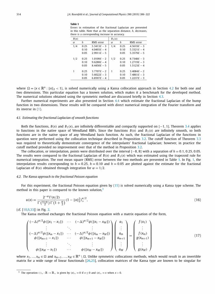

314 J.A. Rosenfeld et al. / Journal of Computational Physics 390 (2019) 306–322

Table 1Errors in estimation of the fractional Laplacian are presented in this table. Note that as the separation distance, h, decreases, there is a corresponding increase in accuracy.

B(x) B1(x)α h RMS error α h RMS error1/4 0.25 5.3413E − 3 1/4 0.25 4.5619E − 3

0.10 4.0493E − 4 0.10 5.3321E − 40.05 2.9911E − 5 0.05 5.3579E − 5

1/2 0.25 1.0109E − 2 1/2 0.25 8.7348E − 30.10 9.6288E − 4 0.10 1.2719E − 30.05 8.4450E − 5 0.05 1.5123E − 4

1 0.25 3.7707E − 2 1 0.25 3.4084E − 20.10 5.6022E − 3 0.10 7.4861E − 30.05 6.8597E − 4 0.05 1.2237E − 3

where � = {x ∈ Rn : ‖x‖2 < 1}, is solved numerically using a Kansa collocation approach in Section 4.2 for both one and two dimensions. This particular equation has a known solution, which makes it a benchmark for the developed method. The numerical solutions obtained using the symmetric method are discussed briefly in Section 4.3.

Further numerical experiments are also presented in Section 4.4 which estimate the fractional Laplacian of the bump function in two dimensions. These results will be compared with direct numerical integration of the Fourier transform and its inverse in (1).

4.1. Estimating the fractional Laplacian of smooth functions

Both the functions, B(x) and B1(x), are infinitely differentiable and compactly supported on [−1, 1]. Theorem 3.4 applies to functions in the native space of Wendland RBFs. Since the functions B(x) and B1(x) are infinitely smooth, so both functions are in the native space of any Wendland basis function. As such, the fractional Laplacian of the functions in question were performed using the collocation technique described in Proposition 3.2. The cutoff function of Theorem 3.3was required to theoretically demonstrate convergence of the interpolants’ fractional Laplacian; however, in practice the cutoff method provided no improvement over that of the method in Proposition 3.2.

The collocation, or interpolation, points were distributed over the interval [−8, 8] with a separation of h = 0.1, 0.25, 0.05. The results were compared to the fractional Laplacian of B(x) and B1(x) which was estimated using the trapezoid rule for numerical integration. The root mean square (RMS) error between the two methods are presented in Table 1. In Fig. 1, the interpolation results corresponding to h = 0.25, h = 0.10 and h = 0.05 are plotted against the estimate for the fractional Laplacian of B(x) obtained through integration for α = 1/2.

4.2. The Kansa approach to the fractional Poisson equation

For this experiment, the fractional Poisson equation given by (15) is solved numerically using a Kansa type scheme. The method in this paper is compared to the known solution,3

u(x) = 2−α�(n/2)

�(n+α

2

)�

(1 + α

2

) (1 − ‖x‖22)

α/2+ , (16)

(cf. [10,9,33]) in Fig. 2.The Kansa method exchanges the fractional Poisson equation with a matrix equation of the form,

⎛⎜⎜⎜⎜⎜⎜⎜⎜⎝

(−�)α/2φ(‖x1 − x1‖) · · · (−�)α/2φ(‖x1 − xM‖)...

. . ....

(−�)α/2φ(‖xm − x1‖) · · · (−�)α/2φ(‖xm − xM‖)φ(‖xm+1 − x1‖) · · · φ(‖xm+1 − xM‖)

.... . .

...

φ(‖xM − x1‖) · · · φ(‖xM − xM‖)

⎞⎟⎟⎟⎟⎟⎟⎟⎟⎠

⎛⎜⎜⎜⎜⎜⎜⎜⎜⎝

a1...

am

am+1...

aM

⎞⎟⎟⎟⎟⎟⎟⎟⎟⎠

=

⎛⎜⎜⎜⎜⎜⎜⎜⎜⎝

f (x1)...

f (xm)

g(xm+1)...

g(xM)

⎞⎟⎟⎟⎟⎟⎟⎟⎟⎠

(17)

where x1, ..., xm ∈ � and xm+1, ..., xM ∈Rn \ �. Unlike symmetric collocations methods, which would result in an invertible matrix for a wide range of linear functionals [26,25], collocation matrices of the Kansa type are known to be singular for

3 The operation (·)+ :R →R+ is given by (x)+ = 0 if x ≤ 0 and (x)+ = x when x > 0.

J.A. Rosenfeld et al. / Journal of Computational Physics 390 (2019) 306–322 315

Fig. 1. The pseudospectral method developed in this paper is framed over the native spaces of RBFs. The Wendland RBF is used to demonstrate the method. The fractional Laplacian of interpolants are plotted against the estimate for the fractional Laplacian of B(x) obtained through integration for α = 1/2. Note that the fractional Laplacian of the interpolant with h = 0.05 is indistinguishable from (−�)1/2 B(x) in this figure (RMS Error of 8.4450E − 5). It should be noted that even with the spacing of h = 0.25, a good approximation (RMS Error of 1.0109E − 2) is achieved. That is the error improved by a factor of approximately 102 when the density was increased by a factor of four. The top right figure emphasizes the accuracy achieved at the peak of the function, and the bottom right shows the worst errors near x = ±1 committed by fractional Laplacian of the interpolant with spacing h = 0.25. (For interpretation of the colors in the figure(s), the reader is referred to the web version of this article.)

Fig. 2. This figure presents the numerical solutions for the fractional Poisson equation given in (15) using the Kansa collocation approach as compared to the actual solution u. Each curve is labeled by the density of the collocation points distributed over [−8, 8]. As can be seen in the figure, the estimation improves as the distance between the collocation points decreases. The bottom right sub figure presents a zoomed version of the Gibbs phenomenon manifesting at x = ±1. The Gibbs phenomenon is an anticipated consequence of estimating a non-smooth function by the smooth Wendland RBFs.

certain choices of collocation points. However, most choices of collocation points result in an invertible collocation matrix, and greedy algorithms exist for selecting such collocation points [34,22].

For the particular problem solved in this section, n = 1, g ≡ 0 on R \ [−1, 1] and f ≡ 1 on [−1, 1]. The collocation points were distributed over [−8, 8] with a spacing of 0.1, 0.05, 0.025, and 0.0125, and the interpolation was performed using the Wendland RBF, φs,k with s = 3 and k = 6. The order of the fractional Laplacian was chosen to be α = 1/2. The results are presented in Fig. 2 and Fig. 3.

As evidenced in Fig. 2, increasing the number of collocation points by reducing width between the points improves the accuracy of the numerical method. A Gibbs phenomenon can be observed near the points x = ±1, and are expected since the Wendland functions are designed to estimate smoother functions, and the solution u is not differentiable at x = ±1. The Gibbs phenomenon manifests for the collocation spacings of 0.1 and 0.05, but is less pronounced for tighter configurations.

Fig. 3 demonstrates how the uncontrolled error that appears in Proposition 3.2 manifests. In particular, outside of the sampled region of [−8, 8], the convergence guarantees for RBFs no longer hold. The results of [32] and of this numerical ex-

316 J.A. Rosenfeld et al. / Journal of Computational Physics 390 (2019) 306–322

Fig. 3. This figure demonstrates the limitations observed in Proposition 3.2. The cutoff function in Theorem 3.3 was not used for the fractional Poisson equation, so the interpolant is uncontrolled outside the sampling region of [−8, 8]. The interpolant returns to zero for larger values of x, since the basis functions are compactly supported. The more pronounced deviation from the actual solution arrises from the numerical method with a spacing of 0.0125.

Table 2Error between the numerical solution and the known so-lution to the fractional Poisson equation given in (15). The accuracy is somewhat lower than what was obtained in Table 1, where the bump function’s fractional Lapla-cian was estimated. A possible explanation for the lower accuracy is that the numerical solution to the fractional Poisson equation (15) is not a smooth function. In par-ticular, the analytical solution to the (15) is not differen-tiable at x = ±1.

α h RMS error

1/4 0.100 6.2218E-20.050 4.2479E-20.025 3.2166E-2

1/2 0.100 5.3583E-20.050 3.3058E-20.025 2.2844E-2

1 0.100 4.4214E-20.050 2.3325E-20.025 1.2101E-2

periment indicate that more collocation points can result in larger errors. For example, the numerical method that produced the most pronounce errors near x = ±8 was the one using a spacing of 0.0125. In the region [−8, 8] accurate estimations are obtained. However, the fractional Laplacian is sensitive to long range errors, and these may limit the accuracy that can be obtained without the use of a cutoff function. The RMS error over [−8, 8] (where samples were taken every 0.01 units) for various parameters is documented in Table 2.

4.3. The symmetric approach to the fractional Poisson equation

The symmetric collocation approach to solving linear PDEs is often seen as a good alternative to the Kansa approach [25]. The symmetric method trades the possibly singular collocation matrix of the Kansa method with that of a collocation matrix that is symmetric and guaranteed invertible [26]. However, in this particular setting, the symmetric collocation method produced poor results, as seen in Fig. 4 where the solution for the Poisson equation in (15) of order α = 1 obtained through symmetric collocation using collocation points distributed over [−8, 8] with 0.05 spacing is compared with the actual solution u. Fig. 5 demonstrates that the interpolant’s fractional Laplacian over [−1, 1] is close to 1 as is desired in (15).

4.4. The fractional Laplacian in two dimensions

Mesh free collocation methods enable a straightforward algorithm that works in any dimension. In this section, the fractional Laplacian is estimated for the bump function, F (x, y) = B(

√x2 + y2). Again the Wendland basis functions, φn,k ,

J.A. Rosenfeld et al. / Journal of Computational Physics 390 (2019) 306–322 317

Fig. 4. This figure presents the numerical solution using the symmetric method with h = 0.05 (Dashed Line) for the fractional Poisson equation given in (15) as compared to the actual solution u (Solid Line). The collocation points are distributed over [−8, 8]. The numerical method provides a poor estimation of the actual solution. Further numerical experiments not presented in this paper showed that as the separation distance between the collocation points decreased, the numerical solution approached zero. Thus, the Kansa approach, presented in Fig. 2 yields a more satisfying numerical method that not only satisfies (15), but also provides an estimate of the actual solution.

Fig. 5. This figure presents the fractional Laplacian of the interpolant in Fig. 4. The circles represent the collocation points, each with a height of 1. The interpolant’s fractional Laplacian is very close to 1 over the interval [−1, 1], but still does not estimate u well.

are used to estimate the fractional Laplacian of F , this time with a shape parameter of 1/√

2, yielding basis functions of the form φn,k

( ‖x−y‖√2

). The function, F , was sampled over [−2, 2]2 with points distributed in a square lattice of widths

0.5, 0.25, and 0.2. Weights were determined with a direct method. The results were again compared with a method using numerical integration. The numerical results are outlined in Table 3. An example comparing the fractional Laplacian of the interpolant with that of the integration method is presented in Fig. 6.

A decrease in the spacing does not always result in an improved estimate. Improvements can be made by selecting a better shape parameter, using collocation points that are not uniformly spaced, and by employing other methods besides a direct method for determining weights.

4.5. Two dimensional example of the solution to the fractional Poisson equation

This numerical experiment demonstrates the effectiveness of the Kansa method for solving the fractional Poisson equa-tion in two dimensions. Table 4 presents the numerical results obtained in estimating the solution to (15). A uniform grid of collocation points was distributed over [−2, 2]2 with spacing h > 0. The RMS Error reported in the table was taken over the region [−2, 2]2, while the RMS % Error was taken over the disk, � = {x ∈Rn : ‖x‖2 < 1}, where the solution is non-zero.

318 J.A. Rosenfeld et al. / Journal of Computational Physics 390 (2019) 306–322

Table 3Error between the numerical solution using collocation and numerical solution using integration for the esti-mation of a 2-D fractional Laplacian. As in Section 4.1, an infinitely differentiable function, the two dimensional bump function, was used as a benchmark for the nu-merical method. The collocation points were selected to be a square lattice over [−2, 2]. When the lattice width, h, decreased below 0.25 the collocation matrix became ill-conditioned, which explains why the accuracy of the rows corresponding to h = 0.25 are slightly better than the rows corresponding to h = 0.2.

α h RMS error

1/4 0.50 9.9118E-20.25 9.8134E-20.20 9.8249E-2

1/2 0.50 8.6836E-20.25 1.0479E-10.20 1.0626E-1

1 0.50 1.7717E-10.25 2.5960E-10.20 2.6994E-1

Fig. 6. This figure compares the fractional Laplacian of order α = 1/4 obtained via collocation with a lattice of spacing 0.2 (Left) with that of the inte-gration method (Right). It can be seen that the pseudospectral method using the Wendland RBFs provide a good estimate of the fractional Laplacian. This figure demonstrates the ability of the numerical method to generalize to higher dimensions. The pseudospectral method takes advantage of interpolation algorithms already in place and reduces computation of the fractional Laplacian by leveraging the fact that the Fourier transform of radial functions can be computed using a one dimensional integral.

Table 4Accuracy of the numerical solutions using the Wendland kernel function for the frac-tional Poisson equation given in (16).

α Kernel width h RMS error RMS % error

1/2 0.2 0.20 5.5911E-1 82.68%0.10 3.6047E-1 51.48%0.05 5.7752E-2 2.59%

0.5 0.20 2.1780E-1 30.32%0.10 7.2090E-2 5.77%

1.0 0.20 1.3056E-1 13.31%0.10 1.2265E-1 17.96%

1 0.2 0.20 3.7427E-1 86.04%0.10 3.4404E-1 77.17%0.05 1.9912E-2 6.40%

0.5 0.20 2.4624E-1 54.14%0.10 3.3210E-2 15.40%

1.0 0.20 6.6557E-2 22.87%

J.A. Rosenfeld et al. / Journal of Computational Physics 390 (2019) 306–322 319

Several kernel widths were selected, and the greatest accuracy was achieved when using a kernel width of 0.2 and h = 0.05. The spacing h = 0.05 was not compatible with larger kernel widths, since the Kansa matrix became ill-conditioned.

5. Discussion

5.1. The fractional Laplacian of RBFs

From Section 3, a compactly supported function’s fractional Laplacian can be approximated by the fractional Laplacian of interpolants of the form (4) (after modification by a cutoff function). Yet, a remaining question is how to compute the fractional Laplacian of the basis functions.

The contribution of Theorem 5.1 is the demonstration that for RBFs, the application of the fractional Laplacian can be simplified considerably by using a one dimensional integral. In particular, the radial nature of the basis functions can be exploited by integrating against a Bessel function along a single axis. This method uses the so called Fourier-Bessel transform [25], and dramatically reduces the computational difficulties that arise when estimating the fractional Laplacian of a high dimensional function.

Theorem 5.1. For α > 0 and n ≥ 2, let φ :Rn →R be a radially symmetric function with a well defined fractional Laplacian of order α. If K :Rn ×Rn →R is a function of the form K (x, y) = φ(‖x − y‖), then

(−�)α/2 K (x, y) = (2π)−n/2

‖x − y‖ n2 −1

∞∫

0

rα+ n2 φ(r) J n

2 −1(r‖x − y‖)dr, (18)

where the fractional Laplacian is taken with respect to the first variable, x ∈Rn, φ is the Fourier transform of φ , and Jν(z) is the νorder Bessel function given by

Jν(z) =∞∑

m=0

(−1)m

m!�(m + ν + 1)

( z

2

)2m+ν. (19)

Proof. By the well known property of the Fourier transform of shifted functions, F [K (·, y)](ξ) = F [φ(‖ · −y‖)](ξ) =e−iy·ξF [φ](ξ) and

(−�)α/2 K (x, y) = F−1[‖ξ‖αF[φ(x − y)]](x) = 1

(2π)n

∫

Rn

‖ξ‖αφ(ξ)ei(x−y)·ξdξ.

Since the Fourier transform of a radial function is itself radial [35], the function ‖ξ‖αφ(ξ) is radial, and the integral can be simplified as

(−�)α/2 K (x, y) = (2π)−n/2

‖x − y‖ n2 −1

∞∫

0

rα+ n2 φ(r) J n

2 −1(r‖x − y‖)dr,

by the results contained in Appendix B.6 of [35]. �In addition to having a one dimensional integration formula for computing the fractional Laplacian, it is also desirable to

have an error bound on the approximation of the infinite integral given in (18) by an integral over a finite interval.

5.2. The use of the cutoff function

In the numerical experiments in Section, the cutoff function experiments produced results that were indistinguishable from experiments that did not use the cutoff function. The use of the RBFs without the cutoff also allows for only one preprocessing computation using a one dimensional integral, which considerably accelerates the estimation process.

For a given radially symmetric cutoff function as in Theorem 3.3, estimating (−�)α/2(G · sX, f )(x) can be performed, through linearity, by computing (−�)α/2(G · φ(‖ · −y‖))(x) for y ∈ Rn . Fortunately, G and φ are both radial functions, which reduces the total number of integrals to be performed. Moreover, once the preprocessing steps are completed, the data can be reused for the estimation of the fractional Laplacian of any function f ∈N�(Rn) after performing interpolation.

If G is selected to be a polynomial in the region B R (0) \ B R/2(0) and φ is a Wendland RBF, then G · φy is a piecewise defined polynomial over the common support of G and φy . If the support of φy is inside of B R/2(0), then (−�)α/2(G ·φy) =(−�)α/2φy . Moreover, φ is radial, which means ‖ξ‖αφ(ξ) is radial, and thus (−�)α/2φ is radial. Therefore, the fractional Laplacian of φy only has to be performed once for a basis function with support in B R/2(0).

320 J.A. Rosenfeld et al. / Journal of Computational Physics 390 (2019) 306–322

In Theorem 3.3, G was selected to reduce the number of preprocessing steps for computing fractional Laplacians. Since Gis radial, the fractional Laplacian for G · φy only needs to be computed for y ∈ {(t, 0, 0, ..., 0) ∈ B R(0)|t ≥ 0}. Thus, for those basis functions with support beyond B R/2(0), the fractional Laplacian of only a one dimensional family of such basis func-tions must be estimated. The use of a radial cutoff function reduces the computation time when estimating the fractional Laplacian in high dimensional spaces.

The Fourier transform of G · φy can be realized through the convolution4 of the Fourier transform of G with φy ,

(G · φy)(ξ) = (G � φy)(ξ) :=∫

Rn

G(ξ − μ)φy(μ)dμ.

Therefore, if G and φy have L1 Fourier transforms, then so does their convolution. This property enables the estimation of the fractional Laplacian of the basis functions, since it is necessary that the Fourier transform decays quickly. The speed at which the Fourier transform decays is governed by the smoothness of both φ and G .

5.3. Evaluation of collocation matrices

For several of the numerical experiments, such as the Kansa approach to the fractional Poisson equation, collocation matrices of the form

⎛⎜⎝

(−�)α/2φ(‖x1 − x1‖) · · · (−�)α/2φ(‖x1 − xm‖)...

. . ....

(−�)α/2φ(‖xm − x1‖) · · · (−�)α/2φ(‖xm − xm‖)

⎞⎟⎠ (20)

must be computed. When the matrix in (20) is computed, the representation of the fractional Laplacian given by (18), implemented directly in a mathematical software package such as MATLAB, provides a sufficient numerical approach to determining the off-diagonal matrix entries. However, the denominator in (18) is zero when computing the diagonal entries, which makes (18) unsuitable for numerically computing the diagonal entries. For matrix entries where the denominator is near zero and more generally when the argument of (−�)α/2φ(‖x‖) is small, the series representation of the Bessel functions, given in (19), will be used to cancel the zero in the denominator. In particular, defining an auxiliary function Aν

as

Aν(r,‖x − y‖) := Jν(r‖x − y‖)‖x − y‖ν

=∞∑

m=0

(−1)mr2m+ν

22m+νm!�(m + ν + 1)‖x − y‖2m

the singularity is eliminated, and when x = y,

Aν(r,0) = rν

2ν�(ν + 1).

6. Comparison with fast Fourier transform (FFT) methods

The fractional Laplacian leverages the Fourier transform in its definition. There are many algorithms available for esti-mating the Fourier transform of a function. Significantly, the FFT method is the most commonly used. Moreover, the FFT algorithm has a computational complexity of O (m log(m)), where m is the number of sampled points, which makes it extremely efficient when computing the Fourier transform of a function.

To use the FFT method to estimate the fractional Laplacian of a function, a large interval must be selected to achieve an accurate result. The FFT is a method to compute the Fourier transform of a function over a finite interval, and is not directly applicable for the Fourier transform over Rn . However, the authors have noted that with a suitably large interval, the FFT can generate accurate estimations of a function’s fractional Laplacian.

In contrast, the method presented in this manuscript has a computational complexity of O (m3). Consequently, the de-veloped method takes considerably longer to generate an estimation of the fractional Laplacian of a function. Both the FFT and the RBF method perform well in estimating fractional Laplacians of smooth functions, and several experiments have indicated that the RBF method exhibits less ringing phenomenon for non-smooth functions. The advantage of using the method presented here is that it motivates RBF collocation methods for solving fractional order PDEs, such as the Kansa method.

4 The convolution of two functions, f :Rn →R and g :Rn →R, is denoted by ( f � g)(x) = ∫Rn f (x − y)g(y)dy.

J.A. Rosenfeld et al. / Journal of Computational Physics 390 (2019) 306–322 321

7. Conclusion

This paper presented a new method for the estimation of the fractional Laplacian of a function. The development lever-aged the theory of RBFs to establish approximation results and to discretize the fractional Laplacian. The resulting method allows for the fractional Laplacian to be estimated for arbitrary dimension, an advantage to many existing techniques. The development was supported by several theorems demonstrating convergence of the fractional Laplacian of the interpolants to the fractional Laplacian of the function being estimated. The convergence results were framed over the native spaces of the RBFs, as is typical for approximations using RBFs.

Several numerical experiments were presented demonstrating the effectiveness of the numerical method. These experi-ments included the estimation of the fractional Laplacian of functions in both one and two dimensions. Another experiment solved the fractional Poisson equation using a Kansa collocation approach, which provided a much better accuracy when compared to the symmetric collocation approach.

Acknowledgements

This research is supported in part by NSF award number 1509516 and Office of Naval Research Grant N00014-13-1-0151. During the revision process, the first author was supported by the Air Force Office of Scientific Research (AFOSR) under contract numbers FA9550-15-1-0258, FA9550-16-1-0246, and FA9550-18-1-0122. Any opinions, findings and conclusions or recommendations expressed in this material are those of the author(s) and do not necessarily reflect the views of the sponsoring agencies.

References

[1] D.A. Benson, S.W. Wheatcraft, M.M. Meerschaert, Application of a fractional advection-dispersion equation, Water Resour. Res. 36 (6) (2000) 1403–1412.[2] P. Clavin, Instabilities and nonlinear patterns of overdriven detonations in gases, in: Nonlinear PDE’s in Condensed Matter and Reactive Flows, Springer,

2002, pp. 49–97.[3] T. Zhu, J.M. Harris, Modeling acoustic wave propagation in heterogeneous attenuating media using decoupled fractional Laplacians, Geophysics 79 (3)

(2014) T105–T116.[4] J.M. Carcione, A generalization of the Fourier pseudospectral method, Geophysics 75 (6) (2010) A53–A56.[5] K. Kirkpatrick, Y. Zhang, Fractional Schrödinger dynamics and decoherence, Phys. D: Nonlinear Phenom. 332 (2016) 41–54.[6] T.-X. Gou, H.-R. Sun, Solutions of nonlinear Schrödinger equation with fractional Laplacian without the Ambrosetti–Rabinowitz condition, Appl. Math.

Comput. 257 (2015) 409–416.[7] S. Duo, Y. Zhang, Computing the ground and first excited states of the fractional Schrödinger equation in an infinite potential well, Commun. Comput.

Phys. 18 (2) (2015) 321–350.[8] N. Laskin, Fractional Schrödinger equation, Phys. Rev. E 66 (5) (2002).[9] Y. Huang, A. Oberman, Numerical methods for the fractional Laplacian: a finite difference-quadrature approach, SIAM J. Numer. Anal. 52 (6) (2014)

3056–3084.[10] X. Ros-Oton, J. Serra, The Dirichlet problem for the fractional Laplacian: regularity up to the boundary, J. Math. Pures Appl. 101 (3) (2014) 275–302.[11] R. Schumer, D.A. Benson, M.M. Meerschaert, S.W. Wheatcraft, Eulerian derivation of the fractional advection–dispersion equation, J. Contam. Hydrol.

48 (1) (2001) 69–88.[12] A. Lodhia, S. Sheffield, X. Sun, S.S. Watson, Fractional Gaussian fields: a survey, Probab. Surv. 13 (2016) 1–56 (electronic).[13] E. Otarola, A.J. Salgado, Finite element approximation of the parabolic fractional obstacle problem, SIAM J. Numer. Anal. 54 (4) (2016) 2619–2639.[14] A space-time fractional optimal control problem: analysis and discretization, SIAM J. Control Optim. 54 (3) (2016) 1295–1328.[15] H. Chen, H. Zhou, Q. Li, Y. Wang, Two efficient modeling schemes for fractional Laplacian viscoacoustic wave equation, Geophysics 81 (5) (2016)

T233–T249.[16] J. Sun, T. Zhu, S. Fomel, Viscoacoustic modeling and imaging using low-rank approximation, Geophysics 80 (5) (2015) A103–A108.[17] D. Brown, L. Ling, E. Kansa, J. Levesley, On approximate cardinal preconditioning methods for solving PDEs with radial basis functions, Eng. Anal. Bound.

Elem. 29 (4) (2005) 343–353.[18] W. Chen, Z.-J. Fu, C.-S. Chen, Recent Advances in Radial Basis Function Collocation Methods, Springer, 2014.[19] G.E. Fasshauer, Solving differential equations with radial basis functions: multilevel methods and smoothing, Adv. Comput. Math. 11 (2–3) (1999)

139–159.[20] G.E. Fasshauer, J.G. Zhang, On choosing “optimal” shape parameters for RBF approximation, Numer. Algorithms 45 (1–4) (2007) 345–368.[21] H.-Y. Hu, Z.-C. Li, A.H.-D. Cheng, Radial basis collocation methods for elliptic boundary value problems, Comput. Math. Appl. 50 (1) (2005) 289–320.[22] R. Schaback, H. Wendland, Adaptive greedy techniques for approximate solution of large RBF systems, Numer. Algorithms 24 (3) (2000) 239–254.[23] H. Wendland, Piecewise polynomial, positive definite and compactly supported radial functions of minimal degree, Adv. Comput. Math. 4 (4) (1995)

389–396.[24] E. Kansa, Multiquadrics - a scattered data approximation scheme with applications to computational fluid-dynamics - II solutions to parabolic, hyper-

bolic and elliptic partial differential equations, Comput. Math. Appl. 19 (8) (1990) 147–161.[25] G.E. Fasshauer, Meshfree Approximation Methods with MATLAB, Interdisciplinary Mathematical Sciences, vol. 6, World Scientific Publishing Co. Pte.

Ltd., Hackensack, NJ, 2007.[26] G.E. Fasshauer, Solving partial differential equations by collocation with radial basis functions, Vanderbilt University Press, 1997, pp. 131–138.[27] G. Pang, W. Chen, Z. Fu, Space-fractional advection-dispersion equations by the Kansa method, in: Fractional PDEs: Theory, Numerics, and Applications,

J. Comput. Phys. 293 (2015) 280–296.[28] S.D. Bond, R.B. Lehoucq, S.T. Rowe, A Galerkin radial basis function method for nonlocal diffusion, Springer International Publishing, Cham, 2015,

pp. 1–21.[29] R. Lehoucq, S. Rowe, A radial basis function Galerkin method for inhomogeneous nonlocal diffusion, Comput. Methods Appl. Mech. Eng. 299 (2016)

366–380.[30] H. Wendland, Scattered Data Approximation, Cambridge Monographs on Applied and Computational Mathematics, vol. 17, Cambridge University Press,

Cambridge, 2005.

322 J.A. Rosenfeld et al. / Journal of Computational Physics 390 (2019) 306–322

[31] L.C. Evans, Partial Differential Equations, vol. 19, American Mathematical Society, Providence, RI, 2010.[32] H. Wendland, Error estimates for interpolation by compactly supported radial basis functions of minimal degree, J. Approx. Theory 93 (2) (1998)

258–272.[33] A.V. Chechkin, R. Metzler, V.Y. Gonchar, J. Klafter, L.V. Tanatarov, First passage and arrival time densities for Lévy flights and the failure of the method

of images, J. Phys. A, Math. Gen. 36 (41) (2003) L537–L544.[34] L. Ling, R. Schaback, An improved subspace selection algorithm for meshless collocation methods, Int. J. Numer. Methods Eng. 80 (2000) 1–6.[35] L. Grafakos, Classical Fourier Analysis, third edition, Graduate Texts in Mathematics, vol. 249, Springer, New York, 2014.