journal of computational physics - purdue university
TRANSCRIPT

Journal of Computational Physics 437 (2021) 110331
Contents lists available at ScienceDirect
Journal of Computational Physics
www.elsevier.com/locate/jcp
A fast algorithm for the electromagnetic scattering from a
large rectangular cavity in three dimensions ✩
Yanli Chen a, Xue Jiang b,∗, Jun Lai c, Peijun Li d
a Department of Mathematics, Northeastern University, Shenyang 110819, Chinab College of Mathematics, Faculty of Science, Beijing University of Technology, Beijing, 100124, Chinac School of Mathematical Sciences, Zhejiang University Hangzhou, Zhejiang 310027, Chinad Department of Mathematics, Purdue University, West Lafayette, IN 47907, USA
a r t i c l e i n f o a b s t r a c t
Article history:Available online 6 April 2021
Keywords:Electromagnetic scattering problemMaxwell’s equationsOpen cavityFast algorithm
The paper is concerned with the three-dimensional electromagnetic scattering from a large open rectangular cavity that is embedded in a perfectly electrically conducting infinite ground plane. By introducing a transparent boundary condition, the scattering problem is formulated into a boundary value problem in the bounded cavity. Based on the Fourier expansions of the electric field, the Maxwell equation is reduced to one-dimensional ordinary differential equations for the Fourier coefficients. A fast algorithm, employing the fast Fourier transform and the Gaussian elimination, is developed to solve the resulting linear system for the cavity which is filled with either a homogeneous or a layered medium. In addition, a novel scheme is designed to evaluate rapidly and accurately the Fourier transform of singular integrals. Numerical experiments are presented for large cavities to demonstrate the superior performance of the proposed method.
© 2021 Elsevier Inc. All rights reserved.
1. Introduction
The electromagnetic scattering from large cavities has received much attention in both engineering and mathematical communities due to its significant industrial and military applications [4,7,13,16,10]. For instance, the radar cross section (RCS) measures the detectability of a target by a radar system. In practice, the cavity RCS caused by objects such as jet engine inlet ducts, exhaust nozzles and cavity-backed antennas can dominate the total RCS. Therefore, mathematical and computational methods to accurately predict the cavity RCS are important for the enhancement or reduction of the total RCS [5,6]. Another example is the non-destructive testing to determine the shape of a cavity embedded in a known object. In these applications, it has played a crucial role to have an efficient forward solver for the optimal design problems of reducing or enhancing the cavity RCS and the inverse problems of determining an unknown cavity.
A variety of numerical methods, including finite difference methods, finite element methods, the moment methods, boundary element methods, and hybrid methods, have been developed to solve the open cavity problems [14,24,29,26,27,12,18,25], In particular, Bao and Sun [7] proposed a finite difference based fast algorithm for the two-dimensional electro-magnetic scattering from large cavities. In the algorithm, an FFT-sine transform in the horizontal direction and the Gaussian
✩ The work of YC is supported in part by NSFC grant 12001086. The work of XJ is supported in part by NSFC grant 11771057. The work of JL was partially supported by the Funds for Creative Research Groups of NSFC (No. 11621101) and NSFC grant No. 11871427. The research of PL is supported in part by the NSF grant DMS-1912704.
* Corresponding author.E-mail addresses: [email protected] (Y. Chen), [email protected] (X. Jiang), [email protected] (J. Lai), [email protected] (P. Li).
https://doi.org/10.1016/j.jcp.2021.1103310021-9991/© 2021 Elsevier Inc. All rights reserved.

Y. Chen, X. Jiang, J. Lai et al. Journal of Computational Physics 437 (2021) 110331
elimination along the vertical direction were used to reduce the global system to a much smaller system imposed only on the open aperture of the cavity. As an extension of this method, a tensor product finite element method was proposed in [10] by employing piecewise polynomials of degree k ≥ 1 to approximate the solution space of the cavity problem. In [31], a fourth order finite difference scheme was developed to discrete the cavity scattering problem in the rectangular domain and to reach a global fourth order convergence in the whole computational domain by a special treatment on the boundary condition. Since the resulting linear system obtained from the cavity problem is usually indefinite and ill-conditioned, con-vergence of iterative methods such as GMRES is very slow. Different kinds of preconditioners were proposed to accelerate the convergence [7,10,31,9,32]. On the other hand, a fast direct solver based on hierarchical matrix factorization technique was used to solve the two-dimensional electromagnetic scattering from an arbitrarily shaped cavity[16]. It was shown that the linear system resulted from the integral equation method can be solved in nearly linear time. The method was ex-tended to the scattering of three-dimensional axis-symmetric cavities in [17]. We refer to [15] for the motivation, modeling, computation, as well as related references on the open cavity scattering problems.
It is worth mentioning that the computation is extremely challenging when the cavities are large compared to the wavelength of the incident wave because of the highly oscillatory nature of the fields. For such a high frequency scattering problem, it is shown that the ratio of the error by the usual Galerkin type method and the error of the best approximation tends to infinity as the wave number increases [3,2]. Due to these difficulties, the discretization by conventional numerical methods becomes very expensive for the large cavity scattering problems especially in three dimensions. In this paper, we intend to develop a fast algorithm for solving the three-dimensional electromagnetic scattering from large rectangular cavities embedded in an infinite perfectly electrically conducting ground plane.
More specifically, we consider the three-dimensional Maxwell equations along with the Silver–Müller radiation condition imposed at infinity. By using the dyadic Green’s function in the half space, we first derive an exact transparent boundary condition (TBC) on the open aperture of the cavity. As a result, the original scattering problem is formulated equivalently to a boundary value problem of Maxwell equations in a bounded domain. We refer to [1] for the mathematical study on the well-posedness of the cavity problem for Maxwell’s equations. Secondly, we introduce the Fourier series expansion of the electric field inside the cavity. By such an expansion, the governing Maxwell equations can be reduced to one-dimensional ordinary differential equations with respect to the vertical direction. A second-order finite difference scheme is adopted to solve the ordinary differential systems. A fast algorithm, based on the fast Fourier transform in the horizontal directions and the Gaussian elimination along the vertical direction, is developed to solve the linear system arising from scattering of large cavities which may be filled with a homogeneous medium or a vertically layered medium. Moreover, we reduce the global system to a linear system on the open aperture of the cavity only and design a novel scheme to evaluate rapidly and accurately the singular integrals appeared in the transparent boundary condition. Numerical results show that our algorithm is very efficient in terms of computational cost.
The paper is organized as follows. In Section 2, we describe the problem formulation of the electromagnetic scattering by a rectangular cavity which is filled with a homogeneous medium. The governing Maxwell equations along with the Silver–Müller radiation condition are introduced. The TBC is presented to reduce the unbounded scattering problem to a boundary value problem formulated in the bounded cavity. The details of the fast algorithm are given in Section 3. Section 4 is devoted to an extension of the fast algorithm to the scattering of a cavity which is filled with a layered medium. Section 5 proposes an FFT based efficient algorithm to evaluate the singular integrals arising from the nonlocal TBC on the open aperture of the cavity. Analysis on the computational complexity for the fast algorithm is discussed in Section 6. Numerical examples are presented in Section 7 to demonstrate the performance of the proposed algorithm. The paper is concluded with some general remarks in Section 8.
2. Problem formulation
Consider the incidence of a time-harmonic electromagnetic wave on a rectangular cavity D ⊂ R3, which is embedded in the infinite ground plane �g . The problem geometry is shown in Fig. 1. The cavity wall S and the ground plane �g are assumed to be perfect electric conductors. We also assume that the open aperture � = [0, a] × [0, b] is aligned with the ground plane �g and the depth of the cavity is c. The half space above the ground and the cavity are assumed to be filled with some homogeneous material with a constant electric permittivity ε0 and a constant magnetic permeability μ0. Let B+
Rbe a half-ball above the ground plane with hemisphere �+
R as part of the boundary, where the radius R is large enough so that �+
R covers the open aperture �. It is clear to note that the full boundary of ∂ B+R consists of the hemisphere �+
R , the open aperture �, and a part of the ground plane �g . Without confusion, we simply denote ∂ B+
R = �+R ∪ � ∪ �g .
The total electric and magnetic fields (E, H) consist of the incident waves (E inc, H inc), the reflected waves (Eref, H ref)
due to the infinite ground plane, and the scattered wave (Es, H s) because of the open cavity. The total fields E and Hsatisfy Maxwell’s equations in R3+ ∪ D:
∇ × E = iωμ0 H , ∇ × H = −iωε0 E, (2.1)
where ω > 0 is the angular frequency. Since the ground plane and the cavity wall are perfect conductors, we have
ν × E = 0 on �g ∪ S, (2.2)
2

Y. Chen, X. Jiang, J. Lai et al. Journal of Computational Physics 437 (2021) 110331
Fig. 1. The problem geometry of the electromagnetic scattering by a rectangular cavity.
where ν is the unit normal vector on �g and S .The incident electromagnetic plane waves (E inc, H inc) are given as
E inc = peiq·x, H inc = seiq·x, s = q × p
ωμ0, p · q = 0,
where x = (x1, x2, x3) ∈R3, p = (p1, p2, p3) and s = (s1, s2, s3) are the polarization vectors, q = (α1, α2, −β) with β ≥ 0 is the propagation direction vector. It is easy to verify that the incident electromagnetic fields (E inc, H inc) satisfy the Maxwell equation (2.1) in R3+ .
Due to the infinite ground plane, the reflected fields (E ref, H ref) can be explicitly written as
Eref = p∗eiq∗·x, H ref = s∗eiq∗·x, s∗ = q∗ × p∗
ωμ0, p∗ · q∗ = 0,
where p∗ = (−p1, −p2, p3) and q∗ = (α1, α2, β). Evidently, the reflected fields (Eref, H ref) also satisfy the Maxwell equation (2.1) in R3+ . In particular, the following homogeneous Dirichlet boundary condition is satisfied for the incident and reflected electric fields on the ground plane:
ν × (E inc + Eref) = 0 on �g .
It follows from (2.1) and the incident and reflected electromagnetic fields that the scattered electromagnetic fields (Es, H s) also satisfy the Maxwell equation
∇ × Es = iωμ0 H s, ∇ × H s = −iωε0 Es, x ∈R3+, (2.3)
and the homogeneous Dirichlet boundary condition
ν × E s = 0 on �g . (2.4)
In addition, the scattered field (Es, H s) are required to satisfy the Silver–Müller radiation condition:
√ε0 Es − √
μ0 H s × x = o(|x|−1), |x| → ∞, (2.5)
where x = x/|x|. By eliminating the scattered magnetic field in (2.3), the scattered electric field satisfies
∇ × (∇ × Es) − κ20 Es = 0 in R3+, (2.6)
where κ0 = ω√
ε0μ0 is the wavenumber.In order to derive a transparent boundary condition on the open aperture �, we introduce the half-space dyadic Green’s
function ¯Ge(x, y), which is given by
¯Ge(x, y) = ¯G0(x, y) − ¯G0(x, yi) + 2z zg(x, yi), (2.7)
where
¯G0(x, y) =(¯I − 1
κ20
∇x∇y
)g(x, y), (2.8)
is the free space dyadic Green’s function, ¯I = xx + y y + z z is the 3 × 3 identity matrix, and
3

Y. Chen, X. Jiang, J. Lai et al. Journal of Computational Physics 437 (2021) 110331
g(x, y) = eiκ0|x−y|
4π |x − y| , (2.9)
is the free space Green’s function for the three-dimensional Helmholtz equation. Here yi = y1x + y2 y − y3 z denotes the image point of y = y1x + y2 y + y3 z, and x, y, z are the unit vectors in the x1, x2, x3 axis, respectively.
The half-space dyadic Green’s function satisfies the Maxwell equation
∇ × (∇ × ¯Ge(x, y)) − κ2
0¯Ge(x, y) = ¯Iδ(x − y) in R3+, (2.10)
and the Dirichlet boundary condition
ν × ¯Ge(x, y) = 0 on �g ∪ �, (2.11)
where δ is the Dirac delta function. Furthermore, the half-space dyadic Green’s function satisfies the Silver–Müller radiation condition.
Next, we present the transparent boundary condition. Multiplying both sides of (2.6) by the half-space dyadic Green’s function and integrating over B+
R , we obtain∫B+
R
((∇x × ∇x × Es(x)) · ¯Ge(x, y) − κ2
0 Es(x) · ¯Ge(x, y))
dx = 0.
It follows from the second vector Green’s theorem that∫B+
R
Es(x) ·(∇x × ∇x × ¯Ge(x, y) − κ2
0¯Ge(x, y)
)dx
= −∫
�+R ∪�∪�g
((ν × Es(x)
) · (∇x × ¯Ge(x, y)) − (
ν × ¯Ge(x, y)) · (∇x × Es(x)
))dsx. (2.12)
Since the scattered field Es(x) and the half-space dyadic Green’s function satisfy the Silver–Müller radiation condition, we get ∫
�+R
((ν × Es(x)
) · (∇x × ¯Ge(x, y)) − (
ν × ¯Ge(x, y)) · (∇x × Es(x)
))dsx = 0. (2.13)
Combining (2.4) and (2.11) gives∫�g
((ν × Es(x)
) · (∇x × ¯Ge(x, y)) − (
ν × ¯Ge(x, y)) · (∇x × Es(x)
))dsx = 0 (2.14)
and ∫�
(ν × ¯Ge(x, y)
) · (∇x × Es(x))dsx = 0. (2.15)
Using (2.12)–(2.15) yields∫B+
R
Es(x) ·(∇x × ∇x × · ¯Ge(x, y) − κ2
0¯Ge(x, y)
)dx
= −∫�
(ν × Es(x)
) · (∇x × ¯Ge(x, y))dsx. (2.16)
Substituting (2.10) into (2.16) and switching variables x and y, we get
Es(x) = −∫�
(ν × Es(y)
) · (∇y × ¯Ge(x, y))ds y .
Noting ν = −z gives
Es(x) =∫ (
z × Es(y)) · (∇y × ¯Ge(x, y)
)ds y .
�
4

Y. Chen, X. Jiang, J. Lai et al. Journal of Computational Physics 437 (2021) 110331
It follows from Es = E − E inc − Eref and z × (E inc + Eref) = 0 on � that
E = E inc + Eref +∫�
(z × E(y)
) · (∇y × ¯Ge(x, y))ds y . (2.17)
Substituting (2.7) into (2.17), we obtain
E = E inc + Eref + 2∫�
(z × E(y)
) · (∇y × ¯G0(x, y))ds y . (2.18)
Taking curl on the both sides of (2.18) yields
∇x × E = ∇x × E inc + ∇x × Eref − 2κ20
∫�
(z × E(y)
) · ¯G0(x, y)ds y . (2.19)
Substituting (2.8) into (2.19), we get
(∇x × E) = ∇x × E inc + ∇x × Eref − 2κ2
0
∫�
(z × E(y)
)g(x, y)ds y
+ 2(∇x
∫�
(z × E(y)
) · (∇y g(x, y))ds y
).
For a continuous differential function u defined in a neighborhood of �, define the surface gradient on � by
∇�u = (ν × ∇u) × ν.
Moreover, we have the decomposition
∇u = ∇�u + ∂u
∂νν, (2.20)
where ∂u∂ν is the normal derivative on �. Let v be a tangent vector on �, then we have∫
�
udiv�vds = −∫�
∇�u · vds. (2.21)
Using (2.20)–(2.21) and taking the limit x3 → 0+, we obtain the following transparent boundary condition (TBC):
z × (∇x × E) = T (E) + g on �, (2.22)
where g = z × (∇x × E inc) + z × (∇x × Eref
)and
T (E) = −2κ20 z ×
∫�
(z × E(y)
)g(x, y)ds y − 2z ×
(∇x
∫�
div�
(z × E(y)
)g(x, y)ds y
).
Then, by eliminating the magnetic field in (2.1) and using the TBC (2.22), the scattering problem (2.1)–(2.2) can be reduced to an equivalent boundary value problem in the cavity D:⎧⎪⎪⎨
⎪⎪⎩∇ × (∇ × E) − κ2
0 E = 0 in D,
ν × E = 0 on S,
z × (∇x × E) = T (E) + g on �.
(2.23)
3. Discretization and fast algorithm
In this section, we present the numerical discretization to the Maxwell equation and the TBC, and a fast algorithm for the resulting system.
Let E = (E1, E2, E3). On the plane surfaces x1 = 0 and x1 = a, the unit outward normal vectors are (−1, 0, 0) and (1, 0, 0), respectively. Using the boundary condition in (2.23), we get the homogeneous Dirichlet boundary condition for E2 and E3:
E2(0, x2, x3) = E2(a, x2, x3), E3(0, x2, x3) = E3(a, x2, x3). (3.1)
5

Y. Chen, X. Jiang, J. Lai et al. Journal of Computational Physics 437 (2021) 110331
Recall the divergence free condition on the surface:
∇ · E = ∂x1 E1 + ∂x2 E2 + ∂x3 E3 = 0,
which, together with (3.1), implies the homogeneous Neumann boundary condition for E1:
∂x1 E1(0, x2, x3) = ∂x1 E1(a, x2, x3) = 0. (3.2)
Similarly, on the plane surfaces x2 = 0 and x2 = b, the unit outward normal vectors are (0, −1, 0) and (0, 1, 0), respectively. Using the boundary condition in (2.23), we have the homogeneous Dirichlet boundary condition for E1 and E3:
E1(x1,0, x3) = E1(x1,b, x3), E3(x1,0, x3) = E3(x1,b, x3). (3.3)
Using (3.3) and the divergence free condition again gives the homogeneous Neumann boundary condition for E2:
∂x2 E2(x1,0, x3) = ∂x2 E2(x1,b, x3) = 0. (3.4)
By the boundary conditions (3.1)–(3.4), it is easy to show that E j, j = 1, 2, 3 admits the following Fourier series expansions:
⎧⎪⎪⎪⎪⎪⎪⎪⎪⎪⎨⎪⎪⎪⎪⎪⎪⎪⎪⎪⎩
E1(x1, x2, x3) =∑
k∈N2
E(k)1 (x3) cos
(k1πx1
a
)sin
(k2πx2
b
),
E2(x1, x2, x3) =∑
k∈N2
E(k)2 (x3) sin
(k1πx1
a
)cos
(k2πx2
b
),
E3(x1, x2, x3) =∑
k∈N2
E(k)3 (x3) sin
(k1πx1
a
)sin
(k2πx2
b
),
(3.5)
where k = (k1, k2) ∈N2.By the vector identity ∇ × (∇ × E) = −�E +∇(∇ · E) and the divergence free condition ∇ · E = 0, the Maxwell equation
in (2.23) can be reduced to the vector Helmholtz equation
�E + κ20 E = 0 in D. (3.6)
Using the boundary condition in (2.23) and the divergence free condition on the plane surfaces x3 = −c, we get the homo-geneous Dirichlet boundary condition
E1(x1, x2,−c) = E2(x1, x2,−c) = 0 (3.7)
and the homogeneous Neumann boundary condition
∂x3 E3(x1, x2,−c) = 0. (3.8)
Substituting (3.5) into (3.6)–(3.8), we may get the second order ordinary differential equations for the Fourier coefficients E(m,n)
l , l = 1, 2:⎧⎪⎨⎪⎩
d2
dx23
E(m,n)
l (x3) +(κ2
0 − (mπ
a
)2 − (nπ
b
)2)
E(m,n)
l (x3) = 0, x3 ∈ (−c,0),
E(m,n)
l (−c) = 0,
(3.9)
where (m, n) ∈N2l , and the second order ordinary differential equations for the Fourier coefficients E(m,n)
3 :⎧⎪⎪⎪⎨⎪⎪⎪⎩
d2
dx23
E(m,n)3 (x3) +
(κ2
0 − (mπ
a
)2 − (nπ
b
)2)
E(m,n)3 (x3) = 0, x3 ∈ (−c,0),
d
dx3E(m,n)
3 (−c) = 0,
(3.10)
where (m, n) ∈N23 . Here N2
1 = {0, 1, 2, · · · , M} ×{1, 2, · · · , N}, N22 = {1, 2, · · · , M} ×{0, 1, 2, · · · , N} and N2
3 = {1, 2, · · · , M}× {1, 2, · · · , N}, M and N are the finite truncation numbers of the Fourier series.
Let {x j3} j= J+1
j=0 be a set of uniformly distributed grid points of [−c, 0] with x j+13 − x j
3 = h. Let E(m,n)
l, j be the finite difference
solution of E(m,n)(x3), l = 1, 2, 3 at the point x3 = x j . The discrete finite difference systems for (3.9)–(3.10) are
l 36

Y. Chen, X. Jiang, J. Lai et al. Journal of Computational Physics 437 (2021) 110331
⎧⎪⎨⎪⎩
E(m,n)
l, j−1 − 2E(m,n)
l, j + E(m,n)
l, j+1
h2+
(κ2
0 − (mπ
a
)2 − (nπ
b
)2)
E(m,n)
l, j = 0, j = 1,2, · · · , J ,
E(m,n)
l,0 = 0,
and ⎧⎪⎨⎪⎩
E(m,n)3, j−1 − 2E(m,n)
3, j + E(m,n)3, j+1
h2+
(κ2
0 − (mπ
a
)2 − (nπ
b
)2)
E(m,n)3, j = 0, j = 1,2, · · · , J ,
E(m,n)3,1 = E(m,n)
3,0 .
The above discrete systems can be written in the matrix form
(A1 + D(m,n)
)E(m,n)
l + a J E(m,n)
l, J+1 = 0, (m,n) ∈N2l , l = 1,2, (3.11)
and
(A2 + D(m,n)
)E(m,n)
3 + a J E(m,n)3, J+1 = 0, (m,n) ∈N2
3 , (3.12)
where the vectors of unknowns E(m,n)
l =(
E(m,n)
l,1 , E(m,n)
l,2 , · · · , E(m,n)
l, J
)�, l = 1, 2, 3,
A1 =
⎛⎜⎜⎜⎝
−2 11 −2 1
. . .. . .
. . .
1 −2
⎞⎟⎟⎟⎠ , A2 =
⎛⎜⎜⎜⎝
−1 11 −2 1
. . .. . .
. . .
1 −2
⎞⎟⎟⎟⎠ , a J =
⎛⎜⎜⎜⎝
0...
01
⎞⎟⎟⎟⎠ ,
and
D(m,n) = h2(κ2
0 − (mπ
a
)2 − (nπ
b
)2)
I J ,
Here I J is the J × J identity matrix.Next, we discuss the discretization of the transparent boundary condition (2.22). A simple calculation from the first
component of (2.22) yields
∂ E3
∂x1− ∂ E1
∂x3= 2(iα1 p3 + iβp1)ei(α1x1+α2x2) + 2κ2
0
∫�
E1(y)g(x, y)ds y
+ 2∫�
( − ∂y1 E2(y) + ∂y2 E1(y))∂x2 g(x, y)ds y . (3.13)
Substituting (3.5) into (3.13), we have
∑k∈N2
3
E(k)3 (0)
k1π
acos
(k1πx1
a
)sin
(k2πx2
b
)−
∑k∈N2
1
dE(k)1 (0)
dx3cos
(k1πx1
a
)sin
(k2πx2
b
)
= 2(iα1 p3 + iβp1)ei(α1x1+α2x2)
+ 2κ20
∑k∈N2
1
E(k)1 (0)
∫�
cos(k1π y1
a
)sin
(k2π y2
b
)g(x, y)ds y
− 2∑
k∈N22
E(k)2 (0)
k1π
a
∫�
cos(k1π y1
a
)cos
(k2π y2
b
)∂x2 g(x, y)ds y
+ 2∑
k∈N21
E(k)1 (0)
k2π
b
∫�
cos(k1π y1
a
)cos
(k2π y2
b
)∂x2 g(x, y)ds y . (3.14)
Multiplying both sides of (3.14) by cos(mπx1
)sin
(nπx2), (m, n) ∈N2 and integrating over �, we obtain
a b 17

Y. Chen, X. Jiang, J. Lai et al. Journal of Computational Physics 437 (2021) 110331
E(m,n)3 (0)p(m,n) − dE(m,n)
1 (0)
dx3q(m,n) = 2(iα1 p3 + iβp1)g(m,n)
1 + 2κ20
∑k∈N2
1
E(k)1 (0) F (m,n)
1,(k)
−2∑
k∈N22
E(k)2 (0)
k1π
aG(m,n)
1,(k)+ 2
∑k∈N2
1
E(k)1 (0)
k2π
bH (m,n)
1,(k),
where
p(m,n) ={
0, if m = 0,bmπ
4 , others,q(m,n) =
{ab2 , if m = 0,
ab4 , others,
and
g(m,n)1 =
∫�
cos(mπx1
a
)sin
(nπx2
b
)ei(α1x1+α2x2)dsx, (3.15)
F (m,n)
1,(k)=
∫�
cos(mπx1
a
)sin
(nπx2
b
)(∫�
cos(k1π y1
a
)sin
(k2π y2
b
)g(x, y)ds y
)dsx, (3.16)
G(m,n)
1,(k)=
∫�
cos(mπx1
a
)sin
(nπx2
b
)(∫�
cos(k1π y1
a
)cos
(k2π y2
b
)∂x2 g(x, y)ds y
)dsx, (3.17)
H (m,n)
1,(k)=
∫�
cos(mπx1
a
)sin
(nπx2
b
)(∫�
cos(k1π y1
a
)cos
(k2π y2
b
)∂x2 g(x, y)ds y
)dsx. (3.18)
By using a backward finite difference scheme for the normal derivative and the fact that E(k)
l, J+1 = E(k)
l (0), l = 1, 2, 3, we get
E(m,n)3, J+1 p(m,n) − E(m,n)
1, J+1 − E(m,n)1, J
hq(m,n) = 2(iα1 p3 + iβp1)g(m,n)
1 + 2κ20
∑k∈N2
1
E(k)1, J+1 F (m,n)
1,(k)
−2∑
k∈N22
E(k)2, J+1
(k1π
a
)G(m,n)
1,(k)+ 2
∑k∈N2
1
E(k)1, J+1
(k2π
b
)H (m,n)
1,(k). (3.19)
For (m, n) ∈N21 , we define the following notations:
g(m,n)1 := h
q(m,n)2(iα1 p3 + iβp1)g(m,n)
1 ,
F (m,n)
1,(k):= h
q(m,n)2κ2
0 F (m,n)
1,(k),
G(m,n)
1,(k):= h
q(m,n)
−2k1π
aG(m,n)
1,(k),
H (m,n)
1,(k):= h
q(m,n)
2k2π
bH (m,n)
1,(k).
Thus, we obtain from (3.19) that
E(m,n)3, J+1
p(m,n)h
q(m,n)− E(m,n)
1, J+1 + E(m,n)1, J −
∑k∈N2
1
E(k)1, J+1 F (m,n)
1,(k)
−∑
k∈N22
E(k)2, J+1G(m,n)
1,(k)−
∑k∈N2
1
E(k)1, J+1 H (m,n)
1,(k)= g(m,n)
1 , (m,n) ∈N21 ,
which can be written in a matrix form
I 1 E1, J + (− I 1 − F 1 − H 1)E1, J+1 − G1 E2, J+1 + I 1 E3, J+1 = g1. (3.20)
Here I1 = I ((M+1)N) , I 1 = I 1 ⊗ I N , ⊗ denotes the Kronecker product, and
8

Y. Chen, X. Jiang, J. Lai et al. Journal of Computational Physics 437 (2021) 110331
I 1 =
⎛⎜⎜⎜⎝
0 · · · 0πha
. . .Mπh
a
⎞⎟⎟⎟⎠ .
For clarity, we refer to Appendix A for the entries of F 1, H 1, G1, g1, and E l, j for l = 1, 2, 3, 0 ≤ j ≤ J + 1.Similarly, the second component of TBC (2.22) can be discretized as
I 2 E2, J − H 2 E1, J+1 + (− I 2 − F 2 − G2)E2, J+1 + I 2 E3, J+1 = g2, (3.21)
where I2 = I (M(N+1)) , I2 = I M ⊗ I 2, and
I 2 =
⎛⎜⎜⎜⎝
0 · · · 0πhb
. . .Nπh
b
⎞⎟⎟⎟⎠
(N+1)×N
.
Again, the entries of the vectors F 2, H 2, G2 and g2 can be found in Appendix A.Recall the divergence free condition on the surface �,
∂x1 E1 + ∂x2 E2 + ∂x3 E3 = 0. (3.22)
Substituting (3.5) into (3.22), we have∑k∈N2
1
E(k)1 (0)
(−k1π
a
)sin
(k1πx1
a
)sin
(k2πx2
b
)+
∑k∈N2
2
E(k)2 (0)
(−k2π
b
)sin
(k1πx1
a
)sin
(k2πx2
b
)
+∑
k∈N23
∂ E(k)3 (0)
∂x3sin
(k1πx1
a
)sin
(k2πx2
b
)= 0. (3.23)
Multiplying both side of (3.23) by sin(mπx1
a
)sin
(nπx2b
), (m, n) ∈ N2
3 , integrating over �, and using the orthogonality of the trigonometric functions, we obtain(−mπ
a
ab
4
)E(m,n)
1 (0) +(−nπ
b
ab
4
)E(m,n)
2 (0) +(
ab
4
)∂ E(m,n)
3 (0)
∂x3= 0. (3.24)
By using a backward finite difference scheme, we get
E(m,n)3, J +
(mπ
a
)E(m,n)
1, J+1 +(nπ
b
)E(m,n)
2, J+1 − E(m,n)3, J+1 = 0. (3.25)
Let
I 3 =⎛⎜⎝
0 πha
.... . .
0 Mπha
⎞⎟⎠ , I 4 =
⎛⎜⎝
0 πhb
.... . .
0 Nπhb
⎞⎟⎠ ,
F 3 = I 3 ⊗ I N and G3 = I M ⊗ I 4. The discrete system (3.25) can be rewritten as
I 3 E3, J + F 3 E1, J+1 + G3 E2, J+1 − I 3 E3, J+1 = 0, (3.26)
where I3 = I (MN) . It follows from (3.20)–(3.21) and (3.26) that⎛⎝ I 1
I 2
I 3
⎞⎠
⎛⎝ E1, J
E2, J
E3, J
⎞⎠ +
⎛⎝− I 1 − F 1 − H 1 −G1 I 1
−H 2 − I 2 − F 2 − G2 I 2
F 3 G3 − I 3
⎞⎠
⎛⎝ E1, J+1
E2, J+1E3, J+1
⎞⎠ =
⎛⎝ g1
g20
⎞⎠ (3.27)
Clearly, the linear systems (3.11)–(3.12) and (3.27) are coupled and give the global system. Next, we use Gaussian elim-ination method to decouple the global system into a linear system with the unknowns only on the aperture, which may reduce the computational complexity greatly and lead to a fast algorithm.
Let
L(m,n)U (m,n) = A1 + D(m,n), (m,n) ∈N2, l = 1,2, (3.28)
1 1 l9

Y. Chen, X. Jiang, J. Lai et al. Journal of Computational Physics 437 (2021) 110331
and
L(m,n)2 U (m,n)
2 = A2 + D(m,n), (m,n) ∈N23 , (3.29)
be the LU-decomposition, where A1 + D(m,n) and A2 + D(m,n) are the symmetric tridiagonal matrices in (3.11) and (3.12), respectively. Since L(m,n)
1 and L(m,n)2 are nonsingular, we obtain
U (m,n)1 E(m,n)
l + (L(m,n)
1
)−1a J+1 E(m,n)
l, J+1 = 0, (m,n) ∈N2l , l = 1,2, (3.30)
U (m,n)2 E(m,n)
3 + (L(m,n)
2
)−1a J+1 E(m,n)
3, J+1 = 0, (m,n) ∈N23 , (3.31)
where U (m,n)1 = (
rm,n1,(pq)
)and U (m,n)
2 = (rm,n
2,(pq)
).
Combining the last equations of the systems (3.30) and (3.31) gives
⎛⎝ R1
R2R3
⎞⎠
⎛⎝ E1, J
E2, J
E3, J
⎞⎠ +
⎛⎝ I 1
I 2
I 3
⎞⎠
⎛⎝ E1, J+1
E2, J+1E3, J+1
⎞⎠ = 0, (3.32)
where
Rl = diag(r(m,n)
1,( J J )
), (m,n) ∈ N2
l , l = 1,2,
R3 = diag(r(m,n)
2,( J J )
), (m,n) ∈N2
3 .
If κ20 is not an eigenvalue of the Helmholtz operator with Dirichlet boundary condition, the continuous Helmholtz problem
admits a unique solution; for h small enough, as an approximate problem, the discrete Helmholtz problem can also be shown to have a unique solution [28], which implies that
r(m,n)1,( J J ) �= 0, (m,n) ∈N2
l , l = 1,2, (3.33)
and
r(m,n)2,( J J ) �= 0, (m,n) ∈N2
3 . (3.34)
Consequently, combining (3.32) and (3.27) yields
⎛⎝− I 1 − F 1 − H 1 − R−1
1 −G1 I 1
−H 2 − I 2 − F 2 − G2 − R−12 I 2
F 3 G3 − I 3 − R−13
⎞⎠
⎛⎝ E1, J+1
E2, J+1E3, J+1
⎞⎠ =
⎛⎝ g1
g20
⎞⎠ . (3.35)
Solving the linear system (3.35) gives the solution El, J+1, l = 1, 2, 3 on the interface �. The rest of the unknowns can be simply obtained by solving the following systems:
(A1 + D(m,n)
)E(m,n)
l = −a J+1 E(m,n)
l, J+1, l = 1,2,(A2 + D(m,n)
)E(m,n)
3 = −a J+1 E(m,n)3, J+1.
(3.36)
Remark 3.1. Since the medium is assumed to be homogeneous in the cavity, it follows from the Maxwell equation (2.23)that the electrical field E is divergence free in D . Although the solutions are solved separately in D , they admit the series expansions (3.5) and satisfy the divergence free condition due to (2.23).
Remark 3.2. In order to fully resolve the wave oscillation, the choice of truncation number M and N depends on the wavenumber κ0 and the size of the aperture. In addition, the accuracy becomes higher when M and N increase. Recently, the convergence analysis has been done on the truncated DtN operators for the two- and three-dimensional obstacle scattering problems in [11,8], and the elastic obstacle scattering problem in [19]. Particularly, a wave-number-explicit exponential convergence has been established on the truncated DtN operators for high-frequency Helmholtz scattering problem when N ≥ λκ0 R for some λ > 1 in [20]. Using the ideas in these work, we believe that the analysis can also be done on the cavity problem of Maxwell’s equations, which will be our future work.
10

Y. Chen, X. Jiang, J. Lai et al. Journal of Computational Physics 437 (2021) 110331
Fig. 2. The problem geometry of the electromagnetic scattering by a rectangular cavity filled with a layered medium.
4. Layered media
This section is devoted to the numerical solution of the electromagnetic scattering by an open cavity with a layered medium. Specifically, we assume that the cavity is filled with a multi-layered medium, which is characterized by the piece-wise constant dielectric permittivity εl, l = 1, 2, · · · , L. The medium is still assumed to be nonmagnetic with a constant magnetic permeability μ = μ0 everywhere and has a constant dielectric permittivity ε = ε0 in the upper half space. With-out loss of generality, we discuss a two-layered medium in D . Denote by c1 and c2 the depth of the two layer domain D1and D2, respectively. The problem geometry is depicted in Fig. 2. The open aperture of the cavity � = [0, a] × [0, b] and the total depth of the cavity is c, i.e., c = c1 + c2.
Let E1 = (u1, u2, u3) and E2 = (v1, v2, v3) be the total electric field in domain D1 and D2, respectively. Similar to the homogeneous case, it can be shown from the boundary condition and divergence free condition that u j and v j, j = 1, 2, 3admit the following Fourier series expansions:⎧⎪⎪⎪⎪⎪⎪⎪⎪⎪⎨
⎪⎪⎪⎪⎪⎪⎪⎪⎪⎩
u1(x1, x2, x3) =∑
k∈N2
u(k)1 (x3) cos
(k1πx1
a
)sin
(k2πx2
b
),
u2(x1, x2, x3) =∑
k∈N2
u(k)2 (x3) sin
(k1πx1
a
)cos
(k2πx2
b
),
u3(x1, x2, x3) =∑
k∈N2
u(k)3 (x3) sin
(k1πx1
a
)sin
(k2πx2
b
),
(4.1)
and ⎧⎪⎪⎪⎪⎪⎪⎪⎪⎪⎨⎪⎪⎪⎪⎪⎪⎪⎪⎪⎩
v1(x1, x2, x3) =∑
k∈N2
v(k)1 (x3) cos
(k1πx1
a
)sin
(k2πx2
b
),
v2(x1, x2, x3) =∑
k∈N2
v(k)2 (x3) sin
(k1πx1
a
)cos
(k2πx2
b
),
v3(x1, x2, x3) =∑
k∈N2
v(k)3 (x3) sin
(k1πx1
a
)sin
(k2πx2
b
),
(4.2)
where k = (k1, k2) ∈N2.In the lower part of the layered medium D2, the electric field E2 = (v1, v2, v3) satisfies the Helmholtz equation
�E2 + κ22 E2 = 0 in D2, (4.3)
the homogeneous Dirichlet boundary condition
v1(x1, x2,−c) = v2(x1, x2,−c) = 0, (4.4)
and the homogeneous Neumann boundary condition
∂x3 v3(x1, x2,−c) = 0, (4.5)
11

Y. Chen, X. Jiang, J. Lai et al. Journal of Computational Physics 437 (2021) 110331
where κ2 = ω√
ε2μ is the wavenumber in D2.Substituting (4.2) into (4.3)–(4.5), we get the second order ordinary differential equations with the homogeneous Dirich-
let boundary condition at x3 = −c for the Fourier coefficients v(m,n)
l , l = 1, 2:⎧⎪⎨⎪⎩
d2
dx23
v(m,n)
l (x3) +(κ2
2 − (mπ
a
)2 − (nπ
b
)2)
v(m,n)
l (x3) = 0, x3 ∈ (−c,−c1),
v(m,n)
l (−c) = 0,
(4.6)
where (m, n) ∈N2l , and the second order ordinary differential equations with the homogeneous Neumann boundary condi-
tion at x3 = −c for the Fourier coefficients v(m,n)3 :⎧⎪⎪⎪⎨
⎪⎪⎪⎩d2
dx23
v(m,n)3 (x3) +
(κ2
2 − (mπ
a
)2 − (nπ
b
)2)
v(m,n)3 (x3) = 0, x3 ∈ (−c,−c1),
d
dx3v(m,n)
3 (−c) = 0.
(4.7)
where (m, n) ∈N23 .
Define by {x j3} j= J+1
j=0 a set of uniformly distributed grid points in [−c, −c1], where h = x j+13 − x j
3. Let v(m,n)
l, j , l = 1, 2, 3
be the finite difference solution of v(m,n)
l (x3) at the point x3 = x j3. Similar to the discretization of (3.9)–(3.10), the discrete
system of (4.6)–(4.7) can be written in the matrix form(A1 + D(m,n)
2
)v(m,n)
l + a J v(m,n)
l, J+1 = 0, (m,n) ∈N2l , l = 1,2, (4.8)
and (A2 + D(m,n)
2
)v(m,n)
3 + a J v(m,n)3, J+1 = 0, (m,n) ∈N2
3 , (4.9)
where the vector of unknowns v(m,n)
l =(
v(m,n)
l,1 , v(m,n)
l,2 , · · · , v(m,n)
l, J
)�, l = 1, 2, 3,
A1 =
⎛⎜⎜⎜⎝
−2 11 −2 1
. . .. . .
. . .
1 −2
⎞⎟⎟⎟⎠ , A2 =
⎛⎜⎜⎜⎝
−1 11 −2 1
. . .. . .
. . .
1 −2
⎞⎟⎟⎟⎠ , a J =
⎛⎜⎜⎜⎝
0...
01
⎞⎟⎟⎟⎠ ,
and
D(m,n)2 = h2
(κ2
2 − (mπ
a
)2 − (nπ
b
)2)
I J .
Again, we apply the Gaussian elimination method to solve the linear system (4.8)–(4.9). Let
L(m,n)1 U (m,n)
1 = A1 + D(m,n)2 , (m,n) ∈N2
l , l = 1,2, (4.10)
and
L(m,n)2 U (m,n)
2 = A2 + D(m,n)2 , (m,n) ∈N2
3 , (4.11)
be the LU-decomposition, where U (m,n)1 = (
r(m,n)1,(pq)
)and U (m,n)
2 = (r(m,n)
2,(pq)
). Since L(m,n)
1 and L(m,n)2 are nonsingular, we obtain
U (m,n)1 v(m,n)
l + (L(m,n)
1
)−1a J v(m,n)
l, J+1 = 0, (m,n) ∈ N2l , l = 1,2, (4.12)
and
U (m,n)2 v(m,n)
3 + (L(m,n)
2
)−1a J v(m,n)
3, J+1 = 0, (m,n) ∈N23 . (4.13)
Combining the last equations of the systems (4.12) and (4.13) gives
r(m,n)1,( J J )v(m,n)
l, J + v(m,n)
l, J+1 = 0, (m,n) ∈N2l , l = 1,2, (4.14)
r(m,n)2,( J J )v(m,n)
3, J + v(m,n)3, J+1 = 0, (m,n) ∈N2
3 . (4.15)
12

Y. Chen, X. Jiang, J. Lai et al. Journal of Computational Physics 437 (2021) 110331
In the upper part of the layered medium D1, the electric field E1 = (u1, u2, u3) satisfies the Helmholtz equation
�E1 + κ21 E1 = 0 in D1, (4.16)
where κ1 = ω√
ε1μ is the wavenumber in D1. Substituting (4.1) into (4.16) yields
d2
dx23
u(m,n)
l (x3) +(κ2
1 − (mπ
a
)2 − (nπ
b
)2)
u(m,n)
l (x3) = 0, x3 ∈ (−c1,0), (m,n) ∈ N2l , (4.17)
for l = 1, 2, 3.Let {xi
3}i=I+1i=0 be a set of uniformly distributed grid points in [−c1, 0] with xi+1
3 −xi3 = h. Let u(m,n)
l,i be the finite difference solution of u(m,n)
l (x3), l = 1, 2, 3 at the point x3 = xi3. The discrete finite difference systems (4.17) can be written as
u(m,n)
l,i−1 − 2u(m,n)
l,i + u(m,n)
l,i+1
h2+
(κ2
1 − (mπ
a
)2 − (nπ
b
)2)
u(m,n)
l,i = 0, i = 1,2, · · · , I, (4.18)
where (m, n) ∈N2l , l = 1, 2, 3.
Next, we consider the continuity conditions on �1 = {x ∈ R3|(x1, x2) ∈ [0, a] × [0, b], x3 = −c1}. By Maxwell’s equations, the tangential traces of the electromagnetic fields are continuous, i.e.,
ν × E1 = ν × E2, ν × H 1 = ν × H 2,
the normal components of the electric and magnetic flux density are continuous, i.e.,
ν · (ε1 E1) = ν · (ε2 E2), ν · (μ0 H 1) = ν · (μ0 H 2).
In addition, the electric field is divergence free, i.e.,
∇ · E1 = ∇ · E2 = 0.
Componentwisely, the above continuity and divergence free conditions are
u1(x1, x2,−c1) = v1(x1, x2,−c1), (4.19)
u2(x1, x2,−c1) = v2(x1, x2,−c1), (4.20)
ε1u3(x1, x2,−c1) = ε2 v3(x1, x2,−c1), (4.21)
∂x1 u3(x1, x2,−c1) − ∂x3 u1(x1, x2,−c1) = ∂x1 v3(x1, x2,−c1) − ∂x3 v1(x1, x2,−c1), (4.22)
∂x2 u3(x1, x2,−c1) − ∂x3 u2(x1, x2,−c1) = ∂x2 v3(x1, x2,−c1) − ∂x3 v2(x1, x2,−c1), (4.23)
∂x3 u3(x1, x2,−c1) = ∂x3 v3(x1, x2,−c1). (4.24)
Substituting (4.1)–(4.2) into (4.19) and matching the modes for the Fourier series expansions, we obtain
u(m,n)1 (−c1) = v(m,n)
1 (−c1), (m,n) ∈ N21 ,
which implies
u(m,n)1,0 = v(m,n)
1, J+1, (m,n) ∈N21 . (4.25)
Similarly, we have from (4.20)–(4.21) that
u(m,n)2,0 = v(m,n)
2, J+1, (m,n) ∈N22 , (4.26)
and
ε1u(m,n)3,0 = ε2 v(m,n)
3, J+1 (m,n) ∈N23 . (4.27)
Substituting (4.1)–(4.2) into (4.22), multiplying the resulting equation by cos(mπx1
a
)sin
(nπx2b
), (m, n) ∈ N2
1 , and integrating over �1, we obtain from the orthogonality of the trigonometric functions that
∂u(0,n)1 (−c1)
∂x3= ∂v(0,n)
1 (−c1)
∂x3, n = 1,2, · · · , N,
and
13

Y. Chen, X. Jiang, J. Lai et al. Journal of Computational Physics 437 (2021) 110331
u(m,n)3 (−c1)
mπ
a− ∂u(m,n)
1 (−c1)
∂x3= v(m,n)
3 (−c1)mπ
a− ∂v(m,n)
1 (−c1)
∂x3, (m,n) ∈N2
3 .
Using the backward and forward finite difference schemes, we obtain
u(0,n)1,1 − u(0,n)
1,0
h= v(0,n)
1, J+1 − v(0,n)1, J
h, n = 1,2, · · · , N, (4.28)
and
(mπ
a
)u(m,n)
3,0 − u(m,n)1,1 − u(m,n)
1,0
h=
(mπ
a
)v(m,n)
3, J+1 − v(m,n)1, J+1 − v(m,n)
1, J
h, (m,n) ∈N2
3 . (4.29)
Combining (4.28)–(4.29), (4.14), (4.25) and (4.27) gives( − 1/r(0,n)1,( J J ) − 2
)u(0,n)
1,0 + u(0,n)1,1 = 0, n = 1,2, · · · , N, (4.30)
and ( − 1/r(m,n)1,( J J ) − 2
)u(m,n)
1,0 +(ε1
ε2− 1
)(mπh
a
)u(m,n)
3,0 + u(m,n)1,1 = 0, (m,n) ∈N2
3 . (4.31)
For simplicity, let u(0,n)3,0 = u(0,n)
3,I+1 = 0, n = 1, 2, · · · , N and u(m,0)3,0 = u(m,0)
3,I+1 = 0, m = 1, 2, · · · , M in the rest of this section. Thus, (4.30)–(4.31) can be written uniformly as
( − 1/r(m,n)1,( J J ) − 2
)u(m,n)
1,0 +(ε1
ε2− 1
)(mπh
a
)u(m,n)
3,0 + u(m,n)1,1 = 0, (m,n) ∈N2
1 . (4.32)
Similarly, based on the condition (4.23)–(4.24), we get
( − 1/r(m,n)1,( J J ) − 2
)u(m,n)
2,0 +(ε1
ε2− 1
)(nπh
b
)u(m,n)
3,0 + u(m,n)2,1 = 0, (m,n) ∈N2
2 , (4.33)
and (( − 1/r(m,n)2,( J J ) − 1
)ε1
ε2− 1
)u(m,n)
3,0 + u(m,n)3,1 = 0, (m,n) ∈ N2
3 . (4.34)
Define
u(m,n)
l =(
u(m,n)
l,1 , u(m,n)
l,2 , · · · , u(m,n)
l,I
)�, l = 1,2,3.
Using (4.34), we can rewrite the discrete system (4.18) with l = 3 in the matrix form(A(m,n)
4 + D(m,n)1
)u(m,n)
3 + aI u(m,n)3,I+1 = 0, (m,n) ∈ N2
3 , (4.35)
where
A(m,n)4 =
⎛⎜⎜⎜⎜⎝
1/((1/r(m,n)
2,( J J ) + 1) ε1ε2
+ 1))
− 2 1
1 −2 1. . .
. . .. . .
1 −2
⎞⎟⎟⎟⎟⎠ , aI =
⎛⎜⎜⎜⎝
0...
01
⎞⎟⎟⎟⎠ ,
and
D(m,n)1 = h2
(κ2
1 − (mπ
a
)2 − (nπ
b
)2)
I I .
Let
A(m,n)4 + D(m,n)
1 = L(m,n)4 U (m,n)
4 , (m,n) ∈N23 (4.36)
be the LU-decomposition. It follows from (4.35)–(4.36) that
U (m,n)4 u(m,n)
3 + (L(m,n)
4
)−1aI u(m,n)
3,I+1 = 0, (m,n) ∈N23 , (4.37)
where U (m,n) = (r(m,n) )
. It follows from (4.37) that
4 4,(pq)14

Y. Chen, X. Jiang, J. Lai et al. Journal of Computational Physics 437 (2021) 110331
u(m,n)3 = −(
U (m,n)4
)−1(L(m,n)
4
)−1aI u(m,n)
3,I+1, (m,n) ∈N23 . (4.38)
It is clear to note that the first equation of the system (4.38) is
u(m,n)3,1 = (−1)2+I(det(U (m,n)
4 ))−1
u(m,n)3,I+1, (m,n) ∈N2
3 . (4.39)
Let
A(m,n)3 =
⎛⎜⎜⎜⎝
1/(1/r(m,n)1,( J J ) + 2) − 2 1
1 −2 1. . .
. . .. . .
1 −2
⎞⎟⎟⎟⎠
I×I
, a(m,n)1 =
⎛⎜⎜⎜⎝
−10...
0,
⎞⎟⎟⎟⎠
I×1
,
where (m, n) ∈ N21 or (m, n) ∈ N2
2 . Using (4.32), (4.34) and (4.39), we can write (4.18) with l = 1 in the following matrix form: (
A(m,n)3 + D(m,n)
1
)u(m,n)
1 + a(m,n)I u(m,n)
1,I+1 = a1d(m,n)1 u(m,n)
3,I+1, (m,n) ∈N21 , (4.40)
where
d(0,n)1 = 0, n = 1,2, · · · , N,
and
d(m,n)1 =
⎛⎝ ( ε1
ε2− 1)mπh
a
1/r(m,n)1,( J J ) + 2
⎞⎠
⎛⎝ 1
(1/r(m,n)2,( J J ) + 1) ε1
ε2+ 1
⎞⎠(
(−1)2+I
det(U (m,n)4 )
), (m,n) ∈N2
3 .
Similarly, we can rewrite (4.18) with l = 2 in the following matrix form:(A(m,n)
3 + D(m,n)1
)u(m,n)
2 + a(m,n)I u(m,n)
2,I+1 = a1d(m,n)2 u(m,n)
3,I+1, (m,n) ∈N22 , (4.41)
where
d(m,0)2 = 0, m = 1,2, · · · , M,
and
d(m,n)2 =
⎛⎝ ( ε1
ε2− 1)nπh
b
1/r(m,n)1,( J J ) + 2
⎞⎠
⎛⎝ 1
(1/r(m,n)2,( J J ) + 1) ε1
ε2+ 1
⎞⎠(
(−1)2+I
det(U (m,n)4 )
), (m,n) ∈ N2
3 .
Let
A(m,n)3 + D(m,n)
1 = L(m,n)3 U (m,n)
3 , (m,n) ∈N21 or (m,n) ∈ N2
2 , (4.42)
be the LU-decomposition. It follows from (4.40)–(4.42) that
U (m,n)3 u(m,n)
l + (L(m,n)
3
)−1aI u(m,n)
l,I+1 = (L(m,n)
3
)−1a1d(m,n)
l u(m,n)3,I+1, (m,n) ∈ N2
l , l = 1,2, (4.43)
where U (m,n)3 = (
r(m,n)3,(pq)
).
Combining the last equations of the systems (4.43) and (4.37) gives
r(m,n)3,(I I)ul,I + ul,I+1 = s(m,n)
l u(m,n)3,I+1, (m,n) ∈N2
l , for l = 1,2,
r(m,n)4,(I I)u3,I + u3,I+1 = 0, (m,n) ∈N2
3 ,
where s(m,n)
l = −l(m,n)I1 d(m,n)
l , l = 1, 2, and l(m,n)I1 is the (I, 1)-th entry of
(L(m,n)
3
)−1. We can write the above system in the
matrix form⎛⎝ R4
R5R6
⎞⎠
⎛⎝u1,I
u2,I
u3,I
⎞⎠ +
⎛⎝ I 4 −D1
I 5 −D2
I 6
⎞⎠
⎛⎝u1,I+1
u2,I+1u3,I+1
⎞⎠ = 0, (4.44)
where
15

Y. Chen, X. Jiang, J. Lai et al. Journal of Computational Physics 437 (2021) 110331
R4 = diag(r(m,n)
3,(I I)
), (m,n) ∈N2
1 ,
R5 = diag(r(m,n)
3,(I I)
), (m,n) ∈N2
2 ,
R6 = diag(r(m,n)
4,(I I)
), (m,n) ∈N2
3 ,
the matrix D1 is the diagonal matrix diag(s(m,n)
1
), (m, n) ∈ N2
1 by deleting the column with respect to m = 0, and the matrix D2 is the diagonal matrix diag
(s(m,n)
2
), (m, n) ∈N2
2 by deleting the column with respect to n = 0.Similar to the homogeneous medium case, the TBC (2.22) can be discretized as
⎛⎝ I 1
I 2
I 3
⎞⎠
⎛⎝u1,I
u2,I
u3,I
⎞⎠ +
⎛⎝− I 1 − F 1 − H 1 −G1 I 1
−H 2 − I 2 − F 2 − G2 I 2
F 3 G3 − I 3
⎞⎠
⎛⎝u1,I+1
u2,I+1u3,I+1
⎞⎠ =
⎛⎝ g1
g20
⎞⎠ . (4.45)
Using (4.44) and (4.45), we obtain
⎛⎝− I 1 − F 1 − H 1 − R−1
4 −G1 I 1 + R−14 D1
−H 2 − I 2 − F 2 − G2 − R−15 I 2 + R−1
5 D2
F 3 G3 − I 3 − R−16
⎞⎠
⎛⎝u1,I+1
u2,I+1u3,I+1
⎞⎠ =
⎛⎝ g1
g20
⎞⎠ . (4.46)
The solution E1 = (u1, u2, u3) on the open aperture � can be obtained by solving the linear system (4.46).
Remark 4.1. For the cavity filled with a multi-layered medium (more than two layers), a similar discretization can be de-veloped for each layer, and similar discrete continuity conditions can be deduced on the interface between every two neighboring layers. As a result, a linear system similar to (4.44) can be obtained for the electric field in the first layer below the ground plane. Consequently, we can get a linear system on the open aperture of the cavity by using the linear system similar to (4.44)–(4.45). The solution E on the open aperture � can be obtained by solving the resulting system.
5. Evaluating singular integrals based on the FFT
One of the key issues in the algorithm is how to evaluate efficiently and accurately the singular integrals in (3.16)–(3.18). Due to the lack of closed form and the existence of singularity, direct numerical integration is notoriously expensive. In this section, we propose an efficient algorithm to evaluate these integrals based on the Fast Fourier Transform (FFT). Specifically, we consider the evaluation of integrals F (m,n)
j,(k), G(m,n)
j,(k), and H (m,n)
j,(k), j = 1, 2 for (m, n) ∈ N2, k ∈ N2, N2 = {0, 1, 2, · · · , M} ×
{0, 1, 2, · · · , N}. We refer to Appendix A for the definition of F (m,n)
2,(k), G(m,n)
2,(k), and H (m,n)
2,(k).
5.1. Reduction of singularity
It is easy to see that F (m,n)
j,(k), j = 1, 2 are weakly singular integrals, while G(m,n)
j,(k), H (m,n)
j,(k), j = 1, 2 include Cauchy type
singular integrals. To make the computation easier, we first apply the integration by parts to reduce the order of singularity
G(m,n)
1,(k)=
∫�
cos(mπx1
a
)sin
(nπx2
b
)∂x2
⎛⎝∫
�
cos
(k1π y1
a
)cos
(k2π y2
b
)g(x, y)ds y
⎞⎠dsx
=a∫
0
cos(mπx1
a
)sin
(nπx2
b
)⎛⎝∫
�
cos
(k1π y1
a
)cos
(k2π y2
b
)g(x, y)dy
⎞⎠∣∣∣x2=b
x2=0dx1
−∫�
∂x2
(cos
(mπx1
a
)sin
(nπx2
b
))⎛⎝∫
�
cos
(k1π y1
a
)cos
(k2π y2
b
)g(x, y)ds y
⎞⎠dsx
= −nπ
b
∫�
cos(mπx1
a
)cos
(nπx2
b
)⎛⎝∫
�
cos
(k1π y1
a
)cos
(k2π y2
b
)g(x, y)ds y
⎞⎠dsx.
Similar simplifications can be done for the integrals G(m,n)
2,(k)and H (m,n)
j,(k), j = 1, 2. In the end, we only need to consider
evaluating the following three integrals:
16

Y. Chen, X. Jiang, J. Lai et al. Journal of Computational Physics 437 (2021) 110331
I(m,n)
1,(k)=
∫�
cos(mπx1
a
)sin
(nπx2
b
)⎛⎝∫
�
cos
(k1π y1
a
)sin
(k2π y2
b
)g(x, y)ds y
⎞⎠dsx,
I(m,n)
2,(k)=
∫�
sin(mπx1
a
)cos
(nπx2
b
)⎛⎝∫
�
sin
(k1π y1
a
)cos
(k2π y2
b
)g(x, y)ds y
⎞⎠dsx,
I(m,n)
3,(k)=
∫�
cos(mπx1
a
)cos
(nπx2
b
)⎛⎝∫
�
cos
(k1π y1
a
)cos
(k2π y2
b
)g(x, y)ds y
⎞⎠dsx.
They belong to the same type of integrals, i.e.,
I(m,n)
(k)=
∫�
exp(mπx1
ai)
exp(nπx2
bi)⎛
⎝∫�
exp
(k1π y1
ai
)exp
(k2π y2
bi
)g(x, y)ds y
⎞⎠dsx.
Next, we propose a fast algorithm to evaluate I(m,n)
(k)by using the FFT.
5.2. Algorithm for I(m,n)
(k)based on the FFT
Without loss of generality, we may assume a ≥ b. To evaluate the integral I(m,n)
(k), we first consider evaluating the inner
integral
Ik(x1, x2) =∫�
exp
(k1π y1
ai
)exp
(k2π y2
bi
)g(x, y)dy
for fixed k1, k2 ∈N and x ∈ �.Define two functions:
fRect(x1, x2) ={
1, if (x1, x2) ∈ �,
0, otherwise,
and
fCirc(r) ={
1, if r ≤ √2a,
0, otherwise.
Then
Ik(x1, x2) =∫R2
exp
(k1π y1
ai
)exp
(k2π y2
bi
)fRect(y1, y2)g(x, y) fCirc(|x − y|)d y, x ∈ �.
Define
F (y) = exp
(k1π y1
ai
)exp
(k2π y2
bi
)fRect(y1, y2)
and
G(x − y) = g(x, y) fCirc(|x − y|).Then
Ik(x1, x2) =∫R2
F (y)G(x − y)ds y,
which is a convolution and can be efficiently evaluated by using the FFT. Denote by F(·) the Fourier transform and F−1(·)the inverse Fourier transform. Clearly, we have from the Fourier transformation that
Ik(x1, x2) = F−1 (F(F ) ·F(G)) .
For ( j1, j2) ∈N2, it is easy to see that
17

Y. Chen, X. Jiang, J. Lai et al. Journal of Computational Physics 437 (2021) 110331
F(F )( j1, j2) =∫R2
e−2π i( j1 y1+ j2 y2) F (y)d y
=∫�
e−2π i( j1 y1+ j2 y2) exp
(k1π y1
ai
)exp
(k2π y2
bi
)d y
= (e−2π j1a+k1π − 1)
(−2π j1 + k1π/a)i
(e−2π j2b+k2π − 1)
(−2π j2 + k2π/b)i.
Denote by B the disk centered at the origin with radius √
2a. The following integral formula is convenient to evaluate F(G)( j1, j2):
F(G)( j1, j2) =∫R2
e−2π i( j1 y1+ j2 y2)G(y)ds y
=∫B
e−2π i( j1 y1+ j2 y2) g(0, y)ds y
= 1
4π
√2a∫
0
2π∫0
e−2π i( j1r cos θ+ j2r sin θ) eiκ0r
rrdθdr
= 1
4π
√2a∫
0
J0
(2π
√j21 + j2
2r
)eiκ0rdr,
where J0(·) is the Bessel function of order zero.
Let R = √2a and c = 2π
√j21 + j2
2. Since there is no closed form for the integral
I =R∫
0
J0(cr)eiκ0rdr
with R > 0 and c > 0, we need an algorithm to evaluate I numerically.
We may assume R and the wavenumber κ0 are both O(1). Since c = 2π√
j21 + j2
2 can be very large for ( j1, j2) ∈N2, in order to evaluate I accurately, we consider two cases:
(1) Case 1: j1 and j2 are small, say, max{| j1|, | j2|} ≤ 10, so that c is O(1). In this case, direct integration by using a high order Gaussian quadrature would efficiently evaluate the integral I .
(2) Case 2: j1 and j2 are large, in which case c is large and J0(cr) is highly oscillatory. We can make use of the asymptotic formula
J0(z) =√
2
π z
(cos(z − π/4) + sin(z − π/4)
8z+O(
1
z2)
),
which is quite accurate for z � 1 if we drop the reminder. Another useful formula is
∞∫0
J0(cr)eiκ0rdr = 1
c2 − κ20
, for c > κ0.
Therefore,
I = 1
c2 − κ20
−∞∫
R
J0(cr)eiκ0rdr
= 1
c2 − κ20
− 1
c
∞∫J0(z)eiκ0 z/cdz
cR
18

Y. Chen, X. Jiang, J. Lai et al. Journal of Computational Physics 437 (2021) 110331
≈ 1
c2 − κ20
− 1
c
√2
π
∞∫cR
(cos(z − π/4)√
z+ sin(z − π/4)
8z3/2
)eiκ0 z/cdz
= 1
c2 − κ20
− 1
c
√2
π
∞∫cR
(e(z−π/4)i + e(π/4−z)i
2√
z+ e(z−π/4)i − e(z−π/4)i
2i8z3/2
)eiκ0 z/cdz.
In other words, we have to evaluate these two kinds of integrals
∞∫R0
epzi
√z
dz,
∞∫R0
eqzi
z3/2dz,
where p, q ∈R and R0 � 1. They belong to the same type of integrals. In fact, we obtain from the integration by parts that
∞∫R0
eqzi
z3/2dz = 2
eqR0i
√R0
+ 2qi
∞∫R0
eqzi
√z
dz.
On the other hand,
∞∫R0
epzi
√z
dz =√
π
2p
(1 + i − 2Fresnelc(
√2pR0/π) − 2iFresnels(
√2pR0/π)
),
where Fresnelc(·) and Fresnels(·) are Fresnel cosine and sine integrals, respectively. To efficiently evaluate them, we make use of the following asymptotic expansions for z � 1:
Fresnelc(z) = 1
2+ f (z) sin(
1
2π z2) − g(z) cos(
1
2π z2),
Fresnels(z) = 1
2− f (z) cos(
1
2π z2) − g(z) sin(
1
2π z2),
where
f (z) = 1
π z
(1 − 3
(π z2)2+O(
1
z8)
),
g(z) = 1
π2z3
(1 − 15
(π z2)2+O(
1
z8)
).
Combining all the ingredients above, we are able to efficiently evaluate the inner integral Ik(x1, x2). Once Ik(x1, x2) is available, for the outer integral with respect to x, we simply use the trapezoidal rule, in which case the FFT can also be directly applied.
6. Implementation and complexity
Our algorithm is extremely efficient in terms of computational cost. A detailed analysis on the computational complexity of Algorithm I for the electromagnetic scattering by an open rectangular cavity filled with a homogeneous medium and Algorithm II for the electromagnetic scattering by an open rectangular cavity filled with a layered medium.
Algorithm I Electromagnetic scattering by a homogeneous cavity.Step 1 Generate the matrices F i , G i , H i , i = 1, 2 and the vectors g i , i = 1, 2;Step 2 Calculate the LU decomposition to get U (m,n)
i , i = 1, 2 and R−1i , i = 1, 2, 3 by using the forward Gaussian elimination with a row
partial pivoting;Step 3 Solve the system (3.35) for E i, J+1, i = 1, 2, 3.
The cost for each step is presented in Table 1. In Step 1, one needs to calculate the singular integrals to generate the matrices F i, G i, H i, i = 1, 2. As shown in Section 5, we evaluate the singular integrals based on FFT, which requires only MN(MN log(MN) + MN log(MN)) complex operations for all the singular integrals. Hence the overall cost of Step 1 is O (M2N2 log(MN)). In Step 2 for Algorithm I, we need to calculate the LU decomposition for A1 + D(m,n), (m, n) ∈N2
1 ∪N22
and A2 + D(m,n), (m, n) ∈N2. By noting the tridiagonal structure of these matrices, only 3 J (M +1)(N +1) +3 J MN complex
319

Y. Chen, X. Jiang, J. Lai et al. Journal of Computational Physics 437 (2021) 110331
Algorithm II Electromagnetic scattering by a layered cavity.Step 1 Generate the matrices F i , G i , H i , i = 1, 2 and the vectors g i , i = 1, 2;Step 2 Calculate the LU decomposition to get U (m,n)
i , i = 1, 2 and R−1i , i = 1, 2, 3 by using the forward Gaussian elimination with a row
partial pivoting. Further, calculate the LU decomposition to get U (m,n)i , U (m,n)
i , i = 3, 4 Di , i = 1, 2 and R−1i , i = 4, 5, 6;
Step 3 Solve the system (4.46) for E on the open aperture �.
Table 1The computational complexity of Algorithms I and II.
Step Homogeneous cavity Layered cavity
1 O (M2 N2 log(MN)) O (M2 N2 log(MN))
2 3 J ((M + 1)(N + 1) + MN) 3 J (M + 1)(N + 1) + 3 J MN+5I(M + 1)(N + 1) + 3I MN
3 (3MN + 2N)3/3 (3MN + 2N)3/3
operations are needed. In Step 2 for Algorithm II, the cost for calculating the LU decomposition in the bottom layer is 3 J (M + 1)(N + 1) + 3 J MN , and the cost for calculating the LU decomposition in the top layer is 5I(M + 1)(N + 1) + 3I MN . In Algorithms I and II, we need to solve the interface system (3.35) and (4.46), respectively. We point out that a direct method, such as the Gaussian elimination scheme, requires (3MN + 2N)3/3 complex operations, which is not efficient. In order to solve the interface system effectively, we may need the effective iterative solver. The efficiency of the iterative algorithm for the interface system depends upon many factors, such as the complicated transparent boundary condition, the regularity of solution, the eigenvalue distribution and the condition numbers of the coefficient matrix. We will carry out the related work in the follow-up work.
7. Numerical experiments
In this section, several numerical examples are presented to demonstrate the performance of the proposed method. Throughout all the examples, the incident wave
E inc(x) = (cosαθ + sinαφ)eiκ0dr,
where α is the polarization angle, θ and φ are the standard unit vectors in the spherical coordinates, and d is the incident direction given by
d = −(sin θ cosφ, sin θ sinφ, cos θ).
The wavenumber κ0 = 2π . The incident angle φ = 0 so that we focus on the xz-plane.The physical quantity of interest associated with the cavity scattering is the radar cross section (RCS), which measures
the detectability of a target by a radar system [15]. When the incident angle and the observation angle are the same, the RCS is called the backscatter RCS. The specific formulas can be found in [13] for the RCS of the three-dimensional cavity-backed apertures.
Our fast algorithm is mainly validated and compared with the adaptive finite element PML method. The fast algorithm is carried out by a laptop with Intel(R) Core(TM) i5-2430M CPU @ 2.40 GHz. The implementation of the adaptive finite element PML method is based on parallel hierarchical grid (PHG) [23,30], which is a toolbox for developing parallel adaptive finite element programs on unstructured tetrahedral meshes. The linear system resulted from the finite element discretization is solved by MUMPS (MUltifrontal Massively Parallel Sparse direct Solver) [22], which is a general purpose library for the direct solution of large linear systems. The computation is done on the high performance computers of State Key Laboratory of Scientific and Engineering Computing, Chinese Academy of Sciences, in which each node has 2 Intel Xeon Gold 6140 CPUs (2.3 GHz, 18 cores) and 192 GB memory and a 100 GB EDR Infiniband network is used for data communication between nodes. We solve the finite element problem for each θ with one node (36 cores). The maximum number of degrees of freedom (DoFs) on the mesh are between 2,000,000 and 3,000,000. The running time (CPU time/cores) is 5 to 10 minutes. By choosing the increment of θ as �θ = 0.5◦ , the finite element problem is solved 100 times in Example 1, and 180 times in Examples 2 and 3.
When presenting the numerical results, we use the following notations:
• M , N: Number of modes for the Fourier expansions in the x1 and x2 directions, respectively.• J : Number of partition points along the x3 direction. For a two-layered medium, another variable I is used.• Tsingular: Amount of time in seconds required to evaluate the singular integrals.• Tassemble: Amount of time in seconds required to assemble the matrix.• Tsolve: Amount of time in seconds required to solve the linear system.• TRCS: Amount of time in seconds required to calculate the RCS.
20

Y. Chen, X. Jiang, J. Lai et al. Journal of Computational Physics 437 (2021) 110331
Fig. 3. Example 1: the backscatter RCS of the cavity with size a = b = 10λ and c = 30λ. The dashed line is the RCS calculated by our fast algorithm, the solid line is the RCS calculated by the mode matching method presented in [4], and the circle is the RCS calculated by the modal approach presented in [21].
Table 2Example 1: The time of the computation for the cavity size a = b = λ, c = 3λ with α = 0, θ = π/6.
M , N J Tsingular Tassemble Tsolve TRCS
M = N = 21 1000 119.697858 0.307505 0.286226 0.006255M = N = 3 1000 4.100736 0.002453 0.000072 0.000715M = N = 3 600 4.013451 0.002015 0.000066 0.000691
7.1. Example 1
In this example, we consider the cavity filled with a homogeneous medium. First, the backscatter RCS of the cavity with size a = b = 10λ and c = 30λ is calculated. The RCS of θ θ and φφ polarizations are shown in Fig. 3 for various incident angle θ . The numerical results show excellent agreement with the calculations by the mode matching method presented in [4] and the modal approach presented in [21]. The detailed computational time is given in Table 2. Most of the time is spent on the evaluation of singular integrals. However, we only need to compute them once for different incident angles. In addition, most of the applications only require a small number of modes to resolve the field. It can also be accelerated by parallelization, as different modes in the outer part of the singular integral I(m,n)
(k)can be evaluated separately. Next, the
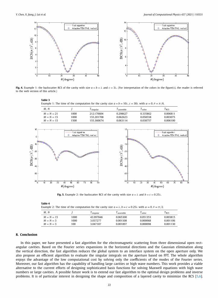
backscatter radar cross section of a cavity with size a = b = λ and c = 3λ is calculated by the fast algorithm and the adaptive finite element PLM method. Fig. 4 shows the RCS versus θ for θ θ and φφ polarizations. The backscatter RCS is shown as red solid lines and blue circles for the fast algorithm and adaptive PML method, respectively. It is clear to note that the results obtained by both methods are consistent with each other. Detailed computational time is given in Table 3.
7.2. Example 2
In this example, we consider the cavity filled with a material having a relative permittivity εr = 7 + 1.5 i and a constant magnetic permeability μ = 1. The backscatter RCS of the cavity with size a = λ, and b = c = 0.25λ is calculated. The RCS of θ θ and φφ polarizations are shown in Fig. 5 for various incident angle θ . The results based on the fast algorithm and the adaptive PML method are again in excellent agreement. Detailed computational time is given in Table 4. Again, the cost is dominated by the evaluation of singular integrals.
7.3. Example 3
This example is concerned with the cavity filled with a two-layer material. The cavity size is a = b = λ and c = 3λ. The top and bottom layer materials have parameters εr = 7 + 1.5 i and εr = 3 + 0.05 i, respectively. The thickness of the top material and the bottom material are c1 = λ and c2 = 2λ, respectively. The backscatter RCS of θ θ and φφ polarizations are shown in Fig. 6 for various incident angle θ . Once again, both methods are consistent with each other very well. Detailed computational time is given in Table 5. It can be seen that the total computational time is less than three minutes by using our fast algorithm.
21
Y. Chen, X. Jiang, J. Lai et al. Journal of Computational Physics 437 (2021) 110331
Fig. 4. Example 1: the backscatter RCS of the cavity with size a = b = λ and c = 3λ. (For interpretation of the colors in the figure(s), the reader is referred to the web version of this article.)
Table 3Example 1: The time of the computation for the cavity size a = b = 10λ, c = 30λ with α = 0, θ = π/6.
M , N J Tsingular Tassemble Tsolve TRCS
M = N = 21 1000 212.170604 0.298627 0.335862 0.006811M = N = 15 1000 155.201708 0.062623 0.058558 0.003075M = N = 15 1500 155.360674 0.063114 0.038757 0.006100
Fig. 5. Example 2: the backscatter RCS of the cavity with size a = λ and b = c = 0.25λ.
Table 4Example 2: The time of the computation for the cavity size a = λ, b = c = 0.25λ with α = 0, θ = π/2.
M , N J Tsingular Tassemble Tsolve TRCS
M = N = 15 1000 43.997846 0.065300 0.051353 0.003815M = N = 3 1000 3.037277 0.001508 0.000068 0.001106M = N = 3 100 3.047187 0.001897 0.000098 0.001130
8. Conclusion
In this paper, we have presented a fast algorithm for the electromagnetic scattering from three dimensional open rect-angular cavities. Based on the Fourier series expansions in the horizontal directions and the Gaussian elimination along the vertical direction, the fast algorithm reduces the global system to an interface system on the open aperture only. We also propose an efficient algorithm to evaluate the singular integrals on the aperture based on FFT. The whole algorithm enjoys the advantage of the low computational cost by solving only the coefficients of the modes of the Fourier series. Moreover, our fast algorithm has the capability of handling large cavities or high wave numbers. This work provides a viable alternative to the current efforts of designing sophisticated basis functions for solving Maxwell equations with high wave numbers or large cavities. A possible future work is to extend our fast algorithm to the optimal design problems and inverse problems. It is of particular interest in designing the shape and composition of a layered cavity to minimize the RCS [5,6].
22

Y. Chen, X. Jiang, J. Lai et al. Journal of Computational Physics 437 (2021) 110331
Fig. 6. Example 3: The backscatter RCS of the cavity with size a = b = λ, c1 = λ and c2 = 2λ.
Table 5Example 3: The time of the computation for the cavity size a = b = λ, c1 = λ, c2 = 2λ with α = 0, θ = π/2.
M , N J , I Tsingular Tassemble Tsolve TRCS
M = N = 21 J = 1000, I = 2000 130.499710 0.329729 0.341623 0.006732M = N = 3 J = 1000, I = 2000 4.075719 0.002566 0.000097 0.001600M = N = 3 J = 100, I = 200 4.194746 0.002448 0.000075 0.001176
Computationally, the design problem can be challenging because of the need of solving the scattering problem repeatedly. The fast algorithm presented here certainly would provide an efficient and accurate numerical tool for these problems.
Declaration of competing interest
The authors declare that they have no known competing financial interests or personal relationships that could have appeared to influence the work reported in this paper.
CRediT authorship contribution statement
Yanli Chen: conceptualization (equal); formal analysis (equal); software (equal); writing (equal).Xue Jiang: formal analysis (equal), software (equal); writing (equal).Jun Lai: formal analysis (equal); software (equal); writing (equal).Peijun Li: conceptualization (equal); formal analysis (equal); writing (equal).
Appendix A. Notations
In the appendix, we list the expressions of the entries for the vectors used in (3.20).The definitions of F 1, G1 and H 1 are given by
F 1 :=
⎛⎜⎜⎜⎜⎝
F (0)1
F (1)1...
F (M)1
⎞⎟⎟⎟⎟⎠ , G1 :=
⎛⎜⎜⎜⎜⎝
G(0)1
G(1)1...
G(M)1
⎞⎟⎟⎟⎟⎠ , H 1 :=
⎛⎜⎜⎜⎜⎝
H (0)1
H (1)1...
H (M)1
⎞⎟⎟⎟⎟⎠ ,
with
F (m)1 :=
⎛⎜⎜⎜⎜⎝
F (m,1)1
F (m,2)1...
F (m,N)1
⎞⎟⎟⎟⎟⎠ , G(m)
1 :=
⎛⎜⎜⎜⎜⎝
G(m,1)1
G(m,2)1...
G(m,N)1
⎞⎟⎟⎟⎟⎠ , H (m)
1 :=
⎛⎜⎜⎜⎜⎝
H (m,1)1
H (m,2)1...
H (m,N)1
⎞⎟⎟⎟⎟⎠ ,
where
F (m,n)1 :=
(F (m,n)
1,(0) F (m,n)1,(1) · · · F (m,n)
1,(M)
), F (m,n)
1,(k ):=
(F (m,n) F (m,n) · · · F (m,n)
),
1 1,(k1,1) 1,(k1,2) 1,(k1,N)
23

Y. Chen, X. Jiang, J. Lai et al. Journal of Computational Physics 437 (2021) 110331
G(m,n)1 :=
(G(m,n)
1,(1) G(m,n)1,(2) · · · G(m,n)
1,(M)
), G(m,n)
1,(k1):=
(G(m,n)
1,(k1,0)G(m,n)
1,(k1,1)· · · G(m,n)
1,(k1,N)
),
H (m,n)1 :=
(H (m,n)
1,(0) H (m,n)1,(1) · · · H (m,n)
1,(M)
), H (m,n)
1,(k1):=
(H (m,n)
1,(k1,1)H (m,n)
1,(k1,2)· · · H (m,n)
1,(k1,N)
).
The definitions of g1 and E l, j with l = 1, 2, 3, 0 ≤ j ≤ J + 1 are given by
g1 :=(
g(0)1 g(1)
1 . . . g(M)1
)�, g(m)
1 :=(
g(m,1)1 g(m,2)
1 . . . g(m,N)1
),
E1, j :=(
E(0)1, j E(1)
1, j . . . E(M)1, j
)�, E(m)
1, j :=(
E(m,1)1, j E(m,2)
1, j . . . E(m,N)1, j
),
E2, j :=(
E(1)2, j E(2)
2, j . . . E(M)2, j
)�, E(m)
2, j :=(
E(m,0)2, j E(m,1)
2, j . . . E(m,N)2, j
),
E3, j :=(
E(1)3, j E(2)
3, j . . . E(M)3, j
)�, E(m)
3, j :=(
E(m,1)3, j E(m,2)
3, j . . . E(m,N)3, j
).
The definitions of F 2, G2 and H 2 are given by
F 2 :=
⎛⎜⎜⎜⎜⎝
F (1)2
F (2)2...
F (M)2
⎞⎟⎟⎟⎟⎠ , G2 :=
⎛⎜⎜⎜⎜⎝
G(1)2
G(2)2...
G(M)2
⎞⎟⎟⎟⎟⎠ , H 2 :=
⎛⎜⎜⎜⎜⎝
H (1)2
H (2)2...
H (M)2
⎞⎟⎟⎟⎟⎠ ,
with
F (m)2 :=
⎛⎜⎜⎜⎜⎝
F (m,0)2
F (m,1)2...
F (m,N)2
⎞⎟⎟⎟⎟⎠ , G(m)
2 :=
⎛⎜⎜⎜⎜⎝
G(m,0)2
G(m,1)2...
G(m,N)2
⎞⎟⎟⎟⎟⎠ , H (m)
2 :=
⎛⎜⎜⎜⎜⎝
H (m,0)2
H (m,1)2...
H (m,N)2
⎞⎟⎟⎟⎟⎠ ,
where
F (m,n)2 :=
(F (m,n)
2,(1) F (m,n)2,(2) · · · F (m,n)
2,(M)
), F (m,n)
2,(k1):=
(F (m,n)
2,(k1,0)F (m,n)
2,(k1,1)· · · F (m,n)
2,(k1,N)
),
G(m,n)2 :=
(G(m,n)
2,(1) G(m,n)2,(2) · · · G(m,n)
2,(M)
), G(m,n)
2,(k1):=
(G(m,n)
2,(k1,0)G(m,n)
2,(k1,1)· · · G(m,n)
2,(k1,N)
),
H (m,n)2 :=
(H (m,n)
2,(0) H (m,n)2,(1) · · · H (m,n)
2,(M)
), H (m,n)
2,(k1):=
(H (m,n)
2,(k1,1)H (m,n)
2,(k1,2)· · · H (m,n)
2,(k1,N)
),
and
F (m,n)
2,(k):= h
c(m,n)2κ2
0 F (m,n)
2,(k), G(m,n)
2,(k):= h
c(m,n)
2k1π
aG(m,n)
2,(k), H (m,n)
2,(k):= h
c(m,n)
−2k2π
bH (m,n)
2,(k),
with
F (m,n)
2,(k):=
∫�
sin(mπx1
a
)cos
(nπx2
b
)(∫�
sin(k1π y1
a
)cos
(k2π y2
b
)g(x, y)ds y
)dsx,
G(m,n)
2,(k):=
∫�
sin(mπx1
a
)cos
(nπx2
b
)(∫�
cos(k1π y1
a
)cos
(k2π y2
b
)∂x1 g(x, y)ds y
)dsx,
H (m,n)
2,(k):=
∫�
sin(mπx1
a
)cos
(nπx2
b
)(∫�
cos(k1π y1
a
)cos
(k2π y2
b
)∂x1 g(x, y)ds y
)dsx.
Here
c(m,n) ={
ab2 , if n = 0,
ab4 , others.
The definition of g2 is given by
g2 :=(
g(1)2 g(2)
2 . . . g(M)2
), g(m)
2 :=(
g(m,0)1 g(m,1)
1 . . . g(m,N)1
),
24

Y. Chen, X. Jiang, J. Lai et al. Journal of Computational Physics 437 (2021) 110331
where
g(m,n)2 := h
c(m,n)2(iα2 p3 + iβp2)
∫�
sin(mπx1
a
)cos
(nπx2
b
)ei(α1x1+α2x2)dsx.
References
[1] H. Ammari, G. Bao, A. Wood, A cavity problem for Maxwell’s equations, Methods Appl. Anal. 9 (2002) 249–260.[2] A. Aziz, R. Kellogg, A. Stephen, A two point boundary value problem with a rapidly oscillating solution, Numer. Math. 53 (1988) 107–121.[3] I. Babuska, S. Sauter, Is the pollution effect of the FEM avoidable for the Helmholtz equation considering high wave number?, SIAM J. Numer. Anal. 34
(1997) 2392–2423.[4] G. Bao, J. Gao, J. Lin, W. Zhang, Mode matching for the electromagnetic scattering from three-dimensional large cavities, IEEE Trans. Antennas Propag.
60 (2012) 2004–2010.[5] G. Bao, J. Lai, Radar cross section reduction of a cavity in the ground plane, Commun. Comput. Phys. 15 (2014) 895–910.[6] G. Bao, J. Lai, Optimal shape design of a cavity for radar cross section reduction, SIAM J. Control Optim. 52 (2014) 2122–2140.[7] G. Bao, W. Sun, A fast algorithm for the electromagnetic scattering from a large cavity, SIAM J. Sci. Comput. 27 (2005) 553–574.[8] G. Bao, M. Zhang, B. Hu, P. Li, An adaptive finite element DtN method for the three-dimensional acoustic wave scattering problem, Discrete Contin.
Dyn. Syst. Ser. B 26 (2021) 61–79.[9] K. Du, A composite preconditioner for the electromagnetic scattering from a large cavity, J. Comput. Phys. 230 (2011) 8089–8108.
[10] K. Du, W. Sun, X. Zhang, Arbitrary high-order C0 tensor product Galerkin finite element methods for the electromagnetic scattering from a large cavity, J. Comput. Phys. 242 (2013) 181–195.
[11] X. Jiang, P. Li, J. Lv, W. Zheng, An adaptive finite element method for the wave scattering with transparent boundary condition, J. Sci. Comput. 72 (2017) 936–956.
[12] S. Hawkins, K. Chen, P. Harris, On the influence of the wavenumber on compression in a wavelet boundary element method for the Helmholtz equation, Int. J. Numer. Anal. Model. 4 (2007) 48–62.
[13] J. Jin, A finite element-boundary integral formulation for scattering by three-dimensional cavity-backed apertures, IEEE Trans. Antennas Propag. 39 (1991) 97–104.
[14] J. Jin, J.L. Volakis, A hybrid finite element method for scattering and radiation by micro strip patch antennas and arrays residing in a cavity, IEEE Trans. Antennas Propag. 39 (1991) 1598–1604.
[15] J. Jin, The Finite Element Method in Electromagnetics, Wiley & Son, New York, 2002.[16] J. Lai, S. Ambikasaran, L. Greengard, A fast direct solve for high frequency scattering from a large cavity in two dimensions, SIAM J. Sci. Comput. 36
(2014) B887–B903.[17] J. Lai, L. Greengard, M. O’Neil, Robust integral formulations for electromagnetic scattering from three-dimensional cavities, J. Comput. Phys. 345 (2017)
1–16.[18] H. Li, H. Ma, W. Sun, Legendre spectral Galerkin method for electromagnetic scattering from large cavities, SIAM J. Numer. Anal. 51 (2013) 253–276.[19] P. Li, X. Yuan, Convergence of an adaptive finite element DtN method for the elastic wave scattering problem, arXiv:1903 .03606.[20] Y. Li, W. Zheng, X. Zhu, A CIP-FEM for high-frequency scattering problem with the truncated DtN boundary condition, CSIAM Trans. Appl. Math. 1
(2020) 530–560.[21] H. Ling, S. Lee, R. Chou, High-frequency RCS of the open cavities with rectangular and circular cross sections, IEEE Trans. Antennas Propag. 37 (1989)
648–654.[22] Mumps: a multifrontal massively parallel sparse direct solver, http://mumps .enseeiht .fr/.[23] PHG (Parallel Hierarchical Grid), http://lsec .cc .ac .cn /phg/.[24] T. Van, A. Wood, Finite element analysis for 2-D cavity problem, IEEE Trans. Antennas Propag. 51 (2003) 1–8.[25] Y. Wang, K. Du, W. Sun, A second-order method for the electromagnetic scattering from a large cavity, Numer. Math. Theor. Meth. Appl. 1 (2008)
357–382.[26] C. Wang, Y. Gan, 2D cavity modeling using method of moments and iterative solvers, Prog. Electromagn. Res. 43 (2003) 123–142.[27] W. Wood, A. Wood, Development and numerical solution of integral equations for electromagneitc scattering from a trough in a ground plane, IEEE
Trans. Antennas Propag. 47 (1999) 1318–1322.[28] X. Yuan, G. Bao, P. Li, An adaptive finite element DtN method for the open cavity scattering problems, CSIAM Trans. Appl. Math. 1 (2020) 316–345.[29] D. Zhang, F. Ma, H. Dong, A finite element method with rectangular perfectly matched layers for the scattering from cavities, J. Comput. Math. 27
(2009) 812–834.[30] L. Zhang, W. Zheng, B. Lu, T. Cui, W. Leng, D. Lin, The toolbox PHG and its applications, Sci. Sin. Inf. 46 (2016) 1442–1464.[31] M. Zhao, Z. Qiao, T. Tang, A fast high order method for electromagnetic scattering by large open cavities, J. Comput. Math. 29 (2011) 278–304.[32] M. Zhao, N. Zhu, A fast precondition iterative method for the electromagnetic scattering by multiple cavities with high wave numbers, J. Comput. Phys.
398 (2019) 108826.
25