journal of contaminant hydrology · n.b. engdahl et al. / journal of contaminant hydrology 149...

Journal of Contaminant Hydrology 149 (2013) 46–60

Contents lists available at SciVerse ScienceDirect

Journal of Contaminant Hydrology

j ourna l homepage: www.e lsev ie r .com/ locate / jconhyd

Scalar dissipation rates in non-conservative transport systems

Nicholas B. Engdahl a,⁎, Timothy R. Ginn b, Graham E. Fogg a

a Department of Land, Air and Water Resources, University of California, Davis, United Statesb Department of Civil and Environmental Engineering, University of California, Davis, United States

a r t i c l e i n f o

⁎ Corresponding author. Tel.: +530 341 3044.E-mail address: [email protected] (N.B. Eng

0169-7722/$ – see front matter © 2013 Elsevier B.V. Ahttp://dx.doi.org/10.1016/j.jconhyd.2013.03.003

a b s t r a c t

Article history:Received 27 June 2012Received in revised form 9 March 2013Accepted 10 March 2013Available online 26 March 2013

This work considers how the inferred mixing state of diffusive and advective–diffusive systemswill vary over time when the solute masses are not constant over time. We develop a number oftools that allow the scalar dissipation rate to be used as a mixing measure in these systemswithout calculating local concentration gradients. The behavior of dissipation rates is investigatedfor single and multi-component kinetic reactions and a commonly studied equilibrium reaction.The scalar dissipation rate of a tracer experiencing first-order decay can be determined exactlyfrom the decay constant and the dissipation rate of a passive tracer, and the mixing rate of aconservative component is not the superposition of the solute specific mixing rates. We thenshow how the behavior of the scalar dissipation rate can be determined from a limited subset ofan infinite domain. Corrections are derived for constant and time dependent limits of integrationthe latter is used to approximate dissipation rates in advective–diffusive systems. Several of thecorrections exhibit similarities to the previous work on mixing, including non-Fickian mixing.This illustrates the importance of accounting for the effects that reaction systems or limitedmonitoring areas may have on the inferred mixing state.

© 2013 Elsevier B.V. All rights reserved.

Keywords:Scalar dissipation rateReactive transportMixing measuresMixing

1. Introduction

Discrepancies between the predicted and observed behav-iors of reactive solutes in groundwater systems often resultfrom differences between laboratory derived rate constantsand upscaled, or effective, reaction rates (Battiato et al., 2009;Kapoor et al., 1997; Tartakovsky et al., 2008; Werth et al.,2006). Many of these differences have been attributed to thefact that laboratory estimates of reaction rates are usuallybased on a well-mixed system but heterogeneities in the flowand transport properties of the subsurface create highlyvariable solute distributions that are poorly mixed. Thepersistence of this imperfect mixing over time can causeeffective reaction rates to remain well below their laboratoryderived values and an accurate representation of mixingbecomes a prerequisite for predicting upscaled reaction rates(De Simoni et al., 2007; Le Borgne et al., 2011; Luo et al., 2008).

dahl).

ll rights reserved.

The physical processes that lead to mixing affect both theinternal structure of a plume and the extents of the plume, butit is important to note that mixing and spreading are notdescribing the same aspects of solute migration. For a passivetracer moving through a groundwater system, the extents ofthe plume over time are often driven by advective forces thatstretch out the plume whereas heterogeneous concentrationdistributions within the solute plume are attenuated bydiffusive or local dispersive processes. There is a complexinteraction between all of these processes in heterogeneousenvironments, and separating the two can be challenging, butunderstanding the spatio-temporal changes in themixing stateof a plume is a critical research area for improving predictionsof reactive transport (Rolle et al., 2009).

The mixing state can be thought of as a measure of howhomogeneous the distribution of a solute is within the plume ata given time; this is in contrast to a mixing rate which is thetime rate of change of a mixingmeasure. Physically, themixingrate quantifies how rapidly the molecules of two or moredistinct populations (i.e. combinations of one or more solutesand clean water) that have come into contact with each other

http://crossmark.dyndns.org/dialog/?doi=10.1016/j.jconhyd.2013.03.003&domain=f

http://dx.doi.org/10.1016/j.jconhyd.2013.03.003

mailto:[email protected]


http://www.sciencedirect.com/science/journal/01697722

47N.B. Engdahl et al. / Journal of Contaminant Hydrology 149 (2013) 46–60

are homogenizing. A well-mixed system is one where thesolute concentrations within the plume are essentially uniformbut descriptions of the mixing state are, to some extent,independent of the shape of the plume, even though mixingand spreading are inextricably linked. For example, heteroge-neous spreading of a plume can enhance the rate of mixingbecause the elongated plumewill havemore area for the forcesof dispersion and diffusion to work on (Cirpka and Kitanidis,2000). In other words, mixing can be enhanced by the dilutionof a plume and Kitanidis (1994) proposed the dilution index asa quantitative measure of the volume occupied by a solute. Thedilution index is calculated from the entropy of the solutedistribution, and a mixing rate can be defined from the timerate of change of the entropy (Dentz et al., 2011). This approachis well established and has been used to quantify mixing in awide variety of passive transport studies but only a recent studyby Chiogna et al. (2012) has considered the dilution index inreactive transport systems. The dilution index is not the onlyapproach to quantifying mixing and stochastic hydrology hasoften modeled the behavior of solute plumes as a linearcombination of the mean behavior of the plume and a fluc-tuation about that mean. This approach is naturally suited todescribingmixing because the relative homogeneity of a plume(i.e. the mixing state) can be expressed in terms of the varianceof the concentration fluctuations (Kapoor and Gelhar, 1994;Miralles-Wilhelm et al., 1997). If there are no deviations fromthe mean concentration, the solute is internally homogeneousand, by definition, well-mixed. Another approach is to considerthe concentration gradients within the solute plume directly(e.g. Le Borgne et al., 2010). This is very similar in principle tothe concentration fluctuation approach but thesemethods haveclassically been applied to turbulent flows and combustion.Gradient based mixing measures have been used recently toquantify the mixing state and estimate reaction rates in avariety of contaminant hydrology problems including multi-component reactive transport.

The definition of a well-mixed system does not changewhen there are multiple solutes because the extent of mixingstill describes how uniformly the solutes are distributedbut the issue of overlap or segregation must be addressed(e.g. Raje and Kapoor, 2000). By overlap we mean thatportions of two or more solute distributions are occupyingthe same physical space (Cirpka and Kitanidis, 2000).Apparent overlap occurs when upscaled or averaged concen-tration fields appear to overlap but there is no physicalcontact and this can have strong effects on effective reactionrates (Kapoor et al., 1997). Since it is an artifact from havingincomplete knowledge of the system, we will not considerapparent overlap here and restrict our discussion of overlapto the case of physically co-located solutes. The concepts ofmixing and overlapping are often poorly delineated in theliterature and are routinely combined into “mixing.” This isan important point because stating that two reactive solutesare merely overlapping is insufficient for predicting reactionrates. Identifying overlapping regions provides little, if any,information about the internal distribution of each solutebecause only their extents have been described (Kapooret al., 1997). As each solute continues to diffuse and becomemore efficiently mixed, the distributions of their masses mayalso be changing due to reactions and this will have an effecton the inferred mixing state (by inferred wemean the mixing

state at some time as estimated or calculated from a globalmixing measure). Although the total mass of the reactionsystem is conserved, the mixing state of individual solutes nolonger appears conservative because of mass transformationsfrom the reactions. The magnitude of these effects at anylocation should be proportionate to the local reaction rate or,more precisely, the rate law governing the reaction (e.g. DeSimoni et al., 2005, 2007). Conceptually, reactions createlocal sources and sinks of mass for one solute relative to theothers and these changes in mass should affect the mixingstate, much like sources and sinks of concentration variance(e.g. Kapoor and Gelhar, 1994); obviously, reactions are notthe only possible mechanism that can cause source/sink likebehavior. A similar effect can be conceived for the case wherewe merely have incomplete knowledge of the concentrationfield. For example, if some portion of the solute mass wereto pass beyond the extents of a monitoring network unac-counted, it would also appear that mass is being lost and thiswould also affect the inferred mixing state. However, it is notimmediately clear if this effect on mixing would mimic thatof a reaction, or precisely how any of these factors will affectthe inferred mixing state, and these questions motivate thecurrent work.

In this article we explore the behavior of a gradient basedmixing measure, the scalar dissipation rate (see Section 2),under non-conservative conditions. We use non-conservativeas a generic term for the effects of changes inmass of individualsolutes caused by reactions or mass migrating beyond themonitored extent of the problem space. The fundamentalquestion in this work is, what should the expected behavior ofthe scalar dissipation rate look like for simple non-conservativesystems and can those behaviors be predicted to improvereactive transport models? To this end, we develop a numberof analytical relationships that show howmass transformationvia reactions affects the inferred mixing state for kineticreactions with up to three reactants in diffusive systems.Diffusion is considered first in order to address the fundamen-tal behavior of themixingmeasure in the presence of reactionsand the effects at different Damkohler numbers. The conse-quences of defining conservative components (e.g. Saaltinket al., 1998) and assuming local equilibrium on the mixingrate are also explored and we show that the mixing state forthe component based case cannot be determined from a simplesuperposition of the individual, solute specific, mixing mea-sures. We then consider the effects of limited monitoringdomains on the mixing measures for non-reacting tracers indiffusive and advective–diffusive systems and compare thoseto the effects of reactions. This work shows that erroneousconclusions about themixing state can bemade if the effects ofnon-conservative conditions are not accounted for and thatreactions can have effects on mixing that are similar to thosecaused by heterogeneities.

2. Scalar dissipation rates of conservative tracers

The scalar dissipation rate (SDR) is a global mixing mea-sure that is based on the integral of concentration gradients.The SDR has been used in several recent studies of transportin porous media where mixing and reaction rates wereinvestigated (e.g. Bolster et al., 2010, 2011a; Chiogna et al.,2011; Jha et al., 2011) and this recent emergence of the SDR

48 N.B. Engdahl et al. / Journal of Contaminant Hydrology 149 (2013) 46–60

in hydrogeology further motivates our investigation. The SDRof a passive scalar is defined to be

χ tð Þ ¼ ∫ΩD∇c x; tð Þ⋅∇c x; tð Þdx ð1Þ

where D can be a diffusion or dispersion coefficient that mayvary spatially, c is the concentration, x is a position vector inthe domainΩ, t is time, and the integral is taken over the entiredomain. The definition of D depends on the type of problembeing considered and the use of a diffusion coefficient is onlyapplicable when there is no hydrodynamic dispersion. Asimilar term lacking the spatial integral can be found in DeSimoni et al. (2005), Fernàndez-Garcia et al. (2008) and Luoet al. (2008), among others, and such constructions arecommon in the mixing and reactive transport literature, oftenbeing called a mixing factor. Eq. (1) follows the notation of LeBorgne et al. (2010) but similar definitions can also be found inthe physics and engineering literature. The dissipation rate canbe determined from the scalar field or the deviations of thescalar field from its mean (e.g. de Dreuzy et al., 2012; Pope,2000) but in either case Eq. (1) is formally describing themixing rate using the overall steepness of the concentrationgradients; however, this is also a proxy for the mixing state.Consider that a homogeneous scalar field has no variationsand the gradients of the concentration field are zero every-where. When there are variations in solute concentrations,there will be gradients and the SDR will be non-zero. The ratethat those gradients are relaxed toward zero is proportionateto the diffusion coefficient and this is quantified by Eq. (1). Asmentioned in Section 1,many othermixingmeasures exist (seealso Dentz et al., 2011), but the SDR is a useful tool fordescribing mixing because it can be approximated withoutcalculating local concentration gradients, and it can be directlyrelated to the global reaction rate in some component basedsimulations of reactive transport (but only when all of thereactants have the same diffusion coefficient) (Le Borgne et al.,2010). If Eq. (1) is evaluated for a plume experiencing diffu-sion in an infinite homogeneous domain, translational motion(advection) will not affect the mixing measure. However,translational motion in infinite heterogeneous domains cancause time dependent fluctuation of the mixing state which isthe cause of the non-Fickian mixing in Le Borgne et al. (2010).The SDR can be qualitatively understood from Eq. (1), but theSDR can also be approximated from the integral of the squaredconcentrations:

M2 tð Þ ¼ ∫Ωc x; tð Þ2dx ð2Þ

and the SDR is then given as

χ tð Þ ¼ −12ddt

M2 tð Þ ð3Þ

A similar equation can be found in Kitanidis (1994) for thedilution index, but the expression in that work carries adependency on the inverse of concentration and is not thesame as Eq. (3). It may not be intuitive why Eq. (3) is capableof approximating Eq. (1), but consider that the time rate ofchange of the integral of the squared concentration will benon-zero unless the solute is perfectly mixed throughout theentire domain. This approximation is exact in a domain with

a divergence free velocity field and infinite limits becausethere is no mass flux outside of the domain. Le Borgne et al.(2010) showed that Eq. (3) was more accurate than theintegral in Eq. (1) for homogeneous porous media and Eq. (3)is also computationally more efficient, providing furthermotivation for using Eq. (3) instead of Eq. (1). We note thatBolster et al. (2010) considered mixing in a plume under-going space-fractional dispersion and used Eq. (3) as thedefinition to compute the SDR, most likely because of thepresence of a fractional derivative in the dispersion operator.This convention does not maintain the equivalence of Eqs. (1)and (3) since the dispersion operator is non-Fickian, but it isstill a valid approach for quantifyingmixing. To our knowledge,the behavior of the SDR in time-fractional systems has not beenexplored in detail but this may be useful since the time-fractional case would maintain the definition of Eq. (1) andproduce an alternative form of Eq. (3) that does not involvespace-fractional derivatives.

The differences between the SDR defined by Eq. (1) andthe integral definition of Eq. (3) have not been studied indetail for non-conservative scalars. Jha et al. (2011) consid-ered the influence of advection on the SDR for a passivetracer but did not derive solutions that can be calculatedwithout evaluating the local concentration gradients and didnot investigate the influence of reactions. Analytical solutionsof the SDR have been considered by Bolster et al. (2010) andLe Borgne et al. (2010), but these have been presented in thecontext of specific transport systems and the behavior of themixing measure when the solute masses vary over time hasnot been addressed in detail.

3. Dissipation rates in reactive systems

3.1. First-order decay

Many environmental tracers experience first-order, ki-netic decay. A common example of this is radioactive decaybut many other reaction mechanisms, including biologicprocesses, can also create first-order decay. Regardless ofthe mechanism causing the decay, the governing equationwe consider is the advection–diffusion-reaction equation(ADRE):

∂c x; tð Þ∂t þ∇⋅ v xð Þc x; tð Þ½ �−∇⋅D∇c x; tð Þ ¼ −λc x; tð Þ ð4Þ

where we will define D as a diffusion coefficient and λ is thedecay rate. This equation is most accurate for describingpore-scale reactive transport where the velocity field is fullyresolved and thus there is no need for a mechanicaldispersion term, but the results may also be applicable tolarger support volumes if diffusion/dispersion in the porousmedium is strictly stationary. Throughout this section we willassume that the concentration field is known at all locationsand times and that the limits of the domain are infinite, butthese restrictions will be addressed or relaxed in Section 4.All of these assumptions are made to simplify the solution ofthese equations and to facilitate the derivation of analyticalsolutions. Following the derivation of Le Borgne et al. (2010),Appendix A, we can determine the relationship betweenEqs. (1) and (3) for first-order decay instead of a passive


solute. Multiply Eq. (4) by c(x,t) and integrate over the entiredomain to find:

12∂∂t ∫Ωc x; tð Þ2dΩþ 1

2∫Ω∇⋅ v xð Þc x; tð Þ2

h idΩ

� 12D∫Ω∇⋅∇c x; tð Þ2dΩþ ∫ΩD∇c x; tð Þ⋅∇c x; tð ÞdΩ

¼ �λ∫Ωc x; tð Þ2dΩ

ð5Þ

If the problem space is infinite, there will be no net flux outof the domain and the terms involving a divergence operatorare zero via the divergence theorem (assuming a divergencefree flow field). Eq. (5) then simplifies to:

−12∂∂t ∫Ωc x; tð Þ2dΩ−λ∫Ωc x; tð Þ2dΩ ¼ ∫ΩD∇c x; tð Þ⋅∇c x; tð ÞdΩ

ð6Þ

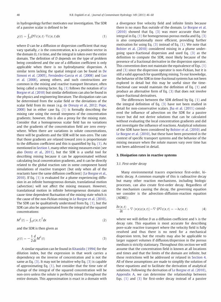
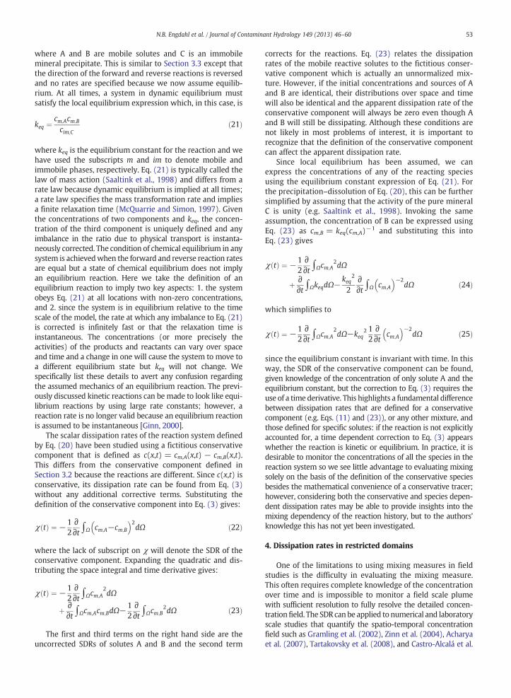
which recovers the passive case when λ = 0 and examplesof passive and decaying dissipation rates are shown in Fig. 1.We will assume throughout this article that D is constantto further simplify our derivations but note that Eq. (1) doesnot require this. Eq. (6) corrects the apparent dissipation rate(i.e. Eq. (3)) for mass changes due to decay and permits anunbiased comparison of the behavior of the mixing rates(defined by Eq. (1)) of passive and decaying tracers withoutneeding to evaluate the local gradients. The quantity on the righthand side of Eq. (6) defines what we will refer to as the true oractual dissipation rate which is consistent with Eq. (1) and thedefinition of the SDR. The expression of Eq. (3) has been used asthe tool for quantifying the SDR in the related work (e.g. Bolsteret al., 2010; Le Borgne et al., 2010) but, as we already can see inEq. (6), it will not immediately be equivalent to the actual SDR innon-conservative systems and will require corrections todetermine the actual dissipation rates. When the SDR iscalculated according to Eq. (3) in a non-conservative system,we will refer to this as the uncorrected dissipation rate. Wedefine the ideal SDR as the analytical solution of Eq. (3) in aninfinite domain which is given in Appendix A and appears inFig. 1 for three values of the diffusion coefficient as the solid,straight lines.

102 104 106 10810−10

10−8

10−6

10−4

Time (d)

χ (t

)

Passive

λC

λU

D/100, λ/10

D∗100, λ∗10D, λ

Fig. 1. Analytical solutions for the passive SDR, and the corrected (Eq. (6),λC) and uncorrected (Eq. (3), λU) SDR for a decaying tracer. Note that theuncorrected SDR slightly overestimates the dissipation rate relative to theinfinite domain problem.

The dissipation rate of a decaying tracer can be determined fromthe dissipation rate of a concentration-normalized passive tracerwhen the decay constant is known (see Appendix A) from:

χλ tð Þ ¼ χ0 tð Þ exp −2λtð Þ½ � ð7Þ

where we use subscripts on χ to denote the decay constant;for example χ0(t) represents the SDR of a conservative tracerwith λ = 0. Analytical solutions for diffusion with decay in ahomogeneous domain using a Gaussian model of diffusion andEq. (6) are shown in Fig. 1 for several combinations of diffusionand decay constants; in all reactive cases, the SDR predictablyapproaches zero as the solute mass is consumed. First-orderdecay is not a complicated reaction and is used here only toillustrate the basic methodology applied throughout Section 3for the simplest possible reaction. The result of Eq. (7) can alsobe derived by defining c(x,t) = c0(x,t)exp(−λt), where c0 is aconservative tracer. This change of variables allows Eq. (4) to beused to calculate the SDRwithout the reaction term; however, indoing so, a conservative component has been defined and wewould not be directly considering the behavior of the reactivesolute. In this special case, the spatio-temporal evolution of theplume representing the conservative component and the plumeof the decaying species are very similar, but we will show inSection 3.2 that this is not necessarily the case formore complexreaction mechanisms.

3.2. Kinetic degradation

Reactions involving multiple species will require additionalterms to correct the dissipation rates of the solutes. Considerirreversible decay of solute A to B, both ofwhich aremobile andhave the same aqueous phase diffusion coefficient:

A→kB ð8Þ

which evolves forward in time according to the rate laws:

dcAdt

¼ −kcA ð9aÞ

dcBdt

¼ kcA ð9bÞ

where the subscripts denote the concentrations of each speciesand k is the rate constant. Throughout this article we will notexplicitly specify the units of the rate constants because theydepend on the rate law expression (McQuarrie and Simon,1997); however, the units of the rate constants can be easilydetermined from a dimensional analysis of the rate law. Weassume unit activity coefficients for simplicity so that activitiesare analogous to concentrations; this assumes that the con-centrations of A and B are dilute (De Simoni et al., 2005;Fernàndez-Garcia et al., 2008). The ADRE of this reactivesystem will be similar to Eq. (4) where the right hand side ofthe ADRE is replaced by the right hand side of the rate lawexpression for each species and we can derive the correcteddissipation rates from the ADREs. The corrected SDR of solute Awill be identical to Eq. (6), however solute B will differ:

χB tð Þ ¼ −12∂∂t ∫ΩcB

2dΩþ k∫ΩcAcBdΩ ð10Þ

100 102 104 106 10810−12

10−10

10−8

10−6

10−4

Time (d)

χ (t

)

10−12

10−10

10−8

10−6

10−4

10−2

χ (t

)

Da=0.01 χA

χB

χA,u

χB,u

Da=100

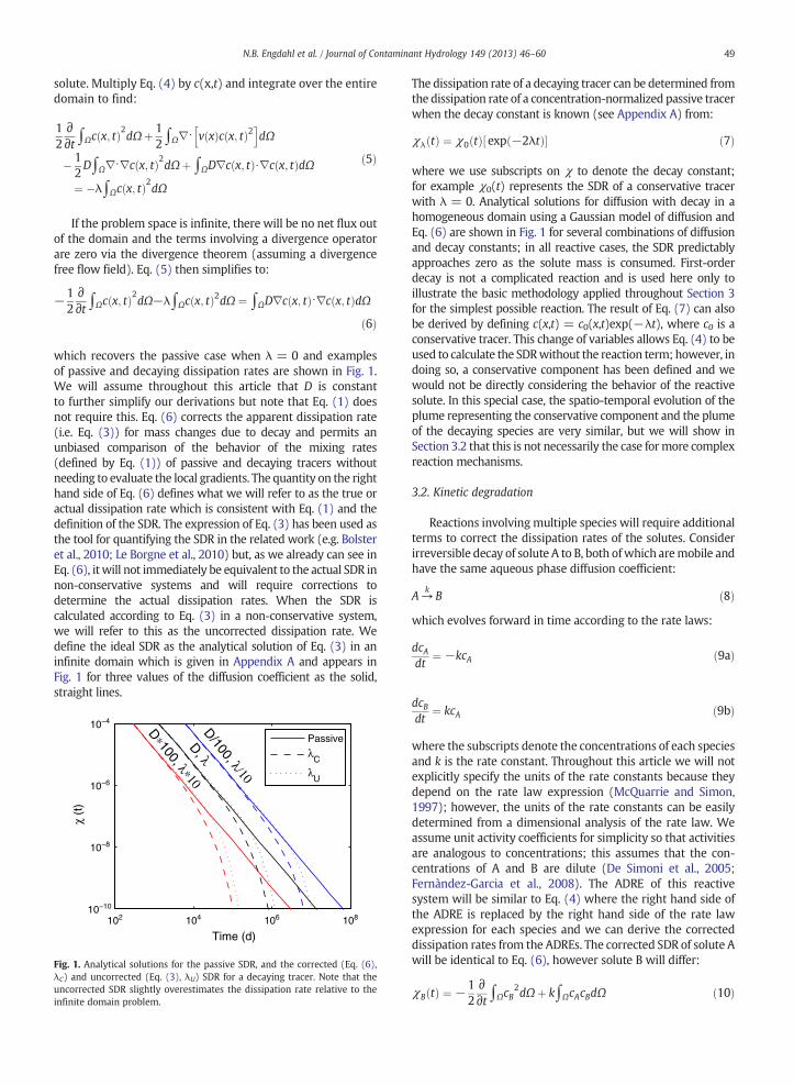
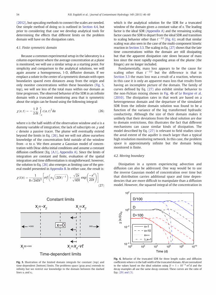
Fig. 2. Corrected and uncorrected scalar dissipation rates for an irreversiblebimolecular reaction (Eq. (10)) across five orders of magnitude of Damkohlernumber (Da). The uncorrected SDRs are denoted with a subscript u in thelegend and A and B denote the solutes described in Section 3.2. At late times,the uncorrected SDR for B is identical to the corrected SDR. Dashed linesindicate negative values.


where we have substituted c(x,t) → c for compactness. This isan example of a dissipation rate that depends on the overlap oftwo species the individual distribution of the solutes since thecorrected SDR of the daughter product depends on theconcentrations of both species. Intuitively this makes sensebecause the rate that B is created is controlled by the amount ofA that is present, but thiswill also be affected by theDamkohlernumber (Da), which is the ratio of the characteristic diffusionand reaction times. Here we define Da = k/D where D is thediffusion coefficient. Notice that the correction in Eq. (10) isadditive but the correction in the previous example was not.This reflects the fact that mass is being added to B whichincreases thedissipation rate by enhancing the spatial gradientsof concentration in the area near the source. However, carefulinspection of Eqs. (3), (6), and (10) raises an important pointthat dissipation rates computed from the definition of Eq. (3)may have negative values (e.g. Bolster et al., 2011b) thoughthis is not possible according to Eq. (1). In the absence ofelectrostatic or other attractive forces, solute mass does notspontaneously agglomerate but instead dissipates and dilutesas the entropy of the system increases towards its maximum(Kitanidis, 1994). Considering this, negative dissipation ratesare physically meaningless quantities that arise from notproperly accounting for source, sink, or reaction terms.

The behavior of the corrected SDRs for Eq. (9) canbe visualized by solving the system of coupled partial dif-ferential equations. Since the system is coupled, findinga direct analytical solution can be tedious, so we usedthe Matlab programming environment to numerically solvethe reaction–diffusion system for this example, and theremaining examples that include reactions. The correctedand uncorrected SDRs for both species in Eq. (8) are shownin Fig. 2 and span five orders of magnitude of Da in a1-D, homogeneous, diffusive domain. Combinations of threevalues of the rate constant and diffusion coefficient were usedto generate the different curves and the differences indiffusion coefficients can be seen by inspecting the pointwhere the SDR intersects the vertical axis. The value of therate constant determines when the SDR of solute A willapproach zero and how long it will take for the SDR of solute Bto reach its passive behavior. The diffusion coefficient controlsthe maximum rate of dissipation but the mixing measureitself is not uniquely affected by Da; different values of D willshift the SDR curves upor down.Overall, the behaviorwe see inFig. 2 is a steady increase in the SDR of solute B as it is producedthen a transition to passive behavior as solute A is completelyconsumed. The SDR of solute A predictably falls off exactly likethe decay example in the previous section. In contrast, theuncorrected SDR for solute A is an overestimate at all but theearliest times and the uncorrected SDR of solute B is negativeuntil the influence of the reaction ceases. After this point,the uncorrected SDR of B does transition into the expectedbehavior of a passive tracer, but the negative dissipation ratescomputed at early times are obviously incorrect.

Sometimes a reactive transport system can be approxi-mated by defining a conservative component (e.g. Cirpka andValocchi, 2007; De Simoni et al., 2005, 2007; Donado et al.,2009; Sanchez-Vila et al., 2010). This can be done for thesystem defined by Eq. (8) by adding the two species c(x,t) =cA(x,t) + cB(x,t) where c without a subscript denotes theconservative component. Expanding the SDR of the conservative

component by inserting its definition into Eq. (3) and simplify-ing shows:

χ tð Þ ¼ −12∂∂t ∫ΩcA

2dΩ− ∂∂t ∫ΩcAcBdΩ−1

2∂∂t ∫ΩcB

2dΩ ð11Þ

The effects of the reactions on the individual components arenested within the definition of their concentration fields so noreaction terms appear explicitly in Eq. (11) but it is clear that thisstill depends on the amount of overlap of the solutes and theirindividual mixing states. The factors driving the SDR of theconservative component can be examined further by incorpo-rating the definition of the corrected SDR. Replacing the left handside of Eq. (10) with the identity of Eq. (1) and rearranging, theuncorrected dissipation rate can be expressed as

−12∂∂t ∫ΩcB

2dΩ ¼ ∫ΩD∇cB⋅∇cBdΩ−k∫ΩcAcBdΩ ð12Þ

Using this, and a similar expression for solute A, substitu-tion into Eq. (11), shows:

χ tð Þ ¼ ∫Ω D∇cA⋅∇cA þ D∇cB⋅∇cBð ÞdΩþ ∫Ω kcA cA−cBð Þ− ∂

∂t cAcB� �

dΩ ð13Þ

The integrals have been grouped to demonstrate that theobserved dissipation rate of the conservative component also

102 104 106 10810−12

10−10

10−8

10−6

10−4

10−2

Time (d)

χ (t

)

χA

χB

χA,u

χB,u

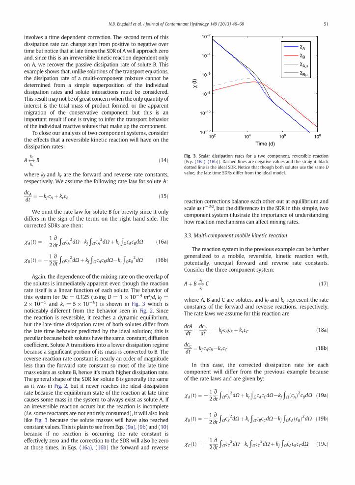
Fig. 3. Scalar dissipation rates for a two component, reversible reaction(Eqs. (16a), (16b)). Dashed lines are negative values and the straight, blackdotted line is the ideal SDR. Notice that though both solutes use the same Dvalue, the late time SDRs differ from the ideal model.


involves a time dependent correction. The second term of thisdissipation rate can change sign from positive to negative overtime but notice that at late times the SDR of Awill approach zeroand, since this is an irreversible kinetic reaction dependent onlyon A, we recover the passive dissipation rate of solute B. Thisexample shows that, unlike solutions of the transport equations,the dissipation rate of a multi-component mixture cannot bedetermined from a simple superposition of the individualdissipation rates and solute interactions must be considered.This resultmaynot be of great concernwhen theonly quantity ofinterest is the total mass of product formed, or the apparentmigration of the conservative component, but this is animportant result if one is trying to infer the transport behaviorof the individual reactive solutes that make up the component.

To close our analysis of two component systems, considerthe effects that a reversible kinetic reaction will have on thedissipation rates:

A⇔kf

krB ð14Þ

where kf and kr are the forward and reverse rate constants,respectively. We assume the following rate law for solute A:

dcAdt

¼ −kf cA þ krcB ð15Þ

We omit the rate law for solute B for brevity since it onlydiffers in the sign of the terms on the right hand side. Thecorrected SDRs are then:

χA tð Þ ¼ −12∂∂t ∫ΩcA

2dΩ−kf∫ΩcA2dΩþ kr∫ΩcAcBdΩ ð16aÞ


2dΩþ kf∫ΩcAcBdΩ−kr∫ΩcB2dΩ ð16bÞ

Again, the dependence of the mixing rate on the overlap ofthe solutes is immediately apparent even though the reactionrate itself is a linear function of each solute. The behavior ofthis system for Da = 0.125 (using D = 1 × 10−4 m2/d, kf =2 × 10−5 and kr = 5 × 10−6) is shown in Fig. 3 which isnoticeably different from the behavior seen in Fig. 2. Sincethe reaction is reversible, it reaches a dynamic equilibrium,but the late time dissipation rates of both solutes differ fromthe late time behavior predicted by the ideal solution; this ispeculiar because both solutes have the same, constant, diffusioncoefficient. Solute A transitions into a lower dissipation regimebecause a significant portion of its mass is converted to B. Thereverse reaction rate constant is nearly an order of magnitudeless than the forward rate constant so most of the late timemass exists as solute B, hence it's much higher dissipation rate.The general shape of the SDR for solute B is generally the sameas it was in Fig. 2, but it never reaches the ideal dissipationrate because the equilibrium state of the reaction at late timecauses some mass in the system to always exist as solute A. Ifan irreversible reaction occurs but the reaction is incomplete(i.e. some reactants are not entirely consumed), it will also looklike Fig. 3 because the solute masses will have also reachedconstant values. This is plain to see fromEqs. (9a), (9b) and (10)because if no reaction is occurring the rate constant iseffectively zero and the correction to the SDR will also be zeroat those times. In Eqs. (16a), (16b) the forward and reverse

reaction corrections balance each other out at equilibrium andscale as t−3/2, but the differences in the SDR in this simple, twocomponent system illustrate the importance of understandinghow reaction mechanisms can affect mixing rates.

3.3. Multi-component mobile kinetic reaction

The reaction system in the previous example can be furthergeneralized to a mobile, reversible, kinetic reaction with,potentially, unequal forward and reverse rate constants.Consider the three component system:

Aþ B⇔kf

krC ð17Þ

where A, B and C are solutes, and kf and kr represent the rateconstants of the forward and reverse reactions, respectively.The rate laws we assume for this reaction are

dcAdt

¼ dcBdt

¼ −kf cAcB þ krcC ð18aÞ

dcCdt

¼ kf cAcB−krcC ð18bÞ

In this case, the corrected dissipation rate for eachcomponent will differ from the previous example becauseof the rate laws and are given by:

χA tð Þ ¼ −12∂∂t ∫ΩcA

2dΩþ kr∫ΩcAcCdΩ−kf∫Ω cAð Þ2cBdΩ ð19aÞ


2dΩþ kr∫ΩcBcCdΩ−kf∫ΩcA cBð Þ2dΩ ð19bÞ

χC tð Þ ¼ −12∂∂t ∫ΩcC

2dΩ−kr∫ΩcC2dΩþ kf∫ΩcAcBcCdΩ ð19cÞ


These equations correct the individual dissipation ratesaccording to the reactions in a way that is consistent with thereaction mechanism, but, like the previous section, thesedissipation rates will deviate from the ideal SDR and thedeviations can change over time (Fig. 4). The self-consistencyof these equations can be demonstrated by considering apoint in the domain where only one solute, say solute A, ispresent: in the absence of B and C, solute A is passive andthe contributions of both corrective terms at that locationare zero; thus, the dependence of SDR on the extent to whichthe solutes overlap is maintained. Three-component kineticreactions that have non-linear rate laws in one or morecomponents (e.g. a rate law proportional to cA

2) will onlydiffer in the order of the exponents of the last two terms butreactions with more chemical species will have additionalvariables in the corrective terms. If we define solute C to be asolid precipitate, it is completely immobile (i.e. no advectionor diffusion) and will not experience mechanical dissipation,however, this will not affect the correction terms of themobile species since they are determined by the rate law andnot the transport equation. Since its concentration will bechanging over time, a dissipation rate can be calculated forthe immobile component but the general behavior andphysical meaning of this rate is different from that of themobile components.

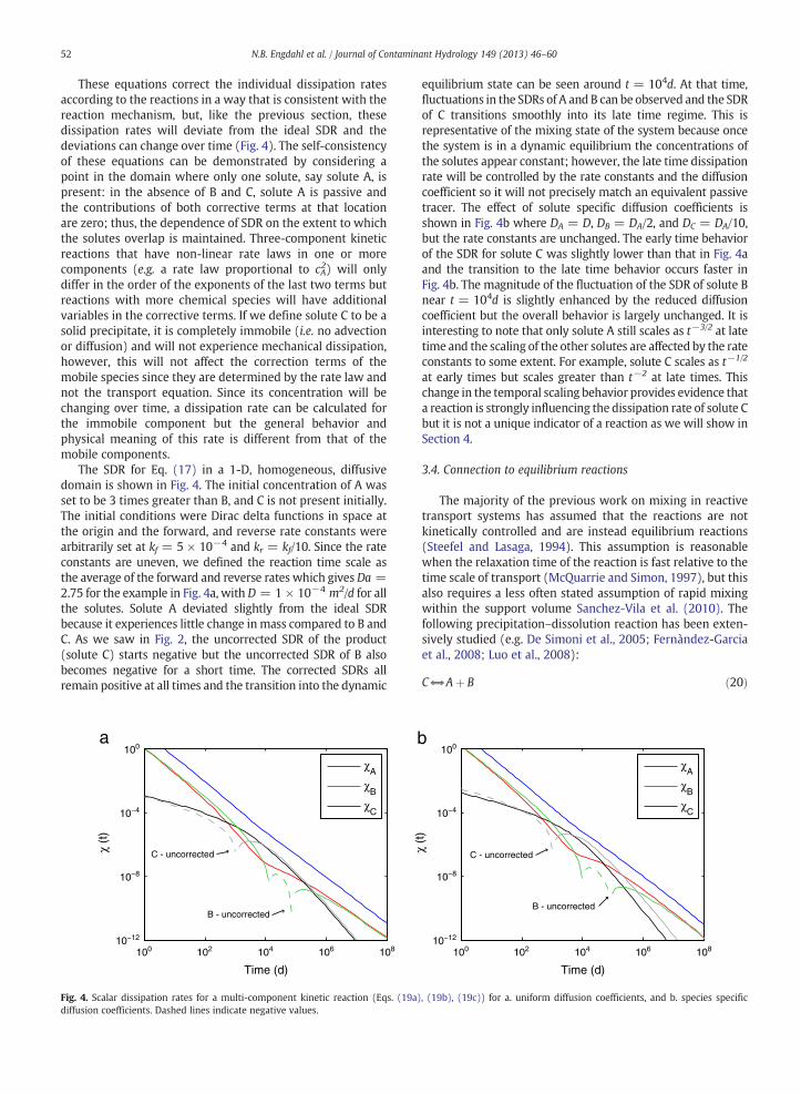
The SDR for Eq. (17) in a 1-D, homogeneous, diffusivedomain is shown in Fig. 4. The initial concentration of A wasset to be 3 times greater than B, and C is not present initially.The initial conditions were Dirac delta functions in space atthe origin and the forward, and reverse rate constants werearbitrarily set at kf = 5 × 10−4 and kr = kf/10. Since the rateconstants are uneven, we defined the reaction time scale asthe average of the forward and reverse rates which gives Da =2.75 for the example in Fig. 4a, with D = 1 × 10−4 m2/d for allthe solutes. Solute A deviated slightly from the ideal SDRbecause it experiences little change inmass compared to B andC. As we saw in Fig. 2, the uncorrected SDR of the product(solute C) starts negative but the uncorrected SDR of B alsobecomes negative for a short time. The corrected SDRs allremain positive at all times and the transition into the dynamic

100 102 104 106 10810−12

10−8

10−4

100

Time (d)

χ (t

)

χ

A

χB

χC

B - uncorrected

C - uncorrected

a

Fig. 4. Scalar dissipation rates for a multi-component kinetic reaction (Eqs. (19a)diffusion coefficients. Dashed lines indicate negative values.

equilibrium state can be seen around t = 104d. At that time,fluctuations in the SDRs of A and B can be observed and the SDRof C transitions smoothly into its late time regime. This isrepresentative of the mixing state of the system because oncethe system is in a dynamic equilibrium the concentrations ofthe solutes appear constant; however, the late time dissipationrate will be controlled by the rate constants and the diffusioncoefficient so it will not precisely match an equivalent passivetracer. The effect of solute specific diffusion coefficients isshown in Fig. 4b where DA = D, DB = DA/2, and DC = DA/10,but the rate constants are unchanged. The early time behaviorof the SDR for solute C was slightly lower than that in Fig. 4aand the transition to the late time behavior occurs faster inFig. 4b. The magnitude of the fluctuation of the SDR of solute Bnear t = 104d is slightly enhanced by the reduced diffusioncoefficient but the overall behavior is largely unchanged. It isinteresting to note that only solute A still scales as t−3/2 at latetime and the scaling of the other solutes are affected by the rateconstants to some extent. For example, solute C scales as t−1/2

at early times but scales greater than t−2 at late times. Thischange in the temporal scaling behavior provides evidence thata reaction is strongly influencing the dissipation rate of solute Cbut it is not a unique indicator of a reaction as we will show inSection 4.

3.4. Connection to equilibrium reactions

The majority of the previous work on mixing in reactivetransport systems has assumed that the reactions are notkinetically controlled and are instead equilibrium reactions(Steefel and Lasaga, 1994). This assumption is reasonablewhen the relaxation time of the reaction is fast relative to thetime scale of transport (McQuarrie and Simon, 1997), but thisalso requires a less often stated assumption of rapid mixingwithin the support volume Sanchez-Vila et al. (2010). Thefollowing precipitation–dissolution reaction has been exten-sively studied (e.g. De Simoni et al., 2005; Fernàndez-Garciaet al., 2008; Luo et al., 2008):

C⇔Aþ B ð20Þ

100 102 104 106 10810−12

10−8

10−4

100

Time (d)

χ (t

)

χ

A

χB

χC

B - uncorrected

C - uncorrected

b

, (19b), (19c)) for a. uniform diffusion coefficients, and b. species specific


where A and B are mobile solutes and C is an immobilemineral precipitate. This is similar to Section 3.3 except thatthe direction of the forward and reverse reactions is reversedand no rates are specified because we now assume equilib-rium. At all times, a system in dynamic equilibrium mustsatisfy the local equilibrium expression which, in this case, is

keq ¼cm;Acm;B

cim;Cð21Þ

where keq is the equilibrium constant for the reaction and wehave used the subscripts m and im to denote mobile andimmobile phases, respectively. Eq. (21) is typically called thelaw of mass action (Saaltink et al., 1998) and differs from arate law because dynamic equilibrium is implied at all times;a rate law specifies the mass transformation rate and impliesa finite relaxation time (McQuarrie and Simon, 1997). Giventhe concentrations of two components and keq, the concen-tration of the third component is uniquely defined and anyimbalance in the ratio due to physical transport is instanta-neously corrected. The condition of chemical equilibrium in anysystem is achievedwhen the forward and reverse reaction ratesare equal but a state of chemical equilibrium does not implyan equilibrium reaction. Here we take the definition of anequilibrium reaction to imply two key aspects: 1. the systemobeys Eq. (21) at all locations with non-zero concentrations,and 2. since the system is in equilibrium relative to the timescale of the model, the rate at which any imbalance to Eq. (21)is corrected is infinitely fast or that the relaxation time isinstantaneous. The concentrations (or more precisely theactivities) of the products and reactants can vary over spaceand time and a change in one will cause the system to move toa different equilibrium state but keq will not change. Wespecifically list these details to avert any confusion regardingthe assumed mechanics of an equilibrium reaction. The previ-ously discussed kinetic reactions can be made to look like equi-librium reactions by using large rate constants; however, areaction rate is no longer valid because an equilibrium reactionis assumed to be instantaneous [Ginn, 2000].

The scalar dissipation rates of the reaction system definedby Eq. (20) have been studied using a fictitious conservativecomponent that is defined as c(x,t) = cm,A(x,t) − cm,B(x,t).This differs from the conservative component defined inSection 3.2 because the reactions are different. Since c(x,t) isconservative, its dissipation rate can be found from Eq. (3)without any additional corrective terms. Substituting thedefinition of the conservative component into Eq. (3) gives:

χ tð Þ ¼ −12∂∂t ∫Ω cm;A−cm;B

� �2dΩ ð22Þ

where the lack of subscript on χ will denote the SDR of theconservative component. Expanding the quadratic and dis-tributing the space integral and time derivative gives:

χ tð Þ ¼ −12∂∂t ∫Ωcm;A

2dΩ

þ ∂∂t ∫Ωcm;Acm;BdΩ−1

2∂∂t ∫Ωcm;B

2dΩ ð23Þ

The first and third terms on the right hand side are theuncorrected SDRs of solutes A and B and the second term

corrects for the reactions. Eq. (23) relates the dissipationrates of the mobile reactive solutes to the fictitious conser-vative component which is actually an unnormalized mix-ture. However, if the initial concentrations and sources of Aand B are identical, their distributions over space and timewill also be identical and the apparent dissipation rate of theconservative component will always be zero even though Aand B will still be dissipating. Although these conditions arenot likely in most problems of interest, it is important torecognize that the definition of the conservative componentcan affect the apparent dissipation rate.

Since local equilibrium has been assumed, we canexpress the concentrations of any of the reacting speciesusing the equilibrium constant expression of Eq. (21). Forthe precipitation–dissolution of Eq. (20), this can be furthersimplified by assuming that the activity of the pure mineralC is unity (e.g. Saaltink et al., 1998). Invoking the sameassumption, the concentration of B can be expressed usingEq. (23) as cm,B = keq(cm,A)−1 and substituting this intoEq. (23) gives


2dΩ

þ ∂∂t ∫ΩkeqdΩ−

keq2

2∂∂t ∫Ω cm;A

� �−2dΩ ð24Þ

which simplifies to


2dΩ−keq

2 12∂∂t cm;A

� �−2dΩ ð25Þ

since the equilibrium constant is invariant with time. In thisway, the SDR of the conservative component can be found,given knowledge of the concentration of only solute A and theequilibrium constant, but the correction to Eq. (3) requires theuse of a time derivative. This highlights a fundamental differencebetween dissipation rates that are defined for a conservativecomponent (e.g. Eqs. (11) and (23)), or any other mixture, andthose defined for specific solutes: if the reaction is not explicitlyaccounted for, a time dependent correction to Eq. (3) appearswhether the reaction is kinetic or equilibrium. In practice, it isdesirable to monitor the concentrations of all the species in thereaction system so we see little advantage to evaluating mixingsolely on the basis of the definition of the conservative speciesbesides the mathematical convenience of a conservative tracer;however, considering both the conservative and species depen-dent dissipation rates may be able to provide insights into themixing dependency of the reaction history, but to the authors'knowledge this has not yet been investigated.

4. Dissipation rates in restricted domains

One of the limitations to using mixing measures in fieldstudies is the difficulty in evaluating the mixing measure.This often requires complete knowledge of the concentrationover time and is impossible to monitor a field scale plumewith sufficient resolution to fully resolve the detailed concen-tration field. The SDR can be applied to numerical and laboratoryscale studies that quantify the spatio-temporal concentrationfield such as Gramling et al. (2002), Zinn et al. (2004), Acharyaet al. (2007), Tartakovsky et al. (2008), and Castro-Alcalá et al.


(2012), but upscalingmethods to connect the scales are needed.One simple method of doing so is outlined in Section 4.4, butprior to considering that case we develop analytical tools fordetermining the effects that different limits on the problemdomain will have on the dissipation rates.

4.1. Finite symmetric domain

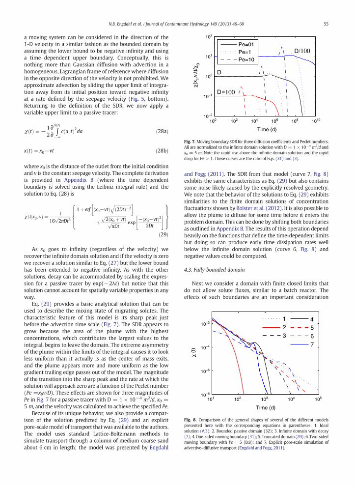
Because a common experimental setup in the laboratory is acolumn experiment where the average concentration at a planeis monitored, we will use a similar setup as a starting point. Forsimplicity and comparison to the analytical solutions, we willagain assume a homogeneous, 1-D, diffusive domain. If weemplace a solute in the center of a symmetric domainwith openboundaries spaced even distances away from the origin andonly monitor concentrations within these boundaries (Fig. 5,top), we will see less of the total mass within our domain astime progresses. The observed behavior of the SDR in an infinitedomain with a truncated monitoring area that is symmetricabout the origin can be found using the following integral:

χ x; tð Þ ¼ −12∂∂t ∫

x

−x

c a; tð Þ2da ð26Þ

where x is the half-width of the observation window and a is adummy variable of integration; the lack of subscripts on χ andc denote a passive tracer. The plume will eventually extendbeyond the limits in Eq. (26), but we will not allow ourselvesknowledge of the concentration field outside of the windowfrom –x to x. We then assume a Gaussian model of concen-tration with Dirac-delta initial conditions and assume a constantdiffusion coefficient (Eq. (A.1), Appendix A). Since the limits ofintegration are constant and finite, evaluation of the spatialintegration and time differentiation is straightforward; however,the solution to Eq. (26) also emerges as limiting case of the gen-eral model presented in Appendix B. In either case, the result is:

χ tjxð Þ ¼ 1

8ffiffiffiffiffiffiffiffiffiffiffiffiffi2πDt3

p erf xffiffiffiffiffiffiffiffiffiffiffiffiffiffiffiffiffi2Dtð Þ−1

q� �þ

ffiffiffiffiffiffi2x

pffiffiffiffiffiffiffiffiπDt

p exp−x2

2Dt

!" #

ð27Þ

∞-∞

xr=x2xl=-x2

xl=-∞

x=0

xr=x0-vt

Constant limits

Time-dependent limits

Fig. 5. Illustration of the limited domain integrals for constant (top) andtime-dependent (bottom) limits. The problems space (gray area) extends toinfinity but we restrict our knowledge to the domain between the dashedlines xl and xr.

100 102 104 106 108 101010−4

10−2

100

102

Time (d)

χ (x

,t)/χ

0

x=1x=10x=∞λ,x=1

D/100

D∗100

D

Fig. 6. Behavior of the truncated SDR for three length scales and diffusioncoefficientswhere x is thehalf-width of the truncateddomain.All are normalizedto the values based on the ideal solution using D = 1 × 10−4 m2/d and thedecay examples all use the same decay constant. These curves are the ratio ofEqs. (29) and (3).

which is the analytical solution for the SDR for a truncatedwindow of the domain given a constant value of x. The leadingfactor is the ideal SDR (Appendix A) and the remaining scalingfactor causes the SDR to depart from the ideal SDR and transitionto scaling behavior other than t−3/2 (Fig. 6); recall that similarscaling was also seen in the case of the multi-component kineticreaction in Section 3.3. The scaling in Eq. (27) shows that the latetime concentrations within the domain are still dissipatingbut that the apparent dissipation rate slows because of massloss since the most rapidly expanding areas of the plume (thefringes) are no longer included.

Fundamentally, mass loss appears to be the cause forscaling other than t−3/2 but the difference is that inSection 3.3 the mass loss was a result of a reaction, whereasin this case it is only an apparent mass loss that results fromhaving an incomplete picture of the domain. The family ofcurves defined by Eq. (27) also exhibit similar behavior tothe non-Fickian mixing shown in Fig. 4b of Le Borgne et al.(2010). The dissipation rates in that work are based on aheterogeneous domain and the departure of the simulatedSDR from the infinite domain solution was found to be afunction of the variance of the log transformed hydraulicconductivity. Although the size of their domain makes itunlikely that their deviations from the ideal solution are dueto domain restrictions, this illustrates the fact that differentmechanisms can cause similar kinds of dissipation. Themodel described by Eq. (27) is relevant to field studies sincethe areal extent of the aquifer is much larger than a typicalhigh resolutionmonitoring network. In this case, the problemspace is approximately infinite but the domain beingmonitored is finite.

4.2. Moving boundary

Dissipation in a system experiencing advection anddiffusion can also be addressed. One way would be to usethe inverse Gaussian model of concentration over time butthat distribution carries additional space and time depen-dencies that are more difficult to manipulate than a diffusionmodel. However, the squared integral of the concentration in

100 102 104 106 108 101010−2

10−1

100

101

102

Time (d)

χ(x 0,

v,t)

/χ0

Pe=0.1Pe=1Pe=10

∗100

D

D/100

D

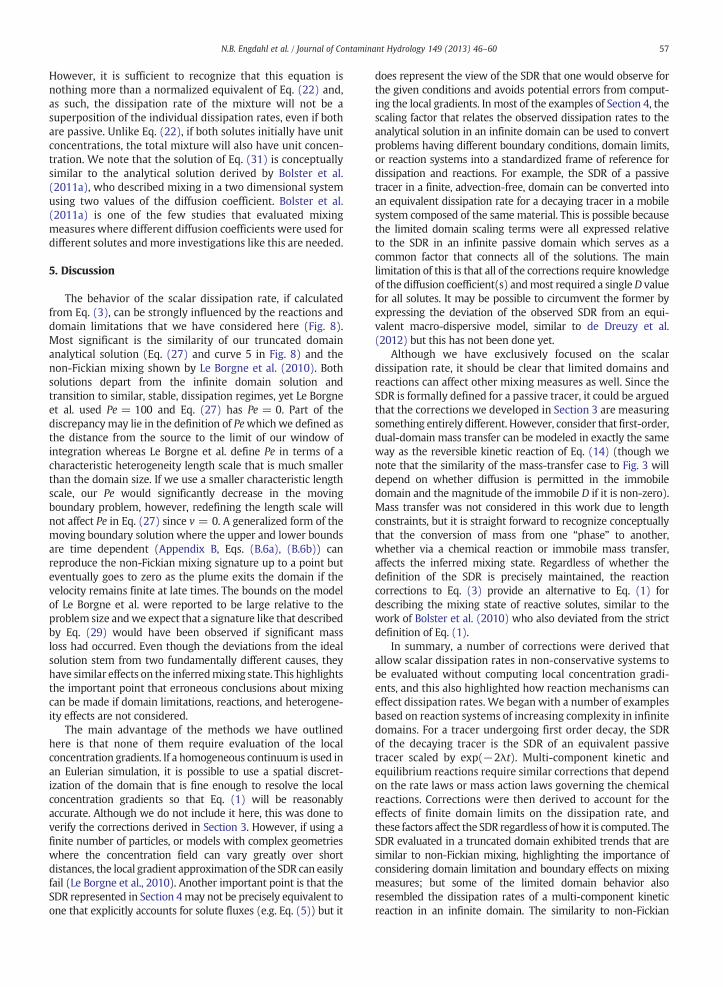
Fig. 7.Moving boundary SDR for three diffusion coefficients andPeclet numbers.All are normalized to the infinite domain solution with D = 1 × 10−4 m2/d andx0 = 5 m. Note the rapid rise above the infinite domain solution and the rapiddrop for Pe > 1. These curves are the ratio of Eqs. (31) and (3).

101 102 103 104 10510−8

10−6

10−4

10−2

Time (d)

χ (t

)

123

45

67

Fig. 8. Comparison of the general shapes of several of the different modelspresented here with the corresponding equations in parentheses: 1. Idealsolution (A.3); 2. Bounded passive domain (32); 3. Infinite domain with decay(7); 4. One-sidedmoving boundary (31); 5. Truncateddomain (29); 6. Two-sidedmoving boundary with Pe = 5 (B.8); and 7. Explicit pore-scale simulation ofadvective–diffusive transport (Engdahl and Fogg, 2011).


a moving system can be considered in the direction of the1-D velocity in a similar fashion as the bounded domain byassuming the lower bound to be negative infinity and usinga time dependent upper boundary. Conceptually, this isnothing more than Gaussian diffusion with advection in ahomogeneous, Lagrangian frame of reference where diffusionin the opposite direction of the velocity is not prohibited. Weapproximate advection by sliding the upper limit of integra-tion away from its initial position toward negative infinityat a rate defined by the seepage velocity (Fig. 5, bottom).Returning to the definition of the SDR, we now apply avariable upper limit to a passive tracer:

χ tð Þ ¼ −12∂∂ ∫

x tð Þ

−∞c a; tð Þ2da ð28aÞ

x tð Þ ¼ x0−vt ð28bÞ

where x0 is the distance of the outlet from the initial conditionand v is the constant seepage velocity. The complete derivationis provided in Appendix B (where the time dependentboundary is solved using the Leibniz integral rule) and thesolution to Eq. (28) is

χ tjx0; vð Þ ¼ 1


p1þ erf x0−vtð Þ

ffiffiffiffiffiffiffiffiffiffiffiffiffiffiffiffiffi2Dtð Þ−2

q� �

þffiffiffiffiffiffiffiffiffiffiffiffiffiffiffiffiffiffiffiffiffiffi2 x0 þ vtð ÞpffiffiffiffiffiffiffiffiπDt

p exp− x0−vtð Þ2

2Dt

" #8>>><>>>:

9>>>=>>>;

ð29Þ

As x0 goes to infinity (regardless of the velocity) werecover the infinite domain solution and if the velocity is zerowe recover a solution similar to Eq. (27) but the lower boundhas been extended to negative infinity. As with the othersolutions, decay can be accommodated by scaling the expres-sion for a passive tracer by exp(−2λt) but notice that thissolution cannot account for spatially variable properties in anyway.

Eq. (29) provides a basic analytical solution that can beused to describe the mixing state of migrating solutes. Thecharacteristic feature of this model is its sharp peak justbefore the advection time scale (Fig. 7). The SDR appears togrow because the area of the plume with the highestconcentrations, which contributes the largest values to theintegral, begins to leave the domain. The extreme asymmetryof the plume within the limits of the integral causes it to lookless uniform than it actually is as the center of mass exits,and the plume appears more and more uniform as the lowgradient trailing edge passes out of the model. The magnitudeof the transition into the sharp peak and the rate at which thesolution will approach zero are a function of the Peclet number(Pe =x0v/D). These effects are shown for three magnitudes ofPe in Fig. 7 for a passive tracer with D = 1 × 10−4 m2/d, x0 =5 m, and the velocitywas calculated to achieve the specified Pe.

Because of its unique behavior, we also provide a compar-ison of the solution predicted by Eq. (29) and an explicitpore-scalemodel of transport thatwas available to the authors.The model uses standard Lattice-Boltzmann methods tosimulate transport through a column of medium-coarse sandabout 6 cm in length; the model was presented by Engdahl

and Fogg (2011). The SDR from that model (curve 7, Fig. 8)exhibits the same characteristics as Eq. (29) but also containssome noise likely caused by the explicitly resolved geometry.We note that the behavior of the solutions to Eq. (29) exhibitssimilarities to the finite domain solutions of concentrationfluctuations shown by Bolster et al. (2012). It is also possible toallow the plume to diffuse for some time before it enters theproblem domain. This can be done by shifting both boundariesas outlined in Appendix B. The results of this operation dependheavily on the functions that define the time-dependent limitsbut doing so can produce early time dissipation rates wellbelow the infinite domain solution (curve 6, Fig. 8) andnegative values could be computed.

4.3. Fully bounded domain

Next we consider a domain with finite closed limits thatdo not allow solute fluxes, similar to a batch reactor. Theeffects of such boundaries are an important consideration


since solute mass will be forced to accumulate rather thanexit the area; this is in contrast to Sections 4.1 and 4.2 wherethe integral was restricted but the problem space was stillinfinite. This problem is deceptive because it cannot besolved in the same fashion as the previous examples since theboundary condition fundamentally changes the late timebehavior of the plume. One way to approximate this solutionis to use Eq. (3) with a model of the concentration field that isa superposition of an infinite number of solutions to Eq. (4)for passive diffusion that are sequentially shifted away fromthe origin as

c x; tð Þ ¼ 1ffiffiffiffiffiffiffiffiffiffiffi4πDt

pX∞n¼−∞

expxþ nLð Þ24Dt

!ð30Þ

where n is the integer index, L is the total width of thesymmetric, bounded domain, and the initial condition is aDirac-delta centered at the origin. The SDR based on thismodel of the concentration can be numerically approximatedwith a finite series provided that the series is large enough toenforce the zero flux condition at x = L/2 which should givea constant concentration at late times. At early times thesystem will behave the same as the infinite domain problembut as time progresses the concentration within the domainwill reach a constant uniform value because there is noeffluent. The solid boundary will increase the concentrationat the limits of the domain and increase the squared mass atthe edge relative to the same location in an equivalent openboundary system. This will cause the dissipation rate toapproach zero much more rapidly than in the open boundarycase once a significant portion of the mass reaches the edgesof the domain. The dissipation rate will continue to decreaseand asymptotically approach zero at late times, but for alleffective purposes the domain becomes a homogeneousuniform mixture.

The amount of time it should take for deviations from theinfinite domain to become visible will depend on thecharacteristic diffusion time scale, (L/2)2/D in this case, butmass will being to accumulate before this time, thus, weshould expect deviations to occur below the characteristicdiffusion time. In Fig. 8 we include a highly discretizednumerical approximation of the SDR computed by Eq. (3)with the concentration defined by Eq. (30). The domainhas width L = 2 m, D = 1 × 10−4 m2/d, and n = 400 wassufficient to enforce the zero flux boundary at x = 1 m overthe simulated time scale. The model exhibits the expectedbehaviors, and the SDR rapidly goes to zero near the diffusiontime scale. However, notice that it tends to zero more slowlythan in the case of the moving boundary dissipation rate, butthat the deviations of the finite, bounded, domain are muchgreater at early times than the moving boundary. Some ofthese differences shown in Fig. 8 are due to the sensitivityof the moving boundary solution to the Peclet number. Toaddress this we varied Pe of the moving boundary solu-tions across 5 orders of magnitude. The advection signaturedominates for Pe > 1; this regime is characterized by ahigher than ideal dissipation rate as we approach theadvective time scale and a rapid drop toward zero afterwardthat is proportional to Pe. For Pe b 1, the advection signaturesteadily diminishes but the transition from higher than idealdissipation towards lower than ideal dissipation occurs at the

characteristic diffusion time. In contrast, the bounded domainsolution calculated from Eq. (30) never exceeds the ideal,infinite domain SDR and reaches zero by (L/2)2/D. Thus,regardless of particular choices of v and D, the definingcharacteristic that separates these two solutions is whetherthe SDR reaches, or passes, zero before or after the diffusiontime scale.

4.4. Inferring dissipation rates from effluent concentrations

The previous derivations have all assumed complete knowl-edge of the concentration field at all times. Such knowledge isunlikely in field settings and also in many laboratory experi-mental setups. A more common source of concentration is theeffluent breakthrough curve (BTC) of a passive tracer. BTCscannot be used to directly quantify the dissipation rate because aBTC does not uniquely represent the spatial variability of theconcentration field within the domain and usually includes thecombined effects of diffusion and dispersion. Certainly BTCs andthe SDR are related but a generalized analytical connection hasnot been developed and is not necessary in some cases. Thesimplest way to infer the SDR from the BTC of a passive diffusingtracer is to assume a model for the concentration field anddetermine the diffusion coefficient by fitting the BTC. Theanalytical solution for the passive SDR in a homogeneous, 1-D,diffusive domain is given in Appendix A (Eq. (A.3)) and onlyrequires the distance from the source and the diffusioncoefficient from a BTC. This is only possible because there is nospatial variability in the aquifer and diffusion is symmetric (orisotropic if generalized to more spatial dimensions) so mixingand spreading are analogous in this special case. In heteroge-neous systems it will certainly be necessary to delineate theeffects of dispersion to correctly infer the mixing state. If thetracer is undergoing first order decay, the decay constant mustalso be determined, but this can also be accomplished by fittingthe effluent BTC or by use of an objective function approach suchas Eqs. (9a), (9b). It is also possible to assume amodel other thanthe Gaussian distribution for the concentration field (e.g. Bolsteret al., 2010). Doing so requires computation of the appropriateanalytical solution of the SDR. There are a number of physicallyplausible distributions, such as the Levy distribution, that will bedifficult to integrate analytically, but numerical approximationsmay be possible.

Instead of assuming a single distribution, the behavior ofthe tracer can also be approximated using a linear combina-tion of tracers. For simplicity we will only describe the casewhere our 1-D plume is described by a weighting of twotracers having different diffusion coefficients. The SDR in aninfinite domain can then be determined by solving thefollowing expression

χc1þc2 tð Þ ¼ −12∂∂t ∫ αc1 x; t D1j Þ þ βc2 x; t D2j Þð �2dx

�hð31Þ

where the subscripts 1 and 2 delineate the concentrationsand diffusion coefficients of the two plumes, and α and β arethe relative fractional contributions of each plume that mustsum to unity. The analytical solution to this equation islengthy and involves multiple correction terms (which canbe further generalized, and greatly complicated, by permit-ting decay at different rates and different initial locations),but it can be found using the procedures in Appendix B.


However, it is sufficient to recognize that this equation isnothing more than a normalized equivalent of Eq. (22) and,as such, the dissipation rate of the mixture will not be asuperposition of the individual dissipation rates, even if bothare passive. Unlike Eq. (22), if both solutes initially have unitconcentrations, the total mixture will also have unit concen-tration. We note that the solution of Eq. (31) is conceptuallysimilar to the analytical solution derived by Bolster et al.(2011a), who described mixing in a two dimensional systemusing two values of the diffusion coefficient. Bolster et al.(2011a) is one of the few studies that evaluated mixingmeasures where different diffusion coefficients were used fordifferent solutes andmore investigations like this are needed.

5. Discussion

The behavior of the scalar dissipation rate, if calculatedfrom Eq. (3), can be strongly influenced by the reactions anddomain limitations that we have considered here (Fig. 8).Most significant is the similarity of our truncated domainanalytical solution (Eq. (27) and curve 5 in Fig. 8) and thenon-Fickian mixing shown by Le Borgne et al. (2010). Bothsolutions depart from the infinite domain solution andtransition to similar, stable, dissipation regimes, yet Le Borgneet al. used Pe = 100 and Eq. (27) has Pe = 0. Part of thediscrepancymay lie in the definition of Pewhichwe defined asthe distance from the source to the limit of our window ofintegration whereas Le Borgne et al. define Pe in terms of acharacteristic heterogeneity length scale that is much smallerthan the domain size. If we use a smaller characteristic lengthscale, our Pe would significantly decrease in the movingboundary problem, however, redefining the length scale willnot affect Pe in Eq. (27) since v = 0. A generalized form of themoving boundary solution where the upper and lower boundsare time dependent (Appendix B, Eqs. (B.6a), (B.6b)) canreproduce the non-Fickian mixing signature up to a point buteventually goes to zero as the plume exits the domain if thevelocity remains finite at late times. The bounds on the modelof Le Borgne et al. were reported to be large relative to theproblem size andwe expect that a signature like that describedby Eq. (29) would have been observed if significant massloss had occurred. Even though the deviations from the idealsolution stem from two fundamentally different causes, theyhave similar effects on the inferredmixing state. This highlightsthe important point that erroneous conclusions about mixingcan be made if domain limitations, reactions, and heterogene-ity effects are not considered.

The main advantage of the methods we have outlinedhere is that none of them require evaluation of the localconcentration gradients. If a homogeneous continuum is used inan Eulerian simulation, it is possible to use a spatial discret-ization of the domain that is fine enough to resolve the localconcentration gradients so that Eq. (1) will be reasonablyaccurate. Although we do not include it here, this was done toverify the corrections derived in Section 3. However, if using afinite number of particles, or models with complex geometrieswhere the concentration field can vary greatly over shortdistances, the local gradient approximation of the SDR can easilyfail (Le Borgne et al., 2010). Another important point is that theSDR represented in Section 4may not be precisely equivalent toone that explicitly accounts for solute fluxes (e.g. Eq. (5)) but it

does represent the view of the SDR that one would observe forthe given conditions and avoids potential errors from comput-ing the local gradients. In most of the examples of Section 4, thescaling factor that relates the observed dissipation rates to theanalytical solution in an infinite domain can be used to convertproblems having different boundary conditions, domain limits,or reaction systems into a standardized frame of reference fordissipation and reactions. For example, the SDR of a passivetracer in a finite, advection-free, domain can be converted intoan equivalent dissipation rate for a decaying tracer in a mobilesystem composed of the samematerial. This is possible becausethe limited domain scaling terms were all expressed relativeto the SDR in an infinite passive domain which serves as acommon factor that connects all of the solutions. The mainlimitation of this is that all of the corrections require knowledgeof the diffusion coefficient(s) andmost required a singleD valuefor all solutes. It may be possible to circumvent the former byexpressing the deviation of the observed SDR from an equi-valent macro-dispersive model, similar to de Dreuzy et al.(2012) but this has not been done yet.

Although we have exclusively focused on the scalardissipation rate, it should be clear that limited domains andreactions can affect other mixing measures as well. Since theSDR is formally defined for a passive tracer, it could be arguedthat the corrections we developed in Section 3 are measuringsomething entirely different. However, consider that first-order,dual-domain mass transfer can be modeled in exactly the sameway as the reversible kinetic reaction of Eq. (14) (though wenote that the similarity of the mass-transfer case to Fig. 3 willdepend on whether diffusion is permitted in the immobiledomain and the magnitude of the immobile D if it is non-zero).Mass transfer was not considered in this work due to lengthconstraints, but it is straight forward to recognize conceptuallythat the conversion of mass from one “phase” to another,whether via a chemical reaction or immobile mass transfer,affects the inferred mixing state. Regardless of whether thedefinition of the SDR is precisely maintained, the reactioncorrections to Eq. (3) provide an alternative to Eq. (1) fordescribing the mixing state of reactive solutes, similar to thework of Bolster et al. (2010) who also deviated from the strictdefinition of Eq. (1).

In summary, a number of corrections were derived thatallow scalar dissipation rates in non-conservative systems tobe evaluated without computing local concentration gradi-ents, and this also highlighted how reaction mechanisms caneffect dissipation rates. We began with a number of examplesbased on reaction systems of increasing complexity in infinitedomains. For a tracer undergoing first order decay, the SDRof the decaying tracer is the SDR of an equivalent passivetracer scaled by exp(−2λt). Multi-component kinetic andequilibrium reactions require similar corrections that dependon the rate laws or mass action laws governing the chemicalreactions. Corrections were then derived to account for theeffects of finite domain limits on the dissipation rate, andthese factors affect the SDR regardless of how it is computed. TheSDR evaluated in a truncated domain exhibited trends that aresimilar to non-Fickian mixing, highlighting the importance ofconsidering domain limitation and boundary effects on mixingmeasures; but some of the limited domain behavior alsoresembled the dissipation rates of a multi-component kineticreaction in an infinite domain. The similarity to non-Fickian


mixing also implies that it may be possible to derive corrections,similar to those we derived here, that account for the influenceof heterogeneities on the dissipation rates.

Acknowledgments

The authors thank the anonymous reviewers for theirconstructive comments that significantly improved the qualityof this manuscript. The project described was supported byaward number P42ES004699 from the National Institute ofEnvironmental Health Sciences. The content is solely theresponsibility of the author and does not necessarily representthe official views of the National Institute of EnvironmentalHealth Sciences or the National Institute of Health.

Appendix A. Scalar dissipation rate of a decaying solute

Here we derive the analytical solution for the correctedscalar dissipation rate (SDR) of a decaying solute. Assumethat a unit concentration tracer is released instantaneously inthe center of an infinite 1-D, homogeneous domain with zerovelocity. In the tracer is conservative, the spatial distributionof concentrations will follow Fick's law of diffusion at alltimes, the solution of which is the Gaussian distribution:

c0 x; tð Þ ¼ 1ffiffiffiffiffiffiffiffiffiffiffi4πDt

p exp − x2

4Dt

!ðA:1Þ

where D quantifies the strength of the diffusion process andsubscriptswill denote the decay rate throughout this appendix.The decay rate is zero in Eq. (A.1) since the tracer is passive.Also note thatwe assume a normalized initial concentration forsimplicity. Integrating the square of Eq. (A.1) over all spacegives

∫∞−∞c0 x; tð Þ2dx ¼ 1ffiffiffiffiffiffiffiffiffiffiffiffi

8πDtp ¼ M2

0 tð Þ ðA:2Þ

Since the domain is infinite, there will be no solute fluxout of the domain at any time and the analytical solution forthe SDR over time can then be found (see Eq. (5)) which is

χ0 tð Þ ¼ −12∂∂t M

20 tð Þ ¼ 1

8ffiffiffiffiffiffiffiffiffiffiffiffiffiffi2πDt3

p ðA:3Þ

This solution is identical to Eqs. (9a), (9b) of Le Borgneet al. (2010) when a unit concentration and unit width of a2-D domain are used in their equation. This can also bederived by inserting Eq. (A.1) into Eq. (1) and solving for aninfinite domain. If the tracer decays according to a first orderrate law, the distribution of the solute from Eq. (A.1)becomes

cλ x; tð Þ ¼ exp −λtð Þffiffiffiffiffiffiffiffiffiffiffi4πDt

p exp − x2

4Dt

!ðA:4Þ

where λ is the decay constant. Integrate the square ofEq. (A.4) over all space to find

∫∞−∞cλ x; tð Þ2dx ¼ 2

exp −2λtð Þffiffiffiffiffiffiffiffiffiffiffiffiffiffiffi32πDt

p� �

¼ 2M2λ tð Þ ðA:5Þ

Applying the product rule, the time derivative of Eq. (A.5)is

−12∂∂t M

2λ tð Þ ¼ M2

λ tð Þ 2λþ 14t

� �ðA:6Þ

where have also introduced the −½ scaling necessary tocalculate the SDR. According to Eq. (6), the corrected SDR fora decaying tracer is found from

χλ tð Þ ¼ −12∂∂t M

2λ tð Þ−λM2

λ tð Þ

¼ M2λ tð Þ 2λþ 1

4t

� �−2λM2

λ tð Þ ðA:7Þ

inserting the appropriate definitions gives

χλ tð Þ ¼ M2λ tð Þ4t

¼ exp −2λtð Þ4t

ffiffiffiffiffiffiffiffiffiffiffiffiffiffiffi32πDt

p ðA:8Þ

The terms of the denominator are the SDR of a passivetracer from Eq. (A.5), so we can rewrite Eq. (A.8) as

χλ tð Þ ¼ exp −2λtð Þ8ffiffiffiffiffiffiffiffiffiffiffiffiffiffi2πDt3

p ¼ χ0 tð Þ exp −2λtð Þ ðA:9Þ

which is the corrected dissipation rate of a decaying tracerover time expressed in terms of the dissipation rate of apassive tracer and a decay constant. This relationship holdsfor all of the models presented here in that the solution for apassive tracer in any configuration need only be scaled by thesquare of the decay term. For example, combining the decayelements of this section with the tools of Appendix B showsthat the limited domain integral about the origin that definesthe SDR of a decaying tracer is

χλ tjxð Þ ¼ exp −2λtð Þ8ffiffiffiffiffiffiffiffiffiffiffiffiffi2πDt3

p erf xffiffiffiffiffiffiffiffiffiffiffiffiffiffiffiffiffiffi2Dtð Þ−1

q� �þ

ffiffiffi2

pxffiffiffiffiffiffiffiffi

πDtp exp

−x2

2Dt

!" #

ðA:10Þ

which is Eq. (29) scaled by the correction for first orderdecay. The relationship of the passive and decaying tracers inEq. (A.9) can also be found by changing variables in Eq. (4)such that c = c′ exp(−λt) where c′ is a dummy variable. Thedifferential Equation is then solved in terms of c′ and thedefinition of c is substituted back into the solution to recoverEq. (A.9). This is a special case where defining a conservativecomponent recovers the actual dissipation rates because onlyone species is being considered.

Appendix B. Scalar dissipation rates in finite domains

The analytical solutions in Section 4 all deal with scalardissipation rates in an infinite domain where only a subset ofthe problem space is considered. Except for the specific caseof impermeable walls where there is no effluent (Section 4.3),the other analytical solutions are limiting cases of the followingintegral:

χ0 tð Þ ¼ −12∂∂t ∫

b tð Þ

a tð Þc x; tð Þ2dx ðB:1Þ


where the limits of the integral are allowed to be arbitrarytime dependent functions and the subscript zero denotes apassive tracer. Time differentiation of an integral with timedependent limits can be solved using the Leibniz integralrule which is

∂∂t ∫

b tð Þ

a tð Þf x; tð Þdx ¼ ∫

b tð Þ

a tð Þ

∂f∂t dxþ f b tð Þ; tð Þ ∂b∂t −f a tð Þ; tð Þ ∂a∂t ðB:2Þ

where a and b are, again, arbitrary time dependent functionsand f is function in x and t. Adopting the Gaussian diffusionmodel without decay:

f ¼ c x; tð Þ2 ¼ 14πDt

exp − x2

2Dt

!ðB:3Þ

where D is the diffusion coefficient. The time derivative ofthis function is:

∂f∂t ¼ exp − x2

2Dt

!x2

8πD2t3− 1

4πDt2

" #ðB:4Þ

which is then integrated to give:

∫b tð Þ

a tð Þ

∂f∂t dx ¼ −1


p erf x

ffiffiffiffiffiffiffiffi1

2Dt

r !þ

ffiffiffi2

pxffiffiffiffiffiffiffiffi

πDtp exp − x2

2Dt

!" #ja tð Þ

b tð ÞðB:5Þ

where erf is the error function. The general solution for anyset of boundaries is found by inserting this and the otherrequisite terms into Eq. (B.2), which is then scaled by−½ todetermine the apparent SDR for that particular problem.With some algebra, it can be shown that the general solutionof Eq. (B.1) is:

χ0 tja; bð Þ ¼ 1


p ψ t bj Þ−ψ t aj Þð �ð½ ðB:6aÞ

with

ψ tjyð Þ ¼ erf y

ffiffiffiffiffiffiffiffi1

2Dt

r !þ

ffiffiffi2

pffiffiffiffiffiffiffiffiπDt

p y−2t∂y∂t

� �exp

−y2

2Dt

!ðB:6bÞ

where y is an arbitrary, differentiable, function. Notice thatonly one term requires the time derivative of y and theremaining terms are evaluated using the function. Towardan expression for a system experiencing diffusion andadvection, we now define time dependent functions todictate the limits:

b tð Þ ¼ x2−vt ðB:7aÞ

a tð Þ ¼ x1−vt ðB:7bÞ

where x1 and x2 are the initial positions of the lower and upperboundaries, respectively, and the velocity of each boundaryis assumed constant and identical at velocity v; the latterassumption is not required but is invoked for simplicity. The

time derivative of both functions is –v and inserting the ap-propriate functions into Eq. (B.6) gives

χ0 tjx1; x2; vð Þ ¼ 1


p ψ2 t x2; vj Þ−ψ1 t x1; vj Þð �ð½ ðB:8aÞ

with

ψi tjxi; vð Þ ¼ erf xi−vtð Þffiffiffiffiffiffiffiffi1

2Dt

r" #þ

ffiffiffi2

pxi þ vtð ÞffiffiffiffiffiffiffiffiπDt

p exp− xi−vtð Þ2

2Dt

" #

ðB:8bÞ

This allows any arbitrary portion of the plume to beintegrated and can be used to approximate advective–diffusive transport in a homogeneous domain. Allow x2 → ∞and x1 → − ∞; both exponential terms will go to zero,erf(∞) − erf(−∞) = 2, and the analytical solution in aninfinite domain is recovered. If only x1 goes to negative infinityand the upper limit of integration is governed by Eq. (B.7a), theexponential in x1 goes to zero and the error function term in x1is −1 resulting in:

χ0 tj−∞; x2; vð Þ ¼ 1


p 1þ ψ2 t x2; vj Þð �½ ðB:9Þ

This solution is most similar to an advection–diffusionmodel in a finite domain where the center of mass exits themodel domain at time L/v, where L is the 1-D length from thesource to themonitoring location. Finally, if we allow a velocityof zero and require symmetric, constant limits on our integral,we see that ψ1 = − ψ2; (ψ2 − ψ1) = 2ψ2 and simplificationshows:

χ0 tjxð Þ ¼ 1


p ψ2 t x; v ¼ 0j Þð �½ ðB:10Þ

which is our Eq. (29) using the definition of Eq. (B.8b). Thesame procedure can be used for decaying tracers and the resultwill obey the expression of Eq. (7) regardless of the particularlimits imposed on the integral.

References

Acharya, R.C., Valocchi, A.J., Werth, C.J., Willingham, T.W., 2007. Pore-scalesimulation of dispersion and reaction along a transverse mixing zone intwo-dimensional porous media. Water Resources Research 43 (10),1–11. http://dx.doi.org/10.1029/2007WR005969.

Battiato, I., Tartakovsky, D.M., Tartakovsky, A.M., Scheibe, T., 2009. Onbreakdown of macroscopic models of mixing-controlled heterogeneousreactions in porous media. Advances in Water Resources 32 (11),1664–1673. http://dx.doi.org/10.1016/j.advwatres.2009.08.008.

Bolster, D., Benson, D., Le Borgne, T., Dentz, M., 2010. Anomalous mixing andreaction induced by superdiffusive nonlocal transport. Physical Review E82 (2), 1–5. http://dx.doi.org/10.1103/PhysRevE.82.021119.

Bolster, D., Dentz, M., Le Borgne, T., 2011a. Hypermixing in linear shear flow.Water Resources Research 47 (9), 1–5. http://dx.doi.org/10.1029/2011WR010737.

Bolster, D., Valdés-Parada, F.J., LeBorgne, T., Dentz, M., Carrera, J., 2011b.Mixing in confined stratified aquifers. Journal of Contaminant Hydrology120–121, 198–212. http://dx.doi.org/10.1016/j.jconhyd.2010.02.003.

Bolster, D., de Anna, P., Benson, D.A., Tartakovsky, A.M., 2012. Incompletemixing and reactions with fractional dispersion. Advances in WaterResources 37, 86–93. http://dx.doi.org/10.1016/j.advwatres.2011.11.005.

Castro-Alcalá, E., Fernàndez-Garcia, D., Carrera, J., Bolster, D., 2012. Visualizationof mixing processes in a heterogeneous sand box aquifer. Environmental

http://dx.doi.org/10.1029/2007WR005969

http://dx.doi.org/10.1016/j.advwatres.2009.08.008

http://dx.doi.org/10.1103/PhysRevE.82.021119

http://dx.doi.org/10.1029/2011WR010737

http://dx.doi.org/10.1029/2011WR010737




Science & Technology 46 (6), 3228–3235. http://dx.doi.org/10.1021/es201779p.

Chiogna, G., Cirpka, O.A., Grathwohl, P., Rolle, M., 2011. Relevance of localcompound-specific transverse dispersion for conservative and reactivemixing in heterogeneous porous media. Water Resources Research 47(7). http://dx.doi.org/10.1029/2010WR010270.

Chiogna, G., Hochstetler, D.L., Bellin, A., Kitanidis, P.K., Rolle, M., 2012.Mixing, entropy, and reactive solute transport. Geophysical ResearchLetters 39, L20405. http://dx.doi.org/10.1029/2012GL053295.

Cirpka, O.A., Kitanidis, P.K., 2000. Characterization of mixing and dilution inheterogeneous aquifers by means of local temporal moments. WaterResources Research 36 (5), 1221–1236.

Cirpka, O.A., Valocchi, A.J., 2007. Two-dimensional concentration distribu-tion for mixing-controlled bioreactive transport in steady state. Advancesin Water Resources 30 (6–7), 1668–1679. http://dx.doi.org/10.1016/j.advwatres.2006.05.022.

de Dreuzy, J.-R., Carrera, J., Dentz, M., Le Borgne, T., 2012. Time evolution ofmixing in heterogeneous porous media. Water Resources Research 48(6). http://dx.doi.org/10.1029/2011WR011360 in press.

De Simoni, M., Carrera, J., Sánchez-Vila, X., Guadagnini, A., 2005. A procedure forthe solution of multicomponent reactive transport problems. Water Re-sources Research 41 (11), 1–16. http://dx.doi.org/10.1029/2005WR004056.

De Simoni,M., Sanchez-Vila, X., Carrera, J., Saaltink,M.W., 2007. Amixing ratios-based formulation formulticomponent reactive transport.Water ResourcesResearch 43 (7), 1–10. http://dx.doi.org/10.1029/2006WR005256.

Dentz, M., Le Borgne, T., Englert, A., Bijeljic, B., 2011. Mixing, spreading andreaction in heterogeneous media: a brief review. Journal of ContaminantHydrology 120–121, 1–17. http://dx.doi.org/10.1016/j.jconhyd.2010.05.002.

Donado, L.D., Sanchez-Vila, X., Dentz, M., Carrera, J., Bolster, D., 2009.Multicomponent reactive transport in multicontinuum media. Water Re-sources Research 45 (11), 1–11. http://dx.doi.org/10.1029/2008WR006823.

Engdahl, N.B., Fogg, G.E., 2011. Direct upscaling of kinetically controlledreactive transport with mobile–immobile mass transfer. Abstract H31E-1209 presented at 2011 Fall Meeting AGU, San Francisco, Calif., 5–9 Dec.

Fernàndez-Garcia, D., Sánchez-Vila, X., Guadagnini, A., 2008. Reaction ratesand effective parameters in stratified aquifers. Advances in WaterResources 31 (10), 1364–1376. http://dx.doi.org/10.1016/j.advwatres.2008.07.001.

Ginn, T.R., 2000. On the distribution of multicomponent mixtures overgeneralized exposure time in subsurface flow and reactive transport: theoryand formulations for residence-time-dependent sorption/desorption withmemory. Water Resources Research 36 (10), 2885–2893.

Gramling, C.M., Harvey, C.F., Meigs, L.C., 2002. Reactive transport in porousmedia: a comparison of model prediction with laboratory visualization.Environmental Science & Technology 36 (11), 2508–2514.

Jha, B., Cueto-Felgueroso, L., Juanes, R., 2011. Quantifying mixing in viscouslyunstable porous media flows. Physical Review E 84 (6). http://dx.doi.org/10.1103/PhysRevE.84.066312.

Kapoor, V., Gelhar, L.W., 1994. Transport in three-dimensionally heteroge-neous aquifers 1. Dynamics of concentration fluctuations.Water ResourcesResearch 30 (6), 1775–1788.

Kapoor, V., Gelhar, L.W., Miralles-Wilhelm, F., 1997. Bimolecular second-order reactions in spatially varying flows: segregation induced scale-

dependent transformation rates. Water Resources Research 33 (4),527–536.

Kitanidis, P.K., 1994. The concept of the dilution index. Water ResourcesResearch 30 (7), 2011–2026.

Le Borgne, T., Dentz, M., Bolster, D., Carrera, J., de Dreuzy, J.-R., Davy, P., 2010.Non-Fickian mixing: temporal evolution of the scalar dissipation rate inheterogeneous porous media. Advances in Water Resources 33 (12),1468–1475. http://dx.doi.org/10.1016/j.advwatres.2010.08.006.

Le Borgne, T., Dentz, M., Davy, P., Bolster, D., Carrera, J., de Dreuzy, J.-R., Bour, O.,2011. Persistence of incomplete mixing: a key to anomalous transport.Physical Review E 84 (1), 1–4. http://dx.doi.org/10.1103/PhysRevE.84.015301.

Luo, J., Dentz,M., Carrera, J., Kitanidis, P., 2008. Effective reaction parameters formixing controlled reactions in heterogeneous media. Water ResourcesResearch 44 (2), 1–12. http://dx.doi.org/10.1029/2006WR005658.

McQuarrie, D.A., Simon, J.D., 1997. Physical Chemistry: A molecularApproach. University Science Books, Sausalito, CA.

Miralles-Wilhelm, F., Gelhar, L.W., Kapoor, V., 1997. Stochastic analysis ofoxygen-limited biodegradation in three-dimensionally heterogeneousaquifers. Water Resources Research 33 (6), 1251–1263.

Pope, S.B., 2000. Turbulent Flows. Cambridge University Press.Raje, D.S., Kapoor, V., 2000. Experimental study of bimolecular reaction

kinetics in porous media. Environmental Science & Technology 34 (7),1234–1239. http://dx.doi.org/10.1021/es9908669.

Rolle, M., Eberhardt, C., Chiogna, G., Cirpka, O.A., Grathwohl, P., 2009.Enhancement of dilution and transverse reactive mixing in porousmedia: experiments and model-based interpretation. Journal of Con-taminant Hydrology 110 (3–4), 130–142. http://dx.doi.org/10.1016/j.jconhyd.2009.10.003.

Saaltink, M.W., Ayora, C., Carrera, J., 1998. A mathematical formulation forreactive transport that eliminates mineral concentrations. Water Re-sources Research 34 (7), 1649–1656.

Sanchez-Vila, X., Donado, L.D., Guadagnini, A., Carrera, J., 2010. A solution formulticomponent reactive transport under equilibrium and kineticreactions. Water Resources Research 46 (7), 1–13. http://dx.doi.org/10.1029/2009WR008439.

Steefel, C., Lasaga, A.C., 1994. A coupled model for transport of multiplechemical species and kinetic precipitation/dissolution reactions withapplication to reactive flow in single phase hydrothermal systems.American Journal of Science 294, 529–592.

Tartakovsky, A.M., Redden, G., Lichtner, P.C., Scheibe, T.D., Meakin, P., 2008.Mixing-induced precipitation: experimental study and multiscalenumerical analysis. Water Resources Research 44 (6), 1–19. http://dx.doi.org/10.1029/2006WR005725.

Werth, C.J., Cirpka, O.A., Grathwohl, P., 2006. Enhanced mixing and reactionthrough flow focusing in heterogeneous porous media. Water ResourcesResearch 42 (12), 1–10. http://dx.doi.org/10.1029/2005WR004511.

Zinn, B., Meigs, L.C., Harvey, C.F., Haggerty, R., Peplinski,W.J., Von Schwerin, C.F.,2004. Experimental visualization of solute transport and mass transferprocesses in two-dimensional conductivity fields with connected regionsof high conductivity. Environmental Science & Technology 38 (14),3916–3926.

http://dx.doi.org/10.1021/es201779p

http://dx.doi.org/10.1021/es201779p

http://dx.doi.org/10.1029/2010WR010270

http://dx.doi.org/10.1029/2012GL053295



http://dx.doi.org/10.1029/2011WR011360

http://dx.doi.org/10.1029/2005WR004056

http://dx.doi.org/10.1029/2006WR005256


http://dx.doi.org/10.1029/2008WR006823







http://dx.doi.org/10.1029/2006WR005658

http://dx.doi.org/10.1021/es9908669



http://dx.doi.org/10.1029/2009WR008439

http://dx.doi.org/10.1029/2006WR005725

http://dx.doi.org/10.1029/2005WR004511

journal of contaminant hydrology · n.b. engdahl et al. / journal of contaminant hydrology 149...

Documents